Embed Size (px)
Citation preview

UNIVERSIDADE FEDERAL DO ESPÍRITO SANTO
CENTRO TECNOLÓGICO
DEPARTAMENTO DE ENGENHARIA MECÂNICA
BRENO VENTORIM DE TASSIS
AVALIAÇÃO E OTIMIZAÇÃO DA PERFORMANCE AERODINÂMICA
DO VEÍCULO TARF-LCV
VITÓRIA
2016

2
BRENO VENTORIM DE TASSIS
AVALIAÇÃO E OTIMIZAÇÃO DA PERFORMANCE AERODINÂMICA
DO VEÍCULO TARF-LCV
Projeto de Graduação apresentado ao
Departamento de Engenharia Mecânica da
Universidade Federal do Espírito Santo,
como requisito parcial para obtenção do
título de Engenheiro Mecânico.
Orientador: Prof. Dr. Bruno Venturini Loureiro
VITÓRIA
2016

3
BRENO VENTORIM DE TASSIS
AVALIAÇÃO E OTIMIZAÇÃO DA PERFORMANCE AERODINÂMICA
DO VEÍCULO TARF-LCV
Trabalho de conclusão de curso apresentado ao Departamento de Engenharia
Mecânica da Universidade Federal do Espírito Santo, como requisito parcial para
obtenção do título de Engenheiro Mecânico.
COMISSÃO EXAMINADORA
Prof. Dr. Bruno Venturini Loureiro
Universidade Federal do Espírito Santo
Orientador
Prof. Oswaldo Paiva Almeida Filho
Universidade Federal do Espírito Santo
Examinador
Bruno Filipe da Penha Sperandio, mestrando.
Universidade Federal do Espírito Santo
Examinador

4
ACKNOWLEDGMENTS
First, I would like to take this opportunity to thank Mr Amit Prem, my project supervisor
at Coventry University. Without his contribution, monitoring and guidance this report
would not have been written.
Special thanks and my gratitude should be given to Mr Bill Dunn, who supported me
during this great year at Coventry University. His support, help, advices and constant
encouragement throughout the academic year were of paramount importance.
I would also like to thanks the former student Dalvy, who helped me setting the first
CFD simulation for the TARF-LCV model.
Last, but not least, I would like to mention my supervisor at Universidade Federal do
Espírito Santo, Bruno Venturini Loureiro.

5
ABSTRACT
Towards Affordable, Closed-Loop Recyclable Future Low Carbon Vehicle or, simply,
TARF-LCV. It is a £5 million project led by Brunel University in partnership with 7 other
British universities and funded by Engineering and Physical Sciences Research
Council (EPSRC).
The TARF-LCV project was created due to big challenges that United Kingdom’s
automotive industry is facing in the last years, such as been responsible for a 19%
growing share of UK annual CO2 emissions. TARF-LCV aims to deliver fundamental
solutions to the key challenges faced by future development of Low Carbon Vehicles
(LCV) (Research Councils UK, 2013).
This project is mainly focused on analysing and evaluating the aerodynamics of the
6th TARF-LCV concept developed in Coventry University, one of the 8 UK universities
members of TARF-LCV research team.
To do so, a brief literature review of vehicle aerodynamics and a case study of previous
TARF-LCV concepts was written.
Keywords: 1. Aerodynamics; 2.Drag; 3. Lift; 4. Vehicle; 5. Optimisation.

6
SUMMARY
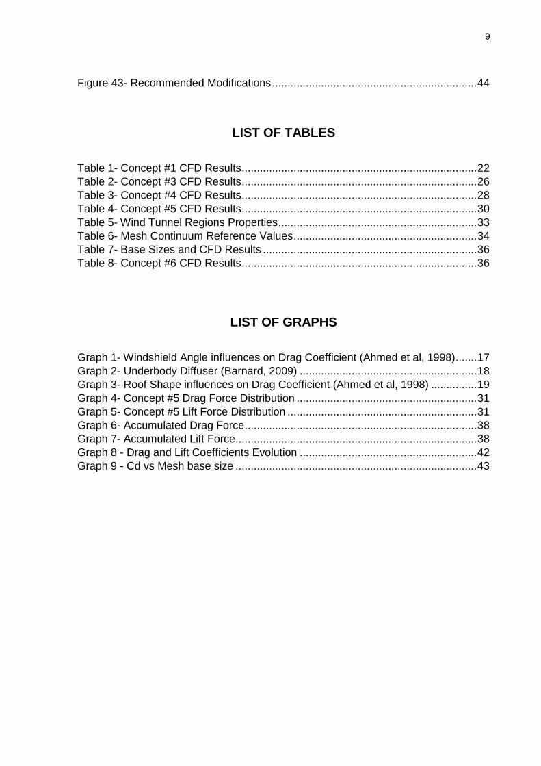
LIST OF FIGURES ...................................................................................................... 8
LIST OF TABLES ....................................................................................................... 9
LIST OF GRAPHS ...................................................................................................... 9
GLOSSARY .............................................................................................................. 10
1. INTRODUCTION ................................................................................................ 11
2. PROJECT OBJECTIVES ................................................................................... 12
3. LITERATURE REVIEW ...................................................................................... 12
3.1. PRINCIPLE AND FUNDAMENTALS OF AERODYNAMICS .................... 12
3.1.1. STREAMLINES ..................................................................................... 12
3.1.2. BOUNDARY LAYERS ........................................................................... 12
3.1.3. LAMINAR AND TURBULENT FLOWS .................................................. 13
3.1.4. FLOW SEPARATION ............................................................................ 14
3.1.5. REYNOLDS NUMBER .......................................................................... 14
3.1.6. DRAG AND LIFT FORCES ................................................................... 14
3.1.7. DRAG AND LIFT COEFFICIENTS ........................................................ 15
3.2. HOW TO IMPROVE AERODYNAMIC PERFORMANCE ......................... 16
3.2.1. WIND TUNNEL TESTING ..................................................................... 16
3.2.2. DESIGN DEVELOPMENT ..................................................................... 16
3.2.3. DEVICES AND GENERAL IMPROVEMENTS ...................................... 19
4. TARF-LCV PREVIOUS CONCEPTS CASE STUDY ......................................... 20
4.1. CONCEPT #1 ........................................................................................... 20
4.1.1. CHARACTERISTICS ............................................................................. 20
4.1.2. AERODYNAMIC ANALYSIS ................................................................. 21
4.2. CONCEPT #2 ........................................................................................... 23
4.2.1. MODIFICATIONS .................................................................................. 23
4.3. CONCEPT #3 ........................................................................................... 25
4.3.1. MODIFICATIONS .................................................................................. 25
4.3.2. AERODYNAMIC ANALYSIS ................................................................. 26
4.4. CONCEPT #4 ........................................................................................... 28
4.4.1. MODIFICATIONS .................................................................................. 28
4.4.2. AERODYNAMIC ANALYSIS ................................................................. 28
4.5. CONCEPT #5 ........................................................................................... 30
5. METHODOLOGY – MODELLING THE CONCEPT #6 CFD SIMULATION ....... 31

7
6. CONCEPT #6 – CFD RESULTS ........................................................................ 36
7. CONCLUSION .................................................................................................... 42
8. REFERENCES ................................................................................................... 45
APPENDIX A – Volume Meshes ............................................................................. 46
APPENDIX B – Residuals Plot ................................................................................ 48

8
LIST OF FIGURES
Figure 1- Streamlines (Barnard, 2009) ...................................................................... 12
Figure 2- Boundary Layers (Barnard, 2009) .............................................................. 13
Figure 3- Flow around a Passengers Car (Ahmed et al, 1998) ................................. 13
Figure 4- Aerodynamic Forces (Accessed in
http://www.kasravi.com/cmu/tec452/aerodynamics/VehicleAero.htm) ...................... 14
Figure 5- Drag Forces (Accessed in http://www.up22.com/Aerodynamics.htm) ........ 15
Figure 6- Lift Forces (Accessed in http://www.up22.com/Aerodynamics.htm) ........... 15
Figure 7- Different front end shapes and drag coefficient (Vasiu et al, 2013) ............ 16
Figure 8- Conical Vortices Generated on Hatchback (Vasiu et al, 2013) .................. 17
Figure 9- Effective Rear Slope Angle (Vasiu et al, 2013) .......................................... 18
Figure 10- General Improvements (Accessed in
http://www.kasravi.com/cmu/tec452/aerodynamics/VehicleAero.htm) ...................... 19
Figure 11- TARF-LCV 1st concept ............................................................................ 20
Figure 12- Concept #1 Streamlines ........................................................................... 21
Figure 13- Concept #1 Pressure Coefficient.............................................................. 22
Figure 14- Concept #1 Velocity Field ........................................................................ 23
Figure 15- Concepts #1 and #2 Front-end ................................................................ 24
Figure 16- Concepts #1 and #2 Side body ................................................................ 24
Figure 17- Concepts #1 and #2 Rear-end ................................................................. 24
Figure 18- Concept #3 Mesh Scene .......................................................................... 25
Figure 19- Concepts #2 and #3 Front-end ................................................................ 26
Figure 20- Concepts #2 and #3 Side body ................................................................ 26
Figure 21- Concepts #2 and #3 Rear-end ................................................................. 26
Figure 22- Concept #4 Velocity Field ........................................................................ 27
Figure 23- Concept #4 Pressure Coefficient.............................................................. 27
Figure 24- Concept #4 Final Design .......................................................................... 28
Figure 25- Concept #4 Pressure Coefficient.............................................................. 29
Figure 26- Concept #4 Velocity Field ........................................................................ 29
Figure 27- Concept #4 Streamlines ........................................................................... 29
Figure 28- Vortex Core and Flow Separation ............................................................ 30
Figure 29- Surface Wrapper Properties ..................................................................... 32
Figure 30- Surface Diagnostic ................................................................................... 33
Figure 31- Wind Tunnel ............................................................................................. 33
Figure 32- Frontal Area Report .................................................................................. 36
Figure 33- Drag Coefficient Report ............................................................................ 37
Figure 34- Lift Coefficient Report ............................................................................... 37
Figure 35- Distance Vehicle - Floor ........................................................................... 37
Figure 36- Velocity Distribution Vectors .................................................................... 39
Figure 37- Velocity Magnitude around Vehicle .......................................................... 39
Figure 38- Wake formation (front view) ..................................................................... 40
Figure 39- Wake formation (rear view) ...................................................................... 40
Figure 40- Pressure Coefficient Distribution (Front view) .......................................... 41
Figure 41- Pressure Coefficient Distribution (Rear view) ........................................... 41
Figure 42- Recommended Modifications ................................................................... 43
9
Figure 43- Recommended Modifications ................................................................... 44
LIST OF TABLES
Table 1- Concept #1 CFD Results ............................................................................. 22
Table 2- Concept #3 CFD Results ............................................................................. 26
Table 3- Concept #4 CFD Results ............................................................................. 28
Table 4- Concept #5 CFD Results ............................................................................. 30
Table 5- Wind Tunnel Regions Properties ................................................................. 33
Table 6- Mesh Continuum Reference Values ............................................................ 34
Table 7- Base Sizes and CFD Results ...................................................................... 36
Table 8- Concept #6 CFD Results ............................................................................. 36
LIST OF GRAPHS
Graph 1- Windshield Angle influences on Drag Coefficient (Ahmed et al, 1998)....... 17
Graph 2- Underbody Diffuser (Barnard, 2009) .......................................................... 18
Graph 3- Roof Shape influences on Drag Coefficient (Ahmed et al, 1998) ............... 19
Graph 4- Concept #5 Drag Force Distribution ........................................................... 31
Graph 5- Concept #5 Lift Force Distribution .............................................................. 31
Graph 6- Accumulated Drag Force ............................................................................ 38
Graph 7- Accumulated Lift Force ............................................................................... 38
Graph 8 - Drag and Lift Coefficients Evolution .......................................................... 42
Graph 9 - Cd vs Mesh base size ............................................................................... 43

10
GLOSSARY
Abbreviations
2D Two Dimensional 3D Three Dimensional A Frontal Area of a car [m2]
𝐶𝐷 Drag Coefficient 𝐶𝐿 Lift Coefficient CAD Computer Aided Design CATIA Computer Aided Three-dimensional Interactive Application
Software CFD Computational Fluid Dynamics CO2 Carbon Dioxide
𝐷 Drag Force [N] ELV End of Life Vehicle EPSRC Engineering and Physical Sciences Research Council
𝐿 Lift Force [N] 𝑙 Length of a body [m] LCV Low Carbon Vehicle OPEC Organization of the Petroleum Exporting Countries R Radius [in]
𝑅𝑒 Reynolds Number STAR-CCM+ Computer Aided Design Software used for CFD analysis TARF-LCV Towards Affordable, Closed Loop Recyclable Future Low Carbon
Vehicle
𝑉, 𝑣 Velocity [m/s]
µ Fluid Viscosity ρ Air Density [kg/m3]
Units
in Inches kg Kilogram m Meter m2 Meter squared m3 Cubic meter min Minute mm Millimetres s Second

11
1. INTRODUCTION
During the first years of the automotive industry, vehicle aerodynamics was only taken
in consideration when designing racing cars.
The major impetus to serious attempts at drag reduction for mass-produced vehicles
came in 1973 when a group of oil exporting countries (OPEC) formed a cartel,
drastically increasing the price of crude oil, and simultaneously cutting production
(Barnard, 2009).
The shortage of fuel in the market at that time frightened the automotive industry.
Automakers had to invest in the production of cars with lower fuel consumption.
The fuel consumption of a vehicle depends on the efficiency of the engine and
transmission system, and the power required to overcome the resistance to motion.
The required power is the product of the total resistance force, and the vehicle speed.
Power = total resistance force × speed
At steady speed on a level road, the total resistance to motion is the sum of two
separate contributions, aerodynamic drag, and tyre rolling resistance (Barnard, 2009).
From the last two decades, emissions standards for road vehicles have been created
by governments and commissions around the world, setting specific limits to the
amount of gas emissions that vehicles can release to the atmosphere. For instance,
UK Department for Transport (DfT) set a challenging aim of 60% reduction in CO2
emission from road vehicles by 2030.
A solution to these challenges comes from the development and manufacture of low
carbon vehicles, as identified by the UK government. Vehicle lightweighting is the most
effective way to improve fuel economy and to reduce CO2 emissions. This has been
demonstrated by many vehicle mass reduction programmes worldwide (Research
Councils UK, 2013).
In fact, a 10% reduction in drag can result in approximately 4% reduction in fuel
consumption combined. This is valid only if the reduction of air drag is achieved by re-
matching of the gear ratios. Reduction in drag by 20-50% results in reduction of fuel
consumption of 8-20% respectively (Businaro et al, 1983).
Therefore, low drag is important for good fuel economy and low emissions. But the
other aspects of vehicle aerodynamics are no less important for the quality of an
automobile: directional stability; wind noise; soiling of the lights, windows and body;
cooling of the engine, gearbox and brakes; and finally, heating ventilating and air
conditioning of the passenger compartment. (Ahmed et al, 1998).

12
2. PROJECT OBJECTIVES
To analyse and evaluate aerodynamic performance of TARF-LCV concept #6
architecture;
To find critical points on the vehicle structure that may cause an increase in
aerodynamic drag force and coefficient;
To modify the design of some parts of the vehicle, such as bumpers and rear
diffusers in order to improve aerodynamic performance, reducing vehicle drag;
To perform different CFD simulations to check if modifications achieved the
expected overall results;
To suggest external modifications at the concept architecture in order to achieve
a cd of 0.25.
3. LITERATURE REVIEW
3.1. PRINCIPLE AND FUNDAMENTALS OF AERODYNAMICS
To analyse and understand vehicle aerodynamics some basic concepts of fluid
mechanics and dynamics are necessary, since any vehicle, when in motion, is
subjected to an air flow around and through itself.
3.1.1. STREAMLINES
Streamlines are curves associated with a pictorial representation of air flow and are
used to study it.
Streamlines are defined as imaginary lines across which there is no flow. If the flow is
steady they also indicate the instantaneous direction of the flow and the path that an
air particle would follow. For most types of road vehicle there are usually regions of
unsteady flow. (Barnard, 2009).
Figure 1- Streamlines (Barnard, 2009)
3.1.2. BOUNDARY LAYERS
An important feature of the flow past a vehicle is that the air appears to stick to the
surface. Right next to the surface there is no measurable relative motion (Barnard,
2009).

13
The thickness of the boundary layer grows with distance from the front of the vehicle,
but does not exceed more than a few centimetres on a car travelling at normal open-
road speeds. Despite the thinness of this layer, it holds the key to understanding how
air flows around a vehicle, and how the lift and drag forces are generated (Barnard,
2009).
There are two different types of boundary layer flows that will be explained ahead.
3.1.3. LAMINAR AND TURBULENT FLOWS
Figure 2- Boundary Layers (Barnard, 2009)
Generally, boundary layers flows are divided into Laminar and Turbulent Flows.
Laminar flows have the ideal aerodynamic properties, since fluid motion is well
organized with parallel velocity vectors. This kind of flow occurs near the front edge of
the vehicle, where the air flows smoothly with no turbulent perturbations.
Further along the vehicle surface, there is a sudden transition to a turbulent flow, in
which a random motion appears. In a turbulent flow the organization of velocity vectors
cannot be defined.
Figure 3- Flow around a Passengers Car (Ahmed et al, 1998)

14
3.1.4. FLOW SEPARATION
It is important to distinguish between turbulent boundary layer flow and separated flow.
In a turbulent boundary layer, the flow is still “streamlined” in the sense that it follows
the contour of the body. The turbulent motions are of very small scales. A separated
flow does not follow the contours of the body (Barnard, 2009).
Flow separation occurs when the boundary layers travels far enough against an
adverse pressure gradient, in other words, when the static pressure increases in the
direction of the flow and consequently the velocity decreases. The flow is said to be
separated from the surface when velocity is reduced to zero or even become reversed.
Flow separation modifies the pressure distribution along the surface and hence the lift
and drag characteristics, which will be mentioned ahead.
3.1.5. REYNOLDS NUMBER
The types of boundary layers flows can be defined mathematically by using Reynolds
Number value. This is a dimensionless number that can indicate the nature of the flow,
as it relates pressure, speed, density, viscosity and the geometry of the body. All of
these factors mentioned can modify the behaviour of the layer flow. Reynolds number
is given by:
𝑅𝑒 =𝜌𝑣𝑙
µ
where 𝜌 is fluid density, 𝑣 is the velocity, 𝑙 is the length of the body and µ is the fluid
viscosity. A higher value of Reynolds number indicates turbulent flow while a lower
level indicates laminar flow.
3.1.6. DRAG AND LIFT FORCES
Figure 4- Aerodynamic Forces (Accessed in http://www.kasravi.com/cmu/tec452/aerodynamics/VehicleAero.htm)
When a car is travelling, it is moving through an air flow. It is known that it takes some
energy to move the car through the air. This energy is used to overcome the drag. The

15
drag force is primarily composed by two forces: the Frontal Pressure and the Rear
Vaccum (where the flow detachment or separation occurs).
Figure 5- Drag Forces (Accessed in http://www.up22.com/Aerodynamics.htm)
Another important force has to be considered in aerodynamic analysis: the Lift Force
or Down Force (Negative Lift Force). The lift forces are “created” by low pressure areas
(where the flow normally separates) around the surface of the vehicle, while down force
is “created” by higher pressure areas.
Lift indirectly affects the drag, but more significantly, considerable improvements in the
roadholding and stability can be obtained by reducing the lift, or even generating down
force (Barnard, 2009).
Figure 6- Lift Forces (Accessed in http://www.up22.com/Aerodynamics.htm)
3.1.7. DRAG AND LIFT COEFFICIENTS
Drag coefficient (𝐶𝐷) is used to compare aerodynamic drag produced by vehicles and
is dependent on the shape of the vehicle, the frontal area and the speed at which the
vehicle is travelling at (Vasiu et al, 2013).
The relationship between drag and these factors can be expressed by:
𝐶𝐷 =𝐷
12𝜌𝑉
2𝐴
Where A is the projected frontal area, 𝜌 is the density of the air, V is the speed of the
vehicle relative to the air and D is the drag force.
Minimising the frontal area of the vehicle will minimise the overall drag coefficient of
the vehicle. Therefore keeping the vehicle compact and low to the ground as possible
will give low frontal projected area value for the vehicle and therefore better
performance (Vasiu et al, 2013).
Lift coefficient (𝐶𝐿) is defined in a similar way to drag coefficient:
16
𝐶𝐿 =𝐿
12𝜌𝑉
2𝐴
Where A is the projected frontal area, 𝜌 is the density of the air, V is the speed of the
vehicle relative to the air and D is the lift force.
3.2. HOW TO IMPROVE AERODYNAMIC PERFORMANCE
3.2.1. WIND TUNNEL TESTING
There are many ways to optimize the aerodynamic performance of a vehicle. The wind
tunnel testing is used to analyse aerodynamics and identify low pressure areas and
regions that can be modified to improve performance.
The main development device for the vehicle aerodynamics testing continues to be the
full-scale wind-tunnel. It is likely that this will be unchanged for many years ahead since
there is no reliable alternative for it. There are two main types of conventional wind-
tunnels: open jet, which has an open test section, and the second type is a closed
wind-tunnel with a closed test section (Le Good, 1998).
3.2.2. DESIGN DEVELOPMENT
During the design development of a car, choosing the front end, rear end, windshield,
roof and underbody configurations, for example, can be crucial to the aerodynamic
performance of the vehicle. Some of these configurations and how they can improve
the aerodynamic performance will be discussed below:
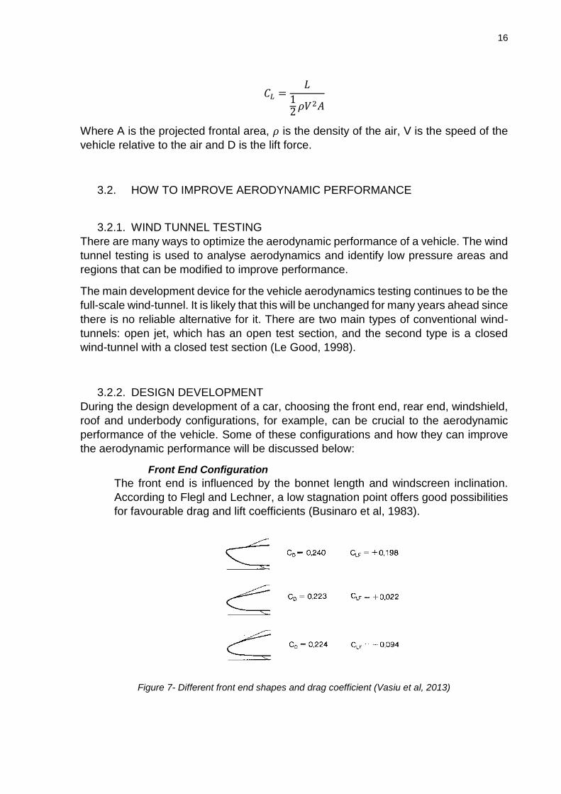
Front End Configuration
The front end is influenced by the bonnet length and windscreen inclination.
According to Flegl and Lechner, a low stagnation point offers good possibilities
for favourable drag and lift coefficients (Businaro et al, 1983).
Figure 7- Different front end shapes and drag coefficient (Vasiu et al, 2013)

17
Windshield and A-Pillar
The next below shows how the windshield inclination influences on drag
coefficient of the Audi 100 III Vehicle.
Graph 1- Windshield Angle influences on Drag Coefficient (Ahmed et al, 1998)
Rear End Configuration
There are different types of rear configurations including fastback (or
hatchback), notchback and square back (Barnard, 2009).
At the rear of a hatch back there is a region of low pressure, and conical vortices
generate due to flow separation from the rear corners, becoming strong trailing
vortices (Barnard, 2009).
Figure 8- Conical Vortices Generated on Hatchback (Vasiu et al, 2013)
In the case of a rear notch back car, the line joining the rear end of the roofline
and the tip of the boot is defined by angle θeff. As indicated on figure 9, the
variation in this angle has similarities to the drag coefficients of a hatchback.
This angle relates with the discovery that raising or lengthening the boot would
usually reduce drag. When the boot height is raised, θeff decreases (Barnard,
2009).

18
Figure 9- Effective Rear Slope Angle (Vasiu et al, 2013)
Underbody
The drag coefficient can be improved by rising the under floor towards the rear
creating a diffuser effect. The diffuser angle (under-body tapering at the rear)
and its effects are illustrated in the figure below:
Graph 2- Underbody Diffuser (Barnard, 2009)
Roof
The drag coefficient can be reduced by arching the roof in the longitudinal
direction; however if the curvature is too great, 𝐶𝐷 again can increase (Ahmed
et al, 1998).
However, the design if the roof arch must ensure that the frontal area of a car
remains constant; if not, the absolute drag (𝐶𝐷 × 𝐴) can increase despite a
reduction in drag coefficient, as shown in the upper graph of the next figure
(Ahmed et al, 1998).

19
Graph 3- Roof Shape influences on Drag Coefficient (Ahmed et al, 1998)
3.2.3. DEVICES AND GENERAL IMPROVEMENTS
The next figure illustrates 13 modifications that can be made in a vehicle design to
improve aerodynamic performance:
Figure 10- General Improvements (Accessed in http://www.kasravi.com/cmu/tec452/aerodynamics/VehicleAero.htm)
1- Front spoiler; 2- Ducted engine cooling; 3- Shrouded windshield wiper arms; 4- Aerodynamic mirrors; 5- Smooth windshield transitions; 6- Smooth side window transitions; 7- Smooth rear window transition; 8- Optimized trunk corner radii; 9- Optimized lower rear panel; 10 - Smooth fuel tank and underbody; 11- Optimized rocker panels; 12- Flush wheel covers; 13- Elimination of the rain gutter.
Spoilers act like barriers to air flow. While rear spoilers are commonly used to create
high pressure areas above the trunk of sedan vehicles (These kind of vehicles tends
to be lighter in the rear end), front spoilers are used to restrict air flow under the vehicle,
consequently reducing pressure under the vehicle and lift forces.
20
Covering wheels, when permitted by regulations, is a great solution to reduce drag,
since open wheels create air flow turbulence and, obviously, increase drag forces.
A vehicle body design needs to be as smooth as possible. A bodywork which quickly
converges forces the air flow into turbulence and, as mentioned previously,
consequently increases drag forces.
4. TARF-LCV PREVIOUS CONCEPTS CASE STUDY
In order to achieve better results in the Concept #6 CFD simulations (the main focus
of this project), it is important to understand the evolution of the project through the
previous concepts.
In this section, the design and aerodynamics of previous TARF-LCV concepts will be
discussed and analyzed.
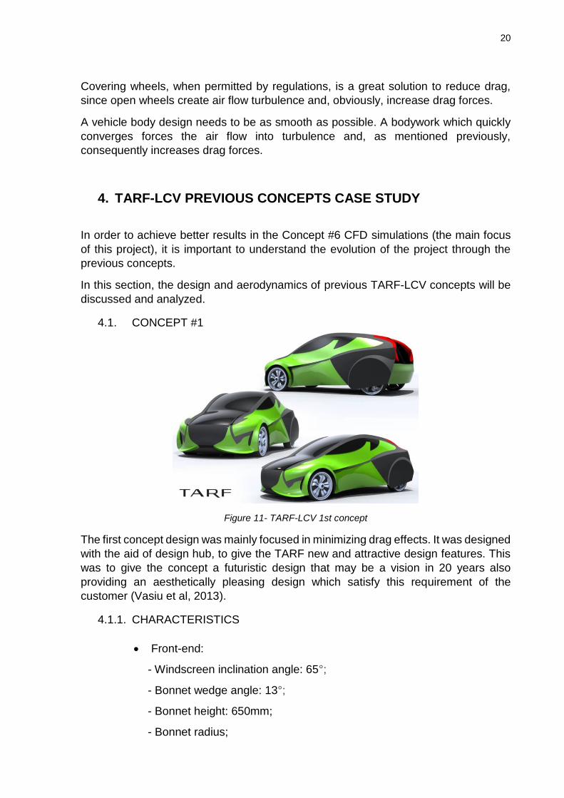
4.1. CONCEPT #1
Figure 11- TARF-LCV 1st concept
The first concept design was mainly focused in minimizing drag effects. It was designed
with the aid of design hub, to give the TARF new and attractive design features. This
was to give the concept a futuristic design that may be a vision in 20 years also
providing an aesthetically pleasing design which satisfy this requirement of the
customer (Vasiu et al, 2013).
4.1.1. CHARACTERISTICS
Front-end:
- Windscreen inclination angle: 65°;
- Bonnet wedge angle: 13°;
- Bonnet height: 650mm;
- Bonnet radius;

21
- Bumper and front wheel arches – curvy design to direct the air flow as recommended from product analysis and maintain flow attachment;
- Head lights design being integrated;
- Extended front wheel arch covers;
Rear-end:
- Rear Rake angle: 25°;
- Spoiler;
- Rear wheel fairing;
Passengers compartment area;
Side body streamlining;
Wheel size: 205/55/R17;
Frontal area.
4.1.2. AERODYNAMIC ANALYSIS
Figure 12- Concept #1 Streamlines

22
The CFD analysis of Concept #1 returned the following results (at an average speed
of 32 m/s):
Frontal Area Drag Coefficient Lift Coefficient
2.4 m2 0.327 0.113 Table 1- Concept #1 CFD Results
The figure below shows the pressure distribution over the vehicle. Regions in red color
refers to high pressure areas, where stagnation points are positioned. Blue regions
illustrate low pressure areas.
Figure 13- Concept #1 Pressure Coefficient
23
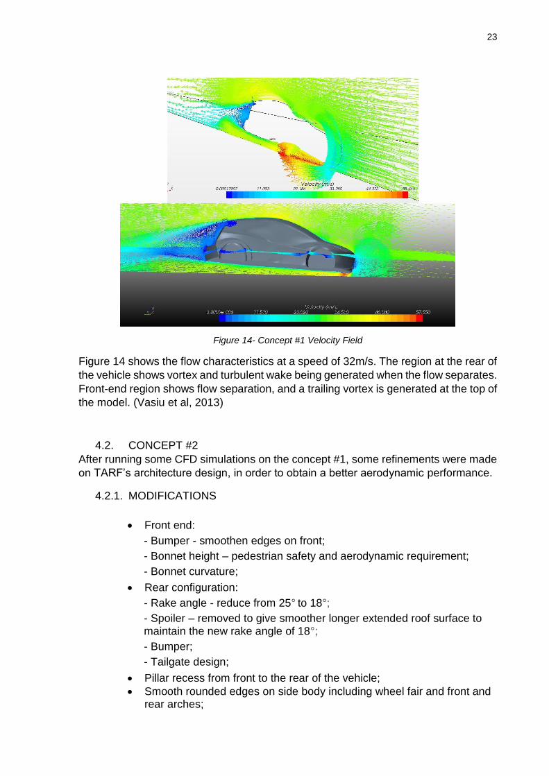
Figure 14- Concept #1 Velocity Field
Figure 14 shows the flow characteristics at a speed of 32m/s. The region at the rear of
the vehicle shows vortex and turbulent wake being generated when the flow separates.
Front-end region shows flow separation, and a trailing vortex is generated at the top of
the model. (Vasiu et al, 2013)
4.2. CONCEPT #2
After running some CFD simulations on the concept #1, some refinements were made
on TARF’s architecture design, in order to obtain a better aerodynamic performance.
4.2.1. MODIFICATIONS
Front end:
- Bumper - smoothen edges on front;
- Bonnet height – pedestrian safety and aerodynamic requirement;
- Bonnet curvature;
Rear configuration:
- Rake angle - reduce from 25° to 18°;
- Spoiler – removed to give smoother longer extended roof surface to maintain the new rake angle of 18°;
- Bumper;
- Tailgate design;
Pillar recess from front to the rear of the vehicle;
Smooth rounded edges on side body including wheel fair and front and rear arches;

24
Transition of side body smoother - front occupants compartment door region wider;
Side streamlined;
Frontal areas reduce. The front bumper and bonnet design of the model was refined to provide smoother edges and transition by increasing the radius of the surface, including the feature on the low region of the front bumper, and lowering the lip feature (Vasiu et al, 2013). The following images demonstrates the modifications made on the front-end, side body and rear-end, respectively:
Figure 15- Concepts #1 and #2 Front-end
Figure 16- Concepts #1 and #2 Side body
Figure 17- Concepts #1 and #2 Rear-end
All modifications made to the model were mainly focused on increasing aerodynamic
performance. However, a few changes were made to meet some regulations. It
includes an approach and departure angles on the bumpers, to ensure that they don’t
touch the floor when going through bumpers or stepped roads, for example. Changes
were also made on the A-pillar and in the tailgate so that driver’s visibility was

25
improved. Modifications to side body and rake angle increased occupant’s
compartment, providing more comfort to them.
4.3. CONCEPT #3
Figure 18- Concept #3 Mesh Scene
Overall there were a few discrepancies with concept model #2 from the designer (due
to design for aesthetics and styling) including the headroom space at the rear
passenger’s compartment. The ground clearance height was not maintained all the
way to the rear of the vehicle. These would need to be refined in the next iteration for
concept #3 to provide better aerodynamic performance (Vasiu et al, 2013).
4.3.1. MODIFICATIONS
In comparison to the previous model, the following modifications were made on the
third concept of TARF:
Front end:
- Added volume, and rounded front bumper with smoother transition between bumper and wheel arch – gives more packaging space as well;
- Bonnet space – for packaging of components;
Rear end:
- Extended rake angle of 12.5° (ideal rear rake angle) - as reviewed from the Mira reference car & Remus;
- Reduced the width of the rear arch (shoulder) also providing a side tape;
- Diffuser angle;
Head room space for manikins – more room added;
Volume added to side body sill section – more flushed for aero and more occupant’s compartment space;
Rounded edges of the models pillar up to the rear of the vehicle (Vasiu et al, 2013).

26
The modifications aforementioned are shown in the figures below. The front-end, side body and rear-end of both vehicles are presented, respectively. The vehicle on the left side is Concept #2, while Concept #3 is on the right side.
Figure 19- Concepts #2 and #3 Front-end
Figure 20- Concepts #2 and #3 Side body
Figure 21- Concepts #2 and #3 Rear-end
4.3.2. AERODYNAMIC ANALYSIS
Results obtained on CFD analysis of Concept #3 are shown on the following table and
figures:
Drag Coefficient Lift Coefficient
0.29 0.32 Table 2- Concept #3 CFD Results

27
Figure 22- Concept #4 Velocity Field
Figure 23- Concept #4 Pressure Coefficient
Figure 22 shows the flow visualization, while figure 23 shows the pressure distribution around
the vehicle surface.

28
4.4. CONCEPT #4
Figure 24- Concept #4 Final Design
4.4.1. MODIFICATIONS
Provided that the target for the drag coefficient for the fourth model was 0.28, there
weren’t too much changes in comparison to the third model, since the previous
achieved a 0.29 drag coefficient.
Basically, these were the changes:
Overall width was decrease from front and rear hence reducing the frontal area;
The frontal arch/fender’s volume was increased;
Front bumper splitter was rounded.
4.4.2. AERODYNAMIC ANALYSIS
After another CFD simulation was carried out, Concept #4 achieved the following
results, at 32 m/s:
Drag Coefficient Lift Coefficient
0.27 0.30 Table 3- Concept #4 CFD Results

29
Figure 25- Concept #4 Pressure Coefficient
Red regions on the figure above shows stagnation pressure, while blue regions
represents low pressure areas, where the flow separates. Red region on wheels occurs
because wheels are slightly exposed.
Figure 26 demonstrates flow behaviour around the vehicle surface.
Figure 26- Concept #4 Velocity Field
Figure 27- Concept #4 Streamlines

30
Figure 28- Vortex Core and Flow Separation
Figures 27 and 28 illustrates flow attachment and separation and also wake formation
around the vehicle.
All information regarding Concepts number 1 to 4 presented in this Case Study were
taken from the “TARF-LCV Product Innovation” project report, from Coventry
University (2013).
4.5. CONCEPT #5
Information about the fifth model are scarce, but it is known that the drag coefficient
has increased in comparison with previous model. It is also known that lift force in the
rear-end is considerably greater than in the front-end.
Following table and graphs illustrates this information:
Drag Coefficient Lift Coefficient - Front Lift Coefficient – Rear
0.31 0.03 0.2 Table 4- Concept #5 CFD Results

31
Graph 4- Concept #5 Drag Force Distribution
Graph 5- Concept #5 Lift Force Distribution
5. METHODOLOGY – MODELLING THE CONCEPT #6 CFD
SIMULATION
Modelling a CFD simulation is the most important task when analysing the
aerodynamic performance. Any mistake made during modelling can influence the
outcome results, as will be shown later on.
The CAD model was imported from CATIA as .stl file in STAR-CCM+, and the first was
to check the geometry surface and repair it. The under body surface manipulations
were done as the surfaces were not closed on either sides. A New surface was made
for half of the vehicle body making a contact with the adjacent surfaces. The created
surface was mirrored with XY plane as reference plane.

32
All parts of the geometry were assigned to one part using the Combine operation. The
combined part was then assigned to a region using the option “Assign parts to regions”.
A region was created to apply surface meshing. To remove all the free edges, non-
manifold edges and non-manifold vertices surface meshing needs to be done. The two
options available for meshing were Surface Remeshing and Surface Wrapping. The
surface remesher will increase the surface quality by re-arranging the triangles. But it
cannot be done for a closed surface. Surface wrapping allows the part to be a closed
surface, but the surface quality might not be increased or may have poor surface
quality. So, surface wrapper was selected to have a closed surface.
The Surface Wrapper tool was created after assigning the geometry parts to regions
(1 region per part and 1 boundary per part surface). Surface Wrapper properties are
shown below:
Figure 29- Surface Wrapper Properties
After the repair tool was activated, the surface was checked again. The result is
presented in Figure 30.

33
Figure 30- Surface Diagnostic
It’s important to remember that not all fields needs to be equal to zero, however the
STAR-CCM+ Auto Repair tool was used to do so.
Next step was to create the wind tunnel. Using STAR-CCM+ CAD features, a block
was created around the left half of the vehicle, considering the vehicle symmetry (the
computation will be easier), as shown below:
Figure 31- Wind Tunnel
After that, the block surface was split by patch, creating the inlet, outlet, floor, walls and
symmetry surfaces.
Then, the vehicle surface was subtracted from the block (wind tunnel), creating a new
part called “Subtract”, and the “Subtract” surfaces were assigned to regions.
Subtract regions received the following properties:
Region Type
Inlet Velocity Inlet
Outlet Pressure Outlet
Symmetry Symmetry Plane Table 5- Wind Tunnel Regions Properties

34
Next step was to create 2 Volumetric Controls around the vehicle. A volumetric control
allows you to refine or coarsen the mesh density for a surface and/or volume mesh,
based on a volume shape (CD-adapco, 2013).
Next task was to set up a new Mesh Continuum. The following mesh models were
selected:
Polyhedral Mesher;
Prism Layer Mesher;
Surface remesher.
Various options for volume meshing were available. Polyhedral mesher was selected
as it produces easy and balanced solution to typical geometrical shapes. It is much
better than tetrahedral mesher in terms of cell productivity as the polyhedral mesh
produces fewer cells comparatively. Prism layer mesher was used in combination of
polyhedral mesher to improve the accuracy of the solution as it helps in settling the
turbulent boundary layer. Embedded thin mesher is selected for creating cells for thin
geometry as the vehicle has fins over the head lights and the wheel arches which were
considerably thin when compared to the vehicle body. Base size, polynomial density
and polynomial volume density were manipulated to have a good volume mesh.
Table 6 shows the reference values used:
Base Size Different Values were used
Surface Size Relative Minimum Size: 25% of base
Relative Target Size: 100% of base
Number of prism layers 6
Prism Layer Thickness (Absolute Size)
10 mm
Surface Growth Rate 1.1 Table 6- Mesh Continuum Reference Values
As table 6 shows, different values were used in different simulations for the base size.
It is also important to remember that specific surface sizes were used for the vehicle:
Relative Minimum size: 1.5% of base size;
Relative Target size: 7.5% of base size.
The “Customise Prism Mesh” feature was disabled for the floor and walls.
From this point, Surface and Volume meshes can be generated, however it was
decided to set up the Physics before generating it.
Physics models selected were:
Three Dimensional Flow;
Steady flow;
Working Fluid – Gas (air);
Segregated flow;
Constant Density;
35
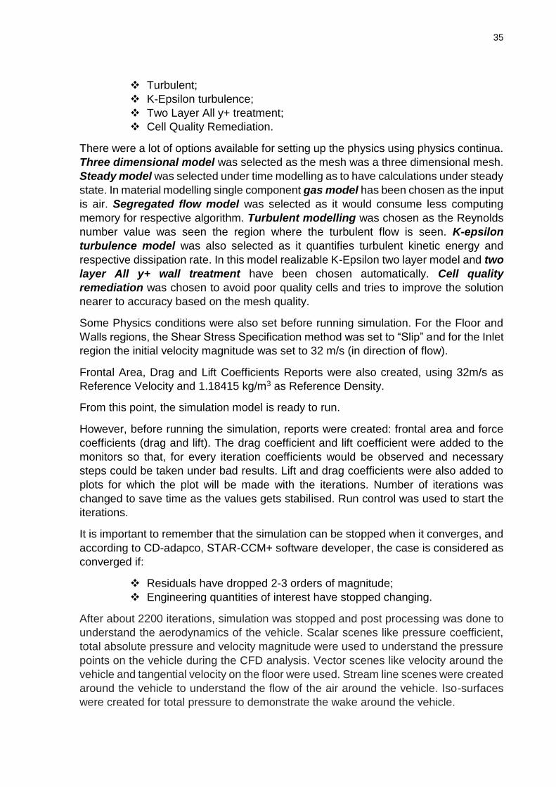
Turbulent;
K-Epsilon turbulence;
Two Layer All y+ treatment;
Cell Quality Remediation.
There were a lot of options available for setting up the physics using physics continua.
Three dimensional model was selected as the mesh was a three dimensional mesh.
Steady model was selected under time modelling as to have calculations under steady
state. In material modelling single component gas model has been chosen as the input
is air. Segregated flow model was selected as it would consume less computing
memory for respective algorithm. Turbulent modelling was chosen as the Reynolds
number value was seen the region where the turbulent flow is seen. K-epsilon
turbulence model was also selected as it quantifies turbulent kinetic energy and
respective dissipation rate. In this model realizable K-Epsilon two layer model and two
layer All y+ wall treatment have been chosen automatically. Cell quality
remediation was chosen to avoid poor quality cells and tries to improve the solution
nearer to accuracy based on the mesh quality.
Some Physics conditions were also set before running simulation. For the Floor and
Walls regions, the Shear Stress Specification method was set to “Slip” and for the Inlet
region the initial velocity magnitude was set to 32 m/s (in direction of flow).
Frontal Area, Drag and Lift Coefficients Reports were also created, using 32m/s as
Reference Velocity and 1.18415 kg/m3 as Reference Density.
From this point, the simulation model is ready to run.
However, before running the simulation, reports were created: frontal area and force
coefficients (drag and lift). The drag coefficient and lift coefficient were added to the
monitors so that, for every iteration coefficients would be observed and necessary
steps could be taken under bad results. Lift and drag coefficients were also added to
plots for which the plot will be made with the iterations. Number of iterations was
changed to save time as the values gets stabilised. Run control was used to start the
iterations.
It is important to remember that the simulation can be stopped when it converges, and
according to CD-adapco, STAR-CCM+ software developer, the case is considered as
converged if:
Residuals have dropped 2-3 orders of magnitude;
Engineering quantities of interest have stopped changing.
After about 2200 iterations, simulation was stopped and post processing was done to
understand the aerodynamics of the vehicle. Scalar scenes like pressure coefficient,
total absolute pressure and velocity magnitude were used to understand the pressure
points on the vehicle during the CFD analysis. Vector scenes like velocity around the
vehicle and tangential velocity on the floor were used. Stream line scenes were created
around the vehicle to understand the flow of the air around the vehicle. Iso-surfaces
were created for total pressure to demonstrate the wake around the vehicle.

36
The results of post processing analysis will be shown in the next section of this report.
6. CONCEPT #6 – CFD RESULTS
As reported before, more than one simulation was created for the geometry, with
different base sizes for the volume meshing, and also with 2 different distances
between the floor and the vehicle, as figure 35 will show. In this section the results of
the simulations will be described.
Four simulations were created with a lower distance between the vehicle and the floor,
using different base sizes for the volume meshing. The Frontal Area of the vehicle in
these simulations was 1.074 m2.
The following table shows the results:
Base Size of Volume Meshing Drag Coefficient
1500 mm 0.316
600 mm 0.296
450 mm 0.283
300 mm 0.269 Table 7- Base Sizes and CFD Results
Mesh scenes are available in the Appendix.
After this simulations, it was realized that the distance between vehicle and floor was
wrong, since the vehicle was too close to the floor surface and it was not representing
the reality.
Therefore, another simulation with a different distance between vehicle and floor was
created, with a Volume Meshing base size of 300 mm. Results are shown above:
Frontal Area Drag Coefficient Lift Coefficient
1.099 m2 0.287 0.067 Table 8- Concept #6 CFD Results
Figure 32- Frontal Area Report
37
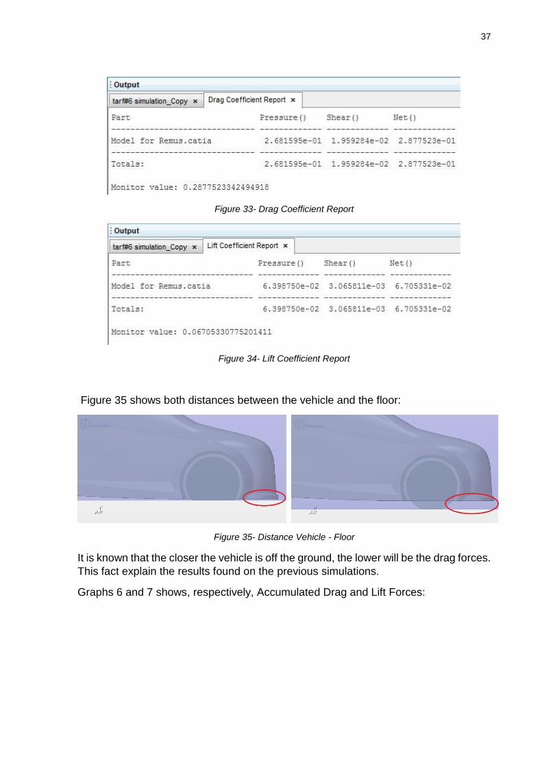
Figure 33- Drag Coefficient Report
Figure 34- Lift Coefficient Report
Figure 35 shows both distances between the vehicle and the floor:
Figure 35- Distance Vehicle - Floor
It is known that the closer the vehicle is off the ground, the lower will be the drag forces.
This fact explain the results found on the previous simulations.
Graphs 6 and 7 shows, respectively, Accumulated Drag and Lift Forces:

38
Graph 6- Accumulated Drag Force
Graph 7- Accumulated Lift Force
As the graph above shows, the accumulated lift force varied from negative values at
the front and the middle of the vehicle to positive values at the rear-end. This variation
can be explained by the velocity distribution and magnitude along the car, as shown in
Figures 36 and 37:

39
Figure 36- Velocity Distribution Vectors
Figure 37- Velocity Magnitude around Vehicle
From the figure above, it is possible to note that at the front, as the flow approaches
the vehicle, it enters in a stagnation point, and then accelerates again, around the car.
The acceleration of the flow under the front part of vehicle generates a low pressure
region, and consequently, down force (Negative lift force). In fact, it can be noticed on
Graph 7.
Figures 38 and 39 illustrates wake formation on the model, while figures 40 and 41
shows the pressure coefficient distribution.

40
Figure 38- Wake formation (front view)
Figure 39- Wake formation (rear view)

41
Figure 40- Pressure Coefficient Distribution (Front view)
Figure 41- Pressure Coefficient Distribution (Rear view)
Red region indicates high pressure areas, while blue regions indicates low pressure.
The front part of the vehicle (red region) concentrates higher pressure areas, therefore,
a considerable amount of drag force is generated in this area.
42
7. CONCLUSION
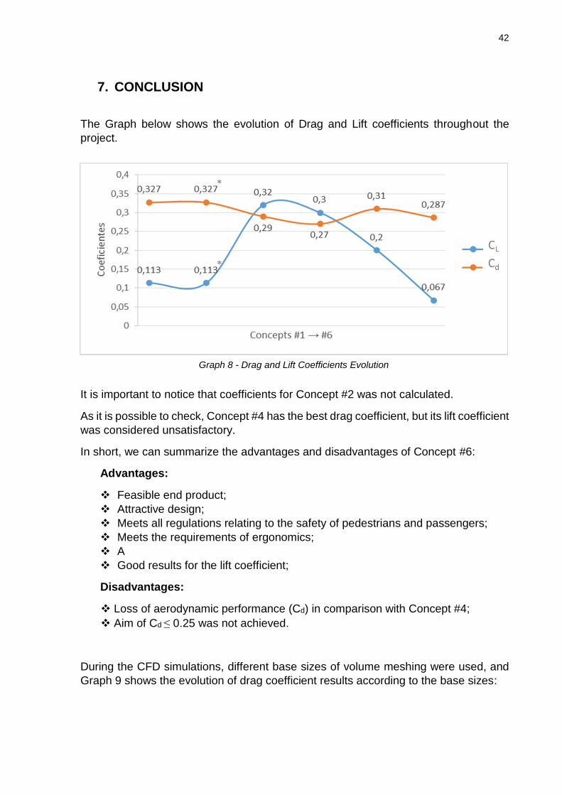
The Graph below shows the evolution of Drag and Lift coefficients throughout the
project.
It is important to notice that coefficients for Concept #2 was not calculated.
As it is possible to check, Concept #4 has the best drag coefficient, but its lift coefficient
was considered unsatisfactory.
In short, we can summarize the advantages and disadvantages of Concept #6:
Advantages:
Feasible end product;
Attractive design;
Meets all regulations relating to the safety of pedestrians and passengers;
Meets the requirements of ergonomics;
A
Good results for the lift coefficient;
Disadvantages:
Loss of aerodynamic performance (Cd) in comparison with Concept #4;
Aim of Cd ≤ 0.25 was not achieved.
During the CFD simulations, different base sizes of volume meshing were used, and
Graph 9 shows the evolution of drag coefficient results according to the base sizes:
Graph 8 - Drag and Lift Coefficients Evolution

43
As it is possible to notice, smaller sizes of base size leads to better results of drag
coefficient. Unfortunately, it was not possible to run new simulations with base sizes
smaller than 300mm because of the computational resource (simulations were taking
too much time). As a suggestion for future works, better computational resources or a
different license of Star-CCM+ Software would lead to better results.
In order to find better results for drag coefficient, it is important to make certain external
modifications. Figures 42 and 43 illustrates regions which can be modified in order to
improve aerodynamic performance.
Figure 42- Recommended Modifications
Graph 9 - Cd vs Mesh base size

44
Front wheels arches are low pressure regions, as the figure above shows. In this
region, the air flow separates, therefore wake formation occurs.
Regions indicated on figure below are also regions where wake formation occurs and
could be modified in order to improve aerodynamic performance.
Figure 43- Recommended Modifications

45
8. REFERENCES
1. Ahmed, S. R. et al (1998) Ed. By Hucho, W. H. Aerodynamics of Road Vehicles. 4th
ed. Warrendale, USA. Society of Automotive Engineers, Inc.
2. Barnard, R. H. (2009) Road Vehicle Aerodynamics Design. 3rd ed. Mech Aero.
3. Businaro, U. L., Dorgham, M. A, International Association for Vehicle Design (1983).
Impact of Aerodynamics on Vehicle Design. UK: Inderscience Enterprises Ltd.
4. Calnev, D. (2013). Designing and Manufacturing of a Scale Model for the TARF-
LCV Vehicle. Coventry University.
5. G M Le Good (1998). A Comparison of On-Road Aerodynamic Drag Measurements
with Wind Tunnel Data from Pininfarina and MIRA. Detroit: SAE International Technical
Paper Series.
6. Kasravi, K. (n. d.). Class Notes: Aerodynamics. [online] available from
<http://www.kasravi.com/cmu/tec452/Aerodynamics/AeroIndex.htm> [6th October
2013]
7. Research Councils UK (2013). Towards Affordable, Closed-Loop Recyclable Future
Low Carbon Vehicle – TARF-LCV. [online] available from
<http://gtr.rcuk.ac.uk/project/D64B3346-249F-49AF-94B4-D90A6F633904> [28th
November 2013]
8. Unlimited Performance Products (2007). Tips: Aerodynamics. [online] available from
<http://www.up22.com/Aerodynamics.htm> [5th October 2013]
9. Vasiu, C. et al, (2013). TARF-LCV Product Innovation. Coventry University.

46
APPENDIX A – Volume Meshes
Volume Mesh – Reference Base Size: 1500 mm
Volume Mesh – Reference Base Size: 600 mm
47
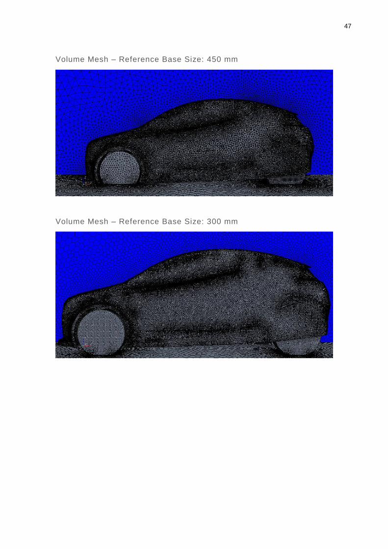
Volume Mesh – Reference Base Size: 450 mm
Volume Mesh – Reference Base Size: 300 mm

48
APPENDIX B – Residuals Plot
450 mm Reference Base Size Simulation

49
300 mm Reference Base Size Simulation


![[Webinar] Performance e otimização de banco de dados MySQL](https://img.document.onl/doc/110x75/5a6e3d8d7f8b9a8b568b552d/webinar-performance-e-otimizacao-de-banco-de-dados-mysql.jpg)

![Questões - Aerodinâmica de Alta Velocidade - []](https://img.document.onl/doc/110x75/577cdb9f1a28ab9e78a8aece/questoes-aerodinamica-de-alta-velocidade-wwwcanalpilotocombr.jpg)