Brazilian Business Cycles and Growth from 1850 to 2000

Est. Econ., são Paulo, v. 38, n. 3, P. 557-581, JulHo-sEtEMBRo 2008

Brazilian Business Cycles and Growth from 1850 to 2000

Eurilton ArAújo luciAnE cArpEnA AlExAndrE B. cunhA

ResumoEstudaram-se neste artigo as propriedades do produto interno bruto per capita brasileiro de 1850 a 2000. Contrariamente ao observado em alguns países desenvolvidos, não se obteve evidência de alterações ex-pressivas na volatilidade do PIB per capita. Contudo, verificou-se que as oscilações na atividade econômica se tornaram mais persistentes após a 2ª Guerra Mundial.

PalavRas-ChavePIB per capita, ciclo de negócios, crescimento, Brasil

abstRaCtWe study the cyclical and growth properties of Brazilian per capita output from 1850 to 2000. We find that, contrary to some developed countries, Brazil did not experience large changes in the volatility of per capita output. However, we obtained evidence that the oscillations in economic activity became more persistent after World War II.

KeywoRdsper capita GDP, business cycles, growth, Brazil

Jel ClassifiCationC22, E32 , N10

This paper highly benefited from comments by two anonymous referees. Financial support from the Brazilian Council

of Science and Technology (CNPq) is gratefully acknowledged. IBMEC São Paulo. Corresponding author address: Rua Quatá, 300 – São Paulo, SP – Brazil – 04546-042. E-mail:

[email protected]. Faculdades IBMEC/RJ e BNDES. Corresponding author address: Av. Pres. Wilson, 118, 2º andar – Rio de Janeiro,

RJ – Brazil – 20.030-020. Faculdades IBMEC/RJ. Corresponding author address: Av. Pres. Wilson, 118, sala 1119 – Rio de Janeiro, RJ – Brazil

– 20.030-020. E-mail: [email protected]. (Recebido em abril de 2005. Aceito para publicação em agosto de 2007).

Est. econ., são Paulo, 38(3): 557-581, jul-set 2008

558 Brazilian Business cycles and Growth from 1850 to 2000

1 IntRoductIon

The reporting of empirical regularities of economic time series has a long tradi-tion in the study of business cycles and economic growth. For instance, Burns and Mitchell (1946) documented several features of the economic cycles in the United States. In the field of economic development, Kaldor’s (1961) summary of some growth evidence became widely known as Kaldor’s stylized facts.

Recently, several papers have sought to document the statistical properties of busi-ness cycles. Backus and Kehoe (1992) and Hodrick and Prescott (1997) are typical examples of this research line. The same research strategy has been followed in the field of economic growth. For instance, Barro and Sala-I-Martin (1995) devoted several chapters of their book to studying of the empirical regularities of economic growth.

While the international literature on the statistical regularities of business cycles and economic growth is very large, its Brazilian counterpart is relatively incipient. One of the reasons is that the lack of available data often restrains studies of Brazilian business cycles to the period after World War II, as in Ellery Jr., Gomes and Sachsida (2002).

We have two main goals in this paper. The first is to construct long GDP and per capita GDP series for the Brazilian economy to be able to compare the statistical properties of these series to the stylized facts provided by Backus and Kehoe (1992) and other international evidence. The second is to investigate the nature of structural changes that may have taken place over time. We place particular emphasis on the study of volatility, persistence and the relation between growth and volatility.

We construct GDP and per capita GDP series for the Brazilian economy that covers the period 1850-2000.1 We combine data from Goldsmith (1986), Haddad (1978) and IBGE (2003) to construct our GDP series. Those sources cover, respectively, the periods 1850-1900, 1900-1947 and 1947-2000. We then use information from IBGE (2003) to generate a population series. We provide additional details about our data set in Section I.

We evaluate some basic business cycle features, such as volatility, persistence, turning points, and the length of recessions and expansions of the per capita GDP series. We assess some of these features over distinct sub-periods of the whole sample and

1 Ellery Jr. and Gomes (2005) have recently managed to construct series for GPD and other macro- Ellery Jr. and Gomes (2005) have recently managed to construct series for GPD and other macro-economic variables such as consumption and investment for the Brazilian economy that cover the entire twentieth century. The GDP series we present in this paper is longer than that of Ellery Jr. and Gomes.

Eurilton araújo, luciane carpena, alexandre B. cunha 559


compare our findings with the international evidence. We also study the volatility and the persistence of the per capita GDP growth rate.

Our main findings are that, unlike the evidence Backus and Kehoe (1992) presented for several industrialized nations, the volatility of Brazilian business cycles did not vary greatly over the sub-periods of our sample. We also show that volatility may be characterized by three phases. There is an initial low volatility period from 1850 to 1875. Then, in an intermediate period, lasting up to 1975, the Brazilian economy displayed high volatility. Finally, low volatility characterized the period from 1976 to 2000.

Concerning persistence, we obtain evidence that the cyclical component of the per capita output became more persistent after 1945. With respect to the relation betwe-en growth and volatility rates, we do not find a statistically significant relationship between these variables. However, we do find that there is a change in the dynamics of the series when we compare pre and post World War II periods. That change can be attributed to an increase in persistence rather than any abrupt change in volatility.

In summary, we provide evidence that the behavior of the volatility of the Brazilian business cycles from 1850 to 2000 was quite different from their counterparts in the US and some other developed economies. Contrary to the experience of those countries, the volatility of the Brazilian economy appears to have been roughly constant. Our analysis also shows that the persistence of the economic activity os-cillations increased after the Second World War. Finally, we do not find a strong relation between economic growth and volatility.

We wish to stress the relevance of our findings. As Backus and Kehoe (1992) and Ellery Jr. and Gomes (2005) pointed out, a crucial question in international business cycles is whether countries display similar economic oscillations. We contribute to this issue by showing that Brazilian business cycles had some distinctive features. Authors such as Black (1987) and Caballero (1991) have argued that an increase in volatility should have some impact on growth and investment rates. We investigate whether this holds in the Brazilian economy and find that its growth was not signi-ficantly affected by economic volatility over the period 1850-2000.

This paper is organized as follows. In Section I we present our data set and evaluate its reliability. In Section II we test the GDP and per capita GDP series for non-sta-tionary behavior. In Section III we study the business cycle properties of Brazilian per capita GDP. In Section IV we focus on the empirical relationship between vola-



tility and growth. Finally, Section V contains our concluding remarks. In addition, we list our population, GDP and per capita GDP series in Section VI (Appendix).

2 tHE data sEt

In this section we explain how we construct our GDP series. We then explain how we obtain the population series. Concerning the per capita GDP series, we derive it by simply taking the ratio between the two former series. We also discuss the reliability of these series.

2.1 the GdP series

Goldsmith (1986) contains a real GDP series from 1850 to 1900 (Table II.1, pages 22 and 23 and Table III.1, pages 82 and 83). Haddad (1978) provides data for the same variable from 1900 to 1947 (Table 3, page 15). The data CD that accompanies IBGE (2003) is the source for the sub-period 1948-2000. The files ‘1_2_scn_conso-lidado.xls’ and ‘1_3_nscn.xls’, both located in the folder ‘economia\contas_nacionais’ of that CD, contain real GDP growth rates from 1948 to 2000. We combined these three sources to obtain a real GDP index from 1850 to 2000.2

We now discuss some issues related to the reliability of our GPD series. As usual, the older the period, the less reliable the data are. In the particular case of our GDP series, the 1850-1900 sub-period deserves more attention.

From 1947 onwards, our data source is the official Brazilian national account sys-tem. The source for the 1900-1947 period is Haddad (1978).3 Despite not being an official GDP measure, Haddad’s figures are widely accepted today. Thus, we can be fairly sure that no available series covering the 1900-2000 years is more accurate than ours.

As explained, we linked Haddad’s series to Goldsmith’s at 1900. We do not know of any other estimate of Brazilian GDP that covers the period 1850-1900. Thus, a strong reason to adopt the Goldsmith’s series is the fact that it is the only one available. The exclusiveness of Goldsmith’s GDP series does not ensure its accuracy. Thus, it is important to check this as far as possible. Contador and Haddad (1975) provided yearly estimations of Brazilian GDP from 1861 to 1900. Table 1 compares the GDP growth rates of those two series.

2 We present our GDP, population and per capita GDP series in Table A1 in the appendix.3 Note that the Brazilian national account system does not cover the period before 1947.



taBlE 1 – coMPaRIson of GdP sERIEs: avERaGE GRowtH RatEs

Period Goldsmith Contador and Haddad

1862-1900 1.61 1.47

1862-1870 2.63 3.96

1871-1880 1.60 1.98

1881-1890 2.14 2.04

1891-1900 0.19 -1.75

For the period 1862-1900, the two series have a similar average growth rate. For smaller intervals, the similarity is smaller. Goldsmith emphasized this point. He suggested that the short-run oscillations of any GDP series for that period should be evaluated with care.

We decided to adopt Goldsmith’s series for two reasons. First, as mentioned, it is the only one that covers the period 1850-1900. Second, Goldsmith constructed his series using information from labor compensation, money supply, foreign trade and public spending, while Contador and Haddad used only foreign trade from 1861 to 1888 and foreign trade plus installed electric power capacity afterwards.

We summarize the above discussion as follows. Our GDP series has f ive properties:

As far as we know, it is the only series that covers the entire 1850-2000 1. period.

Authors such as Goldsmith (1986) and Ellery Jr. and Gomes (2005) have used 2. Haddad’s work in their measurement of Brazilian GDP over the 1900-1947 period. We use Haddad’s latest estimates for the years in question.

Its data for the 1947-2000 sub-period are exactly the ones available from the 3. official Brazilian national account system.

It provides an accurate description of the long-run evolution of Brazilian GDP.4.

Its short-term measurement errors should be larger in the 1850-1900 sub-period 5. than later.



To minimize the problem pointed out in the last item, on several occasions we report results for the whole period 1850-2000 and some selected sub-periods.

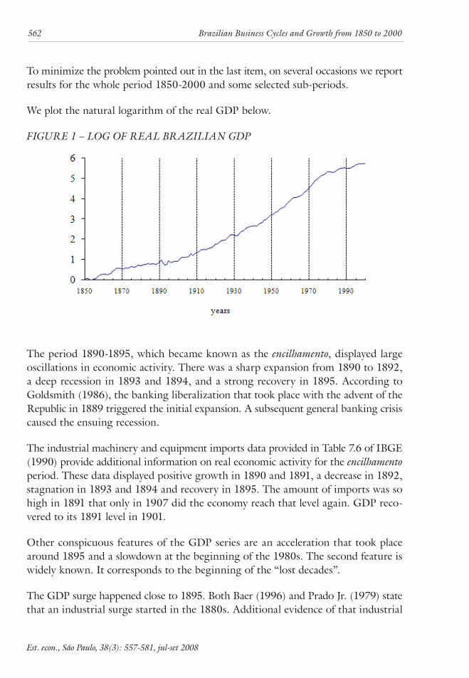
We plot the natural logarithm of the real GDP below.

fIGuRE 1 – loG of REal BRazIlIan GdP

The period 1890-1895, which became known as the encilhamento, displayed large oscillations in economic activity. There was a sharp expansion from 1890 to 1892, a deep recession in 1893 and 1894, and a strong recovery in 1895. According to Goldsmith (1986), the banking liberalization that took place with the advent of the Republic in 1889 triggered the initial expansion. A subsequent general banking crisis caused the ensuing recession.

The industrial machinery and equipment imports data provided in Table 7.6 of IBGE (1990) provide additional information on real economic activity for the encilhamento period. These data displayed positive growth in 1890 and 1891, a decrease in 1892, stagnation in 1893 and 1894 and recovery in 1895. The amount of imports was so high in 1891 that only in 1907 did the economy reach that level again. GDP reco-vered to its 1891 level in 1901.

Other conspicuous features of the GDP series are an acceleration that took place around 1895 and a slowdown at the beginning of the 1980s. The second feature is widely known. It corresponds to the beginning of the “lost decades”.

The GDP surge happened close to 1895. Both Baer (1996) and Prado Jr. (1979) state that an industrial surge started in the 1880s. Additional evidence of that industrial



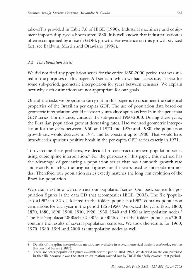
take-off is provided in Table 7.6 of IBGE (1990). Industrial machinery and equip-ment imports displayed a boom after 1880. It is well known that industrialization is often accompanied by a rise in GDP’s growth. For evidence on this growth-stylized fact, see Baldwin, Martin and Ottaviano (1998).

2.2 the Population series

We did not find any population series for the entire 1850-2000 period that was sui-ted to the purposes of this paper. All series to which we had access use, at least for some sub-period, geometric interpolation for years between censuses. We explain next why such estimations are not appropriate for our goals.

One of the tasks we propose to carry out in this paper is to document the statistical properties of the Brazilian per capita GDP. The use of population data based on geometric interpolation would necessarily introduce spurious breaks in the per capita GDP series. For instance, consider the sub-period 1960-2000. During these years, the Brazilian population grew at decreasing rates. Had we used geometric interpo-lation for the years between 1960 and 1970 and 1970 and 1980, the population growth rate would decrease in 1971 and be constant up to 1980. That would have introduced a spurious positive break in the per capita GPD series exactly in 1971.

To overcome these problems, we decided to construct our own population series using cubic spline interpolation.4 For the purposes of this paper, this method has the advantage of generating a population series that has a smooth growth rate and exactly matches the original figures for the years used as interpolation no-des. Therefore, our population series exactly matches the long run evolution of the Brazilian population.

We detail next how we construct our population series. Our basic source for po-pulation figures is the data CD that accompanies IBGE (2003). The file ‘popula-cao_a1952aeb_32.xls’ located in the folder ‘populacao\1952’ contains population estimations for each year in the period 1851-1950. We picked the years 1851, 1860, 1870, 1880, 1890, 1900, 1910, 1920, 1930, 1940 and 1950 as interpolation nodes.5 The file ‘populacao2000aeb_s2_002a_a_002b.xls’ in the folder ‘populacao\2000’ contains the results of several population censuses. We took the results for 1960, 1970, 1980, 1991 and 2000 as interpolation nodes as well.

4 Details of the spline interpolation method are available in several numerical analysis textbooks, such as Burden and Faires (1997).

5 There are other population figures available for the period 1851-1950. We decided on the one provided in that file because it was the latest re-estimation carried out by IBGE that fully covered that period.



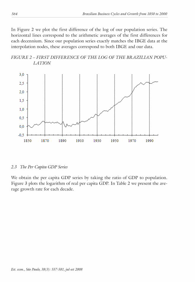
In Figure 2 we plot the first difference of the log of our population series. The horizontal lines correspond to the arithmetic averages of the first differences for each decennium. Since our population series exactly matches the IBGE data at the interpolation nodes, these averages correspond to both IBGE and our data.

fIGuRE 2 – fIRst dIffEREncE of tHE loG of tHE BRazIlIan PoPu-latIon

2.3 the Per capita GdP series

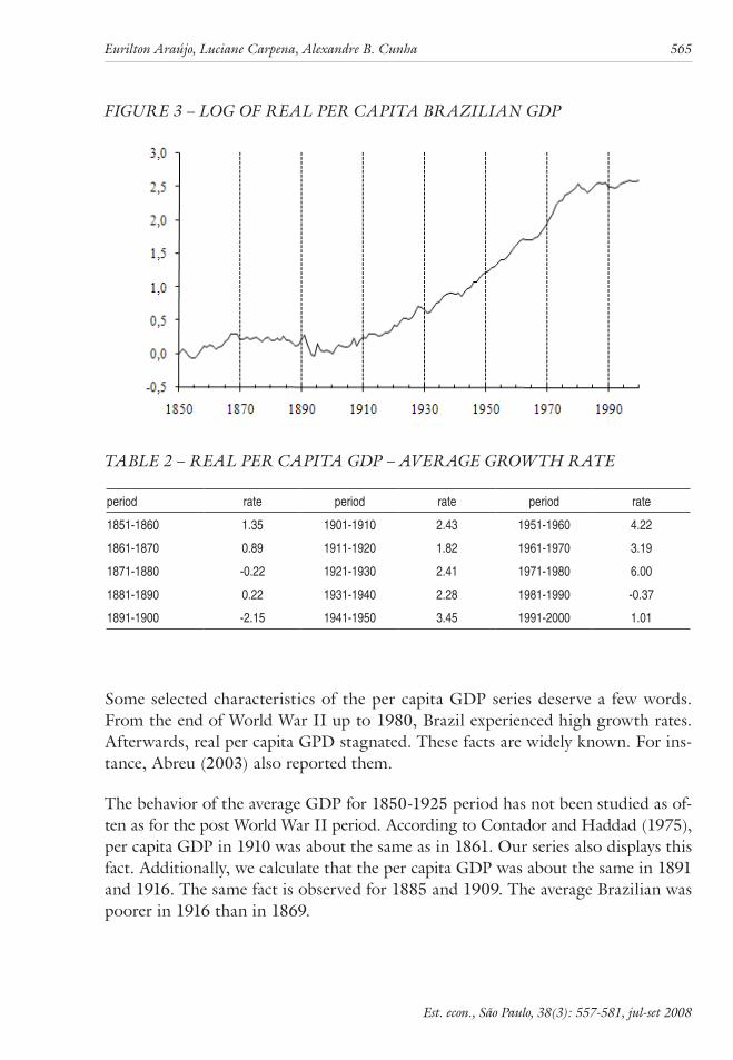
We obtain the per capita GDP series by taking the ratio of GDP to population. Figure 3 plots the logarithm of real per capita GDP. In Table 2 we present the ave-rage growth rate for each decade.



fIGuRE 3 – loG of REal PER caPIta BRazIlIan GdP

taBlE 2 – REal PER caPIta GdP – avERaGE GRowtH RatE

period rate period rate period rate

1851-1860 1.35 1901-1910 2.43 1951-1960 4.22

1861-1870 0.89 1911-1920 1.82 1961-1970 3.19

1871-1880 -0.22 1921-1930 2.41 1971-1980 6.00

1881-1890 0.22 1931-1940 2.28 1981-1990 -0.37

1891-1900 -2.15 1941-1950 3.45 1991-2000 1.01

Some selected characteristics of the per capita GDP series deserve a few words. From the end of World War II up to 1980, Brazil experienced high growth rates. Afterwards, real per capita GPD stagnated. These facts are widely known. For ins-tance, Abreu (2003) also reported them.

The behavior of the average GDP for 1850-1925 period has not been studied as of-ten as for the post World War II period. According to Contador and Haddad (1975), per capita GDP in 1910 was about the same as in 1861. Our series also displays this fact. Additionally, we calculate that the per capita GDP was about the same in 1891 and 1916. The same fact is observed for 1885 and 1909. The average Brazilian was poorer in 1916 than in 1869.



The facts mentioned above are consequences of a major decline in the Brazilian per capita GDP during the 1870-1900 period. According to our series, per capita GDP in 1900 was only 80% of the 1870 figure. Using Contador and Haddad’s (1975) series, the equivalent figure is 68%. Therefore, the available evidence suggests that the Brazilian economy suffered a severe decline in the thirty years that followed the end of the Paraguayan War in 1870.

3 unIt Root PRoPERtIEs

We perform unit root tests to detect the presence of stochastic trends in order to build a time series model for the level of the series. If one of the series follows a unit root process, we need to adopt some detrending procedure. After we perform a lo-garithmic transformation of our data, both GDP and per capita GDP are analyzed. In addition to the ADF test, we conduct unit root tests allowing for breaks in the data, since Cati, Garcia and Perron (1999) showed that some Brazilian time series are better characterized by the presence of structural breaks.

First, we present results based on a simple ADF test without breaks. We search for the optimal lag length using three information criteria (AIC, Schwarz and Hannan-Quinn). For all the criteria employed, after searching for up to 10 lags, we find that the optimal lag length is zero for both series. We allow for a constant and a linear time trend as deterministic components since both series are clearly trended, as shown in Figures 1 and 3. The test results are summarized in Table 3.

taBlE 3 – unIt Root tEst wItHout BREak

Variable Number of Lags

Deterministic Component

Test Statistic

5% Critical Level

10% Critical Level

GDP 0 constant and trend -1.433 -3.41 -3.13

Per Capita GDP 0 constant and trend -1.625 -3.41 -3.13

Second, we allow one endogenous break, as in Perron (1989). The break takes the form of either an impulse dummy or a level shift dummy. We employ a test stra-tegy developed by Saikkonen and Lütkepohl (2002) and Lanne, Lütkepohl and Saikkonen (2002). As in the ADF test, we search for the optimal number of lags using the same information criteria. We allow for a constant and a time trend as in the ADF test. These test results are summarized in Table 4.



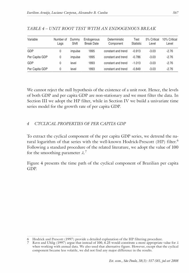
taBlE 4 – unIt Root tEst wItH an EndoGEnous BREak

Variable Number of Lags

Dummy Shift

Endogenous Break Date

Deterministic Component

Test Statistic

5% Critical Level

10% Critical Level

GDP 0 impulse 1895 constant and trend -0.913 -3.03 -2.76

Per Capita GDP 0 impulse 1895 constant and trend -0.786 -3.03 -2.76

GDP 0 level 1893 constant and trend -1.013 -3.03 -2.76

Per Capita GDP 0 level 1893 constant and trend -0.849 -3.03 -2.76

We cannot reject the null hypothesis of the existence of a unit root. Hence, the levels of both GDP and per capita GDP are non-stationary and we must filter the data. In Section III we adopt the HP filter, while in Section IV we build a univariate time series model for the growth rate of per capita GDP.

4 cyclIcal PRoPERtIEs of PER caPIta GdP

To extract the cyclical component of the per capita GDP series, we detrend the na-tural logarithm of that series with the well-known Hodrick-Prescott (HP) filter.6 Following a standard procedure of the related literature, we adopt the value of 100 for the smoothing parameter λ.7

Figure 4 presents the time path of the cyclical component of Brazilian per capita GDP.

6 Hodrick and Prescott (1997) provide a detailed explanation of the HP filtering procedure.7 Ravn and Uhlig (1997) argue that instead of 100, 6.25 would constitute a more appropriate value for λ

when working with annual data. We also used that alternative figure. However, except that the cyclical component became less volatile, we did not find any major difference in the results.



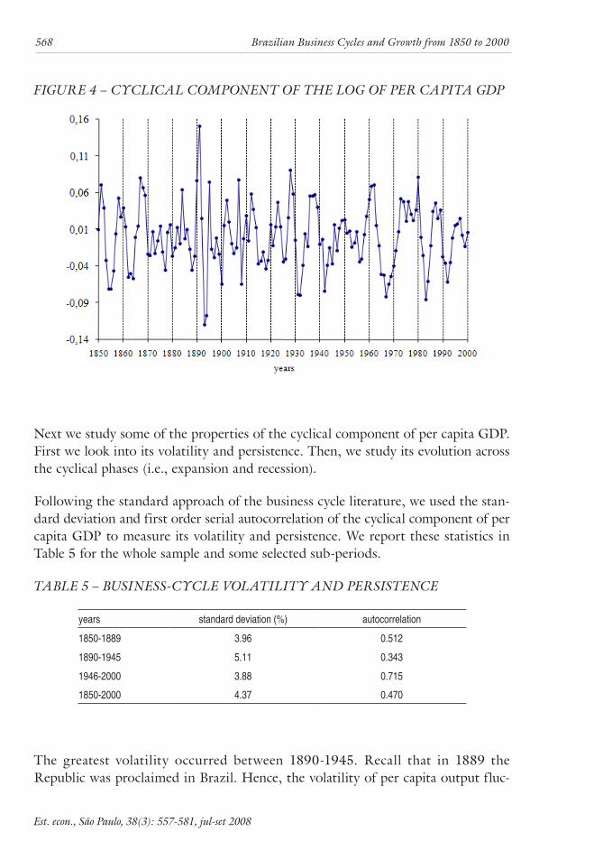
fIGuRE 4 – cyclIcal coMPonEnt of tHE loG of PER caPIta GdP

Next we study some of the properties of the cyclical component of per capita GDP. First we look into its volatility and persistence. Then, we study its evolution across the cyclical phases (i.e., expansion and recession).

Following the standard approach of the business cycle literature, we used the stan-dard deviation and first order serial autocorrelation of the cyclical component of per capita GDP to measure its volatility and persistence. We report these statistics in Table 5 for the whole sample and some selected sub-periods.

taBlE 5 – BusInEss-cyclE volatIlIty and PERsIstEncE

years standard deviation (%) autocorrelation

1850-1889 3.96 0.512

1890-1945 5.11 0.343

1946-2000 3.88 0.715

1850-2000 4.37 0.470

The greatest volatility occurred between 1890-1945. Recall that in 1889 the Republic was proclaimed in Brazil. Hence, the volatility of per capita output fluc-



tuations seems to have increased slightly after the fall of the Monarchy up to the end of World War II. For the other two sub-periods, 1850-1889 and 1946-2000, the vo-latility was roughly the same. Concerning the autocorrelation, the main conclusion is that an appreciable increase in persistence happened after World War II.

It is important to explain how we selected the sub-periods in Table 5. The sub-period 1850-1889 corresponds to the Imperial years of our sample. Hence, we have 111 Republican years (from 1890 to 2000). The end of World War II in 1945 divides these 111 years into two sub-periods of roughly the same duration. In sum-mary, we select two major historical events (the advent of the Republic and the end of World War II) to divide our sample into three sub-periods.

Backus and Kehoe (1992) studied the output volatility, over a hundred years, of ten countries (Australia, Canada, Denmark, Germany, Italy, Japan, Norway, Sweden, the United Kingdom and United States). They focused on three sub-periods, which they labeled as prewar, interwar and postwar. There were slight differences in terms of data coverage for each country, but broadly speaking, the prewar period covers data prior to the beginning of World War I, interwar refers to the period between the end of World War I and beginning of World War II, and postwar deals with data after the end of World War II up to 1985. Their main conclusion was that, except for Australia, all countries in their sample had higher output volatility in the interwar period than in the other periods.

For comparison purposes, we carried out the same exercise with Brazilian per capita GDP. Table 6 contains the results of that exercise.

taBlE 6 – BusInEss-cyclE volatIlIty

Period volatility

prewar (1850-1914) 4.80

interwar (1920-1939) 4.64

postwar (1950-1985) 4.35

We chose the sub-periods in Table 6 to match those of Backus and Kehoe (1992). The Brazilian economy did not display the highest variability during the interwar era. In fact, the volatility reached its maximum in the prewar period. However, it varied very little across the three periods. This is an important difference from other countries. For instance, in Canada and the United States the volatility practically halved from the prewar to the postwar periods.



We obtain another interesting finding when comparing the data in Table 6 to equi-valent statistics that Backus and Kehoe (1992) reported for the United States. That country had prewar, interwar and postwar volatilities of, respectively, 4.28, 9.33 and 2.26. So, the Brazilian volatility was similar to the US one in the prewar period and almost its double in the postwar years.

We now turn to the problem of dating recessions, expansions and turning points. We follow Canova (1994, 1999) and Harding and Pagan (2002) and adopt very simple dating rules.

Let Cty denote the cyclical component of per capita GDP. We say that an expansion

takes place at year t if 01 >− −Ct

Ct yy . Similarly, a recession happens whenever

01 ≤− −Ct

Ct yy . The last year of an expansion corresponds to a peak and the last year

of a recession corresponds to a trough. A turning point takes place whenever the economy hits a peak or a trough.

Our simple dating procedure is in line with the business cycle literature. There are alternative procedures that rely on econometric techniques. Chauvet (2002) and Duarte, Issler and Spacov (2004) adopted some of these alternative procedures to create chronologies of the Brazilian business cycle. Despite these differences, it tur-ned out that our chronology is similar to the one Chauvet constructed using yearly data, as we did.

We present in Table 7 the evolution of Brazilian per capita GDP over the business-cycle phases. A plus sign means expansion and minus sign means recession.

The two longest expansions lasted six years each, from 1957 to 1962 and from 1968 to 1973. The longest recession lasted for five years, from 1963 to 1967.



taBlE 7 – cyclIcal PHasEs of PER caPIta GdP

year phase year phase year phase year phase year phase year phase1851 + 1876 − 1901 + 1926 + 1951 − 1976 +1852 − 1877 − 1902 + 1927 + 1952 + 1977 −1853 − 1878 + 1903 − 1928 + 1953 − 1978 −1854 − 1879 + 1904 − 1929 − 1954 + 1979 +1855 − 1880 − 1905 − 1930 − 1955 + 1980 +1856 + 1881 + 1906 + 1931 − 1956 − 1981 −1857 + 1882 + 1907 + 1932 − 1957 + 1982 −1858 + 1883 − 1908 − 1933 + 1958 + 1983 −1859 − 1884 + 1909 + 1934 + 1959 + 1984 +1860 + 1885 − 1910 + 1935 − 1960 + 1985 +1861 − 1886 + 1911 − 1936 + 1961 + 1986 +1862 − 1887 − 1912 + 1937 + 1962 + 1987 +1863 + 1888 − 1913 − 1938 + 1963 − 1988 −1864 − 1889 + 1914 − 1939 − 1964 − 1989 +1865 + 1890 + 1915 − 1940 − 1965 − 1990 −1866 + 1891 + 1916 + 1941 + 1966 − 1991 −1867 + 1892 − 1917 + 1942 − 1967 − 1992 −1868 − 1893 − 1918 − 1943 + 1968 + 1993 +1869 − 1894 + 1919 + 1944 + 1969 + 1994 +1870 − 1895 + 1920 + 1945 − 1970 + 1995 +1871 − 1896 − 1921 − 1946 + 1971 + 1996 +1872 + 1897 − 1922 + 1947 − 1972 + 1997 +1873 − 1898 + 1923 + 1948 + 1973 + 1998 −1874 + 1899 − 1924 − 1949 + 1974 − 1999 −1875 + 1900 − 1925 − 1950 + 1975 − 2000 +

Legend: ‘+’ means expansion and ‘−’ means recession.

Table 8 contains information on some selected features of the chronology of reces-sions and expansions of the Brazilian economy. We compute these figures using the 1852-1999 period. In other words, we removed from the calculations the two end years of the period covered in Table 7. Had we proceed differently, we would have included in our calculations two one-year expansions that we could not be sure really lasted one year. For instance, if the Brazilian economy experienced an expansion in 2001 it would be definitively wrong to compute the expansion in 2000 as a one-year event.



taBlE 8 – fEatuREs of ExPansIons and REcEssIons

Feature Value

years in expansion 79

years in recession 69

number of expansions 35

number of recessions 37

average expansion length 2.26

average recession length 1.86

There were 79 years of expansion and 69 of recession. The number of recessions (37) was slightly higher than the number of expansions (35). The average expansion lasted 21% longer than the average recession. So, expansions were more frequent and lasted longer than recessions.

5 GRowtH PRoPERtIEs of PER caPIta GdP

We briefly discussed the evolution of Brazilian per capita GDP and its growth rate in Section I.3. We take the discussion a step further in this section. We first inves-tigate if the volatility of the growth rates has been increasing or decreasing over time. Then, we try to identify whether changes in the volatility of per capita GDP impact its growth rate. Finally, we assess if there was a change in the persistence of the per capita GDP growth rate.8

5.1 volatility trend and the fischer Black Hypothesis

We carry out two tasks in this subsection. The first is to assess how per capita ou-tput volatility changes over time. The second is to study the role of volatility in the evolution of the growth rate of per capita output.

We measure volatility as the squared growth rate of per capita output. To find the trend, we just fit a quadratic polynomial to the volatility series of per capita output. We plot the volatility and its trend in Figure 5.

8 We carried out similar exercises for the GDP growth rate. The results were qualitatively similar.



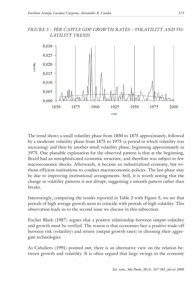
fIGuRE 5 – PER caPIta GdP GRowtH RatEs – volatIlIty and vo-latIlIty tREnd

The trend shows a small volatility phase from 1850 to 1875 approximately, followed by a moderate volatility phase from 1875 to 1975 (a period in which volatility was increasing) and then by another small volatility phase, beginning approximately in 1975. One plausible explanation for the observed pattern is that at the beginning, Brazil had an unsophisticated economic structure, and therefore was subject to few macroeconomic shocks. Afterwards, it became an industrialized economy, but wi-thout efficient institutions to conduct macroeconomic policies. The last phase may be due to improving institutional arrangements. Still, it is worth noting that the change in volatility patterns is not abrupt, suggesting a smooth pattern rather than breaks.

Interestingly, comparing the results reported in Table 2 with Figure 5, we see that periods of high average growth seem to coincide with periods of high volatility. This observation leads us to the second issue we discuss in this subsection.

Fischer Black (1987) argues that a positive relationship between output volatility and growth must be verified. The reason is that economies face a positive trade-off between risk (volatility) and return (output growth rates) in choosing their aggre-gate technologies.

As Caballero (1991) pointed out, there is an alternative view on the relation be-tween growth and volatility. It is often argued that large swings in the economy



make investment extremely risky, and as a result induce less investment, less capital accumulation and consequently less output growth.

Some authors have emphasized a possible relation between instability and growth while studying the performance of the Brazilian economy in the 1980s and 90s. Baer (1996) argued that the generalized uncertainty that affected the country was responsible for the stagnation during those two decades. Pinheiro, Giambiagi and Gostkorzewicz (1999) suggested that the low investment rates observed in the Brazilian economy during the 1980s was a consequence of the economic instability prevailing at that time.

Caporale and MacKiernan (1998) tested the Fischer Black hypothesis for the United States from 1871 and 1993 and found that variability significantly increases output growth rates. We carry out a similar exercise with the Brazilian per capita GDP se-ries. We estimate a GARCH (1,1) in mean model for per capita output.

The GARCH (1,1) is a model for the conditional variance of a time series. In order to capture the effect of volatility on output growth, we introduce the conditio-nal standard deviation in the equation for the mean of per capita output growth process.

Before presenting the results, some notation is in order. Let yt be natural log of the per capita output. As usual, ∆ denotes the first difference operator. The conditional variance is denoted by σt and εt stands for the residual in the mean equation.

The model estimated has a mean equation and an equation for conditional variance, which are, respectively

0 1 1 2t t t ty y −∆ = γ + γ ∆ + γ σ + ε (1)

and

2 21 1t t t− −σ = ω +αε + βσ (2)

We report the estimation results in Table 9.



taBlE 9 – EstIMatIon REsults – GaRcH(1,1) In MEan

parameters estimate standard deviation Z statistics

γ0 0.0621 0.0319 1.9452

γ1 0.1677 0.0863 1.9411

γ2 -0.9859 0.6863 -1.4364

ω 0.0002 0.0001 1.2941

α 0.1035 0.0568 1.8199

β 0.8214 0.0777 10.5631

The estimation results suggest that volatility does not enter in a statistically sig-nificant way in the mean equation. Moreover, the point estimate contradicts the Fischer Black hypothesis. Therefore, that conjecture seems not to hold for Brazil, and if volatility influences growth at all, it is in a negative fashion as other authors suggested.

5.2 are Pre and Post world war II Per capita GdP Growth so different?

Table 5 suggests that business cycles became more persistent after World War II. In this subsection we fit a simple AR (1) – GARCH (1,1) model, similar to the one in the previous subsection, allowing for a dummy variable, denoted by d, associated with observations from 1946 to 2000, in the mean and in the conditional variance equation. The goal is to verify if changes in the dynamics of per capita GDP growth are related to volatility or to persistence.

The dummy is significant in the conditional variance equation only when we specify an ARCH (1) process. With a GARCH (1,1) process, the dummy is not significant, so we drop that variable from the conditional variance equation.

The estimated equations are

0 1 2 1 3 1t t t t t ty d y d y− −∆ = γ + γ + γ ∆ + γ ∆ + ε (3)

and

2 21 1t t t− −σ = ω +αε + βσ (4)



We report the estimation results in Table 10.

taBlE 10 – EstIMatIon REsults – GaRcH(1,1) wItH duMMy

parameters estimate standard deviation Z statistics

γ0 0.0106 0.0049 2.1605

γ1 0.0066 0.0117 0.5629

γ2 0.0032 0.0986 0.0325

γ3 0.3776 0.2511 1.5133

ω 0.0006 0.0005 1.2338

α 0.1929 0.0983 1.9622

β 0.5276 0.2810 1.8777

The estimation provides evidence that per capita GDP growth became much more persistent after the World War II. Therefore, the pre and post World War II dy-namics of the series are very different. Furthermore, that difference is related to a change in persistence rather than a dramatic change in volatility, since the dummy variable in the conditional variance is not significant.

6 conclusIon

We had two major aims in this paper. First, we wanted to verify whether the Brazilian business cycles from 1850 to 2000 displayed statistical regularities similar to those of some developed countries, as reported in Backus and Kehoe (1992). Second, we wanted to investigate if relevant structural breaks took place in that period and to assess the impact of these changes for the relation between growth and volatility rates.

Contrary to the international evidence, the volatility of Brazilian business cycles does not appear to have changed in an appreciable way. However, the business cycle and growth oscillations seemed to be a little higher around the 1950s than in the vicinity of the end-points of our sample. On the other hand, persistence seemed to be higher after World War II than before. We did not find evidence that growth and volatility are related in a statistically significant way.

The relevance of our findings is two-fold. An important question in the field of business cycles is whether this phenomenon is homogenous across nations. We ob-



tained evidence that the Brazilian cyclical oscillations had some distinctive features. On the other hand, the finding that volatility and growth rates may not be strongly correlated has some policy implications. It suggests that a policy aimed at smoothing out the business cycles is unlikely to foster long-run growth. So, Brazilian policy-makers should focus on policies related to education and infrastructure and be less concerned with managing cyclical expansions and recessions.



aPPEndIx

taBlE a1 – PoPulatIon and GdP

year populationreal GDP indexes


aggregate per capita aggregate per capita1850 7213456 1 1 1888 13610080 2.14000 1.134221851 7344000 1.08492 1.06563 1889 13895390 2.20046 1.142321852 7470623 1.07269 1.03576 1890 14199000 2.45862 1.249041853 7593955 1.01970 0.96861 1891 14522204 2.66922 1.325851854 7714625 1.00272 0.93758 1892 14863513 2.37098 1.150671855 7833263 1.02718 0.94590 1893 15220747 2.06730 0.979741856 7950498 1.08289 0.98250 1894 15591724 2.11553 0.978741857 8066960 1.17256 1.04850 1895 15974261 2.57138 1.161151858 8183278 1.27039 1.11983 1896 16366178 2.38591 1.051601859 8300081 1.27786 1.11057 1897 16765292 2.40561 1.035041860 8418000 1.33493 1.14391 1898 17169421 2.52654 1.061491861 8537663 1.34308 1.13477 1899 17576385 2.53605 1.040811862 8659700 1.29553 1.07917 1900 17984000 2.50616 1.005231863 8784741 1.34580 1.10508 1901 18390686 2.80018 1.098331864 8913415 1.38316 1.11936 1902 18797260 2.99619 1.149791865 9046351 1.51360 1.20693 1903 19205140 3.01019 1.130631866 9184179 1.58901 1.24804 1904 19615745 3.02419 1.112111867 9327528 1.74934 1.35285 1905 20030492 3.09419 1.114291868 9477029 1.77448 1.35065 1906 20450800 3.23420 1.140771869 9633309 1.79962 1.34756 1907 20878087 3.68223 1.272221870 9797000 1.69704 1.24952 1908 21313771 3.31821 1.123021871 9968498 1.72625 1.24916 1909 21759269 3.66823 1.216061872 10147273 1.81457 1.28993 1910 22216000 3.93425 1.277441873 10332563 1.79215 1.25115 1911 22685073 3.94825 1.255471874 10523606 1.85193 1.26941 1912 23166360 4.36828 1.360181875 10719641 1.91987 1.29192 1913 23659426 4.43828 1.353171876 10919903 1.88183 1.24310 1914 24163832 4.49428 1.341651877 11123633 1.86485 1.20932 1915 24679144 4.43828 1.297261878 11330067 1.99257 1.26860 1916 25204924 4.63429 1.326301879 11538443 2.04488 1.27839 1917 25740737 4.88631 1.369321880 11748000 1.98985 1.22180 1918 26286144 4.98432 1.367801881 11958433 2.04284 1.23226 1919 26840711 5.27834 1.418561882 12171271 2.12776 1.26104 1920 27404000 5.81037 1.529441883 12388502 2.11010 1.22865 1921 27975723 5.92238 1.527071884 12612111 2.29828 1.31449 1922 28556179 6.38441 1.612741885 12844087 2.17260 1.22017 1923 29145817 6.93045 1.715251886 13086416 2.22016 1.22379 1924 29745085 7.02846 1.704471887 13341084 2.18280 1.18023 1925 30354431 7.02846 1.67025

(Continued at next page)



taBlE a1 – PoPulatIon and GdP (continued)



aggregate per capita aggregate per capita1926 30974302 7.39248 1.7216 1964 78825606 60.37461 5.524981927 31605147 8.19053 1.86938 1965 81115836 61.82360 5.497841928 32247412 9.12859 2.04198 1966 83445179 65.96578 5.702441929 32901548 9.22660 2.02287 1967 85812903 68.73634 5.778001930 33568000 9.03059 1.94059 1968 88218276 75.47250 6.171261931 34247323 8.73657 1.84017 1969 90660564 82.64239 6.575491932 34940492 9.11459 1.88170 1970 93139037 91.23720 7.066161933 35648587 9.92664 2.00865 1971 95652211 101.58616 7.660961934 36372691 10.83670 2.14914 1972 98195605 113.71590 8.353581935 37113882 11.15872 2.16881 1973 100763985 129.60056 9.277801936 37873244 12.50281 2.38132 1974 103352118 140.16811 9.783031937 38651855 13.07685 2.44049 1975 105954772 147.41011 10.035761938 39450798 13.66489 2.49858 1976 108566714 162.53016 10.798931939 40271152 14.00091 2.50787 1977 111182711 170.54993 11.065161940 41114000 13.86090 2.43190 1978 113797531 179.02609 11.348201941 41981380 14.54694 2.49953 1979 116405940 191.12747 11.843811942 42879166 14.15491 2.38125 1980 119002706 208.71120 12.651221943 43814191 15.35899 2.52866 1981 121583741 199.84097 11.856391944 44793288 16.52106 2.66053 1982 124149534 201.49965 11.707731945 45823289 17.05309 2.68448 1983 126701720 195.59571 11.135771946 46911027 19.02722 2.92579 1984 129241933 206.15788 11.506411947 48063335 19.48925 2.92499 1985 131771808 222.34127 12.171411948 49287044 21.37971 3.12905 1986 134292979 238.99463 12.837431949 50588988 23.02595 3.28326 1987 136807080 247.43114 13.046351950 51976000 24.59171 3.41294 1988 139315746 247.28268 12.803741951 53452954 25.79670 3.48125 1989 141820611 255.09681 12.975051952 55016895 27.67986 3.62920 1990 144323309 244.00010 12.195421953 56662911 28.98081 3.68939 1991 146825475 246.51864 12.111331954 58386089 31.24131 3.85979 1992 149328743 245.17741 11.843511955 60181517 33.99055 4.07416 1993 151834748 257.25164 12.221661956 62044282 34.97628 4.06645 1994 154345124 272.30824 12.726571957 63969470 37.66945 4.24776 1995 156861505 283.80997 13.051331958 65952171 41.73775 4.56503 1996 159385526 291.35531 13.186131959 67987471 45.82805 4.86235 1997 161918821 300.88668 13.404451960 70070457 50.13589 5.16128 1998 164463024 301.28361 13.214501961 72196914 54.44758 5.44006 1999 167019770 303.72994 13.117861962 74365412 58.04112 5.63000 2000 169590693 316.97937 13.482561963 76575220 58.38937 5.50033 - - - -



REfEREncEs

ABREU, Marcelo P. O Brasil no século XX: a economia. In: IBGE (ed.). Estatísticas do século xx. Rio de Janeiro: IBGE, 2003.

BACKUS, David; KEHOE, Patrick. International evidence on the historical properties of business cycles. american Economic Review, v. 82, n. 4, p. 864-888, 1992.

BAER, Werner. a economia brasileira. São Paulo: Nobel, 1996.

BALDWIN, Richard; MARTIN, Phillipe; OTTAVIANO, Gianmarco. Global income divergence, trade and industrialization: the geography of growth take-offs. Working paper 6458. Cambridge: National Bureau of Economic Research, 1998.

BARRO, Robert J.; SALA-I-MARTIN, Xavier. Economic growth. New York: McGraw-Hill, 1995.

BLACK, Fischer. Business cycles and equilibrium. New York: Blackwell, 1987.

BURDEN, Richard; FAIRES, J. Douglas. numerical analysis. Sixth edition. Pacific Grove: Brooks/Cole Publishing Company, 1997.

BURNS, Arthur F.; MITCHELL, Wesley C. Measuring business cycles. New York: National Bureau of Economic Research, 1946.

CABALLERO, Ricardo J. On the sign of the investment-uncertainty relationship. american Economic Review, v. 81, n. 1, p. 279-288, 1991.

CANOVA, Fabio. Does detrending matter for the determination of the reference cycle and the selection of turning points?. Economic Journal, v. 109, n. 452, p. 126-150, 1999.

______. Detrending and turning points. European Economic Review, v. 38, n. 3-4, p. 614-623, 1994.

CAPORALE, Tony; McKIERNAN, Barbara. The Fischer Black hypothesis: some time-series evidence. southern Economic Journal, v. 64, n. 3, p. 765-771, 1998.

CATI, Regina; GARCIA, Marcio; PERRON, Pierre. Unit roots in the presence of abrupt governmental interventions with an application to Brazilian data. Journal of applied Econometrics, v. 14, n. 1, p. 27-56, 1999.

CHAUVET, Marcelle. The Brazilian business and growth cycles. Revista Brasileira de Economia, v. 56, n. 1, p. 75-106, 2002.

CONTADOR, Cláudio; HADDAD, Cláudio. Produto real, moeda e preços: a ex-periência brasileira no período 1861-1970. Revista Brasileira de Estatística, v. 36, n. 143, p. 407-440, 1975.

DUARTE, Angelo J. Mont’alverne; ISSLER, João Victor; SPACOV, Andrei. Indica-dores coincidentes de atividade econômica e uma cronologia de recessões para o Brasil. Pesquisa e Planejamento Econômico, v. 34, n. 1, p. 1-37, 2004.



ELLERY Jr., Roberto; GOMES, Victor. Ciclo de negócios no Brasil durante o século XX: uma comparação com a evidência internacional. Economia, v. 6, n. 1, p. 45-66, 2005.

______; SACHSIDA, Adolfo. Business cycle fluctuations in Brazil. Revista Brasileira de Economia, v. 56, n. 2, p. 269-308, 2002.

GOLDSMITH, Raymond. Brasil 1850-1984: desenvolvimento financeiro sob um século de inflação. São Paulo: Harper & Row do Brasil, 1986.

HADDAD, Cláudio. crescimento do produto real no Brasil, 1900-1947. Rio de Janeiro: FGV, 1978.

HARDING, Don; PAGAN, Adrian. Dissecting the cycle: a methodological investi-gation. Journal of Monetary Economics, v. 49, p. 365-381, 2002.

HODRICK, Robert J.; PRESCOTT, Edward C. Postwar U.S. business cycles: an empirical investigation. Journal of Money, credit and Banking, v. 29, n. 1, p. 1-16, 1997.

IBGE. Estatísticas históricas do Brasil: séries econômicas, demográficas e sociais de 1550 a 1988. 2nd edition. Rio de Janeiro: IBGE, 1990.

______. Estatísticas do século xx. Rio de Janeiro: IBGE, 2003.

KALDOR, Nicholas. Capital accumulation and economic growth. In: LUTZ, Frie-drich A.; HAGUE, Douglas C. (eds.). the theory of capital. Londres: Palgrave Macmillan, 1961.

LANNE, Markku; LÜTKEPHOL, Helmut; SAIKKONEN, Pentti. Comparison of unit root tests for time series with level shifts. Journal of time series analysis, v. 23, n. 6, p. 667-685, 2002.

PERRON, Pierre. The Great Crash, the Oil Price Shock, and the unit root hypothesis. Econometrica, v. 57, n. 6, p. 1361-1401, 1989.

PINHEIRO, Armando C.; GIAMBIAGI, Fabio; GOSTKORZEWICZ, Joana. O desempenho macroeconômico do Brasil nos anos 90. In: GIAMBIAGI, Fabio; MOREIRA, Maurício M. (ed.). a economia brasileira nos anos 90. Rio de Ja-neiro: BNDES, 1999.

PRADO JR., Caio. História econômica do Brasil. 22nd edition. São Paulo: Editora Brasiliense, 1979.

RAVN, Morten O.; UHLIG, Harald. on adjusting the HP-filter for the frequency of observations. Discussion Paper 50. Tilburg: Center for Economic Research, Tilburg University, 1997.

SAIKKONEN, Pentti; LÜTKEPOHL, Helmut. Testing for a unit root in a time series with a level shift at unknown time. Econometric theory, v. 18, n. 2 p. 343-364, 2002.

Documents

Brazilian Business Cycles and Growth from 1850 to 2000