Todos os direitos reservados. É proibida a reprodução parcial ou integral do conteúdo

deste documento por qualquer meio de distribuição, digital ou impresso, sem a expressa autorização do

REAP ou de seu autor.

Macroeconomic Effects of Credit Deepening in Latin America

Carlos Viana de Carvalho Eduardo Zilberman

Laura Souza Nilda Pasca

Novembro, 2016 Working Paper 73

Macroeconomic Effects of Credit Deepening in Latin America

Carlos Viana de Carvalho Eduardo Zilberman

Laura Souza Nilda Pasca

Carlos Viana de Carvalho Pontifícia Universidade Católica do Rio de Janeiro (PUC-Rio) Departamento de Economia Rua Marquês de São Vicente, nº 225 Gávea 22451-900 - Rio de Janeiro, RJ - Brasil cvianac@econ.puc-rio.br Eduardo Zilberman Pontifícia Universidade Católica do Rio de Janeiro (PUC-Rio) Departamento de Economia Rua Marquês de São Vicente, nº 225 Gávea 22451-900 - Rio de Janeiro, RJ – Brasil Laura Souza Pontifícia Universidade Católica do Rio de Janeiro (PUC-Rio) Departamento de Economia Rua Marquês de São Vicente, nº 225 Gávea 22451-900 - Rio de Janeiro, RJ - Brasil Nilda Pasca Pontifícia Universidade Católica do Rio de Janeiro (PUC-Rio) Departamento de Economia Rua Marquês de São Vicente, nº 225 Gávea 22451-900 - Rio de Janeiro, RJ - Brasil

Macroeconomic Effects of Credit Deepening in Latin America∗

Carlos Carvalho

Central Bank of Brazil

PUC-Rio

Nilda Pasca

Central Reserve Bank of Peru

Laura Souza

Itau-Unibanco

Eduardo Zilberman

PUC-Rio

November, 2016

Abstract

We augment a relatively standard dynamic general equilibrium model with financial frictions,

in order to quantify the macroeconomic effects of the credit deepening process observed in many

Latin American (LA) countries in the last decade – most notably in Brazil. In the model, a

stylized banking sector intermediates credit from patient households to impatient households

and entrepreneurs. Motivated by the Brazilian experience, we allow the credit constraint faced

by households to depend on current and/or future labor income. Our model is designed to isolate

the effects of credit deepening through demand-side channels. Hence, it abstracts from potential

effects of credit supply on total factor productivity, though factor reallocation. In the calibrated

model, credit deepening generates only modest above-trend growth in consumption, investment,

and GDP. Since Brazil has experienced one of the most intense credit deepening processes in

Latin America, we argue that the quantitative effects that hinge on the channels captured by

the model are unlikely to be sizable for other LA economies.

JEL classification codes: E20; E44; E51.

Keywords: credit deepening; financial frictions; consignado credit; payroll lending.

∗For comments and suggestions we thank Sergio Alves, Juliano Assuncao, Tiago Berriel, Alan Finkelstein-Shapiro,Douglas Gollin, Cezar Santos, two anonymous referees, and participants at the “Macroeconomics in EmergingEconomies” conference held at EESP-FGV, LACEA 2014, INSPER, SBE 2014, and the IDB Discussion Workshop.Authors gratefully acknowledge funding from the IDB under the project “Macroeconomic and Financial ChallengesFacing Latin America and the Caribbean after the Crisis”. We also thank Caue Dobbin for superb research assis-tance. All errors are ours. The views expressed in this paper are those of the authors and do not necessarily reflectthe position of the Central Bank of Brazil or the Central Reserve Bank of Peru. Emails: cvianac@econ.puc-rio.br,nildis87@gmail.com, laurac.souza@gmail.com, zilberman@econ.puc-rio.br.

1

1 Introduction

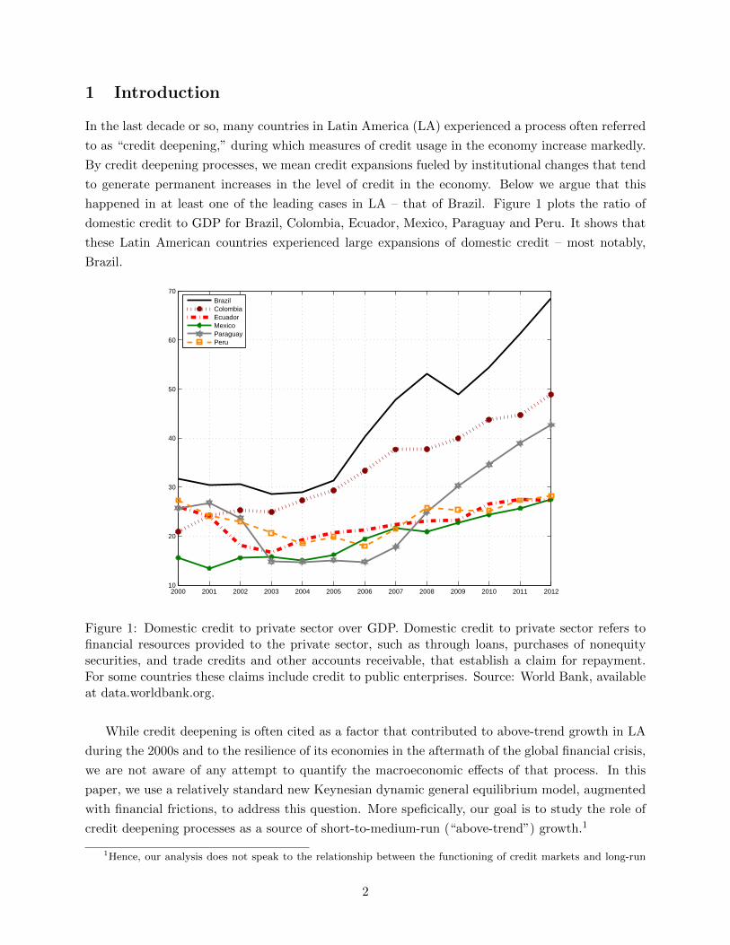
In the last decade or so, many countries in Latin America (LA) experienced a process often referred

to as “credit deepening,” during which measures of credit usage in the economy increase markedly.

By credit deepening processes, we mean credit expansions fueled by institutional changes that tend

to generate permanent increases in the level of credit in the economy. Below we argue that this

happened in at least one of the leading cases in LA – that of Brazil. Figure 1 plots the ratio of

domestic credit to GDP for Brazil, Colombia, Ecuador, Mexico, Paraguay and Peru. It shows that

these Latin American countries experienced large expansions of domestic credit – most notably,

Brazil.

2000 2001 2002 2003 2004 2005 2006 2007 2008 2009 2010 2011 201210

20

30

40

50

60

70

BrazilColombiaEcuadorMexicoParaguayPeru

Figure 1: Domestic credit to private sector over GDP. Domestic credit to private sector refers tofinancial resources provided to the private sector, such as through loans, purchases of nonequitysecurities, and trade credits and other accounts receivable, that establish a claim for repayment.For some countries these claims include credit to public enterprises. Source: World Bank, availableat data.worldbank.org.

While credit deepening is often cited as a factor that contributed to above-trend growth in LA

during the 2000s and to the resilience of its economies in the aftermath of the global financial crisis,

we are not aware of any attempt to quantify the macroeconomic effects of that process. In this

paper, we use a relatively standard new Keynesian dynamic general equilibrium model, augmented

with financial frictions, to address this question. More speficically, our goal is to study the role of

credit deepening processes as a source of short-to-medium-run (“above-trend”) growth.1

1Hence, our analysis does not speak to the relationship between the functioning of credit markets and long-run

2

In the model, a stylized banking sector intermediates credit from patient households to impatient

households and firms. While we borrow from several contributions available in the literature,

our paper departs from these contributions in one specific way. We model the credit constraint

faced by (impatient) households as a function of current and/or future labor income.2 We do so

motivated by the Brazilian experience, which featured a sizable increase in household credit that was

not associated with purchases of real estate or other collaterilizable assets (e.g., durable goods).

In Brazil, an important factor behind the credit expansion was the emergence of the so-called

consignado credit (“payroll lending”), whereby creditors are paid straight out of debtors’ paychecks.

Such lending is thus not collateralized by an asset, but by some valuation of the borrower’s stream

of labor income.

Although our modeling of consignado credit is very stylized, we believe this is an important

feature of the Brazilian credit deepening process that we should try to capture in our analysis, for

two reasons. First, Brazil is the largest economy in LA, and the one that arguably featured one of

the most intense credit deepening processes in the region (see Figure 1). Second, we believe our

modeling of consignado credit might be a useful reduced-form way to account for credit frictions in

other economies in which “non-collateralized” credit was an important part of the credit expansion

process.3

Another important institutional change that spurred the credit deepening process in Brazil was

a change in lending practices backed by a new law that allowed autos to be kept as property of

creditors until the associated loans had been repaid in full. Before this law, a car could be used as

collateral for the loan obtained to finance its purchase, but upon default judges often ruled against

creditors seizing the collateral. As a result, that market was relatively underdeveloped, and credit

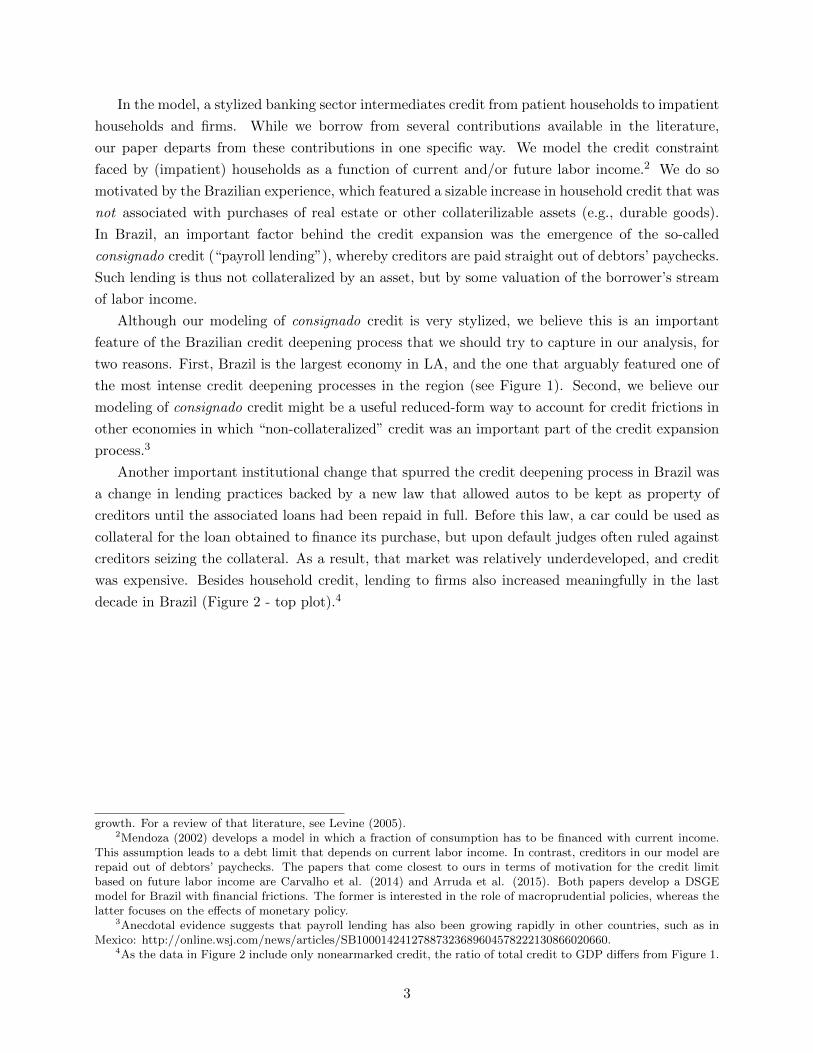
was expensive. Besides household credit, lending to firms also increased meaningfully in the last

decade in Brazil (Figure 2 - top plot).4

growth. For a review of that literature, see Levine (2005).2Mendoza (2002) develops a model in which a fraction of consumption has to be financed with current income.

This assumption leads to a debt limit that depends on current labor income. In contrast, creditors in our model arerepaid out of debtors’ paychecks. The papers that come closest to ours in terms of motivation for the credit limitbased on future labor income are Carvalho et al. (2014) and Arruda et al. (2015). Both papers develop a DSGEmodel for Brazil with financial frictions. The former is interested in the role of macroprudential policies, whereas thelatter focuses on the effects of monetary policy.

3Anecdotal evidence suggests that payroll lending has also been growing rapidly in other countries, such as inMexico: http://online.wsj.com/news/articles/SB10001424127887323689604578222130866020660.

4As the data in Figure 2 include only nonearmarked credit, the ratio of total credit to GDP differs from Figure 1.

3

2004 2005 2006 2007 2008 2009 2010 2011 20125

10

15

20

25

30

35

HouseholdsCorporationsTotal

2004 2005 2006 2007 2008 2009 2010 2011 20122

4

6

8

10

12

14

16

18

Non−collateralizedCollateralizedTotal (Households)

Figure 2: Nonearmarked credit outstanding to GDP ratio in Brazil. Nonearmarked credit is thenominal outstanding balance of credit operations by the National Financial System. Nonearmarkedfunds refer to financing and loans in which rates and destination are freely negotiated betweenfinancial institutions and borrowers, i.e. the financial institution has autonomy to decide in whicheconomic sectors it will apply the funds raised in the market through time deposits, by BankCertificates of Deposit (CDB), funds raised in foreign markets, part of demand deposits, amongother instruments. Collateralized credit consists of vehicles financing, other goods financing andmortgages. Non-collateralized credit consists of credit card, personal credit, overdraft and othernonearmarked credit instruments that were not classified in previous types of credit. Source: CentralBank of Brazil, available at www.bcb.gov.br.

We calibrate the model to replicate the credit deepening process witnessed in Brazil since 2004.

In particular, by emulating a transition from a low-credit to a high-credit steady state, we require

our model to match the credit expansion for both firms and households – including both non-

collateralized and collateralized credit in the latter case (Figure 2 - bottom plot).5 While our model

has features that allow for an endogenous response of credit to economic developments (such as

“valuation effects” in the credit constraints that we impose on borrowers), we essentially match

the path of the various credit measures over GDP by calibrating three time-varying parameters

that dictate the tightness of the credit constraints in the model. This is consistent with the idea

that a large fraction of the credit expansion was due to reforms and “innovations” (such as the

spreading of consignado credit) that fueled the credit deepening process.6 We believe that all these

5Consignado credit accounts for roughly 60 percent of the increase in non-collateralized credit.6Of course, other developments – some of each might be induced by policies – may interact with credit deepening.

However, due to the arguably exogenous nature of the credit innovations that we emphasize, attributing all of the creditdeepening to these innovations within a general equilibrium model seems a natural starting assumption. Investigating

4

characteristics of the Brazilian economy make it an interesting laboratory to understand a credit

deepening process that might be informative of what happened in other countries in LA and other

developing countries.

According to our calibrated model, the aggregate effects of the credit deepening process wit-

nessed in Brazil were quite small in absolute terms. Credit deepening increased GDP by only 0.5

percent between 2004 and 2012 (that is, an annual increase of 0.06 percent). Still according to

the model, during the same period consumption and investment increased by 0.2 and 0.4 percent,

respectively. The effects are also small for arguably extreme calibrations, chosen to generate more

sizable aggregate effects in response to such a credit deepening process.7 Given that Brazil has

experienced one of the most intense credit deepening processes in LA, we argue that analogous

parametrizations of the model for other countries are unlikely to produce sizable macroeconomic

effects.

Because our model does not feature trend growth, in order to assess the contribution of credit

deepening for above-trend growth in Brazil during the period of our analysis, we need to compare

the results generated by the model with measures of above-trend growth during that period. If

one assumes trend growth of 2.5 percent per year, the effects of credit deepening quantified by

the model account for 3.9, 1.1, and 0.9 percent of above-trend growth in GDP, consumption, and

investment, respectively. If one is willing to assume an optimistic trend growth of 3.5 percent, the

model is able to account for 15.6 percent of above-trend growth in GDP. We conclude that, unless

the trend growth rate was quite high during the sample period, the credit deepening process did

not play an important role in terms of short-to-medium-term growth.

Almost goes without saying that these conclusions are conditional on our model. In principle,

some features that are absent from the model may amplify the macroeconomic effects of credit

deepening. We assume, for instance, that Brazil is a closed economy. However, as Justiniano et al.

(2015a) conjecture, results could be amplified in small open economies. In that case the demand for

credit of one agent does not need to be compensated by higher savings (less consumption) by other

agents. Although the assumption that Brazil is relatively closed to trade is realistic, some empirical

evidence suggest that Brazil is not closed to financial flows.8 Hence, in Appendix C, we address

this concern by considering a small open economy version of the model. The macroeconomic effects

stemming from the credit deepening process are not amplified. In particular, the effects on GDP

are similar, although the dynamics of consumption and investment change somewhat.

In a context of heterogeneous agents and/or firms, credit deepening might interact with oc-

cupational choice and/or firm entry. Models with financial frictions and heterogeneous firms can

generate misallocation of resources, which has been documented to decrease total factor productiv-

ity (Hsieh and Klenow 2009, and subsequent literature).9 In addition, financial frictions may be a

possible interactions with other developments is an interesting question for future research.7In our extensive sensitivity analysis, we modify many features of the model. None of these modifications was

able to generate sizeable effects.8See, for instance, the financial openness indices reported by Quinn et al. (2011).9Recently, Midrigan and Xu (2014) argue that misallocation generates fairly small losses in a model disciplined

by establishment-level data.

5

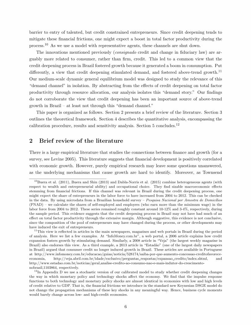
barrier to entry of talented, but credit constrained entrepreneurs. Since credit deepening tends to

mitigate these financial frictions, one might expect a boost in total factor productivity during the

process.10 As we use a model with representative agents, these channels are shut down.

The innovations mentioned previously (consignado credit and change in fiduciary law) are ar-

guably more related to consumer, rather than firm, credit. This led to a common view that the

credit deepening process in Brazil fostered growth because it generated a boom in consumption. Put

differently, a view that credit deepening stimulated demand, and fostered above-trend growth.11

Our medium-scale dynamic general equilibrium model was designed to study the relevance of this

“demand channel” in isolation. By abstracting from the effects of credit deepening on total factor

productivity through resource allocation, our analysis isolates this “demand story.” Our findings

do not corroborate the view that credit deepening has been an important source of above-trend

growth in Brazil – at least not through this “demand channel.”

This paper is organized as follows. Section 2 presents a brief review of the literature. Section 3

outlines the theoretical framework. Section 4 describes the quantitative analysis, encompassing the

calibration procedure, results and sensitivity analysis. Section 5 concludes.12

2 Brief review of the literature

There is a large empirical literature that studies the connections between finance and growth (for a

survey, see Levine 2005). This literature suggests that financial development is positively correlated

with economic growth. However, purely empirical research may leave some questions unanswered,

as the underlying mechanisms that cause growth are hard to identify. Moreover, as Townsend

10Buera et al. (2011), Buera and Shin (2013) and Dabla-Norris et al. (2015) combine heterogeneous agents (withrespect to wealth and entrepreneurial ability) and occupational choice. They find sizable macroeconomic effectsstemming from financial frictions. If this channel was relevant in Brazil during the credit deepening process, onemight expect the share of entrepreneurs in the labor force to have increased from 2004 to 2012. This can be checkedin the data. By using microdata from a Brazilian household survey – Pesquisa Nacional por Amostra de Domicılios(PNAD) – we calculate the shares of self-employed and employers (who earn more than the minimum wage) in thelabor force from 2004 to 2012. These series remained roughly constant around 10-12% and 3-4%, respectively, duringthe sample period. This evidence suggests that the credit deepening process in Brazil may not have had much of aneffect on total factor productivity through the extensive margin. Although suggestive, this evidence is not conclusive,since the composition of the pool of entrepreneurs may have changed during the process, or other developments mayhave induced the exit of entrepreneurs.

11This view is reflected in articles in the main newspapers, magazines and web portals in Brazil during the periodof analysis. Here we list a few examples. At “InfoMoney.com.br”, a web portal, a 2006 article explains how creditexpansion fosters growth by stimulating demand. Similarly, a 2008 article in “Veja” (the largest weekly magazine inBrazil) also endorses this view. As a third example, a 2013 article in “Estadao” (one of the largest daily newspapersin Brazil) argued that consumer credit no longer induced growth in Brazil. These articles are available in Portugueseat http://www.infomoney.com.br/educacao/guias/noticia/528174/saiba-por-que-aumento-concessao-creditofavorece-economia, http://veja.abril.com.br/idade/exclusivo/perguntas_respostas/expansao_credito/index.shtml, andhttp://www.estadao.com.br/noticias/geral,analise-credito-ao-consumo-nao-e-mais-indutor-do-crescimento-nobrasil,1103864, respectively.

12In Appendix D we use a stochastic version of our calibrated model to study whether credit deepening changesthe way in which monetary policy and technology shocks affect the economy. We find that the impulse responsefunctions to both technology and monetary policy shocks are almost identical in economies with low and high levelsof credit relative to GDP. That is, the financial frictions we introduce in the standard new Keynesian DSGE model donot change the propagation mechanisms of these key shocks in any meaningful way. Hence, business cycle momentswould barely change across low- and high-credit economies.

6

and Ueda (2006) emphasize, standard assumptions in regression analysis, such as stationarity and

linearity, are often inconsistent with transitional growth paths in theoretical models. Hence, this

literature should benefit from insights generated by quantitative analysis, in general equilibrium

settings.

Our paper fits a fast growing literature that integrates financial frictions into the new Keynesian

workhorse model. Bernake and Gertler (1989) and Bernanke et al. (1999) are the leading early

references in that literature. See Gertler and Kiyotaki (2010) for a recent survey.

We consider three types of financial frictions. First, we follow Kiyotaki and Moore (1997), who

tied the amount an agent can borrow to the value of some collateral in a general equilibrium model,

and Iacoviello (2005), who introduces this financial friction in a new Keynesian framework. We

also follow these authors by introducing entrepreneurs who can use capital as collateral in order

to borrow. By relaxing this financial friction over time, we can emulate the credit expansion we

observe for firms.

Second, as in Iacoviello and Neri (2010) and Gerali et al. (2010), we also distinguish patient from

impatient households. We tie the capacity to borrow of an impatient household to some collateral as

well. This financial friction allows us emulate the consumer credit expansion we observe in practice.

However, instead of using only durable goods (such as housing) as collateral, we also allow some

valuation of the borrower’s stream of labor income to serve as collateral. This is arguably in line

with the Brazilian experience, where housing-related credit is still a relatively a small fraction of

household credit and consignado credit plays a prominent role.

Financial intermediaries in our model are in line with Curdia and Woodford (2010). In particu-

lar, we assume that there is a cost to some intermediation activities, which generates an endogenous

spread between borrowing and lending rates. This friction is added for the sake of realism.

We study the credit deepening process in Brazil by changing the ability of firms and households

to borrow along the transition from a low-credit to a high-credit steady sate. In that sense, our

work is similar in spirit to Campbell and Hercowitz (2009), who use a general equilibrium model

to study the welfare effects of the increase in collateralized debt in the U.S. since the early 1980s.

The authors interpret this increase as a direct consequence of the deregulation of the mortgage

market triggered by financial innovations. These innovations are modeled as unexpected changes

in two key parameters of their model. Our exercise is similar in spirit, as we interpret the credit

deepening process in Brazil since 2004 as a direct consequence of the aforementioned innovations

in credit markets. In focusing on positive – as opposed to normative – effects of changes in the

tightness of borrowing constraints, our paper is also related to Justiniano et al. (2015a), who study

the macroeconomic effects of household leveraging and deleveraging in the United States. Similarly,

Justiniano et al. (2015b) show that a progressive relaxation of lending – rather than borrowing

constraints in the U.S. mortgage market – explains some empirical features of the housing boom

between 2000 and 2006, before the Great Recession.

Recent papers use new Keynesian DSGE models with financial frictions to address questions

that matter for the Brazilian economy – e.g., De Castro et al. (2011), Da Silva et al. (2012),

Kanczuk (2013), Carvalho et al. (2014) and Arruda et al. (2015). However, we are not aware of

7

other studies of the credit deepening process in Brazil or other Latin American countries using such

a model.

Finally, many papers rely on other frameworks with financial frictions to study somewhat related,

but different, questions (see the references cited in Dabla-Norris et al., 2015). A recent example

is Dabla-Norris et al. (2015), who develop a general equilibrium model in order to identify the

relevant financial friction that prevents financial inclusion, in a model with heterogeneous agents

(with respect to both wealth and skills) and occupational choice. Some of these papers, such as

Buera et al. (2011), Buera and Shin (2013) and Greenwood et al. (2013), find sizable macroeconomic

effects stemming from financial frictions.

3 The analytical framework

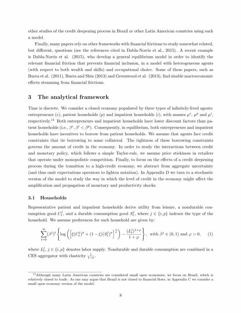
Time is discrete. We consider a closed economy populated by three types of infinitely-lived agents:

entrepreneurs (e), patient households (p) and impatient households (i), with masses µe, µp and µi,

respectively.13 Both entrepreneurs and impatient households have lower discount factors than pa-

tient households (i.e., βe, βi < βp). Consequently, in equilibrium, both entrepreneurs and impatient

households have incentives to borrow from patient households. We assume that agents face credit

constraints that tie borrowing to some collateral. The tightness of these borrowing constraints

governs the amount of credit in the economy. In order to study the interactions between credit

and monetary policy, which follows a simple Taylor-rule, we assume price stickiness in retailers

that operate under monopolistic competition. Finally, to focus on the effects of a credit deepening

process during the transition to a high-credit economy, we abstract from aggregate uncertainty

(and thus omit expectations operators to lighten notation). In Appendix D we turn to a stochastic

version of the model to study the way in which the level of credit in the economy might affect the

amplification and propagation of monetary and productivity shocks.

3.1 Households

Representative patient and impatient households derive utility from leisure, a nondurable con-

sumption good Cjt , and a durable consumption good Sjt , where j ∈ {i, p} indexes the type of the

household. We assume preferences for each household are given by:

∞∑t=0

(βj)t

{log

([ξ(Cjt )

σ + (1− ξ)(Sjt )σ] 1σ

)− (Ljt )

1+ϕ

1 + ϕ

}, with βj ∈ (0, 1) and ϕ > 0, (1)

where Ljt , j ∈ {i, p} denotes labor supply. Nondurable and durable consumption are combined in a

CES aggregator with elasticity 11−σ .

13Although many Latin American countries are considered small open economies, we focus on Brazil, which isrelatively closed to trade. As one may argue that Brazil is not closed to financial flows, in Appendix C we consider asmall open economy version of the model.

8

3.1.1 Patient households

Given that βp > max{βi, βe}, patient households are more prone to save. We focus on transitions

between a low-credit and a high-credit steady state along which patient households are always

lenders. Thus, we do not need to explicitly account for a borrowing constraint in their problems.

In particular, given the real wage rate (W pt ), the relative price of the durable good in terms of the

final good (qSt ), and the interest rate accrued on deposits (rht ), they choose a stream of nondurable

consumption (Cpt ), durable consumption (Spt ), labor services (Lpt ), and bank deposits (Dpt ) in order

to maximize (1) subject to the budget constraint

Cpt + qSt Spt +Dp

t ≤Wpt L

pt + qSt (1− δS)Spt−1 +

(1 + rht−1)

πtDpt−1 + Tt,

where πt = Pt/Pt−1 is the gross inflation rate, and δS is the rate of depreciation of the durable

good. We assume that patient agents own banks and firms in the economy and, thus, receive their

profits, which are aggregated in Tt.

3.1.2 Impatient households

In contrast with patient households, the impatient ones are inclined to borrow, but face borrowing

constraints. In particular, given W it , q

St and rht , they choose a stream of nondurable consumption

Cit , durable consumption Sit , labor services Lit and debt Bit in order to maximize (1) subject to the

budget constraint

Cit + qSt Sit +

1 + rht−1πt

Bit−1 ≤W i

tLit + qSt (1− δS)Sit−1 +Bi

t,

and the following borrowing constraint

Bit ≤ τWL

t bt + τStqSt+1πt+1(1− δS)Sit

1 + rht,

where

bt = λbfutt + (1− λ)WtLt, and bfutt = χπt+1b

futt+1

1 + rht+ (1− χ)

πt+1Wt+1Lt+1

1 + rht.

The borrowing constraint above can accommodate several possibilities. If λ = 1 and χ = 0, as

we assume in the benchmark calibration, these equations collapse to

(1 + rht )Bit ≤ τWL

t πt+1Wit+1L

it+1 + τSt q

St+1πt+1(1− δS)Sit .

This borrowing constraint states that impatient households can borrow in proportion (governed by

τWLt ) to the value of next period’s labor income plus an amount in proportion (governed by τSt ) to

the value of next period’s stock of durable goods.

9

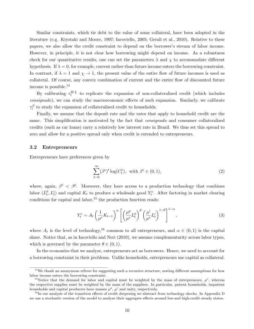
Similar constraints, which tie debt to the value of some collateral, have been adopted in the

literature (e.g. Kiyotaki and Moore, 1997; Iacoviello, 2005; Gerali et al., 2010). Relative to these

papers, we also allow the credit constraint to depend on the borrower’s stream of labor income.

However, in principle, it is not clear how borrowing might depend on income. As a robustness

check for our quantitative results, one can set the parameters λ and χ to accommodate different

hypothesis. If λ = 0, for example, current rather than future income enters the borrowing constraint.

In contrast, if λ = 1 and χ → 1, the present value of the entire flow of future incomes is used as

collateral. Of course, any convex combination of current and the entire flow of discounted future

income is possible.14

By calibrating τWLt to replicate the expansion of non-collateralized credit (which includes

consignado), we can study the macroeconomic effects of such expansion. Similarly, we calibrate

τSt to study the expansion of collateralized credit to households.

Finally, we assume that the deposit rate and the rates that apply to household credit are the

same. This simplification is motivated by the fact that consignado and consumer collateralized

credits (such as car loans) carry a relatively low interest rate in Brazil. We thus set this spread to

zero and allow for a positive spread only when credit is extended to entrepreneurs.

3.2 Entrepreneurs

Entrepreneurs have preferences given by

∞∑t=0

(βe)t log(Cet ), with βe ∈ (0, 1), (2)

where, again, βe < βp. Moreover, they have access to a production technology that combines

labor (Lpt , Lit) and capital Kt to produce a wholesale good Y e

t . After factoring in market clearing

conditions for capital and labor,15 the production function reads:

Y et = At

(1

µeKt−1

)α [(µpµeLpt

)θ (µiµeLit

)1−θ]1−α, (3)

where At is the level of technology,16 common to all entrepreneurs, and α ∈ (0, 1) is the capital

share. Notice that, as in Iacoviello and Neri (2010), we assume complementarity across labor types,

which is governed by the parameter θ ∈ (0, 1).

In the economies that we analyze, entrepreneurs act as borrowers. Hence, we need to account for

a borrowing constraint in their problems. Unlike households, entrepreneurs use capital as collateral.

14We thank an anonymous referee for suggesting such a recursive structure, nesting different assumptions for howlabor income enters the borrowing constraint.

15Notice that the demand for labor and capital must be weighted by the mass of entrepreneurs, µe, whereasthe respective supplies must be weighted by the mass of the suppliers. In particular, patient households, impatienthouseholds and capital producers have masses µp, µi and unity, respectively.

16In our analysis of the transition effects of credit deepening we abstract from technology shocks. In Appendix Dwe use a stochastic version of the model to analyze their aggregate effects around low-and high-credit steady states.

10

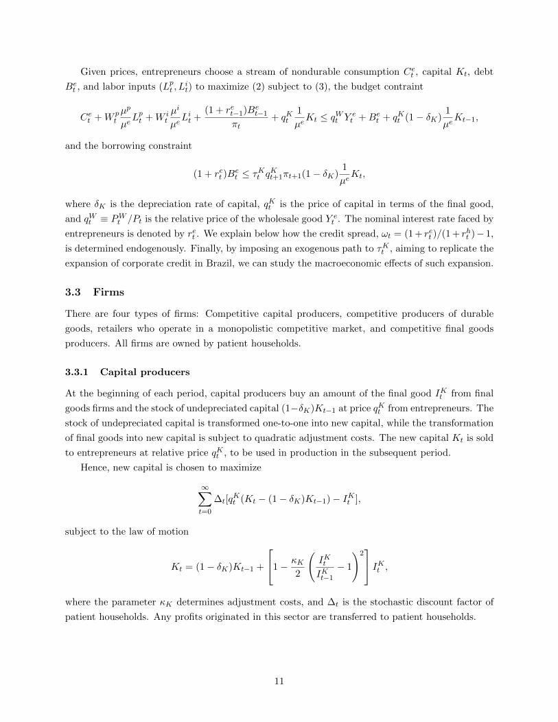
Given prices, entrepreneurs choose a stream of nondurable consumption Cet , capital Kt, debt

Bet , and labor inputs (Lpt , L

it) to maximize (2) subject to (3), the budget contraint

Cet +W pt

µp

µeLpt +W i

t

µi

µeLit +

(1 + ret−1)Bet−1

πt+ qKt

1

µeKt ≤ qWt Y e

t +Bet + qKt (1− δK)

1

µeKt−1,

and the borrowing constraint

(1 + ret )Bet ≤ τKt qKt+1πt+1(1− δK)

1

µeKt,

where δK is the depreciation rate of capital, qKt is the price of capital in terms of the final good,

and qWt ≡ PWt /Pt is the relative price of the wholesale good Y et . The nominal interest rate faced by

entrepreneurs is denoted by ret . We explain below how the credit spread, ωt = (1 + ret )/(1 + rht )− 1,

is determined endogenously. Finally, by imposing an exogenous path to τKt , aiming to replicate the

expansion of corporate credit in Brazil, we can study the macroeconomic effects of such expansion.

3.3 Firms

There are four types of firms: Competitive capital producers, competitive producers of durable

goods, retailers who operate in a monopolistic competitive market, and competitive final goods

producers. All firms are owned by patient households.

3.3.1 Capital producers

At the beginning of each period, capital producers buy an amount of the final good IKt from final

goods firms and the stock of undepreciated capital (1−δK)Kt−1 at price qKt from entrepreneurs. The

stock of undepreciated capital is transformed one-to-one into new capital, while the transformation

of final goods into new capital is subject to quadratic adjustment costs. The new capital Kt is sold

to entrepreneurs at relative price qKt , to be used in production in the subsequent period.

Hence, new capital is chosen to maximize

∞∑t=0

∆t[qKt (Kt − (1− δK)Kt−1)− IKt ],

subject to the law of motion

Kt = (1− δK)Kt−1 +

1− κK2

(IKtIKt−1

− 1

)2 IKt ,

where the parameter κK determines adjustment costs, and ∆t is the stochastic discount factor of

patient households. Any profits originated in this sector are transferred to patient households.

11

3.3.2 Producers of durable goods

At the beginning of each period, producers of durable goods buy an amount of the final good IStfrom final goods firms and the stock of undepreciated durable goods at relative price qSt from both

patient and impatient households. The stock of undepreciated durable goods (1− δS)(Spt−1 +Sit−1)

is transformed one-to-one into new durable goods, while the transformation of final goods into new

durable goods is subject to quadratic adjustment costs. New durable goods St are sold at relative

price qSt to both patient and impatient households.

Hence, durable goods producers choose the level of production to maximize

∞∑t=0

∆t[qSt (St − (1− δS)St−1)− ISt ],

subject to the law of motion

St = (1− δS)St−1 +

1− κS2

(IStISt−1

− 1

)2 ISt ,

where the parameter κS determines how costly it is to adjust durable goods, and St−1 = Spt−1+Sit−1.

Any profits originated in this sector are transferred to patient households.

3.3.3 Retail firms and final goods producers

In order to introduce price rigidities, we assume monopolistic competition among retail firms.17

Each retail firm m buys the wholesale good Y et from entrepreneurs at the price PWt and differentiates

it at no cost. They set prices Pt(m) in order to maximize profits subject to the demand originating

from final goods producers and also subject to quadratic price adjustment costs that arise whenever

a firm changes its price by more than a weighted average of past and steady-state inflation (with

relative weights equal to ι and 1− ι, respectively).

Let Yt(m) denote production of variety m. We assume that final goods producers are competi-

tive, and they simply aggregate the continuum of differentiated varieties produced by retailers in a

CES composite. In particular,

Yt =

[∫ 1

0Yt(m)

ε−1ε dm

] εε−1

,

where ε is the elasticity of substitution between varieties. Let Pt be the associated Dixit-Stiglitz

price index.

This final good is purchased by patient households, impatient households and entrepreneurs for

consumption, and by capital and durable goods producers for production.

17Price rigidities are really only needed in Appendix D, where we turn to a stochastic version of the model tostudy the role of credit in propagating a monetary policy shock. We keep them in the baseline specification to avoidswitching between different frameworks, and analyze the case of flexible prices in a robustness exercise.

12

Finally, it remains to formalize retail firm m’s problem. Pt(m) is chosen to maximize

∞∑t=0

P0

Pt∆t

[Pt(m)Yt(m)− PWt Yt(m)− κP

2

(Pt(m)

Pt−1(m)− πιt−1π1−ι

)2

PtYt

],

subject to the following demand schedule obtained from the cost-minimization problem of final

goods producers

Yt(m) =

(Pt(m)

Pt

)−εYt.

The parameter κP controls the price adjustment cost and dictates the degree of price stickiness

in the economy, and π denotes steady-state inflation. Any profits originated in this sector are

transferred to patient households.

3.4 Banks

For simplicity, we model a single bank that takes both rht and ret as given. Recall that rht is the

interest rate on both the debt of impatient households and the savings of patient ones. At the

beginning of each period, the bank collects deposits from patient households Dt, which are lent to

both impatient households and entrepreneurs. Originating loans to entrepreneurs entails an extra

cost which is borne out in terms of the final good. As in Curdia and Woodford (2010), we assume

such cost is given by η(µeBet )γ , with η > 0 and γ > 1. Intuitively, this is a shortcut to capture both

agency and operational costs that are not modeled explicitly. As explained earlier, we assume that

such costs are not present when the bank lends to impatient households.

The excess funds of the bank are given by

µpDt − µeBet − µiBi

t − η(µeBet )γ , (4)

which are transferred to patient households. Let the credit spread ωt be defined implicitly by

(1 + ret ) = (1 + ωt)(1 + rht ). Given that assets must equal liabilities at the end of the period, the

following equation must hold

µpDt = (1 + ωt)µeBe

t + µiBit. (5)

By plugging (5) into (4), we obtain the following expression for excess funds:

ωtµeBe

t − η(µeBet )γ ,

which is maximized at Bet = (1/µe)(µeωt/ηγ)1/(γ−1). Since γ > 1, the model induces a positive

correlation between the credit spread ωt and the amount borrowed by entrepreneurs Bet .

13

3.5 Monetary policy

Monetary policy is conducted through a Taylor-rule with interest rate smoothing. In particular,

(1 + rht ) = (1 + r)1−ρ(1 + rht−1)ρ(πtπ

)φπ(1−ρ)( ytyt−1

)φy(1−ρ)eu

rt ,

where φπ and φy determine the responses of interest rates to inflation and output stabilization,

respectively, π and r are the steady-state levels of inflation and the policy rate, respectively, and

urt is a monetary policy shock.18

3.6 Market clearing and aggregation

The definition of the equilibrium is standard. We assume that capital, wholesale good, durable

good, and both types of labor markets are competitive. In particular, notice that the market

clearing condition for the wholesale good reads:∫ 1

0Yt(m)dm = µeY e

t .

In contrast, we assume monopolistic competition at the retail level, where the nondurable good

is composed. Given that Ct = µpCpt +µiCit +µeCet , the market clearing condition in the final goods

market is

Yt = Ct + ISt + IKt + η(µeBet )γ + price adjustment costs.

Finally, notice that transfers to impatient households are given by

Tt =sum of profits of all firms, except entrepreneurs, and bank

µp.

4 Quantitative analysis

After calibrating the model outlined above, we use it to perform the following exercise. In order to

assess the macroeconomic effects of the credit expansion observed in Brazil, we solve for the time-

varying paths of τWLt , τSt , and τKt that generate paths for non-collateralized credit, collateralized

credit to households, and credit to non-financial corporations that resemble their counterparts in

the data (see Figure 2). In particular, we emulate a transition from a low-credit to a high-credit

steady state. Notice that, by modeling the evolution of τWLt , τSt , and τKt , this quantitative exercise

is consistent with the idea that a large fraction of the credit expansion was due to institutional

changes that fueled the credit deepening process.

In Appendix D, we consider a stochastic version of the model. The aim is to evaluate the

propagation mechanism of both technology and monetary policy shocks (which we add to the

18In our analysis of the transition effects of credit deepening we abstract from monetary policy shocks. In AppendixD we analyze their aggregate effects around low- and high-credit steady states.

14

model for this exercise only). In particular, we compare impulse response functions to these shocks

in the neighborhood of steady states with low and high levels of credit.

4.1 Calibration

We consider several sources of information to calibrate the parameters of the model, in which the

time period is set to one quarter. Whenever we set a parameter to match a given statistic for the

Brazilian economy, we consider its average between 2004 and 2012. Details of the data used in the

calibration can be found in Appendix E.

Steady state inflation is set to 5.5% per year (5.35% on a logarithmic basis). We set βp = 0.9834

to generate a nominal interest rate that accrues on savings deposit of 12.5 percent per year, in

steady-state (11.8% on a logarithmic basis). This value is in line with the sample average of the

SELIC interest rate, which is the short rate targeted by the Central Bank of Brazil.

Regarding the discount factors for borrowers, we set βi = βe = 0.96, which is associated with

an annual “subjective time-discount rate” of 18 percent. We pick this arguably extreme value for

two reasons. First, as we show below, lower values for βi and βe enhance the ability of the model to

produce meaningful aggregate effects in response to credit deepening. Second, with higher values

for βi and βe, the borrowing constraints for impatient households and entrepreneurs do not bind at

times during the transition.19 In particular, we set βi = βe at the maximum level that guarantees

that credit constraints always bind along the transition.

The Frisch elasticity 1/ϕ is set to one, which is within the range commonly used in the literature.

We follow Fernandez-Villaverde and Krueger (2004) to calibrate the parameters associated with

preferences for durable and nondurable goods. In the absence of definitive estimates for σ, we set

it to zero, so that the consumption composite becomes a Cobb-Douglas aggregate, (Cjt )ξ(Sjt )

1−ξ,

j = i, p, with ξ set to 0.8.

The depreciation rate of capital δK is set to 0.025, so that the investment to GDP ratio is

approximately 18 percent. The adjustment cost parameter κK is 2.53, which is in line with the

value estimated in De Castro et al. (2011). In the absence of similar information regarding the

production of durable goods, we set δS = δK and κS = κK .

Regarding the Cobb-Douglas technology used by entrepreneurs, since information on patient

and impatient labor income shares in Brazil is not available, we set θ = 0.7 to generate a ratio of

average household debt to annual income of 22 percent. The capital share α is set to 0.44, in line

with the evidence for Brazil reported in Paes and Bugarin (2006).

In line with previous literature, the elasticity of substitution ε between goods is set to 6, which

corresponds to a markup of 20 percent. The parameter κP , which measures the degree of price

stickiness in the retail sector, is calibrated to 50. As usual, this parameter can be mapped into a

degree of price stickiness of 0.75 in the Calvo (1983) model, once the quadratic adjustment cost

model and the Calvo model are cast as log-linear approximations around a zero inflation steady

state. Finally, ι, which governs indexation, is set to 0.158, as in Gerali et al. (2010).

19For a recent article that deals with credit constraints that bind occasionally, see Guerrieri and Iacoviello (2014).

15

We follow De Castro et al. (2011) to calibrate the parameters associated with the Taylor Rule.

In particular, φy = 0.16, φπ = 2.43 and ρ = 0.79.

Regarding the banking sector, we set η = 0.0122 and γ = 2 to generate a spread of roughly 4

percent per year – the average difference between the Brazilian prime rate, which reflects interest

rates on loans made to firms that are considered preferential borrowers, and the average rate on

overnight deposits during the sample. Loans to these firms embed lower default risk than loans

to other firms. Hence, the targeted value of 4 percent per year underestimates the average spread

in the Brazilian economy. As we show below, this calibration of η and γ helps the model produce

more meaningful aggregate effects in response to the credit deepening process.

Recall that we set λ = 1 and χ = 0 such that the borrowing constraint of the impatient

household depends on next period’s labor income. We postpone the discussion of how we calibrate

the sequence {τWLt , τSt , τ

Kt } to the next section. Finally, we set the masses µp, µi and µe equal to

one. Table 1 summarizes the calibration procedure.

Parameter Description Value

βp Discount Factor - Patient HH 0.9834

βi, βe Discount Factor - Impatient HH and Entrepreneurs 0.96

µp, µi, µe Mass - Patient HH, Impatient HH and Entrepreneurs 1

ϕ Inverse of the Frisch Elasticity 11

1−σ Elasticity Between Nondurable and Durable Goods 1

ξ Weight of the Nondurable Good in the Utility Function 0.8

δK , δS Depreciation - Capital and Durable Goods 0.025

κK , κS Adjustment Cost - Capital and Durable Goods 2.53

α Capital Share in the Production Function 0.44

θ Share of Patient HH in the Production Function 0.7

κP Price Adjustment Cost - Final Good 50

ι Steady State Inflation Weight - Indexation 0.158

ε Elasticity of Substitution - Final Good 6

ρ Interest Rate Smoothing Parameter 0.79

φy Response to Output in Taylor Rule 0.16

φπ Response to inflation in Taylor Rule 2.43

η Scale of Intermediation Cost Function 0.0122

γ Convexity of Intermediation Cost Function 2

Table 1: Calibration. See Section 4.1 for details.

4.2 Macroeconomic effects of credit deepening

In order to assess the macroeconomic effects of the credit expansion we observe in Brazil, we solve

for the time-varying paths of τWLt , τSt , and τKt that generate paths for non-collateralized credit,

16

collateralized credit to households, and credit to non-financial corporations that resemble their

counterparts in the data. We smooth the trajectories for τWLt , τSt , and τKt using a third degree

polynomial. As in Justiniano et al. (2015a), we assume that the evolution of τWLt , τSt ,and τKt

is perfectly foreseen after the initial unforeseen shock in 2004, when the credit deepening process

arguably started. We keep τWLt , τSt , and τKt constant after 2012. Notice that this economy starts

from a low-credit steady state and, then, converges to a new high-credit steady state.20 We focus

the analysis on the first eight years (short-to-medium-term) of the transition. In Appendix A, we

report the calibrated paths for τWLt , τSt , and τKt .

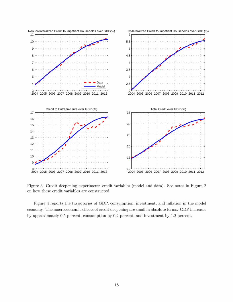
Figure 3 compares the credit deepening experiment in the model with the data.21 Notice that

the model is able to replicate the evolution of the credit series fairly well, except for the last years

of the data on credit to non-financial corporations (“entrepreneurs”).22

20To implement this exercise, we apply the shooting algorithm in Dynare to solve the system of equations given bythe first-order conditions of the agents’ optimization problems and the market clearing conditions. These equationsare described in a separate appendix, available upon request.

21Because we use a model with “representative agents” for each type of agent in the economy, the resulting pathsfor τWL

t , τSt , and τKt should be interpreted as encompassing both the intensive and extensive (“adoption”) marginsunderlying the credit deepening process.

22To be precise, in that case the fitted third degree polynomial would decrease towards the end of the sampleperiod, so we restricted it to be monotonic. In the next section, as a robustness check, we report results for paths ofτWLt , τSt , and τKt chosen to fit the trajectories of the credit variables point-by-point.

17

2004 2005 2006 2007 2008 2009 2010 2011 20123

4

5

6

7

8

9

10

11Non−collateralized Credit to Impatient Households over GDP(%)

DataModel

2004 2005 2006 2007 2008 2009 2010 2011 20122

2.5

3

3.5

4

4.5

5

5.5

6Collateralized Credit to Impatient Households over GDP (%)

2004 2005 2006 2007 2008 2009 2010 2011 20128

9

10

11

12

13

14

15

16

17Credit to Entrepreneurs over GDP (%)

2004 2005 2006 2007 2008 2009 2010 2011 201210

15

20

25

30

35Total Credit over GDP (%)

Figure 3: Credit deepening experiment: credit variables (model and data). See notes in Figure 2on how these credit variables are constructed.

Figure 4 reports the trajectories of GDP, consumption, investment, and inflation in the model

economy. The macroeconomic effects of credit deepening are small in absolute terms. GDP increases

by approximately 0.5 percent, consumption by 0.2 percent, and investment by 1.2 percent.

18

2004 2005 2006 2007 2008 2009 2010 2011 201299.9

100

100.1

100.2

100.3

100.4

100.5

100.6

100.7GDP

2004 2005 2006 2007 2008 2009 2010 2011 201299.9

99.95

100

100.05

100.1

100.15

100.2

100.25Consumption

2004 2005 2006 2007 2008 2009 2010 2011 2012100

100.2

100.4

100.6

100.8

101

101.2

101.4

101.6Investment

2004 2005 2006 2007 2008 2009 2010 2011 2012

5.35

5.4

5.45

5.5

5.55Inflation (% p. y.)

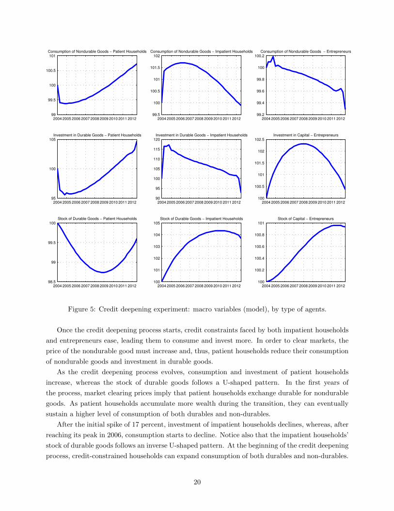
Figure 4: Credit deepening experiment: macro variables (model).

Consumption in the model aggregates nondurable consumption across types of agents, whereas

investment aggregates investment in both durable goods by households and capital by entrepreneurs.

Figure 5 reports the evolution of these variables, as well as the evolution of the stock of durable

goods and capital by types of agents.

19

2004 2005 2006 2007 2008 2009 2010 2011 201299

99.5

100

100.5

101Consumption of Nondurable Goods − Patient Households

2004 2005 2006 2007 2008 2009 2010 2011 201299.5

100

100.5

101

101.5

102Consumption of Nondurable Goods − Impatient Households

2004 2005 2006 2007 2008 2009 2010 2011 201299.2

99.4

99.6

99.8

100

100.2Consumption of Nondurable Goods − Entrepreneurs

2004 2005 2006 2007 2008 2009 2010 2011 201295

100

105Investment in Durable Goods − Patient Households

2004 2005 2006 2007 2008 2009 2010 2011 201290

95

100

105

110

115

120Investment in Durable Goods − Impatient Households

2004 2005 2006 2007 2008 2009 2010 2011 2012100

100.5

101

101.5

102

102.5Investment in Capital − Entrepreneurs

2004 2005 2006 2007 2008 2009 2010 2011 201298.5

99

99.5

100Stock of Durable Goods − Patient Households

2004 2005 2006 2007 2008 2009 2010 2011 2012100

101

102

103

104

105Stock of Durable Goods − Impatient Households

2004 2005 2006 2007 2008 2009 2010 2011 2012100

100.2

100.4

100.6

100.8

101Stock of Capital − Entrepreneurs

Figure 5: Credit deepening experiment: macro variables (model), by type of agents.

Once the credit deepening process starts, credit constraints faced by both impatient households

and entrepreneurs ease, leading them to consume and invest more. In order to clear markets, the

price of the nondurable good must increase and, thus, patient households reduce their consumption

of nondurable goods and investment in durable goods.

As the credit deepening process evolves, consumption and investment of patient households

increase, whereas the stock of durable goods follows a U-shaped pattern. In the first years of

the process, market clearing prices imply that patient households exchange durable for nondurable

goods. As patient households accumulate more wealth during the transition, they can eventually

sustain a higher level of consumption of both durables and non-durables.

After the initial spike of 17 percent, investment of impatient households declines, whereas, after

reaching its peak in 2006, consumption starts to decline. Notice also that the impatient households’

stock of durable goods follows an inverse U-shaped pattern. At the beginning of the credit deepening

process, credit-constrained households can expand consumption of both durables and non-durables.

20

As patient households get wealthier and, thus, increase the demand for these goods, market clearing

prices lead the impatient ones to reduce their purchases.

In terms of magnitude, the strongest effects of credit deepening are on investment in durable

goods by patient households, which increases by almost 5 percent from 2004 to 2012. In contrast,

investment in durable goods by impatient households falls by 7 percent.

Along the transition, investment in capital follows an inverse U-shaped path, leading to an

increase in the stock of capital by almost 1 percent. Notice also that entrepreneurs’ consumption

of nondurable goods falls by almost 0.7 percent, whereas investment increases by 0.4 percent (after

reaching a peak of 2.3 percent). Finally, in Appendix A we report and discuss results pertaining to

both labor and financial market outcomes.

Figure 6 shows that the model can replicate reasonably well the trends of both the spread and

the average household debt to annual income observed in the data. While our calibration targets

their average levels, it is not disciplined by their time paths. Hence, as these variables directly

relate to the credit market conditions, the model seems to be capturing at least some important

aspects of the credit deepening process witnessed in Brazil.

2004 2005 2006 2007 2008 2009 2010 2011 20120

1

2

3

4

5

6

7

8Spread (% p.y.)

DataModel

2005 2006 2007 2008 2009 2010 2011 201210

15

20

25

30Household Debt to 12−month income (%)

DataModel

Figure 6: Credit deepening experiment: spread and ratio of household debt to annual income. Thespread is calculated using the SELIC rate, which is the overnight rate in the interbank markettargeted by monetary policy, and the Brazilian prime rate, which averages interest rates on loansmade to firms that are considered preferential borrowers. For more details on the computationof the Brazilian prime rate, see www.bcb.gov.br/pec/depep/spread/REBC 2011.pdf. Householddebt considers only nonearmarked funds held by financial institutions. Annual income is disposableincome accumulated over the past twelve months. Source: Central Bank of Brazil, available atwww.bcb.gov.br.

In absolute terms, the effects of the credit deepening process are small. However, the model

lacks trend growth. Hence, depending on the actual level of trend growth in Brazil, the effects

of credit deepening as quantified by our model might nevertheless explain a more sizable share of

above-trend growth in actual GDP, consumption and investment during the 2004-2012 period.

21

Table 2 describes five scenarios for trend growth, ranging from 1.5 to 3.5 percent per year. For

each scenario, we divide the percentage increase in GDP, consumption, and investment produced

by the model for the 2004-2012 period by the cumulative above-trend growth in the data for each

of those variables. This yields the share of above-trend growth that can be attributed to the credit

deepening process, according to the calibrated model. In our preferred scenario, which considers

a growth trend of 2.5 percent per year, the credit deepening process accounts for 3.9, 1.1, and 0.9

percent of above-trend growth in GDP, consumption, and investment, respectively.23 Under more

optimistic assumptions about trend growth, the model can account for up to 15.6% of the gap for

GDP. In contrast, if trend growth is only 1.5 percent, the credit deepening process accounts for

only 2.2 percent of above-trend GDP growth.

GDP Consumption Consumption + I. in Durables Investment (capital)

Growth (data): 40.7% Growth (data): 48.4% Growth (data): 48.4% Growth (data): 82.6%

Growth (model): 0.5% Growth (model): 0.2% Growth (model): 0.4% Growth (model): 0.4%

Trend growth Above trend Model Above trend Model Above trend Model Above trend Model

(% p.y.) growth (%) share (%) growth (%) share (%) growth (%) share (%) growth (%) share (%)

1.5% 23.1% 2.2% 29.8% 0.7% 29.8% 1.3% 59.7% 0.7%

2.0% 17.7% 2.8% 24.2% 0.8% 24.2% 1.6% 52.8% 0.8%

2.5% 12.7% 3.9% 18.8% 1.1% 18.8% 2.1% 46.2% 0.9%

3.0% 7.8% 6.4% 13.7% 1.5% 13.7% 2.9% 39.9% 1.0%

3.5% 3.2% 15.6% 8.9% 2.2% 8.9% 4.5% 34.0% 1.2%

Table 2: Credit deepening experiment: comparison with the data. Growth rates between 2004 and2012. Data on GDP, consumption and investment in capital are obtained from National Accounts,available at www.ipeadata.gov.br.

Altogether, these results highlight that, unless trend growth rate was very high during this

period, the credit deepening process did not play an important role in Brazil in terms of generating

short-to-medium-term growth – at least not through the lens of this model.

4.3 Sensitivity analysis

In this section, we show that even “extreme” calibrations of time-discount rate parameters, chosen

to enhance the ability of the model to produce above-trend growth in response to credit deepening

process, fail to generate sizable macroeconomic effects. We also argue that price stickiness is not

the driving force behind our results. We show that the magnitude of the macroeconomic effects

barely changes with alternative modeling of borrowing constraints. Moreover, we show that our

conclusions do not change when we consider a transition that matches the paths of credit variables

pointwise. Furthermore, we show that the macroeconomic effects are slightly higher if we drop the

assumption that the credit deepening process is perfectly foreseen. Finally, results barely change

once we vary the impatient labor share, θ, from 0.5 to 0.8; and the capital share, α, from 0.4 to 0.5

23In the National Accounts, the measure of consumption includes the service flow of some durable goods, such ashousing. Hence, in the model we also consider an alternative measure of consumption that includes investment indurable goods. In this case, the credit deepening process accounts for 2.1 percent of above-trend growth.

22

(results available upon request, but not reported for brevity). We summarize our findings below,

and present the associated figures in Appendix B, for brevity. In addition, Appendix C shows that

the macroeconomic effects are not amplified in a small open economy version of the model.

Borrower impatience Recall that we calibrate βe = βi = 0.96. This is the maximum level of

βe = βi that guarantees that borrowing constraints are binding throughout the transition. This

value is associated with an annual “subjective time-discount rate” of 18 percent, which may already

seem high. In this section, we further decrease βe = βi to 0.93 and 0.91, corresponding to even

higher annual “subjective time-discount rates” of 34 and 46 percent, respectively. The lower βe and

βi are, the higher the impact of the credit deepening process on aggregate variables is.

For βe = βi = 0.93 (0.91), GDP, consumption and investment increase, respectively, by nearly

1.2 (1.7), 0.6 (1.0), and 3.5 (5.0) percent between 2004 and 2012. These figures are higher than

their counterparts in the benchmark calibration, but still small in absolute terms, given the marked

increase in measures of credit over GDP. In relative terms, if trend growth is 2.5 percent, the credit

deepening process accounts for 9.4 (13.4) percent of above-trend GDP growth. If trend growth is

3.5 percent, this figure increases to 37.5 (53.1) percent.

Spread A spread of 4 percent per year might be arguably too low for a calibration that targets the

Brazilian economy. To assess the sensitivity of our results to the level of spread, we vary separately

the parameters γ and η, associated with the financial intermediation technology, to produce different

levels of spread. Higher – and perhaps more realistic – levels of spread are associated with smaller

macroeconomic effects of the credit deepening process. Similarly, lower levels of spread amplify the

macroeconomic effects of credit deepening a bit. Intuitively, spreads are positively associated with

intermediation costs, which drain resources from the economy.

Alternative borrowing constraints As we emphasize above, in our baseline specification we

assume that impatient households’ credit limit depends on next period’s labor income and on the

value of durable goods. In order to inspect the relevance of this assumption, we consider other

parametrizations of the borrowing constraint. By imposing that the path of τWLt is equal zero, and

then calibrating the sequence of τSt to match the trajectory of total (instead of collateralized) credit

to households, we eliminate the direct dependence of borrowing on labor income. Alternatively, we

also consider a case in which only future labor income matters. To do so, the path of τSt is set equal

to zero, whereas τWLt is set to match the path of total credit to households. The effects on GDP

barely change with these alternative borrowing constraints, although the effects on consumption and

investment are a bit affected, but still very modest. We conclude that whether collateral is future

labor income or the value of durables does not affect our main findings. However, consumption

of durable goods by impatient households is strongly affected by the presence of durable goods as

collateral in their borrowing constraint.

Finally, we also run a specification keeping durable goods as collateral, but setting λ = 0,

so that current rather than future income enters the borrowing constraint. We also consider a

23

parametrization that sets λ = 1 and ξ = 0.95, so that the entire flow of future labor incomes serves

as collateral (see Section 3.1.2).24 For each specification, we recalibrate the sequence of credit

shocks to match the credit variables observed in the data. Results are largely independent of the

specification used.

Flexible prices One may wonder about the relevance of price stickiness for our results. To

analyze this issue, we set the parameter that determines the degree of price stickiness, κP , equal to

zero – thus eliminating price rigidities from the model. Except for tiny differences in the first and

last few periods, the trajectories of output, investment, consumption, and inflation overlap almost

perfectly with those produced by the baseline calibration.25

Non-smooth transition We also consider a transition between steady-states in which the per-

fectly foreseen paths of τWLt , τSt , and τKt are chosen to fit the trajectories of the credit variables

pointwise. In order to guarantee that borrowing constraints always bind during the transition, we

decrease both βe and βi to 0.93. This non-smooth transition does not change our conclusion that,

through the lens of the model, the macroeconomic effects of the credit deepening process observed

in Brazil are small.

Finally, in addition to the non-smooth transitions that fit the volumes of credit, we also consider

cases in which the path for either γ or η is chosen to fit the path of the spread pointwise (we

continue to assume that βe = βi = 0.93).26 The conclusion that the macroeconomic effects are

modest survives.

Unanticipated shocks The assumption that agents perfectly foresee the intensity of the credit

deepening process over such a long horizon might be unrealistic. Hence, as a last robustness exercise,

we solve the model under an assumption on the other extreme of the “foresight spectrum”. Namely,

we assume that the credit deepening process takes the form of a sequence of unanticipated shocks to

the parameters that govern the credit constraints. Reality should arguably be somewhere in between

these two extremes assumptions about agents’ foresight. In each period, agents are surprised by

the values of τWLt , τSt , and τKt , but assume they will remain constant thereafter. Shocks are chosen

to fit the trajectories of the credit variables under perfect foresight. In order to guarantee that

borrowing constraints always bind during the transition, we need to decrease the values of βe and

βi to 0.91, so results should not be compared with those under the benchmark calibration (but they

can be compared to the results under perfect foresight with βe = βi = 0.91 – see Appendix B).

At the end of the sample period, the macroeconomic effects of credit deepening are close to those

generated under the benchmark calibration. However, during the first few years of the transition,

output and consumption are between one and one and a half percent higher than their counterparts

24Recall that λ = 1 and ξ → 1 imply that the present value of the entire flow of future incomes is used as collateral.25Nevertheless, we decided to keep price rigidities in the model in order to study the interactions between the level

of credit in the economy and monetary policy (see Appendix D).26Notice that the benchmark calibration endogenously replicates fairly well the trend of the spread observed in the

data. Hence, as robustness check, we consider only the case with non-smooth transition.

24

under the perfect foresight assumption. Nonetheless, the conclusion that, conditional on the model,

the macroeconomic effects of credit deepening are relatively small still holds.27

5 Conclusion

In this paper, we calibrate a relatively standard new Keneysian dynamic general equilibrium model,

augmented with financial frictions, to study the macroeconomic effects of the credit deepening

process experienced recently by Brazil and other LA economies. We conclude that, even under

arguably extreme calibrations chosen to enhance the ability of the model to generate meaningful

macroeconomic effects in response to a credit deepening process, the effects we find are small.

As Figure 1 illustrates, Brazil has experienced one of the most intense credit deepening processes

among LA countries. We conclude that, through the lens of the model, the macroeconomic effects

of the credit deepening processes experienced by other countries in the region are unlikely to be

sizable.

Almost goes without saying that this conclusion is conditional on our model. As Justiniano et

al. (2015a) argue, results may change in the context of a small open economy, in which the supply

of credit is perfectly elastic at a given interest rate. In this case, the macroeconomic effects of credit

deepening may be amplified, as the expansion of the demand for credit by impatient households and

entrepreneurs does not need to be compensated by higher savings on the part of patient households.

In Appendix C, we show that such amplification does not occur in a small open economy version

of the model. In particular, the effects on GDP are similar, although the dynamics of consumption

and investment change somewhat.

Likewise, models with heterogeneous agents and firms subject to credit frictions may produce

different results. Some papers in this literature have found sizable macroeconomic effects stemming

from financial frictions (e.g., Buera and Shin, 2013). These frictions may induce misallocation of

production factors, and barriers to entry of productive but credit-constrained firms. Hence, as the

credit deepening process mitigates financial frictions, a boost in total factor productivity may occur.

Of course, these channels are shut down in models with representative agents, such as the one we

use. Indeed, our medium-scale dynamic general equilibrium model is not readily manageable to

incorporate a meaningful channel that links credit supply and total factor productivity, as in, for

example, Buera and Shin (2013). In particular, it is geared towards analyzing the “demand story” of

above-trend growth due to a credit-induced consumption boom, which fits common wisdom about

what happened in Brazil. This view, however, is not corroborated by our quantitative analysis.

27The credit trajectories under unanticipated shocks are slightly below their counterparts under perfect foresight.Thus, if anything, there is a tiny “bias” against finding higher macroeconomic effects.

25

References

[1] Arruda, G., D. Lima, and V. K. Teles, (2015), “Household Borrowing Constraints and Mone-

tary Policy in Emerging Economies,” FGV-EESP working paper.

[2] Bernanke, B. and M. Gertler, (1989), “Agency costs, net worth and business fluctuations,”

American Economic Review 79(1): 14-31.

[3] Bernanke, B., M. Gertler, and S. Gilchrist, (1999), “The financial accelerator in a quantitative

business cycle framework,” In: Handbook of Macroeconomics, Vol. 1, edited by Taylor, J.,

Woodford, M.

[4] Buera, F., J. Kaboski, and Y. Shin, (2011), “Finance and Development: A Tale of Two Sectors,”

American Economic Review 101(5): 1964-2002.

[5] Buera, F. and Y. Shin, (2013), “Financial Frictions and the Persistence of History: A Quanti-

tative Exploration,” Journal of Political Economy 121(2): 221-272.

[6] Calvo, G. A., (1983), “Staggered prices in a utility-maximizing framework,”Journal of Mone-

tary Economics, 12(3): 383-398.

[7] Campbell, J. R. and Z. Hercowitz, (2009), “Welfare implications of the transition to high

household debt, ” Journal of Monetary Economics, 56:1-16.

[8] Carvalho, F., M. Castro, and S. Costa, (2014), “Traditional and Matter-of-fact Financial Fric-

tions in a DSGE Model for Brazil: The Role of Macroprudential Instruments and Monetary

Policy,” BIS Working Paper No 460.

[9] Chinn, M. D. and H. Ito, (2006), “What Matters for Financial Development? Capital Controls,

Institutions, and Interactions,”Journal of Development Economics, 81: 163-192.

[10] Curdia, V. and M. Woodford, (2010), “Credit Spreads and Monetary Policy,”Journal of Money,

Credit and Banking, 42: 3-35.

[11] Da Silva, M.F., Andrade, J., Silva, G., Brandi, V., (2012), “Financial frictions in the Brazilian

banking system: a DSGE model with Bayesian estimation ”, Working Paper.

[12] Dabla-Norris, E., Y. Ji, R. M. Townsend, and D. F. Unsal, (2015), “Distiguishing Constraints

on Financial Inclusion and their Impact on GDP and Inequality,” NBER Working Paper No

20821.

[13] De Castro, M., S. Gouvea, A. Minella, R. Santos, and N. Souza-Sobrinho, (2011), “SAMBA:

Stochastic Analytical Model with a Bayesian Approach,” Banco Central do Brasil Working

Paper No 239.

[14] Fernandez-Villaverde, J. and D. Krueguer, (2004), “Life-Cycle Consumption, Debt Constraints

and Durable Goods,” Macroeconomic Dynamics 15(5): 725-770.

26

[15] Gerali, A., S. Neri, L. Sessa, and F. Signoretti, (2010), “Credit and Banking in a DSGE Model

of the Euro Area,” Journal of Money, Credit and Banking 42: 107-141.

[16] Gertler, M. and N. Kiyotaki, (2010), “Financial Intermediation and Credit Policy in Busi-

ness Cycle Analysis,” In: Handbook of Monetary Economics, Vol. 3, edited by Friedman, B.,

Woodford, M.

[17] Greenwood, J., J. M. Sanchez, and C. Wang, (2013), “Quantifying the Impact of Financial

Development on Economic Development,” Review of Economic Dynamics 16: 194-215.

[18] Guerrieri, L. and M. Iacoviello, (2016), “Collateral Constraints and Macroeconomic Asymme-

tries,” Working Paper.

[19] Hsieh, C. and P. J. Klenow, (2009), “Misallocation and Manufacturing TFP in China and

India,” Quarterly Journal of Economics 124(4): 1403-1448.

[20] Iacoviello, M., (2005), “House Prices, Borrowing Constraints, and Monetary Policy in the

Business Cycle,” American Economic Review 95(3): 739-764.

[21] Iacoviello, M. and S. Neri, (2010), “Housing market spillovers: evidence from an estimated

DSGE model,” American Economic Journal: Macroeconomics 2: 125-164.

[22] Justiniano, A., G. Primiceri, and A. Tambalotti, (2014), “The Effects of the Saving and Banking

Glut on the U.S. Economy,”Journal of International Economics 92: S52-S67.

[23] Justiniano, A., G. Primiceri, and A. Tambalotti, (2015a), “Household Leveraging and Delever-

aging,”Review of Economic Dynamics 18(1): 3-20.

[24] Justiniano, A., G. Primiceri, and A. Tambalotti, (2015b), “Credit Supply and the Housing

Boom,”Working Paper.

[25] Kanczuk, F., (2013), “Um Termometro para as Macro-Prudenciais,” Revista Brasileira de

Economia 67(4): 739-764.

[26] Kiyotaki, N. and J. Moore, (1997), “Credit Cycles,” Journal of Political Economy 105(2):211-

248.

[27] Levine, R., (2005), “Finance and Growth: Theory and Evidence,” Handbook of Economic

Growth, in: Philippe Aghion & Steven Durlauf (ed.), Handbook of Economic Growth, edition

1, volume 1, chapter 12, pages 865-934.

[28] Liu, Z., P. Wang, and T. Zha, (2013), “Land-Price Dynamics and Macroeconomic Fluctua-

tions,” Econometrica 81(3): 1147-1184.

[29] Mendoza, E., (2002), “Credit, Prices, and Crashes: Business Cycles with a Sudden Stop,” In:

Preventing Currency Crises in Emerging Markets, edited by Edwards, S., Frankel, J.

27

[30] Midrigan, V. and D. Y. Xu, (2014), “Finance and Misallocation: Evidence from Plant-Level

Data,” American Economic Review 104(2): 422-58.

[31] Paes, N. and M. Bugarin, (2006), “Parametros Tributarios da Economia Brasileira,” Estudos

Economicos 36(4): 699-720.

[32] Quinn, D., Schindler, M. and A. M. Toyoda, (2011), “Assessing Measures of Financial Openness

and Integration,”IMF Economic Review 59(3):488-522.

[33] Townsend, R. M. and K. Ueda, (2006), “Financial Deepening, Inequality, and Growth: A

Model-Based Quantitative Evaluation,”Review of Economic Studies 73(1):251-293.

28

A Figures: Additional results

A.1 Calibrated paths of τWLt , τSt , and τKt

Figure 7 plots the trajectories of τWLt , τSt , and τKt that generate paths for non-collateralized credit,

collateralized credit to households, and credit to non-financial corporations close to their counter-

parts in the data.

2004 2005 2006 2007 2008 2009 2010 2011 20120.016

0.018

0.02

0.022

0.024

0.026

0.028

0.03

0.032τK

2004 2005 2006 2007 2008 2009 2010 2011 20120.25

0.3

0.35

0.4

0.45

0.5

0.55

0.6

0.65

0.7

0.75τWL

2004 2005 2006 2007 2008 2009 2010 2011 20120.04

0.05

0.06

0.07

0.08

0.09

0.1

0.11

0.12τS

Figure 7: Credit deepening experiment: evolution of τKt , τWLt and τSt .

29

A.2 Labor market outcomes

Figure 8 shows the evolution of labor market outcomes. As in Justiniano et al. (2015a), once credit

deepening starts, labor services of patient and impatient households move in opposite directions.

However, as the process evolves, labor services supplied by impatient households increase by 0.8

percent, whereas those supplied by patient households barely decrease. Moreover, notice that after

some point patient households end up earning more, while the impatient ones earn less.

2004 2005 2006 2007 2008 2009 2010 2011 201299.6

99.8

100

100.2

100.4

100.6

100.8

101Wage − Impatient Households

2004 2005 2006 2007 2008 2009 2010 2011 201299.6

99.8

100

100.2

100.4

100.6

100.8

101Wage − Patient Households

2004 2005 2006 2007 2008 2009 2010 2011 201299.2

99.4

99.6

99.8

100

100.2

100.4

100.6

100.8

101Labor Services − Impatient Households

2004 2005 2006 2007 2008 2009 2010 2011 2012

99.9

100

100.1

100.2

100.3

100.4Labor Services − Patient Households

Figure 8: Credit deepening experiment: labor market outcomes.

30

A.3 Financial market outcomes

Figure 9 shows the evolution of financial market outcomes, i.e. interest rates. After an initial

increase of roughly 0.4 percentage point (from the steady state value of 11.8 percent per year),

the interest rate that accrues on deposits follows an inverse U-shaped pattern with its peak at

12.6 percent. As the credit deepening process evolves, the interest rate faced by entrepreneurs

increases substantially – and so does the spread (see Figure 6, left plot, in the main text). In fact,

as entrepreneurs get into debt, the intermediation costs to generate these funds increase, yielding

higher interest rates and spreads.

2004 2005 2006 2007 2008 2009 2010 2011 201212.2

12.25

12.3

12.35

12.4

12.45

12.5

12.55

12.6

12.65rh (% p.y.)

2004 2005 2006 2007 2008 2009 2010 2011 201214.5

15

15.5

16

16.5

17

17.5

18re (% p.y.)

Figure 9: Credit deepening experiment: financial market outcomes.

31

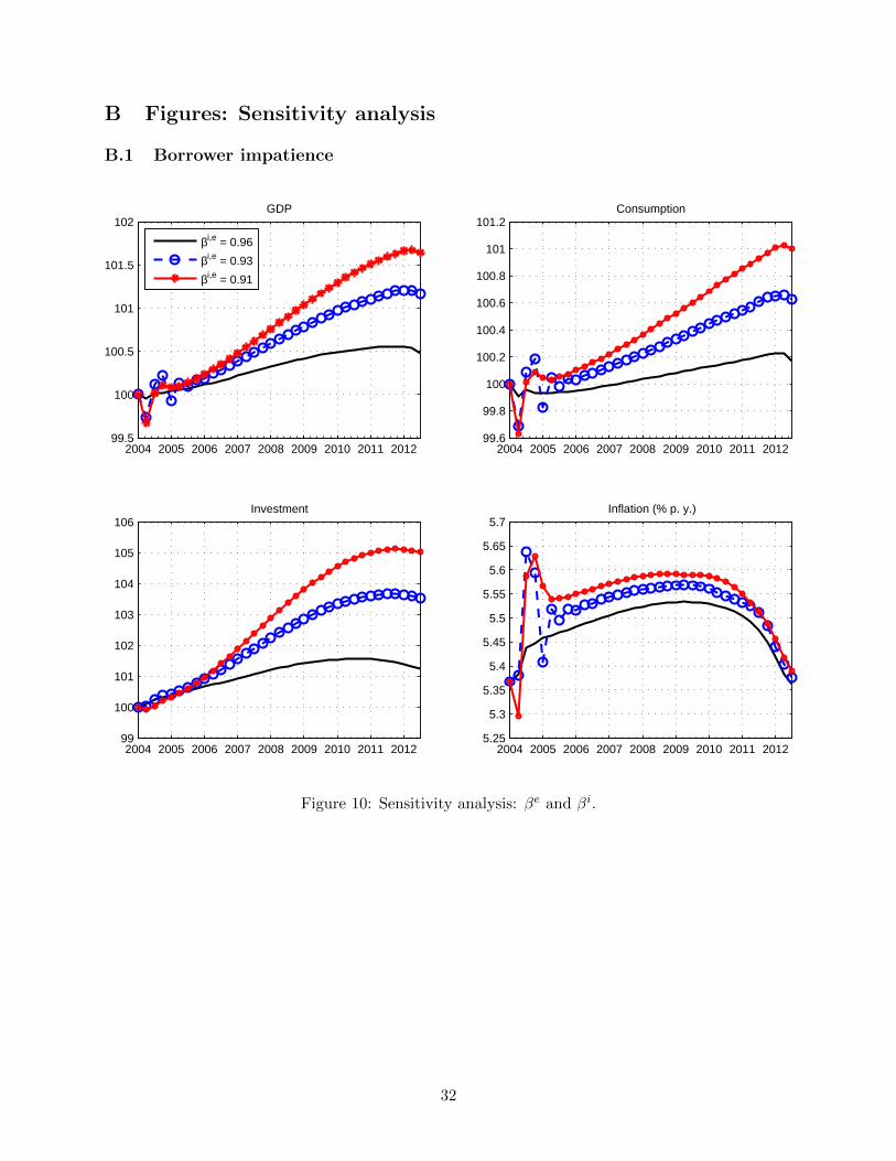
B Figures: Sensitivity analysis

B.1 Borrower impatience

2004 2005 2006 2007 2008 2009 2010 2011 201299.5

100

100.5

101

101.5

102GDP

βi,e = 0.96

βi,e = 0.93

βi,e = 0.91

2004 2005 2006 2007 2008 2009 2010 2011 201299.6

99.8

100

100.2

100.4

100.6

100.8

101

101.2Consumption

2004 2005 2006 2007 2008 2009 2010 2011 201299

100

101

102

103

104

105

106Investment

2004 2005 2006 2007 2008 2009 2010 2011 20125.25

5.3

5.35

5.4

5.45

5.5

5.55

5.6

5.65

5.7Inflation (% p. y.)

Figure 10: Sensitivity analysis: βe and βi.

32

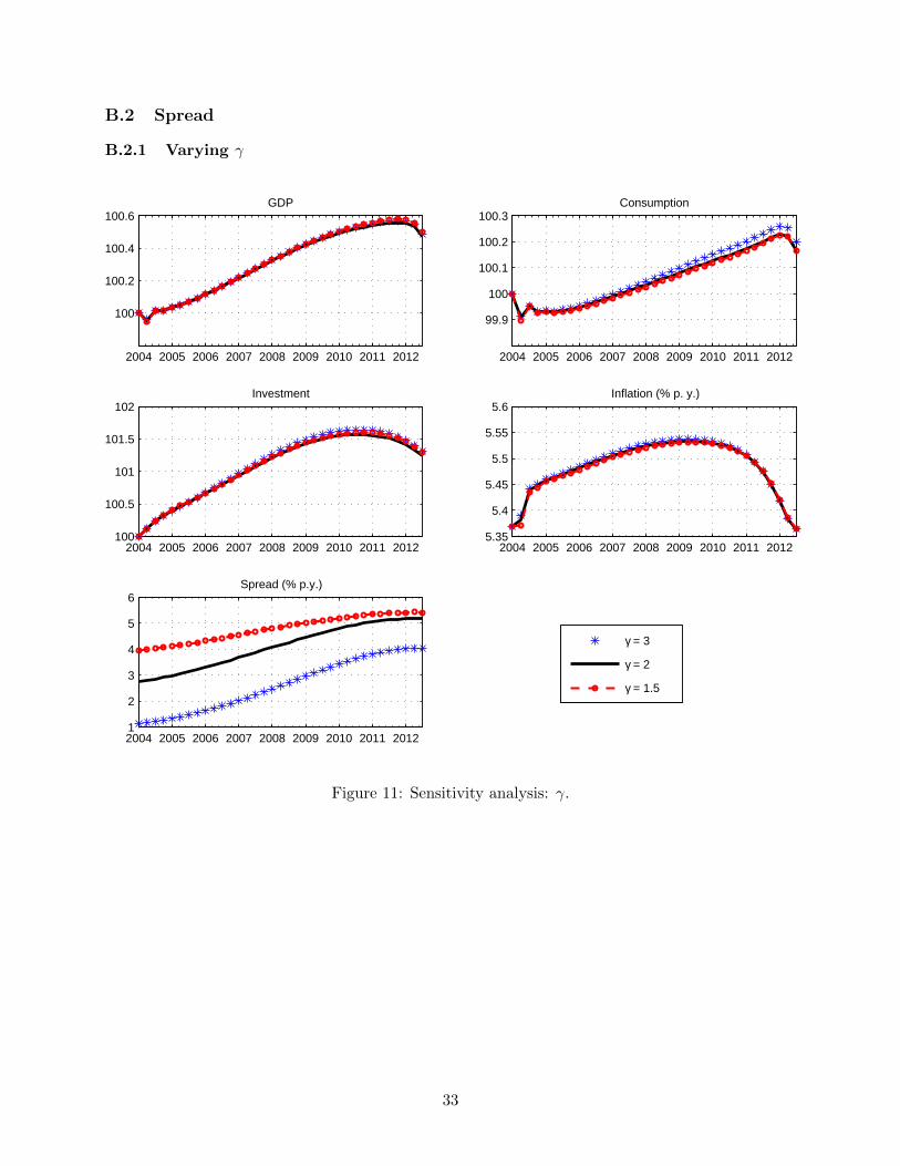
B.2 Spread

B.2.1 Varying γ

2004 2005 2006 2007 2008 2009 2010 2011 2012

100

100.2

100.4

100.6GDP

γ = 3

γ = 2

γ = 1.5

2004 2005 2006 2007 2008 2009 2010 2011 2012

99.9

100

100.1

100.2

100.3Consumption

2004 2005 2006 2007 2008 2009 2010 2011 2012100

100.5

101

101.5

102Investment

2004 2005 2006 2007 2008 2009 2010 2011 20125.35

5.4

5.45

5.5

5.55

5.6Inflation (% p. y.)

2004 2005 2006 2007 2008 2009 2010 2011 20121

2

3

4

5

6Spread (% p.y.)

Figure 11: Sensitivity analysis: γ.

33

B.2.2 Varying η

2004 2005 2006 2007 2008 2009 2010 2011 2012

100

100.2

100.4

100.6GDP

2004 2005 2006 2007 2008 2009 2010 2011 201299.9

100

100.1

100.2

100.3

100.4Consumption

2004 2005 2006 2007 2008 2009 2010 2011 2012100

100.5

101

101.5

102Investment

2004 2005 2006 2007 2008 2009 2010 2011 20125.35

5.4

5.45

5.5

5.55

5.6Inflation (% p.y.)

2004 2005 2006 2007 2008 2009 2010 2011 20122

3

4

5

6

7Spread (% p.y.)

η = 0.0092

η = 0.012

η = 0.0152

Figure 12: Sensitivity analysis: η.

34

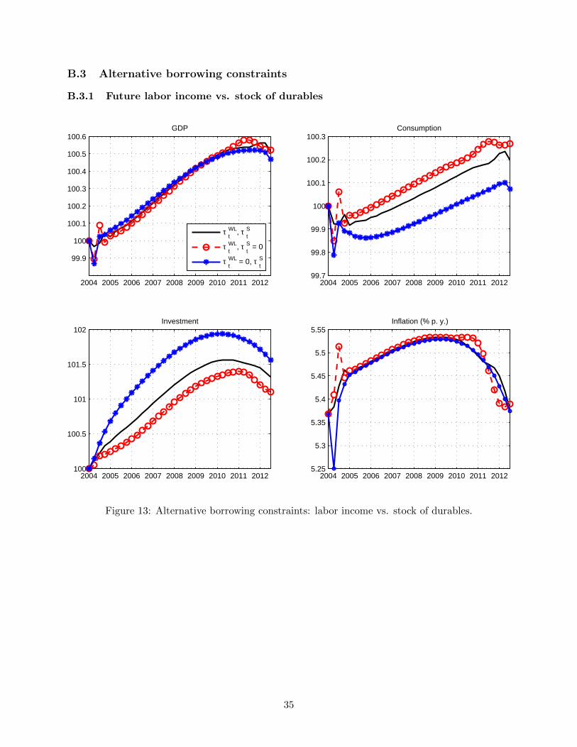
B.3 Alternative borrowing constraints

B.3.1 Future labor income vs. stock of durables

2004 2005 2006 2007 2008 2009 2010 2011 2012

99.9

100

100.1

100.2

100.3

100.4

100.5

100.6GDP

τ tWL, τ

tS

τ tWL, τ

tS = 0

τ tWL = 0, τ

tS

2004 2005 2006 2007 2008 2009 2010 2011 201299.7

99.8

99.9

100

100.1

100.2

100.3Consumption

2004 2005 2006 2007 2008 2009 2010 2011 2012100

100.5

101

101.5

102Investment

2004 2005 2006 2007 2008 2009 2010 2011 20125.25

5.3

5.35

5.4

5.45

5.5

5.55Inflation (% p. y.)

Figure 13: Alternative borrowing constraints: labor income vs. stock of durables.

35

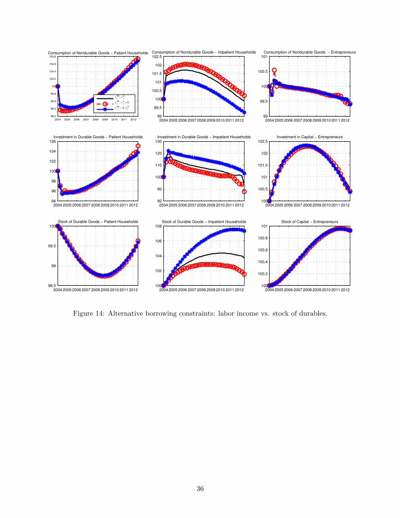
2004 2005 2006 2007 2008 2009 2010 2011 2012

99.2

99.4

99.6

99.8

100

100.2

100.4

100.6

100.8

Consumption of Nondurable Goods − Patient Households

τ t

WL, τ

t

S

τ t

WL, τ

t

S = 0

τ t

WL = 0, τ

t

S

2004 2005 2006 2007 2008 2009 2010 2011 201299

99.5

100

100.5

101

101.5

102

102.5Consumption of Nondurable Goods − Impatient Households

2004 2005 2006 2007 2008 2009 2010 2011 201299

99.5

100

100.5

101Consumption of Nondurable Goods − Entrepreneurs

2004 2005 2006 2007 2008 2009 2010 2011 201294

96

98

100

102

104

106Investment in Durable Goods − Patient Households

2004 2005 2006 2007 2008 2009 2010 2011 201280

90

100

110

120

130Investment in Durable Goods − Impatient Households

2004 2005 2006 2007 2008 2009 2010 2011 2012100

100.5

101

101.5

102

102.5Investment in Capital − Entrepreneurs

2004 2005 2006 2007 2008 2009 2010 2011 201298.5

99

99.5

100Stock of Durable Goods − Patient Households

2004 2005 2006 2007 2008 2009 2010 2011 2012100

102

104

106

108Stock of Durable Goods − Impatient Households

2004 2005 2006 2007 2008 2009 2010 2011 2012100

100.2

100.4

100.6

100.8

101Stock of Capital − Entrepreneurs

Figure 14: Alternative borrowing constraints: labor income vs. stock of durables.

36

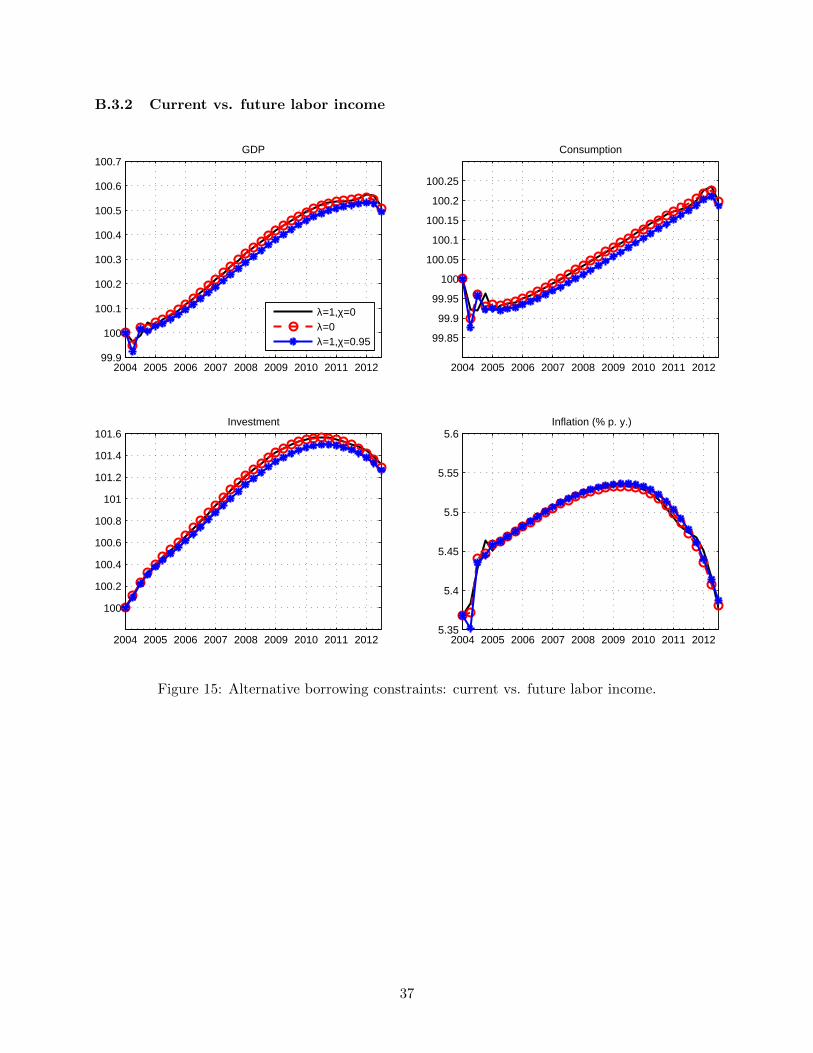
B.3.2 Current vs. future labor income

2004 2005 2006 2007 2008 2009 2010 2011 201299.9

100

100.1

100.2

100.3

100.4

100.5

100.6

100.7GDP

λ=1,χ=0λ=0λ=1,χ=0.95

2004 2005 2006 2007 2008 2009 2010 2011 2012

99.85

99.9

99.95

100

100.05

100.1

100.15

100.2

100.25

Consumption

2004 2005 2006 2007 2008 2009 2010 2011 2012

100

100.2

100.4

100.6

100.8

101

101.2

101.4

101.6Investment

2004 2005 2006 2007 2008 2009 2010 2011 20125.35

5.4

5.45

5.5

5.55

5.6Inflation (% p. y.)

Figure 15: Alternative borrowing constraints: current vs. future labor income.

37

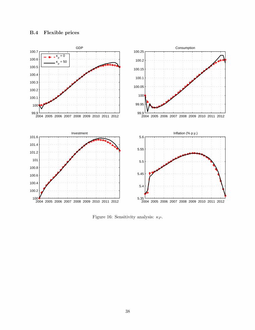
B.4 Flexible prices

2004 2005 2006 2007 2008 2009 2010 2011 201299.9

100

100.1

100.2

100.3

100.4

100.5

100.6

100.7GDP

κ

p = 0

κp = 50

2004 2005 2006 2007 2008 2009 2010 2011 201299.9

99.95

100

100.05

100.1

100.15

100.2

100.25Consumption

2004 2005 2006 2007 2008 2009 2010 2011 2012100

100.2

100.4

100.6

100.8

101

101.2

101.4

101.6Investment

2004 2005 2006 2007 2008 2009 2010 2011 20125.35

5.4

5.45

5.5

5.55

5.6Inflation (% p.y.)

Figure 16: Sensitivity analysis: κP .

38

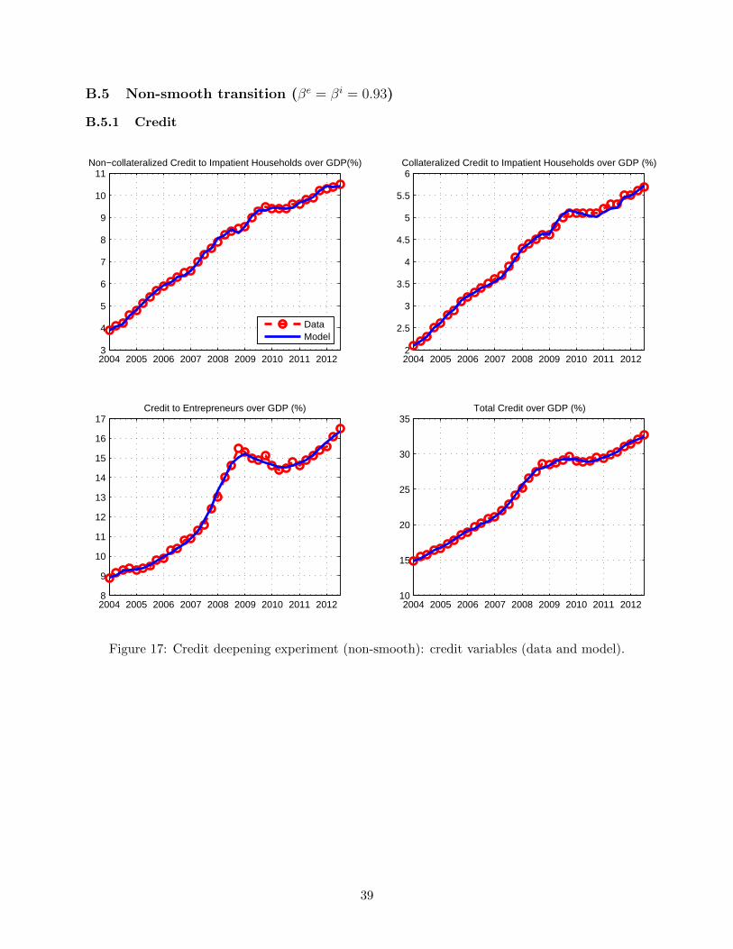
B.5 Non-smooth transition (βe = βi = 0.93)

B.5.1 Credit

2004 2005 2006 2007 2008 2009 2010 2011 20123

4

5

6

7

8

9

10

11Non−collateralized Credit to Impatient Households over GDP(%)

DataModel

2004 2005 2006 2007 2008 2009 2010 2011 20122

2.5

3

3.5

4

4.5

5

5.5

6Collateralized Credit to Impatient Households over GDP (%)

2004 2005 2006 2007 2008 2009 2010 2011 20128

9

10

11

12

13

14

15

16

17Credit to Entrepreneurs over GDP (%)

2004 2005 2006 2007 2008 2009 2010 2011 201210

15

20

25

30

35Total Credit over GDP (%)

Figure 17: Credit deepening experiment (non-smooth): credit variables (data and model).

39

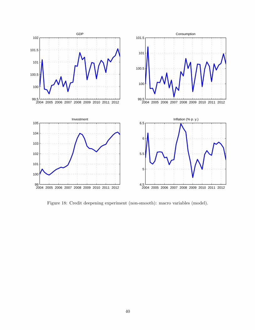
2004 2005 2006 2007 2008 2009 2010 2011 201299.5

100

100.5

101

101.5

102GDP

2004 2005 2006 2007 2008 2009 2010 2011 201299.5

100

100.5

101

101.5Consumption

2004 2005 2006 2007 2008 2009 2010 2011 201299

100

101

102

103

104

105Investment

2004 2005 2006 2007 2008 2009 2010 2011 20124.5

5

5.5

6

6.5Inflation (% p. y.)

Figure 18: Credit deepening experiment (non-smooth): macro variables (model).

40

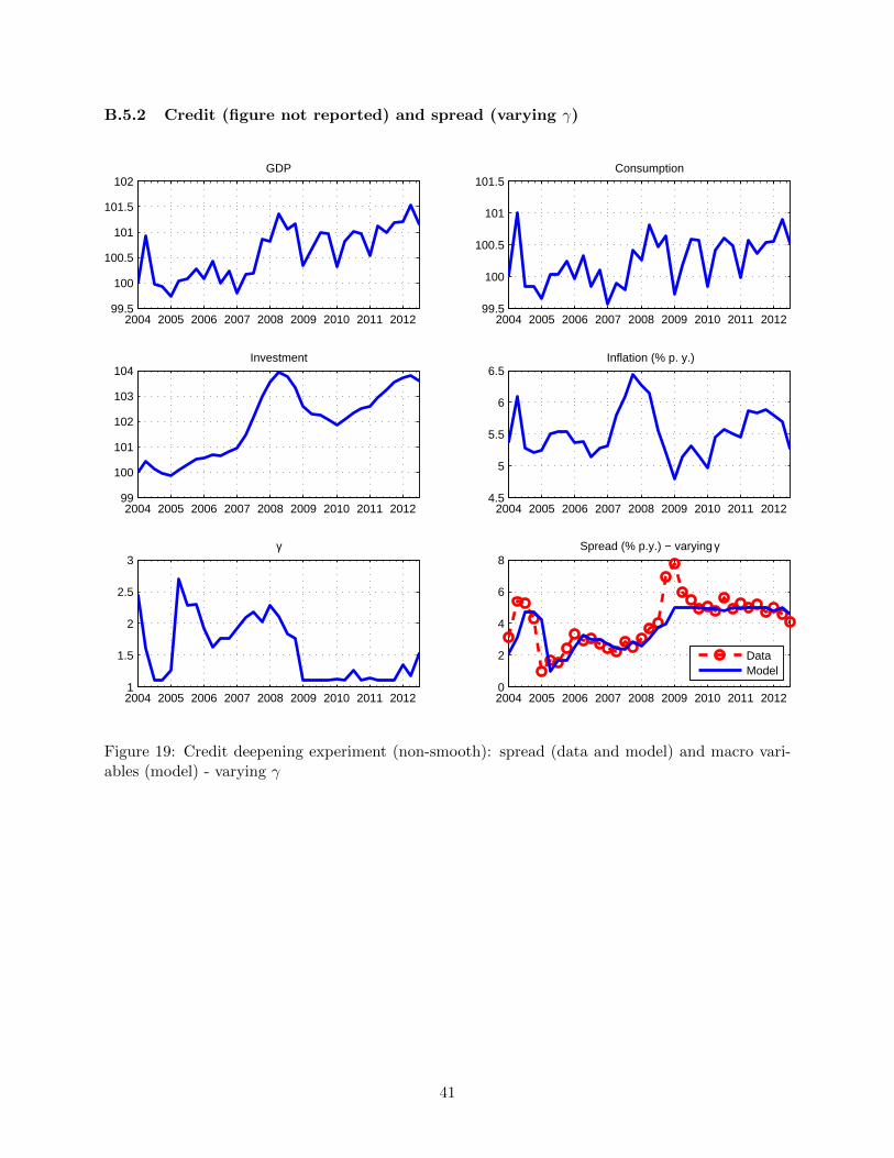
B.5.2 Credit (figure not reported) and spread (varying γ)

2004 2005 2006 2007 2008 2009 2010 2011 201299.5

100

100.5

101

101.5

102GDP

2004 2005 2006 2007 2008 2009 2010 2011 201299.5

100

100.5

101

101.5Consumption

2004 2005 2006 2007 2008 2009 2010 2011 201299

100

101

102

103

104Investment

2004 2005 2006 2007 2008 2009 2010 2011 20124.5

5

5.5

6

6.5Inflation (% p. y.)

2004 2005 2006 2007 2008 2009 2010 2011 20121

1.5

2

2.5

3γ

2004 2005 2006 2007 2008 2009 2010 2011 20120

2

4

6

8Spread (% p.y.) − varying γ

DataModel

Figure 19: Credit deepening experiment (non-smooth): spread (data and model) and macro vari-ables (model) - varying γ

41

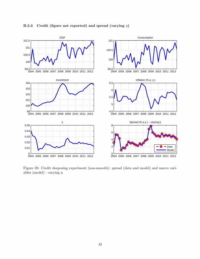
B.5.3 Credit (figure not reported) and spread (varying η)

2004 2005 2006 2007 2008 2009 2010 2011 201299.5

100

100.5

101

101.5GDP

2004 2005 2006 2007 2008 2009 2010 2011 201299.5

100

100.5

101Consumption

2004 2005 2006 2007 2008 2009 2010 2011 201299

100

101

102

103

104Investment

2004 2005 2006 2007 2008 2009 2010 2011 20124.5

5

5.5

6

6.5Inflation (% p. y.)

2004 2005 2006 2007 2008 2009 2010 2011 20120

0.01

0.02

0.03

0.04

0.05η

2004 2005 2006 2007 2008 2009 2010 2011 20120

2

4

6

8Spread (% p.y.) − varying η

DataModel

Figure 20: Credit deepening experiment (non-smooth): spread (data and model) and macro vari-ables (model) - varying η

42

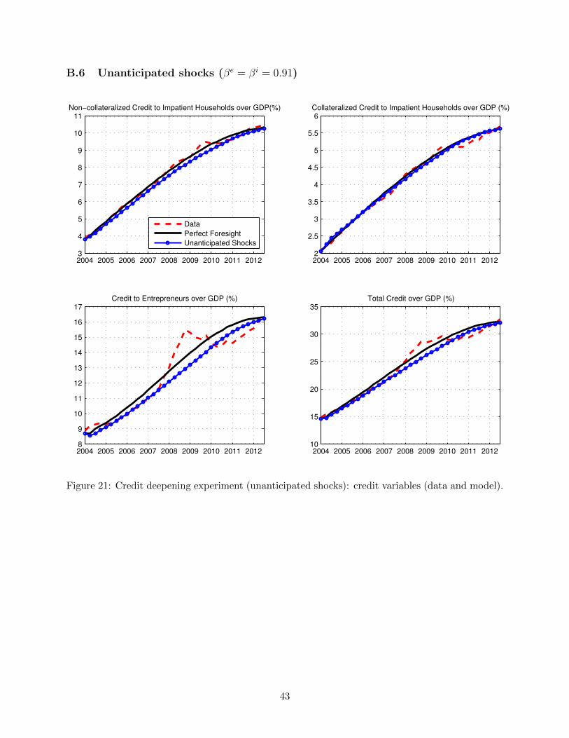
B.6 Unanticipated shocks (βe = βi = 0.91)

2004 2005 2006 2007 2008 2009 2010 2011 20123

4

5

6

7

8

9

10

11Non−collateralized Credit to Impatient Households over GDP(%)

Data

Perfect Foresight

Unanticipated Shocks

2004 2005 2006 2007 2008 2009 2010 2011 20122

2.5

3

3.5

4

4.5

5

5.5

6Collateralized Credit to Impatient Households over GDP (%)

2004 2005 2006 2007 2008 2009 2010 2011 20128

9

10

11

12

13

14

15

16

17Credit to Entrepreneurs over GDP (%)

2004 2005 2006 2007 2008 2009 2010 2011 201210

15

20

25

30

35Total Credit over GDP (%)

Figure 21: Credit deepening experiment (unanticipated shocks): credit variables (data and model).

43

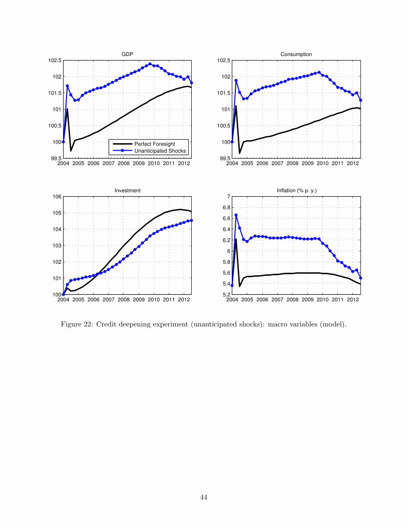
2004 2005 2006 2007 2008 2009 2010 2011 201299.5

100

100.5

101

101.5

102

102.5GDP

Perfect Foresight

Unanticipated Shocks

2004 2005 2006 2007 2008 2009 2010 2011 201299.5

100

100.5

101

101.5

102

102.5Consumption

2004 2005 2006 2007 2008 2009 2010 2011 2012100

101

102

103

104

105

106Investment

2004 2005 2006 2007 2008 2009 2010 2011 20125.2

5.4

5.6

5.8

6

6.2

6.4

6.6

6.8

7Inflation (% p. y.)

Figure 22: Credit deepening experiment (unanticipated shocks): macro variables (model).

44

C Small open economy version

Our benchmark specification assumes that Brazil is a closed economy. However, one can conjecture,

as Justiniano et al. (2015a), that the macroeconomic effects stemming from a credit expansion may

be amplified in small open economies (SOEs). In this case, the demand for credit of firms and

impatient agents does not need to be compensated by higher savings and, thus, less consumption

by patient agents.

Although the assumption that Brazil is relatively closed to trade is realistic, the financial indices

reported by Quinn et al. (2011) as well as the Chinn-Ito index28 suggest that Brazil is not closed

to financial flows. Hence, in this appendix, we consider a SOE version of the model in which the

interest rate is assumed to be constant, so that capital flows equalize demand and supply in this

market, but the wage rate still adjusts to clear the labor market domestically. In particular, we fix

the interest rate at its value obtained in the low-credit steady state of the benchmark economy.

In order to scrutinize the aforementioned conjecture, we consider an economy with only im-

patient households and entrepreneurs that borrow resources from the rest of the world. In this

case, there is no “crowding out effect” of domestic lenders consuming less. Now we assume that

profits generated by all firms in the economy are transferred to entrepreneurs. For simplicity, we

also assume price flexibility. The rest of the model as well as the quantitative strategy remain the

same as in the benchmark exercise.29 Again, we solve for the time-varying paths of τWLt , τSt , and

τKt that generate the smooth paths for non-collateralized credit, collateralized credit to households,

and credit to non-financial corporations, shown in Figure 3, that resemble their counterparts in the

data.

Figure 23 compares the paths for GDP, consumption and investment in the benchmark model

with price flexibility and in the SOE version of the model. It also plots the path of the trade deficit

to GDP in the SOE. In addition, Figure 24 shows the evolution of labor market outcomes in the

SOE.

28See Chinn and Ito (2006). The updated version of the index is available athttp://web.pdx.edu/~ito/Chinn-Ito_website.htm.

29The equations of the SOE version of the model are described in a separate appendix, available upon request.

45

2004 2005 2006 2007 2008 2009 2010 2011 201299.6

99.8

100

100.2

100.4

100.6GDP

SOEBenchmark

2004 2005 2006 2007 2008 2009 2010 2011 201299.9

100

100.1

100.2

100.3

100.4Consumption

2004 2005 2006 2007 2008 2009 2010 2011 2012100

100.5

101

101.5

102

102.5Investment

2004 2005 2006 2007 2008 2009 2010 2011 2012−0.8

−0.6

−0.4

−0.2

0

0.2

0.4

0.6Trade Deficit to GDP (%)

Figure 23: Credit deepening experiment: macro variables (benchmark and SOE).

46

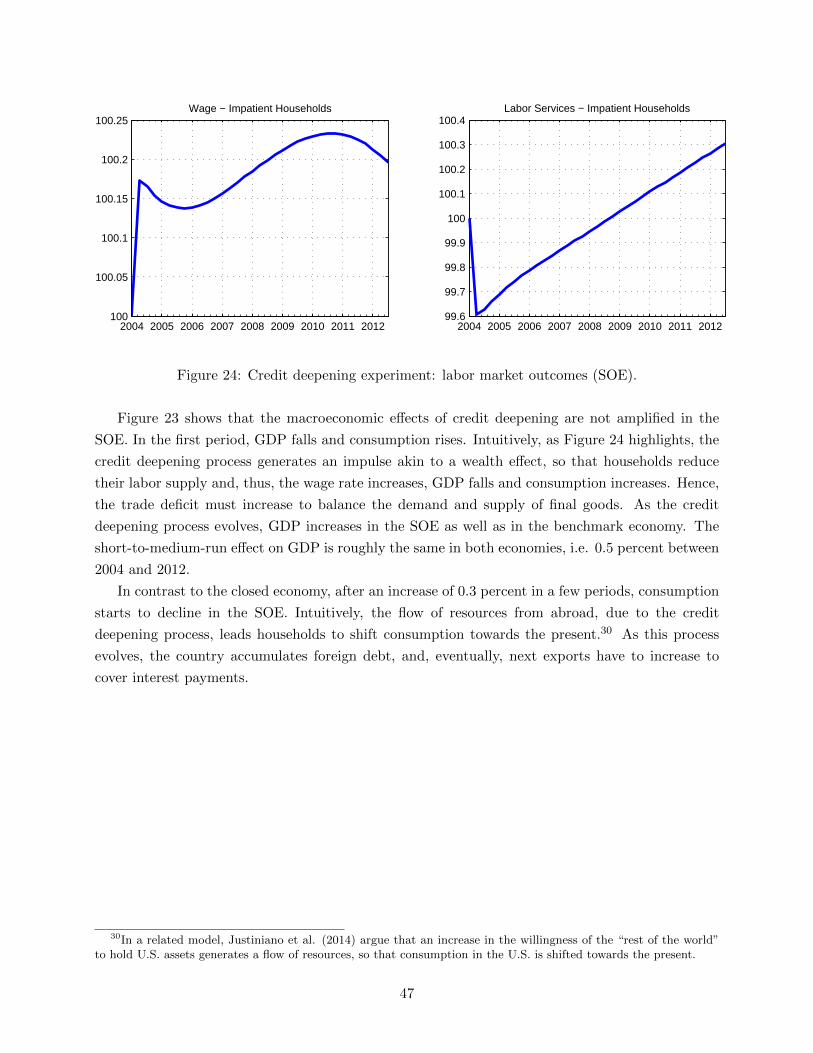
2004 2005 2006 2007 2008 2009 2010 2011 2012100

100.05

100.1

100.15

100.2

100.25Wage − Impatient Households

2004 2005 2006 2007 2008 2009 2010 2011 201299.6

99.7

99.8

99.9

100

100.1

100.2

100.3

100.4Labor Services − Impatient Households

Figure 24: Credit deepening experiment: labor market outcomes (SOE).

Figure 23 shows that the macroeconomic effects of credit deepening are not amplified in the

SOE. In the first period, GDP falls and consumption rises. Intuitively, as Figure 24 highlights, the

credit deepening process generates an impulse akin to a wealth effect, so that households reduce

their labor supply and, thus, the wage rate increases, GDP falls and consumption increases. Hence,

the trade deficit must increase to balance the demand and supply of final goods. As the credit

deepening process evolves, GDP increases in the SOE as well as in the benchmark economy. The

short-to-medium-run effect on GDP is roughly the same in both economies, i.e. 0.5 percent between

2004 and 2012.

In contrast to the closed economy, after an increase of 0.3 percent in a few periods, consumption

starts to decline in the SOE. Intuitively, the flow of resources from abroad, due to the credit

deepening process, leads households to shift consumption towards the present.30 As this process

evolves, the country accumulates foreign debt, and, eventually, next exports have to increase to

cover interest payments.

30In a related model, Justiniano et al. (2014) argue that an increase in the willingness of the “rest of the world”to hold U.S. assets generates a flow of resources, so that consumption in the U.S. is shifted towards the present.

47

D The propagation of shocks in high- and low-credit economies

In this section, we analyze the propagation of two shocks in a stochastic version of the model.31 In

particular, we compare impulse response functions of several variables to technology and monetary

policy shocks (which we add to the model for this exercise only) around two steady-states: One

with low and the other with high levels of credit.32

In the first steady-state, we calibrate τWL = 0.28 to match the ratio of individual non-

collateralized credit to GDP of four percent, τS = 0.07 to match the ratio of individual collat-

eralized credit to GDP oftwo percent, and τK = 0.031 to match the ratio of firm credit to GDP of

9 percent. These figures correspond to the amount of credit we observe in the Brazilian economy at

the beginning of 2004 (see Figure 2), when the credit deepening process described above arguably

started. This is the steady-state with a low credit-to-GDP ratio.

In the second steady-state, we calibrate τWL = 0.759 to match the ratio of individual non-

collateralized credit to GDP of 10 percent, τS = 0.175 to match the ratio of individual collateralized

credit to GDP of 6 percent, and τK = 0.057 to match the ratio of firm credit to GDP of 16 percent.

These figures are close to the amount of credit we observe in the Brazilian economy by mid-2012

(see Figure 2). We set this calibration to represent the steady-state with a high credit-to-GDP

ratio.

We assume that the technology shock follows an AR(1) process with an autocorrelation coeffi-

cient of 0.91, as in De Castro et al. (2001). Monetary shocks are assumed to be i.i.d.

Figures 25 and 26 plot the impulse response functions for selected variables (GDP, consumption,

investment, household interest rate, and inflation) to the technology and monetary policy shocks,

respectively.

31For this exercise, we solve an approximate version of the model by log-linearizing the equilibrium conditions.The latter are in a separate appendix, available upon request.

32Gerali et al. (2010) study how the presence of banks and financial frictions affects the impulse response functionsto technology and monetary policy shocks. They find that banks attenuate the effect of a monetary policy shock.

48

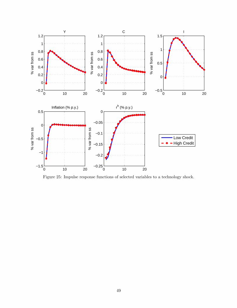
0 10 20−0.2

0

0.2

0.4

0.6

0.8

1

1.2%

var

from

ss

Y

0 10 20−0.2

0

0.2

0.4

0.6

0.8

1

1.2

% v

ar fr

om s

s

C

Low CreditHigh Credit

0 10 20−0.5

0

0.5

1

1.5

% v

ar fr

om s

s

I

0 10 20−1.5

−1

−0.5

0

0.5

% v

ar fr

om s

s

Inflation (% p.y.)

0 10 20−0.25

−0.2

−0.15

−0.1

−0.05

0

% v

ar fr

om s

s

rh (% p.y.)

Figure 25: Impulse response functions of selected variables to a technology shock.

49

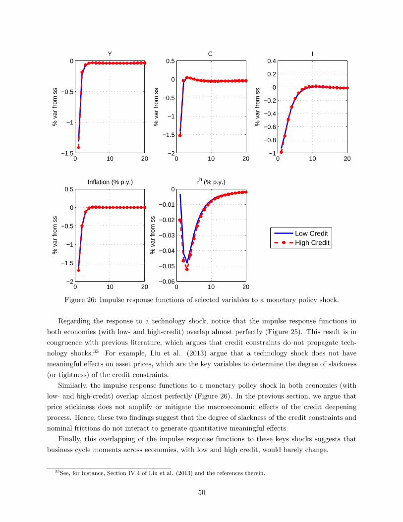
0 10 20−1.5

−1

−0.5

0%

var

from

ss

Y

0 10 20−2

−1.5

−1

−0.5

0

0.5

% v

ar fr

om s

s

C

Low CreditHigh Credit

0 10 20−1

−0.8

−0.6

−0.4

−0.2

0

0.2

0.4

% v

ar fr

om s

s

I

0 10 20−2

−1.5

−1

−0.5

0

0.5

% v

ar fr

om s

s

Inflation (% p.y.)

0 10 20−0.06

−0.05

−0.04

−0.03

−0.02

−0.01

0

% v

ar fr

om s

s

rh (% p.y.)

Figure 26: Impulse response functions of selected variables to a monetary policy shock.

Regarding the response to a technology shock, notice that the impulse response functions in

both economies (with low- and high-credit) overlap almost perfectly (Figure 25). This result is in

congruence with previous literature, which argues that credit constraints do not propagate tech-

nology shocks.33 For example, Liu et al. (2013) argue that a technology shock does not have

meaningful effects on asset prices, which are the key variables to determine the degree of slackness

(or tightness) of the credit constraints.

Similarly, the impulse response functions to a monetary policy shock in both economies (with

low- and high-credit) overlap almost perfectly (Figure 26). In the previous section, we argue that

price stickiness does not amplify or mitigate the macroeconomic effects of the credit deepening

process. Hence, these two findings suggest that the degree of slackness of the credit constraints and

nominal frictions do not interact to generate quantitative meaningful effects.

Finally, this overlapping of the impulse response functions to these keys shocks suggests that

business cycle moments across economies, with low and high credit, would barely change.

33See, for instance, Section IV.4 of Liu et al. (2013) and the references therein.

50

E Sources for credit and interest rate data34

E.1 Domestic credit to private sector/GDP

Domestic credit to private sector refers to financial resources provided to the private sector by

financial corporations, such as through loans, purchases of nonequity securities, and trade credits

and other accounts receivable, that establish a claim for repayment. For some countries these claims

include credit to public enterprises. The financial corporations include monetary authorities and

deposit money banks, as well as other financial corporations where data are available (including

corporations that do not accept transferable deposits but do incur such liabilities as time and

savings deposits). Examples of other financial corporations are finance and leasing companies,

money lenders, insurance corporations, pension funds, and foreign exchange companies.

Source: World Bank (http://data.worldbank.org/indicator/FS.AST.PRVT.GD.ZS).35

E.2 Nonearmarked credit outstanding/GDP

Nonearmarked credit outstanding is the nominal balance of such credit operations by the National

Financial System. Nonearmarked funds refer to financing and loans in which rates and destination

are freely negotiated between financial institutions and borrowers, i.e. the financial institution has

autonomy to decide to which economic sectors it will lend the funds raised in the market through

time deposits, funds raised in foreign markets, part of demand deposits etc. We consider the ratio

of the outstanding balance of credit operations at the end of a period to GDP, which is calculated

by the Central Bank of Brazil (CBB) through interpolation of available quarterly data.

Source: CBB - Data code: 17461.36

E.2.1 Nonearmarked household credit outstanding/GDP

The following types of credit are considered: vehicles financing, other goods financing, mortgages,

credit card, personal credit, overdraft and other nonearmarked credit instruments that were not

classified in previous types of credit.

Source: CBB - Data code: 17483.

E.2.2 Nonearmarked corporate credit outstanding/GDP

The following types of credit are considered: working capital up to 29 days, working capital over

30 days, discount of trade bills, discount of checks, mortgages, goods financing, vendor credit,

advances on exchange contracts, exports financing, foreign transfers and other nonearmarked credit

instruments that were not classified in previous types of credit.

34The remaining data that we use are standard National Account and macroeco-nomic variables, which can be downloaded from http://www.ibge.gov.br/english/ andhttps://www3.bcb.gov.br/sgspub/localizarseries/localizarSeries.do?method=prepararTelaLocalizarSeries.

35Definitions of credit variables are taken ipsis litteris from the source, whenever available.36We collected the data from the Portuguese version of the website. Some data were not available in the English

version.

51

Source: CBB - Data code: 17488.

E.3 Spread

We construct the spread series as the difference between the Brazilian prime rate and the SELIC

overnight interest rate.

E.3.1 Brazilian prime rate (% p.y.)

The Brazilian prime rate is calculated as the average of the operations agreed between financial

institutions and their preferred customers. It tends to reflect the cost of loans for customers with

lower risk.

Source: CBB - Data code: 20019.

E.3.2 Effective Selic rate (% p.y.)

Selic rate is defined as the average rate of daily financing in the Special System of Clearance and

Custody (SELIC for the Portuguese acronym) for federal bonds.

Source: CBB - Data code: 4189.

E.4 Household debt

We calculate household debt as the ratio of household nonearmarked debt held by financial in-

stitutions to disposable income accumulated over the past twelve months (MSAD). MSAD is a

measure of aggregate household earnings. It comprises labor income as measured in the Monthly

Employment Survey (Pesquisa Mensal de Emprego) and the National Household Survey (Pesquisa

Nacional por Amostra de Domicılios) from the Brazilian Institute for Geography and Statistics

(Instituto Brasileiro de Geografia e Estatıstica), social security benefits and pensions, and revenues

from households’ investments in savings deposits, time deposits, Treasury bonds and investment

funds, net of income tax on labor earnings, social security collections and taxes on financial invest-

ments.

Source: CBB - Data code: 19959.

52