D o People Understand Monetary Policy?reap.org.br/wp-content/uploads/2014/04/041-Do... · Do People Understand Monetary Policy? Carlos Carvalho PUC-Rio and Kyros Investimentos Fernanda

Todos os direitos reservados. É proibida a reprodução parcial ou integral do conteúdo

deste documento por qualquer meio de distribuição, digital ou impresso, sem a expressa autorização do

REAP ou de seu autor.

Do People Understand Monetary Policy?

Carlos Viana de Carvalho

Fernanda Nechio

Abril, 2014 Working Paper 041

DO PEOPLE UNDERSTAND MONETARY POLICY?

Carlos Viana de Carvalho

Fernanda Nechio

Carlos Viana de Carvalho Pontifícia Universidade Católica do Rio de Janeiro (PUC-Rio) Departamento de Economia Rua Marquês de São Vicente, nº 225 Gávea 22451-900 - Rio de Janeiro, RJ - Brasil [email protected] Fernanda Nechio Federal Reserve Bank of San Francisco 101 Market Street San Francisco, CA 94105 United States [email protected]

mailto:[email protected]

mailto:[email protected]

Do People Understand Monetary Policy?∗

Carlos CarvalhoPUC-Rio and Kyros Investimentos

Fernanda NechioFederal Reserve Bank of San Francisco

April, 2014

Abstract

We combine questions from the Michigan Survey about future inflation, unemployment, and

interest rates to investigate whether households are aware of the basic features of U.S. monetary

policy. Our findings provide evidence that some households form their expectations in a way

that is consistent with a Taylor (1993)-type rule. We also document a large degree of variation in

the pattern of responses over the business cycle. In particular, the negative relationship between

unemployment and interest rates that is apparent in the data only shows up in households’

answers during periods of labor market weakness.

JEL classification codes: E52, E58

Keywords: survey data, monetary policy, communication, Taylor rule, inflation expectations,

Michigan Survey, Survey of Professional Forecasters

∗For comments and suggestions we thank Klaus Adam, Marty Eichenbaum, five anonymous referees, AlessandroBarbarino, Jeff Campbell, Oleg Itskhoki, Oscar Jorda, Alex Justiniano, Virgiliu Midrigan, Ricardo Reis, AndreaTambalotti, and seminar participants at EEA-ESEM 2013, AEA 2013, 3rd CESifo Conference on “Macroeconomicsand Survey Data”, FEA-USP, Bank of Canada, St. Louis Fed conference on “Expectations in Dynamic MacroeconomicModels”, NASM2012, SED2012, UC Santa Cruz, SBE 2011, EESP-FGV/SP, Central Bank of Brazil, PUC-Rio, SantaClara University, Federal Reserve Macro System Meetings, NBER-SI 2011 (EFWW), SF Fed, EPGE/FGV Advancesin Macroeconomics Workshop, and NY Fed. Eric Hsu and Israel Malkin provided outstanding research assistance.Carlos Carvalho acknowledges financial support from CNPq under grant 486768/2013-9. The views expressed in thispaper are those of the authors and do not necessarily reflect the position of the Federal Reserve Bank of San Franciscoor the Federal Reserve System. E-mails: [email protected], [email protected].

1

1 Introduction

“Improving the public’s understanding of the central bank’s policy strategy reduces

economic and financial uncertainty and helps households and firms make more-informed

decisions. Moreover, clarity about goals and strategies can help anchor the public’s

longer-term inflation expectations more firmly and thereby bolsters the central bank’s

ability to respond forcefully to adverse shocks.”(Bernanke, 2010).

Central bankers often emphasize the need to communicate with the public to improve its under-

standing of monetary policy. As the argument goes, this should allow households and firms to make

better-informed price- and wage-setting decisions, and improve policy effectiveness. More generally,

agents’understanding of how policies that affect their decisions are conducted is perceived to be a

key ingredient in the policy transmission mechanism. This perception is guided by economic theo-

ries in which the behavior of the economy depends on the interaction between the actual conduct

of policy and agents’understanding of it.1

In this paper we take a step back from the literature on central bank communication, expec-

tations formation, and monetary policy effectiveness, and try to answer the more basic question

of whether economic agents —U.S. households in particular —understand how the Fed conducts

monetary policy.

Since the work of Taylor (1993), it became standard practice to posit that the Fed sets interest

rates according to a “Taylor rule”that specifies a target for the policy rate as a function of deviations

of inflation from its objective and some measure of slack in economic activity, such as the output gap.

Our goal is to assess whether U.S. households are aware of what we refer to as the basic principles

underlying the Taylor rule: that the policy interest rate tends to increase with inflation and to

decrease with slack in economic activity. Most of the time, these principles provide a qualitative

description of how the Fed pursues its so-called dual mandate of price stability and full employment.

While there is a large empirical literature on estimation of central banks’ interest rate policy

functions,2 there is much less empirical work on the question of whether households understand

monetary policy. One may wonder why this is the case. A possible answer is that this question

is not important. In a world with complete asset markets, it arguably suffi ces that agents who

participate in financial markets understand monetary policy. If so, asset prices will correctly reflect

1This interaction is well articulated in the work of Eusepi and Preston (2010), for example. In their model, ifagents are not fully aware of the central bank’s behavior, policies that would otherwise guarantee stable inflationexpectations might leave the door open to expectations-driven fluctuations.

2For a survey, see Hamalainen (2004). Overall, Taylor-type interest rate rules are seen as a reasonable descriptionof how policy has been conducted in the United States during most of the time since the late 1980s (see, e.g., Juddand Rudebusch 1998). At times, however, monetary policy seems to deviate more substantially from what Taylorrules would imply (e.g., Taylor 2007).

2

current and future policy developments, and those who do not understand monetary policy can

simply rely on asset prices to make fully informed consumption and investment decisions.

Under incomplete markets, however, households’ expectations about future monetary policy

may affect their behavior. An extreme case is that of an economy with only a one-period nominal

bond. In that case, the short-term nominal bond price only reveals the current interest rate, and

thus its price is not informative of financial market participants’views about future monetary policy.

Hence, households’intertemporal decisions will hinge on individual beliefs about the future course

of the economy —and of monetary policy in particular.3

Beyond these theoretical considerations, the effort that the Federal Reserve devotes to educating

the general public and communicating about monetary policy suggests that the question posed in

this paper is important for policymaking.4 So, perhaps the lack of empirical work in this area simply

reflects the fact that households’perceptions about monetary policy are not directly observed nor

surveyed.

This paper addresses the question of interest by combining households’answers to survey ques-

tions about future inflation, unemployment, and interest rates from the Survey of Consumers

(“Michigan Survey”). At an intuitive level, our simple empirical approach is based on the idea

of separating survey answers about interest rates, inflation, and unemployment that are consistent

with the basic principles underlying the Taylor rule from those that are not. To fix ideas, suppose

that the Fed’s target for the federal funds rate depends positively on contemporaneous inflation and

negatively on contemporaneous unemployment, and changes only with these two variables. Then,

to be consistent with the aforementioned principles, survey answers that indicate unemployment

will go down and inflation will go up in one year would necessarily have to be accompanied by an

answer that the Fed will tighten monetary policy over the same period. Likewise, answers that

unemployment will go up and inflation will drop must be associated with a call that the Fed will

ease policy.5

More generally, however, an answer that is inconsistent with a particular version of the Taylor

3This argument is consistent with the literature that studies the macroeconomic implications of expectationsformation. For example, Woodford (2013) studies models with possibly heterogeneous expectations in which agents’understanding of fiscal and monetary policies matters. Eusepi and Preston (2013) show that asset market structure —in particular the maturity profile of government debt —matters in a model in which agents have to learn about fiscaland monetary policies.

4Such effort includes, for example, lectures about monetary policy and programs to educate the general pub-lic (e.g., http://www.federalreserve.gov/newsevents/lectures/about.htm, http://sffed-education.org/chairman/, andhttp://www.newyorkfed.org/education/fedchallenge_college.html). The concern with the public’s understanding ofmonetary policy is shared by policymakers other than Chairman Bernanke. For example, Yellen (2013) states that“Like the Chairman, I strongly believe that monetary policy is most effective when the public understands what theFed is trying to do and how it plans to do it.”

5Our approach relies on the maintained identification assumption that households’answers about future changesin interest rates are conditional on their answers about future inflation and unemployment. We later discuss howalternative assumptions might affect the interpretation of our results.

3

rule need not imply a misunderstanding of monetary policy. The reason is that no specific interest

rate rule is a perfect description of policy. To address this issue and provide an answer to our

research question that can be relied on more generally, we look for consistency in households’

answers by testing whether various empirical frequencies of households’ responses about future

interest rates, inflation, and unemployment differ from each other in a way that is consistent with

the basic principles underlying the Taylor rule. To give a concrete example, given a response about

future unemployment, our empirical approach is to test if forecasts that interest rates will go up

are more prevalent among households that predict higher inflation than among those that predict

lower inflation.

Despite important limitations, the Michigan Survey data turn out to be informative of the

question posed in this paper. Our results are broadly consistent with the view that (at least

some) U.S. households are aware of the basic principles underlying the Taylor rule when forming

their expectations about interest rates, inflation, and unemployment. The extent to which this

happens, however, is not uniform across income and education levels. Moreover, there are important

differences in the patterns of responses over the business cycle. Specifically, households’answers

are more consistent with a Taylor rule during times of labor market weakness. Our findings survive

an extensive battery of robustness checks.

While our tests are based on a reduced-form empirical approach, the relationships uncovered

between households’answers about inflation and unemployment on one side and interest rates on

the other side can be given a causal interpretation. This requires addressing the possible problems

posed by endogeneity and reverse causality. We do so by resorting to a dynamic, stochastic, general-

equilibrium (DSGE) model as a laboratory. Using the model, we study how the relationships elicited

with our approach are affected by general equilibrium effects of autonomous changes in interest

rates on inflation and unemployment. The results show that the correct signs of the relationships

of interest can be uncovered, despite the presence of those general equilibrium effects.

The paper also provides additional empirical evidence that our tests are indeed informative of

households’perceptions of monetary policy and not of the so-called Fisher equation —a positive

relationship between nominal interest rates and expected inflation. This is done by exploiting time

periods in the mid-2000s during which Fed policy arguably deviated from a Taylor rule. The pattern

of households’responses during those periods changed accordingly.

As an additional step to interpret our results for the Michigan Survey, the same empirical

approach is applied to forecasts from the Survey of Professional Forecasters (SPF). Professional

forecasters are arguably more likely to be aware of how monetary policy is conducted. Despite some

challenges associated with sample size, our findings support the view that professional forecasters’

4

answers to the survey are consistent with the basic principles underlying the Taylor rule in both its

unemployment and (core) inflation dimensions.

A few recent papers investigate whether professional economists’and financial market partici-

pants’forecasts of interest rates, inflation, and output growth or some other measure of economic

activity conform with Taylor-type interest rate rules. Mitchell and Pearce (2009) analyze the Wall

Street Journal’s semiannual survey of professional economists, Carvalho and Minella (2009) study

the Focus Survey of market participants conducted by the Central Bank of Brazil, and Fendel et

al. (2011) rely on the Consensus Economic Forecast poll for the G-7 countries. These three pa-

pers estimate Taylor rules by panel regressions using numerical forecasts and address quantitative

questions, such as whether the estimated coeffi cient on inflation is greater than unity. Schmidt and

Nautz (2010) also use forecasts from financial market experts, but their panel data from the ZEW

Financial Market Survey are categorical in nature —the expected direction of changes in interest

rates, inflation, and the economic situation in the euro zone. They focus on the accuracy of interest

rate forecasts and on decomposing forecast errors into those for inflation and economic activity

and those due to misunderstanding of how the European Central Bank conducts monetary policy.

These four papers are thus related to our analysis of the SPF. However, our empirical approach

differs from theirs, since it is tailored to our analyses of the Michigan Survey. Finally, Hamilton

et al. (2011) use the effects of macroeconomic news on fed funds futures contracts to estimate the

market-perceived Taylor rule.

More broadly, our paper is related to the literature that uses survey (or experimental) data to

study whether agents form expectations in ways that are consistent with economic theories (e.g.,

Armantier et al. 2011, Andrade and Le Bihan 2013, Bachman et al. 2012, Coibion and Gorod-

nichenko 2010, Madeira and Zafar 2012, and Malmendier and Nagel 2013), and to the literature on

financial literacy (e.g., Lusardi and Mitchell 2011, and references therein). More recently, Dräger

et al. (2013) extend our approach to study other macroeconomic relationships.

Section 2 starts by describing the data used in our analyses, and introducing our empirical

approach. Section 3 reports our empirical findings. Section 4 provides a discussion of our results,

addressing issues such as endogeneity and causality. It also discusses possible interpretations of our

results. The last section concludes. The online appendix provides additional analyses and results

that confirm the robustness of our findings.

5

2 Data and empirical approach

2.1 Michigan Survey

Conducted by Thompson Reuters and the University of Michigan, at each month the Michigan

Survey interviews approximately 500 households and asks roughly 50 questions. The questionnaire

covers personal finances, demographics, business conditions, and, key to this paper, it also inquires

households about their expectations of main economic variables, such as interest rates, inflation, and

unemployment. The sample choice is statistically designed to represent all American households,

and survey weights are provided to allow for inference on the population.6 At each month, an

independent cross-section sample of households is selected, and some respondents are re-interviewed

six months later. Under this rotating sample method, at each survey around 40% of households

are being interviewed for the second time and 60% are new respondents. The monthly survey data

begin in January 1978. Besides the inclusion of new questions, no substantial changes have been

made to the pre-existing questionnaire since that time.

Our interest rate variable corresponds to the answer to the following survey question:

“No one can say for sure, but what do you think will happen to interest rates for borrowing

money during the next 12 months —will they go up, stay the same, or go down?”

For unemployment, the survey question is:

“How about people out of work during the coming 12 months —do you think that there will be

more unemployment than now, about the same, or less?”

Households are not asked directly about inflation, but instead about the direction of price

movements and its expected size. In particular, they answer the following two questions:

“During the next 12 months, do you think that prices in general will go up, or go down, or stay

where they are now?” and “By about what percent do you expect prices to go (up/down) on the

average, during the next 12 months?”

Our interest is on whether U.S. household perceptions of how monetary policy operates are in

accordance with the principles underlying the Taylor rule. Unfortunately, the Michigan Survey does

not include explicit questions about slack in economic activity —only about unemployment, which,

because of fluctuations in the unemployment rate that would correspond to full employment, need

not vary one-to-one with measures of economic slack. Likewise, the questions about inflation do

not pertain to deviations from the Fed’s (until recently unstated) inflation objective. Moreover, the

questions about interest rates and unemployment refer to 12-month changes, whereas the quanti-

tative question about the future path of prices amounts to a question about the level of 12-month

6Throughout this paper, all statistics from the Michigan Survey are weighted, unless stated otherwise. Hencethey refer to the U.S. population of households.

6

inflation. Finally, the survey is not explicit about the measures that the questions pertain to.

Using the available survey questions for our study requires some assumptions. To deal with the

fact that the question about interest rates pertains to “interest rates for borrowing money,” and

does not specify the measure it refers to, we assume that the answers to an analogous question

about the policy interest rate would be the same. This is a good assumption as long as the spread

between the borrowing rates that the household has in mind when answering the survey question

and the policy rate does not vary too much. Robustness analyses, presented in the online appendix,

confirm that our findings are essentially unchanged if the sample is restricted to periods in which

borrowing rates and the policy rate move in the same direction.

Regarding the question about unemployment, we assume that the answers to an analogous

question about the direction of the unemployment gap —the difference between the unemployment

rate and the level of unemployment that corresponds to full employment —would be the same.7

The question about prices refers to the general level of inflation expected for the next 12 months,

and does not specify a particular measure. We assume it refers to headline inflation measured by

the Consumer Price Index, and construct artificial responses to a question about the direction of

12-month inflation by subtracting the CPI inflation in the 12 months leading up to the month of

the survey from each individual response.8 Analogously with the question about unemployment,

it is assumed that the direction of change of actual inflation maps one-to-one into the direction of

change of the difference of inflation from the Fed’s objective. This is a sensible assumption given

the Fed’s mandate to pursue price stability, and the low level of inflation during most of our sample

period.

The Michigan Survey also provides demographic characteristics of respondents. This allows for

additional analyses conditional on specific household characteristics, such as household income and

education level of the respondent. Our baseline sample consists of households that were interviewed

only once, and first-time interviews of households that were interviewed twice.9

The sample period starts in August 1987 and ends in December 2007. The starting point

coincides with the beginning of Alan Greenspan’s tenure as chairman of the Federal Reserve Board,

during which the Taylor rule came to be seen as a good description of U.S. monetary policy. The

sample ends in December 2007 because the questions from the Michigan Survey pertain to 12-month

7Our findings are unchanged if the Congressional Budget Offi ce’s estimate of the non-accelerating-inflation rateof unemployment (“NAIRU”) is used to construct a measure of the unemployment gap, and the sample is restrictedto periods in which unemployment and that measure of the unemployment gap move in the same direction.

8The resulting numbers are converted into an answer about the direction of CPI inflation by assigning a valueof one when a household’s 12-month inflation forecast exceeds inflation in the 12 months up to and including themonth of the survey, zero if these two numbers coincide, and -1 otherwise. Categorical answers about interest ratesand unemployment are converted in the same way.

9 In unreported results we analyze samples that also include (or only include) the second interviews of the lattergroup of households, and all our findings go through.

7

forecasts, and at the end of 2008 short-term interest rates in the U.S. had essentially hit the zero

bound. Moreover, as discussed above, the question about interest rates in the Michigan Survey

refers to borrowing rates, which diverged markedly from short-term low-risk rates during most of

2008. When discussing and interpreting our findings we also analyze the pre-1987 period (January

1978 - July 1987).

2.2 Survey of Professional Forecasters

The SPF is conducted at a quarterly frequency and dates from the last quarter of 1968, when it

was implemented by the American Statistical Association and the National Bureau of Economic

Research (NBER). Since the second quarter of 1992, the survey has been conducted by the Federal

Reserve Bank of Philadelphia. The sample size varies from year to year, with an average of approx-

imately 140 forecasters per year. At each quarter, respondents receive the survey questionnaire,

which has to be filled and returned within a pre-established deadline. The survey covers expec-

tations about several inflation, economic activity, unemployment, and interest rate measures, for

various forecasting horizons.

Unlike the Michigan Survey, the SPF asks agents about their expectations for future levels of

interest rates, inflation, and unemployment. In particular, respondents are asked to provide their

forecasts for the next four quarters for well-specified measures of each of the three variables of

interest. Our analysis focuses on 4-quarter-ahead forecasts for the 3-month Treasury bill rate, CPI

inflation, and the urban civilian unemployment rate. CPI inflation forecasts are constructed as an

average across agents’forecasts for the next four quarters.

In addition to using the numerical forecasts provided by the survey, we also build categorical

variables indicating whether the respondents expect the variable to move up, down, or stay the

same. For interest rates and unemployment, the level of the variable in the quarter of the survey is

subtracted from the forecasts before categorizing the data. For CPI inflation, realized inflation in

the four quarters up to and including the quarter of the survey is subtracted from each participant’s

four-quarter forecast.

2.3 “Realized data”

We also apply our empirical approach to realized 12-month changes in inflation (headline CPI),

unemployment (urban civilian unemployment rate), and interest rates (3-month Treasury bill rate).

In order to make the results comparable to those based on the Michigan Survey, the data are

categorized depending on whether each variable moved up, down, or remained constant in each

12-month period.

8

2.4 Empirical approach

To ease the exposition of our empirical approach, let us introduce some notation. For a given

pool of answers about the direction of change of interest rates, inflation, and unemployment in the

subsequent 12 months, let F (x ↓ | y ↑, z ↓) denote the fraction of answers that indicate that x willdecrease in the next 12 months in the pool of answers that indicate that y will increase and z will

decrease over the same period.

With this notation, the partial effects of inflation associated with the basic principles underlying

the Taylor rule are defined as:

F (i ↑ | π ↑, u)−F (i ↑ | π ↓, u) > 0, (1)

F (i ↓ | π ↓, u)−F (i ↓ | π ↑, u) > 0, (2)

where u (↑ or ↓) is a given forecasted change in unemployment. The partial effects of inflationcompare pools of answers that share the same forecast for the direction of unemployment. For

example, for any given forecasted change u, the partial effects of inflation state that going from

a pool of households that predict declining inflation to a pool that predicts rising inflation should

increase the incidence of answers saying that interest rates will go up, and decrease the incidence of

forecasts that interest rates will trend down. Note that our approach relies only on cross-sectional

variation across different pools of responses.

Likewise, the inequalities below define the partial effects of unemployment associated with the

basic principles underlying the Taylor rule:

F (i ↑ | π, u ↓)−F (i ↑ | π, u ↑) > 0, (3)

F (i ↓ | π, u ↑)−F (i ↓ | π, u ↓) > 0, (4)

where π (↑ or ↓) is a given forecasted change in inflation. The partial effects of unemploymentcompare pools of answers that share the same forecast for the direction of inflation. For example, for

any given forecasted change in inflation π, the partial effects of unemployment state that going from

a pool of households that predict rising unemployment to a pool that predicts falling unemployment

should increase the incidence of answers saying that interest rates will go up, and decrease the

incidence of forecasts that interest rates will trend down.

For each of the partial effects defined in equations (1) through (4), we set up a one-sided test

where the null hypothesis is the inequality that violates the basic principles underlying the Taylor

rule (i.e., that contradicts those partial effects). Rejection of a null hypothesis thus amounts to

9

evidence that the particular partial effect being tested conforms with those basic principles.10

Since the approach just laid out is clearly “reduced-form,” one may wonder how to interpret

the results it produces. This question is deferred until Section 4, which addresses issues such

as endogeneity and causality, and discuss alternative interpretations of our findings. The online

appendix also presents results using parametric estimation methods, and shows that our conclusions

are unchanged.

Before presenting our empirical findings, we make two important observations about our ap-

proach. The first one concerns an identification assumption that maintained throughout. Namely,

that households’answers about interest rates are conditional on their answers about inflation and

unemployment. The online appendix presents a simple model with heterogeneity in households’

perceptions of monetary policy and forecast disagreement, in which the importance of this assump-

tion can be seen more clearly. The model provides an environment in which the partial effects

defined above can be shown to recover a weighted average of households’perceptions about mone-

tary policy. Then, building on the insights of Charles Manski (e.g., Manski 2005), we illustrate and

discuss how alternative assumptions about how households respond to the survey questions might

affect the interpretation of our findings.

The second observation pertains to our focus on whether households’answers are consistent with

the principles underlying the Taylor rule. While there is an extensive literature on whether house-

holds’forecasts are “rational”or “effi cient,”11 our research question can be posed independently of

the quality of households’forecasts. Poor forecasts can still be consistent with an understanding of

policy. In what follows we focus solely on whether the Michigan Survey data can be used to tease

out information about how households perceive the relationship between interest rates, inflation,

and unemployment, using the partial effects defined above.

3 Results

We start by applying our empirical approach to the realized data, as this serves to provide evidence

that the basic principles underlying the Taylor rule are actually discernible in the data. For brevity,

descriptive statistics of the empirical distributions underlying our statistical tests are reported only

in the online appendix.12

10Note that the partial effects in (1)-(4) do not involve answers that forecast unchanged (↔) inflation or unem-ployment. This is done to shorten the exposition. The same substantive conclusions are reached if the partial effectsare defined to include those answers. These results are available in the online appendix.

11Regarding inflation, see, for example, Mankiw et al. (2003), Coibion and Gorodnichenko (2010), and Andradeand Le Bihan (2013). For a critical view of the informational content of the Michigan Survey answers regardingunemployment, see Tortorice (2012).

12These statistics raise a series of interesting questions regarding the nature of the Michigan Survey answers relativeto the realized data. For example, in the realized data there are no observations with unchanged interest rates, andonly a handful of observations with unchanged unemployment. This contrasts with the Michigan Survey data, which

10

Table 1: Realized data —Partial effects

Partial Effects of InflationNull Hypothesis mean diff p-valueF (i ↑ |π ↓, u ↓) ≥ F (i ↑ |π ↑, u ↓) 0.21 0.06F (i ↑ |π ↓, u ↑) ≥ F (i ↑ |π ↑, u ↑) - -F (i ↓ |π ↑, u ↓) ≥ F (i ↓ |π ↓, u ↓) 0.21 0.06F (i ↓ |π ↑, u ↑) ≥ F (i ↓ |π ↓, u ↑) - -

Partial Effects of UnemploymentNull Hypothesis mean diff p-valueF (i ↑ |π ↓, u ↑) ≥ F (i ↑ |π ↓, u ↓) 0.57 0.00F (i ↑ |π ↑, u ↑) ≥ F (i ↑ |π ↑, u ↓) 0.77 0.00F (i ↓ |π ↓, u ↓) ≥ F (i ↓ |π ↓, u ↑) 0.57 0.00F (i ↓ |π ↑, u ↓) ≥ F (i ↓ |π ↑, u ↑) 0.77 0.00

One-sided tests of the partial effects of inflation and unemployment. Notation is such that F (i ↑ |π ↓, u ↓) denotes thefraction of 12-month interest rate increases (i ↑) in the pool of cases in which inflation decreases (π ↓) and unemploymentdecreases (u ↓) over the same period. For each line, the column “mean diff”reports the difference in means used to constructthe associated one-sided test. Sample includes data from August 1987 to December 2007. P-values are based on standarderrors computed by a block bootstrap with a 6-month window and 200 replications.

Table 1 reports one-sided tests of the partial effects of inflation and unemployment in the realized

data.13 For each line, the first column reports the difference in means used to construct the asso-

ciated one-sided test. For example, for the one-sided test with null hypothesis F (i ↑ | π ↓, u ↓) ≥F (i ↑ | π ↑, u ↓), the mean difference is given by F (i ↑ | π ↑, u ↓) − F (i ↑ | π ↓, u ↓). The secondcolumn reports the p-values associated with the test statistics, based on standard errors computed

by a block bootstrap.14 Notice that each null hypothesis is an inequality that violates the basic prin-

ciples underlying the Taylor rule. Rejection of a null hypothesis (i.e., a low p-value) thus amounts

to evidence that the particular partial effect being tested conforms with those basic principles. The

results show that all of the partial effects are in line with the principles underlying the Taylor rule

and statistically significant at the 10% level.

Turning to the Michigan Survey, Table 2 reports one-sided tests of the partial effects of inflation

and unemployment perceived by households. All of the partial effects of inflation are in line with

the principles underlying the Taylor rule, and statistically significant at the usual levels. The same

is not true of the partial effects of unemployment. In fact, only one out of four partial effects are

consistent with those principles.

These first results indicate that the partial effects of inflation perceived by households are

consistent with the principles underlying the Taylor rule. For unemployment, however, this is

show a large fraction of answers predicting unchanged unemployment and/or interest rates. These differences suggestthat households might (perhaps unconsciously) apply some rounding procedure when answering if a particular variablewill move up or down in the next 12 months. The online appendix deals with such issues and shows that all of ourconclusions go through.

13The entries with dashes correspond to cases that involve comparison of two degenerate distributions. Thesymmetry in the table comes from the fact that, in the data, interest rates always move (either up or down) in12-month periods, and so the events i ↑ |· and i ↓ |· constitute a partition of the universe of possible outcomes in allof the conditional distributions. For the associated descriptive statistics, see the online appendix.

14Unless stated otherwise, results reported throughout the paper are based on a 6-month window, with 200 repli-cations. Our findings are generally robust to alternative choices in the range of one- to twelve-month windows.

11

not the case. Those partial effects are quite strong in the realized data, but for the Michigan

Survey they are only significant for one case that involves interest rate decreases. This result might

suggest that households do not perceive the relationship between unemployment and interest rates

symmetrically, failing to realize the effects that tightening labor market conditions seem to have

on the likelihood of interest rate increases. To better understand these results, the next subsection

exploits the Michigan Survey’s information about households’demographic characteristics.

Table 2: Michigan Survey —Partial effects

Partial Effects of InflationNull Hypothesis mean diff p-valueF (i ↑ |π ↓, u ↓) ≥ F (i ↑ |π ↑, u ↓) 0.12 0.00F (i ↑ |π ↓, u ↑) ≥ F (i ↑ |π ↑, u ↑) 0.14 0.00F (i ↓ |π ↑, u ↓) ≥ F (i ↓ |π ↓, u ↓) 0.04 0.01F (i ↓ |π ↑, u ↑) ≥ F (i ↓ |π ↓, u ↑) 0.09 0.00

Partial Effects of UnemploymentNull Hypothesis mean diff p-valueF (i ↑ |π ↓, u ↑) ≥ F (i ↑ |π ↓, u ↓) 0.00 0.53F (i ↑ |π ↑, u ↑) ≥ F (i ↑ |π ↑, u ↓) -0.03 0.80F (i ↓ |π ↓, u ↓) ≥ F (i ↓ |π ↓, u ↑) 0.06 0.02F (i ↓ |π ↑, u ↓) ≥ F (i ↓ |π ↑, u ↑) 0.01 0.26

One-sided tests of the partial effects of inflation and unemployment. Notation is such that F (i ↑ |π ↓, u ↓) denotes thefraction of answers that indicate that interest rates will increase (i ↑) in the next 12 months in the pool of answers thatindicate that inflation will decrease (π ↓) and unemployment will decrease (u ↓) over the same period. For each line, thecolumn “mean diff” reports the difference in means used to construct the associated one-sided test. Sample includes datafrom August 1987 to December 2007. P-values are based on standard errors computed by a block bootstrap with a 6-monthwindow and 200 replications.

3.1 Partial effects by demographics

We focus on income and education levels, comparing results for the lowest and highest income

quartiles, and for the groups of respondents with no college degree, and those who have at least

a college degree. For brevity, this subsection only presents results by education levels. Results by

income, available in the online appendix, reveal a similar pattern —with the responses of higher

income households resembling those of respondents with at least a college degree.

Table 3 presents the partial effects of inflation and unemployment for households with different

education levels. Results for inflation corroborate the previous finding that the associated partial

effects are (almost always) statistically significant, and this holds for both education levels. In

contrast, the partial effects of unemployment by education reveal more meaningful differences. In

particular, none of the partial effects for households with less education appear to be consistent with

the principles underlying the Taylor rule, whereas results for households with at least a college degree

are somewhat more in line with those principles —although only one partial effect is statistically

significant at the usual levels. Note also that there is some evidence of an asymmetry between the

partial effects of unemployment associated with interest rate increases and decreases.

From now on our focus will be on households with at least a college degree, commenting on

12

results for other demographic groups whenever relevant.

Table 3: Michigan Survey —Partial effects by education

Partial Effects of InflationNo college degree At least college degree

Null Hypothesis mean diff p-value mean diff p-valueF (i ↑ |π ↓, u ↓) ≥ F (i ↑ |π ↑, u ↓) 0.13 0.00 0.11 0.00F (i ↑ |π ↓, u ↑) ≥ F (i ↑ |π ↑, u ↑) 0.13 0.00 0.15 0.00F (i ↓ |π ↑, u ↓) ≥ F (i ↓ |π ↓, u ↓) 0.05 0.00 0.03 0.11F (i ↓ |π ↑, u ↑) ≥ F (i ↓ |π ↓, u ↑) 0.08 0.00 0.11 0.00

Partial Effects of UnemploymentNo college degree At least college degree

Null Hypothesis mean diff p-value mean diff p-valueF (i ↑ |π ↓, u ↑) ≥ F (i ↑ |π ↓, u ↓) -0.03 0.81 0.05 0.17F (i ↑ |π ↑, u ↑) ≥ F (i ↑ |π ↑, u ↓) -0.04 0.90 0.00 0.47F (i ↓ |π ↓, u ↓) ≥ F (i ↓ |π ↓, u ↑) 0.03 0.11 0.11 0.00F (i ↓ |π ↑, u ↓) ≥ F (i ↓ |π ↑, u ↑) 0.01 0.36 0.02 0.15


3.2 Business cycle variation

Motivated by the evidence of some asymmetry in the partial effects of unemployment perceived by

households, this subsection focuses on business cycle variation in the pattern of Michigan Survey

responses. Reiterating that our empirical approach does not rely on a classification of individual

answers into “right” or “wrong,” we start by looking at the results produced by such a strict

classification.

We classify as “right”answers that involve either the combination (i ↑, π ↑, u ↓) or (i ↓, π ↓, u ↑),and as “wrong”the answers that involve either the combination (i ↑, π ↓, u ↑) or (i ↓, π ↑, u ↓). Withthis classification in hand, for each quarter, one can compute the fraction of right and wrong answers

over the business cycle.

To study whether the pattern of household answers varies in a cyclical way, one can correlate

the fractions of right and wrong answers with a measure of economic slack. One such measure is

the so-called unemployment gap —given by the difference between the unemployment rate and the

non-accelerating-inflation rate of unemployment (“NAIRU”). Using the NAIRU estimated by the

Congressional Budget Offi ce (CBO), the correlation between the share of right answers and the

unemployment gap is 0.41, and the correlation between the latter and the share of wrong answers

is −0.22. That is, during times of labor market weakness, the share of right answers tends to go up

and the share of wrong answers tends to go down.

Figure 1 provides a visual summary of these initial findings based on the strict “right or wrong”

classification of households’answers described above. It shows the evolution of the difference be-

13

tween the share of right answers and the share of wrong answers over time, together with our

measure of the unemployment gap (shaded areas indicate NBER recessions).

-3

-2

-1

0

1

2

3

-0.2

-0.1

0.0

0.1

0.2S

ep-8

7Ju

l-88

May

-89

Mar

-90

Jan-

91N

ov-9

1S

ep-9

2Ju

l-93

May

-94

Mar

-95

Jan-

96N

ov-9

6S

ep-9

7Ju

l-98

May

-99

Mar

-00

Jan-

01N

ov-0

1S

ep-0

2Ju

l-03

May

-04

Mar

-05

Jan-

06N

ov-0

6S

ep-0

7

Households with at least a college degreeShare of "right" minus "wrong" answers

Gap

Unemployment gap

Share difference

Share difference

Source: Michigan Survey, NBER, CBO, BLS

Figure 1: Share of correct minus wrong answers.“Share difference” is the difference between the proportion of right answers and the proportion of wrong answers over time,where “right” answers involve either the combination (i ↑, π ↑, u ↓) or (i ↓, π ↓, u ↑), and “wrong” answers involve either thecombination (i ↑, π ↓, u ↑) or (i ↓, π ↑, u ↓). Unemployment gap is given by the difference between the unemployment rate andthe non-accelerating-inflation rate of unemployment estimated by the Congressional Budget Offi ce. Shaded areas indicate NBERrecessions.

It is clear that the pattern of answers varies systematically over the business cycle. The afore-

mentioned difference in shares of answers peaks during recessions, and tends to be high when the

unemployment gap is high —with a correlation of 0.40.

This result may indicate that households only perceive the partial effects of inflation and un-

employment when the economy and/or labor market conditions are weak and call for a policy rate

decrease. Hence, we now investigate this possibility in more detail.

Unfortunately, the partial effects of inflation and unemployment cannot be estimated by quarter

(nor year), because the number of observations becomes insuffi cient. But the effects of the state of

the economy on the pattern of household answers can be explored by partitioning the sample either

into recession and non-recession months, or into times when the labor market was “tight”(negative

unemployment gap) and times when it was “weak”(positive unemployment gap).

Table 4 reports results when the sample is split according to the sign of the unemployment

gap in each month.15 Our previous conclusions regarding the partial effects of inflation continue

15When the sample is split into recession and non-recession months, many of the partial effects of unemploymentbecome statistically insignificant during recessions. While this may actually reflect household’s perceptions, it mayalso be due to the small number of observations in recessions. We thus choose not to draw conclusions from theseresults. They are available upon request.

14

Table 4: Michigan Survey —Partial effects over the business cycle, households with at least a collegedegree

Partial Effects of InflationUnemp. gap < 0 Unemp. gap > 0


Partial Effects of UnemploymentUnemp. gap < 0 Unemp. gap > 0

Null Hypothesis mean diff p-value mean diff p-valueF (i ↑ |π ↓, u ↑) ≥ F (i ↑ |π ↓, u ↓) -0.07 0.82 0.13 0.01F (i ↑ |π ↑, u ↑) ≥ F (i ↑ |π ↑, u ↓) -0.12 0.99 0.10 0.02F (i ↓ |π ↓, u ↓) ≥ F (i ↓ |π ↓, u ↑) 0.06 0.14 0.14 0.00F (i ↓ |π ↑, u ↓) ≥ F (i ↓ |π ↑, u ↑) -0.02 0.73 0.06 0.03

One-sided tests of the partial effects of inflation and unemployment. Notation is such that F (i ↑ |π ↓, u ↓) denotes thefraction of answers that indicate that interest rates will increase (i ↑) in the next 12 months in the pool of answers thatindicate that inflation will decrease (π ↓) and unemployment will decrease (u ↓) over the same period. For each line, thecolumn “mean diff” reports the difference in means used to construct the associated one-sided test. Unemployment gap isgiven by the difference between the unemployment rate and the non-accelerating-inflation rate of unemployment estimatedby the Congressional Budget Offi ce. Sample includes data from August 1987 to December 2007. P-values are based onstandard errors computed by a block bootstrap with a 6-month window and 200 replications.

to hold irrespective of the stage of the business cycle. In sharp contrast, the state of the labor

market matters a great deal for how households perceive the relationship between unemployment

and interest rates. In particular, all of the partial effects of unemployment are in line with the basic

principles underlying the Taylor rule when the labor market is weak (positive unemployment gap),

and statistically significant at the usual levels. In turn, none of those partial effects are statistically

significant when the labor market is tight.16 In the Conclusion we suggest possible explanations

for this finding, including the idea that households’attention to economic issues may vary over the

business cycle.

4 Interpreting our results

This section discusses how to interpret our empirical findings. We start by investigating an alter-

native interpretation for the strong association between household responses about inflation and

interest rates.

4.1 Why not the Fisher equation?

While our findings for the partial effects of inflation are quite uniform, results for the partial effects

of unemployment are somewhat more nuanced. This difference raises the possibility that what

16Analogous results for less educated households show that the partial effects of unemployment also vary over thebusiness cycle, but in a less stark fashion. For those households, in times of labor market weakness only those partialeffects associated with interest rate decreases become statistically significant (see the online appendix).

15

households have in mind when answering the Michigan Survey is the so-called Fisher equation —a

positive one-to-one relationship between nominal interest rates and expected inflation —rather than

the Fed’s reaction function.

One way to test this alternative explanation would be to estimate the partial effects of inflation

(and unemployment) over a period when monetary policy clearly deviated from its standard practice

and did not respond to inflation in the usual way. If what households have in mind when answering

the Michigan Survey is the Fisher equation —and not the relationship between inflation and interest

rates implied by Fed policy —then the pattern of their answers should not change during such a

period. Instead, if household answers reflect their perceptions on monetary policy, then one should

expect to see changes in the partial effects of inflation.

To perform such a test, we exploit the period in the mid-2000s when the Fed seems to have

deviated from its historical behavior, and arguably did not respond to inflation in the usual way.

Taylor (2007) argues forcefully that, starting in early 2002, the Fed kept interest rates too low, and

only reverted back to the level of interest rates that a Taylor-type rule would have implied by mid-

2006. We thus estimate the partial effects of inflation (and unemployment) for the period January

2002 - June 2006, henceforth “Taylor deviation period.” Alternatively, we consider a subperiod

dictated by the Fed’s actions and communication. During the August 2003 - December 2005 period,

the Fed first kept a constant target of 1% for the federal funds rate (between August 2003 and May

2004), and resorted to forward guidance to communicate that the target rate was expected to be

maintained at this level for a “considerable period.”17 Starting in June 2004, the Fed began to

remove monetary policy accommodation at a pace it said was “likely to be measured,”and raised

its target for the federal funds rate by 25 basis points. The indication that the pace of monetary

tightening would likely be “measured”and the 25-basis-point increases in its policy target continued

until the end of 2005.18 We refer to the August 2003 - December 2005 period as the “Fed deviation

period.”

Table 5 reports our findings for households with at least a college degree. Consistent with

the idea that these households’responses reflect their perceptions of monetary policy, the partial

effects of inflation during the Taylor deviation and Fed deviation periods drop noticeably relative

to the estimates reported in Table 3. Moreover, only one out of eight of those partial effects is

statistically significant at the 5% level, and only two out of eight are statistically significant at the

10% level. Incidentally, there are also some changes in the partial effects of unemployment during

these periods, especially during the Taylor deviation subsample. Because this is a period when

the unemployment gap is mostly positive, this finding accords with our results on how the partial

effects of unemployment vary over the business cycle (Table 4).

A possible concern regarding the results reported in Table 5 has to do with the shorter sample

17More precisely, in January 2004 the Fed dropped the “considerable period” language and switched to sayingthat it believed it could be “patient in removing its policy accommodation.”In its May 2004 meeting, the Committeestated that “policy accommodation could [can] be removed at a pace that is likely to be measured.” Then, in thesubsequent meeting, in June 2004, the FOMC started raising its target for the federal funds rate, in increments of 25basis points.

18At its first meeting in 2006, the FOMC dropped the reference to the pace of tightening — although it keptincreasing its target for the federal funds rate in increments of 25 basis points until June 2006.

16

Table 5: Michigan Survey —Partial effects during Taylor and Fed deviation periods, householdswith at least a college degree

Partial Effects of InflationTaylor deviation Fed deviation


Partial Effects of UnemploymentTaylor deviation Fed deviation

Null Hypothesis mean diff p-value mean diff p-valueF (i ↑ |π ↓, u ↑) ≥ F (i ↑ |π ↓, u ↓) 0.09 0.20 0.01 0.47F (i ↑ |π ↑, u ↑) ≥ F (i ↑ |π ↑, u ↓) 0.12 0.06 0.03 0.35F (i ↓ |π ↓, u ↓) ≥ F (i ↓ |π ↓, u ↑) 0.09 0.01 0.05 0.00F (i ↓ |π ↑, u ↓) ≥ F (i ↓ |π ↑, u ↑) 0.05 0.01 0.02 0.13

One-sided tests of the partial effects of inflation and unemployment. Notation is such that F (i ↑ |π ↓, u ↓) denotes thefraction of answers that indicate that interest rates will increase (i ↑) in the next 12 months in the pool of answers thatindicate that inflation will decrease (π ↓) and unemployment will decrease (u ↓) over the same period. For each line, thecolumn “mean diff” reports the difference in means used to construct the associated one-sided test. “Taylor deviation”corresponds to the January 2002 to June 2006 period. “Fed deviation” corresponds to the August 2003 - December 2005period. P-values are based on standard errors computed by a block bootstrap with a 6-month window and 200 replications.

periods. Despite the fact that our inference on standard errors obtained by block-bootstrap, one

may be concerned that the smaller samples might make the inference procedure less reliable. To

check if this is likely to be the case, we estimate partial effects of inflation in other subsamples with

the same length as the Taylor deviation and Fed deviation periods and find that results comparable

to those reported in Table 5 are somewhat uncommon.19,20

4.2 Endogeneity and causality

An issue that has not yet been discussed is how to think about endogeneity and causality given

our reduced-form empirical approach. Even if households’responses pertain to their views about

monetary policy, they need not reveal the causal effects of inflation and unemployment on interest

rates, because of a potential endogeneity problem.

If none of the variation in inflation and unemployment comes from so-called “monetary policy

shocks”—i.e., departures of the Fed’s policy rate from its reaction function or “systematic interest

19There are 126 54-month samples between August 1987 and December 2001 which can be used as yardsticks forthe Taylor deviation period, and 151 29-month samples over the same period to be used for the comparison with theFed deviation period. For the 54-month samples, considering a 5% significance level, a rejection of three or morepartial effects of inflation happens only in 20% of the samples (at a 10% significance level, a rejection of two or moreof those partial effects happens in 43% of the samples). For the 29-month samples, considering a 5% significance level,a rejection of all four partial effects of inflation happens in 37% of the samples (at a 10% significance level, a rejectionof all four partial effects happens in only 15% of the samples). Details of these results are available upon request.

20After learning that the pattern of households’ answers changed during the Fed and Taylor deviation periods,one may wonder whether our baseline results pooling observations for the whole period should exclude the data fromthe Taylor deviation period (which encompasses all of the Fed deviation period). Doing so does not change ourconclusions.

17

rate policy”—then endogeneity is not a concern. This corresponds to the textbook case in which

the shocks to the equation that we wish to identify are uncorrelated with the regressors.

However, if this is not the case, and such monetary policy shocks affect the endogenous deter-

mination of inflation and output, then there is a clear problem of endogeneity, and our empirical

approach need not recover the true causal relationship between inflation and unemployment on one

side and interest rates on the other side. So, how can one deal with this issue given that, in reality,

there is evidence that interest rate shocks do affect inflation and economic activity?

Our view is that, given our empirical approach, the problem of endogeneity is not likely to be

quantitatively important for two reasons. First, most evidence about the effects of monetary policy

shocks suggests that they only explain a small to moderate fraction of the variance of inflation and

unemployment (e.g., Leeper et al. 1996). Second, while any extent of endogeneity bias immediately

creates a problem for regression-based inference about the magnitude of the parameters of the

monetary policy rule that control the causal effects of interest, this may still not matter for our

conclusions. The reason is that our analysis is based on the signs of the effects of inflation and

unemployment on interest rates — not on the magnitude of these effects. Hence, to the extent

that the endogeneity bias affects the magnitude of the estimated coeffi cients in the reduced-form

relationship between interest rates, inflation, and unemployment, but does not affect their sign, it

will not affect our conclusions.

To support our argument, we simulate a new Keynesian DSGE economy and apply our empirical

approach to model-generated data —namely, the Galí, Smets, and Wouters (2011) estimated DSGE

model of the U.S. economy, which includes unemployment.21 In their estimated model, shocks to

the monetary policy rule explain about 7.6% of the variance of inflation and 6.5% of the variance of

unemployment. We generate artificial time series for the policy rate, inflation, and unemployment,

and build categorical variables corresponding to the direction of 12-month changes in each of the

variables. Our empirical approach is then applied to draw inferences about the partial effects of

inflation and unemployment.22

The Taylor rule in the Galí-Smets-Wouters model includes an interest rate smoothing compo-

nent, as well as current inflation, the model-consistent output gap, and the one-quarter change in

the output gap. So, to allow for an exercise in which the monetary policy rule in the model satisfies

unequivocally the basic principles underlying the Taylor rule, we estimate a variant of the model

with an interest rate rule that only responds to current unemployment and 4-quarter inflation. In

this alternative estimated model, monetary policy shocks explain about 5.1% of the variance of

inflation and 4.5% of the variance of unemployment.

We also consider variants of the two estimated models, obtained by increasing the variance

of the monetary policy shock relative to the estimated values, while keeping all other estimated

parameter values unchanged. This comparison allows an assessment of the effects of increasing

the degree of endogeneity of inflation and unemployment with respect to policy shocks. Under

21We thank the authors for kindly providing us with their data and codes to solve and estimate their model.22The model is estimated using the exact same data and Bayesian methods employed by Galí, Smets, and Wouters

(2011). For brevity we do not provide a detailed explanation of the estimation process here, and refer readers to theirpaper. To approximate the results that would obtain in the population, samples with 50,000 observations are used.

18

Table 6: Galí, Smets, and Wouters (2011) model —Partial effects

Partial Effects of InflationGSW —baseline GSW —volatile


Simple TR —baseline Simple TR —volatileNull Hypothesis mean diff p-value mean diff p-valueF (i ↑ |π ↓, u ↓) ≥ F (i ↑ |π ↑, u ↓) 0.54 0.00 0.33 0.00F (i ↑ |π ↓, u ↑) ≥ F (i ↑ |π ↑, u ↑) 0.53 0.00 0.33 0.00F (i ↓ |π ↑, u ↓) ≥ F (i ↓ |π ↓, u ↓) 0.54 0.00 0.33 0.00F (i ↓ |π ↑, u ↑) ≥ F (i ↓ |π ↓, u ↑) 0.53 0.00 0.33 0.00

Partial Effects of UnemploymentGSW —baseline GSW —volatile

Null Hypothesis mean diff p-value mean diff p-valueF (i ↑ |π ↓, u ↑) ≥ F (i ↑ |π ↓, u ↓) 0.18 0.00 -0.24 1.00F (i ↑ |π ↑, u ↑) ≥ F (i ↑ |π ↑, u ↓) 0.18 0.00 -0.24 1.00F (i ↓ |π ↓, u ↓) ≥ F (i ↓ |π ↓, u ↑) 0.18 0.00 -0.24 1.00F (i ↓ |π ↑, u ↓) ≥ F (i ↓ |π ↑, u ↑) 0.18 0.00 -0.24 1.00

Simple TR —baseline Simple TR —volatileNull Hypothesis mean diff p-value mean diff p-valueF (i ↑ |π ↓, u ↑) ≥ F (i ↑ |π ↓, u ↓) 0.17 0.00 -0.16 1.00F (i ↑ |π ↑, u ↑) ≥ F (i ↑ |π ↑, u ↓) 0.16 0.00 -0.16 1.00F (i ↓ |π ↓, u ↓) ≥ F (i ↓ |π ↓, u ↑) 0.17 0.00 -0.16 1.00F (i ↓ |π ↑, u ↓) ≥ F (i ↓ |π ↑, u ↑) 0.16 0.00 -0.16 1.00

One-sided tests of the partial effects of inflation and unemployment. Notation is such that F (i ↑ |π ↓, u ↓) denotes thefraction of 4-quarter interest rate increases (i ↑) in the pool of cases in which inflation decreases (π ↓) and unemploymentdecreases (u ↓) over the same period. For each line, the column “mean diff”reports the difference in means used to constructthe associated one-sided test. Columns labeled “GSW”show results for the model with the Galí-Smets-Wouters specificationfor the Taylor rule, while columns labeled “Simple TR”provide the results for the model with the alternative Taylor rulethat features only current unemployment and 4-quarter inflation. We use estimated parameter values for the results labeledas “baseline,” and increase the variance of monetary policy shocks by a factor of ten for the results labeled as “volatile.”P-values are based on standard errors computed by a block bootstrap with a 2-quarter window and 200 replications.

19

those two specifications for the Taylor rule, and alternative assumptions for the relative importance

of exogenous movements in interest rates, the partial effects of inflation and unemployment are

obtained from the simulated data.

Table 6 presents the results. Columns labeled “GSW” provide the results for the simulated

model using the original Galí-Smets-Wouters specification for the Taylor rule, while columns labeled

“Simple TR”provide the results from the model with the alternative Taylor rule. Columns indicated

as “baseline” present results using the estimated parameter values, whereas columns labeled as

“volatile shocks.” presents results with more volatile monetary policy shocks. For the latter the

variance of monetary policy shocks is increased by a factor of ten relative to the estimated level.

Corroborating our argument, the partial effects of inflation and unemployment obtained from

data generated by the estimated models come out with the expected signs, and are statistically

significant irrespective of the Taylor rule specification. Results also confirm the intuition that our

approach to inference might become invalid if monetary policy shocks are excessively volatile. In

particular, with policy shocks that are ten times more volatile, the partial effects of unemploy-

ment come out with the wrong sign. This reflects reverse causality running from interest rates to

unemployment.

With large policy shocks, exogenous movements in interest rates explain a relatively large frac-

tion of the variance of unemployment. An exogenous increase in interest rates induces a decline in

unemployment in equilibrium, and this is what produces the inverse sign in the partial effects of

unemployment.23 However, with more volatile policy shocks, the fraction of the variance of inflation

and unemployment that they account for becomes counterfactually large —above 30% for the model

with the simple Taylor rule and above 40% for the Galí-Smets-Wouters model. Our approach to

inference works well with monetary shocks that are up to four times more volatile than what the

estimated models imply. Beyond that point the partial effects of unemployment start to come out

with the wrong sign.24

4.2.1 Partial effects before 1987

The analysis of the DSGE model suggests that, in the presence of large monetary policy shocks,

reverse causality may be a problem when trying to estimate the partial effects of unemployment —

but not the partial effects of inflation. This result encouraged us to exploit the pre-1987 sample

(January 1978 - July 1987). Owing to the so-called Volcker disinflation, it is well known that this

period featured much larger monetary policy shocks than the period that started with Greenspan’s

tenure as chairman of the Federal Reserve.25 Hence, according to the lessons from our analysis

of the DSGE model, one could expect problems trying to infer the sign of the partial effects of

23The same does not occur with inflation. We conjecture that this has to do with the Taylor principle —the factthat the elasticity of the endogenous response of interest rates to inflation is estimated to be greater than unity.

24The fraction of the variance of inflation and unemployment accounted by monetary policy shocks is also coun-terfactually large at this threshold level for the variance of monetary shocks: above 16% in the model with the simpleTaylor rule, and above 20% in the original version of the Galí-Smets-Wouters model.

25See, for example, Primiceri (2005). This difference across periods also shows up clearly in the time series ofmonetary policy shocks estimated in the Galí, Smets and Wouters (2011) model.

20

unemployment in the pre-1987 period.

Table 7 reports the results for the partial effects of inflation and unemployment in the January

1978 - July 1987 sample. They are consistent with the lessons from our analysis of the DSGE model.

For both the Michigan Survey and the realized data, the partial effects of inflation remain positive

and statistically significant. For unemployment, however, this is not the case. In sharp contrast

with the large and highly statistically significant partial effects of unemployment in the post-1987

sample (see bottom panel of Table 1), in the pre-1987 sample those partial effects are negative for

the Michigan Survey and statistically insignificant in the realized data. These results are consistent

with the idea that large monetary policy shocks induced a reverse causality problem during that

period.

Table 7: Michigan Survey and realized data —Partial effects pre-1987

Partial Effects of InflationMichigan Survey Realized data


Partial Effects of UnemploymentMichigan Survey Realized data

Null Hypothesis mean diff p-value mean diff p-valueF (i ↑ |π ↓, u ↑) ≥ F (i ↑ |π ↓, u ↓) -0.16 1.00 0.05 0.40F (i ↑ |π ↑, u ↑) ≥ F (i ↑ |π ↑, u ↓) -0.18 1.00 0.17 0.22F (i ↓ |π ↓, u ↓) ≥ F (i ↓ |π ↓, u ↑) -0.10 0.97 0.05 0.40F (i ↓ |π ↑, u ↓) ≥ F (i ↓ |π ↑, u ↑) -0.09 0.99 0.17 0.22

One-sided tests of the partial effects of inflation and unemployment. For columns labeled as “Michigan Survey,”notation issuch that F (i ↑ |π ↓, u ↓) denotes the fraction of answers that indicate that interest rates will increase (i ↑) in the next 12months in the pool of answers that indicate inflation will decrease (π ↓) and unemployment will decrease (u ↓) over the sameperiod. For columns labeled as “Realized data,” F (i ↑ |π ↓, u ↓) denotes the fraction of 12-month interest rate increasesin the pool of cases in which inflation decreases and unemployment remains unchanged. For each line, the column “meandiff” reports the difference in means used to construct the associated one-sided test. Sample includes data from January1978 to July 1987. P-values are based on standard errors computed by a block bootstrap with a 6-month window and 200replications.

4.3 Survey of Professional Forecasters

Professional forecasters are arguably more aware than households of how monetary policy is con-

ducted in the United States. Hence, results based on this survey can be used as a reference against

which to judge our findings based on the Michigan Survey. One diffi culty when using the SPF is

that the number of observations is much smaller than in the Michigan Survey. However, individual

observations from the SPF should be more informative about our question of interest. As detailed in

Subsection 2.2, the SPF provides the participants’numerical forecasts for inflation, unemployment,

and interest rates.

To exploit the information in the SPF data, we estimate the Ordinary Least Squares (OLS)

21

Table 8: Survey of Professional Forecasters —OLS

(1) (2) (3)Headline Inflation (βπ) 0.06 - -0.13

(0.06) - (0.14)Core Inflation (βπ) - 0.67*** -

- (0.23) -Unemployment (βu) -0.81*** -0.55*** -0.87***

(0.10) (0.07) (0.09)

N 2,499 158 171R-squared 0.24 0.32 0.24Sample period 1987Q3-2007Q4 2007 2007

Coeffi cients from OLS estimation of if4 − i = α + βπ

(πf4 − π

)+ βu

(uf4 − u

)+ v , where if4 pools interest rate forecasts

for the 4-quarter horizon, i is the 3-month Treasury Bill in the quarter when the forecast was made, πf4 pools 4-quarter

inflation forecasts, π is 4-quarter cumulative inflation up to the quarter when the forecasts was made, uf4 pools 4-quarterahead unemployment forecasts, u is the unemployment rate in the quarter when the forecast was made, and v is a vector oferror terms. Column (1) shows results for 1987Q3 - 2007Q4 sample using headline CPI forecasts. Column (2) shows resultsfor 2007 using core CPI forecasts, and column (3) shows results for 2007 using headline CPI forecasts. P-values are basedon standard errors computed by a block bootstrap with a 2-quarter window and 200 replications.

regression:

if4 − i = α+ βπ

(πf4 − π

)+ βu

(uf4 − u

)+ v, (5)

where the vector if4 collects all the interest rate forecasts for the 4-quarter horizon (pooling across

forecasters and survey dates), i is the level of the 3-month Treasury Bill in the quarter when each

such forecast was made, πf4 is a vector pooling all the 4-quarter inflation forecasts, π is 4-quarter

cumulative inflation up to the quarter when each of the forecasts was made, uf4 is a vector pooling

all the 4-quarter ahead unemployment forecasts, u is the unemployment rate in the quarter when

each such forecast was made, and v is a vector of error terms.

Results for the 1987Q3 - 2007Q4 period, with forecasts of headline CPI as the measure of

inflation, are presented in the first column of Table 8. Perhaps surprisingly, the estimated coeffi cient

on “expected changes in headline CPI”(βπ) is small and statistically insignificant. In contrast, the

estimated coeffi cient on the forecasted change in unemployment (βu) is negative, as expected, and

highly statistically significant.

The results of this first regression may suggest that professional forecasters perceive Fed policy

to be tilted towards the employment dimension. Alternatively, they may imply a perception that

headline inflation is not the most important metric for the FOMC’s gauge of price stability. At its

January 2012 meeting the FOMC stated that “... inflation at the rate of 2 percent, as measured

by the annual change in the price index for personal consumption expenditures, is most consistent

over the longer run with the Federal Reserve’s statutory mandate.” However, in several earlier

speeches Fed offi cials highlighted core inflation as being a more useful measure for inflation in the

long run.26 More importantly, Fed offi cials sometimes gave indications that core inflation was the

26For example, Bernanke (2007a) noted that “Food and energy prices tend to be quite volatile, so that, lookingforward, core inflation (which excludes food and energy prices) may be a better gauge than overall inflation ofunderlying inflation trends.”

22

Table 9: Survey of Professional Forecasters —Partial effects

Partial Effects of Inflation - post-1987 sampleNull Hypothesis mean diff p-valueF (i ↑ |π ↓, u ↓) ≥ F (i ↑ |π ↑, u ↓) 0.03 0.24F (i ↑ |π ↓, u ↑) ≥ F (i ↑ |π ↑, u ↑) 0.08 0.13F (i ↓ |π ↑, u ↓) ≥ F (i ↓ |π ↓, u ↓) 0.03 0.24F (i ↓ |π ↑, u ↑) ≥ F (i ↓ |π ↓, u ↑) 0.08 0.13

Partial Effects of Unemployment - post-1987 sampleNull Hypothesis mean diff p-valueF (i ↑ |π ↓, u ↑) ≥ F (i ↑ |π ↓, u ↓) 0.38 0.00F (i ↑ |π ↑, u ↑) ≥ F (i ↑ |π ↑, u ↓) 0.33 0.00F (i ↓ |π ↓, u ↓) ≥ F (i ↓ |π ↓, u ↑) 0.38 0.00F (i ↓ |π ↑, u ↓) ≥ F (i ↓ |π ↑, u ↑) 0.33 0.00

Partial Effects of Core Inflation - 2007Null Hypothesis mean diff p-valueF (i ↑ |π ↓, u ↓) ≥ F (i ↑ |π ↑, u ↓) 0.36 0.03F (i ↑ |π ↓, u ↑) ≥ F (i ↑ |π ↑, u ↑) 0.13 0.28F (i ↓ |π ↑, u ↓) ≥ F (i ↓ |π ↓, u ↓) 0.36 0.03F (i ↓ |π ↑, u ↑) ≥ F (i ↓ |π ↓, u ↑) 0.13 0.28

Partial Effects of Headline Inflation - 2007Null Hypothesis mean diff p-valueF (i ↑ |π ↓, u ↓) ≥ F (i ↑ |π ↑, u ↓) 0.20 0.06F (i ↑ |π ↓, u ↑) ≥ F (i ↑ |π ↑, u ↑) -0.05 0.61F (i ↓ |π ↑, u ↓) ≥ F (i ↓ |π ↓, u ↓) 0.20 0.06F (i ↓ |π ↑, u ↑) ≥ F (i ↓ |π ↓, u ↑) -0.05 0.61

One-sided tests of the partial effects of inflation and unemployment. Notation is such that F (i ↑ |π ↓, u ↓) denotes thefraction of answers that indicate that interest rates will increase (i ↑) in the next 4 quarters in the pool of answers thatindicate that inflation will decrease (π ↓) and unemployment will decrease (u ↓) over the same period. For each line, thecolumn “mean diff” reports the difference in means used to construct the associated one-sided test. P-values are based onstandard errors computed by a block bootstrap with a 2-quarter window and 200 replications.

relevant concept underlying its mandate to pursue price stability.27 Incidentally, every single FOMC

statement in 2007 refers to “core inflation”when describing how the Committee perceived the state

of the economy at the time.

As an attempt to test the conjecture that professional forecasters focus on core inflation, we

reestimate regression (5) using their forecasts for core CPI inflation. Note the caveat that the SPF

only started asking participants about their forecasts for core inflation in 2007, so our sample is

limited to a single year.

Results are reported in the second column of Table 8. The coeffi cient on expected changes in

core CPI is positive and highly statistically significant, and the negative coeffi cient on the forecasted

change in unemployment decreases in absolute value, but remains statistically significant.

One may wonder whether the differences in results between columns (1) and (2) of Table 8 owe

to the distinction between core and headline inflation forecasts, or to something specific to the year

27For example, Bernanke (2007b) stated that “... the current stance of policy is likely to foster sustainable economicgrowth and a gradual ebbing of core inflation.”

23

2007. To investigate the latter possibility, the last column of that table reports the results when

we revert back to headline CPI forecasts, but estimate the regression using only SPF data from

2007. The coeffi cient on inflation goes back to being statistically insignificant, and the coeffi cient

on unemployment remains close to the value obtained in column (1). Hence, the evidence indicates

that the aforementioned differences owe to the distinction between core and headline inflation.

For completeness, we now apply our empirical approach to categorical data constructed from

the SPF forecasts, as described in Subsection 2.2. Once again, note the caveat that the number

of observations in the SPF is much smaller than in the Michigan Survey, and so the conversion to

categorical data might take away too much of the variability in the data that is needed to identify

the effects of interest. Nevertheless, our findings are broadly consistent with those obtained with

the OLS regressions reported in Table 8.

Table 9 reports one-sided tests of the partial effects of inflation and unemployment perceived

by professional forecasters. Echoing the results reported in the first column of Table 8, none of the

partial effects of inflation are statistically significant at the usual significance levels. In contrast, the

partial effects of unemployment are statistically significant, in line with the data, and quite large.

Turning to the distinction between headline and core inflation, which only uses 2007 data, the

bottom half of Table 9 shows that the partial effects of core inflation (top panel) are larger than

the partial effects of headline inflation (bottom), and the associated p-values are smaller.

Taking all of the evidence into account, we conclude that the results presented in this subsection

are supportive of our argument that professional forecasters indeed have a more nuanced view of

how the Fed conducts monetary policy and that our empirical approach is able to capture these

features.

5 Conclusion

We combine questions from the Michigan Survey about inflation, interest rates, and unemployment

to investigate whether U.S. households are aware of how monetary policy is conducted in the United

States. Our estimates of the partial effects of inflation and unemployment are broadly consistent

with the view that at least a fraction of U.S. households have in mind some sort of a Taylor rule

when forming their expectations about those variables —some differences across demographic groups

notwithstanding. In addition, the partial effects of unemployment reveal a large degree of business

cycle variation, which seems to be associated with labor market conditions.

Does this mean that households understand the basic features of U.S. monetary policy? If so,

how should one interpret the important degree of business cycle variation in the pattern of household

responses?

Of course one possible answer to the first question is that they do not. But then, how to

make sense of the estimated partial effects of inflation and unemployment and their statistical

significance, the degree of business cycle variation in the estimated partial effects of unemployment,

the change in the partial effects of inflation precisely during the Taylor deviation and Fed deviation

periods, and the differences in results in the pre- and post-1987 samples? These findings warrant

24

an explanation. Maybe households are “empiricists” and simply repeat patterns they observe in

their own experiences.28 In that case they might end up responding as if they understand monetary

policy.

The other possibility is that at least some groups of households do understand monetary policy.

But then we are left to explain the business cycle variation in the partial effects of unemployment.

There are two possible explanations. The first one is that households are perfectly attentive to

macroeconomic developments and monetary policy, and the relationship between inflation, unem-

ployment, and interest rates implied by Fed policy indeed varies systematically with the state of

the labor market. To the best of our knowledge, this possibility has not yet been investigated in

the empirical literature on Taylor rules.

Alternatively, households may be inattentive and only think about monetary policy at times

when doing so may be worth its while, or at times when monetary policy is relatively more salient.

These might be times in which the labor market is weak, and unemployment makes the headlines.29

To investigate this possibility rigorously, one would need to analyze periods in which unemployment

is not particularly high, but nevertheless people might be paying attention to the state of the

economy for exogenous reasons.

Regardless of the driver of business cycle variation in the pattern of responses, we can conclude

that households’ beliefs about the evolution of inflation, unemployment, and interest rates — as

elicited by the Michigan Survey —are related as if they had some understanding of U.S. monetary

policy —particularly the more educated (and higher income) households.

The natural next step is to investigate whether households act on those beliefs. If so, they

behave as if monetary policy affected their decisions. Recent research has tried to answer related

questions that may help us complete this puzzle. Bachman et al. (2012) investigate whether

households’“readiness to spend”—as measured by the responses to the Michigan Survey questions

about buying intentions —is related to inflation expectations. They find that it is not, but provide

evidence that buying intentions are correlated with expectations about the evolution of borrowing

rates. Armantier et al. (2011) study the relationship between reported inflation expectations

and investment decisions in a financially incentivized experiment in which future inflation affects

investment payoffs. They find that most respondents seem to make investment decisions that are

consistent with their inflation expectations.

To the best of our knowledge, it is still an open question whether household beliefs and actions

are jointly consistent with the individual’s views about monetary policy. Our paper is a first step

in this direction. Given the importance policymakers attach to communicating policy objectives to

the public as a way to enhance its effectiveness, we believe this question warrants further research.

28For evidence that individual experiences affect expectation formation in the Michigan Survey, see Malmendierand Nagel (2013), and Madeira and Zafar (2012).

29Coibion and Gorodnichenko (2010) provide evidence of information rigidities in inflation forecasts using theMichigan Survey and the SPF. They also provide evidence that the degree of rigidities implied by professionals’inflation forecasts varies over the business cycle, decreasing during and after recessions.

25

References

[1] Armantier, O., W. B. de Bruin, G. Topa, W. van der Klaauw, and B. Zafar (2011), “Inflation

Expectations and Behavior: Do Survey Respondents Act on Their Beliefs?,”Federal Reserve

Bank of New York Staff Report 509.

[2] Andrade, P. and H. Le Bihan (2013), “Inattentive Professional Forecasters,”Journal of Mon-

etary Economics 60: 967-982.

[3] Bachman, R., T. Berg, and E. Sims (2012), “Inflation Expectations and Readiness to Spend:

Cross-Sectional Evidence,”NBER Working Paper 17958.

[4] Bernanke, B. (2007a), Semiannual Monetary Policy Report to the Congress Before the Com-

mittee on Financial Services, U.S. House of Representatives, July 18, 2007.

[5] (2007b), Semiannual Monetary Policy Report to the Congress Before the Com-

mittee on Banking, Housing, and Urban Affairs, U.S. Senate, February 14, 2007.

[6] (2010), “Monetary Policy Objectives and Tools in a Low-Inflation Environ-

ment,”Speech at the Federal Reserve Bank of Boston (Revisiting Monetary Policy in a Low-

Inflation Environment Conference).

[7] Carvalho, F. and A. Minella (2009), “Market Forecasts in Brazil: performance and determi-

nants,”Brazilian Central Bank Working Paper Series # 185.

[8] Coibion, O. and Y. Gorodnichenko (2010), “Information Rigidity and the Expectations For-

mation Process: A Simple Framework and New Facts,”NBER Working Paper No. 16537.

[9] Dräger L., M. J. Lamla, and D. Pfajfar (2013), “Are Consumer Expectations Theory-

Consistent? The Role of Macroeconomic Determinants and Central Bank Communication,”

KOF Working Papers No. 345.

[10] Eusepi, S. and B. Preston (2010), “Central Bank Communication and Expectations Stabiliza-

tion,”American Economic Journal: Macroeconomics 2: 235-71.

[11] (2013), “Fiscal Foundations of Inflation: Imperfect Knowledge,”FRBNY Staff

Report # 649.

[12] Fendel R., M. Frenkel, and J. Rülke (2011), “‘Ex-ante’Taylor rules —Newly discovered evidence

from the G7 countries,”Journal of Macroeconomics 33: 224-232.

[13] Galí, J., F. Smets, and R. Wouters (2011), “Unemployment in an Estimated New Keynesian

Model,”NBER Working Papers 17084.

[14] Hamalainen, N. (2004), “A Survey of Taylor-Type Monetary Policy Rules,”Canadian Depart-

ment of Finance Working Paper 2004-02.

26

[15] Hamilton, J., S. Pruitt, and S. Borger (2011), “Estimating the market-perceived monetary

policy rule,”American Economic Journal: Macroeconomics 3: 1-28.

[16] Judd, J. and G. Rudebusch (1998), “Taylor’s Rule and the Fed: 1970—1997,”FRBSF Economic

Review # 3.

[17] Leeper, E., C. Sims, and T. Zha (1996), “What Does Monetary Policy Do?,”Brookings Papers

on Economic Activity 27: 1-78.

[18] Lusardi, A. and O. Mitchell (2011), “Financial Literacy and Retirement Planning in the United

States,”Journal of Pension Economics and Finance 10: 509-525.

[19] Madeira, C. and B. Zafar (2012), “Heterogeneous Inflation Expectations, Learning, and Market

Outcomes,”Federal Reserve Bank of New York Staff Report 536.

[20] Malmendier, U. and S. Nagel (2013), “Learning from Inflation Experiences,”mimeo available

at http://emlab.berkeley.edu/~ulrike/research.html.

[21] Mankiw, N. G., R. Reis, and J. Wolfers (2003), “Disagreement about Inflation Expectations,”

NBER Macroeconomics Annual 18: 209-248.

[22] Manski, C. (2005), “Random Utility Models with Bounded Ambiguity,” in Structural Econo-

metrics, Essays in Methodology and Applications, New Delhi: Oxford University Press, 2010,

pp. 272-284.

[23] Mitchell, K. and D. Pearce (2009), “Do Wall Street economists believe in Okun’s Law and the

Taylor Rule?”Journal of Economics and Finance 34: 196-217.

[24] Primiceri, G. (2005), “Time Varying Structural Vector Autoregressions and Monetary Policy,”

Review of Economic Studies, 72: 821-852.

[25] Schmidt, S. and D. Nautz (2010), “Why Do Financial Market Experts Misperceive Future

Monetary Policy Decisions?”SFB 649 Discussion Paper 2010-036.

[26] Taylor, J. (1993), “Discretion versus policy rules in practice,”Carnegie-Rochester Conference

Series on Public Policy 39: 195-214.

[27] (2007), “Housing and Monetary Policy,”NBER Working Paper 13682.

[28] Tortorice, D. (2012), “Unemployment Expectations and the Business Cycle,”The B.E. Journal

of Macroeconomics, Berkeley Electronic Press.

[29] Woodford, M. (2013), “Macroeconomic Analysis without the Rational Expectations Hypothe-

sis,”forthcoming in the Annual Review of Economics.

[30] Yellen, J. (2013), Confirmation Hearing Before the Committee on Banking, Housing, and Urban

Affairs, U.S. Senate, Washington, D.C.

27

6 Appendix

6.1 Some descriptive statistics

We start by documenting the empirical unconditional frequencies of upward and downward re-

sponses in the Michigan Survey for 12-month changes in interest rates, inflation, and unemployment,

and the empirical conditional frequencies of interest rate responses given inflation and unemploy-

ment responses. We also document the actual frequencies of upward and downward movements in

realized interest rate, inflation, and unemployment data over the baseline sample period (August

1987 to December 2007).

To that end, we first extend the notation introduced in the main text. For a given pool of answers

about the direction of change of interest rates, inflation, and unemployment in the subsequent 12

months, let F (x ↑) denote the fraction of answers that indicate that variable x will increase. Werefer to F (x) as the empirical frequency of predictions for 12-month changes in x. Also, recall

that F (x ↓ | y ↑, z ↔) denotes the fraction of answers that indicate that x will decrease in the next

12 months in the pool of answers that indicate that y will increase and z will remain unchanged

over the same period. We use the same notation to refer to the empirical frequencies of actual

movements in the realized data.

Table 10 documents the unconditional frequencies of responses in the Michigan Survey and of

upward and downward movements in the data. A stark difference in the Michigan Survey responses

relative to the empirical distributions based on the realized data is the unconditional frequency of

responses about the direction of changes in unemployment. While households got it roughly right

that unemployment would increase slightly more than one-third of the time during this sample

period, more than half of their responses indicated that unemployment would be unchanged after

12 months —whereas in reality this only happened around 3% of the time. The discrepancy in the

distribution of answers about changes in interest rates is smaller but also noteworthy.30

Table 10: Michigan Survey and realized data —Empirical unconditional frequencies (%)

Michigan Survey Realized data↓ ↔ ↑ ↓ ↔ ↑

F (i) 14.4 27.4 58.2 58.8 - 41.2F (π) 49.0 - 51.0 47.8 - 52.2F (u) 14.7 49.8 35.5 60.4 3.3 36.3

For columns labeled as “Michigan Survey”, notation is such that F (i ↑) denotes fraction of answers that indicate thatinterest rate will increase in the next 12 months. For columns labeled as “Realized data,” notation is such that F (i ↑)denotes the fraction of 12-month interest rate increases. Sample includes data from August 1987 to December 2007.

Table 11 reports frequencies of interest rate responses given inflation and unemployment re-

30These discrepancies notwithstanding, the Michigan Survey provides evidence that answers to those two questionsprovide useful information about economic developments over time. In particular, the difference between the fraction ofresponses predicting increases and the fraction of responses predicting decreases in interest rates and unemploymentcommove quite strongly with, respectively, the annual percentage point change in the prime borrowing rate andthe annual percentage point change in the unemployment rate. See the material about the Survey available inhttp://www.sca.isr.umich.edu/documents.php?c=i (file Survey Description). For a critical view of the informationalcontent of the answers regarding unemployment, see Tortorice (2012).

28

sponses, and the analogous empirical frequencies based on realized data. (Unreported) Kolmogorov-

Smirnov tests based on the latter suggest that actual changes in interest rates, inflation, and unem-

ployment are statistically related. Applying Kolmogorov-Smirnov tests to the Michigan Survey data

suggests that households’answers about movements in interest rates, inflation, and unemployment,

are also related to one another.

Table 11: Michigan Survey and realized data —Empirical conditional frequencies (%)

Michigan Survey Realized data↓ ↔ ↑ #Obs. ↓ ↔ ↑ #Obs.

F (i | π ↑, u ↓) 11.7 25.0 63.3 7,018 22.8 - 77.2 79F (i | π ↑, u↔) 9.9 27.4 62.7 26,748 100.0 - 0.0 3F (i | π ↑, u ↑) 12.9 21.2 65.9 20,578 100.0 - 0.0 46F (i | π ↓, u ↓) 16.0 32.6 51.3 8,957 43.5 - 56.5 69F (i | π ↓, u↔) 15.3 32.0 52.7 29,640 80.0 - 20.0 5F (i | π ↓, u ↑) 22.2 26.2 51.6 16,658 100.0 - 0.0 43

For columns labeled as “Michigan Survey,” notation is such that F (i ↑ |π ↓, u↔) denotes the fraction of answers thatindicate that interest rates will increase (i ↑) in the next 12 months in the pool of answers that indicate that inflation willdecrease (π ↓) and unemployment will remain unchanged (u↔) over the same period. For columns labeled as “Realizeddata,” notation is such that F (i ↑ |π ↓, u↔) denotes the fraction of 12-month interest rate increases (i ↑) in the pool ofcases in which inflation decreases (π ↓) and unemployment remains unchanged (u↔) over the same period. Sample includesdata from August 1987 to December 2007.

Finally, the top half of Table 12 reports the unconditional frequencies of professional forecasters’

responses regarding the direction of 12-month changes in interest rates, inflation, and unemploy-

ment, while the bottom half of the table reports the conditional frequencies of answers regarding

interest rate changes. Note the small number of observations for distributions that involve forecasts

of stable unemployment, in line with the realized data (Table 10).

Table 12: Survey of Professional Forecasters —Empirical frequencies (%)

Unconditional frequencies↓ ↔ ↑

F (i) 33.5 - 66.5F (π) 47.9 - 52.1F (u) 48.3 1.0 50.7

Conditional frequencies↓ ↔ ↑ #Obs

F (i | π ↑, u ↓) 13.7 - 86.3 680F (i | π ↑, u↔) 21.4 - 78.6 14F (i | π ↑, u ↑) 46.7 - 53.3 608F (i | π ↓, u ↓) 17.1 - 82.9 526F (i | π ↓, u↔) 54.5 - 45.5 11F (i | π ↓, u ↑) 54.7 - 45.3 660

Notation is such that F (i ↑) denotes the fraction of answers that indicate that interest rate will increase in the next 4quarters. F (i ↑ |π ↓, u↔) denotes the fraction of answers that indicate that interest rates will increase (i ↑) in the next12 months in the pool of answers that indicate that inflation will decrease (π ↓) and unemployment will remain unchanged(u↔) over the same period. Sample includes data from 1987Q3 to 2007Q4.

29

6.2 Unchanged-unemployment forecasts

In the paper we bypass households’forecasts of unchanged unemployment and define our partial

effects of inflation and unemployment only considering cases in which unemployment is forecasted

to increase or decrease. Here we redefine and reestimate our partial effects to account for answers

of unchanged unemployment. We also entertain the possibility that respondents may apply some

rounding when answering the survey questionnaire.

6.2.1 Redefining partial effects

We redefine our partial effects while taking into account answers of unchanged unemployment.

Recall that F (x ↓ | y ↑, z ↔) denotes the fraction of answers that indicate that x will decrease in

the next 12 months in the pool of answers that indicate that y will increase and z will remain

unchanged over the same period.

In analogy with equations (1) and (2), we can redefine the partial effects of inflation associated

with the basic principles underlying the Taylor rule as:

F (i ↑ | π ↑, u)−F (i ↑ | π ↔, u) > 0; F (i ↑ | π ↔, u)−F (i ↑ | π ↓, u) > 0, (6)

F (i ↓ | π ↓, u)−F (i ↓ | π ↔, u) > 0; F (i ↓ | π ↔, u)−F (i ↓ | π ↑, u) > 0, (7)

where u (↑, ↓, or ↔) is a given forecasted change in unemployment.Likewise, in analogy with equations (3) and (4), the inequalities below define the partial effects

of unemployment associated with the basic principles underlying the Taylor rule:

F (i ↑ | π, u ↓)−F (i ↑ | π, u↔) > 0; F (i ↑ | π, u↔)−F (i ↑ | π, u ↑) > 0, (8)

F (i ↓ | π, u ↑)−F (i ↓ | π, u↔) > 0; F (i ↓ | π, u↔)−F (i ↓ | π, u ↓) > 0, (9)

where π (↑, ↓, or ↔) is a given forecasted change in inflation.For each of the partial effects defined in equations (6) through (9), we set up a one-sided test

where the null hypothesis is the inequality that violates the basic principles underlying the Taylor

rule (i.e., that contradicts those partial effects). Rejection of a null hypothesis thus amounts to

evidence that the particular partial effect being tested conforms with those basic principles.

Table 13 reports one-sided tests of the partial effects of inflation and unemployment perceived by

households, given in equations (6) through (9). All of the partial effects of inflation are statistically

significant, and in line with the principles underlying the Taylor rule. The same is not true of the

partial effects of unemployment. In fact, only two out of the eight partial effects that we test for

are consistent with those principles —and both involve decreases in interest rates.

Note that relative to Table 2 in the paper, where we report our original partial effects, the

patterns remain. All partial effects of inflation are statistically significant, while the partial effects of

unemployment fail in most cases. The comparison between Table 13 and Table 2 (in the paper) also

reveal that our option for dropping conditional frequencies that involve unchanged unemployment

30

does not alter the results in any significant way. In particular, the scant evidence in favor of the

perceived partial effects of unemployment being consistent with the Taylor rule does not seem to

arise only because of the pools of answers that involve forecasts of stable unemployment.31

Table 13: Michigan Survey —Partial effects including unchanged unemployment

Partial Effects of InflationNull Hypothesis mean diff p-valueF (i ↑ |π ↓, u ↓) ≥ F (i ↑ |π ↑, u ↓) 0.12 0.00F (i ↑ |π ↓, u↔) ≥ F (i ↑ |π ↑, u↔) 0.10 0.00F (i ↑ |π ↓, u ↑) ≥ F (i ↑ |π ↑, u ↑) 0.14 0.00

F (i ↓ |π ↑, u ↓) ≥ F (i ↓ |π ↓, u ↓) 0.04 0.01F (i ↓ |π ↑, u↔) ≥ F (i ↓ |π ↓, u↔) 0.05 0.00F (i ↓ |π ↑, u ↑) ≥ F (i ↓ |π ↓, u ↑) 0.09 0.00

Partial Effects of UnemploymentNull Hypothesis mean diff p-valueF (i ↑ |π ↓, u ↑) ≥ F (i ↑ |π ↓, u↔) 0.01 0.39F (i ↑ |π ↑, u ↑) ≥ F (i ↑ |π ↑, u↔) -0.03 0.87F (i ↑ |π ↓, u↔) ≥ F (i ↑ |π ↓, u ↓) -0.01 0.67F (i ↑ |π ↑, u↔) ≥ F (i ↑ |π ↑, u ↓) 0.01 0.41

F (i ↓ |π ↓, u ↓) ≥ F (i ↓ |π ↓, u↔) -0.01 0.65F (i ↓ |π ↑, u ↓) ≥ F (i ↓ |π ↑, u↔) -0.02 0.89F (i ↓ |π ↓, u↔) ≥ F (i ↓ |π ↓, u ↑) 0.07 0.01F (i ↓ |π ↑, u↔) ≥ F (i ↓ |π ↑, u ↑) 0.03 0.04


6.2.2 Rounding

Table 11 reveals a sharp difference between empirical frequencies based on realized data and house-

holds’responses for changes in unemployment.

One may wonder whether these discrepancies in empirical frequencies reflect the fact that zero

12-month changes in the realized data are extremely unlikely, whereas households might (perhaps

unconsciously) apply some rounding procedure when answering if a particular variable will move

up or down in the next 12 months. Hence, to make results for the Michigan Survey and the realized

data comparable, we can, alternatively, use the empirical distribution of upward and downward

31Tables 13 and Table 2 are also connected by the empirical tests reported. Focusing first on Table 2, the 5th

line tests for the null hypothesis F (i ↑ | π ↓, u ↑) ≥ F (i ↑ | π ↓, u ↓). The mean difference for this test correspondsexactly to the sum of the mean differences obtained from lines 7 and 9 of Table 13, which test for the null hypothesesF (i ↑ | π ↓, u ↑) ≥ F (i ↑ | π ↓, u↔) and F (i ↑ | π ↓, u↔) ≥ F (i ↑ | π ↓, u ↓). Another example would be the com-parison between lines 8 and 10 of Table 13 and line 6 of Table 2, where the sum of mean differences in lines 8 and 10gives the mean difference reported in the 6th line.

31

changes in actual unemployment obtained only after rounding 12-month changes to the nearest

integer.

It turns out that when we take this approach (i.e., unemployment is only said to have moved

in a given 12-month period if changed by more that 0.5 percentage points), the distribution of

outcomes in the data becomes much more similar to that of the Michigan Survey.32 Table 14 shows

that rounding brings the empirical frequencies of the realized data and the Michigan Survey closer

to each other. Despite this change, however, Table 15 shows that when we apply our empirical

approach to the rounded data (as defined by the partial effects equations (1) to (4)), the results are

not too different from the ones reported on Table 1.

Table 14: Realized data —Empirical frequencies after rounding (%)

Unconditional frequencies↓ ↔ ↑

F (i) 58.8 - 41.2F (π) 47.8 - 52.2F (u) 27.8 49.8 22.5

Conditional frequencies↓ ↔ ↑ #Obs.

P (i | π ↑, u ↓) 13.3 - 86.7 30P (i | π ↑, u↔) 54.5 - 45.5 77P (i | π ↑, u ↑) 100.0 - 0.0 21P (i | π ↓, u ↓) 31.6 - 68.4 38P (i | π ↓, u↔) 68.9 - 31.1 45P (i | π ↓, u ↑) 100.0 - 0.0 34

Notation is such that F (i ↑) denotes the fraction of 12-month interest rate increases. F (i ↑ |π ↓, u↔) denotes the fractionof 12-month interest rate increases (i ↑) in the pool of cases in which inflation decreases (π ↓) and unemployment remainsunchanged (u↔) over the same period. Sample includes data from August 1987 to December 2007.

6.3 Robustness analysis

6.3.1 Information about borrowing rates

As mentioned previously, the question about interest rates in the Michigan Survey pertains to

households’expectations about future borrowing rates. In our benchmark results we assume that

the same answers would apply to expectations about the direction of policy rates. Here we redo

our analysis of the partial effects of inflation and unemployment restricting the sample to 12-month

periods in which borrowing rates and the policy rate moved in the same direction. We consider the

3-month Treasury bill rate as the policy rate, which is the measure that features in the question of

the SPF that we use in our analysis.33 As a proxy for borrowing rates, we consider the Freddie Mac

national mortgage rate.34 Results based on this restricted sample are essentially unchanged. Tables

32We thank an anonymous referee for suggesting this route to us.33Results are robust to using the effective federal funds rate.34Freddie Mac’s national mortgage rates are the average of 125 lenders’ rates who contributed rates to Freddie

Mac. These rates are based on a 30-year fixed-rate mortgage, with 20% downpayment and 80% financed over the lifeof the loan.

32

Table 15: Realized rounded data —Partial effects

Partial Effects of InflationNull Hypothesis mean diff p-valueF (i ↑ |π ↓, u ↓) ≥ F (i ↑ |π ↑, u ↓) 0.18 0.07F (i ↑ |π ↓, u ↑) ≥ F (i ↑ |π ↑, u ↑) - -F (i ↓ |π ↑, u ↓) ≥ F (i ↓ |π ↓, u ↓) 0.18 0.07F (i ↓ |π ↑, u ↑) ≥ F (i ↓ |π ↓, u ↑) - -

Partial Effects of UnemploymentNull Hypothesis mean diff p-valueF (i ↑ |π ↓, u ↑) ≥ F (i ↑ |π ↓, u ↓) 0.68 0.00F (i ↑ |π ↑, u ↑) ≥ F (i ↑ |π ↑, u ↓) 0.87 0.00F (i ↓ |π ↓, u ↓) ≥ F (i ↓ |π ↓, u ↑) 0.68 0.00F (i ↓ |π ↑, u ↓) ≥ F (i ↓ |π ↑, u ↑) 0.87 0.00

One-sided tests of the partial effects of inflation and unemployment. Notation is such that F (i ↑ |π ↓, u↔) denotes thefraction of 12-month interest rate increases (i ↑) in the pool of cases in which inflation decreases (π ↓) and unemploymentremains unchanged (u↔) over the same period. For each line, the column “mean diff”reports the difference in means usedto construct the associated one-sided test. Unemployment is only said to have moved in a given 12-month period if changedby more than 0.5 percentage points. Sample includes data from August 1987 to December 2007. P-values are based onstandard errors computed by a block bootstrap with a 6-month window and 200 replications.

16 and 17 report results based on, respectively, a sample of all households, and on households with

at least a college degree over the business cycle.

6.3.2 Additional results by income and education

For brevity, throughout the paper we reported partial effects for households with at least a college

degree, and briefly mentioned the results for lower education households and results by income

quartiles. In this section we complement the analysis and report partial effects by income levels

and for households with no college degree.

Table 18 shows the partial effects of inflation and unemployment for the upper and lower quartile

of the household income distribution. Results for inflation corroborate the previous finding that

the associated partial effects are statistically significant (with only one exception), and this holds

irrespective of household income. In contrast, the partial effects of unemployment by income level

reveal more meaningful differences. In particular, none of the partial effects for households in the

lowest income quartile are consistent with the principles underlying the Taylor rule, whereas results

for households in the highest income quartile are somewhat more in line with those principles.

Note also that there seems to be some evidence of an asymmetry between the partial effects of

unemployment associated with interest rate increases and decreases.

Table 19 complements Table 4 and shows that, as for more educated households, results for

higher income households vary over the business cycle and all partial effects of unemployment turn

statistically significant in times of labor market weakness. Tables 20 and 21 show that for lower

education and lower income households, results also vary over the business cycle. However, only

the partial effects of unemployment associated with interest rate decreases become statistically

significant.

33

Table 16: Michigan Survey —Partial effects accounting for movements in borrowing rates

Partial Effects of InflationNull Hypothesis mean diff p-valueF (i ↑ |π ↓, u ↓) ≥ F (i ↑ |π ↑, u ↓) 0.13 0.00F (i ↑ |π ↓, u ↑) ≥ F (i ↑ |π ↑, u ↑) 0.14 0.00F (i ↓ |π ↑, u ↓) ≥ F (i ↓ |π ↓, u ↓) 0.05 0.01F (i ↓ |π ↑, u ↑) ≥ F (i ↓ |π ↓, u ↑) 0.10 0.00

Partial Effects of UnemploymentNull Hypothesis mean diff p-valueF (i ↑ |π ↓, u ↑) ≥ F (i ↑ |π ↓, u ↓) -0.01 0.58F (i ↑ |π ↑, u ↑) ≥ F (i ↑ |π ↑, u ↓) -0.02 0.77F (i ↓ |π ↓, u ↓) ≥ F (i ↓ |π ↓, u ↑) 0.06 0.03F (i ↓ |π ↑, u ↓) ≥ F (i ↓ |π ↑, u ↑) 0.02 0.18

One-sided tests of the partial effects of inflation and unemployment. Notation is such that F (i ↑ |π ↓, u ↓) denotes thefraction of answers that indicate that interest rates will increase (i ↑) in the next 12 months in the pool of answers thatindicate that inflation will decrease (π ↓) and unemployment will decrease (u ↓) over the same period. For each line, thecolumn “mean diff”reports the difference in means used to construct the associated one-sided test. We restrict the sampleto 12-month periods in which borrowing rates (Freddie Mac national mortgage) and the policy rate (3-month Treasury bill)moved in the same direction. Sample includes data from August 1987 to December 2007. P-values are based on standarderrors computed by a block bootstrap with a 6-month window and 200 replications.

To complement the results reported in Table 5, Table 22 provides the partial effects for house-

holds with no college degree during the “Taylor deviation”and the “Fed deviation”periods. Di-

verging from the results for households with at least a college degree, the results for lower education

households show that during both periods the partial effects of inflation decreased slightly, but

remained statistically significant.

6.3.3 Additional robustness analyses35

We did a series of additional robustness analysis. We split our sample across country regions, and

reconfirmed most of our findings, obtaining no major difference across the four U.S. regions. We

also estimated partial effects by gender, and found no major difference between males or females

respondents.

Throughout the paper we report test statistics and p-values obtained with a block-bootstrap

with a 6-month window. We redid all estimations with windows varying from 1 to 12 months,

and our substantive findings are unchanged. We redid our analysis pooling households by month

for all years in the sample (from January to December) and our results were again qualitatively

unchanged.

We also split our sample between periods in which 12-month inflation was above 2%, and periods

in which it was below 2% and did a separate analysis for each subsample. Results are little changed.

Finally, one may be concerned with the dispersion in the numerical inflation forecasts underlying

our categorical variable. It is well known that the responses to the Michigan Survey question about

inflation reveal a lot of disagreement,36 with some households forecasting inflation above 40% in a

35All results described in this subsection are available upon request.36See, for example, Mankiw et al. (2003).

34

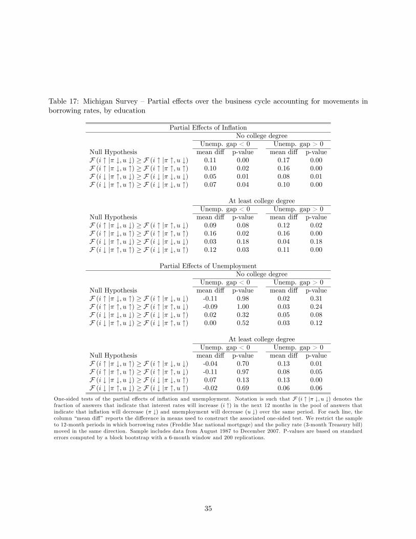
Table 17: Michigan Survey —Partial effects over the business cycle accounting for movements inborrowing rates, by education

Partial Effects of InflationNo college degree

Unemp. gap < 0 Unemp. gap > 0Null Hypothesis mean diff p-value mean diff p-valueF (i ↑ |π ↓, u ↓) ≥ F (i ↑ |π ↑, u ↓) 0.11 0.00 0.17 0.00F (i ↑ |π ↓, u ↑) ≥ F (i ↑ |π ↑, u ↑) 0.10 0.02 0.16 0.00F (i ↓ |π ↑, u ↓) ≥ F (i ↓ |π ↓, u ↓) 0.05 0.01 0.08 0.01F (i ↓ |π ↑, u ↑) ≥ F (i ↓ |π ↓, u ↑) 0.07 0.04 0.10 0.00

At least college degreeUnemp. gap < 0 Unemp. gap > 0


Partial Effects of UnemploymentNo college degree

Unemp. gap < 0 Unemp. gap > 0Null Hypothesis mean diff p-value mean diff p-valueF (i ↑ |π ↓, u ↑) ≥ F (i ↑ |π ↓, u ↓) -0.11 0.98 0.02 0.31F (i ↑ |π ↑, u ↑) ≥ F (i ↑ |π ↑, u ↓) -0.09 1.00 0.03 0.24F (i ↓ |π ↓, u ↓) ≥ F (i ↓ |π ↓, u ↑) 0.02 0.32 0.05 0.08F (i ↓ |π ↑, u ↓) ≥ F (i ↓ |π ↑, u ↑) 0.00 0.52 0.03 0.12

At least college degreeUnemp. gap < 0 Unemp. gap > 0


One-sided tests of the partial effects of inflation and unemployment. Notation is such that F (i ↑ |π ↓, u ↓) denotes thefraction of answers that indicate that interest rates will increase (i ↑) in the next 12 months in the pool of answers thatindicate that inflation will decrease (π ↓) and unemployment will decrease (u ↓) over the same period. For each line, thecolumn “mean diff”reports the difference in means used to construct the associated one-sided test. We restrict the sampleto 12-month periods in which borrowing rates (Freddie Mac national mortgage) and the policy rate (3-month Treasury bill)moved in the same direction. Sample includes data from August 1987 to December 2007. P-values are based on standarderrors computed by a block bootstrap with a 6-month window and 200 replications.

35

Table 18: Michigan Survey —Partial effects by households’income quartiles

Partial Effects of InflationLowest Highest


Partial Effects of UnemploymentLowest Highest

Null Hypothesis mean diff p-value mean diff p-valueF (i ↑ |π ↓, u ↑) ≥ F (i ↑ |π ↓, u ↓) -0.05 0.94 0.07 0.07F (i ↑ |π ↑, u ↑) ≥ F (i ↑ |π ↑, u ↓) -0.05 0.95 0.01 0.47F (i ↓ |π ↓, u ↓) ≥ F (i ↓ |π ↓, u ↑) 0.01 0.34 0.11 0.00F (i ↓ |π ↑, u ↓) ≥ F (i ↓ |π ↑, u ↑) 0.01 0.34 0.03 0.15


Table 19: Michigan Survey —Partial effects over the business cycle, households in the highest incomequartile






36

Table 20: Michigan Survey —Partial effects over the business cycle, households with no collegedegree






Table 21: Michigan Survey —Partial effects over the business cycle, households in the lowest incomequartile




Null Hypothesis mean diff p-value mean diff p-valueF (i ↑ |π ↓, u ↑) ≥ F (i ↑ |π ↓, u ↓) -0.12 1.00 0.00 0.52F (i ↑ |π ↑, u ↑) ≥ F (i ↑ |π ↑, u ↓) -0.13 1.00 0.01 0.37F (i ↓ |π ↓, u ↓) ≥ F (i ↓ |π ↓, u ↑) -0.03 0.83 0.04 0.10F (i ↓ |π ↑, u ↓) ≥ F (i ↓ |π ↑, u ↑) -0.01 0.70 0.03 0.19


37

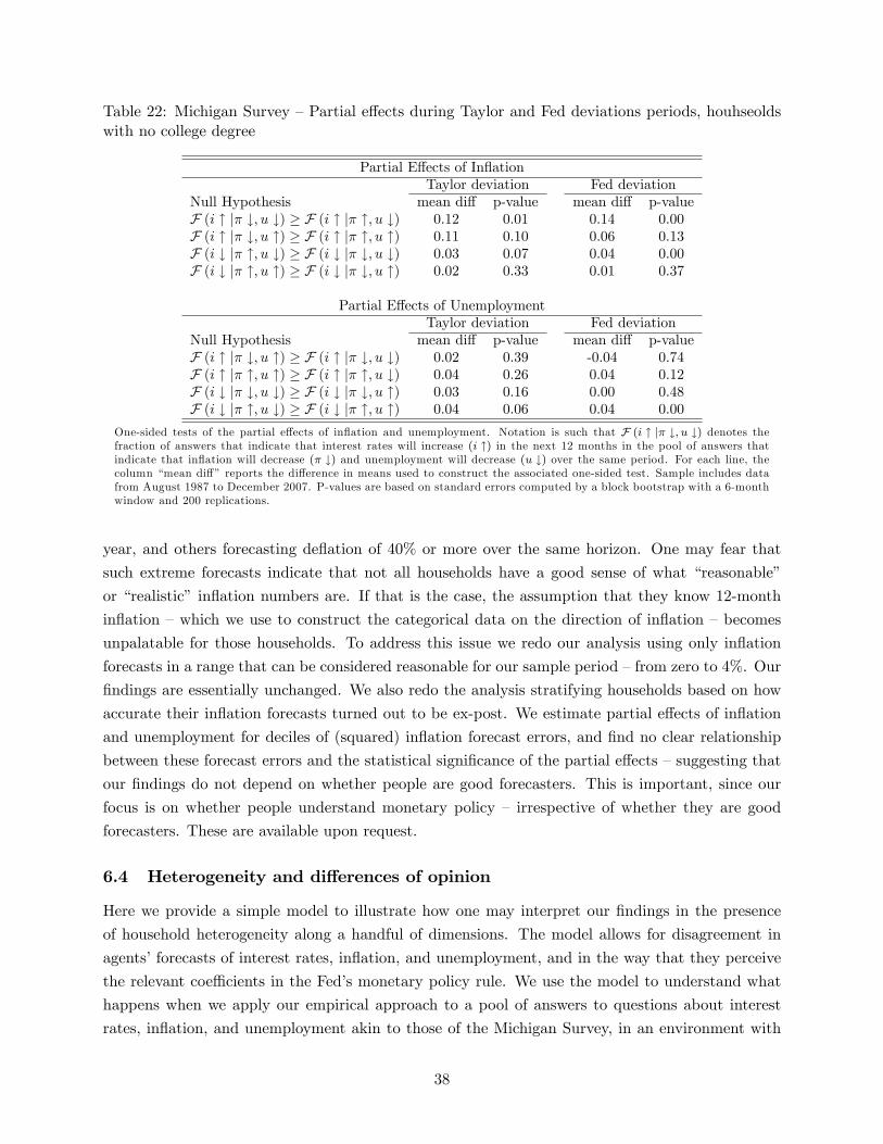
Table 22: Michigan Survey —Partial effects during Taylor and Fed deviations periods, houhseoldswith no college degree

Partial Effects of InflationTaylor deviation Fed deviation


Partial Effects of UnemploymentTaylor deviation Fed deviation

Null Hypothesis mean diff p-value mean diff p-valueF (i ↑ |π ↓, u ↑) ≥ F (i ↑ |π ↓, u ↓) 0.02 0.39 -0.04 0.74F (i ↑ |π ↑, u ↑) ≥ F (i ↑ |π ↑, u ↓) 0.04 0.26 0.04 0.12F (i ↓ |π ↓, u ↓) ≥ F (i ↓ |π ↓, u ↑) 0.03 0.16 0.00 0.48F (i ↓ |π ↑, u ↓) ≥ F (i ↓ |π ↑, u ↑) 0.04 0.06 0.04 0.00


year, and others forecasting deflation of 40% or more over the same horizon. One may fear that

such extreme forecasts indicate that not all households have a good sense of what “reasonable”

or “realistic” inflation numbers are. If that is the case, the assumption that they know 12-month

inflation —which we use to construct the categorical data on the direction of inflation —becomes

unpalatable for those households. To address this issue we redo our analysis using only inflation

forecasts in a range that can be considered reasonable for our sample period —from zero to 4%. Our

findings are essentially unchanged. We also redo the analysis stratifying households based on how

accurate their inflation forecasts turned out to be ex-post. We estimate partial effects of inflation

and unemployment for deciles of (squared) inflation forecast errors, and find no clear relationship

between these forecast errors and the statistical significance of the partial effects —suggesting that

our findings do not depend on whether people are good forecasters. This is important, since our

focus is on whether people understand monetary policy — irrespective of whether they are good

forecasters. These are available upon request.

6.4 Heterogeneity and differences of opinion

Here we provide a simple model to illustrate how one may interpret our findings in the presence

of household heterogeneity along a handful of dimensions. The model allows for disagreement in

agents’forecasts of interest rates, inflation, and unemployment, and in the way that they perceive

the relevant coeffi cients in the Fed’s monetary policy rule. We use the model to understand what

happens when we apply our empirical approach to a pool of answers to questions about interest

rates, inflation, and unemployment akin to those of the Michigan Survey, in an environment with

38

the aforementioned heterogeneity. We find that our approach recovers an average of households’

perceptions of the effects of inflation and unemployment on interest rates.

Our empirical approach provides estimates of the partial effects of inflation and unemployment

by exploiting differences across pools of household answers. How should we think about these

estimates when households hold different views about the relationship between inflation, unemploy-

ment, and interest rates? In this subsection we present a simple framework to interpret the results

that our empirical approach produces in the presence of household heterogeneity.

Our starting point is a population of households that reason about the relationship between

inflation, unemployment, and interest rates according to a simple form of the Taylor rule. We

assume that such a household has in mind a simple rule with two additive components. The

first is a “systematic”component that satisfies the basic principles underlying the Taylor rule and

dictates how, on average, the household’s interest rate forecast for a given date T should be related

to the same household’s forecasts of inflation and unemployment for the same date. We denote

this systematic interest rate forecast by i∗t,T , and assume that it only depends on the household’s

forecasts of unemployment for date T (denoted ut,T ) and of inflation in the 12-month period ending

at date T (denoted πt,T ), according to a simple Taylor-type rule:37

i∗t,T = φππt,T + φuut,T . (10)

The second component of the household’s interest rate forecast for date T is the amount by which

the household believes the interest rate will deviate from the systematic forecast i∗t,T . We introduce

this forecast shock component (denoted −εt,T ) because equation (10) is an imperfect description ofhow the Fed sets its policy rate, and so we want to allow a household that understands the conduct

of monetary policy to make interest rate forecasts that deviate from its systematic component.

We think of εt,T as being drawn by the household when forming its interest rate forecast, from a

distribution with cumulative distribution function Fε (ε), and assume that εt,T is independent of

πt,T , ut,T and of it,t, πt,t, ut,t. This assumption rules out endogeneity problems, and is justified on

the basis of the results of Subsection 4.2 of the paper. Our previous assumption that i∗t,T is the

forecast that the household makes on average implies that εt,T has mean zero.

The variables it,t, πt,t, and ut,t denote, respectively, the household’s perceptions of the policy

rate at time t, of inflation in the 12 months up to and including time t, and of the unemployment

rate at time t, which we assume to coincide with the actual values of these three variables (i.e.,

we assume that they are known to the households when they answer the survey questions at time

t). Because we assume it,t, πt,t, and ut,t to be known at time t, the realization of εt,t also becomes

known at time t.

The actual numerical interest rate forecast of the household is denoted by it,T = i∗t,T − εt,T :

it,T = φππt,T + φuut,T − εt,T . (11)

37For simplicity we abstract from variations in the unemployment rate consistent with full employment and assumea zero inflation target.

39

We do not specify how the household forms inflation and unemployment forecasts and only assume

that they are based on some model that produces a joint distribution of these two forecasts for any

given horizon.38

Recall that with the exception of inflation, the questions in the Michigan Survey that we use

in our analysis pertain to the direction of interest rates and unemployment in the subsequent 12

months. So, to move closer to the analysis that we perform with available data, we need to go from

(11) to a specification in changes instead of levels. To that end, we subtract equation (11) with

T = t from equation (11) itself to arrive at:

∆it,T = φπ∆πt,T + φu∆ut,T − εt,T + εt,t, (12)

where ∆xt,T = xt,T − xt,t for x = i, π, u.

With what we have developed so far, we can ask hypothetical questions such as the following:

Given numerical forecasts of inflation and unemployment that imply a change in 12-month inflation

of ∆π and a change in unemployment of ∆u twelve months from now, what is the probability that

the household will answer that interest rates will go up in the next 12 months? Equation (12)

implies that:

∆it,T ≥ 0⇐⇒ εt,T ≤ φπ∆πt,T + φu∆ut,T + εt,t.

Thus the answer to the hypothetical question would be:

Pr (∆it,T ≥ 0 | Ωt) = Pr (εt,T ≤ φπ∆πt,T + φu∆ut,T + εt,t)

= Fε (φπ∆πt,T + φu∆ut,T + εt,t) ,

where Ωt = ∆πt,T ,∆ut,T , it,t, πt,t, ut,t, φπ, φu. To avoid cluttering the notation we omit the con-ditioning variables in the expressions in the right-hand-side of the expressions above.

We can also ask simple questions of comparative statics, such as how that probability changes

with the household’s inflation and unemployment forecasts:

∂Fε (φπ∆πt,T + φu∆ut,T + εt,t)

∂∆πt,T= F ′ε (φπ∆πt,T + φu∆ut,T + εt,t)φπ ≶ 0, (13)

∂Fε (φπ∆πt,T + φu∆ut,T + εt,t)

∂∆ut,T= F ′ε (φπ∆πt,T + φu∆ut,T + εt,t)φu ≶ 0, (14)

where the signs of the expressions (13) and (14) depend on the signs of φπ and φu, and thus reflect

the basic principles underlying the Taylor rule if φπ > 0 and φu < 0.

The results obtained so far would be useful if we could observe numerical forecasts of households

over time. However, in our sample we do not observe the same household more than once,39 and38Alternative assumptions would also work here. For example, we could assume that the household has in mind

some fully specified model of the economy in which equation (11) holds, and that the household reports the modalforecast from the joint distribution for the three variables implied by the equilibrium of the model. However, it iscrucial that, whatever the forecasts of inflation and unemployment, the forecast for interest rates satisfies (11). Seethe related discussion in Section 6.4.1.

39As mentioned in Subsection 2.1 of the paper, the Michigan Survey does have a small panel dimension, since

40

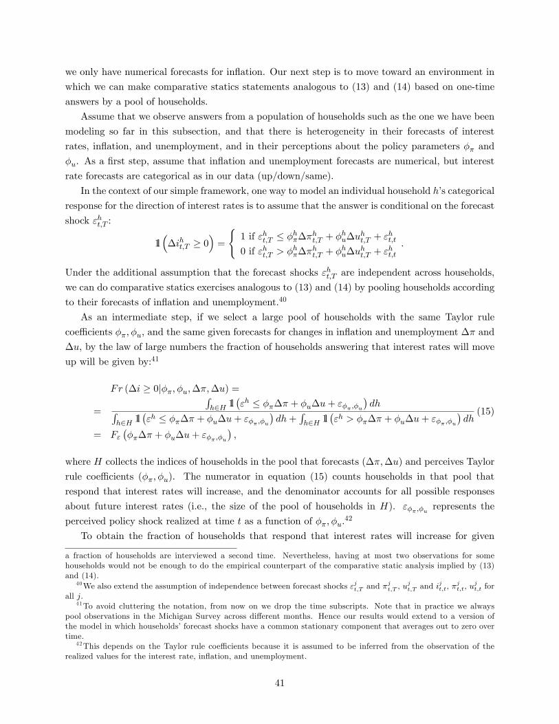
we only have numerical forecasts for inflation. Our next step is to move toward an environment in

which we can make comparative statics statements analogous to (13) and (14) based on one-time

answers by a pool of households.

Assume that we observe answers from a population of households such as the one we have been

modeling so far in this subsection, and that there is heterogeneity in their forecasts of interest

rates, inflation, and unemployment, and in their perceptions about the policy parameters φπ and

φu. As a first step, assume that inflation and unemployment forecasts are numerical, but interest

rate forecasts are categorical as in our data (up/down/same).

In the context of our simple framework, one way to model an individual household h’s categorical

response for the direction of interest rates is to assume that the answer is conditional on the forecast

shock εht,T :

1l(

∆iht,T ≥ 0)

=

1 if εht,T ≤ φhπ∆πht,T + φhu∆uht,T + εht,t0 if εht,T > φhπ∆πht,T + φhu∆uht,T + εht,t

.

Under the additional assumption that the forecast shocks εht,T are independent across households,

we can do comparative statics exercises analogous to (13) and (14) by pooling households according

to their forecasts of inflation and unemployment.40

As an intermediate step, if we select a large pool of households with the same Taylor rule

coeffi cients φπ, φu, and the same given forecasts for changes in inflation and unemployment ∆π and

∆u, by the law of large numbers the fraction of households answering that interest rates will move

up will be given by:41

Fr (∆i ≥ 0|φπ, φu,∆π,∆u) =

=

∫h∈H 1l

(εh ≤ φπ∆π + φu∆u+ εφπ ,φu

)dh∫

h∈H 1l(εh ≤ φπ∆π + φu∆u+ εφπ ,φu

)dh+

∫h∈H 1l

(εh > φπ∆π + φu∆u+ εφπ ,φu

)dh(15)

= Fε(φπ∆π + φu∆u+ εφπ ,φu

),

where H collects the indices of households in the pool that forecasts (∆π,∆u) and perceives Taylor

rule coeffi cients (φπ, φu). The numerator in equation (15) counts households in that pool that

respond that interest rates will increase, and the denominator accounts for all possible responses

about future interest rates (i.e., the size of the pool of households in H). εφπ ,φu represents the

perceived policy shock realized at time t as a function of φπ, φu.42

To obtain the fraction of households that respond that interest rates will increase for given

a fraction of households are interviewed a second time. Nevertheless, having at most two observations for somehouseholds would not be enough to do the empirical counterpart of the comparative static analysis implied by (13)and (14).

40We also extend the assumption of independence between forecast shocks εjt,T and πjt,T , u

jt,T and i

jt,t, π

jt,t, u

jt,t for

all j.41To avoid cluttering the notation, from now on we drop the time subscripts. Note that in practice we always

pool observations in the Michigan Survey across different months. Hence our results would extend to a version ofthe model in which households’forecast shocks have a common stationary component that averages out to zero overtime.

42This depends on the Taylor rule coeffi cients because it is assumed to be inferred from the observation of therealized values for the interest rate, inflation, and unemployment.

41

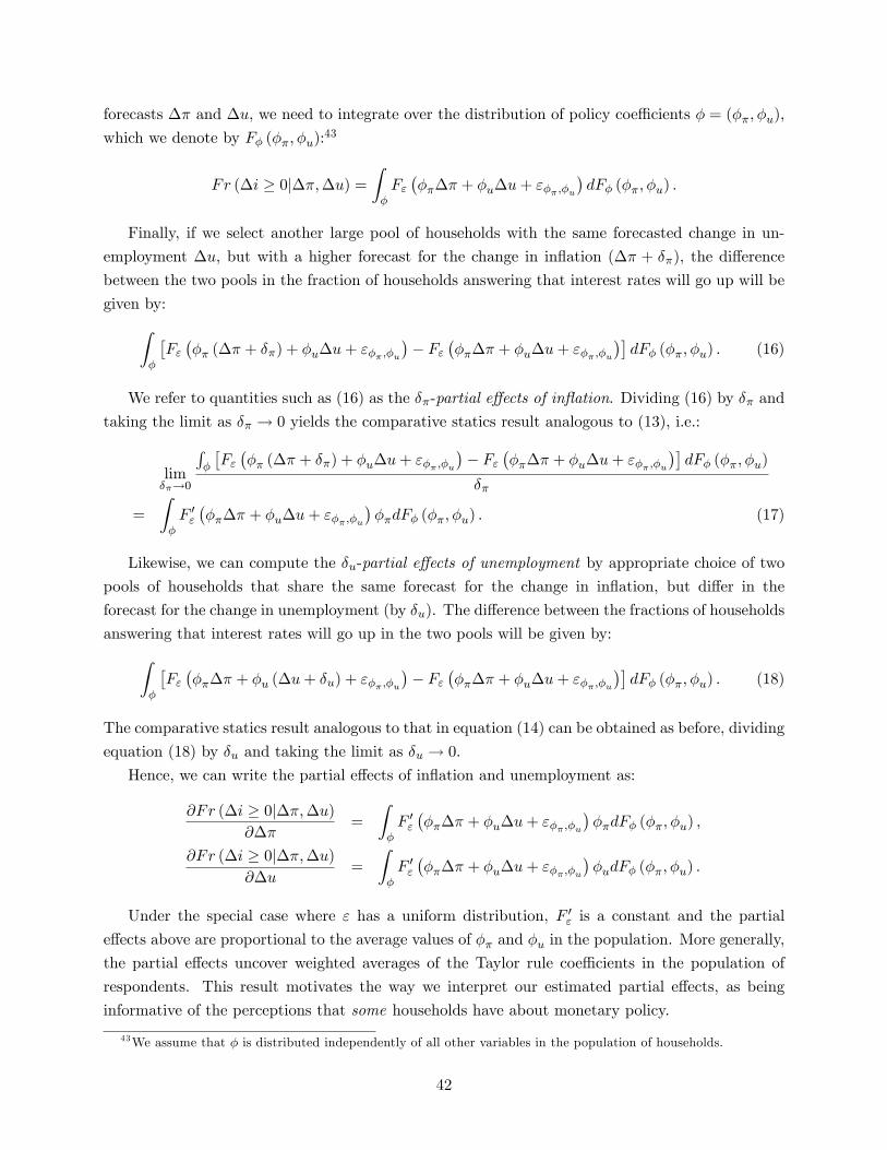
forecasts ∆π and ∆u, we need to integrate over the distribution of policy coeffi cients φ = (φπ, φu),

which we denote by Fφ (φπ, φu):43

Fr (∆i ≥ 0|∆π,∆u) =

∫φFε(φπ∆π + φu∆u+ εφπ ,φu

)dFφ (φπ, φu) .

Finally, if we select another large pool of households with the same forecasted change in un-

employment ∆u, but with a higher forecast for the change in inflation (∆π + δπ), the difference

between the two pools in the fraction of households answering that interest rates will go up will be

given by:∫φ

[Fε(φπ (∆π + δπ) + φu∆u+ εφπ ,φu

)− Fε

(φπ∆π + φu∆u+ εφπ ,φu

)]dFφ (φπ, φu) . (16)

We refer to quantities such as (16) as the δπ-partial effects of inflation. Dividing (16) by δπ and

taking the limit as δπ → 0 yields the comparative statics result analogous to (13), i.e.:

limδπ→0

∫φ

[Fε(φπ (∆π + δπ) + φu∆u+ εφπ ,φu

)− Fε


)]dFφ (φπ, φu)

δπ

=

∫φF ′ε(φπ∆π + φu∆u+ εφπ ,φu

)φπdFφ (φπ, φu) . (17)

Likewise, we can compute the δu-partial effects of unemployment by appropriate choice of two

pools of households that share the same forecast for the change in inflation, but differ in the

forecast for the change in unemployment (by δu). The difference between the fractions of households

answering that interest rates will go up in the two pools will be given by:∫φ

[Fε(φπ∆π + φu (∆u+ δu) + εφπ ,φu

)− Fε


)]dFφ (φπ, φu) . (18)

The comparative statics result analogous to that in equation (14) can be obtained as before, dividing

equation (18) by δu and taking the limit as δu → 0.

Hence, we can write the partial effects of inflation and unemployment as:

∂Fr (∆i ≥ 0|∆π,∆u)

∂∆π=


)φπdFφ (φπ, φu) ,

∂Fr (∆i ≥ 0|∆π,∆u)

∂∆u=


)φudFφ (φπ, φu) .

Under the special case where ε has a uniform distribution, F ′ε is a constant and the partial

effects above are proportional to the average values of φπ and φu in the population. More generally,

the partial effects uncover weighted averages of the Taylor rule coeffi cients in the population of

respondents. This result motivates the way we interpret our estimated partial effects, as being

informative of the perceptions that some households have about monetary policy.

43We assume that φ is distributed independently of all other variables in the population of households.

42

Note that we have assumed that the forecasts for inflation and unemployment are numerical,

whereas in our baseline results we use categorical answers for the questions about the future path

of these two variables. Conditioning on the direction of the forecasted change instead of on the

numerical forecasts can make a difference for some of the results derived in the model. For instance,

it may cause answers that were otherwise well defined to depend on the distribution of Taylor rule

coeffi cients perceived by households in the pool of respondents.

Since we only have categorical responses regarding the future path of unemployment, our em-

pirical approach for estimating the partial effects of inflation can only be imperfectly justified on

the basis of the framework developed in this subsection. We could try to condition on households’

answers to other questions in the Michigan Survey, in the hope that doing so would make it more

likely that the selected pool of respondents had in mind the same (unobserved) forecasted change

in unemployment when answering the survey question. However, this would reduce the number of

observations in each conditional distribution, and we would still have to live with the possibility of

unobserved heterogeneity in those numerical forecasts.

Fortunately, as described in Subsection 2.1 of the paper, the Michigan Survey does ask house-

holds about their numerical forecasts for inflation. Hence, we can calculate the partial effects of

unemployment using those numerical inflation forecasts, instead of only the direction for the change

in inflation. In particular, we estimate the partial effects of unemployment by deciles of inflation

forecasts.

To that end, we divide the expected change in inflation into ten deciles, and estimate the partial

effects of unemployment for each decile. While the results vary across deciles, Table 23 shows that,

in general, they confirm our baseline results. When conditioning on demographics, we find once

again that answers by households that have at least a college degree and households in the highest

income quartile are more in line with the relationship between unemployment and interest rates

implied by the basic principles underlying the Taylor rule than answers by households with less

education and by households in the lowest income quartile. For brevity we do not include the

corresponding tables, which are available upon request.

6.4.1 An important identifying assumption

Our simple framework helps us think about how a household that reasons in accordance with the

basic principles underlying the Taylor rule might answer categorical questions about interest rates,

such as the one in the Michigan Survey. It also shows how, within the framework, those principles

can be recovered from answers by a pool of such households that differ in their forecasts of inflation

and unemployment, and also possibly in their perceived Taylor rule coeffi cients.

It is natural to ask whether the lessons we can draw from our analysis are robust to alternative

assumptions, even strictly within our simple framework. An important identifying assumption that

we make is that households’answers about the direction of interest rates are indeed conditional

on their responses about inflation and unemployment (which we assume come from an unspecified

model that produces a joint forecast for the path of these two variables). If that is not the case and

43

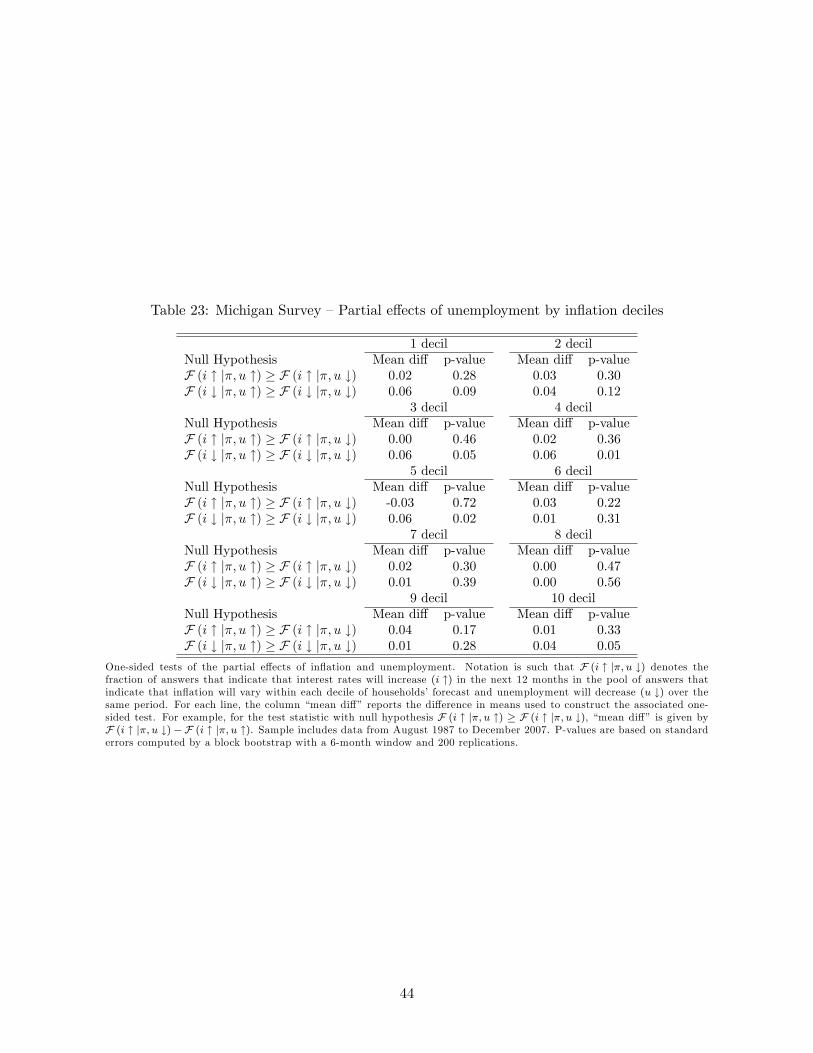
Table 23: Michigan Survey —Partial effects of unemployment by inflation deciles

1 decil 2 decilNull Hypothesis Mean diff p-value Mean diff p-valueF (i ↑ |π, u ↑) ≥ F (i ↑ |π, u ↓) 0.02 0.28 0.03 0.30F (i ↓ |π, u ↑) ≥ F (i ↓ |π, u ↓) 0.06 0.09 0.04 0.12


5 decil 6 decilNull Hypothesis Mean diff p-value Mean diff p-valueF (i ↑ |π, u ↑) ≥ F (i ↑ |π, u ↓) -0.03 0.72 0.03 0.22F (i ↓ |π, u ↑) ≥ F (i ↓ |π, u ↓) 0.06 0.02 0.01 0.31



One-sided tests of the partial effects of inflation and unemployment. Notation is such that F (i ↑ |π, u ↓) denotes thefraction of answers that indicate that interest rates will increase (i ↑) in the next 12 months in the pool of answers thatindicate that inflation will vary within each decile of households’ forecast and unemployment will decrease (u ↓) over thesame period. For each line, the column “mean diff” reports the difference in means used to construct the associated one-sided test. For example, for the test statistic with null hypothesis F (i ↑ |π, u ↑) ≥ F (i ↑ |π, u ↓), “mean diff” is given byF (i ↑ |π, u ↓)−F (i ↑ |π, u ↑). Sample includes data from August 1987 to December 2007. P-values are based on standarderrors computed by a block bootstrap with a 6-month window and 200 replications.

44

households do not answer conditionally, one can build examples where respondents’thoughts are

in line with the Taylor rule but their answers are not.44

For example, consider a household that forms interest rate expectations according to the Taylor

rule, but answers the survey questionnaire by providing the modal forecast from the marginal

distributions of the three variables. For simplicity, assume that the joint probability distribution

for inflation and unemployment is such that:

Pr(π ↑, u ↓) = 0.5

Pr(π ↓, u ↑) = 0.5

Pr(π ↑, u ↑) = 0.0

Pr(π ↓, u ↓) = 0.0

=⇒ Pr (π ↑) = Pr (π ↓) = 0.5

Pr (u ↑) = Pr (u ↓) = 0.5.

Since the household reasons according to the Taylor rule, this implies that Pr(i ↑) = Pr(i ↓) = 0.5.

If the household answers the survey questions by first making a joint forecast for inflation

and unemployment, and then computing the implied interest rate movement (conditional on that

forecast), then Pr(i ↑ | π ↑, u ↓) = 1 and Pr(i ↓ | π ↓, u ↑) = 1, which is consistent with the

basic principles underlying the Taylor rule. Likewise, if the household’s answers correspond to a

point in the joint distribution of interest rates, inflation, and unemployment, then if interest rate

expectations accord with the Taylor rule, the answers will reveal so. In contrast, if the household

answers the questionnaire using the unconditional (marginal) distributions for the three variables

separately, the resulting answers could be π ↑, u ↓ and i ↓, which would clearly violate the Taylorrule.

The above example illustrates a more general problem that arises when making inference based

on survey data. It has to do precisely with the interpretation of what the responses pertain to. For

example, Manski (2005) and Manski and Tamer (2002) raise issues related to those that we face

here, in the context of empirical analyses that rely on categorical and interval survey data. Hence,

the assumption that households’ answers about interest rates are conditional on their answers

about inflation and unemployment can be seen as an identifying assumption without which we

could not proceed. In future research, it would be interesting to test this assumption by explicitly

asking households about their interest rate forecasts conditional on their forecasts for inflation and

unemployment.

6.5 OLS estimates

A natural alternative to our empirical approach would be to use standard regression methods. One

advantage of this alternative is that it imposes a parametric structure that uses information from

all the empirical distributions of household responses to estimate the inflation and unemployment

coeffi cients of interest. In contrast, our nonparametric approach estimates each possible partial

effect using only data from the two conditional distributions that define it. This reduces the number

of observations underlying the estimates.

44We thank John Geweke for suggesting this route to highlighting the importance of our conditionality assumption.

45

On the positive side, precisely because our approach does not impose any structure on the data,

it allows for partial effects that contradict each other. For example, we may estimate partial effects

of inflation that are consistent with the basic principles underlying the Taylor rule when it comes to

interest rate decreases, but which otherwise do not conform with those principles. In other words,

the approach allows for asymmetries in perceptions about monetary policy that a parsimonious

regression specification would rule out.

Of course one could resort to regressions that allow for as many asymmetries as in our empirical

approach based on partial effects. However, that flexibility would require increasing the number of

parameters to be estimated one-to-one with the degrees of freedom that one wished to allow for in

the estimation. In the limit, if the goal is to allow for as much flexibility as in our approach, one

would face essentially the same problem in terms of sample sizes.

In this section we present results using alternative methods, favoring a somewhat more parsimo-

nious regression specification. The bottom line is that our substantive conclusions are essentially

unchanged, with a few exceptions that we flash out when relevant.

Given the nature of the Michigan Survey data, a natural alternative to our empirical approach

would be to use probit models. These models are, however, computationally intensive, especially in

face of our block-bootstrap procedure. Since we are only interested in the signs of the coeffi cients,

we opt instead to use standard ordinary least squares (OLS) regressions, which allow for the same

statistical inference and are computationally less demanding.

The following set of tables report results based on OLS regressions using our categorical variables

for interest rates, inflation, and unemployment. Specifically, let ∆ih,t ∈ down, unchanged, updenote the response of household h to the question about the direction of expected twelve-month

changes in interest rates, when interviewed at time t. We assign values −1, 0, 1 to the possibleanswers down, unchanged, up. Likewise, let ∆πh,t and ∆uh,t denote her answers to the questions

about inflation and unemployment, respectively. We first estimate OLS regressions, pooling all

households:

∆i = α+ βπ∆π + βu∆u+ ε, (19)

where

∆i = [∆i1,t,∆i2,t,∆i3,t, ...,∆in,t+1,∆in+1,t+1,∆in+2,t+1, ...]′ ,

∆π = [∆π1,t,∆π2,t,∆π3,t, ...,∆πn,t+1,∆πn+1,t+1,∆πn+2,t+1, ...]′ ,

∆u = [∆u1,t,∆u2,t,∆u3,t, ...,∆un,t+1,∆un+1,t+1,∆un+2,t+1, ...]′ ,

and ε is an error term. We then estimate additional regressions in which we further partition the

data according to households’demographic characteristics. Finally, we estimate separate regressions

for periods with positive and negative unemployment gap, in analogy with the results reported in

Section 3.2 of the paper.

As explained in the paper, we compare our findings with results obtained using actual interest-

rate, inflation, and unemployment data. To that end, we use monthly data on the 3-month Treasury

46

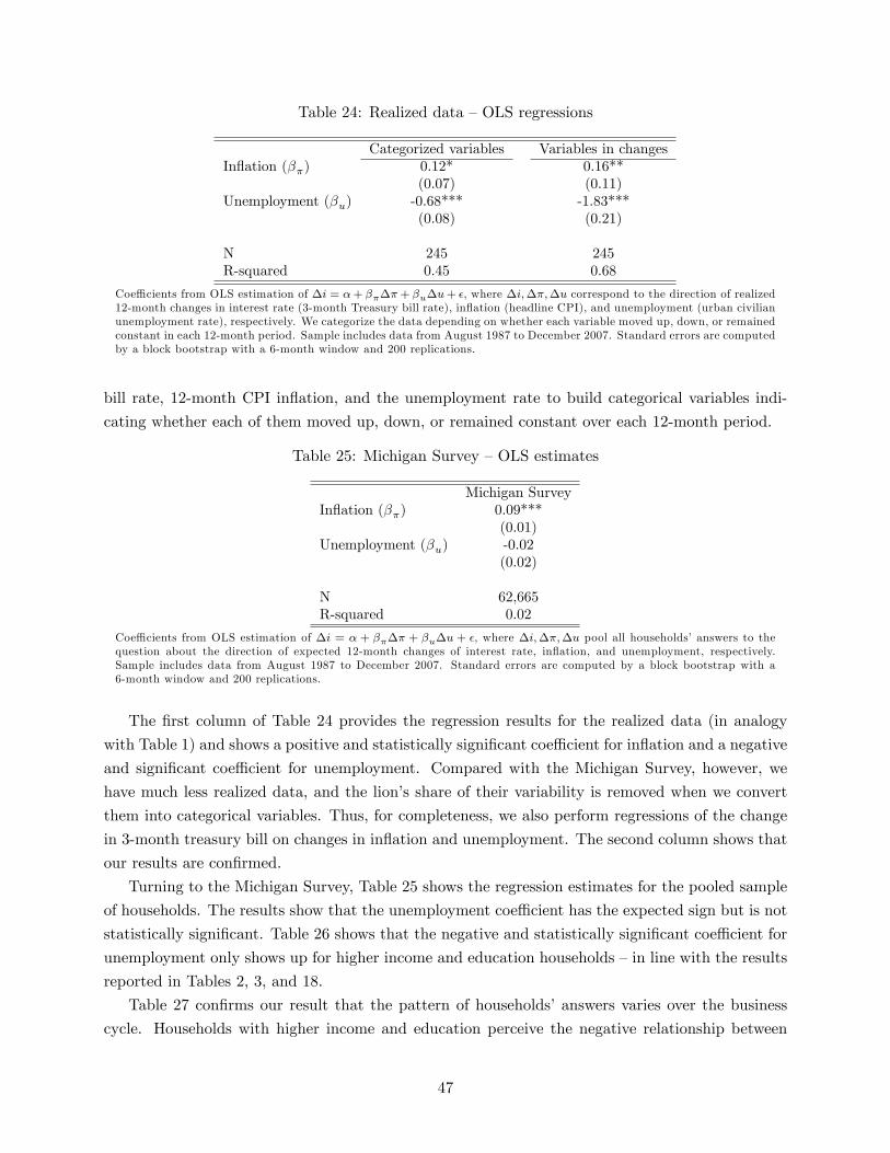
Table 24: Realized data —OLS regressions

Categorized variables Variables in changesInflation (βπ) 0.12* 0.16**

(0.07) (0.11)Unemployment (βu) -0.68*** -1.83***

(0.08) (0.21)

N 245 245R-squared 0.45 0.68

Coeffi cients from OLS estimation of ∆i = α+ βπ∆π+ βu∆u+ ε, where ∆i,∆π,∆u correspond to the direction of realized12-month changes in interest rate (3-month Treasury bill rate), inflation (headline CPI), and unemployment (urban civilianunemployment rate), respectively. We categorize the data depending on whether each variable moved up, down, or remainedconstant in each 12-month period. Sample includes data from August 1987 to December 2007. Standard errors are computedby a block bootstrap with a 6-month window and 200 replications.

bill rate, 12-month CPI inflation, and the unemployment rate to build categorical variables indi-

cating whether each of them moved up, down, or remained constant over each 12-month period.

Table 25: Michigan Survey —OLS estimates

Michigan SurveyInflation (βπ) 0.09***

(0.01)Unemployment (βu) -0.02

(0.02)

N 62,665R-squared 0.02

Coeffi cients from OLS estimation of ∆i = α + βπ∆π + βu∆u + ε, where ∆i,∆π,∆u pool all households’answers to thequestion about the direction of expected 12-month changes of interest rate, inflation, and unemployment, respectively.Sample includes data from August 1987 to December 2007. Standard errors are computed by a block bootstrap with a6-month window and 200 replications.

The first column of Table 24 provides the regression results for the realized data (in analogy

with Table 1) and shows a positive and statistically significant coeffi cient for inflation and a negative

and significant coeffi cient for unemployment. Compared with the Michigan Survey, however, we

have much less realized data, and the lion’s share of their variability is removed when we convert

them into categorical variables. Thus, for completeness, we also perform regressions of the change

in 3-month treasury bill on changes in inflation and unemployment. The second column shows that

our results are confirmed.

Turning to the Michigan Survey, Table 25 shows the regression estimates for the pooled sample

of households. The results show that the unemployment coeffi cient has the expected sign but is not

statistically significant. Table 26 shows that the negative and statistically significant coeffi cient for

unemployment only shows up for higher income and education households —in line with the results

reported in Tables 2, 3, and 18.

Table 27 confirms our result that the pattern of households’answers varies over the business

cycle. Households with higher income and education perceive the negative relationship between

47

Table 26: Michigan Survey —OLS estimation by income and education

Households’income quartiles Respondents’educationLowest Highest No college At least college

Inflation (βπ) 0.10*** 0.09*** 0.09*** 0.09***(0.01) (0.01) (0.01) (0.01)

Unemployment (βu) 0.01 -0.05** 0 -0.05**(0.02) (0.02) (0.01) (0.02)

N 10,136 17,779 39,149 22,877R-squared 0.02 0.02 0.02 0.02


Table 27: Michigan Survey —OLS estimation over the business cycle, by income and education

Households’incomeUnemp. gap < 0 Unemp. gap > 0

Lowest Highest Lowest HighestInflation (βπ) 0.09*** 0.08*** 0.11*** 0.1***

(0.01) (0.02) (0.01) (0.01)Unemployment (βu) 0.07** 0.02 -0.03 -0.10***

(0.03) (0.03) (0.02) (0.02)

N 4,949 8,481 5,187 9,318R-squared 0.02 0.01 0.02 0.03

Respondents’educationUnemp. gap < 0 Unemp. gap > 0

No college At least college No college At least collegeInflation (βπ) 0.07*** 0.09*** 0.11*** 0.10***

(0.01) (0.02) (0.01) (0.01)Unemployment (βu) 0.05** 0.03 -0.04*** -0.10***

(0.02) (0.03) (0.02) (0.02)

N 21,655 10,945 22,592 11,932R-squared 0.01 0.01 0.02 0.03


48

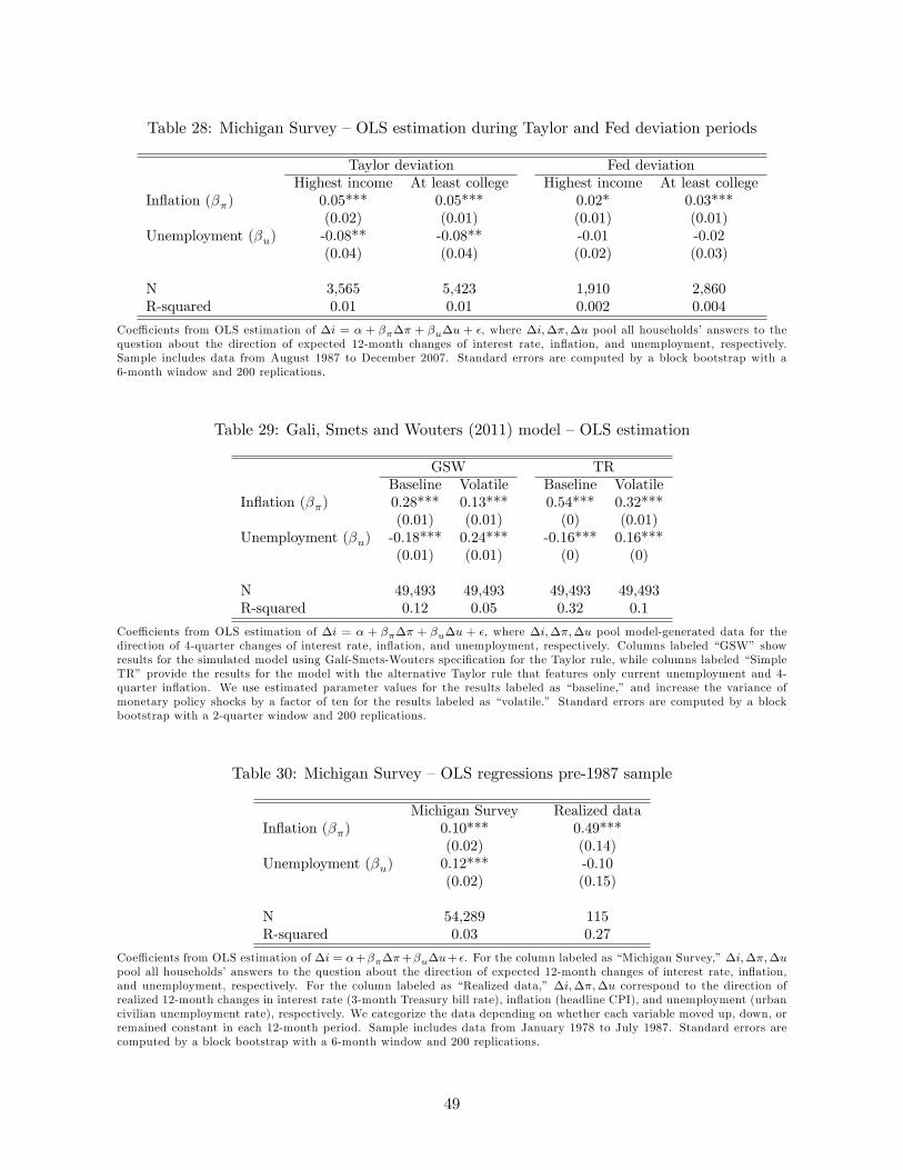
Table 28: Michigan Survey —OLS estimation during Taylor and Fed deviation periods

Taylor deviation Fed deviationHighest income At least college Highest income At least college

Inflation (βπ) 0.05*** 0.05*** 0.02* 0.03***(0.02) (0.01) (0.01) (0.01)

Unemployment (βu) -0.08** -0.08** -0.01 -0.02(0.04) (0.04) (0.02) (0.03)

N 3,565 5,423 1,910 2,860R-squared 0.01 0.01 0.002 0.004


Table 29: Gali, Smets and Wouters (2011) model —OLS estimation

GSW TRBaseline Volatile Baseline Volatile

Inflation (βπ) 0.28*** 0.13*** 0.54*** 0.32***(0.01) (0.01) (0) (0.01)

Unemployment (βu) -0.18*** 0.24*** -0.16*** 0.16***(0.01) (0.01) (0) (0)

N 49,493 49,493 49,493 49,493R-squared 0.12 0.05 0.32 0.1

Coeffi cients from OLS estimation of ∆i = α + βπ∆π + βu∆u + ε, where ∆i,∆π,∆u pool model-generated data for thedirection of 4-quarter changes of interest rate, inflation, and unemployment, respectively. Columns labeled “GSW” showresults for the simulated model using Galí-Smets-Wouters specification for the Taylor rule, while columns labeled “SimpleTR” provide the results for the model with the alternative Taylor rule that features only current unemployment and 4-quarter inflation. We use estimated parameter values for the results labeled as “baseline,” and increase the variance ofmonetary policy shocks by a factor of ten for the results labeled as “volatile.” Standard errors are computed by a blockbootstrap with a 2-quarter window and 200 replications.

Table 30: Michigan Survey —OLS regressions pre-1987 sample

Michigan Survey Realized dataInflation (βπ) 0.10*** 0.49***

(0.02) (0.14)Unemployment (βu) 0.12*** -0.10

(0.02) (0.15)

N 54,289 115R-squared 0.03 0.27

Coeffi cients from OLS estimation of ∆i = α+βπ∆π+βu∆u+ ε. For the column labeled as “Michigan Survey,”∆i,∆π,∆upool all households’answers to the question about the direction of expected 12-month changes of interest rate, inflation,and unemployment, respectively. For the column labeled as “Realized data,” ∆i,∆π,∆u correspond to the direction ofrealized 12-month changes in interest rate (3-month Treasury bill rate), inflation (headline CPI), and unemployment (urbancivilian unemployment rate), respectively. We categorize the data depending on whether each variable moved up, down, orremained constant in each 12-month period. Sample includes data from January 1978 to July 1987. Standard errors arecomputed by a block bootstrap with a 6-month window and 200 replications.

49

interest rates and unemployment when the unemployment gap is positive.

We also report OLS results for the Taylor deviation and Fed deviation periods —Table 28. They

are more muted than those for the partial effects. However, it is still the case that the coeffi cient

on inflation for higher income households becomes statistically insignificant (at 5%) during the

Fed deviation period. Moreover, in all cases the size of the inflation coeffi cient drops substantially

when compared to the results reported in Table 26, indicating that the marginal effect of inflation

diminished during those periods.

In our discussion about the possible effects of endogeneity and reverse causality we make use

of model-generated data to compare the partial effects of inflation and unemployment using in the

estimated model versus those obtained in the presence of counterfactually large monetary shocks.

Table 29 provides the OLS regression results. It shows that our inference based on the signs of

coeffi cients remains valid as long as monetary shocks are not too large. Finally, Table 30 shows the

OLS regression results for both the Michigan Survey and the realized data in the pre-1987 sample

period. In analogy with the results reported in Table 7, while the coeffi cient on inflation is similar

to the one estimated in the post-1987 sample, the coeffi cient on unemployment in the pre-1987

sample is either positive (Michigan Survey) or statistically insignificant (realized data).

References

[1] Manski, C. and E. Tamer (2002), “Inference on Regressions with Interval Data on a Regressor

or Outcome,”Econometrica 70: 519-546.

50

Documents

D o People Understand Monetary Policy?reap.org.br/wp-content/uploads/2014/04/041-Do... · Do People Understand Monetary Policy? Carlos Carvalho PUC-Rio and Kyros Investimentos Fernanda