Embed Size (px)
Citation preview

Revista da Associação Portuguesa de Análise Experimental de Tensões ISSN 1646-7078
Mecânica Experimental, 2016, Vol 26, Pgs 85-95 85
DEVELOPMENT OF A SIMPLIFIED MODEL FOR JOINTS IN STEEL
STRUCTURES
DESENVOLVIMENTO DE UM MODELO SIMPLIFICADO PARA
JUNTAS VIGA-COLUNA EM ESTRUTURAS DE AÇO
F. Gentili1, R. Costa2, L. Simões da Silva1
1Departamento de Engenharia Civil, ISISE, Universidade de Coimbra 2Departamento de Engenharia Civil, Universidade de Coimbra
ABSTRACT
The global behaviour of a framed structure is strongly influenced by the behaviour of the beam-to-column joints. The component method coded in Eurocode 3 allows to characterize the moment-rotation curve of semi-rigid beam-column joints. However, the rigorous application of this method requires a distinction to be made between separate sources of deformability of joints: those in the connection and those in the column web panel. This paper deals with the formulation of a simplified mechanical model composed of extensional springs and rigid links able to cover beam-to-column joints with different beam depths. These models may be used for the interpretation of experimental test and for the formulation of a beam-to-column joint finite element that accurately accounts for its behaviour in global frame analysis.
RESUMO
O comportamento global de uma estrutura porticada é fortemente influenciado pelo comportamento das juntas viga-coluna. O método das componentes codificado no Eurocódigo 3 permite caracterizar as curvas momento-rotação das juntas vigas-colunas semi-rígidas. No entanto, a aplicação rigorosa deste método requer que seja feita uma distinção entre as diferentes fontes de deformação das juntas: as da ligação e as da alma do pilar. Este artigo aborda a formulação de um modelo mecânico simplificado composto por molas lineares e elementos rígidos capaz de lidar com juntas viga-coluna com vigas de diferentes alturas de secção transversal. Estes modelos podem ser usados para interpretar resultados experimentais e para a formulação de um elemento finito para juntas viga-coluna que permita ter em consideração o seu comportamento na análise global de uma estrutura porticada.
1. INTRODUCTION
The appropriate modelling of beam-to-
column joints in the design of steel
structures is essential not only for the
accurate simulation of the overall structural
behaviour but also in order to achieve
economic and sustainable solutions.
Accordingly, in the last decades an
enormous effort was put on developing
accurate and easy-to-use analysis and design
procedures for beam-to-column joints,
leading to the so called component method,
already coded in EN 1993-1-8 (CEN 2005).
According to the component method, the
joints are decomposed in several parts, called
components that represent a specific part of a

F. Gentili, R. Costa, L. Simões da Silva
86
joint that, dependent on the type of loading,
make an identified contribution to one or more
of its structural properties (Simões da Silva et
al, 2002). The constitutive relations of the
components and the way they are assembled
determine the joint behaviour. The relation
between the components and the joint’s
mechanical properties is determined through
equilibrium and compatibility relations.
Several approaches, with different level
of complexity, can be considered for the
modelling of beam-to-column joints in the
framework of the component method. The
traditional approach for global analysis of
steel structures makes use of the component
method to compute moment rotation
relations for each joint and assigns these
relations to rotational springs attached to
the beams ends on both sides (double-side
joint configuration) or just on one side
(single-side joint configuration) of the
column centreline. This approach was
followed since the early stages of the
component method because it allowed the
global analysis of structures making use of
ordinary Finite Element based programs
taking into account the actual behaviour of
beam-to-column joints without requiring
new elements neither changes to the
software code. Alternatively, a refined
approach was also possible, whereby the
joint components are explicitly and
individually accounted for in the model.
However, this approach is very time
consuming and cumbersome, presents
convergence and calibration difficulties, so
that it is usually not considered in design
offices and its application has been
restricted to research purposes.
The need to consider the actual
behaviour of beam-to-column joints in
structural analysis is clear and the
component method is recognized as an
effective procedure to account for it. The
continuous developments in structural
analysis and the increased capacity of
personal computers allow for more robust
and rigorous implementations without
increased burdens on the user.
In the field of beam-to-column joint
modelling, this requirement will be
accomplished in a near future through the
formulation and implementation of 2D and
3D joint macro-elements developed in the
framework of component method in
structural analysis software packages. These
macro-elements will be materialized through
new structural elements suitable for global
analysis of structures and will allow a refined
modelling of joints effortlessly.
In this paper, the main reasons for the
development of macro-component models are
explained and a short state-of-the-art related to
joint macro-elements is presented. Secondly,
two macro-elements mechanical models
suitable for symmetric and asymmetric internal
steel beam-to-column joints are presented, their
modelling in a general purpose nonlinear finite
element program – Abaqus FEA (Simulia
2014) – is explained and the validation
procedure adopted to assess the results is
shown. Finally these models are inserted in a
2D frame in order to highlight its practical
application and relevance.
The models presented are the first step in
an ongoing research project (3DJOINTS) to
validate a new finite element macro-element
already being implemented in OpenSees
(McKenna et al. 2000).
2. THE NEED FOR BEAM-TO-COLUMN
JOINT MACRO-ELEMENTS
Beam-to-column joint modelling making
use of rotational springs attached to the ends
of the beams is an effective procedure for the
simulation of joints. However this procedure
also encompasses some disadvantages.
The first drawback that can be pointed out
is their local kinematic behaviour. Following
the analysis made by Charney and Marshal
(2006), Fig. 1 shows the deflection shapes of
two sub-frames with a double sided joint
configuration where only the shear panel
deformation is accounted for. Fig. 1(a) shows
the kinematics of a Krawinkler type model
(Krawinkler 1978) and Fig. 1(b) shows the
rotational springs attached to beams ends
joint model. From Fig. 1 it is clear that: (i) the
Krawinkler type model provides a better
representation of the actual behaviour of the
joint; and (ii) the local kinematic behaviour
Development of a simplified model for joints in steel structures
87
of both models is different, mainly because
there are no offsets between the beams and
columns centrelines in Fig. 1(b).
The joint modelling making use of
rotational springs attached to beams ends is
also cumbersome whenever it is needed to
account for the interaction between several
types of internal forces transmitted to the
beam-to-column joint by one or more than
one adjacent element, e.g. when there is the
need to couple the effect of the bending
moment and the axial force in the
connections (nonlinear analysis) or when
the shear behaviour of the column web
panel it to be accounted for accurately.
Fig. 1 – Kinematics of joint models: (a) Krawinkler
type model, (b) rotational springs attached to beams
ends joint model.
The latter case, i.e. the shear behaviour of
the column web panel, is of paramount
importance and it should be carefully
considered. In order to account for the
interaction of the internal forces transmitted
to the column shear panel by the beams and
columns connected to the beam-to-column
joint, EN 1993-1-8 (CEN 2005) and EN
1994-1-1 (CEN 2004) define, in a simplified
way (Simões da Silva et al, 2010) an
interaction parameter called the factor that
accounts for the moments transmitted to the
beam-to-column joint by beams. However,
Bayo et al. (2006) showed that the factor
procedure (i) does not account for the
beneficial effect of the columns shear force
for the shear panel behaviour, (ii) requires an
iterative analysis, even if a only a linear
analysis is wished, (iii) may lead to
substantial errors in the internal forces and
(iv) may preclude the convergence of the
iterative process for elastic-plastic analysis.
On the other hand, the factor procedure
cannot deal with beam-to-column joints with
beams with unequal depth because, in these
cases, there is the need to consider two columns
shear panels with different levels of shear
(Jordão et al. 2013).
Finally, it also should be noted that although
the bending deformation mode of steel joints is
usually the most important deformation mode
for the standard static loading conditions, in
certain situations, e.g. fire and seismic loading,
several modes become relevant and should be
accounted for. Besides, robustness
requirements also demand a minimum level of
resistance for any arbitrary loading (Simões da
Silva 2008). A joint macro-element seems to be
the most effective procedure to account for
several deformation modes and for the
behaviour of the beam-to-column joints under
arbitrary loading.
3. STATE OF THE ART
The modelling of beam-to-column joints
through macro-elements in reinforced concrete
(RC) structures, instead of rotational springs
attached to beams ends, has received recently
attention from researchers. There are two main
reasons to choose this strategy in reinforced
concrete frames analysis:
(i) the relative size of the joint region when
compared with the length of beams and
column is much higher in reinforced
concrete frames than in steel frames;
accordingly, a joint model which does
not account for the actual joint size, e.g.
rotational springs attached to the beams
ends near the intersection of beams and
columns centrelines, would be subjected
to internal forces very different from the
ones at the joint periphery (Costa 2013);
(ii) under seismic loads, the joint shear
behaviour is one of the main sources of
energy dissipation and accordingly
should be carefully simulated.
Consequently, some models have been
developed, mainly in the US. Two of most
well know models, already implemented in
OpenSees, are the model developed by
Lowes and Altoontash (2003), later updated
by Mitra and Lowes (2007), and the model
offsets
(a) (b)

F. Gentili, R. Costa, L. Simões da Silva
88
developed by Altoontash (2004). Recently,
Costa (2013) presented a model that aimed
to improve the modelling of the shear
behaviour in the joint panel.
Lowes and Altoontash (2003) proposed
a model comprising: (i) a frame made of
four rigid bi-articulated elements arranged
along the periphery of the beam-to-column
joint; (ii) a panel inside the frame (a plane
stress shear panel); and (iii) interfaces
between the beam-to-column joint and each
of the adjacent beams and columns
modelled by three linear springs (Fig. 2)
placed between each side of the frame and
a rigid element parallel to it. Two of the
springs of each interface are parallel to the
beam/columns centrelines and are intended
to model the anchorage of the longitudinal
rebars of beams and columns inside the
beam-to-column joint. The third spring of
the interface is orthogonal to the
beam/column centreline and is intended for
modelling the shear deformation at the
interface. The panel in the interior of the
frame aims to modelling the shear
deformation in the shear panel and,
according to Lowes and Altoontash (2003),
can also be considered as an angular spring
between two rigid elements in one of the
corners of the frame. Mitra and Lowes
(2007) updated this model by shifting the
anchorage springs so that they become
aligned with the tension and compression
resultants of the beam/column ends and
used a diagonal concrete strut model for the
simulation of the shear panel.
Altoontash (2004) suggested a beam-to-
column joint model based on the model
developed by Lowes and Altoontash
(2003), see Fig. 3, where the beam-to-
column joint was modelled by a frame
made of four rigid bi-articulated elements
arranged along the periphery of the beam-
to-column joint (similar to the one used by
Lowes and Altoontash (2003)), four angular
springs arranged in the midpoints of the
faces of the panel, to which the beams and
the columns are connected and an angular
spring between two line segments that join
the midpoints of the sides of the panel. The
angular springs aim to model the relative
rotation between the joint faces and the end
of the beams - unlike in the model proposed
by Lowes and Altoontash (2003), in the
model proposed by Altoontash (2004) the
shear and the axial deformations at the
interfaces between the beam-to-column joint
and beam and columns are disregarded.
Fig. 2 – Beam-to-column joint model proposed by
Lowes and Altoontash (2003).
Fig. 3 – Beam-to-column joint model proposed by
Altoontash (2004).
Fig. 4 – Beam-to-column joint model proposed by
Costa (2013).
One of the difficulties of some RC models
is the determination of the constitutive
relations suitable for the shear behaviour
component and the standards requirements:
the shear behaviour of RC joints is usually
external nodeinternal node
rigidinterfaces
zero-lengthbar-slip spring
zero-lengthinterface-shear spring
shearpanel
springs
beam/columnelements

Development of a simplified model for joints in steel structures
89
expressed in terms of horizontal shear in the
mid-height of the joint (Vjh) but the internal
forces in these components is usually
different from Vjh. In the model developed
by Costa (2013), see Fig. 4, the geometry of
the rigid frame is such that the internal force
in the shear component is Vjh, allowing for
a direct check of code requirements.
Because these models were developed
for RC beam-column joints and because,
according to the components method
philosophy, all and only the relevant
components should be considered, these
models are not suitable for beam-to-column
joints: (i) the components in the beam-to-
column vs. column interface are not
relevant in steel frames, (ii) the number of
components in the beam connections are
usually much higher than in RC structures
and their arrangement is also different and
(iii) the later models cannot deal with
beam-to-column joints with beams with
unequal depth.
Consequently, two models based in the
findings of Jordão et al. (2013), suitable for
steel beam-to column joints, are presented
and validated in the following sections.
4. MODELS OF BEAM-TO-COLUMN
JOINTS
4.1. Implementation of models in a com-
mercial structural software
Fig. 5 refers to a mechanical model for
joints with beams of equal depth while
Fig. 6 shows the model in case of joints
with beams of unequal depth (Jordão et al.
(2013)).
This paper is mainly focused in the
column web panel modelling. Accordingly,
the components in the interface between the
column web panel and the beams (left and
right connections) are condensed in the
model through a rotational spring. The load
introduction components into the column
web panel are represented as axial springs
parallel to the beams centrelines and
aligned with the beam flanges and the
column web shear panel is represented
through a diagonal spring.
The implementation of the models
represented in Figs. 5 and 6 in Abaqus was
made by defining the coordinates of some
reference nodes and then assigning simple
kinematic and static constraints between
them. In Figs. 5 and 6 these constraints are
represented by straight lines identified by the
reference LE (link type constraint) and RE
(rigid element type constraint).
Fig. 5 – Beam-to-column joint model with beams of
equal depth – single panel (SP) model.
Fig. 6 – Beam-to-column joint model with beams of
unequal depth – double panel (DP) model.
The LE constraint prevents the relative
displacement between two reference nodes in
the direction of the straight line that
represents the LE constraint and imposes
loads in these nodes that prevent that relative
movement. The RE constraint prevents not
only that same relative displacement but also
the relative rotation of the reference nodes.
In Figs. 5 and 6, KLI-T, KLI-C and KS
represent the column web panel components
in tension, compression and shear,
respectively. The rotational spring KROT
embodies the following components: column
flange in bending, end-plate in bending,
angles, bolts in tension and reinforcement in
the case of composite structures. For the
KS
LE RE
RERE
RE
KLI-T RE RE KLI-T
KLI-C RE RE KLI-C
KROTKROT
LE
db
dc1
KS
LE RE
RE
RE
RE
KLI-T RE RE KLI-T
KLI-C RE RE
KLI-C
KROT
KROT
LE
dlb
dc2
drb
KS
LELE
LE
F. Gentili, R. Costa, L. Simões da Silva
90
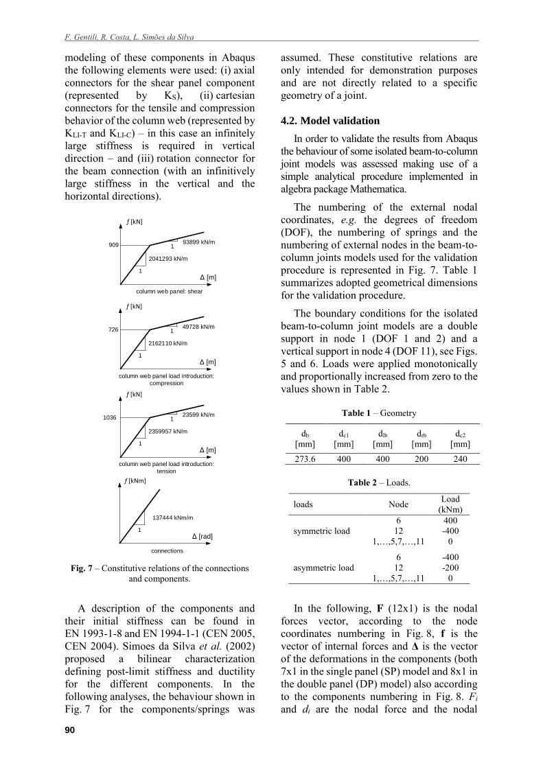
modeling of these components in Abaqus
the following elements were used: (i) axial
connectors for the shear panel component
(represented by KS), (ii) cartesian
connectors for the tensile and compression
behavior of the column web (represented by
KLI-T and KLI-C) – in this case an infinitely
large stiffness is required in vertical
direction – and (iii) rotation connector for
the beam connection (with an infinitively
large stiffness in the vertical and the
horizontal directions).
Fig. 7 – Constitutive relations of the connections
and components.
A description of the components and
their initial stiffness can be found in
EN 1993-1-8 and EN 1994-1-1 (CEN 2005,
CEN 2004). Simoes da Silva et al. (2002)
proposed a bilinear characterization
defining post-limit stiffness and ductility
for the different components. In the
following analyses, the behaviour shown in
Fig. 7 for the components/springs was
assumed. These constitutive relations are
only intended for demonstration purposes
and are not directly related to a specific
geometry of a joint.
4.2. Model validation
In order to validate the results from Abaqus
the behaviour of some isolated beam-to-column
joint models was assessed making use of a
simple analytical procedure implemented in
algebra package Mathematica.
The numbering of the external nodal
coordinates, e.g. the degrees of freedom
(DOF), the numbering of springs and the
numbering of external nodes in the beam-to-
column joints models used for the validation
procedure is represented in Fig. 7. Table 1
summarizes adopted geometrical dimensions
for the validation procedure.
The boundary conditions for the isolated
beam-to-column joint models are a double
support in node 1 (DOF 1 and 2) and a
vertical support in node 4 (DOF 11), see Figs.
5 and 6. Loads were applied monotonically
and proportionally increased from zero to the
values shown in Table 2.
Table 1 – Geometry
db
[mm]
dc1
[mm]
dlb
[mm]
drb
[mm]
dc2
[mm]
273.6 400 400 200 240
Table 2 – Loads.
loads Node Load
(kNm)
symmetric load
6 400
12 -400
1,…,5,7,…,11 0
asymmetric load
6 -400
12 -200
1,…,5,7,…,11 0
In the following, F (12x1) is the nodal
forces vector, according to the node
coordinates numbering in Fig. 8, f is the
vector of internal forces and Δ is the vector
of the deformations in the components (both
7x1 in the single panel (SP) model and 8x1 in
the double panel (DP) model) also according
to the components numbering in Fig. 8. Fi
and di are the nodal force and the nodal
726
f [kN]
Δ [m]
2162110 kN/m
49728 kN/m
1
1
column web panel load introduction:
compression
1036
f [kN]
Δ [m]
2359957 kN/m
23599 kN/m
1
1
column web panel load introduction:
tension
909
f [kN]
Δ [m]
2041293 kN/m
93899 kN/m
1
1
column web panel: shear
f [kNm]
Δ [rad]
137444 kNm/m
1
connections

Development of a simplified model for joints in steel structures
91
displacement, respectively, in DOF i and fi
and Δi are the internal force and the
deformation, respectively, in spring i.
1 1 1
(SP) (DP)
12 7 8
1 1
(SP) (DP)
7 8
, , ,
and
F f f
F f f
F f f
Δ Δ
(1)
The procedure comprises four steps:
Fig. 8 – External degrees of freedom, springs and
external nodes numbering for SP model (top) and
for the DP model (bottom).
Step 1 - Compute the internal forces in all
of the springs. The support reactions were
computed making use of statics leading to
10 4 7
5 8 11
3 6 9
1
2
11
12 7 b
b c10 4 5c
2
2 2
F F F
F F F
F F F F F zz z
F F F
F
z
F
F
(2)
for the single panel isolated beam-to-
column joint model and
10 4 7
5 8 11
3 6 9 12 7 bL
bL bR c10
1
2
14 bL 5c
12
2 2 2
F F F
F F F
F F F F F zz z z
F F z F
F
F
zF
(3)
for the double panel isolated beam-to-column
joint model.
Step 2 - From the free body diagram of the
beam-to-column joint models, the internal
forces in the components were computed
again only making use of statics leading to
2 2c b
6 4
b
6 4
b
6
12 10
b
12 10
b
12
10 4 12 67
c b
2
2
2
2
2
z z
F F
z
F F
z
F
F F
z
F F
z
F
F F F FF
z z
f (4)
for the single panel isolated beam-to-column
joint model (Fig. 5) and
2 2c bR
22c
bL bR
6 4
bR
6 4
bR
6
12 10
bL
12 10
bL
12
10 4 6 127
c bR bL
12 101
c bL
2
2
2
2
2
2
z z
z z z
F F
z
F F
z
F
F F
z
F F
z
F
F F F FF
z z z
F FF
z z
f (5)
for the double panel isolated beam-to-column
joint model (Fig. 6).
Step 3 - Compute the deformations in all the
components. The deformations in the
components were computed making use of
4
5
6
10
1211
78
9
1
2 3
1
2
3
4
5
67
node 1
node 2
node 3
node 4
4
5
6
10
1211
78
9
1
2
3
4
5
6
7
node 2
node 3
node 4
1
2 3
8
node 1
external node
hinge
connection
basic componente
4
5
6
10
1211
78
9
1
2 3
1
2
3
4
5
67
node 1
node 2
node 3
node 4
4
5
6
10
1211
78
9
1
2
3
4
5
6
7
node 2
node 3
node 4
1
2 3
8
node 1
external node
hinge
connection
basic componente
4
5
6
10
1211
78
9
1
2 3
1
2
3
4
5
67
node 1
node 2
node 3
node 4
4
5
6
10
1211
78
9
1
2
3
4
5
6
7
node 2
node 3
node 4
1
2 3
8
node 1
external node
hinge
connection
basic componente
4
5
6
10
1211
78
9
1
2 3
1
2
3
4
5
67
node 1
node 2
node 3
node 4
4
5
6
10
1211
78
9
1
2
3
4
5
6
7
node 2
node 3
node 4
1
2 3
8
node 1
external node
hinge
connection
basic componentehinge external node

F. Gentili, R. Costa, L. Simões da Silva
92
the internal forces and the uniaxial
constitutive relations shown in Fig. 7.
Step 4 - Compute the nodal displacements
of external nodes. The displacements were
computed making used of Second
Castigliano’s Theorem. This theorem
applied for the isolated beam-to-column
joint models (where the only deformable
elements are the springs) states that the
displacement in any of the external DOF
represented in Fig. 8 can be computed
through the sum of the product of the
deformation in each spring caused by the
actual load and the internal force in that
same spring caused by a unit load applied in
the DOF where the displacement is wanted.
For instance the displacement in DOF j may
be computed through eq. (5).
j
j
7(SP) or 8(DP)1Load
j
1T
1Load .
F
i i
i
F
d f
Δ f
(5)
The former procedure is suitable for
statically determinate structures for the
elastic and for the post-elastic range when
the behaviour of the components is
holonomic and has no softening.
Fig. 9 and Fig. 11 illustrate the bending
moment-rotation curve of right side (node 5 in
Fig. 8) of SP and DP joint model under
symmetric and asymmetric loading
conditions, respectively. For both cases, the
yielding of the first component (column web
compression) and the yielding of the second
component (column web tension) are noted.
Fig. 9 – Moment-rotation curve for right side of SP
model under symmetric load condition (node 5 in
Fig. 8).
Fig. 10 – Force-displacements relationship for
tension (f2, f5) and compression (f1, f4) components in
SP model.
Fig. 11 – Moment-rotation curve for right side of DP
model under asymmetric load conditions (node 5 in
Fig. 8).
In Fig. 10 and Fig. 12, the behaviour of
the individual components is highlighted in
case of SP and DP models respectively. It can
be seen from Fig. 9 to Fig. 12 that the values
obtained with Abaqus match the analytical
results from Mathematica.
Fig. 12 – Force-displacements relationship for
tension (f2, f5), compression (f1, f4) and shear (f7, f8)
components in DP model.
0
100
200
300
400
500
0 30 60 90 120 150
Be
nd
ing
Mo
me
nt
[kN
m]
Rotation[mRad]
Mathematica Abaqus
0
400
800
1200
1600
0 5 10 15 20
Fo
rce
[kN
]
Displacement [mm]
f2 f1f2, f5 f1 , f4
0
100
200
300
400
500
0 100 200 300 400 500
Bend
ing
Mom
en
t [k
Nm
]
Rotation[mRad]
Mathematica Abaqus
0
400
800
1200
1600
2000
2400
0 10 20 30 40 50
Fo
rce
[kN
]
Displacement [mm]
f5 f7 f2
f4 f8 f1
Development of a simplified model for joints in steel structures
93
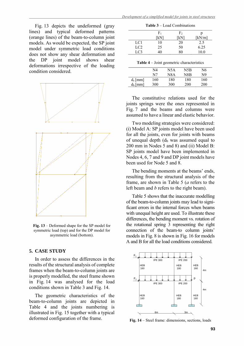
Fig. 13 depicts the undeformed (gray
lines) and typical deformed patterns
(orange lines) of the beam-to-column joint
models. As would be expected, the SP joint
model under symmetric load conditions
does not show any shear deformation and
the DP joint model shows shear
deformations irrespective of the loading
condition considered.
Fig. 13 – Deformed shape for the SP model for
symmetric load (top) and for the DP model for
asymmetric load (bottom).
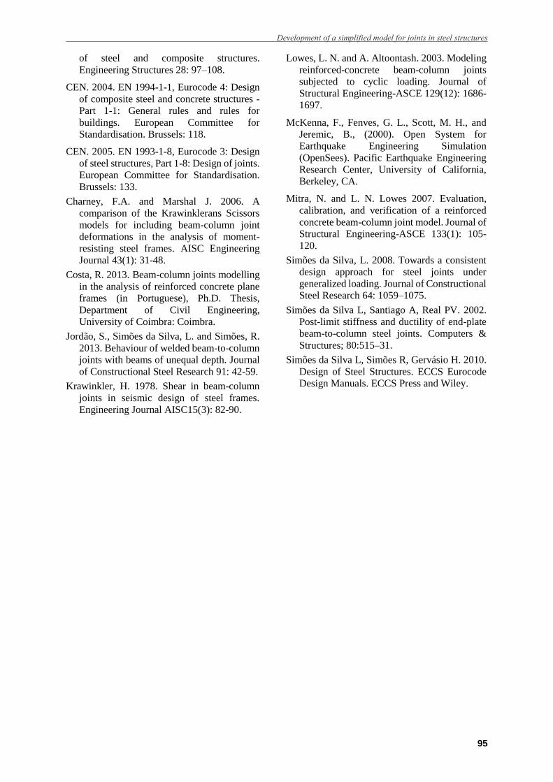
5. CASE STUDY
In order to assess the differences in the
results of the structural analysis of complete
frames when the beam-to-column joints are
is properly modelled, the steel frame shown
in Fig. 14 was analysed for the load
conditions shown in Table 3 and Fig. 14.
The geometric characteristics of the
beam-to-column joints are depicted in
Table 4 and the joints numbering is
illustrated in Fig. 15 together with a typical
deformed configuration of the frame.
Table 3 – Load Combinations
F1
[kN]
F2
[kN]
p
[kN/m]
LC1 10 20 2.5
LC2 25 50 6.25
LC3 40 80 10.0
Table 4 – Joint geometric characteristics
N4
N7
N5A
N8A
N5B
N8B
N6
N9
dc [mm] 160 180 180 160
db [mm] 300 300 200 200
The constitutive relations used for the
joints springs were the ones represented in
Fig. 7 and the beams and columns were
assumed to have a linear and elastic behavior.
Two modeling strategies were considered:
(i) Model A: SP joints model have been used
for all the joints, even for joints with beams
of unequal depth (db was assumed equal to
200 mm in Nodes 5 and 8) and (ii) Model B:
SP joints model have been implemented in
Nodes 4, 6, 7 and 9 and DP joint models have
been used for Node 5 and 8.
The bending moments at the beams’ ends,
resulting from the structural analysis of the
frame, are shown in Table 5 (a refers to the
left beam and b refers to the right beam).
Table 5 shows that the inaccurate modelling
of the beam-to-column joints may lead to signi-
ficant errors in the internal forces when beams
with unequal height are used. To illustrate these
differences, the bending moment vs. rotation of
the rotational spring 3 representing the right
connection of the beam-to column joints’
models in Fig. 8 is shown in Fig. 16 for models
A and B for all the load conditions considered.
Fig. 14 – Steel frame: dimensions, sections, loads
6m 3m
4m
HEB
160
HEB
160
HEB
180
IPE 300 IPE 200
p
IPE 300 IPE 200
4m
F2
F1
HEB
160
HEB
180
HEB
160

F. Gentili, R. Costa, L. Simões da Silva
94
Fig. 15 – Deformed shape of steel frame and joints’
numbering.
Table 5 – Bending moments (kNm).
LC1 LC2 LC3
Mod.
A
Mod.
B
Mod.
A
Mod.
B
Mod.
A
Mod.
B
N4 18.3 19.1 61.3 47.8 60.5 78.5
N5a 71.2 76.8 150.7 192.1 174.7 254.4
N5b 9.2 9.7 13.5 24.3 13.0 20.3
N6 18.0 16.3 51.6 40.9 101.2 77.0
N7 19.8 21.1 48.0 52.8 65.0 81.8
N8a 58.6 61.8 138.8 154.7 166.3 244.7
N8b 20.4 21.1 45.5 52.8 37.9 80.2
N9 7.2 5.8 22.6 14.5 57.4 29.1
Fig. 16 – Bending moment vs. rotation of spring 3.
Fig. 16 shows that spring 3 (i) in LC1
remains in the elastic range in both models,
(ii) in LC3, the most severe combination,
determines the development of plasticity in
the connection for both models but (iii) on
the other hand, in LC2 determines that
plasticity occurs only in model A, i.e. in this
later loading condition the non-linearity in is
only caused by the inaccuracy of the model.
6. CONCLUSIONS
The paper has emphasized the need of
macro-elements for beam-to-column joint
modeling. In was shown that, when compared
with the use of springs attached to the ends of
beams, this modeling strategy would allow to:
(i) reduce the computational cost; (ii) overcome
numerical difficulties due to nonlinearities; and
(iii) provide a more rigorous modeling of the
beam-to-column joints.
Two macro-models suitable for steel
beam-to-column joints with beams of equal
and unequal depth were presented and their
modeling in Abaqus was explained.
These models were validated by means of
an analytical procedure, and later were
included in a 2D steel frame.
The structural analysis of the steel frame
highlighted the potentialities of the proposed
models showing that the inaccurate
modelling of the beam-to-column joints may
lead to significant errors in the results.
This work will carry on to the formulation
of a new finite element suitable for steel
beam-to-column joints.
ACKNOWLEDGEMENTS
Financial support from the Portuguese
Ministry of Science and Higher Education
(Ministério da Ciência e Ensino Superior) under
contract grant PTDC/ECM/116904/2010 is
gratefully acknowledged.
REFERENCES
Simulia. 2014, Abaqus FEA, Dassault Systèmes
Simulia Corp.
Altoontash, A. 2004. Simulation and damage
models for performance assessment of
reinforced concrete beam-column joints.
Ph.D., Stanford University.
Bayo, E., Cabrero, J.M. and Gil. B. 2006. An
effective component-based method to model
semi-rigid connections for the global analysis
N7
N4
N9
N6
N8a
N5a
N8b
N5b
0
50
100
150
200
250
300
0 5 10 15 20 25 30
Be
nd
ing
Mo
me
nt
[kN
m]
Rotation [mRad]
Model A - LC1 Model B - LC1
Model A - LC2 Model B - LC2
Model A - LC3 Model B - LC3
Development of a simplified model for joints in steel structures
95
of steel and composite structures.
Engineering Structures 28: 97–108.
CEN. 2004. EN 1994-1-1, Eurocode 4: Design
of composite steel and concrete structures -
Part 1-1: General rules and rules for
buildings. European Committee for
Standardisation. Brussels: 118.
CEN. 2005. EN 1993-1-8, Eurocode 3: Design
of steel structures, Part 1-8: Design of joints.
European Committee for Standardisation.
Brussels: 133.
Charney, F.A. and Marshal J. 2006. A
comparison of the Krawinklerans Scissors
models for including beam-column joint
deformations in the analysis of moment-
resisting steel frames. AISC Engineering
Journal 43(1): 31-48.
Costa, R. 2013. Beam-column joints modelling
in the analysis of reinforced concrete plane
frames (in Portuguese), Ph.D. Thesis,
Department of Civil Engineering,
University of Coimbra: Coimbra.
Jordão, S., Simões da Silva, L. and Simões, R.
2013. Behaviour of welded beam-to-column
joints with beams of unequal depth. Journal
of Constructional Steel Research 91: 42-59.
Krawinkler, H. 1978. Shear in beam-column
joints in seismic design of steel frames.
Engineering Journal AISC15(3): 82-90.
Lowes, L. N. and A. Altoontash. 2003. Modeling
reinforced-concrete beam-column joints
subjected to cyclic loading. Journal of
Structural Engineering-ASCE 129(12): 1686-
1697.
McKenna, F., Fenves, G. L., Scott, M. H., and
Jeremic, B., (2000). Open System for
Earthquake Engineering Simulation
(OpenSees). Pacific Earthquake Engineering
Research Center, University of California,
Berkeley, CA.
Mitra, N. and L. N. Lowes 2007. Evaluation,
calibration, and verification of a reinforced
concrete beam-column joint model. Journal of
Structural Engineering-ASCE 133(1): 105-
120.
Simões da Silva, L. 2008. Towards a consistent
design approach for steel joints under
generalized loading. Journal of Constructional
Steel Research 64: 1059–1075.
Simões da Silva L, Santiago A, Real PV. 2002.
Post-limit stiffness and ductility of end-plate
beam-to-column steel joints. Computers &
Structures; 80:515–31.
Simões da Silva L, Simões R, Gervásio H. 2010.
Design of Steel Structures. ECCS Eurocode
Design Manuals. ECCS Press and Wiley.

![5th Pan American Conference for · PDF fileFigure 1. Typical adhesive-bonded joint [2]. Adhesive joints have the lowest material cost among all other kinds of joints, and are](https://img.document.onl/doc/110x75/5a9ec2287f8b9a7f178bc83c/5th-pan-american-conference-for-1-typical-adhesive-bonded-joint-2-adhesive-joints.jpg)