Embed Size (px)
Citation preview
Universidade de Aveiro 2008
Departamento de Electrónica, Telecomunicações e Informática
Emanuel Filipe Cunha Miranda
Gerenciador de Recursos
Dissertação apresentada à Universidade de Aveiro para cumprimento dos requisitos necessários à obtenção do grau de Mestre em Electrónica e Telecomunicações (300-9365), realizada sob a orientação científica do Dr. Paulo Pedreiras, Professor Auxiliar do Departamento de Electrónica, Telecomunicações e Informática (DETI) da Universidade de Aveiro (UA).
2 | P a g e U A - D E T I - R e s o u r c e M a n a g e r
Emanuel Miranda 2008
o júri
presidente Doutor António Ferreira Pereira de Melo Professor Catedrático da Universidade de Aveiro
Doutor Paulo Bacelar Reis Pedreiras
Professor Auxiliar da Universidade de Aveiro
Doutor Joaquim José Castro Ferreira
Professor Adjunto do Departamento de Engenharia Informática da Escola Superior de
Tecnologia do Instituto Politécnico de Castelo Branco
Prof. Dr. João Antunes da Silva professor associado da Faculdade de Engenharia da Universidade do Porto
Prof. Dr. João Antunes da Silva professor associado da Faculdade de Engenharia da Universidade do Porto
Prof. Dr. João Antunes da Silva professor associado da Faculdade de Engenharia da Universidade do Porto

3 | P a g e U A - D E T I - R e s o u r c e M a n a g e r
Emanuel Miranda 2008
agradecimentos
Gostaria de agradecer aos meus pais e irmã, Emanuel, Ana e
Anita, que me ajudaram na minha estadia na Holanda e sempre
seguiram de perto os meus passos académicos.
Aos meus amigos na Holanda, João, Rodrigo e Bibiana, que
sempre me apoiaram em todo o processo de adaptação.
Ao Orlando Moreira (NXP) e ao Prof. Paulo Pedreiras (UA),
pela oportunidade e auxílio.
Por último, mas não menos importante, ao meu amigo Luis
Silva que me ajudou na revisão da tese.

4 | P a g e U A - D E T I - R e s o u r c e M a n a g e r
Emanuel Miranda 2008
acknowledgements
I would like to thank my parents and sister, Emanuel, Ana and
Anita, who made my journey to the Netherlands possible and
followed my life and my studies closely.
To my friends in the Netherlands, João, Rodrigo and Bibiana,
who supported me in several milestones during my stay.
To Orlando Moreira (NXP) and Prof. Paulo Pedreiras (UA), who
gave me the opportunity and guidance to help me succeed.
Last but not least, to Luis Silva who reviewed my thesis. No one
could hope for a better friend.
5 | P a g e U A - D E T I - R e s o u r c e M a n a g e r
Emanuel Miranda 2008
palavras-chave
Gerenciador de recursos, Rádio definido por Software,
Sistema heterogéneo de Multi-processadores.
resumo
Esta tese reporta a implementação de um módulo
gerenciador de recursos para uma plataforma heterogénea
multi-processador de rádio para equipamento movel.
Nessa plataforma os rádios são definidos como data flows
e são dinamicamente alocados, ou libertados consuante a
necessidade da aplicação.
Os rádios são alocados em runtime e requerem
vários recursos que podem ou não estar livres na
plataforma. Quando uma tentativa de alocação de um
rádio falha, todos os recursos até ai reservados têm que ser
libertados. Esta metodologia requer tempo e não é
eficiente. O objectivo desta dissertação é investigar
diferentes metodologias e algoritmos para tornar o
processo de alocação mais eficiente. A abordagem
escolhida foi baseada na modelação dos recursos, opção
que permite controle de admissão e é independente da
plataforma. Este trabalho foi desenvolvido o mais
genericamente possível para abranger a maior variedade
de aplicações.
No estado actual do projecto são suportados até 5
standards de rádio simultaneamente, cada um com
diferentes taxas de entrada/saída e com requisitos real-
time. Em conclusão, este projecto contrói o caminho para
a quarta geração (4G) de tecnologia de comunicação.
6 | P a g e U A - D E T I - R e s o u r c e M a n a g e r
Emanuel Miranda 2008
keywords
Resource Manager, Software-Defined Radio,
Heterogeneous Multi-processor system.
abstract
This dissertation addresses the project and
implementation of a Resource Manager module for
heterogeneous multi-processor radio platforms. In the
target platform the radios are defined as data flows and are
dynamically allocated and released, according to the
application needs.
Radios are allocated at runtime and require the
sequential allocation of several resources that may or may
not be available. Whenever the allocation of any necessary
resource fails, the radio allocation procedure has to be
aborted and the eventually allocated resources released.
Allocating and de-allocating resources is costly and thus
this methodology is not efficient. In the scope of this
dissertation are investigated different methods and
algorithms to make the radio allocation process more
efficient. Four different possibilities are considered and
assessed. The chosen approach is based in the use of a
resource model, which permits fast admission control and
is platform-independent, since it does not require any
modification on the platform-specific modules. This
application is being developed as generically as possible
to be able to embrace the largest possible group of
applications.
In its current status this project supports up to 5
different radio standards concurrently, each one exhibiting
specific input/output rates and real-time requirements. In
conclusion, it is the path to fourth generation (4G)
communication technology.
7 | P a g e U A - D E T I - R e s o u r c e M a n a g e r
Emanuel Miranda 2008
Contents
1. INTRODUCTION 13
A. SOFTWARE-DEFINED RADIO 14
B. THIS PROJECT 15
C. BASE-BAND RESOURCE MANAGER 15
D. THESIS OVERVIEW 16
2. BACKGROUND 17
A. REAL-TIME SYSTEMS 17
B. MULTI-PROCESSOR SYSTEM 17
C. MULTI SKILLS SYSTEMS 18
D. SINGLE-RATE DATAFLOW 18
3. SOFTWARE-DEFINED RADIO FRAMEWORK AND RADIO DESCRIPTION 21
A. HARDWARE FRAMEWORK 21
B. SOFTWARE FRAMEWORK 24
C. RADIO MODEL 29
D. RADIO STRUCTURE AND DESIGN 31
E. RADIO EXAMPLE 32
4. DESIGN SPACE, PROBLEMS AND SOLUTIONS 33
A. GOALS OF BB-RM 33
B. DESIGN SPACE 34
C. SOLUTIONS 36
D. SOLUTION ASSESSMENT 38
5. IMPLEMENTATION OF THE BB-RM 39
A. JOB – RADIO INSTANCE 39
B. BB-RM FUNCTIONS 40
C. DATA STRUCTURE OF BB-RM 40
D. JOB STATES 43
E. INTERFACE G-RM <-> BB-RM 44
F. INTERFACE BB-RM <-> SOD 48
G. RESOURCE ALLOCATION PROBLEM 49
H. SORT STRATEGY 51
I. COMPLETE RAP HEURISTICS, INCLUDING COMMUNICATION 53
J. DEBUG 54
K. BB-RM VERSIONS 55
L. SOURCE CODE 56
8 | P a g e U A - D E T I - R e s o u r c e M a n a g e r
Emanuel Miranda 2008
6. EXPERIMENTAL RESULTS 59
A. OPTIMIZATIONS 59
B. MW VS RW RESULTS 62
C. BF VS FF RESULTS 63
D. COMPLETE RESOURCE ALLOCATION PROBLEM RESULTS 65
E. FRAGMENTATION RESULTS 65
7. CONCLUSIONS AND FUTURE WORK 67
A. FUTURE WORK 68
8. BIBLIOGRAPHY 69
9. APPENDICES 71
A. DOXYGEN API CODE DOCUMENTATION 71
B. FUNCTIONS PERFORMANCES IN VERSION 1.2 75
C. FUNCTIONS PERFORMANCES IN VERSION 1.3 78
9 | P a g e U A - D E T I - R e s o u r c e M a n a g e r
Emanuel Miranda 2008
Abbreviations
0G - Zero Generation
1G - First Generation
2G - Second Generation
3G - Third Generation
3GPP - Third Generation Partnership Project
4G - Fourth Generation
ADC - Analog-to-Digital Converter
AHB - Advanced High-performance Bus
API - Application Programmer’s Interface
ARM - Advanced RISC Machine
AXI - Advanced eXtensible Interface
BB-RM - Baseband Resource Manager
BF - Best Fit
CM - Configuration Manager
CPU - Central Processor Unit
DAC - Digital-to-Analog Converter
DSP - Digital Signal Processing
EVP - Embedded Vector Processor
F-ARM - FPGA ARM
FF - First Fit
FIFO - First In First Out
FPGA - Field-Programmable Gate Array
G-RM - Global Resource Manager
GSM - Groupe Special Mobile
J-ARM - JEOME ARM
J-ARM - JEOME ARM
J-EVP - JEOME EVP
J-EVP - JEOME EVP
J-Tile - JEOME tile
LTE - Long Term Evolution
MPS - Multi-Processor System
MW - Module Weights
NM - Network Manager
OS - Operating System
PC - Personal Computer
RAP - Resource Allocation Problem
RISC - Reduced Instruction Set Computer
RM - Resource manager
10 | P a g e U A - D E T I - R e s o u r c e M a n a g e r
Emanuel Miranda 2008
RR - Round Robin
RT - Real-Time
RTOS - Real-Time Operating System
RTS - Real-Time System
RW - Relative Weights
RX - Receive
SDR - Software-Defined Radio
SK - Streaming Kernel
SoC - System On Chip
SoD - Sea of DSP
SRDF - Single Rate Dataflow
TX - Transmit
UART - Universal Asynchronous Receiver/Transmitter
uC/OS - Micro-Controller Operating System
USB - Universal Serial Protocol
VBP - Vector Bin-Packing
WLAN - Wireless Local Area Network
11 | P a g e U A - D E T I - R e s o u r c e M a n a g e r
Emanuel Miranda 2008
List of tables
TABLE 1 : RESOURCE OPTIMIZATION ......................................................................................................................... 60
TABLE 2 : JOB OPTIMIZATION .................................................................................................................................. 60
TABLE 3 : OPTIMIZATION RESULTS ........................................................................................................................... 60
TABLE 4 : FUNCTIONS PERFORMANCES ..................................................................................................................... 61
TABLE 5 : MW AND RW RESULTS ........................................................................................................................... 63
TABLE 6 : BF AND FF RESULTS ................................................................................................................................ 64
List of figures
FIGURE 1 : ORDINARY RADIO ARCHITTECTURE FROM [14] ............................................................................................ 13
FIGURE 2 : SOD RADIO SYSTEMATIC FROM [14] ......................................................................................................... 14
FIGURE 3 : SINGLE-RATE DATAFLOW ........................................................................................................................ 19
FIGURE 4 : TILE STRUCURE ..................................................................................................................................... 21
FIGURE 5 : JEOME STRUCTURE .............................................................................................................................. 22
FIGURE 6 : PLATFORM STRUCTURE ........................................................................................................................... 22
FIGURE 7 : AEROPROTO2 BOARD ............................................................................................................................ 23
FIGURE 8 : SOFTWARE STRUCTURE ........................................................................................................................... 25
FIGURE 9 : SOD CONCEPTUAL VIEW FROM [5] ........................................................................................................... 27
FIGURE 10 : SOD EXECUTION ARCHITECTURE FROM [5] ............................................................................................... 27
FIGURE 11 : WLAN DATFLOW ................................................................................................................................ 29
FIGURE 12 : RADIO STRUCTURE ............................................................................................................................... 31
FIGURE 13 : WLAN 802.11A EXAMPLE FROM [12] ................................................................................................... 32
FIGURE 14 : BB-RM DESIGN SPACE ......................................................................................................................... 34
FIGURE 15 : BB-RM SOLUTION-1 ........................................................................................................................... 36
FIGURE 16 : BB-RM SOLUTION-2 ........................................................................................................................... 37
FIGURE 17 : BB-RM SOLUTION-3 ........................................................................................................................... 37
FIGURE 18 : BB-RM SOLUTION-4 ........................................................................................................................... 38
FIGURE 19 : BB-RM DATA STRUCTURE ..................................................................................................................... 41
FIGURE 20 : JOB STATES ........................................................................................................................................ 44
FIGURE 21 : BBRM_INICIALIZE FUNCTION ................................................................................................................ 45
FIGURE 22 : BBRM_JOB_TEST FUNCTION ................................................................................................................ 45
FIGURE 23 : BBRM_JOB_CREATE FUNCTION ............................................................................................................ 46
FIGURE 24 : BBRM_JOB_RESUME FUNCTION ........................................................................................................... 47
FIGURE 25 : BBRM_JOB_SUSPEND......................................................................................................................... 47
FIGURE 26 : BBRM_JOB_REMOVE ......................................................................................................................... 48
FIGURE 27 : VBP EXAMPLE .................................................................................................................................... 50
FIGURE 28 : MW EXAMPLE .................................................................................................................................... 52
FIGURE 29 : RW EXAMPLE ..................................................................................................................................... 52
FIGURE 30 : DEBUG MESSAGES ............................................................................................................................... 55
FIGURE 31 : ERROR MESSAGES ................................................................................................................................ 55
FIGURE 32 : FILES STRUCTURE ................................................................................................................................. 57
FIGURE 33 : RADIO TO TEST THE MW AND RW METHODS ........................................................................................... 62
FIGURE 34 : RADIO TO TEST THE BF AND FF ALGORITHMS ............................................................................................ 64
FIGURE 35 : RADIOS TO TEST THE FIFO FRAGMENTATION ............................................................................................ 65
FIGURE 36 : FIFO MEMORY ................................................................................................................................... 66

12 | P a g e U A - D E T I - R e s o u r c e M a n a g e r
Emanuel Miranda 2008
(This page was left blank delivered)
13 | P a g e
1. Introduction
The way to the future is built on knowledge from the past, so a brief description of
the cellular mobile radio history will be given next.
As early as 1921 the first communications were done via the mobile radios rigs and
used in vehicles such as taxicabs, police cruisers and ambulances. These devices were not
considered as mobile phones because they were not normally connected to the telepho
network (1).
During the early 1940s, Motorola developed a backpacked two
Walkie-Talkie and later developed a large hand
was in 1945 when the zero generation (0G) o
mobile phone just worked in one station, so the cellular concept did not exist. At this time
several prototypes were invented
Firstly in Tokyo, Japan (1979) and two year latter in De
and Sweden, the first commercial cellular phone networks, called as first generation (1G),
were launched.
In 1982 the Groupe Spécial Mobile
phones, and in 1990 the first GSM mobile communication infrastructure was deployed.
This new release was called second generation (2G). This new variant brought the SMS
service, which permits sending text messages in addition to the voice calls.
Not long after and with th
systems began to develop. There were many different standards created by different
contenders. The meaning of 3G was the standardization of the requirements (maximum
data rate indoors/outdoors) instead o
standards were introduced.
Figure
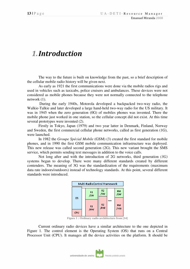
Current ordinary radio devices have a similar
Figure 1. The control element is the Operating System (OS) that runs on a Central
Processor Unit (CPU). It manages all the device activities on the platform. It should be
U A - D E T I - R e s o u r c e M a n a g e r
Emanuel Miranda
Introduction
The way to the future is built on knowledge from the past, so a brief description of
the cellular mobile radio history will be given next.
As early as 1921 the first communications were done via the mobile radios rigs and
used in vehicles such as taxicabs, police cruisers and ambulances. These devices were not
considered as mobile phones because they were not normally connected to the telepho
During the early 1940s, Motorola developed a backpacked two
Talkie and later developed a large hand-held two-way radio for the US military. It
was in 1945 when the zero generation (0G) of mobiles phones was invented. There the
mobile phone just worked in one station, so the cellular concept did not exist. At this time
several prototypes were invented (2).
Firstly in Tokyo, Japan (1979) and two year latter in Denmark, Finland, Norway
and Sweden, the first commercial cellular phone networks, called as first generation (1G),
Groupe Spécial Mobile (GSM) (3) created the first standard for mobile
990 the first GSM mobile communication infrastructure was deployed.
This new release was called second generation (2G). This new variant brought the SMS
service, which permits sending text messages in addition to the voice calls.
Not long after and with the introduction of 2G networks, third generation
systems began to develop. There were many different standards created by different
contenders. The meaning of 3G was the standardization of the requirements (maximum
data rate indoors/outdoors) instead of technology standards. At this point, several different
Figure 1 : Ordinary radio archittecture from [14]
t ordinary radio devices have a similar architecture to the one depicted in
. The control element is the Operating System (OS) that runs on a Central
Processor Unit (CPU). It manages all the device activities on the platform. It should be
R e s o u r c e M a n a g e r
Emanuel Miranda 2008
The way to the future is built on knowledge from the past, so a brief description of
As early as 1921 the first communications were done via the mobile radios rigs and
used in vehicles such as taxicabs, police cruisers and ambulances. These devices were not
considered as mobile phones because they were not normally connected to the telephone
During the early 1940s, Motorola developed a backpacked two-way radio, the
way radio for the US military. It
f mobiles phones was invented. There the
mobile phone just worked in one station, so the cellular concept did not exist. At this time
nmark, Finland, Norway
and Sweden, the first commercial cellular phone networks, called as first generation (1G),
created the first standard for mobile
990 the first GSM mobile communication infrastructure was deployed.
This new release was called second generation (2G). This new variant brought the SMS
service, which permits sending text messages in addition to the voice calls.
e introduction of 2G networks, third generation (3G)
systems began to develop. There were many different standards created by different
contenders. The meaning of 3G was the standardization of the requirements (maximum
f technology standards. At this point, several different
architecture to the one depicted in
. The control element is the Operating System (OS) that runs on a Central
Processor Unit (CPU). It manages all the device activities on the platform. It should be
14 | P a g e
remarked that each radio has
standard is supported by dedicated hardware.
that supports M radio standards with M dedicated hardware modules.
The number of applications supported by mobile devices is growing day by day. Most of
them use remote databases and/or services. The need to make an efficient use of the
communication bandwidth led to th
Nowadays, mobile cell system
Furthermore, some of them (e.g. GSM) have several versions. This imposes a constraint on
the radio devices. If a radio device aims at supporting the
it would need dedicated hardware for each one and so it becomes big and complex.
Another drawback of this radio architecture is that it is not upgradeable, and thus cannot
evolve to support radio standards than are create
Finally, it should be noted that the “classical” architecture depicted in
mobile devices, and thus subject to strict size
number of dedicated HW radios and, consequently, the number of standards supported.
In face of all of these trends, the ordinary phone platform is starting to become obsolete.
Following the personal computer (PC)
heading to Multi-Processor Systems (MPS), called 4G
Multiprocessor systems present several advantages in terms of flexibility, power
efficiency and cost (5).
In conclusion, the balance between installed uni and multi
upcoming years.
A. Software-
The negative aspects pointed out to the current radio platforms can be traced to the
dedicated hardware implementation of the radio components. This observation led to the
development of the Software
revolution in the field of hardware devices. The use of SDR is completely compatible with
the existing network infrastructure and standards, however changes significantly the
internal architecture of the mobile devices.
The major difference between the conventional and SDR radio platforms is the fact
that instead of having dedicated hardware for each radio standard, the radios are
programmable software entities, similar to application programs in a personal computer.
U A - D E T I - R e s o u r c e M a n a g e r
Emanuel Miranda
remarked that each radio has specific hardware to support it and, consequently, each radio
standard is supported by dedicated hardware. Figure 1 depicts a radio architecture example
M radio standards with M dedicated hardware modules.
The number of applications supported by mobile devices is growing day by day. Most of
them use remote databases and/or services. The need to make an efficient use of the
communication bandwidth led to the development of different standards.
Nowadays, mobile cell systems support more than ten radio standards.
Furthermore, some of them (e.g. GSM) have several versions. This imposes a constraint on
the radio devices. If a radio device aims at supporting the majority of these radio standards
it would need dedicated hardware for each one and so it becomes big and complex.
Another drawback of this radio architecture is that it is not upgradeable, and thus cannot
evolve to support radio standards than are created after its development.
Finally, it should be noted that the “classical” architecture depicted in
mobile devices, and thus subject to strict size limitations, which can also constraint the
number of dedicated HW radios and, consequently, the number of standards supported.
In face of all of these trends, the ordinary phone platform is starting to become obsolete.
Following the personal computer (PC) innovation, mobile phone platforms are going
Processor Systems (MPS), called 4G (4).
Multiprocessor systems present several advantages in terms of flexibility, power
In conclusion, the balance between installed uni and multi-processors wi
-Defined Radio
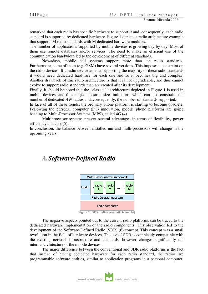
Figure 2 : SDR radio systematic from [14]
The negative aspects pointed out to the current radio platforms can be traced to the
dedicated hardware implementation of the radio components. This observation led to the
development of the Software-Defined Radio (SDR) (6) concept. This concept was a small
revolution in the field of hardware devices. The use of SDR is completely compatible with
the existing network infrastructure and standards, however changes significantly the
internal architecture of the mobile devices.
The major difference between the conventional and SDR radio platforms is the fact
that instead of having dedicated hardware for each radio standard, the radios are
programmable software entities, similar to application programs in a personal computer.
R e s o u r c e M a n a g e r
Emanuel Miranda 2008
specific hardware to support it and, consequently, each radio
depicts a radio architecture example
The number of applications supported by mobile devices is growing day by day. Most of
them use remote databases and/or services. The need to make an efficient use of the
e development of different standards.
support more than ten radio standards.
Furthermore, some of them (e.g. GSM) have several versions. This imposes a constraint on
majority of these radio standards
it would need dedicated hardware for each one and so it becomes big and complex.
Another drawback of this radio architecture is that it is not upgradeable, and thus cannot
d after its development.
Finally, it should be noted that the “classical” architecture depicted in Figure 1 is used in
limitations, which can also constraint the
number of dedicated HW radios and, consequently, the number of standards supported.
In face of all of these trends, the ordinary phone platform is starting to become obsolete.
innovation, mobile phone platforms are going
Multiprocessor systems present several advantages in terms of flexibility, power
processors will change in the
The negative aspects pointed out to the current radio platforms can be traced to the
dedicated hardware implementation of the radio components. This observation led to the
cept. This concept was a small
revolution in the field of hardware devices. The use of SDR is completely compatible with
the existing network infrastructure and standards, however changes significantly the
The major difference between the conventional and SDR radio platforms is the fact
that instead of having dedicated hardware for each radio standard, the radios are
programmable software entities, similar to application programs in a personal computer.
15 | P a g e U A - D E T I - R e s o u r c e M a n a g e r
Emanuel Miranda 2008
Thus, provided that enough resources are available, it becomes possible running multiple
radios simultaneously as well as replacing radios dynamically, according to the needs.
As depicted in Figure 2, the SDR architecture comprises an OS that manages the
platform resources, namely supporting run-time reconfiguration by installing, loading and
activating new radios.
In this approach, the radios are now engineered in software, easily allowing
platform updates with the objective of supporting new radios and standards. Thus, the
platforms become flexible and evolutive.
B. This project
In SDR architectures, the instantiation of radios requires resources such as CPU,
memory and communication channels. These services are provided by the so-called Base-
Band Resource Manager (BB-RM) module. The main target of this master’s dissertation is
to develop a BB-RM module able to manage efficiently the different resources.
The platform used in this work is based in a multi-processor system. Furthermore,
each CPU board has local memory, which is partially used by the local processes and
partially shared, for communication. Hence, the BB-RM has to take in account the
available computational and memory resources available in each processor.
In addition, the platform is heterogeneous, meaning that it uses diverse processor
types. Specifically, the platform has Reduced Instruction Set Computer (RISC) processors
and Embedded Vector Processors (EVP). In this type of systems some functions can be
executed more efficiently in one particular type of processors than in others. Hence, the
BB-RM must also be aware of these possibilities and permit allocating the computation to
the best suited execution platforms. The main purpose of this platform is infotainment
applications. Many of these applications have soft real-time (RT) requirements, and thus
the BB-RM must also guarantee that radio applications meet the associated deadlines.
C. Base-Band Resource Manager
Embedded platforms for media streaming have to handle several streams at the
same time, each one with its own properties (7). Typically the radio can be divided in
minimal groups of components, called processing components that are controlled
independently by an external source. These processing components that form the radio
communicate through First-in-First-out (FIFO) buffers.
16 | P a g e U A - D E T I - R e s o u r c e M a n a g e r
Emanuel Miranda 2008
Working on the radio operating system layer, the BB-RM has the responsibility to
allocate these radios on the platform. It uses a strong policy to ensure:
� Strict admission control - a radio is just allowed to run on the platform if the system
can support the resource budget and RT requirements of each radio component.
� Strict resource reservation - each radio can only use the resources that have been
allocated to it.
To provide these policies the BB-RM copes with several issues like:
� Heterogeneous multi-processor platform - several processors of different types.
� Multiple radios simultaneously active - the platform should provide different radios
and radios standards at the same type.
� Different rates of operation - each component in the radio has its own rate.
� Unpredictable start/stop times - the start/stop of the radios are independent
among them.
� Must provide RT guarantees - radio functions require real-time guarantees.
D. Thesis overview
This master’s thesis is split into six main chapters. The “Background” chapter
introduces basic concepts associated with the work developed. The “Software-Defined
Radio framework and radio description” chapter presents a detailed description of the
platform hardware and software architecture. In the “Design space, problems and
solutions” chapter it is shown the workspace of BB-RM, its problems and possible
solutions. The core chapter of this thesis is “Implementation of the BB-RM”, in which it is
explained the BB-RM implementation, functions and API. The implemented solution to
solve the resource allocation problem and the file structure is also described. The tests and
analysis of the BB-RM implementation are presented in chapter “Experimental results and
analysis”. Finally, an overview and global assessment of the work developed is presented
in chapter “Conclusions and future work”.
17 | P a g e U A - D E T I - R e s o u r c e M a n a g e r
Emanuel Miranda 2008
2. Background
This chapter reviews some fundamental concepts that are associated with the work
developed in this dissertation.
A. Real-Time Systems
Real-Time Systems (RTS) are systems with time constraints. This means that the
system activities have associated temporal constraints. The most common temporal
constraint is called deadline, and indicates an upper bound to the conclusion of a task.
Deadlines can be classified according to the relevance and potential consequences of
failing to meet them. A deadline is classified as Firm if, when violated, the results
obtained are useless to the system. Conversely, deadlines are classified as Soft when
computations obtained after the deadline keep some level utility. A firm deadline is
classified as Hard when its violation can result in catastrophic consequences, e.g. by
threatening human lives or causing significant economical impact. Systems may also be
classified according to the deadlines of the associated tasks. Soft Real-Time Systems
contain only non real-time or real-time tasks having soft or firm deadlines. Hard Real-
Time Systems contain at least one task having a hard deadline (8).
B. Multi-Processor System
MPS is a computational system which has at least two processors, also designated
by cores (9).
The advantage of such system is to increase the computational power, but it doesn't mean
that two processors running the same code as one processor will run in half the time!
One MPS can be composed of several cores of the same type, being designated in this case
by homogeneous system or composed of different core types, in which case is called
heterogeneous system.
18 | P a g e U A - D E T I - R e s o u r c e M a n a g e r
Emanuel Miranda 2008
C. Multi skills systems
Nowadays almost all real-time applications, i.e., applications where the time
response is required are supported by RTOS. These systems became trivial in such a way
that even simple applications where the time response is not hard are frequently based on
RTOS.
On the industry field there are some systems which contain RT behavior running on
a uni-processor system. On a uni-processor system the OS does not need to handle shared
resources or duplicated resources. Early on, most of these platforms were migrated to
MPS. Due to the shared resources and duplicated resources required, a RM was used to
handle them. The MPS can have all processors of a same type, or processors of a different
type (10). To the system which gives RT guaranties and running on a MPS it’s called multi
skill systems.
In summary, to handle the multi skills systems it is necessary to add an additional
background software to manage the shared and duplicated resources in the platform. This
additional software is pretty important. If the resources are not properly handled, a
heterogeneous MPS can be worst than a uni-processor platform in performance terms.
D. Single-Rate Dataflow
Single rate dataflow (SRDF) is a computational model that can be used for the
specification and implementation of Digital Signal Processing (DSP) applications. Its main
advantage over other computational models is that it uses a strict data-driven rule to decide
when each computation can be performed. This allows for rigorous RT analysis, and the
computation of static schedules and buffer sizes that are guaranteed to meet the RT
requirements of the application. As represented in Figure 3, an SRDF graph is a directed
graph where the nodes (normally referred to as actors in the context of SRDF) represent a
block of computation, and edges represent FIFO queues used by actors to communicate
amongst themselves. Each actor has a strict rule for activation; whenever a pre-specified
amount of data – referred to as a token - is available at each of its inputs, it can be
activated. In dataflow jargon this activation is frequently referred to as a firing. When an
SRDF actor fires, it consumes a token from each one of its inputs, and produces a token on
each one of its outputs. The model allows the specification of an arbitrary number of
tokens which have to be stored in the queues prior to the beginning of execution. This
initial number of tokens per edge is often referred to as the delay of that edge. By default,
actors hold no internal state from one firing to another. An edge from an actor to itself,
with a delay of one is frequently used to represent the passage of state between consecutive
firings. For more details see (11).

19 | P a g e
U A - D E T I - R e s o u r c e M a n a g e r
Emanuel Miranda
Figure 3 : Single-Rate dataflow
R e s o u r c e M a n a g e r
Emanuel Miranda 2008

20 | P a g e U A - D E T I - R e s o u r c e M a n a g e r
Emanuel Miranda 2008
(This page was left blank delivered)
21 | P a g e
3. Software
and Radio description
This section presents a general overview of the platform hardware, from the
smallest conceptual unit, calle
global platform. An explanation about the physical connections and the logical relations
between each component will be given further ahead.
A. Hardware Framework
Tile
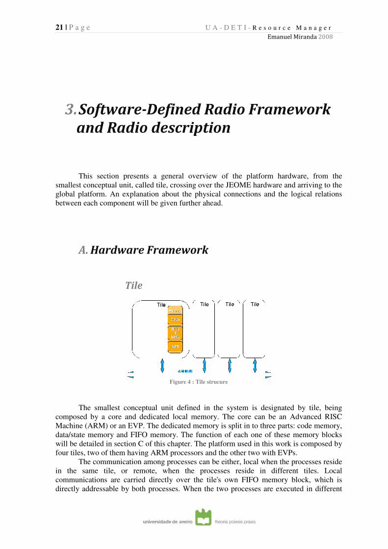
The smallest conceptual unit defined in the system is designated by tile, being
composed by a core and dedicated local memory. The core can be an Advanced RISC
Machine (ARM) or an EVP. The dedicated memory is split in to three parts: code memory,
data/state memory and FIFO memory. The function of each one of these memory blocks
will be detailed in section C
four tiles, two of them having ARM processors and the other two with EVP
The communication among processes can be either, local when the processes reside
in the same tile, or remote, when the processes reside in different tiles. Local
communications are carried directly over the tile's own FIFO memory block, which is
directly addressable by both processes. When the two processes are executed in different
U A - D E T I - R e s o u r c e M a n a g e r
Emanuel Miranda
Software-Defined Radio Framework
and Radio description
This section presents a general overview of the platform hardware, from the
smallest conceptual unit, called tile, crossing over the JEOME hardware and arriving to the
global platform. An explanation about the physical connections and the logical relations
between each component will be given further ahead.
Hardware Framework
Tile
Figure 4 : Tile strucure
The smallest conceptual unit defined in the system is designated by tile, being
composed by a core and dedicated local memory. The core can be an Advanced RISC
Machine (ARM) or an EVP. The dedicated memory is split in to three parts: code memory,
e memory and FIFO memory. The function of each one of these memory blocks
C of this chapter. The platform used in this work is composed
four tiles, two of them having ARM processors and the other two with EVP
The communication among processes can be either, local when the processes reside
in the same tile, or remote, when the processes reside in different tiles. Local
are carried directly over the tile's own FIFO memory block, which is
directly addressable by both processes. When the two processes are executed in different
R e s o u r c e M a n a g e r
Emanuel Miranda 2008
Defined Radio Framework
This section presents a general overview of the platform hardware, from the
d tile, crossing over the JEOME hardware and arriving to the
global platform. An explanation about the physical connections and the logical relations
The smallest conceptual unit defined in the system is designated by tile, being
composed by a core and dedicated local memory. The core can be an Advanced RISC
Machine (ARM) or an EVP. The dedicated memory is split in to three parts: code memory,
e memory and FIFO memory. The function of each one of these memory blocks
of this chapter. The platform used in this work is composed by
four tiles, two of them having ARM processors and the other two with EVPs.
The communication among processes can be either, local when the processes reside
in the same tile, or remote, when the processes reside in different tiles. Local
are carried directly over the tile's own FIFO memory block, which is
directly addressable by both processes. When the two processes are executed in different
22 | P a g e
tiles the communication is carried out via the Advanced eXtensible Interface (AXI) (
4). In this case the FIFO memory is allocated only in the tile of one of the processes.
Consider for instance a process A running on tile #1 that needs to transfer data to a
B that will execute in tile #2. In the example the FIFO memory is allocated in tile B and,
consequently, when process A issues a write operation the data is actually written in FIFO
memory of the tile #2. Process B reads the data it from its own l
operations are more costly than local operations, a factor that has to be taken into account
during the system design. Therefore, communicating processes should, whenever possible,
be allocated to the same tile to minimize the communica
For the sake of performance, the FIFO memory is preferably allocated to the tile of
the consumer process. As stated above, remote operations, carried out via that AXI bus, are
more costly than local operations, issued on local memory. Writin
succeed, provided that the buffers are properly dimensioned. On the other hand, the reader
process has to pool the memory to detect the arrival of new data. Thus, a single data
transaction typically involves a single write operation and
consequently, the complexity of the reading operation end up having a higher impact on
the system performance than the complexity of the write operation.
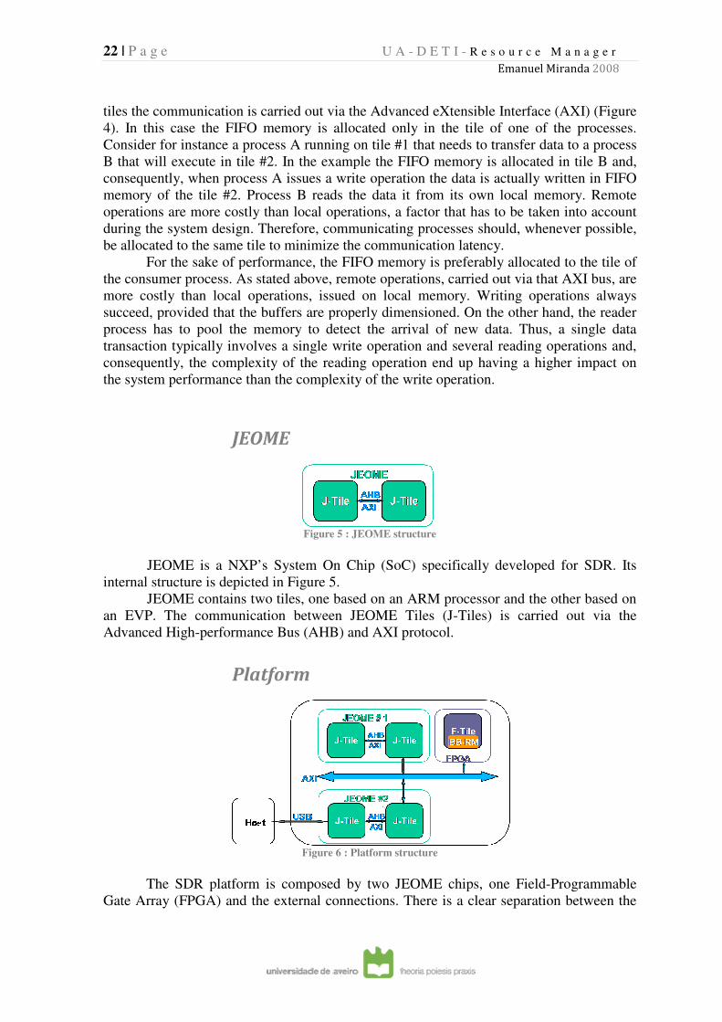
JEOME
JEOME is a NXP’s System On Chip (SoC) specifically developed for SDR. Its
internal structure is depicted in
JEOME contains two tiles,
an EVP. The communication between
Advanced High-performance
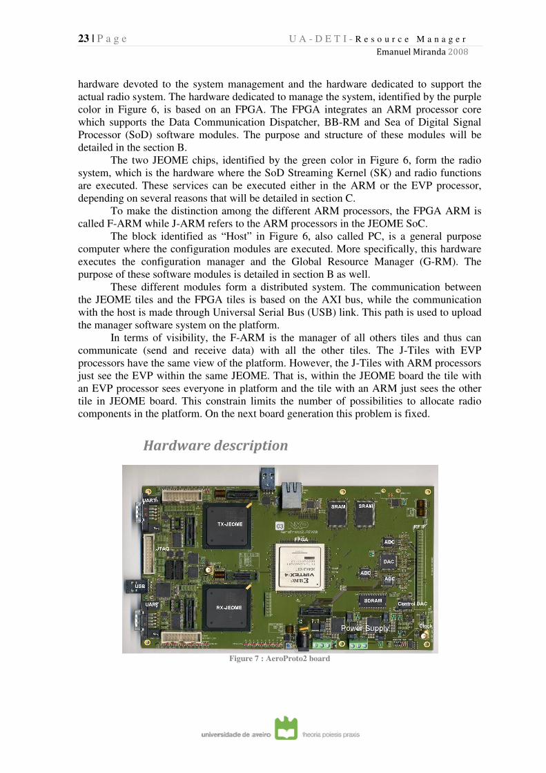
Platform
The SDR platform is composed by two JEOME chips, one
Gate Array (FPGA) and the external connections. There is a clear separation between the
U A - D E T I - R e s o u r c e M a n a g e r
Emanuel Miranda
tiles the communication is carried out via the Advanced eXtensible Interface (AXI) (
). In this case the FIFO memory is allocated only in the tile of one of the processes.
Consider for instance a process A running on tile #1 that needs to transfer data to a
B that will execute in tile #2. In the example the FIFO memory is allocated in tile B and,
consequently, when process A issues a write operation the data is actually written in FIFO
memory of the tile #2. Process B reads the data it from its own local memory. Remote
operations are more costly than local operations, a factor that has to be taken into account
during the system design. Therefore, communicating processes should, whenever possible,
be allocated to the same tile to minimize the communication latency.
For the sake of performance, the FIFO memory is preferably allocated to the tile of
the consumer process. As stated above, remote operations, carried out via that AXI bus, are
more costly than local operations, issued on local memory. Writing operations always
succeed, provided that the buffers are properly dimensioned. On the other hand, the reader
process has to pool the memory to detect the arrival of new data. Thus, a single data
transaction typically involves a single write operation and several reading operations and,
consequently, the complexity of the reading operation end up having a higher impact on
the system performance than the complexity of the write operation.
JEOME
Figure 5 : JEOME structure
JEOME is a NXP’s System On Chip (SoC) specifically developed for SDR. Its
internal structure is depicted in Figure 5.
JEOME contains two tiles, one based on an ARM processor and the other based on
EVP. The communication between JEOME Tiles (J-Tiles) is carried out via the
performance Bus (AHB) and AXI protocol.
Platform
Figure 6 : Platform structure
The SDR platform is composed by two JEOME chips, one Field
(FPGA) and the external connections. There is a clear separation between the
R e s o u r c e M a n a g e r
Emanuel Miranda 2008
tiles the communication is carried out via the Advanced eXtensible Interface (AXI) (Figure
). In this case the FIFO memory is allocated only in the tile of one of the processes.
Consider for instance a process A running on tile #1 that needs to transfer data to a process
B that will execute in tile #2. In the example the FIFO memory is allocated in tile B and,
consequently, when process A issues a write operation the data is actually written in FIFO
ocal memory. Remote
operations are more costly than local operations, a factor that has to be taken into account
during the system design. Therefore, communicating processes should, whenever possible,
For the sake of performance, the FIFO memory is preferably allocated to the tile of
the consumer process. As stated above, remote operations, carried out via that AXI bus, are
g operations always
succeed, provided that the buffers are properly dimensioned. On the other hand, the reader
process has to pool the memory to detect the arrival of new data. Thus, a single data
several reading operations and,
consequently, the complexity of the reading operation end up having a higher impact on
JEOME is a NXP’s System On Chip (SoC) specifically developed for SDR. Its
one based on an ARM processor and the other based on
is carried out via the
Field-Programmable
(FPGA) and the external connections. There is a clear separation between the
23 | P a g e U A - D E T I - R e s o u r c e M a n a g e r
Emanuel Miranda 2008
hardware devoted to the system management and the hardware dedicated to support the
actual radio system. The hardware dedicated to manage the system, identified by the purple
color in Figure 6, is based on an FPGA. The FPGA integrates an ARM processor core
which supports the Data Communication Dispatcher, BB-RM and Sea of Digital Signal
Processor (SoD) software modules. The purpose and structure of these modules will be
detailed in the section B.
The two JEOME chips, identified by the green color in Figure 6, form the radio
system, which is the hardware where the SoD Streaming Kernel (SK) and radio functions
are executed. These services can be executed either in the ARM or the EVP processor,
depending on several reasons that will be detailed in section C.
To make the distinction among the different ARM processors, the FPGA ARM is
called F-ARM while J-ARM refers to the ARM processors in the JEOME SoC.
The block identified as “Host” in Figure 6, also called PC, is a general purpose
computer where the configuration modules are executed. More specifically, this hardware
executes the configuration manager and the Global Resource Manager (G-RM). The
purpose of these software modules is detailed in section B as well.
These different modules form a distributed system. The communication between
the JEOME tiles and the FPGA tiles is based on the AXI bus, while the communication
with the host is made through Universal Serial Bus (USB) link. This path is used to upload
the manager software system on the platform.
In terms of visibility, the F-ARM is the manager of all others tiles and thus can
communicate (send and receive data) with all the other tiles. The J-Tiles with EVP
processors have the same view of the platform. However, the J-Tiles with ARM processors
just see the EVP within the same JEOME. That is, within the JEOME board the tile with
an EVP processor sees everyone in platform and the tile with an ARM just sees the other
tile in JEOME board. This constrain limits the number of possibilities to allocate radio
components in the platform. On the next board generation this problem is fixed.
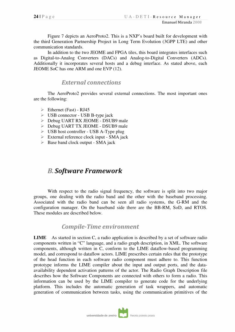
Hardware description
Figure 7 : AeroProto2 board
24 | P a g e U A - D E T I - R e s o u r c e M a n a g e r
Emanuel Miranda 2008
Figure 7 depicts an AeroProto2. This is a NXP’s board built for development with
the third Generation Partnership Project in Long Term Evolution (3GPP LTE) and other
communication standards.
In addition to the two JEOME and FPGA tiles, this board integrates interfaces such
as Digital-to-Analog Converters (DACs) and Analog-to-Digital Converters (ADCs).
Additionally it incorporates several hosts and a debug interface. As stated above, each
JEOME SoC has one ARM and one EVP (12).
External connections
The AeroProto2 provides several external connections. The most important ones
are the following:
� Ethernet (Fast) - RJ45
� USB connector - USB B-type jack
� Debug UART RX JEOME - DSUB9 male
� Debug UART TX JEOME - DSUB9 male
� USB host controller - USB A-Type plug
� External reference clock input - SMA jack
� Base band clock output - SMA jack
B. Software Framework
With respect to the radio signal frequency, the software is split into two major
groups, one dealing with the radio band and the other with the baseband processing.
Associated with the radio band can be seen all radio systems, the G-RM and the
configuration manager. On the baseband side there are the BB-RM, SoD, and RTOS.
These modules are described below.
Compile-Time environment
LIME As started in section C, a radio application is described by a set of software radio
components written in “C” language, and a radio graph description, in XML. The software
components, although written in C, conform to the LIME dataflow-based programming
model, and correspond to dataflow actors. LIME prescribes certain rules that the prototype
of the head function in each software radio component must adhere to. This function
prototype informs the LIME compiler about the input and output ports, and the data-
availability dependent activation patterns of the actor. The Radio Graph Description file
describes how the Software Components are connected with others to form a radio. This
information can be used by the LIME compiler to generate code for the underlying
platform. This includes the automatic generation of task wrappers, and automatic
generation of communication between tasks, using the communication primitives of the
25 | P a g e
underlying multi-processor operating system, which, in the current setup is SoD. The
LIME compiler also generates a dataflow analysis model, that can be used to compute the
amount of platform resources (processor cycles per period, buffer sizes) that ar
for the application to meet its real
sourced by NXP. The code and documentation detailing the usage of the language can be
found in (13).Furthermore, there is not a one
software components and tasks in the platform
compiler may decide –if possible
relative to each other, and merge them onto a single task, as described in
disadvantage that it reduce the run
also reduces the number of tasks in the radio, the tas
the bounds of worst-case timing analysis, which in turn allows the computation of smaller
resource requirements. This is described in detail in
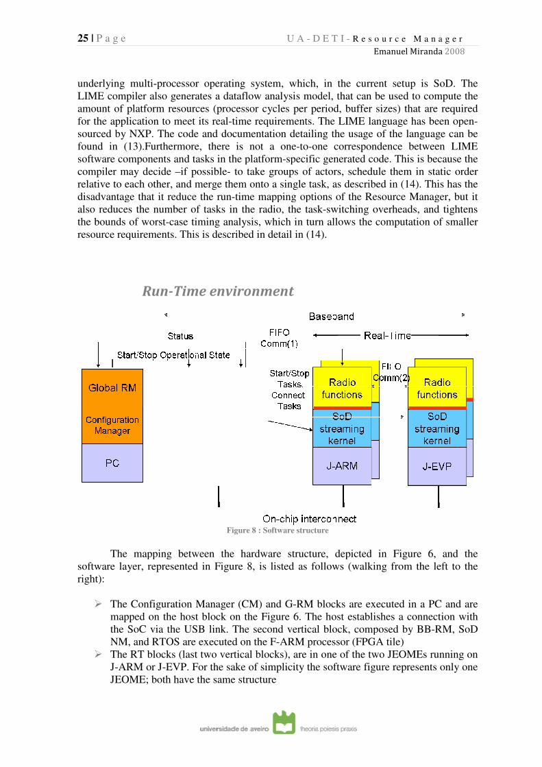
Run-Time environment
The mapping between the hardware structure, depicted in
software layer, represented in
right):
� The Configuration Manager (CM) and G
mapped on the host block on the
the SoC via the USB link. The second vertical block, composed by BB
NM, and RTOS are executed on
� The RT blocks (last two vertical blocks), are in one of the two JEOMEs running on
J-ARM or J-EVP. For the sake of simpli
JEOME; both have the same structure
U A - D E T I - R e s o u r c e M a n a g e r
Emanuel Miranda
processor operating system, which, in the current setup is SoD. The
LIME compiler also generates a dataflow analysis model, that can be used to compute the
amount of platform resources (processor cycles per period, buffer sizes) that ar
for the application to meet its real-time requirements. The LIME language has been open
sourced by NXP. The code and documentation detailing the usage of the language can be
Furthermore, there is not a one-to-one correspondence between LIME
software components and tasks in the platform-specific generated code. This is because the
if possible- to take groups of actors, schedule them in static order
to each other, and merge them onto a single task, as described in
disadvantage that it reduce the run-time mapping options of the Resource Manager, but it
also reduces the number of tasks in the radio, the task-switching overheads, and tightens
case timing analysis, which in turn allows the computation of smaller
resource requirements. This is described in detail in (14).
Time environment
Figure 8 : Software structure
The mapping between the hardware structure, depicted in
software layer, represented in Figure 8, is listed as follows (walking from the left to the
The Configuration Manager (CM) and G-RM blocks are executed in a PC and are
mapped on the host block on the Figure 6. The host establishes a connection with
he SoC via the USB link. The second vertical block, composed by BB
RTOS are executed on the F-ARM processor (FPGA tile)
The RT blocks (last two vertical blocks), are in one of the two JEOMEs running on
EVP. For the sake of simplicity the software figure represents only one
E; both have the same structure
R e s o u r c e M a n a g e r
Emanuel Miranda 2008
processor operating system, which, in the current setup is SoD. The
LIME compiler also generates a dataflow analysis model, that can be used to compute the
amount of platform resources (processor cycles per period, buffer sizes) that are required
time requirements. The LIME language has been open-
sourced by NXP. The code and documentation detailing the usage of the language can be
one correspondence between LIME
specific generated code. This is because the
to take groups of actors, schedule them in static order
to each other, and merge them onto a single task, as described in (14). This has the
time mapping options of the Resource Manager, but it
switching overheads, and tightens
case timing analysis, which in turn allows the computation of smaller
The mapping between the hardware structure, depicted in Figure 6, and the
, is listed as follows (walking from the left to the
RM blocks are executed in a PC and are
. The host establishes a connection with
he SoC via the USB link. The second vertical block, composed by BB-RM, SoD
ARM processor (FPGA tile)
The RT blocks (last two vertical blocks), are in one of the two JEOMEs running on
city the software figure represents only one
26 | P a g e U A - D E T I - R e s o u r c e M a n a g e r
Emanuel Miranda 2008
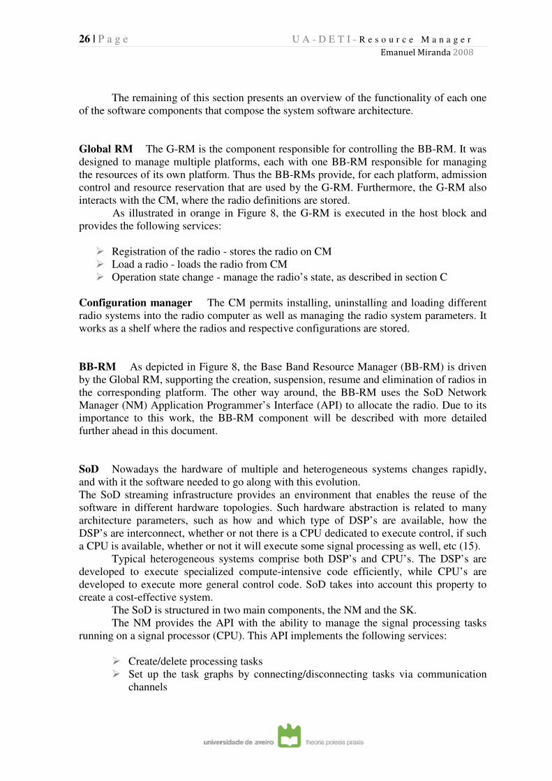
The remaining of this section presents an overview of the functionality of each one
of the software components that compose the system software architecture.
Global RM The G-RM is the component responsible for controlling the BB-RM. It was
designed to manage multiple platforms, each with one BB-RM responsible for managing
the resources of its own platform. Thus the BB-RMs provide, for each platform, admission
control and resource reservation that are used by the G-RM. Furthermore, the G-RM also
interacts with the CM, where the radio definitions are stored.
As illustrated in orange in Figure 8, the G-RM is executed in the host block and
provides the following services:
� Registration of the radio - stores the radio on CM
� Load a radio - loads the radio from CM
� Operation state change - manage the radio’s state, as described in section C
Configuration manager The CM permits installing, uninstalling and loading different
radio systems into the radio computer as well as managing the radio system parameters. It
works as a shelf where the radios and respective configurations are stored.
BB-RM As depicted in Figure 8, the Base Band Resource Manager (BB-RM) is driven
by the Global RM, supporting the creation, suspension, resume and elimination of radios in
the corresponding platform. The other way around, the BB-RM uses the SoD Network
Manager (NM) Application Programmer’s Interface (API) to allocate the radio. Due to its
importance to this work, the BB-RM component will be described with more detailed
further ahead in this document.
SoD Nowadays the hardware of multiple and heterogeneous systems changes rapidly,
and with it the software needed to go along with this evolution.
The SoD streaming infrastructure provides an environment that enables the reuse of the
software in different hardware topologies. Such hardware abstraction is related to many
architecture parameters, such as how and which type of DSP’s are available, how the
DSP’s are interconnect, whether or not there is a CPU dedicated to execute control, if such
a CPU is available, whether or not it will execute some signal processing as well, etc (15).
Typical heterogeneous systems comprise both DSP’s and CPU’s. The DSP’s are
developed to execute specialized compute-intensive code efficiently, while CPU’s are
developed to execute more general control code. SoD takes into account this property to
create a cost-effective system.
The SoD is structured in two main components, the NM and the SK.
The NM provides the API with the ability to manage the signal processing tasks
running on a signal processor (CPU). This API implements the following services:
� Create/delete processing tasks
� Set up the task graphs by connecting/disconnecting tasks via communication
channels
27 | P a g e U A - D E T I - R e s o u r c e M a n a g e r
Emanuel Miranda 2008
� Suspend/resume tasks
� Provide exchange of commands and status information with tasks
The SK executes the task scheduler and supports the data communication required
by the processing tasks by doing the following:
� Dispatching the signal processing tasks on the DSP or control processor
� Controlling the flow of signal data by managing the data dependencies between the
processing tasks
� Handling data exchange between tasks through communication buffers
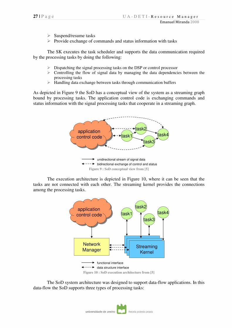
As depicted in Figure 9 the SoD has a conceptual view of the system as a streaming graph
bound by processing tasks. The application control code is exchanging commands and
status information with the signal processing tasks that cooperate in a streaming graph.
Figure 9 : SoD conceptual view from [5]
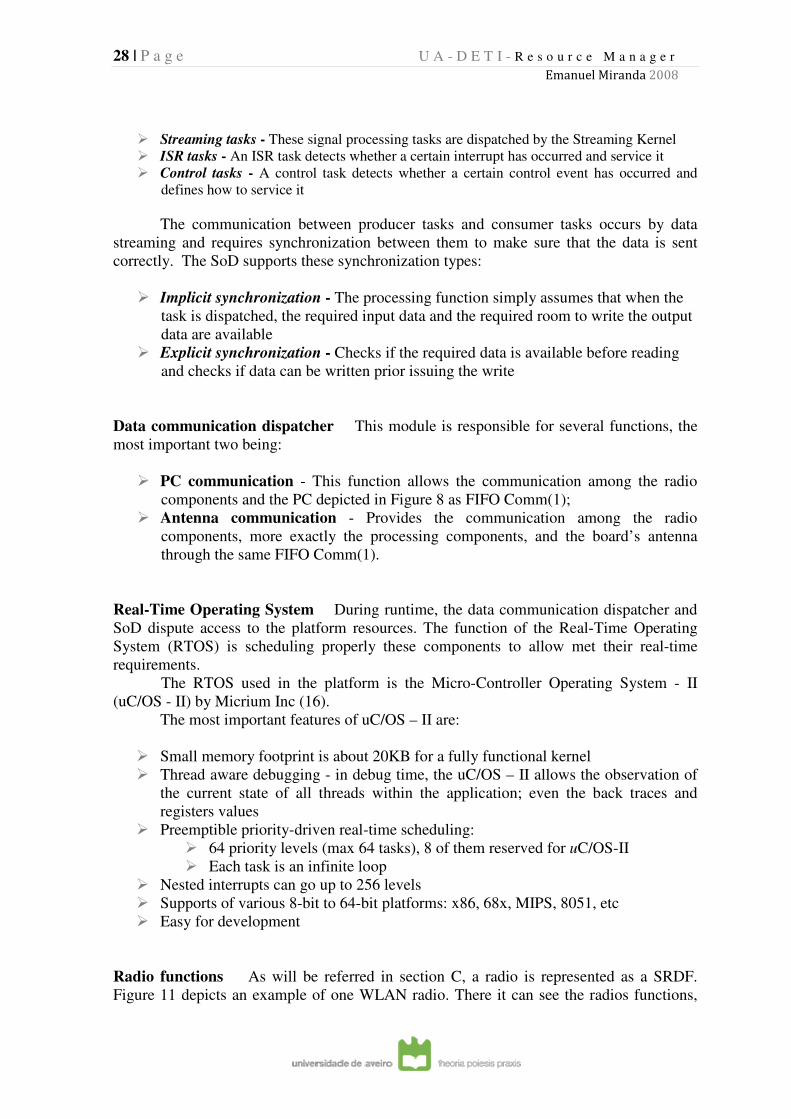
The execution architecture is depicted in Figure 10, where it can be seen that the
tasks are not connected with each other. The streaming kernel provides the connections
among the processing tasks.
Figure 10 : SoD execution architecture from [5]
The SoD system architecture was designed to support data-flow applications. In this
data-flow the SoD supports three types of processing tasks:
task1
task2
task3
task4applicationcontrol code
applicationcontrol code
unidirectional stream of signal data
bidirectional exchange of control and status
Network
Manager
Streaming
KernelStreaming
KernelStreaming
Kernel
task1
task2
task3
task4application
control code
application
control code
functional interface
data structure interface
28 | P a g e U A - D E T I - R e s o u r c e M a n a g e r
Emanuel Miranda 2008
� Streaming tasks - These signal processing tasks are dispatched by the Streaming Kernel
� ISR tasks - An ISR task detects whether a certain interrupt has occurred and service it
� Control tasks - A control task detects whether a certain control event has occurred and
defines how to service it
The communication between producer tasks and consumer tasks occurs by data
streaming and requires synchronization between them to make sure that the data is sent
correctly. The SoD supports these synchronization types:
� Implicit synchronization - The processing function simply assumes that when the
task is dispatched, the required input data and the required room to write the output
data are available
� Explicit synchronization - Checks if the required data is available before reading
and checks if data can be written prior issuing the write
Data communication dispatcher This module is responsible for several functions, the
most important two being:
� PC communication - This function allows the communication among the radio
components and the PC depicted in Figure 8 as FIFO Comm(1);
� Antenna communication - Provides the communication among the radio
components, more exactly the processing components, and the board’s antenna
through the same FIFO Comm(1).
Real-Time Operating System During runtime, the data communication dispatcher and
SoD dispute access to the platform resources. The function of the Real-Time Operating
System (RTOS) is scheduling properly these components to allow met their real-time
requirements.
The RTOS used in the platform is the Micro-Controller Operating System - II
(uC/OS - II) by Micrium Inc (16).
The most important features of uC/OS – II are:
� Small memory footprint is about 20KB for a fully functional kernel
� Thread aware debugging - in debug time, the uC/OS – II allows the observation of
the current state of all threads within the application; even the back traces and
registers values
� Preemptible priority-driven real-time scheduling:
� 64 priority levels (max 64 tasks), 8 of them reserved for uC/OS-II
� Each task is an infinite loop
� Nested interrupts can go up to 256 levels
� Supports of various 8-bit to 64-bit platforms: x86, 68x, MIPS, 8051, etc
� Easy for development
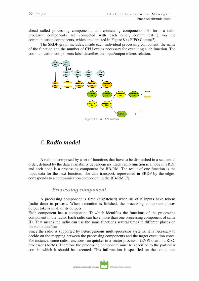
Radio functions As will be referred in section C, a radio is represented as a SRDF.
Figure 11 depicts an example of one WLAN radio. There it can see the radios functions,
29 | P a g e
ahead called processing components, and connecting components. To form a radio
processor components are connected with each other, communicating via the
communication components, which are depicted in
The SRDF graph includes, inside each individual processing component, the name
of the function and the number of CPU cycles necessary for executing such function. The
communication components label describes the input/output tokens relation.
C. Radio model
A radio is composed by a set of functions that have to be dispatched in a sequential
order, defined by the data availability
and each node is a processing component for BB
input data for the next function. The data transport, represented in SRDF by the edges,
corresponds to a communication
Processing component
A processing component is fired (dispatched) when all of it inputs have tokens
(radio data) to process. When
output tokens in all of its outputs.
Each component has a component ID which identifies the functions of the processing
component in the radio. Each radio can have more than one processing component of same
ID. That means the radio can use the same functions sev
the radio dataflow.
Since the radio is supported by heterogeneous multi
decide on the mapping between the processing components and the target execution cores.
For instance, some radio functions run quicker in a vector processor (EVP) than in a RISC
processor (ARM). Therefore the processing component must be specified to the particular
core in which it should be executed. This information is specified on the component
U A - D E T I - R e s o u r c e M a n a g e r
Emanuel Miranda
processing components, and connecting components. To form a radio
processor components are connected with each other, communicating via the
communication components, which are depicted in Figure 8 as FIFO Comm(2).
The SRDF graph includes, inside each individual processing component, the name
of the function and the number of CPU cycles necessary for executing such function. The
tion components label describes the input/output tokens relation.
Figure 11 : WLAN datflow
Radio model
A radio is composed by a set of functions that have to be dispatched in a sequential
order, defined by the data availability dependencies. Each radio function is a node in SRDF
and each node is a processing component for BB-RM. The result of one function is the
input data for the next function. The data transport, represented in SRDF by the edges,
corresponds to a communication component in the BB-RM (7).
Processing component
A processing component is fired (dispatched) when all of it inputs have tokens
(radio data) to process. When execution is finished, the processing component
tokens in all of its outputs.
Each component has a component ID which identifies the functions of the processing
component in the radio. Each radio can have more than one processing component of same
ID. That means the radio can use the same functions several times in different places on
Since the radio is supported by heterogeneous multi-processor systems, it is necessary to
decide on the mapping between the processing components and the target execution cores.
functions run quicker in a vector processor (EVP) than in a RISC
processor (ARM). Therefore the processing component must be specified to the particular
core in which it should be executed. This information is specified on the component
R e s o u r c e M a n a g e r
Emanuel Miranda 2008
processing components, and connecting components. To form a radio
processor components are connected with each other, communicating via the
as FIFO Comm(2).
The SRDF graph includes, inside each individual processing component, the name
of the function and the number of CPU cycles necessary for executing such function. The
tion components label describes the input/output tokens relation.
A radio is composed by a set of functions that have to be dispatched in a sequential
dependencies. Each radio function is a node in SRDF
RM. The result of one function is the
input data for the next function. The data transport, represented in SRDF by the edges,
A processing component is fired (dispatched) when all of it inputs have tokens
, the processing component places
Each component has a component ID which identifies the functions of the processing
component in the radio. Each radio can have more than one processing component of same
eral times in different places on
processor systems, it is necessary to
decide on the mapping between the processing components and the target execution cores.
functions run quicker in a vector processor (EVP) than in a RISC
processor (ARM). Therefore the processing component must be specified to the particular
core in which it should be executed. This information is specified on the component
30 | P a g e U A - D E T I - R e s o u r c e M a n a g e r
Emanuel Miranda 2008
structure. For this reason the radio structure (section D), comprises a field that permits
specifying the permitted execution hardware of the processing components. Each
processing component can either be allocated to a specific core or to a core type of the
available core types in the platform.
The instantiation of a processing component requires different types of resources:
code memory, where the instructions of the processing component are already stored; data
state memory to store the temporary variables and component state; and a CPU to execute
the code.
Communication component
This platform is based on a distributed architecture, thus communication channels
are required to allow the proper cooperation between the diverse system components. This
service is provided by the communication components. Making the analogy between the
radio description and a SRDF graph, the communication component in radio description
corresponds to an arrow in a SRDF.
The communication components implement a FIFO discipline and are responsible for
handling the tokens from each producer processing component to the corresponding
consumer processing component. Communication components have the information about
who are the producer and consumer processing components, as well as their port IDs.
Depending on the placement of the involved nodes the communication process may be
local or involve two different tiles. When the communication is on the same tile, the
reserved FIFO memory is also on the same tile and is directly addressable by both
processes. On the other hand, if the communication is among two components placed in
different tiles the FIFO memory must reside physically on only one of those two tiles. In
this case the communication component can have already defined in which tile the FIFO
memory shall be created or, if this information is not provided in advance, the BB-RM at
allocation time chooses in which tile it will reserve the FIFO memory. In both cases each
communication component has to reserve enough memory resources to guarantee lossless
token delivery.
The radio activity has disparate behaviors, depending on which function is being
executed in each instant. The radios might be receiving data, sending data or just waiting
for some synchronous signal. Such behaviors produce different radio functions, i.e., the
radio data flow is different for each behavior. These different behaviors experienced by the
radios are called radio states. Besides the operating states, associated with the specific
tasks that have to be carried out by the processing nodes, additional radio states are created
explicitly in order to optimize the platform resources. For example, when the radio is not
processing data its state can change to some specific idle state that allows saving battery.
31 | P a g e
D. Radio structure and design
The radio structure design has as its main driving directions modularity, simplicity
and low runtime overheads. These requirements have impact in diverse
implementation aspects.
Fixed size structures, independent of the number of components and even of the
topology (component connections), have been used to simplify and reduce the overhead
associated with the memory management. The radi
particular radio characteristics to facilitate the radio management by the G
RM. Another desirable feature that the radio should exhibit is a clear separation among
resources and topology. This separation allo
having to be aware of the topology as well as traverse the radios without needing to be
aware of the component resources.
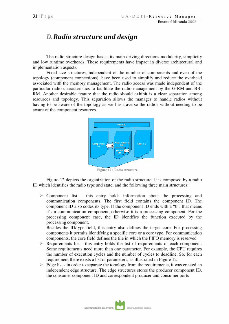
Figure 12 depicts the organization of the radio structure. It is composed by a radio
ID which identifies the radio type and state, and the following three main structures:
� Component list -
communication components. The first field contains the component ID. The
component ID also codes its type. If the component ID ends with a “0”, that means
it’s a communication component, otherwise it
processing component case, the ID identifies the function executed by the
processing component.
Besides the ID/type field, this entry also defines the target core. For processing
components it permits identifying a speci
components, the core field defines the tile in wh
� Requirements list -
Some requirements need more than one parameter. For
the number of execution cycles and the number of cycles to deadline. So, for each
requirement there exists a list of parameters, as illustrated in
� Edge list - in order to separate the topology from the requirements, it was created an
independent edge structure. The edge structures stores the producer component ID,
the consumer component ID and correspond
U A - D E T I - R e s o u r c e M a n a g e r
Emanuel Miranda
Radio structure and design
The radio structure design has as its main driving directions modularity, simplicity
and low runtime overheads. These requirements have impact in diverse
Fixed size structures, independent of the number of components and even of the
topology (component connections), have been used to simplify and reduce the overhead
associated with the memory management. The radio access was made independent of the
particular radio characteristics to facilitate the radio management by the G
RM. Another desirable feature that the radio should exhibit is a clear separation among
resources and topology. This separation allows the manager to handle radios without
having to be aware of the topology as well as traverse the radios without needing to be
aware of the component resources.
Figure 12 : Radio structure
depicts the organization of the radio structure. It is composed by a radio
ID which identifies the radio type and state, and the following three main structures:
this entry holds information about the processing and
communication components. The first field contains the component ID. The
component ID also codes its type. If the component ID ends with a “0”, that means
it’s a communication component, otherwise it is a processing component. For the
processing component case, the ID identifies the function executed by the
processing component.
Besides the ID/type field, this entry also defines the target core. For processing
components it permits identifying a specific core or a core type. For communication
components, the core field defines the tile in which the FIFO memory is reserved
- this entry holds the list of requirements of each component.
Some requirements need more than one parameter. For example, the CPU requires
the number of execution cycles and the number of cycles to deadline. So, for each
requirement there exists a list of parameters, as illustrated in Figure
in order to separate the topology from the requirements, it was created an
independent edge structure. The edge structures stores the producer component ID,
the consumer component ID and correspondent producer and consumer
R e s o u r c e M a n a g e r
Emanuel Miranda 2008
The radio structure design has as its main driving directions modularity, simplicity
and low runtime overheads. These requirements have impact in diverse architectural and
Fixed size structures, independent of the number of components and even of the
topology (component connections), have been used to simplify and reduce the overhead
o access was made independent of the
particular radio characteristics to facilitate the radio management by the G-RM and BB-
RM. Another desirable feature that the radio should exhibit is a clear separation among
ws the manager to handle radios without
having to be aware of the topology as well as traverse the radios without needing to be
depicts the organization of the radio structure. It is composed by a radio
ID which identifies the radio type and state, and the following three main structures:
this entry holds information about the processing and
communication components. The first field contains the component ID. The
component ID also codes its type. If the component ID ends with a “0”, that means
is a processing component. For the
processing component case, the ID identifies the function executed by the
Besides the ID/type field, this entry also defines the target core. For processing
fic core or a core type. For communication
ich the FIFO memory is reserved
this entry holds the list of requirements of each component.
example, the CPU requires
the number of execution cycles and the number of cycles to deadline. So, for each
Figure 12
in order to separate the topology from the requirements, it was created an
independent edge structure. The edge structures stores the producer component ID,
ent producer and consumer ports

32 | P a g e
E. Radio example
The example on Figure
represented as a SRDF, where the processing components are
instructions executing a radio function
implement FIFO semantics.
U A - D E T I - R e s o u r c e M a n a g e r
Emanuel Miranda
Radio example
Figure 13 is a Wireless Local Area Network (WLAN) radio
represented as a SRDF, where the processing components are group
ions executing a radio function. The edges are communication components and
implement FIFO semantics.
Figure 13 : WLAN 802.11a example from [12]
R e s o u r c e M a n a g e r
Emanuel Miranda 2008
is a Wireless Local Area Network (WLAN) radio
groups of “C” language
. The edges are communication components and
33 | P a g e U A - D E T I - R e s o u r c e M a n a g e r
Emanuel Miranda 2008
4. Design space, problems and solutions
This chapter presents the implementation of the BB-RM. It will start by describing
the functionality provided by the BB-RM, followed by a description of the interfaces
between the BB-RM and the other software components of the radio system. Having
described both the intended functionality and interfaces of the BB-RM, the attention is
turned to the practical problem of implementing this functionality within the existing
framework, while taking into account all sorts of constraints, such as the ones imposed by
the hardware and limitations of the software that it must re-use. Four different
implementation solutions are proposed and assessed, one of them being selected for
implementation.
A. Goals of BB-RM
As was explained in chapter 3 section B, the BB-RM functionality establishes an
interface between the G-RM and the SoD modules.
BB-RM must support a wide variety of radios and radio combinations, with
different software components, topologies and temporal requirements. Furthermore, it must
also provide RT guarantees for each running radio, even without having at compile-time
the complete knowledge of all the possible radio combinations that may be active in the
device. Each radio needs to meet its timing requirements, and it must do it independently
of other radios that are running simultaneously. To turn this possible, the BB-RM has to
guarantee to each different radio that a certain amount of system resources (processor
cycles, memory, communication), that match its resource requirements as computed at
compile-time, are available at runtime.
There are two main features that the BB-RM needs to support in order to provide
this functionality:
� Strict admission control - radio instances can only start if there are enough
resources available in the platform to guarantee the RT behavior
� Strict resource reservation - each radio is only allowed to use the resources that
have been allocated to it by BB-RM
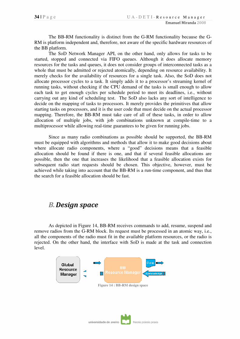
34 | P a g e
The BB-RM functionality is distinct from the G
RM is platform independent and, therefore, not aware of the specific hardware resources of
the BB platform.
The SoD Network Manager API, on the other hand, only allows for tasks to be
started, stopped and connected via FIFO queues. Although it does allocate memory
resources for the tasks and queues, it does not
whole that must be admitted or rejected atomically, depending on resource availability. It
merely checks for the availability of resources for a single task. Also, the SoD does not
allocate processor cycles to a task. It simply adds it to a processor’s streaming
running tasks, without checking if the CPU demand of the tasks is small enough to allow
each task to get enough cycles per schedule period to meet its deadlines, i.e., without
carrying out any kind of scheduling
decide on the mapping of tasks to processors. It merely provides the primitives that allow
starting tasks on processors
mapping. Therefore, the BB
allocation of multiple jobs
multiprocessor while allowing real
Since as many radio combinations as possible should be s
must be equipped with algorithms and methods that allow it to make good decisions about
where allocate radio components, where a “good” decisions means that a feasible
allocation should be found if there is one, and that if several feas
possible, then the one that increases the likelihood that a feasible allocation exists for
subsequent radio start requests should be chosen. This objective, however, must be
achieved while taking into account that the BB
the search for a feasible allocation should be fast.
B. Design space
As depicted in Figure
remove radios from the G-RM block. Its request must be processed in an atomic way, i.e.,
all the components of the radio must fit in the available platform resources, or the radio is
rejected. On the other hand, the interface with SoD is made a
level.
U A - D E T I - R e s o u r c e M a n a g e r
Emanuel Miranda
RM functionality is distinct from the G-RM functionality because the G
RM is platform independent and, therefore, not aware of the specific hardware resources of
he SoD Network Manager API, on the other hand, only allows for tasks to be
started, stopped and connected via FIFO queues. Although it does allocate memory
resources for the tasks and queues, it does not consider groups of interconnected tasks as a
hat must be admitted or rejected atomically, depending on resource availability. It
merely checks for the availability of resources for a single task. Also, the SoD does not
allocate processor cycles to a task. It simply adds it to a processor’s streaming
running tasks, without checking if the CPU demand of the tasks is small enough to allow
each task to get enough cycles per schedule period to meet its deadlines, i.e., without
g out any kind of scheduling test. The SoD also lacks any sort
decide on the mapping of tasks to processors. It merely provides the primitives that allow
s, and it is the user code that must decide on the actual processor
mapping. Therefore, the BB-RM must take care of all of these tasks, in order to allow
allocation of multiple jobs, with job combinations unknown at c
while allowing real-time guarantees to be given for running jobs.
Since as many radio combinations as possible should be supported, the BB
must be equipped with algorithms and methods that allow it to make good decisions about
where allocate radio components, where a “good” decisions means that a feasible
allocation should be found if there is one, and that if several feasible allocations are
possible, then the one that increases the likelihood that a feasible allocation exists for
subsequent radio start requests should be chosen. This objective, however, must be
king into account that the BB-RM is a run-time component, and thus that
the search for a feasible allocation should be fast.
Design space
Figure 14, BB-RM receives commands to add, resume,
RM block. Its request must be processed in an atomic way, i.e.,
all the components of the radio must fit in the available platform resources, or the radio is
rejected. On the other hand, the interface with SoD is made at the task and connection
Figure 14 : BB-RM design space
R e s o u r c e M a n a g e r
Emanuel Miranda 2008
RM functionality because the G-
RM is platform independent and, therefore, not aware of the specific hardware resources of
he SoD Network Manager API, on the other hand, only allows for tasks to be
started, stopped and connected via FIFO queues. Although it does allocate memory
of interconnected tasks as a
hat must be admitted or rejected atomically, depending on resource availability. It
merely checks for the availability of resources for a single task. Also, the SoD does not
allocate processor cycles to a task. It simply adds it to a processor’s streaming kernel of
running tasks, without checking if the CPU demand of the tasks is small enough to allow
each task to get enough cycles per schedule period to meet its deadlines, i.e., without
test. The SoD also lacks any sort of intelligence to
decide on the mapping of tasks to processors. It merely provides the primitives that allow
, and it is the user code that must decide on the actual processor
l of these tasks, in order to allow
with job combinations unknown at compile-time to a
time guarantees to be given for running jobs.
upported, the BB-RM
must be equipped with algorithms and methods that allow it to make good decisions about
where allocate radio components, where a “good” decisions means that a feasible
ible allocations are
possible, then the one that increases the likelihood that a feasible allocation exists for
subsequent radio start requests should be chosen. This objective, however, must be
me component, and thus that
RM receives commands to add, resume, suspend and
RM block. Its request must be processed in an atomic way, i.e.,
all the components of the radio must fit in the available platform resources, or the radio is
t the task and connection
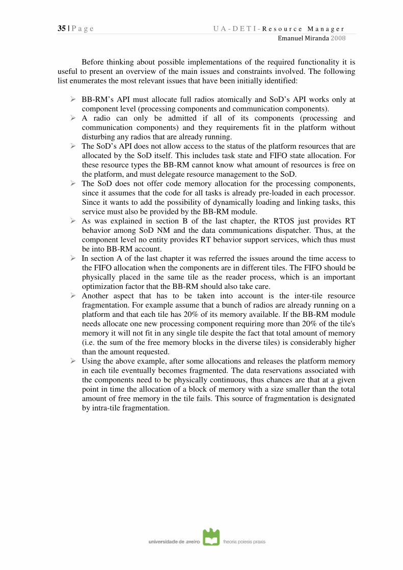
35 | P a g e U A - D E T I - R e s o u r c e M a n a g e r
Emanuel Miranda 2008
Before thinking about possible implementations of the required functionality it is
useful to present an overview of the main issues and constraints involved. The following
list enumerates the most relevant issues that have been initially identified:
� BB-RM’s API must allocate full radios atomically and SoD’s API works only at
component level (processing components and communication components).
� A radio can only be admitted if all of its components (processing and
communication components) and they requirements fit in the platform without
disturbing any radios that are already running.
� The SoD’s API does not allow access to the status of the platform resources that are
allocated by the SoD itself. This includes task state and FIFO state allocation. For
these resource types the BB-RM cannot know what amount of resources is free on
the platform, and must delegate resource management to the SoD.
� The SoD does not offer code memory allocation for the processing components,
since it assumes that the code for all tasks is already pre-loaded in each processor.
Since it wants to add the possibility of dynamically loading and linking tasks, this
service must also be provided by the BB-RM module.
� As was explained in section B of the last chapter, the RTOS just provides RT
behavior among SoD NM and the data communications dispatcher. Thus, at the
component level no entity provides RT behavior support services, which thus must
be into BB-RM account.
� In section A of the last chapter it was referred the issues around the time access to
the FIFO allocation when the components are in different tiles. The FIFO should be
physically placed in the same tile as the reader process, which is an important
optimization factor that the BB-RM should also take care.
� Another aspect that has to be taken into account is the inter-tile resource
fragmentation. For example assume that a bunch of radios are already running on a
platform and that each tile has 20% of its memory available. If the BB-RM module
needs allocate one new processing component requiring more than 20% of the tile's
memory it will not fit in any single tile despite the fact that total amount of memory
(i.e. the sum of the free memory blocks in the diverse tiles) is considerably higher
than the amount requested.
� Using the above example, after some allocations and releases the platform memory
in each tile eventually becomes fragmented. The data reservations associated with
the components need to be physically continuous, thus chances are that at a given
point in time the allocation of a block of memory with a size smaller than the total
amount of free memory in the tile fails. This source of fragmentation is designated
by intra-tile fragmentation.
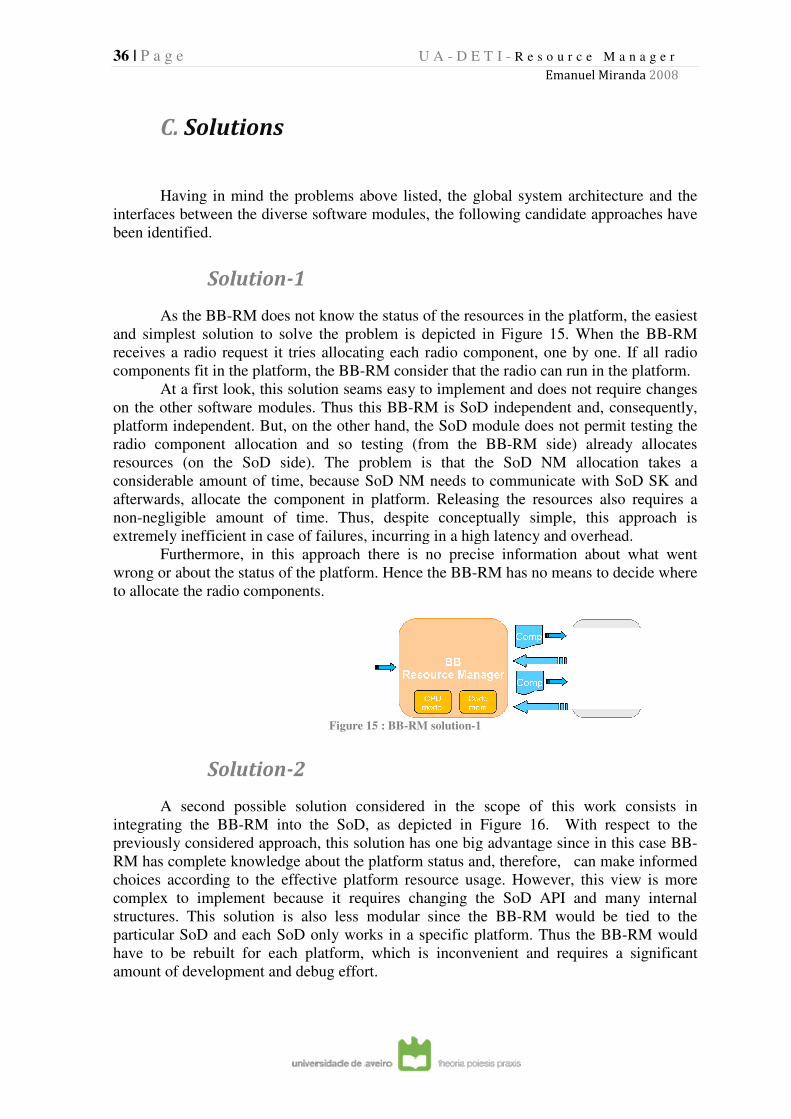
36 | P a g e
C. Solutions
Having in mind the problems
interfaces between the diverse software modules, the following candidate approaches have
been identified.
Solution
As the BB-RM does not know the status of the resources in the platform, the easiest
and simplest solution to solve the problem is depicted in
receives a radio request it tries allocating each radio component, one by one. If all
components fit in the platform, the BB
At a first look, this solution seams easy to implement and does not require changes
on the other software modules. Thus this BB
platform independent. But,
radio component allocation and so testing (from the BB
resources (on the SoD side). The problem is that the SoD NM allocation tak
considerable amount of time, because SoD NM needs to communicate with SoD SK and
afterwards, allocate the comp
non-negligible amount of time. Thus, despite conceptually simple, this approach is
extremely inefficient in case of failures, incurring in a high latency and overhead.
Furthermore, in this approach ther
wrong or about the status of the platform. Hence the BB
to allocate the radio components.
Solution
A second possible solution considered in the scope of this work consists in
integrating the BB-RM into the SoD, as depicted in
previously considered approach, this solution has one big advantage since in this case BB
RM has complete knowledge about the platform status and, therefore, can m
choices according to the effective platform resource usage. However, this view is more
complex to implement because it requires changing the SoD API and many internal
structures. This solution is also less modular since the BB
particular SoD and each SoD only works in a specific platform. Thus the BB
have to be rebuilt for each platform, which is inconvenient and requires a significant
amount of development and debug effort.
U A - D E T I - R e s o u r c e M a n a g e r
Emanuel Miranda
Having in mind the problems above listed, the global system architecture and the
interfaces between the diverse software modules, the following candidate approaches have
Solution-1
RM does not know the status of the resources in the platform, the easiest
d simplest solution to solve the problem is depicted in Figure 15. When the BB
receives a radio request it tries allocating each radio component, one by one. If all
components fit in the platform, the BB-RM consider that the radio can run in the platform.
At a first look, this solution seams easy to implement and does not require changes
on the other software modules. Thus this BB-RM is SoD independent and, con
platform independent. But, on the other hand, the SoD module does not permit testing the
radio component allocation and so testing (from the BB-RM side) already allocates
resources (on the SoD side). The problem is that the SoD NM allocation tak
considerable amount of time, because SoD NM needs to communicate with SoD SK and
afterwards, allocate the component in platform. Releasing the resources also requires a
negligible amount of time. Thus, despite conceptually simple, this approach is
extremely inefficient in case of failures, incurring in a high latency and overhead.
Furthermore, in this approach there is no precise information about what went
or about the status of the platform. Hence the BB-RM has no means to decide where
allocate the radio components.
Figure 15 : BB-RM solution-1
Solution-2
A second possible solution considered in the scope of this work consists in
RM into the SoD, as depicted in Figure 16. With respect to the
previously considered approach, this solution has one big advantage since in this case BB
RM has complete knowledge about the platform status and, therefore, can m
choices according to the effective platform resource usage. However, this view is more
complex to implement because it requires changing the SoD API and many internal
structures. This solution is also less modular since the BB-RM would be tied
particular SoD and each SoD only works in a specific platform. Thus the BB
have to be rebuilt for each platform, which is inconvenient and requires a significant
amount of development and debug effort.
R e s o u r c e M a n a g e r
Emanuel Miranda 2008
above listed, the global system architecture and the
interfaces between the diverse software modules, the following candidate approaches have
RM does not know the status of the resources in the platform, the easiest
. When the BB-RM
receives a radio request it tries allocating each radio component, one by one. If all radio
RM consider that the radio can run in the platform.
At a first look, this solution seams easy to implement and does not require changes
RM is SoD independent and, consequently,
n the other hand, the SoD module does not permit testing the
RM side) already allocates
resources (on the SoD side). The problem is that the SoD NM allocation takes a
considerable amount of time, because SoD NM needs to communicate with SoD SK and
resources also requires a
negligible amount of time. Thus, despite conceptually simple, this approach is
extremely inefficient in case of failures, incurring in a high latency and overhead.
ormation about what went
RM has no means to decide where
A second possible solution considered in the scope of this work consists in
. With respect to the
previously considered approach, this solution has one big advantage since in this case BB-
RM has complete knowledge about the platform status and, therefore, can make informed
choices according to the effective platform resource usage. However, this view is more
complex to implement because it requires changing the SoD API and many internal
RM would be tied to the
particular SoD and each SoD only works in a specific platform. Thus the BB-RM would
have to be rebuilt for each platform, which is inconvenient and requires a significant
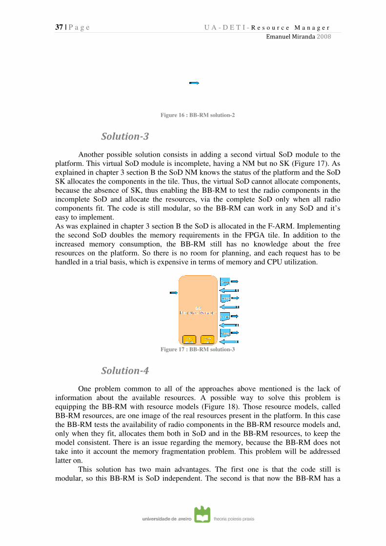
37 | P a g e
Solution
Another possible solution consists in adding a second virtual SoD module to the
platform. This virtual SoD module is incomplete, having a NM but no SK (
explained in chapter 3 section
SK allocates the components in the tile. Thus, the virtual SoD cannot allocate components,
because the absence of SK, thus enabling the BB
incomplete SoD and allocate the resources, via the complete SoD only when all radio
components fit. The code is still modular, so the BB
easy to implement.
As was explained in chapter
the second SoD doubles the memory requirements in the FPGA tile. In addit
increased memory consumption, the BB
resources on the platform. So there is no room for planning, and each request has to be
handled in a trial basis, which is expensive in terms of memory and CPU utiliza
Solution
One problem common to all of the approaches above mentioned is the lack of
information about the available resources. A possible way to solve this problem is
equipping the BB-RM wit
BB-RM resources, are one image of the real resources present in the platform. In this case
the BB-RM tests the availability of radio c
only when they fit, allocates them both in SoD and in the BB
model consistent. There is an issue regarding the memory, because the BB
take into it account the memory fragmentation problem. This problem will be addressed
latter on.
This solution has two main advantages. The first one is that the code still is
modular, so this BB-RM is SoD independent. The second is
U A - D E T I - R e s o u r c e M a n a g e r
Emanuel Miranda
Figure 16 : BB-RM solution-2
Solution-3
Another possible solution consists in adding a second virtual SoD module to the
platform. This virtual SoD module is incomplete, having a NM but no SK (
section B the SoD NM knows the status of the platform and the SoD
SK allocates the components in the tile. Thus, the virtual SoD cannot allocate components,
because the absence of SK, thus enabling the BB-RM to test the radio components in the
locate the resources, via the complete SoD only when all radio
components fit. The code is still modular, so the BB-RM can work in any SoD and it’s
As was explained in chapter 3 section B the SoD is allocated in the F-ARM. Implementing
the second SoD doubles the memory requirements in the FPGA tile. In addit
umption, the BB-RM still has no knowledge about the free
resources on the platform. So there is no room for planning, and each request has to be
handled in a trial basis, which is expensive in terms of memory and CPU utiliza
Figure 17 : BB-RM solution-3
Solution-4
One problem common to all of the approaches above mentioned is the lack of
information about the available resources. A possible way to solve this problem is
RM with resource models (Figure 18). Those resource models, called
RM resources, are one image of the real resources present in the platform. In this case
s the availability of radio components in the BB-RM resource models
only when they fit, allocates them both in SoD and in the BB-RM resources, to keep the
model consistent. There is an issue regarding the memory, because the BB
t account the memory fragmentation problem. This problem will be addressed
This solution has two main advantages. The first one is that the code still is
RM is SoD independent. The second is that now
R e s o u r c e M a n a g e r
Emanuel Miranda 2008
Another possible solution consists in adding a second virtual SoD module to the
platform. This virtual SoD module is incomplete, having a NM but no SK (Figure 17). As
the SoD NM knows the status of the platform and the SoD
SK allocates the components in the tile. Thus, the virtual SoD cannot allocate components,
RM to test the radio components in the
locate the resources, via the complete SoD only when all radio
RM can work in any SoD and it’s
ARM. Implementing
the second SoD doubles the memory requirements in the FPGA tile. In addition to the
knowledge about the free
resources on the platform. So there is no room for planning, and each request has to be
handled in a trial basis, which is expensive in terms of memory and CPU utilization.
One problem common to all of the approaches above mentioned is the lack of
information about the available resources. A possible way to solve this problem is
). Those resource models, called
RM resources, are one image of the real resources present in the platform. In this case
RM resource models and,
RM resources, to keep the
model consistent. There is an issue regarding the memory, because the BB-RM does not
t account the memory fragmentation problem. This problem will be addressed
This solution has two main advantages. The first one is that the code still is
that now the BB-RM has a
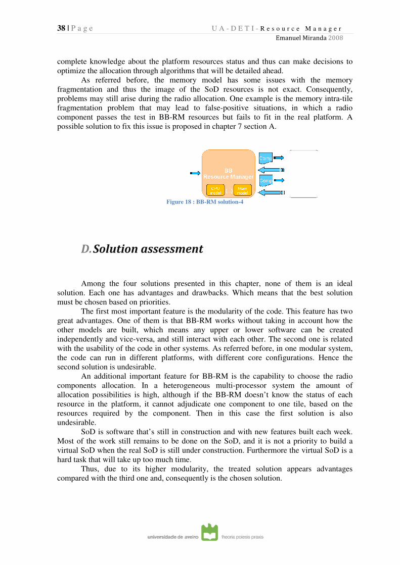
38 | P a g e
complete knowledge about the platform resources status and thus can make decisions to
optimize the allocation through algorithms that will be detailed ahead.
As referred before, the memory model has some issues with the memory
fragmentation and thus the image of
problems may still arise during the radio allocation. One example is the memory intra
fragmentation problem that may lead to false
component passes the test in BB
possible solution to fix this issue is proposed in chapter
D. Solution assessment
Among the four solutions presented in
solution. Each one has advantages and drawbacks.
must be chosen based on priorities.
The first most important feature is the modularity of the code. This feature has two
great advantages. One of them is that BB
other models are built, which means any upper or lower software can be created
independently and vice-versa, and still interact with each other. The second one is related
with the usability of the code in other systems. As referred before, in one modular system,
the code can run in different platforms, with different core configurations. Hence the
second solution is undesirable
An additional important feature for BB
components allocation. In a heterogeneous multi
allocation possibilities is high, although if the BB
resource in the platform, it cannot adjudicate one component to one tile, based on the
resources required by the component. Then in this case the first s
undesirable.
SoD is software that’s still in construction and with new features built each week.
Most of the work still remains to be done on the SoD, and it is not a priority to build a
virtual SoD when the real SoD is still under construc
hard task that will take up too much time.
Thus, due to its higher modularity, the treated
compared with the third one and, consequently is the chosen solution.
U A - D E T I - R e s o u r c e M a n a g e r
Emanuel Miranda
knowledge about the platform resources status and thus can make decisions to
optimize the allocation through algorithms that will be detailed ahead.
As referred before, the memory model has some issues with the memory
fragmentation and thus the image of the SoD resources is not exact. Consequently,
problems may still arise during the radio allocation. One example is the memory intra
fragmentation problem that may lead to false-positive situations, in which a radio
component passes the test in BB-RM resources but fails to fit in the real platform. A
possible solution to fix this issue is proposed in chapter 7 section A.
Figure 18 : BB-RM solution-4
assessment
four solutions presented in this chapter, none of them is
ach one has advantages and drawbacks. Which means that the best solution
must be chosen based on priorities.
The first most important feature is the modularity of the code. This feature has two
great advantages. One of them is that BB-RM works without taking in account how the
e built, which means any upper or lower software can be created
versa, and still interact with each other. The second one is related
with the usability of the code in other systems. As referred before, in one modular system,
can run in different platforms, with different core configurations. Hence the
is undesirable.
An additional important feature for BB-RM is the capability to choose the radio
components allocation. In a heterogeneous multi-processor system
allocation possibilities is high, although if the BB-RM doesn’t know the status of each
resource in the platform, it cannot adjudicate one component to one tile, based on the
resources required by the component. Then in this case the first s
SoD is software that’s still in construction and with new features built each week.
Most of the work still remains to be done on the SoD, and it is not a priority to build a
virtual SoD when the real SoD is still under construction. Furthermore the virtual SoD is a
hard task that will take up too much time.
Thus, due to its higher modularity, the treated solution appears advantages
compared with the third one and, consequently is the chosen solution.
R e s o u r c e M a n a g e r
Emanuel Miranda 2008
knowledge about the platform resources status and thus can make decisions to
As referred before, the memory model has some issues with the memory
the SoD resources is not exact. Consequently,
problems may still arise during the radio allocation. One example is the memory intra-tile
positive situations, in which a radio
esources but fails to fit in the real platform. A
this chapter, none of them is an ideal
hat the best solution
The first most important feature is the modularity of the code. This feature has two
RM works without taking in account how the
e built, which means any upper or lower software can be created
versa, and still interact with each other. The second one is related
with the usability of the code in other systems. As referred before, in one modular system,
can run in different platforms, with different core configurations. Hence the
RM is the capability to choose the radio
processor system the amount of
RM doesn’t know the status of each
resource in the platform, it cannot adjudicate one component to one tile, based on the
resources required by the component. Then in this case the first solution is also
SoD is software that’s still in construction and with new features built each week.
Most of the work still remains to be done on the SoD, and it is not a priority to build a
tion. Furthermore the virtual SoD is a
solution appears advantages
39 | P a g e U A - D E T I - R e s o u r c e M a n a g e r
Emanuel Miranda 2008
5. Implementation of the BB-RM
In the last chapter it was described four feasible solutions to implement a BB-RM.
Here it will dig a little deeper into the details. In its essence, the BB-RM is an allocator of
instances of radio applications. These instances are called jobs. In the following text, it will
further refine the concept of job in section A.
Section B briefly examines the main functions of the BB-RM.
One of the actions the BB-RM needs to perform is mapping the radio to the
hardware platform. Since the problem is NP-complete, BB-RM uses an approach based on
adapting heuristics used to solve the VBP Problem (section G) to allocate the radio
components to the hardware resources. Most heuristics for VBP define a couple of
strategies to solve sub-problems. One of the sub-problems is how to define the order in
which the components are mapped. The other sub-problem is choosing on which tile a
radio component should be allocated to. The strategies used in this work are described in
sections H and J of this chapter.
Finally, section K, describes the evolution of features across different versions of
BB-RM and the directory tree of the project.
A. Job – radio instance
As mentioned before, the main purpose of this project is to run multiple radios,
sharing resources with each other, and allow for many combinations of radios as possible.
Note that multiple instances of the same radio can be active simultaneously.
In chapter 3 at section C, a radio is described as a unique entity. To distinguish
between the unique unallocated radio and the allocated radio instances, it is defined the
concept of job.
Each time a radio is allocated to the platform, a different radio instance – a Job -is
created. The same logic is used when a radio software component is allocated to the
platform; it gets a radio processor component instance, which it refers to as a task. The
instance of a communication component is referred to as a FIFO. In summary, a radio is
composed of processing components and communication components. A job is composed
of tasks and FIFOs.
40 | P a g e U A - D E T I - R e s o u r c e M a n a g e r
Emanuel Miranda 2008
B. BB-RM functions
Until now, the BB-RM has been described as a black box with an input and an
output. This section will provide some brief information about each BB-RM function.
Further ahead the BBRM functions are described in more detail.
� BBRM_initialize - fills the job list with null values.
� BBRM_Job_test - tests if the given radio requirements can run in the HW platform
but will not allocate it.
� BBRM_Job_create - tests the radio requirements and allocates the radio in the
hardware platform; the created job is left on suspended mode.
� BBRM_Job_resume - runs the allocated job.
� BBRM_Job_suspend - suspends the running job.
� BBRM_Job_remove - removes the suspended job from the hardware platform.
C. Data structure of BB-RM
This section will show how the BB-RM stores and manages the information
concerning to jobs.
In the field, G-RM will provide the radio information when the BBRM_Job_create
function is called. Due to that, the BB-RM should store all information that it will need to
resume, suspend and remove a job.
After calling BBRM_Job_create, BB-RM returns a new job ID. This handler is used
to call the additional functions (job resume, job suspend, job remove).
Job list
Figure 19 shows the major internal structures of BB-RM. The job list, where BB-
RM stores all the information about jobs is depicted on the left side of this figure. In the
job list, one job entry is composed by a job settings and a task list. The job settings
structure has a pointer to the radio source and the radio ID; through it BB-RM can get
information about the radio components, its requirements, and the radio topology. Another
field of job settings structure is the job state, which save the status of the job (suspended,
running, resumed and invalid). These states will be detailed in the next section.
As explained before, BB-RM receives a complete radio from G-RM to allocate, but
SoD allocates components one by one. In this level each allocated component is called a
task and saved on a task list. BB-RM can choose where to allocate each component among
the different tiles. The algorithms to choose one tile for each component will be detailed in
section I. From this point on BB-RM should take care of the requirements of this
component to fit in the tile. This information is on the task settings structure. The source
component ID is saved in task settings.
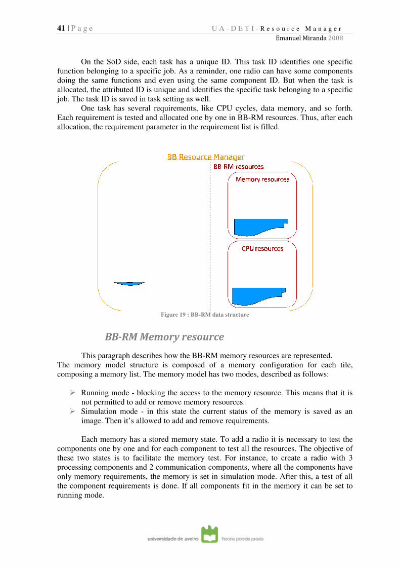
41 | P a g e
On the SoD side, each task has a unique ID. This task ID identifies one specific
function belonging to a specific job. As a reminder, one radio can have some components
doing the same functions and even using
allocated, the attributed ID is unique and identifies the specific task belonging to a specific
job. The task ID is saved in task setting as well.
One task has several requirements, like CPU cycles, data memory, and so forth.
Each requirement is tested and allocated one by one in BB
allocation, the requirement parameter in the requirement list is filled.
BB-RM Memory resource
This paragraph describes how t
The memory model structure is composed of a memory configuration for each tile,
composing a memory list. The memory model has two modes, described as follows:
� Running mode - blocking the access to the memory res
not permitted to add or remove memory resources.
� Simulation mode -
image. Then it’s allowed to add and remove requirements.
Each memory has a stored memory state.
components one by one and for each component to test all the resources. The objective of
these two states is to facilitate the memory test. For instance, to create a radio with 3
processing components and 2 commun
only memory requirements, the memory is set in simulation mode. After this, a test of all
the component requirements is done. If all components fit in the memory it can be set to
running mode.
U A - D E T I - R e s o u r c e M a n a g e r
Emanuel Miranda
On the SoD side, each task has a unique ID. This task ID identifies one specific
function belonging to a specific job. As a reminder, one radio can have some components
and even using the same component ID. But when th
allocated, the attributed ID is unique and identifies the specific task belonging to a specific
job. The task ID is saved in task setting as well.
One task has several requirements, like CPU cycles, data memory, and so forth.
tested and allocated one by one in BB-RM resources. Thus, after each
allocation, the requirement parameter in the requirement list is filled.
Figure 19 : BB-RM data structure
RM Memory resource
This paragraph describes how the BB-RM memory resources are represented.
emory model structure is composed of a memory configuration for each tile,
composing a memory list. The memory model has two modes, described as follows:
blocking the access to the memory resource. This means that it is
not permitted to add or remove memory resources.
in this state the current status of the memory is saved as an
image. Then it’s allowed to add and remove requirements.
Each memory has a stored memory state. To add a radio it is necessary to test the
components one by one and for each component to test all the resources. The objective of
these two states is to facilitate the memory test. For instance, to create a radio with 3
processing components and 2 communication components, where all the components have
only memory requirements, the memory is set in simulation mode. After this, a test of all
the component requirements is done. If all components fit in the memory it can be set to
R e s o u r c e M a n a g e r
Emanuel Miranda 2008
On the SoD side, each task has a unique ID. This task ID identifies one specific
function belonging to a specific job. As a reminder, one radio can have some components
the same component ID. But when the task is
allocated, the attributed ID is unique and identifies the specific task belonging to a specific
One task has several requirements, like CPU cycles, data memory, and so forth.
RM resources. Thus, after each
RM memory resources are represented.
emory model structure is composed of a memory configuration for each tile,
composing a memory list. The memory model has two modes, described as follows:
ource. This means that it is
in this state the current status of the memory is saved as an
To add a radio it is necessary to test the
components one by one and for each component to test all the resources. The objective of
these two states is to facilitate the memory test. For instance, to create a radio with 3
ication components, where all the components have
only memory requirements, the memory is set in simulation mode. After this, a test of all
the component requirements is done. If all components fit in the memory it can be set to
42 | P a g e U A - D E T I - R e s o u r c e M a n a g e r
Emanuel Miranda 2008
The other parameters stored in the memory structure are the free data and FIFO
memory counter. The data memory counter has the number of free blocks in data memory.
The FIFO memory counter has the number of free blocks in FIFO memory.
This is the simplest way to implement a memory resource. As adverted in Solution-
4 in section C of the chapter 4, this solution does not take into account the intra-tile
memory fragmentation problem.
A new memory resource model was being built that includes a memory map and
algorithms that account for and try to avoid fragmentation, but it is still unfinished.
A set of functions (API) was created to implement the functionality of BB-RM:
� Mem_initialize - initialize the memory structure.
� Mem_set_simulation - backup an image of the actual memory status and set the
memory resource in simulation mode.
� Mem_add_comp - add a component memory resource decreasing the number of
free blocks.
� Mem_rem_comp - remove a component memory resource increasing the number of
free blocks.
� Mem_set_restore - restore the previous image of the memory model and set the
memory in running mode.
� Mem_set_run - remove the backup memory image and set the memory model in
running mode.
The memory requests are done in a number of blocks. A component specifies
certain requirement parameters, for example, 15 blocks of data memory or 10 blocks of
FIFO memory.
BB-RM CPU resource
The scheduler, represented by the CPU model, is a Round Robin scheduling.
Round Robin scheduling The Round Robin (RR) scheduler is one of the simplest
schedulers. Without any priority, the tasks are sorted by request order. The RR scheduler
time slice for each task, its adjustable depending only of the task requirements (17) (18).
When a new task (NT) requires an amount of CPU execution cycles ( NTE ) and a
deadline ( NTD ), the RR scheduler model verifies the conditions mathematically expressed
in Equation 1.
The minimum deadline between the smallest deadline of a running task deadline (
LRD ) and the deadline of the new task ( NTD ) has to be less or equal than the sum of the
execution cycles ( E ) of the J running tasks, added to the execution cycles of the new task (
NTE ).
NT
J
JNTLR EEDD +≥∑1
),min(
Equation 1 : Round Robin rule
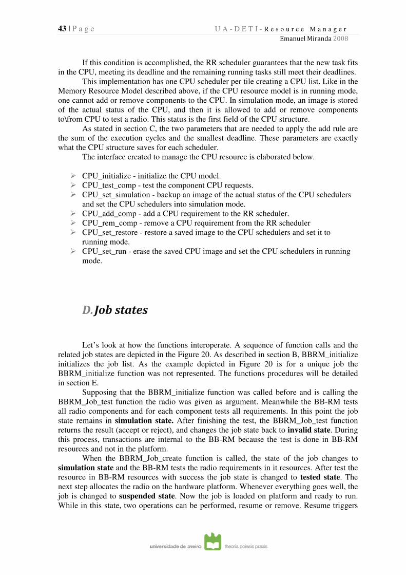
43 | P a g e U A - D E T I - R e s o u r c e M a n a g e r
Emanuel Miranda 2008
If this condition is accomplished, the RR scheduler guarantees that the new task fits
in the CPU, meeting its deadline and the remaining running tasks still meet their deadlines.
This implementation has one CPU scheduler per tile creating a CPU list. Like in the
Memory Resource Model described above, if the CPU resource model is in running mode,
one cannot add or remove components to the CPU. In simulation mode, an image is stored
of the actual status of the CPU, and then it is allowed to add or remove components
to\from CPU to test a radio. This status is the first field of the CPU structure.
As stated in section C, the two parameters that are needed to apply the add rule are
the sum of the execution cycles and the smallest deadline. These parameters are exactly
what the CPU structure saves for each scheduler.
The interface created to manage the CPU resource is elaborated below.
� CPU_initialize - initialize the CPU model.
� CPU_test_comp - test the component CPU requests.
� CPU_set_simulation - backup an image of the actual status of the CPU schedulers
and set the CPU schedulers into simulation mode.
� CPU_add_comp - add a CPU requirement to the RR scheduler.
� CPU_rem_comp - remove a CPU requirement from the RR scheduler
� CPU_set_restore - restore a saved image to the CPU schedulers and set it to
running mode.
� CPU_set_run - erase the saved CPU image and set the CPU schedulers in running
mode.
D. Job states
Let’s look at how the functions interoperate. A sequence of function calls and the
related job states are depicted in the Figure 20. As described in section B, BBRM_initialize
initializes the job list. As the example depicted in Figure 20 is for a unique job the
BBRM_initialize function was not represented. The functions procedures will be detailed
in section E.
Supposing that the BBRM_initialize function was called before and is calling the
BBRM_Job_test function the radio was given as argument. Meanwhile the BB-RM tests
all radio components and for each component tests all requirements. In this point the job
state remains in simulation state. After finishing the test, the BBRM_Job_test function
returns the result (accept or reject), and changes the job state back to invalid state. During
this process, transactions are internal to the BB-RM because the test is done in BB-RM
resources and not in the platform.
When the BBRM_Job_create function is called, the state of the job changes to
simulation state and the BB-RM tests the radio requirements in it resources. After test the
resource in BB-RM resources with success the job state is changed to tested state. The
next step allocates the radio on the hardware platform. Whenever everything goes well, the
job is changed to suspended state. Now the job is loaded on platform and ready to run.
While in this state, two operations can be performed, resume or remove. Resume triggers
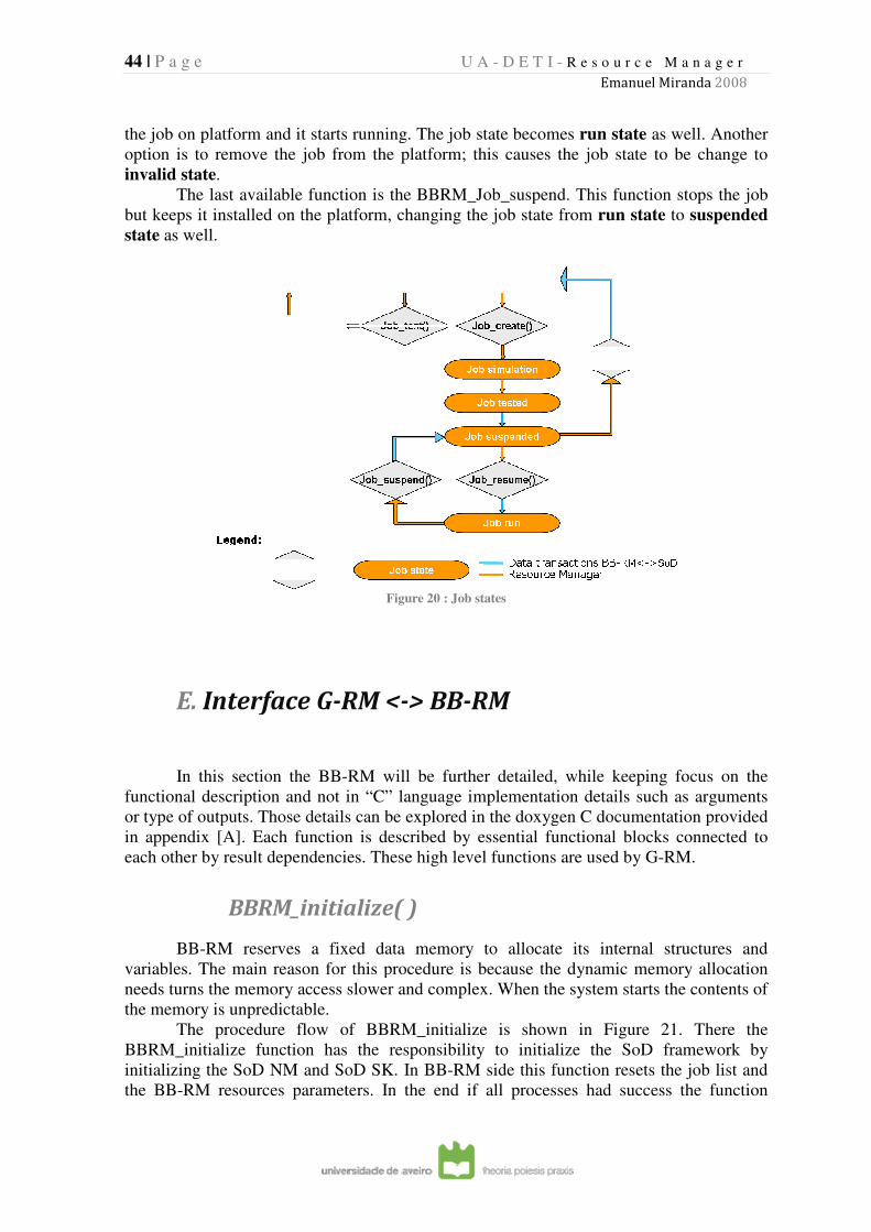
44 | P a g e
the job on platform and it starts running. The job state becomes
option is to remove the job from the
invalid state.
The last available function is the BBRM_Job_suspend. This f
but keeps it installed on the platform, changing the job state from
state as well.
E. Interface G
In this section the BB
functional description and not in
or type of outputs. Those details can be explored in the doxygen C documentation provided
in appendix [A]. Each function is described by essential functional blocks connected
each other by result dependencies. These high level functions are used by
BBRM_initialize( )
BB-RM reserves a fixed data memory to allocate it
variables. The main reason for this procedure is because the dynamic memory
needs turns the memory access slower and complex. When the system st
the memory is unpredictable.
The procedure flow of BBRM_initialize is shown in
BBRM_initialize function has the responsibilit
initializing the SoD NM and SoD SK. In BB
the BB-RM resources parameters. In the end if all processes had success the function
U A - D E T I - R e s o u r c e M a n a g e r
Emanuel Miranda
the job on platform and it starts running. The job state becomes run state
option is to remove the job from the platform; this causes the job state to be change to
The last available function is the BBRM_Job_suspend. This function stops the job
but keeps it installed on the platform, changing the job state from run state
Figure 20 : Job states
Interface G-RM <-> BB-RM
In this section the BB-RM will be further detailed, while keeping focus on
functional description and not in “C” language implementation details such as arguments
or type of outputs. Those details can be explored in the doxygen C documentation provided
]. Each function is described by essential functional blocks connected
each other by result dependencies. These high level functions are used by
BRM_initialize( )
RM reserves a fixed data memory to allocate its internal structures and
variables. The main reason for this procedure is because the dynamic memory
needs turns the memory access slower and complex. When the system st
the memory is unpredictable.
The procedure flow of BBRM_initialize is shown in Figure
BBRM_initialize function has the responsibility to initialize the SoD framework by
initializing the SoD NM and SoD SK. In BB-RM side this function reset
RM resources parameters. In the end if all processes had success the function
R e s o u r c e M a n a g e r
Emanuel Miranda 2008
run state as well. Another
this causes the job state to be change to
unction stops the job
run state to suspended
RM will be further detailed, while keeping focus on the
language implementation details such as arguments
or type of outputs. Those details can be explored in the doxygen C documentation provided
]. Each function is described by essential functional blocks connected to
each other by result dependencies. These high level functions are used by G-RM.
internal structures and
variables. The main reason for this procedure is because the dynamic memory allocation
needs turns the memory access slower and complex. When the system starts the contents of
Figure 21. There the
y to initialize the SoD framework by
RM side this function resets the job list and
RM resources parameters. In the end if all processes had success the function
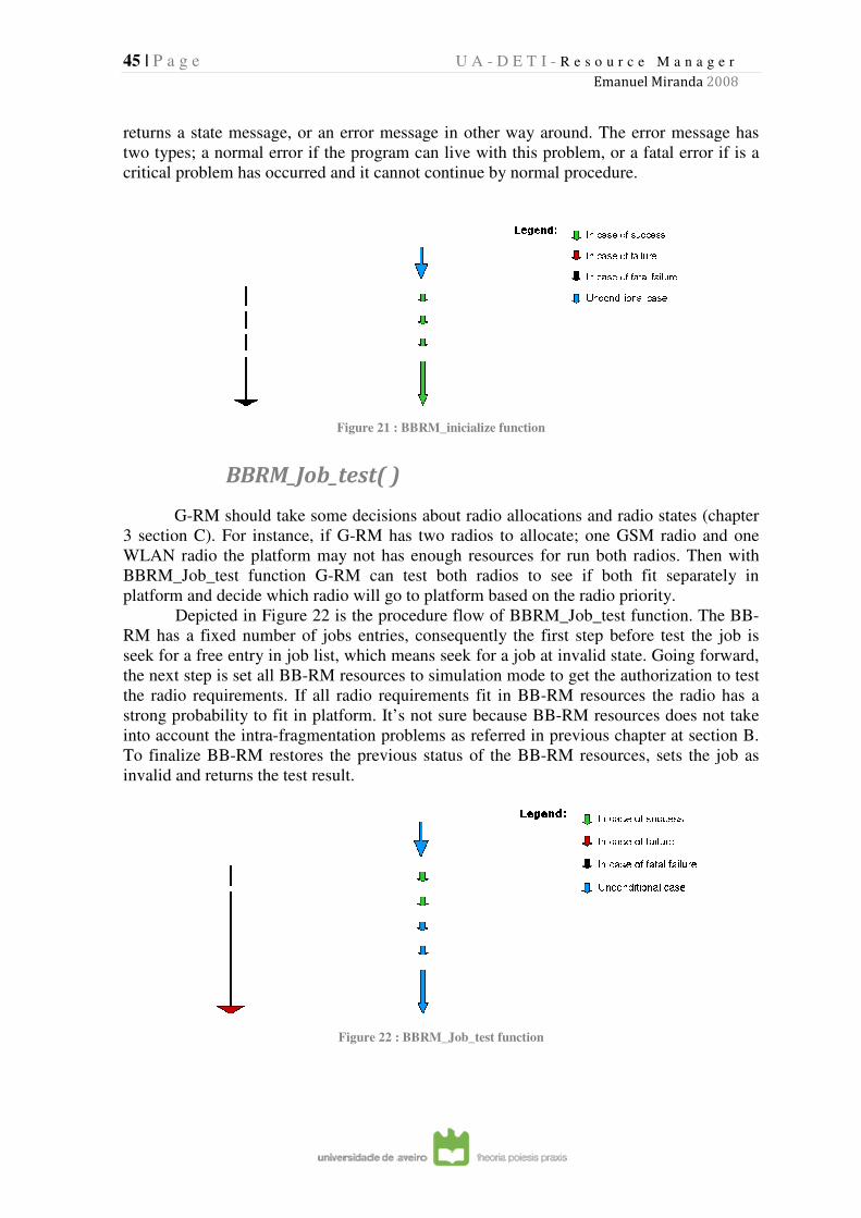
45 | P a g e
returns a state message, or an error message i
two types; a normal error if the program can live with this problem, or a fatal error if is a
critical problem has occurred
BBRM_Job_test( )
G-RM should take some decisions about radio allocations and radio states (chapter
3 section C). For instance, if G
WLAN radio the platform
BBRM_Job_test function G
platform and decide which radio will go to platfo
Depicted in Figure
RM has a fixed number of jobs
seek for a free entry in job list, which means seek for a job at invalid state. Going forward,
the next step is set all BB-RM
the radio requirements. If all radio requirements fit in BB
strong probability to fit in platform. It’s not sure because BB
into account the intra-fragmentation problems
To finalize BB-RM restore
invalid and returns the test result.
U A - D E T I - R e s o u r c e M a n a g e r
Emanuel Miranda
returns a state message, or an error message in other way around. The error message has
two types; a normal error if the program can live with this problem, or a fatal error if is a
has occurred and it cannot continue by normal procedure.
Figure 21 : BBRM_inicialize function
BBRM_Job_test( )
RM should take some decisions about radio allocations and radio states (chapter
ance, if G-RM has two radios to allocate; one GSM radio and one
he platform may not has enough resources for run both radios. Then with
on G-RM can test both radios to see if both fit separately in
platform and decide which radio will go to platform based on the radio priority.
Figure 22 is the procedure flow of BBRM_Job_test function. The BB
RM has a fixed number of jobs entries, consequently the first step before test the job is
seek for a free entry in job list, which means seek for a job at invalid state. Going forward,
RM resources to simulation mode to get the authorization to test
the radio requirements. If all radio requirements fit in BB-RM resources the radio has a
strong probability to fit in platform. It’s not sure because BB-RM resources does not take
fragmentation problems as referred in previous chapter at section
RM restores the previous status of the BB-RM resources, sets the job
invalid and returns the test result.
Figure 22 : BBRM_Job_test function
R e s o u r c e M a n a g e r
Emanuel Miranda 2008
n other way around. The error message has
two types; a normal error if the program can live with this problem, or a fatal error if is a
and it cannot continue by normal procedure.
RM should take some decisions about radio allocations and radio states (chapter
ne GSM radio and one
resources for run both radios. Then with
both radios to see if both fit separately in
rm based on the radio priority.
e flow of BBRM_Job_test function. The BB-
, consequently the first step before test the job is
seek for a free entry in job list, which means seek for a job at invalid state. Going forward,
resources to simulation mode to get the authorization to test
RM resources the radio has a
RM resources does not take
referred in previous chapter at section B.
RM resources, sets the job as
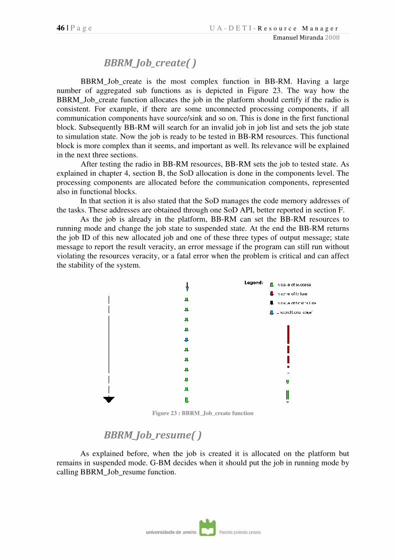
46 | P a g e
BBRM_Job_create( )
BBRM_Job_create is the most complex function in BB
number of aggregated sub functions
BBRM_Job_create function allocates the job in the platform should certify if the radio is
consistent. For example, if there are some unconne
communication components have source/sink and so on. This is done in the first functional
block. Subsequently BB-RM will search for an invalid job in job list and set
to simulation state. Now the job is rea
block is more complex than it seems, and important as well.
in the next three sections.
After testing the radio in BB
explained in chapter 4, section
processing components are allocated before the communication components, represented
also in functional blocks.
In that section it is also stated
the tasks. These addresses are obtaine
As the job is already in the platform, BB
running mode and change the job s
the job ID of this new allocated job and one of these three types of output message; state
message to report the result veracity, an error message if the progr
violating the resources veracity
the stability of the system.
BBRM_Job_resume( )
As explained before, when the job is created it is allocated on the platform but
remains in suspended mode. G
calling BBRM_Job_resume function.
U A - D E T I - R e s o u r c e M a n a g e r
Emanuel Miranda
BBRM_Job_create( )
BBRM_Job_create is the most complex function in BB-RM.
of aggregated sub functions as is depicted in Figure 23.
BBRM_Job_create function allocates the job in the platform should certify if the radio is
consistent. For example, if there are some unconnected processing components, if all
communication components have source/sink and so on. This is done in the first functional
RM will search for an invalid job in job list and set
to simulation state. Now the job is ready to be tested in BB-RM resources. This functional
block is more complex than it seems, and important as well. Its relevance will be explained
the radio in BB-RM resources, BB-RM sets the job to tested state. As
section B, the SoD allocation is done in the components level. The
processing components are allocated before the communication components, represented
In that section it is also stated that the SoD manages the code memory addresses of
are obtained through one SoD API, better reported in section
As the job is already in the platform, BB-RM can set the BB
running mode and change the job state to suspended state. At the end the BB
the job ID of this new allocated job and one of these three types of output message; state
message to report the result veracity, an error message if the program can still run without
urces veracity, or a fatal error when the problem is critical and can affect
Figure 23 : BBRM_Job_create function
BBRM_Job_resume( )
xplained before, when the job is created it is allocated on the platform but
remains in suspended mode. G-BM decides when it should put the job in running
calling BBRM_Job_resume function.
R e s o u r c e M a n a g e r
Emanuel Miranda 2008
RM. Having a large
. The way how the
BBRM_Job_create function allocates the job in the platform should certify if the radio is
cted processing components, if all
communication components have source/sink and so on. This is done in the first functional
RM will search for an invalid job in job list and sets the job state
RM resources. This functional
relevance will be explained
the job to tested state. As
mponents level. The
processing components are allocated before the communication components, represented
that the SoD manages the code memory addresses of
through one SoD API, better reported in section F.
RM can set the BB-RM resources to
tate to suspended state. At the end the BB-RM returns
the job ID of this new allocated job and one of these three types of output message; state
am can still run without
, or a fatal error when the problem is critical and can affect
xplained before, when the job is created it is allocated on the platform but
in running mode by
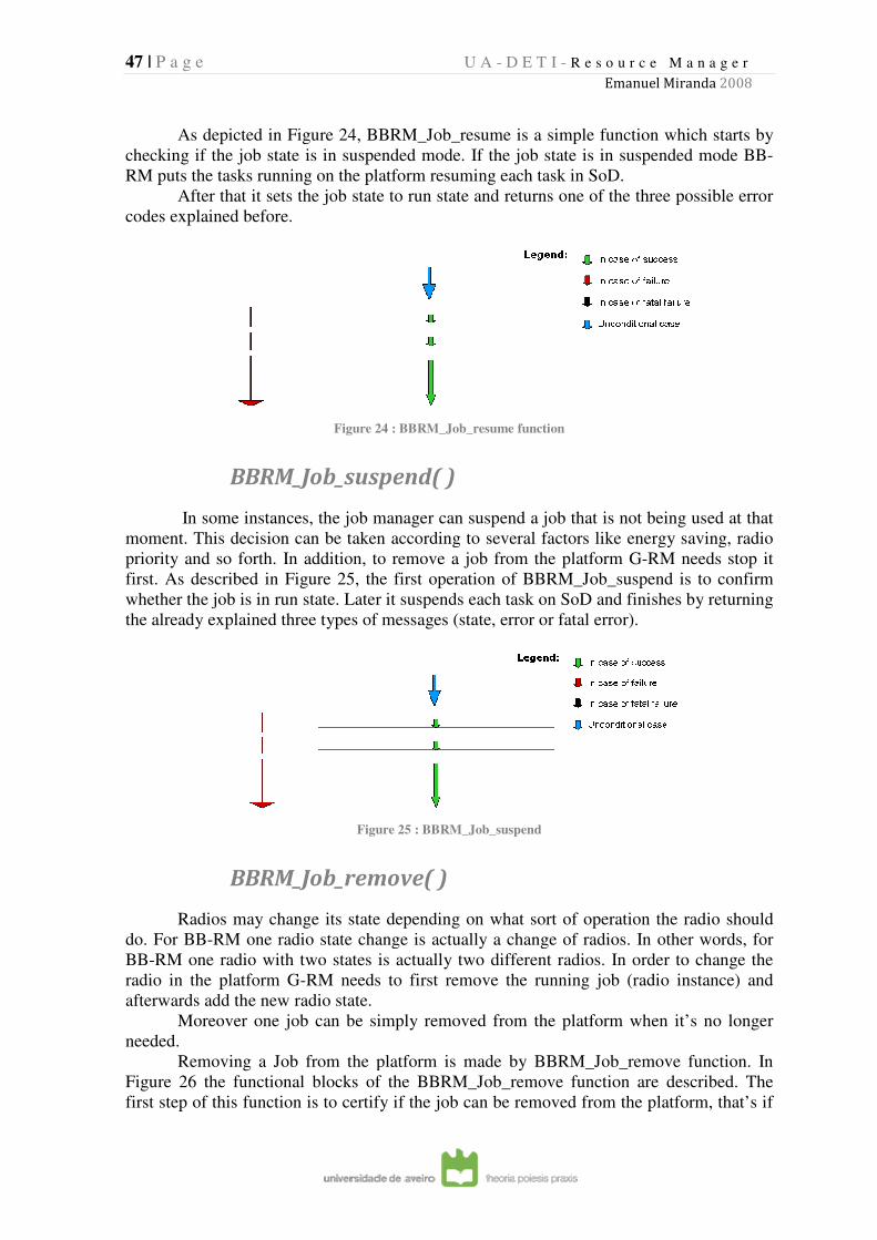
47 | P a g e
As depicted in Figure
checking if the job state is in suspended mode. If the job state is in suspended mode BB
RM puts the tasks running on the platform resuming each
After that it sets the job state to run state and returns one of the three possible error
codes explained before.
BBRM_Job_suspend( )
In some instances, the job manager can susp
moment. This decision can be taken according to several factors like energy saving, radio
priority and so forth. In addition
first. As described in Figure
whether the job is in run state. Later it suspends each task on SoD and finishes by returning
the already explained three types of messages
BBRM_Job_remove( )
Radios may change
do. For BB-RM one radio state change
BB-RM one radio with two states is actually two different radios. In order to change the
radio in the platform G-RM needs to first remove the running job (radio instance) and
afterwards add the new radio sta
Moreover one job can be simply removed from the platform when
needed.
Removing a Job from the platform is made by BBRM_Job_remove function. In
Figure 26 the functional blocks of the BBRM_Job_remove function are described. The
first step of this function is to certify if the job can be removed from the platform,
U A - D E T I - R e s o u r c e M a n a g e r
Emanuel Miranda
Figure 24, BBRM_Job_resume is a simple function which starts by
checking if the job state is in suspended mode. If the job state is in suspended mode BB
RM puts the tasks running on the platform resuming each task in SoD.
After that it sets the job state to run state and returns one of the three possible error
Figure 24 : BBRM_Job_resume function
BBRM_Job_suspend( )
In some instances, the job manager can suspend a job that is not being used at that
moment. This decision can be taken according to several factors like energy saving, radio
priority and so forth. In addition, to remove a job from the platform G
Figure 25, the first operation of BBRM_Job_suspend is to confirm
whether the job is in run state. Later it suspends each task on SoD and finishes by returning
d three types of messages (state, error or fatal error).
Figure 25 : BBRM_Job_suspend
BBRM_Job_remove( )
may change its state depending on what sort of operation the radio should
RM one radio state change is actually a change of radios. In other words, for
RM one radio with two states is actually two different radios. In order to change the
RM needs to first remove the running job (radio instance) and
afterwards add the new radio state.
Moreover one job can be simply removed from the platform when
from the platform is made by BBRM_Job_remove function. In
the functional blocks of the BBRM_Job_remove function are described. The
first step of this function is to certify if the job can be removed from the platform,
R e s o u r c e M a n a g e r
Emanuel Miranda 2008
, BBRM_Job_resume is a simple function which starts by
checking if the job state is in suspended mode. If the job state is in suspended mode BB-
After that it sets the job state to run state and returns one of the three possible error
end a job that is not being used at that
moment. This decision can be taken according to several factors like energy saving, radio
to remove a job from the platform G-RM needs stop it
, the first operation of BBRM_Job_suspend is to confirm
whether the job is in run state. Later it suspends each task on SoD and finishes by returning
.
its state depending on what sort of operation the radio should
a change of radios. In other words, for
RM one radio with two states is actually two different radios. In order to change the
RM needs to first remove the running job (radio instance) and
Moreover one job can be simply removed from the platform when it’s no longer
from the platform is made by BBRM_Job_remove function. In
the functional blocks of the BBRM_Job_remove function are described. The
first step of this function is to certify if the job can be removed from the platform, that’s if
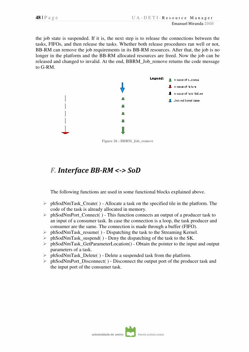
48 | P a g e
the job state is suspended. If it is, the next step is to release the connections between the
tasks, FIFOs, and then release the tasks. Whether both release procedures ran well or not,
BB-RM can remove the job requirements in its BB
longer in the platform and the BB
released and changed to invalid. At the end, BBRM_Job_remove returns the code message
to G-RM.
F. Interface BB
The following functions are used in some functional blocks explained above.
� phSodNmTask_Create( )
code of the task is already allocated in memory.
� phSodNmPort_Connect( )
an input of a consum
consumer are the same. The connection is made through a buffer (FIFO).
� phSodNmTask_resume( )
� phSodNmTask_suspend( )
� phSodNmTask_GetParameterLocatio
parameters of a task.
� phSodNmTask_Delete( )
� phSodNmPort_Disconnect( )
the input port of the consumer task.
U A - D E T I - R e s o u r c e M a n a g e r
Emanuel Miranda
ended. If it is, the next step is to release the connections between the
tasks, FIFOs, and then release the tasks. Whether both release procedures ran well or not,
RM can remove the job requirements in its BB-RM resources. After that, the job is no
er in the platform and the BB-RM allocated resources are freed. Now the job can be
released and changed to invalid. At the end, BBRM_Job_remove returns the code message
Figure 26 : BBRM_Job_remove
Interface BB-RM <-> SoD
The following functions are used in some functional blocks explained above.
phSodNmTask_Create( ) - Allocate a task on the specified tile in the platform. The
task is already allocated in memory.
phSodNmPort_Connect( ) - This function connects an output of a producer task to
an input of a consumer task. In case the connection is a loop, the task producer and
consumer are the same. The connection is made through a buffer (FIFO).
phSodNmTask_resume( ) - Dispatching the task to the Streaming Ke
phSodNmTask_suspend( ) - Deny the dispatching of the task to the SK.
phSodNmTask_GetParameterLocation() - Obtain the pointer to the in
task.
SodNmTask_Delete( ) - Delete a suspended task from the platform.
Disconnect( ) - Disconnect the output port of the producer task and
the input port of the consumer task.
R e s o u r c e M a n a g e r
Emanuel Miranda 2008
ended. If it is, the next step is to release the connections between the
tasks, FIFOs, and then release the tasks. Whether both release procedures ran well or not,
RM resources. After that, the job is no
resources are freed. Now the job can be
released and changed to invalid. At the end, BBRM_Job_remove returns the code message
The following functions are used in some functional blocks explained above.
n the platform. The
cts an output of a producer task to
task. In case the connection is a loop, the task producer and
consumer are the same. The connection is made through a buffer (FIFO).
Dispatching the task to the Streaming Kernel.
Deny the dispatching of the task to the SK.
Obtain the pointer to the input and output
suspended task from the platform.
Disconnect the output port of the producer task and
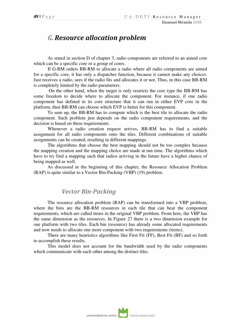
49 | P a g e U A - D E T I - R e s o u r c e M a n a g e r
Emanuel Miranda 2008
G. Resource allocation problem
As stated in section D of chapter 3, radio components are referred to an aimed core
which can be a specific core or a group of cores.
If G-RM orders BB-RM to allocate a radio where all radio components are aimed
for a specific core, it has only a dispatcher function, because it cannot make any choices.
Just receives a radio, sees if the radio fits and allocates it or not. Thus, in this case BB-RM
is completely limited by the radio parameters.
On the other hand, when the target is only restricts the core type the BB-RM has
some freedom to decide where to allocate the component. For instance, if one radio
component has defined in its core structure that it can run in either EVP core in the
platform, then BB-RM can choose which EVP is better for this component.
To sum up, the BB-RM has to compute which is the best tile to allocate the radio
component. Such problem just depends on the radio component requirements, and the
decision is based on these requirements.
Whenever a radio creation request arrives, BB-RM has to find a suitable
assignment for all radio components onto the tiles. Different combinations of suitable
assignments can be created, resulting in different mappings.
The algorithms that choose the best mapping should not be too complex because
the mapping creation and the mapping choice are made at run time. The algorithms which
have to try find a mapping such that radios arriving in the future have a higher chance of
being mapped as well.
As discussed in the beginning of this chapter, the Resource Allocation Problem
(RAP) is quite similar to a Vector Bin-Packing (VBP) (19) problem.
Vector Bin-Packing
The resource allocation problem (RAP) can be transformed into a VBP problem,
where the bins are the BB-RM resources in each tile that can bear the component
requirements, which are called items in the original VBP problem. From here, the VBP has
the same dimension as the resources. In Figure 27 there is a two dimension example for
one platform with two tiles. Each bin (resource) has already some allocated requirements
and now needs to allocate one more component with two requirements (items).
There are many heuristics algorithms like First Fit (FF), Best Fit (BF) and so forth
to accomplish these results.
This model does not account for the bandwidth used by the radio components
which communicate with each other among the distinct tiles.
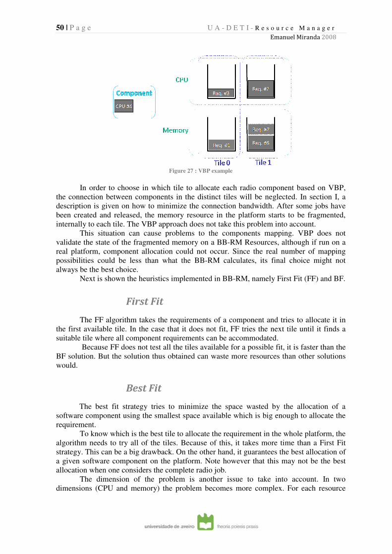
50 | P a g e
In order to choose
the connection between components in the distinct tiles will be neglected. In section
description is given on how to minimize the connection bandwidth. After some jobs have
been created and released, the memory resource in the platform starts t
internally to each tile. The VBP approach does not take this problem into account.
This situation can cause problems to the components mapping. VBP does not
validate the state of the fragmented memory on a BB
real platform, component allocation could not occur. Since the real number of mapping
possibilities could be less than what the BB
always be the best choice.
Next is shown the heuristics im
First Fit
The FF algorithm takes the requirements of a component and tries to allocate it in
the first available tile. In the case that it does not fit, FF tries the next tile until it finds a
suitable tile where all componen
Because FF does not test all the tiles available for a possible fit, it is faster than the
BF solution. But the solution thus obtained can
would.
Best Fit
The best fit strategy
software component using the smallest space available which is big enough to allocate the
requirement.
To know which is the best tile to allocate the requirement in the whole platform, the
algorithm needs to try all of
strategy. This can be a big drawback. On the other hand, it guarantees the best allocation of
a given software component on the platform. Note however that this may not b
allocation when one considers the complete radio job.
The dimension of the problem is another issue to take into account. In two
dimensions (CPU and memory) the problem becomes more complex. For each resource
U A - D E T I - R e s o u r c e M a n a g e r
Emanuel Miranda
Figure 27 : VBP example
in which tile to allocate each radio component based on VBP,
the connection between components in the distinct tiles will be neglected. In section
description is given on how to minimize the connection bandwidth. After some jobs have
been created and released, the memory resource in the platform starts t
internally to each tile. The VBP approach does not take this problem into account.
This situation can cause problems to the components mapping. VBP does not
validate the state of the fragmented memory on a BB-RM Resources, although if run
real platform, component allocation could not occur. Since the real number of mapping
possibilities could be less than what the BB-RM calculates, its final choice might not
Next is shown the heuristics implemented in BB-RM, namely First Fit (FF) and
First Fit
The FF algorithm takes the requirements of a component and tries to allocate it in
the first available tile. In the case that it does not fit, FF tries the next tile until it finds a
suitable tile where all component requirements can be accommodated.
Because FF does not test all the tiles available for a possible fit, it is faster than the
BF solution. But the solution thus obtained can waste more resources tha
Best Fit
The best fit strategy tries to minimize the space wasted by the allo
using the smallest space available which is big enough to allocate the
To know which is the best tile to allocate the requirement in the whole platform, the
of the tiles. Because of this, it takes more time than a First Fit
strategy. This can be a big drawback. On the other hand, it guarantees the best allocation of
a given software component on the platform. Note however that this may not b
allocation when one considers the complete radio job.
The dimension of the problem is another issue to take into account. In two
dimensions (CPU and memory) the problem becomes more complex. For each resource
R e s o u r c e M a n a g e r
Emanuel Miranda 2008
which tile to allocate each radio component based on VBP,
the connection between components in the distinct tiles will be neglected. In section I, a
description is given on how to minimize the connection bandwidth. After some jobs have
been created and released, the memory resource in the platform starts to be fragmented,
internally to each tile. The VBP approach does not take this problem into account.
This situation can cause problems to the components mapping. VBP does not
RM Resources, although if run on a
real platform, component allocation could not occur. Since the real number of mapping
RM calculates, its final choice might not
namely First Fit (FF) and BF.
The FF algorithm takes the requirements of a component and tries to allocate it in
the first available tile. In the case that it does not fit, FF tries the next tile until it finds a
Because FF does not test all the tiles available for a possible fit, it is faster than the
waste more resources than other solutions
tries to minimize the space wasted by the allocation of a
using the smallest space available which is big enough to allocate the
To know which is the best tile to allocate the requirement in the whole platform, the
the tiles. Because of this, it takes more time than a First Fit
strategy. This can be a big drawback. On the other hand, it guarantees the best allocation of
a given software component on the platform. Note however that this may not be the best
The dimension of the problem is another issue to take into account. In two
dimensions (CPU and memory) the problem becomes more complex. For each resource
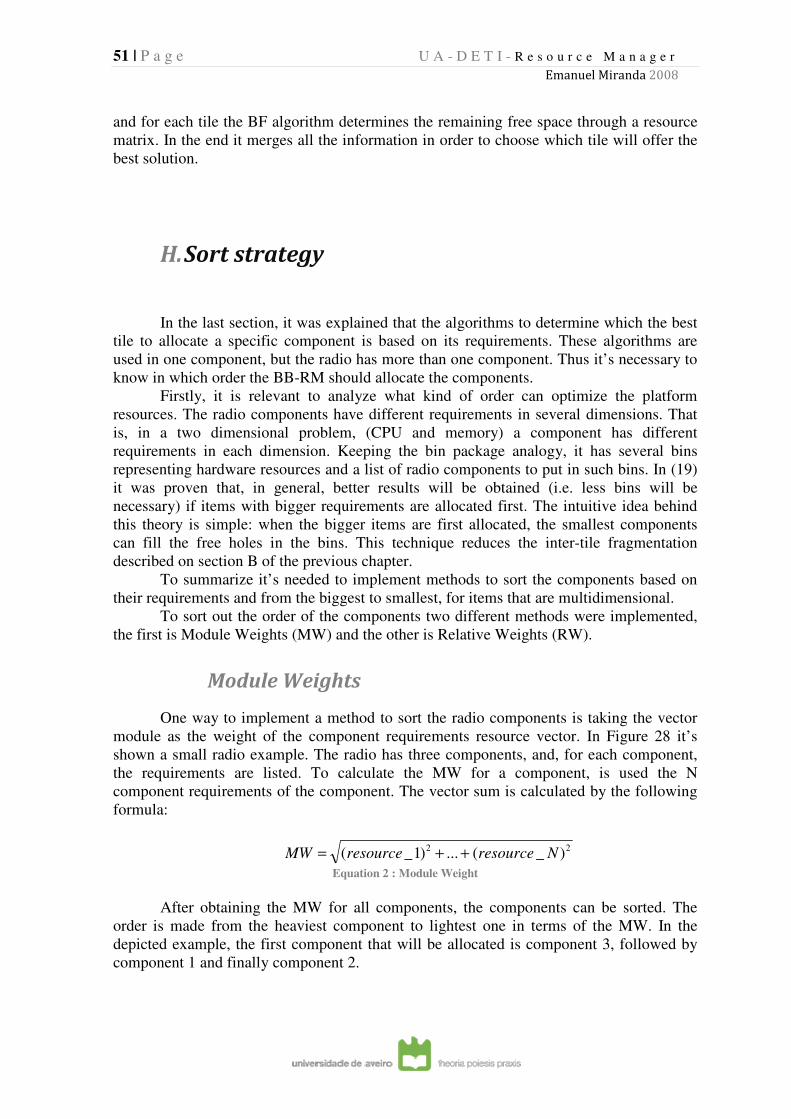
51 | P a g e U A - D E T I - R e s o u r c e M a n a g e r
Emanuel Miranda 2008
and for each tile the BF algorithm determines the remaining free space through a resource
matrix. In the end it merges all the information in order to choose which tile will offer the
best solution.
H. Sort strategy
In the last section, it was explained that the algorithms to determine which the best
tile to allocate a specific component is based on its requirements. These algorithms are
used in one component, but the radio has more than one component. Thus it’s necessary to
know in which order the BB-RM should allocate the components.
Firstly, it is relevant to analyze what kind of order can optimize the platform
resources. The radio components have different requirements in several dimensions. That
is, in a two dimensional problem, (CPU and memory) a component has different
requirements in each dimension. Keeping the bin package analogy, it has several bins
representing hardware resources and a list of radio components to put in such bins. In (19)
it was proven that, in general, better results will be obtained (i.e. less bins will be
necessary) if items with bigger requirements are allocated first. The intuitive idea behind
this theory is simple: when the bigger items are first allocated, the smallest components
can fill the free holes in the bins. This technique reduces the inter-tile fragmentation
described on section B of the previous chapter.
To summarize it’s needed to implement methods to sort the components based on
their requirements and from the biggest to smallest, for items that are multidimensional.
To sort out the order of the components two different methods were implemented,
the first is Module Weights (MW) and the other is Relative Weights (RW).
Module Weights
One way to implement a method to sort the radio components is taking the vector
module as the weight of the component requirements resource vector. In Figure 28 it’s
shown a small radio example. The radio has three components, and, for each component,
the requirements are listed. To calculate the MW for a component, is used the N
component requirements of the component. The vector sum is calculated by the following
formula:
22 )_(...)1_( NresourceresourceMW ++=
Equation 2 : Module Weight
After obtaining the MW for all components, the components can be sorted. The
order is made from the heaviest component to lightest one in terms of the MW. In the
depicted example, the first component that will be allocated is component 3, followed by
component 1 and finally component 2.
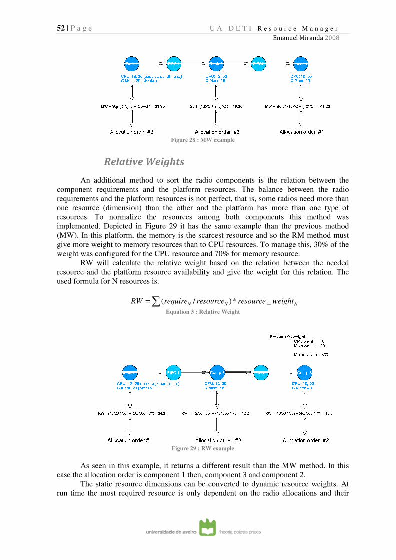
52 | P a g e
Relative Weights
An additional method to sort the radio components is the relation between the
component requirements and the platform resources. The balance between the radio
requirements and the platform resources is not perfect, that is, some radios need more than
one resource (dimension) than the other and the platform has more than one type of
resources. To normalize the resources among both components this method was
implemented. Depicted in
(MW). In this platform, the memory is the scarcest resource and so the RM method must
give more weight to memory resources than to CPU resources. To manage this, 30% of the
weight was configured for the CPU resource and 70% for memory resource.
RW will calculate the relative weight based on the relation between the needed
resource and the platform resource
used formula for N resources is
RW
As seen in this example, it returns a different result than the MW method. In this
case the allocation order is co
The static resource dimensions can be converted to dynamic resource weights. At
run time the most required resource is only dependent on the radio allocations and their
U A - D E T I - R e s o u r c e M a n a g e r
Emanuel Miranda
Figure 28 : MW example
Relative Weights
An additional method to sort the radio components is the relation between the
component requirements and the platform resources. The balance between the radio
requirements and the platform resources is not perfect, that is, some radios need more than
esource (dimension) than the other and the platform has more than one type of
resources. To normalize the resources among both components this method was
implemented. Depicted in Figure 29 it has the same example than the previous method
(MW). In this platform, the memory is the scarcest resource and so the RM method must
give more weight to memory resources than to CPU resources. To manage this, 30% of the
configured for the CPU resource and 70% for memory resource.
RW will calculate the relative weight based on the relation between the needed
resource and the platform resource availability and give the weight for this relation. The
rces is.
∑= NN weightresourceresourcerequire _*)/(
Equation 3 : Relative Weight
Figure 29 : RW example
As seen in this example, it returns a different result than the MW method. In this
case the allocation order is component 1 then, component 3 and component 2.
he static resource dimensions can be converted to dynamic resource weights. At
run time the most required resource is only dependent on the radio allocations and their
R e s o u r c e M a n a g e r
Emanuel Miranda 2008
An additional method to sort the radio components is the relation between the
component requirements and the platform resources. The balance between the radio
requirements and the platform resources is not perfect, that is, some radios need more than
esource (dimension) than the other and the platform has more than one type of
resources. To normalize the resources among both components this method was
the same example than the previous method
(MW). In this platform, the memory is the scarcest resource and so the RM method must
give more weight to memory resources than to CPU resources. To manage this, 30% of the
configured for the CPU resource and 70% for memory resource.
RW will calculate the relative weight based on the relation between the needed
the weight for this relation. The
Nweight
As seen in this example, it returns a different result than the MW method. In this
mponent 1 then, component 3 and component 2.
he static resource dimensions can be converted to dynamic resource weights. At
run time the most required resource is only dependent on the radio allocations and their
53 | P a g e U A - D E T I - R e s o u r c e M a n a g e r
Emanuel Miranda 2008
requirements. This means that the most used resource can be difficult to predict. Using
dynamic weights, the weight values for each resource type change at run-time. This change
is according to the current resource availability across the platform.
I. Complete RAP heuristics, including
communication
Section G described the strategies implemented for selecting the tile for allocating
one specific component based on its requirements, and section H describes the strategies
implemented to choose in which order to allocate components to the platform – the “sort
strategy”.
In the radio structure presented in the section C of chapter 3, the radio is defined as
a set of processing components and communication components. Until now, the focus has
been on the processing components, but now the communication components will come
into play.
A communication component is the mechanism that delivers tokens (data
containers of fixed sized) from the source to the sink software components. As explained
in (19), communication component require resources at both endpoints, i.e., buffers on
both sides, were tokens can be stored. However, if those endpoints are in the same tile,
the communication is completely internal. That means that the communication
component does not require bus resources, or separate send and receive buffers.
The complete RAP is a solution to allocate the radio, taking into account the
processing components and the communication components. Using expert knowledge
and heuristics, the complete RAP can do two main optimizations when mapping a radio.
One is to minimize bus bandwidth usage, since lower bandwidth requirements means
lower chances of network congestion. The other is to minimize fragmentation or tile
resources.
Two RAP heuristics have been implemented in the BB-RM.
Best Fit with Decreasing Module Weights (BFDMW)
This heuristic is to optimize the inter-tile resources fragmentation. Even when the
sums of available resources are bigger than the radio requirements, the fragmentation
problem may private the radio activation. So, the fragmentation reduces the number of
running radios at the same time. Using the module weight methods, it orders the radio
processing components from the bigger to the smaller (section H). Tracing the components
by that order, it allocates each processing component by Best Fit algorithm.
54 | P a g e U A - D E T I - R e s o u r c e M a n a g e r
Emanuel Miranda 2008
First Fit with Clustering (FFC)
As mentioned above, when two radio components are in the same tile they do not
need a network channel or separate buffers. To reduce the bandwidth among the tiles the
First Fit with Clustering (FFC) algorithm was implemented. A detailed explanation of this
algorithm is available in (19). It is a First Fit Decreasing algorithm that, after assigning an
actor to a tile, looks at the neighbors of that actor in the radio job graph, to see if any of
them can be placed in the same tile.
J. Debug
The BB-RM was developed in an incremental manner; with each change, a new
feature was added. To make the work more independent of other modules that are still in
development, the BB-RM was built in a simulation framework. In the real platform, the
SoD NM process runs on top of uC/OS – II and a SoD SK runs on each core. On the
simulation framework all processes run on the PC’s Operating System. In fact, the OS
simulates the behavior of the real hardware platform.
To help the developing process a three level debug system was put in place. At
compilation, a debug level is chosen depending on the level of information that is required
from the following execution. These debug levels are listed next.
� Debug level 1 - shows the info, error or fatal error messages from BB-RM API
explained in section E.
� Debug level 2 - shows the info, error or fatal error messages from the internal
functions of BB-RM. That means the first functions instance internal of BB-RM.
� Debug level 3 - shows the messages from the BB-RM library which has the most
used function of BB-RM, modules weight to order the components, the
requirements algorithms to choose the tile and BB-RM resources, that is, all
external modules of BB-RM.
The debug messages were chosen in such a way as to easily identify their error
source. First they show the origin file, i.e. Resource Manage, Resource Manage Library,
Emulate, CPU Library and so forth. The second information is about the type of message;
information, error or fatal error. The information messages show the trace of the running
code.
The error messages, when shown mean that something not expected happened but
the program can still run without inconsistency. The fatal error appears when the code
becomes corrupt. One example is when the content of BB-RM resource is different than
real resources in platform.
The next item shown in debug messages is the function that prints the debug
message and the message content. Normally the information messages contents tells us
about the input arguments or a returned value. The error messages and fatal error messages
content is a problem description.
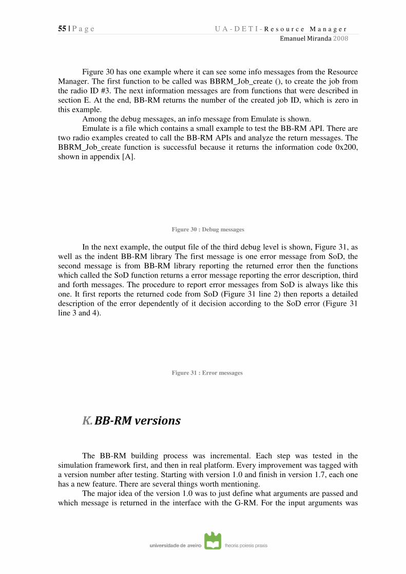
55 | P a g e
Figure 30 has one example where it
Manager. The first function to be called was BBRM_Job_create (), to create the job from
the radio ID #3. The next infor
section E. At the end, BB-
this example.
Among the debug messages, an info message from Emulate is shown.
Emulate is a file which contains a small example to test the BB
two radio examples created to call the BB
BBRM_Job_create function is successful because it returns the information code 0x200,
shown in appendix [A].
In the next example, the output file of the third debug level is shown,
well as the indent BB-RM library The first message is one error message from SoD, the
second message is from BB
which called the SoD function returns a error message reporting the error description, third
and forth messages. The procedure to report error messages from SoD is always like th
one. It first reports the returned code from SoD (
description of the error dependently of it decision according to the So
line 3 and 4).
K. BB-RM versions
The BB-RM building process was incremental. Each step was tested in the
simulation framework first, and then in real platform. Every improvement was tagged with
a version number after testing. Starting with version 1.0 and finish in version 1.7, each one
has a new feature. There are several things worth mentioning.
The major idea of the version 1.0 was to just define what arguments are passed and
which message is returned in the interface with the G
U A - D E T I - R e s o u r c e M a n a g e r
Emanuel Miranda
has one example where it can see some info messages from the Resource
Manager. The first function to be called was BBRM_Job_create (), to create the job from
the radio ID #3. The next information messages are from functions that were described in
-RM returns the number of the created job ID, which is zero in
Among the debug messages, an info message from Emulate is shown.
Emulate is a file which contains a small example to test the BB-
two radio examples created to call the BB-RM APIs and analyze the return messages. The
ion is successful because it returns the information code 0x200,
Figure 30 : Debug messages
example, the output file of the third debug level is shown,
RM library The first message is one error message from SoD, the
message is from BB-RM library reporting the returned error then the functions
which called the SoD function returns a error message reporting the error description, third
and forth messages. The procedure to report error messages from SoD is always like th
one. It first reports the returned code from SoD (Figure 31 line 2) then reports a detailed
description of the error dependently of it decision according to the So
Figure 31 : Error messages
RM versions
RM building process was incremental. Each step was tested in the
simulation framework first, and then in real platform. Every improvement was tagged with
a version number after testing. Starting with version 1.0 and finish in version 1.7, each one
as a new feature. There are several things worth mentioning.
The major idea of the version 1.0 was to just define what arguments are passed and
which message is returned in the interface with the G-RM. For the input arguments was
R e s o u r c e M a n a g e r
Emanuel Miranda 2008
can see some info messages from the Resource
Manager. The first function to be called was BBRM_Job_create (), to create the job from
mation messages are from functions that were described in
RM returns the number of the created job ID, which is zero in
Among the debug messages, an info message from Emulate is shown.
-RM API. There are
RM APIs and analyze the return messages. The
ion is successful because it returns the information code 0x200,
example, the output file of the third debug level is shown, Figure 31, as
RM library The first message is one error message from SoD, the
RM library reporting the returned error then the functions
which called the SoD function returns a error message reporting the error description, third
and forth messages. The procedure to report error messages from SoD is always like this
line 2) then reports a detailed
description of the error dependently of it decision according to the SoD error (Figure 31
RM building process was incremental. Each step was tested in the
simulation framework first, and then in real platform. Every improvement was tagged with
a version number after testing. Starting with version 1.0 and finish in version 1.7, each one
The major idea of the version 1.0 was to just define what arguments are passed and
RM. For the input arguments was
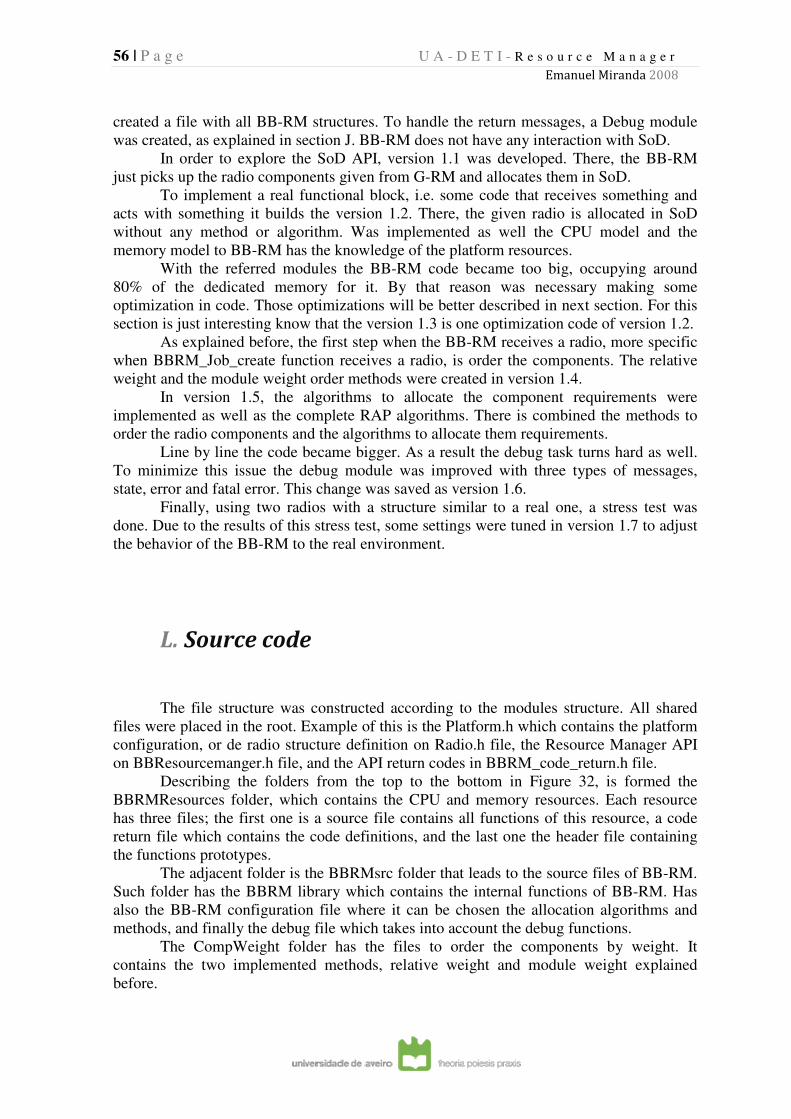
56 | P a g e U A - D E T I - R e s o u r c e M a n a g e r
Emanuel Miranda 2008
created a file with all BB-RM structures. To handle the return messages, a Debug module
was created, as explained in section J. BB-RM does not have any interaction with SoD.
In order to explore the SoD API, version 1.1 was developed. There, the BB-RM
just picks up the radio components given from G-RM and allocates them in SoD.
To implement a real functional block, i.e. some code that receives something and
acts with something it builds the version 1.2. There, the given radio is allocated in SoD
without any method or algorithm. Was implemented as well the CPU model and the
memory model to BB-RM has the knowledge of the platform resources.
With the referred modules the BB-RM code became too big, occupying around
80% of the dedicated memory for it. By that reason was necessary making some
optimization in code. Those optimizations will be better described in next section. For this
section is just interesting know that the version 1.3 is one optimization code of version 1.2.
As explained before, the first step when the BB-RM receives a radio, more specific
when BBRM_Job_create function receives a radio, is order the components. The relative
weight and the module weight order methods were created in version 1.4.
In version 1.5, the algorithms to allocate the component requirements were
implemented as well as the complete RAP algorithms. There is combined the methods to
order the radio components and the algorithms to allocate them requirements.
Line by line the code became bigger. As a result the debug task turns hard as well.
To minimize this issue the debug module was improved with three types of messages,
state, error and fatal error. This change was saved as version 1.6.
Finally, using two radios with a structure similar to a real one, a stress test was
done. Due to the results of this stress test, some settings were tuned in version 1.7 to adjust
the behavior of the BB-RM to the real environment.
L. Source code
The file structure was constructed according to the modules structure. All shared
files were placed in the root. Example of this is the Platform.h which contains the platform
configuration, or de radio structure definition on Radio.h file, the Resource Manager API
on BBResourcemanger.h file, and the API return codes in BBRM_code_return.h file.
Describing the folders from the top to the bottom in Figure 32, is formed the
BBRMResources folder, which contains the CPU and memory resources. Each resource
has three files; the first one is a source file contains all functions of this resource, a code
return file which contains the code definitions, and the last one the header file containing
the functions prototypes.
The adjacent folder is the BBRMsrc folder that leads to the source files of BB-RM.
Such folder has the BBRM library which contains the internal functions of BB-RM. Has
also the BB-RM configuration file where it can be chosen the allocation algorithms and
methods, and finally the debug file which takes into account the debug functions.
The CompWeight folder has the files to order the components by weight. It
contains the two implemented methods, relative weight and module weight explained
before.
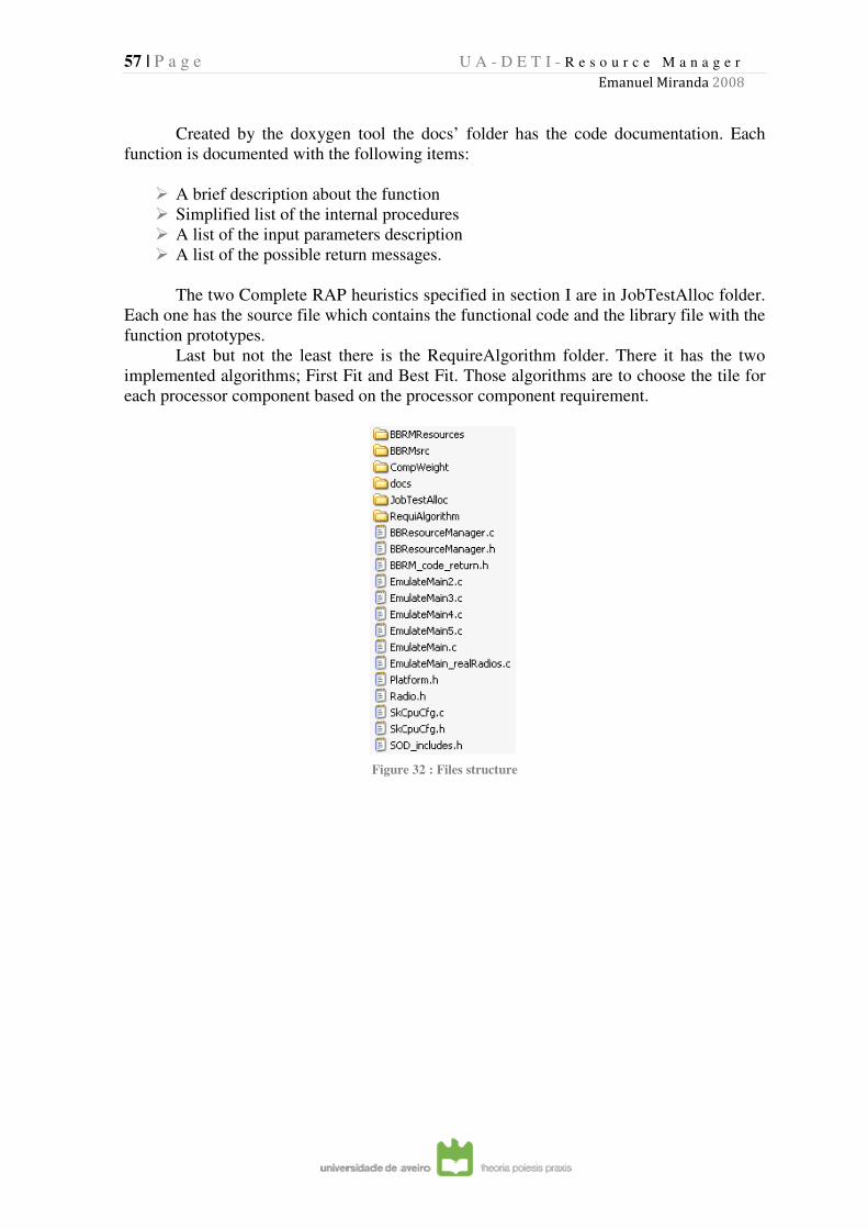
57 | P a g e U A - D E T I - R e s o u r c e M a n a g e r
Emanuel Miranda 2008
Created by the doxygen tool the docs’ folder has the code documentation. Each
function is documented with the following items:
� A brief description about the function
� Simplified list of the internal procedures
� A list of the input parameters description
� A list of the possible return messages.
The two Complete RAP heuristics specified in section I are in JobTestAlloc folder.
Each one has the source file which contains the functional code and the library file with the
function prototypes.
Last but not the least there is the RequireAlgorithm folder. There it has the two
implemented algorithms; First Fit and Best Fit. Those algorithms are to choose the tile for
each processor component based on the processor component requirement.
Figure 32 : Files structure

58 | P a g e U A - D E T I - R e s o u r c e M a n a g e r
Emanuel Miranda 2008
(This page was left blank delivered)
59 | P a g e U A - D E T I - R e s o u r c e M a n a g e r
Emanuel Miranda 2008
6. Experimental results
The work developed in the scope of this dissertation has been extensively assessed
and verified. This section presents some experimental results addressing several aspects of
the work, namely optimizations that have to been carried out to reduce the code size,
resource allocation strategies assessment and verification of the occurrence of
fragmentation.
A. Optimizations
In the beginning the BB-RM operation was relatively simple, consisting only in
allocating radio components without any global strategy. As the work progressed; several
features have been added and the BB-RM became more efficient but, at the same time,
more complex and bigger.
Eventually, in BB-RM version 1.2, the code became too big, using about 80% of
the reserved F-ARM memory for itself. To reduce the code size several optimizations were
done, some of them ending up in execution time improvements as well. This section
presents the main optimizations that have been implemented.
The first optimization addressed the data structures used by the BB-RM. An
exhaustive study about each variable's usage permitted to establish its bounds in the value
domain. The conclusion was that some variables were oversized. Resizing the variables
permitted a considerable gain in memory utilization, which went from the original 1.776
KB per radio to 1.103KB per radio, that is, a reduction of approximately 37.9%.
The same process was applied to all the other structures in the BB-RM resources.
Another kind of optimization consisted in the reduction of the components state
data (Table 1). Originally, when a radio component needed CPU resources to be allocated,
all relevant information about the component was saved on the CPU resource database.
Similarly, when the component required memory, the relevant information was saved on
the memory resource database. This approach drives to the existence of duplicated
information in memory. To avoid this situation it was developed a new approach, in which
only relevant information about the allocations is saved in the job structure. The new
approach consists of just signalizing in the job list structure where the component is
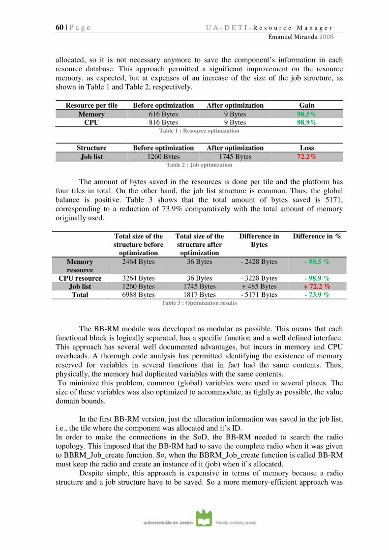
60 | P a g e U A - D E T I - R e s o u r c e M a n a g e r
Emanuel Miranda 2008
allocated, so it is not necessary anymore to save the component’s information in each
resource database. This approach permitted a significant improvement on the resource
memory, as expected, but at expenses of an increase of the size of the job structure, as
shown in Table 1 and Table 2, respectively.
Resource per tile Before optimization After optimization Gain
Memory 616 Bytes 9 Bytes 98.5%
CPU 816 Bytes 9 Bytes 98.9% Table 1 : Resource optimization
Structure Before optimization After optimization Loss
Job list 1260 Bytes 1745 Bytes 72.2% Table 2 : Job optimization
The amount of bytes saved in the resources is done per tile and the platform has
four tiles in total. On the other hand, the job list structure is common. Thus, the global
balance is positive. Table 3 shows that the total amount of bytes saved is 5171,
corresponding to a reduction of 73.9% comparatively with the total amount of memory
originally used.
Total size of the
structure before
optimization
Total size of the
structure after
optimization
Difference in
Bytes
Difference in %
Memory
resource
2464 Bytes 36 Bytes - 2428 Bytes - 98.5 %
CPU resource 3264 Bytes 36 Bytes - 3228 Bytes - 98.9 %
Job list 1260 Bytes 1745 Bytes + 485 Bytes + 72.2 %
Total 6988 Bytes 1817 Bytes - 5171 Bytes - 73.9 % Table 3 : Optimization results
The BB-RM module was developed as modular as possible. This means that each
functional block is logically separated, has a specific function and a well defined interface.
This approach has several well documented advantages, but incurs in memory and CPU
overheads. A thorough code analysis has permitted identifying the existence of memory
reserved for variables in several functions that in fact had the same contents. Thus,
physically, the memory had duplicated variables with the same contents.
To minimize this problem, common (global) variables were used in several places. The
size of these variables was also optimized to accommodate, as tightly as possible, the value
domain bounds.
In the first BB-RM version, just the allocation information was saved in the job list,
i.e., the tile where the component was allocated and it’s ID.
In order to make the connections in the SoD, the BB-RM needed to search the radio
topology. This imposed that the BB-RM had to save the complete radio when it was given
to BBRM_Job_create function. So, when the BBRM_Job_create function is called BB-RM
must keep the radio and create an instance of it (job) when it’s allocated.
Despite simple, this approach is expensive in terms of memory because a radio
structure and a job structure have to be saved. So a more memory-efficient approach was
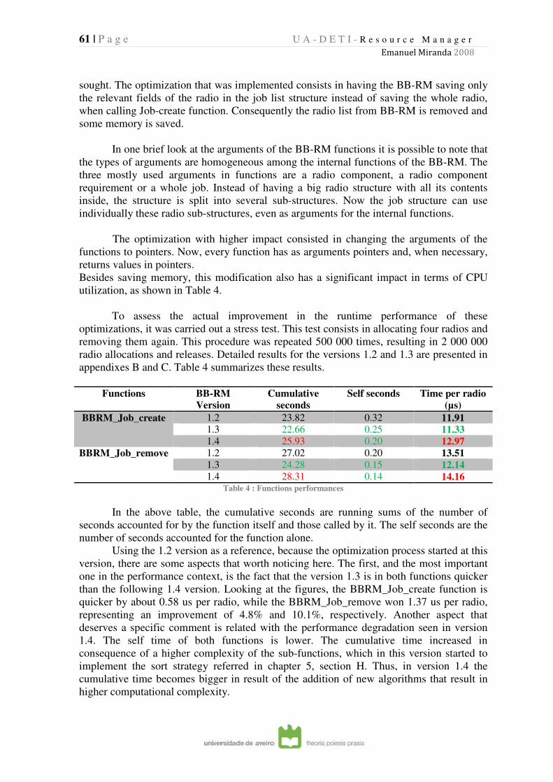
61 | P a g e U A - D E T I - R e s o u r c e M a n a g e r
Emanuel Miranda 2008
sought. The optimization that was implemented consists in having the BB-RM saving only
the relevant fields of the radio in the job list structure instead of saving the whole radio,
when calling Job-create function. Consequently the radio list from BB-RM is removed and
some memory is saved.
In one brief look at the arguments of the BB-RM functions it is possible to note that
the types of arguments are homogeneous among the internal functions of the BB-RM. The
three mostly used arguments in functions are a radio component, a radio component
requirement or a whole job. Instead of having a big radio structure with all its contents
inside, the structure is split into several sub-structures. Now the job structure can use
individually these radio sub-structures, even as arguments for the internal functions.
The optimization with higher impact consisted in changing the arguments of the
functions to pointers. Now, every function has as arguments pointers and, when necessary,
returns values in pointers.
Besides saving memory, this modification also has a significant impact in terms of CPU
utilization, as shown in Table 4.
To assess the actual improvement in the runtime performance of these
optimizations, it was carried out a stress test. This test consists in allocating four radios and
removing them again. This procedure was repeated 500 000 times, resulting in 2 000 000
radio allocations and releases. Detailed results for the versions 1.2 and 1.3 are presented in
appendixes B and C. Table 4 summarizes these results.
Functions BB-RM
Version
Cumulative
seconds
Self seconds Time per radio
(µs)
BBRM_Job_create 1.2 23.82 0.32 11.91 1.3 22.66 0.25 11.33
1.4 25.93 0.20 12.97
BBRM_Job_remove 1.2 27.02 0.20 13.51
1.3 24.28 0.15 12.14 1.4 28.31 0.14 14.16
Table 4 : Functions performances
In the above table, the cumulative seconds are running sums of the number of
seconds accounted for by the function itself and those called by it. The self seconds are the
number of seconds accounted for the function alone.
Using the 1.2 version as a reference, because the optimization process started at this
version, there are some aspects that worth noticing here. The first, and the most important
one in the performance context, is the fact that the version 1.3 is in both functions quicker
than the following 1.4 version. Looking at the figures, the BBRM_Job_create function is
quicker by about 0.58 us per radio, while the BBRM_Job_remove won 1.37 us per radio,
representing an improvement of 4.8% and 10.1%, respectively. Another aspect that
deserves a specific comment is related with the performance degradation seen in version
1.4. The self time of both functions is lower. The cumulative time increased in
consequence of a higher complexity of the sub-functions, which in this version started to
implement the sort strategy referred in chapter 5, section H. Thus, in version 1.4 the
cumulative time becomes bigger in result of the addition of new algorithms that result in
higher computational complexity.
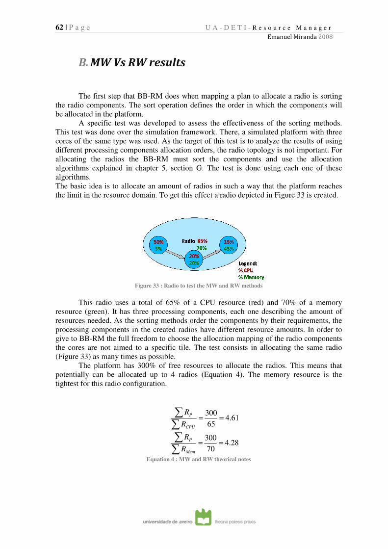
62 | P a g e
B. MW Vs RW results
The first step that BB
the radio components. The sort operation defines the order in which the components will
be allocated in the platform.
A specific test was developed to assess the effectiveness of the sorting methods.
This test was done over the simulation framework. There, a simulated platform with three
cores of the same type was used. As the target of this test is to analyze the results
different processing components allocation orders, the radio topology is not important. For
allocating the radios the BB
algorithms explained in chapter
algorithms.
The basic idea is to allocate an amount of ra
the limit in the resource domain. To get this effect a radio depicted in
Figure
This radio uses a total of 65% of a CPU resource (red) and 70% of a memory
resource (green). It has three processing components, each one describing the amount of
resources needed. As the sorting methods o
processing components in the created radios have different resource amounts. In order to
give to BB-RM the full freedom to choose the allocation mapping of the radio components
the cores are not aimed to a spe
(Figure 33) as many times as possible.
The platform has 300% of free resources to allocate the radios. This
potentially can be allocated up to 4 radios (
tightest for this radio configuration.
U A - D E T I - R e s o u r c e M a n a g e r
Emanuel Miranda
MW Vs RW results
The first step that BB-RM does when mapping a plan to allocate
the radio components. The sort operation defines the order in which the components will
be allocated in the platform.
A specific test was developed to assess the effectiveness of the sorting methods.
This test was done over the simulation framework. There, a simulated platform with three
cores of the same type was used. As the target of this test is to analyze the results
different processing components allocation orders, the radio topology is not important. For
allocating the radios the BB-RM must sort the components and use the allocation
algorithms explained in chapter 5, section G. The test is done using each one of these
The basic idea is to allocate an amount of radios in such a way that the platform reaches
the limit in the resource domain. To get this effect a radio depicted in Figure
Figure 33 : Radio to test the MW and RW methods
This radio uses a total of 65% of a CPU resource (red) and 70% of a memory
resource (green). It has three processing components, each one describing the amount of
resources needed. As the sorting methods order the components by their requirements, the
processing components in the created radios have different resource amounts. In order to
RM the full freedom to choose the allocation mapping of the radio components
the cores are not aimed to a specific tile. The test consists in allocating the same radio
) as many times as possible.
The platform has 300% of free resources to allocate the radios. This
potentially can be allocated up to 4 radios (Equation 4). The memory resource is the
tightest for this radio configuration.
61.465
300==
∑∑
CPU
P
R
R
28.470
300==
∑∑
Mem
P
R
R
Equation 4 : MW and RW theorical notes
R e s o u r c e M a n a g e r
Emanuel Miranda 2008
to allocate a radio is sorting
the radio components. The sort operation defines the order in which the components will
A specific test was developed to assess the effectiveness of the sorting methods.
This test was done over the simulation framework. There, a simulated platform with three
cores of the same type was used. As the target of this test is to analyze the results of using
different processing components allocation orders, the radio topology is not important. For
RM must sort the components and use the allocation
. The test is done using each one of these
dios in such a way that the platform reaches
Figure 33 is created.
This radio uses a total of 65% of a CPU resource (red) and 70% of a memory
resource (green). It has three processing components, each one describing the amount of
rder the components by their requirements, the
processing components in the created radios have different resource amounts. In order to
RM the full freedom to choose the allocation mapping of the radio components
cific tile. The test consists in allocating the same radio
The platform has 300% of free resources to allocate the radios. This means that
). The memory resource is the
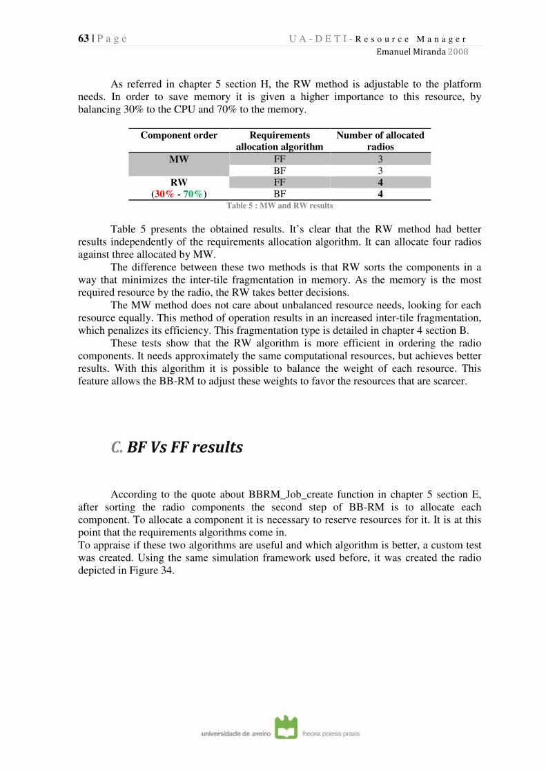
63 | P a g e U A - D E T I - R e s o u r c e M a n a g e r
Emanuel Miranda 2008
As referred in chapter 5 section H, the RW method is adjustable to the platform
needs. In order to save memory it is given a higher importance to this resource, by
balancing 30% to the CPU and 70% to the memory.
Component order Requirements
allocation algorithm
Number of allocated
radios
MW FF 3
BF 3
RW
(30% - 70%)
FF 4 BF 4
Table 5 : MW and RW results
Table 5 presents the obtained results. It’s clear that the RW method had better
results independently of the requirements allocation algorithm. It can allocate four radios
against three allocated by MW.
The difference between these two methods is that RW sorts the components in a
way that minimizes the inter-tile fragmentation in memory. As the memory is the most
required resource by the radio, the RW takes better decisions.
The MW method does not care about unbalanced resource needs, looking for each
resource equally. This method of operation results in an increased inter-tile fragmentation,
which penalizes its efficiency. This fragmentation type is detailed in chapter 4 section B.
These tests show that the RW algorithm is more efficient in ordering the radio
components. It needs approximately the same computational resources, but achieves better
results. With this algorithm it is possible to balance the weight of each resource. This
feature allows the BB-RM to adjust these weights to favor the resources that are scarcer.
C. BF Vs FF results
According to the quote about BBRM_Job_create function in chapter 5 section E,
after sorting the radio components the second step of BB-RM is to allocate each
component. To allocate a component it is necessary to reserve resources for it. It is at this
point that the requirements algorithms come in.
To appraise if these two algorithms are useful and which algorithm is better, a custom test
was created. Using the same simulation framework used before, it was created the radio
depicted in Figure 34.
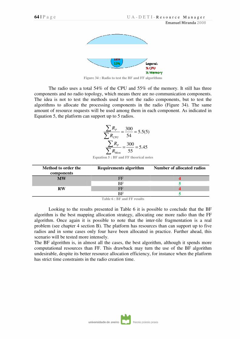
64 | P a g e
Figure
The radio uses a total 54% of the CPU and 55% of the memory. It still has three
components and no radio topology, which means there are no communication components.
The idea is not to test the methods used to sort
algorithms to allocate the processing components in the radio (
amount of resource requests will be used amo
Equation 5, the platform can support up to 5 radios.
Method to order the
components
MW
RW
Looking to the results presented in
algorithm is the best mapping allocation strategy, allocating one more radio than the FF
algorithm. Once again it is pos
problem (see chapter 4 section
radios and in some cases only four have been allocated in practice. Further ahead, this
scenario will be tested more intensely.
The BF algorithm is, in almost all the cases, the best algorithm, although it spends more
computational resources than FF. This drawback may turn the use of the BF algorithm
undesirable, despite its better resource allocation efficiency, for instance when the p
has strict time constraints in the radio creation time.
U A - D E T I - R e s o u r c e M a n a g e r
Emanuel Miranda
Figure 34 : Radio to test the BF and FF algorithms
The radio uses a total 54% of the CPU and 55% of the memory. It still has three
components and no radio topology, which means there are no communication components.
The idea is not to test the methods used to sort the radio components, but to test the
algorithms to allocate the processing components in the radio (Figure
amount of resource requests will be used among them in each component. As indicated in
, the platform can support up to 5 radios.
)5(5.554
300==
∑∑
CPU
P
R
R
45.555
300==
∑∑
Mem
P
R
R
Equation 5 : BF and FF theorical notes
Requirements algorithm Number of allocated radios
FF
BF
FF
BF Table 6 : BF and FF results
Looking to the results presented in Table 6 it is possible to conclude that the BF
algorithm is the best mapping allocation strategy, allocating one more radio than the FF
algorithm. Once again it is possible to note that the inter-tile fragmentation is a real
section B). The platform has resources than can support up to five
radios and in some cases only four have been allocated in practice. Further ahead, this
scenario will be tested more intensely.
F algorithm is, in almost all the cases, the best algorithm, although it spends more
computational resources than FF. This drawback may turn the use of the BF algorithm
undesirable, despite its better resource allocation efficiency, for instance when the p
has strict time constraints in the radio creation time.
R e s o u r c e M a n a g e r
Emanuel Miranda 2008
The radio uses a total 54% of the CPU and 55% of the memory. It still has three
components and no radio topology, which means there are no communication components.
the radio components, but to test the
Figure 34). The same
ng them in each component. As indicated in
Number of allocated radios
4
5
4
5
it is possible to conclude that the BF
algorithm is the best mapping allocation strategy, allocating one more radio than the FF
tile fragmentation is a real
). The platform has resources than can support up to five
radios and in some cases only four have been allocated in practice. Further ahead, this
F algorithm is, in almost all the cases, the best algorithm, although it spends more
computational resources than FF. This drawback may turn the use of the BF algorithm
undesirable, despite its better resource allocation efficiency, for instance when the platform
65 | P a g e
D. Complete
There are two types of RAP heuristics worth noticing. The first type is when it uses
one of the two implemented methods to sort the radio component
algorithms to allocate the component requirements. Thus, this type of heuristic is a strict
combination among various methods and algorithms. One example of this heuristic is the
BFDMW explained in chapter
method and an algorithm as well, but add
latter class is the FFC complete RAP, presented in chapter
The performance assessment of the BFDMW does not need specific testing because
the results are a combination of the base sorting method and algorithm results. On the other
hand, the FFC was developed to save
Consequently the connection times are reduced and the radio becomes faster. Thus, it
would be relevant to measure the resulting performance improvement of this strategy.
However, the simulation framework has a t
code but is unable to measure the radio performance, preventing the possibility of testing
the complete RAP.
E. Fragmentation results
The tests done in the last two sections proved the actual appearance of inter
fragmentation, which caused allocation problems. A paradigmatic example was the FF
results (section C), where the platform had enough resources to allocate five
practice was only able to allocate four. This section presents a test that addresses the
experimental verification of the inter
One problem of the BB
fragmentation problem in its resource model. Due to this fact, the BB
approval to a radio that, in the real platform, will not fit. This situation can happen in two
memory parts of the tile: data & status memory and FIFO memory (see chapter
A). The problem is similar in both cases, thus our tests have been directed
memory fragmentation, only. In this case the test uses both on the simulation and the real
platform, since the simulation framework does not model the fragmentation problems.
Figure
U A - D E T I - R e s o u r c e M a n a g e r
Emanuel Miranda
Complete Resource Allocation Problem
There are two types of RAP heuristics worth noticing. The first type is when it uses
one of the two implemented methods to sort the radio components and one of the two
algorithms to allocate the component requirements. Thus, this type of heuristic is a strict
combination among various methods and algorithms. One example of this heuristic is the
BFDMW explained in chapter 5 section I. The other type of heuristic uses
method and an algorithm as well, but adds specific optimizations. As an example of this
latter class is the FFC complete RAP, presented in chapter 5 section I.
The performance assessment of the BFDMW does not need specific testing because
the results are a combination of the base sorting method and algorithm results. On the other
hand, the FFC was developed to save the bandwidth communication among the tiles.
Consequently the connection times are reduced and the radio becomes faster. Thus, it
would be relevant to measure the resulting performance improvement of this strategy.
However, the simulation framework has a tool to measure the time of the management
code but is unable to measure the radio performance, preventing the possibility of testing
Fragmentation results
The tests done in the last two sections proved the actual appearance of inter
fragmentation, which caused allocation problems. A paradigmatic example was the FF
), where the platform had enough resources to allocate five
practice was only able to allocate four. This section presents a test that addresses the
experimental verification of the inter-tile fragmentation problem.
One problem of the BB-RM is that it does not account for the intra
problem in its resource model. Due to this fact, the BB
approval to a radio that, in the real platform, will not fit. This situation can happen in two
memory parts of the tile: data & status memory and FIFO memory (see chapter
). The problem is similar in both cases, thus our tests have been directed
memory fragmentation, only. In this case the test uses both on the simulation and the real
platform, since the simulation framework does not model the fragmentation problems.
Figure 35 : Radios to test the FIFO fragmentation
R e s o u r c e M a n a g e r
Emanuel Miranda 2008
roblem results
There are two types of RAP heuristics worth noticing. The first type is when it uses
s and one of the two
algorithms to allocate the component requirements. Thus, this type of heuristic is a strict
combination among various methods and algorithms. One example of this heuristic is the
. The other type of heuristic uses an implemented
s specific optimizations. As an example of this
The performance assessment of the BFDMW does not need specific testing because
the results are a combination of the base sorting method and algorithm results. On the other
the bandwidth communication among the tiles.
Consequently the connection times are reduced and the radio becomes faster. Thus, it
would be relevant to measure the resulting performance improvement of this strategy.
ool to measure the time of the management
code but is unable to measure the radio performance, preventing the possibility of testing
The tests done in the last two sections proved the actual appearance of inter-tile
fragmentation, which caused allocation problems. A paradigmatic example was the FF
), where the platform had enough resources to allocate five radios and in
practice was only able to allocate four. This section presents a test that addresses the
RM is that it does not account for the intra-tile
problem in its resource model. Due to this fact, the BB-RM can give an
approval to a radio that, in the real platform, will not fit. This situation can happen in two
memory parts of the tile: data & status memory and FIFO memory (see chapter 3 section
). The problem is similar in both cases, thus our tests have been directed to the FIFO
memory fragmentation, only. In this case the test uses both on the simulation and the real
platform, since the simulation framework does not model the fragmentation problems.
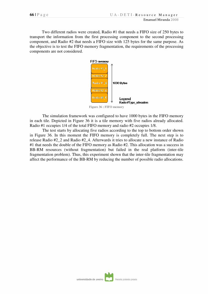
66 | P a g e
Two different radios were created, Radio #1 that needs a FIFO size of 250 bytes to
transport the information from the first processing component to the second processing
component, and Radio #2 that needs a FIFO si
the objective is to test the FIFO memory fragmentation, the requirements of the processing
components are not considered.
The simulation framework was configur
in each tile. Depicted in Figure
Radio #1 occupies 1/4 of the tota
The test starts by allocating five radios according to the top to bottom order shown
in Figure 36. In this moment the FIFO memory is completely full. The next step is to
release Radio #2_2 and Radio #2_4. Afterwards it tries to allocate a new instance of Radio
#1 that needs the double of
BB-RM resources (without fragmentation) but failed in the real platform (inter
fragmentation problem). Thus, this experiment shown that the inter
affect the performance of the BB
U A - D E T I - R e s o u r c e M a n a g e r
Emanuel Miranda
Two different radios were created, Radio #1 that needs a FIFO size of 250 bytes to
transport the information from the first processing component to the second processing
component, and Radio #2 that needs a FIFO size with 125 bytes for the same purpose. As
the objective is to test the FIFO memory fragmentation, the requirements of the processing
components are not considered.
Figure 36 : FIFO memory
The simulation framework was configured to have 1000 bytes in the FIFO memory
Figure 36 it is a tile memory with five radios already allocated.
Radio #1 occupies 1/4 of the total FIFO memory and radio #2 occupies 1/8.
The test starts by allocating five radios according to the top to bottom order shown
. In this moment the FIFO memory is completely full. The next step is to
release Radio #2_2 and Radio #2_4. Afterwards it tries to allocate a new instance of Radio
#1 that needs the double of the FIFO memory as Radio #2. This allocation was a success in
RM resources (without fragmentation) but failed in the real platform (inter
fragmentation problem). Thus, this experiment shown that the inter-tile fragmentation may
ce of the BB-RM by reducing the number of possible radio allocations.
R e s o u r c e M a n a g e r
Emanuel Miranda 2008
Two different radios were created, Radio #1 that needs a FIFO size of 250 bytes to
transport the information from the first processing component to the second processing
ze with 125 bytes for the same purpose. As
the objective is to test the FIFO memory fragmentation, the requirements of the processing
ed to have 1000 bytes in the FIFO memory
it is a tile memory with five radios already allocated.
l FIFO memory and radio #2 occupies 1/8.
The test starts by allocating five radios according to the top to bottom order shown
. In this moment the FIFO memory is completely full. The next step is to
release Radio #2_2 and Radio #2_4. Afterwards it tries to allocate a new instance of Radio
the FIFO memory as Radio #2. This allocation was a success in
RM resources (without fragmentation) but failed in the real platform (inter-tile
tile fragmentation may
RM by reducing the number of possible radio allocations.
67 | P a g e U A - D E T I - R e s o u r c e M a n a g e r
Emanuel Miranda 2008
7. Conclusions and future work
The main objective of this dissertation was the development of a Baseband
Resource Manager module for heterogeneous multi-processor radio platforms. The
developed BB-RM provides:
� Admission control - The BB-RM only allows the creation of additional radios only
if enough resources are available. Thus, new radios do not disturb the already
running radios. As the radios have RT requirements, the BB-RM guarantees that
the deadlines associated with the computations of all the radios (the already running
radios as well as newly added ones) are met.
� Resource reservation - Each radio can only use the resources that have been
reserved for it.
The BB-RM allows and guarantees different rates of operation among functions
within the radio and even among radios. The unpredictable start/stop times of a radio will
not disturb the requirement of the running radios.
In order to be applied in several infotainment mediums, the BB-RM supports a
wide variety of radios and even radio combinations, which makes it completely adjustable
to the platform. The tile configuration or even the processor type is configurable as well.
For instance, in the future it will be possible to run this BB-RM in a platform with the
double or triple of the number of processors. This was accomplished without changing the
SoD, turning the BB-RM autonomous from the SoD platform.
It is estimated that for the current platform, called AeroProto2, it is possible to run
at least five radios simultaneously. In this context BB-RM allows dynamically changing
the radios executed in each instant.
The BB-RM has proven to have a good performance despite using limited
computational resources. In the simulation framework the whole system needs around
14µs to allocate a radio. This time is acceptable in land radio platforms.
The implemented heuristics to allocate the radio components are working perfectly.
In this land radio platform, the RW proved to be the best method to order the radio
components, being able to allocate one more radio than MW (Table 5). The BF allocation
algorithm has proved to be better than FF. In the tests, the BF algorithm allocated one more
radio than FF (Table 6). In conclusion, if the platform has enough computation resources,
the best combination to a complete RAP is RW with BF. On the other hand, if the
computation resources are scarce, the best combination to solve the complete RAP is RW
with FF. In theory the FFC complete RAP should to be a good solution to reduce the
68 | P a g e U A - D E T I - R e s o u r c e M a n a g e r
Emanuel Miranda 2008
communications bandwidth but it was not possible to prove it on the real platform or even
in simulation framework.
A. Future work
Despite all the effort put in this project, some aspects remain to be solved.
Within each tile the memory can become fragmented (intra-tile fragmentation). The
amount of fragmentation increases with memory usage. In its current state the BB-RM
cannot model fragmentation, potentially leading to allocation inconsistencies. This
inconsistency is created when the radio passes the BB-RM tests and it does not fit in the
real platform. This inconsistency is caused by the VBP algorithm used by BB-RM which
does not account with the fragmentation problem, as detailed in chapter 5, section I. To
solve this issue, the BB-RM should implement in the same memory allocation algorithm as
the one used in the real platform. This way the BB-RM would have an exact copy of the
memory mapping of the real platform, solving the inconsistency problem.
Another improvement that can be done in BB-RM is on the RW sort strategy. This
method is used to order the components in an efficient way, this if the resource weights are
properly defined. It is possible to set the right resource weight in the beginning and, after
some allocations, the resource weights may need to be adjusted. This happens because
different radios use different amounts of each resource. To solve this issue the resource
weight should be dynamically adjusted in run-time. Having the knowledge of the resource
status, the resource weights could to be manipulated to save the more scarce resources in
each instant.
69 | P a g e U A - D E T I - R e s o u r c e M a n a g e r
Emanuel Miranda 2008
8. Bibliography
1. Mehrotra, Asha. Cellular radio performance engineering. s.l. : Artech House, 1994.
2. Radio computer: vision, value, stakeholder views, Radio Programming Interface
scenarios. Tolonen, Pertti and Berkel, Kess van.
3. gsmworld. [Online] [Cited: October 12, 2008.]
http://www.gsmworld.com/about/history.shtml.
4. Hennessy, John L. and Patterson, David A. Computer Architecture. s.l. : third edition.
5. Sepillo, A. L. A Comparative Study on Symmetric and Asymmetric Multiprocessors.
Diliman : University of the Philippines.
6. Ahtiainen, Ari, et al. SDR Functional Architecture Overview. 2008.
7. Self-Timed Scheduling Analysis for a Real-Time Applications. Moreira, Orlando and
Bekooij, Marco. 8. Pedreiras, Paulo e Almeida, Luis. Sistemas de Tempo-Real. Aveiro : s.n., 2008.
9. Herlihy, Maurice and Shavit, Nir. The Art of Multiprocessor Programming.
10. Tanenbaum, Andrew S. Operating Systems Design and Implementation. s.l. : third
edition.
11. Timothy, O'Neil W., Edwin, H. and Sha, M. Retiming Synchronous Data-Flow
Graphs to Reduce Execution Time.
12. NXP. User's manuel for AeroSOFT development board. Netherlands : NXP, 2008.
13. Kourzanov, Pjotr. [Online] [Cited: 11 5, 2008.] ://www.bitbucket.org/pjotr/lime/src/.
14. LIME: a future-proof programming model for multi-core. Kouranov, Pjotr, Moreira,
Orlando and Sips, Henk. 15. Pol, E. J., Rutten, M. and Splunter, M. van. Sea of DSP Programmer's user manual.
16. Labrosse, Jean J. MicroC/OS-II - The Real Time Kernel. CMP.
17. Scheduling Multiple Independet Hard-Real-Time Jobs on a Heterogeneous
Multiprocessor. Moreira, Olando, Valente, Frederico and Bekooij, Marco.
18. Online Resource Management in a Multiprocessor with a Network-on-Chip. Moreira,
Orlando, Mol, Jacob Jan-David and Bekooij, Marco. 19. Moreira, Orlando, et al. Multiprocessor resource allocator for Hard-real-time
Streaming with a Dynamic job-mix.
20. Douglass, Bruce Powel. Real-Time design Pattens: Robust Scalable Architecture for
Real-Time Systems.

70 | P a g e U A - D E T I - R e s o u r c e M a n a g e r
Emanuel Miranda 2008
(This page was left blank delivered)
71 | P a g e U A - D E T I - R e s o u r c e M a n a g e r
Emanuel Miranda 2008
9. Appendices
A. Doxygen API code documentation
bbrm_code_return_t BBRM_initialize (void)
This function must be called in the system starter.
This function initializes:
• the Streaming Kernel in SoD by calling phSodEmulateInit() function;
• the job list, by calling BBRM_initialize() function;
• the CPU BB-RM resource model, by calling CPU_initialize() function;
• the memory BB-RM resource model, by calling Mem_initialize() function.
Returns:
• BBRM_FATAL_ERROR_SOD_FAILED - Fatal SOD function failed.
• BBRM_FATAL_ERROR_CPU_FAILED - Round Robin function failed.
• BBRM_FATAL_ERROR_MEM_FAILED - Memory function failed.
• BBRM_OK - Operation successful.
bbrm_code_return_t BBRM_Job_test (const radio_t *
radio_p)
The BBRM_Job_test function tests whether instantiation of a job is possible
The internal procedures are:
• finds the free entry in job list;
• fills the job entry with:
• source radio pointer;
• source radio ID;
• changes the job state to SIMULATION MODE; • sets all BB-RM resources in a simulation mode by calling the BBRM_Set_res_simul() function;
• if failed clean the job in job list by calling BBRM_initialize() function; • allocates the radio requirements by calling the BBRM_Simul_job() function;
• restores the resources by calling BBRM_Set_res_restore() function;
72 | P a g e U A - D E T I - R e s o u r c e M a n a g e r
Emanuel Miranda 2008
• cleans the job in job list by calling BBRM_initialize() function;
Parameters:
radio_p (IN) Pointer to the radio.
Returns:
• BBRM_FATAL_ERROR_RES_STATE - Error while change the BB-RM
resources states.
• BBRM_ERROR_SIMUL - This radio fail in requirements simulation.
• BBRM_OK - Operation successful.
bbrm_code_return_t BBRM_Job_create (const
radio_t * radio_p, uint8_t *const created_job_id)
The BBRM_Job_create function creates a job, (radio instance) and sets it on suspend mode, to
put the job running it needs call the BBRM_Job_resume() function.
The internal procedures are:
• validates the radio by calling the BBRM_Test_radio() function;
• finds the free entry in job list;
• fills the job entry with:
• source radio pointer;
• source radio ID;
• changes the job state to SIMULATION MODE; • sets all resources in a simulation mode by calling the BBRM_Set_res_simul() function;
• if failed cleans the job in job list by calling BBRM_initialize() function; • allocates the radio requirements by calling the BBRM_Simul_job() function;
• if the test failed:
• restores the resources by calling BBRM_Set_res_restore() function;
• cleans the job in job list by calling BBRM_initialize() function;
• in case of success sets the job state as TESTED MODE; • allocates the radio tasks in SoD by calling the BBRM_Alloc_sod_c_comps() function;
• if the test failed:
• restores the BB-RM resources by calling BBRM_Set_res_restore()
function;
• cleans the job in job list by calling BBRM_initialize() function;
• • allocates the radio FIFOs in SoD by calling the BBRM_Alloc_sod_c_comps() function;
• if the test failed:
• restores the BB-RM resources by calling BBRM_Set_res_restore()
function;
• cleans the job in job list by calling BBRM_initialize() function;
• • sets the task parameters in SoD by calling the BBRM_Sod_parameters() function;
• if the test failed:
• restores the BB-RM resources by calling BBRM_Set_res_restore()
function;
73 | P a g e U A - D E T I - R e s o u r c e M a n a g e r
Emanuel Miranda 2008
• cleans the job in job list by calling BBRM_initialize() function;
• • sets all resources in RUNNING MODE;
• sets the job state at SUSPEND MODE;
• returns the created job ID.
Parameters:
radio_p (IN) Radio pointer with all Radio parameters.
created_job_id (OUT) Returns the created job ID.
Returns:
• BBRM_FATAL_ERROR_RADIO - This radio can't to be run.
• BBRM_FATAL_ERROR_RES_STATE - Error while change the BB-RM
resources states.
• BBRM_ERROR_SIMUL - This radio fail in requirements simulation.
• BBRM_FATAL_ERROR_UNAL_T - Tasks release fail.
• BBRM_ERROR_SOD_FAILED - SOD function failed.
• BBRM_FATAL_ERROR_ALLOC_F - Error while allocating the FIFOs in Sod
platform.
• BBRM_ERROR_PARAM - Error while set the task parameters in SoD.
• BBRM_OK - Operation successful.
bbrm_code_return_t BBRM_Job_resume (const
uint8_t job_id)
This function sets the given job running in the platform.
The internal procedures are:
• Validates if the job state, must be in suspend mode;
• For each task in job:
• resumes the task in SoD by calling phSodNmTask_Resume() function;
• validates the result; • Changes the job state.
Parameters:
job_id (IN) ID of the job that will be resumed.
Returns:
• BBRM_ERROR_JOB_RES - Job is not ready to be resumed.
• BBRM_FATAL_ERROR_SOD_FAILED - SOD function failed.
• BBRM_OK - Operation successful.
74 | P a g e U A - D E T I - R e s o u r c e M a n a g e r
Emanuel Miranda 2008
bbrm_code_return_t BBRM_Job_suspend (const
uint8_t job_id)
This function changes the running job to a suspended job, but the job still in the platform, that
means, all requirements of this job still reserved for it.
The internal procedures are:
• verifies if the given job ID is on running mode;
• determines the number of components in radio by calling the BBRM_Nr_of_p_comps() function;
• traces all components inside the given job and suspend each one by calling the
phSodNmTask_Suspend() function.
• sets the job state as suspend mode.
Parameters:
job_id (IN) ID of the job that will be suspended.
Returns:
• BBRM_ERROR_JOB_SUS - Job is not ready to be suspended (must be in run
state).
• BBRM_FATAL_ERROR_SOD_FAILED - SOD function failed.
• BBRM_OK - Operation successful.
bbrm_code_return_t BBRM_Job_remove (const
uint8_t job_id)
The BBRM_Job_remove function removes the suspended job and remove it from the SoD.
That means all resources used by this job are released in BB-RM.
The internal procedures are:
• verifies if the job state is in suspended mode;
• release from SoD:
• calls BBRM_Release_sod_fifos() function to remove all FIFOs of this job;
• calls BBRM_Release_sod_tasks() function to remove all Tasks of this job; • releases the BB-RM resources: by calling BBRM_Release_comp_reqs() function;
• cleans the job in job list by calling BBRM_initialize() function;
Parameters:
job_id (IN) ID of the job that will be removed.
Returns:
• BBRM_ERROR_JOB_NREADY - Job is not ready to be removed (must be in
SUSPEND state).
• BBRM_FATAL_ERROR_CPU_FAILED - Round Robin function failed.
• BBRM_FATAL_ERROR_MEM_FAILED - Memory function failed.
• BBRM_FATAL_ERROR_UNALLOC - (At least one) requirement did not be
release.
75 | P a g e U A - D E T I - R e s o u r c e M a n a g e r
Emanuel Miranda 2008
• BBRM_FATAL_ERROR_UNAL_F - FIFOs unallocated failed.
• BBRM_FATAL_ERROR_UNAL_T - Tasks unallocated failed.
• BBRM_OK - Operation successful.
B. Functions performances in version 1.2
To measure the performance of the BB-RM functions the GNU Profiling (gprof)
program was used. A stress test was created to calls 2000000 times each BB-RM function.
The results of the version 1.2 are next.
Flat profile:
Each sample counts as 0.01 seconds.
% cumulative self self total
time seconds seconds calls us/call us/call name
1.04 23.82 0.32 2000000 0.16 4.28 BBRM_Job_create
1.04 24.14 0.32 phSodNmPort_Connect
1.04 24.46 0.32 phSodNmTask_Delete
0.98 24.77 0.30 phSodMgr_TileInitialized
0.95 25.05 0.29 phSodNmPort_Disconnect
0.65 27.02 0.20 2000000 0.10 1.00 BBRM_Job_remove
0.64 27.21 0.20 phSodMgr_MemStateBlockAlloc
0.00 30.63 0.00 1 0.00 0.00 BBRM_initialize
% time - the percentage of the total running time of the program used by this function.
cumulative seconds - a running sum of the number of seconds accounted for by this
function and those listed above it.
self seconds - the number of seconds accounted for by this function alone. This is the
major sort for this listing.
calls - the number of times this function was invoked, if this function is profiled, else
blank.
self ms/call - the average number of milliseconds spent in this function per call, if this
function is profiled, else blank.
total ms/call - the average number of milliseconds spent in this function and its
descendents per call, if this function is profiled, else blank.
76 | P a g e U A - D E T I - R e s o u r c e M a n a g e r
Emanuel Miranda 2008
name - the name of the function. This is the minor sort for this listing. The index shows
the location of the function in the gprof listing. If the index is in parenthesis it shows where
it would appear in the gprof listing if it were to be printed.
Call graph (explanation follows)
granularity: each sample hit covers 4 byte(s) for 0.03% of 30.63 seconds
index % time self children called name
<spontaneous>
[1] 35.0 0.17 10.54 main [1]
0.32 8.23 2000000/2000000 BBRM_Job_create [2]
0.20 1.79 2000000/2000000 BBRM_Job_remove [6]
0.00 0.00 1/1 BBRM_initialize [76]
-----------------------------------------------
0.32 8.23 2000000/2000000 main [1]
[2] 27.9 0.32 8.23 2000000 BBRM_Job_create [2]
0.19 4.46 2000000/2000000 BBRM_Simul_radio_reqs [4]
1.65 0.00 2000000/2000000 BBRM_Test_radio [8]
0.74 0.00 2000000/2000000 BBRM_Alloc_sod_fifos [15]
0.05 0.50 2000000/2000000 BBRM_Set_res_simul [20]
0.01 0.35 2000000/2000000 BBRM_Set_res_run [25]
0.19 0.00 2000000/2000000 BBRM_Alloc_sod_tasks [42]
0.09 0.00 2000000/2000000 BBRM_Sod_parameters [57]
-----------------------------------------------
0.20 1.79 2000000/2000000 main [1]
[6] 6.5 0.20 1.79 2000000 BBRM_Job_remove [6]
0.56 0.81 10000000/10000000 BBRM_Unalloc_node_reqs [9]
0.33 0.00 2000000/2000000 BBRM_Unalloc_sod_fifos [28]
0.09 0.00 2000000/2000000 BBRM_Unalloc_sod_tasks [58]
-----------------------------------------------
[76] 0.0 0.00 0.00 1 BBRM_initialize [76]
-----------------------------------------------
This table describes the call tree of the program, and was sorted by the total amount of time
spent in each function and its children.
Each entry in this table consists of several lines. The line with the index number at the left
hand margin lists the current function. The lines above it list the functions that called this
function, and the lines below it list the functions this one called.
This line lists:
Index - A unique number given to each element of the table. Index numbers are sorted
numerically. The index number is printed next to every function name so it is easier to look
up where the function in the table.

77 | P a g e U A - D E T I - R e s o u r c e M a n a g e r
Emanuel Miranda 2008
% time - This is the percentage of the `total' time that was spent in this function and its
children. Note that due to different viewpoints, functions excluded by options, etc, these
numbers will NOT add up to 100%.
self - This is the total amount of time spent in this function.
children - This is the total amount of time propagated into this function by its children.
called - This is the number of times the function was called. If the function called itself
recursively, the number only includes non-recursive calls, and is followed by a `+'
and the number of recursive calls.
name - The name of the current function. The index number is printed after it. If the
function is a member of a cycle, the cycle number is printed between the function's name
and the index number.
For the function's parents, the fields have the following meanings:
self - This is the amount of time that was propagated directly from the function into this
parent.
children - This is the amount of time that was propagated from the function's
children into this parent.
called - This is the number of times this parent called the function `/' the total number of
times the function was called. Recursive calls to the function are not included in the
number after the `/'.
name - This is the name of the parent. The parent's index number is printed after it. If
the parent is a member of a cycle, the cycle number is printed between the name and the
index number.
If the parents of the function cannot be determined, the word `<spontaneous>' is printed in
the `name' field, and all the other fields are blank.
For the function's children, the fields have the following meanings:
self - This is the amount of time that was propagated directly from the child into the
function.
children - This is the amount of time that was propagated from the child's children to
the function.
called - This is the number of times the function called this child `/' the total number of
times the child was called. Recursive calls by the child are not listed in the number after
the `/'.
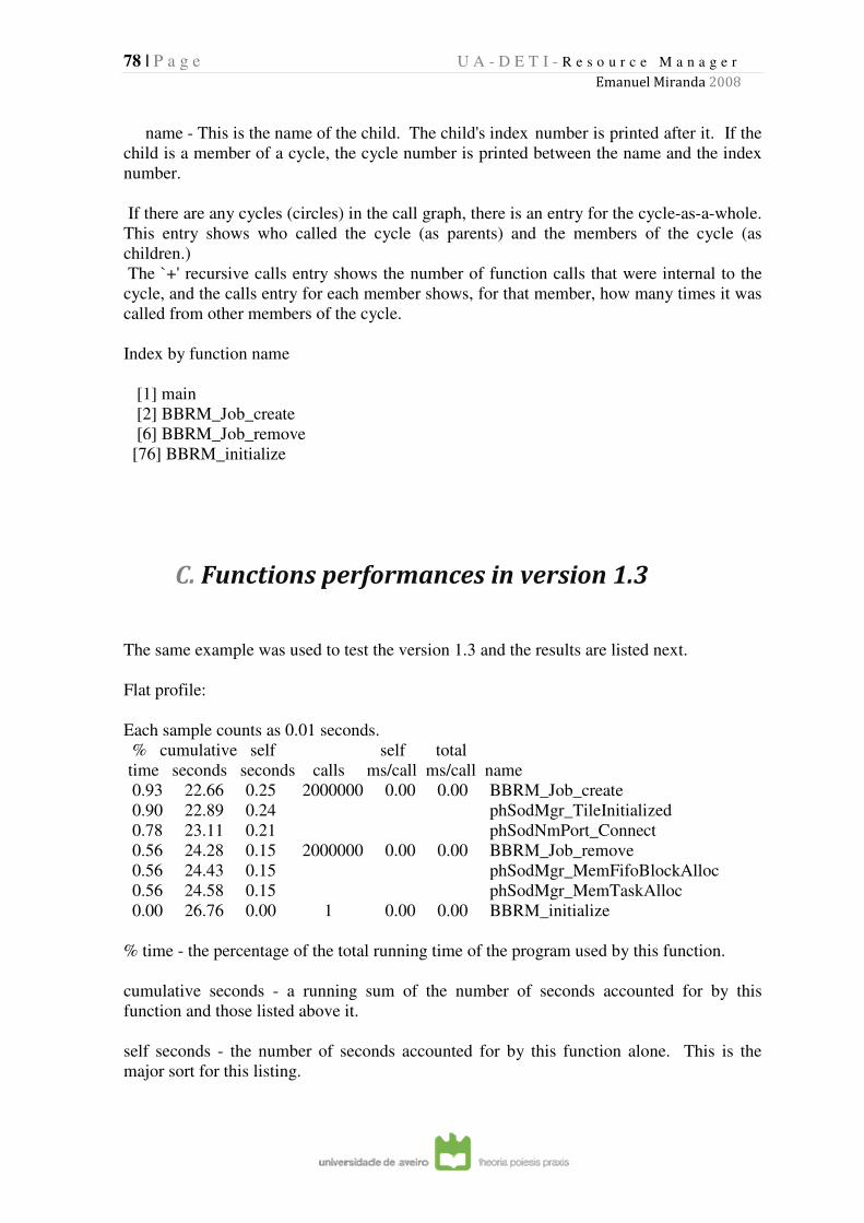
78 | P a g e U A - D E T I - R e s o u r c e M a n a g e r
Emanuel Miranda 2008
name - This is the name of the child. The child's index number is printed after it. If the
child is a member of a cycle, the cycle number is printed between the name and the index
number.
If there are any cycles (circles) in the call graph, there is an entry for the cycle-as-a-whole.
This entry shows who called the cycle (as parents) and the members of the cycle (as
children.)
The `+' recursive calls entry shows the number of function calls that were internal to the
cycle, and the calls entry for each member shows, for that member, how many times it was
called from other members of the cycle.
Index by function name
[1] main
[2] BBRM_Job_create
[6] BBRM_Job_remove
[76] BBRM_initialize
C. Functions performances in version 1.3
The same example was used to test the version 1.3 and the results are listed next.
Flat profile:
Each sample counts as 0.01 seconds.
% cumulative self self total
time seconds seconds calls ms/call ms/call name
0.93 22.66 0.25 2000000 0.00 0.00 BBRM_Job_create
0.90 22.89 0.24 phSodMgr_TileInitialized
0.78 23.11 0.21 phSodNmPort_Connect
0.56 24.28 0.15 2000000 0.00 0.00 BBRM_Job_remove
0.56 24.43 0.15 phSodMgr_MemFifoBlockAlloc
0.56 24.58 0.15 phSodMgr_MemTaskAlloc
0.00 26.76 0.00 1 0.00 0.00 BBRM_initialize
% time - the percentage of the total running time of the program used by this function.
cumulative seconds - a running sum of the number of seconds accounted for by this
function and those listed above it.
self seconds - the number of seconds accounted for by this function alone. This is the
major sort for this listing.

79 | P a g e U A - D E T I - R e s o u r c e M a n a g e r
Emanuel Miranda 2008
calls - the number of times this function was invoked, if this function is profiled, else
blank.
self ms/call - the average number of milliseconds spent in this function per call, if this
function is profiled, else blank.
total ms/call - the average number of milliseconds spent in this function and its
descendents per call, if this function is profiled, else blank.
name - the name of the function. This is the minor sort for this listing. The index shows
the location of the function in the gprof listing. If the index is in parenthesis it shows where
it would appear in the gprof listing if it were to be printed.
Call graph (explanation follows)
granularity: each sample hit covers 4 byte(s) for 0.04% of 26.76 seconds
index % time self children called name
<spontaneous>
[2] 25.9 0.02 6.91 main [2]
0.25 5.12 2000000/2000000 BBRM_Job_create [3]
0.15 1.39 2000000/2000000 BBRM_Job_remove [6]
0.00 0.00 1/1 BBRM_initialize [79]
-----------------------------------------------
0.25 5.12 2000000/2000000 main [2]
[3] 20.1 0.25 5.12 2000000 BBRM_Job_create [3]
0.14 3.00 2000000/2000000 BBRM_Simul_radio_reqs [4]
1.01 0.00 2000000/2000000 BBRM_Test_radio [10]
0.40 0.00 2000000/2000000 BBRM_Alloc_sod_fifos [19]
0.03 0.21 2000000/2000000 BBRM_Set_res_simul [32]
0.00 0.18 2000000/2000000 BBRM_Set_res_run [35]
0.10 0.00 2000000/2000000 BBRM_Alloc_sod_tasks [50]
0.05 0.00 2000000/2000000 BBRM_Sod_parameters [60]
-----------------------------------------------
0.15 1.39 2000000/2000000 main [2]
[6] 5.7 0.15 1.39 2000000 BBRM_Job_remove [6]
0.28 0.84 10000000/10000000 BBRM_Release_node_reqs [9]
0.18 0.00 2000000/2000000 BBRM_Release_sod_fifos [37]
0.09 0.00 2000000/2000000 BBRM_Release_sod_tasks [55]
-----------------------------------------------
[77] 0.0 0.00 0.00 1 BBRM_initialize [77]
-----------------------------------------------
This table describes the call tree of the program, and was sorted by the total amount of time
spent in each function and its children.

80 | P a g e U A - D E T I - R e s o u r c e M a n a g e r
Emanuel Miranda 2008
Each entry in this table consists of several lines. The line with the index number at the left
hand margin lists the current function. The lines above it list the functions that called this
function, and the lines below it list the functions this one called.
This line lists:
Index - A unique number given to each element of the table. Index numbers are sorted
numerically. The index number is printed next to every function name so it is easier to look
up where the function in the table.
% time - This is the percentage of the `total' time that was spent in this function and its
children. Note that due to different viewpoints, functions excluded by options, etc, these
numbers will NOT add up to 100%.
self - This is the total amount of time spent in this function.
children - This is the total amount of time propagated into this function by its children.
called - This is the number of times the function was called. If the function called itself
recursively, the number only includes non-recursive calls, and is followed by a `+'
and the number of recursive calls.
name - The name of the current function. The index number is printed after it. If the
function is a member of a cycle, the cycle number is printed between the function's name
and the index number.
For the function's parents, the fields have the following meanings:
self - This is the amount of time that was propagated directly from the function into this
parent.
children - This is the amount of time that was propagated from the function's
children into this parent.
called - This is the number of times this parent called the function `/' the total number of
times the function was called. Recursive calls to the function are not included in the
number after the `/'.
name - This is the name of the parent. The parent's index number is printed after it. If
the parent is a member of a cycle, the cycle number is printed between the name and the
index number.
If the parents of the function cannot be determined, the word `<spontaneous>' is printed in
the `name' field, and all the other fields are blank.
For the function's children, the fields have the following meanings:

81 | P a g e U A - D E T I - R e s o u r c e M a n a g e r
Emanuel Miranda 2008
self - This is the amount of time that was propagated directly from the child into the
function.
children - This is the amount of time that was propagated from the child's children to
the function.
called - This is the number of times the function called this child `/' the total number of
times the child was called. Recursive calls by the child are not listed in the number after
the `/'.
name - This is the name of the child. The child's index number is printed after it. If the
child is a member of a cycle, the cycle number is printed between the name and the index
number.
If there are any cycles (circles) in the call graph, there is an entry for the cycle-as-a-whole.
This entry shows who called the cycle (as parents) and the members of the cycle (as
children.)
The `+' recursive calls entry shows the number of function calls that were internal to the
cycle, and the calls entry for each member shows, for that member, how many times it was
called from other members of the cycle.
Index by function name
[2] main
[3] BBRM_Job_create
[6] BBRM_Job_remove
[77] BBRM_initialize


![sistemas operacionais [Modo de Compatibilidade] · acesso aos recursos do computador . Sobell . • Um Sistema Operacional pode ser definido como um gerenciador dos recursos que compõem](https://img.document.onl/doc/110x75/5c17870f09d3f2c7368bffa4/sistemas-operacionais-modo-de-compatibilidade-acesso-aos-recursos-do-computador.jpg)