Escalonamento de Enlaces e roteamento multi-caminho para redes

COPPE/UFRJ

ESCALONAMENTO DE ENLACES E ROTEAMENTO MULTI-CAMINHO

PARA REDES EM MALHA SEM FIO

Fabio Rocha Jimenez Vieira

Tese de Doutorado apresentada ao Programa

de Pos-graduacao em Engenharia de

Sistemas e Computacao, COPPE, da

Universidade Federal do Rio de Janeiro,

como parte dos requisitos necessarios a

obtencao do tıtulo de Doutor em Engenharia

de Sistemas e Computacao.

Orientadores: Jose Ferreira de Rezende

Valmir Carneiro Barbosa

Serge Fdida

Rio de Janeiro

Maio de 2012




TESE SUBMETIDA AO CORPO DOCENTE DO INSTITUTO ALBERTO LUIZ

COIMBRA DE POS-GRADUACAO E PESQUISA DE ENGENHARIA (COPPE)

DA UNIVERSIDADE FEDERAL DO RIO DE JANEIRO COMO PARTE DOS

REQUISITOS NECESSARIOS PARA A OBTENCAO DO GRAU DE DOUTOR

EM CIENCIAS EM ENGENHARIA DE SISTEMAS E COMPUTACAO.

Examinada por:

Prof. Jose Ferreira de Rezende, D.Sc.

Prof. Valmir Carneiro Barbosa, Ph.D.

Prof. Serge Fdida, D.Sc.

Prof. Eric Fleury, D.Sc.

Prof. Claudio Silva de Amorim, Ph.D.

Prof. Michel Minoux, D.Sc.

RIO DE JANEIRO, RJ – BRASIL

MAIO DE 2012

Vieira, Fabio Rocha Jimenez

Escalonamento de Enlaces e roteamento multi-caminho

para redes em malha sem fio/Fabio Rocha Jimenez Vieira.

– Rio de Janeiro: UFRJ/COPPE, 2012.

XII, 106 p.: il.; 29, 7cm.



Serge Fdida

Tese (doutorado) – UFRJ/COPPE/Programa de

Engenharia de Sistemas e Computacao, 2012.

Referencias Bibliograficas: p. 14 – 20.

1. Redes sem fio. 2. Roteamento multi-caminho.

3. Escalonamento. I. Rezende, Jose Ferreira de et al.

II. Universidade Federal do Rio de Janeiro, COPPE,

Programa de Engenharia de Sistemas e Computacao. III.

Tıtulo.

iii

A minha mae e ao meu pai pelo

dom da vida e pelo amparo ao

longo desses anos.

A minha esposa Juliana pelo

amor.

Ao professor Fdida pela

oportunidade.

Aos meus orientadores Rezende

e Valmir por tudo, simplesmente

tudo.

.

Le Loup et l’Agneau (La

Fontaine).

Se a educacao sozinha nao

transforma a sociedade, sem ela,

tampouco, a sociedade muda

(Paulo Freire).

Life is the art of drawing

sufficient conclusions from

insufficient premises (Samuel

Butler).

iv

Agradecimentos

We acknowledge partial support from CNPq, CAPES, a FAPERJ BBP grant, and a

scholarship grant from Universite Pierre et Marie Curie. Also, I specially thank Pro-

fessor Otto Carlos Muniz Bandeira Duarte for include me in his COFECUB project.

All computational experiments were carried out on the Grid’5000 experimental test-

bed, which is being developed under the INRIA ALADDIN development action with

support from CNRS, RENATER, and several universities as well as other funding

bodies (see https://www.grid5000.fr).

v

Resumo da Tese apresentada a COPPE/UFRJ como parte dos requisitos necessarios

para a obtencao do grau de Doutor em Ciencias (D.Sc.)




Maio/2012



Serge Fdida

Programa: Engenharia de Sistemas e Computacao

Nos apresentamos duas heurısticas como solucao para dois problemas ligados ainterferencia nas redes sem fio. Inicialmente, nos propomos escalonar os enlaces per-tencentes a um conjunto de rotas dado em uma rede congestionada. Nos adotamosum protocolo TDMA que oferece uma fonte de intervalos de tempo sincronizados ebuscamos escalonar os enlaces das rotas objetivando maximizar o numero de pacotesque sao entregues nos destinos das rotas por intervalo de tempo do escalonamento.Nossa abordagem consiste em construir um grafo nao orientado G e obter multiplascoloracoes paro os nos de G que podem induzir aos escalonamentos de enlaces otimossegundo nosso criterio de entrega de pacotes aos destinos. Em G cada no representaum enlace a ser escalonado e as arestas sao acrescentadas ao grafo para represen-tar todas as possıveis interferencias dentro de um conjunto de hipoteses sobre ainterferencia na rede. Nos apresentamos duas heurısticas de multi-coloracao e estu-damos seus desempenhos baseados em uma longa serie de experimentos. Uma dasheurısticas e baseada em no relaxamento da nocao de multi-coloracao de nos e dessaforma, a heurıstica e capaz de eliminar os desperdıcios de intervalos de tempo pro-vocados pelos escalonamentos com estrita multi-coloracao. Nos constatamos que, odesempenho dela e significativamente superior se comparado as demais heurısticas decoloracao de nos. Na segunda proposta, nos apresentamos uma heurıstica que deter-mina um subconjunto dos multiplos caminhos previamente descobertos por qualqueralgoritmo de roteamento. Esse conjunto possui a distinguıvel caracterıstica de naopossuir caminhos que se interferem. A heurıstica proposta e totalmente local doponto de vista de cada no da rede, pois utiliza apenas a informacao disponıvel navizinhanca imediata do no onde esta sendo executada. Nos executamos extensivosexperimentos computacionais com a nova heurıstica, utilizando os algoritmos AODVe OLSR assim como suas versoes multi-caminho. Para dois mecanismos de acesso aomeio (TDMA e CSMA), nos demonstramos que a heurıstica obtem resultados sig-nificativamente superiores aos algoritmos de roteamento originais, tanto em termosde justica na rede como em taxa de transferencia.

vi

Abstract of Thesis presented to COPPE/UFRJ as a partial fulfillment of the

requirements for the degree of Doctor of Science (D.Sc.)

LINK SCHEDULING AND MULTI-PATH ROUTING IN WIRELESS MESH

NETWORKS


May/2012

Advisors: Jose Ferreira de Rezende


Serge Fdida

Department: Systems Engineering and Computer Science

We present algorithmic solutions for two problems related to the wireless networkinterference. The first one proposes to schedule the links of a given set of routesunder the assumption of a heavy-traffic pattern. We assume some TDMA protocolprovides a background of synchronized time slots and seek to schedule the routes’links to maximize the number of packets that get delivered to their destinations pertime slot. Our approach is to construct an undirected graph G and to heuristicallyobtain node multicolorings for G that can be turned into efficient link schedules. InG each node represents a link to be scheduled and the edges are set up to representevery possible interference for any given set of interference assumptions. We presenttwo multicoloring-based heuristics and study their performance through extensivesimulations. One of the two heuristics is based on relaxing the notion of a nodemulticoloring by dynamically exploiting the availability of communication oppor-tunities that would otherwise be wasted. We have found that, as a consequence,its performance is significantly superior to the other’s. In the second proposal, weconsider wireless mesh networks and the problem of routing end-to-end traffic overmultiple paths for the same origin-destination pair with minimal interference. Weintroduce a heuristic for path determination with two distinguishing characteristics.First, it works by refining an extant set of paths, determined previously by a single-or multi-path routing algorithm. Second, it is totally local, in the sense that itcan be run by each of the origins on information that is available no farther in thenetwork than the node’s immediate neighborhood. We have conducted extensivecomputational experiments with the new heuristic, using AODV and OLSR as wellas their multi-path variants as the underlying routing method. For one TDMAsetting running a path-oriented link scheduling algorithm and two different CSMAsettings (as implemented on 802.11), we have demonstrated that the new heuristic iscapable of improving the average throughput network-wide. When working from thepaths generated by the multi-path routing algorithms, the heuristic is also capableto provide a more evenly distributed traffic pattern.

vii

Sumario

Lista de Figuras x

Lista de Tabelas xii

1 Introducao 1

2 Escalonando enlaces atraves de reversao de arestas 4

2.1 Definicao do problema . . . . . . . . . . . . . . . . . . . . . . . . . . 4

2.2 Escalonado por reversao de arestas . . . . . . . . . . . . . . . . . . . 5

2.2.1 Aperfeicoando SER . . . . . . . . . . . . . . . . . . . . . . . . 5

2.3 metodologia, experimentos e resultados . . . . . . . . . . . . . . . . . 5

2.4 Discussao . . . . . . . . . . . . . . . . . . . . . . . . . . . . . . . . . 5

3 Selecao de multiplos caminhos 8

3.1 Definicao do problema . . . . . . . . . . . . . . . . . . . . . . . . . . 8

3.1.1 MRA . . . . . . . . . . . . . . . . . . . . . . . . . . . . . . . . 8

3.2 Experimentos e resultados . . . . . . . . . . . . . . . . . . . . . . . . 8

3.3 Discussao . . . . . . . . . . . . . . . . . . . . . . . . . . . . . . . . . 11

4 Conclusoes 12

4.1 SER et SERA . . . . . . . . . . . . . . . . . . . . . . . . . . . . . . . 12

4.2 MRA . . . . . . . . . . . . . . . . . . . . . . . . . . . . . . . . . . . . 12

Referencias Bibliograficas 14

A Introduction 21

B Interference in wireless transmissions 24

B.1 Problem formulation . . . . . . . . . . . . . . . . . . . . . . . . . . . 25

B.1.1 Scheduling for maximum network usage . . . . . . . . . . . . . 27

B.2 Graph transformation . . . . . . . . . . . . . . . . . . . . . . . . . . . 27

B.3 Multicoloring-based schedules . . . . . . . . . . . . . . . . . . . . . . 30

B.3.1 Standard coloring . . . . . . . . . . . . . . . . . . . . . . . . . 30

viii

B.3.2 Standard multicoloring . . . . . . . . . . . . . . . . . . . . . . 30

B.3.3 Interleaved multicoloring . . . . . . . . . . . . . . . . . . . . . 31

B.3.4 Discussion . . . . . . . . . . . . . . . . . . . . . . . . . . . . . 31

C Scheduling by edge reversal 34

C.1 Improving on SER . . . . . . . . . . . . . . . . . . . . . . . . . . . . 36

D SER and SERA experimentation 41

D.1 Topology generation . . . . . . . . . . . . . . . . . . . . . . . . . . . 41

D.2 Initial acyclic orientation . . . . . . . . . . . . . . . . . . . . . . . . . 42

D.3 Computational results . . . . . . . . . . . . . . . . . . . . . . . . . . 43

D.3.1 Properties of the networks generated . . . . . . . . . . . . . . 43

D.3.2 Results . . . . . . . . . . . . . . . . . . . . . . . . . . . . . . . 48

D.4 Discussion . . . . . . . . . . . . . . . . . . . . . . . . . . . . . . . . . 51

E Interference among wireless routes 54

E.1 Problem formulation . . . . . . . . . . . . . . . . . . . . . . . . . . . 55

E.2 Selecting paths by the neighbors’ independent set . . . . . . . . . . . 56

E.3 Selecting paths in the absence of multiple routes . . . . . . . . . . . . 60

F MRA experimentation 62

F.1 Path discovery . . . . . . . . . . . . . . . . . . . . . . . . . . . . . . . 62

F.2 Performance evaluation . . . . . . . . . . . . . . . . . . . . . . . . . . 64

F.3 Computational results . . . . . . . . . . . . . . . . . . . . . . . . . . 65

F.3.1 Properties of the networks generated . . . . . . . . . . . . . . 65

F.3.2 Results . . . . . . . . . . . . . . . . . . . . . . . . . . . . . . . 69

F.4 Discussion . . . . . . . . . . . . . . . . . . . . . . . . . . . . . . . . . 77

G Conclusion 79

G.1 SER and SERA . . . . . . . . . . . . . . . . . . . . . . . . . . . . . . 79

G.2 MRA . . . . . . . . . . . . . . . . . . . . . . . . . . . . . . . . . . . . 81

H Supplemental data file 1 83

I Resume etendu 93

ix

Lista de Figuras

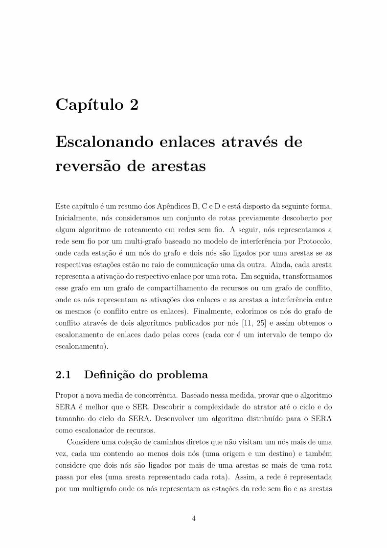
2.1 Comportamento da funcao T (S) para o algoritmo SER sob dois es-

quemas de numeracao, com ∆ = 4 (a), ∆ = 8 (b), ∆ = 16 (c) e

∆ = 32 (d). Barras de erro sao baseadas no intervalo de confianca ao

nıvel de 95%. . . . . . . . . . . . . . . . . . . . . . . . . . . . . . . . 6

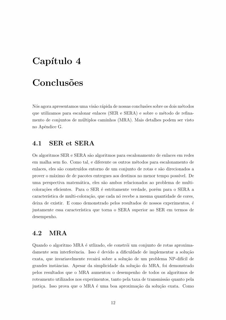
2.2 Comportamento da funcao T (S) para o algoritmo SERA, com ∆ = 4

(a), ∆ = 8 (b), ∆ = 16 (c) e ∆ = 32 (d). Barras de erro sao baseadas

no intervalo de confianca ao nıvel de 95%. . . . . . . . . . . . . . . . 7

3.1 Ratio σ for SERA. . . . . . . . . . . . . . . . . . . . . . . . . . . . . 9

3.2 The fairness index for SERA. . . . . . . . . . . . . . . . . . . . . . . 10

B.1 A set of P = 3 directed paths (a) and the resulting directed multi-

graph D (b). . . . . . . . . . . . . . . . . . . . . . . . . . . . . . . . . 26

B.2 A set of P = 3 directed paths (a) and the resulting directed multi-

graph D (b). . . . . . . . . . . . . . . . . . . . . . . . . . . . . . . . . 27

B.3 The graph-transformation process. . . . . . . . . . . . . . . . . . . . 29

B.4 A set of P = 4 paths (a), with dashed lines indicating all node pairs

representing off-path interference. . . . . . . . . . . . . . . . . . . . . 33

C.1 The functioning of SER when G is the 5-node cycle and ω0 is the

leftmost orientation in the top row. . . . . . . . . . . . . . . . . . . . 35

C.2 A set of P = 3 directed paths (a), the resulting directed multigraph

D (b), and the resulting undirected graph G (c). . . . . . . . . . . . . 37

C.3 Each set in a sink decomposition is represented by a rectangular box

and numbered to indicate the set’s subscript. . . . . . . . . . . . . . . 38

D.1 A sampler of the networks that were generated for n = 80. . . . . . . 45

D.2 Degree distributions of the 1600 networks, for ∆ = 4 (a), ∆ = 8 (b),

∆ = 16 (c), and ∆ = 32 (d). . . . . . . . . . . . . . . . . . . . . . . . 46

D.3 Path-size (number of edges) distributions of the 1600 networks, for

∆ = 4 (a), ∆ = 8 (b), ∆ = 16 (c), and ∆ = 32 (d). . . . . . . . . . . 47

x

D.4 Behavior of T (S) for SER under the two numbering schemes ND-BF

and ND-DF, with ∆ = 4 (a), ∆ = 8 (b), ∆ = 16 (c), and ∆ = 32 (d). 49

D.5 Behavior of T (S) for SERA under the numbering scheme ND-BF,

with ∆ = 4 (a), ∆ = 8 (b), ∆ = 16 (c), and ∆ = 32 (d). . . . . . . . . 50

D.6 Behavior of T (S) for SER and SERA with n = 10 and ∆ = 4. . . . . 53

E.1 A graph representation of a wireless network. . . . . . . . . . . . . . . 56

E.2 A graph model of a wireless network, in which an independent path

set is represented by dashed and dotted lines. . . . . . . . . . . . . . 57

E.3 The reduction of Gij from a given path set. . . . . . . . . . . . . . . . 58

E.4 The construction of the graph Dij. . . . . . . . . . . . . . . . . . . . 59

F.1 Original algorithms’ path size histogram. . . . . . . . . . . . . . . . . 67

F.2 Refined algorithms’ path size histogram. . . . . . . . . . . . . . . . . 68

F.3 Ratio σ for 802.11 with CBR1. . . . . . . . . . . . . . . . . . . . . . . 71

F.4 Ratio σ for 802.11 with CBR2. . . . . . . . . . . . . . . . . . . . . . . 72

F.5 Ratio σ for SERA. . . . . . . . . . . . . . . . . . . . . . . . . . . . . 73

F.6 The fairness index for CRB1. . . . . . . . . . . . . . . . . . . . . . . 74

F.7 The fairness index for CRB2. . . . . . . . . . . . . . . . . . . . . . . 75

F.8 The fairness index for SERA. . . . . . . . . . . . . . . . . . . . . . . 76

H.1 Throughput (packets/time slot) for CBR1. . . . . . . . . . . . . . . . 84

H.2 Throughput (packets/time slot) for CBR2. . . . . . . . . . . . . . . . 85

H.3 Throughput (packets/time slot) for SERA. . . . . . . . . . . . . . . . 86

H.4 The origin-destination fairness index for SERA. . . . . . . . . . . . . 87

H.5 Ratio (SERA)/(CBR1). . . . . . . . . . . . . . . . . . . . . . . . . . 88

H.6 Ratio (SERA)/(CBR2). . . . . . . . . . . . . . . . . . . . . . . . . . 89

H.7 Ratio (CBR1)/(CBR2). . . . . . . . . . . . . . . . . . . . . . . . . . 90

H.8 Origin-destination pairs without packets histogram for CBR1. . . . . 91

H.9 Origin-destination pairs without packets histogram for CBR2. . . . . 92

I.1 Un ensemble de P = 3 chemins orientes. . . . . . . . . . . . . . . . . 97

I.2 Le processus de transformation du graphe. . . . . . . . . . . . . . . . 97

I.3 Chaque ensemble dans une decomposition en puit. . . . . . . . . . . . 99

I.4 Comportement de T (S) pour le SER. . . . . . . . . . . . . . . . . . . 100

I.5 Comportement de T (S) pour le SERA. . . . . . . . . . . . . . . . . . 101

I.6 Une representation graphe d’un reseau sans fil. . . . . . . . . . . . . . 102

I.7 Construction d’un graphe Gij. . . . . . . . . . . . . . . . . . . . . . . 104

I.8 Ratio σ pour le 802.11 with CBR1. . . . . . . . . . . . . . . . . . . . 105

I.9 Ratio σ pour le SERA. . . . . . . . . . . . . . . . . . . . . . . . . . . 106

xi

Lista de Tabelas

D.1 Mean values of the distributions in Figures D.2 and D.3, and the

average ρ(G) values for the 104 G instances corresponding to each

combination of n and ∆ when P = n/2. . . . . . . . . . . . . . . . . 44

F.1 Different parameters used in our tuning experiments. . . . . . . . . . 64

F.2 Parameters adopted in the performance experiments. . . . . . . . . . 65

F.3 Average number of multiple paths per origin-destination pair of no-

des, where n = 120 for 104 path sets corresponding to each combina-

tion of n, ∆ and |OD|. . . . . . . . . . . . . . . . . . . . . . . . . . . 66

xii

Capıtulo 1

Introducao

As rede em malha sem fio (RMSF) sao amplamente divulgadas como solucao para

prover a infraestrutura mınima de acesso a Internet em pequenas comunidades, em-

presas e tambem como solucao do problema de conexao Internet em regioes isoladas

[1, 2]. Todavia, a interferencia de radio entre os nos da rede pode facilmente reduzir

a taxa de transmissao quando a densidade ultrapassa um determinado valor [3] e

assim comprometendo todo o empreendimento. Essa interferencia e causada pelas

tentativas transmissao simultanea entre os proprios membros da rede e constitui a

causa mais comum do desempenho insatisfatorio das redes sem fio (dificilmente atin-

gindo uma fracao das redes cabeadas [4]). Uma abordagem promissora para lidar

com a interferencia parece estar relacionada a tecnicas que unem roteamento com al-

guma tecnica de reducao da interferencia, como controle de potencia, escalonamento

de enlaces ou o uso de radio com multiplos canais [5]. De fato, esse problema foi

estudado por um consideravel numero de diferentes estrategias na literatura [6–9].

Nessa tese, nos atacamos dois problemas das RMSF, ambos relacionados com a

interferencia de radio. O primeiro problema e relacionado a interferencia entre os

enlaces da rede e e causada pela ativacao dos mesmo. Para lidar com esse problema,

nos adotamos uma solucao comum a este problema, ou seja, nos assumimos um

protocolo TDMA livre de contencao [10] e nos escalonamos heuristicamente trans-

missoes simultaneas para ativacao somente se elas nao se interferem. No entanto,

nos consideramos uma variacao do problema, a qual e nova tanto na sua formulacao

quanto na solucao proposta por nos. Nos comecamos assumindo uma rede constante-

mente sobrecarregada de fluxos com um conjunto pre-estabelecido de rotas, as quais

sao controladas pelo protocolo TDMA. Ainda, cada no tem um tamanho limitado

de buffer. Em seguida, nosso algoritmo escalona somente enlaces que pertencem ao

conjunto de rotas, sendo assim nos tentamos maximizar a taxa de transmissao das

origens aos destinos das rotas. Nossa proposta foi publicada em [11] e e apresentada

da seguinte forma. Dado um conjunto de rotas a serem utilizadas, nos comecamos no

Capıtulo 2, com uma definicao precisa de escalonamento e uma formulacao precisa

1

do problema. Nos tambem mostramos, atraves de um exemplo, que se o problema

for definido como um problema de maximizacao da capacidade da rede, um conflito

ocorre entre a restricao de buffers de tamanho finito e a maximizacao da capacidade.

A seguir, nos especificamos um grafo nao dirigido sob o qual nosso algoritmo opera.

Uma premissa que nos assumimos para toda a tese e que o raio de alcance de comu-

nicacao e de interferencia sao os mesmo para nossas redes. Ainda, nos assumimos

as premissas do modelo de interferencia por protocolo [12, 13], incluindo a possi-

bilidade de comunicacao bidirecional em cada transmissao. Entao, nos guiamos o

leitor atraves de diversas possibilidades de multi-coloracao que culminam na Secao

2.2 com um metodo previamente publicado para escalonamento, adaptado da area

de compartilhamento de recursos [14]. Melhoramentos empregados nesse algoritmo

com o intuito de maximizar as transmissoes nas rotas finalmente levam a nossa pro-

posta apresentada na Sessao 2.2.1. Essa proposta, essencialmente, e baseada em um

relaxamento da nocao de multi-coloracao. As duas secoes subsequentes sao dedica-

das a apresentar dos resultados computacionais, com a metodologia empregada e os

resultados descritos na Secao 2.3. Uma discussao e apresentada na Secao 2.4 e nos

concluımos a primeira parte da tese na primeira parte do Capıtulo G.

No segundo problema, nos atacamos a mesma interferencia entre enlaces, mas

do ponto de vista das rotas. Considerando isso, uma abordagem alternativa que

se apresenta naturalmente e o uso de roteamento com multiplas rotas para distri-

buir o trafico entre as rotas que compartilham a mesma origem e destino, ja que a

princıpio isso pode melhorar tanto a resistencia a falhas como o balanceamento de

carga mais que as estrategias com rota unica. Ainda, as multiplas rotas podem levar

a melhores taxas de transmissao para toda a rede [15, 16]. Porem, esses benefıcios

sao atingidos tao somente se as rotas nao se interferem [17, 18], o que infelizmente

nao e uma preocupacao dos algoritmos de roteamento de multiplas rotas. Aqui, nos

propomos uma abordagem diferente para minimizar os efeitos da interferencia no

roteamento de multiplos caminhos. Nossa abordagem e baseada em dois princıpios

gerais. Primeiro, existe uma fase de refinamento sobre um conjunto de multiplas

rotas previamente descoberta por algum algoritmo de roteamento, dessa forma pre-

servando, da maneira mais ampla possıvel, as vantagens dadas pelo algoritmos de

roteamento. Segundo, as informacoes utilizadas para o funcionamento do algoritmo

proposto tem como fonte apenas a informacao que ja esta disponıvel localmente a

cada origem de cada rota do conjunto previamente descoberto. Ou seja, apenas as

informacoes que a origem pode obter pela comunicacao com seus vizinhos diretos

na rede sem fio sao utilizadas. Essa proposta foi submetida a revista Computer

Networks em marco de 2012 e e apresentada da seguinte forma. Dado o conjunto de

multiplos caminhos a serem selecionados (refinados), nos explicamos a formulacao

do problema de selecionar caminho nao interferentes no Capıtulo 3. Nos tambem

2

mostramos, atraves de exemplos, que a abordagem classica por conjuntos disjuntos

utilizada nos trabalhos relacionados nao e livre de interferencia. Entao nos apresen-

tamos, na Secao 3.1.1, nossa proposta para algoritmos de multiplas rotas e no final

da mesma secao uma pequena modificacao que torna possıvel a aplicacao em algorit-

mos de rota unica. A Secao 3.2 e dedicada a explicar nosso metodo de avaliacao e os

resultados computacionais. Nos comparamos nossa proposta com alguns dos mais

importantes algoritmos de roteamento, como os AODV [19], AOMDV [20], OLSR

[21] e MP-OLSR [22]. Nos utilizamos nossa abordagem para alterar o conjunto de

rotas desse algoritmos e nso medimos a taxa de transmissao e a justica [23] contra

os conjunto de rotas originais. Para tal, nos conduzimos extensivos experimentos

utilizando o simulador de redes NS2.34 [24] e o algoritmo de escalonamento chamado

SERA [11]. Nos seguimos na Secao 3.3 com a discussao dos nossos melhoramentos,

e finalmente, nos concluımos na segunda parte do Capıtulo 4.

E importante destacar que, essa tese e resultado de uma cotutela entre a Univer-

sidade Federal do Estado do Rio de Janeiro (PESC -COPPE - UFRJ) e a Universite

Pierre et Marie Curie (LIP6 - UPMC - Paris 6). Dessa forma, a tese possui versoes

em ingles (versao principal), frances e portugues (resumos estendidos).

3

Capıtulo 2

Escalonando enlaces atraves de

reversao de arestas

Este capıtulo e um resumo dos Apendices B, C e D e esta disposto da seguinte forma.

Inicialmente, nos consideramos um conjunto de rotas previamente descoberto por

algum algoritmo de roteamento em redes sem fio. A seguir, nos representamos a

rede sem fio por um multi-grafo baseado no modelo de interferencia por Protocolo,

onde cada estacao e um nos do grafo e dois nos sao ligados por uma arestas se as

respectivas estacoes estao no raio de comunicacao uma da outra. Ainda, cada aresta

representa a ativacao do respectivo enlace por uma rota. Em seguida, transformamos

esse grafo em um grafo de compartilhamento de recursos ou um grafo de conflito,

onde os nos representam as ativacoes dos enlaces e as arestas a interferencia entre

os mesmos (o conflito entre os enlaces). Finalmente, colorimos os nos do grafo de

conflito atraves de dois algoritmos publicados por nos [11, 25] e assim obtemos o

escalonamento de enlaces dado pelas cores (cada cor e um intervalo de tempo do

escalonamento).

2.1 Definicao do problema

Propor a nova media de concorrencia. Baseado nessa medida, provar que o algoritmo

SERA e melhor que o SER. Descobrir a complexidade do atrator ate o ciclo e do

tamanho do ciclo do SERA. Desenvolver um algoritmo distribuıdo para o SERA

como escalonador de recursos.

Considere uma colecao de caminhos diretos que nao visitam um nos mais de uma

vez, cada um contendo ao menos dois nos (uma origem e um destino) e tambem

considere que dois nos sao ligados por mais de uma arestas se mais de uma rota

passa por eles (uma aresta representado cada rota). Assim, a rede e representada

por um multigrafo onde os nos representam as estacoes da rede sem fio e as arestas

4

seus enlaces para cada rota. Nos chamamos de escalonamento uma sequencia finita

de conjuntos de arestas do grafo que representa a rede sem fio, de modo que dentro

de cada conjunto todos os enlaces que as arestas representam pode sem ativados

simultaneamente sem que se interfiram.

Antes de apresentarmos a nossa abordagem algorıtmica para o escalonamento,

precisamos transforma o grafo da rede sem fio em um grafo de conflito. Para tal

basta, representar por um no cada aresta do grafo da rede e unir por uma aresta

dois nos se os enlaces que eles representam se interferem.

2.2 Escalonado por reversao de arestas

Por intermedio do algoritmo SER [25], obtemos um escalonamento baseado em

multi-coloracao do grafo de conflito, porem o grafo devera ser orientado de forma

acıclica.

2.2.1 Aperfeicoando SER

O algoritmo SER desperdica intervalos de tempo nos quais poderia antecipar algu-

mas ativacoes de alguns enlaces. Essa fraqueza foi resolvida no algoritmo denomi-

nado SERA [11].

2.3 metodologia, experimentos e resultados

Basicamente, geramos 1600 topologias de redes sem fio e para cada uma delas ge-

ramos 100 conjuntos aleatorios de rotas. Aplicamos os algoritmos SER e SERA em

cada um desses conjuntos e medimos a taxa de pacotes entregues nos destinos das

rotas. As figuras abaixo mostram os resultados desses experimentos. Fica claro que

o algoritmo SERA supera o seu predecessor em praticamente todos os casos.

2.4 Discussao

Os resultados obtidos tanto pelos algoritmo SER quanto pelo SERA dependem do

clique maximo do grafo de conflito. Porem, SERA consegue alcancar resultados

melhores devido a antecipacao da ativacao de alguns enlaces. E claro que em geral

nao ha uma forma pratica de analisar os desempenhos de SER e SERA apenas

com o grafo de conflito, ja que o desempenho dos dois depende tambem de como

os enlaces serao posicionados na fila de ativacao que SER e SERA produzem (veja

decomposicao em sorvedouros no Apendice C).

5

0.1

0.2

0.3

0.4

0.5

0.6

0.7

0.8T

(S)

(a)

BF, n = 120BF, n = 100BF, n = 80BF, n = 60

DF, n = 120DF, n = 100

DF, n = 80DF, n = 60

0.1

0.2

0.3

0.4

0.5

0.6

0.7

T(S

)

(b)

BF, n = 120BF, n = 100BF, n = 80BF, n = 60

DF, n = 120DF, n = 100

DF, n = 80DF, n = 60

0.1

0.2

0.3

0.4

0.5

0.6

0.7

T(S

)

(c)

BF, n = 120BF, n = 100BF, n = 80BF, n = 60

DF, n = 120DF, n = 100

DF, n = 80DF, n = 60

0.0

0.1

0.2

0.3

0.4

0.5

0.6

0.7

0.0 0.1 0.2 0.3 0.4 0.5 0.6 0.7 0.8 0.9 1.0

T(S

)

P’

(d)

BF, n = 120BF, n = 100BF, n = 80BF, n = 60

DF, n = 120DF, n = 100

DF, n = 80DF, n = 60

Figura 2.1: Comportamento da funcao T (S) para o algoritmo SER sob dois esque-mas de numeracao, com ∆ = 4 (a), ∆ = 8 (b), ∆ = 16 (c) e ∆ = 32 (d). Barras deerro sao baseadas no intervalo de confianca ao nıvel de 95%.

6

0.4

0.8

1.2

1.6

2

2.4T

(S)

(a)

n = 120n = 100

n = 80n = 60, B = 2

n = 60

0.4

0.8

1.2

1.6

2

2.4

T(S

)

(b)

n = 120n = 100

n = 80n = 60

0.4

0.8

1.2

1.6

2

2.4

T(S

)

(c)

n = 120n = 100

n = 80n = 60

0.0

0.4

0.8

1.2

1.6

2

2.4

0.0 0.1 0.2 0.3 0.4 0.5 0.6 0.7 0.8 0.9 1.0

T(S

)

P’

(d)

n = 120n = 100

n = 80n = 60

Figura 2.2: Comportamento da funcao T (S) para o algoritmo SERA, com ∆ = 4(a), ∆ = 8 (b), ∆ = 16 (c) e ∆ = 32 (d). Barras de erro sao baseadas no intervalode confianca ao nıvel de 95%.

7

Capıtulo 3

Selecao de multiplos caminhos

Esse capıtulo e um resumo dos Apendices E e F, onde e apresentado nosso algoritmos

de refinamento de rotas e seus resultados.

3.1 Definicao do problema

inicialmente, nos consideramos um conjunto de multiplas rotas (rotas com mesma

origem e destino) e buscamos selecionar desse conjunto os elementos que nao pos-

suem interferencia mutua.

3.1.1 MRA

Chamamos de MRA o processo de refinamento de caminhos, onde um conjunto

de multiplas rotas e refinado e como resultado obtemos um conjunto disjunto de

interferencia (veja Apendice E).

3.2 Experimentos e resultados

Utilizamo as mesmas instancias das topologias de redes dos experimentos com os

algoritmos SER e SERA. Refinamos os conjuntos de rotas descobertos pelos algo-

ritmos de roteamento AODV, AOMDV, OLSR e MP-OLSR, e medimos seus de-

sempenhos contra os conjuntos de rotas originais (os conjuntos nao refinados dos

referidos algoritmos). As figuras abaixo mostram os resultados desses experimentos,

onde fica claro que os conjuntos de rotas refinados obtiveram melhor desempenho

em praticamente todos os casos.

8

Figura 3.1: Relacao σ para o algoritmos SERA com n = 120 para ∆ = 4 (a), ∆ = 8(b), ∆ = 16 (c) e ∆ = 32 (d). As medias sao baseadas em 104 conjuntos de rotaspara cada valor de ∆ e θ. As barras de erro foram omitida, pois eram menores que1% da media para o intervalo de confianca de 95%.

9

Figura 3.2: O ındice de justica para o algoritmo SERA com n = 120 para ∆ = 4(a), ∆ = 8 (b), ∆ = 16 (c) e ∆ = 32 (d). As medias sao baseadas em 104 conjuntosde rotas para cada valor de ∆. As barras de erro foram omitida, pois eram menoresque 1% da media para o intervalo de confianca de 95%.

10

3.3 Discussao

Segue da discussao apresentada no Apendice F que apesar de nao ser nosso objetivo,

a comparacao entre metodos de roteamento que utilizam TDMA obtem resultados

melhores que os que utilizam CSMA. Isso fica mais claro se compararmos os resul-

tados de justica na rede, pois o CSMA provoca disputas injustas entre os membros

da rede (veja Apendice E).

11

Capıtulo 4

Conclusoes

Nos agora apresentamos uma visao rapida de nossas conclusoes sobre os dois metodos

que utilizamos para escalonar enlaces (SER e SERA) e sobre o metodo de refina-

mento de conjuntos de multiplos caminhos (MRA). Mais detalhes podem ser visto

no Apendice G.

4.1 SER et SERA

Os algoritmos SER e SERA sao algoritmos para escalonamento de enlaces em redes

em malha sem fio. Como tal, e diferente os outros metodos para escalonamento de

enlaces, eles sao construıdos entorno de um conjunto de rotas e sao direcionados a

prover o maximo de de pacotes entregues aos destinos no menor tempo possıvel. De

uma perspectiva matematica, eles sao ambos relacionados ao problema de multi-

coloracoes eficientes. Para o SER e estritamente verdade, porem para o SERA a

caracterıstica de multi-coloracao, que cada no recebe a mesma quantidade de cores,

deixa de existir. E como demonstrado pelos resultados de nossos experimentos, e

justamente essa caracterıstica que torna o SERA superior ao SER em termos de

desempenho.

4.2 MRA

Quando o algoritmo MRA e utlizado, ele constroi um conjunto de rotas aproxima-

damente sem interferencia. Isso e devido a dificuldade de implementar a solucao

exata, que invariavelmente recaira sobre a solucao de um problema NP-difıcil de

grandes instancias. Apesar da simplicidade da solucao do MRA, foi demonstrado

pelos resultados que o MRA aumentou o desempenho de todos os algoritmos de

roteamento utilizados nos experimentos, tanto pela taxa de transmissao quanto pela

justica. Isso prova que o MRA e uma boa aproximacao da solucao exata. Como

12

exemplo dessa melhora, podemos citar o algoritmo R-OLSR que obteve uma me-

lhora de 20% sobre o original. E claro que esse resultado e tambem devido ao fato

do MRA ter refinado um conjunto de rotas ja disjunto de nos, mas principalmente

por que o conjunto de original mesmo sendo disjunto de nos, nao era disjunto de

interferencia.

13

Referencias Bibliograficas

[1] NANDIRAJU, N., NANDIRAJU, D., SANTHANAM, L., et al. “Wireless mesh

networks: current challenges and future directions of web-in-the-sky”,

IEEE Wirel. Commun., v. 14, n. 4, pp. 79–89, 2007.

[2] SIEKKINEN, M., GOEBEL, V., PLAGEMANN, T., et al. “Beyond the future

Internet: requirements of autonomic networking architectures to address

long term future networking challenges”. In: Proceedings of the FTDCS

2007, pp. 89–98, 2007.

[3] BALACHANDRAN, A., VOELKER, G. M., BAHL, P. “Wireless hotspots: cur-

rent challenges and future directions”, Mob. Netw. Appl., v. 10, pp. 265–

274, 2005.

[4] GUPTA, P., KUMAR, P. R. “The capacity of wireless networks”, IEEE Trans.

Inf. Theory, v. 46, pp. 388–404, 2000.

[5] AKYILDIZ, I. F., WANG, X., WANG, W. “Wireless mesh networks: a survey”,

Comput. Netw., v. 47, n. 4, pp. 445–487, march 2005.

[6] CHUN, Y., QIN, L., YONG, L., et al. “Routing protocols overview and design

issues for self-organized network”. In: Proceedings of the WCC ICCT

2000, v. 2, pp. 1298–1303, 2000.

[7] ABOLHASAN, M. “A review of routing protocols for mobile ad hoc networks”,

Ad Hoc Netw., v. 2, n. 1, pp. 1–22, 2004.

[8] CAMPISTA, M. E. M., ESPOSITO, P. M., MORAES, I. M., et al. “Routing

metrics and protocols for wireless mesh networks”, IEEE Netw., v. 22,

n. 1, pp. 6–12, 2008.

[9] SRIKANTH, V., JEEVAN, A. C., A., B., et al. “A review of routing protocols

in wireless mesh networks”, Int. J. Comput. Appl., v. 1, n. 11, pp. 47–51,

2010.

[10] DEMIRKOL, I., ERSOY, C., ALAGOZ, F. “MAC protocols for wireless sensor

networks: a survey”, IEEE Commun. Mag., v. 44, n. 4, pp. 115–121, 2006.

14

[11] VIEIRA, F. R. J., REZENDE, J. F., BARBOSA, V. C., et al. “Scheduling links

for heavy traffic on interfering routes in wireless mesh networks”, Comput.

Netw., 2012. doi: http://dx.doi.org/10.1016/j.comnet.2012.01.011. To

appear.

[12] BEHZAD, A., RUBIN, I. “On the performance of graph-based scheduling algo-

rithms for packet radio networks”. In: Proceedings of IEEE GLOBECOM

2003, pp. 3432–3436, 2003.

[13] SHI, Y., HOU, Y. T., LIU, J., et al. “How to correctly use the protocol in-

terference model for multi-hop wireless networks”. In: Proceedings of the

MobiHoc 2009, pp. 239–248, 2009.

[14] BARBOSA, V. C. An Introduction to Distributed Algorithms. Cambridge, MA,

The MIT Press, 1996.

[15] KTARI, S., LABIOD, H., FRIKHA, M. “Load balanced multipath routing in

mobile ad hoc network”. In: Proceedings of the IEEE ICCS 2006, pp. 1–5,

2006.

[16] AUGUSTO, C. H. P., CARVALHO, C. B., SILVA, M. W. R., et al. “The impact

of joint routing and link scheduling on the performance of wireless mesh

networks”. In: Proceedings of the IEEE LCN 2010, pp. 80–87, 2010.

[17] TSAI, J., MOORS, T. “A review of multipath routing protocols: from wireless

ad hoc to mesh networks”. In: Proceedings of the ACoRN, pp. 17–18,

2006.

[18] TARIQUE, M., TEPE, K. E., ADIBI, S., et al. “Survey of multipath routing

protocols for mobile ad hoc networks”, J. Netw. Comput. Appl., v. 32,

n. 6, pp. 1125–1143, 2009.

[19] PERKINS, C. E., ROYER, E. M. “Ad-hoc on-demand distance vector routing”.

In: Proceedings of the WMCSA 1999, pp. 90–100, 1999.

[20] MARINA, M. K., DAS, S. R. “Ad hoc on-demand multipath distance vector

routing”, Mob. Comput. Commun. Rev., v. 6, pp. 92–93, 2002.

[21] JACQUET, P., MUHLETHALER, P., CLAUSEN, T., et al. “Optimized link

state routing protocol for ad hoc networks”. In: Proceedings of the IEEE

INMIC 2001, pp. 62–68, 2001.

[22] YI, J., ADNANE, A., DAVID, S., et al. “Multipath optimized link state routing

for mobile ad hoc networks”, Ad Hoc Netw., v. 9, pp. 28–47, 2011.

15

[23] JAIN, R., CHIU, D.-M., HAWE, W. A quantitative measure of fairness and dis-

crimination for resource allocation in shared computer systems. Relatorio

tecnico, Digital Equipment Corporation, 1984.

[24] “The network simulator NS-2”. http://www.isi.edu/nsnam/ns/, 1989.

[25] BARBOSA, V. C., GAFNI, E. “Concurrency in heavily loaded neighborhood-

constrained systems”, ACM Trans. Program. Lang. Syst., v. 11, pp. 562–

584, 1989.

[26] BALAKRISHNAN, H., BARRETT, C. L., KUMAR, V. S. A., et al. “The

distance-2 matching problem and its relationship to the MAC-Layer ca-

pacity of ad hoc wireless networks”, IEEE J. Sel. Areas Commun., v. 22,

pp. 1069–1079, 2004.

[27] GOUSSEVSKAIA, O., WATTENHOFER, R., HALLDORSSON, M. M., et al.

“Capacity of arbitrary wireless networks”. In: Proceedings of IEEE IN-

FOCOM 2009, pp. 1872–1880, 2009.

[28] MOSCIBRODA, T., WATTENHOFER, R., ZOLLINGER, A. “Topology con-

trol meets SINR: the scheduling complexity of arbitrary topologies”. In:

Proceedings of MobiHoc 2006, pp. 310–321, 2006.

[29] CRUZ, R. L., SANTHANAM, A. V. “Optimal routing, link scheduling and

power control in multihop wireless networks”. In: Proceedings of the IEEE

INFOCOM 2003, v. 1, pp. 702–711, 2003.

[30] ALICHERRY, M., BHATIA, R., LI, L. E. “Joint channel assignment and rou-

ting for throughput optimization in multiradio wireless mesh networks”,

IEEE J. Sel. Areas Commun., v. 24, n. 11, pp. 1960–1971, 2006.

[31] WANG, W., WANG, Y., LI, X.-Y., et al. “Efficient interference-aware TDMA

link scheduling for static wireless networks”. In: Proceedings of the Mobi-

Com 2006, pp. 262–273, New York, NY, 2006. ACM.

[32] GANDHAM, S., DAWANDE, M., PRAKASH, R. “Link scheduling in wireless

sensor networks: distributed edge-coloring revisited”, J. Parallel Distrib.

Comput., v. 68, pp. 1122–1134, 2008.

[33] HUA, Q.-S., LAU, F. C. M. “Exact and approximate link scheduling algo-

rithms under the physical interference model”. In: Proceedings of DIAL

M-POMC 2008, pp. 45–54, 2008.

16

http://www.isi.edu/nsnam/ns/

[34] WANG, J., DU, P., JIA, W., et al. “Joint bandwidth allocation, element as-

signment and scheduling for wireless mesh networks with MIMO links”,

Comput. Commun., v. 31, pp. 1372–1384, 2008.

[35] SANTI, P., MAHESHWARI, R., RESTA, G., et al. “Wireless link schedu-

ling under a graded SINR interference model”. In: Proceedings of ACM

FOWANC 2009, pp. 3–12, 2009.

[36] XU, X., TANG, S. “A constant approximation algorithm for link scheduling in

arbitrary networks under physical interference model”. In: Proceedings of

ACM FOWANC 2009, pp. 13–20, 2009.

[37] WANG, X., GARCIA-LUNA-ACEVES, J. J. “Embracing interference in ad

hoc networks using joint routing and scheduling with multiple packet re-

ception”, Ad Hoc Netw., v. 7, pp. 460–471, 2009.

[38] BONDY, J. A., MURTY, U. S. R. Graph Theory. New York, NY, Springer,

2008.

[39] STAHL, S. “n-tuple colorings and associated graphs”, J. Comb. Theory B,

v. 20, pp. 185–203, 1976.

[40] BARBOSA, V. C. “The interleaved multichromatic number of a graph”, Ann.

Comb., v. 6, pp. 249–256, 2000.

[41] YEH, H.-G., ZHU, X. “Resource-sharing system scheduling and circular chro-

matic number”, Theor. Comput. Sci., v. 332, pp. 447–460, 2005.

[42] KARP, R. M. “Reducibility among combinatorial problems”. In: Miller, R. E.,

Thatcher, J. W. (Eds.), Complexity of Computer Computations, Plenum

Press, pp. 85–103, New York, NY, 1972.

[43] GROTSCHEL, M., LOVASZ, L., SCHRIJVER, A. “The ellipsoid method and

its consequences in combinatorial optimization”, Combinatorica, v. 1,

pp. 169–197, 1981.

[44] LIN, W. “Some star extremal circulant graphs”, Discrete Math., v. 271,

pp. 169–177, 2003.

[45] BARBOSA, V. C. An Atlas of Edge-Reversal Dynamics. London, UK, Chap-

man & Hall/CRC, 2000.

[46] WAHARTE, S., BOUTABA, R. “Totally disjoint multipath routing in multihop

wireless networks”. In: Proceedings of the IEEE ICC 2006, v. 12, pp.

5576–5581, 2006.

17

[47] WAHARTE, S., BOUTABA, R. “On the probability of finding non-interfering

paths in wireless multihop networks”. In: Proceedings of the IFIP TC6

2008, pp. 914–921, Berlin, Heidelberg, 2008. Springer.

[48] PEARLMAN, M. R., HAAS, Z. J., SHOLANDER, P., et al. “On the impact

of alternate path routing for load balancing in mobile ad hoc networks”.

In: Proceedings of the MobiHoc 2000, pp. 3–10, 2000.

[49] LEE, S. J., GERLA, M. “Split multipath routing with maximally disjoint paths

in ad hoc networks”. In: Proceedings of the IEEE ICC 2001, v. 10, pp.

3201–3205, 2001.

[50] LIN, X., RASOOL, S. “A distributed joint channel-assignment, scheduling

and routing algorithm for multi-channel ad-hoc wireless networks”. In:

Proceedings of the INFOCOM 2007, pp. 1118–1126, 2007.

[51] LEE, S.-J., SU, W., GERLA, M. “Wireless ad hoc multicast routing with

mobility prediction”, Mob. Netw. Appl., v. 6, pp. 351–360, 2001.

[52] TSIRIGOS, A., HAAS, Z. J. “Multipath routing in the presence of frequent

topological changes”, IEEE Commun. Mag., v. 39, n. 11, pp. 132–138,

2001.

[53] SHERIFF, I., ROYER, E. B. “Multipath selection in multi-radio mesh

networks”. In: Proceedings of the BroadNets 2006, pp. 1–11, 2006.

[54] LI, X., CUTHBERT, L. “On-demand node-disjoint multipath routing in wi-

reless ad hoc networks”. In: Proceedings of the IEEE LCN 2004, pp.

419–420, 2004.

[55] RHEE, I., WARRIER, A., MIN, J., et al. “DRAND: distributed randomized

TDMA scheduling for wireless ad-hoc networks”. In: Proceedings of the

MobiHoc 2006, pp. 190–201, New York, NY, 2006. ACM.

[56] “MP-OLSR routing agent for NS-2”. http://jiaziyi.com/MP-OLSR.php,

2008.

[57] YUAN, Y., CHEN, H., JIA, M. “An optimized ad-hoc on-demand multipath

distance vector (AOMDV) routing protocol”. In: Proceedings of the APCC

2005, pp. 569–573, 2005.

[58] ZHOU, X., LU, Y., XI, B. “A novel routing protocol for ad hoc sensor networks

using multiple disjoint paths”. In: Proceedings of the BroadNets 2005, pp.

944–948, 2005.

18

http://jiaziyi.com/MP-OLSR.php

[59] “NO Ad-Hoc Routing Agent (NOAH)”. http://icapeople.epfl.ch/widmer/

uwb/ns-2/noah/, 2004.

[60] KIM, T.-S., LIM, H., HOU, J. C. “Improving spatial reuse through tuning

transmit power, carrier sense threshold, and data rate in multihop wireless

networks”. In: Proceedings of the MobiCom 2006, pp. 366–377, New York,

NY, 2006. ACM.

[61] GUMMALLA, A. C. V., LIMB, J. O. “Wireless medium access control proto-

cols”, IEEE Commun. Surv. Tutor., v. 3, n. 2, pp. 2–15, 2000.

[62] HOFFMAN, A. J. “On the polynomial of a graph”, Amer. Math. Month., v. 70,

n. 1, pp. 30–36, 1963.

[63] DIRAC, G. A. “Some theorems on abstract graphs”, Proc. Lond. Math. Soc.,

v. s3-2, n. 1, pp. 69–81, 1952.

[64] BIRADAR, S. R., MAJUMDER, K., SARKAR, S. K., et al. “Performance

evaluation and comparison of AODV and AOMDV”, Int. J. Comput. Sci.

Eng., v. 2, n. 2, pp. 373–377, 2010.

[65] YI, J., CIZERON, E., HAMMA, S., et al. “Simulation and performance analysis

of MP-OLSR for mobile ad hoc networks”. In: Proceedings of the IEEE

WCNC 2008, pp. 2235–2240, 2008.

[66] DHEKNE, A., UCHAT, N., RAMAN, B. “Implementation and evaluation of a

TDMA MAC for wifi-based rural mesh networks”. In: Proceedings of the

ACM SOSP 2009, 2009.

[67] BANAOUAS, S., MUHLETHALER, P. “Performance evaluation of TDMA

versus CSMA based protocols in SINR models”. In: Proceedings of the

EW 2009, pp. 113–117, 2009.

[68] GUPTA, G. P., PANDEY, A. K. “Performance comparison of ad hoc routing

protocols over IEEE 802.11 DCF and TDMA MAC layer protocols”. In:

Proceedings of the NCC 2007, v. 1, pp. 183–187, 2007.

[69] DING, J., ZHAO, L., MEDIDI, S. R., et al. “MAC protocols for ultra-wide-

band (UWB) wireless networks: impact of channel acquisition time”. In:

Proceedings of the SPIE ITCOM 2002, pp. 1953–1954, 2002.

[70] CAPONE, A., CARELLO, G., FILIPPINI, I., et al. “Routing, scheduling and

channel assignment in wireless mesh networks: optimization models and

algorithms”, Ad Hoc Netw., v. 8, pp. 545–563, 2010.

19

http://icapeople.epfl.ch/widmer/uwb/ns-2/noah/

http://icapeople.epfl.ch/widmer/uwb/ns-2/noah/

[71] CAPONE, A., CARELLO, G., FILIPPINI, I., et al. “Solving a resource allo-

cation problem in wireless mesh networks: a comparison between a CP-

based and a classical column generation”, Networks, v. 55, pp. 221–233,

2010.

[72] CAPONE, A., CHEN, L., GUALANDI, S., et al. “A new computational ap-

proach for maximum link activation in wireless networks under the SINR

model”, IEEE Trans. Wirel. Commun., v. 10, pp. 1368–1372, 2011.

[73] MALKA, Y., RAJSBAUM, S. “Analysis of distributed algorithms based on

recurrence relations”. In: Distributed Algorithms, v. 579, Lecture Notes in

Computer Science, Springer, pp. 242–253, Berlin, Germany, 1992.

[74] MALKA, Y., MORAN, S., ZAKS, S. “A lower bound on the period length of

a distributed scheduler”, Algorithmica, v. 10, pp. 383–398, 1993.

[75] PARDALOS, P. M., DESAI, N. “An algorithm for finding a maximum weighted

independent set in an arbitrary graph”, J. Comput. Math., v. 38, n. 3–4,

pp. 163–175, 1991.

[76] BAHL, P., ADYA, A., PADHYE, J., et al. “Reconsidering wireless systems

with multiple radios”, Comput. Commun. Rev., v. 34, pp. 39–46, 2004.

[77] RANIWALA, A., CHIUEH, T.-C. “Architecture and algorithms for an IEEE

802.11-based multi-channel wireless mesh network”. In: Proceedings of the

IEEE INFOCOM 2005, v. 3, pp. 2223–2234, 2005.

20

Apendice A

Introduction

Wireless mesh networks (WMNs) have lately been recognized as having great po-

tential to provide the necessary networking infrastructure for communities and com-

panies, as well as to help address the problem of providing last-mile connections to

the Internet [1, 2]. However, mutual radio interference among the network’s nodes

can easily reduce the throughput as network density grows above a certain threshold

[3] and therefore compromise the entire endeavor. Such interference is caused by

the attempted concomitant communication among nodes of the same network and

constitutes the most common cause of the network’s throughput’s falling short of

being satisfactory (hardly reaching a fraction of that of a cabled network [4]). A

promising approach to tackle the reduction of mutual interference seems to be to

combine routing algorithms with some interference avoidance approach, such as

power control, link scheduling, or the use of multi-channel radios [5]. In fact, this

type of network interference problem has been addressed by a considerable number

of different strategies to be found in the literature [6–9].

In this thesis, we addressed two wireless network problems, both related with the

radio interference. The first problem is related to the interference among network

links caused by the activation of theses links. To deal with it, we adopted a common

solution to this problem, that is, we assume a contention-free TDMA protocol [10]

and we heuristically schedule simultaneous transmissions for activation only if they

do not interfere with one another. However, we consider a variation of the problem,

which is novel both in its formulation and in the solution type we propose. We

start by assuming a heavily loaded network with pre-established set of origin-to-

destination routes and whose access is controlled by a TDMA protocol, also, each

node has a limited buffer size to store network packets. Next, our algorithm schedule

only links that belong to the set of routes, thus we try to maximize the throughput

of these origin-to-destination routes. Our proposal was published in [11] and is

present here in the following manner. Given the origin-to-destination routes (or

paths) to be used, we begin in Chapter B with a precise definition of a schedule

21

and a precise formulation of the problem. We also show, through an example, that

had the problem been formulated for network-capacity maximization, a conflict with

the requirement of finite buffering might arise. Then we move to the specification

of the undirected graph that underlies our algorithm’s operation. One assumption

throughout most of our work, is that the communication and interference radii are

the same for the WMN at hand. Moreover, we also assume that the tenets of the

protocol-based interference model [12, 13], including the possibility of bidirectional

communication in each transmission, are in effect. Next, we guide the reader through

various multicoloring possibilities, which culminates in Chapter C with a preliminary

method for scheduling, borrowed from the field of resource sharing [14]. Improving

on this preliminary method with the goals of the problem formulated in Chapter B in

mind finally yields our proposal in Section C.1. This proposal, essentially, stems from

a slight relaxation of the notion of a node multicoloring. The subsequent two sections

are dedicated to the presentation of computational results, with the methodology

and the results laid down in Chapter D. Discussion follows in Section D.4 and we

close in the first part of Chapter G.

In the second problem, we deal with the same interference among link, but from

the point of view of the network paths. Considering that, an alternative approach

that presents itself naturally is the use of multi-path routing to distribute traffic

among multiple paths sharing the same origin and the same destination, since in

principle it can help to improve both path recovery and load balance better than

single-path strategies. It may, in addition, lead to better throughput values over the

entire network [15, 16]. But while these benefits accrue only insofar as they relate to

how the multiple paths interfere with one another [17, 18], unfortunately this aspect

of the problem is not commonly addressed by multi-path strategies. Here we propose

a different approach to alleviate the effects of interference in multi-path routing. Our

approach is based on two general principles. First, that it is to work as a refinement

phase over existing routing algorithms, thereby inherently preserving, to the fullest

possible extent, the advantages of any given routing method. Second, that it is to

rely only on information that is locally available to the common origin of any given

set of multiple paths leading to the same destination. That is, only information

that the origin can obtain by communicating with its direct neighbors in the WMN

should be used. This proposal was submitted to The Computer Networks Journal in

march 2012 and is present here as follows. Given the a multi-path set to be selected,

we explain in Chapter E the problem formulation of selecting non-interfering paths.

We also show, through examples, that the classical disjoint sets used in the related

works are not interference free. Then we present, in Section E.2 our proposal for

multi-path routing algorithms and in Section E.3 a small modification that able our

algorithm to work with single-path algorithms. Chapter F is dedicated to explain

22

our evaluation method and the computational results. We compared our results

with some of the most important routing algorithms, such as AODV [19], AOMDV

[20], OLSR [21] and MP-OLSR [22]. We used our approach to alter the path set of

these algorithms and we measured their throughput and fairness [23] against their

original path sets. For that, we carried out extensive experimentation by using the

network simulator NS2.34 [24] and the SERA scheduling algorithm [11]. We follow

in Section F.4 with the discussion of our improvements, and finally, we conclude in

the second part of Chapter G.

23

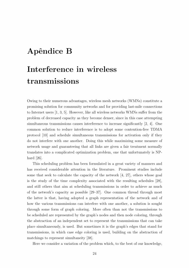
Apendice B

Interference in wireless

transmissions

Owing to their numerous advantages, wireless mesh networks (WMNs) constitute a

promising solution for community networks and for providing last-mile connections

to Internet users [1, 3, 5]. However, like all wireless networks WMNs suffer from the

problem of decreased capacity as they become denser, since in this case attempting

simultaneous transmissions causes interference to increase significantly [2, 4]. One

common solution to reduce interference is to adopt some contention-free TDMA

protocol [10] and schedule simultaneous transmissions for activation only if they

do not interfere with one another. Doing this while maximizing some measure of

network usage and guaranteeing that all links are given a fair treatment normally

translates into a complicated optimization problem, one that unfortunately is NP-

hard [26].

This scheduling problem has been formulated in a great variety of manners and

has received considerable attention in the literature. Prominent studies include

some that seek to calculate the capacity of the network [4, 27], others whose goal

is the study of the time complexity associated with the resulting schedules [28],

and still others that aim at scheduling transmissions in order to achieve as much

of the network’s capacity as possible [29–37]. One common thread through most

the latter is that, having adopted a graph representation of the network and of

how the various transmissions can interfere with one another, a solution is sought

through some form of graph coloring. More often than not the transmissions to

be scheduled are represented by the graph’s nodes and then node coloring, through

the abstraction of an independent set to represent the transmissions that can take

place simultaneously, is used. But sometimes it is the graph’s edges that stand for

transmissions, in which case edge coloring is used, building on the abstraction of

matchings to represent simultaneity [38].

Here we consider a variation of the problem which, to the best of our knowledge,

24

is novel both in its formulation and in the solution type we propose. We start by

assuming a WMN comprising single-channel, single-radio nodes and for which a

set of origin-to-destination routes has already been determined, and consider the

following question. Should there be an infinite supply of packets at each origin to be

delivered to the corresponding destination in the FIFO order, and should all nodes

in the network be endowed with only a finite number of buffers for the temporary

storage of in-transit packets, how can transmissions be scheduled to maximize the

number of packets that get delivered to the destinations per TDMA slot without

ever stalling a transmission, by lack of buffering space, whenever it is scheduled?

This question addresses issues that lie at the core of successfully designing WMNs

and their routing protocols, since it seeks to tackle the problem of transmission

interference when the network is maximally strained. The solution we propose is, like

in so many of the approaches mentioned above, based on coloring a graph’s nodes.

Unlike them, however, we use node multicolorings instead [39], which are more

general and for this reason allow for a more suitable formulation of the optimization

problem to be solved.

B.1 Problem formulation

We consider a collection P1,P2, . . . ,PP of simple directed paths (i.e., directed paths

that visit no node twice), each having at least two nodes (a source and a destination).

These paths’ sets of nodes are X1, X2, . . . , XP , respectively, not necessarily disjoint

from one another, and we let X =⋃P

p=1Xp. Their sets of edges are Y1, Y2, . . . , YP

and we assume that, for p 6= q, a member of Yp and one of Yq are distinguishable

from each other even if they join the same two nodes in the same direction. Letting

Y =⋃P

p=1 Yp, we then see that Y may contain more than one edge joining the

same two nodes in the same direction (parallel edges) or in opposing directions

(antiparallel edges).

Our discussion begins with the definition of the directed multigraph D = (X, Y ),

where all P directed paths are represented without sharing any directed edges among

them. An example is shown in Figure B.1. We take D to be representative of a

wireless network operating under some TDMA protocol. In this network, each of

paths P1,P2, . . . ,PP is to transmit an unbounded sequence of packets from its source

to its destination. Such transmissions are to occur without contention, meaning that

whenever an edge is scheduled to transmit in a given time slot no other edge that

can possibly interfere with that transmission is to be scheduled at the same time

slot. We assume that each transmission sends at most one packet across the edge

in question (more specifically, it sends exactly one packet if there is at least one to

be sent but does nothing otherwise). We also assume that each transmission may

25

involve the need for bidirectional communication for error control.

3

d e3 1

f g2 4

(a) a b c32

a 42

ce

gd

f

b

(b)1

2

3

4

1

Figura B.1: A set of P = 3 directed paths (a) and the resulting directed multigraphD (b).

We call a schedule any finite sequence S = 〈S0, S1, . . . , SL−1〉 such that S` ⊆ Y for

0 ≤ ` ≤ L−1, provided⋃L−1

`=0 S` = Y and moreover no two concurrent transmissions

on edges of the same S` can interfere with each other. To schedule the transmissions

according to S is to cycle through the edge sets S0, S1, . . . , SL−1, indefinitely and in

this order, letting all edges in the same set transmit in the same time slot whenever

that set is reached along the cycling. Given S, we let length(S) = L and denote by

delivered(S) the number of packets that can get delivered to all paths’ destinations

during a single repetition of S in the long run (i.e., in the limit as the number of

repetitions grows without bound). Of course, delivered(S) is bounded from above

by the number of times the P paths’ terminal edges (those leading directly to a

destination node) appear in S altogether.

Before we use these two quantities to define the optimization problem of fin-

ding a suitable schedule for D, we must recognize that our focus on the source-

to-destination packet flows on the paths P1,P2, . . . ,PP carries with it the inherent

constraint that the nodes’ capacity to buffer in-transit packets cannot be allowed

to grow unbounded. We then adopt an upper bound B on the number of in-transit

packets that a node can store for each of the paths (at most P ) that go through it.

However, there is still a decision to be made regarding the effect of such a bound on

the transmission of packets. One possibility would be to impose that, when it is an

edge’s turn to transmit it does so if and only if there is a packet to transmit and,

moreover, there is room to store that packet if it is received as an in-transit packet.

Another possibility, one that seeks to never stall a transmission by lack of a buffer

to store the packet at the next intermediate node, is to only admit schedules that

automatically rule out the occurrence of such a transmission. We adopt the latter

alternative.

The following, then, is how we formulate our scheduling problem on D. Find a

schedule S that maximizes the throughput

T (S) =delivered(S)

length(S), (B.1)

26

subject to the following two constraints:

C1. Every node can store up to B in-transit packets for each of the source-to-

destination paths that go through it.

C2. Whenever an edge is scheduled for transmission in a time slot and a packet

is available to be transmitted, if the edge is not the last one on its source-to-

destination path then there has to be room for the packet to be stored after

it is transmitted.

B.1.1 Scheduling for maximum network usage

Before proceeding, recall that, as mentioned in the beginning of this chapter, the

most commonly solved problem regarding the selection of a schedule S is not the

one we just posed, but rather the problem of maximizing network usage. In terms

of our notation, this problem requires that we find a schedule that maximizes

U(S) =

∑L−1`=0 |S`|

length(S)(B.2)

without any constraints other than those that already participate in the definition

of a schedule.

It is a simple matter to verify that solutions to this problem often fail to respect

constraints C1 and C2 of our formulation. This is exemplified in Figure B.2.

3

d e

(a) a b c1 4

f g

h

(b) a1 3 42 b c

d e fgh1 4

3

6

6

5 7

765

2

Figura B.2: A set of P = 3 directed paths (a) and the resulting directed multigraphD (b). Using the schedule S such that S0 = {a, f}, S1 = {c, d}, S2 = {b}, S3 = {e},S4 = {a, g}, and S5 = {h} causes unbounded packet accumulation at node 2 whenconstraint C2 is in effect, thus violating constraint C1. Enforcing constraint C1 forsome value of B causes constraint C2 to be violated.

B.2 Graph transformation

We wish to address the problem of optimizing T (S) exclusively in terms of some un-

derlying graph. Clearly, though, the directed multigraph D is not a good candidate

for this, since it does not embody any representation of how concurrent transmissi-

ons on its edges can interfere with one another. Our first step is then to transform

27

D into some more suitable entity, which will be the undirected graph G = (N,E)

defined as follows:

1. The node set N of G is the edge set Y of D. In other words, G has a node for

every edge of D. Since D is a multigraph, a same pair of nodes i, j ∈ X such

that (i, j) ∈ Y or (j, i) ∈ Y may appear more than once as a member of N .

2. The edge set E of G is obtained along the following four steps:

i. Enlarge N by including in it all node pairs of D that do not correspond to

edges on any of the P source-to-destination paths but nevertheless reflect

that each node in the pair is within the interference radius of the other.

We refer to these extra members of N as temporary nodes.

ii. Connect any two nodes in N by an edge if, when regarded as node pairs

from D, they share at least one of the nodes of D. In other words, if each

of the two pairs i, j ∈ X and k, l ∈ X corresponds to a node of G (by

virtue of either constituting an edge of D or being a temporary node),

then the two get connected by an edge in G if at least one of i = k, i = l,

j = k, or j = l holds.

iii. Connect any two nodes in N by an edge if, after the previous steps, the

distance between them is 2, but except for temporary nodes.

iv. Eliminate all temporary nodes from N and all edges from E that touch

them.

Together, these four steps amount to using G to represent every possible in-

terference that may arise under the assumptions of the protocol-based model

when communication is bidirectional. Graph G is also known as a distance-2

graph relative to D [26]. The entire transformation process, from the set of P

paths through graph G, is illustrated in Figure B.3.

It follows from this definition of G that any group of nodes corresponding to pa-

rallel or antiparallel edges in D are a clique (a completely connected subgraph) of G.

Similarly, every group of three consecutive edges on any of the paths P1,P2, . . . ,PP

corresponds to a three-node clique in G. As we discuss in Section D.4, these and

other cliques are related to how large T (S) can be under one of the scheduling

methods we introduce.

It is also worth noting that Steps 1 and 2 above are easily adaptable to modi-

fications in any of the assumptions we made. These include the assumptions that

the communication and interference radii are the same and that communication is

bidirectional. Changing assumptions would simply require us to adapt Steps 2.i

through 2.iii accordingly.

28

f

xd

e

a c

g

b(b)

ca

e g

b

d

(d)

a b c(a)

gf

x

d

e

f

(c)ca

xd

e g

b

f

Figura B.3: The graph-transformation process. We start with the directed multi-graph D (a), to which the node pair labeled x is added as a dashed line to indicatethe existence of interference that is not internal to any of the initial P paths. Panel(b) contains the undirected graph G as it stands after Step 2.ii. This stage is rea-ched by creating a node for every directed edge in panel (a) (through Step 1) and anode for every undirected edge in panel (a) (through Step 2.i). Note that the latterresults in the temporary node x of panel (b). In addition to node creation, reachingpanel (b) from (a) requires the creation, through Step 2.ii, of undirected edges tojoin nodes in (b) whenever in (a) the corresponding edges, directed or otherwise,have a node in common. Panel (c) shows G past Step 2.iii, through which the edgeset of G is enlarged by connecting any two nodes that in (b) are two edges apart.These extra edges are shown in dashed lines. Panel (d), finally, results from applyingStep 2.iv to the graph in panel (c). This results in the removal of temporary nodex, along with all its adjacent edges.

29

B.3 Multicoloring-based schedules

Graph G allows us to rephrase the definition of a schedule as follows. We call a

schedule any finite sequence S = 〈S0, S1, . . . , SL−1〉 such that S` ⊆ N for 0 ≤ ` ≤L − 1, provided

⋃L−1`=0 S` = N and moreover every S` is an independent set of G.

The appearance of the notion of an independent set in this definition leads the

way to a special class of schedules, namely those that can be identified with graph

multicolorings [39].

For q ≥ 1, a q-coloring of the nodes of G is a mapping from N , the graph’s

set of nodes, to Nq, where N is the set of natural numbers, such that no two of a

node’s q colors are the same and besides none of them coincides with any one of

any neighbor’s q colors. Of course, the set of nodes receiving one particular color

is an independent set. If p is the total number of colors needed to provide G with

a q-coloring, then N is covered by the p independent sets that correspond to colors

and every node is a member of exactly q of these sets. Therefore, letting L = p

and identifying each S` with the set of nodes receiving color ` implies that to every

q-coloring of the nodes of G there corresponds a schedule S.

These multicoloring-derived schedules constitute a special case in the sense that

every node of G can be found in exactly the same number of sets (q) out of the L

sets that make up the schedule. Clearly, though, there are schedules that do not

correspond to multicolorings. For now we concentrate on those that do and note

that delivered(S) ≤ Pq always holds (recall that P stands for the number of origin-

to-destination paths). That is, the greatest number of packets that the P terminal

edges of D can deliver during the L time slots of schedule S is q per terminal edge.

These schedules can be further specialized, as follows.

B.3.1 Standard coloring

When q = 1 every node of G receives exactly one color and length(S) = L ≥ χ(G),

where χ(G) is the least number of colors with which it is possible to provide G with

a 1-coloring, known as the chromatic number of G. Using T 1(S) to denote T (S) in

this case, we have

T 1(S) ≤ P

χ(G). (B.3)

B.3.2 Standard multicoloring

Coloring G’s nodes optimally in the previous case is minimizing the overall number

of colors. This stems not only from the fact that q = 1, but more generally from

the fact that q is fixed. We can then generalize and define χq(G) to be the least

number of colors with which it is possible to provide G with a q-coloring. Evidently,

30

χ(G) = χ1(G) < χ2(G) < · · · , so the question of multicoloring G’s nodes optimally

when q is not fixed can no longer be viewed as that of minimizing the overall number

of colors needed (as this would readily lead to q = 1 and χ(G) colors). Instead, we

look at how efficiently the overall number of colors is used, i.e., at what the value

of q has to be so that χq(G)/q is minimized. This gives rise to the multichromatic

number of G, denoted by χ∗(G) and given by χ∗(G) = infq≥1 χq(G)/q. Because this

infimum can be shown to be always attained, we use minimum instead and let q∗

be the value of q for which χ∗(G) = χq∗(G)/q∗.

Using a q-coloring for scheduling amounts to having length(S) = L ≥ χq(G). In

this case, letting T ∗(S) stand for T (S) yields

T ∗(S) ≤ Pq

χq(G)≤ Pq∗

χq∗(G)=

P

χ∗(G). (B.4)

B.3.3 Interleaved multicoloring

A special class of q-colorings is what we call interleaved q-colorings [25, 40, 41]. If i

and j are two neighboring nodes of G, let ci1 < ci2 < · · · < ciq be the q colors assigned

to node i by some q-coloring, and likewise let cj1 < cj2 < · · · < cjq be those of node j.

We say that this q-coloring is interleaved if and only if either ci1 < cj1 < ci2 < cj2 <

· · · < ciq < cjq or cj1 < ci1 < cj2 < ci2 < · · · < cjq < ciq for all neighbors i and j. If we

restrict ourselves to interleaved q-colorings, then similarly to what we did above we

use χqint(G) to denote the least number of colors with which it is possible to provide

G with an interleaved q-coloring, and similarly define the interleaved multichromatic

number of G, denoted by χ∗int(G), to be χ∗int(G) = infq≥1 χqint(G)/q. Once again it

is always possible to attain the infimum, so we may take q∗ to be the value of q for

which χ∗int(G) = χq∗

int(G)/q∗.

As for scheduling based on an interleaved q-coloring, it corresponds to having

length(S) = L ≥ χqint(G). As before, we use T ∗int(S) in lieu of T (S) and obtain

T ∗int(S) ≤ Pq

χqint(G)

≤ Pq∗

χq∗

int(G)=

P

χ∗int(G). (B.5)

B.3.4 Discussion

It is a well-known fact that

1

χ(G)≤ 1

χ∗int(G)≤ 1

χ∗(G). (B.6)

The first inequality follows from the definition of χ∗int(G), considering that every

1-coloring is (trivially) interleaved. As for the second inequality, it follows directly

from the definition of χ∗(G). By these inequalities, should all of Eqs. (B.3)–(B.5)

31

hold with equalities, we would have

T 1(S) ≤ T ∗int(S) ≤ T ∗(S). (B.7)

Obtaining equalities in Equations (B.3), (B.4) and (B.5), however, requires both that

delivered(S) = Pq for q = 1 or q = q∗, as the case may be, and that length(S) =

χq(G) with the same possibilities for q or length(S) = χq∗

int(G).

While the combined requirements involve the exact solution of NP-hard problems

(finding any of χ(G), χ∗int(G), and χ∗(G) is NP-hard; cf., respectively, [42], [25], and

[43]), the former requirement alone (that delivered(S) = Pq) is always a property of

schedules based on multicolorings when buffering availability is unbounded. To see

that this is so, first recall that the definition of delivered(S) refers to a repetition

of the whole schedule as far down in time as needed for any transient effects to

have waned. So, given any of the P source-to-destination paths, we can prove that

delivered(S) = Pq by arguing inductively about what happens on such a path during

that future repetition of S. The basis case in this induction is the first directed edge

on the path (the one leading out of the source). The property that every appearance

of this edge does indeed transmit a packet follows trivially from the fact that the

source has an endless supply of new packets to provide whenever needed. Assuming

that this also happens to the next-to-last edge on the path (this is our induction

hypothesis) immediately leads to the same conclusion regarding the last edge, the

one on which delivered(S) is defined. To see this, let e be the last edge and e− the

next-to-last one. Because S is repeated indefinitely, every time slot t sufficiently far

down in time in which e appears is the closing time slot of a window in which both

e and e− appear exactly q times each. By the induction hypothesis, it follows that

at least one packet is guaranteed to exist for transmission through e at time slot t.

Buffering availability, however, is not unbounded, so we must argue for its finite-

ness. We do this by recognizing another important property of multicoloring-based

schedules, one that is related to constraints C1 and C2 introduced earlier. Because

every edge of D (node of G) appears the exact same number q of times in S, there

certainly always is a finite value of B, the number of buffer positions per node per

path that goes through it, such that C1 and C2 are satisfied. In all interleaved cases,

this value is B = 1.

An example illustrating all of this is presented in Figure B.4, where we give a set

of four source-to-destination paths, the graph G that eventually results from them,

and also the three schedules that result in equalities in Eqs. (B.3)–(B.5). In this

case the two inequalities in Eq. (B.6) are strict, since it can be shown that χ(G) = 3,

χ∗int(G) = 8/3, and χ∗(G) = 5/2 [25, 39].

32

hb

d

f

h

(a)

c

e

g

(b)

a

a

e

g c

f d

b

Figura B.4: A set of P = 4 paths (a), with dashed lines indicating all nodepairs representing off-path interference. The resulting graph G is shown in pa-nel (b). Depending on the schedule S it is possible to obtain equalities in allof Eqs. (B.3)–(B.5). The schedules that achieve this while implying strict ine-qualities in Eq. (B.6) are: S = 〈{a, d, g}, {b, f, h}, {c, e}〉 for Eq. (B.3), withT 1(S) = 4/3 ≈ 1.33; S = 〈{a, d, f}, {b, e, g}, {c, f, h}, {a, d, g}, {b, e, h}, {a, c, f},{b, d, g}, {c, e, h}〉 for Eq. (B.5), with T ∗int(S) = 4/(8/3) = 1.5; and S = 〈{a, c, f},{b, e, g}, {c, e, h}, {a, d, g}, {b, d, f, h}〉 for Eq. (B.4), with T ∗(S) = 4/(5/2) = 1.6.

33

Apendice C

Scheduling by edge reversal

From the three schedules illustrated in Figure B.4 it would seem that finding a sche-

dule S to maximize T (S) requires that we give up on the interleaved character of

the underlying multicoloring and, along with it, give up on the equivalent property

that edges of D that are consecutive on some source-to-destination path appear in Salternately. However, once color interleaving is assumed we are automatically provi-

ded with a principled way to heuristically try and maximize T (S) by appealing to a

curious relationship that exists between multicolorings and the acyclic orientations

of G. We now review this heuristic and later build on it by showing how to adapt it

to abandon interleaving only on occasion during a schedule, aiming at maximizing

T (S).

An orientation of G is an assignment of directions to its edges. An orientation of

G is acyclic if no directed cycles are formed. Every acyclic orientation has a set of

sinks (nodes with no edges oriented outward), which by definition are not neighbors

of one another. An acyclic orientation’s set of sinks is then an independent set. The

heuristic we now describe, known as scheduling by edge reversal (SER) [14, 25], is

based on the following property. Should an acyclic orientation be transformed into

another by turning all its sinks into sources (nodes with no edges oriented inward),

and should this be repeated indefinitely, we would obtain an infinite sequence of

independent sets, each given by the set of sinks of the current orientation. Though

infinite, this sequence must necessarily reach a point from which a certain number

of acyclic orientations gets repeated indefinitely. This follows from the facts that

there are only finitely many acyclic orientations of G and that turning one of them

into the next is a deterministic process.

The orientations that participate in this cyclic repetition, henceforth called a

period, have the property that every node of G appears as a sink in the same

number of orientations. Furthermore, any two neighboring nodes of G are sinks in

alternating orientations, regardless of whether the period has already been reached

or not. It clearly follows that the sets of sinks in a period constitute a schedule

34

that is based on an interleaved multicoloring. Depending on the very first acyclic

orientation in the operation of SER more than one period can eventually be reached.

The different periods’ properties vary from one to another, but it can be shown that

at least one of them corresponds to the optimal interleaved multicoloring, i.e., the

one that yields χ∗int(G) [25]. The heuristic nature of SER is then revealed by the

need to determine an appropriate initial acyclic orientation.

Determining a schedule S by SER follows the algorithm given next, whose func-

tioning is illustrated in Figure C.1 for a simple G instance. We use ω0, ω1, . . . to

denote the sequence of acyclic orientations of G. For t = 0, 1, . . ., we denote by

Sinks(ωt) the set of sinks of ωt.

Figura C.1: The functioning of SER whenG is the 5-node cycle and ω0 is the leftmostorientation in the top row. The period that is reached from ω0 has p(ω0) = 5 andm(ω0) = 2.

Algorithm SER:

1. Choose ω0.

2. t := 0.

3. Obtain ωt+1 from ωt.

4. If the period has not yet occurred, then t := t + 1; go to Step 3. If it has,

then let p(ω0) be its number of orientations, m(ω0) the number of times any

node appears in them as a sink, and ωk, ωk+1, . . . , ωk+p(ω0)−1 the orientations

themselves. Output

S = 〈Sinks(ωk), Sinks(ωk+1), . . . , Sinks(ωk+p(ω0)−1)〉

and

T (S) =Pm(ω0)

p(ω0).

35

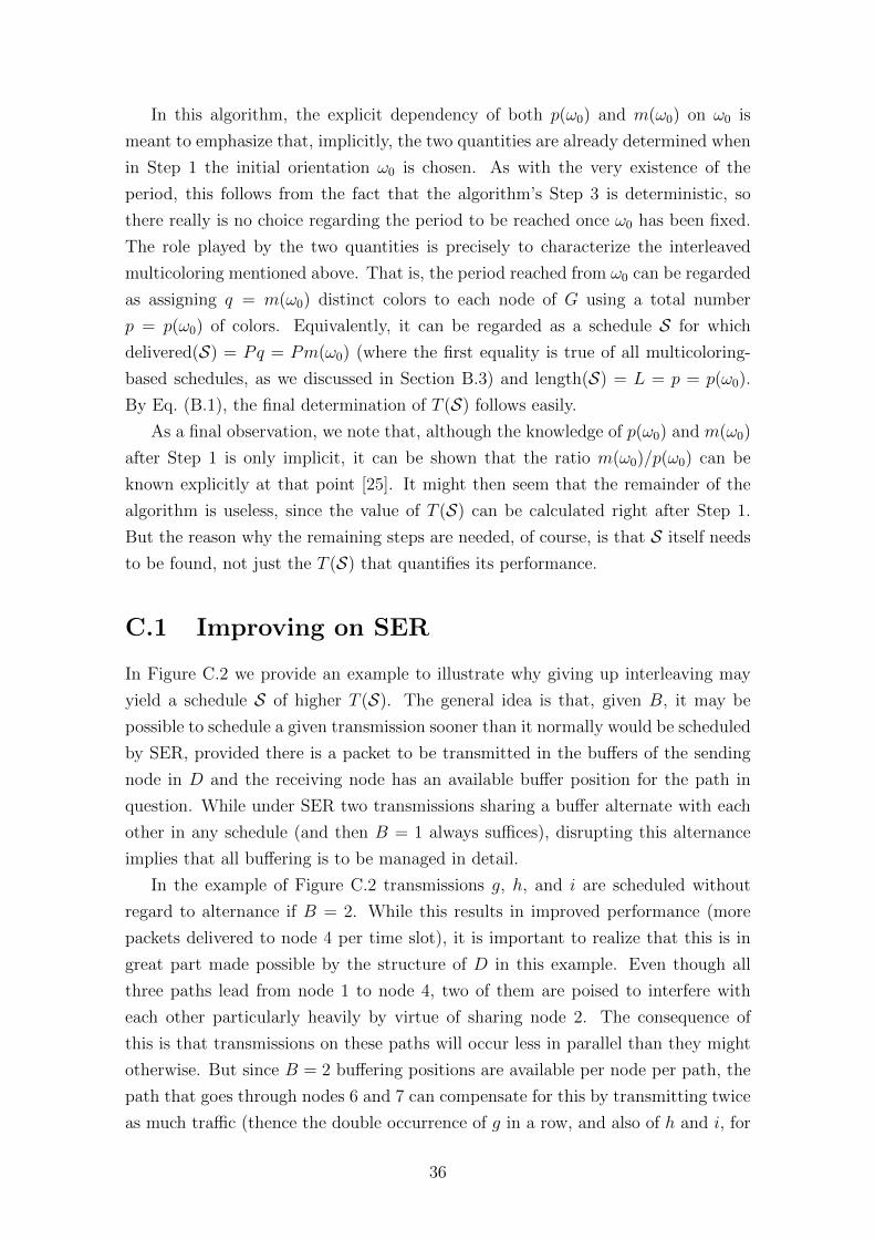
In this algorithm, the explicit dependency of both p(ω0) and m(ω0) on ω0 is

meant to emphasize that, implicitly, the two quantities are already determined when

in Step 1 the initial orientation ω0 is chosen. As with the very existence of the

period, this follows from the fact that the algorithm’s Step 3 is deterministic, so

there really is no choice regarding the period to be reached once ω0 has been fixed.

The role played by the two quantities is precisely to characterize the interleaved

multicoloring mentioned above. That is, the period reached from ω0 can be regarded

as assigning q = m(ω0) distinct colors to each node of G using a total number

p = p(ω0) of colors. Equivalently, it can be regarded as a schedule S for which

delivered(S) = Pq = Pm(ω0) (where the first equality is true of all multicoloring-

based schedules, as we discussed in Section B.3) and length(S) = L = p = p(ω0).

By Eq. (B.1), the final determination of T (S) follows easily.

As a final observation, we note that, although the knowledge of p(ω0) and m(ω0)

after Step 1 is only implicit, it can be shown that the ratio m(ω0)/p(ω0) can be

known explicitly at that point [25]. It might then seem that the remainder of the

algorithm is useless, since the value of T (S) can be calculated right after Step 1.

But the reason why the remaining steps are needed, of course, is that S itself needs

to be found, not just the T (S) that quantifies its performance.

C.1 Improving on SER

In Figure C.2 we provide an example to illustrate why giving up interleaving may

yield a schedule S of higher T (S). The general idea is that, given B, it may be

possible to schedule a given transmission sooner than it normally would be scheduled

by SER, provided there is a packet to be transmitted in the buffers of the sending

node in D and the receiving node has an available buffer position for the path in

question. While under SER two transmissions sharing a buffer alternate with each

other in any schedule (and then B = 1 always suffices), disrupting this alternance

implies that all buffering is to be managed in detail.

In the example of Figure C.2 transmissions g, h, and i are scheduled without

regard to alternance if B = 2. While this results in improved performance (more

packets delivered to node 4 per time slot), it is important to realize that this is in

great part made possible by the structure of D in this example. Even though all

three paths lead from node 1 to node 4, two of them are poised to interfere with

each other particularly heavily by virtue of sharing node 2. The consequence of

this is that transmissions on these paths will occur less in parallel than they might

otherwise. But since B = 2 buffering positions are available per node per path, the

path that goes through nodes 6 and 7 can compensate for this by transmitting twice

as much traffic (thence the double occurrence of g in a row, and also of h and i, for

36

(c)

a

de

c

f

g

hi

b

1 4

3

5

2

76

(b)a b c

d e f

g h i

1

6

2 3 4

7

51

1

2 4

4

(a)

a c

g

e

b

h

i

fd

Figura C.2: A set of P = 3 directed paths (a), the resulting directed multigraphD (b), and the resulting undirected graph G (c). The optimal SER schedule isS = 〈{a}, {b}, {c, g}, {d, i}, {e, h}, {f}〉, yielding T (S) = 3/6 = 0.5. An alternativeschedule that does not comply with the SER alternance condition, with B = 2, isS = 〈{g, c}, {g, f}, {h, b}, {h, e}, {i, a}, {i, d}〉, which results in an improvement toT (S) = 4/6 ≈ 0.67.

each repetition of the schedule). This, however, is never detrimental to the traffic

on the other two paths: all that is being done is to seize the opportunity to transmit

in time slots that would otherwise go unused.

Implementing the careful buffer management alluded to above requires that we

look at the dynamics of acyclic-orientation transformation under SER in more detail.

Given any acyclic orientation ω of G, the node set N of G can be partitioned into

independent sets I1, I2, . . . , Id such that I1 is the set of all sinks in G according to ω,

I2 is the set of all sinks we would obtain if all nodes in I1 were to be eliminated, and

so on. In this partition, known as a sink decomposition, d is the number of nodes

on a longest directed path of G according to ω. When ω is turned into ω′ by SER a

new sink decomposition is obtained, call it I ′1, I′2, . . . , I

′d′ , such that I ′1 = I2, I

′2 ⊇ I3,

etc., with d′ ≤ d. As we illustrate shortly, the reason why equality need not hold in

all cases, but set containment instead, is that each Ik may get enlarged by some of

the previous orientation’s sinks before becoming I ′k−1.

It is then possible to regard the operation of SER as simply a recipe for mani-

pulating sink decompositions. At each iteration the set containing the current sinks

is eliminated and its nodes are redistributed through the other sets. The remaining

sets are renumbered by decrementing their subscripts by 1 and a new, greatest-

subscript set may have to be created. The rule for redistributing each of the former

sinks is to find the set of greatest subscript containing one of the node’s neighbors

in G, say Ik, and then place the node in set Ik+1. This is illustrated in panels (a)

37

and (b) of Figure C.3. From panel (a) we have I1 = {a, b}, I2 = {c}, I3 = {d}, and

so on, and from panel (b) we have I ′1 = {c}, I ′2 = {b, d}, etc. Clearly, then, I ′1 = I2

while I ′2 ⊃ I3. In the latter case we may think of I3 as being enlarged by node b, a

sink from I1, and then becoming I ′2.

5

b c d e

1 2 3 4

a(a)

f

5

1 2 3 4

(c)

d e

fb

a

c

1 2 3 4

(b)

d e

fbc a

Figura C.3: Each set in a sink decomposition is represented by a rectangular box andnumbered to indicate the set’s subscript. Note that directed edges refer to acyclicorientations of G. Applying SER to the sink decomposition in panel (a) yields theone in panel (b). In this transformation both a and b are turned into sources. Thealternative of using SERA, on the other hand, makes it possible for a to be placedin a lower-subscript set, avoiding the transformation into a source and yielding thesink decomposition in panel (c). This can be done only because the set to which ais added contains none of its neighbors in G. Assuming that transmissions a, e, andf are initially arranged consecutively in one of the P paths in the order e, a, f , wehave i− = e, i = a, and i+ = f . We also have, in reference to panel (a), k− = 4,k = 2, and k+ = 5. Then the additional conditions for the move from (a) to (c)to occur are that the buffers shared by transmissions e and a contain at least onepacket (since k < k−), and that those shared by a and f have room for at least onepacket (since k < k+).

Altering this redistribution rule is the core of our modified SER, henceforth

called SER with advancement (SERA). If i is the sink in question, the operation of

SERA is based on placing node i in the least-subscript set that does not contain

a neighbor of i in G. This clearly maintains acyclicity just as the previous rule

does, but now the former sink is not necessarily turned into a source, but rather

into a node that can have edges oriented both inward and outward by the current

orientation, respectively from nodes in sets of greater subscripts and to nodes in sets

of lesser subscripts. Additionally, while this alternative placement of node i does

favor it by virtue of lowering the number of time slots that need to go by before it

is a sink once again, clearly there is no detriment to any of the other transmissions,

which will assuredly become sinks no later than they would otherwise.

38

As we mentioned, however, unlike SER this rule can only be applied as a function

of B and the buffering-related constraints we mentioned. Suppose that i is preceded

by transmission i− and succeeded by transmission i+ on the original path out of

P1,P2, . . . ,PP to which it belongs. Of course, both i− and i+ are nodes of G as

well. Suppose further that these two nodes are in sets Ik− and Ik+ , respectively,

and that we are attempting to place node i in set Ik. The further constraints to

be satisfied are the following. If k < k−, then the buffers shared by transmissions

i− and i must contain at least one packet to be transmitted. If k < k+, then the

buffers shared by transmissions i and i+ must contain room to store at least one

more packet. This can all be implemented rather easily by keeping a dynamic record

of all buffers. A simple case of evolving sink decompositions in the SERA style is

shown in panels (a) and (c) of Figure C.3.

SERA, like SER, operates on finitely many possibilities and deterministically.

A “possibility” is no longer simply an acyclic orientation, but instead an acyclic

orientation together with a configuration of buffer occupation. In any event, periodic

behavior is still guaranteed to occur and we go on denoting by p(ω0) the number

of possibilities in the period that one reaches from ω0. The notion behind m(ω0),

however, has been lost together with the certainty of interleaving, since SERA does

not guarantee that every node of G is a sink in the period the same number of times.

For i ∈ N , an alternative definition is that of mi(ω0), which we henceforth use to

denote the number of times node i is a sink in the period, not necessarily the same

for all nodes.

Determining the schedule S through SERA proceeds according to the following

algorithm.

Algorithm SERA:

1. Choose ω0.

2. t := 0.

3. Obtain ωt+1 from ωt, employing advancement as described.

4. If the period has not yet occurred, then t := t + 1; go to Step 3. If it has,

then let p(ω0) be its number of orientations (with associated buffer-occupation

configurations), mi(ω0) the number of times node i appears in them as a sink,

and ωk, ωk+1, . . . , ωk+p(ω0)−1 the orientations themselves. Output


and

T (S) =

∑i∈T mi(ω0)

p(ω0),

39

where T is the set of the nodes of G that correspond to terminal edges of the

paths P1,P2, . . . ,PP .

In this algorithm, note that the determination of T (S) generalizes what is done in

SER. This is achieved by adopting delivered(S) =∑

i∈T mi(ω0) while maintaining

length(S) = p(ω0) in Eq. (B.1). Particularizing this to the case of SER yields

delivered(S) = Pm(ω0), as desired, since mi(ω0) becomes m(ω0) for any node i of

G and moreover |T | = P .

40

Apendice D

SER and SERA experimentation

We have conducted extensive computational experiments to evaluate algorithms

SER and SERA, the latter with a few different values for the buffering parameter B.

Before we present results in Section D.3, here we pause to introduce the methodology

that was followed. This includes selecting the network topology that eventually leads

to graph G and the choice of the initial acyclic orientation of G.

D.1 Topology generation

We generated 1600 networks by placing n nodes inside a square of side 1500. For

each network the first node was positioned at the square’s center. Given the nodes’

communication (or interference) radius R, and with it the neighborhood relation

among nodes (i.e., two nodes are neighbors of each other if and only if the Eucli-

dean distance between them is no greater than R), we proceeded to positioning the

remaining nodes randomly, one at a time. Positioning a node was subject to the

constraints that it would have at least one neighbor, that no node would have more

than ∆ neighbors, and moreover that no two nodes would be closer to each other

than 25 units of Euclidean distance. Repeated attempts at positioning nodes while

satisfying these constraints were not allowed to number more than 1000 per network.

When this limit was reached the growing network was wiped clean and a new one

was started. The value of R was determined so that, had the nodes been positio-

ned uniformly at random, a randomly chosen radius-R circle would have expected

density proportional to ∆/R2 and about the same density as the whole network,

i.e., ∆/R2 ∝ n. Choosing the proportionality constant to yield R = 200 for n = 80

and ∆ = 4 results in the formula R = 200√

20∆/n. Of the 1600 networks thus

generated, there are 100 networks for each combination of n ∈ {60, 80, 100, 120} and

∆ ∈ {4, 8, 16, 32}.For each network we generated 50n sets of paths P1,P2, . . . ,PP , each 100 sets

corresponding to a different value of P . Each of the sets resulted in a different

41

D, then in G, as explained in Sections B.1 and B.2. The 50n sets comprise 100

groups of n/2 sets each. The first of these sets for a group has P = 1 and the single

path it contains is the shortest path from a randomly chosen node to another in the

network. Each new set in the group is the previous one enlarged by the addition of a

new path, obtained by selecting two distinct nodes randomly, provided they do not

already participate in the previous set. This goes on until P = n/2, so in the last

set every one of the n nodes participates as either the origin or the destination of

one of the P paths. For the sake of normalization, the results we present for T (S),

given for P = 1, 2, . . . , n/2, are shown against the ratio P ′ = 2P/n ∈ (0, 1].

D.2 Initial acyclic orientation

Once G has been built for a fixed network and a fixed set of paths, the acyclic

orientation ω0 of G has to be determined. Our general approach is to label every

node of G with a different number and then to direct each edge from the node

that has the higher number to the one that has the lower. Although the resulting

orientation is clearly acyclic, we are left with the problem of labeling the nodes.

We approach this problem by resorting to the paths P1,P2, . . . ,PP from which G

resulted, since the nodes of G are in one-to-one correspondence with the directed

edges on the paths. It then suffices to number the paths’ edges.

We consider four numbering schemes:

ND-BF. The paths are organized in the nondecreasing order of their numbers of ed-

ges (ties are broken by increasing path number). The edges are then numbered

breadth-first from the path’s origins, given this organization of the paths.

ND-DF. The paths are organized in the nondecreasing order of their numbers of ed-

ges (ties are broken by increasing path number). The edges are then numbered

depth-first from the paths’ origins, given this organization of the paths.

NI-BF. The paths are organized in the nonincreasing order of their numbers of edges

(ties are broken by increasing path number). The edges are then numbered

breadth-first from the paths’ origins, given this organization of the paths.

NI-DF. The paths are organized in the nonincreasing order of their numbers of edges

(ties are broken by increasing path number). The edges are then numbered

depth-first from the paths’ origins, given this organization of the paths.

42

D.3 Computational results

We divide our results into two categories. First we give statistics on the 1600

networks generated for evaluation of the algorithms. Then we report on the values

obtained for T (S) by SER and SERA.

One of the statistics is particularly useful: despite its simplicity, we have found

it to correlate with the SERA results in a fairly direct way. This statistic is based

on a function of G that aims to quantify how the interference among the initial P

directed paths is reflected in the structure of G. We denote this function by ρ(G)

and let it be such that

ρ(G) =P |E ′|∑Pp=1 |Yp|

. (D.1)

In this equation, recall that the sets Y1, Y2, . . . , YP , one for each of the initial directed

paths, contain the edges that ultimately become the nodes of G. Thus,∑P

p=1 |Yp|/Pis the average number of edges on a path. Moreover, we let E ′ ⊆ E be the set of G’s

edges whose end nodes correspond to edges of distinct paths. In words, then, ρ(G)

is the average number of off-path transmissions that interfere with the transmissions

of a path having the average number of edges.

D.3.1 Properties of the networks generated

The 1600 networks we generated comprise a wide variety of topological traits, as

exemplified in Figure D.1, including those that make up star topologies, rings, and

grids. Our results on the value of T (S) for SER and SERA, though statistical in

nature, are therefore to be regarded as reflecting how the presence of such variability

affects our algorithms’ performance.

The networks’ distributions of node degrees are given in Figure D.2, which con-

tains one panel for each of the four values of ∆ and all four values of n. Their

distributions of the numbers of edges on the P paths for P = n/2 are given in

Figure D.3, again with one panel for each of the four values of ∆ and all four values

of n.

We see from Figure D.2 that the degree distributions peak at the degree ∆,

falling approximately linearly toward the lower degrees (except for ∆ = 32, where

a plateau is observed midway). Furthermore, the lowest observed degree grows

with ∆, which is expected from the formula that gives the radius R as an increasing

function of ∆. We also see from the figure that these distributions are approximately

independent of the value of n for fixed ∆; in reference to that same formula, we see

that letting R decrease with n does indeed have the expected effect of maintaining

an approximately uniform node density throughout the containing square.

We also expect path sizes to be smaller as ∆ increases, and this is in fact what

43

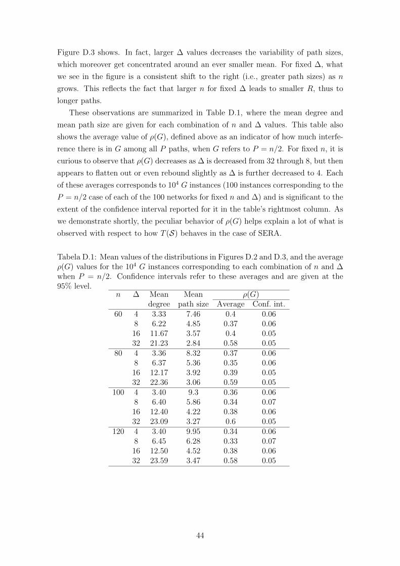
Figure D.3 shows. In fact, larger ∆ values decreases the variability of path sizes,

which moreover get concentrated around an ever smaller mean. For fixed ∆, what

we see in the figure is a consistent shift to the right (i.e., greater path sizes) as n

grows. This reflects the fact that larger n for fixed ∆ leads to smaller R, thus to

longer paths.

These observations are summarized in Table D.1, where the mean degree and

mean path size are given for each combination of n and ∆ values. This table also

shows the average value of ρ(G), defined above as an indicator of how much interfe-

rence there is in G among all P paths, when G refers to P = n/2. For fixed n, it is

curious to observe that ρ(G) decreases as ∆ is decreased from 32 through 8, but then

appears to flatten out or even rebound slightly as ∆ is further decreased to 4. Each

of these averages corresponds to 104 G instances (100 instances corresponding to the

P = n/2 case of each of the 100 networks for fixed n and ∆) and is significant to the

extent of the confidence interval reported for it in the table’s rightmost column. As

we demonstrate shortly, the peculiar behavior of ρ(G) helps explain a lot of what is

observed with respect to how T (S) behaves in the case of SERA.

Tabela D.1: Mean values of the distributions in Figures D.2 and D.3, and the averageρ(G) values for the 104 G instances corresponding to each combination of n and ∆when P = n/2. Confidence intervals refer to these averages and are given at the95% level.

n ∆ Mean Mean ρ(G)degree path size Average Conf. int.

60 4 3.33 7.46 0.4 0.068 6.22 4.85 0.37 0.0616 11.67 3.57 0.4 0.0532 21.23 2.84 0.58 0.05

80 4 3.36 8.32 0.37 0.068 6.37 5.36 0.35 0.0616 12.17 3.92 0.39 0.0532 22.36 3.06 0.59 0.05

100 4 3.40 9.3 0.36 0.068 6.40 5.86 0.34 0.0716 12.40 4.22 0.38 0.0632 23.09 3.27 0.6 0.05

120 4 3.40 9.95 0.34 0.068 6.45 6.28 0.33 0.0716 12.50 4.52 0.38 0.0632 23.59 3.47 0.58 0.05

44

n0

n0 n0

n0

n0 n0

n1

n1

n1

n1

n1

n1

n2

n2

n2

n2

n4

n4

n6

n4

n4

n3

n29

n5

n7

n10

n6

n4n34

n7

n7

n50

n5

n2

n16

n45

n54

n11

n7

n31

n25

n13

n58

n12

n3

n3

n27

n60

n4

n16

n3

n8

n5

n5

n3

n15

n12

n15

n11

n2

n5

n52

n21

n21

n20

n6

n8

n47

n28

n23

n44

n31

n27

n6n8

n11

n14

n10

n24

n6

n14

n19

n39

n25

n13

n8

n18

n52

n9

n77

n28

n39

n24

n11

n41

n41

n10

n12

n47

n13

n10

n42

n14

n46

n16

n6

n21

n15

n12

n22

n22

n39

n16

n25

n74

n17

n60

n23

n30

n75

n9

n38

n66

n9

n19

n24

n78

n13

n7

n15

n11

n20

n8

n42

n12

n15

n3

n60

n17

n16

n23

n9

n40

n33

n23

n14

n32

n17

n31

n7

n33

n21

n27

n18

n37

n21

n39

n26

n13

n19

n47

n9

n18

n18

n19

n20

n48

n24

n34

n29

n54

n28

n37

n21

n25

n20

n43

n26

n30

n72

n5

n22

n57

n28

n26

n8

n35

n36

n50

n29

n63

n14

n14

n37

n32

n51

n17

n51

n70

n45

n37

n23

n73

n39

n24

n15

n25

n49

n44

n45

n35

n43

n59

n34

n55

n67

n9

n47

n38

n58

n29

n18

n62

n10

n20

n38

n33

n44

n17

n64

n43

n47

n53

n71

n18

n22

n52

n62

n27

n28

n34

n42

n53

n35

n39

n46

n58

n30

n36

n37

n67

n31

n30

n27

n46

n31

n46

n40

n30

n41

n40

n62

n60

n31

n58

n35

n36

n41

n26

n33

n61

n41

n36

n27

n51

n17

n32

n70

n49

n29

n23

n75

n60

n75

n74

n28

n62

n36

n42

n73

n25

n43

n73

n40

n76

n33

n10

n48

n54

n45

n19

n55

n50

n60

n53

n24

n56

n63

n70

n29

n11

n32

n38

n56

n47

n16

n56

n49

n22

n53

n64

n43

n64

n40

n26n59

n35

n66

n41

n48

n48

n43

n57

n34

n58

n63

n76

n36

n68

n72

n12

n49

n34

n40

n75

n13

n71

n55

n44

n45

n20

n75

n55

n50

n42

n65

n46

n51

n53

n67

n69

n56

n57

n77

n59

n48

n66

n44

n59

n64

n57

n19

n54

n63

n61

n46

n70

n22

n68

n50

n74

n68

n51

n67

n78

n65

n72

n50

n61

n66

n61

n71

n75

n74

n72

n76

n79

n54

n52

n57n65

n68

n66

n54

n51

n78

n58

n59

n26 n56

n66

n78

n52

n59

n32

n65

n77

n69

n62

n67

n70

n79

n33

n68

n55

n69

n73

n62

n77

n79

n69

n38

n69

n74

n35

n76

n78

n52

n30

n72

n71

n65

n32

n74

n73

bl

n76

br

n79

n79

n78

n72

bl

bl

tr

blbr

br

tl

br

tr

tr

tr

n57

tl

tl tl

n63n64

n42

n37n71

n61

n44

n53

n49

n49

n65

n38

n76

n61

n77

n77

n45

n73

n56

n64

n63

n71

n70

n67

n69

n68

n48

n79

bl br

tr

n55

tl

bl br

trtl

(c) (d)

(f)

(b)

(e)

(a)

Figura D.1: A sampler of the networks that were generated for n = 80. A greatvariety of arrangements is included, ranging from those in which nodes coalesce intogroups that form a star-like topology (a, b), to those in which such groups tend toform rings (c, d), to those that are somewhat grid-like (e, f).

45

Figura D.2: Degree distributions of the 1600 networks, for ∆ = 4 (a), ∆ = 8 (b),∆ = 16 (c), and ∆ = 32 (d). For each combination of n and ∆ the distributionrefers to 100 networks.

46

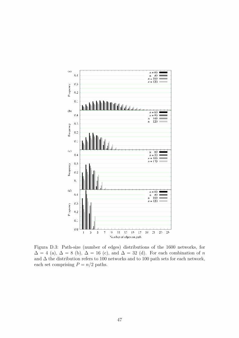
Figura D.3: Path-size (number of edges) distributions of the 1600 networks, for∆ = 4 (a), ∆ = 8 (b), ∆ = 16 (c), and ∆ = 32 (d). For each combination of nand ∆ the distribution refers to 100 networks and to 100 path sets for each network,each set comprising P = n/2 paths.

47

D.3.2 Results

Our results for SER are given in Figure D.4 as plots of T (S) against the P ′ ratio

introduced earlier in this chapter. Each of the figure’s four panels is specific to a

fixed ∆ value and shows a plot for each value of n combined with either the ND-BF

or the ND-DF numbering scheme. All results relating to the NI-BF and NI-DF

schemes are omitted, as we found them to be statistically indistinguishable from

their ND counterparts. From this figure it seems clear that, as P ′ increases (i.e.,

as the number of paths P grows towards n/2), the superiority of the BF schemes

over the DF schemes becomes apparent, more pronouncedly so for the lower values

of ∆. The reason why the BF schemes tend to perform better than the DF schemes

should be intuitively clear: the BF schemes number the transmissions that are closer

to the paths’ origins first, therefore with the lowest numbers. As the initial acyclic

orientation of G is built from these numbers, the first sinks during the operation

of SER will correspond to starting parallel traffic on as many paths as possible.

Overall it also seems that larger values of n lead to better performance for fixed ∆,

but the distinction appears to be only marginal and is sometimes obscured by the

confidence intervals.

A similar set of plots is given in Figure D.5, now displaying our results for SERA

as plots of T (S) against the ratio P ′. Once again there is one panel for each value of

∆, and once again several possibilities regarding the numbering schemes are omitted

because of statistical indistinguishability. This is also true of the various possibilities

for the value of B, with the single exception we mention shortly. Thus, most plots

correspond to the ND-BF numbering scheme with B = 1. The single exception is

that of n = 60 with ∆ = 4, for which we also report on the B = 2 case. For fixed ∆

and P ′, increasing n also leads to increased T (S). In the particular case of n = 60

and ∆ = 4, increasing B from 1 to 2 also causes T (S) to increase.

As we fix ∆, n, and P ′, Figures D.4 and D.5 reveal that T (S) is consistently

higher for SERA than it is for SER (by a factor of about 2 to 4) across all values

for these quantities, thereby establishing the superiority of the former algorithm

over the latter. For sufficiently large n this occurs for the same value of B (that is,

for B = 1), which furthermore establishes that this superiority does not in general

depend on the availability of more buffering space. It is, instead, determined solely

by the elimination in SERA of the mandatory alternance of interfering transmissions

in SER.

Fixing n and P ′ while varying ∆ (i.e., moving between panels) yields further

interesting insight about the two algorithms. While for SER increasing ∆ under

these conditions causes T (S) to increase monotonically (though sometimes almost

imperceptibly) for the same numbering scheme, doing the same for SERA for cons-

48

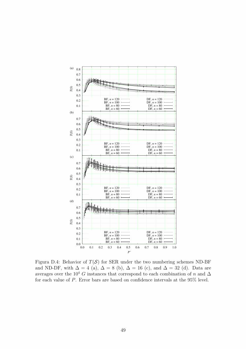
0.1

0.2

0.3

0.4

0.5

0.6

0.7

0.8T

(S)

(a)

BF, n = 120BF, n = 100BF, n = 80BF, n = 60

DF, n = 120DF, n = 100

DF, n = 80DF, n = 60

0.1

0.2

0.3

0.4

0.5

0.6

0.7

T(S

)

(b)

BF, n = 120BF, n = 100BF, n = 80BF, n = 60

DF, n = 120DF, n = 100

DF, n = 80DF, n = 60

0.1

0.2

0.3

0.4

0.5

0.6

0.7

T(S

)

(c)

BF, n = 120BF, n = 100BF, n = 80BF, n = 60

DF, n = 120DF, n = 100

DF, n = 80DF, n = 60

0.0

0.1

0.2

0.3

0.4

0.5

0.6

0.7

0.0 0.1 0.2 0.3 0.4 0.5 0.6 0.7 0.8 0.9 1.0

T(S

)

P’

(d)

BF, n = 120BF, n = 100BF, n = 80BF, n = 60

DF, n = 120DF, n = 100

DF, n = 80DF, n = 60

Figura D.4: Behavior of T (S) for SER under the two numbering schemes ND-BFand ND-DF, with ∆ = 4 (a), ∆ = 8 (b), ∆ = 16 (c), and ∆ = 32 (d). Data areaverages over the 104 G instances that correspond to each combination of n and ∆for each value of P . Error bars are based on confidence intervals at the 95% level.

49

0.4

0.8

1.2

1.6

2

2.4T

(S)

(a)

n = 120n = 100

n = 80n = 60, B = 2

n = 60

0.4

0.8

1.2

1.6

2

2.4

T(S

)

(b)

n = 120n = 100

n = 80n = 60

0.4

0.8

1.2

1.6

2

2.4

T(S

)

(c)

n = 120n = 100

n = 80n = 60

0.0

0.4

0.8

1.2

1.6

2

2.4

0.0 0.1 0.2 0.3 0.4 0.5 0.6 0.7 0.8 0.9 1.0

T(S

)

P’

(d)

n = 120n = 100

n = 80n = 60

Figura D.5: Behavior of T (S) for SERA under the numbering scheme ND-BF, with∆ = 4 (a), ∆ = 8 (b), ∆ = 16 (c), and ∆ = 32 (d). Data are averages over the 104

G instances that correspond to each combination of n and ∆ for each value of P .Error bars are based on confidence intervals at the 95% level.

50

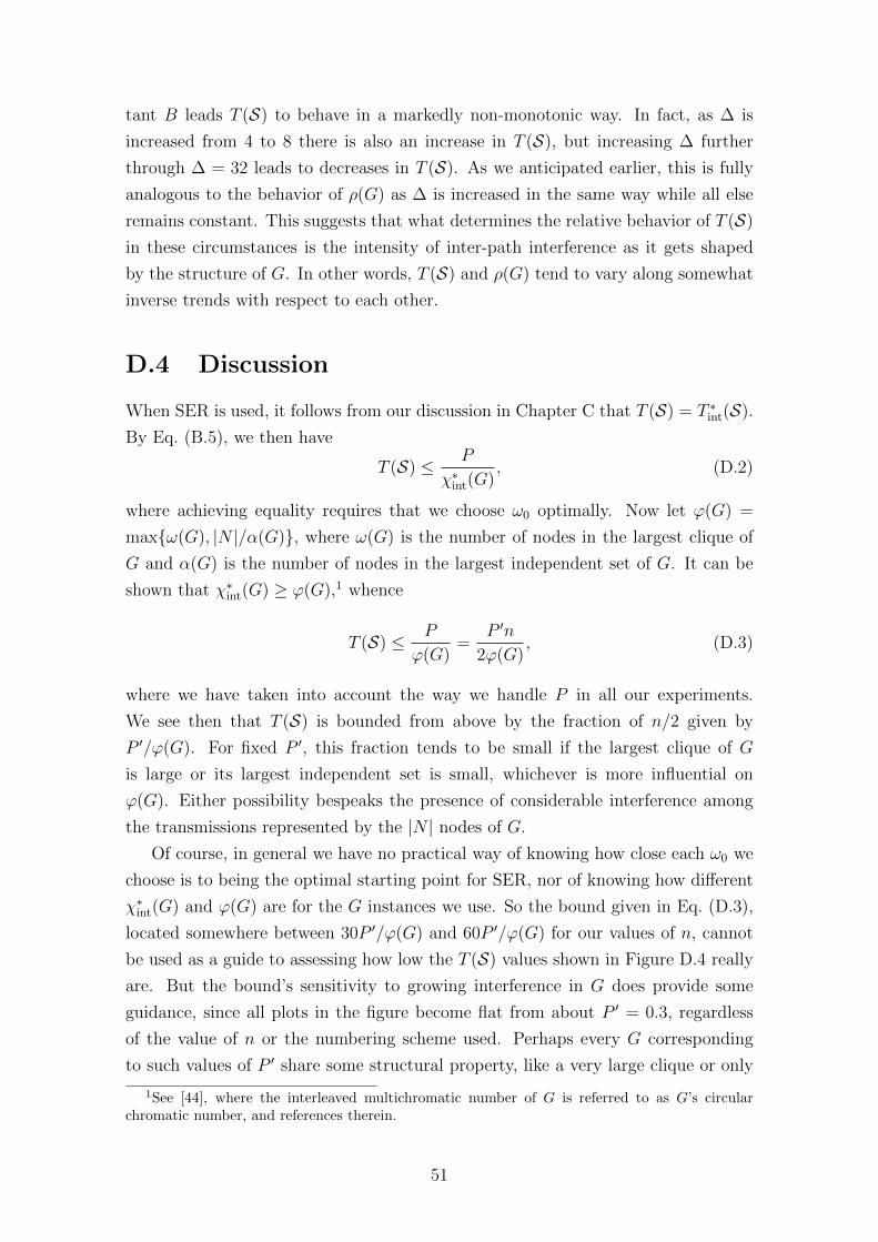
tant B leads T (S) to behave in a markedly non-monotonic way. In fact, as ∆ is

increased from 4 to 8 there is also an increase in T (S), but increasing ∆ further

through ∆ = 32 leads to decreases in T (S). As we anticipated earlier, this is fully

analogous to the behavior of ρ(G) as ∆ is increased in the same way while all else

remains constant. This suggests that what determines the relative behavior of T (S)

in these circumstances is the intensity of inter-path interference as it gets shaped

by the structure of G. In other words, T (S) and ρ(G) tend to vary along somewhat

inverse trends with respect to each other.

D.4 Discussion

When SER is used, it follows from our discussion in Chapter C that T (S) = T ∗int(S).

By Eq. (B.5), we then have

T (S) ≤ P

χ∗int(G), (D.2)

where achieving equality requires that we choose ω0 optimally. Now let ϕ(G) =

max{ω(G), |N |/α(G)}, where ω(G) is the number of nodes in the largest clique of

G and α(G) is the number of nodes in the largest independent set of G. It can be

shown that χ∗int(G) ≥ ϕ(G),1 whence

T (S) ≤ P

ϕ(G)=

P ′n

2ϕ(G), (D.3)

where we have taken into account the way we handle P in all our experiments.

We see then that T (S) is bounded from above by the fraction of n/2 given by

P ′/ϕ(G). For fixed P ′, this fraction tends to be small if the largest clique of G

is large or its largest independent set is small, whichever is more influential on

ϕ(G). Either possibility bespeaks the presence of considerable interference among

the transmissions represented by the |N | nodes of G.

Of course, in general we have no practical way of knowing how close each ω0 we

choose is to being the optimal starting point for SER, nor of knowing how different

χ∗int(G) and ϕ(G) are for the G instances we use. So the bound given in Eq. (D.3),

located somewhere between 30P ′/ϕ(G) and 60P ′/ϕ(G) for our values of n, cannot

be used as a guide to assessing how low the T (S) values shown in Figure D.4 really

are. But the bound’s sensitivity to growing interference in G does provide some

guidance, since all plots in the figure become flat from about P ′ = 0.3, regardless

of the value of n or the numbering scheme used. Perhaps every G corresponding

to such values of P ′ share some structural property, like a very large clique or only

1See [44], where the interleaved multichromatic number of G is referred to as G’s circularchromatic number, and references therein.

51

very small independent sets, that renders the resulting values of T (S) oblivious to

all else.

As for SERA, since the schedules it produces depart from a strict characteriza-

tion as multicolorings of G, no upper bounds on T (S) are known to us. Nevertheless,

a comparison with SER as provided by Figures D.4 and D.5 reveals that T (S) for

SERA surpasses T (S) for SER by a substantial margin, and also that SERA is capa-

ble of finding ways to improve T (S) somewhat even as P ′ grows. If our observation

above regarding the structure of G as an inherent barrier to improving T (S) as P ′

grows is true, then the barrier’s effects under SERA are considerably attenuated.

This, we believe, is to be attributed to SERA’s aggressively opportunistic approach

of abandoning the interleaving that is the hallmark of SER.

Another course of action regarding the discovery of how close SER and SERA

get to the optimal value of T (S) in each case (that is, how close their initial acyclic

orientations come to being optimal) is to concentrate on suitably small problem

instances. If such instances prove amenable to some method to discover what the

optimal orientations are, then we may be able to draw some meaningful conclusion

regarding the performance of SER and SERA despite the modest instance sizes. Un-

fortunately, we have no exact method to optimize our algorithms’ initial conditions,

except for resorting to an explicit enumeration of all possibilities and recording the

best value of T (S) that is found. Although the number of a graph’s distinct acyclic

orientations grows rather quickly with graph size [45], being in the worst case given

by the factorial of the number of nodes, we have found that such enumeration is

feasible for small values of n and ∆. We have therefore proceeded with it for n = 10

and ∆ = 4, following the exact same methodology introduced earlier in this chapter,

and give results in Figure D.6. While these results confirm that SERA outperforms

SER also at this reduced scale, clearly both algorithms come very close to perfor-

ming optimally, i.e., to achieving the value of T (S) that results from the optimal

initial acyclic orientation in each case.

52

Figura D.6: Behavior of T (S) for SER and SERA with n = 10 and ∆ = 4. For eachalgorithm, results are given based on the numbering scheme ND-BF and also for theoptimal numbering scheme. SERA results are for B = 2. Data are averages over104 G instances for each value of P . Error bars are based on confidence intervals atthe 95% level.

53

Apendice E

Interference among wireless routes

A roadmap on reducing mutual radio interference is to join routing algorithms with

an interference avoidance approach such as: power control, link scheduling or multi-

channel radios [5]. This type of network interference problem has been faced by a

considerable amount of different strategies over the literature [6–9]. Some studies

show that the use of multi-path routing to distribute traffic helps to improve route

recovery and load balance more than single-path strategies and it may lead to bet-

ter throughput values over the entire network [15, 16]. Nevertheless, these benefits

are directly related to how multiple paths interferes with each other, an aspect not

addressed by multi-path strategies. Therefore, the lack of performance of most em-

ployed and promising routing algorithms is a direct consequence of the interference

among routes, because they do not tackle directly this interference during route dis-

cover process. The single exception is the algorithm reported in [46], however it uses

geographic information (like localization aided by GPS) to find paths with sufficient

spacial separation, so they do not interfere with each other. Unfortunately, this in-

formation is available only in some types of sensor networks [10] and the algorithm

reported is normally related to larger instances of a NP-hard problem [47].

Here we propose a different approach to avoid interference among multi-path

routes which, to the best of our knowledge, is a novel formulation and solution.

We start by extracting the network path set from a routing algorithm. Next, we

build a new path set that is a sub-set of the paths discovered by the algorithm. For

that, we select paths that avoid mutual interference and by consequence they may

transmit more packets. Our objective is to improve the throughput performance

of the path set, that is, to increase the number of packets delivered to the last

node of each path (the throughput on the route destinations). This approach lies at

the principal problem of successfully design routing protocols for wireless networks,

because it deals with the interference when the network is heavily loaded. The

solution we propose is to build a multi-path set for each possible pair of nodes

in a WMN that avoids mutual interference. Our approach is easily adaptable to

54

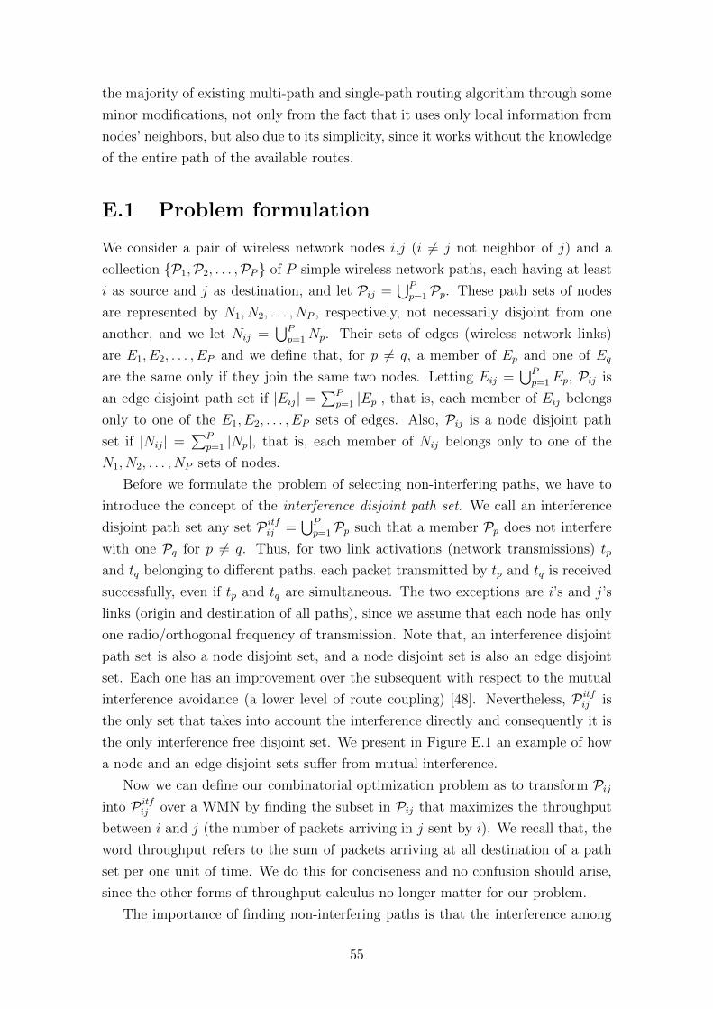
the majority of existing multi-path and single-path routing algorithm through some

minor modifications, not only from the fact that it uses only local information from

nodes’ neighbors, but also due to its simplicity, since it works without the knowledge

of the entire path of the available routes.

E.1 Problem formulation

We consider a pair of wireless network nodes i,j (i 6= j not neighbor of j) and a

collection {P1,P2, . . . ,PP} of P simple wireless network paths, each having at least

i as source and j as destination, and let Pij =⋃P

p=1Pp. These path sets of nodes

are represented by N1, N2, . . . , NP , respectively, not necessarily disjoint from one

another, and we let Nij =⋃P

p=1Np. Their sets of edges (wireless network links)

are E1, E2, . . . , EP and we define that, for p 6= q, a member of Ep and one of Eq

are the same only if they join the same two nodes. Letting Eij =⋃P

p=1Ep, Pij is

an edge disjoint path set if |Eij| =∑P

p=1 |Ep|, that is, each member of Eij belongs

only to one of the E1, E2, . . . , EP sets of edges. Also, Pij is a node disjoint path

set if |Nij| =∑P

p=1 |Np|, that is, each member of Nij belongs only to one of the

N1, N2, . . . , NP sets of nodes.

Before we formulate the problem of selecting non-interfering paths, we have to

introduce the concept of the interference disjoint path set. We call an interference

disjoint path set any set P itfij =

⋃Pp=1Pp such that a member Pp does not interfere

with one Pq for p 6= q. Thus, for two link activations (network transmissions) tp

and tq belonging to different paths, each packet transmitted by tp and tq is received

successfully, even if tp and tq are simultaneous. The two exceptions are i’s and j’s

links (origin and destination of all paths), since we assume that each node has only

one radio/orthogonal frequency of transmission. Note that, an interference disjoint

path set is also a node disjoint set, and a node disjoint set is also an edge disjoint

set. Each one has an improvement over the subsequent with respect to the mutual

interference avoidance (a lower level of route coupling) [48]. Nevertheless, P itfij is

the only set that takes into account the interference directly and consequently it is

the only interference free disjoint set. We present in Figure E.1 an example of how

a node and an edge disjoint sets suffer from mutual interference.

Now we can define our combinatorial optimization problem as to transform Pij

into P itfij over a WMN by finding the subset in Pij that maximizes the throughput

between i and j (the number of packets arriving in j sent by i). We recall that, the

word throughput refers to the sum of packets arriving at all destination of a path

set per one unit of time. We do this for conciseness and no confusion should arise,

since the other forms of throughput calculus no longer matter for our problem.

The importance of finding non-interfering paths is that the interference among

55

(a)

q

o

p q

o

p q

o

(b)

(c)

j

k l

i j

k l

i j

k l

m

m

mi

p

Figura E.1: A graph representation of a wireless network (a), an edge disjoint set in(b) and a node disjoint path set in (c), both represented by dashed and dotted lines.Neither of the paths in (b) may be used simultaneously, because node k cannottransmit two packets at the same time. The same occurs in (c) for k and m, due tothe fact that o is in the communication radius of k and m, then it cannot receivetwo parallel transmissions.

the multiple paths can drastically decrease the capacity of the path set and elimi-

nate the advantages of multi-path routing [17, 18]. However, for the best of our

knowledge, the most commonly multi-path route discovery approach produces at

most a node disjoint path sets and moreover none of them produces a P itfij set [29–

31, 34, 37, 49–53]. Also, P itfij needs information of the interference levels at each

link location for every link activation, so it is more complex to be obtained than

the others disjoint sets. On the other hand, only an exchange of tokens between

nodes are necessary to produce a node or an edge disjoint set [54]. Moreover, a

node disjoint path set is a particular case of P itfij , hence the problem of finding an

interference disjoint path set between i and j is also NP-hard [47].

E.2 Selecting paths by the neighbors’ indepen-

dent set

Obtaining P itfij , however, requires to adopt an interference model and its assumptions

[13], since it is only a conceptual definition of a path set as described before. Under

the assumptions of the protocol interference model, each link may transmit in both

directions for error control and two transmissions tp and tq do not mutually interfere

if tp’s origin and destination are neither neighbors of tq’s origin or destination [26].

We also assume that a node’s communication and interference radii are equal and

that their value R is the same for all nodes. We say that two nodes are neighbors

of each other in the WMN if and only if the Euclidean distance between them is no

56

greater than R. Therefore, we define a graph Gij = (Nij, E∗ij) to be representative

of a wireless network under the protocol interference model, where all P paths in

Pij are presented. E∗ij is the set Eij enlarged by including all edges that do not

correspond to any of the P paths (members of Pij), but nevertheless reflect that

any two members of Nij are within the interference radius of other. In Gij, every

possible interference that may arise between i to j paths is directly related to the

neighborhood of each member of Nij. But before we present an algorithm to build

P itfij in Gij, we need to introduce a new concept of independent sets.

An independent path set between i and j is a set denominated here by P indij ,

where P indij = Pij if Pij is a node disjoint path set and Eij = E∗ij. It follows from

this definition that, any two pair of paths in P indij share no nodes or edges, with

the exception of i, j and their edges. An example of P indij is shown in Figure E.2

as an alternative for the path sets represented in Figure E.1. This set provides

the greatest throughput performance because i may use all these paths simultane-

ously to transmit packets to j, without the inconvenience of the mutual interference

commonly present in wireless transmissions. Also, P indij is the preferential set for

fail-over purposes, due to the fact that none of its paths share resources with the

others, with the exception of i and j. Note that, if a neighbor k of i belongs to

Nij, then i has at least one path through k to j, thus Gij not necessarily have all

neighbors of i in the wireless network.

q

i j

k l

m o

p

Figura E.2: A graph model of a wireless network, in which an independent path setis represented by dashed and dotted lines.

We use the protocol model assumptions to define the path neighborhood of P itfij

obtaining P indij . Adopting a different model would simply require us to define another

neighborhood according to the set of available paths between i and j.

We wish to address the problem of build P indij in terms of the neighborhood of

i and use a set of pre-discovered paths between i and j. Moreover, we desire an

algorithm that uses only local information to the origin and be easily adapted in

any multi-path routing algorithm. Clearly, the graph Gij is not a good candidate

for this, since it assumes that i has a knowledge over every node of every path in

Pij. In our first stage to obtain a graph more suitable, Gij will be reduced to the

sub-graph G′ij = (N ′ij, E′ij) defined as follows:

1. Initially, Nij = N ′ij and E∗ij = E ′ij.

57

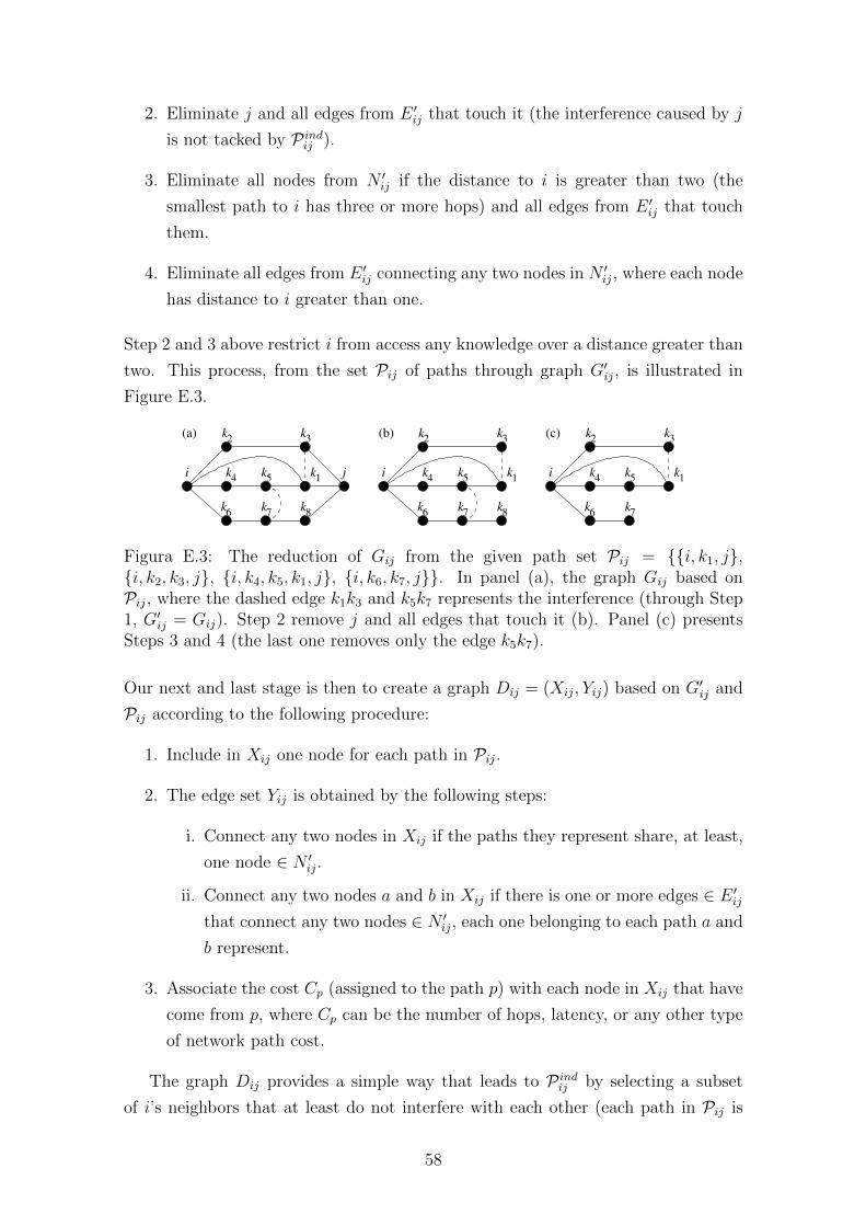
2. Eliminate j and all edges from E ′ij that touch it (the interference caused by j

is not tacked by P indij ).

3. Eliminate all nodes from N ′ij if the distance to i is greater than two (the

smallest path to i has three or more hops) and all edges from E ′ij that touch

them.

4. Eliminate all edges from E ′ij connecting any two nodes in N ′ij, where each node

has distance to i greater than one.

Step 2 and 3 above restrict i from access any knowledge over a distance greater than

two. This process, from the set Pij of paths through graph G′ij, is illustrated in

Figure E.3.

(b)

5k4

k2

k3

k1

k76

k

k5

k4

k2

k3

k1

k76

k k8

k8

k1

k5

k4

k2

k3

k76

k

i

(c)

i j

(a)

ik

Figura E.3: The reduction of Gij from the given path set Pij = {{i, k1, j},{i, k2, k3, j}, {i, k4, k5, k1, j}, {i, k6, k7, j}}. In panel (a), the graph Gij based onPij, where the dashed edge k1k3 and k5k7 represents the interference (through Step1, G′ij = Gij). Step 2 remove j and all edges that touch it (b). Panel (c) presentsSteps 3 and 4 (the last one removes only the edge k5k7).

Our next and last stage is then to create a graph Dij = (Xij, Yij) based on G′ij and

Pij according to the following procedure:

1. Include in Xij one node for each path in Pij.

2. The edge set Yij is obtained by the following steps:

i. Connect any two nodes in Xij if the paths they represent share, at least,

one node ∈ N ′ij.

ii. Connect any two nodes a and b in Xij if there is one or more edges ∈ E ′ijthat connect any two nodes ∈ N ′ij, each one belonging to each path a and

b represent.

3. Associate the cost Cp (assigned to the path p) with each node in Xij that have

come from p, where Cp can be the number of hops, latency, or any other type

of network path cost.

The graph Dij provides a simple way that leads to P indij by selecting a subset

of i’s neighbors that at least do not interfere with each other (each path in Pij is

58

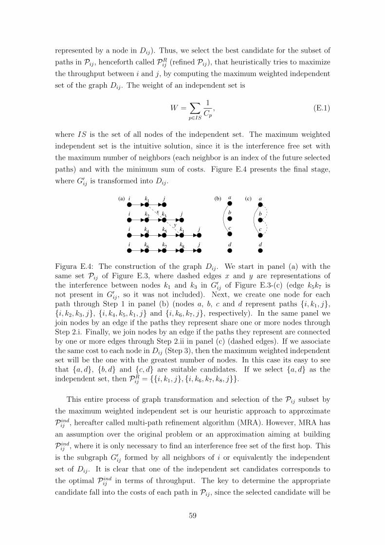
represented by a node in Dij). Thus, we select the best candidate for the subset of

paths in Pij, henceforth called PRij (refined Pij), that heuristically tries to maximize

the throughput between i and j, by computing the maximum weighted independent

set of the graph Dij. The weight of an independent set is

W =∑p∈IS

1

Cp

, (E.1)

where IS is the set of all nodes of the independent set. The maximum weighted

independent set is the intuitive solution, since it is the interference free set with

the maximum number of neighbors (each neighbor is an index of the future selected

paths) and with the minimum sum of costs. Figure E.4 presents the final stage,

where G′ij is transformed into Dij.

j

(b) a

b

c

d

(c) a

b

c

d

k1

k2

k1

k76

k

k4

k5

k3

k8

j

j

i

i

i

i

x

(a)

jy

Figura E.4: The construction of the graph Dij. We start in panel (a) with thesame set Pij of Figure E.3, where dashed edges x and y are representations ofthe interference between nodes k1 and k3 in G′ij of Figure E.3-(c) (edge k5k7 isnot present in G′ij, so it was not included). Next, we create one node for eachpath through Step 1 in panel (b) (nodes a, b, c and d represent paths {i, k1, j},{i, k2, k3, j}, {i, k4, k5, k1, j} and {i, k6, k7, j}, respectively). In the same panel wejoin nodes by an edge if the paths they represent share one or more nodes throughStep 2.i. Finally, we join nodes by an edge if the paths they represent are connectedby one or more edges through Step 2.ii in panel (c) (dashed edges). If we associatethe same cost to each node in Dij (Step 3), then the maximum weighted independentset will be the one with the greatest number of nodes. In this case its easy to seethat {a, d}, {b, d} and {c, d} are suitable candidates. If we select {a, d} as theindependent set, then PR

ij = {{i, k1, j}, {i, k6, k7, k8, j}}.

This entire process of graph transformation and selection of the Pij subset by

the maximum weighted independent set is our heuristic approach to approximate

P indij , hereafter called multi-path refinement algorithm (MRA). However, MRA has

an assumption over the original problem or an approximation aiming at building

P indij , where it is only necessary to find an interference free set of the first hop. This

is the subgraph G′ij formed by all neighbors of i or equivalently the independent

set of Dij. It is clear that one of the independent set candidates corresponds to

the optimal P indij in terms of throughput. The key to determine the appropriate

candidate fall into the costs of each path in Pij, since the selected candidate will be

59

that one with the maximum weight.

Until now we have used only a pair of nodes to describe our algorithm. To

work with an entire wireless network, it is sufficient to apply MRA on all possible

or desirable pairs. Moreover, brought from its simplicity, only a few modifications

have to be made in the majority of multi-path routing algorithms proposed in the

literature. To do so, first i should have one Pij for each possible j destination as

part of its a routing table (or any information that distinguishes multiple paths

such as the two first hops nodes). Next, to obtain the distance 2 knowledge (the

second hop), i requests to each neighbor k to sends its routing table, then only

neighborhood information is used. If k belongs only to one path and it is the

destination, i may discard k’s table or do not request it. Thus, node i builds G′ij

according to the routing tables where j is the destination of the entries. Finally,

i transforms Gij into Dij (according to the process describe earlier) and selects

paths based on the maximum weighted independent set of Dij. Indeed, the routing

algorithms must provide costs for paths and provide multiple paths for at least some

origin-destination pairs of nodes in the network. In the special case of single-path

routing algorithms, we present next simple modification to transform them into a

multi-path version, but before proceeding we tackle another special case. The one is

when Pij contains the single-link path that connects i directly to j. In this case, we

let PRij be the singleton that contains only that path. It is easy to see that we cannot

improve the throughput over the single direct link to the destination by including

other paths, no matter how many interference free paths Pij has.

E.3 Selecting paths in the absence of multiple

routes

In the particular case of the single-path routing algorithms every node i has only one

path to each destination of the network, then Pij = P1. To overcome this restriction,

node i has to request the path set of all its neighbors (the same procedure of the

multi-path routing case). However, i builds G′ij considering only paths given by its

neighbors whose costs are equal or inferior to the cost of the single path i has to j

(for this reason i acquires only loop-free paths). Note that, the original single path

i has to j will be mandatorily passed by one of its neighbors, so i does not need to

consider it for the construction of G′ij.

The following, then, is how we formulate the single-path routing case on Gij.

Given an origin-destination pairs of nodes i,j the new path set Pij, will be cons-

tituted by the single paths from all i neighbors suitably prefixed by the new ori-

gin i, where their costs are less than or equal to Cij (cost from i to j), that is,

60

Pij =⋃

k∈{i neighborhood}Px, where

Px =

Pkj prefixed by i, if Ckj ≤ Cij;

{} otherwise.(E.2)

Now, Pij is a multi-path set and we shall proceeds likewise the multi-path case as

explained previously.

61

Apendice F

MRA experimentation

We evaluated the throughput of the path sets through extensive experimentation

of the following routing algorithms: AODV [19], AOMDV [20], OLSR [21] and

MP-OLSR [22]. For conciseness purposes, we denominated R-AODV, R-AOMDV,

R-OLSR and R-MP-OLSR as the new pool of refined algorithms obtained after the

application of MRA over the path sets of the original routing algorithms. Note that,

we applied the procedure of Section E.3 to transform AODV and OLSR into multi-

path versions as previous discussed. Our experiments were executed in the network

simulator NS2.34 (NS2) [24] and in a simulator that employs SERA link scheduling

algorithm [11], introduced in Section C.1. We used two different configuration sets of

the routing algorithm parameters to compare how them affect the throughput, and

likewise two different configurations of NS2 parameters (one for the path discovery

process and another for the performance evaluation). These configurations were

selected by a wide variation of parameters in the tuning experiments, but before

we present them, we shall note that we used the same network topologies used in

the experiments for SER and SERA (see Section D.1). These network topologies

eventually leaded to the graph Dij.

F.1 Path discovery

For each one of the 1600 networks we generated 100 sets of n random origin-

destination pair of nodes, where each node appears only once as an origin in a

set. Each set of node pairs originates an instance of the path set P discovered by an

original routing algorithm. These path sets were posteriorly used in the experiments

of the originals. In terms of our notation, we can define this path set as

P =⋃

ij∈OD

Pij, (F.1)

62

where OD is the set of n random origin-destination pairs of nodes.

In the experiments of the refined algorithms, every P was refined to the corres-

ponding set PR by the application of MRA on each origin-destination pair of nodes

∈ OD (as explained in the beginning of Section E.2 for multi-routing algorithms

and in Section E.3 for single-routing ones), therefore

PR =⋃

ij∈OD

PRij . (F.2)

In a practical way, we construct P by letting the routing algorithm to build the

routing table of each node and by uniting these tables to produce a single path set,

thus we cover all possible combinations of origin-destination pair of nodes. For that,

we load a network topology into NS2, and we start a simulation of 15 seconds with

one flow agent for one of the possible origin-destination combinations (a CBR with

packets of 1000 bytes generated every one second). Next, we start a wiped clean

new simulation and do the same for another different origin-destination combination

until we cover all possibilities. This procedure minimizes the packet loss due to path

overload problems and it avoids that a previously discovered path interferes with

the discovery of a new one. For example, if a node k is the first to reply a path

request from i to an already known destination j, i will use k’s path even if the

optimum path passes through another node. This argument is only valid for on-

demand routing algorithms (AODV and its variations depend on the network load),

due to the fact of the paths found by OLSR algorithms are identical for the same

network topology. Another advantage is that we obtain always the same path set,

which makes the experiments reliable and reproducible.

The NS2 was used with the default configuration, however we employed the

DRAND protocol [55] to avoid collision in the path discovery process (macType pa-

rameter). To adjust the communication radius R, we also configured the parameter

RXThresh (RXT) with the appropriate value given by the program threshold.cc (see

NS2 manual). We used the implementation of AODV, OLSR and AOMDV routing

agents available in the version 2.34 of the NS2, and the MP-OLSR routing agent

available at [56]. For AOMDV, we made a small modification proposed by [57] to

discover only node disjoint paths with at most K paths for each origin-destination

pair of nodes. We adopted these modifications, since node disjoint paths are clearly

more interference free. We chose K = 5 because it achieved the best throughput

values for 2 ≤ K ≤ 7. The same modifications were made on MP-OLSR (proposed

by [58]) with the same K’s range for the same reason, but K = 3 and K = 5 where

adopted for ∆ ∈ {4, 8} and ∆ ∈ {16, 32} instead.

63

F.2 Performance evaluation

In general, we wish to evaluate the throughput of Ps against the corresponding

PRs according to the size of OD under a heavy traffic network. To see how the

number of paths affects the performance of MRA, we varied the size of OD from 1

to n (vary the size of OD is a simple matter of randomly remove an element from

it until |OD| = 1). We use node weights of Dij such that, Cp is the path’s hop

count. Clearly, though, any other desired metric can be used as well. Since P and

a random set of node pairs in OD have been build for a network, we loaded the

corresponded topology into NS2 and adjusted RXT accordingly. We configured the

macType parameter to 802.11 and the routing agent to NOAH [59] (adhocRouting

parameter). NOAH works only with fixed routes and do not send routing related

packets, so we evaluated only P without the interference of control packets. Next,

we started a CBR from each origin-destination pair of nodes in P and measured

the amount of successfully arrived packets during 120 of 135 seconds of simulation

(the first 15 seconds were used to assure that NS2 had warmed-up properly all CBR

agents).

Before the execution of the performance experiments, we executed a large set

of tuning experiments to choose the best configuration of NS2 parameters. We va-

ried widely three NS2 parameters: the carrier sense threshold (CST) to increase the

spatial re-use and consequently to increase the throughput [60] (802.11 CSThresh -

parameter), the CBR parameter and the network transmissions rates to obtain the

maximum throughput and the maximum fairness possible (802.11 dataRate and ba-

sicRate parameters). Table F.1 presents the first stage of the tuning experiments,

where the CBR interval was varied to find the highest rate without gain of th-

roughput (CBR1) and the lowest rate without gain of fairness (CBR2) 1. Table F.2

presents the values used in the performance experiments chose from the best results

of the tuning experiments. For the sake of normalization, the results we present

for the refined and original algorithms in the performance experiments, given for

|OD| = 1, 2, . . . , n, are shown against the ratio θ = |OD|/n ∈ (0, 1].

Tabela F.1: Different parameters used in our tuning experiments.NS2 parameter variation incrementCBR interval 0.001s .. 0.005s 0.0001

CST 0.1RXT .. 2RXT 0.1RXTdata/basic rate 1/1,2/1,11/2 Mbps

The experiments with the NS2 evaluated the refined and original algorithms un-

der the 802.11, a CSMA protocol. As a second evaluation method, we chose SERA

1We observed that when we varied the CBR rate NS2 parameter, it tends to influence somewhatinversely the fairness and directly the throughput in all simulations with NS2.

64

Tabela F.2: Parameters adopted in the performance experiments.NS2 parameter ∆

4 8 16 32CBR1 interval 0.0025s 0.0027s 0.0029s 0.0031sCBR2 interval 0.0045s

CBR packet size 1000bCST 0.6RXT 0.7RXT 0.8RXT 0.9RXT

data/basic rate 11/2 Mbps

that gives a link schedule under some TDMA protocol to provide a background of

synchronized time slots [61]. We configured SERA with parameters ND-BF numbe-

ring scheme and B = 2. Even though SERA is a link scheduling algorithm, it seeks

to schedule a set of routes’ links to maximize the number of packets delivered to

their destinations. If we calculate the throughput of the resulting schedule, then we

can naturally extract the number of packets arriving in the path destinations during

a schedule cycle (exactly our evaluation objective). Now, to obtain the throughput

we have to compute the time slot size of the experiments under NS2 simulations. For

that, we considered a network composed by only two neighbor nodes and calculated

the number of seconds necessary to send a packet from one node to the other (this

is exactly the definition of SERA time slot). The value found was 0.002 seconds for

the simulations configured with the parameters showed in Table F.2.

F.3 Computational results

We divide our results into two categories. First we present a statistical analysis

of the networks generated and the path sets obtained by the refined and original

routing algorithms. Then, we give the ratio of the refined algorithms’ throughput

to the throughput of their originals (absolute values are presented in Figures 1, 2

and 3 of the supplementary data file 1). For conciseness purposes, we report only

the results for n = 120, since the results of the other network sizes shared great

qualitative similarities with n = 120 results (quantitative differences are discussed

in Section F.4).

F.3.1 Properties of the networks generated

We generated many different network topologies including some close to rings, stars

and grids among the 1600 network instances. Such variety of networks helped us to

analyze how the network density affects the results of MRA over the original routing

algorithms. The few statistics we present here also helped to explain what is observed

in relation to the throughput values obtained. For more statistical details, such as

65

topologies’ examples and the networks’ distributions of node degrees, see Section

D.3.1.

The average number of multiple paths of P and PR given in Table F.3 was sum-

marized over 104 path sets (100 networks × 100 sets of random origin-destination

pair of nodes) produced by each routing algorithm for every combination of n, ∆

and |OD|. MP-OLSR is absent in this table, because the K parameter is not an

upper bound like in AOMDV algorithm, but rather as the fixed value for the num-

ber of multiple paths to be found. We observe from the table that the average

number of multiple paths increases monotonically with ∆, which is expected from

the well known fact that the number of possible multiple paths grows with ∆ in

arbitrary graphs [62]. But, the average does not vary significantly across the values

of |OD|. This is maybe due to the path discovery process we applied. It handles

origin-destination pair of nodes separately, so the discovery of a path set cannot

be influenced by path sets previously discovered. We also observed that the refi-

ned algorithms have always lower average values than the original multi-path ones,

which indicates that MRA decreased the number of multiple paths due to the high

interference on the neighborhood of each node.

Tabela F.3: Average number of multiple paths per origin-destination pair of nodes,where n = 120 for 104 path sets corresponding to each combination of n, ∆ and|OD|.

∆ |OD| R-AODV AOMDV R-AOMDV R-OLSR R-MP-OLSR4 1 .. 10 1.5 3.3 1.7 1.4 1.5

11 .. 90 1.5 3.4 1.8 1.5 1.691 .. 120 1.6 3.4 1.8 1.5 1.6

8 1 .. 10 1.6 3.6 1.9 1.6 1.711 .. 20 1.7 3.6 2.1 1.6 1.721 .. 70 1.7 3.7 2.1 1.6 1.771 .. 80 1.7 3.7 2.1 1.6 1.8

81 .. 120 1.7 3.7 2.2 1.6 1.816 1 .. 10 2 3.9 2.9 2 2

11 .. 50 2.1 3.9 2.9 2 251 .. 90 2.1 4 3 2.1 2

91 .. 120 2.1 4 3 2.1 2.132 1 .. 10 2.2 4.1 3.1 2.2 2.2

11 .. 60 2.2 4.1 3.1 2.2 2.361 .. 70 2.3 4.2 3.2 2.2 2.471 .. 80 2.3 4.2 3.2 2.2 2.581 .. 90 2.3 4.2 3.2 2.2 2.6

91 .. 120 2.3 4.2 3.2 2.3 2.7

Figures F.1 and F.2 show the networks’ path size distribution, respectively for the

refined routing algorithms and their originals, again over 104 path sets for |OD| = n

66

and n = 120. Analyzing sequentially the four panels given for each one of these

figures (one panel for each fixed value of ∆), we see that the path size of the distri-

butions’ peak value decreases as ∆ grows for all routing algorithms. This behavior

was anticipated, since the average number of neighbors is related with the size of

paths in a graph [63]. Another expected result is that, OLSR and its variants have

longest paths than AODVs, because the multi-point relay concept of OLSR (MPR)

tends to enlarge paths more than the shortest path algorithm (SPA) used by AODV.

It is also noteworthy that the application of MRA did not change the distributions.

Figura F.1: Original algorithms’ path size histogram with n = 120 for ∆ = 4 (a),∆ = 8 (b), ∆ = 16 (c), and ∆ = 32 (d). For each value of ∆ the distributionrefers to 100 networks and 100 path sets per network, each corresponding to norigin-destination pairs.

67

Figura F.2: Refined algorithms’ path size histogram with n = 120 for ∆ = 4 (a),∆ = 8 (b), ∆ = 16 (c), and ∆ = 32 (d). For each value of ∆ the distributionrefers to 100 networks and 100 path sets per network, each corresponding to norigin-destination pairs.

68

F.3.2 Results

Our computational results are summarized in Figures F.3, F.4 respectively for NS2

with CBR1 and CBR2 (see Table F.2), and in Figure F.5 for SERA. Each figure

is organized as a set of four panels, like in Figures F.1 and F.2, representing ∆ in

the non-decreasing order of its fixed values. Each panel shows a plot of θ against

the ratio of the refined algorithm throughput to the original throughput (σ). We

included a highlighted horizontal line in each plot for σ = 1 to highlight when a

refined algorithm overtakes its original.

Figure F.3 shows a set of plots with the same structures of panels representing

different values of ∆, but now displaying our results for the routing algorithms

with CBR1. Recall that, as mentioned in Section F.2, CBR1 is the rate where

the throughput of some paths was sacrificed in order to increase the sum of all path

throughputs in the CSMA based network. For a minority of values observed, we see a

transient stage in all plots when θ < 0.1. This indicates that some properties related

to the throughput vary greatly in these small path sets, such as the average path

size and the mutual interference. Moving between panels from ∆ = 4 to ∆ = 32,

we see also that σ slowly decreases as ∆ grows and that σ is almost constant when

θ > 0.5 for any algorithm and value of ∆. Figure F.4, on the other hand, shows

not very constant σ values, thereby establishing that the network load produced by

CBR2 is too low for MRA constantly improve it (the mutual interference is not the

core problem in these experiments), even though MRA improved nearly all path

sets.

It seems clear from Figure F.5 that, MRA successfully improved all routing

algorithms in a network regulated by a TDMA protocol. This is not valid for a

minority of values observed when θ < 0.1, where we observe again the transient

stage in all plots. When θ ≥ 0.1, there are also a minority of AOMDV σ values, in

which part of their confidence intervals is under the threshold line (four of twenty-

tree values of R-AOMDV/AOMDV for ∆ = 32). When 0.1 ≤ θ ≤ 1, it is worth

to observe that all plots have an oscillation behavior, what is not unexpected from

ratios (not absolute values). Even so, the widest variation is no greater than 0.16

(OLSR σ values for ∆ = 16, between θ = 0.8 and θ = 1.5). Furthermore, if we

compare the plots of each algorithm separately, then we observe different behaviors

depending on the algorithm, but σ not vary substantially while changing from one

panel to the next. The greater difference between two panels is 0.2% (OLSR σ values

for θ = 1, between ∆ = 4 and ∆ = 16), again out of the transient stage.

As we remarked earlier, MRA proved to increase the path set throughput of all

routing algorithms, but this proves nothing about an important performance crite-

rion, not always related to the throughput. The criterion we now shortly describe,

69

known as fairness index [23], is neither a qualitative measure so common in the

literature nor a quantitative value designed to some specific cases. Instead, it looks

how efficiently is the use of paths to deliver packets by simply measuring the ratio

(∑P ′′

p xp)2/P ′′

∑P ′′

p (xp)2, where xp is the number of packets delivered by the path p

and P ′′ is the number of paths (in our experiments P ′′ = |P| or P ′′ = |PR|, depen-

ding on the experiment). The influence of MRA and the types of algorithms tested

over the fairness index is showed in Figures F.6, F.7 and F.8 for the experiments

with CBR1, CBR2 and SERA, respectively.

In these figures, R-OLSR and R-AODV (R-AODV, R-OLSR) had a statistical

indistinguishable fairness index, even for CBR1. However, we expected that in a

heavily loaded network, AODV and OLSR based algorithms had very different values

due to SPA and MPR strategies. The same result was also obtained for AODV and

OLSR (AODV, OLSR). For each panel presented, the fairness index decreases as

θ grows, independent of the protocol (SERA, CBR1 or CBR2), which is expected

that larger sets (greater θs) are more likely to unbalance packet flows than smaller

ones. Therefore, we can safely assume that the fairness index is affected by the

path set size. Moreover, if we compute the fairness index from all paths having the

same origin and destination by considering them as a single path (origin-destination

fairness index), then we observe the same behavior, although the fairness index is

significantly greater. AODV and OLSR are exceptions because they are single-path

routing algorithms. An example is shown in Figure 4 of the supplementary data file

1 for the origin-destination fairness index with SERA.

As we fix ∆ and θ, Figures F.6, F.7, F.8 revel that SERA has higher fairness index

than the others due to the nature of its scheduling mechanism. This mechanism will

never let a path suffer to unbounded packet accumulation or absence of packets.

Next, we observe that single-path routing algorithms have the best fairness indexes,

since they have at least 50% less paths than the others for the same θ value. However,

it is important to note that MRA improved the fairness of all multi-path routing

algorithms. It is also interesting to note that, by comparing these figures with

Figures F.3 to F.4 some times the fairness index even varies inversely with the

throughput.

70

Figura F.3: Ratio σ for 802.11 with CBR1 where n = 120 for ∆ = 4 (a), ∆ = 8(b), ∆ = 16 (c), and ∆ = 32 (d). Data are averages over the 104 path sets thatcorrespond to each value of ∆ for each value of θ. Error bars were omitted, sincethey are less than 1% of the mean for confidence intervals at the 95% level.

71

Figura F.4: Ratio σ for 802.11 with CBR2 where n = 120 for ∆ = 4 (a), ∆ = 8(b), ∆ = 16 (c), and ∆ = 32 (d). Data are averages over the 104 path sets thatcorrespond to each value of ∆ for each value of θ. Error bars were omitted, sincethey are less than 1% of the mean for confidence intervals at the 95% level.

72

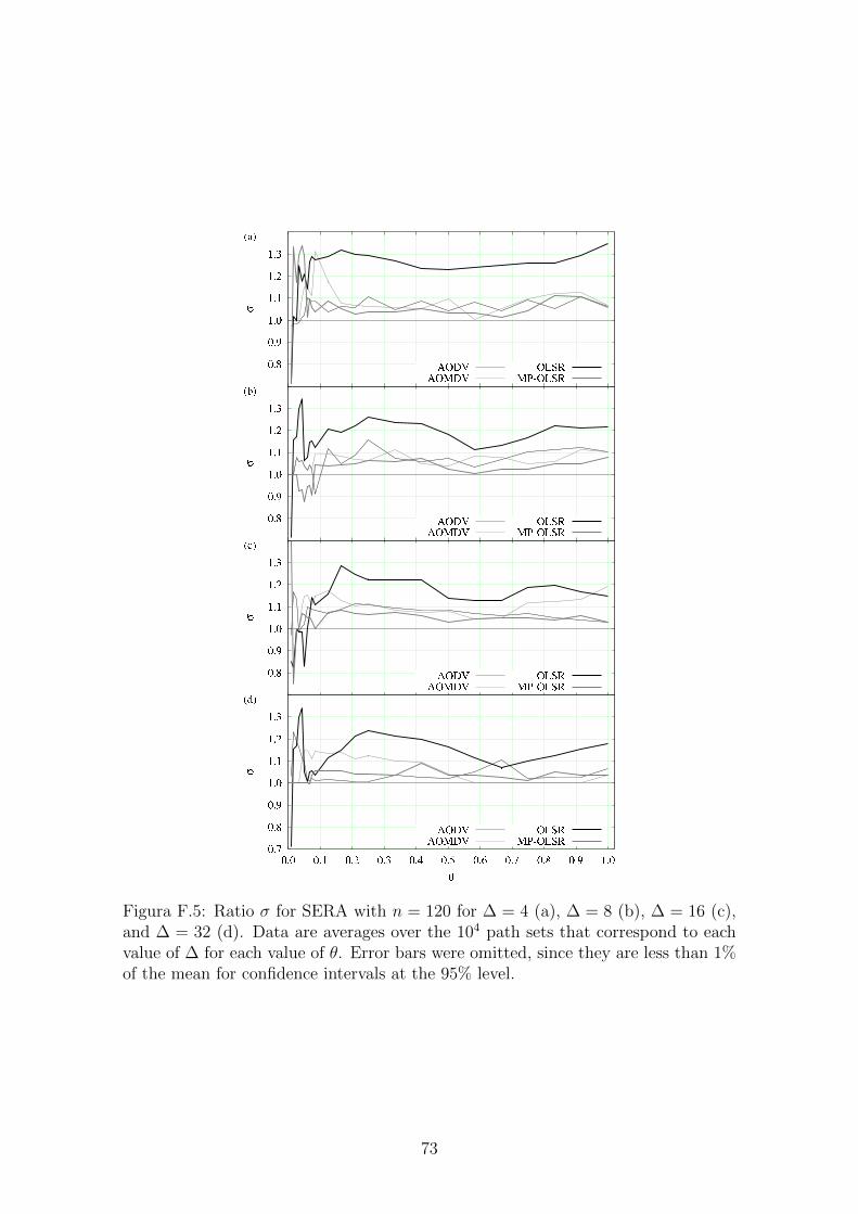
Figura F.5: Ratio σ for SERA with n = 120 for ∆ = 4 (a), ∆ = 8 (b), ∆ = 16 (c),and ∆ = 32 (d). Data are averages over the 104 path sets that correspond to eachvalue of ∆ for each value of θ. Error bars were omitted, since they are less than 1%of the mean for confidence intervals at the 95% level.

73

Figura F.6: The fairness index for 802.11 with CBR1 where n = 120 for ∆ = 4 (a),∆ = 8 (b), ∆ = 16 (c), and ∆ = 32 (d). Data are averages over the 104 path setsthat correspond to each value of ∆ for each value of θ. Error bars were omitted,since they are less than 1% of the mean for confidence intervals at the 95% level.

74

Figura F.7: The fairness index for 802.11 with CBR2 where n = 120 for ∆ = 4 (a),∆ = 8 (b), ∆ = 16 (c), and ∆ = 32 (d). Data are averages over the 104 path setsthat correspond to each value of ∆ for each value of θ. Error bars were omitted,since they are less than 1% of the mean for confidence intervals at the 95% level.

75

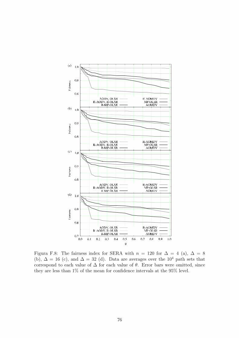
Figura F.8: The fairness index for SERA with n = 120 for ∆ = 4 (a), ∆ = 8(b), ∆ = 16 (c), and ∆ = 32 (d). Data are averages over the 104 path sets thatcorrespond to each value of ∆ for each value of θ. Error bars were omitted, sincethey are less than 1% of the mean for confidence intervals at the 95% level.

76

F.4 Discussion

As we briefly discussed before, the absence of the results for n ∈ {60, 80, 100}are justified due to the behavior of MRA (relatively independent from n) and the

excessive amount of figures produced by the results. In such instances, those results

where n = 60 can be seen, for example, as a sub-section of n = 120 results. More

precisely, if we crop all plots of the Figure F.3 at θ = 0.5, then we would see no

difference in the order of the plots (first OLSR followed by AOMDV, next AODV

and at last MP-OLSR), but σ values for n = 60 are greater than those for n = 120.

This stems not only from the fact that the average path size decreases as n decreases,

but more generally from the fact that the number of links for the same θ is lower

for the networks where n = 60 than for those where n = 120 (less links to interfere

and less to be schedule). Thus, the improvement obtained by MRA seems to be

influenced not only by the network density (∆) and θ, but also by the network path

size distribution.

For the fairness index, the results for n ∈ {60, 80, 100} were not included for

the same reasons. As σ, it slowly decreases as n grows, but we cannot confirm this

relation because the differences are not significative for some routing algorithms.

The fairness index also decreases as ∆ grows, which suggests that the behavior of

the fairness index depends more on other factors, such as the network load and the

path size distribution.

Although investigating the performance issues of the routing algorithms is not

our objective, the implicit ranking among them is interesting to discuss (see Figures

F.3 to F.8). Considering that OLSR and MP-OLSR were the most advantageous

to be refined under heavy loaded network scenarios (SERA and CBR1), we observe

that they have less multiple paths than the others and more longer paths than the

others (see Table F.3). To see that this is so, first recall that OLSR longer paths are a

direct consequence of MPR and the number of multiple paths of a node is somewhat

inversely related to the interference level of its neighborhood, as we briefly discussed

in Section F.3.1. So, R-OLSR and R-MP-OLSR have better results because MRA

and the MRPs. MRA selects less multiple paths than available, thus it decreases the

mutual interference in the neighborhood of each node. MPRs guarantees the spacial

separation necessary to avoid that paths interfere with each other in the middle-way

to their destinations. Moreover, we suspect that AODVs have paths spatially closer

due to SPA and consequently with more mutual interference than OLSRs (MPR

forces the discovery of more isolated paths) [64, 65]. It is also curios to observe

another ranking (see Figures 5, 6 and 7 of the supplementary data file 1), in which

all routing algorithms achieved better throughput results with SERA (a TDMA

protocol) than with CBR1 (a CSMA protocol). The same is true for the fairness

77

index when SERA is compared to CBR2. This may be, in principle, a manifestation

of SERA advantages rather than of the superiority of TDMA over CSMA protocols,

since a considerable amount of research directed toward the matter did not reach

an agreement [66–69].

Another curiosity, now regarding all NS2 simulations with the two configurati-

ons described in Section F.2 (CBR1 and CBR2), we detected that some paths had

transmitted no packets even if we extended the simulation time, reordered and re-

moved the synchronization of the multiple CBRs (common problems of NS2 agents).

We verified by executing another set experiments that 802.11 CSMA was discarding

some paths to increase the throughput of others. Figures 8 and 9 of the supplemen-

tary data file 1 shows the distributions of origin-destination pair whose paths did

not received packets. Obviously, the single-path routing algorithms had less paths

without packets than the multi-paths ones, however R-MP-OLSR and R-AOMDV

had less paths without packet than their originals (MRA attenuated the number of

paths without packets).

78

Apendice G

Conclusion

We now present our conclusions over the two methods we used for link scheduling

(discussed in Chapters B, C and D) and over the refinement method of multi-path

sets we introduced and discussed in Chapters E and F, respectively.

G.1 SER and SERA

Algorithms SER and SERA are methods for link scheduling in WMNs. As such, and

unlike other methods for link scheduling, they are built around a set of origin-to-

destination paths and aim to provide as much throughput on these paths as possible.

From a mathematical perspective they are both related to providing the nodes of a

graph with an efficient multicoloring, in the sense discussed in Section B.3. For SER

this is strictly true, but for SERA the defining characteristic of a multicoloring, that

each node receives the same number of colors, ceases to hold. As we demonstrated

through our computational results in Section D.3, it is precisely this deviation from

the strict definition that allows SERA to surpass SER in terms of performance.

The functioning of both SER and SERA is supported by the use of the integer

parameter B ≥ 1, which indicates how many buffering positions each WMN node

has to store in-transit packets for each of the paths that go through it. Choosing

B = 1 suffices for SER because of its inherent property of alternating interfering

transmissions, but B > 1 may in principle be needed for the advantages of SERA

to become manifest. In the simulations we conducted, however, only rarely has this

been the case, since on average increasing B beyond 1 provided no distinguishable

improvement. In this regard, we find it important for the reader to refer to Fi-

gure C.2 once again. As we remarked upon discussing that figure, profiting from a

B > 1 situation under SERA is largely a matter of how uniformly interference gets

distributed on the particular set of paths at hand. Our results in Section D.3, there-

fore, can safely be assumed to have stemmed from circumstances that, on average,

led to highly uniformly distributed interference patterns.

79

The centerpiece of both SER and SERA is the undirected graph G, which em-

bodies a representation of all the interference affecting the various wireless links

represented by the graph’s nodes. As we explained in Section B.2, the steps to

building G depend on how one assumes the communication and interference radii

to relate to each other, and also on which interference model is adopted. We have

given results for a specific set of assumptions, but clearly there is nothing in either

method precluding its use under any other assumptions, including for example those

of the physical interference model, which incidentally have been used recently in sol-

ving problems related to the one we have considered [70–72]. Whenever different

assumptions are in place, all that needs to be done is construct G accordingly.

Analyzing either method mathematically is a difficult enterprise, but since their

performance depends on the heuristic choice of an initial acyclic orientation of G, any

effort profitably spent in that direction will be welcome. In addition to potentially

better decisions regarding initial conditions, further mathematical knowledge on

SER or SERA may also come to provide a deeper understanding of how upper

bounds on T (S) relate to what is observed. As we mentioned in Section D.4, one

such bound is already known in the case of SER. Obtaining better bounds in this

case, as well as some bound in the case of SERA, remains open to further research.

Another issue that is open to further investigation is how to handle the potential

difficulties that SER may encounter in the face of a growing number of nodes in G

[73, 74]. These difficulties refer to the fact that, in the worst case, the time required

to detect the occurrence of the period may grow exponentially with the square root

of the number of nodes. They are inherited by SERA, since it generalizes SER,

and may require the development of further heuristics if they pose a real problem

in practice. In a related vein, sometimes it may be the case that only the value of

T (S) is needed, not S itself. Knowing the achievable throughput without requiring

knowledge of the schedule itself can be useful for evaluating WMN topologies or

routing algorithms for them.

Should this be the case, then it is possible to estimate T (S) more efficiently than

using the full-fledged algorithms we gave. We can do this in the case of SERA by

recognizing that T (S) is the limit, as t→∞, of

Tt(S) =

∑i∈T mi(ω0, t)

t+ 1, (G.1)

where mi(ω0, t) is the total number of times node i appears as a sink in orientations

ω0, ω1, . . . , ωt. To see this, let o(t) denote any function of t such that limt→∞ o(t)/t =

0. We then have∑

i∈T mi(ω0, t) = r(t)∑

i∈T mi(ω0)+o(t) and t+1 = r(t)p(ω0)+o(t),

where r(t) is the number of times the period has been repeated up to iteration t.

The limit follows easily, and automatically holds also for SER by straightforward

80

extension. The streamlined version of either algorithm consists simply of letting t

evolve either through a sufficiently large value determined beforehand or until Tt(S)

becomes stable. Any of the two alternatives does away with the need to detect the

occurrence of the period.

We also note, that we have found the results given in Figure D.5 to be practically

indistinguishable from those obtained through the strategy outlined above for the

computation of T (S). We have verified this by letting T (S) = Tt+(S), where t+

is the least value of t for which |Tt(S) − Tt−w(S)|/Tt−w(S) ≤ 0.001. Here w is a

window parameter and in our experiments we used w = |N |. As for this particular

choice, it comes from realizing that in both SER and SERA it takes at most |N |− 1

iterations for a node of G that is currently not a sink to become one. This, in turn,

comes from the fact that in each iteration either algorithm necessarily decreases

by 1 the number of edges on a longest directed path from any non-sink node to a

sink. We can see that this is true of SER by viewing its dynamics in terms of how

the orientations’ sink decompositions evolve. We can see that it continues to hold

in the case of SERA because SERA never places a former sink i into one of the

sink-decomposition sets that already contains a neighbor of i in G (cf. Figure C.3).

G.2 MRA

When MRA is used, it follows from its definition in Section E.2 that it builds a Pinf

approximation instead of the exact solution (recall that Pind is a Pinf under the as-

sumptions of the protocol interference model). This is due to the difficult enterprise

of implementing complex changes on any of the well established routing algorithms

without overload the network with more control messages. Moreover, the optimum

Pind involves the exact solution of NP-hard problems, as discussed in Section E.1.

Besides the simplicity of MRA solution, it was demonstrated by the distinguishable

improvements (throughput and fairness) obtained on the computational results that

MRA produces a good approximation of Pinf . For instance, OLSR throughput was

improved over 20% with SERA and over 15% with CBR1 (average values over all

experiments), and with superior fairness index than the original. Of course, this was

achieved in some part because MRA refined an already node disjoint path set (recall

that we used only the node disjoint version of the routing algorithms), but mostly

because the original routing algorithms do not take into account the interference

information like MRA.

Another important advantage of MRA is that even involving the NP-hard pro-

blem of the maximum weighted independent set, the average neighborhood size of a

wireless node is sufficient small to be computed in negligible time compared to arbi-

trary graphs [75]. This leads to an open issue that is how paths from different origins

81

and destinations affect themselves, since the exact solution of Pinf does not involve

the maximum weighted independent set of the network. Analyzing this involves un-

practical instances of this problem and moreover, we have to consider many aspects

such as which nodes really need multiple paths by considering the distribution of

the network load. Also, we have to consider how many multiple paths are necessary

for each node, based on the interference they might produce over the neighborhood.

These aspects are even more difficult to analyze due to the unknown relation among

them.

Another aspect open for further investigation is the benefits of joining multi-

radio network and MRA. In these schemes, orthogonal frequencies can drastically

reduce the number of D edges and increase the number of multiple paths free of

interference. MRA can be benefited of this variety and it can minimize the number

of radios, since it selects a subset of paths [76, 77].

We also remark that, our work depends in great part on the relationship that

exists among the variety of interference free paths and the network density, thus

the availability of these paths affects the results of MRA more than the size of the

network paths. Additionally, the mutual interference is caused by the proximity

among paths and not by the path sizes, hence the objective is to discover paths suf-

ficiently spatial separated to avoid interference, but not too far to loose throughput

from longer paths.

We note, finally, that joint SERA and MRA over some routing protocol (like

OLSR) is a intuitively step that we shall consider for a future work, and in addition

all open aspects discussed in this chapter.

82

Apendice H

Supplemental data file 1

83

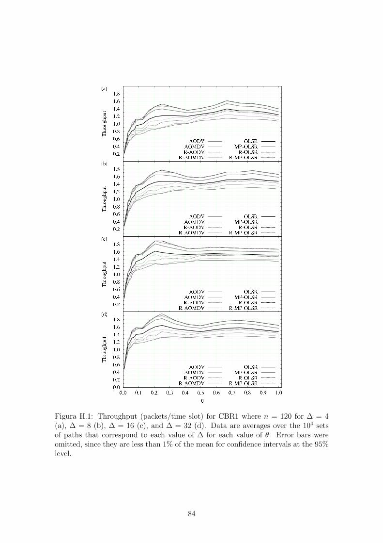
Figura H.1: Throughput (packets/time slot) for CBR1 where n = 120 for ∆ = 4(a), ∆ = 8 (b), ∆ = 16 (c), and ∆ = 32 (d). Data are averages over the 104 setsof paths that correspond to each value of ∆ for each value of θ. Error bars wereomitted, since they are less than 1% of the mean for confidence intervals at the 95%level.

84

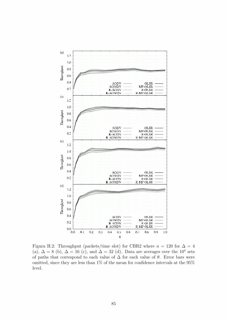
Figura H.2: Throughput (packets/time slot) for CBR2 where n = 120 for ∆ = 4(a), ∆ = 8 (b), ∆ = 16 (c), and ∆ = 32 (d). Data are averages over the 104 setsof paths that correspond to each value of ∆ for each value of θ. Error bars wereomitted, since they are less than 1% of the mean for confidence intervals at the 95%level.

85

Figura H.3: Throughput (packets/time slot) for SERA with n = 120 for ∆ = 4 (a),∆ = 8 (b), ∆ = 16 (c), and ∆ = 32 (d). Data are averages over the 104 sets ofpaths that correspond to each value of ∆ for each value of θ. Error bars are basedon confidence intervals at the 95% level.

86

Figura H.4: The origin-destination fairness index for SERA with n = 120 for ∆ = 4(a), ∆ = 8 (b), ∆ = 16 (c), and ∆ = 32 (d). Data are averages over the 104 setsof paths that correspond to each value of ∆ for each value of θ. Error bars wereomitted, since they are less than 1% of the mean for confidence intervals at the 95%level.

87

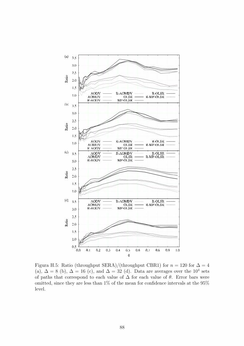
Figura H.5: Ratio (throughput SERA)/(throughput CBR1) for n = 120 for ∆ = 4(a), ∆ = 8 (b), ∆ = 16 (c), and ∆ = 32 (d). Data are averages over the 104 setsof paths that correspond to each value of ∆ for each value of θ. Error bars wereomitted, since they are less than 1% of the mean for confidence intervals at the 95%level.

88

Figura H.6: Ratio (throughput SERA)/(throughput CBR2) for n = 120 for ∆ = 4(a), ∆ = 8 (b), ∆ = 16 (c), and ∆ = 32 (d). Data are averages over the 104 setsof paths that correspond to each value of ∆ for each value of θ. Error bars wereomitted, since they are less than 1% of the mean for confidence intervals at the 95%level.

89

Figura H.7: Ratio (throughput CBR1)/(throughput CBR2) for n = 120 for ∆ = 4(a), ∆ = 8 (b), ∆ = 16 (c), and ∆ = 32 (d). Data are averages over the 104 setsof paths that correspond to each value of ∆ for each value of θ. Error bars wereomitted, since they are less than 1% of the mean for confidence intervals at the 95%level.

90

Figura H.8: Paths without packets histogram for CBR1 where n = 120 for ∆ = 4(a), ∆ = 8 (b), ∆ = 16 (c), and ∆ = 32 (d). Data are averages over the 104 sets ofpaths that correspond to each value of ∆.

91

Figura H.9: Paths without packets histogram for CBR2 where n = 120 for ∆ = 4(a), ∆ = 8 (b), ∆ = 16 (c), and ∆ = 32 (d). Data are averages over the 104 sets ofpaths that correspond to each value of ∆.

92

Apendice I

Resume etendu

Dans cette these, nous avons aborde deux problemes de reseau sans fil, les deux liesa l’interference provoque par les transmissions de radio. Le premier probleme est liea l’interference entre les liens du reseau provoques par l’activation de ces liens. Pourattenue ce probleme, nous avons adopte une solution commune. Nous assumonsun protocole TDMA [10] et nous heuristiquement ordonnancons les transmissionssimultanees qui sont actives si elles ne s’interferent pas. Ensuite, nous presentonsune petite introduction de ce probleme. Il convient de noter que ce resume nesubstitue pas la these, alors la lecture de la these est obligatoire pour evaluer letravail.

En raison de leurs nombreux avantages, les reseaux mailles sans fil (WMNs)constituent une solution prometteuse pour les reseaux communautaires et ils puis-sent fournir des connexions du dernier kilometre pour les utilisateurs de l’Internetlocalises en regions tres isolats [1, 3, 5]. Par contre, comme tous les reseaux sansfil, WMNs souffrent du probleme, sur lequel la capacite diminue a mesure qu’ilsdeviennent plus denses, puisque dans ce cas transmettre simultanement augmentel’interference de maniere significative [2, 4]. Une solution commune pour reduire lesinterferences consiste a adopter un protocole TDMA [10] et de ordonnancer les ac-tivation des transmissions simultanees pour qu’elles ne s’interferent pas. Faire cela,tout en maximisant une certaine mesure de l’utilisation du reseau et de garantir quetous les liens soient equitablement traites est un probleme d’optimisation complexe,qui est malheureusement NP-difficile [26].

Ce probleme d’ordonnancement a ete formule dans une grande variete demanieres et il a recu une attention considerable dans la litterature. Parmi les plusnotables etudes figurent certains qui cherchent a calculer la capacite du reseau [4, 27],d’autres dont le but est l’etude de la complexite de temps associe a des ordonnancesresultants [28], et d’autres encore qui visent a l’ordonnancement de transmissions afind’augmenter la capacite du reseau au maximum possible [29–37]. Un denominateurcommun a travers de la majorite des travails cites anterieurement, c’est que, apresavoir adopte une representation graphe du reseau et de la facon dont les diversestransmissions peuvent interferer avec l’autre, une solution est recherchee une cer-taine forme de coloration de graphe. Plus souvent qu’autrement, les transmissionsa ordonnances sont representees par des noeuds du graphe, puis a colorier noeud atravers de l’abstraction d’un ensemble independant pour representer les transmissi-

93

ons qui peuvent etre actives simultanement. Mais, c’est parfois les arcs du graphequi representent les transmissions, dans lequel la coloration des arcs est utilisee, ens’appuyant sur l’abstraction de couplages pour representer la simultaneite [38].

Ici, nous considerons une variation du probleme qui, a notre connaissance, estnouvelle sur le point de vue de sa formulation et sur le type de solution que nousproposons. Nous commencons par l’assomption d’une WMN comprenant un seulcanal avec noeuds mono-radios et pour lesquels un ensemble de routes a deja etedetermine, et en considerant la question suivante. Devrait-il y avoir une source in-fini de paquets au niveau de chaque origine de route a etre livre a la destinationcorrespondante dans l’ordre PEPS, et devrait tous les noeuds du reseau soit doted’un nombre fini de tampons pour le stockage temporaire des paquets en transit,comment peut maximiser la delivrance de paquets aux destinations par chaque in-tervalle de temps du TDMA sans jamais annuler ou arreter une transmission, parl’absence de espace aux tampons?

Cette question est au coeur de la conception et du succes des WMNs et leursprotocoles de routage, puisque elle vise attaquer le probleme de l’interference destransmissions lorsque le reseau est surcharge. La solution que nous proposons est,comme dans la plupart des approches mentionnees ci-dessus, basee sur la colorationdes noeuds d’un graphe. Contrairement a eux, nous utilisons noeuds avec multiplecolorations [39], qui sont plus generales et pour cette raison notre solution permettreune formulation plus appropriee du probleme d’optimisation a resoudre.

Notre proposition ai ete publie en [11] et elle est presentee de la forme sui-vante. A partir des routes origine-destination (ou chemins) a etre utilises, nouscommencons avec une definition precise de l’ordonnancement et une formulationprecise du probleme (Chapitre B). Nous montrons aussi, a travers d’un exemple,que la forme classique de maximiser la capacite du reseaux cause un conflit avecl’exigence de tampons avec espace finit (voir la Figure I.1). Ensuite, nous passonsa la specification du graphe non oriente qui sous-tend le fonctionnement de notrealgorithme (voir l’Algorithme SERA, les Figures I.2, I.3 et le Chapitre C). Une hy-pothese que nous assumons dans la plupart de notre travail, c’est que la distancede communication et d’interference sont les memes pour la WMN. Aussi, nous as-sumons egalement les principes du modele d’interference basee sur le modele parprotocole [12, 13] avec la possibilite de communication bi-directionnelle dans chaquetransmission. Ensuite, nous guidons le lecteur a travers des possibilites de multiplescolorations, qui culmine avec une methode preliminaire pour l’ordonnancer, emprun-ter au domaine du partage des ressources publie en [14]. Enfin, nous presentons notreproposition qui a ameliore ce methode preliminaire (Session C.1). Cette proposi-tion, essentiellement, provient d’un leger assouplissement de la notion de multiplescolorations en noeuds. Les deux sections suivantes sont consacrees a la presentationdes resultats de calcul, avec la methodologie et les resultats prevus, ou nous prou-vons que notre algorithme a ete victorieu en tous le cas (voir les Figures I.4, I.5 etChapitre D). Une discussion suit et nous concluons la premier parti de la these dansles deniers sections (Session D.4 et Chapitre G, respectivement).

Dans le deuxieme probleme, nous traitons la meme interference entre le lien,mais du point de vue des routes du reseau. Ensuite, nous presentons une autrepetite introduction de ce probleme ainsi que notre proposition.

Les reseaux mailles sans fil (WMNs) ont recemment ete reconnus comme ayant

94

un grand potentiel pour fournir l’infrastructure de reseau necessaire pour les commu-nautes et les entreprises, ainsi que pour aider a resoudre le probleme de la fournituredu dernier kilometre de connexions a l’Internet [1, 2]. Mais, des interferences radiomutuelle entre les noeuds du reseau peuvent facilement reduire le debit quand ladensite du reseau surpasse un certain valeur [3] et donc compromettre l’objective.Cet interference est causee par la tentative de communication concomitante entreles noeuds du meme reseau et constitue la cause plus frequente du debit du reseauetre insatisfaisante (une fraction de celle d’un reseau cable [4]). Une approche pro-metteuse pour reduire les interferences mutuelles est combiner les algorithmes deroutage avec une technique de protection contre les interferences, comme par exem-ple le controle de puissance, l’ordonnancement lien, ou l’utilisation de multiplesfrequences de radios [5]. En fait, ce type de probleme d’interference de reseau aete adresse par un nombre considerable de strategies differentes trouves dans lalitterature [6–9].

Une approche alternative qui se presente naturellement est l’utilisation de mul-tiples chemins de routage pour distribuer le trafic entre les multiples chemins quipartagent la meme origine et la meme destination, car en principe, les chemins peu-vent aider a ameliorer la recuperation des routes et d’equilibrer la charge parmi lesroutes que un seul chemin. les chemins peuvent aussi conduire a valeurs de debitplus hautes sur tout le reseau [15, 16]. Mais ces avantages dependent de la faconcomme les chemins multiples s’interferent [17, 18]. Malheureusement, cet aspectdu probleme n’est pas generalement traite par les strategies de multiples routes.La consequence est que, les strategies bien prometteuses, en vertu de l’adoption deplusieurs chemins d’acces pour diviser le trafic, en general, elles ne parviennent pasa fonctionner comme souhaite, car ils n’attaquent pas le probleme de l’interferencelors de la decouverte des chemins. La seule exception remarquable ici semble etrel’algorithme indiquee dans [46], mais elle utilise l’information geographique (commela localisation par GPS assiste) pour trouver les chemins avec une separation spatialesuffisante pour ne pas s’interferer. A notre avis l’affabilite de cet approche est quece type d’information ne peut pas etre toujours disponible [10]. Aussi, l’algorithmecorrespondant s’appuie sur la solution d’un probleme NP-difficile sur une entree quia la taille du reseau [47], de forme que la solution peut etre irrealisable en pratique.

Nous proposons ici une approche differente pour attenuer les effets des in-terferences dans les routages de multiples chemins. Notre approche est basee surdeux principes generaux. Tout d’abord, elle travaille comme une phase de raffi-nement sur des algorithmes de routage existantes, et de forme a preserver, dansla mesure la plus complete possible, les avantages de toute methodes de routagedonnees. Deuxiemement, qu’elle utilise uniquement l’information qui est disponiblelocalement a l’origine de toutes les routes donnee. Autrement dit, les seuls ren-seignements que l’origine peut obtenir sont obtenu par le communication avec sesvoisins directs dans le WMN. Un resultat derive de ce dernier aspect, en particulier,c’est que le raffinage de l’ensemble des routes au depart de n’importe quelle originecommune devrait etre facilement realisable par le passage de messages directs, etd’ailleurs, que tout calcul requise par ces origines devrait etre realisee efficacement,meme s’il s’agit de la solution d’un probleme de calcul difficile. Afin de se confor-mer a ces deux principes, notre approche fonctionne sur un ensemble de cheminsprealablement etablit a partir d’une origine commune, par exemple i, vers une desti-

95

nation commune, disons j. Il fonctionne exclusivement sur les informations stockeesau niveau de la connaissance que i a sur ses voisins ou a l’un de ses voisins, parexemple k, de sorte que k participe a certains des chemins i a j, ainsi que sur lesinformations stockees a ces memes noeuds sur le routage des paquets vers le noeudj. Une fois que le noeud i a acquis la totalite de cette information, un graphe nonoriente Gij est construit. Ce graphe represente tous les possibles interferences quipeuvent se produire sous forme de paquets qui sont achemines vers j par les voisinsde i qui sont sur les chemins de i a j. Au dernier pas, nous devons resoudre unprobleme NP-difficile bien connu (celui de trouver un ensemble independante maxi-mum pondere) sur ce graphe, typiquement de petite taille, pour decider parmi leschemins disponibles de i a j quelles serons gardes et qui seront ecartes.

C’est important de noter que, une fois determinee en reference au graphe Gij (legraphe qui represente les reseaux seconde le modele d’interference pour protocole),l’ensemble resultant ne contient pas deux chemins qui s’interferent dans la mesuredes noeuds voisins de i, sauf bien sur pour la interferences inevitables qui peuvent seproduire sous forme de paquets quittent i ou arrivent a j. A notre avis, cela donneun fort contraste entre notre approche et d’autres qui offrent des formes plus faiblesde l’independance entre les chemins, par exemple en cherchant des chemins qui nesont que disjoint des arcs ou des noeuds [29–31, 34, 37, 49–53]. Cet affirmationest une consequence, comme divers etudes ont remarque (par exemple, [48]), del’independance par absence de interference englobe l’independance par la disjonctiondes noeuds, qui a son tour englobe l’independance par la disjonction des arcs. Biensur que, la plus eleve solution d’une relation d’independance au niveau de cettehierarchie reflexe le plus dur de le mettre en marche quand les chemins multiplessont decouverts (Ce n’est pas par hasard que le simple echange de messages entreles noeuds est suffisant pour produire des ensembles de chemin disjoints des arcs oudes noeuds [54]).

Notre proposition sera publie apres mars 2012 dans le journal Computer Networkssous le titre Local heuristic for the refinement of multi-path routing in wireless meshnetworks et elle est presentee de la forme suivante. A partir de l’ensemble de chemins(ou routes) a selectionne (ou raffine), nous l’expliquons la formulation du problemede la selection de chemins sans interference (Chapiter E). Nous montrons aussi, atravers des exemples, que les ensembles disjoints classiques utilises dans les tra-vaux connexes ne sont pas sans interference (voir la Figure I.6). Ensuite, nouspresentons notre proposition pour les algorithmes de multiples chemins de routage(voir l’Algorithme MRA, la Figure I.7) et une petite modification qui permettre anotre algorithme etre capable de travailler avec des algorithmes de un seul chemin(Session E.2). En suite, nous dedions a expliquer notre methode d’evaluation et lesresultats de calcul. Nous avons compare nos resultats avec quelques uns des plusimportants algorithmes de routage, comme l’AODV [19], l’AOMDV [20], l’OLSR[21] et le MP-OLSR [22] (Chapitre F). Nous avons utilise notre approche pour mo-difier l’ensemble de chemins de ces algorithmes et nous avons mesure leurs debits etses niveaux de justice [23] contre leurs ensembles de chemins originales. Pour cela,nous avons effectue une vaste experimentation en utilisant le simulateur de reseauNS2.34 [24] et l’algorithme d’ordonnancement SERA [11], ou nous prouvons quenotre algorithme ai ete victorieu en tous les cas (voir les Figures I.8 et I.9). Noussuivons avec la discussion de nos ameliorations, et enfin, nous concluons (Chapitre

96

G).

3

d e

(a) a b c1 4

f g

h

(b) a1 3 42 b c

d e fgh1 4

3

6

6

5 7

765

2

Figura I.1: Un ensemble de P = 3 chemins orientes (a) et le multigraphe resultantoriente D (b). Utiliser l’ordonnancement S tel que S0 = {a, f}, S1 = {c, d}, S2 ={b}, S3 = {e}, S4 = {a, g} provoquent une accumulation de paquets sans limiteau noeud 2 lorsque la contrainte C2 est en vigueur, violant ainsi la contrainte C1.L’application de la contrainte C1 pour une valeur de B provoque la contrainte C2d’etre viole.

f

xd

e

a c

g

b(b)

ca

e g

b

d

(d)

a b c(a)

gf

x

d

e

f

(c)ca

xd

e g

b

f

Figura I.2: Le processus de transformation du graphe. Nous commencons avec lemultigraphe oriente D (a), a laquelle le pair de noeuds sont connecte par une ligneen pointilles (etiquete comme x) pour indiquer l’existence d’une interference quin’est pas interne a l’un des chemins initiaux P . Panneau (b) contient le graphe nonoriente G comme il est apres l’etape 2.ii. Ce stade est obtenu par la creation d’unnoeud pour chaque arc oriente dans le panneau (a) (a l’etape 1) et un noeud pourchaque arc non oriente dans le panneau (a) (a l’Etape 2.i). Notez que les derniersresultats dans le noeud temporaire x de panneau (b). En addition a la creation desnoeuds, obtenir le graphe du panneau (b) a partir de (a) exige la creation, a l’Etape2.ii, des arcs non orientes a joindre des noeuds dans (b) chaque fois que (a) les arcscorrespondants, sous la direction ou autrement, ont un noeud en commun. Panneau(c) represente G apres l’etape 2.iii, a travers laquelle l’ensemble des arcs de G estagrandie en connectant les deux noeuds que dans (b) sont deux arcs de distance del’autre. Ces arcs supplementaires sont pointilles. Panneau (d), enfin, present lesresultats de l’application de l’etape 2.iv au graphe dans le panneau (c). Ca resulteen la suppression du noeud temporaire x, ainsi que tous ses arcs adjacents.

97

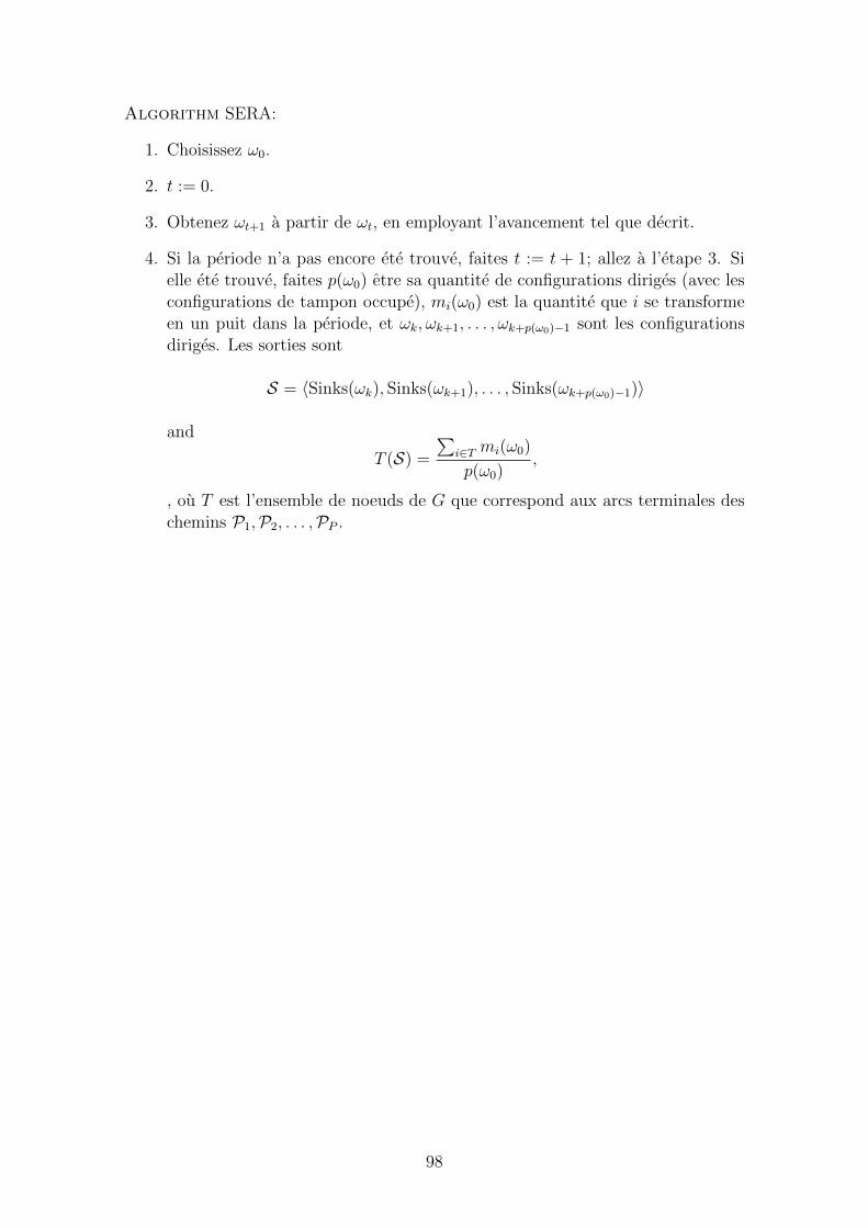
Algorithm SERA:

1. Choisissez ω0.

2. t := 0.

3. Obtenez ωt+1 a partir de ωt, en employant l’avancement tel que decrit.

4. Si la periode n’a pas encore ete trouve, faites t := t + 1; allez a l’etape 3. Sielle ete trouve, faites p(ω0) etre sa quantite de configurations diriges (avec lesconfigurations de tampon occupe), mi(ω0) est la quantite que i se transformeen un puit dans la periode, et ωk, ωk+1, . . . , ωk+p(ω0)−1 sont les configurationsdiriges. Les sorties sont


and

T (S) =

∑i∈T mi(ω0)

p(ω0),

, ou T est l’ensemble de noeuds de G que correspond aux arcs terminales deschemins P1,P2, . . . ,PP .

98

5

b c d e

1 2 3 4

a(a)

f

5

1 2 3 4

(c)

d e

fb

a

c

1 2 3 4

(b)

d e

fbc a

Figura I.3: Chaque ensemble dans une decomposition en puits est represente parun rectangle et numerote pour indiquer l’indice du ensemble. Notez que les arcsdiriges se referer a des orientations acycliques de G. L’application du SER a ladecomposition en puits dans le panneau (a) resulte a la decomposition en puits dansle panneau (b). Dans cette transformation les deux arcs a et b sont transformes ensources. L’alternative d’utiliser SERA, d’autre part, permet de a a etre place dansun ensemble anterieur a celui avec SER, en evitant la transformation en une sourceet qui donne la decomposition en puits dans le panneau (c). Cela peut etre faitseulement parce que l’ensemble auquel a est ajoute ne contient aucun de ses voisinsdans G. En assumant que les transmissions a, e, et f sont initialement disposesconsecutivement dans l’un des chemins de P dans l’ordre e, a, f , nous avons i− = e,i = a, and i+ = f . Nous avons egalement, en reference au panneau (a), k− = 4,k = 2, and k+ = 5. Ensuite, les conditions supplementaires pour le passage de (a) a(c) sont que les tampons partages par les transmissions e et a contient au moins unpaquet (puisque k < k−), et que les tampons partagee par a et f avons des placessuffisant pour au moins un paquet (puisque k < k+).

99

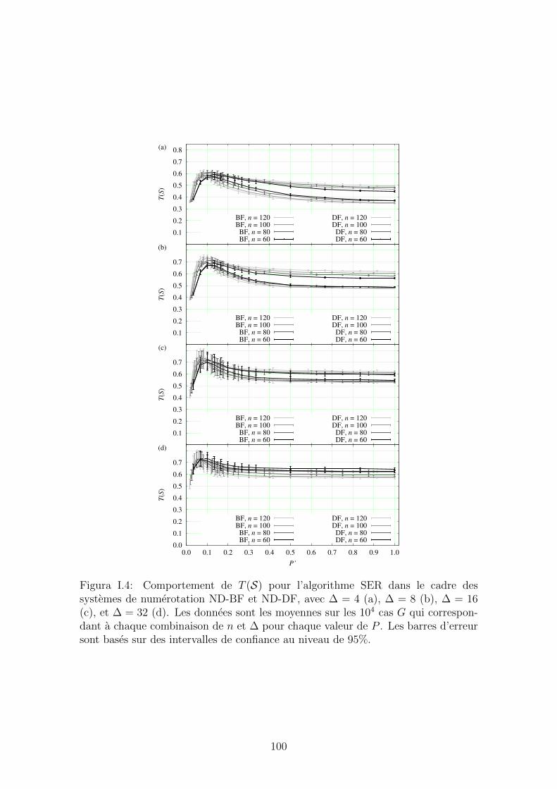
0.1

0.2

0.3

0.4

0.5

0.6

0.7

0.8

T(S

)

(a)

BF, n = 120BF, n = 100BF, n = 80BF, n = 60

DF, n = 120DF, n = 100

DF, n = 80DF, n = 60

0.1

0.2

0.3

0.4

0.5

0.6

0.7

T(S

)

(b)

BF, n = 120BF, n = 100BF, n = 80BF, n = 60

DF, n = 120DF, n = 100

DF, n = 80DF, n = 60

0.1

0.2

0.3

0.4

0.5

0.6

0.7

T(S

)

(c)

BF, n = 120BF, n = 100BF, n = 80BF, n = 60

DF, n = 120DF, n = 100

DF, n = 80DF, n = 60

0.0

0.1

0.2

0.3

0.4

0.5

0.6

0.7

0.0 0.1 0.2 0.3 0.4 0.5 0.6 0.7 0.8 0.9 1.0

T(S

)

P’

(d)

BF, n = 120BF, n = 100BF, n = 80BF, n = 60

DF, n = 120DF, n = 100

DF, n = 80DF, n = 60

Figura I.4: Comportement de T (S) pour l’algorithme SER dans le cadre dessystemes de numerotation ND-BF et ND-DF, avec ∆ = 4 (a), ∆ = 8 (b), ∆ = 16(c), et ∆ = 32 (d). Les donnees sont les moyennes sur les 104 cas G qui correspon-dant a chaque combinaison de n et ∆ pour chaque valeur de P . Les barres d’erreursont bases sur des intervalles de confiance au niveau de 95%.

100

0.4

0.8

1.2

1.6

2

2.4T

(S)

(a)

n = 120n = 100

n = 80n = 60, B = 2

n = 60

0.4

0.8

1.2

1.6

2

2.4

T(S

)

(b)

n = 120n = 100

n = 80n = 60

0.4

0.8

1.2

1.6

2

2.4

T(S

)

(c)

n = 120n = 100

n = 80n = 60

0.0

0.4

0.8

1.2

1.6

2

2.4

0.0 0.1 0.2 0.3 0.4 0.5 0.6 0.7 0.8 0.9 1.0

T(S

)

P’

(d)

n = 120n = 100

n = 80n = 60

Figura I.5: Comportement de T (S) pour l’algorithme SERA dans le cadre de lasysteme de numerotation ND-BF, avec ∆ = 4 (a), ∆ = 8 (b), ∆ = 16 (c), et ∆ = 32(d). Les donnees sont les moyennes sur les 104 cas G qui correspondant a chaquecombinaison de n et ∆ pour chaque valeur de P . Les barres d’erreur sont bases surdes intervalles de confiance au niveau de 95%.

101

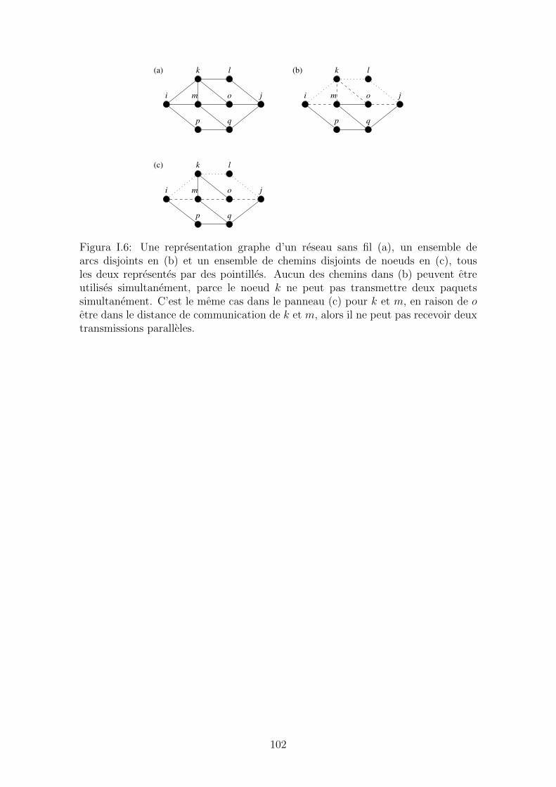
(a)

q

o

p q

o

p q

o

(b)

(c)

j

k l

i j

k l

i j

k l

m

m

mi

p

Figura I.6: Une representation graphe d’un reseau sans fil (a), un ensemble dearcs disjoints en (b) et un ensemble de chemins disjoints de noeuds en (c), tousles deux representes par des pointilles. Aucun des chemins dans (b) peuvent etreutilises simultanement, parce le noeud k ne peut pas transmettre deux paquetssimultanement. C’est le meme cas dans le panneau (c) pour k et m, en raison de oetre dans le distance de communication de k et m, alors il ne peut pas recevoir deuxtransmissions paralleles.

102

Algorithm MRA:

1. Soit N un ensemble qui a un noeud pour chaque chemin de Pij. Ajoutez unnoeud a N pour chaque paire de noeuds voisins du type B. Nous nous referonsa ces noeuds supplementaires comme noeuds temporaires.

2. Construire E seconde les etapes suivantes:

i. Soit k, k′ et l, l′ deux pairs de noeuds voisins, chaque pair du type A ou B.Si k = l, k = l′, k′ = l, ou k′ = l′, ajoutez un arc a E entre chaque noeudcorrespondant a le chemin appartient a Chemins(k, k′) (si le pair est dutype A) ou le correspondant noeud temporaire (si le pair est du type B)pour chaque noeud correspondant a un chemin appartient a Chemins(l, l′)(si le pair est du type A) ou le correspondant noeud temporaire (si le pairest du type B).

ii. Connectez deux noeuds appartient a N par un arc si, apres l’etapeprecedent, la distance entre eux est 2.

iii. Retirez de E tous les noeuds temporaires et les arcs qui les touchent.

3. Calculez l’ensemble independant maximum pondere et repondez l’ensemblePR

ij correspondant.

103

(a)1

k1

k2

k3

k4

k6

k2

k6

k5

k6

d x c

bea

(b)

d x c

bea

(c) d c

bea

(d)

x

:

i

i

i

i

i j

j

j

j

je

d :

c :

b :

a :k

Figura I.7: Construction d’un graphe Gij base sur l’ensemble de chemins Pij ={a, b, c, d, e}. Les chemins de Pij sont affiches dans le panneau (a), ou chaque arcorientee conduit a un noeud dans un certain ensemble Suivant(i, j) (par exem-ple, Suivantk1(i, j) = {j, k5}) et chaque arc pointille rejoint noeuds voisins quine partage pas aucune des chemins i a j. Nous voyons dans ce panneau queChemins(k2, k6) = {b, c}, et aussi qu’il y a cinq paires de noeuds du type A (k1, j;k2, k6; k2, k3; k1, k5; et k4, k6) ainsi que un seul pair de noeud du type B (k3, k5,marque par x). Panneau (b) montre le graphe Gij apres les etapes (1) et (2).i, res-pectivement pour la creation des noeuds mis en N et l’initialisation de son ensembledes arcs E en fonction de coıncidence entre tous les paires de noeuds des types Aou B. La distance 2 determine a l’etape (2).ii est montree dans le panneau (c), avecles arcs supplementaires representes par des lignes pointillees. Panneau (d), enfin,montre Gij, comme il se situe a la fin de l’algorithme MRA, apres l’etape (2).iii. Sides poids egaux ont ete utilises pour tous les noeuds, c’est clair que {a, b}, {a, c},{a, e}, {b, d}, or {d, e} seraient consideres comme un ensemble independant maxi-mal pondere de Gij dans l’etape (3). Mais l’utilisation de 1/Cp comme du poids dunoeud correspondant a la trajectoire p conduit a {a, b} et {a, e} comme les seulespossibilites, chacune avec le poids total de 5/6, puisque Ca = 2 and Cb = Ce = 3.

104

Figura I.8: Ratio σ pour 802.11 avec CBR1 et n = 120 avec ∆ = 4 (a) ∆ = 8 (b)∆ = 16 (c), et ∆ = 32 (d). Les moyennes sont bases en 104 ensembles de cheminscorrespondant a chaque valeurs de ∆ pour chaque valeur de θ. Les barres d’erreuront ete omis parce que elles sont inferieur a 1% de la moyenne de l’intervalle deconfiance au niveau de 95%.

105

Figura I.9: Ratio σ pour SERA et n = 120 avec ∆ = 4 (a) ∆ = 8 (b) ∆ = 16 (c), et∆ = 32 (d). Les moyennes sont bases en 104 ensembles de chemins correspondant achaque valeurs de ∆ pour chaque valeur de θ. Les barres d’erreur ont ete omis parceque elles sont inferieur a 1% de la moyenne de l’intervalle de confiance au niveau de95%.

106

Documents

Escalonamento de Enlaces e roteamento multi-caminho para redes