Instituto Superior de Ciências do Trabalho e da Empresa

ESSAYS ON INTERNATIONAL EQUITY MARKETS

Paulo Miguel Gama

Dissertação submetida como requisito parcial para obtenção do grau de

Doutor em Gestão Especialidade em Finanças

Orientador:

Prof. Doutor Miguel A. Ferreira

Fevereiro de 2005

Abstract

This dissertation consists of three papers on international equity markets. The first paper

uses a volatility decomposition method to study the time series of equity volatility at the

world, country and local industry levels. Between 1974 and 2001 there is no noticeable long-

term trend in any of the volatility measures. Then in the 1990s, there is a sharp increase

in local industry volatility compared to market and country volatility. Thus, correlations

among local industries have declined and more assets are needed to achieve a given level of

diversification.

The second paper studies the impact of sovereign debt rating news of one country on the

stock market returns of other countries between 1989 and 2003. The information spillover

effect is asymmetric and large. A one-notch credit ratings downgrade is associated with a

statistically significant negative two-day return spread of other countries relative to the US

stock market of 28 basis points, on average. Upgrades have no significant impact on return

spreads of countries abroad. Moreover, there is evidence of downgrades spillover effects at

the industry level.

The third paper investigates the time series of correlations between global industries and

aggregate world market over the 1979-2003 period. The behavior of industry correlations

is characterized by long-term swings, in particular with a period of low correlations in the

late 1990s. Small and value (low price-earnings ratio) industries have lower correlations.

Moreover, global industry correlations are counter-cyclical. Global industry correlations are

greater for downside moves than for upside moves. Correlation asymmetry is the largest

among small industries.

JEL classification: F30, G15

Keywords: Volatility, Correlation, Spillover effects, Asymmetries

ii

Resumo

Esta dissertacao engloba tres artigos sobre os mercados internacionais de accoes. O

primeiro artigo utiliza um metodo de decomposicao de variancia para estudar a evolucao

temporal da volatilidade ao nıvel do mundo, do paıs e da industria local. Entre 1974 e 2001,

nao ha evidencia de tendencias de longo prazo em qualquer nıvel de volatilidade. No final

da decada de 90, observa-se um forte aumento do risco da industria local relativamente ao

risco do paıs e do mercado mundial. Em conformidade, a correlacao entre industrias locais

decresce e mais activos sao necessarios para obter um dado nıvel de diversificacao.

O segundo artigo estuda o impacto de alteracoes de ratings da dıvida publica de um

paıs nos mercados accionistas de outros paıses entre 1989 e 2003. O efeito de spillover e

assimetrico e significativo. Em media, um ponto de downgrade do rating da dıvida publica

de um paıs esta associado a um diferencial de retorno face ao mercado dos EUA de 28

pontos base (em dois dias) nos mercados accionistas dos restantes paıses. Os upgrades nao

tem um impacto significativo nos restantes paıses. Adicionalmente, o efeito de spillover dos

downgrades manifesta-se ao nıvel das industrias.

O terceiro artigo analisa as sucessoes cronologicas da correlacao entre industrias globais

e o mercado mundial entre 1979 e 2003. O comportamento das correlacoes e caracterizado

por flutuacoes longas, sendo o final da decada de 90 caracterizado por baixas correlacoes. A

correlacao e inferior nas industrias de menor dimensao e value (racio price-earnings baixo).

Os perıodos de recessao caracterizam-se por um aumento das correlacoes industriais. As

correlacoes das industrias sao maiores para performances negativas do mercado do que para

performances positivas. Esta assimetria e maior nas industrias de menor dimensao.

Classificacao JEL: F30, G15

Palavras-chave: Volatilidade, Correlacao, Efeitos spillover, Assimetrias

iii

Acknowledgements

I am especially indebted to my advisor, Miguel Ferreira, for his kindness, support, and

exceptional guidance. His insightful ideas, helpful discussions and suggestions are invaluable

and greatly acknowledge. A very special thanks to Antonio Gomes Mota for encouragement

and support throughout my doctoral program.

I am also thankful to Geert Bekaert, John Campbell, Jens Jackwerth, Paul Laux, Francois

Longin, Tim Vogelsang, Robert Hodrick, Ana Paula Serra, Amar Gande, Yakov Amihud,

Andrew Ang, Peter Ritchken, for their comments and suggestions on earlier versions of the

papers. I have benefited from the comments of participants at the 2003 European FMA

meeting, the 2003 CEMAF/ISCTE conference, the 2003 North American FMA meeting, the

2004 AFA meeting, and the 2004 PFN meeting.

Any written acknowledgement is not enough for the love, patience, and understanding

of my wife and my two children. I hope that I have made you proud.

iv

Overview

This dissertation analyzes three empirical issues in international equity markets: volatil-

ity (Chapter 1), information spillover effects (Chapter 2), and correlation (Chapter 3). Each

chapter is written as an independent and self-contained paper. This brief overview provides

the motivation, methodology, and main findings of each paper.

The first paper primary goal is to describe the historical behavior of international equity

markets total volatility components and to study the implications for international diversi-

fication. We address three main research questions. First, have world, country, and local

industry risks changed over time? Second, has the power of international diversification to re-

duce risk decreased? Finally, given the recent evidence in the literature, we take another look

at the question of the relative efficiency of country versus industry diversification for global

equity investors. These are important questions for global portfolio managers. If the risk

that must be diversified away has increased, there are more opportunities for international

diversification, but more assets are needed to achieve a given level of diversification.

We extend the Campbell, Lettau Malkiel and Xu (2001) total risk decomposition method

to an international setting. This allows us to measure and study the time series behavior

of risk components without the need to keep track of covariances or estimate risk exposure

parameters for countries and industry portfolios. Moreover, the methodology measures in-

dustry risk on a country basis, which is an alternative to the Heston and Rouwenhorst (1994)

fixed-effects model assumption that asset exposures to global industry shocks are equal across

countries. We use local industry daily index return data, which include 21 developed markets

over the 1974-2001 period.

The paper major findings are the following. First, there is no evidence of a statistically

significant long-term trend in any of the volatility components, although local and global

v

industry volatility shows a sharp increase after 1995 (reaching an all-time peak in April

2000). Accordingly, the ratio of local industry to world risk experienced a considerable

increase during the late 1990s. The average ratio is 3.23 for the 1996-2001 period compared to

2.50 in the 1974-1995 period. This increase cannot be attributed solely to the new economy

bubble. Second, local industry risk dominates world and country risk, except during the

1990-1995 period, when country risk is on average the most important component. Third,

the October 1987 crash was felt at both world and country levels, but had less of an effect

on local industry risk. Fourth, lagged local industry risk is helpful in forecasting world and

country level volatility, while the converse is not true. Finally, the ratio of global industry

risks to country risk increased during the late 1990s. This ratio becomes greater than one in

the late 1990s.

Overall, the paper results show that risk components importance have changed over time,

and that global diversification opportunities using local industry portfolios have increased

after 1995. Moreover, the results support that global industry diversification has become

relatively more efficient than geographic diversification only in the late 1990s, although this

could be a temporary result. This is consistent with the early evidence in Heston and

Rouwenhorst (1994) and the recent evidence in Cavaglia, Brightman, and Aked (2000).

The second paper addresses the question: does sovereign debt ratings news in one country

impact other countries stock markets? Brooks, Faff, Hillier, and Hillier (2004) find that

sovereign ratings downgrades have a negative impact on the re-rated country stock market

returns. Kaminsky and Schmukler (2002) show that emerging market sovereign ratings news

is contagious to bond and stock markets of other emerging markets. Gande and Parsley

(2003) find that the international spillover effect on the sovereign debt market is asymmetric.

In fact, only downgrades abroad are associated with a significant increase in sovereign bond

spreads. Furthermore, there is a need for a through empirical investigation of the cross-

country stock market impact of ratings news with: 1) a sample that includes both emerging

and developed countries; and 2) a methodology that specifically addresses the (potential)

asymmetry of market reactions and the tendency for ratings changes to cluster in time.

vi

The paper basic methodology is an extension to the across-market case of the Gande

and Parsley (2003) research design to study across-countries debt market spillover effect.

Specifically, we consider a large set of countries that includes not only emerging but also

developed markets; we explicitly control for recent rating activity worldwide; we characterize

the spillover effects economically (e.g., by including controls for capital flows and level of

economic and financial development); we study the role of exchange rates in spillover effects;

and we present several new results of cross-country and cross-market news spillover at the

industry level. The impact of sovereign rating news on industry portfolios is of particular

relevance given the increased perception by investors and empirical evidence that industry

factors are becoming more important than country factors in explaining stock returns.

The paper major findings can be summarized as follows. Ratings changes in one country

contain valuable information for the aggregate stock market returns of other countries, but

only downgrades On average, a one-notch ratings downgrade abroad is associated with a

statistical significant negative two-day stock return spreads vis-a-vis the US stock market

of 28 basis points across non-event countries, whereas no significant pattern is found for

ratings upgrades. This pattern is not affected by taking into account time invariant char-

acteristic that proxy for underlying similarities between countries (cultural, regional and

institutional environment as well as level of economic and financial development). Also, rat-

ings downgrades are associated with a depreciation of the US dollar exchange rate against

the non-event country currencies. Thus, the appreciation of non-event country currencies

relative to the US dollar (partially) hedges the negative wealth effect of ratings downgrades

abroad. Finally, the paper evidence shows that ratings downgrades announcements are also

noticed at the local industry level. Sovereign ratings downgrades abroad are associated with

a highly statistical significant negative two-day return spread (25 basis points) of industry

portfolios vis-a-vis their counterpart industry in the US.

Overall, our findings are robust across different empirical specifications, namely explicitly

accounting for recent rating activity, alternative ways to measure the impact in the stock

market (dependent variable), and sub-samples of countries and industries.

vii

The third paper studies international equity markets correlation at the global industry

level. While much is known about cross-country correlation, on the other hand the global

industries correlations have not been studied in the literature. The goal is to contribute

to the literature on international investments with the characterization of global industry

portfolios correlation in terms of time series behavior and asymmetries.

Two features characterize the methodology. First, realized correlation is estimated using

within month daily index return data, which allows the construction of a time series of

correlations between global industries and aggregate world market over the 1979-2003 period.

Second, we study the correlations for different groups of industries, specifically size and price-

earnings ratio.

The paper findings can be summarized as follows. Global industry correlations fluctuate

over time and the 1999-2003 period is characterized by low correlations. However, there is

not a significant long-term trend. Also, correlation is lower for small and value (low price-

earning ratio) industries. Moreover, global industry correlations are counter-cyclical. With

respect to asymmetries, global industry correlations are greater for downside moves than

for upside moves. Correlation asymmetry is insignificant only for the resources and utilities

industries. Correlation asymmetry is the largest among small industries. These findings

are robust to the use of value or equal weighted aggregate market index, two-days returns,

two-month estimation window, outliers correction, and the returns currency denomination.

We further investigate correlation behavior by decomposing it in realized betas and

volatility ratios (market to industry). There is a similarity between correlation and be-

tas behavior over the long-run. Industry betas and, especially, volatility ratios increase for

downside market moves.

The characterization of global industries correlations yields both reassuring and disturb-

ing news for global equity investors. On the bad side, our results confirm for global industry

portfolios, two features that characterizes cross-country correlations. Industry correlations

increase for downside market moves (Longin and Solnik (2001)) and increase during reces-

sions (Erb, Harvey, and Viskanta (1994)). Thus, the power of global industry diversification

viii

to reduce portfolio risk decreases during bad times. On the positive side, we find that indus-

try correlation does not show a systematic increase over time, which is in contrast with the

findings of a positive trend in cross-country correlation (Solnik and Roulet (2000)).

ix

Contents

Abstract ii

Resumo iii

Acknowledgements iv

Overview v

List of Tables xii

List of Figures xv

Chapter 1. Have World, Country and Industry Risks Changed Over Time? An

Investigation of the Developed Stock Markets Volatility 1

1.1. Introduction 1

1.2. Methodology 5

1.3. Data Description 10

1.4. Historical Evolution of Total Volatility Components 12

1.5. Global Portfolio Management Implications 24

1.6. Conclusion 26

References 28

Chapter 2. Does Sovereign Debt Ratings News Spillover to International Stock

Markets? 44

2.1. Introduction 44

2.2. A Selective Review of the Sovereign Ratings Literature 48

2.3. Research Design 51

2.4. Empirical Results on Country Portfolios 56

x

2.5. Empirical Results on Industry Portfolios 68

2.6. Conclusion 72

References 73

Appendix 87

Chapter 3. Correlations of Global Industry Portfolios: An Empirical Investigation of

Trends and Asymmetries 89

3.1. Introduction 89

3.2. Research Design 92

3.3. Time Series of Industry Correlations 95

3.4. Asymmetries in Industry Correlations 107

3.5. Betas and Volatility Ratios 112

3.6. Conclusion 116

References 117

xi

List of Tables

1.1 Descriptive Statistics for Country Portfolios 30

1.2 Descriptive Statistics for Global Industry Portfolios 31

1.3 Descriptive Statistics for World, Country, and Industry Risks 32

1.4 World, Country, and Industry Risk for Alternative Samples 33

1.5 Volatility Measures by Countries 34

1.6 Global Industry Volatility 35

1.7 Total Volatility Mean and Variance Decomposition 36

1.8 Correlation Structure and Granger-causality Tests 37

2.1 Description of Sovereign Ratings Events 75

2.2 International Stock Market Impact of Sovereign Rating News 76

2.3 International Stock Market Impact of Sovereign Rating News - Cultural,

Legal and Institutional Controls 77

2.4 Common and Differential Spillover Effects 78

2.5 International Stock Market Impact of Sovereign Rating News - Crisis and

Liberalizations Controls 79

2.6 International Stock Market Impact of Sovereign Rating News - Local

Currency and Exchange Rate Effects 80

2.7 International Stock Market Impact of Sovereign Rating News - Lag Event

Window and Returns Definition 81

2.8 International Stock Market Impact of Sovereign Rating News - Single

Regression Model 82

xii

2.9 International Stock Market Impact of Sovereign Rating News - Larger

Countries 83

2.10 Industry Portfolios Impact of Sovereign Rating News 84

2.11 Industry Portfolios Impact of Sovereign Rating News - Industry Groups 85

A.1 Variables Definition and Sources 87

A.2 Comprehensive Credit Rating Definition 88

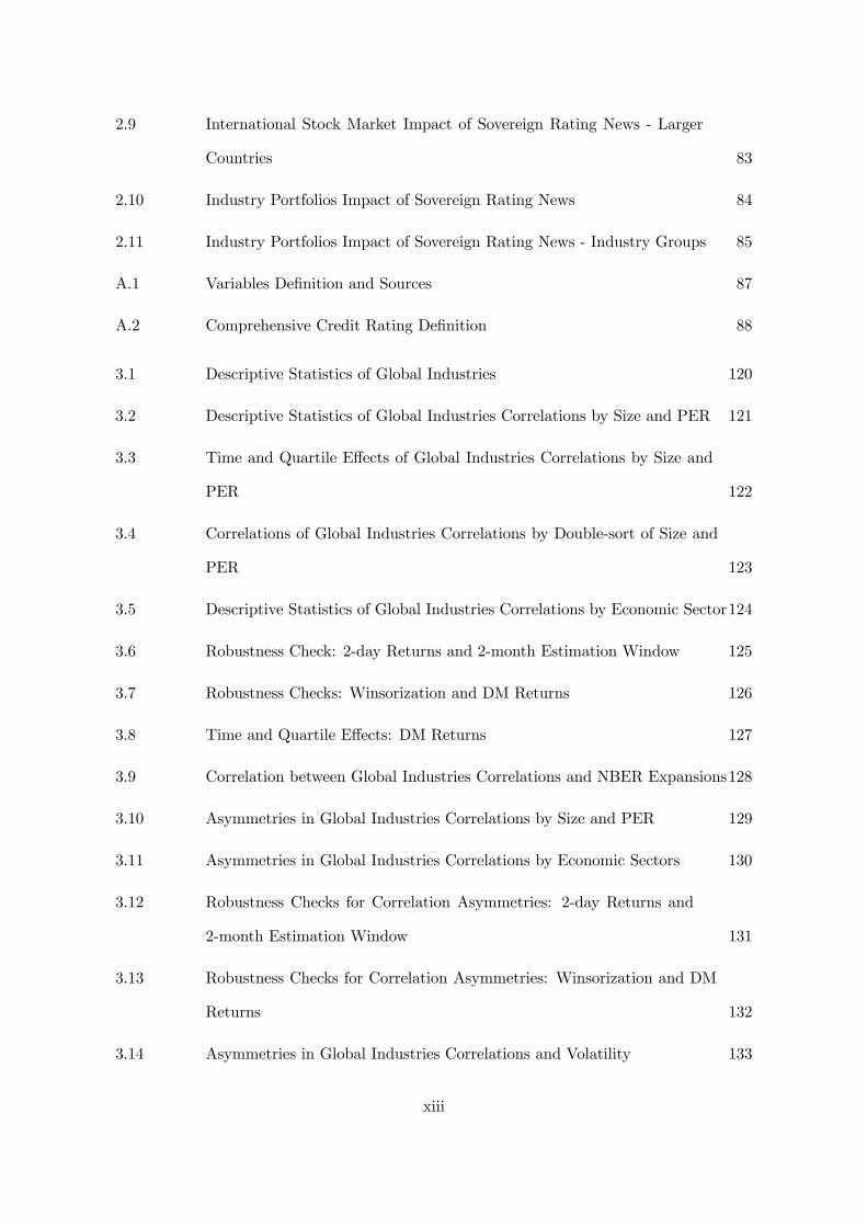
3.1 Descriptive Statistics of Global Industries 120

3.2 Descriptive Statistics of Global Industries Correlations by Size and PER 121

3.3 Time and Quartile Effects of Global Industries Correlations by Size and

PER 122

3.4 Correlations of Global Industries Correlations by Double-sort of Size and

PER 123

3.5 Descriptive Statistics of Global Industries Correlations by Economic Sector124

3.6 Robustness Check: 2-day Returns and 2-month Estimation Window 125

3.7 Robustness Checks: Winsorization and DM Returns 126

3.8 Time and Quartile Effects: DM Returns 127

3.9 Correlation between Global Industries Correlations and NBER Expansions128

3.10 Asymmetries in Global Industries Correlations by Size and PER 129

3.11 Asymmetries in Global Industries Correlations by Economic Sectors 130

3.12 Robustness Checks for Correlation Asymmetries: 2-day Returns and

2-month Estimation Window 131

3.13 Robustness Checks for Correlation Asymmetries: Winsorization and DM

Returns 132

3.14 Asymmetries in Global Industries Correlations and Volatility 133

xiii

3.15 Descriptive Statistics of Global Industries Betas and Volatility Ratios by

Size and PER 134

3.16 Asymmetries in Global Industries Betas and Volatility Ratios by Size and

PER 135

3.17 Variance Decomposition of Global Industries Correlations 136

xiv

List of Figures

1.1 World Volatility 38

1.2 Country Volatility 39

1.3 Local Industry Volatility 40

1.4 Global Industry Volatility 41

1.5 Ratio of Local Industry to World Variance and Average Correlation for

Local Industry Portfolios 42

1.6 International Diversification Benefits Against Time and Number of Local

Industry Portfolios 43

2.1 Comprehensive Credit Rating Changes 86

3.1 Global Industry Correlation 137

3.2 Correlation and Size 138

3.3 Correlation and Price-earnings Ratios 139

xv

CHAPTER 1

Have World, Country and Industry Risks Changed Over

Time? An Investigation of the Developed Stock Markets

Volatility

(with Miguel Ferreira)

1.1. Introduction

The risk reduction benefits of the international diversification of equity portfolios have

been accepted for a long time among academician, e.g., Solnik (1974). Neither individual

nor institutional investors, however, seem to take the advantage of the benefits one would

expect in a frictionless fully integrated world: global portfolios composition is biased toward

domestic shares; see Lewis (1999). Kang and Stulz (1997) moreover find that when investors

decide to invest internationally, they do not hold the market portfolio of the countries they

choose to invest in. What is the total risk exposure faced by investors with undiversified

global stock portfolios? This question is the major motivation of this study.

The historical evolution of total risk is particularly important for global portfolio man-

agers of undiversified international portfolios. If the risk that must be diversified away has

increased, there are both more opportunities for international diversification and more as-

sets needed to achieve a given level of diversification. The benefits of investing abroad may

become harder to achieve, but the compensation for pursuing such an investment strategy

is also greater. If investors face wealth constraints or transaction costs, increased diversifi-

able risk implies less diversification of their investment portfolios, unless they have superior

stock selection capabilities. Total volatility is also an issue for taking advantage of mispriced

1

individual assets, for pricing equity derivatives, and for measuring the market risk of equity

portfolios (e.g., Value-at-Risk).

The relevance of exposure to world portfolio risk in explaining the cross-section of ex-

pected returns has been established in countless empirical tests of international asset pricing

models.1 The empirical evidence in Cavaglia, Hodrick, Vadim, and Zhang (2002) and in

Dahlquist and Sallstrom (2002), for example, shows that exposure to the world return factor

is priced both in the cross section of country and global industry portfolio returns, accord-

ing to various international asset pricing models. Empirical evidence on the importance of

country and industry dimensions is less clear.

While Roll (1992) attributes the low correlation among country indices to diverse local

industry structures, Heston and Rouwenhorst (1994) decompose stock return volatility into

pure country and industry sources of variation and clearly document the dominance of coun-

try specific effects (the average ratio of country to industry variances is 4.5). Griffin and

Karolyi (1998) find that when emerging markets are included in the sample, the proportion

of portfolios variance explained by the time series variation in pure country effects is higher

than previously documented, which again indicates investors would be better off — in terms of

risk reduction — if they pursued a geographic diversification strategy rather than an industry

one.

Conversely, Cavaglia, Brightman, and Aked (2000), among others, find evidence that

industry factors have grown in importance in recent years. Brooks and Catao (2000) also

show that industry sectors are becoming more important in explaining portfolio risk and that

the global industry factor, primarily associated with the information technology sector, has

grown in importance since 1995. More recently, Brooks and Del Negro (2002b) assert that the

rise in industry effects is simply a temporary phenomenon associated with the information

technology bubble rather than an reflection of greater economic integration across countries.2

1Karolyi and Stulz (2001) provide an extensive survey of these studies.2This finding is contrary to the increased consensus among the investment community and in the financialpress that the industry dimension of diversification is today more important than the geographic dimension.

2

We take the perspective of a global investor and use local industry portfolios (within

country) as our individual assets, to study three sources of risk for internationally tradable

equities. Two of the risk sources are diversifiable in a global portfolio: geographic location

and industry affiliation. The remaining source represents the systematic component: world

portfolio volatility.

Our primary goal is to describe the historical behavior of total volatility components and

to study the implications for international diversification. We address three main questions.

First, has the relative importance of world, country, and local industry risk changed over

time? Second, has the power of international diversification to reduce risk been weakening?

Finally, given the conflicting evidence in the literature, we take another look at the question

of the relative efficiency of country versus industry diversification for global equity investors.

We decompose the total volatility of individual assets into specific sources of risk by

extending the Campbell, Lettau, Malkiel, and Xu (2001) volatility decomposition method

to an international setting. We propose a parsimonious total risk decomposition that allows

us, at an appropriate aggregation level to measure and study the time series behavior of

risk components without the need to keep track of covariances or estimate risk exposure

parameters for countries or local industry portfolios, which is an appealing feature of the

approach.

The major simplification of this methodology is reliance on the use of market-adjusted

residuals of country returns relative to world returns, and of local industry returns relative

to country returns, to estimate country and local industry risk measures, respectively. This

hierarchical decomposition is consistent with the traditional top-down approach to global

asset management of first selecting countries and then industries and stocks. In addition, a

simple change of the methodology is consistent with the view of the world for those investors

who organize the world portfolio by industries rather than countries.

Our methodology measures industry risk on a country basis, which is an alternative to

the Heston and Rouwenhorst (1994) fixed-effects model assumption that asset exposures to

global industry shocks are equal across countries, whenever they are non-zero. We take the

3

local industry return in excess of their country of origin return as a measure local industry

risk. Thus, we allow for interactions among countries and industries; i.e., industry-specific

shocks may have different impacts across countries. Moreover, our methodology provides a

direct estimate of the volatility measures.3 We use daily data within a month to estimate

monthly time series of risk measures, without imposing a parametric multivariate volatility

specification.

Our results indicate first, that international diversification benefits have been substantial

over the 1974-2001 period. World risk has always been the least important component of

total risk. There is no evidence of a statistically significant long-term trend in any of the

volatility series, although local and global industry volatility show a sharp increase after

1995, reaching an all-time peak in April 2000. An increase in local industry volatility is

also notable in individual countries. The new economy bubble does not by itself explain the

increase in industry risk, although the technology, media, and telecommunications industries

play an important role in this phenomenon. World and country risk show a much more

modest increase in the 1990s.

Second, the October 1987 crash was felt at both world and country levels, but had less

of an effect on local industry risk. A period of increased local industry volatility may be

seen since the beginning of 1987. The early 1990s may be considered an atypical period

in historical terms; during the 1990-1995 period, the share of country risk in total risk is

unusually high, and total risk is on average lower than in the surrounding years.

Third, using Granger-causality tests, we provide evidence that lagged local industry risk

is helpful in forecasting world and country level volatility, while the converse is not true.

Fourth, the ratio of local industry to world risk experienced a considerable increase during

the final years of our sample. The average ratio is 3.23 for the 1996-2001 period compared to

2.50 in the 1974-1995 period. Accordingly, the average contemporaneous pairwise correlation

3Brooks and Del Negro (2002a) have recently proposed an alternative relaxing the restrictive assumptionsof the fixed-effects model. They estimate stocks’ exposure to global, country, and industry-specific shocksin a arbitrage pricing theory framework. Their approach, however, does not preserve the simplicity of thefixed-effects model. It imposes strong distributional assumptions and requires a balanced panel.

4

between local industry portfolios declines considerably from 0.287 (1974-1995) to 0.203 (1996-

2001). Thus, the benefits of international portfolio diversification have become greater and

the diversification of global portfolios using local industry portfolios has become harder to

achieve as more assets are needed.

Finally, the notable increase in the ratio of industry to country risk, at both local and

global levels, suggests that industry diversification became a more effective tool for risk

reduction in the late 1990s. The share of local industry risk in total risk also increases

considerably toward the end of the sample period, to more than 50% in 1996-2001, while the

share of country risk decreases.

The paper is organized as follows. Section 1.2 presents the model used to decompose total

volatility, discuss some simplifying econometric solutions to the estimation of the volatility

components, and briefly evaluate the exactness of the return structure employed. Section

1.3 gives details on the data set. Section 1.4 presents the empirical findings concerning

the historical evolution of the disaggregated volatility measures. Section 1.5 discusses the

implications for global portfolio management. Section 1.6 offers concluding comments.

1.2. Methodology

We extend the methodology proposed by Campbell et al. (2001) to decompose stock

returns volatility into market, industry, and idiosyncratic components to an international

setting. We take the perspective of a global investor whose returns are calculated in US

dollars. The global investor does not hedge foreign exchange rate risk, and we do not

explicitly address currency risk factors. Moreover, we use local industry portfolios within

countries as basic assets, and specify the same industry grouping variables across countries.

1.2.1. Total Volatility Decomposition

The volatility of a typical (or average) local industry is described by three components:

world market volatility, average country volatility, and average local industry volatility.4 We

4By typical we mean randomly selected local industry portfolio with drawing probability equal to its weightin the world market portfolio.

5

provide a decomposition of volatility that does not require the estimation of covariances or

betas for local industries or countries, which is the most appealing feature of the Campbell et

al. (2001) methodology applied to international stock markets. In fact, beta time-dependence

and error estimation are well documented in the literature and there is some controversy on

which factors should be used in multifactor international asset pricing models to describe

the cross-section of expected returns.

The excess return of industry i portfolio in country c for period t is denoted Rict.5 Raw

returns are US dollar-denominated and the excess return is measured over the US dollar

risk-free rate. Let xict be the weight of industry i in country c. According to a weighting

scheme based on market capitalization, xict =MVict/Pi∈cMVict, where MVict denotes the

market value of the local industry portfolio ic (assumed known at time t). Let xct denote

the weight of country c in the world market portfolio (if market values are used as weights,

then xct =Pi∈cMVict/

Pc

PiMVict). The excess return of country c portfolio for period t

is given by Rct =Pi∈c xictRict. The excess return of world (w) portfolio for period t is given

by Rwt =Pc xctRct.

We assume a simplified country return decomposition:

Rct = Rwt + ect, (1.1)

and similarly for local industry portfolio returns:

Rict = Rct + uict = Rwt + ect + uict. (1.2)

Equation (1.2) specifies that the return on a local industry portfolio (Rict) equals the sum

of the world portfolio return (Rwt), its country portfolio-specific residual (ect), and its local

industry-specific residual (uict).

Thus, the variance of a local industry portfolio return is given by:

5In what follows, the term return is used to express excess return, unless stated otherwise. Following Harvey(1991) we note that these returns may be considered real relatively to US inflation, because the US inflationcomponents in stock raw returns and in the US-dollar nominal riskless interest rate cancel out.

6

Var(Rict) = Var(Rwt) + Var(ect) + Var(uict) (1.3)

+2 Cov(Rwt, ect) + 2 Cov(Rwt, uict) + 2 Cov(ect, uict).

While the local industry return variance in equation (1.3) includes covariance terms, the

cross-sectional weighted average sum of all the basic asset total variance across all local

industry portfolios is free of individual covariance terms, provided that we use the same non-

stochastic weighting scheme to compute the averages that we use to compute country and

world portfolios returns.6 Thus, the volatility of a typical local industry portfolio is given

by:

Xc∈w

xctX

i∈cxictVar(Rict) = Var(Rwt) +

Xc∈w

xctVar(ect) (1.4)

+X

c∈wxctX

i∈cxictVar(uict)

= σ2wt + σ2et + σ2ut,

where σ2wt represents the variance of the world market portfolio; σ2et is the weighted average of

country-level variance across all countries; and σ2ut is the weighted average of within-country

industry-level variance across all local industries and countries. The RHS of equation (1.4)

can be interpreted as the expected variance of a typical local industry portfolio.

We can gain further intuition on our methodology by comparing it with alternative

models of returns. Our simplified market-adjusted return assumes that all countries have

the same exposure to the world market and that all within-country industry portfolios have

the same exposure to the country of domicile market portfolio.

In the framework of the single factor international capital asset pricing model (ICAPM)

of Grauer, Litzenberger, and Stehle (1976), where the factor is the excess return on the world

6We note that it is not required to assume weights based on market capitalization to assure the modelconsistency provided that national and world market returns are computed using the same weighting scheme.

7

portfolio, which allows for country and local industry betas to be different from unity, the

excess return on an individual local industry portfolio is written as:7

Rict = βicRct + uict = βic (βcRwt + ect) + uict = βicβcRwt + βicect + uict, (1.5)

where βic denotes the beta of industry portfolio i in country c with respect to the correspond-

ing local market excess return; βc denotes country c beta with respect to the world market

portfolio; ect is the zero mean country-specific residual; and uict is the local industry-specific

residual.8

In this setting, if we take the average of the variance of country returns and the variance

of the local industry returns, and compare them with the simplified decomposition equivalent

measures, we will find that:

σ2et = σ2et + CSVt(βc)σ2wt, (1.6)

σ2ut = σ2ut + CSVt(βic)σ2et + [CSVt(βiw)− CSVt(βc)]σ2wt, (1.7)

where CSVt(βc) ≡Pc∈W xct(βc − 1)2; CSVt(βic) ≡

Pc∈W xct

Pi∈C xict(βic − 1)2; and

CSVt(βiw) ≡Pc∈W xct

Pi∈C xict(βiw − 1)2.

Equation (1.6) shows that our estimate of country-level volatility is positively biased in

relation to that of the ICAPM by CSVt(βc), which can be seen as the average cross-sectional

variance of βc, times σ2wt. By the same reasoning, equation (1.7) shows that the biases

in the proposed estimate of local industry risk depend on the variation of world returns,

country residuals, and betas. Cross-sectional variation in country and local industry betas

can produce common variation in our variance components - market, country and local

industry. However, we will show in Section 1.4.2 that cross-sectional variation in betas has

only a small effect on the historical behavior of our volatility measures.

7That is, assuming a perfectly integrated frictionless global stock market, where purchasing power parityholds; see Karolyi and Stulz (2001).8We assume that the beta of the local industry i with respect to the world market return satisfies βiw = βicβc.

8

A final note about two features of the proposed volatility decomposition. Local indus-

try risk is less affected by currency fluctuations than world and country level measures of

volatility. Also, the short-term interest rate risk implied by the excess returns specification

affects only the world volatility measure, because the same interest rate is subtracted from

the local industry portfolios returns.

1.2.2. Estimation

We use daily data within a month to construct sample variance estimates for that month.

The volatility components of equation (1.4) are estimated as follows. Let d refer to days in

month t. For the world portfolio variance Wt ≡ σ2wt in month t:

Wt =X

d∈t(Rwd − µwt)2, (1.8)

where Rwd is the world market portfolio excess return, constructed as the weighted average

of the local industry index returns, using all available local industries in a given month, and

µwt is the world portfolio mean return in month t.9 Weights for month t are based on the US

dollar-denominated market value of the local industry portfolios on the last day of month

t− 1, so weights are taken as constant within month t.

For the country-level risk Ct ≡ σ2et in month t:

Ct =X

cxctX

d∈te2cd, (1.9)

where xct stands for the weight of country c in the world portfolio in month t, which we

measure by using the end-of-month t− 1 market capitalization, and e2cd is the square of the

market-adjusted country-specific residual from equation (1.1).

For the weighted average of within-country industry-level risk It ≡ σ2ut:

9As in Schwert (1989) we allow the mean world portfolio return to fluctuate month to month. Campbell etal. (2001) take the mean return over the entire sample, and report that mean-varying means yield almostidentical results.

9

It =X

cxctX

i∈cxict

Xd∈tu2icd, (1.10)

where xict denotes the weight of industry i in country c in month t, andPd∈t u

2icd is the

summation over all days of month t of the square of the local industry-specific residual from

equation (1.2), for each local industry portfolio in the sample.

Campbell et al. (2001) justify this simplified approach to estimate volatility components

by the fact that all models for volatility estimation based on historical values tend to produce

fitted volatility estimates that move close together. Thus, the simple use of daily data to

produce monthly sample variance estimates is enough for historical description purposes.

1.3. Data Description

Our sample consists of daily US dollar-denominated total return indices (including div-

idends) and market capitalizations for up to 38 industries, calculated by Datastream Inter-

national (DS), for the period from January 1974 to December 2001. DS indices are preferred

over other domestic industry indices because: (1) they are constructed on a uniform basis

across countries; (2) they are not backfilled when new constituents are added or deleted; (3)

a long time series of daily data is available; and (4) a comprehensive coverage of the industry

structure of each domestic stock market is assured. These aspects are important because they

eliminate anomalous behavior of the indices attributable to differences in technical aspects

of index construction, and, as Griffin and Karolyi (1998) point out, broad industrial classi-

fications may not provide enough cross-sectional variation in returns to distinguish between

country- and industry-specific sources of variation.10

The 21 developed markets analyzed are selected according to criteria as follows: (1)

coverage by the MSCI developed markets database; (2) no classification ever as an emerging

market by the S&P/IFC EMDB ; and (3) data availability. Thus, both the number of local

10Cavaglia et al. (2002), Brooks and Del Negro (2002b), Dahlquist and Sallstrom (2002), and Brooks andCatao (2000) also rely on DS Global Equity Indices.

10

industry portfolios and the number of countries represented in the world portfolio are allowed

to change over the sample period.11

To compute daily excess returns, we subtract the 30-day Treasury bill continuously com-

pounded return divided by the number of trading days in a month from the daily logarithmic

stock index rate of return.

Tables 1.1 and 1.2 provide descriptive statistics of the country portfolios and the global

industry portfolios. Daily country and global industry portfolio excess returns are computed

using a value-weighted average of the available local industry portfolio aggregate either by

countries or global industries.

The US is by far the largest single market in the sample (representing an average weight

of 45.8% in our G21 developed world), and it is the only country with data on all industries

available since 1974. Because the US returns are not affected by exchange rate risk, it is

no surprise to see that they have the second-lowest standard deviation (15.8% annualized).

The less representative countries both in terms of market value and number of local industry

portfolios are Austria (0.1% average weight, maximum 24 industry portfolios), New Zealand

(0.1%, 26), Ireland (0.2%, 27), Norway (0.2%, 25), and Denmark (0.3%, 22).

Table 1.2 shows that the number of countries that include a particular global industry

has changed dramatically over the last three decades. The average maximum number of

countries that contribute to a given global industry portfolio is almost three times the average

minimum number of countries. Also, the representation of global industry portfolios in the

world portfolio is less concentrated than the representation of country portfolios. No single

global industry portfolio accounts on average for more than 9% in the world portfolio (banks).

Interestingly, the most volatile global industry portfolios are software and computer services

(24.6% annualized standard deviation) and information technology (21.9%).

11The sample starts with 13 countries and 270 local industry portfolios in 1974 and ends with 21 countriesand 640 local industry portfolios in 2000. After its inclusion in the database, no country is eliminated. Theregional components remains the same from 1990 onward with the addition of Ireland.

11

Tables 1.1 and 1.2 together show that, in our sample, the opportunities for global invest-

ment increased substantially during the last three decades, largely because of an increased

number of industries available in each country.

1.4. Historical Evolution of Total Volatility Components

Have the risks of world, country, and local industry return components been changing

over time? We provide a graphical analysis of the time evolution of the W , C, and I risk

measures, estimated using equations (1.8) through (1.10), and discuss relevant descriptive

and test statistics concerning the major features of the estimated volatility series.

1.4.1. Graphical Analysis and Descriptive Statistics

Figures 1.1, 1.2, and 1.3 plot our estimates of the world, country, and local industry volatility.

To facilitate interpretation, we report annualized standard deviation, and backward 12-month

moving average.

Stulz (1999) finds that world portfolio volatility presents considerable time variation,

but has not shown a tendency to increase over time, and that the 1970s and the 1990s were

periods of relatively low volatility. The time pattern revealed by the plots in Figure 1.1 is

consistent with his results.

The all-time high for theW series corresponds to the October 1987 crash (58.6% annual-

ized standard deviation). The second-highest value occurs in August 1990 (28.2% annualized

standard deviation), and clusters of volatility spikes are visible in 1974, 1982, and 1990-1992.

There is also evidence of an increase in world volatility for the 1997-2001 period. In fact, the

smoothed 12-moving average plot suggests thatW has a slow-moving component, reinforcing

the idea of persistent behavior.

Figure 1.2 shows that the country risk measure (C) behaves much the same as the world

volatility (W ). The 1987 crash had a slightly less pronounced effect on C (53.8% annualized

standard deviation in October 1987) but with similar timing. Similar to world risk, the

country volatility shows no upward trend.

12

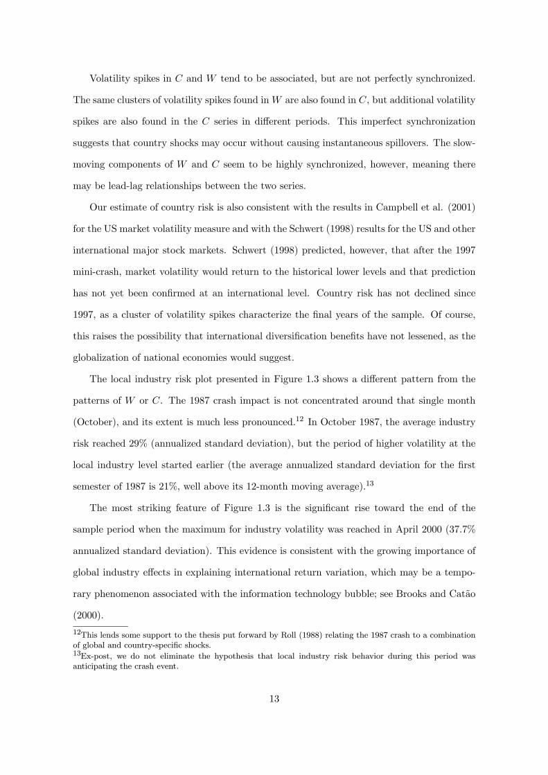
Volatility spikes in C and W tend to be associated, but are not perfectly synchronized.

The same clusters of volatility spikes found inW are also found in C, but additional volatility

spikes are also found in the C series in different periods. This imperfect synchronization

suggests that country shocks may occur without causing instantaneous spillovers. The slow-

moving components of W and C seem to be highly synchronized, however, meaning there

may be lead-lag relationships between the two series.

Our estimate of country risk is also consistent with the results in Campbell et al. (2001)

for the US market volatility measure and with the Schwert (1998) results for the US and other

international major stock markets. Schwert (1998) predicted, however, that after the 1997

mini-crash, market volatility would return to the historical lower levels and that prediction

has not yet been confirmed at an international level. Country risk has not declined since

1997, as a cluster of volatility spikes characterize the final years of the sample. Of course,

this raises the possibility that international diversification benefits have not lessened, as the

globalization of national economies would suggest.

The local industry risk plot presented in Figure 1.3 shows a different pattern from the

patterns of W or C. The 1987 crash impact is not concentrated around that single month

(October), and its extent is much less pronounced.12 In October 1987, the average industry

risk reached 29% (annualized standard deviation), but the period of higher volatility at the

local industry level started earlier (the average annualized standard deviation for the first

semester of 1987 is 21%, well above its 12-month moving average).13

The most striking feature of Figure 1.3 is the significant rise toward the end of the

sample period when the maximum for industry volatility was reached in April 2000 (37.7%

annualized standard deviation). This evidence is consistent with the growing importance of

global industry effects in explaining international return variation, which may be a tempo-

rary phenomenon associated with the information technology bubble; see Brooks and Catao

(2000).

12This lends some support to the thesis put forward by Roll (1988) relating the 1987 crash to a combinationof global and country-specific shocks.13Ex-post, we do not eliminate the hypothesis that local industry risk behavior during this period wasanticipating the crash event.

13

The time evolution of the volatility components over time indicates that monthly volatil-

ity estimates are time-varying; that periods of high volatility are concentrated around specific

times and are followed by periods of relative stability; and, that there is some evidence the

series may be diverging upward from some lower bound, which leaves open the possibility

there may be an upward trend. Especially clear is a rise in local industry risk toward the

end of our sample.

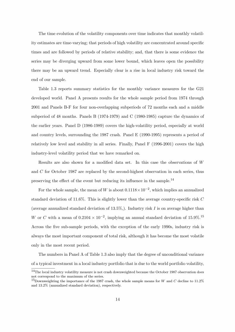
Table 1.3 reports summary statistics for the monthly variance measures for the G21

developed world. Panel A presents results for the whole sample period from 1974 through

2001 and Panels B-F for four non-overlapping subperiods of 72 months each and a middle

subperiod of 48 months. Panels B (1974-1979) and C (1980-1985) capture the dynamics of

the earlier years. Panel D (1986-1989) covers the high-volatility period, especially at world

and country levels, surrounding the 1987 crash. Panel E (1990-1995) represents a period of

relatively low level and stability in all series. Finally, Panel F (1996-2001) covers the high

industry-level volatility period that we have remarked on.

Results are also shown for a modified data set. In this case the observations of W

and C for October 1987 are replaced by the second-highest observation in each series, thus

preserving the effect of the event but reducing its influence in the sample.14

For the whole sample, the mean ofW is about 0.1118×10−2, which implies an annualized

standard deviation of 11.6%. This is slightly lower than the average country-specific risk C

(average annualized standard deviation of 13.5%,). Industry risk I is on average higher than

W or C with a mean of 0.2104 × 10−2, implying an annual standard deviation of 15.9%.15

Across the five sub-sample periods, with the exception of the early 1990s, industry risk is

always the most important component of total risk, although it has become the most volatile

only in the most recent period.

The numbers in Panel A of Table 1.3 also imply that the degree of unconditional variance

of a typical investment in a local industry portfolio that is due to the world portfolio volatility,

14The local industry volatility measure is not crash downweighted because the October 1987 observation doesnot correspond to the maximum of the series.15Downweighting the importance of the 1987 crash, the whole sample means for W and C decline to 11.2%and 13.2% (annualized standard deviation), respectively.

14

or theR2 of a world market model, is about 22.8% for the whole sample period (downweighted

crash). The shares of C and I are 31.7% and 45.6%, respectively.

Comparing the values for the subperiods, we again see an increase in average local in-

dustry volatility during the last years of our sample. The mean of I for the 1996-2001

period (0.3806× 10−2) is about 2.8 times higher than the estimate for the 1974-1979 period

(0.1359× 10−2) and about 1.8 times higher than its overall sample mean. W and C also rise

toward the final years, but not as much as I.

1.4.2. Volatility Trends

The short-lived effect of the 1987 crash on volatility at world and country levels becomes

clear when we compare the autocorrelations for the raw data and the downweighted crash

data. Autocorrelation structure in Table 1.3 indicates that all series show a high degree

of positive serial correlation, especially I. When we downweight the impact of the crash,

W and C are considerably more autocorrelated. This high persistence, together with the

evidence on an upward trend in the volatility series, raises a question about the nature of

possible trends.

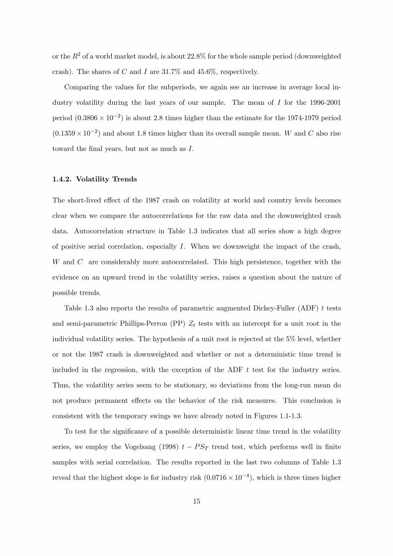
Table 1.3 also reports the results of parametric augmented Dickey-Fuller (ADF) t tests

and semi-parametric Phillips-Perron (PP) Zt tests with an intercept for a unit root in the

individual volatility series. The hypothesis of a unit root is rejected at the 5% level, whether

or not the 1987 crash is downweighted and whether or not a deterministic time trend is

included in the regression, with the exception of the ADF t test for the industry series.

Thus, the volatility series seem to be stationary, so deviations from the long-run mean do

not produce permanent effects on the behavior of the risk measures. This conclusion is

consistent with the temporary swings we have already noted in Figures 1.1-1.3.

To test for the significance of a possible deterministic linear time trend in the volatility

series, we employ the Vogelsang (1998) t − PST trend test, which performs well in finite

samples with serial correlation. The results reported in the last two columns of Table 1.3

reveal that the highest slope is for industry risk (0.0716× 10−4), which is three times higher

15

than for the world risk measure and about 2.8 times higher than the linear trend coefficient

for the country risk measure in the raw data set. The t−PST show that the trend coefficients

are not statistically positive at the 5% level even for I, and so we are unable to reject the

null hypothesis of no deterministic time increase for all volatility series. In fact, volatility

measures are higher by the end of our sample, but this does not seem to be the consequence

of a long-term upward trend.

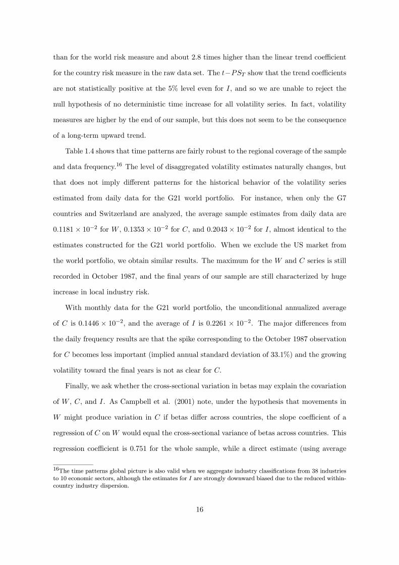
Table 1.4 shows that time patterns are fairly robust to the regional coverage of the sample

and data frequency.16 The level of disaggregated volatility estimates naturally changes, but

that does not imply different patterns for the historical behavior of the volatility series

estimated from daily data for the G21 world portfolio. For instance, when only the G7

countries and Switzerland are analyzed, the average sample estimates from daily data are

0.1181× 10−2 for W , 0.1353× 10−2 for C, and 0.2043× 10−2 for I, almost identical to the

estimates constructed for the G21 world portfolio. When we exclude the US market from

the world portfolio, we obtain similar results. The maximum for the W and C series is still

recorded in October 1987, and the final years of our sample are still characterized by huge

increase in local industry risk.

With monthly data for the G21 world portfolio, the unconditional annualized average

of C is 0.1446 × 10−2, and the average of I is 0.2261 × 10−2. The major differences from

the daily frequency results are that the spike corresponding to the October 1987 observation

for C becomes less important (implied annual standard deviation of 33.1%) and the growing

volatility toward the final years is not as clear for C.

Finally, we ask whether the cross-sectional variation in betas may explain the covariation

of W , C, and I. As Campbell et al. (2001) note, under the hypothesis that movements in

W might produce variation in C if betas differ across countries, the slope coefficient of a

regression of C onW would equal the cross-sectional variance of betas across countries. This

regression coefficient is 0.751 for the whole sample, while a direct estimate (using average

16The time patterns global picture is also valid when we aggregate industry classifications from 38 industriesto 10 economic sectors, although the estimates for I are strongly downward biased due to the reduced within-country industry dispersion.

16

weights) of the cross-sectional variance of country betas is only 0.016. Hence, the cross-

sectional variation in betas explains only a small proportion of the covariation between W

and C.

The importance of the cross-sectional variation in betas in explaining the covariation

between I and the other two volatility measures may be ascertained by a similar calculation.

The slope coefficients of regression of I on C and W are 0.887 and 0.348, respectively, which

seem too high to be explained by plausible cross-sectional variation in local industry beta

coefficients.

1.4.3. Individual Countries Risk Measures

Another interesting question is the behavior of the volatility components for individual coun-

tries. Volatility measures averaged across countries are informative about an ”average” coun-

try, but there can be great deal of variation in the industry composition across countries.

Country exposure to world shocks may also be different across countries.

If one is interested only in the behavior of local industry volatility in each country, we

can easily develop a measure of industry-specific volatility per country. We simply do not

take an average across countries of the industry-specific volatility for each country. That is,

from equation (1.2) and before taking the average across countries in equation (1.4), it can

be shown that:

Xi

xictV ar(Rict) = V ar(Rct) +Xi

xictV ar(uict). (1.11)

To avoid an incomplete variance decomposition, we assume a simple world market model,

and use the estimated country residuals variance to estimate country-specific volatility. The

only new parameters that need to be estimated are country betas, which we take as constant

for the whole sample period.

Consider the country decomposition with country betas relative to the world:

Rct = βcRwt + εct. (1.12)

17

In this framework, the variance of country c return is given by:

V ar(Rct) = β2cV ar(Rwt) + V ar(εct). (1.13)

Table 1.5 reports the individual country results, which give a strong message. The

increased industry volatility documented for the late 1990s at the world level, is also seen in

most individual countries. Linear trend coefficients are positive for 17 countries, although

not statistically significant. The results for the subperiods show that industry volatility is

on average higher for 1996-2001 than for previous years, for all countries with the exception

of New Zealand.17

Overall, smaller countries, or those most concentrated around a single industry portfolio,

or those that have more variation in the number of industry portfolios also tend to have

higher industry risk. The correlation across countries between average industry variance and

country market capitalization is negative (-0.380). Conversely, the correlation of the average

industry variance with the average weight of the largest local industry portfolio is 0.396, and

the correlation with the difference between maximum and minimum number of industries for

a given country is 0.296.

Two features strike us the most with regard to country risk. First, for three countries

(France, Norway, and the UK), a statistically significant negative slope is found.

Second, average country risk is much closer to industry risk than the equivalent aggregate

measures, and it varies more across countries than industry risk. These findings strengthen

the intuition that the characteristics of variance measures may vary considerably across

countries, particularly notable at the country risk level. Countries with higher industry risk

also tend to be riskier at the country level (the correlation between average industry variance

and average country variance across countries is 0.53).

Thus, we are not surprised to see that smaller countries, countries with more weight

given to a single industry, and countries with greater variation in the number of industry

portfolios also tend to have more country risk. The correlation across countries between

17Results are not shown here, but are available upon request.

18

average country variance and country market capitalization is -0.375. The correlation of the

average country variance with the average weight of the largest local industry portfolio is

0.502, and the correlation with the difference between maximum and minimum number of

industries for a given country is 0.571.

1.4.4. Individual Global Industry Risk Measures

To explore the behavior of global industry portfolio risk, we analyze two measures of risk.

The first is based on a version of the variance decomposition method of Campbell et al.

(2001) that decomposes the world portfolio into global industries, and uses the world market-

adjusted return model residuals to estimate global industry-specific variance:

Rit = Rwt + u∗it. (1.14)

As before, when the variances of global industry returns are aggregated using the same

weighting scheme used to compute world returns, a measure of the global level of industry

risk is obtained without having to estimate covariances or betas for global industries:

Xi

xitV ar(Rit) = V ar(Rwt) +Xi

xitV ar(u∗it). (1.15)

The second measure is used to analyze individual industry risk. It is based on the

residuals from a simple world market model for global industries, assuming constant betas

relative to the world returns for the whole sample period. Consider the global industry return

decomposition with global industry betas relative to the world:

Rit = βiRwt + v∗it. (1.16)

In this framework, the variance of global industry i return is given by:

V ar(Rit) = β2iwV ar(Rwt) + V ar(v∗it). (1.17)

19

Aggregate global industry variance,Pi xitV ar(u

∗it), is estimated using daily returns

within each month. Individual global industry variances, V ar(v∗it), are estimated using a

two step procedure. The first step consists of estimating betas by an ordinary least squares

regression of global industry monthly excess returns on world monthly excess returns. In

the second step, daily squared residuals from equation (1.16) are summed within a month

to obtain a monthly estimate for the variance of each global industry portfolio.

Panel A of Table 1.6 presents descriptive statistics and linear trend coefficient for the

global industry risk measure and Panel A of Figure 1.4 plots the series. Comparing indus-

try risk measured locally and globally, both series present positive linear trend coefficients,

although values are not statistically significant. In addition, both series show a significant

increase in the late 1990s; global industry risk reaches a historical maximum of 29.6% in

April 2000. The average global industry risk for the 1996 to 2001 period is about 1.7 times

higher than its unconditional mean and 2.5 times higher than in the early period between

1974 and 1979.

What might explain the increase in local and global industry risk that we document in

the last years of the sample? One possibility is that the anomalous behavior of one group of

industries, technology, media, and telecommunications companies (TMT), may have caused

sufficient cross-sectional dispersion to justify the huge spike in the industry risk series. In

fact, Brooks and Catao (2000) show that a global industry factor associated with the new

economy stocks emerged in the mid-1990s to become the key determinant of stock return

variability, and Brooks and Del Negro (2002b) find that, excluding the TMT stock group,

there is a much less pronounced increase in the importance of industry effects in recent years.

To further investigate this hypothesis and obtain insights into the impact of the new

economy stocks on the behavior of the aggregate risk measures, we reestimate global industry

risk excluding the TMT industries.18 Descriptive statistics on global industry risk excluding

the TMT industries are also shown in Panel A of Table 1.6, and Panel B of Figure 1.4 plots

the series.

18That is, we exclude the information technology hardware, media and photography, software and computerservices, and telecom services industries.

20

With the TMT industries excluded, we still see a sharp increase in global industry risk

in the late 1990s, although less of an increase than considering all industries. The historical

maximum is reached in October 1987 (28.7% annualized standard deviation), and the second-

highest value occurs in March 2000 (21%). The average point estimate for the 1996-2001

period is about 1.4 times higher than its unconditional mean and 1.9 times higher than in

the early period between 1974 and 1979. The full-sample average global industry volatility

for the 1996 to 2001 period is now almost 1.5 times higher than the ex-TMT industry results,

a pattern echoed by the standard deviation point estimates.

These results show that, at a global level, the TMT industries represented an important

component of the increase in industry risk toward the late 1990s, but the increase in risk is

not driven solely by these industries. The old economy also presented an important increase

in industry risk.

Panel B of Table 1.6 presents results for the 10 individual global industries with the largest

average market capitalization.19 There is no statistically significant time trend, although the

coefficients are positive for most global industries. The results suggest that smaller global

industries, with less variation in the number of countries where they operate, or that are

more concentrated in a single country, tend to be riskier. The correlation across global

industries of the average industry specific risk with the global industry market capitalization

is -0.234. The correlation of the average industry specific risk with the difference between

the maximum and minimum number of countries represented is -0.129, and the correlation

with the average weight of the most important country in each global industry is 0.583.

Interestingly, the global industry with highest average industry-specific variance is mining

(18.7%, whole sample annualized standard deviation), followed by the information technology

(18.6%), tobacco (17.7%) and water (17.5%). For the 1996-2001 period, the point estimate

of average industry-specific risk is higher than its unconditional mean for 35 of 38 industries.

Heston and Rouwenhorst (1994) conclude that country diversification is more efficient

than industry diversification. More recent evidence, e.g., Cavaglia et al. (2000), shows that

19Results for other industries are not shown here, but are available upon request.

21

industry diversification became as important as country diversification in the late 1990s. The

results in Table 1.6 suggest that the ratio of global industry risk to country risk has been

fairly stable over the years, with the exception of the notable increase from 1995 onward. This

ratio fluctuated around an average of 0.7 until 1989, followed by a period it was visibly lower

(on average 0.5 between 1990 and 1995), and finally a period of sustained increase in the late

1990s (on average greater than 1.0 after 1998). The ratio of local industry risk to country

risk (see Table 1.3) also shows a clear increase in the late 1990s. Thus, the results suggest

that towards the end of our sample period, international diversification power increases if an

industry dimension is privileged over a geographic dimension. These results are consistent

with the fixed-effects model evidence in Heston and Rouwenhorst (1994) and Cavaglia et al.

(2000).

1.4.5. Covariation and Causality

To assess the relative importance of each risk factor to the total volatility of a “typical”

within-country industry portfolio holding, we perform mean and variance decompositions.

By definition: σ2it = σ2ut+σ2et+σ2wt is the total volatility of a “typical” investment in a local

industry portfolio [see equation (1.4)] for period t. Then, taking expected values and dividing

the RHS elements by the LHS, we obtain a decomposition for the mean total volatility:

1 = E(σ2ut)/E(σ2it) +E(σ

2et)/E(σ

2it) +E(σ

2wt)/E(σ

2it). (1.18)

Specifying a sample period, we can estimate the expected values by their sample means,

using the volatility estimators defined in equations (1.8)-(1.10). Similarly, for the variance

of total volatility:

1 = V ar(σ2ut)/V ar(σ2it) + V ar(σ

2et)/V ar(σ

2it) + V ar(σ

2wt)/V ar(σ

2it) (1.19)

+2Cov(σ2ut,σ2et)/V ar(σ

2it) + 2Cov(σ

2ut,σ

2wt)/V ar(σ

2it)

+2Cov(σ2et,σ2wt)/V ar(σ

2it).

22

From the results in Table 1.3, we know that the variance of a randomly selected local

industry portfolio increases about 125% over the whole sample period (from 0.3224× 10−2

in the 1970’s to 0.007245 in the late 1990s, compared to a long-run unconditional mean

of 0.4620 × 10−2), and that the most significant increase occurred in the late 1990s. The

means in the first column of Table 1.7 confirm that local industry risk has gained increased

importance.

The share of I increased from 42.1% to 52.5% while the share of the other two risk

measures declined (W dropped by 2.2 and C by 8.2 percentage points) from 1974-1979 to

1996-2001, despite the fact that all risk measures rase on average. In the aftermath of the

highly turbulent period of the late 1980s, the early 1990s are an important exception with

regard to the importance of local industry risk across all subperiods (downweighted dataset).

From 1990 through 1995, the average point estimate of the country risk share of total risk is

38.9%, while the share of I is slightly lower (34.2%).

Analysis of the variance of total volatility provides further insight into the importance of

local industry risk. The variance of I represents not only the highest share of total volatility

for the whole sample period (downweighted dataset), but the relationship is also systematic

across subperiods, again with exception of the early 1990s and the 1970s. In fact, for the

1990-1995 period, the highest contribution to the variance of total volatility is given by the

covariance betweenW and C, while during the 1970s it is given by the covariance between C

and I. Interestingly, the share of the covariances between I and C or I andW (downweighted

data set) in total volatility variance are fairly stable across all subperiods (about 20%), with

the exception of the early 1990s (about 13%).

The results for both the mean and volatility decomposition of total volatility strengthen

the hypothesis that the total risk components demonstrate atypical behavior during the early

1990s, and that local industry-specific sources of risk become noticeably more important in

the late 1990s.

The high-frequency movements of the three volatility measures already noted in Figures

1.1-1.3 appear to be correlated, and the contemporaneous correlation estimates reported in

23

Panel A of Table 1.8 confirms this. To investigate the causality issue, we estimate bivariate

and multivariate vector autoregression (VAR). We use crash downweighted variance series,

and the multivariate version of the Akaike information criterion is used to select the VAR

lag length (10 lags for the pairW and C and 6 lags for the remaining pairs and the trivariate

system).

Panels B and C of Table 1.8 report the p-values of a standard F-test on each equation for

the null hypothesis that the lags 1 to k of each variable do not help to forecast the dependent

variable for the VAR systems.

In the bivariate VARs, I appears to Granger-cause both W and C. The world risk

does not help to forecast any of the other series, while C helps to predict W at the 5%

significance level. In the trivariate system, neitherW nor C helps to predict any of the other

series, while I helps to predict W and also Granger-causes C at the 5% significance level.

Thus, our evidence supports the hypothesis that local industry risk leads the other volatility

series.

1.5. Global Portfolio Management Implications

Has the power of international diversification to reduce risk been lessened? Is country

diversification still the most effective diversification strategy for the global equity investor?

In an attempt to corroborate the intuition based on our volatility results, we present results

of traditional correlation and portfolio diversification analyses.

Declining correlations among individual assets returns would let the volatility of the

market portfolio remain stable even if individual volatilities rise. Thus, the growing increase

in the importance of local industry risk relative to the common factor (world risk) noticed

toward the end of our sample (and plotted in Panel A of Figure 1.5) is consistent with

reduced correlations among local industry portfolios.

Panel B of Figure 1.5 plots the equal-weighted average pairwise correlation among lo-

cal industry portfolios available in our sample. We use both monthly and daily returns.20

20In international stock market studies, one cannot ignore the effects of non-overlapping trading hours on thecorrelation between assets traded in non-contemporaneous markets, which are more significant with the use

24

Correlations are calculated each month, between all pairs of industry portfolios for which 60

months (260 days) of data are available for that month. The number of estimated monthly

(daily) pairwise correlations ranges from about 36,000 to over 153,000 (184,000) as the num-

ber of basic assets changes over time. Monthly correlations are systematically higher for the

whole sample (0.265 average) than daily estimates (0.146), which is consistent with the daily

downward biases for positively related markets.

Overall, the average correlation plot confirms our conclusion of reduced correlations.

From 1996 through 2001, monthly (daily) pairwise correlations fluctuate around an average

of 0.203 (0.125), which is lower than the average for the 1990-1995 period, 0.309 (0.175).

The ratio of local industry risk to world risk (I/W ) shows the opposite pattern: 3.23 for

the 1996-2001 period and 1.0 for the early 1990s. This contrasting behavior between average

correlation and the I/W ratio is also clear when we compare the 1996-2001 period with

1974-1995, when the long-term mean of average monthly (daily) pairwise correlation is 0.287

(0.153) and the I/W ratio is on average 2.5.21

As lower correlations imply greater diversification opportunities, we conclude that, for

global investors who invest in local industry portfolios, the risk reduction benefits of inter-

national diversification rose in the late 1990s, over previous years. Another implication of

the observed rise in local industry-level volatility relative to world market risk is that more

randomly selected assets are needed to achieve a given level of diversification. Similarly, the

average volatility of portfolios made of the same number of randomly selected assets will be

higher, with an increased amount of idiosyncratic volatility that has to be diversified away.

To illustrate this point, we construct portfolios containing different numbers of randomly

selected assets, and compute the simple average of the difference between each portfolio

standard deviation and the standard deviation of an equally weighted portfolio of all assets

used in the calculations. For each year-end, we randomly group (without replacement) local

of daily data. Kahya (1997) shows that the estimated correlations of daily returns for positively (negatively)related markets are biased downward (upward). There is no significant bias associated with the use of monthlydata.21Comparison of the daily correlation plot with a 12-month moving average of the I/W ratio plot also revealsan inverse relation between the two measures (correlation of -0.587 for the whole sample).

25

industry portfolios with at least 60 consecutive monthly return observations available up to

that date. Panel A of Figure 1.6 plots annualized excess standard deviations over time for

portfolios of 2, 5, 20, and 40 assets calculated from monthly returns.22

The peak in excess standard deviation is reached in 2000 for all portfolios (10.7%), and

all exhibit a modest increase up through 1995. For the 2-randomly selected local industry

portfolio, the excess standard deviation is 8.0% in 1995 compared with 7.7% in 1978. For

the larger portfolios, the pattern is the same, although at much lower values.

Panel B of Figure 1.6 plots annualized excess standard deviation against number of

assets in the portfolio calculated from monthly returns. Data for these plots are obtained by

averaging the yearly estimates of excess standard deviations over the sample periods. As is

shown, the increase in local industry risk for the 1996-2001 period implies that more basic

assets are needed to reduce excess standard deviation. For instance, estimates show that

to reduce excess volatility to about 2%, 12 industry portfolios are needed in the 1996-2001

period. In earlier sample periods, the same level of diversification could be reached with

approximately 9 industries.

1.6. Conclusion

We have extended the volatility decomposition method of Campbell et al. (2001) to an

international setting in order to take a new look at the historical behavior of volatility in

developed stock markets. We study the time series behavior and international diversification

implications of three non-overlapping monthly measures of stock volatility: variance of world

portfolio returns, average variance of country returns relative to world returns, and average

variance of local industry portfolios returns relative to their countries.

We find that between 1974 and 2001, world and country risk remained fairly stable.

Industry risk, both at the local and the global level, however, displayed a huge increase

during the late 1990s, after a long period of relative stability. This increase is not attributable

solely to the new economy bubble. Local industry risk dominates world and country risk,

22Similar results using daily returns are not shown here, but are available upon request.

26

except during the 1990-1995 period, when country risk is on average the most important

component. World risk is systematically the least important component of total risk.

We show that the October 1987 crash had a short-lived but abnormally high impact on

both world and country risk, but a much less pronounced impact at the local industry level.

Granger causality tests suggest that lagged local industry volatility has explanatory power

in forecasting world and country volatility series, but the converse is not true.

Consistent with the behavior of industry risk, toward the end of our sample, pairwise

correlations among local industry portfolios drop and, not surprisingly, higher numbers of

randomly selected assets are needed to achieve any given level of diversification after 1995.

These results suggest that the power of international diversification to reduce risk has not

been eroded as the process of globalization might imply. Our results also support a con-

clusion that industry diversification has become relatively more efficient than geographic

diversification in the latter years of our sample only, although this may be a temporary

result.

27

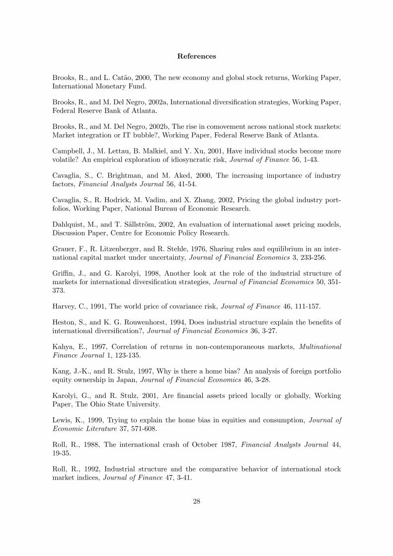
References

Brooks, R., and L. Catao, 2000, The new economy and global stock returns, Working Paper,International Monetary Fund.

Brooks, R., and M. Del Negro, 2002a, International diversification strategies, Working Paper,Federal Reserve Bank of Atlanta.

Brooks, R., and M. Del Negro, 2002b, The rise in comovement across national stock markets:Market integration or IT bubble?, Working Paper, Federal Reserve Bank of Atlanta.

Campbell, J., M. Lettau, B. Malkiel, and Y. Xu, 2001, Have individual stocks become morevolatile? An empirical exploration of idiosyncratic risk, Journal of Finance 56, 1-43.

Cavaglia, S., C. Brightman, and M. Aked, 2000, The increasing importance of industryfactors, Financial Analysts Journal 56, 41-54.

Cavaglia, S., R. Hodrick, M. Vadim, and X. Zhang, 2002, Pricing the global industry port-folios, Working Paper, National Bureau of Economic Research.

Dahlquist, M., and T. Sallstrom, 2002, An evaluation of international asset pricing models,Discussion Paper, Centre for Economic Policy Research.

Grauer, F., R. Litzenberger, and R. Stehle, 1976, Sharing rules and equilibrium in an inter-national capital market under uncertainty, Journal of Financial Economics 3, 233-256.

Griffin, J., and G. Karolyi, 1998, Another look at the role of the industrial structure ofmarkets for international diversification strategies, Journal of Financial Economics 50, 351-373.

Harvey, C., 1991, The world price of covariance risk, Journal of Finance 46, 111-157.

Heston, S., and K. G. Rouwenhorst, 1994, Does industrial structure explain the benefits ofinternational diversification?, Journal of Financial Economics 36, 3-27.

Kahya, E., 1997, Correlation of returns in non-contemporaneous markets, MultinationalFinance Journal 1, 123-135.

Kang, J.-K., and R. Stulz, 1997, Why is there a home bias? An analysis of foreign portfolioequity ownership in Japan, Journal of Financial Economics 46, 3-28.

Karolyi, G., and R. Stulz, 2001, Are financial assets priced locally or globally, WorkingPaper, The Ohio State University.

Lewis, K., 1999, Trying to explain the home bias in equities and consumption, Journal ofEconomic Literature 37, 571-608.

Roll, R., 1988, The international crash of October 1987, Financial Analysts Journal 44,19-35.

Roll, R., 1992, Industrial structure and the comparative behavior of international stockmarket indices, Journal of Finance 47, 3-41.

28

Schwert, G., 1989, Why does stock market volatility change over time?, Journal of Finance44, 1115-1153.

Schwert, G., 1998, Stock market volatility: Ten years after the crash, Brookings-WhartonPapers on Financial Services 1, 65-114.

Solnik, B., 1974, Why not diversify internationally rather than domestically?, FinancialAnalysts Journal 30, 48-54.

Stulz, R., 1999, Globalization of equity markets and the cost of capital, Working Paper, TheOhio State University.

Vogelsang, T., 1998, Trend function hypothesis testing in the presence of serial correlation,Econometrica 66, 123-148.

29

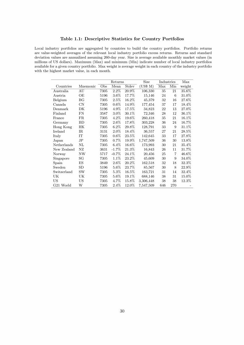
Table 1.1: Descriptive Statistics for Country Portfolios

Local industry portfolios are aggregated by countries to build the country portfolios. Portfolio returnsare value-weighted averages of the relevant local industry portfolio excess returns. Returns and standarddeviation values are annualized assuming 260-day year. Size is average available monthly market values (inmillions of US dollars). Maximum (Max) and minimum (Min) indicate number of local industry portfoliosavailable for a given country portfolio. Max weight is average weight in each country of the industry portfoliowith the highest market value, in each month.

Returns Size Industries MaxCountries Mnemonic Obs Mean Stdev (US$ M) Max Min weight

Australia AU 7305 2.2% 20.9% 106,330 35 21 35.6%Austria OE 5196 3.6% 17.7% 15,146 24 6 31.0%Belgium BG 7305 2.5% 16.2% 45,379 32 16 27.6%Canada CN 7305 0.6% 14.9% 177,454 37 17 18.4%Denmark DK 5196 4.9% 17.5% 34,823 22 13 27.0%Finland FN 3587 3.0% 30.1% 72,346 28 12 36.1%France FR 7305 4.2% 19.6% 260,418 35 21 16.1%Germany BD 7305 2.6% 17.8% 303,228 36 24 16.7%Hong Kong HK 7305 6.2% 29.8% 128,791 33 9 31.1%Ireland IR 3131 2.0% 18.4% 36,557 27 21 28.5%Italy IT 7305 0.6% 23.5% 142,645 33 17 27.8%Japan JP 7305 0.7% 19.9% 1,747,509 36 30 13.8%Netherlands NL 7305 6.4% 16.6% 173,993 30 21 35.4%New Zealand NZ 3631 -1.7% 21.3% 16,843 26 11 31.7%Norway NW 5717 -0.7% 24.1% 20,456 25 7 46.6%Singapore SG 7305 1.1% 23.2% 45,609 30 9 34.0%Spain ES 3849 2.6% 20.2% 162,518 32 18 32.3%Sweden SD 5196 5.6% 23.7% 85,567 30 8 22.9%Switzerland SW 7305 5.3% 16.5% 163,721 31 14 32.4%UK UK 7305 5.6% 19.1% 688,146 38 31 15.0%US US 7305 4.7% 15.8% 3,306,448 38 38 12.3%G21 World W 7305 2.4% 12.0% 7,547,509 646 270 -

30

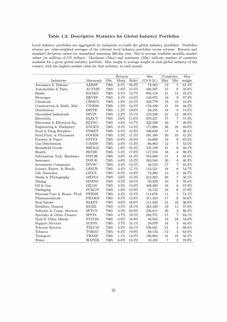
Table 1.2: Descriptive Statistics for Global Industry Portfolios

Local industry portfolios are aggregated by industries to build the global industry portfolios. Portfoliosreturns are value-weighted averages of the relevant local industry portfolios excess returns. Returns andstandard deviation values are annualized assuming 260-day year. Size is average available monthly marketvalues (in millions of US dollars). Maximum (Max) and minimum (Min) indicate number of countriesavailable for a given global industry portfolio. Max weight is average weight in each global industry of thecountry with the highest market value for that industry, in each month.

Returns Size Countries MaxIndustries Mnemonic Obs. Mean Stdev (US $ M.) Max Min weight

Aerospace & Defense AERSP 7305 6.5% 16.8% 72,562 12 5 81.4%Automobiles & Parts AUTMB 7305 1.8% 15.5% 246,507 15 8 50.9%Banks BANKS 7305 3.5% 14.7% 805,118 21 12 44.5%Beverages BEVES 7305 4.1% 14.8% 143,975 18 9 57.3%Chemicals CHMCL 7305 1.9% 13.5% 228,779 19 10 44.4%Construction & Build. Mat. CNSBM 7305 1.5% 14.5% 158,439 21 10 48.2%Distributors DISTR 7305 -1.2% 19.6% 64,195 18 9 74.5%Diversified Industrials DIVIN 7305 2.2% 15.1% 153,249 21 12 39.0%Electricity ELECT 7305 3.6% 11.6% 278,227 17 7 57.3%Electronic & Electrical Eq. ELTNC 7305 4.0% 15.7% 322,339 20 7 46.9%Engineering & Machinery ENGEN 7305 0.4% 14.4% 171,004 20 10 48.0%Food & Drug Retailers FDRET 7305 6.5% 12.9% 106,639 17 6 46.4%Food Prod. & Processors FOODS 7305 5.5% 11.3% 191,100 20 10 41.2%Forestry & Paper FSTPA 7305 -0.6% 16.8% 64,008 19 6 63.3%Gas Distribution GASDS 7305 3.8% 15.4% 66,862 12 7 53.5%Household Goods HHOLD 7305 1.0% 16.2% 105,159 21 6 56.1%Health HLTHC 7305 5.4% 17.6% 117,558 16 4 90.2%Information Tech. Hardware INFOH 7305 3.0% 21.9% 554,989 17 4 65.5%Insurance INSUR 7305 4.6% 13.2% 283,584 20 8 40.3%Investment Companies INVSC 7305 3.4% 12.5% 48,553 17 7 43.3%Leisure, Entert. & Hotels LESUR 7305 4.4% 17.1% 113,521 18 6 54.7%Life Assurance LIFEA 7305 6.2% 14.8% 72,392 14 5 42.7%Media & Photography MEDIA 7305 2.6% 15.3% 212,302 20 7 56.1%Mining MNING 7305 0.3% 19.5% 50,339 10 5 50.8%Oil & Gas OILGS 7305 4.5% 15.6% 449,280 19 8 57.3%Packaging PCKGN 7305 1.9% 13.9% 16,743 16 6 47.9%Personal Care & House. Prod. PERSH 7305 4.4% 15.5% 111,676 11 5 74.1%Pharmaceuticals PHARM 7305 6.5% 14.9% 471,423 17 6 56.6%Real Estate RLEST 7305 0.6% 16.6% 111,942 21 10 36.6%Retailers, General RTAIL 7305 3.5% 16.5% 262,459 19 11 57.9%Software & Comp. Services SFTCS 7305 4.5% 24.6% 236,811 20 2 86.8%Specialty & Other Finance SPFIN 7305 4.7% 19.5% 284,771 17 7 62.1%Steel & Other Metals STLOM 7305 -2.0% 18.9% 89,853 18 10 58.0%Support Services SUPSV 7305 3.7% 14.1% 59,079 18 4 44.8%Telecom Services TELCM 7305 2.2% 16.1% 556,621 21 4 66.0%Tobacco TOBAC 7305 8.3% 19.9% 68,134 12 4 63.0%Transport TRNSP 7305 1.1% 14.0% 186,884 21 10 50.2%Water WATER 7305 6.8% 18.2% 10,432 7 2 70.9%

31

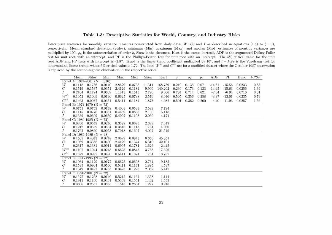
Table 1.3: Descriptive Statistics for World, Country, and Industry Risks

Descriptive statistics for monthly variance measures constructed from daily data, W , C, and I as described in equations (1.8) to (1.10),respectively. Mean, standard deviation (Stdev), minimum (Min), maximum (Max), and median (Med) estimates of monthly variances aremultiplied by 100. ρk is the autocorrelation of order k, Skew is the skewness, Kurt is the excess kurtosis, ADF is the augmented Dickey-Fullertest for unit root with an intercept, and PP is the Phillips-Perron test for unit root with an intercept. The 5% critical value for the unitroot ADF and PP tests with intercept is —2.87. Trend is the linear trend coefficient multiplied by 104, and t − PST is the Vogelsang test fordeterministic linear trends whose 5% critical value is 1.72. The linesW dc and Cdc are for a modified dataset where the October 1987 observationis replaced by the second-highest observation in the respective series.

Mean Stdev Min Max Med Skew Kurt ρ1 ρ2 ρ6 ADF PP Trend t-PSTPanel A: 1974-2001 (N = 336)W 0.1118 0.1786 0.0140 2.8629 0.0738 11.311 168.739 0.219 0.135 0.071 -14.61 -15.56 0.0233 0.83C 0.1519 0.1537 0.0351 2.4129 0.1184 9.900 140.202 0.230 0.173 0.133 -14.45 -15.63 0.0256 1.39I 0.2104 0.1724 0.0669 1.1813 0.1515 2.790 9.066 0.784 0.714 0.621 -2.64 -6.94 0.0716 0.31W dc 0.1052 0.1009 0.0140 0.6625 0.0738 2.576 8.040 0.505 0.356 0.258 -3.37 -12.01 0.0235 0.79Cdc 0.1463 0.0937 0.0351 0.5411 0.1184 1.873 4.082 0.501 0.362 0.260 -4.40 -11.93 0.0257 1.56Panel B: 1974-1979 (N = 72)W 0.0751 0.0742 0.0148 0.4003 0.0533 2.582 7.724C 0.1115 0.0776 0.0351 0.4489 0.0836 2.100 5.118I 0.1359 0.0699 0.0669 0.4092 0.1108 2.030 4.121Panel C: 1980-1985 (N = 72)W 0.0830 0.0549 0.0246 0.3328 0.0695 2.389 7.349C 0.1212 0.0559 0.0504 0.3516 0.1113 1.734 4.060I 0.1762 0.0860 0.0953 0.7018 0.1607 4.092 21.549Panel D: 1986-1989 (N = 48)W 0.1565 0.4043 0.0248 2.8629 0.0843 6.656 45.351C 0.1969 0.3368 0.0490 2.4129 0.1374 6.310 42.101I 0.2317 0.1381 0.0911 0.6997 0.1781 1.626 2.445W dc 0.1107 0.1044 0.0248 0.6625 0.0843 3.758 17.326Cdc 0.1579 0.0997 0.0490 0.5411 0.1374 1.754 3.787Panel E: 1990-1995 (N = 72)W 0.1064 0.1129 0.0172 0.6625 0.0698 2.764 9.185C 0.1535 0.0904 0.0560 0.5411 0.1141 1.885 4.597I 0.1349 0.0497 0.0783 0.3423 0.1226 2.062 5.417Panel F: 1996-2001 (N = 72)W 0.1527 0.1258 0.0140 0.5215 0.1164 1.358 1.144C 0.1911 0.1160 0.0461 0.5309 0.1551 1.402 1.553I 0.3806 0.2657 0.0885 1.1813 0.2834 1.227 0.918

32

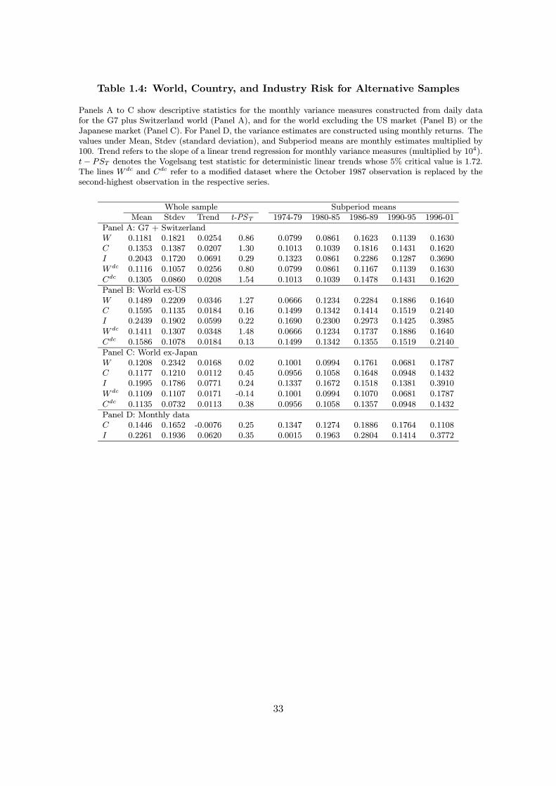
Table 1.4: World, Country, and Industry Risk for Alternative Samples

Panels A to C show descriptive statistics for the monthly variance measures constructed from daily datafor the G7 plus Switzerland world (Panel A), and for the world excluding the US market (Panel B) or theJapanese market (Panel C). For Panel D, the variance estimates are constructed using monthly returns. Thevalues under Mean, Stdev (standard deviation), and Subperiod means are monthly estimates multiplied by100. Trend refers to the slope of a linear trend regression for monthly variance measures (multiplied by 104).t− PST denotes the Vogelsang test statistic for deterministic linear trends whose 5% critical value is 1.72.The lines W dc and Cdc refer to a modified dataset where the October 1987 observation is replaced by thesecond-highest observation in the respective series.

Whole sample Subperiod meansMean Stdev Trend t-PST 1974-79 1980-85 1986-89 1990-95 1996-01

Panel A: G7 + SwitzerlandW 0.1181 0.1821 0.0254 0.86 0.0799 0.0861 0.1623 0.1139 0.1630C 0.1353 0.1387 0.0207 1.30 0.1013 0.1039 0.1816 0.1431 0.1620I 0.2043 0.1720 0.0691 0.29 0.1323 0.0861 0.2286 0.1287 0.3690W dc 0.1116 0.1057 0.0256 0.80 0.0799 0.0861 0.1167 0.1139 0.1630Cdc 0.1305 0.0860 0.0208 1.54 0.1013 0.1039 0.1478 0.1431 0.1620

Panel B: World ex-USW 0.1489 0.2209 0.0346 1.27 0.0666 0.1234 0.2284 0.1886 0.1640C 0.1595 0.1135 0.0184 0.16 0.1499 0.1342 0.1414 0.1519 0.2140I 0.2439 0.1902 0.0599 0.22 0.1690 0.2300 0.2973 0.1425 0.3985W dc 0.1411 0.1307 0.0348 1.48 0.0666 0.1234 0.1737 0.1886 0.1640Cdc 0.1586 0.1078 0.0184 0.13 0.1499 0.1342 0.1355 0.1519 0.2140

Panel C: World ex-JapanW 0.1208 0.2342 0.0168 0.02 0.1001 0.0994 0.1761 0.0681 0.1787C 0.1177 0.1210 0.0112 0.45 0.0956 0.1058 0.1648 0.0948 0.1432I 0.1995 0.1786 0.0771 0.24 0.1337 0.1672 0.1518 0.1381 0.3910W dc 0.1109 0.1107 0.0171 -0.14 0.1001 0.0994 0.1070 0.0681 0.1787Cdc 0.1135 0.0732 0.0113 0.38 0.0956 0.1058 0.1357 0.0948 0.1432

Panel D: Monthly dataC 0.1446 0.1652 -0.0076 0.25 0.1347 0.1274 0.1886 0.1764 0.1108I 0.2261 0.1936 0.0620 0.35 0.0015 0.1963 0.2804 0.1414 0.3772

33

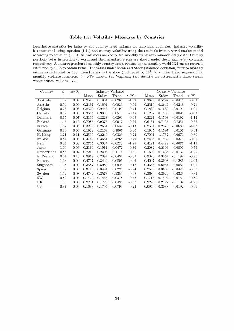
Table 1.5: Volatility Measures by Countries

Descriptive statistics for industry and country level variance for individual countries. Industry volatilityis constructed using equation (1.11) and country volatility using the residuals from a world market modelaccording to equation (1.13). All variances are computed monthly using within-month daily data. Countryportfolio betas in relation to world and their standard errors are shown under the β and se(β) columns,respectively. A linear regression of monthly country excess returns on the monthly world G21 excess return isestimated by OLS to obtain betas. The values under Mean and Stdev (standard deviation) refer to monthlyestimates multiplied by 100. Trend refers to the slope (multiplied by 104) of a linear trend regression formonthly variance measures. t − PST denotes the Vogelsang test statistic for deterministic linear trendswhose critical value is 1.72.

Country β se(β) Industry Variance Country VarianceMean Stdev Trend t-PST Mean Stdev Trend t-PST

Australia 1.02 0.08 0.2580 0.1864 -0.0264 -1.39 0.3626 0.5292 -0.0446 -0.63Austria 0.54 0.09 0.2497 0.1894 0.0823 0.56 0.2319 0.2649 -0.0248 -0.21Belgium 0.76 0.06 0.2579 0.2453 -0.0193 -0.74 0.1880 0.1689 -0.0191 -1.01Canada 0.89 0.05 0.3684 0.9885 0.0515 -0.48 0.1207 0.1356 0.0098 -0.03Denmark 0.65 0.07 0.3136 0.2228 0.0263 -0.39 0.2221 0.1508 -0.0192 -1.12Finland 1.15 0.13 0.7085 0.9375 0.0917 -0.36 0.6181 0.7135 0.7356 0.68France 1.02 0.06 0.3213 0.2661 0.0532 -0.13 0.2534 0.2378 -0.0685 -4.07Germany 0.80 0.06 0.1922 0.2168 0.1067 0.30 0.1935 0.1597 0.0106 0.34H. Kong 1.21 0.11 0.2530 0.2240 0.0323 -0.22 0.7001 1.1762 -0.0671 -0.80Ireland 0.84 0.08 0.4769 0.3551 0.4268 0.79 0.2435 0.1932 0.0371 -0.05Italy 0.84 0.08 0.2715 0.3087 -0.0228 -1.25 0.4121 0.4429 -0.0677 -1.19Japan 1.10 0.06 0.2169 0.1914 0.0472 0.30 0.2082 0.2396 0.0890 0.59Netherlands 0.85 0.04 0.2253 0.2408 0.1115 0.31 0.1603 0.1435 -0.0137 -1.29N. Zealand 0.84 0.10 0.3969 0.2897 -0.0491 -0.69 0.3826 0.3857 -0.1194 -0.95Norway 1.03 0.09 0.4717 0.3440 0.0806 -0.06 0.4097 0.3903 -0.1286 -2.65Singapore 1.18 0.09 0.3587 0.5980 0.0925 0.12 0.4356 0.6057 -0.0569 -1.01Spain 1.02 0.08 0.3128 0.3491 0.0225 -0.24 0.2593 0.3636 -0.0479 -0.67Sweden 1.12 0.08 0.4742 0.3573 0.2359 0.98 0.3680 0.3929 0.0323 -0.39SW 0.82 0.05 0.1479 0.1455 0.0318 0.52 0.1713 0.1492 -0.0151 -0.80UK 1.06 0.06 0.2241 0.1726 0.0434 -0.07 0.2290 0.2722 -0.1109 -1.96US 0.87 0.03 0.1688 0.1795 0.0793 0.23 0.0940 0.2088 0.0192 0.91

34

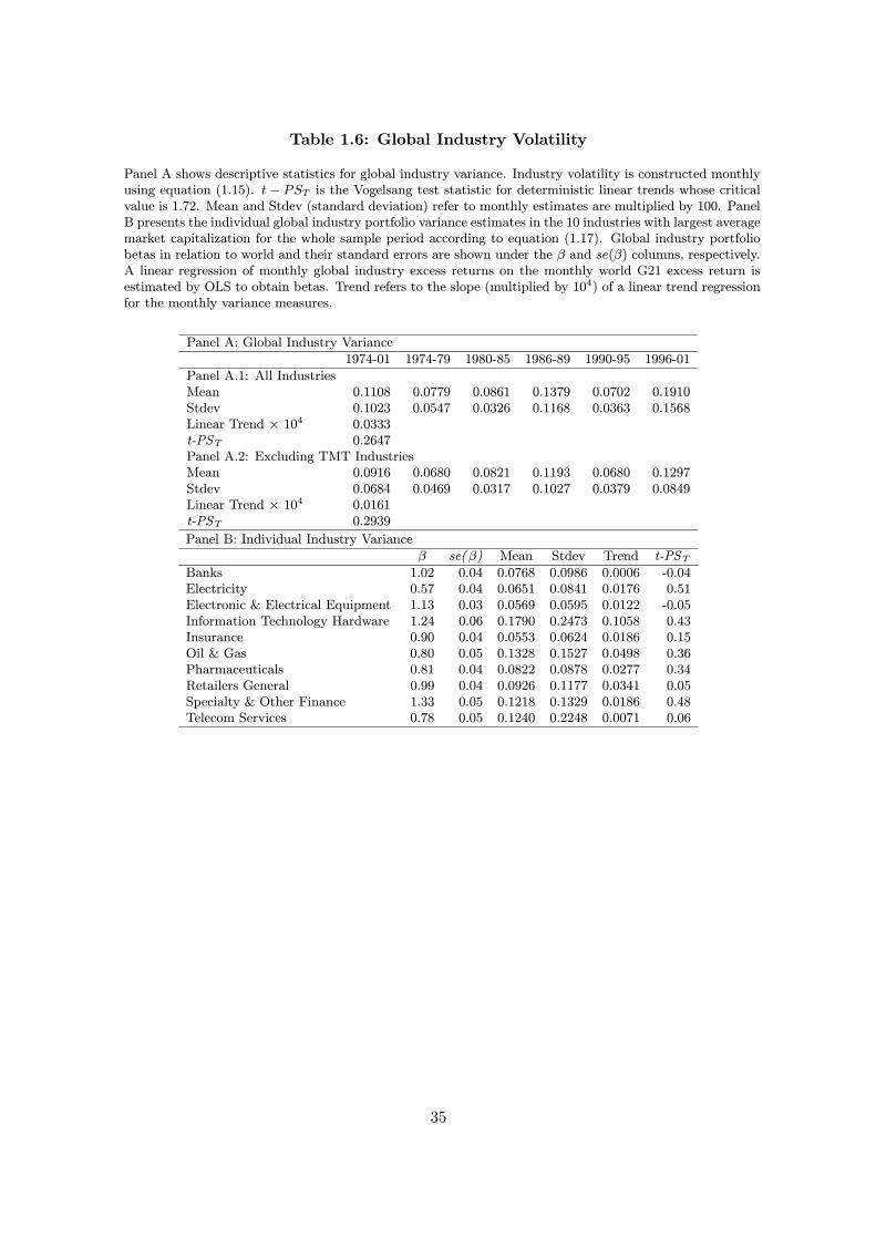
Table 1.6: Global Industry Volatility

Panel A shows descriptive statistics for global industry variance. Industry volatility is constructed monthlyusing equation (1.15). t − PST is the Vogelsang test statistic for deterministic linear trends whose criticalvalue is 1.72. Mean and Stdev (standard deviation) refer to monthly estimates are multiplied by 100. PanelB presents the individual global industry portfolio variance estimates in the 10 industries with largest averagemarket capitalization for the whole sample period according to equation (1.17). Global industry portfoliobetas in relation to world and their standard errors are shown under the β and se(β) columns, respectively.A linear regression of monthly global industry excess returns on the monthly world G21 excess return isestimated by OLS to obtain betas. Trend refers to the slope (multiplied by 104) of a linear trend regressionfor the monthly variance measures.

Panel A: Global Industry Variance

1974-01 1974-79 1980-85 1986-89 1990-95 1996-01

Panel A.1: All IndustriesMean 0.1108 0.0779 0.0861 0.1379 0.0702 0.1910Stdev 0.1023 0.0547 0.0326 0.1168 0.0363 0.1568Linear Trend × 104 0.0333t-PST 0.2647Panel A.2: Excluding TMT IndustriesMean 0.0916 0.0680 0.0821 0.1193 0.0680 0.1297Stdev 0.0684 0.0469 0.0317 0.1027 0.0379 0.0849Linear Trend × 104 0.0161t-PST 0.2939

Panel B: Individual Industry Variance

β se(β) Mean Stdev Trend t-PSTBanks 1.02 0.04 0.0768 0.0986 0.0006 -0.04Electricity 0.57 0.04 0.0651 0.0841 0.0176 0.51Electronic & Electrical Equipment 1.13 0.03 0.0569 0.0595 0.0122 -0.05Information Technology Hardware 1.24 0.06 0.1790 0.2473 0.1058 0.43Insurance 0.90 0.04 0.0553 0.0624 0.0186 0.15Oil & Gas 0.80 0.05 0.1328 0.1527 0.0498 0.36Pharmaceuticals 0.81 0.04 0.0822 0.0878 0.0277 0.34Retailers General 0.99 0.04 0.0926 0.1177 0.0341 0.05Specialty & Other Finance 1.33 0.05 0.1218 0.1329 0.0186 0.48Telecom Services 0.78 0.05 0.1240 0.2248 0.0071 0.06

35

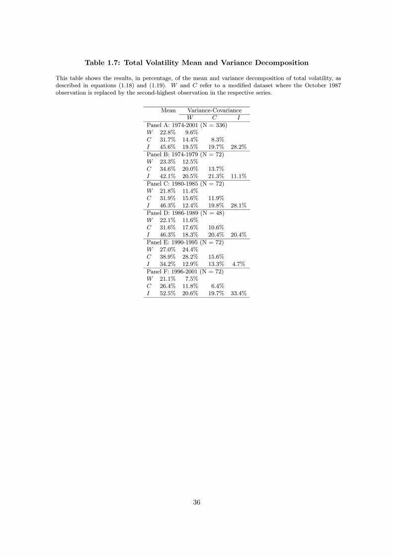
Table 1.7: Total Volatility Mean and Variance Decomposition

This table shows the results, in percentage, of the mean and variance decomposition of total volatility, asdescribed in equations (1.18) and (1.19). W and C refer to a modified dataset where the October 1987observation is replaced by the second-highest observation in the respective series.

Mean Variance-CovarianceW C I

Panel A: 1974-2001 (N = 336)W 22.8% 9.6%C 31.7% 14.4% 8.3%I 45.6% 19.5% 19.7% 28.2%

Panel B: 1974-1979 (N = 72)W 23.3% 12.5%C 34.6% 20.0% 13.7%I 42.1% 20.5% 21.3% 11.1%

Panel C: 1980-1985 (N = 72)W 21.8% 11.4%C 31.9% 15.6% 11.9%I 46.3% 12.4% 19.8% 28.1%

Panel D: 1986-1989 (N = 48)W 22.1% 11.6%C 31.6% 17.6% 10.6%I 46.3% 18.3% 20.4% 20.4%

Panel E: 1990-1995 (N = 72)W 27.0% 24.4%C 38.9% 28.2% 15.6%I 34.2% 12.9% 13.3% 4.7%

Panel F: 1996-2001 (N = 72)W 21.1% 7.5%C 26.4% 11.8% 6.4%I 52.5% 20.6% 19.7% 33.4%

36

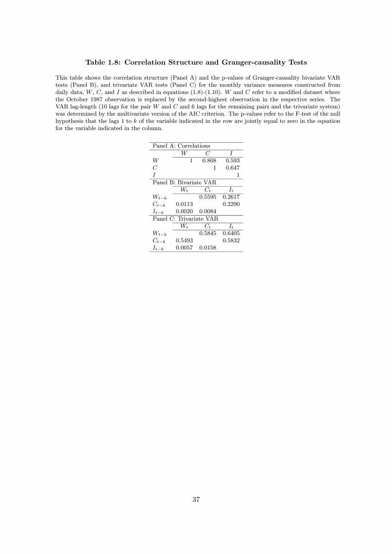
Table 1.8: Correlation Structure and Granger-causality Tests

This table shows the correlation structure (Panel A) and the p-values of Granger-causality bivariate VARtests (Panel B), and trivariate VAR tests (Panel C) for the monthly variance measures constructed fromdaily data, W , C, and I as described in equations (1.8)-(1.10). W and C refer to a modified dataset wherethe October 1987 observation is replaced by the second-highest observation in the respective series. TheVAR lag-length (10 lags for the pair W and C and 6 lags for the remaining pairs and the trivariate system)was determined by the multivariate version of the AIC criterion. The p-values refer to the F-test of the nullhypothesis that the lags 1 to k of the variable indicated in the row are jointly equal to zero in the equationfor the variable indicated in the column.

Panel A: Correlations

W C IW 1 0.808 0.593C 1 0.647I 1

Panel B: Bivariate VARWt Ct It

Wt−k 0.5595 0.2617Ct−k 0.0113 0.2290It−k 0.0020 0.0084

Panel C: Trivariate VARWt Ct It

Wt−k 0.5845 0.6405Ct−k 0.5493 0.5832It−k 0.0057 0.0158

37

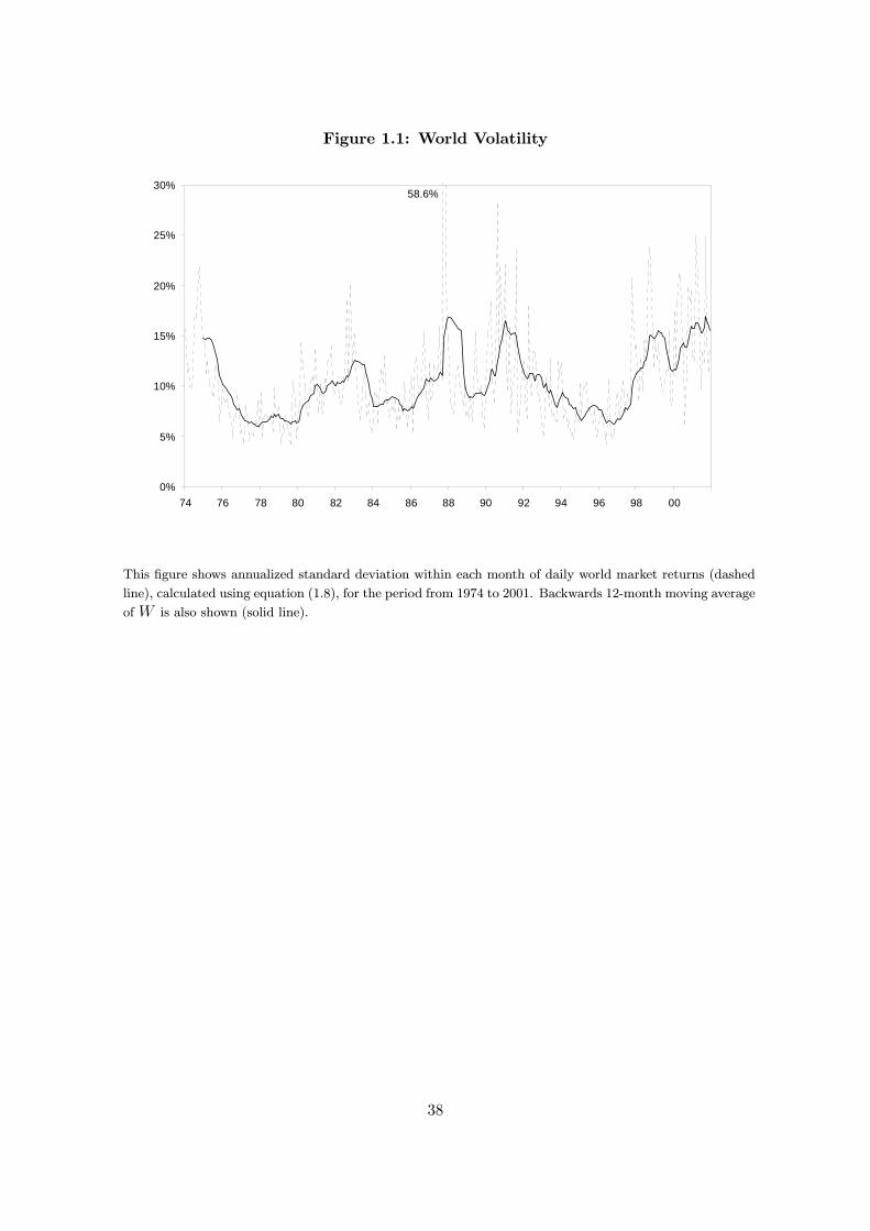
Figure 1.1: World Volatility

58.6%

0%

5%

10%

15%

20%

25%

30%

74 76 78 80 82 84 86 88 90 92 94 96 98 00

This figure shows annualized standard deviation within each month of daily world market returns (dashed

line), calculated using equation (1.8), for the period from 1974 to 2001. Backwards 12-month moving average

ofW is also shown (solid line).

38

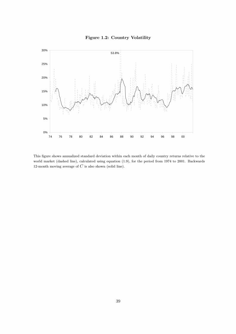
Figure 1.2: Country Volatility

53.8%

0%

5%

10%

15%

20%

25%

30%

74 76 78 80 82 84 86 88 90 92 94 96 98 00

This figure shows annualized standard deviation within each month of daily country returns relative to the

world market (dashed line), calculated using equation (1.9), for the period from 1974 to 2001. Backwards

12-month moving average of C is also shown (solid line).

39

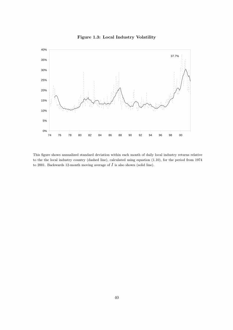
Figure 1.3: Local Industry Volatility

37.7%

0%

5%

10%

15%

20%

25%

30%

35%

40%

74 76 78 80 82 84 86 88 90 92 94 96 98 00

This figure shows annualized standard deviation within each month of daily local industry returns relative

to the the local industry country (dashed line), calculated using equation (1.10), for the period from 1974

to 2001. Backwards 12-month moving average of I is also shown (solid line).

40

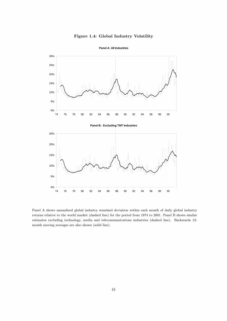
Figure 1.4: Global Industry Volatility

Panel A: All Industries

0%

5%

10%

15%

20%

25%

30%

74 76 78 80 82 84 86 88 90 92 94 96 98 00

Panel B: Excluding TMT Industries

0%

5%

10%

15%

20%

25%

74 76 78 80 82 84 86 88 90 92 94 96 98 00

Panel A shows annualized global industry standard deviation within each month of daily global industry

returns relative to the world market (dashed line) for the period from 1974 to 2001. Panel B shows similar

estimates excluding technology, media and telecommunications industries (dashed line). Backwards 12-

month moving averages are also shown (solid line).

41

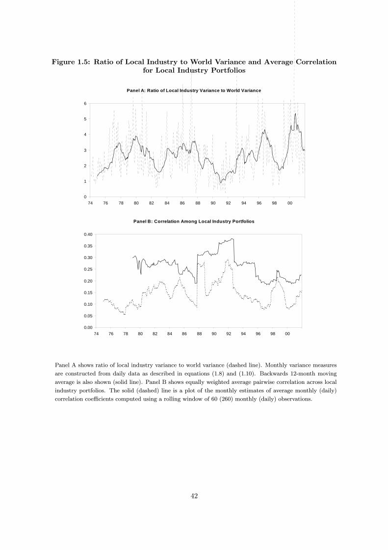
Figure 1.5: Ratio of Local Industry to World Variance and Average Correlationfor Local Industry Portfolios

Panel A: Ratio of Local Industry Variance to World Variance

0

1

2

3

4

5

6

74 76 78 80 82 84 86 88 90 92 94 96 98 00

Panel B: Correlation Among Local Industry Portfolios

0.00

0.05

0.10

0.15

0.20

0.25

0.30

0.35

0.40

74 76 78 80 82 84 86 88 90 92 94 96 98 00

Panel A shows ratio of local industry variance to world variance (dashed line). Monthly variance measures

are constructed from daily data as described in equations (1.8) and (1.10). Backwards 12-month moving

average is also shown (solid line). Panel B shows equally weighted average pairwise correlation across local

industry portfolios. The solid (dashed) line is a plot of the monthly estimates of average monthly (daily)

correlation coefficients computed using a rolling window of 60 (260) monthly (daily) observations.

42

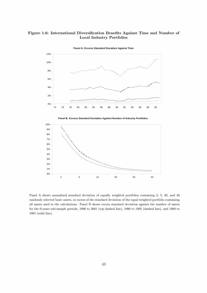
Figure 1.6: International Diversification Benefits Against Time and Number ofLocal Industry Portfolios

Panel A: Excess Standard Deviation Against Time

0%

2%

4%

6%

8%

10%

12%

74 76 78 80 82 84 86 88 90 92 94 96 98 00

Panel B: Excess Standard Deviation Against Number of Industry Portfolios

0%

1%

2%

3%

4%

5%

6%

7%

8%

9%

10%

2 5 10 20 30 40

Panel A shows annualized standard deviation of equally weighted portfolios containing 2, 5, 20, and 40

randomly selected basic assets, in excess of the standard deviation of the equal weighted portfolio containing

all assets used in the calculations. Panel B shows excess standard deviation against the number of assets

for the 6-years sub-sample periods, 1996 to 2001 (top dashed line), 1990 to 1995 (dashed line), and 1980 to

1985 (solid line).

43

CHAPTER 2

Does Sovereign Debt Ratings News Spillover to International

Stock Markets?

(with Miguel Ferreira)

2.1. Introduction

Does sovereign debt ratings news in one country impact other countries stock markets?

In this paper, we find evidence that yes, indeed sovereign ratings unfavorable news spillover

to other countries stock markets. We focus on the cross-country stock market reaction to the

announcements by Standard & Poor’s (S&P) of a sovereign credit rating or credit outlook

change.

Brooks, Faff, Hillier, and Hillier (2004) study own country stock market impact of sov-

ereign debt ratings changes. They find that sovereign ratings downgrades have a negative

impact on the re-rated country stock market returns. Gande and Parsley (2003) study in-

ternational spillover effects on the sovereign debt market and find this spillover to be asym-

metric. In fact, downgrades abroad are associated with a significant increase in sovereign

bond spreads (12 basis points), but upgrades have an insignificant effect. Kaminsky and

Schmukler (2002) show that emerging market sovereign ratings news are contagious to bond

and stock markets of other emerging markets, particularly during periods of turmoil and

among neighbor countries.

We extend the Gande and Parsley (2003) international spillovers pool regression model to

investigate the information spillover effect not only across countries, but also across assets.

That is, we focus on spillovers of credit ratings or credit outlooks of one country (the event

44

country) to stock market return spreads (the return differential vis-a-vis the US market) of

all other countries (the non-event countries). Relative to Kaminsky and Schmukler (2002)

our study contributes in several ways: we consider a much larger set of countries that includes

not only emerging but also developed markets; we explicitly control for recent rating activity

worldwide; we characterize the spillovers economically, e.g., by including controls for capital

flows and level of economic and financial development; we study the role of exchange rates in

spillovers; and we present several new results of cross-country and cross-asset news spillover

at the industry level. The impact of sovereign rating news on industry portfolios is of

particular relevance given the increased perception by investors and evidence that industry

factors are becoming more important than country factors in explaining stock returns; see,

for example, Brooks and Catao (2000).

A sovereign credit rating represents an assessment by the rating agency on the capacity

and willingness of sovereign obligators to ensure timely all sovereign debt service. They are

understood by rating agencies as a forward-looking estimate of sovereign governments default

probability; see S&P (2004). In most situations, the sovereign ceiling doctrine applies, i.e.

the rating assigned to non-sovereign debt issues (or issuers) is the same as or lower than that

assigned to the sovereign of the country of domicile. Thus, sovereign ratings revisions also

relate to non-sovereign debt instruments; see, for example, Radelet and Sachs (1998) and

Bank for International Settlements (2004).1

A stock market reaction to sovereign ratings downgrades is expected because a down-

grade can affect the country’s ability to borrow in international markets, and consequently,

contribute to a credit crunch, which negatively impacts the stock market. Other mecha-

nisms provide further support of the link between sovereign ratings and stock markets. For

instance, sovereign ratings can provide information on the future economic health of the rated

country, which have been overlooked by the stock market participants, and governments’ can

1The final version of the Basel II provides examples of the sovereign rating ceiling doctrine. Under thestandardized approach to calculate minimum capital requirements for bank claims (option 1), all banksincorporated in a given country will be assigned a risk weight one category less favorable than that assignedto claims on the sovereign of that country. For claims on corporates, no claim on an unrated corporate canbe given a risk weight more favorable to that assigned to its sovereign of incorporation.

45

take policy actions that directly affect companies future prospects (e.g., raising corporate

taxes to compensate an increase in debt service following a downgrade). Moreover, because

many institutional investors can only hold investment grade instruments, rating upgrades

(downgrades) may have a positive (negative) impact on securities prices; see Radelet and

Sachs (1998) and Kaminsky and Schmukler (2002).

The empirical question we address is whether sovereign rating news of one country is also

relevant for other countries. If ratings changes are understood by market players as re-rated

country specific issues without further implications, little information impact is expected.

However, the behavior (either rational due to liquidity constraints or irrational herding) of

investors and the financial-real sector linkages across countries could act, and often do, as

transmission vehicles of country shocks; see Dornbusch, Park, and Claessens (2000).

Following Gande and Parsley (2003), we also distinguish between two kinds of reactions:

common versus differential information spillovers. The reasoning is straightforward and

relates the information content of events to the reaction in non-event countries. For example,

if a positive rating event for a given country triggers a reaction of the same sign across all

other countries, we refer to this as a common information effect. If a positive rating event

entails a widespread undetermined (or negative) reaction, for instance due to global portfolio

rebalancing actions, we refer to this as a differential effect.

Our major findings can be summarized as follows. First, we find ratings changes in

one country to contain valuable information for the aggregate stock market returns of other

countries. This spillover effect is found to be asymmetric, both in the direction of the reaction

as well as in terms of economic impact. On average, a one-notch ratings downgrade abroad

is associated with a statistical significant negative two-day stock return spreads vis-a-vis the

US stock market of 28 basis points across non-event countries, whereas no significant pattern

is found for ratings upgrades.

Second, controlling for time invariant characteristic that proxy for underlying similarities

between countries, does not affect the asymmetric spillover pattern. Specifically, we control

46

for the cultural, regional and institutional environment as well as level of economic and

financial development.

Third, we do not find evidence of differential effects for downgrades. For upgrades,

we find evidence of differential spillovers among countries with highly negatively correlated

portfolio flows vis-a-vis the US. In fact, there is a negative significant association between

return spreads and the indicator variable for highly negatively correlated portfolio flows.

This suggests that the typical insignificant positive common spillover effect for upgrades is

eroded by these differential effects.

Fourth, we find ratings downgrades to be associated with a depreciation of the US dol-

lar exchange rate against the non-event country currencies. On average across non-event

countries, sovereign ratings downgrades abroad are associated with a negative local currency

denominated return spread of 42 basis points. Accordingly, we find downgrades to be as-

sociated with statistically significant positive exchange rate return of 12.5 basis points. In

other words, we find that the appreciation of non-event country currencies relative to the

US dollar (partially) hedge the negative wealth effect of ratings downgrades abroad.

Finally, we show that ratings downgrades have a slightly smaller economic effect for local

industry portfolios than for country portfolios. Nevertheless, sovereign ratings downgrades

abroad are associated with a highly statistical significant negative two-day return spread of

industry portfolios vis-a-vis their counterpart industry in the US of 25 basis points.

Overall, the above conclusions are robust across different empirical specifications, namely

explicitly accounting for recent rating activity, alternative ways to measure the impact in

the stock market (dependent variable), and sub-samples of countries or industries.

The remainder of the paper is organized as follows. Section 2.2 reviews related work on

sovereign ratings. Section 2.3 details the empirical strategy and presents the data. Section

2.4 presents and discusses our empirical results on country portfolios. Section 2.5 contains

results on industry portfolios. Section 2.6 concludes.

47

2.2. A Selective Review of the Sovereign Ratings Literature

This section briefly reviews the related work on sovereign ratings. We focus on three

issues: the determinants of sovereign ratings, the timing of sovereign ratings revisions, and

their impact on capital markets.

Cantor and Packer (1996) debut the empirical research on the determinants and impact

of sovereign credit ratings. Their cross-sectional regression results suggest that both agen-

cies (S&P or Moody’s) share the same criteria (per capita income, GDP growth, inflation,

external debt, economic development, and default history), although weight macroeconomic

variables differently. The fiscal and external balances positions are found to be irrelevant for

both agencies. Moreover, Cantor and Packer (1996) also show that sovereign ratings appear

to contain additional information relevant for pricing sovereign bonds beyond the publicly

available macroeconomic indicators.

Juttner and McCarthy (2000) show that the explanatory power of Cantor and Packer

(1996) key macroeconomic variables changes considerably through time, namely after the

Asian crisis. Also they test for new variables, such as interest rate differentials, indicators of

financial sector strength/fragility, and real exchange rates, which could help to restore the

explanatory power.

Another strand of research focus on the timing of ratings revisions - are rating agencies

proactive or reactive in relation to financial crises? Provided that sovereign ratings disclo-

sures have some market impact, early ratings downgrades during euphoric periods would help

dampen expectations and smooth crises. However if ratings lag the market, upgrades (down-

grades) during euphoric (turmoil) periods would reinforce expectations (add panic among

investors), consequently reinforcing crisis cycles.

The actions of ratings agencies in the periods surrounding the 1994-1995 Mexico crisis

and later during the Asian crisis, downgrading ratings after the crisis erupted rather than

anticipating them (Reisen and von Maltzan, 1999) suggests that ratings changes do lag the

market. Moreover, Reinhart (2001) concludes that sovereign ratings are a poor predictor of

48

crises and that they perform much worse than other indicators of financial distress (e.g. real

exchange rates or debt-to-export ratios), although financial crises are hard to predict.

Given the evidence on the relevance of publicly available information for sovereign ratings

assessment, which makes it possible for markets to anticipate ratings announcements, it

comes at surprise that financial markets react to ratings revisions. Of course, it could

be that ratings agencies’ superior research or access to privileged information concerning

countries’ willingness to service sovereign debt, enables them to add value to informative

signals overlooked (or not accessible) by market participants, thus rendering ratings revisions

important news events.

The literature (to our knowledge, relatively scarce) on the market impact of sovereign

ratings revisions finds several interesting results. First, there is some controversy on whether

or not sovereign ratings revisions announcements impact the sovereign bonds prices of the

re-rated countries. Cantor and Packer (1996) event study shows that even though agency

actions could have been preceded by a similar change in market expectations, the imme-

diate effect of announcements over sovereign bond yield spreads relative to US Treasuries

is positive (negative) for ratings downgrades (upgrades). While for all events together the

announcement effect is statistically significant, disaggregating between upgrades and down-

grades shows that only the former effect is statistically significant.

Larraın, Reisen, and von Maltzan (1997) show that the aggregate impact of ratings

changes (or imminent revisions) announcements by the two leading agencies on bond yield

spreads is of the expected sign, but statistically significant only for the emerging markets

subsample. The split of events according to the announcements categories shows that the

immediate impact is statistically significant, only when a country is put on watch for a

possible downgrade.

Reisen and von Maltzan (1999) findings also question Cantor and Packer (1996) results.

A significant market impact (two-day event window) is found only for emerging markets

and when all agencies’ announcements (Moody’s, Standard and Poor’s, and Fitch IBCA)

are combined. The analysis according to the announcements categories shows that the

49

impact in bond yield spreads in emerging markets comes from imminent upgrades and actual

downgrades.

Second, Gande and Parsley (2003) find evidence of a significant asymmetric reaction of

sovereign yield spreads (relative to the US bond market) to announcements concerning other

sovereigns. Sovereign ratings upgrades have no discernible impact, while a one-notch rating

downgrade of a sovereign bond is associated with a 12 basis points (on average) increase

in other sovereign bonds yield spread relative to the US, as a percentage of the US yield.

Moreover, the authors propose a new research design to ascertain the market impact of

news that has several advantages over the traditional event study or time series regression

methods. Namely, it avoids the “event window” contamination problem either by measuring

spreads over a short window of two days as well as by explicitly controlling for the intensity

of past events, but still keeping substantial flexibility to test alternative hypothesis.

Third, the re-rated country stock market returns are positively related to sovereign rat-

ings (or credit outlook) changes; see Kaminsky and Schmukler (2002). This spillover effect

across asset market (within a country) is in fact asymmetric, in line with the stylized findings

on the firms’ stock price reaction to corporate bond ratings revisions. Brooks et al. (2004)

using standard event-studies methodology show that the event-day impact of ratings revi-

sions is statistically significant only for downgrades (abnormal one-day stock market returns

of -1.97% to S&P announcements). This is a particular characteristic of S&P and Fitch

IBCA announcements and of foreign currency ratings.2

Finally, there is some evidence of a positive relation between ratings changes and stock

market returns in emerging markets. Kaminsky and Schmukler (2002) address this issue in

the context of a pool regression and events study methods. They show that ratings and

outlooks changes of emerging sovereigns are positively related to the stock market returns of

other emerging countries. However, Kaminsky and Schmuckler (2002) do not test for asym-

metric effects nor control for time and country-specific effects, and the estimation procedure

2Kaminsky and Schmukler (1999) also study the relevance of news relating to sovereign risk reassessments.The authors look at the type of news that moves the markets during the Asian crisis and find a stock marketof 10% (on average) downturn in the days credit ratings downgrades are announced.

50

does not allow the use of low frequency macroeconomic data. The events study confirms

previous findings on the procyclical behavior of ratings agencies (upgrades tend to occur

during good times and downgrades during bad times) and supports a positive (negative)

reaction of emerging stock markets following other sovereign ratings upgrades (downgrades)

news.

Overall, there is evidence that country-specific macroeconomic data plays a key role in

sovereign debt ratings assessment by the ratings agencies. Sovereign ratings revision activity

tends to follow the market trend either because an anticipation effect by market participants

or, more likely, because rating agencies behave pro-cyclically.

If there is no doubt on the characteristics of own stock market and cross-country bond

market impact of ratings (and/or outlooks) revisions - the same cannot be said about the

own bond market reaction. Furthermore, there is a need for a thorough empirical investiga-

tion of the cross-country stock market impact of ratings news with a sample that includes

both emerging and developed countries, and a methodology that specifically addresses the

(potential) asymmetry of market reactions and the tendency for ratings to cluster in time.

2.3. Research Design

2.3.1. Data

We investigate the cross-country spillover effects of sovereign ratings revisions using the S&P

history of sovereign ratings for those countries analyzed by Gande and Parsley (2003) and

that are covered by the TF Datastream Global Equity Indices database. The data cover the

period from July, 3 1989 to December, 31 2003. The starting date corresponds to the first

complete month for which S&P credit outlook information is available.

S&P foreign currency long term ratings history is preferred to other agencies’ ratings

history because of data availability. Moreover, S&P tends to be more active making rat-

ings revisions (Kaminsky and Schmukler (2002)), and tend to lead other agencies re-ratings

(Brooks et al. (2004) and Gande and Parsley (2003)). In addition, foreign currency ratings

announcements by S&P seem to have a larger own country stock market impact (Brooks et

51

al. (2004)) and seem not to be fully anticipated by the market (Reisen and von Maltzan

(1999)).3

The countries in our dataset obey two criteria: the existence of publicly traded US

dollar denominated sovereign debt, and the availability of country level portfolio total return

index data in the TF Datastream database. The 29 countries meeting these criteria are the

following: Argentina, Austria, Belgium, Brazil, Canada, Chile, China, Colombia, Denmark,

Finland, Greece, Hungary, Indonesia, Ireland, Israel, Italy, Korea, Malaysia, Mexico, New

Zealand, Philippines, Poland, South Africa, Spain, Sweden, Thailand, Turkey, UK, and

Venezuela. Thus, we build a geographically balanced sample that includes both emerging

and developed countries. Moreover, the stock market indexes considered here represent about

80% of each stock market capitalization and are constructed using similar methods across

countries.

We also use data on several country-specific control variables (Table A.1 in the Appendix

to this chapter, presents in detail the variables definitions and data sources). Classification

of countries into emerging or developed is based on Morgan Stanley Capital International,

S&P and ISI Emerging Markets. A country is classified as emerging if it is listed as emerging

in at least one of the above sources.4

We consider bilateral dummy variables for sharing a common language, adjacency, legal

tradition, and membership to a formal trade bloc, either the North American Free Trade

Agreement (Nafta), the Mercado Comun del Sur (Mercosur), the European Union (EU),

or the Association of South East Asian Nations (Asean). In addition, we explicitly control

for the physical distance between countries, computed as the great circular distance between

capital cities. These variables aim to control for historical factors that may influence spillover

effects because they proxy for similarities between countries that could heighten common

spillover effects; see Gande and Parsley (2003). Moreover, “geographical factors” akin to our

control variables are standard controls in the literature explaining cross-country economic

3Sovereigns ratings history are drawn from the S&P website: http//www.standardandpoors.com4Greece is the only country in our sample that was upgraded from emerging to developed either by S&P orMSCI . In this paper we classify Greece as a emerging market. Countries classified as developed are Austria,Belgium, Canada, Denmark, Finland, Ireland, Italy, New Zealand, Spain, Sweden, and United Kingdom.

52

flows and also relate to linkages across stock markets (Portes and Rey (1999) and Rose

(2000)).

We also consider monthly bilateral capital and trade flows between each country and the

US. Specifically, gross flows (sales plus purchases) of foreign stocks are obtained from the US

Treasury’s website (http://www.treas.gov). Monthly bilateral trade flows are obtained from

the US Census Department website (http://www.census.gov).

We explicitly control for crisis periods by including dummy variables for the European

Exchange Rate Mechanism crisis of 1992-93, the Tequila crisis of 1994, the Asian Flu of

1997, and the recent Russian, Brazilian, Turkey and Argentina crisis (49 events in total).

Finally, we use Bekaert, Harvey, and Lundblad (2003) “official liberalization” dates to control

for emerging market segmentation from the world market due to regulatory constraints on

international capital flows.

2.3.2. Ratings Events

We define a rating event as a change in either the explicit credit rating or the credit outlook

assigned to a specific sovereign foreign currency debt. Thus, we follow the recent work on the

spillover effects of sovereign ratings revisions by accounting for effective ratings announce-

ments as well as information on imminent rating actions in a comprehensive credit rating

(CCR) measure. The changes to CCR define our ratings events.

Table A.2 in the Appendix to this chapter, presents the details on the numerical coding

of the CCR measure. First, we map letter explicit ratings to numerical codes by a linear

transformation to a scale from 0 (the lowest rating - SD/D) to 20 (the highest rating — AAA).

Next, we add the credit outlook information (on a scale between -1 for a negative credit

outlook and +1 for a positive credit outlook) to the rating numerical code. Any nonzero

change in the comprehensive credit rating measure defines the events of interest: “upgrades”,

a positive change resulting from an upward move in the (letter) credit ratings of the sovereign

or from a favorable revision in the credit outlook information; and, “downgrades”, a negative

53

change resulting from a downward move in the (letter) rating or from an unfavorable revision

in the credit outlook.

Table 2.1 describes the sovereigns ratings events sample. There are 106 (109) upgrades

(downgrades) between July 1989 and December 2003. The vast majority of events is an-

nounced individually (for one country at given day), though multiple event days occurs for

14.2% (3.6%) of the upgrades (downgrades) cases. The time clustering of events can also be

evaluated looking at the average time elapsed between events and the time periods in which

they occur. Panel B of Table 2.1 show that about 50% of the events (54 upgrades and 50

downgrades) occur within a window of two weeks (ten trading days). Panel C shows that

about 50% of the events (54 upgrades and 44 downgrades) corresponds to announcements

made after 1998.

The strong temporal association of events suggests the use of a short event-window when

evaluating ratings revisions impact and to explicitly control for worldwide recent rating

activity. The use of long event widows can bias the results because stock returns in the

(longer) event window can already incorporate ratings changes in other countries beyond the

one being evaluated. Moreover, if markets see ratings revisions in the context of recent rating

activity, today’s reaction will be a function of prior ratings revisions. In fact, Kaminsky and

Reinhart (2000) show that the domestic market susceptibility to crises elsewhere rises sharply

if a core group of countries (not a single country) is already infected. If the same type of

behavior characterizes the home reaction to sovereign rating changes abroad, this implies

that events in other countries can cumulate.

Also shown in Table 2.1 is the breakdown of events according to the classification of

countries into emerging or developed (Panel D). The vast majority of events, about 85%,

occurs in emerging markets. This shows the importance of investigating if rating news also

affects developed stock markets, an issue that has been overlooked in the literature.

Figure 2.1 plots the number of events on a given year between 1990 and 2003 (no event

occurs in the second semester of 1989). There is an increase in rating activity in the years

surrounding the 1994 Mexican crisis. Downgrades show a visible increase in 1997 and 1998,

54

probably associated with revisions induced by the Asian crisis and Russian default, with a

peak of 17 events in 2001. Interestingly, upgrades are most noticeable in the years of 1999,

2000, and 2003, which is suggestive of a cyclical element in the ratings revision activity.

2.3.3. Testing Procedures

This section details the empirical strategy we use to test for international cross-asset market

spillover effects. We extend the methodology used by Gande and Parsley (2003) to study the

impact of rating changes in international stock markets. We measure the non-event country

j(6= i) stock market response to a rating event in country i(6= j) by the daily logarithmic

change in country j total return index relative to the equivalent change in the US market

total return index (the benchmark). To account for time zone differences between stock

markets, we cumulate the “stock market spreads” in a standard two-day window [0,1].5

Specifically, we pool the data for all countries (j) excluding the event country (i), at each

event time (t), and estimate the following benchmark regression separately for upgrades and

downgrades:

rj,t = α+ β1Eventi,t +Xk

βkXk + ²ij,t,∀j 6= i, (2.1)

where rj,t represents the cumulative [0,1] return spread. The indices i and j represent coun-

tries and t event time. Eventi,t is any non-zero change in the comprehensive credit rating.

For easy of interpretation, we use the absolute value of Eventi,t in the downgrades regression.

Since we analyze separately upgrades and downgrades, this allows for the interpretation of

the stock market reaction as “in the expected direction given the announcement”. Matrix

X contains full sets of year and country dummies (29 event-country and 29 non-event coun-

try) and the levels of event and non-event country comprehensive credit ratings. The latter

5The use of simple “market-adjusted” abnormal stock returns can be found, for example, in Kaminsky andSchmukler (2002) and Griffin and Stulz (2001). In the literature that focus on the bond market reaction tosovereign ratings revisions the standard approach relies in bond yield spreads relative to comparable maturityUS bonds yields, namely due to the difficulties in finding a relevant event-free period (see, for example,Reisen and von Maltzan, 1999). In a later section as robustness check, we also evaluate market modelresiduals (abnormal returns) and results are similar.

55

controls for nonlinearities in market reaction relative to the position of each country pair in

the ratings scale.

This approach has two major advantages. First, it has a great flexibility for testing

alternative hypothesis. For instance, to control for time invariant country-specific charac-

teristics in subsequent regressions, the matrix X is expanded to include additional controls:

emerging/developed status, common language, adjacency, physical distance, legal tradition,

and membership to a formal trade bloc. Likewise, testing for the impact of crisis periods or

stock market liberalizations is done by adding specific variables to the matrix X.

Second, we control for the temporal clustering of events either by measuring the change

in stock prices over a short-window of two days, rather than relying on a longer-window (e.g.,

30 days) and by explicitly controlling for the intensity of past events with the inclusion of a

new variable, Lag Event, which measures the net rating change (event-country prior CCR

changes excluded) in the preceding two (or three) weeks. Thus, we control for nonlinearities

in sense of Kaminsky and Reinhart (2000) relative to the recent worldwide history of rating

activity.

2.4. Empirical Results on Country Portfolios

2.4.1. Asymmetric Spillover Effects

Table 2.2 reports estimates of the coefficients in equation (2.1). There is strong evidence of

an asymmetric common information spillover effect of stock markets to sovereign debt ratings

changes abroad. Sovereign debt credit ratings upgrades are associated with a positive effect

on stock market prices relative to the US, while downgrades with a negative return spread. In

other words, on the days a sovereign credit rating (either implemented or credit outlook) for

a particular country is upgraded, our results suggest that the remaining countries do better

than the US market. When a country is downgraded, the results show that the remaining

countries do much worse than the US market.

However, only for downgrades the effect is statistically significant at the 5% level. The

downgrade effect is also economically larger than the upgrade effect. A one-notch negative

56

event in one country is associated with an average negative two-day stock market return

spread abroad of 28 basis points, while positive events are associated with positive return

spreads of about a half of that magnitude.

Negative news in the sovereign debt market, but not positive ones, does seem to have

impact in the international stock markets. Gande and Parsley (2003) argue that either

because of pre-event information disclosure of the imminent positive change by the event

country government or a reluctance of ratings agencies to lower ratings due to marketing

factors (Larraın, et al. (1997)), downgrades (but not upgrades) can be recognized by the

stock market participants as a wake-up call, especially if in the context of bad times.

Interestingly, the level of event country CCR is significant only for upgrades. The higher

the event country CCR the lower the non-event country stock market response for ratings

upgrades, suggesting that the effect of upgrades is most noticed for low level sovereign ratings.

Moreover, when we control for the clustering in time of events in other countries by including

in the regression a measure (Lag Event) for the rating activity in the prior two weeks, we

find that only for upgrades does rating history matter. This reinforces the intuition that

downgrades are understood by the stock market as surprises while the same does not happen

for upgrades. The insignificance of the lagged event variable coefficient for downgrades, also

does not offer support to a delayed stock market reaction to a rating change abroad.

This comes at odd with the typical reaction of sovereign debt markets to other countries

sovereign rating revisions. In fact, Gande an Parsley (2003) show that only for downgrades

does the level of event country CCR and the recent rating activity have explanatory power.

That is, our results suggest that stock markets are more efficient reacting to sovereign debt

bad news than to incorporating sovereign debt good news.

Overall, our results support an asymmetric common information effect in international

stock markets of a CCR downgrades. Across asset markets and across countries, bad news

in one country is interpreted as negative news in other countries. Positive news has no

discernible impact.6

6The probit model estimates and Granger-causality tests in Gande and Parsley (2003), whose sample of coun-tries is similar to ours, allow the rejection of spillover effects on the comprehensive credit ratings themselves.

57

Table 2.3 expands the matrix X to include controls for emerging/developed country

status, adjacency (sharing of land border) and distance between countries, sharing a common

official language, membership in a trade bloc, and origin of legal systems.

The results in Table 2.3 offer additional support of the previous findings of a common

information spillover effect. Sovereign debt ratings downgrades induce a statistically sig-

nificant negative response in stock markets abroad, while the positive response to ratings

upgrades is statistically insignificant and contaminated by the recent history of rating activ-

ity. The magnitude, sign, and statistical significance of the event variable remains virtually

unchanged relative to Table 2.2, while the adjusted R2 of both regressions increases slightly.

Among the economic characterization variables, only the physical distance is statisti-

cally significant both in the upgrades and the downgrades regressions. We interpret the

opposite sign of the physical distance variable relative to the event variable, as evidence

that an increase in distance between the capital cities reduces the average wealth impact of

spillovers. Likewise, our results suggest that sharing a common trade bloc increases the nega-

tive (positive) international stock market wealth impact of sovereign debt ratings downgrades

(upgrades).7

The coefficient for the development status (i.e., when the event and non-event country

are both developed) is also significant in the downgrades regression. The positive significant

coefficient indicates that downgrades in developed countries have a smaller effect in stock

markets of other developed countries relative to the average impact (notice this does not

mean that overall downgrades have no effect in developed stock markets). Interestingly, the

emerging status dummy has a negative coefficient in the downgrades regression, suggesting an

increased impact among emerging stocks markets (excluding the event country) of a negative

event in an emerging market.

In other words, these results allow us to rule out the possibility that spillover effects are anticipated by ratingagencies and that ratings are adjusted simultaneously across countries.7We do run regressions using physical distance measured in logarithms rather than in thousands of kilometers.Results (not tabulated here) confirm that only downgrades have a statistically significant in international stockmarkets, and the greater distance, the smaller is the impact.

58

By the same reasoning, in the upgrades regression, the positive coefficient for emerging

status, signals that among these countries upward ratings revisions have an increased positive

wealth impact, relative to the average.8

2.4.2. Differential Spillover Effects

This section looks at differential spillover effects. It could be the case that for some stock

markets the response is of different sign of the common information spillover. For instance,

global portfolio rebalancing induced by the own market negative response to sovereign down-

grades (Brooks et al., 2004) could induce spillover effects abroad of different sign relative to

the common negative reaction.

We investigate this issue by explicitly accounting for foreign equity portfolio (and trade)

flows linkages. Following the reasoning of Gande and Parsley (2003), we hypothesize that

common information spillover effects should dominate for two countries with highly positively

correlated portfolio (or trade) flows. Conversely, differential spillover effects should exist

between countries with highly negatively correlated portfolio (or trade) flows.

Empirically, this hypothesis is investigated considering the time series correlation of gross

portfolio (or trade) flows vis-a-vis the US for each country in our sample. At each event

date, we use a moving window of the most recent 6 months of portfolio (and trade) flows to

compute the correlation between the event country flows and all the remaining (non-event)

countries. Next, we construct a dummy variable that takes the value one to those country

pairs with high positive correlation (the top quartile of the cross-sectional distribution), and

zero otherwise. Similarly, a dummy variable is also constructed for those country pairs that

fall in the bottom quartile (highly negative correlation). Results are reported in Table 2.4.

Two findings stand out. First, controlling for the portfolio (or trade) flows correlation

does not change our basic findings that only for downgrades there is a significant common

information spillover effect. In fact, the statistically insignificance of the highly positively

correlated portfolio (or trade) flows dummy does not allow for conclusions regarding the

8Gande and Parsley (2003) show that among developed markets, sovereign ratings downgrades abroad havea smaller effect on sovereign bond markets.

59

increased impact in the expected direction of ratings news for such country pairs. Neverthe-

less, for the highly positively correlated portfolio flows dummy, the positive (negative) sign

in the upgrades (downgrades) regression suggests that, as hypothesized, for these country

pairs’ ratings news could have an increased impact of the expected sign.

Second, there is evidence of differential information effects only for upgrades. Relative

to the typical reaction to ratings upgrades abroad, we find a decrease of about 33 (26) ba-

sis points in stock return spreads for countries with highly negatively correlated portfolio

(or trade) flows with the event country. This is surprising given the positive (but statisti-

cally insignificant) common reaction to upgrades and suggests a possible explanation for the

inexistence of a statistically significant spillover for ratings upgrades.9

Overall, the investigation on differential spillover effects suggests a far more homogenous

reaction of international stock markets (non-event countries) to ratings downgrades than to

ratings upgrades. This yields some support to the hypothesis that global equity portfolio re-

balancing actions may induce differential price reactions across non-event stock markets, but

only for ratings upgrades. Gande and Parsley (2003) find a statistical significant differential

spillover effect in international sovereign debt markets, but only for downgrades. Thus, our

results suggest a more homogeneous reaction of stock markets to ratings downgrades than

the one observed for debt markets. In contrast, debt markets show a more homogeneous

reaction to upgrades than stock markets.

2.4.3. Crisis Periods and Stock Market Liberalizations

In this section, we analyze the sensitivity of our results to the inclusion of controls for crisis

periods and liberalization of local equity markets.

First, we evaluate if the events that occur during periods of capital markets turmoil (49

events) could be driving our results. Table 2.5 (first specification) reports regression results

9We do run regressions (not tabulated here) using 12-month horizon portfolio and trade flows correlations.For upgrades only the highly negatively correlated portfolio flows dummy (not the trade flows) is statisticallysignificant, suggesting a decrease in stock return spreads of about 30 basis points. This robustness suggeststhat the transmission channel is stronger for portfolio than for trade linkages, and that only in the short runcould trade flows play a role as a transmission mechanism. We also run regressions including the four dummyvariables simultaneously, and the conclusions remain virtually unchanged.

60

including a dummy variable that controls for the European Exchange Rate Mechanism crisis

of 1992-93, the Tequila crisis of 1994, the Asian Flu of 1997, and the recent Russian, Brazil-

ian, Turkey and Argentina crises. The basic results remain unchanged. Specifically, only

negative ratings news are associated with a significant international stock market reaction.

Interestingly, the crisis dummy is only significant for the upgrades regression and presents a

negative coefficient. This result suggests that information content of ratings upgrades during

periods of turmoil is overcome by the negative expectations stock market players are acting

upon.

Second, we evaluate the effect of regulatory constraints on foreign capital inflows on the

ability of a country’s stock market to react to a rating change abroad. If foreign investors’

actions are relevant to transmit information across markets, we expect smaller spillover

effects for those countries in which regulation places a barrier to the trade of local equities

by foreign investors. In fact, for 13 countries in our sample, the “official liberalization date”

proposed by Bekaert and Harvey (2000) occurs after our initial sample period. To account for

this effect, we expand the basic specification to include a non-event country dummy variable

that equals one if a rating change occurs before the country official liberalization, and zero

otherwise.10 Table 2.5 (second specification) presents the results.

Spillovers continue to exist only for downgrades and the liberalization effect is not statis-

tically significant. The sign of the (no) liberalization dummy variable is negative for upgrades

which offers support to the hypothesized effect. Concerning downgrades, the negative sign

of the (no) liberalization dummy variable coefficient, comes at odds with the hypothesized

effect, because it suggests an even stronger reaction to ratings news abroad when the country

is not liberalized. Given the probable greater importance that country specific factors have

on equity price behavior for these countries during the periods of no liberalization, these

10Countries in question are: Argentina, Brazil, Chile, China, Colombia, Hungary, Indonesia, Israel, Korea,Philippines, Poland, South Africa, and Venezuela. For those few countries not included in Bekaert et al (2003)sample, we use the major regulatory reform concerning foreign investors in Campbell Harvey’s Country RiskAnalysis website: http://www.duke.edu/˜charvey/Countryrisk/couindex.htm.

61

opens the possibility of irrational herding from domestic investors as a probable cause for

this behavior.11

2.4.4. Local Currency Returns and Exchange Rates

Next, we look with further detail to the definition of stock market return spreads by explicitly

removing currency effects from its calculation. That is, we use local currency denominated

returns to compute the differential return vis-a-vis the US market. In addition, we also look

at exchange rate returns on event days.12

Panel A of Table 2.6 presents the results. The impact of upgrades remains insignificant

and similar to the one found using US dollar denominated return spreads. More interesting

is the increase both in the economic and statistical significance of the negative impact of

downgrades on international stock markets. Using local currency returns, we find downgrades

to be associated with a response of the stock markets abroad of 42 basis points (negative

two-day stock return spreads), which is 13 basis points higher (in absolute terms) than the

equivalent impact measured in US dollars. This suggests that foreign exchange rates are in

part hedging the decrease in the market value of the foreign country equity investment.

In fact, Panel B of Table 2.6 shows that ratings downgrades are associated with a sta-

tistically significant depreciation of the US dollar exchange rate against non-event country

currencies of about 13 basis points (two-day event window). In other words, we find the

appreciation of non-event country currencies relative to the US dollar to hedge in part the

negative stock market wealth effect of ratings downgrades abroad. Concerning positive rat-

ing events, we find exchange rates reaction to be negative (0.5 basis points) and statistically

insignificant, mirroring the results obtained for the stock market reaction.

11Additional specifications (not tabulated here) show that results remain virtually the same if portfolio flowscorrelation dummies are omitted when testing for liberalization effects.12Exchange rates are defined as the number of US dollars per unity of foreign country currency. Daily exchangerate returns are defined as the first difference of consecutive exchange rate observations (in logarithms). Dailyreturns are cumulated (day 0 plus day +1) on event dates.

62

2.4.5. Stock Market Correlations

This section tests whether cross-country correlation matrices between event and non-event

days are equal. If the finding of an international stock market downgrade spillover effect

is more than the manifestation of the existent correlation across countries, the correlation

structure itself should change on event days. Moreover, we argue that the insignificance

of differential spillover effects (namely for downgrades) is consistent with an increase in

correlations.

To investigate these issues, we follow Gande and Parsley (2003) research design and

randomly select (with replacement) a matched (across countries) sample of non-event date

return spreads for each event, imposing the additional condition that the non-event days are

sampled within the window [-60,-21] days relative to the event date. The sampling exercise

is performed 10, 000 times, and a cross-country correlation matrix is computed using each

randomly selected sample of non-event days return spreads. We focus the subsequent analysis

on downgrades - the events for which there is evidence of spillovers.

The first issue of concern is whether correlation matrices differ between event and non-

event periods. Following Gande and Parsley (2003), Longin and Solnik (1995) and Kaplanis

(1988), we test this hypothesis using the Jennrich (1970) test statistic:

χ2 =1

2tr(Z2)− dg0(Z)S−1dg(Z), (2.2)

where tr(.) and dg(.) are the trace and diagonal of a matrix; Z = c12R−1(R1−R2), in which

R = (n1R1 + n2R2)/(n1 + n2) and c = (n1n2)/(n1 + n2), R1 and R2 are the correlations

matrices to be compared, and n1 and n2 are the number of observations on which they are

based; and, S = (δij + rijrij), in which δij is the Kronecker delta and rij (r

ij) denotes the

elements of R (R−1). The Jennrich (1970) test statistic has a chi-square distribution with

p(p− 1)/2 degrees of freedom, with p being the dimension of the correlation matrices.13

13Note that the Jennrich (1970) test is robust to changing volatilities from event to non-event samples (thesamples whose correlations are being tested). This is important in our context because as shown by Forbesand Rigobon (2002) among others, conditional correlation estimates are volatility dependent, which maybias conventional pair-wise tests designed to evaluate correlation changes. As shown by Chakrabarti and Roll(2003), these biases should be a concern only when sub-samples correspond to periods of observed abnormally

63

The results support the conclusion that the downgrades spillover effect is not a simple

manifestation of the existent correlation structure, as correlations itself change in event days

relative to non-event days. The simulations yield a median test statistic of 577.96, while

its 5% critical value is 453.98 (for a chi-square distribution with 406 degrees of freedom).

Moreover, we reject, at the 5% level, the null hypothesis of equal correlation matrices across

all the 10, 000 simulations. Thus, our results strongly suggest that the correlation structure

itself changes on event days.

The second issue of concern is whether correlation increases (or decreases) during the

events periods relative to non-events periods preceding the rating change. To evaluate the

sign of correlations changes, we perform an element-by-element comparison between the

event days’ correlation matrix and each of the randomly sampled non-event day correlation

matrices. Specifically, we compute the proportion of pairwise correlation coefficients which

represent net increases from non-event periods to event periods. As expected, the results

suggest that correlations increase in the event days. Across all 10, 000 matrices evaluations,

we find the proportions of net increases to be higher than the proportions of net decreases in

70.6% of the time. Moreover, the 55.6% average proportions of net increases is statistically

significant at the 5% level.

In summary, the two correlations-based tests show that we can reject the hypothesis of

constant correlation structure between event and non-event periods, and that correlations

increase during event periods.

2.4.6. Additional Tests

In this section, we address the following issues: window size used to measure the cumulative

impact of consecutive ratings changes, the way return spreads are measured, and the esti-

mation procedure. In addition, we look at the impact of ratings events for a sub-sample of

the largest economies.

high volatility of the driving factor and it is reasonable to assume that both the driving factor volatility andidiosyncratic volatility should be constant.

64

Table 2.7 performs two robustness checks. In Panel A, we expand the window to measure

the cumulative impact of consecutive ratings changes to a three-week window instead of a

two-week window. In Panel B, we use market model adjusted spreads (taking the US stock

market as benchmark) instead of simple return spreads. Specifically, we follow Goh and

Ederington (1993) and use a rolling window of 36 months (excluding the event months -1,

0, and +1) centered at each event month, to compute the market model parameters using

monthly returns. Then we use the estimated parameters to compute daily abnormal returns,

which we cumulate during the two-day (0,1) event window.14

Our basic findings continue to hold. In particular, statistically significant common in-

formation spillovers are only found for ratings downgrades. Only for upgrades does recent

rating activity or highly negatively correlated portfolio (or trade) flows have a statistically

significant impact. Also, crisis periods seem to be relevant only to upgrades, and distance

acts to decrease the economic importance of spillovers both for upgrades and downgrades.

The economic impact of upgrades decreases substantially to 5 basis points when recent rating

activity is measured using a three-week window (3.5 basis points for abnormal returns). We

interpret this findings as evidence that favors the hypothesis of an higher anticipation effect

for upgrades than for downgrades. The magnitude of the negative impact of downgrades

remains basically unchanged at 28 basis points.

Next, we look at the estimation procedure. Instead of estimating split regressions for

upgrades and downgrades, we pool all events and allow the spillover effects to be asymmetric

using different slopes for upgrades and downgrades. This procedure forces the influence

of the additional variables to be same across events. Specifically, we pool the data for

all countries (j) excluding the event country (i), at each event time (t), and estimate the

following regression:

14Given the evidence that rating revisions, namely downgrades, tend to occur after periods of poor owncountry performance (e.g. Reisen and von Maltzan, 1999), the use of a simple backward-looking windowwould generate downward biased beta estimates.

65

rj,t = α+ βUIUAbs(Eventi,t) + βDIDAbs(Eventi,t) +Xk

βkXk + ²ij,t,∀j 6= i, (2.3)

where rj,t represents the cumulative [0,1] return spread; the indices i and j represent countries

and t event time; IU (ID) is an indicator variable that equals one if the event is positive

(negative), and zero otherwise; and Eventi,t is any non-zero change in the comprehensive

credit rating. To facilitate interpretation we use of the absolute value of Eventi,t which allows

allows for the interpretation of the stock market reaction as “in the expected direction given

the announcement” since we specify different slopes for upgrades and downgrades.

Table 2.8 presents the results. In the regression in column (1), matrix X contains full

sets of year and country dummies (29 event-country and 29 non-event country), levels of

event and non-event country comprehensive credit ratings, and control (Lag Event) for the

clustering in time of events in other countries. Subsequently, we expand matrix X to include

portfolio and trade flows correlation dummies (column 2), time invariant controls (column

3), and crisis periods (column 4).

We find spillovers to be statistically significant only for downgrades. A downgrade abroad

is associated with a worse performance in non-event countries relative to that of the US

market of 39 basis points. Upgrades abroad have a statistically insignificant reaction. The

impact of recent rating activity is positive and differential spillover effects are found for

country pairs with highly negatively correlated portfolio (or trade) flows. The signs of the

coefficients of these variables agree with those found for the statistically significant coefficients

in the split regressions model.

The introduction of time invariant controls does not change the basic findings. None of

the coefficients is statistically significant, which could be a result of imposing equal coefficients

for upgrades and downgrades. For instance, in the split regressions model, we find distance

to have a statistically significant negative (positive) coefficient for upgrades (downgrades)

suggesting that the decrease in distance between event and non-event countries increases the

impact of rating changes abroad. In the single regression model, the distance coefficient is

66

positive, but statistically insignificant. Moreover, the introduction of the crisis control also

does not change our basic findings.

Finally, we extend our results by looking at a subsample of countries. We use Gross Do-

mestic Product (GDP) to proxy for country size. The news related with the most important

(larger) countries are subject to more attention and scrutiny by global investors (visibility

hypothesis). Moreover, larger countries have greater importance in the international debt

market. Thus, by focusing on larger countries events, we expect information spillovers to be

economically more significant.15

We focus on those countries (15) with purchasing power adjusted GDP greater than 300

billions USD in 2002. Table 2.9 presents the results for two different cases: 1) larger event

country and impact on all countries, and 2) larger event-country and impact only on larger

non-event country. In both cases average return differentials vis-a-vis the US increase relative

to the all countries regression (see Table 2.5), and interestingly the impact is statistically

significant both for upgrades and downgrades.16

Specifically, when we look at the impact on all countries of the larger country events

(Panel A), we find ratings upgrades to be associated with a significant positive two days

return spread of 33 basis points and downgrades with a significant negative return spread

of 43 basis points. When we look at the impact on only larger countries of the events on

other larger countries (Panel B), we find the stock market impact to be of about 30 basis

points for upgrades (significant at the 10% level), and about 55 basis points for downgrades

(significant at the 5% level).

Gande and Parsley (2003) also analyze the impact of sovereign rating news on larger

countries on the sovereign debt yield spreads of other larger countries. Similar to our all

country results for the equity market, only downgrades abroad are associated with a statisti-

cally significant common information spillover effects and with a greater impact on non-event

15GDP data is drawn from the World Bank website: http://www.worldbank.org.16The number of events reduces to 60 upgrades and 76 downgrades. The countries whose events (if any)are included are: Argentina, Brazil, Canada, China, Indonesia, Italy, Korea (South), Mexico, Philippines,Poland, South Africa, Spain, Thailand, Turkey, and United Kingdom.

67

country sovereign bond yield spreads (about 17 basis points) for larger countries relative to

the all countries sample.

In the sovereign debt market, the differential effects also appear for downgrades but

not for upgrades using the sample of larger countries. However, for the stock market our

results suggest that stock market differential spillover effects are a characteristic of smaller

countries. When larger country events’ impact is measured on other larger markets, none of

the portfolio (or trade) correlation dummies is statistically significant. However, when their

impact is measured on all countries (excluding event country), country pairs with highly

negatively correlated portfolio flows present a smaller impact for upgrades.17

2.5. Empirical Results on Industry Portfolios

This section investigates the existence of cross-country spillover effects at the industry

level. Here our definition of event restricts to a sovereign rating comprehensive credit rating

negative change, for which international spillover effects are found in country portfolios.

Akhigbe, Madura, and White (1997) find that individual firm bond ratings downgrades

are associated with a statistically significant negative abnormal stock return for the rival

firms (in the same industry). There is no evidence of industry spillover effects for bond

ratings upgrades. Thus, they conclude that only bond ratings downgrades are informative

for the firm’s industry.

We look at industry spillover effects from a complementary perspective relative to that

of Akhigbe et al. (1997). Since our focus is cross-country sovereign ratings changes spillover

effects, we ask whether a country level event contains any information relevant for industries

in other countries. In other words, we are looking for cross-market and cross-country spillover

effects at the industry level.

17We also run regressions (results not tabulated here) for two alternative sample of countries. We considera sample of economically developed countries measured by GDP per capital and a sample of financiallydeveloped countries measured by marker capitalization/GDP. In both cases, we find that the impact ofdowngrades in stock return spreads is of greater magnitude.

68

The study of local industry portfolios adds to the analysis the impact of industry-specific

risk, a component of global equity portfolio volatility that experiences significant time varia-

tion in the 1990s (Ferreira and Gama (2004)). Moreover, not all industries may react in the

same way to international events. Roll (1992) shows that a major source for the low corre-

lation across country portfolio returns are the differences in the industrial structure of each

country. Brooks and Catao (2000) show that the technology, media, and telecommunications

sector has a crucial role in the increase of importance of industry factors in explaining stock

return variation towards the late 1990s. Griffin and Karolyi (1998) show that pure industry

effects (rather than country effects) have increased importance in explaining stock return

variation for traded-goods industry than for non-traded goods industries. These examples

of a growing body of empirical literature that documents the increasing importance the in-

dustry dimension gained in recent years, further justifies looking at industries in addition to

countries in studies dealing with international stock market linkages.

We proceed as follows. We use the cumulative two-day [0,1] return spread of each local

industry portfolio relative to the same industry in the US as dependent variable. TF Datas-

tream Level 3 local industry portfolios are considered, which are based on a value-weighted

aggregation of stocks in a maximum of 10 industries per country. We use the same set of

countries, with the exception of Venezuela because there is no data on industry portfolios

available from TF Datastream. Next, we pool the data for all local industry portfolios ex-

cluding the event country, at each event time. Thus, our data set as a panel structure with

109 events, 28 countries, and 10 industries. Since not every industry is available for every

country at each event date, the effective number of data point used in the local industry

portfolio regressions (24,639) is less than the maximum of 29,430 data points.

Table 2.10 presents the results of estimating regression (2.1) with the industry portfolio

return spreads denominated in US dollars. We start with the basic specification (column 1)

and then sequentially add controls for non-linearity in the relation arising from the cumulative

impact of recent rating activity (column 2), country level time invariant control variables

(column 3), crisis periods (column 4), and industry-specific effects (column 5).

69

Similarly to country portfolios, the common (across all industries) spillover effect of

sovereign ratings downgrades is negative (25 basis points) and highly significant. Differences

are noticed for the impact of recent rating activity and for the event country comprehensive

credit rating level which are both negative and statistically significant. The introduction of

country level time invariant controls (and crisis control) does not change the overall results

as in country portfolios. Only distance is positive and significant, i.e., for local industries

located in countries far apart, the effect of downgrades is reduced.

Moving into the local industry level slightly reduces the economic impact of ratings

downgrades (3 basis points) relative to country portfolios. This could be a consequence of

adding industry idiosyncratic sources of return variation (which are presumably diversified

away in country portfolios), which may mitigate an otherwise more strong negative reaction.

Finally, we introduce a dummy variable to characterize the spillover effects for each

industry, with exception of Basic Industries which is the benchmark. Results show some

variation across industries in the impact of ratings news abroad. For instance, for the Re-

sources industries the stock market impact of ratings downgrades abroad is smaller in 21

basis points, while for Financials is greater in 19 basis points, relative to the average.18

To conclude this section, we characterize the industry dimension of sovereign ratings

downgrades using subsamples of industries. First, we take Griffin and Karolyi (1998) clas-

sification of industries into traded and non-traded goods, in which the latter are defined as

those for which high transportation cost prevent international trade. They argue that for

traded-goods stocks the importance of variation in global industry factors is higher because

firms’ profitability, cash-flows, and asset values may be more sensitive to price fluctuations

of internationally traded goods (input or output to the industry) and changes in the terms

of competition.

18We do run regressions (not tabulated here) to study the role of the Resources, Financials, and InformationTechnology industries may have on the industry-level international impact of ratings downgrades abroad. Themain conclusion is that the behavior of these industries per se does not have a major impact on spillovers. Infact, when the Resources industry is excluded, the economic impact of downgrades spillovers on the remainingindustries increases about 2.5 basis points and when the Financials industry is removed it decreases by thesame order of magnitude, which is obviously small. When the Information Technology industry is removedfrom the sample, a reduction of about 4 basis points in the economic impact of downgrades is noticed.

70

We use a conservative approach to classify our 10 industries. We consider as traded

goods industries the Resources, Basic Industries, Cyclical Consumer Goods, and Information

Technology industry, and as non-traded goods industries the Cyclical Services, Non-Cyclical

Services, Utilities, and Financials industry. Because in Level 3 of TF Datastream classifi-

cation stocks are classified in a broad grouping scheme of 10 industry groupings, we drop

two industries (General Industries and Non-Cyclical Consumer Goods) whose composition

is mixed.

Second, we form two groups of five industries each according to their market capitalization

in 2002. Specifically, we sum (across all countries) the market capitalization of each industry

in each country and study the downgrades impact within the 5 largest or smallest industries,

alternatively.19

Table 2.11 presents the results. With respect to the traded versus non-traded industries

(Panel A), we find spillover effects to be statistically significant in both cases. However, the

effect of downgrades is economically more significant for traded goods industries (about 29

basis points, negative) than for non-traded goods (20 basis points, negative). This difference

is probably due to non-traded goods industries’ firms being less sensitive to international

sources of variation, of which a foreign country sovereign rating downgrade is an example.20

Concerning the industry size subsamples (Panel B), we see that focusing on smaller

industries yields a noticeable increase (in absolute terms) in the economic impact of sovereign

ratings abroad (to about 33 basis points, negative), while for larger industries we find a

smaller impact (about 18 basis points, negative). Despite the differences across industry

groups, the negative impact of downgrades is always statistically significant.21

19Larger industries are (in decreasing order): Financials, Non-cyclical Services, Resources, Non-cyclical Con-sumer Goods, and Cyclical Services.20Griffin and Stulz (2001) show that exchange rates shocks are marginally more important for traded goodsindustries than for non-traded goods. If, as with country portfolios, for industries portfolios exchange ratesact to decrease (in absolute terms) the downgrades effect, this specific influence cannot explain our results. Infact, results obtained with local currency denominated local industry portfolio return spreads (not reportedhere, but available upon request) suggest that the exchange rate hedging effect is somewhat larger for tradedgoods than for non-traded goods industries.21We also run regressions (results not shown here) industry by industry. The negative effect of rating down-grades is found in nine industries (excepction is the Non-Cyclical Services industry) and statistically significantin four industries.

71

2.6. Conclusion

This paper studies the cross-asset and cross-country impact of sovereign debt rating

news. Specifically, we investigate whether a sovereign rating change (implemented or credit

outlook/watch move) for a given country impacts the stock market returns in other countries.

Consistent with the own country stock market reaction to ratings changes, we find ev-

idence of asymmetric spillovers. Ratings upgrades abroad have no discernible impact on

stock market return spreads, while ratings downgrades are associated with a economically

and statistically significant negative return spread. This suggests that only downgrades

abroad convey information to stock markets. These findings are robust to control variables

that proxy for latent linkages across markets, crisis periods, the nature of affected markets,

the currency in which returns are measured, and to differences in the industrial structure

of each country. Moreover, the economic impact of ratings downgrades is greater for larger

countries and industries with larger foreign exposure (traded goods industries).

While common information spillover dominate the reaction of markets to a rating down-

grade abroad, there is some evidence of differential effects for ratings upgrades. We find

that ratings upgrades abroad are associated with differential spillovers among countries with

highly negatively correlated portfolio flows (vis-a-vis the US). Also, we show that exchange

rates offer a hedging component to foreign investments in relation to the negative effects of

ratings downgrades abroad.

This paper shows that ratings revisions abroad have an instantaneous impact on interna-

tional stock markets. An extension is the investigation whether the adjustment is confined

to the event window or the markets show a delayed reaction. For instance an event day

noisy overreaction would imply an aftermath pattern of correction that could be detected

using a longer observation window. Another extension to this paper is related to the bond

and stock market co-movement. Our results are in line with the international bond market

negative reaction to ratings changes abroad. Thus, an increase in correlation between bond

and stock markets is expected for the days a rating (or credit outlook) downgrade abroad is

announced relative to the no news days.

72

References

Akhigbe, A., J. Madura, and A. Whyte, 1997, Intra-industry effects of bond rating adjust-ments, Journal of Financial Research 20, 545-561.

Bank for International Settlements, 2004, International convergence of capital measurementand capital standards - A revised framework (Basel Committee on Banking Supervision).

Bekaert, G., and C. Harvey, 2000, Foreign speculators and emerging equity markets, Journalof Finance 55, 565-613.

Bekaert, G., C. Harvey, and C. Lundblad, 2003, Equity market liberalization in emergingmarkets, Journal of Financial Research 26, 275-299.

Brooks, R., and L. Catao, 2000, The new economy and global stock returns, Working Paper,International Monetary Fund.

Brooks, R., R. Faff, D. Hillier, and J. Hillier, 2004, The national market impact of sovereignrating changes, Journal of Banking & Finance 28, 233-250.

Cantor, R., and F. Packer, 1996, Determinants and impact of sovereign credit ratings,FRBNY Economic Policy Review, 37-53.

Chakrabarti, R., and R. Roll, 2002, East Asia and Europe during the 1997 Asian collapse:A clinical study of a financial crisis, Journal of Financial Markets 5, 1-30.

Dornbusch, R., Y. Park, and S. Claessens, 2000, Contagion: Understanding how it spreads,World Bank Research Observer 15, 177-197.

Ferreira, M., and P. Gama, 2004, Have world, country, and industry risks changed overtime? An investigation of the developed stock markets volatility, Journal of Financial andQuantitative Analysis, forthcoming.

Forbes, K., and R. Rigobon, 2002, No contagion, only interdependence: Measuring stockmarket comovements, Journal of Finance 57, 2223-2261.

Gande, A., and D. Parsley, 2003, News spillovers in the sovereign debt market, Journal ofFinancial Economics, forthcoming.

Goh, J., and L. Ederington, 1993, Is a bond rating downgrade bad news, good news, or nonews for stockholders?, Journal of Finance 48, 2001-2008.

Griffin, J., and G. Karolyi, 1998, Another look at the role of the industrial structure ofmarkets for international diversification strategies, Journal of Financial Economics 50, 351-373.

Griffin, J., and R. Stulz, 2001, International competition and exchange rate shocks: A cross-country industry analysis of stock returns, Review of Financial Studies 14, 215-241.

Jennrich, R., 1970, An asymptotic chi-square test for the equality of two correlation matrices,Journal of the American Statistical Association 65, 904-912.

Juttner, D., and J. McCarthy, 2000, Modelling a ratings crisis, Working Paper, MacquarieUniversity.

73

Kaminsky, G., and C. Reinhart, 2000, On crises, contagion, and confusion, Journal of Inter-national Economics 51, 145-168.

Kaminsky, G., and S. Schmukler, 1999, What triggers market jitters: A chronicle of theAsian crisis, International Finance Discussion Papers, Board of Governors of the FederalReserve System.

Kaminsky, G., and S. Schmukler, 2002, Emerging markets instability: Do sovereign ratingsaffect country risk and stock returns?, World Bank Economic Review 16, 171-195.

Kaminsky, G., C. Reinhart, and C. Vegh, 2003, The unholy trinity of financial contagion,Journal of Economic Perspectives 17, 51-74.

Kaplanis, E., 1988, Stability and forecasting of the comovement measures of internationalstock market returns, Journal of International Money and Finance 7, 63-75.

Karolyi, G., 2003, Does international financial contagion really exist? International Finance6, 179-199.

La Porta, R., F. Lopez-de-Silanes, A. Shleifer, and R. Vishny, 1997, Legal determinants ofexternal finance, Journal of Finance 52, 1131-1150.

Larrain, G., H. Reisen, and J. von Maltzan, 1997, Emerging market risk and sovereign creditrisk, Technical Papers No. 124, OECD.

Longin, F., and B. Solnik, 1995, Is the correlation in international equity returns constant:1960-1990, Journal of International Money and Finance 14, 3-26.

Portes, R., and H. Rey, 1999, The determinants of cross-border equity flows, Working Paper,NBER.

Radelet, S., and J. Sachs, 1998, The onset of the East Asian financial crisis, Working Paper,NBER.

Reinhart, C., 2001, Sovereign credit ratings before and after financial crises, Working Paper,University of Maryland.

Reisen, H., and J. von Maltzan, 1999, Boom and bust and sovereign ratings, Technical PapersNo. 148, OECD.

Roll, R., 1992, Industrial structure and the comparative behavior of international stockmarket indices, Journal of Finance 47, 3-41.

Rose, A., 2000, One money, one market: Estimating the effect of common currencies ontrade, Economic Policy 30, 9-48.

Standard & Poor’s, 2004, Sovereign credit ratings: A primer (Standard & Poor’s).

74

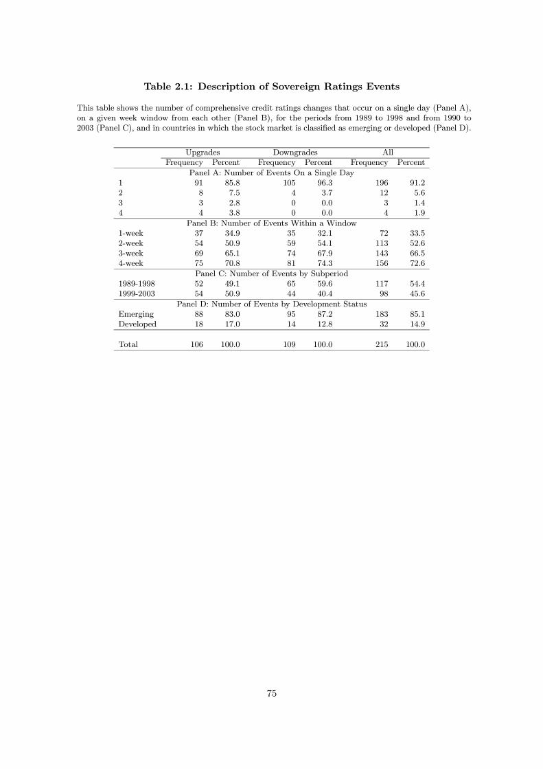
Table 2.1: Description of Sovereign Ratings Events

This table shows the number of comprehensive credit ratings changes that occur on a single day (Panel A),on a given week window from each other (Panel B), for the periods from 1989 to 1998 and from 1990 to2003 (Panel C), and in countries in which the stock market is classified as emerging or developed (Panel D).

Upgrades Downgrades AllFrequency Percent Frequency Percent Frequency Percent

Panel A: Number of Events On a Single Day1 91 85.8 105 96.3 196 91.22 8 7.5 4 3.7 12 5.63 3 2.8 0 0.0 3 1.44 4 3.8 0 0.0 4 1.9

Panel B: Number of Events Within a Window1-week 37 34.9 35 32.1 72 33.52-week 54 50.9 59 54.1 113 52.63-week 69 65.1 74 67.9 143 66.54-week 75 70.8 81 74.3 156 72.6

Panel C: Number of Events by Subperiod1989-1998 52 49.1 65 59.6 117 54.41999-2003 54 50.9 44 40.4 98 45.6

Panel D: Number of Events by Development StatusEmerging 88 83.0 95 87.2 183 85.1Developed 18 17.0 14 12.8 32 14.9

Total 106 100.0 109 100.0 215 100.0

75

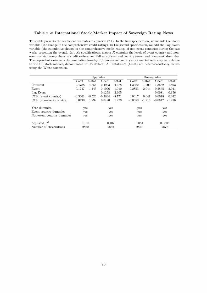
Table 2.2: International Stock Market Impact of Sovereign Rating News

This table presents the coefficient estimates of equation (2.1). In the first specification, we include the Eventvariable (the change in the comprehensive credit rating). In the second specification, we add the Lag Eventvariable (the cumulative change in the comprehensive credit ratings of non-event countries during the twoweeks preceding the event). In both specifications, matrix X contains the levels of event country and non-event country comprehensive credit ratings, and full sets of year and country (event and non-event) dummies.The dependent variable is the cumulative two-day [0,1] non-event country stock market return spread relativeto the US stock market, denominated in US dollars. All t-statistics (t-stat) are heteroscedasticity robustusing the White correction.

Upgrades DowngradesCoeff t-stat Coeff t-stat Coeff t-stat Coeff t-stat

Constant 2.4788 4.354 2.4923 4.378 1.3582 1.909 1.3682 1.893Event 0.1247 1.143 0.1096 1.010 -0.2853 -2.044 -0.2855 -2.041Lag Event 0.1258 2.605 -0.0081 -0.156CCR (event country) -0.3601 -8.526 -0.3834 -8.771 0.0017 0.041 0.0018 0.042CCR (non-event country) 0.0499 1.292 0.0490 1.273 -0.0650 -1.216 -0.0647 -1.216

Year dummies yes yes yes yesEvent country dummies yes yes yes yesNon-event country dummies yes yes yes yes

Adjusted R2 0.106 0.107 0.081 0.0803Number of observations 2862 2862 2877 2877

76

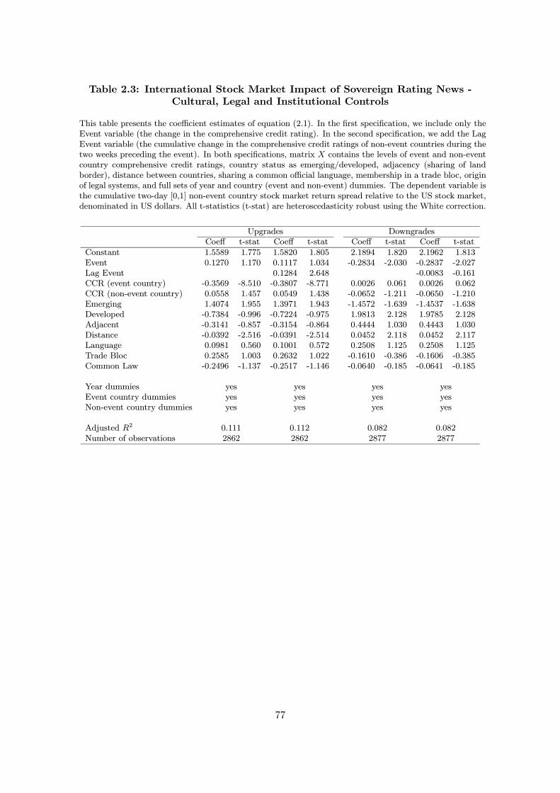
Table 2.3: International Stock Market Impact of Sovereign Rating News -Cultural, Legal and Institutional Controls

This table presents the coefficient estimates of equation (2.1). In the first specification, we include only theEvent variable (the change in the comprehensive credit rating). In the second specification, we add the LagEvent variable (the cumulative change in the comprehensive credit ratings of non-event countries during thetwo weeks preceding the event). In both specifications, matrix X contains the levels of event and non-eventcountry comprehensive credit ratings, country status as emerging/developed, adjacency (sharing of landborder), distance between countries, sharing a common official language, membership in a trade bloc, originof legal systems, and full sets of year and country (event and non-event) dummies. The dependent variable isthe cumulative two-day [0,1] non-event country stock market return spread relative to the US stock market,denominated in US dollars. All t-statistics (t-stat) are heteroscedasticity robust using the White correction.

Upgrades DowngradesCoeff t-stat Coeff t-stat Coeff t-stat Coeff t-stat

Constant 1.5589 1.775 1.5820 1.805 2.1894 1.820 2.1962 1.813Event 0.1270 1.170 0.1117 1.034 -0.2834 -2.030 -0.2837 -2.027Lag Event 0.1284 2.648 -0.0083 -0.161CCR (event country) -0.3569 -8.510 -0.3807 -8.771 0.0026 0.061 0.0026 0.062CCR (non-event country) 0.0558 1.457 0.0549 1.438 -0.0652 -1.211 -0.0650 -1.210Emerging 1.4074 1.955 1.3971 1.943 -1.4572 -1.639 -1.4537 -1.638Developed -0.7384 -0.996 -0.7224 -0.975 1.9813 2.128 1.9785 2.128Adjacent -0.3141 -0.857 -0.3154 -0.864 0.4444 1.030 0.4443 1.030Distance -0.0392 -2.516 -0.0391 -2.514 0.0452 2.118 0.0452 2.117Language 0.0981 0.560 0.1001 0.572 0.2508 1.125 0.2508 1.125Trade Bloc 0.2585 1.003 0.2632 1.022 -0.1610 -0.386 -0.1606 -0.385Common Law -0.2496 -1.137 -0.2517 -1.146 -0.0640 -0.185 -0.0641 -0.185

Year dummies yes yes yes yesEvent country dummies yes yes yes yesNon-event country dummies yes yes yes yes

Adjusted R2 0.111 0.112 0.082 0.082Number of observations 2862 2862 2877 2877

77

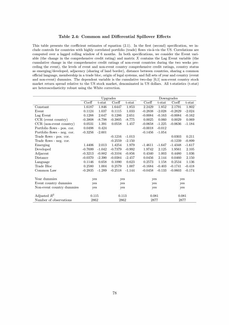
Table 2.4: Common and Differential Spillover Effects

This table presents the coefficient estimates of equation (2.1). In the first (second) specification, we in-clude controls for countries with highly correlated portfolio (trade) flows vis-a-vis the US. Correlations arecomputed over a lagged rolling window of 6 months. In both specifications, we consider the Event vari-able (the change in the comprehensive credit rating) and matrix X contains the Lag Event variable (thecumulative change in the comprehensive credit ratings of non-event countries during the two weeks pre-ceding the event), the levels of event and non-event country comprehensive credit ratings, country statusas emerging/developed, adjacency (sharing of land border), distance between countries, sharing a commonofficial language, membership in a trade bloc, origin of legal systems, and full sets of year and country (eventand non-event) dummies. The dependent variable is the cumulative two-day [0,1] non-event country stockmarket return spread relative to the US stock market, denominated in US dollars. All t-statistics (t-stat)are heteroscedasticity robust using the White correction.

Upgrades DowngradesCoeff t-stat Coeff t-stat Coeff t-stat Coeff t-stat

Constant 1.6187 1.846 1.6447 1.853 2.2429 1.852 2.1791 1.802Event 0.1124 1.037 0.1115 1.033 -0.2838 -2.028 -0.2829 -2.024Lag Event 0.1288 2.647 0.1286 2.651 -0.0084 -0.163 -0.0084 -0.162CCR (event country) -0.3808 -8.798 -0.3805 -8.775 0.0025 0.060 0.0029 0.069CCR (non-event country) 0.0531 1.391 0.0558 1.457 -0.0658 -1.225 -0.0636 -1.184Portfolio flows - pos. cor. 0.0498 0.424 -0.0018 -0.012Portfolio flows - neg. cor. -0.3256 -2.601 -0.1456 -1.054Trade flows - pos. cor. -0.1216 -1.013 0.0303 0.211Trade flows - neg. cor. -0.2559 -2.150 -0.1239 -0.899Emerging 1.4406 2.013 1.4254 1.979 -1.4611 -1.647 -1.4348 -1.617Developed -0.7699 -1.042 -0.7379 -0.992 1.9742 2.125 1.9561 2.105Adjacent -0.3213 -0.882 -0.3104 -0.856 0.4340 1.003 0.4480 1.036Distance -0.0370 -2.390 -0.0384 -2.457 0.0456 2.144 0.0460 2.150Language 0.1146 0.658 0.1090 0.623 0.2573 1.158 0.2534 1.136Trade Bloc 0.2580 1.004 0.2579 1.007 -0.1684 -0.403 -0.1741 -0.418Common Law -0.2835 -1.289 -0.2518 -1.144 -0.0458 -0.133 -0.0603 -0.174

Year dummies yes yes yes yesEvent country dummies yes yes yes yesNon-event country dummies yes yes yes yes

Adjusted R2 0.115 0.113 0.081 0.081Number of observations 2862 2862 2877 2877

78

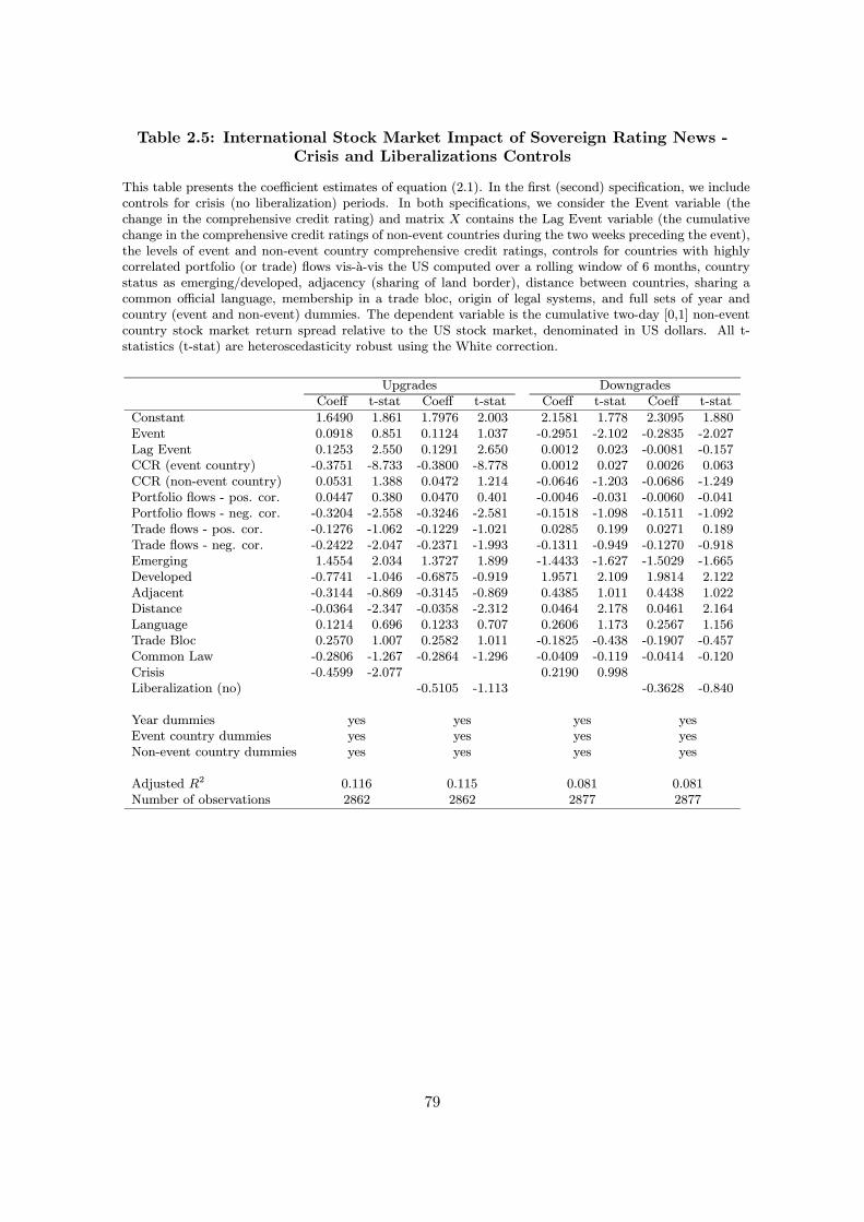
Table 2.5: International Stock Market Impact of Sovereign Rating News -Crisis and Liberalizations Controls

This table presents the coefficient estimates of equation (2.1). In the first (second) specification, we includecontrols for crisis (no liberalization) periods. In both specifications, we consider the Event variable (thechange in the comprehensive credit rating) and matrix X contains the Lag Event variable (the cumulativechange in the comprehensive credit ratings of non-event countries during the two weeks preceding the event),the levels of event and non-event country comprehensive credit ratings, controls for countries with highlycorrelated portfolio (or trade) flows vis-a-vis the US computed over a rolling window of 6 months, countrystatus as emerging/developed, adjacency (sharing of land border), distance between countries, sharing acommon official language, membership in a trade bloc, origin of legal systems, and full sets of year andcountry (event and non-event) dummies. The dependent variable is the cumulative two-day [0,1] non-eventcountry stock market return spread relative to the US stock market, denominated in US dollars. All t-statistics (t-stat) are heteroscedasticity robust using the White correction.

Upgrades DowngradesCoeff t-stat Coeff t-stat Coeff t-stat Coeff t-stat

Constant 1.6490 1.861 1.7976 2.003 2.1581 1.778 2.3095 1.880Event 0.0918 0.851 0.1124 1.037 -0.2951 -2.102 -0.2835 -2.027Lag Event 0.1253 2.550 0.1291 2.650 0.0012 0.023 -0.0081 -0.157CCR (event country) -0.3751 -8.733 -0.3800 -8.778 0.0012 0.027 0.0026 0.063CCR (non-event country) 0.0531 1.388 0.0472 1.214 -0.0646 -1.203 -0.0686 -1.249Portfolio flows - pos. cor. 0.0447 0.380 0.0470 0.401 -0.0046 -0.031 -0.0060 -0.041Portfolio flows - neg. cor. -0.3204 -2.558 -0.3246 -2.581 -0.1518 -1.098 -0.1511 -1.092Trade flows - pos. cor. -0.1276 -1.062 -0.1229 -1.021 0.0285 0.199 0.0271 0.189Trade flows - neg. cor. -0.2422 -2.047 -0.2371 -1.993 -0.1311 -0.949 -0.1270 -0.918Emerging 1.4554 2.034 1.3727 1.899 -1.4433 -1.627 -1.5029 -1.665Developed -0.7741 -1.046 -0.6875 -0.919 1.9571 2.109 1.9814 2.122Adjacent -0.3144 -0.869 -0.3145 -0.869 0.4385 1.011 0.4438 1.022Distance -0.0364 -2.347 -0.0358 -2.312 0.0464 2.178 0.0461 2.164Language 0.1214 0.696 0.1233 0.707 0.2606 1.173 0.2567 1.156Trade Bloc 0.2570 1.007 0.2582 1.011 -0.1825 -0.438 -0.1907 -0.457Common Law -0.2806 -1.267 -0.2864 -1.296 -0.0409 -0.119 -0.0414 -0.120Crisis -0.4599 -2.077 0.2190 0.998Liberalization (no) -0.5105 -1.113 -0.3628 -0.840

Year dummies yes yes yes yesEvent country dummies yes yes yes yesNon-event country dummies yes yes yes yes

Adjusted R2 0.116 0.115 0.081 0.081Number of observations 2862 2862 2877 2877

79

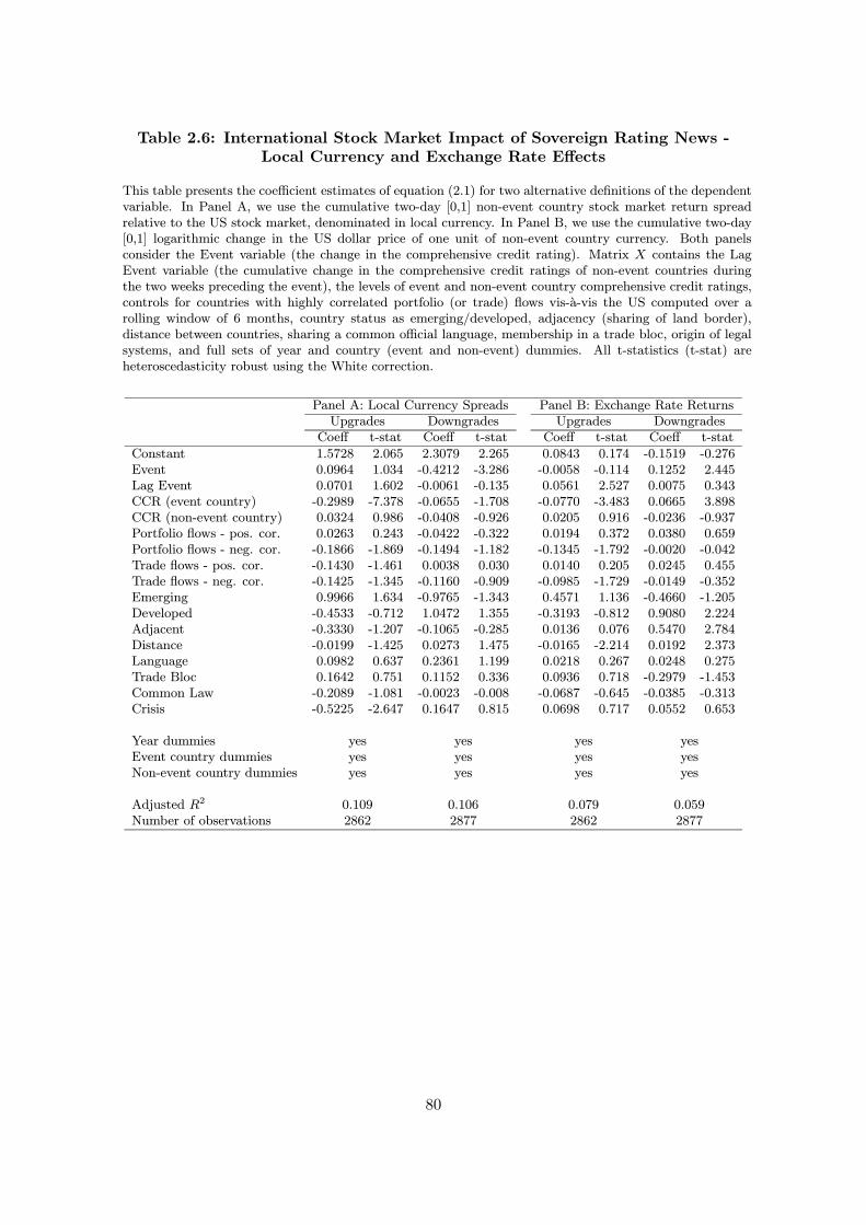
Table 2.6: International Stock Market Impact of Sovereign Rating News -Local Currency and Exchange Rate Effects

This table presents the coefficient estimates of equation (2.1) for two alternative definitions of the dependentvariable. In Panel A, we use the cumulative two-day [0,1] non-event country stock market return spreadrelative to the US stock market, denominated in local currency. In Panel B, we use the cumulative two-day[0,1] logarithmic change in the US dollar price of one unit of non-event country currency. Both panelsconsider the Event variable (the change in the comprehensive credit rating). Matrix X contains the LagEvent variable (the cumulative change in the comprehensive credit ratings of non-event countries duringthe two weeks preceding the event), the levels of event and non-event country comprehensive credit ratings,controls for countries with highly correlated portfolio (or trade) flows vis-a-vis the US computed over arolling window of 6 months, country status as emerging/developed, adjacency (sharing of land border),distance between countries, sharing a common official language, membership in a trade bloc, origin of legalsystems, and full sets of year and country (event and non-event) dummies. All t-statistics (t-stat) areheteroscedasticity robust using the White correction.

Panel A: Local Currency Spreads Panel B: Exchange Rate ReturnsUpgrades Downgrades Upgrades Downgrades

Coeff t-stat Coeff t-stat Coeff t-stat Coeff t-stat

Constant 1.5728 2.065 2.3079 2.265 0.0843 0.174 -0.1519 -0.276Event 0.0964 1.034 -0.4212 -3.286 -0.0058 -0.114 0.1252 2.445Lag Event 0.0701 1.602 -0.0061 -0.135 0.0561 2.527 0.0075 0.343CCR (event country) -0.2989 -7.378 -0.0655 -1.708 -0.0770 -3.483 0.0665 3.898CCR (non-event country) 0.0324 0.986 -0.0408 -0.926 0.0205 0.916 -0.0236 -0.937Portfolio flows - pos. cor. 0.0263 0.243 -0.0422 -0.322 0.0194 0.372 0.0380 0.659Portfolio flows - neg. cor. -0.1866 -1.869 -0.1494 -1.182 -0.1345 -1.792 -0.0020 -0.042Trade flows - pos. cor. -0.1430 -1.461 0.0038 0.030 0.0140 0.205 0.0245 0.455Trade flows - neg. cor. -0.1425 -1.345 -0.1160 -0.909 -0.0985 -1.729 -0.0149 -0.352Emerging 0.9966 1.634 -0.9765 -1.343 0.4571 1.136 -0.4660 -1.205Developed -0.4533 -0.712 1.0472 1.355 -0.3193 -0.812 0.9080 2.224Adjacent -0.3330 -1.207 -0.1065 -0.285 0.0136 0.076 0.5470 2.784Distance -0.0199 -1.425 0.0273 1.475 -0.0165 -2.214 0.0192 2.373Language 0.0982 0.637 0.2361 1.199 0.0218 0.267 0.0248 0.275Trade Bloc 0.1642 0.751 0.1152 0.336 0.0936 0.718 -0.2979 -1.453Common Law -0.2089 -1.081 -0.0023 -0.008 -0.0687 -0.645 -0.0385 -0.313Crisis -0.5225 -2.647 0.1647 0.815 0.0698 0.717 0.0552 0.653

Year dummies yes yes yes yesEvent country dummies yes yes yes yesNon-event country dummies yes yes yes yes

Adjusted R2 0.109 0.106 0.079 0.059Number of observations 2862 2877 2862 2877

80

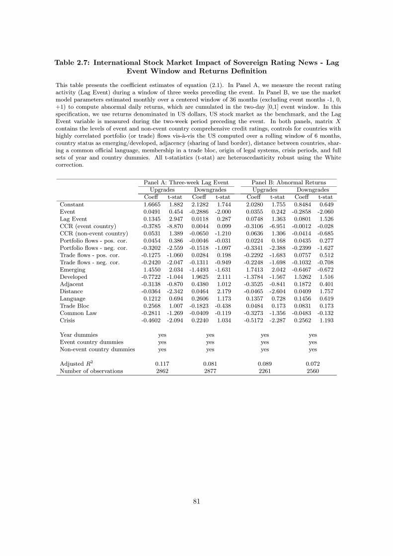
Table 2.7: International Stock Market Impact of Sovereign Rating News - LagEvent Window and Returns Definition

This table presents the coefficient estimates of equation (2.1). In Panel A, we measure the recent ratingactivity (Lag Event) during a window of three weeks preceding the event. In Panel B, we use the marketmodel parameters estimated monthly over a centered window of 36 months (excluding event months -1, 0,+1) to compute abnormal daily returns, which are cumulated in the two-day [0,1] event window. In thisspecification, we use returns denominated in US dollars, US stock market as the benchmark, and the LagEvent variable is measured during the two-week period preceding the event. In both panels, matrix Xcontains the levels of event and non-event country comprehensive credit ratings, controls for countries withhighly correlated portfolio (or trade) flows vis-a-vis the US computed over a rolling window of 6 months,country status as emerging/developed, adjacency (sharing of land border), distance between countries, shar-ing a common official language, membership in a trade bloc, origin of legal systems, crisis periods, and fullsets of year and country dummies. All t-statistics (t-stat) are heteroscedasticity robust using the Whitecorrection.

Panel A: Three-week Lag Event Panel B: Abnormal ReturnsUpgrades Downgrades Upgrades Downgrades

Coeff t-stat Coeff t-stat Coeff t-stat Coeff t-stat

Constant 1.6665 1.882 2.1282 1.744 2.0280 1.755 0.8484 0.649Event 0.0491 0.454 -0.2886 -2.000 0.0355 0.242 -0.2858 -2.060Lag Event 0.1345 2.947 0.0118 0.287 0.0748 1.363 0.0801 1.526CCR (event country) -0.3785 -8.870 0.0044 0.099 -0.3106 -6.951 -0.0012 -0.028CCR (non-event country) 0.0531 1.389 -0.0650 -1.210 0.0636 1.306 -0.0414 -0.685Portfolio flows - pos. cor. 0.0454 0.386 -0.0046 -0.031 0.0224 0.168 0.0435 0.277Portfolio flows - neg. cor. -0.3202 -2.559 -0.1518 -1.097 -0.3341 -2.388 -0.2399 -1.627Trade flows - pos. cor. -0.1275 -1.060 0.0284 0.198 -0.2292 -1.683 0.0757 0.512Trade flows - neg. cor. -0.2420 -2.047 -0.1311 -0.949 -0.2248 -1.698 -0.1032 -0.708Emerging 1.4550 2.034 -1.4493 -1.631 1.7413 2.042 -0.6467 -0.672Developed -0.7722 -1.044 1.9625 2.111 -1.3784 -1.567 1.5262 1.516Adjacent -0.3138 -0.870 0.4380 1.012 -0.3525 -0.841 0.1872 0.401Distance -0.0364 -2.342 0.0464 2.179 -0.0465 -2.604 0.0409 1.757Language 0.1212 0.694 0.2606 1.173 0.1357 0.728 0.1456 0.619Trade Bloc 0.2568 1.007 -0.1823 -0.438 0.0484 0.173 0.0831 0.173Common Law -0.2811 -1.269 -0.0409 -0.119 -0.3273 -1.356 -0.0483 -0.132Crisis -0.4602 -2.094 0.2240 1.034 -0.5172 -2.287 0.2562 1.193

Year dummies yes yes yes yesEvent country dummies yes yes yes yesNon-event country dummies yes yes yes yes

Adjusted R2 0.117 0.081 0.089 0.072Number of observations 2862 2877 2261 2560

81

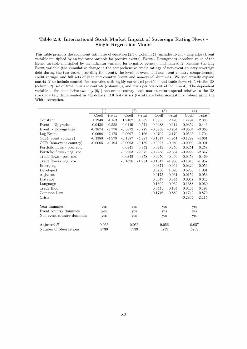
Table 2.8: International Stock Market Impact of Sovereign Rating News -Single Regression Model

This table presents the coefficient estimates of equation (2.3). Column (1) includes Event - Upgrades (Eventvariable multiplied by an indicator variable for positive events), Event - Downgrades (absolute value of theEvent variable multiplied by an indicator variable for negative events), and matrix X contains the LagEvent variable (the cumulative change in the comprehensive credit ratings of non-event country sovereigndebt during the two weeks preceding the event), the levels of event and non-event country comprehensivecredit ratings, and full sets of year and country (event and non-event) dummies. We sequentially expandmatrix X to include controls for countries with highly correlated portfolio and trade flows vis-a-vis the US(column 2), set of time invariant controls (column 3), and crisis periods control (column 4). The dependentvariable is the cumulative two-day [0,1] non-event country stock market return spread relative to the USstock market, denominated in US dollars. All t-statistics (t-stat) are heteroscedasticity robust using theWhite correction.

(1) (2) (3) (4)Coeff t-stat Coeff t-stat Coeff t-stat Coeff t-stat

Constant 1.7948 4.153 1.9102 4.369 1.8055 2.420 1.7794 2.388Event - Upgrades 0.0438 0.558 0.0449 0.571 0.0483 0.614 0.0352 0.446Event - Downgrades -0.3874 -3.776 -0.3872 -3.779 -0.3858 -3.764 -0.3504 -3.368Lag Event 0.0698 2.175 0.0697 2.166 0.0702 2.179 0.0565 1.704CCR (event country) -0.1388 -4.979 -0.1387 -4.987 -0.1377 -4.951 -0.1292 -4.661CCR (non-event country) -0.0065 -0.194 -0.0063 -0.189 -0.0027 -0.080 -0.0030 -0.091Portfolio flows - pos. cor. 0.0341 0.352 0.0249 0.256 0.0251 0.258Portfolio flows - neg. cor. -0.2263 -2.372 -0.2238 -2.354 -0.2229 -2.347Trade flows - pos. cor. -0.0345 -0.358 -0.0450 -0.466 -0.0453 -0.469Trade flows - neg. cor. -0.1828 -1.934 -0.1847 -1.960 -0.1843 -1.957Emerging 0.0374 0.064 0.0326 0.056Developed 0.6236 1.026 0.6266 1.031Adjacent 0.0175 0.061 0.0152 0.053Distance 0.0047 0.344 0.0047 0.345Language 0.1392 0.962 0.1388 0.960Trade Bloc 0.0443 0.184 0.0465 0.193Common Law -0.1746 -0.882 -0.1742 -0.879Crisis -0.2834 -2.115

Year dummies yes yes yes yesEvent country dummies yes yes yes yesNon-event country dummies yes yes yes yes

Adjusted R2 0.055 0.056 0.056 0.057Number of observations 5739 5739 5739 5739

82

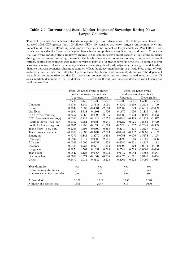
Table 2.9: International Stock Market Impact of Sovereign Rating News -Larger Countries

This table presents the coefficient estimates of equation (2.1) for ratings news in the 15 largest countries (PPPadjusted 2002 GDP greater than 300 billions USD). We consider two cases: larger event country news andimpact in all countries (Panel A), and larger event news and impact on larger countries (Panel B). In bothpanels, we consider the Event variable (the change in the comprehensive credit rating), and matrixX containsthe Lag Event variable (the cumulative change in the comprehensive credit ratings of non-event countriesduring the two weeks preceding the event), the levels of event and non-event country comprehensive creditratings, controls for countries with highly correlated portfolio (or trade) flows vis-a-vis the US computed overa rolling window of 6 months, country status as emerging/developed, adjacency (sharing of land border),distance between countries, sharing a common official language, membership in a trade bloc, origin of legalsystems, crisis periods, and full sets of year and country (event and non-event) dummies. The dependentvariable is the cumulative two-day [0,1] non-event country stock market return spread relative to the USstock market, denominated in US dollars. All t-statistics (t-stat) are heteroscedasticity robust using theWhite correction.

Panel A: Large event countries Panel B: Large eventand all non-event countries and non-event countriesUpgrades Downgrades Upgrades Downgrades

Coeff t-stat Coeff t-stat Coeff t-stat Coeff t-stat

Constant 5.1784 4.549 2.7138 2.091 6.8252 4.659 3.2611 1.799Event 0.3339 2.883 -0.4331 -2.830 0.2982 1.729 -0.5519 -2.489Lag Event 0.1894 2.718 0.1108 1.906 0.1176 1.090 0.1826 1.883CCR (event country) -0.7367 -9.968 0.0398 0.845 -0.8582 -7.933 0.0299 0.423CCR (non-event country) 0.0103 0.213 -0.1218 -2.052 -0.0243 -0.415 -0.1124 -1.317Portfolio flows - pos. cor. -0.1167 -0.781 -0.0420 -0.241 -0.0282 -0.125 -0.2081 -0.770Portfolio flows - neg. cor. -0.3065 -1.956 -0.1630 -1.009 -0.2420 -1.037 -0.2348 -0.903Trade flows - pos. cor. -0.2205 -1.403 -0.0609 -0.368 -0.2740 -1.225 0.2127 0.823Trade flows - neg. cor. -0.1280 -0.833 -0.3734 -2.323 -0.0944 -0.382 -0.3035 -1.162Emerging 0.7376 0.843 -2.2270 -2.258 -0.0258 -0.026 -1.5478 -1.165Developed 0.5892 0.619 2.9580 2.901 1.3220 1.166 2.4095 1.696Adjacent -0.0029 -0.006 0.6658 1.352 -0.4280 -0.521 1.4427 1.182Distance -0.0489 -2.233 0.0279 1.114 -0.0396 -1.222 0.0071 0.180Language 0.3874 1.561 0.1631 0.589 0.2548 0.715 -0.0362 -0.086Trade Bloc 0.0522 0.123 -0.0968 -0.173 0.0912 0.152 -0.5383 -0.581Common Law -0.5580 -1.574 -0.1362 -0.285 -0.5875 -1.071 0.3142 0.454Crisis -0.2470 -1.034 -0.5142 -2.228 -0.2265 -0.622 -0.5999 -1.685

Year dummies yes yes yes yesEvent country dummies yes yes yes yesNon-event country dummies yes yes yes yes

Adjusted R2 0.169 0.111 0.156 0.084Number of observations 1654 2047 816 1000

83

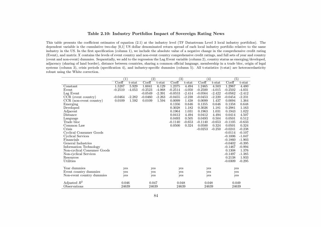
Table 2.10: Industry Portfolios Impact of Sovereign Rating News

This table presents the coefficient estimates of equation (2.1) at the industry level (TF Datastream Level 3 local industry portfolios). Thedependent variable is the cumulative two-day [0,1] US dollar denominated return spread of each local industry portfolio relative to the sameindustry in the US. In the first specification (column 1), we include the absolute value of a negative change in the comprehensive credit rating(Event), and matrix X contains the levels of event country and non-event country comprehensive credit ratings, and full sets of year and country(event and non-event) dummies. Sequentially, we add to the regression the Lag Event variable (column 2), country status as emerging/developed,adjacency (sharing of land border), distance between countries, sharing a common official language, membership in a trade bloc, origin of legalsystems (column 3), crisis periods (specification 4), and industry-specific dummies (column 5). All t-statistics (t-stat) are heteroscedasticityrobust using the White correction.

(1) (2) (3) (4) (5)Coeff t-stat Coeff t-stat Coeff t-stat Coeff t-stat Coeff t-stat

Constant 1.5287 5.929 1.6041 6.129 1.2375 4.494 1.2465 4.503 1.2967 4.480Event -0.2510 -4.053 -0.2523 -4.068 -0.2514 -4.050 -0.2500 -4.015 -0.2502 -4.031Lag Event -0.0549 -2.391 -0.0553 -2.414 -0.0564 -2.422 -0.0562 -2.412CCR (event country) -0.0464 -2.282 -0.0460 -2.263 -0.0455 -2.238 -0.0453 -2.220 -0.0454 -2.231CCR (non-event country) 0.0109 1.592 0.0109 1.594 0.0099 1.438 0.0099 1.437 0.0094 1.364Emerging 0.1356 0.646 0.1355 0.646 0.1358 0.648Developed 0.3028 1.182 0.3026 1.181 0.2981 1.163Adjacent 0.1964 1.031 0.1963 1.031 0.1943 1.022Distance 0.0412 4.494 0.0412 4.494 0.0414 4.507Language 0.0493 0.505 0.0493 0.504 0.0501 0.512Trade bloc -0.1140 -0.653 -0.1140 -0.653 -0.1105 -0.633Common Law 0.0500 0.324 0.0500 0.324 0.0501 0.324Crisis -0.0253 -0.250 -0.0241 -0.238Cyclical Consumer Goods -0.0114 -0.107Cyclical Services -0.1006 -1.047Financials -0.1860 -1.903General Industries -0.0402 -0.395Information Technology -0.1467 -0.994Non-cyclical Consumer Goods 0.1308 1.376Non-cyclical Services -0.1497 -1.385Resources 0.2138 1.933Utilities -0.0309 -0.295

Year dummies yes yes yes yes yesEvent country dummies yes yes yes yes yesNon-event country dummies yes yes yes yes yes

Adjusted R2 0.046 0.047 0.048 0.048 0.049Observations 24639 24639 24639 24639 24639

84

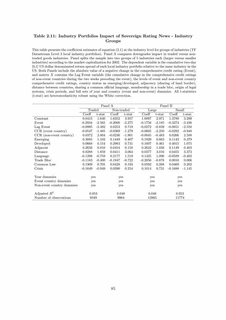
Table 2.11: Industry Portfolios Impact of Sovereign Rating News - IndustryGroups

This table presents the coefficient estimates of equation (2.1) at the industry level for groups of industries (TFDatastream Level 3 local industry portfolios). Panel A compares downgrades impact in traded versus non-traded goods industries. Panel splits the sample into two groups of 5 industries each (larger versus smallerindustries) according to the market capitalization for 2002. The dependent variable is the cumulative two-day[0,1] US dollar denominated return spread of each local industry portfolio relative to the same industry in theUS. Both Panels include the absolute value of a negative change in the comprehensive credit rating (Event),and matrix X contains the Lag Event variable (the cumulative change in the comprehensive credit ratingsof non-event countries during the two weeks preceding the event), the levels of event and non-event countrycomprehensive credit ratings, country status as emerging/developed, adjacency (sharing of land border),distance between countries, sharing a common official language, membership in a trade bloc, origin of legalsystems, crisis periods, and full sets of year and country (event and non-event) dummies. All t-statistics(t-stat) are heteroscedasticity robust using the White correction.

Panel A Panel BTraded Non-traded Large Small

Coeff t-stat Coeff t-stat Coeff t-stat Coeff t-stat

Constant 0.8415 1.640 1.6352 3.957 1.0897 2.971 1.3789 3.299Event -0.2934 -2.565 -0.2000 -2.275 -0.1756 -2.185 -0.3274 -3.436Lag Event -0.0995 -2.492 0.0253 0.719 -0.0272 -0.839 -0.0851 -2.550CCR (event country) -0.0547 -1.485 -0.0369 -1.279 -0.0605 -2.250 -0.0292 -0.948CCR (non-event country) 0.0372 2.804 -0.0236 -1.901 -0.0045 -0.483 0.0266 2.588Emerging 0.3885 1.102 0.1449 0.407 0.1929 0.663 0.1143 0.379Developed 0.0668 0.154 0.2983 0.731 0.1607 0.461 0.4015 1.075Adjacent 0.2656 0.810 0.0454 0.158 0.2632 1.038 0.1149 0.403Distance 0.0288 1.859 0.0411 3.064 0.0377 3.016 0.0455 3.372Language -0.1298 -0.759 0.2177 1.519 0.1425 1.096 -0.0589 -0.402Trade Bloc -0.1183 -0.400 -0.1947 -0.722 -0.2056 -0.878 0.0016 0.006Common Law 0.1909 0.705 0.0428 0.193 0.0592 0.288 0.0469 0.202Crisis -0.1649 -0.949 0.0390 0.254 0.1014 0.731 -0.1688 -1.145

Year dummies yes yes yes yesEvent country dummies yes yes yes yesNon-event country dummies yes yes yes yes

Adjusted R2 0.053 0.048 0.048 0.053Number of observations 9349 9964 12865 11774

85

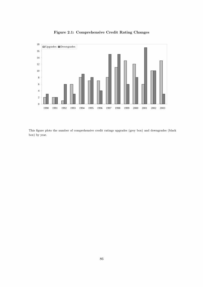
Figure 2.1: Comprehensive Credit Rating Changes

0

2

4

6

8

10

12

14

16

18

1990 1991 1992 1993 1994 1995 1996 1997 1998 1999 2000 2001 2002 2003

Upgrades Downgrades

This figure plots the number of comprehensive credit ratings upgrades (grey box) and downgrades (black

box) by year.

86

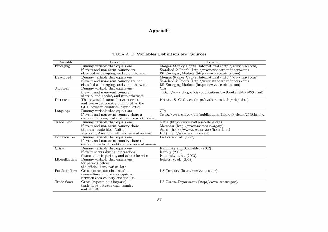
Appendix

Table A.1: Variables Definition and Sources

Variable Description SourcesEmerging Dummy variable that equals one Morgan Stanley Capital International (http://www.msci.com)

if event and non-event country are Standard & Poor’s (http://www.standardandpoors.com)classified as emerging, and zero otherwise ISI Emerging Markets (http://www.securities.com)

Developed Dummy variable that equals one Morgan Stanley Capital International (http://www.msci.com)if event and non-event country are not Standard & Poor’s (http://www.standardandpoors.com)classified as emerging, and zero otherwise ISI Emerging Markets (http://www.securities.com)

Adjacent Dummy variable that equals one CIAif event and non-event country (http://www.cia.gov/cia/publications/factbook/fields/2096.html)share a land border, and zero otherwise

Distance The physical distance between event Kristian S. Gleditsch (http://weber.ucsd.edu/∼kgledits)and non-event country computed as theGCD between countries’ capital cities

Language Dummy variable that equals one CIAif event and non-event country share a (http://www.cia.gov/cia/publications/factbook/fields/2098.html).common language (official), and zero otherwise

Trade Bloc Dummy variable that equals one Nafta (http://www.nafta-sec-alena.org)if event and non-event country share Mercosur (http://www.mercosur.org.uy)the same trade bloc, Nafta, Asean (http://www.aseansec.org/home.htm)Mercosur, Asean, or EU, and zero otherwise EU (http://www.europa.eu.int)

Common law Dummy variable that equals one La Porta et al. (1997).if event and non-event country share thecommon law legal tradition, and zero otherwise

Crisis Dummy variable that equals one Kaminsky and Schmukler (2002),if event occurs during international Karoliy (2003),financial crisis periods, and zero otherwise Kaminsky et al. (2003).

Liberalization Dummy variable that equals one Bekaert et al. (2003).for periods beforethe officialliberalization date

Portfolio flows Gross (purchases plus sales) US Treasury (http://www.treas.gov).transactions in foreigner equitiesbetween each country and the US

Trade flows Gross (exports plus imports) US Census Department (http://www.census.gov).trade flows between each countryand the US

87

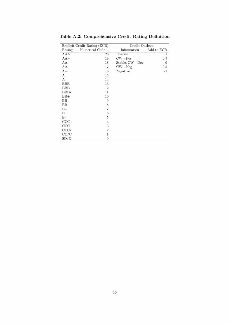
Table A.2: Comprehensive Credit Rating Definition

Explicit Credit Rating (ECR) Credit OutlookRating Numerical Code Information Add to ECR

AAA 20 Positive 1AA+ 19 CW - Pos 0.5AA 18 Stable/CW - Dev 0AA- 17 CW - Neg -0.5A+ 16 Negative -1A 15A- 14BBB+ 13BBB 12BBB- 11BB+ 10BB 9BB- 8B+ 7B 6B- 5CCC+ 4CCC 3CCC- 2CC/C 1SD/D 0

88

CHAPTER 3

Correlations of Global Industry Portfolios: An Empirical

Investigation of Trends and Asymmetries

(with Miguel Ferreira)

3.1. Introduction

Have global industries correlations decreased? Is correlation related to industry specific

characteristics? In this paper, we find that indeed global industry correlation changes over

time. The late 1990s period is characterized by low correlations. Furthermore, industry

correlations are counter-cyclically and small and value (low price-earnings ratios) industries

have lower correlations. Industry correlations increase for market downturns. Correlation

asymmetry is found among all size, price-earnings ratios, and economic sector groups (only

exceptions are resources and utilities), but is more pronounced among small industries.

The increasing integration of economies and the globalization of business activities sug-

gest that global factors should play an increasingly important role in the pricing of securities.

Recent research supports this implication. Diermeier and Solnik (2001) find strong evidence

that firms are priced globally and that it is incorrect to assume that the companies head-

quarters location (or the market its stock is listed) captures the major source of influence in

its stock return behavior.1

In addition, several papers find evidence supporting the growing importance of global

industry factors relative to that of country specific factors in determining equity returns.

For example, Cavaglia, Brightman, and Aked (2000) and Baca, Garbe, and Weiss (2000),

1See also, Brooks and del Negro (2003), Cavaglia, Cho, and Singer (2001), and Lombard, Roulet, and Solnik(1999).

89

show that for developed equity markets, from the mid 1990s onwards, the importance of

country-specific factors declines while that of global industry factors increases. In fact,

Brooks and Catao (2000) show that the importance of global industry factors increases for

both developed and emerging markets, and this is primarily explained by technology stocks.

In contrast with developed markets, emerging markets do not present a decrease in country-

specific factors (Serra (2000)).

These recent evidence is at odds with previous work by Heston and Rouwenhorst (1994)

and Griffin and Karolyi (1998) that shows the dominance of pure country factors relative to

pure global industry factors. Accordingly, “slicing” the world by industries rather than only

by countries could be a useful tool to increase the benefits of international diversification

strategies in terms of risk reduction

While much is known about cross-country correlation (and as we know correlations play a

key role in assessing the power of diversification), on the other hand the empirical analysis of

the correlation of global industries is an issue that, to our knowledge, has been overlooked in

the literature. Thus, our goal is to contribute to the literature on international investments

with the characterization of global industry portfolios correlation dynamics, in particular in

terms of long-term trends and asymmetries.2

Our methodology is characterized by several distinct features. First, we use a simple and

time-varying measure of correlation - realized correlation (e.g., Andersen, Bollerslev, Diebold,

and Ebens (2001)). Specifically, we use within month daily index return data to construct

a time series of correlation at the monthly frequency, which are treated as “observable” and

consequently suitable for posterior analysis using standard econometric models. Relative to

multivariate GARCH alternatives (e.g., Engle (2002)), we do not need to impose a parametric

model to describe the time evolution of covariances or volatilities, but still allowing these

variables to change over time. Relative to rolling window estimates (e.g., Solnik, Boucrelle,

and Le Fur (1996)), realized correlation minimizes autocorrelation and “ghost effects”.

2Global industries presumably diversify away country specific sources of return variation, and thus allow for anew look at the global stock correlation minimizing the dynamics of country factors in explaining the variationof returns.

90

Second, we study the time series behavior and asymmetries of the correlation for alter-

native groups of industries, based on size, price-earnings ratio, and economic sectors. In

fact, we characterize the structure of correlation with the market according to two global

industry characteristics: market capitalization (size) and price-earnings ratios (PER). These

characteristics are known to have predictive power to explain the cross-section of expected

stock returns; see, for example, Banz (1981), Basu (1983), Fama and French (1992,1998),

Haugen and Baker (1996). Recently, Lewellen (2004) demonstrates the ability of market-

level financial ratios to predict market returns, and Lewellen (1999) examines the relation

between US industry portfolios returns and lagged book to market ratios.

Finally, we use time-varying estimates of correlation to investigate asymmetries relative

to the market trend (up and down). Relative to the traditional “exceedance correlations”

method for testing asymmetries (e.g., Ang and Chen (2002) and Longin and Solnik (2001)),

we do not compare time-constant estimates of correlation obtained from pre-sampled returns

that are either higher or lower a given threshold.

The literature offers some key results that are related to our work. With respect to

cross-country correlations, the literature shows that: (1) correlation is time unstable with

tendency to increase over time (e.g. Solnik and Roulet (2000), Longin and Solnik (1995),

Tang (1995)); (2) correlation is positively related to the level of country volatility (e.g.

Solnik, Boucrelle and Le Fur (1996)); (3) correlation is higher in bear markets (e.g. Longin

and Solnik (2001)); and (4) correlation is related to the coherence between countries’ business

cycles and its market phase (Erb, Harvey, and Viskanta (1994).3

With respect to global industry portfolios, Ferreira and Gama (2004) find that between

1974 and 2001 there is no noticeable long-term trend in industry-specific or world portfolio

risk (for developed markets). In contrast, the late 1990s are characterized by an increase

3Serra (2000) shows that within emerging markets, between 1990 and 1996 aggregate correlation across sectorportfolios (0.54) is substantially higher than across country portfolios (0.07). Also, Meric and Meric (1989)show that for a sample of 17 developed markets, between 1973 and 1987 the correlation between globalindustries (0.619) is higher than between countries (0.398). These results are in line with the earlier resultson the dominance of pure country factors in explaining security variation of Heston and Rouwenhorst (1994)and Griffin and Karoliy (1998), but are silent about the cross-section and time-series properties of globalindustry correlation, the subject of our paper.

91

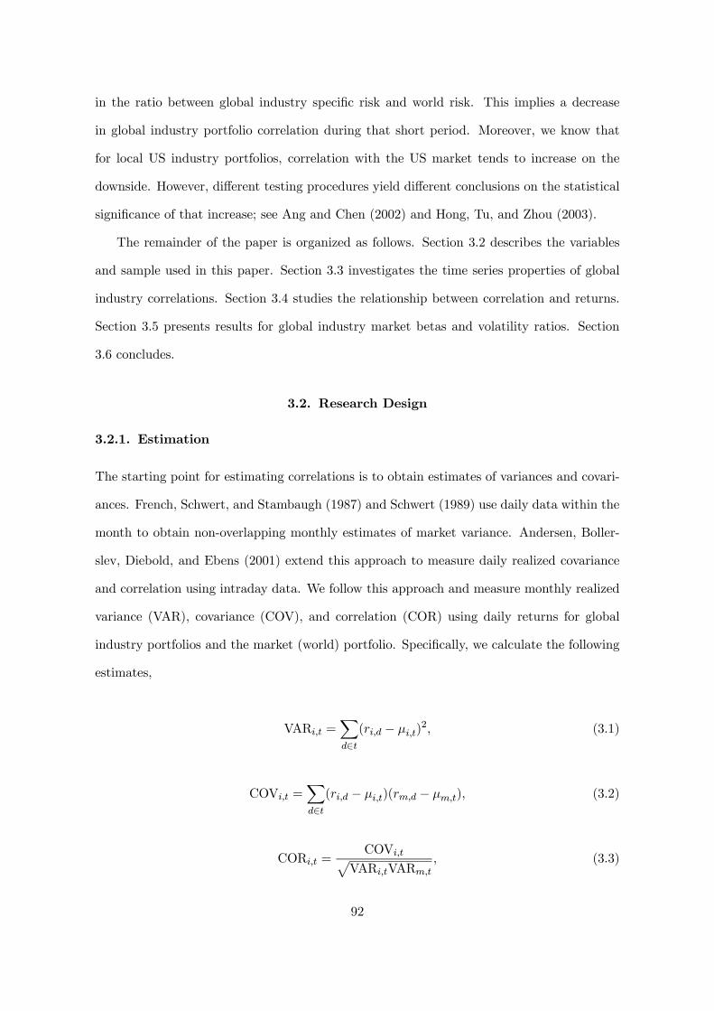
in the ratio between global industry specific risk and world risk. This implies a decrease

in global industry portfolio correlation during that short period. Moreover, we know that

for local US industry portfolios, correlation with the US market tends to increase on the

downside. However, different testing procedures yield different conclusions on the statistical

significance of that increase; see Ang and Chen (2002) and Hong, Tu, and Zhou (2003).

The remainder of the paper is organized as follows. Section 3.2 describes the variables

and sample used in this paper. Section 3.3 investigates the time series properties of global

industry correlations. Section 3.4 studies the relationship between correlation and returns.

Section 3.5 presents results for global industry market betas and volatility ratios. Section

3.6 concludes.

3.2. Research Design

3.2.1. Estimation

The starting point for estimating correlations is to obtain estimates of variances and covari-

ances. French, Schwert, and Stambaugh (1987) and Schwert (1989) use daily data within the

month to obtain non-overlapping monthly estimates of market variance. Andersen, Boller-

slev, Diebold, and Ebens (2001) extend this approach to measure daily realized covariance

and correlation using intraday data. We follow this approach and measure monthly realized

variance (VAR), covariance (COV), and correlation (COR) using daily returns for global

industry portfolios and the market (world) portfolio. Specifically, we calculate the following

estimates,

VARi,t =Xd∈t(ri,d − µi,t)2, (3.1)

COVi,t =Xd∈t(ri,d − µi,t)(rm,d − µm,t), (3.2)

CORi,t =COVi,tp

VARi,tVARm,t, (3.3)

92

where rj,d denotes the world portfolio (j ≡ m) or global industry portfolio i (j ≡ i) logarith-

mic returns on day d of month t, and µj,t is the average daily return of portfolio j on month

t. Variance and covariance estimates are obtained at the monthly horizon. To assure that

the variance estimator is not negative, we follow Schwert (1989) and do not include the one

lagged cross-product of square returns suggested by French, Schwert, and Stambaugh (1987)

aiming at accounting for the return series autocorrelation. The correlation of each industry

portfolio with the world portfolio proxies for the average correlation of each industry with

the remaining industry portfolios, as the covariance with the market is the average of the

pairwise covariances and correlation is a rescaled covariance.4

We note that the pervasive effects of non-overlapping trading periods over correlation

(namely the downward biases documented, for example, by Kayha (1997)) should be more

serious for the estimates comparing different countries than for those comparing different

global industries. The global industry indexes are computed as a weighted average of local

industry indexes in the same trading day (when available). For instance, information arriving

the global market after Japan closes on a given day, would be reflected in the global industries

indexes through the close in the US market. Thus, the global level of information relevant

for pricing arriving the markets during a given trading day is reflected in the global industry

indexes. In contrast, global information available after a market close can only be reflected

by the early closing country stock markets indexes in the next trading day.

We study the behavior of correlation for industry groups based on market capitalization

(size) and price earnings ratio (PER). These attributes are chosen because they are determi-

nants of the cross-section of expected returns; see, e.g., Banz (1981), Basu (1983), Fama and

French (1992, 1998), Haugen and Baker (1996).5 Specifically, we use for each global industry

portfolio (i) in each month (t), the following attributes,

4Thus, the correlation with the market is a positive function of the average pairwise correlations. Ang andChen (2002) and Hong, Tu, and Zhou (2002) also rely on the correlation with the market to study correlationasymmetries in the US market.5Bekaert, Harvey, Lundblad, and Siegel (2004), use local industry price-earnings ratios as a source of infor-mation about countries’ growth opportunities. The study confirms empirically the intuition that countrieswith heavy wheightings on high PER industries have high implied growth opportunities.

93

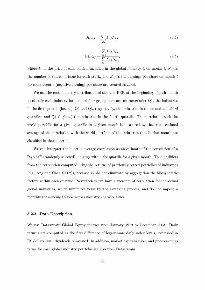
Sizei,t =Xc∈iPc,tNc,t, (3.4)

PERi,t =

Pc∈iPc,tNc,tP

c∈iEc,tNc,t

, (3.5)

where Pc is the price of each stock c included in the global industry i, on month t, Nc,t is

the number of shares in issue for each stock, and Ec,t is the earnings per share on month t

for constituent c (negative earnings per share are treated as zero).

We use the cross-industry distribution of size and PER at the beginning of each month

to classify each industry into one of four groups for each characteristic: Q1, the industries

in the first quartile (lowest), Q2 and Q3, respectively, the industries in the second and third

quartiles, and Q4 (highest) the industries in the fourth quartile. The correlation with the

world portfolio for a given quartile in a given month is measured by the cross-sectional

average of the correlation with the world portfolio of the industries that in that month are

classified in that quartile.

We can interpret the quartile average correlation as an estimate of the correlation of a

”typical” (randomly selected) industry within the quartile for a given month. Thus, it differs

from the correlation computed using the returns of previously sorted portfolios of industries

(e.g. Ang and Chen (2002)), because we do not eliminate by aggregation the idiosyncratic

factors within each quartile. Nevertheless, we have a measure of correlation for individual

global industries, which minimizes noise by the averaging process, and do not impose a

monthly rebalancing to look across industry characteristics.

3.2.2. Data Description

We use Datastream Global Equity indexes from January 1979 to December 2003. Daily

returns are computed as the first difference of logarithmic daily index levels, expressed in

US dollars, with dividends reinvested. In addition, market capitalization, and price earnings

ratios for each global industry portfolio are also from Datastream.

94

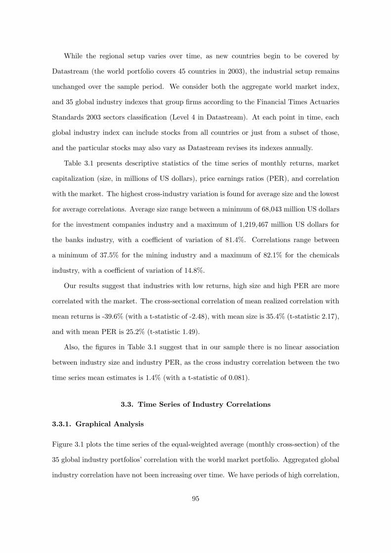
While the regional setup varies over time, as new countries begin to be covered by

Datastream (the world portfolio covers 45 countries in 2003), the industrial setup remains

unchanged over the sample period. We consider both the aggregate world market index,

and 35 global industry indexes that group firms according to the Financial Times Actuaries

Standards 2003 sectors classification (Level 4 in Datastream). At each point in time, each

global industry index can include stocks from all countries or just from a subset of those,

and the particular stocks may also vary as Datastream revises its indexes annually.

Table 3.1 presents descriptive statistics of the time series of monthly returns, market

capitalization (size, in millions of US dollars), price earnings ratios (PER), and correlation

with the market. The highest cross-industry variation is found for average size and the lowest

for average correlations. Average size range between a minimum of 68,043 million US dollars

for the investment companies industry and a maximum of 1,219,467 million US dollars for

the banks industry, with a coefficient of variation of 81.4%. Correlations range between

a minimum of 37.5% for the mining industry and a maximum of 82.1% for the chemicals

industry, with a coefficient of variation of 14.8%.

Our results suggest that industries with low returns, high size and high PER are more

correlated with the market. The cross-sectional correlation of mean realized correlation with

mean returns is -39.6% (with a t-statistic of -2.48), with mean size is 35.4% (t-statistic 2.17),

and with mean PER is 25.2% (t-statistic 1.49).

Also, the figures in Table 3.1 suggest that in our sample there is no linear association

between industry size and industry PER, as the cross industry correlation between the two

time series mean estimates is 1.4% (with a t-statistic of 0.081).

3.3. Time Series of Industry Correlations

3.3.1. Graphical Analysis

Figure 3.1 plots the time series of the equal-weighted average (monthly cross-section) of the

35 global industry portfolios’ correlation with the world market portfolio. Aggregated global

industry correlation have not been increasing over time. We have periods of high correlation,

95

for instance the early 1990s, when the maximum is reached (95.2% in August 1991), but these

do not seem to persist. In fact, average global industry correlation shows wide fluctuations

at the monthly frequency and a slow moving U-shaped pattern during the 1980s and the

1990s. Most noticed is the sharp downward move after 1997, a period characterized by a

cluster of low correlation spikes, namely in April 1999 (22.5%, the minimum) and January

2001 (25.2%, the second lowest). These low levels are followed by a recovery to historical

levels by 2003. Overall, the time evolution of aggregated industry correlation, suggests a

pattern characterized by temporary long-term swings and the absence of a secular increase

in correlation.

The downward move in the late 1990s, is in line with the findings of Ferreira and Gama

(2004). The higher increase in global industry specific risk relative to that of world portfolio

volatility, implies a decrease in global industry correlation.

Also noticed is the tendency of an increase in correlation during economic recessions. In

Figure 3.1, the shaded areas represent the periods of US contraction, as officially dated by

NBER. During recessions, both a cluster of correlation peaks as well as an increase in the

slow moving component is noticed. Particularly evident is the increase in correlation during

the 2001 US recession.

Figures 3.2 and 3.3 show correlation for the lowest (Panel A) and highest (Panel B)

quartiles of size and PER, respectively. Both for size and PER groups , the lowest quartile

(Q1) show wider movements than the highest (Q4) quartile at the low frequency (12-month

moving average). Also, there is no evidence of a secular increase. All the series reach its

maximum in August 1991, with monthly estimates above 90% (a feature that also charac-

terize the middle quartiles). April 1999, is a month of unusually low (and negative) realized

correlations for the lowest quartiles of size (-10.2%) and PER (-13.1%). For the highest quar-

tile of size, April 1999 also represents the time series minimum, but with a positive value

96

(42.1%). For the highest quartile of PER, the time series minimum is reached in January

2001 (28.0%) and August 2000 represents the second lowest estimate (31.8%).6

3.3.2. Trends

Table 3.2 presents descriptive statistics for the quartile correlation time series and investigates

the stochastic behavior of correlation for the whole sample period. Panel A uses the value-

weighted world portfolio return from Datastream, and Panel B uses the equal-weighted (EW)

average return of the 35 global industry portfolios to proxy for the world portfolio return.7

Over the whole sample period, global industry correlation is lower for the lowest size or

price earnings ratios quartiles. The fairly high autocorrelation, does not mean that the series

are integrated. Given that correlation is bounded, technically it can not have a unit root.

Nonetheless, since perfect correlation (either positive or negative) is unnoticed in practice,

correlation can still exhibit nonstationary behavior. The null hypothesis of a unit root is

rejected by the Augmented Dickey-Fuller (ADF) t test, for all series, at the 5% level (the

number of lags is determined by the Akaike Information Criterion) Thus, average correlation

series seem to be stationary, which means that fluctuations around the long-run mean do not

produce permanent effects on its behavior.8 This is consistent with the long-term temporary

swings already uncovered in the graphical analysis.

One important issue for international investors is to evaluate whether correlation remains

constant over time. We can diagnose the time instability in the correlation series by testing

for long-term trends. Following Longin and Solnik (1995) a simple linear trend model is

specified with the sole purpose of testing the existence of a trend. To test for the significance

6For the other quartiles of size the minimum estimate is reached in January 2001 (10.7% Q2, and 22.2% Q3).For the PER Q2 quartile, April 1999 is the minimum (6.0%), and for the PER Q3 quartile, the time seriesminimum is reached in December 1999, with 30.2%.7The EW world return is used to ascertain to what extent the cross sectional characteristics of industrycorrelation, especially for the size quartiles, are a simple manifestation of the, unavoidable, fact that highersize industries weight more on the world portfolio and thus are expected to be more correlated with themarket, in a reality characterized by cross industry positive covariances.8Extensive testing shows that rejection of the null with the Phillips-Perron Zt test is possible for every lagup to 18. As an alternative procedure to handle the bounded variables problem, Cavaliere (2005) uses MonteCarlo simulations to estimate new critical values for the Phillips-Perron Zt test. Our estimates of the Ztstatistic (not reported, but available upon request) are all below the bounded critical values.

97

of the trend coefficient we use the t− PST test of Vogelsang (1998), which performs well in

finite samples for series with serial correlation, and is valid whether or not the errors contain

a unit root. Specifically, we estimate the following regression,

CORQ,t = α0,Q + α1,QT + ²Q,t, (3.6)

where CORQ,t is the correlation with the market portfolio estimate (alternatively it refers

to the correlation with the VW world portfolio returns or the correlation with the EW world

portfolio returns) for quartile Q during month t, and T is a time trend. α1,Q measures the

expected monthly increase in correlation.9

Panel A of Table 3.2 show that the trend coefficients are not statistically significant, al-

though their signs are different. For the all-industry average correlation, the trend coefficient

is negative. For the size-based quartiles, the evidence suggests the existence of a long-term

“size effect” in the behavior of industry portfolios correlation with the market. In fact, the

trend coefficient is negative for Quartiles 1 through 3 and is positive for Quartile 4. For the

price earnings based quartiles, the evidence suggests a U-shaped behavior. The correlation

in the extreme quartiles tends to increase, while that in the middle quartiles tends to be

decreasing in the long run.

As Panel B of Table 3.2 shows, the overall characteristics of these patterns are not

affected by the definition of the world portfolio return. The signs of the (insignificant) trend

coefficients do suggest the same basic pattern: largest industries and extreme PER industries

have higher correlations over the long run. The main change relative to Panel A is that the

monotonic increase with size no longer holds, as the fourth quartile estimate is now lower

than the one for the third quartile. However, difference is small and the estimated correlation

for the fourth quartile is higher than the estimated average correlation for the second and

first quartiles.

9We do run regressions with Fisher z correlation coefficients as dependent variable to minimize the effects onthe residuals’ distribution of using a bounded variable as dependent variable. The conclusions are unaffected,so these results are not reported, but are available on request.

98

Our results point out to a positive relation between industry correlation and size, that is

not due simply to a ”mechanical” size effect. A possible explanation is a diversification effect.

Indeed, if industries with higher market value are also industries characterize by a more

diversified portfolio of activities, namely at the international level, than higher correlation

would result from the expected lower industry-specific risk.10

The absence of an upward trend (or suggestion of downward trend) in industry correlation

with the market, is in contrast with Longin and Solnik (1995) finding of a positive (and

statistically significant in 4 countries) linear trend in the conditional correlation of the G-7

countries stock market index with the US market, between 1960 and 1990. Also, Solnik and

Roulet (2000) show that their estimate of ”cross-sectional” correlation of 15 developed stock

markets returns with the world portfolio returns has a positive and statistically significant

trend slope (between 1971 and 1998).

3.3.3. Time and Quartile Effects

Our evidence suggests that long-term swings rather than a secular trend, characterizes the

behavior of global industry correlations. To further document these patterns, we calculate the

average correlation for 5 equally-spaced sub-periods of 60 months. The statistical significance

of the time variation in average correlation in each sub period, is based on the following

regression,

CORQ,t =XP

θQ,P IP + γCORQ,t−1 + ²Q,t, (3.7)

where CORQ,t is the quartile Q = 1, 2, 3, 4 correlation with the world portfolio during month

t, and IP is equal to one if the month t observation occurs during the sub-period P = 2, ..., 8,

and zero otherwise. Given that it is feasible that the residuals in each quartile regression

would be contemporaneously correlated with the residuals in the other quartile regressions,

we estimate jointly the four equations relating to each characteristic (size or PER), using the

Seemingly Unrelated Regressions(SUR) technique, to increase the efficiency of estimators,

10We thank Peter Ritchken for pointing this to us.

99

and because it allows for a direct test of the differences across quartiles. Lagged correlation is

introduced to capture the high persistence exhibit by the correlation series. Standard errors

are heteroskedasticity and autocorrelation robust using the Newey-West correction with five

lags.

We test for quartile effects (time measured) with a joint Wald χ2 test for the null hy-

pothesis θ1,P = ... = θ4,P , for each period P . We test for time effects with a joint test for

the null hypothesis θQ,1 = ... = θQ,5 for each quartile Q.11

Table 3.3 presents the results.12 Panel A uses value-weighted world portfolio returns.

The 1999-2003 period is characterized low realized correlations. In all quartiles of size (with

the exception of the highest size quartile Q4) and all quartiles of PER, the mean correlation

is lower for the 1999-2003 period, relative to all the other sub-periods. For the largest size

quartile, the decrease in correlation following the upward move in the 1989-1993 period, is

not strong enough to reach beginning of the sample values. The up and down moves in

correlation (time effects) are statistically significant for all quartiles, with the exception of

the lowest size (Q1) quartile.

The lower industry correlations for the 1999-2003 period, are in contrast with the cross-

country correlation increase in the late 1990. For example, Statman and Scheid (2004) show

that correlations between the US stock market and other international stock markets reach

a peak of 0.86 in December 2003.

The absence of time effects in the lowest size group is interesting for global investors, as

these ”small” industry portfolios, are also the ones less correlated with the world portfolio.

In fact, in the five sub-periods, for the size characteristic, the least correlated quartile is

always the lowest size quartile, and the cross quartile mean differences (quartile effects)

are statistically significant. Interestingly, size is more powerful than for PER in explaining

11As Judge et al. (1988) mention, testing for time effects based on the individual significance of individualdifferential coefficients (t test) would not be advisable, because the individual coeficients significance dependon the parameterization adopted.12We do run regressions with Fisher z correlation coefficients as dependent variable to minimize (but noteliminating) the effects on the residuals’ distribution of using a bounded variable as dependent variable. Theconclusions are unaffected, so these results are not reported, but are available on request.

100

the cross-section of correlation, as the statistical significance of the restriction that mean

correlation is equal across quartiles is much higher for the size quartiles.

Panel B addresses the importance of the expected increase in correlation with the world

portfolio for its relative most important components, by using as benchmark the equal-

weighted returns of the 35 global industry portfolios. The overall effect in the sub-period

means is an increase in the smallest size and lowest PER quartiles correlation, and a decrease

in the largest size and highest PER quartile correlation. Surprisingly, the differences are more

noticed for the PER quartiles than for the size quartiles. These differences are related to

the statistical significance of the time and quartile effects, and not to their overall patterns

(lower correlation for the 1999 to 2003 period, and for the Q1 of size or PER).

For the size quartiles, we cannot reject the restriction that mean estimates are different

for the 1999-2003 period, and we find statistically significant quartile effects in all other

sub-periods, and significant time effects in all but the smallest size quartile.

For the PER quartiles, we find statistical insignificant time effects in the lowest quartile,

while for the other quartiles there still is considerable time variation in the level of correla-

tion. Most interesting, with the EW world returns as benchmark, the PER quartile effects

lose statistical significance. This suggests that after controlling for the size effects on the

correlation estimates (via an equalization of size in the determination of world returns), a

statistically significant independent PER effect does not emerge.13

To conclude this section, we look at the interaction between size and PER in determining

the correlation level. We have already seen that smallest and growth industries have lower

correlations. Which of the characteristics dominate (if any)? To illustrate this issue, we

perform a double sort of the correlation industry groups’ series. First, industries are classified

according to the size quartiles. Second, within each size quartile, industries are classified

according to the PER quartiles. Thus, the monthly average of industries correlations allows

the construction of a time series of industries correlations for the 16 industry groups created

13Fama and French (1992) show that the individual explanatory power of E/P is lost in a multivariateregression which also includes Size, when explaning the cross section of expected returns.

101

(e.g. Q1 PER of the Q1 size).14 In addition, we also perform the double sorting of the

industries correlations, using the reverse procedure. That is first sorting on PER and next

on size, within each PER quartile.

Table 3.4 presents the time series mean correlation for each of the 16 groups, together

with the difference between the first and fourth quartile (columns differences). First, the

PER effects are most noticed for the smallest industries. The PER range for the size Q1

(10.5%) is at least twice the PER range for the other quartiles of size.

Second, the size effects are more pronounced for the low PER industries, and are eco-

nomically most significant (measured by the range between size quartiles) than PER effects.

In other words, size effects dominate PER effects. In fact, when we move from the Q1 to Q4

of size (for a given PER) the increase in correlation is greater than when we move from Q1

to Q4 of PER (for a given size).

Panel B uses equal-weighted world portfolio returns. The removal of industry capital-

ization effects on the computation of world returns, reinforces the intuition that size effects

dominate PER effects. When we first sort on size, the PER effects (except for the Q1 of size)

decrease substantially relative to VW world returns. When we first sort on PER, again we

observe a decrease in size effects relative to VW returns, but these are always greater than

the PER effects. This reinforces the importance of size for the estimated level of realized

correlation.

3.3.4. Global Economic Sectors

This section investigates the time series behavior of market correlation behavior for indi-

vidual global economic sectors. We use FTSE Economic sectors classification to aggregate

individual industries correlation into 10 groups representing the economic sectors resources,

basic industries, general industries, cyclical consumer goods, non-cyclical consumer goods,

cyclical Services, non-cyclical services, utilities, information technology, and financials. For

14The procedure assures that at least two global industry portfolios’ correlation is averaged monthly toestimate the monthly realized correlation for a given industry group.

102

example, the correlation for the resources sector is proxied by the average correlation of the

mining and oil & gas global industries.

Table 3.5 presents the results. Panel A uses the value-weighted world portfolio returns.

The average correlation shows significant variation across sectors. Correlation is the low-

est for the resources sector (47.8%) and the highest for the cyclical services sector (75.1%).

Overall, the sector correlation series seem to be stationary.15 Trends tests also support dif-

ferences in the time series behavior of the sector correlations. Trend coefficients are negative

for six sectors and are positive for the remaining four - cyclical services, non-cyclical ser-

vices, information technology, and financials. Similarly to evidence on size and PER groups,

there is no evidence of significant trends for the majority of the sectors correlations time

series. Nevertheless, a statistical significant downward trend is found for the resources sector

(representing a decrease of 12.7% between 1979 and 2003) and non-cyclical consumer goods

sector (a decrease of 26.5%) and a marginally significant positive trend for the non-cyclical

services sector (an increase of 16.5%).

Panel B uses the equal-weighted world returns to define market trends and compute

industry correlations. There is minor effects on the cross-section of mean correlation (the

range is virtually the same, about 27.3%). Also, the signs of the trend coefficients do not

change, though in absolute value they become smaller. Indeed, statistical significant trends

are found for the non-cyclical consumer goods sector (negative trend, implying a decrease of

26.3%) and, interestingly, a significant positive trend for the financials sector (an increase of

10.8%).16

3.3.5. Robustness

This section addresses the influence of the potential downward bias in correlation coefficients

estimated from daily data due to the effects of non-overlapping trading hours across national

markets, the sensitivity of our results to the noise reduction associated with a wider window

15For the basic industries and utilities sector, the null of a unit root is rejected by the ADF T (ρ− 1) at the5% level.16The non-cyclical services sector positive trend coefficient is statistically significant at the 10% level (t −PST (10%) = 1.719, critical value of the t− PST (10%) is 1.33).

103

to estimate the realized correlation, the importance of extreme observations, and the currency

to express returns.

Table 3.6 redefines the sample in two alternative ways. First, we use a simple rolling-

average of two-days returns to minimize the effects of non-overlapping trading hours across

national stock markets, as in Forbes and Rigobon (2002). Monthly realized correlation for

the individual industry portfolios are then computed from these returns. Second, we extend

the estimation window to 2 months, thus doubling (approximately) the number of daily

observations used to estimate each observation of the realized correlation series.17

As the result show, reducing non-overlapping trading hours effects as the non surprising

effect of an increase in mean correlation estimates (about 3%), the signal of the nonsignificant

trend coefficient for the Q4 of PER relative to EW world returns, which is now negative,

and, an overall decrease in the first order serial correlation. Most relevant, the key findings

remain the same. Likewise, enlarging the estimation window to 2-month, does not have

significant effects on the time evolution of correlation. For the size and PER quartiles, trend

coefficients retain the same signs and statistical insignificance.

In Table 3.7, firstly, we follow the intuition of Campbell et al. (2001) and perform a 5%

winsorization of the correlation series (we replace the observations of each quartile correlation

series in the upper (lower) 2.5% percentiles by the 97.5% (2.5%) percentile). This procedure

decreases the influence of the (extreme) observations being replaced, but leaves them as

important upward or downward moves in correlation. Secondly, because correlations are not

immune to exchange rate movements (e.g. Odier and Solnik (1993)) we redenominate the

daily return series in Deutschemarks (DM) by adding to the US$ denominated logarithmic

returns the logarithmic variation of the DM/US$ exchange rate (from January 1999 onwards,

we use the fixed DM/EUR= 1.95583 exchange rate to obtain a notional DM/US$ exchange

rate), and estimate the correlation coefficients from these returns.18

17We use a 2-month window and not the more traditional quarterly window, because we define falling andrising markets by the sign of market returns, thus reducing substancially the sample of quarterly down marketperiods.18Our basic results consider global industry returns denominated is US dollars. As such, we cannot adopt theview of a global investor fully hedged in exchange rate risk by computing global industry returns denominated

104

Results using the ”winsorized” data set remain virtually unaffected. Over the long, the

time series mean is identical in all quartiles, and as expected the standard deviation (first

order serial correlation) decreases (increases), albeit marginally. Moreover, the statistically

insignificant trend coefficients retain the same signs, and present a slight increase.

Results using the German DM denominated do reveal the influence of exchange rate

movements. As with the US dollars denominated returns, quartile correlations using the

German DM denominated returns are lower for the lowest quartiles of size and PER.

Most differences are notice in the long run behavior of industry quartiles correlation.

The correlation trend coefficients for a German-oriented perspective are now all positive,

and significant for quartiles Q1 and Q4 of size and PER. This shows that the time series

behavior of correlation is strongly affected by the exchange rate moves.

Table 3.8 replicates Table 3.3 using the DM denominated returns quartile correlation se-

ries, to further document the temporal behavior of correlation for a different global investors’

perspective. Results show that the 1999 to 2003 period was a period of low correlations rela-

tive to the two preceding 60 months periods (1989 to 1993 and 1994 to 1998), but not relative

to the initial periods (1979-1983 and 1984-1988). As a result of low initial correlation esti-

mates, an upward trend naturally emerges. But a careful look at Table 3.8, also reveals a

long-term ”inverted-U” shaped pattern characterizing the behavior of correlation (computed

from German DM) over the last 25 years. This suggests that the conclusion for a decrease

in the benefits of global sector rotation strategies over the long run, for those investors that

measure returns using the German DM, as implied by the positive trend coefficients, may

be misleading, as the recent tendency is precisely the opposite.

3.3.6. Cyclical Behavior

Erb et al. (1994) find that cross country correlation among the G-7 is higher when two

countries are both in recession than when they are in different market phases or are both

in expansion. Correlation is linked to the business cycle, because expected returns behave

in local currencies. We adress the issue of exchange rates influences indirectly by adopting the view of aGermany-based investor. Exchange rates are drawn from The Federal Reserve Board.

105

countercyclically (e.g., DeStefano (2004)), and so does market and industry-specific volatility

(Campbell et al. (2001)).

This section explores the relation between the US business cycle and the global indus-

try correlation with the world portfolio.19 Indeed, the behavior of the 12-moving average

plotted on Figures 3.1-3.3 during the periods of US economic contraction (the solid grey

columns represent the period between consecutive peaks and troughs, as ”officially” dated

by NBER for the US economy), suggests that months characterized by a US contraction are

also characterized by higher correlations. Most noticed is the upward move in correlation for

the beginning of 2001.

Table 3.9 analyzes this issue further. We compute at different lags (and leads) the cross-

correlation between each quartile correlation series with the world portfolio and a dummy

variable that equals one for NBER dated US expansion periods, and zero otherwise. Thus,

a negative sign means that the correlation between global industries and aggregate world

market is higher during US economic recessions.20

The contemporaneous cross correlations between global industries correlations and the

US expansion indicator are negative for all quartiles of size and PER. Clearly, the global

industry correlations increase during US recession. Among the size (PER) quartiles, Q1 (Q2)

tend to have the most negative contemporaneous correlation. How big is the magnitude of

these moves? For the smallest size quartile, the average global industry correlation is about

10.3% higher during recessions than during expansions. For the largest size quartile the effect

is smaller, as the correlation increase is only of 3.1%. Movements for the PER quartiles are

19We use the US business cycle as a proxy for what might be called a world business cycle. This choice wasdetermined by operational reasons (to our knowledge, there is not an ”officially” dated world business cycle),and rest on the importance the US market as on the Datastream world portfolio (about 46% in 2003), andthe US economy in the world (about 30% of the World GDP in 2003, according to the World Bank - WDI).Moreover, there is some controversy on whether national business cycles have become more synchronized overtime. For example, Bordo and Helbling (2003) find increase synchronization over the last 125 years for 16developed countries. On the other hand, Doyle and Faust (2004) find no evidence of greater output growthrates correlations between the G-7 countries, since 1971.20Forbes and Rigobon (2002) show that the measured increase in correlation could simply be a volatilityeffect. Thus, one cannot conclude that the true linkages across markets - measured by the unconditionalcorrelation - indeed increase during periods of turmoil. However, Chakrabarti and Roll (2002) argue that insituations when the true volatility also increases, higher correlation can be correctly associated with highervolatility.

106

also less pronounced: 8.6% for Q2 (the largest increase) and 4.0% for Q4 (the smallest

increase).

The cross-correlations at different leads and lags reveal an interesting pattern. For the

short term lag (up to 3 months) cross correlations are negative, while starting from the 6

month lag, cross correlations tend to be positive. Concerning the various leads up to the

12 month lead, cross correlation are always negative. Thus, the results suggest that global

industry correlation increases prior to the end of an expansionary period (short term lag

effect), and after the start of an economic recessions in the US (lead effect).

These results are in line with Campbell et al. (2001) findings that industry and, espe-

cially, market volatility are counter-cyclical in the US. US market volatility is about three

times higher in recessions than in expansions, while industry-level volatility roughly double.

Thus, even a well diversified portfolio is exposed to more volatility when economy turns

down. Global industry correlations with the world market are also higher during economic

recessions. The message to global investors is straightforward: the power of global industry

diversification decreases during economic recessions.

3.4. Asymmetries in Industry Correlations

Longin and Solnik (2001) find an asymmetric relation between country portfolios cor-

relation with the US stock market and the (signed) threshold used to define the (signed)

return exceedances. For negative return exceedances the correlation estimates tend to in-

crease with the absolute level of the threshold, while for positive return exceedances that

does not happen.21

In this section, we investigate the contemporaneous relation between monthly realized

market-industry correlation and the sign and size of market returns. We investigate the time

series relationship between realized correlations and returns, over the entire distribution of

21Conditional on the absolute level of returns, correlation is expected to increase when we move to theextremes of the return distribution. Thus an asymmetric effect emerges if this behavior is different in risingand falling markets.

107

returns. Specifically, we estimate jointly for each characteristic (size and PER), the following

regression defined for a given quartile Q correlation series:

CORQ,t = αQ + δ−QI−|Rm,t|+ δ+QI

+|Rm,t|+ γQCORQ,t−1 + ηQ|Rm,t−1|+ ²Q,t, (3.8)

where CORQ,t is the quartile Q correlation with the world portfolio during month t, I−

(I+) is an indicator variable for the months the return is on average negative (positive),

and Rm,t is the market return during month t. The parameters of interest are δ−Q and δ+Q.

They measure the contemporaneous relation between correlation and world portfolio returns

during falling and rising months, respectively, for each industry characteristic quartile. The

lagged variables are included to pick up the serial correlation in the correlation and the

absolute returns series. Standard errors are heteroskedasticity and autocorrelation robust

using Newey-West correction with five lags. We estimate simultaneously the four equations

relating to each characteristic (size or PER), using the Seemingly Unrelated Regressions

(SUR) technique.

An asymmetric relation between correlation and returns implies that the link between

correlation and the size of market returns is different in rising and falling markets. This

difference could arise from the sign of the link (e.g., for down months the correlation in-

creases with the market returns while in up months it decreases), or from the size of the

link (e.g. both for falling and rising markets correlation increases with returns, but the in-

crease is steeper for falling markets than for rising markets). The ”sign effect” resembles the

asymmetric effect documented by Longin and Solnik (2001). The ”size effect” draws its intu-

ition from the volume-absolute returns contemporaneous asymmetric relation (e.g. Karpoff

(1987), Jain and Joh (1988)) and the contemporaneous asymmetric relation between stock

dispersion and returns (e.g. Duffee (2001).22

22We do run regressions with Fisher z correlation coefficients as dependent variable. The conclusions areunaffected, so these results are not reported, but are available on request. Critics may reasonably arguethat specification (3.8) may easily lead to unfeasible estimates of expected correlation, given the bounds ofcorrelation. In fact, that need not be case for reasonable values of market returns and correlations. Forexample, assume that α = 0.4, δ− = 1.1, γ = 0.35, and η = 0.4. If lagged correlation is 0.80, it would need

108

Table 3.10 presents the results. First, we show that a strong asymmetric ”sign effect”

characterizes the contemporaneous link between correlation and market returns. Global

industry correlation is positively related to absolute returns in down markets. In up markets,

the relation is never statistically significant.23

Second, the evidence suggests that an asymmetric size effect also characterizes correla-

tion. The strength of the link (measured by the coefficients δ−Q and δ+Q) is higher for down

months than in up months. Moreover, we can reject the restriction that δ−Q = δ+Q, in all

quartiles of size and PER.

Finally, the asymmetric effect is pervasive across industry groups. The link between

correlation and falling market returns tends to be more pronounced for the smallest industries

relative to the largest industries, although the quartile effects are not statistically significant.

This tendency does not result from the fact that higher size industries weight more on the

world portfolio, as the results using the equal-weighted returns shows.

For the PER quartiles results are mixed. Based on VW world returns, the strength of

the link in down markets tends to be higher for Q4 relative to Q1. However, when market

capitalization effects are normalized in the computation of world returns (EW world returns),

the strength of the contemporaneous relationship between correlation and market returns

tends to be higher for Q1 relative to Q4 (note that the slope coefficients across PER quartiles

are not statistically different, as the Wald test for the restriction that δ−Q1 = ... = δ−Q4 shows).

We also analyze the link between correlation and returns for the FTSE-classified global

economic sectors. Table 3.11 presents the results. Correlation is positive and significantly

linked to (absolute) returns in falling markets and statistically insignificant in rising markets.

The asymmetry is not found in only two sectors - resources and utilities. For these traditional

sectors, we did not find a statistical significant relationship between sector correlation and

(absolute) market returns, though the signs of the slope coefficient suggest that it is positive

in falling markets and negative in rising markets.

a negative world return of less than -20% a month in the current and lagged period so that equation (3.8)would imply an expected correlation greater than 1.23Conclusions are unaffected when intercepts are allowed to be different for down and up markets. Since theintercept dummies were found to be statistically insignificant, we do not report the additional results.

109

What might explain the asymmetric effect? Following Duffee (2001) we argue that an

information diffusion asymmetry is a reasonable candidate-explanation for the industry cor-

relation asymmetric behavior. If it is more likely that negative news have market wide

implications and positive news reflect industry specific events, it is possible that falling mar-

ket returns originates from trades made on the basis of more homogeneous (across industries)

information than rising market returns. More agreement between investors on the downside

is consistent with higher correlation for down months than for up months.24

Intuitively, this explanation suggests that if betas tend to exhibit little asymmetry across

falling and rising markets (e.g., Brown, Nelson, and Sunier (1995) and Ang, Chen, and Xing

(2002)), the ratio of market volatility to total industry volatility would increase during falling

markets, as the importance of market-wide factors relative to industry specific-factors would

increase on the downside.

3.4.1. Robustness

Here, we look at the contemporaneous relationship between quartile correlation and mar-

ket returns for alternative estimates of correlation. In Table 3.12 we perform two exercises.

First, we use within month two-days rolling average daily returns to estimate monthly corre-

lations. Second, we use daily returns but realized correlation is estimated using a two-month

window. Main findings remain unaffected. Correlation increases with returns, but only in

down markets and this effect is pervasive across size and PER quartiles.

Table 3.13 reports the results for two additional exercises using within month daily data.

First, we perform a 5% winsorization of the correlation series. Second, we express the returns

in Deutschemark (DM). The finding that correlations increase with the magnitude of returns,

24We do not discard the possibility of a market volatility effect (Chakrabarty and Roll (2002)) as opposed to amarket volatility bias (Forbes and Rigobon (2002)) for three reasons. First, the effects of market volatility are(implicitly) taken into account by the inclusion of the lagged absolute return variable (a proxy for volatility)as explanatory variable. Second, we condition on the sign of the monthly market returns, not on their size.Third, as Chakrabarty and Roll (2002) argue, if the true volatility of the driving factor is expected to behigher for the conditional set, then one would correctly expect an increase in conditional correlation. Indeed,at the market level, there is a negative contemporaneous relation between stock returns and volatility (Guo(2002)).

110

but only in falling markets, remains unaffected. Interestingly, using DM denominated re-

turns, while the strength of the link among size quartiles does not change (economically most

relevant for the smallest industries), on the other hand the link for the PER quartiles shows

a clear ”U-shaped” pattern.

To conclude this section, we address the following question. Is the positive relation

between correlation and volatility asymmetric? We have already seen that the level of corre-

lation is positively related to the magnitude of the market returns in falling markets. Now, we

test if the contemporaneous relation between correlation and volatility is symmetric relative

to the sign of returns and if it is related to the industry characteristics (size and PER). To

test these hypotheses, we extend the regression model of Solnik et al. (1996), and estimate

using the SUR technique (alternatively considering the join set of equations defined for the

quartiles of each industry characteristic), the following regression,

∆CORQ,t = αQ+δ−QI−∆V ARt+δ

+QI

+∆V ARt+γQ∆CORQ,t−1+ηQ∆V ARt−1+²Q,t, (3.9)

where ∆CORi,t is the first difference of the quartile Q correlation with the world market

during month t, I− (I+) is an indicator variable for the months the return is on average

negative (positive), and ∆V ARt is the first difference of the world market variance series.

The parameters of interest are δ−Q and δ+Q. They measure the contemporaneous relation

between correlation changes and world variance changes during falling and rising months,

respectively, for each industry characteristic quartile. The lagged variables are included to

pick up the serial correlation in the correlation and the volatility series. Standard errors are

heteroskedasticity and autocorrelation robust using Newey-West correction with five lags.

Table 3.14 presents the results. Panel A uses the value-weighted portfolio returns and

Panel B the equal-weighted portfolio returns. A strong message emerges. Changes in corre-

lation are positively related to changes in volatility, and the increase in correlation related

to change in volatility is most noticed in rising markets than in falling markets. In other

words, when volatility increases so does correlation, as the statistically significant positive

111

sign of either δ−Q and δ+Q shows. However, the increase in volatility has a stronger impact on

correlation for upside moves than downside moves (the χ2(1) test for the restriction δ−Q = δ+Q

is significant). Moreover, the ratio of δ+Q of δ−Q is always greater than three (the minimum is

found for the lowest size quartile), which illustrates the economic significance of this effect.

The link between correlation and volatility is asymmetric, being the strongest for upside

market moves.

Across the industry quartiles, we see that size (but not PER) helps to differentiate

the relationship between changes in correlation and changes in market volatility. While

significant quartile effects are found for both down and up slopes among size quartiles, the

same does not occurs for the PER quartiles. Also, the findings are not affected by the use

of the equal-weighted world portfolio return.25

3.5. Betas and Volatility Ratios

In this section we analyze the behavior of betas and volatility ratios. Do betas and

volatility ratios display the same pattern of correlations over time? We note that by a

simple manipulation of equation (3.3), we can obtain estimates (we use within the month

daily data) of realized betas of global industry portfolios relative to the world portfolio (βi,t)

and of the ratio of world volatility to global industry volatility (πi,t). Specifically,

CORi,t =COVi,tV ARm,t

pV ARm,tpV ARi,t

= βi,tπi,t. (3.10)

where βi,t = COVi,t/V ARm,t is the realized market beta of industry portfolio i, and πi,t =pV ARm,t/V ARi,t is the realized ratio of market volatility to industry total volatility, for

month t.

We use the cross-industry distribution of size and PER at the beginning of each month

to classify each industry into one of four groups for each characteristic. The betas with the

world portfolio (or the volatility ratios) for a given quartile is measured by the cross-sectional

25The asymmetric relation between correlation and volatility suggests that the unconditional correlation het-eroskedasticity bias correction (Forbes and Rigobon (2002)) in a time series framework can lead to misleadingconclusions, as it equally penalizes high volatility states correlation regardless the sign of market returns.

112

average of the betas (or volatility ratios) with the world portfolio of the industries that in

that month are classified in that quartile.26

Table 3.15 presents the time series properties of realized betas and volatility ratios. Panel

A uses the value-weighted world portfolio returns. The results show that beta is lower for

industries with smallest size and lowest PER (Q1) compared to industries with largest size

and highest PER (Q4), respectively. Betas series for size and PER quartiles are stationary,

while a unit root is not rejected by the ADF t-test (constant model) for all but the smallest

quartile of size.27 Trends tests reveal the existence of significant negative (positive) trends

for the smallest (highest) quartile of size. These results are consistent with Daves, Ehrhardt,

Kuhlemeyer, and Kunkel (2000) finding of a shift in the systematic risk of small versus large

firms. Before 1980, smaller firms tend to have greater risk systematic risk than larger firms.

After 1980, the situation is reversed. For the PER quartile beta series, we document two

significant downward trends for the Q1 and Q2 quartiles.

With respect to volatility ratios, we find that smallest size and lowest PER quartiles

present lower mean volatility ratios. Quartile volatility ratios series are stationary.28 Smallest

size and lowest PER quartiles present the only significant trend coefficients (positive).

Panel B uses the equal-weighted world market portfolio return. For all quartiles of size

and PER, there is an increase in mean betas. The trends test for the size quartiles remain

unchanged, while for the PER quartiles, three significant trends are found: two are negative

(Q2 and Q3), and a positive trend for Q4. The time series behavior of PER quartile betas

is more influenced by the effects of market capitalization on the determination of world

returns, than the behavior of size quartile betas. With respect to volatility ratios, we note

a decrease in the time series mean for all quartiles (the lowest estimates are found for the

higher quartiles of size and PER). Volatility ratios have no significant trend.

26Note that this procedure does not imply that for a given quartile, the correlation equals the product ofbetas times volatility ratios, as the average of products is different from the product of averages, for nonindependent variables.27In fact, rejections with the Phillips-Perron (PP) test ate possible for all lags up to 18, and wether or not atime trend is included in the regression.28For the Q2 size quartile, the null of a unit root is rejected by the ADF T (ρ− 1) at the 10% level.

113

The long-term behavior of betas and volatility ratios shows interesting similarities to the

one of industry correlations. Realized betas (volatility ratios) are lower (higher) for the small-

est size and lowest PER industries. The negative (positive) trend in the smallest (largest)

industries correlations is associated with a similar trend in betas and a reversed trend in

volatility ratios. This suggests that betas, not volatility ratios, are the key determinant of

the long run behavior of correlations.

Table 3.16 looks at the contemporaneous relationship between realized betas (and volatil-

ity ratios) and market returns.29 Panel A uses the value-weighted world portfolio returns. We

do not find a statistically significant link between betas and market returns in either falling

or rising markets. The absence of a statistically significant asymmetric effect is in line with

the finding of no leverage effects in conditional betas by Brown, Nelson, and Sunier (1995)

for the US market. In contrast, the contemporaneous relation between volatility ratios and

returns is asymmetric. Volatility ratios are positively related to the magnitude of returns,

but only for down markets. In up markets no discernible pattern is found. The strongest

link on the downside is found for the smallest size and lowest PER quartiles. Panel B uses

the equal-weighted world returns. The asymmetric patterns of betas and volatility ratios

remain unaffected, i.e., there is a strong positive link between volatility rations and returns

for down markets.

With respect to the contemporaneous relationship to market returns, the similarities of

the results for correlation and for the volatility ratios are evident. This suggests that the

role of volatility ratios should not be discarded in explaining correlation asymmetries. But

volatility ratios do not seem to explain the entire asymmetric movement of correlation, as

realized betas also tend to be positively related to returns in falling markets, except for the

higher quartiles of size and PER.

To gain further insight into the importance of betas and volatility ratios to the time series

variation of global industries correlations, we perform a volatility decomposition. A simple

logarithmic transformation of the absolute value of industry correlation (see definition(3.3))

29We use equation (3.8) and the estimation procedure thus described. We replace the realized correlationseries by the realized beta series or the realized volatility ratios.

114

yields ln(|CORi,t|) = ln(|βi,t|) + ln(πi,t), Then, taking the time series variance of each

component and dividing the RHS elements by the LHS, we obtain a decomposition for

the time series variance of absolute correlation over a specified sample period,

1 = VAR[ln(|βi,t|)]/VAR[ln(|CORi,t|)] (3.11)

+VAR[ln(πi,t)]/VAR[ln(|CORi,t|)]

+2COV[Ln(|βi,t|), ln(πi,t]/VAR[ln(|CORi,t|)].

The absolute value of the covariance (and therefore of correlation and beta) is used

because we are interested in the magnitude of the linear association between industries and

market return. Also, the logarithmic transformation of the individual industry correlation

series renders consistency to the decomposition when applied to the average correlation of

industry groups, as 1/qPi∈Q ln(|CORi,t|) = 1/q

Pi∈Q ln(|βi,t|)+1/q

Pi∈Q ln(πi,t), where q

is the number on industry portfolios in each industry group Q (e.g., smallest size).

Table 3.17 presents the results of this exercise. Panel A uses value-weighted world re-

turns. For all but the highest quartiles of size and PER, most of the time series variation

in absolute correlation is due to the variation in betas. For the highest quartiles, the most

important component is the variation in volatility ratios. This result characterizes the quar-

tile correlation series both in up and down markets. Another consistent characteristic is

the negative covariance between betas and volatility ratios. These covariance is higher (in

absolute terms) in down markets relative to up markets, in all but the highest quartiles of

size and PER, for which the situation is reversed.

Panel B uses equal-weighted world returns. The importance of time series variance in

volatility ratios increases. Except for the largest size and highest PER quartiles, which

show the opposite patterns, the importance of the negative covariance decreases (in absolute

terms) as well as that of betas.

115

3.6. Conclusion

This paper investigates the time series of realized correlations between global industries

and aggregate world market over the 1979-2003 period using within-month daily data. We

find that global industries correlations fluctuate over time, but there is not a significant long-

term trend. We find that small and value (low price-earnings ratio) industries have lower

correlations. Moreover, global industry correlations are counter-cyclical. Global industry

correlations are greater for downside moves than for upside moves. Correlation asymmetry

is the largest among small industries, but it is pervasive across industry groups.

The characterization of global industry correlation structure yields both reassuring and

disturbing information for global equity investors. On the bad side, our results confirm

for industry portfolios, two features that characterize cross-country correlations. Industry

correlation is higher in falling markets than in rising markets and industry correlation is

positively related to market volatility. During market turmoil, the power of global industry

diversification to reduce portfolio risk decreases.

On the positive side, we find that industry correlation does not show a systematic increase

over time, and the late 1990s is indeed a period characterized by low correlations. Also

favorable is the evidence that the link between correlation and volatility is stronger in rising

markets than in fall markets. Thus, the negative effects for portfolio diversification of the

increase in volatility are most noticed during rising markets than during falling markets.

116

References

Andersen, T., T. Bollerslev, F. Diebold, and H. Ebens, 2001, The distribution of realizedstock return volatility, Journal of Financial Economics 61, 43-76.

Ang, A., and J. Chen, 2002, Asymmetric correlations of equity portfolios, Journal ofFinancial Economics 63, 443-494.

Ang, A., J. Chen, and Y. Xing, 2002, Downside correlation and expected stock returns,Working Paper, Columbia University.

Baca, S., B. Garbe, and R. Weiss, 2000, The rise of sector effects in major equity markets,Financial Analysts Journal 56, 34-40.

Banz, R., 1981, The relationship between earnings yield and market value of common stocks,Journal of Financial Economics 9, 3-18.

Basu, S., 1983, The relationship between earnings yield, market value, and return for NYSEcommon stocks: further evidence, Journal of Financial Economics 12, 129-156.

Bekaert, G., C. Harvey, C. Lundblad, and S. Siegel, 2004, Global growth opportunities andmarket integration, Working Paper, Columbia University.

Bordo, M., and T. Helbling, 2003, Have national business cycles become more synchronized?,Working Paper 10130, National Bureau of Economic Research.

Brooks, R., and L. Catao, 2000, The new economy and global stock returns, Working Paper,International Monetary Fund.

Brooks, R., and M. del Negro, 2003, Firm-Level evidence on international stock marketcomovement, Working Paper 2003-8, Federal Reserve Bank of Atlanta.

Brown, P., D. Nelson, and A. Sunier, 1995, Good news, bad news, volatility, and betas,Journal of Finance 50, 1575-1603.

Campbell, J., M. Lettau, B. Malkiel, and Y. Xu, 2001, Have Individual Stocks Become MoreVolatile? An Empirical Exploration of Idiosyncratic Risk, Journal of Finance 56, 1-43.

Cavaglia, S., C. Brightman, and M. Aked, 2000, The increasing importance of industryfactors, Financial Analysts Journal 56, 41-54.

Cavaglia, S., D. Cho, and B. Singer, 2001, Risks of sector rotation strategies, Journal ofPortfolio Management, 35-44.

Cavaliere, G., 2005, Limited time series with a unit root, Econometric Theory, forthcoming.

Chakrabarti, R., and R. Roll, 2002, East Asia and Europe during de 1997 Asian collapse: Aclinical study of a financial crisis, Journal of Financial Markets 5, 1-30.

Daves, P., M. Ehrhardt, G. Kuhlemeyer, and R. Kunkel (2000), Increases in the systematicrisk of large firms, American Business Review 18, 62-74.

DeStefano, M., 2004, Stock returns and the business cycle, The Financial Review 39, 527-547.

117

Diermeier, J., and B. Solnik, 2001, Global pricing of equity, Financial Analysts Journal57, 37-47.

Doyle, B., and J. Faust, 2004, Breaks in the variability and co-movement of G-7 economicgrowth, Review of Economics and Statistics, forthcoming.

Duffee, G., 2001, Asymmetric cross-sectionl dispersion in stock returns: Evidence and im-plications, Working Paper 00-18, Federal Reserve Bank of San Francisco.

Engle, R., 2002, Dynamic conditional correlation: A simple class of multivariate GARCHModels, Journal of Business and Economic Statistics 20, 339-350.

Erb, C., C. Harvey, and T. Viskanta, 1994, Forecasting international equity correlations,Financial Analysts Journal 50, 32-45.

Fama, E., and K. French, 1992, The cross-section of expected stock returns, Journal ofFinance 47, 427-465.

Fama, E., and K. French, 1998, Value versus growth: The international evidence, Journalof F inance 53, 1975-1999.

Ferreira, M., and P. Gama, 2004, Have world, country and industry risks changed overtime? An investigation of the developed stock markets volatility, Journal of Financial andQuantitative Analysis, forthcoming.

Forbes, K., and R. Rigobon, 2002, No contagion, only interdependence: Measuring stockmarket comovements, Journal of Finance 57, 2223-2261.

French, K., G. Schwert, and R. Stambaugh, 1987, Expected stock returns and volatility,Journal of Financial Economics 19, 3-30.

Griffin, J., and G. Karolyi, 1998, Another look at the role of the industrial structure ofmarkets for international diversification strategies, Journal of Financial Economics 50,351-373.

Guo, H., 2002, Stock market returns, volatility, and future output, Federal Reserve Bankof St. Louis Review, 75-86.

Haugen, R., and N. Baker, 1996, Commonality in the determinants of expected stock returns,Journal of Financial Economics 41, 401-439.

Heston, S., and K. G. Rouwenhorst, 1994, Does industrial structure explain the benefits ofinternational diversification?, Journal of F inancial Economics 36, 3-27.

Hong, Y., J. Tu, and G. Zhou, 2003, Asymmetries in stock returns: Statistical tests andeconomic evaluation, Working Paper, Washington University.

Jain, P., and G. Joh, 1988, The dependence between hourly prices and trading volume,Journal of Financial and Quantitative Analysis 23, 269-283.

Judge, G., R. Hill, W. Griffiths, H. Lutkepohl, and T.Lee, 1988, Introduction to the Theoryand Practice of Econometrics 2ed (Wiley, New York, NY).

Kahya, E., 1997, Correlation of returns in non-contemporaneous markets, MultinationalF inance Journal 1, 123-135.

118

Karpoff, J., 1987, The relation between price changes and trading volume: A survey, Journalof F inancial and Quantitative Analysis 22, 109-126.

Lewellen, J., 1999, The time-series relations among expected return, risk, and book-to-market, Journal of Financial Economics 54, 5-43.

Lewellen, J., 2004, Predicting returns with financial ratios, Journal of Financial Economics74, 209-235.

Lombard, T., J. Roulet, and B. Solnik, 1999, Pricing of domestic versus multinational com-panies, Financial Analysts Journal 55, 35-49.

Longin, F., and B. Solnik, 1995, Is the correlation in international equity returns constant:1960-1990?, Journal of International Money and Finance 14, 3-26.

Longin, F., and B. Solnik, 2001, Extreme correlation of international equity markets, Journalof F inance 56, 649-676.

Meric, I., and G. Meric, 1989, Potential gains from international portfolio diversification andinter-temporal stability and seasonality in international stock market relationships, Journalof Banking and Finance 13, 627-640.

Odier, P., and B. Solnik, 1993, Lessons for international asset allocation, Financial AnalystsJournal 49, 63-77.

Schwert, G., 1989, Why does stock market volatility change over time?, Journal of Finance44, 1115-1153.

Serra, A., 2000, Country and industry factors in returns: evidence from emerging markets’stocks, Emerging Markets Review 1, 127-151.

Solnik, B., and J. Roulet, 2000, Dispersion as cross-sectional correlation, Financial AnalystsJournal 56, 54-61.

Solnik, B., C. Boucrelle, and Y. LeFur, 1996, International market correlation and volatility,Financial Analysts Journal 52, 17-34.

Statman, M., and J. Scheid, 2004, Global diversification, Working Paper, Santa Clara Uni-versity.

Tang, G., 1995, Intertemporal stability in international stock market relationships: A revisit,Quarterly Review of Economics and Finance 35, 579-593.

Vogelsang, T., 1998, Trend function hypothesis testing in the presence of serial correlation,Econometrica 66, 123-148.

119

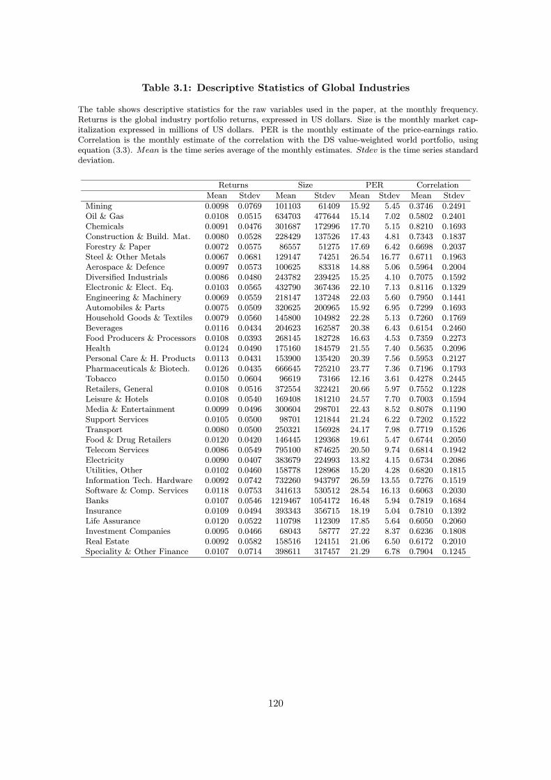
Table 3.1: Descriptive Statistics of Global Industries

The table shows descriptive statistics for the raw variables used in the paper, at the monthly frequency.Returns is the global industry portfolio returns, expressed in US dollars. Size is the monthly market cap-italization expressed in millions of US dollars. PER is the monthly estimate of the price-earnings ratio.Correlation is the monthly estimate of the correlation with the DS value-weighted world portfolio, usingequation (3.3). Mean is the time series average of the monthly estimates. Stdev is the time series standarddeviation.

Returns Size PER Correlation

Mean Stdev Mean Stdev Mean Stdev Mean Stdev

Mining 0.0098 0.0769 101103 61409 15.92 5.45 0.3746 0.2491Oil & Gas 0.0108 0.0515 634703 477644 15.14 7.02 0.5802 0.2401Chemicals 0.0091 0.0476 301687 172996 17.70 5.15 0.8210 0.1693Construction & Build. Mat. 0.0080 0.0528 228429 137526 17.43 4.81 0.7343 0.1837Forestry & Paper 0.0072 0.0575 86557 51275 17.69 6.42 0.6698 0.2037Steel & Other Metals 0.0067 0.0681 129147 74251 26.54 16.77 0.6711 0.1963Aerospace & Defence 0.0097 0.0573 100625 83318 14.88 5.06 0.5964 0.2004Diversified Industrials 0.0086 0.0480 243782 239425 15.25 4.10 0.7075 0.1592Electronic & Elect. Eq. 0.0103 0.0565 432790 367436 22.10 7.13 0.8116 0.1329Engineering & Machinery 0.0069 0.0559 218147 137248 22.03 5.60 0.7950 0.1441Automobiles & Parts 0.0075 0.0509 320625 200965 15.92 6.95 0.7299 0.1693Household Goods & Textiles 0.0079 0.0560 145800 104982 22.28 5.13 0.7260 0.1769Beverages 0.0116 0.0434 204623 162587 20.38 6.43 0.6154 0.2460Food Producers & Processors 0.0108 0.0393 268145 182728 16.63 4.53 0.7359 0.2273Health 0.0124 0.0490 175160 184579 21.55 7.40 0.5635 0.2096Personal Care & H. Products 0.0113 0.0431 153900 135420 20.39 7.56 0.5953 0.2127Pharmaceuticals & Biotech. 0.0126 0.0435 666645 725210 23.77 7.36 0.7196 0.1793Tobacco 0.0150 0.0604 96619 73166 12.16 3.61 0.4278 0.2445Retailers, General 0.0108 0.0516 372554 322421 20.66 5.97 0.7552 0.1228Leisure & Hotels 0.0108 0.0540 169408 181210 24.57 7.70 0.7003 0.1594Media & Entertainment 0.0099 0.0496 300604 298701 22.43 8.52 0.8078 0.1190Support Services 0.0105 0.0500 98701 121844 21.24 6.22 0.7202 0.1522Transport 0.0080 0.0500 250321 156928 24.17 7.98 0.7719 0.1526Food & Drug Retailers 0.0120 0.0420 146445 129368 19.61 5.47 0.6744 0.2050Telecom Services 0.0086 0.0549 795100 874625 20.50 9.74 0.6814 0.1942Electricity 0.0090 0.0407 383679 224993 13.82 4.15 0.6734 0.2086Utilities, Other 0.0102 0.0460 158778 128968 15.20 4.28 0.6820 0.1815Information Tech. Hardware 0.0092 0.0742 732260 943797 26.59 13.55 0.7276 0.1519Software & Comp. Services 0.0118 0.0753 341613 530512 28.54 16.13 0.6063 0.2030Banks 0.0107 0.0546 1219467 1054172 16.48 5.94 0.7819 0.1684Insurance 0.0109 0.0494 393343 356715 18.19 5.04 0.7810 0.1392Life Assurance 0.0120 0.0522 110798 112309 17.85 5.64 0.6050 0.2060Investment Companies 0.0095 0.0466 68043 58777 27.22 8.37 0.6236 0.1808Real Estate 0.0092 0.0582 158516 124151 21.06 6.50 0.6172 0.2010Speciality & Other Finance 0.0107 0.0714 398611 317457 21.29 6.78 0.7904 0.1245

120

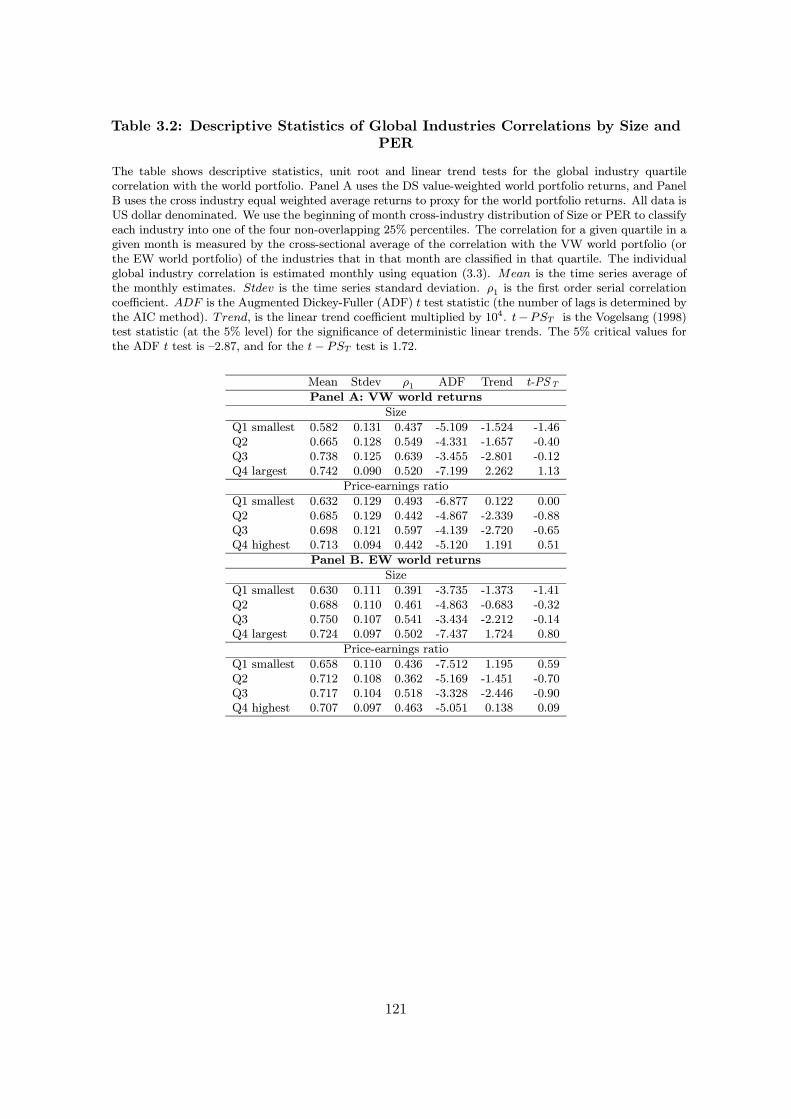
Table 3.2: Descriptive Statistics of Global Industries Correlations by Size andPER

The table shows descriptive statistics, unit root and linear trend tests for the global industry quartilecorrelation with the world portfolio. Panel A uses the DS value-weighted world portfolio returns, and PanelB uses the cross industry equal weighted average returns to proxy for the world portfolio returns. All data isUS dollar denominated. We use the beginning of month cross-industry distribution of Size or PER to classifyeach industry into one of the four non-overlapping 25% percentiles. The correlation for a given quartile in agiven month is measured by the cross-sectional average of the correlation with the VW world portfolio (orthe EW world portfolio) of the industries that in that month are classified in that quartile. The individualglobal industry correlation is estimated monthly using equation (3.3). Mean is the time series average ofthe monthly estimates. Stdev is the time series standard deviation. ρ1 is the first order serial correlationcoefficient. ADF is the Augmented Dickey-Fuller (ADF) t test statistic (the number of lags is determined bythe AIC method). Trend, is the linear trend coefficient multiplied by 104. t−PST is the Vogelsang (1998)test statistic (at the 5% level) for the significance of deterministic linear trends. The 5% critical values forthe ADF t test is —2.87, and for the t− PST test is 1.72.

Mean Stdev ρ1 ADF Trend t-PSTPanel A: VW world returns

Size

Q1 smallest 0.582 0.131 0.437 -5.109 -1.524 -1.46Q2 0.665 0.128 0.549 -4.331 -1.657 -0.40Q3 0.738 0.125 0.639 -3.455 -2.801 -0.12Q4 largest 0.742 0.090 0.520 -7.199 2.262 1.13

Price-earnings ratio

Q1 smallest 0.632 0.129 0.493 -6.877 0.122 0.00Q2 0.685 0.129 0.442 -4.867 -2.339 -0.88Q3 0.698 0.121 0.597 -4.139 -2.720 -0.65Q4 highest 0.713 0.094 0.442 -5.120 1.191 0.51

Panel B. EW world returns

Size

Q1 smallest 0.630 0.111 0.391 -3.735 -1.373 -1.41Q2 0.688 0.110 0.461 -4.863 -0.683 -0.32Q3 0.750 0.107 0.541 -3.434 -2.212 -0.14Q4 largest 0.724 0.097 0.502 -7.437 1.724 0.80

Price-earnings ratio

Q1 smallest 0.658 0.110 0.436 -7.512 1.195 0.59Q2 0.712 0.108 0.362 -5.169 -1.451 -0.70Q3 0.717 0.104 0.518 -3.328 -2.446 -0.90Q4 highest 0.707 0.097 0.463 -5.051 0.138 0.09

121

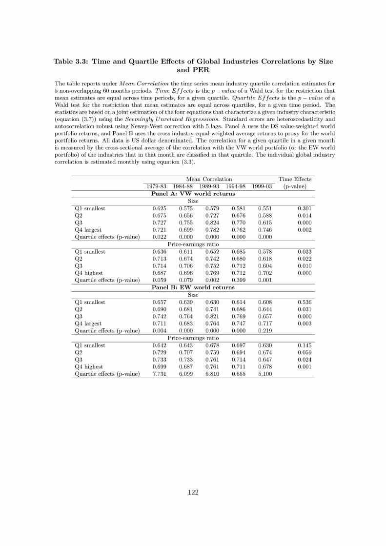
Table 3.3: Time and Quartile Effects of Global Industries Correlations by Sizeand PER

The table reports under Mean Correlation the time series mean industry quartile correlation estimates for5 non-overlapping 60 months periods. Time Effects is the p− value of a Wald test for the restriction thatmean estimates are equal across time periods, for a given quartile. Quartile Effects is the p− value of aWald test for the restriction that mean estimates are equal across quartiles, for a given time period. Thestatistics are based on a joint estimation of the four equations that characterize a given industry characteristic(equation (3.7)) using the Seemingly Unrelated Regressions. Standard errors are heteroscedasticity andautocorrelation robust using Newey-West correction with 5 lags. Panel A uses the DS value-weighted worldportfolio returns, and Panel B uses the cross industry equal-weighted average returns to proxy for the worldportfolio returns. All data is US dollar denominated. The correlation for a given quartile in a given monthis measured by the cross-sectional average of the correlation with the VW world portfolio (or the EW worldportfolio) of the industries that in that month are classified in that quartile. The individual global industrycorrelation is estimated monthly using equation (3.3).

Mean Correlation Time Effects1979-83 1984-88 1989-93 1994-98 1999-03 (p-value)

Panel A: VW world returns

Size

Q1 smallest 0.625 0.575 0.579 0.581 0.551 0.301Q2 0.675 0.656 0.727 0.676 0.588 0.014Q3 0.727 0.755 0.824 0.770 0.615 0.000Q4 largest 0.721 0.699 0.782 0.762 0.746 0.002Quartile effects (p-value) 0.022 0.000 0.000 0.000 0.000

Price-earnings ratio

Q1 smallest 0.636 0.611 0.652 0.685 0.578 0.033Q2 0.713 0.674 0.742 0.680 0.618 0.022Q3 0.714 0.706 0.752 0.712 0.604 0.010Q4 highest 0.687 0.696 0.769 0.712 0.702 0.000Quartile effects (p-value) 0.059 0.079 0.002 0.399 0.001

Panel B: EW world returns

Size

Q1 smallest 0.657 0.639 0.630 0.614 0.608 0.536Q2 0.690 0.681 0.741 0.686 0.644 0.031Q3 0.742 0.764 0.821 0.769 0.657 0.000Q4 largest 0.711 0.683 0.764 0.747 0.717 0.003Quartile effects (p-value) 0.004 0.000 0.000 0.000 0.219

Price-earnings ratio

Q1 smallest 0.642 0.643 0.678 0.697 0.630 0.145Q2 0.729 0.707 0.759 0.694 0.674 0.059Q3 0.733 0.733 0.761 0.714 0.647 0.024Q4 highest 0.699 0.687 0.761 0.711 0.678 0.001Quartile effects (p-value) 7.731 6.099 6.810 0.655 5.100

122

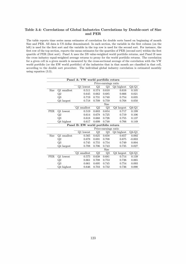
Table 3.4: Correlations of Global Industries Correlations by Double-sort of Sizeand PER

The table reports time series mean estimates of correlation for double sorts based on beginning of monthSize and PER. All data is US dollar denominated. In each section, the variable in the first column (on theleft) is used for the first sort and the variable in the top row is used for the second sort. For instance, thefirst row of the top section, reports the mean estimates for the quartiles of PER (second sort) within the firstquartile of PER (first sort). Panel A uses the DS value-weighted world portfolio returns, and Panel B usesthe cross industry equal-weighted average returns to proxy for the world portfolio returns. The correlationfor a given cell in a given month is measured by the cross-sectional average of the correlation with the VWworld portfolio (or the EW world portfolio) of the industries that in that month are classified in that cell,according to the double sort procedure. The individual global industry correlation is estimated monthlyusing equation (3.3).

Panel A: VW world portfolio return

Price-earnings ratioQ1 lowest Q2 Q3 Q4 highest Q4-Q1

Size Q1 smallest 0.511 0.574 0.610 0.616 0.105Q2 0.645 0.662 0.685 0.666 0.021Q3 0.719 0.731 0.740 0.754 0.035Q4 largest 0.718 0.709 0.759 0.768 0.050

SizeQ1 smallest Q2 Q3 Q4 largest Q4-Q1

PER Q1 lowest 0.519 0.603 0.654 0.717 0.199Q2 0.614 0.678 0.725 0.719 0.106Q3 0.618 0.668 0.726 0.755 0.137Q4 highest 0.617 0.699 0.748 0.766 0.149

Panel B: EW world portfolio return

Price-earnings ratioQ1 lowest Q2 Q3 Q4 highest Q4-Q1

Size Q1 smallest 0.565 0.625 0.658 0.657 0.092Q2 0.678 0.691 0.708 0.675 -0.003Q3 0.745 0.755 0.754 0.749 0.004Q4 largest 0.708 0.706 0.743 0.735 0.027

SizeQ1 smallest Q2 Q3 Q4 largest Q4-Q1

PER Q1 lowest 0.575 0.638 0.681 0.714 0.139Q2 0.661 0.708 0.753 0.726 0.065Q3 0.661 0.695 0.745 0.754 0.093Q4 highest 0.646 0.703 0.732 0.736 0.090

123

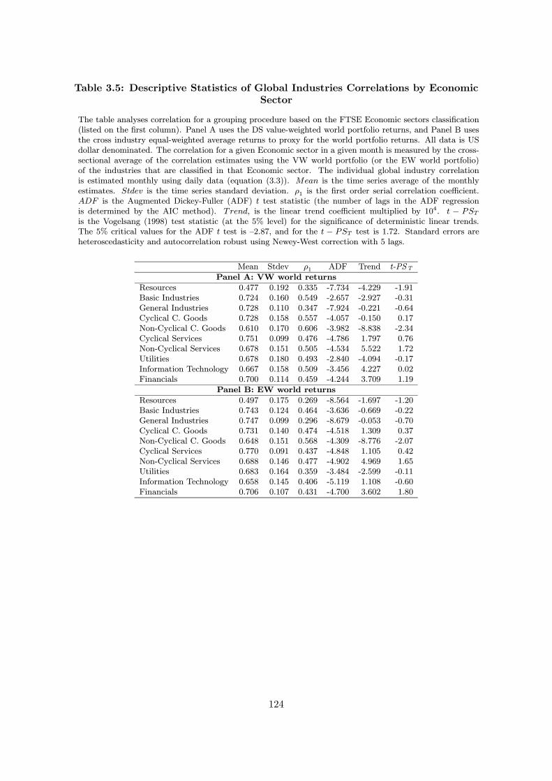
Table 3.5: Descriptive Statistics of Global Industries Correlations by EconomicSector

The table analyses correlation for a grouping procedure based on the FTSE Economic sectors classification(listed on the first column). Panel A uses the DS value-weighted world portfolio returns, and Panel B usesthe cross industry equal-weighted average returns to proxy for the world portfolio returns. All data is USdollar denominated. The correlation for a given Economic sector in a given month is measured by the cross-sectional average of the correlation estimates using the VW world portfolio (or the EW world portfolio)of the industries that are classified in that Economic sector. The individual global industry correlationis estimated monthly using daily data (equation (3.3)). Mean is the time series average of the monthlyestimates. Stdev is the time series standard deviation. ρ1 is the first order serial correlation coefficient.ADF is the Augmented Dickey-Fuller (ADF) t test statistic (the number of lags in the ADF regressionis determined by the AIC method). Trend, is the linear trend coefficient multiplied by 104. t − PSTis the Vogelsang (1998) test statistic (at the 5% level) for the significance of deterministic linear trends.The 5% critical values for the ADF t test is —2.87, and for the t − PST test is 1.72. Standard errors areheteroscedasticity and autocorrelation robust using Newey-West correction with 5 lags.

Mean Stdev ρ1 ADF Trend t-PSTPanel A: VW world returns

Resources 0.477 0.192 0.335 -7.734 -4.229 -1.91Basic Industries 0.724 0.160 0.549 -2.657 -2.927 -0.31General Industries 0.728 0.110 0.347 -7.924 -0.221 -0.64Cyclical C. Goods 0.728 0.158 0.557 -4.057 -0.150 0.17Non-Cyclical C. Goods 0.610 0.170 0.606 -3.982 -8.838 -2.34Cyclical Services 0.751 0.099 0.476 -4.786 1.797 0.76Non-Cyclical Services 0.678 0.151 0.505 -4.534 5.522 1.72Utilities 0.678 0.180 0.493 -2.840 -4.094 -0.17Information Technology 0.667 0.158 0.509 -3.456 4.227 0.02Financials 0.700 0.114 0.459 -4.244 3.709 1.19

Panel B: EW world returns

Resources 0.497 0.175 0.269 -8.564 -1.697 -1.20Basic Industries 0.743 0.124 0.464 -3.636 -0.669 -0.22General Industries 0.747 0.099 0.296 -8.679 -0.053 -0.70Cyclical C. Goods 0.731 0.140 0.474 -4.518 1.309 0.37Non-Cyclical C. Goods 0.648 0.151 0.568 -4.309 -8.776 -2.07Cyclical Services 0.770 0.091 0.437 -4.848 1.105 0.42Non-Cyclical Services 0.688 0.146 0.477 -4.902 4.969 1.65Utilities 0.683 0.164 0.359 -3.484 -2.599 -0.11Information Technology 0.658 0.145 0.406 -5.119 1.108 -0.60Financials 0.706 0.107 0.431 -4.700 3.602 1.80

124

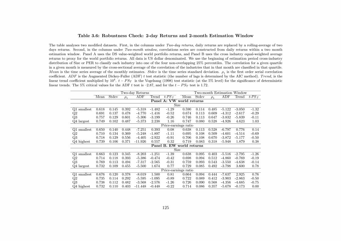
Table 3.6: Robustness Check: 2-day Returns and 2-month Estimation Window

The table analyses two modified datasets. First, in the columns under Two-day returns, daily returns are replaced by a rolling-average of twodays returns. Second, in the columns under Two-month window, correlations series are constructed from daily returns within a two monthestimation window. Panel A uses the DS value-weighted world portfolio returns, and Panel B uses the cross industry equal-weighted averagereturns to proxy for the world portfolio returns. All data is US dollar denominated. We use the beginning of estimation period cross-industrydistribution of Size or PER to classify each industry into one of the four non-overlapping 25% percentiles. The correlation for a given quartilein a given month is measured by the cross-sectional average of the correlation of the industries that in that month are classified in that quartile.Mean is the time series average of the monthly estimates. Stdev is the time series standard deviation. ρ1 is the first order serial correlationcoefficient. ADF is the Augmented Dickey-Fuller (ADF) t test statistic (the number of lags is determined by the AIC method). Trend, is thelinear trend coefficient multiplied by 104. t− PST is the Vogelsang (1998) test statistic (at the 5% level) for the significance of deterministiclinear trends. The 5% critical values for the ADF t test is —2.87, and for the t− PST test is 1.72.

Two-day Returns Two-month Estimation WindowMean Stdev ρ1 ADF Trend t-PST Mean Stdev ρ1 ADF Trend t-PST

Panel A: VW world returnsSize

Q1 smallest 0.618 0.145 0.392 -5.318 -1.482 -1.29 0.590 0.114 0.485 -5.122 -3.050 -1.32Q2 0.691 0.137 0.478 -4.770 -1.416 -0.52 0.674 0.113 0.609 -4.312 -2.617 -0.29Q3 0.757 0.129 0.601 -5.306 -3.199 -0.26 0.746 0.113 0.647 -3.832 -5.839 -0.11Q4 largest 0.749 0.102 0.487 -5.373 2.238 1.16 0.747 0.080 0.528 -4.926 4.623 1.03

Price-earnings ratioQ1 smallest 0.650 0.140 0.448 -7.251 0.393 0.08 0.638 0.113 0.528 -6.797 0.776 0.14Q2 0.710 0.134 0.369 -5.248 -1.897 -1.11 0.695 0.108 0.509 -4.601 -4.514 -0.69Q3 0.718 0.129 0.556 -4.405 -2.922 -0.91 0.706 0.108 0.670 -3.872 -5.177 -0.50Q4 highest 0.739 0.106 0.371 -11.926 0.557 0.32 0.719 0.083 0.318 -5.948 1.879 0.38

Panel B. EW world returnsSize

Q1 smallest 0.663 0.123 0.345 -8.203 -1.251 -1.39 0.638 0.095 0.403 -5.516 -2.795 -1.26Q2 0.714 0.118 0.393 -5.386 -0.474 -0.42 0.698 0.094 0.512 -4.860 -0.769 -0.19Q3 0.769 0.113 0.494 -7.317 -2.565 -0.31 0.759 0.093 0.543 -3.550 -4.638 -0.14Q4 largest 0.732 0.109 0.455 -5.500 1.674 0.77 0.729 0.085 0.492 -3.798 3.600 0.78

Price-earnings ratioQ1 smallest 0.676 0.120 0.378 -8.019 1.500 0.81 0.664 0.094 0.444 -7.637 2.925 0.76Q2 0.735 0.114 0.292 -5.595 -1.095 -0.89 0.722 0.089 0.412 -3.903 -2.863 -0.50Q3 0.738 0.112 0.482 -3.568 -2.576 -1.26 0.726 0.090 0.568 -4.356 -4.685 -0.75Q4 highest 0.732 0.110 0.403 -11.448 -0.448 -0.22 0.714 0.086 0.357 -5.678 -0.173 0.00

125

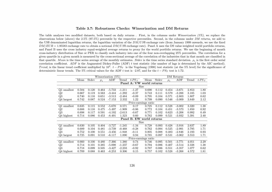
Table 3.7: Robustness Checks: Winsorization and DM Returns

The table analyses two modified datasets, both based on daily returns . First, in the columns under Winsorization (5%), we replace theobservations below (above) the 2.5% (97.5%) percentile by the respective percentiles. Second, in the columns under DM returns, we add tothe US$ denominated logarithm returns, the logarithm variation of the DM/US$ exchange rate (from January 1999 onwards, we use the fixedDM/EUR = 1.95583 exchange rate to obtain a notional DM/US$ exchange rate). Panel A uses the DS value-weighted world portfolio returns,and Panel B uses the cross industry equal-weighted average returns to proxy for the world portfolio returns. We use the beginning of monthcross-industry distribution of Size or PER to classify each industry into one of the four non-overlapping 25% percentiles. The correlation for agiven quartile in a given month is measured by the cross-sectional average of the correlation of the industries that in that month are classified inthat quartile. Mean is the time series average of the monthly estimates. Stdev is the time series standard deviation. ρ1 is the first order serialcorrelation coefficient. ADF is the Augmented Dickey-Fuller (ADF) t test statistic (the number of lags is determined by the AIC method).Trend, is the linear trend coefficient multiplied by 104. t− PST is the Vogelsang (1998) test statistic (at the 5% level) for the significance ofdeterministic linear trends. The 5% critical values for the ADF t test is —2.87, and for the t− PST test is 1.72.

Winsorization (5%) DM ReturnsMean Stdev ρ1 ADF Trend t-PST Mean Stdev ρ1 ADF Trend t-PST

Panel A: VW world returnsSize

Q1 smallest 0.584 0.120 0.464 -5.733 -1.211 -1.27 0.690 0.112 0.454 -3.671 2.853 1.80Q2 0.667 0.119 0.563 -3.444 -1.292 -0.37 0.743 0.111 0.579 -3.288 3.185 1.03Q3 0.740 0.116 0.651 -3.513 -2.484 -0.09 0.795 0.104 0.571 -2.803 1.807 0.62Q4 largest 0.742 0.087 0.524 -7.153 2.332 1.22 0.799 0.090 0.546 -3.009 3.849 2.12

Price-earnings ratioQ1 smallest 0.635 0.115 0.552 -5.670 0.571 0.17 0.725 0.112 0.528 -3.002 3.320 1.38Q2 0.688 0.116 0.475 -5.497 -1.909 -0.86 0.772 0.104 0.451 -3.573 1.850 0.92Q3 0.698 0.117 0.591 -4.192 -2.613 -0.67 0.771 0.102 0.623 -3.208 0.992 0.49Q4 highest 0.714 0.086 0.453 -8.491 1.323 0.60 0.762 0.099 0.521 -3.932 5.391 2.40

Panel B. EW world returnsSize

Q1 smallest 0.630 0.105 0.404 -3.727 -1.245 -1.34 0.728 0.093 0.428 -3.916 2.637 1.89Q2 0.689 0.104 0.481 -3.739 -0.468 -0.28 0.762 0.094 0.525 -2.991 3.795 1.71Q3 0.752 0.100 0.551 -3.456 -1.948 -0.11 0.805 0.088 0.483 -2.846 2.193 0.93Q4 largest 0.725 0.091 0.510 -6.117 1.890 0.94 0.785 0.097 0.531 -3.062 3.553 1.71

Price-earnings ratioQ1 smallest 0.660 0.100 0.480 -7.366 1.380 0.74 0.746 0.095 0.501 -3.771 4.051 2.29Q2 0.714 0.101 0.385 -5.098 -1.237 -0.67 0.794 0.086 0.407 -3.514 2.338 1.38Q3 0.718 0.099 0.505 -3.427 -2.233 -0.92 0.787 0.086 0.551 -3.357 1.077 0.62Q4 highest 0.709 0.088 0.463 -8.253 0.306 0.15 0.757 0.102 0.528 -3.268 4.572 1.81

126

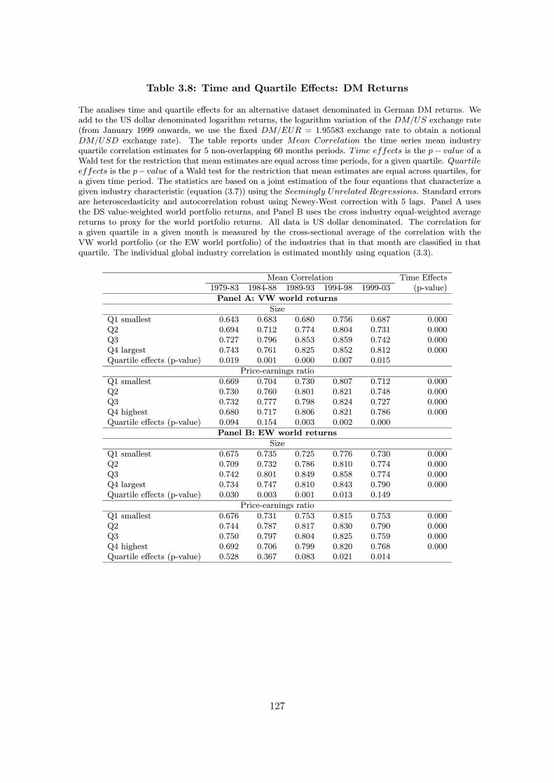
Table 3.8: Time and Quartile Effects: DM Returns

The analises time and quartile effects for an alternative dataset denominated in German DM returns. Weadd to the US dollar denominated logarithm returns, the logarithm variation of the DM/US exchange rate(from January 1999 onwards, we use the fixed DM/EUR = 1.95583 exchange rate to obtain a notionalDM/USD exchange rate). The table reports under Mean Correlation the time series mean industryquartile correlation estimates for 5 non-overlapping 60 months periods. Time effects is the p− value of aWald test for the restriction that mean estimates are equal across time periods, for a given quartile. Quartileeffects is the p− value of a Wald test for the restriction that mean estimates are equal across quartiles, fora given time period. The statistics are based on a joint estimation of the four equations that characterize agiven industry characteristic (equation (3.7)) using the Seemingly Unrelated Regressions. Standard errorsare heteroscedasticity and autocorrelation robust using Newey-West correction with 5 lags. Panel A usesthe DS value-weighted world portfolio returns, and Panel B uses the cross industry equal-weighted averagereturns to proxy for the world portfolio returns. All data is US dollar denominated. The correlation fora given quartile in a given month is measured by the cross-sectional average of the correlation with theVW world portfolio (or the EW world portfolio) of the industries that in that month are classified in thatquartile. The individual global industry correlation is estimated monthly using equation (3.3).

Mean Correlation Time Effects1979-83 1984-88 1989-93 1994-98 1999-03 (p-value)

Panel A: VW world returns

Size

Q1 smallest 0.643 0.683 0.680 0.756 0.687 0.000Q2 0.694 0.712 0.774 0.804 0.731 0.000Q3 0.727 0.796 0.853 0.859 0.742 0.000Q4 largest 0.743 0.761 0.825 0.852 0.812 0.000Quartile effects (p-value) 0.019 0.001 0.000 0.007 0.015

Price-earnings ratio

Q1 smallest 0.669 0.704 0.730 0.807 0.712 0.000Q2 0.730 0.760 0.801 0.821 0.748 0.000Q3 0.732 0.777 0.798 0.824 0.727 0.000Q4 highest 0.680 0.717 0.806 0.821 0.786 0.000Quartile effects (p-value) 0.094 0.154 0.003 0.002 0.000

Panel B: EW world returns

Size

Q1 smallest 0.675 0.735 0.725 0.776 0.730 0.000Q2 0.709 0.732 0.786 0.810 0.774 0.000Q3 0.742 0.801 0.849 0.858 0.774 0.000Q4 largest 0.734 0.747 0.810 0.843 0.790 0.000Quartile effects (p-value) 0.030 0.003 0.001 0.013 0.149

Price-earnings ratio

Q1 smallest 0.676 0.731 0.753 0.815 0.753 0.000Q2 0.744 0.787 0.817 0.830 0.790 0.000Q3 0.750 0.797 0.804 0.825 0.759 0.000Q4 highest 0.692 0.706 0.799 0.820 0.768 0.000Quartile effects (p-value) 0.528 0.367 0.083 0.021 0.014

127

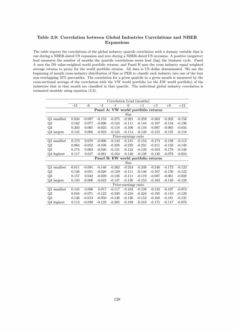
Table 3.9: Correlation between Global Industries Correlations and NBERExpansions

The table reports the correlations of the global industry quartile correlation with a dummy variable that isone during a NBER-dated US expansion and zero during a NBER-dated US recession. A positive (negative)lead measures the number of months the quartile correlations series lead (lag) the business cycle. PanelA uses the DS value-weighted world portfolio returns, and Panel B uses the cross industry equal weightedaverage returns to proxy for the world portfolio returns. All data is US dollar denominated. We use thebeginning of month cross-industry distribution of Size or PER to classify each industry into one of the fournon-overlapping 25% percentiles. The correlation for a given quartile in a given month is measured by thecross-sectional average of the correlation with the VW world portfolio (or the EW world portfolio) of theindustries that in that month are classified in that quartile. The individual global industry correlation isestimated monthly using equation (3.3).

Correlation Lead (months)-12 -6 -3 -1 0 +1 +3 +6 +12

Panel A: VW world portfolio returns

Size

Q1 smallest 0.034 -0.087 -0.153 -0.275 -0.261 -0.259 -0.263 -0.203 -0.156Q2 0.162 0.077 -0.006 -0.124 -0.111 -0.144 -0.167 -0.134 -0.136Q3 0.203 0.065 -0.023 -0.118 -0.106 -0.116 -0.087 -0.065 -0.034Q4 largest 0.145 0.008 -0.023 -0.124 -0.114 -0.140 -0.155 -0.135 -0.116

Price-earnings ratio

Q1 smallest 0.173 0.078 -0.006 -0.143 -0.131 -0.154 -0.174 -0.138 -0.115Q2 0.064 -0.052 -0.108 -0.228 -0.222 -0.231 -0.211 -0.132 -0.148Q3 0.174 0.003 -0.040 -0.131 -0.122 -0.149 -0.163 -0.179 -0.140Q4 highest 0.117 0.017 -0.081 -0.164 -0.140 -0.138 -0.130 -0.079 -0.024

Panel B: EW world portfolio returns

Size

Q1 smallest -0.011 -0.091 -0.146 -0.262 -0.254 -0.249 -0.246 -0.172 -0.123Q2 0.126 0.051 -0.028 -0.129 -0.111 -0.146 -0.167 -0.130 -0.122Q3 0.157 0.042 -0.039 -0.126 -0.111 -0.119 -0.087 -0.061 -0.038Q4 largest 0.150 -0.006 -0.043 -0.147 -0.136 -0.153 -0.163 -0.149 -0.128

Price-earnings ratio

Q1 smallest 0.145 0.096 0.017 -0.117 -0.104 -0.128 -0.142 -0.107 -0.074Q2 0.016 -0.071 -0.122 -0.230 -0.218 -0.224 -0.195 -0.110 -0.129Q3 0.136 -0.013 -0.050 -0.136 -0.126 -0.152 -0.168 -0.181 -0.135Q4 highest 0.113 -0.039 -0.128 -0.205 -0.189 -0.183 -0.175 -0.117 -0.076

128

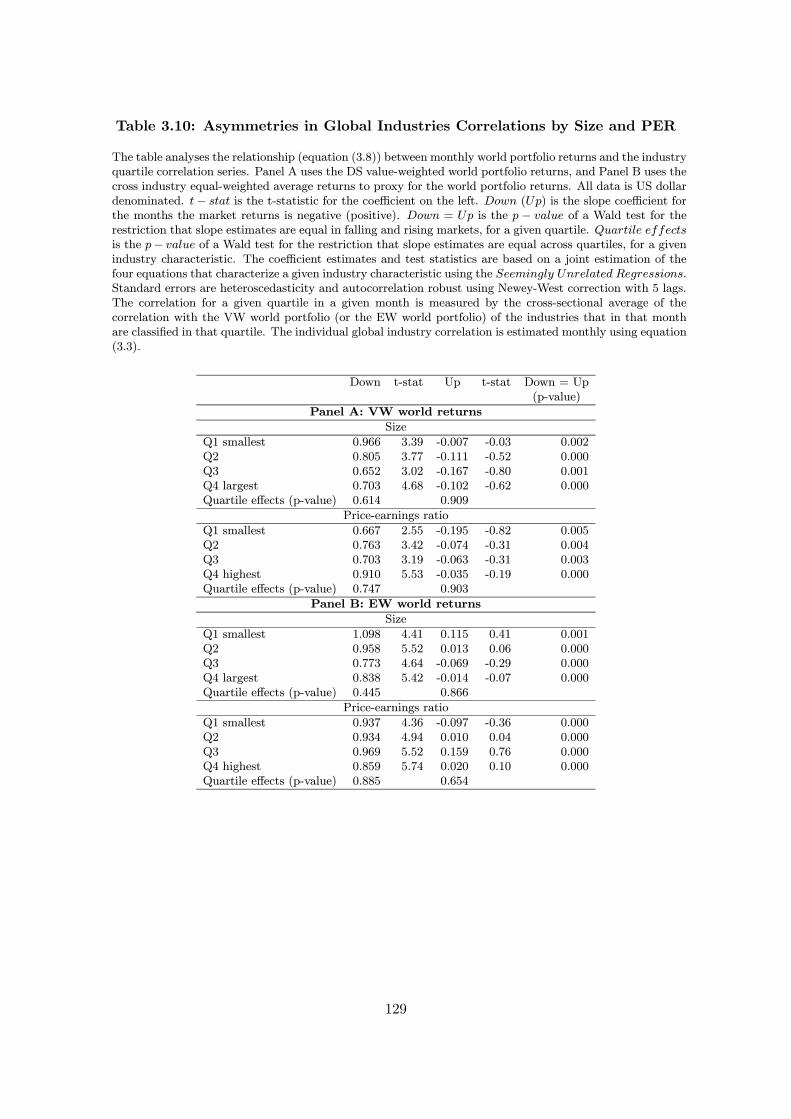
Table 3.10: Asymmetries in Global Industries Correlations by Size and PER

The table analyses the relationship (equation (3.8)) between monthly world portfolio returns and the industryquartile correlation series. Panel A uses the DS value-weighted world portfolio returns, and Panel B uses thecross industry equal-weighted average returns to proxy for the world portfolio returns. All data is US dollardenominated. t− stat is the t-statistic for the coefficient on the left. Down (Up) is the slope coefficient forthe months the market returns is negative (positive). Down = Up is the p − value of a Wald test for therestriction that slope estimates are equal in falling and rising markets, for a given quartile. Quartile effectsis the p− value of a Wald test for the restriction that slope estimates are equal across quartiles, for a givenindustry characteristic. The coefficient estimates and test statistics are based on a joint estimation of thefour equations that characterize a given industry characteristic using the Seemingly Unrelated Regressions.Standard errors are heteroscedasticity and autocorrelation robust using Newey-West correction with 5 lags.The correlation for a given quartile in a given month is measured by the cross-sectional average of thecorrelation with the VW world portfolio (or the EW world portfolio) of the industries that in that monthare classified in that quartile. The individual global industry correlation is estimated monthly using equation(3.3).

Down t-stat Up t-stat Down = Up(p-value)

Panel A: VW world returns

Size

Q1 smallest 0.966 3.39 -0.007 -0.03 0.002Q2 0.805 3.77 -0.111 -0.52 0.000Q3 0.652 3.02 -0.167 -0.80 0.001Q4 largest 0.703 4.68 -0.102 -0.62 0.000Quartile effects (p-value) 0.614 0.909

Price-earnings ratio

Q1 smallest 0.667 2.55 -0.195 -0.82 0.005Q2 0.763 3.42 -0.074 -0.31 0.004Q3 0.703 3.19 -0.063 -0.31 0.003Q4 highest 0.910 5.53 -0.035 -0.19 0.000Quartile effects (p-value) 0.747 0.903

Panel B: EW world returns

Size

Q1 smallest 1.098 4.41 0.115 0.41 0.001Q2 0.958 5.52 0.013 0.06 0.000Q3 0.773 4.64 -0.069 -0.29 0.000Q4 largest 0.838 5.42 -0.014 -0.07 0.000Quartile effects (p-value) 0.445 0.866

Price-earnings ratio

Q1 smallest 0.937 4.36 -0.097 -0.36 0.000Q2 0.934 4.94 0.010 0.04 0.000Q3 0.969 5.52 0.159 0.76 0.000Q4 highest 0.859 5.74 0.020 0.10 0.000Quartile effects (p-value) 0.885 0.654

129

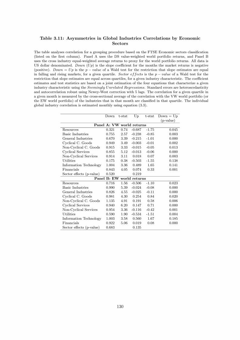
Table 3.11: Asymmetries in Global Industries Correlations by EconomicSectors

The table analyses correlation for a grouping procedure based on the FTSE Economic sectors classification(listed on the first column). Panel A uses the DS value-weighted world portfolio returns, and Panel Buses the cross industry equal-weighted average returns to proxy for the world portfolio returns. All data isUS dollar denominated. Down (Up) is the slope coefficient for the months the market returns is negative(positive). Down = Up is the p − value of a Wald test for the restriction that slope estimates are equalin falling and rising markets, for a given quartile. Sector effects is the p − value of a Wald test for therestriction that slope estimates are equal across quartiles, for a given industry characteristic. The coefficientestimates and test statistics are based on a joint estimation of the four equations that characterize a givenindustry characteristic using the Seemingly Unrelated Regressions. Standard errors are heteroscedasticityand autocorrelation robust using Newey-West correction with 5 lags. The correlation for a given quartile ina given month is measured by the cross-sectional average of the correlation with the VW world portfolio (orthe EW world portfolio) of the industries that in that month are classified in that quartile. The individualglobal industry correlation is estimated monthly using equation (3.3).

Down t-stat Up t-stat Down = Up(p-value)

Panel A: VW world returns

Resources 0.321 0.74 -0.687 -1.75 0.045Basic Industries 0.755 2.57 -0.238 -0.85 0.003General Industries 0.670 3.39 -0.215 -1.01 0.000Cyclical C. Goods 0.949 3.49 -0.003 -0.01 0.002Non-Cyclical C. Goods 0.915 3.33 -0.015 -0.05 0.013Cyclical Services 0.855 5.12 -0.013 -0.06 0.000Non-Cyclical Services 0.914 3.11 0.018 0.07 0.003Utilities 0.175 0.38 -0.503 -1.55 0.138Information Technology 1.004 3.36 0.489 1.65 0.141Financials 0.843 4.05 0.074 0.33 0.001Sector effects (p-value) 0.520 0.219

Panel B: EW world returns

Resources 0.716 1.56 -0.506 -1.10 0.023Basic Industries 0.990 5.39 -0.024 -0.08 0.000General Industries 0.826 4.55 -0.025 -0.11 0.000Cyclical C. Goods 0.981 4.30 0.254 0.84 0.020Non-Cyclical C. Goods 1.135 4.91 0.191 0.58 0.006Cyclical Services 0.940 6.20 0.147 0.71 0.000Non-Cyclical Services 0.954 3.36 -0.116 -0.42 0.001Utilities 0.590 1.90 -0.534 -1.51 0.004Information Technology 1.003 3.58 0.560 1.67 0.185Financials 0.922 5.06 0.019 0.08 0.000Sector effects (p-value) 0.683 0.135

130

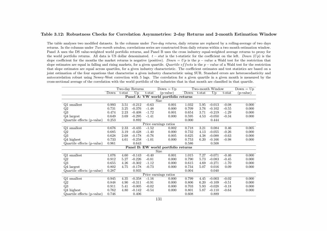
Table 3.12: Robustness Checks for Correlation Asymmetries: 2-day Returns and 2-month Estimation Window

The table analyses two modified datasets. In the columns under Two-day returns, daily returns are replaced by a rolling-average of two daysreturns. In the columns under Two-month window, correlations series are constructed from daily returns within a two month estimation window.Panel A uses the DS value-weighted world portfolio returns, and Panel B uses the cross industry equal-weighted average returns to proxy forthe world portfolio returns. All data is US dollar denominated. t − stat is the t-statistic for the coefficient on the left. Down (Up) is theslope coefficient for the months the market returns is negative (positive). Down = Up is the p − value a Wald test for the restriction thatslope estimates are equal in falling and rising markets, for a given quartile. Quartile effects is the p− value of a Wald test for the restrictionthat slope estimates are equal across quartiles, for a given industry characteristic. The coefficient estimates and test statistics are based on ajoint estimation of the four equations that characterize a given industry characteristic using SUR. Standard errors are heteroscedasticity andautocorrelation robust using Newey-West correction with 5 lags. The correlation for a given quartile in a given month is measured by thecross-sectional average of the correlation with the world portfolio of the industries that in that month are classified in that quartile.

Two-day Returns Down = Up Two-month Window Down = UpDown t-stat Up t-stat (p-value) Down t-stat Up t-stat (p-value)

Panel A: VW world portfolio returnsSize

Q1 smallest 0.993 3.51 -0.212 -0.63 0.001 1.032 5.95 -0.013 -0.08 0.000Q2 0.731 3.25 -0.376 -1.48 0.000 0.709 3.76 -0.102 -0.55 0.000Q3 0.474 2.23 -0.408 -1.72 0.001 0.654 3.71 -0.219 -1.29 0.000Q4 largest 0.649 3.69 -0.295 -1.41 0.000 0.595 4.53 -0.050 -0.34 0.000Quartile effects (p-value) 0.253 0.892 0.000 0.444

Price earnings ratiosQ1 smallest 0.676 2.33 -0.435 -1.52 0.002 0.718 3.21 0.084 0.46 0.005Q2 0.685 3.19 -0.428 -1.40 0.000 0.732 4.13 -0.055 -0.26 0.000Q3 0.628 2.68 -0.178 -0.76 0.005 0.625 4.38 -0.088 -0.63 0.000Q4 highest 0.733 4.61 -0.258 -1.01 0.000 0.753 6.20 -0.166 -0.98 0.000Quartile effects (p-value) 0.961 0.643 0.586 0.508

Panel B: EW world portfolio returnsSize

Q1 smallest 1.076 4.60 -0.143 -0.40 0.001 1.015 7.27 -0.071 -0.46 0.000Q2 0.912 5.27 -0.226 -0.81 0.000 0.790 5.73 -0.083 -0.45 0.000Q3 0.655 4.26 -0.302 -1.12 0.000 0.615 4.69 -0.271 -1.70 0.000Q4 largest 0.802 4.75 -0.178 -0.73 0.000 0.734 5.07 0.016 0.09 0.000Quartile effects (p-value) 0.287 0.935 0.004 0.040

Price earnings ratiosQ1 smallest 0.945 4.35 -0.358 -1.16 0.000 0.799 4.45 -0.003 -0.02 0.000Q2 0.848 4.90 -0.311 -0.91 0.000 0.806 6.20 -0.109 -0.51 0.000Q3 0.911 5.41 -0.005 -0.02 0.000 0.703 5.93 -0.028 -0.18 0.000Q4 highest 0.762 4.80 -0.142 -0.54 0.000 0.801 5.87 -0.110 -0.64 0.000Quartile effects (p-value) 0.746 0.406 0.608 0.889

131

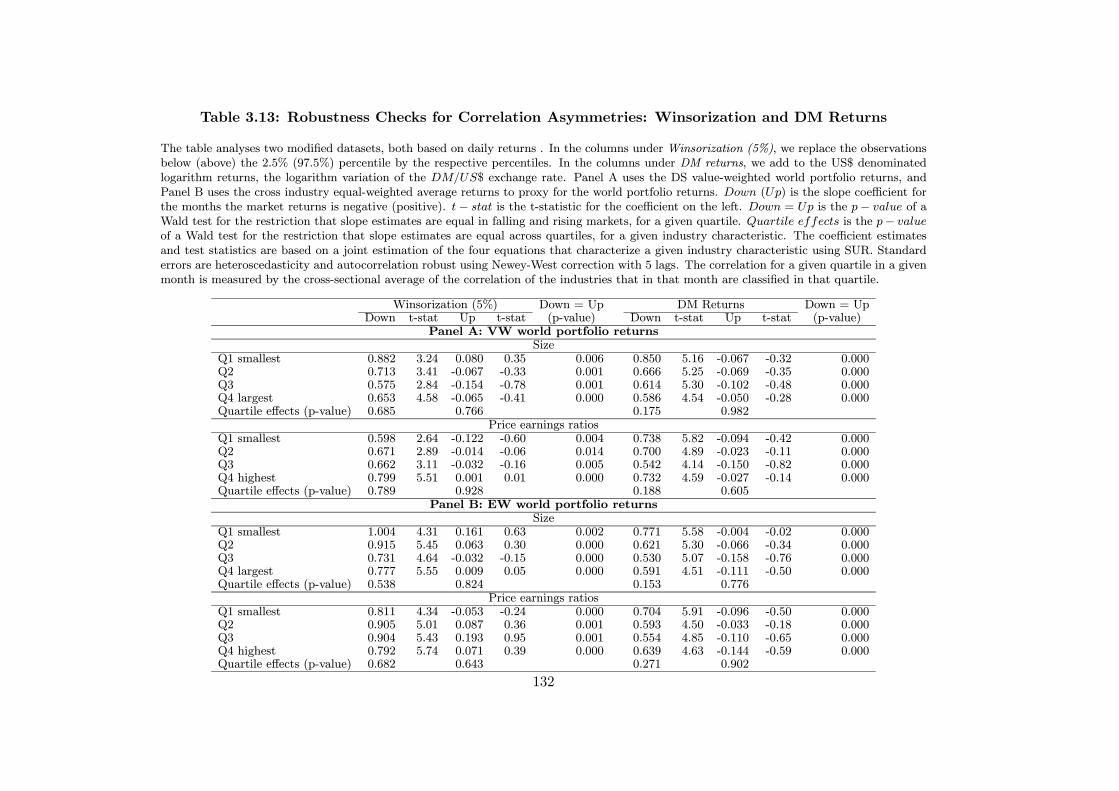
Table 3.13: Robustness Checks for Correlation Asymmetries: Winsorization and DM Returns

The table analyses two modified datasets, both based on daily returns . In the columns under Winsorization (5%), we replace the observationsbelow (above) the 2.5% (97.5%) percentile by the respective percentiles. In the columns under DM returns, we add to the US$ denominatedlogarithm returns, the logarithm variation of the DM/US$ exchange rate. Panel A uses the DS value-weighted world portfolio returns, andPanel B uses the cross industry equal-weighted average returns to proxy for the world portfolio returns. Down (Up) is the slope coefficient forthe months the market returns is negative (positive). t− stat is the t-statistic for the coefficient on the left. Down = Up is the p− value of aWald test for the restriction that slope estimates are equal in falling and rising markets, for a given quartile. Quartile effects is the p− valueof a Wald test for the restriction that slope estimates are equal across quartiles, for a given industry characteristic. The coefficient estimatesand test statistics are based on a joint estimation of the four equations that characterize a given industry characteristic using SUR. Standarderrors are heteroscedasticity and autocorrelation robust using Newey-West correction with 5 lags. The correlation for a given quartile in a givenmonth is measured by the cross-sectional average of the correlation of the industries that in that month are classified in that quartile.

Winsorization (5%) Down = Up DM Returns Down = UpDown t-stat Up t-stat (p-value) Down t-stat Up t-stat (p-value)

Panel A: VW world portfolio returnsSize

Q1 smallest 0.882 3.24 0.080 0.35 0.006 0.850 5.16 -0.067 -0.32 0.000Q2 0.713 3.41 -0.067 -0.33 0.001 0.666 5.25 -0.069 -0.35 0.000Q3 0.575 2.84 -0.154 -0.78 0.001 0.614 5.30 -0.102 -0.48 0.000Q4 largest 0.653 4.58 -0.065 -0.41 0.000 0.586 4.54 -0.050 -0.28 0.000Quartile effects (p-value) 0.685 0.766 0.175 0.982

Price earnings ratiosQ1 smallest 0.598 2.64 -0.122 -0.60 0.004 0.738 5.82 -0.094 -0.42 0.000Q2 0.671 2.89 -0.014 -0.06 0.014 0.700 4.89 -0.023 -0.11 0.000Q3 0.662 3.11 -0.032 -0.16 0.005 0.542 4.14 -0.150 -0.82 0.000Q4 highest 0.799 5.51 0.001 0.01 0.000 0.732 4.59 -0.027 -0.14 0.000Quartile effects (p-value) 0.789 0.928 0.188 0.605

Panel B: EW world portfolio returnsSize

Q1 smallest 1.004 4.31 0.161 0.63 0.002 0.771 5.58 -0.004 -0.02 0.000Q2 0.915 5.45 0.063 0.30 0.000 0.621 5.30 -0.066 -0.34 0.000Q3 0.731 4.64 -0.032 -0.15 0.000 0.530 5.07 -0.158 -0.76 0.000Q4 largest 0.777 5.55 0.009 0.05 0.000 0.591 4.51 -0.111 -0.50 0.000Quartile effects (p-value) 0.538 0.824 0.153 0.776

Price earnings ratiosQ1 smallest 0.811 4.34 -0.053 -0.24 0.000 0.704 5.91 -0.096 -0.50 0.000Q2 0.905 5.01 0.087 0.36 0.001 0.593 4.50 -0.033 -0.18 0.000Q3 0.904 5.43 0.193 0.95 0.001 0.554 4.85 -0.110 -0.65 0.000Q4 highest 0.792 5.74 0.071 0.39 0.000 0.639 4.63 -0.144 -0.59 0.000Quartile effects (p-value) 0.682 0.643 0.271 0.902

132

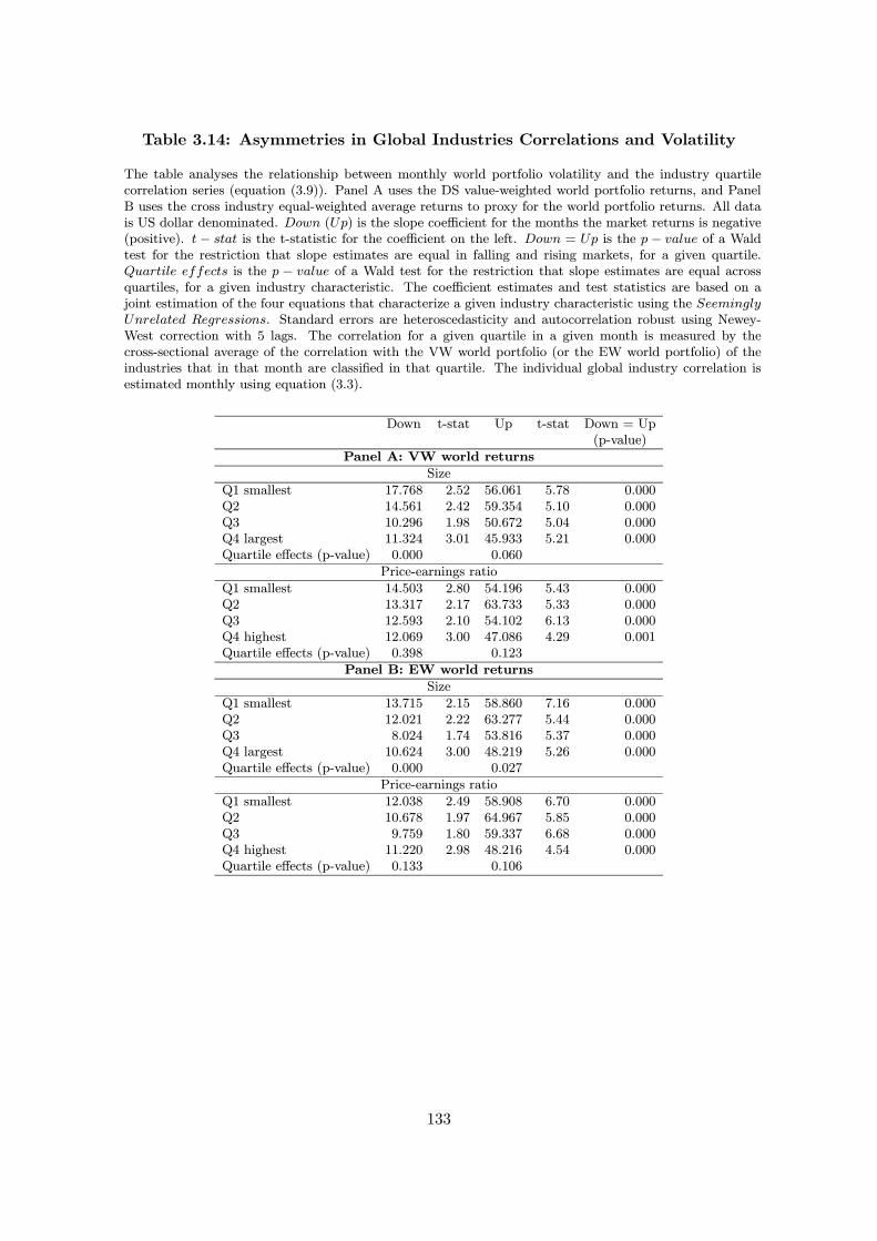
Table 3.14: Asymmetries in Global Industries Correlations and Volatility

The table analyses the relationship between monthly world portfolio volatility and the industry quartilecorrelation series (equation (3.9)). Panel A uses the DS value-weighted world portfolio returns, and PanelB uses the cross industry equal-weighted average returns to proxy for the world portfolio returns. All datais US dollar denominated. Down (Up) is the slope coefficient for the months the market returns is negative(positive). t − stat is the t-statistic for the coefficient on the left. Down = Up is the p − value of a Waldtest for the restriction that slope estimates are equal in falling and rising markets, for a given quartile.Quartile effects is the p − value of a Wald test for the restriction that slope estimates are equal acrossquartiles, for a given industry characteristic. The coefficient estimates and test statistics are based on ajoint estimation of the four equations that characterize a given industry characteristic using the SeeminglyUnrelated Regressions. Standard errors are heteroscedasticity and autocorrelation robust using Newey-West correction with 5 lags. The correlation for a given quartile in a given month is measured by thecross-sectional average of the correlation with the VW world portfolio (or the EW world portfolio) of theindustries that in that month are classified in that quartile. The individual global industry correlation isestimated monthly using equation (3.3).

Down t-stat Up t-stat Down = Up(p-value)

Panel A: VW world returns

Size

Q1 smallest 17.768 2.52 56.061 5.78 0.000Q2 14.561 2.42 59.354 5.10 0.000Q3 10.296 1.98 50.672 5.04 0.000Q4 largest 11.324 3.01 45.933 5.21 0.000Quartile effects (p-value) 0.000 0.060

Price-earnings ratio

Q1 smallest 14.503 2.80 54.196 5.43 0.000Q2 13.317 2.17 63.733 5.33 0.000Q3 12.593 2.10 54.102 6.13 0.000Q4 highest 12.069 3.00 47.086 4.29 0.001Quartile effects (p-value) 0.398 0.123

Panel B: EW world returns

Size

Q1 smallest 13.715 2.15 58.860 7.16 0.000Q2 12.021 2.22 63.277 5.44 0.000Q3 8.024 1.74 53.816 5.37 0.000Q4 largest 10.624 3.00 48.219 5.26 0.000Quartile effects (p-value) 0.000 0.027

Price-earnings ratio

Q1 smallest 12.038 2.49 58.908 6.70 0.000Q2 10.678 1.97 64.967 5.85 0.000Q3 9.759 1.80 59.337 6.68 0.000Q4 highest 11.220 2.98 48.216 4.54 0.000Quartile effects (p-value) 0.133 0.106

133

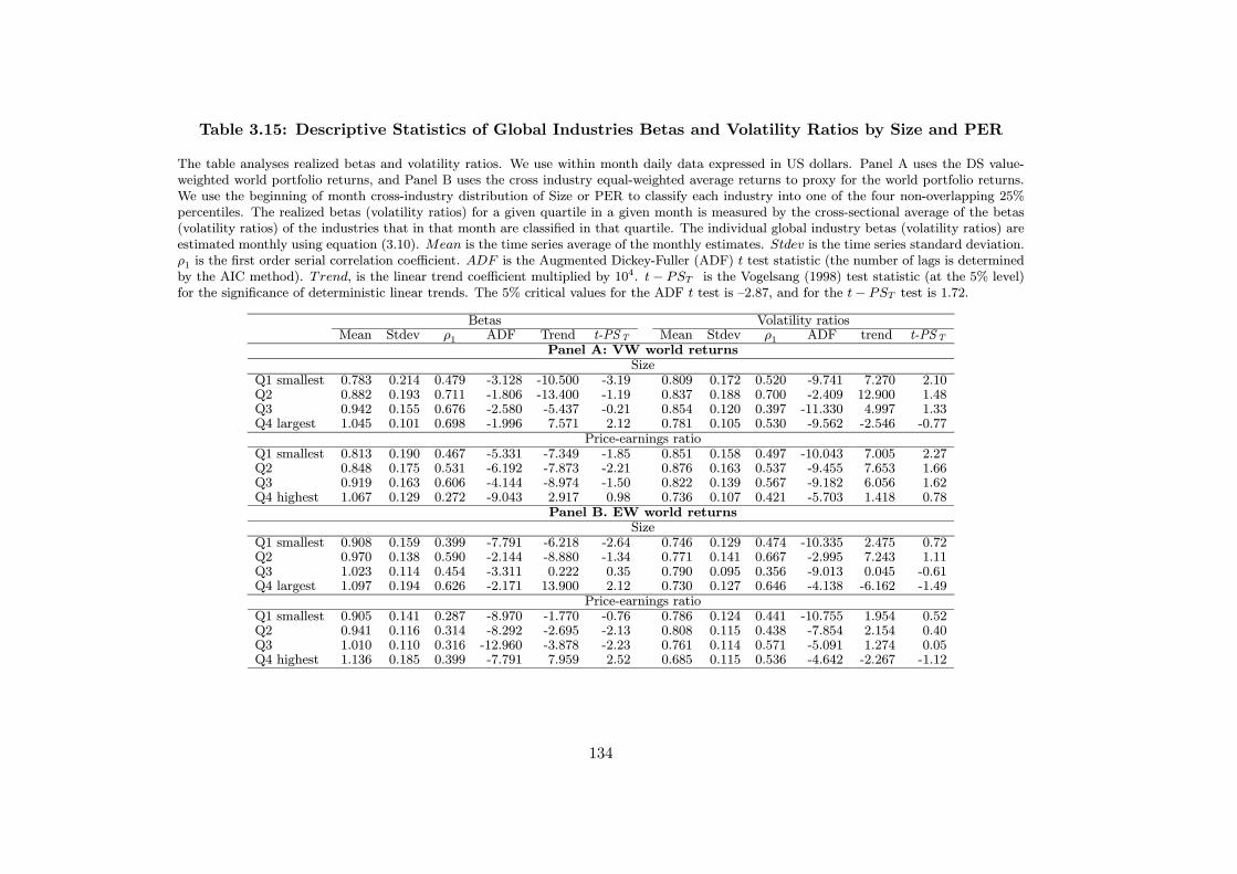
Table 3.15: Descriptive Statistics of Global Industries Betas and Volatility Ratios by Size and PER

The table analyses realized betas and volatility ratios. We use within month daily data expressed in US dollars. Panel A uses the DS value-weighted world portfolio returns, and Panel B uses the cross industry equal-weighted average returns to proxy for the world portfolio returns.We use the beginning of month cross-industry distribution of Size or PER to classify each industry into one of the four non-overlapping 25%percentiles. The realized betas (volatility ratios) for a given quartile in a given month is measured by the cross-sectional average of the betas(volatility ratios) of the industries that in that month are classified in that quartile. The individual global industry betas (volatility ratios) areestimated monthly using equation (3.10). Mean is the time series average of the monthly estimates. Stdev is the time series standard deviation.ρ1 is the first order serial correlation coefficient. ADF is the Augmented Dickey-Fuller (ADF) t test statistic (the number of lags is determinedby the AIC method). Trend, is the linear trend coefficient multiplied by 104. t− PST is the Vogelsang (1998) test statistic (at the 5% level)for the significance of deterministic linear trends. The 5% critical values for the ADF t test is —2.87, and for the t− PST test is 1.72.

Betas Volatility ratiosMean Stdev ρ1 ADF Trend t-PST Mean Stdev ρ1 ADF trend t-PST

Panel A: VW world returnsSize

Q1 smallest 0.783 0.214 0.479 -3.128 -10.500 -3.19 0.809 0.172 0.520 -9.741 7.270 2.10Q2 0.882 0.193 0.711 -1.806 -13.400 -1.19 0.837 0.188 0.700 -2.409 12.900 1.48Q3 0.942 0.155 0.676 -2.580 -5.437 -0.21 0.854 0.120 0.397 -11.330 4.997 1.33Q4 largest 1.045 0.101 0.698 -1.996 7.571 2.12 0.781 0.105 0.530 -9.562 -2.546 -0.77

Price-earnings ratioQ1 smallest 0.813 0.190 0.467 -5.331 -7.349 -1.85 0.851 0.158 0.497 -10.043 7.005 2.27Q2 0.848 0.175 0.531 -6.192 -7.873 -2.21 0.876 0.163 0.537 -9.455 7.653 1.66Q3 0.919 0.163 0.606 -4.144 -8.974 -1.50 0.822 0.139 0.567 -9.182 6.056 1.62Q4 highest 1.067 0.129 0.272 -9.043 2.917 0.98 0.736 0.107 0.421 -5.703 1.418 0.78

Panel B. EW world returnsSize

Q1 smallest 0.908 0.159 0.399 -7.791 -6.218 -2.64 0.746 0.129 0.474 -10.335 2.475 0.72Q2 0.970 0.138 0.590 -2.144 -8.880 -1.34 0.771 0.141 0.667 -2.995 7.243 1.11Q3 1.023 0.114 0.454 -3.311 0.222 0.35 0.790 0.095 0.356 -9.013 0.045 -0.61Q4 largest 1.097 0.194 0.626 -2.171 13.900 2.12 0.730 0.127 0.646 -4.138 -6.162 -1.49

Price-earnings ratioQ1 smallest 0.905 0.141 0.287 -8.970 -1.770 -0.76 0.786 0.124 0.441 -10.755 1.954 0.52Q2 0.941 0.116 0.314 -8.292 -2.695 -2.13 0.808 0.115 0.438 -7.854 2.154 0.40Q3 1.010 0.110 0.316 -12.960 -3.878 -2.23 0.761 0.114 0.571 -5.091 1.274 0.05Q4 highest 1.136 0.185 0.399 -7.791 7.959 2.52 0.685 0.115 0.536 -4.642 -2.267 -1.12

134

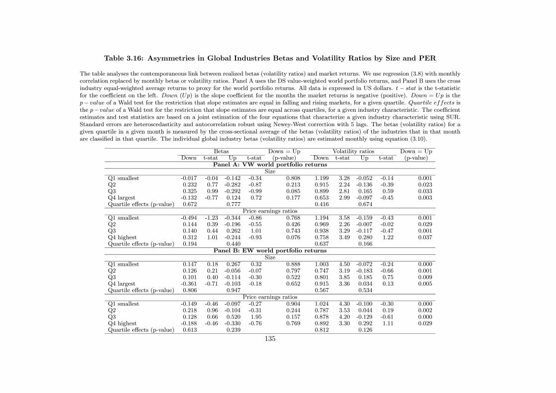
Table 3.16: Asymmetries in Global Industries Betas and Volatility Ratios by Size and PER

The table analyses the contemporaneous link between realized betas (volatility ratios) and market returns. We use regression (3.8) with monthlycorrelation replaced by monthly betas or volatility ratios. Panel A uses the DS value-weighted world portfolio returns, and Panel B uses the crossindustry equal-weighted average returns to proxy for the world portfolio returns. All data is expressed in US dollars. t− stat is the t-statisticfor the coefficient on the left. Down (Up) is the slope coefficient for the months the market returns is negative (positive). Down = Up is thep− value of a Wald test for the restriction that slope estimates are equal in falling and rising markets, for a given quartile. Quartile effects isthe p−value of a Wald test for the restriction that slope estimates are equal across quartiles, for a given industry characteristic. The coefficientestimates and test statistics are based on a joint estimation of the four equations that characterize a given industry characteristic using SUR.Standard errors are heteroscedasticity and autocorrelation robust using Newey-West correction with 5 lags. The betas (volatility ratios) for agiven quartile in a given month is measured by the cross-sectional average of the betas (volatility ratios) of the industries that in that monthare classified in that quartile. The individual global industry betas (volatility ratios) are estimated monthly using equation (3.10).

Betas Down = Up Volatility ratios Down = UpDown t-stat Up t-stat (p-value) Down t-stat Up t-stat (p-value)

Panel A: VW world portfolio returnsSize

Q1 smallest -0.017 -0.04 -0.142 -0.34 0.808 1.199 3.28 -0.052 -0.14 0.001Q2 0.232 0.77 -0.282 -0.87 0.213 0.915 2.24 -0.136 -0.39 0.023Q3 0.325 0.99 -0.292 -0.99 0.085 0.899 2.81 0.165 0.59 0.033Q4 largest -0.132 -0.77 0.124 0.72 0.177 0.653 2.99 -0.097 -0.45 0.003Quartile effects (p-value) 0.672 0.777 0.416 0.674

Price earnings ratiosQ1 smallest -0.494 -1.23 -0.344 -0.86 0.768 1.194 3.58 -0.159 -0.43 0.001Q2 0.144 0.39 -0.196 -0.55 0.426 0.969 2.26 -0.007 -0.02 0.029Q3 0.140 0.44 0.262 1.01 0.743 0.938 3.29 -0.117 -0.47 0.001Q4 highest 0.312 1.01 -0.244 -0.93 0.076 0.758 3.49 0.280 1.22 0.037Quartile effects (p-value) 0.194 0.440 0.637 0.166

Panel B: EW world portfolio returnsSize

Q1 smallest 0.147 0.18 0.267 0.32 0.888 1.003 4.50 -0.072 -0.24 0.000Q2 0.126 0.21 -0.056 -0.07 0.797 0.747 3.19 -0.183 -0.66 0.001Q3 0.101 0.40 -0.114 -0.30 0.522 0.801 3.85 0.185 0.75 0.009Q4 largest -0.361 -0.71 -0.103 -0.18 0.652 0.915 3.36 0.034 0.13 0.005Quartile effects (p-value) 0.806 0.947 0.567 0.534

Price earnings ratiosQ1 smallest -0.149 -0.46 -0.097 -0.27 0.904 1.024 4.30 -0.100 -0.30 0.000Q2 0.218 0.96 -0.104 -0.31 0.244 0.787 3.53 0.044 0.19 0.002Q3 0.128 0.66 0.520 1.95 0.157 0.878 4.20 -0.129 -0.61 0.000Q4 highest -0.188 -0.46 -0.330 -0.76 0.769 0.892 3.30 0.292 1.11 0.029Quartile effects (p-value) 0.613 0.239 0.812 0.126

135

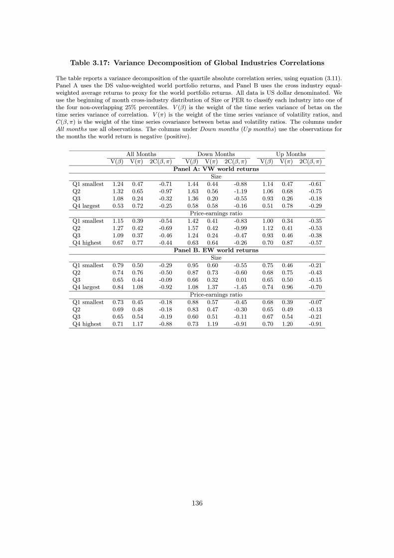
Table 3.17: Variance Decomposition of Global Industries Correlations

The table reports a variance decomposition of the quartile absolute correlation series, using equation (3.11).Panel A uses the DS value-weighted world portfolio returns, and Panel B uses the cross industry equal-weighted average returns to proxy for the world portfolio returns. All data is US dollar denominated. Weuse the beginning of month cross-industry distribution of Size or PER to classify each industry into one ofthe four non-overlapping 25% percentiles. V (β) is the weight of the time series variance of betas on thetime series variance of correlation. V (π) is the weight of the time series variance of volatility ratios, andC(β,π) is the weight of the time series covariance between betas and volatility ratios. The columns underAll months use all observations. The columns under Down months (Up months) use the observations forthe months the world return is negative (positive).

All Months Down Months Up MonthsV(β) V(π) 2C(β,π) V(β) V(π) 2C(β,π) V(β) V(π) 2C(β,π)

Panel A: VW world returns

Size

Q1 smallest 1.24 0.47 -0.71 1.44 0.44 -0.88 1.14 0.47 -0.61Q2 1.32 0.65 -0.97 1.63 0.56 -1.19 1.06 0.68 -0.75Q3 1.08 0.24 -0.32 1.36 0.20 -0.55 0.93 0.26 -0.18Q4 largest 0.53 0.72 -0.25 0.58 0.58 -0.16 0.51 0.78 -0.29

Price-earnings ratio

Q1 smallest 1.15 0.39 -0.54 1.42 0.41 -0.83 1.00 0.34 -0.35Q2 1.27 0.42 -0.69 1.57 0.42 -0.99 1.12 0.41 -0.53Q3 1.09 0.37 -0.46 1.24 0.24 -0.47 0.93 0.46 -0.38Q4 highest 0.67 0.77 -0.44 0.63 0.64 -0.26 0.70 0.87 -0.57

Panel B. EW world returns

Size

Q1 smallest 0.79 0.50 -0.29 0.95 0.60 -0.55 0.75 0.46 -0.21Q2 0.74 0.76 -0.50 0.87 0.73 -0.60 0.68 0.75 -0.43Q3 0.65 0.44 -0.09 0.66 0.32 0.01 0.65 0.50 -0.15Q4 largest 0.84 1.08 -0.92 1.08 1.37 -1.45 0.74 0.96 -0.70

Price-earnings ratio

Q1 smallest 0.73 0.45 -0.18 0.88 0.57 -0.45 0.68 0.39 -0.07Q2 0.69 0.48 -0.18 0.83 0.47 -0.30 0.65 0.49 -0.13Q3 0.65 0.54 -0.19 0.60 0.51 -0.11 0.67 0.54 -0.21Q4 highest 0.71 1.17 -0.88 0.73 1.19 -0.91 0.70 1.20 -0.91

136

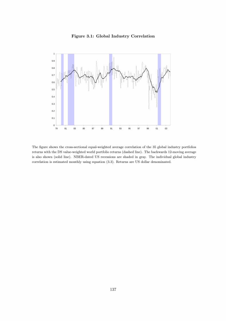
Figure 3.1: Global Industry Correlation

0

0.1

0.2

0.3

0.4

0.5

0.6

0.7

0.8

0.9

1

79 81 83 85 87 89 91 93 95 97 99 01 03

The figure shows the cross-sectional equal-weighted average correlation of the 35 global industry portfolios

returns with the DS value-weighted world portfolio returns (dashed line). The backwards 12-moving average

is also shown (solid line). NBER-dated US recessions are shaded in gray. The individual global industry

correlation is estimated monthly using equation (3.3). Returns are US dollar denominated.

137

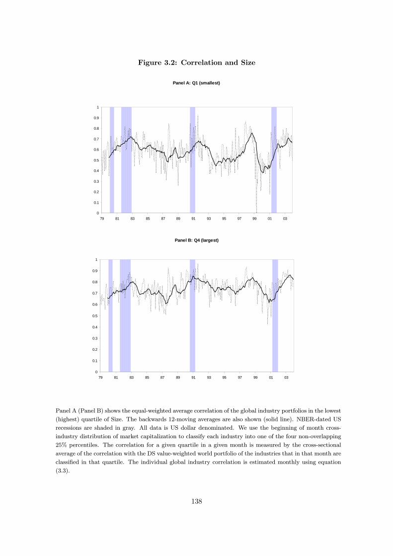
Figure 3.2: Correlation and Size

Panel A: Q1 (smallest)

0

0.1

0.2

0.3

0.4

0.5

0.6

0.7

0.8

0.9

1

79 81 83 85 87 89 91 93 95 97 99 01 03

Panel B: Q4 (largest)

0

0.1

0.2

0.3

0.4

0.5

0.6

0.7

0.8

0.9

1

79 81 83 85 87 89 91 93 95 97 99 01 03

Panel A (Panel B) shows the equal-weighted average correlation of the global industry portfolios in the lowest

(highest) quartile of Size. The backwards 12-moving averages are also shown (solid line). NBER-dated US

recessions are shaded in gray. All data is US dollar denominated. We use the beginning of month cross-

industry distribution of market capitalization to classify each industry into one of the four non-overlapping

25% percentiles. The correlation for a given quartile in a given month is measured by the cross-sectional

average of the correlation with the DS value-weighted world portfolio of the industries that in that month are

classified in that quartile. The individual global industry correlation is estimated monthly using equation

(3.3).

138

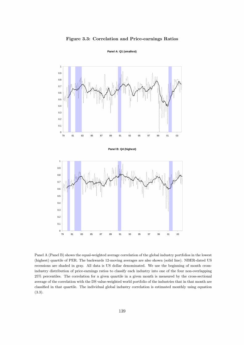
Figure 3.3: Correlation and Price-earnings Ratios

Panel A: Q1 (smallest)

0

0.1

0.2

0.3

0.4

0.5

0.6

0.7

0.8

0.9

1

79 81 83 85 87 89 91 93 95 97 99 01 03

Panel B: Q4 (highest)

0

0.1

0.2

0.3

0.4

0.5

0.6

0.7

0.8

0.9

1

79 81 83 85 87 89 91 93 95 97 99 01 03

Panel A (Panel B) shows the equal-weighted average correlation of the global industry portfolios in the lowest

(highest) quartile of PER. The backwards 12-moving averages are also shown (solid line). NBER-dated US

recessions are shaded in gray. All data is US dollar denominated. We use the beginning of month cross-

industry distribution of price-earnings ratios to classify each industry into one of the four non-overlapping

25% percentiles. The correlation for a given quartile in a given month is measured by the cross-sectional

average of the correlation with the DS value-weighted world portfolio of the industries that in that month are

classified in that quartile. The individual global industry correlation is estimated monthly using equation

(3.3).

139