Embed Size (px)
Citation preview

UNIVERSIDADE ESTADUAL DE CAMPINASFaculdade de Engenharia Mecânica
ALESSANDRO JOSÉ TRUTA BESERRA DE LIMA
Pollutant Formation Simulation Models (CO, NOxand UHC) for Ethanol-fueled Engines
Modelos de Simulação de Formação de Poluentes(CO, NOx e UHC) em Motores a Etanol
CAMPINAS
2017
ALESSANDRO JOSÉ TRUTA BESERRA DE LIMA
Pollutant Formation Simulation Models (CO, NOxand UHC) for Ethanol-fueled Engines
Modelos de Simulação de Formação de Poluentes(CO, NOx e UHC) em Motores a Etanol
Dissertation presented to the School of Me-chanical Engineering of the University ofCampinas in partial fulfillment of the require-ments for the Master’s degree, in the field ofThermal and Fluids.
Dissertação apresentada à Faculdade deEngenharia Mecânica da Universidade Estad-ual de Campinas como parte dos requisitosexigidos para a obtenção do título de Mestreem Engenharia Mecânica, na Área de Térmicae Fluidos.
Orientador: Prof. Dr. Waldyr Luiz Ribeiro Gallo
ESTE EXEMPLAR CORRESPONDE À VERSÃO FINAL DADISSERTAÇÃO DEFENDIDA PELO ALUNO ALESSANDRO JOSÉTRUTA BESERRA DE LIMA, E ORIENTADA PELO PROF. DR.WALDYR LUIZ RIBEIRO GALLO.
CAMPINAS
2017

Agência(s) de fomento e nº(s) de processo(s): FAPESP, 2015/17041-7
Ficha catalográficaUniversidade Estadual de Campinas
Biblioteca da Área de Engenharia e ArquiteturaLuciana Pietrosanto Milla - CRB 8/8129
Lima, Alessandro José Truta Beserra de, 1991- L628p LimPollutant formation simulation models (CO, NOx and UHC) for Ethanol-
fueled engines / Alessandro José Truta Beserra de Lima. – Campinas, SP :[s.n.], 2017.
LimOrientador: Waldyr Luiz Ribeiro Gallo. LimDissertação (mestrado) – Universidade Estadual de Campinas, Faculdade
de Engenharia Mecânica.
Lim1. Termodinâmica. 2. Etanol. 3. Cinética química. 4. Equilíbrio químico. 5.
Motores de combustão interna. I. Gallo, Waldyr Luiz Ribeiro, 1954-. II.Universidade Estadual de Campinas. Faculdade de Engenharia Mecânica. III.Título.
Informações para Biblioteca Digital
Título em outro idioma: Modelos de simulação de formação de poluentes (CO, NOx eUHC) em motores a etanolPalavras-chave em inglês:ThermodynamicsEthanolChemical kineticsChemical equilibriumInternal combustion enginesÁrea de concentração: Térmica e FluídosTitulação: Mestre em Engenharia MecânicaBanca examinadora:Waldyr Luiz Ribeiro Gallo [Orientador]Rogério Gonçalves dos SantosJosé Eduardo Mautone BarrosData de defesa: 01-09-2017Programa de Pós-Graduação: Engenharia Mecânica
Powered by TCPDF (www.tcpdf.org)

UNIVERSIDADE ESTADUAL DE CAMPINASFACULDADE DE ENGENHARIA MECÂNICA
COMISSÃO DE PÓS-GRADUAÇÃO EM ENGENHARIA MECÂNICADEPARTAMENTO DE ENERGIA E FLUIDOS
DISSERTAÇÃO DE MESTRADO ACADÊMICO
Pollutant Formation Simulation Models (CO, NOxand UHC) for Ethanol-fueled Engines
Modelos de Simulação de Formação de Poluentes(CO, NOx e UHC) em Motores a Etanol
Autor: Alessandro José Truta Beserra de LimaOrientador: Prof. Dr. Waldyr Luiz Ribeiro Gallo
A Banca Examinadora composta pelos membros abaixo aprovou esta Dissertação:
Prof. Dr. Waldyr Luiz Ribeiro GalloFEM/UNICAMP
Prof. Dr. Rogério Gonçalves dos SantosFEM/UNICAMP
Prof. Dr. José Eduardo Mautone BarrosDEMEC/UFMG
A Ata da defesa com as respectivas assinaturas dos membros encontra-se no processo de vidaacadêmica do aluno.
Campinas, 01 de Setembro de 2017.

À minha família,
que me proporcionou tudo na minha vida.

ACKNOWLEDGEMENTS
Agradeço primeiramente aos meus pais, Erivaldo e Maria de Fátima, que sempreme estimularam a estudar e aprender, além de me prover um ambiente muito acolhedor duranteminha vida inteira, onde pude ter a liberdade de fazer aquilo que amo na minha vida.
Agradeço também a minha irmã, Nathália, por tudo no nosso relacionamento; quemesmo afastada me apoiou no meu trabalho e na minha vida.
Agradeço ao professor Waldyr Luiz Ribeiro Gallo, por toda a paciência, orien-tações da mais alta qualidade e esforço empenhado em me ajudar a desenvolver este trabalho.Agradeço muito pela oportunidade que o professor me forneceu ao poder vir fazer parte desteprojeto, cujo o mesmo foi uma grande experiência na minha vida.
Agradeço aos meus amigos do laboratório LMB e da UNICAMP, Jair, Renato, Caio,Ana, Felipe e Giovanna, por todo o suporte e aprendizado mútuo no desenvolvimento destetrabalho. Os dias foram bem mais confortáveis e felizes quando estive ao lado de vocês.
Agradeço aos meus amigos Jonatha, Cíntia, Breno e Lívia, por terem tido a exper-iência de um mestrado comigo aqui na UNICAMP, onde pudemos auxiliar cada um de nós nasdificuldades e apreciarmos os momentos felizes. Saibam que vocês fizeram minha mudançapara Campinas muito mais fácil e feliz, além de terem me ajudado a crescer na vida.
Como não posso deixar de agradecer, agraçeço à Letícia, amor de minha vida, porsimplesmente existir no meu cotidiano desde que nos conhecemos! Quero que você saiba quese eu atingi esta meta na minha vida, grande parte disso eu devo a você. Por todos os momentosdifíceis e exaustivos que passei mas que ainda assim consegui encontrar conforto ao seu lado.Você é minha guia eterna, aquela a qual sempre quero estar acompanhado!
Agradeço a FEM-UNICAMP pela oportunidade de trabalho, experiência e o con-hecimento, todos eles fornecidos em um ambiente que estimula adequadamente o aprendizado.
Agradeço também ao Instituto Mauá de Tecnologia, por todo o fornecimento dedados experimentais, cujos quais permitiram o desenvolvimento de resultados deste trabalho.
Finalmente, agradeço a FAPESP, pela oportunidade de trabalho na concessão doauxílio à pesquisa e bolsa de mestrado, através do projeto número 2015/17041-7.

“Quem nunca errou, nunca experimentou nada novo.”
(Albert Einstein, Físico)

RESUMO
A atual necessidade mundial de combustíveis alternativos para automóveis no pla-neta reflete a importância da efetivação do etanol no mercado automobilístico internacional.O etanol brasileiro, proveniente da cana de açúcar, possui maior nível de sustentabilidade secomparado aos combustíveis fósseis e pode ser integralmente aplicado em motores de combus-tão interna. Seu uso apresenta benefícios de desempenho técnico e de poluentes, mesmo coma aplicação geral do catalisador de três vias nos motores atuais. Este trabalho foca no estudoe desenvolvimento de modelos matemáticos para previsão e formação de poluentes regulados(monóxido de carbono, óxido nítrico e hidrocarbonetos não-queimados) por parte do funciona-mento de motores de ignição por centelha movidos a etanol. Concentrações molares de oxidonítrico (NO) e monóxido de carbono (CO) foram calculadas de acordo com a aplicação de con-ceitos de cinética química e equilíbrio químico em um modelo zero-dimensional termodinâmicode duas zonas, o qual simula o funcionamento de um motor de ignição por centelha. A análisede formação contínua destes poluentes é calculada a medida que o modelo de Wiebe calculaas massas das zonas queimada e não-queimada, com base nas condições definidas previamentena simulação da operação do motor. O modelo de cinética é composto de 22 reações químicase 12 espécies (Ar, CO, CO2, H, H2, H2O, OH, O, O2, N, N2, NO), cujo sistema de equaçõesdiferenciais é solucionado pelo método numérico trapezoidal implícito, aplicado durante todoo processo de combustão e expansão do ciclo simulado. Convergência a cada iteração é garan-tida com a aplicação do método de Newton-Raphson para solução de sistemas não-lineares deforma rápida, se considerada que a solução completa das equações diferenciais é obtida. Para omodelo de hidrocarbonetos não-queimados (UHC), desenvolveu-se dois modelos simplificadospara os fenômenos de fenda (crevice) e extinção (quenching), através de aplicações de concei-tos de gases ideais e da termodinâmica. Resultados mostram coerência qualitativa com dadosde formação e emissões presentes na literatura e com medições experimentais para a geome-tria do motor estudado, com capacidade de predizer, no futuro, o efeito nas emissões causadopor sistemas auxiliares do motor, como EGR e turboalimentação, evitando custos com análisesexperimentais para obter-se informações similares.
Palavras-chave: Termodinâmica; Etanol; Cinética Química; Equilíbrio Químico; Motores deCombustão Interna; CO, NOx e UHC.

ABSTRACT
The current worldwide necessity of alternative fuels for automobiles in the planet reflects theimportance of ethanol on the international automotive market. The Brazilian ethanol, whichmostly comes from sugar cane, presents a more sustainable origin than fossil fuels and may beapplied as a fuel on internal combustion engines. Its use presents benefits on technical area andreduction of combustion gases, despite the three-way catalyst presence on current engines. Thisthesis focuses on the study and development of mathematical models for prevision and forma-tion of regulated pollutants (carbon monoxide, nitric oxide and unburned hydrocarbons) derivedfrom combustion process in spark-ignited engines fueled by ethanol. Concentrations of nitricoxide (NO) and carbon monoxide (CO) were calculated based on concepts of chemical kineticsand chemical equilibrium applied on a zero-dimensional two-zone thermodynamic model of aspark-ignited engine. The continuous formation analysis of these pollutants is evaluated at thesame moment as a Wiebe function calculates the amount of unburned and burned masses in thecylinder, considering the conditions previously defined on the engine operation simulator. Thekinetic model is composed by 22 chemical reactions and 12 chemical species (Ar, CO, CO2,H, H2, H2O, OH, O, O2, N, N2, NO), which provides a system of differential equations that issolved by the implicit trapezoidal numerical method, applied during combustion and expansionprocesses of the simulated cycle. Convergence during each iteration is guaranteed by the appli-cation of the Newton-Raphson method for nonlinear system of equations, obtaining relativelyquick solutions, despite the calculation of the full solution of the system on each iteration. Forthe unburned hydrocarbon model (UHC), it was developed two simplified models for the phe-nomenon of crevice and flame quenching, with application of ideal gases and thermodynamicconcepts. Results showed qualitatively coherence with formation and emission data presentedby literature and with experimental measurements of the studied engine. These models maybe applied in the future to predict the effect of auxiliary systems of the engine, such as EGRand turbocharging, on regulated gas emissions, avoiding experimental costs to obtain similarinformation.
Keywords: Thermodynamics; Ethanol; Chemical Kinetics; Chemical Equilibrium; Internal Com-bustion Engines; CO, NOx and UHC.

LIST OF FIGURES
Figure 2.1 – Orders of magnitude for exhaust gases from SI Engines. Ref: (MERKER et
al., 2014) . . . . . . . . . . . . . . . . . . . . . . . . . . . . . . . . . . . . 25Figure 2.2 – NO formation (moles
cm3 ) x time (s) on Lean-stoichiometric mixtures. Ref.: (NEWHALL;SHAHED, 1971) . . . . . . . . . . . . . . . . . . . . . . . . . . . . . . . 42
Figure 2.3 – NO formation (molescm3 ) x time (s) on rich-mixtures. Ref.: (NEWHALL; SHA-
HED, 1971) . . . . . . . . . . . . . . . . . . . . . . . . . . . . . . . . . . 42Figure 2.4 – UHC emission diagram on a SI Engine. Ref.: (MERKER et al., 2014) . . . 51Figure 2.5 – HC formation flowchart. Ref.: (MERKER et al., 2014) . . . . . . . . . . . 53Figure 2.6 – UHC emission diagram on a SI Engine. Ref.: (MERKER et al., 2014) . . . 54Figure 2.7 – UHC emission X engine crank-angle (Exhaust process). Ref.: (FERGU-
SON; KIRKPATRICK, 2001) . . . . . . . . . . . . . . . . . . . . . . . . . 54Figure 2.8 – UHC crevice Volumes on a V-6 Engine. Ref: (HEYWOOD, 1988) . . . . . 55Figure 2.9 – Crevice diagram on a conventional SI Engine. Ref: (HEYWOOD, 1988) . . 56Figure 3.1 – Simplified flowchart of the final chemical kinetic model. . . . . . . . . . . . 70Figure 4.1 – NO formation from dry air in a closed system at T = 1800 : 2100K. . . . . . 78Figure 4.2 – NO formation from dry air in a closed system at T = 2200 : 2500K. . . . . . 78Figure 4.3 – A semi-log plot of NO-formation from dry air in a closed system versus
Temperature. . . . . . . . . . . . . . . . . . . . . . . . . . . . . . . . . . . 79Figure 4.4 – NO profile x Engine Crank Angle on Stoichiometric Condition. . . . . . . . 83Figure 4.5 – NO profile x Engine Crank Angle on λ = 0.9. . . . . . . . . . . . . . . . . 84Figure 4.6 – NO profile x Engine Crank Angle on λ = 0.8. . . . . . . . . . . . . . . . . 85Figure 4.7 – NO profile x Engine Crank Angle on λ = 1.1. . . . . . . . . . . . . . . . . 86Figure 4.8 – NO profile x Engine Crank Angle on λ = 1.2. . . . . . . . . . . . . . . . . 86Figure 4.9 – CO profile x Engine Crank Angle on Stoichiometric Condition. . . . . . . . 88Figure 4.10–CO profile x Engine Crank Angle on λ = 0.9. . . . . . . . . . . . . . . . . 89Figure 4.11–CO profile x Engine Crank Angle on λ = 0.8. . . . . . . . . . . . . . . . . 89Figure 4.12–CO profile x Engine Crank Angle on λ = 1.1. . . . . . . . . . . . . . . . . 90Figure 4.13–CO profile x Engine Crank Angle on λ = 1.2. . . . . . . . . . . . . . . . . 91Figure 4.14–NO formation x Engine speed - Rich/Stoichiometric case. . . . . . . . . . . 92Figure 4.15–NO formation x Engine speed - Stoichiometric/Lean case. . . . . . . . . . . 93Figure 4.16–NO formation x Air-fuel ratio under several engine speeds. . . . . . . . . . 94Figure 4.17–CO formation x Engine speed under several mixtures. . . . . . . . . . . . . 95Figure 4.18–CO formation x Air-fuel ratio under several engine speeds. . . . . . . . . . 96Figure 4.19–NO formation x Spark timing on a stoichiometric mixture. . . . . . . . . . . 97Figure 4.20–CO formation x Spark timing on a stoichiometric mixture. . . . . . . . . . . 98Figure 4.21–UHC emission x Engine Speed under several different mixtures. . . . . . . 100

Figure 4.22–UHC emission x Air Fuel Ratio under several different engine speeds. . . . 101Figure 4.23–UHC emission x Spark Timing on a stoichiometric mixture. . . . . . . . . . 102Figure 4.24–Regulated pollutant concentrations versus lambda. Ref.: (MERKER et al.,
2014) . . . . . . . . . . . . . . . . . . . . . . . . . . . . . . . . . . . . . . 103Figure 4.25–Pollutant complete emission diagram of the simulated case. . . . . . . . . . 104Figure 4.26–Comparison pollutant model x experimental data - Nitric Oxide x engine
speed. . . . . . . . . . . . . . . . . . . . . . . . . . . . . . . . . . . . . . 108Figure 4.27–Comparison pollutant model x experimental data - Nitric Oxide x lambda. . 109Figure 4.28–Comparison pollutant model x experimental data - Carbon Monoxide x en-
gine speed. . . . . . . . . . . . . . . . . . . . . . . . . . . . . . . . . . . . 110Figure 4.29–Comparison pollutant model x experimental data - Carbon Monoxide x lambda.111Figure 4.30–Comparison pollutant model x experimental data - Unburned Hydrocarbons
x engine speed. . . . . . . . . . . . . . . . . . . . . . . . . . . . . . . . . 112Figure 4.31–Comparison pollutant model x experimental data - Unburned Hydrocarbons
x lambda. . . . . . . . . . . . . . . . . . . . . . . . . . . . . . . . . . . . 113

LIST OF TABLES
Table 2.1 – Main Sources of CO emission. Ref: (KUO, 2005) . . . . . . . . . . . . . . . 46Table 2.2 – UHC Emission Sources from an SI Engine (CHENG et al., 1993). . . . . . . 51Table 3.1 – Reaction Rate Constant Parameters . . . . . . . . . . . . . . . . . . . . . . 67Table 3.2 – Dry Air Composition (WAY, 1976) . . . . . . . . . . . . . . . . . . . . . . 71Table 4.1 – NO Tendency to Equilibrium x Usual Engine Temperatures . . . . . . . . . . 80Table 4.2 – Engine operation variables and parameters. . . . . . . . . . . . . . . . . . . 82Table 4.3 – Experimental engine variables - Low revolutions. . . . . . . . . . . . . . . . 105Table 4.4 – Experimental engine variables - High revolutions. . . . . . . . . . . . . . . . 106
LIST OF ABBREVIATIONS AND ACRONYMS
NO Nitric Oxide
CO Carbon Monoxide
Ar Argon
CO2 Carbon Dioxide
H,H2 Atomic Hydrogen, Hydrogen gas
H2O,OH Water, Hydroxyl
O,O2 Atomic Oxygen, Oxygen Gas
N,N2 Atomic Nitrogen, Nitrogen Gas
UHC Unburned Hydrocarbons
NOx Nitrogen Oxides
HC Hydrocarbon
SI Spark Ignited
FFFVs Full Flex-Fuel Vehicles
ICEs Internal Combustion Engines
F Fluorine
Cl Chlorine
CH3 Methyl Radical
CH Methylidyne
C2H5 Ethyl Radical
N2O4 Nitrogen tetroxide
NO2 Nitrogen dioxide
N2O Nitrous Oxide
N2O3 Dinitrogen Trioxide
N2O5 Dinitrogen Pentoxide

NH Nitrogen Monohydride
NH2 Amidogen
NH3 Ammonia
HNO Nitroxyl
HCradicals Hydrocarbon radicals
C2H6O Ethanol
HCN Hydrogen Cyanide
HO2 Hydroperoxyl
E95 Hydrous Ethanol (95% Volume Ethanol + 5% Water)
A/F Air-fuel ratio
TDC Top-Dead Center
RPM Revolutions per minute
EGR Exhaust Gas Recirculation
R Chemical Radical
RCHO General Aldehyde
S/V Surface to volume ratio
ppmC1 Parts per million of carbon
EVO, EVC Exhaust valve opening and closure respectively
IVO, IVC Inlet valve opening and closure respectively
C8H18 n-Octane

LIST OF SYMBOLS
N Number of Chemical Species
i, j ith, jth term
Mi ith Molecule/chemical species
RR Reaction Rate
k Rate constant of the chemical reaction
CP,CR Molar concentration of the products or reactants respectively
Ci Molar concentration of the ith species
A,b Experimental parameters related to Arrhenius Equation
T Temperature
Ea Activation Energy
Ru Universal Constant of the gases
k f ,kb Forward and Backward rate constant of a chemical reaction respectively
dCidt Reaction rate of the ith chemical species
C j,e Molar concentration of the jth chemical species in a chemical equilibriumstate
Kc Chemical equilibrium constant for molar concentration
Kp Chemical equilibrium constant for partial pressure
p j,e Partial pressure of the jth chemical species
po Atmospheric pressure (or reference)
p Absolute/total pressure
V Total volume
nT Total number of moles
M Third-body molecule (usually considered as N2)
(O2)eq Molar concentration of Oxygen gas in a chemical equilibrium state

(N2)eq Molar concentration of Nitrogen gas in a chemical equilibrium state
Pe Peclet Number
SL Laminar flame speed
cp, f Flame constant-pressure specific heat
Tf , Tu Flame and unburned gas temperatures respectively
k f Flame thermal conductivity
dq,2 Two-plate quench distance
dq,1 One-plate quench distance
K1 Ishizawa’s fuel constant
Ppeak Peak pressure
Twall Wall temperature
w j jth Integrated variable of a numerical method
h Step size
A(~x),J(~x) Auxiliary matrix, Jacobian matrix
I Identity matrix
~x,~y Variables of the numerical method
TOL Numerical method tolerance
yi ith molar fraction
ui ith u-variable
()b, ()u Burned and unburned gas properties respectively
Vcrevice Crevice volume
fcrevice Crevice factor
Vclearance Clearance volume
m mass
MM Molar mass
S Stroke

B Cylinder bore
hquench Quench thickness
t time
λ Lambda factor
∆n Number of moles difference
ν′i ,ν
′′i Reactant and product stoichiometric coefficients of the ith species
τ−1NO Nitric oxide characteristic time
φ Equivalence Ratio
ρu Unburned gas specific mass
ω Engine Angular speed
θ Crank Angle

CONTENTS
1 Introduction . . . . . . . . . . . . . . . . . . . . . . . . . . . . . . . . . . . . . . 201.1 Objectives . . . . . . . . . . . . . . . . . . . . . . . . . . . . . . . . . . . . . 211.2 Outline of the dissertation . . . . . . . . . . . . . . . . . . . . . . . . . . . . . 21
2 Literature Review . . . . . . . . . . . . . . . . . . . . . . . . . . . . . . . . . . . 222.1 Ethanol Use in Spark-ignition Engines in Brazil . . . . . . . . . . . . . . . . . 222.2 Pollutant Emission in Spark-Ignited Engines . . . . . . . . . . . . . . . . . . . 242.3 Chemical Kinetics . . . . . . . . . . . . . . . . . . . . . . . . . . . . . . . . . 25
2.3.1 Basic concepts of Chemical Kinetics . . . . . . . . . . . . . . . . . . . 262.3.2 The Arrhenius Law and Order of a Reaction . . . . . . . . . . . . . . . 272.3.3 Consecutive, Competitive and Opposing Reactions . . . . . . . . . . . 292.3.4 Chain Reactions . . . . . . . . . . . . . . . . . . . . . . . . . . . . . . 302.3.5 Relation between Chemical Equilibrium and Chemical Kinetics . . . . 312.3.6 Recent works on chemical kinetics in internal combustion engines . . . 33
2.4 NO-Formation Fundamentals . . . . . . . . . . . . . . . . . . . . . . . . . . . 342.4.1 NOx-Formation Mechanisms . . . . . . . . . . . . . . . . . . . . . . . 35
2.4.1.1 Thermal NO Route . . . . . . . . . . . . . . . . . . . . . . . 352.4.1.2 Global Reaction Mechanism . . . . . . . . . . . . . . . . . . 362.4.1.3 Zeldovich Chain Reaction Mechanism . . . . . . . . . . . . 362.4.1.4 Extended Zeldovich Chain Reaction Mechanism . . . . . . . 372.4.1.5 Lavoie Thermal-NO Mechanism . . . . . . . . . . . . . . . . 372.4.1.6 Annand NO-Formation Mechanism . . . . . . . . . . . . . . 382.4.1.7 Spadaccini NO Mechanism . . . . . . . . . . . . . . . . . . 382.4.1.8 Other models presented by literature . . . . . . . . . . . . . . 382.4.1.9 Prompt-NO Route . . . . . . . . . . . . . . . . . . . . . . . 402.4.1.10 Fuel-Bound Nitrogen (FN) route . . . . . . . . . . . . . . . . 402.4.1.11 NO2 route . . . . . . . . . . . . . . . . . . . . . . . . . . . 412.4.1.12 N2O route . . . . . . . . . . . . . . . . . . . . . . . . . . . . 41
2.4.2 NO Formation in Flames . . . . . . . . . . . . . . . . . . . . . . . . . 412.4.3 Effect of Design and Operating Variables on NOx Emissions . . . . . . 43
2.5 CO-Formation Fundamentals . . . . . . . . . . . . . . . . . . . . . . . . . . . 462.5.1 CO-Formation Mechanism . . . . . . . . . . . . . . . . . . . . . . . . 472.5.2 Effect of Design and Operating Variables on CO-Formation . . . . . . . 48
2.6 Unburned Hydrocarbon Fundamentals . . . . . . . . . . . . . . . . . . . . . . 502.6.1 HC-Formation Mechanisms . . . . . . . . . . . . . . . . . . . . . . . 512.6.2 HC-emission on Exhaust Process . . . . . . . . . . . . . . . . . . . . . 532.6.3 Crevice HC-formation Mechanism . . . . . . . . . . . . . . . . . . . . 55

2.6.4 Flame Quenching HC Mechanism . . . . . . . . . . . . . . . . . . . . 563 Methodology . . . . . . . . . . . . . . . . . . . . . . . . . . . . . . . . . . . . . . 59
3.1 Numerical Solution of Stiff Differential Equations . . . . . . . . . . . . . . . . 593.2 Chemical Kinetic models . . . . . . . . . . . . . . . . . . . . . . . . . . . . . 61
3.2.1 Air dissociation chemical model . . . . . . . . . . . . . . . . . . . . . 623.2.1.1 Procedure and assumptions of the model . . . . . . . . . . . 62
3.2.2 Final chemical kinetic model . . . . . . . . . . . . . . . . . . . . . . . 643.2.2.1 Procedure and assumptions of the model . . . . . . . . . . . 65
3.3 HC-formation and Emission Models . . . . . . . . . . . . . . . . . . . . . . . 703.3.1 UHC Crevice model . . . . . . . . . . . . . . . . . . . . . . . . . . . 703.3.2 UHC Flame Quenching Model . . . . . . . . . . . . . . . . . . . . . . 72
4 Results and Analysis . . . . . . . . . . . . . . . . . . . . . . . . . . . . . . . . . . 764.1 Chemical Kinetic Analysis - Air dissociation chemical model . . . . . . . . . . 764.2 Chemical kinetics model on the two-zone thermodynamic engine simulator . . 80
4.2.1 NO and CO formation profiles with crank angle . . . . . . . . . . . . . 834.2.2 Engine Speed and Air-fuel ratio effects on NO and CO Emissions . . . 914.2.3 Spark Timing Effects on NO and CO Emissions . . . . . . . . . . . . . 96
4.3 UHC-emission model analysis on the two-zone thermodynamic engine simulator 984.3.1 Engine speed and Air-fuel ratio effects on UHC emission model . . . . 994.3.2 Spark timing effects on UHC emission model . . . . . . . . . . . . . . 101
4.4 Theoretical Pollutant profile . . . . . . . . . . . . . . . . . . . . . . . . . . . . 1024.5 Comparison between the pollutant models and experimental data . . . . . . . . 104
4.5.1 Description of experimental data . . . . . . . . . . . . . . . . . . . . . 1054.5.2 Comparison between experimental emission data and engine simulator
emission models . . . . . . . . . . . . . . . . . . . . . . . . . . . . . 1065 Conclusion . . . . . . . . . . . . . . . . . . . . . . . . . . . . . . . . . . . . . . . 114
References . . . . . . . . . . . . . . . . . . . . . . . . . . . . . . . . . . . . . . . . . 116

20
1 INTRODUCTION
Internal Combustion Engines are part of the humankind since final 19th century.Due to the extraordinary expansion in the quantity of the automobiles in the world, the atmo-sphere started to receive great amounts of pollutants from the engines. Nitrogen oxides (NOx),carbon monoxide and dioxide (CO and CO2) and Unburned Hydrocarbons (UHC) are someexamples of the exhaust gases that come from combustion processes in engines.
The necessity of predicting the formation of regulated pollutants from automobilesis not a recent research. Several experiments and models were developed and presented almostfifty years ago (LAVOIE et al., 1970), (SPADACCINI; CHINITZ, 1972), which analyzed theformation and emission of these gases with some precision associated. Though the developmentof the three-way catalyst and its application on the automotive engines reduced the emissionsfrom the transport sector, it had also reduced the researches on pollutant formation and emissionfrom engines. The three-way catalyst, however, requires the gas mixture to be close to stoichio-metric conditions, which stiffed the range of applicable equivalence ratio of the engines.
The ethanol appeared as an alternative fuel for the automotive section on Brazil onthe 20’s. Despite the thermodynamic benefits of its use on automotive vehicles (BRINKMAN,1981), the development of engines focused on this fuel had stopped. The actual necessity of re-duction of CO2 stimulates again the use of ethanol as fuel, although the development of specificethanol-fueled engines would be required to obtain the benefits of this fuel. The development ofsimulation models which are able to predict the gross emission of regulated pollutants from au-tomotive engines is one of the steps required on the development of an advanced ethanol-fueledengine, which would provide a basis for advanced simulations of future ethanol-fueled engines.
To maintain ethanol as a substitute of gasoline as a fuel for the future, it is necessaryto keep its studies to prevent it to lose market for other options of engines, as electric cars, forexample. This dissertation follows this idea, trying to give valor to its emission advantage overother fuels to establish once again ethanol (anhydrous and hydrated) as a trustworthy option ofsource of energy.
Therefore this dissertation focus on the development of models which predict theformation of regulated pollutants from spark-ignited engines fueled with ethanol. Specific mech-anisms for each of the pollutants in study (NO, CO and UHC) are studied and presented. Theimplantation of these models on the advanced ethanol engine simulator is briefly commentedon this paper.
This Master’s thesis is related to a FAPESP project called ’Pollutants formationsimulation models (CO, NOx and HC) in ethanol engines’, number 2015/17041-7, which is partof a bigger project called ’Conceptual study of an advanced ethanol-fueled engine’, associated

Chapter 1. Introduction 21
with the creation of the ’Prof. Urbano Ernesto Stumpf’ Engineering Research Center, whichwas approved by FAPESP under the number 13/50238-3.
1.1 OBJECTIVES
The objective of this dissertation is to develop a pollutant simulation model whichpredicts the gross emission of regulated gases from combustion process (NOx, CO and UHC)originated from a ethanol-fueled engine.
The required goals to achieve this main objective are the following:
∙ To develop a NOx-formation model based on the Zeldovich Kinetic Mechanism;
∙ To develop a CO-formation model based on a semi-empirical chemical kinetics;
∙ To develop a UHC-formation model based on the flame quenching and the crevice mech-anisms;
∙ To add these models on the main engine simulation program for advanced ethanol en-gines. Experimental results will be used to refine the obtained results from the models.
1.2 OUTLINE OF THE DISSERTATION
The following topics outline this dissertation:
∙ A literature review of ethanol and pollutant formation on engines is presented;
∙ The methodology of the study is detailed, with special attention on NO, CO and UHCformation on SI engines;
∙ The results of both chemical kinetics and UHC models are presented and commented;
∙ A conclusion of the study is provided, with details about results obtained from the models.

22
2 LITERATURE REVIEW
The literature review developed for this dissertation involves themes related to pol-lutants formation and emission from spark ignited (SI) engines. First, a review about the appli-cation of Ethanol as a fuel for this type of engines is presented, specifically under Brazilian’spoint of view. Next, some content about pollutant emission from spark-ignite engines is pro-vided, where explanations are made about regulated pollutants from combustion engines, suchas NOx, CO and UHC. Then a review about Chemical Kinetics is presented, explaining thecombustion chemistry related to engines, which yields the studied gas pollutants commented onthis dissertation. Some fundamentals about NOx and CO formation mechanisms on engines arealso provided here. The last topic of the review discuss about UHC formation mechanisms onSI engines, with some detail presented for crevice and flame quenching HC mechanism.
2.1 ETHANOL USE IN SPARK-IGNITION ENGINES IN BRAZIL
Brazil and ethanol have had a narrow relationship for considerable time. The ap-plications of this compound are extensive: paintings and solvents are some of them, but thefocus will be on the use of ethanol as fuel (Nova Cana, 2017a). With large sugar cane planta-tions available, Brazil have started working with ethanol as an option for fuel since the 20’s.Actually, this large territory availability for sugar cane designated for ethanol production isconsidered by some references as one of the most highlighted advantages of using ethanol ap-plication in Brazil; most of the countries in the world does not possess extensive territories toput in practice this ethanol use as fuel. On other hand, this necessity of great areas for ethanolproduction is also seen as a disadvantage, since these soils would be preferably used for foodplantations instead.
Currently ethanol is an important source of energy (fuel) for automotive vehicles incities and in the countryside. Besides, Brazil is the country that bio fuels have more influence(proportionally) on its transport sector in the world. Some information from Ministry of Minesand Energy (EPE, 2016a) corroborates this affirmation: on 2015, 18.4% of its transport energymatrix demand depended on ethanol as fuel. In addition, 41.2% of the Brazilian internal energysupply was renewable; 16.9% of this value came from Sugar Cane Bagasse (EPE, 2016b).
Brazil Bio fuel applications are diverse. Some specific applications are presentedhere: hydrated ethanol in flex-fuel vehicles or in old ethanol-fueled cars; anhydrous ethanolmixed in Gasoline (Gasohol - 20 to 27.5% in volume) (Nova Cana, 2017b); more recently,diesel oil has started to be mixed with biodiesel (8% in volume), with projection to be increasedover the future years (Governo do Brasil, 2017).
The massive application of ethanol as a bio fuel in Brazil had a growth on the 70’s.
Chapter 2. Literature Review 23
The 1970s Oil crisis stimulated the search for a new option of fuel, specially a renewable one;for Brazil, ethanol accomplished both conditions. While the crisis continued, Brazil developedtechnologies with respect to ethanol applications on the transport sector. Ethanol-fueled enginesgained a highlight, receiving investments on its development (TÁVORA, 2011).
However, with the end of the Oil Crisis, ethanol survived for only a short periodas a fuel option for Brazilian vehicles. The fuel started to lose field in the fuel market, due tointernational sugar raising prices, which collaborate to a reduction on the ethanol productioncapacity, besides technical problems presented by ethanol-fueled engines. The Brazilian gov-ernment removed subsidies from the ethanol, with the finalization of Proálcool program andthis stimulated even more the use of sugarcane for sugar exportation. Since then, the obligationof anhydrous ethanol in the mixture of Brazilian commercial Gasoline together with the devel-opment of full flex-fuel vehicles (FFFVs) turned ethanol consistently present in the Brazilianautomotive market.
Lesser efforts have been made to a more efficient use of ethanol in engines, despiteits superiority in many aspects when compared to gasoline. Its qualities over gasoline havenever been highlighted in the market. Currently, ethanol is used in gasoline-designed engines orin flex internal combustion engines, though this type of motor is not able to use completely theethanol main benefits. The literature presents some indications of thermal efficiency reductionon flex-fueled engines when operated with ethanol (NIGRO; SZWARC, 2011).
(ZHANG; ZHAO, 2012), (Dias de Oliveira et al., 2013) discussed about the tech-nical advantages and disadvantages of ethanol as fuel over gasoline. One advantage that is high-lighted is the fact that ethanol is superior than gasoline environmentally speaking. (BRINKMAN,1981) presented that a gain of 3% on thermal efficiency, 40% lesser emission amounts of nitro-gen oxide (NOx), with similar emissions of unburned fuel (UHC) and carbon monoxide (CO)were detected on ethanol exhaust gases when it was compared with gasoline on same compres-sion ratio, although the presence of aldehydes were 110% higher. At higher compression ratios,ethanol presented 18% higher thermal efficiency, which was possible due to its higher knockresistance, when compared to gasoline at normal compression ratios, although higher emis-sions were detected at that time. Another vantage is the reduction of particulate matter presentin ethanol exhaust emissions. One of the most highlighted disadvantages of ethanol as fuel isthe emission of other pollutant compounds in more relevant percentages than gasoline, such asaldehydes.
(STEIN et al., 2013) presented results for ethanol-gasoline blends which indicatesneutral or favorable emission changes in increasing ethanol percentage in fuel blends. Addi-tionally, it was commented that there are positive new strategies to deal with the problematicissue of cold start with ethanol, by the use of direct injection and stratified starting, which pro-vided significantly startability at cold temperatures. The three-way catalyst application on theexhaust of combustion chambers in engines, however, turned the differences in emissions irrel-

Chapter 2. Literature Review 24
evant. The reason for this irrelevance is that the catalyst chemical treatment is independent ofits origin (ethanol or gasoline).
2.2 POLLUTANT EMISSION IN SPARK-IGNITED ENGINES
In the 1940s, some cities in the U.S. started detecting damages on plants and healthproblems on humans caused by air pollution. During the 1960s, pollutant emission has becomesuch an important subject in ICE studies in the world that some studies started to focus on thisspecific subject. Some researchers have always alerted through their publications the disadvan-tages of the detected high levels of gas emissions from the thermal machines (cars, motorcycles,trains, gas turbines, airplanes, etc.) into the air pollution and planet Earth’s environment. Theold engines were especially inefficient in pollutant gas control, either by the condition of theengine’s operation (PATTERSON; HENEIN, 1974) (usually rich-fuel mixtures) or by the dis-interest of the humankind on the sustainability of the world.
The situation started to change when some researchers, in order to learn the causesof pollutant formation by ICEs, started to study details of the combustion process and its re-lated area: the combustion gases formation (ZEL’DOVICH et al., 1947), (NEBEL; JACKSON,1958). Studies started then and the first mathematical models of the pollutants formation arose(NEWHALL, 1969), (SPADACCINI; CHINITZ, 1972), which could predict with some un-certainty the composition of the pollutant gases exhausted by an engine. Specific mechanismmodels were developed for the most common pollutants derived from engines. NOx and COstarted to be predicted based on chemical kinetics (LAVOIE et al., 1970), while UHC sourceshad their influence discovered and measured (WENTWORTH, 1971), (WESTBROOK et al.,1981). Other UHC models were developed based on the engine geometry and pressure balance(HEYWOOD; NAMAZIAN, 1982). These studies have allowed the prediction of these harmfulgas emissions to humankind and the environment.
From the 60s to current days, much has been developed in controlling pollutantemissions from ICE-machines, especially in automotive vehicles, like cars, trucks and motor-cycles. The three-way catalyst is an example of a device that is useful in reducing the quantityof exhaust gases yielded by the combustion process. These gases – some of them are healthdamaging to human society and the planet – are actually emitted after some chemical reactionswhich reduces considerably the molar fraction of most of the pollutant gases that damages ourenvironment. However, this is not the best solution to our emission problems, because it doesnot completely solve the problem.
Figure 2.1 shows qualitative values for the orders of magnitude of various pollu-tant components in the exhaust gas of an ordinary ICE. Focus is given for the values of CO(approximately from 0.01 to 0.1 mg
g ), NO and UHC (approximately from 0.001 to 0.01 mgg ).

Chapter 2. Literature Review 25
Fig. 2.1 – Orders of magnitude for exhaust gases from SI Engines. Ref: (MERKER et al., 2014)
On the next section, it will be discussed the phenomenology of regulated pollutantsfrom ICEs, which are NOx (Nitrogen Oxides), CO (Carbon Monoxide) and UHC (UnburnedHydrocarbons).
2.3 CHEMICAL KINETICS
Physical chemistry is the area of chemistry that has as objective a compact andquantitative description of the subject (BENSON, 1960). Chemical kinetics, as part of the majorgroup physical chemistry, has some definitions that are worth mentioning on this work:
∙ (BENSON, 1960) described “Chemical kinetics is that branch of physical chemistry con-cerned with systems whose properties are time-dependent and whose chemical composi-tion is changing with time“;
∙ (TURNS, 2000) describes chemical kinetics as the study of the elementary reactions andtheir rates;
∙ (KUO, 2005), citing (LAIDLER, 1987), describes “Chemical kinetics is the part of chem-ical science dealing with the quantitative study of the rates of chemical reactions and thefactors (such as temperature, pressure, concentrations of chemical species) upon whichthey depend.”
Additionally other authors have commented the importance of chemical kineticsin the combustion area. (HEYWOOD, 1988), (FERGUSON; KIRKPATRICK, 2001), (WAR-NATZ et al., 2013) and (GLASSMAN, 2008) discuss about the need of advancing the knowl-edge about the phenomenology associated with the combustion process. All of them also indi-cate the importance of understanding the thermodynamics related to ICEs. The composition, thethermodynamic properties and the rates of formation of gas pollutants during the engine cycleare some examples of information that are provided by thermodynamic and chemical kineticstudies in engines.
Chapter 2. Literature Review 26
Chemical equilibrium, as well as chemical kinetics, is capable to improve pollu-tant formation predictions from a SI engine. There are models on the literature which focus ona chemical equilibrium approach to predict NOx and CO formation (WAY, 1976). Althoughchemical equilibrium may qualitatively predict pollutant formation and emission from and en-gine, a chemical kinetics approach predicts the formation of pollutants in ICEs during the wholeengine cycle, considering more coherently rates for each chemical species considered. For in-stance, while chemical equilibrium always assumes that the gases will have enough time toreach equilibrium on engine, chemical kinetics does not; it considers the time influence on thechemical process. This nonequilibrium behavior on pollutant formation in SI engines was al-ready discussed in literature (SPADACCINI; CHINITZ, 1972). Since engine cycles does notprovide enough time to reach chemical equilibrium, chemical kinetics is presented as an alter-native to evaluate the formation of the pollutants from its combustion process.
2.3.1 BASIC CONCEPTS OF CHEMICAL KINETICS
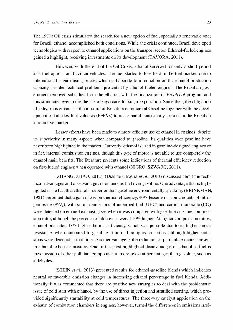
Almost all chemical reactions require time to the total set of reactions to completelyhappen. While the fact that some chemical compounds may react instantly, others may requireconsiderable time to begin. Chemical kinetics explains how a reaction develops with respect totime, consuming some species and forming others.
A review of chemical kinetics is presented from various references, including books,papers and other theses related to the subject. Concepts such as reaction rate, Arrhenius reactionrate constant, order of a reaction are presented below.
For a one-step stoichiometric chemical reaction, the reactants and the products arerepresented based on the mass reaction law, Eq. (2.1) (KUO, 2005):
N
∑i=1
ν′i Mi =
N
∑i=1
ν′′i Mi (2.1)
Where:
∙ ν′i and ν
′′i : Stoichiometric Coefficients of the ith chemical species, related to the reactants
and products, respectively;
∙ Mi: Specification of the molecule of the ith chemical species;
∙ N: Total number of chemical species on the model.
The rate of reaction of a specific chemical reaction is represented by Eq. (2.2):
RR =dCP
dt=
dCR
dt= k
N
∏i=1
Cν′i
i (2.2)

Chapter 2. Literature Review 27
Where:
∙ RR: Reaction Rate;
∙ k: The Rate Constant of the chemical reaction;
∙ CP and CR: Molar concentration of the products or reactants respectively (kmolm3 );
∙ Ci: Molar concentration of the ith chemical species (kmolm3 );
The specific reaction-rate constant for a given reaction is dependent only on thetemperature and in general is expressed by Equation (2.3):
k = AT b exp(−Ea
RuT) (2.3)
Where:
∙ A and b: Parameters related to the studied chemical reaction;
∙ T: Temperature of the chemical reaction (K);
∙ AT B: Collision Frequency;
∙ Ea: Activation Energy of the chemical reaction ( kJkmol );
∙ Ru: Universal Constant of the gases ( kJkmolK );
∙ exp(−EaRuT ): The Boltzmann Factor;
The activation energy Ea represents the energy required for the reaction to start.While the Boltzmann Factor indicates the fraction of collisions that have enough energy to begreater than the activation energy, Ea, A and b indicate of the nature of the elemental reac-tion. The existent chemical bonds from the molecules are represented mathematically by thesecoefficients and are obtained via experimental data.
When a chemical reaction happens under favorable conditions, the collisions lead tothe formation of a transitory chemical species, called the activated complex. This phenomenonhappens on the highest energy on the most favorable path (KUO, 2005).
2.3.2 THE ARRHENIUS LAW AND ORDER OF A REACTION
The equation that allows the calculation of the reaction rate constants of a reactionis the Arrhenius Law, which is described by Eq. (2.4):
k = Aexp−Ea
RuT(2.4)

Chapter 2. Literature Review 28
It is very similar to Equation (2.3), because the term A of this equation englobesthe collision frequency described earlier. This expression is very famous since it was the firstto indicate that the rate constant k is only dependent of the temperature. The intensity of therate constant indicates the tendency of the reaction (if a reaction yields more “products” or“reactants”).
The net rate of reaction of a chemical component on a chemical reaction is rep-resented by the balance between the reactant and product stoichiometric coefficients to thischemical component to react. The mathematical expression to this relationship is:
dCi
dt= (ν
′′i −ν
′i )RR = (ν
′′i −ν
′i )k f
N
∏i=1
Cν′i
i (2.5)
Where:
∙ k f : Forward Reaction Rate Constant;
Since a chemical species may appear in both sides of a chemical reaction, the differ-ence ν
′′i −ν
′i represents the net reaction of the ith chemical species (formation or consumption).
This multiplies the reaction rate to yield the rate of consumption or production of the chemicalspecies.
The reactions have orders which define their dependency of the concentration of thereactants with its reaction rate equation. The most common orders of elementary reactions arefirst, second and third-order.
One-step first order reactions are reactions that usually represent a rearrangement orthermal dissociation of a molecule (unimolecular reactions) (KUO, 2005). This type of reactionis normally described with a chemical reactant molecule colliding with other body. For example,the other body may be another molecule, a wall (which represents the boundaries of the system)or something else that absorb the energy that is released from the collision. If the collision isintense enough to reach the activated complex, the first molecule has its chemical bonds brokenand dissociates. This reaction only depends of the concentration of the reactant molecule, sincethe other molecule that collides with the dissociated one is considered a third-body molecule,i.e. it does not react, just absorbs the excess energy. First-order reactions may also representa bimolecular reaction. This situation happens when a concentration of a chemical reactant ismuch greater than the other reactant (it is in excess). This leads to the reaction to behave like afirst-order reaction.
Second-order reactions are the ones which describe the behavior of most reactions(KUO, 2005). A molecule representing the chemical species A collides with a molecule B,breaking their chemical bonds and generating other chemical species (C and D, for example).Generally, in a complex group of reactions, the second-order reaction is the slowest one, i.e.
Chapter 2. Literature Review 29
the rate-determining reaction. This reaction dictates the speed of the chemical activity of thesystem. A second-order reaction represents atom-transfer reactions.
Finally, third-order reactions represent recombination reactions. These reactionshappen when three molecules collide at the same time and recombine in one or two newmolecules. This type of reaction is more uncommon than the others. A three-molecule collisionhas less probability to happen, although it still happens. A backward reaction for a dissociationreaction is an example of a third-order reaction, because it combines two atoms through a col-lision of them with a third-body or wall. When the concentration of the third body is very highcompared to the other species, one can assume a steady-state system for this reaction. Since itsmolar concentration is steady, the recombination process is reduced from a third-order reactionto a second-order.
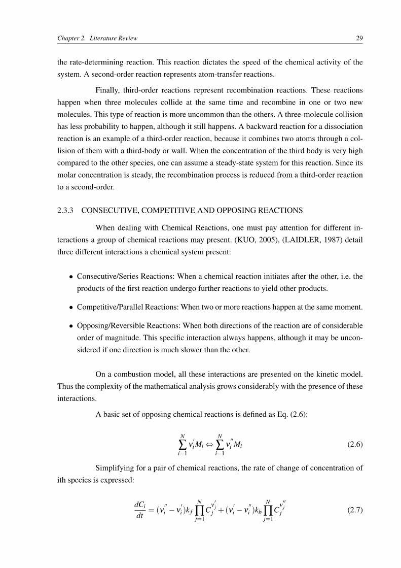
2.3.3 CONSECUTIVE, COMPETITIVE AND OPPOSING REACTIONS
When dealing with Chemical Reactions, one must pay attention for different in-teractions a group of chemical reactions may present. (KUO, 2005), (LAIDLER, 1987) detailthree different interactions a chemical system present:
∙ Consecutive/Series Reactions: When a chemical reaction initiates after the other, i.e. theproducts of the first reaction undergo further reactions to yield other products.
∙ Competitive/Parallel Reactions: When two or more reactions happen at the same moment.
∙ Opposing/Reversible Reactions: When both directions of the reaction are of considerableorder of magnitude. This specific interaction always happens, although it may be uncon-sidered if one direction is much slower than the other.
On a combustion model, all these interactions are presented on the kinetic model.Thus the complexity of the mathematical analysis grows considerably with the presence of theseinteractions.
A basic set of opposing chemical reactions is defined as Eq. (2.6):
N
∑i=1
ν′i Mi ⇔
N
∑i=1
ν′′i Mi (2.6)
Simplifying for a pair of chemical reactions, the rate of change of concentration ofith species is expressed:
dCi
dt= (ν
′′i −ν
′i )k f
N
∏j=1
Cν′j
j +(ν′i −ν
′′i )kb
N
∏j=1
Cν′′j
j (2.7)

Chapter 2. Literature Review 30
When the reaction achieves chemical equilibrium, then:
dCi
dt= 0 (2.8)
On this case, opposing reactions are related with chemical equilibrium and chemicalkinetics. The balance between the two directions of a rate reaction can be obtained with thechemical equilibrium constant. The forward and reverse reaction rate constants are related withthe chemical equilibrium constant for a generic reaction from Eq. (2.9):
k f
kb=
N
∏j=1
C(ν′′i −ν
′i )
j,e = Kc (2.9)
Where:
∙ k f and kb: Represent the forward and backward reaction rate constants of the studiedchemical reaction;
∙ C j,e: The molar concentration of the jth chemical species, in a chemical equilibrium state( kmol
m3 );
∙ Kc: The chemical equilibrium constant related to molar concentration.
Details about the relationship between chemical equilibrium and chemical kineticswill be further presented on the text.
2.3.4 CHAIN REACTIONS
Chain reactions are the most famous and common type of chemical reactions. It is aseries of consecutive, competitive and opposing reaction steps with different rate constant steps.(KUO, 2005).
All chain reactions yield intermediate products. These products yielded on the be-ginning of the reactions generate other reactive intermediate species. These new intermediateinitiate other reactions, generating the first group of intermediate species. This situation createsa loop of reactions, one feeding and accelerating another. Depending on the thermodynamicconditions and the chain reaction, it can generate explosions. A combustion reaction is a naturalexample of a chain reaction, which liberates great amounts of energy.
In chain reactions, the intermediate products have a specific name: free radicals.Free radicals are highly reactive atoms (such as H, O, N, F, Cl. . . ) or radical species (CH3, OH,CH, C2H5, etc.), that can be charged or uncharged, which act as an unit in chemical changes(KUO, 2005). They are the ones that allow most reactions to happen; if yielded without control,they are the ones that release the excess of energy in form of explosion.

Chapter 2. Literature Review 31
Elementary Reactions compose Chain reactions. They can be divided in four differ-ent types of reactions:
∙ Chain Initiating Reactions: the type of reaction that produces free radicals. It usuallyinitiates the chain reaction;
∙ Chain Propagating Reactions: It yields the same amount of free radicals as it consumes;
∙ Chain Branching Reactions: The ratio of production/destruction of free radicals is greaterthan one. They are the reactions which propagates the chain reaction;
∙ Chain Terminating Reactions: Destroys free radicals. Normally it ends the chemical pro-cess;
A chain reaction starts with an elementary reaction that requires less energy tohappen. For instance, this energy is the dissociation energy required to separate two atomsof a molecule. Next a series of chain propagating reactions start, propagating the intermediatespecies yielded in each reaction, which accelerate the chain reaction. Then, chain terminatingreactions started to prevail over the rest, reducing the number of free radicals. This is an indi-cation of the end of the chain reaction. After the concentration of the initial reactants reducesconsiderably, the chain reaction loses intensity and can be considered done.
2.3.5 RELATION BETWEEN CHEMICAL EQUILIBRIUM AND CHEMICAL KINETICS
Reaction rate laws are expressed in terms of the concentration of the reactants andthe rate reaction constants. The concentration is an indicator of both the influence of each chem-ical species in the rate law but also the influence of the pressure (in terms of number of molesinside the system), while the rate reaction constant is an indication of the temperature on thechemical system.
Reaction rate laws can also be expressed in terms of chemical equilibrium variables,such as the equilibrium constants. In Equation (2.9), there is a relation between the chemicalequilibrium constant and the forward and backward reaction rate constants. A first approach isutilize k f and kb to calculate the reaction rates for each chemical reaction. A second approachis to use k f and the chemical equilibrium constant for each chemical reaction to calculate thesame reaction rates.
(NEWHALL, 1969) used the first approach, by taking the reaction rate expres-sions from the literature and calculating the values separately. While other authors, based onNewhall’s work (Lavoie et al. (1970), Spadaccini e Chinitz (1972), Annand (1974), Heywood(1988)), used the second approach, based on the argument that chemical equilibrium constantsare more trustworthy than reaction rate constants, since it is based on thermodynamic equi-librium calculations. This implies on theoretical models well consistent with experimental re-

Chapter 2. Literature Review 32
sults. Even review papers commented the second approach (Bowman (1975), Miller e Bowman(1989)) as a more reliable model. Thus this second model is preferable since the reaction rateconstants have a certain degree of experimental uncertainty (1 a 3%, Warnatz (1984) and Baulchet al. (1994)). Its use restricts the mathematical models from predicting with more precision thechemical behavior. A general reaction rate law for a chemical species related to a chemicalreaction is presented:
dCi
dt= (ν
′′i −ν
′i )k f
N
∏j=1
Cν′i
j (1− 1Kc
N
∏j=1
Cν′′i −ν
′i
j ) (2.10)
It is most common to solve chemical equilibrium problems based on equilibriumconstants related to partial pressures of the chemical species involved in the chemical reaction.Expression (2.11) shows the dependency of Kp with partial pressures:
Kp =N
∏j=1
p j,e
po
ν′′i −ν
′i
(2.11)
Where:
∙ Kp: Chemical Equilibrium Constant related to partial pressures;
∙ p j,e: Partial pressure of the jth chemical species in chemical equilibrium (kPa);
∙ po: Atmospheric pressure (101.325 kPa);
Based on the ideal gas law and Dalton’s law, a relationship between Kp and Kc isdeveloped:
∙ Ideal gas law (for the system):pV = nT RuT (2.12)
∙ Ideal gas law (for the jth chemical species):
p jV = n jRuT (2.13)
Isolating the molar concentration for the jth chemical species on Eq. (2.13):
C j =n j
V=
p j
RuT(2.14)
The expression (2.14) can be both used for a generic case or specifically in chemicalequilibrium.
Chapter 2. Literature Review 33
Manipulating the expressions above, it is found:
k f
kb= Kc = Kp(
RuTpo )∆n (2.15)
Where:
∙ p: Total pressure of the system (kPa);
∙ V: Total volume of the system (m3);
∙ T: Temperature of the system (K);
∙ nT : Total number of moles of the system (kmol);
∙ Ru: Universal Constant of Gases Ru = 8.314( kJkmolK );
∙ pi: Partial pressure of the ith chemical species (kPa);
∙ ni: Number of moles of the ith chemical species (kmol);
∙ Ci: Molar concentration of the ith chemical species (kmolm3 );
∙ ∆n = ∑Ni=1(ν
′′i −ν
′i );
∙ N: Number of chemical species.
With Eq. (2.15) is possible to use chemical equilibrium to obtain the reverse reactionrate constant and calculate with more certainty the reaction rate laws for each chemical speciesof the system.
2.3.6 RECENT WORKS ON CHEMICAL KINETICS IN INTERNAL COMBUSTION EN-GINES
More recently, several works focus on integrating chemical kinetic models withdifferent models of ICEs, passing by quasi-dimensional, multizone or CFD models of cylin-der gases. (ELMQVIST et al., 2003) used chemical kinetics together with a one-dimensionalsimulation tool to predict knock occurrence in turbocharged SI engines.(TINAUT et al., 2013)developed a quasi-dimensional model for predicting pollutant formation in SI engines, couplingchemical kinetics and a multizone model. (YANG, 2013) modeled turbulent flame propagationcombustion process with direct interaction with a robust chemical kinetic model, obtaininggood agreement with experimental measurements. (LI et al., 2017) developed a complex CFDmodel with chemical kinetic considered in a internal combustion engine simulation, with a post-processing tool capable of calculating rates of production of specific desired species in specificpositions of the cylinder.

Chapter 2. Literature Review 34
Some national references related to expanded chemical kinetics in engines are (SAN-TOS, 2011) and (RINCON, 2009). The first developed an engine simulator by considering it areactor in a zero-dimensional thermodynamic model. This model was developed in order tosimulate later on rocket engines, turbines, etc. The latter developed some detailed chemical ki-netic models for ethanol and other multicomponent mixtures of fuel substitutes for gasoline.The analysis involved a detailed study of the sub mechanisms in the ethanol chain reaction andcompared with the software SHOCK 1-D in order to validate the developed models.
2.4 NO-FORMATION FUNDAMENTALS
The nitrogen oxides group are one of the most harmful pollutant gases group emit-ted by an internal combustion engine during its operation. It is compounded by 7 differentchemical species, which each one has specific characteristics, as described below (PATTER-SON; HENEIN, 1974):
∙ NO - Nitric Oxide: Stable, product of combustion at high temperatures; Reactant withO2, forming NO;
∙ N2O4 – Nitrogen Tetroxide: Related with NO2 from the reaction N2O4 ⇔ 2NO2;
∙ NO2 – Nitrogen Dioxide: Stable at 423K; it can appear in a mixture with N2O4;
∙ N2O – Nitrous Oxide: Relatively stable. Always present in the atmosphere at concentra-tions of 0.5 ppm;
∙ N2O3 – Dinitrogen Trioxide: It can react with water, forming HNO2 (Nitrous Acid);
∙ N2O5 – Dinitrogen Pentoxide: Unstable; It can react with water, forming HNO3 (NitricAcid);
From this group, the most important ones for this study will be NO, NO2 and N2O,which are the most stable. In case of combustion emission purposes, NO is by far the mostimportant. This group of chemical species are usually called NOx, in which most of the group’scomposition is NO and NO2 (PATTERSON; HENEIN, 1974).
NO is formed especially during the combustion and it is known for the known char-acteristic: the higher the temperature present in the combustion chamber, the greater will bethe NOx-species produced. This happens because of the high dependence of the reactions re-lated to NO-formation with the temperature of the system. The rate constants, which dictatethe directions of the reactions (production or consumption of a chemical species), start to be-come important usually over temperatures higher than 1800K (KUO, 2005). This lower limit isreached during the initial phase of the combustion process, shortly after its beginning.

Chapter 2. Literature Review 35
2.4.1 NOx-FORMATION MECHANISMS
NO-formation may also be described by a global reaction which tries to representin a mathematical way what happens in the atomic level. Most of the global reactions justrepresent the reactants and the products of the respective reaction, without describing how thereaction happens. For example, questions about the reaction time or the real proportion betweenreactants and products by the end of the reaction are not answered properly by global reactions.By studying the details of a reaction, the presence of intermediate species may be evaluatedcoherently, therefore their influence on the reaction system may be measured.
The importance of studying the formation of nitrogen oxides (NOx) is justified bythe fact they are one of the principal contaminants emitted by combustion processes. Addi-tionally, another reason rises from the fact that energetic materials, such as explosives, alwayscontain traces of nitrogen on its compounds (KUO, 2005).
NO-formation occurs due to a group of reactions that describes the collisions thatmay happen on atomic level. These reactions are called elementary reactions. The NO is formedduring the combustion process as the result of elementary reactions which involve nitrogen gas,N2, which is present in the air used for the combustion process, and oxygen gas, O2 that it is amandatory species for combustion/oxidation processes (PATTERSON; HENEIN, 1974).
The group of elementary reactions which tries to describe what happens in atomiclevel is called the Reaction Mechanism. (TURNS, 2000) prefers to define reaction mechanismas: “The collection of elementary reactions that describe an overall reaction”. A mechanismtries to predict the behavior of a reaction by adding or removing elementary reactions of itsgroup. The results of a specific mechanism are usually compared with experimental results ofthese reactions. Its goal is to achieve very close results, which can implicate that the modelrepresents coherently the real atomic chemistry that happens.
Since the beginning of NOx studies, scientists were able to identify some paths forNO formation, called NO routes. These routes can predict the formation of NO under certaincircumstances. Here it will be described five routes, which describes both NO, NO2 and N2O
formation (KUO, 2005).
2.4.1.1 Thermal NO Route
The initial models adopted to predict NO formation simply considered the globalreaction between N2 and O2, which yields NO. After this point, many studies were undertakenin order to refine the predictions of NO formation, specially related to temperature. Tempera-ture is directly related to Zeldovich chain reaction mechanism that will be detailed later. (PAT-TERSON; HENEIN, 1974) presented some traditional mechanisms related to NO-formation, inorder to achieve a better understanding of this pollutant production. Some of these models arecommented next.

Chapter 2. Literature Review 36
2.4.1.2 Global Reaction Mechanism
This mechanism (EYZAT; GUIBET, 1968) describes that exactly one Nitrogen andone Oxygen molecule collide with each other, breaking all connections between the atoms ofeach molecule, yielding 2 molecules of NO. It is not very realistic, since it is very improbablethat such collision happens and produces this exact result. Because of this unrealistic assump-tion, It produces very low NO-concentrations, when compared with the real NO-formation,obtained by measurements. It can be described by the following reaction:
N2 +O2 ⇔ 2NO (2.16)
2.4.1.3 Zeldovich Chain Reaction Mechanism
The Zeldovich mechanism is very used on ICE studies, since this mechanism con-nects the NO formation with NO high temperature dependency. Besides, it was one of thefirst mechanisms presented for the NO formation. This mechanism occurs significantly in tem-peratures above 1800K, since the rate constants of its reactions depend considerably on hightemperatures. Differently of other routes, this one does not depend on nitrogen-composed fuels;instead, it depends on the presence of oxygen and nitrogen molecules (O2 and N2) on the chem-ical system. NO mechanism is still discussed on the literature. (ZEL’DOVICH et al., 1947)firstly unveil this mechanism and it turned to be a reference until current times.
This mechanism affirms that initially some Oxygen molecules dissociates, due tocollisions with another molecules. This reaction is only considerable in high temperatures(above 1800K), which increases the probability of a O2 collision with another molecule orwith a wall with enough energy to develop the activated complex. These collision-moleculesonly absorbs the energy related with the chemical bounds that existed in oxygen gas; they donot participate directly on the elementary reaction. Considering that this M-molecule just assiststhe dissociation, therefore this molecule does not react. This behavior was commented earlieron this text and the particle is called the third-body molecule. This behavior is probabilisticallyassociated with the molecule with the greatest molar concentration on the system, which is anindication of the pressure of the system. Generally combustion problems on ICEs consider thethird-body molecule as the nitrogen Gas (N2), since its molar fraction is considerably higherthan the other gases (on the air or on the exhaust gases).
In the case of N2, they almost do not have their chemical bonds broken at thistemperature, since the activation energy required for the triple bond of N2 is higher than theenergy required for the double bond of O2.
After the O2-dissociation has begun, the O-atoms start to collide with Nitrogenmolecules, generating a second reaction. This reaction yields nitrogen atoms (N) and nitrogenoxides (NO). Then it starts a third reaction, where N-atoms collide with O2, producing NO andO-atoms. Therefore, both of these chemical reactions produce NO and some free radicals (O

Chapter 2. Literature Review 37
and N), which feed other reactions, thereby forming a chain-reaction system.
The reactions that produce NO require some time to occur significantly. Then theZeldovich mechanism is considered to happen only in the gases left behind the flame frontcreated by the combustion process (FERGUSON; KIRKPATRICK, 2001). Therefore most ofthe NO emitted by engines is produced after the passage of the flame front. A small part is fromthe prompt-NO mechanism, which happens in the flame front and will be commented in thenext section.
This model produces results closer to experimental results than the global reactiondescribed earlier. The chain nature of the classic Zeldovich mechanism is presented below, fromEquation (2.17), that yields the previous global result Eq. (2.16):
O2 +M ⇔ 2O+M
O+N2 ⇔ NO+N
N +O2 ⇔ NO+O
(2.17)
2.4.1.4 Extended Zeldovich Chain Reaction Mechanism
This mechanism is an extension of the traditional Zeldovich mechanism, consider-ing the influence of OH radical in chemical kinetics. Some simplified models (Heywood (1988)and Ferguson e Kirkpatrick (2001)) are commonly used as a refined prediction of NO forma-tion. These models consider the set of equations (2.17) and (2.18), as long as other assumptions,which reduces drastically the computing time, in charge of only NO formation prediction.
{N +OH ⇔ NO+H (2.18)
2.4.1.5 Lavoie Thermal-NO Mechanism
Proposed by Lavoie (LAVOIE et al., 1970), this mechanism extends the reactionsrelated to the traditional Zeldovich Chain reaction by adding a NO-formation reaction related toan hydroxyl (OH) radical. It also considers reactions involving N2O. The last reaction involvestwo molecules of NO, which is slower on their reverse processes. Therefore the NO does nottend to be consumed considerably during the expansion process of a SI engine because of N2O
reactions. This justifies why there is almost no reduction on NO concentration values.
The Equation (2.19), together with the ones presented on the mentioned Zeldovichmodel ((2.17), (2.18)), define the reactions related with this model:
H +N2O ⇔ N2 +OH
O+N2O ⇔ N2 +O2
O+N2O ⇔ 2NO
(2.19)

Chapter 2. Literature Review 38
2.4.1.6 Annand NO-Formation Mechanism
This mechanism was proposed by (ANNAND, 1974), based on the similar modeldescribed in (NEWHALL, 1969). It amplifies the number of reactions used in the model, con-sidering H2O, H2, O2 and N2 dissociations, reactions involving hydroxyl radical (OH) and onereaction involving CO and CO2. This latter reaction also allows the model to predict CO for-mation. This model considers 13 chemical species in 16 reactions (16 forward and 16 reverse)and it is one of the most complete reduced mechanisms, which can represent very well whathappens on the reaction system.
Besides the reactions described on previous mechanisms, this mechanism considersthe following equations:
N2O+M ⇔ N2 +O+M
H2 +O ⇔ OH +H
OH +O ⇔ O2 +H
OH +H2 ⇔ H2O+H
OH +OH ⇔ H2O+O
H2O+M ⇔ OH +H +M
H2 +M ⇔ 2H +M
N2 +M ⇔ 2N +M
CO+OH ⇔CO2 +H
(2.20)
2.4.1.7 Spadaccini NO Mechanism
(SPADACCINI; CHINITZ, 1972) compared his chemical model with Newhall’smodel for a SI engine and obtained some differences related to NO and CO formation. Heaffirmed that the required time for the Runge-Kutta Procedure adopted by Newhall was con-siderably expensive and this fact would prohibit the application of his model. He also madecomparisons with experimental data and obtained coherent results with respect to the pollu-tant emissions (NO and CO) and free radicals (H, OH). Spadaccini’s model was one of thefirst models to consider Chemical Equilibrium Constants to obtain one of the rate constantsof each reaction, instead of using both forward and backward reaction rate constants, obtainedexperimentally. This led the results to be quite different from Newhall’s model. The initial con-ditions presented in Spadaccini’s model were the same as Newhall’s. The same is valid for thereactions, except for the rate constants used.
2.4.1.8 Other models presented by literature
Other mechanisms presented on the literature are simpler than the ones presentedhere, since they consider lesser reactions. For example, (HEYWOOD, 1988) presented a simplemodel with 3 reactions (3 direct and 3 reverse) with O2-dissociation, which could predict NO
Chapter 2. Literature Review 39
formation during a spark ignition engine operation. This model also made some assumptionsrelated to steady-state conditions for N-atoms and that O, O2, OH, H and N2 are in equilib-rium values for each pressure and temperature during the combustion and expansion processes.These assumptions allows the calculations of the NO-formation rate with one equation. Equa-tion (2.21) shows this rate equation ( mol
cm3.s):
d[NO]
dt=
6E16
T12
exp(−69090
T)[O2]
12eq[N2]eq (2.21)
The NO characteristic time, which is the time required for a reaction or a set of reac-tions to yield 1
e of the equilibrium concentration of a certain chemical species, can be describedas Eq. (2.22):
τ−1NO =
1[NO]e
d[NO]
dt(2.22)
(HEYWOOD, 1988) indicates that NO characteristic times are of the same order astypical combustion times (≈ 1 ms). This model is only valid under conditions found in engines.
(FERGUSON; KIRKPATRICK, 2001) utilizes the NO formation model describedby Bowman (MILLER; BOWMAN, 1989) as another simplistic model to obtain the rates offormation of NO in engines. The model considers the extended Zeldovich mechanism in sparkignition engines. This follows the same methodology described in Heywood (HEYWOOD,1988).
(BOWMAN, 1975), (MILLER; BOWMAN, 1989) also commented the applicationof extended Zeldovich mechanism to predict NO formation.
(WAY, 1976) developed other model, based on others from literature (Newhall(1969), Spadaccini e Chinitz (1972), Lavoie et al. (1970)), where chemical kinetics work quiteclose to chemical equilibrium in the same computer program. Benson (BENSON et al., 1975)presented a chemical model based on Lavoie, with the addition of one more reaction involvingN2O in his NO mechanism.
(MILLER et al., 1998) presented a super extension of NO-formation mechanism,considering 67 reactions (direct and reverse) and 13 chemical species (O, O2, OH, H, N2, N,NH, NH2, NH3, HNO, N2O, NO2 and NO) involved in the reaction kinetics, while the rest isconsidered to be in chemical equilibrium. The goal was to refine the prediction of NOx forma-tion. The work describes the Super-Extended Zeldovich Mechanism (SEZM) as a better wayof prediction of NO formation in engines, with results more coherently with experimental mea-surements.
Some recent papers from the literature have also discussed about NO-formationmechanism. (SODRÉ, 2000) have developed a rapid model to Spark-ignition Engines. He con-sidered Heywood’s model (HEYWOOD, 1988) and compared his results with experimental

Chapter 2. Literature Review 40
ones. On his model he also considers that the kinetic concentrations of oxides of nitrogen wereevaluated based on the chemical species equilibrium concentrations.
There are also some national references that dealt with chemical kinetic models inengines. (RAGGI, 2005) presented a model based on other model from (SODRÉ, 1995), con-sidering a 3-reaction NO mechanism, with similar assumptions. These three reactions were theExtended Zeldovich model. His work also considered CO-formation, with two more reactionsto predict CO/CO2 formation. (NETO, 2012) developed a coupled chemical equilibrium andchemical kinetic analysis model to calculate the reaction mechanism of 22 chemical species ininternal combustion engines, considering the Zel’dovich and Fenimore NOx mechanisms, be-sides CO kinetics and the crevice UHC model. Additionally it was compared the simulationpollutant results with AVL BOOST for the same engine.
2.4.1.9 Prompt-NO Route
Some authors commented that thermal-NO route is the most significant NO forma-tion mechanism in spark-ignition engines (FERGUSON; KIRKPATRICK, 2001), (LAVOIE;BLUMBERG, 1980). (PATTERSON; HENEIN, 1974), (TURNS, 2000) and (KUO, 2005) havealso mentioned that there is a small amount of emitted NO that is promptly produced in theflame front of the combustion process. This specific phenomenon, that is known as prompt-NOmechanism, has also kinetic models developed. (FENIMORE, 1971) described the mechanismin the following way: Yielded HC radicals during the initial moments of combustion collidewith Nitrogen Molecules, forming amines or cyano compounds. Then these amines or cyanocompounds would become intermediate species that generate NO. The reaction below (Eq.(2.23)) summarize the idea of this mechanism:
HCradicals +N2 ⇒ Amines or cyano compounds ⇒ NO (2.23)
This mechanism occurs in rich-mixtures, with a mechanism well known. But whenthe equivalence ratio φ is higher than 1.2, the chemistry just becomes very complex and itcomplicates too much to a simple reaction mechanism be able to describe it (Miller e Bowman(1989), Turns (2000)).
Since the volume of the flame front is much smaller than the volume of the burnedgases, therefore prompt-NO mechanism is not much used in studies involving combustion inengines, out of the rich-mixture range and will not be considered in this project.
2.4.1.10 Fuel-Bound Nitrogen (FN) route
Since ethanol (C2H6O) has no nitrogen in its composition, Fuel-bound Nitrogenroute is not considered in this work. However, in fossil fuels (coal and coal-derived fuels) thisnitrogen becomes the primary source of nitrogen oxides formed on their combustion (KUO,

Chapter 2. Literature Review 41
2005). The literature indicates that there is a rapid conversion of fuel nitrogen compounds tohydrogen cyanide (HCN) and Ammonia (NH3). This generates chain reactions which generateNO (MILLER; BOWMAN, 1989).
2.4.1.11 NO2 route
NO2 route is very considerable in Diesel Engines (TURNS, 2000). NO2 can havesignificant concentration in certain combustion conditions, usually near the flame zone. Its for-mation depends on the presence of significant HO2 concentrations and NO concentration, whichwas formed in high-temperature conditions. This NO concentration is transported by diffusionto the low-temperature regions, where this reaction starts (KUO, 2005).
2.4.1.12 N2O route
N2O route is usually considered in fuel-lean conditions (KUO, 2005). This speciesusually has a short-life period and it is formed in reactions involving NO and other nitrogen-containing radicals. The conditions required for its formation are low temperature, in premixedzones. These conditions usually are found in the exhaust process of an engine (TURNS, 2000).
2.4.2 NO FORMATION IN FLAMES
Despite of NO formation having a direct connection with high temperatures, spe-cially the peak gas temperature generated by the combustion, it requires time for the reactionsto happen. It is not formed instantaneously by the flames developed by combustion, though NOis produced by post flame combustion products. (PATTERSON; HENEIN, 1974) commentedthe relation between NO formation with time, after the flame passes through certain controlledpoints in a high pressure combustion vessel.
For rich mixtures, NO is formed in post flames faster than it happens in lean or sto-ichiometric mixtures, due to the higher flame speed presented in rich mixture situations. Thiscreates higher temperature and pressure in the combustion chamber. Nevertheless, the equilib-rium is also reached faster, besides NO concentration in the end of rich mixture combustionsituation is lower than it happens in lean mixture combustion. For lean mixtures, it is the oppo-site: NO is formed slower, but the equilibrium takes more time and its concentration at the endof the process is higher.
The following figures show the experimental results obtained for the situation de-scribed above (NEWHALL; SHAHED, 1971). Figure 2.2 describes the situation for lean andstoichiometric mixtures, while the Figure 2.3 shows for rich-mixtures:

Chapter 2. Literature Review 42
Fig. 2.2 – NO formation (molescm3 ) x time (s) on Lean-stoichiometric mixtures. Ref.: (NEWHALL;
SHAHED, 1971)
Fig. 2.3 – NO formation (molescm3 ) x time (s) on rich-mixtures. Ref.: (NEWHALL; SHAHED,
1971)
Chapter 2. Literature Review 43
2.4.3 EFFECT OF DESIGN AND OPERATING VARIABLES ON NOx EMISSIONS
Some engine variables affect the exhaust gas emissions in ICEs. These variables,which are divided in Design or Operation variables, can minimize or maximize the formation ofcertain pollutants during and after the combustion process inside an ICE. An adequate mixtureof fuel and air, for example, assists the engine to have a homogenous combustion inside thecombustion chamber, which reduces the UHC emissions from the exhaust.
These variables can also affect the NOx emissions, what evidences the need to un-derstand these effects. Most of the factors include (PATTERSON; HENEIN, 1974):
∙ Air-Fuel Ratio (A/F);
∙ Power/Load level;
∙ Speed;
∙ Spark Timing;
∙ Exhaust back pressure;
∙ Valve overlap;
∙ Intake Manifold Pressure;
∙ Combustion chamber deposit build-up;
∙ Surface temperature;
∙ Surface to volume ratio (S/V);
∙ Combustion chamber design;
∙ Stroke to Bore ratio;
∙ Displacement per cylinder;
∙ Compression Ratio.
Once formed, NO is not consumed after the combustion. The temperatures startedto reduce because of the expansion process and the reverse reaction rates are very low, whichleads to a very slow process of NO reduction. Since inside an ICE the expansion and exhaustprocess are faster than the NO reduction process, there is not enough time to the reductionactuates, therefore NO is emitted in concentrations very close to those present during the finalmoments of combustion and initial moments of expansion process.
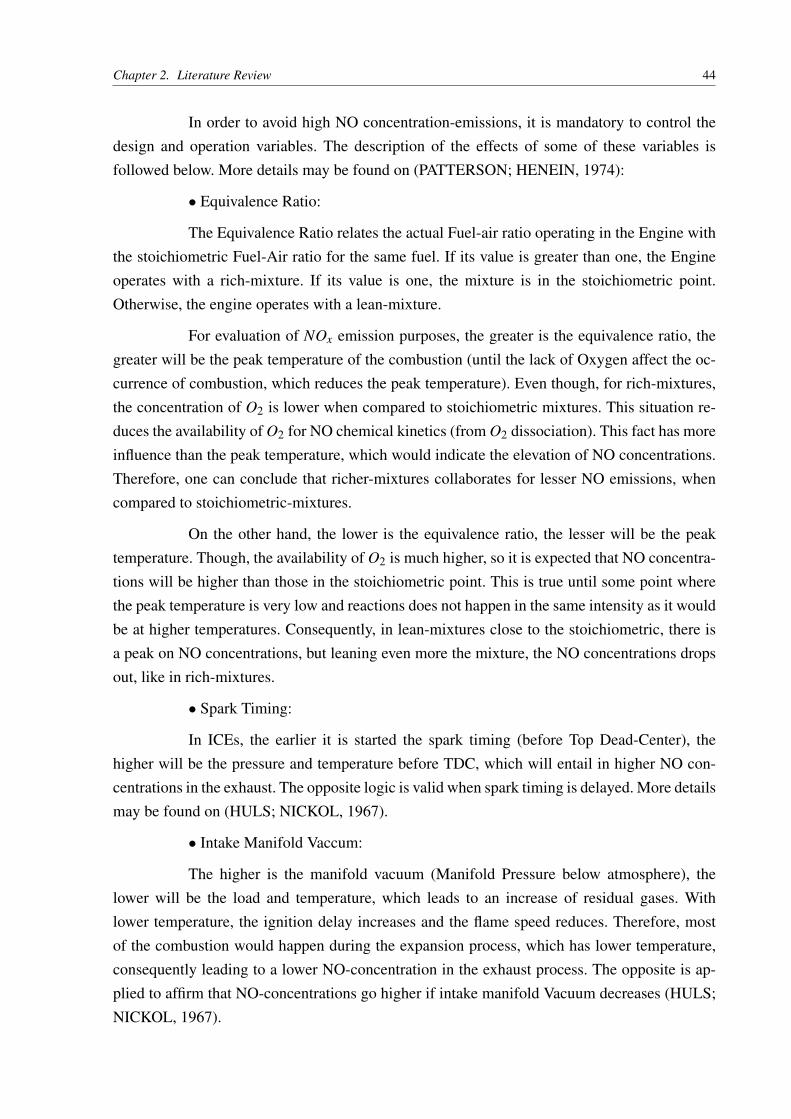
Chapter 2. Literature Review 44
In order to avoid high NO concentration-emissions, it is mandatory to control thedesign and operation variables. The description of the effects of some of these variables isfollowed below. More details may be found on (PATTERSON; HENEIN, 1974):
∙ Equivalence Ratio:
The Equivalence Ratio relates the actual Fuel-air ratio operating in the Engine withthe stoichiometric Fuel-Air ratio for the same fuel. If its value is greater than one, the Engineoperates with a rich-mixture. If its value is one, the mixture is in the stoichiometric point.Otherwise, the engine operates with a lean-mixture.
For evaluation of NOx emission purposes, the greater is the equivalence ratio, thegreater will be the peak temperature of the combustion (until the lack of Oxygen affect the oc-currence of combustion, which reduces the peak temperature). Even though, for rich-mixtures,the concentration of O2 is lower when compared to stoichiometric mixtures. This situation re-duces the availability of O2 for NO chemical kinetics (from O2 dissociation). This fact has moreinfluence than the peak temperature, which would indicate the elevation of NO concentrations.Therefore, one can conclude that richer-mixtures collaborates for lesser NO emissions, whencompared to stoichiometric-mixtures.
On the other hand, the lower is the equivalence ratio, the lesser will be the peaktemperature. Though, the availability of O2 is much higher, so it is expected that NO concentra-tions will be higher than those in the stoichiometric point. This is true until some point wherethe peak temperature is very low and reactions does not happen in the same intensity as it wouldbe at higher temperatures. Consequently, in lean-mixtures close to the stoichiometric, there isa peak on NO concentrations, but leaning even more the mixture, the NO concentrations dropsout, like in rich-mixtures.
∙ Spark Timing:
In ICEs, the earlier it is started the spark timing (before Top Dead-Center), thehigher will be the pressure and temperature before TDC, which will entail in higher NO con-centrations in the exhaust. The opposite logic is valid when spark timing is delayed. More detailsmay be found on (HULS; NICKOL, 1967).
∙ Intake Manifold Vaccum:
The higher is the manifold vacuum (Manifold Pressure below atmosphere), thelower will be the load and temperature, which leads to an increase of residual gases. Withlower temperature, the ignition delay increases and the flame speed reduces. Therefore, mostof the combustion would happen during the expansion process, which has lower temperature,consequently leading to a lower NO-concentration in the exhaust process. The opposite is ap-plied to affirm that NO-concentrations go higher if intake manifold Vacuum decreases (HULS;NICKOL, 1967).

Chapter 2. Literature Review 45
∙ Engine Speed (RPM):
An increase in the engine speed increases the flame speed, due to the higher turbu-lence caused by the increase in speed inside the combustion chamber. This reduces heat lossesper cycle. This factor tends to raise the compression, which leads to higher pressure and temper-ature, which one would expect to elevate NO-concentration. However, with higher speed, thecombustion tends to have a bigger portion of its duration in the expansion process, which leadsto a lower peak temperature that would reduce NO formation. Therefore for richer-mixtures,the heat-loss effect at higher speeds predominates, elevating the rate of NO formation, whilewhen for leaner-mixtures, the late burning effect in higher speeds predominates, decreasing therate of NO formation (NEBEL; JACKSON, 1958).
∙ Coolant Temperature:
The higher is the coolant temperature, more reduced are the engine heat losses.This effect causes higher peak gas temperature, which leads to a higher NO formation. If thereis enough deposit build-up on the cylinder, the deposit thickness collaborates to an increase incompression ratio, in addition to a reduction of heat loss. Both of these effects causes higherNO-concentrations (HULS; NICKOL, 1967).
∙ Humidity:
Higher humidity in mixture composition produces a reduction on the maximum gastemperature in the combustion chamber. NO formation is directly related to the high tempera-tures produced by the combustion process. Therefore, it can be concluded that higher humiditycauses a heavy reduction on the NO formation.
∙ Exhaust Gas Recirculation (EGR)
The increase of EGR in the inlet charge of the combustion chamber causes dilutionof the mixture fuel + air before combustion. This increase reduces the flame speed and thepeak gas temperature, which both are directly related to NO formation. Therefore, addition ofexhaust gases to the inlet charge lead to a reduction of NO formation.

Chapter 2. Literature Review 46
2.5 CO-FORMATION FUNDAMENTALS
Carbon monoxide (CO) is a known pollutant produced by combustion processes.The main sources of CO are showed on the table below (KUO, 2005):
Table 2.1 – Main Sources of CO emission. Ref: (KUO, 2005)
CO Main Sources of EmissionTraffic-related Issues 22%
Domestic Heating 21%Combustion of Biomass 18%
Anthropogenic Oxidation 15%Industry Exhaust 14%
Vegetation 4%Others 6%Total 100%
CO is an intermediate product of combustion and is usually associated with rich-mixture combustion processes (φ > 1). (PATTERSON; HENEIN, 1974) indicates that there is a3% of CO mass fraction reduction when the Air-Fuel Ratio is increased in 1%.
In cases with stoichiometric and lean-mixtures in spark ignition engines, a com-bination between the phenomenon of cycle to cycle and/or cylinder to cylinder fuel irregulardistributions and the slow CO reaction kinetics is the cause of high CO emissions (PATTER-SON; HENEIN, 1974). Better fuel distribution as well as leaner fuel-air mixtures assist on thereduction of CO-emissions by spark-ignition engines.
(NEWHALL, 1969) commented that carbon monoxide presents similar behavior asnitric oxide when it comes to molar concentration in exhaust processes in SI engines. Althoughthe temperature is at order of 1000K, the measured values found on these conditions are moreclose to values found in chemical equilibrium temperature peak conditions (≈ 2300K) thanit is found on equilibrium conditions at exhaust temperatures. This indicates that at a certainmoment during expansion process, the amount of CO and NO freeze and therefore, stays inhigher concentrations than it would be expected at exhaust conditions.
(TURNS, 2000) indicates that CO oxidation is related to hydrocarbon combustion.This process can be divided in a two-step process: the first process is the breakdown of hydro-carbon molecules (fuel) to carbon monoxide (CO), while the second is the oxidation of carbonmonoxide in carbon dioxide (CO2). Carbon monoxide is very slow to oxidize, except whenthere is a hydrogen-containing species (H2O or H2) in the chemical system, which provideshydrogen-atoms for the system and therefore accelerates CO-related reactions.

Chapter 2. Literature Review 47
2.5.1 CO-FORMATION MECHANISM
Detailed kinetics of CO formation are not totally understood until current days.Therefore, several models are still developed, in order to replicate the atomic behavior of thischemical species reaction mechanism.
(YETTER et al., 1991) presented a comprehensive kinetic model for CO-formation,which involves high-temperature and low-temperature cases. Yetter’s paper details how func-tions the main pathway to the reaction process and CO-formation and consumption.
(TURNS, 2000) presents in his book two more simplistic models, where it is consid-ered a model for H2O as the primary hydrogen-containing species and another model that usedH2 instead. The H-containing species influences considerably the CO/CO2 balance. Newhall(NEWHALL, 1969) comments about the CO/CO2 balance in SI engines and how it is influ-enced by free radicals concentration, such as OH and H.
(HEYWOOD, 1988) and (MILLER; BOWMAN, 1989) indicate that CO formationis related to combustion of the fuel, i.e. the hydrocarbon combustion mechanism. This mecha-nism is summarized by Eq. (2.24):
RH ⇒ R ⇒ RO2 ⇒ RCHO ⇒ RCO ⇒CO (2.24)
Where R represents a hydrocarbon radical. Other literature sources (KUO, 2005)provides more details about the complex CO mechanism, with some reactions involving methylradical:
CH3 +O2 ⇔ HCO+H2O (2.25)
HCO+OH ⇔CO+H2O (2.26)
Thus CO reacts to yield CO2, but in a slower rate than the hydrocarbon combustionreactions. The main reaction that describes CO/CO2 formation in normal combustion tempera-tures is presented:
CO+OH ⇔CO2 +H (2.27)
Hydrogen-containing reactions may be also added to the mechanism. Since they arerate-limiting reactions, each one of them are usually considered on extended CO mechanisms:
2H +M ⇔ H2 +M
H +OH +M ⇔ H2O+M
H +O2 +M ⇔ HO2 +M
(2.28)

Chapter 2. Literature Review 48
(TURNS, 2000) presented a four-reaction CO mechanism, with the addition of an-other CO/CO2 reaction:
CO+O2 ⇔CO2 +O
O+H2O ⇔ OH +OH
CO+OH ⇔CO2 +H
H +O2 ⇔ OH +O
(2.29)
2.5.2 EFFECT OF DESIGN AND OPERATING VARIABLES ON CO-FORMATION
Carbon Monoxide formation is also influenced by the design and operating variablesof Spark-Ignited Engines. Such as NO case, by comparing this gas formation with the samevariables used on the NO case, it is possible to predict qualitatively its change. The influenceof some design and operating variables in CO-formation in spark-ignited Engines is describedbelow (more details on (PATTERSON; HENEIN, 1974)):
∙ Air/Fuel Ratio:
As already mentioned, CO is very dependent of Air/Fuel Ratio. In rich mixtures,CO is formed considerably, which indicates a high CO concentration. On the other hand, COconcentration on exhaust is lower on stoichiometric and lean mixtures. The low concentrationof CO in lean mixtures is due to its slow kinetics in combustion conditions (CO ⇒ CO2) andfuel irregular distribution.
∙ Power/Load Level:
There is a direct influence of load level on CO-formation by engines. Since whenthe load level raises the amount of mixture (mass of fuel + air) that it is added to the combustionchamber also raises, then mass CO-emission is higher while the CO-formation speed ratio staysthe same.
∙ Engine Speed (RPM):
CO does not suffer much influence from the engine speed. This happens becauseCO-mechanism is more limited kinetically than it is mixing limited in normal combustion tem-peratures.
∙ Spark Timing:
There is a small relation between the ignition-delay time and CO-formation in En-gines. For instance, if there is a delay in the ignition time during a cycle of a Spark-IgnitedEngine, the exhaust temperature raises, with collaborates with the propagation of more chemi-cal reactions on the exhaust process.
The anticipation or delay of the ignition time does not influence significantly CarbonMonoxide qualitative formation, except in very high ignition delay cases. When the ignition

Chapter 2. Literature Review 49
starts very late in the engine’s cycle, there will be less time to the chemical reactions to happen,therefore CO does not have enough time to convert into CO2. Thus this fact indicates a higherconcentration of CO in the exhaust gases.
In quantitative terms, the ignition delay elevates CO emission, since it is requiredmore air flow in the cylinder, in order to maintain the power level constant (experimental condi-tions). This factor counterbalances the higher exhaust temperature influence. Therefore, the COformation rate is not influenced in a considerable way when related to spark timing.
∙ Exhaust back Pressure:
Exhaust Back Pressure does not have much influence in CO-formation. However,if the back pressure raises considerably until a point where the dilution of the fuel-air mixturewith residual gases becomes high enough, an incomplete combustion may happen. Thus therewill be a high quantity of UHC and CO yielded from the incomplete combustion, thereforeelevating the CO-formation.
∙ Valve Overlap:
This variable interferes the same way as Exhaust Back Pressure. If the duration an-gle where both admission and exhaust valves are opened is considerably high, then the dilutionwill be high enough to complicate the combustion, implying in high CO and UHC concentra-tions.
∙ Combustion Chamber Deposit Buildup:
When controlled, the deposit of UHC can cause delayed combustion processes. Thiswould release more UHC and CO from the deposits to the exhaust process, then implicating inan increase of its emission concentrations. However if removed the deposit buildup does notinterfere in CO-concentrations.
∙ Wall temperature:
This factor has influence in the thickness of the combustion chamber quench layer,besides the degree of after-reaction. Since it interferes in chemical reactions, then it can beconcluded that surface temperature assists the increase of CO-formation.
∙ Surface to Volume Ratio (S/V):
Generally the objective of an ICE is to minimize the surface area of the combustionchamber, in order to have the minimum mass on the combustion chamber quench layer. Theminimization would reduce the quantity of mass of UHC and CO released from these regions,although it does not interfere in CO-concentration inside the engine. The surface minimizationwould just reduce the total quantity emitted by the motor.
∙ Compression Ratio:
The lower the compression ratio, lower is the thermal efficiency. This affirmation
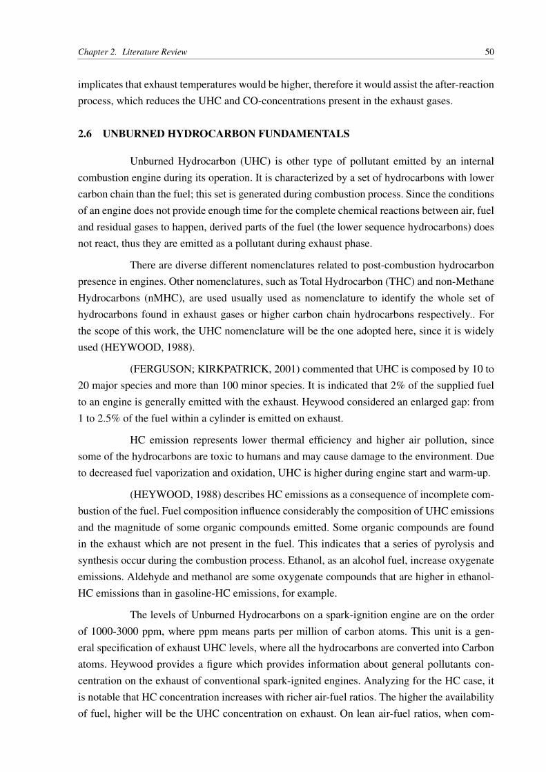
Chapter 2. Literature Review 50
implicates that exhaust temperatures would be higher, therefore it would assist the after-reactionprocess, which reduces the UHC and CO-concentrations present in the exhaust gases.
2.6 UNBURNED HYDROCARBON FUNDAMENTALS
Unburned Hydrocarbon (UHC) is other type of pollutant emitted by an internalcombustion engine during its operation. It is characterized by a set of hydrocarbons with lowercarbon chain than the fuel; this set is generated during combustion process. Since the conditionsof an engine does not provide enough time for the complete chemical reactions between air, fueland residual gases to happen, derived parts of the fuel (the lower sequence hydrocarbons) doesnot react, thus they are emitted as a pollutant during exhaust phase.
There are diverse different nomenclatures related to post-combustion hydrocarbonpresence in engines. Other nomenclatures, such as Total Hydrocarbon (THC) and non-MethaneHydrocarbons (nMHC), are used usually used as nomenclature to identify the whole set ofhydrocarbons found in exhaust gases or higher carbon chain hydrocarbons respectively.. Forthe scope of this work, the UHC nomenclature will be the one adopted here, since it is widelyused (HEYWOOD, 1988).
(FERGUSON; KIRKPATRICK, 2001) commented that UHC is composed by 10 to20 major species and more than 100 minor species. It is indicated that 2% of the supplied fuelto an engine is generally emitted with the exhaust. Heywood considered an enlarged gap: from1 to 2.5% of the fuel within a cylinder is emitted on exhaust.
HC emission represents lower thermal efficiency and higher air pollution, sincesome of the hydrocarbons are toxic to humans and may cause damage to the environment. Dueto decreased fuel vaporization and oxidation, UHC is higher during engine start and warm-up.
(HEYWOOD, 1988) describes HC emissions as a consequence of incomplete com-bustion of the fuel. Fuel composition influence considerably the composition of UHC emissionsand the magnitude of some organic compounds emitted. Some organic compounds are foundin the exhaust which are not present in the fuel. This indicates that a series of pyrolysis andsynthesis occur during the combustion process. Ethanol, as an alcohol fuel, increase oxygenateemissions. Aldehyde and methanol are some oxygenate compounds that are higher in ethanol-HC emissions than in gasoline-HC emissions, for example.
The levels of Unburned Hydrocarbons on a spark-ignition engine are on the orderof 1000-3000 ppm, where ppm means parts per million of carbon atoms. This unit is a gen-eral specification of exhaust UHC levels, where all the hydrocarbons are converted into Carbonatoms. Heywood provides a figure which provides information about general pollutants con-centration on the exhaust of conventional spark-ignited engines. Analyzing for the HC case, itis notable that HC concentration increases with richer air-fuel ratios. The higher the availabilityof fuel, higher will be the UHC concentration on exhaust. On lean air-fuel ratios, when com-

Chapter 2. Literature Review 51
bustion quality deteriorates (misfire situation), UHC concentration increases on exhaust gases.Thus, an optimal operation point is detected for minimum UHC emission. From Figure 2.4, aslightly lean air-fuel mixture provides the lowest UHC concentration.
Fig. 2.4 – UHC emission diagram on a SI Engine. Ref.: (MERKER et al., 2014)
2.6.1 HC-FORMATION MECHANISMS
HC-formation mechanisms are well known on current times, despite they are sev-eral. Table 2.2 provides information about sources of hydrocarbon emission ((FERGUSON;KIRKPATRICK, 2001), from (CHENG et al., 1993)).
Table 2.2 – UHC Emission Sources from an SI Engine (CHENG et al., 1993).
Source % Fuel escaping normal combustion % HC emissionsCrevices 5.2 38Oil Layers 1.0 16Deposits 1.0 16Liquid Fuel 1.2 20Flame Quench 0.5 5Exhaust valve leakage 0.1 5Total 9.0 100
Six principal mechanisms are believed to cause most of UHC emission. Crevices arethe source with most significant influence on HC emissions (38%), besides its percentage on

Chapter 2. Literature Review 52
accumulating fuel escaping from combustion (5.2%). Crevices and flame quenching are treatedwith more details later.
(HEYWOOD, 1988) mentioned four major HC formation mechanisms for spark-ignition engines: Crevice, flame quenching, oil layers from absorption and desorption processand incomplete combustion process (misfire). It was commented that deposits build-up may in-crease HC emissions but that is unclear if this is a specific mechanism or only a modification ofthe mechanisms commented above. All the HC mechanisms, with exception of incomplete com-bustion, result in air-fuel-residual gas accumulation on combustion chamber walls or crevices;not in the bulk (main part) of the cylinder gases.
The quantity of oil within an engine influence the UHC emission. Some fuel istrapped on the oil layers during compression phase by absorption process. Later it is releasedduring expansion phase from adsorption process. Literature provides studies (ADAMCZYK et
al., 1981) that support the fact that not only the quantity of oil influences HC emission, but alsothe solubility of the fuel is a major factor on this type of emission.
Carbon deposits accumulate with engine’s continued use. This matter builds upon valves, cylinder and piston heads and they are porous. This porosity allows some air-fuel-residual gas mixture to accumulate on the pores during compression stage and they are notreached by combustion flames, since these spaces on the deposits are narrow and usually smallerthan the quenching distance (FERGUSON; KIRKPATRICK, 2001). During expansion phaseand blowdown, this mixture comes out of the pores and some of it will be present on the exhaust.
During fuel injection on engines, part of it may not vaporize completely. There aresome cases with port fuel injection allow the fuel to enter the cylinder in the form of liquiddroplets. The less volatile fuel constituents do not vaporize entirely on specific engine condi-tions, such as warm-up and engine start. Therefore, the less volatile fuel part is absorbed byother sources of UHC emissions. Crevices, oil layers and deposits are some examples of thisphenomenon above (FERGUSON; KIRKPATRICK, 2001).
More recently (MERKER et al., 2014) presented a flowchart which relates HC-formation mechanisms in spark-ignited engine combustion. The same mechanisms described byFerguson are currently accepted, although with more consistent results from new experiments.The amount of burned fuel indicated on Figure 2.5 (97.8 ≈ 98.1%) indicates coherence withHeywood and Ferguson’s presented results (1 ≈ 2,5% of unburned fuel). Without a catalyst,HC emissions after exhaust valve are close to 1.8% of initial fuel mass.

Chapter 2. Literature Review 53
Fig. 2.5 – HC formation flowchart. Ref.: (MERKER et al., 2014)
2.6.2 HC-EMISSION ON EXHAUST PROCESS
The HC build-up process on an SI cycle was described on literature by (TABACZYN-SKI et al., 1972). Based on some of the HC mechanisms commented before, he presented aschematic figure which presents how HC hydrocarbons are exhausted in an SI engine. Aftercombustion process, crevice gaps, oil layers (from absorption) and carbon deposits build up HCmixture, trapped in these areas. The mixture also concentrates on cylinder walls on the flamequenching thickness, since flame does not burn the mixture located on gaps lower than thisdistance. When expansion process begins, the cylinder pressure reduces and some part of theHC mixture starts to flow out of the crevice gaps, carbon deposits and HC mixtures located onquench distances. Additionally, desorption process starts under the oil layers, releasing someextra HC mixture built up in the engine oil. Despite the high cylinder temperature during thisphase, it is not enough to burn completely this extra HC mixture, thus only part of the HC build-up mixture is consumed, which allows the rest of it to be released on exhaust valve opening.When the exhaust valve opens, there is a great flux of gases flowing out of the cylinder. Thesegases drag with them some of the HC released from the oil layers and deposits. Then, duringthe exhaust stroke, the piston rolls the air-fuel-residual gases from the crevice volume, whichcreates a vortex great enough that part of it is exhausted with remaining exhaust gases. Thefollowing figure shows the UHC-formation on a IC engine:
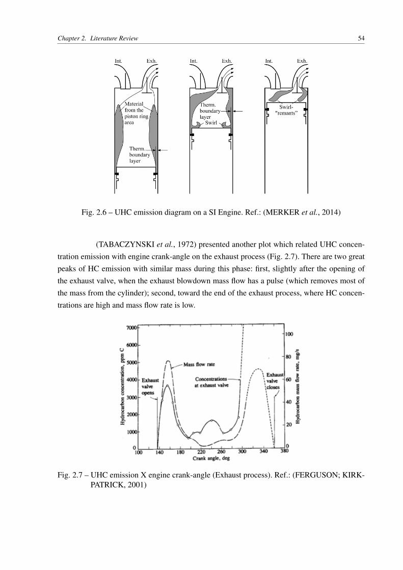
Chapter 2. Literature Review 54
Fig. 2.6 – UHC emission diagram on a SI Engine. Ref.: (MERKER et al., 2014)
(TABACZYNSKI et al., 1972) presented another plot which related UHC concen-tration emission with engine crank-angle on the exhaust process (Fig. 2.7). There are two greatpeaks of HC emission with similar mass during this phase: first, slightly after the opening ofthe exhaust valve, when the exhaust blowdown mass flow has a pulse (which removes most ofthe mass from the cylinder); second, toward the end of the exhaust process, where HC concen-trations are high and mass flow rate is low.
Fig. 2.7 – UHC emission X engine crank-angle (Exhaust process). Ref.: (FERGUSON; KIRK-PATRICK, 2001)

Chapter 2. Literature Review 55
2.6.3 CREVICE HC-FORMATION MECHANISM
Crevices are small volumes with narrow entrances which exist in SI engines andbuild up air-fuel-residual gas mixtures during the engine cycle. The combustion flame is notable to penetrate these volumes and burn the mixture, thus the fuel from the crevice areas is notburned during combustion process (HEYWOOD, 1988).
There are some considerable crevice regions on the gaps of an engine. The figurebelow indicates the values of these crevice volumes and compares them with cylinder volumeand clearance volume. Notice that crevice volume of the studied engine is nearly 3.5% of theengine clearance volume.
Fig. 2.8 – UHC crevice Volumes on a V-6 Engine. Ref: (HEYWOOD, 1988)
The most significant crevice regions on a conventional SI engine are the volumesabove, behind and between the first and second piston rings.
Models presented on the literature (HEYWOOD; NAMAZIAN, 1982) predicts theflows in and out of the crevice ring regions, based on conservation of mass, mass flowrate frompressure gradients between cylinder pressure and the crevices and the piston ring dynamics.The following figure presents the piston-piston ring-cylinder wall assembly, where the studiedcrevice regions are located.

Chapter 2. Literature Review 56
Fig. 2.9 – Crevice diagram on a conventional SI Engine. Ref: (HEYWOOD, 1988)
The Heywood crevice HC mechanism describes the phenomenon as the follow-ing: during compression stroke, cylinder pressure rises and some air-fuel-residual gas mixtureflows into the crevice regions. Besides the flame quenching distance, these areas have a largesurface-to-volume ratio; the gas flowing into them is cooled from cylinder walls, which have atemperature considerably lower than the bulk mass temperature during compression, combus-tion and expansion processes. During combustion, while the pressure still rises, some burnedmixture continues entering into the crevice regions. On expansion process, cylinder pressurestarts to reduce and when it is lower than the crevice pressure, part of the mixture betweenburned and unburned gases from the crevices flows out of these regions. Part of the unburnedmixture is burned, but not completely, since cylinder temperature is not high enough to completecombustion (HEYWOOD, 1988).
Crevice HC mechanism is a major contributor to UHC emission from spark-ignitionengines. (WENTWORTH, 1971) studied the effect on UHC emissions when crevice regionsfrom the piston-piston ring-cylinder wall assembly are minimized. Reductions from 25 to 50%of UHC emission were obtained when the modified assembly (almost without crevice volumeavailable) was compared to a production design assembly.
2.6.4 FLAME QUENCHING HC MECHANISM
Quenching in SI engines is a phenomenon that occurs in the cylinder walls duringthe engine cycle. Experiments have shown that combustion flames are extinguished before itreaches the walls, leaving on these regions some unburned air-fuel-residual gas mixture. Duringexpansion stroke, part of these mixture is released from the quenching area and are burned ifthe cylinder temperature is high enough for allow combustion.
Chapter 2. Literature Review 57
(BENSON, 1960) described the quenching phenomenon as “The quenching mayconsist in sudden cooling to stop the reactions or in the addition of a chemical reagent whichwill remove (by reaction or neutralization) one of the reactive components”. On SI engines, thecylinder walls act as a heat sink, removing heat from the close regions, preventing the mix-ture of gases to burn. Experiments from (DANIEL, 1957) first showed the quenching regions,where combustion flames could not reach it. Later, (LORUSSO et al., 1981) showed the burningefficiency of the quenching unburned gases after later expansion stroke was high enough to con-sider that most of HC presented in these gases were completely burned. This was an indicationthat flame quenching HC mechanism has a minor effect on UHC emission.
Quenching regions on SI engines are located on the cylinder walls, the head of thepiston and on the top of clearance volume. Figure 2.6 shows these regions.
The flame-quenching phenomena on SI engines may be analyzed by energy bal-ances (first law of thermodynamics), relating the heat release within the flame to the heat lossto the cylinder walls (HEYWOOD, 1988). These conditions may be applied when quenchingprocess occurs (combustion processes, for instance).
Peclet number (Pe) is a dimensionless number which relates the quenching process.It relates heat release on the flames with heat loss to the walls. Therefore, Peclet number maybe mathematically described as:
Pe2 =ρuSLcp, f (Tf −Tu)
k f (Tf −Tu)/dq2=
ρuSLcp, f dq2
k f(2.30)
Where:
∙ ρu: Specific mass;
∙ SL: Flame speed;
∙ cp, f : Constant-pressure specific heat;
∙ k f : Conductivity Constant;
∙ dq2: Two-plate quench distance;
∙ Tf andTu: Flame and unburned temperature, respectively;
(FERGUSON; KECK, 1977) analyzed flame quenching application conditions onSI engines. It was presented a physical correlation, considering Peclet number for quenchingprocess on SI engines. The numerical analysis was developed for laminar flame propagationto walls under perpendicular and parallel conditions. (WESTBROOK et al., 1981) consideredflame propagation parallel to the walls on his paper to correlates the phenomenon with HC con-centration on quench regions. It was also showed that the two-place quench distance (which is

Chapter 2. Literature Review 58
generally experimental) relates with one-plate quench distance dq1, which is a more coherentdistance for engine purposes. Heywood indicated some values this distance on engine condi-tions. The thinnest distance is applied on high engine loads.
dq1 = (0.04 ≈ 0.2)(mm) (2.31)
While (MERKER et al., 2014) presented an expanded distance interval.
dq1 = (0.02 ≈ 0.2)(mm) (2.32)
(ISHIZAWA, 1996) presented a relationship between the quench thickness whenthe flame front reached its ion detector on an engine cylinder (on combustion stroke conditions)with the peak pressure of the cycle and the wall temperature.
dq1 = K1P−0.9peak T−0.5
wall (mm) (2.33)
Where:
∙ dq1: Quench thickness (mm);
∙ K1: Fuel constant = 14.8 for Gasoline;
∙ Ppeak: Peak pressure of the engine cycle (MPa);
∙ Twall: Wall temperature (K);
The one-plate quench distance may be used to calculate the amount of HC accumu-lated on quench walls in specific engine conditions. With thermodynamic data from the enginecycle (T,V,P) besides the unburned and burned compositions, the mass of HC unburned onquench regions may be calculated.
59
3 METHODOLOGY
In this section the methodology applied to this research is presented. Two math-ematical models were developed to predict the formation of regulated pollutant gases in anethanol-fueled spark-ignited engine. The NO and CO formation are estimated by a chemicalkinetic model, while UHC is predicted by the application of the crevice and flame quenchingHC-mechanisms.
The main idea of the first model is to combine the information obtained by a ther-modynamic study of a two-zone combustion model with chemical equilibrium and chemicalkinetics. The second model focuses on the same two-zone thermodynamic model to calculateUHC emissions from both HC-formation mechanisms mentioned earlier.
The mathematical model for chemical kinetic calculations involves the applicationof a numerical method to solve a system of ordinary differential equations. Since explicit meth-ods demonstrate difficulties related to stability issues when a set of chemical kinetic equationsis calculated, therefore an implicit method was used to solve this ODE-system.
First, the stiff behavior of the chemical kinetic equations is introduced. Then thechemical kinetic methodology is presented. Lastly, the HC-formation models are explained.
3.1 NUMERICAL SOLUTION OF STIFF DIFFERENTIAL EQUATIONS
Initial-value problems (or IVPs) related to a complex chemical system usually donot have an analytical solution, because of the considerable number of chemical species in-volved in the model. Therefore, numerical techniques are required to solve these problems.
Numerical methods for solving ODE systems have errors associated with their ap-plication, although these errors may be controlled by the methods themselves. For example, afourth order Runge-Kutta method may be applied to solve a chemical kinetic system and yieldsresults that are coherent with the real solution of that problem, although stability issues maybecome apparent, depending on the step-size (h) applied to calculate the method. Chemical sys-tems usually have a special behavior, which requires the numerical method to be stable enoughto solve them without the numerical errors to grow exponentially after each iteration. This spe-cific kind of mathematical problem is called stiff, and to reach stability conditions it requiresconsiderable smaller step-sizes (which is unfeasible on most computer simulations) to solve thesystem for most applied techniques.
(KEE et al., 2003) describes a chemical problem as stiff when the time step requiredto maintain the stability is much smaller than that would be required to maintain the methodaccurate, if stability issues did not exist. Burden (BURDEN; FAIRES, 2013) defines stiff dif-
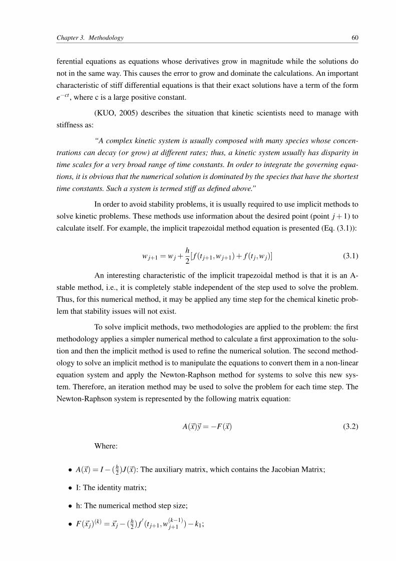
Chapter 3. Methodology 60
ferential equations as equations whose derivatives grow in magnitude while the solutions donot in the same way. This causes the error to grow and dominate the calculations. An importantcharacteristic of stiff differential equations is that their exact solutions have a term of the forme−ct , where c is a large positive constant.
(KUO, 2005) describes the situation that kinetic scientists need to manage withstiffness as:
“A complex kinetic system is usually composed with many species whose concen-
trations can decay (or grow) at different rates; thus, a kinetic system usually has disparity in
time scales for a very broad range of time constants. In order to integrate the governing equa-
tions, it is obvious that the numerical solution is dominated by the species that have the shortest
time constants. Such a system is termed stiff as defined above.”
In order to avoid stability problems, it is usually required to use implicit methods tosolve kinetic problems. These methods use information about the desired point (point j+1) tocalculate itself. For example, the implicit trapezoidal method equation is presented (Eq. (3.1)):
w j+1 = w j +h2[ f (t j+1,w j+1)+ f (t j,w j)] (3.1)
An interesting characteristic of the implicit trapezoidal method is that it is an A-stable method, i.e., it is completely stable independent of the step used to solve the problem.Thus, for this numerical method, it may be applied any time step for the chemical kinetic prob-lem that stability issues will not exist.
To solve implicit methods, two methodologies are applied to the problem: the firstmethodology applies a simpler numerical method to calculate a first approximation to the solu-tion and then the implicit method is used to refine the numerical solution. The second method-ology to solve an implicit method is to manipulate the equations to convert them in a non-linearequation system and apply the Newton-Raphson method for systems to solve this new sys-tem. Therefore, an iteration method may be used to solve the problem for each time step. TheNewton-Raphson system is represented by the following matrix equation:
A(~x)~y =−F(~x) (3.2)
Where:
∙ A(~x) = I − (h2)J(~x): The auxiliary matrix, which contains the Jacobian Matrix;
∙ I: The identity matrix;
∙ h: The numerical method step size;
∙ F(~x j)(k) = ~x j − (h
2) f′(t j+1,w
(k−1)j+1 )− k1;

Chapter 3. Methodology 61
∙ k1 = ~x j +(h2) f
′(t j,~x j);
The Jacobian matrix is presented by Eq. (3.3):
J(~x) =
∂ f1
∂x1
∂ f1
∂x2· · · ∂ f1
∂xn∂ f2
∂x1
∂ f2
∂x2· · · ∂ f2
∂xn...
... . . . ...∂ fn
∂x1
∂ fn
∂x2· · · ∂ fn
∂xn
(3.3)
Each term of the Jacobian matrix is solved numerically by the following equation:
∂ fi
∂xm=
fi(x1,x2, ...,xm +dx, ...,xn)− fi(x1,x2, ...,xm, ...,xn)
dx(3.4)
Where dx is a small variation applied on each dimension of the vector~x.
For each Newton-Raphson iteration, a set of linear equations needs to be solved. Apartially-pivoted Gauss-Seidel method is used to solve the system.
~x(k)j =
~x(k−1)
j +~y (3.5)
Equation (3.5) indicates the kth iteration value.
The Newton-Raphson will be considered solved when the following norm is lowerthan the defined Tolerance:
∥∥∥~xk −~xk−1∥∥∥
∞
≤ TOL (3.6)
3.2 CHEMICAL KINETIC MODELS
The chemical kinetic analysis was divided in three parts:
First a chemical model was developed for air under thermodynamic SI engine con-ditions. The objective was to analyze the behavior of NO-related reactions on high temperaturessuch as found on the combustion stroke. The calculations considered a constant-temperatureand volume model and results such as reaction rates and NO-formation rate were studied andinterpreted. This model considered 3 reactions (Eq. (2.17)) and 5 chemical species.
Then, a second chemical model was developed for a mixture of gases under SIconditions. This analysis considered a (P, V, T) profile from an engine model, instead of con-stant conditions. This analysis involved 12 chemical species. The objectives were studying the

Chapter 3. Methodology 62
NO-formation with the influence of more chemical reactions on the model and evaluate the CO-formation and its behavior under SI engine conditions. This model considered 22 chemical reac-tions related with 12-chemical species model (Ar,CO,CO2,H,H2,H2O,OH,O,O2,N,N2,NO).
The final model considered the application of the final chemical model on a two-zone spark-ignited engine simulator. This model is detailed later on this section.
3.2.1 AIR DISSOCIATION CHEMICAL MODEL
This analysis considered air inside a closed system on constant-volume and constant-temperature conditions. The amount of mass of air was previously defined and the developmentof the chemical kinetics on the defined temperature and pressure is analyzed.
3.2.1.1 Procedure and assumptions of the model
The assumptions of the model are the following:
∙ Some amount of simplified dry air (molar fraction: 0.79N2,0.21O2) is confined in a closedsystem;
∙ The studied system is considered rigid (constant-volume analysis);
∙ The thermodynamic conditions allow the system to operate on constant temperature;
∙ A chemical kinetic model considered the chemical reactions of the classic Zeldovichmodel (Eq. (2.17)), in order to evaluate the quantity of NO yielded after some reactiontime;
∙ The chemical species considered on this model are: (O2,O,N2,N,NO). Therefore fivechemical species were considered;
∙ The third-body M was considered as N2, in order to simulate its influence in a SI en-gine case, where its molar fraction is much higher than the other species on the model(yinitial,N2 = 0.7 ≈ 0.8);
After the assumptions, the procedure of this analysis is the following:
∙ With the initial number of moles of air, the molar concentrations of N2 and O2 are calcu-lated by Equation (3.7):
[Ci] = ui =ni
V(3.7)
∙ The index i represents each chemical species of the model, where i = 1 : 5. The order ofthe index is the same as the chemical species sequence mentioned above for this model(O2 = 1,O = 2,N2 = 3, ...);

Chapter 3. Methodology 63
∙ Next, the classic Zeldovich mechanism is applied. The reactions are the following:
2O+M ⇔ O2 +M
O2 +N ⇔ NO+O
NO+N ⇔ N2 +O
(3.8)
∙ Then the reaction rates are calculated:
q1 = k f ,1u2u2uM − kb,1u1uM
q2 = k f ,2u1u4 − kb,2u5u2
q3 = k f ,3u5u4 − kb,3u3u2
(3.9)
Where:
– u: Molar concentration;
– k f : Forward rate constant;
– kb: Backward rate constant;
– q j:Rate of reaction of the jth chemical reaction;
∙ The stoichiometric coefficient matrix for this system is presented on Eq. (3.10):
ν = ν′′−ν
′=
1 −2 0 0 0−1 1 0 −1 10 1 1 −1 −1
(3.10)
Where:
– ν′′: Stoichiometric coefficient for products;
– ν′: Stoichiometric coefficient for reactants;
∙ The columns represent the chemical species and the lines represent the reactions.
∙ Thus the ODE-system based on Eq. (2.7) is obtained:
dC1dt = u
′1 = q1 −q2
dC2dt = u
′2 =−2q1 +q2 +q3
dC3dt = u
′3 = q3
dC4dt = u
′4 =−q2 −q3
dC5dt = u
′5 = q2 −q3
(3.11)

Chapter 3. Methodology 64
∙ The forward rate constants (k f ) are calculated for the indicated temperature T. The rateconstant for each reaction is based on Eq. (2.3). The parameters A, b and Ea for eachchemical reaction are indicated on the final chemical model section. The backward reac-tion rate constants are calculated based on chemical equilibrium association with chemi-cal kinetics (Eq. (2.15)).
This system of ODEs is solved by the implicit trapezoidal method previously com-mented on this chapter.
3.2.2 FINAL CHEMICAL KINETIC MODEL
The chemical kinetics model operates with a two-zone spark-ignited engine model.This is a zero-dimensional thermodynamic model which is capable of calculating the combus-tion phase from two different control volumes: an unburned zone and a burned zone. The burnedzone is developed during combustion duration, based on a Wiebe Function, while the unburnedzone provides the fuel-air-residual gas mixture to the burned mixture and it is renewed duringthe admission phase. The model also includes open and closed operation phases (based on valvecontrol models), besides different heat transfer models. Therefore, this engine model is a pack-age of algorithms that combines and yields information related to parameters of the simulatedengine, such as power output, thermal and volumetric efficiency, levels of emission, etc.
The chemical kinetic package is one of these algorithms, which is decoupled fromthe engine simulator model and provides the rates of reaction and the composition of the burnedand unburned gases considered in the model. In addition, these compositions allows the majormodel to calculate thermodynamic properties, such as internal energy, enthalpy and entropy ofthe gas mixtures during all phases of the engine cycle, in order to solve first (energy balance)and second (entropy/exergy balance) laws of thermodynamics.
The initial analysis of the model starts on the beginning of compression stroke. Amixture of air, fuel and residual gas is initially assumed on the engine cylinder. A initial guessof the residual gas is assumed on the mixture and it is refined during the next iterations ofthe engine simulator. The universal gas constant (Ru) is calculated based on this mixture. Theproducts assumed as residual gas on the first iteration are calculated initially by a complete com-bustion model described by (FERGUSON; KIRKPATRICK, 2001). The subroutine calculatesthe compression stroke until the combustion stroke initiates.
During combustion, the amount of mass inside the burned zone increases with thecrank angle change. The reactant mixture is assumed as input for the adiabatic flame temper-ature, which is assumed as the initial temperature for the burned zone. This temperature isobtained by a chemical equilibrium model.
The composition of the burned gas is initially assumed as the same as the chemicalequilibrium composition, with exception for nitric oxide. Nitric oxide was assumed the same as

Chapter 3. Methodology 65
its molar fraction on the residual gases from the previous cycle. This assumption for NO wasthe same as (ANNAND, 1974) and produced coherent results. On the first cycle iteration, NO iszero since the combustion model from Ferguson do not consider its presence on the combustionproducts. After the beginning of the second cycle, NO is considered the same as found on theresidual gases.
The continuous addition of mass in the burned zone provided by the Wiebe functionis considered on the chemical kinetic subroutine as input. The differential equation system issolved and then the new composition for the burned zone on the next crank angle is obtained.The next crank angle iteration adds a new mass from the unburned zone to the burned zoneby the same procedure described earlier and this new mass is mixed with the burned massesalready present in the burned zone. Then the chemical kinetic procedure is activated and a newcomposition is calculated. This procedure occurs until the Wiebe function indicates that thereis no more unburned mass to be reacted and therefore the whole mass of the engine cylinder isconsidered the products of combustion.
The chemical kinetic procedure keeps calculating the new compositions based onthe thermodynamic conditions of each iteration until the burned temperature achieves 1500K(Tf reeze). This value is considered the frozen temperature, where the chemical kinetic rates de-value considerably and therefore may be ignored without considerable effects. The compositionis frozen and become the residual gas composition for the next cycle, after exhaust and admis-sion strokes.
The described procedure allows the user to predict NOx and CO formation duringeach position of the crank angle and therefore, predict exhaust emissions.
3.2.2.1 Procedure and assumptions of the model
The chemical kinetic model operates during each step-size of the two-zone enginemodel mentioned earlier. This allows the chemical kinetics model to develop calculations underconstant-volume and constant-temperature conditions for each step-size. This assumption ispossible since the thermodynamic conditions (P, V, T, dV , dT , dP) of a SI engine on a regularstep-size (dθ = 0.05∘) of the two-zone model do not variate considerably. This is the majorassumption of the model, since the molar concentration derivatives (d[Ci]
dt ) will not depend onthe volume derivative of the piston-cylinder assembly (dV
dt = ωdVdθ
). This simplifies the modelwithout removing precision on its results.
Additionally, the model considers the following assumptions:
∙ During all iterations the thermodynamic conditions of the burned zone are applied to thechemical kinetics model (Vb, Tb, Pb);
∙ The model considers 12 chemical species. These chemical species are:

Chapter 3. Methodology 66
(Ar,CO,CO2,H,H2,H2O,OH,O,O2,N,N2,NO)
∙ The index i represents each chemical species of the model.(i = 1 : 12). The order ofthe index is the same as the chemical species sequence mentioned above (Ar = 1,CO =
2,CO2 = 3, ...);
∙ The third-body M was considered to be N2. The same reasons commented on the airdissociation model are used here;
∙ Consideration related to freezing compositions: Freezing compositions happen when thetemperature of the system is low, does not allowing chemical kinetics to actuate. Thechemical reactions are considerably slower, i.e., the rate of reactions are low enough toignore chemical kinetics influence on the system. Thus the composition of the combustiongases is frozen and the molar fraction does not change anymore on the engine cycle.This application is valid from moments close to the end of expansion process, where thetemperatures of the burned zone are usually lower than 1500K;
Based on the mentioned assumptions, the chemical kinetics procedure is the follow-ing:
∙ A mixture of gases from the unburned zone is provided to the chemical model as theinitial burned mass. This mixture had its composition calculated as commented earlieron the description of this model. The conditions for the chemical equilibrium conditionswere the same as the burned zone (Tb,Pb,Vb), which is estimated by the adiabatic flametemperature, cylinder pressure and calculated burned volume obtained by ideal gas law,where the composition is assumed the same as the simplified combustion model describedby Ferguson (FERGUSON; KIRKPATRICK, 2001);
∙ The amount of mass/moles provided to the model comes from the Wiebe function;
∙ The two-zone model also provides the burned zone conditions (Tb,Vb,Pb) as inputs forthe kinetic calculations;
∙ The molar concentration of the ith chemical species is then calculated by Eq. (3.12):
[Ci] = ui =ni
Vb(3.12)

Chapter 3. Methodology 67
∙ The chemical reactions of the final chemical model are presented on Eq. (3.13):
OH +H ⇔ H2 +O
OH +O ⇔ O2 +H
OH +H2 ⇔ H2O+H
OH +OH ⇔ H2O+O
CO+OH ⇔CO2 +H
H +OH +M ⇔ H2O+M
2H +M ⇔ H2 +M
2O+M ⇔ O2 +M
O2 +N ⇔ NO+O
NO+N ⇔ N2 +O
OH +N ⇔ NO+H
(3.13)
∙ The forward rate constants (k f ) are calculated for the burned temperature Tb. The rateconstant for each reaction is based on Eq. (2.3). The parameters A, b and Ea for eachchemical reaction are indicated on the following table. The backward reaction rate con-stants are calculated based on chemical equilibrium additionally with chemical kinet-ics (Eq. (2.15)). The exception for the backward reaction rate constant was the reactionNO+H => N +OH, which rate parameters also follow on Table 3.1.
Table 3.1 – Reaction Rate Constant Parameters
Reaction Rate ParametersReaction A (m3/kmol.s) b Ea (kJ/kmol) ReferenceOH +H => H2 +O 4.3E7 2.8 16.21E3 (TSANG; HAMPSON, 1986)OH +O => O2 +H 2.61E10 -0.5 0.25E3 (TSANG; HAMPSON, 1986)OH +H2 => H2O+H 9.31E8 1.6 13.8E3 (BAULCH et al., 1992)OH +OH => H2O+O 9.95E8 1.14 0.42E3 (BAULCH et al., 1992)CO+OH =>CO2 +H 2.26E7 1.55 -3.34E3 (LISSIANSKI et al., 1995)OH +H +M => H2O+M 2.49E11 -2 0 (BAULCH et al., 1992)2H +M => H2 +M 2.19E9 -1 0 (BAULCH et al., 1992)2O+M => O2 +M 1.89E7 0 -7.48E3 (TSANG; HAMPSON, 1986)N +O2 => NO+O 2.69E9 1 27.19E3 (BAULCH et al., 1992)N +NO => N2 +O 4.28E10 0 6.57E3 (BAULCH et al., 1992)N +OH => NO+H 2.83E10 0 0 (BAULCH et al., 1992)NO+H => N +OH 2.0E11 0 2.365E3 (RAGGI, 2005)
∙ Then the mentioned chemical reactions provide the following ODE-system. The reaction
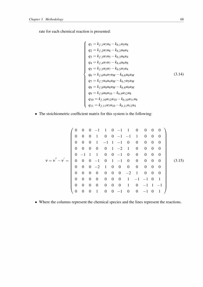
Chapter 3. Methodology 68
rate for each chemical reaction is presented:
q1 = k f ,1u7u4 − kb,1u5u8
q2 = k f ,2u7u8 − kb,2u9u4
q3 = k f ,3u7u5 − kb,3u6u4
q4 = k f ,4u7u7 − kb,4u6u8
q5 = k f ,5u2u7 − kb,5u3u4
q6 = k f ,6u4u7uM − kb,6u6uM
q7 = k f ,7u4u4uM − kb,7u5uM
q8 = k f ,8u8u8uM − kb,8u9uM
q9 = k f ,9u9u10 − kb,9u12u8
q10 = k f ,10u12u10 − kb,10u11u8
q11 = k f ,11u7u10 − kb,11u12u4
(3.14)
∙ The stoichiometric coefficient matrix for this system is the following:
ν = ν′′−ν
′=
0 0 0 −1 1 0 −1 1 0 0 0 00 0 0 1 0 0 −1 −1 1 0 0 00 0 0 1 −1 1 −1 0 0 0 0 00 0 0 0 0 1 −2 1 0 0 0 00 −1 1 1 0 0 −1 0 0 0 0 00 0 0 −1 0 1 −1 0 0 0 0 00 0 0 −2 1 0 0 0 0 0 0 00 0 0 0 0 0 0 −2 1 0 0 00 0 0 0 0 0 0 1 −1 −1 0 10 0 0 0 0 0 0 1 0 −1 1 −10 0 0 1 0 0 −1 0 0 −1 0 1
(3.15)
∙ Where the columns represent the chemical species and the lines represent the reactions.

Chapter 3. Methodology 69
∙ Thus the ODE-system based on Eq. (2.7) is obtained:
dC1dt = u
′1 = 0
dC2dt = u
′2 =−q5
dC3dt = u
′3 = q5
dC4dt = u
′4 =−q1 +q2 +q3 +q5 −q6 −2q7 +q11
dC5dt = u
′5 = q1 −q3 +q7
dC6dt = u
′6 = q3 +q4 +q6
dC7dt = u
′7 =−q1 −q2 −q3 −2q4 −q5 −q6 −q11
dC8dt = u
′8 = q1 −q2 +q4 −2q8 +q9 +q10 −q12 +q13
dC9dt = u
′9 = q2 +q8 −q9 −q13
dC10dt = u
′10 =−q9 −q10 −q11 −2q14
dC11dt = u
′11 = q10 +q14
dC12dt = u
′12 = q9 −q10 +q11 −q12 −q13
dC13dt = u
′13 = q12 +q13
(3.16)
∙ This system of ODEs is solved by the implicit trapezoidal method previously mentionedon this chapter.
∙ The time duration of the chemical reactions are the same as the differential crank-angleof the two-zone model:
dtreaction,step =dθ
ω=
0.05∘
ω(3.17)
∙ Where ω is the angular speed of the engine.
After final calculations, the chemical kinetic algorithm returns the new molar frac-tions to the two-zone algorithm. The kinetic model is required then on the next engine-step. Thekinetic package is required until the freezing temperature is achieved. The fluxogram presentednext (Fig. 3.1) is a simplified version of the procedure presented earlier.

Chapter 3. Methodology 70
Fig. 3.1 – Simplified flowchart of the final chemical kinetic model.
3.3 HC-FORMATION AND EMISSION MODELS
Only the crevice and the flame quenching HC models were considered to evaluatequalitatively UHC emissions by an ethanol-fueled SI engine. The other HC mechanisms, suchas liquid fuel, oil layers, etc., require more robust information from the engine model than itcurrently be provided, thus a more simplistic analysis was developed.
3.3.1 UHC CREVICE MODEL
An UHC crevice model was developed and analyzed to predict HC accumulation onthe crevice regions of a specific engine, with known crevice volumes and burned and unburnedgas compositions.
The model is simpler than Heywood’s model (HEYWOOD; NAMAZIAN, 1982),although it provides qualitatively results. The geometry model is based on the indications fromFig. 2.8.
The followed procedure besides the assumptions for the crevice model are describedbelow:
∙ A two-zone thermodynamic engine model is used to calculate the engine cycle;
∙ Ethanol E95 (95% Ethanol 5% H2O m) was assumed as the fuel;
∙ The composition of the air is detailed on the following table (Tab. 3.2):

Chapter 3. Methodology 71
Table 3.2 – Dry Air Composition (WAY, 1976)
Dry Air CompositionChemical Species %V
N2 78.084O2 20.946
CO2 0.937Ar 0.033
∙ The residual gas is calculated on the two-zone thermodynamic engine simulation. In-formation such as air-fuel ratio (equivalence ratio), humidity of air, load percentage ofthe engine, engine geometry, inlet and exhaust valve timing, ignition delay, combustionduration and combustion efficiency are defined on the engine model;
∙ The product and residual gas compositions may be defined by the chemical equilibriummodel, which can consider 12 or 13 chemical species or the chemical kinetics modeldescribed on this study;
∙ An air-fuel-residual gas mixture is obtained and its composition is assumed constant inthe crevice regions;
∙ The temperature on the crevice regions is always the wall temperature. The temperatureis predefined on the two-zone model;
∙ The pressure adopted on the crevice regions is the cylinder pressure at the moment wherethe crevice HC calculations are made. This consideration is a simplification to the con-servation of mass model from (HEYWOOD; NAMAZIAN, 1982). It considers that anhomogeneous pressure acts on the entire engine;
∙ The specific moments where the crevice HC calculations are developed are the following:the opening of the exhaust valve (EVO) and the closure the exhaust valve (EVC);
∙ The crevice volume regions considered are the ones detailed on Figure 2.8;
∙ For a simplified analysis, it was assumed that the mass presented on the crevice regionsis much lower than the cylinder mass (less than 1% of total mass). Therefore the crevicemass was not subtracted of the cylinder mass;
∙ The range of crevice volume adopted is from 1% to 3.5% (HEYWOOD, 1988) of theclearance volume;
∙ The actual model considers a relationship between the fraction of the crevice volume withengine speed. This relationship is based since on higher engine speeds the turbulence ishigher, thus a reduction of the crevice factor is expected. A linear relationship was as-sumed between 1000RPM and 6000RPM and crevice factors of 2% and 1% respectively;
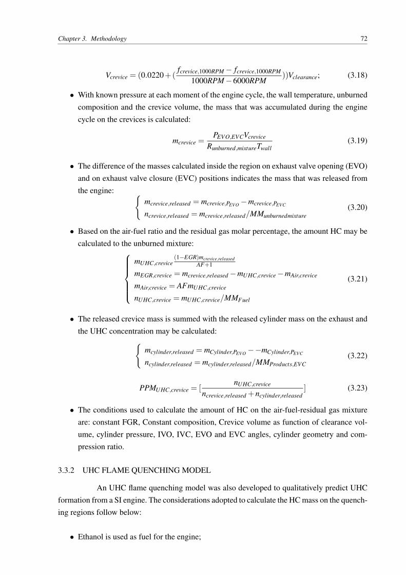
Chapter 3. Methodology 72
Vcrevice = (0.0220+(fcrevice,1000RPM − fcrevice,1000RPM
1000RPM−6000RPM))Vclearance; (3.18)
∙ With known pressure at each moment of the engine cycle, the wall temperature, unburnedcomposition and the crevice volume, the mass that was accumulated during the enginecycle on the crevices is calculated:
mcrevice =PEVO,EVCVcrevice
Runburned,mixtureTwall(3.19)
∙ The difference of the masses calculated inside the region on exhaust valve opening (EVO)and on exhaust valve closure (EVC) positions indicates the mass that was released fromthe engine: {
mcrevice,released = mcrevice,PEVO −mcrevice,PEVC
ncrevice,released = mcrevice,released/MMunburnedmixture(3.20)
∙ Based on the air-fuel ratio and the residual gas molar percentage, the amount HC may becalculated to the unburned mixture:
mUHC,crevice(1−EGR)mcrevice,released
AF+1
mEGR,crevice = mcrevice,released −mUHC,crevice −mAir,crevice
mAir,crevice = AFmUHC,crevice
nUHC,crevice = mUHC,crevice/MMFuel
(3.21)
∙ The released crevice mass is summed with the released cylinder mass on the exhaust andthe UHC concentration may be calculated:{
mcylinder,released = mCylinder,PEVO −−mCylinder,PEVC
ncylinder,released = mcylinder,released/MMProducts,EVC(3.22)
PPMUHC,crevice = [nUHC,crevice
ncrevice,released +ncylinder,released] (3.23)
∙ The conditions used to calculate the amount of HC on the air-fuel-residual gas mixtureare: constant FGR, Constant composition, Crevice volume as function of clearance vol-ume, cylinder pressure, IVO, IVC, EVO and EVC angles, cylinder geometry and com-pression ratio.
3.3.2 UHC FLAME QUENCHING MODEL
An UHC flame quenching model was also developed to qualitatively predict UHCformation from a SI engine. The considerations adopted to calculate the HC mass on the quench-ing regions follow below:
∙ Ethanol is used as fuel for the engine;

Chapter 3. Methodology 73
∙ Air-fuel-residual gas mixture is the same as the UHC crevice model;
∙ Residual gas conditions are the same as UHC crevice model;
∙ The temperature on the crevice regions is always the wall temperature. The temperatureis predefined in the two-zone model;
∙ The pressure adopted on the crevice regions is the cylinder pressure on the moment wherethe crevice HC calculations will be made;
∙ The quench volume is calculated based on (HEYWOOD, 1988) and (MERKER et al.,2014) for the flame quenching film. The thickness is considered the same on the followingareas: on the lateral area of the cylinder, on the superior area of the piston and on thecylinder head area;
∙ The quenching thickness is different when calculated on different engine positions. It isless thicker during exhaust valve opening and it grows while the exhaust process happens(hquench,EVO > hquench,EVC);
∙ A relationship was adjusted for quenching thickness on the opening and closure of ex-haust valve with Ishizawa Equation (2.33) commented earlier. Since the equation presentsthe quench thickness during combustion process, an adjustment was required in order tocalculate the thickness during the initial and final positions of the exhaust valve. Theconstant K1 was adjusted to E95 (hydrous ethanol).
dq1,Exhaust = Kad just,1:2P−0.9peak T−0.5
wall (mm) (3.24)
Where:
– Kad just,1: Adjusted Ethanol constant = 14.8x10⁻⁴;
– Kad just,2: Adjusted Ethanol constant = 7.4x10⁻⁴;
∙ Since it is a simple analysis, the effects of post-combustion were not considered in themodel;
∙ The quenching volume on a specific position of the engine cycle is calculated by Eq.(3.25):
Vquenching f ilm =Vcylinder,position −Vbulkmass,position =piSB2
4−
piSreducedB2reduced
4(3.25)
Where:
∙ S: Stroke partial position of the engine;
∙ B: Bore of the engine;

Chapter 3. Methodology 74
∙ hquench: Quench thickness on a specific position of the engine;
∙ Sreduced = S−2hquench: Reduced stroke partial position;
∙ Breduced = B−2hquench: Reduced bore of the engine;
∙ The pressure on the quenching regions is considered the same of the cylinder. Since thepressure is calculated from a two-zone model, which considers a balance of pressurebetween unburned and burned zones, the same idea was applied to quenching areas;
∙ It is assumed that the mass presented on the quenching regions is much lower than thecylinder mass (same order of crevice mass). Therefore the quenching mass is not sub-tracted of the cylinder mass;
∙ With known pressure at each moment of the engine cycle, the wall temperature, unburnedcomposition and quench volume calculated from quench distance, the mass that was ac-cumulated during the engine cycle on the quench film is calculated:
mquenching,area =PEVO,EVCVquenching f ilm
Runburned,mixtureTwall(3.26)
∙ The amount of air-fuel-residual gas mixture accumulated on the EVO and EVC, in orderto discover how much UHC is released during Exhaust Valve Opening:{
mquench,released = mquench,PEVO −mquench,PEVC
nquench,released = mquench,released/MMUnburnedMix(3.27)
∙ Based on the air-fuel ratio and EGR percentage, the amount HC may be calculated to theunburned mixture:
mUHC,quench(1−EGR)*mquench,released
AF+1
mEGR,quench = mquench,released −mUHC,quench −mAir,quench
mAir,quench = AFmUHC,quench
nUHC,quench = mUHC,quench/MMFuel
(3.28)
∙ The released flame quenching mass is summed with the released cylinder mass on theexhaust and the UHC concentration may be calculated:{
mcylinder,released = mCylinder,PEVO −−mCylinder,PEVC
ncylinder,released = mcylinder,released/MMProducts,EVC(3.29)
PPMUHC,quench = [nUHC,quench
nquench,released +ncylinder,released] (3.30)
∙ The conditions used to calculate the amount of HC on the air-fuel-residual gas mixtureare: constant FGR, constant composition, quench volume, flame quenching thickness,cylinder pressure, IVO, IVC, EVO and EVC angles, cylinder geometry and compressionratio.

Chapter 3. Methodology 75
When the analysis considers the crevice and flame quenching models, the method-ology is the same, except that the masses of UHC from both models will be summed. Therefore,the molar concentration (in PPM UHC C f uel) is calculated:
PPMUHC,total = [nUHC,quench +nUHC,crevice
ncrevice,released +nquench,released +ncylinder,released] (3.31)

76
4 RESULTS AND ANALYSIS
This chapter presents the results obtained from the described chemical kinetics andUHC models.
The chemical kinetic analysis of the previously presented models is divided in twoparts: first, the air dissociation chemical model was studied at temperatures similar as found inspark-ignited engines during combustion and expansion processes. Second, the methodologydescribed earlier on the text about the full chemical kinetic model was applied to two differentcases. A theoretical analysis of the influence of engine operation variables was undertaken onspecific engine conditions. The effect of variables such as engine speed, air-fuel stoichiometricratio and ignition timing were evaluated on the emission of nitric oxide, carbon monoxide andunburned hydrocarbon by this engine. Finally, the full kinetic model results were comparedwith experimental data from a specific engine under rich mixture conditions. Various engineparameters were input in the simulator in order to approximate the most the simulation of thereal engine behavior.
HC-emission analyses were undertaken together with the full kinetic model above.The effect of the same engine operation variables were also analyzed with respect to UHCemission.
4.1 CHEMICAL KINETIC ANALYSIS - AIR DISSOCIATION CHEMICAL MODEL
Preliminary results from the initial model of chemical kinetics are presented on thissection. These models were developed with the function of providing primary approximationsof kinetic variables under thermodynamic conditions found in engines. These results refined themodels, which gave basis for the development of the more complex models.
A chemical kinetics analysis of dry air under engine temperatures was developed.The objective was to verify the tendency of NO formed from the Zel’dovich Mechanism inachieving chemical equilibrium conditions after some reaction time.
The first approximate model is the air dissociation chemical model. This model wasalready described on the methodology section. Based on the equations presented on the previoussection, some results are presented here.
The initial conditions for the calculations presented on this section were the follow-

Chapter 4. Results and Analysis 77
ing:
ninitial,O2 = 0.21x10⁻⁶kmol
ninitial,N2 = 0.79x10⁻⁶kmol
V = 250x10−6m3
T = [1500 : 2500]Ktreaction time = 100s
h = 2x10⁻⁵s(T > 2000K)
h = 1x10⁻⁴s(T < 2000K)
Tol = 1x10⁻⁶;
(4.1)
The initial conditions were chosen based on usual engine conditions, in order tomake a initial simulation of NO-formation on a SI engine. The volume represents the volume ofan ordinary engine cylinder from Brazilian touring car (with each cylinder having 250cm3). Thetemperatures are similar to the operation of the engine on combustion and expansion strokes.
This chemical analysis simulated a 100-second reaction case. There were two ob-jectives behind this simulation. These objectives were:
∙ To analyze the chemical kinetics of Zeldovich NO-mechanism until chemical equilibriumwas achieved. This analysis considered the time required for this reaction mechanism toachieve negligible NO-formation rates (d[CNO]
dt ≈ 0);
∙ To compare the amount of NO formed during an approximate engine cycle time (tengine time ≈1x10⁻³s) with the amount of NO formed when chemical equilibrium or 100 seconds ofreaction is achieved;
∙ To relate the reaction temperature with the orders of magnitude of the amount of NOformed and their rates;
First some plots about the NO-formation at different temperatures are shown. Thesetemperatures represent the profile that a SI engine usually presents under operation.

Chapter 4. Results and Analysis 78
Fig. 4.1 – NO formation from dry air in a closed system at T = 1800 : 2100K.
Fig. 4.2 – NO formation from dry air in a closed system at T = 2200 : 2500K.

Chapter 4. Results and Analysis 79
Figure 4.1 shows that at T = 1800K, NO has not achieved equilibrium even after100 seconds of reaction, while at temperatures above 1800K show a tendency to chemical equi-librium conditions for each case. The time required to achieve equilibrium is also obtained fromthe plot, which shows the different time scales for chemical equilibrium at 2100 K and 1900K. The 2100K curve rapidly raises the NO amount in 7 seconds while the 1900K one requiresalmost 83 seconds to achieve equilibrium.
Figure 4.2 is on a different time order of magnitude. All the curves showed ten-dency to equilibrium in less than 3 seconds. This shows a great temperature dependency ofNO-formation, as commented on literature (KUO, 2005). Another information that is obtainedfrom the plots is the difference between the amounts of NO yielded between cases that achievedchemical equilibrium. The amount produced on the 2500K case is almost four times greater thanthe the amount from the 1900 K case. The time required to produce each of these amounts is400 times greater for the second case than it is for the first one.
The following figure shows the amount of NO formed from the set of temperaturesunder the same time reaction curve.
Fig. 4.3 – A semi-log plot of NO-formation from dry air in a closed system versus Temperature.
From figure 4.3 it is clear that NO demonstrates an exponential tendency with tem-perature. This represents well the Arrhenius behavior described on the review section, despitethe set of the reactions considered on the model. Another notable point is the proximity of each

Chapter 4. Results and Analysis 80
point to the chemical equilibrium reference (from T = 2500K). Above 1800 K, the proximityis considerably higher than it is for lower temperatures.
A last analysis is developed from the results of the model. The following tablecompares the amount of NO yielded by if the reaction time was a standard NO-formation timeon engine cycles (≈ 1ms) with the amount of NO yielded when at 100 seconds of reaction. Thistime represent chemical equilibrium conditions if the temperature is higher than 1900K, suchas described at Fig. 4.1.
Table 4.1 – NO Tendency to Equilibrium x Usual Engine Temperatures
NO Tendency to Equilibriumon SI Engines x Temperature
T (K) %MCNOengine time
MCNO100s
In 100sAt Equilibrium?
1500 1.0080x10⁻¹⁰ No1600 1.0931x10⁻¹⁰ No1700 1.6218x10⁻¹⁰ No1800 4.1609x10⁻¹⁰ No1900 3.3587x10⁻⁹ Yes2000 3.2671x10⁻⁸ Yes2100 2.5609x10⁻⁷ Yes2200 1.6653x10⁻⁶ Yes2300 9.2073x10⁻⁶ Yes2400 4.4191x10⁻⁵ Yes2500 1.8736x10⁻⁴ Yes
It is noticed that the growth on the NO percentage starts at temperatures higher than1800 K. This data corroborates the fact that NO formation becomes relevant on temperaturesover 1800 K, as already mentioned on the literature review section. The NO percentage startsto grow fast on an exponential profile, as noticed by the values. The table also presents how farthe amount of NO formed on SI engine cycle time conditions is from the amount of NO at 100s(or chemical equilibrium conditions for T > 1800K. Even at peak temperatures, such as 2400 ≈2500K, the model does not approximate significantly to chemical equilibrium conditions. Thisresult corroborates the necessity of applying chemical kinetics instead of chemical equilibriumfor coherently predicting SI engine pollutant formations.
4.2 CHEMICAL KINETICS MODEL ON THE TWO-ZONE THERMODYNAMIC EN-GINE SIMULATOR
The second analysis of the result section focuses on the analysis of the chemicalkinetics of the combustion gases during the combustion and expansion strokes of an ethanol-fueled engine. This model was previously described on the methodology section and will con-sider on this analysis 12 chemical species and 22 chemical reactions.

Chapter 4. Results and Analysis 81
The initial mixture of gases are based on thermodynamic conditions found in theengine simulator model. This mixture had its origin from a mixture of air, fuel and residual gaswhich reacted (combustion process) and, with exception of nitric oxide, a chemical equilibriummodel was applied to calculate the molar fractions of the gases considered on this model. Theequilibrium model is based on 12 chemical species, depending on the considerations indicatedby the user. These species are the same as the ones commented earlier for the chemical kineticsmodel.
The thermodynamic conditions of the model are obtained from the P-V-T data sim-ulated by the engine model previously commented. These data are used in order to analyze theNO and CO formations in conditions similar to those found in SI engines. The temperatureprofile comes from the burned zone, since it is on this region where the chemical reactionsfrom combustion happen, while the volume profile is the burned volume of the cylinder. Bothof these profiles initiate from the beginning of the combustion process on the engine until thefrozen temperature is achieved, during expansion process.
This analysis has the objective of qualitatively predict the formation of the men-tioned pollutants. The model provides similar formation tendencies that an experimental anal-ysis of a real engine shows, although in different values. This difference on the values may bejustified by many factors, such as the uncertainty of the experimental procedure, the absenceof the exact engine parameters from the experimental procedure to the engine simulator, etc.The idea of the model is to calculate the formation of the regulated pollutants on the samemagnitude order and presenting the same tendencies as presented by literature results and ex-perimental procedures.
On this work, three main engine operation variables were chosen to analyze theirinfluence on the chemical kinetics of the engine cycle. Engine speed (RPM), air/fuel ratio andspark timing were the chosen engine variables. All other variables were kept constant whenthese variables were studied. The table below (Table 4.2) shows the main conditions of theengine operation variables. The engine speed, air/fuel ratio and spark timing variations are alsoindicated on this table.

Chapter 4. Results and Analysis 82
Table 4.2 – Engine operation variables and parameters.
Engine operation variables and parametersFuel E95
Engine Speed [1000 : 4000] RPMActual Air-Fuel Ratio [0.7:1.3]A/Fstoichiometric
Spark Timing [−30 : 10]∘
Compression Ratio 12.25Vcylinder 400x10−6m3
Cylinder Bore 75 mmCylinder Stroke 90.5 mm
Eccentricity 0.069 mmConnecting Rod length 145.6 mm
Ignition Delay 12∘
Combustion Duration 40∘
Freezing Temperature 1500KAdmission Valve Opening −10∘
Admission Valve Closure 220∘
Exhaust Valve Opening 500∘
Exhaust Valve Closure 10∘
Engine Load 100%PMAX ,admExhaust Temperature 1007K
Admission Temperature 298KExhaust Pressure 130.7093kPa
Admission Pressure 98.2853kPaWall Temperature 520K
Mass Percentage of water on fuel 5%Relative Humidity 50%
ydry air,N2 0.78084ydry air,O2 0.20946ydry air,CO2 0.00937ydry air,Ar 0.00033
The reference for the crank angle is the Top Dead Center (TDC) for the admissionstroke (0∘).
Some variables had to be established in order to simulate a proper engine operationcondition. The inlet and exhaust opening and closure periods, as long as the valve overlap weredefined here as the values presented on Table 4.2 since it gave coherent volumetric efficiency,therefore great amount of mass inside the cylinder, in order to produce coherent values of pres-sure and temperature during the engine cycle. The engine geometry used on this simulation isthe same as the engine simulated on the experimental tests, while the admission and exhaustconditions were established based on some common conditions indicated by experiment data.
Therefore, engine speed was varied between 1000 and 4000 RPM for rich, stoichio-metric and lean cases at full load. The mixture air-fuel was varied from very lean (λ = 1.2|)

Chapter 4. Results and Analysis 83
to very rich (λ = 0.7) mixtures. The engine load considered on this model was based on theadmission pressure on the intake manifold. The spark timing was varied from 330∘ until 370∘.
4.2.1 NO AND CO FORMATION PROFILES WITH CRANK ANGLE
This case was developed varying rich, lean and stoichiometric mixtures of E95 andair at full load. The following plots relate the concentrations of nitric oxide and carbon monox-ide (both in ppm) with crank angle in the engine cycle. They also show the influence of enginespeed on NO and CO formation under these conditions. The analysis of the engine speed influ-ence is presented here for 1000, 2500 and 4000 RPM:
Fig. 4.4 – NO profile x Engine Crank Angle on Stoichiometric Condition.
Figure 4.4 indicates the NO concentration profile on the engine cycle under 1000RPMand on stoichiometric conditions for E95. Similar NO profiles for different engine geometriesand fuels may be found at (ANNAND, 1974) and (NEWHALL, 1969). The behavior of NOpresented on the previous plot shows a rise of its concentration close to the angle of 352∘, closeto the beginning of combustion. This increase is due to the increased temperature (related tothe combustion process) inside the cylinder and the reduced volume, each one that contributesto higher rate constants and increased molar concentrations of each species respectively. Thereis a peak of NO concentration on a point close to the TDC. On the expansion process, the vol-ume and temperature of the cycle started to reduce, which causes the rate of NO to changefrom formation to consumption. This behavior of temperature and volume inside the cylindercollaborates to rate constants and molar concentrations to decrease substantially. Both of these

Chapter 4. Results and Analysis 84
variables stimulates the reduction of reaction rates. The figure also shows that NO concentrationfalls down until achieve a point where its concentration is frozen, i.e. it does not change with theengine crank-angle. This behavior is explained by the low rate constants of the reverse reactions,i.e., the ones which consume nitric oxide. Despite the factor of being in lower temperatures andhigher volumes, their orders of magnitude are severely lower than the forward rate constants.Therefore, both forward and reverse reactions rates fall down and the NO concentration start tobecome steady, or frozen.
Comparing the curves of different engine speeds for each engine cycle gives aninteresting analysis of the influence of this engine operation variable on NO concentrations.From the figure, the higher is the engine speed, the higher is the NO molar fraction on freezingconditions. This behavior happens because on higher speeds the temperature profile is alsohigher, which collaborates to a medium higher production rate of nitric oxide during the cycle.Other factor that collaborates to this behavior is the lesser reaction times that on higher speedsthe mixture has during the expansion stroke. This time stimulates the consumption of NO duringexpansion, which is showed by the deep decrease of NO concentrations just after the peaks.
The same tendencies for NO from Figure 4.4 are also noticed on the other figuresof this text.
Fig. 4.5 – NO profile x Engine Crank Angle on λ = 0.9.

Chapter 4. Results and Analysis 85
Fig. 4.6 – NO profile x Engine Crank Angle on λ = 0.8.
Figures 4.5 and 4.6 present the analysis of NO concentration on engine cycles un-der different engine speeds for rich conditions. It is noticed by the plots that NO decreasedwith the enrichment of the mixture, since both the peak and the frozen concentration droppedwhen the mixture became richer. For example, on 4000RPM curve, NO peak decreased fromalmost 2500ppm to nearly 1500ppm, while the frozen concentration reduced from 1800ppm to950ppm. On lower engine speeds this effect is even stronger. This result occurred since therewas less O2 available on the new mixture, which makes more difficult for the Zeldovich chainreaction mechanism to initiate, because of its oxygen gas dependency on reaction (Eq. (2.17)).On 80% stoichiometric ratio, these values reduce even further, enlightening the O2 dependencyof the mechanism. The temperature dependency of the model is also noticed by the values indi-cated on the figures, but comparing this richer lambda with the stoichiometric, the dependencyof oxygen overcomes the benefits of higher peak temperatures.
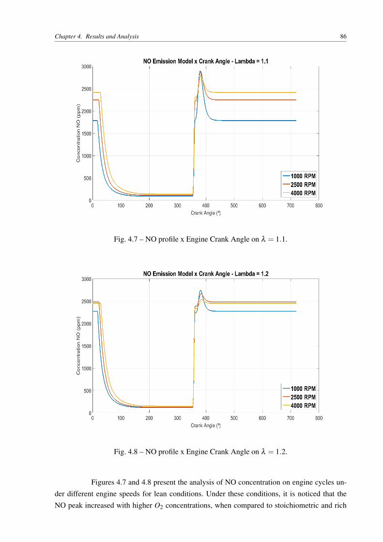
Chapter 4. Results and Analysis 86
Fig. 4.7 – NO profile x Engine Crank Angle on λ = 1.1.
Fig. 4.8 – NO profile x Engine Crank Angle on λ = 1.2.
Figures 4.7 and 4.8 present the analysis of NO concentration on engine cycles un-der different engine speeds for lean conditions. Under these conditions, it is noticed that theNO peak increased with higher O2 concentrations, when compared to stoichiometric and rich

Chapter 4. Results and Analysis 87
mixtures. Both peak and freeze NO concentrations increased on Figure 4.7 when comparedto Fig. 4.4. On 4000RPM, the peak concentration of nitric oxide increased from 2400ppm atλ = 1.0 to 2700ppm and the freeze concentration increased from 1800ppm to nearly 2400ppm.Other engine speeds showed similar behaviors. It is noticed that the NO reduction after peakconditions until the composition is frozen is lower on lean mixtures than it is detected in theother presented cases. The double effect of higher O2 concentrations together with high peaktemperatures optimizes the nitric oxide formation, yielded a point of maximum on slightly leanmixtures. On Figure 4.8 a similar behavior is found, but with smaller peaks than found on theλ = 1.1 case. The temperature effect here presented a smaller effect when related to the higheramount of oxygen available. For leaner mixtures than λ = 1.1, the increase of O2 concentrationin the mixture collaborates to a reduction of NO concentrations, since its increase beyond thispoint does not collaborate to a more efficient combustion process and therefore a reduction ofthe peak temperature is found, which reduces the amount of NO formed.
Now the analysis extends to the behavior of carbon monoxide on the engine cycle.Figure 4.9 presents the profile of CO under stoichiometric conditions and on three differentengine speeds; the same cases commented earlier on the nitric oxide analysis. Such as the nitricoxide case, (ANNAND, 1974) and (NEWHALL, 1969) may be found to compare CO curves,which presented similar results, despite the different geometries and fuels. Carbon monoxideshows a similar behavior that was described on NO. It is increased its concentration duringcombustion process until a peak is achieved. Then, it starts to fall down until freezing conditionsis achieved or the open phase (exhaust valve opens) initiates. CO consumption is stronger thanit is noticed on NO case, decreasing almost 5 times the amount achieved on peak conditions.
Studying the engine speed effect on Figure 4.9, it can be noticed that engine speeddo not have any effect on CO concentrations during the engine cycle. The three curves areoverlapped on each other in a way that no difference is detectable. This behavior was alreadycommented on (PATTERSON; HENEIN, 1974), which commented that CO suffers no influ-ence of this engine operation variable. The explanation for this behavior is based on the highertendency to equilibrium that carbon monoxide has if compared to NO. Its direct and reversereactions have similar orders of magnitude, instead of NO case. Therefore part of the CO pro-duced during higher temperature conditions is consumed, even though its value on freezingconditions is more similar to peak conditions than found on chemical equilibrium models.

Chapter 4. Results and Analysis 88
Fig. 4.9 – CO profile x Engine Crank Angle on Stoichiometric Condition.
The carbon monoxide analysis is extended for rich conditions. Figure 4.10 and 4.11represent the CO profile at λ = 0.9 and λ = 0.8 cases. On richer mixtures the CO concen-tration increased sharply, since incomplete combustion phenomenon is increased due to lowerO2 concentrations. CO peak increased from 26000ppm under stoichiometric conditions to al-most 40000ppm on 90% of the stoichiometric air-fuel ratio. The consumption is smaller than itwas calculated under stoichiometric conditions, which tends the frozen CO concentration to behigher (5000ppm to 24000ppm). On even richer cases, the values of peak and frozen CO arehigher than it was on previous studied cases. No effect of engine speed was detected on richerconditions.
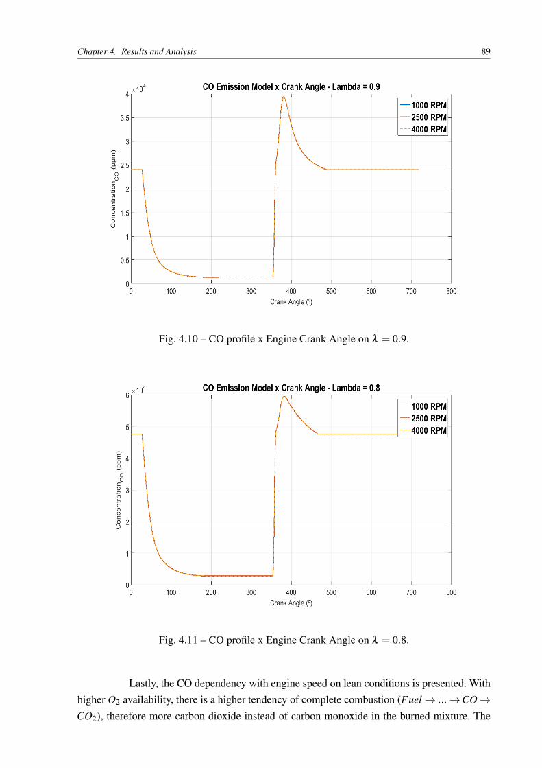
Chapter 4. Results and Analysis 89
Fig. 4.10 – CO profile x Engine Crank Angle on λ = 0.9.
Fig. 4.11 – CO profile x Engine Crank Angle on λ = 0.8.
Lastly, the CO dependency with engine speed on lean conditions is presented. Withhigher O2 availability, there is a higher tendency of complete combustion (Fuel → ...→CO →CO2), therefore more carbon dioxide instead of carbon monoxide in the burned mixture. The

Chapter 4. Results and Analysis 90
figure agrees with this expectation; lower concentrations of CO were calculated from lean mix-tures, as showed by Figures 4.12 and 4.13. Analyzing Figure 4.12 it is noticed that both the peakand frozen CO concentrations are lower than on stoichiometric mixtures, as presented earlier.The peak CO concentration reduced from 26000ppm to 16000ppm, while the frozen concen-tration reduced from nearly 5000ppm to almost 2000ppm. The reduction of CO peak to COfrozen concentrations (CO consumption) is considerably higher on leaner cases. The reductionindicated by Figure 4.12 is almost 8 times the peak concentration, while on Figure 4.13 it canbe detected a reduction of 9 times the peak CO concentration.
Fig. 4.12 – CO profile x Engine Crank Angle on λ = 1.1.
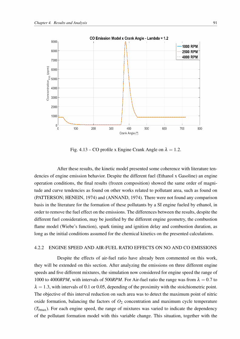
Chapter 4. Results and Analysis 91
Fig. 4.13 – CO profile x Engine Crank Angle on λ = 1.2.
After these results, the kinetic model presented some coherence with literature ten-dencies of engine emission behavior. Despite the different fuel (Ethanol x Gasoline) an engineoperation conditions, the final results (frozen composition) showed the same order of magni-tude and curve tendencies as found on other works related to pollutant area, such as found on(PATTERSON; HENEIN, 1974) and (ANNAND, 1974). There were not found any comparisonbasis in the literature for the formation of these pollutants by a SI engine fueled by ethanol, inorder to remove the fuel effect on the emissions. The differences between the results, despite thedifferent fuel consideration, may be justified by the different engine geometry, the combustionflame model (Wiebe’s function), spark timing and ignition delay and combustion duration, aslong as the initial conditions assumed for the chemical kinetics on the presented calculations.
4.2.2 ENGINE SPEED AND AIR-FUEL RATIO EFFECTS ON NO AND CO EMISSIONS
Despite the effects of air-fuel ratio have already been commented on this work,they will be extended on this section. After analyzing the emissions on three different enginespeeds and five different mixtures, the simulation now considered for engine speed the range of1000 to 4000RPM, with intervals of 500RPM. For Air-fuel ratio the range was from λ = 0.7 toλ = 1.3, with intervals of 0.1 or 0.05, depending of the proximity with the stoichiometric point.The objective of this interval reduction on such area was to detect the maximum point of nitricoxide formation, balancing the factors of O2 concentration and maximum cycle temperature(Tbmax). For each engine speed, the range of mixtures was varied to indicate the dependencyof the pollutant formation model with this variable change. This situation, together with the

Chapter 4. Results and Analysis 92
great amount of different engine speeds, provided a great amount of data to show the engineemission profile on both ranges of these variables. The result curves presented in this sectionwere compared with the curves available at (PATTERSON; HENEIN, 1974), which presenteda series of experimental comparisons relating engine parameters and pollutant emissions.
First presented analysis involves the extension of the relation between NO concen-tration on frozen conditions, which is the value that is emitted by the engine during exhauststroke on the simulator, with engine speeds and different mixtures. Figure 4.14 relates thesevariables in order to obtain a relation between them, under rich or stoichiometric mixtures. It isnoticed by the figure the connection between higher engine speeds with higher NO concentra-tions on frozen composition conditions. With exception of 1000RPM, all cases indicated a riseon the concentration with higher engine speeds. The inclination noticed from the plot betweennitric oxide emission and engine speed increases, which indicates that this relationship appearsstronger on higher revolutions. This is an indication of the strong influence of higher maximumburned zone temperatures and higher O2 concentrations on the unburned mixtures.
Fig. 4.14 – NO formation x Engine speed - Rich/Stoichiometric case.
On Figure 4.15, it is presented the same relationship of the previous figure, but onstoichiometric and lean cases. The behavior of this figure is quite different when compared to thelast one. The NO concentration present on frozen conditions still increases with higher enginespeeds, although the inclination appears to reduce when lean mixtures from λ = 1.1 to λ = 1.2are used. The maximum NO concentration for the studied case is obtained on 4000RPM, onλ = 1.15. This point had both factors (higher temperature profile and oxygen gas availability)
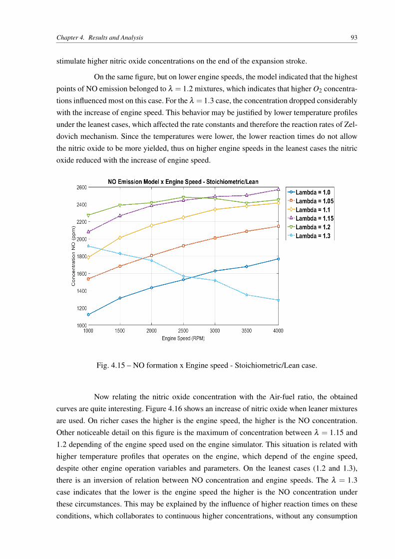
Chapter 4. Results and Analysis 93
stimulate higher nitric oxide concentrations on the end of the expansion stroke.
On the same figure, but on lower engine speeds, the model indicated that the highestpoints of NO emission belonged to λ = 1.2 mixtures, which indicates that higher O2 concentra-tions influenced most on this case. For the λ = 1.3 case, the concentration dropped considerablywith the increase of engine speed. This behavior may be justified by lower temperature profilesunder the leanest cases, which affected the rate constants and therefore the reaction rates of Zel-dovich mechanism. Since the temperatures were lower, the lower reaction times do not allowthe nitric oxide to be more yielded, thus on higher engine speeds in the leanest cases the nitricoxide reduced with the increase of engine speed.
Fig. 4.15 – NO formation x Engine speed - Stoichiometric/Lean case.
Now relating the nitric oxide concentration with the Air-fuel ratio, the obtainedcurves are quite interesting. Figure 4.16 shows an increase of nitric oxide when leaner mixturesare used. On richer cases the higher is the engine speed, the higher is the NO concentration.Other noticeable detail on this figure is the maximum of concentration between λ = 1.15 and1.2 depending of the engine speed used on the engine simulator. This situation is related withhigher temperature profiles that operates on the engine, which depend of the engine speed,despite other engine operation variables and parameters. On the leanest cases (1.2 and 1.3),there is an inversion of relation between NO concentration and engine speeds. The λ = 1.3case indicates that the lower is the engine speed the higher is the NO concentration underthese circumstances. This may be explained by the influence of higher reaction times on theseconditions, which collaborates to continuous higher concentrations, without any consumption

Chapter 4. Results and Analysis 94
of nitric oxide during the cycle.
An important detail about this kinetic model is that it does not consider the properphenomenons on extreme cases, such as on richer mixtures than λ = 0.7 and on leaner mixturesthan λ = 1.3. On these cases, misfire phenomenon may occur, which is not considered by themodel.
Fig. 4.16 – NO formation x Air-fuel ratio under several engine speeds.
On carbon monoxide case, first an extension of the relationship between CO con-centration on frozen conditions and engine speed is presented on Figure 4.17. Such as com-mented earlier on Figure 4.9, the engine speed presents almost no influence on CO formationand emission. Some variations that are presented on the plot may be related with computationalvariations from each case. The rise of lambda collaborates for lesser CO concentrations, as ex-pected and explained earlier. On lean cases, the concentrations were very low when comparedto the rich cases, then the plots almost superpose each other, showing that CO concentrationsbecome very low on these conditions.

Chapter 4. Results and Analysis 95
Fig. 4.17 – CO formation x Engine speed under several mixtures.
On Figure 4.18, CO concentration is related with air-fuel ratio instead of enginespeed. This plot is very clear in its conclusion: practically all the lines were the same on differentengine speeds. This figure presents another way to see the behavior already commented earlierfor CO. The range of concentrations vary from almost 85000ppm to 1000ppm, depending onthe O2 availability on the cylinder. This indicates how dependent CO is from rich mixtures -only a small amount is yielded on stoichiometric and lean cases.

Chapter 4. Results and Analysis 96
Fig. 4.18 – CO formation x Air-fuel ratio under several engine speeds.
4.2.3 SPARK TIMING EFFECTS ON NO AND CO EMISSIONS
The last theoretical variable analyzed in this work is the spark timing. Despite itsvariation changes other engine variables, it will be considered only its variation here, keepingconstant all other variables presented on Table 4.2. The objective here is to verify the sparktiming influence on the engine simulator, with respect to nitric oxide and carbon monoxideformations. Spark timing affects considerably the peak temperature, then it is expected that itinfluences the amount of these two regulated pollutants on peak and frozen conditions.
The simulation considered an engine speed of 3000RPM and a stoichiometric mix-ture while spark timing was changed. The range of spark timing varied from −30∘(330∘) to10∘(370∘), with increments of 5∘ in direction to TDC.
Figure 4.19 shows the relation between nitric oxide concentrations at frozen com-position versus spark timing. In most cases, NO concentration decreased with the retard of thespark timing, although its variation was not considerably high. The maximum and minimumvalues found for this analysis were at −25∘(335∘) (1640ppm) and at 5∘(365∘) (1475ppm).Inside the studied range, there were some fluctuations on the concentration of nitric oxide,which were against the apparent tendency of the curve; it was expected that at −25∘(335∘) and10∘(370∘) the NO concentration would reduce. This behavior happened because the model donot consider the influence of spark timing on other variables, such as ignition delay and com-bustion duration, as commented earlier. Other reason presented here is that with retard of thespark timing, there is also a reduction of reaction time until exhaust valve opens and a reduc-

Chapter 4. Results and Analysis 97
tion on the peak temperature of the cycle. While reaction time may collaborate to a higher NOformation or higher NO consumption (depending on the position of the spark timing), the peaktemperature influences on the temperature profile, which increases or reduces the temperatureswhich the burned mixture is affected. Thus, both factors change the behavior of NO mechanism.A more coherent analysis to evaluate the effect of spark timing must consider its influence onignition delay and combustion duration. Still, spark timing may still be studied on its own byconsidering its influence on the peak temperature and on reaction time.
Fig. 4.19 – NO formation x Spark timing on a stoichiometric mixture.
Analyzing the carbon monoxide relationship with spark timing (Figure 4.20), itis noticed that CO concentration increases with the retard of spark timing. Depending on thepoint, the CO concentration may even be doubled, such as the case at −25∘ and 10∘, whereCO concentrations varied from almost 4500ppm to nearly 9000ppm. This behavior happenedon the model because with the spark timing retard it reduces the peak temperature of the cyclebut it increases the temperature along the expansion stroke. This higher temperature duringthis engine phase increases the amount of carbon monoxide during angles close to the exhaustprocess. Therefore, higher concentrations were found on frozen conditions to the model.

Chapter 4. Results and Analysis 98
Fig. 4.20 – CO formation x Spark timing on a stoichiometric mixture.
To a better comparative analysis with literature of these pollutants with respect tospark timing, the engine model would require a better relation between this variable and otherengine variables, such as the cases of ignition delay and combustion duration, as it was al-ready commented. Since this analysis was just a theoretical one, only the effect of spark timingwas evaluated. Still, a qualitative relationship between this studied variable and the pollutantsstudied was obtained.
4.3 UHC-EMISSION MODEL ANALYSIS ON THE TWO-ZONE THERMODYNAMICENGINE SIMULATOR
The final theoretical analysis presented on this work is related to UHC emission onthe exhaust stroke of SI engines. This analysis is based on the model described on the method-ology section, i.e. considers only the crevice and flame quenching HC-formation mechanisms.
The objectives of this analysis are the following:
∙ To predict some coherent behaviors of the UHC concentration from SI engines, based onliterature results;
∙ To compare UHC emission under the influence of engine speed (RPM), actual air-fuelratio (Lambda) and spark timing.

Chapter 4. Results and Analysis 99
The initial conditions for the UHC models are provided by the two-zone enginemodel, which has already been mentioned on the text. The initial conditions to define the enginemodel are presented on Table 4.2. For this analysis, the engine was always on full load.
The influence of three engine variables was studied on the analysis: engine speed,actual air-fuel ratio (lambda) and the spark timing. Initially the effects of the engine speed andair-fuel ratio on UHC emission were analyzed. Then it was studied the influence of spark timingon the emissions of unburned hydrocarbons.
The results presented are qualitatively coherent with the expected UHC-emissionbehavior. For example, the order of magnitude of HC results is the same as described on theliterature (PATTERSON; HENEIN, 1974), despite the different fuel considered.
4.3.1 ENGINE SPEED AND AIR-FUEL RATIO EFFECTS ON UHC EMISSION MODEL
The first analysis studied the influence of the engine speed on the UHC concentra-tion emitted during the exhaust stroke. Figure 4.21 presents results for the full range of enginespeeds (1000RPM to 4000RPM) studied, under different mixtures. The values on the figure varyfrom 700ppm under rich mixtures to 250ppm on lean mixtures. It is noticed that the higher isthe engine speed, the lower is the mean UHC concentration emitted on the exhaust stroke. Thisbehavior agrees with reality since higher engine speeds increases turbulence, therefore it is ex-pected a better efficiency of combustion process. The model produces results coherently withthis assumption. Values for stoichiometric ratio change from almost 620ppm to nearly 420ppm,as speed increases. This tendency was verified with experimental plots presented by (PATTER-SON; HENEIN, 1974), where engine speeds and mixtures were changed and a linear curve waspresented. Converting the concentration to ppm, a comparison between literature and the modelmay be done. Despite the different fuels (C8H18 was used on the experimental data), the orderof magnitude of UHC emission from the model and from the experiment are the same (520ppm
(model) X 960ppm (literature)).
Since only a qualitatively prediction of UHC concentrations was the main objec-tive of this model, the values showed good agreement with the tendencies of the figure from(PATTERSON; HENEIN, 1974), on stoichiometric and lean mixtures. Rich mixtures involvemore physical effects, such as post-oxidation on expansion stroke, incomplete combustion onthe bulk gas, appropriate changes in quench thickness and crevice regions under these mixturesetc., which were not considered on this model. Therefore, it is expected some uncertainties onrich mixtures on the actual UHC model, although the qualitative tendencies are correct.

Chapter 4. Results and Analysis 100
Fig. 4.21 – UHC emission x Engine Speed under several different mixtures.
On Figure 4.22, the relationship of UHC and air-fuel ratio is presented, under differ-ent engine speeds. This figure shows that on rich mixtures there were low differences between0.7 and 0.8. This is a reflect of the absence of the other physical phenomenons not considered onthis model, as already commented. Still, on leaner mixtures the model shows a higher reductionsof UHC concentrations. On 3000RPM, the model predicted a variation between 550ppm at 0.7and almost 300ppm at 1.3. This represents the higher O2 availability on the mixtures, since itaffects directly the amount of HC on the unburned mixtures on crevice and quenching regions,as long as the peak pressure of the engine cycle. This figure also showed a better tendency tostoichiometric and lean mixtures, when compared to literature (PATTERSON; HENEIN, 1974),such as the case of Figure 4.21.
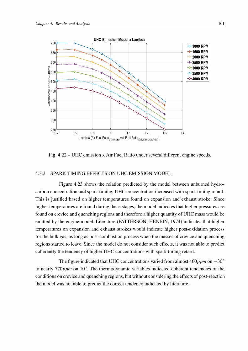
Chapter 4. Results and Analysis 101
Fig. 4.22 – UHC emission x Air Fuel Ratio under several different engine speeds.
4.3.2 SPARK TIMING EFFECTS ON UHC EMISSION MODEL
Figure 4.23 shows the relation predicted by the model between unburned hydro-carbon concentration and spark timing. UHC concentration increased with spark timing retard.This is justified based on higher temperatures found on expansion and exhaust stroke. Sincehigher temperatures are found during these stages, the model indicates that higher pressures arefound on crevice and quenching regions and therefore a higher quantity of UHC mass would beemitted by the engine model. Literature (PATTERSON; HENEIN, 1974) indicates that highertemperatures on expansion and exhaust strokes would indicate higher post-oxidation processfor the bulk gas, as long as post-combustion process when the masses of crevice and quenchingregions started to leave. Since the model do not consider such effects, it was not able to predictcoherently the tendency of higher UHC concentrations with spark timing retard.
The figure indicated that UHC concentrations varied from almost 460ppm on −30∘
to nearly 770ppm on 10∘. The thermodynamic variables indicated coherent tendencies of theconditions on crevice and quenching regions, but without considering the effects of post-reactionthe model was not able to predict the correct tendency indicated by literature.

Chapter 4. Results and Analysis 102
Fig. 4.23 – UHC emission x Spark Timing on a stoichiometric mixture.
4.4 THEORETICAL POLLUTANT PROFILE
The known behavior of the regulated pollutants (nitric oxide, carbon monoxide andunburned hydrocarbon) on spark-ignited engines is usually described by a figure which relatedtheir values with air-fuel ratio. Figure 4.24 (MERKER et al., 2014) showed a plot for thisdescription for an experimental engine with specific operation variables established.

Chapter 4. Results and Analysis 103
Fig. 4.24 – Regulated pollutant concentrations versus lambda. Ref.: (MERKER et al., 2014)
.
A similar figure was developed to show the tendencies of the pollutant models pre-sented in this work. Figure 4.25 shows the data presented on theoretical simulations commentedon this section. The engine conditions are the same as presented on Table 4.2.
NO and CO curves showed similarities with Merker’s curves, despite the differentengine conditions. The NO curve was calculated to lower air-fuel ratio (λ = 1.3) than it ispresented on (MERKER et al., 2014) and provided higher values on leaner cases. This behaviormay be justified by the higher compression ratio and Mean Effective Pressure on the simulatedcase, which consider higher temperatures on the kinetic scheme. CO curve presented a verysimilar curve on the whole range of mixtures, although values were very similar, in order ofmagnitude.
The UHC model curve have a different behavior than on Figure 4.24. On rich mix-tures the UHC model do not predict a great increase on UHC since it does not consider specificphenomenons of this mixture range, as previously commented. This curve, though, shows agood tendency on stoichiometric and lean mixtures, until 1.2. Leaner mixtures than this onemay cause the phenomenon of misfire, which is not considered by the engine model, whichjustifies the absence of increasing UHC concentrations on extreme lean mixtures.

Chapter 4. Results and Analysis 104
Fig. 4.25 – Pollutant complete emission diagram of the simulated case.
Therefore, Figure 4.25 presents qualitatively interesting results when compared toliterature. The behavior of the curves can be improved, becoming more similar to experimentalmeasurements or other models, if engine variables such as combustion duration, valve timings,ignition delay, etc. change together with the studied variables in a way that the behavior of thesimulator is more coherent with a real engine.
4.5 COMPARISON BETWEEN THE POLLUTANT MODELS AND EXPERIMEN-TAL DATA
The final case studied on this work is a comparison between pollutant emissionsfrom a experimental procedure undertaken on a spark-ignited engine and the respective emis-sions from the engine simulator. The objective of this comparison is to check how close theengine model predicts the emissions from a real engine, when the most similar conditions areused on the simulator.
The experimental trials were developed by Instituto Mauá de Tecnologia. The datafrom these procedures, besides performance and emission results were provided as a courtesyto this project.
Data from pollutant emission was only available for rich mixtures, therefore a com-parison between the experiment and the pollutant model was not able to be done under stoi-chiometric and lean mixtures. Eleven experiments on different engine speeds were developedon full load. Several engine parameters were obtained from each case and used on the enginemodel to approximate the most the behavior of the simulation with the real engine.

Chapter 4. Results and Analysis 105
The engine geometry parameters, compression ratio are the same as presented onTable 4.2. If any other data is not presented on the following tables, then its value is the sameas presented on this table.
4.5.1 DESCRIPTION OF EXPERIMENTAL DATA
Several variables from the experimental data were used as inputs on the engine sim-ulator. They include engine speed, lambda (λ =
AFexperimentAFstoichiometric
), environmental conditions, suchas environmental temperature, relative humidity, atmospheric pressure, etc. To consider atmo-spheric pressure changes, an average atmospheric pressure was considered on the calculations(Patm,exp = 92.75kPa). Exhaust thermodynamic conditions (exhaust pressure and temperature)were also used as data for the simulator.
Table 4.3 presents all data used on the simulator for low (≤ 3500RPM) enginespeeds:
Table 4.3 – Experimental engine variables - Low revolutions.
Experimental engine variables - Low revolutionsEngine Speed (RPM) 1000 1500 2000 2500 3000 3500
Lambda 0.901 0.899 0.870 0.874 0.892 0.865Relative Humidity (%) 83.2 50.9 80.3 68.4 50.8 71.6
Admission Temperature (∘C) 20.77 20.96 20.87 21.92 20.59 20.74Admission Vaccum (kPa) -1.15 -1.31 -1.48 -1.90 -2.68 -3.32Exhaust Temperature (∘C) 464.91 576.83 591.21 616.40 675.13 688.74
Exhaust Pressure (kPa) 2.21 4.38 5.56 8.99 12.50 14.49Spark Timing (∘T DC) -10.5 -11.5 -16 -18.5 -17.5 -19
Ignition Delay (∘) 6.5 12 12 10 10.5 9.5Combustion Duration (∘) 27.5 32.0 32.5 33.0 43.0 42.5Inlet Valve Opening (∘) 0 -5 -5 -10 -15 -20
Inlet Valve Operation (∘) 268 220 220 225 235 250Exhaust Valve Operation (∘) 268 220 220 225 235 275Exhaust Valve Closure (∘) 45 10 10 15 20 20
Table 4.4 presents the experimental data related to high (≥ 4000RPM) engine speeds:
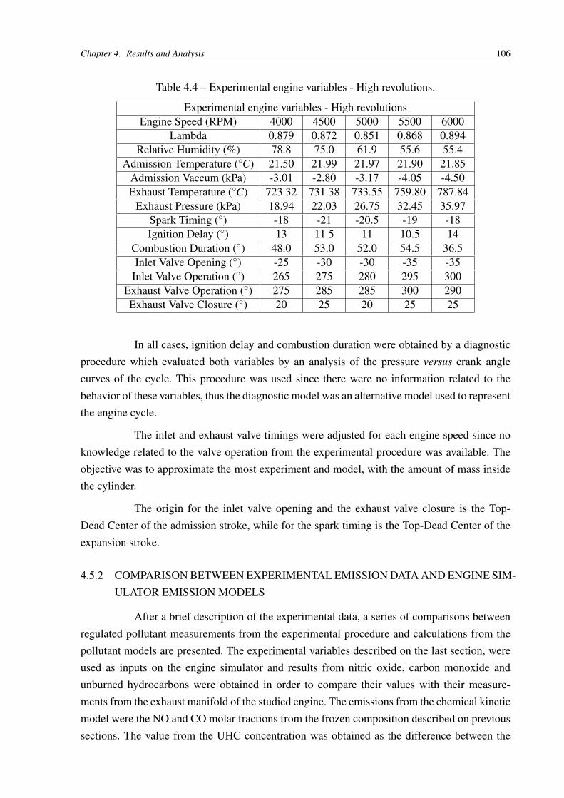
Chapter 4. Results and Analysis 106
Table 4.4 – Experimental engine variables - High revolutions.
Experimental engine variables - High revolutionsEngine Speed (RPM) 4000 4500 5000 5500 6000
Lambda 0.879 0.872 0.851 0.868 0.894Relative Humidity (%) 78.8 75.0 61.9 55.6 55.4
Admission Temperature (∘C) 21.50 21.99 21.97 21.90 21.85Admission Vaccum (kPa) -3.01 -2.80 -3.17 -4.05 -4.50Exhaust Temperature (∘C) 723.32 731.38 733.55 759.80 787.84
Exhaust Pressure (kPa) 18.94 22.03 26.75 32.45 35.97Spark Timing (∘) -18 -21 -20.5 -19 -18Ignition Delay (∘) 13 11.5 11 10.5 14
Combustion Duration (∘) 48.0 53.0 52.0 54.5 36.5Inlet Valve Opening (∘) -25 -30 -30 -35 -35
Inlet Valve Operation (∘) 265 275 280 295 300Exhaust Valve Operation (∘) 275 285 285 300 290Exhaust Valve Closure (∘) 20 25 20 25 25
In all cases, ignition delay and combustion duration were obtained by a diagnosticprocedure which evaluated both variables by an analysis of the pressure versus crank anglecurves of the cycle. This procedure was used since there were no information related to thebehavior of these variables, thus the diagnostic model was an alternative model used to representthe engine cycle.
The inlet and exhaust valve timings were adjusted for each engine speed since noknowledge related to the valve operation from the experimental procedure was available. Theobjective was to approximate the most experiment and model, with the amount of mass insidethe cylinder.
The origin for the inlet valve opening and the exhaust valve closure is the Top-Dead Center of the admission stroke, while for the spark timing is the Top-Dead Center of theexpansion stroke.
4.5.2 COMPARISON BETWEEN EXPERIMENTAL EMISSION DATA AND ENGINE SIM-ULATOR EMISSION MODELS
After a brief description of the experimental data, a series of comparisons betweenregulated pollutant measurements from the experimental procedure and calculations from thepollutant models are presented. The experimental variables described on the last section, wereused as inputs on the engine simulator and results from nitric oxide, carbon monoxide andunburned hydrocarbons were obtained in order to compare their values with their measure-ments from the exhaust manifold of the studied engine. The emissions from the chemical kineticmodel were the NO and CO molar fractions from the frozen composition described on previoussections. The value from the UHC concentration was obtained as the difference between the
Chapter 4. Results and Analysis 107
exhaust valve opening and closure, as explained on the methodology section.
The engine data presented here is referred to one of the engine cylinders. Sinceengine conditions change during experimental trials, these conditions may be different for eachcylinder. The engine conditions was chosen for the cylinder which presented the best and stablebehavior from all cylinders of the experimental engine.
All data originated from the experimental procedure are average measurements aftera certain number of cycles. These data may include some initial and final transient stages.Pollutant measurements were compared with the calculated lambda as long as the engine speedof the experimental procedure for each case.
Figure 4.26 presents the calculated results for nitric oxide from the engine simulatorwith the experimental data. It has the eleven cases presented on Tables 4.3 and 4.4. The figurealso contains the experimental measurements for NO on each case. Both NO calculated andexperimental concentrations were related with the engine speed of their cases. The uncertaintywas also considered on the figure and assumed here as 10% of each measurement.
The model predicted the order of magnitude of nitric oxide from the experimentalmeasurements in most cases, with exception for 1500, 3000 and 4000RPM. Especially, the 1500and 3000RPM experimental cases presented unusual behaviors on their results, which can rep-resent a change on the experimental engine operation. The engine simulator could not considerthis variable change, which explains the great discrepancy of the results. On the other hand, themodel showed good agreement with experimental measurements on high speeds (≥ 5000RPM),where the calculated NO concentration is inside the interval for the NO experimental measure-ment.

Chapter 4. Results and Analysis 108
Fig. 4.26 – Comparison pollutant model x experimental data - Nitric Oxide x engine speed.
Figure 4.27 compared the same nitric oxide data from the engine model and exper-iments, but it relates them with lambda. In most cases the calculated value for the model un-derestimated the measurements from the experimental data, with exception for the cases wherea good agreement were obtained. A possible reason for this behavior is the difference betweenthe amount of mass inside the cylinder on the experimental cases and the simulated ones. Sincethere was no information related to the valve timings, it was not possible to calibrate preciselythe same amount of mass inside the model cylinder. On this figure it is also possible to checkthat the model predicted the same tendencies of the experimental measurements.

Chapter 4. Results and Analysis 109
Fig. 4.27 – Comparison pollutant model x experimental data - Nitric Oxide x lambda.
Despite the considerable differences presented on some specific conditions, the NOmodel was able to correctly predict the same tendencies of the experimental measurements.The increase has not the same intensity as the experiments, however since the objective of thepresented models on this work are qualitative results, they seem to agree with a real engine NOemission behavior.
Carbon monoxide was also calculated on the engine model and compared with theexperimental data available. Figure 4.28 shows the CO concentrations from the chemical ki-netic model and the CO concentration measurements. In most cases the model was able tocalculate the CO concentration inside the experimental intervals of the gas. The exceptions forthis behavior are the cases of 1500 and 5000RPM. The model generally underestimated val-ues of carbon monoxide when they are compared to experimental ones. Only in 1500RPM themodel overestimated its concentration. The simulator presented almost the same tendencies asthe experimental data points, which indicated good agreement with reality.
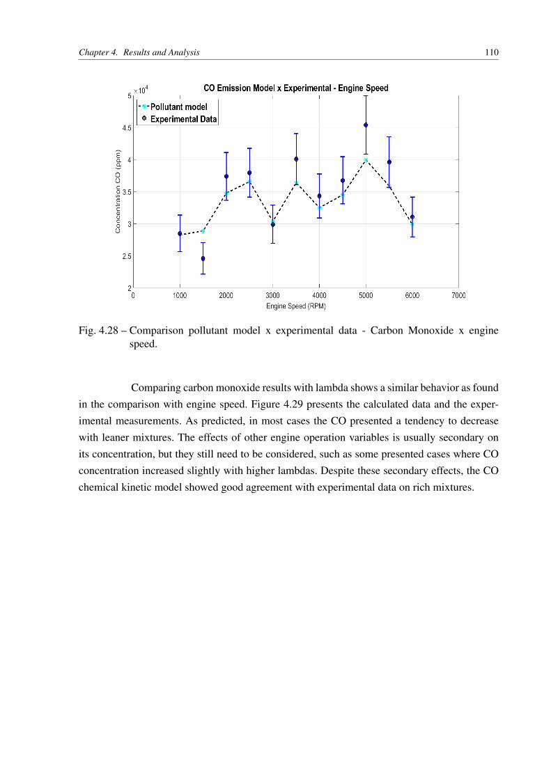
Chapter 4. Results and Analysis 110
Fig. 4.28 – Comparison pollutant model x experimental data - Carbon Monoxide x enginespeed.
Comparing carbon monoxide results with lambda shows a similar behavior as foundin the comparison with engine speed. Figure 4.29 presents the calculated data and the exper-imental measurements. As predicted, in most cases the CO presented a tendency to decreasewith leaner mixtures. The effects of other engine operation variables is usually secondary onits concentration, but they still need to be considered, such as some presented cases where COconcentration increased slightly with higher lambdas. Despite these secondary effects, the COchemical kinetic model showed good agreement with experimental data on rich mixtures.

Chapter 4. Results and Analysis 111
Fig. 4.29 – Comparison pollutant model x experimental data - Carbon Monoxide x lambda.
The final study involves a comparative analysis of the unburned hydrocarbon emis-sion model with the UHC measurement data from the simulated cases. Figure 4.30 related calcu-lated average UHC concentration and experimental HC measurements with engine speed. TheUHC model overestimated the UHC concentrations in most cases, with exception of 1500RPM.While the range of the UHC model for this comparison was between almost 550ppm and930ppm, the range of the experimental trials varied from 220ppm and 920ppm. The modelagreed with experimental measurements on 2000 and 2500RPM and indicated a close value on3000RPM. Therefore, at medium speeds, the model showed similarity with experimental data.On low and high speeds, the model could not calculate precisely the results the experimentalprocedure, despite the model had indicated values on the same order of magnitude.

Chapter 4. Results and Analysis 112
Fig. 4.30 – Comparison pollutant model x experimental data - Unburned Hydrocarbons x en-gine speed.
A relation of UHC calculated and measured concentrations with lambda is also pre-sented. Figure 4.31 shows this relationship, where most of the hydrocarbon concentrations fromexperimental stayed below 600ppm, while calculated concentrations were mostly over 600ppm.Both the linear relationship for the crevice model and the quench thickness model could not pre-dict correctly the variation of UHC emission. Still, a qualitative result was obtained, which wasthe objective of this simple model.
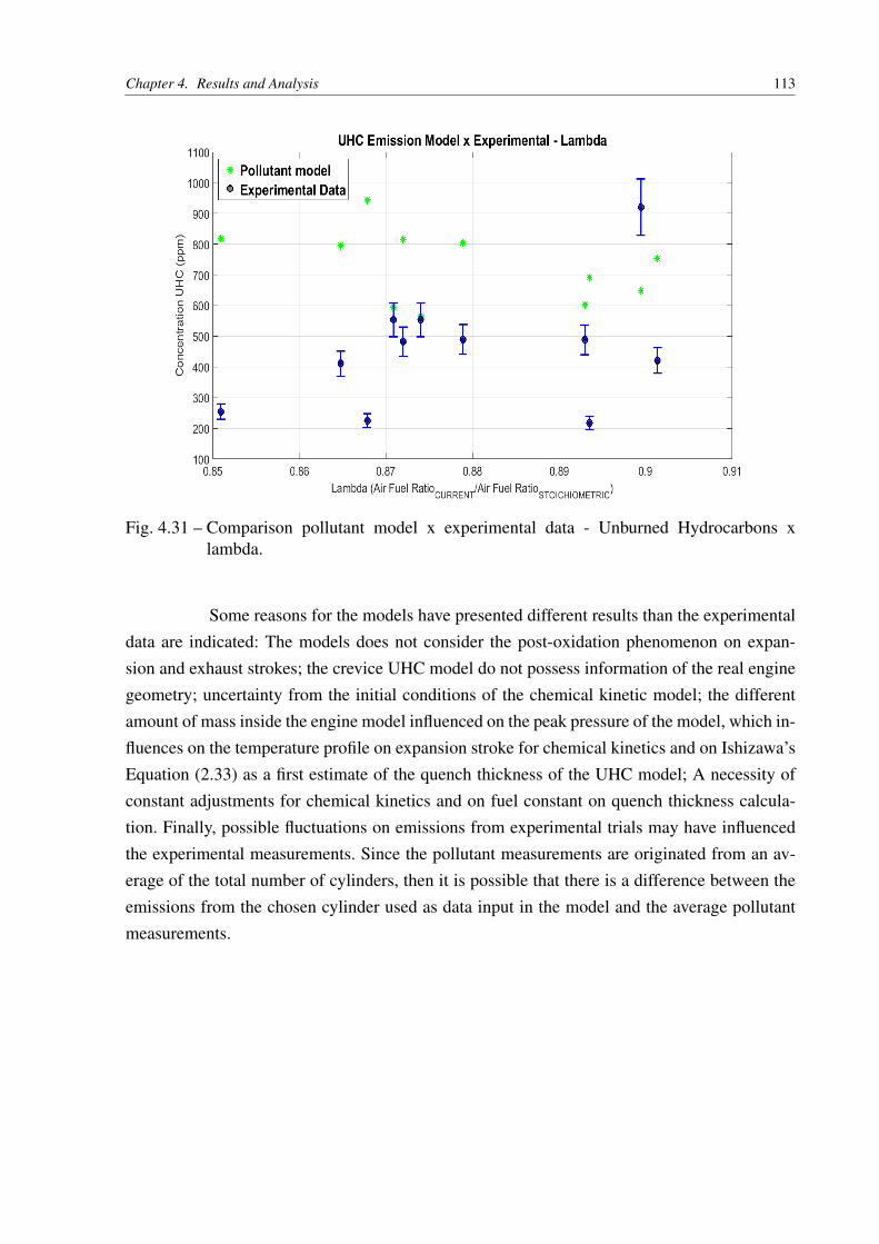
Chapter 4. Results and Analysis 113
Fig. 4.31 – Comparison pollutant model x experimental data - Unburned Hydrocarbons xlambda.
Some reasons for the models have presented different results than the experimentaldata are indicated: The models does not consider the post-oxidation phenomenon on expan-sion and exhaust strokes; the crevice UHC model do not possess information of the real enginegeometry; uncertainty from the initial conditions of the chemical kinetic model; the differentamount of mass inside the engine model influenced on the peak pressure of the model, which in-fluences on the temperature profile on expansion stroke for chemical kinetics and on Ishizawa’sEquation (2.33) as a first estimate of the quench thickness of the UHC model; A necessity ofconstant adjustments for chemical kinetics and on fuel constant on quench thickness calcula-tion. Finally, possible fluctuations on emissions from experimental trials may have influencedthe experimental measurements. Since the pollutant measurements are originated from an av-erage of the total number of cylinders, then it is possible that there is a difference between theemissions from the chosen cylinder used as data input in the model and the average pollutantmeasurements.
114
5 CONCLUSION
The presented study investigated the formation of pollutants on spark-ignited en-gines fueled with hydrated ethanol. The objective of this work was to analyze and developqualitative pollutant formation models for some regulated pollutants and input these models ina thermodynamic two-zone spark ignited engine model. This engine model considers enginegeometry, heat transfer models, valve timings, thermodynamic properties, besides other ade-quate models in order to calculate the engine cycle and its performance under specific engineoperation conditions and the pollutant model is one of these model packages. The consideredgases on the pollutant models were nitric oxide (NO), carbon monoxide (CO) and unburnedhydrocarbons (UHC).
In order to learn and develop specific pollutant models to each of the studied pol-lutant gases, a literature review about these subjects was undertaken. An approach to calculateNO and CO is to calculate their formation by a chemical kinetic model. In order to achievean adequate balance between computer speed and robustness on the model, a reduced reactionmechanism with 22 chemical reactions and 12 chemical species was chosen to calculate the for-mation of these gases. The chemical kinetic system of differential equations was solved by animplicit trapezoidal method, which is completely stable and provided relatively quick solutionsfor the engine simulator.
UHC formation was calculated by simple thermodynamic assumptions based onsome HC formation mechanisms in SI engines. Simple crevice and flame quenching thicknessmodels were prepared in order to qualitatively calculate the amount of UHC on the exhaustvalve opening and closure and then to indicate the UHC concentration emitted by the enginemodel.
The first analysis of this work dealt with a simple air-dissociation analysis, basedon chemical kinetics, with the objective of previously simulate the formation of nitric oxideunder thermodynamic conditions similar to an SI engine. It was shown that as commented onliterature, the NO kinetics is only considerable on temperatures higher than 1800K.
The second analysis studied the full reaction mechanism behavior inside the en-gine model. Chemical kinetics was considered on combustion and expansion strokes, wherethe composition of the gases changed until a frozen temperature was achieved in the end ofthe expansion process. The first study involved the analysis of the formation profiles of nitricoxide and carbon monoxide on the engine simulator. In order to analyze the influence of engineoperation variables on the pollutant model, besides to check the model’s robustness, a secondstudy was undertaken with a sensitivity analysis on these engine operation variables. NO andCO results for these simulations indicated similar tendencies with experimental measurements.

Chapter 5. Conclusion 115
The UHC simple models were also evaluated on both studies, where the emitted UHC concen-trations were calculated on the exhaust stroke and their tendencies compared with literature andexperimental measurements.
Final case involved a comparison between the pollutant model on the engine simu-lator with experimental data of a specific SI engine. Several engine variables were consideredin order to simulate as close as possible the engine real behavior. All pollutant models wereable to indicate results with the same order of magnitude of the experimental measurements.NO results indicated good agreement with the tendencies of experimental measurements. COresults have the same behavior, but also agreed with the quantitative measurements. On theother hand, UHC models seemed to be very simple to show coherent tendency, although it isnecessary to consider the absence of important factors which harm these model’s results, suchas the absence of information related to crevice region geometry and the unknown valve timingsof the experimental engine, which affect the amount of mass on the simulations.
Therefore, in most cases the pollutant models showed good agreement with litera-ture indications, especially considering that the objective of the work was to qualitatively predictthe formation of these pollutants. Both chemical kinetic and UHC models can be improved inspecific characteristics, such as an adequate relation between them and specific engine vari-ables, although they are already useful in calculating the amount of emission a specific enginecondition will emit. The models, with proper adjustments, may be used to predict the emissionbehavior that an engine would have if specific technologies were connected with it, such asEGR and turbocharging. They would be able to check the positive and negative effects of eachtechnology, avoiding the necessity of the construction of an engine prototype, which wouldavoid several costs to a company, for example.
Some future work indications may be presented from this work. On the chemicalkinetic model, other initial conditions for the gases entering the burned zone may be checkedand compared with actual results, in order to discover more realistic conditions to the initialcombustion process and refine the NO and CO formation. An expansion of the reaction mech-anism may be required if a refinement of the results or other species are going to be studied.NO2 and aldehydes are some suggestions of chemical species which would enrich the model.On UHC formation models, the engine crevice geometry must be considered on the model inorder to refine and correctly predicts the amount of unburned gases are in these regions. TheHeywood crevice mechanism (HEYWOOD; NAMAZIAN, 1982) would be a great addition tothe UHC model, since it considers the engine dynamics on the crevice regions. A refinementof the flame quench mechanism would provide a great refinement on the results of this model,especially considering an adequate application of the Ishizawa Equation. A full-cycle analysisof the UHC quench thickness would provide the full story of the UHC concentration on theengine model, which would allow to predict different UHC concentration emissions during theexhaust stroke, not only a difference between exhaust valve opening and closure.

116
REFERENCES
ADAMCZYK, A. A. et al. An experimental study of hydrocarbon emissions from closedvessel explosions. Symposium (International) on Combustion, v. 18, n. 1, p. 1695–1702,1981. ISSN 00820784.
ANNAND, W. J. D. B. Effects Of Simplifying Kinetic Assumptions In Calculating NitricOxide Formation In Spark-Ignition Engines. Proceedings of the Institution of MechanicalEngineers, v. 188, n. 1, p. 431–436, 1974.
BAULCH, D. et al. Evaluated kinetic data for combusion modelling. Supplement I. 1994.Disponível em: <http://kinetics.nist.gov/kinetics/Detail?id=1994BAU/COB847-1033:101>.
BAULCH, D. L. et al. Evaluated kinetic data for combustion modelling. Journal ofPhysical and Chemical Reference Data, v. 21, n. 3, p. 411–734, 1992. Disponível em:<http://dx.doi.org/10.1063/1.555908>.
BENSON, R.; ANNAND, W. J. D. B.; BARUAH, P. A simulation model including intake andexhaust systems for a single cylinder four-stroke cycle spark ignition engine. InternationalJournal of Mechanical Sciences, v. 17, n. 2, p. 97–124, 1975. ISSN 00207403. Disponívelem: <http://linkinghub.elsevier.com/retrieve/pii/0020740375900028>.
BENSON, S. W. The foundations of chemical kinetics. 1st. ed. McGraw-Hill, 1960.732 p. ISSN 00160032. Disponível em: <http://linkinghub.elsevier.com/retrieve/pii/0016003260903057>.
BOWMAN, C. T. Kinetics of pollutant formation and destruction in combustion. Progress inEnergy and Combustion Science, v. 1, n. 1, p. 33–45, jan 1975. ISSN 03601285. Disponívelem: <http://www.sciencedirect.com/science/article/pii/0360128575900052>.
BRINKMAN, N. D. Ethanol Fuel – A single-cylinder engine study of efficiency and exhaustemissions. SAE Technical Paper, 1981.
BURDEN, R. L.; FAIRES, A. G. Numerical Analysis. [S.l.]: Cencage Learning, 2013. v. 53.1 – 895 p. ISSN 1098-6596. ISBN 9788578110796.
CHENG, W. K. et al. An overview of hydrocarbon emissions mechanisms in spark-ignition engines. In: SAE Technical Paper. SAE International, 1993. Disponível em:<http://dx.doi.org/10.4271/932708>.
DANIEL, W. A. Flame quenching at the walls of an internal combustion engine. Symposium(International) on Combustion, v. 6, n. 1, p. 886–894, 1957. ISSN 00820784.
Dias de Oliveira, M. E.; VAUGHAN, B. E.; RYKIEL, E. J. Ethanol as fuel: energy, carbondioxide balances, and ecological footprint. BioScience, v. 55, n. 7, p. 593–602, 2013.
ELMQVIST, C. et al. Optimizing Engine Concepts by Using a Simple Model for KnockPrediction. SAE Technical Paper, n. 2003-01-3123, 2003. ISSN 0148-7191. Disponível em:<http://www.sae.org/technical/papers/2003-01-3123>.
EPE. Balanço Energético nacional 2016: Ano base 2015. Rio de Janeiro, 2016. 62 p.Disponível em: <www.epe.gov.br>.
References 117
EPE. Brazilian Energy Balance 2016. Rio de Janeiro, 2016. 296 p. Disponível em:<www.epe.gov.br>.
EYZAT, P.; GUIBET, J. A New Look at Nitrogen Oxides Formation in Internal CombustionEngines. SAE Technical Paper, n. 680124, 1968.
FENIMORE, C. Formation of nitric oxide in premixed hydrocarbon flames. Symposium(International) on Combustion, v. 13, n. 1, p. 373 – 380, 1971. ISSN 0082-0784. Thirteenthsymposium (International) on Combustion. Disponível em: <http://www.sciencedirect.com/science/article/pii/S0082078471800401>.
FERGUSON, C. R.; KECK, J. C. On laminar flame quenching and its application to sparkignition engines. Combustion and Flame, v. 28, n. C, p. 197–205, 1977. ISSN 00102180.
FERGUSON, C. R.; KIRKPATRICK, A. T. Internal Combustion Engines - AppliedThermosciences. 2nd. ed. [S.l.]: John-Wiley & Sons, 2001. 384 p. ISBN 0-471-35617-4.
GLASSMAN, I. Combustion. 4th. ed. Burlington: Elsevier, 2008. v. 1. ISBN 9780120885732.
Governo do Brasil. Percentual obrigatório de biodiesel no óleo diesel passa para8%. 2017. Disponível em: <http://www.brasil.gov.br/economia-e-emprego/2017/03/percentual-obrigatorio-de-biodiesel-no-oleo-diesel-passa-para-8>.
HEYWOOD, J. B. Internal Combustion Engines Fundamentals. 1st. ed. [S.l.]:McGraw-Hill, 1988. ISBN 0-07-028637-x.
HEYWOOD, J. B.; NAMAZIAN, M. Flow in the Piston-Cylinder-Ring Crevices of aSpark-ignition Engine; Effect on Hydrocarbon Emissions, Efficiency and Power. SAETechnical Paper, n. 820088, p. 28, 1982.
HULS, T. A.; NICKOL, H. A. Influence of Engine Variables on Exhaust Oxides of NitrogenConcentrations from a Multicylinder Engine. SAE Technical Paper, n. 670482, 1967.
ISHIZAWA, S. An experimental study on quenching crevice widths in the combustion chamberof a spark-ignition engine. Symposium (International) on Combustion, v. 26, n. 2, p.2605–2611, 1996. ISSN 00820784.
KEE, R. J.; COLTRIN, M. E.; GLARBORG, P. Chemically reacting flow : theory andpractice. [S.l.: s.n.], 2003. 848 p. ISBN 9780471261797.
KUO, K. Principles of Combustion. 2nd. ed. Hoboken: John-Wiley & Sons, 2005. 732 p.ISBN 0-471-04689-2.
LAIDLER, K. Chemical Kinetics. 3rd. ed. [S.l.]: Pearson, 1987. 540 p. ISBN 978-81-317-0972-6.
LAVOIE, G. A.; BLUMBERG, P. N. A Fundamental Model for Predicting Fuel Consumption,NOx and HC Emissions of the Conventional Spark-Ignited Engine. Combustion Scienceand Technology, v. 21, n. 5-6, p. 225–258, 1980. ISSN 0010-2202. Disponível em:<http://www.tandfonline.com/doi/abs/10.1080/00102208008946939>.
LAVOIE, G. A.; HEYWOOD, J. B.; KECK, J. C. Experimental and Theoretical Study of NitricOxide Formation in Internal Combustion Engines. Combustion Science and Technology, v. 1,n. 4, p. 313–326, 1970. ISSN 0010-2202.

References 118
LI, Y.; GUO, H.; LI, H. Evaluation of kinetics process in cfd model and its application inignition process analysis of a natural gas-diesel dual fuel engine. In: WCXTM 17: SAEWorld Congress Experience. SAE International, 2017. ISSN 0148-7191. Disponível em:<https://doi.org/10.4271/2017-01-0554>.
LISSIANSKI, V. et al. High-temperature measurements of the rate coefficient of the h + co2 =>co + oh reaction. Chemical Physics Letters, v. 240, n. 1, p. 57 – 62, 1995. ISSN 0009-2614.Disponível em: <http://www.sciencedirect.com/science/article/pii/000926149500496Q>.
LORUSSO, J. A.; KAISER, E. W.; LAVOIE, G. A. Quench Layer Contributionto Exhaust Hydrocarbons from a Spark-Ignited Engine. Combustion Science andTechnology, v. 25, n. 3-4, p. 121–125, 1981. ISSN 0010-2202. Disponível em: <http://www.tandfonline.com/doi/abs/10.1080/00102208108547511>.
MERKER, G. et al. Simulating Combustion: Simulation of combustion and pollutantformation for engine-development. [S.l.: s.n.], 2014. 1–5 p. ISSN 13514180. ISBN9780874216561.
MILLER, J. A.; BOWMAN, C. T. Mechanism and modeling of nitrogen chemistry incombustion. Progress in Energy and Combustion Science, v. 15, n. 4, p. 287–338, 1989.ISSN 03601285.
MILLER, R. et al. A Super-Extended Zel’dovich Mechanism for NOx Modeling and EngineCalibration. SAE Technical Paper, n. 980781, 1998.
NEBEL, G. J.; JACKSON, M. W. Some Factors Affecting the Concentration of Oxides ofNitrogen in Exhaust Gases from Spark Ignition Engines. APCA, 1958.
NETO, J. C. B. Simulação de Emissões de Misturas Gasolina/Etanol em Motores deCombustão Interna. Tese (Doutorado) — UFMG, 2012.
NEWHALL, H. K. Kinetics of engine-generated nitrogen oxides and carbon monoxide.Symposium (International) on Combustion, v. 12, n. 1, p. 603–613, 1969. ISSN 00820784.
NEWHALL, H. K.; SHAHED, S. M. Kinetics of nitric oxide formation in high-pressureflames. Symposium (International) on Combustion, v. 13, n. 1, p. 381–389, 1971. ISSN00820784.
NIGRO, F.; SZWARC, A. Ethanol as a Fuel. In: Ethanol and Bioelectricity Sugarcane in theFuture of the Energy Matrix. [S.l.: s.n.], 2011.
Nova Cana. Aplicações e usos do etanol. 2017. Disponível em: <https://www.novacana.com/etanol/aplicacoes/>.
Nova Cana. Tipos de Etanol Combustível. 2017. Disponível em: <https://www.novacana.com/etanol/tipos-combustivel/>.
PATTERSON, D.; HENEIN, N. Emissions from Combustion Engines and Their Control.1st. ed. Ann Arbor: Ann Arbor Science, 1974. 355 p. ISBN 0-250-97514-9.
RAGGI, M. V. K. Modelagem da Cinética Química de Formação de NoX e CO emMotores com Ignição por Centelha. Tese (Doutorado) — PUC-MG, 2005.
References 119
RINCON, L. Desenvolvimento e Aplicação de Modelos Cinéticos Detalhados para Etanole Combustíveis Hidrocarbonetos Contendo Etanol. Tese (Doutorado) — UFSC, 2009.
SANTOS, B. G. S. Simulador de Motores (uma abordagem termodinãmica dos sistemasde propulsão e geração de energia. 109 p. Tese (Doutorado) — ITA, 2011.
SODRÉ, J. R. Formulation and Experimental Validation of a Computer Model for SparkIgnition Engine Exhaust Hydrocarbons. Tese (Doutorado) — University of Manchester,1995.
SODRÉ, J. R. Modelling NOx emissions from spark-ignition engines. Proceedings of theInstitution of Mechanical Engineers, Part D: Journal of Automobile Engineering, v. 214,n. x, p. 929–935, 2000.
SPADACCINI, L. J.; CHINITZ, W. An lnvestigation of Nonequilibrium Effects in an InternalCombustion Engine. ASME, v. 11, 1972.
STEIN, R. A.; ANDERSON, J. E.; WALLINGTON, T. J. An Overview of the Effects ofEthanol-Gasoline Blends on SI Engine Performance, Fuel Efficiency, and Emissions. SAEInternational Journal of Engines, v. 6, n. 1, p. 2013–01–1635, 2013. ISSN 1946-3944.Disponível em: <http://papers.sae.org/2013-01-1635/>.
TABACZYNSKI, R. J.; HEYWOOD, J. B.; KECK, J. C. Time-resolved measurements ofhydrocarbon mass flowrate in the exhaust of a spark-ignition engine. In: SAE TechnicalPaper. SAE International, 1972. Disponível em: <http://dx.doi.org/10.4271/720112>.
TÁVORA, F. L. História e Economia dos Biocombustíveis noBrasil. Brasilia, 2011. Disponível em: <https://www12.senado.leg.br/publicacoes/estudos-legislativos/tipos-de-estudos/textos-para-discussao/td-89-historia-e-economia-dos-biocombustiveis-no-brasil>.
TINAUT, F. V.; MELGAR, a.; HORRILLO, a. J. Utilization of a Quasi-Dimensional Model forPredicting Pollutant Emissions in SI Engines. SAE Technical Paper 1999-01-0223, n. 724,2013.
TSANG, W.; HAMPSON, R. F. Chemical kinetic data base for combustion chemistry. part i.methane and related compounds. Journal of Physical and Chemical Reference Data, v. 15,n. 3, p. 1087–1279, 1986. Disponível em: <http://dx.doi.org/10.1063/1.555759>.
TURNS, S. R. An Introduction to Combustion. 2nd. ed. [S.l.]: McGraw-Hill, 2000. 700 p.ISBN 0-07-230096-5.
WARNATZ, J. 2O + M => O2 + M. 1984. Disponível em: <http://kinetics.nist.gov/kinetics/Detail?id=1984WAR197C:200>.
WARNATZ, J.; MAAS, U.; DIBBLE, R. Combustion: Physical and ChemicalFundamentals, Modeling and Simulation, Experiments, Pollutant Formation. 3rd. ed.[S.l.]: Springer, 2013. 389 p. ISSN 1098-6596. ISBN 9788578110796.
WAY, R. J. B. Methods for Determination of Composition and Thermodynamic Properties ofCombustion Products for Internal Combustion Engine Calculations. Combustion EnginesGroup, p. 11, 1976.

References 120
WENTWORTH, J. T. The Piston Crevice Volume Effect on Exhaust Hydrocarbon Emission.Combustion Science and Technology, v. 4, n. 1, p. 97–100, 1971. ISSN 0010-2202.Disponível em: <http://www.tandfonline.com/doi/abs/10.1080/00102207108952475>.
WESTBROOK; ADAMCZYK; LAVOIE. Numerical Study of Laminar Flame Wall Quenching.Combustion and Flame, v. 40, n. 1, p. 81–99, 1981. ISSN 00102180.
YANG, S. A preliminary research on turbulent flame propagation combustion modelingusing a direct chemical kinetics model. In: 11th International Conference on Enginesand Vehicles. SAE International, 2013. ISSN 0148-7191. Disponível em: <https://doi.org/10.4271/2013-24-0023>.
YETTER, R. A.; DRYER, F. L.; RABITZ, H. A Comprehensive Reaction Mechanism ForCarbon Monoxide / Hydrogen / Oxygen Kinetics. Combustion Science and Technology,v. 79, n. December 2012, p. 97–128, 1991.
ZEL’DOVICH, Y. B.; SADOVNIKOV, R. Y.; Frankkamenetsky, D. A. Nitrogen Oxidation inCombustion (In Russian). USSR Acad. Sci., 1947.
ZHANG, Y.; ZHAO, H. Overview of Centre for Advanced Powertrain and Fuels ( CAPF )at Brunel University London. 2012.