Embed Size (px)
Citation preview

0/21 J. R. Reuter Simplified Models for VBS LCWS 2014, Belgrade, 7.10.2014
High-Energy Vector Boson Scattering after theHiggs Discovery
Jürgen R. Reuter
DESY, Hamburg
in collaboration with: W. Kilian, T. Ohl, M. SekullaAlboteanu/Kilian/JRR, JHEP 0811 (2008) 010;
Beyer/Kilian/Krstonošic/Mönig/JRR/Schmitt/Schröder, EPJC 48 (2006), 353;JRR/Kilian/Sekulla, 1307.8170; Kilian/JRR/Ohl/Sekulla, 1408.6207 + in prep.
LCWS 2014, Belgrade, Oct. 7th, 2014

0/21 J. R. Reuter Simplified Models for VBS LCWS 2014, Belgrade, 7.10.2014
Acknowledgments
for providing the support for my research
Disacknowledgments
for not providing me with internet and phone for 57 days

0/21 J. R. Reuter Simplified Models for VBS LCWS 2014, Belgrade, 7.10.2014
Acknowledgments
for providing the support for my research
Disacknowledgments
for not providing me with internet and phone for 57 days

1/21 J. R. Reuter Simplified Models for VBS LCWS 2014, Belgrade, 7.10.2014
Motivation• Light Higgs boson found
• SM-like (clear from EWPO)
• Mediator of EWSB found
• Mechanism of EWSB still poorly understood:I single Higgs field vs. Higgs sectorI Higgs potential: stable vs. metastable vs. unstable !?I Higgs self-coupling vs. Higgs field scatteringI Importance of longitudinal EW gauge bosons
• Anomalous Triple Gauge Couplings: dibosons
• Anomalous Quartic Gauge Couplings: tribosons, VV scattering
• Higgs suppression makes VBS a prime candidate for BSM searches
• Hot topic: Snowmass BNL 04/13, SM@LHC Freiburg 04/13,LHCEWWG 04/13, Snowmass 07/13, Dresden 10/13, BNL workshop10/14
2/21 J. R. Reuter Simplified Models for VBS LCWS 2014, Belgrade, 7.10.2014
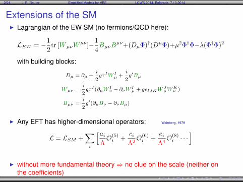
Extensions of the SMI Lagrangian of the EW SM (no fermions/QCD here):
LEW = −1
2tr [WµνW
µν ]−1
4BµνB
µν+(DµΦ)†(DµΦ)+µ2Φ†Φ−λ(Φ†Φ)2
with building blocks:
Dµ = ∂µ +i
2gτIW I
µ +i
2g′Bµ
Wµν =i
2gτI(∂µW
Iν − ∂νW I
µ + gεIJKWJµW
Kν )
Bµν =i
2g′(∂µBν − ∂νBµ)
I Any EFT has higher-dimensional operators: Weinberg, 1979
L = LSM +∑
i
[aiΛO(5)i +
ciΛ2O(6)i +
eiΛ4O(8)i · · ·
]
I without more fundamental theory⇒ no clue on the scale (neither onthe coefficients)
3/21 J. R. Reuter Simplified Models for VBS LCWS 2014, Belgrade, 7.10.2014
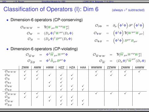
Classification of Operators (I): Dim 6 (always v2 subtracted)
• Dimension-6 operators (CP-conserving)
OWWW = Tr[WµνWνρWµ
ρ ]
OW = (DµΦ)†Wµν(DνΦ)
OB = (DµΦ)†Bµν(DνΦ)
O∂Φ = ∂µ(
Φ†Φ)∂µ(
Φ†Φ)
OΦW =(
Φ†Φ)
Tr[WµνWµν ]
OΦB =(
Φ†Φ)BµνBµν
• Dimension-6 operators (CP-violating)OWW
= Φ†WµνWµνΦ
OBB
= Φ†BµνBµνΦ
OWWW
= Tr[WµνWνρWµ
ρ ]
OW
= (DµΦ)†Wµν
(DνΦ)
ZWW AWW HWW HZZ HZA HAA WWWW ZZWW ZAWW AAWWOWWW X X X X X XOW X X X X X X X XOB X X X XOΦd X XOΦW X X X XOΦB X X XOWWW X X X X X XOW X X X X XOWW X X X XOBB X X X

4/21 J. R. Reuter Simplified Models for VBS LCWS 2014, Belgrade, 7.10.2014
Classification of Operators (II): Dim 8 (always v2 subtracted)
• Dimension-8 operators (only DµΦ)
OS,0 =[(DµΦ)
†DνΦ
]×[(Dµ
Φ)†DνΦ],
OS,1 =[(DµΦ)
†Dµ
Φ]×[(DνΦ)
†DνΦ],
• Dimension-8 operators (only field strength/mixed)
OT,0 = Tr[WµνW
µν] · Tr[WαβW
αβ],
OT,1 = Tr[WανW
µβ]· Tr[WµβW
αν],
OT,2 = Tr[WαµW
µβ]· Tr[WβνW
να],
OT,5 = Tr[WµνW
µν] · BαβBαβ ,OT,6 = Tr
[WανW
µβ]· BµβBαν ,
OT,7 = Tr[WαµW
µβ]· BβνBνα ,
OT,8 = BµνBµνBαβB
αβ
OT,9 = BαµBµβBβνB
να.
OM,0 = Tr[WµνW
µν] · [(DβΦ)†Dβ
Φ],
OM,1 = Tr[WµνW
νβ]·[(DβΦ)
†Dµ
Φ],
OM,2 =[BµνB
µν] · [(DβΦ)†Dβ
Φ],
OM,3 =[BµνB
νβ]·[(DβΦ)
†Dµ
Φ],
OM,4 =[(DµΦ)
†WβνD
µΦ]· Bβν ,
OM,5 =[(DµΦ)
†WβνD
νΦ]· Bβµ ,
OM,6 =[(DµΦ)
†WβνW
βνDµ
Φ],
OM,7 =[(DµΦ)
†WβνW
βµDνΦ],

5/21 J. R. Reuter Simplified Models for VBS LCWS 2014, Belgrade, 7.10.2014
Classification of Operators (III)WWWW WWZZ ZZZZ WWAZ WWAA ZZZA ZZAA ZAAA AAAA
OS,0/1 X X XOM,0/1/6/7 X X X X X X XOM,2/3/4/5 X X X X X XOT,0/1/2 X X X X X X X X XOT,5/6/7 X X X X X X X XOT,8/9 X X X X X
I Dim. 8 operators generate aQGCs, but not aTGCs
I generate neutral quarticsI Redundancy of the operators:
• Equations of motion: DµWµν = Φ†(DνΦ)− (DνΦ)†Φ + . . .
• Gauge symmetry structure: [Dµ, Dν ] Φ ∝WµνΦ• Integration by parts (up to total derivatives)• Leads to relations like:
OB = OW +1
2OWW −
1
2OBB
OBW = −2OW −OWW
O∂W = −4OWWW + gauge-fermion operators
6/21 J. R. Reuter Simplified Models for VBS LCWS 2014, Belgrade, 7.10.2014
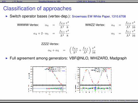
Classification of approachesI Switch operator bases (vertex-dep.): Snowmass EW White Paper, 1310.6708
WWWW-Vertex: α4 =fS,0
Λ4
v4
8
α4 + 2 · α5 =fS,1
Λ4
v4
8
WWZZ-Vertex: α4 =fS,0
Λ4
v4
16
α5 =fS,1
Λ4
v4
16
ZZZZ-Vertex:
α4 + α5 =
(fS,0
Λ4+fS,1
Λ4
)v4
16
I Full agreement among generators: VBF@NLO, WHIZARD, Madgraph

6/21 J. R. Reuter Simplified Models for VBS LCWS 2014, Belgrade, 7.10.2014
Classification of approachesI Switch operator bases (vertex-dep.): Snowmass EW White Paper, 1310.6708
WWWW-Vertex: α4 =fS,0
Λ4
v4
8
α4 + 2 · α5 =fS,1
Λ4
v4
8
WWZZ-Vertex: α4 =fS,0
Λ4
v4
16
α5 =fS,1
Λ4
v4
16
ZZZZ-Vertex:
α4 + α5 =
(fS,0
Λ4+fS,1
Λ4
)v4
16
I For the rest concentrate on:
LHD =FHD tr
[H†H− v2
4
]· tr[(DµH)
†(DµH)
]
LS,0 =FS,0 tr[(DµH)
†DνH
]· tr[(DµH)
†DνH
]
LS,1 =FS,1 tr[(DµH)
†DµH
]· tr[(DνH)
†DνH
]
7/21 J. R. Reuter Simplified Models for VBS LCWS 2014, Belgrade, 7.10.2014
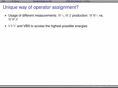
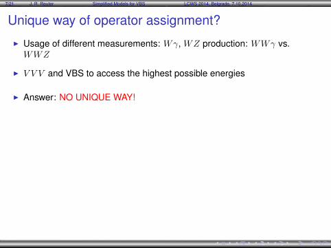
Unique way of operator assignment?
I Usage of different measurements: Wγ, WZ production: WWγ vs.WWZ
I V V V and VBS to access the highest possible energies
I Answer: NO UNIQUE WAY!
I But: at e+e− machines, gauge-fermion operators can be rotated away
I At LHC this is not possible! Buchalla et al., 1302.6481
I There is no common operator basis for V + jets, V V , V V V and VBSat LHC
I Incoherent sum of channels at LHC prevent eliminating operators!
I Similar to B physics: observables process [decay] specific
7/21 J. R. Reuter Simplified Models for VBS LCWS 2014, Belgrade, 7.10.2014
Unique way of operator assignment?
I Usage of different measurements: Wγ, WZ production: WWγ vs.WWZ
I V V V and VBS to access the highest possible energies
I Answer: NO UNIQUE WAY!
I But: at e+e− machines, gauge-fermion operators can be rotated away
I At LHC this is not possible! Buchalla et al., 1302.6481
I There is no common operator basis for V + jets, V V , V V V and VBSat LHC
I Incoherent sum of channels at LHC prevent eliminating operators!
I Similar to B physics: observables process [decay] specific

8/21 J. R. Reuter Simplified Models for VBS LCWS 2014, Belgrade, 7.10.2014
Simplified Models for VBS (and VVV)
I Rise of amplitude (6/8-dim. operator) may be Taylor expansion of aresonance
I A priori: No idea which resonances exist and wherefrom
I Including a resonance in the model, there still may be further sourcesfor anomalous couplings (further resonances, Anonres(s), deviationfrom the Breit-Wigner shape, etc.)
I Beyond the resonance, the amplitude may eventually rise and needunitarization again.
Consequence:I Resonances in all accessible spin/isospin channelsI Couplings to the Higgs and gauge sectors are unrelated and arbitraryI Still include anomalous couplingsI Unitarization (later)

9/21 J. R. Reuter Simplified Models for VBS LCWS 2014, Belgrade, 7.10.2014
ResonancesOperator coefficients⇒ new physics scale Λ: αi = vk/Λk
I Operator normalization is arbitraryI Power counting can be intricate
New physics in electroweak sector:I Narrow resonances ⇒ particlesI Wide resonances ⇒ continuum
SU(2)c custodial symmetry (weak isospin, broken by hyperchargeg′ 6= 0 and fermion masses)
J = 0 J = 1 J = 2
I = 0 σ0 (Higgs ?) ω0 (γ′/Z ′ ?) f0 (Graviton ?)I = 1 π±, π0
(2HDM ?) ρ±, ρ0 (W ′/Z ′ ?) a±, a0
I = 2 φ±±, φ±, φ0 (Higgs triplet ?) — t±±, t±, t0
I I = 0: resonant in W+W− and ZZ scatteringI I = 1: resonant in W+Z and W−Z scatteringI I = 2: resonant in W+W+ and W−W− scattering
accounts for weakly and strongly interacting models

10/21 J. R. Reuter Simplified Models for VBS LCWS 2014, Belgrade, 7.10.2014
Example: a Scalar Resonance [Not counting φ with M = 126 GeV.]
I Mass Mσ.I Coupling to the Higgs sector (Higgs and longitudinal W/Z):
gσL(DµΦ)†(DµΦ)σ
I Coupling to the gauge sector (transversal W/Z):
gσT tr [WµνWµν ] σ
Possible Origin: 2HDM isosinglet (renormalizable)
gσL = O
(1
Mσ
)[tree], gσT = O
(1
4πMσ
)[loop]
Possible Origin: new strong interactions
gσL = O
(1
Mσ
)[tree], gσT = O
(1
Mσ
)[tree]
11/21 J. R. Reuter Simplified Models for VBS LCWS 2014, Belgrade, 7.10.2014
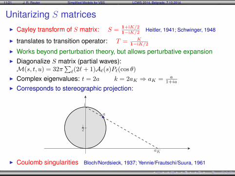
Unitarizing S matricesI Cayley transform of S matrix: S = 1+iK/2
1−iK/2 Heitler, 1941; Schwinger, 1948
I translates to transition operator: T = K1−iK/2
I Works beyond perturbation theory, but allows perturbative expansionI Diagonalize S matrix (partial waves):M(s, t, u) = 32π
∑`(2`+ 1)A`(s)P`(cos θ)
I Complex eigenvalues: t = 2a k = 2aK ⇒ aK = a1+ia
I Corresponds to stereographic projection:
i2
i
a
aK
I Coulomb singularities Bloch/Nordsieck, 1937; Yennie/Frautschi/Suura, 1961

12/21 J. R. Reuter Simplified Models for VBS LCWS 2014, Belgrade, 7.10.2014
Unitarization PrescriptionsI K-matrix unitarization prescription Gupta, 1950; Berger/Chanowitz, 1991
• Hermitian K-matrix interpreted as incompletely calculated approximationto true amplitude
• ⇒ Unitary S, T as a non-perturbativ completion of this approximation• Insert pert. expansion into expansion:
a = aK1−iaK
⇒ a(n) =a
(1)0 +Rea(2)
0 +...
1−i(a(1)0 +Rea(2)
0 +...)
• Prescription does a partial resummation of perturbative series• Example Dyson resummation: a(0)
K (s) = λs−m2 −→ a(0)(s) = λ
s−m2−iλ
I Drawbacks of (original) K-matrix:• Needs to construct self-adjoint K-matrix as intermediate step• Problem if S-matrix is not diagonal, or ...
there are non-perturbative contributions
I T -matrix unitarization• a0 complex approximation to eigenvalue of true T matrix• use again pseudo-stereographic projection (intersection of Argand circle
with line a0 i)
• Results in: a = Rea01−ia∗0
⇒ a(n) =a
(1)0 +Rea(2)
0 +...
1−i(a(1)0 +Rea(2)
0 −iIma(2)0 +...)

13/21 J. R. Reuter Simplified Models for VBS LCWS 2014, Belgrade, 7.10.2014
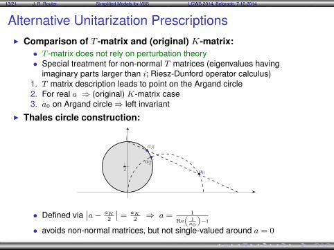
Alternative Unitarization PrescriptionsI Comparison of T -matrix and (original) K-matrix:
• T -matrix does not rely on perturbation theory• Special treatment for non-normal T matrices (eigenvalues having
imaginary parts larger than i; Riesz-Dunford operator calculus)1. T matrix description leads to point on the Argand circle2. For real a ⇒ (original) K-matrix case3. a0 on Argand circle⇒ left invariant
I Thales circle construction:
i2
i
a
aK
• Defined via∣∣a− aK
2
∣∣ = aK2⇒ a = 1
Re(
1a0
)−i
• avoids non-normal matrices, but not single-valued around a = 0

13/21 J. R. Reuter Simplified Models for VBS LCWS 2014, Belgrade, 7.10.2014
Alternative Unitarization PrescriptionsI Comparison of T -matrix and (original) K-matrix:
• T -matrix does not rely on perturbation theory• Special treatment for non-normal T matrices (eigenvalues having
imaginary parts larger than i; Riesz-Dunford operator calculus)1. T matrix description leads to point on the Argand circle2. For real a ⇒ (original) K-matrix case3. a0 on Argand circle⇒ left invariant
I Thales circle construction:
i2
i
a
aKaK2
• Defined via∣∣a− aK
2
∣∣ = aK2⇒ a = 1
Re(
1a0
)−i
• avoids non-normal matrices, but not single-valued around a = 0
13/21 J. R. Reuter Simplified Models for VBS LCWS 2014, Belgrade, 7.10.2014
Alternative Unitarization PrescriptionsI Comparison of T -matrix and (original) K-matrix:
• T -matrix does not rely on perturbation theory• Special treatment for non-normal T matrices (eigenvalues having
imaginary parts larger than i; Riesz-Dunford operator calculus)1. T matrix description leads to point on the Argand circle2. For real a ⇒ (original) K-matrix case3. a0 on Argand circle⇒ left invariant
I Thales circle construction:
i2
iaS
a0
aT
• Defined via∣∣a− aK
2
∣∣ = aK2⇒ a = 1
Re(
1a0
)−i
• avoids non-normal matrices, but not single-valued around a = 0
14/21 J. R. Reuter Simplified Models for VBS LCWS 2014, Belgrade, 7.10.2014
Unitarization Primer Kilian/JRR/Ohl/Sekulla, 1408.6207
I Unitarization prescription not unique
I Padé (reordering pert. series) introduces artificial poles
I Form factors parameterize close-by new physics (additionalparameters)
I minimal version (K or T matrix)⇒ just saturation no new parameters,does not rely on pert. expansion, stable against small perturbations
I Additional known features (resonances) should be implementedbefore unitarization

15/21 J. R. Reuter Simplified Models for VBS LCWS 2014, Belgrade, 7.10.2014
Unitary Description of EW interactionsI Five possible cases:
– Amplitude perturbative, close to zero, small imag. part (SM)– Amplitude rises, gets imag. part, strongly interacting regime (presence of
at least one dim. 8 operator)– Amplitude approaches maximum absolute value asymptotically– Turn over: new resonance– New inelastic channels open: eff. form factor, extra channels observable
in multi-vector boson processes
I Interpretation of EFT operator coefficients changes: formally stilllow-energy coefficients of Taylor expansion⇒ threshold parameters
I Complete description necessary (only) beyond threshold

16/21 J. R. Reuter Simplified Models for VBS LCWS 2014, Belgrade, 7.10.2014
Unitarity Bound for α4 AQGC
Bounds for α4
` = 0 :√s ≤
(6π
α4
) 14
v ≈ 0.5 TeV4√α4
` = 2 :√s ≤
(60π
α4
) 14
v ≈ 0.9 TeV4√α4
α4 AQGC contribution toWW → ZZ
A(s, t, u) = 4α4t2 + u2
v4
I Bound depends on coupling α4
I Use strongest bound

17/21 J. R. Reuter Simplified Models for VBS LCWS 2014, Belgrade, 7.10.2014
Diboson invariant masses
200 400 600 800 1000 1200 1400 1600 1800 2000
M(W+W+)[GeV]
10−4
10−3
10−2
10−1
100
101
∂σ
∂M
[fb
100G
eV
]
pp→ W+W+jj
FS,0 = 480 TeV−4
FS,1 = 480 TeV−4
FHD = 30 TeV−2
SM
200 400 600 800 1000 1200 1400 1600 1800 2000
M(W+W−)[GeV]
10−4
10−3
10−2
10−1
100
101
∂σ
∂M
[fb
100G
eV
]
pp→ W+W−jj
FS,0 = 480 TeV−4
FS,1 = 480 TeV−4
FHD = 30 TeV−2
SM
200 400 600 800 1000 1200 1400 1600 1800 2000
M(W+Z)[GeV]
10−4
10−3
10−2
10−1
100
101
∂σ
∂M
[fb
100G
eV
]
pp→ WZjj
FS,0 = 480 TeV−4
FS,1 = 480 TeV−4
FHD = 30 TeV−2
SM
200 400 600 800 1000 1200 1400 1600 1800 2000
M(ZZ)[GeV]
10−4
10−3
10−2
10−1
100
101
∂σ
∂M
[fb
100G
eV
]
pp→ ZZjj
FS,0 = 480 TeV−4
FS,1 = 480 TeV−4
FHD = 30 TeV−2
SM
General cuts: Mjj > 500 GeV; ∆ηjj > 2.4; pjT > 20 GeV; |ηj | < 4.5

18/21 J. R. Reuter Simplified Models for VBS LCWS 2014, Belgrade, 7.10.2014
pT and angular distributionspp→ e+µ+νeνµjj,
√=14 TeV, L = 1000 fb−1
Simulations with WHIZARD → JRR: Simulation
Not possible to use automated tool due to s-channel prescription
FHD = 30 TeV−2
0.5 1.0 1.5 2.0 2.5 3.0
∆φeµ
0
50
100
150
200
250
300
350
N
bare
unit
SM
500 1000 1500 2000∑l=e,µ |pT(l)|
100
101
102
103
104
N
bare
unit
SM
General cuts: Mjj > 500 GeV; ∆ηjj > 2.4; pjT > 20 GeV; |ηj | < 4.5, p`T > 20 GeV

18/21 J. R. Reuter Simplified Models for VBS LCWS 2014, Belgrade, 7.10.2014
pT and angular distributionspp→ e+µ+νeνµjj,
√=14 TeV, L = 1000 fb−1
Simulations with WHIZARD → JRR: Simulation
Not possible to use automated tool due to s-channel prescription
FS,0 = 480 TeV−4
0.5 1.0 1.5 2.0 2.5 3.0
∆φeµ
0
50
100
150
200
250
300
350
N
bare
unit
SM
500 1000 1500 2000∑l=e,µ |pT(l)|
100
101
102
103
104
N
bare
unit
SM
General cuts: Mjj > 500 GeV; ∆ηjj > 2.4; pjT > 20 GeV; |ηj | < 4.5, p`T > 20 GeV

18/21 J. R. Reuter Simplified Models for VBS LCWS 2014, Belgrade, 7.10.2014
pT and angular distributionspp→ e+µ+νeνµjj,
√=14 TeV, L = 1000 fb−1
Simulations with WHIZARD → JRR: Simulation
Not possible to use automated tool due to s-channel prescription
FS,1 = 480 TeV−4
0.5 1.0 1.5 2.0 2.5 3.0
∆φeµ
0
50
100
150
200
250
300
350
N
bare
unit
SM
500 1000 1500 2000∑l=e,µ |pT(l)|
100
101
102
103
104
N
bare
unit
SM
General cuts: Mjj > 500 GeV; ∆ηjj > 2.4; pjT > 20 GeV; |ηj | < 4.5, p`T > 20 GeV

19/21 J. R. Reuter Simplified Models for VBS LCWS 2014, Belgrade, 7.10.2014
And Triple Vector Boson Production?
relate to ??
Yes, the same Feynman graphs (in the SM), but. . .Tribosons:
• one external W/Z/γ is always far off-shell• Unitarization has to proceed differently• and a different set of (anomalous) couplings contributes• particularly true for resonances
⇒ Important physics which should be treated independently w.r.t. VBSprocesses. Don’t just combine the results!

20/21 J. R. Reuter Simplified Models for VBS LCWS 2014, Belgrade, 7.10.2014
Summary/ConclusionsI Triple/Quartic gauge couplings measured either
– via diboson production– via triple boson production– via vector boson scattering
I Unify LHC and ILC/CLIC descriptionsI SM deviations in EW effective Lagrangian (SM + higher-dim. op.)
I Want to set model independent limits AQGCI But: Energy range for testing AQGC is bound by UnitarityI Simplified Models: minimally unitarized operatorsI Unitarization scheme: no additional structure to the theoryI Unitarization introduces model dependence, but keeps
model-dependence under controlI Sensitivity rises with number of intermediate states:
– LHC sensitivity limited in pure EW sector: ∼ 1−X TeV (???)– ILC1000 : ∼ 1.5− 6 TeV
– (Tensor) Resonances very interesting Kilian/JRR/Sekulla, in preparation
– Guess: 1.4 / 3 TeV e+e− [+ pol. ?] optimal choice

20/21 J. R. Reuter Simplified Models for VBS LCWS 2014, Belgrade, 7.10.2014
Always get the correct ellipses...

20/21 J. R. Reuter Simplified Models for VBS LCWS 2014, Belgrade, 7.10.2014
BACKUP SLIDES

20/21 J. R. Reuter Simplified Models for VBS LCWS 2014, Belgrade, 7.10.2014
Cut-Off Method (a.k.a. “Event Clipping”)
Cut-Off functionΘ(Λ2C − s
)Cut-Off energy ΛC
ΛC equates unitarity bounds(often 0th partial wave)
I Naive prevention of Unitarityviolation
I No continuous transition atΛC
I Ignore any interestingphysics above Unitary bound
I Better: Use observables,which do not conflict unitaritycondition
0 1 2 3 40.0
0.5
1.0
s �H4 Π vL
AHsL¤

20/21 J. R. Reuter Simplified Models for VBS LCWS 2014, Belgrade, 7.10.2014
Form Factor
Form Factor1(
1 + sΛ2FF
)n
Parametersn Chosen to prevent breaking of
UnitarityΛFF Calculate highest possible value
that satisfy real Unitarity bound(0th partial wave )
I Use Form Factor to suppressbreaking of unitarity
I Can be generally used forarbitrary anomalous operator
I Need "Fine Tuning"0 1 2 3 4
0.0
0.5
1.0
s �H4 Π vL
AHsL¤
Unitarity bound
Unitarity broken
Form factor
Bare
21/21 J. R. Reuter Simplified Models for VBS LCWS 2014, Belgrade, 7.10.2014
K-Matrix
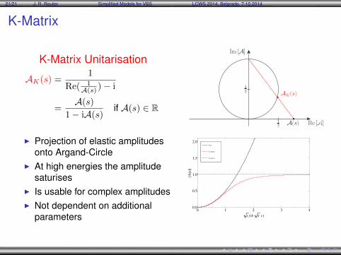
K-Matrix Unitarisation
AK(s) =1
Re( 1A(s) )− i
=A(s)
1− iA(s)if A(s) ∈ R
Im [A]
Re [A]A(s)
AK(s)12
12
I Projection of elastic amplitudesonto Argand-Circle
I At high energies the amplitudesaturises
I Is usable for complex amplitudesI Not dependent on additional
parameters0 1 2 3 4
0.0
0.5
1.0
1.5
2.0
s �H4 Π vL
AHsL¤
Saturation
K-Matrix
Bare

21/21 J. R. Reuter Simplified Models for VBS LCWS 2014, Belgrade, 7.10.2014
"Comparison"
I Which Unitarisation schemeprovides the best description?
→ All of them:Unitarisation schemes are anarbitrary way to guaranteeUnitarity
Form FactorI Suppression of amplitude to
get below Unitarity boundMC Generate less events than
possible
K-MatrixI Saturation of amplitude to
achieve UnitarityMC Generate maximal possible
number of events

21/21 J. R. Reuter Simplified Models for VBS LCWS 2014, Belgrade, 7.10.2014
Vector Boson Scattering Beyer et al.,hep-ph/0604048
1 TeV, 1 ab−1, full 6f final states, 80 % e−R , 60 % e+L polarization, binned likelihood
Contributing channels: WW →WW , WW → ZZ, WZ →WZ, ZZ → ZZ
Process Subprocess σ [fb]
e+e− → νeνeqqqq WW → WW 23.19e+e− → νeνeqqqq WW → ZZ 7.624e+e− → ννqqqq V → V V V 9.344e+e− → νeqqqq WZ → WZ 132.3e+e− → e+e−qqqq ZZ → ZZ 2.09e+e− → e+e−qqqq ZZ → W+W− 414.e+e− → bbX e+e− → tt 331.768e+e− → qqqq e+e− → W+W− 3560.108e+e− → qqqq e+e− → ZZ 173.221e+e− → eνqq e+e− → eνW 279.588e+e− → e+e−qq e+e− → e+e−Z 134.935e+e− → X e+e− → qq 1637.405
SU(2)c conserved case, all channelscoupling σ− σ+
16π2α4 -1.41 1.3816π2α5 -1.16 1.09
SU(2)c broken case, all channelscoupling σ− σ+
16π2α4 -2.72 2.3716π2α5 -2.46 2.3516π2α6 -3.93 5.5316π2α7 -3.22 3.3116π2α10 -5.55 4.55
16π2α5
16π2α4
16π2α5
16π2α4 16π2α6
16π2α7
21/21 J. R. Reuter Simplified Models for VBS LCWS 2014, Belgrade, 7.10.2014
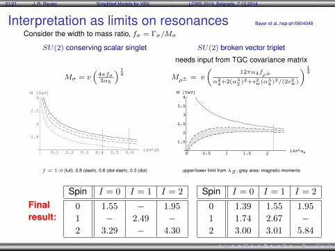
Interpretation as limits on resonances Beyer et al.,hep-ph/0604048
Consider the width to mass ratio, fσ = Γσ/Mσ
SU(2) conserving scalar singlet SU(2) broken vector triplet
needs input from TGC covariance matrix
Mσ = v(
4πfσ3α5
) 14
Mρ± = v
(12πα4fρ±
α24+2(αλ2 )2+s2w(αλ4 )2/(2c2w)
) 14
0.1 0.2 0.3 0.4 0.5 0.616Π2Α5
1.5
2
2.5
3M @TeVD
0.5 1 1.5 216Π2Α4
1.5
2
2.5
3
3.5
4M @TeVD
0.5 1 1.5 216Π2Α4
1.5
2
2.5
3
3.5
4M @TeVD
f = 1.0 (full), 0.8 (dash), 0.6 (dot-dash), 0.3 (dot) upper/lower limit from λZ , grey area: magnetic moments
Finalresult:
Spin I = 0 I = 1 I = 2
0 1.55 − 1.95
1 − 2.49 −2 3.29 − 4.30
Spin I = 0 I = 1 I = 2
0 1.39 1.55 1.95
1 1.74 2.67 −2 3.00 3.01 5.84
21/21 J. R. Reuter Simplified Models for VBS LCWS 2014, Belgrade, 7.10.2014
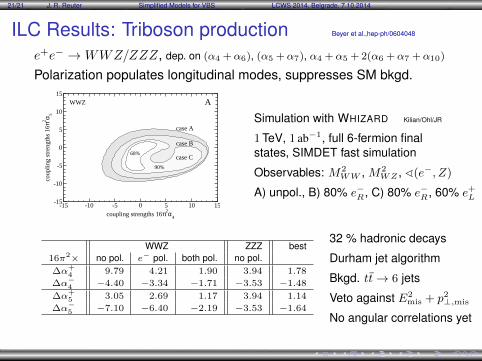
ILC Results: Triboson production Beyer et al.,hep-ph/0604048
e+e− →WWZ/ZZZ, dep. on (α4 +α6), (α5 +α7), α4 +α5 + 2(α6 +α7 +α10)
Polarization populates longitudinal modes, suppresses SM bkgd.
-15 -10 -5 0 5 10 15coupling strengths 16π2α
4
-15
-10
-5
0
5
10
15
coup
ling
stre
ngth
s 16
π2 α 5
WWZ
68%case C
A
case B
case A
90%
Simulation with WHIZARD Kilian/Ohl/JR
1 TeV, 1 ab−1, full 6-fermion finalstates, SIMDET fast simulation
Observables: M2WW , M2
WZ , ^(e−, Z)
A) unpol., B) 80% e−R, C) 80% e−R, 60% e+L
WWZ ZZZ best16π2× no pol. e− pol. both pol. no pol.∆α+
4 9.79 4.21 1.90 3.94 1.78
∆α−4 −4.40 −3.34 −1.71 −3.53 −1.48
∆α+5 3.05 2.69 1.17 3.94 1.14
∆α−5 −7.10 −6.40 −2.19 −3.53 −1.64
32 % hadronic decays
Durham jet algorithm
Bkgd. tt→ 6 jets
Veto against E2mis + p2
⊥,mis
No angular correlations yet
21/21 J. R. Reuter Simplified Models for VBS LCWS 2014, Belgrade, 7.10.2014
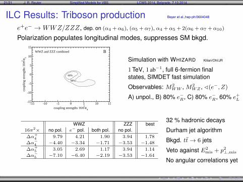
ILC Results: Triboson production Beyer et al.,hep-ph/0604048
e+e− →WWZ/ZZZ, dep. on (α4 +α6), (α5 +α7), α4 +α5 + 2(α6 +α7 +α10)
Polarization populates longitudinal modes, suppresses SM bkgd.
-15 -10 -5 0 5 10 15coupling strengths 16π2α
4
-15
-10
-5
0
5
10
15
coup
ling
stre
ngth
s 16
π2 α 5
WWZ and ZZZ combined
68%
B
90%
Simulation with WHIZARD Kilian/Ohl/JR
1 TeV, 1 ab−1, full 6-fermion finalstates, SIMDET fast simulation
Observables: M2WW , M2
WZ , ^(e−, Z)
A) unpol., B) 80% e−R, C) 80% e−R, 60% e+L
WWZ ZZZ best16π2× no pol. e− pol. both pol. no pol.∆α+
4 9.79 4.21 1.90 3.94 1.78
∆α−4 −4.40 −3.34 −1.71 −3.53 −1.48
∆α+5 3.05 2.69 1.17 3.94 1.14
∆α−5 −7.10 −6.40 −2.19 −3.53 −1.64
32 % hadronic decays
Durham jet algorithm
Bkgd. tt→ 6 jets
Veto against E2mis + p2
⊥,mis
No angular correlations yet

21/21 J. R. Reuter Simplified Models for VBS LCWS 2014, Belgrade, 7.10.2014
Effective EW Dim. 6 OperatorsHagiwara/Hikasa/Peccei/Zeppenfeld, 1987; Hagiwara/Ishihara/Szalapski/Zeppenfeld, 1993
−→ O(I)JJ =
1
Λ2tr[J (I) · J (I)
]
———————————————————————————————
−→O′h,1 = 1
F 2
((DΦ)†Φ
)·(h†(DΦ)
)− v2
2 |DΦ|2
O′hh = 1Λ2 (Φ†Φ− v2/2) (DΦ)† · (DΦ)
———————————————————————————————
−→ O′h,3 =1
Λ2
1
3(Φ†Φ−v2/2)3
21/21 J. R. Reuter Simplified Models for VBS LCWS 2014, Belgrade, 7.10.2014
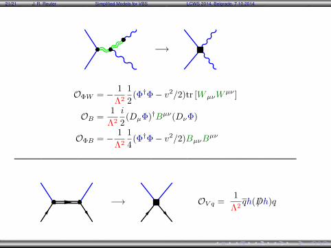
−→
OΦW = − 1
Λ2
1
2(Φ†Φ− v2/2)tr [WµνW
µν ]
OB =1
Λ2
i
2(DµΦ)†Bµν(DνΦ)
OΦB = − 1
Λ2
1
4(Φ†Φ− v2/2)BµνB
µν
———————————————————————————————
−→ OV q =1
Λ2qh( /Dh)q
21/21 J. R. Reuter Simplified Models for VBS LCWS 2014, Belgrade, 7.10.2014
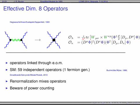
Effective Dim. 8 Operators
Hagiwara/Ishihara/Szalapski/Zeppenfeld, 1993
−→ Oλ = iΛ4 tr
[Wµν ×W νρ(Φ† ~σ2 [Dρ, D
µ] Φ)]
Oκ = (DµΦ)†(DνΦ)(Φ† [Dµ, Dν ] Φ)
———————————————————————————————
I operators linked through e.o.m.
I SM: 59 independent operators (1 fermion gen.) Buchmüller/Wyler, 1986;
Grzadkowski/Iskrzynski/Misiak/Rosiek, 2010
I Renormalization mixes operators
I Beware of power counting

21/21 J. R. Reuter Simplified Models for VBS LCWS 2014, Belgrade, 7.10.2014
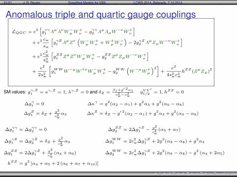
Anomalous triple and quartic gauge couplings
LTGC = ie
[gγ1Aµ
(W−ν W
+µν −W+νW
−µν)
+ κγW−µW
+ν A
µν+
λγ
M2W
W−µνW
+νρA
ρµ
]
+ iecw
sw
[gZ1 Zµ
(W−ν W
+µν −W+νW
−µν)
+ κZW−µW
+ν Z
µν+
λZ
M2W
W−µνW
+νρZ
ρµ
]
SM values: gγ,Z1 = κγ,Z = 1, λγ,Z = 0 and δZ =β1+g′ 2α1c2w−s
2w
gV V′
1/2 = 1, hZZ = 0
∆gγ1 = 0 ∆κ
γ= g
2(α2 − α1) + g
2α3 + g
2(α9 − α8)
∆gZ1 = δZ + g2
c2wα3 ∆κ
Z= δZ − g′ 2(α2 − α1) + g
2α3 + g
2(α9 − α8)
∆gγγ1 = ∆g
γγ2 = 0 ∆g
ZZ2 = 2∆g
γZ1 − g2
c4w(α5 + α7)
∆gγZ1 = ∆g
γZ2 = δZ + g2
c2wα3 ∆g
WW1 = 2c
2w∆g
γZ1 + 2g
2(α9 − α8) + g
2α4
∆gZZ1 = 2∆g
γZ1 + g2
c4w(α4 + α6) ∆g
WW2 = 2c
2w∆g
γZ1 + 2g
2(α9 − α8)− g2
(α4 + 2α5)
hZZ
= g2
[α4 + α5 + 2 (α6 + α7 + α10)]
21/21 J. R. Reuter Simplified Models for VBS LCWS 2014, Belgrade, 7.10.2014
Anomalous triple and quartic gauge couplings
LQGC = e2[gγγ1 A
µAνW−µW
+ν − g
γγ2 A
µAµW
−νW
+ν
]+ e
2 cw
sw
[gγZ1 A
µZν(W−µW
+ν +W
+µW
−ν
)− 2g
γZ2 A
µZµW
−νW
+ν
]+ e
2 c2w
s2w
[gZZ1 Z
µZνW−µW
+ν − g
ZZ2 Z
µZµW
−νW
+ν
]+
e2
2s2w
[gWW1 W
−µW
+νW−µW
+ν − g
WW2
(W−µW
+µ
)2]
+e2
4s2wc4w
hZZ
(ZµZµ)
2
SM values: gγ,Z1 = κγ,Z = 1, λγ,Z = 0 and δZ =β1+g′ 2α1c2w−s
2w
gV V′
1/2 = 1, hZZ = 0
∆gγ1 = 0 ∆κ
γ= g
2(α2 − α1) + g
2α3 + g
2(α9 − α8)
∆gZ1 = δZ + g2
c2wα3 ∆κ
Z= δZ − g′ 2(α2 − α1) + g
2α3 + g
2(α9 − α8)
∆gγγ1 = ∆g
γγ2 = 0 ∆g
ZZ2 = 2∆g
γZ1 − g2
c4w(α5 + α7)
∆gγZ1 = ∆g
γZ2 = δZ + g2
c2wα3 ∆g
WW1 = 2c
2w∆g
γZ1 + 2g
2(α9 − α8) + g
2α4
∆gZZ1 = 2∆g
γZ1 + g2
c4w(α4 + α6) ∆g
WW2 = 2c
2w∆g
γZ1 + 2g
2(α9 − α8)− g2
(α4 + 2α5)
hZZ
= g2
[α4 + α5 + 2 (α6 + α7 + α10)]

21/21 J. R. Reuter Simplified Models for VBS LCWS 2014, Belgrade, 7.10.2014
Parameters
Lσ = −gσv2
Tr [VµVµ]σ
Vµ = −igWµ + ig′Bµ
Wµ = W aµ
τa
2
Bµ = W aµ
τ3
2
Lφ =gφv
4Tr[(
Vµ ⊗Vµ − τaa
6Tr [VµV
µ]
)φ
]
φ =√
2(φ++τ++ + φ+τ+ + φ0τ0 + φ−τ− + φ−−τ−−
)
τ++ = τ+ ⊗ τ+
τ+ =1
2
(τ+ ⊗ τ3 + τ3 + τ+
)
τ0 =1√6
(τ3 ⊗ τ3 − τ+ ⊗ τ− − τ− + τ+
)
τ− =1
2
(τ− ⊗ τ3 + τ3 + τ−
)
τ−− = τ− ⊗ τ−

21/21 J. R. Reuter Simplified Models for VBS LCWS 2014, Belgrade, 7.10.2014
SM Lagrangian
Lmin =− 1
2tr [WµνW
µν ]− 1
2tr [BµνB
µν ] W±, Z
+ (∂µφ)†∂µφ− V (φ) h
+v2
4tr[(DµΣ)†(DµΣ)
]w±, z
− ghv
2tr [VµVµ]h
Vector Bosons
Wµν = ∂µWν − ∂νWµ + ig [Wµ,Wν ]
Bµν = ∂µBν − ∂νBµ
Wµ = Waµ
τa
2Bµ = Bµ
τ3
2
Dµ = ∂µ + igWµ − ig′Bµ
Higgs Sector
φ =1√
2
(0
v + h
)Σ = exp
[−
i
vwaτa
]Vµ = Σ (DµΣ)
21/21 J. R. Reuter Simplified Models for VBS LCWS 2014, Belgrade, 7.10.2014
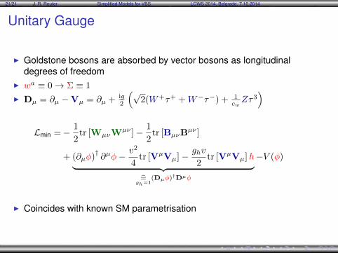
Unitary Gauge
I Goldstone bosons are absorbed by vector bosons as longitudinaldegrees of freedom
I wa ≡ 0→ Σ ≡ 1
I Dµ = ∂µ −Vµ = ∂µ + ig2
(√2(W+τ+ +W−τ−) + 1
cwZτ3
)
Lmin =− 1
2tr [WµνW
µν ]− 1
2tr [BµνB
µν ]
+ (∂µφ)†∂µφ− v2
4tr [VµVµ]− ghv
2tr [VµVµ]h
︸ ︷︷ ︸=
gh=1(Dµφ)†Dµφ
−V (φ)
I Coincides with known SM parametrisation

21/21 J. R. Reuter Simplified Models for VBS LCWS 2014, Belgrade, 7.10.2014
Isospin decompositionI Lowest order chiral Lagrangian (incl. anomalous couplings)
L = −v2
4tr[VµV
µ]+ α4tr [VµVν ] tr
[VµVν]
+ α5
(tr[VµV
µ])2I Leads to the following amplitudes: s = (p1 + p2)2 t = (p1 − p3)2 u = (p1 − p4)2
A(s, t, u) =: A(w+w− → zz) =
s
v2+ 8α5
s2
v4+ 4α4
t2 + u2
v4
A(w+z → w
+z) =
t
v2+ 8α5
t2
v4+ 4α4
s2 + u2
v4
A(w+w− → w
+w−
) = −u
v2+ (4α4 + 2α5)
s2 + t2
v4+ 8α4
u2
v4
A(w+w
+ → w+w
+) = −
s
v2+ 8α4
s2
v4+ 4 (α4 + 2α5)
t2 + u2
v4
A(zz → zz) = 8 (α4 + α5)s2 + t2 + u2
v4
I (Clebsch-Gordan) Decomposition into isospin eigenamplitudes
A(I = 0) = 3A(s, t, u) +A(t, s, u) +A(u, s, t)
A(I = 1) = A(t, s, u)−A(u, s, t)
A(I = 2) = A(t, s, u) +A(u, s, t)