Introdu o da Tese - est.ufmg.br · tatística de teste é longo, o que motiva o desenvolvimento e utilização dos procedimentos sequenciais. Os aspectos que recebem forte atenção

UNIVERSIDADE FEDERAL DE MINAS GERAIS

INSTITUTO DE CIÊNCIAS EXATAS

DEPARTAMENTO DE ESTATÍSTICA

PROGRAMA DE PÓS-GRADUAÇÃO EM ESTATÍSTICA

Otimalidade de Testes Monte Carlo

Ivair Ramos Silva

Tese de doutorado submetida à Banca Examinadora desig-nada pelo Colegiado do Programa de Pós-Graduação em Es-tatística da Universidade Federal de Minas Gerais, como req-uisito parcial para obtenção do título de Doutor em Estatís-tica.

Orientador: Prof. Dr. Renato Martins Assunção

Belo Horizonte/MG, 15 de Abril de 2011.

i

0.1 Resumo

A operacionalização de um teste de hipóteses é condicionada ao conhecimento da dis-tribuição de probabilidade da estatística de teste sob a hipótese nula H0. Caso não se conheçaa distribuição da estatística de teste sob H0, sua distribuição assintótica pode ser usada paraque a decisão sobre a rejeição ou não de H0 possa ser feita, o que exige o estudo dos tamanhosamostrais para os quais tal distribuição assintótica se verifica. Quando a distribuição assin-tótica também não pode ser deduzida analiticamente, métodos de reamostragem podem seraplicados para a construção de um critério alternativo de decisão, tais como reamostragemBootstrap, testes de permutação e simulação Monte Carlo (MC), sendo este último o objetode estudo deste trabalho.

Os testes de hipóteses montados pela utilização de simulações Monte Carlo podem serdivididos em dois tipos: os que se baseiam em um número m fixo de simulações, que é aestratégia convencional; e os procedimentos sequenciais, com os quais o número de simu-lações a serem geradas não é previamente fxado. Apesar de atualmente contarmos com re-cursos computacionais que favorecem o processamento de grandes bases de dados de formaextremamente veloz, ainda existem situações em que o tempo de processamento de uma es-tatística de teste é longo, o que motiva o desenvolvimento e utilização dos procedimentossequenciais.

Os aspectos que recebem forte atenção na literatura sobre testes MC são: a busca porprocedimentos que apresentem reduzido tempo médio de simulação até que a decisão sobreH0 seja efetuada; a estipulação de cotas para a probabilidade da decisão quanto à rejeição deH0 ser diferente da que se tomaria com o teste exato (risco de reamostragem); a estimação dovalor-p; e a estipulação de cotas para as possíveis perdas de poder do teste MC sequencial emrelação ao teste MC convencional ou em relação ao respectivo teste exato.

Usando certas suposições sobre a distribuição de probabilidade e a função poder asso-ciadas à estatística de teste, a literatura mostra que o poder do teste MC convencional épraticamente igual ao poder do teste exato. Um dos objetivos desta tese é demonstrar que épossível obter cotas para a diferença de poder entre o teste MC convencional e o teste exatoque valem para qualquer estatística de teste, ou seja, a validade de tais cotas não depende desuposições além das necessárias à existência de um teste exato.

Besag and Clifford (1991) propuseram um procedimento de teste MC sequencial que,sob H0, apresenta baixo tempo de execução. Objetivamos mostrar aqui como deve ser feita aescolha dos parâmetros de operacionalização deste procedimento sequencial. Primeiramente,mostramos como otimizar a escolha do número máximo de simulações sem afetar seu podere, em seguida, demonstramos a forma de aplicar a regra de interrupção das simulações demodo a garantir um mesmo poder que o teste convencional.

O procedimento sequencial de Besag and Clifford (1991) só apresenta redução no tempode execução nos casos em que H0 é verdadeira. Com a principal finalidade de tornar o testeMC sequencial mais veloz que o MC convencional também quando a hipótese nula é falsa,procedimentos sequenciais alternativos tem sido propostos na literatura. O cálculo analítico

exato do poder de tais procedimentos sequenciais, bem como do valor esperado do númerode simulações, são intratáveis para o caso geral, pois envolve o conhecimento da distribuiçãode probabilidade do valor-p, que por sua vez depende de cada aplicação específica. Pelo usode algumas restrições ao comportamento da distribuição de probabilidade do valor-p, algunsautores obtiveram cotas para o risco de reamostragem e para a esperança do número de simu-lações para procedimentos sequenciais para os quais, em cada tempo t de simulação, a regrade iinterrupção das simulações é dada por uma função linear em t. Nesta tese, construimosum procedimento sequencial que permite um formato geral para a regra de interrupção dassimulações, o qual chamaremos de teste MC sequencial generalizado. Esta construção ab-sorve as principais propostas apresentadas na literatura e permite um tratamento analítico dopoder e do número esperado de simulações para uma estatística de teste qualquer. Isto é feitopela elaboração de cotas superiores para a perda de poder e para a esperança do número desimulações. Com base em conceitos desenvolvidos nesta tese, apresentamos a construção doprocedimento ótimo em termos do número esperado de simulações. Nós também cotamos orisco de reamostragem dentro de uma extensa classe de distribuições de probabilidade para ovalor-p.

iii

0.2 Introdução

A avaliação da eficiência de um teste de hipóteses é fortemente embasada no comporta-mento das probabilidades dos erros tipo I e tipo II, que por sua vez dependem do critério derejeição da hipótese nula. Submeter a decisão sobre a rejeição da hipótese nula à avaliaçãodo valor-p é uma abordagem amplamente aceita, pois, além de ser um critério simples parao controle da probabilidade do erro tipo I, é um recurso que é comumente interpretado comomedidor do quão típico é o valor observado da estatística de teste frente ao que se espera soba hipótese nula. Não é nosso objetivo discutir os méritos desta interpretação do valor-p, masdestacamos que, independentemente da interpretação, o valor-p favorece a tomada de decisãoquanto à rejeição ou não da hipótese nula de forma objetiva. Obviamente, vários poderiamser os critérios, baseados na amostra, para se tomar a decisão sobre a hipótese nula. É nesteaspecto que focamos nosso trabalho. Ou seja, a decisão sobre qual das hipóteses é verdadeiradeve ser feita com base na redução e controle das probabilidades dos erros tipo I e tipo II.Sob essa ótica, se um critério de decisão não é baseado na utilização direta do valor-p, enten-demos que devemos focar a avaliação das probabilidades de ambos os erros gerados por talcritério.

Nos contextos em que não se conhece a distribuição de probabilidade da estatística deteste sob a hipótese nula, sua distribuição assintótica pode ser usada para que uma aproxi-mação do valor-p seja efetuada e usada na tomada de decisão sobre H0. Quando os tamanhosamostrais não são satisfatórios, o artifício de se utilizar a distribuição assintótica para a de-cisão sobre H0 gera probabilidades nominais de erro tipo I bem diferentes das reais. Ademais,não são raros os casos em que não é possível obter analiticamente a distribuição assintótica daestatística de teste, de onde surgem os testes baseados em reamostragem Bootstrap, testes depermutação e os testes MC. O teste MC pode ser interpretado como uma forma de estimar adecisão sobre H0 quando da aplicação do teste exato. Uma interpretação alternativa tambémé cabível, a de que o teste MC define um novo critério de teste, o qual pode ter seu poderavaliado e sua probabilidade de erro tipo I controlada tal como se faz para qualquer critérioconcorrente. Esta interpretação é coerente, pois, apesar de se ter mesmo poder para os testesMC e exato se suas decisões forem sempre coincidentes, a não coincidência entre suas de-cisões não implica poderes menores para o teste MC. Segundo (Gleser, 1996), a primeiralei de estatística aplicada postula que dois pesquisadores, usando a mesma metodologia, nãodevem chegar a conclusões diferentes com um mesmo banco de dados. Apesar de recon-hecermos a importância dessa lei, entendemos que o controle da probabilidade do erro tipo I,combinado a poderes satisfatórios, deve estar em primeiro plano na avaliação de um proced-imento baseado em simulação MC.

Resultados teóricos envolvendo a eficiência dos testes MC o colocam em uma posição dedestaque nos contextos onde sua aplicação é viável, sendo sugerido até mesmo como con-corrente aos testes assintóticos, tal como colocado por Jockel (1984) e exemplificado emChristensen and Kreiner (2007). Uma argumentação mais geral que sustenta tal credibilidade

iv

se baseia na igualdade da probabilidade do erro tipo I e o nível de significância pretendidopelo usuário. Nesta tese, apresentamos uma segunda característica que reforça o potencial deuso da abordagem MC em substituição aos testes assintóticos. Vamos mostrar que o poder doteste MC é comparável ao do respectivo teste exato para qualquer estatística de teste, inde-pendentemente do tamanho amostral. Nem sempre esta característica é assegurada nos testesassintóticos.

A viabilidade da aplicação do teste MC pode ser severamente comprometida quando aestatística de teste é computacionalmente intensa. Com o propósito de reduzir o tempo gastocom a simulação MC, procedimentos sequenciais têm sido propostos. Eles não exigem que onúmero de simulações seja pré-fixado. As simulações são interrompidas tão logo se percebaum comportamento favorável a uma das hipóteses, a nula H0 ou a alternativa HA. Isto oca-siona um número aleatório de simulações. Listamos a seguir os principais aspectos consid-erados pela literatura no que se refere ao desenvolvimento de procedimentos MC sequenciais.

A1 - Perda de poder em relação ao teste MC com m fixo: O ganho no tempo de execuçãoproporcionado pela utilização de um procedimento sequencial deve ser avaliado frente àspotenciais perdas de poder em relação ao teste que fixa o número de simulações em m. Édesejável que o poder do teste sequencial com máximo de simulações em m seja da ordemdaquele que se teria com o MC fixo em m simulações. Com isto, procura-se evitar que otempo de execução seja reduzido em detrimento de um poder maior com o m fixo;

A2 - Perda de poder em relação ao teste exato: O teste MC, sequencial ou não, é umaopção ao teste exato quando este é inviável. Após atender A1, o próximo desafio a umprocedimento é que ele possua poder comparável com o do teste exato;

A3 - Tempo esperado para o número de simulações sob as hipóteses nula e alternativa:Obviamente, este é o principal aspecto que motiva o desenvolvimento de testes MC sequen-ciais. O objetivo é reduzir o valor esperado para o número de simulações sob as hipótesesnula e alternativa;

A4 - Risco de Reamostragem:Este é um conceito que surge pela necessidade de se antender à primeira lei de (Gleser,

1996). O teste MC, para um dado m finito de simulações, oferece uma probabilidade não nulade que a decisão obtida por uma aplicação seja diferente de uma segunda aplicação do testeao mesmo banco de dados. Uma forma de estudar tal probabilidade é comparar a decisão quese obtém pelo uso do MC com a que se teria pelo uso do valor-p real (teste exato). O risco dereamostragem é facilmente confundido com a perda de poder do teste MC em relação ao testeexato. Entretanto, a ocorrência de risco de reamostragem consideravelmente maior que zeronão implica redução de poder do teste MC em relação ao teste exato. De fato, mostramos quemesmo quando a perda de poder é nula, o risco de reamostragem pode ser consideravelmentemaior que zero;

A5 - Estimação do valor-p: O estimador de máxima verossimilhança (EMV) é eventual-mente usado para se estimar o valor-p. Esta abordagem não é criticada pela literatura emprocedimentos para os quais este estimador possui distribuição uniforme discreta entre 0 e

v

1, condição suficiente, mas não necessária, para que um estimador do valor-p seja tido como"válido". Um estimador do valor-p é válido sua distribuição acumulada, sob a hipótese nulae avaliada no ponto α, vale no máximo α, onde α é o nível de significância do teste. Comoalguns procedimentos MC geram EMV não uniformemente distribuídos no intervalo discreto(0,1], algoritmos auxiliares acompanham a descrição de alguns dos procedimentos apresenta-dos na literatura a fim de oferecer estimadores "válidos". Por definição, um estimador válidoimplica probabilidade de erro tipo I menor ou igual a α. Porém, é fácil elaborar estimadorespara o valor-p que geram probabilidade de erro tipo I igual a α e que não possuem distribuiçãouniforme. Portanto, pensando apenas no controle do erro tipo I, a validade do valor-p é umapropriedade importante de se garantir. No entanto, dispensável se um procedimento qualquergarante probabilidade de erro tipo I igual a α.

O aspecto A3 é o mais explorado na literatura. Como veremos nesta tese, propostasinteressantes têm sido apresentadas no sentido de minimizar o valor esperado do número desimulações no teste MC sequencial. O risco de reamostragem tem sido o segundo pontode maior importância nos procedimentos propostos até o momento. A estimação correta dovalor-p vem em terceiro lugar.

0.3 Objetivos Gerais

O objetivo desta tese é, para qualquer estatística de teste e de forma analítica, demonstrarpropriedades e desenvolver conceitos que favoreçam a maximização do poder e a minimiza-ção da esperança do tempo de execução do teste Monte Carlo.

0.4 Objetivos Específicos

O primeiro objetivo é mostrar como usar o teste MC convencional de modo a garantirque possua o mesmo poder que o teste exato, provando assim que, nas situações em que épossível simular sob a hipótese nula, é mais interessante usar o teste baseado em simulaçãoMC do que aplicar testes baseados na distribuição assintótica da estatística de teste. Buscamosprovar também que a escolha do número de simulações no MC com m fixo deve obedecer aum critério que leva em conta o nível de significância estipulado para a rejeição de H0.

O segundo objetivo é provar que, do ponto de vista de preservação e controle das probabil-idades dos erros tipo I e tipo II, o teste MC sequencial por Besag and Clifford (1991) sempredeve ser preferido no lugar do procedimento com número fixo de simulações. Mostramostambém que o número máximo de simulações deste teste sequencial deve ser escolhido comouma função da regra de interrupção das simulações e da probabilidade de erro tipo I fixadapelo usuário.

O terceiro objetivo é propor um procedimento MC sequencial com duas barreiras de inter-rupção das simulações que permita a utilização de um formato geral para tais barreiras, compropriedades válidas para qualquer estatística de teste, que possa ser avaliado analiticamente

vi

e que seja ótimo em termos do tempo médio de execução. Chamaremos tal procedimento de"teste Monte Carlo Sequencial Generalizado"(MCG). Pretendemos mostrar que o MCG apre-senta tempo médio de simulação inferior aos apresentados por procedimentos concorrentese que, ao mesmo tempo, possui o mesmo poder que o procedimento MC convencional. Pre-tendemos fazer isso sem o uso de suposições além das necessárias à existência do teste exato.Objetivamos também cotar o risco de reamostragem associado ao MCG com auxílio de umasuposição razoável do ponto de vista prático.

0.5 Justificativa e Relevância da Pesquisa

O teste de hipóteses é um dos conceitos mais consagrados e utilizados da inferência es-tatística. Sua aplicação varre todas as áreas da ciência e, apesar da controvérsia acerca dasignificância estatística, ainda é amplamente usado em análise de dados, sendo ainda alvo deintensa pesquisa no ambiente acadêmico. Com isso, a simulação Monte Carlo é um métodoimportante do ponto de vista prático, uma vez que oferece um tratamento viável quandoocorre a impossibilidade de realizar testes estatísticos exatos em situações mais complexasou em que os tamanhos amostrais são insuficientes para o uso de resultados assintóticos.Pode-se encontrar uma vasta relação de aplicações do teste Monte Carlo, das quais as di-recionadas à análise espacial de dados são tipicamente citadas como motivadoras do estudoteórico deste método. Como exemplos de aplicações na área de análise espacial podemos citarRipley (1992), Kulldorff (2001), Assunção and Maia (2007) ou Peng et al. (2005). Exemplosde aplicações fora da estatística espacial podem ser vistos em Booth and Butler (1999), Caffoand Booth (2003) ou Wongravee et al. (2009). Os resultados já conhecidos, no que concerneao poder do teste MC, dependem fortemente de suposições que, na prática, são de difícilverificação devido à própria situação em que a abordagem Monte Carlo é requisitada. Isto é,diante do total desconhecimento do comportamento da distribuição da estatística de teste, édifícil verificar as suposições usuais. Portanto, a valoração da aplicação dos testes MC careceda demonstração de resultados mais gerais sobre a magnitude do poder e sobre a escolha donúmero máximo de simulações m. Da mesma forma, os procedimentos sequenciais devemser propostos sob aspectos gerais e de simples aplicação, de modo que possam garantir a suautilização e confiabilidade, uma vez que pretendem ser priorizados em substituição ao MC

com m fixo.

0.6 Organização

Este material é formado pela coleção de três artigos que tratam do teste Monte Carlo paratestes de hipóteses. O primeiro deles considera a escolha dos parâmetros de operacionaliza-ção do teste Monte Carlo sequencial proposto em Besag and Clifford (1991). Este artigo,entitulado "Power of the Sequential Monte Carlo Test", foi publicado no volume 28, edição2, do periódico "Sequential Analysis".

vii

O segundo trabalho desta tese estuda as propriedades do poder e os critérios para escolhado número de simulações do teste Monte Carlo convencional para uma estatística de testequalquer. Este trabalho está condensado no segundo artigo, entitulado "Monte Carlo Testsunder General Conditions: Power and Number of Simulations", submetido em fevereiro de2011 ao "Journal of Statistical Planning and Inference".

A generalização dos testes Monte Carlo sequenciais com duas barreiras, e a construçãodo teste sequencial ótimo em termos do tempo médio de execução, é o conteúdo do terceiro eúltimo artigo desta coleção, entitulado "Optimal Generalized Sequential Monte Carlo Test".Este artigo será submetido ao "Journal of the American Statistical Association".

Referências Bibliográficas

Assunção, R. and Maia, A. (2007). A note on testing separability in spatial-temporal markedpoint processes. Biometrics, 63(1):290–294.

Besag, J. and Clifford, P. (1991). Sequential monte carlo p-value. Biometrika, 78:301–304.

Booth, J. and Butler, R. (1999). An importance sampling algorithm for exact conditional testsin log-linear models. Biometrika, 86:321–332.

Caffo, B. and Booth, J. (2003). Monte carlo conditional inference for log-linear and logis-tic models: a survey of current methodology. Statistical Methods in Medical Research,12:109–123.

Christensen, K. and Kreiner, S. (2007). A monte carlo approach to unidimensionality testingin polytomous rasch models. Applied Psychological Measurement, 31(1):20–30.

Gleser, L. (1996). Comment on "Bootstrap Confidence Intervals"

. Number 11. Statistical Science, T. J. DiCiccio & B. Efron.

Jockel, K. (1984). Application of monte-carlo tests - some considerations. Biometrics,40(1):263–263.

Kulldorff, M. (2001). Prospective time periodic geographical disease surveillance using ascan statistic. Journal of Royal Statistical Society, 164A:61–72.

Peng, R., Schoenberg, F., and Woods, J. (2005). A space-time conditional intensity modelfor evaluating a wildfire hazard index. Journal of the American Statistical Association,100(469):26–35.

Ripley, B. (1992). Applications of monte-carlo methods in spatial and image-analysis. Lec-

ture Notes in Economics and Mathematical Systems, 376:47–53.

Wongravee, K., Lloyd, G., Hall, J., Holmboe, M., Schaefer, M., Reed, R., Trevejo, J., andBrereton, R. (2009). Monte-carlo methods for determining optimal number of significantvariables. application to mouse urinary profiles. Metabolomics, 5(4):387–406.

viii

PLEASE SCROLL DOWN FOR ARTICLE

This article was downloaded by: [Silva, I.]On: 24 April 2009Access details: Access Details: [subscription number 910710910]Publisher Taylor & FrancisInforma Ltd Registered in England and Wales Registered Number: 1072954 Registered office: Mortimer House,

37-41 Mortimer Street, London W1T 3JH, UK

Sequential AnalysisPublication details, including instructions for authors and subscription information:

http://www.informaworld.com/smpp/title~content=t713597296

Power of the Sequential Monte Carlo TestI. Silva a; R. Assunção a; M. Costa a

a Departamento de Estatística, Universidade Federal de Minas Gerais, Belo Horizonte, Minas Gerais, Brazil

Online Publication Date: 01 April 2009

To cite this Article Silva, I., Assunção, R. and Costa, M.(2009)'Power of the Sequential Monte Carlo Test',Sequential Analysis,28:2,163— 174

To link to this Article: DOI: 10.1080/07474940902816601

URL: http://dx.doi.org/10.1080/07474940902816601

Full terms and conditions of use: http://www.informaworld.com/terms-and-conditions-of-access.pdf

This article may be used for research, teaching and private study purposes. Any substantial orsystematic reproduction, re-distribution, re-selling, loan or sub-licensing, systematic supply ordistribution in any form to anyone is expressly forbidden.

The publisher does not give any warranty express or implied or make any representation that the contentswill be complete or accurate or up to date. The accuracy of any instructions, formulae and drug dosesshould be independently verified with primary sources. The publisher shall not be liable for any loss,actions, claims, proceedings, demand or costs or damages whatsoever or howsoever caused arising directlyor indirectly in connection with or arising out of the use of this material.

Sequential Analysis, 28: 163–174, 2009Copyright © Taylor & Francis Group, LLCISSN: 0747-4946 print/1532-4176 onlineDOI: 10.1080/07474940902816601

Power of the Sequential Monte Carlo Test

I. Silva, R. Assunção, and M. Costa

Departamento de Estatística, Universidade Federal de Minas Gerais,

Belo Horizonte, Minas Gerais, Brazil

Abstract: Many statistical tests obtain their p-value from a Monte Carlo sample of m valuesof the test statistic under the null hypothesis. The number m of simulations is fixed by theresearcher prior to any analysis. In contrast, the sequential Monte Carlo test does not fix thenumber of simulations in advance. It keeps simulating the test statistics until it decides tostop based on a certain rule. The final number of simulations is a random number N . Thissequential Monte Carlo procedure can decrease substantially the execution time in order toreach a decision. This paper has two aims concerning the sequential Monte Carlo tests: tominimize N without affecting its power; and to compare its power with that of the fixed-sample Monte Carlo test. We show that the power of the sequential Monte Carlo test isconstant after a certain number of simulations and therefore, that there is a bound to N .We also show that the sequential test is always preferable to a fixed-sample test. That is,for every test with a fixed sample size m there is a sequential Monte Carlo test with equalpower but with smaller number of simulations.

Keywords: Monte Carlo test; p-value; Sequential estimation; Sequential test; Significancetest.

Subject Classifications: 62L05; 62L15; 65C05.

1. INTRODUCTION

To carry out hypothesis testing, one must find the distribution of the test statisticU under the null hypothesis, from which the p-value is calculated. Either because it

Received April 15, 2008, Revised February 1, 2009, February 5, 2009, Accepted

February 8, 2009Recommended by Nitis MukhopadhyayAddress correspondence to I. Silva, Departamento de Estatística, Universidade Federal

de Minas Gerais, Avenida Presıdente Antonio Carlos, 6627, Prédio do ICEx, Sala 4054,Pampulha, Belo Horizonte, Minas Gerais 31270-901, Brazil; Fax: 55-31-3409-5924; E-mail:[email protected]

Downloaded By: [Silva, I.] At: 22:47 24 April 2009

164 Silva et al.

is too cumbersome or it is impossible to obtain this distribution analytically, MonteCarlo tests are used in many situations (Manly, 2006). In particular, areas such asspatial statistics (Assunção et al., 2007; Diggle et al., 2005; Kulldorff, 2001) and datamining (Kulldorff et al., 2003; Rolka et al., 2007) rely heavily on Monte Carlo teststo draw inference. Other areas have situations in which Monte Carlo tests seemsto be the best current approach, such as the exact tests in categorical data analysis(Booth and Butler, 1999; Caffo and Booth, 2003), and some regression problems ineconometrics (Khalaf and Kichian, 2005; Luger, 2006).

The conventional Monte Carlo test generates a large number of independentcopies of U from the null distribution. Assuming that large values of U lead to thenull hypothesis rejection, a Monte Carlo value is calculated based on the proportionof the simulated values that are larger or equal than the observed value of U .

As the statistics field evolves to deal with ever more complex models, MonteCarlo tests become costly. The simulation of each independent copy of U under thenull hypothesis can take a long time.

In many applications, after a few simulations are carried out, it becomesintuitively clear that a large number of simulations is not necessary. For instance,suppose that after 100 simulations, the observed value is around the median of thegenerated values. It is not likely that the null hypothesis will be eventually rejectedeven if a much larger number of simulations (such as 9999) is carried out. Mostresearchers would be confident to stop at this point if a valid p-value could beprovided.

Besag and Clifford (1991) introduced the idea of sequential Monte Carlo tests,an alternative way to obtain p-values without fixing the number of simulationspreviously. Their method makes a decision concerning the null hypothesis aftereach simulated value up to a maximum number of simulations. This approachcan substantially shorten the number of simulations required to decide about thesignificance of the observed test statistic.

Although the proposal of Besag and Clifford (1991) stands as a majorcontribution to the practice of modern data analysis, it is under utilized and hassome unanswered theoretical questions. One important aspect of the sequentialMonte Carlo tests is the relative comparison of its power with that of theconventional Monte Carlo test. Based on the Besag and Clifford results, we canalways obtain a sequential Monte Carlo with significance level � that does notrequire more simulations than a conventional Monte Carlo test at the same level.However, the relationship between the power functions of these tests is not clear.In terms of power, is there a cost when we apply the sequential test instead of theconventional Monte Carlo test? The answer is no, and the first aim of this paper isto demonstrate this. The second objective of this work is to show how we can makethe choice of the maximum number of simulations in the sequential Monte Carlotests without losing power.

The next section contains a summary of the definitions and notation associatedwith the conventional and the sequential Monte Carlo tests. Section 3 discussesthe power of the sequential procedure and Section 4 shows how to establish theparameters of the sequential test such that it has the same power as a givenconventional Monte Carlo test. In Section 5, we develop bounds for the difference ofpower between a conventional and a sequential Monte Carlo tests. Section 6 closesthe paper with a discussion of the implications of our results.


Sequential Monte Carlo Test 165

2. A SEQUENTIAL MONTE CARLO TEST

Let U be a test statistic with distribution F under the null hypothesis H0. Supposethat large values of U leads to the rejection of the null hypothesis. When F can beevaluated explicitly, the p-value of the upper-tail test based on the observed value u0

of U is given by p = 1− F4u05. Let P = 1− F4U5 be the random variable associatedwith the p-value. If F is a continuous function, P has a uniform distribution in401 15 under the null hypothesis. When we can not evaluate F1 we need to find otherways to calculate the p-value. The Monte Carlo test proposed by Dwass (1957) isan alternative if we can simulate samples from the null hypothesis.

The fixed-size or conventional Monte Carlo test generates a sample of sizem− 1 of the test statistic U under the null hypothesis H0. Denote each simulatedvalue by ui, i = 11 0 0 0 1 m− 1. The Monte Carlo p-value pmc is equal to r/m if theobserved value u0 is the rth largest value among the m values u01 u11 0 0 0 1 um−1. Inthis conventional Monte Carlo procedure, if the rank of u0 is among the �m largerranks of u01 u11 0 0 0 1 um−1, we reject the null hypothesis at the � significance level. Wedenote this procedure by MCconv4m1 �5.

Let Pmc be the corresponding random variable associated with the realizedMonte Carlo p-value pmc. Under the null hypothesis, we have ð4Pmc ≤ a5 = a if ais one of the values 1/m1 2/m1 0 0 0 1 1. That is, the Monte Carlo p-value Pmc has auniform distribution on the discrete set 81/m1 2/m1 0 0 0 1 19. Let W be the randomvariable W = Pmc − X where X ∼ U401 1/m5 and it is independent of Pmc. Then, W ∼U401 15 under the null hypothesis. In this sense, Besag and Clifford (1991) say thatthe Monte Carlo p-value is exact, because Pmc has the same uniform distributionunder the null hypothesis than the analytical p-value P = 1− F4U5. In addition tothat, irrespective of the validity of the null hypothesis, Pmc → P almost everywherebecause, for any observed value u0, we have

pmc =1+ #8ui ≥ u09

m=

1

m+

[

#8ui ≥ u09

m− 1

]

m− 1

m→ 1− F4u05

as m goes to infinity.However, when early on there is little evidence against the null hypothesis, it is

wasteful to run the procedure for large values of m such as, for example, m = 10000.This is the main motivation for Besag and Clifford to develop the sequential MonteCarlo test. In brief, the sequential version of the test selects a small integer h, suchas h = 10 or h = 20. It keeps simulating by Monte Carlo from the null hypothesisdistribution until h of the simulated values are larger than the observed value u0.There is also an upper limit n− 1 for the total number of simulations. The p-valueis based on the proportion of simulated values larger than u0 at the stopping time.

In other words, simulate independently and sequentially the random valuesU11 U21 0 0 0 1 UL from the same distribution as U under the null hypothesis.The random variable L has possible values h1 h+ 11 0 0 0 1 n− 1 and its value isdetermined in the following way: L is the first time when there are h simulated valueslarger than u0. If this has not occurred at step n− 1, then let L = n− 1. Let g bethe number of simulated Ui’s larger than u0 at termination. If we denote by l therealized number of Monte Carlo withdrawals, then the sequential p-value is given by

ps =

{

h/l1 if g = h1

4g + 15/n1 if g < h(2.1)


166 Silva et al.

For example, if up to n− 1 = 999 Monte Carlo withdrawals are considered andthe sampling scheme stops as soon as h = 10 exceeding values of U occurs, thenthe possible values of the sequential p-value are 10/10, 10/11, 10/121 0 0 0 1 10/1000,9/1000, 8/10001 0 0 0 1 1/1000. Note that the support of the sequential Monte Carloprocedure is more concentrated on the lower end of the interval 401 15. This is adesirable characteristic because these are the p-value possible values that we wantto know more precisely.

Let the support of ps be denoted by

S = 81/n1 2/n1 0 0 0 1 h/n1 h/4n− 151 0 0 0 1 h/4h+ 251 h/4h+ 151 190

The values of the form 4h− q5/n, with 0 ≤ q ≤ h− 1, occur when we need torun the procedure up to the maximum n− 1 number of simulations without nevergetting h uis larger than u. The other values, of the form h/4h+ q5, with h ≤ h+

q ≤ n− 1, occur when we either stop the procedure earlier than the maximum n− 1or when the hth larger value occur exactly at the 4n− 15th sequential observationand hence l = n− 1. Therefore, we can also define the sequential p-value as

ps =

h/l1 if l < n− 11

h/l1 if l = n− 11 and g = h

4g + 15/4l+ 151 if l = n− 11 and g < h

If a ∈ S, then ð4Ps ≤ a5 = a under the null hypothesis. To see this, assume thata = h/4h+ q5 ≤ 1 with h ≤ h+ q < n. Then

ð4Ps ≤ a5 = ð4Ps ≤ h/4h+ q55 = ð4L ≥ h+ q5

= ð4L > h+ q − 15 =h

h+ q

because L > h+ q − 1 if, and only if, after l− 1 Monte Carlo withdrawals, theobserved u is among the largest h of the sample of equally probable 4l− 15+ 1elements. Consider now that a = 4h− q5/n with 0 ≤ q ≤ h− 1. Then

ð4Ps ≤ a5 = ð4Ps ≤ 4h− q5/n5

= ð4L = n− 1 and only h− q − 1 exceeding u5

= ð4u is the 4h− q5th largest among n5

= 4h− q5/n

We can transform Ps by subtracting a random variable X such that the sequentialp-value also has a continuous uniform distribution in 401 15. For that, defineX conditionally on the observed value of the discrete p-value Ps0 Suppose thatps = b ∈ S. Let a be the largest element of S that is smaller than b0 Define a = 0if b = 1/n. Then X ∼ U4a1 b5 and Ps − X has a uniform distribution in 401 15 underthe null hypothesis, exactly as the p-values P and Pmc. Because this is less commonto be carried out in practice, in the remaining of this paper we will not transformPs in this way, keeping its definition as in (2.1).



The most important random variable in our paper is L, the total number ofsimulations carried out, which has distribution under the null hypothesis given by

ð4L ≤ l5 =

01 se l ≤ h− 1

1− h/4l+ 151 se l = h1 h+ 11 0 0 0 1 n− 1

11 if l = n

Its expected value was found by Besag and Clifford (1991):

å4L5 =n−1∑

l=1

P4L ≥ l5 =n−1∑

l=h+1

l−1 û h+ h log

(

n− 005

h+ 005

)

(2.2)

To reach a decision with the sequential Monte Carlo test, it is necessary to fixthe values of three tuning parameters, n1 h, and �, and hence we denote the testby MCseq4n1 h1 �5. Typically, n is taken equal to the number m of simulations onewould run if carrying out the conventional Monte Carlo test. Whether this typicalchoice is really necessary is one of the issues studied in this paper.

3. POWER OF THE SEQUENTIAL MONTE CARLO TEST

In this section we study the power of the sequential Monte Carlo procedureMCseq4n1 h1 �5. Its behavior depends on the value of n with respect to h/�+ 1. Wedeal initially with the case n ≥ h/�+ 1.

3.1. MCseq4n1 h1 �5 with n ≥ h/� + 1

This constraint implies that � ≥ h/4n− 15. That is, � is not smaller than h dividedby the maximum number of simulations. A typical choice found in practical analysisis n− 1 = 999 and � = 0005. Then, the condition n ≥ h/�+ 1 is valid if h ≤ 49. Thisis likely to cover most of the choices one would make for h in practice.

The power of the procedure MCseq4n1 h1 �5 is constant for all n ≥ h/�+ 1 andhence, taking n larger than h/�+ 1 is not worth in terms of power. In other words,n = �h/�� + 1 is optimal in terms of number of simulations for a test with errortype I probability �. The notation �x� represents the ceiling of x1 the smallest integergreater or equal to x0

To see this result, label the event 6Ui ≥ u07 as a success. Because Ui has c.d.f F1the probability ð4Ui ≥ u05 is the observed p-value p = 1− F4u05. The probability ofcarrying out L simulations until h successes is given by:

ð4L = l �P = p5 =

(

l− 1

h− 1

)

ph41− p5l−h if l = h1 h+ 11 0 0 0 1 n− 2

�∑

x=n−1

(

x − 1

h− 1

)

ph41− p5x−h if l = n− 1


168 Silva et al.

We reject H0 if, and only if, h/� ≤ L ≤ n− 1. This means that in �h/�� − 1simulations, we obtain at most h− 1 successes. Therefore, for an observed value u0,the probability of rejecting H0 in the sequential test is given by

ð4RejectH0 �P = p5 = ð4L ≥ 4h/�5 �P = p5

= ð4L > 4h/�5− 1 �P = p5

=h−1∑

x=0

(

h/�− 1x

)

px41− p5h/�−x−1 (3.1)

Because the last expression does not involve n, the power of the sequentialMonte Carlo test is constant as long as n ≥ 4h/�5+ 1. Because the error type I isfixed at �, �h/�� + 1 is an upper bound for n.

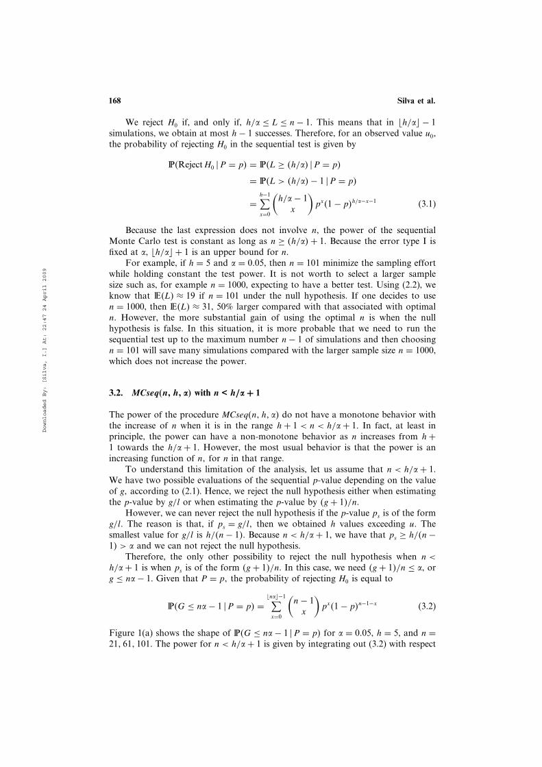
For example, if h = 5 and � = 0005, then n = 101 minimize the sampling effortwhile holding constant the test power. It is not worth to select a larger samplesize such as, for example n = 1000, expecting to have a better test. Using (2.2), weknow that å4L5 ≈ 19 if n = 101 under the null hypothesis. If one decides to usen = 1000, then å4L5 ≈ 31, 50% larger compared with that associated with optimaln0 However, the more substantial gain of using the optimal n is when the nullhypothesis is false. In this situation, it is more probable that we need to run thesequential test up to the maximum number n− 1 of simulations and then choosingn = 101 will save many simulations compared with the larger sample size n = 1000,which does not increase the power.

3.2. MCseq4n1 h1 �5 with n < h/� + 1

The power of the procedure MCseq4n1 h1 �5 do not have a monotone behavior withthe increase of n when it is in the range h+ 1 < n < h/�+ 1. In fact, at least inprinciple, the power can have a non-monotone behavior as n increases from h+

1 towards the h/�+ 1. However, the most usual behavior is that the power is anincreasing function of n1 for n in that range.

To understand this limitation of the analysis, let us assume that n < h/�+ 1.We have two possible evaluations of the sequential p-value depending on the valueof g1 according to (2.1). Hence, we reject the null hypothesis either when estimatingthe p-value by g/l or when estimating the p-value by 4g + 15/n.

However, we can never reject the null hypothesis if the p-value ps is of the formg/l0 The reason is that, if ps = g/l1 then we obtained h values exceeding u0 Thesmallest value for g/l is h/4n− 15. Because n < h/�+ 1, we have that ps ≥ h/4n−

15 > � and we can not reject the null hypothesis.Therefore, the only other possibility to reject the null hypothesis when n <

h/�+ 1 is when ps is of the form 4g + 15/n. In this case, we need 4g + 15/n ≤ �, org ≤ n�− 1. Given that P = p1 the probability of rejecting H0 is equal to

ð4G ≤ n�− 1 �P = p5 =�n��−1∑

x=0

(

n− 1x

)

px41− p5n−1−x (3.2)

Figure 1(a) shows the shape of ð4G ≤ n�− 1 �P = p5 for � = 0005, h = 5, and n =

211 611 101. The power for n < h/�+ 1 is given by integrating out (3.2) with respect



Figure 1. Power behavior of the sequential Monte Carlo test and the p-value density.

to the p-value probability distribution Fp:

�4n1 h1 �1 FP5 =∫ 1

0ð4G ≤ n�− 1 �P = p5FP4dp5

=∫ 1

0

�n��−1∑

x=0

(

n− 1x

)

px41− p5n−1−xFP4dp5 (3.3)

Denote by �4n1 h1 �1 FP5 the power function of the sequential procedure.Depending on FP , the power curve can be non-monotone. To illustrate this result,consider two different FP distributions. One of them assumes that P is distributedaccording to a Beta distribution with parameters 2 and 17. The other assumes a Betadistribution with parameters 1 and 40 (see Figure 1(b)). The graph in Figure 1(c)shows the power (3.3) using FP as a Beta421 175 distribution with h = 5, � = 0005,and n = 20, 40, 60, 80, 100. We can see that the power does not increase with n inthe range 61 ≤ n ≤ 101.

In contrast, Figure 1(d) shows the power using FP ∼ Beta411 405 and the sametuning parameters as before. In this case, the power is increasing with n. Indeed,Hope (1968) and Jockel (1986) showed that we always have the power increasingwith n if the p-value distribution FP belongs to certain distribution classes, whichinclude the Beta411 405 distribution.

This illustrative example shows that, for n < h/�+ 1, the sequential powerbehavior depends heavily on the shape of the p-value density.


170 Silva et al.

4. A SEQUENTIAL MC TEST EQUIVALENT TO A FIXED-SIZE MC TEST

From now on, we consider only the case n ≥ h/�+ 1. Given a conventional MonteCarlo test MCconv4m1 �5, we find in this section a sequential test MCseq4n1 h1 �5

with the same power as the conventional one. For the fixed-size Monte Carlo test,let G be the random count of Uis that are greater or equal to u0 among the m− 1generated. The null hypothesis is rejected if 4G+ 15/m ≤ � or, equivalently, if G ≤

�m− 1. The random variable G has a binomial distribution with parameters m− 1and success probability equal to the p-value P0 Therefore, MCconv4m1 �5 rejects thenull hypothesis with probability

ð4RejectH0 �P = p5 = P4G ≤ ��m� − 1 �P = p5

=��m�−1∑

y=0

(

m− 1y

)

py41− p5m−y−1 (4.1)

The MCconv4m1 �5 power is

�4m1 �1 FP5 =∫ 1

0

��m�−1∑

y=0

(

m− 1y

)

py41− p5m−y−1FP4p5dp (4.2)

whereas the MCseq4n1 h1 �5 power for n > h/�+ 1 is given by integrating out (3.1)with respect to FP :

�4n1 h1 �1 FP5 =∫ 1

0

h−1∑

x=0

(

h/�− 1x

)

px41− p5h/�−x−1FP4p5dp (4.3)

As a result, the power (4.3) of MCseq4n1 h1 �5 and the power (4.2) ofMCconv4m1 �5 are equal if we take h = �m. That is, given a conventional MCprocedure MCconv4m1 �5, we have sequential MC procedure in MCseq4n1 �m1 �5

with equal power. This is valid for all n > h/�+ 1 and hence we take the minimumpossible value n = �h/�� + 1 to have the equivalent procedures MCconv4m1 �5 andMCseq4m+ 11 �m1 �5.

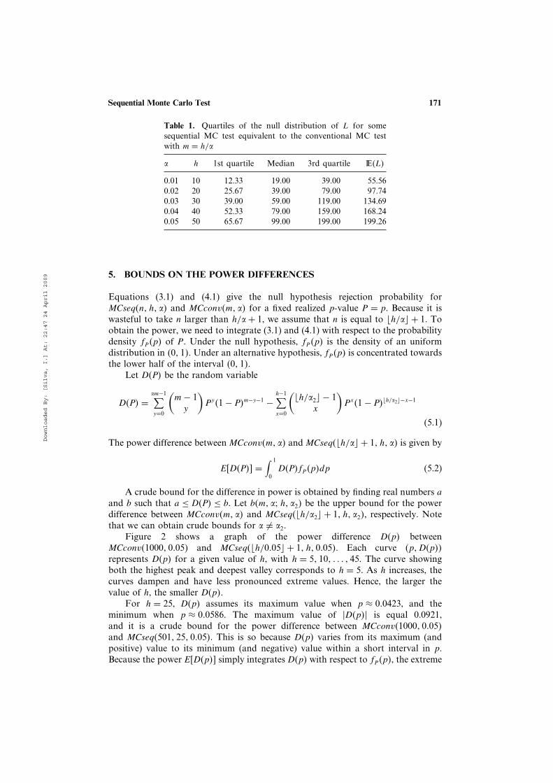
Under the null hypothesis or under an alternative not too far from the null,there will be considerable reduction in the number of simulations required toreach a decision if the sequential test is adopted holding fixed the main statisticalcharacteristic (size and power) of the fixed-size MC tests. Table 1 shows the quartilesof the null distribution of L for the sequential MC test MCseq4m+ 11 �m1 �5

equivalent to the conventional MC test MCconv4m1 �5 with different significancelevel � between 0.01 and 0.05, and with m = 1000 and n = 1001. Therefore, we canhave large gains if the sequential procedure is adopted.

We showed that, given a conventional MC test, there is a simple rule to find asequential MC test with the same power but typically requiring a smaller number ofsimulations. However, one can trade a slight power loss in exchange for a smallernumber of Monte Carlo simulations. If we want to adopt a general sequential MCtest rather than the fixed-size MC test, it is important to have control over the powerloss we are subjected. The next section establishes bounds for this loss.



Table 1. Quartiles of the null distribution of L for somesequential MC test equivalent to the conventional MC testwith m = h/�

� h 1st quartile Median 3rd quartile å4L5

0.01 10 12.33 19.00 39.00 55.560.02 20 25.67 39.00 79.00 97.740.03 30 39.00 59.00 119.00 134.690.04 40 52.33 79.00 159.00 168.240.05 50 65.67 99.00 199.00 199.26

5. BOUNDS ON THE POWER DIFFERENCES

Equations (3.1) and (4.1) give the null hypothesis rejection probability forMCseq4n1 h1 �5 and MCconv4m1 �5 for a fixed realized p-value P = p. Because it iswasteful to take n larger than h/�+ 1, we assume that n is equal to �h/�� + 1. Toobtain the power, we need to integrate (3.1) and (4.1) with respect to the probabilitydensity fP4p5 of P. Under the null hypothesis, fP4p5 is the density of an uniformdistribution in 401 15. Under an alternative hypothesis, fP4p5 is concentrated towardsthe lower half of the interval 401 15.

Let D4P5 be the random variable

D4P5 =�m−1∑

y=0

(

m− 1y

)

Py41− P5m−y−1 −h−1∑

x=0

(

�h/�2� − 1x

)

Px41− P5�h/�2�−x−1

(5.1)

The power difference between MCconv4m1 �5 and MCseq4�h/�� + 11 h1 �5 is given by

E6D4P57 =∫ 1

0D4P5fP4p5dp (5.2)

A crude bound for the difference in power is obtained by finding real numbers aand b such that a ≤ D4P5 ≤ b. Let b4m1 �3 h1 �25 be the upper bound for the powerdifference between MCconv4m1 �5 and MCseq4�h/�2� + 11 h1 �25, respectively. Notethat we can obtain crude bounds for � 6= �2.

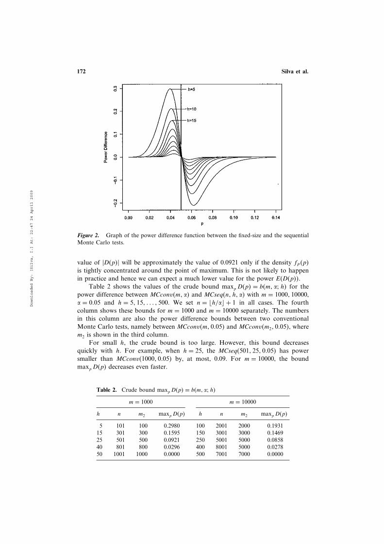
Figure 2 shows a graph of the power difference D4p5 betweenMCconv410001 00055 and MCseq4�h/0005� + 11 h1 00055. Each curve 4p1D4p55

represents D4p5 for a given value of h, with h = 51 101 0 0 0 1 45. The curve showingboth the highest peak and deepest valley corresponds to h = 5. As h increases, thecurves dampen and have less pronounced extreme values. Hence, the larger thevalue of h, the smaller D4p50

For h = 25, D4p5 assumes its maximum value when p ≈ 000423, and theminimum when p ≈ 000586. The maximum value of �D4p5� is equal 0.0921,and it is a crude bound for the power difference between MCconv410001 00055and MCseq45011 251 00055. This is so because D4p5 varies from its maximum (andpositive) value to its minimum (and negative) value within a short interval in p.Because the power E6D4p57 simply integrates D4p5 with respect to fP4p5, the extreme


172 Silva et al.

Figure 2. Graph of the power difference function between the fixed-size and the sequentialMonte Carlo tests.

value of �D4p5� will be approximately the value of 0.0921 only if the density fP4p5

is tightly concentrated around the point of maximum. This is not likely to happen

in practice and hence we can expect a much lower value for the power E4D4p550

Table 2 shows the values of the crude bound maxp D4p5 = b4m1 �3 h5 for the

power difference between MCconv4m1 �5 and MCseq4n1 h1 �5 with m = 10001 10000,

� = 0005 and h = 51 151 0 0 0 1 500. We set n = �h/�� + 1 in all cases. The fourth

column shows these bounds for m = 1000 and m = 10000 separately. The numbers

in this column are also the power difference bounds between two conventional

Monte Carlo tests, namely between MCconv4m1 00055 and MCconv4m21 00055, where

m2 is shown in the third column.

For small h1 the crude bound is too large. However, this bound decreases

quickly with h0 For example, when h = 25, the MCseq45011 251 00055 has power

smaller than MCconv410001 00055 by, at most, 0.09. For m = 10000, the bound

maxp D4p5 decreases even faster.

Table 2. Crude bound maxp D4p5 = b4m1 �3 h5

m = 1000 m = 10000

h n m2 maxp D4p5 h n m2 maxp D4p5

5 101 100 0.2980 100 2001 2000 0.193115 301 300 0.1595 150 3001 3000 0.146925 501 500 0.0921 250 5001 5000 0.085840 801 800 0.0296 400 8001 5000 0.027850 1001 1000 0.0000 500 7001 7000 0.0000



6. DISCUSSION AND CONCLUSIONS

The sequential Monte Carlo test is a feasible and more economical way to reachdecisions in a hypothesis testing under Monte Carlo sampling. We have shown thatfor each conventional Monte Carlo test with m simulations, there is a sequentialMonte Carlo procedure with the same significance level and power. More important,this sequential Monte Carlo test requires at most one additional simulation and itsexpected number of simulations is generally much smaller than m, specially whenthe null hypothesis is true.

If execution time is crucial, the user can trade a small amount of power in thesequential test by a large decrease in number of simulations. To guide this trade-off choice, we develop bounds for the difference in power between the MCconv andMCseq tests. This is more relevant if we consider that the true differences are likelyto be much smaller than the bounds suggest. These bounds can also be used tocompare two conventional Monte Carlo tests.

For n ≥ h/�+ 1, an usual situation, the sequential MC test has a constantpower and this leads to the suggestion of adopting n = h/�+ 1.

ACKNOWLEDGMENTS

The authors are grateful to Martin Kulldorff for very useful comments andsuggestions on an earlier draft of this paper. This research was partially fundedby the National Cancer Institute, grant number R01CA095979, Martin KulldorffPI. The second author was partially supported by the Conselho Nacional deDesenvolvimento Científico e Tecnológico (CNPq). This research was partiallycarried out while the first author was at the Department of Ambulatory Care andPrevention, Harvard Medical School, whose support is gratefully acknowledged.

REFERENCES

Assunção, R., Tavares, A. I., Correa, T., and Kulldorff, M. (2007). Space-Time ClusterIdentification in Point Processes, Canadian Journal of Statistics 35: 9–25.

Besag, J. and Clifford, P. (1991). Sequential Monte Carlo p-Values, Biometrika 78: 301–304.Booth, J. G. and Butler, R. W. (1999). An Importance Sampling Algorithm for Exact

Conditional Tests in Log-Linear Models, Biometrika 86: 321–332.Caffo, B. S. and Booth, J. G. (2003). Monte Carlo Conditional Inference for Log-Linear

and Logistic Models: A Survey of Current Methodology, Statistical Methods in Medical

Research 12: 109–123.Diggle, P. J., Zheng, P., and Durr, P. A. (2005). Non-Parametric Estimation of Spatial

Segregation in a Multivariate Point Process: Bovine Tuberculosis in Cornwall, UK,Journal of Royal Statistical Society, Series C 54: 645–658.

Dwass, M. (1957). Modified Randomization Tests for Nonparametric Hypotheses, Annals ofMathematical Statistics 28: 181–187.

Hope, A. C. A. (1968). A Simplified Monte Carlo Significance Test Procedure, Journal ofRoyal Statistical Society, Series B 30: 582–598.

Jockel, K.-H. (1986). Finite Sample Properties and Asymptotic Efficiency of Monte CarloTests, Annals of Statistics 14: 336–347.

Khalaf, L. and Kichian, M. (2005). Exact Tests of the Stability of the Phillips Curve: TheCanadian Case, Computational Statistics & Data Analysis 49: 445–460.


174 Silva et al.

Kulldorff, M. (2001). Prospective Time Periodic Geographical Disease Surveillance Using aScan Statistic, Journal of Royal Statistical Society, Series A 164: 61–72.

Kulldorff, M., Fang, Z., and Walsh, S. J. (2003). A Tree-Based Scan Statistic for DatabaseDisease Surveillance, Biometrics 59: 323–331.

Luger, R. (2006). Exact Perrmutation Tests for Non-Nested Non-Linear Regression Models,Journal of Econometrics 133: 513–529.

Manly, B. F. J. (2006). Randomization, Bootstrap and Monte Carlo Methods in Biology, 3rd ed.,Boca Raton: Chapman & Hall/CRC.

Marriott, F. H. C. (1979). Bernard’s Monte Carlo Test: How Many Simulations? Applied

Statististics 28: 75–77.Rolka, R., Burkom, H., Cooper, G. F., Kulldorff, M., Madigan, D., and Wong, W. (2007).

Issues in Applied Statistics for Public Health Bioterrorism Surveillance Using MultipleData Streams: Research Needs, Statistics in Medicine 26: 1834–1856.


Monte Carlo test under general conditions: Power and number of

simulations

I.R.Silva∗, R.M.Assuncao

Departamento de Estatıstica, Universidade Federal de Minas Gerais, Belo Horizonte, Minas Gerais, Brazil

Abstract

The statistical tests application demands the probability distribution of the test statistic U under the nullhypothesis. When that distribution can not be obtained analytically, it is necessary to establish alternativemethods to calculate the p-value. If U can be simulated under the null hypothesis, Monte Carlo simulation isone of the ways to estimate the p-value. Under some assumptions about the probability distribution and thepower function of U , the literature has obtained thin upper bounds for the power difference between exacttest and Monte Carlo test. The motivation of this paper is to dispense any assumptions and to demonstratethat the Monte Carlo test and exact test have same magnitude in power, for any test statistic, even for mod-erated m. This demonstration is possible by exploring the trade-off between the power and the significancelevel.

Keywords:

MC Test, Exact Test, Power, p-value, Significance Level

1. Introduction

A current obstacle in the construction of a test statistic U is the fact that in several cases is impossibleto obtain analytically its probability distribution function. Regularly, even its asymptotic distribution cannot be found. An example of that situation is the Scan statistic, Kulldorff (2001), which is applied to detectspatial clusters. Even when it is possible to deduce the asymptotic distribution Fd of U the problem is notproperly solved. An undesirable consequence of using Fd to obtain the p-value is that the real type one errorand the power loss compared to the exact test1 are not controlled for finite samples.

If it is possible to generate samples from the test statistic under the null hypothesis H0, the maximum-likelihood estimator for the p-value is given by the ratio between the number of simulated statistics uisgreater than or equal to the observed value u0, i = 1, 2, ...,m − 1. The null hypothesis is rejected if theestimated p-value is smaller than or equal to the desired significance level αmc. That approach is knownas Monte Carlo test (MC test), proposed by Dwass (1957), introduced by Barnard (1963), and extended byHope (1968) and Birnbaum (1974). A first property which must be mentioned is that estimating the p-valuein that way and rejecting H0 if the estimative is smaller than or equal to αmc induces a probability of typeone error smaller than or equal to αmc. An additional positive property of MC test is that the number mof simulations can be random, Besag and Clifford (1991), without power loss, Silva et al. (2009). Anotherintensifier aspect of MC test application, showed by Dufour (2005), is the fact that MC test is viable evenwhen, under H0, the test statistic involves nuisance parameters.

∗Corresponding authorEmail addresses: [email protected] (I.R.Silva), [email protected] (R.M.Assuncao)

1Exact test here is based on the p-value obtained directly from the real distribution of U under the null hypothesis

Preprint submitted to Journal of Statistical Planning and Inference May 2, 2011

Methods directed to data spatial analysis are strongly cited in the literature to justify the theoreticaldevelopment of MC test. Applications of MC test on spatial analysis are seen in Ripley (1992), Kulldorff(2001), Assuncao and Maia (2007) or Peng et al. (2005). Applications are also sorted in a variety of areas,as we can see in Booth and Butler (1999), Caffo and Booth (2003) or Wongravee et al. (2009).

An important researching aspect involving MC tests is its power compared to that from the exact test.Hope (1968) has considered MC tests on situations when the likelihood ratio f1(u)/f0(u) is a monotoneincreasing function of a fixed test statistic value u, with f1(u) and f0(u) the densities of the test statisticunder the alternative and null hypothesys, respectively . Using αmc = j/m and j ∈ N , he has showedthat the uniformly most powerfull test (UMP) based on U exists and, consequently, the power of MC testconverges, with m, to the power of the UMP. With a less restrictive condition of concavity for the exacttest power function, Jockel (1986) has proved that the MC test power converges uniformly to the one ofthe exact test, and establishes upper bounds to the ratio between them for finite m. Marriott (1979) hasused a normal distribution to approximate the power of MC test, what made possible to deduce that itsconvergence to the exact test power is fast. Fay and Follmann (2002) treated the probability of the sequentialMonte Carlo test to conduce to different decisions about rejecting or not H0 faced to the decisions by usingthe exact test, called resampling risk (RR). They proposed a sophisticated sequential implementation ofMC tests and bound the RR by considering a certain class of distributions to the random variable p-value.Sequential implementation of MC tests are important for saving time when test statistic is computationallyintense. Other efficient designs to implement MC tests sequentially has been proposed, as well the studyof the expected number of simulations under the alternative hypothesis and the control of the resamplingrisk, and concerning these aspects, we can cite Fay and Follmann (2002), Fay et al. (2007), Gandy (2009)and Kim (2010). However, our focus here is to treat MC tests with fixed m, which is the simpler designwhen the test statistic is computationally light. We believe that extensions of our results to the sequentialimplementation is a natural path for future explorations.

We shall show here an approach for establishing upper bounds to the power difference between theexact test and MC test alternative to those described previouslly. Our proposal produces an upper boundsufficiently slim, such that, in practical terms, the possibility of losing power by using MC test should beunconsidered. This result was possible by considering αmc slightly greater than the significance level α ofthe exact test. Assumptions involving the distribution of the test statistic, the exact power function or overthe likelihood in U , are not required here.

Choosing a significance level greater than the initialy planned is not something enjoyable, neither it isa new idea use this artifice for obtaining a better power. But, if we consider that the required differencesbetween αmc and α, sufficient to guarantee slim upper bounds, are negligible even with short m, and suchdifferences are controlled by the user, we conclude that this proposal offers an appeal to treat satisfactorilyan inconvenient arbitration demanded in MC tests, that is the choice of m combined to the necessity ofhaving a power equal to that from the respective exact test.

When the control of type one and type two errors is imperative, a possible interpretation of the resultshere is that MC test is as useful as the own exact test. Therefore, under that aspect, the asymptotic ap-proximation of the distribution of U could be replaced by Monte Carlo procedure, once the test based inasymptotic distributions has no analitical control of the probability of the type one error and upper boundsfor the power loss comparatively to the exact test for each sample size must be studied, analitically or em-pirically, for each specific application.

It is easy to see that, for having a probability of type one error equal to αmc in MC test, it is necessaryto choose m as a multiple of 1/αmc, for rational αmc. However, non-compliance with the rule m = j/αmc,j integer, results in power reduction of MC test as m increases. Let π(m,αmc, FP ) be the MC test powerfor fixed significance level αmc and FP be the probability distribution of the p-value. The existence of FP

depends solely on the existence of the distributions of U under H0 and the alternative hypothesis H1, what

2

can be well understood in Sackrowitz and Samuel-Cahn (1999). It is intuitive that, as larger is m, largeris the power. But that is not true at the generic case. Silva et al. (2009) offers an example about howMC test power can decrease with m, even when m = j/αmc. We shall show here that π(m,αmc, FP ) haspotential for increasing with m only if m = j/αmc. Hope (1968) showed that, when the likelihood ratio isa monotone increasing function of u, for m = j/αmc, π(m,αmc, FP ) is a monotone increasing function ofm. Concerning this topic, our focus is to show what happens with the MC power if m is not a multiple of1/α for any likelihood ratio shape, and with a very simple reasoning, it can be showed that π(m,αmc, FP )is always non-increasing for m on the range [⌊j/αmc⌋, ⌊(j + 1)/αmc⌋).

The next section develops a proposal to obtain upper bounds for the power difference between the exacttest and MC test. In practice, those upper bounds allow the construction of MC tests that present samepower that the exact tests. Section 3 shows that m must be a multiple of 1/αmc and Section 4 finishes thispaper with a discussion.

2. Upper Bound for the Power Difference Between Exact Test and Monte Carlo Test

The calculation of the p-value depends on how the alternative hypothesis is defined. Without loss ofgenerality, this paper works only the cases where the alternative hypothesis is formulated so that largevalues of U lead to the rejection of H0.

As adopted by Silva et al. (2009), for a given test statistic U , with observed value u0, let considerthe event [Ui ≥ u0] as a success, where U1, U2, ..., Um−1 are independent copies from U under the nullhypothesis. Let F be the probability distribution function of Ui under the null hypothesis. Then, theprobability P(Ui ≥ u0) = 1− F (u0) is the p-value.

Let Y be the number of successes for a fixed m. The random variable Y has a binomial distribution withm− 1 essays and success probability equal to the observed p-value. We shall use P for denoting the p-valueas a random variable. Thus, given P = p, the MC procedure leads to the rejection of H0 with probability

P(Y ≤ mαmc − 1 | P = p) = π(m,αmc, p) =

⌊mαmc⌋−1∑

x=0

(

m− 1x

)

px(1− p)m−1−x. (1)

The power of MC test is obtained by integrating, in continuous case, or by summing, in discrete case,(1) with respect to the distribution FP . Without loss of generality, we shall work in this paper only withthe continuous case. The discret case can be treated by applying the randomized test. Therefore, the powerof MC test is:

π(m,αmc, FP ) =

∫ 1

0

⌊mαmc⌋−1∑

x=0

(

m− 1x

)

px(1− p)m−1−xFP (dp). (2)

Let α be the significance level of the exact test. The probability of rejecting H0 by using the exact testis 1, if p ≤ α, and it is 0, otherwise. The power of the exact test can be expressed as follows:

π(α, FP ) =

∫ α

0

FP (dp). (3)

It is easy to prove the convergence of the MC test power to the exact power. Take αmc = α. Whenm →∞, Y/m

ae→ p, then, for p < α, P(Y ≤ mα−1 | P = p)ae→ 1, and if p ≥ α, P(Y ≤ mα−1 | P = p)

ae→ 0.2

Thus, according to the dominated convergence theorem, limm→∞ π(m,α, FP ) = π(α, FP ). However, underthe pratical point of view, it is more important to understand the relation between the exact and MC powers

2The abbreviation ae means almost everywhere convergence

3

for finite m.

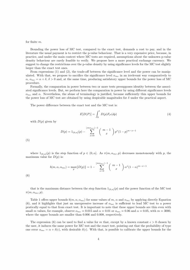
Bounding the power loss of MC test, compared to the exact test, demands a cost to pay, and in theliterature the usual payment is to restrict the p-value behaviour. That is a very expensive price, because, inpractice, and under the main context where MC tests are required, assumptions about the unknown p-valuedensity behaviour are rarely feasible to verify. We propose here a more practical exchange currency. Wesuggest to change the restrictions over the p-value density by using significance levels for the MC test slightlylarger than the exact test ones.

From expressions (1) and (2), the trade-off between the significance level and the power can be manip-ulated. With that, we propose to sacrifice the significance level αmc in an irrelevant way comparatively toα, αmc = α + δ, δ > 0 and, at the same time, producing satisfatory upper bounds for the power loss of MCprocedure.

Formally, the comparation in power between two or more tests presupposes identity between the associ-ated significance levels. But, we perform here the comparation in power by using different significance levelsαmc and α. Nevertheless, the abuse of terminology is justified, because sufficiently thin upper bounds forthe power loss of MC test are obtained by using despicable magnitudes for δ under the practical aspect.

The power difference between the exact test and the MC test is:

E[D(P )] =

∫ 1

0

D(p)FP (dp) (4)

with D(p) given by

D(p) = 1(0,α](p)−⌊mαmc⌋−1

∑

x=0

(

m− 1x

)

px(1− p)m−x−1

(5)

where 1(0,α](p) is the step function of p ∈ (0, α]. As π(m,αmc, p) decreases monotonously with p, themaximum value for D(p) is:

b(m,α, αmc) = maxp{D(p)} = 1−

⌊mαmc⌋−1∑

x=0

(

m− 1x

)

αx(1− α)m−x−1

(6)

that is the maximum distance between the step function 1(0,α](p) and the power function of the MC testπ(m,αmc, p).

Table 1 offers upper bounds b(m,α, αmc) for some values of m, α and αmc by applying directly Equation(6), and it highlights that just an unexpressive increase of αmc is sufficient to lead MC test to a powerpratically equal to that from exact test. It is important to note that these upper bounds are thin even withsmall m values, for example, observe αmc = 0.015 and α = 0.01 or αmc = 0.06 and α = 0.05, with m = 3000,where the upper bounds are smaller than 0.006 and 0.008, respectively.

The expression (6) can be used to find a value for m that, except by a known constant ǫ > 0 chosen bythe user, it induces the same power for MC test and the exact test, pointing out that the probability of typeone error αmc = α + δ(ǫ), with desirable δ(ǫ). With that, is possible to calibrate the upper bounds for the

4

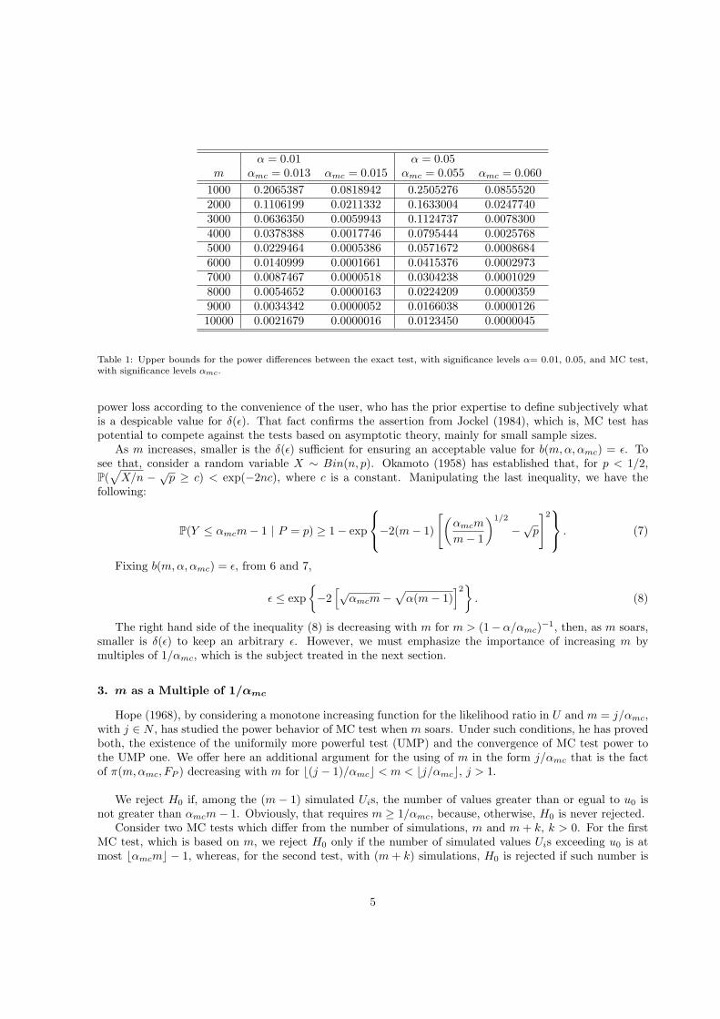
α = 0.01 α = 0.05m αmc = 0.013 αmc = 0.015 αmc = 0.055 αmc = 0.060

1000 0.2065387 0.0818942 0.2505276 0.08555202000 0.1106199 0.0211332 0.1633004 0.02477403000 0.0636350 0.0059943 0.1124737 0.00783004000 0.0378388 0.0017746 0.0795444 0.00257685000 0.0229464 0.0005386 0.0571672 0.00086846000 0.0140999 0.0001661 0.0415376 0.00029737000 0.0087467 0.0000518 0.0304238 0.00010298000 0.0054652 0.0000163 0.0224209 0.00003599000 0.0034342 0.0000052 0.0166038 0.000012610000 0.0021679 0.0000016 0.0123450 0.0000045

Table 1: Upper bounds for the power differences between the exact test, with significance levels α= 0.01, 0.05, and MC test,with significance levels αmc.

power loss according to the convenience of the user, who has the prior expertise to define subjectively whatis a despicable value for δ(ǫ). That fact confirms the assertion from Jockel (1984), which is, MC test haspotential to compete against the tests based on asymptotic theory, mainly for small sample sizes.

As m increases, smaller is the δ(ǫ) sufficient for ensuring an acceptable value for b(m,α, αmc) = ǫ. Tosee that, consider a random variable X ∼ Bin(n, p). Okamoto (1958) has established that, for p < 1/2,P(

√

X/n − √p ≥ c) < exp(−2nc), where c is a constant. Manipulating the last inequality, we have thefollowing:

P(Y ≤ αmcm− 1 | P = p) ≥ 1− exp

−2(m− 1)

[

(

αmcm

m− 1

)1/2

−√p

]2

. (7)

Fixing b(m,α, αmc) = ǫ, from 6 and 7,

ǫ ≤ exp

{

−2[√

αmcm−√

α(m− 1)]2

}

. (8)

The right hand side of the inequality (8) is decreasing with m for m > (1− α/αmc)−1, then, as m soars,

smaller is δ(ǫ) to keep an arbitrary ǫ. However, we must emphasize the importance of increasing m bymultiples of 1/αmc, which is the subject treated in the next section.

3. m as a Multiple of 1/αmc

Hope (1968), by considering a monotone increasing function for the likelihood ratio in U and m = j/αmc,with j ∈ N , has studied the power behavior of MC test when m soars. Under such conditions, he has provedboth, the existence of the uniformily more powerful test (UMP) and the convergence of MC test power tothe UMP one. We offer here an additional argument for the using of m in the form j/αmc that is the factof π(m,αmc, FP ) decreasing with m for ⌊(j − 1)/αmc⌋ < m < ⌊j/αmc⌋, j > 1.

We reject H0 if, among the (m − 1) simulated Uis, the number of values greater than or egual to u0 isnot greater than αmcm− 1. Obviously, that requires m ≥ 1/αmc, because, otherwise, H0 is never rejected.

Consider two MC tests which differ from the number of simulations, m and m + k, k > 0. For the firstMC test, which is based on m, we reject H0 only if the number of simulated values Uis exceeding u0 is atmost ⌊αmcm⌋ − 1, whereas, for the second test, with (m + k) simulations, H0 is rejected if such number is

5

at most ⌊αmc(m + k)⌋− 1. According to (1), for any observed P = p, the power of the second test is greaterthan that from the first test if

⌊αmc(m+k)⌋−1∑

y=0

(

m + k − 1y

)

py(1− p)m−y−1 >

⌊αmcm⌋−1∑

y=0

(

m− 1y

)

py(1− p)m−y−1 (9)

Observe that this inequality is equivalent to

P(X ≤ ⌊αmc(m + k)⌋ − 1) > P(Y ≤ ⌊αmcm⌋ − 1)

where X ∼ Bin(m + k − 1, p) and Y ∼ Bin(m− 1, p). If 0 < k < 1/α, then

P(X ≤ ⌊αmc(m + k)⌋ − 1) = P(X ≤ ⌊αmcm⌋ − 1)

and the inequality (9) becomes

P(X ≤ ⌊αmcm⌋ − 1) > P(Y ≤ ⌊αmcm⌋ − 1) ,

which is not valid. Thus, if 0 < k < 1/α, π(m + k, αmc, FP ) ≤ π(m,αmc, FP ). For example, forαmc = 0.01, a MC test with m1 = 1050 is less powerful than a test with m2 = 1000.

4. Discussion

A considerable parcel of the researchers, who are devoted to the development of statistical tests, arerestricted to study the limit distribution of the test statistic to guide the criterium decision about accep-tance/rejection the null hypothesis. Such works should consider Monte Carlo test application with the sameentusiasm that is currently devoted to asymptotic study. What support this assertion is that Monte Carloapproach preserves power comparatively to the exact test and controls the real probability of the type oneerror, what is not always true in the asymptotic treatment, particularly for moderated sample sizes.

References

Assuncao, R., Maia, A., 2007. A note on testing separability in spatial-temporal marked point processes.Biometrics 63 (1), 290–294.

Barnard, G., 1963. Discussion of professor bartlett´s paper. J. R. Statist. Soc. 25B (294).

Besag, J., Clifford, P., 1991. Sequential monte carlo p-value. Biometrika 78, 301–304.

Birnbaum, Z., 1974. Computers and unconventional test-statistics. in: F. proschan and r.j. serfling. Reliabilityand Biometry, 441–458.

Booth, J., Butler, R., 1999. An importance sampling algorithm for exact conditional tests in log-linearmodels. Biometrika 86, 321–332.

Caffo, B., Booth, J., 2003. Monte carlo conditional inference for log-linear and logistic models: a survey ofcurrent methodology. Statistical Methods in Medical Research 12, 109–123.

Dufour, J., 2005. Monte carlo tests with nuisance parameters: A general approach to finite-sample inferenceand nonstandard asymptotics. Jornal of Econometrics 133 (2), 443–477.

Dwass, M., 1957. Modified randomization tests for nonparametric hypotheses. Annals of Mathematical Statis-tics 28, 181–187.

6

Fay, M., Follmann, D., 2002. Designing monte carlo implementations of permutation or bootstrap hypothesistests. The American Statistician 56 (1), 63–70.

Fay, M., Kim, H.-J., Hachey, M., 2007. On using truncated sequential probability ratio test boundaries formonte carlo implementation of hypothesis tests. Journal of Computational and Graphical Statistics 16,946–967.

Gandy, A., 2009. Sequential implementation of monte carlo tests with uniformly bounded resampling risk.Journal of the American Statistical Association 104 (488), 1504–1511.

Hope, A., 1968. A simplified monte carlo significance test procedure. Journal of the Royal Statistical Society30B, 582–598.

Jockel, K., 1984. Application of monte-carlo tests - some considerations. Biometrics 40 (1), 263–263.

Jockel, K., 1986. Finite sample properties and asymptotic efficiency of monte carlo tests. The Annals ofStatistics 14, 336–347.

Kim, H.-J., 2010. Bounding the resampling risk for sequential monte carlo implementation of hypothesistests. Journal of Statistical Planning and Inference (140), 1834–1843.

Kulldorff, M., 2001. Prospective time periodic geographical disease surveillance using a scan statistic. Journalof Royal Statistical Society 164A, 61–72.

Marriott, F., 1979. Bernard’s monte carlo test: How many simulations? Applied Statististics 28, 75–77.

Okamoto, M., 1958. Some inequalities relating to the partial sum of binomial probabilities. Annals of theInstitute of Statistical Mathematics 10, 29–35.

Peng, R., Schoenberg, F., Woods, J., 2005. A space-time conditional intensity model for evaluating a wildfirehazard index. Journal of the American Statistical Association 100 (469), 26–35.

Ripley, B., 1992. Applications of monte-carlo methods in spatial and image-analysis. Lecture Notes in Eco-nomics and Mathematical Systems 376, 47–53.

Sackrowitz, H., Samuel-Cahn, E., 1999. P values as random variables - expeted p values. The AmericanStatistician 53, 326–331.

Silva, I., Assuncao, R., Costa, M., 2009. Power of the sequential monte carlo test. Sequential Analysis 28 (2),163–174.

Wongravee, K., Lloyd, G., Hall, J., Holmboe, M., Schaefer, M., Reed, R., Trevejo, J., Brereton, R., 2009.Monte-carlo methods for determining optimal number of significant variables. application to mouse urinaryprofiles. Metabolomics 5 (4), 387–406.

Acknowledgements

We are grateful to Martin Kulldorff for very useful comments and suggestions on an earlier draft of thispaper. This research was partially funded by the National Cancer Institute, grant number RO1CA095979,Martin Kulldorff PI. The second author was partially supported by the Conselho Nacional de Desenvolvi-mento Cientıfico e Tecnologico (CNPq). This research was partially carried out while the first author was atthe Department of Ambulatory Care and Prevention, Harvard Medical School, whose support is gratefullyacknowledged.

7

Optimal Generalized Sequential Monte Carlo Test

I. R. Silva∗, R. M. Assuncao

Departamento de Estatıstica, Universidade Federal de Minas Gerais, Belo Horizonte, Minas Gerais, Brazil

Abstract

Conventional Monte Carlo tests require the simulation of m independent copies from the test statistic

U under the null hypothesis H0. The execution time of these procedures can be substantially reduced by

a sequential monitoring of the simulations. The sequential Monte Carlo test power and its expected time

are analytically intractable. The literature has evaluated the properties of sequential Monte Carlo tests

implementations by using some restrictions on the probability distribution of the p-value statistic. Such

restrictions are used to bound the resampling risk, the probability that the accept/reject decision is different

from the decision from the exact test. This paper develops a generalized sequential Monte Carlo test that

includes the main previous proposals and that allows an analytical treatment of the power and the expected

execution time. This results are valid for any test statistic. We also bound the resampling risk and obtain

optimal schemes minimizing the expected execution time within a large class of sequential design.

Keywords: Sequential Monte Carlo test, Power loss, p-value density, Resampling risk, Sequential design,

Sequential probability ratio test.

1. Introduction

In the conventional Monte Carlo (MC) tests, the user selects the number m of simulations of the test

statistic U under H0. A Monte Carlo p-value is calculated based on the proportion of the simulated values

that are larger or equal than the observed value of U , assuming that large values of U lead to the null

hypothesis rejection. This procedure can take a long time to run if the test statistic requires a complicated

calculation as, for example, those involved in complex models. These situations are exactly those where the

MC tests are likely to be most useful, as analytical exact or asymptotic results concerning the test statistic

U is hard to obtain. The adoption of sequential procedures to carry out MC tests is a way to reach a faster

decision. In contrast with the fixed size MC procedure, in the sequential MC test the number of simulated

statistics is a random variable. The basic idea is to stop simulating as soon as there is enough evidence either

to reject or to accept the null hypothesis. For example, it is intuitively clear that, if the observed value of

∗Corresponding authorEmail addresses: [email protected] (I. R. Silva), [email protected] (R. M. Assuncao)

Preprint submitted to Journal of Statistical Planning and Inference May 2, 2011

U is close to the median of the first 100 simulated values, the null hypothesis is not likely to be rejected

even if we perform another 950 simulations. If a valid p-value could be provided, most researchers would be

confident to stop at this point. Sequential Monte Carlo tests are procedures that provide valid p-values in

these situations.

Let Xt be the number of simulated statistics under H0 exceeding the observed value u0 at t-th simulation.

In general, sequential MC procedures track the Xt evolution by checking if it crosses an upper or a lower

boundary. When it does, the test is halted and a decision is reached. Typically, crossing the lower boundary

leads to the rejection of the null hypothesis while the upper boundary crossing leads to the acceptance of

the null hypothesis.

There are different proposals for a sequential Monte Carlo test in the statistical literature. Besag and

Clifford (1991) proposed a very simple scheme that provides valid p-value for a sequential test with an upper

bound n − 1 in the number of simulations of U . It depends on a single tuning parameter h, making it

extremely simple to use. We stop the simulations when Xt = h for the first time and t < n. If Xn−1 < h,

the simulations are halted. If h ≤ l ≤ n− 1 is the number of simulations carried out and if we stop at time

t, the sequential p-value is given by

pBC =

Xt/t, if Xt = h,

(Xt + 1)/n, if Xt < h.(1)

The support set of pBC is

S = {1/n, 2/n, . . . , h/n, h/(n− 1), . . . , h/(h + 2), h/(h + 1), 1} .

and we have P(Ps ≤ a) = a under the null hypothesis if a ∈ S. This is a valid p-value estimator, because, a

p-value estimator Pe is valid if P(Pe ≤ b) ≤ b, where b is an element from the support set of Pe. Additional

randomization can provide a continuous p-value with uniform distribution in the interval (0, 1), rather than

distributed on the discrete set S.

Therefore, the boundaries of Besag and Clifford (1991) are given by the horizontal line Xt = h and

the vertical line t = n − 1. There is no lower boundary but only a predetermined maximum number of

simulations, typically called a truncated sequential Monte Carlo test. The Besag and Clifford sequential

MC test brings a reduction in execution time only when the null hypothesis is true. When it is false, one

will often run the Monte Carlo simulation up to its upper bound n− 1. Therefore, additional gains could be

obtained by adopting a stopping criterium based on large values of Xt. For any fixed type I error probability

α, Silva et al. (2009) showed that one can design a Besag and Clifford sequential MC test with the same

power as a conventional Monte Carlo test and with shorter running time. Silva et al. (2009) showed also

the puzzling result that this sequential Monte Carlo should have a maximum sample size equal to h/α + 1,

because, for n ≥ h/α + 1, the power is constant.

2

In addition to Besag and Clifford (1991), alternative sequential Monte Carlo tests have been suggested

recently. These other procedures are mainly concerned with the resampling risk, defined by Fay and Follmann

(2002) as the probability that the test decision of a realized MC test will be different from a theoretical

MC test with an infinite number of replications. Fay and Follmann (2002) proposed the curtailed sampling

design, where, if Xt ≥ ⌊α(n + 1)⌋, the procedure is interrupted and H0 is not rejected, and, if t − Xt ≥⌈(1− α)(n + 1)⌉ or the number of simulations reaches n, the procedure is interrupted and H0 is rejected,

where n is the maximum number of simulations. They also introduced the interactive push out (IPO)

procedure that requires a sequential algorithm to define the boundaries of the sequential procedure. This

procedure is not proven to be optimal but simply to decrease the sample size with respect to a curtailed

sampling design. For all their results, Fay and Follmann (2002) assumed a specific class of distribution

for the p-value statistic, that distribution implied by a test statistic U that follows the standard normal

distribution under the null hypothesis and follows a N(µ, 1) under the alternative hypothesis. Conditional

to this class of distributions, they found numerically the worst distribution to bound the resampling risk.

IPO has a smaller expected execution time than the curtailed sampling design but its implementation is

not practical for bounding the resampling risk in arbitrarily low values such as 0.01, for example. Also, we

think that the assumption on the p-value distribution is too restrictive and, in fact, we show that it is not

necessary to obtain optimal procedures.

Fay et al. (2007) proposed an algorithm (and an R package) to implement a truncated Sequential Prob-

ability Ratio Test (tSPRT) to bound the resampling risk and studied its behaviour as a function of the

p-value. The algorithm, denoted here as the FKH algorithm, calculates a valid p-value, which depends on

the calculation of the number of ways to reach each point on the stopping boundary of the MC test.

Gandy (2009) proposed an algorithm to build a sequential MC test that uniformly bounds the resampling

risk in arbitrarily small values and provides lower bounds to the expected number of simulations. His

algorithm is not truncated and the expected number of simulations can be infinite for p-values close to

α. Therefore, the simulations may go on indefinitely. One missing issue in his paper is the lack of results

concerning the type I error probability when the number of simulations is truncated.

Kim (2010) explored the approach from Fay and Follmann (2002) to bound the resampling risk using

their same restrictive class of p-value distributions. She used the B-value boundaries proposed by Lan and

Wittes (1988) and applied the algorithm of Fay et al. (2007) to obtain valid p-values estimates. She was able

to obtain arbitrarily low bounds to the resampling risk and showed empirically that the B-value boundaries

produces a smaller expected number of simulations than the IPO designs. In this paper, she also defined an

approximated B-value procedure, which is easy to calculate and has analytical formulas that give insights

on the choice of parameter values of the exact B-value design.

These B-value boundaries have the main advantages from the other procedures cited and, in our opinion,

3

is the best alternative for a sequential MC test at the moment. However, its main results, concerning the

resampling risk and the expected number of simulations, depend on the same restrictive class of p-value

distributions of Fay and Follmann (2002). Moreover, important topics were not explored for the B-value

boundaries such as, for example, its power with respect to the conventional MC test or the establishment

of lower bounds for the expected number of simulations for any test statistic.

In this paper, we introduce a generalized sequential Monte Carlo allowing any monotonic shapes for the

boundaries. For example, it is possible to construct boundaries which are close to each other in the beginning

of the simulations, departing from each other as the simulations proceed and approaching each other again

in the end of the simulations. We have been able to obtain bounds for the power loss of the sequential MC

test. In fact, we establish boundaries shapes such that the sequential MC test has the same power as the

conventional MC test for any α level. These boundaries are simple to calculate and they are valid in the

general case of any p-value distribution. Moreover, we are able to provide an algorithm to find the truncated

boundaries that lead to a design with minimum expected sampling size. Concerning the resampling risk, we

consider a larger class of distributions for the p-value than Fay and Follmann (2002) and we show that it is

suitable to explicit algebraic manipulation allowing simple bounding of the resampling risk for any sequential

MC test design.

This paper is organized in the following way. In the next section, we describe the B-value boundaries.

Section 3 defines our sequential MC test and develops its properties. In Section 4 we discuss a general class

for the p-value distribution and provide some analytical results for the sequential tests. Section 5 presents a

numeric routine for the preliminary choice of our boundaries and some specific suggestions for practical use.

Section 6 offers a comparison between the B-value procedure and our procedure. Section 7 closes the paper

with some discussion.

2. The B-value Procedure

Consider a hypothesis test of a null hypothesis H0 against an alternative hypothesis Ha by means of a

test statistic U . The MC test can be seen as an estimation procedure to the unknown decision from the

exact test based on the null hypothesis distribution of U . Kim (2010) has adopted this point of view by

seeing the MC test as a decision procedure concerning in which (0, 1) interval, either (0, α] or (α, 1), does

belong the exact p-value associated with the test statistic U . The parameter α is the significance level of

the exact test. This interpretation leads to the following pair of hypotheses:

H∗0 : p ≤ α

H∗A : p > α (2)

4

where p is the observed and unknown p-value generated from the random variable p-value. Viewed as a

random variable, we denote the p-value by P . Clearly, the decision in favor of any hypotheses above leads

to a decision concerning the original hypotheses H0 and HA.

Let U be the test statistic, u0 be its observed value for a fixed sample and ui, i = 1, ..., be the independently

simulated values from U under H0. Let

Xt =t

∑

i=1

1{[u0,∞)}(ui) ,

where 1{[u0,∞)}(ui) is the indicator function that ui ≥ u0.

Kim (2010) used the B-value introduced by Lan and Wittes (1988) to propose a sequential procedure to

test H∗0 versus H∗

A. Define:

V (t) = min{

s ≥ 0 : x− tx ≥ c1

√

nα(1 − α)}

and

L(t) = max{

s ≥ 0 : x− tα ≤ c2

√

nα(1− α)}

.

Define also:

BSup ={

(t, x) = (t, min{V (t), r1}) : t = t+0 , t+0 + 1, ..., n)}

,

the upper boundary, and

BInf ={

(t, x) = (t, max{L(t), t− r0}) : t = t−0 , t−0 + 1, ..., n)}

,

the lower boundary of a sequential Monte Carlo test, where t+0 is the smaller value of t such that V (t) ≤ t

and t−0 is the smaller value of t such that L(t) ≥ 0. Similarly, let t+1 be the smaller value of t such that

V (t) ≥ r1 and t−1 the smaller value of t such that L(t) ≤ t− r0. The stopping boundaries from Kim (2010)

are given by B = BInf ∪BSup. The B boundaries are formed by the union of linear functions in t. Figure

1 illustrate the B-boundaries BSup and BInf using c1 = −c2 = 1.282, n = 600 and α = 0.05.

The upper boundary BSup is formed by the union of the line V (t) = c1

√

nα(1− α) + tα until t = t+1 ,

when the upper boundary becomes the horizontal line with height r1 = ⌊α(n + 1)⌋. The lower boundary

BInf is formed by the line L(t) = c2

√

nα(1 − α) + tα up to t = t−1 when it becomes the vertical line

r0 = t− ⌈(1− α)(n + 1)⌉.Kim (2010) uses φFKH , the test criterium based on the valid p-value presented in Fay et al. (2007). The

valid p-value is defined as pv(Xt, t) = FpMLE(Xt/t), where pMLE is the maximum likelihood estimator of p

and Fp is defined in (5.2) from Fay et al. (2007). The estimate pv(Xt, t) of the p-value can be computed

using the FKH algorithm. The test adopted by Kim (2010) for the B boundaries is given by:

φFKH(t, x) =

1, if pv(x, t) ≤ α

0, if pv(x, t) > α.

5

0 100 200 300 400 500 600

05

10

15

20

25

30

t

Xt

Figure 1: Example of the B boundaries with α = 0.05 and maximum number of simulations equal to n = 600.

When φFKH(t, x) = 0, H0 is not rejected (because H∗0 : p ≤ α is rejected). For φFKH(t, x) = 1, H0 is

rejected (that is, H∗0 : p ≤ α is not rejected). Henceforth, this procedure is called MCB.

It is very important to remark that there is no need to check the value of Xt at every moment t. To

see this, noticed that the boundaries BSup and BInf are composed by non-integer numbers while Xt is a

count. As a consequence, there will be times t for which the simulations can not be interrupted by BInf and

therefore there is no need to check against the lower boundary at these times. To illustrate this, consider the

example from Kim (2010) illustrated in Figure 1. Table 1 shows the values of BSup and BInf between the

times 134 and 179. The lower boundary is equal to zero until t = 136 and it is formed by numbers smaller

than 1 until t = 156. Therefore, Xt reach the lower boundary during this period if X137 = 0 and there is no

need to check against it for t ≤ 136. Likewise, if Xt is not interrupted by BInf at t = 156 (that is, X156 ≥ 2),

it will not reach it at least until t = 176. Therefore, in practice, there is no need to check against the lower

boundary for every simulated value. One needs to check only on those times t such that

BInf(t− 1) < BInf(t)

for t = 2, . . . , m where BInf(t) is the value of the lower boundary at time t. This will be explored by our

generalized sequential Monte Carlo method described in Section 3.

Since BSup will typically be non-integer, it is always possible to define step functions equivalent to the

upper boundary. To see this, consider again the Table 1. From t = 134 to t = 143, it is clear that the values

BSup(t) could be all substituted by 14 and the procedure would remain the same.

6

2.1. Bounding the resampling risk of MCB

Fay and Follmann (2002) considered the IPO procedure that, interactively with the current simulations,

adjusts the initial boundaries. This method allows the bounding of the resampling risk. The IPO procedure

is not described in details here, but it should be noted that it is a computationally intensive procedure,

and its implementation is intractable for bounding the resampling risk in arbitrarily small values (see (Kim,

2010)). Fay and Follmann (2002) considered a rather restrictive class of p-value distributions, with cumulative

distribution function given by:

Hα,1−β(p) = 1− Φ{

Φ−1(1− p)− Φ−1(1− α) + Φ−1(β)}

(3)

where Φ(.) is the cumulative distribution function of a standard Normal distribution, α is the desired signif-

icance level and β is the type II error probability. When α = 1 − β, the cumulative distribution Hα,1−β(p)

has a uniform distribution on (0, 1), as is expected when H0 is true.

The p-value distribution defined in (3) assumes a variety of shapes, but the analytical manipulation of

the resampling risk or of the expected number of simulations is intractable. To circumvent this problem,

Fay and Follmann (2002) used a Beta(a, b) distribution to approximate Hα,1−β(p), and this approximation

is denoted by Hα,1−β(p). This approximation is chosen such that the expected value of P coincides with

that from Hα,1−β(p) and such that Hα,1−β(α) = Hα,1−β(α) = 1− β. Numerical studies were performed by

Fay and Follmann (2002) to obtain the worst case F within the class (3) in the sense of having the largest

resampling risk. Let F ∗ be the correspondent Beta distribution approximation to F .

Although MCB is simpler and present a smaller expected time execution than the IPO procedure, it

depends on the FKH algorithm which requires rather complex modifications for each type of sequential

design. Kim (2010) proposes an approximation for the MCB procedure. With this approximation, if BSup

is reached before BInf, H∗0 is rejected, while H∗

A is accepted if BInf is reached first. The approximation

may be used to gain analytic insights on the properties of the MCB procedure or to help on choosing the

parameters c1, c2, and n, as well as providing an approximation for the expected number of simulations. An

undesirable characteristic of the approximated MCB is that it is not truncated and the expected number

of simulations must be calculated letting the maximum number of simulations go to infinity. Moreover, the

approximation to MCB does not offer guarantee that the type I error probability is under control for any

choice of c1 and c2. For this reason, the approximation MCB will not be explored here.

3. Our proposed generalized sequential Monte Carlo test

The analytical treatment of the MC test power function, when it is based on two interruption boundaries,

is a cumbersome task. The reason is that it involves the calculation of the large number of possible trajectories

of the random variable Xt responsible for H0 rejection. Fay et al. (2007) present an algorithm to calculate

7

the terms associated with such number, and they used this algorithm to obtain both, the expected number of

simulations and the resampling risk, for each fixed p-value. Fay et al. (2007) emphasize that such algorithm

is valid only for the specific sequential procedure treated in that article, and adjustments are needed to use it

with other sequential designs. Kim (2010) also used that algorithm for her calculations, and the approximate

MCB is an attempt to escape from the dependence on special algorithms.

Aiming to overcome this limitation, we propose a truncated sequential procedure with two boundaries

that have the shape of step functions. The values of X(t) are checked against the upper boundary for every

t while they are checked against the lower boundary in an arbitrary set of predetermined discrete moments,

possibly a smaller set than all integers between 1 and m. As we showed in Section 2, the B-boundaries can

also be expressed by step functions with jumps equal to positive integer numbers. Therefore, the boundaries

of MCB and of our sequential procedure can be expressed in the same way. To express the boundaries by

means of step functions is more cumbersome in terms of notation. The motivation for this design, where the

lower boundary monitoring is not carried out for every time t, is mainly to allow for the analytical treatment

of the power function, the expected number of simulations of the sequential MC test for any test statistic.

We also bound the resampling risk of our sequential MC test.

Let ηI ={

nI1, n

I2, ..., n

Ik1

}

, with nIj < nI

j+1, be a set containing the moments when Xt must be checked

against the lower boundary given by the values I = {I1, I2, ..., Ik1}. If XnI

j< Ij , the simulations are

interrupted and H0 is rejected.

The monitoring of Xt with respect to the upper boundary crossing is carried out at all moments t =

1, . . . , m and this upper boundary is a step function. Let ηS ={

nS1 , nS

2 , ..., nSk2

}

, with nSj < nS

j+1 be the jump

moments for the upper boundary. For nSj−1 ≤ t < nS

j , the upper boundary is given by Sj where nS0 = 0 and

S1 < S2 . . . < Sk2. Let S = {S1, S2, ..., Sk2

}. Therefore, the simulations are interrupted if Dt = 1, where:

Dt =

1, if (t ∈ ηI and Xt < Ij , for t = nIj ) or (Xt = Sj, for nS

j−1 < t ≤ nSj )

0, otherwise(4)

or if the number of simulations reach a predetermined maximum equal to m.

Let xt be the observed value of the random variable Xt. The p-value can be estimated by:

pI =

xt/t, if xt = Sj , nSj−1 < t ≤ nS

j

(xt + 1)/(t + 1), if xt < Ij , t = nIj .

We define the test decision function for this sequential test:

φI(t, x) =

1, if the lower boundary I is reached before the upper S or the simulations reach m

0, if the upper boundary S is reached before the lower I.

The hypothesis H0 is rejected if φI = 1 and it is not rejected if φI = 0. This sequential MC test will be

denoted by MCG.

8

As an example, take k1 = k2 = 10, m = 600, and consider I = {0, 1, 2, 3, 9, 15, 20, 24, 27, 29} for the

lower boundary values, S = {5, 7, 9, 13, 17, 23, 26, 29, 29, 30} for the upper boundary values, and ηI = ηS =

{20, 50, 79, 119, 239, 359, 459, 539, 569, 600}. Figure 2 shows these boundaries as dashed lines.

The choice of the boundaries is closely linked to the desired αmc, which is equal to 0.05 in this example.

In Section 5, we present an algorithm to obtain the appropriate boundaries for any αmc and m in an easy and

fast way. The solid lines are the B boundaries calculated by Kim (2010) using c1 = −c2 = 1.282, n = 600,

and α = 0.05.

0 100 200 300 400 500 600

05

10

15

20

25

30

t

Xt

B boundaries

S and I

Figure 2: Example of the MCG (S and I) and B boundaries with α = 0.05 and a maximum number of simulations equal to

m = 600.

3.1. Power and Size of the MCG

In the MCG procedure, the rejection of H0 occurs in the first moment t = nIj such that xt < Ij . The

power calculation is simpler if we merge the two sets ηI and ηS . Define η = ηI ∪ ηS = {n1, n2, ..., nk}with k = #η. Let S

′

={

S′

1, S′

2, ..., S′

k

}

be the upper boundary adjusted for each ni ∈ η in the following

way. If ni = nSj ∈ ηS for some j, then S

′

i = Sj . If ni ∈ ηI ∩(

ηS)c

, then S′

i = Sj where j is such that

nSj = max

{

nSr < ni

}

. Thus, if ni matches with some jump time in the set ηS , then S′

i is equal to the value in

S for the time ni. If ni is not an element in ηS , then S′

i is the jump value of the time immediately preceding

ni.

Similarly, let I′

={

I′

1, I′

2, ..., I′

k

}

be the adjusted lower boundary. That is, when ni = nIj ∈ ηI or some

j, then I′

i = Ij . If ni ∈ ηS but ni /∈ ηI , then I′

i = Ij where j is such that nIj = max

{

nIj < ni

}

.

9

Thus, for a given value of p ∈ (0, 1), the power function of the MCG procedure, is given by:

πG(p) =

I′

1−1∑

x1=0

n1

x1

px1(1− p)n1−x1 +

+

min{

S′

1−1,I′

2−1}

∑

x1=I′

1

min{

I′

2−x1−1,n2−n1

}

∑

y=0

n2 − n1

y

py(1− p)n2−n1−y ×

×

n1

x1

px1(1− p)n1−x1

+

+

k−1∑

j=2

min{

S′

j−1,I′

j+1−1}

∑

xj=I′

j

min{

I′

j+1−xj−1,nj+1−nj

}

∑

y=0

min{

S′

j−1−1,xj

}

∑

xj−1=I′

j−1

· · ·

· · ·min

{

S′

1−1,x2

}

∑

x1=I′

1

nj+1 − nj

y

×

×

n1

x1

py+xj(1− p)nj+1−y−xj

j∏

i=2

ni − ni−1

xi − xi−1

. (5)

This expression is composed by k summands. If k is not too large, the direct application of this expression

produces results quickly and easily. The calculation would be computationally hard if we used a similar

expression for sequential procedure where k = m. Note that, in the MCB procedure, the number of

summands in (5) can reach up to 2αmcm.

Under the null hypothesis, p follows the U(0, 1) distribution. Hence, by integrating out (5) with respect

to p with a U(0, 1) density, we obtain the type I error probability for MCG:

P (type I error) =

∫ 1

0

πG(p)dp =I′

1

n1 + 1+

+

min{

S′

1−1,I′

2−1}

∑

x1=I′

1

min{

I′

2−x1−1,n2−n1

}

∑

y=0

n2 − n1

y

n1

x1

(n2 + 1)

n2

y + x1

+

+k−1∑

j=2

min{

S′

j−1,I′

j+1−1}

∑

xj=I′

j

min{

I′

j+1−xj−1,nj+1−nj

}

∑

y=0

min{

S′

j−1−1,xj

}

∑

xj−1=I′

j−1

· · ·

· · ·min

{

S′

1−1,x2

}

∑

x1=I′

1

nj+1 − nj

y

n1

x1

∏ji=2

ni − ni−1

xi − xi−1

(nj+1 + 1)

nj+1

y + xj

.

10

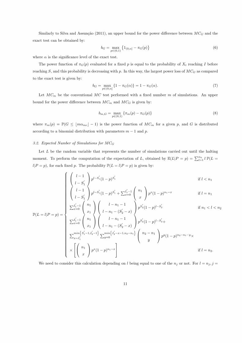
Similarly to Silva and Assuncao (2011), an upper bound for the power difference between MCG and the

exact test can be obtained by:

bG = maxp∈(0,1)

{

1(0,α] − πG(p)}

(6)

where α is the significance level of the exact test.

The power function of πG(p) evaluated for a fixed p is equal to the probability of Xt reaching I before

reaching S, and this probability is decreasing with p. In this way, the largest power loss of MCG as compared

to the exact test is given by:

bG = maxp∈(0,α]

{1− πG(α)} = 1− πG(α). (7)

Let MCm be the conventional MC test performed with a fixed number m of simulations. An upper

bound for the power difference between MCm and MCG is given by:

bm,G = maxp∈(0,1)

{πm(p)− πG(p)} (8)

where πm(p) = P(G ≤ ⌊mαmc⌋ − 1) is the power function of MCm for a given p, and G is distributed

according to a binomial distribution with parameters m− 1 and p.

3.2. Expected Number of Simulations for MCG

Let L be the random variable that represents the number of simulations carried out until the halting

moment. To perform the computation of the expectation of L, obtained by E(L|P = p) =∑nk

l=1 l P(L =

l|P = p), for each fixed p. The probability P(L = l|P = p) is given by:

P(L = l|P = p) =

l − 1

l − S′

1

pl−S′

1(1− p)S′

1 if l < n1

l − 1

l − S′

1

pl−S′

1(1− p)S′

1 +∑I

′

1−1x=0

n1

x

px(1− p)n1−x if l = n1

∑I′

1−1x=0

n1

x1

l − n1 − 1

l − n1 − (S′

2 − x)

pS′

2(1− p)l−S′

2 if n1 < l < n2

∑I′

1−1x=0

n1

x1

l − n1 − 1

l − n1 − (S′

2 − x)

pS′

2(1− p)l−S′

2+

∑min{

S′

1−1,I′

2−1}

x=I′

1

∑min{

I′

2−x−1,n2−n1

}

y=0

n2 − n1

y

py(1 − p)n2−n1−y×

×

n1

x

px(1− p)n1−x

if l = n2.

We need to consider this calculation depending on l being equal to one of the nj or not. For l = nj, j =

11

3, ..., k − 1, we have:

P(L = l|P = p) =

min{

S′

j−1−1,I′

j−1}

∑

xj−1=I′

j−1

min{

I′

j−xj−1−1,nj−nj−1

}

∑

y=0

min{

S′

j−2−1,xj−1

}

∑

xj−2=I′

j−2

· · ·

· · ·min

{

S′

1−1,x2

}

∑

x1=I′

1

nj − nj−1

y

×

×

n1

x1

py+xj−1(1− p)nj−y−xj−1

j−1∏

i=2

ni − ni−1

xi − xi−1

+

+

min{

S′

j−1−1,I′

j−1}

∑

xj−1=I′

j−1

min{

S′

j−2−1,xj−1

}

∑

xj−2=I′

j−2

· · ·

· · ·min

{

S′

1−1,x2

}

∑

x1=I′

1

nj − nj−1 − 1

nj − nj−1 − (S′

j − xj−1)

×

×

n1

x1

pl−S′

j (1− p)S′

j

j−1∏

i=2

ni − ni−1

xi − xi−1

.

For nj−1 < l < nj , j = 3, ..., k:

P(L = l|P = p) =

min{

S′

j−1−1,I′

j−1}

∑

xj−1=I′

j−1

min{

S′

j−2−1,xj−1

}

∑

xj−2=I′

j−2

· · ·

· · ·min

{

S′

1−1,x2

}

∑

x1=I′

1

nj − nj−1 − 1

nj − nj−1 − (S′

j − xj−1)

×

×

n1

x1

pl−S′

j (1− p)S′

j

j−1∏

i=2

ni − ni−1

xi − xi−1

.

Finally, for l = nk:

P(L = l|P = p) =

min{

S′

j−1−1,I′

j−1}

∑

xj−1=I′

j−1

min{

I′

j−xj−1−1,nj−nj−1

}

∑

y=0

min{

S′

j−2−1,xj−1

}

∑

xj−2=I′

j−2

· · ·

· · ·min

{

S′

1−1,x2

}

∑

x1=I′

1

nj − nj−1

y

×

×

n1

x1

py+xj−1(1− p)nj−y−xj−1

j−1∏

i=2

ni − ni−1

xi − xi−1

. (9)

12

Using that p has a U(0, 1) distribution under the null hypothesis, we have

E (L|H0 is true) =

∫ 1

0

E(L|P = p)dp . (10)

To calculate E(L) under HA it is necessary to know the p-value distribution. However, a bound is easier

to calculate as

bE(L) = maxp∈(0,1) {E(L|P = p)} . (11)

bE(L) is a very conservative upper bound for E(L). However, as we will illustrate in Section 5, this bound is

useful to bound the expectation of L in values less than 65% of m.

4. A class of distributions for the p-value

Kim (2010) showed that, for p = α, the resampling risk is at least 0.5. Hence, it is not possible to bound

the resampling risk in relevant values if we allow all distributions of p-values. This is the reason to define a

class for the p-value distribution, taken as the set ℑ of all continuous probability distributions in (0, 1) with

differentiable densities that are non-increasing (that is, f ′P (p) ≤ 0, for all p ∈ (0, 1), with f ′P representing

the first derivative with respect to p of the p-value density function f .

From the p-value definition, its probability distribution function can be written in the following way:

P(P ≤ p) = 1− FA

{

F−10 (1− p)

}

(12)

where FA denotes the probability distribution function of the test statistic U under HA and F0 is the

distribution of U under H0.

Assuming the existence of densities functions fA(u) and f0(u) of U under HA and H0, respectively, the

p-value density can be written as:

fP (p) =fA

{

F−10 (1− p)

}

f0

{

F−10 (1− p)

} . (13)

Hence, we can study the behavior of the p-value distribution by studying the behavior of the ratio between

fA(u) and f0(u).

In the majority of the real applications, the ratio (13) is non-increasing with p and this is the motivation

to restrict the analysis of the resampling risk to the set ℑ. Let ℑB be the class of p-value distributions

defined in Fay and Follmann (2002) with cumulative distribution Hα,1−β(p), as described in Section 2. Let

π be the power of the exact test. We will show now that, for π ≥ α, ℑ is more general than ℑB.

From the expression (3), the densities h(p) ∈ ℑB can be indexed by α and β and they are given by:

hα,1−β(p) = exp

{

−1

2

[

Φ−1(β) − Φ−1(1− α)] [

Φ−1(β)− Φ−1(1 − α) + 2Φ−1(1 − p)]

}

(14)

13

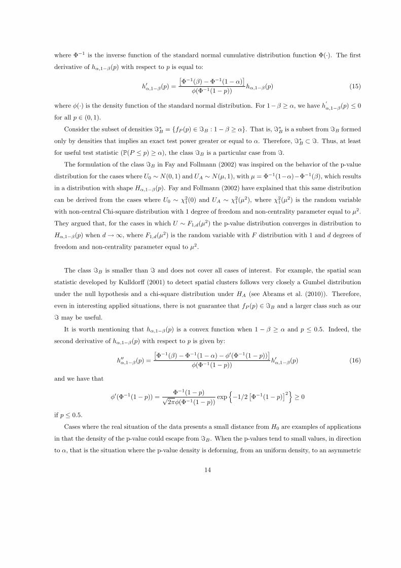
where Φ−1 is the inverse function of the standard normal cumulative distribution function Φ(·). The first

derivative of hα,1−β(p) with respect to p is equal to:

h′α,1−β(p) =

[

Φ−1(β) − Φ−1(1− α)]

φ(Φ−1(1− p))hα,1−β(p) (15)

where φ(·) is the density function of the standard normal distribution. For 1−β ≥ α, we have h′

α,1−β(p) ≤ 0

for all p ∈ (0, 1).

Consider the subset of densities ℑ∗B = {fP (p) ∈ ℑB : 1− β ≥ α}. That is, ℑ∗B is a subset from ℑB formed

only by densities that implies an exact test power greater or equal to α. Therefore, ℑ∗B ⊂ ℑ. Thus, at least

for useful test statistic (P(P ≤ p) ≥ α), the class ℑB is a particular case from ℑ.

The formulation of the class ℑB in Fay and Follmann (2002) was inspired on the behavior of the p-value

distribution for the cases where U0 ∼ N(0, 1) and UA ∼ N(µ, 1), with µ = Φ−1(1−α)−Φ−1(β), which results

in a distribution with shape Hα,1−β(p). Fay and Follmann (2002) have explained that this same distribution

can be derived from the cases where U0 ∼ χ21(0) and UA ∼ χ2

1(µ2), where χ2

1(µ2) is the random variable

with non-central Chi-square distribution with 1 degree of freedom and non-centrality parameter equal to µ2.

They argued that, for the cases in which U ∼ F1,d(µ2) the p-value distribution converges in distribution to

Hα,1−β(p) when d →∞, where F1,d(µ2) is the random variable with F distribution with 1 and d degrees of

freedom and non-centrality parameter equal to µ2.

The class ℑB is smaller than ℑ and does not cover all cases of interest. For example, the spatial scan

statistic developed by Kulldorff (2001) to detect spatial clusters follows very closely a Gumbel distribution

under the null hypothesis and a chi-square distribution under HA (see Abrams et al. (2010)). Therefore,

even in interesting applied situations, there is not guarantee that fP (p) ∈ ℑB and a larger class such as our

ℑ may be useful.

It is worth mentioning that hα,1−β(p) is a convex function when 1 − β ≥ α and p ≤ 0.5. Indeed, the

second derivative of hα,1−β(p) with respect to p is given by:

h′′α,1−β(p) =

[

Φ−1(β)− Φ−1(1− α)− φ′(Φ−1(1− p))]

φ(Φ−1(1− p))h′α,1−β(p) (16)

and we have that

φ′(Φ−1(1− p)) =Φ−1(1− p)√

2πφ(Φ−1(1− p))exp

{

−1/2[

Φ−1(1− p)]2}

≥ 0

if p ≤ 0.5.

Cases where the real situation of the data presents a small distance from H0 are examples of applications

in that the density of the p-value could escape from ℑB. When the p-values tend to small values, in direction

to α, that is the situation where the p-value density is deforming, from an uniform density, to an asymmetric

14

curve to the left hand, the convexity could not be verified for p ≤ 0.5. For example, suppose U0 ∼ χ21(0) e

UA ∼ χ21,01(0). The corresponding p-value density from this conjecture is not concave for p > 0.32.

The family ℑ for bounding the resampling risk is not restricted to families such as the normal, chi-square

or F distributions. It also contains p-value densities with mixed shapes, with concave and convex parts. As

an additional benefit, ℑ allows the bounding of the resampling risk in a very simple way.

In the next subsections, we analyze the power, the expected number of simulations and the resampling

risk of our generalized Monte Carlo test procedure when the p-value distribution belongs to the class ℑ.

It is important to remember that, when using the MCG, the class ℑ is not needed neither to calculate a

bound for the power loss with respect to the MCm or to the exact test nor to establish the bound for the

expected number of simulations under HA. Indeed, the results in the Sub-sections 3.1 and 3.2 are valid for

any test statistic. However, when the additional assumption that the p-value density fP (p) belongs to ℑholds, stronger results can be obtained.

4.1. Upper bound for the power difference between the exact test and MCG

The power of the generalized Monte Carlo test is given by integrating out the probability πG(p) of

rejecting the null hypothesis conditioned on the p-value p with respect to the p-value density:

πG =

∫ 1

0

πG(p)fP (p)dp .

The power difference between the exact test and MCG is given by:

δ∗G =

∫ 1

0

(

1(0,αmc](p)− πG(p))

fP (p)dp. (17)

An upper bound for δ∗I can be obtained if we use fP,w(p) = 1/αmc if p ∈ (0, αmc], and fP,w(p) = 0, otherwise:

δ∗G ≤ b∗I =

∫ 1

0

(

1(0,αmc](p)− πG(p))

fP,w(p)dp =

∫ αmc

0

1

αmcdp−

∫ αmc

0

πG(p)1

αmcdp

= 1− 1

αmc

∫ αmc

0

πG(p)dp. (18)

Because the function (5) is a sum of Beta(a, b) density kernels, the integral (18) can be rewritten as a

function of incomplete Beta(a, b) functions, all of them evaluated at p = αmc, with a and b depending only

of the parameters I, S e η. In the same way, an upper bound for the power difference between MCm and

MCG is given by:

b∗m,G =

∫ αmc

0

(πm(p)− πG(p))1

αmcdp. (19)

As before, (19) can also be expressed using incomplete beta functions.

15

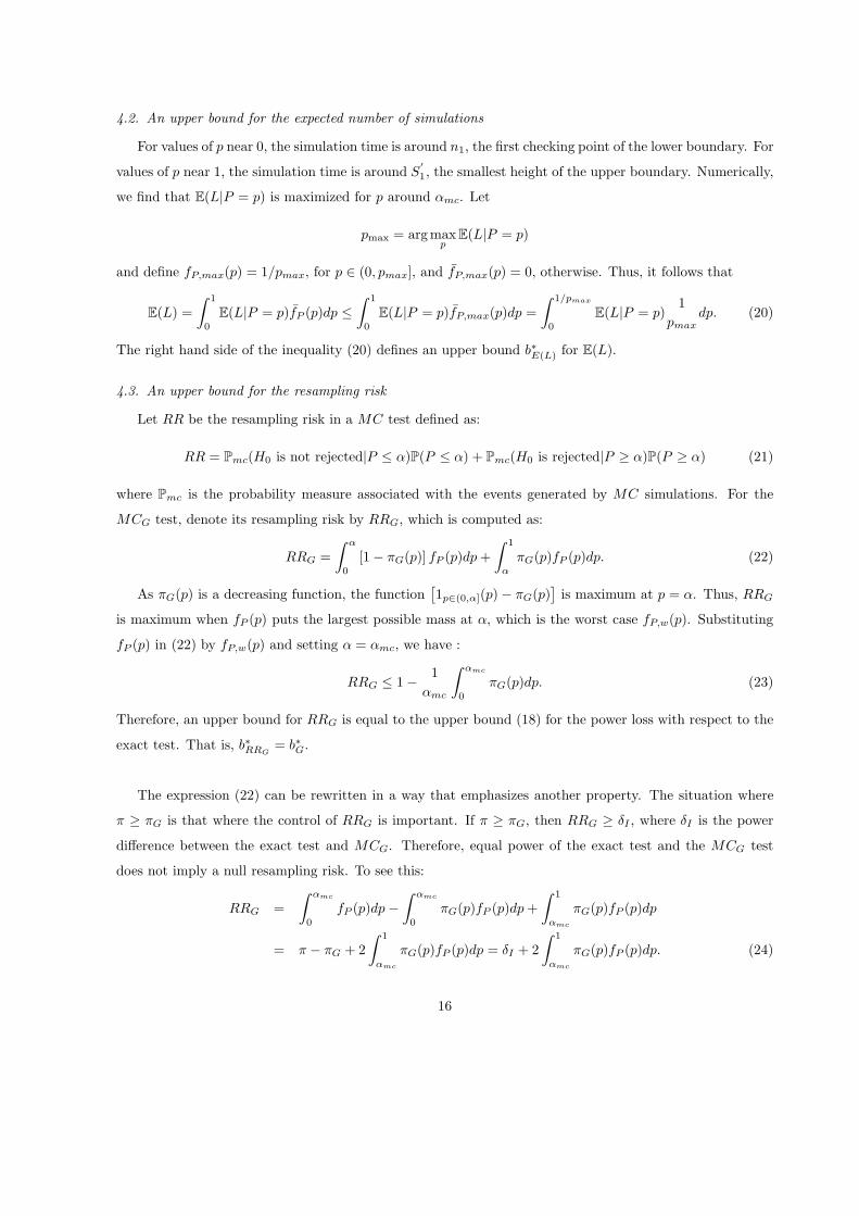
4.2. An upper bound for the expected number of simulations

For values of p near 0, the simulation time is around n1, the first checking point of the lower boundary. For

values of p near 1, the simulation time is around S′

1, the smallest height of the upper boundary. Numerically,

we find that E(L|P = p) is maximized for p around αmc. Let

pmax = argmaxp

E(L|P = p)

and define fP,max(p) = 1/pmax, for p ∈ (0, pmax], and fP,max(p) = 0, otherwise. Thus, it follows that

E(L) =

∫ 1

0

E(L|P = p)fP (p)dp ≤∫ 1

0

E(L|P = p)fP,max(p)dp =

∫ 1/pmax

0

E(L|P = p)1

pmaxdp. (20)

The right hand side of the inequality (20) defines an upper bound b∗E(L) for E(L).

4.3. An upper bound for the resampling risk

Let RR be the resampling risk in a MC test defined as:

RR = Pmc(H0 is not rejected|P ≤ α)P(P ≤ α) + Pmc(H0 is rejected|P ≥ α)P(P ≥ α) (21)

where Pmc is the probability measure associated with the events generated by MC simulations. For the

MCG test, denote its resampling risk by RRG, which is computed as:

RRG =

∫ α

0

[1− πG(p)] fP (p)dp +

∫ 1

α

πG(p)fP (p)dp. (22)

As πG(p) is a decreasing function, the function[

1p∈(0,α](p)− πG(p)]

is maximum at p = α. Thus, RRG

is maximum when fP (p) puts the largest possible mass at α, which is the worst case fP,w(p). Substituting

fP (p) in (22) by fP,w(p) and setting α = αmc, we have :

RRG ≤ 1− 1

αmc

∫ αmc

0

πG(p)dp. (23)

Therefore, an upper bound for RRG is equal to the upper bound (18) for the power loss with respect to the

exact test. That is, b∗RRG= b∗G.

The expression (22) can be rewritten in a way that emphasizes another property. The situation where

π ≥ πG is that where the control of RRG is important. If π ≥ πG, then RRG ≥ δI , where δI is the power

difference between the exact test and MCG. Therefore, equal power of the exact test and the MCG test

does not imply a null resampling risk. To see this:

RRG =

∫ αmc

0

fP (p)dp−∫ αmc

0

πG(p)fP (p)dp +

∫ 1

αmc

πG(p)fP (p)dp

= π − πG + 2

∫ 1

αmc

πG(p)fP (p)dp = δI + 2

∫ 1

αmc

πG(p)fP (p)dp. (24)

16

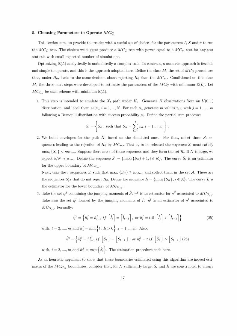
5. Choosing Parameters to Operate MCG

This section aims to provide the reader with a useful set of choices for the parameters I, S and η to run

the MCG test. The choices we suggest produce a MCG test with power equal to a MCm test for any test

statistic with small expected number of simulations.

Optimizing E(L) analytically is undoubtedly a complex task. In contrast, a numeric approach is feasible

and simple to operate, and this is the approach adopted here. Define the class M , the set of MCG procedures

that, under H0, leads to the same decision about rejecting H0 than the MCm. Conditioned on this class

M , the three next steps were developed to estimate the parameters of the MCG with minimum E(L). Let

MCIopbe such scheme with minimum E(L).

1. This step is intended to emulate the Xt path under H0. Generate N observations from an U(0, 1)

distribution, and label them as pi, i = 1, ..., N . For each pi, generate m values xij , with j = 1, . . . , m

following a Bernoulli distribution with success probability pi. Define the partial sum processes

Si =

{

Sit, such that Sit =

t∑

l=1

xil, t = 1, ..., m

}

.

2. We build envelopes for the path Xt based on the simulated ones. For that, select those Si se-

quences leading to the rejection of H0 by MCm. That is, to be selected the sequence Si must satisfy

maxt {Sit} < mαmc. Suppose there are s of those sequences and they form the set R. If N is large, we

expect s/N ≈ αmc. Define the sequence St = {maxi {Sit}+ 1, i ∈ R}. The curve St is an estimator

for the upper boundary of MCGop.

Next, take the r sequences Si such that maxt {Sit} ≥ mαmc and collect them in the set A. These are

the sequences S′is that do not reject H0. Define the sequence It = {mini {Sit} , i ∈ A}. The curve It is

the estimator for the lower boundary of MCGop.

3. Take the set ηS containing the jumping moments of S. ηS is an estimator for ηS associated to MCGop.

Take also the set ηI formed by the jumping moments of I. ηI is an estimator of ηI associated to

MCGop. Formally:

ηI ={

nIt = nI

t−1 if⌈

It

⌉

=⌈

It−1

⌉

, or nIt = t if

⌈

It

⌉

>⌈

It−1

⌉}

(25)

with, t = 2, ...., m and nI1 = min

{

l : Il > 0}

, l = 1, ..., m. Also,

ηS ={

nSt = nS

t−1 if⌊

St ⌋ =⌊

St−1 ⌋ , or nSt = t if

⌊

St ⌋ >⌊

St−1 ⌋ (26)

with, t = 2, ...., m and nS1 = min

{

St

}

. The estimation procedure ends here.

As an heuristic argument to show that these boundaries estimated using this algorithm are indeed esti-

mates of the MCGopboundaries, consider that, for N sufficiently large, St and It are constructed to ensure

17

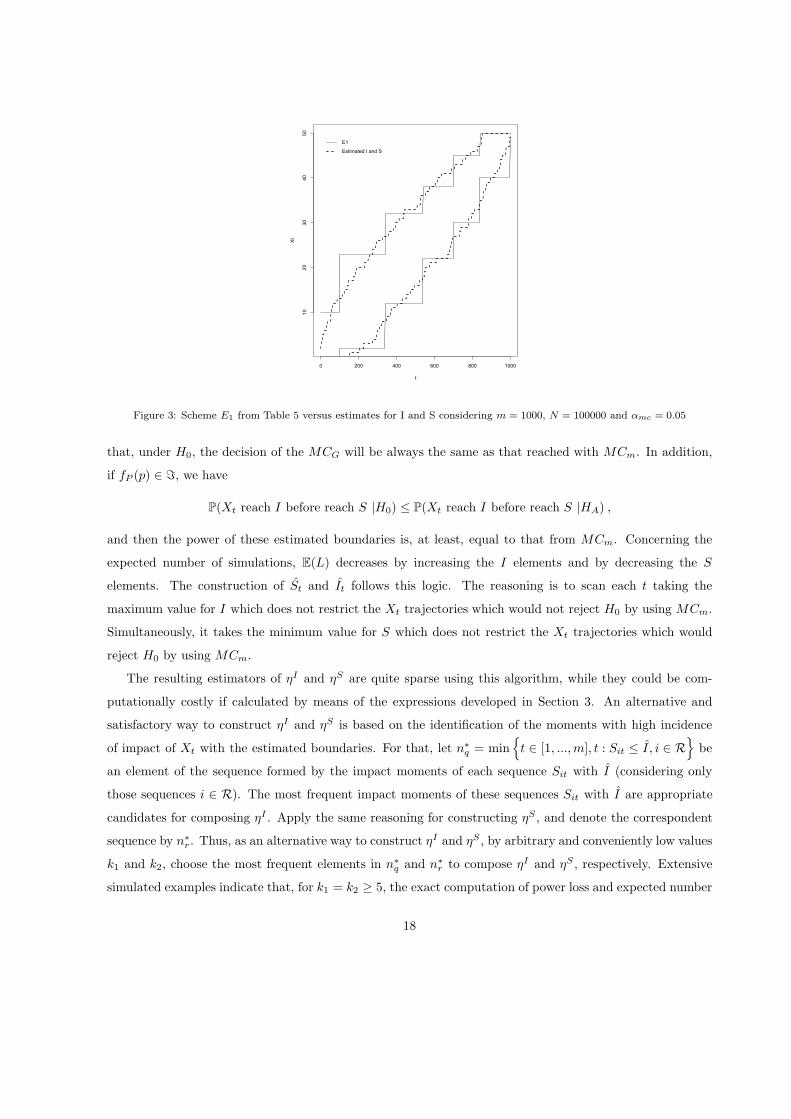
0 200 400 600 800 1000

10

20

30

40

50

t

Xt

E1

Estimated I and S

Figure 3: Scheme E1 from Table 5 versus estimates for I and S considering m = 1000, N = 100000 and αmc = 0.05

that, under H0, the decision of the MCG will be always the same as that reached with MCm. In addition,

if fP (p) ∈ ℑ, we have

P(Xt reach I before reach S |H0) ≤ P(Xt reach I before reach S |HA) ,

and then the power of these estimated boundaries is, at least, equal to that from MCm. Concerning the

expected number of simulations, E(L) decreases by increasing the I elements and by decreasing the S

elements. The construction of St and It follows this logic. The reasoning is to scan each t taking the

maximum value for I which does not restrict the Xt trajectories which would not reject H0 by using MCm.

Simultaneously, it takes the minimum value for S which does not restrict the Xt trajectories which would

reject H0 by using MCm.

The resulting estimators of ηI and ηS are quite sparse using this algorithm, while they could be com-

putationally costly if calculated by means of the expressions developed in Section 3. An alternative and

satisfactory way to construct ηI and ηS is based on the identification of the moments with high incidence

of impact of Xt with the estimated boundaries. For that, let n∗q = min{

t ∈ [1, ..., m], t : Sit ≤ I , i ∈ R}

be

an element of the sequence formed by the impact moments of each sequence Sit with I (considering only

those sequences i ∈ R). The most frequent impact moments of these sequences Sit with I are appropriate

candidates for composing ηI . Apply the same reasoning for constructing ηS , and denote the correspondent

sequence by n∗r . Thus, as an alternative way to construct ηI and ηS , by arbitrary and conveniently low values

k1 and k2, choose the most frequent elements in n∗q and n∗r to compose ηI and ηS , respectively. Extensive

simulated examples indicate that, for k1 = k2 ≥ 5, the exact computation of power loss and expected number

18

of simulations have a small computational cost, and the results are close to that using ηI and ηS .

Figure 3 shows the estimates I and S obtained according to the steps 1, 2, and 3, of our algorithm,

using N = 100000, m = 1000 and αmc = 0.05. The estimated boundaries are not parallel, but they are

characterized by a funnel in the extremities. This behavior was verified in all of the simulations performed by

us. For these specific estimates, if we take η = ηS = ηI , we obtain the times η = {99, 339, 539, 699, 839, 999}.From the estimates plotted in Figure 3, we obtain I = {2, 12, 22, 30, 40, 49}, and S = {10, 23, 32, 38, 45, 50}.This specific scheme for our generalized sequential MC test is available in Table 5 and it is labeled as E1.

As we can see in the Table 2, column bm,I , this scheme is efficient, presenting practically the same power

than MCm for m = 1000, with size equal to 0.049864. From Table 3, columns E(L|H0) and bE(L), we see

that this scheme have a small expected number of simulations, equal to 58.606 under H0, and with an upper

bound under HA for any statistic, that is approximately 65% of the maximum 999. By using the class ℑB

and the larger class ℑ for the p-value distribution, the bounds are expressively low, equal to 172.612 and

246.354, respectively. We consider that this scheme is a good option to replace MCm. We must enphasize

that, although the boundaries presented in Table 5 were guided by the algorithm above, all results in tables

2 and 3 are exact, because they were obtained by applying the expressions from Sections 3 and 4. Such

algorithm is useful to construct preliminary choices of boundaries. The validation of an arbitrary design to

practical use must be based on such exact calculations.

We provide other interesting schemes in Table 5. For each scheme, Table 2 offers the type I error

probability, the upper bound for the power loss comparatively to MCm and to the exact test, and the upper

bound for the resampling risk. Table 3 gives the expected number of simulations under H0 and the upper

bounds under HA. We adopt bm,G to denote the general upper bound for the power loss comparatively

to MCm, b∗G and b∗RRG, the upper bounds for the power loss, with respect to the exact test, and for the

resampling risk, respectively, where the super index ∗ indicates that the calculations are restricted to the

p-value distribution on the class ℑ. The same symbol was used to indicate the use of this class for the bounds

in Table 3. Upper bounds using the class ℑB are also available in Tables 2 and 3, and they are indicated by

a tilde accent. Concerning the use of ℑB, the numerical explorations of Fay and Follmann (2002) were not

used here to define the worst case of a p-value distribution with shape Hα;1−β(p). As discussed in Section

4.3, hα,1−β(p) (for 1− β ≥ α) and πG are decreasing with p. Therefore, the worst case within the class ℑB,

in the sense of bounding RRI , occurs at the point of maximum of the function Hα;1−β(α) with respect to

β. For 1− β ≥ α, the point of maximum in β for the function Hα;1−β(α) is 0.5. Then, the analytical worst

case is given by Hα;0.5(α). We used this result to compute bI , bRRGand bE(L) here.

19

6. MCG versus MCB

In this Section we offer a comparison between the MCB and MCG sequential test procedures. We use an

example of the MCB test given by Kim (2010). In this comparison, we focus on resampling risk bound and

on the expected number of simulations. We assume that the p-value distribution fP (p) belongs to the class

ℑB. We did not consider other important characteristics of a test, such as the power loss with respect to the

exact test and expected number of simulations for an arbitrary fP (p), because they were not treated by Kim

(2010). We built our MCG boundaries using the algorithm from Section 5. After securing an upper bound

for the resampling risk to MCG equal to that presented by the MCB scheme developed in Kim (2010), we

compared the average simulation time of the two procedures.

An obvious fact is that the B boundaries are particular cases of I and S, because MCG was designed to

be a generalized sequential with two stopping boundaries. We can rewrite the B boundaries using the MCG

notation, based on the sets I, S, ηI and ηS . In this way, for an MCB test, the user can apply the general

expressions for the power and the expected number of simulations developed in Section 3.

Define:

T ∗1 ={

t > 2 :⌈

BInf(t− 1)⌉

<⌈

BInf(t)⌉}

and

T ∗2 ={

t > 2 :⌊

BSup(t− 1)⌋

<⌊

BSup(t)⌋}

.

Let t∗11 < t∗12 < ... < t∗1k1be the ordered elements of T ∗1 , and t∗21 < t∗22 < ... < t∗2k2

be the ordered elements

of T ∗2 . Rewritten in terms of I and S, the B boundaries are denoted by I∗, S∗, ηI∗ and ηS∗, and they are

built as follows:

I∗ ={

⌈BInf (t∗11)⌉ , ⌈BInf (t∗12)⌉ , ...,⌈

BInf (t∗1k1)⌉}

S∗ ={

⌊BInf (t∗21)⌋ , ⌊BInf (t∗22)⌋ , ...,⌊

BInf (t∗2k2)⌋}

ηI∗ ={

t∗11, t∗12, ..., t

∗1k1

}

ηS∗ ={

t∗21, t∗22, ..., t

∗2k2

}

.

It should be noted that some important shapes for I and S, as the funnel behavior estimated in Section

5, can not be represented by the MCB boundaries.

Table 4 shows the upper bounds for the resampling risk and for the expected number of simulations

presented in Kim (2010) for n = 600, α = 0.05 and c1 = −c2 = 1.282, as well the bounds associated to MCG

20

0 100 200 300 400 500 600

05

10

15

20

25

30

A

t

Xt

MCB

MCG

0 100 200 300 400 500 600

05

10

15

20

25

30

B

t

Xt

MCB

I and S est

0 100 200 300 400 500 600

05

10

15

20

25

30

C

t

Xt

MCG

I and S est

0 100 200 300 400 500 600

05

10

15

20

25

30

D

t

Xt

MCB

MCG

I and S est

Figure 4: Boundaries for MCG and MCB sequential test procedures.

using the scheme E12 detailed in Table 5. Concerning the worst case of distribution within the class ℑB,

Kim (2010) adopted the numerical studies from Fay and Follmann (2002) and she found F ∗ = H0.05;0.47(p)

for α = 0.05, with approximation H0.05;0.47(p) := Beta(0.389; 2.523).

These bounds are also computed here for the sequential procedure proposed by Besag and Clifford (1991),

which will be denoted by MCh. This MCh procedure is a very simple way to perform sequential tests, because

it is based just in an upper boundary fixed in a value denoted by h and truncated in a maximum number

of simulations n. Silva et al. (2009) had showed that MCh has the same power than MCm if h = αmcm

and its power is constant for n ≥ h/αmc + 1, noting that the combination of this two last rules implies that

MCm must be replaced by MCh, because they have the same power for a maximum number of simulations

practically equal (that is, for n = m + 1).

Under either hypothesis, MCG is substantially faster than the MCB procedure with their expected time

ratio being around 60%. This illustrates the gain provided by our MCG algorithm. The estimated boundaries

for m = 600 and αmc = 0.05 for the MCG procedure are available in Figure 4, where we can also see the B

boundaries and the boundaries I and S (built according to the scheme E12). It is clear the greater flexibility

21

given by the MCG boundaries. While the B boundaries are parallel almost up to the end of the experiment,

the I and S boundaries are tapered when t gets close to the maximum number of simulations. This can

be intuitively thought as if the boundaries were using the information that Xt not touching the boundaries

after a long time was inducing a narrower vigilance.

7. Discussion

The generalized sequential Monte Carlo test has properties that recommend it in substitution to the

conventional Monte Carlo test for any test statistic. In this paper, we gave simple expressions for the

calculation of the test size, the expected number of simulations under the null hypothesis, and upper bounds

for the expected number of simulations under the alternative hypothesis and for the power loss with respect

to the fixed length conventional Monte Carlo test.

Exact calculations for some specific design indicates that our generalized sequential test has a substantially

smaller execution time than other sequential methods proposed in the literature. Under a wide class of

distributions for the p-value statistic, the bounds for the execution time under the alternative hypothesis

is even more substantial. Under this class, the generalized sequential test has power virtually identical to

the exact test, even for such intermediate maximum number of simulations as 4999. The use of this class

allows the construction of optimal boundaries from a simple algorithm and they have a surprising funnel-type

shape. These optimal boundaries, or any other generalized design, for any test statistic, can be evaluated

by calculating the size, expected number of simulations under H0, upper bound for the power loss and for

the expected number of simulations under HA, by using the expressions developed in section 3.

22

t BSup BInf t BSup BInf...

......

......

...

134 13.54 0.00 157 14.69 1.01

135 13.59 0.00 158 14.74 1.06

136 13.64 0.00 159 14.79 1.11

137 13.69 0.01 160 14.84 1.16

138 13.74 0.06 161 14.89 1.21

139 13.79 0.11 162 14.94 1.26

140 13.84 0.16 163 14.99 1.31

141 13.89 0.21 164 15.04 1.36

142 13.94 0.26 165 15.09 1.41

143 13.99 0.31 166 15.14 1.46

144 14.04 0.36 167 15.19 1.51

145 14.09 0.41 168 15.24 1.56

146 14.14 0.46 169 15.29 1.61

147 14.19 0.51 170 15.34 1.66

148 14.24 0.56 171 15.39 1.71

149 14.29 0.61 172 15.44 1.76

150 14.34 0.66 173 15.49 1.81

151 14.39 0.71 174 15.54 1.86

152 14.44 0.76 175 15.59 1.91

153 14.49 0.81 176 15.64 1.96

154 14.54 0.86 177 15.69 2.01

155 14.59 0.91 178 15.74 2.06

156 14.64 0.96 179 15.79 2.11...

......

......

...

Table 1: Boundary values BSup(t) and BInf (t) for 134 ≤ t ≤ 179.

23

α nk Scheme P(erro tipo I) bm,I bI b∗I = b∗RRGbRRG

E1 0.049864 0.031032 0.000000 0.060000 0.023000

E2 0.049681 0.031748 0.000000 0.060895 0.023337

0.05 999 E3 0.049920 0.027828 0.000000 0.060118 0.022348

E4 0.049982 0.024751 0.000000 0.053977 0.022826

E5 0.049998 0.020890 0.000218 0.058518 0.021326

0.01 999 E6 0.009999 0.030136 0.002921 0.136997 0.028048

E7 0.009993 0.000000 0.003344 0.140063 0.028443

0.05 4999 E8 0.050401 0.000000 0.014908 0.021841 0.016746

0,01 E9 0.010003 0.027643 0.000577 0.061952 0.012354

0.05 9999 E10 0.050036 0.008435 0.000000 0.017947 0.001838

0.01 E11 0.009992 0.023415 0.000106 0.043559 0.008821

Table 2: Effective test size, upper bound for the power loss, and for the resampling risk associated to the schemes in the Table

5.

α nk Scheme E(L|H0) bE(L) bE(L) b∗E(L)

E1 58.606 644.654 172.612 246.354

E2 96.739 807.572 235.119 402.704

0.05 999 E3 113.597 792.104 264.587 407.943

E4 108.472 670.761 276.496 396.895

E5 128.276 698.242 335.969 474.473

0.01 999 E6 42.717 677.409 225.362 550.574

E7 41.728 625.841 225.334 523.601

0.05 4999 E8 384.591 4283.575 1016.884 1716.704

0.01 E9 121.992 3580.891 1816.592 687.744

0.05 9999 E10 731.131 9477.250 1951.502 3502.344

0.01 E11 190.355 8706.908 1182.462 3968.661

Table 3: Expected Number of Simulations for Schemes from Table 5.

24

MCG MCB with n = 600 IPO with n = 576 MCh with h = 30 and m = 600

E12 c1 = −c2 = 1.282

P(erro tipo I) 0.050000 0.050000 0.050000 0.050000

b 0.001888 ≤ 0.025000 ≤ 0.025000 0.001888

bRR 0.024562 0.025000 0.025000 0.024562

E(L|H0) 33.720 51.169 62.850 119.351

bE(L) 91.877 163.118 213.508 390.507

Table 4: Upper bounds for the resampling risk and expected number of simulations for comparison among MCG using E12,

MCB , with n = 600, α = 0.05 and c1 = −c2 = 1.282, and IPO.

25

I = {2, 12, 22, 30, 40, 49}E1 S = {10, 23, 32, 38, 45, 50}

η = {99, 339, 539, 699, 839, 999}I = {2, 12, 20, 35, 49}

E2 S = {19, 30, 37, 45, 49}η = {99, 379, 539, 779, 999}

I = {7, 16, 24, 35, 49}E3 S = {28, 35, 41, 49, 49}

η = {199, 499, 699, 899, 999}I = {13, 22, 30, 35, 49}

E4 S = {28, 35, 42, 45, 49}η = {299, 559, 719, 799, 999}

I = {17, 26, 35, 42, 49}E5 S = {34, 39, 43, 46, 49}

η = {399, 639, 799, 899, 999}I = {1, 5, 7, 8, 9}

E6 S = {8, 9, 9, 9, 9}η = {299, 599, 799, 899, 999}

I = {2, 5, 7, 8, 9}E7 S = {8, 8, 8, 9, 9}

η = {399, 599, 769, 899, 999}I = {27, 100, 199, 249}

E8 S = {80, 150, 219, 249}η = {799, 2499, 3999, 4999}

I = {5, 20, 35, 49}E9 S = {20, 31, 43, 49}

η = {799, 2499, 3999, 4999}I = {17, 79, 499}

E10 S = {79, 249, 499}η = {499, 2999, 9999}

I = {79, 199, 499}E11 S = {199, 499, 499}

η = {2399, 4999, 9999}I = {0, 1, 2, 3, 9, 15, 20, 24, 27, 29}

E12 S = {5, 7, 9, 13, 17, 23, 26, 29, 29, 30}η = {20, 50, 79, 119, 239, 359, 459, 539, 569, 600}

Table 5: Appropriate Schemes for Replacing MCm by MCG.

26

References

Abrams, A., Kleinman, K., Kulldorff, M., 2010. Gumbel based p-value approximations for spatial scan

statistics. International Journal of Health Geographics 9 (61).

Besag, J., Clifford, P., 1991. Sequential monte carlo p-value. Biometrika 78, 301–304.

Fay, M., Follmann, D., 2002. Designing monte carlo implementations of permutation or bootstrap hypothesis

tests. The American Statistician 56 (1), 63–70.

Fay, M., Kim, H.-J., Hachey, M., 2007. On using truncated sequential probability ratio test boundaries for

monte carlo implementation of hypothesis tests. Journal of Computational and Graphical Statistics 16,

946–967.

Gandy, A., 2009. Sequential implementation of monte carlo tests with uniformly bounded resampling risk.

Journal of the American Statistical Association 104 (488), 1504–1511.

Kim, H.-J., 2010. Bounding the resampling risk for sequential monte carlo implementation of hypothesis

tests. Journal of Statistical Planning and Inference 140, 1834–1843.

Kulldorff, M., 2001. Prospective time periodic geographical disease surveillance using a scan statistic. Journal

of Royal Statistical Society 164A, 61–72.

Lan, K., Wittes, J., 1988. The b-value: a tool for monitoring data. Biometrics 44, 579–585.

Silva, I., Assuncao, R., 2011. Monte carlo test under general conditions: Power and number of simulations.

Paper submitted to Journal of Statistical Planning and Inference.

Silva, I., Assuncao, R., Costa, M., 2009. Power of the sequential monte carlo test. Sequential Analysis 28 (2),

163–174.

Acknowledgements

We are grateful to Martin Kulldorff for very useful comments and suggestions in the manuscript.

27

Documents

Introdu o da Tese - est.ufmg.br · tatística de teste é longo, o que motiva o desenvolvimento e utilização dos procedimentos sequenciais. Os aspectos que recebem forte atenção