Embed Size (px)
Citation preview

José
Ped
ro F
reita
s da
Cun
ha
Fevereiro de 2013UMin
ho |
201
3M
ODE
LLIN
G O
F BA
LLAS
TED
RAIL
WAY
TRAC
KS F
OR
HIG
H-S
PEED
TRA
INS
Universidade do MinhoEscola de Engenharia
José Pedro Freitas da Cunha
MODELLING OF BALLASTED RAILWAYTRACKS FOR HIGH-SPEED TRAINS

Fevereiro de 2013
Tese de DoutoramentoEngenharia Civil
Trabalho efectuado sob a orientação doProfessor Doutor António Gomes Correia
José Pedro Freitas da Cunha
MODELLING OF BALLASTED RAILWAYTRACKS FOR HIGH-SPEED TRAINS
Universidade do MinhoEscola de Engenharia

The miracle of the appropriateness of the language of mathematics for theformulation of the laws of physics is a wonderful gift which we neitherunderstand nor deserve.
The Unreasonable Effectiveness of Mathematics in the Natural SciencesEugene Wigner


Acknowledgements
The author would like to thank all institutions and persons who made thisthesis possible, namely:
• Professor A. Gomes Correia for supervising this thesis and for all therelevant suggestions made to improve the developed work. I wouldalso like to acknowledge his continuous support and care.
• Professor Geert Degrande for receiving me so well and providing all thenecessary conditions at the Katholieke Universiteit Leuven to improvemy knowledge in relevant matters. Also for is guidance, importantremarks and shared knowledge related to subjects such as 2.5D mod-elling and seismic wave propagation. I would also like to acknowledgethe toolboxes shared that made possible part of the work in this thesis.
• The Portuguese Foundation for Science and Technology (FCT) forthe financial support given through the individual doctoral grantSFRH/BD/46850/2008.
• My colleagues at the University of Minho Joao Paulo Martins, NunoAraujo and Sandra Ferreira, with whom shared informations con-tributed to improve the works.
• All those at the Katholieke Universiteit Leuven who provided im-portant support: Professor Geert Lombaert, Professor MatthiasSchevenels, Sayed Ali Badsar and most especially Stijn Francois.
• My colleagues at FEUP, Nuno Santos and Pedro Alves Costa, for allthe relevant discussions and shared knowledge regarding modelling ofrailway tracks.
• Ana Catarina Teixeira and Joaquim Tinoco for reading and providingimportant remarks upon the thesis.
• My friends and colleagues Nuno Mendes and Rui Silva, for more thana decade of important Engineering discussions.
vii

viii
• Finally I would like to thank all my friends and family. Most espe-cially to my parents who discarded a more comfortable life in order tosupport our studies; and to my wife Claudia, for everything.

Abstract
Ballasted railway tracks are one of the most common structures travelledby high-speed trains. The high circulation speeds of these trains lead toincreased vibrations in the tracks and nearby structures, which can affectthe serviceability and maintenance costs of the tracks. There is a growingdemand for a means of accurately predicting the performance of ballastedrailway tracks in train circulation. Numerical simulations are a highly effec-tive means of predicting track response and the propagation of vibrations tothe free field. However, numerical simplifications often prevent these modelsfrom performing additional in-depth analyses of three-dimensional track re-sponse or non-linear behaviour of the track ballast and foundation soil. Thisthesis aims to expand the knowledge of ballasted railway track response byperforming 3D non-linear railway track simulations and investigating theimportance of non-linear material behaviour in numerical predictions.
The first part of the thesis concentrates on the elastodynamics of railwaytrack response to moving loads and the numerical accuracy of 3D FiniteElement meshes of railway tracks. The advantages and disadvantages of 3DFinite Element simulations for these structures are highlighted and the casesfor which they are suitable are identified.
The second part of this thesis focuses on non-linear ballast and soil re-sponse using time-domain simulations. The study of ballast behaviour isperformed using a constitutive model in which the separated considerationof yield surfaces and pressure dependent Young’s modulus, facilitates theidentification of their individual influences on track response. The 3D na-ture of the model also enables the study of the stress and strain distributionin ballast, in the transversal and longitudinal directions of the track, whichprovide insight into the difference in behaviour between ballast under asleeper and ballast between two sleepers. The evaluation of the non-linearsoil response is conducted using a cyclic non-linear model that was imple-mented in the Finite Element software. This model examines the spatialdistribution and time history of the stiffness degradation experienced by thesoil during the passage of a train axle. Finally, the simulation of the inte-grated non-linear soil and ballast material models demonstrates the influence
ix

x
of non-linear behaviour at different circulation speeds.
Keywords: Ballasted railway track, high-speed train, Finite ElementMethod, response to moving loads, non-linear analyses, cyclic non-linearmodel.

Sumario
Vias ferreas balastradas sao uma das principais estruturas nas quais cir-culam os comboios de alta velocidade. A grande velocidade de circulacaodestes veıculos induz acrescidas vibracoes na via-ferrea e estruturas circun-dantes, que podem afetar a eficacia e custos de manutencao da via. Conse-quentemente e cada vez maior a procura de meios precisos de previsao daresposta de vias ferreas a passagem de comboios de alta velocidade. As sim-ulacoes numericas sao bastante eficientes para prever a resposta da via e apropagacao de ondas no solo. No entanto algumas simplificacoes numericasimpedem muitas vezes estes modelos de permitir analises mais detalhadassobre a resposta tridimensional da via e o comportamento nao-linear dobalastro e do solo de fundacao. Este trabalho contribui para aprofundar oconhecimento existente do comportamento de vias ferreas atraves de analises3D nao-lineares e do estudo da importancia do comportamento nao-lineardos materiais nas previsoes numericas.
A primeira parte do trabalho visa essencialmente o estudo do comporta-mento elastodinamico das vias ferreas e da precisao numerica de malhas emElementos Finitos 3D para a simulacao das vias. As vantagens e desvanta-gens das simulacoes em Elementos Finitos 3D sao discutidas e sao identifi-cados os propositos para os quais estas simulacoes sao mais adequadas.
A segunda parte do trabalho foca-se no estudo da resposta nao-linear debalastro e solo de fundacao atraves de simulacoes no domınio do tempo. Oestudo do comportamento do balastro e feito atraves de um modelo cons-titutivo no qual a consideracao em separado de superfıcies de cedencia eda variacao do modulo de Young com a tensao media permitiu identificara influencia de cada na resposta da via. A analise tridimensional permitiutambem estudar a distribuicao de tensoes e deformacoes na direcao transver-sal e longitudinal da via, facultando uma analise do diferente comportamentode balastro debaixo de uma travessa e de balastro situado entre duas trav-essas. O estudo do comportamento nao-linear do solo e feito atraves deum modelo nao-linear cıclico que foi implementado no software de Elemen-tos Finitos. Isto permitiu o estudo da distribuicao espacial e temporal dadegradacao da rigidez que o solo sofre durante a passagem de um eixo de umcomboio. Finalmente a simulacao integrada do comportamento nao-lineardo solo e do balastro permitiu compreender a importancia do comporta-
xi

xii
mento nao-linear em funcao da velocidade de circulacao do comboio.
Palavras-Chave: Via-ferrea balastrada, comboio de alta velocidade,Metodo dos Elementos Finitos, resposta a cargas rolantes, analise nao-linear,modelo nao-linear cıclico.

Contents
Aknowledgements vii
Abstract ix
Sumario xi
Table of contents xv
List of figures xx
List of tables xxi
Glossary xxiii
1 Introduction 1
2 State of art 5
2.1 The railway track infrastructure . . . . . . . . . . . . . . . . . 52.1.1 Railway track superstructure . . . . . . . . . . . . . . 52.1.2 Railway track substructure . . . . . . . . . . . . . . . 7
2.2 Analytical railway track modelling . . . . . . . . . . . . . . . 132.3 Numerical railway track modelling . . . . . . . . . . . . . . . 15
2.3.1 Introduction . . . . . . . . . . . . . . . . . . . . . . . 152.3.2 2D and 3D FE models . . . . . . . . . . . . . . . . . . 162.3.3 2.5D and 3D FE-BE models . . . . . . . . . . . . . . . 192.3.4 DEM models . . . . . . . . . . . . . . . . . . . . . . . 22
2.4 The achievements of numerical railway track modelling . . . . 232.4.1 Linear modelling . . . . . . . . . . . . . . . . . . . . . 242.4.2 Non-linear ballast modelling . . . . . . . . . . . . . . . 262.4.3 Non-linear soil modelling . . . . . . . . . . . . . . . . 312.4.4 Integrated non-linear modelling . . . . . . . . . . . . . 32
2.5 Conclusions . . . . . . . . . . . . . . . . . . . . . . . . . . . . 32
xiii

xiv
3 Application of linear railway track modelling 35
3.1 Introduction . . . . . . . . . . . . . . . . . . . . . . . . . . . . 353.2 Elastodynamics . . . . . . . . . . . . . . . . . . . . . . . . . . 363.3 Finite Element modelling of high-speed tracks . . . . . . . . . 39
3.3.1 Finite Element Method . . . . . . . . . . . . . . . . . 393.3.2 FEM framework . . . . . . . . . . . . . . . . . . . . . 403.3.3 Newmark time integration . . . . . . . . . . . . . . . . 443.3.4 Viscous Boundaries . . . . . . . . . . . . . . . . . . . . 453.3.5 Case study and experimental data . . . . . . . . . . . 473.3.6 FE Mesh . . . . . . . . . . . . . . . . . . . . . . . . . 513.3.7 Simulation of the moving load . . . . . . . . . . . . . 513.3.8 Results discussion . . . . . . . . . . . . . . . . . . . . 533.3.9 Partial remarks . . . . . . . . . . . . . . . . . . . . . . 55
3.4 2.5D Models . . . . . . . . . . . . . . . . . . . . . . . . . . . . 553.4.1 Introduction . . . . . . . . . . . . . . . . . . . . . . . 553.4.2 Direct Stiffness Method . . . . . . . . . . . . . . . . . 563.4.3 General solution . . . . . . . . . . . . . . . . . . . . . 563.4.4 Case study . . . . . . . . . . . . . . . . . . . . . . . . 613.4.5 Models’ comparison . . . . . . . . . . . . . . . . . . . 623.4.6 Partial remarks . . . . . . . . . . . . . . . . . . . . . . 77
3.5 Comparison between 3D FE and 2.5D models . . . . . . . . . 793.5.1 Introduction . . . . . . . . . . . . . . . . . . . . . . . 793.5.2 Computation of Green’s functions . . . . . . . . . . . 793.5.3 Track-soil transfer functions . . . . . . . . . . . . . . . 893.5.4 Response to a moving axle load . . . . . . . . . . . . . 943.5.5 Partial remarks . . . . . . . . . . . . . . . . . . . . . . 97
3.6 Conclusions . . . . . . . . . . . . . . . . . . . . . . . . . . . . 97
4 Application and development of non-linear models 99
4.1 Introduction . . . . . . . . . . . . . . . . . . . . . . . . . . . . 994.2 Ballast stress analysis . . . . . . . . . . . . . . . . . . . . . . 99
4.2.1 Introduction . . . . . . . . . . . . . . . . . . . . . . . 994.2.2 Constitutive model . . . . . . . . . . . . . . . . . . . . 1004.2.3 Optimization technique . . . . . . . . . . . . . . . . . 1044.2.4 Calibration of the model . . . . . . . . . . . . . . . . . 1094.2.5 Case study . . . . . . . . . . . . . . . . . . . . . . . . 1164.2.6 Numerical simulation . . . . . . . . . . . . . . . . . . 1194.2.7 Stress-strain ballast response . . . . . . . . . . . . . . 1264.2.8 Partial remarks . . . . . . . . . . . . . . . . . . . . . . 134
4.3 Non-linear soil behaviour . . . . . . . . . . . . . . . . . . . . 1354.3.1 Cyclic response . . . . . . . . . . . . . . . . . . . . . . 1354.3.2 Stress-strain models for cyclically loaded soils . . . . . 1394.3.3 Case study . . . . . . . . . . . . . . . . . . . . . . . . 1454.3.4 Linear and equivalent linear analyses . . . . . . . . . . 147

Contents xv
4.3.5 Non-linear model of the soil . . . . . . . . . . . . . . . 1484.3.6 Implementation of the non-linear model . . . . . . . . 1514.3.7 Calibration . . . . . . . . . . . . . . . . . . . . . . . . 1544.3.8 Results discussion . . . . . . . . . . . . . . . . . . . . 1614.3.9 Partial remarks . . . . . . . . . . . . . . . . . . . . . . 167
4.4 Integrated analysis . . . . . . . . . . . . . . . . . . . . . . . . 1714.4.1 Introduction . . . . . . . . . . . . . . . . . . . . . . . 1714.4.2 Case study . . . . . . . . . . . . . . . . . . . . . . . . 1714.4.3 3D FE modelling . . . . . . . . . . . . . . . . . . . . . 1724.4.4 Results discussion . . . . . . . . . . . . . . . . . . . . 1764.4.5 Partial remarks . . . . . . . . . . . . . . . . . . . . . . 182
4.5 Conclusions . . . . . . . . . . . . . . . . . . . . . . . . . . . . 185
5 Main Summary 187
5.1 Main conclusions and contributions . . . . . . . . . . . . . . . 1875.2 Future developments . . . . . . . . . . . . . . . . . . . . . . . 189
Bibliography 192
A Iwan parallel model 207
B The matrix eigenvalue problem 213
B.1 Introduction . . . . . . . . . . . . . . . . . . . . . . . . . . . . 213B.2 Householder reflectors . . . . . . . . . . . . . . . . . . . . . . 213B.3 Wilkinson Shift . . . . . . . . . . . . . . . . . . . . . . . . . . 215B.4 Algorithms . . . . . . . . . . . . . . . . . . . . . . . . . . . . 216


List of Figures
2.1 Ballasted railway track . . . . . . . . . . . . . . . . . . . . . . 62.2 Connection between rail and sleeper . . . . . . . . . . . . . . 62.3 Concrete sleepers . . . . . . . . . . . . . . . . . . . . . . . . . 72.4 Contribution of the materials to track settlement . . . . . . . 82.5 Ballast tamping . . . . . . . . . . . . . . . . . . . . . . . . . . 102.6 Ballast memory . . . . . . . . . . . . . . . . . . . . . . . . . . 112.7 Stoneblowing process . . . . . . . . . . . . . . . . . . . . . . . 112.8 Fluctuation of the bearing capacity of unbound road layers . 122.9 Classical Lamb’s problems . . . . . . . . . . . . . . . . . . . . 132.10 Beam on Winkler foundation . . . . . . . . . . . . . . . . . . 142.11 Coupling of FEM and SBFEM . . . . . . . . . . . . . . . . . 172.12 2D Plane strain model of the track . . . . . . . . . . . . . . . 182.13 3D FE model of the track . . . . . . . . . . . . . . . . . . . . 192.14 Example of a 2.5D FE-BE model . . . . . . . . . . . . . . . . 212.15 Reference cell in a periodic model . . . . . . . . . . . . . . . . 212.16 Example of a 3D FE-BE model . . . . . . . . . . . . . . . . . 222.17 Calculation cycle in PFC2D . . . . . . . . . . . . . . . . . . . 232.18 Response regimes of the cyclic densification model . . . . . . 272.19 Ballast crushing after 200 cycles of 62 kN . . . . . . . . . . . 292.20 Simulation of particle asperities in DEM simulations . . . . . 30
3.1 General technique of the FEM . . . . . . . . . . . . . . . . . 403.2 Wave propagation through a soil element . . . . . . . . . . . 453.3 Bounding elements on a mesh element . . . . . . . . . . . . . 473.4 Geometry and measurement points of the track . . . . . . . . 503.5 Characteristics of the Thalys high-speed train . . . . . . . . . 503.6 FE mesh of the 3D model . . . . . . . . . . . . . . . . . . . . 523.7 Simulation of the moving load . . . . . . . . . . . . . . . . . . 533.8 3D FEM response in the track . . . . . . . . . . . . . . . . . 543.9 3D FEM response in the soil . . . . . . . . . . . . . . . . . . 543.10 Cross section of model A . . . . . . . . . . . . . . . . . . . . . 583.11 Cross section of model B . . . . . . . . . . . . . . . . . . . . . 603.12 Comparison of dynamic stiffness matrix . . . . . . . . . . . . 63
xvii

xviii
3.13 Dispersion curves of the track models in Wavenumber . . . . 643.14 Dispersion curves of the track models in Phase Velocity . . . 653.15 First mode of the track model B . . . . . . . . . . . . . . . . 663.16 Second mode of the track model B . . . . . . . . . . . . . . . 663.17 Receptance of the track-soil coupled system . . . . . . . . . . 683.18 Receptance and dispersion curves of the models . . . . . . . . 693.19 Soil receptance in model A . . . . . . . . . . . . . . . . . . . 703.20 Track receptance in both models . . . . . . . . . . . . . . . . 703.21 Vertical mobility in both models . . . . . . . . . . . . . . . . 713.22 Tractions at the interface in both models . . . . . . . . . . . 723.23 Track compliance in both models . . . . . . . . . . . . . . . . 733.24 Dynamic load of the first axle in both models . . . . . . . . . 733.25 Vertical velocity in the free field . . . . . . . . . . . . . . . . . 743.26 RMS spectra vertical velocity in the free field . . . . . . . . . 753.27 Time history of the vertical velocity in the free field . . . . . 763.28 Running RMS of the vertical velocity in the free field . . . . . 773.29 2D mesh of the FE axisymmetric model of the soil. . . . . . . 803.30 Green’s functions in FE and DSM . . . . . . . . . . . . . . . 813.31 Green’s functions variation with model’s depth . . . . . . . . 823.32 Green’s functions variation with model’s length . . . . . . . . 833.33 3D mesh of the FE model of the soil . . . . . . . . . . . . . . 843.34 Damping of soil in the FE and Direct Stiffness models . . . . 853.35 Ricker pulse applied to the FE model . . . . . . . . . . . . . . 863.36 Soil receptance in the free field . . . . . . . . . . . . . . . . . 873.37 Soil receptance below the track . . . . . . . . . . . . . . . . . 883.38 Soil accelerance in the free field . . . . . . . . . . . . . . . . . 883.39 Soil accelerance below the track . . . . . . . . . . . . . . . . . 893.40 Ballast Mesh in the 3D FE model . . . . . . . . . . . . . . . . 903.41 Rail receptance computed in 3D FE and 2.5D model . . . . . 913.42 Soil receptance in the free field . . . . . . . . . . . . . . . . . 923.43 Soil receptance below the track . . . . . . . . . . . . . . . . . 933.44 Soil accelerance n the free field . . . . . . . . . . . . . . . . . 943.45 Soil accelerance below the track . . . . . . . . . . . . . . . . . 953.46 Rail displacement due to a moving axle load . . . . . . . . . . 953.47 Rail velocity due to a moving axle load . . . . . . . . . . . . . 963.48 Rail acceleration due to a moving axle load . . . . . . . . . . 96
4.1 Modified Mohr-Coulomb model . . . . . . . . . . . . . . . . . 1024.2 Diagram of the shear yield surface hardening/softening . . . . 1034.3 Experimental results of ballast triaxial testing . . . . . . . . . 1104.4 Representation of the ballast response in q/p-εv space . . . . 1114.5 Experimental and numerical ballast results . . . . . . . . . . 1124.6 Variation of the objective function . . . . . . . . . . . . . . . 1144.7 Configuration of the Ave-Alstrom high-speed train . . . . . . 117

List of Figures xix
4.8 FE mesh for non-linear ballast analysis . . . . . . . . . . . . . 1174.9 Comparison of vertical velocity in the sleepers . . . . . . . . . 1194.10 Definition of zones A, B and C across the ballast mesh . . . . 1214.11 Displacements and velocities in the rail . . . . . . . . . . . . . 1234.12 Displacements and velocities in the sleeper . . . . . . . . . . . 1244.13 Ballast sections representations . . . . . . . . . . . . . . . . . 1264.14 Transversal distribution of σyy in the ballast. . . . . . . . . . 1274.15 Transversal distribution of εyy in the ballast . . . . . . . . . . 1294.16 Transversal distribution of σyy in the ballast crib . . . . . . . 1304.17 Longitudinal distribution of σyy in the ballast . . . . . . . . . 1314.18 Time history of the vertical stress . . . . . . . . . . . . . . . . 1324.19 Definition of ballast points A to D . . . . . . . . . . . . . . . 1334.20 Stress paths in the ballast . . . . . . . . . . . . . . . . . . . . 1334.21 Typical stress-strain response of soils to cyclic loading . . . . 1354.22 Variation of stiffness and damping with shear strain . . . . . 1374.23 Variation of Gsec and ξ with shear strain . . . . . . . . . . . . 1374.24 Influence of confining pressure on modulus reduction curves . 1384.25 Backbone curve degradation with number of cycles . . . . . . 1394.26 Relation of degradation index and the number of cycles . . . 1404.27 Soil response according to the Masing rules . . . . . . . . . . 1434.28 Hyperbolic model . . . . . . . . . . . . . . . . . . . . . . . . . 1444.29 Variation of ξ as a function of Gsec
G0in the hyperbolic model . 144
4.30 Experimental versus Masing hysteresis and damping curves. . 1464.31 Experimental results of the M10 clayey sand . . . . . . . . . . 1474.32 Representation of the Iwan parallel model . . . . . . . . . . . 1504.33 Behaviour of the parallel Iwan model . . . . . . . . . . . . . . 1504.34 Determination of Gsec and Gtan in the non-linear model . . . 1534.35 Experimental stiffness reduction (M10 at 392 kPa) . . . . . . 1544.36 Stress-strain behaviour of the clayey sand . . . . . . . . . . . 1554.37 Hysteresis curves of the M10 material at 392 kPa . . . . . . . 1574.38 Experimental and numerical results (M10 at 392 kPa) . . . . 1584.39 Experimental stiffness reduction (M10 at 98 kPa) . . . . . . . 1584.40 Stress-strain behaviour of the M10 material at 98 kPa . . . . 1594.41 Hysteresis curves of the M10 material at 98 kPa . . . . . . . 1604.42 M10 material at confining pressure of 98 kPa . . . . . . . . . 1614.43 Division of the soil in two layers . . . . . . . . . . . . . . . . 1624.44 Transversal distribution of Gsec
G0in the subgrade . . . . . . . . 163
4.45 Time history of the subgrade stiffness reduction iso-lines . . . 1644.46 Transversal distribution of γ in the subgrade . . . . . . . . . 1664.47 τ in the M10 material at 98 kPa . . . . . . . . . . . . . . . . 1684.48 Comparison of rail response in the three approaches. . . . . . 1694.49 Experimental peak sleeper displacements at Ledsgard . . . . 1724.50 Configuration of the X-2000 test train . . . . . . . . . . . . . 1724.51 Geometry of the Ledsgard site . . . . . . . . . . . . . . . . . 173

xx
4.52 Adopted Gsec and ξ variation curves in the subgrade . . . . . 1744.53 Sleeper response to the passage of an axle and a bogie . . . . 1754.54 Time history of the sleeper displacements in Ledsgard . . . . 1774.55 Frequency content of the sleeper displacements . . . . . . . . 1784.56 Peak stiffness reductions in Ledsgard . . . . . . . . . . . . . . 1804.57 Speed-related variation with depth of τ and γ . . . . . . . . . 1814.58 Variation with depth of τ and γ at 70 km/h . . . . . . . . . . 1834.59 Variation with depth of τ and γ at 204 km/h . . . . . . . . . 184
B.1 Reflection of vector x along the line l. . . . . . . . . . . . . . 214

List of Tables
3.1 Case study properties. . . . . . . . . . . . . . . . . . . . . . . 483.2 Dynamic soil characteristics. . . . . . . . . . . . . . . . . . . . 613.3 Soil profile adopted for the simulation of the half-space . . . . 793.4 Soil profile for the computation of Green’s functions . . . . . 83
4.1 Calibrated modified Mohr-Coulomb parameters. . . . . . . . 1124.2 Calibrated values of the hardening curve of the yield surface. 1134.3 Characteristics of the numerical models. . . . . . . . . . . . . 1214.4 Iterative procedure for the equivalent linear analysis. . . . . . 1224.5 Iterative procedure for the equivalent non-linear analysis. . . 1224.6 Peak displacements of the analyses. . . . . . . . . . . . . . . . 1254.7 Iterative procedure of the equivalent linear method. . . . . . 1494.8 Slip stress of the elements (M10 at 392 kPa). . . . . . . . . . 1554.9 Peak axial stress of the triaxial simulations (M10 at 392 kPa). 1564.10 Slip stress of the elements (M10 at 98 kPa). . . . . . . . . . . 1594.11 Peak axial stress of the triaxial simulations (M10 at 98 kPa). 1604.12 Dynamic soil characteristics. . . . . . . . . . . . . . . . . . . . 173
xxi


Glossary
General Symbols
(x, y, z) . . . . . . . .Cartesian Coordinates
ω . . . . . . . . . . . .Circular frequency
λ . . . . . . . . . . . .Wavelength
t . . . . . . . . . . . .Time
T . . . . . . . . . . . .Period
ky . . . . . . . . . . .Wavenumber domain representation of y
kx . . . . . . . . . . .Wavenumber domain representation of x
F() . . . . . . . . .Fourier transform of
. . . . . . . . . . .Frequency domain representation of
. . . . . . . . . . .Frequency-wavenumber domain representation of
. . . . . . . . . . .First order time derivative of
. . . . . . . . . . .Second order time derivative of
sin . . . . . . . . . .Sine of angle
Elastodynamics
Cp . . . . . . . . . . .Primary wave speed
Cr . . . . . . . . . . .Rayleigh wave speed
Cs . . . . . . . . . . .Shear wave speed
Dijkl . . . . . . . . . .Constitutive tensor
E . . . . . . . . . . .Young’s Modulus
P . . . . . . . . . . .Generic vertical load
xxiii

xxiv
Γ . . . . . . . . . . . .Domain boundary
Γt . . . . . . . . . . .Interface portion of the domain boundary
Γu . . . . . . . . . . .Free portion of the domain boundary
Ω . . . . . . . . . . . .Generic domain
Φ . . . . . . . . . . . .Generic scalar function
Ψ . . . . . . . . . . .Generic vector function
δij . . . . . . . . . . .Kronecker delta
λ . . . . . . . . . . . .First Lame coefficient
B . . . . . . . . . . . .Generic body
x . . . . . . . . . . . .Generic point
µ . . . . . . . . . . . .Second Lame coefficient
ν . . . . . . . . . . . .Poisson’s ratio
ρbi . . . . . . . . . . .Body force
ρl . . . . . . . . . . .Mass per unit length
σij . . . . . . . . . . .Stress tensor
εij . . . . . . . . . . .Strain tensor
a(x) . . . . . . . . . .Generic field variable
c . . . . . . . . . . . .Moving load speed
cd . . . . . . . . . . .Viscous damping
k . . . . . . . . . . . .Stiffness
t . . . . . . . . . . . .Stress vector
ui . . . . . . . . . . .Displacement vector
vi . . . . . . . . . . .Generic scalar funcion
Soil-structure interaction in the frequency domain
Ab . . . . . . . . . . .Area of the track section
Kb . . . . . . . . . . .Ballast impedance
Ω . . . . . . . . . . . .Domain

Glossary xxv
Ωb . . . . . . . . . . .Track sub-domain
Ωs . . . . . . . . . . .Soil sub-domain
Σbs . . . . . . . . . . .Track-soil interface
βbs . . . . . . . . . . .Rotation of the rigid track-soil interface
βsl . . . . . . . . . . .Rotation of the rigid sleeper
Kbb . . . . . . . . . .Dynamic track stiffness matrix
Nbs . . . . . . . . . .Shape function at the track-soil interface
fb . . . . . . . . . . .Track force vector
hzi . . . . . . . . . . .Track-soil transfer functions
uG
zi. . . . . . . . . . .Green’s functions
ubs . . . . . . . . . . .Wavefield in the soil
ub . . . . . . . . . . .Track displacement vector
us . . . . . . . . . . .Soil displacements
ut . . . . . . . . . . .Rail displacement
uw/r . . . . . . . . . .Rail unevenness
Cv . . . . . . . . . . .Compliance matrix
gd . . . . . . . . . . .Vehicle-track interaction forces
φbs . . . . . . . . . . .Imposed displacement at the track interface
tbs . . . . . . . . . . .Soil traction at the track-soil interface
ubs . . . . . . . . . . .Soil displacements at the track-soil interface
ur1 . . . . . . . . . . .Displacement of rail 1
ur2 . . . . . . . . . . .Displacement of rail 2
Numerical Analyses
F . . . . . . . . . . .Modulus of the moving load
Gtanγa . . . . . . . . .Tangent shear modulus at the maximum shear strain
Ni . . . . . . . . . . .Global interpolation function of node i
xxvi
N(e)i . . . . . . . . . .Interpolation function associated to node i
R1 . . . . . . . . . . .Contorting parameter for the shape of the yieldsurface in the modified Mohr-Coulomb model
R2 . . . . . . . . . . .Second cap shape factor in the modifiedMohr-Coulomb model
Γ . . . . . . . . . . . .Second pre-consolidation variation shape parameterin the modified Mohr-Coulomb model
Ω . . . . . . . . . . . .Finite element model domain
Ωe . . . . . . . . . . .Domain of a finite element
α . . . . . . . . . . . .First Rayleigh damping coefficient
α . . . . . . . . . . . .First cap shape factor
αb . . . . . . . . . . .Parameter for the determination of thecharacteristic length
αr . . . . . . . . . . .Ramberg-Osgood first calibration parameter
β . . . . . . . . . . . .Second Rayleigh damping coeffient
β1 . . . . . . . . . . .First parameter of the Newmark time integration
β2 . . . . . . . . . . .Second parameter of the Newmark time integration
B . . . . . . . . . . .Strain-displacement matrix
D . . . . . . . . . . .Elasticity matrix
K . . . . . . . . . . .Global stiffness matrix
M . . . . . . . . . . .Mass matrix
α . . . . . . . . . . . .Array of user state variables
σ . . . . . . . . . . . .Array of stress components
f . . . . . . . . . . . .Global vector of nodal forces
u . . . . . . . . . . . .Displacement vector
u . . . . . . . . . . . .Global vector of nodal displacements
vi . . . . . . . . . . .Virtual displacements
Ktan . . . . . . . . . .Global tangent stiffness matrix
Glossary xxvii
N . . . . . . . . . . .Global interpolation matrix
ε . . . . . . . . . . . .Array of engineering strains
u . . . . . . . . . . . .Vector of nodal accelerations
γp . . . . . . . . . . .Plastic shear strain
κ1 . . . . . . . . . . .Equivalent plastic shear strain
λ′ . . . . . . . . . . .Modified first Lame coefficient
xi . . . . . . . . . . .Coordinate of node i
C . . . . . . . . . . .Rayleigh damping matrix
fi . . . . . . . . . . . .Rail node force
µ′ . . . . . . . . . . .Modified second Lame coefficient
npoint . . . . . . . . .Number of nodes in the finite element mesh
εpv . . . . . . . . . . .Plastic volumetric strain
ha . . . . . . . . . . .Interpolation of filed variable a
di . . . . . . . . . . .Multiplication factor to account for the wavevelocity at mesh boundaries
f int . . . . . . . . . .Vector of internal forces
fsec . . . . . . . . . .Reduction factor of the second shear modulus
l . . . . . . . . . . . .Distance between two consecutive rail nodes
li . . . . . . . . . . . .Caracteristic length of the bounding elements
m . . . . . . . . . . .First pre-consolidation variation shape parameterin the modified Mohr-Coulomb model
nk . . . . . . . . . . .Number of elements in the Iwan model
pc . . . . . . . . . . .Pre-consolidation pressure in the modifiedMohr-Coulomb model
pc0 . . . . . . . . . . .Pre-consolidation stress at the beginning of thenon-linear step
pref . . . . . . . . . .Reference pressure in the modified Mohr-Coulombmodel
r . . . . . . . . . . . .Ramberg-Osgood second calibration parameter

xxviii
u(x) . . . . . . . . . .Displacement at generic point x
v . . . . . . . . . . . .Moving load velocity
x0 . . . . . . . . . . .Initial position of the moving load
nnode . . . . . . . . . .Number of nodes in a generic finite element
Track properties
E . . . . . . . . . . .Young’s modulus of track component
k . . . . . . . . . . .Stiffness of track component
A . . . . . . . . . . .Area of track component
I . . . . . . . . . . .Moment of inertia of track component
ρ . . . . . . . . . . .Volumetric mass of track component
m . . . . . . . . . . .Mass of the of track component
h . . . . . . . . . . .Height of track component
l . . . . . . . . . . .Length of track component
ν . . . . . . . . . . .Poisson’s ratio of track component
ξ . . . . . . . . . . .Damping ratio of track component
b . . . . . . . . . . .Width of track component
r . . . . . . . . . . .Parameter of the rail
rp . . . . . . . . . .Parameter of the railpad
sl . . . . . . . . . . .Parameter of the sleeper
b . . . . . . . . . . .Parameter of the ballast
sb . . . . . . . . . .Parameter of the sub-ballast
cl . . . . . . . . . . .Parameter of the capping layer
si . . . . . . . . . . .Parameter of the soil layer i
bs . . . . . . . . . .Parameter of the track-soil interface
br . . . . . . . . . . .Distance from the rail to the track centre
dsl . . . . . . . . . . .Sleeper spacing

Glossary xxix
Geotechnical Symbols
D . . . . . . . . . . .Diameter of triaxial specimen
Fbb . . . . . . . . . . .General function describing the backbone curve
G0 . . . . . . . . . . .Small strain shear modulus
Gtan . . . . . . . . . .Tangent shear modulus
Gsec . . . . . . . . . .Secant shear modulus
H . . . . . . . . . . .Height of triaxial specimen
Mφ . . . . . . . . . . .Slope of the line representing the yield condition
Rγ . . . . . . . . . . .Maximum to effective shear strain ratio
∆W . . . . . . . . . .Area of the hysteresis curve
γ . . . . . . . . . . . .Shear strain
γa . . . . . . . . . . .Effective shear strain of a complete load cycle
γr . . . . . . . . . . .Reference shear strain
γeff . . . . . . . . . .Effective shear strain
M . . . . . . . . . . .Magnitude
φ . . . . . . . . . . . .Friction angle
ψ . . . . . . . . . . . .Dilatancy angle
σ1 . . . . . . . . . . .Major principal stress
σ2 . . . . . . . . . . .Intermediate principal stress
σ3 . . . . . . . . . . .Minor principal stress
σa . . . . . . . . . . .Axial stress in triaxial compression
τ . . . . . . . . . . . .Shear stress
τa . . . . . . . . . . .Effective shear stress of a complete load cycle
τr . . . . . . . . . . .Reference shear stress
τeff . . . . . . . . . .Effective shear stress
ε1 . . . . . . . . . . .Major principal strain
ε3 . . . . . . . . . . .Minor principal strain

xxx
εa . . . . . . . . . . .Axial strain in triaxial compression
c . . . . . . . . . . . .Cohesion
tn . . . . . . . . . . .Degradation parameter
p . . . . . . . . . . . .Isotropic stress
q . . . . . . . . . . . .Deviatoric stress
Optimization
F (x) . . . . . . . . . .Objective function values
H(x) . . . . . . . . . .Hessian of F (x)
S . . . . . . . . . . . .Two-dimensional sub-space
N . . . . . . . . . . .Trust-region
g . . . . . . . . . . . .Gradient of F (x)
m . . . . . . . . . . .Array of lower limit values for the optimizationparameters
n . . . . . . . . . . . .Array of lower higher values for the optimizationparameters
x . . . . . . . . . . . .Array of optimization parameters
H . . . . . . . . . . .Hessian matrix
s1 . . . . . . . . . . .Direction of g
s2 . . . . . . . . . . .Approximate Newton direction or direction ofnegative curvature in Fx
x0 . . . . . . . . . . .Array of initial values of the optimizationparameters
σ∗ . . . . . . . . . . .Array of standard deviation of parameters
σ∗min . . . . . . . . .Array of standard deviation corresponding to theminimum known objective function
xk . . . . . . . . . . .Tentative array of parameter values
xmin . . . . . . . . . .Array of parameter values corresponding to theminimum known objective function
σ0 . . . . . . . . . . .Stress scaling factor

Glossary xxxi
σek . . . . . . . . . . .Experimental stress value
σnk . . . . . . . . . . .Numeric stress value
ε0 . . . . . . . . . . .Strain scaling factor
εek . . . . . . . . . . .Experimental strain value
εnk . . . . . . . . . . .Numeric strain value
g(x) . . . . . . . . . .Gradient of F (x)
n . . . . . . . . . . . .Number of optimization parameters
q0 . . . . . . . . . . .Deviatoric stress scaling factor
qek . . . . . . . . . . .Experimental deviatoric stress
qnk . . . . . . . . . . .Numeric deviatoric stress
r . . . . . . . . . . . .Aproximation to F (x)
s . . . . . . . . . . . .Trial step
u0 . . . . . . . . . . .Pore pressure scaling factor
uek . . . . . . . . . . .Experimental pore pressure
unk . . . . . . . . . . .Numeric pore pressure
ws . . . . . . . . . . .Scaling factor
Acronyms
BE . . . . . . . . . . .Boundary Element
BEM . . . . . . . . .Boundary Element Method
CPT . . . . . . . . . .Cone Penetration Test
DE . . . . . . . . . . .Discrete Element
DEM . . . . . . . . .Discrete Element Method
DSM . . . . . . . . . .Direct Stiffness Method
FE . . . . . . . . . . .Finite Element
FEM . . . . . . . . . .Finite Element Method
PML . . . . . . . . . .Perfectly Matching Layers
RMS . . . . . . . . . .Root Mean Square

xxxii
SASW . . . . . . . . .Spectral Analysis of Surface Waves
SCPT . . . . . . . . .Seismic Cone Penetration Test
SPT . . . . . . . . . .Standard Penetration Test

Chapter 1
Introduction
Railway tracks for high-speed trains are significant innovations for devel-opment and communication in countries that invest in this type of infras-tructure. Significant advancements in this area have been achieved in Eu-rope and Asia; however, France and Japan are internationally recognisedfor their substantial technological investments. Portugal is also exploringthe possibility of constructing a high-speed network that connects Portugalwith Spain and the rest of Europe. This issue has become the main focusof national debate over the last decade.
Quality criteria for high-speed tracks must be significantly more restric-tive than quality criteria for conventional railway tracks. In some locationswith soft-ground conditions, very high levels of displacement have been ob-served (Holm et al., 2002). Faulty track behaviour may lead to increasedvibration in neighbouring structures, discomfort to passengers or even riskof derailment in extreme cases. Thus, the development of tools and method-ologies that can accurately predict the behaviour of high-speed tracks whensubjected to traffic loads, and the study and development of mitigationcountermeasures, has become a primary focus of research over the past fewdecades. There are four main approaches to this problem: field measure-ments, empirical models, analytical models and numerical models.
The field measurements are used to develop the empirical, analytical andnumerical models. These measurements are also used to calibrate the ana-lytical and numerical models, which result in improved agreement regardingthe behaviour of the railway tracks.
The empirical methods still exhibit strong influence in track design, deci-sion making and maintenance planning. However, such methods are subjectto miscalculations that are due to a lack of input, which is caused by a lackof understanding of the mechanical processes that are involved in railwaytrack response. From this perspective, the analytical and numerical modelsare better research contributions.
The analytical approaches use theoretical models to represent the com-
1

2
ponents of track and soil. Because of the necessary simplifications involvedin modelling, analytical solutions are not usually adequate for practical prob-lems. However, they can offer a better understanding of well-defined theoret-ical problems and provide useful references for validating numerical simula-tion results. The need to overcome these limitations led to the developmentof the numerical models, which is reinforced by the increase in processingcapacity of computers.
The overall objective of this thesis is to study and develop advancednumerical models that provide detailed insight into critical physical andmechanical aspects of ballasted railway tracks for high-speed trains. Thestudy is mainly confined to ballasted track response to the passage of high-speed trains, and considers non-linear material models and their influencein the prediction of railway track behaviour.
The thesis is structured in such a way that it demonstrates the increasingcomplexity of the studies, informs the reader of the models and phenomena,and enables better comprehension of the complex considerations that aredescribed in the following sections. The thesis is outlined as follows:
• Chapter 1 presents the theme and thesis outline.
• Chapter 2 describes state-of-the-art railway track modelling. Thecomponents of a typical ballasted railway track and various availablemethods for response prediction are discussed. By focusing on the nu-merical models, the most common numerical techniques used to simu-late railway tracks are examined. Finally, the objectives of this thesisare derived from advancements in the models and by identification ofspecific fields in which developments are less profound .
• Chapter 3 explores linear analyses of railway track behaviour and thevalidation of the 3D Finite Element (FE) mesh methodology. The FEmodel is used to simulate a track whose response has been experimen-tally obtained. Two 2.5D models, which were developed and validatedat the Katholiek Universiteit Leuven, are employed and compared.The track dynamics and the models are examined to understand theelastodynamics of the track-soil system and the models. These mod-els are also used to validate the 3D FE models and to highlight theiradvantages and disadvantages for the simulation of railway tracks forhigh-speed trains.
• Chapter 4 explores non-linear railway track behaviour, which is themain focus of this study. This investigation is initially performedthrough separate studies of the non-linear behaviour of ballast andthe non-linear behaviour of soil. The non-linear behaviour of ballastis achieved through the utilisation of a modified Mohr-Coulomb con-stitutive model, which was calibrated to simulate the experimental

Chapter 1. Introduction 3
behaviour in the literature. A synthetic case is used to obtain rel-evant information about the differences between the consideration oflinear ballast behaviour and the consideration of non-linear ballast be-haviour, and about the differences between the consideration of a con-stant Young’s modulus and consideration of equivalent linear pressure-dependent Young’s modulus. To simulate non-linear soil behaviour, acyclic non-linear model that is based on Iwan’s parallel model is imple-mented, which facilitates simulation of the soil’s hysteresis curve andconsequent stiffness and damping variation with shear strain. The im-plementation of the model is presented and its behaviour is validatedwith experimental results from related research. Later, a syntheticcase is formulated in which the track and soil responses are evaluatedby considering this non-linear soil behaviour. The differences amongconsideration of linear, equivalent-linear and non-linear soil behaviourare presented and discussed. Finally, the real case of the Ledsgard sitein Sweden is simulated by simultaneously considering the non-linearbehaviour of ballast and soil. The differences in the accuracy of the lin-ear and non-linear considerations are discussed in view of the differentcirculation speeds.
• Chapter 5 discusses the main conclusions and contributions of thethesis and suggests research topics for future development.
• Appendix A details the definition of the material properties in theimplemented cyclic non-linear model and presents the Fortan codedeveloped to implement the model in the FE software.
• Appendix B discusses the challenges in determining the eigenvaluesof a matrix, and describes the numerical methods and algorithms thatare employed in the implemented cyclic non-linear model to determinethe principal strains.


Chapter 2
State of art
2.1 The railway track infrastructure
2.1.1 Railway track superstructure
The railway track structure provides the necessary conditions for the circu-lation of trains. There is a great variety of track structures throughout theworld of which the ballasted railway track is one of the most common. Sincethe focus of this thesis relies on the simulation of ballasted railway tracks,the description of track components is mainly restricted to this track type.Usually, the track components are divided into the superstructure and thesubstructure (Figure 2.1).
The superstructure is composed by the rails, rail pads, fastening systemand sleepers. The rails are a pair of longitudinal steel beams which arein contact with the train wheels. Their function is to support the wheelsas smoothly as possible and provide a stable platform for the wheels tocirculate. The cross section of the rail can be very varied throughout theworld but it is usually ”I” shaped as this provides good flexural strength andis economically effective. The rails should transmit the vertical forces to thesleepers as well as any accelerating/breaking and lateral forces. They shouldhave such stiffness so that they distribute the forces to the nearby sleeperswithout suffering too much deflection. They should also be as smooth aspossible because irregularities in the rail (as well as in the train wheels) willgenerate dynamic interaction forces between the rail and the wheel. Theunion of the several rail sections is usually made either by bolted joints or bywelding. As Selig and Waters (1994) pointed out, bolted joints have been asource of problem in railway tracks because they create a discontinuity in therail surface thus generating unwanted vibrations. Although the procedureof bolting the rails has been improved to minimize this problem, it has beenpointed out that continuously welded rails are a better solution, especiallyfor high-speed tracks (Selig and Waters, 1994).
In ballasted tracks the rails are discretely supported by sleepers that are
5

6
Figure 2.1: Ballasted railway track (Selig and Waters, 1994).
periodically placed in the longitudinal direction of the track. The connectionbetween the rail and the sleeper is usually done by a fastening system (Figure2.2). This consists in a mechanical clip that keeps the rail connected withthe sleeper. The rail does not rest directly on top of the sleeper, instead arail pad is used, which consists in an elastic material of 10 to 15mm that isplaced between the two surfaces.
Figure 2.2: Connection between rail and sleeper (adapted from Dahlberg(2003)).
The sleeper distributes the vertical load of the wheels in the transver-sal direction of the track to the ballast, secures the fastening system and

The railway track infrastructure 7
anchorages the superstructure to the ballast preventing lateral and longitu-dinal movements. It can be made of wood for the case of conventional orolder railway tracks. For the case of tracks for high-speed trains, pre-stressedconcrete mono-blocks (Figure 2.3) are more commonly used as these providemore secure fastening of the rails, and are more durable. A disadvantage ofmono-block sleepers is their handling as these are very heavy in comparisonto wood sleepers. Another type of sleeper is more common in France whichis the twin-block sleeper (Figure 2.3). These sleepers consist of two concretereinforced blocks joined together by a steel bar. This is a type of sleeperthat is considerably lighter than the mono-block sleeper but its handling isstill limited because of its tendency to twist when lifted. Sleepers may alsobe of steel (Bonnett, 2005) providing very low weight, although this optionhas been hardly used due to the fear of corrosion and high cost.
Figure 2.3: Concrete mono-block (bottom) and twin-block (top) sleepers.
2.1.2 Railway track substructure
The railway track substructure includes the ballast, sub-ballast and sub-grade.
Ballast is a crushed granular material where the sleepers rest. It hasmany functions, namely retaining track position, distributing the sleeperpressure to the lower layers of the track, restitution of original geometryduring track maintenance, track drainage, to name a few. According toBonnett (2005), to ensure lateral and longitudinal stability of the track,ballast material should be taken up to the level of the sleepers and a goodlateral zone (ballast shoulder) should also be placed. Bonnett (2005) alsostates that the depth of good ballast material that should be used in railwaytracks depends upon the magnitude and frequency of the traffic load, sug-gesting that even for a lightly loaded railway a minimum of 150mm shouldbe used.

8
Several materials are used as ballast, such as granite, limestone or basalt.The choice usually depends on local availability. The particle size should bebetween 28mm and 50mm because a finer grade than this does not provideadequate drainage and larger particles do not provide adequate stress dis-tribution (Bonnett, 2005). It is also preferable that particles present greatangularity as this provides better particle interlocking which results in higherresistance to longitudinal and lateral movement under dynamic loading. Al-though the ballast is usually considered a uniformly graded material, severaldifferent gradations are commonly used such as the AREMA, the Australianand French gradations (Tutumluer et al., 2009).
In the past, most attention was focused into studying the superstructure.However, according to Selig and Waters (1994), ballast contributes the mostto track settlement, as shown in Figure 2.4. In recognition of its importancein the track behaviour, ballast has been recently one of the main focus ofstudy in railway track engineering.
Figure 2.4: Contribution of the materials to track settlement(Selig and Waters, 1994).
Many researchers have performed experimental and laboratory measure-ments aiming at providing insight into ballast behaviour. The most usuallaboratory experiments to determine ballast behaviour are box tests andlarge triaxial tests. In the later ones, large triaxial chambers (300mm di-ameter) are required because a minimum sample size ratio (diameter of thetriaxial specimen divided by the maximum particle dimension) of approxi-mately 6 should be ensured in order to keep the sample size effects negligible(Indraratna et al., 1993).
Indraratna et al. (1998) performed a series of large triaxial tests on uni-formly graded latite basalt which was being used by the Railway ServicesAuthority of New South Wales, Australia in the construction of new railwaytracks. They noted that the deformation and shear behaviour of the latitebasalt at low confining pressures (< 100 kPa) departed significantly fromthe behaviour at high confining pressures. This is confirmed in a literaturereview on the resilient behaviour of unbound aggregates, where Lekarp et al.

The railway track infrastructure 9
(2000a) refer that all studied investigations showed without exception thatthe stress level is the factor that has the most impact on the resilient be-haviour of granular materials. The resilient modulus increases considerablywith confining pressure and is also affected to a much smaller extent by themagnitude of the deviatoric stress. Experimental measurements have shownthat for each deviatoric stress there is an optimum confining pressure thatminimizes the ballast degradation (Indraratna et al., 2005a, Lackenby et al.,2007), usually the optimum confining pressure is above the confining pres-sure of ballast in railway tracks. It is therefore vital that in laboratory ex-periments on ballast material the confining pressure at which the material issubjected in practice is dully known and reproduced. Raymond and Davies(1978) demonstrated that when a maximum wheel load of 150 kN could tre-ble due to wheel or rail effects, the confining stress would hardly developover 140 kPa.
Brown and Hyde (1975) suggested that it was not necessary to cycle theconfining pressure in triaxial tests since they obtained similar resilient resultswhen cycling the axial stress and maintaining the confining pressure equalto the mean of the cyclic value. However, Nataatmajda (1995) would laterreconsider this assumption that either constant or cyclic confining pressurecould be used. The author presented the results of a comprehensive exper-imental program of 200 mm diameter crushed rock in which it was shownthat the pattern of volumetric change differed in the cases of constant andcycling confining pressure.
Besides confining pressure, other factors affect the behaviour of unboundgranulates in general and railway ballast in particular. Higher particle an-gularity leads to higher resilient modulus and smaller plastic deformationsdue to better particle interlocking (Indraratna et al., 1998, Lekarp et al.,2000a,b). Indraratna et al. (2005b) also suggest that higher particle break-age leads to a reduction of the void ratio, thus increasing the inter-particlecontact area and the resilient modulus. The general view regarding theimpact of load duration and frequency on the resilient behaviour of gran-ular materials is that these parameters are of little or no significance(Lekarp et al., 2000a). However, the stress history does have direct im-plication on the permanent strain development. Brown and Hyde (1975)obtained less permanent deformations when applying increasing successivestress levels than when the maximum stress level was immediately appliedto the aggregates. This occurs as a result of gradual material stiffeningby each load application, causing a reduction in the proportion of perma-nent to resilient strains during subsequent loading cycles. Although thisrelation between stress history and permanent deformation has been rec-ognized, it has been seldom acknowledged and studied as most laboratoryexperiments use new specimens for each stress path applied (Lekarp et al.,2000b). Suiker et al. (2005) performed a series of static and cyclic triaxialtests on ballast and sub-ballast material at stress levels relevant for railway
10
structures. They concluded that the application of cyclic loading can leadto material compaction which leads to a considerable increase in materialstrength and stiffness.
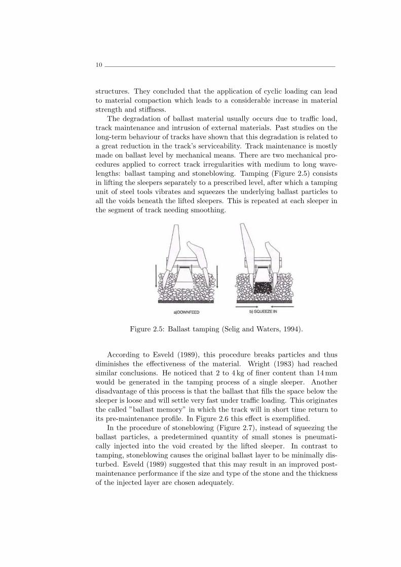
The degradation of ballast material usually occurs due to traffic load,track maintenance and intrusion of external materials. Past studies on thelong-term behaviour of tracks have shown that this degradation is related toa great reduction in the track’s serviceability. Track maintenance is mostlymade on ballast level by mechanical means. There are two mechanical pro-cedures applied to correct track irregularities with medium to long wave-lengths: ballast tamping and stoneblowing. Tamping (Figure 2.5) consistsin lifting the sleepers separately to a prescribed level, after which a tampingunit of steel tools vibrates and squeezes the underlying ballast particles toall the voids beneath the lifted sleepers. This is repeated at each sleeper inthe segment of track needing smoothing.
Figure 2.5: Ballast tamping (Selig and Waters, 1994).
According to Esveld (1989), this procedure breaks particles and thusdiminishes the effectiveness of the material. Wright (1983) had reachedsimilar conclusions. He noticed that 2 to 4 kg of finer content than 14mmwould be generated in the tamping process of a single sleeper. Anotherdisadvantage of this process is that the ballast that fills the space below thesleeper is loose and will settle very fast under traffic loading. This originatesthe called ”ballast memory” in which the track will in short time return toits pre-maintenance profile. In Figure 2.6 this effect is exemplified.
In the procedure of stoneblowing (Figure 2.7), instead of squeezing theballast particles, a predetermined quantity of small stones is pneumati-cally injected into the void created by the lifted sleeper. In contrast totamping, stoneblowing causes the original ballast layer to be minimally dis-turbed. Esveld (1989) suggested that this may result in an improved post-maintenance performance if the size and type of the stone and the thicknessof the injected layer are chosen adequately.

The railway track infrastructure 11
Figure 2.6: Ballast memory (Selig and Waters, 1994).
Figure 2.7: The stoneblowing process (Selig and Waters, 1994).
Wright (1983) showed that both tamping and stoneblowing caused bal-last breakage during the insertion into the ballast layer. However, stoneblow-ing produced up to eight times fewer particles smaller than 14 mm thantamping. Suiker et al. (2005), amongst others, suggest that stoneblowingis preferable to tamping because, from the viewpoint of track stabilization,track maintenance procedures should aim at preserving consolidated granu-lar substructures as much as possible.
Sub-ballast is the layer that usually separates the ballast and the sub-grade, serving as a medium through which the stress from the ballast isfurther distributed to the lower layers. However, according to Lim (2004)the most important function of the sub-ballast is to prevent interpenetra-tion between the subgrade and the ballast and thus, sub-ballast materialsare broadly-graded sand-gravel mixtures. Because of this, sub-ballast must

12
fulfil the filter requirements for the ballast and the subgrade. As long asthese filter requirements are fulfilled, any sand or gravel materials will usu-ally serve as sub-ballast material. However, depending upon the conditionsof the subgrade below, it may be necessary to construct the sub-ballastlayer using asphalt concrete, geo-synthetic materials or cement/lime stabi-lized soils (Selig and Waters, 1994). According to Brandl (2004) the seasonalvariation of road stiffness and bearing capacity (Figure 2.8) is analogous tothat of sub-ballast. Consequently, he suggests that in zones exposed to tem-porary frost periods, the sub-ballast of railway tracks must exhibit sufficientfreezing-thawing resistance.
Figure 2.8: Seasonal fluctuation of the bearing capacity of unbound roadlayer, analogous to sub-ballast (Brandl, 2004).
The subgrade is the foundation upon which the track structure is con-structed, its main requirement is to provide a stable foundation upon whichthe sub-ballast and ballast layers may rest upon. Upon the consideration ofthe vertical stiffness of the full soil-track system, a large component is dueto the subgrade, or foundation soil. Selig and Waters (1994) stressed thatsubgrade has also been pointed out as influencing the ballast and sub-ballastdeterioration as well as rail differential settlement. As a consequence, thesubgrade has a very important influence in the rail deflection and the trackresponse in general. On a related phenomenon, the track-soil critical speedis highly dependent of the soil and with the increasing circulation velocitiesof high-speed trains, the critical speeds may be easily reached in cases ofsoft subgrade. An example occurred shortly after the Gothemburg-Malmoline was opened. It was noticed that in some stretches with soft soil, exces-sive vibrations occurred in the track, surrounding soil and nearby power-linepylons when the X-2000 trains circulated at speeds around 200 km/h. Theimmediate consequence was that the circulation speed in these stretcheshad to be reduced (Madshus and Kaynia, 2000). This example illustrateshow the subgrade conditions may critically condition the track serviceabil-ity. Thus, any prediction model attempting to simulate the track response

Analytical railway track modelling 13
must incorporate the track-soil interaction.When the upper subgrade material is unsuitable, it may be replaced with
soil obtained from nearby formations, but anything beyond soils existing lo-cally is expensive. This upper subgrade layer of higher mechanical propertiesthan the rest of the subgrade, either existing originally or purposely placedis usually called the capping layer, although some authors may also referthe sub-ballast material as capping layer. It is also possible to improve thesubgrade of an existing track without removing the structure. Kouby et al.(2010) suggested such a method that consists in building vertical soil-cementcolumns under the sub-ballast layer. This method was performed in a sitein the north of France without impregnating the ballast and sub-ballast ma-terials. The method also allowed for reduced maintenance works and thuslimited traffic interruption.
2.2 Analytical railway track modelling
The analytical approach uses theoretical models to describe each compo-nent of the system. Concerning the evaluation of wave propagation, Lamb(1904) included in his work most of the elements that are essential to an-alytical studies on the vibration sources and transmission paths in soils.His work focused on studying the influence of an impulsive load appliedin a point or across a line on the surface of an infinite half-space or in-side an unbounded full space (Figure 2.9). After the pioneering work ofLamb (1904) many authors further developed the analytical determinationof the half and full space response to point and line loads, amongst themEwing et al. (1957), Achenbach (1973), Graff (1975), Gutowski and Dym(1976), Dawn and Stanworth (1979).
(a)
exp(iωπ)
z
x
y (b)
exp(iωπ)
z
x
y
Figure 2.9: Classical Lamb’s problems with harmonic a) point load and b)line load.

14
A generic understanding of the response states that an harmonic load ona full space generates two types of waves propagating away from the load:primary waves or P-waves generate particle movement in the direction ofthe wave propagation, secondary or S-waves generate particle movement ina plane normal to the direction of the propagation of the wave. The P-wavesspeed Cp is higher than the speed of the S-waves Cs. In elastic half-spacesa third type of wave called Rayleigh or R-Waves appear at the surface. Theamplitude of Rayleigh waves attenuate exponentially in the normal directionof the free surface and their speed Cr is lower than the speed of S-waves.
After the problem of the elastic response to harmonic loads was wellestablished, researchers began to study the response to moving loads, aproblem that had increasing interest with the increasing speed of the meansof transportation. Fryba (1973) used a triple Fourier integral transformationto obtain the displacements due to a moving point load. The expressionswere determined for three different cases of the moving load problem: thesubsonic case is when the moving load speed is lower than the speed of S-waves in the medium (c < Cs), the transonic case occurs when the movingload speed is higher than the speed of S-waves and lower than the speed ofP-waves (Cs < c < Cp) and the supersonic case occurs when the load movesat higher speed than the speed of P-waves in the medium (c > Cp).
Concerning a moving load on an elastic half-space, Eason (1965) studiedthe three-dimensional steady state problem of moving point loads and ofmoving loads distributed along circular and rectangular areas. Fryba (1973)also determined the steady state response of a moving point load at the freesurface, presented in an integral form.
Concerning the response of the track, a very useful analytical model isthe beam on Winkler foundation. This model approximates the response ofthe track by considering a moving load on a beam discretely supported bysprings and dashpots (Figure 2.10).
c
EI, ρ k cd
P
Figure 2.10: Beam on Winkler foundation.

Numerical railway track modelling 15
The differential equation of this problem is given by:
EId4u(x, t)
∂x4+ ρl
d2u(x, t)
∂x2+ 2cd
du(x, t)
∂x+ kdu = Pδ(x− ct) (2.1)
where EI is the flexural stiffness of the beam, u is the vertical displace-ment, ρl is the mass per unit length of the beam, k is the stiffness coefficientof the Winkler foundation, cd is the viscous damping of the foundation, Pis the vertical load and δ(x − ct) is the Dirac delta function of the movingload at speed c.
The determination of the these properties will depend upon which com-ponents of the structure are considered for the beam and which are consid-ered for the Winkler foundation. One common approach consists in con-sidering only the rails for the beam of the model and all other componentsof the track and subgrade in the Winkler foundation. However, this is nota universally accepted approach as it is also possible to consider the beamas representing the whole track structure and the Winkler foundation rep-resenting only the track subgrade. For the determination of the Winklerstiffness k, many authors have suggested different formulations, amongstthem Biot (1937). Terzaghi (1955) demonstrated that the stiffness of anygiven soil layer is not an intrinsic property of the layer, but rather variesfrom case to case. Heelis et al. (1999) suggested the utilization of a FEmodel to compare deflections under a known applied load.
Despite the usefulness of the beam on Winkler foundation model toestimate track deflection and critical speed of the track, the simplifica-tions it assumes have been pointed out as the cause of some errors, a veryhighlighted disadvantage is that model cannot transmit shear stresses, al-though modified models have been suggested to overcome this drawback(Sadrekarimi and Akbarzad, 2009).
Because of the necessary simplifications and sub-divisions involved, an-alytical solutions are not usually adequate for practical problems. However,they can give a better understanding of well defined theoretical problems andprovide useful references for the validation of numerical simulation tools.
2.3 Numerical railway track modelling
2.3.1 Introduction
The necessity to overcome the limitations of empirical and analytical modelsled to the development of the numerical models, which were backed up bythe increasing processing capacity of computers. Different approaches havebeen used to make numerical predictions in the scope of railway tracks forhigh-speed trains. The main differences regard the numerical method that
16
is used (mainly the FEM, Boundary Element Method (BEM), Discrete Ele-ment Method (DEM) and hybrids). Each numerical method was originallyproposed based on assumptions that are further elaborated and developeduntil the framework of the method is revealed. These assumptions allow todevelop the method toward the desired framework but also ensure that themethod will be implicitly limited into complying with them. Consequentlyeach method will have numerical advantages and short comes making themmore or less suitable for numerical simulations depending on the assump-tions or simplifications that the user is willing to make.
The purpose of this subsection is to describe in a general way the mostcommon numerical approaches in the literature to simulate railway trackresponse, giving a general understanding of their relative advantages andshort comes.
2.3.2 2D and 3D FE models
The FEM has the advantage of being very widespread amongst engineersand such when choosing which numerical method to use in the approach ofthe problem, it becomes a first choice for many. Regarding the predictionof track response and wave propagation to outer zones, the FEM has theadvantage of allowing a detailed definition of the track geometry and thepossibility to consider non-linear material behaviour.
On the other hand, one of the major problems concerns soil modellingwith finite elements, because the soil is an infinite half-space. If the FE meshis constrained in its outer limits, the waves generated by the dynamic loadingspuriously reflect on the fixed constrains instead of continuously propagatingto outer regions. Consequently the results of the numerical simulation willbe affected by this numerical short come. To overcome this drawback, themodels must become larger than those used for static analyses and includea methodology that mitigates or prevents these spurious wave reflections.Lysmer and Kuhlemeyer (1969) and White et al. (1977) have proposed theintroduction non-reflecting viscous boundaries to absorb incoming waves andavoid reflections. These viscous boundaries are perfectly absorbing if alignedin the same direction of the incoming wave, thus it is a perfect solution forone dimensional problems but only mitigates this problem in 2D and 3Dmodels (see sub-section 3.3.4). Another way to address this problem is by in-troducing infinite elements, these were proposed by Bettess (1992) for staticand steady-state problems. These elements are derived from standard finiteelements and modified to represent a decay type behaviour as one or moredimensions approach infinity. Wolf and Song (1996) suggested the consis-tent infinitesimal finite-element cell method also called the Scaled BoundaryFinite Element Method (SBFEM). The method is derived from the similar-ity of the unbounded domain and is used in a substructure method. Thediscretization is limited to the structure-medium interface resulting in a one

Numerical railway track modelling 17
dimension reduction of the spatial dimension that, unlike the BEM, doesnot require a fundamental solution. Ekevid and Wiberg (2002) applied theSBFEM to simulate the dynamic response of a typical railway track stretch(Figure 2.11). The results suggested that the usage of the SBFEM resultedin very small or no reflections of waves even when constraints were used inthe nodes of the soil-structure interface. The calculated time-history plotof the vertical displacements of a point in the track agreed very well withexperimental measurements.
(a) (b)
Figure 2.11: Coupling of FEM and SBFEM for simulation of a rail roadsection: (a) discretization of the structure-unbounded media interface, (b)the FE model (adapted from Ekevid and Wiberg, 2002).
In the context of the simulation of electromagnetic waves, Berenger(1994) introduced the concept of Perfectly Matching Layers (PML) thatconsists in modelling an outer layer of the same material, but having atten-uation characteristics that damp the outgoing and reflected waves withinthe layer thickness. Later, the concept of a PML has been developed forelastodynamics wave equations (Chew and Liu, 1996, Collino and Tsogka,2001).
Even taking into account the fact that the wave propagation to outerzones in FE models has been studied by many authors and mitigated throughdifferent modelling techniques, it is still necessary to include in the FE mesha considerable part of the foundation soil, which makes the models computa-tionally demanding, although in most cases it is possible to consider symme-try conditions and thus reduce the computational efforts to approximately50%.
The approach to modelling railway track behaviour using the FEM isusually done in one of the two following ways: 2D plane strain modellingand 3D modelling. Figure 2.12 presents a 2D plane strain mesh used bySuiker (2002). The 2D plane strain modelling requires the simplificationassumption that the transversal profile of the track is invariable in the lon-gitudinal direction, which, does not correspond to the reality in the case ofballasted tracks where the rail is discretely supported by the sleepers.

18
Figure 2.12: Example of a 2D plane strain FE model of the track and soil(adapted from Suiker (2002)).
Another requirement of these 2D models concerns the assumption of thelongitudinal load distribution. In order to accurately account for the loadtime history in the transversal section of the track, the load distribution inthe longitudinal direction of the track must be previously accounted for. Anapproach was proposed by Gardien and Stuit (2003) studying soil vibrationsfrom railway tunnels. These authors, instead of creating a three-dimensionalmodel for the dynamic analysis built three complementary models: the firstone is three-dimensional, where static loads were applied to obtain equivalentbeam parameters, which were used in the second model to calculate theunder-sleeper force in time; this force was then introduced in the third, aplane strain model of the tunnel cross section.
The 3D FE models do not require such simplifying assumptions. Theload distribution in the longitudinal direction of the track is done by themodel itself invalidating the need to previously account for this. 3D FEmodels also eliminate the necessity to consider continuous support of the railin the longitudinal direction of the track as the discretely support systemcan be discretized in the 3D FE mesh. This usually includes beam elementsto simulate the rails and spring-dashpot elements to simulate the rail pads,although this is not necessarily the case for all models: Araujo (2011) andHall (2003) did not include the rail pads in their simulation, instead havingthe rail rest directly on the sleepers. The remaining model, including thesleepers and all other track and soil layers are usually modelled using brickor wedge elements (Figure 2.13).
Usually only the quasi-static moving load of the train is considered inthese models. As was previously mentioned a disadvantage of these 3DFE models concerns the numerical demand associated with such a largenumber of degrees of freedom. Furthermore, the amount of soil that mustbe simulated in the transversal direction and in the depth of the model is

Numerical railway track modelling 19
Figure 2.13: Example of a 3D FE model of the track and soil (adapted fromHall (2003)).
not clear. Users of these models usually rely on trial and error or their ownexperience to decide upon the size of the model.
Some spurious numerical disturbances in 3D FE modelling were referredby Hall (2003). The author noted that the entrance and exit of the axleloads in the FE model created some disturbances in the model. Anotherremark by the author was that the stress waves in the free field were notfully developed when they entered the FE model. This stems from the factthat the load does not come from infinity but instead begins its movementat the limit of the FE mesh. Consequently the results that the authorobtained were more accurate closest to the track and farther away from theentry point.
2.3.3 2.5D and 3D FE-BE models
A very efficient way to model the propagation of waves in the soil is to usethe BEM. This consists in a method to solve partial differential equations ina boundary integral form. This method requires the definition of a funda-mental solution which, in the particular case of modelling wave propagationin the soil, are very often the Green’s functions in the free field. The Green’sfunctions are obtained as numerically precise solutions of an elastodynam-ics problem of a load in a homogeneous or layered half-space (full-spacesmay be also considered in other cases). The BEM has the advantage ofcorrectly accounting for wave propagation in the half-space but is not ap-propriate to deal with geometrical complexities and non-linearities (Kausel,

20
1981, Domınguez, 1993). Usually in these situations the soil definition is re-stricted to vertical soil layering. Because of its advantages and short comes,in the context of railway track simulations, the BEM is almost exclusivelyused to simulate the foundation soil, while the track is simulated using differ-ent numerical methods, with the two components of the model interacting inorder to obtain a true track-soil response. On top of correctly accounting forwave propagation to outer zones, the BEM has another advantage over FEMin the computational effort as the Direct Stiffness Method (DSM) pioneeredby Kausel and Roesset (1981) allows to do straightforward computations ofthe Green’s functions in the soil. Consequently, only the desired free fieldlocations need to be computed, while in the FEM the system of equationsmust be solved for the whole mesh.
A common and efficient way to implement the track-soil model with thesoil modelled with the BEM, is by defining the model in 2.5D. The designa-tion comes from the fact that the geometry of the problem is only definedin 2D, i.e. only the transversal section of the track is discretized. How-ever, a true 3D response is obtained in these models. This occurs becausethe problem is formulated in the frequency-wavenumber domain, which im-plies a double Fourier transform, from the time domain into frequency do-main and from the longitudinal direction into wavenumber domain. Thesetransformations imply that only linear material properties can be admit-ted and also that the transversal geometry of the model is invariant in thelongitudinal direction. The definition of the model in this 2.5D formula-tion allows to efficiently implement the BEM using as fundamental solutionthe 2.5D Green’s functions of the soil, which are more efficiently evaluatedin frequency-wavenumber domain than in space-time domain. Sheng et al.(1999) defined a model in which the track is simulated as an infinite layeredbeam and the soil as a layered half-space. Following these developments,the model was adapted to account for train-track interaction (Sheng et al.,2003, 2004). Lombaert et al. (2006) applied a similar methodology withBoundary Element (BE) formulation for the soil.
Evolving from modelling the track as an infinite layered beam,Sheng et al. (2006) modelled the track-soil interaction by coupling 2.5D Fi-nite Element (FE) and 2.5D BE formulations. Other authors (Galvın et al.,2010, Costa et al., 2012, Fiala et al., 2007) have used similar formulationsto model track response and wave propagation in the soil due to high-speedtrains (Figure 2.14).
Clouteau et al. (2000) developed an approach in which periodicity in onedirection, instead of invariance, is assumed. The Fourier transform of the2.5D models is replaced by a Floquet transform in these models. The FE-BEdiscretization is reduced to one single reference cell (Figure 2.15). Withinthe context of railway track simulation, the approach has been mostly usedto simulate vibration from underground railway traffic (Degrande et al.,2003, Chatterjee et al., 2003, Clouteau et al., 2004, Gupta et al., 2006a,b).

Numerical railway track modelling 21
Figure 2.14: Example of a 2.5D FE-BE model of the track and soil (adaptedfrom Costa et al. (2012)).
Araujo (2011) used this approach to model train passage in a railway linebetween Paris and Brussels obtaining good correspondence between mea-surements and numerical results.
Figure 2.15: Example of a reference cell in a periodic model (Gupta et al.,2006b).
It is also possible to couple FE-BE methodologies in 3D conditions.The computation of BE solutions in a 3D environment is more computa-tionally expensive but it can be coupled to 3D FE model of the track intime domain allowing for more detailed geometric and material properties.O’Brien and Rizos (2005) proposed a 3D FE-BE methodology (Figure 2.16)for the simulation of high-speed train induced vibrations where the timemarching scheme is adapted to provide the FE and BE solvers with differ-ent time steps to ensure stability of both solvers. The communication of databetween solvers is then done at a time step where the results of one solver

22
are computed and the results of the other solver are linearly interpolated.
Figure 2.16: Example of a 3D FE-BE model of the track and soil(O’Brien and Rizos, 2005).
2.3.4 DEM models
Due to the large size of ballast particles, there is an increasing trend to tryto reproduce ballast behaviour through the DEM. An increasing number ofauthors have used this method in order to reproduce experimental resultsfrom triaxial tests (Lu and McDowell, 2008, Hossain et al., 2007) and boxtests (Lim and McDowell, 2005, Lu and McDowell, 2007).
In general the Discrete Element (DE) codes simulate simple interactionsbetween a great number of micro-particles that combined result in a muchmore complex macro-behaviour. Although usually referred as the (moregeneral) DEM, the Distinct Element Method is the most commonly useddiscrete code in the study of the ballast behaviour.
In the DEM, there are usually only two basic entities: particles and walls.Walls usually represent containers for the particle assemblies allowing themto be constrained to a defined volume region. A wall will only interactwith particles and not with other walls. Also, the position of the wallsmay be constant or time-dependent but will usually not depend upon theinteraction forces with the balls. A particle is subject to gravity loads orcontact forces with other particles and walls and its movement within eachtime step is computed with the consideration of all applied forces. Thecalculations within a single cycle alternate between the computation of theparticles movements and the computation of the interaction forces betweenall elements. For instance, the calculation cycle of the Distinct Element CodePFC2D is represented in Figure 2.17. The particle movements are usuallycomputed with the Newton’s second law while a force-displacement law isapplied to compute the interaction forces. As a result, contacts that mayform or break between the particles are automatically accounted for in the

The achievements of numerical railway track modelling 23
computational scheme. The complex behaviour of the materials then arisefrom the combination of a great number of (usually) simpler particle-particleor particle-wall interactions.
Figure 2.17: Calculation cycle in PFC2D (Itasca).
Due to the large computational effort that DEM requires, seldom has thismethod been used to try to reproduce the ballast behaviour in a numericalmodel of the track. Those track models that have been constructed inwhich the ballast is modelled with DEM only reproduce a small part of thetrack, and the interaction with the subgrade is not simulated. Also, thelongitudinal length of the model is reduced spanning 1 to 5 sleepers in 2D(Lobo-Guerrero and Vallejo, 2006, Saussine et al., 2006) or a single sleeperin 3D (Tutumluer et al., 2007). The limited longitudinal length of thesemodels limits the simulation of the moving loads, which is done usually bythe consideration of a single load with time-dependent modulus.
2.4 The achievements of numerical railway track
modelling
From the various approaches that have been applied to simulate track andsubgrade response to high-speed train passage, various models are now avail-able which have been proved to be very accurate. The possibility to predictthe railway track response and/or propagation of waves to the free field isby itself an important achievement. However, numerical models may pro-vide detailed insight into the phenomenons at hand that even experimentalmeasurements are not able to show. A validated numerical model is alsoan invaluable tool to study different case scenarios where the railway trackresponse may be obtained for alternative geometry/material configurations.Thus in this section a general overview is presented of the achievements thatthe different numerical tools have obtained in further advancing the knowl-edge of railway track and subgrade behaviour. From the understanding of
24
the various approaches presented previously and their achievements hereinpresented, a better comprehension of the state of art in numerical railwaytrack modelling is possible. This allows for a clearer realization of whichniches of knowledge have been well established and which have not been sothoroughly studied, thus highlighting the reasons why the works presentedin this thesis are valuable contributions.
Even though the non-linear behaviour of the track and soil layers mayhave significant influence in the track-soil response, very good results havebeen obtained with numerical models that disregard this complex behaviour.This may be explained by the fact that the influence of the non-linear mate-rial behaviour may be reduced in some cases. Also the dynamic propertiesobtained from optimization of the rail receptance are in many cases obtainedfrom the loaded railway track, thus the model is calibrated to simulate thetrack response using the stiffness that the materials present when the trackis loaded.
The consideration of non-linear behaviour in railway track modelling hasbeen seldom done due to its limited applicability in some cases or due tothe extended computational demands that these models require. In general,non-linear behaviour is studied in the track components such as ballast andsub-ballast or the foundation soil.
2.4.1 Linear modelling
The 2.5D model presented by Lombaert et al. (2006) for the prediction oftrain induced vibrations presented very good correspondence with experi-mental results of the free field transfer functions and the response to thepassage of the Thalys high-speed train. The model was elaborated in orderto account for the dynamic interaction between the vehicle and the track.From this experimental validation, the numerical model was further used(Lombaert and Degrande, 2009) to study the influence of the quasi-staticand the dynamic components of the load at several speeds in the track andsoil response. A major remark made was that the quasi-static componentof the load resulting from the weight per axle moving along the track haslarge influence in the track behaviour and the very near vicinity. On theother hand, the dynamic component of the load that is generated due to therail and wheel unevenness dominates the free field response. The authorsalso remarked that the vertical sleeper velocity due to the quasi-static axleload increases moderately with speed and becomes shorter in time, also theresponse shifts to higher frequencies with increasing speed. The dynamiccomponent of the load only dominates the sleeper response at high frequen-cies. It also has higher duration in time than the static component, andit increases slightly with increasing speed. In the free field, the dynamicresponse also increases with increasing speed while the high frequency com-ponent is attenuated due to the soil damping.

The achievements of numerical railway track modelling 25
Other works have successfully modelled the track with FEM andthe semi-infinite zone through BEM (Andersen and Nielsen, 2005, Celebi,2006, Adam et al., 2000, Madshus and Kaynia, 2000, Galvın et al., 2010,Costa et al., 2012).
Fiala et al. (2007) used a 2.5D model of the track and soil as a sourcemodel for the ground induced vibrations. Using a receiver model with a BEformulation of the soil and FE of the building they were able to study thestructural and acoustic response of the building due to railway traffic. Thenumerical simulations also allowed to simulate the effectiveness of severalvibration countermeasures. Galvın and Domınguez (2009) were also able topredict railway induced vibrations in a a nearby structure using a 3D FE-BEmodel.
The coupled FE-BE model of O’Brien and Rizos (2005) allowed todemonstrate that the vibration characteristics depend on the relative speedbetween soil wave velocities and the train speed and that the relative stiff-ness of the soil with respect to the rail affects the distribution of the wheelload on the sleepers. Similar conclusions were obtained by Yang et al. (2003)using a 2.5D finite-infinite element model to perform parametric studies onthe soil configuration and its influence in the track response. It was ob-served that for layered soils the critical speed at locations near the sourcecan be determined from the Rayleigh wave speed of the top layer soil. Butat locations away from the source, the critical speed might be higher.
Closely related to the conclusions obtained by Lombaert and Degrande(2009), the 3D FE model by Ju et al. (2010) allowed to obtain some in-formation regarding the influence of the rail unevenness on train-inducedground vibrations. The authors confirmed that the ground vibrations aredominated by the dynamic component of the load, however, they noted thatthis dominance only occurs at subsonic speeds. At supersonic train speedsthe ground vibrations in the model were not very different with or with-out rail unevenness. The Vibtrain program, based on sub-structuring inwhich the ground is represented by discrete Green’s functions for layeredhalf-space and the track is represented as a beam by finite elements, allowedKaynia et al. (2000) to demonstrate that embankment stiffening may be aneffective measure to limit ground vibration for trains running near or intransonic regime.
After analysis with 3D finite difference models, Gonzalez-Nicieza et al.(2008) remarked that the existence under one and the same sleeper of verydifferent properties leads to the appearance of micro deformations in thesleeper of more than 150 ηm/m, which is a value above which cracks wouldstart to appear in the concrete.
Galvın and Domınguez (2007) used a 3D time domain BE model to sim-ulate the track and soil. The analysis allowed the authors to state that theballast layers do have significant influence in the system response, and thusshould not be disregarded. Also they suggest that the presence of these lay-
26
ers may be considered in a half-space with equivalent properties, however,an assessment of these properties is difficult.
2.4.2 Non-linear ballast modelling
Due to its key role in the track response, ballast has been the increasingfocus of interest in railway track modelling. Because the particle size is closeto 10% the average ballast width, it can be an exaggerated simplificationto simulate the ballast layer as a continuous medium. Regardless of that,due to the large processing demands of discrete calculations, many authorsmodel the ballast as a continuous media, considering elastic linear behaviouror more complex material behaviour. Even those that consider non-linearcontinuous modelling of the ballast material, often opt to do so in reducedmodels, 2D plane strain or axisymmetric models due to the high demandsof a full 3D non-linear model.
Continuous approach
Nguyen et al. (2003) have proposed a no-tension constitutive law for contin-uum modelling of granular materials. Unlike many other no-tension mod-els previously written, mainly for the purpose of modelling masonry struc-tures, the model proposed in this paper has been derived directly from astrain-energy function which is evaluated by means of a modified functionof stretches. The model has been applied to a quasi-static test on ballast ma-terials in a 3D FE analysis, the compressive stresses found in the no-tensionmodel were approximately 15% higher than those in the non-linear elasticcase. These numerical results revealed that the influence of the no-tensioneffect in a granular structure with the configuration of the ballast layer canbe significant.
Suiker and de Borst (2003) proposed an elasto-plastic material model tosimulate the cyclic deterioration of ballast and sub-ballast. The model cap-tures the envelope of the maximum plastic deformations, allowing to eval-uate the deformation accumulation by means of relatively large load cycleincrements. The plastic deformation is controlled by two mechanisms, fric-tional sliding and volumetric compaction. The frictional shakedown surfaceis represented by a Drucker-Prager cone which is limited by a cap represent-ing the compaction shakedown surface. The frictional failure level understatic loading may not be exceeded and is also represented by a Drucker-Prager cone. The combination of this surfaces with the tensile failure surfacedivide the p-q plane into four zones that represent the four response regimesof the model (Figure 2.18): the shakedown regime where the response of thematerial is purely elastic; the cyclic densification regime in which the cyclicloading leads to plastic strain accumulation; the frictional failure regime inwhich the frictional collapse occurs; and the tensile failure regime in which

The achievements of numerical railway track modelling 27
the material disintegrates. The parameters of the cyclic densification modelwere calibrated for experimental data of cyclic triaxial tests on ballast andsub-ballast materials. The model was able to represent with good accuracythe development of permanent deviatoric and volumetric shear strain withnumber of cycles, for the ballast and sub-ballast materials. Only for caseswhere the cyclic stress levels were close to the static failure level, the modelprediction was inaccurate for a number of cycles inferior to 100. The modelwas also used to predict the development of permanent deformations in aballasted railway track under a large number of train axle passages. Thiswas done in a FE simulation of a moving axle on the track. The predictionsdid not match the experimental results with great accuracy but this wasjustified by the consideration of plane strain behaviour of the track.
Figure 2.18: Map of various response regimes in p - q plane during cyclicloading in the cyclic densification model (adapted from Suiker and de Borst(2003)).
Al Shaer et al. (2008) presented one approach in which the ballast be-haves linearly but accounts for the fact that ballast below the sleeper is moreconfined than in the crib or shoulder. The method was applied in simpleFE model in order to compare numerical results to experimental ones ob-tained in a reduced scale experiment with three sleepers. All experimentcomponents were considered as linear elastic materials. Ballast was decom-posed into two regions of different physical and mechanical characteristics.Ballast in the zones under the blocks at an angle of 45 was consideredcompacted while ballast elsewhere was considered uncompacted. A correctagreement was observed between the measurements and the computationsin most cases.
Indraratna and Nimbalkar (2011) performed numerical simulations us-ing 2D axisymmetric and plane-strain FE analysis in which the behaviourof ballast was simulated using a hardening soil model with a non-associativemodified flow rule capable of capturing the effects of the confining pressureand ballast breakage. The models showed that increased track confinement

28
leads to significant reduction in vertical stresses and deformations, confirm-ing that the optimum confining pressure is usually above those present inthe railway track.
In a rare example of non-linear ballast behaviour modelled in a largescale 3D FE model, Araujo (2011) used the linear elastic, Mohr-Coulomband Hujeux non-linear models in order to study the stress paths in theballast during the passage of a high-speed train boogie. The Hujeux law isan elasto-plastic continuum approach model developed to simulate 3D cyclicsoil behaviour. The model is developed in a multi-mechanism with fourplastic elementary mechanisms: three plastic mechanisms for the deviatoricdeformations and one plastic mechanism for the isotropic deformation. Itwas detected that with the linear elastic models, characteristic stress-pathrange from a slope parallel to the natural state line on the ballast layer toa practically vertical one in the capping layer. This effect, however, wasnot found in the non-linear models. In those cases the slope remains almostconstant and far from the failure envelope. From the comparison of thelinear and non-linear simulations the author suggested that a linear elasticmodel is able to reproduce the vertical displacement and velocity inducedby the passage of a high-speed train but its capability quantify the stressevolution seems questionable.
Discrete approach
Due to the large ratio between particle size and ballast thickness, mostauthors feel that modelling this material with a continuous formulation is anexaggerated simplification that can hardly provide insight into the ballastbehaviour in service conditions. Consequently, an increasingly number ofresearchers have adopted techniques where particle interactions are takeninto account. More so than in the continuous case, the consideration ofdiscrete ballast behaviour is mainly constrained to reduced models, eitherin 2D or 3D.
The tensile strength of ballast as measured by single particle crush-ing tests has been correlated with ballast degradation on oedometer andbox tests (Lim, 2004). However, most DEM implementations do not allowparticle breakage. One way to circumvent this short come is to simulateeach particle as an agglomerate of several smaller particles (Cheng et al.,2003). The individual particle breakage can occur when a predefined condi-tion is met or by using bonds with limited resistance. Hossain et al. (2007)simulated angular ballast breakage under cyclic biaxial loading at variousconfining pressures in 2D DEM. They observed that the breakage of parti-cles has significant influence on the settlement and volumetric strains. Theanalysis also demonstrated that breakage is a function of confining pressure.Lim and McDowell (2005) performed 3D simulations of single particle crush-ing tests using bonded particle agglomerates. The distribution of strengths

The achievements of numerical railway track modelling 29
correctly followed the Weibull distribution, and the size effect on averagestrength was also consistent with that measured in the laboratory.
Another solution to the particle breakage problem is to replace the par-ticles fulfilling a predefined failure criterion with an equivalent group ofsmaller particles. Lobo-Guerrero and Vallejo (2006) studied the effect ofparticle crushing using the DEM. They simulated a track section subjectto cyclic load and the the values of permanent deformation as a function ofnumber of cycles were recorded. The simulation was done twice for the sameidealized material but in one of the simulations particle crushing was allowedwhereas in the other it was not. Crushing was simulated by replacing theparticle with smaller ones. The obtained results showed that the inducedpermanent deformation strongly increased when considering particle crush-ing even though only a few particles were broken. Moreover, it was foundthat crushing concentrated underneath the simulated sleepers (Figure 2.19).
Figure 2.19: Ballast crushing after 200 cycles of 62 kN(Lobo-Guerrero and Vallejo, 2006).
Soon, it became evident that modelling each ballast particle as a spheredid not provide the necessary interlocking between particles to allow for agood ballast simulation. The implementation of more angular particles inDEM simulations of ballast behaviour leads to a greater degree of homo-geneity in the stress distribution (Lu and McDowell, 2007), in accordanceto experimental data. The simulation of angular particles in DEM softwarethat only allows spherical elemental particles is implemented by the simula-tion of a single ballast particle with multiple spheres. The particles can beassembled as an agglomerate of bonded spheres, this increases significantlythe computational cost of the model, but as previously explained allows toconsider ballast breakage. Another solution consists in grouping the spheresin clumps. A clump consists in an agglomerate of overlapping balls. It isrigid internally, which allows the calculation mechanism of the DEM simu-lation to skip computing internal forces between spheres of the same clump,

30
but is deformable at the outer boundaries. One disadvantage of the clumpis that in the spacial zone where balls overlap the density will be the sumof the overlapping balls densities, thus the clump has non-uniform densitythroughout its volume.
Lu and McDowell (2007) simulated ballast material using spheres andusing clumps with different angularities in a box test consisting of one cycleof sleeper load after compaction. The simulation showed that the angularityof clumps increased particle interlocking thus diminishing the displacementand rotations of sphere particles. For the spheres, the deformation of theballast material in the box test simulation concentrated on the corners andsides of the sleeper where ballast particles flew upwards, even on unloading.For the clumps the deformation of the ballast material occurred directlyunder the sleeper.
Lu and McDowell (2008) remarked that previously the DEM had beensuccessfully used to simulate granular materials with crushable particles byseveral authors. Despite that, the authors were not aware of any work wherethe simulation of ballast under a range of confining pressures captured withdetail both the deviatoric and the volumetric behaviour. In addition theywere unaware of any simulation of triaxial tests on ballast where particleabrasion was considered. To suppress these gaps, they modelled each ballastparticle using a clump consisting of ten spheres. Eight smaller spheres werebonded to each clump using contact bonds and parallel bonds (Figure 2.20).The authors remarked that the addition of weak bonded asperities allowedto enhance the particle shear resistance as well as simulate particle abrasion.Monotonic triaxial tests on ballast material were simulated in DEM using theparticle definition that was described. By comparison of numerical responseand experimental measurements, it was shown that by including bondedasperities, approximately the correct response in terms of shear stress andvolumetric strain can be observed.
Figure 2.20: Small spheres are added to clumps in order to simulate particleasperities (Lu and McDowell, 2008).
Tutumluer et al. (2009) used the DEM in order to study the effect ofgradation on ballast settlement. This numerical method allowed the authorsto determine which gradation, of several that were studied, presented least

The achievements of numerical railway track modelling 31
settlement. Furthermore, the study suggested that the gradations couldbe improved by employing a minimum particle size of 36 mm which wouldprovide large enough air voids for drainage and minimize the settlementpotential of ballast.
It is shown that non-linear ballast modelling in DEM has earned greatinterest and developments in the past few years. This method allows fora very thorough study of the material behaviour, with the great innova-tions of allowing to study the inter-particle interaction forces and particlecrushing (Lim and McDowell, 2005). In general, good correspondence hasbeen obtained in ballast behaviour with triaxial tests (Lu and McDowell,2008, Hossain et al., 2007) and box tests (Lim and McDowell, 2005,Lu and McDowell, 2007). Despite these advantages the DEM has a veryhigh computational demand and modelling of DEM ballast in a railwaytrack is mainly confined to a few sleepers (Lobo-Guerrero and Vallejo, 2006,Saussine et al., 2006). The full track-soil system is not yet possible to modelwith DEM due to limitations in the computational capabilities of currentcomputers.
2.4.3 Non-linear soil modelling
In the context of geotechnical engineering, many numerical material modelshave been developed in order to simulate soil behaviour for a long range ofapplications. The many available material models can be used to simulatecohesive or cohensionless materials, account for the no-tension effect andfriction failure, and accurately simulate monotonic or cyclic behaviour ofsoils. Despite the large attention that soil numerical modelling has hadfor many decades, very seldom has its non-linear response been taken intoaccount in the simulation of railway tracks under high-speed trains.
Hall (2003) achieved good agreement between the measured and calcu-lated responses close to the track in three-dimensional analysis with a FElinear model. The model featured dashpots in the boundaries of the mesh inorder to account for outgoing waves. The agreement between the measuredand calculated response from the three-dimensional analysis was achievedafter a reduction in the soil stiffness directly below the track. This reductionwas compliant with the induced shear strain, thus an equivalent linear ap-proach for the soil was used. From the motion orbits calculated in the 3D FEanalysis the author suggested that the Rayleigh wave was the dominatingwave type outside the embankment.
Banimahd and Woodward (2007) used a non-linear elastic behaviour tomodel the soil in a 3D FE model to study the speed effect on railway track re-sponse and correlate these results with anticipated track maintenance level.According to the study, ballasted tracks with speeds from 50% to 70% ofthe critical track velocity were classified as high maintenance and those withspeeds of 70% of the critical track velocity were associated with the rapid de-

32
terioration of the railway track and a potential risk of derailment. The studyconfirmed that the subgrade properties highly influence the critical speed inthe track. Also, the study of the non-linear subgrade behaviour showed thatit has small influence at low speeds (≈ 50m/s), but for increasing speeds ithas a substantial effect.
2.4.4 Integrated non-linear modelling
The non-linear consideration of either the track components or subgrade inthe track behaviour is in itself seldom done, even more rare are cases in whichboth the track and subgrade non-linearities are considered simultaneously.One of such examples is the work by Costa et al. (2010) in which the authorsapplied a linear equivalent method to account for the large strain responseof the embankment and the soil in a 2.5D Finite-Infinite Element Method.This approach allowed to obtain a very good simulation of measurementsof an experimental case in which it is suspected that the non-linear soilresponse contributed for very high displacements in the track and soil. Theauthors also remarked that the error of the predicted displacements in thelinear model was directly connected with the train circulation speed: for lowspeeds the error was neglectable, but for high-speeds the error was very high.The numerical model was also used to predict the response at supercriticalspeed for which it was found that the linear and linear equivalent modelspredicted almost the same response. This led the authors to suggest that atthese high-speeds the dynamic properties of the soil are closer to those ofthe small strain range.
2.5 Conclusions
The processes of generation and propagation of waves in railway tracks forhigh-speed trains are continuously being studied. This chapter presents anoverall understanding of the phenomena that occur in a track during thepassage of high-speed trains, and the developed methodologies to predicttrack response. Due to the high standards of high-speed railway tracks, thetools that facilitate predictions of track behaviour are essential for adequatedecision making in planning, construction or maintenance of the tracks.
A general description of the components in ballasted railway tracks wasprepared initially to provide a better understanding of the study tools, whichare later discussed. This description is followed by a general overview of theapproaches that are adopted in this study.
A detailed examination of the numerical models was performed to deter-mine which areas are lacking in knowledge and numerical tools; this helpedto identify which paths should be pursued for an original contribution. Froma numerical point of view, some distinctive methodologies have been de-

Conclusions 33
veloped and proven that provide an adequate prediction of track and soilvibration levels.
The BE based models allow us to efficiently model soil response andavoid any spurious reflection, these models are usually coupled with differ-ent numerical methods that simulate the track. Although 3D FE-BE modelsmay better represent complex geometries, railway track modelling has pri-marily focused on the more computationally efficient 2.5D models. Theresearches of Lombaert et al. (2006), Galvın et al. (2010) and Costa et al.(2012), amongst others, have proven that these 2.5D models provide verygood predictions of vibrations in the track and soil. The limitations of thesemodels are based on the mandatory assumption of linear behaviour.
FE models within a time domain have been successfully employed to pre-dict track response and, to some extent, soil response. The problem of wavereflection in the limits of the model must be addressed. Although solutionshave been developed, the necessity of modelling a considerable part of thesoil with finite elements greatly increases the computational costs associatedwith such models. 2D FE models of plane strain have been predominantlyutilised in preliminary simulations. 3D FE models are computationally de-manding but have been validated with experimental measurements (Hall,2003, Araujo, 2011). The advantage of 3D FE models is that geometrycomplexities, such as the discrete rail-sleeper support in the longitudinaldirection of the track, may be included. Because the FEM has been ex-tensively employed in many scientific and engineering applications of non-linear analysis, the possibility of explaining this complex behaviour is oneof the main incentives for using FE models. Some authors have modellednon-linear material behaviour in simplified FE track models, but the con-sideration of non-linear material behaviour in full track models is a conceptseldom explored, especially concerning soil non-linearity.
The DEM may be the most accurate model for simulating ballast be-haviour; however, simulation of a track stretch remains cost-prohibitive.
The analysis of modern railway track modelling indicates that the studyof non-linear track and soil behaviour, especially the latter, during the pas-sage of high-speed trains is a problem that should be further explored. Al-though analytical methods provide quick solutions for well-defined cases,they do not allow for analyses of complex cases. The numerical models ofthe BEM only consider linear equivalent simulations, and the DEM is stilltoo computationally expensive to be integrated in a model of the full track.As a result, the FEM is the best method for studying the non-linear responseof ballast and subgrade. The study of how non-linear behaviour influencesthe model results may reveal its importance. In addition, a comprehensivestudy of how stresses are distributed along the track and soil may provideinsight into railway track design to improve vehicle stability or limit costlymaintenance. By considering these aspects and without disregarding itslimitations, this thesis implements and validates a 3D FE model to model

34
non-linear subgrade and track behaviour, study the influence of this non-linear consideration and gain knowledge of track and soil responses duringthe passage of high-speed trains.

Chapter 3
Application of linear railway
track modelling
3.1 Introduction
This chapter introduces the application of two common models to simulaterailway track response under high-speed trains in linear behaviour: 3D FEmodels and 2.5D models. The purpose is to broaden the knowledge notonly of these two tools, thus gaining insight into the cases for which theypresent advantages and limitations, but also to further enrich the knowledgeof the dynamic phenomenons themselves that are at the heart of the railwaytrack response during the passage of a high-speed train and to validate the3D FE model that will be later used to study non-linear ballast and sub-grade behaviour. The chapter begins by a general overlook of the governingelastodynamics equations that are at the genesis of both formulations, thespecific formulations of each modelling technique are further referred in thecorresponding sections.
The FE models herein presented are developed using the commercialsoftware Diana (TNO, 2005). A case study is defined for which the trackresponse has been measured and further on, the 3D FE mesh is used to sim-ulate the passage of the high-speed train. Through comparison of numericaland experimental results, the method’s accuracy is discussed.
Subsequently, two 2.5D models are studied and discussed. Both modelsuse the BEM to simulate the soil but they differ in the track formulation.One model considers undeformable sleeper and track-soil interface in thetransversal plane whereas the other considers deformable track components.The comparisons are used to further enrich knowledge on the dynamics ofthe tracks and establish deeper knowledge of the 2.5D models, which arelatter used to validate the 3D FE model. The 2.5D models herein usedare modelled using numerical toolboxes developed for the MATLAB (Mat,2005) commercial software by the Structural Mechanics Division of the Civil
35

36
Engineering Department at the Katholieke Universiteit Leuven. These tool-boxes have been validated with field results by the authors and were gentlymade available to be used in the scope of this thesis in order to obtain betterknowledge of the phenomenons and also to serve as validation tools for theFE models.
Finally in a third part of the chapter the 3D FE and 2.5D models areused to simulate study cases and compared with each other. The purpose isto further enrich the knowledge of the dynamic response and also to betterunderstand the advantages and limitations of the FE model. Consideringthat often experimental measurements are limited in their availability andin location, it is very useful to have a tool such as the 2.5D models, whosenumerical accuracy has been previously validated, to judge the numericalaccuracy of the 3D FE model. With that purpose, the various components ofthe soil-track system are initially simulated separately with both models andcompared, allowing to better understand the similarities and the differencesthat the full models exhibit when predicting railway track response.
3.2 Elastodynamics
The governing equations of elastodynamics serve as foundation by which thelinear FEM and BEM are developed. It is not the purpose of this thesis todetail the formulations of these numerical methods. However, an overviewis provided in order to give a general understanding of both methods.
Considering a domain Ω, occupied by a generic body B, with a boundaryΓ, a linear elastodynamic problem is defined on Ω by the linearised strain-displacement relation, the equilibrium equations and the Hooke constitutiveequations.
The linearised strain-displacement relation relates the components of thedisplacement vector ui(x, t) and the components of the strain tensor εij :
εij =1
2(ui,j + uj,i) (3.1)
The Hooke law relates the stress σij and the strain εkl through the con-stitutive tensor Dijkl:
σij = Dijklεkl (3.2)
For an elastic, isotropic material the constitutive tensor is given by:
Dijkl = λδijδkl + µ(δikδjl + δilδjk) (3.3)
where λ and µ are the Lame coefficients that can be related to theYoung’s modulus E and Poisson’s ratio ν of the material:

Elastodynamics 37
λ =Eν
(1 + ν)(1− 2ν)(3.4)
µ =E
2(1 + ν)(3.5)
and δij is the Kronecker Delta:
δij =
1, if i = j
0, if i 6= j(3.6)
the constitutive equation then becomes:
σij = λεkkδij + 2µεij (3.7)
The equilibrium equation is given by:
σji,j + ρbi = ρui (3.8)
where ui is the second derivative of the displacement with respect totime, ρ is the density of the elastic medium and ρbi is the body force.
The linear elastodynamic problem is complemented by the initial condi-tions and the boundary conditions.
The initial conditions specify the displacement and velocity at everypoint x of the problem domain Ω:
ui(x, t = 0) = ui0(x) in Ω (3.9)
ui(x, t = 0) = ui0(x) in Ω (3.10)
The boundary conditions specify the components ui(t) of the displace-ment vector on a portion Γu of the boundary Γ and the components ti(t) ofthe stress vector on a portion Γt of the boundary Γ:
ui(x, t) = ui(x) on Γu (3.11)
ti(x, t) = ti(x) on Γt (3.12)
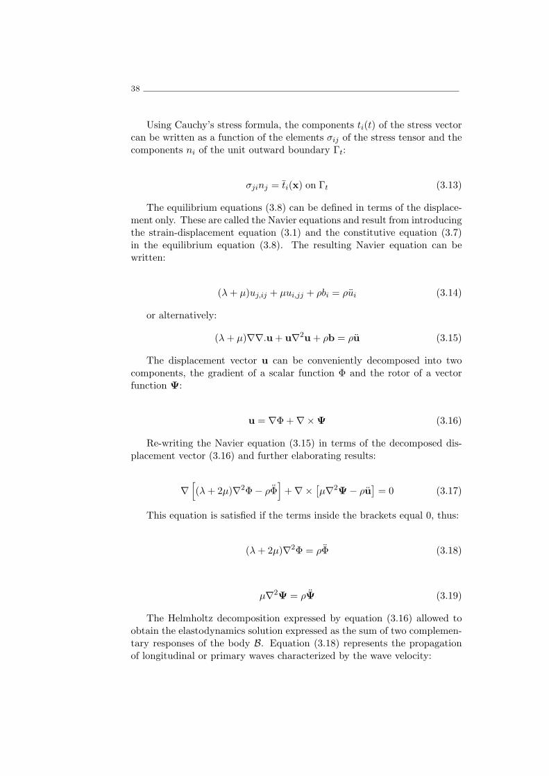
38
Using Cauchy’s stress formula, the components ti(t) of the stress vectorcan be written as a function of the elements σij of the stress tensor and thecomponents ni of the unit outward boundary Γt:
σjinj = ti(x) on Γt (3.13)
The equilibrium equations (3.8) can be defined in terms of the displace-ment only. These are called the Navier equations and result from introducingthe strain-displacement equation (3.1) and the constitutive equation (3.7)in the equilibrium equation (3.8). The resulting Navier equation can bewritten:
(λ+ µ)uj,ij + µui,jj + ρbi = ρui (3.14)
or alternatively:
(λ+ µ)∇∇.u+ u∇2u+ ρb = ρu (3.15)
The displacement vector u can be conveniently decomposed into twocomponents, the gradient of a scalar function Φ and the rotor of a vectorfunction Ψ:
u = ∇Φ+∇×Ψ (3.16)
Re-writing the Navier equation (3.15) in terms of the decomposed dis-placement vector (3.16) and further elaborating results:
∇[(λ+ 2µ)∇2Φ− ρΦ
]+∇×
[µ∇2Ψ− ρu
]= 0 (3.17)
This equation is satisfied if the terms inside the brackets equal 0, thus:
(λ+ 2µ)∇2Φ = ρΦ (3.18)
µ∇2Ψ = ρΨ (3.19)
The Helmholtz decomposition expressed by equation (3.16) allowed toobtain the elastodynamics solution expressed as the sum of two complemen-tary responses of the body B. Equation (3.18) represents the propagationof longitudinal or primary waves characterized by the wave velocity:

Finite Element modelling of high-speed tracks 39
Cp =
√λ+ 2µ
ρ(3.20)
Equation (3.19) represents the propagation of shear or secondary wavescharacterized by the wave velocity:
Cs =
õ
ρ(3.21)
The ratio of primary to secondary wave velocity can be written in termsof the Poisson’s ratio only:
Cs
Cp=
√1− 2ν
2− 2ν(3.22)
3.3 Finite Element modelling of high-speed tracks
3.3.1 Finite Element Method
The FEM is one of the most used computational techniques for the eval-uation of boundary value problems. Its application to multiple physicalproblems, the possibility for dynamical and non-linear problems and the in-creasing availability of multiple commercial and open-source software haveall contributed to its popularity. It is a computational technique that allowsto obtain an approximate result for a boundary value problem. A boundaryvalue or field problem is a mathematical problem in which one or two vari-ables must satisfy a differential equation everywhere within a known domainof independent variables and satisfy specific conditions on the boundary ofthe domain (Hutton, 2004). Depending on the type of physical problembeing analysed, the field variables may include physical displacement, tem-perature, heat flux, and fluid velocity, to name only a few.
Figure 3.1 features a domain Ω in which the field variable a(x) is tobe determined at every point x such that a known governing equation (orequations) is satisfied in every point. The figure also shows a representativeFE mesh of the domain, composed of an assembly of 3-node triangular fi-nite elements. The vertices of the triangular elements are the mesh nodes.Nodes are points of the domain where the field variable is explicitly com-puted. The field variables at non-nodal points of the domain are obtainedby interpolation of the solution at the nodes using shape functions. Thedifferent elements share nodes where the field variables are computed andthat ensures that field continuity is respected between the various elements.

40
This continuity is also ensured in the non-nodal boundaries of the elementsbecause the interpolation functions of the elements are consistent.
The utilization of several elements to model a domain has two main rea-sons: to accurately reproduce the geometry of the domain because the uti-lization of a single element would very inaccurately reproduce the domain’sgeometry for the vast majority of problems; also to increase the density ofmesh nodes, in which the field variables are accurately computed.
xΩ
b
Figure 3.1: General technique of the FEM: a general two-dimensional do-main Ω of field variable a(x) (top) and representative FE mesh (bottom).
In the particular case of structural mechanics, the FEM is a very usefultool. Since it relies on a meshing scheme, it allows for the considerationof complex structural geometries and loading conditions, allowing for thedetermination of the structure’s response to a particular solicitation sce-nario, for example. The method is also applicable to dynamic problems, inwhich modal analysis, frequency response and time integration analysis arepossible.
3.3.2 FEM framework
Weak form of the equilibrium equations
Defining arbitrary scalar functions vi and vi such that vi = 0 and vi = 0on Γu, the equilibrium equations (3.8) and the natural boundary conditions(3.13) can be stated in the following form:
vi
∫
Ω(σji,j + ρbi − ρui) dΩ+ vi
∫
Γt
(σjinj − ti
)dΓ = 0 (3.23)

Finite Element modelling of high-speed tracks 41
For any vi and vi the above equation satisfies the equilibrium equationsand the natural boundary conditions. Integrating the term
∫Ω σji,jvi dΩ by
parts:
∫
Ωσji,jvi dΩ = −
∫
Ωσjivi,j dΩ+
∫
Γviσjinj dΓ (3.24)
allows to write equation (3.23) in a ”weak” form:
−∫
Ωσjivi,j dΩ+
∫
Γviσjinj dΓ+
∫
Ωviρbi dΩ−
∫
Ωρuivi dΩ+ vi
∫
Γt
σjinj − ti dΓ = 0 (3.25)
Taking vi = −vi equation (3.25) becomes:
−∫
Ωσjivi,j dΩ+
∫
Γu
viσjinj dΓ+
∫
ΩviρbidΩ−
∫
Ωρuivi dΩ+
∫
Γt
viti dΓ = 0 (3.26)
and remembering that vi = 0 on Γu the term∫Γuvσjinj dΓ vanishes:
∫
Ωviρbi dΩ+
∫
Γt
viti dΓ =
∫
Ωσjivi,j dΩ+
∫
Ωρuivi dΩ (3.27)
The ”weak form” represented by equation (3.27) is usually referred as thePrinciple of Virtual Work. The importance of this result to the definition ofthe FEM and other numerical methods is that the derivatives in the partialdifferential equations of equilibrium are replaced with equivalent integrals,which are easier to treat numerically.
Finite element interpolation
In a FE discretization of domain Ω, a generic finite element is defined by
nnode nodes with one interpolation function N(e)i (x) associated with each
node i whose coordinate is xi. Each interpolation function takes the unityvalue at xi and zero at every other nodes of the element.
For a generic field a(x) defined over the domain Ωe of the element, itsFE interpolation ha over the element is obtained
ha(x) =
nnode∑
n=1
aiN(e)i (x) (3.28)

42
where ai is the value of a at node i.The generic field a(x) is defined over the entire domain Ω by the dis-
cretization of the domain in a mesh of nelement elements. In each element thegeneric field a(x) is interpolated as stated in equation (3.28). The genericfield is obtained over the domain Ω:
a(x) =
npoint∑
n=1
aiNi(x) (3.29)
where Ni is the global interpolation function of the global node i andnpoint is the total number of nodal points in the FE mesh. Defining a globalinterpolation matrix N:
N(x) =[N1(x),N2(x) ... Nnpoint
(x)]
(3.30)
where N1(x) is the diagonal ndim × ndim matrix:
Ni =
Ni 0 ... 00 Ni ... 0
. . .
0 0 ... Ni
Any displacement u(x) can be determined
u(x) = Nu (3.31)
where u is the global vector of nodal displacements. The strain-displacement matrix B is defined such that
ε = Bu (3.32)
where ε is the array of engineering strains:
ε = εx, εy, εz, γxy, γyz, γxzT (3.33)
in three dimensions the strain-displacement matrix B has the format:
B =
∂N1
∂x 0 0 ∂N2
∂x 0 0 ...∂Nnpoint
∂x 0 0
0 ∂N1
∂y 0 0 ∂N2
∂y 0 ... 0∂Nnpoint
∂y 0
0 0 ∂N1
∂z 0 0 ∂N2
∂z ... 0 0∂Nnpoint
∂z∂N1
∂y∂N1
∂x 0 ∂N2
∂y∂N2
∂x 0 ...∂Nnpoint
∂y
∂Nnpoint
∂x 0
∂N1
∂z 0 ∂N1
∂x∂N2
∂z 0 ∂N2
∂x ...∂Nnpoint
∂z 0∂Nnpoint
∂x
0 ∂N1
∂z∂N1
∂y 0 ∂N2
∂z∂N2
∂y ... 0∂Nnpoint
∂z
∂Nnpoint
∂y

Finite Element modelling of high-speed tracks 43
Defining the array of stress components σ:
σ = σx, σy, σz, τxy, τyz, τxzT (3.34)
it can be related with the array of engineering strains ε by the elasticitymatrix D:
σ = Dε (3.35)
For isotropic materials the three dimensional elasticity matrix D takesthe form:
D =
λ+ 2µ λ λ 0 0 0λ λ+ 2µ λ 0 0 0λ λ λ+ 2µ 0 0 00 0 0 µ 0 00 0 0 0 µ 00 0 0 0 0 µ
Taking the virtual work equation (3.27), writing in matrix notation with thevirtual displacements in evidence, it becomes:
vi
[∫
ΩNTρNu dΩ+
∫
ΩBTDBu dΩ−
∫
Γt
NTt dΓ−∫
ΩNTb dΩ
]
= 0 (3.36)
where vi is the virtual displacement and u is the vector of nodal acceler-ations. Since the above equation must hold for any virtual displacement, theterm inside the brackets must equal 0 and the equation represents a linearsystem that can be expressed in the form:
Mu+Ku− f = 0 (3.37)
where:
K =
∫
ΩBTDB dΩ (3.38)
f =
∫
ΩNTb dΩ+
∫
Γt
NTt dΓ (3.39)
M =
∫
ΩNTρN dΩ (3.40)
where K is the global stiffness matrix, f is the global vector of nodalforces and M is the mass matrix.

44
3.3.3 Newmark time integration
The Newmark time integration method is used in the 3D FE time domainresponse computations. This is one of the most popular time integrationschemes in numerical methods. The time integration problem can be sum-marized as: knowing the displacement u and the velocity u at some timet, one wishes to determine the same variables at a slightly different timet+∆t.
Supposing that the displacement vector u(t) and velocity vector u(t)are known at time step t and that it is possible to obtain estimates for theacceleration vectors u(t) and u(t +∆t), the displacement vector u(t +∆t)and velocity u(t+∆t) can be estimated with a Taylor series expansion:
u(t+∆t) ≈ u(t) + ∆tu(t) +∆t2
2[(1− β2)u(t) + β2u(t+∆t)] (3.41)
u(t+∆t) ≈ u(t) + ∆t [(1− β1)u(t) + β1u(t+∆t)] (3.42)
where β1 and β2 are two adjustable parameters that determine the natureof the time integration scheme. For β1 = β2 = 0 the displacement vectoru(t+∆t) and velocity vector u(t+∆t) are evaluated using the accelerationvector at time step t. This is known as an explicit time integration scheme.Alternatively, for β1 = β2 = 1 the displacement vector u(t+∆t) and velocityvector u(t+∆t) are evaluated using the acceleration vector at time t+∆tand the scheme is known as an implicit time integration. Recalling equation(3.37), the accelerations at t are determined:
u(t) = M−1 [−Ku(t) + f(t)] (3.43)
then, replacing equation (3.42) into equation (3.37):
Mu(t+∆t)
+K
u(t) + ∆tu(t) +
∆t2
2[(1− β2)u(t) + β2u(t+∆t)]
− f(t+∆t) = 0
(3.44)
which can be re-written as:
Mu(t+∆t) + β2∆t2Ku(t+∆t) =
−K
[u(t) + ∆tu(t) +
∆t2
2(1− β2)u(t)
]+ f(t+∆t) (3.45)
the above system of equations can be solved for u(t+∆t). The displace-ment vector u(t + ∆t) and velocity vector u(t + ∆t) are evaluated usingequations (3.41) and (3.42).

Finite Element modelling of high-speed tracks 45
3.3.4 Viscous Boundaries
Considering a soil element (Figure 3.2) in which dilatational waves are prop-agating in the x direction, the equilibrium equation is:
∂σxx∂x
+ ρb = ρ∂2ux∂t2
(3.46)
σxx ρ∂2ux
∂t2σxx +
∂σxx
∂x
Figure 3.2: Wave propagation through a soil element.
The corresponding Navier equation is:
(λ+ 2µ)∂2ux∂x2
+ ρb = ρ∂2ux∂t2
(3.47)
Neglecting the body forces the equation reduces to:
∂2ux∂x2
=1
C2p
∂2ux∂t2
(3.48)
where Cp is again the dilatational wave velocity in the material. Thesolution to the partial differential equation is given by:
ux(x, t) = U
[sin(ωt− ωx
Cp) + cos(ωt− ωx
Cp)
](3.49)
Differentiating the above equation with respect to t:
ux(x, t) = Uω
[cos(ωt− ωx
Cp)− sin(ωt− ωx
Cp)
](3.50)
and differentiation the same equation with respect to x:

46
∂ = Uω
Cp
[cos(ωt− ωx
Cp)− sin(ωt− ωx
Cp)
](3.51)
Thus, considering (3.50) and (3.51):
−ux(x,t)Cp
=∂ux∂x
= εxx (3.52)
Considering that the stress σxx is given by:
σxx = (λ+ 2µ)εxx (3.53)
then:
σxx = −Cp2ρux(x, t)
Cp= −ρCpux (3.54)
Multiplying the stress by the area A of the soil elements, the force isobtained:
Fxx = −ρCpuxA (3.55)
From equation (3.55) it is demonstrated that the force in the x directiondue to the propagation of dilatational waves is identical to the force by aviscous damper with coefficient c = ρCpA. It can be proved in an analogousway that the force due to shear waves propagation is identical to the forceof a viscous damper with coefficient c = ρCsA. Lysmer and Kuhlemeyer(1969) proposed the introduction of such dampers in the boundaries of themesh in order to mitigate spurious wave reflection.
This can be achieved in the FE software Diana through the definitionof ”bounding elements” (TNO, 2005) in the boundaries of the mesh. Theseconsist in the introduction of a set of spring/damper elements in all thenodes that belong to the boundary surface (Figure 3.3).
In each node i the spring/damper element is configured taking into ac-count the area A. The individual spring stiffness is computed by Diana:
k =AE
li(3.56)
where li is a characteristic length in one of the local axes directions. Thecharacteristic length is computed from a user-specified parameter αb:
li =1
αb(3.57)

Finite Element modelling of high-speed tracks 47
b x
y
z
b x
y
z
b x
y
zb x
y
z
Figure 3.3: Bounding elements on a mesh element.
The damping coefficients are defined by Diana:
c = diA (3.58)
where di is a multiplication factor that takes into account the wave velocityto occur at the end of the mesh:
dxy = ρCs (3.59)
dz = ρCp (3.60)
The ”Bounding elements” correspond to the viscous quiet boundaries ofLysmer and Kuhlemeyer (1969) when α = 0.
3.3.5 Case study and experimental data
The experimental data herein used to validate the model is obtained fromthe literature (Degrande and Schillemans, 2001) with material parameterssummarized in Table 3.1.
Experimental measurements are a crucial component to understandrailway track behaviour as they are the best source of information forthe response of the track and the wave propagation to outer zones.Additionally the experimental measurements may be used to calibrateand validate numerical models which may themselves serve as invalu-able tools to better understand the phenomenons at work in thesestudy cases. Over the last decade, an effort has been made by sev-eral authors (Degrande and Lombaert, 2000, Degrande and Schillemans,2001, Chebli et al., 2008, Galvın and Domınguez, 2009, Martins et al., 2009,Kouroussis et al., 2011, Costa et al., 2012, Shuangyang et al., 2012) to ob-tain and share the results of experimental measurements in high-speed tracksproviding an increasing database for others to understand the railway trackbehaviour and/or test their numerical tools.

48
The experimental data herein used to validate the model is obtained fromthe literature (Degrande and Schillemans, 2001) with material parameterssummarized in Table 3.1.
Table 3.1: Case study properties.
Element Parameter Value
Esl 3.0×10¹⁰ PaSleeper ρsl 2054 Kg/m3
hrp 1× 10⁻² mRail pad krp 1× 10⁸ N/m
Ar 7.684× 10⁻³ m2
Ir 3.055× 10⁻⁵ m4
Rail ρr 7800 Kg/m3
Er 2.1× 10¹¹ Pa
ρb 1800 Kg/m3
Ballast υb 0.1Eb 2× 10⁸ Paξb 0.01
ρsb 2200 Kg/m3
Sub-Ballast υsb 0.2Esb 3× 10⁸ Paξsb 0.01
ρcl 2200 Kg/m3
Capping Layer υcl 0.2Ecl 2× 10⁸ Paξcl 0.01
ρs 1850 Kg/m3
υs 0.3ξs 0.03hs1 1.4 mCps1 187 m/s
Soil Layers Css1 100 m/shs2 1.9 mCps2 249 m/sCss2 133 m/shs3 ∞Cpl3 423 m/sCsl3 226 m/s
These data correspond to vibration measurements made during the pas-sage of a Thalys high-speed train at 314 km/h on a track between Brus-
Finite Element modelling of high-speed tracks 49
sels and Paris, more precisely near Ath, 55 km south of Brussels. Thetrack is a classical ballasted railway track with continuously welded UIC 60rails, pre-stressed concrete mono-block sleepers of length lsl = 2.5m, widthbsl = 0.285m, height hsl = 0.205m (under the rail) and mass msl = 300 kg.The flexible rail pads have thickness hrp = 0.01m and a static stiffnesskrp = 100MN/m, for a load varying between 15 and 90 kN. The track issupported by ballast and sub-ballast layers, capping layer and the subgrade.
For the determination of the soil properties many experimental tech-niques are available, either by in situ testing or by collecting samples forposterior analysis at the laboratory. As the properties of the soil materialsdepend largely on their condition it is often preferable to perform in situtests as the laboratory characterizations require that samples are obtainedand transported in an undisturbed state which is often not easy to do. Fromthe in situ tests available the SASW test is often used to complement othertests like Cone Penetration Tests (CPT), Standard Penetration Tests (SPT),Seismic Cone Penetration Tests (SCPT), downhole or crosshole methods.
The dynamic soils characteristics for this case study were determinedby Degrande and Schillemans (2001) through a Spectral Analysis of SurfaceWaves (SASW). The basis of this test are the dispersive characteristics ofthe Rayleigh waves when travelling through a layered medium. In this test,impact solicitations through a hammer or a falling weight are done at asurface point in the soil in order to excite several frequencies. At severaldistances from this point, also at the soil surface, the vertical soil response ismeasured using accelerometers or geophones. From these measurements, thetheoretical dispersion curve of the soil is obtained, usually through the theHaskell-Thomson approach (Nazarian and Desai, 1993, Yuan and Nazarian,1993). An inverse problem is then formulated in which the variation ofthe shear wave velocity with depth is calibrated in a numerical model inorder to minimize the error of the numerical dispersion curve of the soil. Itshould be noted that this is an ill-posed problem which implies that a givenexperimental dispersion curve may correspond to more than one shear wavevelocity profile. From the data obtained in the test it is also possible toobtain the attenuation curve of the soil, solving a similar inverse problemallows to estimate the shear damping profile of the soil.
The main experimental campaign was carried out by measuring the vi-brations in the track and soil during the passage of the train. Usually, themeasurements in the track are restricted to the rail or most commonly thesleeper, as these are solid, compact elements thus making it easier to fix themeasuring instruments. Measurements in the ballast or sub-ballast mate-rials are seldom done because its discrete nature makes it hard to obtaina representative measure of the material response. The soil makes for aneasier medium to measure the vibrations, usually these measurements aremade at the surface by craving a stake in which the measurement equip-ment is attached. The measurements in the soil were made at 10 different

50
distances from the track ranging from a 4m to 72m . The location of themeasurement points (accelerometers) used for this work is presented in Fig-ure 3.4. The first measurement point is at the sleeper, next to the rail, thisallows to obtain the track response to the passage of the train. The secondmeasurement point is located in the soil surface at a horizontal distance of7.25m from the rail. As the main purpose of this work is to test modellingaccuracy at the track and its vicinity, other measurement points at largerdistances from the track are not considered.
1.5 m7.25 m
A
B
RailSleeper
BallastSub-ballast
Capping Layer
Sugrade
Figure 3.4: Geometry and measurement points of the track.
Figure 3.5 shows the configuration of the Thalys high-speed train con-sisting of 2 locomotives and 8 carriages. The total length of the train is200.18 m. The locomotives are supported by 2 bogies and have 4 axles. Thecarriages next to the locomotives share one bogie with the neighbouringcarriage, while the 6 other carriages share both bogies with neighbouringcarriages. The total number of bogies is 13 and, consequently, the numberof axles on the train is 26.
Figure 3.5: Geometry and load characteristics of the Thalys high-speed train(Lombaert et al., 2006).

Finite Element modelling of high-speed tracks 51
3.3.6 FE Mesh
The 3D FE mesh is defined in order to simulate the case presented in section3.3.5. Solid elements of 6 and 8 nodes are used to simulate the subgrade,capping layer, sub-ballast, ballast and sleepers. Each rail pad is simulatedas a spring-dashpot duo separated 0.6m from each other, the rail is mod-elled with beam elements of 3 nodes. The inferior limit of the model isconstrained, the upper limit is unconstrained and the others are assignedwith the bounding elements presented in sub-section 3.3.4.
Due to the great number of degrees of freedom involved, the size of themodel was kept to a minimum. In this case using a computer with 2Gb ofmemory it was noted that at nearly 50.000 mesh nodes there was a thresholdwhere the computational time for each time step was greatly increased. Itis assumed that the software uses the memory of the computer to store thematrices of the model but when the memory is not sufficient the software usesthe hard drives of the computer where the access to data is much slower andthus the computational time is greatly increased. Because of this an effortwas made to keep the model below this threshold. The mesh is achievedby firstly creating a longitudinal module of the track (Figure 3.6.a). Thisallows to easily change the dimensions and refinement of the mesh. Oncethe desired module is achieved it is then copied a set number of times untilit achieves the intended length (Figure 3.6b).
The dimensions of the FE mesh are: 30m of track length, 40m wide and20m of soil depth. These depth dimension was used as previous models inFEM have been validated with 20 m of soil depth. Also, the longitudinallength of the model was subject to a parametric study in order to find theminimum length for which the track model is representative.
3.3.7 Simulation of the moving load
The moving quasi-static load is simulated through the definition of sta-tionary loads at the rail nodes with time dependent modulus. Suiker et al.(1998) have demonstrated that the moving load problem can be analysed us-ing the FEM in which the moving load is modelled by a sequence of discretepulses.
Considering a moving load with constant modulus F, its position x(t)can be computed at any time t provided that the initial position x0 and theconstant speed c are known. At any given time t in which the load is passingat a node of the rail, that node will be solicited by a force of modulus F,and all other nodes will be solicited with loads of modulus 0. At any giventime t in which the load is acting in the rail span between two nodes, thesewill be solicited according to the representation of Figure 3.7.
All nodes are solicited by a force with modulus 0, except those nodes(ni−1 and ni) that limit the span of the rail where the moving load is in-

52
(a)
(b)
Figure 3.6: FE mesh of the 3D model constructed through copying a a)module to achieve the b) final mesh.
stantly acting. For each of these nodes the instant force applied is inverselyproportional to the distance between node and the position of the movingload. Thus for node ni−1 the instant force fi−1(t) is:
fi−1(t) =
(1− x(t)
l
)F (3.61)
where x(t) is the distance between node ni−1 and the position of themoving load and l is the distance between nodes ni−1 and ni. For node n1the instant force fi(t) is:

Finite Element modelling of high-speed tracks 53
F
ni−1 ni
x(t)
fi−1(t) fi(t)
l
Figure 3.7: Simulation of the moving load with time dependent stationaryloads.
fi(t) =
(x(t)
l
)F (3.62)
Taking advantage of the linear behaviour of the model, the passage ofa single axle with unitary load is computed and the effect of the wholetrain is determined in post-processing. Araujo (2011) and Hall (2003) havesuccessfully used similar load schemes to simulate moving loads in 3D FEmodels.
3.3.8 Results discussion
The results obtained from the moving load are processed to represent theresponse due to the passage of the Thalys high-speed train, taking intoaccount the Thalys axle load, the distance between axles and the circulationspeed of 314 km/h. In Figure 3.8 the experimental and numerical verticalaccelerations in the sleeper are compared.
The computed response agrees very well with the experimental measure-ments. The downward accelerations are higher than measurements and theupward accelerations are very well predicted by the 3D FE mesh. Someof the measured peak values are significantly higher than the rest, this isprobably explained by some random occurrence in site like the presence ofdirt on the rail or an uneven distribution of weight or wheel unevennessmore pronounced in those axles. These are obviously unaccounted for in thenumerical model, therefore differences occur between some of the computedpeak values and the corresponding measurements. The numerical simulationof the response at the track vicinity is also studied (Figure 3.9).
The computational and measurement results agree reasonably well. Theupper and downer peak values have similar values although the computedvalues are much ”cleaner” in a sense that the contribution of the axles is stillperceptible while the measurements show a cloud of results where the con-tribution of each set of axles is not noticeable. As Lombaert and Degrande

54
0 0.5 1 1.5 2 2.5 3−40
−30
−20
−10
0
10
20
30
40
50
Time [s]
Acceleration[m/s2]
Figure 3.8: Computed (black) and measured (grey) response at measure-ment point A due to the passage of a Thalys high-speed train at 314 km/h.
0 0.5 1 1.5 2 2.5 3−0.4
−0.3
−0.2
−0.1
0
0.1
0.2
0.3
0.4
Time [s]
Acceleration[m/s
2]
Figure 3.9: Computed (black) and measured (grey) response at measure-ment point B due to the passage of a Thalys high-speed train at 314 km/h.
(2009) concluded, the quasi-static contribution of the load dominates thetrack response and the field response is dominated by the dynamic contri-bution. Therefore, a numerical model, like the 3D FE model presented, thatonly accounts for the quasi-static contribution is only suited to predict theresponse in the immediate vicinity of the track. The numerical predictionsseem to confirm that since the track response agrees well with experimentalresults while the response in the soil at 7.25m from the rail is less accurate.
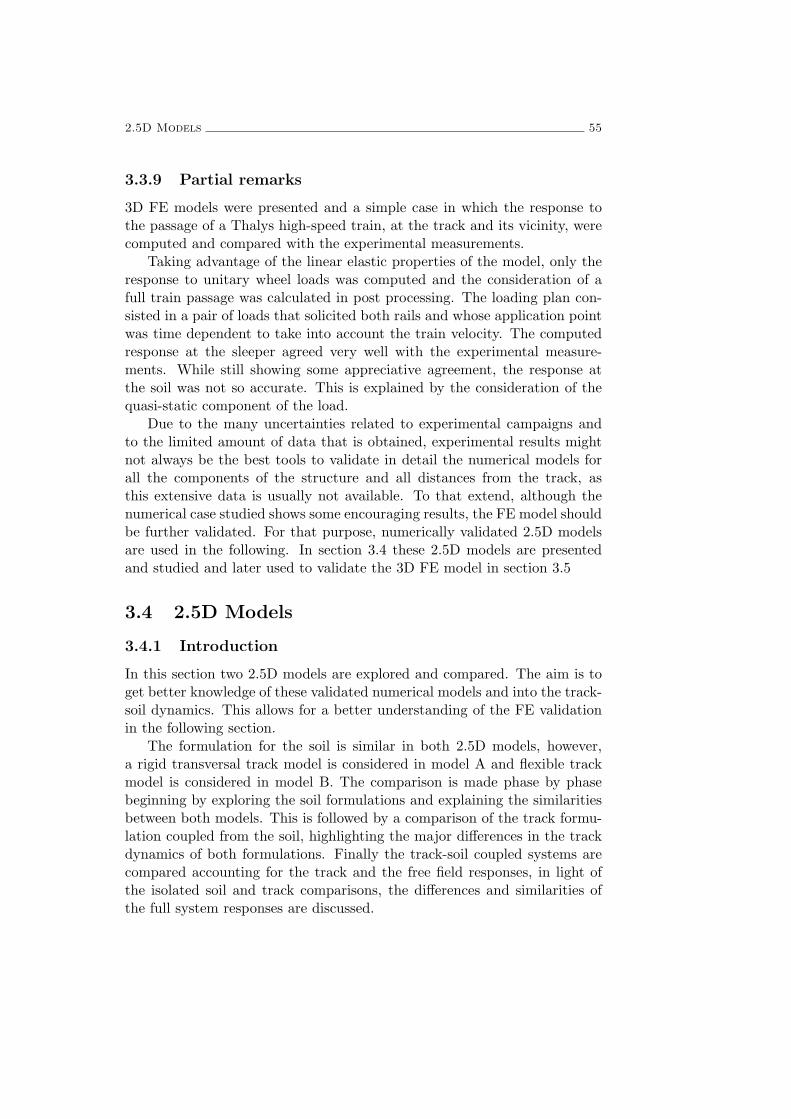
2.5D Models 55
3.3.9 Partial remarks
3D FE models were presented and a simple case in which the response tothe passage of a Thalys high-speed train, at the track and its vicinity, werecomputed and compared with the experimental measurements.
Taking advantage of the linear elastic properties of the model, only theresponse to unitary wheel loads was computed and the consideration of afull train passage was calculated in post processing. The loading plan con-sisted in a pair of loads that solicited both rails and whose application pointwas time dependent to take into account the train velocity. The computedresponse at the sleeper agreed very well with the experimental measure-ments. While still showing some appreciative agreement, the response atthe soil was not so accurate. This is explained by the consideration of thequasi-static component of the load.
Due to the many uncertainties related to experimental campaigns andto the limited amount of data that is obtained, experimental results mightnot always be the best tools to validate in detail the numerical models forall the components of the structure and all distances from the track, asthis extensive data is usually not available. To that extend, although thenumerical case studied shows some encouraging results, the FE model shouldbe further validated. For that purpose, numerically validated 2.5D modelsare used in the following. In section 3.4 these 2.5D models are presentedand studied and later used to validate the 3D FE model in section 3.5
3.4 2.5D Models
3.4.1 Introduction
In this section two 2.5D models are explored and compared. The aim is toget better knowledge of these validated numerical models and into the track-soil dynamics. This allows for a better understanding of the FE validationin the following section.
The formulation for the soil is similar in both 2.5D models, however,a rigid transversal track model is considered in model A and flexible trackmodel is considered in model B. The comparison is made phase by phasebeginning by exploring the soil formulations and explaining the similaritiesbetween both models. This is followed by a comparison of the track formu-lation coupled from the soil, highlighting the major differences in the trackdynamics of both formulations. Finally the track-soil coupled systems arecompared accounting for the track and the free field responses, in light ofthe isolated soil and track comparisons, the differences and similarities ofthe full system responses are discussed.

56
3.4.2 Direct Stiffness Method
In the 2.5D models used in this work, the soil is simulated through the BEM.The Green’s functions are used as fundamental solutions of the BEM and arecomputed through the DSM. The DSM is based on the solution of the wavepropagation in an elastic medium in the frequency-wavenumber domain.
Considering a function formulated in the time-space domain, itsfrequency-wavenumber domain representation is obtained with a doubleFourier transform. A Fourier transform of the time dimension of a functionf(x, y, z, t) formulated in the time-space domain determines its frequencydomain representation f(x, y, z, ω):
f(x, y, z, ω) = F [f(x, y, z, t), ω] =
∫ ∞
−∞exp(−iωt)f(x, y, z, t)dt. (3.63)
Another Fourier transform of one of the spacial dimensions of thefunction f(x, y, z, ω) determines its frequency-wavenumber representationf(kx, y, z, ω):
f(kx, y, z, ω) = F[f(x, y, z, ω), kx
]=
∫ ∞
−∞exp(ikxx)f(x, y, z, w)dx. (3.64)
The DSM is based on a stiffness matrix formulation proposed by Kauseland Roesset (Kausel and Roesset, 1981). The method relies on an assem-bly of element matrices similarly to the FEM, but the formulation in thefrequency-wavenumber domain allows for the computation of exact solutionsof the Navier equations. These exact solutions are used as shape functionsin the DSM. Consequently, the simulation of wave propagation in homoge-neous layers, half-spaces or full spaces is treated exactly. Each homogeneousmedium can be simulated with a single element and there is no need for sub-division as occurs in other methods. For the case of layered media the DSMis restricted to layering in one direction (p.e. an horizontally layered soil).
3.4.3 General solution
The general solution of both models is formulated in a similar way. Thedynamic soil-structure interaction problem is decomposed into two sub-domains: the structure Ωb and the semi-infinite layered soil Ωs. The dy-namic soil-structure interaction problem is solved by enforcing continuity ofdisplacements and equilibrium of stresses on the interface Σbs between bothsub-domains. The section Ab of the structure is invariant with respect to thelongitudinal coordinate y. The dynamic soil-structure interaction problemis assumed to be linear and all equations are elaborated in the frequencydomain. The invariance of the geometry with respect to the longitudinal

2.5D Models 57
coordinate y allows to perform a Fourier transformation of the coordinate yto the wavenumber ky. This results in a solution procedure in the frequency-wavenumber domain, where the equations of motion of the coupled track-soilsystem can be written in the following general form:
[Kbb(ky, ω) + Ks(ky, ω)
]ub(ky, ω) = fb(ky, ω) (3.65)
where Kbb(ky, ω) and Ks(ky, ω) are the dynamic stiffness matrices of thetrack and the soil respectively, while ub(ky, ω) is the track displacementvector and fb(ky, ω) is the force vector applied to the track. The solution ofthe track-soil interaction (3.65) provides the soil displacements ubs at thetrack-soil interface, which allows for the computation of the soil tractionstbs(x, ky, z = 0, ω) at this interface:
tbs(x, ky, z = 0, ω) = tbs(ubs(Nbs))ubs (3.66)
where Nbs are the shape functions related to the degrees of freedom ubs atthe track-soil interface.
The dynamic reciprocity theorem is used for the calculation of the track-soil transfer functions hzi(ky, ω):
hzi(ky, ω) =
∫
Σbs
uGzi(x− x′, ky, z, ω)tbs(x
′, ky, z′ = 0, ω) dΓ (3.67)
where uGzi(x − x′, ky, z, ω) are the Green’s functions between the BE mesh
at the track-soil interface and the receiver locations in the soil.The dynamic load is obtained using a compliance formulation in the
frame of reference that moves with the vehicle (Clouteau et al., 2001), thecontact between the axles and the rails is approximated as a point contact.A perfect contact is assumed between the vehicle and the railway track.The displacement vector ua(ω) that contains the vehicle displacements atthe vehicle-track contact points is equal to:
ua(ω) = ur(ω) + uw/r(ω) (3.68)
where ur(ω) is the rail displacement and uw/r(ω) is the rail unevenness,evaluated at a fixed position in the moving frame of reference.
The vehicle’s compliance matrix Cv(ω) relates the displacements ua(ω)to the vehicle-track interaction forces gd(ω):
ua(ω) = −Cv(ω)gd(ω) (3.69)
In the case of a longitudinally invariant track, the displacements ur at thecontact points between the vehicle and the track can be calculated in asimilar way:
ur(ω) = Ct(ω)gd(ω) (3.70)

58
The track compliance matrix is computed using the transfer function be-tween forces and displacements on the rail:
Ctkl(ω) =
1
2π
∫ +∞
−∞hzi(ky, ω + kyv) exp [−iky(yk0 − yl0)] dky (3.71)
Introducing (3.69) and (3.70) in equation (3.68) results:
[Cv(ω) + Ct(ω)
]gd(ω) = −uw/r(ω) (3.72)
This equation allows to compute the vehicle-track interaction forces gd(ω)from the track unevenness uw/r(ω).
The 2.5D models have been presented and validated by the authors andit is not in the scope of this thesis to detail the formulations of these models.The reader may be referred to Lombaert et al. (2006) or Galvın et al. (2010)for more information on the formulations.
Model A
This model has been previously studied and validated by the authors(Lombaert et al., 2006) and is compared with model B. It relies on an ana-lytical formulation of the track (Figure 3.10).
lsl
lr lr
ur1
kp cp
ur2
usl
βsl
kb cb ubs
βbsbbs
rail
rail pad
sleeper
ballast
interface Σbs
Figure 3.10: Cross section of model A (Lombaert et al., 2006).
The rails are modelled as Euler-Bernoulli beams whose displacementsare denoted as ur1(y, t) and ur2(y, t). The rail pads are modelled as longitu-dinally continuous spring-dashpot elements with an equivalent stiffness krp:

2.5D Models 59
krp =krpdsl
(3.73)
where krp is the single rail pad stiffness and dsl is the sleeper distance.Similarly, the equivalent damping crp is obtained:
crp =crpdsl
(3.74)
where crp is the single pad damping coefficient.The sleepers are assumed to be rigid in the transversal plane and thus
the displacement of any point along the sleeper is a combination of only twobasic motions: displacement usl at the centre of gravity of the sleeper androtation βsl about this centre. To account for the fact that the sleepers in thetrack are not connected with each other, the sleeper elements in the modeldo not contribute for the longitudinal stiffness of the track and are modelledonly as a uniformly distributed mass along the track. The distributed massmsl per unit length is obtained from the total mass of a single sleeper msl
and the sleeper distance dsl
msl =msl
dsl(3.75)
The ballast is modelled as a set of distributed, independent linear springsand dampers. The ballast stiffness kb is obtained assuming that only theballast portion directly below the sleeper contributes for the vertical stiffnessof the model:
kb =lslbslkbdsl
(3.76)
where lsl is the sleeper length, bsl is the sleeper width and kb is theballast stiffness. The ballast viscous damping is accounted for in the ballastimpedance k
∗b:
k∗b = kb + iωcb (3.77)
The ballast mass is determined in a similar way, accounting for the dis-crete support of the sleepers and the sleeper length. The width bbs of thetrack-soil interface is taken equal to the sleeper length lsl.
The track-soil interface is also assumed to be rigid in the transversalplane of the track. Thus, the vertical displacements ubs at the track-soilinterface Σbs are determined as in the sleeper, by the vertical displacementubs at the centre of the interface and the rotation βbs about this centre.

60
Only a generalized displacement and rotation of the track-soil interface isallowed. This restriction is imposed on the computation of the soil stiffnessmatrix:
Ksij(ky, ω) =
∫
Σφbsitsz(ubs(φbsj)) dΓ (3.78)
where ubs(φbsj) is the wavefield in the soil due to an imposed displacementφbsj at the track-soil interface Σbs in the frequency-wavenumber domain,tsz(ubs(φtj)) is the vertical component of the soil tractions ts = σsn ona boundary with a unit outward normal n due to this scattered wavefieldubs(φbsj). The BEM is used to calculate the soil tractions tsz(ubs(φbsj)) atthe track-soil interface, assuming that the track is located at the soil’s sur-face. The BE formulation is based on the boundary integral equations in thefrequency-wavenumber domain, using the Green’s functions of a horizontallylayered soil (Lombaert et al., 2006).
Model B
This model relies on the 2.5D FE formulation in order to represent theballast of the track. It allows the deformation of the sleeper and track-soilinterface providing a wider range of interactions between the track and thesoil.
lsl
l2 − lr
hb
linkbeam
shell
volume3
2
Figure 3.11: Cross section of model B.
The rails and rail pads are modelled with Euler-Bernoulli beams andcontinuous spring-dashpot elements respectively, as in model A. The sleeperis modelled with 2-node 2.5D shell elements and is considered to contributeto the in plane stiffness of the track only. The equivalent Young’s modulusEsl of the sleeper is determined from the original Young’s modulus Esl, thewidth of the sleeper bsl and the distance between sleepers dsl:
Esl =Eslbsldsl
(3.79)

2.5D Models 61
The sleeper mass msl is used to calculate a uniformly distributed mass
msl =msl
dsl(3.80)
The ballast is modelled as a mesh of 2.5D 4-node volume elements. Theequivalent ballast mass mb in the continuous model is calculated from thepart of the ballast that is in contact with the sleepers:
mb =ρbhblslbsl
dsl(3.81)
The formulation of the volume finite elements in 2.5D is presented byFrancois et al. (2010).
3.4.4 Case study
Soil profile
The case study relies on a test site, located in Lincent along the trackBrussels-Koln. In order to determine the soil layering, two SASW tests(Pyl and Degrande, 2001) and five SCPT (Haegeman, 2001) have been per-formed. The SCPT tests proposed by Robertson et al. (1986) result fromthe combined methods of the borehole test and the CPT. A cone penetrom-eter is pushed into the soil and in usual CPT tests the cone end resistance,the sleeve side friction and the pore pressure are measured. These results arethen correlated with the mechanical properties of the soil through empiricalrelations, analytical or numerical models. The main innovation of the SCPTconsisted in adding a geophone in the cone penetrometer and generating ashear wave at the surface of the soil. The time the shear wave takes toreach the geophone is measured and through it the shear wave velocity isdetermined.
It was found that the site consists of a layer with a thickness of 3.0 mand a shear wave velocity between 150 m/s and 160 m/s and a layer witha shear wave velocity between 250 m/s and 280 m/s (Pyl and Degrande,2001). Table 3.2 summarizes the dynamic soil characteristics of the site inLincent.
Table 3.2: Dynamic soil characteristics.
Layer d Cs Cp E ν ρ ξ
[m] [m/s] [m/s] [×106N/m2] [-] [kg/m3] [-]
1 3 150 300 120 0.333 2000 0.032 ∞ 280 560 418 0.333 2000 0.03

62
Track properties
The track in Lincent is a ballasted railway track with UIC 60 rails sup-ported every 0.60 m by concrete mono block sleepers. With very similarcharacteristics to those presented in sub-section 3.3.5.
The distributed sleeper mass per unit length is msl equals 500 kg/m.The dynamic stiffness kb and damping cb of the ballast and the equivalentstiffness krp = krp/d and damping crp = crp/d of the rail pad were obtainedby Lombaert et al. (2006) by means of a rail receptance test. In this test, animpulse hammer was used to induce an impact load on the track, the rail re-sponse was measured and through an optimization procedure, the unknowncharacteristics were calibrated in the numerical model A in order to mini-mize the error of the track receptance. The optimized ballast stiffness kb anddamping cb corresponded 1534.5× 106N/m2 and 27.7× 10³Ns/m2, respec-tively. The equivalent rail pad stiffness krp = 153.4×10⁶N/m, as for mediumto stiff rail pads, and a damping crp = 13.5 × 10³Ns/m (Lombaert et al.,2006).
The Young’s modulus of the ballast in model B is tuned with model Ain the 2D static case. The displacement of the rails due to a unitary loadin one rail is the comparison parameter. Model A presents a displacementof 3.434 × 10⁻⁸m and 2.374 × 10⁻⁸m for the loaded and not loaded railrespectively. Using this optimization, the Young’s modulus in model B istuned to 128.9 × 10⁶N/m2, for which it presents displacements of 3.446 ×10⁻⁸m and 2.353× 10⁻⁸m.
3.4.5 Models’ comparison
Mathematical verification
The two models presented have different kinematics of the track. In bothcases a BE formulation is used to determine the dynamic stiffness of thesoil. In Model A only the generalized degrees of freedom corresponding toa vertical translation and a rotation of the whole soil-track interface areconsidered, in model B the shape functions of the degrees of freedom at theinterface are used. These models also use different tools for the computationof the soil’s stiffness, model A uses Traffic (Lombaert, 2001), while modelB uses Bemfun (Francois et al.). To ensure the consistency of both tools,the Bemfun toolbox is adjusted to compute the stiffness matrix of the soilfor the two generalized degrees of freedom. Figure 3.12 shows one termof the dynamic stiffness matrix of the soil. For a comparison in the fullwavenumber range, a frequency of 100 Hz is chosen from which the stiffnessis compared (Figure 3.12a). The inverse wavenumber transform allows aneasier comparison in the frequency range. The results at the load source areindeterminable and the dynamic stiffness is compared at 0.01 m from thesource.

2.5D Models 63
(a)0 0.5 1 1.5 2 2.5 3 3.5 4
0
0.5
1
1.5
2
2.5
3
3.5
4
4.5x 10
7
Stiffness[N
/m]
ky [-]
(b)0 50 100 150 200 250 300 350 400
0
0.5
1
1.5
2
2.5x 10
13
Stiffness[N
/m]
Frequency [Hz]
Figure 3.12: One term of the dynamic stiffness matrix of the soil for modelA (grey line) and model B (black line) a) in the wavenumber domain at 100Hz and b) in the frequency domain at 0.01 m from the source.
The dynamic stiffness of both formulations fully matches. This goodcorrespondence is found in the whole wavenumber-frequency range ensuringthat both formulations for the soil are numerically equivalent.
Dynamic track behaviour
The track dynamics in model B allows for better insight into ballast be-haviour of high-speed train tracks. Attention must be given to how thisdifferent track modelling affects the overall behaviour of the track. Thecomparison with model A allows to perceive how these different approachesaffect the final outcome. Taking into account the differences in the trackformulations, a thorough comparison and discussion of their respective be-haviour is done in the following.
The dispersion curves of both free track models are computed and shown

64
in Figure 3.13 and Figure 3.14. For model A all 6 modes are shown, these
(a)
0 200 400 600 800 1000 12000
0.5
1
1.5
2
2.5
3
3.5
4
4.5
5
Wavenumber
[rad/m]
Frequency [Hz]
(b)
0 200 400 600 800 1000 12000
0.5
1
1.5
2
2.5
3
3.5
4
4.5
5
Wavenumber
[rad
/m]
Frequency [Hz]
Figure 3.13: Dispersion curves of the track model of a) model A and b)model B in frequency-wavenumber domain.
are coupled in pairs and each mode is undistinguishable from its pair in thegraphical representation. The first pair starts at 0 Hz, the second pair hasa cut-on frequency at 338 Hz and the third pair has a cut-on frequency at589 Hz. For model B the representation is restricted to the first 60 modesdue to the large number of degrees of freedom of the track model. Thismore elaborate model incorporates the kinematics of model A, since therigid behaviour of the interface and sleeper are specific cases of the flexiblebehaviour in model B.
The first pair in model A corresponds to the rigid modes, a translationand a rotation of the whole track, with a slight resonance of the rails without

2.5D Models 65
(a)
0 200 400 600 800 1000 12000
200
400
600
800
1000
1200
1400
1600
1800
2000
Phase
velocity
[m/s]
Frequency [Hz]
(b)
0 200 400 600 800 1000 12000
200
400
600
800
1000
1200
1400
1600
1800
2000
Phasevelocity
[m/s]
Frequency [Hz]
Figure 3.14: Dispersion curves of the track model of a) model A and b)model B in frequency-phase velocity domain.
vertical deformation of the ballast. The first two modes of model B, startingat 0 Hz, are represented in Figure 3.15 and Figure 3.16, the translation androtation of the track provokes a bending of the ballast and sleeper that isnot possible in model A. As the wavenumber increases, so does the bendingof the track and thus these modes appear at increasingly distant frequencies.
The second pair of modes in model A corresponds to the in and out ofphase resonance of the rails. The resonance frequency of the rail pad and
rail is 326.3 Hz at 0 rad/m, considering f =√krp/ρAr. The connection
with the track makes a frequency shift of the resonance to higher frequency,thus making these modes appear at 338 Hz. These modes are not closelyfollowed by any pair of modes in model B, but by a combination of a bigger

66
(a)
(b)
Figure 3.15: First mode of the track model B at a) 1 rad/m and b) 3 rad/m.
(a)
(b)
Figure 3.16: Second mode of the track model B at a) 1 rad/m and b) 3rad/m.
number of these. The dispersion curves of the track model A are noticeableas a trend formed by a great number of modes in model B (Figures 3.13 and3.14)
The third pair of modes in model A corresponds to the resonance ofthe ballast. The resonance of the free ballast occurs at 578 Hz in the 2Dcase, the coupling with the rails makes the mode shift to 589 Hz. These

2.5D Models 67
modes have no influence in the model’s behaviour since calculations for thetrains passage are done at lower frequencies. Again, a combination of severalmodes in model B includes the dispersion curves of the third pair of modesof model A.
Dynamic track-soil system behaviour
The dynamic stiffness matrices Ks and Kbb are assembled and the responseof the track-soil coupled system of both models is compared. Figure 3.17shows the displacement of the rails due to a unitary load equally distributedthrough both rails at frequencies up to 100 Hz.
The receptance at this frequency range is the same in both cases. Thisis due to the fact that in the considered frequency-wavenumber range, theresponse of the model is dominated by the soil. This high receptance oc-curs mainly due to the dispersion properties of the soil. At low frequencies,the high wavelength reflects the properties of the half-space, and the peakresponse is obtained for wave velocities close to the shear wave velocity(280m/s). At higher frequencies, the lower wavelength reflects the proper-ties of the top layer and so the peak response occurs at velocities close tothe shear wave velocity of the top layer (150 m/s).
Figure 3.18 presents the rail receptance for a broader frequency range,along with the dispersion curves of each model. The growing influence ofthe track at higher frequencies is noticeable in both models.
For a better understanding of the tracks behaviour, the soil receptancecomputed with model A (either model computes the same receptance) isshown in Figure 3.19. The differences with Figure 3.18 are due to the trackcomponent. The rail receptance is not considerably affected by the differ-ences in the track models A and B. In both cases, besides the responsegoverned by the soil, peaks of response appear at higher frequencies. Theappearance of these peaks does not occur in the soil receptance and are dueto the track coupling with the soil. These peaks occur due to the fact thatsome resonance can occur at the track-soil interface at frequencies where thefollowing equation is valid:
lbs/λ = a + 0.5 (3.82)
where lbs is the length of the soil/track interface, λ is the wavelength of theshear wave and a is an integer number.
When a+ 0.5 wavelengths fit the soil track interface, the deformation ofthe soil surface tends to be symmetric, which, combined with the symmetricloading of the rails induces amplification of the response. The combinationof the soil and track makes these peaks appear at approximately 105 Hz, 162Hz, 222 Hz and 283 Hz, for model A and 2 to 10 Hz less for model B. Theseare similar frequencies to those predicted by equation (3.82) with an interfaceof 2.5 m: 90 Hz, 150 Hz, 210 Hz, 270 Hz. The kinematics of model B makes

68
(a)
Phase
velocity
[m/s]
Frequency [Hz]
(a)
Phasevelocity
[m/s]
Frequency [Hz]
Figure 3.17: Receptance (m/N) of the track-soil coupled system at the railfor a) model A and b) model B.
it flexible, which explains why these peaks are more pronounced and atlower frequencies. An inverse wavenumber transform is used to compute thetrack receptance from the frequency-wavenumber domain to the frequencydomain. Figure 3.20 shows this comparison between both models.
The comparison of the receptance of both formulations in the frequencydomain confirms the previous conclusions. First, a higher peak appearsdue to the soil response that dominates at these lower frequencies. This isfollowed by a series of lower peaks due to the soil’s symmetrical deformation,the last peak occurs due to the rail’s resonance at 338 Hz for model A and

2.5D Models 69
(a)
Phase
velocity
[m/s]
Frequency [Hz]
(b)
Phasevelocity
[m/s]
Frequency [Hz]
Figure 3.18: Receptance (m/N) and dispersion curves of a) model A and b)model B.
at a wider range of frequencies in model B, thus making this effect moredistributed. At lower frequencies, both models behave similarly, due tothe fact that the soil response dominates the overall behaviour and theballast stiffness in model B is tuned to match with the model A in the 2Dstatic case. At higher frequencies, the behaviour of both models differs dueto the increased influence of the track kinematics. Model B accounts forwave propagation through the ballast that consequently increases with thefrequency. As seen in the comparison of the dispersion curves, differentdefinitions of the interface kinematics leads to different modes of interaction

70
Phase
velocity
[m/s]
Frequency [Hz]
Figure 3.19: Soil receptance (m/N) of both models.
0 50 100 150 200 250 300 350 4000
1
2
3
4
5
6
x 10−9
Receptance
[m/N
]
Frequency [Hz]
Figure 3.20: Track receptance computed with model A (grey) and model B(black).
between the track and the soil, which are reflected in different receptancevalues at higher frequencies.
The overall response in both models has good correspondence. At lowerfrequencies the higher correspondence is a consequence of the tuning andanother proof that the soil formulations are consistent. At higher frequenciesthe receptance is considerably different.

2.5D Models 71
Transfer functions
For the comparison of the free field response of both models, the mobilityis compared in the frequency domain at several distances from the trackranging from 8 m to 64 m. Figure 3.21 shows the mobility obtained withboth formulations at the considered distances from the track.
(a)0 50 100 150
0
0.2
0.4
0.6
0.8
1
1.2
1.4x 10
−7
Frequency [Hz]
Mobility[m
/sN
]
(b)0 50 100 150
0
1
2
3
4
5
6
7x 10
−8
Frequency [Hz]
Mobility[m
/sN
]
(c)0 50 100 150
0
0.5
1
1.5
2
2.5x 10
−8
Frequency [Hz]
Mob
ility[m
/sN]
(d)0 50 100 150
0
0.2
0.4
0.6
0.8
1
1.2x 10
−8
Frequency [Hz]
Mob
ility[m
/sN]
(e)0 50 100 150
0
1
2
3
4
5
6x 10
−9
Frequency [Hz]
Mob
ility[m
/sN]
Figure 3.21: Vertical mobility computed with model A (grey) and model B(black) at (a) 8 m, (b) 16 m, (c) 32 m, (d) 48 m, and (e) 64 m.
In both models the frequency range of the mobility is broader at 8 mthan at higher distances. At this distance there is a small tendency for adecrease of the mobility with increasing frequency. At 16 m this tendencyis higher although the frequency range of the mobility is still broad. Asthe distance to the track increases, the frequency content of the mobilitybecomes more concentrated at a frequency range between 10 Hz and 50Hz and the peak mobility at around 20 Hz. The reason for this is that at

72
higher distances the soil works as a natural filter for higher frequencies andthe mobility concentrates on low frequencies where the models shows goodcorrespondence.
Although showing a general accordance, the trend is that model B un-derestimates the mobility at closer distances, especially at a frequency rangebetween 25 Hz and 50 Hz. At lower frequencies there is a very good agree-ment. The differences in the mobility predicted by both models are ex-plained by the tractions at the interface. Figure 3.22 shows the tractions atthe track-soil interface in both models at the frequency of 100 Hz. This ex-
−2 −1.5 −1 −0.5 0 0.5 1 1.5 20
0.1
0.2
0.3
0.4
0.5
0.6
0.7
0.8
0.9
x [m]
Traction[N
/m]
Figure 3.22: Tractions at the interface at 100 Hz and y = 0.01 m computedwith model A (grey line) and model B (black line).
emplifies how the distribution of the tractions is done through the interfacein both cases. The stiff interface of model A implies a more regular distribu-tion of the tractions through its length with higher values at the centre, anda great disparity of the tractions at the extremities of the interface. This isreminiscent of the stress distribution in the soil for strip foundations foundin the theory of soil mechanics and geotechnical engineering. In model B theinterface is longer allowing a bigger distribution of the tractions. The possi-bility to deform the interface allows for more localized traction concentrationprovoking a bigger traction variation along its length. The extremities ofthe interface are not localized directly below the sleeper and are subject tomuch less tractions than in model A.
These differences in the track-soil interaction explain the differences inthe track mobility in both models.
Free field vibrations
As the final goal of these models is to simulate the effects of the passage ofa high-speed train, the final comparison between the models incorporates afull run to check the influence that the identified differences have in the freefield results. The simulation adopted is the passage of a Thalys high-speed

2.5D Models 73
train at 300 km/h. The track compliance is computed for both models andcompared in Figure 3.23.
0 50 100 1500
1
2
3
4
5
6
x 10−9
Frequency [Hz]
Compliance
[m/N]
Figure 3.23: Track compliance computed with model A (grey line) and modelB (black line) at the first axle .
The compliance of the track is very close in both models for the diagonalelements (track displacement at a point due to a load in the same point).The good correspondence is consistent with that of the track receptance,with higher correspondence at low frequencies.
Using a randomly generated rail unevenness, the frequency content ofthe dynamic moving load is determined. Figure 3.24 shows the one-thirdoctave band Root Mean Square (RMS) spectra of the dynamic load in bothmodels. The dynamic axle loads computed with both models are very near
100
101
102
101
102
103
104
Frequency [Hz]
Axle
load
[N]
Figure 3.24: One-third octave band RMS spectra of the dynamic load of thefirst axle in model A (grey) and model B (black).
through the whole frequency range, again the best fit occurs at up to 25 Hz.
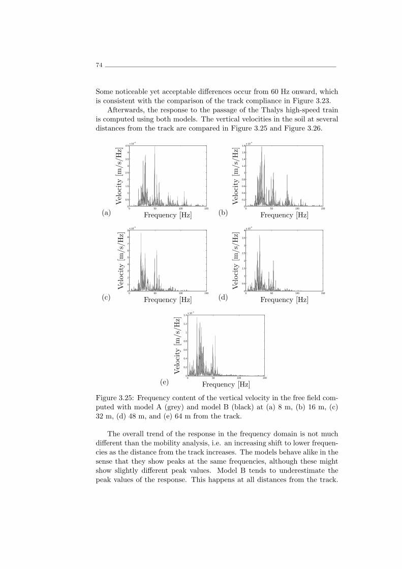
74
Some noticeable yet acceptable differences occur from 60 Hz onward, whichis consistent with the comparison of the track compliance in Figure 3.23.
Afterwards, the response to the passage of the Thalys high-speed trainis computed using both models. The vertical velocities in the soil at severaldistances from the track are compared in Figure 3.25 and Figure 3.26.
(a)0 50 100 150
0
0.5
1
1.5
2
2.5
3
3.5
4
4.5x 10
−4
Frequency [Hz]
Velocity
[m/s/Hz]
(b)0 50 100 150
0
0.2
0.4
0.6
0.8
1
1.2
1.4
1.6
1.8x 10
−4
Frequency [Hz]
Velocity
[m/s/Hz]
(c)0 50 100 150
0
1
2
3
4
5
6
7
8
9x 10
−5
Frequency [Hz]
Velocity
[m/s/H
z]
(d)0 50 100 150
0
0.5
1
1.5
2
2.5
3
3.5
4x 10
−5
Frequency [Hz]
Velocity
[m/s/H
z]
(e)0 50 100 150
0
0.2
0.4
0.6
0.8
1
1.2
1.4x 10
−5
Frequency [Hz]
Velocity
[m/s/H
z]
Figure 3.25: Frequency content of the vertical velocity in the free field com-puted with model A (grey) and model B (black) at (a) 8 m, (b) 16 m, (c)32 m, (d) 48 m, and (e) 64 m from the track.
The overall trend of the response in the frequency domain is not muchdifferent than the mobility analysis, i.e. an increasing shift to lower frequen-cies as the distance from the track increases. The models behave alike in thesense that they show peaks at the same frequencies, although these mightshow slightly different peak values. Model B tends to underestimate thepeak values of the response. This happens at all distances from the track.

2.5D Models 75
(a)10
010
110
210
−8
10−7
10−6
10−5
10−4
Frequency [Hz]
Velocity
[m/s]
(b)10
010
110
210
−8
10−7
10−6
10−5
10−4
Frequency [Hz]
Velocity
[m/s]
(c)10
010
110
2
10−9
10−8
10−7
10−6
10−5
10−4
Frequency [Hz]
Velocity
[m/s]
(d)10
010
110
2
10−10
10−9
10−8
10−7
10−6
10−5
10−4
Frequency [Hz]
Velocity
[m/s]
(e)10
010
110
2
10−11
10−10
10−9
10−8
10−7
10−6
10−5
10−4
Frequency [Hz]
Velocity
[m/s]
Figure 3.26: One-third octave band RMS spectra of the vertical velocity inthe free field computed with model A (grey) and model B (black) at (a) 8m, (b) 16 m, (c) 32 m, (d) 48 m, and (e) 64 m from the track.
Besides these peaks, the computed response is very similar in both cases.The one-third octave band RMS spectra of the response shows a very goodagreement between both models at all distances (Figure 3.26).
Finally the time response at the receptance points and the RMS overa 4 s window is shown in Figure 3.27 and Figure 3.28 respectively. Thevelocities tend naturally to decrease with the distance to the track due togeometric and material damping. The response in Model B tends be lowerthan in model A which can be explained by the lower tractions at the soil-track interface.
The general trend is that both models behave similarly, especially at lowfrequencies where the soil dominates the response. Some small differences do

76
(a)8 10 12 14 16 18 20 22
−10
−8
−6
−4
−2
0
2
4
6
8x 10
−4
Time [s]
Velocity
[m/s]
(b)8 10 12 14 16 18 20 22
−2
−1
0
1
2
3
x 10−4
Time [s]
Velocity
[m/s]
(c)8 10 12 14 16 18 20 22
−1.5
−1
−0.5
0
0.5
1
1.5x 10
−4
Time [s]
Velocity
[m/s]
(d)8 10 12 14 16 18 20 22
−6
−4
−2
0
2
4
6x 10
−5
Time [s]
Velocity
[m/s]
(e)8 10 12 14 16 18 20 22
−3
−2
−1
0
1
2
3x 10
−5
Time [s]
Velocity
[m/s]
Figure 3.27: Time history of the vertical velocity in the free field computedwith model A (grey) and model B (black) at (a) 8 m, (b) 16 m, (c) 32 m,(d) 48 m, and (e) 64 m from the track.
occur due to the different soil-track interaction especially at high frequencies.Galvın et al. (2010) reached similar results, also comparing 2.5D modelsfeaturing stiff and flexible track-soil interface. The authors stated that themodels corresponded very well at low frequencies. At high frequencies thestudy presented higher differences between the models than those hereinfound. However, the comparison by Galvın et al. (2010) was done for a caseof a double tracked embankment where there is no load symmetry and thusthe influence of the track deformability is higher.

2.5D Models 77
(a)0 5 10 15 20 25 30
0
1
2
x 10−4
Time [s]
Velocity
[m/s]
(b)0 5 10 15 20 25 30
0
0.2
0.4
0.6
0.8
1
1.2
1.4x 10
−4
Time [s]
Velocity
[m/s]
(c)0 5 10 15 20 25 30
0
0.5
1
1.5
2
2.5
3
3.5
4
4.5
5x 10
−5
Time [s]
Velocity
[m/s]
(d)0 5 10 15 20 25 30
0
0.5
1
1.5
2
2.5x 10
−5
Time [s]
Velocity
[m/s]
(e)0 5 10 15 20 25 30
0
1
2
3
4
5
6
7
8
9x 10
−6
Time [s]
Velocity
[m/s]
Figure 3.28: Running RMS of the vertical velocity in the free field computedwith model A (grey) and model B (black) at (a) 8 m, (b) 16 m, (c) 32 m,(d) 48 m, and (e) 64 m from the track.
3.4.6 Partial remarks
The comparison between two 2.5D models was presented in this section. Theformulation common to both models was presented as well as the specificcharacteristics of each. The two models differ in the track’s kinematics.
The mathematical verification of the soil formulations was done bychanging the formulation of model B into a formulation similar of the one inmodel A. The values of the soil stiffness are numerically equal proving thecoherence of the formulations. The comparison between both track modelsdone through their dispersion curves showed that their behaviour at lowfrequencies is very similar and the kinematics of the model A are shown tobe a specific case of the more general model B. There is a very good cor-

78
respondence of the full models response at those low frequencies where theresponse is governed mainly by the soil. The receptance of the models athigher frequencies shows higher differences because it is influenced by thetrack-soil interface and by the resonance of the rails.
The differences at the track-soil interfaces result in different distributionof tractions along the interfaces. Model A has a stress distribution simi-lar to that of the stiff foundations which results in high tractions at theedges. Model B allows deformation of the track-soil interface and has lowertractions along all its length. These differences result in slightly differenttransfer functions between the track and the soil.
The track compliance is computed for both models using the rail recep-tance. The compliance differences are coherent with those found in the trackreceptance, with better correspondence at lower frequencies. The dynamicaxle loads due to the passage of a Thalys high-speed train at 300 km/h werecomputed using the compliance of models A and B and show very goodcorrespondence. The response in the free field due to the dynamic loadsalthough not exactly the same is very consistent, both in the frequency andtime domain. RMS values revealed very good agreement of the results.
The different track formulations are shown to have influence in the resultsobtained by the models, although these are not major differences. Model Ais much less computationally expensive due to the reduced number of degreesof freedom. Model B allows for a better insight into ballast behaviour andtrack-soil interactions. For the determination of the rail response and freefield vibration, both models compute similar results.
Throughout the analyses herein presented a better insight into thesemodels and the dynamics of the track-soil system were obtained. These 2.5Dmodels are used in the following to study the accuracy of 3D FE models.

Comparison between 3D FE and 2.5D models 79
3.5 Comparison between 3D FE and 2.5D models
3.5.1 Introduction
In the scope of the final objective of incorporating non-linear subgrade andballast modelling in the rail track response simulations, it is necessary tofurther validate the FE models. In section 3.3.1 the FE model was success-fully used to reproduce track response to the passage of a high speed train,however, experimental results are often scarce and a thorough explorationof the model’s accuracy using only experimental measurements is limited.Because of this, the 3D FE and the 2.5D FE models explored in the previoussection are herein compared. The 2.5D model A that has been thoroughlydeveloped and validated at K.U. Leuven allows to perform a more thoroughexamination of the FE model’s numerical accuracy. With that purpose, thevarious components of the soil-track system are initially analysed separatelywhich allows to better understand the similarities and the differences thatthe full models exhibit when predicting railway track response. Finally thetrack response to a moving load is simulated in both cases and compared.
3.5.2 Computation of Green’s functions
Axisymmetric FE Green’s functions
In a first instance, the computation of the FE 3D Green’s functions is donein the frequency domain, allowing a direct comparison with the frequencydomain Green’s functions of the DSM. The soil is modelled as a semi-infinitehomogeneous layered half space whose dynamic properties are representedin Table 3.3. The solicitation is a vertical load on the soil surface andthe response is observed at several distances from the load, also at the soilsurface. Due to the homogeneity of the soil, the response to the verticalload is axisymmetric with respect to the vertical axis that includes the loadpoint.
The Green’s functions computed with the DSM are obtained using theelastodynamics toolbox EDT (Schevenels et al., 2008). This toolbox hasbeen extensively used by the authors in didactic and research environmentsto compute the elastodynamics response of infinite or semi-infinite media.
Table 3.3: Soil profile adopted for the simulation of the half-space
Layer d Cs Cp ρ ξs ξp[m] [m/s] [m/s] [kg/m3]
1 3 150 300 2000 0.03 0.032 ∞ 280 560 2000 0.03 0.03
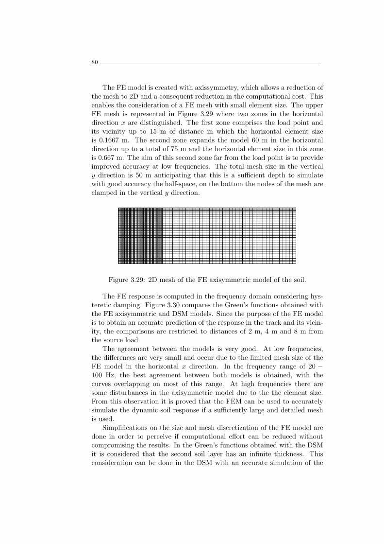
80
The FE model is created with axissymmetry, which allows a reduction ofthe mesh to 2D and a consequent reduction in the computational cost. Thisenables the consideration of a FE mesh with small element size. The upperFE mesh is represented in Figure 3.29 where two zones in the horizontaldirection x are distinguished. The first zone comprises the load point andits vicinity up to 15 m of distance in which the horizontal element sizeis 0.1667 m. The second zone expands the model 60 m in the horizontaldirection up to a total of 75 m and the horizontal element size in this zoneis 0.667 m. The aim of this second zone far from the load point is to provideimproved accuracy at low frequencies. The total mesh size in the verticaly direction is 50 m anticipating that this is a sufficient depth to simulatewith good accuracy the half-space, on the bottom the nodes of the mesh areclamped in the vertical y direction.
Figure 3.29: 2D mesh of the FE axisymmetric model of the soil.
The FE response is computed in the frequency domain considering hys-teretic damping. Figure 3.30 compares the Green’s functions obtained withthe FE axisymmetric and DSM models. Since the purpose of the FE modelis to obtain an accurate prediction of the response in the track and its vicin-ity, the comparisons are restricted to distances of 2 m, 4 m and 8 m fromthe source load.
The agreement between the models is very good. At low frequencies,the differences are very small and occur due to the limited mesh size of theFE model in the horizontal x direction. In the frequency range of 20 −100 Hz, the best agreement between both models is obtained, with thecurves overlapping on most of this range. At high frequencies there aresome disturbances in the axisymmetric model due to the the element size.From this observation it is proved that the FEM can be used to accuratelysimulate the dynamic soil response if a sufficiently large and detailed meshis used.
Simplifications on the size and mesh discretization of the FE model aredone in order to perceive if computational effort can be reduced withoutcompromising the results. In the Green’s functions obtained with the DSMit is considered that the second soil layer has an infinite thickness. Thisconsideration can be done in the DSM with an accurate simulation of the

Comparison between 3D FE and 2.5D models 81
(a)0 50 100 150
0.5
1
1.5
2x 10
−9
Frequency [Hz]
Receptance
[m/N]
(b)0 50 100 150
1
2
3
4
5
6
7
8
9
10
11x 10
−10
Frequency [Hz]
Receptance
[m/N]
(c)0 50 100 150
0
1
2
3
4
5
6
7x 10
−10
Frequency [Hz]
Receptance
[m/N]
Figure 3.30: Comparison of the Green’s functions computed in FE (grey)and DSM (black) at the soil surface a) 2 m, b) 4 m and c) 8 m from thesource load.
soil stiffness and of the propagation of waves into infinity. In the FE modelsthat is not possible and a lower limit is considered at 50 m of depth. Fromthe soil response it is concluded that the consideration of 50 m of soil depthin the FE model ensures a good simulation of the soil response at the surface.
To study the influence of the depth of the FE mesh in the surface re-sponse, the Green’s functions of the aforementioned mesh are compared withthose obtained with a similar mesh where the full depth is reduced to 10m and another mesh where the total depth is reduced to 5 m. Figure 4.57compares the response of FE axisymmetric models representing the samesoil profile, with the same element size but different mesh depth.
The reduction from 50 m to 10 m of depth results in some differences inthe computed Green’s functions, especially at low frequencies at which thewavelength is larger. These, however, are small differences and generallythe model is still accurately representative of the soil behaviour. The reduc-tion to 5 m has a more profound impact in the results, again with specialdifferences at low frequencies.
A study is also done to perceive the influence of the mesh length in thehorizontal x direction. The mesh of the axisymmetric model with 10 m ofdepth has a zone of 15 m of length and beyond that a second zone of 60 m.This second (outer) zone is reduced to 30 m and 20 m, while the zone inthe vicinity of the load point is kept unchanged. The Green’s functions are

82
(a)0 50 100 150
0
0.5
1
1.5
2
2.5x 10
−9
Frequency [Hz]
Receptance
[m/N]
(b)0 50 100 150
0
0.5
1
1.5
2
2.5
3
3.5
4
4.5x 10
−10
Frequency [Hz]
Receptance
[m/N
]
Figure 3.31: Comparison of the Green’s functions computed with FE modelswith 50 m (black), 10 m (grey) and 5 m(doted) of depth at a) 2 m and b)16 m from the source.
then computed. The results are compared in Figure 3.32.When the total length of the mesh is reduced to 45 m, some notice-
able changes occur in the model response at low frequencies. Even though,considering the fact that the number of elements was greatly reduced, thecorrespondence between the model with 45 m and the model with 75 m isappreciable. The model with a total length of 35 m presents less agreementwith the previous models. It should be noticed that despite the differencesthat occur at low frequencies, the response of the various models at highfrequencies is almost the same. Thus it can be concluded that an ”outerzone” with larger element size in the horizontal direction can improve themodel response at low frequencies, and has very limited influence in themesh response at high frequencies.

Comparison between 3D FE and 2.5D models 83
(a)0 50 100 150
0.4
0.6
0.8
1
1.2
1.4
1.6
1.8
2
2.2x 10
−9
Frequency [Hz]
Receptance
[m/N]
(b)0 50 100 150
0
0.5
1
1.5
2
2.5
3
3.5
4
4.5x 10
−10
Frequency [Hz]
Receptance
[m/N
]
Figure 3.32: Comparison of the Green’s functions computed with FE modelswith 75 m (black), 45 m (grey) and 35 m(doted) of total length at a) 2 mand b) 16 m from the source.
3D FE and 2.5D DSM Green’s functions
For the computation of the Green’s functions in FEM 3D, the FE mesh ismodelled with 3D volumetric elements in order to simulate part of the soil.A soil profile is considered with dynamic properties represented in table 3.4.
Table 3.4: Soil profile for the computation of Green’s functions in the soil.
Layer d Cs Cp ρ ξs ξp[m] [m/s] [m/s] [kg/m3]
1 10 259.4 1852.4 2000 0.03 0.03Bedrock ∞ - - - - -

84
FE mesh
The FE mesh is created to simulate the case study and includes the 10m depth of soil (Figure 3.33). The nodes at the bottom are clamped inthe vertical y direction to take into account the presence of the bedrockand bounding elements without spring stiffness are included in the limitsof the mesh to absorb outgoing body waves. At the upper 5 m of soil, thevertical element edge size is 0.5 m and at the lower 5 m of soil the verticalelement size is 1 m. Two zones are considered in the horizontal direction ofthe model, in a similar way as in the axisymmetric models. The first zoneincludes the load point and its vicinity in a total area of 20 m × 20 m, inwhich the edge length of each element is 0.44 m. The second mesh zonesurrounds the first zone and is much less refined. The main objective ofthis second zone is to put the mesh boundaries far from the point load, andprovide good simulation of the response at low frequencies. The dimensionsof the full mesh are 60 m × 60 m × 10 m. The 10 m depth of the model isjustified by the previous parametric study that showed this depth is enoughto ensure numerical accuracy.
Figure 3.33: 3D mesh of the FE model of the soil
Damping
The different formulation of time domain and frequency domain calcula-tions implies that inconsistent material damping formulations must be used.Usually, frequency domain models consider hysteretic damping which is fre-quency independent and regarded as more appropriate for soil modelling.Time dependent calculations generally rely on Rayleigh damping formula-tion which is frequency dependent.
In particular, the direct stiffness formulation admits the adoption ofindependent dilatational damping ξp and shear damping ξs through the def-inition of complex Lame coefficients:

Comparison between 3D FE and 2.5D models 85
(λ∗ + 2µ∗) = (λ+ 2µ)(1 + 2iξp) (3.83)
µ∗ = µ(1 + 2iξs) (3.84)
In the direct stiffness computation of the Green’s functions, the dilata-tional damping ξp = 0.03 and shear damping ξs = 0.03 are defined.
In the FEM, Rayleigh damping is considered according to:
C = αM+ βK (3.85)
where C represents the damping matrix M the mass matrix and K thestiffness matrix. The parameters α and β are the damping coefficients.This defines a frequency-dependent damping ratio ξi:
ξi =1
2(α
ωi+ βωi) (3.86)
where ωi is the angular velocity ωi = 2πfi. In the FE model, the Rayleighdamping coefficients α = 3.406 and β = 6.45× 10⁻⁵ are computed in a leastsquares fitting of equation (3.86) with the hysteretic damping ξ = 0.03 inthe frequency range of 20 Hz to 200 Hz. Figure 3.34 compares the dampingof the FE and Direct Stiffness models.
0 50 100 150 200 250 3000
0.01
0.02
0.03
0.04
0.05
0.06
0.07
0.08
0.09
0.1
Dam
ping,ξ
Frequency [Hz]
Figure 3.34: Damping of soil in the FE (dashed) and Direct Stiffness (full)models.
Due to the Rayleigh damping formulation, the FE model necessarily hasvery high damping at low frequencies. The damping of the FE model islower than the damping of the DSM at frequencies between 10 Hz and 138Hz, at other frequencies the damping is lower in the DSM model.

86
Dynamic load
Considering that the FE 3D soil response is computed in time domain, aprocedure is adopted to compute the transfer functions. The FE mesh issolicited by a point load at the soil surface whose time history and frequencycontent are known. The time history response of the FE 3D model is thentransformed into the frequency domain through a Fourier transform. Finally,the Green’s functions are computed at each frequency as the quotient of theresponse and the load.
A source load is defined with a predominant frequency content on arange of 20 Hz to 250 Hz. The load is a Ricker pulse with the following timehistory:
ty(t) =
[2
(π(t− ts)
TR
)2
− 1
]exp
[−(π(t− ts)
TR
)2]
(3.87)
where TR = 0.01 s is the characteristic period and ts =0.016 s is a timeshift. The time history and frequency content of the load are shown inFigure 3.35.
(a)0 0.005 0.01 0.015 0.02 0.025 0.03 0.035 0.04
−1
−0.5
0
0.5
Time [s]
Force
[N]
(b)0 50 100 150 200 250 300
0
0.5
1
1.5
2
2.5
3
3.5
4
4.5x 10
−3
Force
[N/H
z]
Frequency [Hz]
Figure 3.35: Load applied to the FE model: a) time history and b) frequencycontent.
Green’s functions comparison
Figure 3.36 compares the soil receptance of the FE and DSM models at 2m, 4 m and 8 m from the load point at the soil surface.
The response corresponds well at low frequencies but larger differencesare found with increasing frequency and distance to the source load. Theresponse at high frequencies degrades in the FE model because of the meshelement size.
The boundaries used were formulated to absorb incident dilatational andshear waves, however, they are ineffective in absorbing Rayleigh waves. Thisalso explains the reason why the FE model results agree less with the DSM

Comparison between 3D FE and 2.5D models 87
(a)50 100 150 200 250
0
0.5
1
1.5
2
2.5
3
3.5
4
4.5
x 10−10
Frequency [Hz]
Receptance
[m/N]
(b)50 100 150 200 250
0
0.5
1
1.5
2
2.5
x 10−10
Frequency [Hz]
Receptance
[m/N]
(c)50 100 150 200 250
0
0.2
0.4
0.6
0.8
1
1.2
1.4
1.6
1.8
x 10−10
Frequency [Hz]
Receptance
[m/N]
Figure 3.36: Soil receptance computed in FE (grey) and DSM (black) at thefree surface a) 2 m, b) 4 m and c) 8 m from the source load.
model at increasing horizontal distances from the source load. This is ashort come of the presented FE mesh that should be subject to subsequentstudy in order to be mitigated. Even so, since the simulation of the freefield response at large distances from the track is not the goal of this work,this short come is not considered problematic.
Figure 3.37 compares the soil receptance of the FE and DSM models at2m, 4m and 8m depth below the load point.
In general, better agreement is found in the response of both models inthe soil below the load point. The correspondence of the soil response at lowfrequencies is again good. There is a decrease in the correspondence of theresponses with increasing frequency which is also explained by the elementsize. The response at 4 m depth computed with both models has bettercorrespondence than the response at 2 m depth, which is surprising. At lowfrequencies the response is good at both depths but at higher frequenciesthe results at 4 m depth are very similar in both models, while at 2 mdepth the FE model tends to increasingly overestimate the response withincreasing frequency. At 8 m depth there is also a good agreement eventhough this node belongs to a zone where the FE mesh is less refined andhas a bigger element size, thus making the response reliable at a narrowerfrequency range.
Figure 3.38 shows the accelerance of the FE and DSM models at 2 m, 4m and 8 m from the load point at the soil surface.

88
(a)50 100 150 200 250
0
1
2
3
4
5
6x 10
−10
Frequency [Hz]
Receptance
[m/N]
(b)50 100 150 200 250
0
0.5
1
1.5
2
2.5
x 10−10
Frequency [Hz]
Receptance
[m/N]
(c)50 100 150 200 250
0
0.1
0.2
0.3
0.4
0.5
0.6
0.7
0.8
0.9
1x 10
−10
Frequency [Hz]
Receptance
[m/N]
Figure 3.37: Soil receptance computed in FE (grey) and DSM (black) underthe load at a) 2 m, b) 4 m and c) 8 m depth.
(a)50 100 150 200 250
0
0.2
0.4
0.6
0.8
1
1.2x 10
−3
Frequency [Hz]
Acceleran
ce[m
/Ns2]
(b)50 100 150 200 250
0
1
2
3
4
5
6
7
8x 10
−4
Frequency [Hz]
Acceleran
ce[m
/Ns2]
(c)50 100 150 200 250
0
0.5
1
1.5
2
2.5
3
3.5x 10
−4
Frequency [Hz]
Acceleran
ce[m
/Ns2]
Figure 3.38: Soil accelerance computed in FE (grey) and DSM (black) atthe free surface a) 2 m, b) 4 m and c) 8 m from the source load.
In general, the accelerance in the soil surface has correspondence at low

Comparison between 3D FE and 2.5D models 89
frequencies, although it is at high frequencies that higher accelerances arefound. At 2m from the source load the computed accelerance in the modelsagrees very well up to a frequency of 100 Hz. The accelerance computedwith both models agrees well at 4 m from the source load throughout mostof the frequency range, although at low frequencies the FE model tends toconsiderably overestimate the soil accelerance. At 8 m from the source loadthe correspondence is poorer demonstrating again that the FE mesh is lessaccurate to simulate the propagation of waves to regions far from the sourceload. Figure 3.39 shows the soil accelerance of the FE and Direct Stiffnessmodels under the load.
(a)50 100 150 200 250
0
1
2
3
4
5
6
7
8x 10
−4
Frequency [Hz]
Acceleran
ce[m
/Ns2]
(b)50 100 150 200 250
0
0.2
0.4
0.6
0.8
1
1.2x 10
−4
Frequency [Hz]
Acceleran
ce[m
/Ns2]
(c)50 100 150 200 250
0
0.5
1
1.5
2
2.5
3
3.5
4x 10
−5
Frequency [Hz]
Acceleran
ce[m
/Ns2]
Figure 3.39: Soil accelerance computed in FE (grey) and DSM (black) inthe soil at a) 2m, b) 4m and c) 8m depth.
Again, the point at 4 m depth shows the better correspondence of thethree points showing good correspondence up to 110 Hz. At 2 m the cor-respondence is only good up to 75 Hz, at higher frequencies the FE modeltends to overestimate the soil response. At 8 m of depth the correspondencebetween the accelerance computed with both models is only good at lowfrequencies.
3.5.3 Track-soil transfer functions
The 3D FE model
In this sub-section a railway track is presented and modelled using 2.5Dand 3D FE. The transfer functions between the track and the soil are com-

90
puted and compared between both models. The 3D FE model allows thedefinitions of a more accurate reproduction of the track geometry becausethe consideration of invariable geometry in the longitudinal direction is nolonger necessary consequently the discrete rail connection to the sleepersis considered. Equally, the sleepers are modelled in a discrete way insteadof having their mass and stiffness smeared along the longitudinal directionof the track. The final aim of these models is to give better insight intothe track response due to the passage of a high speed train. With a moredetailed definition of the track geometry, the stress distribution along theballast can be determined more accurately.
These are inevitably more elaborate models and computationally de-manding, easily ascending to hundreds of thousands degrees of freedom.Because of this, much care must be taken into the mesh refinement so thatno more computational effort is taken than the necessary.
The track is modelled to accurately simulate the geometry of ballastedrailway tracks. The rail is modelled as a Mindlin-Reissner beam of 3 nodesand is discretely supported by a two-node translation spring/dashpot ele-ment that connects it with the sleepers
The sleepers are modelled with volumetric elements and embedded inthe ballast. The ballast is modelled with volumetric elements, in transversalsections where no sleeper is present, the ballast top is at the same level asthe top of the sleeper (crib), at transversal sections where a sleeper existsthe top of the ballast layer is limited by the sleeper (Figure 3.40).
Figure 3.40: Ballast Mesh in the 3D FE model.
Track properties
The track properties are the same of section 3.4.4

Comparison between 3D FE and 2.5D models 91
The ballast Young’s modulus of the 3D FE model is the same as inthe 2.5D model. The sleeper has the dimensions lsl × bsl × hsl = 2.5m ×0.235m×0.205m and a Young’s modulus Esl = 30 ×109N/m2. The rail padstiffness krp of the 3D FE model is calibrated with the 2.5D model using asoptimization factor the rail receptance of the track clamped at it’s bottom:at 1 Hz the 2.5D FE model with a rail pad stiffness of krp = 153.4×10⁶N/mhas a rail receptance of 2.362 × 10⁹m/N; the rail pad stiffness in the 3D FEmodel is calibrated for a value of 137×106N/m at which the rail receptanceis 2.34 × 10⁹m/N.
Transfer functions between the track and the soil
The performance of the full 3D FE model and 2.5D model A, incorporatingtrack and soil is evaluated. The soil profile is the same used in the computa-tion of the 3D FE and Direct Stiffness computation of the Green’s Functions(section 3.5.2). The 3D FE mesh incorporates the same soil mesh used forthe computation of the Green’s functions. To compute the transfer func-tions in the 3D FE model, the previous methodology is used, with a Rickerpulse with the characteristic period TR = 0.01 s and time shift ts =0.016s. Figure 3.41 compares the rail receptance computed in 3D FE and 2.5Dmodels.
50 100 150 200 2500
1
2
3
4
5
x 10−9
Frequency [Hz]
Receptance
[m/N
]
Figure 3.41: Rail receptance computed in 3D FE (grey) and 2.5D model(black).
The rail receptance shows good agreement, especially at low frequencies.The rail node of the 3D FE model where the results are computed is directlysupported by a rail pad and thus all the transfer of stress from the rail atan effective zone of 0.6 m is transmitted to the sleeper and ballast throughthis node. The 3D FE model has lower receptance throughout almost allthe considered frequency range. Again, the agreement between both modelsdeteriorates with increasing frequency. The 3D FE receptance at 200 Hz is
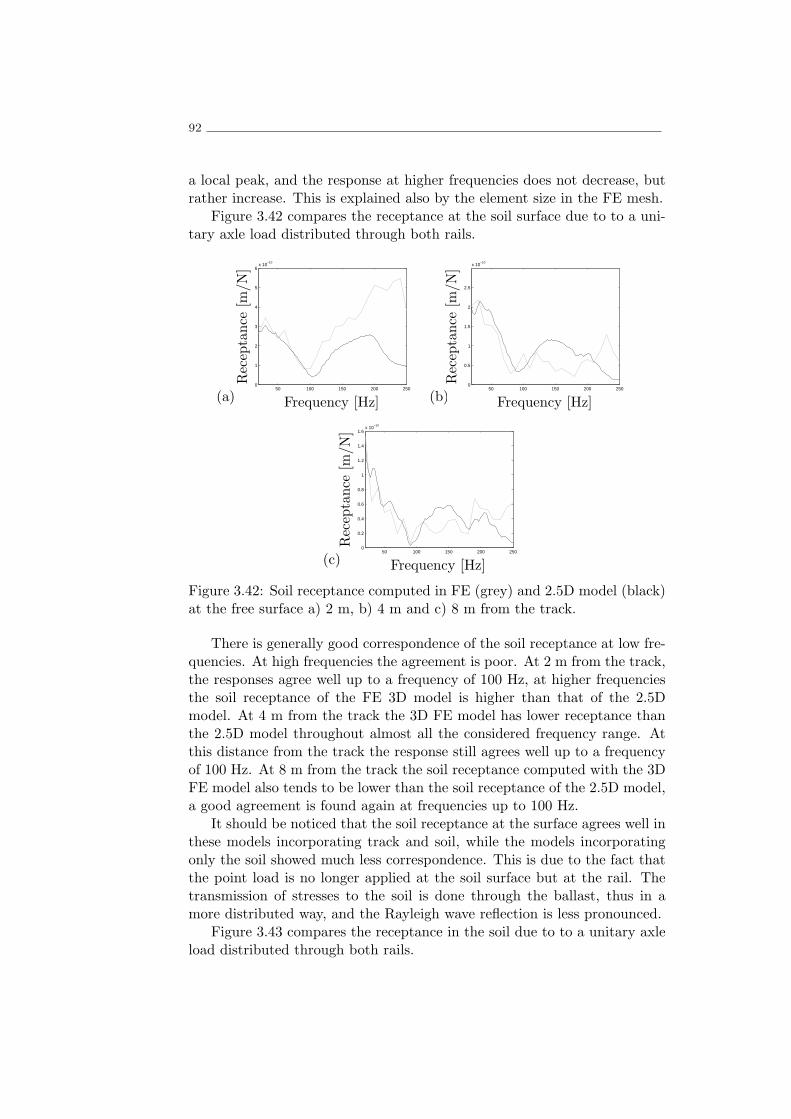
92
a local peak, and the response at higher frequencies does not decrease, butrather increase. This is explained also by the element size in the FE mesh.
Figure 3.42 compares the receptance at the soil surface due to to a uni-tary axle load distributed through both rails.
(a)50 100 150 200 250
0
1
2
3
4
5
6x 10
−10
Frequency [Hz]
Receptance
[m/N]
(b)50 100 150 200 250
0
0.5
1
1.5
2
2.5
x 10−10
Frequency [Hz]
Receptance
[m/N]
(c)50 100 150 200 250
0
0.2
0.4
0.6
0.8
1
1.2
1.4
1.6x 10
−10
Frequency [Hz]
Receptance
[m/N
]
Figure 3.42: Soil receptance computed in FE (grey) and 2.5D model (black)at the free surface a) 2 m, b) 4 m and c) 8 m from the track.
There is generally good correspondence of the soil receptance at low fre-quencies. At high frequencies the agreement is poor. At 2 m from the track,the responses agree well up to a frequency of 100 Hz, at higher frequenciesthe soil receptance of the FE 3D model is higher than that of the 2.5Dmodel. At 4 m from the track the 3D FE model has lower receptance thanthe 2.5D model throughout almost all the considered frequency range. Atthis distance from the track the response still agrees well up to a frequencyof 100 Hz. At 8 m from the track the soil receptance computed with the 3DFE model also tends to be lower than the soil receptance of the 2.5D model,a good agreement is found again at frequencies up to 100 Hz.
It should be noticed that the soil receptance at the surface agrees well inthese models incorporating track and soil, while the models incorporatingonly the soil showed much less correspondence. This is due to the fact thatthe point load is no longer applied at the soil surface but at the rail. Thetransmission of stresses to the soil is done through the ballast, thus in amore distributed way, and the Rayleigh wave reflection is less pronounced.
Figure 3.43 compares the receptance in the soil due to to a unitary axleload distributed through both rails.

Comparison between 3D FE and 2.5D models 93
(a)50 100 150 200 250
0
1
2
3
4
5
6x 10
−10
Frequency [Hz]
Receptance
[m/N]
(b)50 100 150 200 250
0
0.5
1
1.5
2
2.5
3
3.5x 10
−10
Frequency [Hz]
Receptance
[m/N]
(c)50 100 150 200 250
0
0.1
0.2
0.3
0.4
0.5
0.6
0.7
0.8
0.9
1x 10
−10
Frequency [Hz]
Receptance
[m/N]
Figure 3.43: Soil receptance computed in 3D FE (grey) and 2.5D model(black) in the soil at a) 2 m, b) 4 m and c) 8 m depth below the track.
The soil receptances at 2 m depth computed with both formulationsdo not agree well. Throughout almost all the considered frequency rangethe 3D FE model computes a soil receptance that is lower than the soilreceptance computed with the 2.5D model. At 4 m depth the 3D FE modelalso computes lower receptance than the 2.5D model although there is abetter correspondence than the correspondence at 2 m depth. At 8 m depththere is a good correspondence up to a frequency of 150 Hz, although at lowfrequencies there is also the tendency of the 3D FE model to compute lowerreceptance than the 2.5D model.
Figure 3.44 compares the accelerance at the soil surface due to to aunitary axle load distributed through both rails.
The soil accelerance generally agrees well up to 100 Hz. It is shown verywell by these comparisons that the 3D FE model loses accuracy at higherfrequencies. At 2 m from the track the accelerance agrees well up to 100Hz. At higher frequencies the 2.5D model presents a peak response at 200Hz, which also occurs in the track response. The 3D FE model, however,presents very large accelerance. At 4 m from the track the accelerance of the3D FE model at low frequencies is higher than the receptance of the 2.5Dmodel. From 40 Hz to 110 Hz the accelerance of both models correspondvery well, and at higher frequencies the correspondence is very poor. At 8m from the track there is also a high accelerance at low frequencies in the3D FE model that is followed by good agreement up to 90 Hz. Figure 3.45

94
(a)50 100 150 200 250
0
0.2
0.4
0.6
0.8
1
1.2
1.4x 10
−3
Frequency [Hz]
Accelerance
[m/Ns2]
(b)50 100 150 200 250
0
1
2
x 10−4
Frequency [Hz]
Accelerance
[m/Ns2]
(c)50 100 150 200 250
0
0.2
0.4
0.6
0.8
1
1.2x 10
−4
Frequency [Hz]
Accelerance
[m/Ns2]
Figure 3.44: Soil accelerance computed in 3D FE (grey) and 2.5D model(black) at the free surface a) 2 m, b) 4 m and c) 8 m from the source load.
compares the accelerance in the soil due to to a unitary axle load distributedthrough both rails.
The soil accelerance at 2 m depth in the 3D FE model is highly underes-timated in all the frequency range. At 4 m depth the soil accelerance agreeswell at frequencies up to 90 Hz, with the exception of the lower frequenciesat which there is again a tendency of the 3D FE model to overestimate theaccelerance. At 8 m depth there is also an overestimation of the accelerancecomputed with the 3D FE mode, which is followed by good correspondenceup to 90 Hz.
3.5.4 Response to a moving axle load
The response is obtained using the unitary axle load moving at 300 km/h,distributed through both rails. The response of the 3D FE model is ob-tained in time domain with the Newmark scheme while the response of the2.5D model is obtained in the frequency domain and transformed into thetime domain through an inverse Fourier transform. The methodology forthe simulation of the moving load in the 3D FE model is presented in sub-section 3.3.7 and the methodology for the simulation of the moving load inthe 2.5D model can be consulted in Lombaert et al. (2006). The correspon-dence is very good, which is coherent with the good correspondence of therail receptance. The time history of the rail vertical displacement (Figure

Comparison between 3D FE and 2.5D models 95
(a)50 100 150 200 250
0
1
2
x 10−4
Frequency [Hz]
Accelerance
[m/Ns2]
(b)50 100 150 200 250
0
1
2
x 10−4
Frequency [Hz]
Accelerance
[m/Ns2]
(c)50 100 150 200 250
0
0.2
0.4
0.6
0.8
1
1.2x 10
−4
Frequency [Hz]
Accelerance
[m/Ns2]
Figure 3.45: Soil accelerance computed in FE (grey) and 2.5D model (black)in the soil at a) 2 m, b) 4 m and c) 8 m depth below the track.
3.46) has almost the same time duration and the same peak value which,taking into account the different considerations of both models, is appre-ciable. This also proves that the simulation method of the moving load inthe 3D FE model is appropriate, a remark that was already predictable bythe good correspondence obtained of the sleeper response with experimen-tal measurements in section 3.3. The frequency content of the displacementalso corresponds very well at all the frequency range except at the very lowfrequencies.
(a)−0.1 0 0.1 0.2 0.3 0.4 0.5 0.6
−6
−5
−4
−3
−2
−1
0
1
2x 10
−4
Time [s]
Displacement[m
]
(b)0 50 100 150
0
0.2
0.4
0.6
0.8
1
1.2x 10
−5
Displacement[m
/Hz]
Frequency [Hz]
Figure 3.46: Rail displacement due to a moving axle load computed in 3DFE (grey) and 2.5D model (black).
The rail velocity (Figure 3.47) also corresponds very well in both models.The time history of the velocity is almost undistinguishable except for a peak

96
upwards value in the FE model. The frequency content of the velocity showsalso that the models correspond very well, although there seems to be a shiftof the response of approximately 5 Hz from the FE model to the BE model.
(a)0.05 0.1 0.15 0.2 0.25 0.3 0.35 0.4 0.45
−0.05
−0.04
−0.03
−0.02
−0.01
0
0.01
0.02
0.03
0.04
0.05
Time [s]
Velocity
[m/s]
(b)0 50 100 150
0
1
2
3
4
5
6
7
8x 10
−4
Velocity
[m/s.Hz]
Frequency [Hz]
Figure 3.47: Rail velocity due to a moving axle load computed in 3D FE(grey) and 2.5D model (black).
The acceleration of the rail (Figure 3.48) shows a similar trend to the onepresented by the velocity results. Some peak values do show in the FE modelthat are not present in the FE model. This occurs due to the previouslymentioned limited capability of the FE model to reproduce accurate resultsat high frequency levels. These high frequency differences are amplified withthe derivatives in order to time, and consequently the accelerations showmore discrepancies between both models than velocities. The frequencycontent of the accelerations in the rail prove this, as it is clear that the FEmodel starts to lose accuracy at increasing frequency range.
(a)0.05 0.1 0.15 0.2 0.25 0.3 0.35 0.4 0.45
−15
−10
−5
0
5
10
15
20
Time [s]
Acceleration[m
/s2]
(b)0 50 100 150
0
0.02
0.04
0.06
0.08
0.1
0.12
Acceleration[m
/s2.H
z]
Frequency [Hz]
Figure 3.48: Rail acceleration due to a moving axle load computed in 3DFE (grey) and 2.5D model (black).
Despite the differences found mainly at the acceleration of the rail, theresults correspond very well and allow to validate the FE model in the re-production of the rail response due to the passage of a high-speed train.The limitation of the FE model to reproduce with accuracy high frequencyresponse stems from the simplifications to the mesh related to the compu-tation capabilities of nowadays PCs and not from numerical inaccuracies ofthe FE formulation. As shown previously with the axisymmetrical model,

Conclusions 97
when a small enough element size is adopted, the FE models simulate soilresponse with great accuracy even at high frequencies. The evolution ofcomputational capabilities will most likely allow for 3D FE models withsmaller element size and higher accuracy.
3.5.5 Partial remarks
A validation of the 3D FE model using the previously validated 2.5 model isdone in this section. Initially the Green’s functions in FE are computed inthe frequency domain using an axisymmetric model. The computed Green’sfunctions correspond very well up to frequencies of approximately 120 Hz.The decrease of correspondence at higher frequencies occurs due to the ele-ment size in the FE mesh. It is proved that the FEM can compute accurateresults in the simulation of the soil dynamic response as long as the FE meshis carefully considered.
Subsequently, the Green’s functions are computed in a 3D FE mesh.Considering the utilization of the FEM is motivated by the possibility of theconsideration of non-linear material models, the time-domain computationsare essential, and thus the 3D Green’s functions in the soil are computed intime domain. The Green’s functions comparison reveals that the FE modelgenerally simulates with accuracy the soil response at low frequencies. Athigher frequencies the accuracy decreases due to the element size of the 3DFE mesh. At the soil surface the accuracy also decreases with increasingdistance to the source load due to the inefficiency of the quiet boundaries inabsorbing incoming Rayleigh waves. Generally the response computed withthe 3D FE and 2.5D models below the load agree very well. A comparison ofthe transfer functions obtained between the track and the soil using the 2.5Dmodel and the 3D FE model is also done. The rail receptance reveals goodcorrespondence between the 3D FE and 2.5D models up to frequencies of150 Hz. The response at the soil surface has generally very good agreementeven at 8 m from the track. Below the track there is also a good agreementbetween the transfer functions computed with the 3D FE and 2.5D models.
Finally the comparison of the moving load response shows that the 3DFE mesh allows to obtain a very accurate simulation of the track displace-ments, velocities and accelerations.
3.6 Conclusions
This chapter presents the application of two distinct numerical tools forsimulating high-speed track response to the passage of a high-speed train.The main goals include highlighting the dynamics of track-soil interactionand validating the 3D FE mesh computations.
A 3D FEM was initially employed to reproduce experimental measure-ments of a high-speed track. The results obtained are very promising because

98
the model was able to accurately predict the sleeper response. However, thesoil response was not accurately simulated due to the lack of the dynamicload component. Because the results obtained are reasonable but not con-clusive, it was decided to further validate the 3D FE models with a numericaltool whose accuracy was previously proven.
The 2.5D models were explored and two different track formulations wereused and compared. The purpose of this study is to gain better insight oftrack behaviour and the 2.5D models. The track formulations mainly differin two ways: one method considers undeformable sleepers and track-soilinterfaces, whereas the other method allows the interfaces to deform. It wasdemonstrated that the model that allows more deformability of the tracktends to induce less traction at the track-soil interface, whereas the finalpredictions of the free-field response are very similar in both formulations,especially at low frequencies.
Finally, the 3D FE mesh was validated using the 2.5D model. The FEmesh has the capability of simulating the dynamic soil response. Elementsize largely influences responses at high frequencies, whereas mesh size in-fluences responses at low frequencies. Despite these findings, it was possibleto obtain accurate track-soil transfer functions at low frequencies even witha 3D FE mesh. Although the models use different approaches to simulatethe longitudinal geometry of the track and soil damping, the rail responsedue to the passage of a single axle corresponded well.
The main conclusion of this chapter is that the 3D FE mesh is numeri-cally accurate in the simulation of track and soil responses to the passage ofmoving loads. This situation requires careful selection of the FE mesh, withregards to the length of the track stretch, the size of the FE soil simulation,and the absorbing boundaries.

Chapter 4
Application and development
of non-linear models
4.1 Introduction
This chapter presents the study of the non-linear behaviour of ballast andsubgrade using numerical models. From the study of the state of art inChapter 2 it was concluded that, although the railway track numerical sim-ulations have been subject to great development in the last few years, seldomhave these simulations been used to study non-linear behaviour of the trackcomponents. In Chapter 3 the 3D FE models have been studied and val-idated so that in this chapter they can be used to study non-linear trackresponse. The chapter includes studies of the non-linear ballast behaviourin section 4.2 and the non-linear behaviour of the soil is done in section 4.3.
Finally, in section 4.4the non-linear track and subgrade behaviour aresimultaneously accounted for in the simulation of a railway track where itwas demonstrated that the non-linear behaviour had a significant influencein the track serviceability.
4.2 Ballast stress analysis
4.2.1 Introduction
This sub-section presents the study of the non-linear ballast behaviour tothe passage of a high-speed train. This study intends to determine how theconsideration of non-linear ballast behaviour affects the track response inthe numerical method. The study is done through the modelling of a casefor which the 3D FE mesh is validated. The ballast stress-strain responseis obtained from the literature in a case where the large triaxial apparatuswas used. The experimental results are used to calibrate a modified Mohr-Coulomb model in which the hardening/softening is described as a multi-
99

100
linear curve specifying the variation of the friction angle φ. Due to thecomplexity of the model, the calibration procedure is done in three stages.Firstly, using a stochastic search for a broader search, secondly, using a morelocal search along with the Hessian method and thirdly using a parametricstudy to ensure that the objective function is minimized at the calibratedvalues for all parameters. The response to the passage of a train axle isanalysed and the differences between linear, equivalent linear, non-linear andequivalent non-linear analyses are discussed, mainly considering the stressand strain in the ballast layer and the vertical displacements and velocitiesin the rail and sleeper of the track. The importance of pressure-dependentYoung’s Modulus and the yield surfaces are also studied and discussed.
4.2.2 Constitutive model
The constitutive model used to simulate the non-linear ballast behaviour isa Modified Mohr Coulomb model. It has been developed at Delft Universityof Technology (Groen, 1995) and is available in Diana software (TNO, 2005).The model is mostly suitable to model frictional materials like concrete orsand but it has been enhanced so it is suitable for all kinds of soil materials.
The model features a default smooth Mohr-Coulomb shear yield surfacewith optional pressure shift for initial cohesion. An optional hardening-softening multi-linear curve may be specified for the friction angle φ. Themodel allows the definition of associated plasticity (ψ = φ) or the dilatancyangle may be explicitly defined or related to the friction angle via Rowe’sDilatancy rule. The elasticity may be directly defined or it can be relatedwith the effective pressure using either an Exponential Law or a Power Law.Besides the shear yield surface, the model includes a cap shaped compressionyield surface. Its initial position may be defined explicitly or can be derivedfrom the initial stresses. A compression cap hardening rule may also bedefined using either an Exponential Law or a Power Law. In the following,the model features that are used to simulate the ballast are more thoroughlydiscussed.
Shear Yield Surface
The shear yield surface follows the Mohr-Coulomb failure criteria. Thisstates that failure of the soil mass will occur if the following condition applies:
τ = ±(c′ + σ′ tanφ′) (4.1)
Failure does not depend solely on the value of the shear stress τ butinstead on its relation with the effective normal stress σ′. The componentc′ is often called cohesion and sets an initial shear resistance of the soil for0 effective normal stress. For sandy materials the cohesion is commonly

Ballast stress analysis 101
considered equal to 0. In the σ′ : τ stress plane, this failure criteria definesa pair of straight lines, if the Mohr’s circle touches these lines then failureoccurs.
This criteria states that the failure will be independent of the interme-diate principal effective stress σ2. The relation between the major principalstress σ1 and the minor principal stress σ3 is given by:
σ1 + c′ cotφ′
σ3 + c′ cotφ′=
1 + sinφ′
1− sinφ′(4.2)
this can be also stated in terms of stress variables p′ : q. Accounting forthe fact that all considerations of the ballast material are done in drainedconditions, the tilde denoting effective stresses will not be used onwards forsimplification. The stress invariants p and q are given by:
p =σ1 + σ2 + σ3
3(4.3)
q =
√(σ1 − σ2)2 + (σ2 − σ3)2 + (σ3 − σ1)2
2(4.4)
in the case of triaxial compression σ2 = σ3:
p =σ1 + 2× σ3
3(4.5)
q = σ1 − σ3 (4.6)
and σ1 and σ3 correspond to the axial stress and confining pressure,respectively. The critical state of equation (4.1) can then be written interms of p and q:
Mφ =q
p=
6 sinφ
3− sinφ(4.7)
where Mφ is the slope of the line representing the yield condition in thep : q space. Conversely, by knowing the value of Mφ at a particular criticalstate, the value of the friction angle φ can also be obtained:
sinφ =3Mφ
6 +Mφ(4.8)

102
The failure yield surface in the p : q space of the modified Mohr-Coulombmodel is given by:
q
R1(θ)− 6 sinφ
3− sinφ(p+∆p) = 0 (4.9)
where ∆p is the pressure shift for cohesion and R1(θ) is a parameter thatcontrols the shape of the yield surface, by standard it is set so that the yieldsurface corresponds to the Mohr-Coulomb criteria.
Compression cap
Yield may also be defined as a function of the mean stress p. This is definedby a yield surface that is cap shaped (Figure 4.1) and is given by the equation
(p+∆p)2 + α
(q
R2(θ)
)2
− p2c = 0 (4.10)
p
q
pc√α
−∆p pc −∆p
6 sinφ3−sinφ
Figure 4.1: Shear yield surface and compression cap of the modified Mohr-Coulomb model, represented in the p : q space.
pc is the pre-consolidation pressure and α and R2(θ) are cap shape fac-tors.
Flow rule
The direction of the inelastic strain rate is determined by two plastic poten-tial surfaces:
g(1) = q − 6 sinψ
3− sinψ(p+∆p) (4.11)

Ballast stress analysis 103
g(2) = (p+∆p)2 + αq2 − p2c (4.12)
This implies associative behaviour in p : q space and non-associated flow inthe deviatoric space. The dilatancy angle ψ may be related with the frictionangle φ through Rowe’s rule (Rowe, 1962):
sinψ =sinφ− sinφcv1− sinφ sinφcv
(4.13)
where φcv is the friction angle at constant volume.
Hardening behaviour
The modified Mohr-Coulomb model allows uncoupled hardening for bothyield surfaces. For the shear yield surface, hardening is defined as a multi-linear variation of the mobilized friction angle φ (Figure 4.2) with deviatoricplastic strain:
sinφ = sinφ(κ1) (4.14)
sinφ
κ1
(sinφ0, 0)
(sinφ1, κ11)
(sinφ2, κ12)
(sinφ3, κ13)
Figure 4.2: Definition of the shear yield surface hardening/softening througha φ : κ1 diagram.
where κ1 is the equivalent plastic shear strain, that is related to theplastic shear strain γp:
∆κ1 =
√2
3∆γpTRγp (4.15)
Hardening of the compressive cap is defined with a power law variationof the pre-consolidation stress:

104
pc = pref
((pc0pref
)m
− m
Γ∆εpv
) 1
m
(4.16)
m and Γ are parameters that shape the pre-consolidation variation withplastic volumetric strain εpv, pref is a reference pressure and pc0 is the pre-consolidation stress at the beginning of the step.
4.2.3 Optimization technique
Procedure overview
An optimization strategy consists in the definition of a procedure that at-tempts to find the values of x so that F (x) is minimized. Usually anyoptimization procedure requires the definition of a set of initial values forthe variables x0, which the user obtains from an initial analysis of the exper-imental values or from his experience with similar materials or problems. Itis important that x0 may be a set of variables that, in light of the constitu-tive model, defines a material with physical meaning, to which the numericalmethods are oblivious. This prevents the definition of a set of variables x
that may minimize F (x) numerically but whose values are not related tothe real physical properties of the material. To avoid the tendency to findspurious solutions it is also common to define a set of minimum m andmaximum n values for the material parameters.
Starting from the initial values x0 and obeying to the condition
mi ≤ xi ≤ ni, i = 1, 2, ..., n (4.17)
where n is the number of parameters subject to calibration, the opti-mization strategy defines how the search for x is conducted.
Considering that F (x) is twice continuously differentiable, the Gradientg(x) and Hessian H(x) may be defined as
g(x) =∂F (x)
∂x, H(x) =
∂2F (x)
∂x2(4.18)
Taking into account the possibility to compute g(x) and H(x) three gen-eral approaches may be used (Yang and Elgamal, 2003). Zero order strate-gies require only the evaluation of F (x). These strategies generally requirea large number of iterations to converge. First order strategies require theevaluation of F (x) and g(x), if g(x) is not explicitly available, it may ob-tained through finite differences or semi-analytical methods. Second orderstrategies require the evaluation of F (x), g(x) and H(x), these are moreelaborate strategies with better convergence than the previous. Among the

Ballast stress analysis 105
second order strategies the Newton method is usually the most efficient(Gill et al., 1981). The evaluation of g(x) and H(x) when not explicitlyavailable can be obtained through approximation algorithms, in this casethe designation of ”quasi-Newton” methods is common.
A major challenge in the optimization problems stems from the factthat often the optimization methods find local minimum for the objectivefunction F (x), while most often the objective is to find the global minimum.Given a function F (x) and a local minimum, there is no general way to deter-mine whether that corresponds to the global minimum (Yang and Elgamal,2003). To circumvent this, usually the optimization strategy is repeated sev-eral times using different values of x0, assuming that with increased numberfor attempts starting at different points of the domain the probability ofhaving determined the global minimum increases.
Other strategies consist in combining the utilization of global and localsearch algorithms. Cekerevac et al. (2006) developed the ParaID routinethat combines stochastic and quasi-Newton methods. A similar strategyis herein adopted to calibrate the material model with the experimentalresults of ballast material. The general idea behind the combination ofstochastic and quasi-Newton methods relies on the assumption that whilethe quasi-Newton method converges quickly to local minimum, it is usuallythe closest local minimum to the initial values of x and most often does notcorrespond to the global minimum; while the stochastic method, on the otherhand, allows a more general search throughout the domain, finding wherein the domain the objective function takes it’s lower values. Therefore, thestochastic method is used to search the domain for zones of lowest values,and the quasi-Newton is used for a more thorough search in the zone todetermine the local minimum that may correspond to the global minimum.
Objective function
The objective function is based on the function used by Cekerevac et al.(2006) to calibrate Hujeux constitutive model for a clay (Kaolin). A generalobjective function for optimization of triaxial results must incorporate theerror found in the numerical computation of stress, strain and pore pressurein comparison with experimental values. Considering that the experimentalresults are discrete, the objective function for one point can be proposed:
106
f(x)c =1
∑3k,l=1wkl
3∑
k=1
1
σ20(σek − σnk )wk1(σ
ek − σnk )
+3∑
k=1
1
ε20(εek − εnk)wk2(ε
ek − εnk)
+3∑
k=1
1
u20(uek − unk)wk3(u
ek − unk)
(4.19)
where σek, εek and uek are experimental values of stress, strain and pore
pressure, respectively; σ0, ε0 and u0 are the scaling factors of the variableswhich correspond to the maximum experimental values of stress, strain andpore pressure, respectively; and σnk , ε
nk and unk are numerical values of stress,
strain and pore pressure, respectively. The variables w correspond to weight-ing factors to account for the confidence in the various experimental resultsand also to account their correspondent importance in the calibration of themodel.
For the case of triaxial results, it is more convenient to express the ob-jective function in terms of deviatoric stress q, volumetric strain εv and porepressure u:
fk(x)c =1
∑3j,k=1wjk
3∑
j=1
1
q20(qej − qnj )wj1(q
ej − qnj )
+3∑
j=1
1
ε2v0(εevj − εnvj)wj2(ε
evj − εnvj)
+3∑
j=1
1
u20(uej − unj )wj3(u
ej − unj )
(4.20)
In this case the response is calibrated for drained triaxial tests and thusthe third term vanishes.
The calibration is done for various triaxial tests done with different con-fining pressures. Therefore, the final form of the objective function becomes:
F (x) =1∑n
s=1ws
n∑
s=1
wsf(x) (4.21)

Ballast stress analysis 107
where n is the number of experimental results to be calibrated and ws
is weighting factor to allow the inclusion of importance or confidence in thedifferent experimental results.
Stochastic method
The stochastic method conducts a random search following the general al-gorithm:
1. A new set of variables xk is randomly generated from a Gauss proba-bility distribution with mean xmin and standard deviation σ∗.
2. For the set of variables xk at iteration k the corresponding value ofthe objective function F (xk) is determined.
3. If F (xk) < F (xmin) then the best approximation parameters are up-dated: xmin = xk and F (xmin) = F (xk); otherwise no update is madeto F (xmin) and xmin.
4. If the maximum number of iterations has been reached then stop theprocess, otherwise return to the first step.
It is a simple process in which the centre of the search is the point xmin atwhich the minimum value of the objective function F (xmin) has been found.From this point, the direction and length of the new search is randomlygenerated. The advantage this has over first order and second order searchalgorithms is that even when falling on a local minimum, the process will notbe deterred to jump to other zones of the domain in search of other minimumpoints. The disadvantage is that since the process is oblivious to the gradientand Hessian of the objective function, at any point the process may be closeto the global minimum but not find it. The standard deviation should bechosen with criterion, if it is too large then the process may need an excessivenumber of iterations to find the global minimum, and if it is too small thelarge-scale advantage of this process may be lost. A procedure to scalethe variance was proposed by Beckey and Masri (1983) and Pronzato et al.(1984). This method divides the stochastic search procedure into two phases:a phase where the variance is selected and a phase in which the variance isexplored. A similar procedure is herein used to select the standard deviationof the stochastic optimization technique. Initially the standard deviation isselected:
σ∗0 =n−m
2(4.22)
starting at x0 and σ∗0, 100 iterations of the stochastic search are done.

108
The standard deviation selection phase repeats the previous randomsearches. However, in this phase the mean of the Gauss probability dis-tribution is constant and equal to the best approximation set of variablesxmin from the previous phase; the standard deviation, on the other hand, isvariable and consecutively corresponds to:
σ∗i =σ∗010i
; i = 0, 1, 2. (4.23)
after 300 iteration steps each standard deviation is used 100 times and anew exploitation phase begins using xmin and the standard deviation thatprovides the best approximation σ∗min. This alternation between exploita-tion and selection phases is repeated until the best standard deviation isσ0/100 for three consecutive times. After that the procedure moves to theHessian method for a more thorough search in the vicinity of xmin.
Hessian method
The Hessian method used is a subspace trust-region method based onan interior-reflective Newton method described by Coleman and Li (1994,1996). Trust region methods reduce the complexity of the large-scale op-timization problem by approximating the objective function with anotherfunction r which reasonably reflects the behaviour of F (x) in a neighbour-hood N around the current point x. This neighbourhood is the trust region.The function F (x) is approximated using the first two terms of the Taylorseries with an expansion point x = s. The trust region sub-problem is thenformulated:
min
1
2sTHs+ sTg, s ∈ N
(4.24)
where H is the Hessian matrix and g is the gradient of F at x. Solv-ing equation (4.24) allows to determine the trial step s. For many of theaccurate algorithms proposed (More and Sorensen, 1983), the solution ofequation (4.24) in a large-scale problem can be computationally expensive.A simplification is then applied by reducing the trust-region sub-problem toa two-dimensional subspace S, defined:
S =< s1, s2 > (4.25)
where s1 is in the direction of g and s2 is computed to define either theapproximate Newton direction
H.s2 = −g (4.26)

Ballast stress analysis 109
or the direction of negative curvature
s2T .H.s2 < 0 (4.27)
thus enforcing global convergence. Once the subspace S is determined,the solution to equation (4.24) becomes trivial and the trial step s is com-puted.
The iteration is then carried on by determining the value of F (x+ s), ifit is inferior to F (x) then x = x+ s, if not then the trust region is shrunk,either way the procedure is repeated until the convergence is achieved.
Parametric study
The final phase in the optimization procedure is the evaluation of the objec-tive function with the variation of each of the optimization variables. This isdone by selecting a reasonable range within which each variable is changedwhile all the other variables remain equal to the previously optimized valuesin the trust region method. This allows to evaluate the relative influenceof each variable around x and also to check the quality of the optimizationby verifying if the objective function reaches a lower value than F (x). Ifthis happens then x is updated and the whole procedure (starting at thestochastic method) is repeated.
4.2.4 Calibration of the model
The cyclic triaxial results are obtained from the literature. Suiker et al.(2005), Suiker and de Borst (2003) performed a series of static and cyclictriaxial tests on ballast and sub-ballast material. The tests were done atconstant confining pressures of 10.3 kPa, 41.3 kPa and 68.9 kPa, which theauthors considered to be relevant confining pressures for ballast in railwaytracks. The static triaxial tests were used to obtain information on theadmissible stress values to perform the cyclic tests. The ballast material is auniformly graded taprock with maximum particle size of 38mm. The triaxialapparatus had a diameter D = 254mm and height H = 645mm and thespecimen was compacted in eight layers. Further details on the experimentaltests can be obtained in the original publications (Suiker and de Borst, 2003,Suiker et al., 2005). The experimental results of the static triaxial tests onballast are represented in Figure 4.3.
Within the considered axial strains the maximum deviatoric stresses are62 kPa, 237 kPa and 352 kPa for the confining pressures of 10.3 kPa, 41.3 kPaand 68.9 kPa respectively. From the deviatoric stress results, an estimationis obtained on the Young’s modulus using the initial results:
E ≈ q
εa(4.28)

110
(a)0 0.01 0.02 0.03 0.04 0.05 0.06 0.07
0
0.5
1
1.5
2
2.5
3
3.5
4x 10
5
εa
q[Pa]
(b)0 0.01 0.02 0.03 0.04 0.05 0.06 0.07
−0.01
0
0.01
0.02
0.03
0.04
0.05
εa
ε v
Figure 4.3: Experimental results of ballast triaxial testing, a) deviatoric andb) volumetric response at confining pressure: 10.3 kPa (•), 41.3 kPa () and68.9 kPa () (adapted from Suiker et al. (2005)).
which determines an initial value of 230MPa. The volumetric resultsshow that the ballast presents an initial compaction followed by an inversionto dilatational behaviour. There is no clear trend to co-relate the volumetricextensions obtained in the three confining pressures because at the confiningpressure of 41.3 kPa the material presents more compaction than at 68.9 kPaor 10.3 kPa. One explanation for this relates to plastic deformations dueto the isotropic compression stress, with increasing confining pressure thematerial naturally shows higher compaction, however, this may reverse whenplastic strains are developed due to the isotropic compression stress. As suchat confining pressure of 68.9 kPa the plastic strains developed induced a moredilatational behaviour even though the material is more compacted than at41.3 kPa. Other explanation is that the volumetric strains are obtainedfrom the average radial strains measured at 1/3, 1/2 and 2/3 height of thespecimen. However, in some cases there were considerable differences inthe radial strains obtained for the same specimen at different heights whichthe authors explained as resulting from the presence of some friction at thespecimen top and bottom.
There is an increasing q/p ratio with increasing confining pressure forthe ballast material (Figure 4.4). From the q/p ratio an estimate of thefriction angle can be done through equation (4.7). The friction angle isestimated as varying from 37.5 to 48.6, which corresponds to a variationof sinφ between 0.58 and 0.75. These estimations provide initial values forthe calibration procedure.
The calibration is carried on using the procedures described in sub-section 4.2.3. Equal weighting factors are defined for the volumetric anddeviatoric behaviour as well as for all the confining pressures. The initialvalues for the Young’s modulus and the variation of sinφ are those pre-viously estimated from the experimental results. Figure 4.5 presents thecomparison of experimental and numeric results after the calibration of the
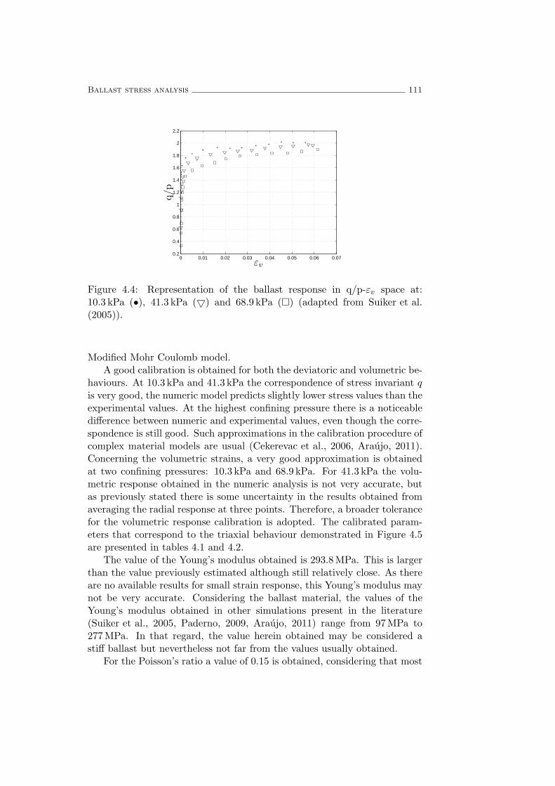
Ballast stress analysis 111
0 0.01 0.02 0.03 0.04 0.05 0.06 0.070.2
0.4
0.6
0.8
1
1.2
1.4
1.6
1.8
2
2.2
εv
q/p
Figure 4.4: Representation of the ballast response in q/p-εv space at:10.3 kPa (•), 41.3 kPa () and 68.9 kPa () (adapted from Suiker et al.(2005)).
Modified Mohr Coulomb model.A good calibration is obtained for both the deviatoric and volumetric be-
haviours. At 10.3 kPa and 41.3 kPa the correspondence of stress invariant qis very good, the numeric model predicts slightly lower stress values than theexperimental values. At the highest confining pressure there is a noticeabledifference between numeric and experimental values, even though the corre-spondence is still good. Such approximations in the calibration procedure ofcomplex material models are usual (Cekerevac et al., 2006, Araujo, 2011).Concerning the volumetric strains, a very good approximation is obtainedat two confining pressures: 10.3 kPa and 68.9 kPa. For 41.3 kPa the volu-metric response obtained in the numeric analysis is not very accurate, butas previously stated there is some uncertainty in the results obtained fromaveraging the radial response at three points. Therefore, a broader tolerancefor the volumetric response calibration is adopted. The calibrated param-eters that correspond to the triaxial behaviour demonstrated in Figure 4.5are presented in tables 4.1 and 4.2.
The value of the Young’s modulus obtained is 293.8MPa. This is largerthan the value previously estimated although still relatively close. As thereare no available results for small strain response, this Young’s modulus maynot be very accurate. Considering the ballast material, the values of theYoung’s modulus obtained in other simulations present in the literature(Suiker et al., 2005, Paderno, 2009, Araujo, 2011) range from 97MPa to277MPa. In that regard, the value herein obtained may be considered astiff ballast but nevertheless not far from the values usually obtained.
For the Poisson’s ratio a value of 0.15 is obtained, considering that most

112
(a)0 0.01 0.02 0.03 0.04 0.05 0.06
0
0.5
1
1.5
2
2.5
3
3.5
4
4.5x 10
5
εa
q[Pa]
(b)0 0.01 0.02 0.03 0.04 0.05 0.06 0.07
−0.01
0
0.01
0.02
0.03
0.04
0.05
εa
ε v
Figure 4.5: Experimental (dotted) and numerical (black) response of theballast after calibration: a) deviatoric response and b) volumetric responseat 10.3 kPa (•), 41.3 kPa () and 68.9 kPa () (adapted from Suiker et al.(2005)).
Table 4.1: Calibrated modified Mohr-Coulomb parameters.
Parameter value
E 293.8 MPa
ν 0.15
pc 87980 Pa
Γ 0.00851
pref 227658.6 Pa
sinφcv 0.520
sinφ0 0.613

Ballast stress analysis 113
Table 4.2: Calibrated values of the hardening curve of the yield surface.
κ sinφ
0.01 0.688
0.02 0.707
0.03 0.713
0.04 0.705
0.05 0.726
0.06 0.735
0.07 0.747
of the analysis consider the Poisson’s ratio ranging from 0.09 to 0.20 thevalue obtained is well within the acceptable range.
The pre-consolidation stress pc obtained corresponds to 87.98 kPa. Atthe consolidation stage none of the triaxial tests reaches this mean stress.It is possible, however, that during the triaxial compression the p : q statemay reach the compression cap. For the internal variables Γ and pref thevalues calibrated are 0.00851 and 227.7 kPa, respectively.
The sine of the friction angle obtained varies from the initial value of0.613 to 0.747 at an equivalent plastic shear strain of 0.07. This corre-sponds to a variation of the friction angle φ between 37.8 and 48.3 whichcorresponds to common values usually obtained for the friction angle of bal-last material. This also corresponds well with the initial estimative made ofa friction angle variation between 37.5 to 48.6.
In retrospect, the calibration procedure is successful in the sense that itallowed to adjust the proposed non-linear material model to the deviatoricand volumetric response of the ballast material and that the parametervalues obtained correspond to usual values for ballasted track, although theYoung’s modulus deviates slightly from the usual values. In the deviatoricstress a good correspondence is obtained for the three confining pressureswhile the volumetric response at 41.4 kPa is not very satisfactory, however,since there is some uncertainty related to the measurements, the obtainedresponse is accepted. It must be regarded that the utilization of a pressuredependent Young’s modulus could result in better correspondence betweennumeric and experimental values, however, the utilization of that behaviourpresents much instability with the non-linear calculation diverging multipletimes, and in that regard, even if the model allows that definition, it is notconsidered initially.
The parametric study in Figure 4.6 allows to better understand the in-fluence of some of calibrated variables in the calibration procedure. Theparametric studies are conducted with all variables constant and equal to

114
10−1
100
101
0.8
1
1.2
1.4
1.6
1.8
2
Normalized variable value
Norm
alizedF(x)
Figure 4.6: Normalized variation of the objective function with calibratedvariable values of Young’s modulus (+ grey), pc (+ black), Γ (. grey) andpref (. black).
the calibrated value, except the variable in study which varies from 0.1 to 10times its calibrated value. For each time the variable is changed the triaxialtest in Diana is simulated and the objective function is determined.
All studied variables exhibit distinct influence in the objective functionvalue. Expectedly, all variables converge for the minimum value of the ob-jective function obtained in the calibration process when they assume theirrespective calibrated value. It is also apparent that none of the variablesallows to obtain a normalized objective function value lower than 1. Thisis a necessary condition (although not sufficient) to assume that the globalminimum is obtained.
It can be observed that not all the variables exhibit a normalized valueof the objective function F (x) value in all the parametric domain. Themissing points correspond to numeric triaxial tests for which the iterativecomputation did not reach convergence.
The Young’s modulus has high influence in the objective function, thevalue of the objective function is 1.97 for Young’s modulus of 0.1 its cali-brated value. As the Young’s modulus approaches the calibrated value fromthe lower end, the objective function presents a monotonically decreasingvariation. When the Young’s modulus increases to values higher than thecalibrated value, the variation of the objective function is much less pro-nounced with the normalized objective function increasing to 1.02 for aYoung’s modulus 1.55 higher than the calibrated value. At higher valuesof the Young’s modulus the numeric triaxial simulations do not converge.
Ballast stress analysis 115
Since the step size of the triaxial simulation is already very small, the func-tion has passed its decreasing behaviour and the obtained value is alreadyon par with some of the highest values for the ballast Young’s modulus; itis reasonable to assume that there is no need to further explore the domain.
The pre-consolidation pressure pc has a very distinct influence in the nor-malized objective function. It is evident that for very low values it will notallow the models to converge. Such can be seen as there is no convergenceuntil the normalized pre-consolidation pressure reaches 0.631, which corre-sponds to 55.5 kPa. For this pre-consolidation value the third triaxial testalready reaches the compression cap with the application of the confiningpressure. When the pre-consolidation stress is higher than the calibratedvalue, the objective function starts to increase rapidly due to the decreaseof plastic strain in the models. For pc = 291 kPa the cap is positioned ata point that neither one of the triaxial specimens reach and thus there isno influence of the compression cap in the response. Consequently for anyhigher values of the pre-consolidation stress the objective function remainsconstant.
Interpretation of the pref and Γ influence in the objective function is notso straightforward. These are internal variables that shape the hardeningof the compression cap and their physical meaning is not easy to grasp.From equation (4.16) the pref is a reference pressure around which the pre-consolidation stress will change. This variation is scaled in function of theratio between the reference pressure and the initial pressure, to this value afraction is subtracted that depends on the variables m (0.5 by default), Γ,and the plastic volumetric strain εpv. It then becomes evident that the term−m
T ∆εpv scales the influence of the reference pre-consolidation stress sincewhen this term is 0, equation (4.16) becomes:
pc = prefpc0pref
⇔ pc = pc0 (4.29)
the implication being that the compression cap does not move at all. Asstated previously the variable m is stated by default in the software and isnot changed. Consequently the only variable that will influence the lengthof the step variation (represent by the second term) will be Γ.
Figure 4.6 confirms the high influence this variable has in the hardeningof the compression cap, which influences the objective function. For lowvalues of Γ a large variation of the position of the compression cap occurs.Consequently it re-positions at high compression values and its influenceis reduced. Consequently the initial variation of the objective function isminimal. For increasing values of Γ the compression cap moves less andthus the parameter will start to have increasing influence in the value ofthe objective function. Thus, when the value of Γ approaches the calibratedvalue the normalized objective function tends to 1 at an increasing ratio.

116
Furthermore, for higher values of Γ the objective function increases at aseemingly exponential rate due to the fact that the compression cap movesless and its influence in the material behaviour increases.
The influence of the reference pre-consolidation stress pref is less pro-nounced, nevertheless a 40% variation of the objective function is obtainedin the whole domain.
4.2.5 Case study
To study the non-linear response of the ballast material a study case isdefined for which a rail track on foundation soil is simulated using the FEMsoftware. Prior to the simulations in non-linear ballast behaviour, the FEMmesh is validated with a published case in which the track response wasmeasured.
Galvın and Domınguez (2009) presented the results obtained experimen-tally during certification testing of a new high-speed train line betweenCordoba and Malaga. These tests were done by the Spanish Railway Infras-tructure Administrator and consisted in recording vibration levels producedby passing trains, in the rails and sleepers, as well as at selected points onthe soil surface and in the steel structures supporting the contact line.
The Cordoba - Malaga HST track is a double track ballasted line withUIC 60 rails and mono-block concrete sleepers with length lsl = 2.60m,width bsl = 0.6m, height hsl = 0.265m (under the rail) and mass msl =300 kg. The sleeper spacing is dsl = 0.6m. The dynamic soil properties wereobtained from a SASW campaign and the inversion procedure correspondedwell with the results obtained previously from boring tests. The soil profilewas then estimated as containing an upper layer of silt and gravel with athickness of 1.2 m and a shear wave velocity Cs = 150m/s, followed by anintermediate layer of clay with sand-like qualities having a thickness of 2.5m and shear wave velocity Cs = 408.4m/s resting on a half-space with shearwave velocity Cs = 635.0m/s consisting of very dense sand and blue loam.The soil damping coefficient of 0.02 was estimated using a homogeneous soilequation (Barkan, 1962) and assuming a Poisson’s ratio of ν = 0.3.
The measurements used for the verification of the FE mesh were doneduring the passage of a Ave-Alstrom high-speed train at 298 km/h. Thefull train configuration was composed of 11 wagons of which 2 locomotiveswith total mass per axle of maxl = 17000 kg , 2 end wagons with massper axle of maxl = 14500 kg, 1 laboratory wagon with mass per axle ofmaxl = 10875 kg and 6 middle wagons with mass per axle ofmaxl = 17000 kg.The configuration of the Ave-Alstrom high-speed train is represented inFigure 4.7
The FE mesh used to simulate this study case is shown in Figure 4.8 Themodel has a total length of 50m and width of 60m (symmetry conditions),the soil is simulated to a depth of 10m. The rail is modelled with beam

Ballast stress analysis 117
Figure 4.7: Configuration of the Ave-Alstrom high-speed train: locomotives(wagons 1 and 11), laboratory wagon (2), end wagons (3 and 10) and middlewagons (4 to 9), (Galvın and Domınguez, 2009).
elements of three nodes, the interface is modelled with spring-dashpot ele-ments connecting the rail and the sleeper. The sleeper, ballast and soil aremodelled with solid prismatic elements. Considering that in non-linear anal-ysis elements with linear interpolation may present numeric shortcomingssuch as parasitic shear and volumetric locking (TNO, 2005), higher orderelements are used comprising 3 nodes per edge for a total of 20 nodes in eachprismatic element. Because of this, the total number of elements is kept toa minimum to reduce the elevated number of degrees of freedom. The fi-nal mesh is composed of 19108 elements of which 63 are beam elements, 21are spring-dashpot elements, 1202 are absorbing elements and 17822 brickelements. The total number of nodes is 80265.
(a) (b)
Figure 4.8: FE mesh for non-linear evaluation of ballast response: a) overallmodel and b) detail of ballast and sleepers.
Because the FE mesh in this case is modified to use second order ele-ments, which implies a reduction of the number of elements and changesin the element size, it is adequate to perform another verification of themodel. This comparison allows to validate the FE mesh, reinforcing thevalidation with experimental results in section 3.3 and the validation with

118
another numerical model in section 3.5. Even if the study case to be used fornon-linear ballast behaviour does not entirely correspond to the case hereinsimulated, the comparison made with experimental results allows to proceedto non-linear analysis with the confidence that the FE mesh is adequate tosimulate the phenomena at hand and that reliable results are obtained.
Since the track uses the same UIC 60 rail of the previously simu-lated cases, the properties used in the FE simulation are assumed to bethe same: bending stiffness ErIr = 6.45 × 10⁶Nm2, mass per unit lengthρrAr = 60.3 kg/m for each rail. For the ballast there are no indications ofmechanical properties, consequently the properties obtained from the cali-bration of the modified Mohr-Coulomb model are admitted, with linear be-haviour: ballast Young’s modulus Eb = 293.8MPa, Poisson’s ratio ν = 0.3.
Galvın and Domınguez (2007) conducted numerical studies for a pointload moving on the surface of a layered medium and found out that thesurface response of the soil was almost the same as that of a homogeneoushalf-space with the dynamic properties of the upper layer. Following thatexperiment, they used the same method to simulate the experimental caseherein presented, obtaining good correspondence between measurements andnumerical results (Galvın and Domınguez, 2009). It should be noted that,as demonstrated in sub-section 3.4, the soil response at low frequencies tendsto reach its peak values for velocities close to the shear wave velocity of thesemi-infinite lower layer. Therefore, the simplification of considering onlythe properties of the upper layer may not be a a reasonable approximationfor all cases. Nevertheless, in order to verify the method, in the FEM thesoil is also simulated as a homogeneous half-space with the dynamic prop-erties of the upper layer, the Rayleigh damping coefficients α = 2.2707 andβ = 4.3001 × 10⁻⁵ are obtained from an optimization problem where thefrequency dependent damping is approximated do 0.02 in the low frequencyrange. The transient analysis is conducted using a time step ∆t = 2×10⁻³ ssimulating the passage of a single axle load. From the single axle response,the full train response is obtained from the known relative distance and massof the Ave-Alstrom axles (Figure 4.9).
The track response is very well simulated in the numerical model. Thetime history of the vertical velocities corresponds very well with the exper-imental values, with special emphasis on the upwards velocities, the down-ward velocities are somewhat overestimated in the numerical case. From thefrequency content it can be observed that in the low-frequency range (0-50Hz) the numerical model predicts peak velocities at the correct frequenciesalthough in some cases it is overestimated. As in the experimental case, themodel predicts peak velocities in the bogie passing frequency f = 4.43Hzand corresponding high-order harmonic frequencies; also peaks occur in theaxle passing frequency f = 27.59Hz and corresponding high-order harmonicfrequencies. As Galvın and Domınguez (2009) remarked, the velocities ob-tained in the frequency range of 40-80 Hz are associated with wheel and rail

Ballast stress analysis 119
(a)
(b)
Figure 4.9: Experimental (black) and numerical (grey) vertical velocity inthe sleeper: a) time history and b) frequency content.
irregularities, it is natural then that the numerical model underestimatedthe velocities in these frequencies as these irregularities are not accountedfor.
4.2.6 Numerical simulation
From the validated mesh, a similar study case is defined. The study casecorresponds to the same ballasted railway track with UIC 60 rails supportedevery 0.60 m by rubber pads on mono-block concrete sleepers. The track issupported by a ballast layer whose material properties corresponds to the
120
calibrated values of sub-section 4.2.4. The ballast layer has a height hb =0.35m and density ρ = 1700 kg/m3. Below the ballast, the soil is uniformcorresponding to an infinite half-space with Young’s modulus E = 350MPa,Poisson’s ratio ν = 0.3 and density ρ = 2000 kg/m3. In the upper ballastcrib and shoulder the continuous modelling approach tends to estimate verylow compressive or even tensile stresses, to avoid numerical instabilities theseportions of the ballast are simulated considering linear elastic behaviour.
The load corresponds to the passage of a single axle of the Thalys high-speed train (2 × 85 kN) at 300 km/h. Due to the limited assumption ofconstant Young’s Modulus in the modified Mohr-Coulomb model, the errorthis assumption may cause in the FE analysis is further on studied. Twoanalyses of the track response are computed in which this effect is accountedfor. For that matter, a pressure dependent bulk modulus, K is considered,described by the equation:
K = Kref
(p
pref
)n
(4.30)
in which p is the mean stress (considering the mean stress approximatelyequal to the coffining stress), n is a material dependent parameter, prefand Kref are reference confining pressure and bulk modulus, respectively.For the ballast material tested by Suiker et al. (2005), Suiker and de Borst(2003), the reference pressure considered is the lowest confining pressure of10.3 kPa of the triaxial tests, and the corresponding bulk modulus is esti-mated from the experimental results Kref = 54.27MPa. From the experi-mental results the bulk modulus at 41.3 kPa is 97.22MPa and at 68.9 kPa thecorresponding bulk modulus is 120.52MPa. From these values, the variablen in equation (4.30) is estimated n ≈ 0.4198. Considering the relation:
E = 3K(1− 2ν) (4.31)
these bulk modulus correspond to Young’s modulus of 97.68MPa,174.98MPa and 216.94MPa, at confining pressures of 10.3 kPa , 41.3 kPaand 68.9 kPa respectively. These values obtained are lower than the ini-tial estimation of the Young’s Modulus by the calibration procedure E =293.8Mpa, which illustrates the difficulty in determining the threshold be-tween linear behaviour and shear yield when using the large strain triaxialresults.
With the definition of parameters pref , Kref and n, equations (4.30)and (4.31) can be used to determine the Young’s modulus at any confin-ing pressure, providing that it is confined between 10.3 kPa and 68.9 kPa.Equivalent linear analyses are defined in which the Young’s Modulus dependupon the confining pressure, according to equations (4.30) and (4.31). Forthe update procedure the ballast is divided into 3 zones (Figure 4.10)
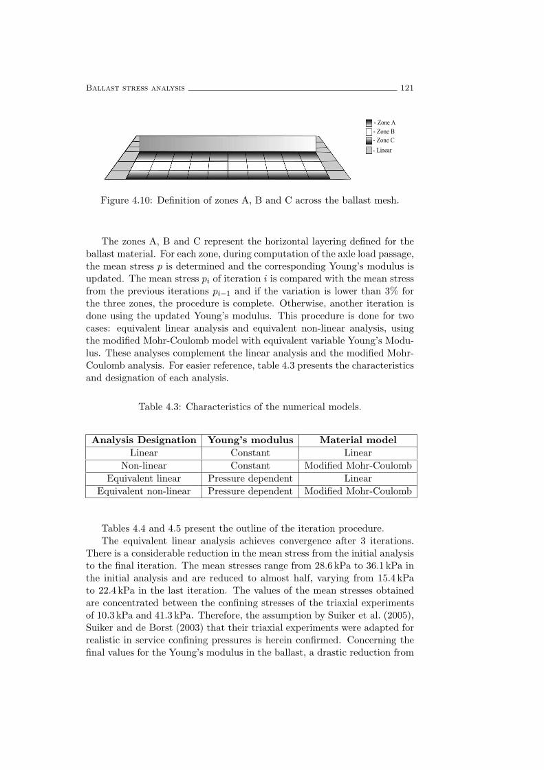
Ballast stress analysis 121
Figure 4.10: Definition of zones A, B and C across the ballast mesh.
The zones A, B and C represent the horizontal layering defined for theballast material. For each zone, during computation of the axle load passage,the mean stress p is determined and the corresponding Young’s modulus isupdated. The mean stress pi of iteration i is compared with the mean stressfrom the previous iterations pi−1 and if the variation is lower than 3% forthe three zones, the procedure is complete. Otherwise, another iteration isdone using the updated Young’s modulus. This procedure is done for twocases: equivalent linear analysis and equivalent non-linear analysis, usingthe modified Mohr-Coulomb model with equivalent variable Young’s Modu-lus. These analyses complement the linear analysis and the modified Mohr-Coulomb analysis. For easier reference, table 4.3 presents the characteristicsand designation of each analysis.
Table 4.3: Characteristics of the numerical models.
Analysis Designation Young’s modulus Material model
Linear Constant Linear
Non-linear Constant Modified Mohr-Coulomb
Equivalent linear Pressure dependent Linear
Equivalent non-linear Pressure dependent Modified Mohr-Coulomb
Tables 4.4 and 4.5 present the outline of the iteration procedure.The equivalent linear analysis achieves convergence after 3 iterations.
There is a considerable reduction in the mean stress from the initial analysisto the final iteration. The mean stresses range from 28.6 kPa to 36.1 kPa inthe initial analysis and are reduced to almost half, varying from 15.4 kPato 22.4 kPa in the last iteration. The values of the mean stresses obtainedare concentrated between the confining stresses of the triaxial experimentsof 10.3 kPa and 41.3 kPa. Therefore, the assumption by Suiker et al. (2005),Suiker and de Borst (2003) that their triaxial experiments were adapted forrealistic in service confining pressures is herein confirmed. Concerning thefinal values for the Young’s modulus in the ballast, a drastic reduction from

122
Table 4.4: Iterative procedure for the equivalent linear analysis.
Iteration Zone Initial E (MPa) p (Pa) pipi−1
Initial analysisA 293.8 36060 -B 293.8 31380 -C 293.8 28580 -
1st IterationA 192.9 22600 0.62B 181.9 15860 0.50C 174.9 13638 0.48
2nd IterationA 158.5 22140 0.98B 136.6 17100 1.08C 128.2 15860 1.16
3rd IterationA 157.2 22360 1.01B 141.0 17020 1.00C 136.6 15410 0.97
the initially calibrated value is obtained. This is explained by several factors,the previously mentioned difficulty in determining a small strain propertyfrom large strain results and the fact that even though the initial calibrationis done for the three coffining pressures, a calibration considering only thefirst two would be more relevant for the case presented.
Table 4.5: Iterative procedure for the equivalent non-linear analysis.
Iteration Zone Initial E (MPa) p (Pa) pipi−1
Initial analysisA 293.8 36060 -B 293.8 31380 -C 293.8 28580 -
1st IterationA 192.9 32040 0.89B 181.9 28660 0.91C 174.9 26600 0.93
2nd IterationA 183.5 31780 0.99B 175.1 28520 1.00C 169.7 26500 1.00
In the non-linear iteration procedure much lower differences in the meanstresses occur. The yield surface and the impossibility of the model to de-velop tensile stresses clearly affects the stress state in the ballast, particularlythe mean stress. This is similar to the remarks by Nguyen et al. (2003) thatfound approximately 15% higher compressive stresses in the ballast when

Ballast stress analysis 123
this was simulated using a no-tension model. Therefore, the considerationor not of yield conditions may have an important influence in the stiffness ofthe ballast. In this case the final Young’s modulus are higher than those ofthe equivalent linear analysis, although still quite distant from that obtainedin the calibration procedure.
The vertical displacements and velocities in the rail and sleeper due tothe passage of the Thalys axle at 300 km/h are presented in Figure 4.11 andFigure 4.12. Table 4.6 lists the peak displacements of the four analyses.
(a)
1.04 1.05 1.06 1.07 1.08 1.09 1.1 1.11 1.12−7
−6
−5
−4
−3
−2
−1
0
1x 10
−4
Displacement[m
]
Time [s]
(b)
1.04 1.05 1.06 1.07 1.08 1.09 1.1 1.11 1.12−0.06
−0.04
−0.02
0
0.02
0.04
0.06
Time [s]
Velocity
[m/s]
Figure 4.11: Vertical a) displacements and b) velocities in the rail fromsingle axle passage using ballast models: linear (grey), non-linear (black),equivalent linear (dashed) and equivalent non-linear (dotted).
The consideration of pressure-dependent Young’s Modulus does have sig-

124
(a)
1.04 1.05 1.06 1.07 1.08 1.09 1.1 1.11 1.12
−3
−2
−1
0x 10
−4
Displacement[m
]
Time [s]
(b)
1.04 1.05 1.06 1.07 1.08 1.09 1.1 1.11 1.12−0.025
−0.02
−0.015
−0.01
−0.005
0
0.005
0.01
0.015
0.02
0.025
Time [s]
Velocity
[m/s]
Figure 4.12: Vertical a) displacement and b) velocity in the sleeper fromsingle axle passage using ballast models: linear (grey), non-linear (black),equivalent linear (dashed) and equivalent non-linear (dotted).
nificant influence in the computed rail response. From all the 4 analyses,those whose difference is the consideration of pressure dependent Young’smodulus present higher differences in the track response than those in whichthe difference is the material model. It is also worthwhile to notice that inthe models that consider pressure independent Young’s modulus the dif-ference between linear and modified Mohr-Coulomb is smaller than in themodels that consider pressure dependent Young’s modulus. Furthermorethere is an inversion in the tendency: when permanent Young’s Modulus isconsidered, the non-linear model presents higher peak displacements than

Ballast stress analysis 125
the linear model; on the other hand, if pressure dependent Young’s modulusis considered, the equivalent non-linear model predicts lower peak displace-ments than the equivalent linear model. Therefore, there is an interactionbetween the two mechanisms that lead to the development of higher meanstresses (see tables 4.4 and 4.5), correspondingly higher ballast stiffness andlower peak displacements. Therefore, by considering the yield, compressionand tensile caps higher mean stresses will develop, resulting in higher ballaststiffness and consequently lower peak displacements.
Table 4.6: Peak displacements of the analyses. (m× 10−4)
Lin Nlin EqLin EqNlin
rail 5.83 5.89 6.30 6.19
sleeper 2.90 2.96 3.42 3.28
The permanent settlements in the linear or equivalent linear naturallytend to 0, while the extended Mohr-Coulomb and the equivalent extendedMohr-Coulomb tend to predict similar values. Therefore, the considerationof pressure-dependent Young’s Modulus seems to bare little influence in thisregard. The velocities in the rail and sleeper are influenced in a similar wayas the displacements.
The consideration of these different ballast behaviours has more influencein the sleeper response than in the rail. In the rail response the differencein the peak displacement from the linear to the equivalent linear analysis is8%, while the peak displacement in the non-linear and equivalent non-linearanalyses varied 5%. However, higher variations occur in the sleeper with a18% variation from the linear to the equivalent linear models, and a varia-tion of 11% in the non-linear and non-linear equivalent model. Also, if weaccount for the influence of the non-linear behaviour, the linear and non-linear models differ 1% in the rail peak displacement and 2% in the sleeperdisplacement. The iterative analyses have a 2% variation in the rails peakdisplacement and a 4% variation in the sleeper peak displacement. In conclu-sion, irrespective of the change that is considered in the ballast behaviour,the relative displacement variation of the sleeper is always approximatelytwice that of the rail. The sleeper resting directly upon the ballast is moresusceptible to any change of its behaviour than the rail which still has therail pad separating it from the sleeper.
From the analysis of this study case and the 4 different considerations ofballast behaviour it is possible to conclude that the correct determination ofthe Young’s modulus is of much importance to the track response. Althoughthe deviatoric behaviour obtained from the triaxial tests in the literature hasan important role in providing higher accuracy to the computations, the mis-

126
take that may be done by disregarding the deviatoric behaviour seems lessimportant than a mistake in the estimation of the Young’s modulus or dis-regard of its variation with mean stress. Therefore, from the observationsand conclusions obtained in this study, it is suggested that future experi-ments for the determination of track ballast behaviour should include themeasurements at very low strains (< 1 × 10⁻⁴) to determine the Young’smodulus, as well as the large strain measurements.
4.2.7 Stress-strain ballast response
The stress-strain ballast response in the 4 analyses is studied and compared.The analyses are compared taking into account the time history and thestress and strain distribution in the ballast during the axle passage. Sincethe 3D FE models consider the discrete rails support, the longitudinal as wellas the transversal stress distribution is studied. Two transversal sections arefurther on referred, the ”sleeper section” refers to a ballast section directlybelow the sleeper, the ”crib section” refers to a ballast section at mid-lengthbetween two sleepers (Figure 4.13).
Crib section
Sleeper section
Ballast
Sleeper
Figure 4.13: Representation of the ballast ”Sleeper section” and ”Crib sec-tion”.
Figure 4.14 presents the distribution of the vertical stress σyy in the”sleeper section” at the time of the passage of the axle load.
The stress distribution is qualitatively similar in the linear and non-linearcases although in the linear case there is a larger concentration of stressesdirectly below the rail. In the non-linear case a maximum vertical stressof 8.1× 10⁴ Pa occurs directly below the rail, while almost no stress occursat the top of the ballast shoulder. Concerning only the ballast material di-rectly below the sleeper, the stresses vary from the mentioned maximum of8.1×104 Pa to a minimum of approximately 2.8×10⁴ Pa. It is noticeable thatthe ballast is reducing the stress levels for the lower layers, at the bottom ofthe ballast the highest vertical stress is approximately 75% the value of the

Ballast stress analysis 127
(a)
(b)
(b)
(c)0 0.1 0.2 0.3 0.4 0.5 0.6 0.7 0.8 0.9 1
0Pa−8.10× 10⁴ Pa
Figure 4.14: Transversal distribution of the vertical stress σyy in the bal-last with a) linear, b) modified Mohr-Coulomb, c) equivalent linear and d)equivalent modified Mohr-Coulomb.
top vertical stress. The quantification of pressure dependent Young’s mod-ulus leads to the development of considerably lower vertical stresses in theequivalent linear and equivalent non-linear models. These analyses presentvery similar stress distributions, either qualitatively or quantitatively. Onceagain the highest differences in the response occurs between analysis that
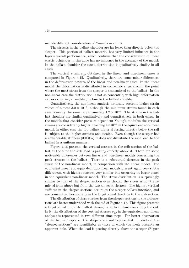
128
include different consideration of Young’s modulus.The stresses in the ballast shoulder are far lower than directly below the
sleeper. This portion of ballast material has very limited influence in thelayer’s overall performance, which confirms that the consideration of linearelastic behaviour in this zone has no influence in the accuracy of the model.In the ballast shoulder the stress distribution is qualitatively similar in allcases.
The vertical strain εyy obtained in the linear and non-linear cases iscompared in Figure 4.15. Qualitatively, there are some minor differencesin the deformation pattern of the linear and non-linear cases. In the linearmodel the deformation is distributed in concentric rings around the pointwhere the most stress from the sleeper is transmitted to the ballast. In thenon-linear case the distribution is not as concentric, with high deformationvalues occurring at mid-high, close to the ballast shoulder.
Quantitatively, the non-linear analysis naturally presents higher strainvalues of almost 3.0 × 10⁻⁴, although the minimum strains found in eachcase is nearly the same, approximately 1.2 × 10⁻⁴. The strains in the bal-last shoulder are similar qualitatively and quantitatively in both cases. Inthe models that consider pressure dependent Young’s modulus the verticalstrains are considerably higher, reaching 4×10⁻⁴ in the equivalent non-linearmodel, in either case the top ballast material resting directly below the railis subject to the higher stresses and strains. Even though the sleeper hasa considerable stiffness (30GPa) it does not distribute the axle load to theballast in a uniform manner.
Figure 4.16 presents the vertical stresses in the crib section of the bal-last at the time the axle load is passing directly above it. There are somenoticeable differences between linear and non-linear models concerning thepeak stresses in the ballast. There is a substantial decrease in the peakstress of the non-linear model, in comparison with the linear model. Theequivalent linear and equivalent non-linear models present again very subtledifferences, with highest stresses very similar but occurring at larger zonesin the equivalent non-linear model. The stress distribution is surprisinglysimilar to that of the sleeper section even though the stress is not trans-mitted from above but from the two adjacent sleepers. The highest verticalstiffness in the sleeper sections occurs at the sleeper-ballast interface, andare transmitted horizontally in the longitudinal direction to the crib section.
The distribution of these stresses from the sleeper sections to the crib sec-tions are better understood with the aid of Figure 4.17. This figure presentsa longitudinal cut of the ballast through a vertical plane containing the rail.In it, the distribution of the vertical stresses σyy in the equivalent non-linearanalysis is represented in two different time steps. For better observationof the ballast response, the sleepers are not represented. Therefore, the”sleeper sections” are identifiable as those in which the mesh presents anapparent hole. When the load is passing directly above the sleeper (Figure

Ballast stress analysis 129
(a)
(b)
(c)
(d)0 0.1 0.2 0.3 0.4 0.5 0.6 0.7 0.8 0.9 1
0−4.00× 10⁻⁴
Figure 4.15: Transversal distribution of the vertical strain εyy in the bal-last with a) linear, b) modified Mohr-Coulomb, c) equivalent linear and d)equivalent modified Mohr-Coulomb.
4.17a), most of the stress is transmitted directly to it and through the sleeperto the ballast below. From this contact point between the sleeper and theballast, the stress is distributed in a radial pattern both in the transversaland the longitudinal directions. Largest strains are transmitted verticallythan horizontally, regardless of that, a considerable stress distribution in the
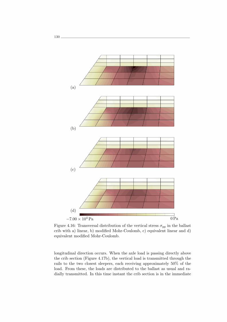
130
(a)
(b)
(c)
(d)0 0.1 0.2 0.3 0.4 0.5 0.6 0.7 0.8 0.9 1
0Pa−7.00× 10⁴ Pa
Figure 4.16: Transversal distribution of the vertical stress σyy in the ballastcrib with a) linear, b) modified Mohr-Coulomb, c) equivalent linear and d)equivalent modified Mohr-Coulomb.
longitudinal direction occurs. When the axle load is passing directly abovethe crib section (Figure 4.17b), the vertical load is transmitted through therails to the two closest sleepers, each receiving approximately 50% of theload. From these, the loads are distributed to the ballast as usual and ra-dially transmitted. In this time instant the crib section is in the immediate

Ballast stress analysis 131
vicinity of the two loaded sleepers. Consequently, it will be subject also tohigh stresses transmitted from both. Although these ballast portions are notdirectly loaded they are still subject to high stresses and their role shouldnot be disregarded. The stresses in the sleeper sections are neverthelesshigher than in the crib section, even if the axle load is in the mid-span ofthe rail (Figure 4.18).
(a)
(b)0 0.1 0.2 0.3 0.4 0.5 0.6 0.7 0.8 0.9 1
07.00× 10⁴ Pa
Figure 4.17: Longitudinal distribution of the vertical stress σyy in the ballastwhen the load is a) directly over the sleeper, b) at mid-span between twosleepers.
The crib section in study is immediately ”after” the sleeper section, inthe direction of the moving axle load. As the axle load passes directlyabove the sleeper section at t = 1.076 s the ballast is subject to a peakstress σyy = 72.1 kPa, in the crib section the stress is increasing as the axleload is only 0.3m away but a substantial lower stress is nevertheless present(σyy = 50.0 kPa). When the axle load passes directly above the crib section(t = 1.080 s) its vertical stress reaches a peak value σyy = 54.5 kPa but stilllower than the stress at the ballast below the sleeper (σyy = 62.5 kPa). With

132
the continuing axle movement the stress in the sleeper section diminishes asthe load is being transmitted mainly to the next sleeper, however, the cribsection is in the vicinity of the next sleeper and thus is subject to higherstresses than the sleeper section.
1 1.02 1.04 1.06 1.08 1.1 1.12 1.14 1.16−8
−7
−6
−5
−4
−3
−2
−1
0x 10
4
σyy[Pa]
Time [s]
Figure 4.18: Time history of the vertical stress σyy in the midle of the ballastlayer in the sleeper section (black) and crib section (grey) obtained in theequivalent non-linear model.
The stress-paths in the ballast of the equivalent non-linear model areanalysed in four different points (Figure 4.19). The four points corre-spond to the nodes most directly below the axle load in the sleeper sec-tion and the corresponding nodes in the crib section. Point A is at thecontact between the ballast and the sleeper, while points B, C and Dare 0.11m, 0.23m and 0.35m below the sleeper, respectively. The stresspaths in the sleeper section are very similar qualitatively (Figure 4.20).Quantitatively the upper ballast points are subject to lower initial stresses(pA0 = 5.3 kPa, qA0 = 7.4 kPa and pD0 = 8.7 kPa, qD0 = 12.6 kPa) due tothe less weight they are subject to. However, these are subject to highervariations of p and q reaching higher maximum values of isotropic and devi-atoric stresses (pAmax = 36.5 kPa, qAmax = 53.8 kPa and pDmax = 28.4 kPa,qDmax = 43.7 kPa). These variations (∆pA = 31.2 kPa, ∆qA = 46.4 kPa and∆pD = 19.7 kPa, ∆qD = 31.1 kPa) are similar to those obtained by Araujo(2011) in the ballast for a different case study, using Mohr-Coulomb andHujeux material models, even though in that case the ballast was subjectto an initial pressure of 20 kPa in its top. The stress paths in the uppercrib section are different due to the fact that the stresses are transmittedto them almost horizontally during the passage of the axle load. Therefore,

Ballast stress analysis 133
these stresses are mostly of the deviatoric kind. Because of this, the upperballast portions in the crib may be subject to the highest mobilized frictionof angle. The crib ballast near the base has stress paths similar in shape andsize to the sleeper section base ballast due to the fact that in that part theprincipal stress is closer to vertical and the local effect of the discontinuousrail support is dissipated. Concerning the mean stress, it is never lower than3.3 kPa in the upper crib section or higher than 36.5 kPa in the upper ballastdirectly below the sleeper.
b
b
b
b
point Apoint B
point Cpoint D
Figure 4.19: Definition of ballast points A to D.
(a)0 0.5 1 1.5 2 2.5 3 3.5 4
x 104
0
1
2
3
4
5
6x 10
4
p [Pa]
q[Pa]
(b)0 0.5 1 1.5 2 2.5 3 3.5 4
x 104
0
1
2
3
4
5
6x 10
4
p [Pa]
q[Pa]
(c)0 0.5 1 1.5 2 2.5 3 3.5
x 104
0
0.5
1
1.5
2
2.5
3
3.5
4
4.5
5x 10
4
p [Pa]
q[Pa]
(d)0 0.5 1 1.5 2 2.5 3
x 104
0
0.5
1
1.5
2
2.5
3
3.5
4
4.5x 10
4
p [Pa]
q[Pa]
Figure 4.20: Stress path in the ballast sleeper section (black) and crib section(grey) in: a) point A, b) point B, c) point C and d) point D.
It is shown that for real representation of the ballast stress conditionsthe discrete ballast support must be considered and to this effect only 3D

134
models (either full 3D or periodic) are suitable. The prospect evolution fromthis work, regarding stress distribution in the ballast from axle passage,would be the definition of 3D DE models for a more accurate determinationof the stresses in the crib sections. The large computational cost of DEmodels prevents the simulation of a full 3D track with moving loads inthe rail. Current models found in the literature focus in the reproductionof the sleeper sections with a single point load with variable magnitude.This loading scheme may be suitable for sleeper sections study but do notrepresent well the conditions of the crib sections in service. It is foreseeablethat the continuous improvement in computing power will in the future allowthe definition of more complex models, namely more refined 3D FE meshesand 3D DE-FE models to reproduce a rail track. Therefore, more elaboratenumerical studies may be developed in the future regarding the distinct rolesof the ”sleeper” ballast and ”crib” ballast.
4.2.8 Partial remarks
The section presented the study of the non-linear ballast behaviour.The deviatoric ballast behaviour was obtained from experimental data(Suiker and de Borst, 2003). The non-linear material model used is a mod-ified Mohr-Coulomb with hardening/softening of the yield cap as well asa compression cap with hardening. Due to numeric instabilities it was notpossible to include pressure-dependent stiffness, however, this was accountedfor in equivalent analyses. Four different ballast behaviour possibilities weredefined, ranging from the linear elastic to the equivalent non-linear. A studycase was defined and the passage of an axle load was simulated consideringthe four different definitions of ballast behaviour.
The results suggest that the consideration of pressure-dependent Young’smodulus of the ballast has more influence in the track response than the def-inition of yield and compressive caps. To these conclusions contribute thefact that the Young’s modulus of the ballast was calibrated to the experimen-tal results of 10.3 kPa, 41.3 kPa and 68.9 kPa whereas the ballast materialis only subject to isotropic pressures close to the first two values, and thatthe Young’s modulus is not easily determined from large strain results.
From the analysis of these results it is suggested that in future exper-imental campaigns on track ballast the Young’s modulus is directly deter-mined experimentally and the deviatoric behaviour is obtained for severalconfining pressures between 5 kPa and 50 kPa. These seem to be the valuesof the mean stresses the ballast is subject to in service conditions.
Results also suggest that the crib ballast is subject to significant stresses,close to those that occur below the sleeper. Future studies with, for instance,3D DE analyses could confirm these results to ensure that the continuousmodelling of the ballast material is not provoking excessive transmission ofstresses from the sleeper ballast to the crib ballast.

Non-linear soil behaviour 135
4.3 Non-linear soil behaviour
4.3.1 Cyclic response
In the consideration of traffic load the soil takes an important role in thetrack response. It is well established that the deformation characteristics ofsoils depend heavily on the level of shear strain to which soils are subjected.Soils respond linearly for very small shear strains and in an increasingly non-linear way with increasing shear strains, the failure takes place normally ata strain level of a few percent.
The majority of soils subject to symmetric cyclic loading present a typicalresponse such as the one shown in Figure 4.21. It represents the typicalresponse to the first load (dashed curve O-A) followed by the unloadingA-B-C and finalized by the reloading C-D-A. This representation is idealbecause it is symmetric and the diagram closes at point A, and so anystiffness degradation through the cycle is neglected.
b
b
b
b
bO
A
B
C
D
γa
τa
Gtan
GsecG0
W
γ
τ
Figure 4.21: Typical stress-strain response of soils to cyclic loading.
The dashed curve O-A is the backbone curve. Starting from point O,the beginning of the backbone curve curve is almost linear, and for verysmall strains the stress-strain (τ − γ) relation can be defined by the initialshear modulus G0. As the shear strain increases the response of the soilfollows the backbone curve and the consideration of linear relation betweenshear and strain becomes decreasingly accurate. If the shear strain increasesmonotonically from 0 to γa and then decreases, the unload will not followthe backbone curve but will follow the curve A-B-C presenting permanentdeformation when the shear stress changes signal. From point C a newreversal in the deformation will follow the curve C-D-A. Upon returning topoint A, the soil will continue along the backbone curve if the shear strain

136
does not reverse again. In rigour, the reload may not return exactly to thepoint A. For now this effect is neglected and thus it is considered that thehysteresis curve closes at point A.
For the load-reload cycle presented in Figure 4.21 a secant shear moduluscan be computed to relate the shear strain γa and the shear stress τa:
Gsec =τaγa
(4.32)
where Gsec is the shear modulus of the soil at the shear strain γa. Thesize of the curve can be conveniently defined through its area, which is ameasurement of the energy dissipation, and is therefore related with thedamping coefficient:
ξ =∆W
4πW(4.33)
∆W is the area of the curve, and W is the energy imposed by the strain γa:
W =Gsecγ
2a
2(4.34)
and thus:
ξ =∆W
2Gsecγ2a(4.35)
ξ is the damping ratio that the soil exhibits for a shear strain level γa. It isthen clear that by knowing the backbone curve of a soil and the rules thatshape the unload and reload curves, it is possible to know the secant shearmodulus Gsec and the damping ratio ξ that correspond to any shear strainlevel γa. Then, curves like the ones shown in Figure 4.22 can be tracedwhere the variation of shear modulus and damping are plotted.
As it is known that the deformation characteristics of the soils are heavilydependent on the deformation level, experiments have been done to properlydetermine the strain dependent variation of shear modulus and damping ina great number of different soils. As stated previously, for small strains theshear modulus remains practically unchanged and it is considered that thesoil is in its elastic state. The shear strain at which the stress-strain relationbecomes markedly non-linear changes from soil to soil, and can change in asoil depending on some factors.
It has been noted that for sands an increasing confining stress results in alarger linear shear strain threshold (Kokusho, 1980). Similarly, the dampingshows smaller variation with shear strain when the confining stress is higher.

Non-linear soil behaviour 137
γa10−510−6 10−4 10−3
0.2
0.4
0.6
0.8
1.0
Gsec
G0
ξ
0.05
0.10
0.15
0.20
0.25
Figure 4.22: Typical soil variation of stiffness (full) and damping (dashed)with shear strain.
Vucetic and Dobry (1991) gathered data from 16 publications that stud-ied the influence of various parameters in the variation of shear modulus anddamping with shear strain (Figure 4.23). It was noticed that the plasticityindex highly influenced the shape of the modulus reduction and dampingincrease curves. Highly plastic soils show less variation of the shear modu-lus, consequently the linear threshold shear strain can be much higher forthese soils than for low plasticity soils. It has been also documented thatthe over-consolidation ratio does not significantly influence the secant shearmodulus Gsec or damping ratio ξ.
(a) (b)
Figure 4.23: Relation of cyclic shear strain with a) normalized shear modulusand b) damping (Vucetic and Dobry, 1991).
Ishibashi (1992) studied the effect of the mean effective shear stress onthe modulus reduction curves of non-plastic and plastic soils (Figure 4.24).In this study, the triaxial tests were done for a variable mean effective stressbetween 1 kN/m2 and 400 kN/m2. The modulus reduction curve is muchless sensible to the mean effective stress on soils of higher plasticity index.
The results of experimental studies conducted by many authors were

138
(a) (b)
Figure 4.24: Influence of mean effective confining pressure on modulus re-duction curves for a) non-plastic and b) plastic soil (after Kramer (1996)and Ishibashi (1992)).
compiled by Ishibashi and Zhang (1993) and they suggested the followingrelations:
Gsec
G0= K(γa, P I)(σ
′m)m(γa,P I)−m0 (4.36)
where:
K(γ, PI) = 0.5
1 + tanh
[ln
(0.000102 + n(PI)
γa
)0.492]
(4.37)
m(γa, P I)−m0 =
0.272
1− tanh
[ln
(0.000556
γa
)0.4]
exp(−0.0145PI1.3) (4.38)
n(PI) =
0 if PI = 0
3.37× 10⁻⁶PI1.404 if 0 < PI ≤ 15
7.0× 10⁻⁷PI1.976 if 15 < PI ≤ 70
2.7× 10⁻⁵PI1.115 if PI > 70
(4.39)
γa is the shear strain amplitude and PI is the plasticity indexWhen subject to undrained cyclic loading, the backbone curve of the soil
can degrade with the number of cycles. This occurs when the shear strainsurpasses a threshold cyclic strain, usually between 0.01% and 0.1% (Figure4.25).

Non-linear soil behaviour 139
Figure 4.25: Representation of the backbone curve degradation with numberof cycles (Matasovic and Vucetic, 1995).
The quantification of this degradation has been introduced byIdriss et al. (1978), by the definition of a degradation index δ that relates thesecant shear modulus of the first cycle Gsec1 with the secant shear modulusof cycle N, GsecN :
δ =GsecN
Gsec1(4.40)
it was observed that the relation of log δ with logN is approximatelyconstant (Figure 4.26), and thus the concept of degradation parameter tNwas created:
tN = − log δ
logN= N−t (4.41)
4.3.2 Stress-strain models for cyclically loaded soils
The realization that the soil deformation characteristics can be highly in-fluenced by the induced level of shear strain has led to the development ofmodels that can simulate this effect. When modelling soils which are cyclicor randomly loaded, it is important to incorporate a material model that isaccurate to simulate the material at the shear strain level that is expected.When the soil behaviour is expected to remain within the small strain range,linear elastic models may be accurate. For higher strain values, usually morecomplex models should be used.

140
Figure 4.26: Relation of degradation index and the number of cycles for aVPN clay (Matasovic and Vucetic, 1995).
Linear visco elastic models
For small strains the linear relation between stress and strain may be accu-rate, however, it is known that there is always a certain degree of dampingin the soils and this can lead to important variations in the soil’s response.One way to overcome this is to recur to linear viscoelastic models. Thesemodels consider the linear stress-strain relation, but by including a viscouscomponent provide the necessary energy dissipation to simulate damping inthe soil. These models can be represented by a spring-dashpot element ofwhich the Kelvin and Maxwell models are prime examples. One drawbackof these models is that the viscous component of the tension is dependent ofthe frequency: in the Kelvin model the damping increases with increasingfrequency while in the Maxwell model the inverse relation is found. Becauseof this, the application of any spring-dashpot model to real cases shouldbe restricted to those where the relevant frequency range is very limited.Models are also available in which this short come is addressed. These relyon the similar consideration of spring-dashpot systems, but in which thedashpot reaction is independent of the frequency. The consideration of arate-independent dashpot has been questioned and it does not have anyphysical correspondence (Ishihara, 1996), but it serves the purpose of pro-viding a numerical approximation of viscoelastic models to soil behaviour.The application of a rate-independent dashpot to the Kelvin model resultsin the non viscous type Kelvin model.

Non-linear soil behaviour 141
Equivalent linear models
One way to incorporate the modulus and damping dependence of shearstrain in soils is by the utilization of linear models in which the deformationcharacteristics are consistent with the induced shear strain. In equivalentlinear models the procedure consists in running the simulation in a linearelastic model, the shear strain level in the soil is then determined, Gsec andξ are updated to be consistent with the shear strain level and the simulationis done again to compute the new strain levels and check if the variationfrom the previous iteration stays within an adopted tolerance. The itera-tive procedure attempts to achieve a linear model in which the deformationcharacteristics are equivalent to those of the non-linear soil response. Oneproblem with this approach is that in dynamic simulations the shear straininduced in the soil can have large variations in the time span that is sim-ulated, therefore, an objective function is needed to define to which shearstrain level are Gsec and ξ updated. For most laboratory tests in whichthe modulus reduction and damping variation curves are defined, the so-licitations are harmonic and the shear strain level is characterized by themaximum shear strain amplitude, however, for transient loading originatingfrom traffic or earthquake, the time history of shear strain can be highly ir-regular and the peak strain is not representative of the strain history of thesoil. It is then adequate to determine an effective shear strain that betterrepresents the soil response. In earthquake engineering the effective shearstrain has been empirically found to be between 50% and 70% of the shearstrain peak value. Since the soil response is little sensitive to variationswithin these percentages it is common to define the effective shear strain as65% of the peak shear strain amplitude. Idriss and Sun used a more rigor-ous approach in which the effective shear strain to maximum shear strainratio Rγ is computed considering the earthquake magnitude M:
Rγ =M − 1
10(4.42)
For transient loads resulting from traffic, no similar suggestions werefound in the literature to compute the effective shear strain ratio. Therefore,authors tend to consider the empirical consideration used in earthquakeengineering (Costa et al., 2010).
Although the procedure allows to approximate the soil response takinginto account the modulus reduction and damping variation with shear strain,it must be noted that the resulting final simulation is still a linear elasticcalculation. This implies that the soil properties, although adequately up-dated, remain constant through the time history of the dynamic simulationand permanent deformations or failure of the soil are not considered.
The advantages of this approach are its simple implementation withinany linear calculation and the possibility of using directly the modulus re-

142
duction and damping variation curves to adjust the model. Because thecalculation is ultimately linear, the approach can be implemented in modelsthat are computed in the frequency domain, usually these have numericaladvantages over models in the time domain and allow for a quicker compu-tation.
This method has been adapted into a highly used one-dimensional soilresponse analysis called SHAKE (Schnabel et al., 1972). Other programsfor 2D and 3D soil seismic response where the equivalent linear approachis employed were developed, such as the FLUSH (Lysmer et al., 1975) andGROUND 2D (Deng et al., 1995).
It has been noted that equivalent linear techniques tend to overestimatethe damping of the soils. Since the damping is updated for the representativeshear level, it does not account for the fact that the higher frequency compo-nent can be considerable and thus the smaller cycles at these frequencies con-tribute with lower damping. Acknowledging these short comes, some authorshave proposed frequency dependent algorithms for equivalent linear modelswith good comparison with measured site responses (Furumoto et al., 2000,Assimaki and Kausel, 2002).
Cyclic non-linear models
Despite the convenience and simplicity of the equivalent linear models, theseare still simplifications that provide only a generic approximation of the soilbehaviour. To better reproduce the soil’s response it is necessary to definenon-linear models computed in a time integration scheme such as the famousNewmark method.
In cyclic non-linear models the hysteresis curve is incorporated in themodel’s response and the shear strain and damping variations result implic-itly from the fact that the model follows the hysteresis curve, in the sameway that occurs in practical cases.
Most of these models are distinguished by the way that they representthe backbone curve and the stress reversal curves, but they usually follow aset of rules called the extended Masing Rules:
1. For the initial load, the stress-strain curve follows the backbone curve.
2. If a stress reversal occurs at a point defined by (γa, τa) the stress-straincurve follows a path given by
τ − τa2
= Fbb
(γ − γa
2
)(4.43)
where Fbb is the function of the backbone curve. This means thatthe unloading and reloading curves will have the same shape as the

Non-linear soil behaviour 143
backbone curve but enlarged by a factor of 2 and with the origintranslated to the point where the stress is reversed.
3. If the unloading or reloading curve exceeds the past maximum strainand intercepts the backbone curve, it will follow the backbone curveonwards.
4. If the unloading or reloading curve crosses an unloading or reloadingcurve of the previous cycle, it will follow the unloading or reloadingcurve of the previous cycle onwards.
Models that comply with these rules are called extended Masing models.Figure 4.27 shows an example of the variation of shear stress with time andthe resulting stress-strain behaviour according to the Masing rules.
(a) (b)
Figure 4.27: Soil response according to the Masing rules: a) variation ofshear stress in time and b) corresponding stress-strain behaviour (Kramer,1996).
At zero shear stress, the shear strain is not necessarily zero, meaningthat these models have the ability to present permanent deformation, whichis an advantage over the equivalent linear models. Many extended Masingmodels have been developed and used throughout the years, a few examplesare presented in the following.
The hyperbolic model defines, as the name states, the backbone curve asa hyperbola. The backbone curve is bounded by two lines that are tangentto it at small and large strains (Figure 4.28 a). The numerical representationof the hyperbolic curve is given by:
Fbb =G0
1 +(|γa|γr
) (4.44)
in which γr is the reference strain, the strain that would occur at failure stressif the soil behaviour was linear. In Figure 4.28 b) the modulus reduction
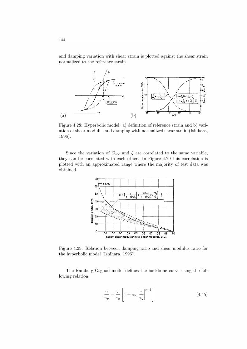
144
and damping variation with shear strain is plotted against the shear strainnormalized to the reference strain.
(a) (b)
Figure 4.28: Hyperbolic model: a) definition of reference strain and b) vari-ation of shear modulus and damping with normalized shear strain (Ishihara,1996).
Since the variation of Gsec and ξ are correlated to the same variable,they can be correlated with each other. In Figure 4.29 this correlation isplotted with an approximated range where the majority of test data wasobtained.
Figure 4.29: Relation between damping ratio and shear modulus ratio forthe hyperbolic model (Ishihara, 1996).
The Ramberg-Osgood model defines the backbone curve using the fol-lowing relation:
γ
γy=
τ
τy
[1 + αr
∣∣∣∣τ
τy
∣∣∣∣r−1
](4.45)

Non-linear soil behaviour 145
where τy and γy are carefully chosen stress and strain, αr and r are alsouser defined parameters that can be calibrated in order to better suit thedesired soil behaviour. Usually τy and γy are set as the maximum stress τfand reference strain γr. This changes equation (4.45) into:
G
G0=
1
1 + α∣∣∣ GG0
γaγ0
∣∣∣r−1 (4.46)
from this, the damping is obtained:
ξ =2
π
r − 1
r + 1α
∣∣∣ GG0
γaγr
∣∣∣r−1
1 + α∣∣∣ GG0
γaγr
∣∣∣r−1 (4.47)
The Iwan model (Iwan, 1967) relies on the assumption that a hystereticsystem can be constructed by a large number of elasto-plastic elements withdifferent yield levels. The model consists in a series of spring-slip elementsdisposed in either a series or parallel combination. Unlike other modelsthat define a function for the backbone curve and the unloading-reloadingcurves separately, this model implicitly complies with the Masing rules andby simply defining the appropriate backbone curve it will ensure that theunloading and reloading are accurate.
There are some limitations of the Masing models in the reproductionof the hysteretic damping at high strains, at which these models tend toincreasingly overestimate the damping. Therefore, if a model is to be appliedin a simulation where repeated cycling at very large strains is expected then aMasing model is not suitable. The short come of these models in reproducingdamping at high strains has been attributed mainly to the second Masingrule which models unloading and reloading (Figure 4.30).
Realising this limitation, several authors have proposed alterations to themodels or to the Masing rules. Pyke (1979) suggested an alternative to thesecond Masing rule in which the factor correlating the backbone curve andthe reload/unload curves is not constantly 2 but rather dependent upon theshear strain. Similarly, other authors suggested formulations that somehowrecur to a damping reduction factor (Darendeli, 2001, Phillips and Hashash,2009). On the other hand Ishihara et al. (1985) suggested that shaping theunload/reload curves with the backbone curve is too restrictive and sug-gested a model in which two distinct backbone curves are defined, one shapesthe initial soil response and the other shapes the stress reversal curves.
4.3.3 Case study
A case study is defined to study the non-linear subgrade behaviour underhigh-speed trains. It relies on the simulation of a hypothetical case of the

146
(a)
γ
τ
(b)10−410−5 10−3
0.2
0.4
0.6
0.8
1.0
ξ
10−2
γa
Figure 4.30: Comparison of experimental (full) and Masing (dashed) a)hysteresis curve at high strains and b) damping curve.
railway track from section 3.4.4 over a soil material for which the straindependent characteristics are known, this experimental data is obtained fromthe literature. To study this, a 3D FE mesh is used with different materialmodels: a linear analysis considers solely the small strain properties of thesoil; an equivalent linear analysis iteratively updates the soil’s properties toaccount for the non-linear behaviour and a non-linear analysis requiring theimplementation of a cyclic non-linear model in the FE software.
Wang and Kuwano (1999) preformed a series of cyclic triaxial tests onclayey sands in order to determine the strain dependency of shear modulusand damping ratio of these soils. This was motivated by the lack of knowl-edge of the influence of the fine content in the dependency of shear modulusand damping with shear strain. For that, the clayey sands were preparedby mixing Kawasaki clay and Toyoura sand obtaining several mixtures withPlasticity Index of 2, 5, 10 and 30. The specimens of each mixture, with50 mm in diameter and 125 mm in height were fully saturated and consoli-dated in confining stresses of 98, 196 and 392 kPa. After consolidation thecyclic triaxial tests were done in undrained conditions by the application ofaxial stress. According to the Japanese Standard, the shear modulus anddamping were obtained and the 10th of 12 cycles. The shear modulus at the10th cycle is obtained using equations (4.32) and (4.33). For each mixtureand consolidation stress, 10 different amplitudes of axial stress were appliedin order to obtain the shear modulus and damping at different shear strainamplitudes. It is easily demonstrated that for the case of triaxial tests, theshear stress τ and shear strain γ can be obtained from the axial stress σaand axial strain εa using
τ = ∆τ =∆σa2
(4.48)

Non-linear soil behaviour 147
γ = ∆γ = ∆εa(1 + υ) (4.49)
Figure 4.31 shows the results for the mixture M10 (i.e. with PlasticityIndex of 10) .
(a) (b)
Figure 4.31: Experimental results of the M10 clayey sand, cyclic shear straindependence of a) shear modulus and b) damping (Wang and Kuwano, 1999).
The synthetic case study herein defined considers that the railway trackrests upon a homogeneous subgrade of M10 clayey sand with propertiesobtained by Wang and Kuwano (1999).
4.3.4 Linear and equivalent linear analyses
The linear analysis considers the small strain properties of the soil and servesas the initial iteration for the equivalent linear analysis. Complementing thelinear and non-linear analysis, an equivalent linear analysis is done in orderto understand how much of an improvement it provides upon the linear case,and how well it simulates the non-linear behaviour. The equivalent linearanalysis is done in the following way:
1. The iterative procedure begins with the linear analysis using the smallstrain soil properties. The soil mesh is divided into nine layers, the first8 layers of 1m each are subject to update of stiffness and damping,the last layer of 2m has permanent small strain properties.
2. The computation is done for the passage of a Thalys axle passage andthe shear strains in the finite elements directly below the track aremonitored. For each finite element the peak shear strain is obtainedand the average peak strains upon each soil layer are computed. Fromthese, the effective shear strain is determined as 65% of the averagepeak strain in each layer.

148
3. For each layer the convergence is checked using the ratio of the effectiveshear strain obtained to the effective shear strain considered in theprevious iteration. A 5% convergence criterion is considered.
4. If convergence is obtained in all the layers then the iterative procedurestops. Otherwise Gsec and ξ are updated for all layers by interpolatingthe experimental results for the effective shear strain in each layer anda new iteration is started, returning the procedure to step 2.
Table 4.7 presents the iterative procedure until convergence is achieved.Large variations of the shear modulus are obtained from the initial anal-
ysis to the final iteration. Naturally as the depth increases the induced shearstrains decrease and the final shear modulus is closer to the initial modulus.The 5th layer has a stiffness variation until convergence of less than 5%,therefore, it is reasonable to conclude that it could have been consideredas a layer with permanent small strain properties and also that the layersbelow it did not need to be updated. Therefore, the initial considerationthat at more than 8m the soil does not need to be updated is completelyacceptable. Even though the stiffness almost didn’t change, the final effec-tive shear strain in that 5th layer is almost 27% higher than the effectiveshear strain in the initial analysis. This demonstrates that even at depthswhere the linear behaviour is acceptable, the shear strains may be highlyinfluenced by the non-linear behaviour of the soil above it. A more in depthlook upon the equivalent linear model response is taken in sub-section 4.3.8where the results obtained from the linear, equivalent linear and non-linearanalysis are discussed.
4.3.5 Non-linear model of the soil
The purpose of this task is to simulate the hysteretic behaviour of the soilrepresented generically by Figure 4.21 and to determine whether the con-sideration of this behaviour results in a considerably different track-soil re-sponse due to the passage of a train, when compared with what is obtainedconsidering linear behaviour. The aim is to simulate materials where thehysteretic behaviour is previously known from the literature and to simu-late the soil for the same conditions. Also, taking into account the largecomputational effort demanded by the track-soil FE mesh, it is necessaryto limit the complexity of the non-linear model of the soil. Because of this,the utilization of advanced constitutive models, where a more detailed soilbehaviour can be modelled, is not considered.
The non-linear model of the soil implemented in Diana is a cyclic non-linear model based on the Iwan equation. The Iwan model relies on theassumption that a hysteretic system can be constructed by a large numberof elasto-plastic elements with different yield levels. The original parallel

Non-linear soil behaviour 149
Table 4.7: Iterative procedure of the equivalent linear method.
Iteration Layer Initial G (MPa) γeffγi
γi−1
Initial analysis
1 61.42 1.72× 10⁻⁴ –2 61.42 1.06× 10⁻⁴ –3 61.42 6.19× 10⁻⁵ –4 61.42 3.80× 10⁻⁵ –5 61.42 2.89× 10⁻⁵ –6 61.42 2.41× 10⁻⁵ –7 61.42 1.90× 10⁻⁵ –8 61.42 1.35× 10⁻⁵ –
1st iteration
1 47.53 2.16× 10⁻⁴ 1.252 52.80 1.27× 10⁻⁴ 1.203 57.12 6.94× 10⁻⁵ 1.124 59.67 4.15× 10⁻⁵ 1.085 60.30 3.50× 10⁻⁵ 1.086 60.62 2.80× 10⁻⁵ 1.167 60.85 2.15× 10⁻⁵ 1.138 61.19 1.46× 10⁻⁵ 1.07
2nd iteration
1 45.35 2.26× 10⁻⁴ 1.052 51.08 1.32× 10⁻⁴ 1.043 56.25 7.04× 10⁻⁵ 1.024 59.44 4.22× 10⁻⁵ 1.045 59.88 3.64× 10⁻⁵ 1.026 60.36 2.86× 10⁻⁵ 1.027 60.74 2.19× 10⁻⁵ 1.028 61.11 1.47× 10⁻⁵ 1.01
3rd iteration
1 44.87 2.28× 10⁻⁴ 1.012 50.67 1.34× 10⁻⁴ 1.013 56.13 7.06× 10⁻⁵ 1.004 59.38 4.24× 10⁻⁵ 1.005 59.78 3.67× 10⁻⁵ 1.016 60.32 2.87× 10⁻⁵ 1.007 60.72 2.21× 10⁻⁵ 1.018 61.09 1.48× 10⁻⁵ 1.00
Iwan model (Iwan, 1967) is explained in the following. Figure 4.32 shows arepresentation of the Iwan parallel model with four elements.
Each element consists in a linear spring with stiffness ki in series with aslip damper with a maximum allowed force τi. Usually all the elements havethe same elastic stiffness k, and different slip stress τi. The initial loading

150
k1
τ1
τ
k2
τ2
k3
τ3
k4
τ4
Figure 4.32: Representation of the Iwan parallel model with 4 elements.
curve is given by:
τ =n∑
i=1
kγ +
nk∑
i=n+1
τi (4.50)
where nk is the total number of elements and n is the number of elementsthat remain elastic for the strain γ. Before the first yield stress is achieved,the model behaves linearly. When the first yield stress is achieved, therespective element no longer resists to deformation and from there onwardsthe overall stiffness of the model is reduced by k until the next yield stressis achieved or an inversion of the load occurs. In fact, the Iwan modelapproximates the stress-strain curve by a series of line segments (Figure4.33).
τ
γ
Figure 4.33: Behaviour of the parallel Iwan model.
When the model is unloaded, the elements that had slipped becomeactive again because the model is now loading in the opposite direction, thismeans that the model stiffness K at the beginning of the unload is the sameas in the beginning of the first load and the elements will unload until they
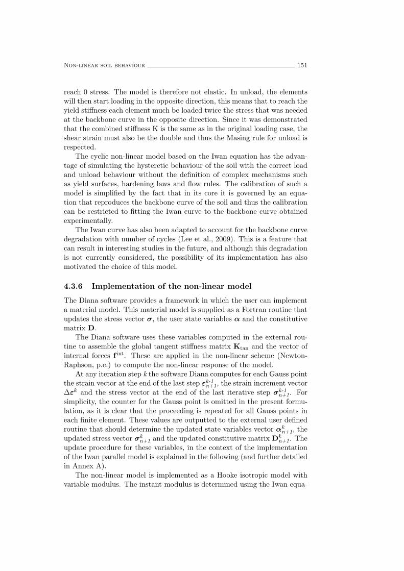
Non-linear soil behaviour 151
reach 0 stress. The model is therefore not elastic. In unload, the elementswill then start loading in the opposite direction, this means that to reach theyield stiffness each element much be loaded twice the stress that was neededat the backbone curve in the opposite direction. Since it was demonstratedthat the combined stiffness K is the same as in the original loading case, theshear strain must also be the double and thus the Masing rule for unload isrespected.
The cyclic non-linear model based on the Iwan equation has the advan-tage of simulating the hysteretic behaviour of the soil with the correct loadand unload behaviour without the definition of complex mechanisms suchas yield surfaces, hardening laws and flow rules. The calibration of such amodel is simplified by the fact that in its core it is governed by an equa-tion that reproduces the backbone curve of the soil and thus the calibrationcan be restricted to fitting the Iwan curve to the backbone curve obtainedexperimentally.
The Iwan curve has also been adapted to account for the backbone curvedegradation with number of cycles (Lee et al., 2009). This is a feature thatcan result in interesting studies in the future, and although this degradationis not currently considered, the possibility of its implementation has alsomotivated the choice of this model.
4.3.6 Implementation of the non-linear model
The Diana software provides a framework in which the user can implementa material model. This material model is supplied as a Fortran routine thatupdates the stress vector σ, the user state variables α and the constitutivematrix D.
The Diana software uses these variables computed in the external rou-tine to assemble the global tangent stiffness matrix Ktan and the vector ofinternal forces f int. These are applied in the non-linear scheme (Newton-Raphson, p.e.) to compute the non-linear response of the model.
At any iteration step k the software Diana computes for each Gauss pointthe strain vector at the end of the last step ε
k-1n+1, the strain increment vector
∆εk and the stress vector at the end of the last iterative step σ
k-1n+1. For
simplicity, the counter for the Gauss point is omitted in the present formu-lation, as it is clear that the proceeding is repeated for all Gauss points ineach finite element. These values are outputted to the external user definedroutine that should determine the updated state variables vector αk
n+1, theupdated stress vector σk
n+1 and the updated constitutive matrix Dkn+1. The
update procedure for these variables, in the context of the implementationof the Iwan parallel model is explained in the following (and further detailedin Annex A).
The non-linear model is implemented as a Hooke isotropic model withvariable modulus. The instant modulus is determined using the Iwan equa-

152
tion.The parameters of the model are the Young’s modulus E, the Poisson’s
ratio ν, the volumetric mass ρ, the number of spring/slip elements nk and theslip-stress of each element τ1, τ2, ...τnk
. An equal stiffness for all spring/slipelements is assumed
k =G0
nk(4.51)
where k is the stiffness of the spring/slip elements.Initially, the iterative strain vector εkn+1 is determined
εkn+1 = ε
k-1n+1 +∆ε
k (4.52)
The Iwan equation (4.50) determines the relation between effective shearstrain, γeff and effective shear stress τeff of the material. From the exper-imental results, the stiffness and damping variation curves are generallydetermined by considering that the effective shear strain and the effectiveshear stress correspond to the maximum shear stress and maximum shearstrain of the load cycle. Consequently, the maximum shear strain is com-puted from the iterative strain vector:
γeff = γkn+1 =ε1 − ε3
2(4.53)
in which ε1 and ε3 are, respectively, the major and minor principal strainsof the strain state represented by ε
kn+1. The principal strains are determined
as the eigenvalues of the strain tensor. These eigenvalues are computed usinga QR decomposition method with Householder reflectors (Annex B).
The Iwan model is updated for the effective shear strain γeff . The shearstress τ is updated with the Iwan model as well as the vector of state vari-ables α that contains information on the tension in each spring/slip elementof the Iwan model as well as its status (contributing to the stiffness of themodel or slipping). From the shear stress and shear strain variation over k,a secant shear modulus is computed (Figure 4.34).
Gsec =(τ kn+1 − τ k-1n+1)
(γkn+1 − γk-1n+1)(4.54)
A reduction factor of the secant shear modulus Gsec from the initial shearmodulus G0 is determined:
fsec =Gsec
G0(4.55)

Non-linear soil behaviour 153
ττ kn+1
τ k-1n+1
γk-1n+1 γkn+1γ
Gsec
Gtan
Figure 4.34: Determination of Gsec and Gtan in the non-linear model.
and a secant matrix Dsec is computed
Dsec = Dfsec (4.56)
The updated stress tensor is determined:
σkn+1 = σ
k-1n+1 +Dsec∆ε
k (4.57)
From the state variables vector αkn+1 the number of active elements
determines the tangent shear modulus Gtan at the end of step k.The modified Lame coefficients are computed:
µ′ = Gtan (4.58)
λ′ = λGtan
G0(4.59)
And the new constitutive matrix is computed from the modified Lamecoefficients:
Dtan =
λ′ + 2µ′ λ′ λ′ 0 0 0λ′ λ′ + 2µ′ λ′ 0 0 0λ′ λ′ λ′ + 2µ′ 0 0 00 0 0 µ′ 0 00 0 0 0 µ′ 00 0 0 0 0 µ′

154
4.3.7 Calibration
M10 clayey sand at 392 kPa
The M10 clayey sand (Wang and Kuwano, 1999) is simulated with the cyclicnon-linear model. The experimental values obtained with a confining pres-sure of 392 kPa (Figure 4.35) are used to calibrate the parameters of theIwan curve using a least squares optimization procedure. For that pur-pose, the results are initially transformed from the representation of shearmodulus to shear stress using equation (4.32). Considering that each elasto-plastic element has equal stiffness k, the experimental results are used tocalibrate the slip stress of each element in the Iwan load curve (4.50) in or-der to simulate the same stiffness degradation. The calibration is repeatedfor a different number of elasto-plastic elements in order to obtain the bestcorrespondence.
Figure 4.35: Experimental stiffness reduction with shear strain of theM10 clayey sand at confining pressure of 392 kPa (adapted fromWang and Kuwano (1999)).
By a carefully choice of the number of elements in the Iwan model andof the initial values of the slip stress to perform the curve fitting procedure,it seems that any curve that follows the typical stiffness degradation curvesof soils (Figure 4.21) can be represented by this model. This is an importantverification because the consideration of equal stiffness k for all the elementsof the Iwan model could have led to a restriction of the soil behaviour pre-venting an accurate calibration of the model. In this work, the number ofslip elements is roughly estimated using:
nk ≈ G0
Gtanγ(4.60)
where Gtanγa is the tangent shear modulus at the maximum shear strainof the experimental results. This estimation is based on the consideration

Non-linear soil behaviour 155
that at the maximum shear strain at least one element must still contributeto the global stiffness of the model (i.e. at least one element must still besubject to stress lower than its slip stress). The stiffness of that element(and therefore of all the others) should then be equal to Gtanγa
k = Gtanγa (4.61)
replacing (4.60) in (4.51) results in equation (4.61).For the M10 clayey sand with confining pressure of 392 kPa, the best
correspondence is obtained with a Iwan model comprised of nk = 20 elasto-plastic elements with stiffness G0
nk, the slip stress of each element is presented
in table 4.8.
Table 4.8: Slip stress of the elements (M10 at 392 kPa).
Element k1 k2 k3 k4 k5 k6 k7Slip Stress (Pa) 179 203 352 625 656 1020 1161
Element k8 k9 k10 k11 k12 k13 k14Slip Stress (Pa) 1246 1370 2707 2786 3020 3533 3891
Element k15 k16 k17 k18 k19 k20 -
Slip Stress (Pa) 6228 6344 6630 7645 8311 45766 -
Figure 4.36 compares the experimental shear stress and the numericalshear stress obtained with the Iwan equation (4.50) using the parameters oftable 4.8.
0 0.5 1 1.5 2 2.5 3 3.5
x 10−3
0
1
2
3
4
5
6
7
8
9x 10
4
τ[Pa]
γa10
−610
−510
−410
−310
−210
2
103
104
105
τ[Pa]
γa(a) (b)
Figure 4.36: Stress-strain behaviour of the clayey sand, experimental (x)and Iwan (full) values in a) decimal and b) log scale.
The Iwan curve represents well the experimental results that determinethe stiffness degradation with shear stress. In the range of shear strain

156
the experimental results and the Iwan results correspond very well. In thefollowing the implemented model, with the calibrated values, is used in thenumerical reproduction of the triaxial tests. This allows to compare theexperimental and numerical results and to verify whether the Iwan curvethat, as shown in Figure 4.36, represents well the soil’s stiffness degradationwith shear strain, is accurately applied by the model that is implementedin Diana. The simulations are done using a single 3D brick element. Asin the experimental cases, the specimen is subject to axial stress variationin order to induce a defined level of shear strain. An initial axial stressis induced in the specimen followed by a cycle of a determined amplitude.Six triaxial tests are done with varying axial stress amplitude in order torecreate the shear strain amplitude of the experimental data (Figure 4.35).Table 4.9 shows the maximum axial stress applied in the numerical cyclictriaxial tests.
Table 4.9: Peak axial stress of the triaxial simulations (M10 at 392 kPa).
Triaxial test 1 2 3 4 5 6
Peak axial stress (kPa) 9.5 16.2 26.7 45.1 73.0 101.9
Figure 4.37 represents hysteresis curves obtained in the triaxial test sim-ulations. At low level of shear strain the model behaves almost linearly aswould be expected. In the first triaxial simulation the unload and reloadcurves follow almost the same path as the initial load. In this triaxial testthe model is already behaving in a non-linear way although very slightly.The hysteretic curve has very small area thus the damping is reduced, butthere is already some hysteretic damping occurring at this shear strain level.On the other hand, in the 6th triaxial test it can be seen that the initial lin-ear behaviour becomes increasingly non-linear with the increase in the shearstrain. This also means that the unload and reload curves are more distantto the backbone curve and consequently the damping is significantly higher.
Using the numerical results of the triaxial simulations (Figure 4.37), thestiffness degradation and damping variation with shear strain are computedusing equations (4.32) and (4.33). Figure 4.38 presents the experimentaland numerical variation of shear modulus and damping with shear strain.
The shear modulus degradation with shear strain is very well simulatedand all the numerical triaxial tests reproduce very well the experimentalresults. It can be concluded that the calibrated Iwan curve is accuratelyimplemented in the Diana environment and that the model does not presentany numerical inaccuracy. The damping is not so accurately simulated bythe model. At shear strains lower than 10−4 the numerical results correspondwell. At higher shear strain amplitudes the implemented model tends toincreasingly overestimate the damping. This tendency to overestimate the

Non-linear soil behaviour 157
(a)−4 −3 −2 −1 0 1 2 3 4
x 10−5
−5000
−4000
−3000
−2000
−1000
0
1000
2000
3000
4000
5000
τ[Pa]
γ (b)−8 −6 −4 −2 0 2 4 6 8
x 10−5
−1
−0.8
−0.6
−0.4
−0.2
0
0.2
0.4
0.6
0.8
1x 10
4
τ[Pa]
γ
(c)−1.5 −1 −0.5 0 0.5 1 1.5
x 10−4
−1.5
−1
−0.5
0
0.5
1
1.5x 10
4
τ[Pa]
γ (d)−3 −2 −1 0 1 2 3
x 10−4
−2.5
−2
−1.5
−1
−0.5
0
0.5
1
1.5
2
2.5x 10
4
τ[Pa]
γ
(e)−5 0 5
x 10−4
−4
−3
−2
−1
0
1
2
3
4x 10
4
τ[Pa]
γ (f)−8 −6 −4 −2 0 2 4 6 8
x 10−4
−6
−4
−2
0
2
4
6x 10
4
τ[Pa]
γ
Figure 4.37: Hysteresis curves of the M10 clayey sand at confining pressureof 392 kPa obtained with the numeric cyclic triaxial tests with peak axialstress of a) 9.5 kPa, b) 16.2 kPa, c) 26.7 kPa, d) 45.1 kPa, e) 73.0 kPa andf) 101.9 kPa.
damping at high shear strains has also been found in other models thatfollow the Masing rules (Lopez-Caballero et al., 2004). This is related to thepreviously referred limitation of the models that follow the Masing rules andhas been mainly appointed to the reload/unload conditions. These modelscan be adapted by the adoption of a coefficient that affects the slope of theunload and reload curves and reduces the area of the hysteresis curve of thesoil. However, this adjustment requires the knowledge of the exact shape ofthe hysteresis curve at these high strain levels, which in the case of theseliterature results (as in the majority of literature works) is not provided.

158
(a)10
−510
−410
−310
−20
2
4
6
8
10
12
14x 10
7
γa
Gsec[kPa]
(b)10
−610
−510
−410
−310
−20
0.02
0.04
0.06
0.08
0.1
0.12
0.14
γa
ξ
Figure 4.38: M10 Clayey sand at confining pressure of 392 kPa, shear straindependency of a) shear modulus and b) damping, comparison of experimen-tal (.) and numerical (x) results.
M10 clayey sand at 98 kPa
The non-linear model is also used to recreate the experimental results of theM10 clayey sand obtained with confining pressure of 98 kPa. Figure 4.39presents the experimental results of the stiffness degradation with shearstrain. Due to the difference in the confining pressure, there is a significantdifference in the stiffness of this specimen and the one subject to 392 kPa.
Figure 4.39: Experimental stiffness reduction with shear strain ofthe M10 clayey sand at confining pressure of 98 kPa (adapted fromWang and Kuwano (1999)).
The calibration procedure is repeated for this specimen. The experi-mental values obtained with a confining pressure of 98 kPa (Figure 4.39)are used to calibrate the parameters of the Iwan curve using a least squaresoptimization procedure. The numerical fitting of the Iwan curve and the ex-perimental results is again repeated for a different number of elasto-plasticelements in order to obtain the best correspondence. For the M10 clayey

Non-linear soil behaviour 159
sand with confining pressure of 98 kPa, the best correspondence is obtainedwith a Iwan model comprised of nk = 14 elasto-plastic elements, the slipstress of each element is presented in Table 4.10.
Table 4.10: Slip stress of the elements (M10 at 98 kPa).
Element k1 k2 k3 k4 k5 k6 k7Slip Stress (Pa) 94 194 247 436 483 680 1189
Element k8 k9 k10 k11 k12 k13 k14Slip Stress (Pa) 1219 1356 1632 1797 3111 4618 24697
Figure 4.40 compares the experimental shear stress and the numericshear stress obtained with the Iwan curve (4.50) using the parameters oftable 4.10. Again, it is shown that the Iwan curve can be calibrated to pro-
0 0.5 1 1.5 2 2.5 3
x 10−3
0
0.5
1
1.5
2
2.5
3x 10
4
γa
τ[Pa]
10−4
10−3
10−2
102
103
104
105
γa
τ[Pa]
(a) (b)
Figure 4.40: Stress-strain behaviour of the M10 clayey sand with confiningpressure of 98 kPa, experimental (x) and Iwan (full) values in a) decimaland b) log scale.
vide very accurate reproduction of the experimental behaviour of the clayeysand. Therefore, the consideration of constant stiffness k for all elements ofthe Iwan model is not a restrictive consideration.
Afterwards, the implemented model with the calibrated values is usedin the numerical reproduction of the triaxial tests. In this case nine triaxialtests are done to obtain the response at the same shear strain of the exper-imental results, in a range of 1.05× 10⁻⁵ to 2.8× 10⁻³. Table 4.11 presentsthe maximum axial stress applied in the numerical cyclic triaxial tests.
The triaxial tests are again very promising as they show that for verylow shear strain amplitudes the model remains linear (Figures 4.41a and4.41b) while for very high shear strain amplitudes the model shows a cleardegradation of the shear modulus, which is demonstrated by the slope of

160
the backbone curve in Figures 4.41g, and 4.41h. At these very high shearstrain amplitudes the area of the hysteresis curve in the specimen responseis large, thus following the experimental results that suggest an increase ofdamping at high shear strains.
Table 4.11: Peak axial stress of the triaxial simulations (M10 at 98 kPa).
Triaxial test 1 2 3 4 5 6 7 8 9
Peak axial stress (kPa) 1.3 1.9 3 5.1 9 16.2 30.1 41.2 58.8
(a)−1.5 −1 −0.5 0 0.5 1 1.5
x 10−5
−800
−600
−400
−200
0
200
400
600
800
τ[Pa]
γ (b)−2 −1.5 −1 −0.5 0 0.5 1 1.5 2
x 10−5
−1000
−800
−600
−400
−200
0
200
400
600
800
1000
τ[Pa]
γ
(c)−1 −0.5 0 0.5 1
x 10−4
−5000
−4000
−3000
−2000
−1000
0
1000
2000
3000
4000
5000
τ[Pa]
γ (d)−2 −1.5 −1 −0.5 0 0.5 1 1.5 2
x 10−4
−1
−0.8
−0.6
−0.4
−0.2
0
0.2
0.4
0.6
0.8
1x 10
4
τ[Pa]
γ
(e)−5 0 5
x 10−4
−2
−1.5
−1
−0.5
0
0.5
1
1.5
2x 10
4
τ[Pa]
γ (f)−1 −0.5 0 0.5 1
x 10−3
−2.5
−2
−1.5
−1
−0.5
0
0.5
1
1.5
2
2.5x 10
4
τ[Pa]
γ
Figure 4.41: Hysteresis curves of the M10 clayey sand at confining pressureof 98 kPa obtained with numeric cyclic triaxial tests with peak axial stressof a) 1.3 kPa, b) 1.9 kPa, c) 9 kPa, d) 16.2, e) 30.1 kPa and f) 41.2 kPa.
The experimental and numerical shear modulus and damping variation

Non-linear soil behaviour 161
with shear strain are compared in Figure 4.42.
(a)10
−510
−410
−310
−21
2
3
4
5
6
7x 10
7
Gsec[Pa]
γa (b)10
−510
−410
−310
−210
−10
0.05
0.1
0.15
0.2
0.25
0.3
0.35
γa
ξFigure 4.42: M10 clayey sand at confining pressure of 98 kPa shear straindependency of a) shear modulus and b) damping in experimental (.) andnumerical (x).
The shear modulus degradation with shear strain is very well simulated.Figure 4.42a shows that there is almost no noticeable difference between theexperimental results and the numerical simulations. These results would beexpected since the Iwan curve that is in the core of the non-linear modelwas calibrated with the experimental shear modulus degradation. However,numerical inaccuracies could lead to some differences in the 3D specimenresponse, nevertheless that is not the case herein presented. The comparisonof the numerical and experimental results of the triaxial tests of this clayeysand at confining pressures of 392 kPa and of 98 kPa are both very good thusit can be concluded that the implemented model simulates with very goodaccuracy the shear modulus degradation with shear strain. The dampingis again increasingly overestimated at shear strain amplitudes higher than10−4.
It is worthwhile to recall that the implemented model is not an advancedconstitutive model but rather a cyclic non-linear model. Because of this, itis numerically less expensive but it does not simulate the soil at varyingconditions. In it’s current state the model does not account for variationsin the confining pressure or pore pressure development. Because of this thenon-linear model has to be calibrated for each confining pressure, like in thepresented examples.
4.3.8 Results discussion
The calibrated model of the M10 clayey sand is used as foundation soil inthe non-linear numerical simulation of the track response. The simulationis done for the confining pressure of 98 kPa because it is a more realisticconfining pressure for the soil at low depths. The situation simulated is thepassage of a single axle of the Thalys high-speed train at 300 km/h. These

162
are inevitably elaborate models and computationally demanding, easily as-cending to hundreds of thousands degrees of freedom. Because of this, muchcare must be taken into the mesh refinement so that no more computationaleffort is taken than the necessary.
Using the information obtained from the equivalent linear model, thenon-linear behaviour is only considered for the upper 5m of subgrade. Forthe lower soil layer the small strain properties of the clayey sand are consid-ered (Figure 4.43).
Figure 4.43: Division of the soil in two layers.
Figure 4.44 presents the stiffness reduction obtained in the equivalentlinear model and the non-linear model at the moment of the passage ofthe train axle in a transversal section directly below the sleeper. It shouldbe noted that only half the soil is represented as symmetry is assumed. Allpoints at x = −0.75m are vertically aligned with the rail and all representedpoints at x > −1.75m are directly below the track.
The most glaring observation that can be made is that a much highersoil stiffness reduction occurs in the non-linear case than in the equivalentlinear, even if that occurs in a very small zone. Since the soil has a low initialshear modulus, high shear strains result from the solicitation and these highshear strains lead to high stiffness reductions. In the track-soil interfacedirectly below the track, the soil can reduce to slightly less than 50% itsoriginal stiffness, which represents a considerable reduction that can affectthe stiffness distribution through the soil, even though this occurs in a verysmall portion of soil, there is also a considerable reduction of 10% stiffnessthat can occur as deep as 3.5m.
Generally speaking, the stiffness reduction found in the equivalent lin-

Non-linear soil behaviour 163
(a)
0.73
0.82
0.91
0.96
0.97
0.73
−2.5 −2 −1.75 −1.5 −1 −0.75 −0.5−5
−4.5
−4
−3.5
−3
−2.5
−2
−1.5
−1
−0.5
x [m]
y[m
]
(b)
0.95
0.90
0.85
0.800.75
0.70 0.65 0.600.55
0.50
−2.5 −2 −1.75 −1.5 −1 −0.75 −0.5−5
−4.5
−4
−3.5
−3
−2.5
−2
−1.5
−1
−0.5
x [m]
y[m
]
Figure 4.44: Transversal distribution of the stiffness reduction ( GG0
) of thesubgrade in the a) equivalent linear and b) non-linear model.
ear case is consistent with that found in the non-linear case, especially atincreasing depths where the iso-lines of the non-linear simulation presentan almost horizontal layering. At depths around 1m or less the horizontallayering seems to be less acceptable as large differences occur between thesoil stiffness in the horizontal direction. Figure 4.45 presents a novel look atthe soil stiffness reduction from the non-linear model, considering both itsspacial and its time distribution. The figure presents the iso-lines of stiffnessreduction Gsec
G0, but instead of presenting only the time instant at which the
axle load is passing through the transversal section (t = 0.116 s), it presentstheir time history.
The soil degradation starts only when the axle load is already very close

164
(a) (b)
(c) (d)
(e) (f)
Figure 4.45: Time history of the subgrade stiffness reduction iso-lines: a)0.95, b) 0.90, c) 0.80, d) 0.70, e) 0.60 and f) 0.50.
to the transversal section. In Figure 4.45 a) it is shown that a 5% reductionstarts to occur at a time t ≈ 0.086 s which is only 0.03 s before the passageof the train axle. So the first soil stiffness reduction occurs when the axleload is less than 2.5m from the section in study. A 10% reduction onlystarts occurring at t = 0.090 s when the axle load is approximately 2maway. The 0.50 iso-line that enclosures a soil portion with a considerable

Non-linear soil behaviour 165
stiffness reduction is limited to a very small time and space span. It appearsonly at the time step in which the axle load is passing through the soilsection. Naturally, all iso-lines appear initially at the soil surface, and verylocalized, further they expand in the horizontal direction and descend alongthe subgrade. Taking as example the 0.95 iso-line, it evolves from the soil-track interface and a horizontal span of 0.5m at t = 0.086 s to a depth ofapproximately 5m and a horizontal span of more than 2.5m when the load ispassing directly above the section in study. In short, the stiffness reductionof the soil is very confined in time, but expands rapidly in space as the axleload approximates. The shear strain induced in the soil (Figure 4.46) isslightly different in the three cases. The shear strain can surpass 3.6× 10⁻⁴
in the soil close to the soil-track interface, especially directly bellow therail. However, the linear and equivalent linear models predict considerablylower peak values of 2 × 10⁻⁴ and 2.4 × 10⁻⁴ respectively. These majordifferences are found mainly directly below the rail and less than 1m depth.Both the linear and equivalent linear models have very good prediction ofthe shear strain in the soil at larger depths than 2m, where the iso-lines ofshear strain follow approximately the same path as the the iso-lines in thenon-linear case.
From the comparison of the shear strain distribution it is fair to con-clude that the equivalent linear model is indeed an improvement upon thelinear model, as it better represents the shear strains in a range of 1m to2m depth. From the observed shear strain distributions in the soil, somepreliminary observations can be made. The shear strain in the soil, whichis the main parameter that determines the soil’s stiffness degradation anddamping variation is concentrated mainly below the track at low depths.Both the linear and equivalent linear models provide a good estimation ofthe shear strain in the soil except for very low depths. A fairly good shearstrain prediction is done by these models in zones where stiffness reductionsas large as 10% occur. Therefore, they seem to be good tools to estimatethe boundaries between linear and non-linear response.
The iso-line of 4 × 10⁻⁵ shear strain is the only that is similar in allthree models and it is plausible that for lower strains the linear model hasgood accuracy. The iso-line of 8 × 10⁻⁵ obtained in the linear model isconsiderably different than those obtained in the equivalent linear and non-linear models. For higher strains the soil behaves increasingly non-linearlyso it is only natural that the linear model does not provide an accuratestrain response. The equivalent linear model obtains good predictions ofthe iso-lines up to 2 × 10⁻⁴ which is a considerable improvement upon thelinear model. Only in the upper soil layer can it be said that there arelarge differences in the shear strains determined in the equivalent linear andnon-linear models. The non-linear response presents shear stresses reaching10 kPa, while in the linear and equivalent linear cases, the model reachesslightly higher shear stresses of 12 kPa (Figure 4.47). This is a hint that
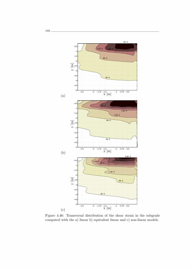
166
(a)
4E−5
8E−5
1.2E−4 1.6E−4
2E−4
−2.5 −2 −1.75 −1.5 −1 −0.75 −0.5−5
−4.5
−4
−3.5
−3
−2.5
−2
−1.5
−1
−0.5
x [m]
y[m
]
(b)
4E−5
8E−5
1.2E−4
1.6E−4
2E−42.4E−4
−2.5 −2 −1.75 −1.5 −1 −0.75 −0.5−5
−4.5
−4
−3.5
−3
−2.5
−2
−1.5
−1
−0.5
x [m]
y[m
]
(c)
4E−5
8E−5
1.2E−4
1.6E−42E−4
2.4E−42.8E−4 3.2E−4
3.6E−4
−2.5 −2 −1.75 −1.5 −1 −0.75 −0.5−5
−4.5
−4
−3.5
−3
−2.5
−2
−1.5
−1
−0.5
x [m]
y[m
]
Figure 4.46: Transversal distribution of the shear strain in the subgradecomputed with the a) linear b) equivalent linear and c) non-linear models.

Non-linear soil behaviour 167
when the soil degrades near the track occurs a redistribution of stresses tostiffer portions of soil. The consequence is that the degraded portion ofsoil is subject to lower stresses than linear models predict. There is a zonevery close to the track, at less than 1.5m depth and less than 1.5m fromthe centre of the track, where the stress distribution is not very accurate inthe linear and equivalent linear cases. Nevertheless, the stress distributionis remarkably accurate for the most part, even in the linear case. Againit is hinted that the equivalent linear case presents an upgrade in accuracyfrom the linear case and in many cases may be a very important tool topredict stress and strain of the subgrade. It seems that the method for theequivalent linear analysis is adequate, although it would be interesting tostudy if different reduction factors for the computation of the effective shearstrain would be more adequate. Regardless of that, it seems that for themost part, the horizontal layering of the soil is an acceptable simplificationexcept for the top 1 to 2m, where a horizontal division of the soil wouldvery likely lead to better representation of the soil degradation.
The analysis of the track response in the three cases (Figure 4.48) sug-gests similar conclusions to those obtained from the stress-strain state of thesoil. The displacement of the rail increases significantly when consideringthe non-linear behaviour. Again, considering the differences between thelinear and non-linear cases, the equivalent linear analysis presents a middleground that approximates the behaviour of the non-linear analysis, althoughwithout the complexity nor the accuracy of the later. The non-linear be-haviour has in this case undeniable influence in the track response, especiallythe rail peak displacement. The shape of the time response does not changemuch. This is confirmed by the analysis of it’s time derivative, in which thevelocity corresponds very well in the three cases.
Naturally, the linear and equivalent linear models do not have the ca-pability to present permanent settlements and after the passage of the axleload the rail response returns to 0, in the non-linear case that does nothappen, indicating that some permanent deformations in the soil occur.
4.3.9 Partial remarks
This section presented the numerical modelling of the effect of the hystereticbehaviour of the foundation soil in the performance of the railway track. Thesection began by presenting a general outline of the hysteretic behaviour ofgranular materials and the influence of some of the material characteristicsin this behaviour.
The experimental results obtained by Wang and Kuwano (1999) wereused define a case study. For the consideration of the soil three differentcomputation models representing the same study case were developed: alinear model, an equivalent linear model and a non-linear model. The lin-ear model simply considered the 3D FE response of the soil using the small
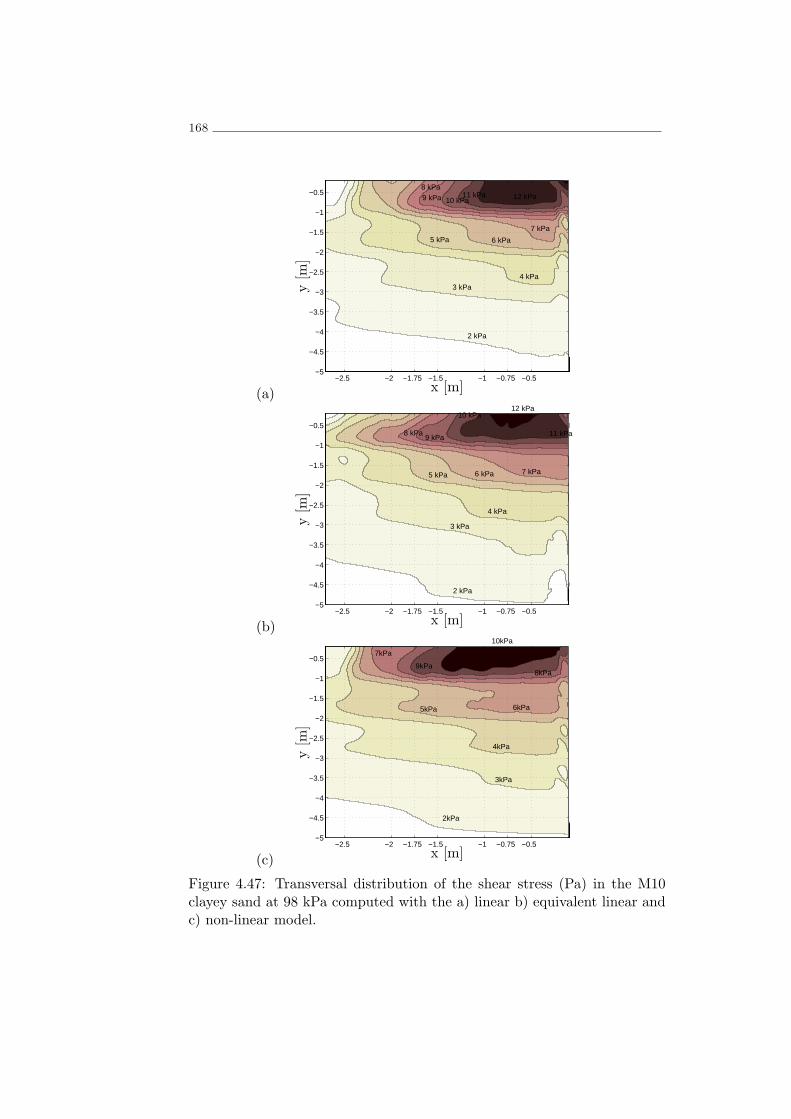
168
(a)
11 kPa 12 kPa10 kPa9 kPa8 kPa
7 kPa
6 kPa5 kPa
4 kPa3 kPa
2 kPa
−2.5 −2 −1.75 −1.5 −1 −0.75 −0.5−5
−4.5
−4
−3.5
−3
−2.5
−2
−1.5
−1
−0.5
x [m]
y[m
]
(b)
2 kPa
3 kPa
4 kPa
5 kPa 6 kPa 7 kPa
8 kPa9 kPa
10 kPa
11 kPa
12 kPa
−2.5 −2 −1.75 −1.5 −1 −0.75 −0.5−5
−4.5
−4
−3.5
−3
−2.5
−2
−1.5
−1
−0.5
x [m]
y[m
]
(c)
2kPa
3kPa
4kPa
5kPa 6kPa
7kPa
8kPa9kPa
10kPa
−2.5 −2 −1.75 −1.5 −1 −0.75 −0.5−5
−4.5
−4
−3.5
−3
−2.5
−2
−1.5
−1
−0.5
x [m]
y[m
]
Figure 4.47: Transversal distribution of the shear stress (Pa) in the M10clayey sand at 98 kPa computed with the a) linear b) equivalent linear andc) non-linear model.
Non-linear soil behaviour 169
(a)0 0.05 0.1 0.15 0.2 0.25 0.3
−10
−8
−6
−4
−2
0
2x 10
−4
Time [s]
Displacement[m
]
(b)0 0.05 0.1 0.15 0.2 0.25
−0.06
−0.04
−0.02
0
0.02
0.04
0.06
0.08
Time [s]
Velocity
[m/s]
Figure 4.48: Rail response of the linear (grey), equivalent linear (dotted)and non-linear (full) M10 material model at 98 kPa: a) displacements, b)velocities.
strains characteristics of the clayey sand. The equivalent linear model usedthe experimental results of Wang and Kuwano (1999) to update the stiff-ness and damping of the soil according to the shear strain obtained in thecalculation. The non-linear model required the implementation in the Di-ana software of the Iwan parallel model, which implicitly complies with theMasing rules. This model follows the Iwan equation that approximates thebackbone curve with a set of parallel elastoplastic elements with the samestiffness but different slip stress. Whenever a stress reversal occurs the com-bined behaviour of the elastoplastic elements follows what was described bythe rules of Masing.
After calibration, the obtained values were used in the cyclic non-linearmodel to reproduce the hysteretic behaviour of the material in several cyclictriaxial simulations. The hysteretic curves that were obtained present thesame shape as would be expected. The comparison between the experimen-tal and numerical stiffness reduction is very good, which suggests that the

170
model is numerically well implemented. Regarding damping variation withshear strain, the numerical model follows the same trend of other Masingmodels which also suggests that the model is numerically efficient in repro-ducing the Masing rules, although it is known that they do not representwell the soil damping at high strains.
After validation of the cyclic model, the influence of the hysteretic be-haviour of the soils in the behaviour of a high speed track was simulatedusing the previously validated FE mesh, with the passage of an axle load at300 km/h. Only the relevant calibrated case of 98 kPa confining pressurewas considered.
The non-linear simulation showed that there is a considerable stiffnessreduction in the soil, which may reduce to less than 50% its initial value ina small portion directly below the rail. The stiffness reduction is very con-fined in time, with relevant variations of stiffness starting only 0.03 s beforethe axle passage. Regarding the track response there are some noticeabledifferences in the rail displacement when non-linear behaviour is considered,with a considerable increase in the peak displacement and a permanent set-tlement. However, in terms of velocities the responses are almost the samein the three cases.
The equivalent linear simulation presented an improvement over the lin-ear method in all the results analysed. It is capable of more accuratelypredicting the non-linear response in terms of stress and strain in the soil,as well as obtain a better approximation of the rail displacements. Althoughit is unclear if a different reduction factor would improve the equivalent lin-ear method, it seems plausible to conclude that a more refined division ofthe soil in homogeneous update zones in the upper 1m would result in moreaccuracy in the representation of the non-linear model. Despite this, thehorizontal layering is still an acceptable simplification and the presentedequivalent linear analysis is an adequate tool to estimate the non-linear soilresponse.

Integrated analysis 171
4.4 Integrated analysis
4.4.1 Introduction
The final analysis uses the knowledge obtained in all the previous analy-ses, with special emphasis on the non-linear analyses, in order to do anintegrated analyses of the track response. This takes into account the rel-evant behaviour at the embankment as well as the soil in order to performa detailed evaluation of the track response. A very well documented caseis chosen to perform this analysis as it has been extensively used to studyand validate other numerical tools (Kaynia et al., 2000, Takemiya, 2003,Karlstrom and Bostrom, 2006, Costa et al., 2010). The response of the trackis very well known as are the track and subgrade properties. Therefore, itis an excellent case to once more validate the numerical tools allowing alsoto study the influence of velocity in the non-linear response.
4.4.2 Case study
The case study is the Ledsgard track site in southern Sweden along theWest Coast between Gothenburg and Malmo. This site gained some atten-tion in railway engineering when, in 1997, shortly after beginning operationthe circulation speeds had to be reduced due to excessive vibrations in thetrack and in its vicinity. What followed was an extensive experimental cam-paign aimed at measuring the track response and the properties of the trackand soil in order to determine the causes of these anomalies in the trackbehaviour. This experimental campaign was promoted by the Swedish Na-tional Rail Administration (Banverket) and had cooperation of several otherinstitutes.
The experimental measurements in the track were performed by 20 testruns, northward and southward, using an X-2000 (Figure 4.50) passengertrain consisting of an engine and four cars at speeds varying from 10 km/h to204 km/h. During these test runs the response in the track was recorded us-ing displacement transducers and accelerometers, the subgrade response wasrecorded using accelerometers and seismometers located at several depthsand at several horizontal distances from the track. The experimental resultsshowed that for circulation speeds lower than 70 km/h the displacements arequasi-static. However, for higher circulation speeds, the peak displacementsincrease drastically (Figure 4.49).
The geotechnical investigation campaign consisted in cross-hole, downhole and SASW in situ tests as well as cyclic triaxial tests on undisturbedsamples. These tests revealed that the soil is characterized by dry crustof 1.1m on top of an organic clay layer with approximately 3m thickness.Under these, lies a layer of soft marine clay with increasing stiffness downto the bedrock at approximately 70m depth. The configuration and small

172
strain properties considered for the subgrade by Kaynia et al. (2000) arepresented in table 4.12.
0 50 100 150 200 250−14
−12
−10
−8
−6
−4
−2
0
2
4
6
8
Train speed [km/h]
Peakdisplacement[m
m]
Figure 4.49: Experimental peak sleeper displacements at Ledsgard (adaptedfrom Kaynia et al. (2000)).
Figure 4.50: Configuration of the X-2000 test train(Karlstrom and Bostrom, 2006).
The Ledsgard line is composed of tree tracks (Figure 4.51a), the X-2000train circulates on the western track only. For the FE simulations a simpli-fication is made to simulate only the western track considering symmetryconditions (Figure 4.51b). The rails are the usual UIC 60 rails spaced every0.67 m, the geometry and properties of the rails, rail pads and sleepers arethe same considered for the previous analyses.
4.4.3 3D FE modelling
The non-linear subgrade behaviour is accounted for using the implementedIwan parallel model. The small strain properties presented in table 4.12 are

Integrated analysis 173
Table 4.12: Dynamic soil characteristics.
Layer d Cs Cp ρ ξ
[m] [m/s] [m/s] [kg/m3] [-]
Dry crust 1.1 72 500 1500 0.04Organic clay 3.0 41 500 1260 0.02
Clay 1 4.5 65 1500 1475 0.05Clay 2 6.0 87 1500 1475 0.05Clay 3 ∞ 100 1500 1475 0.05
(a)
1.2 m
1.25 m1.6 m
4.6 m
(b)
Figure 4.51: Geometry of the Ledsgard site: a) actual geometry(Costa et al., 2010) and b) considered geometry in the 3D FE simulations.
considered for the initial stiffness and damping of the layers. The evolutionof the secant shear modulus of the organic clay was obtained in cyclic triaxialtests in laboratory. The results are obtained from Costa et al. (2010) andused in a least squares optimization procedure in order to obtain the Iwan

174
parallel model parameters that best correspond to the experimental resultsof the variation of the secant shear modulus. The curves of the other layers isobtained from the relations 4.36 and 4.37 published by Ishibashi and Zhang(1993) and the corresponding Iwan parallel properties are obtained in aleast squares optimization procedure. For the dry crust a Plasticity Indexof 30 is considered, while for the Clay layers a higher Plasticity Index of 50 isconsidered. Since for these values of the Plasticity Index the curves are littlesensible to the coffining pressure, the same value of 50 kPa is considered forthe dry crust and the clays. The variations of the secant shear modulusand damping with shear strain in the calibrated Iwan parallel model arepresented in Figure 4.52. The experimentally obtained results of the stiffnessreduction with shear strain for the organic clay are well averaged by thecalibrated model, the damping is higher than experimental results, as usualwith this model.
(a)10
−510
−410
−310
−210
−10
2
4
6
8
10
12x 10
6
γ
Gsec[Pa]
Clay 2
Dry crust
Clay 1
Organic clay
(b)10
−510
−410
−310
−20
0.05
0.1
0.15
0.2
0.25
0.3
0.35
0.4
γ
ξ
Figure 4.52: Adopted Gsec and ξ variation curves in the subgrade with theIwan parallel model, dots represent experimental results for the organic clay.
Concerning the embankment behaviour, the small strain propertiesconsist shear wave velocity Cs = 210m/s and dilatational wave veloc-
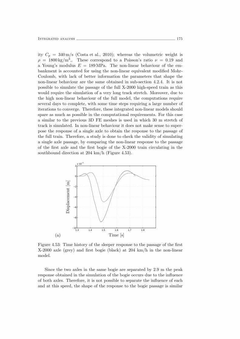
Integrated analysis 175
ity Cp = 340m/s (Costa et al., 2010); whereas the volumetric weight isρ = 1800 kg/m3,. These correspond to a Poisson’s ratio ν = 0.19 anda Young’s modulus E = 189MPa. The non-linear behaviour of the em-bankment is accounted for using the non-linear equivalent modified Mohr-Coulomb, with lack of better information the parameters that shape thenon-linear behaviour are the same obtained in sub-section 4.2.4. It is notpossible to simulate the passage of the full X-2000 high-speed train as thiswould require the simulation of a very long track stretch. Moreover, due tothe high non-linear behaviour of the full model, the computations requireseveral days to complete, with some time steps requiring a large number ofiterations to converge. Therefore, these integrated non-linear models shouldspare as much as possible in the computational requirements. For this casea similar to the previous 3D FE meshes is used in which 30 m stretch oftrack is simulated. In non-linear behaviour it does not make sense to super-pose the response of a single axle to obtain the response to the passage ofthe full train. Therefore, a study is done to check the validity of simulatinga single axle passage, by comparing the non-linear response to the passageof the first axle and the first bogie of the X-2000 train circulating in thesouthbound direction at 204 km/h (Figure 4.53).
(a)
1.3 1.4 1.5 1.6 1.7 1.8−10
−8
−6
−4
−2
0
2x 10
−3
Displacement[m
]
Time [s]
Figure 4.53: Time history of the sleeper response to the passage of the firstX-2000 axle (grey) and first bogie (black) at 204 km/h in the non-linearmodel.
Since the two axles in the same bogie are separated by 2.9 m the peakresponse obtained in the simulation of the bogie occurs due to the influenceof both axles. Therefore, it is not possible to separate the influence of eachand at this speed, the shape of the response to the bogie passage is similar

176
to the shape of a single axle passage, although with higher peak values andlarger duration in time. On the other hand, from the train configuration(Figure 4.50) the second bogie in the southbound direction is distant by 14.5m so it is safe to assume that the response to the passage of the first bogienot significantly affected by the following bogies. From this knowledge, thefollowing simulations are done by simulating the passage of the first bogie ofthe X-2000 train, in the linear analyses the response is superposed to obtainthe response of the full train passage; in the non-linear analyses only thepassage of the first bogie is studied.
4.4.4 Results discussion
Three cases are simulated: the cases involving speeds of 70 km/h and 204km/h are compared with measurements; a third case that involves a lowspeed of 10 km/h is also simulated to observe the influence of the dynamiceffects in the other two cases. In both comparisons of measurements, thenon-linear analysis presents greater accuracy than the linear analysis (Figure4.54).
Velocity was also observed to intensify the non-linear effects. For the70 km/h simulation, the linear analysis presents a suitable prediction ofthe sleeper displacements. The non-linear analysis of the 70 km/h simula-tion improves the prediction of the first axle passage, but not significantlybecause the linear simulation is markedly accurate. For the 204 km/h sim-ulation, the non-linear responses of the track and soil are higher, therefore,the linear analysis is less accurate for predicting the peak displacement ofthe passage of the first bogie. Moreover, the non-linear dynamic effectsare more discernible when the response to the passage of the subsequentcarriages is observed. There is a substantial increase in the upward anddownward peak displacements, which the linear analysis does not predict.The non-linear analysis presents a substantial improvement in the predic-tion of the passage of the first bogie. Similar conclusions were obtainedby Costa et al. (2010), when simulating the same track by using linear andlinear equivalent models. The authors remarked that for low velocities, thelinear analysis could present discrepancies as low as 10% with experimen-tal measurements whereas at higher speeds this error could be higher than100%. Banimahd and Woodward (2007) also reached similar conclusionsfor a different case study when considering non-linear elastic subgrade be-haviour.
Considering the assumptions made about the non-linear behaviour of thematerials, the agreement between measurements and numerical predictionsis good. This analysis allows to again validate the 3D FE mesh and showthat the non-linear response of the materials can significantly impact trackresponse. Although these results were already demonstrated in sections 4.2and 4.3 with synthetic cases, they are demonstrated here again using the

Integrated analysis 177
case of a real track.
(a)
1 2 3 4 5 6 7 8 9−16
−14
−12
−10
−8
−6
−4
−2
0
2x 10
−3
Displacement[m
]
Time [s]
(b)
1.5 2 2.5 3 3.5 4
−0.014
−0.012
−0.01
−0.008
−0.006
−0.004
−0.002
0
0.002
0.004
0.006
0.008
0.01
Displacement[m
]
Time [s]
Figure 4.54: Time history of the sleeper displacements obtained in exper-imental (grey), numerical linear (dashed) and numerical non-linear (black)analyses at circulation speeds of a) 70 km/h and b) 204 km/h.
Figure 4.55 presents the frequency content of the experimental, linearand non-linear numerical analyses. Because only the first bogie response iscomputed in the non-linear analyses, the frequency content of the experi-

178
mental measurements is computed using the truncated time response, whichcorresponds to the same time frame as for the non-linear response.
(a)10
010
110
210
−7
10−6
10−5
10−4
10−3
10−2
Displacement[m
/Hz]
Frequency [Hz]
(b)10
010
110
210
−7
10−6
10−5
10−4
10−3
10−2
Displacement[m
/Hz]
Frequency [Hz]
Figure 4.55: Frequency content of experimental (grey), numerical linear(dashed) and numerical non-linear (black) sleeper displacements at circula-tion speeds of a) 70 km/h and b) 204 km/h.
The quasi-static response is dominant in both cases, with the responserapidly decaying with increasing frequency. In both cases, the amplitudemeasured decays to less than 10% from 1 Hz to 10 Hz. In the numericalmodels, this reduction is exacerbated because the models do not considerthe dynamic component of the load and, as demonstrated in section 3.5,the accuracy is diminished for high frequencies due to the size of the finiteelements. For a circulation speed of 70 km/h, good agreement is obtained at
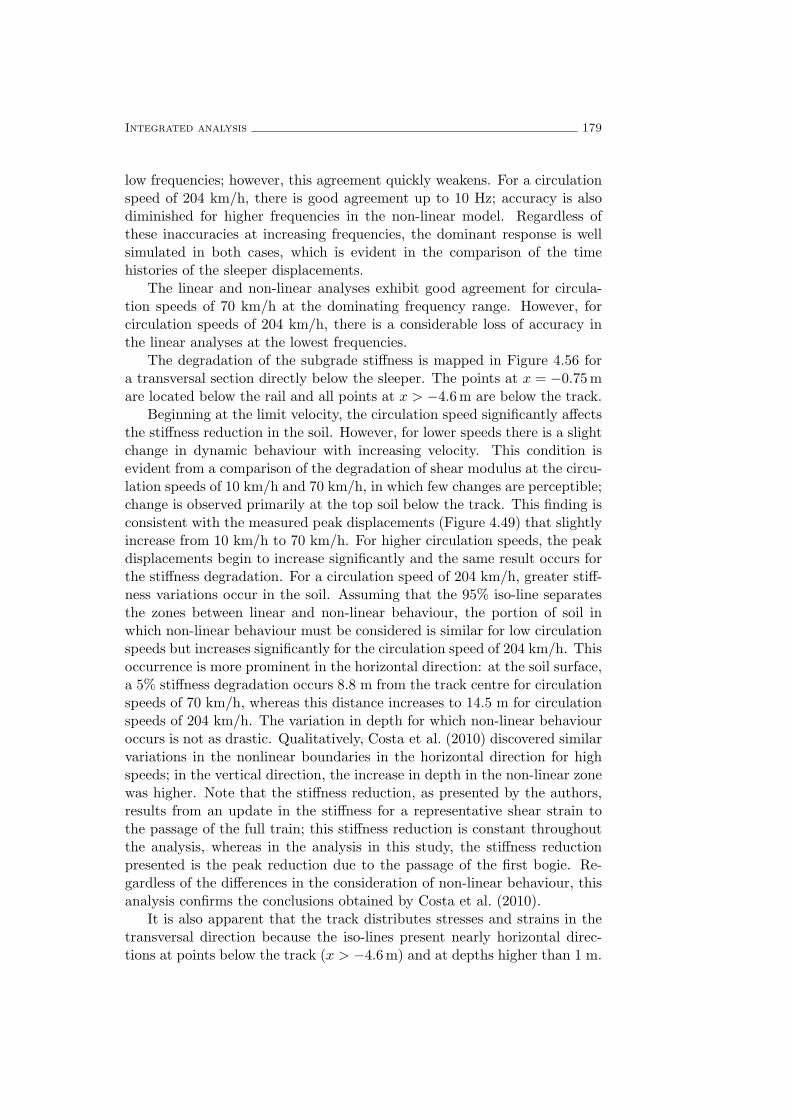
Integrated analysis 179
low frequencies; however, this agreement quickly weakens. For a circulationspeed of 204 km/h, there is good agreement up to 10 Hz; accuracy is alsodiminished for higher frequencies in the non-linear model. Regardless ofthese inaccuracies at increasing frequencies, the dominant response is wellsimulated in both cases, which is evident in the comparison of the timehistories of the sleeper displacements.
The linear and non-linear analyses exhibit good agreement for circula-tion speeds of 70 km/h at the dominating frequency range. However, forcirculation speeds of 204 km/h, there is a considerable loss of accuracy inthe linear analyses at the lowest frequencies.
The degradation of the subgrade stiffness is mapped in Figure 4.56 fora transversal section directly below the sleeper. The points at x = −0.75mare located below the rail and all points at x > −4.6m are below the track.
Beginning at the limit velocity, the circulation speed significantly affectsthe stiffness reduction in the soil. However, for lower speeds there is a slightchange in dynamic behaviour with increasing velocity. This condition isevident from a comparison of the degradation of shear modulus at the circu-lation speeds of 10 km/h and 70 km/h, in which few changes are perceptible;change is observed primarily at the top soil below the track. This finding isconsistent with the measured peak displacements (Figure 4.49) that slightlyincrease from 10 km/h to 70 km/h. For higher circulation speeds, the peakdisplacements begin to increase significantly and the same result occurs forthe stiffness degradation. For a circulation speed of 204 km/h, greater stiff-ness variations occur in the soil. Assuming that the 95% iso-line separatesthe zones between linear and non-linear behaviour, the portion of soil inwhich non-linear behaviour must be considered is similar for low circulationspeeds but increases significantly for the circulation speed of 204 km/h. Thisoccurrence is more prominent in the horizontal direction: at the soil surface,a 5% stiffness degradation occurs 8.8 m from the track centre for circulationspeeds of 70 km/h, whereas this distance increases to 14.5 m for circulationspeeds of 204 km/h. The variation in depth for which non-linear behaviouroccurs is not as drastic. Qualitatively, Costa et al. (2010) discovered similarvariations in the nonlinear boundaries in the horizontal direction for highspeeds; in the vertical direction, the increase in depth in the non-linear zonewas higher. Note that the stiffness reduction, as presented by the authors,results from an update in the stiffness for a representative shear strain tothe passage of the full train; this stiffness reduction is constant throughoutthe analysis, whereas in the analysis in this study, the stiffness reductionpresented is the peak reduction due to the passage of the first bogie. Re-gardless of the differences in the consideration of non-linear behaviour, thisanalysis confirms the conclusions obtained by Costa et al. (2010).
It is also apparent that the track distributes stresses and strains in thetransversal direction because the iso-lines present nearly horizontal direc-tions at points below the track (x > −4.6m) and at depths higher than 1 m.

180
(a)
0.95
0.90
0.80
0.70
−14 −4.6 −0.75−14
−8.6
−4.1
−1.1
x [m]
y[m
]
(b)
0.95
0.90
0.80
0.70
−14 −4.6 −0.75−14
−8.6
−4.1
−1.1
x [m]
y[m
]
(c)
0.95
0.90
0.80
0.70
0.60
0.50
−14 −4.6 −0.75−14
−8.6
−4.1
−1.1
x [m]
y[m
]
Figure 4.56: Peak stiffness reductions Gsec
G0due to the passage of the X-2000
front bogie at a) 10 km/h, b) 70 km/h and c) 204 km/h.
Integrated analysis 181
For the dry crust layer, the soil portions directly below the rail are subject tomaximum non-linear behaviour; however, for the other layers the variationin non-linear behaviour with horizontal position is extremely limited for allportions directly below the track. The stress and strain variations in thesoil are also analysed (Figure 4.57).
(a)
0 2000 4000 6000 8000 10000 12000 14000
−14
−8.6
−4.1
−1.1
τ [Pa]
y[m
]
(b)
0 0.5 1 1.5 2 2.5 3 3.5
x 10−3
−14
−8.6
−4.1
−1.1
y[m
]
γ
Figure 4.57: Variation with depth of a) shear stress τ and b) shear strain γ inthe soil directly below the rail for circulation velocity of 10 km/h (dashed),70 km/h (grey) and 204 km/h (black).
Few changes occur in the soil due to the increase in speeds from 10km/h to 70 km/h, with the most prominent changes appearing at the top.As expected, substantially higher stress and strain variations occur in thesoil at circulation speeds of 204 km/h. These differences are significant at

182
low depths and reduce with increasing depth, whereas non-linear behaviourbecomes less relevant. Nevertheless, even at 14 m depth, the stresses andstrains are higher for circulation speeds of 204 km/h. There is also a ten-dency of the stresses and strains to increase in the vicinity of the interfacebetween the different layers. The stresses in the dry crust layer (0 m to 1.1m depth) are approximately 3 times higher for the circulation speed of 204km/h than at 70 km/h, this is where the highest differences between bothcirculation speeds occur. Conversely, the average shear strains in the organicclay are higher than the average shear strains in the dry crust for both cir-culation speeds because this layer exhibits much lower initial stiffness thanany other layer.
Figures 4.58 and 4.59 present the variation of shear stresses and strainsin the soil directly below the rail, for circulation speeds of 70 km/h and 204km/h.
When non-linear behaviour is considered, there is a considerable reduc-tion in stress at the dry crust for circulation speeds of 70 km/h because thisis where most stiffness degradation occurs and the stresses are redistributedto the remaining layers, whose stiffness is more similar to low strain stiffness.This result, however, does not occur at 204 km/h because a larger portionof the soil presents stiffness degradation. Consequently, the stress can bedistributed to fewer zones.
At the top layers, there is a significant difference between shear strainsin the linear and non-linear analyses for circulation speeds of 70 km/h; thisdifference reflects the resulting soil degradation. However, for speeds of 204km/h, the differences in shear strain are much greater, which further high-lights that non-linear behaviour is more relevant for increasing circulationspeeds and, therefore, the linear analyses are less accurate.
4.4.5 Partial remarks
This section presents the analysis of a railway track by integrating the non-linear behaviour of embankment and subgrade. In the case studied, thenon-linear response of the track leads to extreme vibrations and, therefore,the consideration of non-linearity is necessary to obtain adequate predic-tions.
Due to the limitations of the track size and required computational re-sources, the non-linear analysis incorporated only the simulation of the firsttrain bogie. The simulations confirmed that non-linear behaviour plays animportant role in track response. Beginning with a certain velocity, themagnitude of the non-linear response increases with increased train circula-tion. At 70 km/h, the linear analysis demonstrates considerable accuracyin the prediction of the sleeper displacements. At 204 km/h, the results ofthe linear analysis are very inaccurate, whereas the non-linear analysis yieldsignificant improvement. The stiffness degradation is very similar for circu-

Integrated analysis 183
(a)
0 1000 2000 3000 4000 5000 6000 7000
−14
−8.6
−4.1
−1.1
τ [Pa]
y[m
]
(b)
0 0.2 0.4 0.6 0.8 1 1.2
x 10−3
−14
−8.6
−4.1
−1.1
y[m
]
γ
Figure 4.58: Variation with depth of a) shear stress τ and b) shear strain γin the soil directly below the rail for circulation velocity of 70 km/h in thelinear (grey) and non-linear (black) analysis.
lation speeds of 10 km/h and 70 km/h; however, at 204 km/h, substantialdifferences are obtained with a considerable increase in the zone in whichnon-linear behaviour is obtained. The study of the stresses and strains inthe soil provide similar conclusions because these values are very similar forthe two lowest circulation speeds at most depths. However, considerablyhigher stresses and strains occur at the highest circulation speed to depthsof 10 m.

184
(a)
0 2000 4000 6000 8000 10000 12000 14000
−14
−8.6
−4.1
−1.1
τ [Pa]
y[m
]
(b)
0 0.5 1 1.5 2 2.5 3 3.5
x 10−3
−14
−8.6
−4.1
−1.1
y[m
]
γ
Figure 4.59: Variation with depth of a) shear stress τ and b) shear strain γin the soil directly below the rail for circulation velocity of 204 km/h in thelinear (grey) and non-linear (black) analysis.
Conclusions 185
4.5 Conclusions
This chapter presents the isolated studies of non-linear ballast and subgrademodelling, with an emphasis on their influence in track response and theintegration of non-linearity in a railway track simulation. The ballast wasmodelled using a modified Mohr-Coulomb constitutive model with shear,tensile and compressive caps, and hardening/softening of the shear and com-pressive caps. The non-linear behaviour of the subgrade was obtained usinga cyclic non-linear model that follows the hysteresis curve of the soil be-haviour by using Iwan’s parallel model. In both cases, comparisons betweenthe results obtained with the linear models are presented.
In the study of non-linear behaviour of ballast, it was demonstrated thatballast has significant influence in track response, especially if the definitionof its small strain stiffness is unclear or its variation with isotropic stressis not considered. The definition of limiting caps in the p : q space isalso advisable; even though its influence seems lower than the influence ofthe pressure dependent stiffness. The results of this study, and the resultsobtained by Araujo (2011) indicate that the isotropic pressure of the ballastin service falls predominantly between 5 kPa and 50 kPa. Therefore, it issuggested that future experimental studies of track ballast focus mainly onits behaviour within this range. In both cases, the track peak displacementsmay be considerably influenced by the consideration of non-linearity, butthe peak particle velocities are less influenced by the consideration of non-linearity.
In the case of the subgrade, stiffness reductions greater than 50% of thesmall strain value may occur in the soil immediately below the track. Theselarge stiffness reductions are very localised in time and space. The linearand equivalent linear analyses may provide an estimation of the subgradezone in which non-linear behaviour occurs. In addition, the accuracy of thelinear equivalent behaviour analyses are improved compared with the linearcases.
The study of the Ledsgard site is a rare case in which nonlinear em-bankment and subgrade are considered in the simulation of a track stretch.As concluded by Costa et al. (2010) and Banimahd and Woodward (2007),this consideration of the importance of non-linear behaviour of track re-sponse increases significantly with circulation speed. This notion, however,is only valid when the circulation speed surpasses a threshold value. Atlower speeds, only slight changes in non-linear behaviour are evident. Athigher circulation speeds, the stiffness reduction in the soil and the zonein which non-linear behaviour occurs increase significantly. The obtainedresults indicate that the non-linear 3D FE can be an accurate tool for pre-dicting track response to train passage. However, simulation of non-linearbehaviour of the full train was not possible.
Summarizing the contributions of this chapter, the influence of non-

186
linear behaviour of ballast and subgrade on track response was examined.In this study, relevant information about stress and strain distributions inthe track and soil were obtained, in the transversal and longitudinal direc-tions of the track. The implementation of the cyclic non-linear model is animportant contribution that provides the first 3D simulation of a railwaytrack with cyclic non-linear soil response, which complements the equiva-lent linear analyses of Costa et al. (2010) and non-linear elastic analyses ofBanimahd and Woodward (2007). Although the model can be improved insome regards, it is an invaluable tool that performs innovative analyses. Theintegrated simulation of the Ledsgard railway track, in which the non-lineartrack response is accurately predicted, presents an important contribution asa 3D FE methodology. This simulation facilitates the study of the influenceof circulation speed on stiffness degradation of the soil and the distributionof stresses and strains with depth.

Chapter 5
Main Summary
5.1 Main conclusions and contributions
This thesis presents a study of the numerical prediction of railway trackresponse to the passage of high-speed trains. It is mainly focused on the in-fluence of non-linear material behaviour on track ballast and subgrade. Thisstudy is conducted using 3D FE models, which generated another focus ofthe thesis: to emphasise the advantages and disadvantages of this numericalmethod for this type of simulation.
In Chapter 2, the most common numerical methods and the knowledgegained about railway response were explored. It was concluded that non-linear behaviour is seldom considered in these simulations, especially forthose simulations in which the full track-soil system is modelled. The ob-jectives of this thesis were formulated.
Chapter 3 has a twofold objective: to study the elastodynamics of thelinear soil-track system and validate the adopted FE simulation methodol-ogy. It was confirmed that although the track simulation may be accurateconsidering only the quasi-static moving load, the response away from thetrack requires the consideration of the dynamic components of the load. Itwas concluded that the FEM obtained accurate transfer functions to thefree field; however, this required a very refined mesh which was only ac-complished using a 2D mesh with axisymmetry. When a 3D FE mesh wasemployed, an increased element side had to be adopted that diminished ac-curacy at high frequencies. In spite of this result, the 3D FE mesh obtainedrail receptances and transfer functions between the track and the nearbysubgrade that were similar to those computed by the validated 2.5D mod-els. This finding indicates that the mesh is well suited for modelling railwaytrack response. The 3D FE also obtains a similar rail response to the pas-sage of a moving load, which validates the methodology that was adoptedto simulate moving loads.
Chapter 4 considers non-linear behaviour of the ballast and soil due to
187

188
high-speed train circulation. This main contribution is derived from the factthat non-linear behaviour has seldom been considered in railway track simu-lation, especially in 3D simulations and large-track models. This innovativestudy allowed to formulate the following remarks:
• The non-linear ballast behaviour influences track response with higherpeak displacements and velocities than predicted by linear models.
• Simultaneously considering non-linear ballast behaviour and stress-dependent stiffness predicts distinct results than when consideringthese characteristics separately. Therefore, the consideration of bothcharacteristics is essential for obtaining more accurate ballast re-sponses.
• An accurate determination of the small strain properties of ballastand the consideration of pressure-dependent stiffness may more sig-nificantly influence model response than by the consideration of non-linear behaviour.
• Stresses and strains in ballast are primarily concentrated directly be-low the rail at the contact point with the sleeper, and diminish radiallyfrom this point.
• Stresses in ballast portions between two sleepers are significantly anal-ogous to the stresses in portions directly below the sleepers. Thetransversal distribution of the stresses is also similar in both cases.
• The main differences between the stress paths of crib ballast andsleeper ballast are discovered at the top of the layer. At the bottomlayer, the stress paths are very similar.
• A cyclic non-linear model was implemented that allows the FE sim-ulated soil to follow the hysteresis loops. This model follows Iwan’sparallel model and the Masing rules to determine the relationship be-tween shear stress and shear strain in the material.
• The implemented model obtains a perfect reproduction of the stiffnessreduction with shear strain. The Masing rules imply that an incorrectdamping formulation occurs for shear strains of 1 × 10⁻⁴ and higher;the model also does not consider the variation of material behaviourwith mean stress.
• The non-linear simulation showed that there is a considerable reduc-tion in stiffness of the soil, which may be less than 50% of its initialvalue. The greatest reduction in stiffness is confined to a very smallsoil portion and a very restricted time span.

Future developments 189
• For the equivalent linear analysis, the horizontal layering of soil stiff-ness distribution is sufficient for nearly all soil depths, except for thetop 1 to 2 m, in which a more refined distribution below the track ismore appropriate.
• Both the linear and equivalent linear models present a fairly accu-rate estimation of the boundaries between linear and non-linear soilbehaviour.
• The equivalent linear analysis is an improvement upon the linear case,and allows for an interesting approximation of the results of the non-linear approaches, with much less complexity.
• Consideration of the effective shear strain as 65% of the peak shearstrain results in a good estimation of the soil stiffness reduction.
• The simulation of the Ledsgard railway track demonstrates that thereare cases in which the consideration of non-linear behaviour is essentialto obtain adequate prediction of track response.
• The presented non-linear 3D FE methodology accurately predicts rail-way track response. However, due to the high computational needs ofthe model, only the response to the passage of the first bogie wascomputed.
• The relevance of non-linear behaviour increases with circulation speed.Consequently, for low circulation speeds, the linear analyses presentgood accuracy in railway track response, which is not the case forhigher speeds where non-linear analyses are required.
• The stiffness degradation profile in the soil is also highly influenced bycirculation speed.
5.2 Future developments
The development of these analyses and the interpretation of the results leadsto the realisation that further investigation of this subject is needed. Some ofthese new evaluations will eventually become possible as expanded compu-tational capabilities facilitate enhanced complexity of the models. Althoughthis thesis proves that the 3D FE models can be used to accurately simulaterailway track behaviour, the models still require further understanding, op-timisation, computational resources and computational time to deem themfully functional for works other than research. On the other hand, 2.5Dmodels are much more computationally effective and provide equally accu-rate predictions of the track displacements, and are definitely better suitedto predict propagation of waves to the free field. However, these models do

190
not allow for such a detailed study of the ballast response as the one donein this thesis. Even though non-linear behaviour can be simulated with theequivalent linear analyses, real non-linear behaviour with prediction of per-manent deformations is not possible. Moreover, if available in commercialpacks these are not so user friendly as some FE software. It is the opinionof the author that with the referred increasing capacity of computers, mostdisadvantages of 3D FE computations may fade away making it the bestoption for railway track response prediction. Accounting for these improve-ments in the computational resources, it is suggested the following futureworks:
• Utilization of increasingly large 3D FE meshes allowing for the mod-elling of the full train passage in non-linear behaviour of ballast andsoil.
• Study of the increasing accuracy in the track response prediction oc-curring from the utilization of similar mesh geometry but with muchmore refinement.
• Study of non-linear track and soil response due to the quasi-static anddynamic train loads. These would result from the increase of accuracyat higher frequencies due to improved mesh refinement.
• Comparison between 3D FEM and 3D DEM non-linear ballast re-sponse to moving loads and train circulation. This requires the simu-lation of a representative track stretch.
• 3D DEM study of the differences between inter-particle forces occur-ring in a ballast portion directly below the sleeper and a ballast portionbetween sleepers.
Other developments stemming from the presented works can be sug-gested that do not depend upon the increase of computational resources:
• Simulation of damping evolution at high strains of the implementedcyclic non-linear model. This requires the abandonment of the Mas-ing rule for reload/unload and could be achieved by the utilization ofa factor dependent upon the shear strain level that would scale thestiffness of the Iwan elements when a stress reversal occurs.
• Study of the possibility to include stress dependent small strain prop-erties in the implemented cyclic non-linear model, as well as stressdependent stiffness reduction curves and consequently damping varia-tion curves. A power law relating the mean stress and stiffness of theIwan elements should be sufficient for modelling the low strain stiff-ness. However, to obtain equally accurate stiffness reduction curves, itcould require the definition of a second law relating the mean pressureand the slip-stress of the elements.

Future developments 191
• Parametric study of the accuracy of equivalent linear analyses for arepresentative effective shear strain.
• Study of the long-term track behaviour. This development can leadto very important considerations regarding the influence of the trackproperties in the maintenance frequency, leading to direct implicationsin the design and long-term cost of new tracks and consequently in lifecycle cost analyses.


Bibliography
J.D. Achenbach. Wave propagation in elastic solids, volume 16 of North-Holland Series in Applied Mathematics and Mechanics. North-Holland,Amsterdam, The Netherlands, 1973.
M. Adam, G. Pflanz, and G. Schmid. Two- and three-dimensional modellingof half-space and train-track embankment under dynamic loading. SoilDynamics and Earthquake Engineering, 19:559–573, 2000.
A. Al Shaer, D. Duhamel, K. Sab, G. Foret, and L. Schmitt. Experimentalsettlement and dynamic behavior of a portion of ballasted railway trackunder high speed trains. Journal of Sound and Vibration, (316), 2008.
L. Andersen and S.R.K. Nielsen. Reduction of ground vibration by meansof barriers or soil improvement along a railway track. Soil Dynamics andEarthquake Engineering, 25:701–716, 2005.
N. Araujo. High-speed trains on ballasted railway track - Dynamic stressfield analysis. PhD thesis, Universidade do Minho, Guimaraes, Portugal,2011.
D. Assimaki and E Kausel. An equivalent linear algorithm with frequency-and pressure-dependent moduli and damping for the seismic analysis ofdeep sites. Soil Dynamics and Earthquake Engineering, 22:959–965, 2002.
M. Banimahd and P.K. Woodward. Numerical study of train speed effect onrailway track response. In Proceedings of the 9th International Conferencein Railway Engineering, London, United Kingdom, 2007.
D.D. Barkan. Dynamics of bases and foundations. McGraw-Hill, New York,1962.
G. A. Beckey and S.F. Masri. Random search techniques for optimisation ofnonlinear systems with many parameters. Math Comput Simulation, 25:210–213, 1983.
J.P. Berenger. A perfectly matched layer for the absorption of electromag-netic waves. Journal of Computational Physics, 41:115–135, 1994.
193

194
P. Bettess. Infinite elements. Penshaw Press, Sunderland, United Kingdom,1992.
M.A. Biot. Bending of infinite beams on an elastic foundation. Journal ofApplied Mechanics, Transactions of the ASME, 59:A1–A7, 1937.
F. B. Bonnett. Practical Railway Engineering. Imperial College Press, Lon-don, 2005.
H. Brandl. Geotechnical aspects for high-speed railways. In Proceedingsof the International Seminar on Geotechnics in Pavement and RailwayDesign and Construction, Rotterdam, Netherlands, 2004.
S. F. Brown and F. L. Hyde. Significance of cyclic confining stress inrepeated-load triaxial testing of granular material. Transportation Re-search Record, 537:49–58, 1975.
C. Cekerevac, S. Girardin, G. Klubertanz, and L. Laloui. Calibration of anelasto-plastic constitutive model by a constrained optimisation procedure.Computers and Geotechnics, 33:432–443, 2006.
E. Celebi. Three-dimensional modelling of train-track and sub-soil analysisfor surface vibrations due to moving loads. Applied Mathematics andComputation, 179:209–230, 2006.
P. Chatterjee, G. Degrande, D. Clouteau, T. Al-Hussaini, M. Arnst, andR. Othman. Numerical modelling of ground borne vibrations from un-derground railway traffic. In Proceedings of the 6th National Congress onTheoretical and Applied Mechanics, Ghent, Belgium, May 2003. NationalCommittee for Theoretical and Applied Mechanics.
H. Chebli, D. Clouteau, and L. Schmitt. Dynamic response of high-speedballasted railway tracks: 3D periodic model and in situ measurements.Soil Dynamics and Earthquake Engineering, 28:118–131, 2008.
Y.P. Cheng, Y. Nakata, and M.B. Bolton. Discrete element simulation ofcrushable soil. Geotechnique, 53(7):19–29, 2003.
W.C. Chew and Q.H. Liu. Perfectly matched layers for elastodynamics: Anew absorbing boundary condition. Journal of Computational Acoustics,4(4):341–359, 1996.
D. Clouteau, M.L. Elhabre, and D. Aubry. Periodic BEM and FEM-BEMcoupling: application to seismic behaviour of very long structures. Com-putational Mechanics, 25:567–577, 2000.
D. Clouteau, G. Degrande, and G. Lombaert. Numerical modellingof traffic induced vibrations. Meccanica, 36(4):401–420, 2001. URLhttp://dx.doi.org/10.1023/A:1015005410628.

Bibliography 195
D. Clouteau, R. Othman, M. Arnst, H. Chebli, G. Degrande, R. Klein,P. Chatterjee, and B. Janssens. A numerical model for ground-borne vi-brations from underground railway traffic based on a periodic FE-BE for-mulation. In D. Thompson and C. Jones, editors, 8th International Work-shop on Railway Noise, volume 1, pages 167–178, Buxton, UK, September2004.
T. F. Coleman and Y. Li. On the convergence of reflective Newton methodsfor large-scale nonlinear minimization subject to bounds. MathematicalProgramming, 67(2):189–224, 1994.
T. F. Coleman and Y. Li. An interior, trust region approach for nonlinearminimization subject to bounds. SIAM Journal on Optimization, 6:418–445, 1996.
F. Collino and C. Tsogka. Application of the perfectly matched absorbinglayer model to the linear elastodynamic problem in anisotropic heteroge-neous media. Geophysics, 66, 2001.
A.P. Costa, R. Calcada, S. A. Cardoso, and A. Bodare. Influence of soilnon-linearity on the dynamic response of high-speed railway tracks. SoilDynamics and Earthquake Engineering, 30:221–235, 2010.
A.P. Costa, R. Calcada, and S. A. Cardoso. Trackground vibrations inducedby railway traffic: In-situ measurements and validation of a 2.5D FEM-BEM model. Soil Dynamics and Earthquake Engineering, 32:111–128,2012.
T. Dahlberg. Railway track dynamics - a survey. Technical report, SolidMechanics/IKP, Linkping University, 2003.
M.B. Darendeli. Development of a new family of normalized modulus re-duction and material damping. PhD thesis, University of Texas, Austin,2001.
T.M. Dawn and C.G. Stanworth. Ground vibrations from passing trains.Journal of Sound and Vibration, 66(3):355–362, 1979.
G. Degrande and G. Lombaert. High-speed train induced free field vi-brations: in situ measurements and numerical modelling. In N. Chouwand G. Schmid, editors, Proceedings of the International Workshop Wave2000, Wave propagation, Moving load, Vibration reduction, pages 29–41,Ruhr University Bochum, Germany, December 2000. A.A. Balkema, Rot-terdam. URL ../papers/degrip00b.pdf.
G. Degrande and L. Schillemans. Free field vibrations dur-ing the passage of a Thalys high-speed train at variable speed.

196
Journal of Sound and Vibration, 247(1):131–144, 2001. URLhttp://dx.doi.org/10.1006/jsvi.2001.3718.
G. Degrande, P. Chatterjee, D. Clouteau, T. Al-Hussaini, M. Arnst, andR. Othman. A numerical prediction model for ground-borne vibrationsfrom underground railway traffic using a coupled periodic FEM-BEM ap-proach. In 10th International Congress on Sound and Vibration, Stock-holm, Sweden, July 2003. CD-ROM.
N. Deng, S.A. Ashford, and J. Lysmer. Ground2d: A two-dimensional seis-mic site response analysis program. Technical report, Earthquake Engi-neering Research Center, University of California, Berkeley, 1995.
J. Domınguez. Boundary elements in dynamics. Computational MechanicsPublications and Elsevier Applied Science, Southampton, United King-dom, 1993.
G. Eason. The stresses produced in a semi-infinite solid by a moving surfaceforce. International Journal of Engineering Science, 2:581–609, 1965.
T. Ekevid and N. Wiberg. Wave propagation related to high-speed train. Ascaled boundary FE-approach for unbounded domains. Computer Methodsin Applied Mechanics and Engineering, 191:3947–3964, 2002.
C. Esveld. Modern Railway Track. MRT Productions, Duisburg, WestGermany, 1989.
W.M. Ewing, W.S. Jardetzky, and F. Press. Elastic waves in layered media.McGraw-Hill, New York, Toronto, London, 1957.
P. Fiala, G. Degrande, and F. Augusztinovicz. Numerical modelling ofground borne noise and vibration in buildings due to surface rail traf-fic. Journal of Sound and Vibration, 301(3-5):718–738, 2007. URLhttp://dx.doi.org/10.1016/j.jsv.2006.10.019.
S. Francois, M. Schevenels, and G. Degrande. BEMFUN: MATLAB toolboxfor boundary elements in elastodynamics. Version 2.1 Build 16. User’sguide. Department of Civil Engineering, KU Leuven.
S. Francois, M. Schevenels, P. Galvin, G. Lombaert, and G. Degrande. A2.5D coupled FE-BE methodology for the dynamic interaction betweenlongitudinally invariant structures and a layered halfspace. ComputerMethods in Applied Mechanics and Engineering, 199(23-24), 2010.
L. Fryba. Vibration of solids and structures under moving loads. NoordhoffInternational Publishing, Groningen, 1973.

Bibliography 197
Y. Furumoto, M. Sugito, and A. Yashima. Frequency-dependent equivalentlinearized technique for FEM response analysis of ground. In Proceed-ings of the 12th World Conference in Earthquake Engineering (CD-ROM),Auckland,New Zealand, 2000.
P. Galvın and J. Domınguez. High-speed train-induced ground motion andinteraction with structures. Journal of Sound and Vibration, 307:755–777,2007.
P. Galvın and J. Domınguez. Experimental and numerical analyses of vibra-tions induced by high-speed trains on the CordobaMalaga line. ElectronicJournal of Geotechnical Engineering, 29:641–657, 2009.
P. Galvın, S. Francois, M. Schenevels, E. Bongini, G. Degrande, and G. Lom-baert. A 2.5D coupled FE-BE model for the prediction of railway inducedvibrations. Soil Dynamics and Earthquake Engineering, 30(12), 2010.
W. Gardien and H.G. Stuit. Modelling of soil vibrations from railway tun-nels. Journal of Sound and Vibration, 267:605–619, 2003.
P.E. Gill, W. Murray, and M.H. Wright. Practical Optimization. AcademicPress: London, 1981.
C. Gonzalez-Nicieza, M.I. Alvarez Fernandez, A. Menendez-Dıaz, A.E.Alvarez Vigil, and F. Ariznavarreta-Fernandez. Failure analysis of con-crete sleepers in heavy haul railway tracks. Engineering Failure Analysis,15:90–117, 2008.
K.F. Graff. Wave motion in elastic solids. Ohio State University, 1975.
A. E. Groen. Elastoplastic modelling of sand using a conventional model.Technical report, Delft University of Technology, 1995.
S. Gupta, G. Degrande, H. Chebli, D. Clouteau, M.F.M. Hussein, andH.E.M. Hunt. A numerical model for prediction of vibration from un-derground railways. In 7th World Congress on Computational Mechanics,Los Angeles, California, USA, July 2006a.
S. Gupta, P. Fiala, M.F.M. Hussein, H. Chebli, G. Degrande, F. Auguszti-novicz, H.E.M. Hunt, and D. Clouteau. A numerical model for ground-borne vibrations and re-radiated noise in buildings from underground rail-ways. In P. Sas and M. De Munck, editors, Proceedings of ISMA2006 In-ternational Conference on Noise and Vibration Engineering, pages 1741–1756, Leuven, Belgium, September 2006b.
T.G. Gutowski and C.L. Dym. Propagation of ground vibration: A review.Journal of Sound and Vibration, 2(49):179–193, 1976.

198
W. Haegeman. In situ tests Retie-Waremme-Lincent. Report RUGIV.1.16.3, Soil Mechanics Laboratory, Ghent University, September 2001.STWW Programme Technology and Economy, Project IWT-000152.
L. Hall. Simulations and analyses of train-induced ground vibrations in finiteelement models. Soil Dynamics and Earthquake Engineering, 23:403–413,2003.
M. Heelis, A. Dawson, A. Collop, D. Chapman, and V. Krylov. Resilientmodulus of soft soil beneath high-speed rail lines. Transportation ResearchRecord, 1687:39–46, 1999.
G. Holm, B. Andreasson, P. Bengtsson, A. Bodare, and H. Eriksson. Miti-gation of track and ground vibrations by high speed trains at Ledsgard,Sweden. Technical report, Swedish Deep Stabilization Research Centre,2002.
Z. Hossain, B. Indraratna, F. Darve, and P. K. Thakur. DEM analysis ofangular ballast breakage under cyclic loading. Geomechanics and Geotech-nical Engineering, 2(3), 2007.
D. V. Hutton. Fundamentals of finite element analysis. McGraw-Hill, NewYork, 2004.
I.M. Idriss and J.I. Sun. SHAKE91: a computer program for conductingequivalent linear seismic response analysis of horizontally layered deposits.Users Guide. University of California.
I.M. Idriss, D. Dobry, and R.D. Singh. Nonlinear behavior of soft claysduring cyclic loading. Journal of Geotechnical Engineering, Proceedingsof the ASCE, 104(12):1427–1447, 1978.
B. Indraratna and S. Nimbalkar. Implications of ballast breakage on bal-lasted railway track based on numerical modelling. In Proceedings ofthe , 13th International Conference of the International Association forComputer Methods and Advances in Geomechanics, Melbourne, Australia,2011.
B. Indraratna, L. S. S. Wijewardena, and A. S. Balasubramaniam. Large-scale triaxial testing of graywacke rockfill. Geotechnique, 43(1):37–51,1993.
B. Indraratna, D. Ionescu, and H. D. Christie. Shear behaviour of railwayballast based on large-scale triaxial tests. Journal of Geotechnical andGeoenvironmental Engineering, Proceedings of the ASCE, 124(5):439–449,1998.

Bibliography 199
B. Indraratna, J. Lackenby, and D. Christie. Effect of confining pressureon the degradation of ballast under cyclic loading. Geotechnique, 55(4):325–328, 2005a.
B. Indraratna, J. S. Vindod, and J. Lackenby. Influence of particle breakageon the resilient modulus of railway ballast. Geotechnique, 59(7):643–646,2005b.
I. Ishibashi. Discussion of ”Effect of soil plasticity on cyclic response” by M.Vucetic and R. Dobry. Journal of Geotechnical Engineering, Proceedingsof the ASCE, 118(5):830–832, 1992.
I. Ishibashi and X. Zhang. Unified dynamic shear moduli and damping ratiosof sand and clay. Soils and Foundations, 33(1):182–191, 1993.
K. Ishihara. Soil behaviour in earthquake geotechnics, volume 46 of OxfordEngineering Science Series. Clarendon Press, Oxford, United Kingdom,1996.
K. Ishihara, N. Yoshida, and S. Tsujino. Modelling of stress strain rela-tions of soils. In Proceedings, Fifth International Conference on NumericalMethods in Geomechanics, Nagoya, Japan, 1985.
Itasca. PFC 2D. Particle Flow Code in 3 Dimensions. Online Manual Tableof Contents. http://www.itascacg.com/.
W.D. Iwan. On a class of models for the yielding behaviour of continuousand composit systems. Journal of Applied Mechanics, Transactions of theASME, 34:612–617, 1967.
S.H. Ju, J.R. Liao, and Y.L. Ye. Behavior of ground vibrations induced bytrains moving on embankments with rail roughness. Soil Dynamics andEarthquake Engineering, 30:1237–1249, 2010.
A. Karlstrom and A. Bostrom. An analytical model for train-induced groundvibrations from railways. Journal of Sound and Vibration, 292:221–241,2006.
E. Kausel. An explicit solution for the Green functions for dynamic loads inlayered media. Technical report, Massachusetts Institute of Technology,1981.
E. Kausel and J.M. Roesset. Stiffness matrices for layered soils. Bulletin ofthe Seismological Society of America, 71(6):1743–1761, 1981.
A.M. Kaynia, C. Madshus, and P. Zackrisson. Ground vibration from highspeed trains: prediction and countermeasure. Journal of Geotechnical andGeoenvironmental Engineering, Proceedings of the ASCE, 126(6):531–537,2000.

200
T. Kokusho. A cyclic triaxial test of dynamic soil properties for wide strainrange. Soils and Foundations, 20:45–60, 1980.
A. Kouby, E. Burgeois, and F. Rocher-Lacoste. Subgrade improvementmethod for existing railway lines an experimental and numerical study.Electronic Journal of Geotechnical Engineering, 15:461–494, 2010.
G. Kouroussis, O. Verlinden, and C. Conti. Free field vibrations caused byhigh-speed lines: Measurement and time domain simulation. Soil Dynam-ics and Earthquake Engineering, 31:692–707, 2011.
S.L. Kramer. Geotechnical earthquake engineering. Prentice-Hall, UpperSaddle River, New Jersey, 1996.
J. Lackenby, B. Indraratna, G. McDowell, and D. Christie. Effect of confin-ing pressure on ballast degradation and deformation under cyclic triaxialloading. Geotechnique, 57(6):527–536, 2007.
H. Lamb. On the propagation of tremors over the surface of an elastic solid.Philosophical Transactions of the Royal Society, A203:1–42, 1904.
J.S. Lee, Y.W. Choo, and D.S. Kim. A modified parallel IWAN modelfor cyclic hardening behavior of sand. Soil Dynamics and EarthquakeEngineering, 29(4):630–640, 2009.
F. Lekarp, U. Isacsson, and A. Dawson. State of the art. I: Resilient re-sponse of unbound aggregates. Journal of Transportation Engineering,Proceedings of the ASCE, 126(1):66–75, 2000a.
F. Lekarp, U. Isacsson, and A. Dawson. State of the art. II: Permanent strainresponse of unbound aggregates. Journal of Transportation Engineering,Proceedings of the ASCE, 126(1):76–83, 2000b.
W.L. Lim. Mechanics of Railway Ballast Behaviour. PhD thesis, Universityof Nottingham, Nottingham, United Kingdom, 2004.
W.L. Lim and G.R. McDowell. Discrete element modelling of railway ballast.Granular Matter, (7):19–29, 2005.
S. Lobo-Guerrero and L. E. Vallejo. Discrete element method analysis ofrailtrack ballast degradation during cyclic loading. Granular Matter, 8:195–204, 2006.
G. Lombaert. Development and experimental validation of a numeri-cal model for the free field vibrations induced by road traffic. PhDthesis, Department of Civil Engineering, K.U.Leuven, 2001. URL../papers/lomb01a.pdf.

Bibliography 201
G. Lombaert and G. Degrande. Ground-borne vibration due to static anddynamic axle loads of intercity and high-speed trains. Journal of Soundand Vibration, 319:1036–1066, 2009.
G. Lombaert, G. Degrande, J. Kogut, and S. Francois. The experimentalvalidation of a numerical model for the prediction of railway induced vi-brations. Journal of Sound and Vibration, 297(3-5):512–535, 2006. URLhttp://dx.doi.org/10.1016/j.jsv.2006.03.048.
F. Lopez-Caballero, A. Modaressi, and S. D’Aguiar. Amelioration du modelede comportement non lineaire existant dans le logiciel CyberQuake. Tech-nical report, Ecole Centrale Paris, 2004.
M. Lu and G. R. McDowell. The importance of modelling ballast particleshape in the discrete element method. Granular Matter, 9:69–80, 2007.
M. Lu and G. R. McDowell. Discrete element modelling of railway ballastunder triaxial conditions. Geomechanics and Geotechnical Engineering, 3(4), 2008.
J. Lysmer and R.L. Kuhlemeyer. Finite dynamic model for infinite media.Journal of the Engineering Mechanics Division, Proceedings of the ASCE,95(EM4):859–877, 1969.
J. Lysmer, T. Udaka, C.F. Tsai, and H.B. Seed. Flush: a computer pro-gram for approximate 3D analysis of soil-structure interaction problems.Technical report, Earthquake Engineering Research Center, University ofCalifornia, Berkeley, 1975.
C. Madshus and A.M. Kaynia. High-speed railway lines on soft ground: dy-namic behaviour at critical train speed. Journal of Sound and Vibration,231(3):689–701, 2000.
J. Martins, A. Gomes Correia, L.F. Ramos, J. Marcelino, L. Caldeira, andJ. Delgado. Measurement of vibrations induced by high-speed trains. InProceedings of the Eighth International Conference on the Bearing Capac-ity of Roads, Railways and Airfields, Champaign, Illinois, USA, 2009.
N. Matasovic and M. Vucetic. Generalized cyclic-degradation pore-pressuregeneration model for clays. Journal of Geotechnical Engineering, Proceed-ings of the ASCE, 121(1):33–42, 1995.
Matlab 7.6.0.324. The Mathworks Inc., 2005.
J.J. More and D.C. Sorensen. Computing a trust region step. SIAM Journalon Scientific and Statistical Computing, 23:553–572, 1983.

202
A. Nataatmajda. Significance of cyclic confining stress in repeated loadtriaxial test: a reconsideration. In Proceedings of the 2nd InternationalConference on Road and Airfield Pavement Technology, Vol.2, Singapore,1995.
S. Nazarian and M.R. Desai. Automated surface wave method: field testing.Journal of Geotechnical Engineering, Proceedings of the ASCE, 119(7):1094–1111, 1993.
V. Nguyen, D. Duhamel, and B. Nedjar. A continuum model for granularmaterials taking into account the no-tension effect. Mechanics of Materi-als, (35), 2003.
J. O’Brien and D.C. Rizos. A 3D FEM-BEM methodology for simulationof high speed train induced vibrations. Soil Dynamics and EarthquakeEngineering, 25:289–301, 2005.
C. Paderno. Simulation of ballast behaviour under traffic and tamping pro-cess. In 9th Swiss Transport Research Conference, Lausanne, Switzerland,2009.
C. Phillips and Y.M.A. Hashash. Damping formulation for nonlinear 1Dsite response analyses. Soil Dynamics and Earthquake Engineering, 29:1143–1158, 2009.
L. Pronzato, E. Walter., A. Venot, and J-F. Lebruchec. A general pur-pose global optimiser: implementation and applicaitons. Math ComputSimulation, 26:412–422, 1984.
R.M. Pyke. Nonlinear soil models for irregular cyclic loadings. Journal ofthe Geotechnical Engineering Division, 105(6), 1979.
L. Pyl and G. Degrande. Determination of the dynamic soil characteris-tics with the SASW method at a site in Lincent. Report BWM-2001-02,Department of Civil Engineering, K.U.Leuven, August 2001. STWW Pro-gramme Technology and Economy, Project IWT-000152.
G. P. Raymond and J. R. Davies. Triaxial test on dolomite railroad ballast.Journal of the Soil Mechanics and Foundation Division, Proceedings ofthe ASCE, 104(6):737–751, 1978.
P.K. Robertson, R.G. Campanella, D. Gillespie, and A. Rice. Seismic CPTto measure in situ shear wave velocity. Journal of the Soil Mechanics andFoundation Division, Proceedings of the ASCE, 112(8):791–803, 1986.
P.W. Rowe. The stress-dilatancy relation for static equilibrium of an assem-bly of particles in contact. In Proceedings of the Royal Society of London.Series A, Mathematical and Physical Sciences, pages 500–527, 1962.

Bibliography 203
J. Sadrekarimi and M. Akbarzad. Comparative study of methods of determi-nation of coefficient of subgrade reaction. Electronic Journal of Geotech-nical Engineering, 14, 2009.
G. Saussine, C. Cholet, P.E. Gautier, F. Dubois, C. Bohatier, and J.J.Moreau. Modelling ballast behaviour under dynamic loading. Part 1: A2D polygonal discrete element method approach. Comput. Methods Appl.Mech. Engrg., 195:2841–2859, 2006.
M. Schevenels, G. Degrande, and S. Francois. EDT: an ElastoDynamicsToolbox for Matlab. In Proceedings of the Inaugural International Confer-ence of the Engineering Mechanics Institute (EM08), Minneapolis, Min-nesota, U.S.A., May 2008.
P.B. Schnabel, J. Lysmer, and H.B. Seed. Shake: a computer programfor earthquake response analysis of horizontally layered sites. Technicalreport, Earthquake Engineering Research Center, University of California,Berkeley, 1972.
E.T. Selig and J.M. Waters. Track Geotechnology and Substructure Man-agement. Thomas Telford, London, 1994.
X. Sheng, C.J.C. Jones, and M. Petyt. Ground vibration generated by aharmonic load acting on a railway track. Journal of Sound and Vibration,225(1):3–28, 1999.
X. Sheng, C.J.C. Jones, and D.J. Thompson. A comparison of a theoreticalmodel for quasi-statically and dynamically induced environmental vibra-tion from trains with measurements. Journal of Sound and Vibration, 267(3):621–635, 2003.
X. Sheng, C.J.C. Jones, and D.J. Thompson. A theoretical model for groundvibration from trains generated by vertical track irregularities. Journal ofSound and Vibration, 272(3-5):937–965, 2004.
X. Sheng, C.J.C. Jones, and D.J. Thompson. Prediction of ground vibrationfrom trains using the wavenumber finite and boundary element methods.Journal of Sound and Vibration, 293:575–586, 2006.
L. Shuangyang, L. Yuanming, Z. Shujuan, Y. Yugui, and Y. Wenbing. Dy-namic responses of Qinghai-Tibet railway embankment subjected to trainloading in different seasons. Soil Dynamics and Earthquake Engineering,32:1–14, 2012.
A.S.J. Suiker. The mechanical behaviour of ballasted railway tracks. PhDthesis, Delft University of Technology, 2002.

204
A.S.J. Suiker and R. de Borst. A numerical model for the cyclic deterio-ration of railway tracks. International Journal for Numerical Methods inEngineering, 57(4):441–470, 2003.
A.S.J. Suiker, R. de Borst, and C. Esveld. Critical behaviour of a timo-shenko beam half-plane system under a moving load. Archive of AppliedMechanics, 68:158–168, 1998.
A.S.J. Suiker, E.T. Selig, and R. Frenkel. Static and cyclic triaxial testingof ballast and subballast. Journal of Geotechnical and GeoenvironmentalEngineering, Proceedings of the ASCE, pages 771–782, 2005.
H. Takemiya. Simulation of track-ground vibrations due to a high-speedtrain: the case of X-2000 at Ledsgard. Journal of Sound and Vibration,261:503–526, 2003.
K.V. Terzaghi. Evaluation of coefficient of subgrade reaction. Geotechnique,5:297–326, 1955.
TNO. Diana 9. http://tnodiana.com/, 2005.
E. Tutumluer, H. Huang, and Y.M.A. Hashash. Discrete element modelingof railroad ballast settlement. In Proceedings of the AREMA 2007 AnnualConferences, Chicago, Illinois, USA, 2007.
E. Tutumluer, H. Huang, Y.M.A. Hashash, and J. Ghaboussi. Arema grada-tions affecting ballast performance using discrete element modeling (dem)approach. In Proceedings of the AREMA 2009 Annual Conference & Ex-position, Chicago, Illinois, USA, 2009.
M. Vucetic and R. Dobry. Effect of soil plasticity on cyclic response. Jour-nal of Geotechnical Engineering, Proceedings of the ASCE, 117(1):89–107,1991.
G.X. Wang and J. Kuwano. Modeling of strain dependency of shear modulusand damping of clayey sand. Soil Dynamics and Earthquake Engineering,18:463–471, 1999.
D.S. Watkins. Fundamentals of Matrix Computations. John Wiley & Sons,Inc., New York, 2002.
W. White, S. Valliappan, and I.K. Lee. Unified boundary for finite dynamicmodels. Journal of the Engineering Mechanics Division, Proceedings ofthe ASCE, 103(EM5):949–964, 1977.
J.P. Wolf and C. Song. Finite-element modelling of unbounded media. JohnWiley and Sons, 1996.

Bibliography 205
S.E. Wright. Damage caused to ballast by mechanical maintenance tech-niques. Technical report, British Rail Research Technical Memorandum,1983.
Y.B. Yang, H.H. Hung, and D.W. Chang. Train-induced wave propagationin layered soils using finite/infinite element simulation. Soil Dynamicsand Earthquake Engineering, 23:263–278, 2003.
Z. Yang and A. Elgamal. Application of unconstrained optimization andsensitivity analysis to calibration of a soil constitutive model. Interna-tional Journal for Numerical and Analytical Methods in Geomechanics,27:1277–1297, 2003.
D. Yuan and S. Nazarian. Automated surface wave method: inversion tech-nique. Journal of Geotechnical Engineering, Proceedings of the ASCE,119(7):1112–1126, 1993.


Appendix A
Iwan parallel model
The definition of the material properties in the implemented Iwan materialmodel is defined in a data file which is read by the Diana software. Anexample of such a material model is shown here:
5 YOUNG 1.5969E+08
POISON 3.000000E-01
DENSIT 2.000000E+03
RAYLEI 3.4060 6.4501e-005
USRMAT
USRVAL 1.5969E+08 3.00E-01 4.3872E6 14
USRSTA 0 0 0 0 0 0 0 0 0 0 0 0 0 0 0 0 1 1 1
1 1 1 1 1 1 1 1 1 1 1
USRIND 94 194 247 436 483 680 1189 1219 1356
1632 1797 3111 4618 24697
The first four lines refer to the usual definition of a linear elastic materialmodel in Diana software (TNO, 2005). All variables defined in this field areused in Diana software for the initial predictions of the material behaviour,the external sub-routine does not have access to these values. The firstnumber is a referral to the material model, in this case all elements withmaterial model 5 will behave according to the parameters described above.The first to fourth parameters are the material Young’s modulus, Poisson’sratio, volumetric mass and Rayleigh damping coefficients respectively. Inthis case the units used all SI.
The fifth line refers that the following parameters are to be used in anexternal, user defined, material model. The Diana software is oblivious tothe meaning of these parameters, it only communicates with the externalroutine the values of these parameters at the beginning of the integrationand receives (and stores) values of the variables at the end of the iteration.The first set of parameters is a set of constant values, in this case as theexternal routine doesn’t have access to the small strain properties defined
207
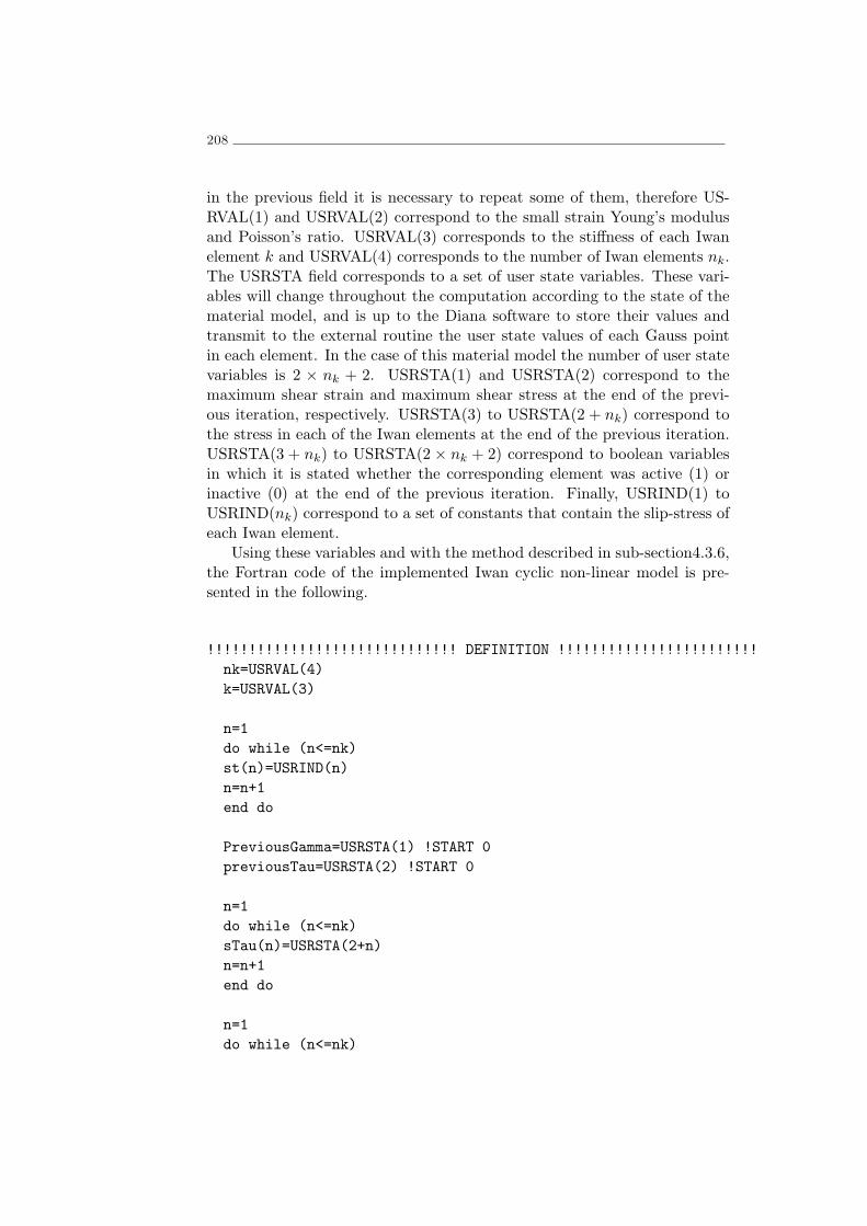
208
in the previous field it is necessary to repeat some of them, therefore US-RVAL(1) and USRVAL(2) correspond to the small strain Young’s modulusand Poisson’s ratio. USRVAL(3) corresponds to the stiffness of each Iwanelement k and USRVAL(4) corresponds to the number of Iwan elements nk.The USRSTA field corresponds to a set of user state variables. These vari-ables will change throughout the computation according to the state of thematerial model, and is up to the Diana software to store their values andtransmit to the external routine the user state values of each Gauss pointin each element. In the case of this material model the number of user statevariables is 2 × nk + 2. USRSTA(1) and USRSTA(2) correspond to themaximum shear strain and maximum shear stress at the end of the previ-ous iteration, respectively. USRSTA(3) to USRSTA(2 + nk) correspond tothe stress in each of the Iwan elements at the end of the previous iteration.USRSTA(3 + nk) to USRSTA(2 × nk + 2) correspond to boolean variablesin which it is stated whether the corresponding element was active (1) orinactive (0) at the end of the previous iteration. Finally, USRIND(1) toUSRIND(nk) correspond to a set of constants that contain the slip-stress ofeach Iwan element.
Using these variables and with the method described in sub-section4.3.6,the Fortran code of the implemented Iwan cyclic non-linear model is pre-sented in the following.
!!!!!!!!!!!!!!!!!!!!!!!!!!!!!! DEFINITION !!!!!!!!!!!!!!!!!!!!!!!!
nk=USRVAL(4)
k=USRVAL(3)
n=1
do while (n<=nk)
st(n)=USRIND(n)
n=n+1
end do
PreviousGamma=USRSTA(1) !START 0
previousTau=USRSTA(2) !START 0
n=1
do while (n<=nk)
sTau(n)=USRSTA(2+n)
n=n+1
end do
n=1
do while (n<=nk)

Appendix A. Iwan parallel model 209
bol(n)=USRSTA(2+nk+n)
n=n+1
end do
tempTau=USRSTA(2)
!!!!!!!!!!!!!!!!!!!!!!!!!!!COMPUTE DELTAGAMMA!!!!!!!!!!!!!!!!!!!
ma(1,1)=DEPS(1)+EPS0(1)
ma(2,1)=DEPS(4)/2+EPS0(4)/2
ma(3,1)=DEPS(6)/2+EPS0(6)/2
ma(1,2)=DEPS(4)/2+EPS0(4)/2
ma(2,2)=DEPS(2)+EPS0(2)
ma(3,2)=DEPS(5)/2+EPS0(5)/2
ma(1,3)=DEPS(6)/2+EPS0(6)/2
ma(2,3)=DEPS(5)/2+EPS0(5)/2
ma(3,3)=DEPS(3)+EPS0(3)
call qrmet(ma, princi)
sigma1=maxval(princi)
sigma3=minval(princi)
DeltaGamma=sign(1.00,princi(1)*princi(2)*princi(3))*
$ (sigma1-sigma3)-PreviousGamma
tempDeltaGamma=DeltaGamma
!!!!!!!!!!!!!!!!!!!!!!!!!!!COMPUTE MAIN !!!!!!!!!!!!!!!!!!!!!!
s=1
do while (s<=nk)
if (abs(sTau(s))<st(s) .OR. sTau(s)*tempDeltaGamma<0) then
dTaus=sTau(s)+tempDeltaGamma*k
if (dTaus>=st(s)) then
tautoblow=st(s)-sTau(s)
tempDeltaGamma=tempDeltaGamma-(tautoblow)/k
c=s
do while (c<=nk)
sTau(c)=sTau(c)+tautoblow

210
c=c+1
end do
bol(s)=0
elseif (dTaus<=-st(s)) then
tautoblow=-st(s)-(stau(s))
tempDeltaGamma=tempDeltaGamma-(tautoblow)/k
c=s
do while (c<=nk)
sTau(c)=sTau(c)+tautoblow
c=c+1
end do
bol(s)=0
else
sTau(s)=dTaus
bol(s)=1
endif
else
bol(s)=0
endif
s=s+1
end do
!!!!!!!!!! COMPUTE UPDATED STIFFNESS MATRIX !!!!!!!!!!!!!!!!!
redfac=sum(bol)/nk
YOUNG=USRVAL(1)*redfac
POIS=USRVAL(2)
G=YOUNG/(2*(1+POIS))
LAMDA=YOUNG*POIS/((1+POIS)*(1-2*POIS))
STIFFN=STIFFN*0
STIFFN(1,1)=LAMDA+2*G
STIFFN(2,2)=STIFFN(1,1)
STIFFN(3,3)=STIFFN(1,1)
STIFFN(2,1)=LAMDA
STIFFN(1,2)=STIFFN(2,1)
STIFFN(1,3)=STIFFN(2,1)

Appendix A. Iwan parallel model 211
STIFFN(3,1)=STIFFN(2,1)
STIFFN(2,3)=STIFFN(2,1)
STIFFN(3,2)=STIFFN(2,1)
STIFFN(4,4)=G
STIFFN(5,5)=G
STIFFN(6,6)=G
!!!!!!!!!!!! COMPUTE UPDATED STRESS VECTOR !!!!!!!!!!!!!!!!!
Tau=sum(sTau)
G2=(Tau-previousTau)/(DeltaGamma)
G0=USRVAL(1)/(2*(1+POIS))
redfac2=G2/G0
YOUNG2=USRVAL(1)*redfac2
LAMDA2=YOUNG2*POIS/((1+POIS)*(1-2*POIS))
SECMAT=SECMAT*0
SECMAT(1,1)=LAMDA2+2*G2
SECMAT(2,2)=SECMAT(1,1)
SECMAT(3,3)=SECMAT(1,1)
SECMAT(2,1)=LAMDA2
SECMAT(1,2)=SECMAT(2,1)
SECMAT(1,3)=SECMAT(2,1)
SECMAT(3,1)=SECMAT(2,1)
SECMAT(2,3)=SECMAT(2,1)
SECMAT(3,2)=SECMAT(2,1)
SECMAT(4,4)=G2
SECMAT(5,5)=G2
SECMAT(6,6)=G2
!!!!!!!!!!!!!!!!!!!! UPDATE VARIABLES !!!!!!!!!!!!!!!!!!!!!!!!
SIG = SIG + MATMUL(SECMAT, DEPS)
STIFF=STIFFN
USRSTA(1)=sign(1.00,princi(1)*princi(2)*princi(3))*
$ (sigma1-sigma3)
USRSTA(2)=Tau
n=1
do while (n<=nk)
USRSTA(2+n)=sTau(n)

212
n=n+1
end do
n=1
do while (n<=nk)
USRSTA(2+nk+n)=bol(n)
n=n+1
end do
RETURN
END

Appendix B
The matrix eigenvalue
problem
B.1 Introduction
The eigenvalue problem has been studied by many researchers for manydecades. In the scope of numeric determination of the eigenvalues of a givenmatrix, it has been proved by Abel’s theorem that it is not possible to solvethe eigenvalue problem using a direct method. Consequently all methods todetermine the eigenvalues are iterative methods Watkins (2002).
The QR decomposition of a matrix is one of the most important op-erations in linear algebra being used to invert a matrix to solve a set ofsimulation operations or in numerous applications in scientific calculation.The decomposition’s purpose is fairly simple: given a matrix A, decomposeit into two matrices Q and R such that Q is an orthogonal matrix QT×Q = I,R is an upper diagonal matrix and Q×R = A. The advantage of producingsuch a decomposition of matrix A is that by inverting the the multiplica-tion of Q and R the result is a matrix A1 that is unitarily similar to A andconsequently they have the same eigenvalues. This in itself does not solvethe problem as the eigenvalues of A1 are also unknown. The biggest gainin this procedure is that matrix A1 is slightly closer to an upper-diagonalform than the original matrix A, consequently if the QR decomposition andmultiplication R×Q are consecutively applied to matrices A1,A2, ...An thefinal result will be a matrix which is upper triangular (the values of theelements bellow the diagonal are neglectable) and whose eigenvalues appearin the main diagonal in descending order of magnitude.
B.2 Householder reflectors
There are several methods for doing the QR decomposition such as theGrand-Schmitt orthonormalization, Householder reflectors or Givens rota-
213

214
tions. Each of them has advantages and disadvantages depending on thetype of problems involved. It is evident that the QR method convergesmore rapidly when using matrices in the Hessenberg form instead of fullmatrices. The Householder reflectors allow to compute the Q matrix in anHessenberg form in order to improve the convergence of the QR method.
The Householder reflection may be described with aid of a 2D example(Figure B.1). Considering a line l passing through the origin it is pretendedto reflect any given vector through that line. A rotation of the coordinatesystem may be conveniently chosen such that one of the axes v coincideswith l and the other u is perpendicular to l. Assuming that there is a vectorx that can be written with vectors v and u
x = αu+ βv (B.1)
its reflection w through line l will be
w = −αu+ βv (B.2)
l
v ux
w
Figure B.1: Reflection of vector x along the line l.
assuming a reflector operator Q it must satisfy:
Q (αu+ βv) = −αu+ βv (B.3)
A the method by which a solution is obtained is beyond the scope of thiswork, however a solution for the reflector operator is:
Q = I− γuuT (B.4)

Wilkinson Shift 215
in which I is the identity matrix, γ is given by:
γ =2
‖u‖22(B.5)
and u is given by:
u = x− α (B.6)
in which α = [σ00] and σ = ‖u‖2. Equation B.13 can be reorganized:
Q = I− 2u
‖u‖2uT
‖u‖2(B.7)
B.3 Wilkinson Shift
In many cases it is numerically advantageous to shift the computation ofthe QR algorithm from the Matrix A to a matrix A− µI. If the value of µis criteriously chosen the convergence of the QR algorithm may be largelyimproved. For the shifted QR algorithm the computation of A1 may bederived:
A− µI = Q×R (B.8)
⇔ A1 = R×Q+ µI (B.9)
⇔ A1 = Qt(A− µI)Q+ µI (B.10)
⇔ A1 = Qt ×A×Q (B.11)
For the consideration of µ must be taken into account the types of ma-trices whose eigenvalues are to be computed and the advantages of eachof the shifts that are available. To ensure the stability of the process, theWilkinson shift was chosen. This shift has quadratic convergence in theworst case scenarios but ensures that convergence is always achieved. Forthe interpretation of the problem, consider a matrix B that corresponds tothe lower-right 2× 2 sub-matrix of A:
B =
[b11 b12b21 b22
]
The Wilkinson shift corresponds to the eigenvalue of B that is closer tob22. The Wilkinson shift may be stably computed using:
µ = b22 −sign(δ)b212
(|δ|+√δ2 + b212)
(B.12)
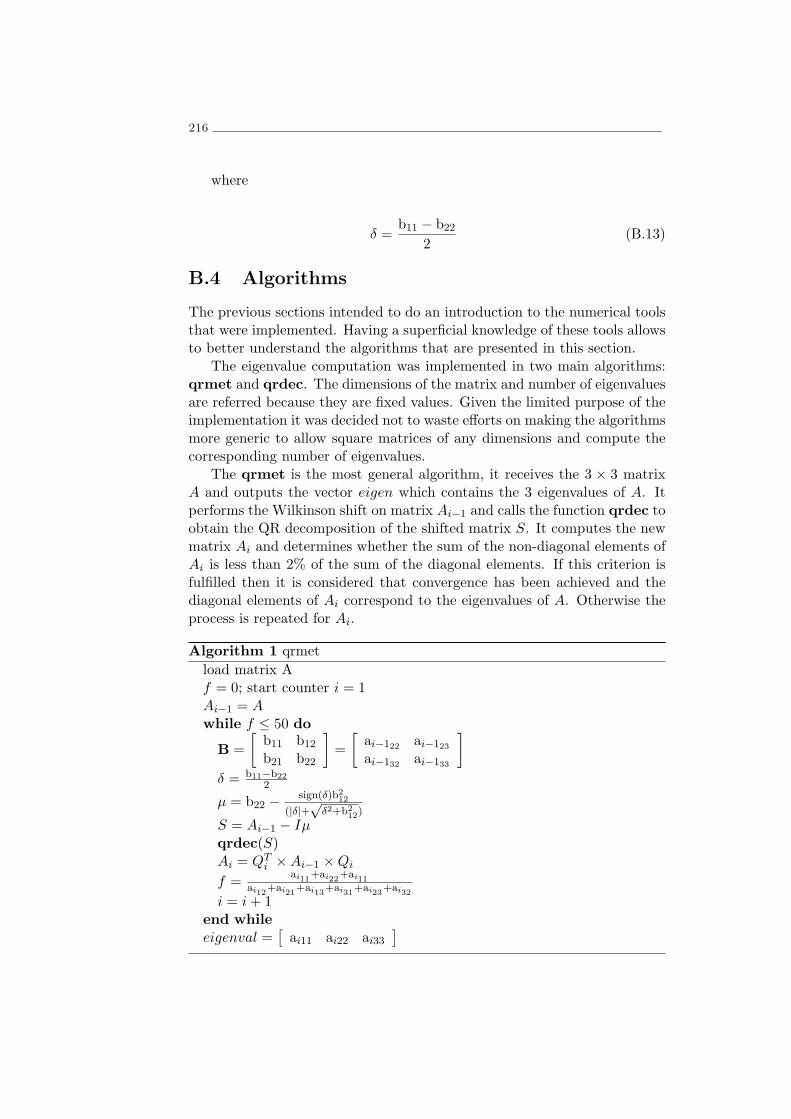
216
where
δ =b11 − b22
2(B.13)
B.4 Algorithms
The previous sections intended to do an introduction to the numerical toolsthat were implemented. Having a superficial knowledge of these tools allowsto better understand the algorithms that are presented in this section.
The eigenvalue computation was implemented in two main algorithms:qrmet and qrdec. The dimensions of the matrix and number of eigenvaluesare referred because they are fixed values. Given the limited purpose of theimplementation it was decided not to waste efforts on making the algorithmsmore generic to allow square matrices of any dimensions and compute thecorresponding number of eigenvalues.
The qrmet is the most general algorithm, it receives the 3 × 3 matrixA and outputs the vector eigen which contains the 3 eigenvalues of A. Itperforms the Wilkinson shift on matrix Ai−1 and calls the function qrdec toobtain the QR decomposition of the shifted matrix S. It computes the newmatrix Ai and determines whether the sum of the non-diagonal elements ofAi is less than 2% of the sum of the diagonal elements. If this criterion isfulfilled then it is considered that convergence has been achieved and thediagonal elements of Ai correspond to the eigenvalues of A. Otherwise theprocess is repeated for Ai.
Algorithm 1 qrmet
load matrix Af = 0; start counter i = 1Ai−1 = Awhile f ≤ 50 do
B =
[b11 b12b21 b22
]=
[ai−122 ai−123
ai−132 ai−133
]
δ = b11−b222
µ = b22 − sign(δ)b212
(|δ|+√
δ2+b212)
S = Ai−1 − Iµqrdec(S)Ai = QT
i ×Ai−1 ×Qi
f =ai11+ai22+ai11
ai12+ai21+ai13+ai31+ai23+ai32i = i+ 1
end while
eigenval =[ai11 ai22 ai33
]

Algorithms 217
The qrdec algorithm performs the QR decomposition of a 3× 3 matrix.
Algorithm 2 qrdec
load matrix SX =
[s11 s12 s13
]T
α =√
x21 + x22 + x23e =
[1 0 0
]Tu = X − αev = u
‖u‖2
clear X; α ; e;u and vQA = I − 2× vvT
RA = QA × S
RB =
[rb11 rb12rb21 rb22
]
X =[rb11 rb11
]T
α =√
x21 + x22e =
[1 0
]Tu = X − αev = u
‖u‖2
Qb = I − 2× vvT