METAS DE REDUÇÃO DA EMISSÃO DE GASES DE EFEITO ESTUFA …

1

METAS DE REDUÇÃO DA EMISSÃO DE GASES DE

EFEITO ESTUFA E INCERTEZAS NOS INVENTÁRIOS

Área temática: Gestão Ambiental e Sustentabilidade

Paulo Souza

[email protected]

Gutemberg Brasil

[email protected]

João Andrade Carvalho

[email protected]

André Castro

[email protected]

Resumo: Resultados de inventários de emissões diretas e anuais de gases de efeito estufa para 110

instalações industriais e para serviços são apresentadas. As incertezas associadas aos métodos de

cálculo das emissões de Gases de Efeito Estufa (GEE) foram também estimadas, e as consequências de

que estas incertezas produzirão impactos na estratégias de negócios são discutidas.

Palavras-chaves: Sustentabilidade, Mudanças climáticas, ISO 14064, Inventários de

GEE

ISSN 1984-9354

mailto:[email protected]

mailto:[email protected]

2

1. INTRODUÇÃO

Corporate greenhouse gas (GHG) inventories are being reported either as a

compulsory or as a voluntary initiative by almost all FT-500 companies. These inventories

are being used for different purposes; private disclosure (i.e., to shareholders and internal

decision makers only) or public disclosures (e.g., Government, other GHG monitoring

initiatives). Inventories have been closely observed by investors already for some years

(e.g., Carbon Disclosure Project (CDP) [CDP (2009]) and are part of sustainability reports

for large corporations [e.g., DJSI (2009)]. Therefore, they are already being used

effectively to guide some investors’ decisions.

Furthermore, GHG emission inventories can be used to support investments in

carbon reduction projects, as well as defining baseline emission scenarios and specific

emissions (e.g., tCO2/t product). It can also be used as the basis for further benchmarking

among industrial facilities in the same business sector. In addition, GHG accounting is

being used to neutralise activities, for example, carbon stocks in forestry can be purchased

to neutralise one’s own emissions [e.g., CN (2009)].

To the best of our knowledge, all the consulted corporate inventories listed in the

CDP, sustainability reports and other disclosure initiatives do not present the uncertainties

associated with their GHG emission inventories; this is not surprising considering the

enormous work associated with the calculation of uncertainties in emissions estimations.

Our results raise concerns over how much confidence businesses and investors can have

given the typical uncertainties we have obtained. In addition to presenting our results we

will discuss some possible ways to overcome this problem.

To illustrate this discussion with real data, we estimated GHG emissions in 110

industrial facilities in Brazil including organisations from the energy, mining, steelmaking,

logistics, energy and associated services. While calculating GHG emissions, uncertainties

associated with this assessment have been estimated.

2. GHG Inventories

Our inventories were calculated considering typical inputs of activity data and

emission factor (EF). Activity data include fuel volume or mass rates, raw material mass

rates and distance driven. The EF provides a relationship between how much a specific

GHG mass will be emitted by specific activity data. To undertake the greenhouse gas

3

inventory we applied the recommendations of the ISO 14064 [ISO,2006], the GHG

Protocol [WRI (2004)], and the IPCC [IPCC (2006, 1997)].

Uncertainties were estimated in both activity data and EF. For example, a type of

plant using calcite to produce CaO, has the uncertainty in its activity data coming from

road and conveyer-belt balances and on concentrations of carbon in the limestone. The

uncertainties in calculating the EF are associated with the efficiency of the process

(amount of carbonate left in the product) and how much carbon is effectively oxidized to

carbon dioxide (other forms would be carbon monoxide and carbon particles); the

uncertainties are then processed accordingly [e.g., IPCC (2006), Taylor (1997), EC (2004)

and ISO (1993)]. This exercise was conducted for all processes for the data presented here.

The calculation is expressed in the annual emission of a particular activity and the

associated uncertainties are shown.

3. Uncertainties in GHG Inventories

Uncertainties in our inventory vary from 3.25% (for a 0.0969 MtCO2e/year source)

up to 17.72% (for a 0.0257 MtCO2e/year source), all with a confidence interval of 95%.

Because the industries in which we performed the inventory are considered to be

modernised in terms of control, measurement and monitoring technologies, we expect that

they are representative of businesses in other sectors. As a result of this evaluation, we

would suggest that uncertainty levels should be disclosed in inventories. The IPCC

recommends typical uncertainties depending on tiers where their accuracy and complexity

increase with the sophistication of the method [e.g., IPCC (2000)]. We understand this can

be applied in the general case, but improving the quality of the information in the inventory

does not necessarily imply a decrease in uncertainty.

The calculation of uncertainties is not a straight forward activity. Operations within

the same company and within the same business can have their emissions added as part of

the generation of the inventory and the uncertainties will be accordingly combined

resulting in a figure which is smaller than the maximum uncertainty.

4. Results and Discussion

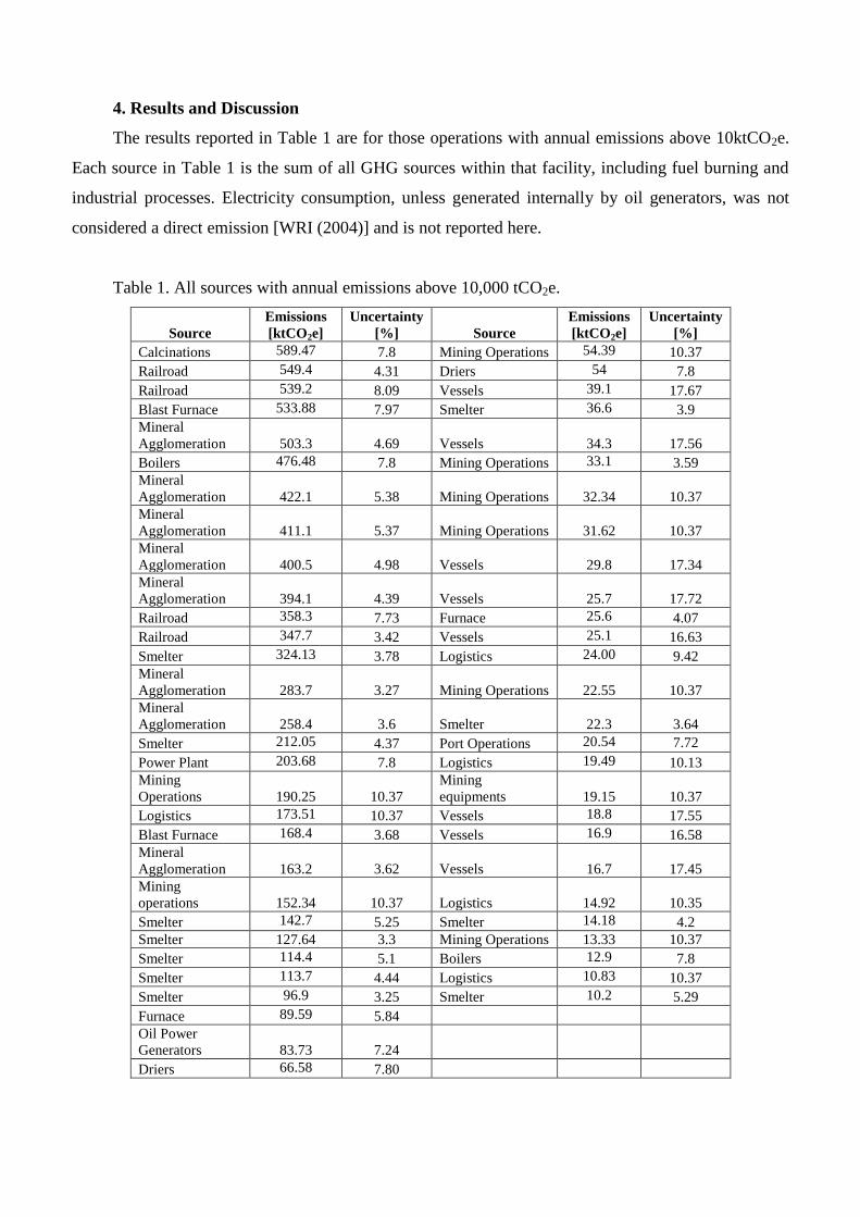
The results reported in Table 1 are for those operations with annual emissions above 10ktCO2e.

Each source in Table 1 is the sum of all GHG sources within that facility, including fuel burning and

industrial processes. Electricity consumption, unless generated internally by oil generators, was not

considered a direct emission [WRI (2004)] and is not reported here.

Table 1. All sources with annual emissions above 10,000 tCO2e.

Source

Emissions

[ktCO2e]

Uncertainty

[%] Source

Emissions

[ktCO2e]

Uncertainty

[%]

Calcinations 589.47 7.8 Mining Operations 54.39 10.37

Railroad 549.4 4.31 Driers 54 7.8

Railroad 539.2 8.09 Vessels 39.1 17.67

Blast Furnace 533.88 7.97 Smelter 36.6 3.9

Mineral

Agglomeration

503.3 4.69 Vessels

34.3 17.56

Boilers 476.48 7.8 Mining Operations 33.1 3.59

Mineral

Agglomeration

422.1 5.38 Mining Operations

32.34 10.37

Mineral

Agglomeration


31.62 10.37

Mineral

Agglomeration

400.5 4.98 Vessels

29.8 17.34

Mineral

Agglomeration

394.1 4.39 Vessels

25.7 17.72

Railroad 358.3 7.73 Furnace 25.6 4.07

Railroad 347.7 3.42 Vessels 25.1 16.63

Smelter 324.13 3.78 Logistics 24.00 9.42

Mineral

Agglomeration


22.55 10.37

Mineral

Agglomeration

258.4 3.6 Smelter

22.3 3.64

Smelter 212.05 4.37 Port Operations 20.54 7.72

Power Plant 203.68 7.8 Logistics 19.49 10.13

Mining

Operations

190.25 10.37

Mining

equipments

19.15 10.37

Logistics 173.51 10.37 Vessels 18.8 17.55

Blast Furnace 168.4 3.68 Vessels 16.9 16.58

Mineral

Agglomeration

163.2 3.62 Vessels

16.7 17.45

Mining

operations

152.34 10.37 Logistics

14.92 10.35

Smelter 142.7 5.25 Smelter 14.18 4.2

Smelter 127.64 3.3 Mining Operations 13.33 10.37

Smelter 114.4 5.1 Boilers 12.9 7.8

Smelter 113.7 4.44 Logistics 10.83 10.37

Smelter 96.9 3.25 Smelter 10.2 5.29

Furnace 89.59 5.84

Oil Power

Generators

83.73 7.24

Driers 66.58 7.80

XI CONGRESSO NACIONAL DE EXCELÊNCIA EM GESTÃO 13 e 14 de agosto de 2015

5

Uncertainties can be used to assess the quality of GHG inventories. Figure 1 presents the results

of our 110 industrial sources. While low emission sources can have high uncertainties without

impacting materially on the inventory figure, high emission sources cannot support such large

uncertainties as these results in significant variation to the reported figure. This plotting can also be

used to assess the quality of the inventory performed by the organisation and guide efforts towards

decreasing uncertainties in the inventory, either by inventing better measuring procedures or

technologies.

0.0 0.1 0.2 0.3 0.4 0.5 0.6

0

2

4

6

8

10

12

14

16

18

Un

ce

rta

inty

[%

]

Emission [MtCO2e]

Figure

1. Greenhouse gas emissions against the experimental uncertainty for 110 industrial facilities. In a

good GHG inventory, small emission sources can have high uncertainty, while sources with high

emission rates cannot have high uncertainty.

Voluntary or compulsory reduction targets and neutralisation of carbon emissions provided by

organisations, while widely announced, should also include a disclosure of the uncertainties involved

in their inventory. We therefore assert that reduction targets in GHG emissions below the level of

uncertainty in the inventory are unrealistic; unless there is some regular trend in the emissions being

recorded over a sustained period of time. This practice raises concerns because it guides the decisions


6

of investors, government policy (e.g., National Allocation Plans, National

Communications/Inventories), and stakeholder perception of the company performance concerning

climate change policy.

Table 2 provides a list of GHG reduction targets established by a number of US organisations.

The outcome of our study indicates that there may be at least a 4% uncertainty associated with the

assessment of GHG outputs, which may introduce some questions about the ability of organisations to

determine success against their commitments for reductions of similar scale to this level of uncertainty.

Conclusion:

From this evaluation there are a number of alternatives that could be encouraged to increase the

confidence in achieving measurable GHG targets including investing in decreasing measurement

uncertainties, adopting aggressive reduction targets such that reductions exceed the uncertainties or

including uncertainties to their emission figures.

Acknowledgements:

P. A. S. J. is grateful to INPE for his post-doc fellowship. The Tasmanian ICT Centre is jointly funded

by the Australian Government through the Intelligent Island Program and CSIRO. The Intelligent

Island Program is administered by the Tasmanian Department of Economic Development, Tourism

and the Arts. The authors are grateful to Stephen Giugni (CSIRO) for providing excellent comments

on a draft of this paper and for some data in Table 2.


7

Table 2. Excerpt from Climate Leaders. Some US Organisations participating in the Climate Leaders Program

(excerpt from ttp://www.epa.gov/climateleaders/documents/directory.pdf). The table identifies GHG target

reductions and the period over which the reduction program will be implemented. As a result of individual

industry sectoral considerations some organisations have adopted a target to reduce total GHG production, while

others have set normalised targets aimed at increased efficiency and are expressed as reduction in GHG per unit

of production or revenue.

Goals Reduction

Target [%]

Period Where Revenue normalised = GHG

per unit of production

Agilent Technologies 10 2006-2011 Worldwide

Alcoa 4 2008-2013 US

Anheuser-Busch 5 2005-2010 US

Bell Corporation 16 2002-2012 US per production index

Baltimore Aircoil 15 2004-2009 US per ton of steel

Campbell Soup

Company

12 2005-2010 US per adjusted case of product

Cisco 25 2007-2012 Worldwide

Citigroup 10 2005-2011 Worldwide

Coors 12 2005-2010 US

Cummins 25 2005-2010 Worldwide

Deere & Company 25 2005-2014 Worldwide

Dell 15 2007-2012 Worldwide per dollar of revenue

net zero GHG by 2008

DuPont 15 2004-2015 Worldwide

Eastman Kodak 10 2002-2008 Worldwide

Fairchild

Semiconductor

30 2003-2010 US per manufacturing index

Frito-Lay 14 2002-2010 US per pound of production

Gap 11 2003-2008 US per sq foot

General Electric 1 2004-2012 Worldwide

Intel 30 2004-2010 Worldwide per production unit

Johnson & Johnson 14 2001-2010 US

Lockheed-Martin 30 2006-2010 US per dollar of revenue

Marriott 6 2004-2010 US per available room

Merck 12 2004-2012 Worldwide

Millipore 20 2006-2011 Worldwide

Oracle 6 2003-2010 US per sq foot non data centre

space

Raytheon 33 2002-2009 US per dollar of revenue

Sprint 15 2007-2017 US

Boeing 1 2006-2011 US

World Bank 7 2006-2011 US

Unilever 25 2004-2012 Worldwide per ton of production

Volvo Trucks (North

America)

20 2003-2010 US per truck produced


8

References:

CDP (2009); Carbon Disclosure Project (2009 - 2015): http://www.cdproject.net/

CN (2009); Carbon Neutral: http://www.carbonneutral.com.au/

DJSI (2009);Dow Jones Sustainability Indexes (2009-20150: http://www.sustainability-index.com/ .

EC (2004); Environment Canada (2004), Guidance Manual for Estimating Greenhouse Gas Emissions

from Fuel Combustion and Process-Related Sources For: Iron and Steel Production, Environment

Canada, March.

IPCC (2006), 2006 IPCC Guidelines for National Greenhouse Gas Inventories, Prepared by the

National Greenhouse Gas Inventories Programme, Eggleston H.S., Buendia L., Miwa K., Ngara T. and

Tanabe K. (eds). Published: IGES, Japan. 2006.

IPCC (1997), revised 1996 IPCC Guidelines for national Greenhouse Gas Inventories Reporting

Instructions, 1997.

IPCC (2000); Good Practice Guidance and Uncertainty Management in National Greenhouse Gas

Inventories. Intergovernmental Panel on Climate Change.

Download at <http://www.ipcc-nggip.iges.or.jp/public/gp/gpgaum.htm>.

ISO (2006); International Organization for Standardization: ISO14064/2006 - Part 1: Specification

with guidance at the organization level for the quantification and reporting of greenhouse gas

emissions and removals; Part 2: Specification with guidance at the project level for the quantification,

monitoring and reporting of greenhouse gas emission reductions and removal enhancements; Part 3:

Specification with guidance for the validation and verification of greenhouse gas assertions. 2006;

ISO (1993) Guide to the Expression of Uncertainty in Measurement, International Organization for

Standardization, Geneva, Switzerland.

Taylor, J. R. (1997), An Introduction to Error Analysis, 2nd

edition, University Science Books,

Sausalito, CA, USA, 1997.

WRI (2004), World Business Council for Sustainable Development e World Resources Institute,

Greenhouse Gas Protocol – Corporate Module, Revised Edition, 2004.

http://www.cdproject.net/

http://www.carbonneutral.com.au/

http://www.sustainability-index.com/


9

Anexo: Abordagem adotada no tratamento das Incertezas

Nos casos específicos dos setores de mineração e siderurgia, as principais fontes de incerteza a ser

consideradas nas metodologias de cálculo das emissões, são aquelas existentes nas mensurações dos

dados de atividade e dos analisadores da qualidade dos insumos (composição química). As usinas de

produção de ferro e aço são intensivas no uso de energia e em atividades que geram emissões de GEE,

especialmente o dióxido de carbono (CO2). Na siderurgia a rota de produção adotada é de extrema

importância; por exemplo, a existência na planta de: redução, refino, laminação ou produção de coque.

Os principais insumos, fontes de carbono em uma usina siderúrgica são (de modo geral): coque, coque

de petróleo, carvão metalúrgico, antracito, carvão vegetal, óleo diesel, óleo combustível, GLP, gás

natural (GN). Existem também outros insumos que geram emissões nos processos siderúrgicos, tais

como: cal (calcítica ou dolomítica), calcário, ferro-ligas contendo carbono, resíduos e gases

recirculados. Esses fatores condicionam, essencialmente, a intensidade da emissão de gases de efeito

estufa (GEE) nas usinas siderúrgicas. Desse modo, as emissões dependerão do tipo de instalação

existente (sinterização, alto-forno, aciaria, laminação, utilidades) e do tipo de insumo utilizado nos

processos, bem como dos próprios processos. Ver Carvalho, Brasil e Souza (2007).

Desse modo, as principais fontes de incerteza consideradas nas metodologias de cálculo das emissões,

são aquelas existentes nas mensurações dos dados de atividade e dos analisadores da qualidade dos

insumos (composição química); Brasil, Souza e Carvalho (2008). Assim, devem ser considerados os

diversos equipamentos de medição, protocolos de calibração e a periodicidade observada nessas

calibrações. Particularmente importantes para o caso das emissões de GEE são os instrumentos

utilizados nas mensurações relacionadas a insumos contendo carbono, aos produtos finais, e

analisadores. Os principais instrumentos são: (i) balanças de pesagem dos Insumos, resíduos e

produtos finais; ii) analisadores; (iii) medidores do consumo de combustível; e, (iv) medidores de

vazão de gases (residuais e re-circulados).


10

Na avaliação das emissões, a abordagem usual utiliza, simplificadamente, para estimar as emissões dos

GEE específicos (i.e., CO2), a relação geral: ababxFEQEmissão ; onde:

a = Tipo de “insumo contendo carbono”;

b = Setor ou fonte de atividade;

abQ = Quantidade utilizada de “insumo contendo carbono”, do tipo “a” na fonte “b”;

abFE = Fator de emissão do “insumo contendo carbono” utilizado, do tipo “a” na fonte “b”.

Para o gás estufa metano (CH4), por exemplo, é necessário utilizar, de forma multiplicativa, o

potencial de aquecimento global (PAG = 21); considerem-se as observações de que as emissões desse

gás são muito mais influenciadas pela combustão e/ou tecnologia empregados, (GHG Protocol, 2008,

p. 9), IPCC (2006). Para a determinação das emissões escopo 2, relativas ao uso de energia elétrica os

fatores de emissão nacionais encontram-se em MCT (2008).

É recomendável verificar-se a existência de históricos de estimações similares. A escolha do método

de cálculo apropriado depende da disponibilidade dos dados (de atividade), dos fatores de emissão

específicos, das tecnologias de combustão utilizadas no processo, e outros. Qualquer que seja a

metodologia adotada, por exemplo, a que usa fatores de emissão, deve-se cuidar para aumentar a

consistência e a transparência, como recomenda o IPCC (2000, 2006). Por exemplo, certificando-se da

adequação dos fatores usados nos processos existentes em cada instalação e tomando cuidado com as

transformações das unidades.

Todas essas práticas são importantes na realização de inventários corporativos de emissões de GEE.

Por exemplo, a classificação dos dados em “tiers” ou “classes de rigor”; (IPCC, 2006, vol 1, p. 6). Um

“tier” representa um nível metodológico de complexidade. São considerados três “tiers”. O “tier” 1 é o

método básico, o “tier” 2 é um nível intermediário e o “tier” 3 é o mais complexo em temos de

exigências dos dados. Como é acentuado no GHG Protocol (2008, p. 8): “à medida que o “tier”

aumenta de 1 para 3, os valores tornam-se mais específicos para cada companhia”. Os métodos “tier”

3 exigem que os dados utilizados sejam específicos de cada instalação, tais como dados de atividade e

a composição do combustível utilizado e também os tipos específicos de tecnologia empregada,

quando pertinente. No “tier” 2 os fatores de emissão podem refletir “as práticas industriais típicas em

dado pais”. Essa escolha tem implicações diretas nas incertezas dos cálculos das emissões.


11

O IPCC (2006, Volume 3), trata das incertezas nas emissões de GEE nos “Processos industriais e uso

de produtos”. Os fatores de emissão para a produção de ferro e aço usados no “tier” 1 devem ter uma

incerteza de ±25%. Já as incertezas para o conteúdo específico de carbono nos materiais seriam em

torno de ±10%, no “tier” 2. Os conteúdos de carbono determinados para o “tier” 3 estariam dentro de

±5%. Por isso o IPCC recomenda que, quando possível, deve-se adotar o “tier” 3.

A propagação de incertezas via combinação de variâncias assume que as variáveis envolvidas são

aproximadamente independentes (pressuposto adotado pelo IPCC e verificado no inventário). No

entanto, se as variáveis apresentarem dependência, basta adequar as relações, que se tornam um pouco

mais complexas; ver por exemplo: Degroot and Schervish (2002); Hogg and Craig (2003); e Mood at

al (1974). Considere as variáveis aleatórias X e Y com médias X)X(E , Y)Y(E e variâncias

2X)X(V , 2

Y)Y(V , respectivamente.

Incertezas combinadas de forma aditiva: Z = X + Y

YX)Y(E)X(E]YX[E]Z[E

2Y

2X

)Y(V)X(V]YX[V]Z[V

2Y

2X

)Y(V)X(V]YX[V]Z[V

Incertezas combinadas de forma multiplicativa Z = X.Y

YXZ )Y(E).X(E]XY[E]Z[E

2Y

2X

2X

2Y

2Y

2X

2Z

]XY[V]Z[V

ZYX)Z(E).Y(E).X(E)XYZ(E)W(E 2z

2y

2x

2z

2y

2x

2z

2y

2x

2z

2y

2x

2z

2y

2x

2z

2y

2x

2z

2y

2x .............. V(W)

Incertezas combinadas na forma de quociente: Y

XZ

)Y(VY

XE]Z[E

3Y

X

Y

XZ

2Y

2X

2

Y

X )Y(V)X(V.

Y

XV]Z[V

Se as incertezas forem dadas em forma percentual, pode-se reportar uma quantidade média junto com

uma medida da incerteza dessa estimativa pela expressão:


12

)X(EP.zX ii

onde iX representa a quantidade média, z representa um p-quantil apropriado (o manual IPCC

recomenda p=0,95) e EP( iX ) é o erro padrão de iX . As incertezas percentuais associadas às fontes

são calculadas como:

i

ii

X

)X(EP.zU ; z = 1,96 ; i = 1, 2, ...n.

Combinação por adição: n1

2nn

211

TOTALXX

)UX()UX(U

onde:

TotalU = A Incerteza percentual na soma das quantidades (metade do intervalo de confiança de 95%

dividida pelo total, i.e. média, e expressa como percentagem). O termo incerteza é baseado no

intervalo de confiança de 95%.

iX e iU = As quantidades incertas (i.e., mensuradas com alguma incerteza) e as incertezas percentuais

associadas a elas, respectivamente.

Combinação por multiplicação: 2n

21TOTAL UUU

onde:

TotalU = A Incerteza percentual no produto das quantidades (metade do intervalo de confiança de 95%

dividido pelo total, i.e. média, e expresso como percentagem).

iU = As incertezas percentuais associadas a cada uma das quantidades.

Comentário

Na propagação das incertezas via variâncias (e também na forma percentual, para se ter uma

equivalência nos resultados), eventualmente deve-se computar uma estimativa do desvio padrão via

amplitude. Assim, estando disponível o erro de um equipamento como um percentual da medida

considerada, pode-se calcular uma estimativa do desvio padrão, simplesmente determinando-se os

valores máximos e mínimos esperados no entorno da mensuração média, calcular a amplitude, e obter

a estimava via relação usual.

Procedimento de Agregação


13

O inventário de GEE é principalmente a soma de produtos de Fatores de Emissão, Dados de Atividade

(consumo) e outros parâmetros de estimação. Logo, as equações de propagação podem ser usadas

repetidamente para estimar a incerteza do inventário total. Inicialmente via forma multiplicativa e, na

agregação final, via forma aditiva.

Referências Adicionais do Anexo

Brasil, Gutemberg Hespanha, Souza, Paulo Antônio e Carvalho, João Andrade, Inventários

Corporativos de Gases de Efeito Estufa: Métodos e Usos, Revista Eletrônica Sistemas & Gestão,

vol 3, nº 1, 15-26, 2008.

Carvalho, J. A.; Brasil, G. H.; de Souza, P. A. (2007), Methodology for Determination of

Greenhouse Gas Emission Rates from a Combustion System: Accounting for CO, UHC, PM, and

Fugitive Gases, 4th European Congress of Economics and Management of Energy in Industry, Porto,

Portugal, cd, 12 pages, november/2007.

Degroot, Morris H. and Schervish, Mark J. (2002), Probability and Statistics, 3rd Edition, Addison-

Wesley, Reading Massachusetts.

GHG Protocol (2008), Calculating Greenhouse Gas Emissions from Iron and Steel Production, A

component tool of the Greenhouse Gas Protocol Initiative, Iron & Steel version 2 Guidance, January

2008. Disponível em: http://www.ghgprotocol.org.

Hogg, R.V. and Craig, A.T. (2003), Introduction to Mathematical Statistics, 5th

Ed, 2003, Macmillan.

IPCC (2006), 2006 IPCC Guidelines for National Greenhouse Gas Inventories, Prepared by the

National Greenhouse Gas Inventories Programme, Eggleston H.S., Buendia L., Miwa K., Ngara T. and

Tanabe K. (eds). Published: IGES, Japan. Available at: http://www.ipcc-nggip.iges.or.jp.

MCT (2008), Fator_Emissão_Grid_MCT_2007, Disponível em: www.mct.gov.br, Planilha Excel com

os fatores de emissão do setor elétrico, divulgada pelo MCT em junho/2008.

http://www.mct.gov.br/


14

Mood, A. M.; Grabyll, F. A.; Boes, D. C. (1974), Introduction to the Theory of Statistics, 3rd edition,

McGraw-Hill, 1974.

Documents

METAS DE REDUÇÃO DA EMISSÃO DE GASES DE EFEITO ESTUFA …