������������ �� ����������������� �� �������� ������

������������ �� ������� �� ����������

Métodos baseados em aprendizagem de máquinapara distinguir RNAs longos não-codificadores

intergênicos de transcritos codificadores de proteínas

Lucas Maciel Vieira

Dissertação apresentada como requisito parcial paraconclusão do Mestrado em Informática

OrientadoraProf.a Dr.a Maria Emilia M. T. Walter

Brasília2018

������������ �� ����������������� �� �������� ������

������������ �� ������� �� ����������

Métodos baseados em aprendizagem de máquinapara distinguir RNAs longos não-codificadores

intergênicos de transcritos codificadores de proteínas

Lucas Maciel Vieira

Dissertação apresentada como requisito parcial paraconclusão do Mestrado em Informática

Prof.a Dr.a Maria Emilia M. T. Walter (Orientadora)CIC/UnB

Prof.a Dr.a Célia Ghedini Ralha Prof. Dr. André Carlos Ponce de Leon F. de CarvalhoCIC/UnB ICMC/USP - São Carlos

Prof.a Dr.a Bruno Luiggi Macchiavello EspinozaCoordenador do Programa de Pós-graduação em Informática

Brasília, 1 de Março de 2018

Abstract

Non-coding RNAs (ncRNAs) constitute an important set of transcripts produced in thecells of organisms. Among them, there is a large amount of a particular class of long ncR-NAs (lncRNAs) that are difficult to predict, the so-called long intergenic ncRNAs (lin-cRNAs), which might play essential roles in gene regulation and other cellular processes,and they can be mistaken with transcripts that code proteins. Despite the importance ofthese lincRNAs, there is still a lack of biological knowledge, and also a few computationalmethods, most of them being specific to organisms, which usually can not be successfullyapplied to other species, different from those that they have been originally designed to.In literature, prediction of lncRNAs performed with machine learning techniques, and lin-cRNA prediction has been explored with supervised learrning methods. In this context,this work proposes two methods for discriminating lincRNAs from protein coding tran-scripts (PCTs). The first one is a workflow to distinguish lincRNAs from PCTs in plants,considering a pipeline that includes known bioinformatics tools together with machinelearning techniques, here Support Vector Machine (SVM). We discuss two case studiesthat were able to identify novel lincRNAs, in sugarcane (Saccharum spp) and in maize(Zea mays). From the results, we also could identify differentially expressed lincRNAs insugarcane and maize plants submitted to pathogenic and beneficial microorganisms. Thesecond method is the distinction of lincRNAs from PCTs using ensemble, a method thatimproves generalizability and robustness. We applied this method in two species, Homosapiens (human), assembly GRCh38, and Mus musculus (mouse), assembly GRCm38.The results show good accuracies of 94% and 96% for human and mouse, respectively,which are best or at least are comparable to the accuracies presented in related works.

Keywords: long intergenic non-coding RNAs, long non-coding RNAs, non-coding RNAs,machine learning, Support Vector Machine, Ensemble

iv

Resumo

Os RNAs não-codificadores (ncRNAs) constituem uma classe importante de moléculasproduzidas nas células de organismos. Dentre eles, temos os ncRNAs longos (lncRNAs),uma classe de ncRNAs com predição díficil, pois podem estar sobrepostas a transcritoscodificadores de proteínas (Protein Coding Transcripts - PCTs). Porém, existe uma classede lncRNAs, os RNAs longos intergênicos (long non-condig RNAS - lincRNAS), que sãolncRNAs que aparecem entre dois genes, que vêm sendo estudados devido a seus papéisregulatórios nos mecanismos celulares e sobretudo porque estão ligados a doenças comocâncer. Apesar da importância destes lincRNAs, poucos métodos computacionais paradistinção entre essa molécula e PCTs estão disponíveis. Além disso, os métodos existentesdevem ser aplicados a organismos específicos, não podendo ser utilizados para distinguirlincRNAs de PCTs em espécies diferentes daquelas para as quais os modelos foram orig-inalmente construídos. Na literatura, a predição de lncRNAs e lincRNAs vem sendoexplorada com técnicas de Aprendizagem de Máquina. Neste contexto, este trabalhopropõe dois métodos para discriminar lincRNAs de PCTs. O primeiro é um workflowpara distinguir lincRNAs de PCTs em plantas, o qual utiliza ferramentas de bioinfor-mática e Máquina de Vetores de Suporte, uma técnica de aprendizagem de máquina. Oworkflow foi aplicado em dois estudos de caso: cana-de-açúcar (Saccharum spp) e milho(Zea mays), tendo sido encontrados potenciais lincRNAs em ambos organismos. Alémdisso, um estudo de expressão diferencial de lincRNAs foi feito em cada estudo de caso,revelando possível interação desses lincRNAs com certos microorganismos que foram in-oculados nas duas espécies de plantas. O segundo método propõe o uso de Ensemble paramelhorar a capacidade de generalização e a robustez no método de distinguir de lincRNAse PCTs. Este método foi aplicado em duas espécies, Homo sapiens (humano), montagemGRCh38, e Mus musculus (camundongo), montagem GRCm38. Os resultados mostramboas acurácias de 94% e 96% para humanos e camundongo, respectivamente. Deve-se no-tar que essas acurácias foram iguais ou melhores do que as acurácias de métodos existentesna literatura.

Palavras-chave: RNAs não-codificadores longos intergênicos, RNAs não-codificadores

v

longos, RNAs não-codificadores, Aprendizagem de Máquina, Máquinas de Vetores deSuporte, Ensemble

vi

Sumário

1 Resumo da dissertação em português 1

2 Introduction 52.1 Motivation . . . . . . . . . . . . . . . . . . . . . . . . . . . . . . . . . . . . 62.2 Problem . . . . . . . . . . . . . . . . . . . . . . . . . . . . . . . . . . . . . 72.3 Goals . . . . . . . . . . . . . . . . . . . . . . . . . . . . . . . . . . . . . . . 72.4 Chapters description . . . . . . . . . . . . . . . . . . . . . . . . . . . . . . 8

3 LincRNAs 93.1 Molecular biology . . . . . . . . . . . . . . . . . . . . . . . . . . . . . . . . 9

3.1.1 RNA . . . . . . . . . . . . . . . . . . . . . . . . . . . . . . . . . . . 93.1.2 The central dogma of molecular biology . . . . . . . . . . . . . . . . 11

3.2 Sequencing and bioinformatics pipeline . . . . . . . . . . . . . . . . . . . . 173.2.1 High-throughput sequencing . . . . . . . . . . . . . . . . . . . . . . 173.2.2 Bioinformatics pipelines . . . . . . . . . . . . . . . . . . . . . . . . 20

3.3 Biological aspects of lincRNAs . . . . . . . . . . . . . . . . . . . . . . . . . 24

4 Machine Learning 274.1 Basic concepts . . . . . . . . . . . . . . . . . . . . . . . . . . . . . . . . . . 27

4.1.1 Training and testing phases . . . . . . . . . . . . . . . . . . . . . . 274.1.2 Learning paradigms . . . . . . . . . . . . . . . . . . . . . . . . . . . 284.1.3 Performance measures . . . . . . . . . . . . . . . . . . . . . . . . . 29

4.2 Support Vector Machine . . . . . . . . . . . . . . . . . . . . . . . . . . . . 304.3 Ensemble . . . . . . . . . . . . . . . . . . . . . . . . . . . . . . . . . . . . 33

4.3.1 K-Nearest Neighbor . . . . . . . . . . . . . . . . . . . . . . . . . . 344.3.2 Ctrees . . . . . . . . . . . . . . . . . . . . . . . . . . . . . . . . . . 354.3.3 Random Forest . . . . . . . . . . . . . . . . . . . . . . . . . . . . . 35

4.4 Literature review . . . . . . . . . . . . . . . . . . . . . . . . . . . . . . . . 364.4.1 Machine learning based tools for distinguishing lncRNAs from PCTs 364.4.2 Machine learning based tools to distinguish lincRNAs from PCTs . 37

vii

5 PlantSniffer 39

6 LincSniffer 406.1 Methods . . . . . . . . . . . . . . . . . . . . . . . . . . . . . . . . . . . . . 40

6.1.1 Data selection and filtering . . . . . . . . . . . . . . . . . . . . . . . 406.1.2 Model construction . . . . . . . . . . . . . . . . . . . . . . . . . . . 41

6.2 Results . . . . . . . . . . . . . . . . . . . . . . . . . . . . . . . . . . . . . . 446.2.1 Human . . . . . . . . . . . . . . . . . . . . . . . . . . . . . . . . . . 446.2.2 Mouse . . . . . . . . . . . . . . . . . . . . . . . . . . . . . . . . . . 476.2.3 Methods comparison . . . . . . . . . . . . . . . . . . . . . . . . . . 51

6.3 Discussion . . . . . . . . . . . . . . . . . . . . . . . . . . . . . . . . . . . . 52

7 Conclusion 547.1 Contributions . . . . . . . . . . . . . . . . . . . . . . . . . . . . . . . . . . 557.2 Future work . . . . . . . . . . . . . . . . . . . . . . . . . . . . . . . . . . . 55

Referências 56

viii

Lista de Abreviaturas e Siglas

BLAST : Basic Local Alignment Search ToolCtree : Conditional Inference TreesDNA: Ácido desoxirribonucléico (Deoxiribonucleic acid)KNN: (K-Nearest Neighbor)lncRNA: RNA não-codificador longo (long non-coding RNA)lincRNA: RNA não-codificador longo intergênico (long intergenic non-coding RNA)ncRNA: RNA não-codificador (non-coding RNA)PCT: Transcrito codificador de proteína (Protein Coding Transcript)RF: Random ForestRNA: Ácido ribonucléico (Ribonucleic acid)SVM: Máquina de Vetores de Suporte (Support Vector Machine)

ix

Lista de Figuras

3.1 Ribose . . . . . . . . . . . . . . . . . . . . . . . . . . . . . . . . . . . . . . 103.2 RNA chain . . . . . . . . . . . . . . . . . . . . . . . . . . . . . . . . . . . 103.3 RNA strands bonded on the same molecule . . . . . . . . . . . . . . . . . . 113.4 The central dogma of molecular biology . . . . . . . . . . . . . . . . . . . . 113.5 Gene structures in (a) eukaryotes and (b) prokaryotes. In eukaryotes the

transcription processes generate a pre-mRNA that passes through a post-transcriptional modification in order to generate the mature mRNAs, whileon prokaryotes the transcription processes do not generate the pre-mRNAs,but the mRNA itself [1]. . . . . . . . . . . . . . . . . . . . . . . . . . . . . 13

3.6 Process of splicing in eukaryotes. The splicing is the post-transcriptionalprocess that transforms the premRNA transcript into a mRNA by remo-ving the introns and joining the exons. We can note that some differenttypes of ncRNAs are involved in the process. This processes can createa variety of different mRNAs from pre-mRNAs, being this phenomenoncalled alternative splicing [2]. . . . . . . . . . . . . . . . . . . . . . . . . . 14

3.7 Translation, noting that two molecules of ncRNAs are involved in the pro-cess, rRNA and tRNA. The translation processes transforms mRNAs intoproteins by translating each RNA tiplet (codon) to its correspond aminoacid, which will form a chain (called polypeptide) and therefore a protein [3]. 15

3.8 Genetic Code . . . . . . . . . . . . . . . . . . . . . . . . . . . . . . . . . . 153.9 Genetic Code . . . . . . . . . . . . . . . . . . . . . . . . . . . . . . . . . . 163.10 Sequencing process used by Illumina [4]. . . . . . . . . . . . . . . . . . . . 183.11 RNA-seq . . . . . . . . . . . . . . . . . . . . . . . . . . . . . . . . . . . . . 193.12 Example of a pipeline, with three steps. . . . . . . . . . . . . . . . . . . . . 203.13 Example of a fasta file. . . . . . . . . . . . . . . . . . . . . . . . . . . . . . 203.14 Example of a fastq file. . . . . . . . . . . . . . . . . . . . . . . . . . . . . . 213.15 Sequences quality . . . . . . . . . . . . . . . . . . . . . . . . . . . . . . . . 223.16 Assembly with reference . . . . . . . . . . . . . . . . . . . . . . . . . . . . 223.17 de novo assembly . . . . . . . . . . . . . . . . . . . . . . . . . . . . . . . . 23

x

3.18 Annotation procces . . . . . . . . . . . . . . . . . . . . . . . . . . . . . . . 243.19 Types of lncRNAs . . . . . . . . . . . . . . . . . . . . . . . . . . . . . . . . 253.20 Some already discovered biological functions for lincRNAs [5]. . . . . . . . 26

4.1 Support vectors . . . . . . . . . . . . . . . . . . . . . . . . . . . . . . . . . 304.2 Svm separation . . . . . . . . . . . . . . . . . . . . . . . . . . . . . . . . . 314.3 Example of k-fold cross-validation with k = 5 [6]. . . . . . . . . . . . . . . 324.4 Example of KNN with neighbors influence example, for K = 3 and K = 7

[7]. . . . . . . . . . . . . . . . . . . . . . . . . . . . . . . . . . . . . . . . . 344.5 Ctree . . . . . . . . . . . . . . . . . . . . . . . . . . . . . . . . . . . . . . . 354.6 Example of Random Forest, where n decision trees are build, given an

input x. Note that their n estimators execute an averaging and generatean output y that serves as the ensemble estimator [8]. . . . . . . . . . . . . 36

6.1 LincSniffer workflow: from the input data (lincRNAs and PCTs), step 1(data selection and filtering) generates the input to build the ensemblemodel (step 2) to distinguish lincRNAs from PCTs. . . . . . . . . . . . . . 40

6.2 Data selection and filtering: 1 - The PCTs and lincRNAs received as inputfrom HAVANA are used as query and database against each other (PCTs XlincRNAs and vice-versa); 2 - The results of BLAST given as output passesthrough a no hit filter script, and only the transcripts not identified in theopposite class are considerated; 3 - The output of the filters guaranteestranscripts with high quality. . . . . . . . . . . . . . . . . . . . . . . . . . . 41

6.3 Single model construction: the input data received from the data selectionand filtering phase, together with the features previously described, areused to build each single model (KNN, Ctree, SVM and RF), which wereconstructed with parameters optimized by grid search. . . . . . . . . . . . 43

6.4 ensemble model: the input data received from the filtering phase is usedto build four single models (KNN, Ctree, SVM and RF) according to theselected features. Each of the single models gives a prediction of the input.With the prediction of each one, a voting (majority or unanimity voting)is done to get the final score. . . . . . . . . . . . . . . . . . . . . . . . . . . 43

6.5 Ctree for human data: The top three nodes of the Ctree decision tree forthe three groups (I and II, I and III, I and IV). . . . . . . . . . . . . . . . 45

6.6 RF ranking for human data, the most important features for discriminatinglincRNAs from PCTs using the three groups (I and II, I and III and I andIV). . . . . . . . . . . . . . . . . . . . . . . . . . . . . . . . . . . . . . . . 45

xi

6.7 Human ROC curves: the ensemble models have good prediction rates whencompared to the single models. . . . . . . . . . . . . . . . . . . . . . . . . 47

6.8 Ctree for mouse data: The top three nodes of the Ctree decision tree forthe five groups (I and II, I and III, I and IV, I and V and I and VI). . . . . 48

6.9 RF ranking for mouse data, the most important features for discriminatinglincRNAs from PCTs using the five groups (I and II, I and III, I and IV, Iand V and I and VI). . . . . . . . . . . . . . . . . . . . . . . . . . . . . . . 49

6.10 Mouse ROC curves: the ensemble models have good prediction rates whencompared to the single models. . . . . . . . . . . . . . . . . . . . . . . . . 51

xii

Lista de Tabelas

3.1 Amino acids . . . . . . . . . . . . . . . . . . . . . . . . . . . . . . . . . . . 16

4.1 Confusion table, where we have the number of true positives (TP), truenegatives (TN), false positives (FP) and false negatives (FN) predicted bythe model in the training phase. . . . . . . . . . . . . . . . . . . . . . . . 29

4.2 Most used kernel functions, where • is the internal product, γ and C areconstants and X is the input. . . . . . . . . . . . . . . . . . . . . . . . . . 31

4.3 Methods to discriminate ncRNAs from PCTs [9]. . . . . . . . . . . . . . . 37

6.1 Performance of each single model and the ensemble methods with bothvoting approaches, for human. . . . . . . . . . . . . . . . . . . . . . . . . . 46

6.2 Performance of each single model and the ensemble methods with bothvoting approaches, for mouse. . . . . . . . . . . . . . . . . . . . . . . . . . 50

6.3 Comparison of LincSniffer and iSeeRNA, for human. . . . . . . . . . . . . 526.4 Comparison of LincSniffer and iSeeRNA, for mouse. . . . . . . . . . . . . . 52

xiii

Capítulo 1

Resumo da dissertação em português

Desde 1953, quando a estrutura de dupla hélice da molécula de DNA foi proposta porWatson e Crick [10], muitos projetos relacionados à investigação desta molécula foramdesenvolvidos. A Biologia Molecular busca compreender as estruturas e funções de pro-teínas e ácidos nucleicos [11]. As proteínas são compostas por uma cadeia de moléculas(aminoácidos) que desempenham diferentes papéis em espécies vivas, como transporte denutrientes, aceleração de reações químicas e construção de células. Os ácidos nucleicosarmazenam informações moleculares essenciais para a manutenção da vida, bem comomecanismos para criação de proteínas e que também permitem a transferência de in-formações para outros organismos, através de processos de reprodução celular [11]. Nanatureza, podemos encontrar dois tipos de ácidos nucleicos: DNA (ácido desoxirribonu-cleico) e RNA (ácido ribonucleico). O DNA armazena informações para gerar aminoácidose moléculas de RNA.

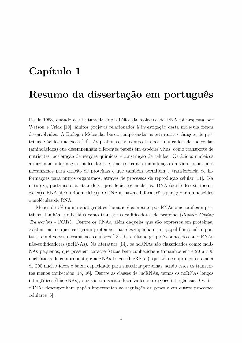
Menos de 2% do material genético humano é composto por RNAs que codificam pro-teínas, também conhecidos como transcritos codificadores de proteína (Protein CodingTranscripts - PCTs). Dentre os RNAs, além daqueles que são expressos em proteínas,existem outros que não geram proteínas, mas desempenham um papel funcional impor-tante em diversos mecanismos celulares [13]. Este último grupo é conhecido como RNAsnão-codificadores (ncRNAs). Na literatura [14], os ncRNAs são classificados como: ncR-NAs pequenos, que possuem características bem conhecidas e tamanhos entre 20 a 300nucleótidos de comprimento; e ncRNAs longos (lncRNAs), que têm comprimentos acimade 200 nucleotídeos e baixa capacidade para sintetizar proteínas, sendo esses os transcri-tos menos conhecidos [15, 16]. Dentre as classes de lncRNAs, temos os ncRNAs longosintergênicos (lincRNAs), que são transcritos localizados em regiões intergênicas. Os lin-cRNAs desempenham papéis importantes na regulação de genes e em outros processoscelulares [5].

1

Com o avanço das tecnologias de projetos utilizando sequenciamento de nova gera-ção com o objetivo de analisar DNA, RNA e proteínas de vários organismos ao redordo mundo, um grande volume de dados biológicos foi criado [21, 22]. Em particular, osprojetos transcritoma procuram analisar o conjunto completo de RNAs em um determi-nado organismo, enquanto aqueles que visam analisam o DNA são chamados de projetosgenoma.

Parte do enorme volume de informações gerado por projetos genoma e transcritomaestão armazenados em bancos de dados contendo diversos tipos de informações biológicas.Por exemplo, o HAVANA [28] disponibiliza informações sobre lincRNAs.

Projetos que buscam descobrir as funções de lncRNAs incluem o problema de distinguirlncRNAs de PCTs, pois algumas classes de lncRNAs encontram-se sobrepostas a PCTs.Os lincRNAs constituem-se na única classe de lncRNAs que não são sobrepostos a PCTs.LincRNAs estão relacionados ao surgimento e supressão de doenças, e isso tem motivadoa proposta de métodos computacionais para predição dessa classe especial de lncRNAs.

Na literatura encontramos poucos métodos computacionais para realizar esta tarefa.Em particular, vários desses métodos utilizam aprendizagem de máquina para distin-guir lncRNAs de PCTs, como CNCI [27] , PLEK [26], lncRNA-MFDL [29], lncRNA-ID [30], lncRScan-SVM [31], lncRNApred [32] e Schneider et al. [33]. Em particular, oiSeeRNA [34] e o linc-SF [35] usam a aprendizagem de máquina para distinguir lincRNAsde PCTs em humanos e camundongos.

Além de poucos métodos para distinguir lincRNAs de PCTs, os disponíveis (descritosanteriormente) funcionam bem para organismos específicos (principalmente humanos ecamundongos), mas, em geral, não têm boa capacidade de generalização, ou seja, nãoproduzem bons resultados em espécies diferentes para as quais foram projetadas ou emdados diferentes dos que foram utilizados para o treinamento do modelo. Métodos paraclassificar lincRNAs em outras espécies, tais como plantas, podem dar suporte ao trabalhode pesquisadores e facilitar a predição das funções exercidas por lincRNAs.

As plantas são um foco de estudo importante, pois participam da manutenção danatureza, têm propriedades medicinais, além de serem utilizadas na produção de combus-tível e alimentos, dentre outras razões. Algumas espécies de plantas, como o milho e acana-de-açúcar, têm uma importância particular, dado o seu amplo uso em todo o mundoe seu grande impacto econômico. Na literatura, podemos encontrar projetos que usamtécnicas laboratoriais para encontrar e caracterizar lncRNAs em plantas [23, 24, 25]. Emparticular, Wang et al. [23] indentificaram lincRNAs, usando uma montagem específicado milho.

Neste contexto, este trabalho propõe inicialmente um workflow que utiliza Máquinasde Vetores de Suporte (Support Vector Machine - SVM) e algumas ferramentas de bioin-

2

formática com o objetivo de distinguir lincRNAs de PCTs em plantas, os quais podemser posteriormente validados experimentalmente. Em seguida, um outro método é pro-posto para distinguir lincRNAs de PCTs em humanos e camundongos, usando ensemblede métodos supervisionados, com o intuito de disponibilizar uma ferrramenta pública.

A primeira ferramenta proposta, o PlantSniffer, foi aplicada em dois estudos de caso,para o Saccharum officinarum (cana-de-açúcar) e para o Zea mays (milho). Na cana-de-açúcar, encontramos 67 lincRNAs potenciais. Além disso, investigamos lincRNAs di-ferencialmente expressos em bibliotecas tratadas com Acidovorax avenae spp avenae, oagente causal da doença da red-streap e duas bibliotecas de controle. No total, 46 dos67 lincRNAs previstos foram diferencialmente expressos. Dentre eles, um foi testado emlaboratório e reconhecido como um lincRNA, o qual demonstrou uma relação com o mir-408. Na cana-de-açúcar, o miR408 é um indício de que um micro-organismo é patógenoou beneficial para a planta. Em relação ao milho, trabalhamos com transcritos obtidasdo sequenciador Illumina HiSeq, armazenados em oito bibliotecas, quatro tratadas comHerbaspirillum seropedicae (duas de controle e duas inoculadas) e quatro Azospirillum bra-silense (duas de controle e duas inoculadas), respectivamente. Nesse caso, nosso métodousando SVM exibiu uma acurácia de 99%. Ainda nesse caso, investigamos a expressãodiferencial dos lincRNAs preditos e obtivemos lincRNAs potenciais para serem analisadosem laboratório. Um artigo foi publicado em Vieira et al. [36] e o texto completo pode serencontrado em http://www.mdpi.com/2311-553X/3/1/11/htm.

A segunda ferramenta proposta, denominado LincSniffer, usa um método de apren-dizagem conhecido como ensemble, que utiliza uma composição de modelos individuaispara discriminar lincRNAs de PCTs. Dois estudos de caso, um para o Homo sapiens(humano), montagem GRCh38, e outro para o Mus musculus (camundongo), montagemGRCm38, foram desenvolvidos para avaliar a acurácia do método. Em geral, os mo-delos construídos com Ensemble apresentaram boas acurácias, melhores do que quandocomparadas aos modelos individuais. No estudo de caso do H. sapiens, nosso modelomostrou uma acurácia de 94% e quando comparados aos resultados obtidos de ferramen-tas encontradas na literatura, o LincSniffer mostrou uma precisão de 91% enquanto oiSeeRNA apresentou uma acurácia de apenas 56%. Em relação ao M. musculus, nossomodelo mostrou uma acurácia de 96%. Quando comparado com o iSeeRNA, que apre-sentou acurácia de 60,10%, o PlantSniffer mostrou acurácia de 90%. Além disso, análisesde importância das características dos lincRNAs foram feitas e indicaram o comprimentode ORF e proporção de ORF relativamente ao tamanho do transcrito como importantespara a discriminação lincRNAs e PCTs. Além das ORFs, nossos testes indicaram queo número de ocorrências TCG’s parece ter papel importante, o que deve ser verificadoexperimentalmente. O LincSniffer, testes, dados e resultados estão disponíveis no GitHub

3

(https://github.com/lmacielvieira/LincSniffer).Ambos os métodos propostos mostraram que modelos baseados em aprendizagem de

máquina para discriminar lincRNAs de PCTs são úteis para indicar propriedades biológi-cas de lincRNAs, a serem validadas experimentalmente.

4

Capítulo 2

Introduction

Since the double helix structure of the DNA molecule was proposed by Watson andCrick [10], many projects related to the investigation of this molecule have been developed.Molecular biology is the field of biology that seeks to understand the structures andfunctions of proteins and nucleic acids [11].

Proteins are composed of a chain of molecules (amino acids) that play different rolesin living species, such as transport of nutrients, acceleration of chemical reactions andconstruction of cells [12].

Nucleic acids store essential molecular information, as well as mechanisms for crea-ting proteins, and also enable to transfer this information to other organisms, throughcell reproduction processes [11]. In nature, we can find two types of nucleic acids: DNA(deoxyribonucleic acid) and RNA (ribonucleic acid). DNA stores information to gene-rate various amino acids and RNA molecules. Among the RNAs, we have those that areexpressed in proteins and others that do not generate proteins, but perform importantfunctions in cellular mechanisms. This last group is known as non-coding RNAs (ncR-NAs). It is well known that ncRNAs play important roles in the cell, such as chemicalreactions catalyzes and various regulatory roles [13].

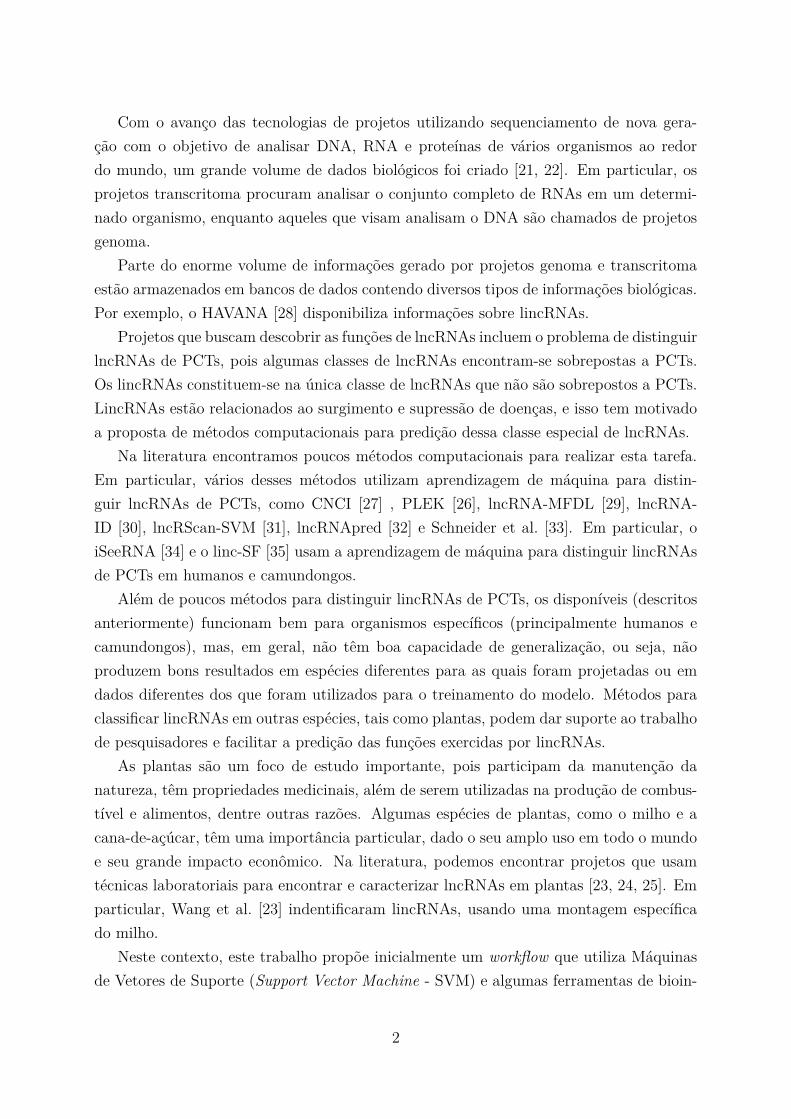
In the literature [14], ncRNAs are classified as: small ncRNAs, which have known cha-racteristics and small size (20 to 300 nucleotides); and long ncRNAs (lncRNAs), whichhave length above 200 nucleotides and almost no capacity to synthesize proteins, thesebeing the least known transcripts [15, 16]. Among the lncRNA classes, we have the longintergenic non-coding RNAs (lincRNAs), which are transcripts located at intergenic regi-ons. LincRNAs play important roles in gene regulation and in other cellular processes [5].

Less then 2% of the human genetic material is composed by RNAs coding for pro-teins, also known as protein coding transcripts (PCTs). A large part of the RNAs havemany other functions, and therefore many types of ncRNAs are known [17]. In plants,lncRNAs are not well known, althought they are involved in many important cellular

5

processes [18]. On the other side, studies of lincRNAs in human and mouse have beendeveloped, and most of them associate these lincRNAs with regulation in diseases, inparticular, cancer [19, 20].

With the improvement of technologies for high-throughput sequencing projects withthe aim of analyzing DNA, RNA and proteins of several organisms around the world, largevolume of biological data were created [21, 22]. In particular, transcriptome projects seekto analyze the full set of RNAs in a given organism, while the ones that analyze DNA arecalled genome projects.

Plants are important focuses of study because they participate in nature maintainence,have medicine properties, are used on fuel production and as food, among other reasons.They serve as food to nearly all organisms and humans eat either plants or other organismsthat eat plant. Some plant species, like maize and sugarcane, have a particular importancegiven their wide use around the world an their huge impact on the economy.

In plants, there are projects to find and characterize lncRNAs [23, 24, 25], relyingmostly in laboratorial techniques. In particular, Wang et al. [23] also identified lincRNAs,using a specific maize assembly. Methods to predict lincRNAs in organisms (plants inspecific) have to have a reference genome. Among the prediction methods present inliterature, few [26, 27] discriminate lncRNAs from PCTs in plants, and they are notfocused on lincRNAs.

Besides, the available methods (described previously) work well for specific organisms(mainly human and mouse), but in general, do not generalize, i.e., they do not producegood results for species different from the ones they have been designed to.

In this context, at first, this work proposes a workflow that uses machine learningand some bioinformatics tools in order to predict lincRNAs in plants aiming to indicatepotential lincRNAs, which have to be further studied to find their biological rules, e.g.,lincRNA association with diseases. We also propose a second method to distinguish lincR-NAs from PCTs in human and mouse, using an ensemble of machine learning supervisedmethods.

2.1 MotivationResearches in lncRNAs have been developed, based on their roles in important cellu-lar processes, like gene expression and regulation [37]. Many studies suggest importantfunctional roles for DNA transcripts that do not express proteins, presented in intergenicregions, the so-called lincRNAs [38, 39, 40, 41]. However, no methods are widely usedto identify lincRNAs, although there are algorithms [34] and databases [42, 43, 44] withlincRNA information.

6

In one hand, despite their importance in medicine and food markets, we find fewdata containing lincRNA information and there are no widely used tools to distinguishlincRNAs from PCTs, which could help to understand lincRNA interactions with plantdiseases as well as to isolate causes associated with them, improving plant production.

On the other hand, in human and mouse, studies related to lincRNAs and PCTsdiscrimination had been done, but most of them use similar workflows for prediction [45,46]. Computational methods to distinguish lincRNAs from PCTs in human and mousecan take advantage of the amount of available data. Thus, taking advantage of thesedifferent methods working together in an ensemble method could improve accuracy andrefine distinction of lincRNAs and PCTs.

2.2 ProblemThere are few methods based on machine learning to discriminate lincRNAs from PCTs,being these methods specific to the species used to create the models.

2.3 GoalsThe main goal is to build a model that uses machine learning to discriminate lincRNAsfrom PCTs.

In this work, the focus is to predict lincRNAs in plants and animals. In more details,the specific goals are:

• To propose a pipeline, using SVM models, to discriminate lincRNAs from PCTs inplants:

– To perform case studies for sugarcane and maize;

– To create a software, public available, for distinguishing lincRNAs from PCTsin plants.

• To devise ensemble learning models to discriminate lincRNAs from PCTs in animals:

– To perform case studies for human and mouse;

– To create a software, public available, for distinguishing lincRNAs from PCTsin human and mouse.

7

2.4 Chapters descriptionIn Chapter 2, we first present basic concepts of molecular biology and bioinformatics.Then we describe lincRNAs, their classification and biological function.

In Chapter 3, we discuss machine learning, focusing on the methods used in this pro-ject, SVM and ensemble. Also, we present a literature review about lincRNAs predictionmethods.

In Chapter 4, we present our first prediction method, called PlantSniffer. First, wepresent the proposed pipeline, then we show case studies in Sorghum bicolor (sorghum)and Zea mays (maize).

In Chapter 5, the LincSniffer prediction method is presented. First, we describe themethod, then we show two case studies in Mus musculus (mouse), assembly GRCm38,and Homo sapiens (human), assembly GRCh38.

Finally, in Chapter 6, we conclude this dissertation and suggest future work.

8

Capítulo 3

LincRNAs

In this chapter, we present biological concepts about lincRNAs, which are the focus of thisdissertation. In Section 3.1, we describe RNA, proteins and the central dogma of mole-cular biology. In Section 3.2, we briefly describe sequencers, together with bioinformaticspipelines and tools. In Section 3.3, we describe biological aspects of lincRNAs.

3.1 Molecular biologyThe biological processes of regulation and structural maintainance that occur in the orga-nisms are directed by the interaction between two group of molecules: nucleic acids andproteins. In nature, we find two types of nucleic acids, DNA (deoxyribonucleic acid) andRNA (ribonucleic acid), which play roles on protein creation and system regulation. Giventhe importance of these molecules in life, the field of molecular biology seeks to unders-tand nucleic acids, as well as structures and functions of proteins [11]. This dissertationfocuses on a specific group of RNAs, the lincRNAs, detailed in this chapter.

3.1.1 RNA

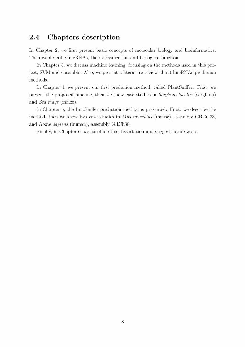
RNA is formed by nucleotides, consisting of phosphate, ribose and a nitrogenous base(Figure 3.1).

There are four types of nitrogenous bases composing a RNA: Adenine (A), Guanine(G), Citosine (C) and Uracil (U) [48]. The RNA nucleotides are bonded through theirphosphate molecules (Figure 3.2).

Usually, the RNA is found in organisms as a single chain (single strand), differentfrom the DNA that usually are found as a double strand, formed by chains that arecomplementar among themselves, with complementary pairs A/T and C/G. Even that

9

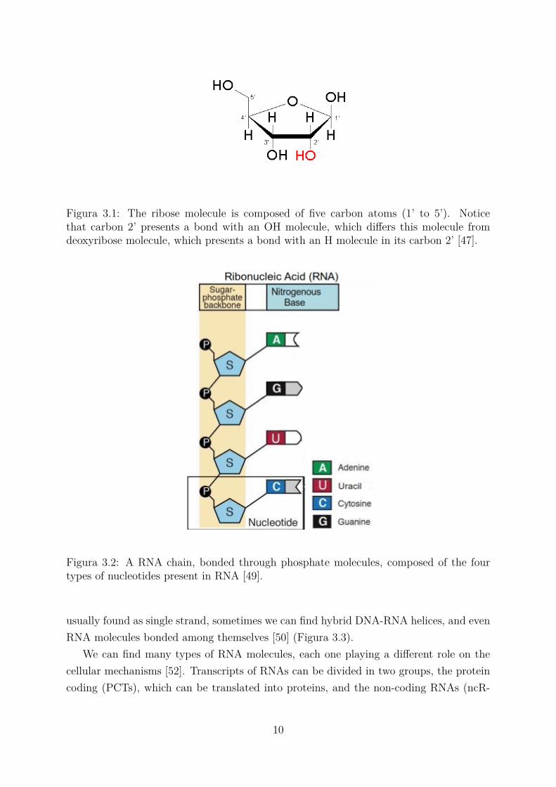
Figura 3.1: The ribose molecule is composed of five carbon atoms (1’ to 5’). Noticethat carbon 2’ presents a bond with an OH molecule, which differs this molecule fromdeoxyribose molecule, which presents a bond with an H molecule in its carbon 2’ [47].

Figura 3.2: A RNA chain, bonded through phosphate molecules, composed of the fourtypes of nucleotides present in RNA [49].

usually found as single strand, sometimes we can find hybrid DNA-RNA helices, and evenRNA molecules bonded among themselves [50] (Figura 3.3).

We can find many types of RNA molecules, each one playing a different role on thecellular mechanisms [52]. Transcripts of RNAs can be divided in two groups, the proteincoding (PCTs), which can be translated into proteins, and the non-coding RNAs (ncR-

10

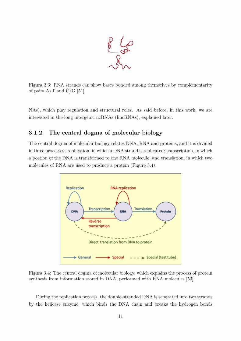
Figura 3.3: RNA strands can show bases bonded among themselves by complementarityof pairs A/T and C/G [51].

NAs), which play regulation and structural roles. As said before, in this work, we areinterested in the long intergenic ncRNAs (lincRNAs), explained later.

3.1.2 The central dogma of molecular biology

The central dogma of molecular biology relates DNA, RNA and proteins, and it is dividedin three processes: replication, in which a DNA strand is replicated; transcription, in whicha portion of the DNA is transformed to one RNA molecule; and translation, in which twomolecules of RNA are used to produce a protein (Figure 3.4).

Figura 3.4: The central dogma of molecular biology, which explains the process of proteinsynthesis from information stored in DNA, performed with RNA molecules [53].

During the replication process, the double-stranded DNA is separated into two strandsby the helicase enzyme, which binds the DNA chain and breaks the hydrogen bonds

11

between the strands. While helicase opens the double strand, another enzyme calledDNA polymerase, responsible for linking the nucleotides of the broken strands in a newcomplementary one, acts in parallel.

The transcription process is also initiated with the separation of the double-strandedDNA by the helicase enzyme. When the strands are separated, the RNA polymeraseenzyme identifies the template strand (5� → 3�) in the region of a gene (explained later).The RNA polymerase recognizes this region, which is usually preceded by a TA sequence(called TATA box) [54]. When the enzyme identifies this promoter region, the RNApolymerase guides the DNA transcription process in a not mature messenger RNA (pre-mRNA) in eukaryotes and in a messenger RNA (mRNA) in procaryotes. This DNAconversion process for RNA transcription occurs towards 5� → 3�, and converts the basesof the template strand to their complementary bases in the generated RNA. In Figure 3.5,we can see the difference of gene structures in eukaryotes and prokaryotes.

In eukaryotes, the pre-mRNA generated by the transcription undergoes a processknown as splicing (Figure 3.6). This process removes some regions (introns) of the pre-mRNA, while binding others (exons), thus forming the mature mRNA. Note that splicingcan generate more than one protein from a single gene. This process is known as alter-native splicing.

After the transcription process and the splicing, the translation is started, in whichthe mRNA synthesizes a protein. An amino acid chain of a protein is formed in ribo-somes, composed of ribosomal RNAs (rRNA), by means of a carrier, called transporterRNA (tRNA). Each tRNA binds triplets of nucleotides called codons in a tip with thecorresponding amino acid on the other one (Figure 3.7).

Figure 3.8 shows the correspondence of each three bases (codon) with their corres-ponding amino acid, while Table 3.1 shows the 20 amino acids most commonly found innature.

Given the genetic code, the nucleotide sequences capable of being translated intoproteins, from a start codon (Methionine - AUG) to a stop codon, are called ORFs (OpenReading Frames) [11]. In Figure 3.9 we can see an example, where an ORF is translatedto a protein.

12

Figura 3.5: Gene structures in (a) eukaryotes and (b) prokaryotes. In eukaryotes thetranscription processes generate a pre-mRNA that passes through a post-transcriptionalmodification in order to generate the mature mRNAs, while on prokaryotes the transcrip-tion processes do not generate the pre-mRNAs, but the mRNA itself [1].

13

Figura 3.6: Process of splicing in eukaryotes. The splicing is the post-transcriptionalprocess that transforms the premRNA transcript into a mRNA by removing the intronsand joining the exons. We can note that some different types of ncRNAs are involved inthe process. This processes can create a variety of different mRNAs from pre-mRNAs,being this phenomenon called alternative splicing [2].

14

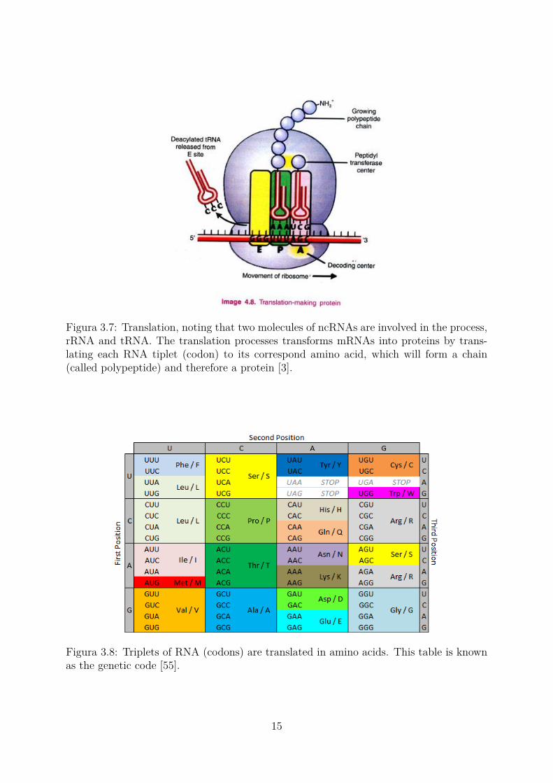
Figura 3.7: Translation, noting that two molecules of ncRNAs are involved in the process,rRNA and tRNA. The translation processes transforms mRNAs into proteins by trans-lating each RNA tiplet (codon) to its correspond amino acid, which will form a chain(called polypeptide) and therefore a protein [3].

Figura 3.8: Triplets of RNA (codons) are translated in amino acids. This table is knownas the genetic code [55].

15

Tabela 3.1: The twenty amino acids most commonly found in nature [11].Abbreviation NameAla AlanineCys CysteineAsp AspartateGlu GlutamatePhe PhenylalanineGly GlycineHis HistidineIle IsoleucineLys LysineRead LeucineMet MethionineAsn AsparaginePro ProlineGin GlutamineArg ArginineSer SerinaThr ThreonineVal ValineTrp TryptophanTyr Tyrosine

Figura 3.9: The mRNA represented by UGAUCAUGAUCUCGUAAGAUAUC, where thestrand goes from 5’ to 3’, and at the sixth base we can find the start of the triplet AUG,the start codon. From the start codon until the fifteenth base pair, which representsthe stop codon UAA, we have two triplets (AUC and UCG), that are translated intoIsoleucine and Serina and result into a protein [56].

16

3.2 Sequencing and bioinformatics pipelineIn this section, we briefly describe sequencing technologies and after, we show how bioin-formatics pipelines are constructed.

3.2.1 High-throughput sequencing

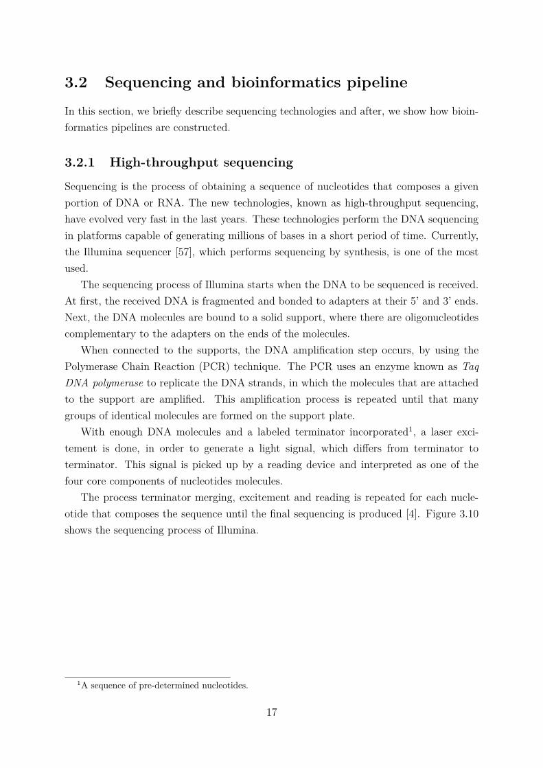
Sequencing is the process of obtaining a sequence of nucleotides that composes a givenportion of DNA or RNA. The new technologies, known as high-throughput sequencing,have evolved very fast in the last years. These technologies perform the DNA sequencingin platforms capable of generating millions of bases in a short period of time. Currently,the Illumina sequencer [57], which performs sequencing by synthesis, is one of the mostused.

The sequencing process of Illumina starts when the DNA to be sequenced is received.At first, the received DNA is fragmented and bonded to adapters at their 5’ and 3’ ends.Next, the DNA molecules are bound to a solid support, where there are oligonucleotidescomplementary to the adapters on the ends of the molecules.

When connected to the supports, the DNA amplification step occurs, by using thePolymerase Chain Reaction (PCR) technique. The PCR uses an enzyme known as TaqDNA polymerase to replicate the DNA strands, in which the molecules that are attachedto the support are amplified. This amplification process is repeated until that manygroups of identical molecules are formed on the support plate.

With enough DNA molecules and a labeled terminator incorporated1, a laser exci-tement is done, in order to generate a light signal, which differs from terminator toterminator. This signal is picked up by a reading device and interpreted as one of thefour core components of nucleotides molecules.

The process terminator merging, excitement and reading is repeated for each nucle-otide that composes the sequence until the final sequencing is produced [4]. Figure 3.10shows the sequencing process of Illumina.

1A sequence of pre-determined nucleotides.

17

Figura 3.10: Sequencing process used by Illumina [4].

Besides Illumina, there are other sequencing technologies and profiling methods, i.e,DNA nanoball sequencing [58] and Helioscope single molecule sequencing [59]. A com-mon used transcriptome profiling method is the RNA-seq, which is used in order toanalyze RNA and can be applied together with other sequencers, e.g, Illumina. RNA-sequses deep-sequencing technologies, also providing a more precise measurement of levels of

18

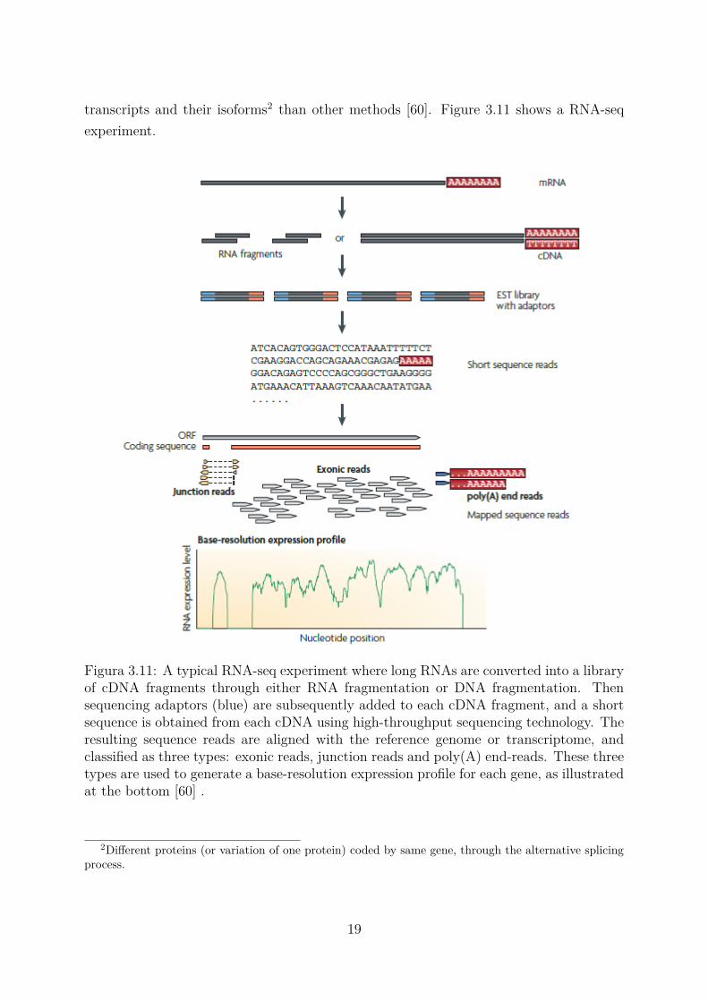
transcripts and their isoforms2 than other methods [60]. Figure 3.11 shows a RNA-seqexperiment.

Figura 3.11: A typical RNA-seq experiment where long RNAs are converted into a libraryof cDNA fragments through either RNA fragmentation or DNA fragmentation. Thensequencing adaptors (blue) are subsequently added to each cDNA fragment, and a shortsequence is obtained from each cDNA using high-throughput sequencing technology. Theresulting sequence reads are aligned with the reference genome or transcriptome, andclassified as three types: exonic reads, junction reads and poly(A) end-reads. These threetypes are used to generate a base-resolution expression profile for each gene, as illustratedat the bottom [60] .

2Different proteins (or variation of one protein) coded by same gene, through the alternative splicingprocess.

19

3.2.2 Bioinformatics pipelines

Bioinformatics is an area where researchers aim to create and apply computational andmathematical techniques to analyze information generated by sequencing projects [61]. Inorder to analyze these DNA and RNA sequences, we use workflows, particularly, pipelines.

A pipeline is defined by a sequence of computational methods used to treat the datagenerated by a transcriptome or a genomic project, where the output files of one step ofthe pipeline is used as input for the next step. An example of pipeline can be seen inFigure 3.12.

Figura 3.12: Example of a pipeline, with three steps.

As said before, in sequencers, the DNA/RNA sequences are transformed in charac-ter chains over the alphabet � = {A, C, G, T/U}. These sequences are stored in fileswith well known and defined formats, as fasta and fastq. Fasta is one of the most usedformats, and it is defined by having its first line started with the character ’>’, whichindicates the identifier of a sequence, followed by other lines that show the charactes inthe genome/transcript sequence (Figure 3.13).

Figura 3.13: Example of a fasta file.

20

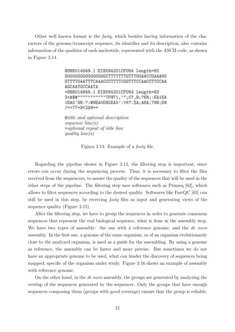
Other well known format is the fastq, which besides having information of the cha-racters of the genome/transcript sequence, its identifier and its description, also containsinformation of the qualities of each nucleotide, represented with the ASCII code, as shownin Figure 3.14.

Figura 3.14: Example of a fastq file.

Regarding the pipeline shown in Figure 3.12, the filtering step is important, sinceerrors can occur during the sequencing process. Thus, it is necessary to filter the filesreceived from the sequencers, to assure the quality of the sequences that will be used in theother steps of the pipeline. The filtering step uses softwares such as Prinseq [62], whichallows to filter sequences according to the desired quality. Softwares like FastQC [63] canstill be used in this step, by receiving fastq files as input and generating views of thesequence quality (Figure 3.15).

After the filtering step, we have to group the sequences in order to generate consensussequences that represent the real biological sequence, what is done in the assembly step.We have two types of assembly: the one with a reference genome; and the de novoassembly. In the first one, a genome of the same organism, or of an organism evolutionarilyclose to the analyzed organism, is used as a guide for the assembling. By using a genomeas reference, the assembly can be faster and more precise. But sometimes we do nothave an appropriate genome to be used, what can hinder the discovery of sequences beingmapped, specific of the organism under study. Figure 3.16 shows an example of assemblywith reference genome.

On the other hand, in the de novo assembly, the groups are generated by analyzing theoverlap of the sequences generated by the sequencer. Only the groups that have enoughsequences composing them (groups with good coverage) ensure that the group is reliable.

21

Figura 3.15: Graphic that show the quality of sequences, generated by FastQC [63].

Figura 3.16: Example of assembly using a reference genome, where the reference se-quence is an organism evolutionarily close to the analyzed sequence organism, whiles1, s2, s3, s4, s5 and s6 are sequences of the studied organism [64].

As we do not have reference genomes, this assembly process can be slow. Figure 3.17shows an example of de novo assembly.

The last pipeline step, anotation, aims to assign biological functions to the consensus ofthe sequences grouped in the assembly step. Annotation changes according to the projectgoal. In transcriptome projects, for example, the annotation aims to describe expressed

22

Figura 3.17: Example of a de novo assembly, containing areas with high and with lowcoverage, according to the number of sequences present on the corresponding group [64].

genes and their isoforms, besides their potential roles on the analyzed organism. However,in genome projects, the goal can be the identification of coding genes, and of non-codinggenes. To perform annotation, biological databases containing sequences with knownbiological functions, together with similarity analyzing tools, can be used. One of themost used tools is Basic Local Alignment Search Tool (BLAST) [65], which finds similarregions among sequences, computing local alignments. BLAST finds the function of thesequence by looking for similarities between the sequence under study and each sequencestored in a database, which have know pre-determined functions.

We have many BLAST variations, depending on the studied sequence and the sequen-ces stored in the database:

• blastn, which uses nucleotides as query, and also in the database;

• blastp, which uses amino acids as query, and also in the database;

• blastx, which uses translated nucleotides as query, and amino acids as database;

• tblastn, which uses amino acids as query, and nucleotides translated in amino acidsas database;

• tblastx, which uses nucleotides translated in amino acids as query, and also in thedatabase.

In Figure 3.18 we can see how the annotation process works.

23

Figura 3.18: General view of the annotation process. A query is the input, that is alignedwith sequences in the database, and scored by the BLAST. Similar sequences indicatefunction conservation.

3.3 Biological aspects of lincRNAsLncRNAs is usually classified into six major categories: (a) sense or (b) antisense, whenthe lncRNA overlaps the transcription region of one or more exons of another gene, on thesame or the opposite strand, respectively; (c) bidirectional, when the start of the lncRNAtranscription and another gene in the opposite strand are close; (d) intronic, when thelncRNAs are derived entirely from introns; (e) enhancer, when the lncRNAs are locatedin enhancer regions; or (f) intergenic, also called lincRNA, when the lncRNA is locatedin the interval between two genes [66]. Figure 3.19 illustrates these categories.

24

Figura 3.19: LncRNA categories: (a) sense; (b) antisense; (c) bidirectional; (d) intronic;(e) enhancer; and (f) intergenic. Adapted from [66].

Broadly speaking, lncRNAs can be divided in two subsets: lncRNAs that overlap withprotein-coding genes; and lincRNAs, found at intergenic regions. The evolutionary his-tory and patterns of conservation (and thereby prediction patterns) of these two lncRNAssubsets are very different. For instance, lncRNAs that overlap with protein-coding geneslook like protein-coding genes. They are spliced (predominantly), exhibit elevated con-servation (relative to lincRNAs), and are expressed (typically) in a manner that is similarto the protein-coding gene they overlap. Therefore, even with the important roles theyplay, it is difficult to predict lincRNAs.

The lincRNA classification differs a bit from the other lncRNAs, because they do nothave a well defined secondary structure. LincRNAs have been broadly studied due to thefact that they do not overlap any gene [5, 45, 46].

Many lincRNA researches reveal their role in a variety of organisms, performing manydifferent biological roles: Hotair, which may have a role in the chromatin regulation [37];H19, which may limit the growth of the placenta in mammals [67]; Tincr, the cyran andthe megamind, which are necessary for a good embryonic development [68]; HotairM1,which regulates the developmental cycle in maturation of the bone marrow [69]; and Gas5

25

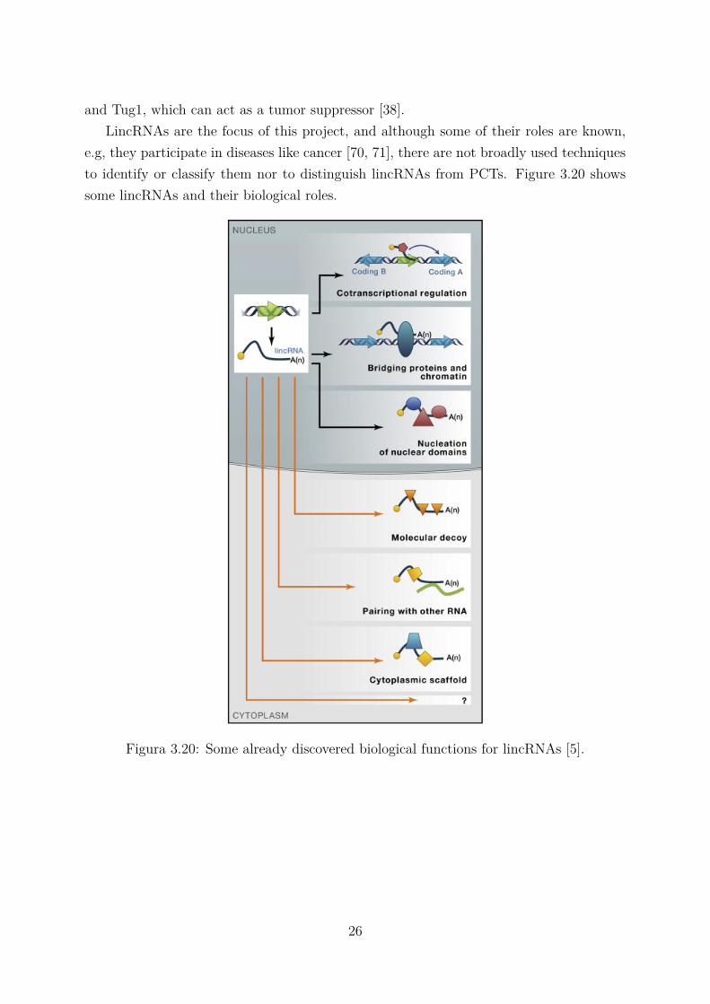
and Tug1, which can act as a tumor suppressor [38].LincRNAs are the focus of this project, and although some of their roles are known,

e.g, they participate in diseases like cancer [70, 71], there are not broadly used techniquesto identify or classify them nor to distinguish lincRNAs from PCTs. Figure 3.20 showssome lincRNAs and their biological roles.

Figura 3.20: Some already discovered biological functions for lincRNAs [5].

26

Capítulo 4

Machine Learning

In this chapter, we present basic concepts on machine learning, particularly, SupportVector Machine (SVM) and ensemble methods, adopted in this work. In Section 4.1,we present basic concepts of machine learning. In Section 4.2, we discuss the SVMmethod. In Section 4.3, we introduce the ensemble method. In Section 4.4, we present aliterature review with methods that use machine learning algorithms to predict lncRNAsand lincRNAs.

4.1 Basic conceptsMachine learning, in artificial intelligence, focuses on the development of algorithms thatdetect patterns and learn by experience [72]. In order to achieve this, the main task inmachine learning is to build a good model for information extracted from datasets.

In order to build a predictive model, machine learning techniques use feature vec-tors [73] alongside with a procedure divided in two main steps: training phase and testingphase, both described next.

4.1.1 Training and testing phases

The training phase is the part of the process where the model is generated from the inputdata [73], and it is where the prediction hypothesis is built.

After building a model on the training phase, this model have to be tested in orderto validate its prediction hypothesis, which is done in the so-called testing phase. In thisphase, the model’s prediction performance can be calculated.

A prediction model can have many goals, among them, clustering data into groups andfinding patterns in the data, such that new input data can be classified in these groups or

27

patterns. Prediction models follow some learning paradigms: unsupervised, supervised,learning by reinforcement and semi-supervised, as briefly described.

4.1.2 Learning paradigms

Supervised algorithms are based on the knowledge of the classes being analyzed. Basically,it classifies the input data as belonging to one of the classes, previously known. Thisclassification is done by a function called hypothesis that, according to the features givenfrom a dataset in the training phase, builds a model capable of classifying new input dataas belonging to specific classes. Some examples of supervised algorithms are SVM [74],Ctree [75] and KNN [76].

Unlike the previous paradigm, unsupervised learning tries to recognize patterns on agiven dataset, in which the labels of the input data are not used. Based on these inputdata features, the algorithm tries to find patterns so that the input data is labeled andgrouped accordingly. The output is composed of sets of input data. Some examples ofunsupervised methods are k-medoids [77] and k-means [78].

Learning by reinforcement is a paradigm in which the algorithm learns on each inte-raction, in order to achieve a final goal. The algorithm interacts with the environment(characterized by elements other than the program itself). A decision made by the pro-gram receives a score, used to decide the best classification. The decisions taken bythe program receive rewards, which inform the best action to take, given the possibleknown states of the environment [79]. Some examples of learning by reinforcement areSARSA [80] and LSTD [81].

Finally, we have the semi-supervised learning paradigm, a method that extends thesupervised learning by using unsupervised learning techniques. In some cases, its per-formance overcomes both the unsupervised and supervised learning approaches, if theywould be used separately. Usually, the algorithm input dataset is constituted by a groupX = {x1, ..., xi∈N}, divided in two groups: (i) Xl = {x1, ..., xl}, in which each xk has a po-sition in Yl = {y1, ..., yl}, which corresponds to its class; and (ii) a group Xu = {x1, ..., xu}of data points with unknown classes [82]. Some examples of semi-supervised learning areLabel Spreading [83] and Label Propagation [84].

Given the learning paradigms, the built models, independently from their goals, shouldhave good performance in order to guarantee that their output are reliable. There aredistinct ways to measure this performance, and some of them are going to be describednext.

28

4.1.3 Performance measures

Aside from the classification, we have to ensure that the built model is reliable. Inorder to analyze "how good" is a model, some metrics are used. Most of these metrics arecalculated based on the number of true positives (TP), true negatives (TN), false positives(FP) and false negatives (FN), from the output classification of the constructed model inthe testing phase. Table 4.1 shows the so-called confusion table, often used to visualizethe performance of the method.

Tabela 4.1: Confusion table, where we have the number of true positives (TP), truenegatives (TN), false positives (FP) and false negatives (FN) predicted by the model inthe training phase.

Class Predicted as True Predicted as FalseInput true objects Number of TP Number of FNInput false objects Number of FP Number of TN

Using the confusion table we can calculate metrics that evaluate the performance of themodel constructed in the training phase. Some metrics will be defined, recall, precision,specificity, F-measure and accuracy, each one measuring a particular aspect of the builtmodel.

Recall shows the rate of TP predicted by the model, and it is calculated by:

recall = TP

TP + FN

Precision shows the rate of the input data classified as positive, which are really positive,and it is calculated by:

precision = TP

TP + FP

Specificity calculates the rate of negatives predicted as so, and it is calculated by:

specificity = TN

TN + FP

F-measure combines precision and recall using a harmonic mean, and it is calculated by:

F − measure = 2 ∗ Precision ∗ recall

Precision + recall

Finally, accuracy is a metric that calculates the general rate of the model:

accuracy = TP + TN

TP + TN + FP + FN

29

The performance can also be represented as graphs. Per Example, the ROC curvescan help understanding the ratio of true positives and false positives, by analysing theArea Under the Curve (AUC), which as closest is to the value one as better is the model.

Given the learning paradigms and metrics for the performance measurement, next wedescribe SVM and ensemble, which are the machine learning algorithms adopted in thiswork.

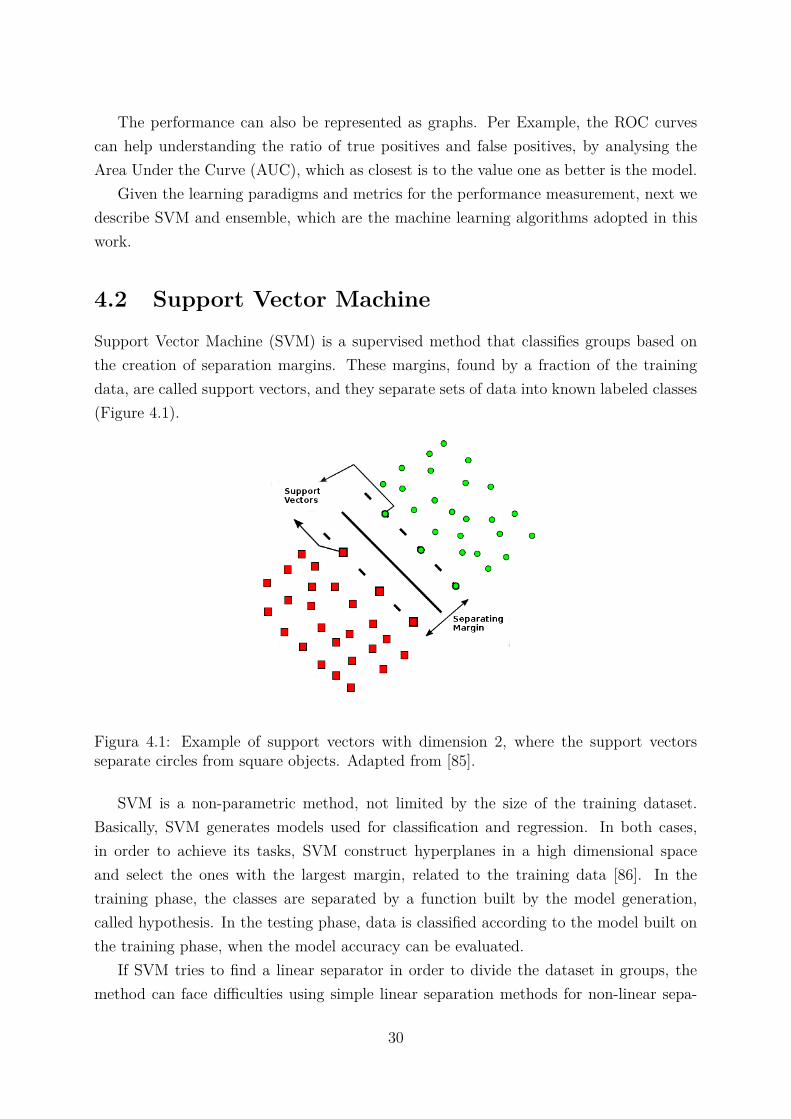
4.2 Support Vector MachineSupport Vector Machine (SVM) is a supervised method that classifies groups based onthe creation of separation margins. These margins, found by a fraction of the trainingdata, are called support vectors, and they separate sets of data into known labeled classes(Figure 4.1).

Figura 4.1: Example of support vectors with dimension 2, where the support vectorsseparate circles from square objects. Adapted from [85].

SVM is a non-parametric method, not limited by the size of the training dataset.Basically, SVM generates models used for classification and regression. In both cases,in order to achieve its tasks, SVM construct hyperplanes in a high dimensional spaceand select the ones with the largest margin, related to the training data [86]. In thetraining phase, the classes are separated by a function built by the model generation,called hypothesis. In the testing phase, data is classified according to the model built onthe training phase, when the model accuracy can be evaluated.

If SVM tries to find a linear separator in order to divide the dataset in groups, themethod can face difficulties using simple linear separation methods for non-linear sepa-

30

rable data. In order to solve this problem, SVM uses kernel functions to increase the di-mensions of the space, allowing to create linearly separable dataset components in higherdimensions (Figure 4.2).

Figura 4.2: Non-linear separable data in low dimension, mapped to a higher dimension,so that the separation of the groups may be simplified in a hyperplane with a higherdimension. Adapted from [87].

One kernel function denotes an inner product in a feature space and it is denoted byK(x, y) = (φ(x), φ(y)). This feature space has a higher dimension and it is used in such away that the dataset of the input space transformed into this feature space can be moreeasily separated. Table 4.2 shows the most commonly used kernel functions.

Tabela 4.2: Most used kernel functions, where • is the internal product, γ and C areconstants and X is the input.

Kernel FórmulaLinear Xi • Xj

Polynomial (γXi • Xj + C)d

RBF (radial) exp(−γ | Xi − Xj |2)Sigmoid tanh(γXi • Xj + C)

In Table 4.2 we can see that some kernel functions, such as the RBF, have a parameterγ. This parameter is adjustable and it has to be used in SVM with an optimal value forbetter classification results. In addition to the change in γ, we can apply several techniquesto try to obtain a SVM model with better accuracy. For example, the change of anotherparameter, the C (cost), affects the penalty in accepting objects on the wrong side ofthe margin and can be improved to obtain a better model. An important observation isthat the values assigned to C can influence the overfitting problem, because the largerthe value of C the more restrict the support vectors are to their respective classes. Thismeans that the model may loose the ability to generalize and may incorrectly sort newdata.

31

As said before, the model performance is an important aspect of the data classification.Some techniques can be used to improve the performance. In this project we use gridsearch [88] to obtain the optimals C and γ and another technique, called k-fold cross-validation to improve the accuracy of the model, both described next.

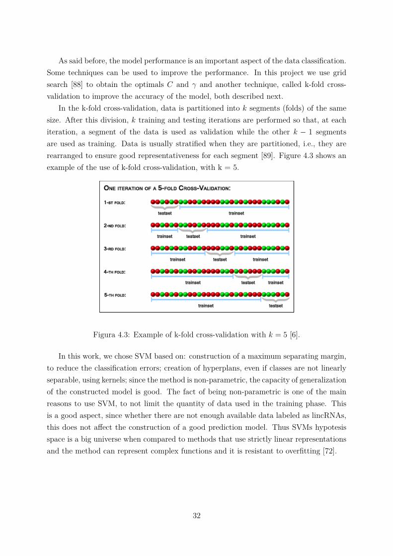
In the k-fold cross-validation, data is partitioned into k segments (folds) of the samesize. After this division, k training and testing iterations are performed so that, at eachiteration, a segment of the data is used as validation while the other k − 1 segmentsare used as training. Data is usually stratified when they are partitioned, i.e., they arerearranged to ensure good representativeness for each segment [89]. Figure 4.3 shows anexample of the use of k-fold cross-validation, with k = 5.

Figura 4.3: Example of k-fold cross-validation with k = 5 [6].

In this work, we chose SVM based on: construction of a maximum separating margin,to reduce the classification errors; creation of hyperplans, even if classes are not linearlyseparable, using kernels; since the method is non-parametric, the capacity of generalizationof the constructed model is good. The fact of being non-parametric is one of the mainreasons to use SVM, to not limit the quantity of data used in the training phase. Thisis a good aspect, since whether there are not enough available data labeled as lincRNAs,this does not affect the construction of a good prediction model. Thus SVMs hypotesisspace is a big universe when compared to methods that use strictly linear representationsand the method can represent complex functions and it is resistant to overfitting [72].

32

4.3 EnsembleEnsemble based systems follow the idea of consulting many sources before making adecision, given their known variability and accuracy in other records [90]. This consultinghappens because, in most of the time, we can not trust that only knowledge of one sourceis enough to predict everything the best way possible, given that other sources knowledgecan improve this prediction.

Based on this, the machine learning method called Ensemble [73] uses a combinationof a set of classifiers estimators, in order to build a classification model with improvedgeneralizability and robustness, when compared to a single estimator model. Ensemblemethods are known by its generalization ability, which is, most of the time, better thanthe results obtained if the used methods are used alone.

According to how the learners are generated, the ensemble methods are divided intwo paradigms: sequential ensemble (boosting methods); and parallel ensemble methods(averaging methods) [73]. The averaging methods are based on the construction of se-veral parallel independent estimators, which will have as output a prediction based onthe average of their estimators. Normally, their combination is better than a single esti-mator because the model variance is reduced. On the other side, we have the boostingmethods, where several estimators are built sequentially, in order to reduce the bias ofthese estimators combination.

When using boosting, the combination of several weak models can produce an impro-ved model, meanwhile the averaging methods work better using the combination of strongestimators. At the first part of this work, we proposed a SVM model (described later)to distinguish lincRNAs from PCTs. The model showed an accuracy close to the perfectperformance, which made possible to classify the SVM learned used as a strong learner.Given that the SVM was the start point to build the Ensemble, and the fact that parallelensemble methods tries to exploit the independence between the base learners [73], in thisproject, a model based on averaging was built.

The base learnes used to build the Ensemble must be complementary in order to im-prove the model accuracy. In order to achieve this complementarity, our Ensemble usedthe following supervised classifiers: Suport Vector Machine (SVM), which is a strongmethod that can take advantage of its independence in an ensemble approach; K-NearestNeighbor (KNN), which relies on objects similarity to make predictions and can be impro-ved when used in an heterogenios ensemble schema; Conditional Inference Trees (ctree),which can have the prediction error rate reduced when used in boosting or averagingensemble schemas; and Random Forest(RF), which is an Ensemble of decision trees thatcan have its prediction error reduced when used with other supervised classifiers in anaveraging ensemble. KNN, Ctree and RF will be detailed next.

33

4.3.1 K-Nearest Neighbor

K-Nearest Neighbor (KNN) is a non parametric lazy learning supervised algorithm, basedon a parameter K, which represents the number of neighbors that influences the classifi-cation. The distance among the input data generates a classification model. KNN plotsthe data input in a feature space where we have the notion of distance.

Basically, KNN finds a group of K objects in the training set that are closest to thetest input data object, and labels each point as belonging to a particular class in thisneighborhood. There are three major parts on this algorithm: a set of labeled input data;a distance metric to compute the distance between two data points; and the value of K,the number of nearest neighbors [91]. Figure 4.4 shows a KNN example.

Figura 4.4: Example of KNN with neighbors influence example, for K = 3 and K = 7[7].

KNN is very intuitive and it can use different distance metrics, if other knowledgedomains are explored. Even with this advantages, KNN has the problem of slow lookupsif the number of dimensions is too high. It is important to say that the bigger thetraining set, the better the KNN efficiency, as it takes advantages of its neighbors and donot generate new insights. KNN was used on this project beacuse of its calculation timespeed, its predictive power and its ease to understand output.

34

4.3.2 Ctrees

Conditional Inference Trees (Ctree) [75] is a non-parametric regression tree estimatorthat embed tree-structured regression models into a well defined theory of conditionalinference procedures. The difference between ctree and other decision trees algorithm,like CART [92] and C4.5 [93], is that it tries to reduce overfitting and a selection biasby generating possible node splits, using a well defined theory of permutation developedby Strasser and Weber [94]. Figure 4.5 shows a ctree example. Ctree was used on thisproject because of its implicity capacity to perform feature ranking and its simplicity.

Figura 4.5: Example of a ctree. The higher the node tree the most relevant is the featurein the data classification. In this case when an input data has as feature less or equal 127,it is most likely labeled as negative [95].

4.3.3 Random Forest

Random Forest receives this name because it builds m decision trees as an ensemble, inorder to build a better classification model. A random forest is an estimator that fitsdecision tree classifiers on various subsamples of the dataset, also using the averaging toimprove the predictive accuracy at the same time controlling overfitting [96].

In one random forest, each tree in the ensemble is built from a sample in the trainingset. In addition, when splitting a node, the chosen split is no longer the best split amongall the features. Instead, the split that is picked up is the best one among a randompart of the features [96]. As a result of this randomness, the bias of the forest usuallyslightly increases but, due to averaging, its variance also decreases, usually more thancompensating for the increase in bias, hence yielding an overall better model. The feature

35

importance can also be extracted by the analysis of the relative rank of a feature used asa decision node in a tree. Features used at the top of the tree are most significant on thefinal prediction. Figure 4.6 shows a Random Forest example. RF was used on this projectbecause of its implicity capacity to perform feature ranking and its reduced predictionerror rate.

Figura 4.6: Example of Random Forest, where n decision trees are build, given an inputx. Note that their n estimators execute an averaging and generate an output y that servesas the ensemble estimator [8].

Given all the machine learning algorithms used on this work, next we present relatedworks that uses machine learning algorithms to discriminate lincRNAs and lncRNAs fromPCTs.

4.4 Literature review

4.4.1 Machine learning based tools for distinguishing lncRNAsfrom PCTs

Han, Siyu, et al. [9] constructed a survey of methods that discriminate PCTs from ncRNAsusing machine learning. There are methods based on machine learning algorithms such as:SVM, logistic regression (LR), deep learning (DL) and random forest (RF). In Table 4.3,we list some characteristics of these projects.

As shown in Table 4.3, there are some computational methods, based on machinelearning techniques, designed to discriminate ncRNAs from PCTs, and to identify someclasses of ncRNAs. Next we briefly discuss some of these methods.

CONC (Coding Or Non-Coding) [97] and CPC (Coding Potential Calculator) [98]have been developed to discriminate protein coding genes from ncRNAs. CONC is slowon analyzing large datasets, CPC works well with known protein coding transcripts but

36

Tabela 4.3: Methods to discriminate ncRNAs from PCTs [9].Year Testing Training Model Query File Web

Datasets Species Format InterfaceCONC [97] 2006 ncRNA Eukaryotic SVM Unknown YesCPC [98] 2007 ncRNA Eukaryotic SVM FASTA YesCNCI [27] 2013 lncRNA Human and Plant SVM FASTA and GTF NoPLEK [26] 2014 lncRNA Human and Maize SVM FASTA No

lncRNA-MFDL [29] 2015 lncRNA Human DL Unknown UnknownlncRNA-ID [30] 2015 lncRNA Human and Mouse RF BED and FASTA No

lncRScan-SVM [31] 2015 lncRNA Human and Mouse SVM GTF NolncRNApred [32] 2016 lncRNA Human RF FASTA Web OnlyHugo et. al [33] 2017 lncRNA Human/Mouse/Zebrafish SVM/PCA FASTA Computer script

may tend to classify novel PCTs into ncRNAs, if they have not been recorded in theprotein databases [97].

CNCI [27] , PLEK [26], lncRNA-MFDL [29], lncRNA-ID [30], lncRScan-SVM [31],lncRNApred [32] and Hugo et. al [33] are methods that use machine learning techniquesin order to classify lncRNAs. In particular, iSeeRNA [34] and linc-SF [35] use machinelearning techniques to classify lincRNAs in human and mouse.

4.4.2 Machine learning based tools to distinguish lincRNAs fromPCTs

As we could see on the previous section, we have many methods to identify and classifylncRNAs, but only two methods to distinguish lincRNAs from PCTs, iSeeRNA [34] andlinc-SF [35], both described next.

ISeeRNA

ISeeRNA [34] is a SVM based classifier for distinguishing lincRNAs from PCTs. ISeeRNAhave a public available webserver and a software for download, which can be used todistinguish lincRNAs in human and mouse assemblies, using gff files as input. In orderto use SVM, iSeeRNA extracted 10 features to characterize lincRNAs, from three groups:conservation, ORFs, di-nucleotides frequencies and tri-nucleotides frequencies.

SVM was set as binary classifier, with lincRNAs as its positive set and PCTs as the ne-gative set. Optimized SVM parameters C and γ were obtained by using the accompanyinggrid.py script, with 5,000 randomly selected instances from the training dataset. To ob-tain the best performance model, 10-fold cross-validation was used. Two models werebuilt, one for human and the other for mouse. The built models presented accuracies of95.4% for human and 94.2% for mouse.

However, tests with other lincRNAs, in the iSeeRNA web interface, showed many falsepositives. In other words, they classify many PCTs and other molecules as lincRNAs.

37

linc-SF

LincRNA classifier, based on Selected Features (linc-SF) [35], was constructed using GA-SVM, using an optimized feature subset. The classifier performance was evaluated topredict lincRNAs, from two independent lincRNA sets composed of human lincRNAs.

In order to build a model using SVM, 74 features were chosen. These features wereextracted from three groups: the first one composed of the length of the sequences,frequencies of uni-nucleotides and tri-nucleotides, and the number of ocurrences of G andC on the sequences, forming 70 features in total; the second group was composed ofstructural features given by RNAfold [99], forming three features; and the third groupwas formed by the score given by CPC [98].

The method used to build the prediction model was GA-SVM, an algorithm that com-bines SVM and genetic algorithm (GA). Basically, many rounds using GA were executed,to generate new feature subsets, used with SVM to generate the model.

The method does not present an open source software to evaluate the results, but itsrecognition rates for the lincRNA human sets achieves 96%. The authors claim that thesenumbers are good and the method is effective, but such high rates can indicate overfitting.

38

Capítulo 5

PlantSniffer

Non-coding RNAs (ncRNAs) constitute an important set of transcripts produced in thecells of organisms. Among them, there is a large amount of a particular class of longncRNAs that are difficult to predict, the so-called long intergenic ncRNAs (lincRNAs),which might play essential roles in gene regulation and other cellular processes. Despitethe importance of these lincRNAs, there is still a lack of biological knowledge, and also afew computational methods, specific to organisms, which usually can not be successfullyapplied to other species, different from those that they have been originally designed to.Besides, prediction of lncRNAs have been performed with machine learning techniques.Particularly, for lincRNA prediction, supervised learning methods have been explored inrecent literature. In this context, this work proposes a workflow to predict lincRNAson plants, considering a pipeline that includes known bioinformatics tools together withmachine learning techniques, here Support Vector Machine (SVM). We discuss two casestudies that were able to identify novel lincRNAs, in sugarcane (Saccharum spp) andin maize (Zea mays). From the results, we also could identify differentially expressedlincRNAs in sugarcane and maize plants submitted to pathogenic and beneficial microor-ganisms.

An article with this work was published at http://www.mdpi.com/2311-553X/3/1/11/htm(doi:10.3390/ncrna3010011 ).

39

Capítulo 6

LincSniffer

In this chapter, we propose a method that uses ensemble to distinguish lincRNAs fromPCTs. In Section 6.1, we present the method, called LincSniffer. In Section 6.2, wefirst present results of the method applied to two study cases: Homo sapiens (AssemblyGRCh38 [100]) and Mus musculus (Assembly GRCm38 [101]). Next, we compare theresults obtained from our method to other tools found in the literature. In Section 6.3,we present a discussion about LincSniffer and its results.

6.1 MethodsLincSniffer is a method based on a workflow composed of: (1) Data selection and filtering;and (2) Model construction with ensemble. Figure 6.1 describes the method to distinguishlincRNAs from PCTs.

Figura 6.1: LincSniffer workflow: from the input data (lincRNAs and PCTs), step 1(data selection and filtering) generates the input to build the ensemble model (step 2) todistinguish lincRNAs from PCTs.

6.1.1 Data selection and filtering

Given the difficulties to discriminate some lncRNAs classes from PCTs, and the advan-tage that lincRNAs have of being found between two genes, the prediction models wereconstructed using lincRNAs as positive class and PCTs as negative class.

In order to build an accurate dataset, we used transcripts of the HAVANA project [28],which contains manually-curated transcripts. The model performance was tested using

40

two organisms: Homo sapiens (Assembly GRCh38 [100]) and Mus musculus (AssemblyGRCm38 [101]). As PCTs are most known than lincRNAs, the number of PCTs wasgreater than the lincRNAs, so we chose PCTs annotated as "known"1 as input data.

Even using data from HAVANA [28] and only "known PCTs", an extra filter step wasadded to confirm data quality. This confirmation was done by filtering the input datausing BLAST [102], as shown in Figure 6.2.

Figura 6.2: Data selection and filtering: 1 - The PCTs and lincRNAs received as inputfrom HAVANA are used as query and database against each other (PCTs X lincRNAsand vice-versa); 2 - The results of BLAST given as output passes through a no hit filterscript, and only the transcripts not identified in the opposite class are considerated; 3 -The output of the filters guarantees transcripts with high quality.

Even after the filtering process, the number of PCTs was greater than the number oflincRNAs, thus in order to keep the data balance, we fixed the training group size as theamount of lincRNA transcripts available after the filtering step. After fixing this size (s),the positive training data group was defined with size s and the negative was divided in n

groups of s. With these groups, n tests were developed, where the positive data group wasfixed and prediction performance were calculated by using n different negative groups, inorder to validate the prediction score.

6.1.2 Model construction

In order to find the most accurate method for distinguishing lincRNAs from PCTs, in-dividual machine learning methods and their combination were used. The combinationof these classifiers, also called ensemble, was used due to its potential capacity to in-crease the prediction generalizability and performance. According to how the learnersare generated, we can divide the ensemble in two paradigms- sequential ensemble (boos-ting methods) and parallel ensemble methods (averaging methods) [73]. The averagingmethods are based on the construction of several parallel independent estimators, whichwill have as output a prediction based on the average of their estimators. In the boostingapproach, several estimators are built sequentially, to decrease the prediction error [96].

1"A known gene or transcript matches to a sequence in a public, scientific database such as UniProtKBand NCBI RefSeq" [42].

41

Usually, ensemble predictions are better then the ones made by single estimators, becausethe model variance is reduced.

In this project, a model based on averaging of four estimators was built. The ave-raging method uses a procedure called stacking, where a learner is trained to combinethe individual learners (first-level learners) and uses a combiner (meta-learner) to give aprediction [73]. The use of the following supervised classifiers were used on this project:Suport Vector Machine (SVM), K-Nearest Neighbor (KNN), Conditional Inference Trees(Ctree) and Random forest (RF), detailed next.

Feature selection

Training features are a key part of building supervised learning models. They allow tobuild a correct model, associating specific characteristics to each class, given as input. Inour case, the features are biological factors that allow to characterize lincRNAs.

Since lincRNAs are sequences that have ORFs but are not expressed into proteins,i.e., they have poor capacity of coding proteins, we chose features related to ORFs, asfollows. The first one is the proportion between the ORF length divided by the sequencelength, which captures the percentage of the coding potential capacity. The other featureis the ORF length, explained by Dinger et al. [103], who defined a lincRNA as a transcriptwith ORF region length less than 100 amino acids. Besides the ORFs, a method basedin machine learning for lncRNAs feature selection [104] was used to extract relevantfeatures from the input dataset. As result, 30 features of 2-nucleotides, 3-nucleotides, and4-nucleotides pattern frequencies more significant to discriminate lincRNAs from PCTswere used (GCGG, TTTT, TCG, AAAA, ACG, TTGT, TAT, TAC,GTT, GTG, AGT,CCGA, TACC, CGTG, CGCT, TACG,TTAG, CGTA, ACCG, CCGT, CGGT, CGAC,CGCA, GCGT,GTAG, CGTT, CGAA, GCGA, CGAT, TAGT). Therefore, we used 32features in our case studies: ORF proportion, ORF length and 30 nucleotide patternfrequencies.

Single models

A home made script using R [105] was created to build the single models and the ensemble.In order to obtain the best accuracy of each single model in the ensemble, which can affectits accuracy, each single model was built using grid search [88, 106], which search foroptimal parameters to build ’the best’ model. Figure 6.3 shows how the single predictionmodels were built.

42

Figura 6.3: Single model construction: the input data received from the data selectionand filtering phase, together with the features previously described, are used to buildeach single model (KNN, Ctree, SVM and RF), which were constructed with parametersoptimized by grid search.

Ensemble

With the single models constructed (SVM, KNN, Ctree and RF), an ensemble approachwas developed using a stacking model. The stacking built with the parallel executionof the methods (show in Figure 6.4) used two voting strategies (meta-learners) to getthe final score: majority voting, where the classification is given when at least three ofthe single models predict a transcript in the same class; and unanimity voting, wherethe transcripts are classified as a given class only when all single models say so. In themajority voting in case of a tie, a greater voting weight was attrubuted to the modelsconstructed that presented the better accuracies.

Figura 6.4: ensemble model: the input data received from the filtering phase is used tobuild four single models (KNN, Ctree, SVM and RF) according to the selected features.Each of the single models gives a prediction of the input. With the prediction of eachone, a voting (majority or unanimity voting) is done to get the final score.

43

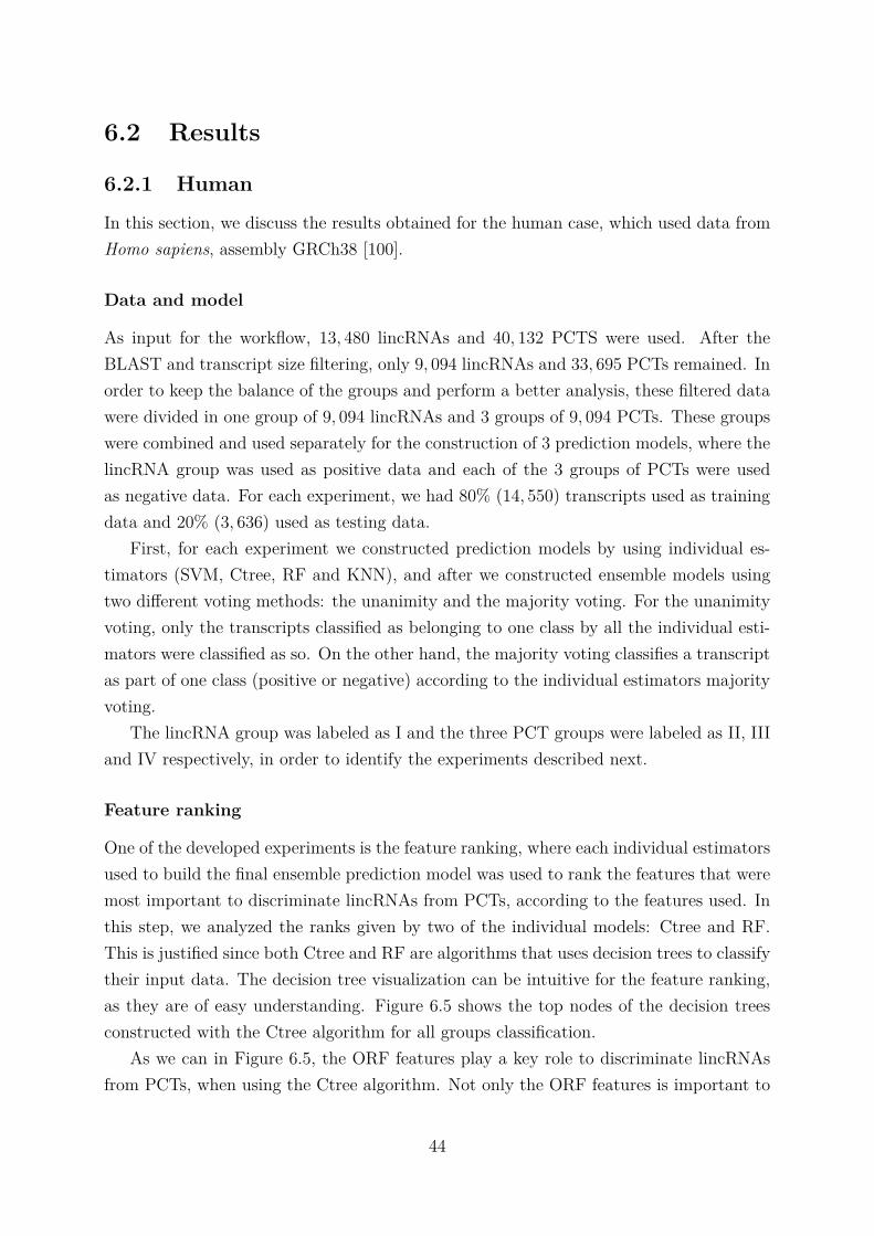
6.2 Results

6.2.1 Human

In this section, we discuss the results obtained for the human case, which used data fromHomo sapiens, assembly GRCh38 [100].

Data and model

As input for the workflow, 13, 480 lincRNAs and 40, 132 PCTS were used. After theBLAST and transcript size filtering, only 9, 094 lincRNAs and 33, 695 PCTs remained. Inorder to keep the balance of the groups and perform a better analysis, these filtered datawere divided in one group of 9, 094 lincRNAs and 3 groups of 9, 094 PCTs. These groupswere combined and used separately for the construction of 3 prediction models, where thelincRNA group was used as positive data and each of the 3 groups of PCTs were usedas negative data. For each experiment, we had 80% (14, 550) transcripts used as trainingdata and 20% (3, 636) used as testing data.

First, for each experiment we constructed prediction models by using individual es-timators (SVM, Ctree, RF and KNN), and after we constructed ensemble models usingtwo different voting methods: the unanimity and the majority voting. For the unanimityvoting, only the transcripts classified as belonging to one class by all the individual esti-mators were classified as so. On the other hand, the majority voting classifies a transcriptas part of one class (positive or negative) according to the individual estimators majorityvoting.

The lincRNA group was labeled as I and the three PCT groups were labeled as II, IIIand IV respectively, in order to identify the experiments described next.

Feature ranking

One of the developed experiments is the feature ranking, where each individual estimatorsused to build the final ensemble prediction model was used to rank the features that weremost important to discriminate lincRNAs from PCTs, according to the features used. Inthis step, we analyzed the ranks given by two of the individual models: Ctree and RF.This is justified since both Ctree and RF are algorithms that uses decision trees to classifytheir input data. The decision tree visualization can be intuitive for the feature ranking,as they are of easy understanding. Figure 6.5 shows the top nodes of the decision treesconstructed with the Ctree algorithm for all groups classification.

As we can in Figure 6.5, the ORF features play a key role to discriminate lincRNAsfrom PCTs, when using the Ctree algorithm. Not only the ORF features is important to

44

Figura 6.5: Ctree for human data: The top three nodes of the Ctree decision tree for thethree groups (I and II, I and III, I and IV).

lincRNAs and PCTs discrimination, but, as we can see in the decision tree, TCG has animportant role, which can indicate to possible biological meaning.

In order to validate the feature rank described by the Ctree decision tree, we used theRF algorithm to build a feature ranking list using Gini, as seen in Figure 6.6.

Figura 6.6: RF ranking for human data, the most important features for discriminatinglincRNAs from PCTs using the three groups (I and II, I and III and I and IV).

In Figure 6.6 we clearly see that the same features were indicated by Ctree and RF,i.e, ORF proportion, ORF length, GCGG and TCG.

Given this feature ranking, we need to validate the performance of the models, in orderto assure its relevance. Next, the evaluation of the single model performance as well asthe ensemble models evaluation are described.

Performance evaluation

The performance evaluation allows to confirm if the proposed ensemble prediction modelis better than the individual models. Table 6.1 describes the results of the performance

45

Tabela 6.1: Performance of each single model and the ensemble methods with both votingapproaches, for human.

Data Groups Method Precision Recall F-measure AccuracyI and II Ctree 93% 88% 90% 90%

KNN 94% 86% 89% 89%SVM 89% 89% 90% 89%RF 94% 90% 92% 92%

unanimity 97% 91% 94% 94%Majority 95% 90% 90% 92%

I and III Ctree 94% 89% 91% 91%KNN 94% 88% 91% 91%SVM 89% 88% 89% 89%RF 94% 88% 91% 90%

unanimity 96% 91% 93% 93%Majority 94% 89% 92% 91%

I and VI Ctree 92% 88% 90% 90%KNN 94% 87% 90% 90%SVM 89% 90% 89% 89%RF 94% 89% 91% 91%

unanimity 97% 92% 94% 94%Majority 95% 90% 93% 92%

evaluation. In this table, it can be seen that the ensemble methods presented a betterperformance in all the cases, when compared to the single models. The unanimity votingmethod is the best one, but as it is based on a unanimity voting, it can be more restrictthan the majority voting method, what can reduce its generability.

Given these results, Figure 6.7 shows the I and II groups experiment ROC curves,which illustrates a binary classifier (in this case, lincRNA or PCT classes) capacity ofcorrectly cllassify the input. The ROC Curves can help understanding the ratio of truepositives and false positives, by analysing the Area Under the Curve (AUC), which asclosest is to the value one as better is the model.

46

Figura 6.7: Human ROC curves: the ensemble models have good prediction rates whencompared to the single models.

6.2.2 Mouse

In this section, we discuss the results obtained for the human case, which used data fromMus musculus (Assembly GRCm38 [101]).

Data and model

As input for the workflow, 6, 108 lincRNAs and 27, 625 PCTS were used. After theBLAST and transcript size filtering, only 4, 766 lincRNAs and 25, 042 PCTs remained. Inorder to keep the balance of the groups and perform a better analysis, these filtered datawere divided in one group of 4, 766 lincRNAs and 5 groups of 4, 766 PCTs. These groupswere combined and used separately for the construction of 5 prediction models, where thelincRNA group was used as positive data and each of the 5 groups of PCTs were usedas negative data. For each experiment, we had 80% (7, 622) transcripts used as trainingdata and 20% (1, 910) used as testing data.

First, for each experiment we constructed prediction models by using individual es-timators (SVM, Ctree, RF and KNN), and after we constructed ensemble models usingtwo different voting methods: the unanimity and the majority voting. For the unanimityvoting, only the transcripts classified as belonging to one class by all the individual esti-mators were classified as so. On the other hand, the majority voting classifies a transcriptas part of one class (positive or negative) according to the individual estimators majorityvoting.

47

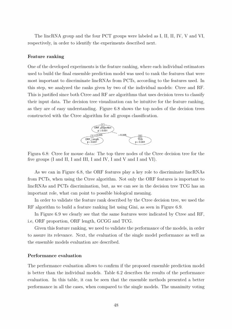
The lincRNA group and the four PCT groups were labeled as I, II, II, IV, V and VI,respectively, in order to identify the experiments described next.

Feature ranking

One of the developed experiments is the feature ranking, where each individual estimatorsused to build the final ensemble prediction model was used to rank the features that weremost important to discriminate lincRNAs from PCTs, according to the features used. Inthis step, we analyzed the ranks given by two of the individual models: Ctree and RF.This is justified since both Ctree and RF are algorithms that uses decision trees to classifytheir input data. The decision tree visualization can be intuitive for the feature ranking,as they are of easy understanding. Figure 6.8 shows the top nodes of the decision treesconstructed with the Ctree algorithm for all groups classification.

Figura 6.8: Ctree for mouse data: The top three nodes of the Ctree decision tree for thefive groups (I and II, I and III, I and IV, I and V and I and VI).

As we can in Figure 6.8, the ORF features play a key role to discriminate lincRNAsfrom PCTs, when using the Ctree algorithm. Not only the ORF features is important tolincRNAs and PCTs discrimination, but, as we can see in the decision tree TCG has animportant role, what can point to possible biological meaning.

In order to validate the feature rank described by the Ctree decision tree, we used theRF algorithm to build a feature ranking list using Gini, as seen in Figure 6.9.

In Figure 6.9 we clearly see that the same features were indicated by Ctree and RF,i.e, ORF proportion, ORF length, GCGG and TCG.

Given this feature ranking, we need to validate the performance of the models, in orderto assure its relevance. Next, the evaluation of the single model performance as well asthe ensemble models evaluation are described.

Performance evaluation

The performance evaluation allows to confirm if the proposed ensemble prediction modelis better than the individual models. Table 6.2 describes the results of the performanceevaluation. In this table, it can be seen that the ensemble methods presented a betterperformance in all the cases, when compared to the single models. The unanimity voting

48

Figura 6.9: RF ranking for mouse data, the most important features for discriminatinglincRNAs from PCTs using the five groups (I and II, I and III, I and IV, I and V and Iand VI).

method is the best one, but as it is based on a unanimity voting, it can be more restrictthan the majority voting method, what can reduce its generability.

49

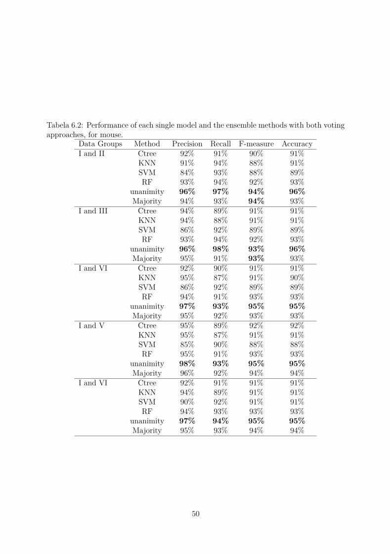
Tabela 6.2: Performance of each single model and the ensemble methods with both votingapproaches, for mouse.

Data Groups Method Precision Recall F-measure AccuracyI and II Ctree 92% 91% 90% 91%

KNN 91% 94% 88% 91%SVM 84% 93% 88% 89%RF 93% 94% 92% 93%

unanimity 96% 97% 94% 96%Majority 94% 93% 94% 93%

I and III Ctree 94% 89% 91% 91%KNN 94% 88% 91% 91%SVM 86% 92% 89% 89%RF 93% 94% 92% 93%

unanimity 96% 98% 93% 96%Majority 95% 91% 93% 93%

I and VI Ctree 92% 90% 91% 91%KNN 95% 87% 91% 90%SVM 86% 92% 89% 89%RF 94% 91% 93% 93%

unanimity 97% 93% 95% 95%Majority 95% 92% 93% 93%

I and V Ctree 95% 89% 92% 92%KNN 95% 87% 91% 91%SVM 85% 90% 88% 88%RF 95% 91% 93% 93%

unanimity 98% 93% 95% 95%Majority 96% 92% 94% 94%

I and VI Ctree 92% 91% 91% 91%KNN 94% 89% 91% 91%SVM 90% 92% 91% 91%RF 94% 93% 93% 93%

unanimity 97% 94% 95% 95%Majority 95% 93% 94% 94%

50

Given these results, Figure 6.10 shows the I and II groups experiment ROC curves,which illustrates a binary classifier (in this case, lincRNA or PCT classes) capacity ofcorrectly cllassify the input. The ROC Curves can help understandin the ratio of truepositives and false positives, by analysing the Area Under the Curve (AUC), which asclosest is to the value one as better is the model.

Figura 6.10: Mouse ROC curves: the ensemble models have good prediction rates whencompared to the single models.

6.2.3 Methods comparison

We did not compared LincSniffer to linc-SF since it does not have a public availabletool. We compared our model to iSeeRNA (http://137.189.133.71/iSeeRNA/ ), the onlyavailable tool to discriminate lincRNAs from PCTs found in the literature. ISeeRNA canonly distinguish transcripts from mouse (assemblies mm9 or mm10) and human (assemblyhg19). ISeeRNA tool only accepts GFF/GTF and BED12 input formats, while LincS-niffer uses Fasta file format. Thus, home made scripts were used to convert FASTA toGFF/GTF , using assembly GRCh37 for human and GRCm38 for mouse.

For Homo sapiens (human), we trained a new model with the GRCh37 assembly, sinceiSeeRNA only accepted this model. Table 6.3 shows the comparison between our methodand iSeeRNA. Note that the GRCh37 model was divided in 5 data groups, where I iscomposed by 1, 521 lincRNAs and II, III, VI, V and VI are groups with 1, 521 PCTs each.In this table, we can see that iSeeRNA classifies most of the input data as lincRNA. On

51

the other hand, LincSniffer shows balanced results, with an overall performance of 91%,which is a high accuracy when compared to iSeeRNA overall accuracy of 56%.

Tabela 6.3: Comparison of LincSniffer and iSeeRNA, for human.Data Groups iSeeRNA LincSniffer

lincRNAs PCTs Accuracy lincRNAs PCTs AccuracyI and II 1466/1521 239/1521 56% 1422/1521 1354/1521 91%I and III 1466/1521 218/1521 55% 1426/1521 1348/1521 91%I and VI 1466/1521 233/1521 55% 1420/1521 1332/1521 91%I and V 1466/1521 219/1521 55% 1430/1521 1348/1521 91%I and VI 1466/1521 225/1521 55% 1420/1521 1347/1521 90%

Regarding Mus musculus (mouse), we compared LincSniffer directly to iSeeRNA sinceboth models use the same assembly (GRCm38). Table 6.4 shows these comparisons.Similarly to the human case, iSeeRNA false positive rate is high, causing a decrease in itsaccuracy, which means that iSeeRNA classifies most of the input data as lincRNA, whileLincSniffer show balanced results, with an overall performance of 90%. We note thatLincSniffer 90% accuracy of this experiment is different from the 96% accuracy reportedin Section 6.2.2. Here, lincRNAs or PCTs are classified as so, only if all the four methodsagree.

Tabela 6.4: Comparison of LincSniffer and iSeeRNA, for mouse.Data Groups iSeeRNA LincSniffer

lincRNAs PCTs Accuracy lincRNAs PCTs AccuracyI and II 931/955 217/955 60.10% 871/955 854/955 90%I and III 931/955 188/955 58.58% 873/955 856/955 90%I and IV 931/955 195/955 58.95% 873/955 852/955 90%I and V 931/955 193/955 58.84% 882/955 840/955 90%I and VI 931/955 214/955 59.94% 867/955 865/955 90%

6.3 DiscussionIn this work, we proposed an ensemble model to discriminate lincRNAs from PCTs. Inorder to test this model, we performed two experiments with Homo sapiens (human),assembly GRCh38, and Mus musculus (mouse), assembly GRCm38.

In general the ensemble models (majority voting and unanimity voting) presentedbetter accuracies when compared to the single models. It is important to note that theunanimity voting can lead to overfitting.

Comparing the results related at iSeeRNA [34] and linc-SF [35] for H. sapiens, 96.1%and 96.19%, respectively, LincSniffer showed an accuracy of 94%, using the unanimity

52

voting. The best approach would be to compare the tools by runing them with thesame datasets. But, linc-SF does not have a public tool and iSeeRNA only works with aspecific assembly. The results obtained when running iSeeRNA with our dataset showed adifferent performance from the ones presented in their article. ISeeRNA presented a bestaccuracy of 56%, while LincSniffer accuracy was 91%, having shown high false positiveprediction rates.

Regarding M. musculus, our model showed an accuracy of 96%, using the unanimityvoting approach, against the 94.7% reported in iSeeRNA. As linc-SF works only withhuman, we could not make comparisons with it. The results obtained when runningiSeeRNA with our dataset showed a different performance from the ones presented intheir article. ISeeRNA presented a best accuracy of 60.10%, while LincSniffer accuracywas 90%, having shown high false positive prediction rates.

LincSniffer was designed to distinguish lincRNAs from PCTs, having shown a goodperformance according to the tests and comparisons made. Thus, LincSniffer generalizebetter than iSeeRNA. Also, our tests indicated that ORF length and ORF proportionare important for lincRNA and PCT discrimination, which was confirmed by experi-ments [107, 108] that indicate the ORF lengths of lincRNAs between 50 and 100 aminoacids. Besides the ORFs, our tests indicated that the number of TCG occurrencies in thetranscripts had a key role, which has to be biologicaly confirmed.

LincSniffer scripts, togheter with all the tests and results are public available athttps://github.com/lmaciel vieira/LincSniffer.

Next steps include improving LincSniffer usability and parallelizing its execution. Also,we plan to include tests with some other ensemble meta-learners, such as arithmetic mean,geometric mean and logistic regression.

53

Capítulo 7

Conclusion

In this work, we built two models based on machine learning to discriminate lincRNAsfrom PCTs. The first one was a pipeline, using SVM models, to discriminate lincRNAsfrom PCTs, in plants. We developed two case studies for sugarcane and maize. Regar-ding sugarcane, we found putative 67 lincRNAs, being 1 of them tested in the laboratory.Besides, lincRNAs differentially expressed were investigated, in libraries treated with Aci-dovorax avenae spp avenae, the causal agent of the red stripe disease, and two controllibraries. In total, 46 of the 67 predicted lincRNAs were differentially expressed, whencomparing the sugarcanes with red stripe disease with the control ones. Regarding maize,we worked with transcripts obtained from Illumina HiSeq, noting that eight libraries wereproduced, two treated with Herbaspirillum seropedicae and Azospirillum brasilense, res-pectively, while the other two were controls. In this case, our SVM model exhibited anaccuracy of 99%. Also in this case, differentially expressed lincRNAs were investigated,comparing the treated libraries with the control ones.

The second model was based on ensemble, to discriminate lincRNAs from PCTs inhuman and mouse. For Homo sapiens, comparing the results related at iSeeRNA [34] andlinc-SF [35], 96.1% and 96.19%, respectively, LincSniffer showed an accuracy of 94%. ForHomo sapiens, the results obtained when running iSeeRNA with our dataset showed adifferent performance from the ones presented in their article. ISeeRNA presented a bestaccuracy of 56%, while LincSniffer accuracy was 91%, having shown high false positiveprediction rates. Regarding Mus musculus, our model showed an accuracy of 96%, againstthe 94.7% reported in iSeeRNA. For Mus musculus, the results obtained when runningiSeeRNA with our dataset showed a different performance from the ones presented intheir article. ISeeRNA presented a best accuracy of 60.10%, while LincSniffer accuracywas 90%, having shown high false positive prediction rates.

54

7.1 ContributionsBoth methods proposed in this work show that computational methods based on machinelearning to distinguish lincRNAs from PCTs are useful to indicate potential lincRNAs,which can be experimentally validated further. LincRNAs show different characteristicsdepending on the species, and probably the biological characteristics have to investigatedin each case.

PlantSniffer method was published (see Vieira et al. [36]), having been cited in Mokh-tarzad et al. [109] and Thiebaut et al. [110]. LincSniffer is public available at https://github.com/lmacielvieira/LincSniffer.

7.2 Future workFor PlantSniffer, we plan to develop an ensemble based model, and perform more casestudies with data available in the literature. Another interesting work is to use genomicdata for the plants that have been sequenced, to improve predictions of PlantSniffer.

For LincSniffer, the next step is to develop more case studies with lincRNAs found inpublic databases. We also intend to use different meta-estimators and a boosting appro-ach, as well as more refined models of individual learners with complementary behaviours,to improve the ensemble method.

55

Referências

[1] T. Shafee and R. Lowe. Eukaryotic and prokaryotic gene structure. Wiki J Med,4(1):002, 2017. x, 13

[2] Splicing. https://pt.wikipedia.org/wiki/Splicing. Accessed: 2015-11-15. x,14

[3] Translation – process of polymerization of amino acids to forma polypeptide. http://www.biologydiscussion.com/biology/translation-process-of-polymerization-of-amino-acids-to-form-a-polypeptide/1888. Accessed: 2016-01-23. x, 15

[4] M. Carvalho, D. Silva, et al. Sequenciamento de DNA de nova geração e suasaplicações na genômica de plantas. Ciência Rural, 40(3):735–744, 2010. x, 17, 18

[5] I. Ulitsky and D. Bartel. LincRNAs: genomics, evolution, and mechanisms. Cell,154(1):26–46, 2013. xi, 1, 5, 25, 26

[6] Cross-validation. http://stats.stackexchange.com/questions/1826/cross-validation-in-plain-english. Accessed: 2016-01-06. xi, 32

[7] KNN classifier approach. https://www.researchgate.net/figure/297728234_fig3_Figure-7k-NN-classifier-approach. Accessed: 2017-11-12. xi, 34

[8] Decision Tree e Random Forest. http://carlosbaia.com/2016/12/24/decision-tree-e-random-forest/. Accessed: 2017-10-10. xi, 36

[9] S. Han, Y. Liang, Y. Li, and W. Du. Long non-coding RNA identification: com-paring machine learning based tools for long non-coding transcripts discrimination.xiii, 36, 37

[10] J. Watson and F. Crick. Molecular structure of nucleic acids. Nature, 171(4356):737–738, 1953. 1, 5

[11] J. Setubal, J. e Meidanis. Introduction to Computational Molecular Biology. PWSPub., 1997. 1, 5, 9, 12, 16

[12] P. Alvarez. Pipelines para transcritomas obtidos por sequenciadores de alto de-sempenho. Monografia de Graduação. Departamento de Ciência da Computação.Universidade de Brasília, 2009. 5

56

[13] J. Wu, D. Delneri, R. O’Keefe, et al. Non-coding RNAs in Saccharomyces cerevisiae:what is the function? Biochemical Society Transactions, 40(4):907, 2012. 1, 5

[14] S. Eddy. Non-coding RNA genes and the modern RNA world. Nature ReviewsGenetics, 2(12):919–929, 2001. 1, 5

[15] C. Ponting, P. Oliver, and W. Reik. Evolution and functions of long noncodingRNAs. Cell, 136(4):629–641, February 2009. 1, 5

[16] U. Ørom and R. Shiekhattar. Noncoding RNAs and enhancers: complications of along-distance relationship. Trends in Genetics, 27(10):433–439, 2011. 1, 5

[17] H. Timmers and L. Tora. The spectacular landscape of chromatin and ncRNAsunder the tico sunlight. EMBO Reports, 11(3):147–149, 2010. 5

[18] M. Szcześniak, W. Rosikiewicz, and I. Makałowska. Cantatadb: A collection ofplant long non-coding RNAs. Plant and Cell Physiology, 57(1):e8–e8, 2016. 6

[19] G. Eades, B. Wolfson, Y. Zhang, Q. Li, Y. Yao, and Q. Zhou. lincrna-ror and mir-145 regulate invasion in triple-negative breast cancer via targeting arf6. MolecularCancer Research, 13(2):330–338, 2015. 6

[20] Y. Chen, G. Wei, H. Xia, H. Yu, Q. Tang, and F. Bi. Down regulation of lincrna-p21contributes to gastric cancer development through hippo-independent activation ofyap. Oncotarget, 8(38):63813, 2017. 6

[21] A. Bernal, U. Ear, and N. Kyrpides. Genomes OnLine Database (GOLD): a monitorof genome projects world-wide. Nucleic Acids Research, 29(1):126–127, 2001. 2, 6

[22] L. Sabin, M. Delás, and G. Hannon. Dogma derailed: The many influences of RNAon the genome. Molecular Cell, 49(5):783–794, 2013. 2, 6

[23] H. Wang, Q.-W. Niu, H.-W. Wu, J. Liu, J. Ye, N. Yu, and N.-H. Chua. Analysisof non-coding transcriptome in rice and maize uncovers roles of conserved lncRNAsassociated with agriculture traits. The Plant Journal, 84(2):404–416, 2015. 2, 6

[24] L. Li, S. R Eichten, K. Shimizu, R.and Petsch, C.-T. Yeh, W. Wu, A. M Chettoor,S. A Givan, R. A Cole, J. E. Fowler, et al. Genome-wide discovery and charac-terization of maize long non-coding RNAs. Genome Biology, 15(2):R40, 2014. 2,6

[25] Y.-C. Zhang, J.-Y. Liao, Z.-Y. Li, Y. Yu, J.-P. Zhang, Q.-F. Li, L.-H. Qu, W.-S.Shu, and Y.-Q. Chen. Genome-wide screening and functional analysis identify alarge number of long noncoding RNAs involved in the sexual reproduction of rice.Genome Biology, 15(12):512, 2014. 2, 6

[26] A. Li, J. Zhang, and Z. Zhou. PLEK: a tool for predicting long non-coding RNAsand messenger RNAs based on an improved k-mer scheme. BMC Bioinformatics,15(1):1, 2014. 2, 6, 37

57

[27] L. Sun, H. Luo, D. Bu, G. Zhao, K. Yu, C. Zhang, Y. Liu, R. Chen, and Y. Zhao.Utilizing sequence intrinsic composition to classify protein-coding and long non-coding transcripts. Nucleic Acids Research, page gkt646, 2013. 2, 6, 37

[28] L. G Wilming, J. GR Gilbert, K. Howe, S Trevanion, T Hubbard, and Jennifer LHarrow. The vertebrate genome annotation (vega) database. Nucleic Acids Rese-arch, 36(suppl 1):D753–D760, 2008. 2, 40, 41

[29] X. Fan and S. Zhang. lncRNA-MFDL: identification of human long non-codingRNAs by fusing multiple features and using deep learning. Molecular Biosystems,11(3):892–897, 2015. 2, 37

[30] R. Achawanantakun, J. Chen, Y. Sun, and Y. Zhang. LncRNA-ID: Long non-codingRNA identification using balanced random forests. Bioinformatics, 31(24):3897–3905, 2015. 2, 37

[31] L. Sun, H. Liu, L. Zhang, and J. Meng. lncRScan-SVM: A tool for predicting longnon-coding RNAs using support vector machine. PloS one, 10(10):e0139654, 2015.2, 37

[32] C. Pian, G. Zhang, Z. Chen, Y. Chen, J. Zhang, T. Yang, and L. Zhang. LncRNA-pred: Classification of Long Non-coding RNAs and protein-coding transcripts bythe ensemble algorithm with a new hybrid feature. PloS one, 11(5):e0154567, 2016.2, 37

[33] H. W Schneider, T. Raiol, M. M Brigido, M. E. MT Walter, and P. F Stadler.A support vector machine based method to distinguish long non-coding rnas fromprotein coding transcripts. BMC genomics, 18(1):804, 2017. 2, 37

[34] K. Sun, X. Chen, P. Jiang, X. Song, H. Wang, and H. Sun. ISeeRNA: identificationof long intergenic non-coding RNA transcripts from transcriptome sequencing data.BMC Genomics, 14 Suppl 2:S7, 2013. 2, 6, 37, 52, 54

[35] Y. Wang, Y. Li, Q. Wang, Y. Lv, S. Wang, X. Chen, X. Yu, W. Jiang, and X. Li.Computational identification of human long intergenic non-coding RNAs using aGA-SVM algorithm. Gene, 533(1):94–99, 2014. 2, 37, 38, 52, 54

[36] L. Vieira, C. Grativol, F. Thiebaut, T. Carvalho, P. Hardoim, A. Hemerly, S. Lifs-chitz, P. C. Ferreira, and M. E. MT Walter. PlantRNA_sniffer: A svm-basedworkflow to predict long intergenic non-coding RNAs in plants. Non-Coding RNA,3(1):11, 2017. 3, 55

[37] T. Mercer, M. Dinger, and J. Mattick. Long non-coding RNAs: insights into func-tions. Nature Reviews Genetics, 10(3):155–159, 2009. 6, 25

[38] J. Li, M. Zhang, G. An, and Q. Ma. LncRNA TUG1 acts as a tumor suppressorin human glioma by promoting cell apoptosis. Experimental Biology and Medicine,2016. 6, 26

58

[39] C. Tong, Q. Chen, L. Zhao, J. Ma, E. Ibeagha-Awemu, and X. Zhao. Identificationand characterization of long intergenic noncoding RNAs in bovine mammary glands.BMC Genomics, 18(1):468, 2017. 6

[40] L. Wang, X. Ma, X. Xu, and Y. Zhang. Systematic identification and characteri-zation of cardiac long intergenic noncoding RNAs in zebrafish. Scientific Reports,7(1):1250, 2017. 6

[41] K. Etebari, S. Asad, G. Zhang, and S. Asgari. Identification of Aedes aegypti longintergenic non-coding RNAs and their association with wolbachia and dengue virusinfection. PLoS neglected tropical diseases, 10(10):e0005069, 2016. 6

[42] Ensembl. http://www.ensembl.org/index.html. Accessed: 2016-01-21. 6, 41

[43] Havana. http://vega.sanger.ac.uk/index.html. Accessed: 2016-01-21. 6

[44] lncRNADisease. http://www.cuilab.cn/lncrnadisease. Accessed: 2015-11-15. 6

[45] M. Sauvageau, L. Goff, S. Lodato, B. Bonev, A. Groff, C. Gerhardinger, D. Sanchez-Gomez, E. Hacisuleyman, E. Li, M. Spence, et al. Multiple knockout mouse modelsreveal lincRNAs are required for life and brain development. Elife, 2:e01749, 2013.7, 25

[46] P. Shuai, D. Liang, S. Tang, Z. Zhang, C.-Y. Ye, Y. Su, X. Xia, and W. Yin. Genome-wide identification and functional prediction of novel and drought-responsive lincR-NAs in populus trichocarpa. Journal of Experimental Botany, page eru256, 2014.7, 25

[47] Composição dos nucleotídeos. http://geneticavirtual.webnode.com.br. Acces-sed: 2016-01-26. 10

[48] T. Silva. SOM-Portrait: um método para identificar RNAs não codificadores uti-lizando Mapas Auto-Organizáveis. monografia. Departamento de Ciência da Com-putação. Universidade de Brasília. 2009. 9

[49] RNA. http://biology.about.com/od/molecularbiology/ss/rna.htm. Acces-sed: 2016-01-23. 10

[50] T. Silva. Identificação de RNA não-codificador utilizando redes neurais artificiais detreinamento não supervisionado. Dissertação de mestrado. Departamento de Ciênciada Computação. Universidade de Brasília. 2012. 10

[51] Five questions for David Root: RNA Interferenceexplained. https://www.broadinstitute.org/blog/five-questions-david-root-rna-interference-explained. Accessed: 2016-01-23. 11

[52] A. Machado-Lima, H. Del Portillo, and A. Durham. Computational methods innoncoding RNA research. Journal of Mathematical Biology, 56(1-2):15–49, 2008. 10

59

[53] Central dogma of molecular biology. http://studyfaq.com/blog/central-dogma-of-molecular-biology. Accessed: 2016-12-05. 11

[54] P. Clote and R. Backofen. Computational molecular biology: an introduction a selfcontained approach to bioinformatics. Chichester Wiley, 2000. 12

[55] The warak warak method. https://biologywarakwarak.wordpress.com. Acces-sed: 2015-11-15. 15

[56] The genetic code. https://www.khanacademy.org/science/biology/gene-expression-central-dogma/central-dogma-transcription/a/the-genetic-code-discovery-and-properties. Accessed:2018-02-05. 16

[57] S. Bennett. Solexa ltd. Pharmacogenomics, 5(4):433–438, 2004. 17

[58] G. Porreca. Genome sequencing on nanoballs. Nature Biotechnology, 28(1):43–44,2010. 18

[59] J. Thompson and K. Steinmann. Single molecule sequencing with a heliscope geneticanalysis system. Current Protocols in Molecular Biology, pages 7–10, 2010. 18

[60] Z. Wang, M. Gerstein, and M. Snyder. RNA-seq: a revolutionary tool for transcrip-tomics. Nature Reviews Genetics, 10(1):57–63, 2009. 19

[61] T. Attwood, A. Gisel, E. Bongcam-Rudloff, and N. Eriksson. Concepts, historicalmilestones and the central place of bioinformatics in modern biology: a Europeanperspective. INTECH Open Access Publisher, 2011. 20

[62] R. Schmieder and R. Edwards. Quality control and preprocessing of metagenomicdatasets. Bioinformatics, 27(6):863–864, 2011. 21

[63] FastQC: A quality control application for FastQ data. http://www.bioinformatics.bbsrc.ac.uk/projects/fastqc. Accessed: 2016-01-23. 21, 22

[64] Montagem. http://compbio.davidson.edu/phast/. Accessed: 2016-01-26. 22, 23

[65] S. Altschul, W. Gish, W. Miller, E. Myers, and D. Lipman. Basic local alignmentsearch tool. Journal of Molecular Biology, 215(3):403–410, 1990. 23

[66] Y. Devaux, J. Zangrando, B. Schroen, E. Creemers, T. Pedrazzini, C. Chang,G. Dorn II, T. Thum, and S. et al. Heymans. Long noncoding RNAs in cardiacdevelopment and ageing. Nature Reviews Cardiology, 12(7):415–425, 2015. 24, 25

[67] A. Keniry, D. Oxley, P. Monnier, M. Kyba, L. Dandolo, G. Smits, and W. Reik.The h19 lincRNA is a developmental reservoir of mir-675 that suppresses growthand Igf1r. Nature Cell Biology, 14(7):659–665, 2012. 25

[68] I. Ulitsky, A. Shkumatava, C. Jan, H. Sive, and D. Bartel. Conserved function oflincRNAs in vertebrate embryonic development despite rapid sequence evolution.Cell, 147(7):1537–1550, 2011. 25

60

[69] X. Zhang, S. Weissman, and P. Newburger. Long intergenic non-coding RNA ho-tairm1 regulates cell cycle progression during myeloid maturation in nb4 humanpromyelocytic leukemia cells. RNA Biology, 11(6):777–787, 2014. 25

[70] J.-H. He, Z.-P. Han, and Y.-G. Li. Association between long non-coding RNA andhuman rare diseases (review). Biomedical Reports, 2(1):19–23, 2014. 26

[71] M. Huarte and J. Rinn. Large non-coding RNAs: missing links in cancer? HumanMolecular Genetics, 19(R2):R152–R161, 2010. 26

[72] S. Russell and P. Norvig. AI a modern approach, volume 3. Pearson, 2010. 27, 32

[73] Z.-H. Zhou. Ensemble methods: foundations and algorithms. CRC press, 2012. 27,33, 41, 42

[74] C. Cortes and V. Vapnik. Support-vector networks. Machine learning, 20(3):273–297, 1995. 28

[75] T. Hothorn, K. Hornik, and A. Zeileis. Unbiased recursive partitioning: A con-ditional inference framework. Journal of Computational and Graphical statistics,15(3):651–674, 2006. 28, 35

[76] N. S. Altman. An introduction to kernel and nearest-neighbor nonparametric re-gression. The American Statistician, 46(3):175–185, 1992. 28

[77] L Kaufman and PJ Rousseeuw. Clustering by means of medoids [w:] statisticaldata analysis based on the ll-norm and related methods, red. y. dodge, 1987. 28

[78] J. MacQueen et al. Some methods for classification and analysis of multivariate ob-servations. In Proceedings of the fifth Berkeley symposium on mathematical statisticsand probability, volume 1, pages 281–297. Oakland, CA, USA., 1967. 28

[79] R. Sutton and A. Barto. Reinforcement learning: an introduction. The MIT Press.Cambridge, MA, 1998. 28

[80] G. A Rummery and M. Niranjan. On-line Q-learning using connectionist systems,volume 37. University of Cambridge, Department of Engineering, 1994. 28

[81] J. A Boyan. Technical update: Least-squares temporal difference learning. MachineLearning, 49(2):233–246, 2002. 28

[82] O. Chapelle, B. Schölkopf, and A. Zien, editors. Semi-Supervised Learning. MITPress, Cambridge, MA, 2006. 28

[83] Z. Xiaojin and G. Zoubin. Learning from labeled and unlabeled data with labelpropagation. Technical Report CMU-CALD-02–107, Carnegie Mellon University,2002. 28

[84] D. Zhou, O. Bousquet, T. N Lal, J. Weston, and B. Schölkopf. Learning with localand global consistency. In Advances in neural information processing systems, pages321–328, 2004. 28

61

[85] Big data optimization at SAS. http://www.maths.ed.ac.uk/~prichtar/Optimization_and_Big_Data/slides/Polik.pdf. Accessed: 2016-01-06. 30

[86] S. Haykin. A comprehensive foundation. Neural Networks, 2(2004), 2004. 30

[87] SVM- Support Vector Machines. https://www.dtreg.com/solution/view/20.Accessed: 2016-01-06. 31

[88] C.-W. Hsu, C.-C. Chang, and C.-J. et al. Lin. A practical guide to support vectorclassification. 2003. 32, 42

[89] P. Refaeilzadeh, L. Tang, and H. Liu. Cross-validation. In Encyclopedia of DatabaseSystems, pages 532–538. Springer, 2009. 32

[90] C. Zhang and Y. Ma. Ensemble machine learning: methods and applications. Sprin-ger, 2012. 33

[91] X. Wu, V. Kumar, J. R. Quinlan, J. Ghosh, Q. Yang, H. Motoda, G. J McLachlan,A. Ng, B. Liu, S. Y. Philip, et al. Top 10 algorithms in data mining. Knowledgeand Information Systems, 14(1):1–37, 2008. 34

[92] L. Breiman, JH Friedman, RA Olshen, and CJ Stone. Classification and regressiontrees (1984). Monterey, ca: Wadsworth Brooks. 35

[93] D Michie, M Nuñez, V Podgorelec, P Kokol, B Stiglic, and I Rozman. C4. 5:Programs for machine learning, 1993. 35

[94] H. Strasser and C. Weber. On the asymptotic theory of permutation statistics.1999. 35

[95] Interpreting Ctree output in R. https://stats.stackexchange.com/questions/171301/interpreting-ctree-partykit-output-in-r. Accessed: 2017-10-10. 35

[96] Ensemble methods. http://scikit-learn.org/stable/modules/ensemble.html. Accessed: 2016-12-03. 35, 41

[97] J. Liu, J. Gough, and B. Rost. Distinguishing protein-coding from non-coding RNAsthrough support vector machines. PLoS Genetics, 2(4):e29, Apr 2006. 36, 37

[98] L. Kong, Y. Zhang, Z.-Q. Ye, X.-Q. Liu, S.-Q. Zhao, L. Wei, and G. Gao. CPC: as-sess the protein-coding potential of transcripts using sequence features and supportvector machine. Nucleic Acids Research, 35:W345–9, Jul 2007. 36, 37, 38

[99] I. Hofacker. Vienna RNA secondary structure server. Nucleic Acids Research,31(13):3429–3431, 2003. 38

[100] Human vega68. http://vega.archive.ensembl.org/Homo_sapiens/Info/Index.Accessed:2017-06-18. 40, 41, 44

[101] Human vega68. http://vega.archive.ensembl.org/Mus_musculus/Info/Index.Accessed:2017-06-18. 40, 41, 47

62

[102] S. F. Altschul, W. Gish, W. Miller, E. W Myers, and D. J. Lipman. Basic localalignment search tool. Journal of Molecular Biology, 215(3):403–410, 1990. 41

[103] M. E Dinger, K. C Pang, T. R Mercer, and J. S Mattick. Differentiating protein-coding and noncoding RNA: challenges and ambiguities. PLoS computational bio-logy, 4(11):e1000176, 2008. 42

[104] B. Kummel. Método baseado em aprendizado de máquina para seleção de carac-terísticas para distinção entre rnas não-codificadores longos e rnas codificadoresde proteínas. Dissertação de mestrado. Departamento de Ciência da Computação.Universidade de Brasília. 2017. 42

[105] B. D Ripley. The r project in statistical computing. MSOR Connections. Thenewsletter of the LTSN Maths, Stats & OR Network, 1(1):23–25, 2001. 42

[106] Tuning machine learning models using the ca-ret r package. http://machinelearningmastery.com/tuning-machine-learning-models-using-the-caret-r-package/.Accessed:2017-06-04. 42

[107] M. B. Clark and J. S. Mattick. Long noncoding rnas in cell biology. In Seminarsin cell & developmental biology, volume 22, pages 366–376. Elsevier, 2011. 53

[108] M. Cabili, C. Trapnell, L. Goff, M. Koziol, B. Tazon-Vega, A. Regev, and J. Rinn.Integrative annotation of human large intergenic noncoding RNAs reveals globalproperties and specific subclasses. Genes & development, 25(18):1915–1927, 2011.53

[109] M. Mokhtarzad, F. Eskandari, N. J. Vanjani, and A. Arabasadi. Drought forecas-ting by ann, anfis, and svm and comparison of the models. Environmental EarthSciences, 76(21):729, 2017. 55

[110] F. Thiebaut, C. A Rojas, C. Grativol, E. P Calixto, M. Motta, H. GF Ballesteros,B. Peixoto, B. NS de Lima, L. M Vieira, M. E. Walter, et al. Roles of non-codingrna in sugarcane-microbe interaction. Non-Coding RNA, 3(4):25, 2017. 55

63