Outras operações - ps.ssdi.di.fct.unl.ptps.ssdi.di.fct.unl.pt/ISCTEM/slides/sbd4.pdf · • Hashing é parecido – os duplicados ﬁcam todos no mesmo bucket 147. ... -Cada processador

José Alferes - Adaptado de Database System Concepts - 6th Edition

Outras operações

- Projeção:• Considerar apenas os atributos em questão • e depois eliminar duplicados

- A eliminação de duplicados pode ser feita com hashing ou ordenação• Ordenando, os duplicados ficam juntos e podem ser facilmente

apagados• Otimização: os duplicados podem ser eliminados durante a geração

de runs e a fase de merge• Hashing é parecido – os duplicados ficam todos no mesmo bucket

147


Agregação

- Agregação pode ser implementada de forma semelhante à eliminação de duplicados• Ordenar ou hash para juntar os registos do mesmo grupo, e

depois aplicar a função de agregação a cada grupo • Otimização: combinar registo de um mesmo grupo durante a

geração de runs e passos de junção› Para count, min, max, sum: ir calculando à medida que se vai

agrupando.› para avg, ir calculando a soma e o count, e no fim dividir

148


Operações de conjuntos

- Set operations (∪, ∩ e ⎯): usar variante de merge-join depois de ordenar, ou variante do hash-join.

- E.g., Set operations com hashing:1. Particionar ambas as relações com uma mesma função de hash2. Processar cada partição i da seguinte forma

1. Com uma função diferente, fazer um hash index para cada ri.2. Processar si da seguinte forma

• r ∪ s: 1. Adicionar registo de si ao hash index se ainda não estiverem

lá 2. No fim de cada si adicionar os registos que ficam no hash

index ao resultado• r ∩ s:

1. mandar registos de si para o resultado sempre que já estão no hash index

• r – s: 1. Para cada registo de si, se estiver no índice, apagá-lo2. No fim de cada si enviar os registo no hash index ao

resultado149


Outer Join

- Outer join podem ser calculados da seguinte forma • Junção normal seguida de adição de registo com nulls• Modificação dos algoritmos de junção normal.

- Modificação do merge-join para calcular r s• Em r s, os registo a adicionar são r – ΠR(r s)

• Durante a fase de merge, para cada registo tr de r que não tem correspondente em s, devolver tr com nulls.

• O right outer-join e full outer-join são semelhantes.- Modificação do hash join para calcular r s

• Se r é probe, devolver registos non-matching de r com nulls• Se r é a build, quando se estiver a percorrer a probing marcar quais

os registos de r que fazem match com registos de s. No fim de cada si devolver os registos non-matched de r depois de juntar os nulls

150


Avaliação de expressões

- Até agora vimos algoritmos para cada operação separadamente• Em geral estes algoritmos têm que se combinar, para avaliar

expressões mais complexas- Alternativas para avaliação de expressões em árvore

• Materialização: gerar os resultados de uma sub-expressão abaixo e materializa-los em disco. Calcular sub-expressões acima.

• Pipelining: passar os registos calculados em sub-expressões abaixo às operações acima

151


Materialização

- Avaliação materializada: Avaliar cada operação separadamente, começando pelos níveis mais abaixo. Use os resultados intermédios materializados em disco para avaliar os níveis seguintes

- E.g., na figura abaixo, comece por calcular e materializar calculando depois a junção do resultado com customer, e finalmente calcular a projeção em customer-name.

152


Materialização (Cont.)

- Pode-se sempre aplicar- Pode exigir um espaço considerável. Além disso, o custo das escritas

do resultado e posteriores leituras, podem ser altos• As fórmulas de custos que vimos ignoravam os custos de escrita,

pelo que:› Custo total = Soma dos custos das operações individuais +

custo da escrita de resultados temporários- Double buffering: usar 2 buffers de output para cada relação; quando

um estiver cheio, escreve-se em disco enquanto o outro continuar a encher• permite um overlap entre escritas em disco e cálculo de

resultados, o que reduz o tempo de execução

153


Pipelining

- Pipelined evaluation : avalia as várias operações em simultâneo, passando os resultados de umas para outras

- E.g., Na árvore atrás, não armazenar o resultado de • Em vez de armazenar, ir passando os resultados diretamente para a

junção.• Da mesma forma, não armazenar o resultado da junção e ir passando

para a projeção- É muito mais barato que a materialização: não precisa de relação

temporária

- Mas pode não ser possível – e.g., sort, hash-join. • Para que o pipelining seja eficaz, use algoritmos de avaliação que

gerem registo do resultado sem necessitarem de todos os registos de input

- Pode executar-se pipelining de duas forma: demand driven ou producer driven 154


Pipelining (Cont.)

- Com avaliação demand driven (ou lazy, ou pull)• O sistema pede, repetidamente, o próximo registo de input para a

operação acima• Cada operação pede o próximo registo dos seus filhos à medida que

são necessários para calcular o resultado• Entre as chamadas, as operações (de baixo) têm que manter um

“estado” para saber o que devolver a seguir- Com pipelining producer-driven (ou eager ou push)

• Os operadores de baixo vão produzindo resultados e passando para buffers entre estes e os seus pais na árvore de avaliação› O pai vai consumindo do buffer› Quando o buffer estiver cheio, a operação filho espera até que

haja espaço

155


Pipelining (Cont.)

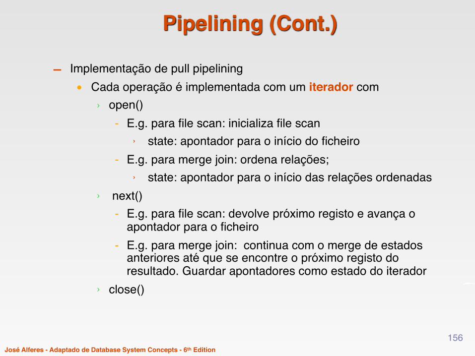
- Implementação de pull pipelining• Cada operação é implementada com um iterador com

› open()- E.g. para file scan: inicializa file scan

› state: apontador para o início do ficheiro- E.g. para merge join: ordena relações;

› state: apontador para o início das relações ordenadas› next()

- E.g. para file scan: devolve próximo registo e avança o apontador para o ficheiro

- E.g. para merge join: continua com o merge de estados anteriores até que se encontre o próximo registo do resultado. Guardar apontadores como estado do iterador

› close()

156


Algoritmos de avaliação com Pipelining

- Alguns algoritmos não funcionam com pipelining• E.g. merge join, ou hash join• Os resultados intermédios têm que ser materializados

- Há variantes de algoritmos para gerar (pelo menos) alguns resultados à medida que os registos de input vão sendo lidos• E.g. hybrid hash join (ver detalhes no livro)

- Parece claro que o pipelining pode beneficiar grandemente de paralelização, especialmente se houver muitas sub-expressões independentes• Mas esta não é a única oportunidade para processamento paralelo!

157


Paralelismo Intraquery

- Execução paralela de uma pergunta em múltiplos processadores/discos; é importante para tornar mais eficiente perguntas longas, quando há vários processadores

- Duas formas complementares de paralelismo intraquery:• Intraoperation Parallelism – paralelizar a execução de cada

operação separadamente• Interoperation Parallelism – executar as diferentes operações em

paralelo (e.g. com pipelining)

- O paralelismo intraoperation tem o potencial para melhorias mais significativas:• o nº de registos a processar por cada operação é tipicamente muito

maior que o nº de operações numa pergunta!

158


Processamento paralelo de operações

- A discussão sobre algoritmos paralelos assume:• shared-nothing architecture (i.e. não há memória ou disco

partilhado)• n processadores, P0, ..., Pn-1, e n discos D0, ..., Dn-1, onde o disco

Di está associado ao processador Pi.

- Se um processador tiver vários discos estes podem ser simulados como apenas um disco Di

- As shared-nothing architectures podem ser simuladas com sistemas de shared-memory ou shared-disk • Os algoritmos para shared-nothing podem assim correr em

shared-memory ou shared-disk systems. › Embora se possam fazer algumas otimizações

159


Parallel Sort

Range-Partitioning Sort

- Escolher processadores P0, ..., Pm para ordenação, onde m ≤ n -1

- Criar vetor de range-partition para m entradas, nos atributos de ordenação

- Redistribuir a relação usando range partitioning• Todos os registos no ith range são enviados para o processador Pi

• Pi armazena temporariamente os registos que recebe, no disco Di. • Este passo tem um overhead de espaço e tempo de escrita.

- Cada processador Pi ordena a sua partição localmente.

- Cada processador executa uma operação (sort) em paralelo com os outros processadores, sem interação entre eles (data parallelism).

- O merge final é trivial: o range-partitioning assegura que para i ≤ j, os valores no processador Pi são todos menores que os valores em Pj.

160


Parallel Sort (Cont.)

Parallel External Sort-Merge

- Assuma-se que a relação já foi partida pelos discos D0, ..., Dn-1 (de qualquer forma)

- Cada processador Pi ordena localmente Di.

- Os runs ordenados em cada processador são juntos para obter o resultado final

- Pode paralelizar-se a junção dos runs ordenados:• As partições ordenadas em cada Pi são range-partitioned pelo

processadores P0, ..., Pm-1.

• Cada Pi faz a junção à medida que vai recebendo resultados, para obter um único run ordenado

• Os runs ordenados nos processadores P0,..., Pm-1 são concatenados para obter o resultado final

161


Parallel Join – Ideia de Base

- Os algoritmos paralelos de junção tentam partir as duas tabelas em partes e dar cada parte a um processador para fazer a junção.• O ideal é que as partes sejam independentes

- No fim, é só juntar as várias partes

162


Partitioned Join

- Para junções com condição de igualdade é possível particionar as duas tabelas e distribuir por processadores

- Sejam r e s duas relações em que queremos calcular r r.A=s.B s.

- r e s são particionadas em n partições, r0, r1, ..., rn-1 e s0, s1, ..., sn-1.

- Pode-se usar range partitioning ou hash partitioning- r e s tem que ser particionadas pelo atributo de junção (r.A e s.B), quer

seja por range ou hash.

- Cada par ri e si é enviado para o processador Pi,

- Cada Pi calcula localmente ri ri.A=si.B si. Qualquer algoritmo de junção serve

163


Partitioned Join (Cont.)

164


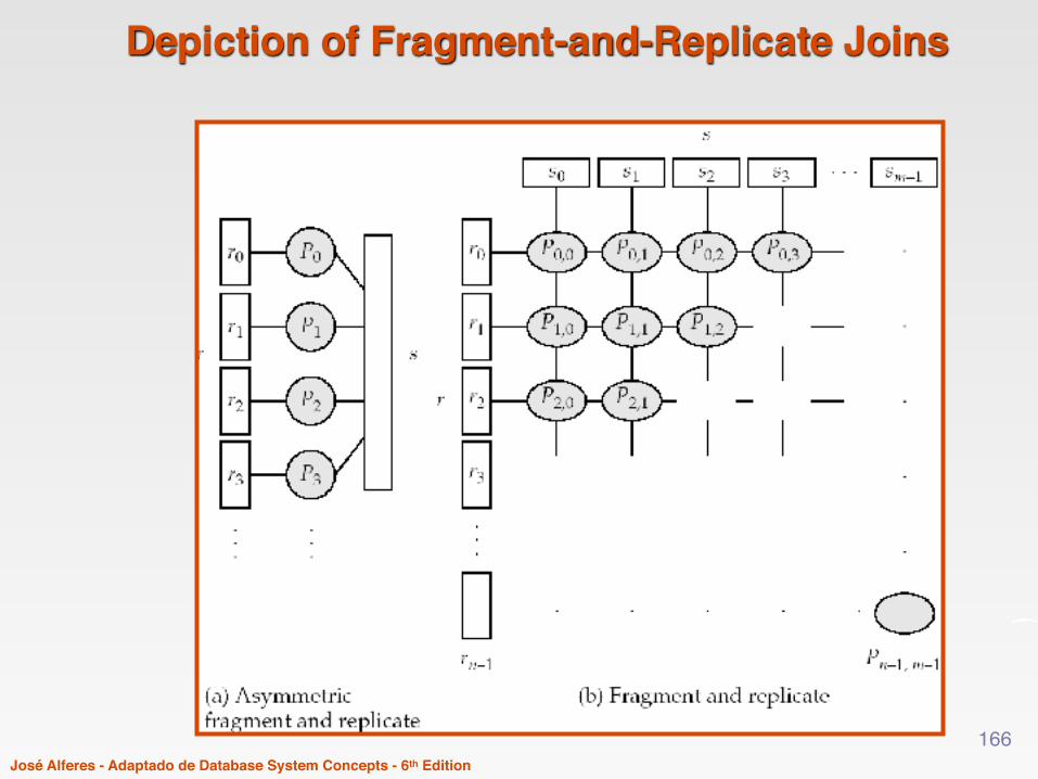
Fragment-and-Replicate Join

- Esta técnica é usado quando não faz sentido particionar as tabelas para a junção• Nem sempre particionar é útil

› e.g., para condições do tipo r.A > s.B.- Ideia de base:

• Partir r em n fragmentos, e s em m fragmentos• Usar n*m processadores para calcular as junções de todos os

pares de fragmentos› Isto obriga a replicar fragmentos

• Fazer a união das junções obtidas

- Caso especial – asymmetric fragment-and-replicate:• Uma das relações, e.g. r, é particionada• A outra relação, s, é replicada pelos vários processadores• O processador Pi calcula localmente a junção de ri com s usando

um qualquer algoritmo de junção165


Depiction of Fragment-and-Replicate Joins

166


Fragment-and-Replicate Join (Cont.)

- Ambas as versões de fragment-and-replicate funcionam com qualquer tipo de condição, pois am ambas todo o registo de r é comparado com todo o registo de s

- Tem um custo maior do que só particionar, pois uma (para asymmetric fragment-and-replicate) ou ambas as relações (para general fragment-and-replicate) têm que ser replicadas

- Por vezes o asymmetric fragment-and-replicate é preferível.• E.g., se s for muito pequeno e r for grande e já estiver particionado.

Nesse caso, pode ser barato replicar s pelos vários processadores, em vez de estar a re-particionar r e s pelo atributo de junção

167


Parallel Selection

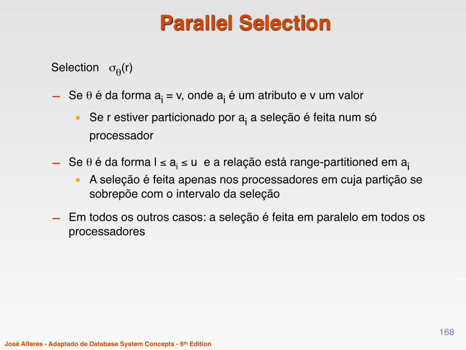
Selection σθ(r)

- Se θ é da forma ai = v, onde ai é um atributo e v um valor

• Se r estiver particionado por ai a seleção é feita num só processador

- Se θ é da forma l ≤ ai ≤ u e a relação está range-partitioned em ai• A seleção é feita apenas nos processadores em cuja partição se

sobrepõe com o intervalo da seleção

- Em todos os outros casos: a seleção é feita em paralelo em todos os processadores

168


Outras operações

- Eliminação de duplicados• Usar técnicas de ordenação paralela

› eliminar os registos duplicados à medida que forem encontrados em cada processador

• Também se pode particionar (usando range- or hash- partitioning) e fazer a eliminação de duplicados localmente em cada processador

- Projeção• Se não tiver eliminação de duplicados, é feita à medida que os

registos são lidos em paralelo• Se há eliminação de duplicados, usar as técnicas acima

169


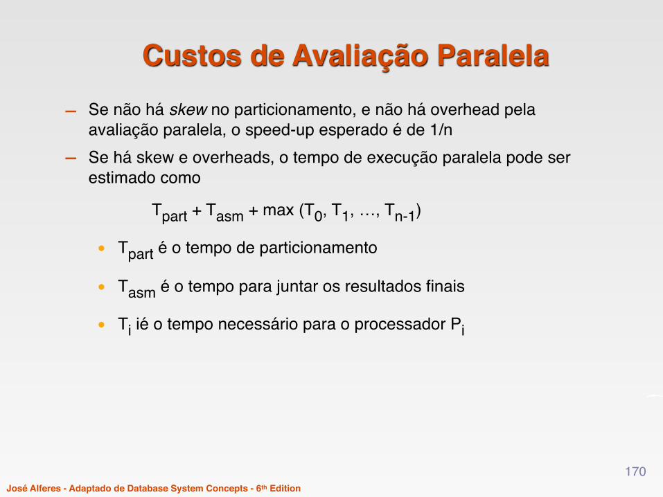
Custos de Avaliação Paralela - Se não há skew no particionamento, e não há overhead pela

avaliação paralela, o speed-up esperado é de 1/n - Se há skew e overheads, o tempo de execução paralela pode ser

estimado como

Tpart + Tasm + max (T0, T1, …, Tn-1)

• Tpart é o tempo de particionamento

• Tasm é o tempo para juntar os resultados finais

• Ti ié o tempo necessário para o processador Pi

170


Interoperator Parallelism

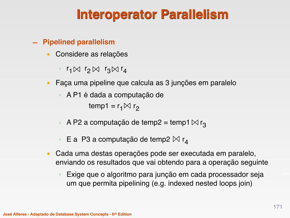
- Pipelined parallelism• Considere as relações

› r1 r2 r3 r4• Faça uma pipeline que calcula as 3 junções em paralelo

› A P1 é dada a computação de temp1 = r1 r2

› A P2 a computação de temp2 = temp1 r3

› E a P3 a computação de temp2 r4• Cada uma destas operações pode ser executada em paralelo,

enviando os resultados que vai obtendo para a operação seguinte› Exige que o algoritmo para junção em cada processador seja

um que permita pipelining (e.g. indexed nested loops join)

171


Limitações de Pipeline Parallelism - O Paralelismo com Pipeline é útil pois evita escritas de resultados

intermédios- É útil quando há um nº pequeno de processadores disponíveis (é raro

haver uma cadeia grande de pipelines)- Não se pode usar vários operadores e algoritmos (e.g. aggregate and

sort) - O speedup é baixo

172


Processamento de perguntas em Oracle

- O Oracle implementa a maior parte do algoritmos que vimos• Para seleção

› Full table scan (i.e. linear search algorithm)› Index scan (as described above in these slides)› Index fast full scan (transverse the whole table using the B+

index)› Cluster and hash cluster access (access data by using cluster

key)• For join

› (Block) nested loop join (possibly using indexes, when available)

› Sort-merge join› Hash join

173


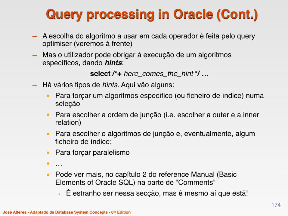
Query processing in Oracle (Cont.)- A escolha do algoritmo a usar em cada operador é feita pelo query

optimiser (veremos à frente)- Mas o utilizador pode obrigar à execução de um algoritmos

específicos, dando hints:select /*+ here_comes_the_hint */ …

- Há vários tipos de hints. Aqui vão alguns:• Para forçar um algoritmos específico (ou ficheiro de índice) numa

seleção• Para escolher a ordem de junção (i.e. escolher a outer e a inner

relation)• Para escolher o algoritmos de junção e, eventualmente, algum

ficheiro de índice;• Para forçar paralelismo• …• Pode ver mais, no capítulo 2 do reference Manual (Basic

Elements of Oracle SQL) na parte de “Comments”› É estranho ser nessa secção, mas é mesmo aí que está!

174


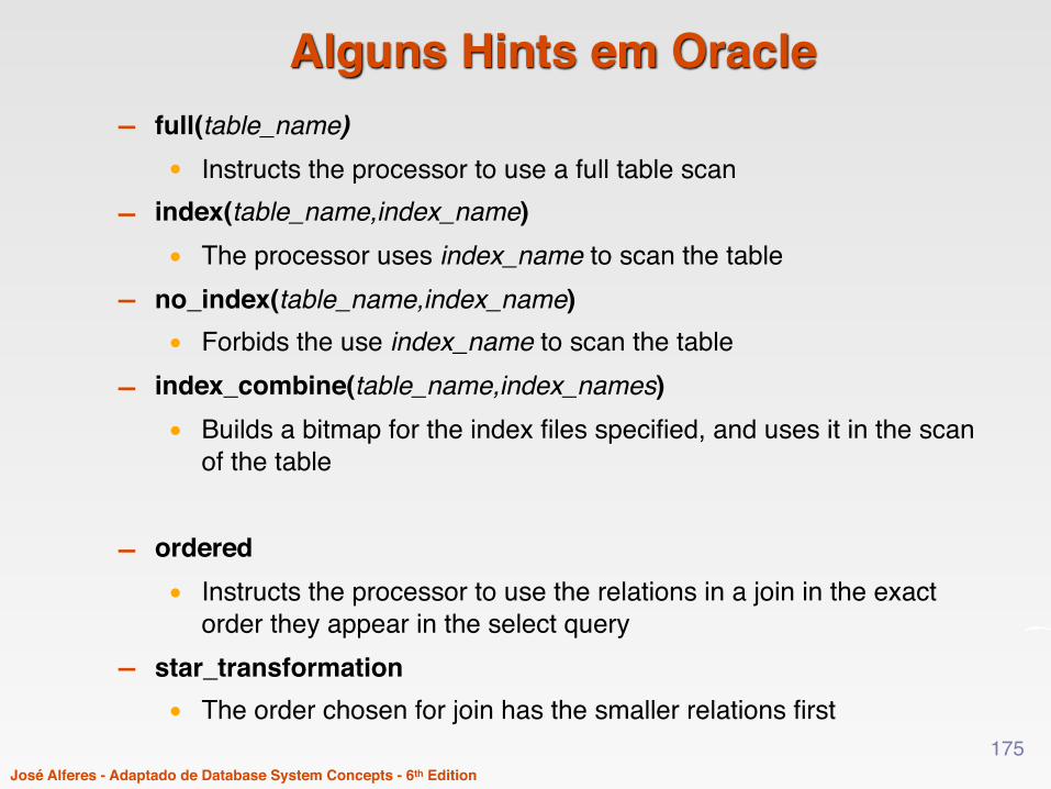
Alguns Hints em Oracle- full(table_name)

• Instructs the processor to use a full table scan- index(table_name,index_name)

• The processor uses index_name to scan the table- no_index(table_name,index_name)

• Forbids the use index_name to scan the table

- index_combine(table_name,index_names)• Builds a bitmap for the index files specified, and uses it in the scan

of the table

- ordered• Instructs the processor to use the relations in a join in the exact

order they appear in the select query- star_transformation

• The order chosen for join has the smaller relations first175


(Mais) alguns Hints em Oracle- use_nl(table_name,table_name)

• Uses (block) nested loop for the join between the tables- use_nl_with_index(table_name,index_name)

• The table is to be used as the inner relation of the join, in a nested loop algorithm, using the index file in the inner loop

- use_merge(table_name,table_name)• Uses merge-join algorithm for the join between the tables

- use_hash(table_name,table_name)• Uses hash join algorithm for the join between the tables

- first_rows(n)• Instructs the processor to use the fastest plan for providing the

first n tuple of the result (as in pipelining)- all_rows

• The optimisation is made assuming taking into account the cost of obtaining all the tuples of the result

176


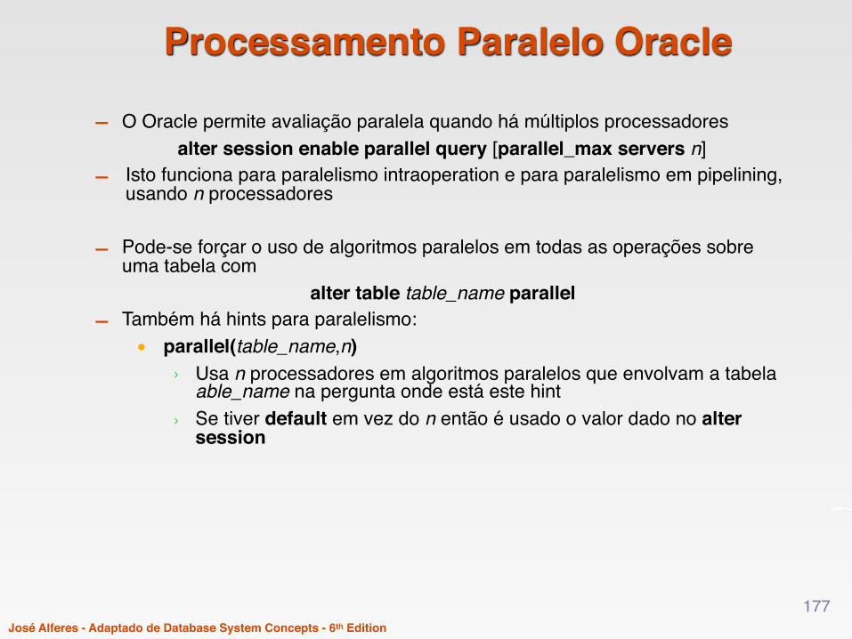
Processamento Paralelo Oracle

- O Oracle permite avaliação paralela quando há múltiplos processadoresalter session enable parallel query [parallel_max servers n]

- Isto funciona para paralelismo intraoperation e para paralelismo em pipelining, usando n processadores

- Pode-se forçar o uso de algoritmos paralelos em todas as operações sobre uma tabela com

alter table table_name parallel- Também há hints para paralelismo:

• parallel(table_name,n)› Usa n processadores em algoritmos paralelos que envolvam a tabela

able_name na pergunta onde está este hint› Se tiver default em vez do n então é usado o valor dado no alter

session

177

José AlferesSistemas de Bases de Dados - ISCTEM janeiro de 2017

Chapter 13: Query Optimisation

178


Chapter 14: Query Optimisation

- Generation of plans• Transformation of relational expressions• Cost-based optimisation• Dynamic Programming for Choosing Evaluation Plans• Heuristics in optimisation

- Optimising nested subqueries, and multi-queries- Statistical Information for Cost Estimation

• Size estimation of (intermediate) results

179


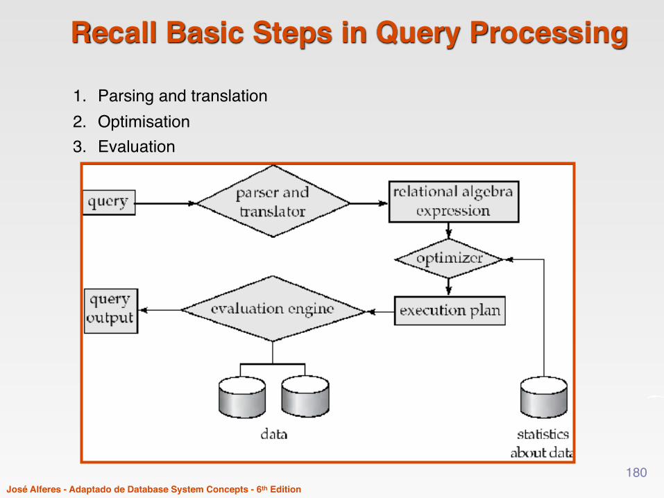
Recall Basic Steps in Query Processing

1. Parsing and translation2. Optimisation3. Evaluation

180


Introduction- Alternative ways of evaluating a given query, by:

• Using different, equivalent, relational expressions• Using different algorithms for each operation in the chosen

expression

181


Introduction (Cont.)

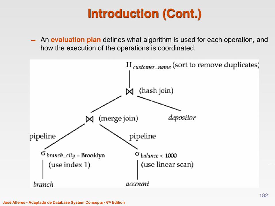
- An evaluation plan defines what algorithm is used for each operation, and how the execution of the operations is coordinated.

182


Introduction (Cont.)

- Cost difference between different evaluation plans for a same query can be huge!

- Steps in cost-based query optimisation are:1. Generate logically equivalent expressions using equivalence rules2. Annotate resultant expressions to get alternative query plans3. Choose the cheapest plan based on estimated cost

- Estimation of plan cost based on:• Statistical information about relations. Examples:

> number of tuples, number of distinct values for an attribute• Statistics estimation for intermediate results

> to estimate cost of complex expressions• Cost formulae for each of the algorithms, computed using statistics

183


Transformation of Relational Expressions

- Two relational algebra expressions are equivalent if the two expressions generate the same set of tuples on every database instance

- In SQL, inputs and outputs are multisets (where the order is not relevant but duplicates may exist) of tuples• Two expressions in the multiset version of the relational algebra

are said to be equivalent if the two expressions generate the same multiset of tuples on every database instance.

- An equivalence rule says that expressions of two forms are equivalent• One can always replace an expression of first form by another in

the second form, or vice versa- It is possible to establish such rules for a formal and declarative

language such as relational algebra- The correctness of equivalence rules is established by formal proofs

184


Equivalence Rules

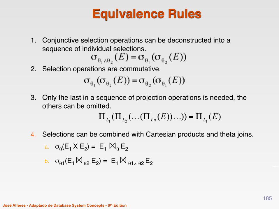
1. Conjunctive selection operations can be deconstructed into a sequence of individual selections.

2. Selection operations are commutative.

3. Only the last in a sequence of projection operations is needed, the others can be omitted.

4. Selections can be combined with Cartesian products and theta joins.a. σθ(E1 X E2) = E1 θ E2

b. σθ1(E1 θ2 E2) = E1 θ1∧ θ2 E2

185


Equivalence Rules (Cont.)

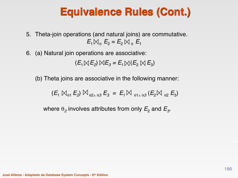
5. Theta-join operations (and natural joins) are commutative.E1 θ E2 = E2 θ E1

6. (a) Natural join operations are associative: (E1 E2) E3 = E1 (E2 E3)

(b) Theta joins are associative in the following manner:

(E1 θ1 E2) θ2∧ θ3 E3 = E1 θ1∧ θ3 (E2 θ2 E3) where θ2 involves attributes from only E2 and E3.

186



7. The selection operation distributes over the theta join operation under the following two conditions:(a) When all the attributes in θ0 involve only the attributes of one of the expressions (E1) being joined. σθ0(E1 θ E2) = (σθ0(E1)) θ E2

(b) When θ 1 involves only the attributes of E1 and θ2 involves only the attributes of E2. σθ1∧θ2 (E1 θ E2) = (σθ1(E1)) θ (σθ2 (E2))

187


Equivalence Rules in Expression Trees

188


Equivalence Rules (Cont.)8. The projection operation distributes over the theta join operation as

follows:(a) if θ involves only attributes from L1 ∪ L2:

(b) Consider a join E1 θ E2.

• Let L1 and L2 be sets of attributes from E1 and E2, respectively.

• Let L3 be attributes of E1 that are involved in join condition θ, but are not in L1 ∪ L2, and

• let L4 be attributes of E2 that are involved in join condition θ, but are not in L1 ∪ L2.

))(())(()( 2121 2121EEEE LLLL

∏∏=∏ ∪ θθ

)))(())((()( 2121 42312121EEEE LLLLLLLL ∪∪∪∪

∏∏∏=∏θθ

189



9. The set operations union and intersection are commutative E1 ∪ E2 = E2 ∪ E1 E1 ∩ E2 = E2 ∩ E1

• (Obviously, set difference is not commutative!).10. Set union and intersection are associative.

(E1 ∪ E2) ∪ E3 = E1 ∪ (E2 ∪ E3) (E1 ∩ E2) ∩ E3 = E1 ∩ (E2 ∩ E3)

11. The selection operation distributes over ∪, ∩ and –. σθ (E1 – E2) = σθ (E1) – σθ(E2) and similarly for ∪ and ∩ in place of – Also: σθ (E1 – E2) = σθ(E1) – E2

and similarly for ∩ in place of –, but not for ∪12. The projection operation distributes over union ΠL(E1 ∪ E2) = (ΠL(E1)) ∪ (ΠL(E2))

190


Transformation Example: Pushing Selections

- Query: Names of all customers who have an account at some branch located in Brooklyn.Πcustomer_name(σbranch_city = “Brooklyn”

(branch (account depositor)))

- Transformation using rule 7a. Πcustomer_name

((σbranch_city =“Brooklyn” (branch)) (account depositor))• It is usually a good idea since performing the selection as early as

possible reduces the size of the relation to be joined.

191


Example with Multiple Transformations

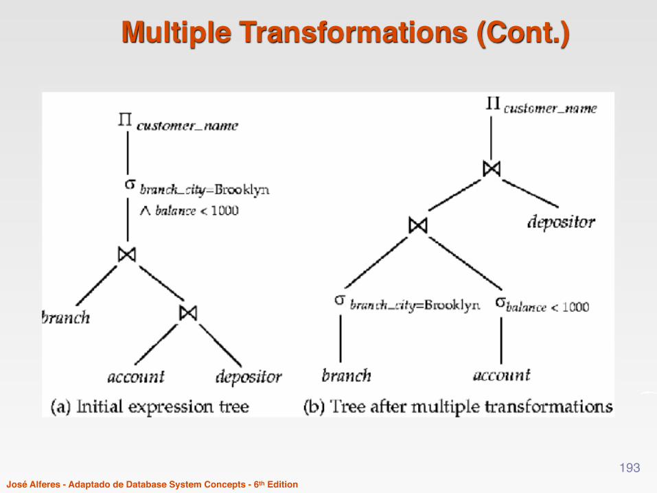
- Query: Names of all customers with an account at a Brooklyn branch whose account balance is over $1000.Πcustomer_name((σbranch_city = “Brooklyn” ∧ balance > 1000

(branch (account depositor)))- Transformation using join associatively (Rule 6a):

Πcustomer_name((σbranch_city = “Brooklyn” ∧ balance > 1000

(branch account)) depositor) - Second form provides an opportunity to apply the “perform

selections early” rule, resulting in the subexpression σbranch_city = “Brooklyn” (branch) σ balance > 1000 (account)

- A sequence of transformations can be useful!

192


Multiple Transformations (Cont.)

193


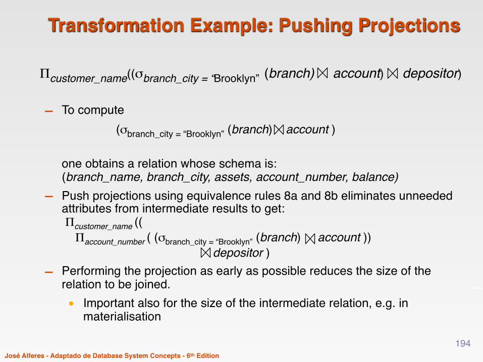
Transformation Example: Pushing Projections

- To compute(σbranch_city = “Brooklyn” (branch) account )

one obtains a relation whose schema is:(branch_name, branch_city, assets, account_number, balance)

- Push projections using equivalence rules 8a and 8b eliminates unneeded attributes from intermediate results to get: Πcustomer_name (( Πaccount_number ( (σbranch_city = “Brooklyn” (branch) account )) depositor )

- Performing the projection as early as possible reduces the size of the relation to be joined. • Important also for the size of the intermediate relation, e.g. in

materialisation

Πcustomer_name((σbranch_city = “Brooklyn” (branch) account) depositor)

194


Join Ordering Example

- For all relations r1, r2, and r3,(r1 r2) r3 = r1 (r2 r3 )

(Join Associativity)

- If r2 r3 is quite large, and r1 r2 is small, we choose (r1 r2) r3

so that the computed temporary relation (in case no pipelining is applied) is smaller.

195


Join Ordering Example (Cont.)

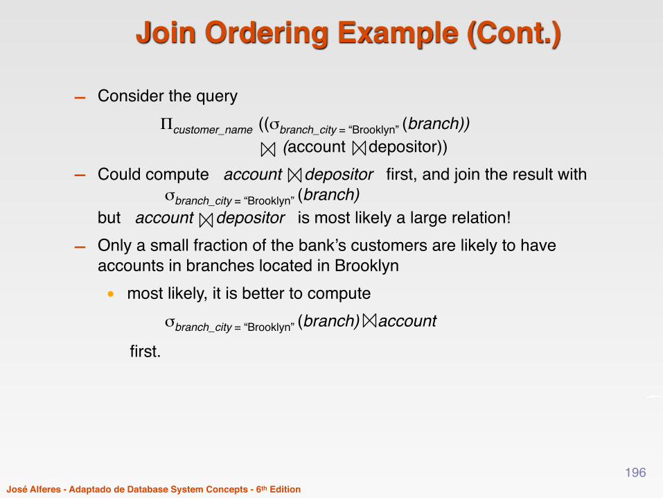
- Consider the queryΠcustomer_name ((σbranch_city = “Brooklyn” (branch))

(account depositor))- Could compute account depositor first, and join the result with

σbranch_city = “Brooklyn” (branch) but account depositor is most likely a large relation!

- Only a small fraction of the bank’s customers are likely to have accounts in branches located in Brooklyn• most likely, it is better to compute

σbranch_city = “Brooklyn” (branch) account first.

196


Enumeration of Equivalent Expressions

- Query optimisers use equivalence rules to systematically generate (all) expressions equivalent to the given expression

- One way to generate all equivalent expressions is: • Repeat

› apply all applicable equivalence rules on every equivalent expression found so far

› add newly generated expressions to the set of equivalent expressions Until no new equivalent expressions are generated above

- The above fixpoint approach is very expensive in space and time, as the number of equivalent expressions is usually too big (exponential on the size of the query)• Two (or three) approaches to reduce the cost

› Optimised plan generation based on transformation rules› Special case approach for queries with only selections, projections and

joins› (Give hints to cut the space of possible generated equivalent expressions)

197


Transformation Based Optimisation- Space requirements can be reduced by sharing common sub-expressions:

• when E1 is generated from E2 by an equivalence rule, usually only the top level of the two are different, subtrees below are the same and can be shared using pointers› E.g. when applying join commutativity

• Same sub-expression may be generated multiple times› Detect duplicate sub-expressions and share one copy

- Time requirements are reduced by not generating all expressions• Dynamic programming

› We will study only the special case of dynamic programming for join order optimisation

E1 E2

198


Cost Estimation

- Cost of each operator computed as described in Query Processing• It needs statistics of input relations (e.g. number of tuples, sizes of

tuples, etc)- Inputs can be results of sub-expressions

• Need to estimate statistics of expression results• To do so, additional statistics are required, e.g. number of distinct

values for an attribute• For now, let us assume that we have some way of estimating the

costs of each operation› Will see afterwards how this can be done

199


Choice of Evaluation Plans

- The interaction of evaluation techniques must be considered when choosing evaluation plans• choosing the cheapest algorithm for each operation independently

may not yield best overall algorithm. E.g.› merge-join may be costlier than hash-join, but may provide a

sorted output which reduces the cost for an outer level aggregation.

› nested-loop join may provide opportunity for pipelining- Practical query optimisers incorporate elements of the following two

broad approaches:1. Search all the plans and choose the best plan in a

cost-based fashion.2. Use heuristics to choose a plan.

200


Cost-Based Optimisation

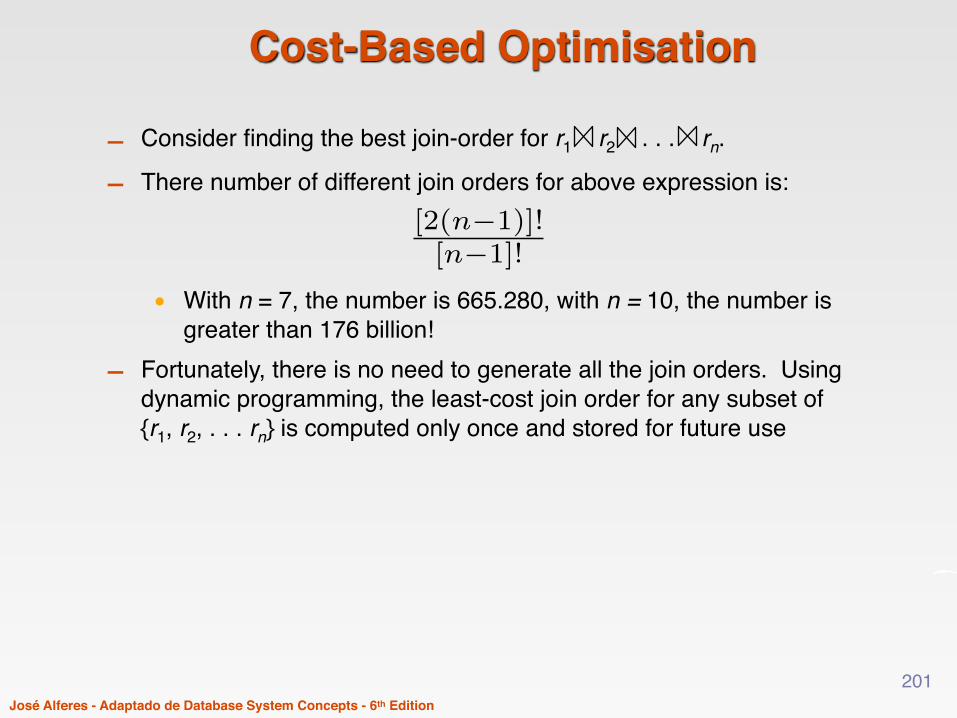
- Consider finding the best join-order for r1 r2 . . . rn.

- There number of different join orders for above expression is:

• With n = 7, the number is 665.280, with n = 10, the number is greater than 176 billion!

- Fortunately, there is no need to generate all the join orders. Using dynamic programming, the least-cost join order for any subset of {r1, r2, . . . rn} is computed only once and stored for future use

201

[2(n�1)]![n�1]!


Dynamic Programming in Optimisation

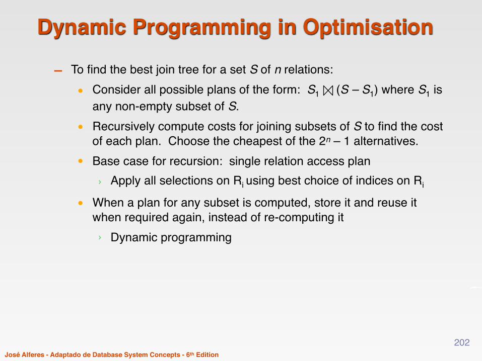
- To find the best join tree for a set S of n relations:• Consider all possible plans of the form: S1 (S – S1) where S1 is

any non-empty subset of S.• Recursively compute costs for joining subsets of S to find the cost

of each plan. Choose the cheapest of the 2n – 1 alternatives.• Base case for recursion: single relation access plan

› Apply all selections on Ri using best choice of indices on Ri

• When a plan for any subset is computed, store it and reuse it when required again, instead of re-computing it› Dynamic programming

202


Join Order Optimisation Algorithm

procedure findbestplan(S)if (bestplan[S].cost ≠ ∞)

return bestplan[S]% else bestplan[S] has not been computed earlier, compute it now if (S contains only 1 relation) set bestplan[S].plan and bestplan[S].cost based on the best way of accessing S /* Using selections on S and indices on S */

else for each non-empty subset S1 of S such that S1 ≠ S

P1= findbestplan(S1)P2= findbestplan(S - S1)A = best algorithm for joining results of P1 and P2 cost = P1.cost + P2.cost + cost of Aif cost < bestplan[S].cost

{bestplan[S].cost = costbestplan[S].plan = “execute P1.plan; execute P2.plan;

join results of P1 and P2 using A”}return bestplan[S]

203


Left Deep Join Trees

- An interesting special case is left-deep join trees• In left-deep join trees, the right-hand-side input for each

join is a relation, not the result of an intermediate join.

204


Cost of Optimisation

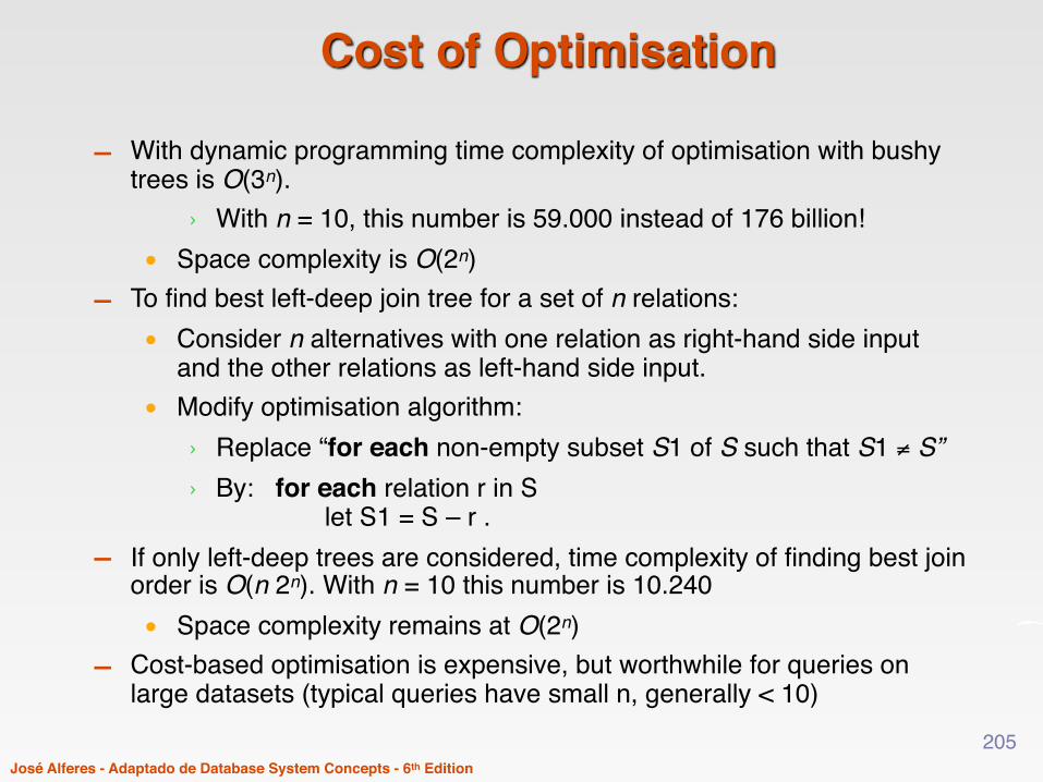
- With dynamic programming time complexity of optimisation with bushy trees is O(3n).

› With n = 10, this number is 59.000 instead of 176 billion!• Space complexity is O(2n)

- To find best left-deep join tree for a set of n relations:• Consider n alternatives with one relation as right-hand side input

and the other relations as left-hand side input.• Modify optimisation algorithm:

› Replace “for each non-empty subset S1 of S such that S1 ≠ S”› By: for each relation r in S

let S1 = S – r .- If only left-deep trees are considered, time complexity of finding best join

order is O(n 2n). With n = 10 this number is 10.240• Space complexity remains at O(2n)

- Cost-based optimisation is expensive, but worthwhile for queries on large datasets (typical queries have small n, generally < 10)

205


Interesting Sort Orders

- Consider the expression (r1 r2) r3 (with A as common attribute)

- An interesting sort order is a particular sort order of tuples that could be useful for a later operation• Using merge-join to compute r1 r2 may be costlier than hash join

but generates the result sorted on A• Which in turn may make merge-join with r3 cheaper, which may

reduce cost of join with r3 and minimising overall cost • Sort order may also be useful for order by and for grouping

- It is not enough to find the best join order for each subset of the set of n given relations• must find the best join order for each subset, for each interesting sort

order• Simple extension of previous dynamic programming algorithms• Usually, number of interesting orders is quite small and doesn’t affect

time/space complexity significantly206


Join Minimisation

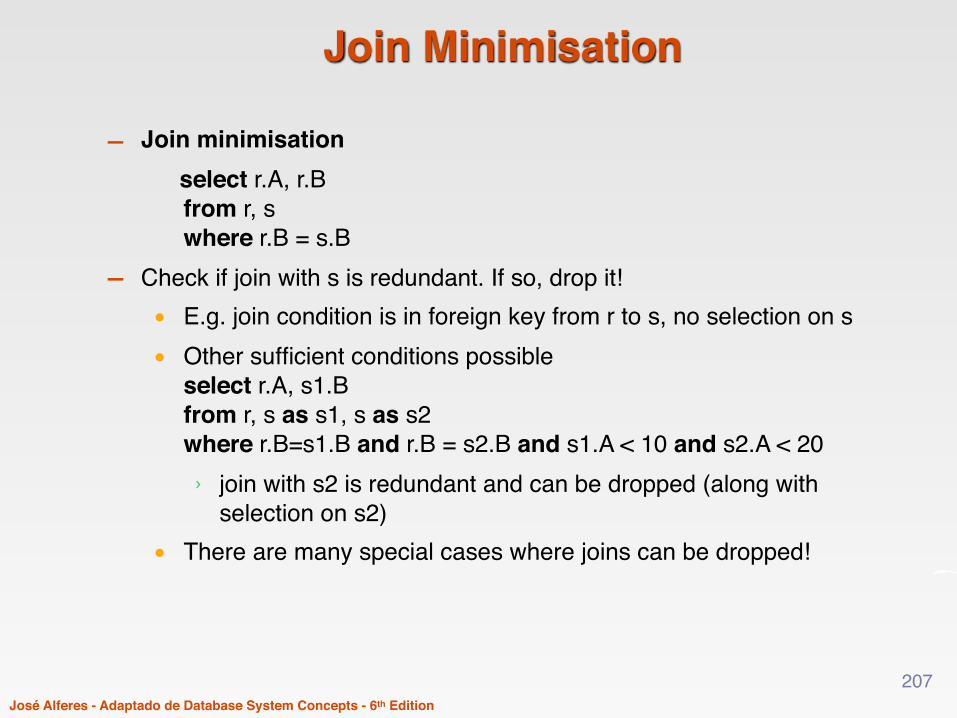
- Join minimisation select r.A, r.B

from r, s where r.B = s.B

- Check if join with s is redundant. If so, drop it!• E.g. join condition is in foreign key from r to s, no selection on s• Other sufficient conditions possible

select r.A, s1.B from r, s as s1, s as s2 where r.B=s1.B and r.B = s2.B and s1.A < 10 and s2.A < 20› join with s2 is redundant and can be dropped (along with

selection on s2)• There are many special cases where joins can be dropped!

207


Optimising Nested Subqueries- Nested query example:

select customer_name from borrowerwhere exists (select *

from depositor where depositor.customer_name =

borrower.customer_name)- SQL conceptually treats nested subqueries in the where clause as

functions that take parameters and return a single value or set of values• Parameters are variables from outer level query that are used in the

nested subquery; such variables are called correlation variables- Conceptually, a nested subquery is executed once for each tuple in the

cross-product generated by the outer level from clause• Such evaluation is called correlated evaluation • Note: other conditions in where clause may be used to compute a join

(instead of a cross-product) before executing the nested subquery

208


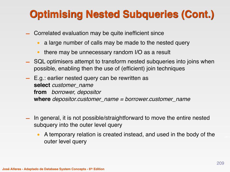
Optimising Nested Subqueries (Cont.)- Correlated evaluation may be quite inefficient since

• a large number of calls may be made to the nested query • there may be unnecessary random I/O as a result

- SQL optimisers attempt to transform nested subqueries into joins when possible, enabling then the use of (efficient) join techniques

- E.g.: earlier nested query can be rewritten as select customer_name from borrower, depositor where depositor.customer_name = borrower.customer_name

- In general, it is not possible/straightforward to move the entire nested subquery into the outer level query• A temporary relation is created instead, and used in the body of the

outer level query

209


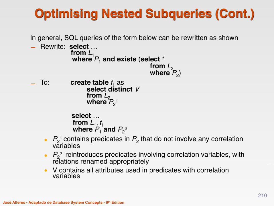
Optimising Nested Subqueries (Cont.)In general, SQL queries of the form below can be rewritten as shown- Rewrite: select …

from L1 where P1 and exists (select *

from L2 where P2)- To: create table t1 as

select distinct V from L2 where P2

1

select …

from L1, t1 where P1 and P22

• P21 contains predicates in P2 that do not involve any correlation

variables• P2

2 reintroduces predicates involving correlation variables, with relations renamed appropriately

• V contains all attributes used in predicates with correlation variables

210


Optimising Nested Subqueries (Cont.)

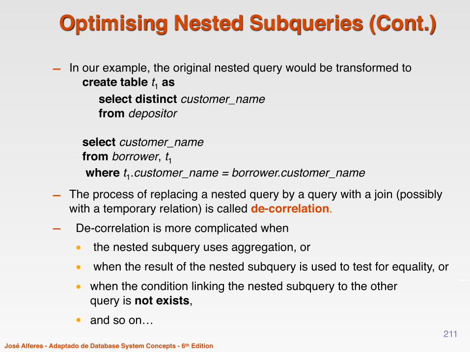
- In our example, the original nested query would be transformed to create table t1 as select distinct customer_name from depositor select customer_name from borrower, t1 where t1.customer_name = borrower.customer_name

- The process of replacing a nested query by a query with a join (possibly with a temporary relation) is called de-correlation.

- De-correlation is more complicated when• the nested subquery uses aggregation, or• when the result of the nested subquery is used to test for equality, or • when the condition linking the nested subquery to the other

query is not exists, • and so on…

211


Heuristic Optimisation

- Cost-based optimisation is expensive, even with dynamic programming.- Systems may use heuristics to reduce the number of choices that must

be made in a cost-based fashion.- Heuristic optimisation transforms the query-tree by using a set of rules

that typically (but not in all cases) improve execution performance:• Perform selection early (reduces the number of tuples)• Perform projection early (reduces the number of attributes)• Perform most restrictive selection and join operations (i.e. with

smallest result size) before other similar operations.- Some systems use only heuristics, others combine heuristics with

partial cost-based optimisation.- Local search (e.g. hill-climbing and genetic algorithms) may also be

used for optimisation

212


Structure of Query Optimisers

- Many optimisers consider only left-deep join orders.• Plus heuristics to push selections and projections down the query

tree• Reduces optimisation complexity and generates plans amenable to

pipelined evaluation.- Heuristic optimisation can be used in Oracle:

• Repeatedly pick “best” relation to join next › Starting from each of n starting points. Pick best among these

- Syntactical variations of SQL complicate query optimisation• E.g. nested subqueries

213


Structure of Query Optimisers (Cont.)

- Some query optimisers integrate heuristic selection and the generation of alternative access plans.• Frequently used approach

› heuristic rewriting of nested block structure and aggregation› followed by cost-based join-order optimisation for each block

• Some optimisers (e.g. SQL Server) apply transformations to entire query and do not depend on block structure

- Even with the use of heuristics, cost-based query optimisation imposes a substantial overhead.• But is worth it for expensive queries in large datasets• Optimisers often use simple heuristics for very cheap queries,

and perform exhaustive enumeration for more expensive queries

• The cost of optimisation is a function of the size of the query, whilst the gains are a functions of the size of the dataset

214


Multiquery Optimisation- Example

Q1: select * from (r natural join t) natural join sQ2: select * from (r natural join u) natural join s

• Both queries share common subexpression (r natural join s)• May be useful to compute (r natural join s) once and use it in both queries

› But this may be more expensive in some situations- e.g. (r natural join s) may be expensive, plans as shown in queries

may be cheaper- Multiquery optimisation: find best overall plan for a set of queries, exploiting

sharing of common subexpressions between queries where it is useful- Simple heuristic used in some database systems:

• optimise each query separately• detect and exploiting common subexpressions in the individual optimal

query plans› May not always give best plan, but is cheap to implement

- Set of materialised views may share common subexpressions• As a result, view maintenance plans may share subexpressions• Multiquery optimisation can be useful in such situations

215


Statistical Information for Cost Estimation

- nr: number of tuples in a relation r.

- br: number of blocks containing tuples of r.

- lr: size of a tuple of r.

- fr: blocking factor of r — i.e., the number of tuples of r that fit into one block.• If tuples of r are stored together physically in a file, then:

- V(A, r): number of distinct values that appear in r for attribute A;› same as the size of ∏A(r).

• Histograms with frequencies of values in attributes may also be used by some systems

216


Selection Size Estimation

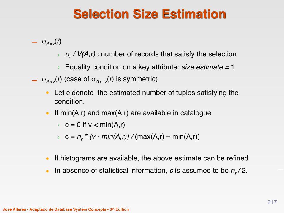
- σA=v(r)› nr / V(A,r) : number of records that satisfy the selection› Equality condition on a key attribute: size estimate = 1

- σA≤V(r) (case of σA ≥ V(r) is symmetric)

• Let c denote the estimated number of tuples satisfying the condition.

• If min(A,r) and max(A,r) are available in catalogue› c = 0 if v < min(A,r)› c = nr * (v - min(A,r)) / (max(A,r) – min(A,r))

• If histograms are available, the above estimate can be refined• In absence of statistical information, c is assumed to be nr / 2.

217


Size Estimation of Complex Selections- The selectivity of a condition θi is the probability that a tuple in the

relation r satisfies θi . • If si is the number of satisfying tuples in r, the selectivity of θi is

given by si /nr.

- Conjunction: σθ1∧ θ2∧. . . ∧ θn (r). Assuming independence, estimate

of tuples in the result is:

- Disjunction:σθ1∨ θ2 ∨. . . ∨ θn (r). Estimated number of tuples:

- Negation: σ¬θ(r). Estimated number of tuples:nr – size(σθ(r))

218

nr ⇤⇣1�

⇣1� s1

nr

⌘⇤⇣1� s2

nr

⌘⇤ . . .

⇣1� sn

nr

⌘⌘


Join Operation: Running Example

Running example: depositor customer

Catalog information for join examples:

- ncustomer = 10.000.

- fcustomer = 25, which implies that bcustomer =10.000/25 = 400.

- ndepositor = 5000.

- fdepositor = 50, which implies that bdepositor = 5.000/50 = 100.

- V(customer_name, depositor) = 2.500, which means that, on average, each customer has two accounts.• Also assume that customer_name in depositor is a foreign key

on customer.• V(customer_name, customer) = 10.000 (primary key!)

219


Estimation of the Size of Joins

- The Cartesian product r x s contains nr .ns tuples; each tuple occupies sr + ss bytes.

- If R ∩ S = ∅, then r s is the same as r x s.

- If R ∩ S is a key for R, then a tuple of s will join with at most one tuple from r• therefore, the number of tuples in r s is not greater than the

number of tuples in s.- If R ∩ S is a foreign key in S referencing R, then the number of tuples

in r s is exactly the same as the number of tuples in s.› The case for R ∩ S being a foreign key referencing S is

symmetric.

- In the example query depositor customer, customer_name in depositor is a foreign key of customer• hence, the result has exactly ndepositor tuples, which is 5.000

220


Estimation of the Size of Joins (Cont.)

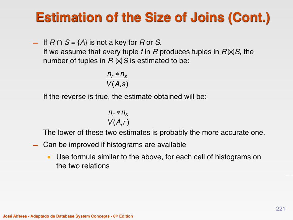
- If R ∩ S = {A} is not a key for R or S.If we assume that every tuple t in R produces tuples in R S, the number of tuples in R S is estimated to be:If the reverse is true, the estimate obtained will be:The lower of these two estimates is probably the more accurate one.

- Can be improved if histograms are available• Use formula similar to the above, for each cell of histograms on

the two relations

221


Estimation of the Size of Joins (Cont.)

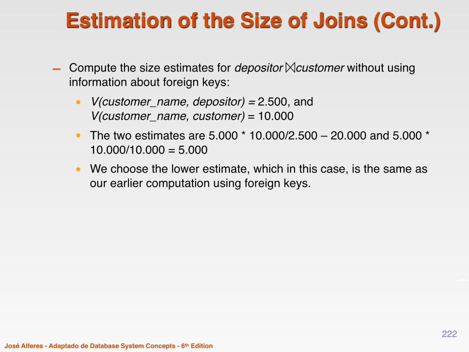
- Compute the size estimates for depositor customer without using information about foreign keys:• V(customer_name, depositor) = 2.500, and

V(customer_name, customer) = 10.000• The two estimates are 5.000 * 10.000/2.500 – 20.000 and 5.000 *

10.000/10.000 = 5.000• We choose the lower estimate, which in this case, is the same as

our earlier computation using foreign keys.

222


Size Estimation (Cont.)

- Outer join: • Estimated size of r s = size of r s + size of r

› Case of right outer join is symmetric• Estimated size of r s = size of r s + size of r + size of s

223


Size Estimation for Other Operations

- Projection: estimated size of ∏A(r) = V(A,r)

- Aggregation : estimated size of AgF(r) = V(A,r)

- Set operations• For unions/intersections of selections on the same relation:

rewrite and use size estimate for selections› E.g. σθ1 (r) ∪ σθ2 (r) can be rewritten as σθ1 σθ2 (r)

• For operations on different relations:› estimated size of r ∪ s = size of r + size of s. › estimated size of r ∩ s = minimum size of r and size of s.› estimated size of r – s = r.

• All the three estimates may be quite inaccurate, but provide upper bounds on the sizes.

224


Estimation of Number of Distinct Values

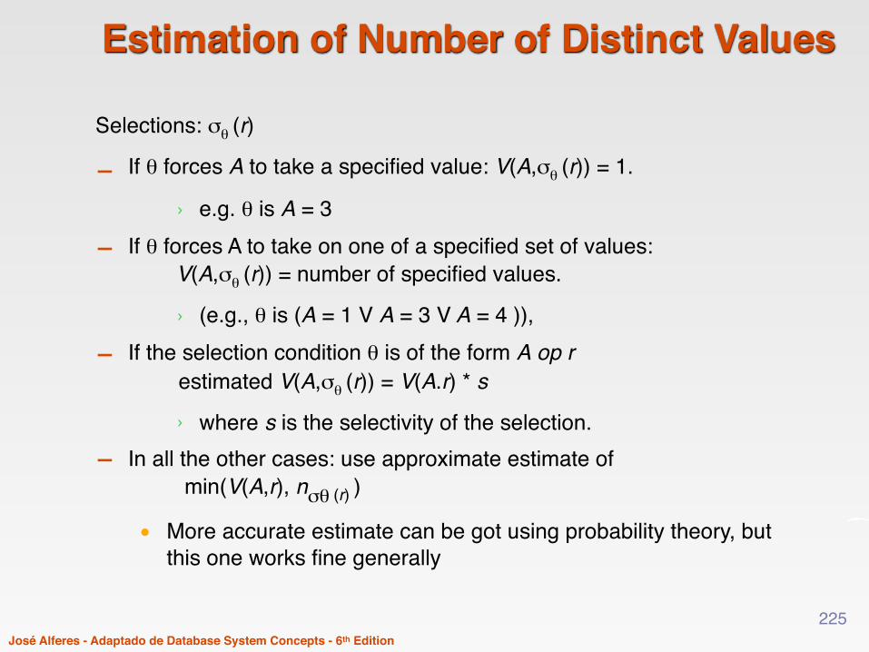
Selections: σθ (r)

- If θ forces A to take a specified value: V(A,σθ (r)) = 1.

› e.g. θ is A = 3

- If θ forces A to take on one of a specified set of values: V(A,σθ (r)) = number of specified values.

› (e.g., θ is (A = 1 V A = 3 V A = 4 )),

- If the selection condition θ is of the form A op restimated V(A,σθ (r)) = V(A.r) * s› where s is the selectivity of the selection.

- In all the other cases: use approximate estimate of min(V(A,r), nσθ (r) )

• More accurate estimate can be got using probability theory, but this one works fine generally

225


Estimation of Distinct Values (Cont.)

Joins: r s- If all attributes in A are from r

estimated V(A, r s) = min (V(A,r), n r s)

- If A contains attributes A1 from r and A2 from s, then estimated V(A,r s) =

min(V(A1,r)*V(A2 – A1,s), V(A1 – A2,r)*V(A2,s), nr s)• More accurate estimate can be got using probability theory, but

this one works fine generally

226


Estimation of Distinct Values (Cont.)

- Estimation of distinct values are straightforward for projections.• They are the same in ∏A (r) as in r.

- The same holds for grouping attributes of aggregation.- For aggregated values

• For min(A) and max(A), the number of distinct values can be estimated as min(V(A,r), V(G,r)) where G denotes grouping attributes

• For other aggregates, assume all values are distinct, and use V(G,r)

227

Documents

Outras operações - ps.ssdi.di.fct.unl.ptps.ssdi.di.fct.unl.pt/ISCTEM/slides/sbd4.pdf · • Hashing é parecido – os duplicados ﬁcam todos no mesmo bucket 147. ... -Cada processador