0

Pós-Graduação em Ciência da Computação

“COGNITIVE RADIO VIRTUAL NETWORKS ENVIRONMENT:

DEFINITION, MODELING AND MAPPING OF SECONDARY

VIRTUAL NETWORKS ONTO WIRELESS SUBSTRATE”

By

ANDSON MARREIROS BALIEIRO

Ph.D Thesis

Universidade Federal de Pernambuco

posgraduacao@cin.ufpe.br

www.cin.ufpe.br/~posgraduacao

RECIFE/2015

1

UNIVERSIDADE FEDERAL DE PERNAMBUCO

CENTRO DE INFORMÁTICA

PÓS-GRADUAÇÃO EM CIÊNCIA DA COMPUTAÇÃO

ANDSON MARREIROS BALIEIRO

“COGNITIVE RADIO VIRTUAL NETWORKS ENVIRONMENT:

DEFINITION, MODELING AND MAPPING OF SECONDARY VIRTUAL

NETWORKS ONTO WIRELESS SUBSTRATE"

THIS THESIS HAS BEEN SUBMITTED TO THE POSTGRADUATE

PROGRAM IN COMPUTER SCIENCE OF THE INFORMATICS

CENTER OF THE FEDERAL UNIVERSITY OF PERNAMBUCO AS A

PARTIAL REQUIREMENT TO OBTAIN THE DEGREE OF DOCTOR

IN COMPUTER SCIENCE.

ADVISOR: KELVIN LOPES DIAS

RECIFE, 2015

2

Catalogação na fonte

Bibliotecária Jane Souto Maior, CRB4-571

B186c Balieiro, Andson Marreiros Cognitive radio virtual networks environment: definition,

modeling and mapping of secondary virtual networks onto wireless substrate / Andson Marreiros Balieiro. – Recife: O Autor, 2015.

137 f.: il. fig., tab. Orientador: Kelvin Lopes Dias. Tese (Doutorado) – Universidade Federal de Pernambuco.

CIn, Ciência da computação, 2015. Inclui referências.

1. Redes de computadores. 2. Redes sem fio. I. Dias, Kelvin Lopes (orientador). II. Título. 004.6 CDD (23. ed.) UFPE- MEI 2015-145

3

Tese de Doutorado apresentada por ANDSON MARREIROS BALIEIRO à Pós-Graduação

em Ciência da Computação do Centro de Informática da Universidade Federal de

Pernambuco, sob o título “Cognitive Radio Virtual Networks Environment: Definition,

Modeling and Mapping of Secondary Virtual Networks onto Wireless Substrate”

orientada pelo Prof. KELVIN LOPES DIAS e aprovada

pela Banca Examinadora formada pelos professores:

______________________________________________

Prof. Paulo Roberto Freire Cunha

Centro de Informática/UFPE

______________________________________________

Prof. José Augusto Suruagy Monteiro

Centro de Informática / UFPE

_______________________________________________

Prof. Paulo Romero Martins Maciel

Centro de Informática / UFPE

_______________________________________________

Prof. Edmundo Roberto Mauro Madeira

Instituto de Computação / UNICAMP

_______________________________________________

Prof. Jose Neuman de Souza

Departamento de Computação / UFC

Visto e permitida a impressão.

Recife, 28 de agosto de 2015.

___________________________________________________

Profa. Edna Natividade da Silva Barros Coordenadora da Pós-Graduação em Ciência da Computação do

Centro de Informática da Universidade Federal de Pernambuco.

4

To my family Natalia, Olinda,

Jacqueline, Viviane, and Liliane.

5

Acknowledgments

First, I would like to give my thanks to God for being with me all the time, and

providing me with the strength to overcome all the challenges.

I would like to thank my mother for her constant encouragement and for being the best

mother of the world. A special thanks too, to my sisters (Viviane, Liliane, and Jacqueline),

nieces, nephews, and aunts (Fatima and Benedita).

I would like to thank my wife Natalia Balieiro for her love and support in the course of

this ´journey´.

I am also very grateful to my advisor Dr. Kelvin Dias, whose expertise and support

have been of great value to my doctoral experience. My sincere thanks to him for believing in

my capacity to conduct this research.

I must also express my gratitude to the committee members, Dr. Edmundo Madeira,

Dr. Neuman de Souza, Dr. Paulo Maciel, Dr. José Augusto Suruagy, and Dr. Paulo Cunha for

agreeing to evaluate my thesis, and offering helpful comments to improve it.

I would also like to thank the Science and Technology Foundation of Pernambuco

(FACEPE) for its financial support, and Center of Informatics (CIn-UFPE) for providing a

suitable environment (both in terms of staff and infrastructure) to undertake this research

study.

6

Abstract

The wireless technologies are progressing at a rapid pace such that the future of digital

communication will be dominated by a dense, ubiquitous and heterogeneous wireless

network. Along with this, there is a growing demand for wireless services with different

requirements. In this respect, the management of this complex wireless ecosystem becomes

challenging, and the wireless virtualization is pointed as an efficient solution to perform it,

where different virtual wireless networks can be created, sharing and running on the same

wireless infrastructure, and providing differentiated services to users. However, to satisfy the

high demand for mobile communications, it is necessary the availability of a natural and

scarce resource, the electromagnetic spectrum. Although the insertion of virtualization in

wireless networks provides better resources utilization, the current approaches to employ the

wireless virtualization can cause resource underutilization. To overcome this underutilization

and enable that new wireless virtual networks can be deployed, the wireless virtualization can

be combined with the cognitive radio technology and dynamic spectrum access (DSA)

techniques in order to achieve the deepest level of wireless virtualization and to improve the

resource utilization through the deployment of opportunistic resource sharing. Thus, virtual

wireless networks with different access priorities to the resources (e.g. primary and

secondary) can be deployed in an overlay form, sharing the same substrate wireless network,

where the secondary virtual network (SVN) accesses the resources only when the primary one

(PVN) is not using them. However, this new scenario brings new challenges: from the

mapping to operation of these networks. The SVN mapping is a NP-hard problem and

presents some constraints and objectives related to both PVNs and SVNs. Achieving all

objectives simultaneously is a challenging process. This thesis addresses the SVNs mapping

problem onto substrate network considering the existence of the PVNs on the same substrate

network. It discloses the environment composed by these networks, denoted as cognitive

radio virtual network environment (CRVNE), models this environment by using a M/M/N/N

queue with preemptive and priority service, and delineates a multi-objective problem

formulation for the SVNs mapping. Moreover, a scheme based on Genetic Algorithms to

solve the SVNs mapping problem is proposed and evaluated in terms of collision, secondary

user (SU) dropping, and SU blocking probabilities, and joint utilization, achieving better

results than other based on the First-Fit strategy.

Keywords: Cognitive Radio Virtual Network Environment. Secondary Virtual Network

Mapping. Primary Virtual Network. Genetic Algorithms. Wireless Virtualization.

7

Resumo

Recentemente, as tecnologias sem fio estão progredindo rapidamente de modo que o futuro da

comunicação digital será dominado por uma rede sem fio densa, ubíqua e heterogênea.

Adicionado a isso, existe uma demanda crescente por serviços sem fio com diferentes

requisitos. Neste aspecto, o gerenciamento deste ecossistema complexo se tona desafiador e a

virtualização sem fio é apontada como uma solução eficiente para realizá-lo, onde redes

virtuais sem fio diferentes podem ser criadas, compartilhando e executando sobre a mesma

infraestrutura de rede sem fio e provendo serviços diferenciados aos usuários. Entretanto, para

satisfazer à alta demanda por comunicação móvel é necessária a disponibilidade de um

recurso natural e escasso, o espectro eletromagnético. Embora a inserção de virtualização em

redes sem fio forneça maior utilização dos recursos, as abordagens atuais para empregar a

virtualização sem fio podem causar subutilização de recursos. Para superar esta subutilização,

a virtualização sem fio pode ser combinada com a tecnologia de rádio cognitivo e técnicas de

acesso dinâmico ao espectro (DSA) para alcançar o mais profundo nível de virtualização sem

fio e melhorar a utilização de recursos através do compartilhamento oportunista deles. Assim,

redes virtuais sem fio com diferentes prioridades de acesso aos recursos (ex. primária e

secundária) podem ser implantadas sobrepostas, compartilhando a mesma infraestrutura de

rede sem fio, onde as redes virtuais secundárias (SVNs) acessam os recursos somente quando

as redes virtuais primárias (PVNs) não os estiverem utilizando. Entretanto, este novo cenário

traz novos desafios, desde o mapeamento até a operação destas redes. O mapeamento de

SVNs é um problema NP-difícil e apresenta restrições e objetivos relacionados tanto às PVNs

quanto às SVNs. Alcançar todos os objetivos simultaneamente é um processo desafiador. Esta

tese aborda o problema de mapeamento de SVNs em redes de substrato considerando a

existência de PVNs na mesma rede de substrato. Ela apresenta o ambiente de redes virtuais de

rádio cognitivo (CRVNE), modela este ambiente utilizando uma fila M/M/N/N preemptiva e

com prioridade e delineia uma formulação multiobjetivo para o mapeamento de SVNs. Além

disso, um esquema baseado em Algoritmos Genéticos (GA) para resolver o problema de

mapeamento de SVNs é proposto e avaliado em termos das probabilidades de colisão,

descarte de usuário secundário (US), bloqueio de US e utilização conjunta, alcançando

melhores resultados do que um esquema baseado na estratégia First-Fit.

Palavras-chave: Ambiente de Redes Virtuais de Rádio Cognitivo. Mapeamento de Rede

Virtual Secundária. Rede Virtual Primária. Algoritmos Genéticos. Virtualização Sem Fio.

8

Figures Index

Fig. 2.1. A radio environment composed of primary and secondary networks 22

Fig. 2.2. Cognitive cycle 25

Fig. 2.3. Network virtualization 27

Fig. 2.4. Main players in network virtualization 27

Fig. 2.5. Main players in wireless virtualization viewed as a four-level model 30

Fig. 2.6. Flow of execution of a basic GA 36

Fig. 2.7. Example of a chromosome with binary encoding 37

Fig. 2.8. One-point crossover operator 40

Fig. 2.9. Two-point crossover operator 40

Fig. 2.10. Uniform crossover operator 41

Fig. 2.11. An example where the first and the third positions of a chromosome suffer mutation

42

Fig. 2.12. Merging of Poisson processes 45

Fig. 2.13. State transition diagram for a M/M/1 queue 47

Fig. 2.14. State transition diagram for a M/M/M queue 49

Fig. 2.15. State transition diagram for a M/M/m/N queue 49

Fig. 3.1. Classification of the related works 63

Fig. 4.1. Cognitive radio virtual networks environment (CRVNE) 66

Fig. 4.2. An example of instantiation of PVNs and SVNs on the same substrate network 68

Fig. 4.3. An example of collision when the PU arrives in a channel occupied by SU 69

Fig. 4.4. An example of SU blocking when there is no enough available resource in the SVN

to admit a new secondary user 70

Fig. 4.5. An example of SU dropping when the PU returns and there is no available resource

in the SVN for resuming the SU communication 71

Fig. 4.6. State transition diagram of the adopted M/M/N/N queue 74

Fig. 4.7. State transition diagram with the types of states highlighted 77

Fig. 4.8. State transition of a M/M/2/2 queue 78

Fig. 4.9. Main blocks of the designed simulator 89

Fig. 4.10. Results obtained by model and simulation in terms of SU blocking probability 94

Fig. 4.11. Results obtained by model and simulation in terms of joint utilization 96

Fig. 4.12. Primary and secondary utilization obtained by model under different loads of PU

and SU 96

9

Fig. 4.13. Results obtained by model and simulation in terms of SU dropping probability 98

Fig. 4.14. Results obtained by model and simulation in terms of collision probability 100

Fig. 5.1. Chromosome Structure 104

Fig. 5.2. Test case results for GA 107

Fig. 5.3. Execution flow of the scheme based on GA 110

Fig. 5.4. Average blocking probability when the SU arrival rate varies 114

Fig. 5.5. Average collision probability when SU arrival rate varies 115

Fig. 5.6. Average SU dropping probability when SU arrival rate varies 116

Fig. 5.7. Average joint utilization when SU arrival rate varies 117

Fig. 5.8. Average execution time of the schemes 119

Fig. 5.9. Results obtained by schemes when the PU arrival rates are within the [0.0 0.5] 120

Fig. 5.10. Results obtained by schemes when the PU arrival rates are within the [0.5 1.0] 122

Fig. 5.11. Results obtained by schemes when 4 SVNs are mapped 124

10

Tables Index

Table 3.1. Characteristics of approaches adopted for wired and wireless virtualization 59

Table 3.2. Drawbacks and strengths of the proposals for wired and wireless virtualization 60

Table 4.1. Event information 89

Table 4.2. System status information 90

Table 4.3. Information on execution logic of the simulator 91

Table 4.4. Stored information to compute the performance metrics 91

Table 4.5. Validation results in terms of SU blocking probability 94

Table 4.6. Validation results in terms of joint utilization 97

Table 4.7. Validation results in terms of SU dropping probability 98

Table 4.8. Validation results in terms of collision probability 100

Table 5.1. Test case values 107

Table 5.2. Results obtained in each test case 108

Table 5.3. GA parameters 108

Table 5.4. Evaluation scenarios 112

Table 5.5. Parameter values adopted in the scenarios 112

Table 5.6. Results for SU blocking probability when the SU arrival rate varies 114

Table 5.7. Average number of channels adopted by the schemes to map the SVN considering

the Scenario 1 114

Table 5.8. Results for collision probability when the SU arrival rate varies 115

Table 5.9. Results for SU dropping probability when the SU arrival rate varies 116

Table 5.10. Results for joint Utilization when SU arrival rate varies 117

Table 5.11. Results obtained by schemes when the PU arrival rates are within the [0.0 0.5]

120

Table 5.12. Average number of channels adopted by the schemes to map the SVN considering

the Scenario 2 120

Table 5.13. Results obtained by schemes when the PU arrival rates are within the [0.5 1.0]

122

Table 5.14 Results obtained by schemes when 4 SVNs are considered for mapping 123

11

Abbreviations and Acronyms Index

AP Access Point

BS Base Station

CDF Cumulative Distribution Function

CDMA Code-Division Multiple Access

CR Cognitive Radio

CRVNE Cognitive Radio Virtual Network Environment

CVM Cognitive Virtualization Manager

DSA Dynamic Spectrum Access

DSP Digital Signal Processor

eNodeB Evolved Node B

FCFS First Come, First Served

GA Genetic Algorithm

HetNet Heterogeneous Networks

IEEE Institute of Electrical and Electronics Engineers

IID Independent and Identically Distributed

InP Infrastructure Provider

ISP Internet Service Provider

LCFS Last Come, First Served

LTE Long Term Evolution

MAC Media Access Control

MNO Mobile Network Operator

MOGA Multi-Objective Genetic Algorithm

MVNO Mobile Virtual Network Operator

MVNP Mobile Virtual Network Provider

NIC Network Interface Card

NPGA Niched-Pareto Genetic Algorithm

NSGA Nondominated Sorting Genetic Algorithm

OFDMA Orthogonal Frequency-Division Multiple Access

OSA Opportunistic Spectrum Access

pdf Probability Density Function

PHY Physical

pmf Probability Mass Function

PRB Physical Resource Block

12

PSM Power Saving Mode

PU Primary User

PVN Primary Virtual Network

QoE Quality of Experience

QoS Quality of Service

RF Radio Frequency

RR Round Robin

SDMA Space-Division Multiple Access

SDN Software Defined Networking

SIRO Service In Random Order

SLA Service-Level Agreement

SLS Service-Level Specification

SP Service Provider

SVN Secondary Virtual Network

SU Secondary User

TDMA Time-Division Multiple Access

UHF Ultra High Frequency

veNodeB Virtual eNodeB

VN Virtual network

VNO Virtual Network Operator

VNP Virtual Network Provider

Wi-Fi Wireless Fidelity

WiMAx Worldwide Interoperability for Microwave Access

WLAN Wireless Local Area Network

3G Third Generation

13

Contents

CHAPTER 1 - INTRODUCTION .............................................................................. 16

1.1 OBJECTIVES ....................................................................................................... 19

1.2 ORGANIZATION OF THE THESIS ................................................................... 19

CHAPTER 2 - TECHNICAL BACKGROUND ........................................................ 20

2.1 COGNITIVE RADIO ........................................................................................... 20

2.1.1 Motivation and Concept ................................................................................. 20

2.1.2 Cognitive Capability and Reconfigurability .................................................. 21

2.1.3 Main Functionalities ...................................................................................... 23

2.1.4 Cognitive Cycle .............................................................................................. 24

2.1.4 Approaches for DSA ....................................................................................... 25

2.2 NETWORK VIRTUALIZATION ........................................................................ 26

2.2.1 Concept........................................................................................................... 26

2.2.2 Players in Network Virtualization .................................................................. 27

2.3 WIRELESS VIRTUALIZATION ........................................................................ 28

2.3.1 Concept and Characteristics .......................................................................... 28

2.3.2 Players in Wireless Virtualization ................................................................. 29

2.3.3 Types of Wireless Virtualization .................................................................... 30

2. 4. VIRTUAL NETWORK EMBEDDING/MAPPING IN WIRED AND WIRELESS

DOMAINS .................................................................................................................. 32

2.5 END-TO-END VIRTUAL NETWORKS ............................................................ 33

2.6 COGNITIVE RADIO AND WIRELESS VIRTUALIZATION .......................... 34

2. 7 GENETIC ALGORITHMS ................................................................................. 35

2.7.1 Chromosome Encoding .................................................................................. 36

2.7.2 Fitness Function ............................................................................................. 37

2.7.3 Selection Operator ......................................................................................... 38

14

2.7.4 Crossover Operator ....................................................................................... 39

2.7.5 Mutation Operator ......................................................................................... 41

2. 8 RANDOM VARIABLES AND QUEUEING THEORY .................................... 42

2.8.1. Radom Variables ........................................................................................... 42

2.8.2 Queueing Theory ............................................................................................ 45

2.8.2.1 The M/M/1 Queue .................................................................................... 47

2.8.2.2 The M/M/m Queue ................................................................................... 48

2.8.2.3 The M/M/m/N Queue ............................................................................... 49

2.8.2.4 The M/M/N/N Queue ............................................................................... 50

2.8.2.5 Priority Disciplines.................................................................................. 50

2.9 THE MULTI-OBJECTIVE OPTIMIZATION ..................................................... 51

2.9.1 Weighted Sum Method .................................................................................... 52

2.9.2 - Constraint Method ................................................................................. 52

2.9.3 Goal Programming Method ........................................................................... 53

2.10 CHAPTER SUMMARY ..................................................................................... 54

CHAPTER 3 - RELATED WORKS ........................................................................... 55

3.1 OVERVIEW OF APPROACHES/SCHEMES FOR WIRELESS VIRTUALIZATION

.................................................................................................................................... 55

3.2 CLASSIFICATION OF THE RELATED WORKS ............................................ 61

3.3 CHAPTER SUMMARY ....................................................................................... 63

CHAPTER 4 - DEFINITION AND MODELING OF THE COGNITIVE RADIO

VIRTUAL NETWORKS ENVIRONMENT ............................................................. 65

4.1 THE COGNITIVE RADIO VIRTUAL NETWORKS ENVIRONMENT .......... 65

4.2 IMPORTANT SITUATIONS IN CRVNE ........................................................... 68

4.3 FORMULATION OF THE CRVNE .................................................................... 71

4.4 STEADY-STATE PROBABILITIES .................................................................. 75

4.5. FORMULATION FOR COLLISION PROBABILITY ...................................... 80

4.6 FORMULATION FOR SU BLOCKING PROBABILITY ................................. 85

4.7 FORMULATION FOR JOINT UTILIZATION .................................................. 86

15

4.8 FORMULATION FOR SU DROPPING PROBABILITY .................................. 87

4.9 VALIDATION OF THE MODEL ....................................................................... 88

4.9.1 Designed Simulator ........................................................................................ 88

4.9.2. Validation Results: Analytical Model versus Simulation Model .................. 92

4.10 CHAPTER SUMMARY ................................................................................... 101

CHAPTER 5 - A SCHEME BASED ON GENETIC ALGORITHMS FOR A SVNS

MULTI-OBJECTIVE MAPPING PROBLEM ....................................................... 102

5.1 FORMULATING THE SVN MAPPING OPTIMIZATION PROBLEM ......... 102

5.2 CHROMOSOME STRUCTURE AND FITNESS FUNCTIONS ...................... 103

5.3 GENETIC OPERATORS AND PARAMETERS .............................................. 106

5.4 EXECUTION FLOW OF THE SCHEME ......................................................... 109

5.5 SCHEME EVALUATION ................................................................................. 110

5.5.1 Evaluated Metrics ........................................................................................ 110

5.5.2 Evaluation Scenarios.................................................................................... 111

5.5.3 Results .......................................................................................................... 113

5.5.3.1 Scenario 1 .............................................................................................. 113

5.5.3.2 Scenario 2 .............................................................................................. 119

5.5.3.3 Scenario 3 .............................................................................................. 122

5.5.4 Additional Discussion .................................................................................. 124

5.6 CHAPTER SUMMARY ..................................................................................... 126

CHAPTER 6 - CONCLUDING REMARKS ........................................................... 127

6.1. CONSIDERATIONS ......................................................................................... 127

6.2. CONTRIBUTIONS ........................................................................................... 127

6.3 FUTURE WORKS ............................................................................................. 128

REFERENCES ........................................................................................................... 131

16

Chapter 1 - Introduction

Wireless standards and mobile device technologies are progressing at such a rapid

pace that the future of digital communication will soon be dominated by a dense, ubiquitous

and heterogeneous wireless network, with different wireless access technologies (e.g., LTE,

WiMax, IEEE 802.11, 3G), topologies (e.g. infrastructure and ad hoc with single or multi-hop

links), geographic coverage (e.g. wide, metro, local, and personal area) and so on (WEN;

TIWARY; LE-NGOC, 2013a). Along with this, there is a growing demand for wireless

services with different requirements in terms of security, quality of service (QoS) and quality

of experience (QoE). In this respect, handling this complex wireless ecosystem is becoming a

challenging issue, and wireless virtualization is put forward as an efficient solution since

different virtual networks (virtual wireless networks) can be created, that share and run on

the same wireless infrastructure, and provide differentiated services for users.

Wireless virtualization involves both infrastructure and spectrum sharing, and

introduces new players to the business model: the mobile network operator (MNO) who

owns the network infrastructure and creates the virtual wireless networks, and the service

provider (SP), who leases the virtual wireless networks, programs them and offers end-to-end

services to users, by considering a two-level model (LIANG; YU, 2014).

Moreover, there is a rapid increase in the amount of mobile traffic in the world

(HASEGAWA et al.,2014) caused by the significant growth of mobile computing platforms

(e.g. smart phones and tablets), and the need for connection to the Internet anywhere and

anytime in the modern world. A natural and scarce resource – the electromagnetic spectrum –

must be made available to allow new wireless systems to be employed and to increase the

capacity of current mobile wireless networks and thus satisfy the great demand for mobile

communications.

Although the inclusion of virtualization in wireless networks ensures a better use of

resources, since the infrastructure is more widely shared, the current approaches adopted for

wireless virtualization can cause an underutilization of resources, which is a problem, mainly

with regard to the spectrum.

In current virtualization approaches, the resources are divided and allocated for each

wireless virtual network, where the resources provided for one network are not shared with

another during the life time of the virtual networks. However, as their traffic load varies over

time, there may be cases where the wireless virtual networks are not making full use of the

resources allocated to them, i.e. they are underutilized. This underutilization can have an

17

adverse effect on the deployment of new wireless networks and lead to a loss of revenue for

the infrastructure provider, since the underutilized resources could be used for embedding

new virtual networks.

This problem of underutilization can be overcome and new wireless virtual networks

can be deployed by combining wireless virtualization with the cognitive radio (CR)

technology and dynamic spectrum access (DSA) technique (AKYILDIZ et al., 2006). This

combination enables to achieve the deepest level of wireless virtualization (spectrum based

virtualization (WEN; TIWARY; LE-NGOC, 2013a)) and improve resource utilization

through opportunistic resource sharing. Thus, virtual wireless networks with different access

priorities to resources (e.g., primary and secondary) can be deployed in an overlay form, and

share the same substrate wireless network, in a situation where the virtual wireless network

with lower priority (e.g., secondary) only has access to the resources when the other network

(e.g., higher priority, primary) is not using them. With its cognitive and reconfiguration

capabilities, the cognitive radio is able to sense the environment, detect the available spectrum

bands (resources) and act on them, and thus enable the deployment of virtual networks with

different priorities.

Moreover, the inclusion of cognitive radio into wireless virtualization enables

spectrum- based virtualization, which decouples the Radio Frequency (RF) front end from the

protocols. This enables a wireless protocol stack to use non-contiguous and arbitrary

frequency-bands, and a full virtualization of the wireless stack protocol. Moreover, it allows

multiple virtual wireless nodes to share a single front end, or else multiple front ends can be

used by a single node.

From this perspective, a new business model can be designed to define services that

encompass these networks with different access priorities for the wireless resources. This

model could also assign different prices to virtual networks communications depending on

their level of access. In addition, the level of access could define the kind of service that the

virtual network seeks to support. This means that virtual networks with higher priority could

offer any type of application that is supported by the substrate network, such as voice

services, multimedia, and real time applications. At the same time, lower priority networks

could offer services such as web browsing, and Best Effort Internet, for example. However,

this new scenario raises new challenges: ranging from the mapping to the operation of these

networks.

Mapping virtual wireless networks onto wireless substrate networks is a NP-hard

problem (BELBEKKOUCHE; HASAN; KARMOUCH, 2012). This problem becomes more

18

complex and challenging when it involves an environment composed of virtual wireless

networks with different access priorities to the resources (e.g. Primary Virtual Networks

(PVNs) and SVNs (Secondary Virtual Networks)) and that shares common resources. The

reason for this is that the SVN mapping must consider both the demand requested by each

SVN in terms of number of users and the requested bandwidth, for example, and provide

good quality of service to the SUs, and the activities of the primary users, who are the users of

the PVNs, to avoid causing harmful interference to PVN communication.

Thus, the mapping problem of the SVNs is NP-hard and imposes some constraints on

primary communication, such as reducing or avoiding the interference to PU (represented by

collision probability). It also seeks to focus on secondary communication, so as to minimize

the SU dropping and SU blocking. There are further aims with regard to the provider

infrastructure and network environment, such as ensuring an efficient utilization of resources.

Achieving all these objectives simultaneously is a challenging task, because some are

in conflict with each other. For example, when the mapping of the SVNs is focused on a

specific objective (e.g. resource utilization), it can impair the performance of others (e.g. SU

dropping).

This thesis addresses the problem of mapping the SVNs onto the substrate network by

considering the coexistence between PVNs and SVNs in the same substrate network as that in

which the SVNs access the resources in an opportunistic way. It outlines the cognitive radio

virtual network environment (CRVNE), which is formed by PVNs, SVNs and the substrate

network, performs a modeling of this environment by using a M/M/N/N queue with priority

and preemptive service, and formulates the SVN mapping as a multi-objective problem. In

addition, there is an evaluation, in terms of collision, SU dropping, SU blocking probabilities

and joint utilization, of a proposed scheme based on Genetic Algorithms to solve the SVNs

mapping problem and this achieved better results than the alternative method based on the

First-Fit strategy.

To the best of our knowledge, this is the first study to undertake the following:

present the cognitive radio virtual network environment, model this environment, outline a

formulation for the multi-objective problem of mapping virtual secondary networks onto

substrate networks, considering the coexistence of the SVNs with the PVNs, and propose a

scheme based on GA to tackle this mapping problem.

19

1.1 Objectives

The main objective of this work is to embed/map the secondary virtual networks onto

a substrate network, while meeting the requirements of the SVNs and ensuring protection for

the primary user communication. The following specific aims have been defined to achieve

this objective:

To present the cognitive radio networks environment and main features.

To model the interactions between PVN and SVNs in this environment

To validate the designed model.

To propose and evaluate a scheme based on Genetic Algorithms to solve the

mapping multi-objective problem of the SVNs.

1.2 Organization of the Thesis

This thesis is structured as follows. Chapter 2 examines the background material for

this work, and includes a discussion of the concepts and characteristics of cognitive radio,

together with network and wireless virtualization. Moreover, it presents a review about

genetic algorithms (GA), queueing theory, and multi-objective optimization. There is an

overview of related works in Chapter 3, which includes the ideas/architectures proposed in the

literature to deal with virtualization in the wireless domain, as well as the inclusion of

cognitive radio in wireless virtualization. In addition, a classification of the related works is

proposed. The virtual networks environment for cognitive radio and the types of networks that

compose it are described in Chapter 4. In addition, the modeling of this environment by using

queueing theory and its validation is performed, and there is a formulation of the multi-

objective problem of mapping secondary virtual networks onto a substrate network with

primary virtual networks in the fourth Chapter. The proposed GA-based scheme for solving

the defined mapping multi-objective problem is detailed in Chapter 5. The simulation and

results of the analysis are discussed in the same Chapter. Finally, Chapter 6 concludes this

thesis and highlights the future works.

20

Chapter 2 - Technical Background

This Chapter outlines the background that is required to give the reader some basic

concepts of cognitive radio, wired/wireless virtualization, genetic algorithms (GAs), queueing

theory, and multi-objective optimization. It sets out by addressing the reasons for adopting

cognitive radio in wireless communication, and examines some features of this technology.

Next, there is a description of the concepts and players in network virtualization. After this,

the characteristics, types and players in wireless virtualization are discussed. Following this,

an examination of the concepts of mapping virtual networks onto a substrate networks in both

wireless and wired domains, and end-to-end virtual networks are presented. Some benefits

obtained from the inclusion of cognitive radio into wireless virtualization are pointed out.

Next, the basic concepts about genetic algorithms and queueing theory are discussed. Finally,

a brief review on multi-objective optimization is given.

2.1 Cognitive Radio

This section presents the concept, characteristics and main functionalities of cognitive

radio.

2.1.1 Motivation and Concept

Recently, there has been a rapid rise in the amount of mobile traffic in the world

caused by a significant growth of mobile computing platforms (e.g., smart phones and tablets)

(HASEGAWA et al., 2014), and the need for connection to the Internet anywhere and

anytime in the modern world, where services like social networks, video streaming, e-

commerce, and so on are widely used. A natural and scarce resource – the electromagnetic

spectrum – must be made available to employ new wireless systems and increase the capacity

of current mobile wireless networks as a means of satisfying the great demand for mobile

communications.

The current static allocation policy for spectrum management allocates a given

spectrum band to each licensed service or system, called the primary user (PU), to ensure that

the primary users cause each other minimal interference. However, this static allocation

policy causes two problems - spectrum scarcity and inefficient spectrum utilization (XIN;

SONG, 2012).

The former is the result of spectral segmentation and the exclusive allocation of some

bands (licensed ones) to primary users, in general, for long periods, where the license for

21

exclusive usage is often obtained by auctions. This problem makes it difficult to deploy new

wireless systems. The latter occurs because some licensed spectrum bands are not fully used

even in densely populated urban areas and the PU lacks enough pressure to maintain its

spectrum utilization at a reasonable level (FCC, 2002; MCHENRY; MCCLOSKEY, 2005).

Studies have pointed the Dynamic Spectrum Access (DSA) policy as a means of

achieving effective and efficient spectrum allocation and access (XIN; SONG, 2012), and

cognitive radio (CR), as a key technology for its deployment, since it improves spectral

efficiency, and ensures non-interference in primary user communication.

Cognitive radio is a radio that can change its transmitter parameters by means of

interactions with the environment in which it operates and in accordance with user

requirements (AKYILDIZ et al., 2006). CR is able to detect idle licensed spectrum bands

(temporally non-used by PU) and enables new wireless systems/users, access to the licensed

band called secondary users (SUs), to use these bands to carry out their communication, and

provide their services. When the PU returns to its spectrum band, the SU vacates that band

and searches for another one so that it can resume its communication, by performing a

spectrum handoff. This way of accessing the spectrum, denoted as spectrum overlay

(AKYILDIZ et al., 2006) or opportunistic spectrum access (OSA) (XIN; SONG, 2012), is

based on opportunistic access to the licensed band by SU, i.e. the SU uses the band spectrum

while the primary users are not using it.

2.1.2 Cognitive Capability and Reconfigurability

In its definition, the cognitive radio has two main characteristics - cognitive capability

and reconfigurability (AKYILDIZ et al., 2006). The first refers to the ability of the radio

technology to sense and pick up information from the radio environment. Thus, spectrum

opportunities, i.e. available frequency bands (or channels), location of neighboring users, type

of available systems/services and so on, can be identified to estimate the best spectrum band

and the most appropriate operational parameters (e.g. frequency carrier, modulation scheme,

transmission power, access technology) to be used by SU in its communication.

The second characteristic (reconfigurability) enables the radio to be dynamically

programmed to the radio environment, by adjusting operating parameters for the transmission

on the fly without any modifications to the hardware components. Thus, CR is able to adapt to

changes in the radio environment and reconfigure the transmission parameters, such as

transmission power, encoding scheme, frequency carrier and so on, to act on the target

channel.

22

Nodes with these two capabilities can form a network, called the cognitive radio

network. Thus, in a radio environment based on cognitive radio two types of networks can be

identified: primary and secondary. The primary network is composed of users who own a

license to use a given spectrum band. The secondary network uses the cognitive radio

technology to access the licensed spectrum dynamically and opportunistically and then carry

out its communication, without causing harmful interference to primary communication. Fig.

2.1 illustrates a radio environment composed of primary and secondary networks. The

primary users (PU1, PU2 and PU3) are served by the primary base station (e.g. evolved base

station in LTE systems). When providing communication in the primary network, the primary

base station uses the licensed spectrum band and does not take into account the activity in the

secondary network, i.e. it does not need to be aware of the activity in the secondary network.

The secondary users (SU1, SU2 and SU3) are served by a secondary base station or

can communicate with each other in an ad-hoc way too. The secondary network performs its

communication by using the primary network spectrum band opportunistically, i.e. it uses the

licensed spectrum band when the primary network is not using it. Unlike the primary network,

the secondary network must be aware of the activity in the primary network so that it can

provide its communication and not cause interference to the primary communication. Thus,

before starting the communication with the secondary users (SU1, SU2 or SU3), the secondary

base station has to check if the licensed spectrum band is available, i.e., there is no primary

communication. Unless this is checked, it can cause interference to PU3 communication, for

example.

Fig. 2.1. A radio environment composed of primary and secondary networks

Source: The author

23

2.1.3 Main Functionalities

The cognitive and reconfigurability capabilities can be achieved through four main

spectrum management functionalities, which are spectrum sensing, spectrum decision,

spectrum mobility and spectrum sharing (AKYILDIZ et al., 2006).

Spectrum sensing is a dynamic and periodic process of spectral environment

monitoring that seeks to find transmission opportunities and avoid interference in PU

transmission. This procedure can be carried out as a two-layer mechanism, PHY and MAC

(KIM; SCHIN, 2008). The PHY-layer sensing focuses on efficiently detecting the PU´s

signals to find opportunities for spectrum utilization by SU. Energy detection, matched filter

and feature detection are well known candidate methods for PHY-layer sensing. MAC-layer

sensing aims to determine when the SU has to sense the spectrum, i.e. the sensing periodicity

of the spectrum bands (channels). A survey of spectrum sensing methods at PHY layer can be

found in (YUCEK; ARSLAN, 2009). Tradeoffs in spectrum sensing at MAC layer and a

scheme based on Genetic Algorithms (GA) to define the sensing period of the channels, i.e.,

the interval time between two consecutive sensing instances, are discussed in (BALIEIRO. et

al., 2014). An additional way to discover spectrum opportunities is through centralized

spectrum databases (TWSD, 2013; WBWSD, 2013), which keep track of the PUs and

corresponding channel availability within certain areas. Thus, before using a channel, the SU

must access the spectrum database to find out if it is available or what channels are available.

In the spectrum decision functionality, the CR analyses the information obtained by

sensing spectrum and user/application requirements, and selects the best channel and

operating parameters so that it can perform the secondary communication without causing

harmful interference to the primary communication. A survey on spectrum decision is

conducted in (MASONTA; MZYECE; NTLATLAPA, 2013).

The spectrum mobility acts when the PU returns to the band occupied by SU or when

this band no longer meets the SU requirements. Thus, the SU must vacate this band and

search for another free one so that it can resume its communication quickly and thus minimize

degradation in the SU communication. The spectrum mobility is divided into two processes -

spectrum handoff and connection management (CRISTIAN et al., 2012). The first process

transfers the ongoing data transmission from the current channel to another free one. The

second process handles and adjusts the protocol stack parameters to compensate for the delay

caused by spectrum handoff. Many schemes for spectrum handoff have been proposed in the

literature. In (BALIEIRO et al., 2010) a proactive spectrum handoff scheme based on

24

artificial neural networks (ANN) is proposed and evaluated, and in (CRISTIAN et al., 2012),

a qualitative comparison is made between the handoff latency of various handoff strategies.

The spectrum sharing provides methods for a fair spectrum scheduling among the

secondary users, which coordinates the access and prevents collision between multiple SUs

trying to access common spectrum bands. Thus, spectrum sharing includes some

functionalities of a MAC protocol. A general classification of some works on spectrum

sharing is provided in (AKYILDIZ et al., 2006).

2.1.4 Cognitive Cycle

Due to the dynamics of the radio environment, the secondary user or cognitive radio

must be fully aware of the surrounding environment in order to perform its communication

and not cause harmful interference to the primary user. To achieve this, the cognitive radio is

continually carrying out the activities which compose the so-called cognitive cycle (MITOLA

III, 2000). Fig. 2.2 illustrates the cognitive cycle proposed by (AKYILDIZ et al., 2006),

which follows a sequence in three states - spectrum sensing, spectrum analysis and spectrum

decision.

In the first state, the cognitive radio monitors the environment, by picking up

information on available spectrum bands and passing it on to other states. The spectrum

sensing functionality, outlined in Section 2.1.3, is performed in this state. In the spectrum

analysis state, the characteristics of the spectrum bands are estimated (e.g. channel capacity,

interference level, path loss and available time for secondary use) and passed on to the

spectrum decision state, which decides which of the available spectrum band and the best

operating parameters will be used in the secondary communication.

25

Fig. 2.2. Cognitive cycle

Source: Adapted from (KIM; SCHIN, 2008)

2.1.4 Approaches for DSA

In addition to spectrum overlay, spectrum underlay, spectrum leasing and dynamic

spectrum allocation are additional approaches for DSA (XIN; SONG, 2012). With spectrum

underlay, the SU is able to access the spectrum, where the SU uses spread spectrum

techniques to perform its communication simultaneously with the PU, and thus ensure that its

transmission power at the shared spectrum does not exceed a predefined threshold. Its signal

is considered to be noise by the primary communication (BALIEIRO. et al., 2014).

By using spectrum leasing, the PU leases its spectrum band to SUs for a period of time

in exchange of some return (e.g. relaying PU packets by SUs).

In dynamic spectrum allocation, the spectrum owner creates a common pool of open

spectrum, i.e. spectrum bands are not often used (e.g. unused broadcast UHF TV channels:

450–470 MHz, 470–512 MHz, 512–698 MHz, 698–806 MHz), and allocates these bands

dynamically to users, in accordance with their requirements (SENGUPTA; CHATTERJEE,

2009). Each user is granted a spectrum band for exclusive use within a certain period of time

(e.g. in an order of minutes). This approach does not distinguish between primary and

secondary users, unlike OSA, spectrum underlay and spectrum leasing.

Compared with spectrum leasing and dynamic spectrum allocation, spectrum underlay

and spectrum overlay incur low costs, because they adopt spectrum sensing (cost in terms of

time and energy) in order to attract bands to their communication, unlike the leasing and

26

dynamic allocation approaches, which depend on the result of negotiating between PU and

SU or paying a higher charge to use a primary channel. On the other hand, the sensing result

is often uncertain due to the stochastic nature of the primary activity (DUAN; HUANG;

SHOU, 2010) and this uncertainty should be taken into account in the channel allocation to

the SU to prevent degradation to both communications: primary and secondary.

2.2 Network Virtualization

This section addresses the concepts and players involved in network virtualization,

i.e., when the virtualization is applied in wired networks.

2.2.1 Concept

Network virtualization is a technology that enables multiple isolated virtual networks

(VNs) to share the same physical network infrastructure, also called substrate network (WEN;

TIWARY; LE-NGOC, 2013b).

Network virtualization is commonly referred to as the application of virtualization to

wired networks. It occurs where physical nodes and links are virtualized and resources such as

the CPU capacity of physical nodes (routers or switches), bandwidth of physical links,

memory of nodes and the propagation delay of each link, are parameters required for the

creation of virtual networks (CHEN, 2014). Thus, virtual networks are made up of virtual

nodes and links of the underlying physical network (CHOWDHURY; BOUTABA, 2010).

Surveys and papers like (KHAN et al., 2012) and (CHOWDHURY; BOUTABA, 2010)

provide an overview of network virtualization.

Network virtualization decouples the network infrastructure from the services that it

provides, and thus allows virtual networks with truly differentiated services to coexist within

the same physical infrastructure. Fig. 2.3 illustrates the concept of network virtualization.

Currently, the main actors in the Internet are Internet Service Providers (ISPs) and

Service Providers (SPs). The former provide a connectivity service, often they own

infrastructure (e.g. AT&T) and handle the network equipment. The latter offer services on the

Internet (e.g. Google) (SCHAFFRATH et al., 2009). The next section outlines the players

involved in network virtualization.

27

Fig. 2.3. Network virtualization

Source: The author

2.2.2 Players in Network Virtualization

The introduction of network virtualization, which allows the co-existence of several

service-tailored networks, leads to a need to redefine existing roles and add new ones, by

separating the management and business roles of the SP. Thus, four main players can be

categorized in this scenario: Infrastructure Provider (InP), Virtual Network Provider (VNP),

Virtual Network Operator (VNO) and Service Provider (SP). Fig. 2.4 illustrates these players.

Service Provider (SP)

Virtual Network Operator (VNO)

Virtual Network Provider (VNP)

Infrastructure Provider (InP)

Source: Adapted from (SCHAFFRATH et al., 2009)

Fig. 2.4. Main players in network virtualization

28

The InP deploys and manages the network equipments and, substrate networks, as well

as it owns the physical resources to support the virtual networks. The VNP is responsible for

assembling virtual resources from one or multiple InPs and creating the virtual networks. The

VNO is responsible for the installation and operation of a virtual network provided by the

VNP, depending on the needs of the SP. The service provider is free of management concerns

and can thus concentrate on business by using the virtual networks to offer customized

services, such as application service (e.g. IPTV, Video-On-Demand, online gaming, etc.) and

transport service (SCHAFFRATH et al., 2009; FISCHER et al., 2013). Despite this separation

of roles, it should be noted that a single company can play multiple roles at the same time

(e.g. it can be InP and VNP, or VNP and VNO).

Through the reuse of the existing infrastructure, network virtualization is able to offer

benefits to both industry and the academic world (WEN; TIWARY; LE-NGOC, 2013a). It

can improve the efficiency of network resources; reduce capital expenditure and remove

barriers to entry for new service providers, since it enables them to offer their services to the

users without having a network infrastructure. Moreover, network virtualization enables

different protocols, architectures and network solutions to be tested independently, within the

same network infrastructure; it is often adopted in research on the Future Internet. Additional

benefits from network virtualization can be found in (KHAN et al., 2012) and (LIANG; YU,

2014).

2.3 Wireless Virtualization

This section addresses the concepts, players involved in wireless virtualization and

types of wireless virtualization described in literature.

2.3.1 Concept and Characteristics

Existing concepts and techniques used in network virtualization have also been

applied to the wireless domain (WEN; TIWARY; LE-NGOC, 2013a). In this case, the

virtualization concept enables the creation of virtual wireless networks, where multiple

concurrent wireless networks can run on a shared wireless substrate resource (YANG et.al,

2013). Wireless network virtualization involves abstracting, slicing, isolating and sharing of

wireless networks (LIANG; YU, 2014). Thus, each virtual network owner, called a ´tenant´,

has the illusion of ownership of its ´slice´ defined by a service-level agreement (SLA).

With different wireless access technologies (e.g., LTE, WiMax, IEEE 802.11, 3G),

topologies (e.g. infrastructure and ad hoc with single or multi-hop networks), geographic

29

coverage (e.g. wide, metro, local, and personal area) and rapid progress of wireless standards

and mobile devices, leading to a ubiquitous and heterogeneous wireless environment, the

wireless virtualization can be viewed as a means of simplifying the management of this

complex wireless system (WEN; TIWARY; LE-NGOC, 2013a).

Although the virtualization concept is applied to both domains, wireless virtualization

raises some issues which did not occur in wired virtualization, such as the variety of wireless

access technologies and standards, unlike network virtualization, which is largely Ethernet-

based. The unpredictable nature of wireless transmission and the multi-user multi-accessed

wireless medium makes the convergence, sharing of resources and abstraction more complex

in this environment (WEN; TIWARY; LE-NGOC, 2013b).

Wireless virtualization includes sharing both the infrastructure and spectrum (WANG;

KRISHNAMURTHY; TIPPER, 2013). In the case of the former , the physical equipment is

virtualized (e.g. Base Station in WiMax and cellular networks, Access points in Wi-Fi

networks, wireless nodes in ad-hoc networks). The spectrum sharing focuses on the air

interface virtualization/wireless spectrum virtualization, how to schedule the spectral

resources for virtual wireless networks in order to achieve efficient resource utilization and

meet the requirements of the users. A survey of concepts, issues and challenges in wireless

virtualization can be found in (LIANG; YU, 2014).

2.3.2 Players in Wireless Virtualization

In a similar way to the wired domain, the inclusion of virtualization in the wireless

system introduces new players to the business model. There is the mobile network operator

(MNO), who owns the network infrastructure (e.g. radio access networks, backhaul,

transmission networks, and licensed spectrum and core networks), operates the radio

resources and creates the virtual wireless networks. There is also the service provider (SP),

who leases the virtual wireless networks, programs them and offers end-to-end services to

users. These are the two players present in this environment, when a two-level model is

considered (LIANG; YU, 2014).

If a more specialized approach is adopted, it is possible to define a four-level model

by breaking down the MNO into two roles: MNO (also called InP) and Mobile Virtual

Network Provider (MVNP); and splitting the SP into the Mobile Virtual Network Operator

(MVNO) and SP (LIANG; YU, 2014), which is illustrated in Fig. 2.5. This model simplifies

the function of each role and can create more opportunities in the market. Moreover, this four-

30

level model has similar players to the model employed for network virtualization (wired

domain) in Section 2.2.2.

In the four-level model, the MNO or InP owns the wireless infrastructure, which is

analogous to the role of InP in the wired domain. The MVNP leases the resources from one or

more MNOs and creates the virtual wireless networks. Its role is similar to the VNP in the

wired domain. The virtual networks are operated and assigned to SP by MVNOs. In some

approaches the MVNO plays the role of both MVNO and MVNP. Finally, the SP focuses on

providing services to users based on the virtual wireless networks provided by MVNO. In

short, (LIANG; YU, 2014) defines the task of each player as follows: the SP requests virtual

wireless resources; MVNO manages the virtual wireless networks created by MVNP and

implemented at MNO/InP.

2.3.3 Types of Wireless Virtualization

According to (WEN; TIWARY; LE-NGOC, 2013b), wireless virtualization can be

regarded as a multi-dimensional concept, which has different perspectives and scope.

In terms of scope, wireless virtualization can range from generic frameworks to

solutions based on specific virtualization techniques. Moreover, it can have a network-wide

scope, where the virtualization is focused on wireless network management and integration of

wireless resources into a virtualized network infrastructure, or local scope, where the

virtualization is explored from the perspective of each individual wireless node.

The requirements and goals of specific applications in the wireless domain lead to the

adoption of different virtualization perspectives, each being more appropriate to each kind of

Service Provider (SP)

Mobile Virtual Network Operator (MVNO)

Mobile Virtual Network Provider (MVNP)

Mobile Network Operator (MNO) / InP

Source: Adapted from (LIANG; YU, 2014)

Fig. 2.5. Main players in wireless virtualization viewed as a four-level model

31

application and service. In (WEN; TIWARY; LE-NGOC, 2013b) the authors classify three

key perspectives of wireless virtualization: flow-based, protocol-based and spectrum-based.

These perspectives provide different ´depths´ of virtualization. The depth means the degree of

penetration obtained by the slicing and partitioning of wireless resources. It is related to the

granularity of virtualized resources and generally indicates where the hypervisor, (the

interface between virtual and physical domains), is placed within the virtualization

architecture.

Flow-based virtualization is inspired by flow-based Software Defined Network (SDN)

technologies such as OpenFlow (LIANG; YU, 2014). It provides isolation, scheduling,

management and service differentiation of traffic flows from different slices, where a flow

can be considered to be a data stream sharing a common signature. Due to its proximity to

network virtualization (in the wired domain), this perspective is also referred to as mobile

network virtualization (WEN; TIWARY; LE-NGOC, 2013a). It can be implemented as an

overlay filter and a switch module over the hardware, which is handled as a black box. In

terms of virtualization ´depth´, this perspective is low and imposes constraints in terms of the

granularity of the control and resource allocation. Moreover, if only flow-based virtualization

is adopted, it means that all the virtual slices1 share the same wireless protocol stack (WEN;

TIWARY; LE-NGOC, 2013b).

Unlike flow-based virtualization, the protocol-based virtualization was uniquely

designed for wireless virtualization. It provides the isolation, customization and management

of multiple wireless protocol instances in the same radio hardware. From this perspective, the

type of resource to be sliced is determined by how the wireless protocol is being processed on

a given hardware platform (WEN; TIWARY; LE-NGOC, 2013a). Thus, in cases where the

protocol layers only involve software, software-based resources must be sliced to provide the

processing support and in those cases where the protocol processing is performed in

hardware, hardware resources such as DSP blocks are sliced. In addition, functionalities from

existing MAC and PHY protocols can be modified and abstracted in order to achieve

virtualization. As an example of protocol-based virtualization, the authors in (AL-HAZMI;

DE MEER, 2011) designed a method based on Power Saving Mode (PSM) available in

802.11 networks in order to achieve Network Interface Card (NIC) virtualization in 802.11

wireless mesh networks, which provides to the stations: simultaneous connectivity to multiple

1 The terms ´virtual slices´ and ´virtual networks´ will be used interchangeably throughout the text.

32

networks and soft handover between the Access Points (APs); and energy efficiency in the

Access Points.

The spectrum-based virtualization uses radio reshaping and radio slicing techniques

for performing dynamic spectrum allocation to each virtual network. It decouples the Radio

Frequency (RF) front end from the protocols. This allows a wireless protocol stack to use

non-contiguous and arbitrary frequency-bands. Moreover, this perspective allows multiple

wireless virtual nodes to share a single front end, or multiple front ends are used by a single

node.

The spectrum-based virtualization adopts cognitive radio technology and DSA

techniques in its implementation to provide these features. Compared with previous

perspectives, this third type provides the ´deepest´ form of slicing currently possible, since it

means that the wireless stack protocol can be fully virtualized.

Beyond the question of scope and perspective, other forms of wireless virtualization

are classified in the literature. In (LIANG; YU, 2014), the authors propose a classification of

the existing approaches by enabling technologies for wireless network virtualization. Thus,

they divide them into categories such as IEEE 802.11-based Wireless Network Virtualization,

3GPP LTE-based Wireless Network Virtualization, IEEE 802.16-based Wireless Network

Virtualization, Wireless Network Virtualization in Heterogeneous Wireless Networks and

others; these include approaches that do not specify what radio access technology has been

adopted.

A classification based on where the wireless network virtualization origins are rooted

is presented in (WANG; KRISHNAMURTHY; TIPPER, 2013), where two key categories are

defined: DSA and MVNO, and technology- oriented approaches. The DSA and MVNO

category deals with wireless virtualization from the standpoint of dynamic spectrum access,

which adopts cognitive radio as a key technology, and a mobile virtual network operator,

respectively. The second main category encompasses approaches that are based on Long

Term Evolution (LTE) or Wireless Local Area Network (WLAN) technologies.

2. 4. Virtual Network Embedding/Mapping in Wired and Wireless

Domains

The problem of embedding/mapping virtual networks in an infrastructure network is

the main challenge with regard to resource allocation in network and wireless virtualization

(FISCHER et al., 2013). Embedding/mapping is the process of reserving and allocating

33

physical resources to elements that compose the virtual networks such as virtual nodes and

virtual links, in network virtualization (wired domain), virtual base stations, virtual access

points and virtual communication channels, in wireless virtualization. Solving the problem of

virtual networks embedding/mapping is NP-hard (BELBEKKOUCHE; HASAN;

KARMOUCH, 2012) because it must take into account many restrictions and parameters (e.g.

nodes and link capacities, diverse topologies, and location constraints).

In network virtualization, the virtual network embedding can be divided into two

problems: virtual node mapping and virtual link mapping (FISCHER et al., 2013). In the first,

virtual nodes are allocated to physical nodes. In the second, virtual links connecting these

virtual nodes are mapped to paths that connect with the corresponding nodes in the

infrastructure/substrate network.

Similarly, virtual network embedding in wireless networks can be seen in two parts.

Mapping of virtual BSs/APs/wireless nodes in physical BS/APs/wireless nodes and

scheduling of spectral resources to virtual BSs/APs/wireless nodes that compose the virtual

wireless networks.

For the scheduling of spectral resources, the strategy that is employed is to divide

them into fundamental units, which can have different dimensions like frequency, time, code,

and so on, and to adopt techniques of access multiple and multiplexing to allocate these

fundamental resources to wireless virtual networks. Code-division multiple access (CDMA),

time-division multiple access (TDMA), orthogonal frequency-division multiple access

(OFDMA) and space-division multiple access (SDMA) are some of the multiple access and

multiplexing techniques that are widely used in wireless technologies. Their concepts,

advantages and disadvantages can be found in (PAUL; SESHAN, 2006) and (MAHINDRA et

al., 2008).

In general, these techniques have a common objective: to share the physical resources

among multiple parties. In virtualized scenarios, these parties are virtual wireless networks or

groups of users, unlike non-virtualized scenarios, where they are individual users or Quality

of Service (QoS) classes of traffic (WEN; TIWARY; LE-NGOC, 2013b).

2.5 End-to-End Virtual Networks

Extending the virtualization from a wired to a wireless domain enables the creation of

end-to-end virtual networks, also called end-to-end slices, i.e. virtual networks made up of

wired and wireless resources (NAKAUCHI et al., 2011). One technical challenge for this kind

of extension is how to provide seamless connection between wired and wireless virtual

34

networks, i.e. how to manage the resources in both domains (wired and wireless) and

coordinate the creation of end-end virtual networks that meet target requirements.

2.6 Cognitive Radio and Wireless Virtualization

As mentioned earlier, the wireless domain is a heterogeneous environment, composed

of different networks (e.g. Wi-Fi, Celular, WiMax, and Bluetooth) with distinct access

technologies (e.g. TDMA, FDMA, OFDMA, and CDMA), geographic coverage (e.g.

personal, local, wide, and metropolitan) and spectrum bands (e.g. licensed and unlicensed),

and virtualization can be viewed as a means of simplifying the management of this complex

ecosystem.

Wireless virtualization can be viewed from different perspectives, and cognitive radio

has emerged as a technology that enables the implementation of virtualization at the deepest

level, i.e. spectrum-based virtualization. The inclusion of cognitive radio into wireless

virtualization provides a number of benefits such as:

a) Virtualization of the wireless protocol stack: as shown in Section 2.3.3,

spectrum-based virtualization, assisted by cognitive radio technology, decouples RF

front end from the protocols. Thus, it enables each virtual wireless network to adopt

the stack protocol in a way that is more suited to its service (different from other

virtual wireless networks), without modifying the hardware.

b) Treatment of the wireless heterogeneity: due to its reconfiguration capability,

cognitive radio is able to deal with different wireless technologies with no

modification to its hardware. Thus, it is possible to have wireless virtual networks that

adopt different access technologies in the same network substrate, for example.

c) Efficient use of resources: wireless virtualization enables several virtual

wireless networks to share the same wireless network infrastructure, which improves

resource utilization. With cognitive radio, this utilization can be better. Through its

cognitive capability, the cognitive radio can choose the best transmission parameters

that can be used by virtual wireless networks to achieve a greater sharing of

resources and, as a result, improve resource utilization, such as spectrum, for

example.

d) Definition and coexistence of virtual wireless networks with different

access priorities: the inclusion of cognitive radio in wireless virtualization

naturally opens up new perspectives of access and resource utilization. With its

35

cognitive and reconfiguration capabilities, the cognitive radio is able to sense the

environment, detect the available spectrum bands and act on them. As in a non-

virtualized scenario, in scenarios that are virtualized, the resources are allocated to

wireless virtual networks for a given period (e.g. the lifetime of the virtual wireless

network). During this time, the virtual wireless network may have low traffic load

instants, which can lead to the underutilization of the allocated resources.

To overcome this problem, virtual wireless networks with different priorities of

access to resources (e.g. primary and secondary) can be created in an overlay form.

This allows them to share the same substrate wireless network, in which the virtual

wireless network with lower priority (e.g. secondary) only has access to the resources

when the other network (e.g. higher priority, primary) is not using them. The cognitive

radio is a technology that can enable this scenario possible.

Thus, a novel business model can be designed to define services that

encompass these networks with different priorities of access to the wireless resources.

Moreover, this new scenario raises new challenges: ranging from the mapping to the

operation of these networks. This thesis addresses the mapping problem, and sets out

the first formulation of the secondary (lower priority) virtual wireless networks

mapping problem, which considers the coexistence between primary and secondary

virtual networks (see Chapters 4 and 5), puts forward a scheme based on genetic

algorithms for solving this problem, and evaluates the obtained results (Chapter 5).

2. 7 Genetic Algorithms

Genetic Algorithms (GAs) is a search heuristic and optimization technique inspired by

Charles Darwin‟s evolution theory, in which the strongest individuals are likely to be winners

in a competitive environment. They were first put forward by John Holland as a way of

tackling problems that could not be solved by traditional approaches (MACCALL, 2005).

In a GA, each candidate solution is denoted as an individual or chromosome and has a

„fitness‟, a real value which expresses the suitability of a solution to a particular problem

(MICHALEWICZ, 1996). During its execution, GA tries out a set of solutions (termed

population) simultaneously.

GA starts with an initial population, which is randomly generated within the problem

domain. At each iteration (also described as generation), individuals are evaluated, and the

GA evolves them by using genetic operators (e.g. selection, crossover and mutation), which

mimic those that can be found in Darwin‟s theory, in order to find a good solution to the

36

problem. After these operators have been applied, a new population is formed, which will be

used in the next generation. This process (from evaluation to mutation) continues until the

stop criterion has been satisfied. The stop criterion can be the number of generations, degree

of variation of individuals between different generations, or a predefined value of fitness, for

example (MAN; TANG; KWONG, 1996). When it is satisfied, the best individual of the

population is chosen as „the solution to the problem‟. Generally, this choice is based on the

fitness value of the individuals. Fig. 2.6 illustrates the flow of execution of a basic GA. By

means of this process, a good will eventually be found by combining different possible

solutions (BALIEIRO. et al., 2014).

Fig. 2.6. Flow of execution of a basic GA

Source: The author

The GA can be described in terms of five main components. These components can be

re-used, with slight adaptations, to allow GAs to be employed for solving many different

problems. This factor provides modularity to GA implementation. The five main components

are chromosome encoding, fitness function, selection, crossover and mutation (MACCALL,

2005). These standard components are described below.

2.7.1 Chromosome Encoding

A GA manipulates populations of chromosomes, which are abstractions of biological

DNA chromosomes, and represent candidate solutions for a given problem. In a chromosome,

each position or „locus‟ is termed a gene and the code or value placed in that position is

denoted as its „allele value‟ or simply „allele‟ (MACCALL, 2005).

37

The representation of the chromosome is an important stage in the GA design, since it

is a link between the GA and the problem that needs to be solved. It expresses the information

contained in the problem in a viable way so that it can be encoded. This means that any

particular representation used for a given problem is referred to as „the GA encoding of the

problem‟. Classical GAs adopt binary encoding to represent chromosomes/individuals. In this

type of representation, the chromosomes are strings of genes where the allele values are 0 or

1. Fig. 2.7 illustrates an example of an individual with binary encoding.

Fig. 2.7. Example of a chromosome with binary encoding

Source: The author

In addition to binary encoding, other types of encoding can be adopted to represent the

chromosome, such as real (decimal base), octal, hexadecimal, permutation or those that adopt

symbols that are different from numbers (e.g. letters of the alphabet). The choice of which

encoding to adopt must consider how well it matches the problem. Moreover, other factors

should be taken into account in this selection process, such as which genetic operators are

available to use with a given encoding scheme or how hard it is to adapt the current genetic

operators or create new operators to work with it. In (KUMAR, 2013), a number of different

encoding schemes are outlined, as well as the main kinds of problems they are designed to

tackle. In (KUMAR, 2012), there is a study of the limitations of some of the encoding

schemes and some new schemes are designed to overcome them.

2.7.2 Fitness Function

As shown in the previous section, the chromosome encoding only contains partial

information of the problem. Much of the meaning of a specific problem is encoded in the

„fitness function‟.

The fitness function evaluates the quality of each chromosome to find a solution to a

particular problem and this quality is shown by a value, denoted as the „fitness value‟. This

means that the higher the fitness value, the better the solution.

Moreover, the fitness function guides the evolutionary process of the

chromosome/candidate in accordance with clearly defined performance goals and constraints,

38

and exerts a strong influence on the effectiveness of the GA. Thus, its choice is an important

stage in the design of the GA, since different fitness functions can lead to different solutions,

although each has its own fitness landscape. With regard to this, in (SILVA et al., 2014), the

authors conduct a study on the efficiency of the fitness function in a problem of time series

forecasting and employ a methodology based on data envelopment analysis to select the most

efficient fitness function from a set of candidates.

2.7.3 Selection Operator

This operator selects the chromosomes for reproduction. There are several types of

selection operators described in the literature such as Roulette Wheel, sequential, tournament,

dominant, hybrid, and kin selection operators (KAYA, 2011a). Roulette Wheel is one of the

most widely used of these operators. This operator selects the individuals on the basis of their

fitness value. Thus, individuals with a higher fitness value are more likely to be chosen for

reproduction. It carries this out by allocating each individual or chromosome i , a probability

( ip ) of being selected that is proportional to its relative fitness ( if ). This proportional value

is obtained by dividing the fitness of each individual by the sum of the fitness of all

chromosomes in the population, as shown in Eq. 2.1, where N is the population size

(GOLDBERG, 1989).

1

ii N

i

i

fp

f

In seeking to mimic a roulette wheel, this operator divides a circle into N sectors.

Following this, each individual is placed in a sector of the circle, which has a width equal to

the probability of the individual being selected. The sum of the widths of the intervals in the

circle is equal to one.

The circle is turned N times during the selection process. At each time, the individual

indicated by the roulette wheel is added to a pool of individuals for reproduction, i.e. the

individuals that will be submitted to the crossover operator (GOLDBERG, 1989). In practice,

the following steps provide a summary of how the roulette wheel selection operator can be

implemented.

1. First, compute the probability ip for each individual.

2. Next, put the individuals in the circle in a clockwise direction. To find out where

each sector starts and finishes, compute the cumulative probability of individuals

(2.1)

39

before i ( iP ) according to Eq. 2.2. Hence, the sector of the individual i starts in iP

and finishes in i iP p (not included), i.e., it is defined by ,i i iP P p .

1

1

0, 1

, 1i

i

k

k

if i

Pp if i N

3. Then, spin the roulette wheel. The spin of the roulette wheel can be simulated by

generating a random number ( r ) uniformly distributed between 0 and 1.

4. Finally, the selected individual is that of the raffled value within its sector, i.e., the

individual i is selected if ,i i ir P P p .

Information about other selection operators can be found in (GOLDBERG, 1989). A

study on effects of a new selection operator on the performance of a genetic algorithm is

conducted in (KAYA, 2011a), where the proposed operator is compared to existing selection

operators.

2.7.4 Crossover Operator

Crossover is the process in which chromosomes selected by a selection operator are

combined to form members of a successor population. Its idea is to simulate the mixing of

genetic material that can occur when organisms reproduce. So, the crossover operator

performs the combination of genetic material from two selected chromosomes (parents) to

produce one or two other chromosomes (children) (MACCALL, 2005).

The crossover operation is applied to each pair of chromosomes according to a given

probability, denoted as crossover probability. Once two parent chromosomes have been

selected for crossover, a random number uniformly distributed in the interval [0, 1] is

generated and compared to crossover probability. If the random number is greater than the

crossover probability, no crossover occurs and one or both parents move unchanged onto the

next stage of the GA. Otherwise, the crossover operator is applied.

In general, the crossover operator indicates how the combination of genetic material

from the parent chromosomes for new child ones takes place. Many crossover operators have

been proposed (KAYA, 2011b). Among them, one-point, two-point, and uniform are the most

traditional and well known crossover operators.

In one-point crossover, a single cut-off point on both parent chromosomes is selected.

This point is obtained by generating a random integer number uniformly distributed between

1 and 1K , where K is the number of genes that compose the chromosome (length of the

(2.2)

40

chromosome). In binary coding, K is the number of bits adopted to represent an

individual/chromosome. After the definition of the point, one child chromosome is then

formed by the first part of the first parent (a part before the crossover point) and the second

part of the second parent. Another child is generated from the first part of the second parent

and the second part of the first parent. Fig. 2.8 illustrates the one-point crossover operator

using two parent chromosomes with binary encoding and length equal to 5. The selected

crossover point is indicated by a vertical dotted line.

Fig. 2.8. One-point crossover operator

Source: The author

In two-point crossover, two cut-off points (CP1 and CP2) on chromosomes of both

parents are selected. So, one child chromosome is formed by first and last parts of the first

parent (parts before CP1 and after CP2, respectively) and the second part of the second parent

(between CP1 and CP2). Another child is generated from the first and last parts of the second

parent, and the second part of the first parent. The two-point crossover operator is illustrated

in Fig. 2.9.

Fig. 2.9. Two-point crossover operator

Source: The author

The uniform crossover operator adopts a crossover mask that indicates how the parents

will be combined to generate the children. It is defined as a binary string and its length is

equal to the chromosomes‟ length. To compose each child chromosome, the following rule is

41

used. For the first child chromosome, if the ith bit of the mask is 0 , then the code of the first

parent is used in the position i of this child. Otherwise, the code of the second parent is used

in this position. For the second child, if the crossover mask has the bit 0 in the position i ,

then the code of the second parent is used in the ith position of the second child. Otherwise,

the code for this position comes from the first parent. Fig. 2.10 shows an example of the

uniform crossover operator.

Fig. 2.10. Uniform crossover operator

Source: The author

Some studies have argued that the uniform crossover outperforms the single-point and

two-point ones (SYSWERDA, 1989). Since the uniform crossover exchanges bits rather than

segments, it can combine features regardless of their relative locations (MAN; TANG;

KWONG, 1996). Therefore, it is able to keep certain building blocks in the same individual

during the crossover process. Moreover, the one-point and two-point crossover can be

obtained from a uniform operator by selecting particular masks. In (KAYA, 2011b), the

author proposes two new crossover operators and evaluates their effects on genetic algorithm

performance by comparing them to previous crossover operators.

2.7.5 Mutation Operator

The mutation operator is critical to the success of GAs since it determines the search

directions and avoids convergence to local optima by inserting diversity in the searching

process performed by GA (KAYA, 2011b). The mutation is applied to each individual after

the crossover operator. It alters each position of the chromosome according to a given

probability, denoted as mutation probability. So, for each position of the chromosome, a

random number between 0 and 1 is generated according to a uniform probability distribution

and compared to mutation probability. If this value is less than the mutation probability, then

the position suffers mutation, i.e., its value is changed. Otherwise, it remains unchanged. In

binary coding, the mutation flips the chromosome position value of from 0 to 1 and vice-

42

versa, and it is termed bit mutation. Fig. 2.11 shows an example where the first and the third

positions of a chromosome suffer mutation.

Fig. 2.11. An example where the first and the third positions of a chromosome suffer mutation

Source: The author

2. 8 Random Variables and Queueing Theory

This section addresses important concepts of random variables and queueing theory.

Moreover, it addresses some common queues, widely used to model real systems.

2.8.1. Radom Variables

A Random variable is a function that expresses the results of a random experiment

(BOLCH et al, 2006). It associates a real number to each element from the sample space. As

the value of a random variable is determined by the outcome of the experiment, we may

assign probabilities to the possible values of the random variable. For example, the result of

the experiment „toss a single die‟ can be described by a random variable that can assume the

values 1, 2, 3, 4, 5 or 6, and each one of these values has a given probability to occur. In this

case, we note that the random variable can only assume discrete values. But, there are other

cases, where the outcome of an experiment can assume continuous values, for example, the

experiment „the time interval between the arrivals of two consecutive customers in a

drugstore‟. The random variable that describes the results of this experiment can assume

continuous values. Thus, a random variable can be classified as continuous or discrete.

A discrete random variable is the one that can only assume discrete values. It is

described by the set of values that it can assume and by the probabilities for each of these

values (BOLCH et al, 2006). The set of probabilities is termed probability mass function

(pmf) of the variable. Considering a random variable X that only assumes non-negative

integer values, then its pmf is given by Eq. 2.3, which defines the probability of the random

variable X to assume the value k

, 0,1,2,3,...kp P X k for k

In order to be considered a pmf of a random variable, a function has to satisfy two

conditions expressed in Eq. 2.4 and Eq. 2.5. The first indicates that the probability of a value

(2.3)

43

to occur cannot be negative. The second condition is denoted as boundary condition, which

states that the sum of all probabilities must be equal to 1.

0, P X k for all k

1for all k

P X k

In terms of discrete random variables, the Poisson random variable is a very important

one. It expresses the probability of an event to happen k times in a certain time interval. Its

pmf is given by Eq. 2.6, where is the occurrence rate of events. Poisson random variable

has been widely used to describe many kinds of events such as the number of network failures

per day, the number of visitors to a Web site per minute, and the number of telephone calls

per minute in a small business, for example.

( )!

keP X k

k

The mean or expected value is one of the most important parameters that can be

derived from a pmf of a discrete random variable (BOLCH et al, 2006). It can be obtained by

Eq. 2.7. The mean of a Poisson random variable is .

[ ] .for all k

X E X k P X k

A random variable X is continuous if it can assume all values in the interval [a, b]. It

is described by its cumulative distribution function (CDF), which is expressed by Eq. 2.8.

This equation specifies the probability that the random variable X assumes values less than or

equal to x .

( ) ( )xF x P X x

In addition to CDF, a continuous random variable can be characterized by its

probability density function (pdf), which represents the slope of the CDF. It can be obtained

by getting the derivative of the CDF as shown in Eq. 2.9.

( )( ) x

x

dF xf x

dx

Probability density function has some properties similar to pmf, which are described in

Eqs. 2.10-2.14. The first two are analogous to properties of the pmf. The third one (Eq. 2.12)

shows how to compute the probability of a random variable X to take values between 1x

and 2x . The fourth indicates that the probability of a continuous random variable to assume a

(2.4)

(2.5)

(2.6)

(2.7)

(2.8)

(2.9)

(2.10)

44

specific value (point) is equal to 0. The last property describes how to compute the probability

of X to be higher than a certain value 3x

( ) 0, xf x for all k

( ) 1xf x dx

2

11 2( ) ( )

x

xx

P x X x f x dx

( ) ( ) 0x

xx

P X x f x dx

33( ) ( )x

xP X x f x dx

As in the discrete case, the mean value or expected value of a continuous random

variable is also an important parameter, and it can be obtained by using the pdf as shown in

Eq. 2.15.

[ ] . ( )xX E X x f x dx

A well known and important continuous distribution function is the exponential

function. It is used in queueing theory to describe exactly or approximately the inter-arrival

times and service times of customers (BOLCH et al, 2006). Its CDF and pdf are shown in Eq.

2.16 and Eq.2.17, respectively, where denotes the parameter of the exponential random

variable.

1 , 0( )

0,

x

x

e xF x

otherwise

( ) x

xf x e

Moreover, the mean value of an exponential random variable is given by Eq. 2.18,

which is the inverse of . Thus, an exponential distribution is determined by its mean value.

1X

An important aspect of the exponential distribution (random variable) is its

memoryless property. It states that remembering the time since the last event does not help in

predicting the time till the next event (JAIN, 1991), and it is expressed in Eq. 2.19.

[ | ] 1 [ ]tP X t u X u e P X t

Another relevant property is the relation between the exponential and Poisson random

variables. When the inter-arrival times are described by an exponential distribution and

successive inter-arrival times are independent with mean X , then the number of arrival

(2.18)

(2.17)

(2.16)

(2.15)

(2.14)

(2.13)

(2.12)

(2.11)

(2.19)

45

events in a fixed interval (with length t ) of time is determined by a Poisson distribution with

parameter (arrival rate) 1

.tX

.

From this relationship, an additional property that involves Poisson and exponential

distributions is derived (BOLCH et al, 2006). It states that if n Poisson processes, whose

inter-arrival times are given by distributions1 , 1ite i n , are merged into one single

process, then the result is a Poisson process for which the inter-arrival times follow

distribution1 te , with1

n

i

i

. Fig. 2.12 illustrates this property.

Fig. 2.12. Merging of Poisson processes

Source: (BOLCH et al, 2006)

2.8.2 Queueing Theory

Waiting in line is a common phenomenon that occurs in many different scenarios such

as in supermarkets to check-out, jobs wait in line to use the resources of a computer system,

and cars wait in line in traffic jams. Queueing theory is a branch of applied probability theory

that deals with quantifying this phenomenon (COOPER, 1981). It is also known under the

names of traffic theory, congestion theory etc., and has been applied in systems performance

analysis in different areas such as communication networks, computer systems, machine

plants and so forth. Although the term queueing theory is often used to describe the

mathematical theory of waiting in lines (well known as queues), it also involves useful

models based on systems in which queues are not allowed to form.

A general example of queueing system can be described as customers come to use a

service provided by one or more servers. In case of all servers are busy, the arriving customer

takes a specified action such as waiting for service or going away. Otherwise, the customer

will be served and leave the system after being served. Systems such as this can be defined in

terms of the following characteristics (JAIN, 1991).

Process arrival: describes the sequence of customer arrivals for service. In

general, the process of customer arrivals is stochastic. So, it is necessary to

46

know the distribution probability that describes the times between successive

customer arrivals (inter-arrival times) (GROSS et al., 2008). The most

common arrival process is the Poisson, which means that the inter-arrival times

are independent and identically distributed (IID) and are given by an

exponential distribution.

Service time distribution: specifies how long the customer spends being served,

which is denoted as service time. It is usual to assume that the service times are

IID random variables. The exponential distribution is commonly used to

describe the service times in queueing systems.

Number of servers: indicates how many servers are considered in the system to

attend the customers.

System capacity: specifies the maximum number of customers who can stay in

the system. It can be limited due to space availability or to avoid the customers

suffer with long waiting time, for example. This capacity includes customers

that are waiting for service and those customers that are being served. In most

systems, the system capacity is finite. But there are systems where it is very

large so an infinite capacity is assumed in order to make the analysis of these

systems easier (JAIN, 1991).

Population size: is the total number of potential customers that can come to the

system. In many real cases, it is finite. But, there are cases where it is

considered infinite.

Service discipline: defines the order in which the customers are served. The

most common discipline is First Come, First Served (FCFS), where customers

are served in the order of their arrival. Other disciplines are possible such as

Last Come, First Served (LCFS), Service In Random Order (SIRO), Round

Robin (RR), and Static Priorities, for example. The latter selects customers to

be served based on priorities that are permanently assigned to them. In

addition, a preemption discipline can be used in conjunction with the LCFS or

Static Priorities. This discipline interrupts and preempts the customer currently

being served if there is a customer in the queue with a higher priority (BOLCH

et al, 2006).

In order to specify a queueing system, we have to define these six characteristics. To

do so, a shorthand notation called Kendall notation has been widely used. This notation uses

47

symbols and slashes such as A/S/m/N/K/SD to describe queering systems, where A indicates

the inter-arrival times distribution, S is the service time distribution, m is the number of

serves, N is the system capacity, K is the population size and SD is the service discipline. To

denote that the inter-arrival times and service times are exponential distributed in Kendall

notation, the letter M is used. The letters associated to other distributions can be found in

(JAIN, 1991). Moreover, acronyms such as FCFS, SIRO and LCFS, might be adopted to

indicate the service discipline considered in a queueing system.

When the system capacity is infinite, the population size is infinite or the service

discipline is FIFO, a simplified notation can be used. For these cases, the symbol that

describes the characteristic considered infinite or the FIFO discipline is omitted in the

notation. So, a system queueing / /1/ / /M M FIFO can be represented as / /1M M , for

example. Next, some common queueing systems are briefly described.

2.8.2.1 The M/M/1 Queue

An M/M/1 queue, also denoted as a single-server queue, is a widely used type of

queue to model systems where a single server/channel/device provides the service to the

customers. In this queue, the inter-arrival times and service times are exponentially

distributed, there is no population size or system capacity limitations, and the adopted service

discipline is FCFS (JAIN, 1991).

Two parameters are important to analyze this type of queue, which are the mean

arrival rate of customers and the mean service rate . The number of customers in the

system denotes its state, and a state transition diagram is shown in Fig 2.13. In this diagram,

we observe that arrival rate and service rate are fixed, regardless of the number of users in the

system. A M/M/1 queue is a birth-death process (GROSS et al., 2008), where customer

arrivals can be considered as „births‟ to the system, departures as „deaths‟, and the rates

and are fixed.

Fig. 2.13. State transition diagram for a M/M/1 queue

Source: The author

48

Considering that , which indicates a stability condition, i.e., that the number of

customers in the system will not increase indefinitely, the probability of n customers in the

system (in steady-state) is given by Eq. 2.20.

0. , 1,2,3,...,

n

np p n

Where 0p denotes the probability of the system being empty and it is given by Eq.

2.21. Moreover, the quantity

is called traffic intensity and it is denotes as .

0 1 1p

Equations 2.20 and 2.21 can be derived by solving the linear system composed of

flow-balance equations obtained from state transition diagram, and the boundary

condition

1i

for all i

p . The idea to get the flow-balance equations is that in steady state, the

rate of transitions out of a given state must equal the rate of transitions into that state (GROSS

et al., 2008). So, the following equations (Eq. 2.23) can be obtained from diagram illustrated

in Fig. 2.13.

1 1

0 1

( ) , ( 1)n n np p p n

p p

2.8.2.2 The M/M/m Queue

The M/M/m queue is a multi-server model where the arrival rate is customers per

time unit and there are m identical servers, where each one has a service rate equals

customers per unit time. In this system, if there is at least one server idle, the arriving

customer is service immediately. Otherwise, the customer waits in a queue to be served. As in

previous queue system, in M/M/m queue, the system capacity and population size is not

limited, and the state of the system is given by the number of customers in the system (JAIN,

1991). Moreover, this queue can be modeled as a birth-death process, with n for 0n ,

and n n (when 0 1n m ) or n m (when n m ). Based on this, the diagram for

state transition of M/M/m queue is illustrated in Fig.2.14.

(2.20)

(2.21)

(2.23)

49

Fig. 2.14. State transition diagram for a M/M/M queue

Source: The author

Considering that the system is stable, i.e., m , the steady-state probabilities ( n

customers in the system) are given by Eq.2.24, where m

is the traffic intensity.

0

0

, 1,2,..., 1!

, , 1,...,!

n

nn m

mp n m

npm

p n m mm

Moreover, the probability of the system being empty 0p is given by Eq. 2.25.

1

1

0

1.

! ! 1

n n mm

o

n

m mp

n m

2.8.2.3 The M/M/m/N Queue

This system is similar to the previous one (M/M/m), but there is a limit N placed on

the number allowed in the system at any time, i.e., the system capacity is limited (GROSS et

al., 2008). So, after the system is full, all arrivals for new customers are lost. In the transition

state diagram, the arrival rate must be 0 whenever n N , as shown in Fig. 2.15. M/M/m/N

queue is also termed truncated queue.

Fig. 2.15. State transition diagram for a M/M/m/N queue

Source: The author

The probability of having n customers in the system (in steady-state) is given by Eq.

2.26, where m

denotes the traffic intensity in the system (JAIN, 1991).

(2.24)

(2.25)

50

1( 1)

0

0

(1 )( )1 , 0 1

!(1 )

( ), 1 1

!

, !

N m m nN

n m

n

n

n m

m mn and

m n

mp p n m

n

mp m n N

m

2.8.2.4 The M/M/N/N Queue

A special case of the M/M/m/N queue is when the system‟s capacity is exactly equal

to the number of servers, i.e., N m . This results in an M/M/N/N queue, where no line is

allowed to form (GROSS et al., 2008). The probability of n customers in the system is given

by Eq. 2.27.

0

! , 0 n N

n

n iN

i

np

When n N , Np is called Erlang‟s loss formula and denotes the probability for loss

of customers, which occurs when the system is full (JAIN, 1991).

2.8.2.5 Priority Disciplines

In the previous queueing system, we have considered the service discipline as being

FIFO, where customers are serviced according to their arrival order. But, there are queueing

systems in which priorities are associated to the customers, and customers with higher priority

are selected for service ahead of those with lower priorities, independent of their arrival time

arrival into the system.

In addition, queueing systems with priority can be preemptive or non-preemptive. In

preemptive system, the customer with the highest priority is serviced immediately even if

another with lower priority is already being served when the higher customer arrives. In non-

preemptive one, there is no interruption, and the highest priority customer just goes to the

head of the queue to wait to be served.

Moreover, in preemptive systems, there are additional decisions to be made. First,

whether the preempted customers can resume their service or whether they must be dropped

(2.26)

(2.27)

51

from the system. Second, in cases where the customers can resume their service, whether the

service continues from the point of preemption or whether it restarts from the beginning.

2.9 The Multi-objective Optimization

A multi-objective problem is a problem with two or more objectives that need to be

optimized (maximized or minimized) simultaneously. In general, in this type of problem,

some objectives are conflicting with each other, and there are constraints that must be

satisfied by the candidate solution in order to be considered as „feasible‟ to the problem

(DEB, 2001). Formally, a multi-objective problem can be defined as shown in Eq. 2.28.

maximizing / minimizing ( ), 1,2,...

subject to g ( ) 0, 1,2,...,

( ) 0, 1,2,...,

m

j

k

f x m M

x j J

h x k K

, 1,2,...,i i iInf x Sup i I

Where x is a vector composed of I decision variables, 1 2,[ , ..., ]T

Ix x x x , which is

termed solution. iInf and iSup are the inferior and superior limits(respectively) for the

decision variable ix . These limits define the decision space of the problem. mf denotes a

specific objective (from a set of M ) to be optimized. The J inequalities g j and K equalities

kh are the denoted as constraint functions of the problem. A solution x is feasible if satisfies

all J K constraint functions and the 2I limits. The set of all feasible solutions defines the

search space for the problem.

In multi-objective problems each solution x is mapped in a vector ( )f x , whose

dimension is M . When the objectives are conflicting with each other, the idea to have a

solution to optimize all objectives is not sustained. So, it aims at finding solutions that result

in a good trade-off between the objectives of the problem. To do so, the Pareto‟s dominance

concept is adopted, where two feasible solutions are compared in order to know whether one

dominates the other solution or not. Given two feasible solutions x and y , x is said to

dominate y (denoted as x y ) if the two following conditions are satisfied (DEB, 2001).

1. The solution x is no worse than y in all objectives functions, i.e., ( ) ( )m mf x f y ,

for 1,2,...,m M .

(2.28)

52

2. The solution x is strictly better than y in at least one objective function, i.e.,

( ) ( )m mf x f y , for at least one {1,2,..., }m M .

The set of non-dominated solutions is called Pareto-optimal set, which represents the

optimal solutions to the problem. Since the dominance concept compares two solutions in

multi-objective problems, it is widely used in many optimization methods to search for non-

dominated solutions and solve this kind of problem. More details about Pareto‟s dominance

can be found in (DEB, 2001).

There are some classical approaches to handle multi-objectives problems. Next, we

present three main approaches, which are weighted sum, -constraint, and goal programming

method.

2.9.1 Weighted Sum Method

This method combines a set of objective functions in a single function. It is obtained

by summing each objective function multiplied by a factor (weight). This method is the most

simple and widely used classical approach. An important aspect in this approach is the

definition of the weights. The weight of an objective function must express the level of

importance of that objective function in the problem (DEB, 2001). Moreover, setting up

appropriate weights also depends on the scaling of each fitness function. So, before defining

weights, the objectives functions need to be normalized, i.e., they have to be expressed in the

same magnitude order. After the objectives have been normalized, the objective function can

be formed as expressed in Eq. 2.29, which converts a multi-objective problem into a single-

objective problem, where m is the weight of the mth objective.

1

minimizing ( )

subject to g ( ) 0, 1,2,...,

( ) 0, 1,2,...,

M

m m

m

j

k

f x

x j J

h x k K

, 1,2,...,i i iInf x Sup i I

When the weights are positives, it is possible to demonstrate that the solution to the

problem expressed in Eq. 2.29 is Pareto-optimal (DEB, 2001).

2.9.2 - Constraint Method

This method suggests reformulating the multi-objective problem by just keeping one

of the objectives and restricting the rest of objectives within specified values by the user. So,

(2.29)

53

the modified multi-objective problem can be expressed as in Eq. 2.30, where m represents an

upper-bound of the values of mf (in minimizing problem, for example (DEB, 2001).

minimizing ( )

subject to ( ) , 1,2,...,

g ( ) 0, 1,2,...,

u

m m

j

f x

f x m M and m u

x j J

( ) 0, 1,2,...,

, 1,2,...,

k

i i i

h x k K

Inf x Sup i I

To make sure this method works, each m value must be defined in a feasible region

of mf . Moreover, by using the -constraint method, it is possible to find Pareto-optimal

solutions (DEB, 2001).

2.9.3 Goal Programming Method

This method tries to find solutions which achieves a predefined target (goal) for one or

more objective functions (DEB, 2001). If there is no solution that meets all goals, the method

focuses on finding solutions which minimize deviations from the targets. So, goals (target

values) mb are defined for each objective function mf , and the optimization problem can be

formulated as shown in Eq. 2.31, given that mb and mf are positive values.

1 1

minimizing

subject to g ( ) 0, 1,2,...,

( ) 0, 1,2,...,

M M

m m m

m m

j

k

d b f

x j J

h x k K

, 1,2,...,i i iInf x Sup i I

In addition, weights can be used to express the importance of each goal. Thus, the

objective function from Eq.2.31 can be expressed as in Eq. 2.32.

1 1

M M

m m m m m

m m

d b f

As shown, these classical approaches allow the user to specify preferences, which may

be done in terms of goals or the relative importance of objectives. Moreover, they try to

reduce the complexity of the multi-objective problems by converting their objective functions

in a single function. So, they introduce additional parameters such as weights and target

values (goals), for example. In general, the main advantage of these approaches is that they

are able to find at least one Pareto-optimal solution, i.e., the convergence is guaranteed (DEB,

2001).

(2.30)

(2.31)

(2.32)

54

2.10 Chapter Summary

In this Chapter we reviewed the main concepts that the reader needs to know in order

to have a good understanding of the following chapters. First, concepts of cognitive radio and

virtualization in wired and wireless networks were explained. These concepts will be used to

compose and describe the environment that adopts cognitive radio to allow virtual wireless

networks with different priorities for accessing resources coexist on the same physical

wireless network, which is presented in Chapter 4. In addition, these concepts are important to

understand how the current approaches for wireless virtualization are structured, their

strengths and shortcomings, and classify them according to some aspects (as it will be

performed in Chapter 3).

Concepts on queueing theory were also addressed. These will be used in Chapter 4 to

model the proposed virtual networks environment and derive useful performance metrics.

Some points on multi-objective optimization was discussed in order to assist the formulation

of the multi-objective problem of mapping secondary virtual networks onto wireless substrate

that will be presented in Chapter 5. Classical approaches to deal with multi-objective problem

and notions of genetic algorithms were also described in this Chapter. They will be combined

in Chapter 5 to build a scheme to solve the SVN mapping problem.

This Chapter also aimed at discussing the relationship between cognitive radio and

wireless virtualization, as well as the benefits of the inclusion of cognitive radio into wireless

virtualization.

55

Chapter 3 - Related Works

This Chapter provides an overview of some schemes and approaches proposed in the

literature to deal with the question of virtualization, particularly in the wireless domain, as

well as to adopt the cognitive radio technology in wireless virtualization. It seeks to clarify

what already exists in this field and highlight the differences between this thesis and research

studies in the literature. Moreover, a classification of the works presented is performed.

3.1 Overview of Approaches/Schemes for Wireless Virtualization

Network virtualization is gaining momentum in both industry and the academic world

(WEN; TIWARY; LE-NGOC, 2013a). Several studies have been proposed for network

virtualization in both wired (CHOWDHURY; BOUTABA, 2010; ZHANG et. al, 2012) and

wireless environments (ZAKI et al., 2010; ZAKI et al., 2011). They present the potential of

network virtualization to provide new services, together with better resource utilization and

environments to test solutions for the Internet ossification problem (WEN; TIWARY; LE-

NGOC, 2013a; LIANG; YU, 2014). In (ZAKI et al., 2010) the authors address the question of

the virtualization of base stations (eNodeB) and air interface of LTE systems, and focus on

the scheduling of physical resource blocks (PRBs2) to each virtual eNodeBs (VeNodeB),

based on contract information (static) and demand estimated by each VeNodeB. They

evaluate the performance gains achieved by the virtualization of LTE systems, through

metrics like throughput, delay and number of PRBs used by VeNodeBs.

With regard to wireless networks, some studies have focused on virtualization

considering a specific network technology, as in (ZAKI et al., 2010) and (ZAKI et al., 2011),

where the mapping of virtual networks is proposed for the substrate network composed of

LTE networks and in (BANCHS et al., 2012) and (SMITH et al., 2007), where the network

virtualization is proposed for wireless local area networks. Other studies have made proposals

for wireless network virtualization in a generic approach, without specifying any adopted

technology in the substrate network (FU; KOZAT, 2010), or considering a scenario with

heterogeneous wireless networks (CAEIRO; CARDOSO; CORREIA, 2012). These studies

assume that the resources allocated to a virtual network cannot be allocated to another

network even if the first is not using it all the time. This restriction can cause resource

2 PRB is the smallest resource unit that the LTE Medium Access Control (MAC) scheduler can allocate to a user.

A PRB consists of 12 subcarriers and 7 OFDMA symbols.

56

underutilization, especially when the first virtual network experiences periods of low traffic

load.

In light of this, in (ZHANG et. al, 2012) the problem of embedding virtual networks in

wired networks, based on an opportunistic sharing of resources is raised. The virtualized

resources are node and link capacities, which are abstracted as time slots. The authors

consider the workload in a virtual network to be the combination of a basic sub-workload,

which always exists, and a variable sub-workload, which occurs with some probability. Thus,

multiple variable flows (traffic) from different virtual networks are allowed to share some

common resources to achieve efficient resource utilization. However, this sharing can cause

collisions/interference between variable traffic from different virtual networks when they

access the resources simultaneously. It has been suggested that the tradeoff between resource

utilization and collision of variable traffic could be handled by an online approximation

algorithm, based on the first-fit strategy and a Markov chain-based node ranking method. The

purpose of this is to provide better resource utilization and, hence, increase the revenue of the

infrastructure provider, by keeping the collision probability of variable traffic below a certain

threshold. The proposed scheme is evaluated in terms of two metrics: acceptance ratio of

virtual networks (VNs) and cumulative distribution function (CDF) of node and link

utilization ratios.

Following a transfer of the formulation given in (ZHANG et. al, 2012) from the wired

network scenario to wireless environment, in (YANG et.al, 2013) two algorithms are

proposed for resource allocation to wireless virtual networks. Their aim is to increase the

revenue of the infrastructure provider and keep the collision probability below a threshold, in

a similar way to (ZHANG et. al, 2012). The first algorithm adopts dynamic programming to

achieve an approximate optimal solution. However, it has polynomial complexity, which

makes it unfeasible to use in real scenarios with high complexity. The second is a heuristic

algorithm that has lower complexity, but its results are below those of the First-Fit strategy

when the utility rate is evaluated. Algorithmic evaluation is performed in terms of utility rate,

revenue and number of accepted virtual networks. As in (ZHANG et. al, 2012), in (YANG

et.al, 2013) the authors consider the resources to be homogeneous in terms of offered

bandwidth. However, this does not encompass scenarios with heterogeneous networks (e.g.

WiMax, LTE, Wi-Fi), where different technologies have distinct resource units and different

data rates (WANG; KRISHNAMURTHY; TIPPER, 2013). Moreover, even with a single

physical network technology, a factor such as noise can have an impact on the data rate

achieved in a communication channel (CHENA et al., 2011). Unlike our proposal, in

57

(ZHANG et. al, 2012) and (YANG et.al, 2013) the virtual networks keep the same level,

regarding right of access to the resource, with no difference between primary virtual

network/primary users (higher priority) and secondary virtual networks/secondary user (lower

priority). In view of this, although the formulations in (ZHANG et. al, 2012) and (YANG

et.al, 2013) are based on opportunistic resource sharing, they do not include these two

elements of the cognitive radio environment: the secondary and primary users, being

(ZHANG et. al, 2012) only focused on wired networks. In addition, in scenarios composed of

virtual networks with different access priorities (e.g. primary and secondary), there are other

factors (apart from the collision probability) that affect both user communication and resource

utilization and that must be taken into account during the virtual networks mapping, such as

the SU blocking and SU dropping probabilities, for example, which are neglected in both

these studies - (ZHANG et. al, 2012) and (YANG et.al, 2013).

A platform for end- to- end network virtualization is proposed in (NAKAUCHI et al.,

2011). This extends the virtual networks to wireless domains and raises two important

challenges for the authors. The first is how to abstract the heterogeneous wireless access

networks for seamless connection with the wired virtual network. The second is how to

isolate the wireless resources such as radio frequency, throughput, or namespaces to

accommodate multiple virtual networks in a single wireless access network. They only

tackled the first of these. They propose a platform that uses a) the CoreLab framework as a

management mechanism for the virtual network in the wired part, b) the standardized

cognitive radio control mechanism (IEEE 1900.4 ) for the wireless part, and c) a third

element, denoted as the cognitive virtualization manager (CVM), responsible for

orchestrating the two previous mechanisms. The authors only provide a schematic illustration

of the interaction between elements of the platform. They neither implement it, nor propose

any scheme for resource allocation to virtual networks in the wireless part. In this respect, it

differs from our study which addresses the second challenge. Our aim is to provide a

formulation and scheme for secondary virtual network mapping onto wireless substrate

networks, while taking account of the coexistence of primary and secondary virtual networks

in the same wireless environment.

With regard to end- to- end network virtualization, an overview of the ENVIRAN

research project is given in (POPESCU et al., 2013). It proposes the development of a

virtualization platform that combines mobile communication, with the aid of cognitive radio

technology, and cloud computing (ARMBRUST at al., 2010). ENVIRAN aims to provide an

integral solution for greater resource use efficiency in areas like energy, radio spectrum and so

58

on, which are not fully used today, and thus reduce the costs incurred to support the Quality

of Services (QoS) and Quality of Experience (QoE) requirements of the requested services. In

a similar way to (ZHANG et. al, 2012), the authors only describe the elements that compose

the platform and do not propose any mechanism for resource allocation/virtual networks

mapping in the wired or wireless environments.

It should be noted that (NAKAUCHI et al., 2011) and (POPESCU et al., 2013)

recommend the use of cognitive radio as a technology for wireless virtualization networks. By

using cognitive radio, in (XIN; SONG, 2012) the authors adopt an approach denoted as:

spectrum demand access as a service to achieve dynamic spectrum access (DSA). This

approach dynamically offers spectrum services to users, which enable them to set up dynamic

virtual topologies to meet the needs of a specific application. They adopt the dynamic

spectrum allocation approach for DSA, which does not distinguish between primary and

secondary users. Thus, each user has a spectrum band for exclusive use within a certain time

period, e.g. in the order of minutes. This type of exclusive allocation can cause spectrum

underutilization when the traffic load is low. Moreover, the authors only consider

homogeneous requests in their formulation (i.e. consider all virtual topologies request the

same amount of spectrum, which is not always the case in real scenarios), and they fail to

draw on any proposal in the literature to make a comparative evaluation

Unlike (XIN; SONG, 2012), our study adopts the opportunistic spectrum access

(OSA) approach for DSA, where a difference is established between primary and secondary

users. In OSA, the secondary users dynamically search and access idle primary user spectrum

bands through spectrum sensing or spectrum databases (MIN et at., 2011). In view of this, in

the secondary virtual network mapping, we take into account the existence of the primary

virtual networks, which have common resources allocated to secondary networks and a higher

access priority. In addition, we consider the heterogeneous demands (requests) in our

formulation.

Table 3.1 summarizes the following: the main features of the approaches described

in this section and our work in terms of domain (where the virtualization occurs), which

resources are virtualized, the focal point of the study, the techniques that are employed , the

key objectives to be achieved and the metrics adopted in their evaluation.

59

Table 3.1. Characteristics of approaches adopted for wired and wireless virtualization

Paper Domain Virtualized

resources

Focus Approaches/

Technique(s)

Goals Evaluation

Metrics

An

Opportuni

stic

Resource

Sharing

„[47]‟

Wired Node and

link

capacities

Time- slot

allocation

Allocation

algorithm based

on First-Fit and

node ranking.

To improve

resource

utilization and

increase InP

revenue

Acceptance

ratio of

VNs and

CDF of

node and

link

utilization

ratios

Opportuni

stic

Spectrum

Sharing

„[26]‟

Wireless Nodes and

Channels

On channel

allocation

An algorithm

based on

dynamic

programming

and a heuristic

for channel

allocation

To increase

the InP

revenue.

Utilization,

revenue

and number

of accepted

VNs

LTE

Wireless

Virtualizat

ion

„[48]‟

Wireless eNodeBs,

LTE air

interface

On

scheduling

of PRBs

Resource

scheduling

based on

contract

information and

demand

estimated by

vENodeBs.

To show the

performance

gains achieved

by the LTE

systems

virtualization.

Throughput

, delay and

number of

PRBs used

by VNs

Dynamic

Spectrum

as a

Service

„[6]‟

Wireless Spectrum

On

spectrum

allocation

Uses dynamic

spectrum

allocation for

DSA.

To offer

spectrums for

VNs

dynamically.

To achieve an

efficient

spectrum

utilization.

Blocking

probability

of

requested

demand.

AMPHIBI

A

„[31]‟

Wired

and

Wireless

Core nodes,

wired links

and BSs

On

seamless

connection

between

the virtual

wired and

wireless

networks

Architecture

composed of the

CoreLab

framework,

IEEE 1900.4,

and the CVM.

To provide an

architecture to

enable end-to-

end slicing

and seamless

connection

between

wireless and

wired

domains.

The

architecture

is not

evaluated.

ENVIRA

N

„[55]‟

Wired

and

Wireless

BSs and

satellite

segments.

On

efficient

usage of

the

network

infrastruct

ure.

Uses network

virtualization,

cloud

computing,

cognition, and

DSA.

To deliver an

integral

solution for

more efficient

usage of radio

resources in

the definition

of end-to-end

virtual

networks

The

architecture

is not

evaluated.

60

Present

thesis

Wireless Air interface

(Spectrum)

A

spectrum

allocation

for

secondary

virtual

networks(S

VNs)

A GA-based

scheme

allocation that

considers

aspects from

Primary Virtual

Networks(PVNs

) and SVNs

To improve

the resource

utilization,

reduce the SU

blocking, SU

dropping and

interference in

the primary

communicatio

n.

Collision

probability,

SU

blocking

probability,

SU

dropping

probability,

and joint

utilization.

Source: The author

Table 3.2 shows the advantages and disadvantages of the proposals previously

described. It should be noted that although there are many proposals for wireless

virtualization and some proposals adopt cognitive radio in their approach, none of them

include the environment composed of virtual networks with different access priorities, or

primary and secondary virtual networks.

Table 3.2. Drawbacks and strengths of the proposals for wired and wireless virtualization

Paper Drawbacks Strengths

An

Opportunistic

Resource

Sharing

„[47]‟

It considers all the links (bandwidth) to be

homogeneous.

It does not consider virtual networks with different

access priorities to the resources

It is based on opportunistic

resource sharing.

Opportunistic

Spectrum

Sharing

„[26]‟

It only considers homogeneous channels (bandwidth).

No difference between PU and SU.

The metric as handover probability of VNs is

neglected.

Dynamic programming algorithm has polynomial

complexity.

It adopts opportunistic

resource sharing

LTE Wireless

Virtualization

„[48]‟

Not applicable to heterogeneous networks.

It does not include opportunistic resource sharing

Metrics like the VN handover and blocking

probabilities are neglected.

In a simple way, it shows

the benefits obtained from

the virtualization of LTE

systems.

Dynamic

Spectrum as a

Service

„[6]‟

It only considers a homogeneous demand.

No difference between PU and SU.

It can cause spectrum underutilization.

The evaluation does not consider any other proposal

from the literature

It is based on spectrum

virtualization (the deepest

level).

AMPHIBIA

„[31]‟

It does not deal with the problem of virtual networks

mapping into wired or wireless networks.

It uses cognitive radio to

deal with a heterogeneous

wireless environment

It provides an overview of

the system prototype (BS)

ENVIRAN

„[55]‟

It does not deal with the problem of virtual networks

mapping into wired or wireless networks.

It only considers LTE terrestrial access networks.

It combines cloud

computing with cognitive

mobile communication for

defining end-to-end slicing.

61

Present thesis

It considers homogeneous channels in terms of

bandwidth.

It considers that the bandwidth requested by each user

(PU or SU) is satisfied by one channel.

It does not deal with SU handover between SVNs

It is based on spectrum

virtualization (at the

deepest level).

It uses cognitive radio to

provide opportunistic

resource sharing.

It considers virtual

networks with different

access priorities to the

resources.

It formulates and solves the

SVNs mapping problem.

It evaluates the proposed

scheme in terms of metrics

related to primary and

secondary communications

Source: The author

As it can be seen, many works have proposed algorithms for wireless network

virtualization, whereas some have proposed virtual network mapping in an opportunistic

way or adopted the spectrum demand as a service approach, that only takes account of users

or networks with the same access priority. Other studies established a framework for end-to-

end network virtualization and recommended the use of the cognitive radio as the technology

for the wireless part. However, no formulation for virtual network mapping with different

priorities of access to the resources has been described or any scheme set out for virtual

network mapping.

Unlike the case of previous studies, we formulate the secondary virtual networks

mapping problem considering the coexistence with the primary virtual networks, as a multi-

objective problem, and propose a scheme based on Genetic Algorithms for solving it, i.e.,

mapping the virtual secondary network onto a wireless substrate network based on cognitive

radio technology.

3.2 Classification of the Related Works

In the wireless virtualization domain, works described previously can be divided into

two main categories (see Fig. 3.1): dynamic spectrum access and static spectrum access,

which are defined based on the adoption of the concept of dynamic spectrum access or not,

respectively. The former encompasses works where there is not a static and pre-defined set of

channels (spectrum portions) to be allocated to a specific virtual network. Proposals where the

resources are allocated dynamically to virtual networks or in an opportunistic manner are

included in this category. Schemes or architectures for wireless virtualization that are based

on cognitive radio technology, or use the TV white spaces (opportunistically) to employ the

virtual networks are common examples of this category.

62

The latter includes proposals where the spectrum used in the virtualization is only that

licensed to a specific technology (or technologies) adopted as substrate network or unlicensed

spectrum, in cases of Wi-Fi networks, and there is no spectrum sharing of resources between

two virtual networks. It includes proposals that just adopt well known wireless technologies

such as LTE, WiMax, Wi-Fi, for example, and do not include cognitive radio in their scope.

Schemes for LTE network virtualization that only use the spectrum allocated statically to LTE

cell network to create virtual networks and do not allow resources allocated to a virtual

network are shared with another during their life time are examples of works placed in this

category. Moreover, works in this category does not enable a full virtualization of the stack

protocol.

Moreover, we can split the first main category into two more specialized ones,

dynamic spectrum allocation and opportunistic spectrum access. The first includes schemes

where there is a pool of resources and the resources are allocated dynamically to virtual

networks for a period of time. During this period, the virtual network uses this allocated

resource exclusively. Spectrum demand access as a service proposed in (XIN; SONG, 2012)

is placed in this category (which is denoted as „[6]‟ in Fig. 3.1). The second involves

proposals where there is not exclusive allocation of resource for a while. In this subcategory,

the resources are accessed opportunistically. So, they need to be monitored in order to know

when they are available for use by virtual networks.

In terms of opportunistic spectrum access, there are proposals that adopt different

types of virtual networks (users) and thus, define a hierarchy between them. These proposals

are placed in the category „hierarchical‟. On the other hand, there are works where the

networks (users) are homogeneous in terms of priority of access to the resources, which are

denoted as non-hierarchical approaches. The work proposed in (YANG et.al, 2013) is placed

in this category (it is denoted as „[26]‟ in Fig.3.1). Our thesis, in turn, is placed in the

hierarchical category, because it considers two types of virtual networks in the environment,

PVNs and SVNs, where the SVNs have priority to access the resources lower than PVN, and

SVNs access them opportunistically, i.e., when the PVNs are not using them. The

AMPHIBIA platform presented in (NAKAUCHI et al., 2011) can be classified as hierarchical

(see „[31]‟ in Fig. 3.1) since it considers the TV whites spaces (spectrum) to define virtual

networks, and in this spectrum there are legacy users that has higher priority of access to the

resources.

In addition, the second main category „static spectrum access‟ can be divided into

three more specialized ones, which are homogeneous technologies, heterogeneous

63

technologies and generic. The first involves wireless virtualization considering a single and

specific type of network technology. Works as (ZAKI et al., 2010), (ZAKI et al., 2011),

(BANCHS et al., 2012) and (SMITH et al., 2007), which are denoted as „[48]‟, „[49]‟, „[50]‟,

and „[51]‟, respectively, in Fig. 3.1, belong to this category. The second category involves

works where more than one type of network technology is considered for virtualization. It

encompasses proposals where the virtualization is applied in heterogeneous wireless networks

or heterogeneous networks (HetNets) (WANG et. al, 2015). Work as (CAEIRO; CARDOSO;

CORREIA, 2012) is placed in this category (it is represented as „[53]‟ in Fig. 3.1). The third

category involves works where the proposed schemes or architectures for wireless

virtualization do not consider a specific network type, being a generic approach, as in (FU;

KOZAT, 2010), which is denoted as „[52]‟ in Fig. 3.1.

Fig. 3.1. Classification of the related works

Source: The author

3.3 Chapter Summary

Understanding what the current approaches are and how they are structured is an

important step in the development of any new environment and scheme of any area. So, in

this Chapter we delineated the main works related to our research. We highlighted their

characteristics, strengths and shortcomings, and performed a qualitative comparison between

them and our thesis in order to show where our proposal is placed and clarify its

contributions.

In addition, a classification/taxonomy of the related works was performed. It took

into account aspects such as the way of spectrum access adopted, types of network

64

technologies and matters of hierarchy, for example, to define the categories and which works

belonged to each category.

65

Chapter 4 - Definition and Modeling of the Cognitive

Radio Virtual Networks Environment

This Chapter defines the types of virtual wireless networks that compose the cognitive

radio virtual networks environment, an environment where virtual wireless networks with

different priorities of access to resources co-exist and cognitive radio technology is adopted to

establish this coexistence. In light of the environment described, a M/M/N/N queue system

with preemptive and priority service is adopted to model the interactions between primary and

secondary virtual networks that coexist in the same substrate network. To the best of our

knowledge, this is the first work that presents this formulation, as well as, the scenario

composed of virtual wireless networks with different priorities, where the cognitive radio

technology is adopted to provide the deepest level of virtualization and allow the

opportunistic use of resources by virtual networks with lower priority.

This Chapter is structured as follows. First, in Section 4.1, the cognitive radio virtual

networks environment is described. Some important situations/events that can occur in this

environment are highlighted is Section 4.2. After this, in Sections 4.3 and 4.4, there is the

formulation/modeling for the networks that compose the cognitive radio virtual networks

environment. Following this, Sections 4.5 – 4.8 outline the formulation for each metric

adopted in this environment, which are the collision, SU blocking and SU dropping

probabilities, and joint utilization. Finally, the validation based on simulation of the proposed

model is performed in Section 4.9.

4.1 The Cognitive Radio Virtual Networks Environment

The cognitive radio virtual network environment (CRVNE) is made up of three types

of wireless networks, substrate/infrastructure network, primary virtual networks3 (PVNs), and

secondary virtual networks4 (SVNs), where each one is represented in Fig.4.1 and each

network type is illustrated in a specific layer. The physical layer encompasses the substrate

networks and consists of channels, spectrum bands, base stations, servers, and other features

that compose the infrastructure of the wireless environment. The primary virtual networks are

3 The term ´primary networks´ will be used throughout the thesis to represent primary virtual wireless networks

4 The term ´secondary networks´ will be used throughout the thesis to represent secondary virtual wireless

networks

66

located on the primary virtual layer. The secondary virtual layer is formed by secondary

virtual networks.

The substrate networks are used in the instantiation of both virtual networks (primary

and secondary). In architectures like that proposed in (NAKAUCHI et al., 2011), the

infrastructure provider is the entity responsible for the management of the physical resources,

which can cover different types of communication technologies such as WiMax, Wi-Fi, and

3G/LTE. Moreover, these physical resources might belong to different infrastructure

providers.

The primary virtual networks have higher access priority to the resources (e.g.,

communication channels) than SVN. The primary virtual network mapping is performed

without taking account of the existence of the secondary virtual networks, in usual

circumstances (FU; KOZAT, 2010). It does not take into account the concept of opportunistic

sharing and is only concerned with meeting the PVN requirements. In this approach, the

resources are divided and allocated to each PVN. The resources allocated for one network are

not shared with another during the lifetime of the virtual networks. However, as their traffic

load varies over time, there may be cases where the primary virtual networks are not making

full use of the resources allocated to them, which causes underutilization of the resources in

the primary virtual networks, especially in periods of low traffic load. This underutilization

can lead to loss of revenue to the infrastructure provider, since the underutilized resources

could be used for embedding new virtual networks.

Fig. 4.1. Cognitive radio virtual networks environment (CRVNE)

Source: The author

67

Owing to the existence of low traffic periods in the primary virtual networks, new

virtual networks can be embedded through the opportunistic utilization of underutilized

resources. These networks, denoted as secondary virtual networks, have lower access priority

to the resources and only use them when the primary virtual networks are not performing their

communication. Thus, new business models can arise as a result of the adoption of SVNs

through an opportunistic use of resources in the substrate networks. Moreover, the adoption of

SVNs can provide better resource utilization (e.g. spectrum) and increased revenue for the

provider infrastructure, because more virtual networks can be admitted.

However, in order to provide the opportunistic access to the resources, the elements of

the SVNs must have mechanisms to identify the PVN users activity, denoted as primary user

(PU) and access the resource during the absence of the PU, and release it when the PU

returns. In this respect, the cognitive radio emerges as an essential technology for deploying

the SVNs, due to its cognition and reconfiguration capabilities (AKYILDIZ et al., 2006).

With these capabilities, the SVN users, denoted as secondary users (SUs), are able to

detect the presence of the primary user , choose the best resources for communication, and

reconfigure their operating parameters, like transmission power, and modulation schemes, in

order to achieve a good communication performance and cause minimal interference to PVN

communication.

An example of instantiation of PVNs and SVNs on the same substrate network (SN) is

illustrated by Fig.4.2. As the PVNs have higher priority of access than SVNs, they could offer

any type of application supported by substrate network such as voice service, multimedia,

web browsing, real time applications, and so on. Due to the preemption possibility of their

service, the SVNs present some limitations on the types of application they support. Delay

sensitive or critical time (e.g., real time applications) applications might not work well on this

type of networks. As shown in Fig. 4.2, various secondary networks can be mapped onto the

same network infrastructure, where each SVN could offer specialized service for its users

(e.g., banking access network and best effort Internet access network). A set of resources from

substrate network (e.g., base station processing capacity, channels of communications) is

allocated for each SVN, which is shared with the PVNs.

68

Fig. 4.2. An example of instantiation of PVNs and SVNs on the same substrate network

Source: The author

4.2 Important Situations in CRVNE

Mapping the virtual networks onto substrate networks is a challenging task. Owing to

its complexity, it is a NP-hard problem (BELBEKKOUCHE; HASAN; KARMOUCH, 2012).

Several mapping schemes have been proposed for virtual network mapping in both wired

(CHOWDHURY; RAHMA, 2009; FISCHER et al., 2013) and wireless (ZAKI et al., 2010;

FU; KOZAT, 2010) environments. However, these proposals only consider a scenario made

up of a substrate network and virtual networks that have the same access priority to resources

(e.g., only PVNs).

Virtual network mapping becomes more complex and challenging when viewed as an

environment composed of virtual networks with different access priorities to resources (e.g.,

PVNs and SVNs) and that share common resources. This is because the SVN mapping must

take into account of both the demand requested by the SVN in terms of the number of users

and requested bandwidth, for example, and the activity of the primary users, who are the users

of the PVNs.

Thus, two points are important in the SVN mapping: awareness of higher access

priority and the activities of the PVNs, to protect the primary communication from harmful

interference caused by secondary users; and to meet the requirements of the SVNs.

69

In this regard, during the mapping of SVNs, it is important to be aware of the

situations that can impair the primary or secondary communications in the cognitive radio

virtual networks environment in order to avoid or reduce the possibility of their occurrence.

The collision between PU and SU is one of these situations. It happens when a PU

returns to a channel that is being used by a SU. PU collides with SU and both

communications suffer degradation. Moreover, as PU has higher priority of access to the

resources than SU, so the SU has to vacate the channel and find another available channel to

resume its communication.

A collision situation between PU and SU is shown in Fig. 4.3. In this example, PVN

was mapped onto channels (Ch) #1, #2 and #3 and shares these channels with the SVN. Ch #2

is occupied by PU #2 of the PVN (i.e., the channel is in ON state). Thus, the channel #2

cannot be used by users from the SVN at this moment. SU #1 is performing its

communication in the channel Ch #1, which is denoted as OFF state due to the PU not using

it. At this moment, when PU #1 arrives at PVN and accesses Ch #1, which is occupied by SU

#1, a collision occurs and the primary communication suffers interference from the secondary

one and vice-versa. Consequently, SU has to vacate channel #1 and find another available

channel to resume its communication (Ch #3, for example). Avoiding or keeping this

interference below a threshold is a feature that must be taken into account in the mapping of

SVNs in order to ensure less interference on primary communication.

Fig. 4.3. An example of collision when the PU arrives in a channel occupied by SU

Source: The author

When a SU tries to access the SVN and there are not enough resources to its

communication, it is blocked/rejected, which damages the secondary communication. Thus,

70

admitting as many SU as possible dimensioned for each SVN or reducing the blocking

probability of SUs is an important goal in the SVNs mapping in order to provide good quality

of service for SUs.

A situation in which a SU is blocked due to the scarcity of resource in its SVN is

shown in Fig. 4.4. In terms of networks and number of channels allocated to PVN, the

scenario is similar to the previous one. PVN shares channels #1 and #2 with the SVN. Users

PU #2 and PU #3 are occupying channels #2 and #3, respectively. Here, there are two

secondary users (SU #1 and SU #2) arriving at SVN, but there is only one channel available

(Ch #1) to be used for communication, since channels #2 and #3 are in ON state. Thus, only

one SU can be admitted at SVN and the other SU is rejected.

Fig. 4.4. An example of SU blocking when there is no enough available resource in the SVN to admit a new

secondary user

Source: The author

Another situation that can affect the quality of service of the secondary

communication is when the SU is dropped from SVN, since the PU returned to the channel

occupied by SU and there is no available channel in its current SVN. An example where the

SU dropping happens is depicted in Fig. 4.5. There are two primary users (#2 and #3) in the

PVN, which are using channels #2 and #3, represented as channels ON (in ON state). Ch #1 is

not being used by PVN, which is represented as a channel OFF (in OFF state), but the SU #1

is using it in an opportunistic way. When a new PU arrives at PVN, SU #1 is preempted from

channel #1 and it searches for another one to resume its communication. However, as in its

71

SVN there is no channel available, SU #1 is dropped from the SVN. This event forces the

termination of the secondary communication prematurely.

Fig. 4.5. An example of SU dropping when the PU returns and there is no available resource in the SVN for

resuming the SU communication

Source: The author

4.3 Formulation of the CRVNE

In a cognitive radio virtual networks scenario (adopting the two-level model described

in Section 2.3.2), the service provider requests the creation of and manages L primary virtual

networks (PVNs). Given that the substrate network is composed of M channels5 (unit of

resources), which are used for mapping the virtual networks, and that the mapping algorithm

divides the resources between the PVNs according to percentage jq , with 1,2,3,...,j L ,

0 1jq and 1

1L

j

j

q

, then for each PVN j is allocated

| | . . j j jQ M q or M q channels, where jQ means the set of channels allocated to PVN

j , x and x are the ceiling and floor functions, respectively, aimed at keeping the

following equality 1

| |L

j

j

Q M

.

5 Throughout the text, the term “channel” is used as the smallest resource unit.

72

We consider that the primary users arrival at channel i ( iC ) of the virtual network j ,

with i jC Q , follows a Poisson process with arrival rate , ,PU i j , and the user holding time is

given by an exponential distribution with mean, ,

1

PU i j.

In this approach, in a similar way to (AKTER; NATARAJAN; SCOGLIO, 2008), we

abstract the existence of many primary users on the same channel. Thus, we consider each

channel occupied by a PU per time at maximum and each channel has capacity to satisfy one

primary user.

Given that N channels were allocated to PVN j , i.e. | |jQ N , the total primary user

arrival rate can be obtained by Eq.4.1.

, , ,

i j

PU j PU i j

C Q

As illustrated in Fig. 4.1, the cognitive radio virtual network environment is composed

of PVNs and SVNs. The SVNs provide their services by using the resources allocated to the

PVNs in an opportunistic way. In virtual network mapping, there is no one-to-one relationship

between PVNs and SVNs in this environment, i.e. each SVN only has to be mapped over one

PVN and vice-versa. Thus, channels allocated to different PVNs can be used by the same

SVN, as shown in Fig. 4.1, where SVN #3 uses the channels allocated to PVN #1 and PVN

#4, for example, which provides broader network mapping and more possibilities for SVN

mapping. This is unlike (LAI et al., 2011) and (WANG et al., 2009) which adopt an approach

that is restricted to an one-to-one relationship between SVNs and PVNs. Thus, in the

following formulations, we adopted „the channel‟ as level of granularity, when information

about primary virtual activity is taken into account.

For the secondary virtual layer, in this approach, we consider that there are Z SVNs

to be mapped onto the substrate network. In each SVN l ( lSVN ), with 1,2,3..,l Z , the arrival

of SUs follows a Poisson distribution with rate ,SU l users per second. The SU holding time is

given by an exponential distribution with mean ,1/ SU l seconds (ZHAO et al., 2011). In a way

similar to PVN, we consider that the bandwidth/data rate requested by each SU can be

satisfied by one channel. Thus, the average number of SUs in the lSVN , and the amount of

resources requested by SUs, considering each channel with bandwidth w bps, can be

calculated by Eq. 4.2 and Eq. 4.3, respectively.

,

,

1.l SU l

SU l

NSU

(4.2)

(4.1)

73

When all the SVNs are considered, the total average demand (in bps) of the secondary

virtual layer is given by Eq. 4.4.

,

1

Z

SE req l

l

D Bw

Given that the mapping of the lSVN onto the substrate network adopted the set of N

channels, 1 2{ , ,..., }l NSC C C C , where l j

j

SC Q , and l uSC SC , for all ,l u with

, 1,2,3,...,l u Z being identifiers of SVNs, and that the primary user service rate of the

channels are homogeneous and represented as ,PU l , i.e.

, , , , , , ,PU l PU i l PU d l i d lC C SC ,

the coexistence/interaction between PVN and SVN can be modeled as an M/M/N/N queue

with preemptive-priority service, where two types of users (primary and secondary) compete

for N channels (SMITH et al., 2012). In this queueing system, resources are limited ( N

channels) and no queue (line) is allowed to form (GROSS et al., 2008). Moreover, this system

admits loss of the secondary user being served, which occurs when SU is preempted by PU

and there is no available channel in the lSVN . This user does not resume its communication at

another time. It has its communication terminated abruptly. This feature models the event of

SU dropping presented in Section 4.2.

The two-dimensional state space diagram of the M/M/N/N queue adopted in our work

is illustrated in Fig. 4.6. Each circle labeled ,i j , with 0 ,i j N and 0 i j N ,

represents a state where there are i primary users and j secondary users in the system

( lSVN ). Horizontal flows to right (left) represent arrivals (departures) of PUs and vertical

flows to top (down) mean arrivals (departures) of SUs. The states ( , )i N i denote a full

system, where all resources are being used by PUs or SUs. Specifically, when 1N i , these

states model situations where the SU is dropped from SVN due to PU arrival and there is no

available channel to resume its communication. These states are located in the extreme right

diagonal of the diagram.

, ,

,

1. . .req l SU l l

SU l

Bw w NSU w

(4.3)

(4.4)

74

The states placed in the first line (bottom) and the ones in the extreme left column,

except the state (0,0) , represent the cases where there are only primary users and secondary

users in the network, respectively.

When the system is in state ( ,0)i , it means that is not possible for a collision to happen

between PU and SU as the PU arrives. On the other hand, when it is in the state ( , )N j j ,

with 1j , the arrival of a PU in the network triggers a collision for sure.

0,N

0,N-1

0,2

0,1

0,0 N,0N-1,02,01,0

2,11,1

1,2

1,N-1

N-1,1

N-2,22,2

0,N-2 1,N-2 2,N-2

N-2,0

N-2,1

,PU l

,PU l

,PU l

,PU l

,PU l

,PU l,PU l

,PU l

,PU l

,PU l

,PU l

,PU l

,PU l

,PU l ,PU l

,PU l ,PU l

,PU l

,PU l

,PU l

,PU l

,PU l

,2 PU l

,2 PU l

,2 PU l

,( 2) PU lN

,2 PU l

,PU l

,PU l

,( 2) PU lN

,3 PU l

,3 PU l

,3 PU l

,PU l ,PU l

,( 1) PU lN

,( 2) PU lN ,( 1) PU lN

,PU l ,PU l

,PU lN

,SU l

,SU l

,SU l,SU l

,SU l ,SU l

,SU l,SU l

,SU l ,SU l

,SU l

,SU l,SU l

,SU l

,SU l

,SU l

,SU l

,SU lN

,SU l ,SU l ,SU l ,SU l ,SU l

,( 2) SU lN

,2 SU l,2 SU l ,2 SU l ,2 SU l

,3 SU l ,3 SU l,3 SU l

,( 2) SU lN ,( 2) SU lN

,( 1) SU lN ,( 1) SU lN

Source: The author

Fig. 4.6. State transition diagram of the adopted M/M/N/N queue

75

4.4 Steady-State Probabilities

In order to get the steady-state probabilities of the queue M/M/N/N illustrated in Fig.

4.6, the linear system composed of flow balance equations must be solved. For each

state ( , )i j , a flow balance equation is defined. It takes into account all flows that involve the

state ( , )i j and follows the rule outflow in flow (GROSS et al., 2008). Given a queue

( SVN ) with N servers (channels), the number of states ( NoS ) is given by Eq. 4.5.

( 1)( 2)( )

2

N NNoS N

To describe all NoS states, there are just seven types of balance equation (SMITH et

al., 2012). The space state diagram with the identification, by rectangles and triangle with

dotted lines, of the states that have the same type of balance equation is illustrated in Fig. 4.7.

Next, each type of balance equation is described.

For state ( ,0)N , identified with a purple rectangle, the balance equation is given by

Eq. 4.6. This state models a situation where the N channels are being occupied by PUs.

, , ,( ,0) ( 1,0) ( 1,1)PU l PU l PU lN P N P N P N

Where ( , )P i j is the steady-state probability of the state ( , )i j . Moreover, it is noted

that there is only one state for this type of equation.

For state (0,0) , highlighted with a green rectangle, the balance-equation is expressed

in Eq. 4.7. This is the single state that follows this equation and it models the empty network.

, , , ,( ) (0,0) (1,0) (0,1)PU l SU l PU l SU lP P P

The balance equation of the state (0, )N is given by Eq. 4.8. Similar to previous

equations, there is only one state with this type of equation, which is identified with a yellow

rectangle in Fig. 4.7.

, , ,( ) (0, ) (0, 1)SU l PU l SU lN P N P N

For states ( ,0)i with 1 1i N and 1N , which are within the red rectangle, the

balance equation is given by Eq. 4.9. It is noted that 1N states follows this equation type.

, , , , ,

,

( ) ( ,0) ( 1,0) ( 1) ( 1,0)

( ,1)

PU l SU l PU l PU l PU l

SU l

i P i P i i P i

P i

(4.6)

(4.7)

(4.8)

(4.9)

(4.5)

76

The states (0, )j , with 1 1i N and 1N , which are highlighted with a blue

rectangle, present the following balance equation (see in Eq. 4.10). Similar to the previous

case, there are 1N states that are encompassed by this equation type.

, , , , ,

,

( ) (0, ) (0, 1) (1, )

( 1) (0, 1)

SU l PU l SU l SU l PU l

SU l

j P j P j P j

j P j

For states ( , )N j j , with 1 1j N and 1N , the balance equation is given by

Eq. 4.11. This equation covers the 1N states within the orange rectangle illustrated in Fig.

4.7.

, , , ,

, ,

(( ) ) ( , ) ( 1, )

( 1, 1) ( , 1)

PU l SU l PU l PU l

PU l SU l

N j j P N j j P N j j

P N j j P N j j

The last type of balance equation covers the states ( , )i j , with1 2j N ,

1 1i N j and 2N , which are placed within the pink triangle in Fig, 4.7. It is given

by Eq. 4.12.

, , , , ,

, ,

( ) ( , ) ( 1) ( , 1)

( 1, ) ( , 1)

SU l PU l SU l PU l SU l

PU l SU l

j i P i j j P i j

P i j P i j

, ( 1) ( 1, )PU li P i j

For this last type of equation, we have the following number of states denoted in Eq.

4.13 for each j value.

1 1 1 1 1 2 2 states

2 1 2 1 1 3 3 states

3 1 3 1 1 4 4 states

2 1 ( 2) 1 1 1 1 state

j i N i N N

j i N i N N

j i N i N N

j N i N N i

By adding the 2N terms from Eq. 4.13, i.e., ( 2) ( 3) ( 4) ... 1N N N , the

total number of states covered by Eq. 4.13 is equal to ( 1)( 2)

2

N N . This result can be

obtained using the formula for the sum of an arithmetic progression with 2N terms and that

has common difference equals -1, first term equals 2N and last term equals 1, as shown in

Eq. 4.14.

1

2

( ), 2

2

( 2) 1 ( 2) ( 1)( 2)

2 2

kk

N

a a kS k N

N N N NS

(4.10)

(4.11)

(4.12)

(4.13)

(4.14)

77

In addition to the NoS equations described previously, the boundary condition

equation (Eq. 4.15) can be extracted from M/M/N/N queue illustrated in Fig. 4.6. This

equation (Eq. 4.15) indicates that the sum of the probabilities of all states is equal to 1

(GROSS et al., 2008).

0 0

( , ) 1N N i

i j

P i j

(4.15)

Source: The author

0,N

0,N-1

0,2

0,1

0,0 N,0N-1,02,01,0

2,11,1

1,2

1,N-1

N-1,1

N-2,22,2

0,N-2 1,N-2 2,N-2

N-2,0

N-2,1

,PU l

,PU l

,PU l

,PU l

,PU l

,PU l,PU l

,PU l

,PU l

,PU l

,PU l

,PU l

,PU l

,PU l ,PU l

,PU l ,PU l

,PU l

,PU l

,PU l

,PU l

,PU l

,2 PU l

,2 PU l

,2 PU l

,( 2) PU lN

,2 PU l

,PU l

,PU l

,( 2) PU lN

,3 PU l

,3 PU l

,3 PU l

,PU l ,PU l

,( 1) PU lN

,( 2) PU lN ,( 1) PU lN

,PU l ,PU l

,PU lN

,SU l

,SU l

,SU l,SU l

,SU l ,SU l

,SU l,SU l

,SU l ,SU l

,SU l

,SU l,SU l

,SU l

,SU l

,SU l

,SU l

,SU lN

,SU l ,SU l ,SU l ,SU l ,SU l

,( 2) SU lN

,2 SU l,2 SU l ,2 SU l ,2 SU l

,3 SU l ,3 SU l,3 SU l

,( 2) SU lN ,( 2) SU lN

,( 1) SU lN ,( 1) SU lN

Fig. 4.7. State transition diagram with the types of states highlighted

78

With all these equations, the linear system is formed, which has 1NoS equations

and NoS unknowns. Solving it, we get the following vector of steady-state probabilities (see

4.16).

(0,0)

(0,1)

(0,2)

(0, )

( 1,0)

( 1,1)

P(N,0)

P

P

P

P P N

P N

P N

An example of how the steady-state probabilities can be obtained is shown below.

Given a SVN with SU arrival rate 0.5SU , SU service rate 0.2SU . Considering that 2

channels were used in its mapping, which have PU arrival rates ,1 0.2PU and ,2 0.5PU

(with total PU arrival rate ,1 ,2PU PU PU ), and a common PU service rate equals 1PU ,

the state space diagram of the M/M/2/2 queue that represents the interactions between SVN

and PVN is shown in Fig. 4.8. There are six states according to Eq.4.5.

0,2

0,1

0,0 2,01,0

1,1

Extracting the balance equation from diagram, we have the set of equations given by

Eq. 4.17.

PU

PU

PU PU

PU

PU 2 PU

SU SU

SU 2 SU

SU

PU

SU

(4.16)

Source: The author

Fig. 4.8. State transition of a M/M/2/2 queue

79

( ) (0,0) (0,1) (1,0)

( ) (0,1) 2 (0,2) (0,0) (1,1)

(2 ) (0,2) (0,1)

( ) (1,0) 2 (2,0) (0,0) (1,1)

2 (2,0) (1,0) (1,1)

(

PU SU SU PU

SU PU SU SU SU PU

SU PU SU

PU SU PU PU PU SU

PU PU PU

PU SU

P P P

P P P P

P P

P P P P

P P P

) (1,1) (0,1) (0,2) (1,0)PU PU PU SUP P P P

Rewriting the equations and isolating the independent terms, the linear system given

by Eq. 4.18 is obtained.

( ) (0,0) (0,1) (1,0) 0

(0,0) ( ) (0,1) 2 (0,2) (1,1) 0

(0,1) (2 ) (0,2) 0

(0,0) (1,1) ( ) (1,0) 2 (2,0) 0

(1,0) (1,1) 2 (2,0)

PU SU SU PU

SU SU PU SU SU PU

SU SU PU

PU SU PU SU PU PU

PU PU PU

P P P

P P P P

P P

P P P P

P P P

0

(0,1) (0,2) (1,0) ( ) (1,1) 0PU PU SU PU SU PUP P P P

Inserting the boundary equation, we have the full linear system given by Eq. 4.19.

( ) (0,0) (0,1) (1,0) 0

(0,0) ( ) (0,1) 2 (0,2) (1,1) 0

(0,1) (2 ) (0,2) 0

(0,0) (1,1) ( ) (1,0) 2 (2,0) 0

(1,0) (1,1) 2 (2,0)

PU SU SU PU

SU SU PU SU SU PU

SU SU PU

PU SU PU SU PU PU

PU PU PU

P P P

P P P P

P P

P P P P

P P P

0

(0,1) (0,2) (1,0) ( ) (1,1) 0

(0,0) (0,1) (0,2) (1,0) (1,1) (2,0) 1

PU PU SU PU SU PUP P P P

P P P P P P

Replacing the values of rates ( PU , SU , PU and SU ) we get the following linear

system given by Eq.4.20.

1.2 (0,0) 0.2 (0,1) (1,0) 0

0.5 (0,0) 1.4(0,1) 0.4 (0,2) (1,1) 0

0.5 (0,1) 1.1 (0,2) 0

0.7 (0,0) 0.2 (1,1) 2.2(1,0) 2 (2,0) 0

0.7 (1,0) 0.7 (1,1) 2 (2,0) 0

0.7 (0,1) 0.7 (0,2) 0.5 (1,0) 1.9 (1,1) 0

(0,0)

P P P

P P P

P P

P P P

P P P

P P P P

P

(0,1) (0,2) (1,0) (1,1) (2,0) 1P P P P P

Writing the linear system in matrix form .A P B , where A is the coefficient matrix

(with 7 rows and 6 columns), P is the column vector of unknowns (with 6 rows), i.e. steady-

(4.17)

(4.18)

(4.20)

(4.19)

80

state probabilities, and B is a column vector (with 7 rows) with independent terms, we can

represent the previous linear system as shown in (Eq. 4.21)

1.2 0.2 0 1 0 0(0,0)

0.5 1.4 0.4 0 1 0(0,1)

0 0.5 1.1 0 0 0(0,2)

0.7 0 0 2.2 0.2 2 .(1,0)

0 0 0 0.7 0.7 2(1,1

0 0.7 0.7 0.5 1.9 0

1 1 1 1 1 1

P

P

P

P

P

0

0

0

0

0)

0(2,0)

1P

Solving it, we obtain the following solution vector P (shown in Eq. 4.22).

0.1966

0.2183

0.0992

0.1923

0.1676

0.1260

P

4.5. Formulation for Collision Probability

In the SVNs mapping, it is important to consider other factors apart from the demand

for these networks. As the channels adopted in this mapping are shared with the PVNs, which

have higher access priority, it is necessary to ensure that the interference level caused to

primary communication is reduced or does not go beyond a defined threshold. This threshold

can be defined on the basis of the service level agreement (SLA)/service level specification

(SLS) from the PVNs or for example, the interference level that can be tolerated by the

applications/signals of the primary virtual networks. Thus, in selecting the channels that must

be allocated to each SVN, the interference or collision probability between PU and SU must

be calculated to ensure that its value will be reduced or below the defined threshold.

A collision between PU and SU happens when a PU returns to a channel that is being

used by SU. This event damages both primary and secondary communications and needs to

be taken into account during the mapping of SVNs. The condition for a collision to take place

is to have at least one SU in the SVN.

(4.21)

(4.22)

81

Given that the mapping of the lSVN onto the substrate network adopted the set of N

channels, 1 2{ , ,..., }l NSC C C C , where | |lSC N , l j

j

SC Q , and l uSC SC , for

all ,l u with , 1,2,3,...,l u Z being identifiers of SVNs, we can create a M/M/N/N queue

system as shown in Fig. 4.6.

From the model, we can note that the arrival of a PU in the lSVN leads to collision

with SU when the lSVN is full and there is at least one SU in the lSVN , i.e., for states

( , )N j j , with 0j , the arrival of a PU triggers a collision for sure. Thus, the sum of

probabilities of these states (see Eq. 4.23) represents an inferior boundary to the collision

probability.

inf,

1

( , )N

l

j

Pc P N j j

When there is at least one SU in the lSVN and it is not full, the arrival of a PU does not

necessarily lead to a collision, since the PU may have returned to a channel that is not being

occupied by any SU. This situation is modeled by states ( , )i j , with 0,j and i j N . The

sum of probabilities of these states ( ,lcol , in Eq. 4.24) denotes the probability that it might

occur.

( )

,

0, 1

( , )i j N

l

i j

col P i j

In this situation, in order to compute the collision probability between PU and SU, it is

necessary to know which channels are being used by PU, SU or which ones are not being

used by both. However, this specific information is not represented by the M/M/N/N model.

The model expresses the steady-state probabilities in terms of how many channels are being

used by PUs and SUs. It does not specify which user is using which channel. For example,

given that 7 channels were used to map a SVN, the steady–state probability P (2, 3), which is

obtained from de model M/M/7/7, only expresses the probability that there are 2 PUs and 3

SUs in the SVN. It does not indicate which channel (1th, 2th, ..., or 7th) is occupied by which

user (PU or SU). Generally, this kind of information can be obtained during the network

operation, because it involves channel allocation for each user individually. The SVN

mapping, in turn, just deals with the allocation of a set of channels to each virtual network.

As for sates ( ,0)i , with 0i , the arrival of a PU does not lead to a collision, because

there is no any SU in the lSVN , the collision only happens or might happen in the previous

(4.23)

(4.24)

82

two cases. Thus, we can use Eq. 4.25 to estimate the collision probability in the lSVN . It uses

Eq. 23 as an inferior boundary and Eq.24 multiplied by a factor as an increment. The

factor aims to express how probable a collision is to happen when the lSVN is in the

states ( , )i j , with 0j , and i j N .

inf, ,.l l lPc Pc col

One way to define is using the average probability that the PU returns to the channel

while the SU is using it, as given by Eq. 4.26. So, for each channel i allocated to lSVN , the

probability that PU returns to the channel during the SU communication ( ,back iP ) is calculated,

i.e., the probability of the OFF time of the channel (time that the PU is absent) being lower

than the SU service time.

,

1

N

back i

i

P

N

Given that the PU arrival rate in a channel i is modeled as following a Poisson

process with rate ,PU i and that the PU service time is defined by an exponential distribution

with rate ,PU i , the mean OFF period of the channel is given by Eq.4.27, which is the

difference between the mean inter-arrival time (inverse of ,PU i ) and the mean PU service

time (inverse of ,PU i ).

, ,

1 1OFFi

PU i PU i

T

¨

With the mean OFF period, the exponential distribution that describes the OFF times

of the channel i has rates given by Eq. 4.28.

1OFFi

OFFiT

Assuming that the SU service time follows an exponential distribution with rate SU

and using the previous rate (Eq. 4.28), the probability that the OFF time of the channel is

lower than the SU service time is given by Eq.4.29.

, [ ] OFFiback i

OFFi SU

P P OFF time SU service time

Proof:

(4.25)

(4.26)

(4.27)

(4.28)

(4.29)

83

Being ( ) OFFiy

OFFi OFFif y e , with 0y , the probability density function (pdf) of the

variable Y that describes the OFF periods of the channel i and ( ) SUx

SU SUf x e , with

0x , the pdf of the random variable X , which models the SU service time. Expressing a

random variable Z in terms of X and Y asY

ZX

, we can obtain

the [ ]P OFF time SU service time , i.e., [ ]P Y X , by calculating the [ 1]P Z .

As X and Y are independent random variables, the joint pdf ( , )OFFiSUf x y is given

by product between the pdfs of X and Y , as shown in Eq. 4.30.

( , ) OFFi SUy x

OFFiSU OFFi SUf x y e e

From joint pdf, we can get the cumulative distribution function (CDF) for Z (see

4.31).

Y

P Z z P z P Y zXX

0 0

SU OFFi

xz

x y

SU OFFiP Z z e e dydx

0 0

SU OFFi

xz

x y

SU OFFie e dydx

0 0

SU OFFi

xz

x y

SU OFFie e dydx

SU OFFi 0

OFFi

SU

yx

OFFi

ee

0

xz

dx

0

(1 )SU OFFix xz

SUe e dx

0 0

SU SU OFFix x xz

SU e dx e e dx

( )

00

)SU

SU OFFi

xz x

SU

SU

ee dx

( )

0

(0 1)

( )

SU OFFi z x

SU

SU SU OFFi

e

z

(4.30)

84

1 (0 1)

( )SU

SU SU OFFi z

1 1

( )SU

SU SU OFFi z

1( )

SU

SU OFFi z

( )

( )

SU OFFi SU

SU OFFi

z

z

( )( )

OFFiz

SU OFFi

zF z

z

Then, we can take the derivative of zF to get the pdf of Z , as shown in Eqs. 4.32-

4.34.

2

( ) ( )( )( ) OFFi SU OFFi OFFi OFFiz

z

SU OFFi

z zdF zf z

dz z

2 2

2( ) OFFi SU OFFi OFFi

z

SU OFFi

z zf z

z

2

( ) OFFi SUz

SU OFFi

f zz

Next, by using integral, we can get [ ]P Y X as presented in Eq. 4.35.

1 1

2

0 0

[ ] [ 1] ( ) OFFi SUz

SU OFFi

P Y X P Z f z dz dzz

In order to solve this integral (Eq. 4.35), we can use the variable substitution. So,

making SU OFFiv z , and getting its derivative, we have the expressions shown in Eq. 4.36

and Eq. 4.37.

OFFi

dv

dz

OFFi

dvdz

Replacing v and dz in Eq. 4.35, we obtain (Eq. 4.38):

[ ]OFFi

P Y X

2

SU

OFFi

dv

v

1

0

(4.31)

(4.32)

(4.35)

(4.36)

(4.37)

(4.38)

(4.33)

(4.34)

85

Solving this integral and returning with SU OFFiz replacing v , we have the

expressions (Eqs. 4.39-4.41).

1

2

0

1[ ] SUP Y X dv

v

1

0

1[ ] SUP Y X

v

1

0

[ ] SU

SU OFFi

P Y Xz

Replacing the limit values, we obtain the probability

[ ]P OFF time SU service time as shown in Eqs. 4.42-4.44.

[ ] 1 SU

SU OFFi

P Y X

( )[ ] SU OFFi SU

SU OFFi

P Y X

[ ] OFFi

SU OFFi

P Y X

When the collision probability of each SVN is obtained, the average collision

probability on the secondary virtual layer, if all the N mapped SVNs are considered, is given

by Eq. 4.45.

1

Z

l

l

Pc

PcZ

4.6 Formulation for SU Blocking Probability

As well as giving protection to the primary users by restricting or reducing the

collision probability, the mapping of SVNs onto the substrate network must provide good

quality of service for the SUs. Thus, it must admit as many SUs as possible dimensioned for

each SVN. For this reason, the SU blocking probability needs to be determined in the

mapping process. As shown in Section 4.2, the SU blocking occurs in the lSVN when the

arrival of a SU encounters all channels busy (by PU or other SUs), i.e., the full

network/system. Hence, the SU blocking probability on the lSVN is calculated by Eq. 4.46,

which is the sum of probabilities of the states that represent the full system.

(4.45)

(4.39)

(4.43)

(4.40)

(4.41)

(4.42)

(4.44)

86

When the mapping of Z SVNs is considered, the SU blocking probability on the

secondary virtual layer (on average) is given by Eq.4.47.

,

1

Z

SU l

lSU

Pb

PbZ

4.7 Formulation for Joint Utilization

As well as seeking to admit as many users as possible, providing better resource

utilization (e.g. better utilization of channels) is also a goal of both SVN mapping and

cognitive radio technology through opportunistic access to the resources. Before defining the

resource utilization achieved by a given SVN mapping that uses channels shared with PVNs,

the activities of both the SVN and PVNs must be considered. Thus, given the set of

N channels 1 2{ , ,..., }l NSC C C C used in the lSVN mapping, the joint utilization (primary and

secondary usage) of these channels is given by Eq.4.48, which is the ratio of the average

number of channels occupied by PUs or SUs to the number of channels allocated to lSVN .

Where lNPU is the average number of PU in channels shared with lSVN , calculated by

Eq. 4.49.

lNSU means the average number of SU in the lSVN , which can be obtained by using

Eq. 4.50.

In the SVN mapping, it is important to avoid resource underutilization, such as

spectrum, which is a scarce natural resource, and to increase the revenue of the infrastructure

provider. When the average resource utilization is provided by each SVN, the average joint

utilization achieved by mapping of Z SVNs ( 1Z ) in conjunction with the utilization

provided by primary virtual networks is given by Eq.4.51.

,

0

( , )N

SU l

i

Pb P i N i

l l

l

NPU NSUutil

N

(4.46)

(4.48)

(4.51)

0 0

. ( , )N N i

l

i j

NPU i P i j

1

Z

l

l

util

utilZ

(4.49)

(4.47)

0 0

. ( , )N jN

l

j i

NSU j P i j

(4.50)

87

4.8 Formulation for SU Dropping Probability

The SU blocking probability given in Eq.4.46 means the rejection level of new SUs in

the SVN, i.e. the network capacity of ´admit/reject´ new secondary users.

Once the SUs are admitted, some events triggered by PU activity can affect the quality

of service offered to them. Among these events, the spectrum (channel) handover and SU

dropping can be highlighted. They occur as a result of the return of the PU to the channel

occupied by SU. In the spectrum handover, the SU leaves the current channel and select

another available channel to resume its communication in its SVN. In this case, there is at

least one available channel in its SVN. On the other hand, in the SU dropping, the SU has its

communication terminated abruptly, since there is no available channel to resume it.

The SU dropping causes greater degradation to secondary communication than

spectrum handover, because it does not enable that a SU has its service completed. As

presented, the SU dropping occurs due to the appearance of PU in the channel occupied by

SU when the SVN is full, i.e., a collision between PU and SU takes place with a full network.

With a full network, each collision between PU and SU leads to preemption of a SU. Thus,

the rate of SUs preempted from lSVN is numerically equal to rate of PUs that suffered

collision, which are given by Eq. 4.52.

Where the summation considers the states that represent the full network and there is

at least one SU performing communication.

By dividing the rate of SU preempted from lSVN by the rate of SU admitted in the

lSVN , the dropping probability of the SU from lSVN can be obtained, which is given by Eq.

4.53.

,

,

, ,(1 )

SU l

SU l

SU l SU l

RdPd

Pb

Taking into account the mapping of Z SVNs, the average SU dropping probability, in

the secondary virtual layer, is denoted by Eq. 4.54.

,

1

Z

SU l

lSU

Pd

PdZ

(4.54)

, ,

1

( , )N

SU l PU l

j

Rd P N j j

(4.53)

(4.52)

88

4.9 Validation of the Model

To validate the expressions presented in Sections 4.5-4.8, which are obtained by using

the analytical model described in Sections 4.3-4.4, we adopted an approach based on

simulation (simulation model). So, given a particular scenario, we compared the results

obtained from the analytical model and those from the simulator (simulation model).

We developed a new simulator to validate our model and represent the cognitive radio

virtual networks environment. In this simulator, the interactions between PVN and SVNs are

implemented and useful performance metrics can be obtained, and thus compared to those

from the model.

This section is organized as follows. Subsection 4.9.1 describes the designed

simulator, and Section 4.9.2 presents the results obtained in the model validation process.

4.9.1 Designed Simulator

A discrete event simulator was designed and coded in Matlab (MATHWORKS, 2015).

There are three main blocks, which are event generation, event sorting and event execution, as

shown in Fig. 4.9. The first block is responsible for generating the events (e.g. PUs arrival,

SUs arrival, and PUs departure). In terms of generation time, the events can be classified in

static and dynamic, which are generated before the start of the simulation and during the

simulation, respectively. PU arrival, SU arrival, and PU departure are static events. SU

departure, collision between PU and SU, SU dropping and spectrum handoff are dynamic

events. To generate these events, the event generation block receives the characteristics of the

channels and mapped SVN. So, number of channels, PU/SU user arrival rate, PU/SU service

rate and simulation time are inputs to this block. Each generated event has an associated time

instance, which is the time that the event will happen during the simulation. A list of events is

the output of this block.

The second block receives the list of events generated by the first block and sorts it in

crescent order of occurrence time of the events. Thus, this block provides an ordered events

list to the third one. The two first blocks generate and sort both static and dynamic events,

respectively.

The event execution block gets the event from the ordered list and runs it. To decide

which action must be performed, it combines the information about the next event from the

list and the system status (illustrated by „System Status‟ in Fig. 4.9) with the execution logic

defined in „Logic‟. Thus, it can request the creation of dynamic events when necessary, for

89

example. Moreover, it updates the system status and registers all events that have occurred

during the simulation as well as the values of state variables of the system. This block is the

core of the simulator and implements its execution logic.

Fig. 4.9. Main blocks of the designed simulator

Source: The author

Our simulator follows an event-advance design (PERROS, 2008). So, the status of

system changes every time an event occurs. In the interval between two successive events, the

system status remains unchanged. To implement this feature, a global clock is adopted, which

advances to occurrence time of the next event from the ordered list.

In addition to static and dynamic, we structured the simulation according to four main

events that are PU arrival, PU departure, SU arrival and SU departure. These events in

conjunction with current status of the system determine which action will occur or which

event will be created during the simulation. So, information associated to the events and

system status is used by the simulator. The information about events considered in the

simulator are summarized in Table 4.1. It describes which events are related to each type of

information.

Table 4.1. Event information

Information Description Related event

Time

instance

It is the time when the event will

occur

All types of events

Type of

event

Identifies the type of event, which

might be PU arrival, PU departure,

SU arrival or SU departure

All types of events

Network id Identifies the network where the

event will occur

All types of events

User id

Identifier for each user. Along with

the type of event, it identifies which

user (main) is related to the event.

All types of events

Target

Channel

Identifies the channel where the

event will occur.

PU arrival, PU departure

and SU departure

90

Service

Duration

It is the service time required by the

user to finish its communication.

PU and SU arrival.

Handled

Resource

Quantity of resources being required

or released by the event.

All types of events

Source: The author

In terms of system status, the simulator keeps the following information presented in

Table 4.2. They are updated after the occurrence of each event and assist the simulator to

decide which action must be performed. They are represented by „Status System‟ in Fig. 4.9.

Table 4.2. System status information

Information Description

Current time Current time of the simulation. It advances according to the

occurrence time of the events from the events list.

Number of users Number of users in the system.

Busy channels Indicates which channels are busy.

Users

Identifies which users are in the system. Along with „busy

channels‟, simulator maps which channel is occupied by

which user.

Start time Time when a channel started to be occupied by a user.

Required hold time Time required by each user in the system to finish its

communication.

Source: The author

As presented previously, the simulator decides which action must be performed based

on the next type of event from the list and current status of the system. The logic for this

operation is summarized in Table 4.3. It is noted that the PU arrival event can lead to more

actions or dynamic events than the other ones. It might trigger events as collision, spectrum

handoff or SU dropping. An example of how this works is seen when a PU arrives at a

channel used by a SU, a collision happens (event), the PU is admitted (action) in the network

and the SU vacates this channel. In cases when there is an available channel in the SVN (not

being used by PU or SU) a spectrum handoff event is triggered and the SU switches to a

different channel. Otherwise, a SU dropping event is triggered and the SU is dropped from

SVN.

91

Table 4.3. Information on execution logic of the simulator

Main

Event System Status (condition) Action Triggered Event

PU arrival

SU is using the target

channel, but the SVN is not

full.

PU is admitted and SU

switches to another

channel.

Collision and

Spectrum handoff

SU is using the target

channel and the SVN is

full.

PU is admitted and SU

is dropped.

Collision and SU

dropping

PU

departure

No Channel is released No

SU arrival SVN is not full SU is admitted No

SVN is full SU is rejected SU blocking

SU

departure

No Channel is released No

Source: The author

Moreover, the simulator records additional information used to compute performance

metrics of the system when the simulation finishes (represented by „Logs‟ in Fig. 4.9). Table

4.4 summarizes the stored information.

Table 4.4. Stored information to compute the performance metrics

Information Description

Number of PU

arrivals

Number of PUs that arrived in the channels shared with the

SVN.

Number of SU

arrivals

Number of SU that arrived in the SVN, including admitted

and rejected ones.

Number of blocked

SUs

Number of SUs rejected due to scarcity of available

channels in the SVN.

Number of admitted

SUs

Number of SUs that were accepted in the SVN.

Number of collisions Number of collisions between PU and SU that happened

during the simulation.

Number of dropped

SUs

Number of SU that were dropped from SVN during the

simulation.

Number of busy

channels

Number of busy channels (used by PU or SU) after each

event occurrence, throughout the simulation.

Number of channels

allocated to SVN

Number of channels used to map the SVN

Source: The author

92

By using the information presented in Table 4.4, the following performance metrics

can be obtained. Collision ratio, which is the ratio between the number of collision and the

number of PU arrivals as denoted by Eq. 4.55.

SU blocking ratio, which takes into account the number of SU arrivals and the number

of SU rejected in the SVN, is given by Eq. 4.56.

ratio

number of blocked SUsBlocking

number of SU arrivals

SU dropping ratio, which is computed by dividing the number of SU dropped from

SVN by the number of admitted SUs, is given by Eq. 4.57.

ratio

number of dropped SUsDrop

number of admitted SUs

Joint utilization, which is achieved by considering the average number of busy

channels (by PU or SU) during the simulation and the number of channels allocated to SVN,

is described in Eq. 4.58, whereas at least one channel was allocated to SVN.

average number of busy channelsUtil

number of channels allocated to SVN

4.9.2. Validation Results: Analytical Model versus Simulation Model

In order to validate the model adopted in our work, we considered a scenario

composed of 2 channels, which are shared by a SVN and PUs (from PVNs). The PU service

rate of the channels and the SU service rate were defined as 1 and 0.1(users per second),

respectively. PU arrival rate (in users/s) in each channel was varied (from 0.1 to 0.9) in order

to analyze the model behavior when different loads of PUs are considered. In a similar way,

the model was evaluated considering different SU arrival rates (ranging from 0.2 to 2.5

users/s) to analyze it under different loads of SUs.

To compare the results obtained from the model (Eq. 4.25, Eq. 4.46, Eq. 4.48, and Eq.

4.53) with those from simulation (Eq. 4.55 to 4.58), 10 instances of simulation were

performed for each evaluated point (case). The simulation time was 10,000 seconds. The

average results are presented considering a 95% confidence level, which were obtained by

using the Bootstrap method (SINGH; XIE, 2008), with „resample‟ size and number of

ratio

number of collisionsCollision

number of PU arrivals

(4.58)

(4.56)

(4.55)

(4.57)

93

(re)samplings equal to 10 and 1000, respectively. In the following figures, „Model‟ and „Sim‟

mean results obtained through the model and simulation, respectively.

Results obtained by model and simulation in terms of SU blocking probability/ratio in

the described scenario are presented in Fig. 4.10. These are also summarized in Table 4.5.

Results obtained by the model follow the ones from the simulation. They have similar

behavior and they are close to each other.

It is noted that initially the SU blocking probability/ratio tends to decrease when the

PU arrival rate increases. This behavior occurs until a certain value of PU arrival rate. Beyond

this value, the more PU arrival rates increase, the more SU blocking will increase.

Considering SU arrival rate equals 0.2, it is noted that the SU blocking probability/ratio

changes its behavior (decreasing to increasing) when PU arrival rate is about 0.2. Similarly,

when we consider the cases with SU arrival rates equal to 0.4 and 0.6, the change happens in

the points where the PU arrival rate is about 0.4 and 0.6, respectively. So, in this scenario, we

note that there is a range where the increase of the PU arrival rate does not necessarily lead to

an increase of SU blocking probability/ratio.

This initial decreasing occurs due to cases where the SU is dropped from the SVN, and

the PU only uses the channels for a short time, releasing it afterwards. So, a new SU can be

accepted in the SVN, which might experience the same situation.

For the cases where the SU arrival rate is equal to 1.0, 1.5, 2.0 or 2.5, it was observed

that the SU blocking probability/ratio decreases when the PU arrival rate increases in the

interval [0.1, 0.9]. In this interval, as the SU arrival rate is bigger than PU arrival, i.e., the SU

inter-arrival time is shorter than the PU inter-arrival time, the SU can access the channel when

it is idle (in OFF state). But, as its service time is larger (on average) than the OFF period of

the channel, it is preempted due to the return of the PU, experiencing the situation described

in the paragraph above.

The increase of SU blocking, in turn, is caused by the increase in the number of PUs

that arrived and the consequent reduction of the possibility of opportunistic access by SUs. In

this scenario, this behavior is observed when SU arrival rate is equal to 0.2, 0.4 or 0.6.

Moreover, it is shown in Fig. 4.10 that when SU arrival rate increases, the SU

blocking increases too, once the same quantity of resources is considered while the load of

SUs increases.

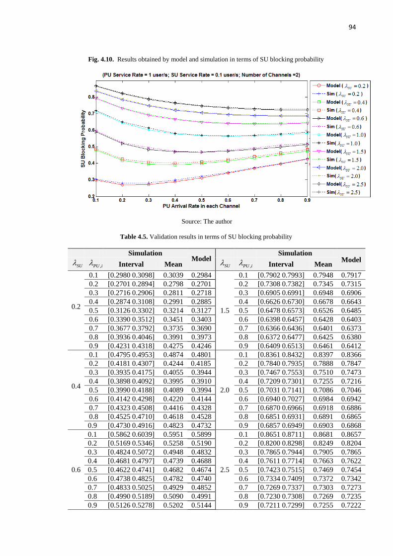
94

Fig. 4.10. Results obtained by model and simulation in terms of SU blocking probability

Source: The author

Table 4.5. Validation results in terms of SU blocking probability

Simulation Model

Simulation Model

SU

,PU i

Interval Mean SU

,PU i

Interval Mean

0.2

0.1 [0.2980 0.3098] 0.3039 0.2984

1.5

0.1 [0.7902 0.7993] 0.7948 0.7917

0.2 [0.2701 0.2894] 0.2798 0.2701 0.2 [0.7308 0.7382] 0.7345 0.7315

0.3 [0.2716 0.2906] 0.2811 0.2718 0.3 [0.6905 0.6991] 0.6948 0.6906

0.4 [0.2874 0.3108] 0.2991 0.2885 0.4 [0.6626 0.6730] 0.6678 0.6643

0.5 [0.3126 0.3302] 0.3214 0.3127 0.5 [0.6478 0.6573] 0.6526 0.6485

0.6 [0.3390 0.3512] 0.3451 0.3403 0.6 [0.6398 0.6457] 0.6428 0.6403

0.7 [0.3677 0.3792] 0.3735 0.3690 0.7 [0.6366 0.6436] 0.6401 0.6373

0.8 [0.3936 0.4046] 0.3991 0.3973 0.8 [0.6372 0.6477] 0.6425 0.6380

0.9 [0.4231 0.4318] 0.4275 0.4246 0.9 [0.6409 0.6513] 0.6461 0.6412

0.4

0.1 [0.4795 0.4953] 0.4874 0.4801

2.0

0.1 [0.8361 0.8432] 0.8397 0.8366

0.2 [0.4181 0.4307] 0.4244 0.4185 0.2 [0.7840 0.7935] 0.7888 0.7847

0.3 [0.3935 0.4175] 0.4055 0.3944 0.3 [0.7467 0.7553] 0.7510 0.7473

0.4 [0.3898 0.4092] 0.3995 0.3910 0.4 [0.7209 0.7301] 0.7255 0.7216

0.5 [0.3990 0.4188] 0.4089 0.3994 0.5 [0.7031 0.7141] 0.7086 0.7046

0.6 [0.4142 0.4298] 0.4220 0.4144 0.6 [0.6940 0.7027] 0.6984 0.6942

0.7 [0.4323 0.4508] 0.4416 0.4328 0.7 [0.6870 0.6966] 0.6918 0.6886

0.8 [0.4525 0.4710] 0.4618 0.4528 0.8 [0.6851 0.6931] 0.6891 0.6865

0.9 [0.4730 0.4916] 0.4823 0.4732 0.9 [0.6857 0.6949] 0.6903 0.6868

0.6

0.1 [0.5862 0.6039] 0.5951 0.5899

2.5

0.1 [0.8651 0.8711] 0.8681 0.8657

0.2 [0.5169 0.5346] 0.5258 0.5190 0.2 [0.8200 0.8298] 0.8249 0.8204

0.3 [0.4824 0.5072] 0.4948 0.4832 0.3 [0.7865 0.7944] 0.7905 0.7865

0.4 [0.4681 0.4797] 0.4739 0.4688 0.4 [0.7611 0.7714] 0.7663 0.7622

0.5 [0.4622 0.4741] 0.4682 0.4674 0.5 [0.7423 0.7515] 0.7469 0.7454

0.6 [0.4738 0.4825] 0.4782 0.4740 0.6 [0.7334 0.7409] 0.7372 0.7342

0.7 [0.4833 0.5025] 0.4929 0.4852 0.7 [0.7269 0.7337] 0.7303 0.7273

0.8 [0.4990 0.5189] 0.5090 0.4991 0.8 [0.7230 0.7308] 0.7269 0.7235

0.9 [0.5126 0.5278] 0.5202 0.5144 0.9 [0.7211 0.7299] 0.7255 0.7222

95

1.0

0.1 [0.7121 0.7240] 0.7181 0.7130

0.2 [0.6417 0.6585] 0.6501 0.6438

0.3 [0.6011 0.6250] 0.6131 0.6015

0.4 [0.5755 0.5872] 0.5814 0.5777

0.5 [0.5661 0.5741] 0.5701 0.5664

0.6 [0.5614 0.5710] 0.5662 0.5634

0.7 [0.5639 0.5740] 0.5690 0.5659

0.8 [0.5710 0.5808] 0.5759 0.5720

0.9 [0.5802 0.5984] 0.5893 0.5802

Source: The author

Fig.4.11 and Table 4.6 present results obtained in terms of joint utilization from model

and simulation. It is noted that they have the same behavior and are close to each other.

Moreover, the joint utilization has a similar behavior to SU Blocking probability/rate.

Initially, it decreases and later it starts to increase when the PU arrival rate increases. In order

to analyze such behavior, it is highlighted that the joint utilization is obtained by taking into

account the primary and secondary utilization of the channels. As the primary user has higher

access priority to the channels than SU, the utilization of resources provided by primary

communication does not suffer any influence from the secondary communication. So, it

increases when the PU arrival rate increases, as shown in Fig. 4.12. The secondary utilization,

in turn, suffers impact by PU communication. So, when the PU arrival rate increases, the

secondary utilization decreases once there are fewer chances for opportunistic access to the

channels.

In this regard, when the PU arrival rate varies, the secondary utilization also varies

consequently providing different levels of contribution to joint utilization (see Fig. 4.12). In

some cases, the reduction in secondary communication is compensated by primary

communication, leading to an increase in the joint utilization. This can be noted in the cases

where the SU arrival rate is equal to 0.2, 0.4 or 0.6, for example (see Fig. 4.11). But, in some

other cases, the primary utilization cannot compensate the reduction in the secondary

utilization. So, the joint utilization tends to decrease, which is noted in cases where the SU

arrival rate is higher than 0.6 as shown in Fig. 4.11.

96

Fig. 4.11. Results obtained by model and simulation in terms of joint utilization

Source: The author

Moreover, in Fig. 4.11, when SU arrival rate increases, the joint utilization also

increases, which is an expected result since the load of SU is bigger. This bigger load leads to

an increase of secondary utilization, as shown in Fig. 4.12.

Fig. 4.12. Primary and secondary utilization obtained by model under different loads of PU and SU

Source: The author

97

Table 4.6. Validation results in terms of joint utilization

Simulation Model

Simulation Model

SU

,PU i

Interval Mean SU

,PU i

Interval Mean

0.2

0.1 [0.5178 0.5250] 0.5214 0.5180

1.5

0.1 [0.8846 0.8903] 0.8875 0.8853

0.2 [0.4859 0.4943] 0.4901 0.4870 0.2 [0.8467 0.8535] 0.8501 0.8478

0.3 [0.4855 0.4940] 0.4898 0.4860 0.3 [0.8212 0.8287] 0.8250 0.8214

0.4 [0.4955 0.5072] 0.5014 0.5011 0.4 [0.8011 0.8089] 0.8050 0.8039

0.5 [0.5196 0.5279] 0.5238 0.5238 0.5 [0.7917 0.8002] 0.7960 0.7934

0.6 [0.5483 0.5550] 0.5517 0.5492 0.6 [0.7870 0.7933] 0.7902 0.7878

0.7 [0.5742 0.5821] 0.5782 0.5749 0.7 [0.7839 0.7901] 0.7870 0.7859

0.8 [0.5984 0.6048] 0.6016 0.5997 0.8 [0.7850 0.7915] 0.7883 0.7864

0.9 [0.6227 0.6305] 0.6266 0.6229 0.9 [0.7877 0.7943] 0.7910 0.7886

0.4

0.1 [0.6739 0.6853] 0.6796 0.6744

2.0

0.1 [0.9108 0.9182] 0.9145 0.9117

0.2 [0.6218 0.6313] 0.6266 0.6233 0.2 [0.8797 0.8840] 0.8819 0.8806

0.3 [0.6000 0.6104] 0.6052 0.6013 0.3 [0.8551 0.8623] 0.8587 0.8575

0.4 [0.5955 0.6041] 0.5998 0.5973 0.4 [0.8410 0.8489] 0.8450 0.8412

0.5 [0.6031 0.6112] 0.6072 0.6039 0.5 [0.8288 0.8364] 0.8326 0.8304

0.6 [0.6134 0.6196] 0.6165 0.6162 0.6 [0.8217 0.8295] 0.8256 0.8238

0.7 [0.6309 0.6404] 0.6357 0.6313 0.7 [0.8189 0.8258] 0.8224 0.8202

0.8 [0.6456 0.6544] 0.6500 0.6474 0.8 [0.8161 0.8223] 0.8192 0.8188

0.9 [0.6627 0.6696 ] 0.6662 0.6637 0.9 [0.8180 0.8241] 0.8211 0.8191

0.6

0.1 [0.7539 0.7632] 0.7586 0.7550

2.5

0.1 [0.9265 0.9337] 0.9301 0.9283

0.2 [0.7013 0.7140] 0.7077 0.7024 0.2 [0.9005 0.9089] 0.9047 0.9019

0.3 [0.6737 0.6843] 0.6790 0.6740 0.3 [0.8807 0.8890] 0.8849 0.8816

0.4 [0.6602 0.6698] 0.6650 0.6620 0.4 [0.8659 0.8714] 0.8687 0.8667

0.5 [0.6575 0.6671] 0.6623 0.6606 0.5 [0.8552 0.8623] 0.8588 0.8563

0.6 [0.6613 0.6715] 0.6664 0.6655 0.6 [0.8485 0.8539] 0.8512 0.8494

0.7 [0.6742 0.6829] 0.6786 0.6742 0.7 [0.8424 0.8495] 0.8460 0.8451

0.8 [0.6841 0.6926] 0.6884 0.6848 0.8 [0.8403 0.8483] 0.8443 0.8428

0.9 [0.6955 0.7000] 0.6978 0.6964 0.9 [0.8397 0.8462] 0.8430 0.8420

1.0

0.1 [0.8340 0.8422] 0.8381 0.8369

0.2 [0.7888 0.7965] 0.7927 0.7908

0.3 [0.7602 0.7681] 0.7642 0.7612

0.4 [0.7426 0.7495] 0.7461 0.7442

0.5 [0.7351 0.7422] 0.7387 0.7359

0.6 [0.7302 0.7399] 0.7351 0.7337

0.7 [0.7333 0.7416] 0.7375 0.7355

0.8 [0.7387 0.7461] 0.7424 0.7398

0.9 [0.7447 0.7529] 0.7488 0.7457

Source: The author

Fig. 4.13 and Table 4.7 present the results in terms of SU dropping probability/rate

obtained by model and simulation. Model matches well with the simulation. They have

similar behavior and their results are close to each other. In Fig. 4.13, we note that the SU

dropping increases when the PU arrival rate increases. This is an expected result, since a

98

higher PU arrival rate leads to a higher PU load and a shorter PU inter-arrival time, which

increases the possibility of the admitted SU be preempted from SVN.

Moreover, when the SU arrival rate increases, the SU dropping probability/rate also

increases, as shown in Fig. 4.13. This occurs due to an increase in the SU load in the SVN,

while the amount of resources used to service the users is the same.

Fig. 4.13. Results obtained by model and simulation in terms of SU dropping probability

Source: The author

Table 4.7. Validation results in terms of SU dropping probability

Simulation Model

Simulation Model

SU

,PU i

Interval Mean SU

,PU i

Interval Mean

0.2

0.1 [0.3856 0.4033] 0.3945 0.4019

1.5

0.1 [0.4865 0.4972] 0.4919 0.4963

0.2 [0.5791 0.5935] 0.5863 0.5920 0.2 [0.6628 0.6741] 0.6685 0.6729

0.3 [0.6898 0.7030] 0.6964 0.7029 0.3 [0.7535 0.7633] 0.7584 0.7622

0.4 [0.7597 0.7755] 0.7676 0.7730 0.4 [0.8047 0.8166] 0.8107 0.8156

0.5 [0.8092 0.8213] 0.8153 0.8199 0.5 [0.8411 0.8528] 0.8470 0.8508

0.6 [0.8389 0.8535] 0.8462 0.8527 0.6 [0.8662 0.8772] 0.8717 0.8755

0.7 [0.8679 0.8773 ] 0.8726 0.8766 0.7 [0.8826 0.8940] 0.8883 0.8938

0.8 [0.8894 0.8975] 0.8935 0.8945 0.8 [0.8975 0.9089] 0.9032 0.9078

0.9 [0.8922 0.9089] 0.9006 0.9084 0.9 [0.9093 0.9201] 0.9147 0.9188

0.4

0.1 [0.4349 0.4474] 0.4412 0.4460

2.0

0.1 [0.4927 0.5040] 0.4984 0.5021

0.2 [0.6122 0.6270] 0.6196 0.6267 0.2 [0.6689 0.6797] 0.6743 0.6788

0.3 [0.7164 0.7269] 0.7217 0.7262 0.3 [0.7551 0.7685] 0.7618 0.7673

0.4 [0.7785 0.7890] 0.7838 0.7884 0.4 [0.8087 0.8204] 0.8146 0.8198

0.5 [0.8201 0.8327] 0.8264 0.8302 0.5 [0.8461 0.8550] 0.8506 0.8543

0.6 [0.8513 0.8607] 0.8560 0.8599 0.6 [0.8693 0.8796] 0.8745 0.8784

0.7 [0.8719 0.8821] 0.8770 0.8817 0.7 [0.8884 0.8977] 0.8931 0.8962

0.8 [0.8899 0.8992] 0.8946 0.8983 0.8 [0.9008 0.9110] 0.9059 0.9098

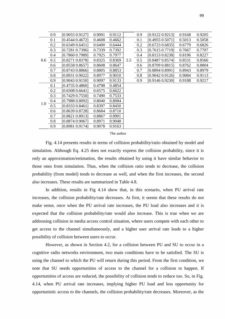
99

0.9 [0.9055 0.9127] 0.9091 0.9112 0.9 [0.9122 0.9213] 0.9168 0.9205

0.6

0.1 [0.4544 0.4672] 0.4608 0.4662

2.5

0.1 [0.4955 0.5071] 0.5013 0.5058

0.2 [0.6349 0.6451] 0.6400 0.6444 0.2 [0.6723 0.6835] 0.6779 0.6826

0.3 [0.7281 0.7396] 0.7339 0.7392 0.3 [0.7615 0.7719] 0.7667 0.7707

0.4 [0.7860 0.7989] 0.7925 0.7977 0.4 [0.8153 0.8238] 0.8196 0.8227

0.5 [0.8271 0.8378] 0.8325 0.8369 0.5 [0.8487 0.8574] 0.8531 0.8566

0.6 [0.8558 0.8657] 0.8608 0.8647 0.6 [0.8709 0.8815] 0.8762 0.8804

0.7 [0.8743 0.8866] 0.8805 0.8853 0.7 [0.8894 0.8991] 0.8943 0.8979

0.8 [0.8931 0.9022] 0.8977 0.9010 0.8 [0.9042 0.9126] 0.9084 0.9113

0.9 [0.9043 0.9150] 0.9097 0.9133 0.9 [0.9146 0.9230] 0.9188 0.9217

1.0

0.1 [0.4735 0.4860] 0.4798 0.4854

0.2 [0.6508 0.6641] 0.6575 0.6622

0.3 [0.7429 0.7550] 0.7490 0.7533

0.4 [0.7988 0.8092] 0.8040 0.8084

0.5 [0.8333 0.8461] 0.8397 0.8450

0.6 [0.8639 0.8728] 0.8684 0.8710

0.7 [0.8821 0.8913] 0.8867 0.8901

0.8 [0.8874 0.9067] 0.8971 0.9048

0.9 [0.8981 0.9174] 0.9078 0.9163

The author

Fig. 4.14 presents results in terms of collision probability/ratio obtained by model and

simulation. Although Eq. 4.25 does not exactly express the collision probability, since it is

only an approximation/estimation, the results obtained by using it have similar behavior to

those ones from simulation. Thus, when the collision ratio tends to decrease, the collision

probability (from model) tends to decrease as well, and when the first increases, the second

also increases. These results are summarized in Table 4.8.

In addition, results in Fig 4.14 show that, in this scenario, when PU arrival rate

increases, the collision probability/rate decreases. At first, it seems that these results do not

make sense, once when the PU arrival rate increases, the PU load also increases and it is

expected that the collision probability/rate would also increase. This is true when we are

addressing collision in media access control situation, where users compete with each other to

get access to the channel simultaneously, and a higher user arrival rate leads to a higher

possibility of collision between users to occur.

However, as shown in Section 4.2, for a collision between PU and SU to occur in a

cognitive radio networks environment, two main conditions have to be satisfied. The SU is

using the channel to which the PU will return during this period. From the first condition, we

note that SU needs opportunities of access to the channel for a collision to happen. If

opportunities of access are reduced, the possibility of collision tends to reduce too. So, in Fig.

4.14, when PU arrival rate increases, implying higher PU load and less opportunity for

opportunistic access to the channels, the collision probability/rate decreases. Moreover, as the

100

SU service time is higher (on average) than the channels OFF time (period in which the PU is

not using it), when the SU gets the access to the channel, it is very likely that the SU will still

be using the channel when the PU returns.

In addition, Fig. 4.14 shows that the collision probability increases when the SU

arrival rate increases. With higher load of SUs in the SVN, it is more likely to have SUs using

the channels when PUs return.

Fig. 4.14. Results obtained by model and simulation in terms of collision probability

Source: The author

Table 4.8. Validation results in terms of collision probability

Simulation Model

Simulation Model

SU

,PU i

Interval Mean SU

,PU i

Interval Mean

0.2

0.1 [0.4410 0.4544] 0.4477 0.4775

1.5

0.1 [0.8344 0.8442] 0.8393 0.8638

0.2 [0.3531 0.3660] 0.3596 0.4194 0.2 [0.7524 0.7617] 0.7571 0.8080

0.3 [0.2919 0.2981] 0.2950 0.3406 0.3 [0.6885 0.6951] 0.6918 0.7344

0.4 [0.2378 0.2446] 0.2412 0.2719 0.4 [0.6339 0.6387] 0.6363 0.6578

0.5 [0.2050 0.2120] 0.2085 0.2178 0.5 [0.5868 0.5936] 0.5902 0.5852

0.6 [0.1798 0.1846] 0.1822 0.1763 0.6 [0.5486 0.5544] 0.5515 0.5195

0.7 [0.1551 0.1602] 0.1577 0.1445 0.7 [0.5051 0.5111] 0.5081 0.4613

0.8 [0.1359 0.1397] 0.1378 0.1199 0.8 [0.4694 0.4749] 0.4722 0.4105

0.9 [0.1229 0.1261] 0.1245 0.1007 0.9 [0.4350 0.4412] 0.4381 0.3664

0.4

0.1 [0.6093 0.6201] 0.6147 0.6449

2.0

0.1 [0.8628 0.8690] 0.8659 0.8910

0.2 [0.5101 0.5201] 0.5151 0.5803 0.2 [0.7926 0.7979] 0.7953 0.8382

0.3 [0.4246 0.4323] 0.4285 0.4932 0.3 [0.7357 0.7423] 0.7390 0.7689

0.4 [0.3720 0.3768] 0.3744 0.4111 0.4 [0.6866 0.6921] 0.6894 0.6960

0.5 [0.3252 0.3302] 0.3277 0.3415 0.5 [0.6444 0.6490] 0.6467 0.6261

0.6 [0.2865 0.2939] 0.2902 0.2848 0.6 [0.6071 0.6127] 0.6099 0.5618

0.7 [0.2576 0.2622] 0.2599 0.2392 0.7 [0.5722 0.5779] 0.5751 0.5042

101

0.8 [0.2317 0.2355] 0.2336 0.2026 0.8 [0.5351 0.5399] 0.5375 0.4531

0.9 [0.2005 0.2051] 0.2028 0.1730 0.9 [0.4995 0.5038] 0.5017 0.4082

0.6

0.1 [0.6866 0.6992] 0.6929 0.7293

2.5

0.1 [0.8828 0.8883] 0.8856 0.9081

0.2 [0.5866 0.5946] 0.5906 0.6655 0.2 [0.8218 0.8298] 0.8258 0.8574

0.3 [0.5144 0.5210] 0.5177 0.5797 0.3 [0.7690 0.7760] 0.7725 0.7912

0.4 [0.4519 0.4571] 0.4545 0.4955 0.4 [0.7227 0.7287] 0.7257 0.7213

0.5 [0.4042 0.4126] 0.4084 0.4212 0.5 [0.6840 0.6890] 0.6890 0.6536

0.6 [0.3622 0.3678] 0.3650 0.3583 0.6 [0.6425 0.6485] 0.6455 0.5909

0.7 [0.3293 0.3333] 0.3313 0.3062 0.7 [0.6068 0.6132] 0.6100 0.5341

0.8 [0.2918 0.2966] 0.2942 0.2631 0.8 [0.5691 0.5739] 0.5715 0.4834

0.9 [0.2562 0.2609] 0.2586 0.2275 0.9 [0.5309 0.5368] 0.5339 0.4383

1.0

0.1 [0.7740 0.7824] 0.7782 0.8139

0.2 [0.6850 0.6920] 0.6885 0.7541

0.3 [0.6174 0.6234] 0.6204 0.6743

0.4 [0.5592 0.5650] 0.5621 0.5930

0.5 [0.5085 0.5147] 0.5116 0.5179

0.6 [0.4669 0.4715] 0.4692 0.4517

0.7 [0.4317 0.4361] 0.4339 0.3945

0.8 [0.3891 0.3955] 0.3923 0.3458

0.9 [0.3535 0.3577] 0.3556 0.3044

Source: The author

4.10 Chapter Summary

In this Chapter we described the elements that compose the environment termed

cognitive radio virtual networks (CRVNE) and pointed out important situations that might

occur and impact primary and secondary communications. Once the environment was

defined, a model was designed to denote the interactions between PUs (PVNs) and SUs

(SVNs). For this, an M/M/N/N queue with priority and loss of SUs was considered and useful

performance metrics were derived. To validate the analytical model, an approach based on

simulation was used. Next Chapter, the multi-objective problem of SVNs mapping is

formulated and a scheme based on genetic algorithms to solve this problem is proposed and

evaluated

102

Chapter 5 - A Scheme Based on Genetic Algorithms

for a SVNs multi-objective mapping problem

This Chapter starts with the formulation of the multi-objective problem of SVNs

mapping onto a wireless substrate network (Section 5.1), which considers objectives

discussed in Chapter 4. After, it proposes a scheme based on genetic algorithms to solve this

multi-objective problem. It sets out by describing the chromosome structure and the fitness

function designed to evaluate the solutions (individuals) during the evolution of the GA

(Section 5.2). It takes into account the metrics formulated in Chapter 4. Following this, the

genetic operators and the test results that are needed to choose the mutation and crossover

probability values adopted by GA are presented (Section 5.3) and a discussion of the

execution flow of the proposed scheme is performed (Section 5.4). Next (Section 5.5), the

evaluation scenario and metrics adopted to analyze the proposed scheme are delineated.

Finally, it shows the results obtained by the proposed scheme and compares them with a

scheme based on First-Fit, where an analysis is performed.

5.1 Formulating the SVN Mapping Optimization Problem

As shown in Chapter 4, several objectives must be considered in the SVN mapping

process. When the influence of each of these objectives on the SU and PU communications is

taken into account, the following optimization problem is formulated (see Eq. 5.1). Given a

set of Z SVN requests and the usage pattern of the channels (resources) for the primary

networks, to perform the mapping of the SVNs in order to minimize the collision, SU

blocking, and SU dropping probabilities and maximize the joint utilization. Two constraints

must be satisfied: the amount of resources allocated to each SVN cannot be less than the

requested demand, and a common channel cannot be allocated to different SVNs. Formally,

we have:

,

, ,

to :

, l 1,2,3,...,

, , , 1,2,3,...,

c SU SU

l req l

l u

Minimize P Pb Pd and Maximize util

Subject

Ralloc Bw Z

SC SC l u l u Z

(5.1)

103

Where lRalloc and lSC are the amount of resources and the set of allocated channels

to lSVN , respectively.

Achieving all these objectives simultaneously is a challenging process, because some

conflict with each other. If the SVN mapping is focused on a specific objective, it can

deteriorate the other one. Next sections (5.2-5.4), a scheme based on genetic algorithms is

proposed to solve this problem.

5.2 Chromosome Structure and Fitness Functions

A SVN mapping scheme based on Genetic Algorithms (GA) is proposed to solve the

secondary virtual network mapping problem outlined in Section 5.1, i.e. to achieve a tradeoff

between its objectives during the mapping process.

As shown in Section 2.7, GA is a search algorithm based on the principles of natural

selection and genetics. It relies upon evolving a set of solutions, represented by the so-called

chromosomes, over a period of time. Eventually, through the GA operators (selection,

crossover and mutation) a good solution will be found by combining different possible

solutions (CHEN et al., 2010; BALIEIRO. et al., 2014). Although the GA has a well known

large convergence time, some solutions to reduce this time have been proposed (CHEN et al.,

2010).

Some characteristics of the GA make its adoption interesting for our problem.

Differently from other methods, it handles many solutions simultaneously at each interaction

and evolves them in order to achieve a good solution. Thus, many possible mappings are

evaluated at each interaction. In general, GA works well in problems with many objectives or

constraints, and can be combined with classical approaches such as those presented in Section

2.9 to deal with this kind of problem. In addition, GA has been widely adopted in the

literature to solve problems in cognitive radio and it has achieved good results (BALIEIRO. et

al., 2014).

In the proposed scheme, the individual or chromosome j

lX is represented by a

sequence of K bits (see Fig. 5.1), where K is the number of available channels that can be

used to meet the requested SVN l , and 1,2,3...,j S , where S is the population size. Each

gene (bit) in the chromosome refers to an available channel for allocation. If the gene value is

equal to 1, then the respective channel is selected for mapping the SVN. Otherwise, the

channel is not selected. In the individual shown in Figure 5.1, Channels 1 and k are selected

104

for mapping the SVN requested. Our proposal takes into account the intrinsic parallelism of

the GA when seeking to find an optimal or sub-optimal mapping for each SVN.

Fig. 5.1. Chromosome Structure

Source: The author

It should be noted that there is an equivalence between an individual in the GA and a

set of channels. Thus, given an individual j

lX , it is possible to know the set of channels

represented by it ( j

lSC ), and vice-versa. Eq. 5.2 describes how to obtain the set of channels

represented by an individual j

lX in the GA, where lAC is the set of available channels for

mapping the SVN l , iC is the channel associated with the gene ix . The gene (bit) ix composes

the chromosome or individual j

lX .

| and 1j j

l i l i l iSC C AC x X x

In our scheme, the SVNs are mapped sequentially, so a population is created for each

SVN and evolves to obtain a good solution represented by a set of channels that can be

allocated to the respective SVN.

The fitness function defined in our approach to evaluate the individuals (solutions) is

expressed in Eq. 5.3. We adopted the classical approaches described in Section 2.9 to handle

the multi-objective problem of SVNs mapping and reduce its complexity. So, our fitness

function was defined by two expressions. The weighted sum method was adopted to compose

the first part of the fitness function, where the collision and SU dropping probabilities were

taken into account, which are mainly related to primary and secondary communications,

respectively. In addition, the -constraint method was also used in this part, where blockT and

utilT were the constraints defined to SU blocking probability and joint utilization, respectively.

Thus, the first part of our fitness function aims to reduce the collision and SU dropping

probabilities and keep the joint utilization and SU blocking within certain limits.

As seen in Section 2.9.2, for -constraint method working well, constraints must be

defined in a feasible region, otherwise no solution will be found for the problem, i.e., the set

(5.2)

105

of solutions will be empty. However, it is hard to do so for all possible scenarios of SVN

mapping, since for some scenarios, constraint values may be in a feasible region, but in some

other ones they may not. Therefore, the second expression for our fitness function adopts the

goal programming method along with the expression given by weighted sum ( mainf ) in order

to deal with the cases where no solution meets the constraints defined in the first part of the

fitness function.

Thus, goals (target values) were defined for SU blocking probability and joint

utilization, which are also represented by blockT and utilT , respectively. The second expression

(in Eq. 5.3) adopts the average between block and util as a penalization factor for mainf .

block is the relative difference between the collision probability and its target value (goal).

Similarly, the relative difference between the joint utilization and its target value is util . They

are expressed in Eq. 5.5 and 5.6, respectively. In our approach, blockT and utilT were set up as

0.1 and 0.8, respectively.

,,

( )1 ,

2

main SU l block l util

j

l block util

main

f if Pb T and util T

fitness Xf otherwise

Where mainf is defined in Eq. 5.4

,( ) 100 (1 ( )) (1 ( ))j j l

main l l l SU l jf X Pc X Pd X

, ,/ 1 , ( )

0,

SU l block block SU l blockj

block l

Pb T T if Pb TX

otherwise

/ , ( )

0,

util l util l utilj

util l

T util T if util TX

otherwise

It is noted that Eqs.5.5 and 5.6 just present values different from zero when the

collision probability or joint utilization values provided by a given mapping (individual) are

worse than the defined target values. In addition, the more distant (or worse) the collision and

utilization are from the target values, the greater the penalty in the fitness of the individual.

Both expressions in Eq. 5.3 aim to achieve a good tradeoff between the objectives of the

optimization problem presented in Section 5.1.

Although there are GA approaches for solving multi-objective problems such as

Multi-Objective Generic Algorithms (MOGA), Nondominated Sorting Genetic Algorithm

(5.3)

(5.5)

(5.6)

(5.4)

106

(NSGA), and Niched-Pareto Genetic Algorithm (NPGA) (COELHO; LAMONT;

VELDHUIZEN, 2007), for example, in our scheme, (as shown in Eq. 5.3), the classical

methods was used to deal with multiple objectives. With this approach, the complexity of the

multi-objective problem is reduced and just handled in the fitness function of the GA.

Moreover, it does not require any changes to the basic mechanism of a GA (described in

Section 2.7). So, it is very simple and easy to implement. In addition, the literature includes

studies that have successfully used this approach in a multi-objective optimization

(SAOUCHA; LAMMARI; BENATCHBA, 2013; BALIEIRO. et al., 2014).

5.3 Genetic Operators and Parameters

We adopted the roulette wheel as the selection operator; this involves selecting

individuals for the crossover process based on their fitness values. This process simulates the

natural selection mechanism, which acts on biological species (GOLDBERG, 1989). Thus,

individuals with the highest fitness values are best suited for survival to the next generation.

A uniform operator was employed for the crossover operation, which selects genes

(bits) from the chromosomes of parents and creates new offspring (individuals). A bit

mutation was used for the mutation operator, which randomly changes the new offspring

(GOLDBERG, 1989).

It is important to define correct parameters for setting up the GA to obtain good

results. Two key parameters in the GA are the crossover (pc) and mutation (pm) rates

(probabilities) since they express the frequency with which the crossover and mutation

operations are carried out. A high mutation rate may result in the loss of good solutions

during the GA evolution, because there is a greater likelihood of alterations in the solutions,

especially if elitist techniques are not used. On the other hand, a lower mutation rate may

cause a lack of diversity in the solutions, as well as premature convergence via GA

(BALIEIRO. et al., 2014).

The number of chromosomes that comprise a crossover pool is influenced by the

crossover rate. Thus, if a very small crossover rate is adopted, it may generate an insufficient

number of new offspring (i.e. solutions). In contrast, when there is a high crossover rate, a

large number of new chromosomes can be added to the population, which might result in the

loss of good blocks inside a chromosome, and the destruction of good schemes

(GOLDBERG, 1989).

Thus, multiple tests were conducted to define the probability values (pc and pm)

which could be used in our GA-based scheme. This involved employing 8 test values within

107

the interval [0.1 0.8] for the crossover probability (pc) and 8 test values within the interval

[0.01 0.8] for the mutation probability (pm), as shown in Table 5.1. When all these values

were combined, it meant that we evaluated 64 test cases. For each test case, 5 instances of

simulation were performed. The test scenario was composed of 40 channels, PU service rate

equals 1 for all channels and PU arrival rate in each channel defined within [0 1]. Moreover,

the SU arrival rate and average SU service time were uniformly distributed in [1 3] and [1 4],

respectively.

Table 5.1. Test case values

Pc 0.1/0.2/0.3/0.4/0.5/0.6/0.7/0.8

Pm 0.01/0.03/0.05/0.1/0.3/0.5/0.7/0.8 Source: The author

Figure 5.2 shows the test results for our GA. The test case we selected for GA was the

one that provides the greatest average fitness value for the population in the last generation. In

Fig. 5.2, the test case 49 displayed the best performance for the GA (highlighted with a red

circle). It has crossover and mutation rates equal to 0.7 and 0.01, respectively, as can be

checked in Table 5.2, which summarizes the results obtained in each test case.

Fig. 5.2. Test case results for GA

Source: The author

108

Table 5.2. Results obtained in each test case

Test

Case Pc Pm

Average

Fitness

Test

Case Pc Pm

Average

Fitness

1 0.1 0.01 119.1698 33 0.5 0.01 118.1421

2 0.1 0.03 116.7660 34 0.5 0.03 117.3723

3 0.1 0.05 116.9360 35 0.5 0.05 115.8689

4 0.1 0.1 115.9225 36 0.5 0.1 115.2682

5 0.1 0.3 115.1776 37 0.5 0.3 115.2560

6 0.1 0.5 114.9199 38 0.5 0.5 115.3619

7 0.1 0.7 115.2660 39 0.5 0.7 115.6775

8 0.1 0.8 115.3263 40 0.5 0.8 115.7074

9 0.2 0.01 118.5283 41 0.6 0.01 118.7164

10 0.2 0.03 117.2563 42 0.6 0.03 117.4148

11 0.2 0.05 116.6521 43 0.6 0.05 116.5770

12 0.2 0.1 116.2509 44 0.6 0.1 116.1628

13 0.2 0.3 115.6320 45 0.6 0.3 115.4003

14 0.2 0.5 115.1364 46 0.6 0.5 115.0778

15 0.2 0.7 114.9908 47 0.6 0.7 115.2419

16 0.2 0.8 114.5472 48 0.6 0.8 115.3517

17 0.3 0.01 119.1763 49 0.7 0.01 119.5824

18 0.3 0.03 115.9700 50 0.7 0.03 117.3533

19 0.3 0.05 116.6532 51 0.7 0.05 115.3365

20 0.3 0.1 116.0313 52 0.7 0.1 115.6692

21 0.3 0.3 115.6146 53 0.7 0.3 115.6106

22 0.3 0.5 114.6916 54 0.7 0.5 114.7992

23 0.3 0.7 115.3769 55 0.7 0.7 115.4012

24 0.3 0.8 114.3925 56 0.7 0.8 114.6932

25 0.4 0.01 118.1286 57 0.8 0.01 119.3329

26 0.4 0.03 117.6229 58 0.8 0.03 116.0471

27 0.4 0.05 116.0248 59 0.8 0.05 116.4886

28 0.4 0.1 116.0653 60 0.8 0.1 115.6919

29 0.4 0.3 114.9953 61 0.8 0.3 115.6403

30 0.4 0.5 115.4040 62 0.8 0.5 115.1482

32 0.4 0.7 115.3126 63 0.8 0.7 115.1228

32 0.4 0.8 114.9567 64 0.8 0.8 115.6581

Source: The author

In addition to crossover and mutation probabilities, the population size (S) and number

of generations (G) were defined as being equal to 100 and 200, respectively. Table 5.3

summarizes the GA parameters employed in this work.

Table 5.3. GA parameters

Parameter Value

Number of generations (G) 200

Population size (L) 100

Crossover rate (pc) 0.7

Mutation rate (pm) 0.01

Source: The author

109

5.4 Execution Flow of the Scheme

The execution flow of our secondary virtual network (SVN) mapping GA-based

scheme is as follows (see Fig. 5.3). Initially, given a request of SVN to be mapped, the

population (i.e. which might be used for mapping the SVN) is randomly generated to provide

candidate solutions to the problem. In this process, information about available channels, (i.e.

those that are not allocated to other SVNs), is considered to generate feasible solutions (i.e.

individuals). Following this, the individuals are evaluated in accordance with the fitness

functions adopted in our GA, which, in general, take into account the SU blocking

probability, joint utilization, SU dropping probability, and collision probability for computing

the fitness value of each individual. Afterwards, the individuals are submitted for selection,

together with the crossover and mutation operators. Moreover, an elitist strategy is employed

to ensure that the individuals with best fitness will not be lost during the selection process, but

will be carried over to the next generation to form a new population. After these operations

have been completed, a new generation of candidate mappings will be created and the stop

criterion, which is determined by the number of generations (G), is evaluated. If the stop

criterion is not satisfied, the process is repeated in the fitness evaluation stage. Otherwise, the

best individual is chosen as the solution to the problem. This represents the set of channels

that will be allocated to the requested SVN. In this way, the SVN embedding is performed

and the pool of available channels is updated.

110

Fig. 5.3. Execution flow of the scheme based on GA

Source: The author

5.5 Scheme Evaluation

This section describes the evaluation scenario and metrics adopted to analyze the

proposed scheme outlined in previous sections of this Chapter. It shows the results obtained

by the proposed scheme and compares them with a scheme in the literature, where an analysis

is performed.

5.5.1 Evaluated Metrics

Four metrics were employed to evaluate our scheme, which are as follows: collision

probability, SU blocking probability, SU dropping probability, and joint utilization. They

were defined in Sections 4.5-4.8. These metrics aim to show the impact of the mapping that

was carried out, on both primary and secondary communications, and on the resource

utilization. In addition, in order to give to the reader a notion of time spent by schemes to

compute the final solution (mapping of a given SVN), we present the average execution time

of each scheme for the first scenario of evaluation, which is described in Section 5.5.2.

111

5.5.2 Evaluation Scenarios

Three evaluation scenarios were defined to analyze the proposed scheme

performance. In all the scenarios, the primary service rate for all channels and the secondary

service rate were defined as 1 user/s. The PU arrival rate of each channel i ( ,PU i ) was

defined within the interval min max[ , ]PU PU , with min maxPU PU .

In the first scenario, the SU arrival rate varied from 4 to 16 with a step of 4, with the

aim of showing the behavior of the proposed scheme under different levels of SU load. The

minPU and maxPU were defined as 0 and 1, respectively. The substrate network was

composed of 50 channels. Moreover, one SVN was considered to be mapped. The remaining

parameters were configured as described in the first paragraph of this section.

In order to evaluate the performance of our scheme in cases where the environment

has different loads of primary users and, hence, distinct possibilities of opportunistic use by

SU, in the second scenario, two cases (intervals for ,PU i ) were defined. In the first, the values

of minPU and maxPU were set up as 0 and 0.5, respectively. Thus, the channels that compose

this scenario are more susceptible to opportunistic use by SU. The channels have lower

primary load. In the second case, the interval to define the PU arrival rates of the channels

was [0.5 1]. It represents scenarios with high PU load, which reduces the possibility of

opportunistic use of the resources by SUs. In addition, the SU arrival rate was set up as 5

users/s. The number of channels and SVN requests considered in this scenario are the same as

the previous one, and all the other parameters were set up as described in the first paragraph

of this section.

The goal in the two previous scenarios was not to check how the proposed scheme

operates when dealing with more than one SVN request. Thus, the number of SVNs that had

to be mapped was one SVN in both scenarios.

The aim of the third scenario was to evaluate the performance of the scheme when

more than one SVN need to be mapped. Thus, the number of SVN requests was set up as 4.

The SU arrival rate of the SVNs was uniformly distributed between 2 and 4 users/s. The

substrate network was composed of 80 channels. Similarly to the first scenario, the PU arrival

rates of the channels are uniformly distributed in [0 1]. The remaining parameters followed

the general values described for all the scenarios.

Table 5.4 summarizes the evaluation scenarios and Table 5.5 shows the parameter

values considered in the scenarios.

112

Table 5.4. Evaluation scenarios

Scenario Focus

1 To evaluate the schemes considering different secondary user loads

2 To evaluate the schemes considering different loads of PUs

3 To evaluate the schemes considering more than one SVN requests

Source: The author

In addition to these different scenarios, we analyzed the effectiveness of our scheme

by comparing it with a scheme based on the first-fit strategy, which is similar to that used in

(ZHANG et. al, 2012).

The First-Fit scheme (denoted as First-Fit) maps the SVNs sequentially, in the same

way as the GA scheme does. In mapping the SVNs, it follows a number of stages. First, all

the SVN requests are sorted in a descending order in terms of requested demand and are

placed in a queue. Next, the first-fit strategy is employed to allocate channels (sequentially) to

each SVN in the sorted queue. It takes the next available channel (channel that is not being

used by other SVNs) to map a current SVN. In this process, the scheme aims to achieve the

lowest collision probability, i.e., to protect the PU communication. Moreover, as in the case of

the GA scheme, in the First-Fit scheme, the restrictions to the problem defined in Eq. 5.1 are

met during the SVN mapping. This ensures that the demand requested by the mapped SVNs

( ,l req lRalloc Bw ) and l uSC SC are met.

Table 5.5. Parameter values adopted in the scenarios

All Scenarios

Parameter Value

,PU i min max[ , ]PU PUU

,PU i 1 user/s

,SU l 1 user/s

usKHz Scenario 1 Scenario 2 Scenario 3

min max[ , ]PU PU [0 1] [0 0.5] and [0.5 1] [0 1]

,SU l 4/8/12/16 5 U[2 4]

#Channels 50 50 80

#SVN 1 1 4

Source: The author

113

5.5.3 Results

This section draws a comparison between our scheme based on GA and First-Fit,

defined in Section 5.4.2. For each evaluated point, 30 instances were performed. The average

results are presented considering a 95% confidence level, which were obtained by using the

Bootstrap method (SINGH; XIE, 2008), with „resample‟ size and number of (re)samplings

equal to 30 and 1000, respectively.

5.5.3.1 Scenario 1

Results of metrics for all the schemes are shown in Figures 5.4, 5.5, 5.6 and 5.7,

considering scenario 1. These results and the confidence intervals computed for each metric

are summarized in Tables 5.6, 5.8, 5.9, and 5.10.

Results for the average SU blocking probability obtained by the schemes is shown in

Fig. 5.4, and the confidence interval computed for SU blocking probability is presented in

Table 5.6. According to the table, schemes achieved similar performance (there are

intersections between the confidence intervals), with slight superiority for the First-Fit, when

SU arrival rate is 8, 12, or 16 (see Fig. 5.4).

In Fig. 5.4, it might be noted that our GA-based scheme has a stable performance

under different levels of SU load in the virtual environment. It was able to select the

appropriate channels to meet each demand. Moreover, it achieved the goal defined for SU

blocking probability, which was to provide a SU blocking probability below 0.1.

Both schemes presented good and similar levels of admission of SUs dimensioned for

the SVN. However, in order to achieve this result, First-Fit adopted more channels than our

GA-based scheme (see Table 5.7). This shows that more important than the number of

channels to be allocated, it is the selection of the proper ones to achieve good solution, since

they have different primary usage patterns.

In addition, it is noted in Fig. 5.4 an intersection between the two schemes when the

SU arrival rate varies from 4 to 6. For the first value, the First-Fit adopts channels that

provide a higher user per channel density, which leads to a higher SU blocking probability

than our GA-based scheme. When the SU arrival is equal to 6, the First-Fit allocates much

more channels (sequentially) to SVN in order to reduce the collision probability. So, with

more channels, the possibility of opportunistic access by SU increases and, consequently, the

SU blocking probability reduces.

114

Table 5.6. Results for SU blocking probability when the SU arrival rate varies

First-Fit GA

,SU l CI Average CI Average

4 [0.0310 0.0627] 0.04685 [0.0346 0.0482] 0.0414

8 [0.0308 0.0406] 0.0388 [0.0452 0.0584] 0.0518

12 [0.0332 0.0524] 0.0428 [0.0510 0.0592] 0.0551

16 [0.0449 0.0530] 0.0489 [0.0562 0.0636] 0.0600

Source: The author

Fig. 5.4. Average blocking probability when the SU arrival rate varies

Source: The author

Table 5.7. Average number of channels adopted by the schemes to map the SVN considering the Scenario 1

,SU l First-Fit GA

4 17,9 11,5

8 26,7 16,8

12 34,9 22,9

16 40,8 30

Source: The author

The average values for the collision probability obtained by all the schemes are shown

in Fig. 5.5. Results with the respective confidence intervals are also summarized in Table 5.8.

It is observed that the GA-based scheme achieved better results than First-Fit for all SU

arrival rates considered. GA reduced the collision probability in up to 39.08% compared to

the First-Fit. In the first three cases ( ,SU l equals 4, 8 or 12), the average reduction in the

collision probability achieved by GA was 38.57% (on average). In addition, even when a high

load of SU ( ,SU l equals 16), our GA-based scheme obtained a performance gain of 24.01%.

115

This behavior shows the capability for our scheme to work well in scenarios with

different loads of SUs, including those scenarios with high demand in terms of SUs. With our

scheme, the interference caused to PU communication is greatly reduced, when compared

with First-Fit.

In order to achieve a low collision probability in this scenario, First-Fit scheme

allocated more channels to SVN than our GA scheme (see Table 5.7). However, just

allocating more channels does not ensure that a low collision probability will be achieved.

The PU load of the selected channels must be observed in order to select properly the

channels that provide less interference to PU communication. As the GA evaluates more than

one solution in each generation and builds the final solution by using building blocks (good

parts of the individuals), it was able to achieve a lower collision probability even adopting

less channels than First-Fit. First-Fit, in turn, does not analyze the PU load of the channels to

choose which channels to allocate. It just allocates the available channels sequentially to

SVN.

Table 5.8. Results for collision probability when the SU arrival rate varies

First-Fit GA

,SU l CI Average CI Average

4 [0.4584 0.5004] 0.4794 [0.2750 0.3110] 0.2930

8 [0.4610 0.5127] 0.4869 [0.2766 0.3167] 0.2966

12 [0.4707 0.5244] 0.4926 [0.2731 0.3402] 0.3067

16 [0.4733 0.5143] 0.4938 [0.3438 0.4057] 0.3748

Source: The author

Fig. 5.5. Average collision probability when SU arrival rate varies

Source: The author

116

Results obtained by the schemes in terms of the average SU dropping probability are

illustrated in Fig. 5.6, and are detailed in Table 5.9 by showing the confidence intervals for

this metric. Similarly to the previous metric (collision probability), our GA-based scheme

outperformed First-Fit in all values of ,SU l evaluated.

Our GA-based scheme significantly reduced the SU dropping probability in up to

62.13% compared to the First-Fit. These results were achieved when ,SU l was 4. Even in

the worst case, when ,SU l was 16, our scheme reduced the SU dropping probability by

32.46%. Considering all cases ( ,SU l values), GA-based scheme reduced the SU dropping

probability by 48.90 % (on average) when compared to First-Fit. These results show that our

scheme is able to provide a good service to SVN by enabling that SUs admitted in the SVN

have higher chance of finishing their communications normally, i.e., they will probably not be

dropped from the SVN.

Table 5.9. Results for SU dropping probability when the SU arrival rate varies

First-Fit GA

,SU l IC Average IC Average

4 [0.0642 0.1031] 0.0837 [0.0297 0.0337] 0.0317

8 [0.0529 0.0665] 0.0597 [0.0274 0.0297] 0.0285

12 [0.0486 0.0643] 0.0564 [0.0238 0.0340] 0.0289

16 [0.0539 0.0687] 0.0613 [0.0354 0.0474] 0.0414

Source: The author

Fig. 5.6. Average SU dropping probability when SU arrival rate varies

Source: The author

117

Results obtained by the schemes in terms of joint utilization of the channels are shown

in Fig. 5.7, and summarized in Table 5.10. It is noted that First-Fit has better performance

than our scheme, mainly in cases where the SU arrival rate is low such as 4 and 8 users/s, for

example. In these cases the performance gain was of 13.65% and 6.71%, respectively. But, it

is also noted that the difference between them decreases when cases with higher load of SUs

are considered. With ,SU l equals 12 or 16, the difference between the schemes reduces to

3.44% and 1.85% in absolute values, where in the last case the schemes have similar

performances.

Although the First-Fit presents better joint utilization, this does not imply that the

secondary utilization provided by it is higher than that provided by our GA-based scheme.

Since the schemes have similar performances in terms of SU blocking, and our scheme is

better than First-Fit (when the SU dropping is considered), then the secondary utilization

achieved by GA scheme is probably higher than that obtained by First-Fit. So, in this

scenario, the First-Fit tries to achieve a high joint utilization by selecting channels with high

PU load, which reduces the possibility of opportunistic access by users from SVN and,

consequently, impacts on secondary utilization.

Table 5.10. Results for joint Utilization when SU arrival rate varies

First-Fit GA

,SU l IC Average IC Average

4 [0.6633 0.6922] 0.6778 [0.5924 0.6003] 0.5964

8 [0.7376 0.7508] 0.7442 [0.6950 0.6998] 0.6974

12 [0.7782 0.7941] 0.7861 [0.7436 0.7598] 0.7517

16 [0.8149 0.8279] 0.8214 [0.7956 0.8103] 0.8029

Source: The author

Fig. 5.7. Average joint utilization when SU arrival rate varies

118

Source: The author

In terms of execution time, Fig. 5.8 presents the average execution time of each

scheme for the first evaluation scenario. It is noted that when the SU arrival rate increases, the

execution time of the schemes also increases, since that a higher number of channels is

adopted to map the SVN (see Table 5.7). With more channels used in the mapping, the

number of states in the M/M/N/N queue (see Fig. 4.5) increases, as well as the linear system

formed to get the steady-state probabilities. So, more time is spent to solve the linear system

and the mapping problem when the SU arrival rate increases.

Moreover, our GA-based scheme presents a larger execution time than the First-Fit for

all values of SU arrival rates. It was a expected result, since that in order to define the solution

for the mapping problem, the GA tries a set of possible solutions (population of individuals)

at each iteration and evolves them during many iterations (number of generations). This

process incurs in a processing overhead and a larger time to obtain the solution by using our

GA-based scheme.

119

Fig. 5.8. Average execution time of the schemes

Source: The author

5.5.3.2 Scenario 2

Results obtained by the schemes in scenario 2 are shown in Figs. 5.9 and 5.10, and

summarized in Tables 5.11 and 5.13.

Results obtained by schemes when channels with low PU load are considered to

compose the substrate network are shown in Fig. 5.9 and Table 5.11. First, it is noted that the

First-Fit scheme achieved SU blocking and SU dropping probabilities extremely close to zero.

To reduce the collision probability, First-Fit allocated more channels to SVN than our GA

scheme (see Table 5.12). As the channels had low PU load (PU arrival rate defined between 0

and 0.5), the possibility of opportunistic access by secondary users increased and, as a

consequence, the SU blocking and SU dropping probabilities were greatly reduced. Although

the Fist-Fit scheme aimed to reduce the collision probability, it is noted that our GA scheme

outperformed it. GA-based scheme reduced the collision probability by 24.32% compared to

First-Fit.

As more SUs are admitted and stay at SVN during all their service times when the

First-Fit is adopted, the probability of having SUs at SVN increases. In addition, when more

channels are allocated and each one has a PU load, the total PU arrival rate increases. So, just

allocating more channels to SVN does not necessarily provide lower collision probability.

Moreover, this way of mapping used by First-Fit impaired significantly in the joint utilization,

as shown in Fig. 5.9, where the First-Fit just provided a joint utilization of 38.79%.

Our scheme, in turn, was able to provide a good tradeoff between the metrics adopted.

It selected the most appropriate channels to map the SVN. Although their SU blocking and

120

SU dropping probabilities are higher than those got by First-Fit, the values obtained by GA-

based scheme were low. In addition, they achieved a higher joint utilization, with gain of

51.40 % when compared to the First-Fit.

Table 5.11. Results obtained by schemes when the PU arrival rates are within the [0.0 0.5]

Metric First-Fit GA

IC Average IC Average

Collision Probability [0.2243 0.2469] 0.2356 [0.1663 0.1902] 0.1783

SU Blocking Probability [0.083 2.967]410 1.5252

410 [0.0377 0.0509] 0.0432

SU Dropping Probability [0.096 2.936]410 1.5160

410 [0.0116 0.0162] 0.0139

Joint Utilization [0.3578 0.4180] 0.3879 [0.5771 0.5974] 0.5873

Source: The author

Fig. 5.9. Results obtained by schemes when the PU arrival rates are within the [0.0 0.5]

Source: The author

Table 5.12. Average number of channels adopted by the schemes to map the SVN considering the Scenario 2

PU Arrival Rate First-Fit GA

[0 0.5] 35,6 10,6

[0.5 1] 5 27,3

Results when the PU arrival rates are defined between 0.5 and 1.0 are presented in Fig.

5.10 and Table 5.13. In terms of blocking probability (see Fig. 5.10), our GA-based scheme

presented better performance than First-Fit. With GA, the blocking probability was reduced

by 88.55% compared to First-Fit scheme. It is clear that First-Fit scheme has a high blocking

probability when the PU load is high. Due to high primary load of the channels, First-Fit

scheme allocates fewer channels for the SVNs in order to achieve lower collision probability,

121

by reducing the possibility of the SU accessing the SVN. But, it increases the density of user

per channel in the network, which has an effect on the blocking probability and, consequently,

on the admission of new SU users in the SVNs. This shows that the First-Fit scheme is not

able to provide a good service to the SUs when the channels have high primary load.

In terms of collision probability, it is noted in Fig. 5.10 that the First-Fit had a slightly

superior performance with regard to our GA scheme. The absolute difference between their

performances was 3.79%, which means a reduction by 6.17% in the collision probability.

Although this result suggests it would be desirable to use the First-Fit scheme, there are

problems in the way this result was achieved. Similar to what was described in the previous

paragraph, the First-Fit achieved a lower collision probability because it allocated fewer

channels to SVN (see Table 5.12) and its SU blocking probability was high (see Fig. 5.10),

which is bad for SU, since the admission of new SUs in the SVN is greatly reduced. With

fewer secondary users admitted to the SVN, the collision probability tends to be lower.

Hence, the result obtained by the First-Fit scheme in terms of collision probability was

obscured by its high blocking probability, and this way of providing protection to PU

communication significantly impairs the secondary one. Our GA-based scheme, in turn,

provided a similar protection to PU and a good service to SVN.

Results obtained by the schemes in terms of SU dropping probability are also shown in

Fig.5.10. It can be observed that the GA scheme had better performance than the First-Fit.

Compared to the First-Fit, the GA gain was 64.47%, on average. It shows the ability for our

scheme to provide a better service to secondary communication, by admitting more secondary

users and reducing the possibility of their communications suffer an abrupt and forced

termination.

In terms of joint utilization achieved by the schemes, it is noted in Fig. 5.10 that the

First-Fit scheme outperformed our GA scheme. It improved the joint utilization by 6.68% (in

absolute value). To get this result, First-Fit selected fewer channels to map the SVN (see

Table 5.12). So, the user per channel density was higher. However, this action caused an

adverse effect in the secondary communication, since more secondary users were rejected and

dropped. Thus, the joint utilization achieved by First-Fit does not mean a higher secondary

usage.

Our scheme in turn achieved a good level of joint utilization and provided more

opportunities of secondary access to the resources than the First-Fit. In addition, it reached the

goal defined for SU blocking probability and a close result to that defined for joint utilization.

122

Table 5.13. Results obtained by schemes when the PU arrival rates are within the [0.5 1.0]

Metric First-Fit GA

IC Average IC Average

Collision Probability [0.5669 0.5850] 0.5759 [0.5928 0.6349] 0.6138

SU Blocking Probability [0.5035 0.5206] 0.5120 [0.0501 0.0672] 0.0586

SU Dropping Probability [0.4895 0.5378 0.5136 [0.1571 0.2078] 0.1825

Joint Utilization [0.8453 0.8533] 0.8493 [0.7730 0.7920] 0.7825

Source: The author

Fig. 5.10. Results obtained by schemes when the PU arrival rates are within the [0.5 1.0]

Source: The author

5.5.3.3 Scenario 3

Results obtained by the schemes when the third simulation scenario is considered are

shown in Fig.5.11 and summarized in Table 5.14. Similarly to the first scenario, our scheme,

based on GA had the best performance in terms of blocking probability, as shown in Fig.

5.11, which provides evidence on the capability for our scheme to map the SVNs to meet

requirements of secondary users dimensioned for each SVN, i.e. to ensure that the SUs access

the SVNs.

In Fig. 5.11, the First-Fit achieved an average blocking probability of 0.4783 when 4

SVNs were mapped. Our GA scheme, in turn, obtained a blocking probability of 0.0693.

Thus, GA scheme reduced the blocking probability by 85.51% regarding the First-Fit. The

results show the capability for our schemes to achieve a low SU rejection rate in the SVNs,

which indicates that the set of channels allocated to each SVN is able to meet the demand

dimensioned for it.

In terms of collision probability, our GA-based scheme outperformed First-Fit, as

shown in Fig. 5.11. We found that the GA reduced the collision probability by 10.85% when

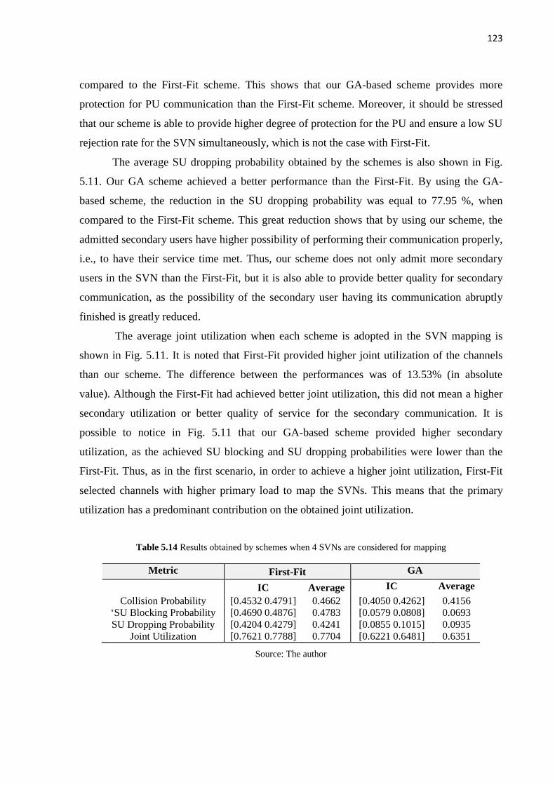
123

compared to the First-Fit scheme. This shows that our GA-based scheme provides more

protection for PU communication than the First-Fit scheme. Moreover, it should be stressed

that our scheme is able to provide higher degree of protection for the PU and ensure a low SU

rejection rate for the SVN simultaneously, which is not the case with First-Fit.

The average SU dropping probability obtained by the schemes is also shown in Fig.

5.11. Our GA scheme achieved a better performance than the First-Fit. By using the GA-

based scheme, the reduction in the SU dropping probability was equal to 77.95 %, when

compared to the First-Fit scheme. This great reduction shows that by using our scheme, the

admitted secondary users have higher possibility of performing their communication properly,

i.e., to have their service time met. Thus, our scheme does not only admit more secondary

users in the SVN than the First-Fit, but it is also able to provide better quality for secondary

communication, as the possibility of the secondary user having its communication abruptly

finished is greatly reduced.

The average joint utilization when each scheme is adopted in the SVN mapping is

shown in Fig. 5.11. It is noted that First-Fit provided higher joint utilization of the channels

than our scheme. The difference between the performances was of 13.53% (in absolute

value). Although the First-Fit had achieved better joint utilization, this did not mean a higher

secondary utilization or better quality of service for the secondary communication. It is

possible to notice in Fig. 5.11 that our GA-based scheme provided higher secondary

utilization, as the achieved SU blocking and SU dropping probabilities were lower than the

First-Fit. Thus, as in the first scenario, in order to achieve a higher joint utilization, First-Fit

selected channels with higher primary load to map the SVNs. This means that the primary

utilization has a predominant contribution on the obtained joint utilization.

Table 5.14 Results obtained by schemes when 4 SVNs are considered for mapping

Metric First-Fit GA

IC Average IC Average

Collision Probability [0.4532 0.4791] 0.4662 [0.4050 0.4262] 0.4156

„SU Blocking Probability [0.4690 0.4876] 0.4783 [0.0579 0.0808] 0.0693

SU Dropping Probability [0.4204 0.4279] 0.4241 [0.0855 0.1015] 0.0935

Joint Utilization [0.7621 0.7788] 0.7704 [0.6221 0.6481] 0.6351

Source: The author

124

Fig. 5.11. Results obtained by schemes when 4 SVNs are mapped

Source: The author

5.5.4 Additional Discussion

On the basis of our previous results, it should be noted that our schemes based on GA

outperformed the First-Fit, since they achieved a good tradeoff between the objectives defined

in the mapping problem formulated in Section 5.1. It were able to achieve in most cases a

good level of joint utilization and provide good quality of service to both secondary and

primary communication by obtaining lower values for SU blocking, SU dropping and

collision probabilities.

In the first scenario, it was found that even with the increase of SU arrival rate, our

schemes achieved the lower values for SU dropping and collision probabilities and a similar

performance in terms of SU blocking probability when compared to the First-Fit. Thus it

reduced the likelihood of these problems to occur. This shows the capacity of our scheme to

allocate channels to SVNs and thus provide a good level of protection for the PU, low

rejection and dropping rates for secondary users in both scenarios (with either a high or low

load of secondary activity), i.e. different levels of demand of the SVN. Along with this, it was

able to achieve a reasonable level of joint utilization, and combine each SVN with the most

suitable channels for it.

Two points need to be highlighted to explain the superiority of our scheme to that of

First-Fit, which are as follows: the intrinsic parallelism of the GA, and the fitness functions

that encompass more than one objective in order to find solutions that provide a good trade-

off between them. The GA parallelism enables many solutions (and builder blocks) to be

handled, improved and evaluated simultaneously so that the right solutions can be found.

125

During the mapping process, our scheme does not only deal with matters concerning the

collision probability, SU dropping probability and demand requested by SVN. It also takes a

broad view of the SU blocking probability, and joint utilization, which also compose the

objectives defined for the mapping problem (in Section 4.10). Thus, in order to define the

mapping (set of channels) that must be considered in a SVN, each possible solution,

represented by an individual, is evaluated and awarded a score, which measures its degree of

success in achieving the desired objectives.

Thus, results such as those obtained in the second scenario are possible, even when

there is a high load of PU, which indicates less possibility of opportunist access by SU. Our

scheme is able to keep the SU blocking and SU dropping at low values, because it is aware

that if the user density per channel is increased, these probabilities would be affected.

As shown in the last scenario, our scheme is also able to handle more than one SVN

request and achieves, in general, a better performance than the First-Fit scheme.

Several practical implications emerge from the results obtained by our scheme. The

first is related to the business model. We found that it is possible to share resources (e.g.

channels) between users with different access priorities and meet their demands. Thus, a

business model that offers services with different access priorities (e.g. primary and

secondary) to the customers could be deployed. It could also assign different prices to virtual

networks communications depending on their level of access to the resources.

The second implication refers to the problem of guaranteeing access levels. When

sharing resources between virtual networks (PVNs and SVNs) with different access levels, it

is important to ensure that their demands and restrictions are met, for example, in the case of a

primary virtual network that imposes tight restrictions regarding interference to its

communication. This restriction must be satisfied during the SVN mapping process by the

scheme adopted. In a similar way, during the SVN mapping, it is necessary to ensure that the

SVN can access opportunistically, i.e. to prevent that the mapped SVNs suffer starvation,

even in a scenario with a high load of primary activity. We have sought to show that our GA-

based scheme is able to meet the restrictions and demand from primary and secondary virtual

networks.

It should be stressed that our scheme can be adopted to improve the joint utilization of

resources. This means that the requirements of more users can be met, and as a result, the

infrastructure provider will be in a position to increase its revenue.

Finally, from three previous evaluation scenarios, we can highlight the second as the

most suitable for application of our GA-based scheme. We observed that in the low PU load

126

case, GA-based scheme provided less interference to PU communication and higher joint

utilization than the First-Fit. Moreover, it achieved good levels of SU blocking and dropping.

When the PU load is high, GA-based scheme provided lower SU dropping and blocking

probabilities and reasonable levels of joint utilization and protection to the PU in relation to

the First-Fit scheme. So, it is noted that the GA-based scheme is able to work well in both

cases: low PU load (possibility of opportunistic access is higher) and high PU load

(possibility of opportunistic access is lower).

5.6 Chapter Summary

In this Chapter, the multi-objective problem of SVNs mapping onto wireless substrate

in CRVNE was formulated and a scheme based on GA was designed to solve it. The scheme

adopted classical approaches in its structure to deal with the multiple objectives of the

problem and reduce the problem complexity. In addition, in order to verify its effectiveness,

an evaluation was performed, where a scheme based on First-Fit was adopted as baseline and

important metrics related to primary and secondary communications were considered. Results

showed that GA-based scheme achieve a good tradeoff between the objectives of the

problems and, in general, a better performance than First-Fit.

127

Chapter 6 - Concluding Remarks

This Chapter concludes this thesis by offering some considerations, showing its main

value as a contribution to studies in the field, and proposing future studies.

6.1. Considerations

We have addressed the combination of cognitive radio, dynamic spectrum access

techniques and wireless virtualization in order to overcome the problem of resource

underutilization likely to occur when current approaches to wireless virtualization are

adopted. Although this combination enables virtual wireless networks with different priorities

of access to the resources (PVNs and SVNs) to share common substrate networks, where the

SVNs access the resources opportunistically, the mapping of SVNs onto substrate networks is

a challenging problem, where there are objectives related to the primary and secondary

communications, and substrate network. Thus, we have outlined a new scenario, modeled it,

and formulated the SVNs mapping onto substrate networks as a multi-objective problem. In

addition, we have proposed a scheme based on GA to solve this problem. It outperformed a

scheme based on the First-Fit strategy. Our GA-based scheme provided better level of

protection to the primary communication and achieved a good tradeoff in terms of SU

blocking, SU dropping, and joint resource utilization.

We hope that this work will encourage further research in Cognitive Radio Virtual

Networks Environment and architectures, business models and mechanisms for mapping

secondary networks that deal with the many challenges that emerge in this environment.

Moreover, we hope that the proposed GA-based scheme can yield good results for

Infrastructure providers, PVNs and SVNs communications, in terms of metrics such as

resource utilization, SU blocking probability, SU dropping probability, and collision

probability.

6.2. Contributions

The main contributions to the area of study provided by this thesis can be summarized

as follows:

Description of the elements that compose the environment termed cognitive

radio virtual networks environment (CRVNE) and benefits from the

incorporation of cognitive radio in wireless virtualization.

128

Modeling of the CRVNE and formulation of important performance metrics

related to primary and secondary communications.

Formulation of the multi-objective problem of mapping SVN onto substrate

networks, while considering a cognitive radio virtual network environment.

A GA-based scheme to solve the multi-objective problem and its evaluation.

6.3 Future Works

Some studies have been identified for further development. They can be divided into

two groups: model and schemes. The first involves aspects related to the model designed to

represent CRVNE. It includes the insertion of new features and improvements in current ones.

The second is related to the investigation of possible schemes to solve the multi-objective

problem of SVN mapping. Both groups are outlined below.

In terms of future works related to the model, the following points are highlighted.

To extend the queue model in order to support secondary users (secondary

applications) that request more than one channel (e.g. two or three) to perform

their communications. Thus, scenarios with heterogeneous users in terms of

requested bandwidth might be analyzed.

To extend the model to cover the event in which the SU switches of SVN to

resume its communication, when there is no free channel in its current SVN.

This event is denoted as SU handover between SVNs. With this new feature, a

new performance metric might be formulated to evaluate the schemes designed

to solve the SVN mapping problem.

To include new metrics to express the QoS of the secondary communication. In

this thesis, the joint utilization was adopted to express the level of utilization of

the resources by PUs and SUs. So, it was computed as a combination of the

primary and secondary utilization. However, in some cases, this joint approach

did not reflect well how good a given solution was for the SVN, since a high

joint utilization did not necessarily mean a high secondary utilization.

Moreover, it is interesting to analyze how many SUs has their services

completed successful. Thus, metrics such as SU utilization and SU Throughput

can be derivate from the model and adopt to analyze the performance of the

secondary communication when each scheme is adopted.

129

To adopt other probability distributions in the model to express different type

of traffic or applications. In this thesis, we adopted Poisson and exponential

distributions to express the arrival process and service time of the users.

However, other probability distributions such as Hyper-Exponential and Erlang

General can be considered to model HE/M/N/N and EG/M/N/N systems,

where the arrival process of users is not given by Poisson distribution.

With regard to schemes for solving the discussed problem, the following future works

are pointed out:

To study the most adequate multi-objective GA approach to be used to map

SVNs onto substrate networks. In this point, a comparative study of the main

approaches presents in literature can be accomplished.

To evaluate other bio-inspired approaches to solve this problem and compared

them to the current one.

To design a Fuzzy-Genetic scheme to deal with the SVN mapping problem. In

the literature, many approaches use Pareto sets to solve multi-objective

problems, and allow the user to decide what trade-offs in performance

measurements are acceptable for the problem and then choose the final

solution from the Pareto set. However, this can result in a large number of

solutions for the user to choose from, and a good solution with respect to one

objective can produce a poor result with respect to another. The adoption of a

Fuzzy System as a fitness function is a means of overcoming this problem,

because it indicates what individual is the best from the population when all

the defined objectives have been taken into account. This eliminates the need

for the user to choose a final solution from a large set (ALLARD, 2007).

Other work that can be explored is the combination of Cognitive Radio, Wireless

Virtualization and DSA techniques in the scenario of 5G Networks. In 5G networks is

envisioned to have a densification of cellular networks with HetNets (macrocells, femtocells

and picocells), provision for peer-to-peer communication (e.g. device to device- D2D) and

machine to machine communication (M2M), diversity of devices (e.g. wearable devices,

smart phone, smart machines), higher data rate, differentiated services, and focus on QoE to

evaluate the networks services. Moreover, it is expected that 5G networks coexist with other

networks technologies such as WiFi, WiMax, for example. So, questions such as how to

manage this complex environment, how to deal with interference between networks, how to

130

provide differentiated service to various types of devices, how to employ new services and

networks using a limited natural resources and how to provide a efficient resource utilization

are raised in this future scenario. Cognitive radio, DSA techniques and wireless virtualizations

are claimed as important elements in 5G networks. So, a study on the role of each one in this

scenario can be carried out and how they are related.

131

References

WEN, H.; TIWARY, P. K.; LE-NGOC, T. Current trends and perspectives in

wireless virtualization, International Conference on Selected Topics in Mobile and

Wireless Networking (MoWNeT), 2013a.

LIANG, C.; YU, F. R. Wireless Network Virtualization: A Survey, Some Research

Issues and Challenges, IEEE Communications Survey and Tutorials, v.17, issue 1,

p.358-380, 2014.

HASEGAWA, M. et. al. Optimization for Centralized and Decentralized Cognitive

Radio Networks, Proceedings of the IEEE, v. 102, issue 4, p.574-584, 2014.

AKYILDIZ, I. F. et. al. Next generation/dynamic spectrum access/cognitive radio

wireless networks: A survey, Elsevier Computer Networks, v. 50, issue 13, p. 2127–

2159, 2006.

BELBEKKOUCHE, A.; HASAN, M. M.; KARMOUCH, A. Resource Discovery and

Allocation in Network Virtualization, IEEE Communications Surveys & Tutorials, v.

14, issue 4, p.1114-1128, 2012.

XIN, C.; SONG, M. Dynamic Spectrum Access as a Service, Proceedings IEEE

INFOCOM, p.666-674, 2012.

FCC. Federal Communications Commission, Spectrum policy task force report: FCC

02-155, Nov. 2002.

MCHENRY, M. A; MCCLOSKEY, D. Spectrum occupancy measurements:

Chicago, Illinois, November 16-18, 2005, Shared Spectrum Company, Tech. Rep.,

2005.

KIM, H.; SHIN, K. G. Efficient Discovery of Spectrum Opportunities with MAC-

Layer Sensing in Cognitive Radio Networks, IEEE Transactions on mobile

computing, v . 7, n. 5, p. 533-545, 2008.

YUCEK, T.; ARSLAN, H. A survey of spectrum sensing algorithms for cognitive radio

applications, IEEE Communications Surveys & Tutorials, v. 11, n. 1, p. 116-130,

2009.

132

BALIEIRO, A. et. al. A multi-objective genetic optimization for spectrum sensing in

cognitive radio, Expert Systems with Applications, v. 41, issue 8, p. 3640–3650,

2014.

TWSD. Telcordia's TV Bands White Space Database. Disponível em <

http://www.telcordia. om/services/interconnection/white-

spaces.html?sc_cid=whitespace_vanity>. Acesso em: 10 Maio de 2013.

WBWSD. Spectrum Bridge's White Space database. Disponível em:

<http://whitespaces.s pectrumbridge.com/whitespaces/home.aspx>. Acesso em: 10

Maio de 2013.

MASONTA, M.T.; MZYECE, M.; NTLATLAPA, N. Spectrum Decision in Cognitive

Radio Networks: A Survey, IEEE Communications Surveys and Tutorials, v. 15,

n.3, p. 1088 - 1107, 2013.

CHRISTIAN, I. et. al. Spectrum Mobility in Cognitive Radio Networks, IEEE

Communications Magazine, v. 50, issue 6, p.114-121, 2012.

BALIEIRO, A. M. et. al. Handoff de Espectro em Redes Baseadas em Rádio

Cognitivo Utilizando Redes Neurais Artificiais, In: IX WPerformance, 2010, Belo

Horizonte. Proceedings of XXX Congresso da Sociedade Brasileira de Computação,

2010.

MITOLA III, J. An Integrated Agent Architecture for Software Defined Radio,

Ph.D Thesis, Royal Institute of Technology (KTH), Sweden, 2000.

SENGUPTA, S.; CHATTERJEE, M. An Economic Framework for Dynamic Spectrum

Access and Service Pricing, IEEE/ACM Transactions on Networking, v. 17, issue 4,

p. 1200-1213, 2009.

DUAN, L.; HUANG, J.; SHOU, B. Cognitive Mobile Virtual Network Operator:

Investment and Pricing with Supply Uncertainty, Proceedings IEEE INFOCOM, p.

1-9, 2010.

WEN, H.; TIWARY, P.K.; LE-NGOC, T. Wireless Virtualization, Springer, 2013b.

CHEN, X. Resource Allocation and Pricing in Virtual Wireless Networks,

University of Massachusetts Amherst, Master Thesis, February 2014.

133

CHOWDHURY, N.M.M.K.; BOUTABA, R. A survey of network virtualization,

Computer Networks, v. 54, issue 5, p.862–876, 2010.

KHAN, A. et. al. Network Virtualization: A Hypervisor for the Internet?, IEEE

Communications Magazine, v. 50, issue 1, p. 136-143, 2012.

SCHAFFRATH, G. et.al. Network virtualization architecture: proposal and initial

prototype, Proceedings of the 1st ACM workshop on Virtualized infrastructure systems

and architectures, p. 63-72, 2009.

FISCHER, A. et. al. Virtual Network Embedding: A Survey, IEEE Communications

Surveys & Tutorials, v. 15, n. 4, p.1888-1906, 2013.

YANG, M. et. al. Opportunistic Spectrum Sharing Based Resource Allocation for

Wireless Virtualization, Seventh International Conference on Innovative Mobile and

Internet Services in Ubiquitous Computing (IMIS), p. 51-58, 2013.

WANG, X.; KRISHNAMURTHY, P.; TIPPER, D. Wireless Network Virtualization,

International Conference on Computing, Networking and Communications, p. 818-822,

2013.

AL-HAZMI, Y.; DE MEER, H. Virtualization of 802.11 Interfaces for Wireless

Mesh Networks, Eighth International Conference on Wireless On-Demand Network

Systems and Services (WONS), p.44-51, 2011.

PAUL, S.; SESHAN, S. Technical Document on Wireless Virtualization, GENI

Technical Report GDD-06-17, 2006.

MAHINDRA, R. et. al. Space Versus Time Separation for Wireless Virtualization

on an Indoor Grid, Next Generation Internet Networks (NGI), p. 215 – 222, 2008.

NAKAUCHI, K. et al. AMPHIBIA: A Cognitive Virtualization Platform for End-

to-End Slicing, IEEE International Conference on Communications (ICC), p. 1-5,

2011.

MACCALL, J. Genetic algorithms for modelling and optimisation. Journal of

Computational and Applied Mathematics, v. 184, issue 1, p. 205-222, 2005.

134

MICHALEWICZ, Z. Genetic Algorithms + Data Strucutures = Evolution

Programs. Third Edition, Springer, 1996.

MAN, K. F; TANG, K. S; KWONG, S. Genetic algorithms: concepts and applications,

IEEE Transactions on Industrial Electronics, v.43, n. 5, p.519-534, 1996.

KUMAR, A. Enconding Schemes in Genetic Algorithm, International Journal of

Advanced Research in IT and Engineering. 2, n.3, p.1-7, 2013.

KUMAR, R. Novel Encoding Scheme in Genetic Algorithms for Better Fitness.

International Journal of Engineering and Advanced Technology, v.1, issue 6, p.

214-218, 2012.

SILVA, D. A. et al. Measurement of Fitness Function efficiency using Data

Envelopment Analysis, Elsevier Expert Systems with Applications, v.41, issue 16,

p.7147-7160, 2014.

KAYA, M. The effects of a new selection operator on the performance of a genetic

algorithm, Applied Mathematics and Computation, v. 217, issue 1, p.7669–7678,

2011a.

GOLDBERG, D.E., Genetic Algorithms in Search, Optimization and Machine

Learning, Addison-Wesley, 1989.

KAYA, M. The effects of two new crossover operators on genetic algorithm

performance. Expert Applied Soft Computing, vl.11, issue 1, p.881–890, 2011b.

[41] SYSWERDA, G. Uniform Crossover in Genetic Algorithms. Proceedings of the

3rd International Conference on Genetic Algorithms, p. 2-9, 1989.

BOLCH, G. et. al. Queueing Networks and Markov Chains, 2. ed, Wiley, 2006.

JAIN, R. The Art of Computer Systems Performance Analysis: Techniques for

Experimental Design, Measurement, Simulation, and Modeling, Wiley, 1991.

COOPER, R. B. Introduction to Queueing Theory, 2. ed. North Holland, 1981.

GROSS, D. et. al. Fundamentals of Queueing Theory, 4. Ed. Wiley, 2008.

135

DEB, K. Multi-objective optimization using evolutionary algorithms, John Wiley &

Sons, 2001.

ZHANG, S. et. al. An Opportunistic Resource Sharing and Topology-Aware

mapping framework for virtual networks, Proceedings of IEEE INFOCOM, p. 2408-

2416, 2012.

ZAKI, Y. et. al. LTE wireless virtualization and spectrum management, Third Joint

IFIP Wireless and Mobile Networking Conference, p. 1-6, 2010.

ZAKI, Y. et. al. LTE mobile network virtualization, Springer Mobile Networks and

Applications, v. 16, issue 4, p. 424-432, 2011.

BANCHS, A. et. al. Providing Throughput and Fairness Guarantees in Virtualized

WLANs Through Control Theory, Springer Mobile Networks and Applications, v.17,

issue 4, p 435-446, 2012.

SMITH, G. et. al. Wireless virtualization on commodity 802.11 hardware,

Proceedings of the second ACM international workshop on Wireless network testbeds,

experimental evaluation and characterization (WinTECH‟07), p.75-82, 2007.

FU, F.; KOZAT, U. C. Wireless Network Virtualization as A Sequential Auction

Game, Proceedings of IEEE INFOCOM, p.1-9, 2010.

CAEIRO, L.; CARDOSO, F. D.; CORREIA, L. M. Adaptive allocation of Virtual

Radio Resources over heterogeneous wireless networks, 18th European Wireless

Conference (European Wireless), p.1-7, 2012.

CHENA, Y-S. et. al. A Cross-Layer Protocol of Spectrum Mobility and Handover in

Cognitive LTE Networks, Simulation Modelling Practice and Theory, v. 19, issue 8,

p.1723–1744, 2011.

POPESCU, A. et. al. ENVIRAN: Energy Efficient Virtual Radio Access Networks,

16th International Symposium on Wireless Personal Multimedia Communications

(WPMC), p. 1-5, 2013.

ARMBRUST, M. et.al. A view of Cloud Computing”, Communications of the ACM

Magazine, v. 53, issue 4, p.50-58, 2010.

136

MIN, A.W. et.al. Opportunistic spectrum access for mobile cognitive radios,

Proceedings of IEEE INFOCOM, p. 2993-3001, 2011.

WANG, L. et.al. Converged Management in Heterogeneous Wireless Networks Based

on Resource Virtualization, Mobile Networks and Applications, v. 20, issue 1, p. 53-

61, 2015.

CHOWDHURY, N. M. M.; RAHMA, M. R. Virtual Network Embedding with

Coordinated Node and Link Mapping, IEEE INFOCOM, p.783-791, 2009.

AKTER, L.; NATARAJAN, B.; SCOGLIO, C. Modeling and Forecasting Secondary

User Activity in Cognitive Radio Networks, Proceedings of 17th International

Conference on Computer Communications and Networks (ICCCN), p. 1-6, 2008.

LAI, J. et al. Network Selection in Cooperative Cognitive Radio Networks, 11th

International Symposium on Communications and Information Technologies (ISCIT),

p.378-383, 2011.

WANG, C. et. al. Network Selection in Cognitive Radio Systems, IEEE Global

Telecommunications Conference, (GLOBECOM), p.1-6, 2009.

ZHAO, L. et. al. LTE Virtualization: from Theoretical Gain to Practical Solution,

23rd International Teletraffic Congress (ITC), p.71-78, 2011.

SMITH, P. J. et. al. Analysis of the M/M/N/N Queue with Two Types of Arrival

Process: Applications to Future Mobile Radio Systems, Journal of Applied

Mathematics, v. 2012, p.1-14, 2012.

MATHWORKS. Disponível em: <http://www.mathworks.com/>. Acesso em: 10 Maio

de 2015.

PERROS, H. Computer Simulation Techniques:The definitive introduction!, North

Carolina State University, 2008.

SINGH, K.; XIE, M. Bootstrap: A Statistical Method, Rutgers University, 2008.

Disponível em: <http://www.stat.rutgers.edu/home/mxie/rcpapers/ bootstrap.pdf>.

Acesso em: 1 Junho de 2015.

137

CHEN, S. et. al. Genetic algorithm-based optimization for cognitive radio

networks, IEEE Sarnoff Symposium, 2010.

COELHO, C.A.C; LAMONT,G.B.; VELDHUIZEN, D.A.V. Evolutionary Algorithms

for Solving Multi-Objective Problems, 2. ed. Springer, 2007.

SAOUCHA, N. A.; LAMMARI, A. C.; BENATCHBA, K. Real-Coded Genetic

Algorithm Parameter Setting for Cognitive Radio Adaptation, International

Conference on Smart Communications in Network Technologies, 2013.

ALLARD, D.M. A Multi-Objective Genetic Algorithm To Solve Single Machine

Scheduling Problems Using A Fuzzy Fitness Function, College of Engineering and

Technology of Ohio University, Master Thesis, June 2007.