I

Pós-Graduação em Sistemas Costeiros e Oceânicos (PGSISCO)

Centro de Estudos de Mar (CEM)

Universidade Federal do Paraná (UFPR)

Ana Lúcia Lindroth Dauner

HIDROCARBONETOS NO MATERIAL PARTICULADO DA BAÍA DE

GUARATUBA, PR, E SISTEMAS AQUÁTICOS ADJACENTES.

Pontal do Paraná

Março de 2015

II

Ana Lúcia Lindroth Dauner

HIDROCARBONETOS NO MATERIAL PARTICULADO DA BAÍA DE

GUARATUBA, PR, E SISTEMAS AQUÁTICOS ADJACENTES

Dissertação apresentada ao Programa de Pós-

Graduação em Sistemas Costeiros e

Oceânicos, Universidade Federal do Paraná,

como requisito parcial para obtenção de grau

de Mestre.

Orientador: Dr. César de Castro Martins

Pontal do Paraná

Março de 2015

III

III

... Não se prende nesse medo de errar,

Que é errando que se aprende.

O caminho até parece complicado

E às vezes tão difícil que você se surpreende

quando sente de repente que era tudo muito simples.

Vai em frente que você entende.

Gabriel, o Pensador

IV

“Hidrocarbonetos no material particulado da Baía de Guaratuba, PR, Brasil, e sistemas

aquáticos adjacentes”

por

Ana Lúcia Lindroth Dauner

Dissertação nº 124 aprovada como requisito parcial do grau de Mestre(a) no

Curso de Pós-Graduação em Sistemas Costeiros e Oceânicos da Universidade

Federal do Paraná, pela Comissão formada pelos professores:

Pontal do Paraná, 24/04/2015.

CURSO DE PÓS-GRADUAÇÃO EM SISTEMAS

COSTEIROS E OCEÂNICOS Centro de Estudos do Mar - Setor Ciências da Terra - UFPR Avn. Beira-mar, s/nº - Pontal do Sul – Pontal do Paraná – Paraná - Brasil Tel. (41) 3511-8644 - Fax (41) 3511-8648 - www.cem.ufpr.br - E-mail: pgsisco@ufpr.br

V

VI

AGRADECIMENTOS

À Coordenação de Aperfeiçoamento de Pessoal de Ensino Superior

(CAPES) pela bolsa de mestrado e à Fundação Araucária de Apoio ao

Desenvolvimento Científico e Tecnológico do Estado do Paraná pelo auxílio

financeiro (401/2012 – 15.078).

Ao Ângelo Breda, do Simepar, e ao Edson Nagashima, do Instituto das

Águas do Paraná, pelo fornecimento dos dados de precipitação.

Ao César, um exemplo de orientador, que me ensinou muito ao longo

dos anos e, mais importante, que confiou na minha capacidade de trabalho,

mesmo à distância.

Às meninas do LaGPoM que me acompanharam ao longo do meu

mestrado. Josi, Fer Ishii, Carol, Dóris, Amanda e Aline, muito obrigada pela

companhia e pela ajuda, tanto nas coletas (inclusive durante o carnaval) quanto

no laboratório.

Aos professores da PGSISCO, que sempre tem algo a mais para nos

ensinar. Agradeço também aos membros externos e internos – Eunice

Machado, Juliana Leonel, Rafael Lourenço, Marco Grassi e Renato Rodigues

Neto – que me avaliaram ao longo das semanas acadêmicas e ajudaram a

melhorar o trabalho.

Aos alunos da PGSISCO e meus amigos, com quem a gente pode

contar para discutir os nossos trabalhos, problemas e sucessos. Além de

sempre arranjarem um motivo para comemorar.

Em especial, à Fer e ao Eli, que sempre estiveram no corredor ao lado,

para ajudar com o R, bater um papo, procrastinar o trabalho e divagar sobre os

mais diversos temas e assuntos. Muito obrigada pela amizade duradoura.

À minha família, que sempre me apoiou, confiou no meu potencial e

nunca duvidou que tudo daria certo no final.

Por fim, ao Mihael. Muito obrigada pelo companheirismo, pelo incentivo

e pelos inúmeros motivos de risadas/gargalhadas ao longo desses anos. Eu te

amo demais.

RESUMO

O objetivo desta dissertação foi avaliar a distribuição espacial e temporal,

de curta escala, de hidrocarbonetos (hidrocarbonetos policíclicos aromáticos –

HPAs, hidrocarbonetos alifáticos – HAs, Alquilbenzenos lineares – LABs) no

material particulado em suspensão (MPS) da Baía de Guaratuba, PR, Brasil,

bem como identificar as suas principais fontes e verificar como os parâmetros da

coluna d’água afetam a sua distribuição. Para tanto, foram coletadas 22

amostras em três períodos distintos (04/2013, 08/2013 e 03/2014).

De um modo geral, foram observados altos valores na porção mediana do

estuário, relacionados a fenômenos hidrodinâmicos que contribuem para o

acúmulo de matéria orgânica, gerando uma região atuante como um filtro

geoquímico de partículas. Também foram observadas altas concentrações na

desembocadura da baía, próximo à passagem de balsas indicando um aporte

contínuo durante o ano, e na porção mais interna da baía, sugerindo o aporte

fluvial como fonte da introdução de hidrocarbonetos. Por fim, foram observados

altos valores de HPAs e de HAs próximo à marina de Guaratuba na coleta

realizada durante o Carnaval (Março/2014), indicando um aumento da

introdução desses compostos nesse período. Ainda, as maiores concentrações

foram observadas durante o verão, período de aumento populacional na região.

A análise de razões diagnósticas permitiu avaliar as principais fontes dos

hidrocarbonetos na Baía de Guaratuba. A distribuição dos HPAs e dos HAs

sugere uma importante fonte petrogênica recente, provavelmente associada ao

tráfego de embarcações e balsas na baía, além de uma contribuição natural de

matéria orgânica proveniente de fontes biogênicas terrestres, provavelmente

oriundas da floresta de manguezal existente nas margens da baía.

Assim, foi possível observar que a introdução de óleo e esgoto são

problemas emergentes na Baía de Guaratuba, especialmente durante o verão.

Além disso, este trabalho evidenciou a importância da avaliação de

contaminantes em curtas escalas temporais e de considerar as características

físico-químicas da coluna d’água em estudos de avaliação ambiental envolvendo

o MPS, uma vez que eles podem ser responsáveis por acumular material

orgânico em regiões afastadas de fontes pontuais de poluentes.

ABSTRACT

The aim of this work was to evaluate the spatial and temporal (short range)

distribution of hydrocarbons (polycyclic aromatic hydrocarbons - PAHs, aliphatic

hydrocarbons - AHs, Linear Alkyl Benzenes - LABs) in suspended particulate

matter (SPM) in Guaratuba Bay, Brazil, as well as identify their main sources and

observe how the parameters of the water column affect their distribution. For this

purpose, 22 samples were collected in three distinct periods (04/2013, 08/2013

and 03/2014).

In general, we observed high values in the middle portion of the estuary,

related to hydrodynamic phenomena that contribute to the accumulation of

organic matter, creating a region that acts as a geochemical particulate filter. We

also observed high concentrations in the bay mouth, next to the passage of ferries

indicating a continuous supply throughout the year, and in the innermost portion

of the bay, suggesting the fluvial contribution as a source of the hydrocarbon

introduction. Finally, we observed high PAHs and HAs values near Guaratuba

marina during Carnival (03/2014), indicating an increase in the introduction of

these compounds in this period. Generally, the highest concentrations were

observed during the summer, population growth period in the region.

The analysis of diagnostic reasons allowed us to evaluate the main sources

of hydrocarbons in the Bay of Guaratuba. The distribution of PAHs and AHs

suggests an important recent petrogenic source, probably associated with the

traffic of vessels and ferries on the bay, as well as a natural contribution of organic

matter from terrestrial biogenic sources, probably derived from the existing

mangrove forest in the Bay shores.

Thus, it was observed that the introduction of oil and sewage are emerging

problems in Guaratuba Bay, especially during the summer. In addition, this study

showed the importance of the evaluation of contaminants in short timescales and

to consider the physical and chemical characteristics of the water column in

environmental assessment studies involving SPM samples, since they may be

responsible for accumulating organic material areas far from the point sources of

pollutants.

VII

SUMÁRIO

Agradecimentos ................................................................................................ VI

Sumário ............................................................................................................ VII

Prefácio ............................................................................................................. IX

Capítulo 1 ......................................................................................................... XII

Effect of seasonal population fluctuation in the temporal and spatial distribution

of polycyclic aromatic hydrocarbons in a subtropical estuary. .......................... 13

Research Highlights ......................................................................................... 14

Abstract ............................................................................................................ 15

1. Introduction ................................................................................................... 16

2. Study area .................................................................................................... 17

3. Material and Methods ................................................................................... 18

3.1. Sampling ............................................................................................... 18

3.2. Analytical procedure .............................................................................. 22

3.2.1. Hydrological parameters ................................................................ 22

3.2.2. PAHs .............................................................................................. 22

3.2.3. Analytical control ............................................................................ 23

3.3. Data analysis ......................................................................................... 24

4. Results and Discussion ................................................................................ 25

4.1. Hydrological parameters ....................................................................... 25

4.2. Spatial and temporal distribution of PAHs ............................................. 28

4.3. Comparison with other studies .............................................................. 32

4.4. Evaluation of PAH sources by diagnostic ratios .................................... 33

4.5. Principal Component Analysis ............................................................... 34

5. Summary and Conclusions ........................................................................... 37

Appendix A. Supplementary data ..................................................................... 39

6. References ................................................................................................... 39

Appendix A. Supplementary data ..................................................................... 44

Capítulo 2 ..................................................................................................... XLVI

Spatial and temporal distribution of aliphatic hydrocarbons and linear

alkylbenzenes in the particulate phase from a subtropical estuary (Guaratuba

Bay, SW Atlantic) under seasonal population fluctuation. ................................ 47

Research Highlights ......................................................................................... 48

VIII

Abstract ............................................................................................................ 49

1. Introduction ................................................................................................... 50

2. Study area .................................................................................................... 52

3. Material and Methods ................................................................................... 53

3.1. Sampling ............................................................................................... 53

3.2. Analytical procedure .............................................................................. 54

3.2.1. Sample preparation ........................................................................ 54

3.2.2. Sample extraction and instrumental analysis ................................. 54

3.2.3. Analytical control ............................................................................ 56

3.3. Data analysis ......................................................................................... 56

4. Results and Discussion ................................................................................ 57

4.1. AH and LAB concentrations .................................................................. 57

4.2. Spatial distribution ................................................................................. 62

4.3. Temporal distribution ............................................................................. 64

4.4. Evaluation of AH sources and degradation ........................................... 66

4.5. Evaluation of LAB degradation .............................................................. 69

5. Summary and Conclusions ........................................................................... 71

6. References ................................................................................................... 72

Posfácio ................................................................................................... LXXVIII

Anexo – Dados Brutos ................................................................................ LXXX

IX

PREFÁCIO

Estuários são caracterizados por receber grandes quantidades de matéria

orgânica e nutrientes, provenientes da bacia de drenagem e da plataforma

continental. Esse fluxo de material, aliado à transferência de energia e à

reatividade interna do sistema (COSTA et al., 2010), faz com que esses

ecossistemas sejam alguns dos mais importantes da biosfera em termos de

atividade biológica (GATTUSO et al., 1998). No entanto, os estuários também

estão sujeitos a diferentes tipos de mudanças ambientais originárias das

atividades antrópicas existentes nas bacias de drenagem, nas margens e

dentro do próprio estuário. Os principais impactos antrópicos em regiões

estuarinas são as atividades portuárias e de navegação, drenagem urbana e

descarte direto de efluentes urbanos e industriais (GRIGORIADOU et al., 2008;

VENTURINI et al., 2008), as quais podem variar de intensidade ao longo do

ano. Assim, devido à interação entre os ambientes marinho e terrestre, e à

influência antrópica, os estuários são ecossistemas altamente variáveis, tanto

na escala temporal quanto na escala espacial (BIANCHI, 2007).

O aporte de matéria orgânica e contaminantes em um ambiente pode ser

determinado através do uso de marcadores orgânicos geoquímicos, os quais

podem ser de origem natural ou antrópica, apresentam natureza específica e

resistência à degradação (COLOMBO et al., 1989). Nesse grupo, incluem-se os

hidrocarbonetos policíclicos aromáticos (HPAs), os hidrocarbonetos alifáticos

(HAs) e os alquilbenzenos lineares (LABs).

Os HPAs são compostos orgânicos de origem petrogênica, pirolítica ou

diagenética, associados principalmente a atividades antrópicas (WANG et al.,

1999, 2009), podendo bioacumular e biomagnificar (VENTURINI et al., 2008;

CHIZHOVA et al., 2013). Os HAs podem ser oriundos tanto de fontes naturais

quanto petrogênicas (UNEP, 1992; BURNS & BRINKMAN, 2011; MARTINS et

al., 2012a), sendo que a Mistura Complexa Não Resolvida (MCNR) é

geralmente associada à presença de resíduos de óleo degradado (READMAN

et al., 2002; MAIOLI et al., 2011). Por fim, os LABs são hidrocarbonetos

presentes na matéria prima utilizada na composição dos principais

surfactantes, sendo assim bons indicadores da introdução de esgotos

X

domésticos e industriais (RAYMUNDO & PRESTON, 1992; TAKADA &

EGANHOUSE, 1998; MARTINS et al., 2012b).

Por se tratarem de moléculas de caráter apolar e, portanto, hidrofóbicas,

os marcadores orgânicos geoquímicos tendem a se associar ao material

particulado em suspensão (MPS) (MONTUORI & TRIASSI, 2012). O material

particulado reflete as condições do sistema aquático no instante da coleta,

sendo que a distribuição dos marcadores no ambiente está sujeita a alterações

momentâneas tanto das fontes quanto de forçantes ambientais, como a

salinidade e a concentração de MPS (LIU et al., 2014; RÜGNER et al., 2014).

Assim, o MPS pode ser utilizado para avaliar a variabilidade espacial e

temporal de contaminantes em ambientes com influência antrópica variável ao

longo do ano. Assim, nos últimos anos, o comportamento dos hidrocarbonetos

no material particulado de sistemas estuarinos e costeiros tem recebido cada

vez mais atenção, uma vez que essas são áreas de transição onde os

poluentes antrópicos podem ser transferidos para ecossistemas adjacentes,

como as plataformas continentais (LUO et al., 2008; GUO et al., 2010; MAIOLI

et al., 2011; MONTUORI & TRIASSI, 2012; LIU et al., 2014).

A Baía de Guaratuba, PR, Brasil, é um exemplo de um ambiente

estuarino sob influência antrópica variável ao longo do ano. Ela apresenta uma

área superficial de aproximadamente 50,2 km2, e o aporte fluvial ocorre

principalmente através dos rios São João e Cubatão na porção interna na baía

(MARONE et al., 2006). Ela é margeada por florestas de manguezal e

marismas e está inserida dentro da Área de Proteção Ambiental de Guaratuba,

mas na sua desembocadura estão localizados os municípios de Guaratuba e

Matinhos. A região não apresenta um grau elevado de industrialização, sendo

que a agricultura e o turismo são as principais atividades econômicas

(PIETZSCH et al., 2010). Durante o verão, ocorre um aumento de até seis

vezes na população (IAP, 2006), o que acarreta na intensificação dos impactos

antrópicos, como o tráfego de veículos e embarcações, e o despejo de

efluentes. Dessa forma, diversos estudos já observaram a introdução de

contaminantes na Baía de Guaratuba (SANDERS et al., 2006; PIETZSCH et

al., 2010; FROEHNER et al., 2012; COMBI et al., 2013). No entanto, esses

estudos focaram a análise da matriz sedimentar, a qual reflete a contaminação

acumulada ao longo dos anos.

XI

Assim, o objetivo deste estudo foi avaliar a distribuição espacial e

temporal, de curta escala, dos hidrocarbonetos (HPAs, HAs e LABs) no MPS

da Baía de Guaratuba, PR, Brasil, bem como identificar as suas principais

fontes e verificar como os parâmetros da coluna d’água afetam a sua

distribuição. Para tanto, foram coletadas 22 amostras de água superficial em

três períodos distintos (Abril/2013, Agosto/2013 e Março/2014). Devido à

importância ecológica e econômica da baía, estudos como este são essenciais

para o estabelecimento de práticas adequadas e efetivas de manejo para a

preservação dos recursos disponíveis.

Dessa forma, foram propostas as seguintes hipóteses: (i) se os

contaminantes orgânicos forem oriundos da bacia de drenagem, então as

concentrações de HPAs serão maiores na porção interna do estuário e durante

períodos chuvosos; (ii) se o aumento populacional nas cidades que circundam

a baía afetar as concentrações de HPAs, então os níveis de HPAs serão

maiores durante o verão austral; (iii) se os HAs e os LABs possuem a mesma

fonte, então as suas distribuições espaciais serão similares; (iv) se os

hidrocarbonetos (HAs e LABs) forem relacionados a atividades antrópicas,

então as suas concentrações variarão de acordo com a oscilação populacional.

Esta dissertação é formada por dois capítulos, sendo o primeiro deles

referente à introdução de HPAs na Baía de Guaratuba, enquanto o segundo

capítulo se foca na distribuição de HAs e LABs na Baía de Guaratuba. Ambos

os capítulos estão formatados de acordo com as revistas pretendidas,

indicadas abaixo dos cabeçalhos.

XII

CAPÍTULO 1

Effect of seasonal population fluctuation in the temporal and spatial distribution

of polycyclic aromatic hydrocarbons in a subtropical estuary.

Manuscrito formatado para submissão segundo as normas da revista:

Water Research; ISSN (0043-1354)

Fator de Impacto 2013: 5.323

Thomson Reuters Journal Citation Reports 2014

Qualis CAPES (Biodiversidade): Estrato A1

13

Effect of seasonal population fluctuation in the temporal and spatial distribution of 1

polycyclic aromatic hydrocarbons in a subtropical estuary. 2

3

* Ana Lúcia L. Dauner 1,2, Rafael A. Lourenço 3, $ César C. Martins 1 4

5

1 Centro de Estudos do Mar da Universidade Federal do Paraná, P.O. Box 61, 83255-6

976, Pontal do Paraná, PR, Brazil. 7

8

2 Programa de Pós-Graduação em Sistemas Costeiros e Oceânicos (PGSISCO) da 9

Universidade Federal do Paraná, P.O. Box 61, 83255-976, Pontal do Paraná, PR, Brazil. 10

11

3 Instituto Oceanográfico, Universidade de São Paulo, Praça do Oceanográfico, 191, 12

05508-120 São Paulo, SP, Brazil. 13

14

Corresponding authors: Tel.: +55 41 35118637 15

E-mail addresses: * anadauner@gmail.com (A.L.L. Dauner) 16

$ ccmart@ufpr.br (C.C. Martins) 17

14

Research Highlights 18

19

> PAH concentrations on surficial suspended particulate matter were determined. 20

> PAH temporal distribution appears to be affected by population fluctuations. 21

> The PAH spatial distribution and the water physical parameters were related. 22

> PAHs were primarily related to petrogenic sources, with some pyrolytic contribution. 23

> The distribution of alkyl PAHs with different molar weights was discussed. 24

Resumo 50

A Baía de Guaratuba é um estuário subtropical localizada dentro de uma Área de 51

Proteção Ambiental e entre dois municípios turísticos. Apesar do recente crescimento de 52

atividades antrópicas, a região ainda é considerada semiprístina. As cidades são 53

fortemente influenciadas pelo turismo de veraneio. Hidrocarbonetos policíclicos 54

aromáticos (HPAs) são poluentes orgânicos que podem ser introduzidos nos ambientes 55

marinhos a partir de fontes petrogênicas ou pirolíticas. Com o intuito de avaliar a 56

introdução recente de hidrocarbonetos do petróleo na Baía de Guaratuba, amostras de 57

material particulado em suspensão (MPS) foram coletadas em 22 pontos e em três 58

diferentes períodos (Abril/2013, Agosto/2013 e Março/2014). Os HPAs foram 59

determinados através de cromatografia gasosa acoplada a um espectrômetro de massa 60

(GC/MS). A área estudada foi setorizada em função dos parâmetros hidrológicos 61

(temperatura, salinidade, oxigênio dissolvido e pH). As concentrações de HPAs totais 62

variaram de 25,4 a 226,7 ng L-1, sendo que os maiores valores foram observados 63

durante o período de Carnaval (Março/2014) devido ao aumento populacional. 64

Espacialmente, as maiores concentrações foram verificadas nas regiões mesohalina e 65

euhalina do estuário, devido a características ambientais que favoreceram o acúmulo de 66

material, e à proximidade a docas e marinas. As razões diagnósticas e a análise de 67

componentes principais sugeriram fontes predominantemente petrogênicas, como o 68

tráfego de embarcações na baía. As fontes pirolíticas, associadas a emissões veiculares, 69

foram episódicas gerando uma menor contribuição. 70

71

Palavras-chave: Hidrocarbonetos aromáticos; Fontes petrogênicas; Material 72

particulado em suspensão; Variações espaciais; Variações temporais; Baía de 73

Guaratuba.74

15

Abstract 25

26

Guaratuba Bay is a subtropical estuary in an Environmental Protection Area, located 27

between two touristic cities, and despite the recent growth of anthropic activities, the 28

region is considered semi-pristine. These cities are strongly influenced by seasonal 29

increased population during austral summer. Polycyclic aromatic hydrocarbons (PAHs) 30

are organic pollutants that can be introduced into marine environments from petrogenic 31

or pyrolytic sources. To evaluate the recent introduction of petroleum hydrocarbons in 32

Guaratuba Bay, samples of surficial suspended particulate matter (SPM) were collected 33

at 22 sites and at three different times (April 2013, August 2013 and March 2014). 34

PAHs were determined by gas chromatography coupled to a mass spectrometer 35

(GC/MS). The studied area was sectored according to hydrological parameters 36

(temperature, salinity, dissolved oxygen and pH). Total PAH concentrations ranged 37

from 25.4 to 226.7 ng L-1, and the highest concentrations were observed during the 38

Carnival period (March 2014) due to the tourism and population increase. Spatially, the 39

highest concentrations were verified in the mesohaline and euhaline estuarine regions 40

and were related to the environmental characteristics that facilitate material 41

accumulation and the proximity to ship docks, respectively. The diagnostic ratios and 42

the principal component analysis suggest that the main sources of PAHs are petrogenic 43

inputs related to the boat traffic in the bay. Pyrolytic sources presented a lower 44

contribution because they are episodic and associated with vessel emissions. 45

46

Keywords: Aromatic hydrocarbons; Petrogenic Source; Suspended particulate matter; 47

Spatial variations; Temporal variations; Guaratuba Bay. 48

Study area coordinates: 25°51.8’S; 48°38.2’W. 49

16

1. Introduction 75

Estuaries are characterized by receiving large amounts of organic matter, 76

nutrients and detritus from the watershed and shallow continental shelf. This material 77

flux, energy transference and environmental reactivity (Costa et al., 2010) make this 78

ecosystem one of the most important in terms of biological activity (Gattuso et al., 79

1998). However, estuaries are also subject to different environmental changes caused by 80

anthropogenic activities in the watersheds and estuarine margins, whose intensity may 81

vary drastically throughout the year, especially in resort cities. 82

The organic matter input and contamination in coastal systems can be 83

determined by organic geochemical proxies associated with anthropic sources due to 84

their chemical stability and resistance to degradation (Colombo et al., 1989), thus aiding 85

the comprehension of the status and transport of contaminants in a region. Polycyclic 86

aromatic hydrocarbons (PAHs) can be bioaccumulated, and low molar weight (LMW, 87

two to three rings) PAHs present chronic toxicity, whereas certain PAHs with a high 88

molar weight (HMW) are carcinogenic (Chizhova et al., 2013; Readman et al., 2002). 89

Due to these characteristics, the United States Environmental Protection Agency (EPA) 90

has included 16 PAHs on their priority pollutant list (Wang et al., 2008). 91

Because of their hydrophobicity, PAHs tend to associate with suspended 92

particulate matter (SPM) (Montuori and Triassi, 2012), which can reflect the aquatic 93

system conditions at the time of the sampling campaign. The environmental distribution 94

of PAHs is subject to alterations of the sources and environmental conditions, such as 95

salinity and SPM concentration (Liu et al., 2014). Thus, in recent years, the trend of 96

PAHs on SPM from estuarine and coastal systems has received increasing attention, as 97

pollutants can be transferred from these transition areas into adjacent ecosystems, such 98

17

as continental shelves (Liu et al., 2014; Maioli et al., 2011; Montuori and Triassi, 2012; 99

Yang et al., 2013). 100

Therefore, the aim of this study was to determine the concentrations and spatial 101

distribution of PAHs on the SPM from a subtropical estuary located in the southwestern 102

Atlantic Ocean (Guaratuba Bay) during three periods with distinct water column 103

characteristics and anthropogenic influences, and to identify the primary sources of the 104

PAHs, including the spatial and temporal variability due to population oscillation and 105

different environmental conditions. The following hypotheses were proposed: (i) if 106

there are organic contaminants coming from the watershed, then the PAH 107

concentrations will be higher in the internal portion of the estuary and during rainy 108

periods; and (ii) if the increased population in the cities surrounding the bay affects 109

PAH concentrations, then the levels will be higher during the austral summer holiday. 110

111

2. Study area 112

Guaratuba Bay is located on the southern coast of Paraná State, Brazil, 113

(25°51.8’S; 48°38.2’W) and has a surficial area of approximately 50.2 km2 and a mean 114

depth of 3 m (Fig. 1). The estuary has a fairway that reaches 27 m in its mouth, whereas 115

24% of the estuary is formed by tidal flats (Marone et al., 2006). The watershed covers 116

an area of approximately 1,724 km2, and the freshwater runoff, with a mean flow of 117

more than 80 m3 s-1 (Marone et al., 2006), is formed by two main rivers, the Cubatão 118

and São João Rivers, which flow into the inner portion of the estuary (Mizerkowski et 119

al., 2012). The area surrounding the bay is primarily formed by mangrove forests and 120

salt marshes, and the region is in an Environmental Protection Area (APA Guaratuba) 121

(Pietzsch et al., 2010). 122

18

The region is not industrialized, and the main economic activity is agriculture 123

(Pietzsch et al., 2010), followed by fishery, mollusc collection from natural banks and 124

aquaculture (Lehmkuhl et al., 2010). The cities of Guaratuba and Matinhos are located 125

on the southern and northern margins, respectively, with approximately 61,000 126

inhabitants (IBGE, 2010) in both of the municipalities. However, during the austral 127

summer, this number reaches nearly 400,000 inhabitants, including permanent residents 128

and tourists (IAP, 2006). In addition, during the middle austral summer period, 129

Carnival, the biggest celebration in Brazil, occurs and lasts for five days during which a 130

significant number of people visit the beaches. Vehicle transport by ferries occurs 131

approximately every 30 minutes in the narrowest portion of the estuary mouth, and 132

during the austral summer vacation period, more than 500,000 vehicles are transported 133

by five ferries (Alves, 2014). 134

Despite the environmental relevance, few studies have been developed to 135

evaluate the organic contamination in Guaratuba Bay. The presence of estrogens in 136

recent sediments (Froehner et al., 2012), detectable levels of polychlorinated biphenyls 137

(PCBs) and organochlorine pesticides (Combi et al., 2013), increasing levels of mercury 138

(Hg) (Sanders et al., 2006) and PAHs (Pietzsch et al., 2010) primarily after the 1960s 139

have indicated the effects of human occupation on the region. 140

141

3. Material and Methods 142

3.1. Sampling 143

Three campaigns of surficial water sampling were conducted at 22 sites in 144

Guaratuba Bay and its surrounding area (Fig. 1, Table 1). The sites were chosen to 145

cover geographically the bay with 1 km semiregular intervals among the samples. The 146

samples were obtained during ebb spring tides, and the rainfall conditions are shown in 147

19

Fig. 2. The precipitation was monitored for nine days before the sampling because the 148

residence time of Guaratuba Bay is approximately 9.3 days (Marone et al., 2006). The 149

precipitation data were obtained from two pluviometric stations, one at the Guaratuba 150

dock and the other on the Cubatão River. The former reflects the rainfall conditions in 151

the bay, whereas the latter reflects the precipitation in the watershed, thus reflecting the 152

conditions of the material input into the bay. 153

154

155 Fig. 1. Study area map indicating the sample sites location. 156 157

20

Table 1. Sites coordinates, mean water depth (in meters), mean data and standard deviation of the 158 temperature (in °C), salinity (in PSU), pH, dissolved oxygen (DO; in % saturation) and total polycyclic 159 aromatic hydrocarbons (PAHs) (in ng L-1) in the samples from Guaratuba Bay, SW Atlantic. 160

Site Latitude Longitude Mean

depth [m]

Temperature

[°C]

Salinity

[UPS] pH DO [% sat] PAHs [ng L-1]

1 25° 51' 50" S 48° 43' 43" W 2.9 22.6 ± 2.9 5.1 ± 3.0 7.0 ± 0.3 82.1 ± 7.0 93.2 ± 51.0

2 25° 52' 06" S 48° 42' 36" W 2.2 23.0 ± 3.0 6.2 ± 2.9 7.4 ± 0.1 84.4 ± 6.5 68.5 ± 42.4

3 25° 51' 57" S 48° 41' 39" W 2.2 23.1 ± 3.0 8.7 ± 4.5 7.5 ± 0.5 89.9 ± 11.3 67.5 ± 44.0

4 25° 52' 25" S 48° 41' 04" W 4.6 23.4 ± 3.3 10.8 ± 4.4 7.2 ± 0.3 95.3 ± 11.7 28.7 ± 9.7

5 25° 52' 01" S 48° 40' 30" W 2.8 23.7 ± 3.4 13.5 ± 3.6 7.5 ± 0.4 95.4 ± 11.0 187.5 ± 219.6

6 25° 51' 18" S 48° 40' 08" W 1.4 23.8 ± 3.2 13.4 ± 2.9 7.3 ± 0.3 91.9 ± 0.8 a 59.6 ± 14.8

7 25° 52' 27" S 48° 39' 40" W 1.4 23.7 ± 3.4 17.0 ± 1.7 7.5 ± 0.2 90.4 ± 10.2 148.8 ± 161.0

8 25° 51' 35" S 48° 39' 18" W 2.1 23.6 ± 3.3 14.5 ± 2.9 7.5 ± 0.3 91.4 ± 12.0 195.6 ± 56.3

9 25° 50' 59" S 48° 39' 26" W 2.0 22.3 ± 3.4 18.4 ± 0.6 7.4 ± 0.2 92.3 ± 5.4 203.2 ± 163.1 b

10 25° 52' 21" S 48° 38' 37" W 1.2 23.7 ± 3.6 20.7 ± 1.9 7.5 ± 0.2 92.2 ± 10.4 167.8 ± 53.6

11 25° 51' 39" S 48° 38' 06" W 3.1 23.8 ± 3.5 20.7 ± 1.1 7.6 ± 0.2 90.3 ± 9.1 75.5 ± 32.6

12 25° 52' 15" S 48° 37' 23" W 6.5 23.5 ± 3.6 22.4 ± 3.7 7.6 ± 0.2 91.7 ± 8.5 25.4 ± 3.1

13 25° 51' 07" S 48° 37' 40" W 1.6 23.7 ± 3.3 18.1 ± 0.9 7.2 ± 0.1 75.7 ± 4.0 47.8 ± 9.0

14 25° 51' 19" S 48° 36' 34" W 0.8 23.7 ± 3.6 22.6 ± 0.6 7.8 ± 0.1 91.5 ± 4.9 62.6 ± 25.4

15 25° 51' 57" S 48° 36' 18" W 7.4 23.4 ± 3.7 25.2 ± 4.8 7.7 ± 0.2 92.1 ± 7.6 226.7 ± 299.8

16 25° 50' 42" S 48° 36' 03" W 1.8 23.8 ± 3.3 22.3 ± 0.4 7.5 ± 0.1 79.1 ± 7.7 48.2 ± 37.9

17 25° 52' 10" S 48° 35' 04" W 6.2 23.5 ± 3.9 29.0 ± 2.0 7.9 ± 0.0 90.5 ± 5.3 c 138.8 ± 125.2

18 25° 49' 53" S 48° 35' 52" W 4.7 23.9 ± 3.3 22.0 ± 0.8 7.5 ± 0.3 76.8 ± 9.4 59.6 ± 34.8 d

19 25° 51' 03" S 48° 34' 49" W 2.1 23.7 ± 3.7 24.6 ± 1.8 7.6 ± 0.2 86.3 ± 8.4 94.1 ± 68.0

20 25° 51' 32" S 48° 34' 15" W 9.0 23.4 ± 4.0 30.8 ± 1.2 7.8 ± 0.2 93.9 ± 4.4 63.9 ± 29.7

21 25° 51' 32" S 48° 33' 20" W 12.3 23.5 ± 4.0 31.3 ± 0.7 7.9 ± 0.1 96.7 ± 2.1 81.4 ± 60.7

22 25° 51' 43" S 48° 33' 39" W 3.4 23.4 ± 4.0 31.5 ± 0.9 7.8 ± 0.2 97.0 ± 2.5 178.4 ± 75.6 a mean values from two sampling campaigns (April 2013 and August 2013) 161 b mean values from two sampling campaigns (April 2013 and August 2013; site #9 was not collected in 162 March 2014) 163 c mean values from two sampling campaigns (April 2013 and March 2014) 164 d mean values from two sampling campaigns (April 2013 and August 2013; site #18 from the March 2014 165 campaign did not present acceptable values of recoveries and was excluded from the analysis) 166

167

21

168 Fig. 2. Precipitation (in millimeters) in Guaratuba Bay during the nine days before the samplings (arrows 169 indicate the sampling day). 170

171

The sampling grid was defined to properly understand the evolution of the 172

biogeochemical processes along the salinity gradient. The sampling sites geographically 173

cover the bay with semi-regular intervals of 1 km. Certain sampling sites were also 174

selected in the fluvial channels to evaluate the direct input from the watershed. 175

Samples of the surficial water were collected for SPM determination using 176

previously washed and decontaminated 4L amber glasses. Water samples were also 177

collected for the dissolved oxygen (DO) and pH determination. The temperature, 178

salinity and depth were obtained in situ with CTD profiles (CastAway P/N 400313 179

SonTek). 180

181

22

3.2. Analytical procedure 182

3.2.1. Hydrological parameters 183

The DO analysis followed the titration method described by Winkler (1888), 184

using an automatic titrator (Metrohm 702 SM Titrino), and the pH values were obtained 185

using a pHmeter (Denver UP-25). 186

From the total sampled volume, 3.5 L were filtered. The SPM was retained on 187

GF/F Whatman® (ᴓ 0.45 μm) filters, previously calcinated at 450°C for 12 h, cooled in 188

a desiccator and weighed individually. The filters with the SPM were frozen and freeze-189

dried for the seston determination and organic compound analyses. The SPM was 190

determined using a gravimetric method. 191

192

3.2.2. PAHs 193

The PAH analysis followed the method described for a sedimentary matrix and 194

was adapted from Wisnieski et al. (2014). The filters with the SPM were Soxhlet 195

extracted with 90 mL of ethanol (EtOH):dichloromethane (DCM) (2:1, v/v), and a 196

mixture of deuterated PAHs was added as surrogate standards (SS). The resultant 197

extracts were concentrated using rotary evaporation. 198

The extracts were then purified and fractionated by liquid chromatography on 199

5% deactivated silica and alumina columns. The extracts were eluted with hexanes to 200

remove the saturated hydrocarbons, and a mixture of hexanes and dichloromethane 201

(3:7,v/v) was used to elute the PAHs. The PAH fraction was concentrated using a rotary 202

evaporator and a slight stream of nitrogen, and was spiked with the internal standard 203

benzo(b)fluoranthene-d12. 204

The PAHs were analyzed using an Agilent GC 7890A gas chromatograph 205

equipped with an Agilent 19091J-433 capillary fused-silica column coated with 5% 206

23

diphenyl/dimethylsiloxane (30 m length, 0.25 mm ID, 0.25 mm film thickness) and 207

coupled with an Agilent 5975C inert MSD with a Triple-Axis Detector Mass 208

Spectrometer, following an adaptation of the method described by Martins et al. (2012). 209

Helium was used as the carrier gas. The temperature of the GC oven was programmed 210

as follows: from 40°C to 60°C at 20°C min-1, then to 250°C at 5°C min-1 and, finally, to 211

300°C at 6°C min-1 (held for 20 min). The injector temperature was adjusted to 280°C. 212

Splitless mode was adopted. The detector and ion source temperatures were adjusted to 213

300°C and 230°C, respectively. 214

The data were acquired using SIM (Selected Ion Monitoring) mode, and the 215

quantification was based on each compound's peak area integration using an Agilent 216

Enhanced Chemstation G1701 CA. The PAHs were identified by matching the 217

retention time and ion mass fragments with the results obtained from the standard 218

mixtures (AccuStandard Z-014G-FL PAHs Mix), with a calibration curve ranging 219

from 0.1 to 2.0 ng µL-1. The complete list of PAHs analyzed is presented as 220

Supplementary data. 221

222

3.2.3. Analytical control 223

The analytical control was based on extraction blanks and the recoveries of the 224

SS in all of the samples. Procedural blanks were performed for each series of 11 225

samples, and the results of the blanks were sufficiently low (< 3 times the detection 226

limit) to not interfere with the analyses of the target compounds. The mean of the 227

analyte values in the blanks was discounted from the samples. 228

The deuterated PAH surrogate recoveries were considered satisfactory, with 229

mean values of 45 ± 14% for phenanthrene-d10, 56 ± 19% for chrysene-d12 and 53 ± 230

19% for perylene-d12 for at least 80% of the samples analyzed. Although reference 231

24

material for the SPM was unavailable, regular analyses of the reference material for 232

sediment from the IAEA (International Atomic Energy Agency, IAEA-408) showed 233

satisfactory results, with recoveries for most of the target PAHs ranging from 90 to 234

110%. The detection limits (DL) were 1.4 ng L−1 for PAHs, based the lowest sensitive 235

PAH concentration (0.02 ng µL-1), multiplied by the final extracted volume (250 µL) 236

and divided by the filtered water volume (3.5 L). 237

238

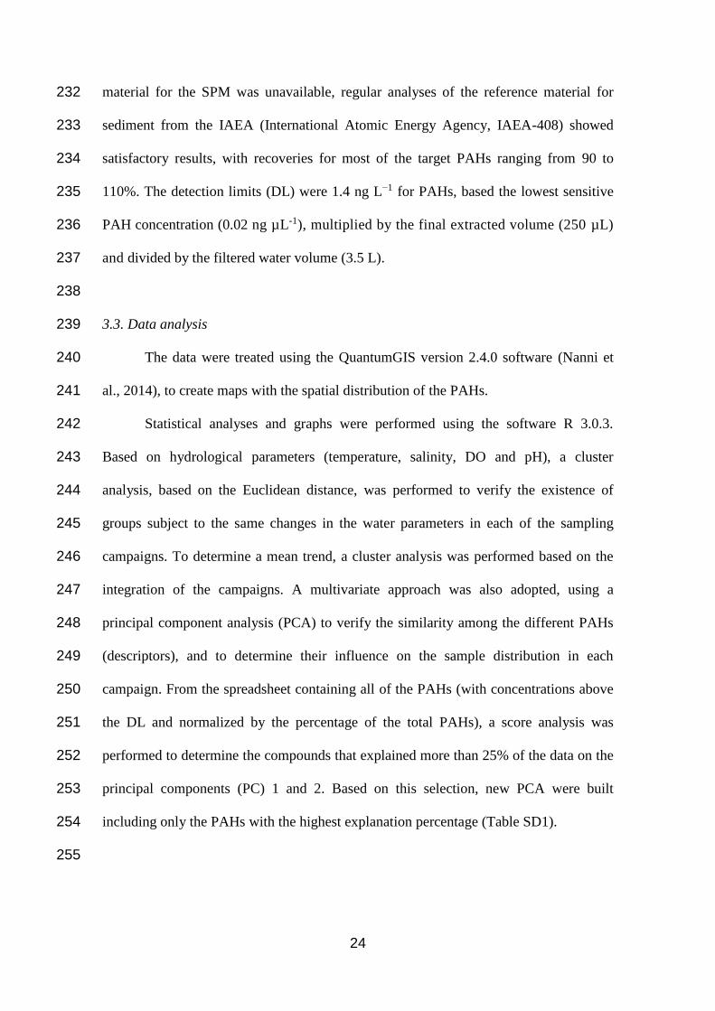
3.3. Data analysis 239

The data were treated using the QuantumGIS version 2.4.0 software (Nanni et 240

al., 2014), to create maps with the spatial distribution of the PAHs. 241

Statistical analyses and graphs were performed using the software R 3.0.3. 242

Based on hydrological parameters (temperature, salinity, DO and pH), a cluster 243

analysis, based on the Euclidean distance, was performed to verify the existence of 244

groups subject to the same changes in the water parameters in each of the sampling 245

campaigns. To determine a mean trend, a cluster analysis was performed based on the 246

integration of the campaigns. A multivariate approach was also adopted, using a 247

principal component analysis (PCA) to verify the similarity among the different PAHs 248

(descriptors), and to determine their influence on the sample distribution in each 249

campaign. From the spreadsheet containing all of the PAHs (with concentrations above 250

the DL and normalized by the percentage of the total PAHs), a score analysis was 251

performed to determine the compounds that explained more than 25% of the data on the 252

principal components (PC) 1 and 2. Based on this selection, new PCA were built 253

including only the PAHs with the highest explanation percentage (Table SD1). 254

255

25

4. Results and Discussion 256

4.1. Hydrological parameters 257

Pietzsch et al. (2010) suggested that the estuarine circulation and salinity may 258

also have an important role as environmental conditions in the transport/deposition of 259

the sedimentary PAH. Therefore, the temperature, salinity, pH and DO data were used 260

to build clusters for each sampling campaign. In each campaign, Guaratuba Bay could 261

be categorized into three sectors according to the hydrological influences (fluvial, 262

marine and mixture zone; similarity limit of 10%), and the sampling sites grouped into 263

the sectors varied according to the campaigns. The samples were considered marine-264

influenced due to the highest values of salinity, DO and pH, whereas the fluvial-265

influenced samples presented the lowest values of those parameters due to the proximity 266

to rivers. 267

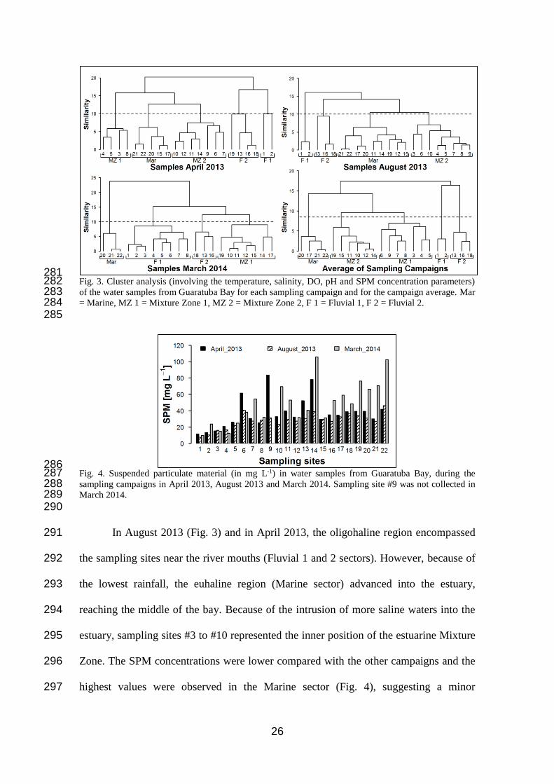
In April 2013 (Fig. 3), the oligohaline region encompassed the sampling sites 268

near the São João and Cubatão river mouths (Fluvial 1 sector) and the sites in or near 269

the rivers of the north margin (Fluvial 2 sector). Fluvial 1 sector presented lower values 270

of SPM, whereas Fluvial 2 sector presented relatively higher concentrations (Fig. 4), 271

which suggested the input of terrestrial material. The euhaline region was restricted to 272

the influence of the estuary mouth and to the beginning of the main ebb channel 273

(Marine sector). The mesohaline region was divided into two sectors: one sector under 274

the influence of the São João and Cubatão Rivers (Mixture Zone 1 sector) and the other 275

sector in the middle of the bay (Mixture Zone 2 sector). The highest SPM values and the 276

shallower depths were presented in Mixture Zone 2, especially on the north margin. 277

Therefore, the seston input may be related to the terrestrial input via river flows or 278

sediment resuspension. 279

280

26

281 Fig. 3. Cluster analysis (involving the temperature, salinity, DO, pH and SPM concentration parameters) 282 of the water samples from Guaratuba Bay for each sampling campaign and for the campaign average. Mar 283 = Marine, MZ 1 = Mixture Zone 1, MZ 2 = Mixture Zone 2, F 1 = Fluvial 1, F 2 = Fluvial 2. 284

285

286 Fig. 4. Suspended particulate material (in mg L-1) in water samples from Guaratuba Bay, during the 287 sampling campaigns in April 2013, August 2013 and March 2014. Sampling site #9 was not collected in 288 March 2014. 289

290

In August 2013 (Fig. 3) and in April 2013, the oligohaline region encompassed 291

the sampling sites near the river mouths (Fluvial 1 and 2 sectors). However, because of 292

the lowest rainfall, the euhaline region (Marine sector) advanced into the estuary, 293

reaching the middle of the bay. Because of the intrusion of more saline waters into the 294

estuary, sampling sites #3 to #10 represented the inner position of the estuarine Mixture 295

Zone. The SPM concentrations were lower compared with the other campaigns and the 296

highest values were observed in the Marine sector (Fig. 4), suggesting a minor 297

27

contribution of terrestrial material from the watersheds, which could be caused by the 298

relatively low precipitation rates in this period (Fig. 2). 299

In March 2014 (Fig. 3), the effect of the highest pluviometric values registered 300

on the Cubatão basin was observed. Fluvial 1 sector encompassed the bay upstream, 301

whereas Fluvial 2 sector encompassed only three sites, and the Marine sector was 302

restricted to the estuary mouth. Thus, the Mixture Zone was located in an outer position 303

compared with August 2013. Generally, the highest values of SPM were observed in the 304

mesohaline and euhaline regions. Based on a visual analysis of the filters, the 305

predominant material of the SPM of the external samples consisted of coarser fractions 306

than those found in the intermediate sites, as verified by Mizerkowski et al. (2012). 307

Because the SPM concentrations are based on the mass of the material retained on the 308

filters, and because of the probable difference between the crystalline matrix densities, 309

the values observed in the outer samples suggest a denser SPM compared with other 310

sampling sites. 311

Finally, the cluster of the average variation of the hydrological parameters in 312

Guaratuba Bay (Fig. 3, Table 1) emphasizes the estuary sectoring (cut into 8%). The 313

Marine sector was restricted to the estuary mouth and to the beginning of the main ebb 314

channel. The Fluvial sectors encompassed the sites near the São João and Cubatão 315

Rivers and the rivers of the north margin. Generally, the highest SPM concentrations 316

were observed in the mesohaline region, most likely due to the increased bay width and, 317

consequently, in the tidal prism. This increase leads to a decrease in the flow velocities 318

(fluvial and marine) creating an area of material accumulation (Marone et al., 2006). In 319

addition, there is a significant lateral input of detritus and dissolved substances from the 320

mangrove forests existing on the north margin (Mizerkowski et al., 2012). 321

322

28

4.2. Spatial and temporal distribution of PAHs 323

The PAH concentration can be expressed in terms of the filtered water volume 324

(e.g., Chizhova et al., 2013; Liu et al., 2014) as the SPM mass retained on the filters 325

(e.g., Curtosi et al., 2009; Maioli et al., 2011). Generally, the samples presented a 326

similar trend, regardless of the concentration unit (Fig. SD1). 327

The spatial distributions of the total PAHs (in ng L-1) on the SPM from 328

Guaratuba Bay for the three samplings campaigns are shown in Fig. 5. In April 2013, 329

the concentrations ranged from 21.02 to 366.28 ng L-1, and the highest values were 330

observed in the estuarine mixture zone (sampling sites #8, #9 and #10; Fig. 3). The 331

relatively high concentrations were found in a region that acts as a particle trap due to 332

the increased bay width and the merging of opposite flows. Additionally, those sites, 333

which are primarily the north margin, are located far from urbanized areas and are 334

therefore far from potential sources of petroleum hydrocarbons as urban runoffs. The 335

upstream region and the estuary mouth presented moderate PAH concentrations. The 336

PAHs detected in the inner part of Guaratuba Bay (sector Fluvial 1) may be related to 337

the vehicle traffic on an existing road that follows the São João River for more than 15 338

km, while the main source of PAHs on the estuary mouth (sector Marine) may be 339

related to the ferry traffic, the urban runoff of Guaratuba City and the presence of a 340

semi-commercial fishing fleet. 341

342

29

343 Fig. 5. Spatial distribution of the total PAHs (in ng L-1) on surficial suspended particulate matter from 344 Guaratuba Bay, SW Atlantic. The values in the circled scale represent the lowest, intermediate and 345 highest concentrations of PAHs. Mar = Marine, MZ 1 = Mixture Zone 1, MZ 2 = Mixture Zone 2, F 1 = 346 Fluvial 1, F 2 = Fluvial 2. 347

348

In August 2013, during the austral winter, the samples presented the lowest PAH 349

concentrations, ranged from 5.89 to 208.87 ng L-1 (Fig. 5), which could be explained by 350

30

the reduced tourism and the consequent reduction of urban runoff and vessel traffic. The 351

highest values were observed at sites #8 and #10 (sector Mixture Zone 2), such as in 352

April 2013, which were related to the maximum turbidity zone existing in the estuarine 353

mixture zone. High concentrations were also found at sites #20 and #22 (sector Marine) 354

and were most likely associated with the ferries and vessel activities, which emphasize 355

the importance of these PAH sources throughout the year. 356

In March 2014, the highest concentrations of total PAHs were observed, ranging 357

from 20.39 to 650.51 ng L-1 (Fig. 5), with relatively high values at sites #5, #7, #15 and 358

#17. The importance of the middle region as a geochemical particle filter was again 359

observed due to the high values at sites #5 and #7. Sites #15 and #17 may be affected by 360

a local source, the Guaratuba dock. This sampling campaign was performed during the 361

Carnival period when there is an intense touristic activity in the region, resulting in an 362

increase in urban runoff and in the number of moving vessels. Rice et al. (2008) also 363

observed that the PAH concentrations increased sharply during summer periods, due the 364

use intensification of recreational watercraft in a small Alaskan lake. 365

Based on the three campaigns, the mean concentrations of the total PAHs ranged 366

from 25.40 to 226.69 ng L-1 (Fig. 6, Table 1). The spatial distribution evidenced three 367

regions with high PAH concentrations. One region encompassed sites #5, #7, #8, #9 and 368

#10 in the estuarine mixture zone (sector Mixture Zone 1). These findings show the 369

importance of physico-chemical processes in the retention of fine particles in this 370

region, thus favoring the adsorption of organic contaminants on the SPM. 371

372

31

373 Fig. 6. Spatial distribution of the total PAH averages (in ng L-1) on surficial suspended particulate matter 374 from Guaratuba Bay, SW Atlantic. The values in the legend represent the lowest, intermediate and 375 highest concentrations of PAHs. 376

377

The second region encompasses the estuarine outer portion (sites #21 and #22 – 378

sector Marine) and the PAHs may be related to the local sources of petroleum 379

hydrocarbons, such as vessels, ferries and fishing boats. This region also acts as a 380

second particle filter. Primarily during ebb tides, the tidal currents lose the capacity to 381

transport in the estuary mouth due to the increase in the section area, resulting in the 382

deposition of the material from the estuary and hindering its transport to the shelf 383

(Angulo, 1999). Finally, the third region (sites #15 and #17) presented high mean 384

concentrations of total PAHs due to the high values observed in March 2014, during the 385

Carnival holiday. The values were related to local sources because of the drastically 386

increase in tourism and moving vessels during the Carnival period, especially near the 387

docks. 388

389

32

4.3. Comparison with other studies 390

The PAH concentrations in the SPM observed in Guaratuba Bay were below 391

those observed in highly urbanized and industrialized regions (Fig. 7) of Italy (Montuori 392

and Triassi, 2012) and several estuaries and rivers of China (Guo et al., 2007; Liu et al., 393

2014). Because of it wide range, the highest values observed in Guaratuba Bay are of 394

the same magnitude as other anthropized environments, such as the French and Spanish 395

coast of the Mediterranean Sea (Guitart et al., 2007), the Maguaba Lagoon and the 396

Paraíba do Sul River in Brazil (Maioli et al., 2011), and the Langat River in Malaysia 397

(Bakhtiari et al., 2009), whereas the other values are comparable with pristine regions, 398

such as Antarctica (Chizhova et al., 2013; Curtosi et al., 2009). Therefore, the PAH 399

concentrations verified in Guaratuba Bay indicate that this region, although considered 400

semi-pristine in previous studies (Cotovicz Junior et al., 2013; Pietzsch et al., 2010), is 401

already showing evidence of anthropic impacts. 402

403 Fig. 7. Concentration range of the Σ16PAHs on suspended particulate matter from different coastal 404 regions of the world and the estimated population. * industrialized area; xxx = no data available. 405

406

33

4.4. Evaluation of PAH sources by diagnostic ratios 407

Diagnostic ratios can be calculated from certain HMW PAH isomer 408

concentrations to determine the primary PAH sources in an environment (Yunker et al., 409

2002). However, because the concentrations of most HMW compounds were below the 410

DL, only the ratio between phenanthrene and methyl phenanthrene could be calculated 411

(Fig. 8). According to this ratio, SPM samples collected in Guaratuba Bay were 412

influenced primarily by petrogenic sources, especially fuel spills during refueling of 413

boats and leakage during navigation (Pietzsch et al., 2010). The average values obtained 414

were 0.29 ± 0.09 in April 2013, 0.33 ± 0.11 in August 2013 and 0.27 ± 0.13 in March 415

2014. Only a few samples, especially those collected in August 2013, suggested that the 416

PAHs were from pyrolytic sources, primarily those associated with the combustion of 417

oil and its derivatives. However, this trend was not consistent with the other sampling 418

campaigns, strengthening the petrogenic contribution as the main component of the 419

PAH input in this environment. 420

421

422 Fig. 8. Cross plot of the diagnostic ratios Σ(2-3)/Σ(4-6) versus C0-phenanthrenes/Σ(C0+C1)phenanthrenes 423 (when they could be calculated) on the samples of the surficial suspended particulate matter from 424 Guaratuba Bay, SW Atlantic. 425

426

34

The Σ(2-3)/Σ(4-6) ratio is also used to determine the primary sources of PAHs. 427

The relative predominance of LMW PAHs is more related to petrogenic input, whereas 428

HMW PAHs are associated with combustion processes (Wang et al., 1999). In 78% of 429

the calculated ratios, the predominance of LMW PAHs was observed (Σ(2-3)/Σ(4-6) > 430

1.0) (Fig. 8). Values below 1.0 were observed only in March 2014, suggesting the 431

punctual and sporadic introduction of PAHs by pyrolytic sources. Therefore, this ratio 432

confirms the introduction of crude oil and its derivatives as the main source of 433

petroleum hydrocarbons into Guaratuba Bay, and a mixture of sources can occur 434

occasionally. 435

Finally, all of the samples presented a predominance of alkylated compounds, 436

ranging from 59% to 92% of the total PAHs. Wang et al. (1999) observed that samples 437

subjected to a recent introduction of petroleum showed large quantities of alkylated 438

compounds, corroborating the recent introduction of petroleum and its derivatives as the 439

main source of PAHs in Guaratuba Bay. 440

Perylene is one of the few PAHs that can be associated with natural and 441

anthropogenic sources (Montuori and Triassi, 2012; Venkatesan, 1988). Perylene was 442

the only pentacyclic PAH found, suggesting a diagenetic origin from natural, most 443

likely terrigenous, precursors (Readman et al., 2002). Most of the samples containing 444

perylene were collected in the sampling sites near the north margin (64%), which could 445

receive a considerable input of organic matter from the mangrove forest. 446

447

4.5. Principal Component Analysis 448

The PCA was performed with the most abundant PAHs, namely naphthalene, 449

C1-naphthalene, C2-naphthalene, phenanthrene, C1-phenanthrene and C2-phenanthrene 450

(Fig. 9). Principal component (PC) 1 explained more than 80% of the data and was 451

35

related to the C2-phenanthrenes and naphthalenes, whereas PC 2 explained 12% of the 452

variability and was associated with phenanthrene and also naphthalenes. Generally, 453

marine-influenced sites presented a higher proportion of C2-phenanthrenes, the same 454

observed by Leonov and Nemirovskaya (2011), whereas sites #3, #10 and #20 455

presented a higher proportion of naphthalenes. The samples from the mixture zone did 456

not present a clear distribution pattern for the individual PAHs, but they appeared to be 457

more associated with the phenanthrenes. 458

459

460 Fig. 9. Principal Component Analysis based on PAH average concentrations in samples of surficial 461 suspended particulate matter from Guaratuba Bay, SW Atlantic. Mar = Marine, MZ 1 = Mixture Zone 1, 462 MZ 2 = Mixture Zone 2, F 1 = Fluvial 1, F 2 = Fluvial 2. 463

464

Sites that are influenced by naphthalenes and those influenced by phenanthrenes 465

can be distinguished by their volatilization, solubilization, degradation and sorption 466

processes (Huang et al., 2004; Lee et al., 1978; Massie et al., 1985). Naphthalenes are 467

more volatile and more soluble than phenanthrenes. Furthermore, naphthalene 468

degradation has been reported in waters from pristine and oil-contaminated ecosystems 469

(Herbes and Schwall, 1978; Lee and Ryan, 1983; Lee et al., 1978; Massie et al., 1985). 470

36

Naphthalene is relatively water soluble (31.2 mg L-1) and has a high vapor pressure 471

(0.08 mm Hg at 20-25°C), indicating that biodegradation and volatilization in open 472

waters may be important processes that affect its fate in aquatic systems. The addition 473

of a third fused-benzene ring (phenanthrene) significantly decreases the compound’s 474

water solubility (30 to 700 times lower), vapor pressure (330 to 1,180 times lower) and 475

microbial degradation rates (2 to 50 times lower) (Bauer and Capone, 1985; Herbes and 476

Schwall, 1978; Herbes, 1981; Huang et al., 2004; Lee et al., 1978; Rochman et al., 477

2013), what causes it to be the most stable polyarene in the geochemical background 478

(Leonov and Nemirovskaya, 2011). This suggest the sites mainly influenced more by 479

naphthalenes may be exposed to a fresher material input than those sites more related to 480

phenanthrenes, especially site #20 that is located in the ferries trajectory. 481

The different rates of adsorption among the alkylated PAHs may also explain 482

this separation between the compounds. Oren et al. (2006) have suggested that regions 483

with high levels of aromatic compounds and vegetal lipids promote adsorption and 484

scavenging of phenanthrene on SPM compared with other PAHs. Because the PAH 485

polarity tends to diminish as the molar weight increases (Delgado-Saborit et al., 2013) 486

and adsorption on the SPM depends on the polarity (Rochman et al., 2013), 487

alkylphenanthrenes should present a higher adsorption rate than the parental compound. 488

Thus, the greater tendency of alkylphenanthrene adsorption on SPM can explain this 489

differentiation in samples with high PAH concentrations (#5, #7, #8, #9, #15 and #22), 490

as suggested by Pietzsch et al. (2010). This sorption distinction could also explain the 491

elevated association between site #3 and naphthalenes, 492

Another possible explanation for this distinction could be the existence of 493

different sources of these alkyl PAHs. Although the predominant source of PAHs in 494

Guaratuba Bay is petrogenic, certain PAHs can be related to pyrolytic introductions. 495

37

Alkylnaphthalenes are strong indicators of the presence of crude oil and its derivatives 496

(Kim et al., 2006), whereas alkylphenanthrenes (especially dimethylphenanthrenes) 497

have been shown to originate from pyrolytic processes, such as vehicle emissions 498

(Aboul-Kassim and Simoneit, 1995; Pereira et al., 1999; Yunker et al., 2002). The 499

samples sites from the Marine sector (#17, #21 and #22) and the sites near the docks 500

(#15, #17 and #18) presented a higher proportion of alkyl PAHs with higher molar 501

weights. Thus these regions can be subject to the introduction of PAHs from 502

combustion of fuels in vessels. 503

504

5. Summary and Conclusions 505

The spatiotemporal variations of PAH concentrations adsorbed on SPM in a SW 506

Atlantic subtropical estuary was studied. The results showed that the spatial distribution 507

of the PAHs varies according to the population oscillation and meteorological factors. 508

Based on physico-chemical parameters, it was possible to separate the bay into three 509

different areas with relatively constant patterns throughout the year. Generally, the 510

middle and outer regions of the estuary presented the highest PAH concentrations. The 511

former region is located far from anthropic activities and the physico-chemical 512

parameters were useful to explain this distribution, once the presence of the estuarine 513

mixture zone favors the material retention and pollutant accumulation. The marine-514

influenced region is located near the docks and ferries, which, in addition to urban 515

runoff, are the primary sources of hydrocarbons in the bay. This spatial distribution 516

refutes the hypothesis (i) that fluvial inputs are significant PAH sources to this 517

environment. The temporal distribution, with the highest PAH concentrations near 518

Guaratuba dock, did not refute the hypothesis (ii), emphasizing the importance of the 519

38

sharp population increase during summer holidays, which intensifies the hydrocarbon 520

input in Guaratuba Bay. 521

The PAH concentrations in Guaratuba Bay are in the same range as those 522

observed in certain pristine environments and certain impacted regions, indicating that 523

although considered semi-pristine, this estuary is already subject to anthropic effects. 524

The analysis of the diagnostic ratios and the PCA showed that the main source of 525

petroleum hydrocarbons to the bay is crude oil and its derivatives, and a mixture of 526

sources related with the sporadic introduction of pyrolytic PAH from the vessel traffic 527

may occur. Because the diffuse input of crude oil and its derivatives from vessels is the 528

main entry route of PAHs in Guaratuba Bay, public programs to monitor and inspect the 529

vessels, especially during high seasons when occurs a seasonal and sharp population 530

increase, would assist in the mitigation of the chronic anthropic effect. 531

532

Acknowledgments 533

A.L.L. Dauner would like to thank CAPES (Coordenação de Aperfeiçoamento de 534

Pessoal de Ensino Superior) for the MSc Scholarship. C.C. Martins would like to thank 535

CNPq (Brazilian National Council for Scientific and Technological Development) for a 536

research grant (477047/2011-4) and Fundação Araucária de Apoio ao Desenvolvimento 537

Científico e Tecnológico do Estado do Paraná (401/2012; 15.078). We are grateful to 538

R.R. Neto [Department of Oceanography, Federal University of Espírito Santo (UFES)] 539

and M.T. Grassi [Department of Chemistry, Federal University of Paraná (UFPR)] for 540

assistance with the preliminary evaluation of this article. This study was developed as 541

part of a post-graduate course on estuarine and ocean systems at the Federal University 542

of Paraná (PGSISCO-UFPR). 543

544

39

Appendix A. Supplementary data 545

Supplementary data to this article can be found online at 546

http://dx.doi.org/XX.XXX. 547

548

6. References 549

Aboul-Kassim, T.A.T., Simoneit, B.R.T., 1995. Aliphatic and aromatic hydrocarbons in 550 particulate fallout of Alexandria, Egypt : Sources and implications. Environ. Sci. 551 Technol. 29, 2473–2483. 552

Alves, D.M., 2014. Guaratuba ferry should receive 500 thousand cars (Travessia de 553 Guaratuba deve receber 500 mil carros). Gaz. do Povo. 554

Angulo, R.J., 1999. Morphological characterization of the tidal deltas on the coast of the 555 State of Paraná. An. Acad. Bras. Cienc. 71, 935–959. 556

Bakhtiari, A.R., Zakaria, M.P., Yaziz, M.I., Lajis, M.N.H., Bi, X., 2009. Polycyclic 557 aromatic hydrocarbons and n-alkanes in suspended particulate matter and 558 sediments from the Langat River, Peninsular Malaysia. Environ. Asia 2, 1–10. 559

Bauer, J.E.T., Capone, D.G., 1985. Degradation and mineralization of the polycyclic 560 aromatic hydrocarbons anthracene and naphthalene in intertidal marine sediments. 561 Appl. Environ. Microbiol. 50, 81–90. 562

Burns, K.A., Hernes, P.J., Brinkman, D., Poulsen, A., Benner, R., 2008. Dispersion and 563 cycling of organic matter from the Sepik River outflow to the Papua New Guinea 564 coast as determined from biomarkers. Org. Geochem. 39, 1747–1764. 565 doi:10.1016/j.orggeochem.2008.08.003 566

Chizhova, T., Hayakawa, K., Tishchenko, P., Nakase, H., Koudryashova, Y., 2013. 567 Distribution of PAHs in the northwestern part of the Japan Sea. Deep Sea Res. Part 568 II Top. Stud. Oceanogr. 86-87, 19–24. doi:10.1016/j.dsr2.2012.07.042 569

Colombo, J.C., Pelletier, E., Brochu, C., Khalll, M., 1989. Determination of 570 hydrocarbon sources using n-alkane and polyaromatic hydrocarbon distribution 571 indexes. Case study: Rio de La Plata estuary, Argentina. Environ. Sci. Technol. 23, 572 888–894. 573

Combi, T., Taniguchi, S., Figueira, R.C.L., Mahiques, M.M., Martins, C.C., 2013. 574 Spatial distribution and historical input of polychlorinated biphenyls (PCBs) and 575 organochlorine pesticides (OCPs) in sediments from a subtropical estuary 576 (Guaratuba Bay, SW Atlantic). Mar. Pollut. Bull. 70, 247–52. 577 doi:10.1016/j.marpolbul.2013.02.022 578

40

Costa, T.L.F., Araújo, M.P., Knoppers, B.A., Carreira, R.D.S., 2010. Sources and 579 distribution of particulate organic matter of a tropical Estuarine-Lagoon System 580 from NE Brazil as indicated by lipid biomarkers. Aquat. Geochemistry 17, 1–19. 581 doi:10.1007/s10498-010-9104-1 582

Cotovicz Junior, L.C., Machado, E.C., Brandini, N., Zem, R.C., Knoppers, B.A., 2013. 583 Distributions of total, inorganic and organic phosphorus in surface and recent 584 sediments of the sub-tropical and semi-pristine Guaratuba Bay estuary, SE Brazil. 585 Environ. Earth Sci. 72, 373–386. doi:10.1007/s12665-013-2958-y 586

Curtosi, A., Pelletier, E., Vodopivez, C.L., Mac Cormack, W.P., 2009. Distribution of 587 PAHs in the water column, sediments and biota of Potter Cove, South Shetland 588 Islands, Antarctica. Antarct. Sci. 21, 329–339. doi:10.1017/S0954102009002004 589

Delgado-Saborit, J.M., Alam, M.S., Godri Pollitt, K.J., Stark, C., Harrison, R.M., 2013. 590 Analysis of atmospheric concentrations of quinones and polycyclic aromatic 591 hydrocarbons in vapour and particulate phases. Atmos. Environ. 77, 974–982. 592 doi:10.1016/j.atmosenv.2013.05.080 593

Froehner, S., Machado, K.S., Stefan, E., Bleninger, T., Rosa, E.C. da, Martins, C.C., 594 2012. Occurrence of selected estrogens in mangrove sediments. Mar. Pollut. Bull. 595 64, 75–79. doi:10.1016/j.marpolbul.2011.10.021 596

Gattuso, J.-P., Frankignoulle, M., Wollast, R., 1998. Carbon and carbonate metabolism 597 in coastal aquatic ecosystems. Annu. Rev. Ecol. Syst. 29, 405–434. 598

Guitart, C., García-Flor, N., Bayona, J.M., Albaigés, J., 2007. Occurrence and fate of 599 polycyclic aromatic hydrocarbons in the coastal surface microlayer. Mar. Pollut. 600 Bull. 54, 186–94. doi:10.1016/j.marpolbul.2006.10.008 601

Guo, W., He, M.-C., Yang, Z.-F., Lin, C.-Y., Quan, X.-C., Wang, H., 2007. Distribution 602 of polycyclic aromatic hydrocarbons in water, suspended particulate matter and 603 sediment from Daliao River watershed, China. Chemosphere 68, 93–104. 604 doi:10.1016/j.chemosphere.2006.12.072 605

Herbes, S.E., 1981. Rates of microbial transformation of polycyclic aromatic 606 hydrocarbons in water and sediments in the vicinity of a coal-coking wastewater 607 discharge. Appl. Environ. Microbiol. 41, 20–28. 608

Herbes, S.E., Schwall, L.R., 1978. Microbial transformation of polycyclic aromatic 609 hydrocarbons in pristine and petroleum-contaminated sediments. Appl. Environ. 610 Microbiol. 35, 306–316. 611

Huang, H., Bowler, B.F.J., Oldenburg, T.B.P., Larter, S.R., 2004. The effect of 612 biodegradation on polycyclic aromatic hydrocarbons in reservoired oils from the 613 Liaohe basin, NE China. Org. Geochem. 35, 1619–1634. 614 doi:10.1016/j.orggeochem.2004.05.009 615

IAP, Instituto Ambiental do Paraná, 2006. Plano de manejo da Área de Proteção 616 Ambiental de Guaratuba. Curitiba. 617

41

IBGE, Instituto Brasileiro de Geografia e Estatística, 2010. http://www.ibge.gov.br. 618

Kim, M., Kennicutt II, M.C., Qian, Y., 2006. Molecular and stable carbon isotopic 619 characterization of PAH contaminants at McMurdo Station, Antarctica. Mar. 620 Pollut. Bull. 52, 1585–90. doi:10.1016/j.marpolbul.2006.03.024 621

Lee, R.F., Gardner, W.S., Anderson, J.W., Blaylock, J.W., Barwell-Clarke, J., 1978. 622 Fate of polycyclic aromatic hydrocarbons in controlled ecosystem enclosures. 623 Environ. Sci. Technol. 12, 832–838. doi:10.1021/es60143a007 624

Lee, R.F., Ryan, C., 1983. Microbial and photochemical degradation of polycyclic 625 aromatic hydrocarbons in estuarine waters and sediments. Can. J. Fish. Aquat. Sci. 626 40, 86–94. 627

Lehmkuhl, E.A., Tremarin, P.I., Moreira-Filho, H., Ludwig, T.A.V., 2010. 628 Thalassiosirales (Diatomeae) da baía de Guaratuba, Estado do Paraná, Brasil. Biota 629 Neotrop. 10, 313–324. 630

Leonov, A. V., Nemirovskaya, I.A., 2011. Petroleum hydrocarbons in the waters of 631 major tributaries of the White Sea and its water areas: A review of available 632 information. Water Resour. 38, 324–351. doi:10.1134/S0097807811030055 633

Li, H., Lu, L., Huang, W., Yang, J., Ran, Y., 2014. In-situ partitioning and 634 bioconcentration of polycyclic aromatic hydrocarbons among water, suspended 635 particulate matter, and fish in the Dongjiang and Pearl Rivers and the Pearl River 636 Estuary, China. Mar. Pollut. Bull. 83, 306–316. 637 doi:10.1016/j.marpolbul.2014.04.036 638

Liu, F., Yang, Q.-S., Hu, Y., Du, H., Yuan, F., 2014. Distribution and transportation of 639 polycyclic aromatic hydrocarbons (PAHs) at the Humen river mouth in the Pearl 640 River delta and their influencing factors. Mar. Pollut. Bull. 84, 401–410. 641 doi:10.1016/j.marpolbul.2014.04.045 642

Luo, X.-J., Mai, B.-X., Yang, Q.-S., Fu, J.-M., Sheng, G.-Y., Wang, Z., 2004. 643 Polycyclic aromatic hydrocarbons (PAHs) and organochlorine pesticides in water 644 columns from the Pearl River and the Macao harbor in the Pearl River Delta in 645 South China. Mar. Pollut. Bull. 48, 1102–15. doi:10.1016/j.marpolbul.2003.12.018 646

Ma, W.-L., Liu, L.-Y., Qi, H., Zhang, Z.-F., Song, W.-W., Shen, J.-M., Chen, Z.-L., 647 Ren, N.-Q., Grabuski, J., Li, Y.-F., 2013. Polycyclic aromatic hydrocarbons in 648 water, sediment and soil of the Songhua River Basin, China. Environ. Monit. 649 Assess. 185, 8399–8409. doi:10.1007/s10661-013-3182-7 650

Maioli, O.L.G., Rodrigues, K.C., Knoppers, B.A., Azevedo, D.A., 2011. Distribution 651 and sources of aliphatic and polycyclic aromatic hydrocarbons in suspended 652 particulate matter in water from two Brazilian estuarine systems. Cont. Shelf Res. 653 31, 1116–1127. doi:10.1016/j.csr.2011.04.004 654

42

Marone, E., Noernberg, M.A., Santos, I. Dos, Lautert, L.F., Andreoli, O.R., Buba, H., 655 Fill, H.D., 2006. Hydrodynamic of Guaratuba Bay, PR, Brazil. J. Coast. Res. 39, 656 1879–1883. 657

Martins, C.C., Bícego, M.C., Figueira, R.C.L., Angelli, J.L.F., Combi, T., Gallice, 658 W.C., Mansur, A.V., Nardes, E., Rocha, M.L., Wisnieski, E., Ceschim, L.M.M., 659 Ribeiro, A.P., 2012. Multi-molecular markers and metals as tracers of organic 660 matter inputs and contamination status from an Environmental Protection Area in 661 the SW Atlantic (Laranjeiras Bay, Brazil). Sci. Total Environ. 417-418, 158–68. 662 doi:10.1016/j.scitotenv.2011.11.086 663

Massie, L.C., Ward, A.P., Davies, J.M., 1985. The effects of oil exploration and 664 production in the northern North Sea: Part 2 - microbial biodegradation of 665 hydrocarbons in water and sediments, 1978–1981. Mar. Environ. Res. 15, 235–666 262. doi:10.1016/0141-1136(85)90004-2 667

Mizerkowski, B.D., Machado, E.C., Brandini, N., Nazario, M.G., Bonfim, K.V., 2012. 668 Environmental water quality assessment in Guaratuba bay, state of Paraná, 669 southern Brazil. Brazilian J. Oceanogr. 60, 109–115. doi:10.1590/S1679-670 87592012000200001 671

Montuori, P., Triassi, M., 2012. Polycyclic aromatic hydrocarbons loads into the 672 Mediterranean Sea: estimate of Sarno River inputs. Mar. Pollut. Bull. 64, 512–20. 673 doi:10.1016/j.marpolbul.2012.01.003 674

Nanni, A.S., Descovi-Filho, L., Virtuoso, M.A., Montenegro, D., Willrich, G., 675 Machado, P.H., Sperb, R., Dantas, G.S., Calazans, Y., 2014. Quantum GIS - 676 Versão 2.4.0 “Chugiak.” 677

Oren, A., Aizenshtat, Z., Chefetz, B., 2006. Persistent organic pollutants and 678 sedimentary organic matter properties: a case study in the Kishon River, Israel. 679 Environ. Pollut. 141, 265–74. doi:10.1016/j.envpol.2005.08.039 680

Pereira, W.E., Hostettler, F.D., Luoma, S.N., Van Geek, A., Fuller, C.C., Anima, R.J., 681 1999. Sedimentary record of anthropogenic and biogenic polycyclic aromatic 682 hydrocarbons in San Francisco Bay, California. Mar. Chem. 64, 99–113. 683 doi:10.1016/S0304-4203(98)00087-5 684

Pietzsch, R., Patchineelam, S.R., Torres, J.P.M., 2010. Polycyclic aromatic 685 hydrocarbons in recent sediments from a subtropical estuary in Brazil. Mar. Chem. 686 118, 56–66. doi:10.1016/j.marchem.2009.10.004 687

Readman, J.W., Fillmann, G., Tolosa, I., Bartocci, J., Villeneuve, J.. P., Catinni, C., 688 Mee, L.D., 2002. Petroleum and PAH contamination of the Black Sea. Mar. Pollut. 689 Bull. 44, 48–62. 690

Rice, S.D., Holland, L., Moles, A., 2008. Seasonal increases in polycyclic aromatic 691 hydrocarbons related to two-stroke engine use in a small Alaskan lake. Lake 692 Reserv. Manag. 24, 10–17. doi:10.1080/07438140809354046 693

43

Rocha, G.O. da, Guarieiro, A.L.N., Andrade, J.B. de, Eça, G.F., Aragão, N.M., Aguiar, 694 R.M., Korn, M.G.A., Brito, G.B., Moura, C.W.N., Hatje, V., 2012. Contaminação 695 na Baía de Todos os Santos. Rev. Virtual Química 4, 583–610. 696

Rochman, C.M., Manzano, C., Hentschel, B.T., Simonich, S.L.M., Hoh, E., 2013. 697 Polyestyrene plastic: a source and sink for polycyclic aromatic hydrocarbons in the 698 marine environment. Environ. Sci. Technol. 47, 13976–13984. 699

Sanders, C.J., Santos, I.R., Silva-Filho, E. V., Patchineelam, S.R., 2006. Mercury flux to 700 estuarine sediments, derived from Pb-210 and Cs-137 geochronologies (Guaratuba 701 Bay, Brazil). Mar. Pollut. Bull. 52, 1085–9. doi:10.1016/j.marpolbul.2006.06.004 702

Venkatesan, M.I., 1988. Occurrence and possible sources of perylene in marine 703 sediments - a Review. Mar. Chem. 25, 1–27. 704

Wang, J.-Z., Nie, Y.-F., Luo, X.-L., Zeng, E.Y., 2008. Occurrence and phase 705 distribution of polycyclic aromatic hydrocarbons in riverine runoff of the Pearl 706 River Delta, China. Mar. Pollut. Bull. 57, 767–74. 707 doi:10.1016/j.marpolbul.2008.01.007 708

Wang, Z., Fingas, M., Page, D.S., 1999. Oil spill identification. J. Chromatogr. A 843, 709 369–411. doi:10.1016/S0021-9673(99)00120-X 710

Wisnieski, E., Bícego, M.C., Montone, R.C., Figueira, R.C.L., Ceschim, L.M.M., 711 Mahiques, M.M., Martins, C.C., 2014. Characterization of sources and temporal 712 variation in the organic matter input indicated by n-alkanols and sterols in 713 sediment cores from Admiralty Bay, King George Island, Antarctica. Polar Biol. 714 37, 483–496. doi:10.1007/s00300-014-1445-6 715

Yang, D., Qi, S., Zhang, Y., Xing, X., Liu, H., Qu, C., Liu, J., Li, F., 2013. Levels, 716 sources and potential risks of polycyclic aromatic hydrocarbons (PAHs) in 717 multimedia environment along the Jinjiang River mainstream to Quanzhou Bay, 718 China. Mar. Pollut. Bull. 76, 298–306. doi:10.1016/j.marpolbul.2013.08.016 719

Yunker, M.B., Macdonald, R.W., Vingarzan, R., Mitchell, R.H., Goyette, D., Sylvestre, 720 S., 2002. PAHs in the Fraser River basin: a critical appraisal of PAH ratios as 721 indicators of PAH source and composition. Org. Geochem. 33, 489–515. 722 doi:10.1016/S0146-6380(02)00002-5 723

44

Appendix A. Supplementary data 724

725

Table SD1. Explanation percentage of the polycyclic aromatic hydrocarbons of the two first principal 726 components of the Principal Component Analysis. Naph = naphthalene; Acy = acenaphthylene; Flu = 727 fluorene; Phen = phenanthrene; Ant = anthracene; BaA = benz[a]anthracene; Chry = chrysene; IndP = 728 indeno[1,2,3-cd]pyrene; C1naph = methylnaphthalene; C2naph = dimethylnaphthalene; C3naph = 729 trimethylnaphthalene; C1phen = methylphenanthrene; C2dbt = dimethyldibenzothiophene; C2phen = 730 dimethylphenanthrene; C1fla = methylfluoranthene; C1pyr = methylpyrene; C1chry = methylchrysene; 731 Ret = retene; Peryl = perylene. 732

PC1 PC2

Naph * 0.01 0.48 *

Acy 0.00 0.03

Flu 0.00 0.01

Phen * 0.05 0.11 *

Ant 0.00 0.00

BaA 0.00 0.00

Chr 0.02 -0.01

IndP 0.00 0.01

C1naph * 0.01 0.48 *

C2naph * 0.04 0.57 *

C3naph 0.00 0.07

C1phen * 0.40 * 0.22 *

C2dbt 0.02 -0.01

C2phen * 0.88 * -0.19 *

C1fla 0.11 -0.06

C1pyr 0.09 -0.05

C1chr 0.01 -0.01

Ret 0.03 -0.02

Peryl 0.00 0.04

45

733 Fig. SD1. PAH concentrations (in ng g-1 SPM and in ng L-1) of filtered water samples from Guaratuba 734 Bay, SW Atlantic, from each sampling campaign. 735

XLVI

CAPÍTULO 2

Spatial and temporal distribution of aliphatic hydrocarbons and linear

alkylbenzenes in the particulate phase from a subtropical estuary (Guaratuba

Bay, SW Atlantic) under seasonal population fluctuation.

Manuscrito formatado para submissão segundo as normas da revista:

Marine Environmental Research; ISSN (0141-1136)

Fator de Impacto 2013: 2.328

Thomson Reuters Journal Citation Reports 2014

Qualis CAPES (Biodiversidade): Estrato A2

47

Spatial and temporal distribution of aliphatic hydrocarbons and linear 1

alkylbenzenes in the particulate phase from a subtropical estuary (Guaratuba Bay, 2

SW Atlantic) under seasonal population fluctuation. 3

4

* Ana Lúcia L. Dauner a, b, $ César C. Martins a 5

6

a Centro de Estudos do Mar da Universidade Federal do Paraná, P.O. Box 61, 83255-7

976, Pontal do Paraná, PR, Brazil. 8

9

b Programa de Pós-Graduação em Sistemas Costeiros e Oceânicos (PGSISCO) da 10

Universidade Federal do Paraná, P.O. Box 61, 83255-976, Pontal do Paraná, PR, Brazil. 11

12

Corresponding authors: Tel.: +55 41 35118637 13

E-mail addresses: * anadauner@gmail.com (A.L.L. Dauner) 14

$ ccmart@ufpr.br (C.C. Martins) 15

48

Research Highlights 16

17

> AH and LAB contents were determined on surficial suspended particulate matter. 18

> Temporal and spatial distributions and compositions of AHs and LABs were 19

evaluated. 20

> AHs were related to petrogenic and biogenic sources. 21

> LABs showed preferential degradation during the austral summer. 22

Resumo 42

A Baía de Guaratuba, um estuário subtropical localizado no Atlântico SO, está sob a 43

influência de uma pressão antrópica variável ao longo do ano. Amostras de material 44

particulado em suspensão foram coletadas em 22 pontos durante três diferentes períodos 45

a fim de avaliar a variabilidade espacial e temporal dos hidrocarbonetos alifáticos (HAs) 46

e alquilbenzenos lineares (LABs). Esses compostos foram determinados através de 47

cromatografia gasosa acoplada a um detector por ionização de chama (GC-FID) e a um 48

espectrômetro de massa (GC/MS). As distribuições espaciais de ambos os compostos 49

foram similares e variaram entre as campanhas amostrais. De modo geral, as maiores 50

concentrações foram observadas durante o verão, realçando a importância do aumento 51

de intensidade da pressão antrópica durante esse período. As distribuições dos 52

compostos também foram afetadas por processos geoquímicos naturais de acúmulo de 53

matéria orgânica. Os HAs foram associados à introdução de petróleo e derivados, a 54

partir do tráfego de embarcações e veículos, e a fontes biogênicas, como as florestas de 55

manguezal e a produção autóctone. A composição de LABs evidenciou a sua 56

degradação preferencial durante o verão. 57

58

Palavras-chave: fontes; degradação; material particulado em suspensão; variações 59

espaciais; variações temporais. 60

49

Abstract 23

Guaratuba Bay, a subtropical estuary located in the SW Atlantic, is under variable 24

anthropic pressure throughout the year. Samples of surficial suspended particulate 25

matter (SPM) were collected at 22 sites during three different periods to evaluate the 26

temporal and spatial variability of aliphatic hydrocarbons (AHs) and linear 27

alkylbenzenes (LABs). These compounds were determined by gas chromatography with 28

flame ionization detection (GC-FID) and mass spectrometry (GC/MS). The spatial 29

distributions of both compound classes were similar and varied among the sampling 30

campaigns. Generally, the highest concentrations were observed during the austral 31

summer, highlighting the importance of the increased human influence during this 32

season. The compound distributions were also affected by the natural geochemical 33

processes of organic matter accumulation. AHs were associated with petroleum, derived 34

from boat and vehicle traffic, and biogenic sources, related to mangrove forests and 35

autochthonous production. The LAB composition evidenced preferential degradation 36

processes during the austral summer. 37

38

Keywords: sources; degradation; suspended particulate matter; spatial variations; 39

temporal variations. 40

Study area coordinates: 25°51.8’S; 48°38.2’W. 41

50

1. Introduction 61

Coastal environments are influenced by anthropic activities throughout the year 62

and may receive organic and inorganic contaminant loads through riverine, terrestrial 63

and autochthonous emissions. Some of the primary sources of organic pollutants to 64

estuarine regions are shipping and harbor activities, urban runoff and the direct 65

discharge of industrial and urban wastes (Grigoriadou et al., 2008; Venturini et al., 66

2008). This anthropic influence can also be intensified during specific periods that are 67

generally associated with temperature and hydrological cycle changes (Jennerjahn, 68

2012). Due to the interaction between terrestrial and marine environments, estuaries are 69

highly variable environments on both temporal and spatial scales (Bianchi, 2007). 70

Several studies using molecular proxies have determined the contamination in 71

several coastal areas of the world (e.g. Martins et al., 2014; Montuori and Triassi, 2012; 72

Notar et al., 2001; Pinturier-Geiss et al., 2002), but the majority of these studies have 73

used a sedimentary matrix, which causes difficulty when evaluating on a short time 74

scale. 75

Only a few studies have focused on the temporal variability based on the 76

evaluation of contaminants in the water column and suspended particulate matter 77

(SPM). Because most organic markers are lipophilic and have a high octanol-water 78

partition coefficient (Ni et al., 2009; Wang et al., 2008), SPM can be a useful tool to 79

evaluate the temporal and spatial variability in regions in which the anthropic influence 80

may vary significantly over the year. 81

The transport of hydrophobic organic pollutants, such as hydrocarbons, in rivers 82

and estuaries is primarily coupled to the transport of suspended particles (Schwientek et 83

al., 2013). Therefore, the total concentrations of hydrophobic pollutants tend to increase 84

with increasing discharge, e.g., during floods, which increases the SPM input, possibly 85

51

remobilizing the bottom sediments (Rügner et al., 2014). Due to the characteristics of 86

organic proxies, such as persistency and source specificity (Colombo et al., 1989; 87

Kannan et al., 2012), it is possible to determine the source (anthropogenic, terrestrial or 88

marine) of the compounds and their degradation degree (e.g., Aboul-Kassim and 89

Simoneit, 1996; Luo et al., 2008). Linear alkylbenzenes (LABs) are known as sewage 90

tracers (e.g., Martins et al., 2012a; Raymundo and Preston, 1992; Takada and 91

Eganhouse, 1998), whereas aliphatic hydrocarbons (AHs) are associated with natural 92

and anthropic sources (Burns and Brinkman, 2011; Colombo et al., 1989; Martins et al., 93

2012b). 94

Guaratuba Bay, located in the SW Atlantic, is an example of a region with a 95

variable temporal anthropic pressure. The number of inhabitant increases drastically 96

during the summer season (IAP, 2006). Several studies have been developed to evaluate 97

the organic contamination in Guaratuba Bay and have indicated increased levels of 98

mercury and polycyclic aromatic hydrocarbons (Pietzsch et al., 2010; Sanders et al., 99

2006) as well as detectable levels of estrogens and polychlorinated biphenyls (Combi et 100

al., 2013; Froehner et al., 2012). However, these studies have focused on the analysis of 101

the sedimentary matrix, which presents an accumulated contamination on a relatively 102

long-time scale. 103

Because estuaries are areas of ecological and economic value, understanding the 104

contaminant transport and the fate in estuaries is imperative for adopting effective 105

management initiatives to protect these resources. Therefore, the objective of this study 106

was to evaluate the spatial and temporal variability in the distribution and composition 107

of AHs and LABs in the surface SPM for the determination of the priority regions and 108

periods to implement management policies. Therefore two hypotheses have been 109

proposed: (i) if AHs and LABs have the same sources, then their spatial distribution will 110

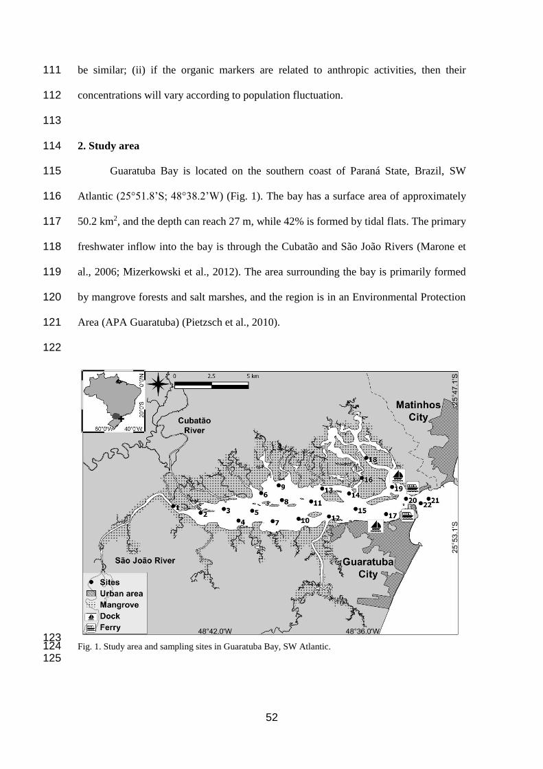
52

be similar; (ii) if the organic markers are related to anthropic activities, then their 111

concentrations will vary according to population fluctuation. 112

113

2. Study area 114

Guaratuba Bay is located on the southern coast of Paraná State, Brazil, SW 115

Atlantic (25°51.8’S; 48°38.2’W) (Fig. 1). The bay has a surface area of approximately 116

50.2 km2, and the depth can reach 27 m, while 42% is formed by tidal flats. The primary 117

freshwater inflow into the bay is through the Cubatão and São João Rivers (Marone et 118

al., 2006; Mizerkowski et al., 2012). The area surrounding the bay is primarily formed 119

by mangrove forests and salt marshes, and the region is in an Environmental Protection 120

Area (APA Guaratuba) (Pietzsch et al., 2010). 121

122

123 Fig. 1. Study area and sampling sites in Guaratuba Bay, SW Atlantic. 124

125

53

The primary economic activities throughout the year are agriculture and fishery 126

(Lehmkuhl et al., 2010; Pietzsch et al., 2010). During the austral summer, tourism 127

enhances the economic activities in the cities of Guaratuba and Matinhos, located on the 128

southern and northern margins, respectively. The number of inhabitant can increase six-129

fold, reaching nearly 400,000 inhabitants, including permanent residents and tourists 130

(IAP, 2006; IBGE, 2010). In the narrowest portion of the estuary mouth, a vehicle 131

transport by ferries occurs approximately every 30 minutes. 132

133

3. Material and Methods 134

3.1. Sampling 135

Sampling was performed in three campaigns (April 2013, August 2013 and 136

March 2014) during ebb spring tides, at 22 sites in Guaratuba Bay and its surrounding 137

area (Fig. 1). The campaign dates were selected to encompass three distinct 138

environmental and anthropic conditions. April 2013 and March 2014 represent the 139

austral summer, with warm and wet weather conditions, while August 2013 represents 140

the austral cold, dry winter. The difference between the summer campaigns is the level 141

of human impact. The March 2014 sampling occurred during the Brazilian Carnival, 142

when a significant number of people visit the coastal zone. The April 2013 sampling did 143

not occur on any holiday, therefore representing the most typical anthropic effect 144

throughout the year. 145

Surface water was collected using previously washed and decontaminated 4 L 146

amber glasses. Temperature, salinity and depth were obtained in situ with CTD profiles 147

(CastAway P/N 400313 SonTek). 148

149

54

3.2. Analytical procedure 150

3.2.1. Sample preparation 151

Surface water samples (approximately 3.5 L) were vacuum filtered through GF/F 152

Whatman® (ᴓ 0.45 μm) filters, previously calcinated at 450 °C for 12 h, to obtain the 153

SPM. The filters with SPM were freeze-dried and stored until analysis. SPM was 154

determined using a gravimetric method. 155

156

3.2.2. Sample extraction and instrumental analysis 157

The analytical procedure for hydrocarbons analysis was based on the United 158

Nations Environment Programme (UNEP, 1992) and was adapted from Wisnieski et al. 159

(2014) as described for a sedimentary matrix. The filters with the SPM were Soxhlet 160

extracted with 90 mL of ethanol (EtOH):dichloromethane (DCM) (2:1, v/v) for 8 h and 161

spiked with the surrogate standards 1-eicosene and 1-C12-LAB (purchased from Supelco 162

Analytical) for the quantitation of AHs and LABs, respectively. The resultant extracts 163

were concentrated using rotary evaporation. 164

The extracts were purified and fractionated by liquid chromatography on 5% 165

deactivated silica and alumina columns. The extracts were eluted with hexanes to 166

remove the saturated hydrocarbons, and 10 mL of hexanes was used to elute the AHs 167

and LABs. The fraction was concentrated using a rotary evaporator with a slight stream 168

of nitrogen and was spiked with the internal standard 1-tetradecene (Supelco 169

Analytical). 170

The instrumental analysis procedures used to quantify the AHs and LABs are 171

described in Dauner et al. (2015). AHs were analyzed using an Agilent GC (model 172

7890A) equipped with a flame ionization detector and an Agilent 19091J-413 capillary 173

fused silica column coated with 5% diphenyl/dimethylsiloxane (30 m in length, 0.32 174

55

mm ID, and 0.25 μm film thickness). Hydrogen was used as the carrier gas. The oven 175

temperature was programmed to ramp from 40 °C to 60 °C at 20 °C min−1, then to 290 176

°C at 5 °C min−1 and, finally, to 300 °C at 5 °C min−1, remaining constant for 9 min. 177

The compounds were individually identified by matching their retention times with 178

those from standard mixtures of n-alkanes (C10–C40), pristane and phytane 179

(AccuStandard DRH-008S-R2), over the range from 0.25 to 15.0 μg L−1. 180

The LABs were analyzed using an Agilent GC 7890A gas chromatograph 181

equipped with an Agilent 19091J-433 capillary fused-silica column coated with 5% 182

diphenyl/dimethylsiloxane (30 m length, 0.25 mm ID, 0.25 mm film thickness) coupled 183

with an Agilent 5975C inert MSD with a Triple-Axis Detector Mass Spectrometer, 184

following an adaptation of the method described by Martins et al. (2010). Helium was 185

used as the carrier gas. The temperature of the GC oven was programmed as follows: 186

from 40 °C to 60 °C at 20 °C min-1, then to 290 °C at 5 °C min-1 and, finally, to 300 °C 187

at 5 °C min-1. The injector temperature was adjusted to 280 °C. The splitless mode was 188

adopted. The detector and ion source temperatures were adjusted to 300 °C and 230 °C, 189

respectively. 190

The data were acquired using the SIM (Selected Ion Monitoring) mode, and the 191

quantification was based on each compound's peak area integration using an Agilent 192

Enhanced Chemstation G1701 CA. Calibration was performed based on an external 193

standard solution containing 1-Cm LABs (m = 10, 11, 13 and 14) (Supelco Analytical, 194

99% purity) at different concentrations (0.1 to 2.0 ng µL-1). LABs were identified by 195

ion mass fragments (m/z 91, 92 and 105) and by matching the retention times with a 196

mixture of all of the n-Cm-LABs (m = 10-13) provided by Deten Química S.A. (LABs 197

Mix Lot LPS 0025/08). 198

199

56

3.2.3. Analytical control 200

The analytical control was based on extraction blanks and the recoveries of the 201

surrogate standards in all of the samples. Procedural blanks were performed for each 202

series of 11 samples, and the blank results were sufficiently low (< 3 times the detection 203

limit) to not interfere with the analyses of the target compounds. The mean of the 204

analyte values in the blanks was subtracted from the samples. 205

The surrogate recoveries were considered satisfactory, with mean values of 62 ± 206

16% for eicosene and 84 ± 34% for 1-C12-LAB for at least 80% of the samples 207

analyzed. Although reference material for the SPM was unavailable, regular analyses of 208

the reference material for sediment from the IAEA (International Atomic Energy 209

Agency, IAEA-408) showed satisfactory results for AHs, with recoveries for most of 210

the target compounds ranging from 90 to 110%. The detection limit (DL) for AHs was 211

0.004 µg L−1, based on the lowest sensitive AH concentration (0.05 ng µL-1) multiplied 212

by the final extracted volume (250 µL) and divided by the filtered water volume (3.5 213

L). The DL for LABs was 1.4 ng L−1, based the lowest sensitive LAB concentration 214

(0.02 ng µL-1) multiplied by the final extracted volume (250 µL) and divided by the 215

filtered water volume (3.5 L). 216

217

3.3. Data analysis 218

The data were treated using the QuantumGIS version 2.4.0 software (Nanni et 219

al., 2014) to create maps with the spatial distribution of the AHs and LABs. Statistical 220

analyses were performed and graphs were constructed using the R 3.0.3 software. To 221

evaluate the correlation between AHs and LABs, type II regression using Ordinary 222

Least Squares (OLS) method and Spearman correlation were performed. Based on the 223

AH and LAB concentrations, the non-parametric Kruskal-Wallis test was performed to 224

57

determine whether there is a significant difference (p-value < 0.05) in the organic 225

marker distributions among the sampling campaigns. Once a difference was observed, 226

the non-parametric Mann-Whitney test was used to determine the campaigns for which 227

the difference was observed (p-value < 0.1 = marginally significantly; p-value < 0.05 = 228

significantly). 229

230

4. Results and Discussion 231

4.1. AH and LAB concentrations 232

The quantitative results of the AH and LAB determinations in SPM are shown in 233

Tables 1 and 2, respectively. The total n-alkane concentrations by SPM weight ranged 234

from 2.7 to 109.0 µg g-1 dry weight (mean = 25.8 ± 19.3 µg g-1). The total AH 235

concentrations by SPM weight ranged from 39.3 to 1591.4 µg g-1 dry weight (mean = 236

313.2 ± 273.6 µg g-1). These levels are over the same range as those found in other 237

coastal regions under anthropic influence, such as the Rio de La Plata estuary (Colombo 238

et al., 2007), Lake Tunis (Mzoughi and Chouba, 2011) and certain Chinese rivers (Guo 239

et al., 2010), and the levels are above those found in the Mundaú-Manguaba estuarine 240

system, which receives agricultural and urban sewage (Maioli et al., 2011). However, 241

due to the wide mangrove coverage, the hydrocarbons levels observed in Guaratuba Bay 242

may also be related to natural sources. These data are higher than those found in 243

environments distant from direct human influence, such as the continental shelf in 244

Papua New Guinea (Burns et al., 2008) and in Australia (Burns and Brinkman, 2011). 245

However, the data are one order of magnitude lower than the AH concentrations found 246

in an industrial zone in Malaysia (Bakhtiari et al., 2009) and in sewage sludge in France 247

(Mansuy-Huault et al., 2009), indicating an environment with a lower organic load. 248

58

The LAB concentrations by MPS weight ranged from below the detection limit 249

(<DL) to 3769.7 ng g-1 dry weight (mean = 906.7 ± 1031.0 µg g-1). LABs are not 250

commonly studied, especially in the SPM, but the measurements found in this study are 251

one order of magnitude lower than those found in the Rio de La Plata estuary (Colombo 252

et al., 2007), in the Pearl River Delta (Ni et al., 2008) and in the sewage sludge (Luo et 253

al., 2008). This result suggests that Guaratuba Bay is less affected by sewage compared 254

with other environments under human influence. 255

59

Table 1. Concentrations of total n-alkanes and total aliphatic hydrocarbons (in µg g-1 dw) and diagnostic ratios in samples of surface suspended particulate matter from 256 Guaratuba Bay, SW Atlantic. Cmax = the n-alkane with the highest concentration; Pri/Phy = ratio between pristane and phytane; Pri/n-C17 = ratio between pristane and the n-257 alkane n-C17; Phy/n-C18 = ratio between phytane and the n-alkane n-C18; LMW/HMW = ratio between low molecular weight n-alkanes (n-C15 - n-C20) and high molecular 258 weight n-alkanes (n-C27 - n-C32). 259

Sampling April 2013

Site 1 2 3 4 5 6 7 8 9 10 11 12 13 14 15 16 17 18 19 20 21 22

n-Alkanes 75.94 73.79 40.28 24.92 36.79 15.73 25.37 39.43 25.63 33.26 29.72 15.87 23.61 15.05 12.79 11.19 10.77 23.85 33.16 10.38 16.40 17.65

AHs 721.6 1162.0 451.0 373.6 346.1 145.5 322.3 753.1 407.9 636.9 401.4 222.1 138.0 98.9 256.2 231.2 235.0 219.6 219.6 229.4 303.7 218.94

% UCM 63.1 76.4 69.4 65.7 65.5 64.3 75.6 81.9 83.2 80.9 75.6 69.0 66.7 64.6 62.6 60.7 58.9 57.2 55.6 54.1 52.7 51.4

Cmax 18 18 29 18 31 29 29 18 18 18 18 16 29 15 15 15 18 18 18 18 18 18

Pri/Phy 0.7 0.7 1.9 0.9 1.0 1.5 0.9 0.5 0.8 0.6 0.9 1.1 1.0 1.1 0.4 1.2 0.6 0.8 0.6 0.6 0.6 0.9

Pri/n-C17 0.6 0.6 0.9 0.5 0.6 0.7 0.6 0.5 0.6 0.6 0.6 0.6 0.6 0.6 0.4 0.6 0.6 0.5 0.5 0.5 0.6 0.6

Phy/n-C18 0.6 0.5 0.7 0.4 0.7 0.4 0.5 0.6 0.6 0.6 0.5 0.8 0.5 0.6 0.6 0.4 0.6 0.5 0.6 0.6 0.5 0.5

LMW/HMW 3.3 3.9 0.8 2.7 0.6 0.9 1.3 7.4 2.4 8.9 2.0 1.5 0.8 1.5 2.0 4.0 12.1 7.8 9.1 18.9 9.3 30.4

Sampling August 2013

Site 1 2 3 4 5 6 7 8 9 10 11 12 13 14 15 16 17 18 19 20 21 22

n-Alkanes 38.21 109.05 18.82 28.53 24.10 23.05 21.34 36.55 26.03 32.26 25.59 25.00 25.05 19.10 8.04 16.56 7.29 11.62 14.29 11.02 6.50 21.86

AHs 557.0 490.0 184.5 329.5 175.8 107.7 189.3 448.3 208.9 511.7 238.5 249.3 252.3 157.3 94.5 146.9 79.8 105.5 103.5 138.2 140.7 240.7

% UCM 57.3 46.0 35.9 63.4 55.7 39.3 67.6 81.7 66.2 77.7 59.5 69.9 63.9 60.4 29.4 51.5 30.6 49.6 46.2 47.4 47.2 70.0

Cmax 17 31 17 17 17 17 17 17 17 19 17 17 17 17 12 17 17 17 17 17 18 18

Pri/Phy 1.4 1.2 1.3 0.8 1.1 1.4 1.0 0.6 0.9 0.6 1.3 0.8 1.1 1.0 1.8 1.4 1.6 1.3 2.1 1.8 0.9 1.3

Pri/n-C17 0.6 0.5 0.3 0.1 0.2 0.3 0.2 0.2 0.1 0.3 0.2 0.1 0.2 0.2 0.8 0.2 0.7 0.4 0.4 0.7 0.9 0.6

Phy/n-C18 0.5 0.5 0.4 0.5 0.4 0.4 0.5 0.5 0.5 0.6 0.5 0.5 0.5 0.5 0.5 0.5 0.4 0.4 0.4 0.5 0.5 0.4

LMW/HMW 11.8 0.2 8.2 15.4 9.0 1.8 11.4 15.0 4.0 35.6 5.7 24.4 5.4 4.5 3.9 8.7 6.7 5.3 2.7 13.6 n.c. 10.1

Sampling March 2014

Site 1 2 3 4 5 6 7 8 9 10 11 12 13 14 15 16 17 18 19 20 21 22

n-Alkanes 38.60 27.06 n.a. 33.81 88.84 22.20 41.77 40.80 n.a. 7.99 8.29 8.05 17.54 8.97 49.78 14.51 21.63 26.43 8.04 2.67 8.53 13.09

AHs 249.5 228.7 n.a. 188.4 1591.4 195.1 592.1 611.0 n.a. 77.4 39.3 101.6 137.6 82.6 1064.8 182.4 395.8 453.6 137.3 62.2 171.2 242.0

60

% UCM 3.0 55.1 n.a. 0.0 91.7 61.1 84.8 84.2 n.a. 55.0 0.0 31.5 50.2 66.3 90.3 72.5 86.3 85.1 71.6 40.5 82.0 86.7

Cmax 17 17 n.a. 15 19 29 19 19 n.a. 17 29 15 29 29 19 19 19 19 19 15 19 19

Pri/Phy 1.2 2.5 n.a. 2.6 0.4 1.8 0.7 0.5 n.a. 1.8 1.8 1.3 1.8 1.4 0.3 0.9 0.5 0.5 0.8 1.7 0.7 0.6

Pri/n-C17 0.3 0.6 n.a. 0.6 0.5 0.8 0.8 0.5 n.a. 0.7 0.6 0.5 0.7 0.6 0.6 0.7 0.6 0.8 0.5 0.8 0.7 0.6

Phy/n-C18 0.7 0.7 n.a. 0.7 0.4 0.7 0.6 0.5 n.a. 0.7 0.9 0.9 0.8 0.7 0.6 0.6 0.5 0.5 0.5 1.5 0.6 0.5

LMW/HMW 2.8 1.2 n.a. 3.3 20.1 0.8 3.1 5.2 n.a. 1.5 1.2 3.5 0.9 1.0 30.5 1.8 10.8 9.1 4.7 11.0 n.c. 8.2

n.a.: not analyzed 260 n.c.: not calculated 261 262

Table 2. Concentrations of total linear alkylbenzenes (in ng g-1 dw) and diagnostic ratios in samples of surface suspended particulate matter from Guaratuba Bay, SW Atlantic. 263 I/E C12 = ratio between the internal and external isomers of C12-LABs; I/E C13 = ratio between the internal and external isomers of C13-LABs; C12 / C13 = ratio between the 264 combined abundance of C13-LABs and C12-LABs. 265

Sampling April 2013

Site 1 2 3 4 5 6 7 8 9 10 11 12 13 14 15 16 17 18 19 20 21 22

LABs 2486.8 3769.7 838.6 830.7 722.9 247.3 760.4 645.6 710.7 834.4 1020.0 1281.1 607.0 512.3 212.2 152.0 325.0 407.4 394.6 174.6 514.0 388.9

% C10 n.d. n.d. n.d. n.d. n.d. n.d. n.d. n.d. n.d. n.d. n.d. n.d. n.d. n.d. n.d. n.d. n.d. n.d. n.d. n.d. n.d. n.d.

% C11 11.2 19.9 n.d. n.d. 16.0 19.7 25.0 n.d. 23.3 6.2 25.7 20.4 30.0 29.6 n.d. n.d. n.d. n.d. n.d. n.d. n.d. n.d.

% C12 33.8 30.7 25.9 30.5 21.4 20.7 22.8 21.2 30.3 32.7 30.9 26.6 24.2 30.9 24.4 n.d. 12.7 19.5 12.4 n.d. 11.3 18.6

% C13 55.0 49.4 74.1 69.5 62.6 59.6 52.2 78.8 46.4 61.1 43.4 53.0 45.8 39.5 75.6 100.0 87.3 80.5 87.6 100.0 88.7 81.4

I/E C12 2.5 1.2 n.c. 2.8 n.c. n.c. n.c. n.c. 1.0 1.2 1.2 1.4 2.7 1.1 n.c. n.c. n.c. 1.3 n.c. n.c. n.c. 1.2

I/E C13 1.6 1.8 1.0 1.3 1.6 1.9 1.3 1.1 1.1 1.0 1.2 0.8 1.1 1.4 0.6 1.9 1.0 0.7 0.6 1.2 0.7 0.8

C12 / C13 1.6 1.6 2.9 2.3 2.9 2.9 2.3 3.7 1.5 1.9 1.4 2.0 1.9 1.3 3.1 n.c. 6.9 4.1 7.1 n.c. 7.8 4.4

Sampling August 2013

Site 1 2 3 4 5 6 7 8 9 10 11 12 13 14 15 16 17 18 19 20 21 22

LABs 3452.6 1919.7 983.8 1007.6 1969.4 1550.7 1365.2 1496.4 896.6 1665.6 716.4 1215.3 2179.9 771.0 709.8 685.9 463.9 1597.3 1437.0 446.0 438.0 1312.7

% C10 n.d. n.d. n.d. n.d. n.d. n.d. n.d. n.d. n.d. n.d. n.d. n.d. 2.3 n.d. n.d. n.d. n.d. n.d. n.d. n.d. n.d. n.d.

% C11 12.9 n.d. n.d. n.d. 4.8 21.2 4.5 6.4 16.0 4.4 n.d. n.d. 18.5 5.2 7.0 n.d. n.d. 21.7 28.1 n.d. n.d. 12.7

% C12 30.6 31.4 37.8 17.9 32.3 31.3 31.4 35.9 30.8 31.2 25.0 28.0 27.9 30.7 39.6 30.2 24.8 34.2 35.2 11.5 13.4 30.5

61

% C13 56.5 68.6 62.2 82.1 62.9 47.5 64.1 57.7 53.2 64.4 75.0 72.0 51.3 64.1 53.4 69.8 75.2 44.1 36.7 88.5 86.6 56.8

I/E C12 1.7 1.2 3.2 1.2 0.8 1.1 0.9 0.9 1.3 0.9 2.4 1.3 1.0 1.3 1.5 3.0 n.c. 1.1 1.4 n.c. n.c. 0.9

I/E C13 1.3 1.0 1.4 1.0 1.0 1.3 1.2 1.1 1.3 1.1 1.1 1.2 1.1 1.2 1.7 1.0 1.2 1.5 1.5 0.9 1.1 1.6

C12 / C13 1.8 2.2 1.6 4.6 2.0 1.5 2.0 1.6 1.7 2.1 3.0 2.6 1.8 2.1 1.3 2.3 3.0 1.3 1.0 7.7 6.5 1.9

Sampling March 2014

Site 1 2 3 4 5 6 7 8 9 10 11 12 13 14 15 16 17 18 19 20 21 22

LABs n.a. 908.0 n.a. 1196.4 1440.3 201.9 600.6 332.2 n.a. 35.5 26.8 n.d. 57.4 n.d. 480.8 27.1 85.8 92.7 10.4 5.9 46.6 46.6

% C10 n.a. 8.6 n.a. 11.3 n.d. n.d. n.d. n.d. n.a. n.d. n.d. n.c. n.d. n.c. n.d. n.d. n.d. n.d. n.d. n.d. n.d. n.d.

% C11 n.a. 36.4 n.a. 30.9 n.d. n.d. n.d. n.d. n.a. n.d. n.d. n.c. n.d. n.c. n.d. n.d. n.d. n.d. n.d. n.d. n.d. n.d.

% C12 n.a. 9.4 n.a. 20.2 26.6 19.0 23.5 n.d. n.a. n.d. n.d. n.c. n.d. n.c. n.d. n.d. n.d. n.d. n.d. n.d. n.d. n.d.

% C13 n.a. 45.6 n.a. 37.6 73.4 81.0 76.5 100.0 n.a. 100.0 100.0 n.c. 100.0 n.c. 100.0 100.0 100.0 100.0 100.0 100.0 100.0 100.0

I/E C12 n.a. n.c. n.a. 1.1 0.7 n.c. 1.1 n.c. n.a. n.c. n.c. n.c. n.c. n.c. n.c. n.c. n.c. n.c. n.c. n.c. n.c. n.c.

I/E C13 n.a. 0.7 n.a. n.c. 0.7 2.5 0.9 0.7 n.a. n.c. n.c. n.c. n.c. n.c. 0.7 n.d. 0.4 0.6 n.c. n.c. 0.7 0.5

C12 / C13 n.a. 4.8 n.a. 1.9 2.8 4.3 3.3 n.c. n.a. n.c. n.c. n.c. n.c. n.c. n.c. n.c. n.c. n.c. n.c. n.c. n.c. n.c.

n.a.: not analyzed 266 n.c.: not calculated 267 n.d.: not detected 268

62

269

4.2. Spatial distribution 270

In all of the sampling campaigns, the AH and LAB distributions were similar 271

(Fig. 2). The correlation between the AH and LAB concentrations may indicate that 272

they have the same sources (Fig. 3), as found by Ni et al. (2009), or that the transport 273

pathways are similar for these two groups of compounds (Ni et al., 2008). 274

In April 2013, the highest AH and LAB concentrations were found in the inner 275

sampling stations (#1 and #2) near Cubatão and São João Rivers (see location in Fig. 1), 276

suggesting an common source via fluvial transport (Spearman correlation = 0.64; p-277

value = 0.002). In August 2013, both of the lipid markers showed a homogeneous 278

distribution, suggesting an absence of specific and precise sources (Spearman 279

correlation = 0.53; p-value = 0.012). In March 2014, high AH and LAB concentrations 280

were found near site #5, distant from anthropic influences (Spearman correlation = 0.81; 281

p-value = 3.5e-5). These high concentrations could be associated with the local 282

hydrodynamic and geochemical interactions, such as coagulation and flocculation of 283

dissolved hydrocarbons (Nemirovskaya, 2011). AH concentrations were also high at 284

site #15, near the Guaratuba dock. Therefore, boat traffic could be an important source 285

of petroleum hydrocarbons in this region, which can be corroborated by the elevated 286

PAH concentrations observed by Dauner et al. (submitted). 287

288

63

Fig. 2. Spatial distribution of the total AHs (in µg g-1) and total LABs (in ng g-1) on surficial suspended 289 particulate matter from Guaratuba Bay, SW Atlantic. 290

291

292 Fig. 3. Type II regression between AHs and LABs (in µg g-1 and ng g-1, respectively) for each sampling 293 campaign. R = Spearman Correlation. 294

295

Fig. 4 presents the AH and LAB concentrations vs. salinity. In all of the 296

sampling campaigns, the highest AH and LAB values were found over the salinity 297

range of 5 – 10 PSU. Initially, this result may suggest that the riverine flux is a possible 298

source of hydrocarbons to Guaratuba Bay. Leonov and Nemirovskaya (2011) have 299

described the three removal mechanisms of hydrocarbons in an estuary (gravitational, 300

physicochemical and biological). Over the range of 5 – 10 PSU, the mixing between the 301

64

fresh riverine and the salty marine water may favor the flocculation and coagulation of 302

particles. Due to the physicochemical processes of organic compound sorption and 303

desorption, the dissolved forms pass to the particulate phase, creating a region of 304

accumulated biomarkers (Leonov and Nemirovskaya, 2011). In addition, they also 305

described the biological zone as the region where the increase in hydrocarbon 306

concentrations may be related to natural (biogenic) origin because of phytoplankton 307

synthesis. In Guaratuba Bay, the highest concentrations of chlorophyll-a were observed 308

in this region, indicating a peak of phytoplankton productivity (Cotovicz Junior et al., 309

2013; Mizerkowski et al., 2012). It may suggest the biogenic (marine) HA origin could 310

explain the increase of hydrocarbon concentrations in the 5-10 PSU range. The second 311

AH peak is over the range of 15 – 20 PSU, but in this case, the high values appear to be 312

associated with local sources. 313

314

315 Fig. 4. Dispersion plot of AH and LAB concentrations (in µg g-1 and ng g-1, respectively) vs. salinity (in 316 PSU). 317

318

4.3. Temporal distribution 319

One of the advantages of analyzing the SPM matrix is the capacity to evaluate 320

variations on a short time scale. The intensity of the anthropic influence varies 321

significantly over the year in Guaratuba Bay primarily because of the summer tourism. 322

During this period, the increase in the number of inhabitants causes intensification in 323

65

car and boat traffic and in non-treated sewage discharge (IAP, 2006; Kolm et al., 2007). 324

The Kruskal-Wallis test (Table 3) indicates that the AH and LAB contents varied 325

among the sampling campaigns. 326

327

Table 3. Results from the non-parametric analysis of variance between the sampling campaigns using the 328 Kruskal-Wallis test and the Mann-Whitney test. ° = Non-significant; * = Marginally significant; ** = 329 Significant. 330

Kruskal-Wallis Test

Sampling Campaigns April 2013 – August 2013 – March 2014

AHs p-value = 0.07797

*

LABs p-value = 2.254e-06

**

Mann-Whitney Test

Sampling Campaigns April 2013 –

August 2013

April 2013 –

March 2014

August 2013 –

March 2014

AHs p-value = 0.0289

**

p-value = 0.0994

*

p-value = 0.9305

°

LABs p-value = 0.0022

**

p-value = 0.0006

**

p-value = 1.1 e-6

**

331

For the total AHs, the differences occurred between the austral summer 332

campaigns (April 2013 and March 2014) and the winter campaign (August 2013), with 333

the highest mean values and widest ranges occurring during the austral summer (Fig. 5). 334

This result may be associated with the seasonal importance of tourism. In addition, the 335

high temperatures during summer favor biological productivity, possibly increasing the 336

production of biogenic hydrocarbons. The summer period is also the rainy season, with 337

rainfall amounts of 67.5 mm in April 2013 and 61.3 mm in March 2014, which are 338

extremely higher than the value of 1.2 mm in August 2013, comparing the ten days 339

prior to samplings (the residence time of Guaratuba Bay is approximately 9.3 days; 340

Marone et al., 2006). This input of a greater fresh water volume in the austral summer 341

also transports a higher quantity of organic and inorganic load from the watershed, 342

which can contain pollutants and increase the biological productivity. 343

344

66

345 Fig. 5. Boxplots of AH and LAB concentrations (in µg g-1 and ng g-1, respectively) for each sampling 346 campaign. 347 348

The total LAB concentrations also varied significantly between the sampling 349

stations, but in a distinct manner from the AH variation, suggesting different sources. 350

The highest value was observed in April 2013, whereas the highest mean was observed 351

in August 2013. Because LABs are indicative of sewage input (Takada and Eganhouse, 352

1998), the highest mean LAB concentration observed during the austral winter suggests 353

that the input of sewage is relatively constant over the year, with local increases during 354

the austral summer. 355

356

4.4. Evaluation of AH sources and degradation 357

The samples showed a wide variety of n-alkane distributions, revealing complex 358

inputs of hydrocarbons (Fig. 6). Due to this variability of AH sources, Commendatore 359

and Esteves (2004) have suggested the use of several evaluation indices (Tab. 1). One of 360

the most common indices used to distinguish between the anthropic and biogenic AH 361

origin is the Carbon Preference Index (CPI) (Aboul-Kassim and Simoneit, 1995; Wang 362

et al., 2009). CPI is typically calculated based on high molecular weight (HMW) n-363

alkanes. However, a complementary evaluation of CPI based on low molecular weight 364

(LMW) n-alkanes (Charriau et al., 2009; Colombo et al., 2007) is more representative in 365

67

samples with bimodal n-alkane profiles (Guo et al., 2011; Leonov and Nemirovskaya, 366

2011). 367

368

LMW CPI = 0.5 * (((C13 – C21)/(C12 – C20)) + ((C13 – C21)/(C14 – C22))) 369

HMW CPI = 0.5 * (((C25 – C33)/(C24 – C32)) + ((C25 – C33)/(C26 – C34))) 370

371

372 Fig. 6. Chromatograms of aliphatic hydrocarbons in three different SPM samples. IS = Internal standard; 373 SS = Surrogate standard. 374 375

Fig. 7 presents the distribution of LMW and HMW CPI in each sampling 376

campaign. If the evaluation was based only on the HMW CPI, then this index would 377

indicate a predominantly biogenic origin (Wang et al., 2009). However, the HMW CPI 378

presented higher values than the LMW CPI, suggesting that most of the samples have a 379

petrogenic source of LMW AHs and a biogenic source of HMW AHs (Colombo et al., 380

2007). This trend is clearly observed in April 2013, when all of the samples presented 381

low LMW CPI and the majority of the samples showed the n-C18 as the major n-alkane 382

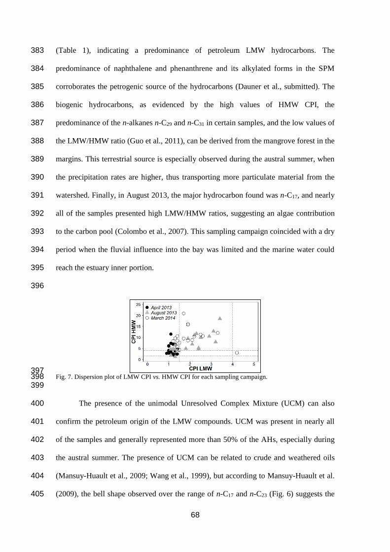
68

(Table 1), indicating a predominance of petroleum LMW hydrocarbons. The 383

predominance of naphthalene and phenanthrene and its alkylated forms in the SPM 384

corroborates the petrogenic source of the hydrocarbons (Dauner et al., submitted). The 385

biogenic hydrocarbons, as evidenced by the high values of HMW CPI, the 386

predominance of the n-alkanes n-C29 and n-C31 in certain samples, and the low values of 387

the LMW/HMW ratio (Guo et al., 2011), can be derived from the mangrove forest in the 388

margins. This terrestrial source is especially observed during the austral summer, when 389

the precipitation rates are higher, thus transporting more particulate material from the 390

watershed. Finally, in August 2013, the major hydrocarbon found was n-C17, and nearly 391

all of the samples presented high LMW/HMW ratios, suggesting an algae contribution 392

to the carbon pool (Colombo et al., 2007). This sampling campaign coincided with a dry 393

period when the fluvial influence into the bay was limited and the marine water could 394

reach the estuary inner portion. 395

396

397 Fig. 7. Dispersion plot of LMW CPI vs. HMW CPI for each sampling campaign. 398

399

The presence of the unimodal Unresolved Complex Mixture (UCM) can also 400

confirm the petroleum origin of the LMW compounds. UCM was present in nearly all 401

of the samples and generally represented more than 50% of the AHs, especially during 402

the austral summer. The presence of UCM can be related to crude and weathered oils 403

(Mansuy-Huault et al., 2009; Wang et al., 1999), but according to Mansuy-Huault et al. 404

(2009), the bell shape observed over the range of n-C17 and n-C23 (Fig. 6) suggests the 405

69

presence of fuel oil. The oil may originate from the boat and ferry traffic in the bay and 406

from the vehicle traffic on the road that follows the São João River for more than 15 407

km, evidencing the importance of its increasing during the austral summer. 408

Finally, the presence of the isoprenoids pristane and phytane can also be used to 409

evaluate the petroleum contamination in an environment. Pristane can be formed by 410

biogenic processes, while phytane originates from petroleum hydrocarbons 411

(Commendatore and Esteves, 2004; Mzoughi and Chouba, 2011), and the 412

pristane/phytane ratio values close to 1.0 indicate the petroleum input in the majority of 413

the samples. Both of the compounds can also be used to determine the relative 414

biodegradation of n-alkanes because they are decomposed more slowly than the n-C17 415

and n-C18 n-alkanes (Commendatore and Esteves, 2004; Short et al., 2007). Due to the 416

presence of relatively high concentrations of AHs, the low values of Pristane/n-C17 and 417

Phytane/ n-C18 indicate fresh oil inputs in all of the samples (Table 1). 418

419

4.5. Evaluation of LAB degradation 420

The relative composition of the LAB isomers can also be indicative of their 421

sources and degradation degree. Higher concentrations of C13-LABs were found, 422

especially in March 2014, followed by isomers with 12 carbon atoms (C12-LABs) 423

(Table 2). This result agrees with studies published by Martins et al. (2010) and Martins 424

et al. (2014) in other Brazilian estuaries and may reflect the use of surfactants with the 425

same composition in these regions. 426

Typically, the isomer composition can be used to determine the LAB 427

degradation rate using the ratio between their internal and external isomers (I/E ratio) 428

(Takada and Ishiwatari, 1990). Based on this parameter, calculated with C12-LABs and 429

C13-LABs, most of the samples presented recent inputs of LABs. 430

70

Luo et al. (2008) proposed a new indicator, C13-LABs/C12-LABs, to estimate the 431

LAB biodegradation in aquatic environments based on the combined abundance of C13-432

LABs and C12-LABs in environmental samples compared with detergent solutions and 433

sewage sludge. Using this ratio, a greater number of samples collected in Guaratuba 434

Bay could be evaluated, and more than 60% of the samples presented values higher than 435

2.0, suggesting degradation processes. These processes can be observed especially 436

during the austral summer, when the highest values were recorded, and in the outermost 437

sampling sites. 438

The difference between the spatial degradation degrees is most likely due to the 439

exposure time in which the compounds remain in the water column from the source 440

(inner sites) to the estuary mouth. High values of the C13-LABs/C12-LABs ratio 441

observed during the austral summer are most likely due to the higher temperatures, 442

which favor microbial activity (Lalli and Parsons, 1997). This enhanced degradation 443

trend in the warmer months was also observed for AHs, with the highest values of the 444

pristane/n-C17 ratio also found in April 2013 and March 2014, corroborating the 445

preferential degradation of these organic compounds during the austral summer. 446

Another explanation to the highest LAB mean concentrations observed in 447

August 2013 could be the difference in precipitation rates and, consequently, in the 448

dilution by fluvial water. In August 2013, the rainfall was sixty times lower than in 449

summer months (April 2013 and March 2014). The high precipitation rates observed in 450

the summer could cause a dilution of the organic markers by fluvial and pluvial waters, 451

leading to the low values observed. On the opposite way, the low riverine flux observed 452

in August 2013 may generate an accumulation of LABs in the estuary, although the 453

LAB input has not necessarily been increased. 454

455

71

5. Summary and Conclusions 456

Through the determination of organic markers, AHs and LABs, adsorbed on 457

SPM, it was possible to evaluate the spatial and short time scale variability of 458

hydrocarbon inputs and composition in Guaratuba Bay. The spatial distribution of the 459

compounds varied among the sampling campaigns. 460

Generally, the highest concentrations were observed during the austral summer, 461

not refuting the hypothesis (ii) and highlighting the importance of increased human 462

influence during summer holidays. However, the highest mean LAB values during the 463

austral winter may be explained by the decreased microbial degradation rates due to low 464

temperatures or the dilution by fluvial and pluvial waters during the austral summer. In 465

all of the sampling campaigns, both lipid classes presented similar spatial trends, 466

suggesting common transportation routes, such as the riverine flux in the inner portion 467

of the estuary, partially accepting the hypothesis (i). The compound distributions were 468

also affected by natural geochemical processes of organic matter accumulation. 469

LABs presented the same composition as that observed in other Brazilian 470

estuaries, and AHs were associated with petroleum and biogenic sources. The 471

introduction of fuel oil was observed, most likely originating from boat and vehicle 472

traffic, along with signs of a biogenic input, most likely from the mangrove forest 473

surrounding the bay and from autochthonous primary production. Finally, due to the 474

low precipitation rates and the advance of salt water into the bay, it was possible to 475

detect an autochthonous signal in August 2013. 476

The results of this study demonstrated that the introduction of sewage and oil 477

could be considered an emergent problem for the Guaratuba Bay ecosystem. Although 478

the concentrations are not comparable to severely polluted environments, they are 479

already over the same range as that in more urbanized and industrialized regions. This 480

72

study also showed the importance of evaluating the contaminant inputs on a short time 481

scale and highlighted the need for sewage input monitoring programs in the upper 482

estuary and for boat maintenance inspections to avoid the release of crude oil, primarily 483

during the summer. 484

485

Acknowledgments 486

A.L.L. Dauner would like to thank CAPES (Coordenação de Aperfeiçoamento 487

de Pessoal de Ensino Superior) for the MSc Scholarship. C.C. Martins would like to 488

thank CNPq (Brazilian National Council for Scientific and Technological Development) 489

for a research grant (477047/2011-4) and Fundação Araucária de Apoio ao 490

Desenvolvimento Científico e Tecnológico do Estado do Paraná (401/2012; 15.078). 491

We are grateful to R.R. Neto [Department of Oceanography, Federal University of 492

Espírito Santo (UFES)] and M.T. Grassi [Department of Chemistry, Federal University 493

of Paraná (UFPR)] for assistance with the preliminary evaluation of this article. This 494

study was developed as part of a post-graduate course on estuarine and ocean systems at 495

the Federal University of Paraná (PGSISCO-UFPR). 496

497

6. References 498

499

Aboul-Kassim, T.A.T., Simoneit, B.R.T., 1995. Aliphatic and aromatic hydrocarbons in 500 particulate fallout of Alexandria, Egypt : Sources and implications. Environ. Sci. 501 Technol. 29, 2473–2483. 502

Aboul-Kassim, T.A.T., Simoneit, B.R.T., 1996. Lipid geochemistry of surficial 503 sediments from the coastal environment of Egypt. I. Aliphatic hydrocarbons-504 characterization and sources. Mar. Chem. 54, 135–158. doi:10.1016/0304-505 4203(95)00098-4 506

Bakhtiari, A.R., Zakaria, M.P., Yaziz, M.I., Lajis, M.N.H., Bi, X., 2009. Polycyclic 507 aromatic hydrocarbons and n-alkanes in suspended particulate matter and 508 sediments from the Langat River, Peninsular Malaysia. Environ. Asia 2, 1–10. 509

73

Bianchi, T.S., 2007. Biogeochemistry of estuaries, 1st ed. Oxford University Press, Inc, 510 New York, U.S.A. 511

Burns, K., Brinkman, D., 2011. Organic biomarkers to describe the major carbon inputs 512 and cycling of organic matter in the central Great Barrier Reef region. Estuar. 513 Coast. Shelf Sci. 93, 132–141. doi:10.1016/j.ecss.2011.04.001 514

Burns, K.A., Hernes, P.J., Brinkman, D., Poulsen, A., Benner, R., 2008. Dispersion and 515 cycling of organic matter from the Sepik River outflow to the Papua New Guinea 516 coast as determined from biomarkers. Org. Geochem. 39, 1747–1764. 517 doi:10.1016/j.orggeochem.2008.08.003 518

Charriau, A., Bodineau, L., Ouddane, B., Fischer, J.-C., 2009. Polycyclic aromatic 519 hydrocarbons and n-alkanes in sediments of the Upper Scheldt River Basin: 520 contamination levels and source apportionment. J. Environ. Monit. 11, 1086–93. 521 doi:10.1039/b819928k 522

Colombo, J.C., Cappelletti, N., Speranza, E., Migoya, M.C., Lasci, J., Skorupka, C.N., 523 2007. Vertical fluxes and organic composition of settling material from the sewage 524 impacted Buenos Aires coastal area, Argentina. Org. Geochem. 38, 1941–1952. 525 doi:10.1016/j.orggeochem.2007.07.005 526

Colombo, J.C., Pelletier, E., Brochu, C., Khalll, M., 1989. Determination of 527 hydrocarbon sources using n-alkane and polyaromatic hydrocarbon distribution 528 indexes. Case study: Rio de La Plata estuary, Argentina. Environ. Sci. Technol. 23, 529 888–894. 530

Combi, T., Taniguchi, S., Figueira, R.C.L., Mahiques, M.M., Martins, C.C., 2013. 531 Spatial distribution and historical input of polychlorinated biphenyls (PCBs) and 532 organochlorine pesticides (OCPs) in sediments from a subtropical estuary 533 (Guaratuba Bay, SW Atlantic). Mar. Pollut. Bull. 70, 247–52. 534 doi:10.1016/j.marpolbul.2013.02.022 535

Commendatore, M.G., Esteves, J.L., 2004. Natural and anthropogenic hydrocarbons in 536 sediments from the Chubut River (Patagonia, Argentina). Mar. Pollut. Bull. 48, 537 910–8. doi:10.1016/j.marpolbul.2003.11.015 538

Cotovicz Junior, L.C., Machado, E.C., Brandini, N., Zem, R.C., Knoppers, B.A., 2013. 539 Distributions of total, inorganic and organic phosphorus in surface and recent 540 sediments of the sub-tropical and semi-pristine Guaratuba Bay estuary, SE Brazil. 541 Environ. Earth Sci. 72, 373–386. doi:10.1007/s12665-013-2958-y 542

Dauner, A.L.L., Hernández, E.A., MacCormack, W.P., Martins, C.C., 2015. Molecular 543 characterisation of anthropogenic sources of sedimentary organic matter from 544 Potter Cove, King George Island, Antarctica. Sci. Total Environ. 502, 408–416. 545 doi:10.1016/j.scitotenv.2014.09.043 546

Dauner, A.L.L., Lourenço, R.A., Martins, C.C. Submitted. Polycyclic aromatic 547 hydrocarbons in suspended matter from a subtropical estuary (Guaratuba Bay, SW 548 Atlantic). Water Research. 549

74

Froehner, S., Machado, K.S., Stefan, E., Bleninger, T., Rosa, E.C. da, Martins, C.C., 550 2012. Occurrence of selected estrogens in mangrove sediments. Mar. Pollut. Bull. 551 64, 75–79. doi:10.1016/j.marpolbul.2011.10.021 552

Grigoriadou, A., Schwarzbauer, J., Georgakopoulos, A., 2008. Organic geochemical 553 parameters for estimation of petrogenic inputs in the coastal area of Kavala City, 554 Greece. J. Soils Sediments 8, 253–262. doi:10.1007/s11368-008-0014-4 555

Guo, W., He, M., Yang, Z., Lin, C., Quan, X., 2011. Aliphatic and polycyclic aromatic 556 hydrocarbons in the Xihe River, an urban river in China’s Shenyang City: 557 distribution and risk assessment. J. Hazard. Mater. 186, 1193–9. 558 doi:10.1016/j.jhazmat.2010.11.122 559

Guo, W., He, M.-C., Yang, Z.-F., Lin, C.-Y., Quan, X.-C., 2010. Occurrence of 560 aliphatic hydrocarbons in water , suspended particulate matter and sediments of 561 Daliao River System, China. Bull. Environ. Contam. Toxicol. 84, 519–523. 562 doi:10.1007/s00128-010-9992-1 563

IAP, Instituto Ambiental do Paraná, 2006. Plano de manejo da Área de Proteção 564 Ambiental de Guaratuba. Curitiba. 565

IBGE, Instituto Brasileiro de Geografia e Estatística, 2010. http://www.ibge.gov.br. 566

Jennerjahn, T.C., 2012. Biogeochemical response of tropical coastal systems to present 567 and past environmental change. Earth-Science Rev. 114, 19–41. 568 doi:10.1016/j.earscirev.2012.04.005 569

Kannan, N., Kim, M., Hong, S.H., Jin, Y., Yim, U.H., Ha, S.Y., Son, Y.B., Choi, D.-L., 570 Shim, W.J., 2012. Chemical tracers, sterol biomarkers and satellite imagery in the 571 study of a river plume ecosystem in the Yellow Sea. Cont. Shelf Res. 33, 29–36. 572 doi:10.1016/j.csr.2011.10.001 573

Kolm, H.E., dos Santos, P.R.N. de M., Sautter, K.D., 2007. Bacteria in water and 574 sediments of Guaratuba Bay, Paraná, Brazil. Trop. Oceanogr. 35, 51–69. 575

Lalli, C.M., Parsons, T.R., 1997. Biological oceanography - An introduction, 2nd ed. 576 Butterworth-Heinemann - Elsevier, Oxford. 577

Lehmkuhl, E.A., Tremarin, P.I., Moreira-Filho, H., Ludwig, T.A.V., 2010. 578 Thalassiosirales (Diatomeae) da baía de Guaratuba, Estado do Paraná, Brasil. Biota 579 Neotrop. 10, 313–324. 580

Leonov, A. V., Nemirovskaya, I.A., 2011. Petroleum hydrocarbons in the waters of 581 major tributaries of the White Sea and its water areas: A review of available 582 information. Water Resour. 38, 324–351. doi:10.1134/S0097807811030055 583

Luo, X.-J., Chen, S.-J., Ni, H.-G., Yu, M., Mai, B.-X., 2008. Tracing sewage pollution 584 in the Pearl River Delta and its adjacent coastal area of South China Sea using 585 linear alkylbenzenes (LABs). Environ. Sci. Technol. 56, 158–162. 586 doi:10.1016/j.marpolbul.2007.09.033 587

75

Maioli, O.L.G., Rodrigues, K.C., Knoppers, B.A., Azevedo, D.A., 2011. Distribution 588 and sources of aliphatic and polycyclic aromatic hydrocarbons in suspended 589 particulate matter in water from two Brazilian estuarine systems. Cont. Shelf Res. 590 31, 1116–1127. doi:10.1016/j.csr.2011.04.004 591

Mansuy-Huault, L., Regier, A., Faure, P., 2009. Analyzing hydrocarbons in sewer to 592 help in PAH source apportionment in sewage sludges. Chemosphere 75, 995–1002. 593 doi:10.1016/j.chemosphere.2009.01.059 594

Marone, E., Noernberg, M.A., Santos, I. Dos, Lautert, L.F., Andreoli, O.R., Buba, H., 595 Fill, H.D., 2006. Hydrodynamic of Guaratuba Bay, PR, Brazil. J. Coast. Res. 39, 596 1879–1883. 597

Martins, C.C., Aguiar, S.N., Bícego, M.C., Montone, R.C., 2012a. Sewage organic 598 markers in surface sediments around the Brazilian Antarctic station: Results from 599 the 2009/10 austral summer and historical tendencies. Mar. Pollut. Bull. 64, 2867–600 2870. doi:10.1016/j.marpolbul.2012.08.019 601

Martins, C.C., Bícego, M.C., Figueira, R.C.L., Angelli, J.L.F., Combi, T., Gallice, 602 W.C., Mansur, A.V., Nardes, E., Rocha, M.L., Wisnieski, E., Ceschim, L.M.M., 603 Ribeiro, A.P., 2012b. Multi-molecular markers and metals as tracers of organic 604 matter inputs and contamination status from an Environmental Protection Area in 605 the SW Atlantic (Laranjeiras Bay, Brazil). Sci. Total Environ. 417-418, 158–68. 606 doi:10.1016/j.scitotenv.2011.11.086 607

Martins, C.C., Bícego, M.C., Mahiques, M.M., Figueira, R.C.L., Tessler, M.G., 608 Montone, R.C., 2010. Depositional history of sedimentary linear alkylbenzenes 609 (LABs) in a large South American industrial coastal area (Santos Estuary, 610 Southeastern Brazil). Environ. Pollut. 158, 3355–3364. 611 doi:10.1016/j.envpol.2010.07.040 612

Martins, C.C., Cabral, A.C., Barbosa-Cintra, S.C.T., Dauner, A.L.L., Souza, F.M., 613 2014. An integrated evaluation of molecular marker indices and linear 614 alkylbenzenes (LABs) to measure sewage input in a subtropical estuary (Babitonga 615 Bay, Brazil). Environ. Pollut. 188, 71–80. doi:10.1016/j.envpol.2014.01.022 616

Mizerkowski, B.D., Machado, E.C., Brandini, N., Nazario, M.G., Bonfim, K.V., 2012. 617 Environmental water quality assessment in Guaratuba bay, state of Paraná, 618 southern Brazil. Brazilian J. Oceanogr. 60, 109–115. doi:10.1590/S1679-619 87592012000200001 620

Montuori, P., Triassi, M., 2012. Polycyclic aromatic hydrocarbons loads into the 621 Mediterranean Sea: estimate of Sarno River inputs. Mar. Pollut. Bull. 64, 512–20. 622 doi:10.1016/j.marpolbul.2012.01.003 623

Mzoughi, N., Chouba, L., 2011. Distribution and partitioning of aliphatic hydrocarbons 624 and polycyclic aromatic hydrocarbons between water, suspended particulate 625 matter, and sediment in harbours of the West coastal of the Gulf of Tunis 626 (Tunisia). J. Environ. Monit. 13, 689–698. doi:10.1039/c0em00616e 627

76

Nanni, A.S., Descovi-Filho, L., Virtuoso, M.A., Montenegro, D., Willrich, G., 628 Machado, P.H., Sperb, R., Dantas, G.S., Calazans, Y., 2014. Quantum GIS - 629 Versão 2.4.0 “Chugiak.” 630

Nemirovskaya, I.A., 2011. Distribution of hydrocarbons in the estuarine area of the 631 Northern Dvina River during seasonal flood. Geochemistry Int. 49, 815–826. 632 doi:10.1134/S0016702911080052 633

Ni, H., Lu, F., Wang, J., Guan, Y., 2008. Linear alkylbenzenes in riverine runoff of the 634 Pearl River Delta (China) and their application as anthropogenic molecular 635 markers in coastal environments. Environ. Pollut. 154, 348–355. 636 doi:10.1016/j.envpol.2007.09.010 637

Ni, H., Shen, R., Zeng, H., Zeng, E.Y., 2009. Fate of linear alkylbenzenes and 638 benzothiazoles of anthropogenic origin and their potential as environmental 639 molecular markers in the Pearl River Delta , South China. Environ. Pollut. 157, 640 3502–3507. doi:10.1016/j.envpol.2009.06.005 641

Notar, M., Leskovsek, H., Faganeli, J., 2001. Composition, distribution and sources of 642 polycyclic aromatic hydrocarbons in sediments of the Gulf of Trieste, Northern 643 Adriatic Sea. Mar. Pollut. Bull. 42, 36–44. 644

Pietzsch, R., Patchineelam, S.R., Torres, J.P.M., 2010. Polycyclic aromatic 645 hydrocarbons in recent sediments from a subtropical estuary in Brazil. Mar. Chem. 646 118, 56–66. doi:10.1016/j.marchem.2009.10.004 647

Pinturier-Geiss, L., Méjanelle, L., Dale, B., Karlsen, D.A., 2002. Lipids as indicators of 648 eutrophication in marine coastal sediments. J. Microbiol. Methods 48, 239–57. 649

Raymundo, C.C., Preston, M.R., 1992. The distribution of linear alkylbenzenes in 650 coastal and estuarine sediments of the western North Sea. Mar. Pollut. Bull. 14, 651 138–145. 652

Rügner, H., Schwientek, M., Egner, M., Grathwohl, P., 2014. Monitoring of event-653 based mobilization of hydrophobic pollutants in rivers: Calibration of turbidity as a 654 proxy for particle facilitated transport in field and laboratory. Sci. Total Environ. 655 490, 191–198. doi:10.1016/j.scitotenv.2014.04.110 656

Sanders, C.J., Santos, I.R., Silva-Filho, E. V., Patchineelam, S.R., 2006. Mercury flux to 657 estuarine sediments, derived from Pb-210 and Cs-137 geochronologies (Guaratuba 658 Bay, Brazil). Mar. Pollut. Bull. 52, 1085–9. doi:10.1016/j.marpolbul.2006.06.004 659

Schwientek, M., Rügner, H., Beckingham, B., Kuch, B., Grathwohl, P., 2013. Integrated 660 monitoring of particle associated transport of PAHs in contrasting catchments. 661 Environ. Pollut. 172, 155–162. doi:10.1016/j.envpol.2012.09.004 662

Short, J.W., Kolak, J.J., Payne, J.R., Van Kooten, G.K., 2007. An evaluation of 663 petrogenic hydrocarbons in northern Gulf of Alaska continental shelf sediments - 664 The role of coastal oil seep inputs. Org. Geochem. 38, 643–670. 665 doi:10.1016/j.orggeochem.2006.12.005 666

77

Takada, H., Eganhouse, R.P., 1998. Molecular markers of anthropogenic waste, in: 667 Meyers, R.A. (Ed.), Encyclopedia of Environmental Analysis and Remediation. 668 John Wiley & Sons, Inc., p. 5488. 669

Takada, H., Ishiwatari, R., 1990. Biodegradation experiments of linear alkylbenzenes 670 (LABs): isomeric composition of C12 LABs as an indicator of the degree of LAB 671 degradation in the aquatic environment. Environ. Sci. Technol. 24, 86–91. 672

UNEP, 1992. Determination of petroleum hydrocarbons in sediments - Reference 673 methods for marine pollution studies, n.20. Burns. 674

Venturini, N., Muniz, P., Bícego, M.C., Martins, C.C., Tommasi, L.R., 2008. Petroleum 675 contamination impact on macrobenthic communities under the influence of an oil 676 refinery: Integrating chemical and biological multivariate data. Estuar. Coast. Shelf 677 Sci. 78, 457–467. doi:10.1016/j.ecss.2008.01.008 678

Wang, J.-Z., Nie, Y.-F., Luo, X.-L., Zeng, E.Y., 2008. Occurrence and phase 679 distribution of polycyclic aromatic hydrocarbons in riverine runoff of the Pearl 680 River Delta, China. Mar. Pollut. Bull. 57, 767–74. 681 doi:10.1016/j.marpolbul.2008.01.007 682

Wang, Z., Fingas, M., Page, D.S., 1999. Oil spill identification. J. Chromatogr. A 843, 683 369–411. doi:10.1016/S0021-9673(99)00120-X 684

Wang, Z., Yang, C., Kelly-Hooper, F., Hollebone, B.P., Peng, X., Brown, C.E., 685 Landriault, M., Sun, J., Yang, Z., 2009. Forensic differentiation of biogenic 686 organic compounds from petroleum hydrocarbons in biogenic and petrogenic 687 compounds cross-contaminated soils and sediments. J. Chromatogr. A 1216, 1174–688 91. doi:10.1016/j.chroma.2008.12.036 689

Wisnieski, E., Bícego, M.C., Montone, R.C., Figueira, R.C.L., Ceschim, L.M.M., 690 Mahiques, M.M., Martins, C.C., 2014. Characterization of sources and temporal 691 variation in the organic matter input indicated by n-alkanols and sterols in 692 sediment cores from Admiralty Bay, King George Island, Antarctica. Polar Biol. 693 37, 483–496. doi:10.1007/s00300-014-1445-6 694

LXXVIII

POSFÁCIO

A partir da análise das distribuições espacial e temporal de

hidrocarbonetos (HPAs, HAs e LABs) no MPS da Baía de Guaratuba foi

possível identificar as suas principais fontes e verificar como os processos

geoquímicos naturais e a flutuação populacional afetam as suas distribuições.

O somatório das concentrações de HPAs totais variaram entre 5,89 e

650,51 ng L-1, enquanto o somatório das concentrações de HAs e LABs totais

variaram entre 39,3 e 1591,4 µg g-1 e <DL (abaixo do limite de detecção) e

3769,7 ng g-1, respectivamente. As concentrações de HPAs estão na mesma

faixa de alguns ambientes costeiros já antropizados, como o litoral do Mar

Mediterrâneo (França e Espanha; GUITART et al., 2007) e a laguna Manguaba

(Brasil; MAIOLI et al., 2011), mas abaixo dos valores observados em regiões

altamente urbanizadas e industrializadas, como o estuário do Rio Sarno (Itália;

MONTUORI & TRIASSI, 2012) e o rio Daliao (China; GUO et al., 2007). Os

valores de HAs estão na mesma faixa dos encontrados em outras regiões

costeiras sob influência antrópica, como a estuário do Rio da Prata (Argentina e

Uruguai; COLOMBO et al., 2007) e o lago de Tunis (Tunísia; MZOUGHI &

CHOUBA, 2011), enquanto as concentrações de LABs são até uma ordem de

magnitude inferiores às encontradas no estuário do Rio da Prata (Argentina a

Uruguai; COLOMBO et al., 2007) e no delta do Rio Pearl (China; NI et al.,

2008).

De um modo geral, foram observados altos valores na porção mediana do

estuário, relacionados a processos físico-químicos que contribuem para o

acúmulo de matéria orgânica (LEONOV & NEMIROVSKAYA, 2011). Nessa

região, ocorre um aumento da área de seção da baía e o encontro de fluxos

com direções opostas e características físicas distintas, o que favorece

processos de floculação e adsorção de compostos orgânicos no MPS, gerando

uma região atuante como um filtro geoquímico de partículas (BIANCHI, 2007).

Também foram observados altos valores de HPAs na desembocadura da

baía, próximo à passagem de balsas, sugerindo uma introdução contínua de

HPAs ao longo do ano. Já os HAs e os LABs apresentaram altos valores na

porção mais interna da baía, sugerindo o aporte fluvial como fonte da

introdução desses compostos. Por fim, foram observados altos valores de

HPAs e de HAs próximo à marina de Guaratuba na coleta realizada durante o

Carnaval (Março/2014), indicando um aumento da introdução desses

LXXIX

compostos nesse período. Ainda, as maiores concentrações foram observadas

durante o verão, período de aumento populacional na região costeira.

A análise de razões diagnósticas permitiu avaliar as principais fontes dos

hidrocarbonetos na Baía de Guaratuba. A predominância de HPAs da baixa

massa molar e de compostos alquilados, como os alquilnaftalenos e

alquilfenantrenos, indicou a presença de fontes petrogênicas (WANG et al.,

1999), provavelmente associado ao tráfego de embarcações e balsas na baía,

com alguns pontos de introdução pirolítica de HPAs.

Os HAs apresentaram múltiplas fontes, podendo ser associados tanto a

fontes petrogênicas quanto naturais. A presença de MCNR unimodal, composta

de n-alcanos de baixa massa molar (n-C17 – n-C23) e os baixos valores do

Índice Preferencial de Carbono (IPC ≈ 1) em 56% das amostras sugerem a

presença de óleo combustível (COLOMBO et al., 2007), podendo estar

associado ao tráfego de veículos e embarcações. No entanto, a distribuição

dos n-alcanos de alta massa molar (n-C27 – n-C33) com número ímpar de

carbonos, além da presença de altas concentrações de perileno (em 64% das

amostras), sugere a introdução de matéria orgânica proveniente de fontes

biogênicas terrestres (READMAN et al., 2002; GUO et al., 2011),

provavelmente oriundas da floresta de manguezal existente nas margens da

baía. Os LABs apresentaram a mesma composição observada em outros

estuários brasileiros (MARTINS et al., 2010, 2014), com predominância de n-

C13-LABs e n-C12-LABs.

A predominância de HPAs alquilados e a as baixas concentrações de

alcanos isoprenoides (pristano e fitano), se comparados aos n-alcanos

correspondentes (n-C17 e n-C18), indicam a introdução de material petrogênico

recente (WANG et al., 1999; COMMENDATORE & ESTEVES, 2004). No

entanto, as razões envolvendo LABs indicaram a presença de processos de

degradação microbiana, especialmente durante o verão, provavelmente devido

às maiores temperaturas (LUO et al., 2008).

Assim, foi possível observar que a introdução de óleo e esgoto são

problemas emergentes na Baía de Guaratuba, especialmente durante os

momentos de explosão populacional durante o verão, enfatizando assim a

importância da avaliação de contaminantes em curtas escalas temporais.

Também é importante considerar as características físico-químicas da coluna

d’água em estudos de avaliação ambiental envolvendo o MPS, uma vez que

eles podem ser responsáveis por acumular material orgânico em regiões

afastadas de fontes pontuais de poluentes.

LXXX

ANEXO – DADOS BRUTOS

Tabela 1. Parâmetros da coluna d’água da Baía de Guaratuba em Abril/2013.

Ponto Lat Long Horário T [°C] Salin [USP] Prof [m] pH OD [mL/L] OD [% sat] MPS [mg/L]

1 25° 51' 49,8" S 48° 43' 42,6" W 16h03 24,50 6,71 3,1 7,15 4,48 78,88 11,80

2 25° 52' 6,2" S 48° 42' 35,8" W 15h56 24,80 6,93 2,5 7,29 4,94 87,48 13,37

3 25° 51' 56,9" S 48° 41' 39,4" W 16h13 24,94 9,78 2,5 7,22 5,54 99,20 15,47

4 25° 52' 25,3" S 48° 41' 3,6" W 15h50 25,42 11,94 4,6 7,54 5,71 105,89 20,93

5 25° 52' 1,3" S 48° 40' 30,2" W 15h45 25,72 15,31 3,2 7,77 5,54 104,61 26,03

6 25° 51' 18,3" S 48° 40' 8,3" W 16h20 25,81 14,90 1,4 7,26 4,86 91,12 61,37

7 25° 52' 26,7" S 48° 39' 40,2" W 15h40 25,69 18,06 1,4 7,74 4,96 95,24 30,63

8 25° 51' 35,3" S 48° 39' 17,7" W 16h25 25,47 15,05 3,2 7,66 5,37 101,37 25,20

9 25° 50' 59,4" S 48° 39' 25,6" W 16h35 25,69 17,81 1,5 7,48 4,55 86,90 83,70

10 25° 52' 20,9" S 48° 38' 37,1" W 15h30 25,67 22,76 1,5 7,71 4,84 95,13 32,80

11 25° 51' 38,6" S 48° 38' 6,4" W 16h42 25,59 21,18 3,5 7,68 4,73 92,45 39,70

12 25° 52' 15,2" S 48° 37' 23,0" W 15h23 25,58 24,92 7,3 7,85 4,75 94,34 32,20

13 25° 51' 7,3" S 48° 37' 39,6" W 16h46 25,75 17,60 2,1 7,28 4,01 76,46 52,27

14 25° 51' 19,3" S 48° 36' 34,1" W 16h55 25,63 23,12 1,2 7,81 4,57 90,22 78,17

15 25° 51' 56,9" S 48° 36' 18,0" W 15h00 25,81 30,14 8 7,85 4,64 95,56 29,70

16 25° 50' 41,6" S 48° 36' 2,7" W 17h02 25,79 21,95 2 7,45 3,90 76,12 34,93

17 25° 52' 9,5" S 48° 35' 3,8" W 14h52 25,82 31,24 6,7 7,85 4,64 95,81 34,43

18 25° 49' 52,6" S 48° 35' 52,2" W 17h10 25,92 22,57 5 7,86 3,92 77,01 38,80

19 25° 51' 3,4" S 48° 34' 49,1" W 17h18 25,66 25,93 2,3 7,77 4,24 84,73 39,43

20 25° 51' 32,1" S 48° 34' 15,2" W 14h45 25,70 32,44 8,8 7,76 4,46 92,69 39,30

21 25° 51' 32,1" S 48° 33' 20,1" W 14h40 25,87 31,52 12,5 7,83 4,82 99,60 30,27

22 25° 51' 42,9" S 48° 33' 39,2" W 14h25 25,85 32,61 5,1 7,47 4,83 100,47 41,80

LXXXI

Tabela 2. Parâmetros da coluna d’água da Baía de Guaratuba em Agosto/2013.

Ponto Lat Long Horário T [°C] Salin [USP] Prof [m] pH OD [mL/L] OD [% sat] MPS [mg/L]

1 25° 51' 49,8" S 48° 43' 42,6" W 16h34 18,52 7,64 3,01 7,29 5,67 91,78 7,80

2 25° 52' 6,2" S 48° 42' 35,8" W 16h27 18,72 9,35 2,78 7,60 5,54 90,30 10,37

3 25° 51' 56,9" S 48° 41' 39,4" W 16h45 18,85 13,58 2,49 7,06 5,75 96,52 16,31

4 25° 52' 25,3" S 48° 41' 3,6" W 16h15 18,76 15,50 5,02 7,23 5,95 101,00 17,00

5 25° 52' 1,3" S 48° 40' 30,2" W 16h10 18,96 16,61 3,24 7,69 5,95 101,51 21,83

6 25° 51' 18,3" S 48° 40' 8,3" W 16h56 19,20 15,92 1,34 7,62 5,46 92,75 40,49

7 25° 52' 26,7" S 48° 39' 40,2" W 16h03 18,92 18,31 1,34 7,48 5,81 99,84 27,31

8 25° 51' 35,3" S 48° 39' 17,7" W 17h09 18,96 17,78 2,33 7,60 5,73 98,44 28,43

9 25° 50' 59,4" S 48° 39' 25,6" W 17h03 18,99 18,94 2,49 7,79 5,65 97,63 31,43

10 25° 52' 20,9" S 48° 38' 37,1" W 15h56 18,74 21,14 1,11 7,46 5,90 103,20 23,34

11 25° 51' 38,6" S 48° 38' 6,4" W 17h15 18,79 21,63 2,99 7,83 5,70 100,25 29,34

12 25° 52' 15,2" S 48° 37' 23,0" W 15h01 18,41 25,16 4,87 7,51 5,72 100,55 27,40

13 25° 51' 7,3" S 48° 37' 39,6" W 17h21 19,09 19,32 1,84 7,18 4,64 80,11 30,66

14 25° 51' 19,3" S 48° 36' 34,1" W 17h29 18,66 22,74 1,03 7,90 5,54 98,09 38,74

15 25° 51' 56,9" S 48° 36' 18,0" W 14h51 18,21 26,83 7,33 7,89 5,59 99,20 29,71

16 25° 50' 41,6" S 48° 36' 2,7" W 17h36 19,15 22,78 1,70 7,64 5,07 89,70 27,00

17 25° 52' 9,5" S 48° 35' 3,8" W 14h46 18,03 29,35 6,55 7,88 6,24 112,19 32,66

18 25° 49' 52,6" S 48° 35' 52,2" W 17h44 19,35 22,43 4,78 7,41 5,01 88,12 36,74

19 25° 51' 3,4" S 48° 34' 49,1" W 17h53 18,57 25,71 2,42 7,34 5,40 97,21 34,09

20 25° 51' 32,1" S 48° 34' 15,2" W 14h38 17,86 30,33 8,63 7,58 5,52 99,74 31,03

21 25° 51' 32,1" S 48° 33' 20,1" W 14h32 17,91 30,35 14,47 7,74 5,29 95,60 26,94

22 25° 51' 42,9" S 48° 33' 39,2" W 14h19 17,88 30,35 3,07 7,89 5,30 95,81 46,26

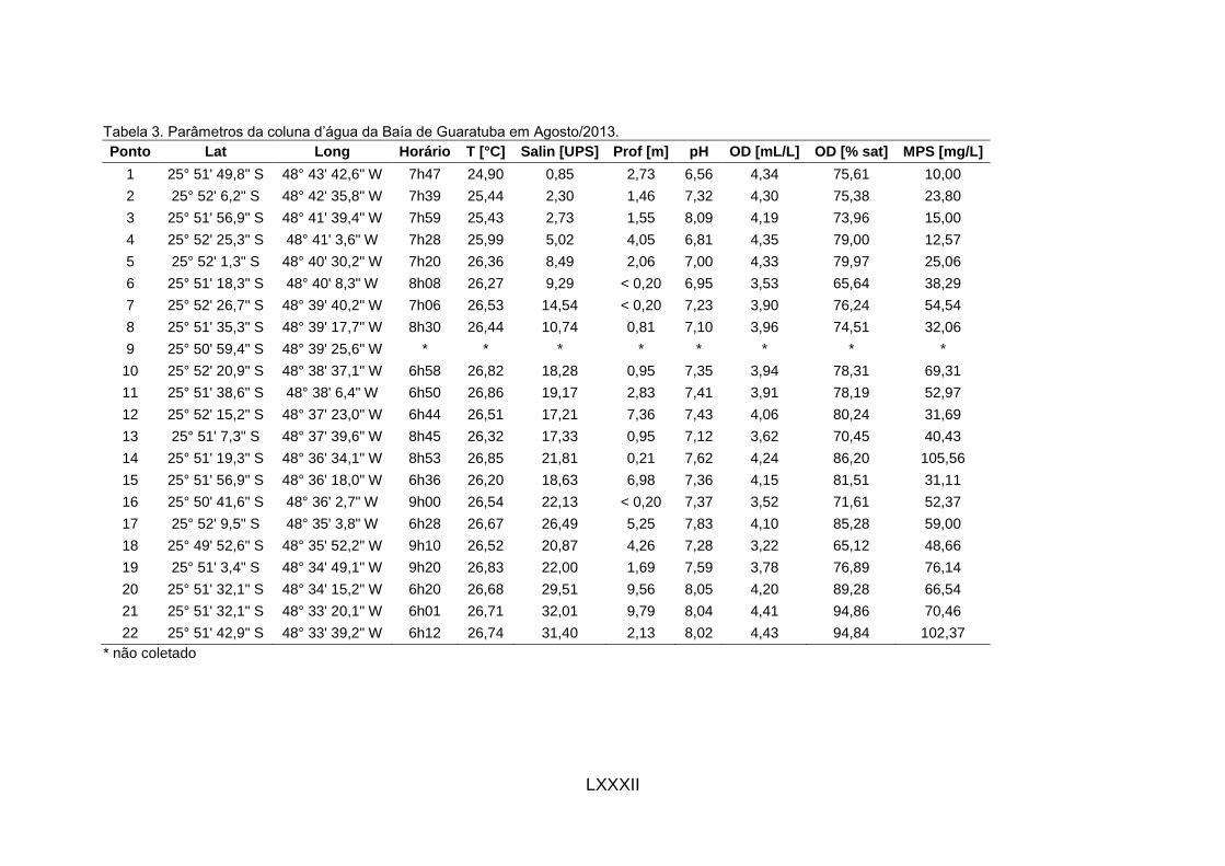
LXXXII

Tabela 3. Parâmetros da coluna d’água da Baía de Guaratuba em Agosto/2013.

Ponto Lat Long Horário T [°C] Salin [UPS] Prof [m] pH OD [mL/L] OD [% sat] MPS [mg/L]

1 25° 51' 49,8" S 48° 43' 42,6" W 7h47 24,90 0,85 2,73 6,56 4,34 75,61 10,00

2 25° 52' 6,2" S 48° 42' 35,8" W 7h39 25,44 2,30 1,46 7,32 4,30 75,38 23,80

3 25° 51' 56,9" S 48° 41' 39,4" W 7h59 25,43 2,73 1,55 8,09 4,19 73,96 15,00

4 25° 52' 25,3" S 48° 41' 3,6" W 7h28 25,99 5,02 4,05 6,81 4,35 79,00 12,57

5 25° 52' 1,3" S 48° 40' 30,2" W 7h20 26,36 8,49 2,06 7,00 4,33 79,97 25,06

6 25° 51' 18,3" S 48° 40' 8,3" W 8h08 26,27 9,29 < 0,20 6,95 3,53 65,64 38,29

7 25° 52' 26,7" S 48° 39' 40,2" W 7h06 26,53 14,54 < 0,20 7,23 3,90 76,24 54,54

8 25° 51' 35,3" S 48° 39' 17,7" W 8h30 26,44 10,74 0,81 7,10 3,96 74,51 32,06

9 25° 50' 59,4" S 48° 39' 25,6" W * * * * * * * *

10 25° 52' 20,9" S 48° 38' 37,1" W 6h58 26,82 18,28 0,95 7,35 3,94 78,31 69,31

11 25° 51' 38,6" S 48° 38' 6,4" W 6h50 26,86 19,17 2,83 7,41 3,91 78,19 52,97

12 25° 52' 15,2" S 48° 37' 23,0" W 6h44 26,51 17,21 7,36 7,43 4,06 80,24 31,69

13 25° 51' 7,3" S 48° 37' 39,6" W 8h45 26,32 17,33 0,95 7,12 3,62 70,45 40,43

14 25° 51' 19,3" S 48° 36' 34,1" W 8h53 26,85 21,81 0,21 7,62 4,24 86,20 105,56

15 25° 51' 56,9" S 48° 36' 18,0" W 6h36 26,20 18,63 6,98 7,36 4,15 81,51 31,11

16 25° 50' 41,6" S 48° 36' 2,7" W 9h00 26,54 22,13 < 0,20 7,37 3,52 71,61 52,37

17 25° 52' 9,5" S 48° 35' 3,8" W 6h28 26,67 26,49 5,25 7,83 4,10 85,28 59,00

18 25° 49' 52,6" S 48° 35' 52,2" W 9h10 26,52 20,87 4,26 7,28 3,22 65,12 48,66

19 25° 51' 3,4" S 48° 34' 49,1" W 9h20 26,83 22,00 1,69 7,59 3,78 76,89 76,14

20 25° 51' 32,1" S 48° 34' 15,2" W 6h20 26,68 29,51 9,56 8,05 4,20 89,28 66,54

21 25° 51' 32,1" S 48° 33' 20,1" W 6h01 26,71 32,01 9,79 8,04 4,41 94,86 70,46

22 25° 51' 42,9" S 48° 33' 39,2" W 6h12 26,74 31,40 2,13 8,02 4,43 94,84 102,37

* não coletado

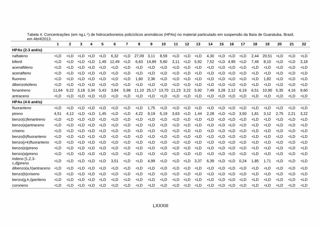
LXXXIII

Tabela 4. Concentrações (em ng.L-1) de hidrocarbonetos policíclicos aromáticos (HPAs) no material particulado em suspensão da Baía de Guaratuba, Brasil, em Abril/2013.

1 2 3 4 5 6 7 8 9 10 11 12 13 14 15 16 17 18 19 20 21 22

HPAs (2-3 anéis)

naftaleno <LD <LD <LD <LD <LD 6,32 <LD 27,09 3,11 8,59 <LD <LD <LD 4,30 <LD <LD <LD 2,44 20,51 <LD <LD <LD

bifenil <LD <LD <LD <LD 1,49 12,49 <LD 6,63 14,89 5,60 3,11 <LD 5,92 7,52 <LD 4,95 <LD 7,46 8,10 <LD <LD 3,18

acenaftileno <LD <LD <LD <LD <LD <LD <LD <LD <LD <LD <LD <LD <LD <LD <LD <LD <LD <LD <LD <LD <LD <LD

acenafteno <LD <LD <LD <LD <LD <LD <LD <LD <LD <LD <LD <LD <LD <LD <LD <LD <LD <LD <LD <LD <LD <LD

fluoreno <LD <LD <LD <LD <LD <LD <LD 1,60 2,36 <LD <LD <LD <LD <LD <LD <LD <LD <LD 1,82 <LD <LD <LD

dibenzotiofeno <LD <LD <LD <LD <LD <LD <LD <LD <LD <LD <LD <LD <LD <LD <LD <LD <LD <LD <LD <LD <LD <LD

fenantreno 11,64 9,22 3,18 3,34 5,43 3,84 5,98 11,10 25,17 13,70 11,23 3,22 5,92 7,49 3,28 2,12 6,19 6,51 10,90 5,35 4,16 9,60

antraceno <LD <LD <LD <LD <LD <LD <LD <LD <LD <LD <LD <LD <LD <LD <LD <LD <LD <LD <LD <LD <LD <LD

HPAs (4-6 anéis)

fluoranteno <LD <LD <LD <LD <LD <LD <LD <LD 1,75 <LD <LD <LD <LD <LD <LD <LD <LD <LD <LD <LD <LD <LD

pireno 4,51 4,12 <LD <LD 1,45 <LD <LD 4,22 9,19 5,19 3,63 <LD 1,44 2,28 <LD <LD 3,50 1,81 3,12 2,75 2,21 3,22

benzo(c)fenantreno <LD <LD <LD <LD <LD <LD <LD <LD <LD <LD <LD <LD <LD <LD <LD <LD <LD <LD <LD <LD <LD <LD

benzo(a)antraceno <LD <LD <LD <LD <LD <LD <LD <LD <LD <LD <LD <LD <LD <LD <LD <LD <LD <LD <LD <LD <LD <LD

criseno <LD <LD <LD <LD <LD <LD <LD <LD <LD <LD <LD <LD <LD <LD <LD <LD <LD <LD <LD <LD <LD <LD

benzo(b)fluoranteno <LD <LD <LD <LD <LD <LD <LD <LD <LD <LD <LD <LD <LD <LD <LD <LD <LD <LD <LD <LD <LD <LD

benzo(j+k)fluoranteno <LD <LD <LD <LD <LD <LD <LD <LD <LD <LD <LD <LD <LD <LD <LD <LD <LD <LD <LD <LD <LD <LD

benzo(e)pireno <LD <LD <LD <LD <LD <LD <LD <LD <LD <LD <LD <LD <LD <LD <LD <LD <LD <LD <LD <LD <LD <LD

benzo(a)pireno <LD <LD <LD <LD <LD <LD <LD <LD <LD <LD <LD <LD <LD <LD <LD <LD <LD <LD <LD <LD <LD <LD

indeno [1,2,3-c,d]pireno

<LD <LD <LD <LD <LD 3,51 <LD <LD 4,99 <LD <LD <LD 3,37 6,39 <LD <LD 0,24 1,85 1,71 <LD <LD <LD

dibenzo(a,h)antraceno <LD <LD <LD <LD <LD <LD <LD <LD <LD <LD <LD <LD <LD <LD <LD <LD <LD <LD <LD <LD <LD <LD

benzo(b)criseno <LD <LD <LD <LD <LD <LD <LD <LD <LD <LD <LD <LD <LD <LD <LD <LD <LD <LD <LD <LD <LD <LD

benzo(g,h,i)perileno <LD <LD <LD <LD <LD <LD <LD <LD <LD <LD <LD <LD <LD <LD <LD <LD <LD <LD <LD <LD <LD <LD

coroneno <LD <LD <LD <LD <LD <LD <LD <LD <LD <LD <LD <LD <LD <LD <LD <LD <LD <LD <LD <LD <LD <LD

LXXXIV

Alquil HPAs

2-metilnaftaleno <LD <LD <LD <LD <LD 6,82 <LD 14,77 7,31 6,29 <LD <LD <LD 1,72 <LD <LD <LD 1,54 <LD <LD <LD <LD

1-metilnaftaleno <LD <LD <LD <LD <LD 4,08 <LD 8,82 4,08 4,09 <LD <LD <LD 1,42 <LD <LD <LD <LD 5,90 <LD <LD <LD

C2-naftaleno <LD <LD <LD <LD <LD 19,02 <LD 24,76 34,64 16,26 <LD <LD 2,91 12,42 <LD 4,21 <LD 15,69 21,92 <LD 4,45 5,68

C3-naftaleno 3,49 2,57 1,48 <LD 1,61 5,53 2,07 6,34 12,20 4,69 4,26 1,45 4,16 5,46 <LD 2,53 <LD 5,14 6,95 <LD <LD 3,37

C1-fluoreno 10,83 8,53 3,92 5,78 6,82 7,92 5,54 28,82 38,26 23,68 11,57 4,50 8,39 9,91 4,25 5,42 6,86 14,94 26,73 8,55 5,88 14,98

C1-dibenzotiofeno <LD <LD <LD <LD <LD <LD <LD <LD <LD <LD <LD <LD <LD <LD <LD <LD <LD <LD <LD <LD <LD <LD

C2-fluoreno 19,79 13,85 2,65 2,66 5,86 2,48 5,43 16,18 45,12 21,03 17,09 2,78 7,08 7,85 2,99 <LD 13,16 9,24 18,39 12,36 6,63 17,35

C1-fenantreno 39,08 33,89 6,33 6,57 13,87 4,18 13,07 37,59 77,70 44,96 31,60 5,48 11,57 13,31 7,39 1,79 23,58 15,33 30,32 23,36 16,46 30,29

C2-dibenzotiofeno <LD <LD <LD <LD <LD <LD <LD <LD 1,99 <LD <LD <LD <LD <LD <LD <LD <LD <LD <LD <LD <LD <LD

C2-fenantreno 40,00 35,67 4,61 5,02 10,58 2,28 9,88 37,18 74,81 43,87 27,23 4,44 8,68 11,42 5,67 <LD 28,33 12,39 24,86 26,78 17,83 27,97

C1-fluoranteno 1,92 1,90 <LD <LD <LD <LD <LD 1,69 4,58 2,27 1,46 <LD <LD <LD <LD <LD 1,59 <LD <LD <LD <LD <LD

C1-pireno 1,90 1,86 <LD <LD <LD <LD <LD 1,70 4,14 2,13 <LD <LD <LD <LD <LD <LD 1,48 <LD <LD <LD <LD <LD

C1-criseno <LD <LD <LD <LD <LD <LD <LD <LD <LD <LD <LD <LD <LD <LD <LD <LD <LD <LD <LD <LD <LD <LD

C2-criseno <LD <LD <LD <LD <LD <LD <LD <LD <LD <LD <LD <LD <LD <LD <LD <LD <LD <LD <LD <LD <LD <LD

Naturais

reteno <LD <LD <LD <LD <LD <LD <LD <LD 1,80 <LD <LD <LD <LD <LD <LD <LD <LD <LD <LD <LD <LD <LD

perileno <LD <LD <LD <LD <LD 3,51 <LD <LD 4,99 <LD <LD <LD 3,37 6,39 <LD <LD <LD 1,85 1,71 <LD <LD <LD

<LD = abaixo do limite de detecção do método (1,4 ng.L-1)

LXXXV

Tabela 5. Concentrações (em ng.L-1) de hidrocarbonetos policíclicos aromáticos (HPAs) no material particulado em suspensão da Baía de Guaratuba, Brasil, em Agosto/2013.

1 2 3 4 5 6 7 8 9 10 11 12 13 14 15 16 17 18 19 20 21 22

HPAs (2-3 anéis)

naftaleno <LD <LD 10,64 10,58 4,30 4,04 6,70 10,46 4,29 52,82 18,41 <LD 1,66 <LD <LD 3,01 3,39 2,06 <LD 23,96 <LD 11,80

bifenil <LD <LD 3,00 1,78 <LD <LD 1,59 3,09 <LD 9,98 5,48 <LD <LD <LD <LD <LD <LD <LD <LD 4,23 <LD 6,88

acenaftileno <LD <LD <LD <LD <LD <LD <LD 1,56 <LD 5,81 2,65 <LD <LD <LD <LD <LD <LD <LD <LD <LD <LD <LD

acenafteno <LD <LD <LD <LD <LD <LD <LD <LD <LD <LD <LD <LD <LD <LD <LD <LD <LD <LD <LD <LD <LD <LD

fluoreno <LD <LD <LD <LD <LD <LD <LD <LD <LD <LD <LD <LD <LD <LD <LD <LD <LD <LD <LD <LD <LD <LD

dibenzotiofeno <LD <LD <LD <LD <LD <LD <LD <LD <LD <LD <LD <LD <LD <LD <LD <LD <LD <LD <LD <LD <LD <LD

fenantreno 2,08 1,62 1,45 1,63 2,78 8,93 3,19 4,78 3,94 3,41 3,40 2,00 3,19 2,95 1,44 1,84 1,57 2,39 2,20 1,66 1,77 5,40

antraceno <LD <LD <LD <LD <LD <LD <LD <LD <LD <LD <LD <LD <LD <LD <LD <LD <LD <LD <LD <LD <LD <LD

HPAs (4-6 anéis)

fluoranteno <LD <LD <LD <LD <LD 1,95 <LD 1,64 <LD 1,67 <LD <LD <LD <LD <LD <LD <LD <LD <LD <LD <LD <LD

pireno <LD <LD <LD <LD <LD 2,48 <LD 5,35 2,16 5,17 1,69 1,85 2,10 1,77 <LD <LD <LD <LD <LD <LD <LD 3,47

benzo(c)fenantreno <LD <LD <LD <LD <LD <LD <LD <LD <LD <LD <LD <LD <LD <LD <LD <LD <LD <LD <LD <LD <LD <LD

benzo(a)antraceno <LD <LD <LD <LD <LD <LD <LD <LD <LD <LD <LD <LD <LD <LD <LD <LD <LD <LD <LD <LD <LD <LD

criseno <LD <LD <LD <LD <LD <LD <LD <LD <LD <LD <LD <LD <LD <LD <LD <LD <LD <LD <LD <LD <LD <LD

benzo(b)fluoranteno <LD <LD <LD <LD <LD <LD <LD <LD <LD <LD <LD <LD <LD <LD <LD <LD <LD <LD <LD <LD <LD <LD

benzo(j+k)fluoranteno <LD <LD <LD <LD <LD <LD <LD <LD <LD <LD <LD <LD <LD <LD <LD <LD <LD <LD <LD <LD <LD <LD

benzo(e)pireno <LD <LD <LD <LD <LD <LD <LD <LD <LD <LD <LD <LD <LD <LD <LD <LD <LD <LD <LD <LD <LD <LD

benzo(a)pireno <LD <LD <LD <LD <LD <LD <LD <LD <LD <LD <LD <LD <LD <LD <LD <LD <LD <LD <LD <LD <LD <LD

indeno [1,2,3- c,d]pireno

<LD <LD <LD <LD <LD <LD <LD <LD <LD <LD <LD <LD <LD <LD <LD <LD <LD <LD <LD <LD <LD <LD

dibenzo(a,h)antraceno <LD <LD <LD <LD <LD <LD <LD <LD <LD <LD <LD <LD <LD <LD <LD <LD <LD <LD <LD <LD <LD <LD

benzo(b)criseno <LD <LD <LD <LD <LD <LD <LD <LD <LD <LD <LD <LD <LD <LD <LD <LD <LD <LD <LD <LD <LD <LD

benzo(g,h,i)perileno <LD <LD <LD <LD <LD <LD <LD <LD <LD <LD <LD <LD <LD <LD <LD <LD <LD <LD <LD <LD <LD <LD

coroneno <LD <LD <LD <LD <LD <LD <LD <LD <LD <LD <LD <LD <LD <LD <LD <LD <LD <LD <LD <LD <LD <LD

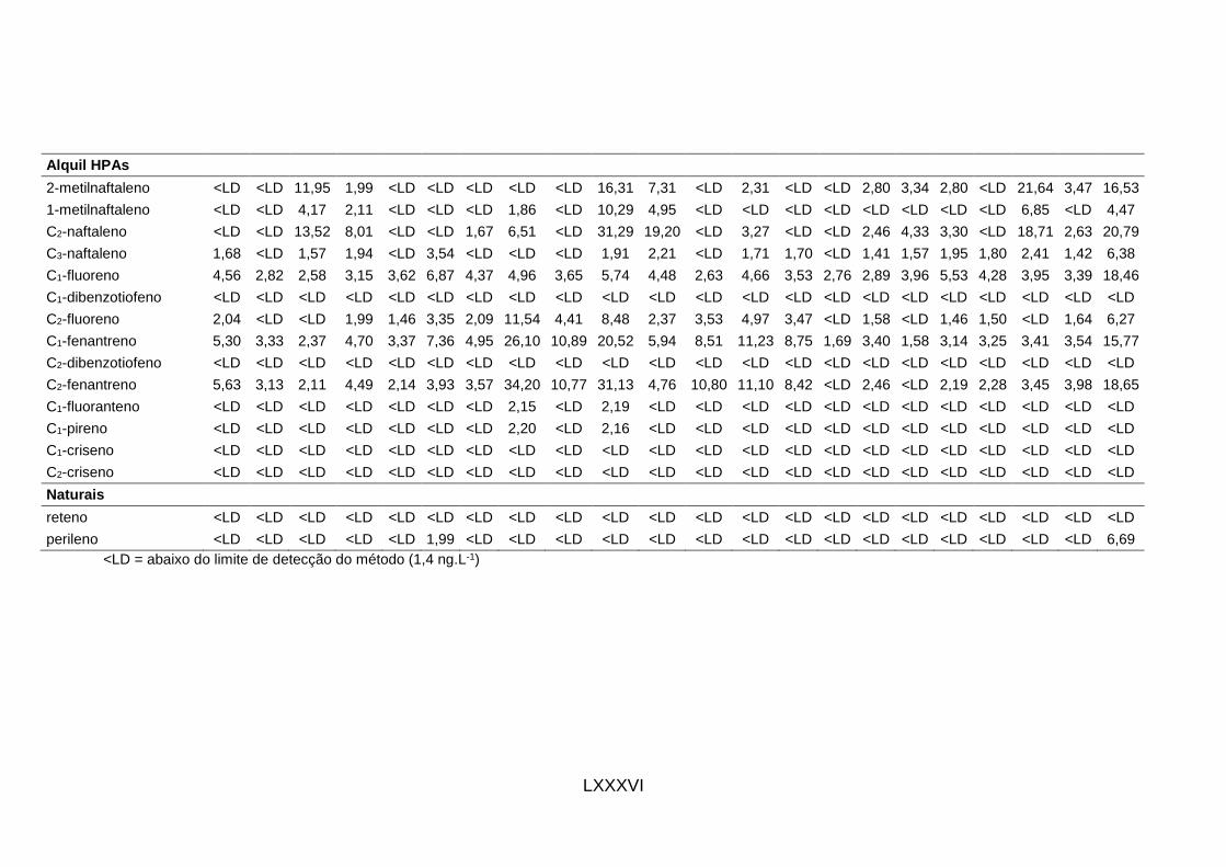
LXXXVI

Alquil HPAs

2-metilnaftaleno <LD <LD 11,95 1,99 <LD <LD <LD <LD <LD 16,31 7,31 <LD 2,31 <LD <LD 2,80 3,34 2,80 <LD 21,64 3,47 16,53

1-metilnaftaleno <LD <LD 4,17 2,11 <LD <LD <LD 1,86 <LD 10,29 4,95 <LD <LD <LD <LD <LD <LD <LD <LD 6,85 <LD 4,47

C2-naftaleno <LD <LD 13,52 8,01 <LD <LD 1,67 6,51 <LD 31,29 19,20 <LD 3,27 <LD <LD 2,46 4,33 3,30 <LD 18,71 2,63 20,79

C3-naftaleno 1,68 <LD 1,57 1,94 <LD 3,54 <LD <LD <LD 1,91 2,21 <LD 1,71 1,70 <LD 1,41 1,57 1,95 1,80 2,41 1,42 6,38

C1-fluoreno 4,56 2,82 2,58 3,15 3,62 6,87 4,37 4,96 3,65 5,74 4,48 2,63 4,66 3,53 2,76 2,89 3,96 5,53 4,28 3,95 3,39 18,46

C1-dibenzotiofeno <LD <LD <LD <LD <LD <LD <LD <LD <LD <LD <LD <LD <LD <LD <LD <LD <LD <LD <LD <LD <LD <LD

C2-fluoreno 2,04 <LD <LD 1,99 1,46 3,35 2,09 11,54 4,41 8,48 2,37 3,53 4,97 3,47 <LD 1,58 <LD 1,46 1,50 <LD 1,64 6,27

C1-fenantreno 5,30 3,33 2,37 4,70 3,37 7,36 4,95 26,10 10,89 20,52 5,94 8,51 11,23 8,75 1,69 3,40 1,58 3,14 3,25 3,41 3,54 15,77

C2-dibenzotiofeno <LD <LD <LD <LD <LD <LD <LD <LD <LD <LD <LD <LD <LD <LD <LD <LD <LD <LD <LD <LD <LD <LD

C2-fenantreno 5,63 3,13 2,11 4,49 2,14 3,93 3,57 34,20 10,77 31,13 4,76 10,80 11,10 8,42 <LD 2,46 <LD 2,19 2,28 3,45 3,98 18,65

C1-fluoranteno <LD <LD <LD <LD <LD <LD <LD 2,15 <LD 2,19 <LD <LD <LD <LD <LD <LD <LD <LD <LD <LD <LD <LD

C1-pireno <LD <LD <LD <LD <LD <LD <LD 2,20 <LD 2,16 <LD <LD <LD <LD <LD <LD <LD <LD <LD <LD <LD <LD

C1-criseno <LD <LD <LD <LD <LD <LD <LD <LD <LD <LD <LD <LD <LD <LD <LD <LD <LD <LD <LD <LD <LD <LD

C2-criseno <LD <LD <LD <LD <LD <LD <LD <LD <LD <LD <LD <LD <LD <LD <LD <LD <LD <LD <LD <LD <LD <LD

Naturais

reteno <LD <LD <LD <LD <LD <LD <LD <LD <LD <LD <LD <LD <LD <LD <LD <LD <LD <LD <LD <LD <LD <LD

perileno <LD <LD <LD <LD <LD 1,99 <LD <LD <LD <LD <LD <LD <LD <LD <LD <LD <LD <LD <LD <LD <LD 6,69

<LD = abaixo do limite de detecção do método (1,4 ng.L-1)

LXXXVII

Tabela 6. Concentrações (em ng.L-1) de hidrocarbonetos policíclicos aromáticos (HPAs) no material particulado em suspensão da Baía de Guaratuba, Brasil, em Março/2014.

1 2 3 4 5 6 7 8 9 10 11 12 13 14 15 16 17 18 19 20 21 22

HPAs (2-3 anéis)

naftaleno 26,60 11,74 20,61 2,14 5,66 4,02 3,13 4,00 na 10,01 5,10 4,62 4,76 5,26 26,92 2,14 2,57 na 4,53 3,94 2,26 1,85

bifenil 4,79 2,32 6,03 <LD <LD <LD <LD <LD na 2,75 <LD <LD <LD <LD 7,27 <LD <LD na <LD <LD <LD <LD

acenaftileno <LD <LD <LD <LD <LD <LD <LD <LD na <LD <LD <LD <LD <LD <LD <LD <LD na <LD <LD <LD <LD

acenafteno <LD <LD <LD <LD <LD <LD <LD <LD na <LD <LD <LD <LD <LD <LD <LD <LD na <LD <LD <LD <LD

fluoreno <LD <LD <LD <LD <LD <LD <LD <LD na <LD <LD <LD <LD <LD <LD <LD <LD na <LD <LD <LD <LD

dibenzotiofeno <LD <LD <LD <LD <LD <LD <LD <LD na <LD <LD <LD <LD <LD <LD <LD <LD na <LD <LD <LD <LD

fenantreno 3,60 3,86 2,48 1,94 18,00 4,93 16,35 6,88 na 4,67 2,16 1,82 3,85 5,72 7,44 4,15 6,49 na 4,54 1,60 4,83 6,66

antraceno <LD 4,92 <LD <LD <LD <LD <LD <LD na <LD <LD <LD <LD <LD <LD <LD <LD na <LD <LD <LD <LD

HPAs (4-6 anéis)

fluoranteno <LD <LD <LD <LD 5,90 <LD 4,21 2,71 na <LD <LD <LD <LD <LD 8,18 1,71 5,30 na <LD <LD 2,02 2,97

pireno <LD <LD <LD <LD 28,46 1,81 20,31 13,99 na 1,71 <LD <LD <LD 1,66 34,26 5,53 18,70 na 4,25 <LD 10,81 16,70

benzo(c)fenantreno <LD <LD <LD <LD <LD <LD <LD <LD na <LD <LD <LD <LD <LD <LD <LD <LD na <LD <LD <LD <LD

benzo(a)antraceno <LD <LD <LD <LD 1,50 <LD 1,68 <LD na <LD <LD <LD <LD <LD <LD <LD <LD na <LD <LD <LD 3,25

criseno <LD <LD <LD <LD 2,60 <LD 3,00 2,67 na <LD <LD <LD <LD <LD 5,87 <LD 5,08 na <LD <LD <LD 4,54

benzo(b)fluoranteno <LD <LD <LD <LD <LD <LD <LD <LD na <LD <LD <LD <LD <LD <LD <LD <LD na <LD <LD <LD <LD

benzo(j+k)fluoranteno <LD <LD <LD <LD <LD <LD <LD <LD na <LD <LD <LD <LD <LD <LD <LD <LD na <LD <LD <LD <LD

benzo(e)pireno <LD <LD <LD <LD <LD <LD <LD <LD na <LD <LD <LD <LD <LD <LD <LD <LD na <LD <LD <LD <LD

benzo(a)pireno <LD <LD <LD <LD <LD <LD <LD <LD na <LD <LD <LD <LD <LD <LD <LD <LD na <LD <LD <LD <LD

indeno [1,2,3-c,d]pireno

<LD <LD <LD <LD <LD <LD <LD <LD na <LD <LD <LD <LD <LD <LD <LD <LD na <LD <LD <LD <LD

dibenzo(a,h)antraceno <LD <LD <LD <LD <LD <LD <LD <LD na <LD <LD <LD <LD <LD <LD <LD <LD na <LD <LD <LD <LD

benzo(b)criseno <LD <LD <LD <LD <LD <LD <LD <LD na <LD <LD <LD <LD <LD <LD <LD <LD na <LD <LD <LD <LD

benzo(g,h,i)perileno <LD <LD <LD <LD <LD <LD <LD <LD na <LD <LD <LD <LD <LD <LD <LD <LD na <LD <LD <LD <LD

coroneno <LD <LD <LD <LD <LD <LD <LD <LD na <LD <LD <LD <LD <LD <LD <LD <LD na <LD <LD <LD <LD

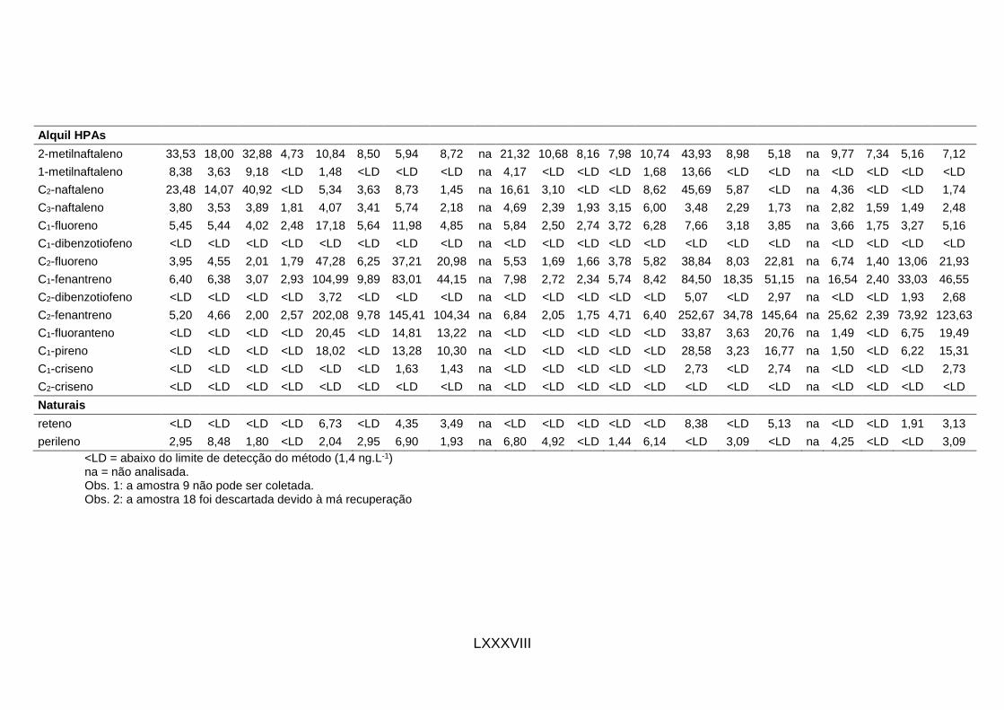
LXXXVIII

Alquil HPAs

2-metilnaftaleno 33,53 18,00 32,88 4,73 10,84 8,50 5,94 8,72 na 21,32 10,68 8,16 7,98 10,74 43,93 8,98 5,18 na 9,77 7,34 5,16 7,12

1-metilnaftaleno 8,38 3,63 9,18 <LD 1,48 <LD <LD <LD na 4,17 <LD <LD <LD 1,68 13,66 <LD <LD na <LD <LD <LD <LD

C2-naftaleno 23,48 14,07 40,92 <LD 5,34 3,63 8,73 1,45 na 16,61 3,10 <LD <LD 8,62 45,69 5,87 <LD na 4,36 <LD <LD 1,74

C3-naftaleno 3,80 3,53 3,89 1,81 4,07 3,41 5,74 2,18 na 4,69 2,39 1,93 3,15 6,00 3,48 2,29 1,73 na 2,82 1,59 1,49 2,48

C1-fluoreno 5,45 5,44 4,02 2,48 17,18 5,64 11,98 4,85 na 5,84 2,50 2,74 3,72 6,28 7,66 3,18 3,85 na 3,66 1,75 3,27 5,16

C1-dibenzotiofeno <LD <LD <LD <LD <LD <LD <LD <LD na <LD <LD <LD <LD <LD <LD <LD <LD na <LD <LD <LD <LD

C2-fluoreno 3,95 4,55 2,01 1,79 47,28 6,25 37,21 20,98 na 5,53 1,69 1,66 3,78 5,82 38,84 8,03 22,81 na 6,74 1,40 13,06 21,93

C1-fenantreno 6,40 6,38 3,07 2,93 104,99 9,89 83,01 44,15 na 7,98 2,72 2,34 5,74 8,42 84,50 18,35 51,15 na 16,54 2,40 33,03 46,55

C2-dibenzotiofeno <LD <LD <LD <LD 3,72 <LD <LD <LD na <LD <LD <LD <LD <LD 5,07 <LD 2,97 na <LD <LD 1,93 2,68

C2-fenantreno 5,20 4,66 2,00 2,57 202,08 9,78 145,41 104,34 na 6,84 2,05 1,75 4,71 6,40 252,67 34,78 145,64 na 25,62 2,39 73,92 123,63

C1-fluoranteno <LD <LD <LD <LD 20,45 <LD 14,81 13,22 na <LD <LD <LD <LD <LD 33,87 3,63 20,76 na 1,49 <LD 6,75 19,49

C1-pireno <LD <LD <LD <LD 18,02 <LD 13,28 10,30 na <LD <LD <LD <LD <LD 28,58 3,23 16,77 na 1,50 <LD 6,22 15,31

C1-criseno <LD <LD <LD <LD <LD <LD 1,63 1,43 na <LD <LD <LD <LD <LD 2,73 <LD 2,74 na <LD <LD <LD 2,73

C2-criseno <LD <LD <LD <LD <LD <LD <LD <LD na <LD <LD <LD <LD <LD <LD <LD <LD na <LD <LD <LD <LD

Naturais

reteno <LD <LD <LD <LD 6,73 <LD 4,35 3,49 na <LD <LD <LD <LD <LD 8,38 <LD 5,13 na <LD <LD 1,91 3,13

perileno 2,95 8,48 1,80 <LD 2,04 2,95 6,90 1,93 na 6,80 4,92 <LD 1,44 6,14 <LD 3,09 <LD na 4,25 <LD <LD 3,09

<LD = abaixo do limite de detecção do método (1,4 ng.L-1) na = não analisada. Obs. 1: a amostra 9 não pode ser coletada. Obs. 2: a amostra 18 foi descartada devido à má recuperação

LXXXIX

Tabela 7. Concentrações (em ng.g-1) de hidrocarbonetos policíclicos aromáticos (HPAs) no material particulado em suspensão da Baía de Guaratuba, Brasil, em Abril/2013.

1 2 3 4 5 6 7 8 9 10 11 12 13 14 15 16 17 18 19 20 21 22

HPAs (2-3 anéis)

naftaleno < LD <LD <LD <LD <LD 100,58 <LD 1052,20 36,38 258,19 <LD <LD <LD 54,45 <LD <LD <LD 60,79 497,39 <LD <LD <LD

bifenil <LD <LD <LD <LD 56,74 198,83 <LD 257,42 174,32 168,28 77,01 <LD 108,14 95,25 <LD 137,74 <LD 186,02 196,38 <LD <LD 70,95

acenaftileno <LD <LD <LD <LD <LD <LD <LD <LD <LD <LD <LD <LD <LD <LD <LD <LD <LD <LD <LD <LD <LD <LD

acenafteno <LD <LD <LD <LD <LD <LD <LD <LD <LD <LD <LD <LD <LD <LD <LD <LD <LD <LD <LD <LD <LD <LD

fluoreno <LD <LD <LD <LD <LD <LD <LD 62,15 27,63 <LD <LD <LD <LD <LD <LD <LD <LD <LD 44,14 <LD <LD <LD

dibenzotiofeno <LD <LD <LD <LD <LD <LD <LD <LD <LD <LD <LD <LD <LD <LD <LD <LD <LD <LD <LD <LD <LD <LD

fenantreno 974,64 685,14 197,69 155,87 207,25 61,15 190,10 431,19 294,73 411,94 278,36 97,91 108,20 94,91 104,36 59,03 170,05 162,40 264,38 131,96 132,24 214,42

antraceno <LD <LD <LD <LD <LD <LD <LD <LD <LD <LD <LD <LD <LD <LD <LD <LD <LD <LD <LD <LD <LD <LD

HPAs (4-6 anéis)

fluoranteno <LD <LD <LD <LD <LD <LD <LD <LD 20,49 <LD <LD <LD <LD <LD <LD <LD <LD <LD <LD <LD <LD <LD

pireno 377,63 306,16 <LD <LD 55,34 <LD <LD 163,93 107,61 156,06 89,98 <LD 26,32 28,89 <LD <LD 96,15 45,15 75,68 67,83 70,25 71,92

benzo(c) fenantreno

<LD <LD <LD <LD <LD <LD <LD <LD <LD <LD <LD <LD <LD <LD <LD <LD <LD <LD <LD <LD <LD <LD

benzo(a) antraceno

<LD <LD <LD <LD <LD <LD <LD <LD <LD <LD <LD <LD <LD <LD <LD <LD <LD <LD <LD <LD <LD <LD

criseno <LD <LD <LD <LD <LD <LD <LD <LD <LD <LD <LD <LD <LD <LD <LD <LD <LD <LD <LD <LD <LD <LD

benzo(b) fluoranteno

<LD <LD <LD <LD <LD <LD <LD <LD <LD <LD <LD <LD <LD <LD <LD <LD <LD <LD <LD <LD <LD <LD

benzo(j+k) fluoranteno

<LD <LD <LD <LD <LD <LD <LD <LD <LD <LD <LD <LD <LD <LD <LD <LD <LD <LD <LD <LD <LD <LD

benzo(e)pireno <LD <LD <LD <LD <LD <LD <LD <LD <LD <LD <LD <LD <LD <LD <LD <LD <LD <LD <LD <LD <LD <LD

benzo(a)pireno <LD <LD <LD <LD <LD <LD <LD <LD <LD <LD <LD <LD <LD <LD <LD <LD <LD <LD <LD <LD <LD <LD

indeno [1,2,3- c,d]pireno

<LD <LD <LD <LD <LD <LD <LD <LD <LD <LD <LD <LD <LD <LD <LD <LD <LD <LD <LD <LD <LD <LD

dibenzo(a,h) antraceno

<LD <LD <LD <LD <LD <LD <LD <LD <LD <LD <LD <LD <LD <LD <LD <LD <LD <LD <LD <LD <LD <LD

benzo(b)criseno <LD <LD <LD <LD <LD <LD <LD <LD <LD <LD <LD <LD <LD <LD <LD <LD <LD <LD <LD <LD <LD <LD

benzo(g,h,i) perileno

<LD <LD <LD <LD <LD <LD <LD <LD <LD <LD <LD <LD <LD <LD <LD <LD <LD <LD <LD <LD <LD <LD

XC

coroneno <LD <LD <LD <LD <LD <LD <LD <LD <LD <LD <LD <LD <LD <LD <LD <LD <LD <LD <LD <LD <LD <LD

Alquil HPAs

2-metilnaftaleno <LD <LD <LD <LD <LD 108,55 <LD 573,62 85,56 189,03 <LD <LD <LD 21,75 <LD <LD <LD 38,33 <LD <LD <LD <LD

1-metilnaftaleno <LD <LD <LD <LD <LD 65,02 <LD 342,75 47,81 123,08 <LD <LD <LD 18,04 <LD <LD <LD <LD 143,19 <LD <LD <LD

C2-naftaleno <LD <LD <LD <LD <LD 302,81 <LD 961,69 405,58 488,82 <LD <LD 53,12 157,34 <LD 117,13 <LD 391,33 531,59 <LD 141,36 126,79

C3-naftaleno 292,50 191,22 92,21 <LD 61,58 88,11 65,91 246,41 142,90 141,12 105,68 44,19 76,09 69,23 <LD 70,54 <LD 128,31 168,65 <LD <LD 75,35

C1-fluoreno 906,82 633,86 243,69 269,73 260,31 126,11 176,11 1119,53 448,01 712,03 286,79 136,84 153,34 125,58 135,23 150,91 188,46 372,70 648,34 210,89 186,92 334,59

C1-dibenzo tiofeno

<LD <LD <LD <LD <LD <LD <LD <LD <LD <LD <LD <LD <LD <LD <LD <LD <LD <LD <LD <LD <LD <LD

C2-fluoreno 1657,06 1029,19 164,74 124,13 223,66 39,49 172,62 628,52 528,34 632,35 423,62 84,54 129,40 99,48 95,14 <LD 361,54 230,51 446,05 304,86 210,76 387,52

C1-fenantreno 3272,25 2518,37 393,52 306,60 529,39 66,56 415,49 1460,21 909,84 1351,89 783,29 166,64 211,46 168,66 235,14 49,84 647,80 382,43 735,41 576,18 523,25 676,55

C2-dibenzo tiofeno

<LD <LD <LD <LD <LD <LD <LD <LD 23,30 <LD <LD <LD <LD <LD <LD <LD <LD <LD <LD <LD <LD <LD

C2-fenantreno 3349,28 2650,64 286,59 234,27 403,82 36,31 314,08 1444,28 876,00 1319,12 674,96 135,01 158,64 144,71 180,41 <LD 778,30 309,09 602,98 660,54 566,80 624,73

C1-fluoranteno 160,77 141,19 <LD <LD <LD <LD <LD 65,65 53,63 68,26 36,19 <LD <LD <LD <LD <LD 43,68 <LD <LD <LD <LD <LD

C1-pireno 159,09 138,22 <LD <LD <LD <LD <LD 66,04 48,48 64,05 <LD <LD <LD <LD <LD <LD 40,66 <LD <LD <LD <LD <LD

C1-criseno <LD <LD <LD <LD <LD <LD <LD <LD <LD <LD <LD <LD <LD <LD <LD <LD <LD <LD <LD <LD <LD <LD

C2-criseno <LD <LD <LD <LD <LD <LD <LD <LD <LD <LD <LD <LD <LD <LD <LD <LD <LD <LD <LD <LD <LD <LD

Naturais

reteno <LD <LD <LD <LD <LD <LD <LD <LD 21,08 <LD <LD <LD <LD <LD <LD <LD <LD <LD <LD <LD <LD <LD

perileno <LD <LD <LD <LD <LD 55,89 <LD <LD 58,43 <LD <LD <LD 61,59 80,97 <LD <LD <LD 46,15 41,48 <LD <LD <LD

<LD = abaixo do limite de detecção do método.

XCI

Tabela 8. Concentrações (em ng.g-1) de hidrocarbonetos policíclicos aromáticos (HPAs) no material particulado em suspensão da Baía de Guaratuba, Brasil, em Agosto/2013.

1 2 3 4 5 6 7 8 9 10 11 12 13 14 15 16 17 18 19 20 21 22

HPAs (2-3 anéis)

naftaleno <LD <LD 651,98 622,16 196,84 99,71 245,17 367,82 136,39 2262,65 627,30 <LD 54,04 <LD <LD 111,36 103,70 55,97 <LD 772,08 <LD 255,02

bifenil <LD <LD 183,68 104,51 <LD <LD 58,09 108,58 <LD 427,40 186,64 <LD <LD <LD <LD <LD <LD <LD <LD 136,22 <LD 148,66

acenaftileno <LD <LD <LD <LD <LD <LD <LD 54,76 <LD 248,76 90,20 <LD <LD <LD <LD <LD <LD <LD <LD <LD <LD <LD

acenafteno <LD <LD <LD <LD <LD <LD <LD <LD <LD <LD <LD <LD <LD <LD <LD <LD <LD <LD <LD <LD <LD <LD

fluoreno <LD <LD <LD <LD <LD <LD <LD <LD <LD <LD <LD <LD <LD <LD <LD <LD <LD <LD <LD <LD <LD <LD

dibenzotiofeno <LD <LD <LD <LD <LD <LD <LD <LD <LD <LD <LD <LD <LD <LD <LD <LD <LD <LD <LD <LD <LD <LD

fenantreno 266,67 156,20 88,88 95,88 127,36 220,57 116,79 168,14 125,36 146,08 115,87 72,99 104,05 76,14 48,46 68,15 48,08 65,05 64,54 53,50 65,69 116,74

antraceno <LD <LD <LD <LD <LD <LD <LD <LD <LD <LD <LD <LD <LD <LD <LD <LD <LD <LD <LD <LD <LD <LD

HPAs (4-6 anéis)

fluoranteno <LD <LD <LD <LD <LD 48,17 <LD 57,69 <LD 71,54 <LD <LD <LD <LD <LD <LD <LD <LD <LD <LD <LD <LD

pireno <LD <LD <LD <LD <LD 61,26 <LD 188,19 68,73 221,48 57,59 67,52 68,50 45,69 <LD <LD <LD <LD <LD <LD <LD 75,02

benzo(c) fenantreno

<LD <LD <LD <LD <LD <LD <LD <LD <LD <LD <LD <LD <LD <LD <LD <LD <LD <LD <LD <LD <LD <LD

benzo(a) antraceno

<LD <LD <LD <LD <LD <LD <LD <LD <LD <LD <LD <LD <LD <LD <LD <LD <LD <LD <LD <LD <LD <LD

criseno <LD <LD <LD <LD <LD <LD <LD <LD <LD <LD <LD <LD <LD <LD <LD <LD <LD <LD <LD <LD <LD <LD

benzo(b) fluoranteno

<LD <LD <LD <LD <LD <LD <LD <LD <LD <LD <LD <LD <LD <LD <LD <LD <LD <LD <LD <LD <LD <LD

benzo(j+k) fluoranteno

<LD <LD <LD <LD <LD <LD <LD <LD <LD <LD <LD <LD <LD <LD <LD <LD <LD <LD <LD <LD <LD <LD

benzo(e)pireno <LD <LD <LD <LD <LD <LD <LD <LD <LD <LD <LD <LD <LD <LD <LD <LD <LD <LD <LD <LD <LD <LD

benzo(a)pireno <LD <LD <LD <LD <LD <LD <LD <LD <LD <LD <LD <LD <LD <LD <LD <LD <LD <LD <LD <LD <LD <LD

indeno [1,2,3- c,d]pireno

<LD <LD <LD <LD <LD <LD <LD <LD <LD <LD <LD <LD <LD <LD <LD <LD <LD <LD <LD <LD <LD <LD

dibenzo(a,h) antraceno

<LD <LD <LD <LD <LD <LD <LD <LD <LD <LD <LD <LD <LD <LD <LD <LD <LD <LD <LD <LD <LD <LD

benzo(b)criseno <LD <LD <LD <LD <LD <LD <LD <LD <LD <LD <LD <LD <LD <LD <LD <LD <LD <LD <LD <LD <LD <LD

benzo(g,h,i) perileno

<LD <LD <LD <LD <LD <LD <LD <LD <LD <LD <LD <LD <LD <LD <LD <LD <LD <LD <LD <LD <LD <LD

XCII

coroneno <LD <LD <LD <LD <LD <LD <LD <LD <LD <LD <LD <LD <LD <LD <LD <LD <LD <LD <LD <LD <LD <LD

Alquil HPAs

2-metilnaftaleno <LD <LD 732,28 116,86 <LD <LD <LD <LD <LD 698,57 249,01 <LD 75,24 <LD <LD 103,58 102,17 76,11 <LD 697,31 128,67 357,28

1-metilnaftaleno <LD <LD 255,81 124,31 <LD <LD <LD 65,54 <LD 440,96 168,81 <LD <LD <LD <LD <LD <LD <LD <LD 220,87 <LD 96,71

C2-naftaleno <LD <LD 828,52 470,98 <LD <LD 61,02 228,88 <LD 1340,31 654,22 <LD 106,55 <LD <LD 90,99 132,49 89,72 <LD 602,89 97,49 449,37

C3-naftaleno 215,81 <LD 96,44 114,31 <LD 87,52 <LD <LD <LD 81,97 75,43 <LD 55,89 43,97 <LD 52,35 48,18 53,16 52,91 77,78 52,83 138,00

C1-fluoreno 584,62 271,90 158,14 185,29 165,84 169,69 159,99 174,47 116,14 245,90 152,68 95,99 152,00 91,11 92,88 107,04 121,26 150,51 125,57 127,30 125,82 399,07

C1-dibenzo tiofeno

<LD <LD <LD <LD <LD <LD <LD <LD <LD <LD <LD <LD <LD <LD <LD <LD <LD <LD <LD <LD <LD <LD

C2-fluoreno 261,54 <LD <LD 117,06 66,88 82,75 76,52 405,93 140,32 363,28 80,77 128,83 162,12 89,56 <LD 58,52 <LD 39,74 44,01 <LD 60,87 135,55

C1-fenantreno 679,49 321,07 145,27 276,47 154,38 181,79 181,22 918,09 346,50 879,07 202,43 310,58 366,31 225,85 56,88 125,93 48,38 85,46 95,35 109,90 131,39 340,92

C2-dibenzo tiofeno

<LD <LD <LD <LD <LD <LD <LD <LD <LD <LD <LD <LD <LD <LD <LD <LD <LD <LD <LD <LD <LD <LD

C2-fenantreno 721,79 301,79 129,33 264,12 98,04 97,07 130,70 1203,02 342,68 1333,60 162,22 394,16 362,07 217,33 <LD 91,11 <LD 59,60 66,89 111,19 147,72 403,18

C1-fluoranteno <LD <LD <LD <LD <LD <LD <LD 75,63 <LD 93,82 <LD <LD <LD <LD <LD <LD <LD <LD <LD <LD <LD <LD

C1-pireno <LD <LD <LD <LD <LD <LD <LD 77,39 <LD 92,53 <LD <LD <LD <LD <LD <LD <LD <LD <LD <LD <LD <LD

C1-criseno <LD <LD <LD <LD <LD <LD <LD <LD <LD <LD <LD <LD <LD <LD <LD <LD <LD <LD <LD <LD <LD <LD

C2-criseno <LD <LD <LD <LD <LD <LD <LD <LD <LD <LD <LD <LD <LD <LD <LD <LD <LD <LD <LD <LD <LD <LD

Naturais

reteno <LD <LD <LD <LD <LD <LD <LD <LD <LD <LD <LD <LD <LD <LD <LD <LD <LD <LD <LD <LD <LD <LD

perileno <LD <LD <LD <LD <LD 49,15 <LD <LD <LD <LD <LD <LD <LD <LD <LD <LD <LD <LD <LD <LD <LD 144,63

<LD = abaixo do limite de detecção do método.

XCIII

Tabela 9. Concentrações (em ng.g-1) de hidrocarbonetos policíclicos aromáticos (HPAs) no material particulado em suspensão da Baía de Guaratuba, Brasil, em Março/2014.

1 2 3 4 5 6 7 8 9 10 11 12 13 14 15 16 17 18 19 20 21 22

HPAs (2-3 anéis)

naftaleno 2659,67 493,14 1329,46 169,96 225,75 104,91 57,32 124,67 na 144,37 96,22 145,70 117,66 51,26 865,09 40,80 43,50 na 59,45 59,16 32,03 18,04

bifenil 478,67 97,34 388,82 <LD <LD <LD <LD <LD na 39,63 <LD <LD <LD <LD 233,55 <LD <LD na <LD <LD <LD <LD

acenaftileno <LD <LD <LD <LD <LD <LD <LD <LD na <LD <LD <LD <LD <LD <LD <LD <LD na <LD <LD <LD <LD

acenafteno <LD <LD <LD <LD <LD <LD <LD <LD na <LD <LD 7,57 6,93 4,29 11,25 4,58 3,90 na 3,81 3,76 2,84 2,25

fluoreno <LD <LD <LD <LD <LD <LD <LD <LD na <LD <LD 13,57 11,87 7,90 20,89 8,21 6,27 na 7,35 6,46 4,83 4,20

dibenzotiofeno <LD <LD <LD <LD <LD <LD <LD <LD na <LD <LD <LD <LD <LD <LD <LD <LD na <LD <LD <LD <LD

fenantreno 360,00 162,18 160,00 154,32 718,36 128,77 299,76 214,62 na 67,37 40,78 57,44 95,23 55,78 239,12 79,24 110,00 na 59,62 24,04 68,55 65,06

antraceno <LD 206,72 <LD <LD <LD <LD <LD <LD na <LD <LD <LD <LD <LD <LD <LD <LD na <LD <LD <LD <LD

HPAs (4-6 anéis)

fluoranteno <LD <LD <LD <LD 235,46 <LD 77,19 84,54 na <LD <LD <LD <LD <LD 262,90 32,65 89,83 na <LD <LD 28,67 29,01

pireno <LD <LD <LD <LD 1135,80 47,28 372,37 436,41 na 24,67 <LD <LD <LD 16,19 1101,10 105,59 316,95 na 55,82 <LD 153,43 163,13

benzo(c) fenantreno

<LD <LD <LD <LD <LD <LD <LD <LD na <LD <LD <LD <LD <LD <LD <LD <LD na <LD <LD <LD <LD

benzo(a) antraceno

<LD <LD <LD <LD 59,86 <LD 30,80 <LD na <LD <LD <LD <LD <LD <LD <LD <LD na <LD <LD <LD 31,75

criseno <LD <LD <LD <LD 103,76 <LD 55,00 83,29 na <LD <LD <LD <LD <LD 188,66 <LD 86,10 na <LD <LD <LD 44,35

benzo(b) fluoranteno

<LD <LD <LD <LD <LD <LD <LD <LD na <LD <LD <LD <LD <LD <LD <LD <LD na <LD <LD <LD <LD

benzo(j+k) fluoranteno

<LD <LD <LD <LD <LD <LD <LD <LD na <LD <LD <LD <LD <LD <LD <LD <LD na <LD <LD <LD <LD

benzo(e)pireno <LD <LD <LD <LD <LD <LD <LD <LD na <LD <LD <LD <LD <LD <LD <LD <LD na <LD <LD <LD <LD

benzo(a)pireno <LD <LD <LD <LD <LD <LD <LD <LD na <LD <LD <LD <LD <LD <LD <LD <LD na <LD <LD <LD <LD

indeno [1,2,3- c,d]pireno

<LD <LD <LD <LD <LD <LD <LD <LD na <LD <LD <LD <LD <LD <LD <LD <LD na <LD <LD <LD <LD

dibenzo(a,h) antraceno

<LD <LD <LD <LD <LD <LD <LD <LD na <LD <LD <LD <LD <LD <LD <LD <LD na <LD <LD <LD <LD

benzo(b)criseno <LD <LD <LD <LD <LD <LD <LD <LD na <LD <LD <LD <LD <LD <LD <LD <LD na <LD <LD <LD <LD

benzo(g,h,i) perileno

<LD <LD <LD <LD <LD <LD <LD <LD na <LD <LD <LD <LD <LD <LD <LD <LD na <LD <LD <LD <LD

XCIV

Coroneno <LD <LD <LD <LD <LD <LD <LD <LD na <LD <LD <LD <LD <LD <LD <LD <LD na <LD <LD <LD <LD

Alquil HPAs

2-metilnaftaleno 3352,67 756,16 2121,08 375,98 432,48 221,93 108,84 271,91 na 307,54 201,56 257,42 197,30 104,70 1411,78 171,40 87,74 na 128,27 110,25 73,19 69,52

1-metilnaftaleno 838,33 152,66 592,47 <LD 59,20 <LD <LD <LD na 60,21 <LD <LD 7,50 16,42 439,13 <LD <LD na <LD <LD <LD <LD

C2-naftaleno 2347,67 591,04 2639,78 <LD 212,98 94,73 160,00 45,13 na 239,59 58,46 <LD <LD 84,03 1468,35 112,02 <LD na 57,22 <LD <LD 16,96

C3-naftaleno 380,33 148,46 251,18 144,24 162,56 89,15 105,30 68,11 na 67,71 45,18 61,02 78,00 58,54 111,95 43,79 29,38 na 37,08 23,94 21,19 24,26

C1-fluoreno 545,00 228,57 259,35 197,27 685,63 147,31 219,64 151,29 na 84,25 47,20 86,47 92,01 61,24 246,19 60,72 65,25 na 48,07 26,30 46,41 50,40

C1-dibenzo tiofeno

<LD <LD <LD <LD <LD <LD <LD <LD na <LD <LD <LD <LD <LD <LD <LD <LD na <LD <LD <LD <LD

C2-fluoreno 395,00 191,18 129,68 142,39 1886,89 163,25 682,22 654,46 na 79,78 31,90 52,39 93,50 56,76 1248,30 153,33 386,61 na 88,52 21,04 185,36 214,22

C1-fenantreno 64,00 268,07 198,06 233,07 4190,02 258,32 1521,92 1377,23 na 115,13 51,35 73,85 141,98 82,11 2715,79 350,38 866,95 na 217,22 36,07 468,80 454,72

C2-dibenzo tiofeno

<LD <LD <LD <LD 148,46 <LD <LD <LD na <LD <LD <LD <LD <LD 162,95 <LD 50,34 na <LD <LD 27,39 26,18

C2-fenantreno 52,00 195,80 129,03 204,43 8064,77 255,45 2665,98 3254,81 na 98,68 38,70 55,23 116,50 62,41 8120,71 664,10 2468,47 na 336,47 35,92 1049,15 1207,66

C1-fluoranteno <LD <LD <LD <LD 816,13 <LD 271,53 412,39 na <LD <LD <LD <LD <LD 1088,57 69,31 351,86 na 19,57 <LD 95,80 190,39

C1-pireno <LD <LD <LD <LD 719,16 <LD 243,48 321,30 na <LD <LD <LD <LD <LD 918,55 61,67 284,24 na 19,70 <LD 88,28 149,55

C1-criseno <LD <LD <LD <LD <LD <LD 29,88 44,61 na <LD <LD <LD <LD <LD 87,74 <LD 46,44 na <LD <LD <LD 26,67

C2-criseno <LD <LD <LD <LD <LD <LD <LD <LD na <LD <LD <LD <LD <LD <LD <LD <LD na <LD <LD <LD <LD

Naturais

Reteno <LD <LD <LD <LD 268,59 <LD 79,75 108,87 na <LD <LD <LD <LD <LD 269,33 <LD 86,95 na <LD <LD 27,11 30,57

Perileno 295,00 356,30 116,13 <LD 81,41 77,05 126,51 60,20 na 98,10 92,88 <LD 35,62 59,88 <LD 59,00 <LD na 55,82 <LD <LD 30,18

<LD = abaixo do limite de detecção do método. na = não analisada. Obs. 1: a amostra 9 não pode ser coletada. Obs. 2: a amostra 18 foi descartada devido à má recuperação.

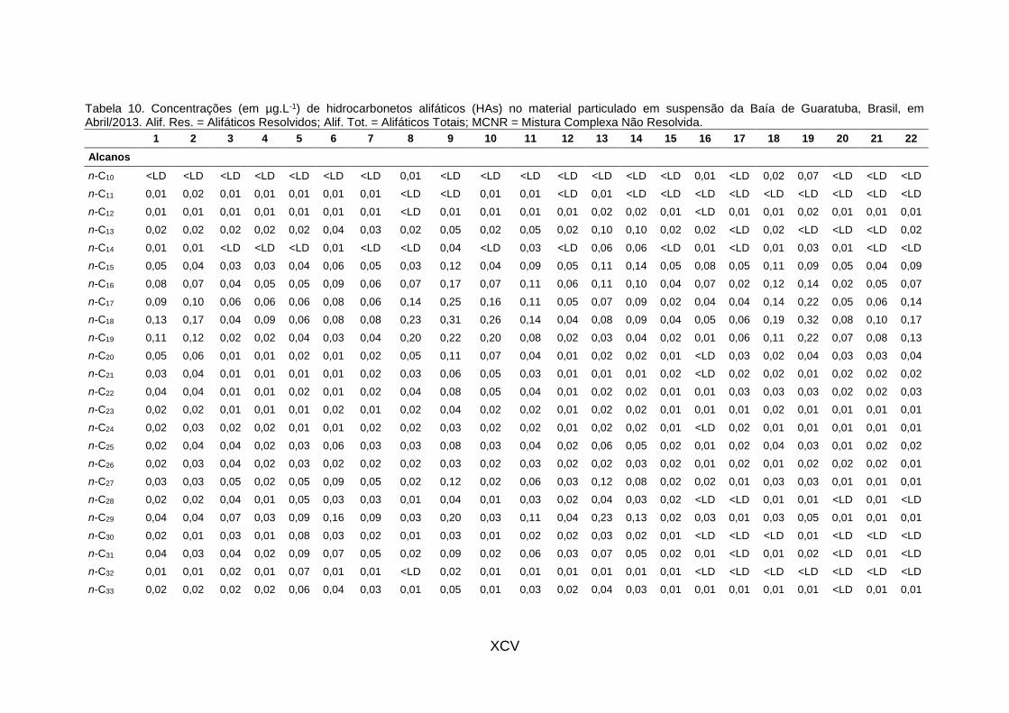
XCV

Tabela 10. Concentrações (em µg.L-1) de hidrocarbonetos alifáticos (HAs) no material particulado em suspensão da Baía de Guaratuba, Brasil, em Abril/2013. Alif. Res. = Alifáticos Resolvidos; Alif. Tot. = Alifáticos Totais; MCNR = Mistura Complexa Não Resolvida.

1 2 3 4 5 6 7 8 9 10 11 12 13 14 15 16 17 18 19 20 21 22

Alcanos

n-C10 <LD <LD <LD <LD <LD <LD <LD 0,01 <LD <LD <LD <LD <LD <LD <LD 0,01 <LD 0,02 0,07 <LD <LD <LD

n-C11 0,01 0,02 0,01 0,01 0,01 0,01 0,01 <LD <LD 0,01 0,01 <LD 0,01 <LD <LD <LD <LD <LD <LD <LD <LD <LD

n-C12 0,01 0,01 0,01 0,01 0,01 0,01 0,01 <LD 0,01 0,01 0,01 0,01 0,02 0,02 0,01 <LD 0,01 0,01 0,02 0,01 0,01 0,01

n-C13 0,02 0,02 0,02 0,02 0,02 0,04 0,03 0,02 0,05 0,02 0,05 0,02 0,10 0,10 0,02 0,02 <LD 0,02 <LD <LD <LD 0,02

n-C14 0,01 0,01 <LD <LD <LD 0,01 <LD <LD 0,04 <LD 0,03 <LD 0,06 0,06 <LD 0,01 <LD 0,01 0,03 0,01 <LD <LD

n-C15 0,05 0,04 0,03 0,03 0,04 0,06 0,05 0,03 0,12 0,04 0,09 0,05 0,11 0,14 0,05 0,08 0,05 0,11 0,09 0,05 0,04 0,09

n-C16 0,08 0,07 0,04 0,05 0,05 0,09 0,06 0,07 0,17 0,07 0,11 0,06 0,11 0,10 0,04 0,07 0,02 0,12 0,14 0,02 0,05 0,07

n-C17 0,09 0,10 0,06 0,06 0,06 0,08 0,06 0,14 0,25 0,16 0,11 0,05 0,07 0,09 0,02 0,04 0,04 0,14 0,22 0,05 0,06 0,14

n-C18 0,13 0,17 0,04 0,09 0,06 0,08 0,08 0,23 0,31 0,26 0,14 0,04 0,08 0,09 0,04 0,05 0,06 0,19 0,32 0,08 0,10 0,17

n-C19 0,11 0,12 0,02 0,02 0,04 0,03 0,04 0,20 0,22 0,20 0,08 0,02 0,03 0,04 0,02 0,01 0,06 0,11 0,22 0,07 0,08 0,13

n-C20 0,05 0,06 0,01 0,01 0,02 0,01 0,02 0,05 0,11 0,07 0,04 0,01 0,02 0,02 0,01 <LD 0,03 0,02 0,04 0,03 0,03 0,04

n-C21 0,03 0,04 0,01 0,01 0,01 0,01 0,02 0,03 0,06 0,05 0,03 0,01 0,01 0,01 0,02 <LD 0,02 0,02 0,01 0,02 0,02 0,02

n-C22 0,04 0,04 0,01 0,01 0,02 0,01 0,02 0,04 0,08 0,05 0,04 0,01 0,02 0,02 0,01 0,01 0,03 0,03 0,03 0,02 0,02 0,03

n-C23 0,02 0,02 0,01 0,01 0,01 0,02 0,01 0,02 0,04 0,02 0,02 0,01 0,02 0,02 0,01 0,01 0,01 0,02 0,01 0,01 0,01 0,01

n-C24 0,02 0,03 0,02 0,02 0,01 0,01 0,02 0,02 0,03 0,02 0,02 0,01 0,02 0,02 0,01 <LD 0,02 0,01 0,01 0,01 0,01 0,01

n-C25 0,02 0,04 0,04 0,02 0,03 0,06 0,03 0,03 0,08 0,03 0,04 0,02 0,06 0,05 0,02 0,01 0,02 0,04 0,03 0,01 0,02 0,02

n-C26 0,02 0,03 0,04 0,02 0,03 0,02 0,02 0,02 0,03 0,02 0,03 0,02 0,02 0,03 0,02 0,01 0,02 0,01 0,02 0,02 0,02 0,01

n-C27 0,03 0,03 0,05 0,02 0,05 0,09 0,05 0,02 0,12 0,02 0,06 0,03 0,12 0,08 0,02 0,02 0,01 0,03 0,03 0,01 0,01 0,01

n-C28 0,02 0,02 0,04 0,01 0,05 0,03 0,03 0,01 0,04 0,01 0,03 0,02 0,04 0,03 0,02 <LD <LD 0,01 0,01 <LD 0,01 <LD

n-C29 0,04 0,04 0,07 0,03 0,09 0,16 0,09 0,03 0,20 0,03 0,11 0,04 0,23 0,13 0,02 0,03 0,01 0,03 0,05 0,01 0,01 0,01

n-C30 0,02 0,01 0,03 0,01 0,08 0,03 0,02 0,01 0,03 0,01 0,02 0,02 0,03 0,02 0,01 <LD <LD <LD 0,01 <LD <LD <LD

n-C31 0,04 0,03 0,04 0,02 0,09 0,07 0,05 0,02 0,09 0,02 0,06 0,03 0,07 0,05 0,02 0,01 <LD 0,01 0,02 <LD 0,01 <LD

n-C32 0,01 0,01 0,02 0,01 0,07 0,01 0,01 <LD 0,02 0,01 0,01 0,01 0,01 0,01 0,01 <LD <LD <LD <LD <LD <LD <LD

n-C33 0,02 0,02 0,02 0,02 0,06 0,04 0,03 0,01 0,05 0,01 0,03 0,02 0,04 0,03 0,01 0,01 0,01 0,01 0,01 <LD 0,01 0,01

XCVI

n-C34 0,01 <LD 0,02 0,01 0,03 0,02 0,02 0,01 0,02 <LD 0,02 0,01 0,01 0,02 <LD <LD <LD <LD <LD <LD <LD <LD

n-C35 0,02 0,02 0,02 0,02 0,02 0,02 0,02 <LD 0,03 <LD 0,02 <LD 0,02 0,02 <LD <LD <LD <LD <LD <LD <LD <LD

n-C36 <LD <LD <LD <LD <LD <LD <LD <LD <LD <LD <LD <LD <LD <LD <LD <LD <LD <LD <LD <LD <LD <LD

n-C37 <LD <LD <LD <LD <LD <LD <LD <LD <LD <LD <LD <LD <LD <LD <LD <LD <LD <LD <LD <LD <LD <LD

n-C38 <LD <LD <LD <LD <LD <LD <LD <LD <LD <LD <LD <LD <LD <LD <LD <LD <LD <LD <LD <LD <LD <LD

n-C39 <LD <LD <LD <LD <LD <LD <LD <LD <LD <LD <LD <LD <LD <LD <LD <LD <LD <LD <LD <LD <LD <LD

n-C40 <LD <LD <LD <LD <LD <LD <LD <LD <LD <LD <LD <LD <LD <LD <LD <LD <LD <LD <LD <LD <LD <LD

Pristano 0,06 0,06 0,05 0,03 0,04 0,05 0,04 0,07 0,14 0,09 0,06 0,03 0,04 0,05 0,01 0,02 0,02 0,07 0,11 0,03 0,03 0,08

Fitano 0,08 0,09 0,03 0,04 0,04 0,03 0,04 0,15 0,17 0,14 0,07 0,03 0,04 0,05 0,02 0,02 0,04 0,09 0,19 0,04 0,05 0,09

Somas

Alif. Res. 3,18 3,69 2,22 2,74 3,13 3,26 2,48 3,51 5,85 4,04 3,96 2,27 2,52 2,77 3,02 3,27 3,52 3,77 4,02 4,27 4,52 4,77

Alif. Tot. 8,62 15,64 7,25 8,01 9,07 9,14 10,14 19,39 34,84 21,18 16,19 7,30 7,55 7,80 8,05 8,30 8,55 8,80 9,05 9,30 9,55 9,80

MCNR 5,44 11,95 5,03 5,26 5,94 5,87 7,66 15,87 28,99 17,14 12,23 5,04 5,04 5,04 5,04 5,04 5,04 5,04 5,04 5,04 5,04 5,04

<LD = abaixo do limite de detecção do método (0,004 µg.L-1).

XCVII

Tabela 11. Concentrações (em µg.L-1) de hidrocarbonetos alifáticos (HAs) no material particulado em suspensão da Baía de Guaratuba, Brasil, em Agosto/2013. Alif. Res. = Alifáticos Resolvidos; Alif. Tot. = Alifáticos Totais; MCNR = Mistura Complexa Não Resolvida.

1 2 3 4 5 6 7 8 9 10 11 12 13 14 15 16 17 18 19 20 21 22

Alcanos

n-C10 <LD <LD <LD <LD <LD <LD <LD <LD <LD <LD <LD <LD 0,03 <LD <LD <LD <LD <LD <LD 0,03 <LD 0,02

n-C11 0,03 0,01 0,01 <LD 0,01 0,02 0,01 <LD 0,01 0,01 0,01 0,01 0,01 0,02 0,02 0,01 0,01 0,01 0,02 <LD <LD 0,01

n-C12 0,02 0,01 0,01 0,01 0,02 0,04 0,02 0,01 0,03 0,01 0,01 0,01 0,01 0,03 0,03 0,02 0,02 0,02 0,02 0,01 0,02 0,01

n-C13 0,02 0,02 0,02 0,02 0,02 0,03 0,02 0,02 0,02 0,02 <LD 0,02 0,02 0,02 0,02 0,02 0,02 0,02 0,02 <LD 0,02 0,02

n-C14 <LD <LD <LD <LD <LD 0,01 <LD <LD <LD <LD <LD <LD 0,01 <LD <LD <LD <LD <LD <LD 0,01 <LD 0,02

n-C15 0,02 0,02 0,02 0,01 0,02 0,04 0,02 0,02 0,03 0,02 0,02 0,02 0,03 0,04 0,02 0,02 0,02 0,02 0,02 0,03 0,01 0,04

n-C16 0,03 0,02 0,02 0,03 0,03 0,06 0,03 0,03 0,04 0,03 0,03 0,03 0,05 0,04 0,02 0,02 0,02 0,03 0,04 0,03 0,01 0,09

n-C17 0,05 0,05 0,08 0,17 0,17 0,19 0,23 0,31 0,27 0,16 0,30 0,26 0,25 0,22 0,03 0,17 0,04 0,09 0,10 0,07 0,02 0,19

n-C18 0,05 0,04 0,04 0,06 0,08 0,09 0,09 0,15 0,07 0,15 0,08 0,09 0,09 0,07 0,02 0,04 0,04 0,06 0,04 0,05 0,03 0,22

n-C19 0,03 0,02 0,05 0,10 0,09 0,07 0,10 0,25 0,11 0,21 0,12 0,15 0,10 0,08 0,01 0,07 0,02 0,07 0,05 0,04 0,02 0,13

n-C20 0,01 0,01 <LD 0,01 0,01 <LD 0,01 0,06 0,02 0,05 0,01 0,02 0,02 0,01 <LD 0,01 <LD <LD <LD 0,01 0,01 0,03

n-C21 0,01 0,01 <LD 0,01 0,01 0,01 0,01 0,03 0,01 0,03 0,01 0,01 0,01 0,01 <LD 0,01 <LD 0,01 0,01 0,01 0,01 0,02

n-C22 0,01 0,01 <LD 0,01 0,01 0,01 0,01 0,04 0,01 0,03 0,01 0,01 0,01 0,01 <LD 0,01 <LD <LD <LD <LD 0,01 0,02

n-C23 <LD 0,01 <LD <LD 0,01 0,01 <LD 0,01 0,01 0,01 0,01 <LD 0,01 0,01 <LD 0,01 <LD 0,01 0,01 <LD <LD 0,01

n-C24 0,01 0,01 <LD 0,01 <LD 0,01 <LD 0,01 <LD 0,01 0,01 0,01 0,01 0,01 <LD <LD <LD 0,01 0,01 <LD <LD 0,01

n-C25 0,01 0,01 0,01 0,01 0,01 0,04 0,01 0,01 0,02 0,01 0,02 0,01 0,02 0,02 0,01 0,01 0,01 0,01 0,02 0,01 0,01 0,02

n-C26 0,01 0,02 0,01 0,01 0,01 0,01 <LD 0,01 0,01 <LD 0,01 0,01 0,01 0,01 0,01 <LD <LD 0,01 0,01 0,01 0,01 0,02

n-C27 0,01 0,04 0,01 0,01 0,01 0,06 0,01 0,01 0,03 <LD 0,03 0,01 0,03 0,03 0,01 0,01 0,01 0,02 0,02 0,01 <LD 0,02

n-C28 <LD 0,06 <LD <LD <LD 0,01 <LD <LD 0,01 <LD <LD <LD 0,01 <LD <LD <LD <LD <LD 0,01 <LD <LD 0,01

n-C29 0,01 0,12 0,01 0,01 0,02 0,11 0,02 0,02 0,07 0,01 0,05 0,01 0,05 0,05 0,01 0,02 0,01 0,02 0,04 0,01 <LD 0,03

n-C30 <LD 0,16 <LD <LD <LD 0,01 <LD <LD <LD <LD <LD <LD <LD <LD <LD <LD <LD <LD <LD <LD <LD <LD

n-C31 <LD 0,20 0,01 <LD 0,01 0,04 0,01 0,01 0,03 <LD 0,02 0,01 0,01 0,02 0,01 <LD <LD 0,01 0,02 <LD <LD 0,01

n-C32 <LD 0,17 <LD <LD <LD <LD <LD <LD <LD <LD <LD <LD <LD <LD <LD <LD <LD <LD <LD <LD <LD <LD

n-C33 <LD <LD 0,01 0,01 0,01 0,03 0,01 0,01 0,02 0,01 0,01 0,01 <LD 0,01 0,01 0,01 0,01 0,01 0,02 0,01 <LD 0,01

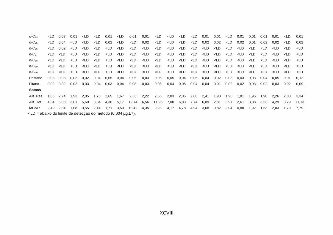
XCVIII

n-C34 <LD 0,07 0,01 <LD <LD 0,01 <LD 0,01 0,01 <LD <LD <LD <LD 0,01 0,01 <LD 0,01 0,01 0,01 0,01 <LD 0,01

n-C35 <LD 0,04 <LD <LD <LD 0,02 <LD <LD 0,02 <LD <LD <LD <LD 0,02 0,02 <LD 0,02 0,01 0,02 0,02 <LD 0,02

n-C36 <LD 0,02 <LD <LD <LD <LD <LD <LD <LD <LD <LD <LD <LD <LD <LD <LD <LD <LD <LD <LD <LD <LD

n-C37 <LD <LD <LD <LD <LD <LD <LD <LD <LD <LD <LD <LD <LD <LD <LD <LD <LD <LD <LD <LD <LD <LD

n-C38 <LD <LD <LD <LD <LD <LD <LD <LD <LD <LD <LD <LD <LD <LD <LD <LD <LD <LD <LD <LD <LD <LD

n-C39 <LD <LD <LD <LD <LD <LD <LD <LD <LD <LD <LD <LD <LD <LD <LD <LD <LD <LD <LD <LD <LD <LD

n-C40 <LD <LD <LD <LD <LD <LD <LD <LD <LD <LD <LD <LD <LD <LD <LD <LD <LD <LD <LD <LD <LD <LD

Pristano 0,03 0,03 0,02 0,02 0,04 0,05 0,04 0,05 0,03 0,05 0,05 0,04 0,05 0,04 0,02 0,03 0,03 0,03 0,04 0,05 0,01 0,12

Fitano 0,02 0,02 0,02 0,03 0,04 0,03 0,04 0,08 0,03 0,08 0,04 0,05 0,04 0,04 0,01 0,02 0,02 0,03 0,02 0,03 0,02 0,09

Somas

Alif. Res. 1,86 2,74 1,93 2,05 1,70 2,65 1,67 2,33 2,22 2,66 2,83 2,05 2,80 2,41 1,98 1,93 1,81 1,95 1,90 2,26 2,00 3,34

Alif. Tot. 4,34 5,08 3,01 5,60 3,84 4,36 5,17 12,74 6,56 11,95 7,00 6,83 7,74 6,09 2,81 3,97 2,61 3,88 3,53 4,29 3,79 11,13

MCNR 2,49 2,34 1,08 3,55 2,14 1,71 3,50 10,42 4,35 9,28 4,17 4,78 4,94 3,68 0,82 2,04 0,80 1,92 1,63 2,03 1,79 7,79

<LD = abaixo do limite de detecção do método (0,004 µg.L-1).

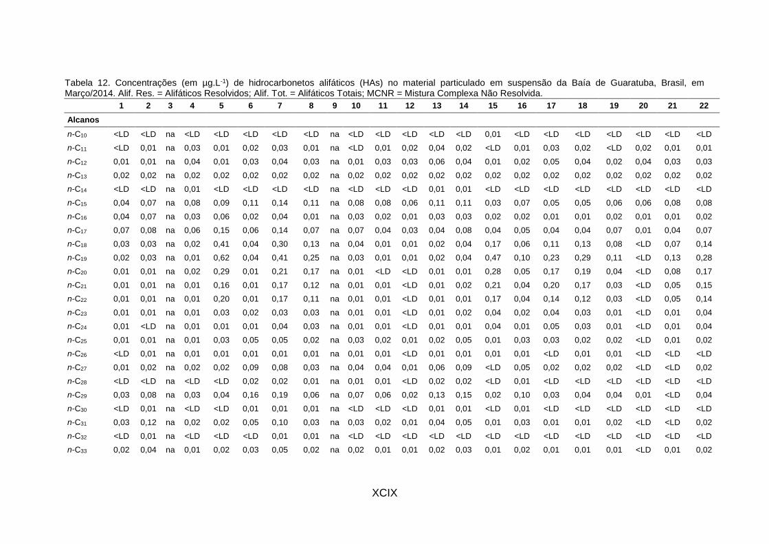
XCIX

Tabela 12. Concentrações (em µg.L-1) de hidrocarbonetos alifáticos (HAs) no material particulado em suspensão da Baía de Guaratuba, Brasil, em Março/2014. Alif. Res. = Alifáticos Resolvidos; Alif. Tot. = Alifáticos Totais; MCNR = Mistura Complexa Não Resolvida.

1 2 3 4 5 6 7 8 9 10 11 12 13 14 15 16 17 18 19 20 21 22

Alcanos

n-C10 <LD <LD na <LD <LD <LD <LD <LD na <LD <LD <LD <LD <LD 0,01 <LD <LD <LD <LD <LD <LD <LD

n-C11 <LD 0,01 na 0,03 0,01 0,02 0,03 0,01 na <LD 0,01 0,02 0,04 0,02 <LD 0,01 0,03 0,02 <LD 0,02 0,01 0,01

n-C12 0,01 0,01 na 0,04 0,01 0,03 0,04 0,03 na 0,01 0,03 0,03 0,06 0,04 0,01 0,02 0,05 0,04 0,02 0,04 0,03 0,03

n-C13 0,02 0,02 na 0,02 0,02 0,02 0,02 0,02 na 0,02 0,02 0,02 0,02 0,02 0,02 0,02 0,02 0,02 0,02 0,02 0,02 0,02

n-C14 <LD <LD na 0,01 <LD <LD <LD <LD na <LD <LD <LD 0,01 0,01 <LD <LD <LD <LD <LD <LD <LD <LD

n-C15 0,04 0,07 na 0,08 0,09 0,11 0,14 0,11 na 0,08 0,08 0,06 0,11 0,11 0,03 0,07 0,05 0,05 0,06 0,06 0,08 0,08

n-C16 0,04 0,07 na 0,03 0,06 0,02 0,04 0,01 na 0,03 0,02 0,01 0,03 0,03 0,02 0,02 0,01 0,01 0,02 0,01 0,01 0,02

n-C17 0,07 0,08 na 0,06 0,15 0,06 0,14 0,07 na 0,07 0,04 0,03 0,04 0,08 0,04 0,05 0,04 0,04 0,07 0,01 0,04 0,07

n-C18 0,03 0,03 na 0,02 0,41 0,04 0,30 0,13 na 0,04 0,01 0,01 0,02 0,04 0,17 0,06 0,11 0,13 0,08 <LD 0,07 0,14

n-C19 0,02 0,03 na 0,01 0,62 0,04 0,41 0,25 na 0,03 0,01 0,01 0,02 0,04 0,47 0,10 0,23 0,29 0,11 <LD 0,13 0,28

n-C20 0,01 0,01 na 0,02 0,29 0,01 0,21 0,17 na 0,01 <LD <LD 0,01 0,01 0,28 0,05 0,17 0,19 0,04 <LD 0,08 0,17

n-C21 0,01 0,01 na 0,01 0,16 0,01 0,17 0,12 na 0,01 0,01 <LD 0,01 0,02 0,21 0,04 0,20 0,17 0,03 <LD 0,05 0,15

n-C22 0,01 0,01 na 0,01 0,20 0,01 0,17 0,11 na 0,01 0,01 <LD 0,01 0,01 0,17 0,04 0,14 0,12 0,03 <LD 0,05 0,14

n-C23 0,01 0,01 na 0,01 0,03 0,02 0,03 0,03 na 0,01 0,01 <LD 0,01 0,02 0,04 0,02 0,04 0,03 0,01 <LD 0,01 0,04

n-C24 0,01 <LD na 0,01 0,01 0,01 0,04 0,03 na 0,01 0,01 <LD 0,01 0,01 0,04 0,01 0,05 0,03 0,01 <LD 0,01 0,04

n-C25 0,01 0,01 na 0,01 0,03 0,05 0,05 0,02 na 0,03 0,02 0,01 0,02 0,05 0,01 0,03 0,03 0,02 0,02 <LD 0,01 0,02

n-C26 <LD 0,01 na 0,01 0,01 0,01 0,01 0,01 na 0,01 0,01 <LD 0,01 0,01 0,01 0,01 <LD 0,01 0,01 <LD <LD <LD

n-C27 0,01 0,02 na 0,02 0,02 0,09 0,08 0,03 na 0,04 0,04 0,01 0,06 0,09 <LD 0,05 0,02 0,02 0,02 <LD <LD 0,02

n-C28 <LD <LD na <LD <LD 0,02 0,02 0,01 na 0,01 0,01 <LD 0,02 0,02 <LD 0,01 <LD <LD <LD <LD <LD <LD

n-C29 0,03 0,08 na 0,03 0,04 0,16 0,19 0,06 na 0,07 0,06 0,02 0,13 0,15 0,02 0,10 0,03 0,04 0,04 0,01 <LD 0,04

n-C30 <LD 0,01 na <LD <LD 0,01 0,01 0,01 na <LD <LD <LD 0,01 0,01 <LD 0,01 <LD <LD <LD <LD <LD <LD

n-C31 0,03 0,12 na 0,02 0,02 0,05 0,10 0,03 na 0,03 0,02 0,01 0,04 0,05 0,01 0,03 0,01 0,01 0,02 <LD <LD 0,02

n-C32 <LD 0,01 na <LD <LD <LD 0,01 0,01 na <LD <LD <LD <LD <LD <LD <LD <LD <LD <LD <LD <LD <LD

n-C33 0,02 0,04 na 0,01 0,02 0,03 0,05 0,02 na 0,02 0,01 0,01 0,02 0,03 0,01 0,02 0,01 0,01 0,01 <LD 0,01 0,02

C

n-C34 0,01 <LD na <LD 0,01 0,01 0,01 0,01 na 0,01 0,01 <LD 0,01 0,01 <LD 0,01 0,01 0,01 <LD <LD <LD 0,01

n-C35 0,02 <LD na <LD 0,02 0,02 0,02 0,02 na 0,02 0,02 <LD <LD 0,02 <LD 0,02 0,02 0,02 0,02 <LD <LD 0,02

n-C36 <LD <LD na <LD <LD <LD <LD <LD na <LD <LD <LD <LD <LD <LD <LD <LD <LD <LD <LD <LD <LD

n-C37 <LD <LD na <LD <LD <LD <LD <LD na <LD <LD <LD <LD <LD <LD <LD <LD <LD <LD <LD <LD <LD

n-C38 <LD <LD na <LD <LD <LD <LD <LD na <LD <LD <LD <LD <LD <LD <LD <LD <LD <LD <LD <LD <LD

n-C39 <LD <LD na <LD <LD <LD <LD <LD na <LD <LD <LD <LD <LD <LD <LD <LD <LD <LD <LD <LD <LD

n-C40 <LD <LD na <LD <LD <LD <LD <LD na <LD <LD <LD <LD <LD <LD <LD <LD <LD <LD <LD <LD <LD

Pristano 0,02 0,05 na 0,03 0,08 0,05 0,11 0,03 na 0,05 0,02 0,01 0,03 0,04 0,02 0,03 0,02 0,03 0,04 0,01 0,03 0,04

Fitano 0,02 0,02 na 0,01 0,17 0,03 0,17 0,06 na 0,03 0,01 0,01 0,02 0,03 0,10 0,04 0,05 0,07 0,05 0,01 0,04 0,07

Somas

Alif. Res. 2,42 2,44 na 2,37 3,32 2,91 4,92 3,10 na 2,42 2,08 2,21 2,77 2,85 3,21 2,62 3,20 3,29 2,97 2,46 2,17 3,30

Alif. Tot. 2,49 5,44 na 2,37 39,88 7,47 32,29 19,59 na 5,36 2,08 3,22 5,56 8,46 33,13 9,55 23,35 22,07 10,46 4,14 12,06 24,77

MCNR 0,07 3,00 na <LD 36,56 4,56 27,37 16,48 na 2,95 <LD 1,01 2,79 5,62 29,92 6,93 20,15 18,79 7,48 1,68 9,90 21,47

<LD = abaixo do limite de detecção do método (0,004 µg.L-1). na = não analisada Obs. 1: a amostra 3 não pode ser analisada. Obs. 2: a amostra 9 não pode ser coletada.

CI

Tabela 13. Concentrações (em µg.g-1) de hidrocarbonetos alifáticos (HAs) no material particulado em suspensão da Baía de Guaratuba, Brasil, em Abril/2013. Alif. Res. = Alifáticos Resolvidos; Alif. Tot. = Alifáticos Totais; MCNR = Mistura Complexa Não Resolvida.

1 2 3 4 5 6 7 8 9 10 11 12 13 14 15 16 17 18 19 20 21 22

Alcanos

n-C10 <LD <LD <LD <LD <LD <LD <LD 0,31 <LD <LD <LD <LD <LD <LD <LD 0,36 <LD 0,45 1,58 <LD <LD <LD

n-C11 0,84 1,19 0,50 0,51 0,31 0,08 0,16 0,16 <LD 0,30 0,22 0,12 0,09 <LD <LD <LD <LD 0,10 <LD <LD <LD <LD

n-C12 0,59 0,82 0,44 0,37 0,31 0,13 0,29 <LD 0,09 0,27 0,20 0,27 0,33 0,20 0,22 <LD 0,19 0,22 0,39 0,22 0,25 0,16

n-C13 2,01 1,71 1,31 0,93 0,80 0,56 0,79 0,78 0,63 0,63 1,14 0,58 1,81 1,31 0,57 0,58 <LD 0,52 <LD <LD <LD 0,38

n-C14 0,84 0,52 <LD <LD <LD 0,16 <LD <LD 0,50 <LD 0,67 <LD 1,01 0,73 <LD 0,31 <LD 0,30 0,75 0,17 <LD <LD

n-C15 3,94 2,97 2,05 1,45 1,56 0,99 1,65 1,20 1,41 1,05 2,31 1,43 1,92 1,79 1,50 2,12 1,29 2,62 2,23 1,23 1,34 2,01

n-C16 6,61 4,83 2,61 2,15 2,02 1,48 1,94 2,68 2,01 2,23 2,78 1,85 1,94 1,24 1,15 2,06 0,47 2,97 3,40 0,52 1,62 1,65

n-C17 7,70 7,58 3,48 2,71 2,33 1,21 2,00 5,28 2,88 4,75 2,75 1,46 1,28 1,13 0,76 1,03 1,10 3,39 5,31 1,21 1,84 3,19

n-C18 10,80 12,41 2,24 4,20 2,10 1,31 2,61 8,93 3,64 7,67 3,45 1,09 1,48 1,10 1,18 1,31 1,68 4,67 7,64 1,90 3,12 3,77

n-C19 8,96 8,84 1,06 1,03 1,68 0,45 1,24 7,57 2,59 5,89 1,91 0,70 0,58 0,47 0,73 0,31 1,54 2,72 5,34 1,80 2,48 2,86

n-C20 4,35 4,24 0,68 0,61 0,92 0,11 0,76 2,02 1,29 2,07 1,04 0,30 0,27 0,22 0,45 <LD 0,93 0,57 0,90 0,81 0,86 0,78

n-C21 2,34 2,97 0,44 0,37 0,34 0,13 0,54 1,20 0,74 1,38 0,67 0,24 0,20 0,16 0,51 0,11 0,49 0,37 0,32 0,37 0,64 0,42

n-C22 3,27 3,20 0,68 0,61 0,61 0,14 0,70 1,51 0,93 1,50 0,92 0,33 0,29 0,24 0,41 0,14 0,69 0,62 0,63 0,57 0,73 0,74

n-C23 1,26 1,63 0,81 0,56 0,31 0,32 0,45 0,66 0,46 0,51 0,50 0,36 0,35 0,29 0,29 0,14 0,30 0,45 0,27 0,20 0,38 0,20

n-C24 1,42 2,15 1,24 0,70 0,50 0,19 0,57 0,74 0,36 0,63 0,55 0,40 0,27 0,24 0,41 0,11 0,41 0,32 0,32 0,25 0,45 0,27

n-C25 1,84 3,20 2,18 1,07 0,95 0,94 1,05 1,05 0,96 0,81 1,09 0,70 1,04 0,67 0,60 0,36 0,47 0,90 0,61 0,27 0,67 0,38

n-C26 1,84 2,15 2,36 0,98 1,18 0,30 0,73 0,62 0,29 0,48 0,72 0,64 0,42 0,33 0,67 0,31 0,41 0,22 0,44 0,47 0,57 0,18

n-C27 2,43 2,45 3,05 1,03 1,87 1,39 1,56 0,93 1,35 0,63 1,59 0,88 2,21 0,98 0,60 0,53 0,25 0,85 0,80 0,17 0,41 0,18

n-C28 1,67 1,49 2,24 0,51 1,95 0,49 0,86 0,47 0,47 0,30 0,74 0,64 0,69 0,41 0,48 0,11 <LD 0,12 0,17 <LD 0,25 <LD

n-C29 3,68 3,12 4,10 1,40 3,55 2,60 2,77 1,24 2,39 0,84 2,68 1,34 4,24 1,61 0,73 0,86 0,22 0,85 1,16 0,22 0,35 0,20

n-C30 1,42 0,89 1,74 0,42 3,05 0,40 0,76 0,35 0,36 0,24 0,57 0,49 0,48 0,29 0,35 <LD <LD <LD 0,15 <LD <LD <LD

n-C31 2,93 2,08 2,61 0,93 3,55 1,05 1,56 0,58 1,04 0,45 1,36 0,76 1,26 0,65 0,48 0,19 0,11 0,35 0,44 <LD 0,19 0,09

n-C32 0,75 0,37 0,93 0,28 2,63 0,16 0,41 0,16 0,18 0,18 0,30 0,33 0,20 0,16 0,29 <LD <LD <LD <LD <LD <LD <LD

n-C33 1,93 1,56 1,49 0,75 2,21 0,59 0,89 0,50 0,57 0,42 0,77 0,52 0,64 0,42 0,41 0,25 0,22 0,25 0,34 <LD 0,25 0,18

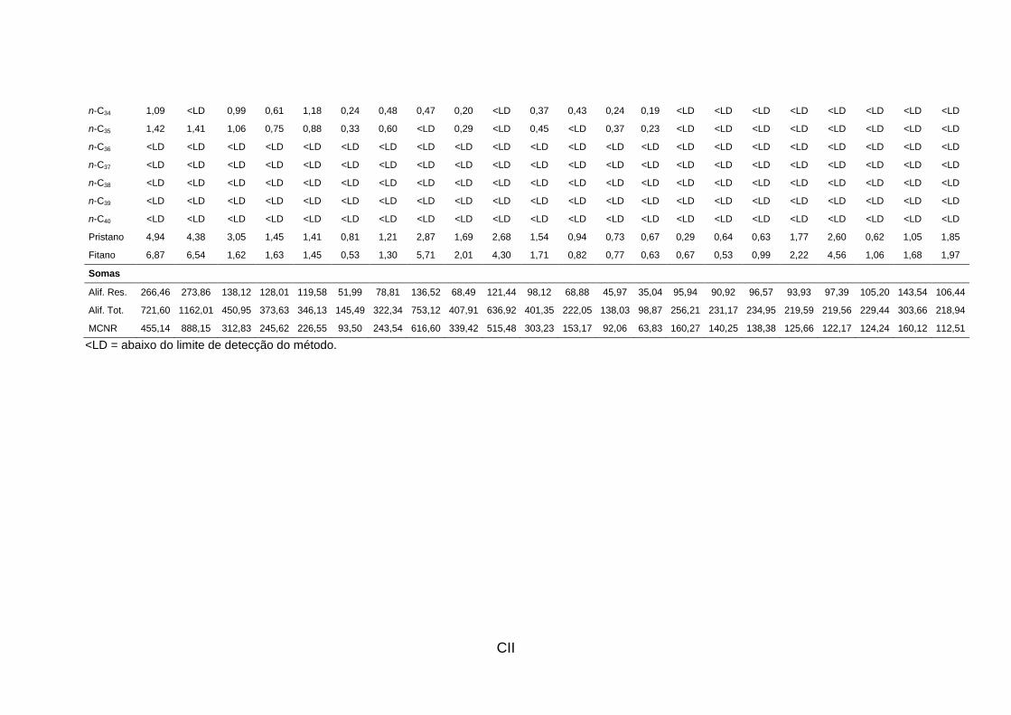
CII

n-C34 1,09 <LD 0,99 0,61 1,18 0,24 0,48 0,47 0,20 <LD 0,37 0,43 0,24 0,19 <LD <LD <LD <LD <LD <LD <LD <LD

n-C35 1,42 1,41 1,06 0,75 0,88 0,33 0,60 <LD 0,29 <LD 0,45 <LD 0,37 0,23 <LD <LD <LD <LD <LD <LD <LD <LD

n-C36 <LD <LD <LD <LD <LD <LD <LD <LD <LD <LD <LD <LD <LD <LD <LD <LD <LD <LD <LD <LD <LD <LD

n-C37 <LD <LD <LD <LD <LD <LD <LD <LD <LD <LD <LD <LD <LD <LD <LD <LD <LD <LD <LD <LD <LD <LD

n-C38 <LD <LD <LD <LD <LD <LD <LD <LD <LD <LD <LD <LD <LD <LD <LD <LD <LD <LD <LD <LD <LD <LD

n-C39 <LD <LD <LD <LD <LD <LD <LD <LD <LD <LD <LD <LD <LD <LD <LD <LD <LD <LD <LD <LD <LD <LD

n-C40 <LD <LD <LD <LD <LD <LD <LD <LD <LD <LD <LD <LD <LD <LD <LD <LD <LD <LD <LD <LD <LD <LD

Pristano 4,94 4,38 3,05 1,45 1,41 0,81 1,21 2,87 1,69 2,68 1,54 0,94 0,73 0,67 0,29 0,64 0,63 1,77 2,60 0,62 1,05 1,85

Fitano 6,87 6,54 1,62 1,63 1,45 0,53 1,30 5,71 2,01 4,30 1,71 0,82 0,77 0,63 0,67 0,53 0,99 2,22 4,56 1,06 1,68 1,97

Somas

Alif. Res. 266,46 273,86 138,12 128,01 119,58 51,99 78,81 136,52 68,49 121,44 98,12 68,88 45,97 35,04 95,94 90,92 96,57 93,93 97,39 105,20 143,54 106,44

Alif. Tot. 721,60 1162,01 450,95 373,63 346,13 145,49 322,34 753,12 407,91 636,92 401,35 222,05 138,03 98,87 256,21 231,17 234,95 219,59 219,56 229,44 303,66 218,94

MCNR 455,14 888,15 312,83 245,62 226,55 93,50 243,54 616,60 339,42 515,48 303,23 153,17 92,06 63,83 160,27 140,25 138,38 125,66 122,17 124,24 160,12 112,51

<LD = abaixo do limite de detecção do método.

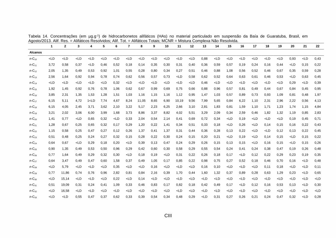
CIII

Tabela 14. Concentrações (em µg.g-1) de hidrocarbonetos alifáticos (HAs) no material particulado em suspensão da Baía de Guaratuba, Brasil, em Agosto/2013. Alif. Res. = Alifáticos Resolvidos; Alif. Tot. = Alifáticos Totais; MCNR = Mistura Complexa Não Resolvida.

1 2 3 4 5 6 7 8 9 10 11 12 13 14 15 16 17 18 19 20 21 22

Alcanos

n-C10 <LD <LD <LD <LD <LD <LD <LD <LD <LD <LD <LD <LD 0,88 <LD <LD <LD <LD <LD <LD 0,93 <LD 0,43

n-C11 3,72 0,58 0,37 <LD 0,46 0,52 0,18 0,14 0,35 0,30 0,31 0,40 0,36 0,59 0,57 0,19 0,24 0,16 0,44 <LD 0,15 0,22

n-C12 2,05 1,35 0,49 0,53 0,92 1,01 0,55 0,28 0,80 0,34 0,27 0,51 0,46 0,88 1,08 0,56 0,52 0,46 0,67 0,35 0,59 0,28

n-C13 2,56 1,64 0,92 0,94 0,78 0,74 0,62 0,56 0,57 0,73 <LD 0,58 0,62 0,52 0,64 0,63 0,61 0,46 0,53 <LD 0,63 0,45

n-C14 <LD <LD <LD <LD <LD 0,32 <LD <LD <LD <LD <LD <LD 0,46 <LD <LD <LD <LD <LD <LD 0,29 <LD 0,39

n-C15 1,92 1,45 0,92 0,76 0,78 1,06 0,62 0,67 0,99 0,69 0,75 0,66 0,88 0,96 0,57 0,81 0,49 0,44 0,67 0,84 0,45 0,95

n-C16 3,85 2,31 1,35 1,53 1,28 1,51 1,03 1,16 1,15 1,16 1,12 0,95 1,47 1,03 0,57 0,89 0,73 0,93 1,09 0,81 0,48 1,97

n-C17 6,15 5,11 4,72 1<LD 7,74 4,67 8,24 11,05 8,65 6,90 10,19 9,56 7,99 5,65 0,84 6,22 1,10 2,31 2,96 2,22 0,56 4,13

n-C18 6,15 4,05 2,45 3,71 3,62 2,10 3,22 5,17 2,23 6,25 2,66 3,10 2,81 1,83 0,81 1,59 1,10 1,71 1,23 1,74 1,15 4,84

n-C19 3,21 2,02 3,06 6,00 3,99 1,68 3,73 8,86 3,37 8,82 4,02 5,51 3,29 2,09 0,34 2,59 0,46 1,82 1,32 1,19 0,85 2,83

n-C20 1,41 0,77 <LD 0,65 0,32 <LD 0,33 2,04 0,54 2,14 0,41 0,69 0,72 0,34 <LD 0,19 <LD <LD <LD 0,19 0,45 0,71

n-C21 1,28 0,67 0,25 0,65 0,32 0,17 0,29 1,20 0,22 1,41 0,34 0,51 0,33 0,18 <LD 0,26 <LD 0,14 0,15 0,16 0,22 0,43

n-C22 1,15 0,58 0,25 0,47 0,27 0,12 0,26 1,37 0,41 1,37 0,31 0,44 0,36 0,28 0,13 0,22 <LD <LD 0,12 0,13 0,22 0,45

n-C23 0,51 0,48 0,25 0,24 0,27 0,32 0,15 0,28 0,22 0,30 0,24 0,15 0,20 0,21 <LD 0,19 <LD 0,14 0,15 <LD 0,15 0,22

n-C24 0,64 0,67 <LD 0,29 0,18 0,20 <LD 0,39 0,13 0,47 0,24 0,29 0,26 0,15 0,13 0,15 <LD 0,16 0,15 <LD 0,15 0,26

n-C25 0,90 1,35 0,49 0,53 0,50 0,96 0,29 0,42 0,60 0,30 0,58 0,29 0,55 0,54 0,24 0,41 0,24 0,38 0,47 0,19 0,26 0,48

n-C26 0,77 1,64 0,49 0,29 0,32 0,30 <LD 0,18 0,19 <LD 0,31 0,22 0,26 0,18 0,17 <LD 0,12 0,22 0,29 0,23 0,19 0,35

n-C27 0,64 3,47 0,49 0,47 0,60 1,58 0,37 0,49 1,05 0,17 0,85 0,22 0,98 0,75 0,27 0,52 0,18 0,46 0,70 0,16 <LD 0,48

n-C28 <LD 5,79 <LD <LD <LD 0,35 <LD <LD 0,16 <LD <LD <LD 0,16 0,10 <LD <LD <LD 0,11 0,18 <LD <LD 0,11

n-C29 0,77 11,86 0,74 0,76 0,96 2,82 0,81 0,84 2,16 0,39 1,70 0,44 1,60 1,32 0,37 0,89 0,28 0,63 1,29 0,23 <LD 0,65

n-C30 <LD 15,14 <LD <LD <LD 0,22 <LD 0,14 <LD <LD <LD <LD <LD <LD <LD <LD <LD <LD <LD <LD <LD <LD

n-C31 0,51 19,09 0,31 0,24 0,41 1,09 0,33 0,46 0,83 0,17 0,82 0,18 0,42 0,49 0,17 <LD 0,12 0,16 0,53 0,13 <LD 0,30

n-C32 <LD 16,58 <LD <LD <LD <LD <LD <LD <LD <LD <LD <LD <LD <LD <LD <LD <LD <LD <LD <LD <LD <LD

n-C33 <LD <LD 0,55 0,47 0,37 0,62 0,33 0,39 0,54 0,34 0,48 0,29 <LD 0,31 0,27 0,26 0,21 0,24 0,47 0,32 <LD 0,28

CIV

n-C34 <LD 6,94 0,74 <LD <LD 0,27 <LD 0,46 0,35 <LD <LD <LD <LD 0,28 0,37 <LD 0,37 0,30 0,38 0,39 <LD 0,26

n-C35 <LD 3,47 <LD <LD <LD 0,42 <LD <LD 0,51 <LD <LD <LD <LD 0,41 0,50 <LD 0,49 0,38 0,50 0,52 <LD 0,39

n-C36 <LD 2,02 <LD <LD <LD <LD <LD <LD <LD <LD <LD <LD <LD <LD <LD <LD <LD <LD <LD <LD <LD <LD

n-C37 <LD <LD <LD <LD <LD <LD <LD <LD <LD <LD <LD <LD <LD <LD <LD <LD <LD <LD <LD <LD <LD <LD

n-C38 <LD <LD <LD <LD <LD <LD <LD <LD <LD <LD <LD <LD <LD <LD <LD <LD <LD <LD <LD <LD <LD <LD

n-C39 <LD <LD <LD <LD <LD <LD <LD <LD <LD <LD <LD <LD <LD <LD <LD <LD <LD <LD <LD <LD <LD <LD

n-C40 <LD <LD <LD <LD <LD <LD <LD <LD <LD <LD <LD <LD <LD <LD <LD <LD <LD <LD <LD <LD <LD <LD

Pristano 3,97 2,51 1,35 1,35 1,83 1,21 1,54 1,72 0,99 2,01 1,64 1,31 1,57 0,93 0,71 1,15 0,80 0,90 1,06 1,45 0,52 2,49

Fitano 2,82 2,02 1,04 1,76 1,60 0,84 1,57 2,78 1,05 3,56 1,30 1,68 1,44 0,90 0,40 0,81 0,49 0,71 0,50 0,81 0,59 1,95

Somas

Alif. Res. 237,96 264,47 118,21 120,59 77,80 65,43 61,27 81,84 70,52 114,07 96,49 74,99 91,18 62,31 66,77 71,31 55,36 53,20 55,73 72,70 74,36 72,16

Alif. Tot. 557,04 489,95 184,48 329,47 175,75 107,72 189,27 448,25 208,86 511,73 238,47 249,33 252,37 157,30 94,52 146,89 79,79 105,53 103,54 138,20 140,73 240,66

MCNR 319,08 225,49 66,26 208,88 97,94 42,29 128,01 366,41 138,34 397,66 141,98 174,34 161,19 94,99 27,75 75,58 24,44 52,33 47,82 65,50 66,37 168,50

<LD = abaixo do limite de detecção do método.

CV

Tabela 15. Concentrações (em µg.g-1) de hidrocarbonetos alifáticos (HAs) no material particulado em suspensão da Baía de Guaratuba, Brasil, em Março/2014. Alif. Res. = Alifáticos Resolvidos; Alif. Tot. = Alifáticos Totais; MCNR = Mistura Complexa Não Resolvida.

1 2 3 4 5 6 7 8 9 10 11 12 13 14 15 16 17 18 19 20 21 22

Alcanos

n-C10 <LD <LD na <LD <LD <LD <LD <LD na <LD <LD <LD <LD <LD 0,26 <LD <LD <LD <LD <LD <LD <LD

n-C11 <LD 0,21 na 2,23 0,20 0,44 0,53 0,41 na <LD 0,26 0,47 1,01 0,21 <LD 0,11 0,54 0,45 <LD 0,29 0,17 0,14

n-C12 1,20 0,55 na 3,34 0,56 0,76 0,79 0,84 na 0,19 0,57 1,04 1,48 0,41 0,35 0,40 0,80 0,80 0,21 0,59 0,44 0,29

n-C13 1,60 0,76 na 1,51 0,68 0,52 0,39 0,56 na 0,23 0,34 0,57 0,54 0,23 0,58 0,34 0,36 0,41 0,22 0,30 0,28 0,19

n-C14 <LD <LD na 0,56 <LD <LD <LD <LD na <LD <LD <LD 0,15 0,10 <LD <LD <LD <LD <LD <LD <LD <LD

n-C15 4,20 3,07 na 6,20 3,71 2,74 2,53 3,46 na 1,10 1,45 1,93 2,80 1,10 1,03 1,39 0,88 0,92 0,83 0,92 1,15 0,80

n-C16 3,80 2,73 na 2,47 2,55 0,60 0,70 0,44 na 0,36 0,30 0,41 0,62 0,31 0,51 0,29 0,20 0,27 0,21 0,15 0,16 0,18

n-C17 6,90 3,53 na 4,45 6,15 1,62 2,57 2,15 na 0,95 0,66 0,82 0,94 0,74 1,38 0,86 0,68 0,78 0,87 0,20 0,53 0,64

n-C18 2,80 1,18 na 1,35 16,20 1,07 5,45 4,02 na 0,53 0,26 0,38 0,49 0,42 5,30 1,20 1,78 2,75 1,08 0,06 0,98 1,35

n-C19 1,70 1,05 na 1,11 24,90 1,04 7,43 7,67 na 0,42 0,19 0,32 0,37 0,38 15,17 1,85 3,97 6,00 1,38 <LD 1,89 2,69

n-C20 0,50 0,46 na 1,19 11,53 0,26 3,83 5,18 na 0,10 <LD 0,13 0,32 0,12 8,93 0,90 2,95 3,82 0,53 <LD 1,16 1,67

n-C21 0,80 0,50 na 0,48 6,51 0,31 3,03 3,65 na 0,14 0,11 0,13 0,15 0,16 6,59 0,67 3,42 3,58 0,33 <LD 0,68 1,50

n-C22 0,60 0,34 na 0,48 7,98 0,26 3,17 3,56 na 0,13 0,09 0,13 0,17 0,13 5,50 0,74 2,37 2,49 0,38 <LD 0,72 1,34

n-C23 0,70 0,38 na 0,48 1,08 0,50 0,61 0,87 na 0,19 0,23 0,13 0,25 0,22 1,19 0,31 0,75 0,66 0,11 <LD 0,09 0,36

n-C24 0,50 <LD na 0,48 0,48 0,16 0,64 0,87 na 0,09 0,09 <LD 0,22 0,10 1,22 0,23 0,92 0,66 0,18 <LD 0,10 0,34

n-C25 1,00 0,59 na 0,80 1,08 1,31 0,90 0,75 na 0,43 0,45 0,22 0,57 0,53 0,26 0,48 0,42 0,31 0,22 <LD 0,11 0,22

n-C26 0,40 0,25 na 0,56 0,20 0,29 0,22 0,41 na 0,10 0,09 <LD 0,32 0,14 0,16 0,13 <LD 0,12 0,08 0,06 <LD 0,04

n-C27 1,30 0,88 na 1,19 0,68 2,35 1,47 1,00 na 0,61 0,70 0,28 1,46 0,87 0,13 0,95 0,31 0,45 0,30 <LD <LD 0,22

n-C28 0,40 0,17 na <LD 0,16 0,47 0,35 0,37 na 0,09 0,09 <LD 0,37 0,18 <LD 0,19 <LD 0,08 <LD <LD <LD 0,04

n-C29 2,70 3,32 na 2,39 1,44 4,15 3,39 1,78 na 1,07 1,15 0,63 3,29 1,43 0,64 1,85 0,47 0,80 0,54 0,12 <LD 0,43

n-C30 <LD 0,34 na <LD <LD 0,29 0,26 0,25 na 0,06 <LD <LD 0,20 0,10 <LD 0,10 <LD <LD <LD <LD <LD <LD

n-C31 2,80 4,92 na 1,43 0,96 1,36 1,76 0,87 na 0,49 0,43 0,22 0,96 0,51 0,29 0,52 0,19 0,27 0,20 <LD <LD 0,21

n-C32 <LD 0,29 na <LD <LD 0,10 0,15 0,16 na <LD <LD <LD <LD <LD <LD <LD <LD <LD <LD <LD <LD <LD

n-C33 1,90 1,55 na 1,11 0,64 0,78 0,99 0,56 na 0,30 0,25 0,25 0,54 0,27 0,29 0,38 0,17 0,25 0,17 <LD 0,07 0,15

CVI

n-C34 1,20 <LD na <LD 0,52 0,31 0,26 0,44 na 0,17 0,25 <LD 0,30 0,12 <LD 0,25 0,20 0,25 <LD <LD <LD 0,13

n-C35 1,60 <LD na <LD 0,64 0,50 0,39 0,53 na 0,25 0,30 <LD <LD 0,20 <LD 0,36 0,25 0,31 0,21 <LD <LD 0,17

n-C36 <LD <LD na <LD <LD <LD <LD <LD na <LD <LD <LD <LD <LD <LD <LD <LD <LD <LD <LD <LD <LD

n-C37 <LD <LD na <LD <LD <LD <LD <LD na <LD <LD <LD <LD <LD <LD <LD <LD <LD <LD <LD <LD <LD

n-C38 <LD <LD na <LD <LD <LD <LD <LD na <LD <LD <LD <LD <LD <LD <LD <LD <LD <LD <LD <LD <LD

n-C39 <LD <LD na <LD <LD <LD <LD <LD na <LD <LD <LD <LD <LD <LD <LD <LD <LD <LD <LD <LD <LD

n-C40 <LD <LD na <LD <LD <LD <LD <LD na <LD <LD <LD <LD <LD <LD <LD <LD <LD <LD <LD <LD <LD

Pristano 2,40 2,10 na 2,47 2,99 1,28 2,05 1,03 na 0,71 0,42 0,44 0,69 0,41 0,77 0,59 0,41 0,64 0,47 0,15 0,35 0,38

Fitano 2,00 0,84 na 0,95 6,90 0,73 3,10 1,97 na 0,39 0,23 0,35 0,40 0,30 3,09 0,67 0,90 1,38 0,59 0,09 0,54 0,64

Somas

Alif. Res. 242,07 102,64 na 188,40 132,30 75,98 90,20 96,83 na 34,86 39,30 69,62 68,49 27,78 103,26 50,07 54,22 67,51 39,03 37,04 30,77 32,25

Alif. Tot. 249,47 228,73 na 188,40 1591,43 195,12 592,05 611,01 na 77,39 39,30 101,64 137,61 82,55 1064,82 182,38 395,76 453,64 137,33 62,24 171,23 241,96

MCNR 7,40 126,09 na <LD 1459,13 119,14 501,86 514,18 na 42,53 <LD 32,02 69,12 54,77 961,56 132,30 341,53 386,13 98,30 25,20 140,46 209,71

<LD = abaixo do limite de detecção do método. na = não analisada Obs. 1: a amostra 3 não pode ser analisada. Obs. 2: a amostra 9 não pode ser coletada.

CVII

Tabela 16. Concentrações (em ng.L-1) de alquilbenzenos lineares (LABs) no material particulado em suspensão da Baía de Guaratuba, Brasil, em Abril/2013.

1 2 3 4 5 6 7 8 9 10 11 12 13 14 15 16 17 18 19 20 21 22

LABs

5-C10-LAB <LD <LD <LD <LD <LD <LD <LD <LD <LD <LD <LD <LD <LD <LD <LD <LD <LD <LD <LD <LD <LD <LD

4-C10-LAB <LD <LD <LD <LD <LD <LD <LD <LD <LD <LD <LD <LD <LD <LD <LD <LD <LD <LD <LD <LD <LD <LD

3-C10-LAB <LD <LD <LD <LD <LD <LD <LD <LD <LD <LD <LD <LD <LD <LD <LD <LD <LD <LD <LD <LD <LD <LD

2-C10-LAB <LD <LD <LD <LD <LD <LD <LD <LD <LD <LD <LD <LD <LD <LD <LD <LD <LD <LD <LD <LD <LD <LD

6-C11-LAB 1,78 2,31 <LD <LD 1,52 1,56 2,50 <LD 2,51 <LD 1,95 2,57 2,26 2,07 <LD <LD <LD <LD <LD <LD <LD <LD

5-C11-LAB 1,56 1,89 <LD <LD <LD <LD 1,80 <LD 2,55 <LD 2,11 2,07 2,05 2,47 <LD <LD <LD <LD <LD <LD <LD <LD

4-C11-LAB <LD 2,03 <LD <LD <LD <LD 1,68 <LD 3,33 <LD 2,50 2,27 2,16 2,84 <LD <LD <LD <LD <LD <LD <LD <LD

3-C11-LAB <LD 1,44 <LD <LD <LD <LD <LD <LD 2,04 <LD 1,89 1,72 1,64 2,10 <LD <LD <LD <LD <LD <LD <LD <LD

2-C11-LAB <LD 1,73 <LD <LD 1,50 1,50 <LD <LD 3,27 1,71 2,11 <LD 1,86 2,47 <LD <LD <LD <LD <LD <LD <LD <LD

6-C12-LAB 4,54 4,35 2,08 2,46 2,60 1,66 3,12 2,01 4,76 3,08 4,00 3,96 3,43 3,74 1,63 <LD 1,50 1,77 2,01 <LD 1,83 1,74

5-C12-LAB 2,61 3,56 1,41 1,55 1,46 1,56 2,33 1,52 3,93 1,92 2,97 2,64 2,42 2,76 <LD <LD <LD <LD <LD <LD <LD <LD

4-C12-LAB 1,41 2,92 <LD 1,42 <LD <LD <LD <LD 3,45 2,07 2,09 2,65 2,19 2,58 <LD <LD <LD <LD <LD <LD <LD <LD

3-C12-LAB <LD 2,04 <LD <LD <LD <LD <LD <LD 2,71 <LD 1,76 1,94 <LD 1,47 <LD <LD <LD <LD <LD <LD <LD <LD

2-C12-LAB 1,47 1,61 <LD <LD <LD <LD <LD <LD 2,98 2,00 1,89 <LD <LD 1,98 <LD <LD <LD 1,41 <LD <LD <LD 1,49

(7+6)-C13-

LAB 6,13 8,23 3,23 4,27 4,69 3,89 3,82 3,80 8,25 5,11 5,24 5,67 4,92 5,31 1,85 2,02 3,30 3,02 2,94 2,35 3,38 4,00

5-C13-LAB 3,89 6,64 1,77 2,75 2,64 2,17 3,19 3,14 6,02 3,48 4,52 4,16 3,11 3,91 <LD 1,54 1,89 2,52 2,57 1,50 2,31 2,43

4-C13-LAB 2,64 3,61 1,55 1,65 1,50 1,04 2,38 1,95 4,43 2,30 2,24 2,53 2,57 1,94 <LD <LD 1,72 2,09 2,02 <LD 1,97 2,07

3-C13-LAB 1,81 2,30 0,91 1,20 1,11 0,80 1,68 1,76 3,14 1,78 2,78 6,93 1,70 2,01 1,69 <LD <LD 2,51 2,82 <LD 2,27 2,17

2-C13-LAB 1,86 2,55 2,54 2,50 1,92 1,35 1,42 2,44 5,52 4,30 3,10 3,02 2,90 2,78 1,50 1,90 3,42 3,01 3,91 3,23 4,41 3,51

7-C14-LAB <LD <LD <LD <LD <LD <LD <LD <LD <LD <LD <LD <LD <LD <LD <LD <LD <LD <LD <LD <LD <LD <LD

6-C14-LAB <LD <LD <LD <LD <LD <LD <LD <LD <LD <LD <LD <LD <LD <LD <LD <LD <LD <LD <LD <LD <LD <LD

5-C14-LAB <LD <LD <LD <LD <LD <LD <LD <LD <LD <LD <LD <LD <LD <LD <LD <LD <LD <LD <LD <LD <LD <LD

4-C14-LAB <LD 1,86 <LD <LD <LD <LD <LD <LD 1,80 <LD <LD <LD <LD <LD <LD <LD <LD <LD <LD <LD <LD <LD

3-C14-LAB <LD 1,66 <LD <LD <LD <LD <LD <LD <LD <LD <LD <LD <LD <LD <LD <LD <LD <LD <LD <LD <LD <LD

2-C14-LAB <LD <LD <LD <LD <LD <LD <LD <LD <LD <LD <LD <LD <LD <LD <LD <LD <LD <LD <LD <LD <LD <LD

<LD = abaixo do limite de detecção do método (1,4 ng.L-1).

CVIII

Tabela 17. Concentrações (em ng.L-1) de alquilbenzenos lineares (LABs) no material particulado em suspensão da Baía de Guaratuba, Brasil, em Agosto/2013.

1 2 3 4 5 6 7 8 9 10 11 12 13 14 15 16 17 18 19 20 21 22

LABs

5-C10-LAB <LD <LD <LD <LD <LD <LD <LD <LD <LD <LD <LD <LD <LD <LD <LD <LD <LD <LD <LD <LD <LD <LD

4-C10-LAB <LD <LD <LD <LD <LD <LD <LD <LD <LD <LD <LD <LD <LD <LD <LD <LD <LD <LD <LD <LD <LD <LD

3-C10-LAB <LD <LD <LD <LD <LD <LD <LD <LD <LD <LD <LD <LD <LD <LD <LD <LD <LD <LD <LD <LD <LD <LD

2-C10-LAB <LD <LD <LD <LD <LD <LD <LD <LD <LD <LD <LD <LD 1,52 <LD <LD <LD <LD <LD <LD <LD <LD <LD

6-C11-LAB <LD <LD <LD <LD <LD 2,17 <LD <LD <LD <LD <LD <LD 2,70 <LD <LD <LD <LD 2,54 2,28 <LD <LD 1,71

5-C11-LAB <LD <LD <LD <LD <LD 2,60 <LD <LD 1,50 <LD <LD <LD 2,23 <LD <LD <LD <LD 2,76 3,43 <LD <LD 1,49

4-C11-LAB 1,59 <LD <LD <LD <LD 2,93 <LD <LD 1,45 <LD <LD <LD 2,07 1,56 <LD <LD <LD 2,75 2,99 <LD <LD 2,42

3-C11-LAB <LD <LD <LD <LD <LD 2,11 <LD <LD <LD <LD <LD <LD 1,67 <LD <LD <LD <LD 2,12 2,31 <LD <LD <LD

2-C11-LAB 1,87 <LD <LD <LD 2,07 3,53 1,67 2,71 1,56 1,70 <LD <LD 3,72 <LD 1,48 <LD <LD 2,58 2,75 <LD <LD 2,09

6-C12-LAB 3,05 1,91 2,78 1,64 3,35 6,43 3,03 3,96 2,66 3,32 2,15 2,96 4,89 2,95 3,04 2,59 2,13 5,69 5,88 1,59 1,58 4,90

5-C12-LAB 2,11 1,44 1,84 <LD 2,69 4,02 2,46 3,28 2,22 2,58 1,56 2,29 4,37 2,24 1,98 1,60 1,63 4,89 4,16 <LD <LD 3,90

4-C12-LAB 1,58 1,44 1,45 1,42 2,72 3,30 2,19 3,14 2,11 1,94 <LD 2,46 3,22 2,31 1,91 1,41 <LD 4,57 3,24 <LD <LD 4,40

3-C12-LAB <LD <LD <LD <LD 2,01 2,39 1,60 2,10 <LD 1,87 <LD <LD 3,67 <LD <LD <LD <LD 2,55 1,94 <LD <LD 2,96

2-C12-LAB 1,51 1,46 <LD <LD 3,10 3,49 2,44 2,81 1,70 2,43 1,55 1,63 2,51 1,67 1,42 <LD <LD 2,36 2,02 <LD <LD 2,33

(7+6)-C13-

LAB 5,41 4,10 3,45 3,90 8,18 10,30 7,86 7,98 5,18 8,67 5,11 8,23 10,04 5,85 4,53 3,72 3,75 10,04 6,76 3,52 2,88 12,69

5-C13-LAB 3,20 2,82 2,35 3,03 5,60 6,76 5,21 4,73 3,24 4,70 3,26 5,00 7,85 4,59 2,61 2,78 2,54 5,63 4,08 2,12 2,57 8,33

4-C13-LAB 2,39 2,27 1,92 2,04 4,33 4,86 3,81 3,60 2,47 3,29 2,42 3,02 5,43 3,03 2,09 2,15 1,87 3,88 2,90 1,78 1,42 3,81

3-C13-LAB 1,47 1,69 <LD 2,35 3,73 3,45 2,88 2,98 1,78 3,49 2,00 2,97 5,26 2,20 <LD 1,73 1,47 2,64 1,84 1,68 1,59 5,08

2-C13-LAB 2,75 2,78 2,26 2,75 5,21 4,44 4,14 5,25 2,31 4,89 2,97 4,74 5,68 3,47 2,03 2,54 1,76 3,69 2,40 3,15 1,76 4,61

7-C14-LAB <LD <LD <LD <LD <LD <LD <LD <LD <LD <LD <LD <LD <LD <LD <LD <LD <LD <LD <LD <LD <LD <LD

6-C14-LAB <LD <LD <LD <LD <LD <LD <LD <LD <LD <LD <LD <LD <LD <LD <LD <LD <LD <LD <LD <LD <LD <LD

5-C14-LAB <LD <LD <LD <LD <LD <LD <LD <LD <LD <LD <LD <LD <LD <LD <LD <LD <LD <LD <LD <LD <LD <LD

4-C14-LAB <LD <LD <LD <LD <LD <LD <LD <LD <LD <LD <LD <LD <LD <LD <LD <LD <LD <LD <LD <LD <LD <LD

3-C14-LAB <LD <LD <LD <LD <LD <LD <LD <LD <LD <LD <LD <LD <LD <LD <LD <LD <LD <LD <LD <LD <LD <LD

2-C14-LAB <LD <LD <LD <LD <LD <LD <LD <LD <LD <LD <LD <LD <LD <LD <LD <LD <LD <LD <LD <LD <LD <LD

<LD = abaixo do limite de detecção do método (1,4 ng.L-1).

CIX

Tabela 18. Concentrações (em ng.L-1) de alquilbenzenos lineares (LABs) no material particulado em suspensão da Baía de Guaratuba, Brasil, em Março/2014.

1 2 3 4 5 6 7 8 9 10 11 12 13 14 15 16 17 18 19 20 21 22

LABs

5-C10-LAB na <LD na <LD <LD <LD <LD <LD na <LD <LD <LD <LD <LD <LD <LD <LD <LD <LD <LD <LD <LD

4-C10-LAB na <LD na <LD <LD <LD <LD <LD na <LD <LD <LD <LD <LD <LD <LD <LD <LD <LD <LD <LD <LD

3-C10-LAB na <LD na <LD <LD <LD <LD <LD na <LD <LD <LD <LD <LD <LD <LD <LD <LD <LD <LD <LD <LD

2-C10-LAB na 1,74 na 1,70 <LD <LD <LD <LD na <LD <LD <LD <LD <LD <LD <LD <LD <LD <LD <LD <LD <LD

6-C11-LAB na 1,52 na 1,41 <LD <LD <LD <LD na <LD <LD <LD <LD <LD <LD <LD <LD <LD <LD <LD <LD <LD

5-C11-LAB na <LD na <LD <LD <LD <LD <LD na <LD <LD <LD <LD <LD <LD <LD <LD <LD <LD <LD <LD <LD

4-C11-LAB na 2,12 na 1,53 <LD <LD <LD <LD na <LD <LD <LD <LD <LD <LD <LD <LD <LD <LD <LD <LD <LD

3-C11-LAB na 2,05 na <LD <LD <LD <LD <LD na <LD <LD <LD <LD <LD <LD <LD <LD <LD <LD <LD <LD <LD

2-C11-LAB na 1,65 na 1,70 <LD <LD <LD <LD na <LD <LD <LD <LD <LD <LD <LD <LD <LD <LD <LD <LD <LD

6-C12-LAB na <LD na 1,58 2,05 1,47 1,97 <LD na <LD <LD <LD <LD <LD <LD <LD <LD <LD <LD <LD <LD <LD

5-C12-LAB na 1,90 na <LD 1,74 <LD 1,59 <LD na <LD <LD <LD <LD <LD <LD <LD <LD <LD <LD <LD <LD <LD

4-C12-LAB na <LD na <LD 1,46 <LD 1,56 <LD na <LD <LD <LD <LD <LD <LD <LD <LD <LD <LD <LD <LD <LD

3-C12-LAB na <LD na <LD 1,43 <LD <LD <LD na <LD <LD <LD <LD <LD <LD <LD <LD <LD <LD <LD <LD <LD

2-C12-LAB na <LD na 1,46 2,50 <LD 1,66 <LD na <LD <LD <LD <LD <LD <LD <LD <LD <LD <LD <LD <LD <LD

(7+6)-C13-LAB na 2,10 na <LD 6,51 2,47 5,59 2,54 na 2,46 1,42 <LD <LD <LD 3,00 <LD 1,52 1,62 0,79 0,39 1,40 1,64

5-C13-LAB na 1,84 na <LD 4,24 1,99 4,75 1,69 na <LD <LD <LD <LD <LD 2,42 <LD <LD <LD <LD <LD <LD <LD

4-C13-LAB na 1,59 na <LD 4,01 1,80 3,71 1,72 na <LD <LD <LD <LD <LD <LD <LD <LD <LD <LD <LD <LD <LD

3-C13-LAB na 3,67 na 3,90 4,00 <LD 3,52 1,57 na <LD <LD <LD <LD <LD <LD <LD <LD <LD <LD <LD <LD <LD

2-C13-LAB na <LD na 1,76 6,60 <LD 4,55 3,13 na <LD <LD <LD 2,32 <LD 7,56 1,42 3,54 2,89 <LD <LD 1,88 3,13

7-C14-LAB na <LD na <LD <LD <LD <LD <LD na <LD <LD <LD <LD <LD <LD <LD <LD <LD <LD <LD <LD <LD

6-C14-LAB na <LD na <LD <LD <LD <LD <LD na <LD <LD <LD <LD <LD <LD <LD <LD <LD <LD <LD <LD <LD

5-C14-LAB na <LD na <LD 1,55 <LD 1,56 <LD na <LD <LD <LD <LD <LD <LD <LD <LD <LD <LD <LD <LD <LD

4-C14-LAB na 1,43 na <LD <LD <LD <LD <LD na <LD <LD <LD <LD <LD <LD <LD <LD <LD <LD <LD <LD <LD

3-C14-LAB na <LD na <LD <LD <LD 2,30 <LD na <LD <LD <LD <LD <LD <LD <LD <LD <LD <LD <LD <LD <LD

2-C14-LAB na <LD na <LD <LD <LD <LD <LD na <LD <LD <LD <LD <LD 1,98 <LD <LD <LD <LD <LD <LD <LD

<LD = abaixo do limite de detecção do método (1,4 ng.L-1). na = não analisada. Obs. 1: a amostra 1 foi descartada devido à má recuperação. Obs. 2: a amostra 3 não pode ser analisada. Obs. 3: a amostra 9 não pode ser coletada.

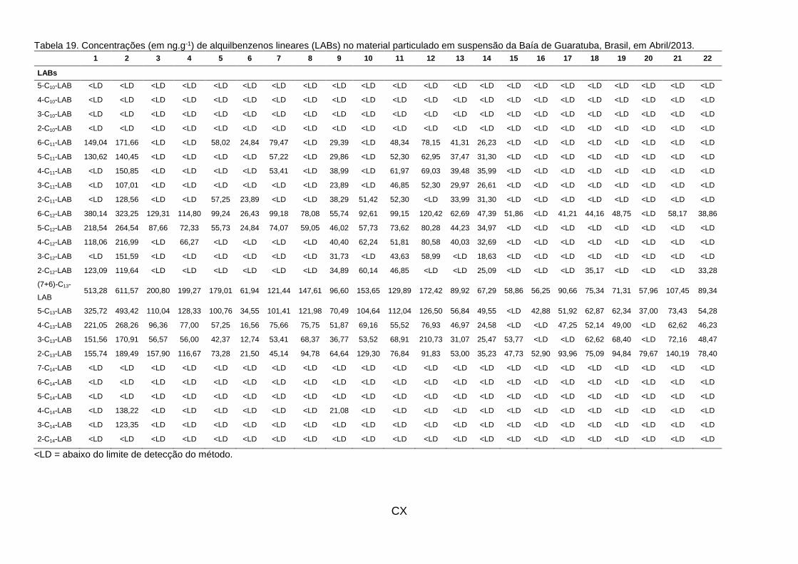
CX

Tabela 19. Concentrações (em ng.g-1) de alquilbenzenos lineares (LABs) no material particulado em suspensão da Baía de Guaratuba, Brasil, em Abril/2013.

1 2 3 4 5 6 7 8 9 10 11 12 13 14 15 16 17 18 19 20 21 22

LABs

5-C10-LAB <LD <LD <LD <LD <LD <LD <LD <LD <LD <LD <LD <LD <LD <LD <LD <LD <LD <LD <LD <LD <LD <LD

4-C10-LAB <LD <LD <LD <LD <LD <LD <LD <LD <LD <LD <LD <LD <LD <LD <LD <LD <LD <LD <LD <LD <LD <LD

3-C10-LAB <LD <LD <LD <LD <LD <LD <LD <LD <LD <LD <LD <LD <LD <LD <LD <LD <LD <LD <LD <LD <LD <LD

2-C10-LAB <LD <LD <LD <LD <LD <LD <LD <LD <LD <LD <LD <LD <LD <LD <LD <LD <LD <LD <LD <LD <LD <LD

6-C11-LAB 149,04 171,66 <LD <LD 58,02 24,84 79,47 <LD 29,39 <LD 48,34 78,15 41,31 26,23 <LD <LD <LD <LD <LD <LD <LD <LD

5-C11-LAB 130,62 140,45 <LD <LD <LD <LD 57,22 <LD 29,86 <LD 52,30 62,95 37,47 31,30 <LD <LD <LD <LD <LD <LD <LD <LD

4-C11-LAB <LD 150,85 <LD <LD <LD <LD 53,41 <LD 38,99 <LD 61,97 69,03 39,48 35,99 <LD <LD <LD <LD <LD <LD <LD <LD

3-C11-LAB <LD 107,01 <LD <LD <LD <LD <LD <LD 23,89 <LD 46,85 52,30 29,97 26,61 <LD <LD <LD <LD <LD <LD <LD <LD

2-C11-LAB <LD 128,56 <LD <LD 57,25 23,89 <LD <LD 38,29 51,42 52,30 <LD 33,99 31,30 <LD <LD <LD <LD <LD <LD <LD <LD

6-C12-LAB 380,14 323,25 129,31 114,80 99,24 26,43 99,18 78,08 55,74 92,61 99,15 120,42 62,69 47,39 51,86 <LD 41,21 44,16 48,75 <LD 58,17 38,86

5-C12-LAB 218,54 264,54 87,66 72,33 55,73 24,84 74,07 59,05 46,02 57,73 73,62 80,28 44,23 34,97 <LD <LD <LD <LD <LD <LD <LD <LD

4-C12-LAB 118,06 216,99 <LD 66,27 <LD <LD <LD <LD 40,40 62,24 51,81 80,58 40,03 32,69 <LD <LD <LD <LD <LD <LD <LD <LD

3-C12-LAB <LD 151,59 <LD <LD <LD <LD <LD <LD 31,73 <LD 43,63 58,99 <LD 18,63 <LD <LD <LD <LD <LD <LD <LD <LD

2-C12-LAB 123,09 119,64 <LD <LD <LD <LD <LD <LD 34,89 60,14 46,85 <LD <LD 25,09 <LD <LD <LD 35,17 <LD <LD <LD 33,28

(7+6)-C13-

LAB 513,28 611,57 200,80 199,27 179,01 61,94 121,44 147,61 96,60 153,65 129,89 172,42 89,92 67,29 58,86 56,25 90,66 75,34 71,31 57,96 107,45 89,34

5-C13-LAB 325,72 493,42 110,04 128,33 100,76 34,55 101,41 121,98 70,49 104,64 112,04 126,50 56,84 49,55 <LD 42,88 51,92 62,87 62,34 37,00 73,43 54,28

4-C13-LAB 221,05 268,26 96,36 77,00 57,25 16,56 75,66 75,75 51,87 69,16 55,52 76,93 46,97 24,58 <LD <LD 47,25 52,14 49,00 <LD 62,62 46,23

3-C13-LAB 151,56 170,91 56,57 56,00 42,37 12,74 53,41 68,37 36,77 53,52 68,91 210,73 31,07 25,47 53,77 <LD <LD 62,62 68,40 <LD 72,16 48,47

2-C13-LAB 155,74 189,49 157,90 116,67 73,28 21,50 45,14 94,78 64,64 129,30 76,84 91,83 53,00 35,23 47,73 52,90 93,96 75,09 94,84 79,67 140,19 78,40

7-C14-LAB <LD <LD <LD <LD <LD <LD <LD <LD <LD <LD <LD <LD <LD <LD <LD <LD <LD <LD <LD <LD <LD <LD

6-C14-LAB <LD <LD <LD <LD <LD <LD <LD <LD <LD <LD <LD <LD <LD <LD <LD <LD <LD <LD <LD <LD <LD <LD

5-C14-LAB <LD <LD <LD <LD <LD <LD <LD <LD <LD <LD <LD <LD <LD <LD <LD <LD <LD <LD <LD <LD <LD <LD

4-C14-LAB <LD 138,22 <LD <LD <LD <LD <LD <LD 21,08 <LD <LD <LD <LD <LD <LD <LD <LD <LD <LD <LD <LD <LD

3-C14-LAB <LD 123,35 <LD <LD <LD <LD <LD <LD <LD <LD <LD <LD <LD <LD <LD <LD <LD <LD <LD <LD <LD <LD

2-C14-LAB <LD <LD <LD <LD <LD <LD <LD <LD <LD <LD <LD <LD <LD <LD <LD <LD <LD <LD <LD <LD <LD <LD

<LD = abaixo do limite de detecção do método.

CXI

Tabela 20. Concentrações (em ng.g-1) de alquilbenzenos lineares (LABs) no material particulado em suspensão da Baía de Guaratuba, Brasil, em Agosto/2013.

1 2 3 4 5 6 7 8 9 10 11 12 13 14 15 16 17 18 19 20 21 22

LABs

5-C10-LAB <LD <LD <LD <LD <LD <LD <LD <LD <LD <LD <LD <LD <LD <LD <LD <LD <LD <LD <LD <LD <LD <LD

4-C10-LAB <LD <LD <LD <LD <LD <LD <LD <LD <LD <LD <LD <LD <LD <LD <LD <LD <LD <LD <LD <LD <LD <LD

3-C10-LAB <LD <LD <LD <LD <LD <LD <LD <LD <LD <LD <LD <LD <LD <LD <LD <LD <LD <LD <LD <LD <LD <LD

2-C10-LAB <LD <LD <LD <LD <LD <LD <LD <LD <LD <LD <LD <LD 49,58 <LD <LD <LD <LD <LD <LD <LD <LD <LD

6-C11-LAB <LD <LD <LD <LD <LD 53,60 <LD <LD <LD <LD <LD <LD 88,07 <LD <LD <LD <LD 69,13 66,89 <LD <LD 36,97

5-C11-LAB <LD <LD <LD <LD <LD 64,22 <LD <LD 47,73 <LD <LD <LD 72,74 <LD <LD <LD <LD 75,12 100,63 <LD <LD 32,21

4-C11-LAB 203,85 <LD <LD <LD <LD 72,37 <LD <LD 46,14 <LD <LD <LD 67,52 40,27 <LD <LD <LD 74,84 87,72 <LD <LD 52,32

3-C11-LAB <LD <LD <LD <LD <LD 52,12 <LD <LD <LD <LD <LD <LD 54,47 <LD <LD <LD <LD 57,70 67,77 <LD <LD <LD

2-C11-LAB 239,74 <LD <LD <LD 94,83 87,19 61,14 95,33 49,64 72,83 <LD <LD 121,34 <LD 49,81 <LD <LD 70,22 80,68 <LD <LD 45,18

6-C12-LAB 391,03 184,16 170,40 96,47 153,47 158,82 110,93 139,30 84,64 142,23 73,27 108,03 159,51 76,14 102,31 95,93 65,22 154,86 172,51 51,24 58,64 105,93

5-C12-LAB 270,51 138,84 112,78 <LD 123,23 99,29 90,06 115,38 70,64 110,53 53,16 83,58 142,54 57,82 66,63 59,26 49,91 133,09 122,05 <LD <LD 84,31

4-C12-LAB 202,56 138,84 88,88 83,53 124,61 81,51 80,18 110,45 67,14 83,11 <LD 89,78 105,03 59,62 64,28 52,22 <LD 124,38 95,05 <LD <LD 95,12

3-C12-LAB <LD <LD <LD <LD 92,08 59,03 58,58 73,87 <LD 80,11 <LD <LD 119,71 <LD <LD <LD <LD 69,40 56,92 <LD <LD 63,99

2-C12-LAB 193,59 140,77 <LD <LD 142,02 86,20 89,33 98,84 54,09 104,10 52,82 59,49 81,87 43,10 47,79 <LD <LD 64,23 59,26 <LD <LD 50,37

(7+6)-C13-

LAB 693,59 395,32 211,47 229,41 374,74 254,41 287,76 280,70 164,82 371,42 174,15 300,36 327,49 151,00 152,45 137,78 114,83 273,25 198,32 113,44 106,89 274,34

5-C13-LAB 410,26 271,90 144,05 178,24 256,54 166,97 190,74 166,38 103,09 201,35 111,10 182,48 256,06 118,47 87,84 102,96 77,78 153,23 119,70 68,32 95,39 180,08

4-C13-LAB 306,41 218,87 117,69 12<LD 198,36 120,04 139,49 126,63 78,59 140,94 82,47 110,22 177,12 78,21 70,34 79,63 57,26 105,60 85,08 57,37 52,70 82,37

3-C13-LAB 188,46 162,95 <LD 138,24 170,88 85,22 105,44 104,82 56,64 149,51 68,16 108,39 171,58 56,78 <LD 64,07 45,01 71,85 53,98 54,14 59,01 109,82

2-C13-LAB 352,56 268,04 138,53 161,76 238,68 109,67 151,57 184,67 73,50 209,49 101,22 172,99 185,27 89,56 68,32 94,07 53,89 100,43 70,41 101,52 65,32 99,66

7-C14-LAB <LD <LD <LD <LD <LD <LD <LD <LD <LD <LD <LD <LD <LD <LD <LD <LD <LD <LD <LD <LD <LD <LD

6-C14-LAB <LD <LD <LD <LD <LD <LD <LD <LD <LD <LD <LD <LD <LD <LD <LD <LD <LD <LD <LD <LD <LD <LD

5-C14-LAB <LD <LD <LD <LD <LD <LD <LD <LD <LD <LD <LD <LD <LD <LD <LD <LD <LD <LD <LD <LD <LD <LD

4-C14-LAB <LD <LD <LD <LD <LD <LD <LD <LD <LD <LD <LD <LD <LD <LD <LD <LD <LD <LD <LD <LD <LD <LD

3-C14-LAB <LD <LD <LD <LD <LD <LD <LD <LD <LD <LD <LD <LD <LD <LD <LD <LD <LD <LD <LD <LD <LD <LD

2-C14-LAB <LD <LD <LD <LD <LD <LD <LD <LD <LD <LD <LD <LD <LD <LD <LD <LD <LD <LD <LD <LD <LD <LD

<LD = abaixo do limite de detecção do método.

CXII

Tabela 21. Concentrações (em ng.g-1) de alquilbenzenos lineares (LABs) no material particulado em suspensão da Baía de Guaratuba, Brasil, em Março/2014.

1 2 3 4 5 6 7 8 9 10 11 12 13 14 15 16 17 18 19 20 21 22

LABs

5-C10-LAB na <LD na <LD <LD <LD <LD <LD na <LD <LD <LD <LD <LD <LD <LD <LD <LD <LD <LD <LD <LD

4-C10-LAB na <LD na <LD <LD <LD <LD <LD na <LD <LD <LD <LD <LD <LD <LD <LD <LD <LD <LD <LD <LD

3-C10-LAB na <LD na <LD <LD <LD <LD <LD na <LD <LD <LD <LD <LD <LD <LD <LD <LD <LD <LD <LD <LD

2-C10-LAB na 73,11 na 135,23 <LD <LD <LD <LD na <LD <LD <LD <LD <LD <LD <LD <LD <LD <LD <LD <LD <LD

6-C11-LAB na 63,87 na 112,16 <LD <LD <LD <LD na <LD <LD <LD <LD <LD <LD <LD <LD <LD <LD <LD <LD <LD

5-C11-LAB na <LD na <LD <LD <LD <LD <LD na <LD <LD <LD <LD <LD <LD <LD <LD <LD <LD <LD <LD <LD

4-C11-LAB na 89,08 na 121,70 <LD <LD <LD <LD na <LD <LD <LD <LD <LD <LD <LD <LD <LD <LD <LD <LD <LD

3-C11-LAB na 86,13 na <LD <LD <LD <LD <LD na <LD <LD <LD <LD <LD <LD <LD <LD <LD <LD <LD <LD <LD

2-C11-LAB na 69,33 na 135,23 <LD <LD <LD <LD na <LD <LD <LD <LD <LD <LD <LD <LD <LD <LD <LD <LD <LD

6-C12-LAB na <LD na 125,68 81,81 38,40 36,12 <LD na <LD <LD <LD <LD <LD <LD <LD <LD <LD <LD <LD <LD <LD

5-C12-LAB na 79,83 na <LD 69,44 <LD 29,15 <LD na <LD <LD <LD <LD <LD <LD <LD <LD <LD <LD <LD <LD <LD

4-C12-LAB na <LD na <LD 58,27 <LD 28,60 <LD na <LD <LD <LD <LD <LD <LD <LD <LD <LD <LD <LD <LD <LD

3-C12-LAB na <LD na <LD 57,07 <LD <LD <LD na <LD <LD <LD <LD <LD <LD <LD <LD <LD <LD <LD <LD <LD

2-C12-LAB na <LD na 116,14 99,77 <LD 30,43 <LD na <LD <LD <LD <LD <LD <LD <LD <LD <LD <LD <LD <LD <LD

(7+6)-C13-

LAB na 88,24 na <LD 259,81 64,51 102,49 79,23 na 35,49 26,81 <LD <LD <LD 96,42 <LD 25,76 33,29 10,38 5,86 19,87 16,02

5-C13-LAB na 77,31 na <LD 169,21 51,98 87,09 52,72 na <LD <LD <LD <LD <LD 77,78 <LD <LD <LD <LD <LD <LD <LD

4-C13-LAB na 66,81 na <LD 160,03 47,01 68,02 53,65 na <LD <LD <LD <LD <LD <LD <LD <LD <LD <LD <LD <LD <LD

3-C13-LAB na 154,20 na 310,23 159,64 <LD 64,54 48,98 na <LD <LD <LD <LD <LD <LD <LD <LD <LD <LD <LD <LD <LD

2-C13-LAB na <LD na 140,00 263,40 <LD 83,42 97,64 na <LD <LD <LD 57,39 <LD 242,98 27,11 60,00 59,40 <LD <LD 26,68 30,57

7-C14-LAB na <LD na <LD <LD <LD <LD <LD na <LD <LD <LD <LD <LD <LD <LD <LD <LD <LD <LD <LD <LD

6-C14-LAB na <LD na <LD <LD <LD <LD <LD na <LD <LD <LD <LD <LD <LD <LD <LD <LD <LD <LD <LD <LD

5-C14-LAB na <LD na <LD 61,86 <LD 28,60 <LD na <LD <LD <LD <LD <LD <LD <LD <LD <LD <LD <LD <LD <LD

4-C14-LAB na 60,08 na <LD <LD <LD <LD <LD na <LD <LD <LD <LD <LD <LD <LD <LD <LD <LD <LD <LD <LD

3-C14-LAB na <LD na <LD <LD <LD 42,17 <LD na <LD <LD <LD <LD <LD <LD <LD <LD <LD <LD <LD <LD <LD

2-C14-LAB na <LD na <LD <LD <LD <LD <LD na <LD <LD <LD <LD <LD 63,64 <LD <LD <LD <LD <LD <LD <LD

<LD = abaixo do limite de detecção do método. na = não analisada. Obs. 1: a amostra 1 foi descartada devido à má recuperação. Obs. 2: a amostra 3 não pode ser analisada. Obs. 3: a amostra 9 não pode ser coletada.