Embed Size (px)
Citation preview

Instituto Nacional de Matematica Pura e Aplicada
REDUCTION OF INCENTIVE
CONSTRAINTS IN BIDIMENSIONAL
ADVERSE SELECTION AND
APPLICATIONS
Jose Braulio Calagua Mendoza
Doctoral Thesis
Rio de JaneiroApril 2017

Instituto Nacional de Matematica Pura e Aplicada
Jose Braulio Calagua Mendoza
REDUCTION OF INCENTIVE
CONSTRAINTS IN BIDIMENSIONAL
ADVERSE SELECTION AND
APPLICATIONS
Thesis presented to the Post-graduate Program inMathematics at Instituto de Matematica Pura e Apli-cada as partial fulfillment of the requirements for thedegree of Doctor of Philosophy in Mathematics.Advisor: Aloısio AraujoCo-advisor: Carolina Parra
Rio de JaneiroApril 2017

.

.
A mi Soledad

Agradecimentos
Agradezco a mis padres Jose Calagua y Zoila Mendoza, a mis hermanas Valeria,
Natalia, Cecilia y Jimena, ası como a mis sobrinos y sobrinas por el afecto, el apoyo y
la confianza. Con gran carino agradezco a Soledad Papel, mi ahora esposa, por creer
en mi, entenderme y alentarme en este camino que decidı tomar hace unos anos.
Mi gratitud a mis profesores de la UNI e IMCA, entre ellos a Yboon Garcıa
por recomendarme para llegar al IMPA. Mencion especial para el profesor Ramon
Garcıa-Cobian quien gracias al rigor matematico y claridad de las interpretaciones
economicas en los cursos de maestrıa fue determinante para decidirme en hacer
doctorado en economıa matematica.
Agradeco profundamente ao professor Aloısio Araujo por ter aceitado trabalhar
comigo como orientador de tese, pelas sugestoes e dedicacao no meu trabalho.
Agradecimentos a Carolina Parra com quem discuti as ideias e detalhes das provas,
ao Mauricio Villalba pela revisao detalhada e correccoes, ao Sergei Vieira e ao
Paulo Kingler Monteiro pelo seu tempo para discutir topicos puntuais da tese, e ao
Alexandre Belloni pela leitura minuciosa e recomendacoes em parte do trabalho.
Sou muito grato com os amigos que fiz e me acompanharam nesse periodo, entre
eles: Juan Pablo Luna, Ruben Lizarbe, Eric Biagioli, Aldo Zang, Enrique Chavez,
Andres Chirre, Gabriel Munoz, Percy Abanto, Juan Pablo Gamma-Torres e Lorenzo
Bastianello. Mencao especial merece meu amigo Liev Maribondo, com quem estudei
para aprovar o exame de qualificacao e passamos simultaneamente o processo de
fazer uma tese.
Finalmente, minha gratidao com os funcionarios e trabalhadores do IMPA, espe-
cialmente com o pessoal do Departamento de Ensino, pela eficiencia da sua labor. O
presente trabalho foi realizado gracas ao apoio financeiro do Conselho Nacional de
Desenvolvimento Cientıfico e Tecnologico - CNPq.
i
Abstract
In this work, we study a bidimensional adverse selection problem in the framework
of nonlinear pricing by a monopolist, where the firm produces a one-dimensional
product and customers’ preferences are described by two dimensions of uncertainty.
We prove that it is sufficient to consider, for each type of customer, incentive
compatibility constraints over a one-dimensional set rather than the entire two-
dimensional set as required by definition. For this purpose, we introduce a pre-order
among types to compare their marginal valuation of consumption and we also take
account possible shape of isoquants. As a consequence, the discretized problem is
computationally tractable for relative fine discretizations.
Due to we extend the ideas applied in the unidimensional case with finite types
when single-crossing condition is satisfied, our main assumption is the validity of
single-crossing over each direction of uncertainty. Thus, we are able to have well-
educated insights of the solution for a large class of valuation function and types’
distributions.
Keywords: incentive compatibility, bidimensional types, monopolist’s problem,
regulation model.
ii

Resumo
Neste trabalho, estudamos o problema de selecao adversa bidimensional no marco
de referencia de precos nao lineares por um monopolista, onde a empresa produz um
produto unidimensional e as preferencias dos consumidores sao descritas por duas
dimensoes de incerteza.
Provamos que e suficiente considerar, para cada tipo de consumidor, restricoes de
compatibilidade de incentivo sobre um conjunto numa dimensao em vez de todo o
conjunto bidimensional como e exigido por definicao. Isto e feito introduzindo um pre-
ordem comparando tipos de acordo com a valoracao marginal de consumo e levando
em consideracao a possıvel forma das isoquantas. Com esse resultado, o problema
discretizado e computacionalmente tratavel para discretizacoes relativamente finas.
Devido a que estendemos as ideias aplicadas no caso unidimensional com finitos
tipos quando a condicao de single-crossing e satisfeita, nossa suposicao principal e a
validade de single-crossing em cada direcao de incerteza. Assim, somos capazes de
ter nocoes bem educadas da solucao para uma grande classe de funcoes de valoracao
e distribuicoes dos tipos.
Palabras-chave: compatibilidade de incentivos, tipos bidimensionaies, problema
do monopolista, modelo de regulacao.
iii

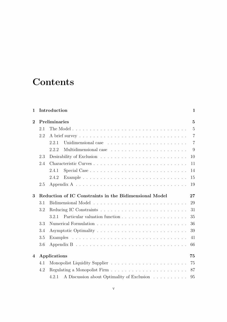
Contents
1 Introduction 1
2 Preliminaries 5
2.1 The Model . . . . . . . . . . . . . . . . . . . . . . . . . . . . . . . . . 5
2.2 A brief survey . . . . . . . . . . . . . . . . . . . . . . . . . . . . . . . 7
2.2.1 Unidimensional case . . . . . . . . . . . . . . . . . . . . . . . 7
2.2.2 Multidimensional case . . . . . . . . . . . . . . . . . . . . . . 9
2.3 Desirability of Exclusion . . . . . . . . . . . . . . . . . . . . . . . . . 10
2.4 Characteristic Curves . . . . . . . . . . . . . . . . . . . . . . . . . . . 11
2.4.1 Special Case . . . . . . . . . . . . . . . . . . . . . . . . . . . . 14
2.4.2 Example . . . . . . . . . . . . . . . . . . . . . . . . . . . . . . 15
2.5 Appendix A . . . . . . . . . . . . . . . . . . . . . . . . . . . . . . . . 19
3 Reduction of IC Constraints in the Bidimensional Model 27
3.1 Bidimensional Model . . . . . . . . . . . . . . . . . . . . . . . . . . . 29
3.2 Reducing IC Constraints . . . . . . . . . . . . . . . . . . . . . . . . . 31
3.2.1 Particular valuation function . . . . . . . . . . . . . . . . . . . 35
3.3 Numerical Formulation . . . . . . . . . . . . . . . . . . . . . . . . . . 36
3.4 Asymptotic Optimality . . . . . . . . . . . . . . . . . . . . . . . . . . 39
3.5 Examples . . . . . . . . . . . . . . . . . . . . . . . . . . . . . . . . . 41
3.6 Appendix B . . . . . . . . . . . . . . . . . . . . . . . . . . . . . . . . 66
4 Applications 75
4.1 Monopolist Liquidity Supplier . . . . . . . . . . . . . . . . . . . . . . 75
4.2 Regulating a Monopolist Firm . . . . . . . . . . . . . . . . . . . . . . 87
4.2.1 A Discussion about Optimality of Exclusion . . . . . . . . . . 95
v

CONTENTS
Conclusions 98
Bibliography 101
vi
Chapter 1
Introduction
Adverse selection models (or screening models) refer to a kind of asymmetric
information problems, where an informed part (the agent) possesses its private
knowledge before a transaction takes place with an uninformed part (the principal)
who design a contract establishing the terms in which the relationship works. This
contract is a menu of options from which the agent chooses his preferred action and
the principal is commit to the contract offered.
Since the late 1970s, the development of the theory of screening models has been
one of the major advances in economic theory, being notably applied to diverse
issues such as optimal taxation, nonlinear pricing, regulatory policy of a monopolist
firm, and auctions. The majority of these applications have assumed that agents’
preferences can be ordered by a single parameter of private information, the well-know
single-crossing condition, which facilitates finding the optimal solution.
Nevertheless, a one-dimensional parameter does not seem to reflect in an appropri-
ate manner agents’ private information in many economic environments. For instance,
when establishing a price for its product a monopolist firm could be uncertain about
the parameters describing customers’ demand function (as Laffont et al. (1987) who
considered linear demand curves with unknowing slope and intercep) or maybe wish
to include socio-economic and demographic parameters such as wealth, age, etc. In
the design of regulatory policy at least two dimensions of private cost information
(fix and marginal costs) naturally arise, as was noticed by Baron and Myerson
(1982). In the same framework Lewis and Sappington (1988b) have considered a
regulator uncertain about both cost and demand functions of the monopolist firm he
1

Introduction
is regulating. In labor market, several unobservable worker’s characteristics such as
ability, effort or leisure preferences could be considered by the employer.
In this work we focus in adverse selection models where agents characteristics are
captured by a two-dimensional vector and the principal disposes of one-dimensional
instrument. Initially, we concentrate in the nonlinear pricing by a monopolist firm
framework but later we analyze a model in the regulation setting.
Thus, consider a monopolistic firm producing a one-dimensional quality product
and customer’s private preferences described by two dimensions of uncertainty. The
firm would like to design a contract extracting maximum benefit from each customer’s
type, but typically customer will not choose this contract selecting rather a contract
designed to another type of customer. Therefore, in order to maximize revenue, the
firm designs a contract in a way that ensures customers do not misrepresent their
preferences strategically. This kind of restriction, called incentive compatibility (IC),
is central in the theory and arises by the asymmetry of information.
In the one-dimensional version of the problem when single-crossing condition
holds, since there is complete order of preferences, IC constraints binding for each
type are determined by local conditions. The resulting optimal quality allocation
increases according with types’ order, and just customers’ type with highest valuation
for the product gets same quality as when there is not asymmetry of information,
which is the case when firm sets efficient prices at marginal cost level. To give and
economic intuition of this result, we appeal to the excellent explanation given by
Matthews and Moore (1987):
“The intuition behind its solution starts with the observation that profit is po-
tencially greatest on contracts designed for ‘high’ type consumers, those with a high
evaluation of quality. Because high type consumers cannot be prevent from choosing
contracts meant for low types, this profit can only be realized by distorting the con-
tracts meant for low types in a direction that makes them relatively unattractive to
high types. All but the highest type of consumer should therefore receive products of
inefficiently low quality.”
In the multidimensional version, and particulary in the bidimensional case we are
concern with, there is not general treatment to deal with the problem. The essential
difficulty is the lack of an exogenous complete order of preferences, which implies
that we need to look for which IC constraints are binding in a far larger set of global
constraints, for each type of customer.
2
Some techniques have been developed to reach the solution, for example by
Laffont et al. (1987), Basov (2001), Deneckere and Severinov (2015) and Araujo and
Vieira (2010). However, with these techniques we are limitated to use simple forms
of customers’ valuation function (generally linear-quadratic forms or extensions) and
type’s distribution (usually uniform distribution).
Therefore, because in general we cannot obtain closed-form solutions, we could
attempt to get numerical approximations of the solution discretizing agents’ type set,
as the model is formulated in a continuous way. However, due to the IC constraints,
computational difficulties are severe when types are multidimensional. For instance
when agents’ type set is a square in R2 taking n points over each dimension derives
on n4 − n2 (usually non-convex) IC constraints, which may lead to memory storage
problems if discretization is fine enough (Parra (2014) has reported computer’s
memory exhausted for tests with n = 14).
Some numerical methods to deal with the problem are described in Wilson
(1995). Although these methods were formulated allowing multidimensional types
and product, they were designed to solve a relax version of the problem in which
only local incentive compatibility constraints are assume to be binding. Even when
local IC constraints are sufficient in one-dimension, this is not the usual case in
multidimensions, so we cannot rely on these approximations as the solution of the
complete problem.
The main contribution of this work is to prove that is sufficient to consider, for
each type, IC constraints over a unidimensional set instead of the whole bidimensional
type set as it is required by definition. With this result the number of IC constraints
in the discretized problem is of order n3, making it computationally tractable for
relative fine discretization. Thus, we are able to have well educated predictions about
some features of the solution, such as optimal quality, agents’ surplus and optimal
tariff shapes, as well as the participation set and how types are bunching. Specially
when valuation function is such that IC constraints are convex, as we will see in two
applications.
We are extending the ideas being applied in the unidimensional case with finite
types when single-crossing condition holds. With the aim of extend the order induce
by single-crossing in one-dimension, we introduce a pre-order among types by their
marginal valuation for the product. We also consider the possible shape of isoquants
using a PDE derived in Araujo and Vieira (2010). Our main assumption is the
3

Introduction
validity of single-crossing over each direction of uncertainty. Therefore, our approach
is valid for a large class of valuation function and types’ distributions.
This work is organized as follows. In Chapter 2 we describe the general model,
review the main contributions from the literature and discuss with more detail two
topics that will be important for further chapters. Chapter 3 is dedicated to our
main contribution, first explaining the ideas we are extending from unidimensional
case, and then justifying the reduction of IC constraints. We test our approach
comparing numerical and analytic solutions of three examples already solved in the
literature. Additionally, three new examples are proposed. In Chapter 4 we use our
approach to analyze and give additional insights in two models already studied. In
the first one we provide some conclusions about monopolist’s behavior varying types’
distribution. In the second one we provide the numerical solution of a model with
unknown solution, which allows us to give relevant conclusions. We hope that this
work will be useful for the kind of analysis that this chapter contains.
4
Chapter 2
Preliminaries
The aim of this chapter is to describe the problem we are concerned with and,
because shall be important for further chapters, to expose some topics with more
detail. In Section 1 we establish the formal model in the framework of nonlinear
pricing by a monopolist and review some main results from the literature in Section
2. Armstrong’s result about the optimality of exclusion is the subject of Section 3.
Section 4 presents the methodology used by Araujo and Vieira (2010) who derived a
necessary condition of optimality. This section also contains our first contribution.
2.1 The Model
Consider a monopolistic firm (the principal) supplier of N different goods q ∈Q ⊂ RN
+ at cost C(q) facing a population of customers (the agents). Customers’
characteristics, reflecting their preferences over the products, are captured by a vector
θ ∈ Θ ⊂ RM which we will refer as their type. This type is private information of
each customer, but the monopolist knows the customers’ population distribution
over the set Θ according to a strictly positive density function f .
A common assumption is that agents’ utility is quasilinear (linear in money
transfer), i.e., the utility of type θ for consumption q and payment t ∈ R+ is
v(q, θ)− t
where v(q, θ) is the θ−type agent’s valuation when consumes q.
5
Preliminaries
The firm is able to design a menu of options to offer to the agent specifying the
quantity and corresponding payment according with customers’ type revealed. This
menu of options q(θ), t(θ)θ∈Θ it is call a contract. The monopolist would wish to
extract the maximum payment from each agent ensuring that agent’s benefit is at
least his reservation utility (the utility of the outside option); this is the individual
rationality (IR) constraint. Also, the monopolist tries to avoid that customers take
advantage of their private information because distortion of true preferences could
lead to nonoptimal firm’s income. By the Revelation Principle (Myerson (1979)),
this can be done restricting to a class of contracts where true-telling is the best
response for the agents. That is, the contract offered must ensure that agents have
not the incentive of misrepresent their true type; this is the incentive compatibility
(IC) constraint.
Thus, because firm’s objective is to maximize expected net income, the monopo-
list’s problem is
maxq(·),t(·)
∫Θ
t(θ)− C(q(θ))f(θ)dθ
subject to
(IR) v(q(θ), θ)− t(θ) ≥ 0 ∀ θ ∈ Θ
(IC) v(q(θ), θ)− t(θ) ≥ v(q(θ), θ)− t(θ) ∀ θ, θ ∈ Θ
In IR constraints we are assuming that reservation utility is type independent
and normalized it to be zero. Note that IC constraints can be written as
θ ∈ argmaxθ∈Θ
v(q(θ), θ)− t(θ) ∀ θ ∈ Θ
then, given (q, t) agents are maximizing their own utility. We say that q : Θ→ R+ is
implementable if there exists t : Θ→ R+ such that (q, t) satisfies the IC constraints.
The Taxation Principle (Guesnerie (1981), Rochet (1985)) establishes that any
incentive compatible contract (q, t) can be implemented by a tariff T : Q → R+
s.t. T (q(θ)) = t(θ). Faced with a tariff T , the θ−agent will choose the bundle that
6
A brief survey
maximizes his utility, then the IC constraints can be written as:
q(θ) ∈ argmaxq∈Q
v(q, θ)− T (q) ∀ θ ∈ Θ
Given an incentive compatible contract (q, t), agents’ surplus or informational
rent is defined as
V (θ) = maxθ∈Θv(q(θ), θ)− t(θ)
= v(q(θ), θ)− t(θ)
We can use the informational rent to replace transfers in the principal’s objective
function and transform the monopolist’s problem
maxq(·),V (·)
∫Θ
v(q(θ), θ)− C(q(θ))− V (θ)f(θ)dθ
subject to
(IR) V (θ) ≥ 0 ∀ θ ∈ Θ
(IC) V (θ)− V (θ) ≥ v(q(θ), θ)− v(q(θ), θ) ∀ θ, θ ∈ Θ
With this change of variables the new expression of the objective function can
be seen as the expected social value of trade (v(q(θ), θ)− t(θ)+ t(θ)− C(q(θ)))minus the expected informational rent of the agents.
2.2 A brief survey
2.2.1 Unidimensional case
The unidimensional case (N = 1,M = 1) of this problem has been extensively
studied in the literature1. When Spence-Mirrless or single-crossing condition vqθ > 0
is satisfied, first and second order necessary conditions for agent’s maximization
1Seminal papers are Mussa and Rosen (1978), Maskin and Riley (1984)
7
Preliminaries
problem are also sufficient. These conditions are equivalent to V ′(θ) = vθ(q(θ), θ)
for a.e. θ ∈ [θ, θ] and to q being non-decreasing function of θ. From the former
condition, V (θ) = V (θ)+∫ θθvθ(q(ξ), ξ)dξ then, after replacing V into firm’s objective
via integration by parts, the constant V (θ) negatively affects monopolist’ expected
income, therefore making V (θ) = 0 is the best firm’s option. The result is the
following problem
maxq(·)
∫ θ
θ
v(q(θ), θ)− C(q(θ))− 1− F (θ)
f(θ)vθ(q(θ), θ)f(θ)dθ
subject to
q(·) non-decreasing
where F is the cumulative distribution of f . What we have done is decompose
the problem: first, agents’ surplus V is expressed as a function of q and second,
the allocation q that maximizes firms’ revenue net of the expected agents’ surplus
computed previously is determined. This is known as the direct approach of the
problem.
If we relax the condition of q being non-decreasing we have a classic calculus
variation problem and by the Euler’s equation2 we obtain a function that may be
non-decreasing. If this is not the case, by the Ironing Procedure3 a non-decreasing
function is defined, which is the solution of the complete program.
As we have seen, the unidimensional problem can be solved by simple considera-
tions if the single-crossing property is valid, because global incentive compatibility
constraints are determined by local conditions and implementable allocations can be
completely characterized. Araujo and Moreira (2010) studied the model when the
single-crossing condition is relaxed allowing vqθ to change the sign over Q×Θ. Then,
local IC constraints are not sufficient anymore for implementability and nonlocal
constraints can be binding. In this case, implementable allocations q may not be
monotonic and they concluded that types getting the same allocation receives the
same marginal tariff.
2See Kamien and Schwartz (1981)
3See Mussa and Rosen (1978), or Fundenberg and Tirole (1991) for details.
8
A brief survey
2.2.2 Multidimensional case
In multidimensional problems, McAfee and McMillan (1988) introduced a genera-
lized single-crossing property and concluded that first and second-order necessary
conditions are also sufficient for implementability; however, it forces the set of types
getting the same allocation to be hyperplanes.
In a celebrated paper, Rochet (1987) provides the following characterization:
q is implementable if and only if for all finite cycles θ0, θ1, . . . , θJ+1 ⊂ Θ, with
θJ+1 = θ0J∑k=0
(v(q(θk), θk+1)− v(q(θk), θk)
)≤ 0
This result is quite general since it not assumes neither special structure of Θ nor
regularity conditions of v; however, in practice it is not useful. When v is linear in
types and Θ convex, Rochet (1987) also shows that q is implementable if and only if
there exists a convex function V such that
∇θv(q(θ), θ) = V ′(θ) a.e. θ
Carlier (2001) generalizes previous result in terms of v−convex functions and,
with this equivalence, he obtains an existence result for the problem although with
strong conditions on v.
At this point it is important to mention the work of Monteiro and Page (1998)
where another existence result is provided. They considered customers with budget
constraints which derive in compactness considerations. In their model, existence is
guarantee only if other goods are available and only if the monopolist’s goods are
nonessential relative to other goods.
Rochet and Chone (1998) analyzed the especial case that quality dimension equals
types dimension (N = M) and agents’ valuation is v(q, θ) = 〈θ, q〉. In this model,
Rochet’s implementability characterization derives on ∇θv(q, θ) = q = V ′(θ) , so
the authors expressed firm’s objective in terms of V and V ′ with the constraint of
V being non-negative and convex. Thus, agents’ informational rent is used as the
instrument chosen by the monopolist; this is known as the dual approach. Their main
contributions were to prove existence of the optimal contract in both the relax (i.e.
without the convex constraint) and complete problem, provide its characterization,
9
Preliminaries
and introduce the Sweeping Procedure which generalizes the Ironing Procedure to
multidimensions.
One of the main differences between unidimensional and multidimensional cases
is the optimality of exclusion, discovered by Armstrong (1996) (next section explains
with more detail this result). In that work some multidimensional examples were
explicit solved, as well in Wilson (1993) 4. However, as was noticed by Rochet
and Stole (2003) 5, in all these examples types set can be partitioned a priori into
unidimensional subsets, i.e., are special cases of problems that can be reduced.
Basov (2001) introduced the Hamiltonian approach and showed that, when
N > M , qualitative features of the solution are alike of those found by Rochet and
Chone (1998). Additionally, when N < M full separation of types is not possible over
open sets of Θ, and q may be discontinuous in the lower boundary of participation
set. In Basov (2005) some examples are solved with that technique.
In this work we are concerned with the specific case N = 1 and M = 2, i.e.,
one-dimension of the product offered and two dimensions of customers’ attributes.
For this case, Laffont et al. (1987) have found the explicit solution when customers’
demand function is linear, and the monopolist is uncertain about both the slope and
intercep that define such individual demand function. They have shown that the
optimal tariff is convex. In this particular problem customers’ valuation of consume
v has linear-quadratic form, a class of functions that has been explored in several
examples.
2.3 Desirability of Exclusion
Armstrong (1996) demonstrated that excluding types with low product’s valuation
is generally optimal for the firm in the multidimensional case. This is a salient result
because in one-dimesional setup it is optimal to serve all types.
The intuiton of that result is straightforward: If it were the case that it is optimal
to serve all customers, increasing the tariff by ε > 0 the monopolist could get extra
gain from types who remain in the market but has to assume the lost (not more
4In Wilson (1993) the called demand-profile approach is broadly explained.
5Rochet and Stole (2003) is one of the main surveys of multidimensional screening.
10
Characteristic Curves
income) from types who will exit (those with surplus < ε). As it was proved in that
paper, the former is greater than the latter for small values of ε, so exclusion will be
optimal. The theorem goes as follow:
Theorem 2.3.1 (Armstrong(1996)). Let v be such that v(0, θ) = 0, v(q, 0) = 0,
v(q, ·) convex, increasing and homogenous of degree one, and consider Θ ⊂ RM
(M ≥ 2) closed, strictly convex, and of full dimension in RM . Then, at the optimum
the set
θ ∈ Θ : V (θ) = 0
has positive Lebesgue measure.
The proof of this theorem can be find in Armstrong (1996) or Basov (2005).
Barelli et al. (2014) have extended Armstrong’s result providing alternative
sufficient conditions not relying on any form of convexity, and then have shown that
exclusion is obtained generically. Deneckere and Severinov (2015) have provided
necessary and sufficient conditions to ensure full participation, although this means
a strictly positive quantity (common in nonlinear pricing) instead of strictly positive
informational rent.
2.4 Characteristic Curves
This section expose a summary of the methodology used by Araujo and Vieira
(2010)6 to derive a necessary condition for optimality when N = 1 and M = 2.
They have assumed validity of single-crossing on each axis, with perfect negative
correlation between the two dimentions: vqa > 0 , vqb < 0 . They have also assumed
va > 0 , vb < 0.
Let (q, t) be an incentive compatible contract. Suppose that q and t are continuous
and a.e. twice continuously differentiable functions. For any (a, b) ∈ [0, 1]2 we have
(a, b) ∈ argmax(a,b)∈[0,1]2
v(q(a, b), a, b)− t(a, b)
6See also Vieira (2008)
11
Preliminaries
The first-order necessary condition imply
vq(q(a, b), a, b)qa(a, b) = ta(a, b)
vq(q(a, b), a, b)qb(a, b) = tb(a, b)
At any point (a, b) of twice continuous differentiability by the Young’s theorem
tab = tba, then an implementable allocation rule q must satisfy a.e.7
− vqbvqa
qa + qb = 0 (2.1)
Following the Characteristic Method to solve previous PDE, if an initial curve
φ(r) is fixed over the segment (r, 0) : r ∈ [r, 1] for some r ∈ (0, 1), there is a family
of plane characteristics curves (a(r, s), b(r, s)) forming a partition on the participation
set’s interior, and satisfying:
as(r, s) = −vqbvqa
(φ(r), a(r, s), b(r, s)) , a(r, 0) = r
bs(r, s) = 1 , b(r, 0) = 0
For a fixed r, all types over the characteristic curve (a(r, s), b(r, s)) gets the
same allocation φ(r). That is, plane characteristic curves are the isoquants of q(·, ·).Moreover, all the isoquants are strictly increasing in view of − vqb
vqa> 0.
Now, in view of (a, b) can be expressed in terms of new variables (r, s), after
replacing into the expected profit the monopolist’s problem can be set as
maxφ(·)
∫ 1
r
∫ s(r)
0
G(φ(r), a(r, s), b(r, s))∣∣∣∂(a, b)
∂(r, s)
∣∣∣ds drwhere G is the virtual surplus8 and s(r) is such that a(r, s(r)) = 1.
7The same PDE is derived with the necessary implementability condition given by Rochet(1987) (see Proposition 3 in that paper): Assume ∃ A ∈ R2×2 s.t. ∀ (q, (a, b)) ∈ Q×[0, 1]2
∇2θv(q, (a, b))− A is positive semi-definite. Then, for q to be implementable, it is necessary that
(a, b)→ ∇θv(q(a, b), a, b) is a.e. differentiable, and rot[∇θv(q(a, b), a, b)] = 0 a.e.With this result, those strong differentiability assumptions of q and t are not needed.
8In Appendix A we show how to determine virtual surplus G
12
Characteristic Curves
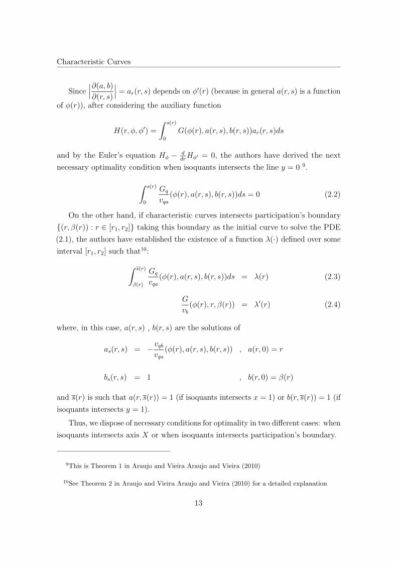
Since∣∣∣∂(a, b)
∂(r, s)
∣∣∣ = ar(r, s) depends on φ′(r) (because in general a(r, s) is a function
of φ(r)), after considering the auxiliary function
H(r, φ, φ′) =
∫ s(r)
0
G(φ(r), a(r, s), b(r, s))ar(r, s)ds
and by the Euler’s equation Hφ − ddrHφ′ = 0, the authors have derived the next
necessary optimality condition when isoquants intersects the line y = 0 9.
∫ s(r)
0
Gq
vqa(φ(r), a(r, s), b(r, s))ds = 0 (2.2)
On the other hand, if characteristic curves intersects participation’s boundary
(r, β(r)) : r ∈ [r1, r2] taking this boundary as the initial curve to solve the PDE
(2.1), the authors have established the existence of a function λ(·) defined over some
interval [r1, r2] such that10:∫ s(r)
β(r)
Gq
vqa(φ(r), a(r, s), b(r, s))ds = λ(r) (2.3)
G
vb(φ(r), r, β(r)) = λ′(r) (2.4)
where, in this case, a(r, s) , b(r, s) are the solutions of
as(r, s) = −vqbvqa
(φ(r), a(r, s), b(r, s)) , a(r, 0) = r
bs(r, s) = 1 , b(r, 0) = β(r)
and s(r) is such that a(r, s(r)) = 1 (if isoquants intersects x = 1) or b(r, s(r)) = 1 (if
isoquants intersects y = 1).
Thus, we dispose of necessary conditions for optimality in two different cases: when
isoquants intersects axis X or when isoquants intersects participation’s boundary.
9This is Theorem 1 in Araujo and Vieira Araujo and Vieira (2010)
10See Theorem 2 in Araujo and Vieira Araujo and Vieira (2010) for a detailed explanation
13
Preliminaries
2.4.1 Special Case
If characteristic curves are concurrent at some point (x, y), we establish a necessary
condition for optimality, not established by Araujo and Vieira (2010) but with the
same methodology. This is the case when type (x, y) is indifferent between any
quantity in some interval [q, q].
Following the characteristic method to solve the PDE (2.1), and considering that
isoquants intersects the line y = 1 11, we fix (r, 1) : r ∈ [R1, R2] as initial curve.
Then, we have to solve:
as(r, s) = −vqbvqa
(φ(r), a(r, s), b(r, s)) , a(r, 1) = r
bs(r, s) = 1 , b(r, 1) = 1
(2.5)
where φ : [R1, R2]→ [q, q] describes the quantity (or quality) allocated to (r, 1). This
function is strictly increasing in view of the assumption vqa > 0.
If a(r, s) = A(φ(r), r, s) , b(r, s) = s are solutions of (2.5), and ϕ : [q, q]→ [R1, R2]
is the inverse of φ, a and b can be expressed in terms of new variables q and s (q for
quantity and s for the position on the characteristic curve of (a, b)). Hence
a(q, s) = A(q, ϕ(q), s) , b(q, s) = s
where q ∈ [q, q] , s ∈ [y, 1].
Besides, the fact that type (x, y) is indifferent between any q ∈ [q, q] gives us
a special restriction: Fix any q ∈ [q, q]. Due to (x, y) and (ϕ(q), 1) gets the same
allocation q, such q is the solution of both
maxqv(q, x, y)− T (q) , max
qv(q, ϕ(q), 1)− T (q)
from which vq(q, x, y) = vq(q, ϕ(q), 1) , ∀ q ∈ [q, q]. Then
∫ q
q
vq(q, x, y)− vq(q, ϕ(q), 1) dq = 0
11The case of isoquants intersecting the line x = 1 is analogous
14
Characteristic Curves
so this new restriction must be considered into the optimization problem:
maxϕ(·)
∫ q
q
∫ 1
y
G(q, A(q, ϕ(q), s), s)(Aϕϕ′ + Aq) ds dq
subject to (2.6)∫ q
q
vq(q, x, y)− vq(q, ϕ(q), 1) dq = 0
As we see, an isoperimetric problem arise in case an agent is indifferent between
any allocation in a range. Thus, the integral constraint constitute the main difference
with cases analyzed in Araujo and Vieira (2010).
From this problem, we derive the following necessary optimal condition
Proposition 2.4.1. If ϕ = ϕ(q) is optimal, then ∃ λ ∈ R such that∫ 1
y
Gq
vqa(q, A(q, ϕ, s), s) ds = λ (2.7)
The proof is left to Appendix A.
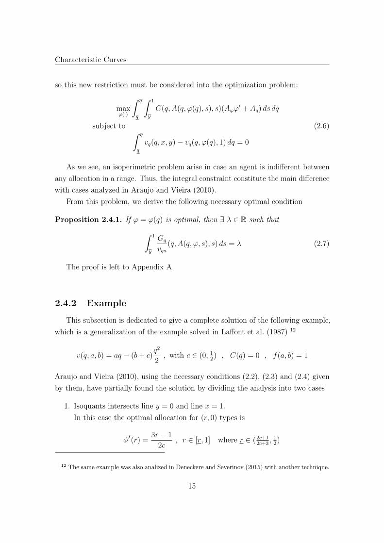
2.4.2 Example
This subsection is dedicated to give a complete solution of the following example,
which is a generalization of the example solved in Laffont et al. (1987) 12
v(q, a, b) = aq − (b+ c)q2
2, with c ∈ (0, 1
2) , C(q) = 0 , f(a, b) = 1
Araujo and Vieira (2010), using the necessary conditions (2.2), (2.3) and (2.4) given
by them, have partially found the solution by dividing the analysis into two cases
1. Isoquants intersects line y = 0 and line x = 1.
In this case the optimal allocation for (r, 0) types is
φI(r) =3r − 1
2c, r ∈ [r, 1] where r ∈ (2c+1
2c+3, 1
2)
12 The same example was also analized in Deneckere and Severinov (2015) with another technique.
15

Preliminaries
2. Isoquants intersects the participation’s boundary β(r) and line x = 1.
In this case the participation’s boundary is
β(r) =2r3 − 4r2 + 2r
K0
+K1 (K0, K1 constants)
and the optimal allocation rule for (r, β(r)) types is
φII(r) =K0
3r2 − 4r + 1, r ∈ [r, x]
Setting y = β(x), we are able to complete the solution of this example by the
following claims:
Claim 1.
There are no isoquants intersecting participation’s boundary and y = 1 line.
Claim 2.
There are no isoquants concurrent at the point (x, y) and intersecting the line x = 1.
Claim 3.
There exists isoquants concurrent at the point (x, y) and intersecting the line y = 1.
In this case y =1− 2c
3and the optimal allocation rule for (r, 1) types is
φIII(r) =r − x1− y
, r ∈ [x, 1]
In order to determine the constants K0, K1, r, and x note that, by continuity of
the allocation rule and boundary conditions, it must be true:
1. φI(r) = φII(r) 3. β(r) = 0
2. φII(x) = φIII(1) 4. β(x) = y
Conditions 1. and 3. implies
K0 =−(1− r)(3r − 1)2
2c, K1 =
4cr(1− r)(3r − 1)2
(2.8)
16

Characteristic Curves
Because of 4., we can write φIII(r) = (r − x)/(1− β(x)), so condition 2. yields on
β(x) = 1− (1−3x)(1−x)2
K0. Then, using the expression of β and (2.8)
(1− x)3 =(9 + 4c)r3 − (15 + 8c)r2 + (7 + 4c)r − 1
2c(2.9)
On the other hand, by conditions 2. and 4.
(1− 3x)(x− 1)2 = K0(1− y) and 2x(x− 1)2 = K0(y −K1)
dividing (seeing that 13< 2c+1
2c+3< x < 1), clearing x, and using (2.8), we get
1− x =(54 + 24c)r2 − (36 + 24c)r + 6
(63 + 18c)r2 − (42 + 24c)r + (7− 2c)
therefore, by (2.9), we have that r is the solution on (2c+12c+3
, 12) of
( (54 + 24c)r2 − (36 + 24c)r + 6
(63 + 18c)r2 − (42 + 24c)r + (7− 2c)
)3=
(9 + 4c)r3 − (15 + 8c)r2 + (7 + 4c)r − 1
2c
and with that r, we obtain
x =(9− 6c)r2 − 6r + 1− 2c
(63 + 18c)r2 − (42 + 24c)r + (7− 2c)(2.10)
Thus, all the elements defining φI , φII , φIII , and β are determined as well as the
special point (x, y). This type (x, y) is indifferent between any quantity in the interval
[0, 3(1−x)2(1+c)
], while the optimal quantity allocation range is [0, 1c].
To express the optimal quantity in terms of (a, b), note that the type set [0, 1]2 can
be partitioned into four sets Z0, ZI , ZII and ZIII defined as:
Z0 = (a, b) ∈ [0, 1]2 : a < x ∧ b > β(a)
ZI = (a, b) ∈ [0, 1]2 : b ≤ ( 2c3r−1
)a− r3r−1
ZII = (a, b) ∈ [0, 1]2 : a ≥ x ∧ b > ( 2c3r−1
)a− r3r−1
∧ b ≤ ( 1−y1−x)a+ y−x
1−x
∪ (a, b) ∈ [0, 1]2 : a < x ∧ b > ( 2c3r−1
)a− r3r−1
∧ b ≤ β(a)
ZIII = (a, b) ∈ [0, 1]2 : a ≥ x ∧ b > ( 1−y1−x)a+ y−x
1−x
17
Preliminaries
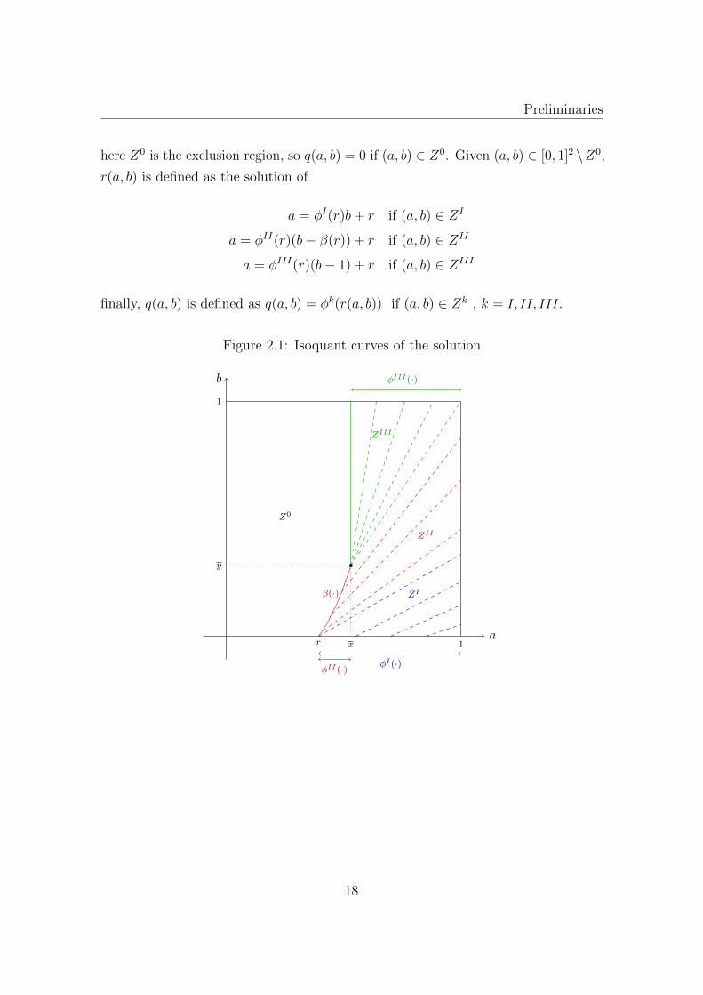
here Z0 is the exclusion region, so q(a, b) = 0 if (a, b) ∈ Z0. Given (a, b) ∈ [0, 1]2 \Z0,
r(a, b) is defined as the solution of
a = φI(r)b+ r if (a, b) ∈ ZI
a = φII(r)(b− β(r)) + r if (a, b) ∈ ZII
a = φIII(r)(b− 1) + r if (a, b) ∈ ZIII
finally, q(a, b) is defined as q(a, b) = φk(r(a, b)) if (a, b) ∈ Zk , k = I, II, III.
Figure 2.1: Isoquant curves of the solution
a
b φIII(·)
ZIII
φII(·)
ZII
φI(·)
ZI
r 1
1
x
y
β(·)
Z0
18
Appendix A
2.5 Appendix A
Determining virtual surplus G:
Here we show how the virtual surplus G for the bidimensional case can be determined
if the optimal quantity allocated to types (0, b) is the exclude option quantity qout,
that is q(0, b) = qout. Also, assume v(qout, a, b) is constant and distributions f over
a and g over b are independent, so ρ(a, b) = f(a)g(b). We will show
G(q, a, b) =(v(q, a, b)− C(q)− 1− F (a)
f(a)va(q, a, b)
)f(a)g(b)
Note that, by the Fundamental Theorem of Calculus and the Envelope Theorem
V (a, b)− V (0, 1) = V (a, b)− V (0, b) + V (0, b)− V (0, 1)
=
∫ a
0
Va(a, b)da+
∫ b
1
Vb(0, b)db
=
∫ a
0
va(q(a, b), a, b)da+
∫ b
1
vb(q(0, b), 0, b)db
since V (0, 1) = 0 and vb(q(0, b), 0, b) = vb(qout, 0, b) = 0 (because v(qout, a, b) is
constant), we have
V (a, b) =
∫ a
0
va(q(a, b), a, b)da
Then, through integration by parts∫ 1
0
∫ 1
0
V (a, b)ρ(a, b) da db
=
∫ 1
0
∫ 1
0
(∫ a
0
va(q(a, b), a, b)da)f(a)g(b) da db
=
∫ 1
0
∫ 1
0
(∫ a
0
va(q(a, b), a, b)da)dF (a) g(b) db
=
∫ 1
0
[( ∫ a
0
va(q(a, b), a, b)da)F (a)
∣∣∣a=1
a=0−∫ 1
0
F (a)va(q(a, b), a, b)da]g(b) db
=
∫ 1
0
[ ∫ 1
0
va(q(a, b), a, b) da−∫ 1
0
F (a)va(q(a, b), a, b)da]g(b) db
=
∫ 1
0
∫ 1
0
(1− F (a)
f(a)va(q(a, b), a, b)
)f(a)g(b) da db
19
Preliminaries
Thus, the expected income∫ 1
0
∫ 1
0
(v(q(a, b), a, b)− C(q(a, b))− V (a, b)
)f(a)g(b) da db
can be written as ∫ 1
0
∫ 1
0
G(q(a, b), a, b) da db
Proof of Proposition 2.4.1.
Because a(q, s) = A(q, ϕ(q), s) , b(q, s) = s, we have
∂(a, b)
∂(q, s)=
∣∣∣∣∣ aq bq
as bs
∣∣∣∣∣ =
∣∣∣∣∣ aq 0
as 1
∣∣∣∣∣ = aq = Aϕϕ′ + Aq
At this point, the aditional assumption aq > 0 is requiered 13. Then, the revenue can
be written as∫ q
q
∫ 1
yG(q, A(q, ϕ(q), s), s)×
∣∣∣∂(a, b)
∂(q, s)
∣∣∣ ds dq =
∫ q
q
∫ 1
yG(q, A(q, ϕ(q), s), s)(Aϕϕ
′+Aq) ds dq
which explain objective’s function in (2.6) takes that form. For such isoperimetric
problem, the necessary condition for optimality is 14
Hϕ −d
dq(Hϕ′) = λ(Fϕ −
d
dq(Fϕ′))
for some λ ∈ R, where
H(q, ϕ, ϕ′) =
∫ 1
y
G(q, A(q, ϕ, s), s)(Aϕϕ′ + Aq) ds
F (q, ϕ, ϕ′) = vq(q, x, y)− vq(q, ϕ, 1)
13Since ϕ′ > 0, it would be sufficient to assume that ar > 0 (in the original variables) whichseems natural due to for any fix s , a(r, s) should be increasing in r (for example, if s = 1 over theinitial curve (r, 1) : r ∈ [R1, R2] first component is increasing in r)
14See Kamien and Schwartz (1981)
20

Appendix A
We have
Hϕ =
∫ 1
y
GaAϕ(Aϕϕ′ + Aq) +G(Aϕϕϕ
′ + Aϕq)ds
Hϕ′ =
∫ 1
y
GAϕ ds
d
dq(Hϕ′) =
∫ 1
y
(Gq +Ga(Aϕϕ′ + Aq))Aϕ +G(Aϕϕϕ
′ + Aϕq) ds
Fϕ = −vqa(q, ϕ, 1)
Fϕ′ = 0
Then
Hϕ −d
dr(Hϕ′) = −
∫ 1
y
Gq(q, A(q, ϕ, s), s)Aϕ(q, ϕ, s) ds
Fϕ −d
dq(Fϕ′) = −vqa(q, ϕ, 1)
Since for any q and s fixed, vq(q, ϕ, 1) = vq(q, A(q, ϕ, s), s), taking the derivative
with respect to ϕ:
vqa(q, ϕ, 1) = vqa(q, A(q, ϕ, s), s)Aϕ(q, ϕ, s)
thus, we can replace Aϕ(q, ϕ, s) and obtain, as a necessary optimal condition, that
exists some λ ∈ R such that
−vqa(q, ϕ, 1)
∫ 1
y
Gq
vqa(q, A(q, ϕ, s), s) ds = −λvqa(q, ϕ, 1)
and since vqa > 0 ∫ 1
y
Gq
vqa(q, A(q, ϕ, s), s) ds = λ
Proof of Claim 1.
For this example G(q, a, b) = (2a− 1)q − (b+c)2q2 , vqa = 1 and vb(q, a, b) = − q2
2.
Also a(r, s) = sφ(r) + r , b(r, s) = s + β(r) are the solutions of (2.5) system, and
s(r) = 1− β(r) because we are looking for isoquants intersecting y = 1.
21
Preliminaries
Then, necessary conditions (2.3) and (2.4) yields on
λ(r) =3
2β(r)2φ(r) + (c− 2)β(r)φ(r) +
1− 2c
2φ(r) + (2r − 1)(1− β(r)) (2.11)
λ′(r) =2(1− 2r)
φ(r)+ β(r) + c (2.12)
Taking the derivative on (2.11), by (2.12) we get
φ′(r) =2(2− c− 3β(r))
(3β(r) + 2c− 1)(β(r)− 1)(2.13)
Additionally V (r, β(r)) = 0 for all types over the boundary. Then, fromddrV (r, β(r)) = 0 and by the Envelope Theorem, we have 15
va(φ(r), r, β(r)) + vb(φ(r), r, β(r))β′(r) = 0
for this example, this condition yields to
φ(r)β′(r) = 2 (2.14)
taking the derivative on (2.14), by (2.13) we obtain the following differential equation
β′′ +(2− c− 3β)
(3β + 2c− 1)(β − 1)(β′)2 = 0
Thus, in case isoquants intersects the line y = 1 and participation’s boundary β,
such curve β satisfies previous differential equation.
The solutions (besides constant functions) are of the form
β(r) =e√
3B0r
2√
3B1
+B1(c+ 1)2
6√
3e−√
3B0r − c− 2
3
with B0, B1 constants.
Note that, for this example, informational rent V is a convex function so the
15This condition was established in Araujo and Vieira (2010) before to derive the necessaryconditions (2.3) and (2.4)
22

Appendix A
non-participation region Ω = (a, b) : V (a, b) = 0 is a convex set and boundary
curves must to be convex functions, i.e., β′′(r) ≥ 0 which implies B1 > 0. Since√
3e√3B0r
(c+1)B1+ (c+1)B1√
3e√
3B0r≥ 2 we have
β(r) =(√3e
√3B0r
(c+ 1)B1
+(c+ 1)B1√
3e√
3B0r
)(c+ 1)
6− c− 2
3≥ 1
therefore, such curves cannot represent the boundary because are not contained in
the interior of [0, 1]2.
Proof of Claim 2.
First, we will establish the necessary condition in case isoquants are concurrent at
the point (x, y) and intersects the x = 1 line. The PDE (2.1) can be written as
qa + (−vqavqb
)qb = 0
Considering (1, r) : r ∈ [R1, R2] as initial curve, we have to solve
as(r, s) = 1 , a(r, 1) = 1
bs(r, s) = −vqavqb
(φ(r), a(r, s), b(r, s)) , b(r, 1) = r
where φ : [R1, R2]→ [q, q] describes the quantity (or quality) allocated to (1, r) types.
In view of vqb < 0 this function φ is strictly decreasing, so consider ϕ : [q, q]→ [R1, R2]
as the inverse of φ . If a(r, s) = s and b(r, s) = B(φ(r), r, s) are the solutions of the
previous system, a and b can be expressed in terms of q and s :
a(q, s) = s , b(q, s) = B(q, ϕ(q), s)
where q ∈ [q, q] , s ∈ [x, 1]. With these variables, the revenue is
∫ q
q
∫ 1
x
G(q, s, B(q, ϕ(q), s))(− (Bq +Bϕϕ
′))ds dq
As before (x, y) is indifferent between any q ∈ [q, q] , then vq(q, x, y) = vq(q, 1, ϕ).
23

Preliminaries
Setting
H(q, ϕ, ϕ′) = −∫ 1
x
G(q, s, B(q, ϕ(q), s))(Bq +Bϕϕ′) ds
F (q, ϕ, ϕ′) = vq(q, x, y)− vq(q, 1, ϕ)
the problem can be written as
maxϕ(·)
∫ q
q
H(q, ϕ, ϕ′) dq
subject to∫ q
q
F (q, ϕ, ϕ′) dq = 0
The necessary condition for optimality is Hϕ − ddq
(Hϕ′) = λ(Fϕ − ddq
(Fϕ′)) for some
λ ∈ R, which yields to ∫ 1
x
Gq
vqb(q, s, B(q, ϕ, s)) ds = λ (2.15)
Next, we will see that cannot be the case of isoquants intersecting x = 1 be
concurrent at (x, y). The solutions of the system
as(r, s) = 1 , a(r, 1) = 1
bs(r, s) = 1φ(r)
, b(r, 1) = r
are a(r, s) = s , b(r, s) = s−1φ(r)
+ r . Then a(q, s) = s , b(q, s) = (s−1)q
+ ϕ(q). For this
example Gq(q, a, b) = 2a − 1 − (b + c)q , vqb(q, a, b) = −q. Then, by the necessary
condition (2.15), there exists λ ∈ R such that∫ 1
x
(1− 2s
q+
(s− 1)
q+ ϕ+ c
)ds = λ
from which
ϕ(q) =1 + x
2q+
λ
1− x− c
24

Appendix A
On the other hand, vq(q, x, y) = vq(q, 1, ϕ) implies
ϕ(q) =1− xq
+ y
Thus, by comparison of terms x = 13
in contradiction with 13< 2c+1
2c+3< x < 1.
Proof of Claim 3.
The solutions of the system
as(r, s) = φ(r) , a(r, 1) = r
bs(r, s) = 1 , b(r, 1) = 1
are a(r, s) = (s− 1)φ(r) + r , b(r, s) = s . Then a(q, s) = (s− 1)q+ϕ(q) , b(q, s) = s.
Also, we have G(q, a, b) = (2a− 1)q − (b+ c)q2
2In case the isoquants are concurrent at the point (x, y) intersecting y = 1 line, by
the Proposition 2.4.1 there exists λ ∈ R such that∫ 1
y
2((s− 1)q + ϕ)− 1− (s+ c)q ds = λ
which yields on
ϕ(q) = (2c+ 3− y
4)q +
1
2+
λ
2(1− y)
Moreover,
vq(q, x, y) = vq(q, ϕ(q), 1) =⇒ ϕ(q) = x+ (1− y)q
So, by comparison of terms we obtain
x =1
2+
3λ
4(c+ 1), y =
1− 2c
3
where λ is constant for a given c ∈ (0, 12]. Also, we have
φIII(r) =r − x1− y
where φIII is the optimal allocation of type (r, 1). Because φIII(x) = 0, the domain
of φIII is [x, 1] .
25

Preliminaries
26
Chapter 3
Reduction of IC Constraints in the
Bidimensional Model
This chapter contains the main contribution of this work which consist in justify
that, for a pair (q, V ) to be incentive compatible, it is sufficient that each point
verifies IC constraints with all the points over a unidimensional set instead of the
whole type set as it is required by definition. With that, numerical approximations
can be done with relative fine discretization. This approach, while specific for the
case of bidimensional types and one-dimensional quantity product, is general in
terms of the valuation function involved as well as types’ distribution. The main
assumption is the validity of single-crossing in each axis.
Before discuss our approach, in the following lines we illustrate the ideas being
applied to deal with IC constraints in the unidimensional case with finite type set
when single-crossing holds1. This explanation would be useful since we are extending
these ideas in the bidimensional context.
Consider, for example, Θ = θ1, . . . , θ6 ⊂ R with θ1 < θ2 < · · · < θ6 and a given
(q, V ). The following incentive compatibility (IC) constraints must be satisfied:
V (θ)− V (θ) ≥ v(q(θ), θ)− v(q(θ), θ) ∀ θ, θ ∈ Θ
1See Laffont and Martimort (2002).
27
Reduction of IC Constraints in the Bidimensional Model
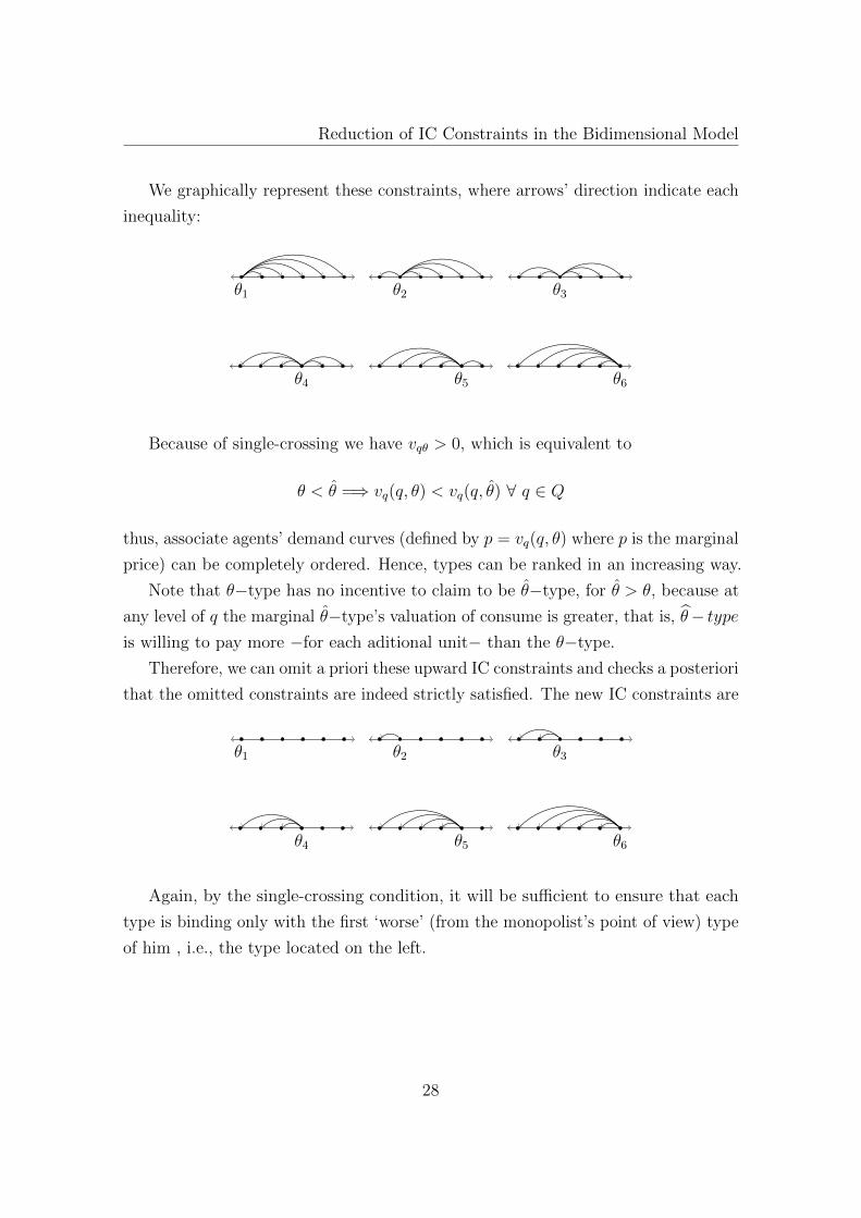
We graphically represent these constraints, where arrows’ direction indicate each
inequality:
θ1 θ2 θ3
θ4 θ5 θ6
Because of single-crossing we have vqθ > 0, which is equivalent to
θ < θ =⇒ vq(q, θ) < vq(q, θ) ∀ q ∈ Q
thus, associate agents’ demand curves (defined by p = vq(q, θ) where p is the marginal
price) can be completely ordered. Hence, types can be ranked in an increasing way.
Note that θ−type has no incentive to claim to be θ−type, for θ > θ, because at
any level of q the marginal θ−type’s valuation of consume is greater, that is, θ− typeis willing to pay more −for each aditional unit− than the θ−type.
Therefore, we can omit a priori these upward IC constraints and checks a posteriori
that the omitted constraints are indeed strictly satisfied. The new IC constraints are
θ1 θ2 θ3
θ4 θ5 θ6
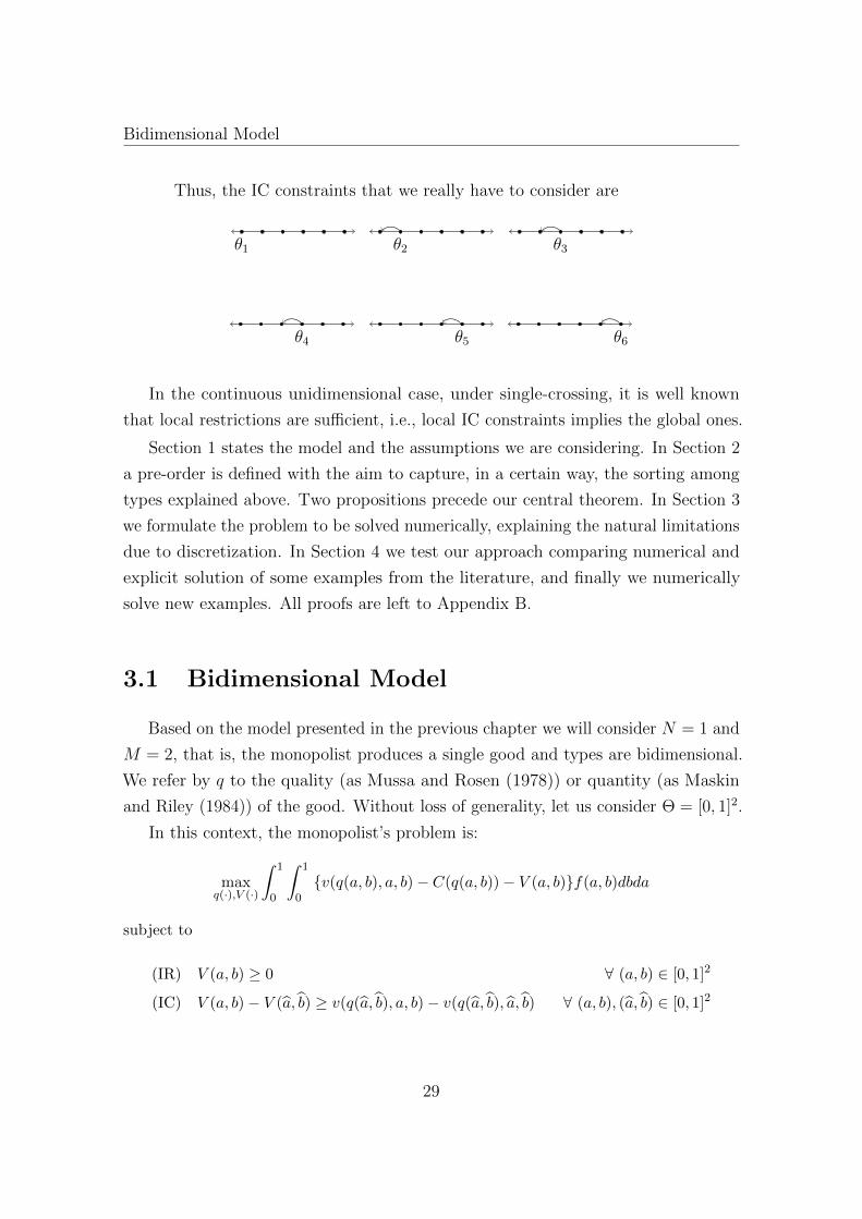
Again, by the single-crossing condition, it will be sufficient to ensure that each
type is binding only with the first ‘worse’ (from the monopolist’s point of view) type
of him , i.e., the type located on the left.
28
Bidimensional Model
Thus, the IC constraints that we really have to consider are
θ1 θ2 θ3
θ4 θ5 θ6
In the continuous unidimensional case, under single-crossing, it is well known
that local restrictions are sufficient, i.e., local IC constraints implies the global ones.
Section 1 states the model and the assumptions we are considering. In Section 2
a pre-order is defined with the aim to capture, in a certain way, the sorting among
types explained above. Two propositions precede our central theorem. In Section 3
we formulate the problem to be solved numerically, explaining the natural limitations
due to discretization. In Section 4 we test our approach comparing numerical and
explicit solution of some examples from the literature, and finally we numerically
solve new examples. All proofs are left to Appendix B.
3.1 Bidimensional Model
Based on the model presented in the previous chapter we will consider N = 1 and
M = 2, that is, the monopolist produces a single good and types are bidimensional.
We refer by q to the quality (as Mussa and Rosen (1978)) or quantity (as Maskin
and Riley (1984)) of the good. Without loss of generality, let us consider Θ = [0, 1]2.
In this context, the monopolist’s problem is:
maxq(·),V (·)
∫ 1
0
∫ 1
0v(q(a, b), a, b)− C(q(a, b))− V (a, b)f(a, b)dbda
subject to
(IR) V (a, b) ≥ 0 ∀ (a, b) ∈ [0, 1]2
(IC) V (a, b)− V (a, b) ≥ v(q(a, b), a, b)− v(q(a, b), a, b) ∀ (a, b), (a, b) ∈ [0, 1]2
29
Reduction of IC Constraints in the Bidimensional Model
We assume v ∈ C3, q and t to be continuous, and a.e. twice continuously
differentiable2. These assumptions imply that V has the same features.
Also, the following assumptions are considered:
A1 vq2 < 0
A2 C(0) = 0 , C ′(q) ≥ 0 and C′′(q) ≥ 0
A3 vqa > 0 and vqb < 0 when q > 0
A4 va > 0 and vb < 0 when q > 0
A5 v(qout, a, b) is constant
Assumption A1 means that each type’s valuation function is strictly concave. A2
means that costs and marginal costs are non-decreasing. Assumption A3 is the
single-crossing condition on each axis. We are assuming those signs for vqa and vqb
because coincides with the assumptions in Araujo and Vieira (2010) and we are
going to use later their necessary condition for optimality (2.2) in an example. Since
we are interested in determine if characteristic curves are increasing or decreasing,
which is given by the sign of−vqbvqa
, other cases are easily adapted.
Note that the assumption A4 allows us to rule out all the IR constraints providing
that V (0, 1) = 0. In fact, due to V (a, b) = max(a,b)v(q(a, b), a, b) − t(a, b) by the
Envelope Theorem3
Va(a, b) = va(q(a, b), a, b) , Vb(a, b) = vb(q(a, b), a, b) a.e. (a, b)
then Va > 0 and Vb < 0 when q > 0, so V is strictly increasing in a and strictly
decreasing in b on the interior of the participation set. Thus, it will be sufficient to
impose V (0, 1) = 0 and all the IR constraints will be satisfied.
2By assumption A3. stated below and using the Monotone Maximum Theorem, it can be provedthat q is non-decreasing in a and non-increasing in b, and therefore a.e. differentiable. Our strongerassumptions allows us to give another (perphaps more familiar) proof. Also, those assumptions arerequired to establish the PDE (2.1) in section 2.4, that we will use later.
3See Milgrom and I.Segal (2002)
30
Reducing IC Constraints
Usually assumption A5 is presented as v(0, a, b) = 0 because in the monopolist’s
problem framework the outside option is qout = 0 and any agent assigns the value
zero to this qout. However, in other adverse selection problems this could be no
longer true, so we assume the more general expression A5 .
Proposition 3.1.1. If q(·, ·) is implementable, at any point (a, b) of twice continuous
differentiability, we have qa(a, b) ≥ 0 and qb(a, b) ≤ 0
Thus, q is non-decreasing in a and non-increasing in b. This result is consequence
of assumption A3. Unlike the unidimensional case, this necessary condition for
implementability is not longer sufficient.
3.2 Reducing IC Constraints
In bidimensional models we do not have a condition similar to the single-crossing
in the unidimensional case, where all types can exogenously be ordered by their
marginal valuation for consumption (vqθ > 0 means θ1 < θ2 =⇒ vq(q, θ1) < vq(q, θ2)
for any q ∈ Q fixed). In order to be able of compare apriori two different types, at
least partially, we introduce the following binary relation:
Definition 3.2.1. Given (a, b), (a, b) ∈ [0, 1]2 we will say that (a, b) is worse than
(a, b), denoted by (a, b) (a, b), if and only if
vq(q, a, b) ≤ vq(q, a, b) ∀ q ∈ Q
Note that is a pre-order (reflexive and transitive) on [0, 1]2.
With this definition we try to capture the idea that, when (a, b) (a, b), the
(a, b)-agent is not willing to announce to be the (a, b)−agent, since at any level of
q ∈ Q the (a, b)−agent has greater marginal utility, so (a, b)−agent is willing to pay
more for each aditional unit of the product.
As a direct consequence of the assumptions vqa > 0 and vqb < 0 we have that
(a, b) is worse than any type on the southeast.
Proposition 3.2.1. For any fixed (a, b), if (a, b) is such that a > a and b < b, then
(a, b) (a, b)
31
Reduction of IC Constraints in the Bidimensional Model
At this point, it is useful remember what we have seen in Section 2.4. For an
allocation rule q(·) to be implementable, it must satisfy a.e.
−vqbvqa
qa + qb = 0
by the characteristic method to solve the previous PDE, we obtain a family of
plane characteristic curves parametrized by r, s where, for a fix r, all types over the
curve (a(r, s), b(r, s)) gets the same allocation, that is, plane characteristic curves
are the isoquants of q. Also, in view of at any point of any isoquant, the tangent
vector (as, bs) = (− vqbvqa, 1) has both components positive, all the isoquants are strictly
increasing in the participation set interior.
Note: In order to facilitate reading, sometimes we will write c.c. instead of both
characteristic curve or characteristic curves.
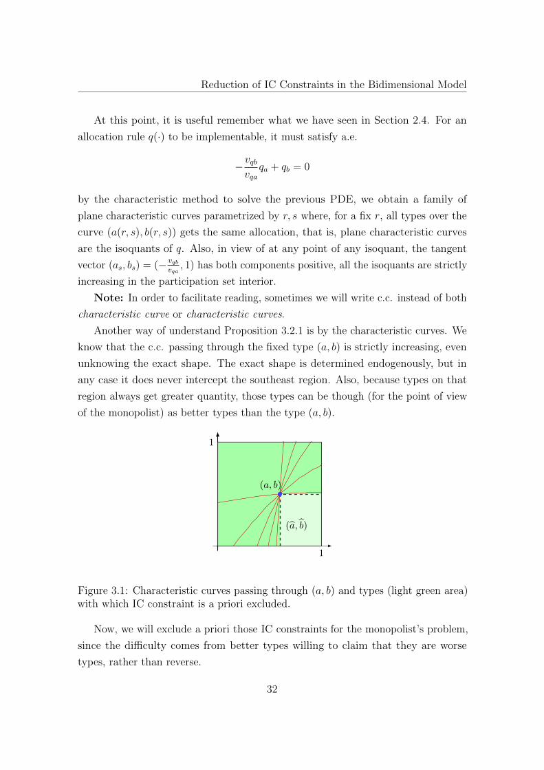
Another way of understand Proposition 3.2.1 is by the characteristic curves. We
know that the c.c. passing through the fixed type (a, b) is strictly increasing, even
unknowing the exact shape. The exact shape is determined endogenously, but in
any case it does never intercept the southeast region. Also, because types on that
region always get greater quantity, those types can be though (for the point of view
of the monopolist) as better types than the type (a, b).
1
1
(a, b)
a
(a, b)
Figure 3.1: Characteristic curves passing through (a, b) and types (light green area)with which IC constraint is a priori excluded.
Now, we will exclude a priori those IC constraints for the monopolist’s problem,
since the difficulty comes from better types willing to claim that they are worse
types, rather than reverse.
32

Reducing IC Constraints
Specifically we will omit the following IC constraints, for a fixed type (a, b)
V (a, b)− V (a, b) ≥ v(q(a, b), a, b)− v(q(a, b), a, b) ∀(a, b) with a > a, b < b
We should be able to checks a posteriori (i.e., after solution is obtained) that these
omitted constraints are indeed strictly satisfied4.
After that, we will see that it is sufficient for the monopolist to guarantee that
the type (a, b) satisfies the IC constraint with the closest type to him, in terms that
will be clear later.
Notations
• We say “ (a, b) is IC with (a, b) ” when
V (a, b)− V (a, b) ≥ v(q(a, b), a, b)− v(q(a, b), a, b)
that is, when the (a, b)-agent has not the incentive to announce to be the
(a, b)-agent.
• CC(a, b) is the plane characteristic curve that contains (a, b)
Proposition 3.2.2. Let (a, b), (a, b) be such that (a, b) is IC with (a, b). Then (a, b)
is IC with (x, y) , ∀ (x, y) ∈ CC(a, b)
By this proposition, we just need to verify IC constraint with a representative
type of each c.c., so we will focus on the border of the square.
Proposition 3.2.3. Let (x, y), (a, b), (a, b) be such that (a, b) verifies IC with (a, b)
and (a, b) verifies IC with (x, y). If (a, b) (a, b) and q(x, y) ≤ q(a, b) then (a, b)
verifies IC with (x, y).
Due to the kind of transitivity that this proposition shows, it is not necessary
that a fixed (a, b) type verifies IC constraints with all the types (x, y) on the left of
certain characteristic curve, instead, it is sufficient to verify the IC constraint with
any type worse than (a, b) over such curve, ensuring that this type verifies the IC
constraint with all of those (x, y).
4Because we are interesting on numerical approximations, the verification will also be numerical.
33
Reduction of IC Constraints in the Bidimensional Model
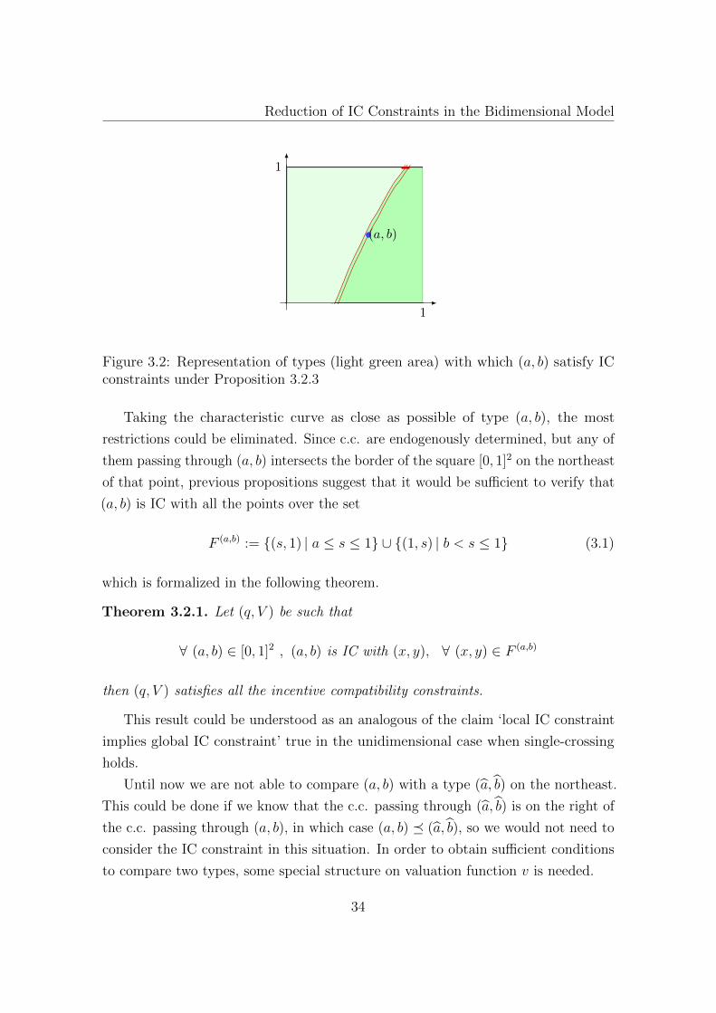
1
1
(a, b)
Figure 3.2: Representation of types (light green area) with which (a, b) satisfy ICconstraints under Proposition 3.2.3
Taking the characteristic curve as close as possible of type (a, b), the most
restrictions could be eliminated. Since c.c. are endogenously determined, but any of
them passing through (a, b) intersects the border of the square [0, 1]2 on the northeast
of that point, previous propositions suggest that it would be sufficient to verify that
(a, b) is IC with all the points over the set
F (a,b) := (s, 1) | a ≤ s ≤ 1 ∪ (1, s) | b < s ≤ 1 (3.1)
which is formalized in the following theorem.
Theorem 3.2.1. Let (q, V ) be such that
∀ (a, b) ∈ [0, 1]2 , (a, b) is IC with (x, y), ∀ (x, y) ∈ F (a,b)
then (q, V ) satisfies all the incentive compatibility constraints.
This result could be understood as an analogous of the claim ‘local IC constraint
implies global IC constraint’ true in the unidimensional case when single-crossing
holds.
Until now we are not able to compare (a, b) with a type (a, b) on the northeast.
This could be done if we know that the c.c. passing through (a, b) is on the right of
the c.c. passing through (a, b), in which case (a, b) (a, b), so we would not need to
consider the IC constraint in this situation. In order to obtain sufficient conditions
to compare two types, some special structure on valuation function v is needed.
34

Reducing IC Constraints
3.2.1 Particular valuation function
The following propositions allows us to reduce even more the IC constraints,
when the valuation function v has a special structure.
Proposition 3.2.4. Assume that vq is concave in a and convex in b. Let (a, b) ,
(a, b) be in [0, 1]2 with a < a , b < b . Then
1. (a, b) (a, b) =⇒ b− ba− a
≤ −vqa(q, a, b)vqb(q, a, b)
2.b− ba− a
≤ −vqa(q, a, b)vqb(q, a, b)
=⇒ (a, b) (a, b)
This proposition says that, in order to (a, b) (a, b), it is necessary that CC(a, b)
be on the left of CC(a, b), because at the point (a, b) the slope of CC(a, b) is greater
than the slope between (a, b) and (a, b).
Similarly, and more useful, a sufficient condition for (a, b) (a, b) is that the
slope of CC(a, b) at the point (a, b) be greater than the slope between (a, b) and
(a, b). With that CC(a, b) will be at the right of CC(a, b).
We illustrate previous proposition in the following graphics.
Case vqaa ≤ 0 and vqbb ≥ 0
(a, b) (a, b) =⇒(a, b) (a, b)
(a, b)(a, b)
(a, b) (a, b)
(a, b)(a, b)
=⇒ (a, b) (a, b)
35
Reduction of IC Constraints in the Bidimensional Model
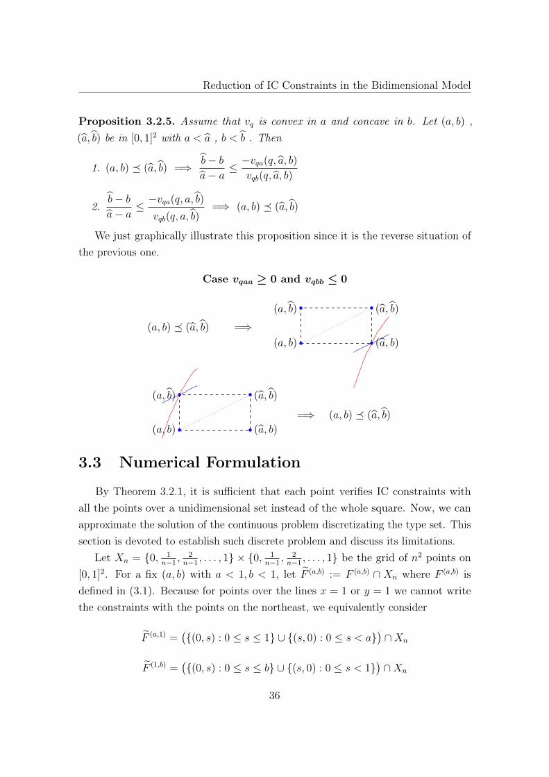
Proposition 3.2.5. Assume that vq is convex in a and concave in b. Let (a, b) ,
(a, b) be in [0, 1]2 with a < a , b < b . Then
1. (a, b) (a, b) =⇒ b− ba− a
≤ −vqa(q, a, b)vqb(q, a, b)
2.b− ba− a
≤ −vqa(q, a, b)vqb(q, a, b)
=⇒ (a, b) (a, b)
We just graphically illustrate this proposition since it is the reverse situation of
the previous one.
Case vqaa ≥ 0 and vqbb ≤ 0
(a, b) (a, b) =⇒(a, b) (a, b)
(a, b)(a, b)
(a, b) (a, b)
(a, b)(a, b)
=⇒ (a, b) (a, b)
3.3 Numerical Formulation
By Theorem 3.2.1, it is sufficient that each point verifies IC constraints with
all the points over a unidimensional set instead of the whole square. Now, we can
approximate the solution of the continuous problem discretizating the type set. This
section is devoted to establish such discrete problem and discuss its limitations.
Let Xn = 0, 1n−1
, 2n−1
, . . . , 1 × 0, 1n−1
, 2n−1
, . . . , 1 be the grid of n2 points on
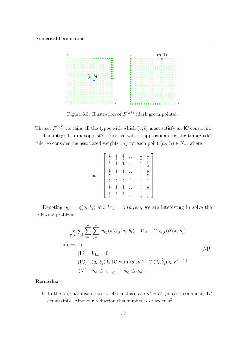
[0, 1]2. For a fix (a, b) with a < 1, b < 1, let F (a,b) := F (a,b) ∩ Xn where F (a,b) is
defined in (3.1). Because for points over the lines x = 1 or y = 1 we cannot write
the constraints with the points on the northeast, we equivalently consider
F (a,1) =((0, s) : 0 ≤ s ≤ 1 ∪ (s, 0) : 0 ≤ s < a
)∩Xn
F (1,b) =((0, s) : 0 ≤ s ≤ b ∪ (s, 0) : 0 ≤ s < 1
)∩Xn
36
Numerical Formulation
(a, b)
(a, 1)
Figure 3.3: Illustration of F (a,b) (dark green points).
The set F (a,b) contains all the types with which (a, b) must satisfy an IC constraint.
The integral in monopolist’s objective will be approximate by the trapezoidal
rule, so consider the associated weights wi,j for each point (ai, bj) ∈ Xn, where
w =
14
12
12
. . . 12
14
12
1 1 . . . 1 12
12
1 1 . . . 1 12
......
.... . .
......
12
1 1 . . . 1 12
14
12
12
. . . 12
14
Denoting qi,j = q(ai, bj) and Vi,j = V (ai, bj), we are interesting in solve the
following problem:
maxqi,j ,Vi,j
n∑i=1
n∑j=1
wi,j(v(qi,j, ai, bj)− Vi,j − C(qi,j))f(ai, bj)
subject to
(IR) V1,n = 0
(IC) (ai, bj) is IC with (ai, bj) , ∀ (ai, bj) ∈ F (ai,bj)
(M) qi,j ≤ qi+1,j , qi,j ≤ qi,j−1
(NP)
Remarks:
I. In the original discretized problem there are n4 − n2 (maybe nonlinear) IC
constraints. After our reduction this number is of order n3.
37
Reduction of IC Constraints in the Bidimensional Model
II. The monotonicity constraints are added in order to obtain better accuracy
of the solution although, as we know, monotonicity is a necessary condition.
These 2n2 linear restrictions added do not represent big numerical cost.
III. In case assumption A4 cannot be verifed, we just consider all the IR constraints
Vi,j ≥ 0.
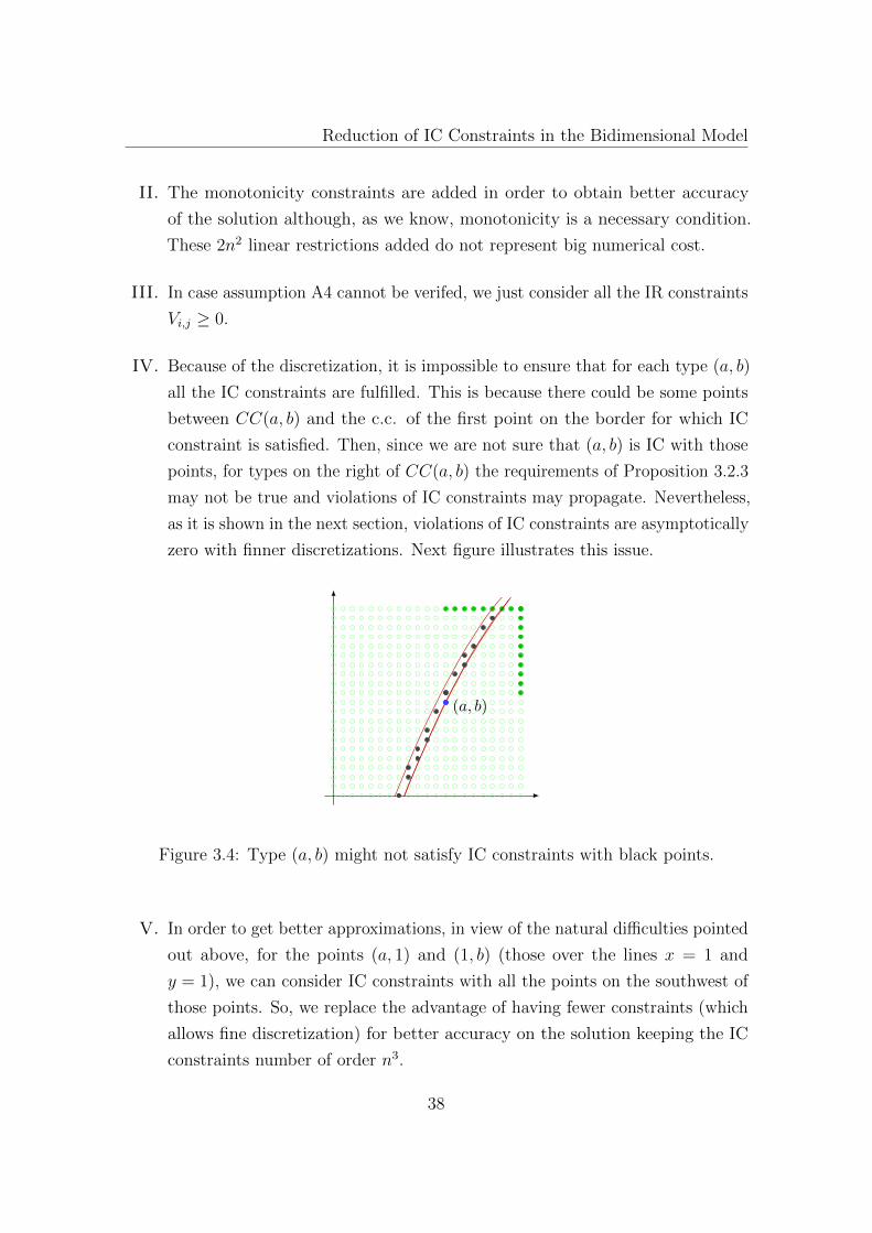
IV. Because of the discretization, it is impossible to ensure that for each type (a, b)
all the IC constraints are fulfilled. This is because there could be some points
between CC(a, b) and the c.c. of the first point on the border for which IC
constraint is satisfied. Then, since we are not sure that (a, b) is IC with those
points, for types on the right of CC(a, b) the requirements of Proposition 3.2.3
may not be true and violations of IC constraints may propagate. Nevertheless,
as it is shown in the next section, violations of IC constraints are asymptotically
zero with finner discretizations. Next figure illustrates this issue.
(a, b)
Figure 3.4: Type (a, b) might not satisfy IC constraints with black points.
V. In order to get better approximations, in view of the natural difficulties pointed
out above, for the points (a, 1) and (1, b) (those over the lines x = 1 and
y = 1), we can consider IC constraints with all the points on the southwest of
those points. So, we replace the advantage of having fewer constraints (which
allows fine discretization) for better accuracy on the solution keeping the IC
constraints number of order n3.
38

Asymptotic Optimality
VI. When valuation function has the special ‘multiplicative separable’ form
v(q, a, b) = ψ(q) + α(a, b)×q + β(a, b)
the IC constraints become linear in qi,j. Therefore, since IC constraints are
linear in V (regardless v) and the objective function is strictly concave, the
solution is unique and we can rely on numerical approximation.
3.4 Asymptotic Optimality
Next, following Belloni et al. (2010) we prove that extending the solutions of
the discretized problem in an appropiate manner, all the IC violations converge
uniformly to zero, and the sequence of optimal values converge to the optimal value
of the continuous problem. They have considered a linear model including multiple
agents and Border constraints5, which are not present in our setting. In contrast,
we consider a valuation function v that could be nonlinear, so we assume that v is
Lipschitz6 over [0, 1]2.
As before, let Xn be the grid of n2 points over [0, 1]2. Let Qn, V n be the numerical
solutions of the problem formulated in 3.3. These solutions are defined over the
discret set Xn, so we define the extensions Qn, V n : [0, 1]2 → R as
Qn(a, b) := Qn(a, b) , V n(a, b) := V n(a, b)
where (a, b) ∈ Xn is such that
a ≤ a < a+ 1n−1 , b− 1
n−1 < b ≤ b
Proposition 3.4.1. Given (a, b) ∈ Xn, we have
V n(a, b)− V n(x, y) ≥ v(Qn(x, y), a, b)− v(Qn(x, y), x, y)−O( 1n−1) ∀ (x, y) ∈ F (a,b)
5These constraints are related with allocation treated as a probability, since for their modelthere are N buyers and J degrees of product quality.
6We allow v to be continuos on [0, 1]2 and differentiable on (0, 1)2
39

Reduction of IC Constraints in the Bidimensional Model
That is, since (a, b) ∈ Xn verifies IC with all the points in F (a,b) = F (a,b) ∩Xn,
satisfies IC with all the points in the continuous set F (a,b) now with some tolerance
that is asymptotically zero. Following proposition shows that between any two points
on the grid Xn same relaxed version of IC constraint is satisfied.
Proposition 3.4.2. Given (a, b), (a, b) ∈ Xn, we have
V n(a, b)− V n(a, b) ≥ v(Qn(a, b), a, b)− v(Qn(a, b), a, b)−O( 1n−1)
Let δ∗(Qn, V n) denote the supremum over all IC constraint violations by the pair
(Qn, V n). That is, because of the discretization not all IC constraints are satisfied by
the extensions (Qn, V n) but we can be sure that
V n(a, b)− V n(a, b)− (v(Qn(a, b), a, b)− v(Qn(a, b), a, b)) ≥ −δ∗(Qn, V n)
for any (a, b), (a, b) ∈ [0, 1]2
Proposition 3.4.3. If v is Lipschitz, we have:
δ∗(Qn, V n) ≤ O(1
n− 1)
Thus, all IC constraint violations converge uniformly to zero, which guarantees
the asymptotic feasibility of the extensions. Next proposition shows that optimality
can be achieved in the limit.
Proposition 3.4.4. Let OPTn the optimal value of the discretized problem, and
OPT ∗ the optimal value of the continuous problem. If v is Lipschitz, we have:
lim infn→∞
OPTn ≥ OPT ∗
If, additionally, ∃ limn→∞
Qn(a, b) and limn→∞
V n(a, b) for any (a, b) ∈ [0, 1]2, we have
limn→∞
OPTn = OPT ∗
40
Examples
3.5 Examples
There are not many examples with closed-form solution in the literature for the
case of bidimensional types and unidimensional quantity.
Laffont et al. (1987) have considered that monopolist faces customers with linear
demand curves and is uncertain about both the slope and intercept of such linear
demand, which yields on linear-quadratic customers’ valuation v(q, a, b) = aq− 1+b2q2.
Basov (2005) proposed the Hamiltonian Approach and solved the generalization
v(q, a, b) = aq − 1+b2qγ with γ ≥ 2. In this case demand curves are concave. Vieira
(2008) have considered that agent’s characteristic might not linearly affect the
valuation function. He have solved v(q, a, b) = aq − 1+b2
2q2 usign the necessary
condition (2.2). We propose an example in which demand curves are convex and use
(2.2) to solve it.
In this section we test our approach comparing the numerical approximation with
the analytic solution of above examples.
We have two criteria to compare our approximations. The first one is compute
the average quadratic error (a.q.e.) between analytic quantity Qreal and numeric
quantity Qnum (the same calculation is made for informational rent)
a.q.e.(Qnum, Qreal) =1
n2
n∑i,j=1
(Qnumi,j −Qreal
i,j )2
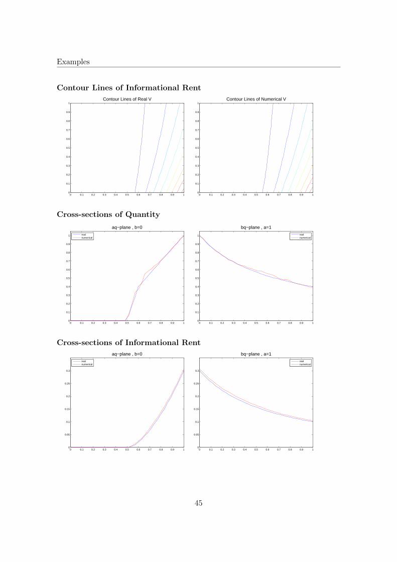
The second criteria is just a visual comparation. Despite no being formal, in practice
numerical approximations help us to formulate predictions about the functional form
of the solution, like the participation set or the contour levels (i.e. how types are
bunching). So, we provide graphics of the quantity, the informational rent, their
contour levels and cross-section for both numerical and real solutions. We also exhibit
numerical and real profits’ difference for some values of n.
Furthermore, we numerically solve two additional examples that, to the best
of our knowledge, have not been previously analysed in the literature. For these
examples we just show the graphs of numerical solutions, contour lines, and the
profit’s sequence for some values of n.
As was mentioned, when we ommited IC constraints on the southeast for each
type it is required to verify a posteriori if the ommited constraints are indeed strictly
41
Reduction of IC Constraints in the Bidimensional Model
satisfied. It is clear that such verification can only be numeric. For this reason,
we provide graphs showing whether a fix type (ai, bj) (in blue) is IC with all the
others types in Xn, drawinall the types on the southeast of the points considered are
satisfying IC.
In view of numerical optimization, as well as the limitations by the discretization
pointed out in the remarks of section (3.3), it is not surprising the existence of red
points (i.e. not satisfying IC constraints) in some graphs, however, the violations
may be considered small. The value of δ = δi,j in each one of the graphs indicates
the minimum violation of IC constraints among the red types. That is, if we allow
some tolerance toli,j > −δi,j, all the IC constraints will be verified for such (ai, bj)
blue point. Furthermore, setting δ∗ = mini,jδi,j implies that when tol > −δ∗ all
the IC constraints will be satisfied for all the points on the square. We provide the
value of δ∗ in each example.
The numerical solutions were performed via Knitro/AMPL using the Active
Set Algorithm. Otimization process stopped if one of the following tolerances were
achieved: maxit= 104 , feastol= 10−15 , xtol= 10−15 , opttol= 10−15 , where
maxit is the maximum number of iterations, feastol refers to feasibility tolerance,
xtol is the relative change of decision variables and opttol is the optimality KKT
sttoping tolerance. In all examples, xtol were achieved first.
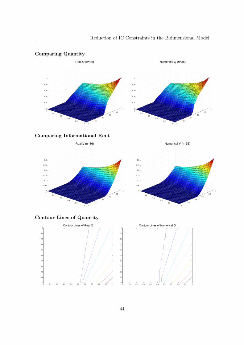
Example 1 [Laffont, Maskin & Rochet (1987)]
In Laffont et al. (1987) the authors have solved the original monopolist’s problem
for these data
v(q, a, b) = aq − (1 + b)
2q2 , C(q) = 0 , f(a, b) = 1
The solutions q and T they have found are:
q(a, b) =
0 , a ≤ 12
4a− 2
4b+ 1,
1
2≤ a+ 2b
4b+ 1≤ 3
5
3a− 1
2 + 3b,
3
5≤ 2a+ b
2 + 3b≤ 1
42
Examples
T (q) =
q
2− 3q2
8, q ≤ 2
5
q
3− q2
6+
1
30,
2
5≤ q ≤ 1
Before solving the problem numerically note that vq is linear in a and b, so we
can apply Proposition 3.2.4 and reduce even more the number of constraints. Since
there is no distortion at the top (the type (1, 0) has no distortion with respect to
the contract over complete information), we must have vq(q(1, 0), 1, 0) = 0 (marginal
utility equals marginal cost, which is zero) which implies q(1, 0) = 1, then Q = [0, 1].
Therefore −vqavqb
= 1q≥ 1. Thus, for any (a, b), (a, b) with a > a, b > b, it is sufficient
that b−ba−a ≤ 1 to ensure that (a, b) (a, b).
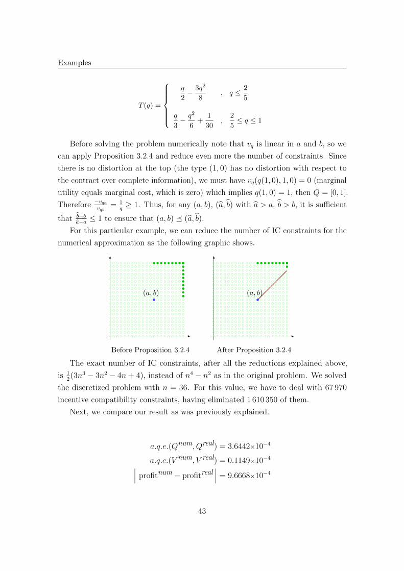
For this particular example, we can reduce the number of IC constraints for the
numerical approximation as the following graphic shows.
(a, b)
Before Proposition 3.2.4
(a, b)
After Proposition 3.2.4
The exact number of IC constraints, after all the reductions explained above,
is 12(3n3 − 3n2 − 4n+ 4), instead of n4 − n2 as in the original problem. We solved
the discretized problem with n = 36. For this value, we have to deal with 67 970
incentive compatibility constraints, having eliminated 1 610 350 of them.
Next, we compare our result as was previously explained.
a.q.e.(Qnum, Qreal) = 3.6442×10⁻⁴
a.q.e.(V num, V real) = 0.1149×10⁻⁴∣∣∣ profitnum − profitreal∣∣∣ = 9.6668×10⁻⁴
43
Reduction of IC Constraints in the Bidimensional Model
Comparing Quantity
0
0.2
0.4
0.6
0.8
1
0
0.2
0.4
0.6
0.8
10
0.2
0.4
0.6
0.8
1
Real Q (n=36)
0
0.2
0.4
0.6
0.8
1
0
0.2
0.4
0.6
0.8
10
0.2
0.4
0.6
0.8
1
Numerical Q (n=36)
Comparing Informational Rent
0
0.2
0.4
0.6
0.8
1
0
0.2
0.4
0.6
0.8
10
0.05
0.1
0.15
0.2
0.25
0.3
Real V (n=36)
0
0.2
0.4
0.6
0.8
1
0
0.2
0.4
0.6
0.8
10
0.05
0.1
0.15
0.2
0.25
0.3
Numerical V (n=36)
Contour Lines of Quantity
Contour Lines of Real Q
0 0.1 0.2 0.3 0.4 0.5 0.6 0.7 0.8 0.9 10
0.1
0.2
0.3
0.4
0.5
0.6
0.7
0.8
0.9
1Contour Lines of Numerical Q
0 0.1 0.2 0.3 0.4 0.5 0.6 0.7 0.8 0.9 10
0.1
0.2
0.3
0.4
0.5
0.6
0.7
0.8
0.9
1
44
Examples
Contour Lines of Informational Rent
Contour Lines of Real V
0 0.1 0.2 0.3 0.4 0.5 0.6 0.7 0.8 0.9 10
0.1
0.2
0.3
0.4
0.5
0.6
0.7
0.8
0.9
1Contour Lines of Numerical V
0 0.1 0.2 0.3 0.4 0.5 0.6 0.7 0.8 0.9 10
0.1
0.2
0.3
0.4
0.5
0.6
0.7
0.8
0.9
1
Cross-sections of Quantity
0 0.1 0.2 0.3 0.4 0.5 0.6 0.7 0.8 0.9 10
0.1
0.2
0.3
0.4
0.5
0.6
0.7
0.8
0.9
1
aq−plane , b=0
realnumerical
0 0.1 0.2 0.3 0.4 0.5 0.6 0.7 0.8 0.9 10
0.1
0.2
0.3
0.4
0.5
0.6
0.7
0.8
0.9
1
bq−plane , a=1
realnumerical
Cross-sections of Informational Rent
0 0.1 0.2 0.3 0.4 0.5 0.6 0.7 0.8 0.9 10
0.05
0.1
0.15
0.2
0.25
0.3
aq−plane , b=0
realnumerical
0 0.1 0.2 0.3 0.4 0.5 0.6 0.7 0.8 0.9 10
0.05
0.1
0.15
0.2
0.25
0.3
bq−plane , a=1
realnumerical
45
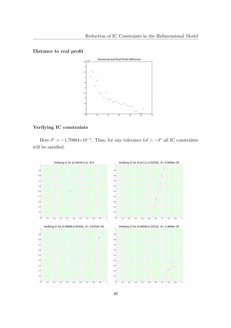
Reduction of IC Constraints in the Bidimensional Model
Distance to real profit
10 15 20 25 30 35 400.5
1
1.5
2
2.5
3
3.5
4
4.5
5
5.5x 10
−3 Numerical and Real Profit Difference
Verifying IC constraints
Here δ∗ = −1.70804×10⁻⁴. Thus, for any tolerance tol > −δ∗ all IC constraints
will be satisfied.
0 0.1 0.2 0.3 0.4 0.5 0.6 0.7 0.8 0.9 10
0.1
0.2
0.3
0.4
0.5
0.6
0.7
0.8
0.9
1
Verifying IC for (0.44444,0.5) . δ=0
0 0.1 0.2 0.3 0.4 0.5 0.6 0.7 0.8 0.9 10
0.1
0.2
0.3
0.4
0.5
0.6
0.7
0.8
0.9
1
Verifying IC for (0.61111,0.33333) . δ=−9.9586e−05
0 0.1 0.2 0.3 0.4 0.5 0.6 0.7 0.8 0.9 10
0.1
0.2
0.3
0.4
0.5
0.6
0.7
0.8
0.9
1
Verifying IC for (0.88889,0.83333) . δ=−3.5232e−05
0 0.1 0.2 0.3 0.4 0.5 0.6 0.7 0.8 0.9 10
0.1
0.2
0.3
0.4
0.5
0.6
0.7
0.8
0.9
1
Verifying IC for (0.80556,0.22222) . δ=−1.4869e−05
46

Examples
Example 2 [Basov (2005)]
In Basov (2005) the author solved the original problem for the data
v(q, a, b) = aq − (c+ b)
γqγ , C(q) = 0 , f(a, b) = 1
where c > 12
and γ ≥ 2 are constants. The solutions q and T he have found are:
q(a, b) =
0 , a ≤ 12
( 4a− 2
4b+ 2c− 1
) 1γ−1
, (3 + 2c)a− 2b ≤ 2c+ 1
( 3a− 1
3b+ 2c
) 1γ−1
, (3 + 2c)a− 2b > 2c+ 1
T (q) =
q
2−
( c2 + 14)
γqγ , q ≤
( 2
3 + 2c
) 1γ−1
1
6
( 2
3 + 2c
) 1γ−1 −
( c6 + 14)
γ
( 2
3 + 2c
) γγ−1
+q
3− c
3γqγ , q >
( 2
3 + 2c
) 1γ−1
Note vq is linear in a and b, so Proposition 3.2.4 can be applied and by analogous
considerations of Example 1, we can ruled out the same additional constraints.
We solved the discretized problem for the case γ = 3 with n = 30 points. For
this value, 39 092 incentive compatibility constraints were considered, and 770 008
were eliminated.
Next, we compare our result as was previously explained.
a.q.e.(Qnum, Qreal) = 4.5853×10⁻⁴
a.q.e.(V num, V real) = 0.0384×10⁻⁴∣∣∣ profitnum − profitreal∣∣∣ = 2.5717×10⁻³
47
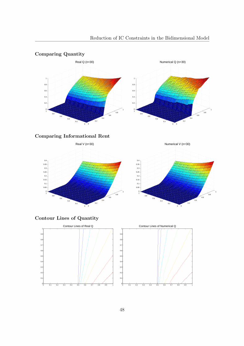
Reduction of IC Constraints in the Bidimensional Model
Comparing Quantity
0
0.2
0.4
0.6
0.8
1
0
0.2
0.4
0.6
0.8
10
0.2
0.4
0.6
0.8
1
Real Q (n=30)
0
0.2
0.4
0.6
0.8
1
0
0.2
0.4
0.6
0.8
10
0.2
0.4
0.6
0.8
1
Numerical Q (n=30)
Comparing Informational Rent
0
0.2
0.4
0.6
0.8
1
0
0.2
0.4
0.6
0.8
10
0.05
0.1
0.15
0.2
0.25
0.3
0.35
0.4
Real V (n=30)
0
0.2
0.4
0.6
0.8
1
0
0.2
0.4
0.6
0.8
10
0.05
0.1
0.15
0.2
0.25
0.3
0.35
0.4
Numerical V (n=30)
Contour Lines of Quantity
Contour Lines of Real Q
0 0.1 0.2 0.3 0.4 0.5 0.6 0.7 0.8 0.9 10
0.1
0.2
0.3
0.4
0.5
0.6
0.7
0.8
0.9
1Contour Lines of Numerical Q
0 0.1 0.2 0.3 0.4 0.5 0.6 0.7 0.8 0.9 10
0.1
0.2
0.3
0.4
0.5
0.6
0.7
0.8
0.9
1
48
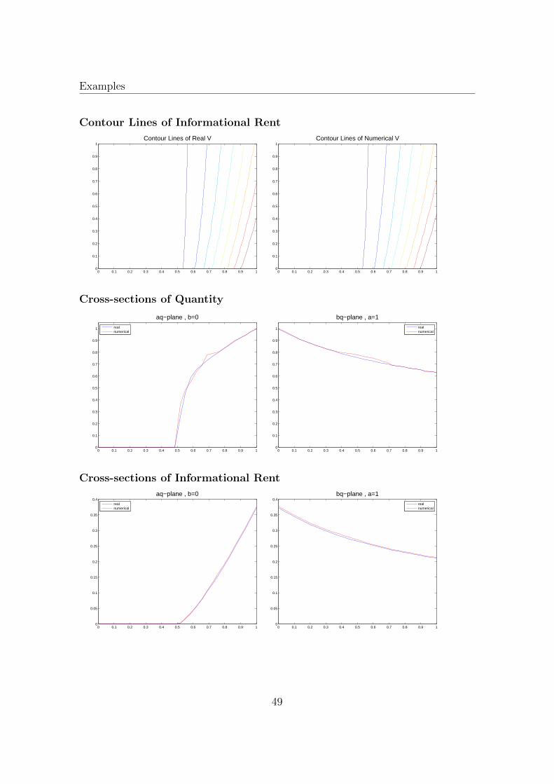
Examples
Contour Lines of Informational Rent
Contour Lines of Real V
0 0.1 0.2 0.3 0.4 0.5 0.6 0.7 0.8 0.9 10
0.1
0.2
0.3
0.4
0.5
0.6
0.7
0.8
0.9
1Contour Lines of Numerical V
0 0.1 0.2 0.3 0.4 0.5 0.6 0.7 0.8 0.9 10
0.1
0.2
0.3
0.4
0.5
0.6
0.7
0.8
0.9
1
Cross-sections of Quantity
0 0.1 0.2 0.3 0.4 0.5 0.6 0.7 0.8 0.9 10
0.1
0.2
0.3
0.4
0.5
0.6
0.7
0.8
0.9
1
aq−plane , b=0
realnumerical
0 0.1 0.2 0.3 0.4 0.5 0.6 0.7 0.8 0.9 10
0.1
0.2
0.3
0.4
0.5
0.6
0.7
0.8
0.9
1
bq−plane , a=1
realnumerical
Cross-sections of Informational Rent
0 0.1 0.2 0.3 0.4 0.5 0.6 0.7 0.8 0.9 10
0.05
0.1
0.15
0.2
0.25
0.3
0.35
0.4aq−plane , b=0
realnumerical
0 0.1 0.2 0.3 0.4 0.5 0.6 0.7 0.8 0.9 10
0.05
0.1
0.15
0.2
0.25
0.3
0.35
0.4bq−plane , a=1
realnumerical
49
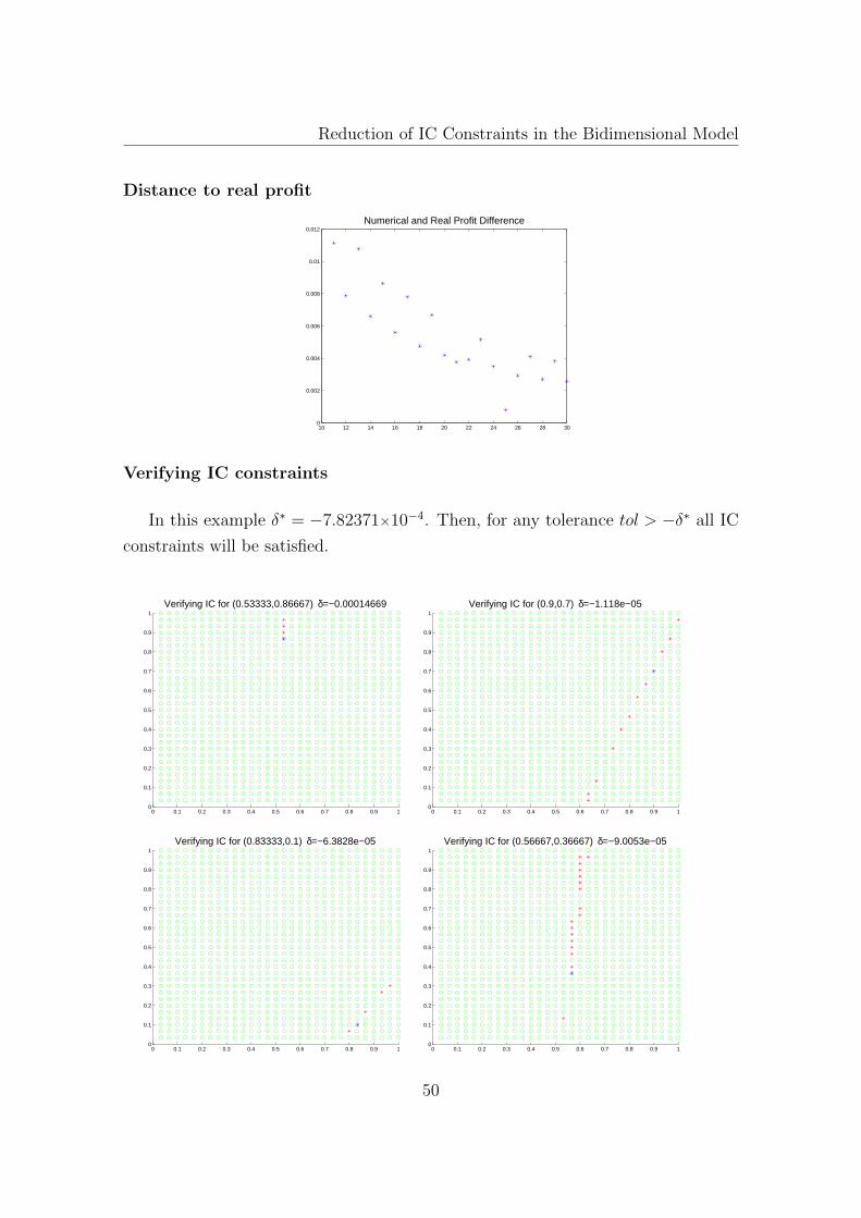
Reduction of IC Constraints in the Bidimensional Model
Distance to real profit
10 12 14 16 18 20 22 24 26 28 300
0.002
0.004
0.006
0.008
0.01
0.012Numerical and Real Profit Difference
Verifying IC constraints
In this example δ∗ = −7.82371×10⁻⁴. Then, for any tolerance tol > −δ∗ all IC
constraints will be satisfied.
0 0.1 0.2 0.3 0.4 0.5 0.6 0.7 0.8 0.9 10
0.1
0.2
0.3
0.4
0.5
0.6
0.7
0.8
0.9
1
Verifying IC for (0.53333,0.86667) δ=−0.00014669
0 0.1 0.2 0.3 0.4 0.5 0.6 0.7 0.8 0.9 10
0.1
0.2
0.3
0.4
0.5
0.6
0.7
0.8
0.9
1
Verifying IC for (0.9,0.7) δ=−1.118e−05
0 0.1 0.2 0.3 0.4 0.5 0.6 0.7 0.8 0.9 10
0.1
0.2
0.3
0.4
0.5
0.6
0.7
0.8
0.9
1
Verifying IC for (0.83333,0.1) δ=−6.3828e−05
0 0.1 0.2 0.3 0.4 0.5 0.6 0.7 0.8 0.9 10
0.1
0.2
0.3
0.4
0.5
0.6
0.7
0.8
0.9
1
Verifying IC for (0.56667,0.36667) δ=−9.0053e−05
50
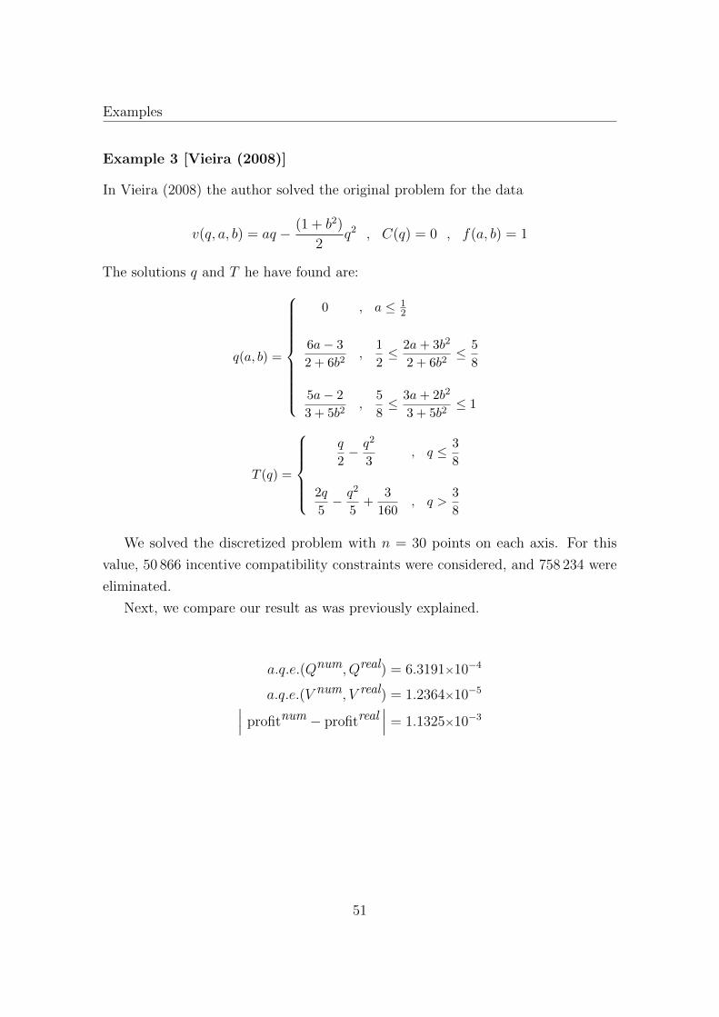
Examples
Example 3 [Vieira (2008)]
In Vieira (2008) the author solved the original problem for the data
v(q, a, b) = aq − (1 + b2)
2q2 , C(q) = 0 , f(a, b) = 1
The solutions q and T he have found are:
q(a, b) =
0 , a ≤ 12
6a− 3
2 + 6b2,
1
2≤ 2a+ 3b2
2 + 6b2≤ 5
8
5a− 2
3 + 5b2,
5
8≤ 3a+ 2b2
3 + 5b2≤ 1
T (q) =
q
2− q2
3, q ≤ 3
8
2q
5− q2
5+
3
160, q >
3
8
We solved the discretized problem with n = 30 points on each axis. For this
value, 50 866 incentive compatibility constraints were considered, and 758 234 were
eliminated.
Next, we compare our result as was previously explained.
a.q.e.(Qnum, Qreal) = 6.3191×10⁻⁴
a.q.e.(V num, V real) = 1.2364×10⁻⁵∣∣∣ profitnum − profitreal∣∣∣ = 1.1325×10⁻³
51
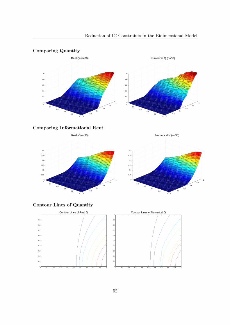
Reduction of IC Constraints in the Bidimensional Model
Comparing Quantity
0
0.2
0.4
0.6
0.8
1
0
0.2
0.4
0.6
0.8
10
0.2
0.4
0.6
0.8
1
Real Q (n=30)
0
0.2
0.4
0.6
0.8
1
0
0.2
0.4
0.6
0.8
10
0.2
0.4
0.6
0.8
1
Numerical Q (n=30)
Comparing Informational Rent
0
0.2
0.4
0.6
0.8
1
0
0.2
0.4
0.6
0.8
10
0.05
0.1
0.15
0.2
0.25
0.3
Real V (n=30)
0
0.2
0.4
0.6
0.8
1
0
0.2
0.4
0.6
0.8
10
0.05
0.1
0.15
0.2
0.25
0.3
Numerical V (n=30)
Contour Lines of Quantity
Contour Lines of Real Q
0 0.1 0.2 0.3 0.4 0.5 0.6 0.7 0.8 0.9 10
0.1
0.2
0.3
0.4
0.5
0.6
0.7
0.8
0.9
1Contour Lines of Numerical Q
0 0.1 0.2 0.3 0.4 0.5 0.6 0.7 0.8 0.9 10
0.1
0.2
0.3
0.4
0.5
0.6
0.7
0.8
0.9
1
52
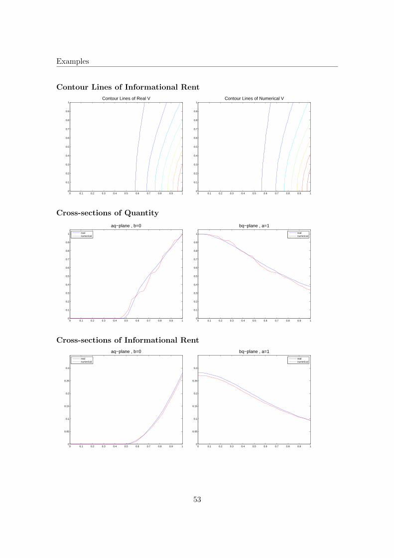
Examples
Contour Lines of Informational Rent
Contour Lines of Real V
0 0.1 0.2 0.3 0.4 0.5 0.6 0.7 0.8 0.9 10
0.1
0.2
0.3
0.4
0.5
0.6
0.7
0.8
0.9
1Contour Lines of Numerical V
0 0.1 0.2 0.3 0.4 0.5 0.6 0.7 0.8 0.9 10
0.1
0.2
0.3
0.4
0.5
0.6
0.7
0.8
0.9
1
Cross-sections of Quantity
0 0.1 0.2 0.3 0.4 0.5 0.6 0.7 0.8 0.9 10
0.1
0.2
0.3
0.4
0.5
0.6
0.7
0.8
0.9
1
aq−plane , b=0
realnumerical
0 0.1 0.2 0.3 0.4 0.5 0.6 0.7 0.8 0.9 10
0.1
0.2
0.3
0.4
0.5
0.6
0.7
0.8
0.9
1
bq−plane , a=1
realnumerical
Cross-sections of Informational Rent
0 0.1 0.2 0.3 0.4 0.5 0.6 0.7 0.8 0.9 10
0.05
0.1
0.15
0.2
0.25
0.3
aq−plane , b=0
realnumerical
0 0.1 0.2 0.3 0.4 0.5 0.6 0.7 0.8 0.9 10
0.05
0.1
0.15
0.2
0.25
0.3
bq−plane , a=1
realnumerical
53
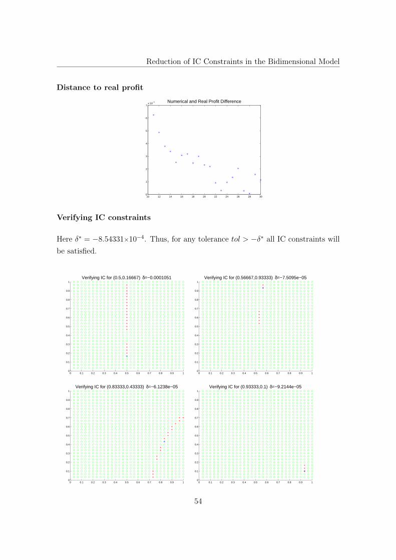
Reduction of IC Constraints in the Bidimensional Model
Distance to real profit
10 12 14 16 18 20 22 24 26 28 300
1
2
3
4
5
6
7x 10
−3 Numerical and Real Profit Difference
Verifying IC constraints
Here δ∗ = −8.54331×10⁻⁴. Thus, for any tolerance tol > −δ∗ all IC constraints will
be satisfied.
0 0.1 0.2 0.3 0.4 0.5 0.6 0.7 0.8 0.9 10
0.1
0.2
0.3
0.4
0.5
0.6
0.7
0.8
0.9
1
Verifying IC for (0.5,0.16667) δ=−0.0001051
0 0.1 0.2 0.3 0.4 0.5 0.6 0.7 0.8 0.9 10
0.1
0.2
0.3
0.4
0.5
0.6
0.7
0.8
0.9
1
Verifying IC for (0.56667,0.93333) δ=−7.5095e−05
0 0.1 0.2 0.3 0.4 0.5 0.6 0.7 0.8 0.9 10
0.1
0.2
0.3
0.4
0.5
0.6
0.7
0.8
0.9
1
Verifying IC for (0.83333,0.43333) δ=−6.1238e−05
0 0.1 0.2 0.3 0.4 0.5 0.6 0.7 0.8 0.9 10
0.1
0.2
0.3
0.4
0.5
0.6
0.7
0.8
0.9
1
Verifying IC for (0.93333,0.1) δ=−9.2144e−05
54
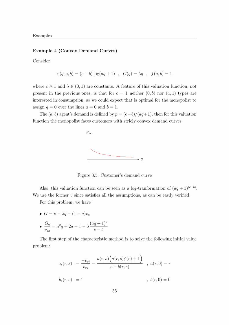
Examples
Example 4 (Convex Demand Curves)
Consider
v(q, a, b) = (c− b) log(aq + 1) , C(q) = λq , f(a, b) = 1
where c ≥ 1 and λ ∈ (0, 1) are constants. A feature of this valuation function, not
present in the previous ones, is that for c = 1 neither (0, b) nor (a, 1) types are
interested in consumption, so we could expect that is optimal for the monopolist to
assign q = 0 over the lines a = 0 and b = 1.
The (a, b) agent’s demand is defined by p = (c−b)/(aq+1), then for this valuation
function the monopolist faces customers with stricly convex demand curves
q
p
Figure 3.5: Customer’s demand curve
Also, this valuation function can be seen as a log-tranformation of (aq + 1)(c−b).
We use the former v since satisfies all the assumptions, as can be easily verified.
For this problem, we have
• G = v − λq − (1− a)va
• Gq
vqa= a2q + 2a− 1− λ(aq + 1)2
c− b
The first step of the characteristic method is to solve the following initial value
problem:
as(r, s) =−vqbvqa
=a(r, s)
(a(r, s)φ(r) + 1
)c− b(r, s)
, a(r, 0) = r
bs(r, s) = 1 , b(r, 0) = 0
55

Reduction of IC Constraints in the Bidimensional Model
which have solutions
a(r, s) =c r
c− (1 + rφ(r))sand b(r, s) = s
Then, using the optimality necessary condition (2.2), we have that if φ(r) is the
optimal allocation over the curve (a(r, s), b(r, s)) where r ∈ [r, 1] is fixed, then∫ s(r)
0
Gq
vqa(φ(r), a(r, s), b(r, s))ds = 0
So, we have to solve for φ∫ s(r)
0
c2r2φ
(c− (1 + rφ)s)2+
2cr
c− (1 + rφ)s− 1− λ(1 + rφ)2(c− s)
(c− (1 + rφ)s)2ds = 0
where s(r) is such that a(r, s(r)) = 1, i.e. s(r) = c(1−r)1+rφ
After calculations, for a fixed r ∈ [r, 1] , φ(r) is the positive solution of
D(r)φ2 + E(r)φ+ F (r) = 0 (3.2)
where
D(r) = λr(1− r)
E(r) = λ(1− r)− λr log(r)− c r(1− r)
F (r) = 2c r log(r) + c(1− r)− λ log(r)
Since F ′′(r) = 2cr
+ λr2
, F is stricly convex on (0, 1). Note that F has a minimum
over (0, 1) in view of F ′(r) > 0 when r ≈ 1 and F ′(r) < 0 when r ≈ 0. Besides, in
view of F (r) > 0 for r ≈ 0 and F (r∗) < 0 for some r∗ ∈ (0, 1) (the minimum value
must be negative in view of F (1) = 0), there exists a unique r0 ∈ (0, 1) such that
F (r0) = 0. Since φ(r) = 0 implies F (r) = 0 we must have r = r0. Therefore, r is
defined as the unique solution on (0, 1) of
(2c r − λ) log(r) + c(1− r) = 0
Because F (r) < 0 on (r, 1) (F is stricly convex, F (1) = 0 and F (r) = 0) and
56

Examples
D(r) > 0 one solution of the quadratic equation (3.2) is always negative on (r, 1),
then we can express φ(r) in the closed form:
φ(r) =−E(r) +
√E(r)2 − 4D(r)F (r)
2D(r), r ∈ (r, 1)
Because φ(1) is not defined, by continuity we can define q(1, 0) as
q(1, 0) = limr→1
φ(r) =c
λ− 1
this value of q(1, 0) solves the equation vq(q, 1, 0) = C ′(q) meaning that there is not
distortion at the top, as expected on the solution.
Note that r defines participation’s boundary because φ(r) = 0. This boundary is
given by b = c− (cr)/a.
Next we return to the original variables. Fix (a, b) ∈ [0, 1]2
• If b ≥ c− (cr)/a then q(a, b) = 0 i.e., (a, b) type is excluded.
• If b < c− (cr)/a, r(a, b) is defined as the solution of
c− bbr− c
ab=−E(r) +
√E(r)2 − 4D(r)F (r)
2D(r)
such that r(a, b) ∈ (r, 1) , φ(r(a, b)) > 0 and φ′(r(a, b)) > 0. With such r(a, b)
we define
q(a, b) =c− bb r(a, b)
− c
ab
Furthermore, the tariff as a function of r over (r, 1) can be expressed as
T (r) =
∫ r
r
vq(φ(r), r, 0)φ′(r)dr
So, the type (a, b) has to transfer t(a, b) = T (r(a, b)) to the monopolist.
Finally, knowing q(a, b) and t(a, b) we can find the informational rent V (a, b).
For the case c = 1 and λ = 0.4 we did it numerically.
57
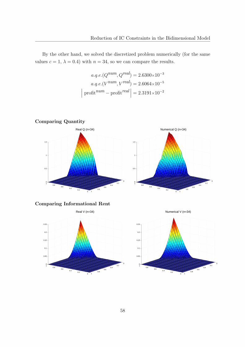
Reduction of IC Constraints in the Bidimensional Model
By the other hand, we solved the discretized problem numerically (for the same
values c = 1, λ = 0.4) with n = 34, so we can compare the results.
a.q.e.(Qnum, Qreal) = 2.6300×10⁻³
a.q.e.(V num, V real) = 2.6064×10⁻⁵∣∣∣ profitnum − profitreal∣∣∣ = 2.3191×10⁻²
Comparing Quantity
00.2
0.40.6
0.81
00.2
0.40.6
0.81
0
0.5
1
1.5
Real Q (n=34)
00.2
0.40.6
0.81
00.2
0.40.6
0.81
0
0.5
1
1.5
Numerical Q (n=34)
Comparing Informational Rent
00.2
0.40.6
0.81
00.2
0.40.6
0.81
0
0.05
0.1
0.15
0.2
0.25
Real V (n=34)
00.2
0.40.6
0.81
00.2
0.40.6
0.81
0
0.05
0.1
0.15
0.2
0.25
Numerical V (n=34)
58
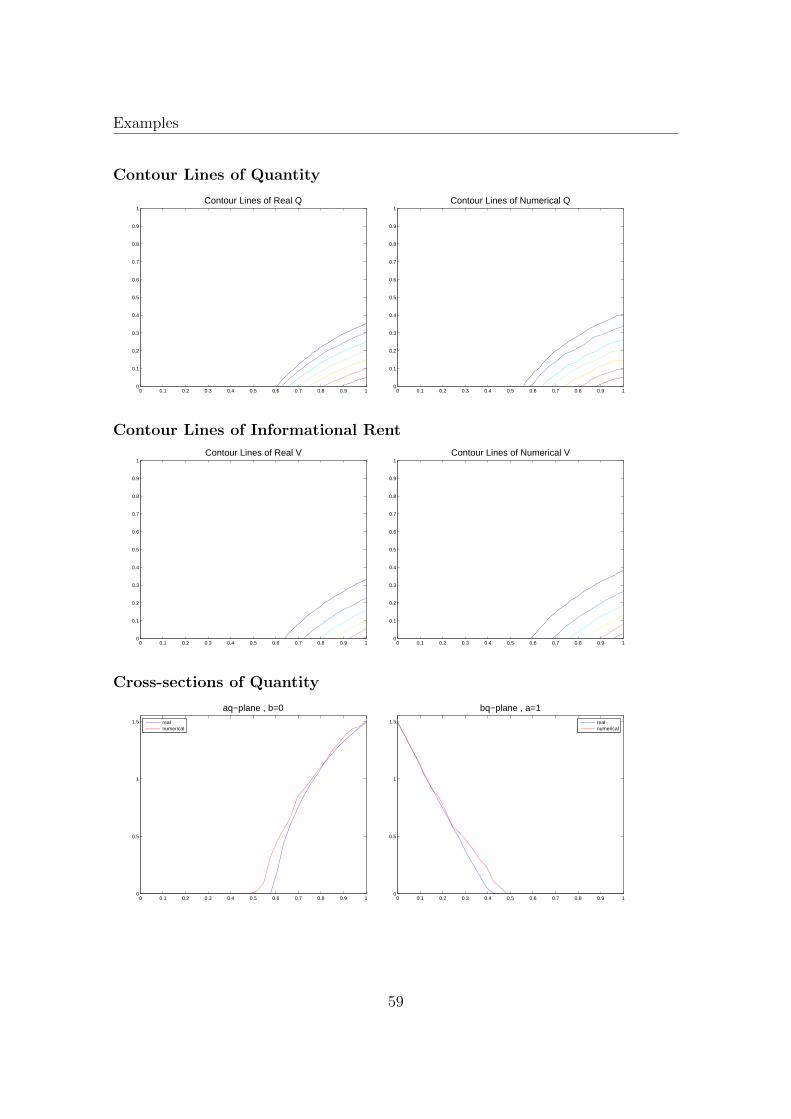
Examples
Contour Lines of Quantity
Contour Lines of Real Q
0 0.1 0.2 0.3 0.4 0.5 0.6 0.7 0.8 0.9 10
0.1
0.2
0.3
0.4
0.5
0.6
0.7
0.8
0.9
1Contour Lines of Numerical Q
0 0.1 0.2 0.3 0.4 0.5 0.6 0.7 0.8 0.9 10
0.1
0.2
0.3
0.4
0.5
0.6
0.7
0.8
0.9
1
Contour Lines of Informational Rent
Contour Lines of Real V
0 0.1 0.2 0.3 0.4 0.5 0.6 0.7 0.8 0.9 10
0.1
0.2
0.3
0.4
0.5
0.6
0.7
0.8
0.9
1Contour Lines of Numerical V
0 0.1 0.2 0.3 0.4 0.5 0.6 0.7 0.8 0.9 10
0.1
0.2
0.3
0.4
0.5
0.6
0.7
0.8
0.9
1
Cross-sections of Quantity
0 0.1 0.2 0.3 0.4 0.5 0.6 0.7 0.8 0.9 10
0.5
1
1.5
aq−plane , b=0
realnumerical
0 0.1 0.2 0.3 0.4 0.5 0.6 0.7 0.8 0.9 10
0.5
1
1.5
bq−plane , a=1
realnumerical
59
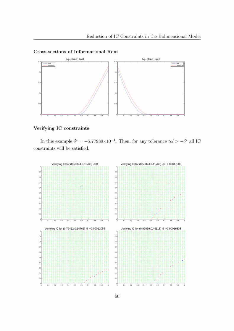
Reduction of IC Constraints in the Bidimensional Model
Cross-sections of Informational Rent
0 0.1 0.2 0.3 0.4 0.5 0.6 0.7 0.8 0.9 10
0.05
0.1
0.15
0.2
0.25aq−plane , b=0
realnumerical
0 0.1 0.2 0.3 0.4 0.5 0.6 0.7 0.8 0.9 10
0.05
0.1
0.15
0.2
0.25bq−plane , a=1
realnumerical
Verifying IC constraints
In this example δ∗ = −5.77989×10⁻⁴. Then, for any tolerance tol > −δ∗ all IC
constraints will be satisfied.
0 0.1 0.2 0.3 0.4 0.5 0.6 0.7 0.8 0.9 10
0.1
0.2
0.3
0.4
0.5
0.6
0.7
0.8
0.9
1
Verifying IC for (0.58824,0.61765) δ=0
0 0.1 0.2 0.3 0.4 0.5 0.6 0.7 0.8 0.9 10
0.1
0.2
0.3
0.4
0.5
0.6
0.7
0.8
0.9
1
Verifying IC for (0.58824,0.11765) δ=−0.00017502
0 0.1 0.2 0.3 0.4 0.5 0.6 0.7 0.8 0.9 10
0.1
0.2
0.3
0.4
0.5
0.6
0.7
0.8
0.9
1
Verifying IC for (0.79412,0.14706) δ=−0.00011054
0 0.1 0.2 0.3 0.4 0.5 0.6 0.7 0.8 0.9 10
0.1
0.2
0.3
0.4
0.5
0.6
0.7
0.8
0.9
1
Verifying IC for (0.97059,0.44118) δ=−0.00016835
60
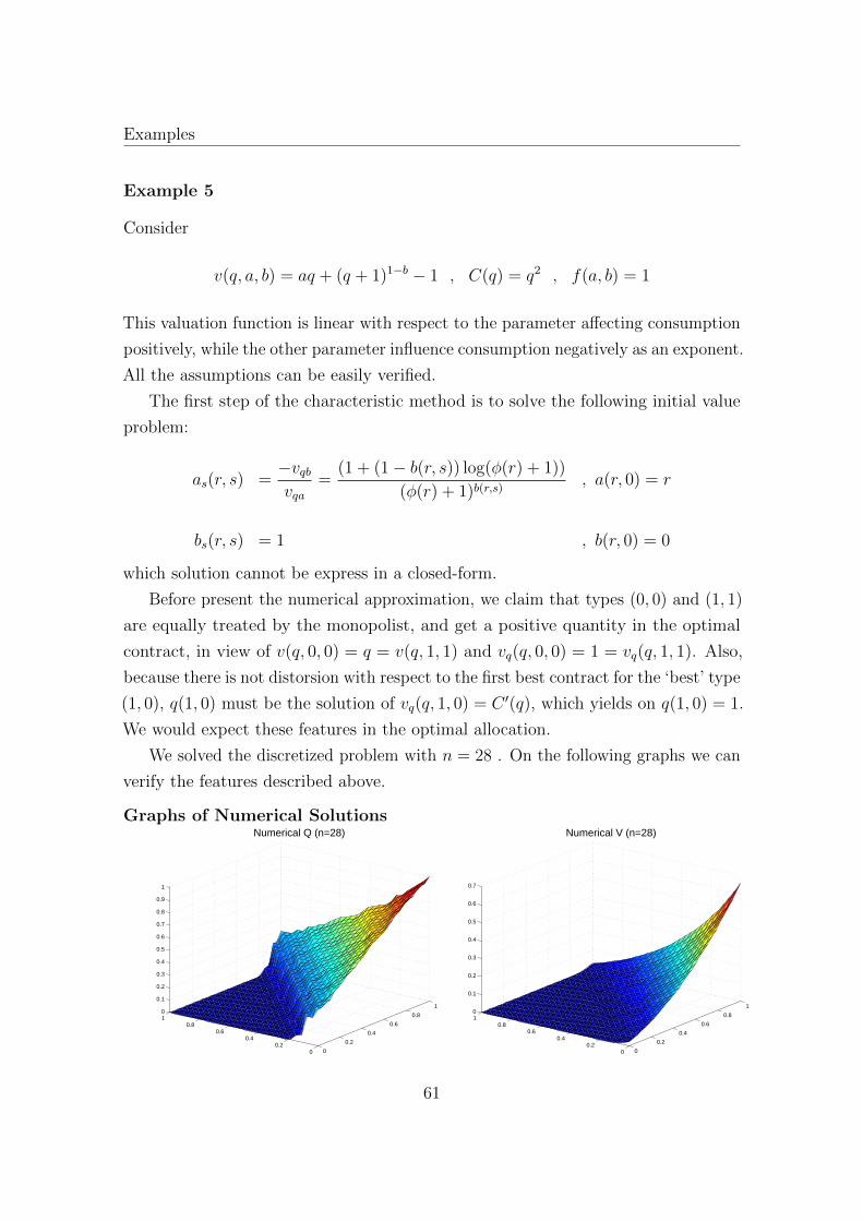
Examples
Example 5
Consider
v(q, a, b) = aq + (q + 1)1−b − 1 , C(q) = q2 , f(a, b) = 1
This valuation function is linear with respect to the parameter affecting consumption
positively, while the other parameter influence consumption negatively as an exponent.
All the assumptions can be easily verified.
The first step of the characteristic method is to solve the following initial value
problem:
as(r, s) =−vqbvqa
=(1 + (1− b(r, s)) log(φ(r) + 1))
(φ(r) + 1)b(r,s), a(r, 0) = r
bs(r, s) = 1 , b(r, 0) = 0
which solution cannot be express in a closed-form.
Before present the numerical approximation, we claim that types (0, 0) and (1, 1)
are equally treated by the monopolist, and get a positive quantity in the optimal
contract, in view of v(q, 0, 0) = q = v(q, 1, 1) and vq(q, 0, 0) = 1 = vq(q, 1, 1). Also,
because there is not distorsion with respect to the first best contract for the ‘best’ type
(1, 0), q(1, 0) must be the solution of vq(q, 1, 0) = C ′(q), which yields on q(1, 0) = 1.
We would expect these features in the optimal allocation.
We solved the discretized problem with n = 28 . On the following graphs we can
verify the features described above.
Graphs of Numerical Solutions
0
0.2
0.4
0.6
0.8
1
00.2
0.40.6
0.810
0.1
0.2
0.3
0.4
0.5
0.6
0.7
0.8
0.9
1
Numerical Q (n=28)
0
0.2
0.4
0.6
0.8
1
00.2
0.40.6
0.810
0.1
0.2
0.3
0.4
0.5
0.6
0.7
Numerical V (n=28)
61
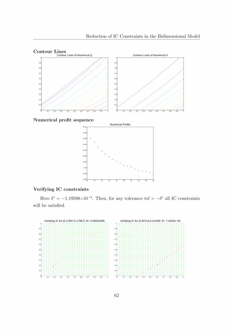
Reduction of IC Constraints in the Bidimensional Model
Contour LinesContour Lines of Numerical Q
0 0.1 0.2 0.3 0.4 0.5 0.6 0.7 0.8 0.9 10
0.1
0.2
0.3
0.4
0.5
0.6
0.7
0.8
0.9
1Contour Lines of Numerical V
0 0.1 0.2 0.3 0.4 0.5 0.6 0.7 0.8 0.9 10
0.1
0.2
0.3
0.4
0.5
0.6
0.7
0.8
0.9
1
Numerical profit sequence
10 12 14 16 18 20 22 24 26 280.138
0.139
0.14
0.141
0.142
0.143
0.144
0.145
0.146
0.147Numerical Profits
Verifying IC constraints
Here δ∗ = −1.19598×10⁻³. Then, for any tolerance tol > −δ∗ all IC constraints
will be satisfied.
0 0.1 0.2 0.3 0.4 0.5 0.6 0.7 0.8 0.9 10
0.1
0.2
0.3
0.4
0.5
0.6
0.7
0.8
0.9
1
Verifying IC for (0.17857,0.17857) δ=−0.00024495
0 0.1 0.2 0.3 0.4 0.5 0.6 0.7 0.8 0.9 10
0.1
0.2
0.3
0.4
0.5
0.6
0.7
0.8
0.9
1
Verifying IC for (0.60714,0.21429) δ=−7.6332e−05
62
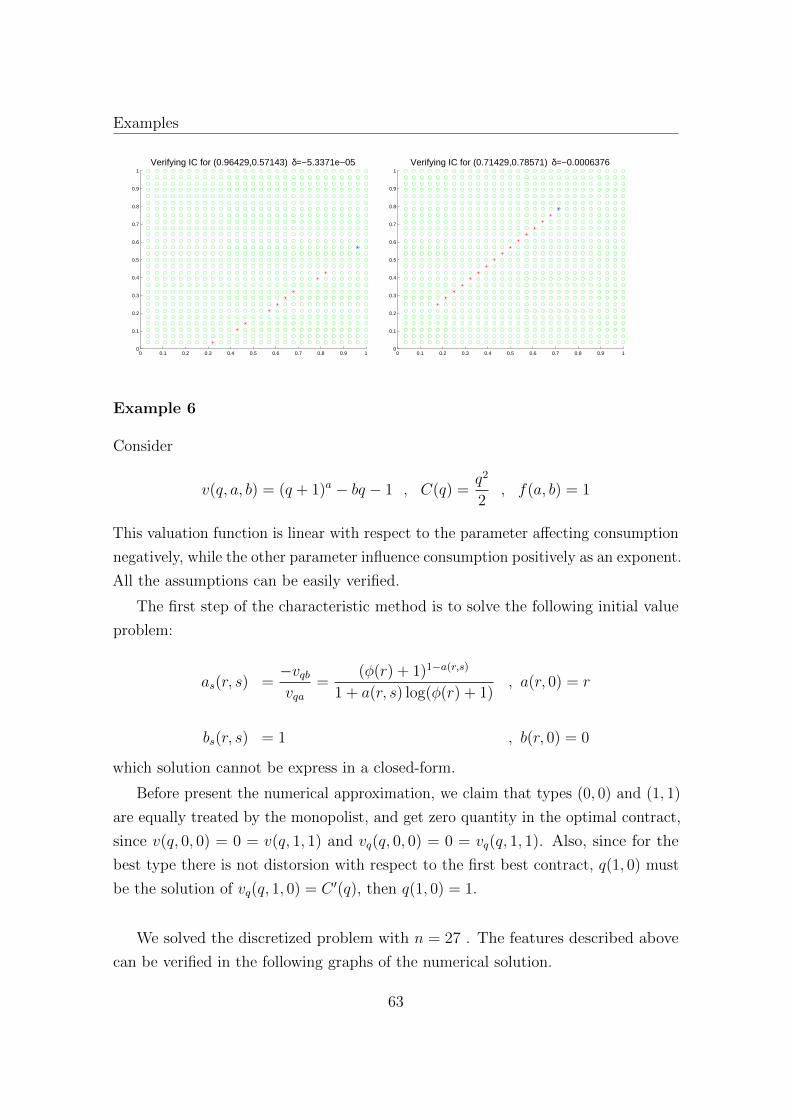
Examples
0 0.1 0.2 0.3 0.4 0.5 0.6 0.7 0.8 0.9 10
0.1
0.2
0.3
0.4
0.5
0.6
0.7
0.8
0.9
1
Verifying IC for (0.96429,0.57143) δ=−5.3371e−05
0 0.1 0.2 0.3 0.4 0.5 0.6 0.7 0.8 0.9 10
0.1
0.2
0.3
0.4
0.5
0.6
0.7
0.8
0.9
1
Verifying IC for (0.71429,0.78571) δ=−0.0006376
Example 6
Consider
v(q, a, b) = (q + 1)a − bq − 1 , C(q) =q2
2, f(a, b) = 1
This valuation function is linear with respect to the parameter affecting consumption
negatively, while the other parameter influence consumption positively as an exponent.
All the assumptions can be easily verified.
The first step of the characteristic method is to solve the following initial value
problem:
as(r, s) =−vqbvqa
=(φ(r) + 1)1−a(r,s)
1 + a(r, s) log(φ(r) + 1), a(r, 0) = r
bs(r, s) = 1 , b(r, 0) = 0
which solution cannot be express in a closed-form.
Before present the numerical approximation, we claim that types (0, 0) and (1, 1)
are equally treated by the monopolist, and get zero quantity in the optimal contract,
since v(q, 0, 0) = 0 = v(q, 1, 1) and vq(q, 0, 0) = 0 = vq(q, 1, 1). Also, since for the
best type there is not distorsion with respect to the first best contract, q(1, 0) must
be the solution of vq(q, 1, 0) = C ′(q), then q(1, 0) = 1.
We solved the discretized problem with n = 27 . The features described above
can be verified in the following graphs of the numerical solution.
63
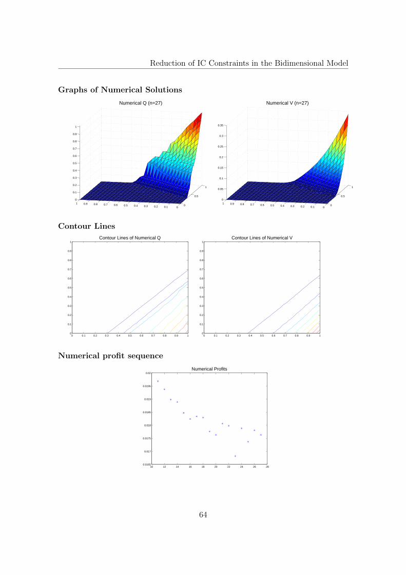
Reduction of IC Constraints in the Bidimensional Model
Graphs of Numerical Solutions
0
0.5
1
00.10.20.30.40.50.60.70.80.910
0.1
0.2
0.3
0.4
0.5
0.6
0.7
0.8
0.9
1
Numerical Q (n=27)
0
0.5
1
00.10.20.30.40.50.60.70.80.910
0.05
0.1
0.15
0.2
0.25
0.3
0.35
Numerical V (n=27)
Contour Lines
Contour Lines of Numerical Q
0 0.1 0.2 0.3 0.4 0.5 0.6 0.7 0.8 0.9 10
0.1
0.2
0.3
0.4
0.5
0.6
0.7
0.8
0.9
1Contour Lines of Numerical V
0 0.1 0.2 0.3 0.4 0.5 0.6 0.7 0.8 0.9 10
0.1
0.2
0.3
0.4
0.5
0.6
0.7
0.8
0.9
1
Numerical profit sequence
10 12 14 16 18 20 22 24 26 280.0165
0.017
0.0175
0.018
0.0185
0.019
0.0195
0.02Numerical Profits
64
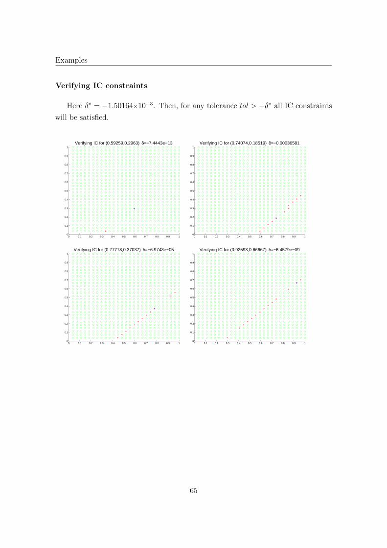
Examples
Verifying IC constraints
Here δ∗ = −1.50164×10⁻³. Then, for any tolerance tol > −δ∗ all IC constraints
will be satisfied.
0 0.1 0.2 0.3 0.4 0.5 0.6 0.7 0.8 0.9 10
0.1
0.2
0.3
0.4
0.5
0.6
0.7
0.8
0.9
1
Verifying IC for (0.59259,0.2963) δ=−7.4443e−13
0 0.1 0.2 0.3 0.4 0.5 0.6 0.7 0.8 0.9 10
0.1
0.2
0.3
0.4
0.5
0.6
0.7
0.8
0.9
1
Verifying IC for (0.74074,0.18519) δ=−0.00036581
0 0.1 0.2 0.3 0.4 0.5 0.6 0.7 0.8 0.9 10
0.1
0.2
0.3
0.4
0.5
0.6
0.7
0.8
0.9
1
Verifying IC for (0.77778,0.37037) δ=−6.9743e−05
0 0.1 0.2 0.3 0.4 0.5 0.6 0.7 0.8 0.9 10
0.1
0.2
0.3
0.4
0.5
0.6
0.7
0.8
0.9
1
Verifying IC for (0.92593,0.66667) δ=−6.4579e−09
65
Reduction of IC Constraints in the Bidimensional Model
3.6 Appendix B
Proof of Proposition 3.1.1.
Let (q, t) be an incentive compatible contract. For any (a, b) ∈ [0, 1]2:
(a, b) ∈ argmax(a,b)∈[0,1]2
v(q(a, b), a, b)− t(a, b)
Given (a, b) ∈ (0, 1)×(0, 1), consider F (·, ·) := v(q(·, ·), a, b)− t(·, ·). At any point of
twice continuous differentiability, since (a, b) maximizes F , the necessary condition
F ′(a, b) = 0 yields on
ta(a, b) = vq(q(a, b), a, b)qa(a, b)
tb(a, b) = vq(q(a, b), a, b)qb(a, b)
then
taa = vqqq2a + vqaqa + vqqaa
tbb = vqqq2b + vqbqb + vqqbb
tab = vqqqaqb + vqbqa + vqqab
tba = vqqqaqb + vqaqb + vqqba
By the other hand, F ′′(a, b) must be negative semi-definite, where
F ′′(a, b) =
[vqqq
2a + vqqaa − taa vqqqaqb + vqqab − tab
vqqqaqb + vqqba − tab vqqq2b + vqqbb − tbb
]
(all the arguments are (a, b)). Replacing those expressions of taa, tab, tba and tbb on
F ′′(a, b) we obtain that −vqa(q(a, b), a, b)qa(a, b) −vqb(q(a, b), a, b)qa(a, b)−vqa(q(a, b), a, b)qb(a, b) −vqb(q(a, b), a, b)qb(a, b)
is negative semi-definite matrix.
Then vqaqa ≥ 0 and vqbqb ≥ 0. By Assumption A3 we have vqa > 0 , vqb < 0 which
implies qa(a, b) ≥ 0 and qb(a, b) ≤ 0.
66
Appendix B
Proof of Proposition 3.2.1.
Fix q ∈ Q, by A3 vq(q, ·, b) is strictly increasing and vq(q, a, ·) is strictly decreasing, so
a > a and b < b implies vq(q, a, b) < vq(q, a, b) and vq(q, a, b) < vq(q, a, b) respectively.
Thus, vq(q, a, b) < vq(q, a, b).
Proof of Proposition 3.2.2.
If (x, y) ∈ CC(a, b) then q(a, b) = q(x, y) so, by the Taxation Principle, t(a, b) =
T (q(a, b)) = T (q(x, y)) = t(x, y). Because (a, b) is IC with (a, b) we have
v(q(a, b), a, b)− t(a, b) ≥ v(q(a, b), a, b)− t(a, b)
= v(q(x, y), a, b)− t(x, y)
that is, (a, b) is IC with (x, y).
Proof of Proposition 3.2.3.
We have
V (a, b)− V (a, b) ≥ v(q(a, b), a, b)− v(q(a, b), a, b)
V (a, b)− V (x, y) ≥ v(q(x, y), a, b)− v(q(x, y), x, y)
then
V (a, b)− V (x, y) + v(q(x, y), x, y) ≥ v(q(a, b), a, b)− v(q(a, b), a, b) + v(q(x, y), a, b)
Besides, because vq(q, a, b) ≤ vq(q, a, b) ∀ q ∈ Q, and q(x, y) ≤ q(a, b) :
∫ q(a,b)
q(x,y)
vq(q, a, b)dq ≤∫ q(a,b)
q(x,y)
vq(q, a, b)dq
then
v(q(a, b), a, b)− v(q(x, y), a, b) ≤ v(q(a, b), a, b)− v(q(x, y), a, b)
Therefore
V (a, b)− V (x, y) + v(q(x, y), x, y) ≥
v(q(a, b), a, b)− v(q(a, b), a, b) + v(q(x, y), a, b) ≥ v(q(x, y), a, b)
67

Reduction of IC Constraints in the Bidimensional Model
thus
V (a, b)− V (x, y) ≥ v(q(x, y), a, b)− v(q(x, y), x, y)
which means that (a, b) verifies IC with (x, y).
Proof of Theorem 3.2.1.
Fix any (a, b), (a, b) ∈ [0, 1]2. Let us prove that (a, b) is IC with (a, b).
If q(a, b) = qout (that is, if type (a, b) is excluded) we have V (a, b) = 0 so, from
IR constraint V (a, b) ≥ 0 we can write
V (a, b)− V (a, b) ≥ v(qout, a, b)− v(qout, a, b)
in view of v(qout, a, b) = v(qout, a, b) by Assumption A5
If q(a, b) 6= qout, because CC(a, b) is strictly increasing there are three possible
cases:
Case 1 CC(a, b) intersects F (a,b):
Let (x, y) the point of intersection. Because (a, b) is IC with (x, y) and (x, y) ∈CC(a, b), by Proposition 3.2.2 (a, b) is IC with (a, b).
Case 2 CC(a, b) intersects (1, s) : 0 ≤ s ≤ b:Since CC(a, b) is strictly increasing then b < b. If a > a, by Proposition 3.2.1, we
have that (a, b) (a, b), then (a, b) is IC with (a, b). If a ≤ a, consider (x, y) ∈CC(a, b) ∩ conv(a, b), (1, 0) 7, then (x, y) is such that x > a and y < b, so we are
in the previous case, i.e. (a, b) is IC with (x, y) and by Proposition 3.2.2 (a, b) is IC
with (a, b).
Case 3 CC(a, b) intersects (s, 1) : 0 ≤ s ≤ a:Since CC(a, b) is strictly increasing then a < a. Without loss of generality, we
consider that b > b (if this is not the case, replace (a, b) for any point in CC(a, b)
on the northwest of (a, b)). Then, by Proposition 3.2.1 (a, b) (a, b). Let (x1, 1) ∈CC(a, b) ∩ (s, 1) : 0 ≤ s ≤ a, and consider (x1, y1) ∈ (x1, y) : y ∈ R ∩conv(a, b), (a, b). Because (x1, 1) ∈ F (x1,y1) and Proposition 3.2.2, (x1, y1) is IC
with (a, b). Note also that q(a, b) < q(x1, y1) then, by Proposition 3.2.3, it will be
sufficient that (a, b) is IC with (x1, y1). If this is not the case, repeat the procedure
taking (x2, 1) ∈ CC(x1, y1) ∩ (s, 1) : 0 ≤ s ≤ a and (x2, y2) ∈ (x2, y) : y ∈
7conv(a, b), (1, 0) is the convex hull of these points, i.e. the line segment between them.
68
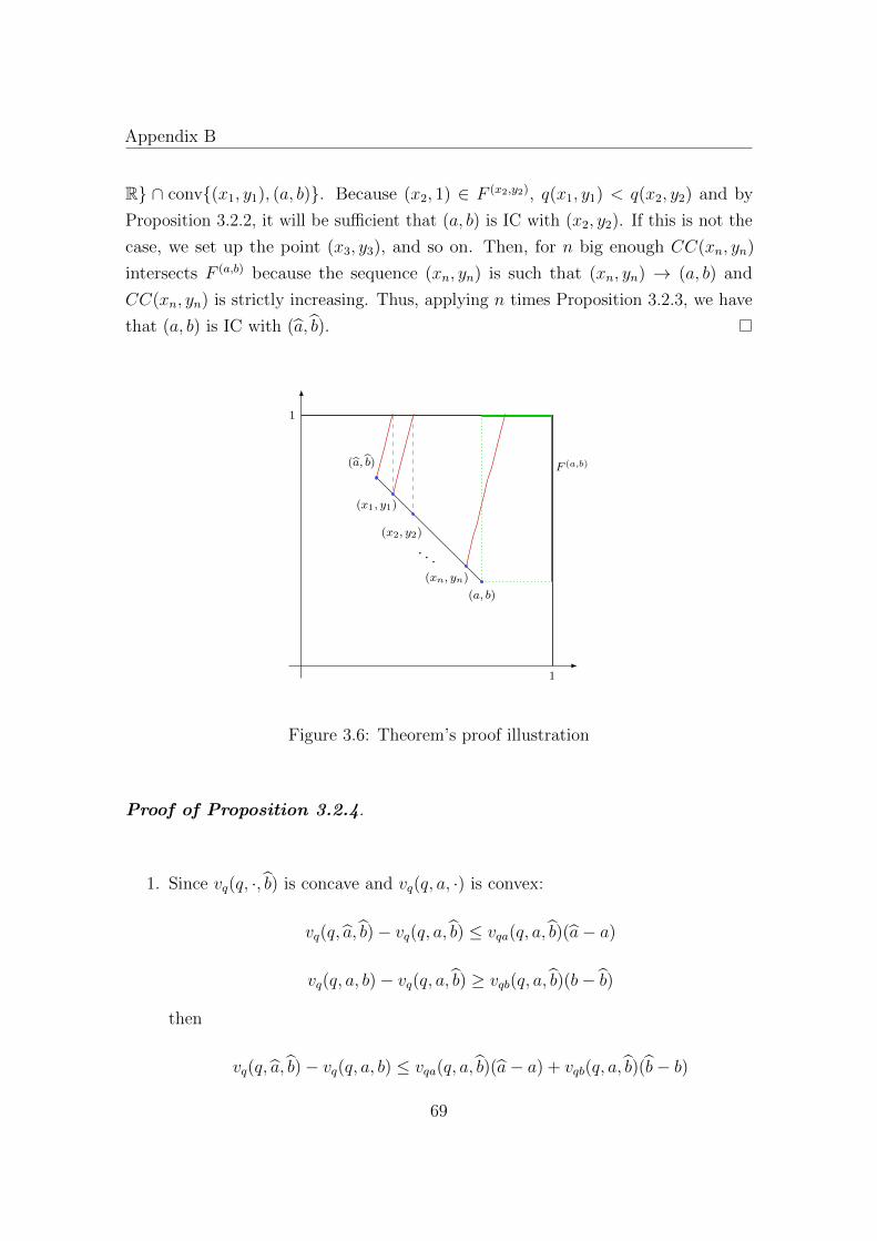
Appendix B
R ∩ conv(x1, y1), (a, b). Because (x2, 1) ∈ F (x2,y2), q(x1, y1) < q(x2, y2) and by
Proposition 3.2.2, it will be sufficient that (a, b) is IC with (x2, y2). If this is not the
case, we set up the point (x3, y3), and so on. Then, for n big enough CC(xn, yn)
intersects F (a,b) because the sequence (xn, yn) is such that (xn, yn) → (a, b) and
CC(xn, yn) is strictly increasing. Thus, applying n times Proposition 3.2.3, we have
that (a, b) is IC with (a, b).
1
1
F (a,b)
(a, b)
(a, b)
(x1, y1)
(x2, y2)
(xn, yn)
. . .
Figure 3.6: Theorem’s proof illustration
Proof of Proposition 3.2.4.
1. Since vq(q, ·, b) is concave and vq(q, a, ·) is convex:
vq(q, a, b)− vq(q, a, b) ≤ vqa(q, a, b)(a− a)
vq(q, a, b)− vq(q, a, b) ≥ vqb(q, a, b)(b− b)
then
vq(q, a, b)− vq(q, a, b) ≤ vqa(q, a, b)(a− a) + vqb(q, a, b)(b− b)
69

Reduction of IC Constraints in the Bidimensional Model
So, if (a, b) (a, b) we have 0 ≤ vq(q, a, b)− vq(q, a, b) which implies
b− ba− a
≤ −vqa(q, a, b)vqb(q, a, b)
in view of a > a and −vqb > 0.
2. Since vq(q, ·, b) is concave and vq(q, a, ·) is convex:
vq(q, a, b)− vq(q, a, b) ≥ vqa(q, a, b)(a− a)
vq(q, a, b)− vq(q, a, b) ≥ vqb(q, a, b)(b− b)
then
vq(q, a, b)− vq(q, a, b) ≥ vqa(q, a, b)(a− a) + vqb(q, a, b)(b− b)
So, if b−ba−a ≤
−vqa(q,a,b)
vqb(q,a,b)then vqa(q, a, b)(a − a) + vqb(q, a, b)(b − b) ≥ 0 thus
vq(q, a, b)− vq(q, a, b) ≥ 0 for any q ∈ Q, that is (a, b) (a, b)
Proof of Proposition 3.2.5.
The proof is completely analogous of Proposition 3.2.4, so we omitted it.
Proof of Proposition 3.4.1.
Let (x, y) ∈ F (a,b) be such that x = 1 (case y = 1 is analogous), and let b be such
that
b− 1
n− 1< y ≤ b
Because (Qn, V n) are solutions of problem (NP), (a, b) satisfies IC with (1, b) :
V n(a, b)− V n(1, b) ≥ v(Qn(1, b), a, b)− v(Qn(1, b), 1, b)
By definition Qn(x, y) = Qn(1, b) , V n(x, y) = V n(1, b) . Also, in view of (a, b) ∈ Xn
we have V n(a, b) = V n(a, b). Then
V n(a, b)− V n(x, y) ≥ v(Qn(x, y), a, b)− v(Qn(x, y), 1, b)
70

Appendix B
On the other hand, since v is Lipschitz:∣∣∣v(Qn(x, y), 1, b)− v(Qn(x, y), x, y)∣∣∣ ≤ L||(1, b)− (x, y)|| = O( 1
n−1)
then
−v(Qn(x, y), 1, b) ≥ −v(Qn(x, y), x, y)−O( 1n−1)
Thus
V n(a, b)− V n(x, y) ≥ v(Qn(x, y), a, b)− v(Qn(x, y), 1, b)
≥ v(Qn(x, y), a, b)− v(Qn(x, y), x, y)−O( 1n−1)
Proof of Proposition 3.4.2.
If CC(a, b) ∩ F (a,b) = (x, y) we apply Proposition 3.4.1 for (a, b) with (x, y) and
considering that Qn(a, b) = Qn(x, y) and t(x, y) = t(a, b) we conclude. Another cases
are treated analogously as in the proof of Theorem 3.2.1.
Proof of Proposition 3.4.3.
Given (a, b), (a′, b′) ∈ [0, 1]2, it will be sufficient to prove that
V n(a′, b′)− V n(a, b)− (v(Qn(a, b), a′, b′)− v(Qn(a, b), a, b)) ≥ −O( 1n−1)
Let (a, b), (a′, b′) ∈ Xn be such that a ≤ a < a + 1n−1 , b − 1
n−1 < b ≤ b and
a′ ≤ a′ < a′ + 1n−1 , b′ − 1
n−1 < b′ ≤ b′. Lets denote q = Qn(a′, b′) = Qn(a′, b′). Since
V n(a, b) = V n(a, b) , V n(a′, b′) = V n(a′, b′) we have
V n(a, b)− V n(a′, b′)− (v(q, a, b)−v(q, a′, b′)) =
V n(a, b)− V n(a′, b′)− (v(q, a, b)− v(q, a′, b′))
+ v(q, a, b)− v(q, a, b) + v(q, a′, b′)− v(q, a′, b′)
because (a, b), (a′, b′) ∈ Xn, by Proposition 3.4.2
V n(a, b)− V n(a′, b′)− (v(q, a, b)− v(q, a′, b′)) ≥ −O( 1n−1)
Besides, va > 0 and a′ ≤ a′ implies v(q, a′, b′) ≤ v(q, a′, b′). Also vb < 0 and b′ ≤ b′
71

Reduction of IC Constraints in the Bidimensional Model
implies v(q, a′, b′) ≤ v(q, a′, b′). Then v(q, a′, b′)− v(q, a′, b′) ≥ 0. Hence
V n(a, b)− V n(a′, b′)− (v(q, a, b)− v(q, a′, b′)) ≥ v(q, a, b)− v(q, a, b)−O( 1n−1)
Because v is Lipschitz (with constant L)∣∣∣v(q, a, b)− v(q, a, b)∣∣∣ ≤ L||(a, b)− (a, b)|| ≤ O( 1
n−1)
then v(q, a, b)− v(q, a, b) ≥ −O( 1n−1) and finally
V n(a, b)− V n(a′, b′)− (v(q, a, b)− v(q, a′, b′)) ≥ −O( 1n−1)
Proof of Proposition 3.4.4.
Let (Q, V ) denote the solution for the continuos problem, and let (Qn, V
n) be their
restriction on the grid Xn. If (Qn, V n) are the solutions of the discretized problem
and OPTn is the optimal value, we have:
OPTn ≥n∑i=1
n∑j=1
w(i, j)(v(Qn
i,j, ai, bj)− Vn
i,j − C(Qn
i,j))f(ai, bj)
=
∫ 1
0
∫ 1
0
(v(Q(a, b), a, b)− V (a, b)− C(Q(a, b)))f(a, b) da db−O(1
n)
= OPT ∗ −O(1
n)
then lim infn→∞OPTn ≥ OPT ∗.
On the other hand, if ∃ limn→∞
Qn(a, b) and limn→∞
V n(a, b) for any (a, b) ∈ [0, 1]2,
define:
Q(a, b) := limn→∞
Qn(a, b) , V (a, b) := limn→∞
V n(a, b)
By Proposition 3.4.3 (Q, V ) is factible, then
OPT ∗ ≥∫ 1
0
∫ 1
0
(v(Q(a, b), a, b)− V (a, b)− C(Q(a, b)))f(a, b) da db
= limn→∞
(∫ 1
0
∫ 1
0
(v(Qn(a, b), a, b)− V n(a, b)− C(Qn(a, b)))f(a, b) da db)
72
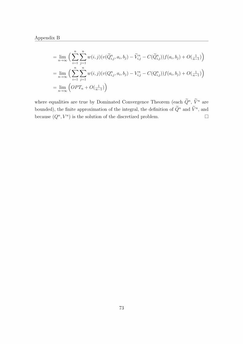
Appendix B
= limn→∞
( n∑i=1
n∑j=1
w(i, j)(v(Qni,j, ai, bj)− V n
i,j − C(Qni,j))f(ai, bj) +O( 1
n−1))
= limn→∞
( n∑i=1
n∑j=1
w(i, j)(v(Qni,j, ai, bj)− V n
i,j − C(Qni,j))f(ai, bj) +O( 1
n−1))
= limn→∞
(OPTn +O( 1
n−1))
where equalities are true by Dominated Convergence Theorem (each Qn, V n are
bounded), the finite approximation of the integral, the definition of Qn and V n, and
because (Qn, V n) is the solution of the discretized problem.
73

Reduction of IC Constraints in the Bidimensional Model
74
Chapter 4
Applications
In this chapter we analyse two models already formulated in the literature in
order to give additional insights by the numerical solution.
The first model, about a monopolist liquidity supplier in financial market, was
introduced by Biais et al. (2000). Although formulated as bidimensional, it was solved
as unidimensional after aggregating the two uncerntainty dimensions into one. This
technique (when applicable) could generate loss of information. Thereby, it would
be valuable a direct analysis in two dimensions, as we do based on approximations.
The second model concerns to regulation of a monopolistic firm with unknown
demand and cost functions. It was introduced by Lewis and Sappington (1988b) and
then review by Armstrong (1999) who showed that Lewis and Sappington’s solution
was wrong. Since the solution is unknown, numerical approximation may be relevant.
The desirability of exclusion property, valid in other contexts, was attempted to
extend to this model. However, as the numerical solution suggest, exclusion of a
positive mass of agents should not be optimal. We provide technical and economic
arguments about this feature.
4.1 Monopolist Liquidity Supplier
In Biais et al. (2000), the authors considered a monopolist who sells a risky
asset to a population of potential investors. Each agent is characterized by a vector
(a, b) ∈ [al, au]× [bl, bu] where a is the investor’s evaluation of the asset’s liquidation
value (the true liquidation value is ν = a+ ξ with ξ ∼ N(0, σ2)) and b is his initial
75
Applications
position in the risky asset (the hedging needs).
When agent trades q, his final wealth is
W = (b+ q)(a+ ξ)− T (q)
Assuming that the informed agent has constant absolute risk aversion preferences
with parameter γ, i.e. u(W ) = −e−γW , the objective function of the agent is
E[W |(a, b)]− γ2V (W |(a, b)) which can be written as
(ab− γσ2
2b2)
+(
(a− γσ2b)q − γσ2
2q2 − T (q)
)The first term measures agent’s reservation utility1, while the second term
measures the gains from trade with the monopolist. So, the valuation function is
defined as
v(q, a, b) = (a− γσ2b)q − γσ2
2q2 with a ∈ [al, au] , b ∈ [bl, bu]
Defining θ = a− γσ2b the authors have reduced the two dimensional screening
into one-dimensional problem. They made direct assumptions on the cumulative
distribution F (θ) with density f(θ), and have found the existence of θ∗b < 0 and θ∗a > 0
such that the optimal trading volume offered by the monopolistic market-maker is
q(θ) =
q∗(θ) +
F (θ)
γσ2f(θ), θ ∈ [θ, θ∗b )
0 , θ ∈ [θ∗b , θ∗a]
q∗(θ)− 1− F (θ)
γσ2f(θ), θ ∈ (θ∗a, θ]
where q∗(θ) =θ − w(θ)
γσ2is the first best solution. Here w(θ) = E(ν|θ) is the
expectation of the asset’s liquidation value given θ.
They have concluded that the optimal tariff is differentiable everywhere except
at 0, and that a positive measure of agents with intermediate types are rationed as a
consequence of adverse selection.
1Setting u0(a, b) = ab− γσ2
2 b2, note that u0(a, b) + v(q(a, b), a, b)− t(a, b) ≥ u0(a, b) is equivalentto V (a, b) ≥ 0 for the usual definition of informational rent V .
76
Monopolist Liquidity Supplier
On the next lines we analyse this model in the original bidimensional formulation
showing that, when agents are uniformly distributed, a closed-form solution can be
obtained using the optimality necessary condition (2.2). Besides, when a closed-form
solution cannot be obtained, the numerical approximation allows us to make robust
predictions in view of multiplicative separable valuation.
First, defining
a :=a− alau − al
, b :=b− blbu − bl
we have a ∈ [0, 1] , b ∈ [0, 1] and
v(q, a, b) =(
(au − al)a− γσ2(bu − bl)b+ (al − γσ2bl))q − γσ2
2q2
setting A = au − al , B = γσ2(bu − bl) , C = al − γσ2bl and, with some abuse of
notation, redifining a := a , b := b we obtain
v(q, a, b) = (Aa−Bb+ C)q − γσ2
2q2
Let ρ be the density over [al, au]× [bl, bu]. Assuming independence, let f , g be
the density distributions over [al, au] , [bl, bu] respectively, let f , g be the density
distributions over [0, 1] induced by the change of variables, and let F , G be their
respective cumulative distribution functions.
Because in this model a negative quantity is allowed, we separate the analysis.
Case q > 0
In view of va > 0 and vb < 0, the type (0, 1) is not willing to acept a positive
quantity, then the virtual surplus is
G(q, a, b) = (v(q, a, b)− 1− F (a)
f(a)va(q, a, b))f(a)g(b)
Solving the initial value problem
as = − vqbvqa
= BA
, a(r, 0) = r
bs = 1 , b(r, 0) = 0
we obtain a(r, s) = BAs+ r , b(r, s) = s.
77

Applications
By the necessary condition (2.2), if φX defined over [rX , 1] is optimal, then∫ s(r)0
Gqvqa
(φX(r), a(r, s), b(r, s))ds = 0 where s(r) = AB
(1− r). This condition yields on
φX(r) =(Ar + C)
γσ2−A
∫ AB
(1−r)
0
(1− F (BAs+ r))g(s) ds
γσ2
∫ AB
(1−r)
0
f(BAs+ r)g(s) ds
(4.1)
for r ∈ [rX , 1], where rX is such that φX(rX) = 0.
Case q < 0
Because of va < 0 and vb > 0, the type (1, 0) is not willing to acept a negative
quantity, so for this case
G(q, a, b) = (v(q, a, b)− 1− G(b)
g(b)vb(q, a, b))f(a)g(b)
Solving the initial value problem
as = − vqbvqa
= BA
, a(r, 0) = 0
bs = 1 , b(r, 0) = r
we have a(r, s) = BAs , b(r, s) = s+ r.
By the necessary condition (2.2), if φY defined over [rY , 1] is optimal, then∫ s(r)0
Gqvqa
(φY (r), a(r, s), b(r, s))ds = 0 where s(r) = 1− r. This condition yields on
φY (r) =(−Br + C)
γσ2+
B
∫ 1−r
0
(1− G(s+ r))f(BAs) ds
γσ2
∫ 1−r
0
f(BAs)g(s+ r) ds
(4.2)
for r ∈ [rY , 1], where rY is such that φY (rY ) = 0.
Now, we will consider particular distributions.
78

Monopolist Liquidity Supplier
Uniform Distributions
Here we assume that f(a) = 1 and g(b) = 1 over [0, 1].
Case q > 0
The expression of φX established on (4.1) derives on
φX(r) =(3r − 1)A+ 2C
2γσ2, ∀ r ∈ [
A− 2C
3A, 1]
To return to the original variables, given (a, b) we can express r(a, b) = a− bBA
,
and considering that q(a, b) = φX(r(a, b)) when r(a, b) ≥ rX = A−2C3A
we obtain
q(a, b) =(3a− 1)A− 3bB + 2C
2γσ2when Aa−Bb− (A− 2C)
3≥ 0
Now, lets compute the tariff. For r ∈ [rX , 1] we have
t(r, 0) = T (φX(r)) =
∫ r
rXvq(φ
X(r), r, 0)(φX)′(r) dr
after some calculus, and considering r = (φX)−1(q) we get
T (q) =−γσ2q2 + 2q(A+ C)
6when q > 0
Case q < 0
The expression of φY established on (4.2) derives on
φY (r) =(1− 3r)B + 2C
2γσ2, ∀ r ∈ [
B + 2C
3B, 1]
To return to the original variables, given (a, b) we can express r(a, b) = b− aAB
,
and considering that q(a, b) = φY (r(a, b)) when r(a, b) ≥ rY = B+2C3B
we obtain
q(a, b) =3Aa+ (1− 3b)B + 2C
2γσ2when a
A
B− b+
(B + 2C)
3B≤ 0
79
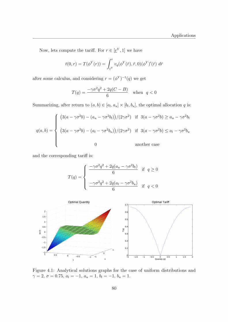
Applications
Now, lets compute the tariff. For r ∈ [rY , 1] we have
t(0, r) = T (φY (r)) =
∫ r
rYvq(φ
Y (r), r, 0)(φY )′(r) dr
after some calculus, and considering r = (φY )−1(q) we get
T (q) =−γσ2q2 + 2q(C −B)
6when q < 0
Summarizing, after return to (a, b) ∈ [al, au]× [bl, bu], the optimal allocation q is:
q(a, b) =
(3(a− γσ2b)− (au − γσ2bl)
)/(2γσ2) if 3(a− γσ2b) ≥ au − γσ2bl
(3(a− γσ2b)− (al − γσ2bu)
)/(2γσ2) if 3(a− γσ2b) ≤ al − γσ2bu
0 another case
and the corresponding tariff is:
T (q) =
−γσ2q2 + 2q(au − γσ2bl)
6if q ≥ 0
−γσ2q2 + 2q(al − γσ2bu)
6if q < 0
−1
0
1
−1−0.500.51−2
−1.5
−1
−0.5
0
0.5
1
1.5
2
a
Optimal Quantity
b
q(a,
b)
−2 −1.5 −1 −0.5 0 0.5 1 1.5 20
0.1
0.2
0.3
0.4
0.5
0.6
0.7Optimal Tariff
Quantity (q)
T(q
)
Figure 4.1: Analytical solutions graphs for the case of uniform distributions andγ = 2, σ = 0.75, al = −1, au = 1, bl = −1, bu = 1.
80
Monopolist Liquidity Supplier
Truncated Normal Distributions
Assuming that types a, b presents truncated normal distribution over [0, 1] with
means µ1, µ2 and variances σ21, σ2
2 respectively, we have:
f(a) =e− (a−µ1)
2
2σ21
√2πσ1Λ1
, g(b) =e− (b−µ2)
2
2σ22
√2πσ2Λ2
where Λi = 1√2πσi
∫ 1
0
e− (t−µi)
2
2σ2i dt , i = 1, 2
The expressions of φX and φY given in (4.1) and (4.2) transforms on
φX(r) =(Ar + C)
γσ2−A
∫ AB
(1−r)
0
(1−
∫ BAs+r
0
e− (t−µ1)
2
2σ21
√2πσ1Λ1
dt)( e− (s−µ2)
2
2σ22
√2πσ2Λ2
)ds
γσ2
∫ AB
(1−r)
0
(e−((BAs+r−µ1)
2
2σ21+
(s−µ2)2
2σ22)
2πσ1σ2Λ1Λ2
)ds
φY (r) =(−Br + C)
γσ2+
B
∫ 1−r
0
(1−
∫ s+r
0
e− (t−µ2)
2
2σ22
√2πσ2Λ2
dt)(e− (B
As−µ1)
2
2σ21
√2πσ1Λ1
)ds
γσ2
∫ 1−r
0
(e−((BAs−µ1)
2
2σ21+
(s+r−µ2)2
2σ22)
2πσ1σ2Λ1Λ2
)ds
These expressions involve integrals that cannot be expressed in terms of elementary
functions, so neither φX , φY nor the derivatives (which are required to compute the
tariff T ) can be expressed in closed-form.
In this situation we appeal to numerical approximations solving (NP). Note that
valuation function is multiplicative separable then, by remark VI in section 3.3,
numerical solutions are reliable.
On the next pages we show the numerical solutions (with n = 26) for differents
mean and variance’s values. We fix γ = 2 (parameter of CARA preferences) and
σ = 0.75 (variance of true liquidation). Because agents’ parameter a is the assets
liquidation valuation, we are calling ‘optimistic’ (‘pessimistic’) to agents with hight
(low) value. Remember that b reflects the agent’s initial position of the risky asset.
81
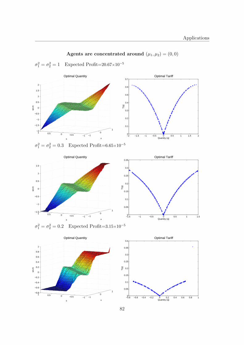
Applications
Agents are concentrated around (µ1, µ2) = (0, 0)
σ21 = σ2
2 = 1 Expected Profit=20.67×10⁻⁵
−10
1
−1−0.500.51−2
−1.5
−1
−0.5
0
0.5
1
1.5
2
a
Optimal Quantity
b
q(a,
b)
−2 −1.5 −1 −0.5 0 0.5 1 1.5 20
0.1
0.2
0.3
0.4
0.5
0.6
0.7Optimal Tariff
Quantity (q)
T(q
)
σ21 = σ2
2 = 0.3 Expected Profit=6.65×10⁻⁵
−10
1
−1−0.500.51−1.5
−1
−0.5
0
0.5
1
1.5
a
Optimal Quantity
b
q(a,
b)
−1.5 −1 −0.5 0 0.5 1 1.50
0.05
0.1
0.15
0.2
0.25
0.3
0.35Optimal Tariff
Quantity (q)
T(q
)
σ21 = σ2
2 = 0.2 Expected Profit=3.15×10⁻⁵
−10
1
−1−0.500.51−0.8
−0.6
−0.4
−0.2
0
0.2
0.4
0.6
0.8
1
a
Optimal Quantity
b
q(a,
b)
−0.8 −0.6 −0.4 −0.2 0 0.2 0.4 0.6 0.8 10
0.05
0.1
0.15
0.2
0.25
0.3
0.35
0.4Optimal Tariff
Quantity (q)
T(q
)
82
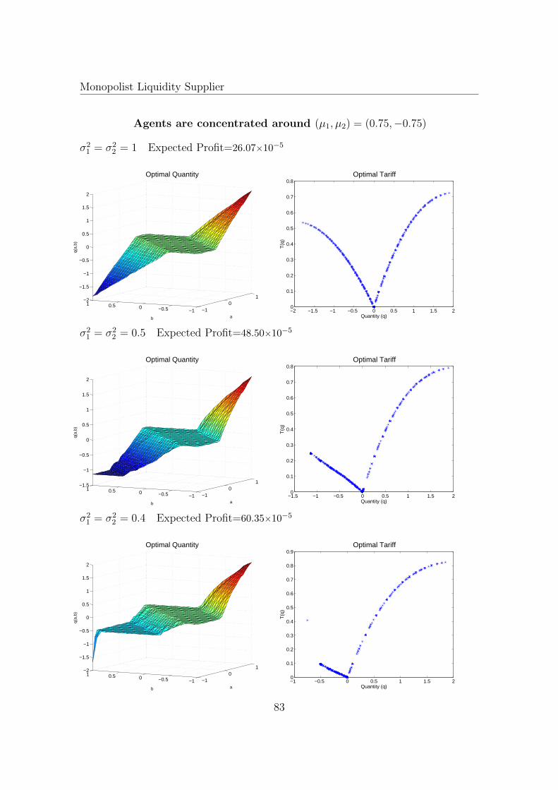
Monopolist Liquidity Supplier
Agents are concentrated around (µ1, µ2) = (0.75,−0.75)
σ21 = σ2
2 = 1 Expected Profit=26.07×10⁻⁵
−10
1
−1−0.500.51−2
−1.5
−1
−0.5
0
0.5
1
1.5
2
a
Optimal Quantity
b
q(a,
b)
−2 −1.5 −1 −0.5 0 0.5 1 1.5 20
0.1
0.2
0.3
0.4
0.5
0.6
0.7
0.8Optimal Tariff
Quantity (q)
T(q
)
σ21 = σ2
2 = 0.5 Expected Profit=48.50×10⁻⁵
−10
1
−1−0.500.51−1.5
−1
−0.5
0
0.5
1
1.5
2
a
Optimal Quantity
b
q(a,
b)
−1.5 −1 −0.5 0 0.5 1 1.5 20
0.1
0.2
0.3
0.4
0.5
0.6
0.7
0.8Optimal Tariff
Quantity (q)
T(q
)
σ21 = σ2
2 = 0.4 Expected Profit=60.35×10⁻⁵
−10
1
−1−0.500.51−2
−1.5
−1
−0.5
0
0.5
1
1.5
2
a
Optimal Quantity
b
q(a,
b)
−1 −0.5 0 0.5 1 1.5 20
0.1
0.2
0.3
0.4
0.5
0.6
0.7
0.8
0.9Optimal Tariff
Quantity (q)
T(q
)
83
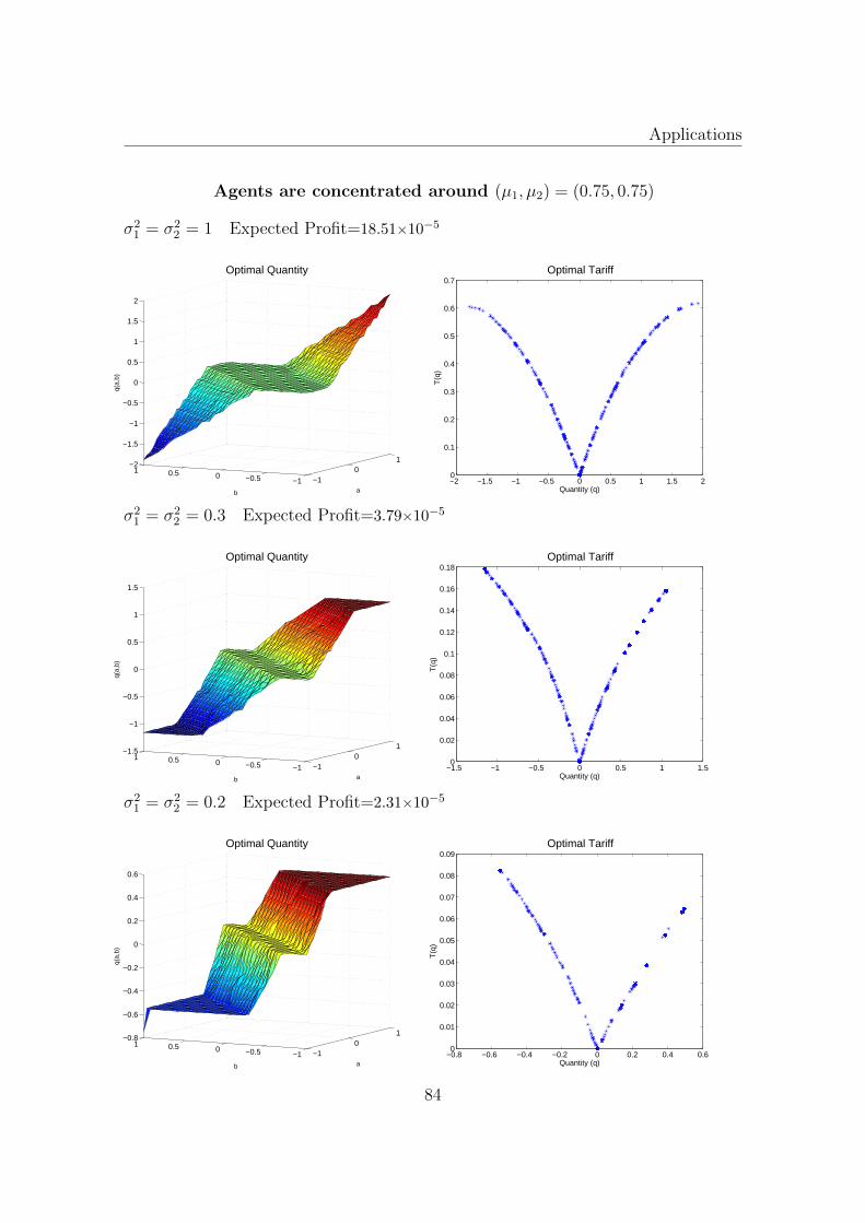
Applications
Agents are concentrated around (µ1, µ2) = (0.75, 0.75)
σ21 = σ2
2 = 1 Expected Profit=18.51×10⁻⁵
−10
1
−1−0.500.51−2
−1.5
−1
−0.5
0
0.5
1
1.5
2
a
Optimal Quantity
b
q(a,
b)
−2 −1.5 −1 −0.5 0 0.5 1 1.5 20
0.1
0.2
0.3
0.4
0.5
0.6
0.7Optimal Tariff
Quantity (q)
T(q
)
σ21 = σ2
2 = 0.3 Expected Profit=3.79×10⁻⁵
−10
1
−1−0.500.51−1.5
−1
−0.5
0
0.5
1
1.5
a
Optimal Quantity
b
q(a,
b)
−1.5 −1 −0.5 0 0.5 1 1.50
0.02
0.04
0.06
0.08
0.1
0.12
0.14
0.16
0.18Optimal Tariff
Quantity (q)
T(q
)
σ21 = σ2
2 = 0.2 Expected Profit=2.31×10⁻⁵
−10
1
−1−0.500.51−0.8
−0.6
−0.4
−0.2
0
0.2
0.4
0.6
a
Optimal Quantity
b
q(a,
b)
−0.8 −0.6 −0.4 −0.2 0 0.2 0.4 0.60
0.01
0.02
0.03
0.04
0.05
0.06
0.07
0.08
0.09Optimal Tariff
Quantity (q)
T(q
)
84
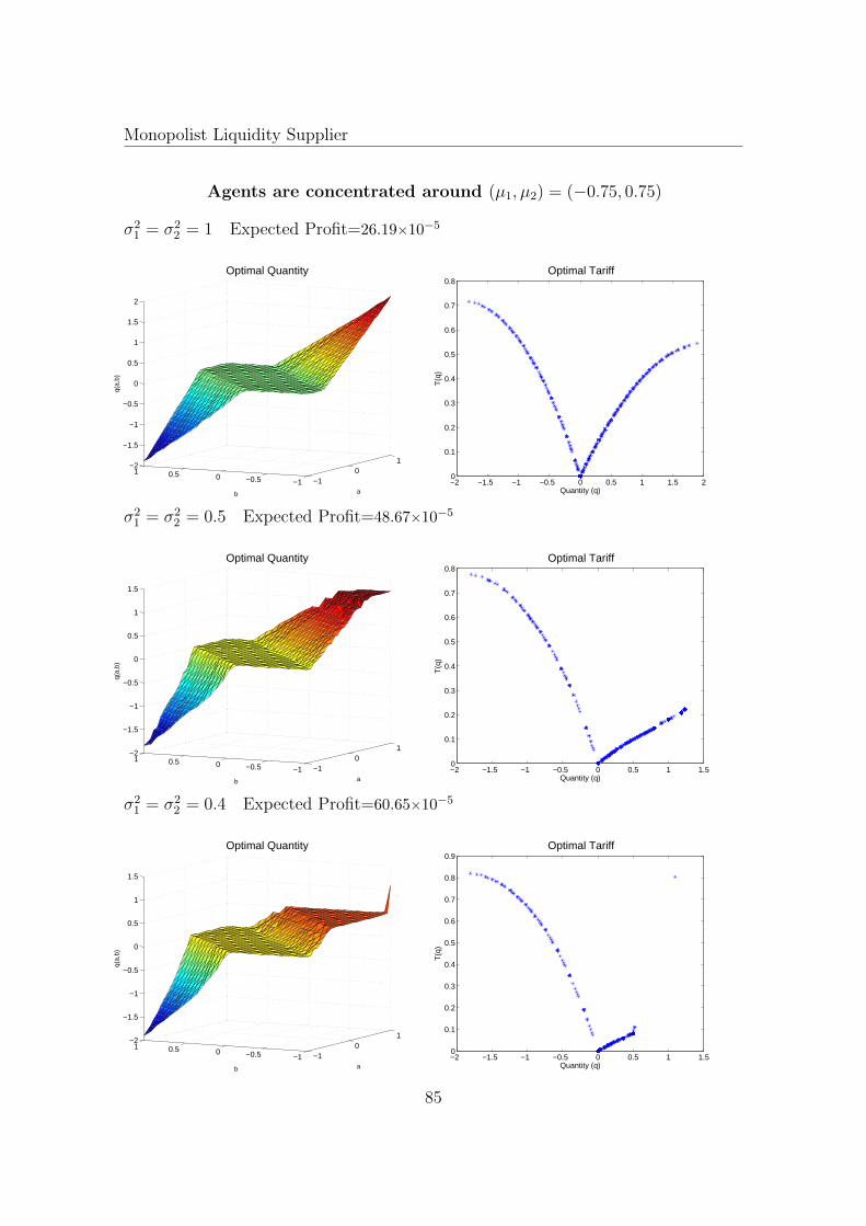
Monopolist Liquidity Supplier
Agents are concentrated around (µ1, µ2) = (−0.75, 0.75)
σ21 = σ2
2 = 1 Expected Profit=26.19×10⁻⁵
−10
1
−1−0.500.51−2
−1.5
−1
−0.5
0
0.5
1
1.5
2
a
Optimal Quantity
b
q(a,
b)
−2 −1.5 −1 −0.5 0 0.5 1 1.5 20
0.1
0.2
0.3
0.4
0.5
0.6
0.7
0.8Optimal Tariff
Quantity (q)
T(q
)
σ21 = σ2
2 = 0.5 Expected Profit=48.67×10⁻⁵
−10
1
−1−0.500.51−2
−1.5
−1
−0.5
0
0.5
1
1.5
a
Optimal Quantity
b
q(a,
b)
−2 −1.5 −1 −0.5 0 0.5 1 1.50
0.1
0.2
0.3
0.4
0.5
0.6
0.7
0.8Optimal Tariff
Quantity (q)
T(q
)
σ21 = σ2
2 = 0.4 Expected Profit=60.65×10⁻⁵
−10
1
−1−0.500.51−2
−1.5
−1
−0.5
0
0.5
1
1.5
a
Optimal Quantity
b
q(a,
b)
−2 −1.5 −1 −0.5 0 0.5 1 1.50
0.1
0.2
0.3
0.4
0.5
0.6
0.7
0.8
0.9Optimal Tariff
Quantity (q)
T(q
)
85
Applications
Some insights from these solutions:
1. When agents’ distribution is not too concentrate the solution does not differ too
much from the uniform distribution case, no matters the point of concentration.
Thus, trade will take place with two opposite sides of the market: optimistic
agents with short position (a high, b low) and pessimistic agents with large
position (a low, b high). With middle agents it is optimal not to trade.
2. Because type (0, 0) is neither optimistic nor pessimistic about the final value
of the asset (a = 0) and does not have the need to transact the asset (b = 0),
when the mass of agents around this type increases (i.e. if σ21 → 0, σ2
2 → 0) the
monopolist does not have to discriminate neither between optimistic agents with
short position nor between pessimistic agents with large position, but designs
a contract in which middle agents are increasingly included and discriminated.
Thus, optimal quantity for the two sides becomes flat and smaller as well as
the tariff for this quantity offered. As a result, expected profit decrease.
Same features are observed when agents concentrate around (0.75, 0.75) because
this agent is also not willing to trade with the monopolist, due to he has large
position of the asset and is optimistic about its final value.
3. The type (0.75,−0.75) reflects an optimistic agent with short position, therefore
a potential buyer. So, when the mass of agents around this type increases,
the monopolist discriminates this side of the market whereas bunching the
opposite side (pessimistic agents with large position) at a fewer quantity and
tariff. Because there are more potential buyers, expected profit increases.
Similar features are observed in the reverse situation when agents increasingly
concentrate around (−0.75, 0.75) (a potentially seller) since this type of agents
are also willing to trade because of their large position of the asset and its
pessimistic valuation.
86
Regulating a Monopolist Firm
4.2 Regulating a Monopolist Firm
In Lewis and Sappington (1988b) the authors studied the design of regulatory
policy when the regulator is imperfectly informed about both cost and demand
functions of the monopolist firm he is regulating.
In particular, they have considered that demand for the firm’s product q = Q(p, a)
and cost of producing output q, C(q, b) are given by
Q(p, a) = h(p) + a , C(q, b) = C(q) + bq
where (a, b) are firm’s private information parameters, distributed over [0, 1]×[0, 1]
according to a strictly positive density function f(a, b).
The regulator offers the firm a menu of contracts (p(a, b), t(a, b)) whereby if
the firm sets unit price p(a, b) for its output, it receives the subsidy t(a, b) from
consumers. It is assumed that regulator can ensure that the firm serves all demand
at the established prices. The objective function is the expected consumer surplus
net of the transfer to the firm.
Thus, the regulator’s problem is to find two functions p : [0, 1]2 → R+ and
t : [0, 1]2 → R+ in order to solve
maxp(·),t(·)
∫ 1
0
∫ 1
0
Π(Q(p(a, b), a), a)− p(a, b)Q(p(a, b), a))− t(a, b)f(a, b)dbda
subject to
(IR) p(a, b)Q(p(a, b), a)) + t(a, b)− C(Q(p(a, b), a), b) ≥ 0
(IC) p(a, b)Q(p(a, b), a)) + t(a, b)− C(Q(p(a, b), a), b) ≥
p(a, b)Q(p(a, b), a)) + t(a, b)− C(Q(p(a, b), a), b)
where Π(Q, a) =∫ Q
0P (ξ, a)dξ, and P (·) denotes the inverse demand curve.
Lewis and Sappington considered the example
Q(p, a) = α− p+ a , C(q, b) = K + (c0 + b)q
with α,K, c0 positive constants and uniform distribution of types. They developed a
similar idea to that exposed in section 2.4 to deal with the problem, transforming
87
Applications
the two-dimensional maximization problem into a single-dimensional one, and have
found as ‘solution’ p(a, b) = r(a+ b) where
r(s) =
c0 +s
2+
s
2√
2for s ∈ [0, 1]
c0 +s
2+
2s− 1− s2/2√2(2− s)
for s ∈ [1, s1]
c0 + 1 for s ∈ [s1,√
2]
c0 +s
2+
2s− 1− s2/2√2(2− s)
− 1√2
for s ∈ [√
2, 2[
and s1 ≈ 1.062.
Nevertheless, as Armstrong (1999) has noticed, this cannot be the solution,
because r(s) → ∞ as s → 2, and therefore q = α + a − p(a, b) < 0 for (a, b) close
to (1, 1). In that paper Armstrong argued that excluding a positive mass of types
should be optimal, as in the nonlinear pricing model (see section 2.3) but, because of
the change of variables he used, the type set is not convex and his exclusion argument
cannot strictly be applied. He also pointed out:
• “Nevertheless, I believe that the condition that the support be convex is strongly
sufficient and that it will be the usual case that exclusion is optimal...”
• “I have not found it possible to solve this precise example correctly...” (in
reference to the Lewis and Sappington’s example above)
Then, we are facing a bidimensional adverse selection model with unknown
solution, where a conjecture about optimality of exclusion were made.
Next, we show that regulator’s problem can be seen as a monopolist’s problem in
order to apply the reduction of IC constraints and provide a numerical approximation
of the solution. Setting
v(p, a, b) = pQ(p, a)− C(Q(p, a), b)
H(p, a) = pQ(p, a)− Π(Q(p, a), a)
V (a, b) = v(p(a, b), a, b) + t(a, b)
88
Regulating a Monopolist Firm
we can rewrite the regulator’s problem as
maxp(·),V (·)
∫ 1
0
∫ 1
0
v(p(a, b), a, b)−H(p(a, b), a)− V (a, b)f(a, b)dbda
subject to
(IR) V (a, b) ≥ 0 ∀ (a, b) ∈ [0, 1]2
(IC) V (a, b)− V (a, b) ≥ v(p(a, b), a, b)− v(p(a, b), a, b) ∀ (a, b), (a, b) ∈ [0, 1]2
This formulation fits the standard nonlinear pricing by a monopolist problem
studied in Chapter 3. That is, the regulator’s problem may be understood as the
monopolist’s problem where −in this case− the firm’s costs function is H(p) and
(a, b)−agent’s valuation for ‘consumption’ p is v(p, a, b).
Consider the following assumptions on demand and cost functions: Qp < 0 , Cq >
0 , Cqq ≥ 0 , which means that demand decreases with prices and costs and marginal
costs are increasing with output.
Given that Q(p, a) = h(p) + a and C(q, b) = C(q) + bq we have
va = p− Cq(Q(p, a), b)
vb = −Cb(Q(p, a), b) = −Q(p, a) < 0
vpa = 1− Cqq(Q(p, a), b)h′(p) > 0
vpb = −h′(p) > 0
Assumption A4 of section 3.1 cannot be verified (the sign of va is endogenously
determined), so the problem must consider all the IR constraints. Besides, even
Assumption A3 is not valid, what really matters is the constant sign of vpa and
vpb. In this case, p(·, ·) will be non-decreasing on a and b. Also, since−vpbvpa
< 0, the
characteristic curves are strictly decreasing.
Seeing the regulator’s problem as if it were the monopolist’s problem, type (1, 1)
would be considered the best type from the monopolist’s point of view (vp(p, 1, 1) ≥vp(p, a, b) for any (a, b)). Then, following the same considerations of section 3.2, it
will be sufficient that each (a, b)−agent verifies IC constraints with all the points
over the set
F (a,b) := (0, s) | b ≤ s ≤ 1 ∪ (s, 1) | 0 ≤ s ≤ a
89

Applications
Note that the necessary condition for optimality (2.2) established by Araujo and
Vieira (2010) cannot be applied in this case, because assumption A.4 is not verified.
In fact, we believe that this lack of consideration could be one of the failures on
Lewis and Sappington’s work, because after had transformed the problem into a
single-dimesional (by incorporating local incentive compatibility constraints in the
regulator’s objective function), they have not considered the IR constraints, which
cannot be ruled out if A.4 fails.
Consider the same example
Q(p, a) = α− p+ a , C(q, b) = K + (c0 + b)q
with α,K, c0 positive constants and uniform distribution of types. Then
v(p, a, b) = (α + a− p)(p− c0 − b)−K
H(p, a) = −(α + a− p)2
2
Even when Hpp < 0, what we need to ensure strictly concavity of the objective
function in the discretized problems is vpp −Hpp < 0, which is true. Note also that
IC constraints become linear, by the multiplicative separable form of v. Then, the
discretized problem have unique solution.
We solved the discretized problem numerically for three cases:
c0 = 1, α = 5, K = 2
c0 = 2, α = 4, K = 4.5
c0 = 3, α = 4.5, K = 3
all of them with n = 51 points. For this value, 256 225 incentive compatibility
constraints were considered, and 6 506 375 were eliminated.
On the next pages we show the graphs of these solutions. Also, we show the
numerical differences between unit prices and marginal costs on the last set of figures.
90
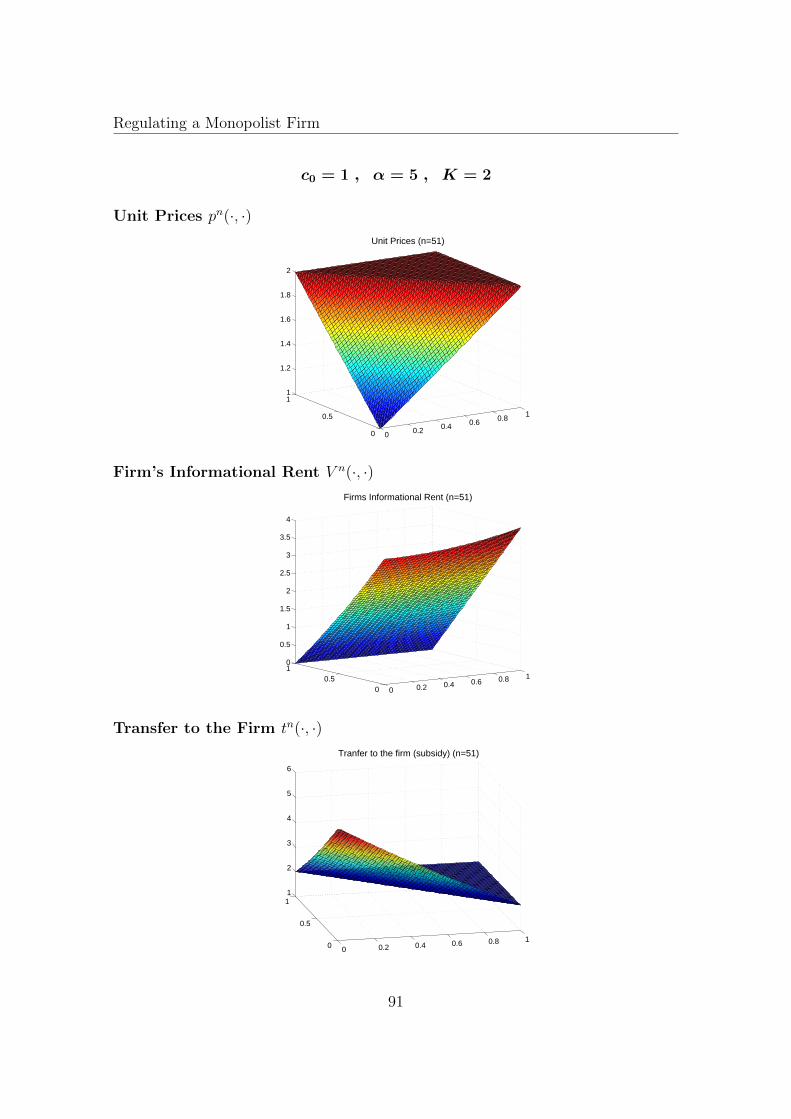
Regulating a Monopolist Firm
c0 = 1 , α = 5 , K = 2
Unit Prices pn(·, ·)
0 0.2 0.4 0.6 0.8 1
0
0.5
11
1.2
1.4
1.6
1.8
2
Unit Prices (n=51)
Firm’s Informational Rent V n(·, ·)
0 0.2 0.4 0.6 0.8 1
00.5
10
0.5
1
1.5
2
2.5
3
3.5
4
Firms Informational Rent (n=51)
Transfer to the Firm tn(·, ·)
0 0.2 0.4 0.6 0.8 10
0.5
11
2
3
4
5
6
Tranfer to the firm (subsidy) (n=51)
91
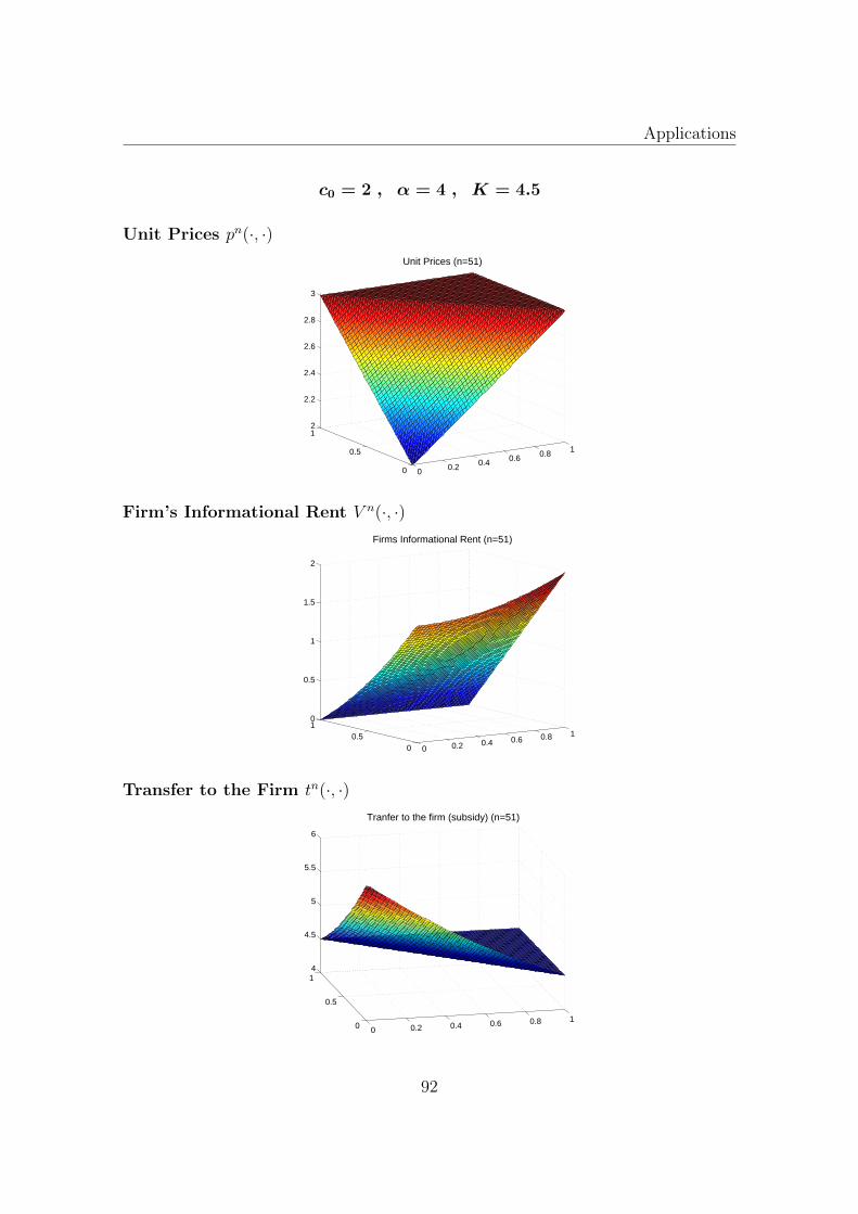
Applications
c0 = 2 , α = 4 , K = 4.5
Unit Prices pn(·, ·)
0 0.2 0.4 0.6 0.8 1
0
0.5
12
2.2
2.4
2.6
2.8
3
Unit Prices (n=51)
Firm’s Informational Rent V n(·, ·)
0 0.2 0.4 0.6 0.8 1
00.5
10
0.5
1
1.5
2
Firms Informational Rent (n=51)
Transfer to the Firm tn(·, ·)
0 0.2 0.4 0.6 0.8 10
0.5
14
4.5
5
5.5
6
Tranfer to the firm (subsidy) (n=51)
92
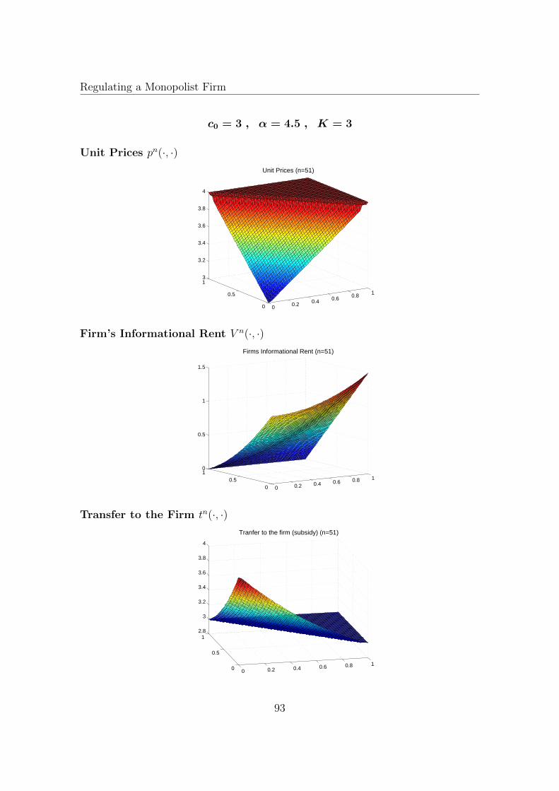
Regulating a Monopolist Firm
c0 = 3 , α = 4.5 , K = 3
Unit Prices pn(·, ·)
0 0.2 0.4 0.6 0.8 1
0
0.5
13
3.2
3.4
3.6
3.8
4
Unit Prices (n=51)
Firm’s Informational Rent V n(·, ·)
0 0.2 0.4 0.6 0.8 1
00.5
10
0.5
1
1.5
Firms Informational Rent (n=51)
Transfer to the Firm tn(·, ·)
0 0.2 0.4 0.6 0.8 10
0.5
12.8
3
3.2
3.4
3.6
3.8
4
Tranfer to the firm (subsidy) (n=51)
93
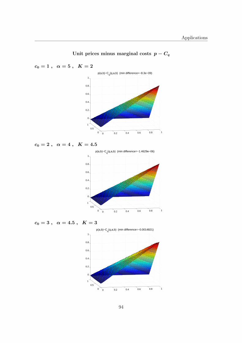
Applications
Unit prices minus marginal costs p− Cq
c0 = 1 , α = 5 , K = 2
0 0.2 0.4 0.6 0.8 10
0.5
1
0
0.2
0.4
0.6
0.8
1
p(a,b)−Cq(q,a,b) (min difference=−8.3e−09)
c0 = 2 , α = 4 , K = 4.5
0 0.2 0.4 0.6 0.8 10
0.5
1
0
0.2
0.4
0.6
0.8
1
p(a,b)−Cq(q,a,b) (min difference=−1.4629e−06)
c0 = 3 , α = 4.5 , K = 3
0 0.2 0.4 0.6 0.8 10
0.5
1
0
0.2
0.4
0.6
0.8
1
p(a,b)−Cq(q,a,b) (min difference=−0.0014821)
94
Regulating a Monopolist Firm
Some insights from these solutions:
We stress that this example derives into a optimization problem with unique
solution. In fact, because the objective function is quadratic and strictly concave
with linear restrictions, the numerical methods to solve it are efficient.
Thus, the statements below are reliable:
1. It seems that at the optimum, all types (a, b) such that a+ b ≥ 1 are bunching
with unit price c0 + 1, and subsidy for them is the fix cost K. Also, unit price
assigned to type (0, 0) it seems to be c0.2
2. In view of the numerical difference p− Cq, regulator induce the firm to price
above marginal cost, for almost all (a, b) types other than a = 0 or b = 1, i.e.
such types with lowest demand function or such types who gets zero surplus3.
3. The numerical informational rent suggests that there is no exclusion.
4.2.1 A Discussion about Optimality of Exclusion
Perhaps the most intriguing insight from the numerical solutions of this example
is that it should be optimal non-exclusion of types, contrary to the Armstrong’s
conjecture stated previously.
Besides, in Barelli et al. (2014) the authors have relaxed Armstrong’s strong
conditions (strictly convexity, homogeneity of degree one) and have proved a more
general result of desirability of exclusion. For this example they have considered that
prices belongs to [c0 + 1, α] to conclude that their result can be applied and confirm
Armstrong (1999)’s conjecture, generically. However, as can be seen, it is not true
that P ⊂ [c0 + 1, α], so their theorem should not be applied.
2In fact, we can conjecture the optimum price p to be p(a, b) = c0 + a+ b when a+ b ≤ 1, andp(a, b) = c0 + 1 when a+ b > 1
3 In Baron and Myerson (1982) the authors have analysed a model in which the regulator isuncertain only about the firm’s cost function. At the optimum, prices are above marginal costs forall cost realizations other than the lowest. In the model of Lewis and Sappington (1988a) regulatoris uncertain only about the position of demand curves. In that model, if C ′′(q) ≥ 0 (like here),setting prices at the level of marginal cost for the reported demand is optimal (p = Cq).
95
Applications
We are able to provide one technical argument explaining why Armstrong’s
Theorem 2.3.1 about desirability of exclusion, formulated in the nonlinear pricing
context, cannot be extended to this model. Also, an economic argument about why
should not be optimal excluding types.
1. Because in the nonlinear pricing by a monopolist model the outside option
for customers is to consume qout = 0, the natural assumptions v(qout, a, b) = 0,
C(qout) = 0 made in Armstrong (1996) imply the monopolist’s revenue
v(qout, a, b)− C(qout)− V (a, b)
to be zero when V (a, b) = 0, that is, if type (a, b) is excluded. Then, the monopolist’s
penalty of causing some customers to exit the market is just not to receive income
from them. On the other hand, in the regulation model the outside option is the
unit price at which there is not production, i.e. pout is such that Qout = 0 . With
these values
Π(Qout, a)− poutQout − t(a, b) = −t(a, b)
when type (a, b) is excluded, i.e., when t(a, b) = C(Qout, b) = C(0, b) (because IR is
binding). That is, the regulator’s penalty of excluding a firm type (a, b) is to subsidy
the firm’s fixed cost.
Thereby, in contrast with monopolist, regulator has to assume a negative penalty
whenever firm’s fixed cost is positive. (In previous example, pout(a, b) = α + a ,
v(pout, a, b) = −K and C(0, a, b) = K > 0). Thus, the Armstrong’s argument of
comparing benefit (more income from agents still in the market) versus penalty (zero
income from agents excluded), might not be applied in this model in view of penalty
could be strictly negative.
Therefore, the main technical assumption not satisfied in Armstrong’s Theorem
is neither related with strictly convexity of types’ set nor with homogeneity of the
degree one of the valuation function (his strong technical assumptions). It is the not
validity of v(pout, a, b) = 0.
2. In the nonlinear pricing setting, when designing the contract the monopolist
is faced with a population of customers with different characteristics, where the mass
of customers with certain characteristics is reflected by the distribution. Then, as
Armstrong have formalized, it is optimal for the monopolist not to serve customers
96
Regulating a Monopolist Firm
with low valuation of the product, because there is a mass of other customers who
valuates it high.
In contrast, in the regulation model, the regulator is faced with one single firm
who is going to exercise the monopoly of certain good. Here, the types’s distribution
reflects the probability of such firm to have certain characteristics unknown by the
regulator. So, consider what will happen if regulator designs a contract with the
posibility of exclusion and such unique firm choose to be excluded as its best option.
As a consequence, neither production nor consumption of the good takes place in
the economy and, even in this case, consumers has to subsidy (probably non-zero)
fixed cost of the company. Such situation cannot be optimal.
97

Applications
98
Conclusions
Based on what have been exposed in this work, we make the following conclusions:
1) A necessary condition for optimality can be established in case isoquants are
concurrent at certain point, or equivalently, in case there is a type indifferent between
any allocation in an interval.
2) Comparing types according to their marginal valuation of consumption and taking
account the posible shape of isoquants, allows us to reduce incentive compatibility
contraints making the discretized problem numerically tractable for relative fine
discretization. In applications, numerical approximations gives us the opportunity of
predict features of the solution when the problem has not closed-form solution, which
is the usual case. Futhermore, allows us to analyze different situations according to
types’ distribution.
3) In all the examples, the numerical solution of informational rent V n was more
approximate and smoother than the numerical solution of quality Qn. This is because
the problem is linear with respect to V , regardless the valuation function v.
4) We can provide the solution of the optimal contract when agents’ demand curves
are convex and the monopolist is uncertain about the parameters defining such curve
(Example 4, Chapter 3, page 55). To the best of our knowledge, this kind of example
has not been previously analyzed.
5) In the regulation model a conjecture about desirability of exclusion had been
made as well as the attempt to formalize it. Nevertheless, this exclusion feature is not
present on the reliable numerical approximations. The main technical assumption
why Armstrong’s result cannot be applied to this model is the not validity of
v(pout, a, b) = 0 and, by the nature of the model, it should not be optimal a contract
with the possibility of excluding types.
99

100

Bibliography
Araujo, A. and Moreira, H. (2010). Adverse selection problems without the spence-
mirrlees condition. Journal of Economic Theory, 145(3):1113–1141.
Araujo, A. and Vieira, S. (2010). Two-dimensional screening: a useful optimality
condition. Preprint.
Armstrong, M. (1996). Multiproduct nonlinear pricing. Econometrica, 64(1):51–75.
Armstrong, M. (1999). Optimal regulation with unknown demand and cost functions.
Journal of Economic Theory, 84:196–215.
Barelli, P., Basov, S., Bugarin, M., and King, I. (2014). On the optimality of exclusion
in multi-dimensional screening. Journal of Mathematical Economics, 54:74–83.
Baron, D. and Myerson, R. (1982). Regulating a monopolist with unknown costs.
Econometrica, 50(4):911–930.
Basov, S. (2001). Hamiltonian approach to multi-dimensional screening. Journal of
Mathematical Economics, 36:77–94.
Basov, S. (2005). Multidimensional Screening. Springer-Verlag.
Belloni, A., Lopomo, G., and Shouqiang, W. (2010). Multidimensional mechanism
design: Finite-dimensional approximations and efficient computation. Operations
Research, 58(4):1079–1089.
Biais, B., Martimort, D., and Rochet, J. (2000). Competing mechanisms in a common
value environment. Econometrica, 68(4):799–837.
Carlier, G. (2001). A general existence result for the principal-agent problem with
adverse selection. Journal of Mathematical Economics, 35(1):129–150.
101
BIBLIOGRAPHY
Deneckere, R. and Severinov, S. (2015). Multi-dimensional screening: A solution to
a class of problems. Preprint.
Fundenberg, D. and Tirole, J. (1991). Game Theory. MIT Press.
Guesnerie, R. (1981). On taxation and incentives: Further reflections on the limits
to redistribution. Mimeo.
Kamien, M. and Schwartz, N. (1981). Dynamics Optimization. New York: North-
Holland.
Laffont, J. and Martimort, D. (2002). The Theory of Incentives: The Principal-Agent
Model. Princeton University Press.
Laffont, J., Maskin, E., and Rochet, J. (1987). Optimal nonlinear pricing with
two-dimensional characteristics. In Incentives and Economic Mechanisms (essays
in honor of Leonid Hurwicz), pages 256–266. T.Groves, R.Radner, S. Reiter, Eds.,
Minneapolis.
Lewis, T. and Sappington, D. (1988a). Regulating a monopolist with unknown
demand. American Economic Review, 78:986–998.
Lewis, T. and Sappington, D. (1988b). Regulating a monopolist with unknown
demand and cost functions. RAND Journal of Economics, 19(3):438–457.
Maskin, E. and Riley, J. (1984). Monopoly with incomplete information. RAND
Journal of Economics, 15:171–196.
Matthews, S. and Moore, J. (1987). Monopoly provision of quality and warranties: An
exploration in the theory of multidimensional screening. Econometrica, 55(2):441–
467.
McAfee, R. and McMillan, J. (1988). Multidimensional incentive compatibility and
mechanism design. Journal of Economic Theory, 46(2):335–354.
Milgrom, P. and I.Segal (2002). Envelope theorems for arbitrary choice sets. Econo-
metrica, 70:583–601.
102
BIBLIOGRAPHY
Monteiro, P. and Page, F. J. (1998). Optimal selling mechanisms for multiproduct
monopolists: incentive compatibility in the presence of budget constraints. Journal
of Mathematical Economics, 30(4):473–502.
Mussa, M. and Rosen, S. (1978). Monopoly and product quality. Journal of Economic
Theory, 18(2):301–317.
Myerson, R. (1979). Incentive compatibility and the bargaining problem. Economet-
rica, 47:61–74.
Parra, C. (2014). Numerical and Theoretical Approaches to Adverse Selection Prob-
lems. PhD thesis, Instituto de Matematica Pura e Aplicada.
Rochet, J. and Stole, L. (2003). The economics of multidimensional screening,
chapter 5. Advances in Economics and Econometrics. M. Dewatripont, L. P.
Hansen, and S. J. Turnovsky, Eds.
Rochet, J.-C. (1985). The taxation principle and multi-time hamilton-jacobi equations.
Journal of Mathematical Economics, 14:113–128.
Rochet, J.-C. (1987). A necessary and sufficient condition for rationalizability in a
quasi-linear context. Journal of Mathematical Economics, 16(2):191–200.
Rochet, J.-C. and Chone (1998). Ironing, sweeping, and multidimensional screening.
Econometrica, 66(4):783–826.
Vieira, S. (2008). Price discrimination without the single-crossing. PhD thesis,
Instituto de Matematica Pura e Aplicada.
Wilson, R. (1993). Non-linear Pricing. Oxford University Press.
Wilson, R. (1995). Nonlinear pricing and mechanism design. In Amman, H.,
Kendrick, D., and Rust, J., editors, Handbook of Computational Ecnonomics,
volume 1. Elsevier Science Publishers. Revised: 10 October 1999.
103