RESUMO - anpec.org.br · RESUMO Neste artigo investigam-se os impactos da subnutrição sobre a produtividade do trabalho, analisando a armadilha da pobreza nutricional (APN). Verifica-se

IMPACTS OF MALNUTRITION ON LABOR PRODUCTIVITY: EMPIRICAL EVIDENCES IN

RURAL BRAZIL

Guaracyane Campêlo*

João França

**

Emerson Marinho

***

RESUMO

Neste artigo investigam-se os impactos da subnutrição sobre a produtividade do trabalho,

analisando a armadilha da pobreza nutricional (APN). Verifica-se o efeito da ingestão de

micronutrientes (ferro e vitaminas A, B1 e B2) e de calorias sobre as rendas dos chefes de famílias

para os setores agrícola, não agrícola, conta-própria e outros empregos. Utiliza-se uma variação do

método de Durbin e McFadden (1984) para correção de viés de seleção baseado em modelos logit

multinomiais. Os dados foram provenientes das Pesquisas de Orçamento Familiar/IBGE de 2002-

2003 e 2008-2009 para a área rural do Brasil. Os resultados demonstram que embora as deficiências

de micronutrientes ainda persistam como problemas de saúde pública no Brasil, ocorreu uma

melhora no período analisado.

Palavras-chave: Armadilha da pobreza nutricional, privação de calorias e micronutrientes, Modelo

Logit Multinomial

Classificação JEL: C24, I32, J43

Área ANPEC: Área 13 - Economia do Trabalho

ABSTRACT

This article studies the impacts of malnutrition on labor productivity, analyzing the Nutrition-

Based Poverty Trap (NPT). We verify the effects of micronutrient and calorie intake (iron and

vitamins A, B1 and B2) on the incomes of household heads for the agricultural, non-agricultural,

independent and other employments sectors. We applied a variation of the Durbin and McFadden

(1984) methods for the correction of the selection bias based on the multinomial logit data, obtained

from the Family Budget Research/IBGE carried out from 2002-2003 and 2008-2009 in rural Brazil.

Results suggest that although micronutrient deficiencies still persist as a public health problem in

Brazil, there was an improvement during the analyzed period of time.

Keywords: nutrition-based poverty trap, calorie and micronutrient deprivation, multinomial logit

model.

Classification: JEL: C24. I32. J43

Área ANPEC: Área 13 -Economia do Trabalho

________________________________________

* Professor of the Economy and Finance Graduate Course – Ceará Federal University (UFC/ Sobral). E-mail: [email protected]

**Professor of the Post-Graduate Course in Economy, Ceará Federal University - (CAEN/UFC). E-mail: [email protected]

*** Professor of the Post-Graduate Course in Economy, Ceará Federal University (CAEN/UFC). E-mail: [email protected]

1 INTRODUCTION

A considerable amount of the recent literature on economic development has been concerned

about wellbeing determinants included in the millennium goals. One of the key elements to comply

with such goals is the reduction of malnutrition. With this perspective, the main proposal of this

study is to investigate the impacts of malnutrition on labor productivity in densely populated

countries, where labor demand is often lower than labor offer. As a consequence, the lack of

opportunities in the labor market results in low wages. In this context, the poor are doubly affected:

they don´t receive any profits from assets, as they don´t have them, and they also have a restricted

access to working opportunities.

Micronutrients and wage categories may suggest that a policy aimed at increasing nutritional

intake by the malnourished population sector may lead to a growth in salary revenues. This would

demonstrate the importance of a policy to grant nutritional supplements to the deprived population.

The crucial question to be answered is if an improvement in nutrient intake could have any

significant effects on rural income and therefore, on the possibility to break this trap, as well as on

the reduction of poverty in rural Brazil. Consequently, the main focus of the public policies should

be on raising awareness on nutritional implications. This would highlight the importance of a direct

nutritional supplements policy, besides the inclusion of policies to directly reduce poverty.

The effects of nutritional intake on labor productivity and on wage levels have been an

important research area for health economists and nutritionists. The hypothesis of efficient wages

shows that in developing countries such as Brazil, which suffer from particularly low nutritional

levels, workers are physically incapable of performing hard physical work, which results in low

productivity and low wages, low purchase power and consequently, low nutritional levels,

completing a vicious cycle of misery. This cycle also diminishes the chances of these workers to

escape the Nutrition-Based Poverty Trap. (NPT).

Among the papers that empirically test the existence of a NPT we can mention those of

Strauss (1986), Thomas and Strauss (1997), Deolalik (1988), Barret (2002) and Jha, Gaiha and

Sharma (2009). There are also other studies that analyze the effects of micronutrient and calorie

deficiency in workers’ productivity, such as Stamoulis, Pingaly and Shetty in 2004. As for the

national production however, there is no economics literature on the importance of quantifying

micronutrient and calorie deficiency in the nutrition-based poverty trap development and

consequently on the impact of this deprivation in labor productivity. With this in mind, this article

aims mainly at analyzing the poverty trap with regards to nutrition, verifying the effect of

micronutrients intake (iron and vitamins A, B1 and B2) and calories on the income of family heads.

Seeking to comply with these goals, we apply a variation o the Durbin –Mcfadden method (1984) to

correct the selection bias based on multinomial logit models, in agreement with Bourguignon,

Fournier and Gurgand (2004). The main goal is to foresee the probabilities of an individual to

participate in the labor market and use them as income determinants to verify the existence of the

nutrition-based poverty trap (NPT). The database is created based on the Family Budget Research

(FBD) 2002-2003 and 2008-2009 for rural Brazil.

The rest of this paper is organized in seven sections. Sections 2 and 3 review specialized

literature on nutrition deprivation and on the nutrition-based poverty trap. The fourth section

introduces a methodology that corrects the selection bias problem based on multinomial logit

models. The fifth section introduces the database and the econometric models to be estimated. The

sixth and seventh sections analyze estimated results and draw the final conclusions.

2 THEORETICAL AND EMPIRICAL ASPECTS OF NUTRITIONAL DEPRIVATION

AND THE NUTRITION-BASED POVERTY TRAP

The pioneering works that relate wages, nutrition and productivity at work expressed by the

initial hypothesis of an efficiency wage were developed by Leibenstein (1957), Mirrlees (1975) and

Stiglitz (1976) among others. They advocate that productivity has a non-linear dependency on

nutrition and that an increase in worker calorie intake generates marginal productivity gains and

consequently, higher wages.

The hypothesis of efficiency wage models based on nutrition according to Mirrleees (1975) is

that high wages may increase worker productivity as with higher wages, they may buy more food,

becoming better nourished and therefore, more productive at work.

According to Leibenstein (1957), worker productivity is determined by the salary, as it

enables for the purchase of food, which supplies the energy that allows the worker to become more

productive at work. With this same perspective, Stiglitz’s theoretical essay (1976) describes the

productivity dependence of workers on the nutritional contents of their eating habits, which means

that the consumption of more nutritive foods has a positive impact on productivity and therefore, on

wages. On the other hand, the study developed by Ahmed et al (2007) corroborated that there was a

significant reduction in calorie deprivation in India from 1997 to 2003.

There is a specific international literature that empirically tests the existence of the NPT.

Using data from rural families in Sierra Leone, from May 1974 to April 1975, Strauss (1986)

quantified the effects of nutritional patterns measured through the caloric intake in the annual

agricultural production and in the labor productivity. He found that calorie intake had significant

and important effects on the agricultural production. He concluded that an adequate calorie intake

exerted a positive correlation with family productivity.

In a research based on the impact of four health indicators (height, body mass index, calorie

intake per capita and protein intake) developed for Brazilian workers’ wages in urban areas,

Thomas and Strauss (1997) using a database provided by the National Studies on Family Expenses

(ENDEF) between August 1974 and August 1975, verified that these four indicators had a positive

and significant effect on wages. Such fact was due to an improvement in the health and nutrition

situation of the urban poor.

Contrary to this however, Deolalik (1988) applying a regression panel data of fixed effects of

an adequacy of wages and rural agricultural production in Southern India from 1976 to 1978,

discovered that calorie intake does not affect wages or productivity, suggesting that the human body

can adapt to short-term calorie intake deficits. However, he found out that height and weight does

affect wages and productivity and that such results suggest that malnutrition is an important

determinant of productivity and wages.

By analyzing rural data from India from 1966 to 1969, Swamy (1997) proved that wages

based on the efficiency wage modes based on nutrition are rigid, as when they decrease they also

reduce the workers activity and increase the cost per labor efficiency unit. In a theoretical study,

Barret (2002) discovered that micronutrient deficiency reduces physical and cognitive activity, thus

affecting work productivity. Such deficiency also indirectly decreases productivity by increasing

worker susceptibility to disease and infections.

Using data from the World Bank from 1994 to 1996, Horton and Ross (2003) showed that

iron deficiency in ten developing countries such as Honduras, Bangladesh, Nicaragua and Bolivia

among others is related to a number of functional consequences with economic implications, such

as mental deterioration in children and low productivity in adult work. Likewise, Lorch (2001)

proved that vitamin A deficiency (carotene) is a serious malnutrition that weakens the immunologic

system and may lead to blindness.

Micronutrient deficiency may also provoke a deep impact on worker productivity and

performance, as advocated by the study developed by Lukaski (2004). Specifically, a deficiency in

Vitamin B may cause weakness, reduced stamina, loss of weight and body mass, whereas a

deficiency in vitamin B2 may lead to alterations in the skin, the mucous membrane and the nervous

system. Vitamin A deficiency may cause loss of appetite and increased susceptibility to infections

while iron deficiency is a common cause of anemia, cognitive deterioration and abnormalities in the

immunologic system. Therefore, it is important to examine the effects of micronutrient and calorie

deficiency in workers’ productivity, in which the specialized literature has been focused on.

(LAKDAWALLA, PHILIPSON and BHATTACHARYA, 2005).

In an analysis of micronutrient deficiency, Lakdawalla, Philipson, and Bhattacharya (2005)

adopted data from the National Health and Nutrition Examination Survey III (NHANES) which

contains demographic features, laboratorial analysis with blood samples and nutritional information

collected from families from 1988 to 1994 in the USA. They estimated linear probability models

and discovered that nutritional deficiencies (vitamins A and C, folic acid and anemia) vary

according to food prices, as lower costs improve nutrition and obesity is the adverse effect of

economic growth.

The existent gap in specialized literature on nutrition, poverty and wages is the negligence of

the impact of micronutrient deprivation on labor productivity, in other words, the possibility of the

existence of NPT related to micronutrient deficiency. An important contribution in this sense was

made by Weinberg (2003) who adopted the two-stage least square estimation method (2SLS) and

analyzed the impact of iron deficiency in labor productivity in rural India from July 1992 to June

1994. However, this author does not model the impact of micronutrient deficiency applying the

nutrition-based poverty trap.

Seeking to fill that gap, Jha, Gaiha and Sharma (2009) tested the existence of the nutrition-

based poverty trap (NPT) for four micronutrients and calorie intake (carotene, iron, riboflavin and

thiamine) for rural India from January to June 1994 for three different wage levels (plantation,

harvest and others) in male and female workers. They used the Heckman sample (1976, 1979) and

verified the existence of NPT in ten cases, which proves that micronutrient deficiency has a

significant impact on agricultural worker productivity, mainly on females.

In the national literature we should highlight Castro’s work (1932.1946) as one of the

pioneers in the topic of hunger, poverty, malnutrition and infant mortality, as he analyzed nutrition

needs based on data on the metabolism of the Brazilian population.

The referred author performed an economics study on nutrition patterns of the Recife working

class, highlighting the living conditions of this population sector, which are narrated in his book The

Physiological Problem of Nutrition in Brazil (1932). He concluded that most workers lived in

famine and died of hunger, as the wages they were paid were insufficient to select food according to

the calories they provide and the amount they needed. In his work The Geography of Famine

(1946), the referred author introduced the problem of malnutrition and feeding deficiency by

demonstrating that Brazilians suffered from nutritional deficiency (in proteins, mineral salts and

vitamins) diversified in the most widespread areas of the national territory.

At a national level, there is no economics literature on the importance of quantifying the

micronutrient and calorie deficiency and the progress of the nutrition-based poverty trap and

consequently, the impact of such deprivation on labor productivity. This paper seeks to fill that gap.

3 NUTRITION-BASED POVERTY TRAP

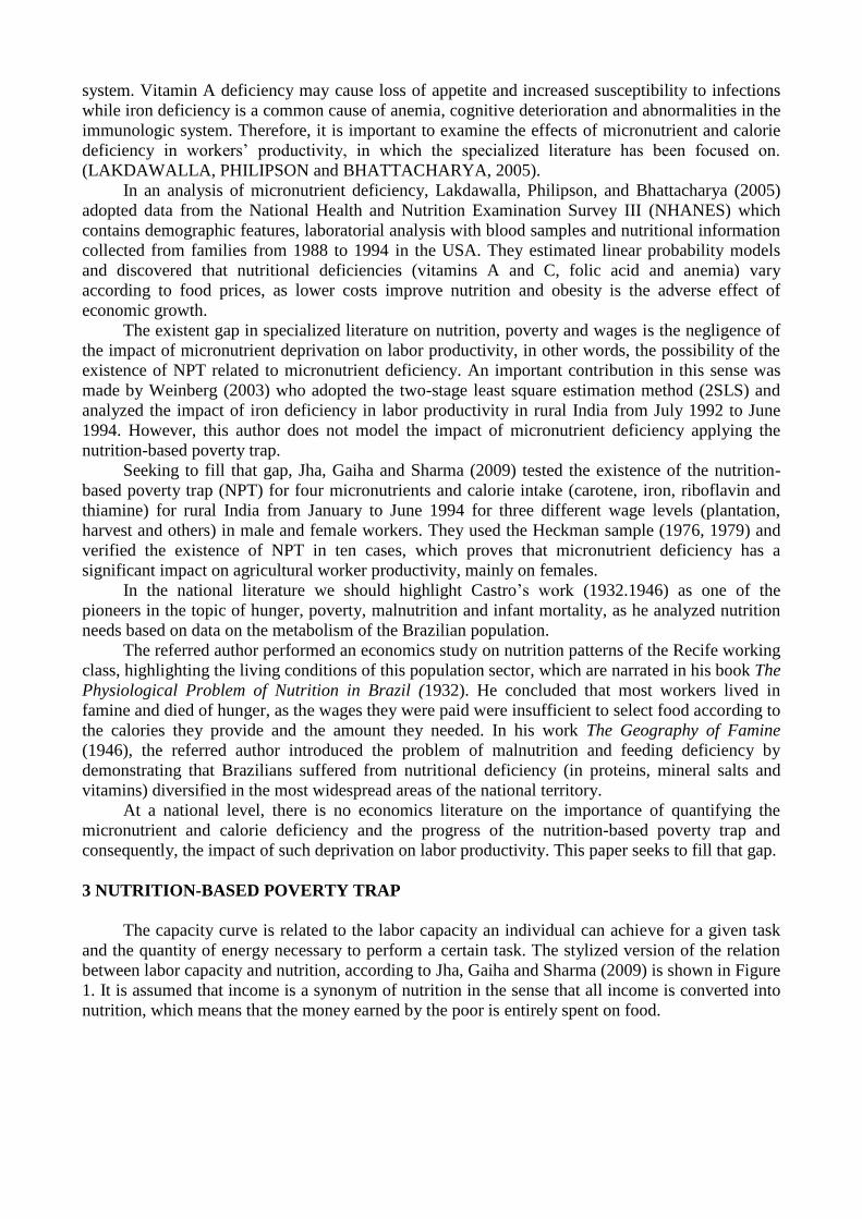
The capacity curve is related to the labor capacity an individual can achieve for a given task

and the quantity of energy necessary to perform a certain task. The stylized version of the relation

between labor capacity and nutrition, according to Jha, Gaiha and Sharma (2009) is shown in Figure

1. It is assumed that income is a synonym of nutrition in the sense that all income is converted into

nutrition, which means that the money earned by the poor is entirely spent on food.

Figure 1- Capacity Curve

Source: Jha, Gaiha and Sharma (2009)

For much lower income levels, all the energy from food intake goes to the resting

metabolism, which is the minimum calorie quantity that the body needs to keep working properly

(breathing, body temperature, etc). According to FAO (Food and Agriculture Organization) data

from 2001, the minimum amount of energy for a Brazilian “reference man” with a weight of 65

kilos would be of 1,900 kcal per person a day. During this stage, little energy is allocated to work,

so the capacity curve in this area is next to zero. When the resting metabolism is filled, the

additional energy is sent to fill the energy required to perform physical work. As from a certain

income level, the labor capacity quickly improves due to the growth in the required energy to

perform work.

When all the human body energy obtained from food intake is satisfied, the capacity to work

increases at decreasing rates, due to the natural limit imposed by the human body. In other words,

for very low income levels, we have the well- known decreasing scale returns factor. The non-linear

graphic represented by a convex and a concave region represents the possibility of the existence of

involuntary unemployment and the consequent persistence of poverty.

The labor market is a mechanism of income and opportunity generation to acquire good

health and nutrition. According to Dadgupta and Ray (1986) the labor market movement can be

affected by a malnutrition problem, as it affects the capacity of the human body to perform tasks

that generate income. Poverty may lead to malnutrition and the latter provokes low productivity.

Consequently, a large part of the population may be prisoner of a poverty trap due to the

malnutrition problem.

4 SELECTION BIAS CORRECTIONS BASED ON MULTINOMIAL LOGIT MODELS

Among the different sample selection modalities, there is one that appears when the dependent

variable is observed solely for a defined population subgroup such as the income variable that is

only noticed in individuals with a strictly positive labor day. In the simplest cases, in which the

observation of the variable of interest is determined by a binary variable, the problem of

endogenous selection may be easily solved through the procedure proposed by Heckman (1979)

which consists of a two-stage regression on the system:

1111 uxy (1a)

01 2222 vxy (1b)

In which (1a) is the equation that explains the variable of interest with regards to a vector of

observable behavior 1x and a disturbance 1u , called structural equation; (1b) is the equation that

explains the binary variable 2y through the observable behavior vector 2x and the non-observable

characteristics 2v , called selection equation; ( 1x , 2x ) are always observable and the variable 1y is

only observed when 12 y .

Labor

Capacity

Income

According to Heckman (1979), consistent estimators for 1 and 1 may be obtained through

the regression of Ordinary Least Squares (OLS) of 1iy on 1ix and 22ˆ,ˆ ix , being the last one

an estimator of 2 obtained through the previous estimation of a probit for (1b), in which is the

inverse Mills ratio such that 22

2222

x

xx

1

,

In more complex models however, the selection takes place through a discrete choice

multinomial process. According to Bourguignon, Fournier and Gurgand (2004), the configuration

problem is as follows:

111 uxy (2a)

,

*

jjj zy , j = 1. 2...., M (2b)

Where disturbances 1u satisfy 0,1 zxuE and 2

1 , zxuV ; j represents a category variable

that describes the agent choice among the M alternatives based on “utilities” *

jy o; vectors z and x

contain the variables that explain alternatives and the variable of interest respectively, without loss

of generality. It is assumed that the variable y1 is observed only if the category 1 is selected, which

happens when *

1

*

1 max jj

yy

. This condition equals to 01 if we define

11

1

*

1

*

11 maxmax

zzyy jj

jj

j. As demonstrated by McFadden (1973) and

assuming that j are independent and identically distributed through the Gumbel distribution, this

specification leads to the multinomial logit model, with the response probability

j jz

zzP

exp

)exp(0 1

1.

Therefore, based on the above equation, consistent estimators for j ’s may be easily

obtained through maximum likelihood. However, the problem continues to be how to estimate the

vector for 1 parameters, considering that disturbances 1u may not be independent from all the j

’s, in such a way that this may introduce some correlation among explanatory variables and the

disturbances term in the equation of interest (2nd

). Consequently, OLS estimators for 1 are

inconsistent.

Generalizing on the Heckman process (1979), Bourguignon, Fournier and Gurgand (2004)

demonstrated that the selection bias correction may be based on the 1u conditional median such that

11

0

1

111

110

,,0 dud

P

ufuuE , where, Mzzz ,...,, 21 and 11 ,uf

is the joint conditional density of 1u and 1 .

They also concluded that as relations among the M components of Γ and the corresponding M

probabilities may be inverted, there is an unique μ function that may be replaced by λ in such a way

that MPPuE ,...,,0 111 .

Thus, consistent estimators for 1 may be obtained through one of the two following

regressions: 11111 ,..., wPPxy M ou 1111 wxy where 1w is the independent

residual of the average regression.

However, as the estimation of a large number of parameters becomes necessary when we have

a vast choice of alternatives, restrictions on MPP ,...,1 or likewise, on λ(Γ), must be imposed in

order to keep the problem within control and it is exactly in that respect that bias correction

methods proposed in literature differ.

1 e are the density function and the normal standard of accumulated distribution function respectively.

In the method proposed by Durbin and Mc Fadden (1984), we accept the hypothesis of

linear disturbances, expressed through the 1u average conditional to j ’s through

Mj

jjjM EruE,...1

11 ,..., com

Mj

jr...1

0 (3)

This means that

Mj

jjM ruE...2

111 ... . Based on this condition and on the

multinomial logit model, Durbin and McFadden (1984) obtained that

11

**

11 ln1

ln,max P

P

PPyyE

j

jj

ssj

, 1j . Consequently, they proposed that the

model described in (2a) and (2b) could be estimated through the OLS by the following equation:

1

...2

1111 ln1

lnwP

P

PPrxy

Mj j

jj

j

(4)

When analyzing such procedure, Bourguignon, Fournier and Gurgand (2004) noticed that the

hypothesis (3) imposed a specific kind of linearity between entre 1u and the Gumbel distributions of

j ’s, thus restricting the distribution types permitted for 1u . They suggested a hypothesis

variation that could turn 1u linear in a set of normal distributions, allowing 1u to be normal with:

Mj

jjM ruE...1

**

11 ... 2 in which *

jr are correlations between 1u and standardized normal

variables jjj GJ 1* , j = 1....M,

3. Considering a sample selection, the authors derived

the following conditional logits: 1

**

1

*

1 ,max PmyyEs

s

and

1,max **

1

*

jjj

ssj PPPmyyE where dvvgPvJPm jj log , j .With this,

they concluded that after the hypothesis alteration, the regression equation (4) could be expressed

as:

1

...2

*

1

*

11111

wP

PPmrPmrxy

j

j

Mj

jj

(5)

According to equation (5), the factors or variables that correct the selection bias are defined

as )( 10 Pmm and )1(

)(1

11

j

jjj

P

PPmm for j=1.2....,M-1 in which *

1r , *2r , *

3r , ..., *Mr are

the respective parameters to be estimated.

By applying Monte-Carlo experiments to compare bias correction methods performances

based on multinomial logit models (MLM), the authors verified that most of the times the method

proposed by Dubin and McFadden (1984) was preferable to both the most commonly used Lee

method (1983), and to the semi-parametric alternative proposed by Dahl (2002). Experiments

showed that the Durbin - McFadden performance model (1984) is fairly sensitive to the imposed

normalization restriction and that the suggested variation, however usually less robust than the

original version, boasts higher performance when the normalization hypothesis is violated. Besides,

it seems to be more capable of capturing intensely non-linear selection terms. Finally, through

2 Please note that (3) is a special case of (4) for jEjjJ and a normalization on the correlations, as Dubin and McFadden

(1984) normalized errors whereas in (4) this normalization does not happen due to a non-linear J transformation.

3 Observe that for each j, Bourguignon et al. (2004) assumed that expected values of u1 and

*j are linearly related, which is

maintained through the classic hypothesis in which 1u is normal and *1, ju is bi-varied normal for any J alternative.

Monte-Carlo simulations, they concluded that the selection bias correction based on the multinomial

logit model provides corrections that are good enough for the selection equation, even when the

independence hypothesis of irrelevant alternatives (IIA) is violated.

5 DATABASE DESCRIPTIONS AND ANALYSIS

The database used was the Family Budget Research (FBR) 2002-2003 and 2008-2009

supplied by IBGE (Brazilian Institute of Geography and Statistics) for all rural Brazil states. From

this database, variables related to the category “family reference person”, who corresponds to the

household head, were obtained. The variable average rainfall was built based on information

provided by INMET (National Meteorology Institute).

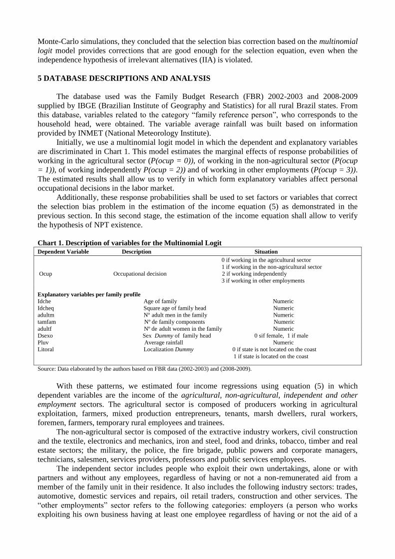
Initially, we use a multinomial logit model in which the dependent and explanatory variables

are discriminated in Chart 1. This model estimates the marginal effects of response probabilities of

working in the agricultural sector (P(ocup = 0)), of working in the non-agricultural sector (P(ocup

= 1)), of working independently P(ocup = 2)) and of working in other employments (P(ocup = 3)).

The estimated results shall allow us to verify in which form explanatory variables affect personal

occupational decisions in the labor market.

Additionally, these response probabilities shall be used to set factors or variables that correct

the selection bias problem in the estimation of the income equation (5) as demonstrated in the

previous section. In this second stage, the estimation of the income equation shall allow to verify

the hypothesis of NPT existence.

Chart 1. Description of variables for the Multinomial Logit

Dependent Variable Description Situation

0 if working in the agricultural sector

1 if working in the non-agricultural sector

Ocup Occupational decision 2 if working independently

3 if working in other employments

Explanatory variables per family profile

Idche Age of family Numeric

Idcheq Square age of family head Numeric

adultm Nº adult men in the family Numeric

tamfam Nº de family components Numeric

adultf Nº de adult women in the family Numeric

Dsexo Sex Dummy of family head 0 sif female, 1 if male

Pluv Average rainfall Numeric

Litoral Localization Dummy 0 if state is not located on the coast

1 if state is located on the coast

Source: Data elaborated by the authors based on FBR data (2002-2003) and (2008-2009).

With these patterns, we estimated four income regressions using equation (5) in which

dependent variables are the income of the agricultural, non-agricultural, independent and other

employment sectors. The agricultural sector is composed of producers working in agricultural

exploitation, farmers, mixed production entrepreneurs, tenants, marsh dwellers, rural workers,

foremen, farmers, temporary rural employees and trainees.

The non-agricultural sector is composed of the extractive industry workers, civil construction

and the textile, electronics and mechanics, iron and steel, food and drinks, tobacco, timber and real

estate sectors; the military, the police, the fire brigade, public powers and corporate managers,

technicians, salesmen, services providers, professors and public services employees.

The independent sector includes people who exploit their own undertakings, alone or with

partners and without any employees, regardless of having or not a non-remunerated aid from a

member of the family unit in their residence. It also includes the following industry sectors: trades,

automotive, domestic services and repairs, oil retail traders, construction and other services. The

“other employments” sector refers to the following categories: employers (a person who works

exploiting his own business having at least one employee regardless of having or not the aid of a

non-remunerated worker from the family unit where he resides) and workers producing for their

own consumption.

Besides the factors that correct the selection bias, the other explanatory variables used in the

equation estimation (5) are described in Chart 2.

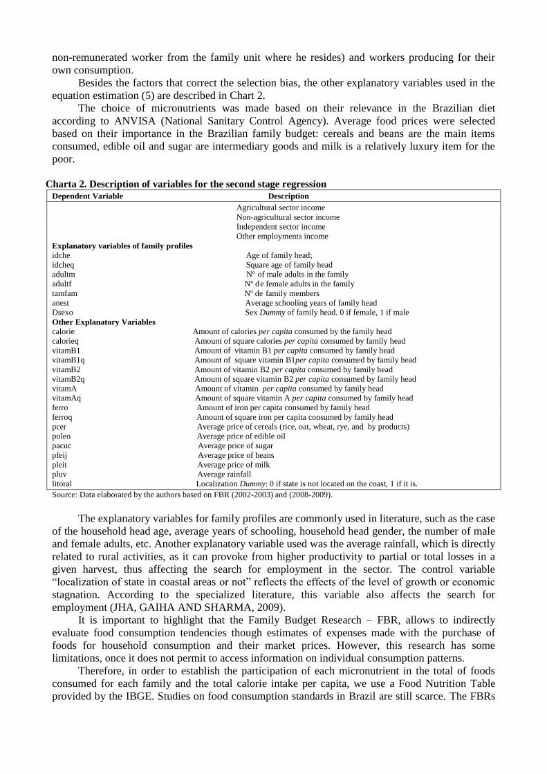
The choice of micronutrients was made based on their relevance in the Brazilian diet

according to ANVISA (National Sanitary Control Agency). Average food prices were selected

based on their importance in the Brazilian family budget: cereals and beans are the main items

consumed, edible oil and sugar are intermediary goods and milk is a relatively luxury item for the

poor.

Charta 2. Description of variables for the second stage regression

Dependent Variable Description

Agricultural sector income

Non-agricultural sector income

Independent sector income

Other employments income

Explanatory variables of family profiles idche Age of family head;

idcheq Square age of family head

adultm Nº of male adults in the family

adultf Nº de female adults in the family

tamfam Nº de family members

anest Average schooling years of family head

Dsexo Sex Dummy of family head. 0 if female, 1 if male

Other Explanatory Variables

calorie Amount of calories per capita consumed by the family head

calorieq Amount of square calories per capita consumed by family head

vitamB1 Amount of vitamin B1 per capita consumed by family head

vitamB1q Amount of square vitamin B1per capita consumed by family head

vitamB2 Amount of vitamin B2 per capita consumed by family head

vitamB2q Amount of square vitamin B2 per capita consumed by family head

vitamA Amount of vitamin per capita consumed by family head

vitamAq Amount of square vitamin A per capita consumed by family head

ferro Amount of iron per capita consumed by family head

ferroq Amount of square iron per capita consumed by family head

pcer Average price of cereals (rice, oat, wheat, rye, and by products)

poleo Average price of edible oil

pacuc Average price of sugar

pfeij Average price of beans

pleit Average price of milk

pluv Average rainfall

litoral Localization Dummy: 0 if state is not located on the coast, 1 if it is.

Source: Data elaborated by the authors based on FBR (2002-2003) and (2008-2009).

The explanatory variables for family profiles are commonly used in literature, such as the case

of the household head age, average years of schooling, household head gender, the number of male

and female adults, etc. Another explanatory variable used was the average rainfall, which is directly

related to rural activities, as it can provoke from higher productivity to partial or total losses in a

given harvest, thus affecting the search for employment in the sector. The control variable

“localization of state in coastal areas or not” reflects the effects of the level of growth or economic

stagnation. According to the specialized literature, this variable also affects the search for

employment (JHA, GAIHA AND SHARMA, 2009).

It is important to highlight that the Family Budget Research – FBR, allows to indirectly

evaluate food consumption tendencies though estimates of expenses made with the purchase of

foods for household consumption and their market prices. However, this research has some

limitations, once it does not permit to access information on individual consumption patterns.

Therefore, in order to establish the participation of each micronutrient in the total of foods

consumed for each family and the total calorie intake per capita, we use a Food Nutrition Table

provided by the IBGE. Studies on food consumption standards in Brazil are still scarce. The FBRs

of 2002-2003 and 2008-2009 are the only nationwide ones that include urban areas (Brazilian states

and greater regions) and rural areas (Brazil and greater regions) available in the country.

6 RESULTS ANALYSIS

6.1 Results for Brazil using the FBR 2002-2003

6.1.1 Multinomial logit results:

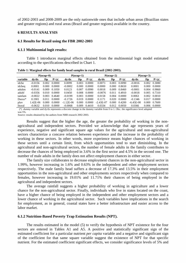
Table 1 introduces marginal effects obtained from the multinomial logit model estimated

according to the specifications described in Chart 1.

Table 1: Marginal effects for family head samples in rural Brazil (2002-2003).

(*) dummy variable and dy/dx represents a discrete change in the dummy variable from 0 to 1. Obs.: the significance level adopted

was 5%. Source: results obtained by the authors from NBR research 2002-2003.

Results suggest that the higher the age, the greater the probability of working in the non-

agricultural and independent sectors. Provided we acknowledge that age represents years of

experience, negative and significant square age values for the agricultural and non-agricultural

sectors characterize a concave relation between experience and the increase in the probability of

working in these sectors. In other words, more experience means higher chances of working in

these sectors until a certain limit, from which opportunities tend to start diminishing. In the

agricultural and non-agricultural sectors, the number of female adults in the family contributes to

decrease the chances of being employed in 3.6% in the first sector and 4.5% in the second one. The

number of male adults in the family does not affect employment chances in either sector.

The family size collaborates to decrease employment chances in the non-agricultural sector in

1.99%, however increasing in 1.6% and 0.63% in the independent and other employment sectors

respectively. The male family head suffers a decrease of 17.3% and 13.5% in their employment

opportunities in the non-agricultural and other employments sectors respectively when compared to

females, however increasing in 19.01% and 11.71% their chances of being employed in the

agricultural and independent sectors.

The average rainfall suggests a higher probability of working in agriculture and a lower

chance for the non-agricultural sector. Finally, individuals who live in states located on the coast,

have a higher chance of being employed in the independent and other employment sectors and a

lower chance of working in the agricultural sector. Such variables have implications in the search

for employment, as in general, coastal states have a better infrastructure and easier access to the

labor market.

6.1.2 Nutrition-Based Poverty Trap Estimation Results (NPT).

The results estimated in the model (5) to verify the hypothesis of NPT existence for the four

sectors are entered in Tables A1 and A5. A positive and statistically significant sign of the

estimated coefficient for a particular nutrient per capita variable and a negative and significant sign

of the coefficient for that same square variable suggest the existence of NPT for that specific

nutrient. For the estimated coefficient significant effects, we consider significance levels of 5% and

P(ocup=0) P(ocup=1) P(ocup=2) P(ocup=3)

variable dy/dx Dp P>|z| dy/dx Dp P>|z| dy/dx Dp P>|z| dy/dx Dp P>|z|

idche -0.0156 0.002 0.0000 0.0099 0.003 0.0000 0.0073 0.003 0.0090 -0.0016 0.002 0.3080

idcheq 0.0001 0.000 0.0000 -0.0002 0.000 0.0000 0.0000 0.000 0.8650 0.0001 0.000 0.0000

adultm -0.0141 0.009 0.1050 0.0123 0.007 0.0990 0.0018 0.009 0.8460 -0.0001 0.004 0.9860

adultf -0.0356 0.010 0.0000 0.0450 0.008 0.0000 -0.0076 0.011 0.4910 -0.0018 0.005 0.7310

tamfam -0.0022 0.003 0.4640 -0.0199 0.003 0.0000 0.0158 0.004 0.0000 0.0063 0.002 0.0010

Dsexo* 0.1901 0.011 0.0000 -0.1726 0.019 0.0000 0.1171 0.020 0.0000 -0.1346 0.017 0.0000

pluv 1.42E-06 0.000 0.0000 -1.12E-06 0.000 0.0000 -2.43E-07 0.000 0.4200 -6.45E-08 0.000 0.7600

litoral -0.0632 0.010 0.0000 -0.0068 0.009 0.4410 0.0334 0.012 0.0050 0.0366 0.006 0.0000

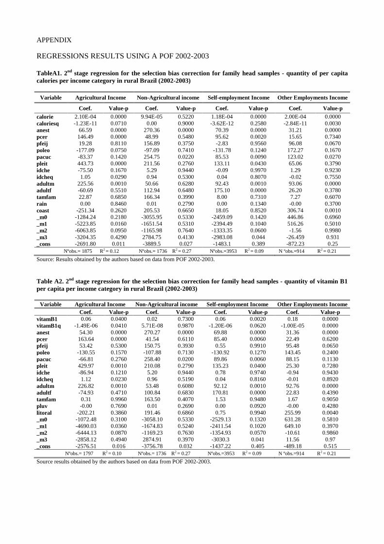
10%. In rural Brazil, according to Table A1, we observe the phenomenon of nutrition-based poverty

trap for the case of calories in the agricultural, independent and other employment categories.

According to data provided in Tables A2 and A3, we perceive that the nutrition-based poverty trap

phenomenon is present for vitamins B1 and B2 in the agricultural, independent and other

employment sectors, as the coefficients for these variables were positive and statistically significant.

In table A4 we verify that workers in the non-agricultural, independent and other employments

sectors are subject to the poverty trap with regards to vitamin A. As for nutrient iron, we can see

that Table 5 shows that the agricultural, independent and other employments sectors are also subject

to the poverty trap.

With regards to the other determinants, the estimated coefficient for the variable of average

years of schooling was positive and significant in all regressions. This is a standard result observed

in most empirical studies that correlate income and education. The coefficients for the price of sugar

and oil obtained a negative and significant result for the regressions of vitamin B2 and iron

(agricultural sector in Tables A3 and A5). As for the calorie regressions (agricultural sector in Table

A1) the oil coefficient presented the same result. Nutritional deficiencies vary with food prices, as

lower prices improve nutrition. For the other regressions, the price variable expressed a result that

contradicted expectations.

The family profile variables, such as the number of male adults, showed a positive and

significant result for the regressions of calories, vitamin B1, B2 and A and iron for the agricultural,

independent and other employment categories, as shown in Tables A, A2, A3, A4 and A5

respectively. Results entered in Tables A1, A5, A2 and A4 suggest that the female adult variable

boasted positive and significant results for the regressions of calories, iron and vitamins B1 and A

for the independent sector and for vitamin B2 in the agricultural sector (Table A3). This means that

a higher number of adults in the family working in these sectors will result in higher income for

household heads. The family head age exerted a negative effect on income for the agricultural

sector and this square variable had a positive impact on vitamin B2 regressions (agricultural sector,

Table A3). This seems to suggest that workers in their initial stage of their labor lives earn less than

after they reach a certain age and achieve some work experience.

The estimated coefficient for the coastal area variable was positive and significant in the

regressions for calories, vitamins B1, B2 and A for the other employments category, as

demonstrated by results shown on Tables A1, A2, A3 and A4. However, results from tables A3 and

A5 show that the variable localization presented a negative and significant coefficient for the

Vitamin B2 and iron regressions in the agricultural sector. This proves that agricultural workers

located in coastal states tend to earn lower wages than workers in the other employments sector,

possibly due to the fact that coastal states are more dynamic in economic terms. The average

rainfall variable did not show any statistical significance for the agricultural sector in any of the

analyzed regressions. In most of the studied regressions, some of the estimated coefficients for the

variables m0, m1, m2 and m3 were statistically significant, thus showing that the selections bias

correction was really necessary.

6.2 Results for Brazil using the FBR 2008-2009

6.2.1 Multinomial Logit model Results

Table 2 below shows the marginal effects obtained through the multinomial logit model

estimated according to the specifications described in Chart 1.

Table 2: marginal effects for family head samples in rural Brazil (2008-2009).

(*) Dummy variable and dy/dx represents a discrete change in the dummy variable from 0 to 1. Obs.: the significance level adopted was 5%,.

Source: results obtained by the authors based on data from POF 2008-2009.

According to the results entered in this table, in the agricultural sector, as an individual gets

older, employment chances diminish. In this sector, age reduces employment opportunities in

1.05%. This shows that the older the age, the lower the chance to work in the farming sector,

perhaps because agricultural activities demand more physical effort. This same result is not verified

in other sectors. Still, in this area, the number of male adults in the family contributes to the chance

of being employed in 6.75%. On the other hand, the number of female adults in the family

contributes to reducing employment opportunities in 4.92% and 7.96% for the independent sector.

This shows that female labor is associated to activities that demand less physical effort. On the

other hand, in the non-agricultural sector the possibility for women to be employed growths in

12.55%.

The family size variable negatively affects employment chances in the non-agricultural sector

in 3.49%, however increasing 3.13% in the independent sector. If compared to the female

household head, the male head suffers a reduction of 11.06% in his chances to be employed in the

non-farming sector and an increase of 6.99% in the farming sector. The average rainfall suggests a

higher chance of working in agriculture and a lower chance of working in the non-agricultural and

other employments categories. The coastal variable demonstrates that individuals located in coastal

states have a lower probability of being employed in the farming sector, once coastal states in Brazil

have a more developed economic infrastructure.

6.2.2 Nutrition-based Poverty Trap (NPT) Estimation Results

According to the results obtained from Tables A6 to A10, only the non-agricultural sector is

subject to the poverty trap with regards to calories. In this same sector, the poverty trap is also

verified for the the iron micronutrient, according to results entered in Table A10. Analyzing results

from Table A7, we corroborate that the poverty trap is present in the non-agricultural and

independent sectors with regards to the vitamin B1 nutrient as well. In the farming sector, we

noticed the poverty trap phenomenon for the vitamin B2 and iron nutrients, as shown in Table A8

and A10 respectively. Table A9 shows that workers in other employments are subject to the poverty

trap related to a vitamin A deficiency. As for the other determinants, again, the average schooling

years was positively correlated to income in all regressions and the average rainfall did not present

any statistical significance in any of the studied sectors through all analyzed regressions. The price

of oil showed a negative and significant result for the regressions of calories, iron, and vitamins B1

and A (independent sector, Table A8). The number of female adults in the family presented a

positive and significant coefficient for the vitamin B2 regression in the agricultural sector, as

expressed by the results in Table A8. Some estimated coefficients of variables 0, m1, m2 and m3

were statistically significant in several regressions, thus suggesting the need to correct the selection

bias.

P(ocup=0) P(ocup=1) P(ocup=2) P(ocup=3)

variable dy/dx Dp P>|z| dy/dx Dp P>|z| dy/dx Dp P>|z| dy/dx Dp P>|z|

Idche -0.0105 0.004 0.0090 0.0029 0.004 0.4860 0.0058 0.004 0.1420 0.0018 0.002 0.24000

Idcheq 0.0001 0.000 0.1570 -7.90E-05 0.000 0.0670 0.0000 0.000 0.7820 8.32E-06 0.000 0.54900

Adultm 0.0675 0.015 0.0000 0.0171 0.016 0.2810 -0.0655 0.016 0.0000 -0.0192 0.007 0.00400

Adultf -0.0492 0.019 0.0080 0.1255 0.019 0.0000 -0.0796 0.020 0.0000 0.0033 0.007 0.61100

tamfam 0.0036 0.007 0.6220 -0.0349 0.008 0.0000 0.0313 0.008 0.0000 0.0001 0.003 0.98600

Dsexo* 0.0699 0.028 0.0130 -0.1106 0.031 0.0000 0.0478 0.029 0.0950 -0.0072 0.012 0.53500

Pluv 1.83E-06 0.000 0.0010 -4.27E-07 0.000 0.4610 -6.22E-07 0.000 0.2620 -7.80E-07 0.000 0.00400

litoral -0.0571 0.021 0.0070 0.0308 0.021 0.1480 0.0174 0.022 0.4250 0.0089 0.009 0.29600

6.3 Summary of Results for the Nutrition-based Poverty Trap

Table 3: Nutritional Poverty Trap for family head samples in rural Brazil

Source: results obtained by the authors based on date provided by POFs 2002-2003 and 2008-2009.

For rural Brazil, in the 2002-2003 period, the existence of NPT was verified for calories, iron

and vitamins B1, B2 and A for workers in the independent and other employments categories.

Employees of the agricultural sector obtained the same result, except for vitamin A. Workers in the

non-agricultural sector are subject to the poverty trap only with regards to vitamin A. In the period

from 2008 to 2009, NPT was proved for workers in the agricultural sector but only for iron and

vitamin 2. Non-agricultural sector workers suffered the poverty trap for calories, vitamin B1 and

iron. Self-employed workers suffered NPT related to vitamin B and workers in other employments

did not suffer from NPT for calories or the other analyzed nutrients.

7 FINAL CONSIDERATIONS

The main goal of this study was to verify the existence of the nutrition-based poverty trap

(NPT) analyzing the effects of micronutrient intake (calories, iron and vitamins A, B1 and B2) on

income in rural Brazil, correcting the problem of endogeneity between these variables. Although

micronutrient deficiencies still persist as a public health problem in Brazil, it is worth highlighting

that there has been an NPT reduction in the studied period for most workers in the analyzed sectors,

except for non-agricultural employees. The improvement in food consumption patterns in the

Brazilian population is probably originated in the economic and social transformations that resulted

in a reduction of poverty and malnutrition. Such facts suggest that the increase in family income

among the poorest and the reduction of essential food prices would be effective ways to increase the

intake of key nutrients in the diet of Brazilian families. These results agree with economics

literature, which highlights that nutritional policies are essential for the reduction of extreme

poverty and the acceleration of economic growth, as specialized economy and nutrition studies

remark that healthy workers in better nutritional state are more productive at work.

Besides these public policies, it is worth mentioning the National Policy for Nutrition and

Feeding, approved in 1999 by the Ministry of Health, which has as its main objective the promotion

of food and nutrition safety for the Brazilian population. The Ministry of Health, Nutrition and

Public Health Programs that seeks to reduce micronutrient deficiencies in the Brazilian population

include vitamin A supplements, as well as ferrous sulphate for risk groups (babies, children and

pregnant women); the fortification of foods such as wheat flower and corn with iron and folic acid

and the addition of salt iodide for human consumption, as regulated by the National Agency of

Sanitary Control (Anvisa) through the Fome Zero Project and the program to reduce iron deficiency

anemia in Brazil, signed together with the food industry.

With regards to the explanatory variables that affect the occupational decision of agents in the

labor market, we can infer that the older the age, the higher the probability of working outside the

agricultural sector and in self-employment. This evidence confirms the traditional literature

argument that older people have more difficulty getting jobs. Education measured through years of

schooling strongly contributes to the increase in income in the four sectors analyzed: agricultural,

non-agricultural, independent and other employments.

In this context, we remark the need for long-term national public policies that consider

nutritional aspects and involve multiple initiatives such as raising more awareness among the target

Micronutrients and calories

Sectors 2002-2003 2008-2009

Agricultural Calories, vitamins B1 and B2, iron Iron and vitamin B2

Non-agricultural Vitamin A Calories, vitamin B1 and iron

Independent Calories, vitamins B1, B2 and A, iron Vitamin B1

Other Employments Calories, vitamins B, B2 and A, iron ----

populations, the regularity of food intake research, employment and income policies focused on the

low-end income sector, reduction of food prices and support to the food farming industry and

nutritional education initiatives.

We can therefore highlight the relevance of this study in the sense of offering a contribution

to the economics and nutrition literature by quantifying the micronutrient and calorie deficiency in

the progress of the nutrition-based poverty trap, and as a consequence, the impact of such

deprivation in labor productivity, which emphasizes the importance of nutritional policies aimed at

breaking this trap and reducing poverty in the rural areas of Brazil.

8 BIBLIOGRAPHIC REFERENCES

AHMED, A. U., HILL, R. V., SMITH, L. C., WIESMANN, D. M., & FRANKENBERGER, T.

(2007). The world’s most deprived: Characteristics and causes of extreme poverty and hunger.

Discussion Paper prepared for the Forum A 2020 Vision for Food, Agriculture, and the

Environment, 43.

BARRETT, C. (2002). Food security and food assistance programs, In B. GARDNER, & G.

RAUSSER, (Eds,), Handbook of agricultural economics, 2103–2190. Amsterdam: Elsevier

Science.

BOURGUIGNON, F., FOURNIER, M., & GURGAND, M. (2007). Selection bias corrections

based on the the multinomial logit model: Monte-Carlo comparisons. Journal of Economic

Surveys, 21, 174-205.

CASTRO, J. de. (1932).O Problema Fisiológico da Alimentação no Brasil. Editora Imprensa

Industrial, Recife.

CASTRO, J. de. (1946). A geografia da fome. A fome no Brasil. Rio de Janeiro, Empresa Gráfica O

Cruzeiro.

DAHL,G. B. (2002). "Mobility and the Returns to Education: Testing a Roy Model with Multiple

Markets". Econometrica, 70, 2367-2420.

DASGUPTA, P.; RAY, D. (1986). Inequality as a determinant of malnutrition and unemployment:

Theory. Economic Journal, 96(384), 1011–1034.

DEOLALIKAR, A. (1988). Nutrition and labour productivity in agriculture: Estimates for rural

south India. Review of Economics and Statistics, 70, 406–413.

DURBIN, J. A; MCFADDEN, D. L. (1984). An Econometric Analysis of Residential Electric

Appliance Holdings and Consumption. Econometrica, 52(2), 345-362.

FAO – Food and Agriculture Organization of the United Nations. (2001). Food Insecurity; when

People Live with Hunger and Fear Starvation. Rome.

HADDAD, L., & BOUIS, H. (1991).The Impact of nutritional status on agricultural productivity:

Wage evidence from the Philippines. Oxford Bulletin of Economics and Statistics, 53(1), 45-68.

HECKMAN, J. (1976). The common structure of statistical models of truncation, sample selection,

and limited dependent variables and a simple estimator for such models. Annals of Economic and

Social Measurement, 5, 475–492.

HECKMAN, J. (1979). Sample selection bias as a specification error. Econometrica, 47, 153-161.

HORTON, S., & ROSS, J. (2003). The economics of iron deficiency. Food Policy, 28, 51–75.

JHA, R., GAIHA, R., & SHARMA, A. (2009). Calorie and micronutrient deprivation and poverty

nutrition traps in rural India. World Development, 37(5), 982-991.

LAKDAWALLA, D., PHILIPSON, T., & BHATTACHARYA, J. (2005). Welfare enhancing

technological change and the growth of obesity. American Economic Review, 95, 253–257.

LEE, L. F. (1983). "Generalized Econometric Models with Selectivity". Econometrica, 51, 507-

512.

LEIBENSTEIN, H. (1957). Economic backwardness and economic growth: Studies in the theory of

economic development. New York: Wiley & Sons.

LORCH, A. (2001). Is this the way to solve malnutrition? Biotechnology and Development

Monitor, 44, 18–22.

LUKASKI, H. (2004). Vitamin and mineral status: Effects on physical performance, Nutrition, 20,

632–644.

MCFADDEN, D. (1973). Conditional logit analysis of qualitative choice behavior, In:

ZAREMBKA, P, (ed,), Frontiers of Econometrics, 105-142. New York: Academic Press.

MIRRLEES, J. (1975). A pure theory of underdeveloped economies. In L. Reynolds (Ed.),

Agriculture in development theory, p. 84–108. New Haven: Yale University Press.

STAMOULIS, K., PINGALI, P., & SHETTY, P. (2004). Emerging challenges for food and

nutrition policy in developing countries. Electronic Journal of Agricultural and Development

Economics, 1,154–167.

STIGLITZ, J. E. (1976). The efficiency wage hypothesis, surplus labour and the distribution of

income in LDCs. Oxford Economic Papers, New Series, 28(2), 185-207.

STRAUSS, J, (1986). Does better nutrition raise farm productivity? Journal of Political Economy,

94, 297–320.

SWAMY, A. (1997). A simple test of the nutrition-based efficiency wage model. Journal of

Development Economics, 53, 85–98.

THOMAS, D., & STRAUSS, J. (1997) Health and wages: Evidence on men and women in urban

Brazil. Journal of Econometrics, 77, 159–185.

WEINBERGER, K. (2003). The impact of micronutrients on labour productivity: Evidence from

rural India. Paper presented at the 25th international conference of agricultural economists, 16

August, 16-22. Durban, South Africa.

WORLD BANK. (2006). Repositioning nutrition as central to development: A strategy for large-

scale action. Washington DC.

WORLD HEALTH ORGANIZATION. (2001). Macroeconomics and health: Investing in health for

economic development. Report of the commission on Macroeconomics and Health, Geneva.

APPENDIX

REGRESSIONS RESULTS USING A POF 2002-2003

TableA1. 2

nd stage regression for the selection bias correction for family head samples - quantity of per capita

calories per income category in rural Brazil (2002-2003)

Variable Agricultural Income Non-Agricultural income Self-employment Income Other Employments Income

Coef. Value-p Coef. Value-p Coef. Value-p Coef. Value-p

calorie 2.10E-04 0.0000 9.94E-05 0.5220 1.18E-04 0.0000 2.00E-04 0.0000

caloriesq -1.23E-11 0.0710 0.00 0.9000 -3.62E-12 0.2580 -2.84E-11 0.0030

anest 66.59 0.0000 270.36 0.0000 70.39 0.0000 31.21 0.0000

pcer 146.49 0.0000 48.99 0.5480 95.62 0.0020 15.65 0.7340

pfeij 19.28 0.8110 156.89 0.3750 -2.83 0.9560 96.08 0.0670

poleo -177.09 0.0750 -97.09 0.7410 -131.78 0.1240 172.27 0.1670

pacuc -83.37 0.1420 254.75 0.0220 85.53 0.0090 123.02 0.0270

pleit 443.73 0.0000 211.56 0.2760 133.11 0.0430 65.06 0.3790

idche -75.50 0.1670 5.29 0.9440 -0.09 0.9970 1.29 0.9230

idcheq 1.05 0.0290 0.94 0.5300 0.04 0.8070 -0.02 0.7550

adultm 225.56 0.0010 50.66 0.6280 92.43 0.0010 93.06 0.0000

adultf -60.69 0.5510 112.94 0.6480 175.10 0.0000 26.20 0.3780

tamfam 22.87 0.6850 166.34 0.3990 8.00 0.7310 7.27 0.6070

rain 0.00 0.8460 0.01 0.2790 0.00 0.1340 -0.00 0.3700

coast -251.34 0.2620 205.53 0.6650 18.05 0.8520 306.74 0.0010

_m0 -1284.24 0.2180 -3055.95 0.5330 -2459.09 0.1420 446.86 0.6960

_m1 -5223.85 0.0160 -1651.54 0.5310 -2394.49 0.1040 516.26 0.5010

_m2 -6063.85 0.0950 -1165.98 0.7640 -1333.35 0.0600 -1.56 0.9980

_m3 -3204.35 0.4290 2784.75 0.4130 -2983.08 0.044 -26.459 0.931

_cons -2691.80 0.011 -3889.5 0.027 -1483.1 0.389 -872.23 0.25

Nºobs.= 1875 R2 = 0.12 Nºobs.= 1736 R2 = 0.27 Nºobs.=3953 R2 = 0.09 N ºobs.=914 R2 = 0.21

Source: Results obtained by the authors based on data from POF 2002-2003.

Table A2. 2nd

stage regression for the selection bias correction for family head samples - quantity of vitamin B1

per capita per income category in rural Brazil (2002-2003)



vitamB1 0.06 0.0400 0.02 0.7300 0.06 0.0020 0.18 0.0000

vitamB1q -1.49E-06 0.0410 5.71E-08 0.9870 -1.20E-06 0.0620 -1.00E-05 0.0000

anest 54.30 0.0000 270.27 0.0000 69.88 0.0000 31.36 0.0000

pcer 163.64 0.0000 41.54 0.6110 85.40 0.0060 22.49 0.6200

pfeij 53.42 0.5300 150.75 0.3930 0.55 0.9910 95.48 0.0650

poleo -130.55 0.1570 -107.88 0.7130 -130.92 0.1270 143.45 0.2400

pacuc -66.81 0.2760 258.40 0.0200 89.86 0.0060 88.15 0.1130

pleit 429.97 0.0010 210.08 0.2790 135.23 0.0400 25.30 0.7280

idche -86.94 0.1210 5.20 0.9440 0.78 0.9740 -0.94 0.9430

idcheq 1.12 0.0230 0.96 0.5190 0.04 0.8160 -0.01 0.8920

adultm 226.82 0.0010 53.48 0.6080 92.12 0.0010 92.76 0.0000

adultf -74.93 0.4710 100.84 0.6830 170.81 0.0000 22.83 0.4390

tamfam 0.31 0.9960 163.50 0.4070 1.53 0.9480 1.67 0.9050

pluv -0.00 0.7690 0.01 0.2690 0.00 0.0920 -0.00 0.4280

litoral -202.21 0.3860 191.46 0.6860 0.75 0.9940 255.99 0.0040

_m0 -1072.48 0.3100 -3058.10 0.5330 -2529.13 0.1320 631.28 0.5810

_m1 -4690.03 0.0360 -1674.83 0.5240 -2411.54 0.1020 649.10 0.3970

_m2 -6444.13 0.0870 -1169.23 0.7630 -1354.93 0.0570 -10.61 0.9860

_m3 -2858.12 0.4940 2874.91 0.3970 -3030.3 0.041 11.56 0.97

_cons -2576.51 0.016 -3756.78 0.032 -1437.22 0.405 -489.18 0.515

Nºobs.= 1797 R2 = 0.10 Nºobs.= 1736 R2 = 0.27 Nºobs.=3953 R2 = 0.09 N ºobs.=914 R2 = 0.21

Source results obtained by the authors based on data from POF 2002-2003.

Table A3. 2nd

stage regression for the selection bias correction for family head samples - quantity of B2 vitamin




vitamB2 0.09 0.0010 0.06 0.4510 0.10 0.0000 0.21 0.0000

vitamB2q -3.12e-06 0.0030 0.00 0.7340 -3.21E-06 0.0020 -1.49E-05 0.0000

anest 64.90 0.0000 269.63 0.0000 68.70 0.0000 30.31 0.0000

pcer 155.21 0.0000 40.34 0.6210 86.87 0.0050 21.75 0.6340

pfeij 26.86 0.7290 150.81 0.3930 11.59 0.8200 92.97 0.0740

poleo -213.90 0.0300 -105.58 0.7190 -129.87 0.1290 150.49 0.2230

pacuc -114.79 0.0340 257.79 0.0210 77.07 0.0190 89.02 0.1120

pleit 425.58 0.0000 212.69 0.2730 135.03 0.0400 41.84 0.5670

idche -109.68 0.0250 4.83 0.9480 0.18 0.9940 0.93 0.9440

idcheq 1.30 0.0050 0.96 0.5220 0.04 0.8130 -0.02 0.7680

adultm 210.71 0.0010 53.62 0.6070 92.80 0.0010 95.27 0.0000

adultf -74.42 0.4530 102.10 0.6790 170.80 0.0000 13.11 0.6580

tamfam -11.63 0.8160 163.78 0.4050 4.22 0.8560 4.99 0.7210

pluv 0.00 0.9980 0.01 0.2660 0.00 0.0880 -0.00 0.5610

litoral -391.75 0.0340 190.09 0.6880 6.12 0.9500 262.89 0.0040

_m0 -996.43 0.3250 -3028.17 0.5360 -2607.64 0.1200 510.04 0.6550

_m1 -5209.94 0.0110 -1665.75 0.5260 -2458.08 0.0960 557.44 0.4660

_m2 -7895.39 0.0090 -1209.39 0.7550 -1395.10 0.0500 38.57 0.9480

_m3 -3391.20 0.3500 2851.02 0.4010 -3148.04 0.034 -26.621 0.931

_cons -2435.29 0.012 -3778.22 0.031 -1484.81 0.388 -585.07 0.437 Nºobs.= 1916 R2 = 0.12 Nºobs.= 1736 R2 = 0.27 Nºobs.=3953 R2 = 0.09 N obs.=914 R2 = 0.20


Table A4. 2nd

stage regression for the selection bias correction for family head samples - quantity of vitamin A




vitamA 4.68E-05 0.5290 7.93E-04 0.0440 4.25E-04 0.0000 0.0004 0.0000

vitamAq -1.32E-12 0.5290 -2.33E-10 0.0660 -3.64E-11 0.0000 -7.96E-11 0.0010

anest 59.86 0.0000 267.35 0.0000 68.62 0.0000 31.5568 0.0000

pcer 125.66 0.0010 50.22 0.5370 92.49 0.0030 10.3883 0.8220

pfeij 18.58 0.8310 151.39 0.3900 -8.03 0.8740 93.5672 0.0760

poleo -164.75 0.0790 -98.72 0.7360 -128.76 0.1320 173.4329 0.1650

pacuc -32.23 0.5960 252.44 0.0230 94.07 0.0040 127.0358 0.0230

pleit 439.78 0.0010 218.17 0.2600 155.30 0.0180 71.5468 0.3310

idche -65.13 0.2430 8.96 0.9040 3.17 0.8960 5.1568 0.7000

idcheq 0.94 0.0520 0.83 0.5770 0.03 0.8830 -0.0539 0.5260

adultm 245.63 0.0000 50.17 0.6290 98.97 0.0000 97.7041 0.0000

adultf -69.88 0.4880 110.49 0.6530 171.76 0.0000 19.6510 0.5110

tamfam 3.23 0.9550 152.32 0.4370 3.51 0.8810 -0.2206 0.9870

pluv 0.00 0.8940 0.01 0.2880 0.00 0.0600 -0.0016 0.4570

litoral -238.72 0.2980 168.34 0.7210 12.73 0.8960 308.3382 0.0010

_m0 -1297.57 0.2130 -2607.94 0.5920 -2817.13 0.0960 397.1644 0.7310

_m1 -4955.01 0.0260 -1412.65 0.5900 -2566.24 0.0840 565.2173 0.4640

_m2 -5836.78 0.1190 -1184.37 0.7580 -1372.77 0.0560 163.7285 0.7820

_m3 -3428.90 0.4000 2822.62 0.4020 -3240.95 0.03 -34.93929 0.91

_cons -2609.35 0.014 -3838.37 0.027 -1746.82 0.314 -787.88 0.301

Nºobs.= 1807 R2 = 0.09 Nºobs.= 1736 R2 = 0.26 Nº obs.=3953 R2 = 0.09 Nºobs.=914 R2 = 0.19

Source: results obtained by the authors based on data from POF 2002-2003. .

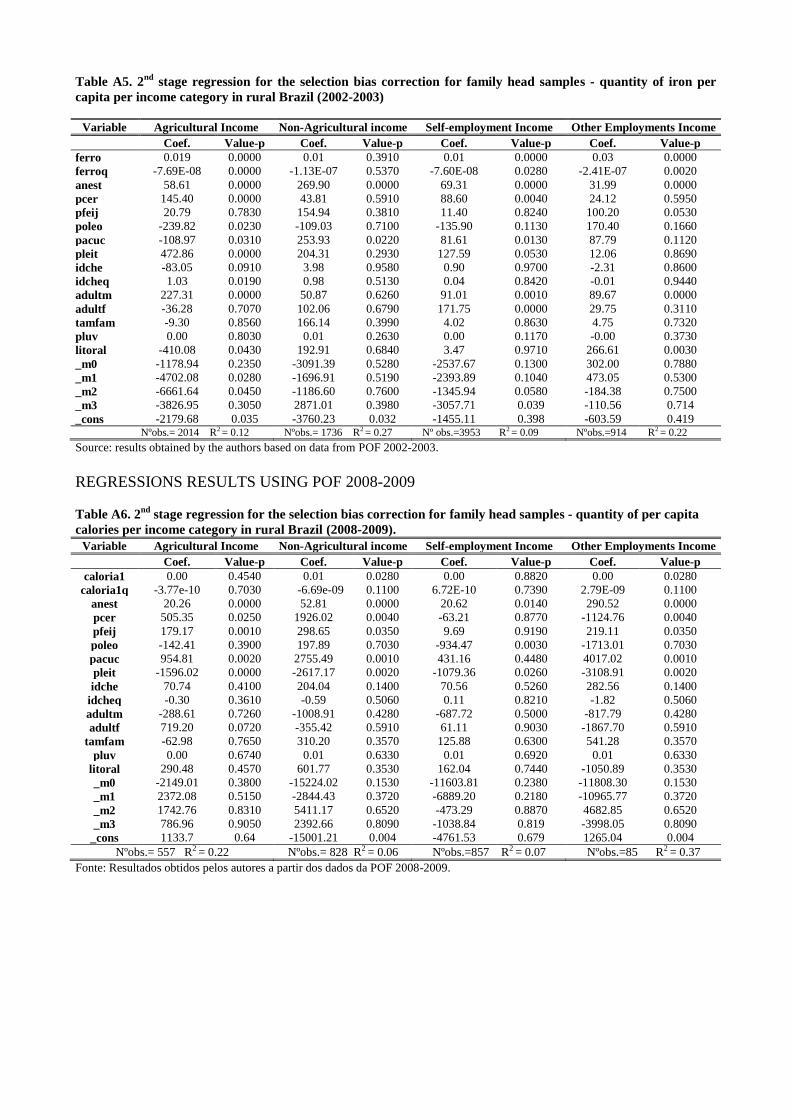
Table A5. 2nd

stage regression for the selection bias correction for family head samples - quantity of iron per

capita per income category in rural Brazil (2002-2003)



ferro 0.019 0.0000 0.01 0.3910 0.01 0.0000 0.03 0.0000

ferroq -7.69E-08 0.0000 -1.13E-07 0.5370 -7.60E-08 0.0280 -2.41E-07 0.0020

anest 58.61 0.0000 269.90 0.0000 69.31 0.0000 31.99 0.0000

pcer 145.40 0.0000 43.81 0.5910 88.60 0.0040 24.12 0.5950

pfeij 20.79 0.7830 154.94 0.3810 11.40 0.8240 100.20 0.0530

poleo -239.82 0.0230 -109.03 0.7100 -135.90 0.1130 170.40 0.1660

pacuc -108.97 0.0310 253.93 0.0220 81.61 0.0130 87.79 0.1120

pleit 472.86 0.0000 204.31 0.2930 127.59 0.0530 12.06 0.8690

idche -83.05 0.0910 3.98 0.9580 0.90 0.9700 -2.31 0.8600

idcheq 1.03 0.0190 0.98 0.5130 0.04 0.8420 -0.01 0.9440

adultm 227.31 0.0000 50.87 0.6260 91.01 0.0010 89.67 0.0000

adultf -36.28 0.7070 102.06 0.6790 171.75 0.0000 29.75 0.3110

tamfam -9.30 0.8560 166.14 0.3990 4.02 0.8630 4.75 0.7320

pluv 0.00 0.8030 0.01 0.2630 0.00 0.1170 -0.00 0.3730

litoral -410.08 0.0430 192.91 0.6840 3.47 0.9710 266.61 0.0030

_m0 -1178.94 0.2350 -3091.39 0.5280 -2537.67 0.1300 302.00 0.7880

_m1 -4702.08 0.0280 -1696.91 0.5190 -2393.89 0.1040 473.05 0.5300

_m2 -6661.64 0.0450 -1186.60 0.7600 -1345.94 0.0580 -184.38 0.7500

_m3 -3826.95 0.3050 2871.01 0.3980 -3057.71 0.039 -110.56 0.714

_cons -2179.68 0.035 -3760.23 0.032 -1455.11 0.398 -603.59 0.419 Nºobs.= 2014 R2 = 0.12 Nºobs.= 1736 R2 = 0.27 Nº obs.=3953 R2 = 0.09 Nºobs.=914 R2 = 0.22


REGRESSIONS RESULTS USING POF 2008-2009

Table A6. 2nd

stage regression for the selection bias correction for family head samples - quantity of per capita

calories per income category in rural Brazil (2008-2009).



caloria1 0.00 0.4540 0.01 0.0280 0.00 0.8820 0.00 0.0280

caloria1q -3.77e-10 0.7030 -6.69e-09 0.1100 6.72E-10 0.7390 2.79E-09 0.1100

anest 20.26 0.0000 52.81 0.0000 20.62 0.0140 290.52 0.0000

pcer 505.35 0.0250 1926.02 0.0040 -63.21 0.8770 -1124.76 0.0040

pfeij 179.17 0.0010 298.65 0.0350 9.69 0.9190 219.11 0.0350

poleo -142.41 0.3900 197.89 0.7030 -934.47 0.0030 -1713.01 0.7030

pacuc 954.81 0.0020 2755.49 0.0010 431.16 0.4480 4017.02 0.0010

pleit -1596.02 0.0000 -2617.17 0.0020 -1079.36 0.0260 -3108.91 0.0020

idche 70.74 0.4100 204.04 0.1400 70.56 0.5260 282.56 0.1400

idcheq -0.30 0.3610 -0.59 0.5060 0.11 0.8210 -1.82 0.5060

adultm -288.61 0.7260 -1008.91 0.4280 -687.72 0.5000 -817.79 0.4280

adultf 719.20 0.0720 -355.42 0.5910 61.11 0.9030 -1867.70 0.5910

tamfam -62.98 0.7650 310.20 0.3570 125.88 0.6300 541.28 0.3570

pluv 0.00 0.6740 0.01 0.6330 0.01 0.6920 0.01 0.6330

litoral 290.48 0.4570 601.77 0.3530 162.04 0.7440 -1050.89 0.3530

_m0 -2149.01 0.3800 -15224.02 0.1530 -11603.81 0.2380 -11808.30 0.1530

_m1 2372.08 0.5150 -2844.43 0.3720 -6889.20 0.2180 -10965.77 0.3720

_m2 1742.76 0.8310 5411.17 0.6520 -473.29 0.8870 4682.85 0.6520

_m3 786.96 0.9050 2392.66 0.8090 -1038.84 0.819 -3998.05 0.8090

_cons 1133.7 0.64 -15001.21 0.004 -4761.53 0.679 1265.04 0.004

Nºobs.= 557 R2 = 0.22 Nºobs.= 828 R2 = 0.06 Nºobs.=857 R2 = 0.07 Nºobs.=85 R2 = 0.37

Fonte: Resultados obtidos pelos autores a partir dos dados da POF 2008-2009.

Table A7. 2nd

stage regression for the selection bias correction for family head samples – quantity of B1 vitamin

per capita per income category in rural Brazil (2008-2009).



vitamB1 0.96 0.2160 8.93 0.0050 4.12 0.0180 6.56 0.3650

vitamB1q -0.00 0.4990 -0.01 0.0940 -6.06E-03 0.0520 -1.00E-03 0.9320

anest 19.10 0.0000 50.38 0.0000 20.09 0.0160 334.70 0.0080

pcer 508.03 0.0260 1947.12 0.0040 -153.03 0.7070 -604.09 0.8150

pfeij 186.15 0.0010 313.19 0.0260 5.84 0.9510 447.12 0.3530

poleo -125.64 0.4690 39.36 0.9400 -931.58 0.0030 -1100.10 0.3560

pacuc 956.84 0.0020 2672.67 0.0020 258.87 0.6490 1179.54 0.7180

pleit -1606.19 0.0000 -2540.61 0.0020 -929.41 0.0550 -1684.00 0.5960

idche 61.57 0.4800 209.51 0.1340 79.68 0.4750 350.30 0.3140

idcheq -0.25 0.4490 -0.50 0.5720 0.10 0.8370 -1.52 0.3660

adultm -238.19 0.7750 -1174.09 0.3610 -794.06 0.4340 -1185.31 0.7210

adultf 708.24 0.0800 -457.40 0.4930 -14.09 0.9770 -2811.70 0.0780

tamfam -62.87 0.7670 378.60 0.2660 162.11 0.5320 744.92 0.3390

pluv 0.01 0.6470 0.01 0.5920 0.01 0.6310 -0.01 0.8680

litoral 281.38 0.4750 601.57 0.3570 195.11 0.6930 -410.28 0.8190

_m0 -2130.15 0.3830 -16335.58 0.1290 -12052.94 0.2180 -3874.04 0.9140

_m1 2249.98 0.5390 -3080.27 0.3360 -6947.60 0.2100 -12024.30 0.5520

_m2 1435.27 0.8620 6196.90 0.6100 -83.61 0.9800 10667.96 0.5610

_m3 -536.80 0.9410 2965.88 0.7660 -708.15 0.875 81.48 0.993

_cons 976.35 0.693 -14896.75 0.005 -5723.16 0.618 -8728.18 0.811 Nºobs.= 555 R2 = 0.22 Nºobs.= 828 R2 = 0.07 Nºobs.=857 R2 = 0.07 Nºobs.=88 R2 = 0.36


Table A8. 2nd

stage regression for the selection bias correction for family head samples - quantity of B2 vitamin




vitamB2 1.98 0.0030 0.06 0.4510 1.86 0.1120 -5.34 0.2820

vitamB2q -0.00 0.0110 0.00 0.7340 -1.30E-03 0.3880 1.54E-02 0.0080

anest 26.88 0.0000 269.63 0.0000 19.90 0.0180 314.98 0.0060

pcer 339.70 0.1550 40.34 0.6210 -123.08 0.7630 -3477.80 0.1110

pfeij 232.08 0.0000 150.81 0.3930 -3.89 0.9670 345.07 0.4310

poleo -361.28 0.0400 -105.58 0.7190 -959.74 0.0020 -1045.96 0.3600

pacuc 530.68 0.0980 257.79 0.0210 322.69 0.5710 -2173.14 0.4010

pleit -1553.22 0.0000 212.69 0.2730 -920.61 0.0600 1523.44 0.5570

idche 45.03 0.6140 4.83 0.9480 71.45 0.5220 390.64 0.2250

idcheq -0.07 0.8270 0.96 0.5220 0.12 0.8030 -0.87 0.5180

adultm -314.55 0.7120 53.62 0.6070 -726.69 0.4760 -2237.12 0.4610

adultf 875.58 0.0350 102.10 0.6790 22.91 0.9630 -1385.86 0.3310

tamfam -55.04 0.8030 163.78 0.4050 145.87 0.5750 508.51 0.4650

pluv 0.02 0.2030 0.01 0.2660 0.01 0.6620 0.01 0.8450

litoral 299.89 0.4540 190.09 0.6880 158.26 0.7490 524.13 0.7600

_m0 -4545.35 0.0660 -3028.17 0.5360 -11873.13 0.2270 -30226.91 0.3590

_m1 848.36 0.8110 -1665.75 0.5260 -7051.63 0.2070 -15431.14 0.3760

_m2 1137.04 0.8950 -1209.39 0.7550 -412.50 0.9010 11676.97 0.4700

_m3 -14892.76 0.0230 2851.02 0.4010 -1015.50 0.823 135.61 0.986

_cons 2503.44 0.32 -3778.22 0.031 -5050.51 0.661 -14631.18 0.641 Nºobs.= 558 R2 = 0.43 Nºobs.= 1736 R2 = 0.28 Nºobs.=857 R2 = 0.07 Nº obs.=88 R2 = 0.46


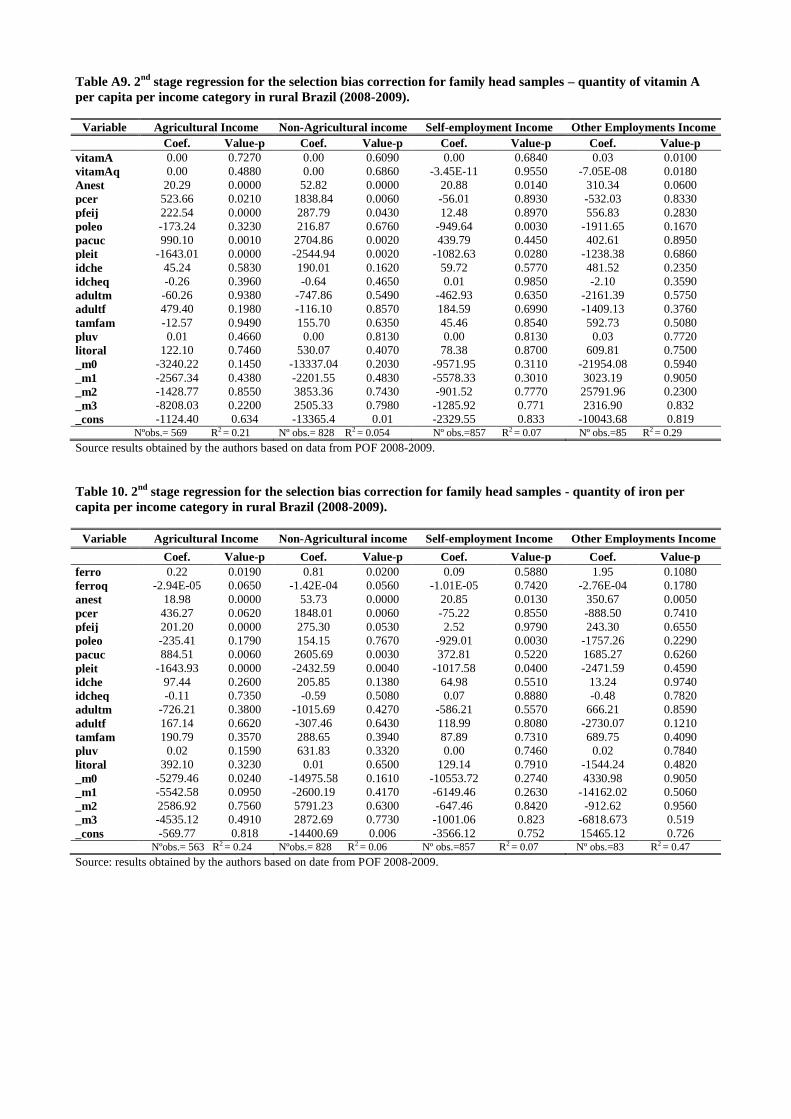
Table A9. 2nd

stage regression for the selection bias correction for family head samples – quantity of vitamin A




vitamA 0.00 0.7270 0.00 0.6090 0.00 0.6840 0.03 0.0100

vitamAq 0.00 0.4880 0.00 0.6860 -3.45E-11 0.9550 -7.05E-08 0.0180

Anest 20.29 0.0000 52.82 0.0000 20.88 0.0140 310.34 0.0600

pcer 523.66 0.0210 1838.84 0.0060 -56.01 0.8930 -532.03 0.8330

pfeij 222.54 0.0000 287.79 0.0430 12.48 0.8970 556.83 0.2830

poleo -173.24 0.3230 216.87 0.6760 -949.64 0.0030 -1911.65 0.1670

pacuc 990.10 0.0010 2704.86 0.0020 439.79 0.4450 402.61 0.8950

pleit -1643.01 0.0000 -2544.94 0.0020 -1082.63 0.0280 -1238.38 0.6860

idche 45.24 0.5830 190.01 0.1620 59.72 0.5770 481.52 0.2350

idcheq -0.26 0.3960 -0.64 0.4650 0.01 0.9850 -2.10 0.3590

adultm -60.26 0.9380 -747.86 0.5490 -462.93 0.6350 -2161.39 0.5750

adultf 479.40 0.1980 -116.10 0.8570 184.59 0.6990 -1409.13 0.3760

tamfam -12.57 0.9490 155.70 0.6350 45.46 0.8540 592.73 0.5080

pluv 0.01 0.4660 0.00 0.8130 0.00 0.8130 0.03 0.7720

litoral 122.10 0.7460 530.07 0.4070 78.38 0.8700 609.81 0.7500

_m0 -3240.22 0.1450 -13337.04 0.2030 -9571.95 0.3110 -21954.08 0.5940

_m1 -2567.34 0.4380 -2201.55 0.4830 -5578.33 0.3010 3023.19 0.9050

_m2 -1428.77 0.8550 3853.36 0.7430 -901.52 0.7770 25791.96 0.2300

_m3 -8208.03 0.2200 2505.33 0.7980 -1285.92 0.771 2316.90 0.832

_cons -1124.40 0.634 -13365.4 0.01 -2329.55 0.833 -10043.68 0.819 Nºobs.= 569 R2 = 0.21 Nº obs.= 828 R2 = 0.054 Nº obs.=857 R2 = 0.07 Nº obs.=85 R2 = 0.29

Source results obtained by the authors based on data from POF 2008-2009.

Table 10. 2nd

stage regression for the selection bias correction for family head samples - quantity of iron per

capita per income category in rural Brazil (2008-2009).



ferro 0.22 0.0190 0.81 0.0200 0.09 0.5880 1.95 0.1080

ferroq -2.94E-05 0.0650 -1.42E-04 0.0560 -1.01E-05 0.7420 -2.76E-04 0.1780

anest 18.98 0.0000 53.73 0.0000 20.85 0.0130 350.67 0.0050

pcer 436.27 0.0620 1848.01 0.0060 -75.22 0.8550 -888.50 0.7410

pfeij 201.20 0.0000 275.30 0.0530 2.52 0.9790 243.30 0.6550

poleo -235.41 0.1790 154.15 0.7670 -929.01 0.0030 -1757.26 0.2290

pacuc 884.51 0.0060 2605.69 0.0030 372.81 0.5220 1685.27 0.6260

pleit -1643.93 0.0000 -2432.59 0.0040 -1017.58 0.0400 -2471.59 0.4590

idche 97.44 0.2600 205.85 0.1380 64.98 0.5510 13.24 0.9740

idcheq -0.11 0.7350 -0.59 0.5080 0.07 0.8880 -0.48 0.7820

adultm -726.21 0.3800 -1015.69 0.4270 -586.21 0.5570 666.21 0.8590

adultf 167.14 0.6620 -307.46 0.6430 118.99 0.8080 -2730.07 0.1210

tamfam 190.79 0.3570 288.65 0.3940 87.89 0.7310 689.75 0.4090

pluv 0.02 0.1590 631.83 0.3320 0.00 0.7460 0.02 0.7840

litoral 392.10 0.3230 0.01 0.6500 129.14 0.7910 -1544.24 0.4820

_m0 -5279.46 0.0240 -14975.58 0.1610 -10553.72 0.2740 4330.98 0.9050

_m1 -5542.58 0.0950 -2600.19 0.4170 -6149.46 0.2630 -14162.02 0.5060

_m2 2586.92 0.7560 5791.23 0.6300 -647.46 0.8420 -912.62 0.9560

_m3 -4535.12 0.4910 2872.69 0.7730 -1001.06 0.823 -6818.673 0.519

_cons -569.77 0.818 -14400.69 0.006 -3566.12 0.752 15465.12 0.726 Nºobs.= 563 R2 = 0.24 Nºobs.= 828 R2 = 0.06 Nº obs.=857 R2 = 0.07 Nº obs.=83 R2 = 0.47

Source: results obtained by the authors based on date from POF 2008-2009.

Documents

RESUMO - anpec.org.br · RESUMO Neste artigo investigam-se os impactos da subnutrição sobre a produtividade do trabalho, analisando a armadilha da pobreza nutricional (APN). Verifica-se