Ricardo Jorge Santos Monteiro Dissertação Jorge... · Ricardo Jorge Santos Monteiro ... Professor of Escola Superior de Tecnologia e Gest˜ao do Instituto Polit ... and BMGT (right)

DISSERTACAO

Mestrado em Engenharia Eletrotecnica - Telecomunicacoes

Disparity Compensation using Geometric Transforms

Ricardo Jorge Santos Monteiro

Leiria, Setembro de 2014

MASTER DISSERTATION

Electrical Engineering - Telecommunications

Disparity Compensation using Geometric Transforms

Ricardo Jorge Santos Monteiro

Master dissertation performed under the guidance of Doctor Nuno Miguel Morais

Rodrigues, Professor of Escola Superior de Tecnologia e Gestao do Instituto Politecnico

de Leiria and co-orientation of Doctor Sergio Manuel Maciel Faria, Professor of Escola

Superior de Tecnologia e Gestao do Instituto Politecnico de Leiria.

Leiria, September 2014

You have to learn the rules of

the game. And then you have to

play better than anyone else.

(Albert Einstein)

Acknowledgements

I would like to express my sincere gratitude to my advisers Dr. Nuno Rodrigrues and Dr.

Sergio Faria, that trusted me throughout the years. I’m thankful for their guidance and

friendship shown inside and outside of our working environment.

To Instituto de Telecomunicacoes for the excellent working conditions.

To my research group colleagues Luıs Lucas, Gilberto Jorge, Joao Santos, Andre

Guarda, Filipe Gama and Sylvain Marcelino, for the companionship and for creating

such a great working environment. A special thanks to Luıs Lucas and Gilberto Jorge for

helping me understand the HEVC code and working with linux.

To my family, who have always supported and believed in me.

To Tania, for the unconditional love and patience, mainly when this work didn’t let

us be together as much as we would like.

Last but not least, to my great friends, Andre Sousa, Nuno Miguel, Nuno Santos, Vera

Pereira, Alexandre Raimundo for the distracting moments outside IT.

iii

Abstract

This dissertation describes the research and development of some techniques to enhance

the disparity compensation in 3D video compression algorithms. Disparity compensation

is usually performed using a block matching technique between views, disregarding the

various levels of disparity present for objects at different depths in the scene. An alterna-

tive coding scheme is proposed, taking advantage of the cameras setup information and

the object’s depth in the scene, to compensate more complex spatial distortions, being

able to improve disparity compensation even with convergent cameras.

In order to perform a more accurate disparity compensation, the reference picture

list is enriched with additional geometrically transformed images, for the most relevant

object’s levels of depth in the scene, resulting from projections of one view to another.

This scheme can be implemented in any state-of-the-art video codec, as H.264/AVC or

HEVC, in order to improve the disparity matching accuracy between views.

Experimental results, using MV-HEVC extension, show the efficiency of the proposed

method for coding stereo video, presenting bitrate savings up to 2.87%, for convergent

camera sequences, and 1.52% for parallel camera sequences. Also a method to choose

the geometrically transformed inter view reference pictures was developed, in order to

reduce unnecessary overhead for unused reference pictures. By selecting and adding to

the reference picture list, only the most useful pictures, all results improved, presenting

bitrate savings up to 3.06% for convergent camera sequences, and 2% for parallel camera

sequences.

Keywords: Disparity compensation, 3D video coding, Geometric transforms

v

Resumo

Esta dissertacao descreve o estudo e desenvolvimento de um conjunto de tecnicas para

melhorar a compensacao de disparidade em algoritmos para compressao de video 3D.

A compensacao de disparidade e normalmente aplicada utilizando tecnicas baseadas em

block matching, sem ter em conta a distorcao geometrica que afeta cada objeto na cena, a

varias profundidades e disparidades. Desta forma, e proposto um esquema de codificacao

alternativo, que tem em conta a orientacao e posicao das camaras, bem como a profun-

didade dos objetos na cena relativamente as camaras. Desta forma mesmo em agregados

de camaras convergentes e possıvel melhorar a qualidade da compensacao de disparidade.

Com o objetivo de melhorar a compensacao de disparidade, sao criadas novas imagens

de referencia geometricamente transformadas, que compensam a distorcao geometrica dos

objetos que se encontram nos nıveis de profundidade mais relevantes da cena. Este metodo

pode ser aplicado em qualquer codec do estado da arte como o H.264/AVC ou o HEVC

com o objetivo de melhorar a precisao da compensacao de disparidade entre vistas.

Os resultados experimentais, obtidos com extensao MV-HEVC, comprovam a eficiencia

do metodo proposto em vıdeo stereo, apresentando poupancas de debito binario que vao

ate 2.87% para sequencias com conjuntos de camaras convergentes e 1.52% para sequencias

com conjuntos de camaras paralelas. Foi tambem desenvolvido um metodo para escolher

as imagens compensadas geometricamente para predicao inter vista, de forma a reduzir o

custo em debito binario acrescido por cada imagem de referencia, mesmo que as imagens

nao sejam utilizadas. Selecionando apenas as imagens mais uteis para o processo de

codificacao, e colocado-as na lista de imagens de referencia, todos os resultados anteriores

melhoraram, apresentando poupancas de debito binario que vao ate 3.06% para sequencias

com conjuntos de camaras convergentes e 2% para sequencias com conjuntos de camaras

paralelas.

Palavras-chave: Compensacao de disparidade, Codificacao de vıdeo 3D, Trans-

formacoes geometricas

vii

Contents

Acknowledgements iii

Abstract v

Resumo vii

Contents x

List of Figures xi

List of Tables xiii

List of Abbreviations xv

1 Introduction 1

1.1 Context and motivations . . . . . . . . . . . . . . . . . . . . . . . . . . . . 1

1.2 Objectives . . . . . . . . . . . . . . . . . . . . . . . . . . . . . . . . . . . . 2

1.3 Dissertation structure . . . . . . . . . . . . . . . . . . . . . . . . . . . . . . 2

2 3D Video Coding 5

2.1 Common codec tools . . . . . . . . . . . . . . . . . . . . . . . . . . . . . . 6

2.2 3D-HEVC tools . . . . . . . . . . . . . . . . . . . . . . . . . . . . . . . . . 10

3 Related State-of-the-art 15

3.1 Geometric transforms . . . . . . . . . . . . . . . . . . . . . . . . . . . . . . 15

3.1.1 Projective transform . . . . . . . . . . . . . . . . . . . . . . . . . . 16

3.1.2 Bilinear transform . . . . . . . . . . . . . . . . . . . . . . . . . . . 23

3.2 Applications of geometric transforms on motion and disparity compensation 25

3.2.1 Block-level approaches . . . . . . . . . . . . . . . . . . . . . . . . . 25

ix

3.2.2 Picture-level approaches . . . . . . . . . . . . . . . . . . . . . . . . 27

3.2.3 Applications summary . . . . . . . . . . . . . . . . . . . . . . . . . 32

4 Disparity compensation using geometric transforms 33

4.1 Block based approach . . . . . . . . . . . . . . . . . . . . . . . . . . . . . . 35

4.1.1 Block matching using geometric transforms . . . . . . . . . . . . . . 36

4.1.2 BMA+BMGT using a grid . . . . . . . . . . . . . . . . . . . . . . . 41

4.2 Region based approach . . . . . . . . . . . . . . . . . . . . . . . . . . . . . 49

4.2.1 Segmentation step . . . . . . . . . . . . . . . . . . . . . . . . . . . 50

4.2.2 Region Matching using Geometric Transforms . . . . . . . . . . . . 51

5 Integration of proposed methods on MV-HEVC 57

5.1 Proposed methods . . . . . . . . . . . . . . . . . . . . . . . . . . . . . . . 57

5.1.1 K-Means+RMGT . . . . . . . . . . . . . . . . . . . . . . . . . . . . 59

5.1.2 K-Means+VSRS . . . . . . . . . . . . . . . . . . . . . . . . . . . . 59

5.1.3 Experimental results . . . . . . . . . . . . . . . . . . . . . . . . . . 61

5.2 Optimized Reference List . . . . . . . . . . . . . . . . . . . . . . . . . . . . 64

5.2.1 Experimental results . . . . . . . . . . . . . . . . . . . . . . . . . . 67

6 Conclusions 71

Bibliografia 75

A Contributions 79

A.1 Conferences . . . . . . . . . . . . . . . . . . . . . . . . . . . . . . . . . . . 79

x

List of Figures

2.1 HEVC video encoder and decoder on the gray blocks [2]. . . . . . . . . . . 7

2.2 Intra prediction angular modes [6]. . . . . . . . . . . . . . . . . . . . . . . 8

2.3 Inferred motion vector by NBDV [3]. . . . . . . . . . . . . . . . . . . . . . 11

2.4 Advanced residual prediction example [3]. . . . . . . . . . . . . . . . . . . 12

3.1 Example of forward and inverse mapping between two distinct coordinate

system . . . . . . . . . . . . . . . . . . . . . . . . . . . . . . . . . . . . . . 15

3.2 Example of an Euclidean transform . . . . . . . . . . . . . . . . . . . . . . 18

3.3 Example of a Similarity transform . . . . . . . . . . . . . . . . . . . . . . . 19

3.4 Example of an Affine transform . . . . . . . . . . . . . . . . . . . . . . . . 20

3.5 Example of a Projective transform on a m× n image . . . . . . . . . . . . 22

3.6 Prediction image using BMA (left) and BMGT (right) on frame 20 of Sergio

sequence [20] . . . . . . . . . . . . . . . . . . . . . . . . . . . . . . . . . . 27

3.7 Navigation sequences examples: Basell2D (left) and Insbruck3D (right)

with two distinct areas: map and semi-transparent static areas [25] . . . . 31

4.1 Example of binocular disparity [31] . . . . . . . . . . . . . . . . . . . . . . 34

4.2 Example of disparity in a pair of images acquired with parallel camera

arrangement . . . . . . . . . . . . . . . . . . . . . . . . . . . . . . . . . . . 34

4.3 An example of a pair of images acquired with a stereo pair of convergent

camera arrangement . . . . . . . . . . . . . . . . . . . . . . . . . . . . . . 35

4.4 An example of one of the matching cases when applying BMA. . . . . . . 37

4.5 Example of block matching with BMGT. . . . . . . . . . . . . . . . . . . 38

4.6 An example of one of the matching cases when applying OSA. . . . . . . . 39

4.7 An example of one of the matching cases when applying TSS. . . . . . . . 39

4.8 An example of one of the matching cases when applying HEXBS. . . . . . 40

xi

4.9 An example of one of the matching cases when applying BMGT to the grid

of the red block. . . . . . . . . . . . . . . . . . . . . . . . . . . . . . . . . 43

4.10 Part of the reconstructed images of Ballet. . . . . . . . . . . . . . . . . . . 45

4.11 PSNR variation for the same number of steps/iterations with different grid

sizes. . . . . . . . . . . . . . . . . . . . . . . . . . . . . . . . . . . . . . . . 48


sizes. . . . . . . . . . . . . . . . . . . . . . . . . . . . . . . . . . . . . . . . 48


sizes. . . . . . . . . . . . . . . . . . . . . . . . . . . . . . . . . . . . . . . . 49

4.14 Segmentation of the first frame of the depth map sequences Breakdancers

(left) and Ballet (right) using K-Means and Watershed methods. . . . . . 52

4.15 An example of RMGT method application. . . . . . . . . . . . . . . . . . . 53

4.16 An example of the output images of RMGT. . . . . . . . . . . . . . . . . . 54

4.17 Objective quality reconstruction at each region. . . . . . . . . . . . . . . . 55

5.1 Modified inter-view prediction structure, where View 0 corresponds to the

left view and View 1 is the right view. . . . . . . . . . . . . . . . . . . . . 58

5.2 Example of the method where K-Means clustering and RMGT are com-

bined to generate new reference pictures for MV-HEVC. . . . . . . . . . . 60

5.3 Example of VSRS output for the same picture using different depth planes. 62

5.4 Example of the method where K-Means clustering and VSRS are combined

to generate new reference pictures for MV-HEVC. . . . . . . . . . . . . . . 63

5.5 Usage of the GT reference pictures on the Ballet and Balloons sequences. . 65

xii

List of Tables

2.1 Possible CTB, CB, PB and TB luminance sizes. . . . . . . . . . . . . . . . 8

3.1 Summary of the previously described applications . . . . . . . . . . . . . . 32

4.1 Experimental results comparing the BMA and the BMA+BMGT and the

different fast search methods. . . . . . . . . . . . . . . . . . . . . . . . . . 40

4.2 Experimental results comparing BMA and BMA+BMGT for different grid

sizes. . . . . . . . . . . . . . . . . . . . . . . . . . . . . . . . . . . . . . . 42

4.3 Experimental results comparing the BMA and the BMA+BMGT and dif-

ferent grid sizes. . . . . . . . . . . . . . . . . . . . . . . . . . . . . . . . . . 45

4.4 Experimental results using the TSS method. . . . . . . . . . . . . . . . . . 46

4.5 Experimental results comparing the Souza’s search method and the TSS. . 46

4.6 Experimental results comparing the search method used by Souza et al.

and the TSS. . . . . . . . . . . . . . . . . . . . . . . . . . . . . . . . . . . 47

5.1 Number of transmitted extra bits, necessary to reconstruct the GT refer-

ence frames at the decoder. . . . . . . . . . . . . . . . . . . . . . . . . . . 62

5.2 Experimental results using both RMGT and VSRS proposed methods for

1 and 3 regions. . . . . . . . . . . . . . . . . . . . . . . . . . . . . . . . . . 63

5.3 Reference pictures, by POC (Picture Order Count), used to encode the

enhancement view. . . . . . . . . . . . . . . . . . . . . . . . . . . . . . . . 65

5.4 Experimental results using both VSRS proposed methods for 1, 2, 3 and 4

regions on convergent camera array sequences. . . . . . . . . . . . . . . . 68

5.5 Experimental results using both RMGT 2 DoF and VSRS proposed meth-

ods for 1, 2, 3 and 4 regions parallel camera array sequences. . . . . . . . 68

xiii

List of Abbreviations

2D Two Dimensions

3D Three Dimensions

AMP Aymmetric Motion Prediction

ARP Advanced Residual Prediction

AVC Advanced Video Coding

BMA Block Matching Algorithm

BMGT Block Matching with Geometric Transforms

CABAC Context Adaptive Binary Arithmetic Coding

CB Coding Block

CTB Coding Tree Block

CTU Coding Tree Unit

CU Coding Unit

DBF Deblocking Filter

DCT Discrete Cosine Transform

DLT Depth Look-up Table

DMM Depth Modelling Modes

DST Discrete Sine Transform

DoF Degrees of Freedom

FS Full Search

GT Geometric Transform

xv

HD High Definition

HEVC High Efficiency Video Coding

HEXBS Hexagonal-Based Search algorithm

HTE Helmholtz Tradeoff Estimator

IEC International Electrotechnical Commission

ISO International Standards Organization

ITU-T International Telecommunications Union - Telecommunications

Standardization Sector

JCT-3V Joint Collaborative Team on 3D video

JCT-VC Joint Collaborative Team on Video Coding

KLT Kanade-Lucas-Tomasi

MPEG Moving Picture Experts Group

MSE Mean Squared Error

NBDV Neighbouring Block-Based Disparity Vector Derivation

OSA Orthogonal Search Algorithm

PB Prediction Block

POC Picture Order Count

PSKIP Parameter Skip

PSNR Peak Signal-to-Noise Ratio

PU Prediction Unit

QP Quantization Parameter

RANSAC Random Sample Consensus

RBC Region Boundary Chain

RDO Rate-Distortion Optimization

RD Rate-Distortion

xvi

RMGT Region Matching using Geometric Transforms

SAD Sum of Absolute Differences

SAO Sample Adaptive Offset

SDC Simplified Depth Coding

SIFT Scale-Invariant Feature Transform

SSD Sum of Square Differences

SURF Speeded-Up Robust Features

TB Transform Block

TSS Three-Step Search

TUC Temporal Updated Centroids

TU Transform Unit

VCEG Video Coding Experts Group

VSO View Synthesis Optimization

VSRS View Synthesis Reference Software

WPP Wavefront parallel processing

xvii

Chapter 1

Introduction

1.1 Context and motivations

In recent years there has been a growing interest of the consumer market in 3D video ser-

vices and applications, spanning from broadcasting to internet and gaming, enhancing the

user experience towards immersive and more natural viewing environments. This interest

was followed by a standardization effort, allowing the development of several techniques,

to further improve the compression performance of the existing encoders. State-of-the-art

video coding standards, like H.264/AVC [1] and the most recent H.265/HEVC [2], are

being extended to support multiview and video-plus-depth formats.

Among the various techniques developed to exploit the redundancy between adjacent

pictures, motion estimation plays an essential role, by eliminating the temporal redun-

dancy. In multiview video formats there is an additional source of redundancy between

views of a sequence. In order to eliminate this redundant information among views,

captured by different cameras, disparity compensation can be performed.

Current video standards use an algorithm similar to motion estimation Block Matching

Algorithm (BMA) to perform block matching between a pair of images, and use a vector to

represent either motion or disparity. However, this algorithm assumes that all pixels pixels

in a block have the same motion/disparity, and are accurately described by a translation.

In most disparity compensation scenarios these restrictions do not apply, particularly

for convergent camera arrangements. In such cases, the use of more flexible disparity

compensation schemes, using a higher degree of freedom (DoF) operation, may result in

performance gains. This can be obtained through the use of geometric transformations

(GT) where, depending on the available DoF, it is possible to describe not only transla-

tions, but also rotations, scaling and shear. In order to achieve a higher motion/disparity

compensation accuracy, the compression scheme using block matching requires more in-

2 Chapter 1. Introduction

formation to describe the transformation associated with each block. When the block size

is reduced, the amount of data, per pixel, required to represent the block transformations

increases significantly. However, the newest video coding standard HEVC supports larger

block sizes, up to 64 × 64 pixels. Therefore, compensating the disparity of larger blocks

with a more accurate block matching algorithm may overcome the necessary extra amount

of bits, in terms of RDO (Rate-Distortion Optimization) .

The proposed method divides each scene into regions, corresponding to objects with

different disparities. This segmentation is applied on the base view depth map and consid-

ers the amount of pixels present at each depth level. Based on the 3D scene information

and the distortion achieved by a matching technique, new reference pictures are gener-

ated using geometric transforms (GT). These GT reference pictures, represented by its

own coefficients, are used in MV-HEVC encoding scheme to compress a pair of video

sequences.

1.2 Objectives

This work initially presents a study on the state-of-the-art proposals on this topic, as well

as, the HEVC standard and multiview extensions, namely MV-HEVC and 3D-HEVC.

Afterwards the following topics were developed:

• Implementation of various types of geometric transforms;

• Study and development of segmentation methods;

• Development of various disparity compensation techniques, through the use of geo-

metric transforms;

• Integration of the proposed techniques in a state-of-the-art video codec;

• Objective performance evaluation using the state-of-the-art video codec as a bench-

mark.

The proposed techniques integrated in the state-of-the-art video codec are expected

to improve RD performance.

1.3 Dissertation structure

This dissertation is organized in six chapters. This first chapter addresses a overall de-

scription of this work and objectives. The second chapter describes an overview of the

most relevant coding tools in 3D video coding, based on HEVC standard and 3D-HEVC

1.3. Dissertation structure 3

extensions. The third chapter includes the related state-of-the-art, with a detailed study

on geometric transforms, and their application to compensate motion. The fourth chapter

shows an evaluation of two types of approaches developed to compensate disparity. The

fifth chapter presents the result of the integration of the proposed methods on MV-HEVC

extension and experimental results. Finally, in chapter six some conclusions are drawn

and some possible future work.

In Appendix A, contributions associated with this dissertation are presented.

Chapter 2

3D Video Coding

State-of-the-art video coding standards, like H.264/AVC [1] and the most recent

H.265/HEVC [2], are being extended to support multiview and video-plus-depth formats

[3]. HEVC is the most recent joint video project of the ITU-T Video Coding Experts

Group (VCEG) and the ISO/IEC Moving Picture Experts Group (MPEG) standard-

ization organizations. This partnership is known by Joint Collaborative Team on Video

Coding (JCT-VC) .

HEVC has been developed to address the increasing diversity of services that use HD

(High Definition) video e.g. 1920 × 1080 pixels, and ultra HD video e.g. 3840 × 2160

pixels. Not only it is necessary to have a codec that is more efficient for storage, but also

for streaming through the network. The amount of necessary bandwidth increases even

more when dealing with stereo or multiview video. HEVC development is also focused on

parallel processing architectures due to the increasing availability of multi-core solutions

for processing.

The main concept of the codec architecture is the same as H.264/AVC. Each picture

is split into blocks. In order to exploit spatial and temporal redundancy, prediction

algorithms are applied. Depending on the prediction scheme, the picture to be encoded

can be either I, P or B. If the picture is I, intra prediction is applied, where only spatial

redundancy is exploited. If the picture is either P or B, temporal prediction can be

performed, which is usually the most common. The residue, i.e. the difference between

the predicted block and the original block, is transformed using a spatial transform.

The resulting coefficients are scaled and quantized. This information is entropy coded

and transmitted with the prediction information, like the selected mode, or the motion

vectors.

The encoder also includes an decoder such that the decoding process is replicated in

the encoder side. This allows the decoded pictures to be used as reference pictures for the

future frames. The decoding loop includes the reconstruction of the approximated residue

6 Chapter 2. 3D Video Coding

using the inverse quantization and transform. The residue is added to the prediction

generating the decoded block. In order to reduce artifacts, the decoded picture may be

filtered in the decoding loop process.

What differentiates HEVC from other extensions is the type and number of input

signals. HEVC standard only accepts one input video sequence. MV-HEVC[4], the mul-

tiview extension, is used to encode several videos exploiting inter-view redundancy, while

still maintaining backwards compatibility with monoscopic video coded by HEVC. This

is done by adding pictures from one view to the reference picture list of another view.

Since the various cameras capture the same scene a high percentage of the picture can be

predicted using another camera perspective. The Joint Collaborative Team on 3D video

(JCT-3V) , which is the team that is working on the 3D extensions for HEVC, is also

developing 3D-HEVC[5]. This 3D video group has been created to study advanced tools

for coding multiple views. Just like MV-HEVC, inter-view prediction is performed, but

also using depth maps, that are coded and transmitted. This video-plus-depth format

uses coding tools specific to depth maps where sharp edges and large homogeneous areas

are predominant. The main advantage of the this format, is the high number of views

that can be artificially created on the receiver, due to the availability of the depth maps.

MV-HEVC does not have any exclusive coding tools, since inter-view prediction is also

used by 3D-HEVC. Therefore the two following sections will address the common tools

that are used in all extensions and the most relevant 3D-HEVC tools.

2.1 Common codec tools

Regardless of the extension, both MV-HEVC and 3D-HEVC are based on HEVC, in

order to maintain compatibility [3]. At least the first video sequence encoded by one of

these extensions uses HEVC. Either way the common tools are the tools used by HEVC.

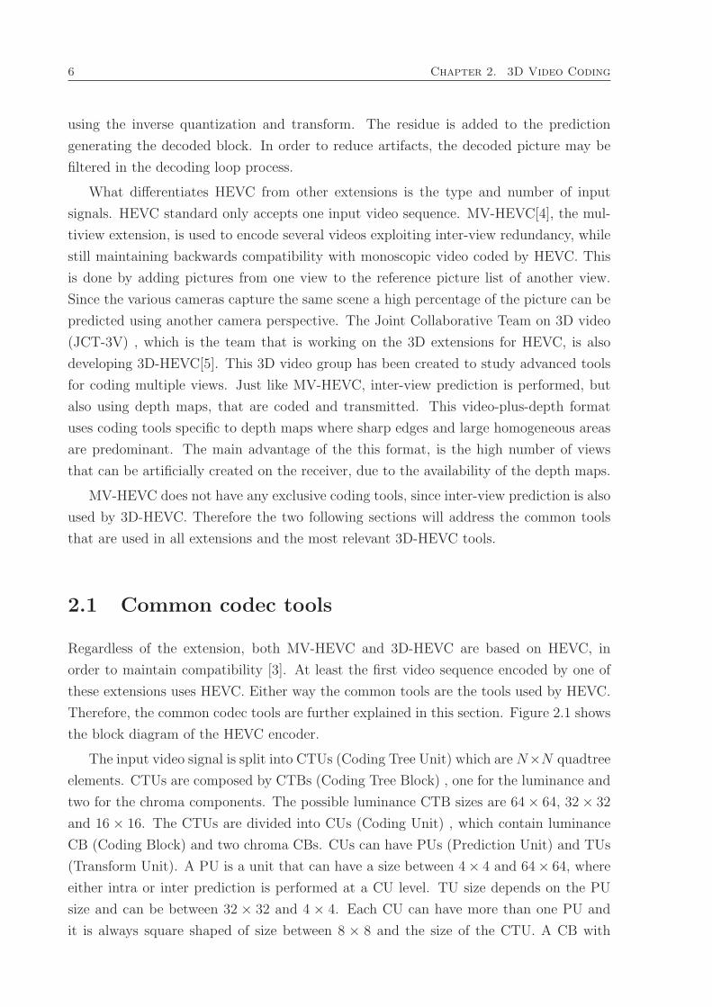
Therefore, the common codec tools are further explained in this section. Figure 2.1 shows

the block diagram of the HEVC encoder.

The input video signal is split into CTUs (Coding Tree Unit) which are N×N quadtree

elements. CTUs are composed by CTBs (Coding Tree Block) , one for the luminance and

two for the chroma components. The possible luminance CTB sizes are 64× 64, 32× 32

and 16 × 16. The CTUs are divided into CUs (Coding Unit) , which contain luminance

CB (Coding Block) and two chroma CBs. CUs can have PUs (Prediction Unit) and TUs

(Transform Unit). A PU is a unit that can have a size between 4× 4 and 64× 64, where

either intra or inter prediction is performed at a CU level. TU size depends on the PU

size and can be between 32 × 32 and 4 × 4. Each CU can have more than one PU and

it is always square shaped of size between 8 × 8 and the size of the CTU. A CB with

2.1. Common codec tools 7

Figure 2.1: HEVC video encoder and decoder on the gray blocks [2].

M×M pixels can have partitioned PBs (Prediction Block) , which are the luminance and

chroma components of PU, as 2N ×2N , N ×N , N ×2N and 2N ×N , where M = 2N . A

PB can also be partitioned asymmetrically using AMP (Asymmetric Motion Prediction)

using sizes: 2N × nU , 2N × nD, nL× 2N and nR × 2N . U , D, L and R correspond to

Up, Down, Left and Right. For example, if M = 16, the 2N × nU the resulting partition

will be one 16 × 4 block on top and a 16× 12 on the bottom, because the division is on

horizontal and on the upper part of the block.

Table 2.1 shows all possible sizes for luma CTB, CB, PB and TB . Also the table is

hierarchy organized. For example, for 16×16 CTB size, the only possible sizes for CB, PB

and TB are the ones on the same line or below in the table. Therefore the only possible

CB sizes are 16× 16 and 8× 8 and TB sizes are between 16× 16 and 4× 4.

The spatial redundancy of the picture is exploited by using decoded boundary samples

of adjacent blocks as reference data for intra prediction. The intra predictions modes

include: DC mode, planar mode and 33 angular modes. The DC mode creates a flat

surface that is the mean of the boundary samples. The planar mode is used to predict

gradient surfaces of the picture. The 33 angular modes are only available for PB sizes of

32× 32, 16× 16 and 8× 8. When the PB is 64× 64 only 4 angular modes are available

and if the PB is 4× 4 only 16 are available. Figure 2.2 shows the intra prediction angular

modes.

The inter prediction techniques are used to exploit temporal redundancy. Using de-


CTB CB PB TB

64× 64 64× 64

64× 6464× 3232× 64

64× 16 and 64× 4816× 64 and 48× 64

32× 32 32× 32

32× 32

32× 3232× 1616× 32

32× 8 and 32× 248× 32 and 24× 32

16× 16 16× 16

16× 16

16× 1616× 88× 16

16× 4 and 16× 124× 16 and 12× 16

8× 88× 8

8× 88× 44× 84× 4 4× 4

Table 2.1: Possible CTB, CB, PB and TB luminance sizes.

Figure 2.2: Intra prediction angular modes [6].

2.1. Common codec tools 9

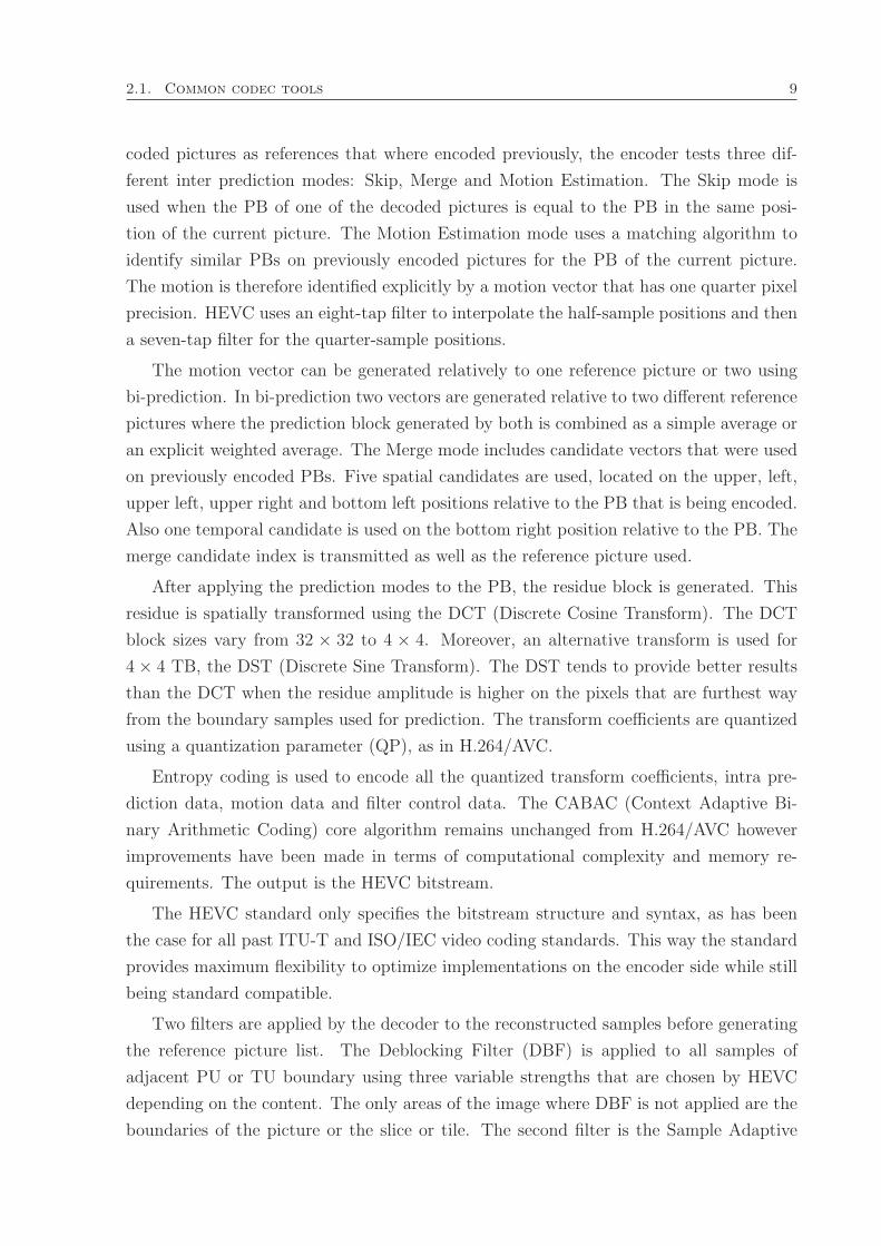
coded pictures as references that where encoded previously, the encoder tests three dif-

ferent inter prediction modes: Skip, Merge and Motion Estimation. The Skip mode is

used when the PB of one of the decoded pictures is equal to the PB in the same posi-

tion of the current picture. The Motion Estimation mode uses a matching algorithm to

identify similar PBs on previously encoded pictures for the PB of the current picture.

The motion is therefore identified explicitly by a motion vector that has one quarter pixel

precision. HEVC uses an eight-tap filter to interpolate the half-sample positions and then

a seven-tap filter for the quarter-sample positions.

The motion vector can be generated relatively to one reference picture or two using

bi-prediction. In bi-prediction two vectors are generated relative to two different reference

pictures where the prediction block generated by both is combined as a simple average or

an explicit weighted average. The Merge mode includes candidate vectors that were used

on previously encoded PBs. Five spatial candidates are used, located on the upper, left,

upper left, upper right and bottom left positions relative to the PB that is being encoded.

Also one temporal candidate is used on the bottom right position relative to the PB. The

merge candidate index is transmitted as well as the reference picture used.

After applying the prediction modes to the PB, the residue block is generated. This

residue is spatially transformed using the DCT (Discrete Cosine Transform). The DCT

block sizes vary from 32 × 32 to 4 × 4. Moreover, an alternative transform is used for

4 × 4 TB, the DST (Discrete Sine Transform). The DST tends to provide better results

than the DCT when the residue amplitude is higher on the pixels that are furthest way

from the boundary samples used for prediction. The transform coefficients are quantized

using a quantization parameter (QP), as in H.264/AVC.

Entropy coding is used to encode all the quantized transform coefficients, intra pre-

diction data, motion data and filter control data. The CABAC (Context Adaptive Bi-

nary Arithmetic Coding) core algorithm remains unchanged from H.264/AVC however

improvements have been made in terms of computational complexity and memory re-

quirements. The output is the HEVC bitstream.

The HEVC standard only specifies the bitstream structure and syntax, as has been

the case for all past ITU-T and ISO/IEC video coding standards. This way the standard

provides maximum flexibility to optimize implementations on the encoder side while still

being standard compatible.

Two filters are applied by the decoder to the reconstructed samples before generating

the reference picture list. The Deblocking Filter (DBF) is applied to all samples of

adjacent PU or TU boundary using three variable strengths that are chosen by HEVC

depending on the content. The only areas of the image where DBF is not applied are the

boundaries of the picture or the slice or tile. The second filter is the Sample Adaptive


Offset (SAO), that is used after DBF in order to further improve the signal representation

in smooth areas and around edges. The application of SAO consists in adding an offset

value to the decoded samples that is based on a look-up table transmitted by HEVC

encoder.

As stated before one of the key implementation features of HEVC is the possibility to

use parallel processing. For this purpose two features have been added where the picture

being encoded is divided into either tiles or rows of CTUs. Each region is encoded or

decoded using a different CPU thread. The Tiles are similar to Slices although it is not

intended to increase the error resilience and therefore some header information for each

tile is shared. The advantage of this method is the fact that each tile is independent from

each other, so it is not necessary to synchronize threads that are encoding or decoding

each tile. The alternative to tiles is to use WPP (Wavefront parallel processing) where

each thread is assigned to process each row of CTUs. Each row has to be processed with

2 CTUs distance from each other, so that when a second row of CTUs is being processed

the upper CTUs can be available for prediction. The advantage of WPP is the fact that

the performance is not affected as for the Tiles feature and also avoids visual artefacts on

the boundaries of the tile. However it is necessary to maintain synchronization among all

the threads in order to maintain the 2 CTU distance.

2.2 3D-HEVC tools

3D-HEVC is the extension created to use advanced coding tools specifically designed

for the video-plus-depth formats. The higher efficiency compared with HEVC and MV-

HEVC comes from two types of tools: improved inter-view prediction and specific depth

map coding tools [3]. As mentioned before, in order to maintain backwards compatibility

with the single view video encoded by HEVC, the first view, or the base view is encoded

using standard HEVC. Only the additional views or depth maps will use the 3D-HEVC

exclusive tools.

3D-HEVC performs inter-view motion prediction by adding additional candidates to

the list of merge mode. Merge mode includes six candidates as HEVC, and two that are

generated using Neighbouring Block-Based Disparity Vector Derivation(NBDV) [7].

NBDV has its own various spatial and temporal candidates near the current PU. These

candidates are checked in order to find a disparity vector. If a disparity vector is found

the process stops saving the vector, the chosen candidate, and the reference picture index.

If no disparity vector is found NBDV returns a null disparity vector.

As shown in Figure 2.3, the motion vector associated with the block found by NBDV

is the first candidate. Moreover, this first candidate is called the inter-view candidate.

2.2. 3D-HEVC tools 11

Figure 2.3: Inferred motion vector by NBDV [3].

The disparity vector derived by NBDV is used as the second candidate. This way, as

in merge mode, if any candidate is chosen only one index is transmitted. Also if motion

or disparity estimation is performed the vector is predicted using one of the candidates.

The motion that occured in the base-view is correlated with the motion occuring in the

non-base view. Also the disparity vector used in the previous PU or on a neighbouring

PU is also probably very similar to the current PU.

NBDV is also used to perform inter-view residual prediction. As shown in Figure 2.4,

NBDV identifies the Bc block as the reference block. This block was predicted using a

motion vector VD. By calculating the difference between the reconstructed Bc and Br of

the base view, a residue block is generated. This residue block is used for prediction when

the same VD vector is applied for motion compensation in the non-base view. Moreover,

when this Advanced Residual Prediction (ARP)[8] technique is applied the prediction of

the residue can be weighted by 0.5 or 1.

When performing disparity compensation using an inter-view reference picture, there

may be the need to adjust the illumination conditions [9] of one view relative to another,

in order to improve the prediction efficiency. After the prediction is applied using a

disparity vector for the current PU, the neighbouring samples, namely the upper row and

left column of pixels relative to the reference block are used to calculate a linear model.

This linear model is characterized by a scaling factor a, that has to be close to 1, and an

offset b, where both values are calculated using least-squares. The linear model is applied

to each value improving the prediction.

In terms of specific depth coding tools, first it is necessary to point the differences

between a depth map and texture. Depth maps are characterized by large homogeneous

areas and sharp edges. The preservation of edges is very important because it directly

affects the quality of synthesized views using reconstructed depth maps. Therefore some


Figure 2.4: Advanced residual prediction example [3].

tools used for texture are not used for depth map coding like DBF and SAO. Also motion

compensation uses integer precision in order to disable interpolation filters.

A set of tools was created to divide the depth blocks into non-rectangular partitions.

Depth Modelling Modes (DMM) [10] and Region Boundary Chain (RBC) [11] are used

to divide the current PU into two zone with a DC value each. This DC value is predicted

using neighbouring pixels. DMM has two modes, where the partition occur in a wedge-

shaped pattern or contour pattern. The wedge-shaped pattern consists in dividing the

PU into two parts using a straight line. The contour pattern uses the co-located texture

PU contour to divide the current depth PU. The RBC uses series of connected chains

within eight possible angles starting at 0, 45, -45, 90, -90, and so on.

Simplified depth coding (SDC) [12] is used if DMM and RBC modes are used. SDC

adds one partition per PU to model smooth regions. Transform and quantization is

skipped when these modes are used, i.e. the samples of residual block are encoded.

When encoding residual blocks directly, in order to reduce the dynamic range of values

a Depth Look-up Table (DLT) is used, where all only used depth values appear. DLT is

useful because in some cases not all the dynamic range is used, some depth maps have an

accuracy lower than 8 bits.

Considering the correlation between texture and depth motion information, the motion

vectors can be inherited from the texture to the depth map. Since texture is encoded first,

the decoded motion vector used by a co-located PU is added as an extra merge candidate

for the current depth PU. When this vector is chosen to be reused by the current depth

PU the precision is adjusted from quarter pixel precision to integer precision, since depth

motion compensation does not use interpolation filter.

2.2. 3D-HEVC tools 13

3D-HEVC includes View Synthesis Optimization (VSO)[10], which is tool that is able

to control and optimize the depth map encoding process. The encoding process of depth

maps is very relevant for the final quality of synthesised views. Therefore a new distortion

metric is used to encode the depth maps, where instead of controlling the distortion

of the depth map, the distortion of the synthesised view is controlled. This control

can be performed by rendering the actual synthesized view in the encoding process and

calculating the distortion, or by estimating the result distortion of the synthesized view.

Chapter 3

Related State-of-the-art

The main objective of this chapter is to present a review of the state-of-the-art. This

chapter is divided into two sections: the first section reviews the most relevant geometric

transforms in the context of disparity compensation; in the second section, the most

relevant applications of geometric transforms on motion compensation are addressed.

3.1 Geometric transforms

The main concept of geometric transforms is the mapping of one coordinate system into

another. This process uses a function that contains the spatial correspondence between

both coordinate systems. This function can be manipulated in order to adjust the shape

of a quadrilateral in relation to another quadrilateral. An example of a forward and

inverse mapping can be seen in Figure 3.1.

In Figure 3.1 two coordinate systems are presented, [x, y] and [u, v], showing the com-

mon Cartesian coordinates used in Euclidean geometry. The forward mapping function,

Figure 3.1: Example of forward and inverse mapping between two distinct coordinatesystem

16 Chapter 3. Related State-of-the-art

that spatially relates both coordinate systems, can be described as:

[x, y] = [X(u, v), Y (u, v)] (3.1)

The inverse operation is:

[u, v] = [U(x, y), V (x, y)] (3.2)

In the forward mapping each point in the quadrilateral is mapped onto a different

position given by X and Y mapping functions [13]. In the inverse mapping the U and V

functions can be used, so that all points in the quadrilateral are mapped onto the original

shape.

Geometric transforms can be characterized by a set of coefficients that are used by the

mapping function. The number of coefficients influences the number of points that can

be independently matched between two different coordinate systems, i.e the number of

non-collinear points. In the case of 2D planes, each non-collinear point of correspondence

needs 2 DoF (Degrees of Freedom). This means that in order to freely create a triangle

one needs 6 DoF and 8 DoF for a quadrilateral. The number of DoF is directly related to

the number of different shapes that is possible to create. However, the higher the number

of DoF the higher the number of coefficients, resulting in a more complex transform. In

the context of this dissertation, only simple geometric transforms will be considered i.e.

geometric transforms with a small number of coefficients. The geometric transforms that

will be considered are:

• Projective;

• Bilinear

These geometric transforms are the most commonly used for the purpose of this dis-

sertation, that is disparity compensation[14, 15, 16, 17].

Although both geometric transforms have 8 DoF, the main difference lays on the

distance between points along certain lines. If these points are equispaced, that property

will be preserved only in the case of the bilinear transform [16].

3.1.1 Projective transform

In order to define these geometric transforms an homogeneous coordinate system is used.

This coordinate system is used in projective geometry[18]. An Euclidean coordinate, like

[x, y], is represented by an homogeneous vector [u, v, h]. The correspondence between the

two coordinate systems is given by:

3.1. Geometric transforms 17

[u, v, h] = [xh, yh, h] (3.3)

Although the third coordinate h can be any value except zero, in this context it’s

simplified to h = 1. Because an image can be defined with two dimensions only. The

plane h = 1 is going to be intersected by the homogeneous vector. The intersection of the

various homogeneous vectors will result on the projection of the image on that plane.

The conversion between coordinate systems is made through a 3x3 transform matrix:

[x, y, 1] = [u, v, 1]H (3.4)

where:

H =

h11 h12 h13

h21 h22 h23

h31 h32 h33

(3.5)

This matrix defines how the conversion between two coordinate systems is made.

When transforming a quadrilateral into another quadrilateral, the various coefficients in

this matrix will have a certain role on that transformation. Taking this into, account the

H matrix can been divided into four parts:

H =

[

H11 H12

H21 h33

]

(3.6)

where:

H11 =

[

h11 h12

h21 h22

]

, H12 =

[

h13

h23

]

, H21 =[

h31 h32

]

(3.7)

The sub-matrix H11 is responsible for a linear transform capable of rotations, scaling

and shear. Moreover, the vector H12 is used to generate perspective changes, while the

vector H21 specifies a translation of the x and y coordinates, respectively. Finally, the h33

coefficient is a scaling factor of the plane h. Since the coefficients in the sub-matrix H12

can be used for scaling purposes, the h33 coefficient becomes redundant. Therefore, it is

normally simplified to h33 = 1.

Projective transforms include some simpler transformations, which rely only on a sub-

set of the described coefficients. Those particular cases are Euclidean, Similarity and

Affine transform.


Euclidean transform

An Euclidean transform is a composition of a translation (T ) and a rotation (R). This

transform is represented as:

[x, y, 1] = [u, v, 1]

[

R 0

T 1

]

= [u, v, 1]

cos(α) sin(α) 0

− sin(α) cos(α) 0

tx ty 1

. (3.8)

This operation is isometric because it preserves length between two points, angle between

two lines and area. Figure 3.2 shows an example of an Euclidean transform applied to a

square. The transform E allows 3 DoF that are directly related to tx, ty, and α.

Figure 3.2: Example of an Euclidean transform

The mapping functions for this transform are:

x = u cos(α)− v sin(α) + tx, (3.9)

y = u sin(α) + v cos(α) + ty. (3.10)

Similarity transform

A Similarity transform is a composition of a translation (T ), a rotation (R) and scale (s).

The scale is isotropic because it’s equal in both axis, and therefore preserves the shape.

This transform can be represented as:

[x, y, 1] = [u, v, 1]

[

sR 0

T 1

]

= [u, v, 1]

s cos(α) s sin(α) 0

−s sin(α) s cos(α) 0

tx ty 1

. (3.11)

This transform allows 4 DoF since it has the same properties of the Euclidean transform

and additionally performs scale. Figure 3.3 shows an example of a Similarity transform

applied to a square. Transform S allows 4 DoF and is directly related to tx, ty, α and s.


Note that s is a scaling ratio between the square before the transformation and after.

Figure 3.3: Example of a Similarity transform

The mapping functions for this transform can be described as:

x = s[u cos(α)− v sin(α)] + tx, (3.12)

y = s[u sin(α) + v cos(α)] + ty. (3.13)

Affine transform

The affine transform is characterized by a linear transformation (A) followed by a trans-

lation (T ) and it’s represented in the following form:

[x, y, 1] = [u, v, 1]

[

A 0

T 1

]

= [u, v, 1]

a11 a12 0

a21 a22 0

tx ty 1

. (3.14)

The main difference to the previous transforms is that the A sub-matrix is not restricted

by only one angle or scale factor. A is a composition of rotations and non-isotropic scalings

(the scale factors are not equal in both axis). The A sub-matrix can be decomposed as:

A = R(α)R(−φ)DR(φ) (3.15)

where,

D =

[

λ1 0

0 λ2

]

. (3.16)

The angle α is responsible for the same rotation as before, however the angle φ specifies

the scale direction and λ1 and λ2 values are the scaling values for both axis. Notice that

if φ = 0 and λ1 = λ2 = s, then A = R(α)s, which represents the similarity transform

without the translation coefficients.


By separating x and y, the mapping functions became:

x = a11u+ a21v + tx, (3.17)

y = a12u+ a22v + ty. (3.18)

The Affine transform achieves 6 DoF, allowing the transformation of a triangle into

another triangle, because 6 DoF allow the correspondence of 3 non-collinear points in two

different coordinate systems. Considering that those points are represented by [xk, yk],

where k = 0, 1 and 2, Equation 3.19 is used to determine the 6 coefficients that describe

the mapping between the 3 corresponding points:

x0 y0 1

x1 y1 1

x2 y2 1

=

u0 v0 1

u1 v1 1

u2 v2 1

a11 a21 0

a21 a22 0

tx ty 1

. (3.19)

Nevertheless, 6 DoF are not enough to transform parallel lines into non-parallel. This

transformation only allows to transform a square onto a parallelogram, not being able to

perform more complex transformations on quadrilaterals. Figure 3.4 shows an example

of the described transformation.

Figure 3.4: Example of an Affine transform

Projective transform

The projective transform adds the missing parameters from the original H matrix (H12)

to the Affine transform:

[x, y, 1] = [u, v, 1]

h11 h12 h13

h21 h22 h23

h31 h32 h33

. (3.20)

changing the mapping functions to (note that h33 = 1):

x = uh11 + vh21 + h31 − xuh13 − xvh23, (3.21)


y = uh12 + vh22 + h32 − xuh13 − xvh23. (3.22)

By using 8 DoF, the projective transform is able to transform one quadrilateral into

another quadrilateral. The quadrilateral transform is defined by 4 correspondent points

[xk, yk] where k = 0, 1, 2 and 3 (one for each corner). In order to find the coefficients for

that correspondence the system described in 3.23 must be solved:

x0

x1

x2

x3

y0

y1

y2

y3

=

u0 v0 1 0 0 0 −u0x0 −v0x0

u1 v1 1 0 0 0 −u1x1 −v1x1

u2 v2 1 0 0 0 −u2x2 −v2x2

u3 v3 1 0 0 0 −u3x3 −v3x3

0 0 0 u0 v0 1 −u0y0 −v0y0

0 0 0 u1 v1 1 −u1y1 −v1y1

0 0 0 u2 v2 1 −u2y2 −v2y2

0 0 0 u3 v3 1 −u3y3 −v3y3

h11

h21

h31

h12

h22

h32

h13

h23

. (3.23)

The equation system 3.23 can be rearranged as:

h11 =x1 − h31

u1

+ x1h13 −v1(h21 − x1h23)

u1

h12 =y1 − h23

u1

+ y1h13 −v1(h22 − x1h23)

u1

h13 =v2h21 + u2h11 + x0 − x2 − v2h23x2

u2x2

h21 =x3 − h31

v3+ x3h23 −

u3(h11 − x3h13)

v3

h22 =y3 − h32

v3+ y3h23 −

u3(h12 − y3h13)

v3

h23 =v2h22 + v2h12 + y0 − y2 − u2h13y2

v2y2

h31 = −u0h11 − v0h21 + x0 + u0x0h13 + v0x0h23

h32 = −u0h12 − v0h22 + y0 + u0y0h13 + v0y0h23

(3.24)

Equations 3.24 allow the calculations of the transform coefficients given the [uk, vk] for

the initial coordinates and [xk, yk] for the intended coordinates after the transformation,

the H matrix is known.

If we consider the common case where a m×n rectangle is transformed into a quadri-

lateral, represented in Figure 3.5.


Figure 3.5: Example of a Projective transform on a m× n image

The system of equations results in:

h11 =x1 − x0

m− 1+ x1h13

h12 =y1 − y0

m− 1+ y1h13

h13 =(n− 1)h21 + (m− 1)h11 + x0 − x2 − (n− 1)h23x2

(m− 1)x2

h21 =x3 − x0

n− 1+ x3h23

h22 =y3 − y0

n− 1+ y3h23

h23 =(n− 1)h22 + (n− 1)h12 + y0 − y2 − (m− 1)h13y2

(n− 1)y2

h31 = x0

h32 = y0

(3.25)

At this point only h13 and h23 need to be determine in order to find all the remaining

coefficients. In order to determine these two coefficients first the following terms have

been defined:

∆x1 = x1 − x2

∆x2 = x3 − x2

∆x3 = x2 − x3 + x0 − x1

∆y1 = y1 − y2

∆y2 = y3 − y2

∆y3 = y2 − y3 + y0 − y1

(3.26)

The coefficients h13 and h23 can be determined by solving Equations 3.27 and 3.28:


h13 =1

m− 1

∣

∣

∣

∣

∣

∆x3 ∆x2

∆y3 ∆y2

∣

∣

∣

∣

∣

∣

∣

∣

∣

∣

∆x1 ∆x2

∆y1 ∆y2

∣

∣

∣

∣

∣

, (3.27)

h23 =1

n− 1

∣

∣

∣

∣

∣

∆y3 ∆y1

∆x3 ∆x1

∣

∣

∣

∣

∣

∣

∣

∣

∣

∣

∆y2 ∆y1

∆x2 ∆x1

∣

∣

∣

∣

∣

. (3.28)

After determining the coefficients in 3.27 and 3.28 those values can be substituted in

the other equations, finding the complete projective matrix. Notice that, this example is

valid for both images and blocks, because in the case of square blocks m = n. Also, if

∆x3 = 0 and ∆y3 = 0, then H12 = 0 and the resulting transform is Affine.

The case of square/rectangle-to-quadrilateral transform is important since it corre-

sponds to the problem that is going to be exploited in the context of this dissertation due

to the fact that both block and images are squares or rectangles.

3.1.2 Bilinear transform

The bilinear transform allows quadrilateral to non-planar quadrilateral transforms. Hori-

zontal, vertical lines and points along these directions are preserved. The bilinear mapping

functions are described as follows:

[x, y] = [uv, u, v, 1]

a0 b0

a1 b1

a2 b2

a3 b3

. (3.29)

Performing the matrix multiplication:

x = a0 + a1u+ a2v + a3uv, (3.30)

y = b0 + b1u+ b2v + b3uv. (3.31)

In order to find the coefficients of two correspondent quadrilaterals from different

coordinate systems 4 points are needed. These 4 points are related by using Equation

3.32:


x0 y0

x1 y1

x2 y2

x3 y3

=

1 u0 v0 u0v0

1 u1 v1 u1v1

1 u2 v2 u2v2

1 u3 v3 u3v3

a3 b3

a2 b2

a1 b1

a0 b0

. (3.32)

Although the bilinear transform has the same number of DoF, the number of calcula-

tions needed to find the coefficients is smaller, compared to the Projective transform. As

for the Projective transform, for an m × n (Figure 3.5) rectangle the coordinates of the

corners may be substituted:

x0 = a0

x1 = x0 + (m− 1)a1

x2 = x0 + (m− 1)a1 + (n− 1)a2 + (m− 1)(n− 1)a3

x3 = x0 + (n− 1)a2

y0 = b0

y1 = y0 + (m− 1)b1

y2 = y0 + (m− 1)b1 + (n− 1)b2 + (m− 1)(n− 1)b3

y3 = y0 + (n− 1)b2

(3.33)

Rearranging the system of equations the transform coefficients may be obtained:

a0 = x0

a1 =x1 − x0

m− 1

a2 =x3 − x0

n− 1

a3 =x2 − x3 − x1 + x0

(m− 1)(n− 1)

b0 = y0

b1 =y1 − y0

m− 1

b2 =y3 − y0

n− 1

b3 =y2 − y3 − y1 + y0

(m− 1)(n− 1)

(3.34)

In the case of bilinear transform if a3 = 0 and b3 = 0, the resulting quadrilateral will

be a parallelogram.

3.2. Applications of geometric transforms on motion and disparity compensation 25

3.2 Applications of geometric transforms on motion

and disparity compensation

Geometric transforms have been applied for both disparity and motion compensation.

Although disparity and motion are two distinct types of information in multiview video

coding, similar methods can be used to compensate both disparity and motion. The only

difference is on the reference images used by the encoder. In the case of motion compen-

sation reference images belong to the past or future of the video sequence in relation to

the current frame. For disparity compensation, reference images belong to another view,

either on the right or left, of the current frame. Hereupon the discussed proposals that are

more relevant to this dissertation can be either about motion or disparity compensation.

When dealing with geometric transforms, the approaches may vary in terms of:

• Type of transform;

• Coefficient estimation;

• The area where the transformation is applied;

• Coefficients transmission.

Regardless of these properties the application of these techniques on video coding

standards has been done at two levels: block-level and picture-level. At the block-level,

the geometric transform is applied on each encoded block, using RDO (Rate-Distortion

Optimization) criteria, and the coefficients need to be transmitted for each block. At

a picture-level, prior encoded frames are analysed and compared with pictures that are

being encoded. Geometrically transformed pictures are generated based on its similarity

to the picture, or to some regions of the picture that is being encoded.

3.2.1 Block-level approaches

Extending HEVC by an affine motion model

In previous research, Narroschke et al. [19] demonstrated that when using a motion com-

pensated prediction based on an Affine model (6 DoF) the coding efficiency is improved.

The affine model was integrated in HEVC as another motion compensated prediction

technique. For each block, either the standard translation model is used or the affine

model. The model is selected through a minimization of the Lagrangian cost, based on

the required data the rate and sum of absolute values of the prediction error. The se-

lected model is transmitted as additional information. The algorithm is more thoroughly

explained through the following steps:


1. The translational model is applied by HEVC;

2. The affine parameters are estimated by a minimization of the squared prediction

error |E2|:

e(xi, yj) ≅ φ(xi, yj)− h(xi, yj)A, (3.35)

where φ represents the difference between the pixel value of the current image (s)

and the reference frame (s′):

φ(xi, yj) = s(xi, yj)− s′(xi, yj) (3.36)

h(xi, yj) is calculated using spatial gradients (Gxiand Gyj) on both axis (using Sobel

operator):

h(xi, yj) = (GxiGyj xiGxi

xiGyj yjGxiyjGyj) (3.37)

and A represents the affine parameters:

A = (a1 a2 a3 a4 a5 a6)T (3.38)

resulting in:

A = (HTH)−1HTφ (3.39)

3. The parameters that minimize the Lagrangian cost of data rate and summed abso-

lute values of prediction error are selected;

In order to reduce the amount of additional information, the affine parameters are

quantized with a step size of 1/16 for a1 and a2 and 1/512 for the remaining values.

The lower precision for the first two coefficients is due to the fact that those values are

responsible for x and y translations.

The authors tested this method limiting HEVC to a maximum block size of 16x16,

64x64 and 128x128. The average data rate reduction for a set of 10 sequences with

non-transnational motion is 0.1%, 6.3% and 7.6% respectively. This shows that for these

experimental tests, the increasing maximum block size benefits the application of an affine

motion model.

Motion compensation for very low bit-rate video

On this proposal, by Faria et al.[20], bilinear transforms are used to compensate motion.

Each corner of a block is associated with a vector that must be transmitted in order to

correctly decode the image. In order to find these vectors the BMA (Block Matching Al-

gorithm) is applied between the current frame and the reference frame. After determining


the motion vector the algorithm BMGT (Block Matching with Geometric Transforms) is

used as a enhancement step. The estimation of the transform coefficients is done by mov-

ing the four corners of each block of the frame independently. In order to compare the

warped block with a square block, inverse mapping is applied to the warped block.

In order to reduce the complexity of this method, a fast search method, based on

OSA (Orthogonal Search Algorithm), was implemented for each one of the corners of the

blocks.

The experimental results demonstrate considerable improvements, compared to H.261,

in terms of objective and subjective quality of the reconstructed frames using geometric

transforms. Figure 3.6 shows the subjective quality achieved using only BMA (left image)

and BMGT (right side).

Figure 3.6: Prediction image using BMA (left) and BMGT (right) on frame 20 of Sergio

sequence [20]

3.2.2 Picture-level approaches

A block-adaptive skip mode for inter prediction based on parametric motion

models

The proposal of Glantz et al.[21] aims to improve the performance of a reference codec

by adding a new prediction mode called PSKIP (Parameter SKIP). This new prediction

mode is associated with a reference image generated using geometric transforms.

A group of parameters is generated for each image to be encoded. These parameters

are used to describe the background movement i.e global motion. The algorithm used in

this technique is divided into four steps:

1. Find correspondent features between the current frame and the reference frame


using KLT (Kanade-Lucas-Tomasi) algorithm;

2. Estimate the parametric model of movement through a method based on the

Helmholtz principle [22] using the correspondent points;

3. After generating several groups of parameters, the HTE (Helmholtz Tradeoff Es-

timator) algorithm is used to remove the outliers in order to select the best group.

This algorithm has the ability to detect 80% of the outliers in a given dataset[21];

4. After the best set of parameters has been found, blocks with this model are coded

with the PSKIP mode.

The main advantage of the PSKIP mode, as for the traditional SKIP mode, is the fact

that a block can be coded without transmitting any residue, which reduces the necessary

bit-rate to code the block. However when using this mode, 8 uncompressed floats are

transmitted, in order to describe the perspective transform. These 8 floats imply an

increase of 256 bits per image. Even if the PSKIP mode is not used, these parameters are

transmitted.

The integration of this mode on the encoder is done side by side with other prediction

modes. The encoder tests all the available modes and the RDO (Rate Distortion Opti-

mizer) selects the mode that is more appropriated to the block to be coded. The more

appropriated mode is chosen taking into account both objective quality and the necessary

bit-rate.

The PSKIP mode has been incorporated into the test module HM 1.0 of HEVC.

The results show a bit-rate decrease, relative to the HM 1.0 without PSKIP mode, that

reaches 29,1% (Low Delay condition). The worst case is an increase of 1,8% of the bit-rate

(Random Access condition). However the author states that, by compressing the 8 float

parameters, or by transmitting one vector for each corner of the image these results may

improve.

This method has some drawbacks, like the fact that the transform coefficients are

uncompressed and transmitted as floats. Instead of the eight float coefficients, four vectors

could be transmitted (one for each corner of the image) in order to further decrease the

bit-rate.

Picture-level parametric motion representation for efficient motion compen-

sation

This proposal, presented by Sung et al.[23], describes the introduction of geometric trans-

forms on an hybrid codec like MPEG-4 or H.264/AVC, in order to improve the motion


compensation performance. Through the use of geometric transform new reference im-

ages are generated. Only the most similar images are selected to be reference images.

This method provides an improved motion resulting in a reduction of the bit-rate, in

comparison with reference codecs.

The proposed algorithm is divided into five steps:

1. Detection of common features points between the current frame and a reference

frame that is available on the decoders buffer, using the KLT algorithm;

2. The corresponding points between the two frames are organized in clusters depend-

ing on the movement of each region of the image, using an algorithm based on region

growing;

3. The perspective transformation coefficients are extracted for each set of points;

4. The new possible reference frames are generated using the Perspective transforma-

tion coefficients;

5. The generated frame that is more likely to be chosen by the encoder RDO is selected

to be the new reference frame.

In order to decrease the computational complexity, two rules have been added to the

algorithm:

• The new frame its added to the reference frame list only if at least 15% of the frame

blocks have a SAD two times lower than the SAD of the same block of the original

reference frame (without geometric transformation)

• If no image is inserted on the reference frame list it is assumed that the extracted

coefficients are not correct. If this happens the algorithm is disabled for all the

frames between the current frame and the reference frame without geometric trans-

formations.

In order to be fully described the perspective transform needs eight coefficients to

be transmitted. In this case, four vectors are transmitted that correspond to each one

of the corners of the warped frame. This alternative uses a smaller amount of bits, by

transmitting four vectors with quarter pixel precision in comparison with the eight float

coefficients.

This proposal has been implemented on the test module TMuC 0.7.3 of HEVC. For

low delay and random acess conditions the results show a decrease on the bit-rate by

3,1% and 3,5%, respectively (in average). As expected the best results occur on the test


sequences that are characterized by complex motion, for example, the Station2 reaches

41,1% (Low Delay) and 28,9% (Random Access) of bit-rate reduction when comparing

with TMuC 0.7.3 (HEVC).

This method has proven to be more efficient in terms of rate-distortion performance,

comparing with TMuC 0.7.3 (HEVC).

Improving H.264/AVC video coding with geometric transforms

Souza et al.[24] introduces the use of geometric transforms in the reference codec

H.264/AVC to improve its performance. The proposal is entitled H.264/AVC-GT-N and

includes N reference frames generated by geometric transforms (GT).

This algorithm is organized as follows:

1. Partitioning of the macroblocks and motion estimation by H.264/AVC;

2. Estimate the best geometric transform for each block of the current frame;

3. A technique, based on region growing, is used to create N sets of geometric trans-

form, that better represent N regions of the current frame;

4. N new reference frames are generated with the geometric coefficients determined

in the previous step;

5. The geometric transform is described by four vectors (one for each corner of the

frame). These vectors are encoded using CABAC in order to be inserted on the

bitstream.

The estimation of the best geometric transform is made through a search method

for each corner of the frame. Each corner of the frame uses a 64 × 64 pixel search

window. A search method, similar to FS (Full Search), is applied for each corner. The FS

method applied in this context would imply testing more than 1019 possibilities for each

block, because all the combinations of the four corners inside the 64x64 search window

would be tested. This method would clearly be impracticable. By limiting the number

of combinations between the four corners of the block the computational complexity is

highly reduced.

This proposal was tested using N = 4 and N = 8 new reference frames generated

through geometric transforms, achieving a mean bitrate saving of -6,11% and -5,18%

respectively. These results indicate that having a higher number of reference frames is

not always the most advantageous approach.

This proposal has shown to improve the reference codec H.264/AVC in terms of rate-

distortion performance. The block-based search for the best N sets of coefficients provide


a more localized motion compensation. The transform parameters are transmitted as four

vectors for each of the N reference frames, and these vectors are encoded using CABAC.

The major drawbacks of this proposal are the necessary overhead to describe the geometric

transforms and the computational complexity necessary by the search method.

Motion vector analysis based homography estimation for efficient HEVC com-

pression of 2D and 3D navigation video sequences

In the work by Springer et al.[25] the application of geometric transformed pictures is used

to efficiently compress navigation video sequences. This type of sequences is mainly char-

acterized by rotational motion, besides translational motion. Also these sequences have

semi-transparent static areas that normally display information about the trip. Figure

3.7 shows an example of this type of sequences, highlighting both described areas.

Figure 3.7: Navigation sequences examples: Basell2D (left) and Insbruck3D (right) with

two distinct areas: map and semi-transparent static areas [25]

HEVC was modified to accept these navigation sequences, using the following algo-

rithm:

1. During the motion estimation process, all vector are collected in a list of floating

point coordinates;

2. RANSAC [26] is used to filter all outliers (vectors that correspond to the static

areas);

3. The selected inlier vectors are used to generate a Projective transformationH matrix

using least squares;


4. If the transform is a rotation the first reference frame is geometrically compensated

using the H matrix becoming a substitute for the second reference frame;

5. The motion estimation process step is reinitialized using the new reference image.

The H parameters are transmitted as 18 bytes of additional information per frame,

representing 9 numbers with a precision of 2 bytes each.

When comparing the application with the original encoder, on a low delay scenario,

using four sequences, a mean BD-rate saving of 8,78% is achieved.

The authors claim that using the motion vectors and RANSAC instead of using a

feature based approach (like their previous work [27]) combined with SIFT [28] or SURF

[29] provides a similar performance with about 21% less computational complexity.

3.2.3 Applications summary

Table 3.1 shows a summary of the previously described applications. It is possible to

identify a tendency towards transforms with 8 DoF where a quadrilateral to quadrilateral

transform is available. Also none of the studied references uses an implicit algorithm,

every transform that is chosen, either on a block or picture level, needs to be explicitly

transmitted. In terms of computational complexity, methods based on Least Squares or

Feature-based are normally faster than Brute force or Region growing.

Table 3.1: Summary of the previously described applications

Approach Ref. Transform Coefficient estimation Coefficient transmission

Block-level [19] AffineLeast squares 6 quantized

+ Lagrangian cost coefficients

Block-level [20] Bilinear Brute force4 vectors

compressed with VLC

Picture-level [21] ProjectiveKLT + Helmholtz 8 floats

principle + HTE (256 bit)

Picture-level [23] ProjectiveKLT + region 4 vectors with

growing 1/4 pixel precision

Picture-level [24] ProjectiveBrute force + 4 vectors compressed

region growing with CABAC

Picture-level [25] ProjectiveMotion estimation + 9 values with

RANSAC + Least squares 2 bytes of precision

Chapter 4

Disparity compensation using geo-

metric transforms

The creation of 3D content is usually done through the recording of a scene using two or

more cameras. Regardless of the displaying method, in the simplest form, i.e. stereo, one

video sequence corresponds to the left eye and another video corresponds to the right eye.

The human visual system is able to have a 3D perception of the world using two

images projected into our retina [30]. Since such images represent two different points

of view depth can be perceived. Depth perception is the result of binocular disparity,

corresponding to the difference in position of an object between the two projected images.

Figure 4.1 shows an example of binocular disparity.

The example in Figure 4.1 shows that when the circle is being focused the square

appears in different positions of the retina for both eyes. From the left eye perspective

the square appears to be close to the circle, however from the right eye point of view the

objects are further away. This difference between the position of the square in the left

eye and the right eye (disparity) is dependent on the depth of the square relative to the

eyes plane.

When using two cameras to replicate the two different points of view, the same dis-

parity can be observed. Figure 4.2 shows a pair of images captured with a pair of cameras

where the left picture corresponds to the left camera point of view and the right picture

corresponds to the right camera point of view.

Three green blocks are marked in the same position in both images, where a small

horizontal displacement of the scenes objects can be noticed. If the correspondent objects

are marked on the right picture with blue squares, the displacement can be measured in

pixels.

In 3D video coding the inter-view redundancy between adjacent views can be exploited

34 Chapter 4. Disparity compensation using geometric transforms

Figure 4.1: Example of binocular disparity [31]

Figure 4.2: Example of disparity in a pair of images acquired with parallel camera ar-rangement

4.1. Block based approach 35

using the disparity information, in order to encode the various videos more efficiently.

Since images captured from several cameras are very similar, one view can be predicted

using previously encoded views. The most recent standards use vectors to describe the

disparity between adjacent views, using similar techniques to those used for motion es-

timation, like BMA (Block Matching Algorithm). Disparity is highly dependent on the

position and orientation of the camera array. If the camera array is parallel, like the ex-

ample in Figure 4.2, the disparity is mainly horizontal. However, in a convergent camera

array (Figure 4.3)the existing disparity is much more complex, and may not be accurately

describe by only one translational vector i.e. 2 DoF.

Figure 4.3: An example of a pair of images acquired with a stereo pair of convergent

camera arrangement

The following sections present other techniques based on geometric transforms that

can be used to estimate disparity in block and region based approaches in a more accurate

way. These techniques were implemented outside of a coding environment in order to be

compared and individually tested. The technique that achieves the best tradeoff between

distortion and extra bits generated is integrated in a coding environment described in the

next chapter.

4.1 Block based approach

Disparity compensation is preformed by the multiview extensions of the most recent

coding standards, in order to exploit the redundancy between different views of the same

scene. BMA (Block Matching Algorithm) is used to compensate disparity at the block

level. BMA divides the image into blocks and searches for the best match of each block

on another image. The disparity is described by a vector that represents the difference

in position between corresponding areas in both images. The matching is performed by

measuring the distortion between a block in a reference picture and a block in the other


picture, for several locations. The block location that represents the lowest distortion

is used to determine the disparity of that area. Figure 4.4 shows an example of block

matching using m×n blocks. The left image represents a block from the reference picture

and the right image represents a block on the picture that is being compared. The

difference in position is given by the vector v.

The metric used to calculate the distortion is normally the SAD (Sum of Absolute

Differences) or the SSD (Sum of Square Difference), as represented by equations 4.1 and

4.2. Equations 4.3 and 4.4 define the x and y components of vector v, respectively.

SAD =n

∑

j=j0

m∑

i=i0

|p0(j, i)− p1(j + vy, i+ vx)|; (4.1)

SSD =n

∑

j=j0

m∑

i=i0

[p0(j, i)− p1(j + vy, i+ vx)]2. (4.2)

vx = i1 − i0; (4.3)

vy = j1 − j0. (4.4)

On the example shown in Figure 4.4 the SAD and SSD are calculated for vector v,

where p0 and p1 represent the pixel value in both blocks, respectively.

SSD normally achieves better results because the most commonly used metric to evalu-

ate objective quality, PSNR (Peak Signal-to-Noise Ratio), is calculated using MSE (Mean

Squared Error), which is the SSD divided by the number of pixels. However, SSD has a

higher computational complexity due to the multiplication of each pixel difference.

BMA may not be the most appropriated matching algorithm for all cases. The fol-

lowing subsections represent a study showing how geometric transforms can be added to

BMA to improve the algorithm performance.

4.1.1 Block matching using geometric transforms

When performing BMGT (Block Matching with Geometric Transforms), instead of de-

scribing the matching between blocks by a translation, using one vector, four vectors are

used, one for each corner. This results in a block matching that can move any corner

of the block independently from each other, allowing to match more complex geometric

distortions.

Although this method strongly increases the matching efficiency, the computational

complexity is much higher than BMA. Even if the search area for each corner of the block

is limited by a search window, it’s impracticable to use a FS (Full Search) method to

test all the possible combination of corner positions. In order to reduce the number of


Figure 4.4: An example of one of the matching cases when applying BMA.

matching positions, the block matching is divided into two steps:

• The BMA is applied using FS method;

• The BMGT is applied as a refinement step using a fast search method (applied to

the vector associated with each corner of the block).

The first step is used to center the block on the best matching position of the picture,

within a search window. The second step, shown on Figure 4.5, is used to improve the

BMA result, if possible. Each one of the four corners has its own search window, where

the fast search method is applied. All combinations within the fast search methods of the

four corners are tested. In this algorithm instead of one vector, like BMA, four vectors are

necessary, one for each corner of the block. The gray squares on each one of the corners

represent the search window for the fast search method.

By dividing the algorithm into two steps one can ensure that the final result has, at

least, the same distortion as applying the BMA alone, while reducing substantially the

computational complexity, making this method more practicable.

Several algorithms have been developed to reduce the number of matching possibilities.

The matching solution obtained by these methods is sub-optimal However the computa-

tional complexity is largely reduced when compared with the FS method. In this context,

three fast search methods were tested:

• OSA (Orthogonal Search Algorithm) [32];

• TSS (Three-Step Search algorithm) [33];

• HEXBS (Hexagonal-Based Search algorithm) [34].


Figure 4.5: Example of block matching with BMGT.

The OSA starts by applying a step that is half the size of the search window. For

each iteration the step size is halved until it becomes unitary. The search direction is

alternated between the horizontal and vertical axis after each iteration. Figure 4.6 shows

an example of OSA. Each color represents two iterations. For each pair of iterations,

the first search is in the horizontal direction and the second is vertical, centred on the

horizontal point with lowest distortion.

The TSS has a nine point square format. All nine points are tested and the one with

the lowest distortion value will be the origin to the next iteration. At each iteration the

step size is halved until it becomes unitary, ending the search afterwards. Figure 4.7

shows an example of TSS. Each color represents one iteration that is directly related with

the step size, 4, 2 and 1 for this example. Each square shape of one iteration is centred

on the previous best point.

The HEXBS is divided into two steps. The first step is a seven point hexagonal format

with a fixed size step (does not varies with the window size). All the seven points are

tested and if the point with the lowest distortion is not at the center of the hexagon then

a new hexagon format is centred on the point with the lowest distortion. This happens

on every iteration until the point with the lowest distortion is the center of the hexagon.

When it occurs, a five point cross format is tested on the center of the hexagon. Selecting

the best match by the lowest distortion. Figure 4.8 shows an example of HEXSB. Each

iteration is a different hexagon. When the point with the lowest distortion is in the center

of the hexagon, a cross search is preformed around that point.

In order to test the BMGT algorithm two images from different views of the same


Figure 4.6: An example of one of the matching cases when applying OSA.

Figure 4.7: An example of one of the matching cases when applying TSS.


Figure 4.8: An example of one of the matching cases when applying HEXBS.

Block size BMGT Window BMA onlyBMGT

OSA TSS HEXBSVassar

8x83x3

31.75733.121 33,397 33,121

7x7 33,822 34,181 33,995

16x167x7

29.16730,591 30,832 30,719

15x15 31,070 31,358 30,867Ballet

8x83x3

32.10132.841 32.992 32.841

7x7 33.493 33.775 33.634

16x167x7

29,50130.363 30.542 30.456

15x15 30.922 31.206 30.613Book Arrival

8x83x3

32.53933.249 33,317 33,249

7x7 33,763 33,900 33,768

16x167x7

31.53632.557 32.629 32.594

15x15 32.941 33.052 32.674

Table 4.1: Experimental results comparing the BMA and the BMA+BMGT and thedifferent fast search methods.


scene were processed with this method. The result is the best match between the two

images using a vector for each corner of every block in the image. Using this information

and the right view, the left image is reconstructed. The result is compared with the

original image using the PSNR. The preformed tests are shown on Table 4.1. The BMA

window is 65× 65 for Vassar sequence and 193× 193 for the Ballet and Book Arrival.

The chosen values for the BMGT window take into account the block size. For each

block size the BMGT search window has either, half the size of the block (on each di-

rection) or the same size. This way, the tested deformations will always remain a convex

quadrilateral.

As expected, all the tests using the refinement step with BMGT resulted in a recon-

structed image with higher PSNR. Even when using a small search window, like 3× 3 the

PSNR increases almost 1dB in many cases. In the best cases the PSNR is increased by

more than 2dB.

The fast search algorithm that achieved the best results on the preformed tests is the

TSS. This is an expected result because it tests a higher number of matches than its

counterparts. However the TSS is the most complex algorithm amongst the three.

4.1.2 BMA+BMGT using a grid

One of the methods that achieved a high improvement in standard codecs performance

was the use of non-integer precision like half or quarter pixel when applying the inter-

frame prediction. That improvement results from the fact that motion can not always be

correctly described by a vector with integer coordinates, in terms of pixel distance. When

applying a higher precision the final result is able to describe more precisely the motion

or the disparity between two images.

To test this technique with geometric transform a new parameter was added, the grid

size. As is shown on Figure 4.9 instead of deforming the block, the grid that surrounds

the block is deformed. Comparatively, in the previous tests the grid was the same size as

the block, resulting in integer precision.

In the following tests the grid is twice, four times and eight times the size of the block.

Because the block is centred on the grid, a change of one pixel on the corner of the grid

results in a change of only a fraction of a pixel in the correspondent corner of the block.

A change to the corner of the block is proportional in the relation between a block and

the grid size. The search window for each corner was the same size as the grid. The

preformed test results are shown in Table 4.2. The BMA window is 65 × 65 for Vassar

sequence and 193× 193 for the Ballet and Book Arrival.

As in the previous tests, the TSS algorithm achieves the highest PSNR. All fast search


Block size BMGT Window Grid Size BMA onlyBMGT

OSA TSS HEXBSVassar

8x8

7x7 8x8

31.757

33,822 34,181 33,99515x15 16x16 33.950 34.308 33.70231x31 32x32 33.923 34.299 33.23063x63 64x64 33.968 34.417 32.924

16x16

15x15 16x16

29.167

31,070 31,358 30,86731x31 32x32 31.142 31.516 30.56963x63 64x64 31.238 31.548 30.335127x127 128x128 31.247 31.627 30.171

Ballet

8x8

7x7 8x8

32.101

33,493 33.775 33,63415x15 16x16 33,678 33,994 33,30331x31 32x32 33,761 34,173 32,95863x63 64x64 33,983 34,495 32,783

16x16

15x15 16x16

29.501

30.922 31.206 30.61331x31 32x32 31,125 31,463 30,32763x63 64x64 31,314 31,735 30,192127x127 128x128 31,622 32,168 30,140

Book Arrival

8x8

7x7 8x8

32.539

33.763 33.900 33.76815x15 16x16 34.090 34.376 33.64931x31 32x32 33.094 34.259 33.43763x63 64x64 33.984 34.137 32.287

16x16

15x15 16x16

31.536

32.941 33.052 32.67431x31 32x32 33.125 33.318 32.52163x63 64x64 32.955 33.135 32.440127x127 128x128 33.410 33.650 32.368

Table 4.2: Experimental results comparing BMA and BMA+BMGT for different gridsizes.


Figure 4.9: An example of one of the matching cases when applying BMGT to the gridof the red block.

algorithms achieved improvements in PSNR when increasing the grid size, with the excep-

tion of HEXBS. HEXBS is the only one of the tested algorithms that does not increases

the size of its format with the search window. This is why the PSNR tendentiously

decreases when the grid size is increased.

In most cases for OSA and TSS algorithms the increase of the grid size improves the

PSNR of the reconstructed view. In particular, the results for the sequence Ballet show

the highest PSNR increase grid size increases. This is because the camera setup of this

scene is convergent instead of parallel, like the Vassar or Book Arrival sequences. This

kind of sequences take most advantage of geometric transformation in terms of subjective

results.

For some cases the PSNR decreases with the increase of the grid size. By increasing the

grid size, the precision of the geometric transformation is improved, but it is a different

quadrilateral that is deformed. The matches are not the same, so the final result is

different and the reconstructed image can have a lower PSNR.

However, in general the highest PSNRs were achieved for larger grid sizes. In order

to establish the increase in precision and the increase in PSNR, more tests are necessary,

using larger grid sizes. Tests in Table 4.3 use a grid that in the first test starts of as block

size and the last test is 128 times the size of the block. Note that, since the TSS algorithm


is the search method presenting highest PSNR for all tests, from now on it will be used

with BMGT. Moreover, a block size of 8× 8 is used for all experimental tests. The BMA

window is 65× 65 for Vassar sequence and 193× 193 for the Ballet and Book Arrival.

The experimental results confirm that the increase in grid precision will result in

an increase in PSNR. This occurs for both sequence types, either using a parallel or

convergent camera setup.

Nevertheless it’s important to understand why the increase on objective quality occurs.

Figure 4.10 compares reconstructed images of Ballet sequence using a grid size of 64× 64

and 1024 × 1024. The image on the left use a 64 × 64 grid and the image on the right

were reconstructed using a 1024× 1024 grid

The improvement in PSNR when increasing the grid size resulted for the better recon-

structed occlusion areas. The reconstructed images from Book Arrival only differ on the

left side of the picture where there is an occlusion. The same occurs on Ballet, although

in this case the occlusion areas are much larger because of the convergent camera setup.

In the occlusion areas the right camera has no information about some areas of the scene,

so the BMA tries to fit the best matching block within its search range. When the BMGT

is applied the deformation allows an improvement on the matching capabilities. When

increasing the precision of the deformation more matching possibilities are tested so its

more likely to find a match with lower distortion.

One should notice that despite the increase in PSNR when using higher grid sizes,

each time the grid size is doubled the search window is also doubled. Consequently, the

amount of bits necessary to represent the deformation vector increases by 1 bit each time

the vector’s dynamic range is doubled. It’s necessary to have this into account if using

this kind of methods within a codec.

The TSS search algorithm preforms one more step each time the search window is

doubled. This means that when using a grid size of 8 × 8 the TSS preforms two steps,

using step sizes of: 2 and 1. When using the 1024×1024 grid the number of steps is nine,

with step size of: 256, 128, 64, 32, 16, 8, 4, 2, 1. However, for the 1024× 1024 grid not all

the steps introduce the same gain in the final PSNR. Table 4.4 shows the PSNR of the

reconstructed view of Ballet and Book Arrival using the 1024× 1024 grid. The TSS was

limited to a certain number of iterations in order to understand what is the gain of each

step, when doubling the vector dynamic range

As expected, the progressive increase in the number of steps results in a progressive

increase of the PSNR, for both reconstructed images. The first iteration reconstructs the

Book Arrival image with a PSNR of 37.329dB and the disparity vectors can be represented

with only 4 bits per vector, because there are only 3 possible values: -256, 0 and 256. The

same number of bits necessary to represent the first test on Table 4.3 where the grid size


BMGT Window Grid Size BMA only BMGTBallet

7x7 8x8

32.101

33.77515x15 16x16 33.99431x31 32x32 34.17363x63 64x64 34.495127x127 128x128 35.140255x255 256x256 36.249511x511 512x512 37.7001023x1023 1024x1024 39.789

Book Arrival7x7 8x8

32.539

33.90015x15 16x16 34.37631x31 32x32 34.25963x63 64x64 34.137127x127 128x128 36.592255x255 256x256 38.476511x511 512x512 39.5451023x1023 1024x1024 39.988

Table 4.3: Experimental results comparing the BMA and the BMA+BMGT and differentgrid sizes.

Figure 4.10: Part of the reconstructed images of Ballet.


Last step Iterations Book Arrival Ballet256 1 37.329 35.315128 2 38.200 36.55664 3 38.535 37.55132 4 38.813 38.32416 5 38.993 38.9298 6 39.152 39.3421 9 39.988 39.789

Table 4.4: Experimental results using the TSS method.

is 8x8 resulting in a PSNR of 33.9dB. This means that using the same amount of bits the

difference in distortion is about 3.5dB. Also in Table 4.4 one can see that the increase on

PSNR tends to be smaller each time a new step is added. This means that not all step

are worth the extra complexity and bitrate.

Not all step introduce the same gain, in terms of PSNR, and each step greatly increases

the complexity, and the computation time. Table 4.5 shows the amount of time needed

to process the first frame of the Ballet sequence with different grid sizes and the number

of steps for each test. Also the complexity is compared with the search method used by

Souza et al. [24] when applied to the same test sequence under the same test conditions.

These conditions include the grid size represented on Table 4.5 using a search window

with the same size for each corner of the grid.

Souza et al. [24] search method matches each corner individually. The upper left corner

is matched first and all the possible positions within that corner are tested. Then the

upper right corner is matched using all possible corner positions. This method continuous

using a clockwise order through all four corners. Testing the four corner is considered an

iteration. After five iterations the method stops and the resulting value is the one with

the lowest distortion. Moreover, if after one iteration no change occurs that combination

of vectors is chosen.

Grid SizeSouza et al.[24] TSS

PSNR Time PSNR Time Steps8x8 32,741 0m17.709s 33,775 33m12.793s 216x16 32,738 0m29.150s 33,994 155m6.510s 332x32 32,816 1m7.524s 34,173 427m21.334s 464x64 33,095 3m16.288s 34,495 878m58.156s 5128x128 33,826 10m42.180s 35,140 1519m3.192s 6256x256 35,178 36m17.132s 36,249 2374m15.523s 7512x512 36,959 131m7.200s 37,700 3525m14.651s 81024x1024 37,351 452m35.057s 39,789 5037m41.010s 9

Table 4.5: Experimental results comparing the Souza’s search method and the TSS.


All the processing time tests, on Table 4.5, were achieved using the following speci-

fications: Intel R© Xeon(R) CPU E5504 @ 2.00GHz, 12Gb Ram, Ubuntu 12.04 LTS (64

bits).

As can be seen the complexity of the developed method is much higher then the

proposed by Souza et al. This results in a higher PSNR for the proposed method. In

order to decrease the computational complexity of the proposed method using the TSS

the resulting PSNR of all the steps must be analysed. For example the last steps of the

higher grids may not represent a significant increase in the final PSNR. In order to test

this, Figures 4.11, 4.12 and 4.13 compare the PSNR using various grid sizes with the

same limited number of steps. The BMA search window is 193× 193 for Ballet and Book

Arrival and 65× 65 for Vassar.

As can be seen in both Figures 4.12 and 4.13 using the same number of steps but a

larger grid, widely increases the PSNR. This occurs due to the fact that when the grid

size is increased the BMGT window is also increased, allowing the block to reach larger

areas. Note that when both grid and window sizes are increased but the number of steps

is maintained, the resulting vectors can be described using the same amount of bits and

no processing time is added. This happens because the total number of tested cases is

the same.

In the case of Figure 4.13 the PSNR variation is relatively small compared to the

previous figures. Comparing the 64 × 64 grid with the highest grid 1024 × 1024 for 1, 3

and 5 steps the maximum PSNR variation is about 0.4dB. In terms of different number

of steps, generally the PSNR increase is very high when using 3 steps instead of just 1.

However when comparing 3 and 5 steps the same does not occur with the same magnitude

and the complexity increases about six times higher.

These experimental results show that in terms of complexity, final PSNR and necessary

bits to represent the transformation vectors, using a 1024 × 1024 grid with only 3 steps

is the most favourable scenario. Table 4.6 shows the experimental results using the TSS

search algorithm using the previously described set of parameters and the equivalent

application of Souza et al. search algorithm (i.e. the same grid and window size).

SequenceSouza et al. [24] TSS

PSNR Time PSNR Time

Ballet 37.351 452m35.057s 37.551 65m39.626s

Book Arrival 38.995 380m43.508s 38.535 64m10.949s

Vassar 34.041 172m33.603s 33.677 27m43.076s

Table 4.6: Experimental results comparing the search method used by Souza et al. and

the TSS.


Figure 4.11: PSNR variation for the same number of steps/iterations with different gridsizes.


4.2. Region based approach 49


As shown in Table 4.6, the PSNR is similar for both methods, the highest difference

is about 0.4 dB for the Vassar sequence. However the TSS achieves a similar objective

quality in about one sixth of the time. This shows that the TSS search algorithm is more

efficient compared with Souza et al. search method.

The lack of efficiency in the compared algorithm lies on the fact that each iteration

of the search algorithm fixates each corner while matching the remaining ones. When

matching one corner the other remain fixated on their last position. This fact drasti-

cally reduces the probability of finding good matches on the next corner. By the time

all 4 corners were tested a new adjustment to any corner rarely decreases the resulting

distortion.

4.2 Region based approach

In the region based approaches, instead of a high number of blocks, each one associated

with a geometric transform, a smaller number of regions is used. On this type of ap-

proaches, the first step is to segment the picture that is going to be compensated and

then compensate the disparity of each region individually. The segmentation step can be

applied to various types of information depending on the intended desired regions. These

types of information can be, texture, motion, disparity or depth. In this case, since it

is intended to compensate disparity, the disparity map can be used. However the depth

map can be captured using depth cameras or generated using the disparity map and the

camera parameters that are normally known in multiview arrays of cameras. Also the


depth map gives more information about the actual 3D scene than the disparity map.

4.2.1 Segmentation step

Several types of image segmentation methods can be used, like: threshold, clustering,

histogram, edge detection and region growing methods. In this dissertation two methods

were tested to segment the depth map, a clustering method (K-Means [35]) and an edge

detection method (Watershed [36]).

The K-Means based method is a clustering method that divides the depth map into

K clusters. The algorithm for this method is described as follows:

1. K seeds are randomly placed in the depth map that represent the initial centroids;

2. The distance between the centroids and all the remaining pixels is calculated. The

distance can be calculated using several metrics, in this case, the Squared Euclidean

distance was used;

3. Each cluster is created by grouping the pixels that have the lowest distance to each

centroid;

4. K new centroids are calculated by averaging all the pixels on each cluster. The new

centroid on each cluster substitutes the last centroid;

5. Steps 2, 3 and 4 are repeated until no changes occur on each cluster, which means

that the method has converged, or, in this case, until the steps are repeated ten

times.

Moreover, for this application, if any of the final clusters are empty, the whole algo-

rithm is repeated.

The used Watershed based method, has some initial steps that are used to improve the

application of the Watershed transform. In this case, the background and foreground are

marked to reduce over-segmentation result that is common on the Watershed approach.

The algorithm is explained as follows:

1. A segmentation function is used to detect the objects to be segmented. In this case

a gradient function was used with the Sobel edge masks. The resulting image has

typically high values on edges and low values on the inside the objects;

2. The foreground is marked using a method that can create plane surfaces inside each

object. This is normally done using morphological operators such as an erosion

followed by a dilation;


3. The background is marked using a thresholding operation applied to the resulting

picture of Step 2 and then applying the watershed transform. The result is a picture

with rigid lines marking the background;

4. The Watershed transform is applied to a picture that combines the foreground and

background markers. The output picture contains the segmented regions.

The results of applying both K-Means and Watershed methods on segmenting depth

maps is shown on Figure 4.14. The first pair of images is the original depth map, the

second is the result of a segmentation using K-Means and the last one is using Watershed.

The segmentation of Breakdancers resulted into five regions and the Ballet sequence

resulted in six regions.

Observing the results on Figure 4.14 it is clear that the K-Means algorithm adapts

better to the segmentation of both depth maps. In the K-Means case each zone represents

an area where the depth is fairly constant relative to the camera. The Watershed results,

even when marking the background and foreground using the described algorithm, groups

background and foreground areas. This effect is more notorious on the Ballet depth map,

where the background is on the same region as the man’s legs, which is clearly the closest

object to the camera. For these reasons, the segmentation method which was used in this

work is the K-Means.

4.2.2 Region Matching using Geometric Transforms

Region Matching using Geometric Transforms (RMGT) uses the same algorithm as

BMGT, although instead of matching blocks, regions are matched. These regions are

determined using the segmentation step previously discussed. A geometric transform is

applied to each region by associating four vectors to the corners of the picture. The search

method is applied the same way as for the BMGT method where the first step is to match

the whole region using only one vector per region (similar to BMA). The second step is

to combine four TSS methods, one for each corner of the picture (for each region). The

resulting vectors represent the geometric transform achieving 8 DoF. Figure 4.15 repre-

sents an example a of one region being geometrically compensated. In the example the

first region to be matched is the black region, and then, the white region, resulting in two

groups of vectors.

After determining the N geometric transforms for each of the N regions, the vectors

are used to create N geometrically compensated images. These pictures become useful in

the next chapter to be used as additional reference frames for MV-HEVC. An example of

these pictures can be seen in Figure 4.16, for 3 regions. The first two images are the left

and right cameras of the Ballet sequence. The picture on the second row on the left side


Figure 4.14: Segmentation of the first frame of the depth map sequences Breakdancers(left) and Ballet (right) using K-Means and Watershed methods.


Figure 4.15: An example of RMGT method application.

has the segmentation result for three regions using K-Means method on the left depth

map. The following three pictures, on the second row on the right and the third row,

represent the reconstruction of each region of the segmentation map.

Figure 4.17 show the objective results when performing RMGT using 2 DoF (similar

to BMA) and 8 DoF using both Projective and Bilinear transform. The PSNR results for

each picture are calculated using only the pixels that where within the segmentation masks

of the respective region. The experimental results are shown using K-Means method with

2, 4 and 8 regions for two sequences. Balloons and Ballet, with a parallel and convergent

camera array, respectively. Each bar represents the PSNR of a region of the picture. The

results for the Balloons sequence are in the left side and Ballet on the right side. The

tests where performed using 2 Dof, 8 DoF using Projective transform and 8 DoF using

the Bilinear transform.

In both sequences when increasing the number of regions, each region normally

achieves a higher PSNR, since a smaller region is being matched, improving the efficiency.

Both 8 DoF transforms achieve higher PSNR, on the corresponding regions, than in the 2

DoF transforms. Moreover, this improvement occurs in both type of sequences, although

not with the same magnitude. As expected, convergent camera array sequences tend to

take more advantage of the more complex geometric transform matching approach. The

Bilinear transform is less complex and since it achieved similar results compared with the

Projective transform, it’s going to be used as transform for the proposed method

In terms of comparing this type of approach with the block-based one, it depends


Figure 4.16: An example of the output images of RMGT.


Figure 4.17: Objective quality reconstruction at each region.


on application. Since when using a block-based approach the objective quality is largely

improved so is the necessary overhead, when on a region-based approach the improvement

is not so high however the overhead is lower. The trade-off between distortion and the

necessary bits to transmit the extra information can be optimized using an encoder RDO

cost function.

Chapter 5

Integration of proposed methods on

MV-HEVC

In the previous chapter, the performance of two types of approaches have been tested,

block based and region based approaches. The block based approach has the advantage

of achieving low distortions when reconstructing the geometrical compensated pictures.

However, a high amount of extra information is necessary for each picture, which makes

this approach less viable. Since the region based approach generates less extra informa-

tion, it’s more suitable to incorporate in a codec environment.

The MV-HEVC codec was chosen as the basis for the methods proposed in this dis-

sertation, because it is a state-of-the-art multiview video codec. The integration of the

proposed methods was done on MV-HEVC using a combination of techniques to generate

new reference pictures to improve the inter view prediction for the non-base views. All

the proposed methods have been implemented in a stereo video codec only, but they can

be used in a multiview environment, with more than two views.

5.1 Proposed methods

The proposed methods are based on a four step algorithm:

1. Segment the depth map into N regions;

2. Estimate geometric transform coefficients for each one of the N regions;

3. Compensate disparity using the N set of estimated parameters generating N pic-

tures;

4. Insert the N pictures into the MV-HEVC reference picture list.

58 Chapter 5. Integration of proposed methods on MV-HEVC

The segmentation step is used to identify which are the most relevant regions in the

3D scene. Because we intended to identify regions which can be represented with the

same geometric transform, it is very useful to use a depth map. With this information

it is possible to obtain a projection from one view to another. Additionally, the depth

map presents less information than a texture view, allowing for a simple segmentation

approach. A depth map may be regarded as parallel to the camera with similar disparity.

Taking this into account, one geometric transform could be associated with each depth

plane, being used to compensate the disparity for each plane individually. However, the

depth map normally has a precision of 8 bits, which corresponds to 256 possible depth

values. Since not all planes may include useful information, it is necessary to select the

key depth planes that are used the most on the 3D scene.

The estimation of the geometric transform coefficients that provide the best possible

match for each region is done using either a brute force method like RMGT or by exploring

the 3D scene geometry. This process is followed by a disparity compensation step, where

the left view is compensated using the geometric transform coefficients.

Finally the generated pictures are added to the reference picture list for iter-view

prediction i.e. only being used when encoding the right view. Since every time a picture

is added to reference picture buffer more bits are needed to signal the usage of the selected

reference pictures, the number of added pictures is limited to 4.

The inter-view prediction structure of MV-HEVC will work as in the example of Figure

5.1, where N geometrically transformed frames are added as reference pictures.

Note that, since these methods are implemented in MV-HEVC, the picture, from the

left camera, that is being compensated, is a reconstructed picture previously encoded.

Figure 5.1: Modified inter-view prediction structure, where View 0 corresponds to the left

view and View 1 is the right view.

5.1. Proposed methods 59

5.1.1 K-Means+RMGT

In the first proposed method, K-Means algorithm is used to generate a segmentation map

of the depth map into N regions, as explained in chapter 4. Using the segmentation

map, the reconstructed left picture and the right picture the RMGT algorithm generates

the geometric transform coefficients, using any number of DoF between 2 and 8. After

estimating the geometric transform coefficients the disparity is compensated on the left

camera aiming to achieve a point of view similar to the right camera, for each region.

This approach is shown in Figure 5.2.

Some side information has to be transmitted, in order to correctly reconstruct the new

reference pictures. When using RMGT, it is necessary to transmit the GT coefficients,

the amount of data depends on which number of DoF used to perform the matching.

5.1.2 K-Means+VSRS

The second approach consists on using the 3D scene information to generate the reference

pictures that compensate the disparity of each region. The 3D scene information includes

both camera parameters, and the centroids selected by the K-Means method.

The camera parameters are used to map world coordinates (3D) onto pixel coordinates

(2D grid). There are two types of camera parameters: extrinsic and intrinsic. Extrinsic

camera parameters describe the position and orientation of the camera, relative to the

world. Thus, the world coordinates [xw, yw, zw] can be mapped onto camera coordinates

[xc, yc, zc], using the same principle as in homogeneous coordinates, by a 4× 4 matrix:

[xc, yc, zc, 1] = [xw, yw, zw, 1]

r11 r12 r13 t1

r21 r22 r23 t2

r31 r32 r33 t3

0 0 0 1

. (5.1)

The orientation and position of the camera relative to the world is described in (5.1) by R

(3× 3 matrix) and T (3× 1 matrix), respectively. Parallel camera setups usually present

the same orientation as world coordinates in order to simplify the calculations, in this

case R = I3.

In order to convert 3D camera coordinates to a 2D grid of pixels, another transforma-

tion is performed using the intrinsic camera parameters:

[xpixel, ypixel, 1] = [xc, yc, zc]

αx s px

0 αy py

0 0 1

. (5.2)


Figure 5.2: Example of the method where K-Means clustering and RMGT are combinedto generate new reference pictures for MV-HEVC.

The matrix on (5.2) is also known as calibration matrix. The values of αx and αy

represent the focal length in terms of pixels. As pixels are not always perfectly square,

the s factor is used to shear the pixels to a square format. The principal point of the

camera, ideally in the middle of the plane, is given by px and py. At this point, the

relation between world coordinates [xw, yw, zw] and the pixels of a picture [xpixel, ypixel]

can be found. By considering this relation in a two camera setup, it is possible to create

a projection of the left view onto the right camera perspective. This process is referred

to as synthesis.

In this approach the complete depth map is not available at the decoder. Depth is

only being used as additional information about the 3D scene at the encoders side, it is

not encoded and transmitted. Also a depth sensor is not imperative because the depth

map can be generated using a disparity map and the camera parameters. The depth map

was used for sake of simplicity.

Alternatively to transmit the depth map, only the centroids generated by K-Means are

transmitted, representing the key depth planes of the 3D scene. The centroids, camera

parameters and the left view are used to generate a projection onto the right view. The

VSRS [37] (View Synthesis Reference Software) was used to perform the projection, due

to the fact that is capable of performing synthesis on both parallel and convergent camera

arrays. This software is used to map the left camera 2D grid onto the 3D world, where

the coordinates are common to any point of view, and then project those points to a 2D

grid that is in a different point of view (right camera position). The centroids are used as


depth maps for the VSRS, where each one represents a plane parallel to the camera as it

is shown in Figure 5.3.

The depth values represented on Figure 5.3 are 82, 111 and 143. The first value

represents a region that is further away from the camera, and the last value represents a

value that is closer to the camera. Notice that, the region on the left side of the second

and third picture, are the occlusions, unknown pixels. Also the size of that region is

related with the amount of disparity that was compensated. The third picture represents

the disparity compensation of the region including the man, the disparity is higher than

in the first picture where the key region is the background. This approach that combines

K-Means clustering and VSRS is shown in Figure 5.4.

In the case of the VSRS method, it is only necessary to send the centroid values.

However, the VSRS method can also be implicit, if instead of estimating the centroids

with K-Means clustering, the centroids are assumed to be uniformly distributed e.g. 32,

96, 160 and 224 (for 4 regions).

5.1.3 Experimental results

The proposed methods have been tested using version 10.0 of the reference software HTM,

with a random access prediction structure. Four pairs of test sequences where used, Ballet

(cameras 2 and 0), Breakdancers (cameras 2 and 0), Balloons (cameras 1 and 3) and Kendo

(cameras 1 and 3). The first two use a convergent camera array and the remaining use

parallel camera arrangement. Encoding 24 frames of each sequence, using four QPs, 23,

28, 33 and 38, the quality of the results is measured using the Bjoontegard delta metrics

[38]. The PSNR and bitrate achieved when compressing the non-base view, corresponds

to the right view, using the original HTM reference software, and HTM using the extra

GT reference frames.

Both proposed methods were tested using 1 or 3 regions, resulting in 1 or 3 extra

reference pictures for inter-view prediction. The K-Means+RMGT method was tested

using either 2 Dof or 8 Dof using the bilinear transform. The VSRS method was tested

using K-Means to generate the centroids and using uniformly spaced centroids. Some

additional data may be transmitted to the decoder to generate the extra reference frames.

The amount of necessary data is shown on Table 5.1. The nr value corresponds to the

number of regions, the 16 bit value corresponds to the size of a vector with a precision

of 8 bits for each dimension. In the case of K-Means+VSRS 8 bits is the precision of the

centroids.

The experimental results for the chosen methods is shown in Table 5.2. The results

marked with bold are the positive results, where there exits PSNR gains and Bitrate

savings.


Figure 5.3: Example of VSRS output for the same picture using different depth planes.

Method Bits Region updateK-Means + RMGT 2 DoF 16× nr every secondK-Means + RMGT 8 DoF 16× 4× nr every second

K-Means + VSRS 8× nr every frameUniform + VSRS 0 no update

Table 5.1: Number of transmitted extra bits, necessary to reconstruct the GT referenceframes at the decoder.


Figure 5.4: Example of the method where K-Means clustering and VSRS are combinedto generate new reference pictures for MV-HEVC.

SequencesBallet Breakdancers Balloons Kendo

❛❛

❛❛

❛❛❛

❛❛❛

❛❛

Methods

Number ofregions 1 3 1 3 1 3 1 3

K-Means+VSRS0.05 0.06 0.01 -0.01 -0.02 -0.05 0.01 0.00 PSNR-1.48 -1.96 -0.30 0.37 0.62 1.38 -0.35 0.04 BD (%)

Uniform+VSRS0.09 0.08 0.01 -0.01 -0.01 -0.06 0.05 0.02 PSNR-2.87 -2.60 -0.31 0.16 0.09 1.60 -1.52 -0.61 BD (%)

RMGT 2 DoF-0.01 -0.05 0.00 -0.03 0.00 -0.04 0.04 0.01 PSNR0.58 1.02 0.66 1.33 -0.01 1.02 -1.02 -0.36 BD (%)

RMGT 8 DoF-0.02 0.00 -0.02 -0.02 -0.01 -0.07 0.04 0.01 PSNR0.84 0.29 0.82 0.95 0.04 1.79 -0.98 -0.22 BD (%)

Table 5.2: Experimental results using both RMGT and VSRS proposed methods for 1and 3 regions.


The experimental results show that, in general using the 3D scene information to

generate disparity compensated pictures is better than using a distortion based method

such as RMGT 8 DoF. This fact is most noticeable when using convergent camera array

sequences such as Ballet or Breakdancers. In this cases the VSRS results show bitrate

savings, but RMGT always needs more bits to achieve a similar result. This happens

regardless of the fact that RMGT produces reference pictures that are more similar to

the picture that is being encoded.

RMGT 2 DoF remains competitive against VSRS methods, for parallel camera setups,

because it performs a simple transformation (translation) that works like a global disparity

value and also the amount of extra bits is relatively low e.g. 32 and 96 bits per second for

1 and 3 regions, respectively. Also RMGT 2 DoF achieves the best results for Balloons

sequence among the remaining techniques. As expected, for convergent camera arrays,

the 2 DoF are not enough to generate useful reference pictures.

Regarding the two methods that select the centroids for VSRS, Uniform and K-Means,

one is implicit and the other is explicit. This means that when using the Uniform method

no extra bits are needed because the centroids are determined implicitly and are dependent

on the number of regions. The clear advantage in terms of data transmission is noticed

on the results because in most cases the resulting centroids are similar in both methods.

However in some cases even not considering the extra bits for the K-Means method, the

Uniform is still superior. This particular case occurs more frequently on Ballet and Kendo

with one region only. When using the K-Means method on one region the result is not

very accurate because it represents a mean value of the depth map. The K-Means tends

to be more accurate when using a higher number of regions.

The new reference pictures demonstrate to have potential to improve the MV-HEVC

encoding performance. However, when introducing the pictures in the reference list, some

overhead added for signalling these new reference pictures. Nevertheless not all reference

pictures may be necessary every time in the encoding process.

5.2 Optimized Reference List

In order to improve previous results, the number and order of the pictures that are added

to the reference list was optimized. Pictures that are added to the list are not always

useful and therefore have different importance among in the prediction structure. When

encoding the first pictures of the enhancement view not always near temporal references

exist. Table 5.3 shows the reference pictures POC (Picture Order Count) used for each

picture of the first nine frames of the enhancement view. Note that POC represents the

visualization order of the pictures.

5.2. Optimized Reference List 65

POC 0 8 4 2 1 3 6 5 7

References

MV 0 0 0 0 0 2 0 4N GT MV 8 4 2 2 4 4 6

N GT MV 8 4 4 8 6 8N GT MV MV 8 MV 8 MV

N GT N GT MV N GT MV N GTN GT N GT

Table 5.3: Reference pictures, by POC (Picture Order Count), used to encode the en-hancement view.

In order to maximize the efficiency the reference picture must be as close as possible

to the current picture. Notice that, on Table 5.3 the first frame (POC 0) only has inter-

view references, the MV (Main view) reference and N GT pictures. The second frame

already has temporal references. However such reference occurs 8 frames earlier in the

video sequence. This distance between the current picture and the reference picture may

compromise the efficiency of the encoding process, depending on the video content. This

distance between the reference and the current picture is only 2. The usefulness of the

inter-view reference pictures may be therefore higher on the first frames of the GOP and

lower for the last frames. Figure 5.5 shows the usage of GT reference pictures for the

Ballet and Balloons sequences.

As shown in Figure 5.5, the highest usage for both sequences is on the first frames of

the GOP. These examples where chosen because they achieved the highest and the lowest

results on the previous experimental tests, respectively. Notice that in the case of Ballet

sequence non of the GT references is used, however in the Balloons case this happens in

several pictures for every GT reference. On convergent camera array sequences like Ballet,

the inter-view prediction usage is normally very low when compared to parallel camera

array sequences. This difference in inter-view prediction usage is due to the existing

Figure 5.5: Usage of the GT reference pictures on the Ballet and Balloons sequences.


disparity on both types of camera arrangements, where in the case of convergent cameras

is much more complex. Since in some cases not all references are being used, unnecessary

overhead is being added to the encoding process.

The encoding loop has two steps, the coding optimization and the encoding step. The

coding optimization step is where all the possible decisions in terms of block structure,

intra and inter prediction are tested and chosen using RDO, where a cost function (5.3)

is minimized.

J = D + λR (5.3)

Where D is the distortion, λ is the Lagrangian multiplier, related to the QP, R is the

rate and J is the resultant cost. After this step, each CU has an associated cost that is

the minimum possible value among all possible decisions.

The encoding step is where those decisions are gathered and used to encode the video

sequence creating a stream.

The encoding loop has been modified, such that after the coding optimization step

all the cost values for each CU are gathered in order to analyse the importance of each

reference picture. The goal is to estimate the cost J per pixel associated with each

reference. Using this information and the usage of each reference picture, the reference

pictures that are used less than a 1% threshold, are removed from the list. The remaining

pictures are reordered in an ascendant order of cost, because the first pictures on the

list are encoded using less bits than the last positions. This method is more thoroughly

explained as follows:

Every CU has a cost value referent to 64×64 pixels (JCU). Each CU has 256 elements

of 4× 4 pixels, associated with a reference picture if inter prediction was used. For each

CU the cost per reference frame is calculated according to Equation 5.4.

JCUr =JCU × elemr

256(5.4)

Considering the number of elements using each reference picture elemr, where r rep-

resents the index of the GT reference picture. JCUr is an estimate cost for the reference

picture r for that CU.

By adding all the cost contributions, of every N CUs, for a reference picture, and

dividing it by the total number of pixels compensated using that reference picture, the

cost per pixel is calculated for each reference picture (Equation 5.5).


Jr =

N∑

n=1

JCUr

N∑

n=1

elemr × 4× 4

(5.5)

This Jr represents both the necessary cost to use the reference picture and the amount

of compensated pixels. Therefore the lowest the value the higher the quality of the

reference picture is considered.

The inter-view reference pictures, including the inter-view reference that is not geomet-

rically compensated, are classified using this process. After being classified the inter-view

reference pictures are first reordered in a crescent order of Jr and the ones with a pixel

usage lower than %1 are discarded. The coding optimization step is repeated with the

changes in the reference picture lists. The resultant global cost of the encoding process

is compared with the one achieved in the first run of the coding optimization step. The

inter-view reference picture selection that achieves the lowest global cost is chosen to be

transmitted in the encoding step.

Moreover, the disparity estimation performed by MV-HEVC was disabled for the inter-

view reference pictures for parallel camera array sequences. Since this case is simpler than

the convergent camera arrays, the reference pictures are enough to provide global disparity

compensation. This way the disparity vectors are always null when using these reference

pictures. Moreover, experimental results confirm the improved efficiency.

5.2.1 Experimental results

The experimental results where obtained with the same experimental setup as before.

However in these experiments every possible number of regions between 1 and 4 was

tested. Also a new variation of K-Means+VSRS method is introduced, the K-Means-

TUC+VSRS (Temporal Updated Centroids), where the centroids are updated only once

a second, instead of once a frame. The RMGT 8 DoF was not tested because it has been

proven to be inefficient, when compared with VSRS based methods.

The experimental results for convergent and parallel camera array sequences are shown

in Table 5.4 and 5.5, respectively. The results marked with bold are the positive results

where it is achieved PSNR gain and Bitrate saving.

Table 5.4 and 5.5 shows that, all the results have been improved with the introduction

of the reference list optimization. Since the overhead is reduced the same methods are

allowed to use more regions and still manage to achieve bitrate savings e.g. the bitrate

saving increase of 1% in Kendo sequence for 3 regions. Also, almost all negative results

have been mitigated, because the reference pictures are only used when necessary.


SequencesBallet Breakdancers

❛❛❛

❛❛❛

❛❛

❛❛❛❛

Methods


K-Means+VSRS0.05 0.05 0.07 0.08 0.01 0.01 -0.01 -0.01 PSNR-1.76 -1.58 -2.09 -2.46 -0.40 -0.24 0.23 0.46 BD (%)

Uniform+VSRS0.10 0.09 0.09 0.08 0.01 0.01 0.00 0.00 PSNR-3.06 -2.95 -2.92 -2.81 -0.43 -0.33 0.01 -0.10 BD (%)

K-Means-TUC+VSRS0.06 0.06 0.07 0.09 0.01 0.01 0.01 0.00 PSNR-2.20 -2.20 -2.34 -3.05 -0.39 -0.43 -0.39 0.34 BD (%)

Table 5.4: Experimental results using both VSRS proposed methods for 1, 2, 3 and 4regions on convergent camera array sequences.

SequencesBalloons Kendo

❛❛❛

❛❛❛

❛❛

❛❛❛❛

Methods


K-Means+VSRS0.00 -0.01 -0.04 -0.02 0.07 0.06 0.03 0.01 PSNR0.02 0.23 0.97 0.64 -1.84 -1.65 -0.91 -0.43 BD (%)

Uniform+VSRS0.01 0.01 -0.01 -0.02 0.07 0.06 0.05 0.03 PSNR-0.21 -0.22 0.28 0.56 -2.00 -1.65 -1.41 -0.74 BD (%)

K-Means-TUC+VSRS0.01 0.01 0.01 0.01 0.05 0.05 0.04 0.05 PSNR-0.28 -0.32 -0.20 -0.06 -1.40 -1.43 -1.31 -1.32 BD (%)

RMGT 2 DoF0.01 0.00 -0.01 -0.03 0.05 0.05 0.06 0.05 PSNR-0.18 -0.07 0.19 0.82 -1.44 -1.47 -1.66 -1.31 BD (%)

Table 5.5: Experimental results using both RMGT 2 DoF and VSRS proposed methodsfor 1, 2, 3 and 4 regions parallel camera array sequences.


The K-Means+VSRS method, was implemented to be more accurate in terms of de-

scribing the 3D scene than the uniform selection. Nevertheless, since it has to transmit

extra bits for the centroids to be available on the decoder side, it becomes less efficient.

By choosing only the most useful reference pictures the bitrate saving improved between

0.2% and 1.5%. However, in most cases the centroid values did not change that much

on every frame. This led to the development of TUC in which the centroids are updated

only once a second. K-Means+VSRS achieves a high efficiency improvement when this

change is applied. Almost all results improve the bitrate savings, up to 0.7%.

The fact that the K-Means-TUC+VSRS and the Uniform+VSRS methods have the

best overall results shows that the necessary accuracy for the centroid selection is not very

high. The tradeoff between precision and extra bits is achieved by K-Means-TUC+VSRS

which obtained almost no negative results for all test sequences and number of regions.

The only drawback of this method is the increase in computational complexity, because

the coding optimization step contributes for most complexity of the encoding loop. Also

each one of the included reference pictures adds computational complexity because the

encoder has to test disparity compensation for all reference pictures. However in order

to reduce the increasing computational complexity instead of running the full coding

optimization step twice, partial coding optimization steps could be tested, only on 64×64

blocks for example.

Chapter 6

Conclusions

The most recent video coding standard, HEVC, has been developed to be more efficient

than its predecessors, when encoding pictures HD and ultra HD resolutions. The increased

efficiency has been achieved using mostly the same architecture as its predecessors.

HEVC extensions like MV-HEVC and 3D-HEVC provide coding tools that can improve

the coding efficiency, however they depend on the application. MV-HEVC extension can

be used for multiview inputs where inter view prediction is applied to non base views. 3D-

HEVC extension encodes a video-plus-depth format where more advanced coding tools

are used. These tools include improved inter view prediction and tools specific to depth

maps. Depending on the application it may be necessary to implement a simpler codec

like MV-HEVC or a more efficient codec like 3D-HEVC.

Even in the most recent multiview extensions, motion and disparity are estimated

using a technique like BMA. The resulting disparity is described by a disparity vector.

However, this algorithm assumes that all pixels in a block have the same disparity, and

are accurately described by a translation. Disparity estimation can benefit from the use

of more complex transformations.

In order to improve the matching algorithm, various geometric transforms have been

studied. Geometric transforms based on projective transform can have between 2 and

8 DoF. The higher the number of DoF the higher the number of coefficients that are

necessary to represent the geometric transform. An alternative geometric transform, the

bilinear transform, has been studied as well. This transform has the same 8 DoF as the

projective transform, however the computational cost is lower. The bilinear transform was

chosen to be used as one of the proposed methods geometric transform for this reason.

When combining geometric transforms with a matching algorithm, two types of ap-

proaches have been tested: block and region based approaches. On the block base ap-

proach instead of using one vector to represent disparity, four vectors are used, one for

each corner of the block. In order to improve the matching precision, instead of trans-

72 Chapter 6. Conclusions

forming the block, a grid surrounding the block is transformed. Since the grid has a larger

size than the block and the vectors are on the corners of the grid a precision equivalent

to fractions of pixels can be achieved on the block region. However even using fast search

methods like TSS to find the best match coefficients, the BMGT has proven to be very

computational expensive. For this reason the number of matching possibilities used by

the fast search method was reduced. The results that achieve lower distortions for the

computational cost where using a grid size 128 times the size of the block and limiting

the TSS to only three step sizes.

Since BMGT generates a considerably high amount of coefficients that have to be

transmitted as side information in order to correctly reconstruct the predicted blocks,

RMGT was implemented. RMGT uses the same basis of BMGT although using a re-

gion based approach. By segmenting the picture into a limited number of regions and

compensating disparity on each region using a vector on each corner much less side infor-

mation is necessary. However, as expected the reconstructed images have higher distortion

compared with BMGT results.

The integration of the proposed method was done on MV-HEVC using a combination

of techniques to generate new reference pictures to improve the inter view prediction for

the non-base views. The first combination of techniques was the K-Means+RMGT using

2 and 8 DoF, where K-Means was used to segment the picture and RMGT to generate the

coefficient parameters. The second technique was K-Means+VSRS where the generated

centroids by K-Means are used to identify the key depth planes. VSRS was used to

project the base view into the non-base view perspective. A variation of this method,

Uniform+VSRS, was also tested where the centroids are implicit. Experimental results

show potential to improve MV-HEVC encoding performance achieving bitrate savings

of 2.87% for a convergent camera sequence and 1.52% parallel camera sequence using

Uniform+VSRS. However the overhead that was being added by each picture even when

some pictures were not being used affected the results.

In order to prevent the unnecessary overhead produced by adding reference pictures

that were not being used an optimization method was created to selected the most useful

reference pictures. By analysing the achieved cost per pixel for each reference picture, the

pictures are reorder within the list and the pictures that are not used are removed. The

encoding optimization step is repeated with the optimized choices in terms of reference

pictures. Experimental results show improvements in all previous tests achieving bitrate

savings of 3.06% for a convergent camera sequence and 2% parallel for camera sequences

using Uniform+VSRS. Moreover a variation of K-Means+VSRS method was also tested

where the centroids are reset only once a second reducing the necessary side information.

Experimental results has shown that K-Means-TUC+VSRS remains competitive against

Uniform+VSRS and in some cases when the number of regions is higher achieves better

73

results.

Future work includes further study of the optimization process of the pictures added

to the reference picture list. As well as reducing the extra amount of computational

complexity added by this process.

Bibliography

[1] T. Wiegand, G. Sullivan, G. Bjontegaard, and A. Luthra, “Overview of the

H.264/AVC video coding standard,” Circuits and Systems for Video Technology,

IEEE Transactions on, vol. 13, no. 7, pp. 560–576, July 2003.

[2] G. Sullivan, J. Ohm, W.-J. Han, and T. Wiegand, “Overview of the High Efficiency

Video Coding (HEVC) Standard,” Circuits and Systems for Video Technology, IEEE

Transactions on, vol. 22, no. 12, pp. 1649–1668, Dec 2012.

[3] G. Sullivan, J. Boyce, Y. Chen, J.-R. Ohm, C. Segall, and A. Vetro, “Standardized

extensions of high efficiency video coding (hevc),” Selected Topics in Signal Process-

ing, IEEE Journal of, vol. 7, no. 6, pp. 1001–1016, Dec 2013.

[4] G. Tech, K. Wegner, M. Chen, Y. Hannuksela, and J. Boyce, “Mv-hevc draft text

5,” Joint Collaborative Team on 3D Video Coding Extensions (JCT-3V) Document

JCT3V-E1004,5th Meeting: Vienna, Austria, 2013.

[5] G. Tech, K. Wegner, Y. Chen, and S. Yea, “3d-hevc draft text 1,” Joint Collabora-

tive Team on 3D Video Coding Extensions (JCT-3V) Document JCT3V-E1001,5th

Meeting: Vienna, Austria, 2013.

[6] P. Bordes, G. Clare, F. Henry, M. Raulet, and J. Vieron, “An overview of the emerg-

ing HEVC standard,” 2012.

[7] L. Zhang, Y. Chen, and M. Karczewicz, “Disparity vector based advanced inter-view

prediction in 3d-hevc,” in Circuits and Systems (ISCAS), 2013 IEEE International

Symposium on, May 2013, pp. 1632–1635.

[8] L. Zhang, Y. Chen, X. Li, and M. Karczewicz, “Ce4: Advanced residual prediction

for multiview coding,” Joint Collaborative Team on 3D Video Coding Extensions

(JCT-3V)Document JCT3V-D0117, 4th Meeting: Incheon, Korea, 2013.

[9] H. Liu, J. Jung, J. Sung, J. Jia, and S. Yea, “3d-ce2.h:results of illumination com-

pensation for inter-view prediction,” Joint Collaborative Team on 3D Video Cod-

76 Bibliography

ing Extensions (JCT-3V)Document JCT3V-B0045, 2nd Meeting: Shanghai, China,

2012.

[10] K. Muller, P. Merkle, G. Tech, and T. Wiegand, “3d video coding with depth mod-

eling modes and view synthesis optimization,” in Signal Information Processing As-

sociation Annual Summit and Conference (APSIPA ASC), 2012 Asia-Pacific, Dec

2012, pp. 1–4.

[11] J. Heo, E. Son, and S. Yea, “3d-ce6.h: Region boundary chain coding for depth-

map,” Joint Collaborative Team on 3D Video Coding Extensions (JCT-3V)Document

JCT3V-A0070, 1st Meeting: Stockholm, Sweden, 2012.

[12] F. Jager, “3d-ce6.h results on simplified depth coding with an optional depth lookup

table,” Joint Collaborative Team on 3D Video Coding Extensions (JCT-3V) Docu-

ment JCT3V-B0036,2nd Meeting: Shanghai, China, 2012.

[13] R. Szeliski, Computer vision: Algorithms and Applications. Springer, 2010.

[14] S. M. M. de Faria, “Very low bit rate video coding using geometric transfom motion

compensation,” Ph.D. dissertation, University of Essex, June 1996.

[15] N. M. M. Rodrigues, “Codificacao de vıdeo usando transformacoes geometricas e de

luminancia,” Master’s thesis, Universidade de Coimbra, Coimbra, July 2000.

[16] P. S. Heckbert, “Fundamentals of texture mapping and image warping,” Master’s

thesis, University of California, June 1989.

[17] P. A. F. Monteiro, “Distributed video coding with geometric transform,” Master’s

thesis, Instituto Superior Tecnico de Lisboa, Lisboa, March 2013.

[18] R. Hartley and A. Zisserman, Multiple View Geometry in computer vision. Cambrige

University Press, 2003.

[19] M. Narroschke and R. Swoboda, “Extending HEVC by an affine motion model,” in

Picture Coding Symposium (PCS), Dec 2013, pp. 321–324.

[20] M. Ghanbari, S. de Faria, I. Goh, and K. Tan, “Motion compensation for very low

bit-rate video,” Signal Processing: Image Communication, vol. 7, no. 4–6, pp. 567 –

580, 1995.

[21] A. Glantz, M. Tok, A. Krutz, and T. Sikora, “A block-adaptive skip mode for inter

prediction based on parametric motion models,” in Image Processing (ICIP), 2011

18th IEEE International Conference on, 2011, pp. 1201–1204.

Bibliography 77

[22] R. Felip, X. Binefa, and J. Diaz-Caro, “A new parameter estimator based on the

helmholtz principle,” in Image Processing, 2005. ICIP 2005. IEEE International

Conference on, vol. 2, Sept 2005, pp. II–306–9.

[23] J. Sung, S.-W. Park, J. Park, and B.-M. Jeon, “Picture-level parameteric motion

representation for efficient motion compensation,” in Image Processing (ICIP), 2011

18th IEEE International Conference on, 2011, pp. 1217–1220.

[24] D. F. de Souza, J. Ascenso, N. M. M. Rodrigues, S. M. M. Faria, and F. Pereira,

“Improving h.264/avc video coding with geometric transforms,” 9th Conference on

Telecommunications - ConfTele 2013.

[25] D. Springer, F. Simmet, D. Niederkorn, and A. Kaup, “Motion vector analysis based

homography estimation for efficient HEVC compression of 2D and 3D navigation

video sequences,” in Image Processing (ICIP), 2013 20th IEEE International Con-

ference on, Sept 2013, pp. 1742–1746.

[26] M. A. Fischler and R. C. Bolles, “Random sample consensus: A paradigm for model

fitting with applications to image analysis and automated cartography,” Commun.

ACM, vol. 24, no. 6, pp. 381–395, Jun. 1981.

[27] D. Springer, F. Simmet, D. Niederkorn, and A. Kaup, “Compression of 2d and 3d

navigation video sequences using skip mode masking of static areas,” in Picture

Coding Symposium (PCS), 2012, May 2012, pp. 301–304.

[28] D. G. Lowe, “Distinctive image features from scale-invariant keypoints,” Int. J. Com-

put. Vision, vol. 60, no. 2, pp. 91–110, Nov. 2004.

[29] H. Bay, T. Tuytelaars, and L. V. Gool, “Surf: Speeded up robust features,” in

Proceedings of the ninth European Conference on Computer Vision, May 2006.

[30] N. Qian, “Binocular disparity review and the perception of depth,” Neuron, vol. 18,

pp. 359–368, 1997.

[31] M. S. Banks, “Stereo geometry: The correspondence problem, limits in space & time,

and natural disparity statistics,” 2014.

[32] A. Puri, H.-M. Hang, and D. Schilling, “An efficient block-matching algorithm for

motion-compensated coding,” in Acoustics, Speech, and Signal Processing, IEEE In-

ternational Conference on ICASSP ’87., vol. 12, Apr 1987, pp. 1063–1066.

[33] T. Koga, K. Linuma, A. Hirano, Y. Lijima, and T. Ishiguro, “Motion compensated

interframe coding for video conferencing,” in NTC 81, New Orleans, LA, Nov 1981,

pp. C9.6.1–9.6.4.

78 Bibliography

[34] C. Zhu, X. Lin, and L.-P. Chau, “Hexagon-based search pattern for fast block mo-

tion estimation,” Circuits and Systems for Video Technology, IEEE Transactions on,

vol. 12, no. 5, pp. 349–355, May 2002.

[35] G. A. F. Seber, Multivariate Observations, 1984, wiley (August 24, 2004).

[36] M. Bicego, M. Cristani, A. Fusiello, and V. Murino, “Watershed-based unsupervised

clustering.”

[37] View Synthesis Reference Software (VSRS) version 3.5, avalaible at:

http://wg11.sc29.org/svn/repos/MPEG-4//test/tags/3D/view-synthesis/VSRS-

3-5.

[38] G. Bjontegaard, “Calculation of Average PSNR Differences between RD-curves.”

ITU-T video Coding Experts Group document VCEG-M33, Mar 2001.

Appendix A

Contributions

A.1 Conferences

R. J. S. Monteiro, S. M. M. Faria, N. M. M. Rodrigues, ”Disparity compensation using

geometric transforms” in 3DTV-Conference: The True Vision - Capture, Transmission

and Display of 3D Video (3DTV-CON), 2014, Budapest, Hungary, July 2014.

Documents

Ricardo Jorge Santos Monteiro Dissertação Jorge... · Ricardo Jorge Santos Monteiro ... Professor of Escola Superior de Tecnologia e Gest˜ao do Instituto Polit ... and BMGT (right)