Embed Size (px)
Citation preview

Gest. Prod., São Carlos, v. 24, n. 1, p. 108-122, 2017http://dx.doi.org/10.1590/0104-530X1266-16
Resumo: Este trabalho tem como objetivo principal discutir o uso de métodos sistemáticos para geração de designs de experimentos com boas propriedades estatísticas e custos baixos. O foco da pesquisa é o sequenciamento dos experimentos, de maneira que são analisados os resultados de três diferentes abordagens para construção de designs fatoriais (ortogonais e não ortogonais) com dois níveis, em que o sequenciamento é feito de forma aleatória ou sistemática. Em particular, simulou-se a condução do design gerado por cada abordagem no contexto de um processo real de fabricação de embalagens de vidro, sem a presença de efeitos de tendências lineares e com a presença desses efeitos. Os resultados das análises indicam que em relação à ordem aleatória, sequências sistemáticas podem resultar em menor número de mudanças de níveis dos fatores e maior robustez a efeitos de tendências lineares, compatibilizando, portanto, o custo e a qualidade do design.Palavras-chave: Projeto fatorial de experimentos; Sequências aleatórias e sistemáticas; Tendências lineares; Custo; Simulação.
Abstract: The current study aims to discuss the use of systematic methods to generate experimental designs with good statistical properties and low costs. The research focuses on the sequence of experiments and on analysis the results of three different approaches used to build (orthogonal and non-orthogonal) two-level factorial designs, wherein sequencing is randomly or systematically performed. The study simulated the design generated by each approach in the context of an actual glass container manufacturing process, with and without the presence of linear trend effects. The results indicate that, in comparison to the random order, systematic sequences may lead to fewer factor level changes and to increased robustness to linear trend effects. Therefore, they may attach design cost and quality.Keywords: Factorial design of experiments; Random and systematic sequences; Linear trends; Cost; Simulation.
Systematic sequencing of factorial experiments as an alternative to the random order
Sequenciamento sistemático de experimentos fatoriais como alternativa à ordem aleatória
Pedro Carlos Oprime1
Vitória Maria Miranda Pureza1
Samuel Conceição de Oliveira2
1 Universidade Federal de São Carlos – UFSCar, Rodovia Washington Luís, Km 235, SP-310, CEP 13565-905, São Carlos, SP, Brazil, e-mail: [email protected]; [email protected]
2 Departamento de Bioprocessos e Biotecnologia, Faculdade de Ciências Farmacêuticas, Universidade Estadual Paulista – UNESP, Rodovia Araraquara-Jaú, Km 1, CEP 14801-902, Araraquara, SP, Brazil, e-mail: [email protected]
Received Feb. 14, 2015 - Accepted Sept. 2, 2015Financial support: None.
1 IntroductionThe design of experiments (DoE) is one of the
most used statistical techniques in projects involving the improvement and development of products and processes, and it is widely disseminated due to the Total Quality Movement. Its disclosure took place in Brazil in the late 1980s and early 1990s, when the first concepts of quality emerged according to the Japanese model. There are several books (Toledo, 1986; Imai, 1997; Kume, 1993) and articles on this topic, which relate the use of these techniques
to continuous improvement (Marin-Garcia et al., 2008; Oprime et al., 2010) and the effects of these activities on productivity (Bessant & Caffyn, 1997; Savolainen, 1999; Harrison, 2000; Bessant et al., 2001; Delbridge & Barton, 2002; Hyland et al., 2003).
DoE is generally defined as a combination of planned experiments (treatments) that allow relating the effect of a set of independent factors’ (variables) levels (values) to one or more dependent response variables deemed of interest. Based on
Systematic sequencing of factorial experiments... 109
these experiments, it is possible to statistically test the significance of the factors’ effects, as well as to develop empirical models that allow predicting the effects certain combinations of factors have on the system response variables, according to the testing interval that was took into consideration (Davis, 1956; Box et al., 1978; Montgomery, 1991).
Since the pioneering study by Fisher (1926), the specialized literature has been showing the constant evolution of the DoE techniques. The researches focused on orthogonal arrangements and there was little progress on non-orthogonal arrangements until 1950 (Addelman, 1972). From 1965 on, a large number of studies on DoE addressed aspects related to the fractioning of regular experiments (associated with the classical concept of orthogonal experiments). Studies using irregular experiments were introduced in the early 1970s in order to engage the planning quality and the associated experimental costs. Thus, more attention has been given to irregular fractional designs (associated with non-orthogonal experiments) and to studies about the execution order (sequencing) of treatments (Atkinson & Bailey, 2001)
Overall, it is possible to identify three basic issues related to the DoE research, namely: (i) selecting experiments to compose optimal designs, i.e., experiments producing lesser error in the estimates of the effects and statistical parameters of the empirical model; (ii) setting the sequencing of previously defined experiments in order to minimize their implementation cost; and (iii) planning the design (selection and sequencing) of experiments that present robustness to linear trend effects (i.e., to time effects).
Regarding the generation of optimal designs, it is sought to minimize the variance associated with errors in estimating the effects of the treatments by maximizing the determinant X X′ , wherein X is the design matrix. The larger the determinant is, the lower the error estimating the effects and statistical parameters of the multiple regression models used in the application of the response surface technique. Further details on the construction of optimal experiments can be found in Dykstra (1971), Galil & Kiefer (1980), Aggarwal et al. (2003), Street & Burgess (2008), Wilmut & Zhou (2011), Alonso et al. (2011), and in Suen & Midha (2013).
According to the other two research issues, the experiment execution order affects not only the cost of the transition between experiments (Daniel & Wilcoxon, 1966; Draper & Stoneman, 1968; Cheng, 1990; Wang, 1991;Wang & Jan, 1995; Wang & Chen, 1998; Garroi et al., 2009), but also the design robustness, since the estimates of the main effects and of the interactions along the experiments may be susceptible to non-controlled variables and lead
to biases in the estimates (Hilow, 2013). Therefore, the (non-random) systematic experiment execution order has great practical relevance due to its impact on these two aspects. In addition, the systematization of the experiment execution order is directly confronted with one of the main DoE paradigms: the sequencing randomization (Box et al., 1978; Montgomery, 1991; Montgomery et al., 2009).
Thus, the current research presents a comparative study of three approaches that generate two-level factorial experimental designs: (i) the generation of orthogonal and non-orthogonal designs using DETMAX technique (see Cook & Nachtsheim (1980) for the mathematical details of the technique), followed by the random sequencing of the experiments; (ii) the systematic construction of orthogonal designs that present robustness to linear trend effects, using the algorithm by Angelopoulos et al. (2009); and (iii) the systematic sequencing of orthogonal and non-orthogonal designs generated by DETMAX technique, by solving a mathematical programming model using an accurate optimization method.
The approaches were applied to six examples comprising from 12 to 28 experiments and 4 and 5 factors, and the resulting designs were analyzed according to four criteria: D-efficiency, time count, correlation between the factors, and the time and number of factor changes. Then, the absence and the presence of linear trend effects were simulated by an actual DoE application with 16 experiments and 5 factors, according to the designs of the 3 approaches. Type I and II errors were then evaluated for each design.
The rest of the current article is organized as follows. Section 2 presents a brief theoretical framework of two-level factorial experiments in the presence of linear trend effects as well as a literature review. Section 3 describes the systematic and random approaches addressed in the study. Section 4 discusses the results of these approaches in the six examples. Section 5 describes the simulation procedure and analyzes the results of the approaches in the real case. Finally, Section 6 presents the study conclusions and the perspective for future researches.
2 Two-level factorial experimental designs in the presence of linear trend effectsCreating factorial designs is a practical way to
plan experiments. It allows simultaneously analyzing a large number of factors as well as identifying the effect each factor has on the response variable and the effect of interactions among factors. Regarding factorial experiments, the experimenter selects a
Oprime, P. C. et al.110 Gest. Prod., São Carlos, v. 24, n. 1, p. 108-122, 2017
fixed number of levels for each k factor and performs experiments using all level combinations.
The 2k factorial experiments (two-level experiments with k factors) belong to an experimental design class, which is widely used in the industry, and its mathematical model is given by the following general Equation 1:
0 1 1 ' 1 p p pk k kk k kk k ky x x xβ β β ε= ′ ′= == + Σ +Σ Σ + (1)
wherein the 0β parameter is the global mean, kβ are the parameters related to the main effects, kkβ ′ are the parameters related to interactions between each two factors (second order) and ε is the random experimental error. In cases holding a large number of factors, one fractioning of the full planning becomes convenient, although it is done at the expense of the main effects overlap and of second order interactions. The confounding levels (overlap) of the effects determine the resolution planning degree. Thus, the higher the confounding factor is, the lower the design resolution (Box et al., 1978; Montgomery, 1991). A two-level fractional factorial design is denoted as 2k p− factorials, wherein p indicates the experiment fractioning.
Three core properties are used to build experiments with good statistical properties, namely: the orthogonality and the balancing of the experimental design X matrix and the robustness to the linear trend effects. As for the orthogonal (or semi-orthogonal) designs, the 'X X matrix is diagonal, i.e., its elements have values equal to zero (or near zero) outside the diagonal. Thus, the variance in the estimates of the model parameters (1) (this estimate is given by
( ) 1ˆ ' ' )X X X yβ −= is minimized and the correlation among the X factors is zero (or near zero) (Dykstra, 1971; Mitchell, 1974; Galil & Kiefer, 1980). A balanced matrix, in turn, has the same number of levels in each factor (Addelman, 1972; Adekeye & Kunert, 2005).
The maximum efficiency occurs when X is balanced and orthogonal, which defines different efficiency measures that provide information on the quality of the model parameters estimates. The so-called D-efficiency used by Atkinson (1996), Tack & Vandebroek (2004), Atkinson et al. (2007), Triefenbach (2008) and Alonso et al. (2011) is calculated by Equation 2
1
p
effX X
DN′
= (2)
wherein N is the number of experiments in the design and p is the number of model parameters. Note that
0 1effD ≤≤ and the ideal is that effD s equals to 1.As for the minimization of possible linear trend
effects, conventional approaches say that the sequence
of the experiments should be randomly produced. In addition to randomization, the model diagnosis is another key procedure used to check the residua distribution behavior (possible linear trend effects) and the model adequacy to the experimental data (Box et al., 1978).
As an alternative to randomization, the sequencing of experiments may be set in a systematic way, by taking into consideration the time count (TC) criterion (Draper & Stoneman, 1968). This criterion explicitly measures the correlation between the X X′ matrix factors and the time (or treatment execution order). As for a two-level design with k factors and N experiments, the time count criterion is given by Equation 3
1 {| * |}Nij ijTC iMa ux == Σ (3)
wherein uij ∈ {−1, +1} denotes the j factor level (upper and lower, respectively) in the i-th conducted experiment. When the time count for a given factor equals to zero, there is no correlation between this factor and the temporal execution order of the experiments; i.e., the factor is not susceptible to linear trend effects. In other words, there is no bias in the estimate of the regression model parameter associated with the factor. The correlation ρ is obtained from TC in the following Equation 4 (Angelopoulos et al., 2009):
2
112
TC
NN
ρ = −
(4)
i.e., the greater the TC value is, the greater the correlation ρ .
Besides the statistical quality, the experiment cost is clearly a criterion that influences the experimental design definition in practical contexts. In the general case, the cost is given by the number of changes in the factors levels (NFC) as the experiments are performed (Draper & Stoneman, 1968). Although, in practice, the transition cost may be different in each factor, it is believed that the higher the NFC is, the more expensive the design. As for a two-level design with k factors and N experiments, this criterion is formalized by Equation 5
( )1
1 1 1 | |N ki j ij i jNFC u u−= = +=Σ Σ − (5)
wherein, again, uij ∈ {−1, +1} denotes the j factor level (upper and lower, respectively) in the i-th performed experiment.
Over the past 50 years, a great deal of research efforts has been observed in the study or proposal of methods to produce designs that take into account one or more criteria among the aforementioned

Systematic sequencing of factorial experiments... 111
ones. The article by Daniel and Wilcoxon (1966), in particular, was one of the first studies that discussed the effect that sequencing two-factorial experiments had on the number of changes in the factors levels and on the maximum time count. It is worth highlighting that using explicit enumeration to select the best sequence according to any of these criteria has limited application, since the number of sequences geometrically increases with the number of factors, thus making it impossible to obtain optimal solutions for larger designs. The solutions for such a barrier are discussed by Dickinson (1974) and Joiner & Campbell (1976) who suggested algorithms that seek to generate viable sequences for designs comprising up to 16 experiments. High quality solutions for larger designs were actually developed since the XX century, due to the computer technology evolution.
Addelman (1972) presents a literature review on the sequencing of factorial designs and fractional factorials involving issues such as cost and robustness to linear trend effects. Although the studies conducted by Draper and Stoneman (1968), Dickinson (1974) and Joiner and Campbell (1976) already considered linear trend effects through maximum time count, only in the late twentieth century these criteria were actually used to develop factorial designs, especially in the studies by Cheng and Jacroux (1988), Bailey et al. (1992) and Atkinson & Donev (1996). Coster & Cheng (1988), Jacroux (1994), Githinji & Jacroux (1998), and Tsao & Liu (2008), in turn, approached the issue either based on time count or on the number of factor level changes.
Since the 1990s, several authors have suggested procedures to develop optimal and low cost designs as well as those robust to linear trends. Cheng (1985) developed the generalized foldover scheme in order to build sequences of experiments robust to the linear trend effects of full factorial and fractional factorial designs. Subsequently, Cheng & Jacroux (1988) generalize the scheme by minimizing the biases in the estimates of the main effects as well as in the estimates of double interactions in 2k experiments. Tack & Vandebroek (2004) innovated the research in the field when they simultaneously studied the robustness and cost of two-factorial orthogonal and semi-orthogonal experiments. Angelopoulos et al. (2009), in turn, suggested a constructive procedure, which produces two-factorial orthogonal designs of minimum cost, with maximum D-efficiency, and that are robust to linear trend effects. More recently, Hilow (2013) extended the analyses by studying four algorithms to sequence 2k designs and he targeted two criteria: i) minimizing the number of factor changes, and ii) minimizing the main effects and the second order interactions of the linear trend effects.
The analysis of the traditional randomization approach and of the experiment-sequencing systematization approach is formally addressed by Adekeye & Kunert (2005). According to the authors, as the linear trend effects are theoretically diluted in the experimental error during randomization (the presence of non-controlled variables increases the random error), using a systematic experimentation order seems to be more appropriate. However, the results obtained from the application of simulation methods showed no advantage in the systematic order in comparison to the randomized one.
However, such a conclusion is questioned by other authors who claim that randomization is not necessarily the best practice. Cheng & Jacroux (1988) presented mathematical evidences that the randomization is inadequate for experiments subjected to linear trend effects. They suggested developing plans that are robust to time effects in order to obtain null covariance between variables and time. Bertsimas et al. (2015) also showed the benefits of the systematic approach in experiments with “guinea pigs”, by applying mathematical optimization techniques. Ganju & Lucas (2004) studied the systematic sequencing of the experiments’ order, and they indicated the inadequacy of the randomization as a practice to be followed in any situation.
3 Study approachesThis section discusses three two-factorial design
generating approaches, which solutions were analyzed in terms of cost and statistical quality.
The first approach (hereinafter called RAN) consists of applying the DETMAX technique (Mitchell, 1974) using Statistica commercial software. The design matrix is built aiming at maximum efficiency, whereas the sequencing of its experiments is randomly done.
The second approach (called AEK09) is the algorithm suggested by Angelopoulos et al. (2009), and it is designed to build orthogonal and balanced designs, which are free from linear trend effects on the main effects, with high D-efficiency and minimum number of variable changes. Thus, a set of columns describing all possible level combinations that result in null time count by considering N experiments is initially listed. The columns are divided into conjoint N-1, disjoint Sj with j factor changes, and they are arranged in ascending order of j. In other words, the columns of the 1S set have one change of factor; the 2S columns have two changes of factor, and so forth. All possible orthogonal matrices are built for a number of k factors, by selecting k columns from the first non-empty k sets in ascending order. The most efficient matrix is chosen among the generated ones, and if its efficiency is equal to the maximum value

Oprime, P. C. et al.112 Gest. Prod., São Carlos, v. 24, n. 1, p. 108-122, 2017
known for the application, the procedure is finalized by returning to the matrix and to the sequencing of experiments. Otherwise, the research is extended to the first 1k + sets. The matrix construction implicitly defines the sequencing aiming at the minimal number of factor changes.
Finally, the third approach (hereinafter called POC) consists in applying the branch and cut integer linear optimization method (Cordier et al., 1999) - included in the GAMS/CPLEX commercial software - to the mixed integer programming model by Pureza et al. (2014). This model formalizes the two-factor N experiments sequencing problem. Specifically, the aim of the model is to find an execution sequence with minimum number of factor level changes and minimal time count for a given matrix of experiments. Different weights are attributed to these measures, so that the minimization of the number of factor changes dominates the time count minimization. The sequencing of treatments is given by ijx binary variables, wherein i and j denote experiments different from the matrix. The variable equals to 1 when the experiment i precedes the experiment j, otherwise it is set to 0.
Therefore, when the model is solved, the values of the variables define the path from the first to the last experiment (i.e., the execution order). The model includes a restriction that calculates the number of factor level changes, three restriction families that
account for the time count, two restriction families that dictate that only one experiment can precede and succeed each experiment, and one restriction family that eliminates the sub-cycles. The model was used in the current study in order to sequence the designs generated by the RAN approach.
4 Comparative analysis of the systematic and random approaches in six examplesTable 1 shows the solutions obtained using the
three approaches in six examples. The numbers in the first column characterize the example input data, indicating the number of experiments and the desired number of factors in the design; for example, 12.4 indicates designs with 12 experiments and 4 factors. The second column shows the used approach and the third column shows the experiments of each design in order of execution. A concise notation was used to present the sequence of experiments; taking into consideration that the first factor is denoted by the letter “a”, the second factor is denoted by the letter “b”, and so forth, only the top level factors are pointed at each experiment of the sequence. Experiments showing all factors in the lower level are denoted by the symbol (1).
Table 2 shows the relevant measures of the obtained designs (D-efficiency ( effD column), the
Table 1. Results of the approaches.Exemplo Abordagem Experimentos em ordem de execução
12.4RAN d b abcd 1 a bd abc acd abd c cd bc
AEK09 (1) abcd ac ad bcd bd ab bc c d ab acdPOC abc ac a bd b d cd c bcd ab abcd ad
16.5RAN d cde c ace abcde a bcd acd abe be ade b abd abc e bde
AEK09 (1) ab abcd abce acde de ce cd bd bcde be ae abde ad ac bcPOC c b bde cde ade abe abc acd abcde ace a abd d bcd bce e
20.4RAN abcd cd bd bc a acd abd d ac ab (1) bcd abc ad b c abd bcd d ac
AEK09 (1) (1) bd bcd bcd abc ac acd acd ad a abc abd abd ab b bc c cd dPOC ad acd cd bcd bc b ab a a ac c c (1) d d bd abd abcd abcd abc
24.4RAN d abcd cd c bd bc ac acd abcd abc d bcd abd a cd bc ac a b abd ab ad b (1)
AEK09 (1) (1) a abd abd abcd acd acd cd c bc bc bcd bcd bd b ab ab abc ac ac ad d dPOC ab ab abc bc c c cd d d ad ad abd bd bcd bcd abcd abcd acd ac ac a (1) b b
28.4
RAN ad bc ac acd abcd cd d d ab bcd c c abcd bc a d bcd (1) ab ac ad b (1) ab bd acd abd bd
AEK09 (1) a ac cd c bc bcd bcd bd bd abd abd ad a ab ab abc abc abcd acd acd acd d d (1) c bc b
POC d d ad ad ab ab b b bc bc abc abcd abcd bcd cd cd acd a a ac ac c c (1) bd bd abd abd
28.5
RAN cd de ce ac bc bcde ab ad abde (1) bcde be abde abce abcd ce bd bc acde ac (1) ab ae abcd ae ad de
AEK09 (1), ac,ab,ade,de,ac,cd,cde,bc,bcde,bd,abcde,abce,abcd,abd,abde,ae,ae, be, be,bce,ce,(1),cd,bd,ad,abc,acde
POC a ad abd ab b bc bce ce cde de ade abde abcde abcd abc ac c (1) e ae abe abce ace acd d bde bd bcd

Systematic sequencing of factorial experiments... 113
time count (TC column), the number of level changes of each factor (FC column), the total number of factor level changes (NFC column), the mean correlation (ρ column) and the maximum correlation ( maxρ column). These measures were calculated by Equations 2-5, using the Maple software.
By analyzing Table 2, it is possible to see that the maximum correlation between the columns of interest (main effects and second order interactions) and the time is lower when the random experiment execution order is employed. As for the treated examples, the percentage deviations of this measure is approximately -28% in comparison to the results of the systematic approaches. On the other hand, the mean correlation of the randomized sequences is, on average, 10% higher than that of the AEK09 and POC sequences. Another negative aspect of RAN is the fact that it resulted in a substantially higher number of factor level changes, with obvious effects on the cost and time of execution of the experimental designs. As for the systematic approaches, the number of level changes represents a mean increase of 115%.
Regarding the systematic approaches, the AEK09 sequences showed lower mean and maximum correlations than those observed in the POC sequences (on average, 27% and 11%, respectively). However, they presented, on average, a 7% higher mean number of factor level changes. As for the D-efficiency criterion, the POC sequences were slightly higher than the AEK09 sequences, a fact that was justified by the fact that the designs were
not limited to the orthogonal type. The sequences produced by RAN and POC, in turn, showed the same D-efficiency value, which was expected since the set of experiments was the same in both the RAN and the POC, and the sequencing did not affect this measure.
5 Analysis of the systematic and random sequences in a real caseThe analysis of the maximum correlations for
the six examples of the previous section indicates some advantages of the sequencing randomization over its systematization. However, the correlation is not a definitive indicator, since it does not evaluate the effects of the biases caused by the linear trends on each factor alone.
One way to assess such effects is by reproducing the experiments via simulation. In fact, Gibbons & Chakraborti (2011) indicate the simulation as an efficient method to determine type I (false positives) and type II errors (false negatives). The standard error of the type I (also known as α error) and type II error (β error) estimates are respectively given by Equations 6 and 7
( )1 α
α ασ
η−
= (6)
( )1 β
β βσ
η−
= (7)
Table 2. Measures of the obtained designs.
Exemplo Abordagem Deff(%) FC NFC ρ ρmax
12.4RAN 85.473 6 7 5 9 27 0.311 0.435
AEK09 79.750 5 6 7 7 25 0.155 0.628POC 85.473 2 5 5 5 17 0.193 0.483
16.5RAN 100 8 9 8 10 7 42 0.208 0.461
AEK09 100 4 4 7 7 8 30 0.147 0.651POC 100 2 10 7 5 6 30 0.130 0.705
20.4RAN 96.750 10 13 14 9 46 0.147 0.434
AEK09 93.950 2 4 6 7 19 0.169 0.468POC 96.750 4 3 5 3 15 0.277 0.763
24.4RAN 96.530 10 14 8 13 45 0.195 0.494
AEK09 96.840 4 4 4 5 17 0.171 0.554POC 96.530 5 4 4 2 15 0.209 0.506
28.4RAN 97.920 15 17 14 12 58 0.129 0.274
AEK09 96.840 4 5 6 6 21 0.120 0.451POC 97.920 7 3 4 4 18 0.182 0.787
28.5RAN 96.420 12 14 11 18 17 72 0.164 0.424
AEK09 94.090 5 6 7 7 7 32 0.126 0.557POC 96.420 5 7 7 5 6 30 0.218 0.478

Oprime, P. C. et al.114 Gest. Prod., São Carlos, v. 24, n. 1, p. 108-122, 2017
wherein α is the probability of false positives, β is the probability of false negatives and η is the number of simulations.
Thus, design conduction simulations with 16 treatments and 5 factors (16.5) generated by each approach were carried out, both under stationary condition and subjected to linear trends. This example was selected because it had the same number of experiments and factors of a design applied in a case study in the industry. The iµ parameters of each i and σ treatment of the random error (experimental error) considered in the simulations were, therefore, obtained from the experimental data collected in the case study.
5.1 Simulation procedure descriptionThe simulations involve a glass container
manufacturing process used in the food industry. A brief description of this process indicates four macro-stages: i) the merging stage, in which the chemical properties of the molten liquid has great influence on the quality of the final product; ii) the hot-forming stage, which key elements are mechanical components and operating procedures; iii) the product cooling stage, which final quality depends on the cooling cycle; and finally, iv) the final inspection of 100% products stage, which critical variable is the inspection equipment instability. This stage is a factor that may produce linear trend effects due to the loss of accuracy in the measurement system over time.
In order to analyze the 16.5 designs of the three approaches, a routine was developed in Maple 13. The study followed the following steps for each design: i) the design execution was simulated η times, the model parameters of Equation 1 were estimated, and the values of each experiment were generated according to the normal distribution with
iµ and σ ; ii) the ˆ 2β σ± confidence interval of the statistical parameters of the model was set; iii) if the
confidence interval did not contain the value zero, there would be evidence for the decision-maker to state that the parameter was statistically significant, otherwise, nothing could be said. The α error was estimated according to the frequency in which the event occurred, and it could be expressed by
( )1 0 2 ;2Pα σ σ= − ∈ − .The simulated model is represented by Equation 1,
with terms referring to the main effects and to the second order interactions considered to be relevant to the case study (i.e., not all the possible double interactions of the Equation 1 model were taken into consideration). The study simulated 1000η = design executions under stationary condition (i.e., without linear trend effects) and under dynamic condition (i.e., with linear trend effects derived from non-controlled variables). Since the occurrence of a point outside the confidence interval ( 2 ;2σ σ− ) follows the binomial distribution, it is possible to estimate the 95% confidence interval for α and β errors ( ,1,96 α βσ ) and, thus, infer the impact the linear trend effects have on type I and type II errors in the statistical tests in order to determine the significance of the model parameters of Equation 1. The complete procedure simulation is shown in Figure 1.
Five factors (defined as A, B, C, D and E) related to the manufacturing process were selected: i) melting process parameters; ii) lubrication of melting molds; iii) features of the raw materials used in the fusion; iv) shaping process parameters; v) lifecycle of the equipment used in the shaping stage. The response variable is the process yield (number of defectless bottles), and it is expressed in percentage.
The parameters related to the main effects are identified by the relative order of their respective factors, i.e., as β1 (factor A), β2 (factor B), ..., β5 (factor E), whereas β0 is the global average. The parameters of the second order interactions ( )kkβ ′ are identified by combining the orders of the involved factors; for example, the number 12 represents the
Figure 1. Synthesis of the simulation procedure.

Systematic sequencing of factorial experiments... 115
interaction between factors A and B, and β12 is its respective parameter.
The model parameter values used in the simulation are: 70; 2.79; 2.27; 0.17; 0;0 1 2 3 4
3.80; 1.74; 1.0; 0; 2.41;5 12 13 14 150.5; 0; 0; 0; 0 and 0.23 24 25 34 35 45
β β β β β
β β β β β
β β β β β β
= = − = − = − =
= − = = = =
= = = = = =
These parameters were used to generate the estimated response values in each experiment, and 0.2145eσ = was the standard deviation of the experimental error adopted in the simulations. The linear trend effect was 1% accumulated throughout the experiments; i.e., the first experiment showed 1% bias in the population mean ( 10.01µ ), the second experiment showed 2% bias ( 20.02µ ), and so forth, up to the sixteenth experiment, which showed 16% bias ( 160.16µ ). This bias is reasonable to the studied case, since the measuring system instability leads to an approximately linear effect.
5.2 Analyzing the simulations
Table 3 shows the simulation results for each treatment of 16.5 design resulting from the RAN approach (random sequencing) without linear trend effects (Normal) and with linear trend effects (LT). It also shows the number of occurrences in which the column effect is detected as statistically significant (column: Statistical significance detection). Factor A was considered to be statistically significant in the 1000 performed significance tests, both under the Normal condition and under the LT condition. This result was expected since 1 2.79β = − and 1 2.7 6 5ˆ 9 0β = − showed no linear trend effects, and
1 2.7 3 5ˆ 2 7β = − showed linear trend effects. As for Factor D (wherein 4 0β = ), 69 tests were statistically significant (error 69 0.0690
1000α = = ) under the Normal
condition. Regarding the LT condition, 427 false positives ( 42.7%α = ) were obtained. Thus, this result shows the impact the linear trend effects had on the tests that were statistically significant to the randomized sequence.
The estimate bias is shown in column Dif of Table 3 and it indicates that the occurrence of LT effects increases the type I error (α), which postulates that a variable is statistically significant when it is not. It can be seen, for instance, in the results of variable D and of AD interaction. As for AD interaction, the false positive error is 0.315; under Normal condition, this error is below 0.07.
Table 4 shows the time count and the correlation for each of the main effects and second order interactions columns (those considered to be relevant to the real case study) of the 16.5 design produced by RAN. This analysis is important because it indicates the column showing greater bias when the experiments are subjected to linear trend effects. Thus, it is observed that the highest correlation under this type of effect occurs in column B, followed by column D. This result is significant for the planning of industrial experiments; disregarding it may lead to wrong conclusions about the process, thus affecting quality and productivity.
A similar analysis was performed in the AEK09 approach sequence (Tables 5 and 6). Table 6 shows that the columns A, B, C, D, E, and AE have time count equal to zero, which means null correlation with time (columns factors orthogonal to time). The robustness of columns A-E dues to the very nature of AEK04, since the approach was designed to exclusively build designs with linear-trend-free main effects. This property has not been observed in the columns of the design produced by RAN. As it was identified in the simulations, the AEK09
Table 3. Estimate of the main effects and second order interactions for the 16.5 design produced by RAN approach.
Factors Estimated Dif Statistical significanceNormal TL Normal TL
A –2.79605 –2.72375 -–0.0723 1000 1000B –2.27672 –2.48656 0.209839 1000 1000C –0.16492 –0.10071 -0.06421 384 142D –0.00299 –0.18243 0.179438 69 427E –3.79776 –3.97455 0.176787 1000 1000
AB 1.734983 1.719464 0.015519 1000 1000AC 1.004719 0.988173 0.016546 1000 1000AD 0.002595 0.153406 –0.15081 63 315AE 2.411162 2.535522 –0.12436 1000 1000BC 0.501172 0.407948 0.093224 992 964BD 0.0045 –0.02836 0.032861 65 59BE 0.00219 –0.15005 0.152237 62 78
Average 0.03873

Oprime, P. C. et al.116 Gest. Prod., São Carlos, v. 24, n. 1, p. 108-122, 2017
designs have lower biases in the parameter estimates of Equation 1 model (observe and compare column Dif of Tables 3 and 5); consequently, there are lesser α and β errors in the systematic AEK09 approach than in RAN designs in the presence of linear trends. For example, Table 3 shows that, in the presence of linear trend effects, the false positive α of variable D is 42.7%, against 6.9% under normal conditions.
The results of POC approach analyses are shown in Tables 7 and 8. Table 8 shows robustness in columns A, B, C, D, E, AB, AC and AD. Regarding the AEK09 sequence, the mean bias is lower (from 0.020156 to 0.00499). By comparing the systematic approach designs and random approach ones, it is possible to see the lower number of false positives in POC and AEK09 designs (see Tables 3, 5 and 7 in the column named statistical significance detection). These results motivate the search for systematic methods able to generate low
cost experimental designs that are more robust to linear trend effects.
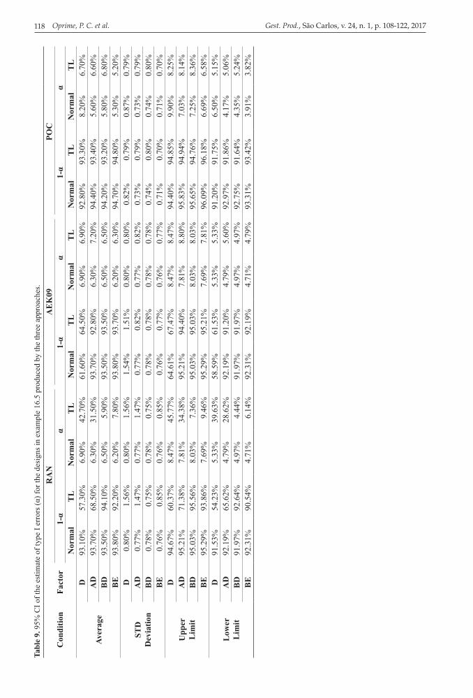
Regarding example 16.5, Figure 2 shows that the design produced by RAN approach has higher mean correlation and lower maximum correlation than the AEK09 and POC designs. It also shows that estimation errors (ε ), number of factor changes and time count are smaller in the systematic approaches. These results implied lesser types I and II errors and lower correlation with time, i.e., more robustness to the linear trend effects in AEK09 and POC. The differences among the three approaches in terms of type I and II errors are shown in Tables 9 and 10.
Table 9 shows, for each approach, the estimate of type I error at 95% confidence interval (95% CI) and the probability of making the correct decision (1-α) when the factor has effect on the response variable. Note that there is no intersection between the confidence intervals under LT and Normal conditions for factor D and the AD interaction
Table 4. Time count and correlation between the columns in the 16.5 design produced by RAN approach.Factors TC ρ
A 0 0.136B 34 0.461C 12 0.163D 30 0.407E 6 0.081
AB 4 0.054AC 2 0.027AD 24 0.325AE 20 0.271BC 14 0.190BD 4 0.054BE 24 0.325
Average (ρ) 0.208
Table 5. Estimate of the main effects and second order interactions for the 16.5 design produced by the AEK09 approach.
Factors Estimated Dif Statistical significanceNormal TL Normal TL
A –2.79605 –2.76683 –0.02922 1000 1000B –2.27672 –2.17525 –0.10147 1000 1000C –0.16492 –0.16587 0.000952 384 355D –0.00299 –0.00769 0.004698 69 69E –3.79776 –3.76686 –0.0309 1000 1000
AB 1.734983 1.767742 –0.03276 1000 1000AC 1.004719 1.001869 0.00285 1000 1000AD 0.002595 -0.00023 0.00282 63 72AE 2.411162 2.381798 0.029364 1000 1000BC 0.501172 0.502724 –0.00155 992 994BD 0.0045 0.001125 0.003375 65 65BE 0.00219 0.004117 –0.00193 62 63
Average 0.020156

Systematic sequencing of factorial experiments... 117
for RAN approach (for example, the upper limit of variable D under normal condition, α = 8.47%, is lesser than the lower limit under LT condition, α = 39.63%). As for AEK09, the variable D interval
under normal condition is [5.33%; 8.47%]; under LT condition, the confidence interval is equal to [5.33%; 8.47%]; as for AD, BD and BE interactions under normal condition, they are, respectively:
Table 7. Estimate of the main effects and second order interactions in the 16.5 design produced by the POC approach.Factors Estimated Dif Statistical significance
Normal TL Normal TLA –2.7879 –2.7888 0.0009 1000 1000B –2.2779 –2.268 –0.0099 1000 1000C –0.1679 –0.16 –0.0079 329 353D –0.0021 0.0021 –0.0042 82 67E –3.7992 –3.8 0.0008 1000 1000
AB 1.7371 1.7395 –0.0024 1000 1000AC 1.0004 0.9999 0.0005 1000 1000AD 0.0079 0.0011 0.0068 56 66AE 2.4135 2.3907 0.0228 1000 1000BC 0.4988 0.5523 –0.0535 995 1000BD 0.0037 0.0214 –0.0177 58 68BE 0.0003 –0.0036 0.0039 53 52
Average –0.00499167
Table 6. Count time and correlation in the 16.5 design produced by the AEK09 approach.Factors TC ρ
A 0 0.000B 0 0.000C 0 0.000D 0 0.000E 0 0.000
AB 48 0.651AC 28 0.380AD 4 0.054AE 0 0.000BC 4 0.054BD 4 0.054BE 16 0.217
Average (ρ) 0.118
Table 8. Time count and correlation between the columns in the 16.5 design produced by the POC approach.Factors TC ρ
A 0 0.000B 0 0.000C 0 0.000D 0 0.000E 0 0.000
AB 0 0.000AC 0 0.000AD 0 0.000AE 16 0.217BC 44 0.597BD 16 0.217BE 4 0.054
Average (ρ) 0.090
Oprime, P. C. et al.118 Gest. Prod., São Carlos, v. 24, n. 1, p. 108-122, 2017Ta
ble
9. 9
5% C
I of t
he e
stim
ate
of ty
pe I
erro
rs (α
) for
the
desi
gns i
n ex
ampl
e 16
.5 p
rodu
ced
by th
e th
ree
appr
oach
es.
Con
ditio
nFa
ctor
RA
NA
EK
09PO
C1-
αα
1-α
α1-
αα
Nor
mal
TL
Nor
mal
TL
Nor
mal
TL
Nor
mal
TL
Nor
mal
TL
Nor
mal
TL
Aver
age
D93
.10%
57.3
0%6.
90%
42.7
0%61
.60%
64.5
0%6.
90%
6.90
%92
.80%
93.3
0%8.
20%
6.70
%A
D93
.70%
68.5
0%6.
30%
31.5
0%93
.70%
92.8
0%6.
30%
7.20
%94
.40%
93.4
0%5.
60%
6.60
%B
D93
.50%
94.1
0%6.
50%
5.90
%93
.50%
93.5
0%6.
50%
6.50
%94
.20%
93.2
0%5.
80%
6.80
%B
E93
.80%
92.2
0%6.
20%
7.80
%93
.80%
93.7
0%6.
20%
6.30
%94
.70%
94.8
0%5.
30%
5.20
%
STD
Dev
iatio
n
D0.
80%
1.56
%0.
80%
1.56
%1.
54%
1.51
%0.
80%
0.80
%0.
82%
0.79
%0.
87%
0.79
%A
D0.
77%
1.47
%0.
77%
1.47
%0.
77%
0.82
%0.
77%
0.82
%0.
73%
0.79
%0.
73%
0.79
%B
D0.
78%
0.75
%0.
78%
0.75
%0.
78%
0.78
%0.
78%
0.78
%0.
74%
0.80
%0.
74%
0.80
%B
E0.
76%
0.85
%0.
76%
0.85
%0.
76%
0.77
%0.
76%
0.77
%0.
71%
0.70
%0.
71%
0.70
%
Upp
erL
imit
D94
.67%
60.3
7%8.
47%
45.7
7%64
.61%
67.4
7%8.
47%
8.47
%94
.40%
94.8
5%9.
90%
8.25
%A
D95
.21%
71.3
8%7.
81%
34.3
8%95
.21%
94.4
0%7.
81%
8.80
%95
.83%
94.9
4%7.
03%
8.14
%B
D95
.03%
95.5
6%8.
03%
7.36
%95
.03%
95.0
3%8.
03%
8.03
%95
.65%
94.7
6%7.
25%
8.36
%B
E95
.29%
93.8
6%7.
69%
9.46
%95
.29%
95.2
1%7.
69%
7.81
%96
.09%
96.1
8%6.
69%
6.58
%
Low
erL
imit
D91
.53%
54.2
3%5.
33%
39.6
3%58
.59%
61.5
3%5.
33%
5.33
%91
.20%
91.7
5%6.
50%
5.15
%A
D92
.19%
65.6
2%4.
79%
28.6
2%92
.19%
91.2
0%4.
79%
5.60
%92
.97%
91.8
6%4.
17%
5.06
%B
D91
.97%
92.6
4%4.
97%
4.44
%91
.97%
91.9
7%4.
97%
4.97
%92
.75%
91.6
4%4.
35%
5.24
%B
E92
.31%
90.5
4%4.
71%
6.14
%92
.31%
92.1
9%4.
71%
4.79
%93
.31%
93.4
2%3.
91%
3.82
%
Systematic sequencing of factorial experiments... 119
Tabl
e 10
. 95%
CI o
f the
type
II e
rror
s (β)
est
imat
e fo
r the
16.
5 de
sign
s pro
duce
d by
the
thre
e ap
proa
ches
.
Con
ditio
nsFa
ctor
RA
NA
EK
09PO
C1-
βΒ
1- β
β1-
βΒ
Nor
mal
TL
Nor
mal
TL
Nor
mal
TL
Nor
mal
TL
Nor
mal
TL
Nor
mal
TL
Aver
age
A10
0.00
%10
0.00
%0.
00%
0.00
%10
0.00
%10
0.00
%0.
00%
0.00
%10
0.00
%10
0.00
%0.
00%
0.00
%B
100.
00%
100.
00%
0.00
%0.
00%
100.
00%
100.
00%
0.00
%0.
00%
100.
00%
100.
00%
0.00
%0.
00%
C38
.40%
14.2
0%61
.60%
85.8
0%38
.40%
35.5
0%61
.60%
64.5
0%32
.90%
35.3
0%67
.10%
64.7
0%E
100.
00%
100.
00%
0.00
%0.
00%
100.
00%
100.
00%
0.00
%0.
00%
100.
00%
100.
00%
0.00
%0.
00%
AB
100.
00%
100.
00%
0.00
%0.
00%
100.
00%
100.
00%
0.00
%0.
00%
100.
00%
100.
00%
0.00
%0.
00%
AC
100.
00%
100.
00%
100.
00%
100.
00%
100.
00%
100.
00%
0.00
%0.
00%
100.
00%
100.
00%
0.00
%0.
00%
AE
100.
00%
100.
00%
100.
00%
100.
00%
100.
00%
100.
00%
0.00
%‘0
.00%
100.
00%
100.
00%
0.00
%0.
00%
BC
99.2
0%96
.40%
0.80
%3.
60%
99.2
0%99
.40%
0.80
%0.
60%
99.5
0%10
0.00
%0.
50%
0.00
%
STD
Dev
iatio
n
A0.
00%
0.00
%0.
00%
0.00
%0.
00%
0.00
%0.
00%
0.00
%0.
00%
0.00
%0.
00%
0.00
%B
0.00
%0.
00%
0.00
%0.
00%
0.00
%0.
00%
0.00
%0.
00%
0.00
%0.
00%
0.00
%0.
00%
C1.
54%
1.10
%1.
54%
1.10
%1.
54%
1.51
%1.
54%
1.51
%1.
49%
1.51
%1.
49%
1.51
%E
0.00
%0.
00%
0.00
%0.
00%
0.00
%0.
00%
0.00
%0.
00%
0.00
%0.
00%
0.00
%0.
00%
AB
0.00
%0.
00%
0.00
%0.
00%
0.00
%0.
00%
0.00
%0.
00%
0.00
%0.
00%
0.00
%0.
00%
AC
0.00
%0.
00%
0.00
%0.
00%
0.00
%0.
00%
0.00
%0.
00%
0.00
%0.
00%
0.00
%0.
00%
AE
0.00
%0.
00%
0.00
%0.
00%
0.00
%0.
00%
0.00
%0.
00%
0.00
%0.
00%
0.00
%0.
00%
BC
0.28
%0.
59%
0.28
%0.
59%
0.28
%0.
24%
0.28
%0.
24%
0.22
%0.
00%
0.22
%0.
00%
Upp
erlim
its
A10
0.00
%10
0.00
%0.
00%
0.00
%10
0.00
%10
0.00
%0.
00%
0.00
%10
0.00
%10
0.00
%0.
00%
0.00
%B
100.
00%
100.
00%
0.00
%0.
00%
100.
00%
100.
00%
0.00
%0.
00%
100.
00%
100.
00%
0.00
%0.
00%
C41
.41%
16.3
6%64
.61%
87.9
6%41
.41%
38.4
7%64
.61%
67.4
7%35
.81%
38.2
6%70
.01%
67.6
6%E
100.
00%
100.
00%
0.00
%0.
00%
100.
00%
100.
00%
0.00
%0.
00%
100.
00%
100.
00%
0.00
%0.
00%
AB
100.
00%
100.
00%
0.00
%0.
00%
100.
00%
100.
00%
0.00
%0.
00%
100.
00%
100.
00%
0.00
%0.
00%
AC
100.
00%
100.
00%
100.
00%
100.
00%
100.
00%
100.
00%
0.00
%0.
00%
100.
00%
100.
00%
0.00
%0.
00%
AE
100.
00%
100.
00%
100.
00%
100.
00%
100.
00%
100.
00%
0.00
%0.
00%
100.
00%
100.
00%
0.00
%0.
00%
BC
99.7
5%97
.55%
1.35
%4.
75%
99.7
5%99
.88%
1.35
%1.
08%
99.9
4%10
0.00
%0.
94%
0.00
%
Low
erL
imits
A10
0.00
%10
0.00
%0.
00%
0.00
%10
0.00
%10
0.00
%0.
00%
0.00
%10
0.00
%10
0.00
%0.
00%
0.00
%B
100.
00%
100.
00%
0.00
%0.
00%
100.
00%
100.
00%
0.00
%0.
00%
100.
00%
100.
00%
0.00
%0.
00%
C35
.39%
12.0
4%58
.59%
83.6
4%35
.39%
32.5
3%58
.59%
61.5
3%29
.99%
32.3
4%64
.19%
61.7
4%E
100.
00%
100.
00%
0.00
%0.
00%
100.
00%
100.
00%
0.00
%0.
00%
100.
00%
100.
00%
0.00
%0.
00%
AB
100.
00%
100.
00%
0.00
%0.
00%
100.
00%
100.
00%
0.00
%0.
00%
100.
00%
100.
00%
0.00
%0.
00%
AC
100.
00%
100.
00%
100.
00%
100.
00%
100.
00%
100.
00%
0.00
%0.
00%
100.
00%
100.
00%
0.00
%0.
00%
AE
100.
00%
100.
00%
100.
00%
100.
00%
100.
00%
100.
00%
0.00
%0.
00%
100.
00%
100.
00%
0.00
%0.
00%
BC
98.6
5%95
.25%
0.25
%2.
45%
98.6
5%98
.92%
0.25
%0.
12%
99.0
6%10
0.00
%0.
06%
0.00
%

Oprime, P. C. et al.120 Gest. Prod., São Carlos, v. 24, n. 1, p. 108-122, 2017
[4.49%, 7.81%], [4.97%, 8.03%] and [4.71%, 7.69%]. Regarding LT condition, still considering the AEK09 approach, the confidence intervals are [5.60%, 8.88%], [4.97%, 8.03%] and [4.79%; 7.81%]. By comparing the CI of these variables between LT and Normal conditions, there is intersection between the intervals, with no statistically significant difference between the two conditions. The POC approach showed the same result, and it indicates that the systematic approach was more robust than the random approach in the presence of linear trend effects. Therefore, the systematic approach shows lesser false positives than the classical experiment-sequence-randomization approach in the presence of linear trend effects.
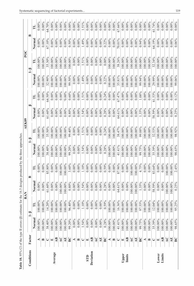
Table 10 shows the results of the estimate of type II errors and of the power of the test given by (1-β) at 95% confidence interval (95% CI). As for the main effect C and BC interaction, it was possible to see that the type II error was greater when the design was subjected to linear trend effects and the execution order was randomized (RAN procedure). However, it was not observed in the AEK09 and POC procedures. Statistical evidences were obtained by comparing the confidence intervals. Regarding the AEK09 approach under LT condition, it was observed that the CI of variable C was [61.53%; 67.47%]; under the normal condition, it was [58.59%; 64.61%]; therefore, there was intersection between the two conditions, a fact that did not occur in the random approach. Thus, there were strong statistical evidences that the two systematic approaches generated lesser type II error and better power of the test than the random approach.
The analyses show statistical evidence that the systematic experiment execution order may have advantages over randomization. In the case of example 16.5, the advantages were related to statistical properties, in terms of type I and II errors, as well as to the number of factor changes in the experiments. It was also possible to observe that the POC approach
in this example had the best performance in terms of the number of factor changes and in the mean and maximum correlations in comparison to the AEK09 approach, whereas AEK09 ensured designs that were robust in the main effects.
6 Conclusions and future research perspectivesThe classic DoE books recommend randomizing
the experiments execution order to minimize possible linear trend effects. However, Daniel & Wilcoxon (1966) and Draper & Stoneman (1968) questioned this practice since the 1960s. More recently, several authors have been emphatically exposing the inadequate experiment randomization issue and they suggest using algorithms to generate designs according to different criteria.
The current study sought to contribute to this debate by taking into consideration two design-generating approaches in which the sequencing of experiments is systematically done and one approach that randomizes the sequencing. The three proposals were compared based on six examples of two-level factorial design, and it was possible to see that systematic approaches had advantages over randomization in most of the analyzed criteria. In particular, the simulation of a real case statistically proved that the randomization increased the type I and II errors, which reduced the power of the experiment to detect important process factors and to make correct assumptions about the significance of factors.
As for the future research perspective, the good results obtained by the mathematical programming model for the sequencing of experiments motivate the research extension in order to include the decision about the set of experiments to form the matrix. Such extension must simultaneously take into consideration criteria such as D-efficiency, time count and number of factor changes at the time the experiments are chosen. Given the greater complexity of the involved
Figure 2. Estimation errors, mean correlation, maximum correlation and number of factor changes in the designs of the approaches for example 16.5.
Systematic sequencing of factorial experiments... 121
decisions, the major challenge will be to develop a well-settled formulation by optimization methods.
ReferencesAddelman, S. (1972). Recent development in the designs of
factorial experiments. Journal of the American Statistical Association, 67(337), 103-111. http://dx.doi.org/10.1080/01621459.1972.10481211.
Adekeye, K.S., & Kunert, J. (2005). On the comparison of run orders of unreplicated 2k-p-design in the process of a time-trend. Techinical Report, Universitat Dortmund, (3), 475.
Aggarwal, M. L., Budhraja, V., & Lin, D. K. J. (2003). New class of orthogonal arrays and its applications. IAPQR Transactions, 28(1), 23-32.
Alonso, M. C., Bousbaine, A., Llovet, J., & Malpica, J. A. (2011). Obtaining industrial experimental designs using a heuristic technique. Expert Systems with Applications, 38(8), 10094-10098. http://dx.doi.org/10.1016/j.eswa.2011.02.004.
Angelopoulos, P., Evangelaras, H., & Koukouvinos, C. (2009). Run orders for efficient two level experimental plans with minimum factor level changes robust to time trends. Journal of Statistical Planning and Inference, 139(10), 3718-3724. http://dx.doi.org/10.1016/j.jspi.2009.05.002.
Atkinson, A. C. (1996). The usefulness of optimum experimental designs. Journal of the Royal Statistical Society. Series B. Methodological, 58(1), 59-76.
Atkinson, A. C., & Bailey, R. A. (2001). On hundred year of the design of experiments on and off the pages of Biometrika. Biometrika, 88(1), 53-97. http://dx.doi.org/10.1093/biomet/88.1.53.
Atkinson, A. C., & Donev, A. N. (1996). Experimental designs optimally balanced for trend. Technometrics, 38(4), 333-341. http://dx.doi.org/10.1080/00401706.1996.10484545.
Atkinson, A. C., Donev, A. N., & Tobias, R. D. (2007). Optimum experiments design with SAS. New York: Oxford Press.
Bailey, R. A., Cheng, C. S., & Kipnis, P. (1992). Construction of trend-resistant factorial designs. Statistica Sinica, 2, 393-411.
Bertsimas, D., Johnson, M., & Kallus, N. (2015). The power of optimization over randomization in designing experiments involving small samples. Operations Research, 63(4), 868-876. http://dx.doi.org/10.1287/opre.2015.1361.
Bessant, J., Caffyn, S., & Gallagher, M. (2001). An evolutionary model of continuous improvement behavior. Technovation, 21(2), 67-77. http://dx.doi.org/10.1016/S0166-4972(00)00023-7.
Bessant, J., & Caffyn, S. (1997). High involvement innovation through continuous improvement. International Journal
of Technology Management, 14(3), 7-28. http://dx.doi.org/10.1504/IJTM.1997.001705.
Box, G. E. P., Hunter, W. G., & Hunter, J. S. (1978). Statistics for experimenters. New York: Wiley.
Cheng, C.-S. (1985). Run orders of factorial designs. In L. LeCam & R. A. Olshen (Eds.), Proceedings of the Berkeley Conference in Honor of Jerzy Neyman and Jack Kiefer (pp. 619-633). Wadsworth.
Cheng, C.-S. (1990). Construction of run orders of factorial designs. In S. Ghosh (Ed.), Statistical design and analysis of industrial experiments (pp. 423-39). New York: Subir Ghosh.
Cheng, C.-S., & Jacroux, M. (1988). On the construction of trend-free run orders of two level factorial designs. Journal of the American Statistical Association, 83(404), 1152-1158. http://dx.doi.org/10.1080/01621459.1988.10478713.
Cook, R. D., & Nachtsheim, C. J. A. (1980). Comparison of algorithms for constructing exact D-optimal designs. Technometrics, 22(3), 315-324. http://dx.doi.org/10.1080/00401706.1980.10486162.
Cordier, C., Marchand, H., Laundy, R., & Wolsey, L. A. (1999). bc-opt: a branch-and-cut code for mixed integer programs. Mathematical Programming, 86(2), 335-353. http://dx.doi.org/10.1007/s101070050092.
Coster, D. C., & Cheng, C.-S. (1988). Minimum cost trend-free run orders of fractional factorial designs. Annals of Statistics, 16(3), 1188-1205. http://dx.doi.org/10.1214/aos/1176350955.
Daniel, C., & Wilcoxon, F. (1966). Factorial 2p-q plans robust against linear and quadratic trends. Technometrics, 8, 259-278.
Davis, O. L. (1956). The design and analysis of industrial experiments. London: Longman. 637 p.
Delbridge, R., & Barton, H. (2002). Organizing for continuous improvement: structures and roles in automotive components plants. International Journal of Operations & Production Management, 22(6), 680-692. http://dx.doi.org/10.1108/01443570210427686.
Dickinson, A. W. (1974). Some run orders requirements a minimum number of factor level changes for the 24 and 25 main effect plans. Technometrics, 16, 31-37.
Draper, N. R., & Stoneman, D. M. (1968). Factor changes and linear trends in eight-run two level factorial designs. Technometrics, 10(2), 301-311. http://dx.doi.org/10.1080/00401706.1968.10490562.
Dykstra, O. (1971). The Augmentation of experimental data to maximize |X′X|. Technometrics, 13(3), 682-688.
Fisher, R. (1926). The arrangement of field experiments. Journal of the Ministry of Agriculture of Great Britain, 33, 503-513.
Galil, Z., & Kiefer, J. (1980). Time- and space-saving computer methods related to Mitchell’s DETMAX for

Oprime, P. C. et al.122 Gest. Prod., São Carlos, v. 24, n. 1, p. 108-122, 2017
finding D-Optimum designs. Technometrics, 22(3), 301-313. http://dx.doi.org/10.1080/00401706.1980.10486161.
Ganju, J., & Lucas, J. M. (2004). Randomized and random run order experiments. Journal of Statistical Planning and Inference, 133(1), 199-210. http://dx.doi.org/10.1016/j.jspi.2004.03.009.
Garroi, J. J., Goos, P., & Sorensen, K. (2009). A variable-neighborhood search algorithm for finding optimal run orders in the presence of serial correlation. Journal of Statistical Planning and Inference, 139(1), 30-44. http://dx.doi.org/10.1016/j.jspi.2008.05.014.
Gibbons, J. D., & Chakraborti, S. (2011). Nonparametric statistical inference (5th ed.). New York: Taylor & Francis.
Githinji, F., & Jacroux, M. (1998). On the determination and construction of optimal designs for comparing a set of test treatments with a set of controls in the presence of a linear trend. Journal of Statistical Planning and Inference, 66(1), 61-74. http://dx.doi.org/10.1016/S0378-3758(97)00067-0.
Harrison, A. (2000). Continuous improvement: the trade-off between self-management and discipline. Integrated Manufacturing Systems, 11(3), 180-187. http://dx.doi.org/10.1108/09576060010320416.
Hilow, H. (2013). Comparison among run order algorithms for sequential factorial experiments. Computational Statistics & Data Analysis, 58, 397-406. http://dx.doi.org/10.1016/j.csda.2012.09.013.
Hyland, P. W., Soosay, C., & Sloan, T. R. (2003). Continuous improvement and learning in the supply chain. International Journal of Physical Distribution & Logistics Management, 33(4), 316-335. http://dx.doi.org/10.1108/09600030310478793.
Imai, M. (1997). Gemba Kaisen: a common sense, low-cost approach to management. New York: McGraw-Hill.
Jacroux, M. (1994). On the construction of trend-resistant fractional factorial row-column designs. The Indian Journal of Statistics, 56(Pt. 2), 251-258.
Joiner, B. L., & Campbell, C. (1976). Designing experiments when run order is important. Technometrics, 18(3), 249-259. http://dx.doi.org/10.1080/00401706.1976.10489445.
Kume, H. (1993). Métodos estatísticos para melhoria da qualidade (11. ed.). São Paulo: Gente. 245 p.
Marin-Garcia, J. A., Val, M. P., & Martin, T. B. (2008). Longitudinal study of the results of continuous improvement in an industrial company. Team Performance Management, 14(1/2), 56-6.
Mitchell, T. J. (1974). An algorithm for the construction of D-optimal experimental designs. Technometrics, 16, 203-211.
Montgomery, C. D., Runger, G. C., & Hubele, N. F. (2009). Engineering statistics. New York: John Wiley & Sons.
Montgomery, D. C. (1991). Design and analysis of experiments. New York: John Wiley & Sons.
Oprime, P. C., Monsanto, R., & Donadone, J. C. (2010). Análise da complexidade, estratégias e aprendizagem em projetos de melhoria contínua: estudos de caso em empresas brasileiras. Gestão & Produção, 17, 669-682.
Pureza, V., Oprime, P. C., & Costa, A. F. (2014). Some experiments on mathematical programming for experiment sequencing (Documento de pesquisa).
Savolainen, T. I. (1999). Cycles of continuous improvement: realizing competitive advantages through quality. International Journal of Operations & Production Management, 19(11), 1203-1222. http://dx.doi.org/10.1108/01443579910291096.
Street, D. J., & Burgess, L. (2008). Some open combinatorial problems in the design of stated choice experiments. Discrete Mathematics, 308(13), 2781-2788. http://dx.doi.org/10.1016/j.disc.2006.06.042.
Suen, C., & Midha, A. C. K. (2013). Optimal fractional factorial designs and their construction. Journal of Statistical Planning and Inference, 143(10), 1828-1834. http://dx.doi.org/10.1016/j.jspi.2013.05.004.
Tack, L., & Vandebroek, M. (2004). Trend-resistant and cost-efficient cross-over designs for mixed models. Computation Statistics & Data Analysis, (46), 721-746.
Toledo, J. C. (1986). Qualidade Industrial: conceitos, sistemas e estratégias. São Paulo: Editora Atlas.
Triefenbach, F. (2008). Design of experiments: the D-Optimal approach and its implementation as a computer algorithm (Bachelor’s thesis). UMEA University, Umea; South Westphalia University of Applied Sciences, Meschede.
Tsao, H.-S. J., & Liu, H. (2008). Optimal sequencing of test conditions in 2k factorial experimental design for run-size minimization. Computers & Industrial Engineering, 55(2), 450-464. http://dx.doi.org/10.1016/j.cie.2008.01.006.
Wang, P. C. (1991). Symbol changes and trend resistance in orthogonal plans of symmetric factorials. The Indian Journal of Statistics, 53(Pt. 3), 297-303.
Wang, P. C., & Chen, M. H. (1998). Level changes and trend resistance on replacement in asymmetric orthogonal arrays. Journal of Statistical Planning and Inference, 69(2), 349-358. http://dx.doi.org/10.1016/S0378-3758(97)00168-7.
Wang, P. C., & Jan, H. W. (1995). Designing two-level factorial experiments using orthogonal arrays when the run order is important. The Statistician, 44(3), 379-388. http://dx.doi.org/10.2307/2348709.
Wilmut, M., & Zhou, J. (2011). D-optimal minimax design criterion for two-level fractional factorial designs. Journal of Statistical Planning and Inference, 141(1), 576-587. http://dx.doi.org/10.1016/j.jspi.2010.07.002.