Embed Size (px)
Citation preview
Temporal reasoning in a logic programminglanguage with modularity
Vitor Beires Nogueira
Orientador: Professor Doutor Salvador Pinto Abreu
Tese submetida à Universidade de Évora
para obtenção do grau de Doutor em Informática
Departamento de InformáticaUniversidade de Évora
Dezembro de 2008

Temporal reasoning in a logic programminglanguage with modularity
Vitor Beires Nogueira
Orientador: Professor Doutor Salvador Pinto Abreu
Departamento de InformáticaUniversidade de Évora
Dezembro de 2008


To Miguel and Susana with love


Acknowledgments
First of all, I would like to thank my son Miguel and my wife Susana for their caringsupport throughout the years of this work. To my parents and sister also goes myendless gratitude.
I thank my supervisor, Prof. Salvador Pinto Abreu, without whom this work wouldn'thave started, continued and most of all, �nished. His participation on this thesis wentfar beyond the expected critical watching and directing. I am thankful for the manyinteresting discussions that we had, during which he guided me into how to do scienti�cresearch. I thank him also for the great working conditions and for carefully reviewingnot only the contents but also the English, making this work not only understandablebut also readable.
I would also like to thank Prof. Gabriel Torcato David for his participation in this work.Besides providing me with great working conditions at the Faculdade de Engenhariaof Universidade do Porto, he also supervised the beginning of this thesis.
Throughout this thesis, I also had the chance of working with members of ProjetContraintes at INRIA Rocquencourt and in particular with Prof. Daniel Diaz. Severalimportant results came out of such cooperation. I acknowledge the INRIA/GRICESproject �Extensions au Logiciel Libre GNU Prolog� for the �nancial support that madethis collaboration possible.
I would like to acknowledge the Universidade de Évora and speci�cally the Departmentode Informática not only for the conditions given but also for the leave that allowed meto focus entirely on this work.
I also acknowledge the Centria (Centro de Inteligência Arti�cial) that by providingsupervisor funds, allowed me to participate in summer schools, conferences, workshops,doctoral programs, etc.
Last, but de�nitely not least, I would like to dedicate this work to my friends, and inparticular to Paulo Estudante who was there for me on many occasions.
i


Abstract
Current Organisational Information Systems (OIS) deal with more and more infor-mation that is time dependent. In this work we provide a framework to constructand maintain Temporal OIS. This framework builds upon a logical language calledTemporal Contextual Logic Programming that deeply integrates modularity with tem-poral reasoning making the usage of a module time dependent. This language is anevolution of another one, also introduced in this thesis, that combines ContextualLogic Programming with Temporal Annotated Constraint Logic Programming wheremodularity and time are orthogonal features. Both languages are formally discussedand illustrated.
The main contributions of the work described in this thesis include:
• Optimisation of Contextual Logic Programming (CxLP) through abstract inter-pretation.
• Syntax and operational semantics for an independent combination of the temporalframework Temporal Annotated Constraint Logic Programming (TACLP) andCxLP. A compiler for this language is also provided.
• Language (syntax and semantics) that integrates in a innovative way modularity(CxLP) with temporal reasoning (TACLP). In this language the usage of a givenmodule depends of the time of the context. An interpreter and a compiler forthis language are described.
• Framework to construct and maintain Temporal Organisational Information Sys-tems. It builds upon a revised speci�cation of the language ISCO, adding tempo-ral classes and temporal data manipulation. A compiler targeting the languagepresented in the previous item is also given.
iii


Sumário
Actualmente os Sistemas de Informação Organizacionais (SIO) lidam cada vez maiscom informação que tem dependências temporais. Neste trabalho concebemos umambiente de trabalho para construir e manter SIO Temporais. Este ambiente assentasobre um linguagem lógica denominada Temporal Contextual Logic Programmingque integra modularidade com raciocínio temporal fazendo com que a utilização deum módulo dependa do tempo do contexto. Esta linguagem é a evolução de umaoutra, também introduzida nesta tese, que combina Contextual Logic Programmingcom Temporal Annotated Constraint Logic Programming, na qual a modularidade e otempo são características ortogonais. Ambas as linguagens são formalmente discutidase exempli�cadas.
As principais contribuições do trabalho descrito nesta tese incluem:
• Optimização de Contextual Logic Programming (CxLP) através de interpretaçãoabstracta.
• Sintaxe e semântica operacional para uma linguagem que combina de um modoindependente as linguagens Temporal Annotated Constraint Logic Programming(TACLP) e CxLP. É apresentado um compilador para esta linguagem.
• Linguagem (sintaxe e semântica) que integra de um modo inovador modularidade(CxLP) com raciocínio temporal (TACLP). Nesta linguagem a utilização de umdado módulo está dependente do tempo do contexto. É descrito um interpretadore um compilador para esta linguagem.
• Ambiente de trabalho para construir e fazer a manutenção de SIO Temporais.Assenta sobre uma especi�cação revista da linguagem ISCO, adicionando classes emanipulação de dados temporais. É fornecido um compilador em que a linguagemresultante é a descrita no item anterior.
v


Contents
Acknowledgments i
Abstract iii
Sumário v
List of Acronyms xix
Preface 1
1 Introduction and Motivation 3
1.1 Introduction . . . . . . . . . . . . . . . . . . . . . . . . . . . . . . . . . . . . . 3
1.1.1 Time . . . . . . . . . . . . . . . . . . . . . . . . . . . . . . . . . . . . . 3
1.1.2 Modularity . . . . . . . . . . . . . . . . . . . . . . . . . . . . . . . . . 4
1.1.3 Organisational Information Systems . . . . . . . . . . . . . . . . . . . 5
1.2 Temporal (Logic-Based) OIS . . . . . . . . . . . . . . . . . . . . . . . . . . . . 5
2 Temporal Reasoning in AI 7
2.1 Introduction . . . . . . . . . . . . . . . . . . . . . . . . . . . . . . . . . . . . . 7
2.2 General Notions of Time . . . . . . . . . . . . . . . . . . . . . . . . . . . . . . 8
2.2.1 Model of Time . . . . . . . . . . . . . . . . . . . . . . . . . . . . . . . 8
2.2.2 Temporal Quali�cation . . . . . . . . . . . . . . . . . . . . . . . . . . . 8
2.3 Constraint-Based Temporal Reasoning . . . . . . . . . . . . . . . . . . . . . . 9
2.3.1 Qualitative Temporal Constraints . . . . . . . . . . . . . . . . . . . . . 10
vii

viii CONTENTS
2.3.2 Metric Point Constraints . . . . . . . . . . . . . . . . . . . . . . . . . . 11
2.3.3 Hybrid Approaches . . . . . . . . . . . . . . . . . . . . . . . . . . . . . 12
2.3.4 Programming Languages . . . . . . . . . . . . . . . . . . . . . . . . . . 12
2.4 Temporal Modal Logic . . . . . . . . . . . . . . . . . . . . . . . . . . . . . . . 15
2.4.1 Temporal Logic Programming . . . . . . . . . . . . . . . . . . . . . . . 15
2.5 Reasoning About Actions and Change . . . . . . . . . . . . . . . . . . . . . . 16
2.5.1 The Situation Calculus . . . . . . . . . . . . . . . . . . . . . . . . . . . 17
2.5.2 The Event Calculus . . . . . . . . . . . . . . . . . . . . . . . . . . . . 18
2.5.3 Temporal Nonmonotonic Reasoning . . . . . . . . . . . . . . . . . . . 18
2.6 Conclusions . . . . . . . . . . . . . . . . . . . . . . . . . . . . . . . . . . . . . 19
3 Temporal Databases 21
3.1 Introduction . . . . . . . . . . . . . . . . . . . . . . . . . . . . . . . . . . . . . 21
3.2 Temporal Data Semantics . . . . . . . . . . . . . . . . . . . . . . . . . . . . . 22
3.3 Temporal Data Models and Languages . . . . . . . . . . . . . . . . . . . . . . 22
3.3.1 Temporal Data Model . . . . . . . . . . . . . . . . . . . . . . . . . . . 23
3.3.2 Temporal Languages . . . . . . . . . . . . . . . . . . . . . . . . . . . . 26
3.4 Temporal Databases Design . . . . . . . . . . . . . . . . . . . . . . . . . . . . 32
3.5 Temporal Database Products . . . . . . . . . . . . . . . . . . . . . . . . . . . 32
3.5.1 Log Explorer . . . . . . . . . . . . . . . . . . . . . . . . . . . . . . . . 32
3.5.2 Time Navigator . . . . . . . . . . . . . . . . . . . . . . . . . . . . . . . 33
3.5.3 Data Propagator . . . . . . . . . . . . . . . . . . . . . . . . . . . . . . 33
3.5.4 SQL:2003 . . . . . . . . . . . . . . . . . . . . . . . . . . . . . . . . . . 33
3.5.5 Oracle . . . . . . . . . . . . . . . . . . . . . . . . . . . . . . . . . . . . 34
3.5.6 TimeDB . . . . . . . . . . . . . . . . . . . . . . . . . . . . . . . . . . . 35
3.6 Conclusions and Future Pointers . . . . . . . . . . . . . . . . . . . . . . . . . 35
4 Modular Logic Programming 37
4.1 Introduction . . . . . . . . . . . . . . . . . . . . . . . . . . . . . . . . . . . . . 37

CONTENTS ix
4.2 Algebraic Approach . . . . . . . . . . . . . . . . . . . . . . . . . . . . . . . . 38
4.2.1 The Algebra of Programs and Its Operators . . . . . . . . . . . . . . . 38
4.3 Logical Approach . . . . . . . . . . . . . . . . . . . . . . . . . . . . . . . . . . 39
4.3.1 Embedded Implications . . . . . . . . . . . . . . . . . . . . . . . . . . 39
4.3.2 Lexical Scoping . . . . . . . . . . . . . . . . . . . . . . . . . . . . . . . 41
4.3.3 Closed Scope Mechanisms . . . . . . . . . . . . . . . . . . . . . . . . . 42
4.3.4 Contextual Logic Programming . . . . . . . . . . . . . . . . . . . . . . 43
4.3.5 Lexical Scoping as Universal Quanti�cation . . . . . . . . . . . . . . . 44
4.4 Syntactic Approach . . . . . . . . . . . . . . . . . . . . . . . . . . . . . . . . . 45
4.4.1 Prolog Modules: the ISO Standard . . . . . . . . . . . . . . . . . . . . 46
4.4.2 Implementations . . . . . . . . . . . . . . . . . . . . . . . . . . . . . . 47
4.5 Logic and Objects . . . . . . . . . . . . . . . . . . . . . . . . . . . . . . . . . 50
4.5.1 Object-Oriented Programming and Embedded Implications . . . . . . 50
4.5.2 Logtalk . . . . . . . . . . . . . . . . . . . . . . . . . . . . . . . . . . . 51
4.6 Conclusions . . . . . . . . . . . . . . . . . . . . . . . . . . . . . . . . . . . . . 52
5 Contextual Logic Programming 53
5.1 Introduction . . . . . . . . . . . . . . . . . . . . . . . . . . . . . . . . . . . . . 53
5.2 The CxLP Language . . . . . . . . . . . . . . . . . . . . . . . . . . . . . . . . 54
5.3 Operational Semantics . . . . . . . . . . . . . . . . . . . . . . . . . . . . . . . 55
5.3.1 Application of the Rules . . . . . . . . . . . . . . . . . . . . . . . . . . 57
5.4 Declarative/Fix-Point Semantics . . . . . . . . . . . . . . . . . . . . . . . . . 57
5.5 Extensions . . . . . . . . . . . . . . . . . . . . . . . . . . . . . . . . . . . . . . 58
5.6 Optimisations . . . . . . . . . . . . . . . . . . . . . . . . . . . . . . . . . . . . 59
5.6.1 Abstract Interpretation for Static Scope Systems . . . . . . . . . . . . 60
5.7 Implementations . . . . . . . . . . . . . . . . . . . . . . . . . . . . . . . . . . 62
5.7.1 CSM (Contexts as SICStus Modules) . . . . . . . . . . . . . . . . . . . 62
5.7.2 GNU Prolog/CX . . . . . . . . . . . . . . . . . . . . . . . . . . . . . . 63

x CONTENTS
5.8 Conclusions . . . . . . . . . . . . . . . . . . . . . . . . . . . . . . . . . . . . . 66
6 Temporal Reasoning in a Modular Language 67
6.1 Introduction . . . . . . . . . . . . . . . . . . . . . . . . . . . . . . . . . . . . . 67
6.2 CxLP with Temporal Annotations . . . . . . . . . . . . . . . . . . . . . . . . 68
6.3 Constraint Theory . . . . . . . . . . . . . . . . . . . . . . . . . . . . . . . . . 70
6.4 Operational Semantics . . . . . . . . . . . . . . . . . . . . . . . . . . . . . . . 70
6.5 Interpreter and Compiler . . . . . . . . . . . . . . . . . . . . . . . . . . . . . . 71
6.5.1 Time Point Domain . . . . . . . . . . . . . . . . . . . . . . . . . . . . 71
6.6 Related Work . . . . . . . . . . . . . . . . . . . . . . . . . . . . . . . . . . . . 73
6.6.1 MuTACLP . . . . . . . . . . . . . . . . . . . . . . . . . . . . . . . . . 74
6.6.2 Other Approaches . . . . . . . . . . . . . . . . . . . . . . . . . . . . . 76
6.7 Concluding Remarks . . . . . . . . . . . . . . . . . . . . . . . . . . . . . . . . 77
7 Temporal Contextual Logic Programming 79
7.1 Introduction . . . . . . . . . . . . . . . . . . . . . . . . . . . . . . . . . . . . . 79
7.2 Language of TCxLP . . . . . . . . . . . . . . . . . . . . . . . . . . . . . . . . 80
7.2.1 Annotating Units . . . . . . . . . . . . . . . . . . . . . . . . . . . . . . 80
7.2.2 Temporal Annotated Contexts . . . . . . . . . . . . . . . . . . . . . . 81
7.2.3 Relating Temporal Contexts with Temporal Units . . . . . . . . . . . . 81
7.3 Computing the Least Upper Bound . . . . . . . . . . . . . . . . . . . . . . . . 84
7.3.1 Ground Temporal Conditions . . . . . . . . . . . . . . . . . . . . . . . 84
7.3.2 Non Ground Temporal Conditions . . . . . . . . . . . . . . . . . . . . 85
7.4 Operational Semantics . . . . . . . . . . . . . . . . . . . . . . . . . . . . . . . 87
7.4.1 Inference Rules . . . . . . . . . . . . . . . . . . . . . . . . . . . . . . . 87
7.5 TCxLP Compiler and Interpreter . . . . . . . . . . . . . . . . . . . . . . . . . 89
7.5.1 From TCxLP to CxLP+TACLP . . . . . . . . . . . . . . . . . . . . . 89
7.6 Application Examples . . . . . . . . . . . . . . . . . . . . . . . . . . . . . . . 91
7.6.1 Management of Work�ow Systems . . . . . . . . . . . . . . . . . . . . 91

CONTENTS xi
7.6.2 Legal Reasoning . . . . . . . . . . . . . . . . . . . . . . . . . . . . . . 94
7.6.3 Vaccination Program . . . . . . . . . . . . . . . . . . . . . . . . . . . . 95
7.7 Related Work . . . . . . . . . . . . . . . . . . . . . . . . . . . . . . . . . . . . 97
7.8 Conclusions . . . . . . . . . . . . . . . . . . . . . . . . . . . . . . . . . . . . . 98
8 Language for Temporal OIS 99
8.1 Introduction . . . . . . . . . . . . . . . . . . . . . . . . . . . . . . . . . . . . . 99
8.2 Revising the ISCO Programming Language . . . . . . . . . . . . . . . . . . . 100
8.2.1 Classes . . . . . . . . . . . . . . . . . . . . . . . . . . . . . . . . . . . . 100
8.2.2 Methods . . . . . . . . . . . . . . . . . . . . . . . . . . . . . . . . . . . 101
8.2.3 Inheritance . . . . . . . . . . . . . . . . . . . . . . . . . . . . . . . . . 102
8.2.4 Composition . . . . . . . . . . . . . . . . . . . . . . . . . . . . . . . . 102
8.2.5 Persistence . . . . . . . . . . . . . . . . . . . . . . . . . . . . . . . . . 103
8.2.6 Data Manipulation Goals . . . . . . . . . . . . . . . . . . . . . . . . . 105
8.3 The ISTO Language . . . . . . . . . . . . . . . . . . . . . . . . . . . . . . . . 106
8.3.1 Temporal Classes . . . . . . . . . . . . . . . . . . . . . . . . . . . . . . 106
8.3.2 Temporal Data Manipulation . . . . . . . . . . . . . . . . . . . . . . . 107
8.4 Compilation Scheme for ISTO . . . . . . . . . . . . . . . . . . . . . . . . . . . 107
8.4.1 Classes . . . . . . . . . . . . . . . . . . . . . . . . . . . . . . . . . . . . 108
8.4.2 Methods . . . . . . . . . . . . . . . . . . . . . . . . . . . . . . . . . . . 108
8.4.3 Inheritance . . . . . . . . . . . . . . . . . . . . . . . . . . . . . . . . . 108
8.4.4 Composition . . . . . . . . . . . . . . . . . . . . . . . . . . . . . . . . 109
8.4.5 Persistence . . . . . . . . . . . . . . . . . . . . . . . . . . . . . . . . . 110
8.4.6 Data Manipulation Goals . . . . . . . . . . . . . . . . . . . . . . . . . 110
8.4.7 Temporal Classes . . . . . . . . . . . . . . . . . . . . . . . . . . . . . . 110
8.4.8 Temporal Data Manipulation Goals . . . . . . . . . . . . . . . . . . . . 111
8.5 Comparison with Other Approaches . . . . . . . . . . . . . . . . . . . . . . . 112
8.6 Conclusions . . . . . . . . . . . . . . . . . . . . . . . . . . . . . . . . . . . . . 112

xii CONTENTS
9 Conclusions and Future Work 115
9.1 Conclusions . . . . . . . . . . . . . . . . . . . . . . . . . . . . . . . . . . . . . 115
9.2 Future Work . . . . . . . . . . . . . . . . . . . . . . . . . . . . . . . . . . . . 116
A GNU Prolog/CX 117
A.1 Tutorial . . . . . . . . . . . . . . . . . . . . . . . . . . . . . . . . . . . . . . . 117
A.1.1 Unit Directive . . . . . . . . . . . . . . . . . . . . . . . . . . . . . . . . 117
A.1.2 Unit Arguments . . . . . . . . . . . . . . . . . . . . . . . . . . . . . . 118
A.1.3 Context Extension . . . . . . . . . . . . . . . . . . . . . . . . . . . . . 119
A.1.4 Current Context . . . . . . . . . . . . . . . . . . . . . . . . . . . . . . 119
A.1.5 Context Traversal . . . . . . . . . . . . . . . . . . . . . . . . . . . . . 120
A.1.6 Context Switch . . . . . . . . . . . . . . . . . . . . . . . . . . . . . . . 123
A.1.7 Supercontext . . . . . . . . . . . . . . . . . . . . . . . . . . . . . . . . 124
A.1.8 Guided Context Traversal . . . . . . . . . . . . . . . . . . . . . . . . . 124
A.1.9 Calling Context . . . . . . . . . . . . . . . . . . . . . . . . . . . . . . . 125
A.1.10 Lazy Call . . . . . . . . . . . . . . . . . . . . . . . . . . . . . . . . . . 126
A.2 Reference Manual . . . . . . . . . . . . . . . . . . . . . . . . . . . . . . . . . . 128
A.2.1 Introduction . . . . . . . . . . . . . . . . . . . . . . . . . . . . . . . . . 128
A.2.2 Directives . . . . . . . . . . . . . . . . . . . . . . . . . . . . . . . . . . 128
A.2.3 Operators . . . . . . . . . . . . . . . . . . . . . . . . . . . . . . . . . . 128
A.2.4 Utilities . . . . . . . . . . . . . . . . . . . . . . . . . . . . . . . . . . . 132
B Constraint Logic Programming 133
B.1 Introduction . . . . . . . . . . . . . . . . . . . . . . . . . . . . . . . . . . . . . 133
B.2 Constraint Domains . . . . . . . . . . . . . . . . . . . . . . . . . . . . . . . . 134
B.2.1 Booleans: CLP(B) . . . . . . . . . . . . . . . . . . . . . . . . . . . . . 134
B.2.2 Pseudo�Booleans: CLP(PB) . . . . . . . . . . . . . . . . . . . . . . . . 134
B.2.3 Rationals/Reals: CLP(R) . . . . . . . . . . . . . . . . . . . . . . . . . 134
B.2.4 Finite Domains: CLP(FD) . . . . . . . . . . . . . . . . . . . . . . . . . 134
CONTENTS xiii
B.3 Constraint Solvers . . . . . . . . . . . . . . . . . . . . . . . . . . . . . . . . . 134
B.3.1 Incomplete Constraint Solvers . . . . . . . . . . . . . . . . . . . . . . . 135
B.4 Finite Domains . . . . . . . . . . . . . . . . . . . . . . . . . . . . . . . . . . . 136
B.4.1 Finite Domain Solvers . . . . . . . . . . . . . . . . . . . . . . . . . . . 136
B.4.2 Network Consistency . . . . . . . . . . . . . . . . . . . . . . . . . . . . 136
B.4.3 Constraint Propagation (CP) vs. Backtracking . . . . . . . . . . . . . 137
B.4.4 Constraint Propagation and Heuristics . . . . . . . . . . . . . . . . . . 137
B.4.5 Advanced Techniques . . . . . . . . . . . . . . . . . . . . . . . . . . . . 138
B.4.6 Global Constraints . . . . . . . . . . . . . . . . . . . . . . . . . . . . . 138
B.4.7 Optimisation Constraints . . . . . . . . . . . . . . . . . . . . . . . . . 138
B.5 Defeasible Constraints . . . . . . . . . . . . . . . . . . . . . . . . . . . . . . . 138
B.6 Conclusions . . . . . . . . . . . . . . . . . . . . . . . . . . . . . . . . . . . . . 139
References 140


List of Tables
1 Reading paths . . . . . . . . . . . . . . . . . . . . . . . . . . . . . . . . . . . . 2
2.1 Tense logic modal operators . . . . . . . . . . . . . . . . . . . . . . . . . . . . 15
3.1 Prototypical temporally ungrouped employee relation . . . . . . . . . . . . . . 23
3.2 Prototypical temporally grouped employee relation . . . . . . . . . . . . . . . 24
3.3 Temporal data models . . . . . . . . . . . . . . . . . . . . . . . . . . . . . . . 25
3.4 BCDM tuple . . . . . . . . . . . . . . . . . . . . . . . . . . . . . . . . . . . . 25
3.5 Evaluation of algebras against criteria . . . . . . . . . . . . . . . . . . . . . . 27
3.6 Table 3.5 (continued) . . . . . . . . . . . . . . . . . . . . . . . . . . . . . . . . 29
5.1 Derivation: CxLP and embedded implications . . . . . . . . . . . . . . . . . . 62
7.1 Vaccination recommended scheme . . . . . . . . . . . . . . . . . . . . . . . . . 96
xv


List of Figures
2.1 Temporal quali�cation methods . . . . . . . . . . . . . . . . . . . . . . . . . . 9
7.1 The student enrolment process model . . . . . . . . . . . . . . . . . . . . . . . 92
A.1 File system . . . . . . . . . . . . . . . . . . . . . . . . . . . . . . . . . . . . . 122
xvii

List of Acronyms
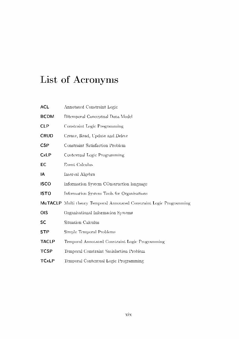
ACL Annotated Constraint Logic
BCDM Bitemporal Conceptual Data Model
CLP Constraint Logic Programming
CRUD Create, Read, Update and Delete
CSP Constraint Satisfaction Problem
CxLP Contextual Logic Programming
EC Event Calculus
IA Interval Algebra
ISCO Information System COnstruction language
ISTO Information System Tools for Organisations
MuTACLP Multi-theory Temporal Annotated Constraint Logic Programming
OIS Organisational Information Systems
SC Situation Calculus
STP Simple Temporal Problems
TACLP Temporal Annotated Constraint Logic Programming
TCSP Temporal Constraint Satisfaction Problem
TCxLP Temporal Contextual Logic Programming
xix

Preface
This work is the synthesis of several years1 of research. One of the most importantlessons learned during that time was that research is by no means a straight line, onemight even say that it is an (acyclic) graph. Not only did we follow paths that turnedout to be dead-ends but also sometimes we had to abandon others which, althoughpromising, would cause us to stray from our goals.
One must say, that due to the (at least) lack of excellency of the author in the Englishlanguage, writing this thesis in such language was a bold act. We ask for the readersympathy on this subject.
Structure of the Work
Chapter 1 brie�y introduces the concepts of time and modularity together with a logicprogramming perspective of Organisational Information Systems (OIS). This chapteralso motivates for the integration of temporal reasoning with modularity in order toobtain a language to construct and maintain OIS.
For self containment reasons, we survey several approaches to temporal reasoning inArti�cial Intelligence, temporal databases and modularity in logic programming inChap(s). 2, 3 and 4, respectively.
Chapter 5, besides describing the modular logic language that is at core of this workcalled Contextual Logic Programming (CxLP), also presents a revised speci�cationtogether with an optimisation framework obtained with abstract interpretation.
In Chap. 6 we combine consolidated approaches for temporal reasoning (in this caseTemporal Annotated Constraint Logic Programming) and modularity (CxLP) into asingle language. Although such a combination provides an expressive language, inChap. 7 we propose a model where the usage of a module is in�uenced by temporalconditions. Moreover, the CxLP program structure is very suitable for integrating withtemporal reasoning since it is quite straightforward to add the notion of time of the
1The use of an inde�nite adjective was (unfortunately) on purpose.
1
2 LIST OF FIGURES
context and let that time help in deciding whether a certain module is eligible or notto solve a goal.
In Chap. 8 we propose to augment the ISCO framework for constructing OIS withan expressive means of representing and implicitly using temporal information. Thisevolution builds upon the frameworks proposed in the previous chapters. Havingsimplicity as a design goal, we present a revised and stripped-down version of ISCO,keeping just some of the core features that we consider crucial in a language for thedevelopment of Temporal OIS.
We draw some concluding remarks and provide pointers for future work in Chap. 9.
In Appendix A we present a tutorial and a reference manual for the contextual partof GNU Prolog/CX. Finally, in Appendix B we brie�y overview Constraint Logic Pro-gramming.
Part of this work has appeared before in joint publications with Prof. Salvador Abreu(my supervisor), Prof. Gabriel David and Prof. Daniel Diaz. I thank all of them forletting me use the following common work [NAD03, NAD04, ADN04, AN05, NA06b,AN06, ET06, NA06a, NA07d, NA07b, NA07a, NA07c].
Roadmap
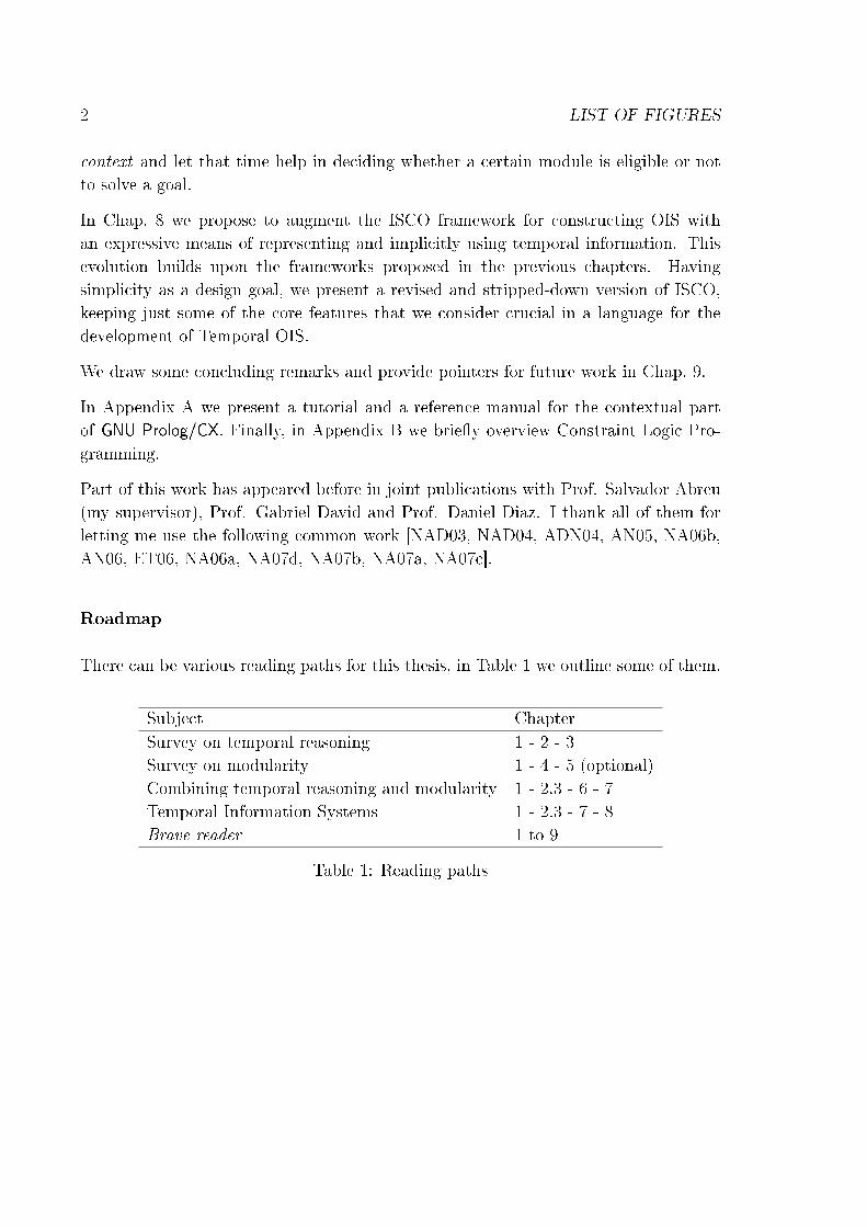
There can be various reading paths for this thesis, in Table 1 we outline some of them.
Subject ChapterSurvey on temporal reasoning 1 - 2 - 3Survey on modularity 1 - 4 - 5 (optional)Combining temporal reasoning and modularity 1 - 2.3 - 6 - 7Temporal Information Systems 1 - 2.3 - 7 - 8Brave reader 1 to 9
Table 1: Reading paths

Chapter 1
Introduction and Motivation
In this chapter we start with a brief overview of the concepts that are at the
core of this work: time and modularity. We also provide a short description
of Organisational Information Systems from a logic programming point of view.
Subsequently we argue for the need to integrate modularity with temporal reasoning
in order to provide a high level language in which to construct and maintain
Organisational Information Systems.
1.1 Introduction
1.1.1 Time
Time is an elusive concept, studied across such diverse disciplines as physics, mathemat-ics, linguistics, philosophy, etc. Each one provides an evolving perspective of Time: inphysics, Newton de�ned Time as a dimension in which events occur in sequence whereasEinstein, in the special theory of relativity, stated �time intervals appear lengthenedfor events associated with objects in motion relative to an inertial observer� [Wik08].
In the last decades a great number of logic languages that deal with Time have beenproposed. According to Van Benthem [Joh91], logic can be considered as a bridgebetween linguistics and mathematics since logic takes into consideration both theaspects of language and ontology. This author also points out that logics multiplicityof languages, theories of inference and formal semantics are adequate for the diverseintuitions inherent to the study of Time.
In a broad sense we can de�ne a temporal database as a repository of temporal informa-tion [Cho94] therefore one can say that most database applications are supported bytemporal databases. SQL [fS03] is often the language chosen for interacting with suchdatabases. Although SQL is a very powerful language for writing queries, modi�cations
3

4 CHAPTER 1. INTRODUCTION AND MOTIVATION
or constraints in the current state, it does not provide adequate support for thetemporal counterparts: for instance the temporal equivalent to an ordinary querycan be a very challenging task to express in SQL. To overcome such di�culties,several temporal data models, algebras and languages have been proposed. Moreover,McKenzie and Snodgrass [LEMS91] demonstrated that the design space for temporalalgebras has, in some sense, been explored in that all combinations of basic designdecisions have at least one representative algebra.
The logical and the database approach to Time are closely related: according to[BMRT02] temporal logic languages are responsible not only for the temporal databasestheoretical foundations but also for their powerful knowledge representation and querylanguages.
Temporal reasoning plays an important role in many areas of Arti�cial Intelligencesuch as Natural Language, Planning, Agent-Based Systems, etc. Most approaches arerestricted to the propositional case and follow an interval-based view originated inAllen's Interval Algebra [All83]. Moreover, temporal reasoning in AI is concerned withusing additional assumptions (such as persistence or defaults) or special procedures(like abduction) to derive conclusions [Cho94].
1.1.2 Modularity
Module systems are an essential feature of programming languages, namely becausebesides structuring programs they also allow the development of general purpose li-braries.
A modular extension to logic programming has been the object of research over the lastdecades. In a broad sense one can distinguish three di�erent approaches to modularity:the algebraic, the logical and the syntactic. The algebraic approach started with workby O'Keefe [O'K85] and considers logic programs as elements of an algebra, whoseoperators are the operators for composing programs. The logical approach is based onwork by Miller [Mil86, Mil89a], and extends the Horn language with logic connectivesfor building and composing modules. Finally, the syntactic approach (see [HF06] fora recent overview and a proposal of such approach) addresses the issue of the globaland �at name space, dealing with the alphabet of symbols as a mean to partition largeprograms.
Contextual Logic Programming is modular extension of Horn clause logic proposedby Monteiro and Porto [MP89, MP93]. The CxLP extension goal can be regardedas a non-monotonic version of Miller implication goal [Mil86, Mil89a]. The extensiongoal is denoted by � and D � G (D is a set of clauses and G a goal) is derivablefrom a program P if G is derivable from A ∪ D and A is derivable from P , for some

1.2. TEMPORAL (LOGIC-BASED) OIS 5
�nite set A of atoms for predicates not de�ned in D. Therefore � provides a sort oflexical scoping for predicates: predicates in G which are de�ned in D are bound tosuch de�nitions, the others can be obtained from program P . Besides lexical scoping,CxLP also accounts for contextual reasoning, that is widely used for several Arti�cialIntelligence tasks such as natural language processing, planning, temporal reasoning,etc. Work by [AD03a] presents a revised speci�cation of CxLP together with a newimplementation for it and also explains how this language can be viewed as a shift intothe Object-Oriented Programming paradigm.
1.1.3 Organisational Information Systems
Organisational Information Systems (OIS) have a lot to bene�t from Logic Program-ming (LP) characteristics such as the rapid prototyping ability, the relative simplicityof program development and maintenance, the declarative reading which facilitatesboth development and the understanding of existing code, the built-in solution-spacesearch mechanism, the close semantic link with relational databases, just to name afew. In [Por03, ADN04] we �nd examples of LP languages that were used to developand maintain information systems.
Information System COnstruction language (ISCO) [Abr01] is a state-of-the-art logicalframework for constructing Organisational Information Systems. ISCO is an evolutionof the previous language DL [Abr00] and is based on a Constraint Logic Programming(CLP) framework to de�ne the schema, represent data, access heterogeneous datasources and perform arbitrary computations. In ISCO, processes and data are struc-tured as classes which are represented as typed1 Prolog predicates. An ISCO class maymap to an external data source or sink, such as a table or view in a relational database,or be entirely implemented as a regular Prolog predicate. Operations pertaining toISCO classes include a query which is similar to a Prolog call as well as three forms ofupdate.
1.2 Temporal (Logic-Based) OIS
Chomicki and Toman [CT98] stated that current Information Systems deal with moreand more complex applications where, besides the static aspects of the world, onealso has to model the dynamics, i. e., time, change and concurrency. This statementillustrates very clearly the importance of Time in OIS. It is our opinion that a languagefor OIS must have the capability of performing temporal representation and reasoningbeyond the ad hoc approaches.
1The type system applies to class members, which are viewed as Prolog predicate arguments.
6 CHAPTER 1. INTRODUCTION AND MOTIVATION
The amount of information handled by OIS is enormous and has increased by orders ofmagnitude over the last decades. Besides the already mentioned bene�ts of modularity,we consider that this fact by itself should be su�cient to justify that modularity is asine qua non condition for designing and implementing OIS.
One common approach in combining modularity and time in a language is to considerthem as independent, or orthogonal, features. In this work we start by presenting alogical based language that follows such guidelines.
Nevertheless, time and modularity can combine into a more fruitful environment, i. e.one where these features are more intertwined. We propose an extension of a modularlogic language where temporal reasoning is deeply integrated, making the usage of amodule itself time dependent. We consider this proposition to be natural and in factlargely employed in several domains where a given law, criteria application is timedependent.
Finally, we will show that the language above provides a sound basis for a frameworkto construct and maintain Temporal Organisational Information Systems.

Chapter 2
Temporal Reasoning in Arti�cial
Intelligence
This chapter provides an overview of temporal reasoning in Arti�cial Intelligence.
It starts by introducing the notion of model of time and temporal quali�cation.
Afterwards it describes several constraint and modal logic based proposals for
temporal reasoning. Finally, some theories for reasoning about actions and change
are discussed.
2.1 Introduction
Temporal reasoning plays an important role in many areas of Arti�cial Intelligencesuch as Natural Language, Planning, Agent-Based Systems, etc. Most approaches arerestricted to the propositional case and follow an interval-based view originated inAllen's Interval Algebra [All83] (see Sect. 2.3.1 for a description of such an algebra).Moreover, temporal reasoning in AI is concerned with using additional assumptions(such as persistence or defaults) or special procedures (like abduction) to obtain con-clusions [Cho94]. For further reading on this subject see for instance [Vil94, CM00,Aug01, FGV05].
This chapter, for self-containment reasons, presents a general survey of temporal rea-soning in AI and is organised as follows: Sect. 2.2 starts out by specifying severalkey concepts pertaining to the foundations of temporal reasoning such as temporal
ontology, topology and quali�cation. Afterwards, we present three sub�elds of temporalrepresentation and reasoning in AI: constraint-based temporal reasoning (Sect. 2.3),temporal modal logic (Sect. 2.4) and reasoning about actions and change (Sect. 2.5).The chapter ends with a brief summary of the concepts and approaches describedtherein.
7
8 CHAPTER 2. TEMPORAL REASONING IN AI
2.2 General Notions of Time
In this section we brie�y describe the notions of model of time and temporal quali�ca-tion.
2.2.1 Model of Time
To de�ne a model of time we need to de�ne not only the time ontology but also thetime topology. By time ontology we mean the class or classes of objects time is made of,i.e. one has to choose between time points and intervals as the basic temporal entities.
Regarding the time topology we can consider di�erent structures for time, namelywhether it is:
• discrete, dense or continuous;
• bounded, partially bounded or unbounded;
• linear, branching, circular or with a di�erent structure.
Moreover, it is helpful to know what kind of properties the structure of temporalindividuals have as a whole, i.e.:
• are all individuals comparable by the order relation (connectedness)?
• are all individuals equal (homogeneity)?
• is it the same to look at one side or at the other (symmetry)?
2.2.2 Temporal Quali�cation
Temporal quali�cation refers �to the way logic is used to express that temporal propo-sitions are true or false at di�erent times� [RV05] and is by itself a very proli�c �eld ofresearch.
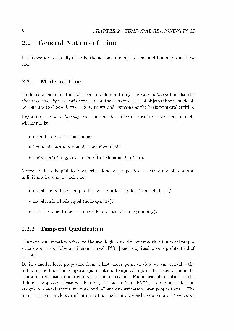
Besides modal logic proposals, from a �rst�order point of view we can consider thefollowing methods for temporal quali�cation: temporal arguments, token arguments,temporal rei�cation and temporal token rei�cation. For a brief description of thedi�erent proposals please consider Fig. 2.1 taken from [RV05]. Temporal rei�cationassigns a special status to time and allows quanti�cation over propositions. Themain criticism made to rei�cation is that such an approach requires a sort structure

2.3. CONSTRAINT-BASED TEMPORAL REASONING 9
Temporal Arguments Token Reification
Classical LogicAtomic Formula
Temporal Reification
Token Arguments
Modal Temporal Logics
Add_argument(t ime)
effective(o, a, b, ...)
effective(o, a, b, ..., t1, t2) holds(effective(o, a, b, ..., t1, t2))
Reify_into(token)
Reify_into(type) + Add_argument(t ime)
holds(effective(o, a, b, ...), t1, t2))
Add_argument(token)
effect ive(o, a, b, . . . , t t1), holds(tt1), begin(tt1)=t1, end(tt1)=t2
holds [t1, t2] (effective(o, a, b, ...))
First-Order Logic
Modal Logic
Figure 2.1: Temporal quali�cation methods
to distinguish betewen terms that denote real objects of the domain (terms of theoriginal object language) and terms that denote propositional objects (propositions ofthe original object language).
2.3 Constraint-Based Temporal Reasoning
According to [Pao] constraint�based approaches mainly focus on the de�nition of arepresentation formalism and of reasoning techniques to deal speci�cally with temporalconstraints between temporal entities, independently of the events and states associatedwith them. Following these guidelines, a class of Constraint Satisfaction Problem (CSP)was de�ned, called Temporal Constraint Satisfaction Problem (TCSP), where variablesrepresent time and constraints represent temporal relations between them. Di�erentTCSPs are de�ned depending on the time entity that variables can represent, namelytime points, time intervals, durations (i.e. distances between time points) and the classof constraints, namely qualitative, metric or both [SV98]. Each class of constraints ischaracterised by the underlying set of basic temporal relations.1
TCSP constraints are binary and Cij = {r1, . . . , rk} is a constraint2 between thevariables Xi and Xj where each ri is a basic temporal relation. A singleton labelling
1The elements of all basic temporal relations are mutually exclusive and their union is the universal
constraint.2The set is interpreted as a disjunction of relations.

10 CHAPTER 2. TEMPORAL REASONING IN AI
assigns an ri to the pair Xi, Xj, and the solutions of a TCSP are its consistent singletonlabelling.
The main techniques to �nd a solution to the general problem are path-consistencyand backtracking algorithms. Finally, there are typically two tasks when working withTCSP: deciding consistency and answering queries about scenarios that satisfy allconstraints.
For a comprehensive survey on this subject see for instance [SKD94, Kou95, SV96,Sch98, SV98]
2.3.1 Qualitative Temporal Constraints
Qualitative temporal constraints deal with the relative position between time pointsor intervals.
Allen's Interval Algebra
The Interval Algebra (IA) was proposed by James F. Allen [All83]. In this work, domainelements are temporal intervals3 and constraints are built using the thirteen basicrelations between intervals: before, after, meets, met by, equal, overlaps, overlapped by,during, contained by, starts, started by, �nishes, �nished by. The operations on thoserelations include composition and Boolean operators.
Intervals are used to qualify properties, events and processes. We say that a property
holds over an interval if and only if it holds for all its subintervals whereas a proccess
occurs over an interval if it occurs in at least one of its subintervals. Events occur overthe smallest possible interval [Rib93].
In [VKvB90] it is shown that the satis�ability of Allen's algebra is NP-complete. Thestudy of maximal tractable subclasses started with Nebel and Bürckert (ORD-Hornalgebra [NB94]) and recently Krokhin et. al. [KJJ03] showed that the IA containsexactly eighteen maximal tractable subalgebras. Moreover, they also proved thatreasoning in any fragment not entirely contained in one of the these subalgebras isNP-complete.
3Besides intervals, the only other structural property de�ned is that time is linear. Everything else
is set by the user according to the application.
2.3. CONSTRAINT-BASED TEMPORAL REASONING 11
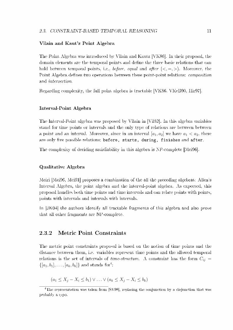
Vilain and Kaut'z Point Algebra
The Point Algebra was introduced by Vilain and Kautz [VK86]. In their proposal, thedomain elements are the temporal points and de�ne the three basic relations that canhold between temporal points, i.e., before, equal and after (<,=, >). Moreover, thePoint Algebra de�nes two operations between these point-point relations: compositionand intersection.
Regarding complexity, the full point algebra is tractable [VK86, VKvB90, Hir97].
Interval-Point Algebra
The Interval-Point algebra was proposed by Vilain in [Vil82]. In this algebra variablesstand for time points or intervals and the only type of relations are between betweena point and an interval. Moreover, since in an interval [a1, a2] we have a1 < a2, thereare only �ve possible relations: before, starts, during, finishes and after.
The complexity of deciding satis�ability in this algebra is NP-complete [Mei96].
Qualitative Algebra
Meiri [Mei96, Mei91] proposes a combination of the all the preceding algebras: Allen'sInterval Algebra, the point algebra and the interval-point algebra. As expected, thisproposal handles both time points and time intervals and can relate points with points,points with intervals and intervals with intervals.
In [JK04] the authors identify all tractable fragments of this algebra and also provethat all other fragments are NP-complete.
2.3.2 Metric Point Constraints
The metric point constraints proposal is based on the notion of time points and thedistance between them, i.e. variables represent time points and the allowed temporalrelations is the set of intervals of time-structure. A constraint has the form Cij =
{[a1, b1], . . . , [ak, bk]} and stands for4:
(a1 ≤ Xj −Xi ≤ b1) ∨ . . . ∨ (ak ≤ Xj −Xi ≤ bk)
4The representation was taken from [SV98], replacing the conjunction by a disjunction that was
probably a typo.

12 CHAPTER 2. TEMPORAL REASONING IN AI
There are three operators for the metric constraints: inverse, intersection and compo-
sition. With respect to complexity we have that deciding consistency and computinga solution of a metric point constraint problem is NP-complete [DMP91]. Finally,[SV98] describes the three known relation based tractable classes, i.e. Simple TemporalProblems (STP), STP with inequation constraints (for continuous domains only) andStar TCSPs.
2.3.3 Hybrid Approaches
Meiri [Mei96] proposed a very expressive constraint language in which both qualitativeand quantitative/metric constraints can be represented, this way allowing the repre-sentation and processing of most types of constraints. This proposal combines theQualitative Algebra (Sect. 2.3.1) with Metric Point Constraints (Sect. 2.3.2).
Besides this general proposal, Meiri studied other subclasses that were also found tobe intractable:
• qualitative point with unary metric;
• qualitative interval with unary metric.
2.3.4 Programming Languages
This section describes a short list of languages for temporal reasoning that, besidesbeing constraint-based, have some a�nity to (Constraint) Logic Programming.
Temporal Prolog
Temporal Prolog [Hry93] can be regarded as a �synthesis of temporal logic and of theConstraint Logic Programming paradigm, in which temporal constraints are formu-lated�. Temporal Prolog has several objectives, namely: the temporal logic inherentto the language should be intuitive and e�cient, easily integrated in a LP paradigmand easy to implement on top of the Prolog interpreters. Following these guidelines,Temporal Prolog proposed a �rst-order rei�ed logic where HOLDS(P,T) means that thestatement (e.g. a Prolog clause) P holds (i.e., is true) in interval T and HOLDS(P) meansthat P holds without limitation to a temporal interval. The interval-based axioms ofTemporal Prolog are the following:
• HOLDS(A, S) & subinterval(T, S) → HOLDS(A, T).

2.3. CONSTRAINT-BASED TEMPORAL REASONING 13
• HOLDS(A) → (∀ T) HOLDS(A, T).
• HOLDS(A, T) & HOLDS(B, T) → HOLDS(A & B, T).
• HOLDS(A, U) & HOLDS(B, V) & union(U, V, T) → HOLDS(A ∨ B, T).
• HOLDS(A, S) & HOLDS( ¬ A, T) → disjoint(S, T).
Horn Temporal Reference Language
Horn Temporal Reference Language [Pan95] is also a temporal extension of Prolog.In this language, atoms can have temporal labels to express their validity. It allowstwo types of extended atoms: events (not necessarily true over every subinterval) andproperties (hold over every subinterval). Moreover, it provides inference rules for theseextended atoms together with a transformation from this language to Constraint LogicProgramming.
Temporal Annotated Constraint Logic Programming
Temporal Annotated Constraint Logic Programming (TACLP) [Frü93, Frü94b, Frü96]is presented as an instance of Annotated Constraint Logic (ACL) [Frü96], suited forreasoning about time. ACL generalises basic �rst�order languages with a distinguishedclass of predicates called constraints, and a distinguished class of terms, called anno-
tations, used to label a formula.
TACLP allow us to reason about qualitative and quantitative, de�nite and inde�nitetemporal information using time points and time periods as labels for atoms [RF00a].This section presents a brief overview of TACLP that follows closely Sect. 2 of [RF00a].For a more detailed explanation of TACLP see for instance [Frü96].
We consider the subset of TACLP where time points are totally ordered, sets oftime points are convex and non-empty, and only atomic formulas can be annotated.Moreover clauses are free of negation.
Time can be discrete or dense. Time points are totally ordered by the relation ≤. Wecall the set of time points D and suppose that a set of operations (such as the binaryoperations +,−) to manage such points, is associated with it. We assume that thetime-line is left-bounded by the number 0 and open to the future (∞). A time period
is an interval [r, s] with 0 ≤ r ≤ s < ∞, r ∈ D, s ∈ D and represents the convex,non-empty set of time points {t | r ≤ t ≤ s}. Therefore the interval [0,∞[ denotes thewhole time line.

14 CHAPTER 2. TEMPORAL REASONING IN AI
De�nition 1 (Annotated Formula) An annotated formula is of the form Aα where
A is an atomic formula and α an annotation. Let t be a time point and I be a time
period:
(at) The annotated formula A at t means that A holds at time point t.
(th) The annotated formula A th I means that A holds throughout I, i.e. at every
time point in the period I.
A th-annotated formula can be de�ned in terms of an at-annotated as: A th I ⇔∀t (t ∈ I → A at t)
(in) The annotated formula A in I means that A holds at some time point(s) in the
time period I, but there is no knowledge when exactly. The in annotation accounts
for inde�nite temporal information.
An in-annotated formula can also be de�ned in terms of an at-annotated as:
A in I ⇔ ∃t (t ∈ I ∧ A at t).
The set of annotations is endowed with a partial order relation v which induces alattice. Given two annotations α and β, the intuition is that α v β if α is �lessinformative� than β in the sense that for all formulas A, Aβ ⇒ Aα.
In addition to Modus Ponens, TACLP has the following two inference rules:
Aα γ v α
Aγrule (v)
Aα Aβ γ = α t βAγ
rule (t)
The rule (v) states that if a formula holds with some annotation, then it also holds withall annotations that are smaller according to the lattice ordering. The rule (t) saysthat if a formula holds with some annotation and the same formula holds with anotherannotation then it holds in the least upper bound (denoted by t) of the annotations.TACLP provides a constraint theory (detailed in Sect. 6.3).
A TACLP program is a �nite set of TACLP clauses. A TACLP clause is a formula ofthe form Aα← C1, . . . , Cn, B1α1, . . . , Bmαm (m,n ≥ 0) where A is an atom, α and αi
are optional temporal annotations, the Cj's are the constraints and the Bi's are theatomic formulas. Frühwirth [Frü96], besides providing a meta-interpreter for TACLPclauses, also presents a compilation scheme that translates TACLP into ConstraintLogic Programming. Finally, Ra�aetà and Frühwirth [RF00b, RF00a] provide both anoperational semantics and a �x-point one for TACLP.

2.4. TEMPORAL MODAL LOGIC 15
2.4 Temporal Modal Logic
In a succinct way we can say that Modal Logics can be regarded as the logics ofquali�ed truth [Che80]. In this logic besides standard logical symbols one also hasmodal operators that are used to qualify formulas in the following way: if A is aformula and ∇ is a modal operator then ∇A is a formula.
Although the term Temporal Logic is used in a broad sense when referring to anyapproach that deals with temporal information within a logic framework, it has amore speci�c de�nition related to the Modal Logic approach to temporal informa-tion [DMG94, Gal08]. Tense Logic [Pri57, Pri67, Pri68] de�ned by Arthur Prior isregarded as the seminal work on this �eld. Prior proposed the four modal operatorsdescribed in Table 2.1. There are several formalisms that provide variations or exten-sions to the Tense Logic, such as:
• Event Logic [Gal87];
• TM [Rei89] of Reichgelt;
• Logic of time intervals [HS91] of Halpern and Shoham.
See [Aug01] for an overview on the formalisms above.
Symbol Expression SymbolisedG �It will always be the case that . . . �F �It will at some time be the case that . . . �H �It has always been the case that . . . �P �It has at some time been the case that . . . �
Table 2.1: Tense logic modal operators
2.4.1 Temporal Logic Programming
This section follows the survey of Gergatsoulis in [Ger01] that states that the basis fordeveloping temporal logic programming languages are syntactic subsets of temporal andmodal logic which present well de�ned computational behaviour. One can consider twobroad approaches to the speci�cation of these languages: linear-time and branching-time temporal logic programming languages.
The following languages use linear-time:

16 CHAPTER 2. TEMPORAL REASONING IN AI
• Templog [AM89] extends Horn logic programming with the operators © (next),� (always) and ♦ (eventually). As an illustration consider the Fibonacci sequenceusing Templog:
fib (0).
©fib (1).
�(© © fib(Z) <- fib(X), ©fib(Y), Z is X+Y).
• Chronolog [Org91] has two temporal operators �rst and next where �rst standsfor the �rst moment in time and next to the next moment in time. The followingis a simple example of this language:
first light(green ).
next light(amber) <- light(green ).
next light(red) <- light(amber ).
next light(green) <- light(red).
• Disjunctive Chronolog [GRP96] that combines Chronolog with Disjunctive LogicProgramming.
• Chronolog(MC) [LO96] is an extension of Chronolog based on Clocked Temporal
Logic where predicates are associated with local clocks.
• Metric Temporal Logic Programming (MTL) [Brz98] time can be either discreteor dense. MTL has two temporal operators �I and ♦I de�ned as: �IA is trueif A is true in all moments in the interval I and ♦IA is true if A is true in somemoment in the interval I. As an illustration of a simple fact in this languageconsider:
�[2005,2007]salary(peter , 55000).
Cactus [RGP97] is a proposal of a branching-time language that supports two mainoperators: the temporal operator first which refers to the beginning of time and thetemporal operator nexti which refers to the i-th child of the current moment.
2.5 Reasoning About Actions and Change
Reasoning about actions and change studies the evolution of (a portion of) the worldas the result of the occurrence of a set of actions and/or events [CM00]. The mainmechanism of this �eld is temporal projection, which can be further re�ned as:
2.5. REASONING ABOUT ACTIONS AND CHANGE 17
• forward temporal projection that can be regarded as inferring consequences ofactions having some knowledge of what is currently believed. Usually this isperformed by deduction.
• backward temporal projection that can be regarded as inferring explanations ofgiven situations having some knowledge of what is currently believed. Usuallythis is performed by induction.
For a comprehensive study on inference of temporal knowledge see for instance [Rib93].
According to [CM00], temporal projection has to deal with three main problems:
• the rami�cation problem: concerns the speci�cation of the e�ects of a given event;
• the quali�cation problem: concerns the speci�cation of the conditions under whichan event actually produces the expected e�ects;
• the frame problem: its related with the ones above and its the problem ofdetermining what stays the same about the world as time passes and actionsare performed.
Next we survey some of the more relevant theories of action and change.
2.5.1 The Situation Calculus
The Situation Calculus (SC) proposed by McCarthy and Hayes [MH69] was the �rstformal representation of time in Arti�cial Intelligence. This formalism allows one tomodel the evolution of a world and, although there is no explicit representation of time,situations are used to model the �ow of time. Besides situations, the SC also speci�es�uents and actions :
• �uents are functions and predicates that change over time;
• actions stand for the possible actions that can be performed in the modeledworld.
Except for the initial situation (usually denoted by S0), all other situations are gener-ated by applying an action to a situation. As a simple illustration taken from the blocksworld, consider the (rei�ed) �uent on(A, B) stating that block A is on top of block B
and the auxiliary predicate HoldsAt to specify when the �uents are true, one can say:HoldsAt(on(A, B), result(move(A, B), S)) to state that its true that A is on top B

18 CHAPTER 2. TEMPORAL REASONING IN AI
in the situation that results from moving A to B in situation S. Using predicates insteadof functions, i.e. in a non-rei�ed form we have on(A, B, result(move(A, B), S)).
Finally, the main objection to SC comes from the fact that is impossible to modelconcurrent actions.
2.5.2 The Event Calculus
The Event Calculus (EC) formalism was proposed by Kowalski and Sergot [KS86] andas the name states, the primitive objects are events. In the EC, time is explicit andevents are somewhat similar to the actions of SC. An EC �uent holds at time pointsand there is an axiom to allow us to reason about intervals of time5: a �uent is true ata point in time if an event initiated the �uent at some time in the past and was notterminated by an intervening event [RN03].
The relation Initiates (Terminates) expresses that the occurrence of an event e at atime point t causes a �uent f to become (cease to be) true. There is also the relationHappens that is used to state that an event e happens at a time t. As an example,Happens(TurnOff(LightSwitch), 0:00) states that the lightswitch was turned o� atexactly 0:00.
Finally, Kowalski and Sadri [KS97] proved that the Event Calculus and the SituationCalculus are equivalent.
2.5.3 Temporal Nonmonotonic Reasoning
The research on temporal nonmonotonic reasoning was triggered by the Yale ShootingProblem [HM87]. Although this is a (very broad) �eld of research reaching beyondthe focus of the present work, for completeness reasons we decided to present a briefoverview (that follows [Aug01]) of several key formalisms in this area.
Shoham's Non-Monotonic Temporal Logic
Shoham's non-monotonic temporal logic [Sho88] is based on model preference and usesChronological Ignorance as a criterion to de�ne a partial order between the models, i.e.it prefers those models where a fact holds as late as possible.
5In the EC an interval stands for the set of points between the interval bounds.

2.6. CONCLUSIONS 19
Extended Situation Calculus
In [Pin94] Pinto adds explicit time to Situation Calculus and addresses several problemssuch as: representation of concurrent and complex action; reasoning on a continuousontology; easy reference to dates; etc.
Defeasible Temporal Reasoning
In a broad sense one can say that argumentation systems allow us to reason about achanging world where the available information is incomplete or unreliable. There areseveral examples of argumentation system that embed temporal reasoning based onintervals, on instants or both (see [Aug01] for an overview).
2.6 Conclusions
We started this section by describing the notions of model of time and of temporalquali�cation. We then reviewed several constraint-based and modal approaches totemporal reasoning, with a stronger emphasis on the former since the temporal repre-sentation and reasoning followed throughout this work is constraint-based. Although,on a �rst look, �rst-order and modal approaches can be regarded as radically di�erent,Galton noted that they rely on the common use of a �rst�order language: the formeruses it as the proper representation language and the later as a model theory. Finally,we brie�y sketched the foundational theories for reasoning about actions and change.
The research on temporal representation and reasoning, even restricted to the one that��ts� under the domain of arti�cial intelligence is so vast that a chapter such as this onecan only lightly brush over some aspects. For a more systematic and comprehensiveapproach we suggest [FGV05].


Chapter 3
Temporal Databases
This chapter reviews the main concepts concerning temporal databases, namely
temporal data semantics, models and languages. Moreover, besides some considera-
tions about the design of these databases it also describes several temporal database
products.
3.1 Introduction
In a broad sense we can de�ne a temporal database as a repository of temporal informa-tion [Cho94] therefore one can say that most database applications are supported bytemporal databases. SQL [fS03] is often the language chosen for interacting with suchdatabases. Although it is a very powerful language for writing queries, modi�cations orconstraints in the current state, it does not provide adequate support for the temporalcounterparts: for instance, expressing the temporal equivalent of an ordinary querycan be a very challenging task in SQL. To overcome such di�culties, several temporaldata models, algebras and languages have been proposed.
McKenzie and Snodgrass [LEMS91] have shown that the design space for temporalalgebras has in some sense been explored in that all combinations of basic designdecisions have at least one representative algebra.
In this section we present a brief overview of the temporal data semantics (Sect. 3.2)together with the models and languages (Sect. 3.3) that we consider more signi�cant.For a more in depth study on this subject the reader may refer to [TCG+93, DD02].Since the practical aspects of databases are highly important, we also review severalproducts that extend regular database management system in order to include temporalcapabilities (Sect. 3.5). Although most of these products only consider the time betweenthe insertion and the removal of a fact from the database some applications already
21

22 CHAPTER 3. TEMPORAL DATABASES
suport the time when the fact is true in the modeled reality.
3.2 Temporal Data Semantics
According to [Jen00] a database models and records information about a part of reality(modeled reality) where the di�erent aspects of this reality are represented by databaseentities. In temporal databases, the facts recorded by the database entities can havean associated time and this is usually de�ned as valid time or as transaction time:
De�nition 2 (Valid Time) The valid time of a fact is the collected times - possibly
spanning the past, present, and future - when the fact is true in the modeled reality.
De�nition 3 (Transaction Time) The transaction time of a database fact is the
time spanning between when it was inserted into the database and when it was logically
removed from the database.
Unlike the valid time, the transaction time may be associated with any database entity(not only with facts) and captures the time-varying states of the database. Applicationsthat demand accountability or �traceability� rely on databases that record transactiontime. Moreover, data consistency is ensured since the transaction timestamps aremaintained automatically by the DBMS.
There is no single answer on how to perceive time in reality and how to represent timein a database. As mentioned in Sect. 2.2, to de�ne a model of time we need to considernot only the time ontology but also the time topology. In databases, a �nite and discretetime domain is typically assumed. Most often, time is assumed to be totally ordered,but various partial orders have also been used.
3.3 Temporal Data Models and Languages
According to [Dat99] a data model is an abstract, self-contained, logical de�nition ofthe objects, operators, and so forth, that together constitute the abstract machinewith which users interact. In the relational data model, the relations are the objectsand data is operated on by means of a relational calculus or algebra, with equivalentexpressive power.
Several proposals for extending the relational data model to incorporate the temporaldimension of data have appeared in the literature. These proposals have di�ered

3.3. TEMPORAL DATA MODELS AND LANGUAGES 23
considerably in the way that the temporal dimension has been incorporated both intothe structure of the extended relations of these temporal models and into the extendedrelational algebra or calculus that they de�ne.
Since there several dozen temporal data models, instead of providing a detailed descrip-tion of each one we present a list with their names, main properties and references. Asimilar approach will be followed in overviewing the temporal languages in Sect. 3.3.2.The only exception is the language TSQL2 [IABC+95] and its temporal data model(Bitemporal Conceptual Data Model), since this language is regarded as a consensualtemporal extension of SQL-92.
3.3.1 Temporal Data Model
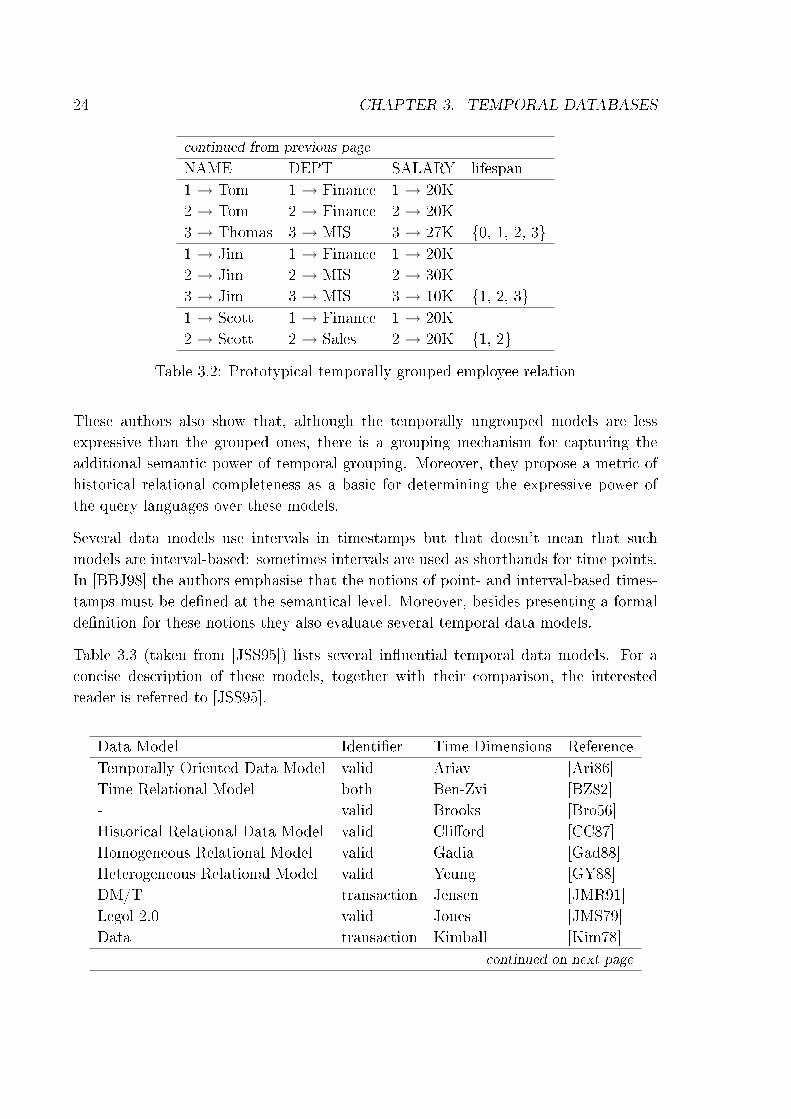
A useful taxonomy for temporal data models was introduced by Cli�ord et. al. [CCT94,CCGT95] who classi�ed them into two main categories: temporally ungrouped (tupletime stamping) and temporally grouped (attribute time stamping) data models. Toillustrate these two categories please consider tables 3.1 and 3.2 taken from [CCT94],to represent a temporal ungrouped and grouped, respectively, version of an employee
relation (in this modeled reality, employee Tom changes his name to Thomas at time3).
EMPLOYEENAME DEPT SALARY timeTom Sales 20K 0Tom Finance 20K 1Tom Finance 20K 2Thomas MIS 27K 3Jim Finance 20K 1Jim MIS 30K 2Jim MIS 40K 3Scott Finance 20K 1Scott Sales 20K 2
Table 3.1: Prototypical temporally ungrouped employee relation
EMPLOYEENAME DEPT SALARY lifespan0 → Tom 0 → Sales 0 → 20K
continued on next page
24 CHAPTER 3. TEMPORAL DATABASES
continued from previous page
NAME DEPT SALARY lifespan1 → Tom 1 → Finance 1 → 20K2 → Tom 2 → Finance 2 → 20K3 → Thomas 3 → MIS 3 → 27K {0, 1, 2, 3}1 → Jim 1 → Finance 1 → 20K2 → Jim 2 → MIS 2 → 30K3 → Jim 3 → MIS 3 → 10K {1, 2, 3}1 → Scott 1 → Finance 1 → 20K2 → Scott 2 → Sales 2 → 20K {1, 2}
Table 3.2: Prototypical temporally grouped employee relation
These authors also show that, although the temporally ungrouped models are lessexpressive than the grouped ones, there is a grouping mechanism for capturing theadditional semantic power of temporal grouping. Moreover, they propose a metric ofhistorical relational completeness as a basic for determining the expressive power ofthe query languages over these models.
Several data models use intervals in timestamps but that doesn't mean that suchmodels are interval-based: sometimes intervals are used as shorthands for time points.In [BBJ98] the authors emphasise that the notions of point- and interval-based times-tamps must be de�ned at the semantical level. Moreover, besides presenting a formalde�nition for these notions they also evaluate several temporal data models.
Table 3.3 (taken from [JSS95]) lists several in�uential temporal data models. For aconcise description of these models, together with their comparison, the interestedreader is referred to [JSS95].
Data Model Identi�er Time Dimensions ReferenceTemporally Oriented Data Model valid Ariav [Ari86]Time Relational Model both Ben-Zvi [BZ82]- valid Brooks [Bro56]Historical Relational Data Model valid Cli�ord [CC87]Homogeneous Relational Model valid Gadia [Gad88]Heterogeneous Relational Model valid Yeung [GY88]DM/T transaction Jensen [JMR91]Legol 2.0 valid Jones [JMS79]Data transaction Kimball [Kim78]
continued on next page

3.3. TEMPORAL DATA MODELS AND LANGUAGES 25
continued from previous page
Data Model Identi�er Time Dimensions ReferenceTemporal Relational Model valid Lorentzos [Lor88]Temporal Relational Model valid Navathe [NA89]HQL valid Sadeghi [Sad87]HSQL valid Sarda [Sar90b]Temporal Data Model valid Segev [SS87]TQuel both Snodgrass [Sno87]Postgres transaction Stonebraker [SK91]HQuel valid Tansel [TA86]Accounting Data Model both Thompson [Tho91]Time Oriented Data Base Model valid Wiederhold [GWW75]
Table 3.3: Temporal data models
Bitemporal Conceptual Data Model
The Bitemporal Conceptual Data Model (BCDM) [JS96] tries to maintain the simplic-ity of the relational model and capture the temporal aspects of the facts stored in adatabase. One possible de�nition of the BCDM according to [Jen00] is:
De�nition 4 (Bitemporal Conceptual Data Model) both valid and transaction
times are supported and the relations are coalesced.1 Moreover, the value now and
until changed are introduced for valid time and transaction time, respectively.
This is a conceptual model where no two tuples with mutually identical explicit at-tribute values are allowed, i.e. the full history of a fact is contained in exactly one tuple.To illustrate this model, please consider a relation recording employee/departmentinformation, taken from [JSS95]: employee Jake was hired by the company in theshipping department for the interval from time 10 to time 15, and this fact becamecurrent in the database at time 5. Afterwards, the personnel department discoversthat Jake had really been hired from time 5 to time 20, and the database is correctedbeginning at time 10. Table 3.4 shows the corresponding bitemporal element.
Emp Dept TJake Ship {(5, 10), . . . , (5, 15), . . . , (9, 10),
. . . ,(9, 15), (10, 5), . . . , (10, 20), . . . }
Table 3.4: BCDM tuple
1Value equivalent tuples with the same non-timestamp attributes and adjacent or overlapping time
intervals are merged.

26 CHAPTER 3. TEMPORAL DATABASES
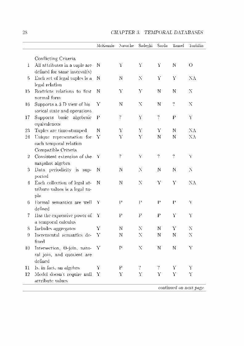
3.3.2 Temporal Languages
McKenzie and Snodgrass [LEMS91] provided a set of 26 criteria for evaluating temporalalgebras. Moreover, they also show that, out of these 26 criteria, seven criteria arecon�icting, i.e. no algebra can satisfy all 26 criteria. Finally, the authors evalu-ate 12 algebras (Jones [JMS79], Ben-Zvi [BZ82], Navathe [NA89], Sadeghi [Sad87],Sarda [Sar90a], Cli�ord [CC87], Tansel [TA86], Gadia [Gad88], Yeung [GY88], Lorent-zos [LJ88], McKenzie [LEM88], Tuzhilin [TC90]) that extend the snapshot algebrato support valid and/or transaction time. The result of such evaluation is depictedin Tables 3.5 and 3.6. The possible table entries are: Y - satis�es criterion, P -partial compliance, N - criterion not satis�ed, NA - applicable, ? - not speci�ed,O - see [LEMS91].
Ben-Zvi Cli�ord Gadia Yeung Jones Lorentzos
Con�icting Criteria1 All attributes in a tuple are
de�ned for same interval(s)Y N Y N Y N
5 Each set of legal tuples is alegal relation
Y N Y N Y Y
15 Restricts relations to �rstnormal form
Y N N N Y Y
16 Supports a 3-D view ofhistorical state and opera-tions
N N N ? N N
17 Supports basic algebraicequivalences
Y P Y ? P Y
23 Tuples are time-stamped Y P N N Y N24 Unique representation for
each temporal relationN N N Y N N
Compatible Criteria2 Consistent extension of the
snapshot algebraY Y Y ? Y Y
3 Data periodicity is sup-ported
N N N N N Y
4 Each collection of legal at-tribute values is a legal tu-ple
N N N Y N N
continued on next page

3.3. TEMPORAL DATA MODELS AND LANGUAGES 27
continued from previous page
Ben-Zvi Cli�ord Gadia Yeung Jones Lorentzos
6 Formal semantics are wellde�ned
P Y Y P N Y
7 Has the expressive powerof a temporal calculus
P ? Y P ? ?
8 Includes aggregates Y N P P P Y9 Incremental semantics de-
�nedN N N N N N
10 Intersection, Θ-join, natu-ral join, and quotient arede�ned
P P P N N N
11 Is, in fact, an algebra Y N Y N Y Y12 Model doesn't require null
attribute valuesY N Y Y Y Y
13 Multidimensional time-stamps are supported
N N N Y N N
14 Reduces to the snapshotalgebra
Y P Y P Y P
18 Supports relations of allfour classes
P P P Y P P
19 Supports rollback opera-tions
P N N Y N N
20 Supports multiple storedschemas
N N N N N N
21 Supports static attributes N N N Y N Y22 Treats valid time
and transaction timeorthogonally
Y ? ? Y ? ?
25 Unisorted (notmultisorted)
N N N Y Y Y
26 Update semantics arespeci�ed
P N N N N N
Table 3.5: Evaluation of algebras against criteria
28 CHAPTER 3. TEMPORAL DATABASES
McKenzie Navathe Sadeghi Sarda Tansel Tuzhilin
Con�icting Criteria1 All attributes in a tuple are
de�ned for same interval(s)N Y Y Y N O
5 Each set of legal tuples is alegal relation
N N N Y Y NA
15 Restricts relations to �rstnormal form
N Y Y N N N
16 Supports a 3-D view of his-torical state and operations
Y N N N ? N
17 Supports basic algebraicequivalences
P ? Y ? P Y
23 Tuples are time-stamped N Y Y Y N NA24 Unique representation for
each temporal relationY Y Y N N NA
Compatible Criteria2 Consistent extension of the
snapshot algebraY ? Y ? ? Y
3 Data periodicity is sup-ported
N N N N N N
4 Each collection of legal at-tribute values is a legal tu-ple
N N N Y Y NA
6 Formal semantics are wellde�ned
Y P P P P Y
7 Has the expressive power ofa temporal calculus
Y P P P Y Y
8 Includes aggregates Y N N N Y N9 Incremental semantics de-
�nedY N N N N N
10 Intersection, Θ-join, natu-ral join, and quotient arede�ned
Y P N N N Y
11 Is, in fact, an algebra Y P ? ? Y Y12 Model doesn't require null
attribute valuesY Y Y Y Y Y
continued on next page

3.3. TEMPORAL DATA MODELS AND LANGUAGES 29
continued from previous page
McKenzie Navathe Sadeghi Sarda Tansel Tuzhilin
13 Multidimensional time-stamps are supported
N N N N N NA
14 Reduces to the snapshot al-gebra
P Y Y Y P Y
18 Supports relations of allfour classes
Y P P P P P
19 Supports rollback opera-tions
Y N N N N N
20 Supports multiple storedschemas
Y N N N N N
21 Supports static attributes Y Y Y N Y Y22 Treats valid time and trans-
action time orthogonallyP ? ? ? ? ?
25 Unisorted (notmultisorted)
N N Y N Y Y
26 Update semantics are spec-i�ed
Y N N N N N
Table 3.6: Table 3.5 (continued)
TSQL2 and SQL/Temporal
TSQL2 [IABC+95] is a consensual temporal extension to the SQL-92 language stan-dard [Int92]. The relations are similar to TQuel [Sno87] except that facts are times-tamped not with (maximal) intervals but with �nite unions of maximal intervals. ATSQL2 fact has exactly one timestamp and there is a temporal algebra to give specialmeaning to those timestamps. It was one of the design goals to make the format oftimestamps irrelevant, i. e. there is no commitment to a speci�c temporal domain andconsequently it does not allow testing for equality of time instants. TSQL2 is a point-based data model. [IABC+95] presents an extensive discussion of the design decisions,including an in-depth comparison with the other temporal query languages.
In 1994 the speci�cation of TSQL2 was published which later result in proposalsfor an extension to SQL3 called SQL3/Temporal (see [Sno]). The formulation ofSQL/Temporal has three very important requirements:
• upward compatibility;
• temporal upward compatibility;

30 CHAPTER 3. TEMPORAL DATABASES
• sequenced valid semantics.
Upward compatibility guarantees that (non-historical) legacy application code willcontinue to work without change when migrating, and temporal upward compatibilityin addition allows legacy code to coexist with new temporal applications followingthe migration. A logical consequence of the temporal upward compatibility is thattimestamps are implemented as hidden columns. Therefore one can conceptualisetemporal tables as being special �views� on conventional tables which include explicittimestamp columns.
Sequenced valid semantics de�nes that SQL/Temporal must o�er, for each query inSQL3, a temporal query that �naturally� generalises the initial query.
Finally, the full temporal functionality normally associated with a temporal languageis added, speci�cally, non-sequenced temporal queries, assertions, constraints, views,and modi�cations. These additions include temporal queries and modi�cations thathave no syntactic counterpart in SQL3.
SQL/Temporal has three di�erent semantics for the queries, namely:
• temporally upward compatible: the query is evaluated only on the current state;
• sequenced: the query is e�ectively evaluated on each state independently2;
• non-sequenced: the query is evaluated at the speci�ed state.
The semantics above apply orthogonally to valid time and transaction time.
For a better understanding of the proposed language we use a motivational examplefrom [Sno07]. Consider the following table schema:
Employees SSN FirstName LastName Birthdate
Positions PCN Jobtitle
Incumbents SSN PCN FromDate ToDate
Salary SSN Amount FromDate ToDate
With the schema above, consider a SQL-92 sequenced query to provide the salary andposition history for all employees:
SELECT S.SSN , Amount , PCN , S.FromDate , S.ToDate
2Intuitively, a sequenced query is the temporal analogue of a query on the current state.

3.3. TEMPORAL DATA MODELS AND LANGUAGES 31
FROM Salary S, Incumbents I
WHERE S.SSN = I.SSN
AND I.FromDate < S.FromDate AND S.ToDate <= I.ToDate
UNION ALL
SELECT S.SSN , Amount , PCN , S.FromDate , I.ToDate
FROM Salary S, Incumbents I
WHERE S.SSN = I.SSN
AND S.FromDate >= I.FromDate
AND S.FromDate < I.ToDate AND I.ToDate < S.ToDate
UNION ALL
SELECT S.SSN , Amount , PCN , I.FromDate , S.ToDate
FROM Salary S, Incumbents I
WHERE S.SSN = I.SSN
AND I.FromDate >= S.FromDate
AND I.FromDate < S.ToDate AND S.ToDate < I.ToDate
UNION ALL
SELECT S.SSN , Amount , PCN , I.FromDate , I.ToDate
FROM Salary S, Incumbents I
WHERE S.SSN = I.SSN
AND I.FromDate > S.FromDate AND I.ToDate < S.ToDate
The size and complexity of the query above has to due with the di�erent possible rela-tions between the intervals ([FromDate, ToDate]) of tables Salary and Incumbents.In SQL/Temporal and assuming that Incumbents and Salary are valid time tables,this query reduces to:
VALIDTIME SELECT S.SSN , Amount , PCN
FROM Incumbents I, Salary S
WHERE S.SSN = I.SSN
Nevertheless, although this language was accepted by the ANSI committee, from theISO committee point of view the SQL/Temporal is in limbo, at the time of thiswriting. This is mainly because of criticisms that appeared during its ISO discussion:in [DD05] the authors take a brief look at TSQL2 and compare this language withthe one proposed in [Dat99, DD02]. According to the authors the major �aw is thatTSQL2 involves �hidden attributes�3 therefore leading to a major departure from The
Information Principle which states that all information in the database should berepresented in one and only one way, namely, by means of relations. This uniformitycarries with it uniformity of access mode (all data in a table is accessed by referenceto its columns names) and uniformity of description (to study the structure of a table,one needs only to examine the description).
3TSQL2 valid and transaction time columns are always hidden by de�nition.
32 CHAPTER 3. TEMPORAL DATABASES
Moreover, the authors also consider that the concept of statement modi�ers to belogically �awed. Finally, regarding temporal upward compatibility of TSQL2, theseauthors reject the very idea that the goal might be desirable, let alone achievable.
In [DD02] Date et. al. deal with the problems of data representing beliefs that holdthroughout given intervals and propose a foundation for the inclusion of support fortemporal data in a truly relational database management system where additional oper-ators on relations and relation variables having interval-valued attributes are de�nablein terms of existing operators and constructs.
3.4 Temporal Databases Design
With respect to their logical design, temporal databases have higher needs for designguidelines nevertheless concepts such as normalisation are not directly applicable totemporal data modelling. One approach considered applying the concepts to all thesnapshots of a temporal relation, but this isn't truly temporal as it applies to eachsnapshot in isolation.
Semantic modelling is traditionally done through a high-level conceptual design modelsuch as the Entity-Relationship model. Although these models are quite understand-able and natural, the introduction of temporal issues make them cluttered (for a surveyon this subject the reader is referred to [GJ99]).
3.5 Temporal Database Products
In this section we present a brief overview of all the products (at least to our knowledge)that allow some sort of temporal support in the context of databases. As we will see,most of the products provide only (some sort of) transaction time support. OracleWorkspace Manager and TimeDB are the only ones with valid time support. Thereviews about Log Explorer, Time Navigator, Data Propagator and FlashBack Queriesfollow closely [Sno].
3.5.1 Log Explorer
Log Explorer [Lum] is a product from Lumigent that allows the analysis of SQL Serverlogs. Log Explorer gives the ability to view the evolution of rows over time and thenselectively recover modi�ed, deleted, dropped, or truncated data, exporting data forfollow-up analysis and reporting (on both the relational data and the schema).

3.5. TEMPORAL DATABASE PRODUCTS 33
3.5.2 Time Navigator
Time Navigator [Ate] from Atempo is a high performance online backup and recoverysolution for heterogeneous environments, including several major DBMS such as Oracle,Microsoft SQL Server, DB2, Sybase and MySQL. It builds a sliced repository of adatabase, thereby enabling image-based restoration of a past slice.
3.5.3 Data Propagator
DataPropagator [IBM] from IBM can use data replication of a DB2 log to create bothbefore and after images of every row modi�cation to create a transaction-time databasethat can be later queried.
3.5.4 SQL:2003
SQL:2003 [EMK+04], is at the time of writing, the most recent revision of the SQLstandard. The full length de�nition of this language can be obtained from the ISOdocuments [fS03], but since we are interested in the temporal aspects, below we presenta brief overview of them.
In SQL:2003 there are three datetime types, each of which speci�es values comprisingdatetime �elds:
• TIME comprises values of the datetime �elds HOUR, MINUTE and SECOND(possibly WITH TIME ZONE). TIME is a valid time of day.
• DATE comprises values of the datetime �elds YEAR (between 0001 and 9999),MONTH, and DAY. DATE is a valid Gregorian date.
• TIMESTAMP comprises values of the datetime �elds YEAR (between 0001 and9999), MONTH, DAY, HOUR, MINUTE and SECOND (possibly WITH TIMEZONE).
For the data types above there are several comparison predicates. Besides theseelementary types SQL:2003 also has an interval type to represent the duration of aperiod of time. Moreover, we can consider two classes of intervals. One class, calledyear-month intervals, has a datetime precision that includes a YEAR �eld or a MONTH�eld, or both. The other class, called day-time intervals, has an express or impliedinterval precision that can include any set of contiguous �elds other than YEAR orMONTH.

34 CHAPTER 3. TEMPORAL DATABASES
Besides intervals and datetime arithmetic there is an explicit CAST between datetimetypes and character string type. Finally, there are several time-varying system vari-ables such as CURRENT_DATE, CURRENT_TIME, CURRENT_TIMESTAMP,LOCALTIME, LOCALTIMESTAMP.
Although SQL:2003 isn't really a temporal database language, in fact almost all the fea-tures above are legacy from previous SQL versions, we decided to include a descriptionof this language due to its widespread.
3.5.5 Oracle
Oracle DBMS support for temporal data goes far beyond the one we saw in the previoussection (SQL:2003). Among the features/tools related with temporal information,below we describe the ones that we consider more relevant for this work.
FlashBack Queries
Oracle 9i �ashback queries allows the application to access prior transaction time statesof the database. Oracle 10g extends these queries to retrieve all the versions of a rowbetween two transaction times and allows tables and databases to be rolled back to aprevious transaction time, discarding all changes after that time.
Workspace Manager
Workspace manager appeared on Oracle database 10g and according to [Cor05] allowscurrent, proposed and historical values for data in the same database using workspaces.A workspace4 is a virtual environment that logically groups collections of changes thatare physically contained in one or more version-enable tables. Version-enabled tablesare tables where all rows can support multiple versions of the data. Since this versioningis invisible to the users of the database, DML statements continue to work in the usualway. Moreover, version-enabled tables have the history option, adding a transactiontime timestamp every time the row is changed and allowing users in a workspace to goback to any point in time and view the entire database from a perspective of changesmade in that workspace.
Finally, its possible to associate a valid time to stored data. To use such valid time,the user sets a valid time in his session context before executing a query. Afterwards,all queries only return versions stamped with a valid time that falls within the validtime set for the session context.
4Unless speci�ed, the default user workspace is the current one.

3.6. CONCLUSIONS AND FUTURE POINTERS 35
3.5.6 TimeDB
Instead of being integrated with the internal modules of a DBMS, TimeDB [Ste05]provides a software layer between the user-applications and a conventional (atemporal)DBMS. TimeDB supports a temporal version of SQL called ATSQL2 [SBJS97] bytranslating temporal SQL statements into standard SQL statements which are thenevaluated using a regular database management system. The language supports validand transaction time, along with temporal queries, insert, update and delete state-ments. Finally, it has temporal tables (along with temporal constraints and assertions)and views.
3.6 Conclusions and Future Pointers
It is an acknowledged fact that most (if not all) database applications have temporalissues. In this chapter we saw that the research community has provided severaltemporal data models and languages. Therefore one question arises: why do mostDBMS only have basic temporal support?
One possible answer to this question comes from the fact that even the more elementarynotions of temporal databases (valid and transaction time) are quite complex leading toa departure from one of the reasons that made the relational model so widely accepted:its simplicity.
Another possible answer has to do with legacy issues. Most applications deal withthe temporal issues in an ad-hoc way. When migrating to a temporal DBMS, someapplications should also change in order to bene�t from the new temporal mechanisms,but legacy applications are not very likely to change.
Wang et. al. [WZZ05] advocated that SQL:2003 and the XML/XQuery standards haveactually enhanced our ability to support temporal applications in commercial databasesystems. To this end, they showed that the integration of SQL and XML allowed themanagement of transaction time information and stated that this approach could beextended to valid time and bitemporal databases.
The area of spatiotemporal databases is becoming increasingly important (see [AR99,SN04]). There is a strong need to support objects with extents in space and in time,therefore a whole new �eld of (database) applications will be available which requiresupport for these features.
Multimedia presentations and virtual reality scenarios are in fact special breeds ofspatiotemporal databases. Also the new area of temporal data mining is emerging.

36 CHAPTER 3. TEMPORAL DATABASES
As a concluding remark one would like to say that temporal databases do require anew way of thinking about information and there are still several directions for futuredevelopments.

Chapter 4
Modular Logic Programming
This chapter provides an overview of the di�erent logic programming approaches
to modularity, namely the algebraic, the logical and the syntactic approach.
Afterwards, the relations between logic and objects are brie�y described.
4.1 Introduction
Module systems are an essential feature of programming languages, namely because be-sides structuring programs they also allow the development of general purpose libraries,therefore code re-use.
A modular extension to logic programming has been subject of research over the lastdecades. In a broad sense one can distinguish three di�erent approaches to modularity:the algebraic, the logical and the syntactic. The algebraic approach started with workby O'Keefe [O'K85] and considers logic programs as elements of an algebra, whoseoperators are the operators for composing programs. The logical approach is based ona work of Miller [Mil86, Mil89a], and extends the Horn language with logic connectivesfor building and composing modules. Finally, the syntactic approach (see [HF06] for arecent overview and proposal of such approach) addresses the issue of the global and�at name space, dealing with the alphabet of symbols as a means to partition largeprograms.
In this chapter, and for completeness reasons, we present a brief overview of theseapproaches where the algebraic (Sect. 4.2) and logical (Sect. 4.3) overview followsclosely [LM94, BLM94]. Although Contextual Logic Programming �ts into the log-ical category, due to the relevance to this work we decided to present a very briefpresentation here and dedicate an entire chapter (5) to its description.
This chapter is organised as follows: in Sect(s). 4.2, 4.3 and 4.4 we review the algebraic,
37
38 CHAPTER 4. MODULAR LOGIC PROGRAMMING
the logical and the syntactic approach, respectively. In Sect. 4.5 we relate with Object-Oriented concepts and frameworks. Finally, in Sect. 4.6 we state some conclusions.
4.2 Algebraic Approach
The algebraic approach started with the work of O'Keefe [O'K85] and the main ideabehind this proposal is that a logic program should always be understood as part ofa system of programs. He provided an algebraic approach where a logic program wasviewed as an element of an algebra and composition operators over that algebra. Thisprogram composition approach has several bene�ts, namely:
• it is a powerful tool for structuring programs without any need to extend thetheory of Horn clauses;
• it supports the re-use of the same program within di�erent composite programs;
• it is highly �exible since new composition mechanisms can be achieved by in-serting the corresponding operator in the algebra or by combining the existingones;
• it allows one to model powerful forms of encapsulation and information hidingwhen coupled with mechanisms for specifying the interfaces between components.
4.2.1 The Algebra of Programs and Its Operators
The programs of the algebra are regular de�nite logic programs and we will considerthree algebraic operators: union (∪), closure (∗) and overriding-union (C). The unionof two programs stands for taking the set-theoretic union of their clauses; the closureof a program makes the resulting program visible to others only in terms of its logi-cal consequences (encapsulating the program's intensional knowledge); the overridingunion of P and Q (P CQ) restricts the union of those programs to the case where thede�nitions in P override the corresponding de�nitions provided in Q.
These operators composition will be denoted with the extension formulas de�ned bythe following productions:
E ::= P | E ∪ E | E∗ | E C E
where P stands for the name of a logic program.

4.3. LOGICAL APPROACH 39
The immediate consequence operator can be taken as the denotation of a program inorder to provide the semantics for the programs and for the composition operators(see [BLM94] for the detailed de�nition).
Since the notion of program equivalence induced by the immediate consequence op-erator is essentially operational, other more abstract semantics can also be provided(see [BLM94]).
Finally, operators can be composed in order to obtain more complex scope policies.Typical examples are the operators for nested composition and static or dynamicinheritance-based compositions.
4.3 Logical Approach
One criticism made to the algebraic approach is that the modular composition chosenfor a top-level goal is used for all its sub-goals, i.e. it's not possible to dynamicallymodify the structure of modules and evaluate a sub-goal in a collection of modules dif-ferent from the one associated with the top-level goal. The logical approach overcomesthis restriction by enriching the language with operators for building and composingmodules that modify the language's evaluation procedure.
Following [BLM94] the operational semantics of the logical extensions proposed inthis section are de�ned proof theoretically where the associated proof-relation will bepresented in terms of the corresponding inference system in the sequent calculus. Eachsequent is denoted as pairs of the form ∆ ` Γ where the antecedent ∆ and the succedentΓ stand for sets of formulas and such sequent states that there exists a proof from theantecedent ∆ to some of the formulas in the succedent Γ.
Proofs are de�ned constructively by composing inference �gures of the form:
upper sequent(s)
lower sequent
4.3.1 Embedded Implications
The seminal work of Miller [Mil86] proposed a notion of modular programming basedon the use of embedded implications D ⊃ G where D and G stand respectively forde�nite clauses and goals. The Horn clauses extended with implication goals can bede�ned as:

40 CHAPTER 4. MODULAR LOGIC PROGRAMMING
D ::= A | D ∧D| ∀xD | G ⊃ A
G ::= > | A | G ∧G | ∃xG | D ⊃ G
where > and A denote, respectively, the distinguished formula true and an atomicformula. The intuition behind implication goal is that querying a program P withthe goal D ⊃ G amounts to requesting that the proof of G to be drawn from Pby assuming D as further hypothesis. This mechanism is similar to the programcomposition presented in Sect. 4.2.1, nevertheless the main di�erence between them isthat in the former the program structure is static during the evaluation of a goal andin the latter it is dynamic, as intended.
The implication goal can be formalised by the following inference rule:
(AUGMENT)P ∪D ` GP ` D ⊃ G
The inference rules for the remaining goals are the usual ones:
(SUCCESS)P ` > (AND)
P ` G1 P ` G2
P ` G1 ∧G2
(INSTANCE)P ` G[x/t]
P ` ∃xG(BACKCHAIN)
P ` GP ` A
with the condition G ⊃ A ∈ [P ]Σ for backchain.
In this approach, modules can be introduced as named collection of clauses and pro-grams can be regarded as collections of modules.
Encapsulation and Scope
Embedded implications also allow us to model forms of encapsulation and scope. Toillustrate it let us consider the list-reverse predicate taken from [BLM94]:

4.3. LOGICAL APPROACH 41
Example 1 List-reverse predicate with embedded implications:
∀x, y rev(x, y) ← {∀l rev1([ ], l, l).
∀x, l1, l2, k rev1([x|l1], l2, k)← rev1(l1, l2, [x|k]).
} ⊃ rev1(x, y, [ ])
In this example the de�nition of the auxiliary predicate (rev1) is encapsulated in theembedded implications. Therefore, the clauses of rev1 are local to the de�nition of therev predicate.
Parametric Modules
Using embedded implications with free variables one can also account for the notionof parametric modules. As an illustration, consider a module named A that containsthe clause ∃x (D(x) ⊃ G(x)). Since the variable x is free, we can refer to this moduleby MA(x), i.e. the arguments for the module name designate the parameters of thismodule.
Variable Inheritance
Embedded implications with free variables can also be employed to model forms ofvariable inheritance between nested scopes:
Example 2 List-reverse predicate with free variables:
∀x, y rev(x, y) ← {rev2([ ], y).
∀x, l1, l2 rev2([x|l1], l2)← rev2(l1, [x|l2]).
} ⊃ rev2(x, [ ])
In this example, the binding of the variable y is propagated from the nested de�nitionto the outer de�nition. Moreover, variable x of the rule in the nested de�nition isdi�erent from variable x in the outer de�nition.
4.3.2 Lexical Scoping
Giordano et al. [GMR88] provide a notion of lexical scope that allows one to determinethe set of formulas for reducing each goal by looking at the syntactic structure of a pro-

42 CHAPTER 4. MODULAR LOGIC PROGRAMMING
gram. These authors consider a di�erent interpretation for the embedded implications:assume that P∗ is the set of atomic consequences of P , i.e.
P∗ = {A | A is atomic and P ` A}
the following rule formalises their proposal:
P∗ ∪D ` GP ` D ⊃ G
The main di�erence w.r.t. the (AUGMENT) (see page 40) rule is that the body ofD depends on P but not vice-versa. Therefore all the references to a predicate in theouter scope P can be bound lexically to the de�nitions occurring in that scope.
Finally, in order to avoid the (potentially expensive) computation of P∗, Giordano etal. provided an equivalent proof system with a more complex structure for sequentsand where the antecedents of a sequent forms a stack (as opposed to set) of clauses.
(ANDstk) S`stkG1 S`stkG2
S`stkG1∧G2(INSTANCEstk) S`stkG[x/t]
S`stk∃xG
(BACKCHAINstk) Pi |···| P1`stkGPn |···| P1`stkA
(AUGMENTstk) D | S`stkGS`stkD⊃G
The conditional stipulation of (BACKCHAINstk) is that the clause G ⊃ A used tobackchain on A belongs to Pi, the top of the stack in the antecedent of the uppersequent. Moreover, one notices that if i < n, this inference rule shrinks the programstack therefore reducing the de�nitions available for subsequent backchaining steps (inthe same nesting level). On the opposite side, the (AUGMENTstk) rule increases thestack size by pushing the new scope D on top of the current stack.
As we shall see, a similar approach is used for the proof system of Contextual LogicProgramming (see Sect. 4.3.4).
4.3.3 Closed Scope Mechanisms
Here we provide an even stronger notion of scope where the meaning of the nestedscope D doesn't depend on the meaning of the outer scope associated with D ⊃ G
(as it happens in all the previous proposals). The following inference rule accounts forsuch a notion of scope:
D ` GP ` D ⊃ G
The semantics of this rule is the same as that of the demo predicate de�ned by Bowenand Kowalski in [BK82].

4.3. LOGICAL APPROACH 43
4.3.4 Contextual Logic Programming
Although we provide a very thorough description of Contextual Logic Programming(CxLP) in Chap. 5, for completeness of the comparison with other logical approaches,we present a brief description of this language. The interpretation of the implicationgoal in CxLP also models a lexical notion of scope, nevertheless the di�erence of theevaluation of the implication goal D ⊃ G (or D � G in the CxLP notation) is thatthe extension of the search space is non-monotonic, i.e. the de�nitions coming fromthe nested scope D override the corresponding de�nitions provided by the outer scope.To model this behaviour we can consider the following inference rule:1
(AUGMENT�)D C P∗ ` GP ` D � G
From the interpretation of this rule we can state that the nested scope D depends onthe outer scope P only for those de�nitions which are not local to D.
Using proof rules similar to the ones we saw for `stk (see Sect. 4.3.2) we can describethe provability relation for CxLP (denoted by `�) by:
(BACKCHAIN�)Pi | · · · | P1 `� G
Pn | · · · | P1 `� A
imposing that Pi be the top-most component of Pn | · · · | P1 which contains a de�nition(G ⊃ A) for the predicate symbol of A (in `stk the choice of Pi was non-deterministic).
Returning to the list-reverse given in Example 2, consider the CxLP version:
Example 3 List-reverse in Contextual Logic Programming
∀x, y rev(x, y) ← {rev([ ], y).
∀x, l1, l2 rev([x|l1], l2)← rev(l1, [x|l2]).
} � rev(x, [ ])
The program of the example above is very similar with the one that we saw with inExample 2 (see page 41). The di�erence is that now there is no need to rename thenested predicate since the override semantics ensures that the inner de�nition of rev/2is the one that is used to solve rev(x, []).
1The overriding-union operator (C) was de�ned in Sect. 4.2.1.

44 CHAPTER 4. MODULAR LOGIC PROGRAMMING
Overriding and Dynamic Scope
Mello et al. [MNR89] proposed an alternative semantics for extension goals that com-bines the overriding semantics of CxLP with dynamic scope. This semantics can bedescribed by the following proof rule:
D C P ` GP ` D � G
In the rule above P stands for a set (as opposed to a stack) of clauses, where thedependency between D and P is again bi-directional but constrained by virtue of therestricted form of union provided by the overriding-union operator (C).
4.3.5 Lexical Scoping as Universal Quanti�cation
In [NM88] the authors propose an extension of the language presented in Sect. 4.3.1 inorder to incorporate universal quanti�cation of goals, i.e.
D ::= A | D ∧D | ∀xD | G ⊃ A
G ::= > | A | G ∧G | ∃xG | D ⊃ G | ∀xG
The formulas built according to the rules above are called Hereditary Harrop Formulas.
Due to the universal quanti�cation, the sequent proofs for this language need torepresent the domain, i.e. are of the form Σ;P ` G where Σ is the signature ofthe current domain. Additionally to the sequents we need to add the following rule tothe proof system:
(GENERIC∀)Σ + {c};P `∀ G[x/c]
Σ;P `∀ ∀xG
where c 6∈ Σ, i.e. (GENERIC∀) extends the current signature with a new constant(c). Therefore, universally quanti�ed embedded implications provide a mechanism tointroduce constants with local scope.
Finally, Miller and Nadathur [NM88, Mil89b] also propose an extension called Higher-
Order Hereditary Harrop Formulas that allows universal quanti�ers over the predicatesymbols that occur in the embedded implications. This predicate quanti�cation en-compasses an overriding mechanism similar to the one that we saw with the operator� of Contextual Logic Programming.

4.4. SYNTACTIC APPROACH 45
The λProlog Module System
Higher-Order Hereditary Harrop Formulas is the underlying logical foundation of thedeclarative language λProlog [NM88]. Each module system of this language [Mil93]contains three parts: header, preamble and declarations and clauses. The header statedthe module name being de�ned, the preamble (optional) declares the other modulesthat can be accumulated or imported and the remaining part of the module can containsignatures declarations and program clauses. Modules can accumulate or import othermodules. If a module mod1 contains the line
accumulate mod2 mod3.
the intended meaning is that the clauses in mod2 and mod3 are made available at theend of the clauses in mod1.
If a module mod1 contains the line
import mod2 mod3.
modules mod2 and mod3 are made available (via implications) during the search forproofs of the body of clauses listed in mod1. To better grasp the dynamic semantics ofimport vs accumulate see [Mil93].
There are multiple implementations of this language, Teyjus2 being the most activelysupported.
4.4 Syntactic Approach
Initially Prolog systems had a global and �at predicate name space, leading to severaldi�culties specially when developping large applications. Modules in current Prologsystems address this issue. Paradoxically, although there is a standard for Prologmodules [fS00] almost each Prolog system has its own and incompatible module spec-i�cation.
There are two types of modules systems: name-based and predicate-based. In theformer each atom is tagged with the module name, with the exception of those atomsthat are de�ned as public. In the latter, each module has its own independent predicatename space.
One great disadvantage of the name-based approach is that all data is local to a module,therefore atom foo from module m1 is di�erent from atom foo in module m2. Of course
2See http://teyjus.cs.umn.edu/.
46 CHAPTER 4. MODULAR LOGIC PROGRAMMING
that this feature poses several di�culties, even for developping simple programs basedon modules.
One well known problem of an independent name space for each module (predicate-based approach) is related to meta�predicates such as call(Goal) that have to knowin which module the Goal must be resolved. Moreover, the call predicate interfereswith the protection of the code, an essential task of a module system. In [HF06]the authors take a further step down and distinguish between the called module code
protection (only the visible predicates of a module can be called from the outside) fromthe calling module code protection (the called module does not call any predicate ofthe calling module, as they are not visible3). Furthermore, they classify several Prologsystems in terms of called/calling module code protection and propose a formal modulesystem with both forms of code protection.
In this section besides the ISO standard for modules we also present a brief overviewof several Prolog systems that address the issue of modularity. As we shall see, almostall these systems are predicate-based,4 i.e. they prefer to have global data and dealin some way with the problem of meta-predicates. Wielemaker [Wie97] points out ajusti�cation for this (almost) unanimous preference: it is much more frequent to passdata across modules in program than writing meta-predicates that have to be usedacross modules.
4.4.1 Prolog Modules: the ISO Standard
According to the ISO standard proposal for Prolog modules [fS00], a module is a namedcollection of procedures and directives together with provisions to export some of theprocedures and to import and re-export procedures from other modules. A modulename M can be used to qualify terms T, leading to a term whose principal functor is(:)/2, i.e. M:T.
Since this is a predicate-based approach a special attention is given to meta-predicates.Namely, it de�nes the calling context as the name of the module from where a call ismade together with the notion of meta-procedure and meta-variable where the former isa procedure whose actions depend on the calling context and the latter is a variable usedas argument of a meta-procedure which will be subject to module name quali�cationwhen the meta-procedure is activated.
The standard also de�nes that procedures can be (re-)exported and, of course, importedby modules. Moreover, such actions can be selective meaning that only speci�ed
3Nevertheless one must consider the exception where calling a non-exported predicate is indeed
the intended behaviour as it happens for instance in the implementation of the predicate forall/2.4The exception to the rule is the name-based XSB.

4.4. SYNTACTIC APPROACH 47
procedures are exported/imported.
Moreover, two important notions are de�ned in this standard: accessibility and visibilityof procedures. A procedure is visible in a module M if it can be activated from M withoutusing quali�cation. A procedure is accessible if it can be activated with module namequali�cation.
Finally, ISO doesn't provide any sort of module code protection although it allows anextension that hides certain procedures de�ned in a module M so that they cannot beactivated, inspected or modi�ed except from within a body of the module M.
4.4.2 Implementations
Ciao Prolog
The Ciao Prolog System [BCC+97] is a predicate-based Prolog where the predicatesvisible in a module are those de�ned in that module, plus the predicates importedfrom other modules (these predicates must always be referred with the module nameas pre�x, i.e. Module:Predicate). The default module of a given predicate name isthe local one if the predicate is de�ned locally, else it is the last module from which thepredicate is imported. Finally, only predicates exported by a module can be importedinto other modules. All predicates de�ned in �les with no module declaration belong toa special module called user, and all are implicitly exported. Every user or module �leimplicitly imports all the builtin modules. These aspects accommodate compatibilitywith traditional module-less Prolog.
Before calling meta-predicates, Ciao Prolog translates the meta-arguments into aninternal representation containing the goal and the context in which the goal must becalled, therefore correctly selecting the context in which the meta-data must be called.Ciao observes both forms of module code protection, i.e. called and calling modulecode protection.
ECLiPSe
According to [Aea07] ECLiPSe (ECLiPSe Common Logic Programming System) isa Prolog based system whose aim is to serve as a platform for integrating variousLogic Programming extensions, in particular CLP. It provides a module system thatfollows most of the ISO directives, namely it supports (re)exporting and importingpredicates. An exported predicate is accessible everywhere although it may requireexplicit module name quali�cation via :/2. Meta-predicates are declared by means ofthe :- tool directive. Besides the usual quali�cation, the system also provides the

48 CHAPTER 4. MODULAR LOGIC PROGRAMMING
construct call(Goal)@Module that (in some situations) can be used to access non-exported predicates. Nevertheless, once a module implementation is stable its possibleto lock it and after that not even call(Goal)@Module can access to the hidden partsof the module, i.e. locked modules provide both forms of code protection.
Mercury
Mercury [F. 06] is an e�cient, purely declarative logic programming language. It istouted by its proponents as a successor of Prolog that is a syntax for �rst-order logicaugmented with types and modes. Mercury supports programming-in-the-large: themodule system is �at and loosely based on the module system of imperative languagessuch as Modula-2. A module:
• starts with a module declaration directive,
• is followed by an interface section where the exported items are declared,
• ends with an implementation section that contains the de�nitions of the exportedentities and the declarations and de�nitions of entities used only within themodule.
Mercury protects module code: a module cannot get access in any way to the entitiesprivate to another.
SICStus Prolog
The module module system of SICStus Prolog [The07] is modeled after the QuintusProlog module [Lab03] and is described as:
• procedure based;
• �at, i.e. all modules are visible to one another;
• non-strict, i.e. the normal visibility rules can be overridden by special syntax(M:P).
Due to non-strictness there is no called module code protection: the special syntaxallows calling non-exported predicates of a given module. Although it is possible todeclare meta-predicates and corresponding meta-arguments that must be module nameexpanded, one can use a similar expansion to access any predicate of the calling module,therefore there is no calling module code protection in SICStus.

4.4. SYNTACTIC APPROACH 49
SWI-Prolog
SWI-Prolog [Wie97] has a module system where predicates can be exported (usingthe module directive) and imported (by means of predicates use_module/[1,2] orimport/1). It has two special modules: system and user. The �rst module contains allbuilt-in predicates and the second forms the initial workspace of the user. Moreover, toavoid explicitly importing predicates such as system predicates, it is assigned a defaultmodule to every module: the default module of user is system and all other modulesimport from user.
In order to work with meta-predicates in modules, SWI-Prolog introduces the notionof context module for active goals: by default is the de�nition module5 of the pred-icate running the goal; for meta-predicates is the context module of the goal thatinvoked them. This mechanism is called module transparent and di�ers from themeta_predicate/1 of SICStus (see [Wie97] for a comparison). This module systemdoesn't ensure any kind of module code protection.
XSB
XSB's [SSW+07] module system is �at (no module nesting), �le based (one moduleper �le) and name-based where any symbol in a module can be imported, exportedor be a local symbol. Moreover, all non-predicate symbols are assumed to be globalwhereas predicate symbols are assumed local to that model unless declared otherwise.Nevertheless, symbols cannot be re-exported.
A �le is treated as a module if it has one or more export declarations. Since there is nomodule directive, the module name is equal to the base �le name.
Finally, XSB fully satis�es the code protection property: the meta-call of a termcorresponds to the call of the predicate of the same symbol and arity as the modulewhere the term has been created.
YAP
YAP [YAP06] is a high-performance Prolog compiler that implements a module systemcompatible with the Quintus Prolog [Lab03] modules. Like SICStus, the module systemis predicate-based, �at and non-strict. Therefore, YAP has no module code protection.There are two special modules: default module user to where new predicates belongand primitive module to where system predicates belong. Besides module/{1,2,3}
declaration, YAP has also meta_predicate/1 directive to state that some arguments
5Module in which the predicate was originally de�ned.

50 CHAPTER 4. MODULAR LOGIC PROGRAMMING
of a procedure are goals, clauses or clauses heads, and that these arguments must beexpanded to receive the current source module.
4.5 Logic and Objects
Modularity provides concepts that are similar to some of the core ideas in Object-Oriented programming: for instance, [AD03b] shows how contexts (see Sect. 4.3.4) canbe used as objects.
Due to this proximity between Object-Oriented and Modularity, for completenessreasons we decided to include a description of how embedded implications can be usedto model Object-Oriented concepts such as inheritance. Finally, in order to provide apractical point view, we brie�y describe an object-oriented extension of Prolog calledLogtalk.
4.5.1 Object-Oriented Programming and Embedded Implica-
tions
According to [BLM94]6 the integration of OO and logic programming paradigms canbe considered from two di�erent approaches:
1. one approach started with the work of Aït-Kaci and Nasr on LOGIN [AKN86].This language can be described as a logic language with inheritance where classesand objects are represented as compound terms whose arguments designate theobjects attributes.
2. the other approach started with McCabe's Class Template Language [McC92]and is based on the idea of representing an object as a �rst-order logic theory.
Following the second approach, classes can be introduced as parametric modules whoseparameters act as (stateless) instance variables in conventional OO languages. More-over, a message O : G requesting that G be evaluated in object O can be modeledas:
O `oo G
O `oo O : G
6This subsection follows closely this reference.

4.5. LOGIC AND OBJECTS 51
Inheritance
Considering the approach that represents an object as a �rst-order logic theory, Mon-teiro and Porto in [MP90] divide inheritance into two kinds: semantic and syntactic.In order to better de�ne these types of inheritance consider two units u and v such thatu isa v. With the semantic (also called relational or predicate) we can consider thatthe compositionality is at the semantic level by using relations from the model of v inorder to construct the model of u. If the inheritance is syntactic, one must composesyntactic de�nitions of v and u in order to build the model of u.
Another orthogonal concept also related to inheritance presented in [MP90] was themode of inheritance: extension or overriding. These concepts are similar to thealgebraic operators union (∪) and overriding-union (C) presented in Sect. 4.2.1.
One can also use embedded implications to model inheritance, where the message-sentO : G causes the evaluation of G to take place not simply in O but in the programobtained by the composition of O with all of its ancestors in the object hierarchy.Consider the hierarchy On isa On−1 . . . O2 isa O1 and the message-sent OJ : G. Asystem with syntactic overriding inheritance is modeled by means of the following proofrule:
Oj COj−1 C . . .CO1 `oo G
H `oo Oj : G
where H is the current object hierarchy.
A system with semantic overriding inheritance can be modeled by the rule:
(Oj C (Oj−1 C (. . .CO∗1) . . .)∗)∗ `oo G
H `oo Oj : G
4.5.2 Logtalk
Logtalk [Mou03] is an object-oriented extension of Prolog. As expected, this languageallows the de�nition of several namespaces. It supports both prototype and class-basedsystem and objects can have multiple independent hierarchies. Inheritance and objectpredicates can be private, protected or public. Objects can have parameters [Mou00],nevertheless the access to parameter values is through a built-in method.7 Althoughprivate predicates enable calling module code protection, meta-predicates can accessthe private predicates of the calling object, therefore there is no calling module codeprotection.
7Instead of making the parameters scope global over the whole object.

52 CHAPTER 4. MODULAR LOGIC PROGRAMMING
4.6 Conclusions
In this chapter we presented an overview of the main approaches to modularity inLogic Programming. Namely, we described the algebraic approach that considers logicprograms as elements of an algebra whose operators are operators for composing pro-grams; the logical approach that enriches the language with operators for building andcomposing modules that modify the language evaluation procedure and the syntacticalapproach that addresses the issue of the global and �at name space, dealing with thealphabet of symbols as a mean to partitionate large programs. To further perspec-tive this issue we also included the Object-Oriented approaches in LP, since OO andmodularity intersect in several ways. Finally, although most implementations/systemsherein described follow the syntactic approach, there are also examples of systems thatuse the OO or the logical approach.
Chapter 5
Contextual Logic Programming
This chapter presents a detailed overview of Contextual Logic Programming, namely
its language, operational and declarative/�x-point semantics. It also describes
several extensions to the base language and an optimisation through abstract
interpretation. Finally, the virtual-machine-based implementations CSM (Contexts
as SICStus Modules) and GNU Prolog/CX are reviewed.
5.1 Introduction
Contextual Logic Programming (CxLP) is a modular extension of Horn clause logicproposed by Monteiro and Porto [MP89, MP93]. The CxLP �extension goal� can beregarded as a non-monotonic version of Miller's �implication goal� [Mil86, Mil89a].1
The extension goal is denoted with the � operator and D � G (pronounced extendwith D for goal G) is derivable from a program P if G is derivable from A ∪ D andA is derivable from P , for some �nite set A of atoms for predicates not de�ned in D.Therefore� provides a sort of lexical scoping for predicates: predicates in G which arede�ned inD are bound to those de�nitions, the others can be obtained from program P .Besides lexical scoping, CxLP also accounts for contextual reasoning that is widely usedfor several Arti�cial Intelligence tasks such as natural language processing, planning,temporal reasoning, etc.
Work by Abreu and Diaz [AD03a] presented a revised speci�cation of CxLP togetherwith a new implementation for it and explained how this language could be seen as ashift into the Object-Oriented Programming paradigm.
In this chapter we start by de�ning the syntax of the language (Sect. 5.2), afterwardswe present its operational (Sect. 5.3) and corresponding �x-point semantics (Sect. 5.4).
1See Sect. 4.3 for an overview of logical approaches to modularity.
53

54 CHAPTER 5. CONTEXTUAL LOGIC PROGRAMMING
Next a possible optimisation through abstract interpretation is given (Sect. 5.6). Fi-nally, we brie�y review two proposed systems for CxLP (Sect. 5.7), namely CSM
(Contexts as Sicstus Modules) [NO93, NO] and GNU Prolog/CX [AD03a].
5.2 The CxLP Language
The vocabulary of Contextual Logic Programming, besides the usual sets of variables,constants, functions and predicates symbols also contains a set of unit names. Althoughwe are going to see a formal de�nition of unit for now assume that it stands for a �niteset of Horn clauses, i.e. the unit represents the concept of �module�.
De�nition 5 (Vocabulary of CxLP) The vocabulary of Contextual Logic Program-
ming contains the following �nite and pairwise disjoint sets:
• V ar of variables
• Fun of functions
• Pred of predicates
• Un of unit names
Terms, atomic formulas and clauses are de�ned in the usual way, with the only di�er-ence that clauses can have extension formulas in their bodies:
De�nition 6 (Extension Formula) An extension formula is a formula u� G where
u is a unit name (u ∈ Un) and G is a �nite conjunction of atomic or extension formulas.
Using the de�nitions above we are now in position to provide a more formal de�nitionof units:
De�nition 7 (Unit) A unit is a formula of the form u : U , where u ∈ Un and U is
a �nite set of clauses. We call u the name of the unit and U its body (also denoted by
|u|). Moreover, the set of predicates de�ned in U is denoted by ||u|| (the sort of u).
Finally, a system of units is a set U of units such that no two distinct units in U havethe same name.
5.3. OPERATIONAL SEMANTICS 55
5.3 Operational Semantics
The system of units that we saw above is a static concept of a program. The dynamicview of a program is the derivation of formulas in contexts. Context names are arbitrarysequences of unit names (Cn = Un
∗). The empty context is represented by λ and thecontext that results from extending the context C ∈ Cn with unit u ∈ Un is representedby uC.
The operational semantics is presented by means of derivations. For self-containmentreasons, we explain brie�y what is a derivation and this description follows closely theone presented in [MP93].
Derivations are de�ned in a a declarative style, by considering a derivation relation andintroducing a set of inference rules for it. A tuple in the derivation relation is writtenas:
U , C ` G[θ]
where U is a system of units, C a context name, G a goal and θ a substitution. Sincethe system of units remains the same for a derivation, we will omit U in the de�nitionof the inference rules. Each inference rule has the following structure:
Antecedents
Consequent{Conditions
The Consequent is a derivation tuple, the Antecedents are zero, one or two derivationtuples and Conditions are a set of arbitrary conditions.
The inference rules can be interpreted in a declarative or operational way. In thedeclarative reading we say that the Consequent holds if the Conditions are true andthe Antecedents hold. From a operational reading we get that if the Conditions aretrue, to obtain the Consequent we must establish the Antecedents. A derivation is atree such that:
1. any node is a derivation tuple;
2. in all leaves the goal is null;
3. the relation between any node and its children is that between the consequentand the antecedents of an instance of an inference rule;
4. all clause variants mentioned in these rule instances introduce new variablesdi�erent from each other and from those in the root.

56 CHAPTER 5. CONTEXTUAL LOGIC PROGRAMMING
The operation of the contextual logic system is as follows: given a context C and agoal G the system will try to construct a derivation whose root is C ` G [θ], givingθ as the result substitution, if it succeeds. The substitution θ is called the computedanswer substitution.
We may now enumerate the inference rules which specify computations. These rulesare based on the ones presented in [MP89], that can be regarded as the base for the onesin [MP93]. Together with each rule we will also present its name and a correspondingnumber. Moreover, the paragraph after each rule gives an informal explanation of howit works.
Null goal
C ` ∆[ε](5.1)
The null goal is derivable in any context, with the empty substitution ε.
Conjunction of goals
C ` G1[θ] C ` G2θ [σ]
C ` G1, G2[θσ](5.2)
To derive the conjunction derive one conjunct �rst, and then the other in thesame context with the given substitutions.
Reduction
uC ` (G1, G2 · · ·Gn)θ[σ]
uC ` G[θσ]
{H ← G1, G2 · · ·Gn ∈ |u|θ = mgu(G,H)
(5.3)
If the unit at the top of the context (u) de�nes the predicate of the atomic formulaG, reduce such formula in the unit and derive the body of the clause used in thereduction.
Extension Formula:
uC ` G[θ]
C ` u� G[θ](5.4)
To derive an extension formula, derive the �inner� formula in the context obtainedby extending the current one with the unit name in the extension formula.

5.4. DECLARATIVE/FIX-POINT SEMANTICS 57
Context traversal:
C ` G[θ]
uC ` G[θ]
{name(G) 6∈ ||u|| (5.5)
When none of the previous rules applies remove the top element of the context,i.e. resolve goal G in the supercontext, i.e. the context that results from removingthe top unit from the current context.
5.3.1 Application of the Rules
It is rather straightforward to check that the inference rules are mutually exclusive,leading to the fact that given a derivation tuple C ` G[θ] only one rule can be applied.Moreover, the operational semantics of a goal G is the set of all substitutions θ suchthat λ ` G[θ].
Finally, in [MP89] besides the top-down derivation above there is also a bottom-upone. Since both approaches were proven equivalent and the bottom-up is similar to thedeclarative reading of the inference rules presented, we considered the inference rulesabove to be su�cient.
5.4 Declarative/Fix-Point Semantics
Similarly to the Herbrand interpretation of a �rst-order language, in CxLP the domainof an interpretation is the Herbrand universe H, each function of arity n is interpretedas a function from Hn to H. Nevertheless, instead of considering an interpretation asan assignment of a subset of the Herbrand base B (set of all ground atomic formulas)to every predicate symbol, CxLP interpretations associate unit names with functionsfrom ℘(B)2 to ℘(B). For instance, u� G is true in a subset S of the Herbrand base,from here on called situation, if every formula in G is true in the situation obtainedfrom S by the transformation associated with u.
More formally, and considering P ⊆ Pred, S ⊆ B, SP the restriction of S to P , i.e.the set of all p(t1, . . . , tn) ∈ S such that p ∈ P . Considering also S−P = SPred−P , aninterpretation I is an assignment, for each u ∈ Un, of a continuous function:
uI : ℘(B−||u||)→ ℘(B||u||)
2℘(B) is the powerset of B.

58 CHAPTER 5. CONTEXTUAL LOGIC PROGRAMMING
Moreover, the update of S ⊆ B by u ∈ Un is:
S[uI ] = S−||u|| ∪ uI(S−||u||)
Denoting S |=I f by the fact that f is true in S with respect to I, the relation |=I isde�ned by:
• S |=I u : U if and only if S[uI ] |=I U
• S |=I H ← B, where H ← B is ground, if and only if S |=I H whenever S |=I B
• S |=I u� G if and only if S[uI ] |=I G
• S |=I g where g is a ground atomic formula, if and only if g ∈ S
Similarly, an interpretation I is a model of a system of units U if every unit in U is truein every situation with respect to I. Monteiro and Porto also proved that any systemof units has a minimal model and this model could also be obtained by means of a�x-point operator (for the description of this operator see [MP89]). Finally, they alsoshowed that the operational semantics (see Sect. 5.3) and the declarative presentedherein are equivalent.
5.5 Extensions
Several extensions were proposed to the basic theory above. In this section we presenta brief description of the extensions that are relevant for this work and that were thesubject of a recent revision of CxLP [AD03a]. A more formal and complete descriptionof all the extensions (including extensions for predicate hiding, two-level contexts, etc)can be found in [MP89] and [MP93].
Parametrised UnitsUnit parameters act as �global variables� for units and these parameters areencoded as arguments of a term whose main functor is the unit name. Thereforeinstead of referring to a unit with an atom we can use terms whose main functionis the unit name, such terms are called unit descriptor. To account for thisextension, several inference rules of Sect. 5.3 need an extra uni�cation since nowunit descriptors (and therefore contexts) can have variables. For instance, therule for conjunction of goals becomes:
C ` G1[θ] Cθ ` G2θ [σ]
C ` G1, G2[θσ](5.6)

5.6. OPTIMISATIONS 59
Since C may contain variables in unit descriptors that may be bound by thesubstitution θ obtained from the derivation of G1, we have that θ must also beapplied to C in order to obtain the updated context in which to derive G2θ.
Context switch
C ′ ` G[θ]
C ` C ′ :< G[θ](5.7)
The purpose of this rule is to allow execution of a goal in an arbitrary context,independently of the current context. This rule causes goal G to be executed incontext C ′.
Context inquiry
C ` :< X[θ]
{θ = mgu(X,C) (5.8)
To complement the context switch operation, there is an operation which fetchesthe current context. This rule recovers the current context C as a term anduni�es it with term X, so that it may be used elsewhere in the program.
5.6 Optimisations
One way to classify modular languages, according to [BCLM98] concerns the way inwhich the set of clauses that de�ne a goal are found. Considering the evaluation of agoal g in a context C = [un, . . . , u1], we have:
• Dynamic scope rules: is a system in which the de�nition associated with eachpredicate call is given by the clauses for g contained in the whole context C,regardless of the unit where the call occurs.
• Static scope rules: is a system in which the de�nition associated with predicatecall g occurring in the unit ui, is given by the clauses for g contained in the sub-context [ui, . . . , u1]. The de�nitions visible from a unit u are therefore those foundin u and its ancestors in the context.
CxLP is a system with static scope rules, and a useful optimisation for these systems ispartial deduction or partial evaluation. One possible approach can be found in [BLM93]where the authors assume that each goal goal is evaluated in a context and thereforepropose a transformation that's not only a function of the goal, but also of the initial

60 CHAPTER 5. CONTEXTUAL LOGIC PROGRAMMING
context where this goal has to be evaluated. This program transformation leads to anew, still modular program where some of (possibly all) the modules occurring in theinitial context are replaced by the specialised version.
Nevertheless, to make use of a partial evaluation based approach, one has to knowbeforehand what the initial context and goal will be. If this knowledge is absent, thisoptimisation cannot be applied.
For dynamic scope rules systems the optimisation proposed in [CLM96] is based on abottom�up abstract interpretation [CC92]. In that proposal an abstract transformationfunction is presented, which returns sets of pairs 〈c, p〉 where c is a minimal context forpredicate p, i.e. any successfull derivation for an atom whose predicate is p must mustcontain (at least) one of those minimal contexts. Moreover, this condition is necessarybut not su�cient since the computation with a minimal context may still fail, just notbecause of unde�ned predicates.
5.6.1 Abstract Interpretation for Static Scope Systems
Although the proposal of [CLM96] was designed for dynamic scope rules systems likethe language of embedded implications (see Sect. 4.3.1), in this section we are goingshow that it can be applied to a static scope system such as CxLP. Before formallydeveloping our proposal, we start with the following motivating modular program:
:- unit(u1).
p :- q.
:- unit(u2).
q :- r.
:- unit(u3).
r.
From the abstract analysis of [CLM96] we get pairs 〈c, p〉 where c stands for the minimalcontext for predicate p. In this case we have:
〈{u1, u2, u3}, p〉 ∪ 〈{u2, u3}, q〉 ∪ 〈{u3}, r〉
Although in CxLP the order in which the units appears in the context is important,we can state that the computation for p in a context without units u1, u2 and u3 willcertainly lead to a failure. Therefore, we claim that this method is also suitable foroptimising CxLP. Nevertheless, as the reader might have noticed, this way we alsoallow the evaluation of p in contexts like [u2, u1, u3] or [u3, u1, u2] and thisought to be avoided with a �ner pruning mechanism.
To prove that this method can be applied to a static scope language we rely upon theunifying formalisation presented in Sect. 4.3 (page 39) for embedded implications andCxLP. Returning to the formalisation of that chapter can be misleading since there the

5.6. OPTIMISATIONS 61
provability relation for embedded implications and CxLP was ` and `�, respectively,and in this chapter ` stands for the provability of CxLP. The reason for that hasto do with the fact that in Sect. 4.3 there were several logical approaches (embeddedimplications being the �rst); in this chapter, CxLP is the only language described.Nevertheless, since we need the unifying framework of Sect. 4.3 we will return to thatnotation.
Proposition 1 Given a goal G, a stack of clauses P and the set P ′ that results fromthe union of all the clauses in the stack P, we have
P `� G ⇒ P ′ ` G
Proof: P `� G is true if there is a tree of derivation tuples that starts with P `� G,the relation between two consecutive tuples is that between the antecedents and theconsequent of the inference rules above and where the goal of the last tuple is null.
The basic idea for this proof is to construct a derivation tree for P ′ ` G using theexisting (by hypothesis) derivation for P `� G. More speci�cally, we are going toreplace each inference rule used in the CxLP derivation by the equivalent embeddedimplications rule.
Therefore the tree for P ′ ` G has P ′ ` G as its root and to build the children of anynode consider the inference rule that was applied in the tree for P `� G.
The rules for (SUCCESS�), (AND�) and (INSTANCE�) can be trivially replaced bythe identical counterparts (SUCCESS), (AND) and (INSTANCE).
Both versions of the Augment have no conditions, therefore instead of (AUGMENT�)we can use (AUGMENT), with the proper substitutions, i.e. if P ′ ` D ⊃ G is theparent, then its child is P ′ ∪D ` G (instead of D | P ` G).
It remains to verify we can replace (BACKCHAIN�) by (BACKCHAIN). For that, onemust notice that the set of rules in the embedded implications increases continuously.If (BACKCHAIN�) was used then there is a component in the stack that containsa rule G ⊃ A, therefore from the monotony of embedded implications set of clauses,we have that that G ⊃ A also belongs to the set that results from that stack, i.e.(AUGMENT) condition is veri�ed and therefore it can be used. �
In Table 5.1 we �nd a CxLP derivation and the corresponding embedded implicationsone that illustrates the proof procedure considered above.

62 CHAPTER 5. CONTEXTUAL LOGIC PROGRAMMING
CxLP Embedded implicationsλ `� {r} � ({q : −r} � q) λ ` {r} ⊃ ({q : −r} ⊃ q)
{r} | λ `� {q : −r} � q {r} ∪ λ ` {q : −r} ⊃ q
{q : −r} | {r} | λ `� q {q : −r} ∪ {r} ∪ λ ` q
{q : −r} | {r} | λ `� r {q : −r} ∪ {r} ∪ λ ` r
{r} | λ `� > {q : −r} ∪ {r} ∪ λ ` >{r} | λ `� {q : −r} ∪ {r} ∪ λ `
Table 5.1: Derivation: CxLP and embedded implications
It follows from Proposition 1 that P ′ 6` G⇒ P 6`� G. Therefore, consider that we wantto verify if atomic goal G is true in the stack (context) P , i.e. P `� G and that p isthe predicate of G. Furthermore, suppose also that P ′ is the (embedded implications)program that results from the union of all the clauses in the P . If P ′ doesn't containsany minimal context for p, them P ′ 6` G and therefore P 6`� G.
5.7 Implementations
There are two main approaches to implement CxLP in a logic programming framework:
• Prolog-based
• Virtual-machine-based
Meta-interpretation and translation to Prolog are two widely used techniques in Prolog-based approaches. Although these systems are rather simple to implement, due toe�ciency reasons they aren't used to build real-world applications. Virtual-machine-based implementations although more elaborate in development, are more e�cient.For a comparison between the approaches see for instance [DLM+92].
In this section we present a brief overview of the more relevant, at least to ourknowledge, virtual-machine-based implementations.
5.7.1 CSM (Contexts as SICStus Modules)
The Contexts as SICStus Modules (CSM) system [DNO92] can be regarded as anenhanced virtual-machine that exploits the program representation and the predicateaddressing mechanism of a modular Prolog programming system. As the name statesthe modular Prolog system chosen was SICStus (see Sect. 4.4.2) and in this implementa-tion, contexts are �rst-class objects which can be referred to by logic variables. Besides

5.7. IMPLEMENTATIONS 63
the basic CxLP theory, CSM also implements two-level contexts, context enquiry andcontext switch.
In [NO, NO93] the authors extend the implementation above in order to includeobject-oriented abstractions and mechanisms such as state modi�cation. In order toincorporate the notion of update they make a clear distinction between deductive andupdating phases: the deductive activity isn't a�ect by the update actions it produces;updates are backtrackable and just take place when the corresponding demonstrationsends.
5.7.2 GNU Prolog/CX
GNU Prolog/CX [AD03a] is a WAM-based approach, i.e. extends the standard WarrenAbstract Machine (WAM) [War83] with a minimal set of instructions and new datastructures in order to provide the CxLP characteristics. For a prior WAM-basedapproach to CxLP see [LMN92].
Besides the basic CxLP theory, GNU Prolog/CX presents several extensions such asunits arguments, two-level contexts, context enquiry and context switch. A full detailedtutorial (A.1) together with its reference manual (A.2) can be found in Appendix A.
In [AD03a] the authors show that this compiler incurs a low overhead when comparedto regular GNU Prolog when the CxLP extensions are not being used. Moreover, theyalso compare it to CSM (see Sect. 5.7.1) and state that the relative performance ismuch better, allowing GNU Prolog/CX to have deeper contexts.
Finally, this system was used to represent and query ontologies [LFA07], to developUniversity Information Systems [ADN04] and applied for temporal representation andreasoning (see Sect(s). 6.5 and 7.5, respectively).
University Employees
Using the syntax of GNU Prolog/CX consider a unit named employee to represent somebasic facts about university employees, using ta and ap as an abbreviation of teachingassistant and associate professor, respectively:
:-unit(employee(NAME , POSITION )).
name(NAME).
position(POSITION ).
item :- employee(NAME , POSITION ).

64 CHAPTER 5. CONTEXTUAL LOGIC PROGRAMMING
employee(bill , ta).
employee(joe , ap).
The main di�erence between the example above and a plain logic program is the�rst line that declares the unit name (employee) along with the unit arguments(NAME, POSITION). Unit arguments help avoid the annoying proliferation of predicatearguments, which occur whenever a global structure needs to be passed around. A unitargument can be interpreted as a �unit global� variable, i.e. one which is shared by allclauses de�ned in the unit. Therefore, as soon as a unit argument gets instantiated,all the occurrences of that variable in the unit are replaced accordingly.
For instance if the variable NAME gets instantiated with bill, it is as if the followingchanges had occurred:
:-unit(employee(bill , POSITION )).
name(bill).
position(POSITION ).
item :- employee(bill , POSITION ).
employee(bill , ta).
employee(joe , ap).
Suppose also that each employee's position has an associated index (integer) that willbe used to calculate the salary. Such a relation can be easily expressed by the followingunit index:
:- unit(index(POSITION , INDEX )).
position(POSITION ).
index(INDEX ).
item :-
index(POSITION , INDEX).
index(ta, 12).
index(ap, 20).
With the units above we can build the program P = {employee, index}.
Given that in the same program we can have two or more units with the same namebut di�erent arities, to be more precise besides the unit name we should also refer itsarity i.e. the number of arguments. Nevertheless, since most of the times there is noambiguity, we omit the arity of the units, without loss of generality. If we consider that

5.7. IMPLEMENTATIONS 65
employee and index designate sets of clauses, then the resulting program is given bythe union of these sets.
Contexts are implemented as lists of unit descriptors and each computation has a notionof its current context. The program denoted by a particular context is the union of thepredicates that are de�ned in each unit. Moreover, we resort to the override semanticsto deal with multiple occurrences of a given predicate: only the topmost de�nition isvisible.
To construct contexts, we have the context extension operation denoted by :> . Thegoal U :> G extends the current context with unit U and resolves goal G in the newcontext. For instance to obtain Bill's position we could do:
?- employee(bill , P) :> item.
P = ta
In this query we extend the initial empty context []3 with unit employee obtainingcontext [employee(bill, P)] and then resolve query item. This leads to P beinginstantiated with ta.
Suppose also that the employee's salary is obtained by multiplying the index of hisposition by the base salary. To implement this rule consider the unit salary:
:-unit(salary(SALARY )).
item :-
position(P),
[index(P, I)] :< item ,
base_salary(B),
SALARY is I*B.
base_salary (100).
The unit above introduces a new operator (:<) called context switch: goal [index(P,I)] :< item invokes item in context [index(P, I)]. To better grasp the de�nitionof this unit consider the goal:
?- employee(bill , P) :> (item , salary(S) :> item).
Since we already explained the beginning of this goal, lets see the remaining part. Aftersalary/1 is added, we are left with the context [salary(S), employee(bill,ta)].
3In the GNU Prolog/CX implementation the empty context its not entirely empty since it contains
all the standard Prolog built-in predicates such as =/2.

66 CHAPTER 5. CONTEXTUAL LOGIC PROGRAMMING
The second item is evaluated and the �rst matching de�nition is found in unit salary.Goal position(P) is called and because there is no rule for this goal in the currentunit (salary), a search in the context is performed. Since employee is the topmostunit that has a rule for position(P), this goal is resolved in the (reduced) context[employee(bill, ta)]. In an informal way, we queried the context for the positionof whom we want to calculate the salary, obtaining ta. Next, the index corresponding tosuch position is computed, i.e. [index(ta, I)] :< item obtaining I = 12. Finally,to calculate the salary, we just need to multiply the index by the base salary, getting S
= 1200 as answer and [salary(1200), employee(bill, ta)] as the �nal context.
5.8 Conclusions
In this chapter we reviewed the modular logic language called Contextual Logic Pro-gramming, namely its syntax and semantics (not only the operational but also thedeclarative/�x-point semantics). This thorough overview is motivated by the fact thatCxLP is the modular logic language used as a basis for this work.
We showed one possible optimisation of CxLP by means of abstract interpretation. Itis our opinion that implementing this optimisation (see [CLM96]) would incur a lowoverhead and allow any implementation to avoid resolving goals bound to fail becauseof unde�ned predicates.
Finally, we reviewed the implementations CSM and GNU Prolog/CX. A much deeperdescription of GNU Prolog/CX is given (including a tutorial and reference manual inAppendix A) because this system encompasses more features of CxLP and has betterperformance than CSM.

Chapter 6
Temporal Reasoning in a Modular
Language
This chapter merges the languages Contextual Logic Programming and Temporal
Annotated Constraint Logic Programming. It presents the constraint theory of this
combination together with its operational semantics. Afterwards, an interpreter
together with a compilation scheme are described. Finally, some comparisons
with the related approach Multi-theory Temporal Annotated Constraint Logic
Programming are brought forward.
6.1 Introduction
It is our belief that not only is modularity a mechanism essential for real world appli-cations, but also that the ability to represent and reason about temporal informationis obligatory for the vast majority of domains. Therefore the combination of these twoparadigms comes as a natural requisite for any language suitable for designing andimplementing Organisational Information Systems.
In this chapter we propose we propose to merge consolidated proposals for temporalreasoning and modularity into a common language. More speci�cally, we combineTemporal Annotated Constraint Logic Programming (an overview of TACLP waspresented in Sect. 2.3.4) with Contextual Logic Programming (an overview of CxLPwas presented in Chap. 5).
The choice for the modular logic language CxLP was motivated by the recent work ofAbreu and Diaz [AD03b] that presented a revised speci�cation of CxLP, together witha native-code compiler for it, GNU Prolog/CX, itself based on GNU Prolog [DC01].Besides providing a usable initial performance, this proposal introduces an enhance-ment over the original Contextual Logic Programming of Monteiro and Porto which
67

68 CHAPTER 6. TEMPORAL REASONING IN A MODULAR LANGUAGE
has far-reaching consequences: the parametrisation of units and the use of unit-widelogic variables.
TACLP was chosen because the annotations make time explicit but avoid the prolifer-ation of temporal variables and quanti�ers of the �rst-order approach [BMRT01]. Alsoof great importance was the fact that, besides an interpreter, there is also a compilerfrom TACLP to CLP, allowing its use in real world applications. Finally, the languageMulti-theory Temporal Annotated Constraint Logic Programming (MuTACLP) (seeSect. 6.6.1) is one of the few languages that combines temporal reasoning (TACLPalso) with a mechanism for structuring programs and combining di�erent knowledgesource in the style of Brogi et al. [BMPT94]. Therefore, taking preference for TACLPmakes the comparisons with similar approaches more clear.
This chapter is organised as follows: we start by building in a incremental way thelanguage that extends CxLP with temporal annotations. We also present severalillustrative examples (Sect. 6.2). Afterwards, we deal with the semantics of this pro-posal, more speci�cally, the constraint theory (Sect. 6.3) and the operational semantics(Sect. 6.4). An implementation with an instantiation for the time point domain followsin Sect. 6.5. Then we give some comparisons between our framework and related work(Sect. 6.6) and �nally, we present some conclusions in Sect. 6.7.
6.2 CxLP with Temporal Annotations
As mentioned, Temporal Annotated Constraint Logic Programming is an instance ofannotated constraint logic (ACL), designed for temporal reasoning. The inference rulesfor annotated formulas were given in Sect. 2.3.4 (page 13).
Following an incremental approach, in order to combine temporal annotations withContextual Logic Programming we start by adding constraints to CxLP turning intowhat can be designated as CCxLP (Constraint Context Logic Programming), i.e. weadd a distinguished class of predicates called relational constraints and a distinguishedclass of of interpreted functions called functional constraints. Afterwards, we allowformulas to be annotated with a distinguished class of constraint terms called anno-
tation terms obtaining what will be called Annotated Constraint Contextual LogicProgramming. In this phase, as in ACL, we have the partial ordering v as a relationalconstraint and the least upper bound t as a functional constraint, along with aconstraint theory (see [Frü94b]) as well as inference rules for annotations (alreadypresented in Sect. 2.3.4). Instantiating to the temporal case, we consider the annotatedformulas A at t as meaning that the formula A is true at time point t1 and relate
1�Indivisible, duration-less instant or moment in time� [Frü94b]
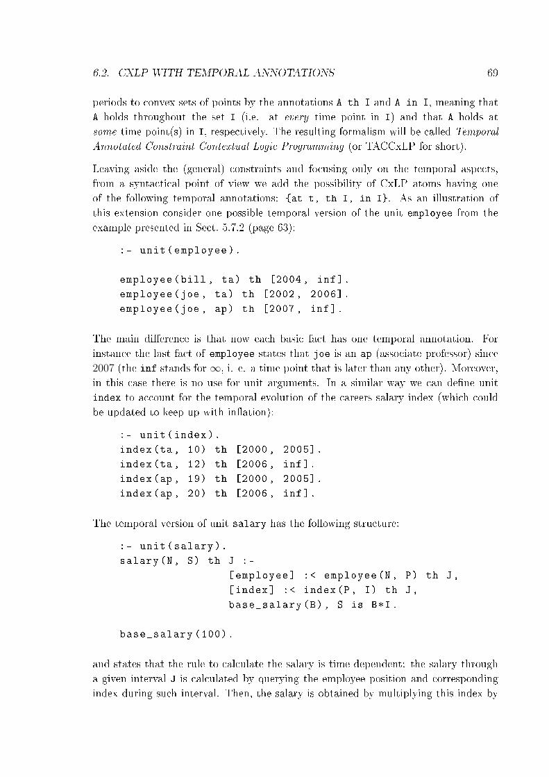
6.2. CXLP WITH TEMPORAL ANNOTATIONS 69
periods to convex sets of points by the annotations A th I and A in I, meaning thatA holds throughout the set I (i.e. at every time point in I) and that A holds atsome time point(s) in I, respectively. The resulting formalism will be called Temporal
Annotated Constraint Contextual Logic Programming (or TACCxLP for short).
Leaving aside the (general) constraints and focusing only on the temporal aspects,from a syntactical point of view we add the possibility of CxLP atoms having oneof the following temporal annotations: {at t, th I, in I}. As an illustration ofthis extension consider one possible temporal version of the unit employee from theexample presented in Sect. 5.7.2 (page 63):
:- unit(employee ).
employee(bill , ta) th [2004, inf].
employee(joe , ta) th [2002, 2006].
employee(joe , ap) th [2007, inf].
The main di�erence is that now each basic fact has one temporal annotation. Forinstance the last fact of employee states that joe is an ap (associate professor) since2007 (the inf stands for∞, i. e. a time point that is later than any other). Moreover,in this case there is no use for unit arguments. In a similar way we can de�ne unitindex to account for the temporal evolution of the careers salary index (which couldbe updated to keep up with in�ation):
:- unit(index).
index(ta, 10) th [2000, 2005].
index(ta, 12) th [2006, inf].
index(ap, 19) th [2000, 2005].
index(ap, 20) th [2006, inf].
The temporal version of unit salary has the following structure:
:- unit(salary ).
salary(N, S) th J :-
[employee] :< employee(N, P) th J,
[index] :< index(P, I) th J,
base_salary(B), S is B*I.
base_salary (100).
and states that the rule to calculate the salary is time dependent: the salary througha given interval J is calculated by querying the employee position and correspondingindex during such interval. Then, the salary is obtained by multiplying this index by

70 CHAPTER 6. TEMPORAL REASONING IN A MODULAR LANGUAGE
the base salary.2 As an illustration consider the following goal to discover joe's salaryin [2005, 2007]:
?- salary :> salary(joe , S) in [2005 , 2007].
S = 1000; S = 1200; S = 2000
The reader should notice that the salary of a teaching assistant (ta) was raised in 2006
(S = 1000 and S = 1200) and that joe achieved the position of associate professor
(ap) in 2007 (S = 2200).
6.3 Constraint Theory
The constraint theory is identical to the one of TACLP [BMRT02], i.e. a constraintdomain for time points includes suitable constants for time points, function symbols foroperations on time points (e.g., +,-, ...) and the predicate symbol ≤, modelling thetotal order relation on time points. This constraint domain is extended to a constraintdomain A for handling annotations, by enriching the signature with function symbols[., .], at, th, in, t and the predicate symbol v. Moreover, assuming r1 ≤ s1,s1 ≤ s2 and s2 ≤ r2, the axioms for the predicate symbol v can be summarised as:
in[r1, r2] v in[s1, s2] v in[s1, s1] = at s1 = th[s1, s1] v th[s1, s2] v th[r1, r2]
Finally, the axioms of the least upper bound t (function symbol) can be restricted to:3
th[s1, s2] t th[r1, r2] = th[s1, r2]⇔ s1 < r1, r1 ≤ s2, s2 < r2
6.4 Operational Semantics
To obtain the operational semantics of this language one needs to replace the inferencerules (v) and (t) of Sect. 2.3.4 by their contextual versions, i.e. instead of annotatedatoms Aα we must have C ` Aα.
C ` Aα γ v α
C ` Aγrule (vC)
C ` Aα C ` Aβ γ = α t βC ` Aγ
rule (tC)
2Of course that it would be reasonable to annotate the base salary. However, doing so wouldn't
bring any novelty to the problem.3The least upper bound only has to be computed for overlapping th�annotations.

6.5. INTERPRETER AND COMPILER 71
Moreover, the inference rules of CxLP must be adapted to the case where literals canbe annotated. These rules can be obtained in a rather straightforward manner from theones for CxLP (see Sect. 5.3 on page 55) by substituting each goal G by its annotatedversion Gα.
6.5 Interpreter and Compiler
Meta-interpretation and compilation are two widely used techniques to implementlogic languages. Frühwirth [Frü96] provides both an interpreter and a compiler forTACLP where the compiler transforms TACLP into CLP. Moreover, the same authorin [Frü94b] presents an e�cient optimised interpreter for TACLP were only atomicformulas can be annotated.
An obvious implementation of the proposed language can be obtained with a slightmodi�cation of the compiler (interpreter) for TACLP in order to handle context oper-ations (leaving them unchanged). Therefore, to get a full blown implementation it issu�cient to de�ne the constraint domain C for the TACLP, i.e. one has to de�ne thetime point domain.
6.5.1 Time Point Domain
The main motivation behind our temporal data model was to be able to represent awide variety of notions of time, not only common ones such as the 24�Hour timekeepingsystem or the Gregorian calendar but also more specialised ones such as time in digitalcircuits. As we will see in this section, Constraint Logic Programming [JL87] specialisedto Finite Domains (CLP(FD)) and rei�ed Booleans (CLP(B)) turns out to be a verysuitable framework: the size of the temporal variables domain admits an e�cientimplementation with Finite Domains and the rei�ed Booleans allows us to expresselaborated temporal constraints. Moreover, since CLP(X) is so pervasive to this work,an overview of the main characteristics of this paradigm can be found in Appendix B.
Although constraints are widely used for temporal reasoning, their application intemporal information representation is rare. One of the exceptions is the work ofKabanza et. al [KSW90] with in�nite temporal information. Here we present anotherway of using constraints to represent temporal data: by interpreting a ConstraintSatisfaction Problem as an intensional way of specifying a set of time points, i.e. as atime point domain:
De�nition 8 (Time Point Domain) A time point domain is a Constraint Satisfac-
tion Problem on �nite domains.

72 CHAPTER 6. TEMPORAL REASONING IN A MODULAR LANGUAGE
If n is the number of variables of the CSP we say that the domain is n-dimensional. Atime point is a tuple that is solution of the CSP:
De�nition 9 (Time Point) Given a time point domain D on variables {X1, . . . , Xn}we say that the tuple X = (x1, . . . , xn) is a time point of D if the assignment {X1 =
x1, . . . , Xn = xn} satis�es all the constraints of D.
With this representation the domain D24 can be formulated as:
Example 4 (24�Hour) The CSP D24 = H ∈ [0, 23] ∧ M ∈ [0, 59] on variables
{H,M} is a time point domain representing the 24�Hour system. The tuples x =
(10, 30) and y = (13, 20) are examples of time points of this domain.
Finally it is rather straightforward, although not as trivial as the 24�Hour, to use aCSP to represent a calendar (Gregorian, Julian, etc).
Considering there are bene�ts in dealing with each of the tuple members instead of thetuple as a whole, we modi�ed the temporal variables to accommodate this:
De�nition 10 (Time Variable) We say that X is a time variable of the n-dimensional
time point domain D i� X is a n-tuple of D variables.
For instance X1 = (H1,M1) and X2 = (H2,M2) are variables of D24. With thisrepresentation for variables it is easy to express constraints that correspond to theequal, before and after relations. For instance, X1 < X2 corresponds to the constraintH1 < H2 ∨ (H1 = H2 ∧M1 < M2). Note that this constraint may be expressed usingCLP(FD, B).
Finally, since GNU Prolog/CX, besides providing the CxLP primitives, also has aconstraint solver over �nite domains and rei�ed booleans (CLP(FD, B)), making theimplementation of this language relatively straightforward.
Relations Between Di�erent Time Point Domains
Applications such as Heterogeneous Information Systems have to deal with temporaldata described in di�erent domains. There are several reasons for this state of thingssuch as:
• information relative to di�erent timezones or calendars (Julian, Gregorian andChinese lunar calendar);

6.6. RELATED WORK 73
• information from di�erent domains that share temporal units. For instance anewspaper is characterised by {Y ear,Month,Day} and a speci�c news can befurther described by Hour and Minute.
Therefore there is a strong need to establish (whenever possible) temporal relationsbetween these di�erent time domains. To have this capability in our framework wejust need to add a function that converts a time point from one domain to another.
A simple illustration of such function is the one that relates the 24�Hour domain withseconds (denoted by D24s) and the D24:
f : D24s −→ D24
(h,m, s) −→ (h,m)
Another basic example is the one derived from the problem of conversion of timezones.For that consider the domain D+1 on variables {Y,Mo,D,H,Mi} for time in thetimezone GMT+1 and a similar D+2 to express time in the timezone GMT+2. Thefollowing function converts time points from D+1 to D+2:
g : D+1 −→ D+2
(y,mo, d, h,mi) −→
(y,mo, d, h+ 1,mi) if h < 23
(y,mo, d+ 1, 0,mi) if d < max_day(y,mo)
. . .
Please notice that, although the inverse of g is still a function, this doesn't happen for fbecause, to each time point ofD24 corresponds a set of time points ofD24s : for instance,to the point (14, 20) corresponds the set of points {(14, 20, 0), . . . , (14, 20, 59)}.
If there is at least one conversion function between two domains, it is easy to relate(=, < or >) points on these domains. The procedure its quite simple and can bedescribed in two steps: convert the points to the same domain and apply the corre-sponding domain relation.
As an illustration, consider the point (16, 20) of D24 and (15, 30, 12) from D24s . Therelation (15, 30, 12) < (16, 20) its valid because f(15, 30, 12) = (15, 30) and (15, 30) <
(16, 20) in the domain D24.
6.6 Related Work
In this section we describe other formalisms that combine temporal reasoning withmodularity. Since Multi-theory Temporal Annotated Constraint Logic Programming
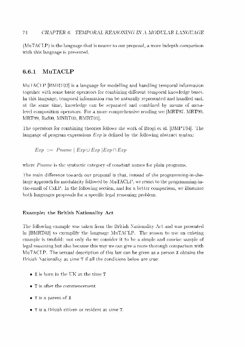
74 CHAPTER 6. TEMPORAL REASONING IN A MODULAR LANGUAGE
(MuTACLP) is the language that is nearer to our proposal, a more indepth comparisonwith this language is presented.
6.6.1 MuTACLP
MuTACLP [BMRT02] is a language for modelling and handling temporal informationtogether with some basic operators for combining di�erent temporal knowledge bases.In this language, temporal information can be naturally represented and handled and,at the same time, knowledge can be separated and combined by means of meta-level composition operators. For a more comprehensive reading see [MRT97, MRT99,MRT99, Raf00, MNRT00, BMRT01].
The operators for combining theories follows the work of Brogi et al. [BMPT94]. Thelanguage of program expressions Exp is de�ned by the following abstract syntax:
Exp ::= Pname | Exp ∪ Exp |Exp ∩ Exp
where Pname is the syntactic category of constant names for plain programs.
The main di�erence towards our proposal is that, instead of the programming-in-the-large approach for modularity followed by MuTACLP, we resort to the programming-in-the-small of CxLP. In the following section, and for a better comparison, we illustrateboth languages proposals for a speci�c legal reasoning problem.
Example: the British Nationality Act
The following example was taken from the British Nationality Act and was presentedin [BMRT02] to exemplify the language MuTACLP. The reason to use an existingexample is twofold: not only do we consider it to be a simple and concise sample oflegal reasoning but also because this way we can give a more thorough comparison withMuTACLP. The textual description of this law can be given as a person X obtains theBritish Nationality at time T if all the conditions below are true:
• X is born in the UK at the time T
• T is after the commencement
• Y is a parent of X
• Y is a British citizen or resident at time T.

6.6. RELATED WORK 75
Assuming that Jan 1 1955 is the commencement date of the law, the MuTACLPprogram for this problem is:
BNA:
get_citizenship(X) at T <- T >= Jan 1 1955,
born(X, uk) at T,
parent(Y, X) at T,
british_citizen(Y) at T.
get_citizenship(X) at T <- T >= Jan 1 1955,
born(X, uk) at T,
parent(Y, X) at T,
british_resident(Y) at T.
Moreover, those authors also assume a separate program to encode the data for a givenperson John whose parent Bob is a British citizen since Sep 6 1940 :
JOHN:
born(john , uk) at Aug 10 1969.
parent(bob , john) th [T, inf] <- born(john , _) at T.
british_citizen(bob) th [Sep 6 1940, inf].
Finally, the citizenship of John can be queried as:
demo(BNA ∪ JOHN , get_citizenship(john) at T)
and the result is T = Aug 10 1969.
Our proposal to solve this problem is a more modular way since we will opt to de�neone unit for each predicate. More speci�cally, unit born/2 represents the name andcountry where a person was born:
:- unit(born(Name , Country )).
born(john , uk) at 'Aug 10 1969 '.
item at T :- born(Name , Country) at T.
It this unit (and in the subsequent one) we present dates as atoms such as 'Aug 10
1969', this is only for the reader's confort since, as mentioned in Sect. 6.5 we resortto CLP(FD, B) to implement the temporal elements. Moreover, in order to providean implementation coherent with the current CxLP proposal we also de�ne predicateitem to instantiate the units arguments.
The unit british_citizen/14 states when a person started to be a British citizen:
4In a similar way we could have de�ned an analogous unit british_resident/1.
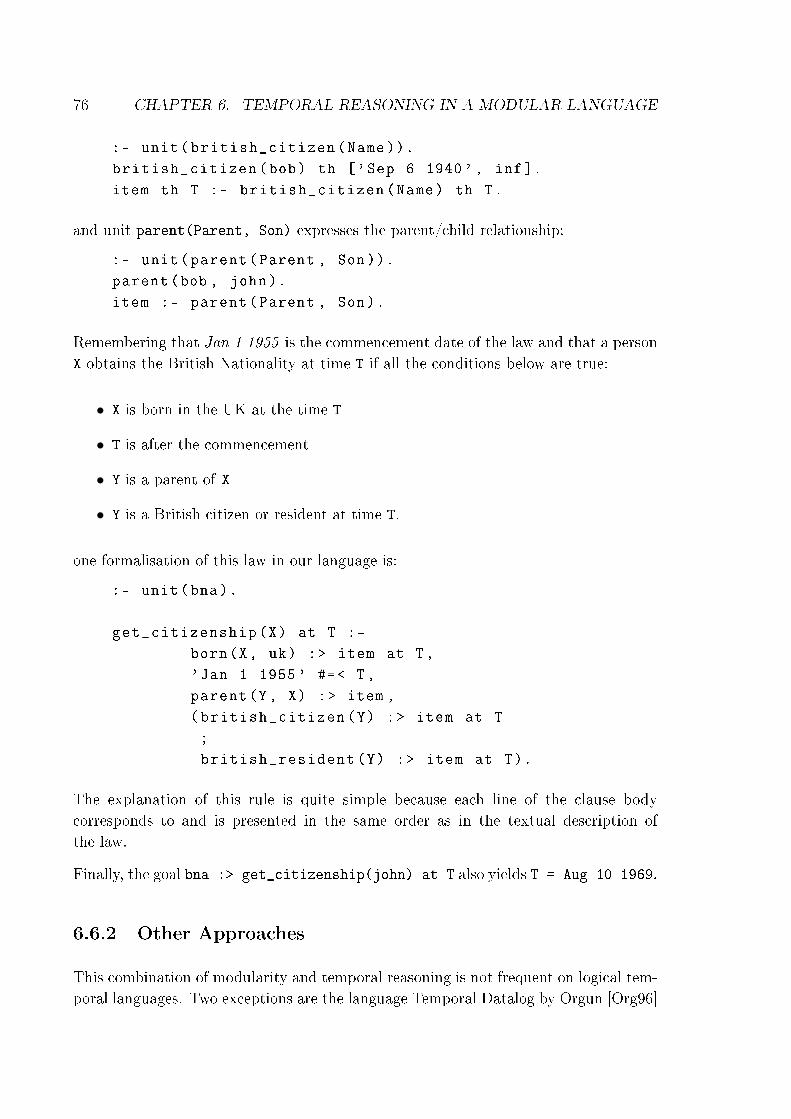
76 CHAPTER 6. TEMPORAL REASONING IN A MODULAR LANGUAGE
:- unit(british_citizen(Name )).
british_citizen(bob) th ['Sep 6 1940', inf].
item th T :- british_citizen(Name) th T.
and unit parent(Parent, Son) expresses the parent/child relationship:
:- unit(parent(Parent , Son)).
parent(bob , john).
item :- parent(Parent , Son).
Remembering that Jan 1 1955 is the commencement date of the law and that a personX obtains the British Nationality at time T if all the conditions below are true:
• X is born in the UK at the time T
• T is after the commencement
• Y is a parent of X
• Y is a British citizen or resident at time T.
one formalisation of this law in our language is:
:- unit(bna).
get_citizenship(X) at T :-
born(X, uk) :> item at T,
'Jan 1 1955' #=< T,
parent(Y, X) :> item ,
(british_citizen(Y) :> item at T
;
british_resident(Y) :> item at T).
The explanation of this rule is quite simple because each line of the clause bodycorresponds to and is presented in the same order as in the textual description ofthe law.
Finally, the goal bna :> get_citizenship(john) at T also yields T = Aug 10 1969.
6.6.2 Other Approaches
This combination of modularity and temporal reasoning is not frequent on logical tem-poral languages. Two exceptions are the language Temporal Datalog by Orgun [Org96]

6.7. CONCLUDING REMARKS 77
and the work on amalgamating knowledge bases by Subrahmanian [Sub94]. TemporalDatalog introduces the concept of module which, however, seems to be used as a meansfor de�ning new non-standard algebraic operators, rather than as a knowledge tools.On the other hand, the work on amalgamating knowledge bases o�ers a multi-theoryframework, based on annotated logics, where temporal information can be handled, butonly a limited interaction among the di�erent knowledge sources is allowed: essentiallya kind of message passing mechanism allows one to delegate the resolution of an atomto other databases.
6.7 Concluding Remarks
In this chapter we added temporal reasoning capabilities to a modular logic language.More speci�cally, we joined the Temporal Annotated Constraint Logic Programmingwith Contextual Logic Programming. The aim of this proposal is to have both for-malisms in the same language, without de�ning any sort of relation between temporalreasoning and modularity.
Besides de�ning the language, we also provided an operational semantics. Moreover, wesketched a compiler for the proposed language and speci�ed a possible implementationfor a speci�c time point domain. Finally, we reviewed related work on this subject, inparticular, the MuTACLP language that also combines the chosen temporal formalismwith another modular logic language.


Chapter 7
Temporal Contextual Logic
Programming
This chapter presents a temporal extension of CxLP, called Temporal Contextual
Logic Programming (TCxLP). It describes the language syntax, operational
semantics and a procedure that computes the last upper bound of the temporal
annotations. Afterwards, an interpreter and a compilation scheme are given. Finally,
this language is applied to several domains and compared with similar approaches.
7.1 Introduction
One possible way of devising a language with modularity and temporal reasoning isto consider that these two characteristics can co-exist without any direct relationship.This was the approach followed in Chap. 6. Nevertheless we can also conceive a scenariowhere those concepts are more integrated or more related. In this chapter we take theinteraction between modularity and time to the next level by considering that the usageof a module is in�uenced by temporal conditions. The intuition for this proposal camefrom common sense reasoning where it is usual to consider that the usage of (part of)knowledge (law, criteria) can be time dependent.
Contextual Logic Programming structure is very suitable for integrating with temporalreasoning since, as we shall see, it is quite straightforward to add the notion of time ofthe context and let that time help in deciding if a certain module is eligible or not tosolve a goal. Regarding the temporal paradigm we shall continue to use TACLP, notonly because of the reasons enumerated in Sect. 6.1, but also because, this way, theoriginal contribution stands out.
This chapter is organised as follows: we start incrementally building a language thatextends CxLP with temporal annotations (Sect. 7.2). An algorithm to compute the
79

80 CHAPTER 7. TEMPORAL CONTEXTUAL LOGIC PROGRAMMING
least upper bound of annotations is described in Sect. 7.3. Afterwards, we dealwith the semantics of this proposal, more speci�cally, the constraint theory and theoperational semantics (Sect. 7.4). An implementation with an instantiation for thetime point domain (see page 71) follows in Sect. 7.5. Applications to several domainsis presented in Sect. 7.6 and comparisons between our framework and related workfollows (Sect. 7.7). Finally, we provide some conclusions in Sect. 7.8.
7.2 Language of TCxLP
The basic mechanism of CxLP is called context search and can be described as follows:to solve a goal G in a context C, a search is performed until the topmost unit of C thatcontains clauses for the predicate of G is found. We propose to incorporate temporalreasoning into this mechanism. To accomplish this we add temporal annotations tonot only the dynamic part of CxLP (contexts) but also to the static one (units) andit will be the relation between those two types of annotations that will determine if agiven unit is eligible to match a goal during a context search.
7.2.1 Annotating Units
Considering the initial unit de�nition (i.e. without parameters), adding temporalannotations to these units could be done simply by annotating the unit name. Usingan extended GNU Prolog/CX syntax, an annotated unit could be de�ned as:
:- unit(foo) th [1,4].
Nevertheless, units with arguments ought to allow for a re�nement of the temporalquali�cation, i.e. we can have several quali�cations, one for each possible argumentinstantiation. As an illustration consider the following example:
Example 5 Temporal annotated unit bar/1:
:- unit(bar(X)).
bar(a) th [1,2].
bar(b) th [3,4].
where the annotated facts state that unit bar with its argument instantiated to a hasthe annotation th [1,2] and with its argument instantiated to b has the annotationth [3,4], respectively. Moreover, it should be clear that this is more expressive thanthe proposal at the beginning of this section since it is still possible to annotate the

7.2. LANGUAGE OF TCXLP 81
unit most general descriptor (for the de�nition of unit descriptors see Parametrised
Units in Sect. 5.5) :
:- unit(foo).
foo th [1 ,4].
As we saw in the example above, the unit descriptor is the same as the annotatedpredicate, foo. Such overloading is intentional and makes it easier to express whether agiven unit (descriptor) in a context satis�es a temporal condition (annotated predicate).This relation will be made precise when we present the operational semantics (seeinference rule 7.5 in page 88).
Therefore we propose to temporally annotate the unit descriptors and those annotatedfacts are designated as the unit temporal conditions.
7.2.2 Temporal Annotated Contexts
The addition of time to a context is rather simple and intuitive: instead of a sequenceof unit descriptors C we now have a temporally annotated sequence of units descriptorsC∆, where ∆ is a temporal annotation of the type at t, th I or in I (see page 13).This annotation ∆ is called the time of the context and by default contexts are implicitlyannotated with the current time. As the name implies, the time of the context speci�esthe time when a given context should be considered, making all the computationsrelative to that time.
Recall that in GNU Prolog/CX a context is implemented as list of units descriptorssuch as [u1(X), u2(Y,Z)]: a temporal annotated context can be for instance [u1(X),u2(Y,Z)] th [1,4].
7.2.3 Relating Temporal Contexts with Temporal Units
Although the relation between temporal annotated contexts and units will be madeprecise when we present the semantics (Sect. 7.4), in this section we illustrate what wemean when we say that the relation between those two types of annotations (contextand units) determines if a given unit is eligible to match a goal during a context search.
Contexts for a Simple Temporal Unit
Consider the unit bar/1 of Example 5 (page 80). Roughly speaking, this unit will beeligible to match a goal in a context like:

82 CHAPTER 7. TEMPORAL CONTEXTUAL LOGIC PROGRAMMING
[..., bar(a), ...] in [1,4]
if �bar(a) in [1,4]� can be proved.
Since one of the unit temporal conditions is �bar(a) th [1,2]� and we known thatin [1,4] v th [1,2], then by the inference rule (v) (see page 14) one can derive�bar(a) in [1,4]�. In a similar way we say that this unit its not eligible in thefollowing context (recall that th [3,6] 6v th [3,4]):
[..., bar(b), ...] th [3,6]
Conversely, suppose that unit bar/1 has some de�nition for the predicate of an atomicgoal G, then in order to use this de�nition in a goal like:
?- [bar(X), ...] in [1,4] :< G
besides the instantiations for the variables of G, one also obtains bindings for the unitarguments:
X = a or X = b.
University Employees Example: Temporal Version
Revisiting the University employees example (already seen in page 63 to illustrateCxLP and in page 68 to exemplify CxLP with temporal annotations), unit employeewith temporal information can be written as:
:- unit(employee(NAME , POSITION )).
name(NAME).
position(POSITION ).
item.
employee(bill , ta) th [2004, inf].
employee(joe , ta) th [2002, 2006].
employee(joe , ap) th [2007, inf].
This way it is possible to represent the history of the employees positions: joe wasa teaching assistant (ta) between 2002 and 2006. The same person is a associateprofessor (ap) since 2007. Moreover, in this case the rule for predicate item/0 doesn'tneed to be �item :- employee(NAME, POSITION).� because the goal item is true onlyif the unit is (temporally) eligible and, for that to happen, the unit arguments must be

7.2. LANGUAGE OF TCXLP 83
instantiated. To better understand this example, consider the goal that queries joe'sposition throughout [2005,2006]:
?- [employee(joe , P)] th [2005 ,2006] :< item.
the evaluation of item is true as long as the unit is eligible in the current context, andthis happens when P is instantiated with ta (teaching assistant), therefore we get theanswer P = ta.
In a similar way we can de�ne a temporal version of unit index/2 as:
:- unit(index(POSITION , INDEX )).
position(POSITION ).
index(INDEX ).
item.
index(ta, 10) th [2000, 2005].
index(ta, 12) th [2006, inf].
index(ap, 19) th [2000, 2005].
index(ap, 20) th [2006, inf].
to express the evolving index associated with each position. Unit salary can be de�nedas:
:- unit(salary(SALARY )).
item :-
position(P),
index(P, I) :> item ,
base_salary(B),
SALARY is B*I.
base_salary (100).
There is no need to annotate the goals position(P) or index(P, I) :> item sincethese are evaluated in a context which already has the same temporal annotation. To�nd out joe's salary in 2005 we can say:
?- [salary(S), employee(joe , P)] at 2005 :< item.
which yields the bindings:
P = ta
S = 1000

84 CHAPTER 7. TEMPORAL CONTEXTUAL LOGIC PROGRAMMING
Since salary is the topmost unit that de�nes a rule for item/0, the body of therule for this predicate is evaluated. In order to use the unit employee(joe, P) tosolve position(P), the unit must satisfy the temporal conditions �at 2005�, that inthis case means instantiating P with ta, therefore we obtain position(ta). A similarreasoning applies for goal �index(ta, I) :> item�, i.e. this item is resolved in context�[index(ta, 10), salary(S), employee(joe, ta)] at 2005�. The remainder ofthe rule body is straightforward, leading to the answer substitution P = ta and S =
1000.
7.3 Computing the Least Upper Bound
One obvious drawback stemming from incorporating temporal reasoning into contextsearch is the extra computation that results from processing the units/contexts tempo-ral annotations. Moreover, since context search is a basic mechanism, extra care mustbe taken to minimise this overhead.
In order to lighten the process, we propose to calculate, at compile time, the leastupper bound (t) of the units descriptors temporal annotations. This way context onlyneeds to verify the satisfaction of the relation between annotations of the context andthat of the units, i.e. only relation v is left for runtime.
According to [BMRT02] it su�ces to consider the least upper bound (or lub forshort) for time periods that produce another di�erent meaningful time period, i.e.one may consider only overlapping time periods that do not include one another (seeSect. 6.3). In this section we present a procedure that iterates over the set of each unitth-annotated descriptors, calculating the lub of uni�able atoms with th-overlappingintervals, inserting the output of the computation and (possibly) removing (some of)the inputs. This procedure is presented in an incremental way, starting with groundannotated unit descriptors and afterwards we handle the non ground case.
7.3.1 Ground Temporal Conditions
In this case the set of temporally annotated unit descriptors is not only �nite (byde�nition) but also ground. Before giving a formal description let us consider anexample that provides the general intuition behind this procedure. To that purpose,consider the unit baz/1:
:- unit(baz(X)).
baz(a) th [1,4].
baz(a) th [3,7].

7.3. COMPUTING THE LEAST UPPER BOUND 85
...
Since th [1,4] and th [3,7] are two overlapping th-annotations for the same unitdescriptor (baz(a)), we compute their lub, obtaining th [1,7]. Therefore, we canreplace these two temporal conditions by a more general one:
:- unit(baz(X)).
baz(a) th [1 ,7].
...
A formal description of this procedure is given in Algorithm 1 (page 85). Basically,the algorithm iterates over the set of units of a given program and for each pair of th-annotated temporal conditions that have the same unit descriptor (u) and overlappingintervals (I1 overlaps I2), remove that pair from the unit temporal conditions and insertone with the same unit descriptor and the annotation that results from the computingthe lub of those annotations, i.e. insert a new temporal condition that subsumes theprevious two.
One can easily see that this procedure terminates not only because the set of units is�nite (for loop) but also due to the fact that each iteration of the while loop decreasesthe size of the said set, the set of th-annotated temporal conditions of a unit.
Algorithm 1 Computing the least upper bound of ground th-annotationsLet {u1, . . . , un} be the set of units of a given program P and Thui
the set of th-annotated temporal conditions of unit ui (that, by hypothesis, are all ground):
1. For each unit ui ∈ P
(a) while (∃ u th I1, u th I2 ∈ Thui: I1 overlaps I2)
i. remove u th I1 and u th I2 from Thui
ii. insert u th (I1 t I2) into Thui
7.3.2 Non Ground Temporal Conditions
In this section we provide a generalisation of Algorithm 1 to non ground th-annotatedtemporal conditions. As a simple illustration consider unit foo/2:
1 :- unit(foo(X, Y)).
2 foo(_, b) th [1, 3].
3 foo(a, _) th [4, 6].
4 foo(a, b) th [5, 8].

86 CHAPTER 7. TEMPORAL CONTEXTUAL LOGIC PROGRAMMING
Previously, a unit u with parameter variables −→p was a set of clauses, for which allvariables in −→p are implicitly existentially quanti�ed over all clauses of the unit. Thesame existential quanti�cation also applies to the unit temporal conditions. Therefore,in the example above there is no need to name the variables in the temporal conditions(lines 2 and 3) since the �rst argument of foo already coincides with X and the secondwith Y, i.e. the unit arguments.
Before describing the procedure for the non ground case, we have yet to de�ne whatwe mean by an annotated atom being subsumed by a set of the same elements:
De�nition 11 (`v) Consider that S is a set of temporal annotated atoms. We say
that A th I is subsumed by the set S and denote by S `v A th I if and only if there is
a B th J ∈ S and a substitution θ such that A = Bθ and I v J , i.e. if there is an
annotated atom in S that is at least as informative as A th I.
The procedure for this case is formally presented as Algorithm 2 (page 86) and can bedescribed as: for every unit, �nd two th-annotated temporal conditions that overlap(I1 overlaps I2) and whose unit descriptors are uni�able (θ =mgu(U1, U2)). Them(possibly) remove those temporal conditions and insert a new one with the annotationthat results from computing the lub (I1 t I2) and uni�ed descriptor (U1θ). Moreover,the body of the while loop is executed if the temporal condition that can be generatedisn't already subsumed by the set of th-annotated temporal conditions (Thui
6`v(U1θ) th(I1 t I2)).
Algorithm 2 Computing the least upper bound th-annotationsLet {u1, . . . , un} be the set of units of a given program P and Thui
the set of th-annotated temporal conditions of unit ui:
1. For each unit ui
(a) while (∃ U1 th I1, U2 th I2 ∈ Thui, θ = mgu(U1, U2): I1 overlaps I2 and
Thui6`v (U1θ) th(I1 t I2)
i. if U1 (U2) is ground, remove U1 th I1 (U2 th I2) from Thui.
ii. insert U1θ th (I1 t I2) into Thui.
For a better understanding, let us consider unit foo/2 above. According to thisalgorithm one possible evolution of the set Thfoo/2 is:
1. {foo(_, b) th [1, 3], foo(a, _) th [4, 6], foo(a, b) th [5, 8]}.
2. {foo(_, b) th [1, 3], foo(a, _) th [4, 6], foo(a, b) th [1, 6],
foo(a, b) th [5, 8]}.

7.4. OPERATIONAL SEMANTICS 87
3. {foo(_, b) th [1, 3], foo(a, _) th [4, 6], foo(a, b) th [1, 8]}.
The �rst iteration computes the lub of the {foo(_, b) th [1, 3]} and {foo(a, _)
th [4, 6]}, yielding {foo(a, b) th [1, 6]}. In the next iteration, the lub of theinserted annotation ({foo(a, b) th [1, 6]}) and {foo(a, b) th [5, 8]} is com-puted, yielding {foo(a, b) th [1, 8]}.
Like the algorithm for the ground case, we also iterate over a �nite set of units (for loop),nevertheless showing the termination of the while loop requires more explanation sincenow the set of th-annotated temporal conditions may not decrease. In fact, as we saw inthe example above, the �rst iteration increases the set and the second decreases. Beforeexplaining the termination the reader should keep in mind that the unit descriptor isa �nite term and the set of temporal conditions is also �nite. Moreover, the temporalperiods of the th-annotations are of the form [T1, T2] where T1 and T21 are integers,greater or equal than 0, with T2 ≥ T1. Therefore, the number of temporal conditionsthat can result from combining overlapping intervals or by specialising descriptors is�nite. Since each iteration of the while loop introduces a new temporal condition (notsubsumed by the others) of a �nite set, the loop terminates.
7.4 Operational Semantics
Similar to the operational semantics of Contextual Logic Programming (see Sect. 5.3)and as usual in logic programming, we present the operational semantics by means ofderivations. We will name and enumerate the inference rules which specify computa-tions. Finally, the paragraph after each rule gives an informal explanation of how itworks.
7.4.1 Inference Rules
To de�ne the operational semantics we consider the following notation: C and C ′ arecontexts; Tu is the set of temporal conditions of unit u; θ, σ and ε are substitutions; ∆
and Λ are temporal annotations and ∅ and G are goals. Moreover, we also assume thatAlgorithm 2 (page 86) has been applied to the subset of th-annotated atoms of Tu.
Null goal
C∆ ` ∅ [ε](7.1)
1With the possible exception of T2 = inf.
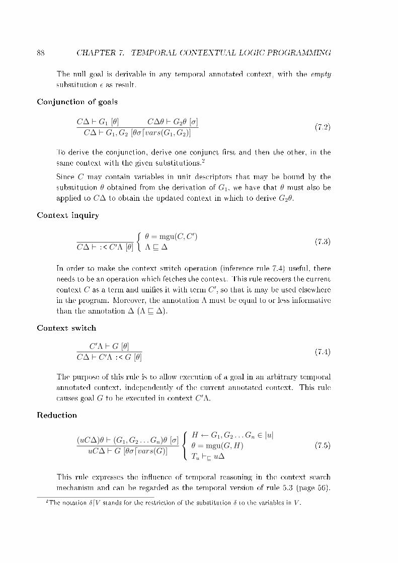
88 CHAPTER 7. TEMPORAL CONTEXTUAL LOGIC PROGRAMMING
The null goal is derivable in any temporal annotated context, with the empty
substitution ε as result.
Conjunction of goals
C∆ ` G1 [θ] C∆θ ` G2θ [σ]
C∆ ` G1, G2 [θσdvars(G1, G2)](7.2)
To derive the conjunction, derive one conjunct �rst and then the other, in thesame context with the given substitutions.2
Since C may contain variables in unit descriptors that may be bound by thesubstitution θ obtained from the derivation of G1, we have that θ must also beapplied to C∆ to obtain the updated context in which to derive G2θ.
Context inquiry
C∆ ` :< C ′Λ [θ]
{θ = mgu(C,C ′)
Λ v ∆(7.3)
In order to make the context switch operation (inference rule 7.4) useful, thereneeds to be an operation which fetches the context. This rule recovers the currentcontext C as a term and uni�es it with term C ′, so that it may be used elsewherein the program. Moreover, the annotation Λ must be equal to or less informativethan the annotation ∆ (Λ v ∆).
Context switch
C ′Λ ` G [θ]
C∆ ` C ′Λ :< G [θ](7.4)
The purpose of this rule is to allow execution of a goal in an arbitrary temporalannotated context, independently of the current annotated context. This rulecauses goal G to be executed in context C ′Λ.
Reduction
(uC∆)θ ` (G1, G2 . . . Gn)θ [σ]
uC∆ ` G [θσdvars(G)]
H ← G1, G2 . . . Gn ∈ |u|θ = mgu(G,H)
Tu `v u∆
(7.5)
This rule expresses the in�uence of temporal reasoning in the context searchmechanism and can be regarded as the temporal version of rule 5.3 (page 56).
2The notation δdV stands for the restriction of the substitution δ to the variables in V .

7.5. TCXLP COMPILER AND INTERPRETER 89
Informally it can be described as: when a goal (G) has a de�nition (H ←G1, G2, . . . Gn ∈ |u| and θ = mgu(G,H)) in the topmost unit (u) of the an-notated context (uC∆) and the unit temporal conditions subsume the �time ofthe context� (Tu `v u∆), to derive the goal we must call the body of the matchingclause, after uni�cation. The main di�erence towards the non-temporal versionis that we now also check whether the unit is �temporally eligible�.
Context traversal:
C∆ ` G[θ]
uC∆ ` G[θ]
{pred(G) 6∈ ||u|| (7.6)
When none of the previous rules apply and, in particular, when the predicateof G isn't de�ned in the predicates of u (||u||), remove the top element of thecontext and proceed, i.e. resolve goal G in the supercontext.
Application of the Rules
It is straightforward to verify that the inference rules are mutually exclusive, leadingto the fact that, given a derivation tuple C∆ ` G[θ], only one rule can be applied.
7.5 TCxLP Compiler and Interpreter
In this section we propose a source-to-source program transformation that allows usto convert from Temporal Contextual Logic Programming into CxLP where the unitdescriptors can have temporal annotations. Since after this transformation we obtain(a subset of) the language proposed in Chap. 6 we can use the compiler (or interpreter)described in Sect. 6.5 on the resulting program. This way we obtain a compiler (orinterpreter) for TCxLP.
7.5.1 From TCxLP to CxLP+TACLP
Our goal is to convert a TCxLP program into CxLP (with annotations), such that thislast program expresses the behaviour of context search being in�uenced by temporalreasoning. Informally, we add to every unit a sort of �frontend� that makes the unitbody (the �backend�) accessible only if the unit temporal conditions are satis�ed bythe time of the context, otherwise context search must continue, bypassing the unit.
In the �rst step of Algorithm 3, throughout renaming the predicates we de�ne the�backend�. The access to the renamed predicate (p') is controlled by means of the
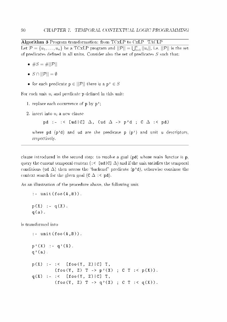
90 CHAPTER 7. TEMPORAL CONTEXTUAL LOGIC PROGRAMMING
Algorithm 3 Program transformation: from TCxLP to CxLP+TACLPLet P = {u1, . . . , un} be a TCxLP program and ||P|| =
⋃ni=1 ||ui||, i.e. ||P|| is the set
of predicates de�ned in all units. Consider also the set of predicates S such that:
• #S = #||P||
• S ∩ ||P|| = ∅
• for each predicate p ∈ ||P|| there is a p' ∈ S
For each unit ui and predicate p de�ned in this unit:
1. replace each occurrence of p by p';
2. insert into ui a new clause
pd :- :< [ud|C] ∆, (ud ∆ -> p'd ; C ∆ :< pd)
where pd (p'd) and ud are the predicate p (p') and unit u descriptors,respectively.
clause introduced in the second step: to resolve a goal (pd) whose main functor is p,query the current temporal context (:< [ud|C] ∆) and if the unit satis�es the temporalconditions (ud ∆) then access the �backend� predicate (p'd), otherwise continue thecontext search for the given goal (C ∆ :< pd).
As an illustration of the procedure above, the following unit
:- unit(foo(A,B)).
p(X) :- q(X).
q(a).
is transformed into
:- unit(foo(A,B)).
p'(X) :- q'(X).
q'(a).
p(X) :- :< [foo(Y, Z)|C] T,
(foo(Y, Z) T -> p'(X) ; C T :< p(X)).
q(X) :- :< [foo(Y, Z)|C] T,
(foo(Y, Z) T -> q'(X) ; C T :< q(X)).

7.6. APPLICATION EXAMPLES 91
For reading purposes, in the program above we used an abstract version of the generatedcode, since C T or :< [foo(Y, Z)|C] T isn't valid CxLP code.3
7.6 Application Examples
We now present a few examples which will sustain the adequacy of TCxLP. To easethe reading, in this section we present dates by atoms such as 'Aug 10 1969'. Nev-ertheless, as mentioned in Sect. 6.5 (page 71), we resort to CLP(FD, B) to implementthe temporal elements. Moreover, unless stated otherwise, we assume that all temporalunits implement the fact item.
7.6.1 Management of Work�ow Systems
Work�ow management systems (WfMS) are software systems that support the au-tomatic execution of work�ows. Although time is an important resource here, thetime management o�ered by most of these systems must be handled explicitly and israther limited. Therefore, automatic management of temporal aspects of informationis an interesting and growing �eld of research [CP03, CP04, CP06, MMZ06]. Suchmanagement can be de�ned not only at the conceptual level (for instance changesde�ned over a schema) but also at run time (for instance workload balancing amongagents).
The example used to illustrate the application of our language to WfMS is based onthe one given in [CP04] and can be described as the process of enrolment of graduatestudents applying for PhD candidate positions. In the �rst proposal of the processmodel, from September 1st, 2008, any received application leads to an interview of theapplicant (see work�ow on the left of Fig. 7.1). After September 30th, 2008, the processmodel was re�ned and the applicants CVs must be analysed �rst: only applicants withan acceptable CV will be interviewed (see work�ow on the right of Fig 7.1).
One of the functionalities performed by the work�ow engine is selecting the successortask. Combi and Pozzi in [CP04] implemented their functionality by means of a triggerFindSuccessor. Since the active features of this trigger are outside the scope of thiswork, we are going to illustrate in our language the temporal aspects, recurring to theunits: task_history, case_history, work_task and next_task. Below, for eachunit we present a short explanation together with its implementation.
Unit task_history has the case identi�er, the name of the tasks that were e�ectively
3In the actual implementation we use special units to represent the temporal information of the
context.

92 CHAPTER 7. TEMPORAL CONTEXTUAL LOGIC PROGRAMMING
Figure 7.1: The student enrolment process model: initial proposal (left) and re�nement(right)
executed for that case along with the executing agent.
:- unit(task_history(CaseID , Task , FinalState , Agent )).
task_history (27, receiveApplication , completed , r01)
th ['Sep 9 2008', 'Sep 9 2008 '].
task_history (89, receiveApplication , completed , b01)
th ['Oct 3 2008', 'Oct 3 2008 '].
Unit case_history has the unique identi�er for every case together with the respon-sible agent.
:- unit(case_history(CaseId , Schema , Responsible )).
case_history (27, studentEnrollment , r01)
th ['Sep 9 2008', 'Sep 27 2008 '].
case_history (89, studentEnrollment , b01)
th ['Oct 3 2008', 'Oct 31 2008 '].
Unit work_task has the name of the task and the role required by the agent for theexecution.
:- unit(work_task(Schema , Task , Role )).
work_task(studentEnrollment , receiveApplication ,
secretary) th ['Sep 1 2008', inf].
work_task(studentEnrollment , interview ,
committeeMember) th ['Sep 1 2008', inf].
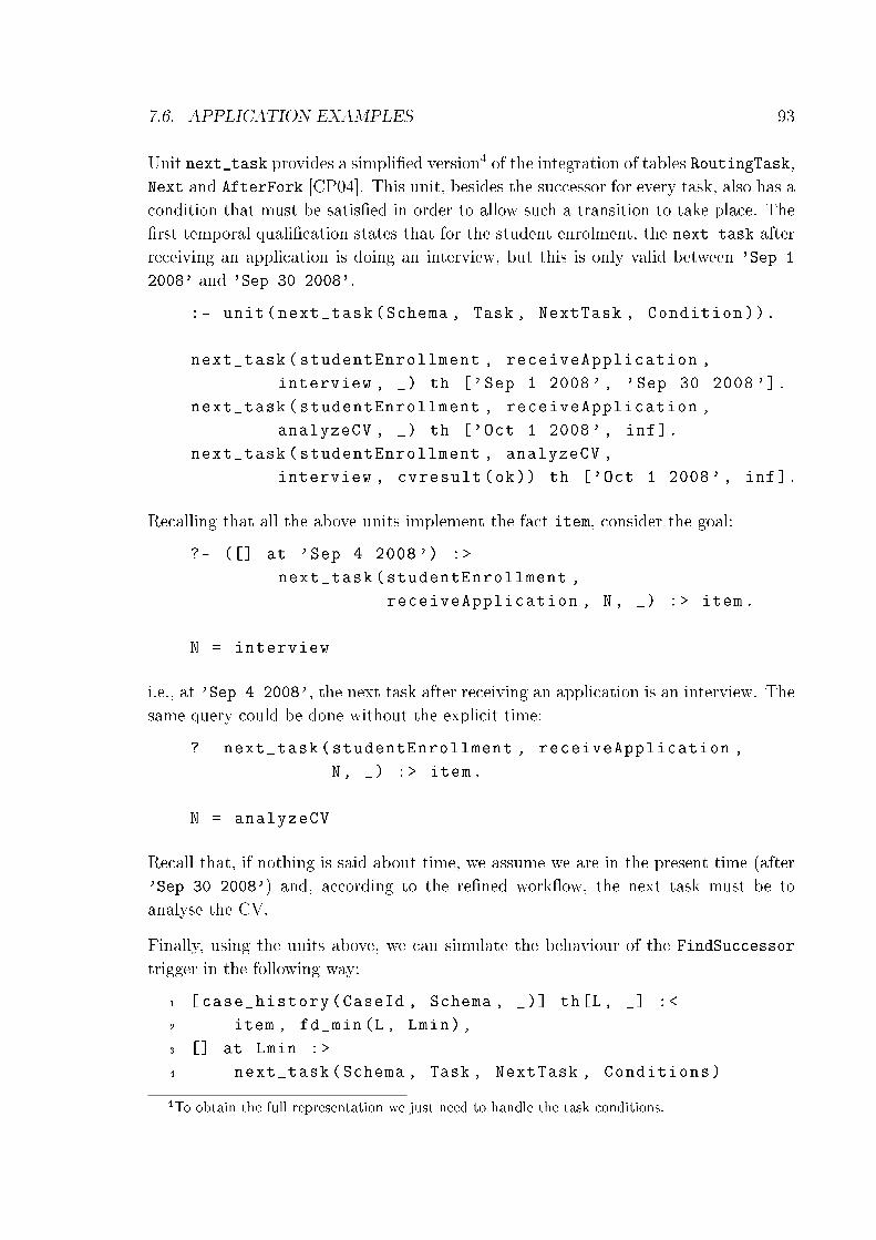
7.6. APPLICATION EXAMPLES 93
Unit next_task provides a simpli�ed version4 of the integration of tables RoutingTask,Next and AfterFork [CP04]. This unit, besides the successor for every task, also has acondition that must be satis�ed in order to allow such a transition to take place. The�rst temporal quali�cation states that for the student enrolment, the next task afterreceiving an application is doing an interview, but this is only valid between 'Sep 1
2008' and 'Sep 30 2008'.
:- unit(next_task(Schema , Task , NextTask , Condition )).
next_task(studentEnrollment , receiveApplication ,
interview , _) th ['Sep 1 2008', 'Sep 30 2008 '].
next_task(studentEnrollment , receiveApplication ,
analyzeCV , _) th ['Oct 1 2008', inf].
next_task(studentEnrollment , analyzeCV ,
interview , cvresult(ok)) th ['Oct 1 2008', inf].
Recalling that all the above units implement the fact item, consider the goal:
?- ([] at 'Sep 4 2008') :>
next_task(studentEnrollment ,
receiveApplication , N, _) :> item.
N = interview
i.e., at 'Sep 4 2008', the next task after receiving an application is an interview. Thesame query could be done without the explicit time:
?- next_task(studentEnrollment , receiveApplication ,
N, _) :> item.
N = analyzeCV
Recall that, if nothing is said about time, we assume we are in the present time (after'Sep 30 2008') and, according to the re�ned work�ow, the next task must be toanalyse the CV.
Finally, using the units above, we can simulate the behaviour of the FindSuccessor
trigger in the following way:
1 [case_history(CaseId , Schema , _)] th[L, _] :<
2 item , fd_min(L, Lmin),
3 [] at Lmin :>
4 next_task(Schema , Task , NextTask , Conditions)
4To obtain the full representation we just need to handle the task conditions.

94 CHAPTER 7. TEMPORAL CONTEXTUAL LOGIC PROGRAMMING
5 :> (item ,
6 work_task(Schema , NextTask , Role) :> item)
The �rst two lines query when the case started, allowing us to know which version ofthe work�ow must be applied.5 Then the context time is set to the lower bound andthe next task, along with the conditions for this transition to take place are speci�edin lines 4 and 5. In the last line, the role of the employee which will execute this taskis given.
7.6.2 Legal Reasoning
Legal reasoning is a very proli�c �eld in which to illustrate the application of temporallanguages. Not only is a modular approach very suitable for reasoning about lawsbut also time is pervasive in their de�nition. To illustrate the use of TCxLP in thelegal reasoning domain, we return to the British Nationality Act already exploited inSect. 6.6.1 (page 74).
The solution below presents several similarities with the CxLP with temporal annota-tions. The intention of focus on the di�erences between the proposals.
The TCxLP solution also has a unit born/2:
:- unit(born(Name , Country )).
born(john , uk) at 'Aug 10 1969'.
Although it might seem that this unit is almost identical, in the case of TCxLP (andremembering that all temporal units implement the fact item), now we can ask whenJohn was born as:
?- [born(john , uk)] at T :< item.
in this case the context has the temporal informations, as opposed to the CxLP withannotations query:
?- [born(john , uk)] :< item at T.
Before presenting the rule for the nationality act we still need to state some facts aboutwho is a British citizen along with who is parent of whom:
:- unit(british_citizen(Name )).
british_citizen(bob)
th ['Sep 9 1940', inf].
5fd_min(L, Lmin) succeeds if Lmin is the minimal value of the current domain of L.

7.6. APPLICATION EXAMPLES 95
:- unit(parent(Parent , Son)).
parent(bob , john)
th ['Aug 10 1969', inf].
To declare that the commencement date is 'Jan 1 1955', consider the following unit:
:- unit(bna).
bna th ['Jan 1 1955', inf].
Now we can give a formulation of this law in our language:
1 [] at T :< (born(X, uk) :> item ,
2 parent(Y, X) :> item ,
3 bna :> item ,
4 (british_citizen(Y) :> item;
5 british_resident(Y) :> item )).
Notice that, by making use of the time of the context (T), there is no need to explicitlymention this anywhere else. This is the main di�erence w.r.t. CxLP with temporalannotations versions. As an informal description of this rule, we can say that westart by de�ning the time of the context as the time when the person was born (1).Afterwards, we query the name of the parent (2) and if the bna law can be applied (3)in this temporal context. Finally, we ask whether the parent is a British citizen (4) ora British resident (5).
7.6.3 Vaccination Program
Vaccinations programs are a very proli�c domain for temporal reasoning. Not onlyis the inoculation of a given vaccine (doses) time dependent, but also the vaccinationplans evolve throughout time. In this section we illustrate the use of TCxLP to reasonabout changes that occurred in a vaccination program. Although we are going to reportour example to the Portuguese case, we do so without loss of generality.
In Portugal, a new National Vaccination Program was introduced in the year 2006.Several changes regarding the previous program (that started in 2000) were made,namely the introduction of the Meningococcal C vaccine. In Table 7.1 we can see a(partial) representation of this vaccination program.

96 CHAPTER 7. TEMPORAL CONTEXTUAL LOGIC PROGRAMMING
AgeVaccine against 0 (birth) 2 months 3 months 4 monthsTuberculosis BCGPoliomyelitis VIP 1 VIP 2Diphteria-Tetanus-Whooping cough DTPa 1 DTPa 2Haemophilus in�uenza b Hib 1 Hib 2Hepatitis B VHB 1 VHB 2Meningococcal C MenC 1
Table 7.1: Vaccination recommended scheme
One can regard it as set of facts that specify when one given vaccine should beinoculated, for instance the vaccines against Tuberculosis and Hepatitis B (�rst doses)should be inoculated at birth, Poliomyelitis (�rst doses), Diphtheria-Tetanus-Whoopingcough (�rst doses), Haemophilus in�uenza b (�rst doses) and Hepatitis B (second doses)should be inoculated at the age of 2 months, etc.
Regarding vaccines, the most common questions made by a health care professionalare:
• when was the last one?
• when should the next one be performed?
The answer to the former its quite straightforward whereas the latter entails know-ing the vaccination program. To represent the scheme of Table 7.1 let us considerunit vaccination_plan where the temporal quali�cation of the facts represents theirvalidity :
:- unit(vaccination_plan(Age , Vaccine )).
vaccination_plan(age(0,0), [bcg ,
vhb (1)]) th [2000 , inf].
vaccination_plan(age(0,2), [vip(1), dtpa(1), hib(1),
vhb (2)]) th [2000 , inf].
vaccination_plan(age(0,3), [menC (1)]) th [2006, inf].
vaccination_plan(age(0,4), [vip(2), dtpa(2), hib (2)])
th [2000 , inf].
As we can see, the inoculation of menC is valid only in temporal contexts after 2006while the remaining ones are valid after 2000. To query about the next vaccine considerunit next_vaccine/1:
1 :- unit(next_vaccine(Vaccine )).
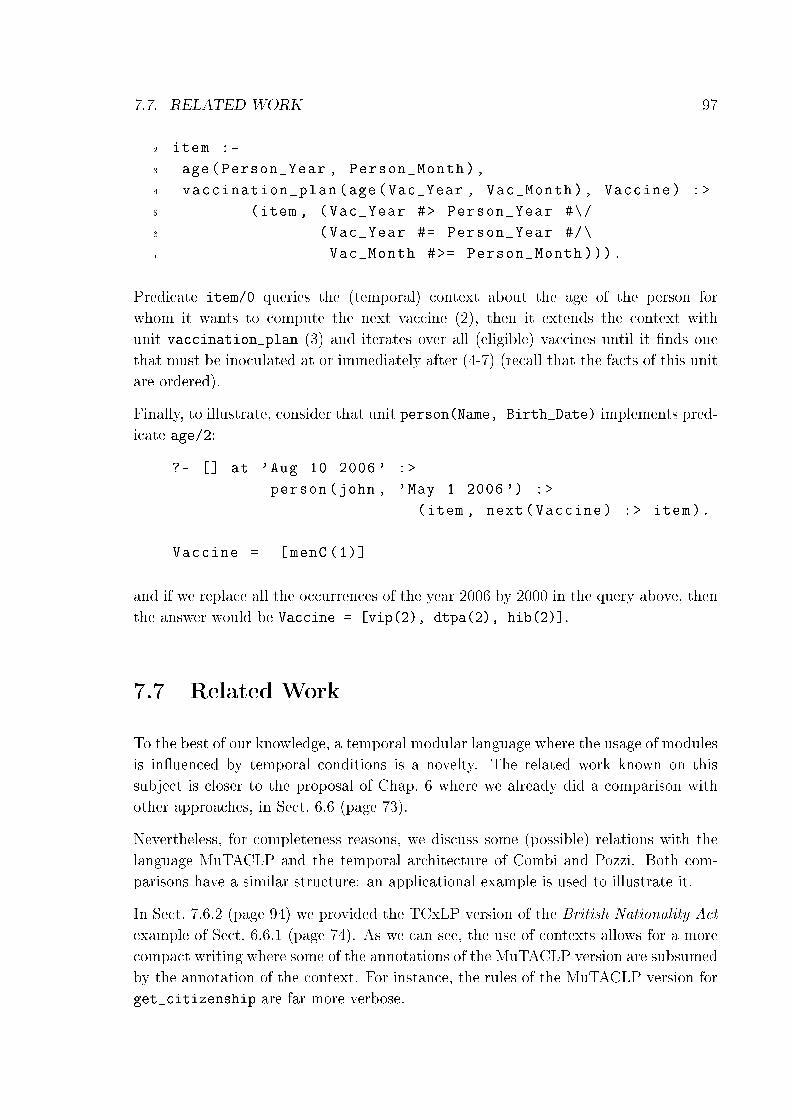
7.7. RELATED WORK 97
2 item :-
3 age(Person_Year , Person_Month),
4 vaccination_plan(age(Vac_Year , Vac_Month), Vaccine) :>
5 (item , (Vac_Year #> Person_Year #\/
6 (Vac_Year #= Person_Year #/\
7 Vac_Month #>= Person_Month ))).
Predicate item/0 queries the (temporal) context about the age of the person forwhom it wants to compute the next vaccine (2), then it extends the context withunit vaccination_plan (3) and iterates over all (eligible) vaccines until it �nds onethat must be inoculated at or immediately after (4-7) (recall that the facts of this unitare ordered).
Finally, to illustrate, consider that unit person(Name, Birth_Date) implements pred-icate age/2:
?- [] at 'Aug 10 2006' :>
person(john , 'May 1 2006') :>
(item , next(Vaccine) :> item).
Vaccine = [menC (1)]
and if we replace all the occurrences of the year 2006 by 2000 in the query above, thenthe answer would be Vaccine = [vip(2), dtpa(2), hib(2)].
7.7 Related Work
To the best of our knowledge, a temporal modular language where the usage of modulesis in�uenced by temporal conditions is a novelty. The related work known on thissubject is closer to the proposal of Chap. 6 where we already did a comparison withother approaches, in Sect. 6.6 (page 73).
Nevertheless, for completeness reasons, we discuss some (possible) relations with thelanguage MuTACLP and the temporal architecture of Combi and Pozzi. Both com-parisons have a similar structure: an applicational example is used to illustrate it.
In Sect. 7.6.2 (page 94) we provided the TCxLP version of the British Nationality Act
example of Sect. 6.6.1 (page 74). As we can see, the use of contexts allows for a morecompact writing where some of the annotations of the MuTACLP version are subsumedby the annotation of the context. For instance, the rules of the MuTACLP version forget_citizenship are far more verbose.
98 CHAPTER 7. TEMPORAL CONTEXTUAL LOGIC PROGRAMMING
A similar reasoning applies when comparing the TCxLP solution for work�ow man-agement systems (see Sect. 7.6.1) with relational frameworks such as the one proposedby Combi and Pozzi in [CP04] where relational queries contained far more explicitreferences to time that the contextual version.
7.8 Conclusions
In this chapter we presented a temporal extension of CxLP where time in�uences theeligibility of a module to be used in solving a goal. We consider that such interactionbetween modularity and temporal reasoning comes naturally and, as far as we know,is original.
Besides the operational semantics for this language we proposed a procedure thatcomputes the least upper bound of the units annotation at runtime.
An interpreter together with a compiler for this language were presented, forming thebasis of a prototype implementation.
Several domains of applications were illustrated, namely legal reasoning, work�owmanagement systems and medicine.
Chapter 8
Language for Temporal Organisational
Information Systems
In this chapter we start with a revised and stripped-down version of the logical
framework ISCO (Information System COnstruction language). We then describe a
temporal extension together with a compilation scheme for this language.
8.1 Introduction
Organisational Information Systems (OIS) have a lot to bene�t from Logic Program-ming (LP) characteristics such as a rapid prototyping ability, the relative simplicityof program development and maintenance, the declarative reading which facilitatesboth development and the understanding of existing code, the built-in solution-spacesearch mechanism, the close semantic link with relational databases, just to name afew. In [Por03, ADN04] we �nd examples of LP languages that were used to developand maintain OIS.
ISCO (Information System COnstruction language) [Abr01] is a logical framework forconstructing Organisational Information Systems. ISCO is an evolution of the previouslanguage DL [Abr00] and is based on a Constraint Logic Programming framework tode�ne the schema, represent data, access heterogeneous data sources and perform ar-bitrary computations. In ISCO, processes and data are structured as classes which arerepresented as typed1 Prolog predicates. An ISCO class may map to an external datasource or sink like a table or view in a relational database, or be entirely implementedas a regular Prolog predicate. Operations pertaining to ISCO classes include a query
which is similar to a Prolog call as well as three forms of update, i.e. ISCO implementsCreate, Read, Update and Delete (CRUD) access to Relational Database Management
1The type system applies to class members, which are viewed as Prolog predicate arguments.
99
100 CHAPTER 8. LANGUAGE FOR TEMPORAL OIS
System.
In this chapter we propose to extend ISCO with an expressive means of representingand implicitly using temporal information. As it should be expected, this evolutionrelies upon the frameworks proposed in Chap(s). 6 and 7. Moreover, having simplicity(syntactic, semantic, etc) as a guideline we present a revised and stripped-down versionof ISCO, keeping just some of the core features that we consider indispensable in alanguage for Temporal OIS. Leaving out aspects such as access control [Abr02] doesnot mean they are deprecated, only not essential for the purpose at hand. The mainmotivation of this chapter is to provide a language suited to construct and maintainTemporal OIS where contexts aren't explicit but implicit (they are obtained throughoutthe compilation of this language).
This chapter is organised as follows: in Sect. 8.2 we review the ISCO language and inSect. 8.3 we present its temporal extension ISTO. Section 8.4 discusses a compilationscheme for this language and Sect. 8.5 compares it with other approaches. Finally, inSect. 8.6 we draw some conclusions.
8.2 Revising the ISCO Programming Language
In this section we present a revised and stripped-down version of ISCO focusing on whatwe consider the required features in a language to construct and maintain (Temporal)Organisational Information Systems.
8.2.1 Classes
When dealing with large amounts of data, one must be able to organise information ina modular way. The ISCO proposal for this point are classes. Although ISCO classescan be regarded as equivalent to Prolog predicates, they provide the homonymous OOconcept, along with the related data encapsulation capability.
Before presenting a formal description of classes, let us see an ISCO class that handlesdata about persons, namely its name and social security number:
Example 6 Class Person
class person.
name: text.
ssn: int.

8.2. REVISING THE ISCO PROGRAMMING LANGUAGE 101
In this example after de�ning the class name to be person, we state its arguments andtypes: ssn (Social Security Number) type int(eger) and name type text.
Using a De�nite Clause Grammar, the ISCO class syntax can be de�ned in the followingway:
De�nition 12 Simple class syntax
class --> class_head , arguments.
class_head --> [class NAME].
arguments --> [].
arguments --> argument , arguments.
argument --> [NAME : type].
type --> [int].
type --> [float ].
type --> [bool].
type --> [text].
type --> [date].
From the de�nition above, we can see that a class is formed by a head and a (possiblyempty) set of arguments. The class head starts with the keyword class and is followedby a descriptor. An argument de�nition its composed by its name concatenated with":" and an argument type (int, �oat, bool, text or date). This is the basic de�nitionof a class that we will enrich it as long as we add other features.
8.2.2 Methods
By de�ning class arguments we are also implicitly setting class methods for access-ing those arguments. For instance, in class person we have the predicates ssn/1
and name/1. Therefore to query John's ssn, besides the (positional) Prolog goal ?-person(john, S). we can also state:
Example 7 John's social security number
?- person(name(john), ssn(N)).
N = 123

102 CHAPTER 8. LANGUAGE FOR TEMPORAL OIS
Besides these implicit methods, there can also be explicit ones de�ned by means ofregular Horn clauses. To allow for class methods, we enrich the rule for class asfollows:
class --> class_head , arguments , horn_clauses.
As an illustration of an Horn clause, consider that argument name of class person is anatom with the syntactical structure 'SURNAME FIRST_NAME'. Therefore, to obtainthe surname we add the following clause to the class de�nition:
surname(Surname) :-
name(Name),
atom_chars(Name , Name_Chars),
append(Surname_Chars , [' '|_], Name_Chars),
atom_chars(Surname , Surname_Chars ).
8.2.3 Inheritance
Inheritance is another Object Oriented feature of ISCO that we would like to retainin our language. The reasons for that are quite natural since it allow us to share notonly methods, but also data among di�erent classes. The ISCO inheritance syntax isobtained by replacing the class_head of De�nition 12 by:
class_head --> [class NAME], superclass.
superclass --> [].
superclass --> [: NAME].
Consider class person of Example 6 (page 100) and that we want to represent some facts(name, social security number and salary) about the employees of a given company.Therefore, we de�ne employee to be a subclass of person with the argument salary:
Example 8 Class employee
class employee: person.
salary: int.
8.2.4 Composition
As we already saw, we have �ve basic types: int, float, bool, text and date. Inorder to have the OO feature of composition, we include ISCO possibility to re�use theclass de�nitions as a data type. Therefore, the type syntactical de�nition becomes:

8.2. REVISING THE ISCO PROGRAMMING LANGUAGE 103
type --> basic_type.
type --> class_type.
basic_type --> [int].
basic_type --> [float].
basic_type --> [bool].
basic_type --> [text].
basic_type --> [date].
class_type --> [NAME].
Suppose that we want to deal with the employees home address and have the possibilityof using the address schema in other places (suppliers, etc). For that we de�ne a newclass address and re�de�ne the employee class adding a new argument (home) whosetype is address:
Example 9 Class employee with home address
class address.
street: text.
number: int.
class employee: person.
home: address.
salary: int.
The access to compound types its quite natural, for instance suppose that we want toknow John's street name:
Example 10 John's home address
?- employee(name(john), home(address(street(S)))).
S = upstreet
Actually, as the reader might see, there is no real need for the basic types since wecould develop one class for each. Nevertheless, because they are quite intuitive to use,we decided to keep them.
8.2.5 Persistence
Having persistence in a Logic Programming language is a required feature to constructactual OIS; this could conceivably be provided by Prolog's internal database but is best

104 CHAPTER 8. LANGUAGE FOR TEMPORAL OIS
accounted for by software designed to handle large quantities of factual informatione�ciently, as is the case in relational database management systems. The semanticproximity between relational database query languages and logic programming lan-guages have made the former privileged candidates to provide Prolog with persistence.
ISCO's approach for interfacing to existing RDBMS2 involves providing declarations foran external database together with de�ning equivalences between classes and databaserelations. As an illustration, consider that the employee facts are stored in a homony-mous table of a PostgreSQL [SK91] database named db running in the localhost:
Example 11 External Databases
external(db_link , postgres(db , localhost )).
external(db_link , employee) class employee: person.
home: address.
salary: int.
Since the database table has the same name as the class, the employee inside theexternal term above is optional. Finally, we can specify the full class de�nition:
De�nition 13 ISCO class syntax with external DB references
class --> class_head , arguments , horn_clauses.
class_head --> external , [class NAME], superclass.
external --> [].
external --> [external(DB_LINK )].
external --> [external(DB_LINK , RELATION_NAME )].
superclass --> [].
superclass --> [: NAME].
arguments --> [].
arguments --> argument , arguments.
argument --> [NAME : type].
2ISCO access to frameworks beyond relational databases, such as LDAP directory services or web
services is out of scope for the present work. We shall stick to RDMBS only.

8.2. REVISING THE ISCO PROGRAMMING LANGUAGE 105
type --> basic_type.
type --> class_type.
basic_type --> [int].
basic_type --> [float].
basic_type --> [bool].
basic_type --> [text].
basic_type --> [date].
class_type --> [NAME].
8.2.6 Data Manipulation Goals
Under the data manipulation operations we include not only insertion, removal andupdate but also query operations, i.e. Create, Read, Update and Delete access toRDBMS. The (simpli�ed) formal syntax of these operations can be described as:
De�nition 14 Goal De�nition
goal --> prolog_goal.
goal --> modification_goal.
modification_goal --> prolog_goal , [+].
modification_goal --> prolog_goal , [-].
modification_goal --> prolog_goal , [#], prolog_goal.
From the de�nition above, we have that a goal is either a Prolog goal or a modi�cationgoal. For illustrations of the �rst type of goals see Examples 7 and 10.
The modi�cation goals (insert, delete and update) are based on simple queries, nonbacktrackable and all follow the tuple-at-a-time approach, which is more consistentwith the usual Prolog operational semantics. As an example, suppose that we want toinsert the employee Smith, update his address and then remove this employee:
Example 12 Modi�cation Goals
?- employee(name(smith), ssn(111), salary (20),
home(address(street(up), number (1)))) +.
?- employee(name(smith)) #
(home(address(street(down), number (2)))).

106 CHAPTER 8. LANGUAGE FOR TEMPORAL OIS
?- employee(name(smith )) -.
This concludes our overview of the simpli�ed ISCO language. In the next section we'lldeal with temporal concerns.
8.3 The ISTO Language
In this section we provide a revised ISCO language with the ability to represent andimplicitly use temporal information. This temporal evolution of the ISCO languagewill be called ISTO (Information System Tools for Organisations). The capability ofrepresenting temporal information will be achieved by extending ISCO classes to theirtemporal counterpart. As expected, in order to handle such temporal informationISTO includes temporal data manipulation operations.
8.3.1 Temporal Classes
In pursuing our goal of simplicity, temporal classes are given by introducing the keywordtemporal before the keyword class. Therefore the class head syntax becomes:
class_head --> external , temporal , [class NAME],
superclass.
temporal --> [].
temporal --> [temporal ].
Facts of a temporal class have a temporal dimension, i.e. all tuples have associateda temporal stamp. In line with the other temporal languages proposed in this work,these stamps will stand for instants or intervals (their precise de�nition is given inSect. 8.3.2).
As an illustration, class employee can be temporal (Example 9), since it makes sensethat the salary and home address of a given employee evolves throughout time. On theother hand class person should continue atemporal since the facts it stores shouldn'tevolve over time.
Example 13 Temporal class employee
temporal class employee: person.
home:address.
salary: int.

8.4. COMPILATION SCHEME FOR ISTO 107
8.3.2 Temporal Data Manipulation
Here we present the temporal equivalent of the data manipulation goals described inSect. 8.2.6 (page 105), i.e. we provide a temporal query, insertion, removal and updategoals.
Again trying to keep the syntax as simple as possible we shall distinguish temporaloperations from regular ones by adding the operator �@� followed by a temporal de-scriptor annotation. The interval representation is the standard one [T1, T2] andstands for all time points between T1 and T2 (where T2 ≥ T1). Moreover, in order tobe able to handle in-annotated information (see page 13), we also allow another typeof intervals [T1; T2] to represent some time points (not necessarily all) between T1
and T2, i.e. [T1; T2] is a subset of [T1, T2]. The ISTO temporal operations will be:
goal --> prolog_goal , temporal_condition.
goal --> modification_goal , temporal_condition.
temporal_condition --> [].
temporal_condition --> [ @ [Point , Point] ]
temporal_condition --> [ @ [Point ; Point] ]
Although an instant T can be represented by the interval [T, T], to ease the readingwe use just T. As an illustration consider that we want to know John's street name inthe year 2007:
Example 14 John's street name in the year 2007
?- employee(name(john), home(address(street(S)))) @ 2007
S = upstreet
The goal above is a temporal version of the one we saw in Example 10 (page 103).
8.4 Compilation Scheme for ISTO
The ISTO compilation scheme is describe along the same incremental line that we sawin the language presentation. As expected, the compilation of the non-temporal partyields CxLP and from the temporal extension we target TCxLP.

108 CHAPTER 8. LANGUAGE FOR TEMPORAL OIS
8.4.1 Classes
The translation from an ISTO class to CxLP can be roughly described as: everyclass becomes a corresponding unit, with the class arguments transformed into unitarguments and predicates for accessing these arguments. For instance, class person ofExample 6 (page 100) is compiled into the CxLP unit:
:- unit(person(OID , NAME , SSN)).
oid(OID).
name(NAME).
ssn(SSN).
item :- person(OID , NAME , SSN).
The unit argument OID stands for Object Identi�er and as the name implies, is used todiscriminate a given tuple in a class (and throughout the database in the correspondingsuperclass as we will see). The predicate item/0 simply fetches facts from the internaldatabase and binds the unit arguments. In the Sect. 8.4.5 (page 110) we see how toaccess external databases.
8.4.2 Methods
The compilation of Horn clauses is trivial since they remain unaltered. Regardingthe implicit methods resulting from the class arguments, we already saw them in theprevious section.
8.4.3 Inheritance
Since CxLP already has dynamic inheritance, it is rather simple to simulate the singlestatic inheritance of ISTO. Take for instance the class employee of Example 8 (seepage 102), subclass of person. Since person is a toplevel class, to use it we can simplydo:
[person(OID , NAME , SSN)] :< (item , ...)
whereas to use employee we do:
[employee(OID , SALARY), person(OID , NAME , SSN)]
:< (item , ...)

8.4. COMPILATION SCHEME FOR ISTO 109
As mentioned previously, OID is used to join a class with its superclass. Finally, classemployee of Example 8 is compiled as:
:- unit(employee(OID , SALARY )).
oid(OID).
salary(SALARY ).
item :- employee(OID , SALARY),
:^ item.
As we can see predicate item/0 �rst invokes the local database and then calls item inthe superclass, this way building the whole tuple. This de�nition requires the contextto include the unit(s) corresponding to the superclass(es).
8.4.4 Composition
For the compound types the idea is similar to the one we saw with inheritance, i.e.we use an identi�er to relate an argument to its compound type. In this case insteadinstead of using this identi�er to perform a join operation, we use it as a pointer. Tobetter understand let us see the compilation of the employee class with home argument(see Example 9 in page 103):
Example 15 Compilation of employee with home address.
:- unit(employee(OID , HOME_OID , SALARY )).
2
oid(OID).
4
home(address(GOAL)) :-
6 [address(HOME_OID , STREET , NUMBER )] :< (item , GOAL).
8 salary(SALARY ).
10 item :- employee(OID , HOME_OID , SALARY),
:^ item.
In Example 10 (page 103) we saw that a query to an employee address has thestructure home(address(GOAL)). The unit above explain how this query is handled:GOAL is resolved in a context with unit address. Moreover, the unit arguments
110 CHAPTER 8. LANGUAGE FOR TEMPORAL OIS
are obtained by binding the address object identi�er with the employee argumentHOME_OID, i.e. HOME_OID can be regarded as a pointer for the home address.
8.4.5 Persistence
Due to the possibility of having di�erent backends, persistence related compilation canbe more elaborate than what we are going to present. Nevertheless we consider theexplanation below su�cient to grasp how it's done. Returning to the employee class,its modi�cation into an external class presented in Example 11 (page 104) modi�es theitem predicate to:
item :- [isto_backend(db_link, employee)] :<
query(employee(OID, HOME_OID, SALARY)),
:^ item.
8.4.6 Data Manipulation Goals
The compilation of the manipulation goals is quite simple, in fact we already saw howthe query translation could be obtained when we presented the Persistence. Knowingthat unit isto_backend also implements insert/1, delete/1 and update/2 it issimple to determine the compilation of the modi�cation goals. For instance, the removalof employee Smith that we saw in Example 12 (page 105) is translated into:
1 ?- [employee(OID , HOME_OID , SALARY),
person(OID , NAME , SSN)] :< (item , name(smith)),
3
[isto_backend(db_link , employee )] :<
5 delete(employee(OID , HOME_OID , SALARY)),
7 [isto_backend(db_link , person )] :<
delete(person(OID , NAME , SSN)).
In the goal above we start by querying the whole tuple of the employee Smith (lines1 and 2) and them we remove it from the employee backend (lines 4 and 5) and fromthe person backend (lines 7 and 8).
8.4.7 Temporal Classes
Before presenting the compilation of temporal classes and goals one must observe thatnon-temporal classes must behave as if they were valid throughout the entire time line.
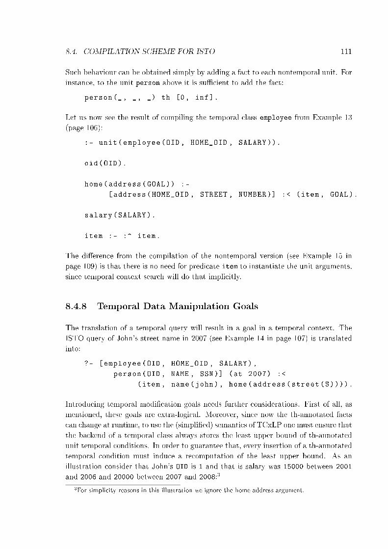
8.4. COMPILATION SCHEME FOR ISTO 111
Such behaviour can be obtained simply by adding a fact to each nontemporal unit. Forinstance, to the unit person above it is su�cient to add the fact:
person(_, _, _) th [0, inf].
Let us now see the result of compiling the temporal class employee from Example 13(page 106):
:- unit(employee(OID , HOME_OID , SALARY )).
oid(OID).
home(address(GOAL)) :-
[address(HOME_OID , STREET , NUMBER )] :< (item , GOAL).
salary(SALARY ).
item :- :^ item.
The di�erence from the compilation of the nontemporal version (see Example 15 inpage 109) is that there is no need for predicate item to instantiate the unit arguments,since temporal context search will do that implicitly.
8.4.8 Temporal Data Manipulation Goals
The translation of a temporal query will result in a goal in a temporal context. TheISTO query of John's street name in 2007 (see Example 14 in page 107) is translatedinto:
?- [employee(OID , HOME_OID , SALARY),
person(OID , NAME , SSN)] (at 2007) :<
(item , name(john), home(address(street(S)))).
Introducing temporal modi�cation goals needs further considerations. First of all, asmentioned, these goals are extra-logical. Moreover, since now the th-annotated factscan change at runtime, to use the (simpli�ed) semantics of TCxLP one must ensure thatthe backend of a temporal class always stores the least upper bound of th-annotatedunit temporal conditions. In order to guarantee that, every insertion of a th-annotatedtemporal condition must induce a recomputation of the least upper bound. As anillustration consider that John's OID is 1 and that is salary was 15000 between 2001
and 2006 and 20000 between 2007 and 2008:3
3For simplicity reasons in this illustration we ignore the home address argument.
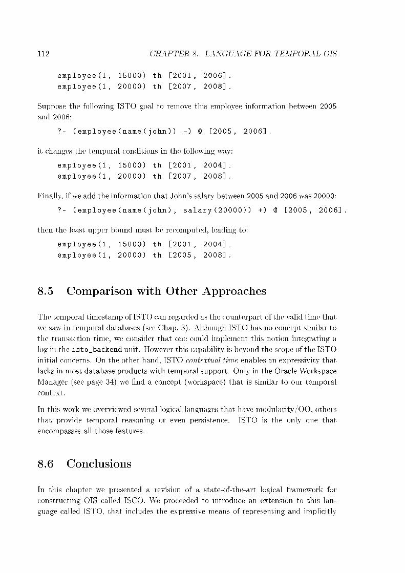
112 CHAPTER 8. LANGUAGE FOR TEMPORAL OIS
employee(1, 15000) th [2001, 2006].
employee(1, 20000) th [2007, 2008].
Suppose the following ISTO goal to remove this employee information between 2005
and 2006:
?- (employee(name(john)) -) @ [2005 , 2006].
it changes the temporal conditions in the following way:
employee(1, 15000) th [2001, 2004].
employee(1, 20000) th [2007, 2008].
Finally, if we add the information that John's salary between 2005 and 2006 was 20000:
?- (employee(name(john), salary (20000)) +) @ [2005 , 2006].
then the least upper bound must be recomputed, leading to:
employee(1, 15000) th [2001, 2004].
employee(1, 20000) th [2005, 2008].
8.5 Comparison with Other Approaches
The temporal timestamp of ISTO can regarded as the counterpart of the valid time thatwe saw in temporal databases (see Chap. 3). Although ISTO has no concept similar tothe transaction time, we consider that one could implement this notion integrating alog in the isto_backend unit. However this capability is beyond the scope of the ISTOinitial concerns. On the other hand, ISTO contextual time enables an expressivity thatlacks in most database products with temporal support. Only in the Oracle WorkspaceManager (see page 34) we �nd a concept (workspace) that is similar to our temporalcontext.
In this work we overviewed several logical languages that have modularity/OO, othersthat provide temporal reasoning or even persistence. ISTO is the only one thatencompasses all those features.
8.6 Conclusions
In this chapter we presented a revision of a state-of-the-art logical framework forconstructing OIS called ISCO. We proceeded to introduce an extension to this lan-guage called ISTO, that includes the expressive means of representing and implicitly

8.6. CONCLUSIONS 113
using temporal information. Together with a syntactical de�nition of ISTO we alsopresented a compilation scheme from this language into Temporal Contextual LogicProgramming.
ISTO can take advantage of the experience gained from several real-world applicationdeveloped in ISCO in order to act as backbone for constructing and maintainingTemporal OIS.

Chapter 9
Conclusions and Future Work
This short chapter presents the main conclusions of this work along with several
pointers for future work.
9.1 Conclusions
In this work we started with a modular logic programming language called ContextualLogic Programming (CxLP) and presented a possible optimisation for it throughoutabstract interpretation. Moreover, we coupled it with a consolidated temporal rea-soning language called Temporal Annotated Constraint Logic Programming, for whichtwo di�erent paths were considered:
• one where those languages were (almost) independent, i.e. there was no implicitrelation between Time and Modularity;
• another where Time is integrated with and a�ects Modularity, more speci�cally,it is the time of the context that helps decide if a given module is eligible or notfor a computation.
For both approaches we described the language syntax and semantics (operational),provided an interpreter, a compilation scheme and illustrated its usage in variousapplicational domains.
It was not our goal to develop another temporal or modular theory, but to choose theones that could have a natural integration within a logical framework. Although severalcriteria were used as a foundation for our choice, we would like to highlight pragmatics :the languages should be expressive enough to conveniently represent common or usualreasoning tasks in a temporal modular logic environment. Morever, the languages hadto have a practical implementation.
115
116 CHAPTER 9. CONCLUSIONS AND FUTURE WORK
Finally, and relying upon these formal languages, we extended a high level languagefor OIS with an expressive means of representing and implicitly using temporal infor-mation.
9.2 Future Work
The possibilities for future work are so vast that we must restrain a little and presentjust the ones that we would like to tackle in the near future:
• we would like to apply the ISTO language to real world problems. Perhaps,starting with University Information Systems, since this was the main applicationdomain of its nontemporal predecessor.
• There are very promising developments in the �elds of business intelligence andinformation retrieval which would stand to gain from the integration of temporalinformation.
• ISTO would also bene�t from a logical semantics to the modi�cation goals, byrecurring to frameworks such as Transaction Logic [BK94].
• A declarative semantics for Temporal Contextual Logic Programming wouldprovide a more solid theoretical foundation.
• The relation with other frameworks such as temporal XML [WZZ05] or Con-straint Handling Rules [Frü94a] could be of great interest.
• Another appealing direction is looking into ways of integrating Logic Program-ming based tools like as ISTO into Content-Management Systems such as Ploneor Mambo. It is our belief that these CMS will bene�t from having plug-inswith the expressiveness provided by Constraint Contextual Logic Programming,namely uni�cation and constraint solving.
• The decision of whether a given module is eligible or not for a computation couldbe extended in order to incorporate other concepts such as Space, etc.
Finally, we also consider that it would be interesting to use the logical frameworksdescribed in this work to model OS-level applications such as the Mac OSX backupsystem, Time Machine.
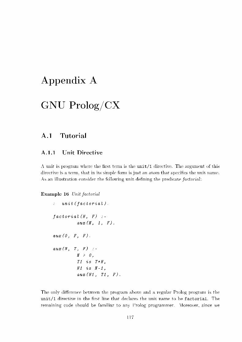
Appendix A
GNU Prolog/CX
A.1 Tutorial
A.1.1 Unit Directive
A unit is program where the �rst term is the unit/1 directive. The argument of thisdirective is a term, that in its simple form is just an atom that speci�es the unit name.As an illustration consider the following unit de�ning the predicate factorial :
Example 16 Unit factorial
:- unit(factorial ).
factorial(N, F) :-
aux(N, 1, F).
aux(0, F, F).
aux(N, T, F) :-
N > 0,
T1 is T*N,
N1 is N-1,
aux(N1 , T1 , F).
The only di�erence between the program above and a regular Prolog program is theunit/1 directive in the �rst line that declares the unit name to be factorial. Theremaining code should be familiar to any Prolog programmer. Moreover, since we
117
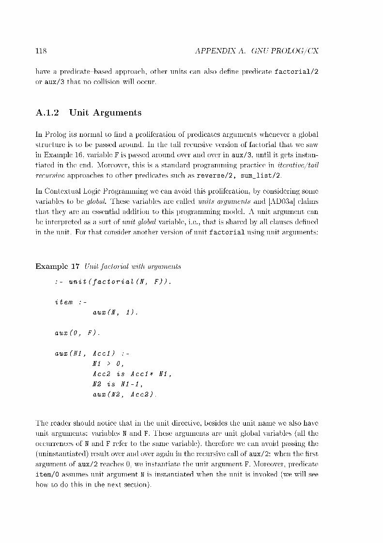
118 APPENDIX A. GNU PROLOG/CX
have a predicate�based approach, other units can also de�ne predicate factorial/2
or aux/3 that no collision will occur.
A.1.2 Unit Arguments
In Prolog its normal to �nd a proliferation of predicates arguments whenever a globalstructure is to be passed around. In the tail recursive version of factorial that we sawin Example 16, variable F is passed around over and over in aux/3, until it gets instan-tiated in the end. Moreover, this is a standard programming practice in iterative/tail
recursive approaches to other predicates such as reverse/2, sum_list/2.
In Contextual Logic Programming we can avoid this proliferation, by considering somevariables to be global. These variables are called units arguments and [AD03a] claimsthat they are an essential addition to this programming model. A unit argument canbe interpreted as a sort of unit global variable, i.e., that is shared by all clauses de�nedin the unit. For that consider another version of unit factorial using unit arguments:
Example 17 Unit factorial with arguments
:- unit(factorial(N, F)).
item :-
aux(N, 1).
aux(0, F).
aux(N1 , Acc1) :-
N1 > 0,
Acc2 is Acc1* N1,
N2 is N1 -1,
aux(N2 , Acc2).
The reader should notice that in the unit directive, besides the unit name we also haveunit arguments: variables N and F. These arguments are unit global variables (all theoccurrences of N and F refer to the same variable), therefore we can avoid passing the(uninstantiated) result over and over again in the recursive call of aux/2: when the �rstargument of aux/2 reaches 0, we instantiate the unit argument F. Moreover, predicateitem/0 assumes unit argument N is instantiated when the unit is invoked (we will seehow to do this in the next section).
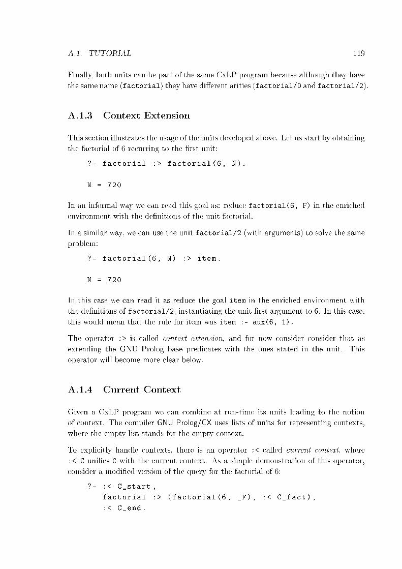
A.1. TUTORIAL 119
Finally, both units can be part of the same CxLP program because although they havethe same name (factorial) they have di�erent arities (factorial/0 and factorial/2).
A.1.3 Context Extension
This section illustrates the usage of the units developed above. Let us start by obtainingthe factorial of 6 recurring to the �rst unit:
?- factorial :> factorial(6, N).
N = 720
In an informal way we can read this goal as: reduce factorial(6, F) in the enrichedenvironment with the de�nitions of the unit factorial.
In a similar way, we can use the unit factorial/2 (with arguments) to solve the sameproblem:
?- factorial (6, N) :> item.
N = 720
In this case we can read it as reduce the goal item in the enriched environment withthe de�nitions of factorial/2, instantiating the unit �rst argument to 6. In this case,this would mean that the rule for item was item :- aux(6, 1).
The operator :> is called context extension, and for now consider consider that asextending the GNU Prolog base predicates with the ones stated in the unit. Thisoperator will become more clear below.
A.1.4 Current Context
Given a CxLP program we can combine at run-time its units leading to the notionof context. The compiler GNU Prolog/CX uses lists of units for representing contexts,where the empty list stands for the empty context.
To explicitly handle contexts, there is an operator :< called current context, where:< C uni�es C with the current context. As a simple demonstration of this operator,consider a modi�ed version of the query for the factorial of 6:
?- :< C_start ,
factorial :> (factorial (6, _F), :< C_fact),
:< C_end.

120 APPENDIX A. GNU PROLOG/CX
C_end = []
C_fact = [factorial]
C_start = []
In this example we decided to use variable _F because we are only interested in theinstantiation of the contexts. Let us start with the empty contexts C_start and C_end.They are empty because the place where they occur is not under the scope of any unit.The context C_fact on the contrary, is inside the environment of the unit factorial,therefore it should be no surprise that C_fact = [factorial].
Moreover, and remembering that the empty list is a member of all the lists, it shouldbe clear why :> is a context extension: we extended the empty context [] with theunit factorial, yielding the context [factorial | [] ], i.e. [factorial].
A similar modi�cation can be done to obtain the contexts for the case of factorial/2:
?- :< C_start ,
factorial(6, _F) :> (item , :< C_fact),
:< C_end.
C_end = []
C_fact = [factorial (6, 720)]
C_start = []
The di�erence from the previous example is the context C_fact = [factorial(6,
720)], i.e. from a simple context inspection we know that the factorial of 6 is 720.Therefore, it should be clear why we state that units arguments make contexts moretransparent.
A.1.5 Context Traversal
Until now we just saw simple contexts, namely empty or single contexts. Nevertheless,contexts can be more elaborated and as we are going to see, they are a natural wayto represent dynamic inheritance. Dynamic inheritance allows objects to change andevolve over time. Since base classes provide properties and attributes for objects,changing base classes changes the properties and attributes of a class. More speci�cally,dynamic inheritance refers to the ability to add, delete or change parents from objects(or classes) at runtime.
To illustrate this feature we are going to build an example based on the cd (changeworking d irectory) of the Unix system V shell. Since this command is strongly con-nected not only to the directory tree but also to the user that is issuing it, we also

A.1. TUTORIAL 121
decided to represent these concepts.1 Regarding the unit user we represented just theuser name and its home directory inode:
Example 18 Unit user
:- unit(user(NAME , HOME )).
item :- user(NAME , HOME).
user(foo , 4).
user(bar , 5).
user(baz , 6).
name(NAME).
home(HOME).
pwd(HOME).
In this unit besides the user/2 facts, we have one predicate to access each unitargument and another called item to instantiate the unit arguments using the factsretrieved from the database. Moreover, instead of the full path to the user homedirectory we decided to represent just the inode number of that directory. Using thisnumber�based approach for directories, we represented a typical Unix �lesystem as:
Example 19 Unit fs (�lesystem)
:- unit(fs).
fs(1, /, nil).
fs(2, bin , 1).
fs(3, home , 1).
fs(4, foo , 3).
fs(5, bar , 3).
fs(6, work , 4).
fs(7, papers , 6).
In the unit above, each directory is represented by a triple: inode number, name andinode of its parent directory. This example represents the �le system of Figure A.1.
1Since directory permissions didn't bring any advantage to illustrate concepts of CxLP we decided
to omit them.

122 APPENDIX A. GNU PROLOG/CX
Figure A.1: File system
For instance, directory number 4 is /home/foo: 3 (home) is the parent of 4 (foo) and1 (/) is the parent of 3.
Let us see a goal to �nd out if the name of the user home directory is the same as theuser name. This can be achieved by a simple join between unit fs and unit user:
?- user(U, I) :> item , fs :> fs(I, U, _).
I = 4
U = foo ? ;
I = 5
U = bar
Having de�ned these two units we can now see the intended behaviour of the cd
command. Suppose that user foo logs into the system and issues the command cd
work, i.e. this command is executed in the context of user(foo,_) and in the �lesystemseen above (fs). Using CxLP we can expect something like:
?- fs :> user(foo , _ ) :> (item , cd(work) :> check).
Therefore predicate check/0 of unit cd must ask the context the working directoryand then check if work is a subdirectory2 of it. Therefore unit cd could be somethinglike:
:- unit(cd(ARG)).
check :- pwd(WD),
fs(_, ARG , WD).
Since predicate pwd/1 isn't de�ned in this unit, is performed a search in the contextfor the topmost unit that de�nes this predicate. Thefore, although pwd(WD) was called
2We are just going to consider arguments that specify a direct subdirectory of the current one.
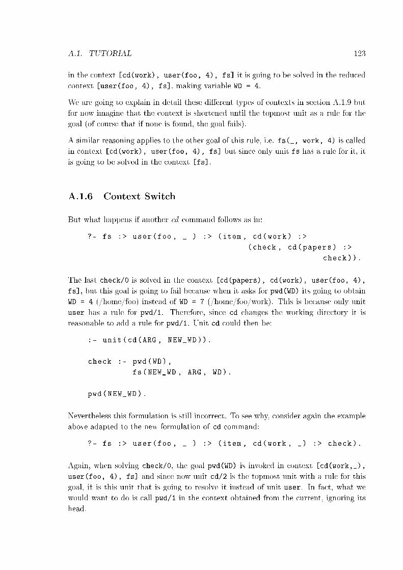
A.1. TUTORIAL 123
in the context [cd(work), user(foo, 4), fs] it is going to be solved in the reducedcontext [user(foo, 4), fs], making variable WD = 4.
We are going to explain in detail these di�erent types of contexts in section A.1.9 butfor now imagine that the context is shortened until the topmost unit as a rule for thegoal (of course that if none is found, the goal fails).
A similar reasoning applies to the other goal of this rule, i.e. fs(_, work, 4) is calledin context [cd(work), user(foo, 4), fs] but since only unit fs has a rule for it, itis going to be solved in the context [fs].
A.1.6 Context Switch
But what happens if another cd command follows as in:
?- fs :> user(foo , _ ) :> (item , cd(work) :>
(check , cd(papers) :>
check )).
The last check/0 is solved in the context [cd(papers), cd(work), user(foo, 4),
fs], but this goal is going to fail because when it asks for pwd(WD) its going to obtainWD = 4 (/home/foo) instead of WD = 7 (/home/foo/work). This is because only unituser has a rule for pwd/1. Therefore, since cd changes the working directory it isreasonable to add a rule for pwd/1. Unit cd could then be:
:- unit(cd(ARG , NEW_WD )).
check :- pwd(WD),
fs(NEW_WD , ARG , WD).
pwd(NEW_WD ).
Nevertheless this formulation is still incorrect. To see why, consider again the exampleabove adapted to the new formulation of cd command:
?- fs :> user(foo , _ ) :> (item , cd(work , _) :> check).
Again, when solving check/0, the goal pwd(WD) is invoked in context [cd(work,_),user(foo, 4), fs] and since now unit cd/2 is the topmost unit with a rule for thisgoal, it is this unit that is going to resolve it instead of unit user. In fact, what wewould want to do is call pwd/1 in the context obtained from the current, ignoring itshead.

124 APPENDIX A. GNU PROLOG/CX
To solve this problem another operator called context switch is presented C :< G andstands for solving goal G in context C. This leads to the correct formulation of unit cd:
:- unit(cd(ARG , NEW_WD )).
check :- :< [_|C],
C :< pwd(WD),
fs(NEW_WD , ARG , WD).
pwd(NEW_WD ).
Now check/0 �rst queries for the current context (operator :<) and then solves pwd/1in the subcontext obtained from ignoring the head of the current context.
A.1.7 Supercontext
Using the immediate subcontext to solve a goal is so recurrent that an operator wasproposed for that purpose. This operator is denoted by :� G is called supercontextand behaves as if de�ned by the Prolog clause:
:^ G :- :< [_| C], C :< G.
Using this operator, the unit cd becomes:
:- unit(cd(ARG , NEW_WD )).
check :- :^ pwd(WD),
fs(NEW_WD , ARG , WD).
pwd(NEW_WD ).
A.1.8 Guided Context Traversal
Until now we just considered paths that were immediate subdirectories of the currentone. But there is a variation of the command cd where no arguments are given. Inthis case it must change to the home directory of the user currently logged. How canwe do this in our framework? If the argument of cd is empty (or nil as we are going torepresent), then pwd(WD) must be solved in the greatest subcontext of the current onethat contains unit user in its head.
Of course that we could do this by considering the su�x of the current context thatcontains unit user in his head and then, by a context switch, solve pwd(WD) in this

A.1. TUTORIAL 125
su�x. Again, since this technique is so widely used, there is an operator U::G calledguided context traversal, for that.
Therefore, we could add the following rule in unit cd:
check :- ARG = nil ,
!,
user(_, _) :: pwd(NEW_WD ).
This operator behaves as if de�ned by the Prolog clause:
U :: G :- :< C, GC = [U|_], suffixchk(GC, C), GC :< G.
Where suffixchk(SUFFIX, LIST) is a deterministic predicate that succeeds if SUFFIXis a su�x of LIST.
As an illustration, consider the following sequence of cd commands:
?- fs :> user(foo , _) :> (item , cd(work , _) :>
(check , cd(nil , NEW_WD) :> check )).
NEW_WD = 4
as expected, 4 is the inode of foo home directory.
A.1.9 Calling Context
Suppose that besides regular user logins we also want to have ftp anonymous login. Inthis case just a subtree of the current �lesystem is visible, i.e. the root of the �lesystemis changed. To incorporate the chroot (change root) command to our frameworkconsider a new unit chroot de�ned as follows:
:- unit(chroot(INODE )).
root(INODE).
where INODE is the inode of the new root.
Of course that unit fs must re�ect these changes, i.e. when asked for fs(INODE, /,
_) it must answer according to the latest changes of root in the system. Moreover,if no change has occurred, it must have a default root of the system. The intendedbehaviour can be illustrated with the following goal:
Example 20 (Sequence of chroots)?- fs :> (fs(I1, /, _) ,
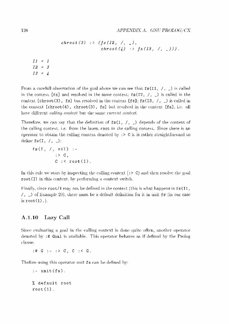
126 APPENDIX A. GNU PROLOG/CX
chroot (3) :> (fs(I2, /, _),
chroot (4) :> fs(I3, /, _))).
I1 = 1
I2 = 3
I3 = 4
From a carefull observation of the goal above we can see that fs(I1, /, _) is calledin the context [fs] and resolved in the same context; fs(I2, /, _) is called in thecontext [chroot(3), fs] but resolved in the context [fs]; fs(I3, /, _) is called inthe context [chroot(4), chroot(3), fs] but resolved in the context [fs], i.e. allhave di�erent calling context but the same current context.
Therefore, we can say that the de�nition of fs(I, /, _) depends of the content ofthe calling context, i.e. from the latest root in the calling context. Since there is anoperator to obtain the calling context denoted by :> C it is rather straightforward tode�ne fs(I, /, _):
fs(I, /, nil) :-
:> C,
C :< root(I).
In this rule we start by inspecting the calling context (:> C) and then resolve the goalroot(I) in this context, by performing a context switch.
Finally, since root/1may not be de�ned in the context (this is what happens in fs(I1,
/, _) of Example 20), there must be a default de�nition for it in unit fs (in our caseis root(1).).
A.1.10 Lazy Call
Since evaluating a goal in the calling context is done quite often, another operatordenoted by :# Goal is available. This operator behaves as if de�ned by the Prologclause:
:# G :- :> C, C :< G.
Thefore using this operator unit fs can be de�ned by:
:- unit(fs).
% default root
root (1).
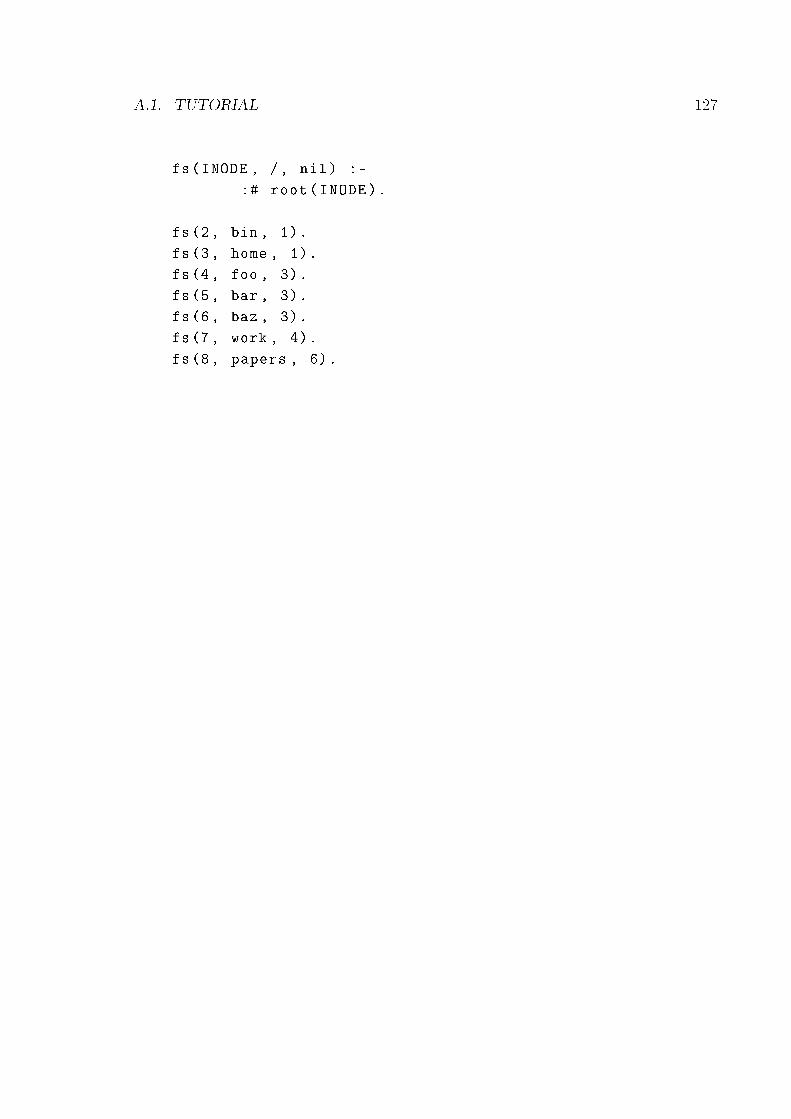
A.1. TUTORIAL 127
fs(INODE , /, nil) :-
:# root(INODE).
fs(2, bin , 1).
fs(3, home , 1).
fs(4, foo , 3).
fs(5, bar , 3).
fs(6, baz , 3).
fs(7, work , 4).
fs(8, papers , 6).

128 APPENDIX A. GNU PROLOG/CX
A.2 Reference Manual
A.2.1 Introduction
In this section we present the Contextual Logic Programming directives, operators andpredicates that are part of the GNU Prolog/CX implementation.
A.2.2 Directives
unit/1
Templates
unit(+unit_descriptor)
Description
unit(Name) declares unit Name if the argument is an atom, otherwise declares a unitwhose name is the principal functor of Name and whose arguments are the argumentsof Name.
The type unit_descriptor is either an atom or a compound term with the struc-ture functor(Var_1, ..., Var_n) where Var_1, ..., Var_n are di�erent variablenames.
Errors
None.
Portability
CxLP directive.
A.2.3 Operators
Context Switch - :</2
Templates
:< (+unit_descriptor_list, +callable_term)

A.2. REFERENCE MANUAL 129
Description
Context :< Goal evaluates Goal in context Context, ie. totally bypassing the currentcontext.
Errors
None.
Portability
CxLP operator.
Current Context - :</1
Templates
:< (-unit_descriptor_list)
Description
:< Context uni�es Context with the current context.
Errors
None.
Portability
CxLP operator.
Calling Context - :>/1
Templates
:> (-unit_descriptor_list)
Description
:> Context uni�es Context with the calling context.
Errors
None.

130 APPENDIX A. GNU PROLOG/CX
Portability
CxLP operator.
Context Extension - :>/2
Templates
:> (+unit_descriptor, +callable_term)
Description
Unit :> Goal extends the current context with unit Unit before attempting to reducegoal Goal. This operator behaves as if de�ned by the Prolog clause:
U :> G :- :< C, [U|C] :< G.
Errors
None.
Portability
CxLP operator.
Guided Context Traversal - ::/2
Templates
::(+unit_descriptor, +callable_term)
Description
Unit :: Goal behaves as if de�ned by the Prolog clause:
U :: G :- :< C, GC = [U|_], suffixchk(GC, C), GC :< G.
Where suffixchk/2 is a deterministic predicate where suffixchk(SUFFIX, LIST)
succeeds if SUFFIX is a su�x of LIST.
Errors

A.2. REFERENCE MANUAL 131
None.
Portability
CxLP operator.
Supercontext - :�/1
Templates
:�(+callable_term)
Description
� Goal evaluates Goal in the context obtained by dropping the topmost unit of thecurrent context. This operator behaves as if de�ned by the Prolog clause:
:^ G :- :< [_|C], C :< G.
Errors
None.
Portability
CxLP operator.
Lazy Call - :#/1
Templates
:#(+callable_term)
Description
# Goal evaluates Goal in the calling context. This operator behaves as if de�ned bythe Prolog clause:
:# G :- :> C, C :< G.

132 APPENDIX A. GNU PROLOG/CX
Errors
None.
Portability
CxLP operator.
A.2.4 Utilities
current_unit/2
Templates
current_unit(?atom,?integer)
Description
current_unit(Name, Arity) succeeds if there is a unit Name with Arity arguments.This predicate is re-executable on backtracking and can be thus used to enumerate allthe units.
Errors
None.
Portability
CxLP predicate.

Appendix B
Constraint Logic Programming
B.1 Introduction
Formally, a Constraint Satisfaction Problem (CSP) consists of a tuple 〈V,D,C〉 whereV is a set of variables, D their domains and C the set of constraints to be satis�ed,i.e. all CSP have the following abstract structure:
• there are variables to instantiate;
• the variables range over some domain;
• the solutions must satisfy a set of constraints.
The Constraint Logic Programming (CLP) scheme CLP(X) [JL87, JM94], has beenproposed as a generalisation of Logic Programming to deal with constraints in somearbitrary domain. In the CLP(X) scheme, the parameter X refers the specialiseddomain of the constraints. More speci�cally, to the:
• domain of the variables
• language of constraints
In the following section we will brie�y overview the domain and language of the mainconstraint domains.
133

134 APPENDIX B. CONSTRAINT LOGIC PROGRAMMING
B.2 Constraint Domains
B.2.1 Booleans: CLP(B)
• Domain: boolean (True/False).
• Language: equality (=) of well formed formulas on the usual boolean operators(¬,∧,∨, . . .).
B.2.2 Pseudo�Booleans: CLP(PB)
• Domain: boolean variables (0/1).
• Language: a relation of the set {=, <,≤, >,≥} applied to pseudo�boolean terms(i.e. arithmetic expressions with operators {+,−, .}).
B.2.3 Rationals/Reals: CLP(R)
• Domain: rational (real) variables.
• Language: a relation of the set {=, 6=, <,≤, >,≥} applied to linear terms (i.e.arithmetic expressions built with operator {+}).
B.2.4 Finite Domains: CLP(FD)
• Domain: a �nite set of (ordered) values, possible interpreted to some numericaldomain.
• Language: quite varied.
Finite domains subsume booleans and pseudo�booleans. All CLP(B) and CLP(PB)problems can thus be used as �nite domain problems, declaring variables to be in thedomain {0, 1}.
B.3 Constraint Solvers
There are two types of constraint solvers in CLP:

B.3. CONSTRAINT SOLVERS 135
• complete solvers: if it is guaranteed that there is an infer function that detectscontradiction;
• incomplete solvers: if it is not guaranteed that the infer function always detectscontradiction. In this case, the solver is augmented with a second constraintstore, where all the constraints whose e�ects have not been fully assessed aremaintained.
Regarding the properties of constraint solvers, they:
• must be incremental. The addition of a constraint must cause as little computa-tion as possible. The later retraction of a constraint (upon backtracking) mustalso be as e�ortless as possible.
• must be e�cient;
• must be sound;
• might not be complete.
Answers
• LP provides de�nite answers: the answers are the most general terms that makethe query consistent with the program.
• CLP also provides de�nite answers if the solvers are complete. If the solver isincomplete, the answers are conditional: they represent terms that make thequery consistent with the program.
B.3.1 Incomplete Constraint Solvers
Incomplete solvers are used in domains where no general algebraic theory exists (or ise�cient). Rather than guaranteeing that a set of constraints is consistent, incompleteconstraint solvers aim at reducing the possible values of the variables so as to prune thesearch for solutions. These solvers are based on local propagation, that can be brie�ydescribed as:
if the domain of a variable is reduced by some constraint, all constraintsinvolving that variable are awaken to check whether the domain of othervariables can be further reduced. If that is true, the procedure recurs.Otherwise it stops, and is ready to handle further constraints.
136 APPENDIX B. CONSTRAINT LOGIC PROGRAMMING
Local propagation is usually much more e�cient that algebraic methods, but requiresthe use of a complementary enumeration procedure.
If all that is required is one solution, then incomplete solvers are usually preferably. Ifone needs all solutions, then the trade�o� is uncertain.
B.4 Finite Domains
There are three types of constraints in the �nite domains:
• declaration of �nite domain variables and their domains.
• general constraints on these variables. Such constraints are used actively toreduce the initial domains, before and during the enumeration.
• enumeration predicates. These predicates are used to �nd solutions. The reduceddomains of some variables can contain elements that do not belong to a solution.If these values are assigned to the variables, other domains are eventually reducedto the empty set, this way detecting unsatis�ability.
B.4.1 Finite Domain Solvers
The �nite domain solvers are based on local propagation and can be formalised asconstraint networks where:
• variables are the nodes of the network;
• constraints are the arcs of the network.
B.4.2 Network Consistency
There are three types of network consistency:
• Node consistency: any value in the domain of a variable A that is not consistentwith the constraints on that variable alone must be removed. Is quite inexpensiveto maintain, but it has limited pruning capabilities.
• Arc Consistency: any value in the domain of a variable A that is not supportedby a value in a variable B for which there is an arc A�B, must be removed. It ismore expensive to maintain and, sometimes the extra e�ort does not pay o� interms of increased pruning.

B.4. FINITE DOMAINS 137
• Path Consistency: any value in the domain of a variable A, which is eithernot supported by a value in variable B for which there is an arc A�B, or by avariable C for which there are arcs A�B and B�C, must be removed. It is stillmore expensive to maintain and quite often it does not increase domain pruningsigni�cantly.
Since node and arc consistency can leave values in the domain of a variable that cannotbe part of a solution, they are not complete.
B.4.3 Constraint Propagation (CP) vs. Backtracking
The advantages (+) and disadvantages (-) of constraint propagations versus backtrack-ing are:
- in the early stages of a program CP spends a large time inspecting values of thevariables domains, possibly to verify that they are X�consistent.
+ in the later stages of the programs, CP has to instantiate less values for thevariables, since their domains have been pruned by constraint propagation.
+ CP anticipates the detection of failures, and thus backtracking.
+ CP prevents irrelevant backtracking. By anticipating backtracing, it does notbacktrack to the wrong choice points.
B.4.4 Constraint Propagation and Heuristics
There are two major procedures to speed up the execution of constraint solvers:
1. reducing the number of alternatives throughout constraint propagation;
2. guessing the right alternatives recurring to heuristics (which are often problemdependent).
Regarding �nite domains, there are two choice points in the enumeration phase:
1. the variable to instantiate next;
2. the value to instantiate the variable with.

138 APPENDIX B. CONSTRAINT LOGIC PROGRAMMING
B.4.5 Advanced Techniques
So far, choice points were only considered in the enumeration phase. A conjunctionof constraints was assumed in the constraint declaration phase to set up a uniqueconstraint network. However some applications require the introduction of disjunctionsin the constraint speci�cation phase. The possibilities for circumventing this problemare:
• delay the choice as much as possible;
• derive common information.
B.4.6 Global Constraints
Constraint solvers based on local propagation do not detect global inconsistency overlarger sets of constraints in the network. Maintaining k�consistency (consistency ofall sets of k variables) is very expensive (path consistency maintains 3�consistency,etc). However, special and important cases like alldifferent, cumulative, among,
diffn and cycle, might be handled separately.
B.4.7 Optimisation Constraints
In many applications one is interested not only in satisfying a set of constraints butalso in optimising (minimising or maximising) some objective function.
B.5 Defeasible Constraints
In several applications to keep the declarative style of programming, it is necessary toconsider soft constraints, i.e. constraints that might be relaxed to make the problemsolvable. This was the motivation of Hierarchical Constraint Logic Programming (orHCLP for short), where constraints were assigned some preference weight.
The goal of a HCLP program is therefore to compute a solution (or solutions) thatcomplies with:
• optimisation, i.e. satis�es as much constraints as possible;
• satisfaction, i.e. satis�es a su�cient number of constraints.
B.6. CONCLUSIONS 139
B.6 Conclusions
• So far, �nite domains are the most successful domain of application of CLP, beingmore e�cient than Operations Research approaches.
• Complete solvers, namely the ones for linear constraints over rationals, are lesse�cient than Operations Research packages for very large problems.
• Programming a CLP application is still an engineering task. One has to:
� �nd the best constraint solving technique;
� discover heuristics applicable to the problem;
� introduce redundant constraints to help the (incomplete) constraint solver;
� adapt, if possible, the solver to match the user needs.
• The need to experiment several techniques and possibly adapt the constraintsolver favours the approach of glass�box constraint solvers rather than back�box
solvers.
• There is room to improve not only the capabilities of constraint solvers, but alsoto take advantage of the �exibility of the CLP approach to tackle applicationsrequiring mixed techniques.
• Many applications are naturally over constrained and there is much research tobe done in defeasible constraint solving.
• Constraint solving over reals (intervals) shows good potential for engineeringapplications.


References
[Abr00] Salvador Abreu. A Logic-based Information System. In Enrico Pontelliand Vitor Santos-Costa, editors, 2nd International Workshop on Practical
Aspects of Declarative Languages (PADL'2000), volume 1753 of LectureNotes in Computer Science, pages 141�153, Boston, MA, USA, January2000. Springer-Verlag.
[Abr01] Salvador Abreu. Isco: A practical language for heterogeneous informationsystem construction. In Proceedings of INAP'01, Tokyo, Japan, October2001. Prolog Association of Japan.
[Abr02] Salvador Abreu. Modeling Role-Based Access Control in ISCO. InLÃgia Maria Ribeiro and José Marques dos Santos, editors, The 8th
International Conference of European University Information Systems.FEUP Edições, June 2002. ISBN 972-752-051-0.
[AD03a] Salvador Abreu and Daniel Diaz. Objective: In minimum context. InCatuscia Palamidessi, editor, ICLP, volume 2916 of Lecture Notes in
Computer Science, pages 128�147. Springer, 2003.
[AD03b] Salvador Abreu and Daniel Diaz. Objective: in Minimum Context.In Catuscia Palamidessi, editor, Logic Programming, 19th International
Conference, ICLP 2003, Mumbai, India, December 9-13, 2003, Proceedings,volume 2916 of Lecture Notes in Computer Science, pages 128�147.Springer-Verlag, 2003. ISBN 3-540-20642-6.
[ADN04] Salvador Abreu, Daniel Diaz, and Vitor Nogueira. Organizational in-formation systems design and implementation with contextual constraintlogic programming. In IT Innovation in a Changing World � The 10th
International Conference of European University Information Systems,Ljubljana, Slovenia, June 2004.
[Aea07] A. Aggoun and et. al. Eclipse user manual release 5.10, November 2007.
141

142 REFERENCES
[AKN86] H Aït-Kaci and R Nasr. Login: A logic programming language with built-ininheritance. J. Log. Program., 3(3):185�215, 1986.
[All83] J .F. Allen. Maintaining knowledge about temporal intervals. cacm,26(11):832�843, nov 1983.
[AM89] Martín Abadi and Zohar Manna. Temporal logic programming. J. Symb.Comput., 8(3):277�295, 1989.
[AN05] Salvador Abreu and Vitor Nogueira. Using a Logic Programming Languagewith Persistence and Contexts. In Masanobu Umeda and Armin Wolf,editors, Proceedings of the 16th International Conference on Applications
of Declarative Programming and Knowledge Management (INAP 2005),Fukuoka, Japan, October 2005. Waseda University.
[AN06] Salvador Abreu and Vitor Nogueira. Towards structured contexts andmodules. In Etalle and Truszczynski [ET06], pages 436�438.
[AR99] Tamas Abraham and John F. Roddick. Survey of spatio-temporaldatabases. Geoinformatica, 3(1):61�99, 1999.
[Ari86] Gad Ariav. A temporally oriented data model. ACM Trans. Database
Syst., 11(4):499�527, 1986.
[Ate] Atempo. Time navigator. http://www.atempo.com/.
[Aug01] Juan Carlos Augusto. The logical approach to temporal reasoning. Artif.Intell. Rev., 16(4):301�333, 2001.
[BBJ98] Michael H. Böhlen, R. Busatto, and Christian S. Jensen. Point-versusinterval-based temporal data models. In ICDE '98: Proceedings of the
Fourteenth International Conference on Data Engineering, pages 192�200,Washington, DC, USA, 1998. IEEE Computer Society.
[BCC+97] F. Bueno, D. Cabeza, M. Carro, M. Hermenegildo, P. López-García, andG. Puebla. The ciao prolog system. reference manual. Technical ReportCLIP3/97.1, School of Computer Science, Technical University of Madrid(UPM), August 1997. Available from http://www.clip.dia.�.upm.es/.
[BCLM98] Michele Bugliesi, Anna Ciampolini, Evelina Lamma, and Paola Mello.Optimizing modular logic languages. ACM Comput. Surv., 30(3es):10,1998.
[BK82] K. A. Bowen and R. A. Kowalski. Amalgamating language and metalan-guage in logic programming. In K. L. Clark and S.-A. Tärnlund, editors,Logic Programming, pages 153�172. Academic Press, London, 1982.

REFERENCES 143
[BK94] Anthony J. Bonner and Michael Kifer. An overview of transaction logic.In Theoretical Computer Science (TCS), pages 133:205�265, 1994.
[BLM93] Michele Bugliesi, Evelina Lamma, and Paola Mello. Partial deduction forstructured logic programming. J. Log. Program., 16(1):89�122, 1993.
[BLM94] Michele Bugliesi, Evelina Lamma, and Paola Mello. Modularity in logicprogramming. The Journal of Logic Programming, 19 & 20:443�502, May1994.
[BMPT94] Antonio Brogi, Paolo Mancarella, Dino Pedreschi, and Franco Turini. Mod-ular logic programming. ACM Trans. Program. Lang. Syst., 16(4):1361�1398, 1994.
[BMRT01] P. Baldan, P. Mancarella, A. Ra�aetà, and F. Turini. MuTACLP: Alanguage for temporal reasoning with multiple theories. Technical ReportTR-01-22, Dipartimento di Informatica, Università di Pisa, 23 2001.
[BMRT02] Paolo Baldan, Paolo Mancarella, Alessandra Ra�aetà, and Franco Turini.Mutaclp: A language for temporal reasoning with multiple theories. InAntonis C. Kakas and Fariba Sadri, editors, Computational Logic: Logic
Programming and Beyond, volume 2408 of Lecture Notes in Computer
Science, pages 1�40. Springer, 2002.
[Bro56] F. P. Brooks. The Analytic Design of Automatic Data Processing Systems.
PhD thesis, Harvard University, May 1956.
[Brz98] Christoph Brzoska. Programming in metric temporal logic. Theor. Comput.Sci., 202(1-2):55�125, 1998.
[BZ82] Jacov Ben-Zvi. The time relational model. PhD thesis, 1982.
[CC87] James Cli�ord and Albert Croker. The historical relational data model(hrdm) and algebra based on lifespans. In Proceedings of the Third In-
ternational Conference on Data Engineering, pages 528�537, Washington,DC, USA, 1987. IEEE Computer Society.
[CC92] Patrick Cousot and Radhia Cousot. Abstract interpretation and applica-tion to logic programs. J. Log. Program., 13(2&3):103�179, 1992.
[CCGT95] James Cli�ord, Albert Croker, Fabio Grandi, and Alexander Tuzhilin.On temporal grouping. In Proceedings of the International Workshop on
Temporal Databases, pages 194�213, London, UK, 1995. Springer-Verlag.
144 REFERENCES
[CCT94] James Cli�ord, Albert Croker, and Alexander Tuzhilin. On completenessof historical relational query languages. ACM Trans. Database Syst.,19(1):64�116, 1994.
[Che80] Brian F. Chellas. Modal Logic: An Introduction. Cambridge UniversityPress, Cambridge, 1980.
[Cho94] J. Chomicki. Temporal query languages: a survey. In D. M. Gabbay andH. J. Ohlbach, editors, Temporal Logic: ICTL'94, volume 827, pages 506�534. Springer-Verlag, 1994.
[CLM96] Anna Ciampolini, Evelina Lamma, and Paola Mello. An abstractinterpretation framework for optimizing dynamic modular logic languages.Inf. Process. Lett., 58(4):163�170, 1996.
[CM00] Luca Chittaro and Angelo Montanari. Temporal representation andreasoning in arti�cial intelligence: Issues and approaches. Annals of
Mathematics and Arti�cial Intelligence, 28(1-4):47�106, 2000.
[Cor05] Oracle Corportation. Oracle database 10g workspace manager overview.Oracle White Paper, May 2005.
[CP03] Carlo Combi and Giuseppe Pozzi. Temporal conceptual modelling ofwork�ows. In Il-Yeol Song, Stephen W. Liddle, Tok Wang Ling, and PeterScheuermann, editors, ER, volume 2813 of Lecture Notes in Computer
Science, pages 59�76. Springer, 2003.
[CP04] Carlo Combi and Giuseppe Pozzi. Architectures for a temporal work�owmanagement system. In SAC '04: Proceedings of the 2004 ACM symposium
on Applied computing, pages 659�666, New York, NY, USA, 2004. ACMPress.
[CP06] Carlo Combi and Giuseppe Pozzi. Task scheduling for a temporal work�owmanagement system. Thirteenth International Symposium on Temporal
Representation and Reasoning (TIME'06), 0:61�68, 2006.
[CT98] Jan Chomicki and David Toman. Temporal logic in information systems.In Jan Chomicki and Gunter Saake, editors, Logics for Databases and
Information Systems (the book grow out of the Dagstuhl Seminar 9529:
Role of Logics in Information Systems, 1995), pages 31�70. Kluwer, 1998.
[Dat99] C. J. Date. An introduction to database systems (7th ed.). Addison-WesleyLongman Publishing Co., Inc., Boston, MA, USA, 1999.

REFERENCES 145
[DBL07] 14th International Symposium on Temporal Representation and Reasoning
(TIME 2007), 28-30 June 2007, Alicante, Spain. IEEE Computer Society,2007.
[DC01] Daniel Diaz and Philippe Codognet. Design and implementation of thegnu prolog system. Journal of Functional and Logic Programming, 2001(6),October 2001.
[DD02] Chris Date and Hugh Darwen. Temporal Data and the Relational Model.Morgan Kaufmann Publishers Inc., San Francisco, CA, USA, 2002.
[DD05] Hugh Darwen and C. J. Date. An overview and analysis of proposalsbased on the tsql2 approach. http://www.dcs.warwick.ac.uk/~hugh/TTM/OnTSQL2.pdf, March 2005.
[DLM+92] Enrico Denti, Evelina Lamma, Paola Mello, Antonio Natali, and AndreaOmicini. Implementing contexts in Logic Programming. In Evelina Lammaand Paola Mello, editors, 3rd International Workshop on Extensions of
Logic Programming (ELP'92), pages 145�170, Bologna, Italy, 26�28 1992.Tecnoprint Bologna.
[DMG94] M A Reynolds DMGabbay, I M Hodkinson. Temporal Logic: Mathematical
foundations and computational aspects, volume 1. Clarendon Press, Oxford,1994.
[DMP91] Rina Dechter, Itay Meiri, and Judea Pearl. Temporal constraint networks.Artif. Intell., 49(1-3):61�95, 1991.
[DNO92] Enrico Denti, Antonio Natali, and Andrea Omicini. Contexts as �rst-class objects: An implementation based on the SICStus Prolog system. InStefania Costantini, editor, 7th Italian Conference on Logic Programming
(GULP'92), pages 307�320, Tremezzo, Como, Italy, 17�19 1992. CittàStudi, Milano, Italy.
[EMK+04] Andrew Eisenberg, Jim Melton, Krishna Kulkarni, Jan-Eike Michels, andFred Zemke. Sql:2003 has been published. SIGMOD Rec., 33(1):119�126,2004.
[ET06] Sandro Etalle and Miroslaw Truszczynski, editors. Logic Programming,
22nd International Conference, ICLP 2006, Seattle, WA, USA, August 17-
20, 2006, Proceedings, volume 4079 of Lecture Notes in Computer Science.Springer, 2006.
[F. 06] F. Henderson and T. Conway and Z. Somogyi and D. Je�ery and P.Schachte and S. Taylor and C. Speirs and T. Dowd and R. Becket and
146 REFERENCES
M. Brown. The Mercury Language Reference Manual. The University ofMelbourne, 0.13.1 edition, 2006.
[FGV05] Michael Fisher, Dov Gabbay, and Lluis Vila. Handbook of Temporal
Reasoning in Arti�cial Intelligence (Foundations of Arti�cial Intelligence
(Elsevier)). Elsevier Science Inc., New York, NY, USA, 2005.
[Frü93] Thom W. Frühwirth. Temporal logic and annotated constraint logicprogramming. In Michael Fisher and Richard Owens, editors, ExecutableModal and Temporal Logics, volume 897 of Lecture Notes in Computer
Science, pages 58�68. Springer, 1993.
[Frü94a] T. Frühwirth. Temporal reasoning with constraint handling rules. TechnicalReport ECRC-94-5, European Computer-Industry Research Centre GmbH,ECRC Munich, Germany, 1994.
[Frü94b] Thom W. Frühwirth. Annotated constraint logic programming applied totemporal reasoning. In Manuel V. Hermenegildo and Jaan Penjam, editors,PLILP, volume 844 of Lecture Notes in Computer Science, pages 230�243.Springer, 1994.
[Frü96] Thom W. Frühwirth. Temporal annotated constraint logic programming.J. Symb. Comput., 22(5/6):555�583, 1996.
[fS00] International Organization for Standardization. ISO IEC 13211-2:2000:
Information technology � Programming languages � Prolog � Part 2: Mod-
ules. International Organization for Standardization, Geneva, Switzerland,2000.
[fS03] International Organization for Standardization. ISO/IEC 9075-*:2003.
Information technology � Database languages � SQL. International Or-ganization for Standardization, Geneva, Switzerland, 2003.
[Gad88] Shashi K. Gadia. A homogeneous relational model and query languagesfor temporal databases. ACM Trans. Database Syst., 13(4):418�448, 1988.
[Gal87] Antony Galton. The logic of occurrence. pages 169�196, 1987.
[Gal08] Antony Galton. Temporal logic. In Edward N. Zalta, editor, The StanfordEncyclopedia of Philosophy. Spring 2008.
[Ger01] Manolis Gergatsoulis. Temporal and modal logic programming languages.In A. Kent and J. G. Williams, editors, Encyclopedia of Microcomputers,volume 27,Supplement 6, pages 393�408. Marcel Dekker, Inc, New York,2001.
REFERENCES 147
[GJ99] Heidi Gregersen and Christian S. Jensen. Temporal entity-relationshipmodels-a survey. IEEE Transactions on Knowledge and Data Engineering,11(3):464�497, 1999.
[GMR88] Laura Giordano, Alberto Martelli, and Gianfranco Rossi. Local de�nitionswith static scope rules in logic programming. In FGCS, pages 389�396,1988.
[GRP96] M. Gergatsoulis, P. Rondogiannis, and T. Panayiotopoulos. Disjunctivechronolog, 1996.
[GWW75] J.F. Fries G. Wiederhold and S. Weyl. Structured organization of clinicaldata bases. In AFIPS National Computer Conference, pages 479�485, 1975.
[GY88] Shashi K. Gadia and Chuen-Sing Yeung. A generalized model for arelational temporal database. In SIGMOD '88: Proceedings of the 1988
ACM SIGMOD international conference on Management of data, pages251�259, New York, NY, USA, 1988. ACM Press.
[HF06] Rémy Haemmerlé and François Fages. Modules for prolog revisited. InEtalle and Truszczynski [ET06], pages 41�55.
[Hir97] Robin Hirsch. Expressive power and complexity in algebraic logic. Journalof Logic and Computation, 7(3):309�351, 1997.
[HM87] S. Hanks and D. McDermott. Default reasoning, nonmonotonic logics, andthe frame problem. pages 390�395, 1987.
[Hry93] Tomas Hrycej. A temporal extension of prolog. J. Log. Program., 15(1-2):113�145, 1993.
[HS91] Joseph Y. Halpern and Yoav Shoham. A propositional modal logic of timeintervals. J. ACM, 38(4):935�962, 1991.
[IABC+95] Gad Ariav Ilsoo Ahn, Don Batory, James Cli�ord, Curtis E. Dyreson,Ramez Elmasri, Fabio Grandi, Christian S. Jensen, Wolfgang Käfer, NickKline, Krishna Kulkarni, T. Y. Cli� Leung, Nikos Lorentzos, John F.Roddick, Arie Segev, Michael D. Soo, and Suryanarayana M. Sripada. TheTSQL2 Temporal Query Language. Kluwer Academic Publishers, 1995.
[IBM] IBM. Data propagator. http://www-306.ibm.com/software/data/integration/replication/.
[Int92] International Organization for Standardization. ISO/IEC 9075:1992:
Title: Information technology � Database languages � SQL. 1992.Available in English only.
148 REFERENCES
[Jen00] Christian S. Jensen. Temporal database management. Dr. Techn. Thesis,2000.
[JK04] Peter Jonsson and Andrei Krokhin. Complexity classi�cation in qualitativetemporal constraint reasoning. Artif. Intell., 160(1):35�51, 2004.
[JL87] J. Ja�ar and J.-L. Lassez. Constraint logic programming. In POPL '87:
Proceedings of the 14th ACM SIGACT-SIGPLAN symposium on Principles
of programming languages, pages 111�119. ACM Press, 1987.
[JM94] Joxan Ja�ar and Michael J. Maher. Constraint logic programming: Asurvey. Journal of Logic Programming, 19/20:503�581, 1994.
[JMR91] C. S. Jensen, L. Mark, and N. Roussopoulos. Incremental implementationmodel for relational databases with transaction time. IEEE Transactions
on Knowledge and Data Engineering, 3(4):461�473, 1991.
[JMS79] Susan Jones, Peter Mason, and Ronald K. Stamper. Legol 2.0: A relationalspeci�cation language for complex rules. Inf. Syst., 4(4):293�305, 1979.
[Joh91] Johan Van Benthem. The Logic of Time: A Model-Theoretic Investigation
into the Varieties of Temporal Ontology and Temporal Discourse, volume156 of Synthese Library. Kluwer Academic Publishers, second edition, 1991.
[JS96] Christian S. Jensen and Richard Thomas Snodgrass. Semantics of time-varying information. Inf. Syst., 21(4):311�352, 1996.
[JSS95] Christian S. Jensen, Richard T. Snodgrass, and Michael D. Soo. The tsql2data model. In The TSQL2 Temporal Query Language, pages 153�238.1995.
[Kim78] K. A. Kimball. The data system. Master's thesis, University ofPennsylvania, 1978.
[KJJ03] Andrei A. Krokhin, Peter Jeavons, and Peter Jonsson. Reasoning abouttemporal relations: The tractable subalgebras of allen's interval algebra.J. ACM, 50(5):591�640, 2003.
[Kou95] M. Koubarakis. Databases and temporal constraints: Semantics and com-plexity. In S. Cli�ord and A. Tuzhilin, editors, Recent Advances in TemporalDatabases, pages 93�112, Zurich, Switzerland, sep 1995. Proceedings of theInternational Workshop on Temporal Databases, Springer Verlag.
[KS86] R. A. Kowalski and M. J. Sergot. A logic-based calculus of events. New
Generation Computing, 4(1):67�95, 1986.

REFERENCES 149
[KS97] Robert A. Kowalski and Fariba Sadri. Reconciling the event calculus withthe situation calculus. J. Log. Program., 31(1-3):39�58, 1997.
[KSW90] F. Kabanza, J-M Stevenne, and P. Wolper. Handling in�nite temporaldata. In 9th Annual ACM SIGACT-SIGMOD-SIGART Symposium on
Principles of Database Systems, Nashville, TN, apr 1990.
[Lab03] The Intelligent Systems Laboratory. Quintus Prolog User's Manual.Swedish Institute of Computer Science, PO Box 1263, SE-164 29 Kista,Sweden, release 3.5 edition, December 2003.
[LEM88] Jr. Leslie Edwin Mckenzie. An algebraic language for query and update of
temporal databases. PhD thesis, 1988. Director-Richard Snodgrass.
[LEMS91] Jr. L. Edwin McKenzie and Richard Thomas Snodgrass. Evaluation ofrelational algebras incorporating the time dimension in databases. ACM
Comput. Surv., 23(4):501�543, 1991.
[LFA07] Nuno Lopes, Cláudio Fernandes, and Salvador Abreu. Contextual LogicProgramming for Ontology Representation and Querying. In Axel Polleres,David Pearce, Stijn Heymans, and Edna Ruckhaus, editors, Proceedings ofthe ICLP'07 Workshop on Applications of Logic Programming to the Web,
Semantic Web and Semantic Web Services (ALPSWS 2007), volume 287of CEUR Workshop Proceedings ISSN 1613-0073, October 2007.
[LJ88] N. A. Lorentzos and R. G. Johnson. Extending relational algebra tomanipulate temporal data. Inf. Syst., 13(3):289�296, 1988.
[LM94] Evelina Lamma and Paola Mello. Modularity in logic programming. InPascal Van Hentenryck, editor, Logic Programming - Proceedings of the
Eleventh International Conference on Logic Programming, pages 15�17,Massachusetts Institute of Technology, 1994. The MIT Press.
[LMN92] E. Lamma, P. Mello, and A. Natali. An Extended Warren AbstractMachine for the Execution of Structured Logic Programs. Journal of LogicProgramming, 14(3-4):187�222, 1992.
[LO96] Chuchang Liu and Mehmet Ali Orgun. Clocked Temporal Logic Pro-gramming. In Proceedings of The 19th Australasian Computer Science
Conference, Melbourne, Australia, January 31-February 2 1996.
[Lor88] N. A. Lorentzos. A Formal Extension of the Relational Model for the
Representation of Generic Intervals. PhD thesis, Birkbeck College, 1988.
[Lum] Lumigent. Log explorer for sql server. http://www.lumigent.com/products/le_sql.html.

150 REFERENCES
[McC92] Francis G. McCabe. Logic and objects. Prentice-Hall, Inc., Upper SaddleRiver, NJ, USA, 1992.
[Mei91] Itay Meiri. Combining qualitative and quantitative constraints in temporalreasoning. In Thomas Dean and Kathleen McKeown, editors, Proceedingsof the Ninth National Conference on Arti�cial Intelligence, pages 260�267,Menlo Park, California, 1991. AAAI Press.
[Mei96] Itay Meiri. Combining qualitative and quantitative constraints in temporalreasoning. Artif. Intell., 87(1-2):343�385, 1996.
[MH69] John McCarthy and Patrick J. Hayes. Some philosophical problems fromthe standpoint of arti�cial intelligence. In B. Meltzer and D. Michie,editors, Machine Intelligence 4, pages 463�502. Edinburgh UniversityPress, 1969. reprinted in McC90.
[Mil86] Dale Miller. A theory of modules for logic programming. In Symposium
on Logic Programming, pages 106�114, 1986.
[Mil89a] Dale Miller. A Logical Analysis of Modules in Logic Programming. Journalof Logic Programming, 6(2):79�108, 1989.
[Mil89b] Dale Miller. Lexical scoping as universal quanti�cation. In Sixth Inter-
national Logic Programming Conference, pages 268�283, Lisbon, Portugal,June 1989. MIT Press.
[Mil93] Dale Miller. A proposal for modules in lambda-prolog. In Roy Dyckho�,editor, ELP, volume 798 of Lecture Notes in Computer Science, pages 206�221. Springer, 1993.
[MMZ06] Elisabetta De Maria, Angelo Montanari, and Marco Zantoni. Anautomaton-based approach to the veri�cation of timed work�ow schemas.In TIME '06: Proceedings of the Thirteenth International Symposium
on Temporal Representation and Reasoning (TIME'06), pages 87�94,Washington, DC, USA, 2006. IEEE Computer Society.
[MNR89] Paola Mello, Antonio Natali, and Cristina Ruggieri. Logic programmingin a software engineering perspective. In NACLP, pages 441�458, 1989.
[MNRT00] Paolo Mancarella, Gianluca Nerbini, Alessandra Ra�aetà, and FrancoTurini. Mutaclp: A language for declarative gis analysis. In John W.Lloyd, Verónica Dahl, Ulrich Furbach, Manfred Kerber, Kung-Kiu Lau,Catuscia Palamidessi, Luís Moniz Pereira, Yehoshua Sagiv, and Peter J.Stuckey, editors, Computational Logic, volume 1861 of Lecture Notes in
Computer Science, pages 1002�1016. Springer, 2000.
REFERENCES 151
[Mou00] Paulo Moura. Logtalk 2.6 Documentation. Technical Report DMI 2000/1,University of Beira Interior, Portugal, July 2000.
[Mou03] Paulo Moura. Logtalk - Design of an Object-Oriented Logic Programming
Language. PhD thesis, Department of Computer Science, University ofBeira Interior, Portugal, September 2003.
[MP89] Luís Monteiro and António Porto. Contextual logic programming. In Mau-rizio Levi, Giorgio; Martelli, editor, Proceedings of the 6th International
Conference on Logic Programming (ICLP '89), pages 284�302, Lisbon,Portugal, June 1989. MIT Press.
[MP90] Luís Monteiro and António Porto. A transformational view of inheritancein logic programming. In ICLP, pages 481�494, 1990.
[MP93] Luís Monteiro and António Porto. A Language for Contextual LogicProgramming. In K.R. Apt, J.W. de Bakker, and J.J.M.M. Rutten, editors,Logic Programming Languages: Constraints, Functions and Objects, pages115�147. MIT Press, 1993.
[MRT97] Paolo Mancarella, Alessandra Ra�aetà, and Franco Turini. Time in amulti-theory logical framework. In TIME, pages 62�70, 1997.
[MRT99] Paolo Mancarella, Alessandra Ra�aetà, and Franco Turini. Knowledgerepresentation with multiple logical theories and time. J. Exp. Theor.
Artif. Intell., 11(1):47�76, 1999.
[NA89] S. B. Navathe and R. Ahmed. A temporal relational model and a querylanguage. Inf. Sci., 49(1-3):147�175, 1989.
[NA06a] Vitor Nogueira and Salvador Abreu. Temporal contextual logic program-ming. In Francisco J. López Fraguas, editor, Proceedings of the 15th
Workshop on Functional and (Constraint) Logic Programming (WFLP'06),Madrid, Spain, November 2006. Electronic Notes in Theoretical ComputerScience.
[NA06b] Vitor Nogueira and Salvador Abreu. Towards temporal contextual logicprogramming. In Etalle and Truszczynski [ET06], pages 439�441.
[NA07a] Vitor Nogueira and Salvador Abreu. Integrating temporal annotationsin a modular logic language. In Dietmar Seipel, Michael Hanus, ArminWolf, and Joachim Baumeister, editors, 17th International Conference
on Applications of Declarative Programming and Knowledge Management
(INAP 2007), volume Technical Report 434, Würzburg, Germany, October2007. Bayerische Julius-Maximilians-Universität Würzburg.

152 REFERENCES
[NA07b] Vitor Nogueira and Salvador Abreu. Modularity and temporal reasoning:a logic programming approach. In Time [DBL07].
[NA07c] Vitor Nogueira and Salvador Abreu. Temporal Annotations for a Contex-tual Logic Programming Language. In José Neves, Manuel Santos, andJosé Machado, editors, Progress in Arti�cial Intelligence, 13th Portuguese
Conference on Arti�cial Intellige nce, EPIA 2007, Universidade do Minho,2007.
[NA07d] Vitor Nogueira and Salvador Abreu. Temporal contextual logic program-ming. Electr. Notes Theor. Comput. Sci., 177:219�233, 2007.
[NAD03] Vitor Nogueira, Salvador Abreu, and Gabriel David. Using contextual logicprogramming for temporal reasoning. In Jaime Gómez Ernesto Pimentel,Nieves J. Brisaboa, editor, Proceedings of the VIII Jornadas de Ingenieríadel Software y Bases de Datos, pages 479�489, Alicante, Spain, November2003.
[NAD04] Vitor Beires Nogueira, Salvador Abreu, and Gabriel David. Towardstemporal reasoning in constraint contextual logic programming. InProceedings of the 3rd International Workshop on Multiparadigm Constraint
Programming Languages MultiCPL'04 associated to ICLP'04, Saint�Malo,France, September 2004.
[NB94] Bernhard Nebel and Hans-Jürgen Bürckert. Reasoning about temporalrelations: a maximal tractable subclass of allen's interval algebra. In AAAI'94: Proceedings of the twelfth national conference on Arti�cial intelligence
(vol. 1), pages 356�361, Menlo Park, CA, USA, 1994. American Associationfor Arti�cial Intelligence.
[NM88] Gopalan Nadathur and Dale Miller. An Overview of λProlog. InFifth International Logic Programming Conference, pages 810�827, Seattle,August 1988. MIT Press.
[NO] Antonio Natali and Andrea Omicini. Objects with state in ContextualLogic Programming. In Maurice Bruynooghe and Jaan Penjam, editors,Programming Language Implementation and Logic Programming, volume714 of LNCS, pages 220�234. Springer-Verlag. 5th International Sympo-sium (PLILP'93), Tallinn, Estonia, 25�27.
[NO93] Antonio Natali and Andrea Omicini. Objects with state in CSM. In 2nd
Compulog Network Area Meeting on Programming Languages joint with
Workshop on Logic Languages, pages 1�2, Pisa, Italy, 6�7 1993.

REFERENCES 153
[O'K85] R. O'Keefe. Towards an algebra for constructing logic programs. In In J.Cohen and J. Conery, editors, Proceedings of IEEE Symposium on Logic
Programming, pages 152�160. IEEE Computer Society Press, 1985.
[Org91] Mehmet Ali Orgun. Intensional logic programming. PhD thesis, Victoria,B.C., Canada, Canada, 1991.
[Org96] Mehmet A. Orgun. On temporal deductive databases. Computational
Intelligence, 12:235�259, 1996.
[Pan95] M. Panayiotopoulos, T. and Gergatsoulis. A Prolog like temporal reasoningsystem. In M. H. Hamza, editor, Proc. of 13th IASTED International Con-
ference on APPLIED INFORMATICS, pages 123�126, ICLS (Innsbruck),Austria, 1995.
[Pao] Paolo Terenziani. Reasoning about Time.
[Pin94] Javier Pinto. Temporal Reasoning in the Situation Calculus. PhD thesis,Department of Computer Science, University of Toronto, Toronto, Canada,January 1994.
[Por03] António Porto. An integrated information system powered by prolog. InVerónica Dahl and Philip Wadler, editors, PADL, volume 2562 of LectureNotes in Computer Science, pages 92�109. Springer, 2003.
[Pri57] A. N. Prior. Time and Modality. The Clarendon Press, Oxford, 1957.
[Pri67] A. N. Prior. Past, present and future. The Clarendon Press, Oxford, 1967.
[Pri68] A. N. Prior. Papers on Time and Tense. The Clarendon Press, Oxford,1968.
[Raf00] Alessandra Ra�aetá. Spatio-temporal knowlegde bases in constraint logic
programming framework with multiple theories. PhD thesis, UniversitáDegli Studi di Pisa, Dipartamento di Informatica, Pisa, Italy, March 2000.
[Rei89] H. Reichgelt. A comparison of �rst order and modal logics of time.In P. Jackson, H. Reichgelt, and F. van Harmelen, editors, Logic-BasedKnowledge Representation, pages 143�176. MIT Press, Cambridge, MA,1989.
[RF00a] Alessandra Ra�aetà and Thom Frühwirth. Labelled deduction, chapterSemantics for temporal annotated constraint logic programming, pages215�243. Kluwer Academic Publishers, Norwell, MA, USA, 2000.

154 REFERENCES
[RF00b] Alessandra Ra�aetà and Thom Frühwirth. Two semantics for temporalannotated constraint logic programming. In M. Gergatsoulis and P. Ron-dogiannis, editors, Intensional Programming II, Based on the Papers at
ISLIP'99, pages 78�92. World Scienti�c Singapore, 2000.
[RGP97] Panos Rondogiannis, Manolis Gergatsoulis, and Themis Panayiotopoulos.Cactus: A branching-time logic programming language. In ECSQARU-
FAPR, pages 511�524, 1997.
[Rib93] Cristina Ribeiro. Representation and Inference of Temporal Knowledge.PhD thesis, Faculdade de Ciências e Tecnologia, Universidade Nova deLisboa, 1993.
[RN03] Stuart J. Russell and Peter Norvig. Arti�cial Intelligence: A Modern
Approach. Pearson Education, 2003.
[RV05] H. Reichgelt and L. Vila. Handbook of Temporal Reasoning in Arti�cial
Intelligence (Foundations of Arti�cial Intelligence (Elsevier)), chapterTemporal Quali�cation in Arti�cial Intelligence. In [FGV05], 2005.
[Sad87] Rubik Sadeghi. A database query language for operations on historical
data. PhD thesis, 1987.
[Sar90a] N. L. Sarda. Algebra and query language for a historical data model.Comput. J., 33(1):11�18, 1990.
[Sar90b] N. L. Sarda. Extensions to sql for historical databases. IEEE Transactions
on Knowledge and Data Engineering, 2(2):220�230, 1990.
[SBJS97] Richard T. Snodgrass, Michael H. Böhlen, Christian S. Jensen, andAndreas Steiner. Transitioning temporal support in tsql2 to sql3. InTemporal Databases, Dagstuhl, pages 150�194, 1997.
[Sch98] Eddie Schwalb. Temporal Reasoning With Constraints. PhD thesis,University of California Irvine, June 1998.
[Sho88] Y. Shoham. Chronological ignorance: experiments in nonmonotonictemporal reasoning. Artif. Intell., 36(3):279�331, 1988.
[SK91] Michael Stonebraker and Greg Kemnitz. The postgres next generationdatabase management system. Commun. ACM, 34(10):78�92, 1991.
[SKD94] Eddie Schwalb, Kalev Kask, and Rina Dechter. Temporal reasoning withconstraints on �uents and events. In Proceedings of the Twelfth National
Conference on Arti�cial Intelligence (AAAI-94), volume 2, pages 1067�1072, Seattle, Washington, USA, 1994. AAAI Press/MIT Press.

REFERENCES 155
[SN04] Jörg Sander and Mario A. Nascimento, editors. Spatio-Temporal DatabaseManagement, 2nd International Workshop STDBM'04, Toronto, Canada,
August 30, 2004, 2004.
[Sno] Richard Snodgrass. Tsql2 and sql3 interactions. http://www.cs.arizona.edu/~rts/sql3.html.
[Sno87] Richard T. Snodgrass. The temporal query language tquel. ACM Trans.
Database Syst., 12(2):247�298, 1987.
[Sno07] Richard T. Snodgrass. Towards a science of temporal databases. In TIME
[DBL07], pages 6�7.
[SS87] Arie Segev and Arie Shoshani. Logical modeling of temporal data. InSIGMOD '87: Proceedings of the 1987 ACM SIGMOD international
conference on Management of data, pages 454�466, New York, NY, USA,1987. ACM.
[SSW+07] K. F. Sagonas, T. Swift, D. S. Warren, J. Freire, P. Rao, B. Cui, E. Johnson,L. de Castro, R. F. Marques, D. Saha, S. Dawnson, and M. Kifer. The XSBSystem Version 3.1 Volume 1: Programmer's Manual, August 2007.
[Ste05] Andreas Steiner. Timedb. http://www.TimeConsult.com/, 2005.
[Sub94] V. S. Subrahmanian. Amalgamating knowledge bases. ACM Trans.
Database Syst., 19(2):291�331, 1994.
[SV96] E. Schwalb and L. Vila. Logic programming with temporal constraints. InTIME '96: Proceedings of the 3rd Workshop on Temporal Representation
and Reasoning (TIME'96), page 51, Washington, DC, USA, 1996. IEEEComputer Society.
[SV98] Eddie Schwalb and Lluis Vila. Temporal constraints: A survey. Con-
straints, 3(2/3):129�149, 1998.
[TA86] Abdullah Uz Tansel and M. Erol Arkun. Hquel, a query language forhistorical relational databases. In SSDBM'86: Proceedings of the 3rd
international workshop on Statistical and scienti�c database management,pages 135�142, Berkeley, CA, US, 1986. Lawrence Berkeley Laboratory.
[TC90] Alexander Tuzhilin and James Cli�ord. A temporal relational algebraas a basis for temporal relational completeness. In Proceedings of the
sixteenth international conference on Very large databases, pages 13�23,San Francisco, CA, USA, 1990. Morgan Kaufmann Publishers Inc.

156 REFERENCES
[TCG+93] Abdullah Uz Tansel, James Cli�ord, Shashi Gadia, Sushil Jajodia, ArieSegev, and Richard Snodgrass, editors. Temporal databases: theory, design,and implementation. Benjamin-Cummings Publishing Co., Inc., RedwoodCity, CA, USA, 1993.
[The07] The Intelligent Systems Laboratory. SICStus Prolog User's Manual.Swedish Institute of Computer Science, PO Box 1263, SE-164 29 Kista,Sweden, release 4.0.2 edition, November 2007.
[Tho91] P. M. Thompson. A Temporal Data Model Based on Accounting Principles.PhD thesis, Department of Computer Science, University of Calgary, Mar1991.
[Vil82] Marc B. Vilain. A system for reasoning about time. In AAAI, pages 197�201, 1982.
[Vil94] Lluis Vila. A survey on temporal reasoning in arti�cial intelligence. AI
Communications, 7(1):4�28, 1994.
[VK86] Marc Vilain and Henry Kautz. Constraint Propagation Algorithms forTemporal Reasoning. In Proc. Fifth National Conference on Arti�cial
Intelligence, pages 377�382, Philadelphia, PA, USA, 1986.
[VKvB90] Marc Vilain, Henry Kautz, and Peter van Beek. Constraint propagationalgorithms for temporal reasoning: a revised report. pages 373�381, 1990.
[War83] D.H.D. Warren. An abstract prolog instruction set. Technical Note 309,Arti�cial Intelligence Center, SRI International, Menlo Park CA, 1983.
[Wie97] J. Wielemaker. Swi-prolog reference manual, 1997.
[Wik08] Wikipedia. Time � wikipedia, the free encyclopedia, 2008. [Online;accessed 28-August-2008].
[WZZ05] Fusheng Wang, Carlo Zaniolo, and Xin Zhou. Temporal xml? sql strikesback! In TIME '05: Proceedings of the 12th International Symposium
on Temporal Representation and Reasoning (TIME'05), pages 47�55,Washington, DC, USA, 2005. IEEE Computer Society.
[YAP06] The YAP Prolog System. http://www.ncc.up.pt/~vsc/Yap. 2006.


![Logic office mall & stay[1]](https://img.document.onl/doc/110x75/559f76281a28abe6718b4877/logic-office-mall-stay1.jpg)