Embed Size (px)
Citation preview

The influence
of mutation models
in kinship
likelihoods Pedro Filipe dos Santos Machado
Mestrado em Genética Forense Departamento de Biologia 2016/2017
Orientador Nádia Maria Gonçalves de Almeida Pinto, i3S, FCUP
Coorientador Eduardo Conde-Sousa, CBMA

Todas as correções determinadas pelo júri, e só essas, foram efetuadas.
O Presidente do Júri,
Porto, ______/______/_________

FCUP The influence of mutation models in kinship likelihoods
i
Acknowledgments
First of all, I would like to thank both of my supervisors – Nádia Pinto, who
promptly accepted to work with me, who kept pushing for a better and richer work, and
from whom I have learnt immensely throughout this year; and Eduardo Conde-Sousa,
without whom this work would not have been impossible, and who introduced me to the
whole new world of coding and computational statistics. Both have greatly contributed to
my professional and personal development, and to an unexpected (but not unwelcome)
shift in my Biology background. I would like to thank them for all the help, the
lightheartedness and the patience in the many times my sloppiness caused work to have
been redone.
I would also like to thank my colleague and friend Sofia Sousa for the multiple
times she has helped me and advised me in the elaboration of this thesis despite not
having any direct involvement in this work, for the multiple times she has saved me form
missing deadlines or any crucial information regarding this Master’s degree in general,
and, most of all, for the close company throughout this journey.
Finally, I would like to thank my family and friends, for all the support they’ve
always given me, with a very special thanks to my dear sister and to my friend Pedro
Barbosa for bearing with my hundreds of daily questions and helping me with this work
even though they are sociologists. Many thanks also to my dear mother for reminding
me to keep on track, and to Ana Luísa who helped me keep my mind fresh and at ease.

FCUP The influence of mutation models in kinship likelihoods
ii
Abstract
Different mutation models have been developed to consider the genotypic
observations of parent(s)/offspring duos or trios, even though, for autosomal
transmission, only Mendelian incompatibilities, not mutations, are able to be identified.
The most commonly considered mutation models are the so-called “Equal”,
“Proportional”, “Stepwise” and “Extended Stepwise”, all implemented in the software
Familias.
In this work we simulated 100,000 families (in duos and trios) of Parent-Child,
Full-siblings, and Half-siblings, as well as 100,000 profiles of Unrelated individuals,
assuming a specific database for 17 autosomal STRs and probabilities of incompatibility
inferred from the American Association of Blood Banks (AABB) report, 2008. 10 markers
with fictitious allele frequencies were also considered. Using the R version of the
software Familias, we calculated the likelihood ratios (LRs, where the probability of the
genotypic configuration of the individuals assuming each of the pedigrees was compared
with the probability of the same observations assuming unrelatedness, for each marker,
considering each of the aforementioned models, as well as assuming the absence of
mutation (Null model), and also increasing the integer-length mutation rate in the
Extended Stepwise model parameters. In the case of full-siblings, the comparison
assuming half-sibship as the alternative pedigree was also considered.
The results show that the use of the different mutation models and the increase
in the considered mutation rate do not result in major differences in the LRs. The
comparisons between the LRs obtained with the Null model and the others in cases with
no incompatibilities show that the consideration of hidden mutations also does not have
a major influence in the final result. Regarding the fictitious markers, no clear conclusions
could be taken regarding the relationship between a marker’s allele frequencies’
configuration and its proneness to be influenced by the use of different mutation models
or parameters. Future work could be developed to take a broader approach regarding
the fictitious markers (more variability should be introduced) and the paternity cases
where the putative father is a close relative of the real father.

FCUP The influence of mutation models in kinship likelihoods
iii
Resumo
Vários modelos de mutação foram desenvolvidos para considerar as
observações genotípicas de duos ou trios de pai(s)/filho(s), apesar de, na transmissão
autossómica, apenas possam ser identificadas incompatibilidades Mendelianas, e não
mutações. Os modelos de mutação mais comummente considerados são os chamados
“Equal”, “Proportional”, “Stepwise” e “Extended Stepwise”, todos eles implementados no
software Familias.
Neste trabalho simulamos 100,000 famílias (em duos e trios) de Pai-Filho,
Irmãos, Meios-irmãos, bem como 100,000 perfis de indivíduos não-relacionados,
assumindo uma base de dados específica com 17 microssatélites autossómicos e
probabilidades de incompatibilidade inferidas do relatório de 2008 da American
Association of Blood Banks (AABB). 10 marcadores com frequências alélicas fictícias
foram também considerados.
Usando a versão R do software Familias, calculamos as razões de
verosimilhança (LRs), onde a probabilidade da configuração genotípica dos indivíduos
assumindo cada um dos pedigrees foi comparado com a probabilidade dessas mesmas
observações assumindo que os indivíduos não são relacionados, para cada marcador.
Considerando cada um dos modelos acima mencionados, bem como assumindo
ausência de mutação (modelo Nulo) e também aumentando a taxa de mutação entre
repetições completas, nos parâmetros do modelo Extended Stepwise. No caso dos
Irmãos, foi também feita a comparação assumindo Meios-irmãos como a hipótese
alternativa.
Os resultados mostram que o uso de diferentes modelos de mutação e o
aumento da taxa de mutação considerada não resultam em grandes diferenças nos LRs.
As comparações entre os LRs obtidos com o modelo Nulo e os restantes, em casos sem
incompatibilidades, mostram que a consideração de mutações silenciosas também não
tem um grande impacto no resultado final. Relativamente aos marcadores fictícios, não
puderam ser retiradas conclusões claras quanto à relação entre a configuração das
frequências alélicas de um marcador e a sua propensão para ser influenciado pelo uso
de diferentes modelos de mutação ou parâmetros. Poderá ser desenvolvido trabalho
futuro para alargar a abordagem aos marcadores fictícios (deverá ser introduzida maior
variabilidade) e aos casos de paternidade em que o suposto pai é um parente próximo
do pai verdadeiro.

FCUP The influence of mutation models in kinship likelihoods
iv
Table of contents
Acknowledgments .......................................................................................................... i
Abstract ........................................................................................................................ ii
Resumo ........................................................................................................................ iii
List of Tables and Figures ............................................................................................ vi
1.1. Forensic Genetics ........................................................................................... 1
1.2. Kinship Evaluation .......................................................................................... 1
1.2.1. Applications ............................................................................................. 1
1.2.2. Types of markers ..................................................................................... 2
1.2.3. Evaluation of DNA evidence .................................................................... 4
1.3. Mutation Models ............................................................................................. 6
1.3.1. Mutation rate estimates ........................................................................... 6
1.3.2. Mutation models ...................................................................................... 7
2. Aims .................................................................................................................... 11
3. Material and methods .......................................................................................... 12
3.1. Genetic markers ........................................................................................... 12
3.2. Computations ............................................................................................... 13
3.2.1. Determination of incompatibility rates .................................................... 13
3.2.2. Simulations ............................................................................................ 14
3.2.3. The Stepwise model problem ................................................................ 15
3.3. Kinship problems .......................................................................................... 16
3.4. Mutation models ........................................................................................... 19
3.5. Statistical analysis ........................................................................................ 19
3.5.1. LR Calculations ..................................................................................... 19
3.5.2. Mendelian incompatibilities .................................................................... 19
3.5.3. The impact of considering mutations when no Mendelian incompatibilities
are found (i.e. Hidden mutations) ......................................................................... 20
3.5.4. The impact of considering different mutation models ............................. 20
3.5.5. The impact of the parameters in the Extended Stepwise Model ............. 20
4. Results and Discussion ........................................................................................ 21
4.1. Mendelian incompatibilities ........................................................................... 21
4.1.1. Parent-Child vs. Unrelated ..................................................................... 21
4.1.2. Full-siblings vs. Unrelated ...................................................................... 23
4.1.3. Half-siblings vs. Unrelated ..................................................................... 24

v FCUP
The influence of mutation models in kinship likelihoods
4.1.4. Full-siblings vs. Half-siblings .................................................................. 24
4.2. The impact of considering mutations in cases with no incompatibilities (i.e.
Hidden mutations) ................................................................................................... 25
4.2.2. Half-siblings vs. Unrelated ..................................................................... 28
4.2.3. Full-siblings vs. Half-siblings .................................................................. 28
4.3. The impact of considering different mutation models .................................... 29
4.3.1. For the 17 Au-STRs from the database of North Portugal ...................... 29
4.3.2. For the 10 markers with fictitious allele frequencies: .............................. 38
4.4. The impact of the parameters in the Extended Stepwise model .................... 39
4.4.1. For the 17 Au-STRs from the database of North Portugal ...................... 39
4.4.2. For the 10 markers with fictitious allele frequencies ............................... 43
5. Conclusions ......................................................................................................... 48
References: ................................................................................................................ 50
Appendices ................................................................................................................. 56

FCUP
The influence of mutation models in kinship likelihoods vi
List of Tables and Figures
Table 1 – Alleles and respective frequencies of the fictitious STRs to be analyzed
………………………………………………………………………………………………. 12
Figure 1 – Pedigree representing the case where the putative father A is the real father
of B…………………………………………………………………………………………..…16
Figure 2 – Pedigree representing the case where the putative father A is a full brother
of the real father (parents are related as full-siblings) of
B…………………………………………..…………………………………………….…...... 17
Figure 3 – Pedigree representing the case where the putative father A is a full brother
of the real father (parents are related as first cousins) of
B………………………………………………………………………..……………..………..17
Figure 4 – Pedigree representing the case where the putative father A is a full brother
of the real father (parents are unrelated) of B ………………………………………………18
Figure 5 – Pedigree representing the case where the putative father A is unrelated to
B……………………………………………………………………………..………………… 18
Table 2 – The proportion of paternal and maternal incompatibilities found in each
case…………………………………………………………………………………………… 21
Table 3 – Summary of the ratios between the LRs obtained with the Null model (in the
numerator) and the remaining models (in the denominator) in cases with no
incompatibilities……………………………………………………………………………… 25
Figure 6 – Case-example showing the genotypes of a Parent-Child duo for marker TH01
and respective LRs, calculated with the Null and Extended Stepwise mutation models
considering paternity and unrelatedness as the main and alternative hypotheses,
respectively……………………………………………………………………………………27
Figure 7 – Case-example showing the genotypes of a trio of individuals simulated
assuming the hypothesis of Full-sibship for marker D21S11 and respective LRs,
calculated with the Null and Extended Stepwise mutation models considering full-sibship
and unrelatedness as the main and alternative hypotheses, respectively……………..28

vii FCUP
The influence of mutation models in kinship likelihoods
Figure 8 – Case-example showing the genotypes of a Parent-Child duo for marker
D21S11 and respective LRs, calculated with the Extended Stepwise and Proportional to
Frequency mutation models considering paternity and unrelatedness as the main and
alternative hypotheses, respectively. Note that the LR considering the Extended
Stepwise model favors the first hypothesis, paternity (albeit weekly), while the LR with
the Proportional mutation model favors the alternative hypothesis,
unrelatedness................................................................................................................30
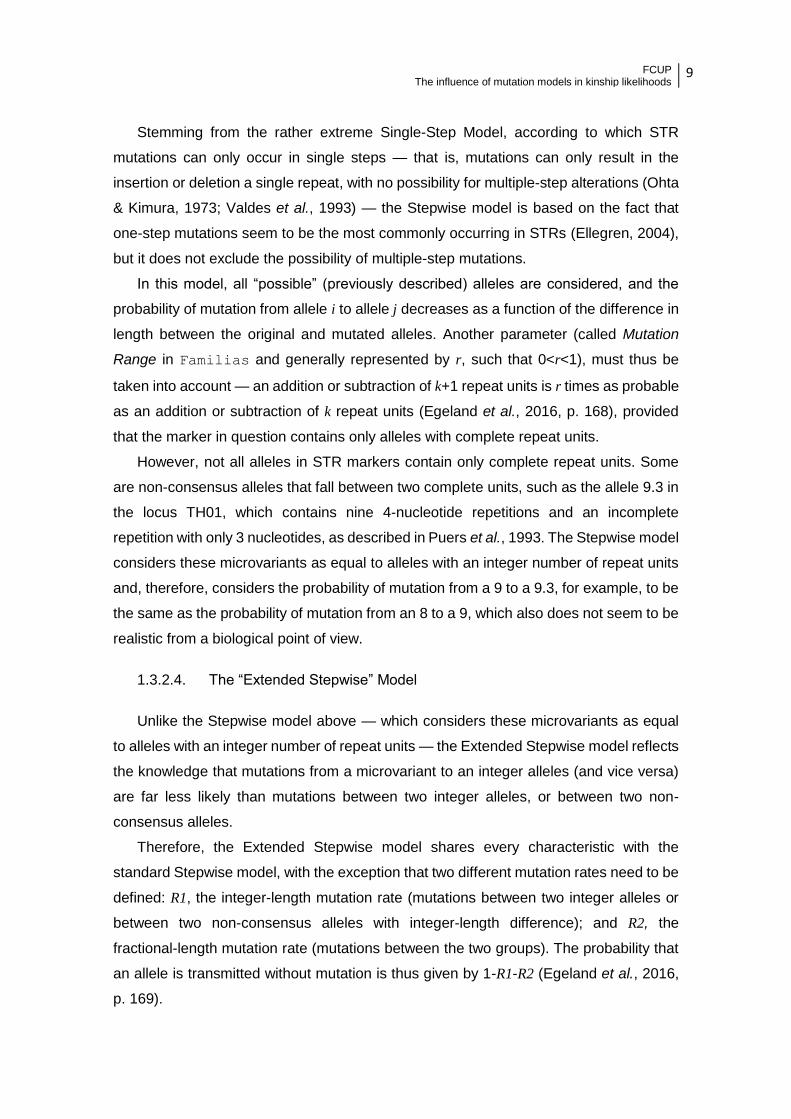
Figure 9 – Case-example showing the genotypes of a trio of individuals simulated
assuming the hypothesis of paternity for marker D21S11 and respective LRs, calculated
with the Extended Stepwise and Proportional to Frequency mutation models considering
paternity and unrelatedness as the main and alternative hypotheses, respectively. Note
that in this case, a maternal incompatibility was found, while both alleles of B are
compatible with those of individual A………………………………………………………..31
Figure 10 – Case-example showing the genotypes of a trio of individuals simulated
assuming the hypothesis of Full-sibship for marker Penta E and respective LRs,
calculated with the Proportional and Stepwise mutation models considering full-sibship
and unrelatedness as the main and alternative hypotheses, respectively. Note that the
LR considering the Proportional model favors the alternative hypothesis, unrelatedness,
while the LR with the Stepwise mutation model favors the main hypothesis, full-
sibship………………………………………………………………………………….……....33
Figure 11 – Case-example showing the genotypes of a trio simulated assuming the
hypothesis of Half-sibship for marker Penta E and respective LRs, calculated with the
Proportional and Stepwise mutation models considering full-sibship and unrelatedness
as the main and alternative hypotheses, respectively………………………………….. 36
Figure 12 – Case-example showing the genotypes of a trio of individuals simulated
assuming the hypothesis of Full-sibship for marker D18S51 and respective LRs,
calculated with the Equal and Stepwise mutation models considering full-sibship and
half-sibship as the main and alternative hypotheses, respectively ………………….......37
Figure 13 – Case-example showing the genotypes of a trio of individuals simulated
assuming the hypothesis of paternity for marker FGA and respective LRs, calculated with
the Extended Stepwise II and Extended Stepwise I mutation models considering
paternity and unrelatedness as the main and alternative hypotheses, respectively……41

FCUP
The influence of mutation models in kinship likelihoods viii
Figure 14 – Case-example showing the genotypes of a trio of individuals simulated
assuming the hypothesis of full-sibship for marker D18S51 and respective LRs,
calculated with the Extended Stepwise II and Extended Stepwise I mutation models
considering full-sibship and unrelatedness as the main and alternative hypotheses,
respectively…………………………………………………………………………………....41
Figure 15 – Case-example showing the genotypes of a trio of individuals simulated
assuming the hypothesis of full-sibship for marker Penta E and respective LRs,
calculated with the Extended Stepwise II and Extended Stepwise I mutation models
considering full-sibship and half-sibship as the main and alternative hypotheses,
respectively………………………………………………………………………………..…..43

FCUP
The influence of mutation models in kinship likelihoods 1
Introduction
1.1. Forensic Genetics
Forensic Genetics is an applied science which has been described as “the
application of genetics to human and non-human material (in the sense of a science with
the purpose of studying inherited characteristics for the analysis of inter- and intra-
specific variations in populations) for the resolution of legal conflicts” (Carracedo, 1998).
Unlike many other forensic sciences, Forensic Genetics is capable of producing
evidence which is not evaluated in a purely empirical way, but framed within population
genetics theory. A solid theoretical basis, substantial validation and continuous quality
assurance practices, along with vast peer-reviewed literature, differentiate Forensic
Genetics from other forensic sciences (Amorim & Budowle, 2017, p. 4). It does not rely
on the assumption of discernible uniqueness, according to which any two marks that are
indistinguishable must have been produced by the same agent, since every object must
leave unique traces (Saks and Koehler, 2005), instead basing its conclusions on
Probability Theory.
The work of a forensic geneticist focuses on either interpretation of mixtures (Gill et
al., 1998), which is especially relevant in rape cases (see Weir et al., 1997), or kinship
evaluation (including identification), which will be the focus of this work.
1.2. Kinship Evaluation
1.2.1. Applications
DNA profiling provides a reliable means to establish or discard biological
relationships between individuals, whether in a criminal or civil context. In a criminal
context, kinship testing mostly serves identification purposes, using biological traces
from the perpetrators found in crime scenes or on the victims, such as saliva in sexual
assault cases (Williams et al., 2015)., and paternity testing, namely in late reported cases
of rape resulting in pregnancy – such cases might also involve interpretation of mixtures,
when identifying the fetus’ genotype from abortion material, which is a mixture of the
mother’s and the fetus’ genotypes.
In the civil framework of kinship evaluations, paternity testing is the most frequent
analysis, with hundreds of thousands of tests being performed per year (AABB, 2008).
Other commonly tested kinships include sibship and half-sibship (Thomson et al., 2001;

FCUP
The influence of mutation models in kinship likelihoods 2
Mayor & Balding, 2006) when the parent(s) in doubt isn’t (aren’t) available for testing.
Kinship tests may also be performed in the context of: (a.) identification of victims of
mass disasters (see Hsu et al., 1999; Calacal et al., 2005 for examples), (b.) identification
of ancient human remains — such as the famous case of identification of the remains of
the Romanov family through mitochondrial DNA sequencing, Short Tandem Repeat
analysis and PCR cloning (Gill et al., 1994) —, (c.) proving biological relationships in
cases of inheritance claims, or (d.) resolution of immigration cases, such as the first
kinship test using DNA fingerprinting (Jeffreys et al., 1985).
Besides these human-centered applications, kinship tests can also be performed
using non-human DNA, such as, for example, canine DNA (van Asch et al., 2009). Non-
human DNA can be used to solve judicial disputes of undue appropriation, as described
by Lirón et al., 2003, through parentage testing in cattle, it can act as evidence to link
suspects to a given crime scene, as shown by Menotti-Raymond et al., 2009, using
domestic cat hair to implicate a murder suspect. Identity testing using non-human DNA
might also be useful to confirm (or exclude) a given specimen as the perpetrator of an
attack (see Tsuji et al., 2008 and Frosch et al. 2011 for examples).
Throughout this work, we will focus on human paternity, sibship and half-sibship
evaluations, which means the databases and STRs kits considered are based in human
forensic markers, even though the theoretical and statistical approach is analogous for
non-human material.
1.2.2. Types of markers
Depending on the type of analysis to be performed and its objective, multiple types
of DNA polymorphisms may be used in forensic and/or population genetics. These
polymorphisms can be divided into two main groups — bi-allelic and multi-allelic
polymorphisms.
Bi-allelic markers are loci which present two possible variants and, therefore, three
possible genotypes. These markers include Single Nucleotide Polymorphisms and
Insertion/Deletion Polymorphisms. Multi-allelic markers have multiple variants per locus
(and, therefore, a multitude of possible genotypes). It is worth to note that neither one of
these types of markers are exclusively bi-allelic – there are multi-allelic Single Nucleotide
and Insertion/Deletion Polymorphisms, although the vast majority of them are indeed bi-
allelic. The most commonly used multi-allelic markers in Forensic Genetics are Short
Tandem Repeats.

FCUP
The influence of mutation models in kinship likelihoods 3
1.2.2.1. Single Nucleotide Polymorphisms (SNPs)
SNPs are single-base sequence variations between individuals, located in specific
physical locations in the genome. They are the most common human polymorphism, with
millions of occurrences throughout the genome — they have been estimated to occur at
1 in every 1,000-2,000 bases (Sachidanandam et al., 2001). These markers are usually
considered unique polymorphic events, due to their low mutation rates, in the order of
magnitude of 10-8 (Nachman & Crowell, 2000). SNPs can be used for identity
testing/individual identification and to infer lineages, ancestry, or even phenotypes
(Budowle & Van Daal, 2008).
1.2.2.2. Insertion/Deletion Polymorphisms (Indels)
Another type of bi-allelic markers are Indels, which are characterized by insertions or
deletions of one or multiple nucleotides in the genome. Over 2,000 insertion/deletion
polymorphisms have been characterized throughout the human genome (Weber et al.,
2002). Most have allele-length differences of up to 4 nucleotides, but some rare cases
may even have differences of hundreds of kilobase pairs (Lupski et al., 1996). Indels can
also be used for identity testing — for example, a multiplex assay with 38 non-coding bi-
allelic autosomal Indels has been developed by Pereira et al., 2009, which produces
random match probabilities within the orders of magnitude of 10-14 to 10-15. They have
also proven to be particularly useful for ancestry inference, as shown in Pereira et al.,
2012.
However, since the low polymorphism of bi-allelic markers leads to a greater
probability that two individuals share identical alleles by chance, both Indels and the
aforementioned SNPs should be taken with caution in the inclusion of an alleged father
(Pinto et al., 2013; Amorim & Pereira, 2005).
1.2.2.3. Short Tandem Repeats (STRs)
STRs, or microsatellites, are multi-allelic markers consisting of a number of
repetitions of a certain nucleotide sequence. Their core repeat region is usually between
1bp and 6bp long, with the most preferred in Forensic Genetics usually having core
repeats of 4–5bp. Depending on the configuration of the repeat, they can be classified
as simple, simple with non-consensus (incomplete) repeats, compound, and complex
STRs (Gill et al., 1997). These markers typically have estimated mutation rates in the
order of magnitude of 10-3 (Weber & Wong, 1993) and they are the most commonly used

FCUP
The influence of mutation models in kinship likelihoods 4
markers in forensic and kinship investigations, given the simplicity of their analysis, their
high heterozygosity and high discrimination power, when compared, for example, to the
aforementioned SNPs (Amorim & Pereira, 2005). Autosomal STRs are the most used
for kinship evaluations, though STRs in the X and Y-chromosomes can also be used to
complement those found in the autosomes (Diegoli, 2015).
1.2.3. Evaluation of DNA evidence
1.2.3.1. Likelihood Ratio
After analysis of the genetic markers’ (e.g. STRs) results, the quantification of the
evidence is made and presented through a Likelihood Ratio (LR), which measures the
strength of the evidence regarding the hypothesis being tested. If the variable E
represents the genetic evidence and H1 and H2 represent two competing hypotheses a
priori defined, which are mutually exclusive and exhaustive — assuming a standard
paternity test, for example, H1 is the hypothesis that the individuals are related as father
and child and H2 is the hypothesis that the individuals are unrelated – then P(H1|E) and
P(H2|E) are the probabilities of the first and second hypotheses, respectively, according
to the evidence. Therefore, according to the Bayes Theorem, we get:
𝑃(𝐻1|𝐸)
𝑃(𝐻2|𝐸)=
𝑃(𝐻1)
𝑃(𝐻2) ×
𝑃(𝐸|𝐻1)
𝑃(𝐸|𝐻2)
P(H1) and P(H2) are the probabilities a priori of each of the hypotheses, based on prior
non-scientific data. However, generally, each of the hypotheses is considered to have
the same probability a priori, which means that 𝑃(𝐻1)
𝑃(𝐻2) = 1. Therefore, the final Likelihood
Ratio shall be given by:
𝐿𝑅 = 𝑃(𝐸|𝐻1)
𝑃(𝐸|𝐻2)
where P(E|H1) is the probability of the observations assuming that the individuals are
related as father and child, and P(E|H2) is the probability of such evidence assuming that
they are unrelated. The numerical result (let’s say X) means that the evidence is X times
more likely assuming H1 than assuming H2. It is worth to note that this is not the same
as stating that H1 is X times more likely than H2, as such an equivalence would constitute
the transposed conditional fallacy, or prosecutor’s fallacy (Balding & Donnelly, 1994).

FCUP
The influence of mutation models in kinship likelihoods 5
When working with a battery of independently segregated markers, as will be the
case on this work (focusing on independent autosomal STRs, an overall result is
achieved by multiplication of the partial values obtained for each marker.
1.2.3.2. Software Familias
One of the most used software programs to perform this quantitative evaluation
is Familias, which has been developed by Petter Mostad and Thore Egeland
(Norwegian Computing Center) in cooperation with Bjørnar Olaisen, Margurethe
Stenersen, and Bente Mevåg (Institute of Forensic Medicine, Oslo) (Egeland et al.,
2000). Familias has been validated for calculating likelihood ratios for parentage and
kinship by Drábek, 2009 and it has undergone multiple updates and improvements since
then. Our choice of this software is based on the facts that it is available for free, it allows
for the use of different mutation models and it can be used either through its own user
interface, or through the package Familias for the R programming language (Mostad
et al., 2016), allowing for calculations at very large scales – which is the case of our work.
1.2.3.3. Mendelian incompatibilities: mutations and silent alleles
Mutation can be defined as a genetic phenomenon characterized by an
unexpected change in the genome of some cells of an individual, which can be
transmitted to the offspring if occurring in the germinal line. This often results in a child
not sharing any alleles with one of the parents in a given genetic marker, or having an
allele that is different from all of their parents’ alleles in the same marker, which is
designated as a Mendelian incompatibility, since it does not follow the rules of
codominant transmission established by Gregor Mendel in 1866 (Bateson, 1901). From
this point onwards, mentions to mutations will refer to germinal mutations, which are
those that are relevant to kinship analysis.
Mutations in STRs can have multiple causes, the most frequent being a
phenomenon called strand slippage (Schlötterer & Tautz, 1992), during DNA replication,
where the polymerase duplicates or skips a sequence repetition, producing a different
variant with either more or fewer repetitions than the original allele (Ellegren, 2004).
Besides mutations, Mendelian incompatibilities might also be observed due to
undetected silent alleles, which may lead to apparent opposite homozygosity between,
for example, a father and his child. Such a case, which could be explained by the
presence of a silent allele, is considered a second order incompatibility. When such
consideration is not possible (e.g.: the two alleles from the child (heterozygous) are both

FCUP
The influence of mutation models in kinship likelihoods 6
absent from the father, or the child has an allele which is absent in both the mother and
the father), the incompatibilities can only be explained with the occurrence of mutations
and, therefore, classify as first order incompatibilities (Pinto et al., 2013). The occurrence
of silent alleles has always been taken into account throughout this work.
In the presence of Mendelian incompatibilities, the likelihood ratios regarding a
given kinship must thus account for mutations and also for the occurrence of silent
alleles, which might lower the kinship indices (Amorim & Carneiro, 2008). However,
Mendelian incompatibilities cannot be found in all kinships – for example, a pair of
full-siblings or half-siblings may not share any Identity-by-Descent alleles on a given
marker with 25% and 50% probability, respectively, which means that no possible
genetic observation between them (when tested in duos, without another relative, such
as the mother, to add genetic information) could lead to a Mendelian incompatibility.
1.3. Mutation Models
1.3.1. Mutation rate estimates
Mutation rate estimations for human autosomal STRs are generally obtained by
genotyping a large group of pedigrees (trios) where parentage is undoubted or has
previously been confirmed with a negligible degree of uncertainty. Mendelian
incompatibilities between filial and parental alleles should then be identified and
attributed to one of the paternal lineages. The frequency of such incompatibilities, given
the total number of meiosis analyzed, is considered to correspond to an estimate of the
general mutation rate for the marker in question (AABB, 2008).
However, considerations about the origin of mutations tend to be biased — for
example, in a case where an incompatibility can be explained either by a 1-step mutation
or a 3-step mutation, a prior preference for a model emphasizing single-step mutations
would lead to the mutational event being ascribed to one of the parental lines, when, in
reality, it might have happened in the other (Vicard & Dawid, 2004). This ambiguity is a
problem in all modes of transmission except for the Y-chromosome, where, given its
haploidy, there is no ambiguity as to which paternal allele has mutated into which filial
allele (Pinto et al., 2014).
Not all forensic laboratories adopt the same practices when considering mutations:
some routinely specify mutation models for all markers independently of the case data,
as recommended in Egeland et al., 2016 (p. 26), who states that it might be dubious to

FCUP
The influence of mutation models in kinship likelihoods 7
change the mutation model only to fit specific observations, after a Mendelian
incompatibility is found. However, some laboratories choose to only do so when in the
presence of incompatibilities. This option can be justified by the fact that the apparent
mutation rates that have been estimated for autosomal markers are generally
underestimated (they are actually incompatibility rates, since hidden mutations are not
considered).
Hidden mutations are mutational events that do not lead to Mendelian
incompatibilities, due to one parental allele mutating into an allele that coincides with the
alternative parental allele. Such mutations cannot be detected, as they will be (wrongly)
considered as “normal”, non-mutated, allelic transmissions. Further analysis on this
subject has been carried out by Slooten & Ricciardi (2013).
It is here worth to note that hidden mutations, despite not being considered in the
estimation of mutation rates, are considered in the computations of the software we
choose to develop the work (unless the user specifies a null mutation rate).
1.3.2. Mutation models
Mutation rates have been shown to differ significantly across different STRs, with
factors such as the structure or length of the original allele (Brinkmann et al., 1998), or
the difference in number of repeats of the original and mutated alleles (Weber & Wong,
1993). The Appendix 1 of the Annual Report Summary for Testing in 2008 by the
American Association of Blood Banks (AABB) provides a list of estimated mutation rates
for 17 commonly used STRs (under the biased framework previously referred),
demonstrating large differences between paternal and maternal meiosis, as well as
within each lineage. While paternal estimated mutation rates range from 7x10⁻⁵ to 3.7x10-
3, maternal rates are generally lower, ranging from 4.3x10⁻⁵ to 1.3x10⁻³.
Therefore, different parameterized models exist, based on apparent mutation
frequencies, and can be used to account for Mendelian incompatibilities found between
two supposed relatives in kinship investigations (Egeland et al., 2016; Simonsson &
Mostad, 2016). In the pedigrees where no Mendelian incompatibilities can be observed,
the possibility of mutations is still considered when using our chosen software and
settings. Mutation matrices can thus be constructed using few parameters based on the
different mutation models, and are generally represented by:

FCUP
The influence of mutation models in kinship likelihoods 8
M=
[ 𝑚11 𝑚12 𝑚13 ⋯ 𝑚1𝑛
𝑚21 𝑚22 𝑚23 ⋯ 𝑚2𝑛
𝑚31 𝑚32 𝑚33 ⋯ 𝑚3𝑛
⋮ ⋮ ⋮ ⋱ ⋮𝑚𝑛1 𝑚𝑛2 𝑚𝑛3 ⋯ 𝑚𝑛𝑛]
where n is the number of possible alleles for the marker in question and mij represents
the probability that allele i is transmitted as allele j (mutated) assuming that allele i was
transmitted. Values along the diagonal (mii) are the probabilities of each allele being
transmitted without mutating and should therefore be close to 1. If R represents the
overall mutation rate, assuming that the probability is independent of which is the initial
allele, then mii = 1-R. All values must be positive and each row must sum 1 (Egeland et
al., 2016, pp. 166-167).
1.3.2.1. The “Equal” Model
The Equal Mutation Model is the simplest and relies on the assumptions that every
allele has the same probability to suffer a mutation, and also that the probabilities of
mutation from a given allele to any other possible allele are the same. Although it does
not seem to be biologically realistic in the case of STRs, it is used for its simplicity of
computation (as some pedigrees could take large amounts of time to process with more
complex mutation models), or when little information is known about which mutations are
more or less likely than others in the markers in question, such as in the case of SNPs.
1.3.2.2. The “Proportional to Frequency” Model
According to this model based on allele frequencies, the probability of mutating to an
allele is proportional to that allele’s frequency, irrespectively of the type or frequency of
the original allele. In other words, it assumes that when a mutation takes place, the
resulting allele is simply randomly generated from the population gene frequency
distribution. It does not seem to be a biologically realistic model (Vicard & Dawid, 2004).
1.3.2.3. The “Stepwise” Model
FCUP
The influence of mutation models in kinship likelihoods 9
Stemming from the rather extreme Single-Step Model, according to which STR
mutations can only occur in single steps — that is, mutations can only result in the
insertion or deletion a single repeat, with no possibility for multiple-step alterations (Ohta
& Kimura, 1973; Valdes et al., 1993) — the Stepwise model is based on the fact that
one-step mutations seem to be the most commonly occurring in STRs (Ellegren, 2004),
but it does not exclude the possibility of multiple-step mutations.
In this model, all “possible” (previously described) alleles are considered, and the
probability of mutation from allele i to allele j decreases as a function of the difference in
length between the original and mutated alleles. Another parameter (called Mutation
Range in Familias and generally represented by r, such that 0<r<1), must thus be
taken into account — an addition or subtraction of k+1 repeat units is r times as probable
as an addition or subtraction of k repeat units (Egeland et al., 2016, p. 168), provided
that the marker in question contains only alleles with complete repeat units.
However, not all alleles in STR markers contain only complete repeat units. Some
are non-consensus alleles that fall between two complete units, such as the allele 9.3 in
the locus TH01, which contains nine 4-nucleotide repetitions and an incomplete
repetition with only 3 nucleotides, as described in Puers et al., 1993. The Stepwise model
considers these microvariants as equal to alleles with an integer number of repeat units
and, therefore, considers the probability of mutation from a 9 to a 9.3, for example, to be
the same as the probability of mutation from an 8 to a 9, which also does not seem to be
realistic from a biological point of view.
1.3.2.4. The “Extended Stepwise” Model
Unlike the Stepwise model above — which considers these microvariants as equal
to alleles with an integer number of repeat units — the Extended Stepwise model reflects
the knowledge that mutations from a microvariant to an integer alleles (and vice versa)
are far less likely than mutations between two integer alleles, or between two non-
consensus alleles.
Therefore, the Extended Stepwise model shares every characteristic with the
standard Stepwise model, with the exception that two different mutation rates need to be
defined: R1, the integer-length mutation rate (mutations between two integer alleles or
between two non-consensus alleles with integer-length difference); and R2, the
fractional-length mutation rate (mutations between the two groups). The probability that
an allele is transmitted without mutation is thus given by 1-R1-R2 (Egeland et al., 2016,
p. 169).

FCUP
The influence of mutation models in kinship likelihoods 10
Full mutation matrices for all the aforementioned models may be consulted in
Egeland et al., 2016, pp. 166-172.

FCUP
The influence of mutation models in kinship likelihoods 11
2. Aims
In this work, we intend to analyze and quantify the extent of the impact that the use
of different mutation models and parameters has on the likelihoods of some commonly
tested kinship problems: paternity, full-sibship and half-sibship. The analyses will be
computed both per marker and at a global scale resorting to computer-simulated genetic
family profiles of the different pedigrees assumed in the hypotheses. In the case of
paternity tests, we also considered the case where, unknowingly, a close relative of the
real father is tested as the putative one. We will also analyze the impact of consistently
considering the possibility of mutation, or considering it only in the genetic profiles
revealing Mendelian incompatibilities.

FCUP
The influence of mutation models in kinship likelihoods 12
3. Material and methods
3.1. Genetic markers
Ideally, the set of markers to be used in the simulations and kinship analyses should
be large enough to provide sufficient discriminating power, be well described and have
extensive information available on their apparent mutation or incompatibility rates.
A set of 17 independent autosomal STRs (CSF1PO, D2S1338, D3S1358, D5S818,
D7S820, D8S1179, D13S317, D16S539, D18S51, D19S433, D21S11, FGA, Penta D,
Penta E, TH01, TPO, and VWA) was thus selected, corresponding to the markers
included in the commercial kits AmpF/STR Identifiler and Powerplex 16 System. The
database considered was the one of the Northern Portugal (Amorim et al. 2006; Melo et
al., 2014) and extensive information on their apparent mutation frequencies as gathered
from the previously mentioned Annual Report Summary for Testing in 2008, by the
American Association of Blood Banks. This report was arguably the most adequate
source we were able to find for this purpose since more recent reports from the same
organization do not present such detailed information.
Additionally, 10 fictitious STR markers have been created with specific distributions
of allele frequencies, as follows:
Table 1 – Alleles and respective frequencies of the fictitious STRs to be analyzed.
Frequency
Allele Marker 1 Marker 2 Marker 3 Marker 4 Marker 5
8 0.125 0.1 0.02 0.066667 0.066667
9 0.125 0.1 0.08 0.066667 0.066667
10 0.125 0.1 0.15 0.3 0.3
10.1 0 0 0 0 0
11 0.125 0.1 0.25 0.066667 0.066667
11.1 0 0 0 0 0
12 0.125 0.3 0.25 0.3 0.066667
12.1 0 0 0 0 0
13 0.125 0.1 0.15 0.066667 0.3
14 0.125 0.1 0.08 0.066667 0.066667
15 0.125 0.1 0.02 0.066667 0.066667
Frequency
Allele Marker 6 Marker 7 Marker 8 Marker 9 Marker 10
8 0 0 0.015 0.061667 0.061667
9 0.125 0.1 0.075 0.061667 0.061667
10 0.125 0.1 0.145 0.3 0.3

FCUP
The influence of mutation models in kinship likelihoods 13
10.1 0 0 0.01 0.01 0.01
11 0.125 0.1 0.25 0.061667 0.061667
11.1 0.125 0.1 0.01 0.01 0.01
12 0.125 0.3 0.25 0.3 0.061667
12.1 0.125 0.1 0.01 0.01 0.01
13 0.125 0.1 0.145 0.061667 0.3
14 0.125 0.1 0.075 0.061667 0.061667
15 0 0 0.015 0.061667 0.061667
3.2. Computations
3.2.1. Determination of incompatibility rates
In order to generate a realistic sample, real incompatibility rates had to be included
in our code for generating the profiles. Using the aforementioned 2008 AABB Report as
a source, determination of both male and female Mendelian incompatibility rates was
performed by dividing the sum of the male/female reported incompatibilities for each
marker by the overall number of respective meiosis analyzed. Separate incompatibility
rates were calculated the same way for 1-, 2-, 3-, and 4-step incompatibilities, according
to the data from the report, in order to fit the requirements of the Stepwise and Extended
Stepwise mutation models.
Indeterminate incompatibilities – that is, those whose paternal or maternal origin is
uncertain – were also included and attributed to the paternal/maternal lineages in the
same proportion as they appeared in those respective lineages in the cases where no
indetermination existed (AABB, 2008, p.11). All of these were considered to be 1-step
incompatibilities, which is considered to be the most likely scenario by the scientific
community, as previously mentioned in section 1.3.1. Thus, incompatibility rates were
obtained for each of the 17 real STRs, as presented in Appendix 1.
It is worth to note that the considered report did not present detailed data for the
Penta D and Penta E markers, aside from two general incompatibility rates for males
and females, with no differentiation according to the number of mutational steps. These
rates were thus considered to be exclusively referring to 1-step incompatibilities and
multiple-step incompatibility rates for these markers were set to 0.
For the 10 fictitious markers, 1- to 4-step incompatibility rates were established by
calculating the mean values of the 17 real STRs’ incompatibility rates obtained, and
applied equally to all ten markers.

FCUP
The influence of mutation models in kinship likelihoods 14
3.2.2. Simulations
The generation of the simulated genetic profiles for the kinship problems to be
addressed was carried out through algorithms computed in R, considering a table file
with the allele frequencies for all markers involved. In order to simulate a realistic
occurrence of silent alleles, an extra allele (called “99” for clarity and easy identification)
was manually added to every marker in the allele frequency table, with a relative
frequency of 5x10⁻³. All frequencies were then normalized so that their sum was equal to
1.
For the “seed” ancestral individuals of each pedigree, alleles were assigned
according to the allele frequencies in the aforementioned table: for each marker, the
allele frequencies were converted into cumulative frequencies — that is, after ordering
all alleles by size, each allele should have a frequency equal to the sum of the original
frequencies of the allele in question and all alleles above it, so that the cumulative
frequency of the largest allele equals 1. Using randomly generated numbers between 0
and 1, random selection of all alleles according to the frequency distribution of the
markers was made, whereby the shortest allele among those whose cumulative
frequencies were greater than the respective randomly generated number was selected
each time. This way, it was assured that the proportion of times each allele was assigned
to ancestral individuals matched the population frequency of that specific allele.
The previously determined incompatibility rates were then incorporated in the
script for the generation of offspring. It is important to highlight that the whole process is
based on incompatibility rates and not mutation rates, so it would be inadequate to simply
determine the outcomes of an allele transmission by defining the length of the filial allele
(from parental-4 to parental+4 repeats) and applying the previously determined rates.
Doing so would be incorrectly using the determined rates as mutation rates and since
not every mutation would result in an incompatibility (hidden mutations would also be
considered), the incompatibility rates would be incompatible with those obtained from the
AABB Report.
A secondary script was thus created that would take, for each marker, a total of
five variables: two vectors with the parents’ alleles, two vectors consisting of the male
and female incompatibility rates for 1–4 steps, and a vector with the list of possible alleles
for the respective locus. The script would then generate a matrix listing all possible
children genotypes for the marker in question and their respective probabilities, based
on the differences in STR lengths (0 to 4, when applicable) and the incompatibility rates
provided. These genotypic probabilities were then converted into cumulative frequencies

FCUP
The influence of mutation models in kinship likelihoods 15
and randomly generated numbers were once again used to select one of the possible
genotypes for each child, per marker.
The R scripts were also adapted to consider the silent allele and perform
computations in its presence, according with biological rules of genetic transmission.
Whenever allele “99” had been selected as a first allele on a given locus for the “seed”
individuals, we restricted the second allele selection to only the codominant alleles list
(with no allele “99”), avoiding the occurrence of homozygous individuals for the silent
allele, which we had no reliable way of analyzing through Familias or its R package
(Patter et al., 2016). When simulating meiosis – that is, when creating the offspring
individuals – and where both parents had one “99” allele in a given marker, the resulting
genotype 99–99 was automatically deleted from the possible genotype matrices (the
remaining frequencies were normalized), again to avoid cases of homozygosity for the
silent allele.
Lastly, after allele assignment to all individuals, every “99” allele found was
replaced with the alternative allele in the same locus, that is, every individual possessing
a silent allele was converted into an apparent homozygous for the alternative allele. This
way, as required, the software Familias was given no information as to whether such
individuals were homozygous, or heterozygous with a silent allele.
3.2.3. The Stepwise model problem
Unlike the user-interface of Familias, the R package did not allow direct use of
the standard Stepwise mutation model, since it could not assimilate microvariants as full
repeats – R would never interpret a mutation from 15 to 15.2 repeats as a full-step
mutation and use the primary mutation rate for its consideration, as required by the
standard Stepwise model. Instead, it would inevitably interpret it as a microvariant and
use a secondary mutation rate, which corresponds to the Extended Stepwise mutation
model. Indeed, in this particular topic, the use of Familias interface does not provide
the same result of its R version. Thus, all profiles had to go through a transformation to
exclude microvariants while maintaining all the relevant information for Familias. This
was achieved by scanning through every profile and replacing every allele with its
respective row number (after filling in any existing gaps between alleles differing in more
than one repetition with no intermediate alleles) in the external allele frequency tables. A
marker with alleles 12, 13, 13.2 and 14, for example, would be converted into 1, 2, 3 and
4.

FCUP
The influence of mutation models in kinship likelihoods 16
This profile conversion process occurred automatically upon calculation of the
Likelihood Ratios using the Stepwise mutation model, also providing Familias with the
converted allele names. This way, the relative genotypes were preserved, but the
software could not detect the “masked” microvariants, which could be treated as full
repeats, thus enabling proper calculation of the likelihoods.
3.3. Kinship problems
The problems we chose to address were some of the most commonly questioned
kinships, as follows:
3.3.1. Parent-Child vs Unrelated
Individuals were simulated as pictured in figures 1-5 (100,000 families each), where the
blue-colored individuals are the ones whose kinship is questioned and the red-colored
individuals (the mother of B in all cases) can be (or not) available for testing, depending
on whether analyzing duos or trios.
a)
Figure 1 – Pedigree representing the case where the putative father A is the real father of B

FCUP
The influence of mutation models in kinship likelihoods 17
b)
Figure 2 – Pedigree representing the case where the putative father A is a full brother of the real father (parents are
related as full-siblings) of B
c)
Figure 3 Pedigree representing the case where the putative father A is a full brother of the real father (parents are related
as first cousins) of B

FCUP
The influence of mutation models in kinship likelihoods 18
d)
Figure 4 – Pedigree representing the case where the putative father A is a full brother of the real father (parents are
unrelated) of B
e)
Figure 5 – Pedigree representing the case where the putative father A is unrelated to B.
3.3.2. Full-siblings vs Unrelated
Individuals were simulated as (100,000 families each):
3.3.2.1. A and B are related as full-siblings
3.3.2.2. A and B are unrelated
3.3.3. Half-siblings vs Unrelated
Individuals were simulated as (100,000 families each):
3.3.3.1. A and B are related as half-siblings
3.3.3.2. A and B are unrelated
3.3.4. Full-siblings vs Half-siblings
Individuals were simulated as (100,000 families each):

FCUP
The influence of mutation models in kinship likelihoods 19
3.3.4.1. A and B are related as full-siblings
3.3.4.2. A and B are related as half-siblings
In all of the abovementioned cases, the genetic information of the mother of B was
considered when analyzing trios, and absent when analyzing duos.
3.4. Mutation models
The following, already described (see section 1.3.2), mutation models and
parameters were used for kinship evaluations:
3.4.1. Null (mutation rate = 0);
3.4.2. Equal (mutation rate=10-3);
3.4.3. Proportional to Frequency (mutation rate=10-3);
3.4.4. Stepwise (mutation rate=10-3, range=0.1);
3.4.5. Extended Stepwise (mutation rate1=10-3, mutation rate2 = 10-6, range=0.1);
3.4.6. Extended Stepwise II (mutation rate1=5x10⁻³, mutation rate2 = 10-6,
range=0.1).
3.5. Statistical analysis
3.5.1. LR Calculations
With multiple R scripts, Likelihood Ratios with the six different mutation models and
parameters (from 3.4.1. to 3.4.6.) were obtained using the functions from the Familias
R package, after reading the generated profiles and allele frequencies and defining the
two alternative hypotheses at stake. Every case was analyzed both assuming duos (only
the genetic information of the individuals A and B, whose kinship is questioned, was used
in the analysis) and trios (the genetic profile of the mother of B was also considered).
Partial (per marker) and total (for the complete set of 17 STRs) results were stored.
3.5.2. Mendelian incompatibilities
For each case (from 3.3.1. to 3.3.3.), the proportion of observed paternal and
maternal Mendelian incompatibilities was analyzed, and comparisons were made
regarding the number of incompatibilities found when analyzing the cases in duos (when
applicable) and trios.

FCUP
The influence of mutation models in kinship likelihoods 20
3.5.3. The impact of considering mutations when no Mendelian incompatibilities are
found (i.e. Hidden mutations)
The null mutation model was used to measure the impact of consistently considering,
or not, the possibility of mutations, namely when they do not lead to incompatibilities –
the so-called hidden mutations. When considering no mutation (using the Null model),
any incompatibility would lead to LR=0, or LR=NA (when in the presence of
incompatibilities in relationships given as certain (in cases when trios are analyzed and
there is an incompatibility mother/offspring), resulting in an attempted division by 0).
Excluding all such cases, thus focusing only on cases where no Mendelian
incompatibilities have been found, it was possible to compare, using tables of simple
ratios, the results obtained when using the Null model (assuming no mutations) with the
results obtained assuming the different mutation models (considering hidden mutations).
In these tables, each ratio (r) was allocated to one of five main categories: R<1/1.1;
1/1.1<R<0.9999; R=1; 1.0001<R<1.1; and R>1.1. Note that the category R=1 is actually
defined by R=1±ε, with ε=10-5, to account for minor differences caused by the rounding
off of the resulting LRs.
3.5.4. The impact of considering different mutation models
Setting the Null and Extended Stepwise II models aside (the latter will only be
compared to the Extended Stepwise model to analyze the impact of altering the
parameters within the same model), the results obtained assuming each of the remaining
models were also compared through a similar analysis to the one already performed for
hidden mutations, with the same tables of ratios described in 3.5.3. The cases where
incompatibilities were found were analyzed separately from those with no
incompatibilities. The ratios when analyzing duos were also compared to those when
analyzing trios.
3.5.5. The impact of the parameters in the Extended Stepwise Model
Assuming the Extended Stepwise mutation model as the most biologically realistic,
this model was used to weigh the impact of altering the parameters. Specifically, the LRs
were calculated using a mutation rate 1 (within the same microvariant group) equal to
10-3 (Extended Stepwise I), or equal to 5x10⁻³ (Extended Stepwise II). Ratios were
computed to compare the results obtained with the different parameters, considering

FCUP
The influence of mutation models in kinship likelihoods 21
cases where Mendelian incompatibilities had been found separately from those where
no incompatibilities existed. As in 3.5.4., the differences between these models when
considering duos were compared to the differences when analyzing trios.
4. Results and Discussion
4.1. Mendelian incompatibilities
4.1.1. Parent-Child vs. Unrelated
In the problem of paternity, since the sharing of IBD (Identity-by-descent) alleles
is required between parents and offspring (unless mutation), Mendelian incompatibilities
can be found when analyzing both duos and trios. In the case of duos, incompatibilities
can be found between A and B whenever the two individuals do not share any allele on
a given locus. In the case of trios, two types of incompatibility may occur: between A and
B, whose relationship is in doubt (LR=0 when not considering mutations), and between
B and his/her mother C, whose relationship is given as certain, therefore resulting in an
attempted division by 0 in the LR calculation. A summary is presented in table 1 below:
Table 2 – The proportion of paternal and maternal incompatibilities found in each case.
a. Putative father A is the real father of B
The analysis performed in duos revealed 1,736 incompatibilities between A and B,
which corresponds to a proportion of ~10-3, out of 17 (markers) * 100,000 (simulations).
When analyzing trios, this number increased by a factor of ~1.55 (2,611 incompatibilities,
proportion of 1.5x10⁻³), while 515 (proportion of 3x10⁻⁴) incompatibilities between B and
the real mother C were observed.
b. Putative father A and the real father of B are full brothers (whose parents are related
as full-siblings)
Duos Trios
Case Paternal (proportion) Paternal (proportion) Maternal(proportion)
a. 0.0010 0.0015 0.0003
b. 0.0186 0.2453 0.0002
c. 0.2033 0.2816 0.0003
d. 0.2155 0.3008 0.0003
e. 0.4219 0.5894 0.0003

FCUP
The influence of mutation models in kinship likelihoods 22
In duos, 315,581 incompatibilities (proportion of ~0.18) were found between A and
B, which increased by a factor of ~1.32 when analyzing trios, with 417,072
incompatibilities (proportion of ~0.2453) observed. These values were roughly 182 and
160 times those of case a., respectively. Meanwhile, the number of maternal
incompatibilities found was 389 (proportion of ~2.3x10⁻⁴).
c. Putative father A and the real father of B are full brothers (whose parents are related
as first cousins)
In this case, 345,634 incompatibilities (proportion of ~0.2033) occurred between A
and B when in duos, while this value increased by a factor of ~1.39 times when trios
were considered (478,796 incompatibilities, proportion of ~0.2816). These values
represent ~1.10 times and ~1.15 times the values of case b, respectively. The number
of maternal incompatibilities observed was 496 (proportion of ~2.9x10⁻⁴).
d. Putative father A and the real father of B are full brothers (whose parents are
unrelated)
In this case, 366,288 incompatibilities (proportion of ~0.2155) between A and B were
found in duos, while 511,363 incompatibilities (proportion of ~0.3008), corresponding to
an increase by a factor of ~1.4 in relation to duos, were found when analyzing trios. Once
again, these values are greater than those in the previous cases, as they correspond to
~1.06 times and ~1.07 times, respectively, the values of case c. The number of maternal
incompatibilities observed was ~505.
e. Putative father A is unrelated to the real father of B
Lastly, when individuals A and B were simulated as unrelated, 717,243
incompatibilities (proportion of ~0.4219) were found between A and B in duos, while
1,002,062 incompatibilities (proportion of ~0.5894) occurred in trios, representing an
increase by a factor of ~1.42 from duos to trios, and an amount corresponding to 1.96
times the values of case d., in both duos and trios. The number of maternal
incompatibilities remained practically stable, as 522 incompatibilities (proportion of 3x10-
4) were found.
As expected, the number of paternal incompatibilities decreases with the increase in
genetic relatedness of the putative father to the real father (and, consequently, to the
child whose paternity needs to be tested) and it is greater when analyzing trios, since

FCUP
The influence of mutation models in kinship likelihoods 23
the relationship of the child with the mother is unquestioned, which leads to the exclusion
of certain paternal allele transmissions that are considered to occur when analyzing only
duos – any ambiguous incompatibility will be preferably ascribed by the software to the
parent whose relationship is questioned, which, in this case, is the paternal relationship.
(e.g., consider a case where the child presents the alleles 14-15, while the supposed
father and the mother have the alleles 14-16 and 13-14, respectively – when considering
trios, the transmission of the allele 14 will be ascribed by the software to the maternal
meiosis, leaving the supposed father sharing no alleles with the child. In the absence of
the mother, the allele 14 would be considered to have come from the supposed father,
while the allele 15 could have come from the mother, who had not been genotyped).
When comparing cases a. to e., the differences in the number of paternal
incompatibilities found (in both duos and trios) are largest between case a. and all other
cases, by two orders of magnitude, in relation to the comparisons between all the
remaining cases. Considering only the cases where A is a full-brother of the real father
of B (cases b., c. and d.), the genetic relatedness of their parents does not seem to have
much impact on the number of incompatibilities found, with the maximum ratio being
equal to ~1.23, between cases b. and d., when considering trios. The number of paternal
incompatibilities approximately doubled when comparing these cases with case e.,
where A is unrelated to B.
The quantity of maternal incompatibilities, on the other hand, remained roughly the
same, within the order of magnitude of 10-4 throughout all the cases, since the maternal
relationship was always given as certain, so incompatibilities can occur only in the
presence of maternal mutations.
4.1.2. Full-siblings vs. Unrelated
In this problem, Mendelian incompatibilities can only be found when analyzing
trios, since there is a 25% probability that two full-brothers do not share IBD alleles in a
given market (in other words, two full-siblings can be genetically as unrelated individuals
with 25% probability). Thus, and assuming C as the undoubted mother of B, two types
of incompatibilities can be observed in trios: incompatibilities involving individual A,
whose relationship with the mother, C, is uncertain; and incompatibilities between B and
the mother C, whose relationship is unquestioned.
Therefore, considering trios, when individuals were simulated as full-siblings, 529
Mendelian incompatibilities (proportion of 3x10⁻⁴) regarding individual A were found. This
number, as expected, increased (~1353 times) when individuals were simulated as

FCUP
The influence of mutation models in kinship likelihoods 24
unrelated, with 715,635 incompatibilities (proportion of ~0.4210) occurring. On the other
hand, and similarly to the case of paternity, 507 and 522 (proportion of ~3x10⁻⁴)
incompatibilities were found between B and his/her mother C, in the cases where A and
B were simulated as full-siblings and as unrelated, respectively, since their relationship
was not questioned in both cases.
4.1.3. Half-siblings vs. Unrelated
Since a pair of half-siblings (A and B, in this case) does not share IBD alleles in
a given marker with 50% probability, no Mendelian incompatibilities can occur between
them whether duos or trios are being analyzed. Therefore, only incompatibilities between
B and the undoubted mother C can occur when analyzing trios. In cases where A and B
were simulated as half-siblings, 507 incompatibilities were found between B and C, while
522 incompatibilities were found when they were simulated as unrelated, both
corresponding to proportions of ~3x10⁻⁴, as in the previous problems (1.1.1 and 1.2.1).
4.1.4. Full-siblings vs. Half-siblings
As in the problem of Full-siblings vs Unrelated, in this case, Mendelian
incompatibilities between A and B can only be found when considering trios, since two
full-siblings have 25% probability of not sharing any IBD alleles on a given marker (50%
in the case of half-siblings). Incompatibilities between B and the mother C can also be
observed when analyzing trios.
Thus, excluding the aforementioned 507 incompatibilities (proportion of ~3x10⁻⁴)
found between B and the mother C in individuals simulated assuming full-sibship – and
the same number when individuals were simulated assuming half-sibship – 529
incompatibilities (proportion of ~3x10⁻⁴) were found in trios when the individuals were
simulated as full-siblings, while this number increased by a factor of 1357.5 when they
were simulated as half-siblings (718,115 incompatibilities found, proportion of ~0.4224,
which is similar to that of the unrelated individuals in the problem of Full-siblings vs
Unrelated).

FCUP
The influence of mutation models in kinship likelihoods 25
4.2. The impact of considering mutations in cases with no
incompatibilities (i.e. Hidden mutations)
As previously described, in order to evaluate the impact of consistently
considering or disregarding the occurrence of hidden mutations in the 17 Au-STRs from
the database of North Portugal, we compared the Likelihood Ratios obtained for all the
cases where no incompatibilities were found when using the Null mutation model with
the results obtained with all of the other models, through tables of simple ratios – that is,
ratios were calculated using the LRs considering the Null model as the numerator, and
each of the remaining models as the denominator. The results are summarized in Table
3 below, for all kinship problems. The average ratio per marker corresponds to the
average of the mean ratios obtained for each marker, while the average ratio in 17
markers corresponds to the product of all mean ratios of each marker.
Note that cases b., c. and d. of the first kinship problem have not been considered
in this analysis, since they would not provide any further information regarding the impact
of considering hidden mutations, since each individual case must be either compatible
or incompatible with the hypothesis of paternity, regardless of how they have been
generated, so cases a. and e. should be sufficient to provide all necessary information.
Table 3 – Summary of the ratios between the LRs obtained with the Null model (in the numerator) and the remaining
models (in the denominator) in cases with no incompatibilities.
Parent-Child vs. Unrelated
When the pedigrees at stake were Parent-Child and Unrelated, the assumption
of absence of mutations led to higher likelihood ratios in most of the cases, for most
Kinship Problem
Main Hypothesis Alternative Hypothesis
Parent-Child vs Unrelated
Average ratio per marker (r) 1.0005 to 1.0012 0.9995 to 1.0005
Average ratio in 17 markers 1.0088 to 1.0203 0.9919 to 1.0093
Proportion of r<1/1.1 or r>1.1 0 to 0.0002 0 to 0.0003
Full-Siblings vs Unrelated
Average ratio per marker (r) 1 to 1.0007 0.9970 to 0.9978
Average ratio in 17 markers 0.9995 to 1.0137 0.9502 to 0.9647
Proportion of r<1/1.1 or r>1.1 0 to 0.0036 0 to 0.0071
Half-siblings vs Unrelated
Average ratio per marker (r) 1 to 1.0001 0.9986 to 0.9992
Average ratio in 17 markers 0.9996 to 1.0023 0.9756 to 0.9863
Proportion of r<1/1.1 or r>1.1 0 to 0.0019 0 to 0.0034
Full-siblings vs Half-siblings
Average ratio per marker (r) 0. 9994 to 1.0008 0.9980 to 0.9989
Average ratio in 17 markers 0.9904 to 1.0126 0.9651 to 0.9808
Proportion of r<1/1.1 or r>1.1 0 to 0.0025 0 to 0.0034

FCUP
The influence of mutation models in kinship likelihoods 26
mutation models and markers and for families generated under the different
assumptions. Indeed, even for the cases where the individuals were simulated as
Unrelated, the LRs were mostly greater (and thus favoring paternity) if assuming the
absence of mutation than otherwise.
It should however be remarked that when the set of fictitious markers is
considered, if the higher LRs (in the absence of mutation) occur for all models, markers
and individuals in duos, the same is not observed when trios are considered.
Overall, and despite the occurrence of some extreme cases, the impact of
consistently considering or not hidden mutations is expected to be smooth. Indeed, the
proportion of cases where the LR, per marker, differed in less than 10% equated
99.9908%, and after analyzing the set of 17 Au-STRs, the expected average value of
the ratio of the obtained LRs assuming or not the possibility of hidden mutations varied
between ~0.9919 (for a duo of unrelated individuals and the Proportional Mutation
Model) and ~1.0203 (for a trio of Parent-Child and the Equal Mutation Model).
Particularly, when the results per marker obtained assuming the Extended model were
compared with those assuming the Null model, in 99.9906% of cases the likelihood ratios
differed in less than 10%, and the final LR is expected to differ in less than 2%.
We had a poster presentation at the 27th Congress of the International Society of
Forensic Genetics (2017, Seoul, Republic of Korea), where we discussed the cases
where the individuals are simulated assuming the main hypothesis of the different kinship
problems (Parent-Child, in this case), considering the 17 real Au-STRs analyzed as a
set, and the mutation models here presented. This poster resulted in a conference
proceeding (Machado et al., in press), which is also attached in Appendix 6.
As shown in the mentioned work, after analyzing the 17 Au-STRs as a set in
individuals related as Parent-Child (duos and trios), the ratio between the total LR
considering no mutation and the one considering different models varied from ~1.0088
(for duos and the Proportional mutation model) to ~1.0203 (for trios and the Equal
mutation model).
Nevertheless, despite their low frequency, there are cases where the impact was
substantial. Figure 6 below shows an example of such a case, found in marker TH01,
where the ratio between the LRs obtained with the Null and Extended Stepwise mutation
models (considered as numerator and denominator, respectively), is ~0.5982.

FCUP
The influence of mutation models in kinship likelihoods 27
Figure 6 – Case-example showing the genotypes of a Parent-Child duo for marker TH01 and respective LRs, calculated
with the Null and Extended Stepwise mutation models considering paternity and unrelatedness as the main and alternative
hypotheses, respectively.
4.2.1. Full-siblings vs. Unrelated
In the case where the hypotheses are full-sibship and unrelatedness, the impact
of considering (or not) hidden mutations seems to be slightly higher than for the previous
case, likely due to the higher number of meiosis involved.
In this kinship problem, the analysis per marker leading to LRs differing in less
than 10% equated ~ 99.8312%. After analyzing 17 Au-STRs, the expected average
value varied between ~0.9502 (for a trio “unrelated” and the Proportional Model) and
~1.0137 (for a trio of Full-siblings and the Equal model).
In this case, it seems clear that the impact is greater when the individuals were
simulated as unrelated and when trios are considered. Particularly, when the Extended
Mutation Model is considered, a difference inferior to 10% is expected in 99.9028% of
the analyses (per marker), and the final LR after analyzing 17 Au-STRs is expected to
differ in less than 5%.
After analyzing the 17 Au-STRs and individuals related as full-siblings (duos and
trios) the ratio between the final LR considering no mutation and the one considering
different mutation models varied from ~0.9995 (for duos and the Proportional mutation
model) to ~1.0136 (for trios and the Equal mutation model) (Machado et al., in press).
As before, some sporadic cases showed significant differences, as has happened
in the example below, for the marker D21S11:

FCUP
The influence of mutation models in kinship likelihoods 28
Figure 7 – Case-example showing the genotypes of a trio of individuals simulated assuming the hypothesis of Full-sibship
for marker D21S11 and respective LRs, calculated with the Null and Extended Stepwise mutation models considering full-
sibship and unrelatedness as the main and alternative hypotheses, respectively.
Figure 5 above shows an example of the genotypes of two full-siblings and the mother
in marker D21S11 and the respective LRs calculated considering the Null and Extended
Stepwise mutation models. As we can see, the ratio between the LRs using these models
equals ~0.1598, which, even though it represents an outlier, is a considerable difference.
4.2.2. Half-siblings vs. Unrelated
The impact when considering the kinship problem involving the hypotheses of
half-sibship and unrelatedness is intermediate to the previous two, which is justified by
the intermediate number of meiosis involved. Also in this case the impact is stronger
when the individuals were simulated as unrelated and trios were analyzed. The
proportion of cases reaching differences under 10% equated 99.9039% of the analyzed
allelic transmissions. The average difference in the final result is expected to vary
between ~1.0023 and ~0.9756.
Considering the Extended model, a difference lesser than 10% is expected in
99.9506% of cases, and the final LR is expected to differ in less than 3%.
The final LR after considering the analysis of the 17 independent markers as a
set and individuals simulated as half-siblings (duos and trios) revealed ratios varying
between ~0.9996 (for trios and the Proportional mutation model) to ~1.0023 (for trios and
the Equal mutation model) (Machado et al., in press).
4.2.3. Full-siblings vs. Half-siblings
In the case where the hypotheses of full-sibship and half-sibship are compared
the results were similar: 99.9109% of the comparisons revealed differences lesser than

FCUP
The influence of mutation models in kinship likelihoods 29
10%, and the final result after analyzing 17 STRs is expected to vary between ~0.9651
(for trios, half-siblings and Proportional model) and 1.0135 (for trios, full-siblings and
Equal Model).
Assuming the Extended Mutation Model as the alternative model, a difference
lesser than 10% is expected in 99.9504% of the cases (analyses per marker), and the
final LR is expected to differ in less than 3%.
Assuming individuals simulated as Full-siblings (duos and trios) and, as before,
a battery of 17 STRs, we obtained ratios between LR not considering mutations and
otherwise varying between ~0.9904 (for duos and the Proportional mutation model) and
~1.0135 (for trios and the Equal mutation model) (Machado et al., in press).
4.3. The impact of considering different mutation models
Similar analyses to those of section 1.2 were performed for comparing the
remaining four mutation models between them, both for the 17 Au-STRS from the
database of North Portugal and the 10 markers with fictitious allele frequencies. The
results for cases with Mendelian incompatibilities and cases without them are presented
in separate, as well as the results obtained when analyzing duos or trios.
4.3.1. For the 17 Au-STRs from the database of North Portugal
Parent-Child vs Unrelated
The results obtained for the 17 real Au-STRs in compatible and incompatible
cases of this kinship problem are presented in Tables A3 to A6, Appendix 2.
As expected, the influence of the use of different mutation models in cases where no
Mendelian incompatibilities occur (Tables A3 and A4, Appendix 2) is small, with the
frequency of cases where the ratio per marker is lower than 1/1.1 or greater than 1.1 (i.e.
LRs differing in more than 10%) never exceeding ~0.0002 when analyzing individuals
simulated as Parent-Child, or ~0.0004 when analyzing unrelated individuals in duos. For
the Unrelated trios, this proportion was null for all models. For example, the average ratio
per marker in Parent-Child duos, considering all models, ranges from ~0.9999 to
~1.0001, while the median ratio ranges from ~0.9998 to ~1.0002. Considering the 17
markers (through the product of the average ratios per maker), the average impact of
altering the mutation model for the same cases is expected to range from ~0.9987 to
~1.0015, while the median impact should range from ~0.9967 to ~1.0033. Similar values
are also observed in Parent-Child trios and in duos and trios of unrelated individuals.

FCUP
The influence of mutation models in kinship likelihoods 30
The Proportional model seems to result in overall higher likelihood ratios, as the ratios
between the LRs with this model and the others seem to consistently produce higher
results, with the average and median ratios being always greater than 1.
For all cases where the real father of B is a full-brother of the putative father A (that
is, cases b., c. and d. of this problem) the ratios are extremely similar, both when
analyzing duos or trios, although the average ratios per marker seem to be slightly lower
than those of case a. and slightly higher than those of case e, but in this case we must
be aware that much less cases (compatibilities) can be observed and consequently
analyzed, so these slight differences can be due to a smaller sample.
However, when isolating the cases with Mendelian incompatibilities (Tables A5 and
A6, Appendix 2), the variation was, as expected, greater. For example, the average ratios
per marker using the Extended Stepwise model as the numerator range from ~2.9255 to
~19.2089 in Parent-Child duos, as opposed to the cases with no Mendelian
incompatibilities, where the same ratios ranged from ~1 to ~1.0001.
As usual, some extreme sporadic cases occurred. Take Figure 8 below as a case-
example of such a result in Parent-Child duos, in the comparison between the LRs
obtained with the Extended Stepwise model (in the numerator) and the Proportional
model (in the denominator), where the difference in the LRs leads to a ratio of
~1046.6667:
Figure 8 – Case-example showing the genotypes of a Parent-Child duo for marker D21S11 and respective LRs, calculated
with the Extended Stepwise and Proportional to Frequency mutation models considering paternity and unrelatedness as
the main and alternative hypotheses, respectively. Note that the LR considering the Extended Stepwise model favors the
first hypothesis, paternity (albeit weekly), while the LR with the Proportional mutation model favors the alternative
hypothesis, unrelatedness.
As expected, the results also seem to point towards much greater differences
between the average and the median ratios per marker when analyzing unrelated
individuals, due to the much greater variation in the results throughout the 17 (markers)
* 100,000 (simulated profiles) = 1,700,000 allelic transmissions analyzed, than when
considering individuals that have been generated as Parent-Child.
FCUP
The influence of mutation models in kinship likelihoods 31
When analyzing Parent-Child individuals in duos, the proportion of cases where
the ratio per marker shows differences between LRs greater than 10% is never lower
than ~0.9136 when considering the Equal or Proportional models as the numerators,
while this minimum frequency drops to ~0.2713 when comparing the Stepwise and
Extended Stepwise models. The latter is due to the mutation models only differing when
considering markers with microvariant alleles, which are not recognized as such by the
Stepwise model that simply ranks the alleles by size, considering only their relative
position. The maximum frequency of such cases (i.e. LRs differing in more than 10%) is
similar for all models (~0.9407 for the Proportional model, when compared to the Equal
model, and ~0.9781 for the remaining models).
Considering the respective trios, however, this proportion seems to be lower,
ranging from ~0.8884 to ~0.8938 for the Equal model (when compared to the Stepwise
and Proportional models, respectively) and from ~0.8938 to ~0.9050 for the Proportional
model (when compared to the Equal and Stepwise models, respectively). For the
Stepwise and Extended Stepwise models, these frequencies range from ~0.2246 when
comparing the LRs with each of these models to one another, to ~0.9050 and ~0.8948,
respectively, when both are compared to the Proportional model. The average ratios per
marker when the Extended Stepwise model is compared to the Proportional model (as
the numerator and denominator, respectively), range from ~2.9070 to ~14.1721 in
Parent-Child individuals, in trios.
A further extreme case-example is provided in Figure 9, again observed in marker
D21S11:
Figure 9 – Case-example showing the genotypes of a trio of individuals simulated assuming the hypothesis of paternity
for marker D21S11 and respective LRs, calculated with the Extended Stepwise and Proportional to Frequency mutation
models considering paternity and unrelatedness as the main and alternative hypotheses, respectively. Note that in this
case, a maternal incompatibility was found, while both alleles of B are compatible with those of individual A.
The proportion of cases where LRs differ in more than 10% appear to be similar
within cases b. to e. (where the putative father is not the real father of the child) and

FCUP
The influence of mutation models in kinship likelihoods 32
they do not seem to consistently increase or decrease when analyzing trios. While there
is no apparent significant difference between duos and trios of case a., regarding the
average ratios per marker, all other cases (b. to e.) show major increases in the variation
average ratios per marker, by several orders of magnitude, when analyzing trios, in
comparison with duos. The exception is the comparisons using the LRs obtained with
the Stepwise model (in the numerator), which only slightly increase from duos to trios.
For example, considering case b., the average ratios per marker with the LRs
considering the Extended Stepwise model (in the numerator) range from ~1.2355 to
~5065.5 in duos, and a major increase in the variation these average ratios occurs when
considering trios, ranging from ~1.2193 to ~2.3x10⁷. In contrast, the average ratios with
the LRs obtained with the Stepwise model (in the numerator) show a much smaller
difference between duos and trios – they vary from ~1.2279 to ~31.9154 in duos, and
from ~1.2975 to ~47.0158.
As expected, in the cases where the real father and putative father are full-brothers,
case b. produces the lowest average ratios (closer to those of case a.), since the genetic
similarity between them is the greatest. However, rather surprisingly, case c. presents
consistently higher ratios than those of case d., which were expected to be higher due
to the lower genetic similarity of the real and putative fathers in case d.
According to Machado et al. (in press), after analysis of the 17 markers as a set in
individuals simulated as Parent-Child (duos and trios), the final LR revealed ratios
varying from ~0.9824 (when comparing the LRs obtained with the Equal/Stepwise
mutation models, in trios) to ~1.3386 (when comparing the LRs obtained with the
Extended Stepwise/Proportional mutation models, in trios).
Full-siblings vs Unrelated
According to Table A7 in Appendix 2, the average and mean ratios per marker
obtained for cases with no Mendelian incompatibilities are similar to those observed for
the previous kinship problem (Parent-Child vs Unrelated).
In Full-siblings individuals, the average ratios per marker range from ~1 to
~1.0003, while the median ratios per marker range from ~0.9983 to ~1.0017, which
translate to average impacts of ~0.9992 to ~1.005 when considering the 17 STRs in
question. No significant differences are observed between mutation models or between
duos and trios. Similar results were obtained for the unrelated individuals, with the
average ratios per marker varying from ~0.9999 to ~1.0009 and the median ratios per
marker from ~0.0.997 to ~1.003. However, the proportion of cases where the difference

FCUP
The influence of mutation models in kinship likelihoods 33
in the LRs was greater than 10% is generally higher than in the previous problem
(approximately by one order of magnitude), ranging from ~0.0008 (when comparing the
Proportional and Extended Stepwise models) to ~0.0035 (when comparing the Equal
and Proportional models), in duos of Full-siblings. These percentages approximately
double when considering unrelated individuals, ranging from ~0.0014 to ~0.0066
observed in the same models’ comparisons. Slight decreases occur when considering
trios, such that these proportions range from ~0.0006 to ~0.0025 for Full-siblings and
from ~0.0011 to ~0.0050 for unrelated individuals.
The analysis of the cases of Full-siblings with incompatibilities only (due to the
consideration of the genetic profile of the undoubted mother of one of the two putative
full-siblings), whose results are presented in Table A8, Appendix 2, revealed much
greater variations, with the average ratios per marker for the Extended Stepwise model,
for example, ranging from ~2.2646 to ~13.1598 (when compared to the Equal and
Proportional models, respectively), while the average ratios per marker for the
Proportional model range from ~0.8786 to ~2.1186 (when compared to the Extended
Stepwise and Stepwise models, respectively).
Once again, some cases with extreme differences were found, such as the case
portrayed in Figure 10, regarding the comparison of the LRs with the Proportional (in the
numerator) and Stepwise (in the denominator) models, respectively, for marker Penta E:
Figure 10 – Case-example showing the genotypes of a trio of individuals simulated assuming the hypothesis of Full-
sibship for marker Penta E and respective LRs, calculated with the Proportional and Stepwise mutation models
considering full-sibship and unrelatedness as the main and alternative hypotheses, respectively. Note that the LR
considering the Proportional model favors the alternative hypothesis, unrelatedness, while the LR with the Stepwise
mutation model favors the main hypothesis, full-sibship.
When considering the whole set of 17 markers (through the product of the average
ratios obtained for each marker), the average impact of the latter should range from
~0.0743 to ~319.5788, while this impact would range from ~7516 to 4.3x10¹² when
considering the former. The comparisons between either the Stepwise or Extended
Stepwise and the other two models result in much greater variations than when
comparing these two models between them (especially since they produce exactly the

FCUP
The influence of mutation models in kinship likelihoods 34
same results in the absence of microvariant alleles), or between the Equal and
Proportional models.
When analyzing the unrelated individuals, the ratios were expectedly more
variable – considering the same examples, the average ratios per marker for the
Extended model range from ~1.097 to ~10887.9 (when compared to the Proportional
and Stepwise models, respectively), and from ~2.3031 to 5.17x10⁷ for the Proportional
model (when compared to the Equal and Stepwise models, respectively). When
considering the set of 17 markers, however, the Stepwise model seems to produce much
more variable average ratios in Full-siblings (ranging from ~0.209 to ~1011, when
compared to the Extended Stepwise and Proportional models, respectively), than in
unrelated individuals, where they range from ~9.312 to ~2.38x10⁷ (when compared to
the same models).
Therefore, as in the problem of paternity, the difference between the median
ratios per marker and the average ratios per marker is much more pronounced when
considering unrelated individuals than when analyzing individuals simulated as Full-
siblings.
For full-sibling individuals, the proportion of cases where the difference in the
LRs was greater than 10% varies from ~0.6506 to ~0.6988 when considering the Equal
model (in comparisons with the Extended and Proportional models, respectively) and,
similarly, from ~0.6988 to ~0.7191 for the Proportional model (when compared to the
Proportional and Stepwise models, respectively). As in the problem of paternity, the
minimum proportion of such cases when considering the Stepwise or Extended Stepwise
model in the numerator occurs when comparing these models to one another (~0.2056)
while the maximum proportions of such cases in for the same comparisons are ~0.7191
and ~0.7172, respectively, when both are compared to the Proportional model.
Since no incompatibilities can occur in duos of full-siblings, as explained in
section 4.1, no comparisons between duos and trios are applicable.
After analysis of the 17 markers as a set in individuals simulated as Full-siblings
(duos and trios), the final LR revealed ratios varying from ~0.9909 (when comparing the
LRs obtained with the Equal/Null mutation models, in trios) to ~1.0797 (when comparing
the LRs obtained with the Extended Stepwise/Proportional mutation models, in trios)
(Machado et al., in press). However, the minimum ratio observed disregarding those
involving the Null mutation model – which we do not intend to consider in this section,
was ~0.999 (when comparing the LRs obtained with the Stepwise/Extended Stepwise
mutation models, in trios).

FCUP
The influence of mutation models in kinship likelihoods 35
Half-siblings vs Unrelated
The results for cases with no Mendelian incompatibilities for the kinship problem
of Half-siblings vs Unrelated are shown in Table A9, Appendix 2. The average and mean
ratios per marker are similar to those from the previous kinship problems. For half-
siblings, the average ratios per marker range from ~1 to ~1.0001 in duos and from ~1 to
~1.0003 in trios. Considering the full set of 17 markers, the average ratios are expected
to range from ~0.9999 to ~1.0012 in duos and from ~0.9996 to ~1.0027 in trios. For
unrelated individuals, the average ratios per marker range from ~0.9999 to ~1.0002 in
duos and from ~0.9999 to ~1.0003 in trios. Considering the full set of 17 markers, the
average ratios range from ~0.9987 to ~1.0037 in duos and from ~0.9984 to ~1.0059 in
trios. The Proportional mutation model seems, once again, to result in generally higher
likelihood ratios, as the median ratios (both per marker and considering the set of 17
markers) using the LRs obtained with the Proportional mutation model in the numerator
are consistently higher than 1. In contrast, the median ratios using the LRs obtained with
the Equal model as the numerator are consistently inferior to 1.
The proportion of cases where the difference in the LRs was greater than 10% is
equivalent for all models, ranging from ~0.0004 to ~0.0014 in duos and from ~0.0004 to
~0.0018 in trios of half-siblings. As expected, these proportions are higher when
analyzing unrelated individuals, ranging from ~0.0006 to ~0.0024 in duos and from
~0.0006 to ~0.0033 in trios.
Since a pair of Half-siblings may not share any IBD alleles with 50% probability,
the results when analyzing cases with Mendelian incompatibilities in this kinship problem
(presented in Table A10) correspond only to incompatibilities found between individual
B and his/her mother C. They are, therefore, much less variable than the results
presented in the previous kinship problems, since they are not directly connected to the
kinship being questioned. In fact, the average ratios per marker for half-siblings vary only
from ~0.9887 (for Proportional/Extended Stepwise) to ~1.1921 (for Extended
Stepwise/Equal).
Figure 11 shows a case-example where one the largest differences was found in
Half-siblings trios (between the LRs obtained with the Extended Stepwise and Equal
models, as the numerator and denominator, respectively, for marker D21S11):

FCUP
The influence of mutation models in kinship likelihoods 36
Figure 11 – Case-example showing the genotypes of a trio simulated assuming the hypothesis of Half-sibship for marker
Penta E and respective LRs, calculated with the Proportional and Stepwise mutation models considering full-sibship and
unrelatedness as the main and alternative hypotheses, respectively.
After analysis of the 17 markers as a set in individuals simulated as Half-siblings
(duos and trios), the final LR revealed ratios varying from ~0.9996 (when comparing the
LRs obtained with the Stepwise/Extended Stepwise mutation models, in trios) to ~1.044
(when comparing the LRs obtained with the Extended Stepwise/Equal mutation models,
in trios) (Machado et al., in press).
Full-siblings vs Half-siblings
In the cases where no Mendelian incompatibilities occur (Table A11, Appendix
2), when analyzing full-siblings, the average ratios per marker range from ~1 to ~1.0001
in both duos and trios, considering all markers. The variation is greater (albeit small)
when analyzing half-siblings, since the average ratio per marker ranges from ~0.9992 to
~1.0007. Likewise, the expected average ratio considering the 17 markers ranges from
~1 to ~1.0024 for full-siblings, and from ~0.9873 to ~1.017 for half-siblings.
In full-sibling duos, the proportion of cases where the difference in the LRs was
greater than 10% varies from ~0.0005 (when comparing the Extended Stepwise and
Proportional models) to ~0.0024 (when comparing the Equal and Proportional models).
A decrease is observed when analyzing trios, where this frequency ranges from ~0.0004
(when comparing the Extended Stepwise and Proportional models) to ~0.0014 (when
comparing the Equal and Stepwise models). When analyzing half-siblings, the frequency
of such cases ranges from ~0.0007 to ~0.0033 in duos (when comparing the
Proportional/Extended Stepwise and Equal/Proportional models, respectively). In trios,
the frequency drops to a minimum of ~0.0005 and a maximum of ~0.0022 in trios (when
comparing the LRs obtained with the Proportional/Extended Stepwise and
Equal/Stepwise mutation models, respectively). None of the models seems to produce
significantly higher or lower results than the others.

FCUP
The influence of mutation models in kinship likelihoods 37
In the cases with Mendelian incompatibilities only (Table A12), the average ratios
per marker range from ~0.9132 to ~11.6465 (when comparing the Proportional/Extended
Stepwise models, and the opposite). Therefore, when considering the set of 17 markers,
the expected average ratio ranges from ~0.1557 to ~1.9x10¹². Much greater variation in
the average ratios per marker is found in half-siblings, where the ratios using the Equal
model as the numerator, for example, range from ~8.6406 to ~4.87x1061.
Figure 12 shows an extreme example of two full-siblings analyzed in trios (using
the genetic information of the mother C) tested for this kinship problem, with full-sibship
as the main hypothesis, and half-sibship as the alternative, for marker D18S51 and
comparing the LRs obtained with the Equal and Stepwise mutation models:
Figure 12 – Case-example showing the genotypes of a trio of individuals simulated assuming the hypothesis of Full-
sibship for marker D18S51 and respective LRs, calculated with the Equal and Stepwise mutation models considering full-
sibship and half-sibship as the main and alternative hypotheses, respectively.
For the Equal and Proportional models, in full-siblings, the proportion of cases
where the difference in the LRs was greater than 10% ranges from ~0.5193 (when these
models are compared to one another) to ~0.5598 and ~0.5405 respectively, when both
are compared to the Stepwise model. For the Stepwise and Extended Stepwise models,
however, the minimum proportion of such cases is expectedly lower (~0.1882) when
compared to one another, and the maximums are ~0.5598 and ~0.5569, respectively,
when both are compared to the Equal model.
In half-siblings, however, these proportions range from ~0.9599 to ~0.9787 for
the Equal model (when compared to the Proportional and Stepwise models, respectively)
and from ~0.9276 to ~0.9599 for the Proportional model (when compared to the
Extended Stepwise and Equal models, respectively). When comparing the Stepwise and
Extended Stepwise models to one another, the proportion of such cases is ~0.3341,
while each of them reach the maximum proportions of ~0.9787 and ~0.9746,
respectively, when compared to the Equal model.
After analysis of the 17 markers as a set in individuals simulated as Full-siblings
(duos and trios), the final LR revealed ratios varying from ~0.9988 (when comparing the

FCUP
The influence of mutation models in kinship likelihoods 38
LRs obtained with the Stepwise/Extended Stepwise mutation models, in trios) to ~1.0747
(when comparing the LRs obtained with the Extended Stepwise/Proportional mutation
models, in trios) (Machado et al., in press).
4.3.2. For the 10 markers with fictitious allele frequencies:
Due to size constraints and the different purpose of the analysis of the fictitious
alleles (they are intended to enlighten about which types of markers, in terms of allele
frequency distribution, are more prone to be influenced by the use of different mutation
models), the results obtained for these markers are presented in Appendix 3 (Tables A13
to A22), with no specification and differentiation between the models, as previously
presented for the 17 real STRs, but instead with differentiation between each of the 10
markers to allow for comparison between them.
We can see that in the problem of paternity and the two problems of full-sibship,
in the presence of incompatibilities only, alleles 8, 9 and 10 seem to result in much more
variation and magnitude of the average ratios than the other markers when analyzing
individuals generated as the alternative hypotheses or intermediate cases in the
paternity problem (that is, as half-siblings in the problem of Full-siblings vs Half-siblings,
and unrelated individuals for the problem of Full-siblings vs Unrelated, and cases b. to
e. of Parent-Child vs Unrelated). For example, while the average ratios in marker 4 in
unrelated duos of the paternity problem range from ~0.9934 to ~58.5, the variation in
marker 8 is from ~0.7402 to ~4172.58. In Full-siblings vs Half-siblings, as another
example, the average ratios vary from ~0.995 to ~327.7 in marker 1, while in marker 10
this variation is from ~0.8798 to ~77416.
Such a discrepancy seems to be correlated with the fact that the three last
markers have a significantly larger number of alleles (11, while the remaining seven
markers have only 8). However, this discrepancy is not observed in the results regarding
individuals generated as the first hypothesis in question, or in any of the cases in the
Half-siblings vs Unrelated problem, which could be explained by the fact that half-siblings
may not share IBD alleles with 50% probability, therefore the kinship indices (and thus
the variation thereof) are lower.
As we can observe for all kinship problems, the minimum proportion of cases in
which the difference between the LRs was greater than 10% in markers 1 to 6 is null. In
markers 1 to 5, the reason is the fact that they do not have any microvariant alleles,
which means that the likelihood ratios obtained when considering either the Stepwise or
the Extended Stepwise mutation models must be exactly the same, resulting in all ratios

FCUP
The influence of mutation models in kinship likelihoods 39
equal to one. For marker 6, however, the reason is that all its alleles are equifrequent,
which means that when considering the Proportional to Frequency model, all alleles are
equivalent, leading to ratios equal to one when comparing the LRs obtained with this
model and the Equal model. Marker 1 combines both of these situations, since it has 8
equifrequent alleles with no microvariants.
In both problems of full-sibship (and in cases with incompatibilities only) marker
3 presents the lowest maximum proportion of cases where the difference in the LRs was
greater than 10% of all markers, in full-siblings individuals – when Unrelated is the
alternative hypothesis, the maximum proportion of such cases in marker 3 is ~0.4474,
while the lowest maximum of other markers is ~0.5652, observed in marker 5. Likewise,
when Half-siblings is the alternative hypothesis, ~0.3158 is the maximum percentage of
such cases in marker 3, while the lowest maximum percentage of the remaining markers
occurs in marker 1, at ~0.4878.
4.4. The impact of the parameters in the Extended Stepwise model
A similar analysis to that of the previous section was performed aiming to
compare the results obtained considering the same mutation model – the Extended
Stepwise – but assuming a different integer-length mutation rate. Thus, in the numerator
of the comparative ratios was considered the Extended Stepwise II (mutation rate 1 =
5x10⁻³; mutation rate 2 = 1x10⁻⁶; mutation range = 0.1) , and the Extended Stepwise I
(mutation rate 1 = 1x10⁻³; mutation rate 2 = 1x10⁻⁶; mutation range = 0.1), was considered
in the denominator, in order to get an insight on the impact of increasing the integer-
length mutation rate by a factor of 5. The results of these analyses are presented in
Appendix 4.
4.4.1. For the 17 Au-STRs from the database of North Portugal
Parent-Child vs Unrelated
In the problem of paternity, in cases with no incompatibilities (Tables A23 and
A24), we can see that the impact of altering the mutation model in duos is highest case
a., where the average ratio per marker equals ~0.9978, and lowest in case b., where the

FCUP
The influence of mutation models in kinship likelihoods 40
average ratio per marker equals ~0.9992, being intermediate for cases c. (average ratio
per marker ~0.9991), d. (~0.9991) and e. (~1.0009), which, despite being greater than
one, reflects an equivalent impact to those of cases c. and d. In trios, the average ratios
per marker are consistently lower than 1, at ~0.9959, ~0.9975, 0.9972, ~0.9972 and
~0.9999 for cases a. to e., respectively. This means that, when considering trios, cases
a. to d. show larger impacts when compared to the analysis in duos, while case e. shows
a smaller impact, with an average ratio per marker closer to 1, becoming the case where
the impact is lower.
The proportion of cases where the difference is greater than 10% is similar in
both duos and trios (although slightly higher in trios). In the intermediate cases, the
proportion is approximately to 10 times greater than that of case a. (~0.0060 to ~0.0077,
in comparison with ~0.0007 in case a.), while the same increase is of ~20 times for case
e.
In the presence of incompatibilities only (Tables A25 and A26), the average ratios
per marker are consistently close to 5 in duos (ranging from ~4.8742 to ~4.9992, in cases
b. and a., respectively), which directly relates to the increase in the integer-length
mutation rate in the Extended Stepwise Model II (considered in the numerator) which is
5 times higher than the mutation rate considered in Extended Stepwise Model I
(considered in the denominator). When analyzing trios, the average ratios per marker
are roughly maintained in cases b. to e., while it drops to ~4.478 in case a. The proportion
of cases where the difference exceeds 10% decreases in all cases, from duos to trios,
albeit decreasing more significantly in case a. – in duos, the proportion equals 1, while
in trios it drops to ~0.8356. In cases b. to e., the decrease is significantly smoother, with
the maximum being from ~0.9685 (duos) to ~0.9396 (trios), in case b.
Figure 13 shows an example of a case (Parent-Child trios) where the impact of
the increase in the mutation rate was highest:

FCUP
The influence of mutation models in kinship likelihoods 41
Figure 13 – Case-example showing the genotypes of a trio of individuals simulated assuming the hypothesis of paternity
for marker FGA and respective LRs, calculated with the Extended Stepwise II and Extended Stepwise I mutation models
considering paternity and unrelatedness as the main and alternative hypotheses, respectively.
Full-siblings vs Unrelated
In this kinship problem, in the absence of incompatibilities (Table A27, Appendix
4), the average ratios are similar to those of the previous problem, decreasing slightly
when trios are considered, both when the individuals were simulated assuming the main
or the alternative hypothesis. In full-sibling individuals, the increase in the mutation rate
when cases with no incompatibilities are considered seems to lead to lower likelihood
ratios, as the average ratios per marker are lower than 1 (~0.9999 in duos, ~0.9977 in
trios), while the opposite occurs with unrelated individuals, with average ratios per
marker of ~1.0111 (duos) and ~1.0107 (trios).
In cases with incompatibilities, however, the increase in the mutation rate seems
to lead to a clear increase in the likelihood ratio, as the average ratios per marker are
~3.0410 and ~4.9235 for full-siblings and unrelated individuals, respectively (in trios,
since no incompatibilities can occur in duos).
An example of a case (Full-siblings, trio) where the impact of increasing the
integer-length mutation rate was highest is provided in Figure 14 below:
Figure 14 – Case-example showing the genotypes of a trio of individuals simulated assuming the hypothesis of full-sibship
for marker D18S51 and respective LRs, calculated with the Extended Stepwise II and Extended Stepwise I mutation
models considering full-sibship and unrelatedness as the main and alternative hypotheses, respectively.
The proportion of cases where the difference exceeds 10% in compatible cases
is roughly maintained between duos and trios of full-sibling individuals (~0.0058 and
~0.0057, respectively), while it approximately triplicates (from ~0.0117 to ~0.0333) in
unrelated individuals. In cases with incompatibilities (Table A28), close to half of the
ratios (~0.5116) in full-siblings individuals correspond to differences over 10%, while
~0.9751 do so in unrelated individuals.

FCUP
The influence of mutation models in kinship likelihoods 42
Half-siblings vs Unrelated
Out of all kinship problems analyzed, this problem shows the smaller impact from
the fivefold increase in the integer-length mutation rate. In the absence of
incompatibilities (Table A29, Appendix 4), the average ratios per marker in half-sibling
individuals are ~1 in both duos and trios (the expected average ratios after the product
of the 17 markers are ~1.0006 and ~0.9997, respectively). For unrelated individuals, the
differences are only slightly larger, with average ratios per marker of ~1.0035 in duos
and ~1.0056 in trios.
The proportion of cases where the impact reaches 10% approximately doubles
for both cases, from duos to trios – in half-sibling individuals, from ~0.0015 to ~0.0029,
and in unrelated individuals, from ~0.0024 to ~0.0050.
When analyzing cases with incompatibilities only (Table A30), the difference is
expectedly minimal, since incompatibilities can only be found between B and the mother
C, although it shows that the mutation rate increase leads to lower LRs in Half-siblings
(average ratio per marker of ~0.9998, median ratio per marker of ~0.9967), while the
opposite is observed for unrelated individuals (average ratio per marker of ~1.0083,
median ratio per marker of ~1.0029). The proportion of cases with at least 10% difference
is similar in both situations (~0.0059 in Half-siblings, ~0.0057 in Unrelated).
Full-siblings vs Half-siblings
In compatible cases only (Table A31, Appendix 4), when analyzing duos, the
average ratios per marker are greater when the individuals simulated assuming the
hypothesis of half-sibship (~1.0058) than when individuals simulated assuming full-
sibship are considered (~1.0020) and, for both cases, the increase in mutation rate in
the mutation model seems to lead to higher LRs. However, when trios were considered,
the average ratios seem to decrease for full-sibling individuals (to values lesser than 1 –
the average ratio per marker in Full-siblings trios is ~0.9973), but increase for half-sibling
individuals.
The proportion of cases where the difference is greater than 10% is similar
between duos and trios of Full-siblings (~0.0034 and ~0.0033, respectively), but
increases ~6.48 times (from ~0.0044 in duos to ~0.0285 in trios) in individuals generated
as Half-siblings.

FCUP
The influence of mutation models in kinship likelihoods 43
When considering cases with incompatibilities only (trios, since no
incompatibilities are found in duos) (Table A32), the average ratio per marker in Full-
siblings is ~3.0022, with the proportion of cases where the difference is greater than 10%
being of approximately half of the total (~0.5116), while the average ratio per marker is
closer to 5 (~4.8988) in Half-sibling individuals, with the proportion of cases with greater
than 10% difference being ~0.9747.
An example of a case where the impact was highest, in individuals generated
assuming the hypothesis of full-sibship (and analyzed in trios) was found in marker Penta
E, as pictured below:
Figure 15 – Case-example showing the genotypes of a trio of individuals simulated assuming the hypothesis of full-sibship
for marker Penta E and respective LRs, calculated with the Extended Stepwise II and Extended Stepwise I mutation
models considering full-sibship and half-sibship as the main and alternative hypotheses, respectively.
4.4.2. For the 10 markers with fictitious allele frequencies
Parent-Child vs Unrelated
In cases with no incompatibilities, for both duos and trios (Tables A33 and A34 of
Appendix 5), all cases, from a. to e., present overall similar results for all markers. It
seems that the increase in the integer-length mutation rate in the Extended Stepwise
Model II leads in most of the cases to lower LRs, as the average ratios are consistently
lower than 1. The exceptions are markers 3 and 8, in case e. only, since both show
ratios of ~1.0007 in duos and ~1.0001 in trios. There could be a correlation between this
observations and the allele frequency configurations of these markers – out of all 10
fictitious markers, 3 and 8 are those who have 6 alleles with bell-shaped frequencies
(along with two centered, consecutive, and equifrequent modal alleles in marker 3, and
two equifrequent modal integer alleles differing in one repeat, surrounded by two non-
integer low equifrequent alleles in marker 8, with another one separating the modal
alleles from one another).

FCUP
The influence of mutation models in kinship likelihoods 44
The proportion of cases where the difference in LRs is greater than 10% is
roughly similar for most markers, in both duos and trios, in the cases where the putative
father is either the real father or a full-brother of him – this proportion ranges from
~0.0002 to ~0.0006 in case a. a from ~0.0006 to ~0.0025 in cases b., c., and d., which
only slightly vary. The exceptions are, again, markers 3 and 8, along with marker 1 (all
equifrequent alleles, with no microvariants). For these markers, the proportion of cases
where the difference in the LRs is greater than 10% is null.
When the individuals were simulated as unrelated, however, the differences in
these proportions are more accentuated, both between markers and between duos and
trios (showing a clear increase when trios are analyzed, with the exception of the three
aforementioned markers). Marker 7 seems to have the significantly highest proportion of
cases with greater than 10% difference in the LRs, with ~0.0051 in duos and ~0.0074 in
trios (for reference, the second marker with highest proportions is marker 4, with ~0.0033
in duos and ~0.0044 in trios. Conversely, marker 2 shows the lowest proportions of such
cases, at ~0.0014 in duos and ~0.0021 in trios.
However, no conclusions could be pointed out from these observations, at least
considering allele distributions, since both of these markers have somewhat similar allele
frequency configurations, with one centered modal allele and seven equifrequent alleles
(although marker 7 has two non-integer alleles surrounding the modal allele).
In the cases with incompatibilities only, in duos (Table A35, Appendix 5), all
markers with no microvariants (1 to 5) show the same results for all cases (a. to e.) in
regards to the average ratio (5.0000), median ratio (5.0000) and the proportion of cases
where the difference exceeds 10% (which equals 1). The remaining markers have
slightly lower average ratios and proportions (with the exception of case a., where the
proportion of cases with more than 10% difference remains equal to 1), with marker 6,
which has 8 equifrequent alleles with two non-integers differing in one repeat, presenting
clearly lower average ratios and proportions in cases b. to e.. For example, for case b.,
while the average ratios of other markers range from ~4.3658 to 5, the average ratio in
marker 6 is ~3.4246. The same is observed regarding the proportion of cases where the
difference is greater than 10%, with other markers ranging from ~0.8630 to 1 in case b.,
while marker 6 shows a proportion of ~0.6087.
When trios are considered (Table A36), there is slightly more variability between
markers and cases. In case a., there is no evident difference in the average ratios
between the ten markers, ranging from ~4.3604 (marker 10) to ~4.5924 (marker 5).
However, in cases b. to e., markers 1 to 5 consistently show ratios slightly greater than
5, while markers 6 to 10 showing ratios somewhere between 4 and 5, similar to those of

FCUP
The influence of mutation models in kinship likelihoods 45
all markers in case a. As in the analysis of duos, marker 6 presents significantly lower
average ratios (from ~3.1290 to ~3.3583) and proportions of cases with more than 10%
difference in LRs (from ~0.4815 to ~0.5475) than the remaining markers, for cases b. to
e.
Full-siblings vs Unrelated
In this problem, in the absence of incompatibilities (Table A37, Appendix 5), the
average ratios per marker are roughly similar for all markers, in both duos and trios for
both hypotheses in question, with the exception of marker 2, which shows greater
average rations than the other markers. For example, in duos of full-sibling individuals,
the average ratio in marker 2 is ~1.0023, while the maximum average ratio of other
markers is 1.0002 (in marker 3). The same occurs in full-sibling trios and in both duos
and trios of unrelated individuals. It is worth to note that all 10 markers showed a
decrease in the average ratios of full-siblings individuals, to values lower than 1, when
trios were considered. The same is not observed in unrelated individuals, where a
general slight increase in the average ratios occurs.
Regarding the proportion of cases where the difference in the LRs is greater than
10%, markers 3 and 8, once again, present the highest values – in the same example of
full-sibling duos, this proportions are ~0.0055 for marker 3 and ~0.0062 for marker 8,
while the maximum proportion of the remaining markers is ~0.0014, in marker 10. Again,
as described in section 3.3.2, a larger number of alleles seems to be correlated with an
increase in these proportions, as happens in markers 8, 9 and 10, for all cases.
When only incompatibilities are considered (Table A38), the results for the
individuals simulated assuming half-sibship show the average ratios are roughly similar
for all marker, ranging only from ~2.0457, in marker 3, to ~3.5366, in marker 8. Regarding
the proportion of cases where the difference in LRs exceeds 10%, there is more evident
variability – marker 3 is the marker with the clear lowest proportion ~0.2362 (for
reference, the second lowest is found in marker 9, with ~0.3409), while marker 8 presents
the highest proportion of such cases: ~0.6327. No clear patterns were found to allow
(either in the average ratios or the proportion of cases where the difference is greater
than 10%) for conclusions to be taken regarding the relationship between the
configuration of the allele frequencies of the markers, and the effect of increasing the
integer-length mutation rate in the mutation model considered.
Half-siblings vs Unrelated

FCUP
The influence of mutation models in kinship likelihoods 46
In cases with no Mendelian incompatibilities (Table A39, Appendix 5), all of the
average ratios, for all markers are extremely close to 1. Indeed, in the cases simulated
assuming the hypothesis of half-sibship, the average ratios vary only from ~1.000
(markers 6 and 9, in duos; markers 6, 7, 9 and 10 in trios) to ~1.0011 (marker 2, in both
duos and trios). In unrelated individuals, the average ratios range from ~1.0034 (markers
3 and 8, in duos) to ~1.0078 (marker 2, in trios). In fact, marker 2 present higher ratios
(and, since the values are greater than one, greater impacts) than the rest of the models
– in unrelated individuals, for example, the average ratios in marker 3 are ~1.0054 in
duos and ~1.0078 in trios, while the second highest average ratios are ~1.0038 in duos
(markers 1 and 6), and ~1.0065 in trios (marker 9).
Marker 2 has one centered modal allele with seven other equifrequent alleles,
thus it could be suggested that such a configuration results in higher impacts, at least in
cases with no incompatibilities of the problem of Half-siblings vs Unrelated.
In fact, the same is observed for the unrelated individuals tested for half-sibship,
in cases with mendelian incompatibilities only (Table A40), although, as previously
mentioned, these incompatibilities pertain only to the relationship between one of the
supposed half-siblings and his/her mother – the average ratio in marker 2 is ~1.0101,
while the second highest ratio is equal to ~1.0086, in marker 10.
However, such is not the case in the case when the individuals are, in fact,
simulated assuming the hypothesis of half-sibship, where the highest impact is found in
marker 6, with an average ratio of ~0.9971.
Regarding the proportion of cases where the difference in the LRs is greater than
10%, it is null for all markers of both hypotheses, in incompatible cases only. In cases
with no Mendelian incompatibilities, only markers 8, 9 and 10 show such proportions
greater than 0 in duos of both hypotheses, with ~0.0007, ~0.0006 and ~0.0006,
respectively, for half-sibling individuals, and ~0.0015, ~0.0012 and ~0.0011 for unrelated
individuals. In trios, only markers 1 and 6 have null frequencies of such cases, with the
proportions in the remaining markers ranging from ~0.0001 (marker 4) to ~0.0014
(marker 8) in half-sibling individuals, and from ~0.0001 (marker 2) to ~0.0010 (marker 3)
in unrelated individuals.
As before, no clear patterns allow for conclusions to be taken regarding the
relationship between the allele frequency configurations of the markers and the impact
of increasing the mutation rate in the mutation model.

FCUP
The influence of mutation models in kinship likelihoods 47
Full-siblings vs Half-siblings
In this problem, for cases with no Mendelian incompatibilities only (Table A41,
Appendix 5) and individuals simulated assuming the hypothesis of full-sibship, the
average ratios in duos are greater than one for all markers, which indicates that, on
average, the increase in the integer-length mutation rate in the mutation model leads to
higher LRs in all markers. The opposite happens when analyzing trios of the same cases,
as the average ratios are lower than 1 for all markers. Such as in the previous kinship
problem, an increase in the impact is found on marker 2, in duos, as the average ratio is
~1.0040, while the average ratios in all other markers range from ~1.0022 to ~1.0025.
However, the same is not observed in trios, where marker 2 shows an average ratio of
~0.9970, while the average ratios in the other markers range from ~1.0068 to ~1.0074.
In the presence of Mendelian incompatibilities only (Table A42), for the individuals
simulated assuming the hypothesis of full-sibship, the average ratios range from ~2.0492
(for marker 3) to ~3.5248 (in marker 8).
Regarding the proportion of cases where the difference in the LRs is greater than
10%, these same two markers (3 and 8) also show the lowest and highest proportions
(~0.2632 and ~0.6327, respectively). Again, both of these markers have two modal
equifrequent alleles and six alleles with bell-shaped frequencies (although marker 8 has
3 non-integer alleles, separating the modal alleles from the rest of the alleles and from
one another). In the cases where no incompatibilities are observed, only markers 3, 8, 9
and 10 show proportions greater than zero (~0.0020, ~0.0041, ~0.0006 and ~0.0007,
respectively) in full-siblings duos, while they range from ~0.0001 (marker 1) to ~0.0027
(marker 9) throughout all markers, in the respective trio.
Due to an unfortunate and late-detected problem with the output text files
containing the LRs relative to the fictitious markers in individuals simulated assuming
half-sibship for this kinship problem and analysis (they were accidentally overwritten),
such results are therefore not here presented or discussed.

FCUP
The influence of mutation models in kinship likelihoods 48
5. Conclusions
In regards to the impact of consistently considering mutation in kinship analyses
even in cases where no incompatibilities are found, in comparison with its use only
in the case of Mendelian incompatibilities (i.e. the impact of considering the
occurrence of hidden mutations), it is expected to be very low, whichever mutation
model is considered. Given our results, the impact seems to depend on the kinship
in question, on the allele frequencies of the analyzed markers and on the genotyped
individuals (i.e. whether duos or trios are considered).
The same applies for the comparisons between the likelihood ratios obtained with
each one of the four mutation models considered (Equal, Proportional, Stepwise and
Extended Stepwise), in cases where no Mendelian incompatibilities are observed. In
the case where only incompatibilities are considered, however, the results seem to
be much more variable – especially when individuals simulated assuming the
alternative hypothesis in a given kinship problem are tested, given that the
incompatibilities found are generally of greater magnitudes – but not to an extent that
could robustly point towards different hypotheses depending on the mutation model
considered, with the exception of some extreme cases, which are outliers, found in
all kinship problems.
No clear distinction could be made regarding which type of markers is more prone
to larger differences due to the mutation model, although it could be suggested that
markers with a greater number of alleles show greater variability, at least when
individuals are simulated assuming the alternative or hypotheses (namely Half-
siblings in Full-siblings vs Half-siblings, and Unrelated in Full-siblings vs Unrelated
and Parent-Child vs Unrelated), as well as the intermediate cases (e., c. and d.) in
the paternity problem.
Concerning the increase in the integer-length mutation rate specified in the
Extended Stepwise mutation model, it shows little to no impact in cases with no
Mendelian incompatibilities (although the increase in the mutation rate, as expected,
seems to result in an increase in the likelihood ratios calculated). In cases with
Mendelian incompatibilities only, the maximum average impact seems to be roughly
the increase in the mutation rate (i.e. 5 times greater).
Future work could be developed with fictitious markers (with more variability,
especially regarding the number of alleles, which seems to have an unexpected
impact) to evaluate which kinds are more prone to suffer differences due to the use

FCUP
The influence of mutation models in kinship likelihoods 49
of different mutation models. Furthermore, as mentioned in (Machado et al., in press),
a broader approach should be taken considering the paternity cases where the
individuals tested as the putative father is, in fact, a close relative of him, as well as
the cases where individuals are simulated assuming the alternative hypothesis, in all
of the kinship problems.
FCUP
The influence of mutation models in kinship likelihoods 50
References:
American Association of Blood Banks (2008). Annual report summary for testing in 2008.
Retrieved from: https://www.aabb.org/sa/facilities/Documents/rtannrpt08.pdf
Amorim, A., Alves, C., Gusmão, L., & Pereira, L. (2006). Extended Northern Portuguese
database on 21 autosomal STRs used in genetic identification. In International Congress
Series (Vol. 1288, pp. 364-366). Elsevier.
Amorim, A., & Budowle, B. (2017). Definition and Purpose. In Handbook of Forensic
Genetics: Biodiversity and Heredity in Civil and Criminal Investigation (pp. 1-12).
Amorim, A., & Carneiro, J. (2008). The impact of silent alleles in kinship probability
calculations. Forensic Science International: Genetics Supplement Series, 1(1), 638-
639.
Amorim, A., & Pereira, L. (2005). Pros and cons in the use of SNPs in forensic kinship
investigation: a comparative analysis with STRs. Forensic science international,
150(1), 17-21.
Balding, D. J., & Donnelly, P. (1994). The prosecutor’s fallacy and DNA evidence. Crim
Law Rev, 711-721.
Bateson, W. (1901). Problems of heredity as a subject for horticultural investigation.
Journal of the Royal Horticultural Society of London, 25, 54-61.
Brinkmann, B., Klintschar, M., Neuhuber, F., Hühne, J., & Rolf, B. (1998). Mutation rate
in human microsatellites: influence of the structure and length of the tandem repeat. The
American Journal of Human Genetics, 62(6), 1408-1415.
Budowle, B., & Van Daal, A. (2008). Forensically relevant SNP classes. BioTechniques:
The international journal of life science methods, 44(5), 603.

FCUP
The influence of mutation models in kinship likelihoods 51
Calacal, G. C., Delfin, F. C., Tan, M. M. M., Roewer, L., Magtanong, D. L., Lara, M. C.,
& De Ungria, M. C. A. (2005). Identification of exhumed remains of fire tragedy victims
using conventional methods and autosomal/Y-chromosomal short tandem repeat DNA
profiling. The American journal of forensic medicine and pathology, 26(3), 285-291.
Carracedo, Á. (1998). Investigación de la Paternidad. In Gisbert Calabuig (ed), Medicina
legal y toxicología. Barcelona: Editorial Masson.
Diegoli, T. M. (2015). Forensic typing of short tandem repeat markers on the X and Y
chromosomes. Forensic Science International: Genetics, 18, 140-151.
Drábek, J. (2009). Validation of software for calculating the likelihood ratio for parentage
and kinship. Forensic Science International: Genetics, 3(2), 112-118
Egeland, T., Kling, D., & Mostad, P. (2016). Relationship Inference with Familias and R:
Statistical Methods in Forensic Genetics. Academic Press.
Egeland, T., Mostad, P. F., Mevåg, B., & Stenersen, M. (2000). Beyond traditional
paternity and identification cases: selecting the most probable pedigree. Forensic
Science International, 110(1), 47-59.
Ellegren, H. (2004). Microsatellites: simple sequences with complex evolution. Nature
reviews genetics, 5(6), 435-445.
Frosch, C., Dutsov, A., Georgiev, G., & Nowak, C. (2011). Case report of a fatal bear
attack documented by forensic wildlife genetics. Forensic Science International:
Genetics, 5(4), 342-344.
Gill, P., Brinkmann, B., d'Aloja, E., Andersen, J., Bar, W., Carracedo, A., ... &
Kloosterman, A. D. (1997). Considerations from the European DNA profiling group
(EDNAP) concerning STR nomenclature. Forensic Science International, 87(3), 185-
192.
Gill, P., Ivanov, P. L., Kimpton, C., Piercy, R., Benson, N., Tully, G., ... & Sullivan, K.
(1994). Identification of the remains of the Romanov family by DNA analysis. Nature
genetics, 6(2), 130-135.

FCUP
The influence of mutation models in kinship likelihoods 52
Gill, P., Sparkes, R., Pinchin, R., Clayton, T., Whitaker, J., & Buckleton, J. (1998).
Interpreting simple STR mixtures using allele peak areas. Forensic science international,
91(1), 41-53.
Hsu, C. M., Huang, N. E., Tsai, L. C., Kao, L. G., Chao, C. H., Linacre, A., & Lee, J. I.
(1999). Identification of victims of the 1998 Taoyuan Airbus crash accident using DNA
analysis. International journal of legal medicine, 113(1), 43-46.
Jeffreys, A. J., Brookfield, J. F., & Semeonoff, R. (1985). Positive identification of an
immigration test-case using human DNA fingerprints. Nature, 317(6040), 818-819.
Lirón, J. P., Ripoli, M. V., Garcia, P. P., & Giovambattista, G. (2003). Assignment of
paternity in a judicial dispute between two neighbor Holstein dairy farmers. Journal of
Forensic Science, 49(1), 1-3.
Lupski, J. R., Roth, J. R., & Weinstock, G. M. (1996). Chromosomal duplications in
bacteria, fruit flies, and humans. American journal of human genetics, 58(1), 21.
Machado, P., Gusmão, L., Conde-Sousa E., & Pinto, N. (in press). The influence of the
different mutation models in kinship evaluation. Forensic Science International: Genetics
Supplement Series. doi: 10.1016/j.fsigss.2017.09.093
Mayor, L. R., & Balding, D. J. (2006). Discrimination of half-siblings when maternal
genotypes are known. Forensic Science International, 159(2), 141-147.
Melo, F., Amorim, A., & Alves, C. (2014). Comparative performance between “next
generation” multiplex systems and the new European Standard Set of STR markers in
the Portuguese Population. Forensic Science International: Genetics, 8(1), 137-142.
Mendel, G. (1866). Versuche über Pflanzen-Hybriden. Verhandlungen
desnaturforschenden Vereins in Brünn, IV
Menotti-Raymond, M. A., David, V. A., & O'brien, S. J. (1997). Pet cat hair implicates
murder suspect. Nature, 386, 774.

FCUP
The influence of mutation models in kinship likelihoods 53
Nachman, M. W., & Crowell, S. L. (2000). Estimate of the mutation rate per nucleotide in
humans. Genetics, 156(1), 297-304.
Ohta, T., & Kimura, M. (1973). A model of mutation appropriate to estimate the
number of electrophoretically detectable alleles in a finite population. Genetical
research, 22(02), 201-204.
Pereira, R., Phillips, C., Alves, C., Amorim, A., Carracedo, Á., & Gusmão, L. (2009).
Insertion/deletion polymorphisms: a multiplex assay and forensic applications. Forensic
Science International: Genetics Supplement Series, 2(1), 513-515.
Pereira, R., Phillips, C., Pinto, N., Santos, C., dos Santos, S. E. B., Amorim, A., ... &
Gusmão, L. (2012). Straightforward inference of ancestry and admixture proportions
through ancestry-informative insertion deletion multiplexing. PloS one, 7(1), e29684.
Petter Mostad, Thore Egeland and Ivar Simonsson (2016). Familias: Probabilities for
Pedigrees Given DNA Data. R package version 2.4. URL https://CRAN.R-
project.org/package=Familias/.
Pinto, N., Gusmão, L., & Amorim, A. (2014). Mutation and mutation rates at Y
chromosome specific Short Tandem Repeat Polymorphisms (STRs): A reappraisal.
Forensic Science International: Genetics, 9, 20-24.
Pinto, N., Magalhães, M., Conde-Sousa, E., Gomes, C., Pereira, R., Alves, C., ... &
Amorim, A. (2013). Assessing paternities with inconclusive STR results: the suitability of
bi-allelic markers. Forensic Science International: Genetics, 7(1), 16-21.
Puers, C., Hammond, H. A., Jin, L., Caskey, C. T., & Schumm, J. W. (1993). Identification
of repeat sequence heterogeneity at the polymorphic short tandem repeat locus
HUMTH01 [AATG] n and reassignment of alleles in population analysis by using a locus-
specific allelic ladder. American journal of human genetics, 53(4), 953.
R Core Team (2016). R: A language and environment for statistical computing. R
Foundation for Statistical Computing, Vienna, Austria. URL https://www.R-project.org/.

FCUP
The influence of mutation models in kinship likelihoods 54
RStudio Team (2016). RStudio: Integrated Development for R. RStudio, Inc., Boston,
MA. URL http://www.rstudio.com/.
Sachidanandam, R., Weissman, D., Schmidt, S. C., Kakol, J. M., Stein, L. D., Marth, G.,
... & Hunt, S. E. (2001). A map of human genome sequence variation containing 1.42
million single nucleotide polymorphisms. Nature, 409(6822), 928-933.
Saks, M. J., & Koehler, J. J. (2005). The coming paradigm shift in forensic identification
science. Science, 309(5736), 892-895.
Schlötterer, C., & Tautz, D. (1992). Slippage synthesis of simple sequence DNA. Nucleic
acids research, 20(2), 211-215.
Simonsson, I., & Mostad, P. (2016). Stationary mutation models. Forensic Science
International: Genetics, 23, 217-225.
Slooten, K., & Ricciardi, F. (2013). Estimation of mutation probabilities for autosomal
STR markers. Forensic Science International: Genetics, 7(3), 337-344.
Thomson, J. A., Ayres, K. L., Pilotti, V., Barrett, M. N., Walker, J. I. H., & Debenham, P.
G. (2001). Analysis of disputed single-parent/child and sibling relationships using 16 STR
loci. International journal of legal medicine, 115(3), 128-134.
Tsuji, A., Ishiko, A., Kimura, H., Nurimoto, M., Kudo, K., & Ikeda, N. (2008). Unusual
death of a baby: a dog attack and confirmation using human and canine STRs.
International journal of legal medicine, 122(1), 59-62.
Valdes, A. M., Slatkin, M., & Freimer, N. B. (1993). Allele frequencies at microsatellite
loci: the stepwise mutation model revisited. Genetics, 133(3), 737-749.
van Asch, B., Alves, C., Gusmão, L., Pereira, V., Pereira, F., & Amorim, A. (2009). A new
autosomal STR nineplex for canine identification and parentage testing. Electrophoresis,
30(2), 417-423.

FCUP
The influence of mutation models in kinship likelihoods 55
Vicard, P., & Dawid, A. P. (2004). A statistical treatment of biases affecting the estimation
of mutation rates. Mutation Research/Fundamental and Molecular Mechanisms of
Mutagenesis, 547(1), 19-33.
Weber, J. L., David, D., Heil, J., Fan, Y., Zhao, C., & Marth, G. (2002). Human diallelic
insertion/deletion polymorphisms. The American Journal of Human Genetics, 71(4), 854-
862.
Weber, J. L., & Wong, C. (1993). Mutation of human short tandem repeats. Human
molecular genetics, 2(8), 1123-1128.
Weir, B. S., Triggs, C. M., Starling, L., Stowell, L. I., Walsh, K. A. J., & Buckleton, J.
(1997). Interpreting DNA mixtures. Journal of Forensic Science, 42(2), 213-222.
Williams, S., Panacek, E., Green, W., Kanthaswamy, S., Hopkins, C., & Calloway, C.
(2015). Recovery of salivary DNA from the skin after showering. Forensic science,
medicine, and pathology, 11(1), 29-34.

FCUP
The influence of mutation models in kinship likelihoods 56
Appendices

FCUP
The influence of mutation models in kinship likelihoods 57
Appendix 1
Table A1 – Estimated maternal incompatibility rates for the 17 real Au-STRs
Marker 1-step 2-step 3-step 4-step
CSF1PO 0.000254825 0 0 0
D2S1338 0.000177078 5.44855E-05 0 1.36214E-05
D3S1358 0.000204922 6.02711E-06 0 0
D5S818 0.000299652 0 0 0
D7S820 7.26141E-05 0 0 0
D8S1179 0.000321584 5.95525E-06 0 0
D13S317 0.000425653 1.01346E-05 0 0
D16S539 0.000481093 0 0 0
D18S51 0.000665215 4.23319E-05 0 0
D19S433 0.000583226 1.29606E-05 0 0
D21S11 0.00128916 5.96833E-06 0 0
FGA 0.000509431 6.13772E-06 0 6.13772E-06
PD 0.000253 0 0 0
PE 0.000253 0 0 0
TH01 4.31186E-05 0 0 0
TPO 8.1367E-05 0 0 0
VWA 0.000445606 1.80651E-05 0 0
Table A2 – Estimated paternal incompatibility rates for the 17 real Au-STRs
Marker 1-step 2-step 3-step 4-step
CSF1PO 0.002024768 0 0 0
D2S1338 0.001512139 1.40013E-05 0 0
D3S1358 0.001673754 1.13091E-05 0 5.65457E-06
D5S818 0.001732689 9.16767E-06 0 0
D7S820 0.001341491 0 0 0
D8S1179 0.002007785 2.79636E-05 0 0
D13S317 0.001806972 9.08026E-06 0 0
D16S539 0.001121051 5.66187E-06 0 0
D18S51 0.002446019 7.22961E-05 1.20494E-05 0
D19S433 0.000718716 2.66191E-05 0 0
D21S11 0.001691779 1.69744E-05 0 0
FGA 0.003637103 6.97208E-05 5.81007E-06 0
PD 0.000259 0 0 0
PE 0.00026 0 0 0
TH01 5.84426E-05 1.16885E-05 0 0
TPO 0.000130114 0 0 0
VWA 0.003229942 2.79891E-05 0 0

FCUP
The influence of mutation models in kinship likelihoods 58
Appendix 2
Summarized tables of ratios regarding the impact of considering different mutation models, for the 17 real
autosomal STRs:
Table A3 – Summary of the ratios between the LRs obtained with the different mutation models, for the 17 real Au-STRs considered and for cases with no incompatibilities, of
the Parent-Child vs Unrelated problem, in duos. In each row, the mutation model in the first column was considered in the numerator, with the remaining models being in the
denominators.
Mutation model (numerator) a b c d e
Equal
Average ratio per marker (r) 0.9999 to 1 0.9996 to 0.9998 0.9997 to 0.9999 0.9997 to 0.9999 0.9994 to 0.9997
Average ratio in 17 markers 0.9987 to 0.9995 0.9934 to 0.9971 0.9944 to 0.9978 0.9945 to 0.9979 0.9892 to 0.9956
Median ratio per marker 0.9998 to 1 0.9998 to 1 0.9998 to 1 0.9997 to 0.9999 0.9997 to 0.9999
Proportion of r<1/1.1 or r>1.1 0.0002 to 0.0002 0.0002 to 0.0002 0.0002 to 0.0003 0.0002 to 0.0003 0.0003 to 0.0004
Proportional
Average ratio per marker (r) 1 to 1.0001 1.0002 to 1.0004 1.0001 to 1.0003 1.0001 to 1.0003 1.0003 to 1.0007
Average ratio in 17 markers 1.0005 to 1.0015 1.0031 to 1.0069 1.0025 to 1.0059 1.0025 to 1.0059 1.0047 to 1.0113
Median ratio per marker 1.0001 to 1.0002 1.0001 to 1.0002 1.0001 to 1.0002 1.0001 to 1.0003 1.0002 to 1.0003
Proportion of r<1/1.1 or r>1.1 0.0001 to 0.0002 0 to 0.0002 0.0001 to 0.0002 0.0001 to 0.0002 0.0002 to 0.0003
Stepwise
Average ratio per marker (r) 1 to 1 0.9998 to 1.0002 0.9998 to 1.0002 0.9998 to 1.0001 0.9996 to 1.0003
Average ratio in 17 markers 0.9993 to 1.0007 0.9965 to 1.0032 0.9968 to 1.0026 0.9967 to 1.0025 0.9939 to 1.0049
Median ratio per marker 0.9999 to 1 0.9999 to 1 0.9998 to 1 0.9998 to 1.0001 0.9998 to 1.0001
Proportion of r<1/1.1 or r>1.1 0.0001 to 0.0002 0.0001 to 0.0002 0.0001 to 0.0003 0.0001 to 0.0003 0.0002 to 0.0004
Extended Stepwise
Average ratio per marker (r) 1 to 1.0001 0.9998 to 1.0002 0.9999 to 1.0002 0.9999 to 1.0002 0.9997 to 1.0004
Average ratio in 17 markers 0.9996 to 1.001 0.9971 to 1.0039 0.9977 to 1.0035 0.9977 to 1.0034 0.9957 to 1.0068
Median ratio per marker 0.9999 to 1.0001 0.9999 to 1 0.9999 to 1.0001 0.9999 to 1.0001 0.9998 to 1.0001
Proportion of r<1/1.1 or r>1.1 0.0001 to 0.0002 0 to 0.0002 0.0001 to 0.0003 0.0001 to 0.0002 0.0002 to 0.0004

FCUP
The influence of mutation models in kinship likelihoods 59
Table A4 – Summary of the ratios between the LRs obtained with the different mutation models, for the 17 real Au-STRs considered and for cases with no incompatibilities, of
the Parent-Child vs Unrelated problem, in trios. In each row, the mutation model in the first column was considered in the numerator, with the remaining models being in the
denominators.
Mutation model (numerator) a b c d e
Equal
Average ratio per marker (r) 0.9998 to 0.9999 0.9995 to 0.9998 0.9995 to 0.9998 0.9995 to 0.9998 0.9991 to 0.9996
Average ratio in 17 markers 0.996 to 0.9985 0.9909 to 0.9963 0.9916 to 0.9966 0.9918 to 0.9967 0.985 to 0.9936
Median ratio per marker 0.9999 to 1 1 to 1 0.9999 to 1 0.9999 to 1 0.9998 to 1
Proportion of r<1/1.1 or r>1.1 0.0002 to 0.0002 0.0001 to 0.0003 0.0002 to 0.0002 0.0001 to 0.0002 0 to 0
Proportional
Average ratio per marker (r) 1.0001 to 1.0002 1.0002 to 1.0006 1.0002 to 1.0005 1.0002 to 1.0005 1.0004 to 1.0009
Average ratio in 17 markers 1.0018 to 1.0041 1.004 to 1.0096 1.0038 to 1.0087 1.0037 to 1.0085 1.0065 to 1.0155
Median ratio per marker 1 to 1.0001 1 to 1 1 to 1.0001 1.0001 to 1.0001 1.0001 to 1.0002
Proportion of r<1/1.1 or r>1.1 0.0001 to 0.0002 0.0001 to 0.0003 0.0001 to 0.0002 0.0001 to 0.0001 0 to 0
Stepwise
Average ratio per marker (r) 0.9999 to 1.0001 0.9997 to 1.0002 0.9997 to 1.0002 0.9997 to 1.0002 0.9995 to 1.0004
Average ratio in 17 markers 0.9977 to 1.0017 0.9947 to 1.0041 0.9951 to 1.0037 0.9952 to 1.0036 0.9914 to 1.0066
Median ratio per marker 1 to 1 1 to 1 0.9999 to 1 0.9999 to 1 0.9999 to 1
Proportion of r<1/1.1 or r>1.1 0.0001 to 0.0002 0.0002 to 0.0003 0.0001 to 0.0002 0.0001 to 0.0002 0 to 0
Extended Stepwise
Average ratio per marker (r) 0.9999 to 1.0001 0.9998 to 1.0003 0.9998 to 1.0003 0.9998 to 1.0003 0.9996 to 1.0005
Average ratio in 17 markers 0.9983 to 1.0024 0.9962 to 1.0056 0.9964 to 1.005 0.9965 to 1.0049 0.9938 to 1.0091
Median ratio per marker 1 to 1 1 to 1 1 to 1 0.9999 to 1 0.9999 to 1.0001
Proportion of r<1/1.1 or r>1.1 0.0001 to 0.0002 0.0001 to 0.0002 0.0001 to 0.0002 0.0001 to 0.0002 0 to 0

FCUP
The influence of mutation models in kinship likelihoods 60
Table A5 – Summary of the ratios between the LRs obtained with the different mutation models, for the 17 real Au-STRs considered and for cases with only incompatibilities,
of the Parent-Child vs Unrelated problem, in duos. In each row, the mutation model in the first column was considered in the numerator, with the remaining models being in the
denominators.
Mutation model (numerator) a b c d e
Equal
Average ratio per marker (r)
0.6863 to 5.4531 1.1112 to 1.24x10⁸ 1.1816 to 7.34x10⁸ 1.1651 to 4.99x10⁸
1.1747 to
7.8x10⁸
Average ratio in 17 markers
0.0004 to 9.9x10⁷ 3.7583 to 3.9x1052 16.0326 to 6.77x1061 12.77 to 5.85x1059
14.5129 to
1.5x1062
Median ratio per marker 0.3776 to 3.6931 0.4582 to 2.8836 0.4689 to 1.9234 0.4658 to 1.7101
0.4685 to 1.7103
Proportion of r<1/1.1 or r>1.1 0.9407 to 0.9781 0.9577 to 0.9779 0.9583 to 0.9725 0.9583 to 0.9713
0.9584 to 0.9714
Proportional
Average ratio per marker (r)
0.7388 to 4.176 2.2582 to 3.88x10⁷ 2.2927 to 1.9x10⁹ 2.3054 to 3.19x10⁸
2.3037 to
1.23x10⁹
Average ratio in 17 markers
0.0001 to 50.4903 6.6x10⁵ to 1.8x1054 8.2x10⁵ to 3x1059 9.1x10⁵ to 1.4x1056
8.0x10⁵ to 3x10 56
Median ratio per marker 0.5855 to 1.5465 1.6455 to 7.7147 1.5746 to 3.6989 1.5593 to 3.5123
1.5361 to 3.4976
Proportion of r<1/1.1 or r>1.1 0.9136 to 0.9407 0.9124 to 0.9577 0.9132 to 0.9583 0.9111 to 0.9583
0.9122 to 0.9584
Stepwise
Average ratio per marker (r) 0.8751 to 16.3804 1.2279 to 31.9154 1.1321 to 23.4312 1.1144 to 21.5672
1.0912 to 21.4139
Average ratio in 17 markers
0.0579 to 3.14x10¹³ 12.2953 to 1.6x10⁷ 7.7267 to 2.5x10⁷ 6.1104 to 1.7x10⁷
4.1877 to
1.5x10⁷ Median ratio per marker
0.8324 to 12.8766 0.4884 to 1.119 0.5309 to 1.1641 0.5389 to 1.2055 0.5438 to 1.1964
Proportion of r<1/1.1 or r>1.1 0.2713 to 0.9781 0.3208 to 0.9779 0.333 to 0.9725 0.3326 to 0.9713
0.3337 to 0.9714
Extended Stepwise
Average ratio per marker (r) 2.9255 to 19.2089 1.2355 to 5065.2 1.1146 to 68068.7 1.0996 to 28583.5
1.0687 to 10745.2
Average ratio in 17 markers
105 to 1015 21.4772 to 6.5x10¹³ 5.9082 to 3.46x10¹⁷ 4.7735 to 187x1018
2.9573 to
4.5x10¹⁸ Median ratio per marker
2.6356 to 13.1709 0.6501 to 3.6137 0.67 to 2.6772 0.6724 to 2.6143 0.6788 to 2.6143
Proportion of r<1/1.1 or r>1.1 0.2713 to 0.9781 0.3208 to 0.9742 0.333 to 0.9692 0.3326 to 0.9682
0.3337 to 0.9682
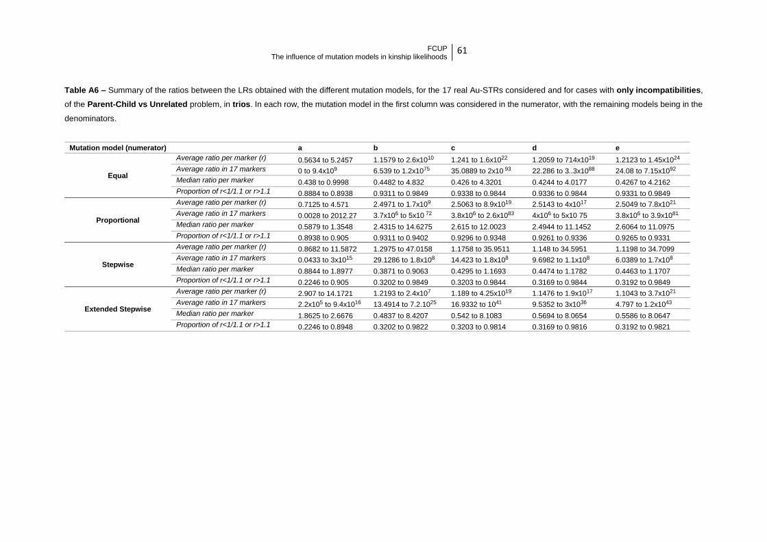
FCUP
The influence of mutation models in kinship likelihoods 61
Table A6 – Summary of the ratios between the LRs obtained with the different mutation models, for the 17 real Au-STRs considered and for cases with only incompatibilities,
of the Parent-Child vs Unrelated problem, in trios. In each row, the mutation model in the first column was considered in the numerator, with the remaining models being in the
denominators.
Mutation model (numerator) a b c d e
Equal
Average ratio per marker (r) 0.5634 to 5.2457 1.1579 to 2.6x10¹⁰ 1.241 to 1.6x10²² 1.2059 to 714x1019 1.2123 to 1.45x1024
Average ratio in 17 markers 0 to 9.4x10⁹ 6.539 to 1.2x1075 35.0889 to 2x10 93 22.286 to 3..3x1088 24.08 to 7.15x1092
Median ratio per marker 0.438 to 0.9998 0.4482 to 4.832 0.426 to 4.3201 0.4244 to 4.0177 0.4267 to 4.2162
Proportion of r<1/1.1 or r>1.1 0.8884 to 0.8938 0.9311 to 0.9849 0.9338 to 0.9844 0.9336 to 0.9844 0.9331 to 0.9849
Proportional
Average ratio per marker (r) 0.7125 to 4.571 2.4971 to 1.7x10⁹ 2.5063 to 8.9x10¹⁹ 2.5143 to 4x10¹⁷ 2.5049 to 7.8x10²¹
Average ratio in 17 markers 0.0028 to 2012.27 3.7x10⁶ to 5x10 72 3.8x10⁶ to 2.6x1083 4x10⁶ to 5x10 75 3.8x10⁶ to 3.9x1081
Median ratio per marker 0.5879 to 1.3548 2.4315 to 14.6275 2.615 to 12.0023 2.4944 to 11.1452 2.6064 to 11.0975
Proportion of r<1/1.1 or r>1.1 0.8938 to 0.905 0.9311 to 0.9402 0.9296 to 0.9348 0.9261 to 0.9336 0.9265 to 0.9331
Stepwise
Average ratio per marker (r) 0.8682 to 11.5872 1.2975 to 47.0158 1.1758 to 35.9511 1.148 to 34.5951 1.1198 to 34.7099
Average ratio in 17 markers 0.0433 to 3x10¹⁵ 29.1286 to 1.8x10⁸ 14.423 to 1.8x10⁸ 9.6982 to 1.1x10⁸ 6.0389 to 1.7x10⁸
Median ratio per marker 0.8844 to 1.8977 0.3871 to 0.9063 0.4295 to 1.1693 0.4474 to 1.1782 0.4463 to 1.1707
Proportion of r<1/1.1 or r>1.1 0.2246 to 0.905 0.3202 to 0.9849 0.3203 to 0.9844 0.3169 to 0.9844 0.3192 to 0.9849
Extended Stepwise
Average ratio per marker (r) 2.907 to 14.1721 1.2193 to 2.4x10⁷ 1.189 to 4.25x10¹⁹ 1.1476 to 1.9x10¹⁷ 1.1043 to 3.7x10²¹
Average ratio in 17 markers 2.2x10⁵ to 9.4x10¹⁶ 13.4914 to 7.2.1025 16.9332 to 1041 9.5352 to 3x1036 4.797 to 1.2x1043
Median ratio per marker 1.8625 to 2.6676 0.4837 to 8.4207 0.542 to 8.1083 0.5694 to 8.0654 0.5586 to 8.0647
Proportion of r<1/1.1 or r>1.1 0.2246 to 0.8948 0.3202 to 0.9822 0.3203 to 0.9814 0.3169 to 0.9816 0.3192 to 0.9821

FCUP
The influence of mutation models in kinship likelihoods 62
Table A7 – Summary of the ratios between the LRs obtained with the different mutation models, for the 17 real Au-STRs considered and for cases with no incompatibilities, of
the Full-siblings vs Unrelated problem, in duos and trios. In each row, the mutation model in the first column was considered in the numerator, with the remaining models
being in the denominators.
Mutation model (numerator)
Full-siblings (duos) Unrelated (duos) Full-siblings (trios) Unrelated (trios)
Equal
Average ratio per marker (r) 1.0001 to 1.0002 1.0005 to 1.0008 1 to 1.0001 0.9996 to 1.0001
Average ratio in 17 markers 1.0009 to 1.0027 1.0089 to 1.0129 0.9992 to 1.0013 0.9936 to 1.0012
Median ratio per marker 0.9983 to 0.9999 0.997 to 0.9995 0.9994 to 0.9999 0.9976 to 1
Proportion of r<1/1.1 or r>1.1 0.0032 to 0.0035 0.006 to 0.0066 0.0023 to 0.0025 0.0045 to 0.005
Proportional
Average ratio per marker (r) 1.0001 to 1.0003 0.9999 to 1.0001 1.0001 to 1.0003 1.0003 to 1.0009
Average ratio in 17 markers 1.0009 to 1.0047 0.9979 to 1.0016 1.0011 to 1.0051 1.0051 to 1.0158
Median ratio per marker 1.0005 to 1.0017 1.0012 to 1.003 1.0003 to 1.0006 1.001 to 1.0024
Proportion of r<1/1.1 or r>1.1 0.0008 to 0.0035 0.0014 to 0.0066 0.0006 to 0.0025 0.0011 to 0.005
Stepwise
Average ratio per marker (r) 1.0001 to 1.0002 1 to 1.0004 1 to 1.0002 0.9998 to 1.0005
Average ratio in 17 markers 1.0009 to 1.0031 0.9999 to 1.0071 1.0001 to 1.0031 0.9965 to 1.0081
Median ratio per marker 0.999 to 1.0001 0.998 to 1.0005 0.9996 to 1.0001 0.9983 to 1
Proportion of r<1/1.1 or r>1.1 0.0009 to 0.0033 0.0017 to 0.0063 0.0007 to 0.0024 0.0012 to 0.0047
Extended Stepwise
Average ratio per marker (r) 1.0001 to 1.0003 1 to 1.0003 1 to 1.0003 0.9999 to 1.0007
Average ratio in 17 markers 1.001 to 1.0044 1.0008 to 1.005 1.0004 to 1.0045 0.998 to 1.0118
Median ratio per marker 0.9995 to 1.0004 0.9988 to 1.0011 0.9997 to 1.0001 0.999 to 1.0004
Proportion of r<1/1.1 or r>1.1 0.0008 to 0.0032 0.0014 to 0.006 0.0006 to 0.0023 0.0011 to 0.0045

FCUP
The influence of mutation models in kinship likelihoods 63
Table A8 – Summary of the ratios between the LRs obtained with the different mutation models, for the 17 real Au-STRs considered and for cases with only incompatibilities,
of the Full-siblings vs Unrelated problem, in trios. In each row, the mutation model in the first column was considered in the numerator, with the remaining models being in the
denominators.
Mutation model (numerator)
Full-siblings (trios) Unrelated (trios)
Equal
Average ratio per marker (r) 1.3172 to 4.3371 1.2572 to 1.16x10⁸
Median ratio per marker 0.6336 to 0.9891 0.4729 to 2.0376
Proportion of r<1/1.1 or r>1.1 0.6506 to 0.6988 0.9601 to 0.9748
Proportional
Average ratio per marker (r) 0.8786 to 2.1186 2.3031 to 5.17x10⁷
Median ratio per marker 0.7842 to 1.0604 1.6502 to 4.1569
Proportion of r<1/1.1 or r>1.1 0.6988 to 0.7191 0.92 to 0.9601
Stepwise
Average ratio per marker (r) 0.9216 to 12.0141 1.1452 to 21.4089
Median ratio per marker 0.9532 to 1.3821 0.5188 to 1.1777
Proportion of r<1/1.1 or r>1.1 0.2056 to 0.7191 0.3349 to 0.9748
Extended Stepwise
Average ratio per marker (r) 2.2646 to 13.1598 1.097 to 10887.864
Median ratio per marker 1.0762 to 1.8308 0.6517 to 2.7271
Proportion of r<1/1.1 or r>1.1 0.2056 to 0.7172 0.3349 to 0.9706

FCUP
The influence of mutation models in kinship likelihoods 64
Table A9 – Summary of the ratios between the LRs obtained with the different mutation models, for the 17 real Au-STRs considered and for cases with no incompatibilities, of
the Half-siblings vs Unrelated problem, in duos and trios. In each row, the mutation model in the first column was considered in the numerator, with the remaining models
being in the denominators.
Mutation model (numerator)
Half-siblings (duos) Unrelated (duos) Half-siblings (trios) Unrelated (trios)
Equal
Average ratio per marker (r) 1 to 1 1.0002 to 1.0002 1 to 1.0001 1.0002 to 1.0003
Average ratio in 17 markers 1 to 1.0008 1.0027 to 1.0037 0.9996 to 1.0009 1.004 to 1.0059
Median ratio per marker 0.9992 to 0.9998 0.999 to 0.9997 0.9994 to 0.9999 0.9986 to 0.9999
Proportion of r<1/1.1 or r>1.1 0.0014 to 0.0014 0.0023 to 0.0024 0.0017 to 0.0018 0.0031 to 0.0033
Proportional
Average ratio per marker (r) 1 to 1.0001 0.9999 to 1 1 to 1.0002 0.9999 to 1
Average ratio in 17 markers 1.0001 to 1.0012 0.9987 to 1.0004 1.0003 to 1.0027 0.9984 to 1.0007
Median ratio per marker 1.0003 to 1.0008 1.0004 to 1.001 1.0003 to 1.0006 1.0004 to 1.0014
Proportion of r<1/1.1 or r>1.1 0.0004 to 0.0014 0.0006 to 0.0024 0.0004 to 0.0018 0.0006 to 0.0033
Stepwise
Average ratio per marker (r) 1 to 1 1 to 1.0001 1 to 1.0001 1 to 1.0002
Average ratio in 17 markers 0.9999 to 1.0007 0.9994 to 1.0018 0.9997 to 1.0015 0.9993 to 1.0028
Median ratio per marker 0.9995 to 1.0002 0.9994 to 1.0003 0.9996 to 1.0001 0.9991 to 1.0001
Proportion of r<1/1.1 or r>1.1 0.0006 to 0.0014 0.0009 to 0.0023 0.0006 to 0.0018 0.0009 to 0.0032
Extended Stepwise
Average ratio per marker (r) 1 to 1.0001 1 to 1.0001 1 to 1.0002 1 to 1.0001
Average ratio in 17 markers 1.0004 to 1.0013 0.9994 to 1.0012 1.0007 to 1.0027 1 to 1.0024
Median ratio per marker 0.9997 to 1.0004 0.9996 to 1.0005 0.9997 to 1.0002 0.9996 to 1.0004
Proportion of r<1/1.1 or r>1.1 0.0004 to 0.0014 0.0006 to 0.0023 0.0004 to 0.0017 0.0006 to 0.0031

FCUP
The influence of mutation models in kinship likelihoods 65
Table A10 – Summary of the ratios between the LRs obtained with the different mutation models, for the 17 real Au-STRs considered and for cases with only incompatibilities,
of the Half-siblings vs Unrelated problem, in trios. In each row, the mutation model in the first column was considered in the numerator, with the remaining models being in the
denominators.
Mutation model (numerator)
Half-siblings (trios) Unrelated (trios)
Equal
Average ratio per marker (r) 1.0065 to 1.0702 1.0659 to 1.0775
Average ratio in 17 markers 0.9838 to 3.0431 2.8569 to 3.4078
Median ratio per marker 0.9877 to 1.0264 0.9987 to 1.0221
Proportion of r<1/1.1 or r>1.1 0.3294 to 0.426 0.1954 to 0.2759
Proportional
Average ratio per marker (r) 0.9887 to 1.0383 0.9623 to 1.0349
Average ratio in 17 markers 0.6446 to 1.6942 0.5043 to 1.6102
Median ratio per marker 0.9394 to 0.9798 0.9809 to 0.9841
Proportion of r<1/1.1 or r>1.1 0.426 to 0.5286 0.2759 to 0.3352
Stepwise
Average ratio per marker (r) 0.9931 to 1.1805 0.9975 to 1.0631
Average ratio in 17 markers 0.8859 to 13.6125 0.9572 to 2.7018
Median ratio per marker 0.9966 to 1.0786 1.0005 to 1.0264
Proportion of r<1/1.1 or r>1.1 0.1164 to 0.5286 0.0575 to 0.3352
Extended Stepwise
Average ratio per marker (r) 1.0389 to 1.1921 1.0122 to 1.0671
Average ratio in 17 markers 1.8413 to 15.7977 1.217 to 2.8814
Median ratio per marker 1.0038 to 1.0837 0.9995 to 1.0272
Proportion of r<1/1.1 or r>1.1 0.1164 to 0.5148 0.0575 to 0.3295
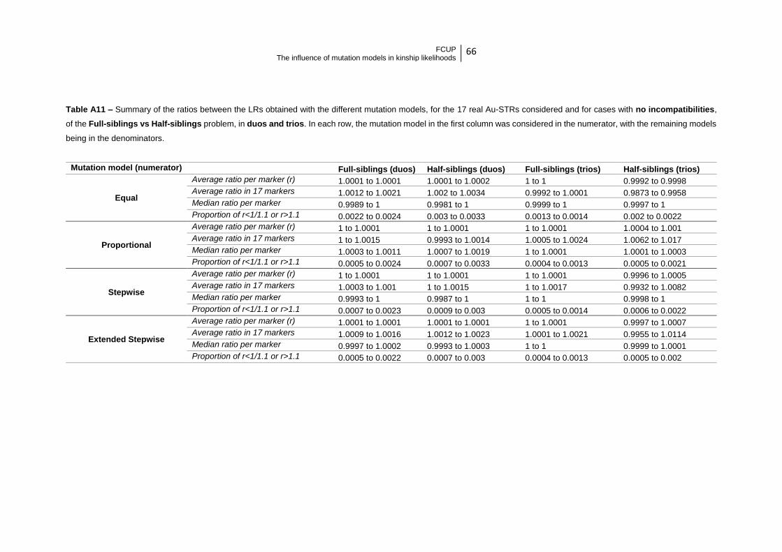
FCUP
The influence of mutation models in kinship likelihoods 66
Table A11 – Summary of the ratios between the LRs obtained with the different mutation models, for the 17 real Au-STRs considered and for cases with no incompatibilities,
of the Full-siblings vs Half-siblings problem, in duos and trios. In each row, the mutation model in the first column was considered in the numerator, with the remaining models
being in the denominators.
Mutation model (numerator)
Full-siblings (duos) Half-siblings (duos) Full-siblings (trios) Half-siblings (trios)
Equal
Average ratio per marker (r) 1.0001 to 1.0001 1.0001 to 1.0002 1 to 1 0.9992 to 0.9998
Average ratio in 17 markers 1.0012 to 1.0021 1.002 to 1.0034 0.9992 to 1.0001 0.9873 to 0.9958
Median ratio per marker 0.9989 to 1 0.9981 to 1 0.9999 to 1 0.9997 to 1
Proportion of r<1/1.1 or r>1.1 0.0022 to 0.0024 0.003 to 0.0033 0.0013 to 0.0014 0.002 to 0.0022
Proportional
Average ratio per marker (r) 1 to 1.0001 1 to 1.0001 1 to 1.0001 1.0004 to 1.001
Average ratio in 17 markers 1 to 1.0015 0.9993 to 1.0014 1.0005 to 1.0024 1.0062 to 1.017
Median ratio per marker 1.0003 to 1.0011 1.0007 to 1.0019 1 to 1.0001 1.0001 to 1.0003
Proportion of r<1/1.1 or r>1.1 0.0005 to 0.0024 0.0007 to 0.0033 0.0004 to 0.0013 0.0005 to 0.0021
Stepwise
Average ratio per marker (r) 1 to 1.0001 1 to 1.0001 1 to 1.0001 0.9996 to 1.0005
Average ratio in 17 markers 1.0003 to 1.001 1 to 1.0015 1 to 1.0017 0.9932 to 1.0082
Median ratio per marker 0.9993 to 1 0.9987 to 1 1 to 1 0.9998 to 1
Proportion of r<1/1.1 or r>1.1 0.0007 to 0.0023 0.0009 to 0.003 0.0005 to 0.0014 0.0006 to 0.0022
Extended Stepwise
Average ratio per marker (r) 1.0001 to 1.0001 1.0001 to 1.0001 1 to 1.0001 0.9997 to 1.0007
Average ratio in 17 markers 1.0009 to 1.0016 1.0012 to 1.0023 1.0001 to 1.0021 0.9955 to 1.0114
Median ratio per marker 0.9997 to 1.0002 0.9993 to 1.0003 1 to 1 0.9999 to 1.0001
Proportion of r<1/1.1 or r>1.1 0.0005 to 0.0022 0.0007 to 0.003 0.0004 to 0.0013 0.0005 to 0.002

FCUP
The influence of mutation models in kinship likelihoods 67
Table A12 – Summary of the ratios between the LRs obtained with the different mutation models, for the 17 real Au-STRs considered and for cases with only incompatibilities,
of the Full-siblings vs Half-siblings problem, in trios. In each row, the mutation model in the first column was considered in the numerator, with the remaining models being in
the denominators.
Mutation model (numerator)
Full-siblings (trios) Half-siblings (trios)
Equal
Average ratio per marker (r) 1.3327 to 3.7094 1.138 to 7.5x10⁸
Average ratio in 17 markers 0.2784 to 1.56x10⁶ 8.6406 to 4.87x1061
Median ratio per marker 0.7986 to 0.9703 0.4361 to 2.2014
Proportion of r<1/1.1 or r>1.1 0.5193 to 0.5598 0.9599 to 0.9787
Proportional
Average ratio per marker (r) 0.9132 to 2.1307 2.432 to 1.2x10⁹
Average ratio in 17 markers 0.1557 to 412.4864 2.2x10⁶ to 3.9x1055
Median ratio per marker 0.9164 to 1.0701 1.9637 to 5.3203
Proportion of r<1/1.1 or r>1.1 0.5193 to 0.5405 0.9276 to 0.9599
Stepwise
Average ratio per marker (r) 0.916 to 10.2828 1.0978 to 21.7097
Average ratio in 17 markers 0.1799 to 3.6x10¹⁰ 4.6505 to 3.1x10⁷
Median ratio per marker 0.967 to 1.1792 0.4654 to 1.2066
Proportion of r<1/1.1 or r>1.1 0.1882 to 0.5598 0.3341 to 0.9787
Extended Stepwise
Average ratio per marker (r) 2.1204 to 11.6465 1.0709 to 92774.6344
Average ratio in 17 markers 6784.6 to 1.9x10¹² 3.0665 to 5x10¹⁸
Median ratio per marker 1.045 to 1.4041 0.5971 to 2.8047
Proportion of r<1/1.1 or r>1.1 0.1882 to 0.5569 0.3341 to 0.9746

FCUP
The influence of mutation models in kinship likelihoods 68
Appendix 3
Summarized tables of ratios regarding the impact of considering different mutation models, for the 10 markers with
fictitious allele frequencies:
Table A13 – Summary of the ratios between the LRs obtained with the different mutation models, for the 10 fictitious markers considered and for cases with no incompatibilities,
of the Parent-Child vs Unrelated problem, in duos. All ratios between all models are considered for each marker.
Marker a b c d e
1 Average ratio per marker (r) 1 to 1 1 to 1 1 to 1 1 to 1 1 to 1 Median ratio per marker 1 to 1 0.9999 to 1.0001 1 to 1 1 to 1 1 to 1 Proportion of r<1/1.1 or r>1.1 0 to 0 0 to 0 0 to 0 0 to 0 0 to 0
2 Average ratio per marker (r) 0.9999 to 1.0001 0.9999 to 1.0001 0.9999 to 1.0001 0.9999 to 1.0001 0.9999 to 1.0001 Median ratio per marker 0.9999 to 1.0001 0.9999 to 1.0001 0.9999 to 1.0001 0.9999 to 1.0001 0.9999 to 1.0001 Proportion of r<1/1.1 or r>1.1 0 to 0 0 to 0 0 to 0 0 to 0 0 to 0
3 Average ratio per marker (r) 1 to 1 0.9998 to 1.0002 0.9998 to 1.0002 0.9999 to 1.0002 0.9997 to 1.0003 Median ratio per marker 0.9999 to 1.0001 0.9999 to 1.0001 0.9999 to 1.0001 0.9999 to 1.0001 0.9998 to 1.0002 Proportion of r<1/1.1 or r>1.1 0 to 0 0 to 0 0 to 0 0 to 0 0 to 0
4 Average ratio per marker (r) 1 to 1 0.9996 to 1.0004 0.9997 to 1.0003 0.9997 to 1.0003 0.9993 to 1.0007 Median ratio per marker 0.9999 to 1.0001 0.9999 to 1.0001 0.9999 to 1.0001 0.9999 to 1.0001 0.9996 to 1.0004 Proportion of r<1/1.1 or r>1.1 0 to 0 0 to 0 0 to 0 0 to 0 0 to 0
5 Average ratio per marker (r) 1 to 1 0.9996 to 1.0004 0.9996 to 1.0004 0.9997 to 1.0003 0.9992 to 1.0008 Median ratio per marker 0.9999 to 1.0001 0.9999 to 1.0001 0.9999 to 1.0001 0.9999 to 1.0001 0.9995 to 1.0005 Proportion of r<1/1.1 or r>1.1 0 to 0 0 to 0 0 to 0 0 to 0 0 to 0
6 Average ratio per marker (r) 1 to 1 1 to 1 1 to 1 1 to 1 1 to 1

FCUP
The influence of mutation models in kinship likelihoods 69
Median ratio per marker 0.9999 to 1.0001 0.9999 to 1.0001 0.9999 to 1.0001 0.9999 to 1.0001 0.9999 to 1.0001 Proportion of r<1/1.1 or r>1.1 0 to 0 0 to 0 0 to 0 0 to 0 0 to 0
7 Average ratio per marker (r) 1 to 1 0.9999 to 1.0001 0.9999 to 1.0001 1 to 1 0.9999 to 1.0001 Median ratio per marker 0.9999 to 1.0001 0.9999 to 1.0001 0.9999 to 1.0001 0.9999 to 1.0001 0.9999 to 1.0001 Proportion of r<1/1.1 or r>1.1 0 to 0 0 to 0 0 to 0 0 to 0 0 to 0
8 Average ratio per marker (r) 0.9999 to 1.0001 0.9996 to 1.0004 0.9997 to 1.0003 0.9997 to 1.0003 0.9994 to 1.0006 Median ratio per marker 0.9997 to 1.0003 0.9997 to 1.0003 0.9997 to 1.0003 0.9997 to 1.0003 0.9996 to 1.0004 Proportion of r<1/1.1 or r>1.1 0 to 0 0 to 0 0 to 0 0 to 0 0 to 0
9 Average ratio per marker (r) 0.9999 to 1.0001 0.9995 to 1.0005 0.9996 to 1.0004 0.9996 to 1.0004 0.9991 to 1.0009 Median ratio per marker 0.9999 to 1.0001 0.9997 to 1.0003 0.9995 to 1.0005 0.9995 to 1.0005 0.9995 to 1.0005 Proportion of r<1/1.1 or r>1.1 0 to 0 0 to 0 0 to 0 0 to 0 0 to 0
10 Average ratio per marker (r) 0.9999 to 1.0001 0.9995 to 1.0005 0.9996 to 1.0004 0.9996 to 1.0004 0.9992 to 1.0008 Median ratio per marker 0.9999 to 1.0001 0.9997 to 1.0003 0.9996 to 1.0004 0.9995 to 1.0005 0.9995 to 1.0005 Proportion of r<1/1.1 or r>1.1 0 to 0 0 to 0 0 to 0 0 to 0 0 to 0
Table A14 – Summary of the ratios between the LRs obtained with the different mutation models, for the 10 fictitious markers considered and for cases with no incompatibilities,
of the Parent-Child vs Unrelated problem, in trios. All ratios between all models are considered for each marker.
Marker a b c d e
1 Average ratio per marker (r) 1 to 1 1 to 1 1 to 1 1 to 1 1 to 1 Median ratio per marker 1 to 1 1 to 1 1 to 1 1 to 1 1 to 1 Proportion of r<1/1.1 or r>1.1 0 to 0 0 to 0 0 to 0 0 to 0 0 to 0
2 Average ratio per marker (r) 1 to 1 1 to 1 1 to 1 1 to 1 1 to 1 Median ratio per marker 0.9999 to 1.0001 0.9999 to 1.0001 0.9999 to 1.0001 0.9999 to 1.0001 0.9999 to 1.0001 Proportion of r<1/1.1 or r>1.1 0 to 0 0 to 0 0 to 0 0 to 0 0 to 0
3 Average ratio per marker (r) 0.9999 to 1.0001 0.9997 to 1.0003 0.9998 to 1.0002 0.9999 to 1.0001 0.9995 to 1.0005 Median ratio per marker 1 to 1 1 to 1 1 to 1 1 to 1 0.9999 to 1.0001

FCUP
The influence of mutation models in kinship likelihoods 70
Proportion of r<1/1.1 or r>1.1 0 to 0 0 to 0 0 to 0 0 to 0 0 to 0
4 Average ratio per marker (r) 0.9998 to 1.0002 0.9995 to 1.0005 0.9995 to 1.0005 0.9998 to 1.0002 0.999 to 1.0011 Median ratio per marker 0.9998 to 1.0002 0.9999 to 1.0001 0.9998 to 1.0002 0.9998 to 1.0002 0.9996 to 1.0004 Proportion of r<1/1.1 or r>1.1 0 to 0 0 to 0 0 to 0 0 to 0 0 to 0
5 Average ratio per marker (r) 0.9998 to 1.0002 0.9994 to 1.0006 0.9995 to 1.0005 0.9998 to 1.0002 0.9988 to 1.0012 Median ratio per marker 0.9998 to 1.0002 0.9999 to 1.0001 0.9998 to 1.0002 0.9998 to 1.0002 0.9996 to 1.0004 Proportion of r<1/1.1 or r>1.1 0 to 0 0 to 0 0 to 0 0 to 0 0 to 0
6 Average ratio per marker (r) 1 to 1 1 to 1 1 to 1 1 to 1 1 to 1 Median ratio per marker 1 to 1 1 to 1 1 to 1 1 to 1 1 to 1 Proportion of r<1/1.1 or r>1.1 0 to 0 0 to 0 0 to 0 0 to 0 0 to 0
7 Average ratio per marker (r) 1 to 1 0.9999 to 1.0001 0.9999 to 1.0001 1 to 1 0.9998 to 1.0002 Median ratio per marker 1 to 1 1 to 1 1 to 1 1 to 1 0.9998 to 1.0002 Proportion of r<1/1.1 or r>1.1 0 to 0 0 to 0 0 to 0 0 to 0 0 to 0
8 Average ratio per marker (r) 0.9997 to 1.0003 0.9995 to 1.0005 0.9996 to 1.0004 0.9997 to 1.0003 0.9992 to 1.0009 Median ratio per marker 0.9999 to 1.0001 0.9999 to 1.0001 0.9999 to 1.0001 0.9999 to 1.0001 0.9998 to 1.0002 Proportion of r<1/1.1 or r>1.1 0 to 0 0 to 0 0 to 0 0 to 0 0 to 0
9 Average ratio per marker (r) 0.9997 to 1.0003 0.9993 to 1.0007 0.9994 to 1.0006 0.9997 to 1.0003 0.9987 to 1.0013 Median ratio per marker 0.9999 to 1.0001 0.9999 to 1.0001 0.9999 to 1.0001 0.9999 to 1.0001 0.9996 to 1.0004 Proportion of r<1/1.1 or r>1.1 0 to 0 0 to 0 0 to 0 0 to 0 0 to 0
10 Average ratio per marker (r) 0.9997 to 1.0003 0.9994 to 1.0006 0.9994 to 1.0006 0.9997 to 1.0003 0.9987 to 1.0013 Median ratio per marker 0.9999 to 1.0001 0.9999 to 1.0001 0.9999 to 1.0001 0.9999 to 1.0001 0.9996 to 1.0004 Proportion of r<1/1.1 or r>1.1 0 to 0 0 to 0 0 to 0 0 to 0 0 to 0

FCUP
The influence of mutation models in kinship likelihoods 71
Table A15 – Summary of the ratios between the LRs obtained with the different mutation models, for the 10 fictitious markers considered and for cases with only incompatibilities,
of the Parent-Child vs Unrelated problem, in duos. All ratios between all models are considered for each marker.
Marker a b c d e
1 Average ratio per marker (r) 0.6984 to 1.6777 0.995 to 386.6008 0.995 to 274.8774 0.995 to 262.7402 0.995 to 269.7246 Median ratio per marker 0.6182 to 1.6175 0.8781 to 1.1388 0.9037 to 1.1066 0.9041 to 1.1061 0.9037 to 1.1066 Proportion of r<1/1.1 or r>1.1 0 to 0.873 0 to 0.9254 0 to 0.8848 0 to 0.8753 0 to 0.8752
2 Average ratio per marker (r) 0.9106 to 1.7138 0.9526 to 296.3508 0.9588 to 288.0465 0.9605 to 265.7433 0.9603 to 263.5246 Median ratio per marker 0.5259 to 1.9014 0.8375 to 1.194 0.8375 to 1.194 0.8375 to 1.194 0.8375 to 1.194 Proportion of r<1/1.1 or r>1.1 0 to 1 0 to 1 0 to 1 0 to 1 0 to 1
3 Average ratio per marker (r) 0.8443 to 1.8916 1 to 36.5049 1 to 18.1249 1 to 13.4261 1 to 15.3036 Median ratio per marker 0.6031 to 1.6581 0.7737 to 1.2926 0.7737 to 1.2926 0.7737 to 1.2926 0.7737 to 1.2926 Proportion of r<1/1.1 or r>1.1 0 to 0.9921 0 to 0.9561 0 to 0.954 0 to 0.9558 0 to 0.9552
4 Average ratio per marker (r) 0.7222 to 2.1226 1 to 137.8512 1 to 81.4549 1 to 72.0581 0.9934 to 58.5032 Median ratio per marker 0.5363 to 1.8647 0.5447 to 1.836 0.5962 to 1.6773 0.5983 to 1.6714 0.5983 to 1.6714 Proportion of r<1/1.1 or r>1.1 0 to 1 0 to 1 0 to 1 0 to 1 0 to 1
5 Average ratio per marker (r) 0.6114 to 2.2763 1 to 171.5042 0.9942 to 108.2354 0.988 to 95.8469 0.9934 to 89.0471 Median ratio per marker 0.3734 to 2.6778 0.5887 to 1.6987 0.593 to 1.6864 0.593 to 1.6864 0.5983 to 1.6714 Proportion of r<1/1.1 or r>1.1 0 to 1 0 to 1 0 to 1 0 to 1 0 to 1
6 Average ratio per marker (r) 0.6992 to 23.3408 0.99 to 348.2299 0.995 to 294.2469 0.9861 to 296.0458 0.9945 to 278.6698 Median ratio per marker 0.4591 to 2.1782 0.1667 to 5.9985 0.8302 to 1.2045 0.8302 to 1.2045 0.8302 to 1.2045 Proportion of r<1/1.1 or r>1.1 0 to 0.9225 0 to 0.9668 0 to 0.9472 0 to 0.9426 0 to 0.943
7 Average ratio per marker (r) 0.7417 to 4.1914 1.0143 to 195.4828 1.0037 to 125.8518 1.0019 to 126.9848 0.9978 to 136.5506 Median ratio per marker 0.5282 to 1.8931 0.4294 to 2.3289 0.662 to 1.5106 0.6963 to 1.4361 0.6963 to 1.4361 Proportion of r<1/1.1 or r>1.1 0.694 to 1 0.7893 to 1 0.7881 to 1 0.7856 to 1 0.7838 to 1
8 Average ratio per marker (r) 0.8519 to 5.2702 0.7561 to 13402.0864 0.7442 to 4013.0628 0.7351 to 4019.0531
0.7402 to 4172.5803
Median ratio per marker 0.4082 to 2.45 0.086 to 11.6334 0.0998 to 10.0154 0.0999 to 10.0112 0.0999 to 10.0112 Proportion of r<1/1.1 or r>1.1 0.7685 to 0.9907 0.8759 to 0.9946 0.8842 to 0.9923 0.8932 to 0.992 0.8937 to 0.9918

FCUP
The influence of mutation models in kinship likelihoods 72
9 Average ratio per marker (r) 0.606 to 4.5965 0.8049 to 71647.2043 0.8061 to 33064.9829 0.803 to 26485.1286
0.7958 to 27610.475
Median ratio per marker 0.3413 to 2.9302 0.1 to 10.005 0.1 to 10 0.133 to 7.5178 0.1324 to 7.551 Proportion of r<1/1.1 or r>1.1 0.6372 to 1 0.7861 to 1 0.7927 to 1 0.7858 to 1 0.7882 to 1
10 Average ratio per marker (r) 0.5361 to 3.9349 0.9145 to 106210.3928 0.9214 to 64415.2449 0.9124 to 53487.1129
0.9049 to 56569.1572
Median ratio per marker 0.3434 to 2.912 0.2284 to 4.3784 0.2643 to 3.7835 0.2643 to 3.783 0.2643 to 3.783 Proportion of r<1/1.1 or r>1.1 0.4615 to 1 0.6725 to 1 0.6824 to 1 0.6793 to 1 0.6846 to 1
Table A16 – Summary of the ratios between the LRs obtained with the different mutation models, for the 10 fictitious markers considered and for cases with only incompatibilities,
of the Parent-Child vs Unrelated problem, in trios. All ratios between all models are considered for each marker.
Marker a b c d e
1 Average ratio per marker (r) 0.5968 to 2.1111 0.995 to 2754.6854 0.9935 to 1422.2084 0.995 to 1254.7255 0.995 to 1254.7255 Median ratio per marker 0.5997 to 1.6675 0.3149 to 3.1761 0.3231 to 3.0955 0.3313 to 3.0184 0.3313 to 3.0184 Proportion of r<1/1.1 or r>1.1 0 to 0.9231 0 to 0.9771 0 to 0.9738 0 to 0.9707 0 to 0.9707
2 Average ratio per marker (r) 0.7298 to 2.1578 1 to 2815.7774 1 to 1515.8152 0.9941 to 1215.2795 0.9941 to 1215.2795 Median ratio per marker 0.5051 to 1.9797 0.3164 to 3.1603 0.3247 to 3.0802 0.3312 to 3.0189 0.3312 to 3.0189 Proportion of r<1/1.1 or r>1.1 0 to 0.9378 0 to 0.9993 0 to 0.9996 0 to 0.9999 0 to 0.9999
3 Average ratio per marker (r) 0.6135 to 2.3413 1 to 209.6045 1 to 87.8354 1 to 74.8187 1 to 74.8187 Median ratio per marker 0.5769 to 1.7335 0.6339 to 1.5775 0.6283 to 1.5916 0.6283 to 1.5916 0.6283 to 1.5916 Proportion of r<1/1.1 or r>1.1 0 to 0.9437 0 to 0.9896 0 to 0.9896 0 to 0.9889 0 to 0.9889
4 Average ratio per marker (r) 0.6828 to 3.031 0.9694 to 1173.7053 0.9751 to 472.2844 0.956 to 405.5798 0.956 to 405.5798 Median ratio per marker 0.356 to 2.809 0.2681 to 3.7303 0.3121 to 3.2043 0.3178 to 3.1468 0.3178 to 3.1468 Proportion of r<1/1.1 or r>1.1 0 to 0.974 0 to 0.9996 0 to 0.9996 0 to 0.9999 0 to 0.9999
5 Average ratio per marker (r) 0.5031 to 3.1103 0.947 to 1115.2974 0.9454 to 525.7158 0.941 to 383.816 0.941 to 383.816 Median ratio per marker 0.3566 to 2.8042 0.3166 to 3.1587 0.3308 to 3.0229 0.3308 to 3.0227 0.3308 to 3.0227 Proportion of r<1/1.1 or r>1.1 0 to 0.9554 0 to 0.9998 0 to 0.9996 0 to 1 0 to 1

FCUP
The influence of mutation models in kinship likelihoods 73
6 Average ratio per marker (r) 0.4101 to 56.573 0.9847 to 2796.2306 0.995 to 1509.3751 0.9922 to 1282.5698 0.9922 to 1282.5698 Median ratio per marker 0.1469 to 7.2817 0.0017 to 573.9607 0.0167 to 59.8692 0.032 to 31.2939 0.032 to 31.2939 Proportion of r<1/1.1 or r>1.1 0 to 0.9526 0 to 0.9935 0 to 0.9903 0 to 0.9899 0 to 0.9899
7 Average ratio per marker (r) 0.6083 to 5.6152 1.0186 to 1866.7298 1.0006 to 1011.5282 0.9987 to 753.4341 0.9987 to 753.4341 Median ratio per marker 0.5013 to 1.9948 0.1912 to 5.2304 0.2087 to 4.7909 0.2089 to 4.7872 0.2089 to 4.7872 Proportion of r<1/1.1 or r>1.1 0.5708 to 0.967 0.8064 to 0.9997 0.7846 to 0.9997 0.7753 to 0.9999 0.7753 to 0.9999
8 Average ratio per marker (r) 0.4631 to 5.489 0.6483 to 94829.3133 0.6493 to 23597.087 0.6407 to 23299.631 0.6407 to 23299.631 Median ratio per marker 0.404 to 2.4751 0.0816 to 12.2515 0.0928 to 10.7735 0.0928 to 10.7735 0.0928 to 10.7735 Proportion of r<1/1.1 or r>1.1 0.5968 to 0.957 0.8085 to 0.9998 0.8068 to 0.9998 0.8074 to 0.9999 0.8074 to 0.9999
9 Average ratio per marker (r) 0.4387 to 5.4243 0.6945 to 568532.6547 0.6955 to 224365.8518 0.6935 to 174345.5654 0.6935 to 174345.5654 Median ratio per marker 0.3332 to 3.0019 0.0595 to 16.8111 0.0604 to 16.5658 0.0604 to 16.5634 0.0604 to 16.5634 Proportion of r<1/1.1 or r>1.1 0.5158 to 0.9737 0.7921 to 0.9998 0.7765 to 1 0.7729 to 1 0.7729 to 1
10 Average ratio per marker (r) 0.4498 to 4.8859 0.8454 to 543352.3474 0.8491 to 254478.8679 0.8347 to 230473.3729 0.8347 to 230473.3729 Median ratio per marker 0.3405 to 2.9369 0.1 to 9.9996 0.1002 to 9.9781 0.1099 to 9.1016 0.1099 to 9.1016 Proportion of r<1/1.1 or r>1.1 0.3906 to 0.974 0.6775 to 0.9999 0.6449 to 0.9999 0.64 to 1 0.64 to 1
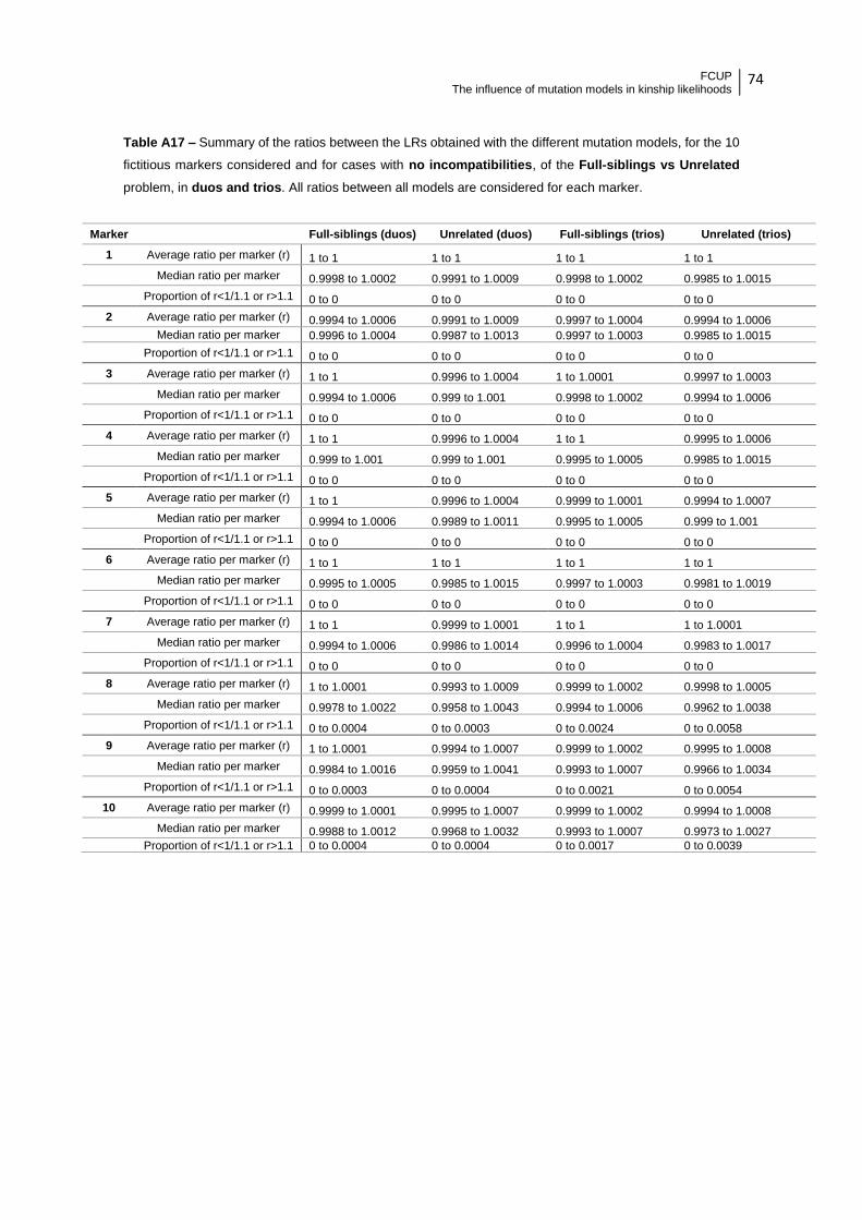
FCUP
The influence of mutation models in kinship likelihoods 74
Table A17 – Summary of the ratios between the LRs obtained with the different mutation models, for the 10
fictitious markers considered and for cases with no incompatibilities, of the Full-siblings vs Unrelated
problem, in duos and trios. All ratios between all models are considered for each marker.
Marker Full-siblings (duos) Unrelated (duos) Full-siblings (trios) Unrelated (trios)
1 Average ratio per marker (r) 1 to 1 1 to 1 1 to 1 1 to 1 Median ratio per marker 0.9998 to 1.0002 0.9991 to 1.0009 0.9998 to 1.0002 0.9985 to 1.0015 Proportion of r<1/1.1 or r>1.1 0 to 0 0 to 0 0 to 0 0 to 0
2 Average ratio per marker (r) 0.9994 to 1.0006 0.9991 to 1.0009 0.9997 to 1.0004 0.9994 to 1.0006 Median ratio per marker 0.9996 to 1.0004 0.9987 to 1.0013 0.9997 to 1.0003 0.9985 to 1.0015 Proportion of r<1/1.1 or r>1.1 0 to 0 0 to 0 0 to 0 0 to 0
3 Average ratio per marker (r) 1 to 1 0.9996 to 1.0004 1 to 1.0001 0.9997 to 1.0003 Median ratio per marker 0.9994 to 1.0006 0.999 to 1.001 0.9998 to 1.0002 0.9994 to 1.0006 Proportion of r<1/1.1 or r>1.1 0 to 0 0 to 0 0 to 0 0 to 0
4 Average ratio per marker (r) 1 to 1 0.9996 to 1.0004 1 to 1 0.9995 to 1.0006 Median ratio per marker 0.999 to 1.001 0.999 to 1.001 0.9995 to 1.0005 0.9985 to 1.0015 Proportion of r<1/1.1 or r>1.1 0 to 0 0 to 0 0 to 0 0 to 0
5 Average ratio per marker (r) 1 to 1 0.9996 to 1.0004 0.9999 to 1.0001 0.9994 to 1.0007 Median ratio per marker 0.9994 to 1.0006 0.9989 to 1.0011 0.9995 to 1.0005 0.999 to 1.001 Proportion of r<1/1.1 or r>1.1 0 to 0 0 to 0 0 to 0 0 to 0
6 Average ratio per marker (r) 1 to 1 1 to 1 1 to 1 1 to 1 Median ratio per marker 0.9995 to 1.0005 0.9985 to 1.0015 0.9997 to 1.0003 0.9981 to 1.0019 Proportion of r<1/1.1 or r>1.1 0 to 0 0 to 0 0 to 0 0 to 0
7 Average ratio per marker (r) 1 to 1 0.9999 to 1.0001 1 to 1 1 to 1.0001 Median ratio per marker 0.9994 to 1.0006 0.9986 to 1.0014 0.9996 to 1.0004 0.9983 to 1.0017 Proportion of r<1/1.1 or r>1.1 0 to 0 0 to 0 0 to 0 0 to 0
8 Average ratio per marker (r) 1 to 1.0001 0.9993 to 1.0009 0.9999 to 1.0002 0.9998 to 1.0005 Median ratio per marker 0.9978 to 1.0022 0.9958 to 1.0043 0.9994 to 1.0006 0.9962 to 1.0038 Proportion of r<1/1.1 or r>1.1 0 to 0.0004 0 to 0.0003 0 to 0.0024 0 to 0.0058
9 Average ratio per marker (r) 1 to 1.0001 0.9994 to 1.0007 0.9999 to 1.0002 0.9995 to 1.0008 Median ratio per marker 0.9984 to 1.0016 0.9959 to 1.0041 0.9993 to 1.0007 0.9966 to 1.0034 Proportion of r<1/1.1 or r>1.1 0 to 0.0003 0 to 0.0004 0 to 0.0021 0 to 0.0054
10 Average ratio per marker (r) 0.9999 to 1.0001 0.9995 to 1.0007 0.9999 to 1.0002 0.9994 to 1.0008 Median ratio per marker 0.9988 to 1.0012 0.9968 to 1.0032 0.9993 to 1.0007 0.9973 to 1.0027 Proportion of r<1/1.1 or r>1.1 0 to 0.0004 0 to 0.0004 0 to 0.0017 0 to 0.0039

FCUP
The influence of mutation models in kinship likelihoods 75
Table A18 – Summary of the ratios between the LRs obtained with the different mutation models, for the 10
fictitious markers considered and for cases with only incompatibilities, of the Full-siblings vs Unrelated
problem, in trios. All ratios between all models are considered for each marker.
Marker Full-siblings (trios) Unrelated (trios)
1 Average ratio per marker (r) 0.7037 to 1.6217 0.9916 to 315.3244 Median ratio per marker 0.6164 to 1.6222 0.8776 to 1.1395 Proportion of r<1/1.1 or r>1.1 0 to 0.6829 0 to 0.9029
2 Average ratio per marker (r) 0.7241 to 1.8188 0.9726 to 274.981 Median ratio per marker 0.5699 to 1.7545 0.8373 to 1.1943 Proportion of r<1/1.1 or r>1.1 0 to 0.7059 0 to 0.9731
3 Average ratio per marker (r) 0.8295 to 1.5768 1 to 17.2846 Median ratio per marker 0.9966 to 1.0034 0.7725 to 1.2944 Proportion of r<1/1.1 or r>1.1 0 to 0.4474 0 to 0.9731
4 Average ratio per marker (r) 0.6428 to 2.3499 0.995 to 76.8993 Median ratio per marker 0.6109 to 1.6371 0.5389 to 1.8557 Proportion of r<1/1.1 or r>1.1 0 to 0.7857 0 to 0.9959
5 Average ratio per marker (r) 0.9145 to 1.9893 0.9952 to 120.0442 Median ratio per marker 0.8561 to 1.2002 0.5793 to 1.7262 Proportion of r<1/1.1 or r>1.1 0 to 0.5652 0 to 0.9946
6 Average ratio per marker (r) 0.6835 to 15.2718 0.995 to 293.2293 Median ratio per marker 0.6 to 1.6668 0.3442 to 2.9053 Proportion of r<1/1.1 or r>1.1 0 to 0.7049 0 to 0.9572
7 Average ratio per marker (r) 0.9934 to 1.9937 0.9992 to 157.1275 Median ratio per marker 0.5732 to 1.7445 0.6289 to 1.5901 Proportion of r<1/1.1 or r>1.1 0.4722 to 0.6944 0.7823 to 0.9647
8 Average ratio per marker (r) 0.901 to 4.3084 0.7358 to 5941.8932 Median ratio per marker 0.7492 to 1.3348 0.0996 to 10.0353 Proportion of r<1/1.1 or r>1.1 0.5306 to 0.7959 0.8893 to 0.9941
9 Average ratio per marker (r) 0.6268 to 2.6877 0.796 to 31685.8645 Median ratio per marker 0.6246 to 1.6011 0.1313 to 7.6158 Proportion of r<1/1.1 or r>1.1 0.3409 to 0.7045 0.7902 to 0.9982
10 Average ratio per marker (r) 0.8346 to 2.0256 0.9051 to 64922.7633 Median ratio per marker 0.6541 to 1.5332 0.2387 to 4.1894 Proportion of r<1/1.1 or r>1.1 0.2692 to 0.7308 0.687 to 0.998

FCUP
The influence of mutation models in kinship likelihoods 76
Table A19 – Summary of the ratios between the LRs obtained with the different mutation models, for the 10
fictitious markers considered and for cases with no incompatibilities, of the Half-siblings vs Unrelated
problem, in duos and trios. All ratios between all models are considered for each marker.
Marker Half-siblings (duos) Unrelated (duos) Half-siblings (trios) Unrelated (trios)
1 Average ratio per marker (r) 1 to 1 1 to 1 1 to 1 1 to 1 Median ratio per marker 1 to 1 1 to 1 0.9999 to 1.0001 0.9998 to 1.0002 Proportion of r<1/1.1 or r>1.1 0 to 0 0 to 0 0 to 0 0 to 0
2 Average ratio per marker (r) 0.9997 to 1.0003 0.9996 to 1.0004 0.9997 to 1.0003 0.9996 to 1.0004 Median ratio per marker 0.9997 to 1.0003 0.9996 to 1.0004 0.9998 to 1.0002 0.9997 to 1.0003 Proportion of r<1/1.1 or r>1.1 0 to 0 0 to 0 0 to 0 0 to 0
3 Average ratio per marker (r) 1 to 1 0.9999 to 1.0001 1 to 1 0.9998 to 1.0002 Median ratio per marker 0.9997 to 1.0003 0.9995 to 1.0005 0.9997 to 1.0003 0.9995 to 1.0005 Proportion of r<1/1.1 or r>1.1 0 to 0 0 to 0 0 to 0 0 to 0
4 Average ratio per marker (r) 1 to 1 0.9999 to 1.0001 1 to 1 0.9998 to 1.0002 Median ratio per marker 0.9997 to 1.0003 0.9997 to 1.0003 0.9995 to 1.0005 0.9992 to 1.0008 Proportion of r<1/1.1 or r>1.1 0 to 0 0 to 0 0 to 0 0 to 0
5 Average ratio per marker (r) 1 to 1 0.9999 to 1.0001 1 to 1 0.9998 to 1.0002 Median ratio per marker 0.9997 to 1.0003 0.9997 to 1.0003 0.9995 to 1.0005 0.9994 to 1.0006 Proportion of r<1/1.1 or r>1.1 0 to 0 0 to 0 0 to 0 0 to 0
6 Average ratio per marker (r) 1 to 1 1 to 1 1 to 1 1 to 1 Median ratio per marker 0.9998 to 1.0002 0.9998 to 1.0002 0.9998 to 1.0002 0.9992 to 1.0008 Proportion of r<1/1.1 or r>1.1 0 to 0 0 to 0 0 to 0 0 to 0
7 Average ratio per marker (r) 1 to 1 1 to 1 1 to 1 0.9999 to 1.0001 Median ratio per marker 0.9999 to 1.0001 0.9997 to 1.0003 0.9999 to 1.0001 0.9995 to 1.0005 Proportion of r<1/1.1 or r>1.1 0 to 0 0 to 0 0 to 0 0 to 0
8 Average ratio per marker (r) 1 to 1 0.9998 to 1.0003 1 to 1 0.9997 to 1.0004 Median ratio per marker 0.999 to 1.001 0.9989 to 1.0011 0.9992 to 1.0008 0.9986 to 1.0014 Proportion of r<1/1.1 or r>1.1 0 to 0 0 to 0 0 to 0.0006 0 to 0.0011
9 Average ratio per marker (r) 1 to 1 0.9999 to 1.0002 1 to 1.0001 0.9997 to 1.0004 Median ratio per marker 0.999 to 1.001 0.9987 to 1.0013 0.999 to 1.001 0.9987 to 1.0013 Proportion of r<1/1.1 or r>1.1 0 to 0 0 to 0 0 to 0.0004 0 to 0.0008
10 Average ratio per marker (r) 1 to 1 0.9999 to 1.0002 1 to 1.0001 0.9997 to 1.0003 Median ratio per marker 0.9994 to 1.0006 0.9988 to 1.0012 0.9992 to 1.0008 0.9988 to 1.0012 Proportion of r<1/1.1 or r>1.1 0 to 0 0 to 0 0 to 0.0003 0 to 0.0006

FCUP
The influence of mutation models in kinship likelihoods 77
Table A20 – Summary of the ratios between the LRs obtained with the different mutation models, for the 10
fictitious markers considered and for cases with only incompatibilities, of the Half-siblings vs Unrelated
problem, in trios. All ratios between all models are considered for each marker.
Marker Half-siblings (trios) Unrelated (trios)
1 Average ratio per marker (r) 0.9785 to 1.1345 1 to 1.1783 Median ratio per marker 1 to 1 0.9999 to 1.0001 Proportion of r<1/1.1 or r>1.1 0 to 0.3704 0 to 0.3571
2 Average ratio per marker (r) 0.975 to 1.2364 0.9345 to 1.2405 Median ratio per marker 0.906 to 1.1148 0.9964 to 1.0036 Proportion of r<1/1.1 or r>1.1 0 to 0.8 0 to 0.3889
3 Average ratio per marker (r) 0.7946 to 2.1533 0.9503 to 1.1878 Median ratio per marker 0.9991 to 1.0009 0.9994 to 1.0006 Proportion of r<1/1.1 or r>1.1 0 to 0.5238 0 to 0.3333
4 Average ratio per marker (r) 0.9278 to 1.1656 0.9624 to 1.1752 Median ratio per marker 0.9996 to 1.0004 0.9959 to 1.0042 Proportion of r<1/1.1 or r>1.1 0 to 0.3889 0 to 0.5
5 Average ratio per marker (r) 0.9591 to 1.2055 0.908 to 1.4126 Median ratio per marker 0.8922 to 1.135 0.9976 to 1.0024 Proportion of r<1/1.1 or r>1.1 0 to 0.6429 0 to 0.4091
6 Average ratio per marker (r) 0.8548 to 1.7877 0.8656 to 1.4276 Median ratio per marker 0.9988 to 1.0012 0.9972 to 1.0028 Proportion of r<1/1.1 or r>1.1 0 to 0.4783 0 to 0.3333
7 Average ratio per marker (r) 0.8861 to 1.3371 0.9533 to 1.2562 Median ratio per marker 0.9928 to 1.0073 0.9991 to 1.0009 Proportion of r<1/1.1 or r>1.1 0.1429 to 0.5238 0.2308 to 0.4615
8 Average ratio per marker (r) 0.9295 to 1.4125 0.9898 to 1.0375 Median ratio per marker 0.9984 to 1.0016 0.998 to 1.002 Proportion of r<1/1.1 or r>1.1 0.0952 to 0.5238 0 to 0.1818
9 Average ratio per marker (r) 0.9455 to 1.2525 0.9503 to 1.349 Median ratio per marker 0.7723 to 1.2949 0.999 to 1.001 Proportion of r<1/1.1 or r>1.1 0.1364 to 0.6364 0.1333 to 0.4667
10 Average ratio per marker (r) 0.8405 to 1.2643 0.9019 to 2.0958 Median ratio per marker 0.9956 to 1.0044 0.9974 to 1.0026 Proportion of r<1/1.1 or r>1.1 0.1852 to 0.4815 0.1071 to 0.3214

FCUP
The influence of mutation models in kinship likelihoods 78
Table A21 – Summary of the ratios between the LRs obtained with the different mutation models, for the 10
fictitious markers considered and for cases with no incompatibilities, of the Full-siblings vs Half-siblings
problem, in duos and trios. All ratios between all models are considered for each marker.
Marker Full-siblings (duos) Half-siblings (duos) Full-siblings (trios) Half-siblings (trios)
1 Average ratio per marker (r) 1 to 1 1 to 1 1 to 1 1 to 1 Median ratio per marker 0.9996 to 1.0004 0.9988 to 1.0012 1 to 1 1 to 1 Proportion of r<1/1.1 or r>1.1 0 to 0 0 to 0 0 to 0 0 to 0
2 Average ratio per marker (r) 0.9997 to 1.0004 0.9995 to 1.0005 0.9999 to 1.0001 0.9998 to 1.0002 Median ratio per marker 0.9996 to 1.0004 0.9989 to 1.0011 0.9999 to 1.0001 0.9999 to 1.0001 Proportion of r<1/1.1 or r>1.1 0 to 0 0 to 0 0 to 0 0 to 0
3 Average ratio per marker (r) 1 to 1 0.9999 to 1.0001 1 to 1 0.9996 to 1.0004 Median ratio per marker 0.9998 to 1.0002 0.9995 to 1.0005 0.9999 to 1.0001 0.9999 to 1.0001 Proportion of r<1/1.1 or r>1.1 0 to 0 0 to 0 0 to 0 0 to 0
4 Average ratio per marker (r) 1 to 1 0.9998 to 1.0002 1 to 1.0001 0.9992 to 1.0009 Median ratio per marker 0.9995 to 1.0005 0.9992 to 1.0008 0.9999 to 1.0001 0.9996 to 1.0004 Proportion of r<1/1.1 or r>1.1 0 to 0 0 to 0 0 to 0 0 to 0
5 Average ratio per marker (r) 1 to 1 0.9998 to 1.0002 1 to 1.0001 0.999 to 1.001 Median ratio per marker 0.9995 to 1.0005 0.9991 to 1.0009 0.9999 to 1.0001 0.9996 to 1.0004 Proportion of r<1/1.1 or r>1.1 0 to 0 0 to 0 0 to 0 0 to 0
6 Average ratio per marker (r) 1 to 1 1 to 1 1 to 1 1 to 1 Median ratio per marker 0.999 to 1.001 0.9984 to 1.0016 0.9999 to 1.0001 0.9999 to 1.0001 Proportion of r<1/1.1 or r>1.1 0 to 0 0 to 0 0 to 0 0 to 0
7 Average ratio per marker (r) 1 to 1 1 to 1 1 to 1 1 to 1.0001 Median ratio per marker 0.9995 to 1.0005 0.9987 to 1.0013 1 to 1 0.9999 to 1.0001 Proportion of r<1/1.1 or r>1.1 0 to 0 0 to 0 0 to 0 0 to 0
8 Average ratio per marker (r) 0.9999 to 1.0001 0.9997 to 1.0004 0.9999 to 1.0001 0.9993 to 1.0008 Median ratio per marker 0.9986 to 1.0014 0.9973 to 1.0028 0.9999 to 1.0001 0.9997 to 1.0003 Proportion of r<1/1.1 or r>1.1 0 to 0.0002 0 to 0.0002 0 to 0.0011 0 to 0.0047
9 Average ratio per marker (r) 1 to 1.0001 0.9998 to 1.0003 0.9999 to 1.0001 0.999 to 1.0011 Median ratio per marker 0.9992 to 1.0008 0.9975 to 1.0025 0.9999 to 1.0001 0.9995 to 1.0005 Proportion of r<1/1.1 or r>1.1 0 to 0.0001 0 to 0.0001 0 to 0.0009 0 to 0.0042
10 Average ratio per marker (r) 1 to 1.0001 0.9998 to 1.0002 0.9999 to 1.0001 0.9991 to 1.0011 Median ratio per marker 0.9994 to 1.0006 0.9978 to 1.0022 0.9999 to 1.0001 0.9995 to 1.0005 Proportion of r<1/1.1 or r>1.1 0 to 0.0001 0 to 0.0002 0 to 0.0007 0 to 0.003

FCUP
The influence of mutation models in kinship likelihoods 79
Table A22 – Summary of the ratios between the LRs obtained with the different mutation models, for the 10
fictitious markers considered and for cases with only incompatibilities, of the Full-siblings vs
Half-siblings problem, in trios. All ratios between all models are considered for each marker.
Marker Full-siblings (trios) Half-siblings (trios)
1 Average ratio per marker (r) 0.7664 to 1.5078 0.995 to 327.1711 Median ratio per marker 0.9264 to 1.0795 0.8413 to 1.1887 Proportion of r<1/1.1 or r>1.1 0 to 0.4878 0 to 0.9519
2 Average ratio per marker (r) 0.7923 to 1.6907 0.9977 to 323.3316 Median ratio per marker 0.9342 to 1.0705 0.6285 to 1.5912 Proportion of r<1/1.1 or r>1.1 0 to 0.549 0 to 0.9603
3 Average ratio per marker (r) 0.8843 to 1.4954 1 to 18.08 Median ratio per marker 0.9988 to 1.0012 0.6944 to 1.4401 Proportion of r<1/1.1 or r>1.1 0 to 0.3158 0 to 0.9866
4 Average ratio per marker (r) 0.7039 to 2.2371 0.9806 to 87.5962 Median ratio per marker 0.6995 to 1.4336 0.438 to 2.283 Proportion of r<1/1.1 or r>1.1 0 to 0.6786 0 to 0.9963
5 Average ratio per marker (r) 0.9584 to 1.8929 0.9698 to 122.2923 Median ratio per marker 0.9604 to 1.0429 0.4376 to 2.2853 Proportion of r<1/1.1 or r>1.1 0 to 0.5217 0 to 0.9936
6 Average ratio per marker (r) 0.7237 to 14.8718 0.994 to 293.5305 Median ratio per marker 0.9266 to 1.0792 0.3143 to 3.1814 Proportion of r<1/1.1 or r>1.1 0 to 0.5902 0 to 0.9793
7 Average ratio per marker (r) 1.0033 to 1.9659 0.9996 to 178.0701 Median ratio per marker 0.8919 to 1.1239 0.3721 to 2.6878 Proportion of r<1/1.1 or r>1.1 0.4444 to 0.6111 0.7789 to 0.977
8 Average ratio per marker (r) 0.8745 to 4.2309 0.7033 to 5357.1217 Median ratio per marker 0.9185 to 1.0887 0.0999 to 10.0087 Proportion of r<1/1.1 or r>1.1 0.4898 to 0.7143 0.8681 to 0.995
9 Average ratio per marker (r) 0.7279 to 2.6877 0.756 to 42580.1983 Median ratio per marker 0.8975 to 1.1143 0.1092 to 9.1535 Proportion of r<1/1.1 or r>1.1 0.2727 to 0.5682 0.7891 to 0.9973
10 Average ratio per marker (r) 0.8173 to 1.9132 0.8798 to 77416.5972 Median ratio per marker 0.9559 to 1.0462 0.2137 to 4.6787 Proportion of r<1/1.1 or r>1.1 0.2308 to 0.5 0.6749 to 0.9961

FCUP
The influence of mutation models in kinship likelihoods 80
Appendix 4
Summarized tables of ratios regarding the impact of increasing the
integer-length mutation rate (5 times) in the Extended Stepwise
model, for the 17 real autosomal STRs:
Table A23 – Summary of the ratios between the LRs obtained with the different mutation rates (5:1) specified
in the Extended Stepwise model, for the 17 real Au-STRs considered and for cases with no
incompatibilities, of the Parent-Child vs Unrelated problem, in duos and trios.
Parent-Child (duos)
Unrelated (duos)
Parent-Child (trios)
Unrelated (trios)
Average ratio per marker (r) 0.9978 1.0009 0.9959 0.9999
Average ratio in 17 markers 0.9636 1.0146 0.9321 0.9980
Median ratio per marker (r) 0.9971 0.9975 0.9960 0.9965
Proportion of r<1/1.1 or r>1.1 0.0007 0.0138 0.0007 0.0185
Table A24 – Summary of the ratios between the LRs obtained with the different mutation rates (5:1) specified
in the Extended Stepwise model, for the 17 real Au-STRs considered and for cases with no
incompatibilities, of the Parent-Child vs Unrelated problem, in trios.
a b c d e
Average ratio per marker (r) 0.9959 0.9975 0.9972 0.9972 0.9999
Average ratio in 17 markers 0.9321 0.9577 0.9542 0.9539 0.9980
Median ratio per marker (r) 0.9960 0.9960 0.9961 0.9961 0.9965
Proportion of r<1/1.1 or r>1.1 0.0007 0.0077 0.0065 0.0064 0.0185
Table A25 – Summary of the ratios between the LRs obtained with the different mutation rates (5:1) specified
in the Extended Stepwise model, for the 17 real Au-STRs considered and for cases with only
incompatibilities, of the Parent-Child vs Unrelated problem, in duos and trios.
Parent-Child (duos)
Unrelated (duos)
Parent-Child (trios)
Unrelated (trios)
Average ratio per marker (r) 4.9992 4.8979 4.0478 4.8730
Median ratio per marker (r) 5.0000 4.9996 4.4982 4.9986
Proportion of r<1/1.1 or r>1.1 1.0000 0.9751 0.8356 0.9507

FCUP
The influence of mutation models in kinship likelihoods 81
Table A26 – Summary of the ratios between the LRs obtained with the different mutation rates (5:1) specified
in the Extended Stepwise model, for the 17 real Au-STRs considered and for cases with only
incompatibilities, of the Parent-Child vs Unrelated problem, in trios.
a b c d e
Average ratio per marker (r) 4.0478 4.8851 4.8733 4.8740 4.8730
Median ratio per marker (r) 4.4982 4.9983 4.9985 4.9986 4.9986
Proportion of r<1/1.1 or r>1.1 0.8356 0.9396 0.9490 0.9510 0.9507
Table A27 – Summary of the ratios between the LRs obtained with the different mutation rates (5:1) specified
in the Extended Stepwise model, for the 17 real Au-STRs considered and for cases with no
incompatibilities, of the Full-siblings vs Unrelated problem, in duos and trios.
Full-siblings (duos)
Unrelated (duos)
Full-siblings (trios)
Unrelated (trios)
Average ratio per marker (r) 0.9999 1.0111 0.9977 1.0107
Average ratio in 17 markers 0.9984 1.2066 0.9620 1.1991
Median ratio per marker (r) 0.9938 1.0048 0.9905 1.0006
Proportion of r<1/1.1 or r>1.1 0.0058 0.0117 0.0057 0.0333
Table A28 – Summary of the ratios between the LRs obtained with the different mutation rates (5:1) specified
in the Extended Stepwise model, for the 17 real Au-STRs considered and for cases with only
incompatibilities, of the Full-siblings vs Unrelated problem, in trios.
Full-siblings (trios)
Unrelated (trios)
Average ratio per marker (r) 3.0410 4.9235
Average ratio in 17 markers 1.37X10⁸ 5.75X10¹¹
Median ratio per marker (r) 3.3148 5.0007
Proportion of r<1/1.1 or r>1.1 0.5116 0.9751
Table A29 – Summary of the ratios between the LRs obtained with the different mutation rates (5:1) specified
in the Extended Stepwise model, for the 17 real Au-STRs considered and for cases with no
incompatibilities, of the Half-siblings vs Unrelated problem, in duos and trios.
Half-siblings (duos)
Unrelated (duos)
Half-siblings (trios)
Unrelated (trios)
Average ratio per marker (r) 1.0000 1.0035 1.0000 1.0056
Average ratio in 17 markers 1.0006 1.0604 0.9997 1.0992
Median ratio per marker (r) 0.9968 0.9994 0.9956 0.9999
Proportion of r<1/1.1 or r>1.1 0.0015 0.0024 0.0029 0.0050

FCUP
The influence of mutation models in kinship likelihoods 82
Table A30 – Summary of the ratios between the LRs obtained with the different mutation rates (5:1) specified
in the Extended Stepwise model, for the 17 real Au-STRs considered and for cases with only
incompatibilities, of the Full-siblings vs Unrelated problem, in trios.
Half-siblings (trios)
Unrelated (trios)
Average ratio per marker (r) 0.9998 1.0083
Average ratio in 17 markers 0.9970 1.1499
Median ratio per marker (r) 0.9967 1.0029
Proportion of r<1/1.1 or r>1.1 0.0059 0.0057
Table A31 – Summary of the ratios between the LRs obtained with the different mutation rates (5:1) specified
in the Extended Stepwise model, for the 17 real Au-STRs considered and for cases with no
incompatibilities, of the Full-siblings vs Half-siblings problem, in duos and trios.
Full-siblings (duos)
Half-siblings (duos)
Full-siblings (trios)
Half-siblings (trios)
Average ratio per marker (r) 1.0020 1.0058 0.9973 1.0069
Average ratio in 17 markers 1.0350 1.1026 0.9556 1.1239
Median ratio per marker (r) 0.9980 1.0018 0.9960 0.9975
Proportion of r<1/1.1 or r>1.1 0.0034 0.0044 0.0033 0.0285
Table A32 – Summary of the ratios between the LRs obtained with the different mutation rates (5:1) specified
in the Extended Stepwise model, for the 17 real Au-STRs considered and for cases with only
incompatibilities, of the Full-siblings vs Half-siblings problem, in trios.
Full-siblings (trios)
Half-siblings (trios)
Average ratio per marker (r) 3.0022 4.8988
Average ratio in 17 markers 1.05x10⁸ 5.28X10¹¹
Median ratio per marker (r) 3.2675 4.9990
Proportion of r<1/1.1 or r>1.1 0.5116 0.9747

FCUP
The influence of mutation models in kinship likelihoods 83
Appendix 5
Summarized tables of ratios regarding the impact of increasing the
integer-length mutation rate (5 times) in the Extended Stepwise
model, for the 10 markers with fictitious allele frequencies:
Table A33 – Summary of the ratios between the LRs obtained with the different mutation rates (5:1) specified
in the Extended Stepwise model, for the 10 fictitious markers considered and for cases with no
incompatibilities, of the Parent-Child vs Unrelated problem, in duos and trios
Marker Parent-Child (duos)
Unrelated (duos)
Parent-Child (trios)
Unrelated (trios)
1 Average ratio per marker (r) 0.9974 0.9982 0.9960 0.9972 Median ratio per marker 0.9978 0.9978 0.9960 0.9960 Proportion of r<1/1.1 or r>1.1 0.0000 0.0000 0.0000 0.0000
2 Average ratio per marker (r) 0.9975 0.9983 0.9959 0.9971 Median ratio per marker 0.9966 0.9978 0.9960 0.9960 Proportion of r<1/1.1 or r>1.1 0.0002 0.0014 0.0002 0.0021
3 Average ratio per marker (r) 0.9978 1.0007 0.9961 1.0001 Median ratio per marker 0.9978 0.9979 0.9961 0.9964 Proportion of r<1/1.1 or r>1.1 0.0000 0.0000 0.0000 0.0000
4 Average ratio per marker (r) 0.9978 0.9995 0.9955 0.9975 Median ratio per marker 0.9962 0.9968 0.9960 0.9962 Proportion of r<1/1.1 or r>1.1 0.0006 0.0033 0.0006 0.0044
5 Average ratio per marker (r) 0.9978 0.9992 0.9954 0.9971 Median ratio per marker 0.9964 0.9968 0.9960 0.9960 Proportion of r<1/1.1 or r>1.1 0.0004 0.0032 0.0004 0.0043
6 Average ratio per marker (r) 0.9974 0.9982 0.9960 0.9972 Median ratio per marker 0.9962 0.9964 0.9960 0.9960 Proportion of r<1/1.1 or r>1.1 0.0003 0.0028 0.0003 0.0042
7 Average ratio per marker (r) 0.9976 0.9991 0.9958 0.9977 Median ratio per marker 0.9964 0.9966 0.9960 0.9960 Proportion of r<1/1.1 or r>1.1 0.0004 0.0051 0.0004 0.0074
8 Average ratio per marker (r) 0.9978 1.0007 0.9961 1.0001 Median ratio per marker 0.9978 0.9978 0.9960 0.9964 Proportion of r<1/1.1 or r>1.1 0.0000 0.0000 0.0000 0.0000
9 Average ratio per marker (r) 0.9977 0.9995 0.9954 0.9974 Median ratio per marker 0.9962 0.9964 0.9960 0.9962 Proportion of r<1/1.1 or r>1.1 0.0004 0.0032 0.0004 0.0041
10 Average ratio per marker (r) 0.9977 0.9992 0.9954 0.9970 Median ratio per marker 0.9963 0.9969 0.9960 0.9960 Proportion of r<1/1.1 or r>1.1 0.0004 0.0032 0.0004 0.0041

FCUP
The influence of mutation models in kinship likelihoods 84
Table A34 – Summary of the ratios between the LRs obtained with the different mutation rates (5:1) specified
in the Extended Stepwise model, for the 10 fictitious markers considered and for cases with no
incompatibilities, of the Parent-Child vs Unrelated problem, in trios.
Marker a b c d e
1 Average ratio per marker (r) 0.9960 0.9964 0.9963 0.9962 0.9972 Median ratio per marker 0.9960 0.9960 0.9960 0.9960 0.9960 Proportion of r<1/1.1 or r>1.1 0.0000 0.0000 0.0000 0.0000 0.0000
2 Average ratio per marker (r) 0.9959 0.9963 0.9961 0.9961 0.9971 Median ratio per marker 0.9960 0.9960 0.9960 0.9960 0.9960 Proportion of r<1/1.1 or r>1.1 0.0002 0.0014 0.0006 0.0006 0.0021
3 Average ratio per marker (r) 0.9961 0.9977 0.9973 0.9973 1.0001 Median ratio per marker 0.9961 0.9960 0.9961 0.9961 0.9964 Proportion of r<1/1.1 or r>1.1 0.0000 0.0000 0.0000 0.0000 0.0000
4 Average ratio per marker (r) 0.9955 0.9962 0.9961 0.9961 0.9975 Median ratio per marker 0.9960 0.9960 0.9960 0.9961 0.9962 Proportion of r<1/1.1 or r>1.1 0.0006 0.0020 0.0018 0.0018 0.0044
5 Average ratio per marker (r) 0.9954 0.9960 0.9959 0.9959 0.9971 Median ratio per marker 0.9960 0.9960 0.9960 0.9960 0.9960 Proportion of r<1/1.1 or r>1.1 0.0004 0.0022 0.0018 0.0016 0.0043
6 Average ratio per marker (r) 0.9960 0.9964 0.9962 0.9962 0.9972 Median ratio per marker 0.9960 0.9960 0.9960 0.9960 0.9960 Proportion of r<1/1.1 or r>1.1 0.0003 0.0024 0.0015 0.0010 0.0042
7 Average ratio per marker (r) 0.9958 0.9965 0.9963 0.9963 0.9977 Median ratio per marker 0.9960 0.9960 0.9960 0.9960 0.9960 Proportion of r<1/1.1 or r>1.1 0.0004 0.0025 0.0018 0.0021 0.0074
8 Average ratio per marker (r) 0.9961 0.9975 0.9973 0.9972 1.0001 Median ratio per marker 0.9960 0.9960 0.9961 0.9961 0.9964 Proportion of r<1/1.1 or r>1.1 0.0000 0.0000 0.0000 0.0000 0.0000
9 Average ratio per marker (r) 0.9954 0.9961 0.9960 0.9960 0.9974 Median ratio per marker 0.9960 0.9960 0.9960 0.9960 0.9962 Proportion of r<1/1.1 or r>1.1 0.0004 0.0021 0.0015 0.0014 0.0041
10 Average ratio per marker (r) 0.9954 0.9959 0.9959 0.9959 0.9970 Median ratio per marker 0.9960 0.9960 0.9960 0.9960 0.9960 Proportion of r<1/1.1 or r>1.1 0.0004 0.0021 0.0017 0.0016 0.0041

FCUP
The influence of mutation models in kinship likelihoods 85
Table A35 – Summary of the ratios between the LRs obtained with the different mutation rates (5:1) specified
in the Extended Stepwise model, for the 10 fictitious markers considered and for cases with only
incompatibilities, of the Parent-Child vs Unrelated problem, in duos and trios.
Marker Parent-Child (duos)
Unrelated (duos)
Parent-Child (trios)
Unrelated (trios)
1 Average ratio per marker (r) 5.0000 5.0000 4.4423 5.1536 Median ratio per marker 5.0000 5.0000 4.9990 5.0000 Proportion of r<1/1.1 or r>1.1 1.0000 1.0000 0.8615 0.9999
2 Average ratio per marker (r) 5.0000 5.0000 4.3746 5.1552 Median ratio per marker 5.0000 5.0000 4.9992 5.0000 Proportion of r<1/1.1 or r>1.1 1.0000 1.0000 0.8446 0.9999
3 Average ratio per marker (r) 5.0000 5.0000 4.4685 5.0329 Median ratio per marker 5.0000 5.0000 4.9979 5.0000 Proportion of r<1/1.1 or r>1.1 1.0000 1.0000 0.8685 0.9998
4 Average ratio per marker (r) 5.0000 5.0000 4.4413 5.0542 Median ratio per marker 5.0000 5.0000 4.9909 5.0000 Proportion of r<1/1.1 or r>1.1 1.0000 1.0000 0.8646 0.9998
5 Average ratio per marker (r) 5.0000 5.0000 4.5924 5.0758 Median ratio per marker 5.0000 5.0000 4.9959 5.0000 Proportion of r<1/1.1 or r>1.1 1.0000 1.0000 0.9018 0.9998
6 Average ratio per marker (r) 4.9976 3.6822 4.4904 3.3317 Median ratio per marker 4.9986 4.9951 4.9986 4.9584 Proportion of r<1/1.1 or r>1.1 1.0000 0.6735 0.8737 0.5409
7 Average ratio per marker (r) 4.9978 4.5695 4.5583 4.2325 Median ratio per marker 4.9990 4.9972 4.9968 4.9926 Proportion of r<1/1.1 or r>1.1 1.0000 0.9078 0.8915 0.8078
8 Average ratio per marker (r) 4.9936 4.9390 4.4782 4.8315 Median ratio per marker 5.0000 5.0000 4.9984 4.9998 Proportion of r<1/1.1 or r>1.1 1.0000 0.9953 0.8710 0.9541
9 Average ratio per marker (r) 4.9967 4.8973 4.5183 4.8233 Median ratio per marker 5.0000 5.0000 4.9902 4.9999 Proportion of r<1/1.1 or r>1.1 1.0000 0.9928 0.8842 0.9503
10 Average ratio per marker (r) 4.9994 4.8610 4.3604 4.8359 Median ratio per marker 5.0000 5.0000 4.9909 4.9999 Proportion of r<1/1.1 or r>1.1 1.0000 0.9909 0.8438 0.9517

FCUP
The influence of mutation models in kinship likelihoods 86
Table A36 – Summary of the ratios between the LRs obtained with the different mutation rates (5:1) specified
in the Extended Stepwise model, for the 10 fictitious markers considered and for cases with only
incompatibilities, of the Parent-Child vs Unrelated problem, in trios.
Marker a b c d e
1 Average ratio per marker (r) 4.4423 5.2678 5.1771 5.1570 5.1536 Median ratio per marker 4.9990 5.0000 5.0000 5.0000 5.0000 Proportion of r<1/1.1 or r>1.1 0.8615 0.9993 0.9996 0.9996 0.9999
2 Average ratio per marker (r) 4.3746 5.2671 5.1824 5.1516 5.1552 Median ratio per marker 4.9992 5.0000 5.0000 5.0000 5.0000 Proportion of r<1/1.1 or r>1.1 0.8446 0.9991 0.9994 0.9994 0.9999
3 Average ratio per marker (r) 4.4685 5.0702 5.0366 5.0279 5.0329 Median ratio per marker 4.9979 5.0000 5.0000 5.0000 5.0000 Proportion of r<1/1.1 or r>1.1 0.8685 0.9994 0.9995 0.9993 0.9998
4 Average ratio per marker (r) 4.4413 5.1114 5.0552 5.0454 5.0542 Median ratio per marker 4.9909 5.0000 5.0000 5.0000 5.0000 Proportion of r<1/1.1 or r>1.1 0.8646 0.9993 0.9995 0.9993 0.9998
5 Average ratio per marker (r) 4.5924 5.1707 5.0912 5.0801 5.0758 Median ratio per marker 4.9959 5.0000 5.0000 5.0000 5.0000 Proportion of r<1/1.1 or r>1.1 0.9018 0.9994 0.9994 0.9995 0.9998
6 Average ratio per marker (r) 4.4904 3.1290 3.2860 3.3583 3.3317 Median ratio per marker 4.9986 1.0060 4.9273 4.9712 4.9584 Proportion of r<1/1.1 or r>1.1 0.8737 0.4815 0.5296 0.5475 0.5409
7 Average ratio per marker (r) 4.5583 4.0625 4.1961 4.2369 4.2325 Median ratio per marker 4.9968 4.9914 4.9923 4.9926 4.9926 Proportion of r<1/1.1 or r>1.1 0.8915 0.7537 0.7960 0.8071 0.8078
8 Average ratio per marker (r) 4.4782 4.8148 4.8271 4.8333 4.8315 Median ratio per marker 4.9984 4.9997 4.9997 4.9998 4.9998 Proportion of r<1/1.1 or r>1.1 0.8710 0.9406 0.9505 0.9538 0.9541
9 Average ratio per marker (r) 4.5183 4.8361 4.8269 4.8247 4.8233 Median ratio per marker 4.9902 4.9998 4.9999 4.9999 4.9999 Proportion of r<1/1.1 or r>1.1 0.8842 0.9398 0.9499 0.9513 0.9503
10 Average ratio per marker (r) 4.3604 4.8641 4.8386 4.8354 4.8359 Median ratio per marker 4.9909 4.9999 4.9999 4.9999 4.9999 Proportion of r<1/1.1 or r>1.1 0.8438 0.9381 0.9495 0.9500 0.9517

FCUP
The influence of mutation models in kinship likelihoods 87
Table A37 – Summary of the ratios between the LRs obtained with the different mutation rates (5:1) specified
in the Extended Stepwise model, for the 10 fictitious markers considered and for cases with no
incompatibilities, of the Full-siblings vs Unrelated problem, in duos and trios.
Marker Full-siblings (duos)
Unrelated (duos)
Full-siblings (trios)
Unrelated (trios)
1 Average ratio per marker (r) 1.0001 1.0114 0.9975 1.0065 Median ratio per marker 0.9955 1.0051 0.9908 0.9996 Proportion of r<1/1.1 or r>1.1 0.0000 0.0000 0.0001 0.0029
2 Average ratio per marker (r) 1.0023 1.0154 0.9987 1.0090 Median ratio per marker 0.9965 1.0095 0.9909 1.0013 Proportion of r<1/1.1 or r>1.1 0.0000 0.0000 0.0007 0.0043
3 Average ratio per marker (r) 1.0002 1.0034 0.9979 1.0056 Median ratio per marker 0.9972 1.0005 0.9910 1.0023 Proportion of r<1/1.1 or r>1.1 0.0055 0.0000 0.0043 0.0010
4 Average ratio per marker (r) 1.0000 1.0037 0.9978 1.0063 Median ratio per marker 0.9890 1.0004 0.9897 0.9994 Proportion of r<1/1.1 or r>1.1 0.0002 0.0000 0.0026 0.0002
5 Average ratio per marker (r) 1.0001 1.0037 0.9977 1.0064 Median ratio per marker 0.9899 1.0006 0.9900 1.0004 Proportion of r<1/1.1 or r>1.1 0.0004 0.0000 0.0020 0.0003
6 Average ratio per marker (r) 1.0001 1.0038 0.9975 1.0059 Median ratio per marker 0.9944 1.0000 0.9908 1.0000 Proportion of r<1/1.1 or r>1.1 0.0006 0.0000 0.0004 0.0000
7 Average ratio per marker (r) 1.0001 1.0037 0.9977 1.0060 Median ratio per marker 0.9933 0.9997 0.9906 1.0001 Proportion of r<1/1.1 or r>1.1 0.0001 0.0000 0.0016 0.0003
8 Average ratio per marker (r) 1.0001 1.0034 0.9978 1.0056 Median ratio per marker 0.9969 1.0001 0.9909 1.0021 Proportion of r<1/1.1 or r>1.1 0.0062 0.0015 0.0037 0.0027
9 Average ratio per marker (r) 1.0000 1.0039 0.9978 1.0064 Median ratio per marker 0.9884 1.0000 0.9895 0.9990 Proportion of r<1/1.1 or r>1.1 0.0011 0.0012 0.0030 0.0012
10 Average ratio per marker (r) 1.0002 1.0039 0.9978 1.0065 Median ratio per marker 0.9892 1.0010 0.9897 0.9999 Proportion of r<1/1.1 or r>1.1 0.0014 0.0011 0.0029 0.0011

FCUP
The influence of mutation models in kinship likelihoods 88
Table A38 – Summary of the ratios between the LRs obtained with the different mutation rates (5:1) specified
in the Extended Stepwise model, for the 10 fictitious markers considered and for cases with only
incompatibilities, of the Full-siblings vs Unrelated problem, in trios.
Marker Full-siblings (trios)
Unrelated (trios)
1 Average ratio per marker (r) 3.0380 5.0284 Median ratio per marker 4.9586 5.0090 Proportion of r<1/1.1 or r>1.1 0.5122 0.9999
2 Average ratio per marker (r) 3.1993 5.0375 Median ratio per marker 4.9601 5.0116 Proportion of r<1/1.1 or r>1.1 0.5490 0.9998
3 Average ratio per marker (r) 2.0457 1.0042 Median ratio per marker 1.0061 1.0022 Proportion of r<1/1.1 or r>1.1 0.2632 0.0000
4 Average ratio per marker (r) 3.3509 1.0024 Median ratio per marker 4.9381 0.9972 Proportion of r<1/1.1 or r>1.1 0.5893 0.0000
5 Average ratio per marker (r) 2.5642 1.0026 Median ratio per marker 1.0077 0.9986 Proportion of r<1/1.1 or r>1.1 0.3913 0.0000
6 Average ratio per marker (r) 3.1621 1.0064 Median ratio per marker 4.9541 1.0011 Proportion of r<1/1.1 or r>1.1 0.5410 0.0000
7 Average ratio per marker (r) 3.2094 1.0035 Median ratio per marker 4.9474 0.9991 Proportion of r<1/1.1 or r>1.1 0.5556 0.0000
8 Average ratio per marker (r) 3.5366 0.9988 Median ratio per marker 4.9640 1.0002 Proportion of r<1/1.1 or r>1.1 0.6327 0.0000
9 Average ratio per marker (r) 2.3694 1.0043 Median ratio per marker 0.9961 0.9995 Proportion of r<1/1.1 or r>1.1 0.3409 0.0000
10 Average ratio per marker (r) 2.5335 1.0086 Median ratio per marker 1.0060 1.0014 Proportion of r<1/1.1 or r>1.1 0.3846 0.0000

FCUP
The influence of mutation models in kinship likelihoods 89
Table A39 – Summary of the ratios between the LRs obtained with the different mutation rates (5:1) specified
in the Extended Stepwise model, for the 10 fictitious markers considered and for cases with no
incompatibilities, of the Half-siblings vs Unrelated problem, in duos and trios.
Marker Half-siblings (duos)
Unrelated (duos)
Half-siblings (trios)
Unrelated (trios)
1 Average ratio per marker (r) 1.0001 1.0038 1.0001 1.0059 Median ratio per marker 0.9976 1.0007 0.9964 1.0017 Proportion of r<1/1.1 or r>1.1 0.0000 0.0000 0.0000 0.0000
2 Average ratio per marker (r) 1.0011 1.0054 1.0011 1.0078 Median ratio per marker 0.9980 1.0018 0.9961 1.0031 Proportion of r<1/1.1 or r>1.1 0.0000 0.0000 0.0000 0.0001
3 Average ratio per marker (r) 1.0001 1.0034 1.0001 1.0056 Median ratio per marker 0.9977 1.0005 0.9964 1.0023 Proportion of r<1/1.1 or r>1.1 0.0000 0.0000 0.0006 0.0010
4 Average ratio per marker (r) 1.0001 1.0037 1.0001 1.0063 Median ratio per marker 0.9965 1.0004 0.9943 0.9994 Proportion of r<1/1.1 or r>1.1 0.0000 0.0000 0.0001 0.0002
5 Average ratio per marker (r) 1.0001 1.0037 1.0001 1.0064 Median ratio per marker 0.9969 1.0006 0.9944 1.0004 Proportion of r<1/1.1 or r>1.1 0.0000 0.0000 0.0002 0.0003
6 Average ratio per marker (r) 1.0000 1.0038 1.0000 1.0059 Median ratio per marker 0.9982 1.0000 0.9951 1.0000 Proportion of r<1/1.1 or r>1.1 0.0000 0.0000 0.0000 0.0000
7 Average ratio per marker (r) 1.0001 1.0037 1.0000 1.0060 Median ratio per marker 0.9976 0.9997 0.9950 1.0001 Proportion of r<1/1.1 or r>1.1 0.0000 0.0000 0.0001 0.0003
8 Average ratio per marker (r) 1.0001 1.0034 1.0001 1.0056 Median ratio per marker 0.9977 1.0001 0.9963 1.0021 Proportion of r<1/1.1 or r>1.1 0.0007 0.0015 0.0014 0.0027
9 Average ratio per marker (r) 1.0000 1.0039 1.0000 1.0064 Median ratio per marker 0.9961 1.0000 0.9941 0.9990 Proportion of r<1/1.1 or r>1.1 0.0006 0.0012 0.0007 0.0012
10 Average ratio per marker (r) 1.0001 1.0039 1.0000 1.0065 Median ratio per marker 0.9965 1.0010 0.9943 0.9999 Proportion of r<1/1.1 or r>1.1 0.0006 0.0011 0.0006 0.0011

FCUP
The influence of mutation models in kinship likelihoods 90
Table A40 – Summary of the ratios between the LRs obtained with the different mutation rates (5:1) specified
in the Extended Stepwise model, for the 10 fictitious markers considered and for cases with only
incompatibilities, of the Half-siblings vs Unrelated problem, in trios.
Marker Half-siblings (trios)
Unrelated (trios)
1 Average ratio per marker (r) 1.0000 1.0051 Median ratio per marker 0.9955 1.0023 Proportion of r<1/1.1 or r>1.1 0.0000 0.0000
2 Average ratio per marker (r) 0.9985 1.0101 Median ratio per marker 0.9962 1.0065 Proportion of r<1/1.1 or r>1.1 0.0000 0.0000
3 Average ratio per marker (r) 0.9976 1.0042 Median ratio per marker 0.9958 1.0022 Proportion of r<1/1.1 or r>1.1 0.0000 0.0000
4 Average ratio per marker (r) 1.0012 1.0024 Median ratio per marker 0.9982 0.9972 Proportion of r<1/1.1 or r>1.1 0.0000 0.0000
5 Average ratio per marker (r) 1.0009 1.0026 Median ratio per marker 0.9948 0.9986 Proportion of r<1/1.1 or r>1.1 0.0000 0.0000
6 Average ratio per marker (r) 0.9971 1.0064 Median ratio per marker 0.9939 1.0011 Proportion of r<1/1.1 or r>1.1 0.0000 0.0000
7 Average ratio per marker (r) 1.0012 1.0035 Median ratio per marker 0.9968 0.9991 Proportion of r<1/1.1 or r>1.1 0.0000 0.0000
8 Average ratio per marker (r) 1.0010 0.9988 Median ratio per marker 0.9970 1.0002 Proportion of r<1/1.1 or r>1.1 0.0000 0.0000
9 Average ratio per marker (r) 0.9981 1.0043 Median ratio per marker 0.9942 0.9995 Proportion of r<1/1.1 or r>1.1 0.0000 0.0000
10 Average ratio per marker (r) 1.0010 1.0086 Median ratio per marker 0.9956 1.0014 Proportion of r<1/1.1 or r>1.1 0.0000 0.0000

FCUP
The influence of mutation models in kinship likelihoods 91
Table A41 – Summary of the ratios between the LRs obtained with the different mutation rates (5:1) specified
in the Extended Stepwise model, for the 10 fictitious markers considered and for cases with no
incompatibilities, of the Full-siblings vs Half-siblings problem, in duos and trios. Only individuals
simulated assuming full-sibship could be analyzed.
Marker Full-siblings (duos)
Full-siblings (trios)
1 Average ratio per marker (r) 1.0024 0.9968 Median ratio per marker 0.9995 0.9960 Proportion of r<1/1.1 or r>1.1 0.0000 0.0001
2 Average ratio per marker (r) 1.0040 0.9970 Median ratio per marker 1.0006 0.9960 Proportion of r<1/1.1 or r>1.1 0.0000 0.0007
3 Average ratio per marker (r) 1.0022 0.9973 Median ratio per marker 1.0004 0.9960 Proportion of r<1/1.1 or r>1.1 0.0020 0.0018
4 Average ratio per marker (r) 1.0023 0.9973 Median ratio per marker 0.9952 0.9960 Proportion of r<1/1.1 or r>1.1 0.0000 0.0020
5 Average ratio per marker (r) 1.0024 0.9973 Median ratio per marker 0.9951 0.9960 Proportion of r<1/1.1 or r>1.1 0.0000 0.0013
6 Average ratio per marker (r) 1.0024 0.9969 Median ratio per marker 0.9984 0.9960 Proportion of r<1/1.1 or r>1.1 0.0000 0.0003
7 Average ratio per marker (r) 1.0024 0.9971 Median ratio per marker 0.9977 0.9960 Proportion of r<1/1.1 or r>1.1 0.0000 0.0010
8 Average ratio per marker (r) 1.0022 0.9973 Median ratio per marker 1.0004 0.9960 Proportion of r<1/1.1 or r>1.1 0.0041 0.0026
9 Average ratio per marker (r) 1.0024 0.9973 Median ratio per marker 0.9951 0.9960 Proportion of r<1/1.1 or r>1.1 0.0006 0.0027
10 Average ratio per marker (r) 1.0025 0.9974 Median ratio per marker 0.9951 0.9960 Proportion of r<1/1.1 or r>1.1 0.0007 0.0018

FCUP
The influence of mutation models in kinship likelihoods 92
Table A42 – Summary of the ratios between the LRs obtained with the different mutation rates (5:1) specified
in the Extended Stepwise model, for the 10 fictitious markers considered and for cases with no
incompatibilities, of the Full-siblings vs Half-siblings problem, in trios. Only individuals simulated
assuming full-sibship could be analyzed.
Marker Full-siblings (trios)
1 Average ratio per marker (r) 3.0418 Median ratio per marker 4.9328 Proportion of r<1/1.1 or r>1.1 0.5122
2 Average ratio per marker (r) 3.1930 Median ratio per marker 4.9779 Proportion of r<1/1.1 or r>1.1 0.5490
3 Average ratio per marker (r) 2.0492 Median ratio per marker 0.9970 Proportion of r<1/1.1 or r>1.1 0.2632
4 Average ratio per marker (r) 3.3531 Median ratio per marker 4.9719 Proportion of r<1/1.1 or r>1.1 0.5893
5 Average ratio per marker (r) 2.5674 Median ratio per marker 0.9978 Proportion of r<1/1.1 or r>1.1 0.3913
6 Average ratio per marker (r) 3.1609 Median ratio per marker 4.9636 Proportion of r<1/1.1 or r>1.1 0.5410
7 Average ratio per marker (r) 3.2214 Median ratio per marker 4.9805 Proportion of r<1/1.1 or r>1.1 0.5556
8 Average ratio per marker (r) 3.5248 Median ratio per marker 4.9855 Proportion of r<1/1.1 or r>1.1 0.6327
9 Average ratio per marker (r) 2.3558 Median ratio per marker 0.9961 Proportion of r<1/1.1 or r>1.1 0.3409
10 Average ratio per marker (r) 2.5303 Median ratio per marker 0.9977 Proportion of r<1/1.1 or r>1.1 0.3846

FCUP
The influence of mutation models in kinship likelihoods 93
Appendix 6
Conference proceedings resulting from the poster presentation at
the 27th Conference of the International Society of Forensic
Genetics.

UNCO
RREC
TED
PROOF
Forensic Science International: Genetics Supplement Series xxx (2017) xxx-xxx
Contents lists available at ScienceDirect
Forensic Science International: Genetics Supplement Seriesjournal homepage: www.elsevier.com
The influence of the different mutation models in kinship evaluationP. Machado a, L. Gusmãob, c, d, E. Conde-Sousa e, N. Pintob, c, e, ⁎
a Faculdade de Ciências da Universidade do Porto, Portugalb Institute of Molecular Pathology and Immunology of the University of Porto (IPATIMUP), Portugalc Instituto de Investigação e Inovação em Saúde (i3S), Porto, Portugald DNA Diagnostic Laboratory (LDD), State University of Rio de Janeiro (UERJ), Brazile CMUP, Centro de Matemática da Universidade do Porto, Porto, Portugal
A R T I C L E I N F O
Keywords:Mendelian incompatibilitiesMutation modelsFamiliasAutosomal STRs
A B S T R A C T
Different mutation models have been developed considering the genotypic observations of parent(s)/offspringduos or trios, even though, for autosomal transmission, only Mendelian incompatibilities, not mutations, areable to be identified. The most commonly considered mutation models are the so-called “Equal”, “Proportional”,“Stepwise” and “Extended Stepwise”, all implemented in the software Familias.
In this work we simulated 100,000 profiles (duos and trios) of parent-child, full-siblings, and half-siblings,assuming a specific database for 17 autosomal STRs and probabilities of incompatibility inferred from the Ameri-can Association of Blood Banks (AABB) report, 2008. Using the R version of the software Familias, we calculatedthe likelihood ratios where the probability of the genotypic configuration of the individuals assuming each ofthe pedigrees was compared with the probability of the same observations assuming unrelatedness. In the caseof full-siblings, the comparison assuming half-sibship as the alternative pedigree was also considered. The resultsshow that for profiles generated assuming the above mentioned pedigrees, except for unrelated, the use of differ-ent mutation models with parameters inferred from the proportion of observed mendelian incompatibilities doesnot result in major differences, which also indicates that the consideration of hidden mutations does not have amajor influence in the final result.
Future work should be developed to measure the impact for cases where a close relative of the father, such asa brother, is analyzed as the putative father in a standard paternity test.
1. Introduction
Mendelian incompatibilities in autosomal loci might be observeddue to germinal mutations or silent alleles. Even though only incompat-ibilities, not mutations, can be identified for autosomal transmissions,different parameterized mutation models have been developed, namelyto conciliate the genotypic profiles of the individuals with the hypoth-esis under assumption in kinship investigations [1,2]. The most com-monly considered are the “Equal”, “Proportional to Frequency”, “Step-wise” and “Extended Stepwise” models, which are all implemented inthe software Familias [3]. In this work, we analyze the impact that theuse of different mutation models has on the kinship indices, consider-ing pedigrees simulated under the assumption of the main hypothesis ofkinship.
2. Material and methods
Resorting to the R programming language, we generated 100,000pedigrees of each considered kinships: parent-child, full- and half-sib-lings, for both duos and trios (undoubted mother available for testing),assuming a set of 17 independent autosomal STRs (AmpF/STR Iden-tifiler and Powerplex 16 System) and a database from the North ofPortugal [4]. The occurrence of silent alleles was taken into account,with frequency equal to 5 × 10⁻³. Incompatibility rates per marker, pre-sented in the AABB Annual Report Summary for Testing (2008) [5],were considered. Likelihood ratios (LRs) were obtained using the R ver-sion of Familias, where the probability of the genotypic observationsassuming each of the pedigrees was compared with the probability ofthe same observations assuming unrelatedness, considering each of thedifferent mutation models and also the absence of mutation (“Null”
⁎ Corresponding author at: Institute of Molecular Pathology and Immunology of the University of Porto (IPATIMUP), Portugal.Email address: [email protected] (N. Pinto)
https://doi.org/10.1016/j.fsigss.2017.09.093Received 4 September 2017; Accepted 18 September 2017Available online xxx1875-1768/ © 2017.

UNCO
RREC
TED
PROOF
P. Machado et al. Forensic Science International: Genetics Supplement Series xxx (2017) xxx-xxx
mutation model). In the case of full-siblings, the comparison assuminghalf-sibship as the alternative pedigree was also considered. The LR re-sults obtained for each pedigree and mutation model were then com-pared between them through simple ratios. This allowed for an insighton the impact of (a.) using different mutation models, and (b.) consid-ering the occurrence of the so-called hidden mutations, which are thosethat do not lead to Mendelian incompatibilities.
3. Results and discussion
The results of the ratios between each of the models and all othersare summarized in Table 1 below.
Considering the complete set of 17 independent STRs, the aver-age ratios observed for all kinship problems revealed little impact onthe (final) LR results depending on the mutation model considered,when pedigrees simulated under the assumption of the main kinshiphypothesis were considered. For example, when pedigrees simulatedas parent-child (undoubted mother available for testing or not) wereconsidered the average ratio between the LR obtained considering the“Equal” model (“Equal” row, “PC vs U” column) and the “ExtendedStepwise” mutation model equaled 0.9824 (in trios) and an average ra-tio of 1.1103 was achieved when the LR considering the “Equal” modelwas compared with the one obtained assuming the “Stepwise” model(in duos). For this case, the other comparisons revealed intermediateaverage ratios. Moreover, the proportions of ratios that were lowerthan 1/1.1 or higher than 1.1 were smaller than 6% for all models’comparisons and kinship problems. Considering again the case-examplewhere parent-child duos and trios were simulated and “Equal” muta
tion model assumed, ratios between LRs differing in 10% were verifiedin a proportion of 0.0192 when the “Proportional” model (in duos) wasconsidered, and a proportion of 0.031 was reached for comparison withthe “Stepwise” model (in trios). The same is true for comparisons be-tween the Null model and the others, which indicates that, under theaforementioned assumptions, there is little impact on the results de-pending on whether or not hidden mutations are considered. Neverthe-less, despite the low frequencies, some sporadic cases were found wherethe use of different models (or the consideration or disregarding of hid-den mutations) led to substantially different results, in all cases.
Preliminary results show that greater impact is observed when geno-typic information of pedigrees simulated as unrelated are considered.Indeed, future work should be developed to measure the impact on thecases where individuals are related by a different pedigree than the oneassumed in the main hypothesis.
Conflict of interests
All authors declare no conflict of interests.
Acknowledgment
FCT − Fundação para a Ciência e a Tecnologia, Portugal, financedthis work through the post-doctoral grant SFRH/BPD/97414/2013 andthrough progams FEDER - Fundo Europeu de DesenvolvimentoRegional, COMPETE 2020 - Operacional Programme forCompetitiveness and Internationalisation (POCI) and Portugal 2020 -projects POCI-01-0145-FEDER-007274 and UID/MAT/00144/2013.
Table 1General summary of the ratios between LRs assuming each of the models considered and the others. The models indicated correspond to the numerators in the ratios, over each of theremaining models. The Null mutation model was considered only for pedigrees with no mendelian incompatibilities.
PC vs U FS vs U HS vs U FS vs HS
Null Average ratio (r) 1.0088–1.0203 0.9995–1.0136 0.9996–1.0023 0.9904–1.0135Proportion of r < 1/1.1 or r > 1.1 0–0.0041 0–0.0556 0–0.0319 0–0.0438
Equal Average ratio (r) 0.9824–1.1103 0.9909–1.0167 0.9997–1.0013 1.0013–1.0154Proportion of r < 1/1.1 or r > 1.1 0.0192–0.031 0.0426–0.057 0.0234–0.0332 0.0268–0.0385
Proportional Average ratio (r) 0.9929–1.2170 1.0002–1.0301 1.0001–1.0033 1–1.0275Proportion of r < 1/1.1 or r > 1.1 0.0172–0.0306 0.0133–0.0535 0.0058–0.0332 0.0093–0.0385
Stepwise Average ratio (r) 0.9939–1.2057 0.999–1.0587 0.9996–1.0031 0.9988–1.0533Proportion of r < 1/1.1 or r > 1.1 0.0068–0.031 0.0137–0.057 0.0098–0.0327 0.0108–0.0379
Extended Stepwise Average ratio (r) 1.0369–1.3386 1.001–1.0797 1.0004–1.0044 1.0009–1.0747Proportion of r < 1/1.1 or r > 1.1 0.0068–0.03048 0.0133–0.0516 0.0058–0.0311 0.0093–0.0364
2

UNCO
RREC
TED
PROOF
P. Machado et al. Forensic Science International: Genetics Supplement Series xxx (2017) xxx-xxx
References
[1] Thore Egeland, Daniel Kling, Petter Mostad, Relationship Inference with Familiasand R: Statistical Methods in Forensic Genetics, Academic Press, 2015.
[2] Ivar Simonsson, Petter Mostad, Stationary mutation models, Forensic Sci. Int. Genet.23 (2016) 217–225.
[3] Thore Egeland, et al., Beyond traditional paternity and identification cases: selectingthe most probable pedigree, Forensic Sci. Int. 110 (1) (2000) 47–59.
[4] A. Amorim, et al., Extended Northern Portuguese database on 21 autosomal STRsused in genetic identification, Int. Congr. Ser. 1288 (2006), (Elsevier).
[5] Annual Report Summary for Testing in 2008, American Association of Blood Banks,2008.
3