UNIVERSIDADE FEDERAL DO RIO DE JANEIROINSTITUTO DE MATEMÁTICA

PROGRAMA DE PÓS-GRADUAÇÃO EM MATEMÁTICA

FILIPE GOULART CABRAL

THE ROLE OF EXTREME POINTSFOR CONVEX HULL OPERATIONS

Rio de Janeiro2018

UNIVERSIDADE FEDERAL DO RIO DE JANEIROINSTITUTO DE MATEMÁTICA

PROGRAMA DE PÓS-GRADUAÇÃO EM MATEMÁTICA

FILIPE GOULART CABRAL

THE ROLE OF EXTREME POINTSFOR CONVEX HULL OPERATIONS

Dissertação de Mestrado apresentadaao Programa de Pós-graduação emMatemática, Instituto de Matemáticada Universidade Federal do Rio deJaneiro (UFRJ), como parte dos requi-sitos necessários à obtenção do título deMestre em Matemática.

Advisor: Bernardo Freitas Paulo da Costa

Rio de Janeiro2018

CBIB Cabral, Filipe Goulart

The role of extreme points for convex hull operations / FilipeGoulart Cabral. � 2018.

172 f.: il.

Dissertação (Mestrado em Matemática) � Universidade Federal doRio de Janeiro, Instituto de Matemática, Programa de Pós-Graduação emMatemática, Rio de Janeiro, 2018.

Advisor: Bernardo Freitas Paulo da Costa..

1. Programação Inteira Mista Estocástica. 2. Programação InteiraMista. 3. Programação Disjuntiva. 4. Análise Convexa. � Teses. I. da Costa,Bernardo Freitas Paulo (Orient.). II. Universidade Federal do Rio de Janeiro,Instituto de Matemática, Programa de Pós-Graduação em Matemática. III.Título

CDD

FILIPE GOULART CABRAL

The role of extreme points for convex hull operations

Dissertação de Mestrado apresentada ao Pro-grama de Pós-graduação em Matemática, Insti-tuto de Matemática da Universidade Federal doRio de Janeiro (UFRJ), como parte dos requisi-tos necessários à obtenção do título de Mestre emMatemática.

Aprovado em: Rio de Janeiro, de de .

�����������������������Prof. Bernardo Freitas Paulo da Costa (Orientador)

�����������������������Prof. Alexandre Street de Aguiar

�����������������������Dr. Mario Veiga Ferraz Pereira

�����������������������Prof. Nelson Maculan Filho

�����������������������Prof. Shabbir Ahmed

To all Brazilians who dream

of a fair and prosperous country.

ii

ACKNOWLEDGEMENTS

I would �rst like to thank my mother Rita, sister Daniella and family for theirongoing support and encouragement during all my academic endeavors. My heartfeltthanks go to my girlfriend Liliane Portugal for her love and a�ection that contributedexpressively to the success of this dissertation.

I am profoundly grateful to my advisor Bernardo Costa for all his partnershipand dedication that allowed me to go beyond my own expectations. It worth em-phasizing that my research would have been impossible without the aid and supportof Joari Costa, whose guidance, comments and teachings go beyond the scope of thiswork. I would also like to extend my deepest gratitude to Evandro Mendes for hisencouragement and advice since I started working at ONS and for his remarkablemotto to hard situations: �discernment, calmness and perseverance�.

My sincere thanks to professors Shabbir Ahmed, Mario Veiga, Nelson Maculanand Alexander Street for being my dissertation examiners and providing valuablecomments for this dissertation. I am also gratefully indebted to professor AlexanderShapiro for his helpful advice to this work and all his teaching since I joined ONS.

A very special thank you to Alberto Kligerman, Mario Daher and FranciscoArteiro from ONS for believing in my research and for supporting the technicalcooperation agreement between ONS and UFRJ that resulted in this master disser-tation.

I cannot forget mentioning friends from UFRJ who went through hard timestogether, cheered me on, and celebrated each accomplishment: Claudio Verdun,Ivani Ivanova, Guilherme Sales, Leonardo Assumpção, Vitor Luiz, Iago Leal, HugoCarvalho, and professors Fábio Ramos, Marcelo Tavares and Bruno Scardua fromthe Mathematics Department, Carolina E�o and professor José Herskovits from theMechanical Engineering Departartment, professor Abilio Lucena from the Compu-tational Engineering Department, and professor Suely Freitas from the ChemicalEngineering Department.

Some special words of gratitude go to my friends from ONS that have alwaysbeen a major source of support when things would get a bit discouraging: PauloNascimento, Lucas Khenay�s, Alessandra Mattos, Francislene Madeira, CandidaAbib, Maria Helena Azevedo, Liciane Pataca, Hugo Torraca, Gabriel Gonçalves,Rogério Saturnino, Carlos Vilas Boas, Carlos Junior and Vitor Duarte. Thanksguys for always being there for me.

iii

RESUMO

Cabral, Filipe Goulart. The role of extreme points for convex hull opera-tions. 2018. 160 f. Dissertação (Mestrado em Matemática) - PGMat, Instituto deMatemática, Universidade Federal do Rio de Janeiro, Rio de Janeiro, 2018.

Esta dissertação trata de métodos de otimização convexa para problemas deotimização estocástica não convexos, e foi motivada pelos recentes desenvolvimentosno uso de variáveis binárias para problemas multi-estágio. Buscamos, aqui, apresen-tar de forma uni�cada dois resultados que estão no coração de dois algoritmos muitousados para programação não-convexa: o clássico teorema de Balas sobre o fechoconvexo de uniões de poliedros, e o mais recente teorema da �bênção das variáveisbinárias� de Zou, Ahmed e Sun, garantindo dualidade forte para programação es-tocástica com variáveis de estado binárias. Esta uni�cação será vista da forma maisgeométrica que pudemos dar, interpretando ambos resultados em termo de produtoscartesianos e projeções. Esta mesma intuição geométrica será usada no momentode descrever novos modelos que se encaixem no arcabouço desta teoria.

Keywords: Programação Inteira Mista Estocástica, Programação Inteira Mista,Programação Disjuntiva, Análise Convexa.

iv

ABSTRACT

Cabral, Filipe Goulart. The role of extreme points for convex hull opera-tions. 2018. 160 f. Dissertação (Mestrado em Matemática) - PGMat, Instituto deMatemática, Universidade Federal do Rio de Janeiro, Rio de Janeiro, 2018.

This dissertation deals with convex optimization methods for non-convex stochas-tic optimization problems, and was motivated by recent developments for using bi-nary variables in the multi-stage setting. Our text aims to present in a uni�ed waytwo results which lie in the core of two widely used algorithms for non-convex pro-gramming: the classical Balas's Theorem about the convex hull of union of polihedra,and the more recent �Blessing of Binary� theorem from Zou, Ahmed and Sun, prov-ing strong duality for stochastic programming with purely binary state variables.We strived for the most geometrical formulation, interpreting both results by meansof cartesian products and projections. This same geometrical intuition will be usedfor describing new models that are amenable to this theory.

Keywords: Stochastic Mixed Integer Programming, Mixed Integer Programming,Disjunctive Programming, Convex Analysis.

v

LIST OF FIGURES

2.1 Convex (left side) and non-convex (right side) sets. . . . . . . . . 112.2 Recession cone of a convex set. . . . . . . . . . . . . . . . . . . . 112.3 Extreme points of convex sets. . . . . . . . . . . . . . . . . . . . . 132.4 Minkowski-Weyl Theorem. . . . . . . . . . . . . . . . . . . . . . . 132.5 Conical lifting. . . . . . . . . . . . . . . . . . . . . . . . . . . . . 152.6 Non-closed image of closed convex set under linear map. . . . . . 212.7 Convex hull of union of closed convex sets. . . . . . . . . . . . . . 282.8 Lack of extremes points when the convex hull formula (2.2) does

not holds as an equality. . . . . . . . . . . . . . . . . . . . . . . . 32

3.1 Convex (left) and non-convex function (right). . . . . . . . . . . . 363.2 Closed and non-closed functions. . . . . . . . . . . . . . . . . . . 383.3 Polyhedral function. . . . . . . . . . . . . . . . . . . . . . . . . . 413.4 Counter-example of Meyer's Theorem when G is not rational. On

the left, we have X = {(z1, z2) ∈ Z2 | 0 ≤ z2 ≤√

2z1}, and onthe right, we have conv(X). . . . . . . . . . . . . . . . . . . . . . 49

3.5 Partial minimization and epigraph projection . . . . . . . . . . . 513.6 Sensitivity analysis of a MILP and LP problems . . . . . . . . . . 573.7 Sensitivity analysis for LP and MILP. . . . . . . . . . . . . . . . . 593.8 Support hyperplane to the epigraph of a function . . . . . . . . . 613.9 Convex regularization of a nonconvex function. . . . . . . . . . . 633.10 Subgradient of a convex function. . . . . . . . . . . . . . . . . . . 703.11 Subgradient of the modulus function. . . . . . . . . . . . . . . . . 71

4.1 Stagewise independent scenario tree. . . . . . . . . . . . . . . . . 894.2 Cost-to-go and future cost-to-go functions for a SWI problem. . . 904.3 Future cost-to-go function approximation. . . . . . . . . . . . . . 91

5.1 Union of polyhedra not representable by binary variables and lin-ear constraints. . . . . . . . . . . . . . . . . . . . . . . . . . . . . 101

5.2 Binary Risk Aversion Curve (CAR-B). . . . . . . . . . . . . . . . 1055.3 SAR region . . . . . . . . . . . . . . . . . . . . . . . . . . . . . . 1065.4 Suppression of Preventive De�cit (SPDef). . . . . . . . . . . . . . 1075.5 Binary Minimum Out�ow (QMinB). . . . . . . . . . . . . . . . . 109

6.1 Pictorial illustration of a 0-1 MILP optimal value function. . . . . 1116.2 Local cut . . . . . . . . . . . . . . . . . . . . . . . . . . . . . . . 111

vi

6.3 Benders cut . . . . . . . . . . . . . . . . . . . . . . . . . . . . . . 1146.4 Lagrangian cut . . . . . . . . . . . . . . . . . . . . . . . . . . . . 1156.5 Lagrangian Relaxation . . . . . . . . . . . . . . . . . . . . . . . . 1176.6 Strengthened Benders cut . . . . . . . . . . . . . . . . . . . . . . 1196.7 All cuts . . . . . . . . . . . . . . . . . . . . . . . . . . . . . . . . 1196.8 Binarization of a non-convex function . . . . . . . . . . . . . . . . 1246.9 SDDiP and the Blessing of Binary. . . . . . . . . . . . . . . . . . 1256.10 Stored energy. . . . . . . . . . . . . . . . . . . . . . . . . . . . . . 1306.11 Thermal generation. . . . . . . . . . . . . . . . . . . . . . . . . . 1326.12 Load shedding. . . . . . . . . . . . . . . . . . . . . . . . . . . . . 1356.13 De�cit of level 1 (MWmonth) for each policy and subsystem. . . . 1366.14 Operational cost. . . . . . . . . . . . . . . . . . . . . . . . . . . . 1396.15 Impact of the grid precision ε of the state variable vt (initial stor-

age of stage t) in the policy estimation. . . . . . . . . . . . . . . . 142

7.1 Pictorial representation of the Lifted Balas theorem. . . . . . . . 1457.2 Non-extremal lifted set and the corresponding convex closure. . . 1507.3 The Blessing of extreme points using the vertex of a cube. . . . . 1507.4 Illustration of the Blessing of extreme points � continuous version

and the Corollary 7.7. . . . . . . . . . . . . . . . . . . . . . . . . 1527.5 Extreme points of dom(f) have zero regularization gap. . . . . . . 154

vii

LIST OF TABLES

6.1 Case study parameters in MWmed. . . . . . . . . . . . . . . . . . 1296.2 De�cit average (MWmonth) along 36 stages and over 200 scenarios.1346.3 Expected value of cost and relative increase of each policy. . . . . 138

viii

CONTENTS

1 INTRODUCTION . . . . . . . . . . . . . . . . . . . . . . . . . . . . 2

2 CONVEX HULL OF UNION OF CLOSED CONVEX SETS . . . . 92.1 Basic results on convex analysis . . . . . . . . . . . . . . . . . . . . 102.2 Conical lifting . . . . . . . . . . . . . . . . . . . . . . . . . . . . . . . 142.3 Closedness under linear transformation . . . . . . . . . . . . . . . 212.4 Convex hull of union of closed convex sets . . . . . . . . . . . . . 27

3 OPTIMAL VALUE FUNCTIONS . . . . . . . . . . . . . . . . . . . 353.1 More basic results on convex analysis . . . . . . . . . . . . . . . . 353.2 Existence of primal solutions . . . . . . . . . . . . . . . . . . . . . . 433.3 Partial minimization of functions . . . . . . . . . . . . . . . . . . . 503.4 Conjugacy, Duality and Lagrangian Relaxation . . . . . . . . . . 603.5 Subgradient, chain rule and optimality condition . . . . . . . . . 69

4 DECISION UNDER UNCERTAINTY . . . . . . . . . . . . . . . . . 814.1 Stochastic dynamic programming . . . . . . . . . . . . . . . . . . . 814.2 Scenario tree for stagewise independent process (SWI) . . . . . 864.3 The Stochastic Dual Dynamic Programming (SDDP) algorithm 904.4 Case study: Long-term hydrothermal operational planning

model . . . . . . . . . . . . . . . . . . . . . . . . . . . . . . . . . . . . 94

5 DISJUNCTIVE CONSTRAINTS . . . . . . . . . . . . . . . . . . . . 965.1 Modeling non-convex constraints with binary variables . . . . . 965.2 Some applications of Disjunctive Constraints . . . . . . . . . . . 1035.2.1 Binary Risk Aversion Curve � CAR-B . . . . . . . . . . . . . . . . . . 1045.2.2 Binary Risk Aversion Surface � SAR-B . . . . . . . . . . . . . . . . . 1055.2.3 Suppression of preventive de�cit (SPDef) . . . . . . . . . . . . . . . . 1075.2.4 Binary Minimum Out�ow � QMinB . . . . . . . . . . . . . . . . . . . 108

6 STOCHASTIC DUAL DYNAMIC INTEGER PROGRAMMING . . 1106.1 Local, Benders, Strengthened Benders and Lagrangian cuts . . 1106.2 SDDiP and the Blessing of Binary . . . . . . . . . . . . . . . . . . 1206.3 Case study: hydrothermal operational planning with Disjunc-

tive Constraints . . . . . . . . . . . . . . . . . . . . . . . . . . . . . . 1266.3.1 Stored energy . . . . . . . . . . . . . . . . . . . . . . . . . . . . . . . 1296.3.2 Thermal generation . . . . . . . . . . . . . . . . . . . . . . . . . . . . 131

ix

6.3.3 De�cit . . . . . . . . . . . . . . . . . . . . . . . . . . . . . . . . . . . 1336.3.4 Operational cost . . . . . . . . . . . . . . . . . . . . . . . . . . . . . . 1376.3.5 Discretization error . . . . . . . . . . . . . . . . . . . . . . . . . . . . 140

7 BLESSING OF EXTREME POINTS . . . . . . . . . . . . . . . . . 1437.1 Balas's theorem revisited . . . . . . . . . . . . . . . . . . . . . . . . 1437.2 Blessing of Binary revisited . . . . . . . . . . . . . . . . . . . . . . 151

8 CONCLUSION . . . . . . . . . . . . . . . . . . . . . . . . . . . . . . 155

REFERENCES . . . . . . . . . . . . . . . . . . . . . . . . . . . . . . . . 158

1

2

1 INTRODUCTION

Decision under uncertainty represents the heart of decision theory. This

modeling paradigm takes into account all possible future outcomes when making

a decision and how decisions over time a�ect each other. One such branch of de-

cision under uncertainty is the Stochastic Programming �eld which assumes that

the probability distribution of the underlying uncertainty is known1, see SHAPIRO;

DENTCHEVA; RUSZCZY�SKI [26] and BIRGE; LOUVEAUX [7]. In this setting,

the decision at a given point in time depends on past decisions and data observa-

tions, and the uncertainty are typically on the constraints and objective function

parameters of a given mathematical program. Thus, a solution to a stochastic pro-

gramming problem is a decision rule (also called policy), since we must obtain a

function that returns a decision for a particular time and state of the system.

Modeling a real-life problem is a delicate balance between choosing the most

relevant issues, having a mathematical framework available to represent the de-

sired phenomenon, and having an algorithm able to solve the proposed formulation

in a reasonable time. The main motivation of this study is the modeling limi-

tation imposed by the convexity condition required in standard algorithms that

solve large-scale multi-stage stochastic optimization programs such as the L-Shaped

and the SDDP methods, see PEREIRA; PINTO [20], SHAPIRO [24], SHAPIRO;

DENTCHEVA; RUSZCZY�SKI [26], BIRGE; LOUVEAUX [7] and RUSZCZYN-

SKI [23]. The convexity requirement prevents the precise representation of several

operational constraints that are relevant for the Brazilian power system operational

planning such as the minimum reservoir out�ow, unit commitment, AC power �ow

1In practice, an expert �ts a model for the uncertainty using statistical techniques, and in thiswork we assume that the �tted model describes perfectly our data.

3

constraints, and low storage volume risk aversion. With the increasing penetration

of wind and solar generation, an accurate assessment of the physical and �nancial

impacts of each decision is becoming even more relevant.

Recently, ZOU; AHMED; SUN [28] proposed the SDDiP algorithm to solve

an important class of non-convex problems: the class of multistage stochastic integer

programming (MSIP) problems. In light of this progress, we decided to investigate

the theoretical and practical limits of the mixed integer modeling tool. We have

found the Disjunctive Programming area (JEROSLOW [17], BALAS [1], BALAS

[2]), which uses binary variables to model systems of linear inequalities joined by

logical operators such as conjunctions (�and�), negations (�complement�) and dis-

junctions (�or�), which motivated the name of Disjunctive Programming. Such log-

ical constraints induce unions of polyhedra and the representation of this set using

linear constraints and binary variables is performed by using an important formula

referred in this dissertation as Balas's formula, which we introduce in chapter 5.

Balas's formula is able to describe a large class of union of polyhedral sets, and

when it fails, there is no set of linear constraints involving binary variables that is

able to describe that given set.

Balas's formula also enjoys other properties. Actually, it is possible to com-

pute the convex hull of a union of polyhedra by using that formula and considering

the binary variables as continuous variables in the interval [0, 1]. This simplicity

and e�ciency for computing convex hulls gave rise to the Lift and Project algorithm

(BALAS; CERIA; CORNUÉJOLS [3]) which is one of the tools presented in most

commercial solvers for 0-1 mixed integer programs, see GOMORY [15] and COR-

NUÉJOLS [13] for details.

After studying the SDDiP and Balas's formula, we noticed a common phe-

nomenon: both techniques take the convex hull of non-convex sets, but do not

4

introduce new boundary points at certain regions after such operation. We prove

that those boundary points are the extreme points of a particular convex set, and

we call that property the �Blessing of extreme points�. In particular, this result

extends the �Blessing of Binary� of ZOU; AHMED; SUN [28] which states that for

a function f of a class of mixed integer value functions, the corresponding convex

regularization f equals f at some notable points. This is an important theorem for

analyzing the convergence of the SDDiP algorithm.

The whole development of this dissertation was motivated by geometric intu-

itions on convex sets. This is an approach presented in some convex programming

books such as ROCKAFELLAR [22] and BERTSEKAS [5], which we frequently

refer to in this work. An example of this geometric view is the study of functions

by means of the epigraph, i.e., the set of points lying on or above its graph:

epi(f) = {(x,w) ∈ Rn+1 | f(x) ≤ w}.

It is possible to show that a function f is convex if, and only if, its epigraph epi(f)

is a convex set. This equivalence remains true even if f can assume the values −∞or +∞. Another example is the interpretation of operations on functions in terms

of operations on sets. The pointwise maxima of functions can be described by the

intersection of epigraphs and partial minimization of a multivariate function can

be represented by the projection of the epigraph. Moreover, this approach is also

suitable for the analysis of some nonconvex problems such as mixed integer linear

programming (MILP) problems, since the feasible sets of MILP problems are unions

of polyhedra and the epigraph of optimal value functions of MILP problems are also

unions of polyhedra.

We divided this dissertation into two parts: the necessary background of con-

vex analysis and stochastic programming, which comprises chapters 2, 3 and 4, and

the application of that theory to Disjunctive Programming, the SDDiP algorithm

5

and the Blessing of Extreme Points, which are presented in chapters 5, 6, and 7,

respectively. Below we describe in more details the content of each chapter.

• Chapter 2 is intended to prove the convex closure formula for the union of

closed convex sets. We note that the proof of this result found in CERIA;

SOARES [12] is wrong, which motivated us to write chapter 2 in greater detail.

This formula is important for chapters 5 and 7. In a �rst reading, it is possible

skip the proof of the main result of this chapter and just read the de�nitions

presented in section 2.1.

• Chapter 3 analyzes the properties of optimal functions of mathematical pro-

gramming problems. We use extended real-valued functions to unify the anal-

ysis of optimization problems that may be infeasible or in�nite. Another ad-

vantage of this approach is the easiness of interpretation of every result in

terms of geometrical operations in the epigraph of the analyzed function.

Sections 3.1, 3.2 and 3.3 present some results that clarify important properties

of the cost-to-go functions associated to the dynamic programming formulation

of a multi-stage stochastic programming problem.

Section 3.4 establishes a connection between the Lagrangian Relaxation of an

optimization problem and the biconjugate operator for extended real valued

functions. These are equivalent techniques to obtain convex approximations

from non-convex optimal value functions. An important result of this section

that will be used in Chapter 6 is the Lagrangian Relaxation formula for a

mixed integer linear programming problem.

Section 3.5 presents the subgradient notion, which extends the concept of

derivative for non-di�erentiable convex functions. We demonstrate the chain

rule for some operations that preserve convexity and the optimality condition

in terms of subgradients. The main application of the notion of subgradient

is the calculation of linear approximations, called cuts, used in both SDDP

6

and SDDiP algorithms to estimate the cost-to-go function iteratively. We

also prove that the optimal dual solutions of a given convex program are the

subgradients of the corresponding primal optimal value function.

• Chapter 4 presents a brief introduction to stochastic optimization and the

SDDP algorithm.

Section 4.1 introduces the stochastic optimization formalism and the dynamic

programming formulation for stagewise independent (SWI) processes.

Section 4.2 introduces the notion of a SWI scenario tree to approximate the

distribution of the underlying random process. In this case, the expected value

in the future cost-to-go function de�nition becomes a weighted sum whose

weights are the probability of the corresponding outcome. We comment on

properties of the cost-to-go and future cost-to-go functions based on the theory

developed in chapter 3.

Section 4.3 presents the SDDP algorithm of PEREIRA; PINTO [20], which is

a widely used algorithm for solving large-scale multi-stage stochastic program-

ming problems. The description of the SDDP is crucial for understanding of

ideas of SDDiP algorithms in chapter 6.

Section 4.4 describes a long-term power system operational planning model

used as a running examples through this dissertation.

• Chapter 5 deals with the theory of Disjunctive Constraints and their applica-

tions.

Section 5.1 introduces the concept of Disjunctive Constraints and Balas's for-

mula that allows the representation of certain union of polyhedra by linear

constraints and mixed integer binary variables. We present an elementary

proof of Jeroslow's theorem (JEROSLOW [18]) which states that if Balas's

formula does not represent a given union of polyhedra then no set of linear

constraints on mixed binary variables could represent it. Also in this section,

7

we prove that the convex hull of the union of polyhedra can be obtained from

Balas formula if we consider the binary variables as continuous in the interval

[0, 1]. In Chapter 7 we investigate a common property between Balas formula

and the SDDiP algorithm.

Section 5.2 presents nonconvex constraints that aim to describe operational

rules more precisely and illustrates the use of Balas's formula. We introduce

(i) the risk aversion proposals of low stored volumes called CAR-B and SAR-

B, which impose a minimum amount of thermal generation if the stored

volume is outside a safe operating region;

(ii) the suppression of preventive de�cit constraint, which makes infeasible

any amount of de�cit if the stored volume is not su�ciently low;

(iii) and the minimum out�ow constraints which decreases the out�ow re-

quirement for low stored volumes.

• Chapter 6 contains our description of the SDDiP algorithm.

Section 6.1 presents some cut de�nitions for a non-convex function f . The

Lagrangian cut is the most important among them, since it plays a central

role for the description of the SDDiP algorithm. Given a function f , the

Lagrangian cut is obtained from the subgradient of the convex regularization

f ∗∗, where f ∗∗ is the greatest closed convex function less than or equal to f ;

Section 6.2 presents the Blessing of Binary theorem which states that the

Lagrangian cuts are �tight� in the binary coordinates λ ∈ {0, 1}p for particularclass of optimal value functions φ of Mixed Integer Linear Programs (MILP),

or equivalently, φ∗∗(λ) = φ(λ) for all λ ∈ {0, 1}p. This is the main theorem

that explains how SDDiP estimates the cost-to-go functions of a multistage

MILP stochastic program. Indeed, the SDDiP algorithm has the same forward

and backward structure as the SDDP. However, it discretizes the state space,

so it only computes feasible solutions in the forward step and Lagrangian cuts

8

in the backwards step at the discrete states.

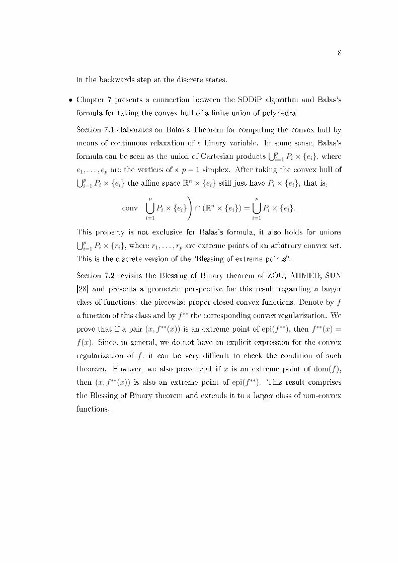
• Chapter 7 presents a connection between the SDDiP algorithm and Balas's

formula for taking the convex hull of a �nite union of polyhedra.

Section 7.1 elaborates on Balas's Theorem for computing the convex hull by

means of continuous relaxation of a binary variable. In some sense, Balas's

formula can be seen as the union of Cartesian products⋃pi=1 Pi × {ei}, where

e1, . . . , ep are the vertices of a p − 1 simplex. After taking the convex hull of⋃pi=1 Pi × {ei} the a�ne space Rn × {ei} still just have Pi × {ei}, that is,

conv

(p⋃

i=1

Pi × {ei})∩ (Rn × {ei}) =

p⋃

i=1

Pi × {ei}.

This property is not exclusive for Balas's formula, it also holds for unions⋃pi=1 Pi × {ri}, where r1, . . . , rp are extreme points of an arbitrary convex set.

This is the discrete version of the �Blessing of extreme points�.

Section 7.2 revisits the Blessing of Binary theorem of ZOU; AHMED; SUN

[28] and presents a geometric perspective for this result regarding a larger

class of functions: the piecewise proper closed convex functions. Denote by f

a function of this class and by f ∗∗ the corresponding convex regularization. We

prove that if a pair (x, f ∗∗(x)) is an extreme point of epi(f ∗∗), then f ∗∗(x) =

f(x). Since, in general, we do not have an explicit expression for the convex

regularization of f , it can be very di�cult to check the condition of such

theorem. However, we also prove that if x is an extreme point of dom(f),

then (x, f ∗∗(x)) is also an extreme point of epi(f ∗∗). This result comprises

the Blessing of Binary theorem and extends it to a larger class of non-convex

functions.

9

2 CONVEX HULL OF UNION OF CLOSED CON-

VEX SETS

In this chapter, we prove some important facts concerning the convex hull of

union of closed convex sets. Those are the key arguments to understand our main

result: the Blessing of Extreme Points.

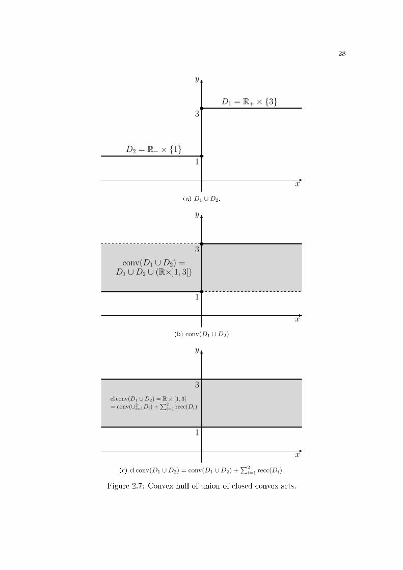
It is instructive to note that the convex hull of union of closed convex sets

may not be closed, see �gures 2.7a and 2.7b (page 28). However, for the particular

class of closed convex sets, we have an enlightening identity. Under mild regularity

conditions detailed in Theorem 2.10 (page 27), we have that

cl conv

(m⋃

i=1

Di

)= conv

(m⋃

i=1

Di

)+

m∑

i=1

recc(Di), (2.1)

where D1, . . . , Dm are nonempty closed convex sets of Rn, and recc(Di) is the re-

cession cone of Di, which contains all directions di ∈ Rn such that starting at

any xi ∈ Di and going inde�nitely along di, we never leave Di. Thus, if the set

conv (∪mi=1Di) is not closed, we simply add the recession directions to make it closed,

see �gures 2.7b and 2.7c (page 28), for an example. Moreover, if each Di is a poly-

hedral set, then formula (2.1) holds without any further regularity condition.

The purpose of the following sections is to build the necessary theory to

establish identity (2.1). We have chosen to carefully prove (2.1), since we have found

a critical mistake in the proof of CERIA; SOARES [12] (page 601). We provide an

original proof for (2.1) under the suitable regularity conditions. On a �rst reading,

it is possible to go through section 2.1 for basic results in convex analysis, and use

equation (2.1) when necessary.

10

We organize the exposition as:

1. In section 2.1, we present some basic results on convex analysis;

2. In section 2.2, we prove some properties of sum and closure of lifted cones

K = cone({1} ×D);

3. In section 2.3, we show the conditions for commuting a given linear map A

with the closure operation, that is, when cl(AD) = A cl(D);

4. In section 2.4, we conclude that the equality cl (∑m

i=1 Ki) =∑m

i=1 cl(Ki) im-

plies the desired equation (2.1), where Ki = cone({1} ×Di).

2.1 Basic results on convex analysis

In this section, we introduce some basic de�nitions and results of convex

analysis that will be important throughout this work.

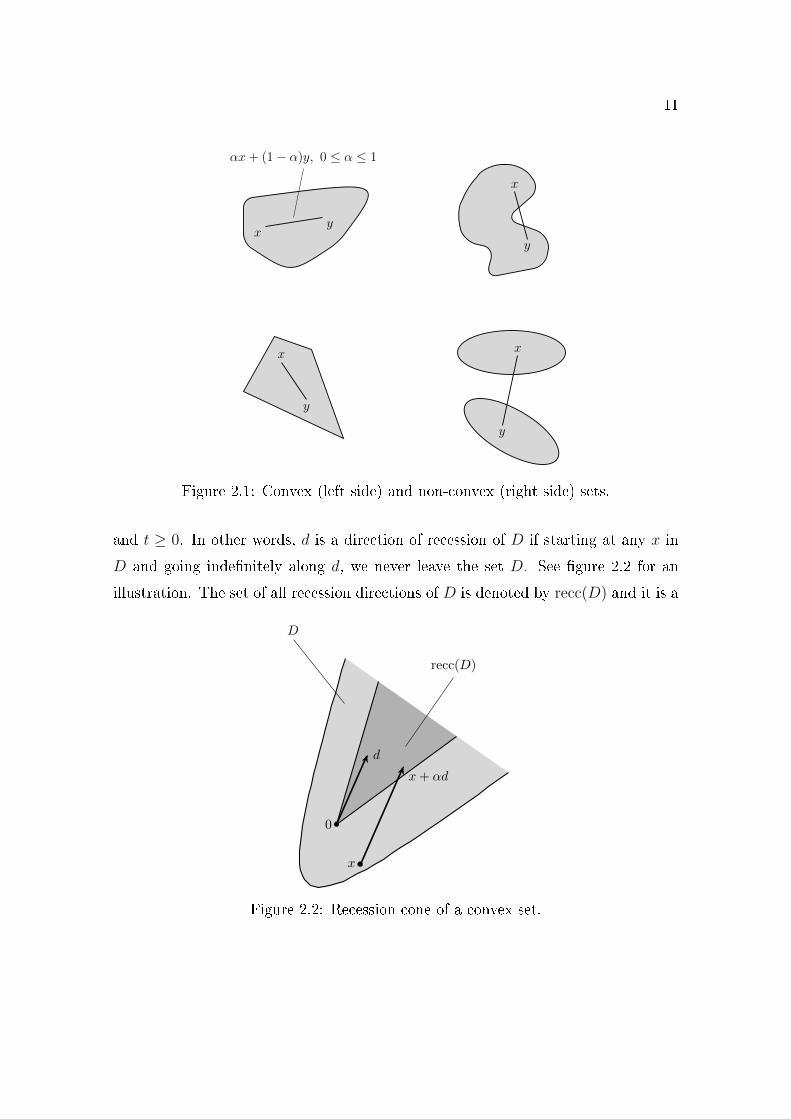
Let D be a set of Rn. We say that D is convex if for any two points of D,

the line segment that joins them is also within D, see �gure 2.1. The set P ⊂ Rn

is a polyhedron if it is the intersection of a �nite number of hyperspaces a>j x ≤ bj,

that is,

P = {x ∈ Rn | Ax ≤ b},

for some A ∈ Rm×n and b ∈ Rm. In particular, P is a convex set, since any

hyperspace is a convex set and the intersection of convex sets is convex. We say

that C ⊂ Rn is a cone if for each vector x ∈ C and scalar α ≥ 0, the product αx

belongs to C.

A vector d is a direction of recession of D if x+ td belongs to D, for all x ∈ D

11

xy

αx+ (1− α)y, 0 ≤ α ≤ 1

x

y

x

y

x

y

Figure 2.1: Convex (left side) and non-convex (right side) sets.

and t ≥ 0. In other words, d is a direction of recession of D if starting at any x in

D and going inde�nitely along d, we never leave the set D. See �gure 2.2 for an

illustration. The set of all recession directions of D is denoted by recc(D) and it is a

d

0

x

x+ αd

D

recc(D)

Figure 2.2: Recession cone of a convex set.

12

convex cone containing the origin. We note that the recession cone of a convex cone

is the cone itself. The following result regarding the directions of recession states

that if one can go inde�nitely along d starting at one given point, we can go along d

starting at any point, so d is a direction of recession. For a proof, see BERTSEKAS

[5, page 43].

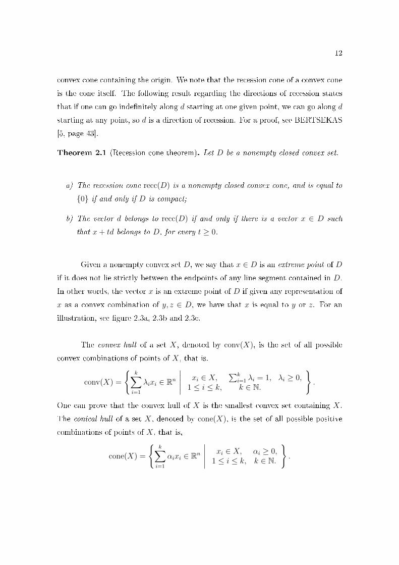
Theorem 2.1 (Recession cone theorem). Let D be a nonempty closed convex set.

a) The recession cone recc(D) is a nonempty closed convex cone, and is equal to

{0} if and only if D is compact;

b) The vector d belongs to recc(D) if and only if there is a vector x ∈ D such

that x+ td belongs to D, for every t ≥ 0.

Given a nonempty convex set D, we say that x ∈ D is an extreme point of D

if it does not lie strictly between the endpoints of any line segment contained in D.

In other words, the vector x is an extreme point of D if given any representation of

x as a convex combination of y, z ∈ D, we have that x is equal to y or z. For an

illustration, see �gure 2.3a, 2.3b and 2.3c.

The convex hull of a set X, denoted by conv(X), is the set of all possible

convex combinations of points of X, that is,

conv(X) =

{k∑

i=1

λixi ∈ Rn

∣∣∣∣∣xi ∈ X,

∑ki=1 λi = 1, λi ≥ 0,

1 ≤ i ≤ k, k ∈ N.

}.

One can prove that the convex hull of X is the smallest convex set containing X.

The conical hull of a set X, denoted by cone(X), is the set of all possible positive

combinations of points of X, that is,

cone(X) =

{k∑

i=1

αixi ∈ Rn

∣∣∣∣∣xi ∈ X, αi ≥ 0,

1 ≤ i ≤ k, k ∈ N.

}.

13

ExtremePoints

(a) Extremes of a linesegment.

ExtremePoints

(b) Extremes of a polyhedra.

ExtremePoints

(c) Extremes of a convex set.

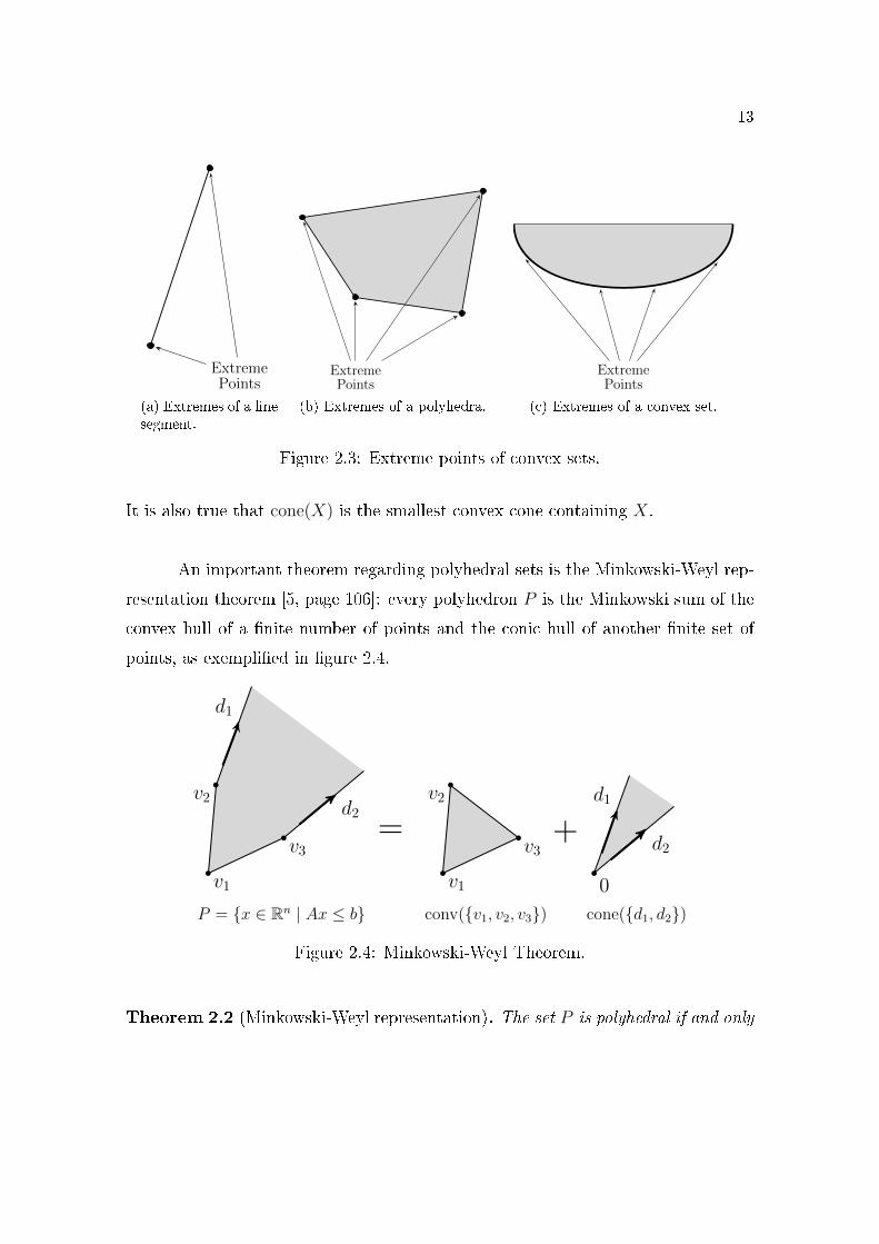
Figure 2.3: Extreme points of convex sets.

It is also true that cone(X) is the smallest convex cone containing X.

An important theorem regarding polyhedral sets is the Minkowski-Weyl rep-

resentation theorem [5, page 106]: every polyhedron P is the Minkowski sum of the

convex hull of a �nite number of points and the conic hull of another �nite set of

points, as exempli�ed in �gure 2.4.

v1

v2

v3

d1

d2

v1

v2

v3

0

d1

d2= +

P = {x ∈ Rn | Ax ≤ b} conv({v1, v2, v3}) cone({d1, d2})

Figure 2.4: Minkowski-Weyl Theorem.

Theorem 2.2 (Minkowski-Weyl representation). The set P is polyhedral if and only

14

if there is a �nite number of vectors {v1, . . . , vk} ⊂ Rn and {w1, . . . , wl} ⊂ Rn such

that

P = conv({v1, . . . , vk}) + cone({w1, . . . , wl}).

In particular, the recession cone of P is equal to cone({w1, . . . , wl}).

The Minkowski-Weyl representation is an important theorem since several

complicated results for the general convex case can be easily demonstrated in the

polyhedral case thanks to this theorem without any further regularity condition.

2.2 Conical lifting

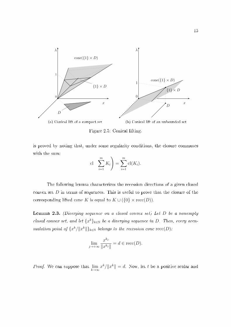
We de�ne the conical lift of a set D ⊂ Rn as the conic hull K of the particular

set {1} × D, as depicted in �gures 2.5a and 2.5b. It is instructive to note that

K is always convex, independently of the convexity of D, since K is the set of

all positive combinations of elements of {1} × D. The set K is equal to the set

{(λ, λx) ∈ Rn+1 | x ∈ D,λ ≥ 0} if, and only if, the set D is convex.

The advantage of transforming a convex set into this special convex cone is

that the convex hull of the union of convex sets is closely related to the sum of the

corresponding lifted cones, as we will see in Corollary 2.5, page 18.

Another important result for us is the characterization of the closure of the

lift cone. For any unbounded closed convex set D, the cone({1} ×D) is not closed,

and the missing boundary set is {0} × recc(D), see �gure 2.5b. Let D1, . . . , Dm be

nonempty closed convex sets, and let Ki = cone({1} × Di) be the corresponding

conical lifts. We shall see that the closure of the convex hull of ∪mi=1Di can be

obtained from the closure of the sum of lifted cones∑m

i=1Ki. Thus, formula (2.1)

15

λ

0

1

D

x

{1} ×D

cone({1} ×D)

(a) Conical lift of a compact set

λ

0

D

{1} ×D1

cone({1} ×D)

x

(b) Conical lift of an unbounded set

Figure 2.5: Conical lifting.

is proved by noting that, under some regularity conditions, the closure commutes

with the sum:

cl

(m∑

i=1

Ki

)=

m∑

i=1

cl(Ki).

The following lemma characterizes the recession directions of a given closed

convex set D in terms of sequences. This is useful to prove that the closure of the

corresponding lifted cone K is equal to K ∪ ({0} × recc(D)).

Lemma 2.3. (Diverging sequence on a closed convex set) Let D be a nonempty

closed convex set, and let {xk}k∈N be a diverging sequence in D. Then, every accu-

mulation point of {xk/‖xk‖}k∈N belongs to the recession cone recc(D):

limj→+∞

xkj

‖xkj‖ = d ∈ recc(D).

Proof. We can suppose that limk→∞

xk/‖xk‖ = d. Now, let t be a positive scalar and

16

note that limk→∞

(xk − x1)/‖xk − x1‖ = d since ‖xk‖ is unbounded:

limj→∞

(xkj − x1)

‖xkj − x1‖ = limj→∞

(xkj

‖xkj‖‖xkj‖

‖xkj − x1‖ −x1

‖xkj − x1‖

)= lim

j→∞xkj

‖xkj‖ = d.

Denote by dk the vector given by (xk − x1)/‖xk − x1‖, and by tk the scalar

‖xk − x1‖. Since ‖xk‖ diverges, there is N ∈ N such that tk is greater than t for

every k greater than N . Note that x1 + tkdk belongs to D for every k,

xk = x1 + tkdk ∈ D, ∀k ∈ N,

and x1 + tdk also belongs to D, for all k greater than N , since it is a convex

combinations of x1 and x1 + tkdk. So, x1 + tdk converges to x1 + td, which belongs to

D since D is a closed set. Therefore, x1 + td belongs to D for every positive scalar

t, that is, d is a direction of recession from D.

The following theorem formalizes the intuition about taking the closure of a

cone K = cone({1} ×D), where D is a convex set.

Theorem 2.4 (Closure of lift cone). Let D be a nonempty convex set, and let K be

the conic hull of the Cartesian product {1} ×D = {(1, x) ∈ Rn+1 | x ∈ D}, that is,K = cone({1}×D). Denote by D the closure of D. Then, the closure of K is given

by

clK = cone({1} ×D) ∪ ({0} × recc(D)).

Proof. Let C0, C1, K0 and K+ be the following sets:

C0 = {0} × recc(D) K0 = clK ∩({0} × Rn

)

C1 = cone({1} ×D) K+ = clK ∩((0,∞)× Rn)

)

We need to prove that C0 equals K0 and C1\{(0, 0)} equals K+. This is su�cient

to prove this theorem, since clK = K+ ∪K0.

17

Let's start by proving the equality between K0 and C0. Let y ∈ K0. Then,

y is equal to (0, d) for some d ∈ Rn and there is a sequence {yk}k∈N from K that

converges to y. For each yk ∈ K, there is λk ≥ 0 and xk ∈ D such that yk = λk(1, xk).

Thus, we have that

limk→∞

λk = 0, limk→∞

λkxk = d.

If d is 0, then y belongs to C0. If d is di�erent from 0, then ‖xk‖ goes to in�nity:

limk→∞‖xk‖ = lim

k→∞

‖λkxk‖λk

=‖d‖0+

= +∞.

Denote by dk the vector xk/‖xk‖. From Lemma 2.3, every convergent subsequence

of {dk}k∈N converges to a vector u that belongs to the recession cone recc(D). Taking

a subsequence if necessary, we have the following limit:

d = limk→∞

λkxk = limk→∞‖λkxk‖

xk‖xk‖

= ‖d‖u.

Thus, d is also a recession direction of D, and y belongs to C0. Therefore, K0 ⊆ C0.

Let's prove the opposite inclusion. Let y ∈ C0. If y is equal to (0, 0), then y

belongs to K0, trivially. Suppose that y is equal to (0, d), where d is some non-zero

vector of recc(D). Let x0 ∈ D and note that xk = x0 + kd belongs to D, for every

k ∈ N. Let xk ∈ D be such that ‖xk − xk‖ ≤ 1, and let yk = 1k(1, xk). Note that yk

belongs to K, for every k ∈ N, and

limk→∞

yk = limk→∞

[1

k(1, xk − xk) +

1

k(1, xk)

]= (0, 0) + (0, d) = y.

So, y belongs to K0. Therefore, K0 = C0.

Now, let's prove the equality K+ = C1\{(0, 0)}. Let y ∈ K+. Then, y is

equal to (λ, x) for some λ > 0 and x ∈ Rn, and there is a sequence {yk}k∈N from K

such that limk→∞

yk = (λ, x). Thus, yk = λk(1, xk) for some λk ≥ 0 and xk ∈ D. Note

that

limk→∞

xk = limk→∞

1

λk(λkxk) =

1

λx ∈ D.

18

So, y = λ(1, x

λ

)belongs to C1\{(0, 0)}. Therefore, K+ ⊆ C1\{(0, 0)}.

Let's prove the opposite inclusion. Let y ∈ C0\{(0, 0)}. Then, y = λ(1, x)

for some λ > 0 and x ∈ D. Let {xk}k∈N be a sequence from D that converges to x,

and denote by yk the vector λ(1, xk). Therefore, yk belongs to K for every k, and

we have that

limk→∞

yk = (λ, λ limk→∞

xk) = (λ, λx) = y.

So, y belongs to K+. Therefore, K+ = C1\{(0, 0)}.

One advantage of the conical lift is to transform the convex hull of a union of

convex sets Di into a sum of convex cones K1 + · · ·Km, where Ki = cone({1}×Di).

Moreover, by adding the closure of the cones clK1 + · · · + clKm we obtain an

expression that contains the right-hand side of equation (2.1): conv(⋃mi=1 Di) +

∑mi=1 recc(Di).

Corollary 2.5 (Convex hull by conical lift). Let D1, . . . , Dm be nonempty closed

convex sets, let D be the union ∪mi=1Di, let R be the sum of recession cones∑m

i=1 recc(Di),

and let Ki be the conic hull of {1} ×Di, for all i = 1, . . . ,m. Then,

K1 + · · ·+Km = cone({1} × conv(D)

),

clK1 + · · ·+ clKm = cone({1} × [conv(D) +R]

)∪({0} ×R

).

Proof. Let K be the sum of cones K1, . . . , Km, that is, K =∑m

i=1Ki. We shall

prove that K is equal to cone({1} × conv(D)

). Indeed, let y be a vector of K.

Then, there is a scalar λ ≥ 0 and a vector u ∈ Rn such that y = (λ, u) and

(λ, u) =m∑

i=1

λi(1, xi),

for some λi ≥ 0, and xi ∈ Di, for i = 1, . . . ,m. If λ is equal to 0, then each λi is

equal to 0. In particular, y is equal to 0 and it belongs to cone({1} × conv(D)

)

19

trivially. Suppose that λ is positive. Then,

y = λm∑

i=1

λiλ

(1, xi) = λ

(1,

m∑

i=1

γixi

),

where γi := λi/λ. Therefore, y belongs to cone({1} × conv(D)

), since

∑γi =

∑λi/λ = λ/λ = 1. On the other hand, let y be a vector of cone

({1} × conv(D)

).

Then, there are scalars λ ≥ 0, γj ∈ [0, 1], and vectors xj ∈ Dj such that∑m

i=1 γi = 1

and

y = λ

(1,

m∑

i=1

γixi

)=

m∑

i=1

λγi(1, xi),

for all j = 1, . . . ,m. Therefore, y belongs to K, and we have that K is equal to

cone({1} × conv(D)

).

We now prove the second equality. Let K be the sum of cones cl(K1), . . . ,

cl(Km), i.e., K =∑m

i=1 clKi. Then, the second equality can be stated as

K = cone({1} × [conv(D) +R]

)∪({0} ×R

).

Now, let y be a vector of K. Since y belongs to K, there is a scalar λ ∈ R and a

vector u ∈ Rn such that y = (λ, u) and

(λ, u) =m∑

i=1

(λi, ui),

for some (λi, ui) ∈ cl(Ki), for i = 1, . . . ,m. From Theorem 2.4 and since Di are

closed, the closure of Ki is equal to Ki∪{0}× recc(Di). Let I+ be the set of indexes

i such that λi is greater than zero, and let I0 be the set of indexes i such that λi is

equal to zero. For each i ∈ I+, there is xi ∈ Di such that ui is equal to λixi, and

for each i ∈ I0, there is di ∈ recc(Di) such that ui is equal to di. Then,

(λ, u) =∑

i∈I+λi(1, xi) +

∑

i∈I0(0, di).

20

If λ is equal to zero, then each λi is equal to zero. Therefore, the vector y belongs

to {0} ×R. If λ is positive, denote by γi the ratio λi/λ. Then, we have that

(λ, u) = λ∑

i∈I+γi(1, xi) + λ

∑

i∈I0

(0,

1

λdi

)

= λ

(1,∑

i∈I+γixi +

∑

i∈I0

1

λdi

),

and so y belongs to cone({1} × [conv(D) + R]

). Lets prove the opposite inclusion.

First, note that the inclusion ({0} × R) ⊂ (cl(K1) + · · ·+ cl(Km)) follows from the

closure formula for cl(Ki), that is, cl(Ki) = Ki× ({0}× recc(Di)). Let y be a vector

of the set cone({1}× [conv(D) +R]

). Then, y has the form (λ, u) ∈ Rn+1 such that

(λ, u) = λ

(1,

m∑

i=1

γixi +m∑

i=1

di

),

for some xi ∈ Di, di ∈ recc(Di), and γi ∈ [0, 1] with∑m

j=1 γj = 1, for i = 1, . . . ,m.

Let I+ and I0 be the set of indexes i for which γi is equal to zero and positive,

respectively. Then, we can split the sum∑m

i=1 di into∑

i∈I+ di and∑

i∈I0 di, and

we have that

(λ, u) = λ

(1,∑

i∈I+γi(xi + γ−1

i di)

+∑

i∈I0di

)

=∑

i∈I+λγi(1, xi + γ−1

i di) +∑

i∈I0(0, λdi).

Note that xi + γ−1i di ∈ Di, for all i ∈ I+, and λdi ∈ recc(Di), for all i ∈ I0. Thus,

it follows that

λγi(1, xi + γ−1i di) ∈ cl(Ki), ∀i ∈ I+,

(0, λdi) ∈ cl(Ki), ∀i ∈ I0.

Therefore, y belongs to K.

21

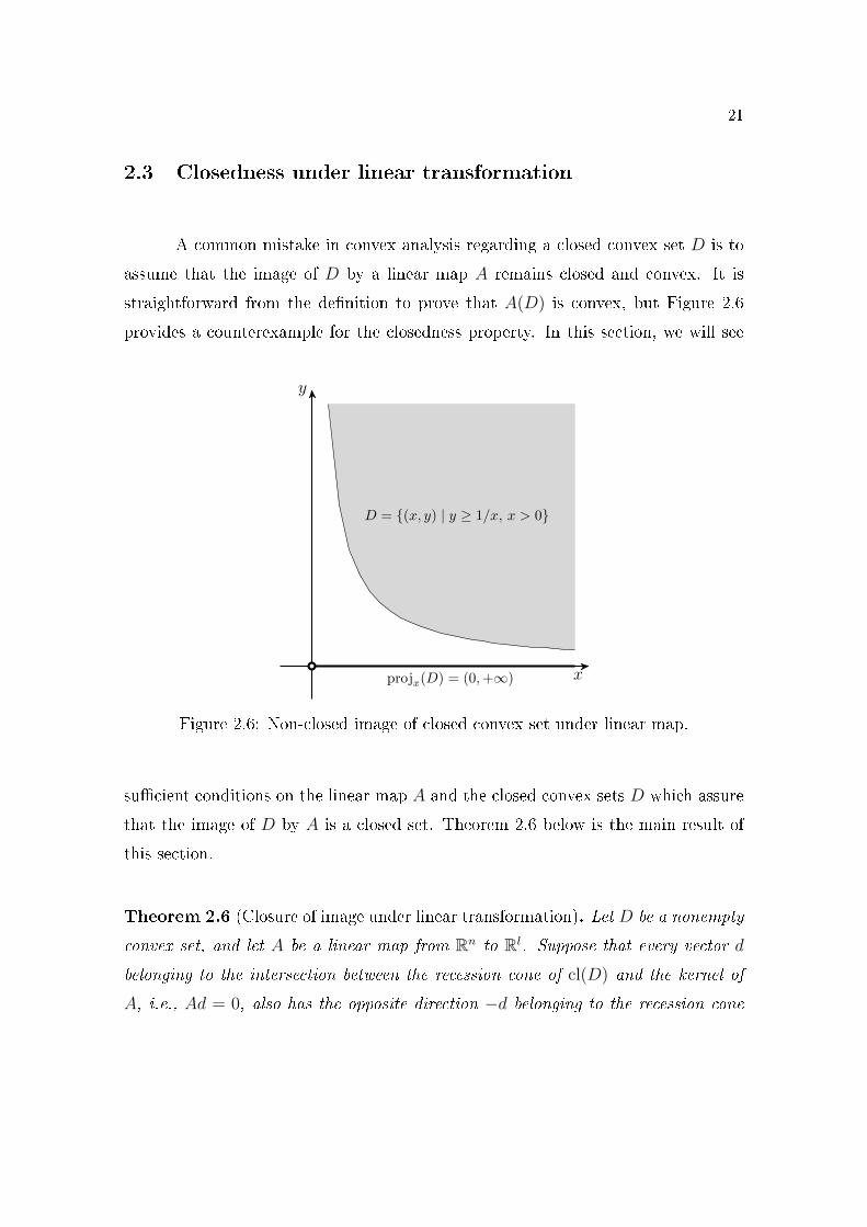
2.3 Closedness under linear transformation

A common mistake in convex analysis regarding a closed convex set D is to

assume that the image of D by a linear map A remains closed and convex. It is

straightforward from the de�nition to prove that A(D) is convex, but Figure 2.6

provides a counterexample for the closedness property. In this section, we will see

x

y

D = {(x, y) | y ≥ 1/x, x > 0}

projx(D) = (0,+∞)

Figure 2.6: Non-closed image of closed convex set under linear map.

su�cient conditions on the linear map A and the closed convex sets D which assure

that the image of D by A is a closed set. Theorem 2.6 below is the main result of

this section.

Theorem 2.6 (Closure of image under linear transformation). Let D be a nonempty

convex set, and let A be a linear map from Rn to Rl. Suppose that every vector d

belonging to the intersection between the recession cone of cl(D) and the kernel of

A, i.e., Ad = 0, also has the opposite direction −d belonging to the recession cone

22

of cl(D), i.e., recc(cl(D)) ∩ ker(A) ⊆ − recc(cl(D)). Then,

cl(AD) = A(cl(D)),

recc(cl(AD)) = A(recc(cl(D))).

In particular, if D is closed then AD is also closed.

Proof. Let y be a vector of A(cl(D)). So, y is equal to Ax, for some x ∈ cl(D). Since

x is an adherent point of D, there is a sequence {xk}k∈N from D that converges to x.

Denote by yk the vector Axk. Note that yk belongs to AD, for all k ∈ N, and {yk}k∈Nconverges to y:

limk→∞

yk = limk→∞

Axk = Ax = y.

Therefore, y belongs to cl(AD), so we conclude that A cl(D) ⊂ cl(AD).

Let y be a vector of cl(AD), and let {yk}k∈N be a sequence from AD that

converges to y. Let xk be a vector of cl(D) with minimum norm such that Axk = yk,

i.e., let xk be the optimal solution of the following problem:

minx ‖x‖s.t. Ax = yk,

x ∈ clD.

Note that xk is unique, since the euclidean norm is a strictly convex function. Thus,

there are two possibilities for the sequence {xk}k∈N:

1. The sequence {xk}k∈N is bounded. Then, there is a subsequence {xkj}j∈N that

converges to some x ∈ cl(D). Then,

y = limj→∞

ykj = limj→∞

Axkj = Ax,

so y belongs to A(cl(D)).

23

2. The sequence {xk}k∈N has an unbounded subsequence. Without loss of gen-

erality, suppose that {xk}k∈N is unbounded, and let d be a cluster point

of {xk/‖xk‖}k∈N. Taking a subsequence if necessary, assume that {xk/‖xk‖}k∈Nconverges to d. From Lemma 2.3, d is a direction of recession of cl(D), and d

also belongs to the kernel of A:

‖Ad‖ = limk→∞

‖Axk‖‖xk‖

= limk→∞

‖yk‖‖xk‖

=‖y‖+∞ = 0.

So, by hypothesis, the opposite direction −d is a direction of recession of cl(D).

Denote by xk the vector xk − ‖xk‖d. Note that xk ∈ cl(D), and Axk = yk, for

all k ∈ N. In particular, the sequence {xk/‖xk‖}k∈N converges to 0:

limk→∞

‖xk‖‖xk‖

= limk→∞

‖(xk − ‖xk‖d)‖‖xk‖

= 0.

So, for su�ciently large k, ‖xk‖ < xk, contradicting the hypothesis of xk being

a vector of minimum norm such that xk ∈ cl(D) and Axk = yk. Therefore,

the sequence {xk}k∈N is bounded, and this proves that cl(AD) = A(clD).

We now prove the formula for the recession cone

recc(cl(AD)) = A(recc(cl(D))).

The idea for this proof is to take the conical lift K of D, extend the linear map

A ∈ Rn×l to a linear map B =

[1 00 A

]∈ R(n+1)×(l+1), and conclude that the closure

operation and the linear map B commute, that is, cl(BK) = B cl(K). Indeed, from

Theorem 2.4 (page 16), we have the following expression for B cl(K):

B cl(K) = B(

cone({1} × cl(D)

)∪({0} × recc(cl(D))

))

= cone({1} × A cl(D)

)∪({0} × A recc(cl(D))

).

On the other hand, the set cl(BK) has the following form:

cl(BK) = cl(B cone

({1} ×D

))= cl

(cone

({1} × AD

))

= cone({1} × cl(AD)

)∪({0} × recc(cl(AD))

),

24

where the last equality follows from Theorem 2.4, page 16.

If the closure operation commutes with the linear map B, i.e., if cl(BK) =

B cl(K), taking intersection of both sets with {0} × Rn we obtain

{0} × A recc(cl(D)) = {0} × recc(cl(AD)),

which yields the required formula for the recession cone. So, it is enough to show

that cl(BK) = B cl(K), and for this purpose we use the �rst part of this theorem.

Note that the kernel of B is equal to {0} × ker(A), and the recession cone of

cl(K) is equal to itself, since the recession cone of a convex cone is the cone itself.

So,

ker(B) ∩ cl(K) = {0} ×(

ker(A) ∩ recc(cl(D)))

⊂ {0} ×(− recc(cl(D))

)

⊂ − cl(K),

where the second relation follows from the hypothesis, and the �rst and third follow

from the expression of cl(K) (Theorem 2.4). Using the �rst part of this theorem,

we conclude that cl(BK) = B cl(K).

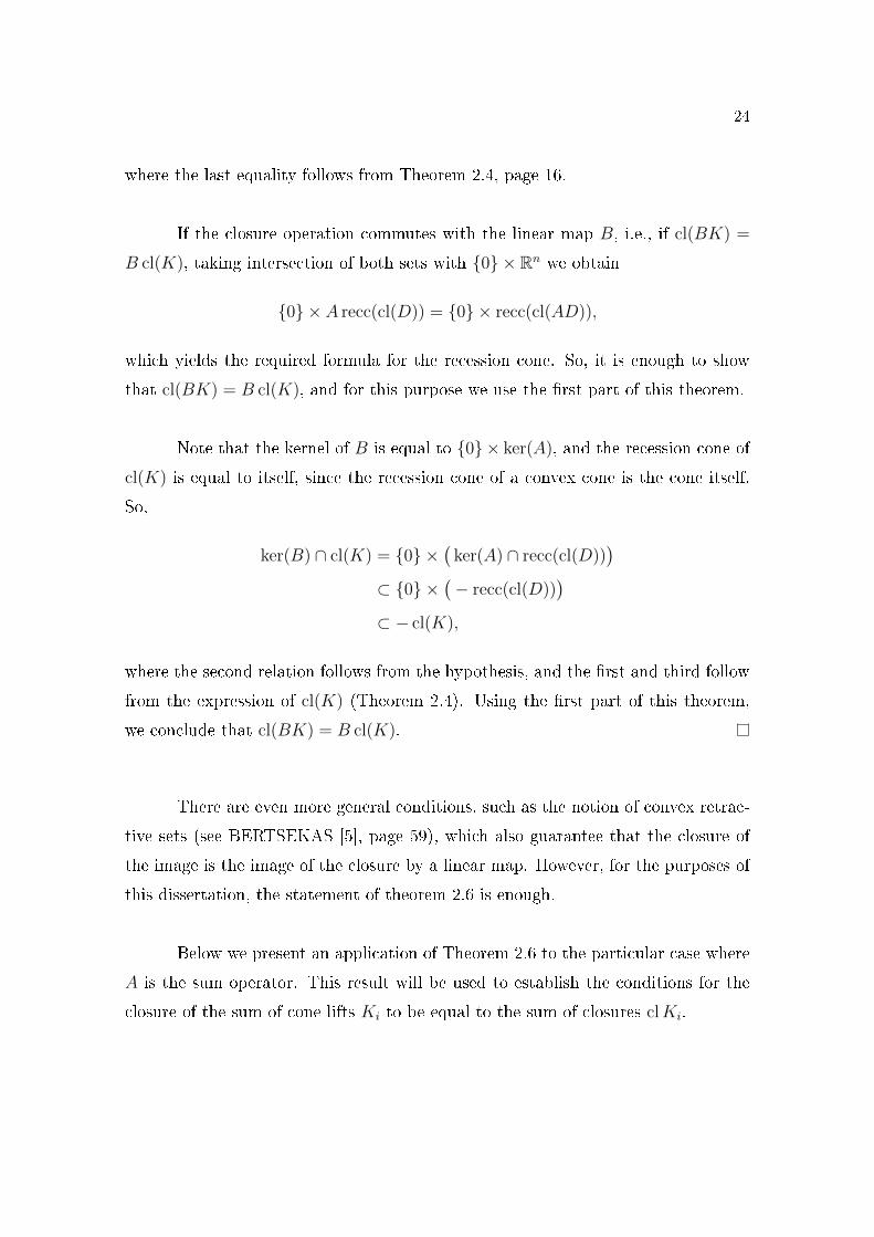
There are even more general conditions, such as the notion of convex retrac-

tive sets (see BERTSEKAS [5], page 59), which also guarantee that the closure of

the image is the image of the closure by a linear map. However, for the purposes of

this dissertation, the statement of theorem 2.6 is enough.

Below we present an application of Theorem 2.6 to the particular case where

A is the sum operator. This result will be used to establish the conditions for the

closure of the sum of cone lifts Ki to be equal to the sum of closures clKi.

25

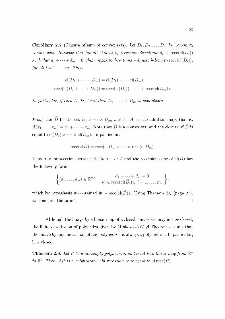
Corollary 2.7 (Closure of sum of convex sets). Let D1, D2, . . . , Dm be nonempty

convex sets. Suppose that for all choices of recession directions di ∈ recc(cl(Di))

such that d1 + · · ·+dm = 0, their opposite directions −di also belong to recc(cl(Di)),

for all i = 1, . . . ,m. Then,

cl(D1 + · · ·+Dm) = cl(D1) + · · · cl(Dm),

recc(cl(D1 + · · ·+Dm)) = recc(cl(D1)) + · · ·+ recc(cl(Dm)).

In particular, if each Di is closed then D1 + · · ·+Dm is also closed.

Proof. Let D be the set D1 × · · · × Dm, and let A be the addition map, that is,

A(x1, . . . , xm) = x1 + · · ·+ xm. Note that D is a convex set, and the closure of D is

equal to cl(D1)× · · · × cl(Dm). In particular,

recc(cl D) = recc(clD1)× · · · × recc(clDm).

Thus, the intersection between the kernel of A and the recession cone of cl(D) has

the following form:{

(d1, . . . , dm) ∈ Rmn

∣∣∣∣d1 + · · ·+ dm = 0

di ∈ recc(cl(Di)), i = 1, . . . ,m.

},

which by hypothesis is contained in − recc(cl(D)). Using Theorem 2.6 (page 21),

we conclude the proof.

Although the image by a linear map of a closed convex set may not be closed,

the �nite description of polyhedra given by Minkowski-Weyl Theorem ensures that

the image by any linear map of any polyhedron is always a polyhedron. In particular,

it is closed.

Theorem 2.8. Let P be a nonempty polyhedron, and let A be a linear map from Rn

to Rl. Then, AP is a polyhedron with recession cone equal to A recc(P ).

26

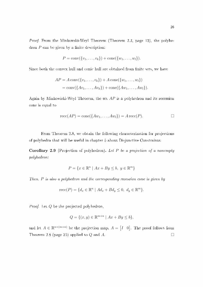
Proof. From the Minkowski-Weyl Theorem (Theorem 2.2, page 13), the polyhe-

dron P can be given by a �nite description:

P = conv({v1, . . . , vk}) + cone({w1, . . . , wl}).

Since both the convex hull and conic hull are obtained from �nite sets, we have

AP = A conv({v1, . . . , vk}) + A cone({w1, . . . , wl})= conv({Av1, . . . , Avk}) + cone({Aw1, . . . , Awl}).

Again by Minkowiski-Weyl Theorem, the set AP is a polyhedron and its recession

cone is equal to

recc(AP ) = cone({Aw1, . . . , Awl}) = A recc(P ).

From Theorem 2.8, we obtain the following characterization for projections

of polyhedra that will be useful in chapter 5 about Disjunctive Constraints:

Corollary 2.9 (Projection of polyhedron). Let P be a projection of a nonempty

polyhedron:

P = {x ∈ Rn | Ax+By ≤ b, y ∈ Rm}

Then, P is also a polyhedron and the corresponding recession cone is given by

recc(P ) = {dx ∈ Rn | Adx +Bdy ≤ 0, dy ∈ Rm}.

Proof. Let Q be the projected polyhedron,

Q = {(x, y) ∈ Rm+n | Ax+By ≤ b},

and let A ∈ Rn×(m+n) be the projection map, A =[I 0

]. The proof follows from

Theorem 2.8 (page 25) applied to Q and A.

27

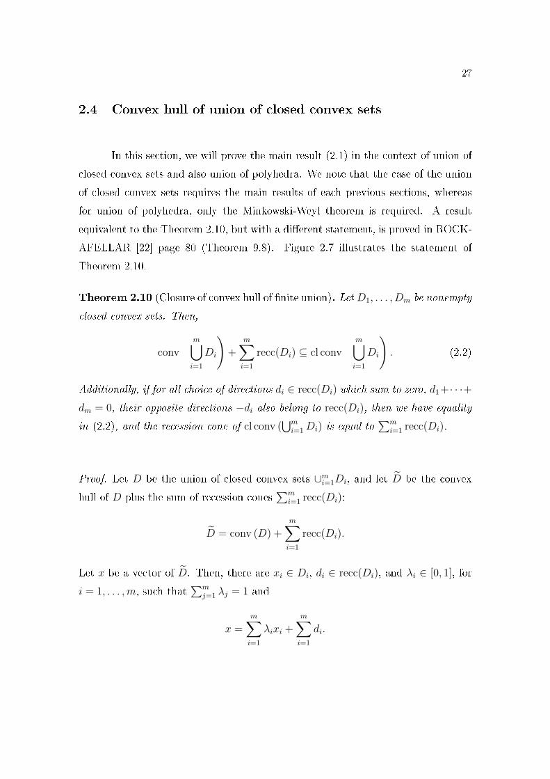
2.4 Convex hull of union of closed convex sets

In this section, we will prove the main result (2.1) in the context of union of

closed convex sets and also union of polyhedra. We note that the case of the union

of closed convex sets requires the main results of each previous sections, whereas

for union of polyhedra, only the Minkowski-Weyl theorem is required. A result

equivalent to the Theorem 2.10, but with a di�erent statement, is proved in ROCK-

AFELLAR [22] page 80 (Theorem 9.8). Figure 2.7 illustrates the statement of

Theorem 2.10.

Theorem 2.10 (Closure of convex hull of �nite union). Let D1, . . . , Dm be nonempty

closed convex sets. Then,

conv

(m⋃

i=1

Di

)+

m∑

i=1

recc(Di) ⊆ cl conv

(m⋃

i=1

Di

). (2.2)

Additionally, if for all choice of directions di ∈ recc(Di) which sum to zero, d1+· · ·+dm = 0, their opposite directions −di also belong to recc(Di), then we have equality

in (2.2), and the recession cone of cl conv (⋃mi=1 Di) is equal to

∑mi=1 recc(Di).

Proof. Let D be the union of closed convex sets ∪mi=1Di, and let D be the convex

hull of D plus the sum of recession cones∑m

i=1 recc(Di):

D = conv (D) +m∑

i=1

recc(Di).

Let x be a vector of D. Then, there are xi ∈ Di, di ∈ recc(Di), and λi ∈ [0, 1], for

i = 1, . . . ,m, such that∑m

j=1 λj = 1 and

x =m∑

i=1

λixi +m∑

i=1

di.

28

x

y

3

D1 = R+ × {3}

1

D2 = R− × {1}

(a) D1 ∪D2.

x

y

3

1

conv(D1 ∪D2) =D1 ∪D2 ∪ (R×]1, 3[)

(b) conv(D1 ∪D2)

x

y

3

1

cl conv(D1 ∪D2) = R× [1, 3]

= conv(∪2i=1Di) +∑2

i=1 recc(Di)

(c) cl conv(D1 ∪D2) = conv(D1 ∪D2) +∑2

i=1 recc(Di).

Figure 2.7: Convex hull of union of closed convex sets.

29

For each 1 ≤ i ≤ 2m, let {αki }k∈N be a sequence in [0, 1] such that∑2m

i=1 αki is equal

to 1, for all k ∈ N, and the limit of αki when k goes to in�nity is equal to

limk→∞

αki =

{λ−i , if 1 ≤ i ≤ m,

0+ , if m+ 1 ≤ i ≤ 2m.

For instance, we can consider the sequence {αki }k∈N given by

αki =

λi − rk+1

, if 1 ≤ i ≤ m and λi > 0,

0 , if 1 ≤ i ≤ m and λi = 0,r

k+1, if m+ 1 ≤ i ≤ m+ p,

0 , if m+ p+ 1 ≤ i ≤ 2m,

where r is the lowest value of λi among all λi greater than 0, that is, r = minλi>0 λi,

and p is the number of λi greater than 0. Let {yk}k∈N be the sequence given by

yk =m∑

i=1

αki xi +m∑

i=1

αki+m

(xi +

1

αki+mdi

),

and note that yk belongs to conv(D), for every k ∈ N. Taking the limit in k, we

have that yk converges to x. Therefore, x belongs to cl(conv(D)).

We now proceed to the equality case in (2.2) under the additional regularity

condition on the recession cones. Let Ki be the conical lift of Di, that is, Ki =

cone({1} × Di), and let K be the product of cones K1 × · · · × Km. Let A be

the addition map

A(v1, . . . , vm) = v1 + · · ·+ vm,

where vi ∈ Rn+1, for all i = 1, . . . ,m. From Corollary 2.5 page 18

AK = cone({1} × conv(D)

),

A cl(K) = cone({1} × (conv(D) +R)

)∪({0} ×R

),

where R =∑m

i=1 recc(Di), and from Theorem 2.4 page 16 applied to AK, we get:

cl(AK) = cone({1} × cl(conv(D))

)∪({0} × recc(cl(conv(D)))

).

30

So, it is su�cient to prove that cl(AK) is equal to A cl(K). For this purpose, we

want to apply Theorem 2.6 (page 21) about the interchangeability between the linear

map and closure. Recall that the recession cone of a convex cone is the cone itself.

Therefore, we must verify if the intersection between the kernel of A and cl(K) is

contained in − cl(K). Let v be a vector of ker(A) ∩ cl(K). Then, v is equal to

(v1, . . . , vm), for some v1 ∈ cl(K1), . . . , vm ∈ cl(Km), and v1 + · · · + vm = 0. Since

each vi is equal to (λi, ui) for some λi ≥ 0 and ui ∈ Rn, we have that

λ1 + · · ·+ λm = 0, and u1 + · · ·+ um = 0.

Therefore, each λi is equal to 0, and ui belongs to recc(Di), by the characterization

of cl(Ki), for all i = 1, . . . ,m. By hypothesis, −ui belongs to recc(Di), and so −vbelongs to cl(K).

One article that motivated this chapter was CERIA; SOARES [12], where the

authors extend the theory of Disjunctive Programming to closed convex sets. There,

the authors establish the fundamental formula (2.1) for a class of closed convex set

that are included in the statement of Theorem 2.10, namely lower or upper bounded

sets. Indeed, in this case the recession directions always have positive (respectively

negative) components, so their sum cannot vanish, except for being all equal to

zero. Then, they claim that the same result holds for the union of arbitrary closed

convex sets. Figure 2.8 presents a counterexample to this statement, violating the

regularity condition for sums of recession directions: d1 + d2 = (1, 0) + (−1, 0) = 0,

but −d1 is not in recc(D1).

An interesting result is that if all closed convex sets have a common recession

cone, then the convex closure of the union also closed.

Corollary 2.11 (Common recession cone). Let D1, . . . , Dm be nonempty closed con-

31

vex sets such that recc(Di) = R, for all i = 1, . . . ,m. Then

conv

(m⋃

i=1

Di

)is closed.

and its recession cone is also R.

Proof. Denote by D the convex hull of⋃mi=1Di. From Theorem 2.10 (page 27), we

just have to prove that

D +R = D,

since D + R is equal to cl(D). Note that D is contained in D + R, because the

vector 0 is also a recession direction. Let x be a vector of D +R. Then, for each i,

there is xi ∈ Di, d ∈ R, and λi ∈ [0, 1] such that∑m

i=1 λi = 1 and

x =m∑

i=1

λixi + d =m∑

i=1

λi(xi + d).

Since xi + d belongs to Di for each i, x belongs to D.

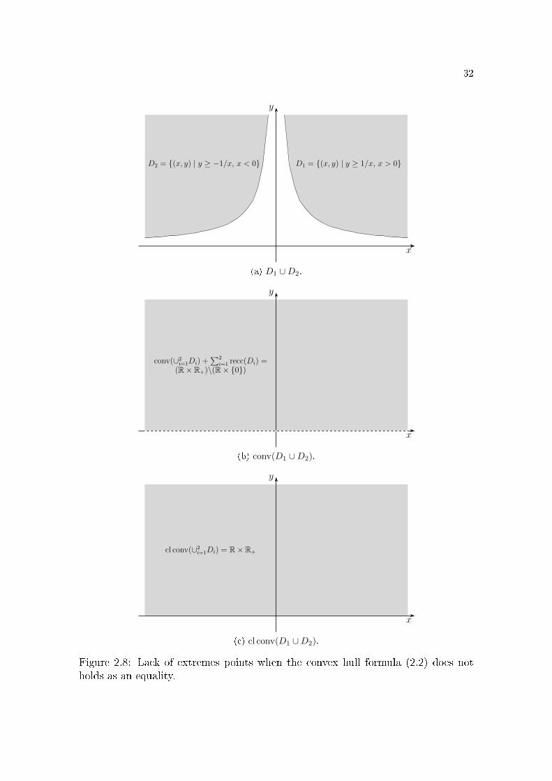
Curiously, if we don't have equality in formula (2.1) (page 9, then the convex

closure cl conv (⋃mi=1Di) has no extreme points. This will appear in the proof of the

Blessing of Extreme Points in chapter 7.

Corollary 2.12. (Lack of extreme points) Let D1, . . . , Dm be nonempty closed con-

vex sets. If we have strict inclusion in (2.2), that is, if

conv

(m⋃

i=1

Di

)+

m∑

i=1

recc(Di) ( cl conv

(m⋃

i=1

Di

), (2.3)

then cl conv (⋃mi=1Di) has no extreme points.

Proof. If condition (2.3) holds, then there are recession directions di ∈ recc(Di) such

that d1 + · · · dm = 0, but an opposite direction −dj does not belongs to recc(Dj),

32

x

y

D1 = {(x, y) | y ≥ 1/x, x > 0}D2 = {(x, y) | y ≥ −1/x, x < 0}

(a) D1 ∪D2.

conv(∪2i=1Di) +

∑2i=1 recc(Di) =

(R× R+)\(R× {0})

x

y

(b) conv(D1 ∪D2).

cl conv(∪2i=1Di) = R× R+

x

y

(c) cl conv(D1 ∪D2).

Figure 2.8: Lack of extremes points when the convex hull formula (2.2) does notholds as an equality.

33

for some j. Note that dj is not equal to 0, since the vector 0 belongs to every cone.

Moreover, we have that

−dj ∈m∑

i=1i 6=j

recc(Di).

Therefore, both vectors dj and −dj belong to the recession cone of cl conv (⋃mi=1Di),

and so cl conv (⋃mi=1Di) has no extreme points.

As in other cases, the same result for the polyhedral case always hold without

any additional regularity condition.

Theorem 2.13 (Closure of convex hull of union of polyhedra). Let P1, . . . , Pm be

nonempty polyhedra. Then,

conv

(m⋃

i=1

Pi

)+

m∑

i=1

recc(Pi) = cl conv

(m⋃

i=1

Pi

). (2.4)

In particular, the set cl conv (⋃mi=1 Pi) is a polyhedron with recession cone equal to

∑mi=1 recc(Pi).

Proof. Denote by P the set [conv (∪mi=1Pi) +∑m

i=1 recc(Pi)]. From Theorem 2.10

(page 27), we have the following inclusion

conv

(m⋃

i=1

Pi

)⊆ P ⊆ cl conv

(m⋃

i=1

Pi

),

so it is su�cient to prove that P is a closed set.

According to the Minkowiski-Weyl Theorem, each polyhedron Pi can be rep-

resented by a convex combination plus a positive combination of a �xed number of

vectors, denoted by {vi,r}kir=1 and {wi,s}lis=1, respectively. We claim that

P = conv

(m⋃

i=1

{vi,r}kir=1

)+ cone

(m⋃

i=1

{wi,s}lis=1

).

34

Indeed, let Q be the polyhedron of the right-hand side. Note that Q is a subset of

P , since

m⋃

i=1

{vi,r}kir=1 ⊂ conv

(m⋃

i=1

Pi

),

m⋃

i=1

{wi,s}lis=1 ⊂m∑

i=1

recc(Pi),

and the sets on the right-hand side are already convex conical, respectively. We

shall prove the opposite inclusion. Let x be a vector of P . Then, x has the form

x =m∑

i=1

λixi +m∑

i=1

αidi

=m∑

i=1

(ki∑

r=1

λi,rvi,r

)+

m∑

i=1

(li∑

s=1

αi,swi,s

).

for some vectors xi ∈ Pi, directions di ∈ recc(Pi) and scalars λi, λi,r, αi, αi,s ≥ 0,

such that∑

j λj =∑

j,r λj,r = 1. Therefore, x belongs to Q.

A similar result to Corollary 2.11 is also valid in the polyhedral case.

Corollary 2.14 (Common recession cone of polyhedra). Let P1, . . . , Pm be nonempty

polyhedra with a common recession cone, recc(Pi) = R, for all i = 1, . . . ,m. Then,

conv

(m⋃

i=1

Pi

)is a polyhedron,

and the corresponding recession cone is R.

Proof. From Corollary 2.11 (page 30), the set conv(∪mi=1Pi) is closed with recession

cone equal to R, and from Theorem 2.13 (page 33) we have that cl conv(∪mi=1Pi) is

a polyhedron.

35

3 OPTIMAL VALUE FUNCTIONS

3.1 More basic results on convex analysis

The ideas throughout this dissertation are described in terms of extended real

valued functions, i.e., functions that can take values −∞ and +∞ at some points. In

convex optimization, the extended real valued functions bring in important geomet-

ric insights that connect results from convex sets with those from convex functions.

They also provide a uni�ed framework to analyze convex optimization problems,

especially when the objective function may assume in�nite values, as in the case of

objective functions that are the pointwise supremum of a family of functions, e.g.,

the cost-to-go functions from a dynamic programming problem.

Traditional constrained optimization problems can be easily transformed into

unconstrained ones by using extended real value functions. Let f : Rn → R be a

function, and let X be a subset of Rn, and consider the problem of minimizing f

over X:minx f(x)s.t. x ∈ X.

Let us denote by δX the indicator function of X which is equal to 0 if x belongs to

X, or equal to +∞ otherwise:

δX(x) =

{0 if x ∈ X,

+∞ otherwise.

Then, the constrained problem is equivalent to minimizing f + δX over Rn. Using

this idea, we can always restrict our attention to the unconstrained minimization

of extended real valued functions. Next, we introduce some concepts that establish

the connections between extended real valued functions and sets.

36

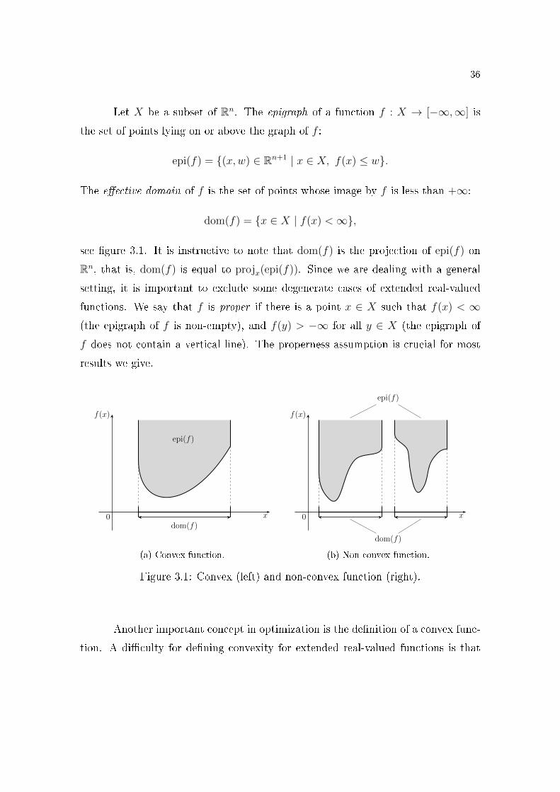
Let X be a subset of Rn. The epigraph of a function f : X → [−∞,∞] is

the set of points lying on or above the graph of f :

epi(f) = {(x,w) ∈ Rn+1 | x ∈ X, f(x) ≤ w}.

The e�ective domain of f is the set of points whose image by f is less than +∞:

dom(f) = {x ∈ X | f(x) <∞},

see �gure 3.1. It is instructive to note that dom(f) is the projection of epi(f) on

Rn, that is, dom(f) is equal to projx(epi(f)). Since we are dealing with a general

setting, it is important to exclude some degenerate cases of extended real-valued

functions. We say that f is proper if there is a point x ∈ X such that f(x) < ∞(the epigraph of f is non-empty), and f(y) > −∞ for all y ∈ X (the epigraph of

f does not contain a vertical line). The properness assumption is crucial for most

results we give.

f(x)

x0

epi(f)

dom(f)

(a) Convex function.

f(x)

x0

epi(f)

dom(f)

(b) Non-convex function.

Figure 3.1: Convex (left) and non-convex function (right).

Another important concept in optimization is the de�nition of a convex func-

tion. A di�culty for de�ning convexity for extended real-valued functions is that

37

they may assume both values −∞ and +∞, so the standard de�nition

f(αx+ (1− α)y) ≤ αf(x) + (1− α)f(y)

may result in unde�ned expression +∞ −∞. The epigraph provides an e�ective

and geometric way of dealing with this di�culty. We say that f : Rn → [−∞,∞]

is convex if epi(f) is a convex subset of Rn+1, see again �gure 3.1. It is a classical

result to show the following properties of operations on convex functions:

• Let f : Rn → [−∞,∞] be a convex function. The function αf is convex, for

any non-negative scalar α ≥ 0;

• Let f, g : Rn → (−∞,+∞] be two convex functions. The sum f + g is well

de�ned and convex;

• Let fi : Rn → [−∞,∞] be convex functions, for all i ∈ I. Then, the pointwisesupremum supi∈I fi(x) is also a convex function;

• Let D be a convex set. Then, the indicator function δD is a convex function.

So, we say that the four operations, respectively positive scaling, sums, pointwise

supremum and indicator are �convex-preserving operations�.

It is also worth mentioning that the level set of a convex function f ,

Lα = {x ∈ Rn | f(x) ≤ α},

is a convex set for every α ∈ R, since it is the projection in Rn of the convex set

epi(f) ∩(Rn × (−∞, α]

).

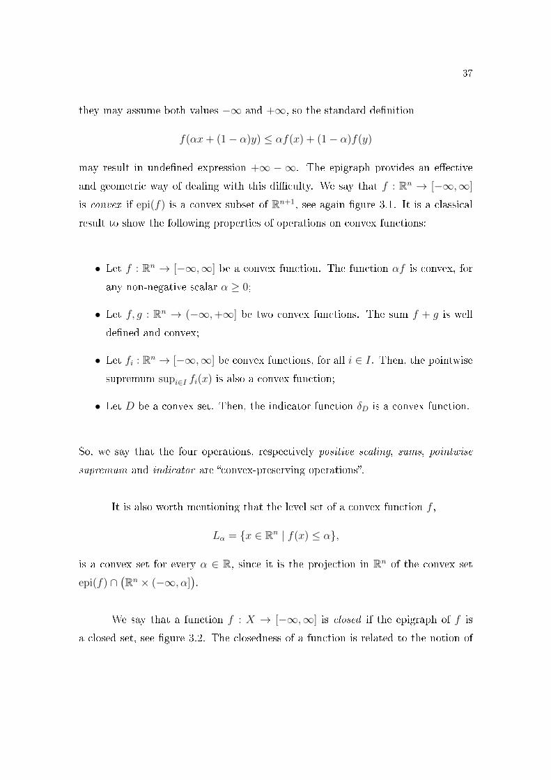
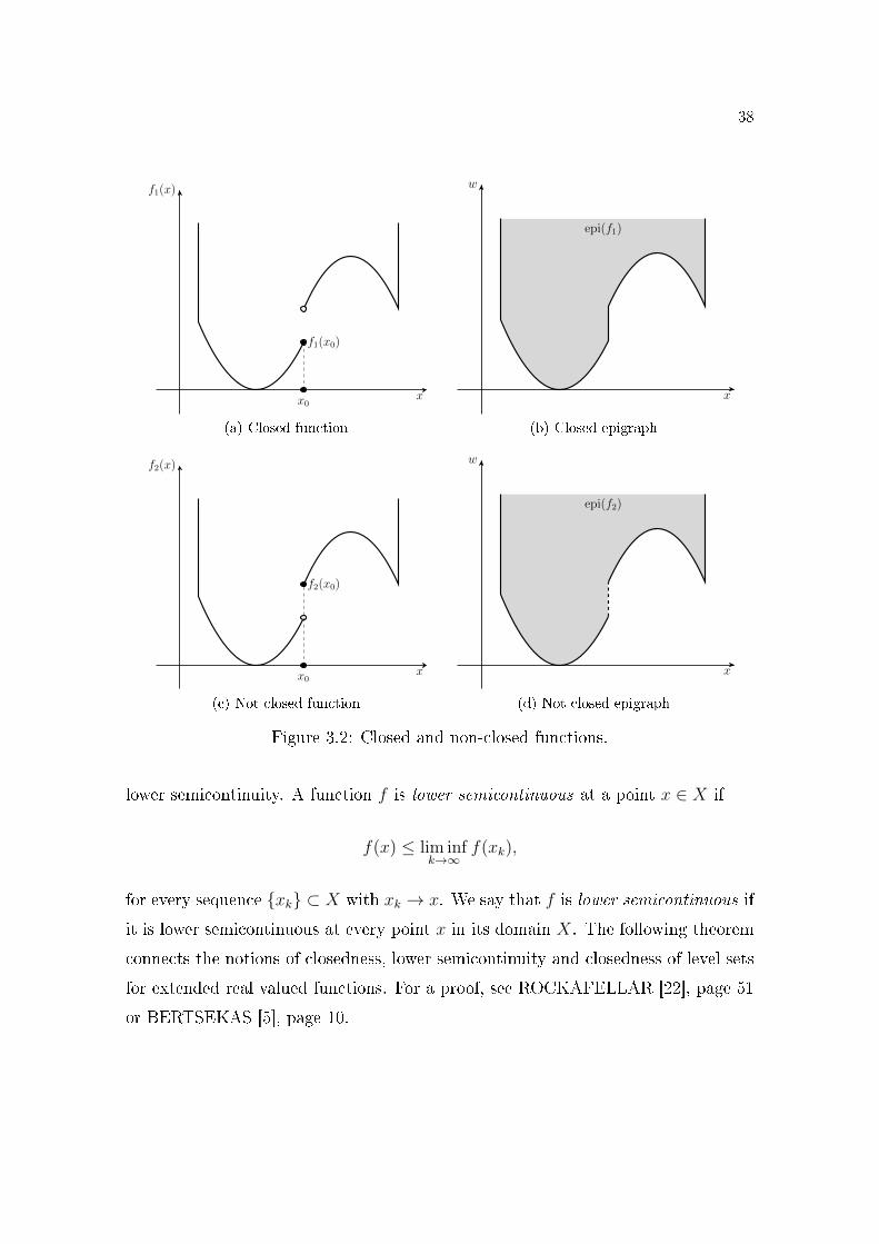
We say that a function f : X → [−∞,∞] is closed if the epigraph of f is

a closed set, see �gure 3.2. The closedness of a function is related to the notion of

38

x

f1(x)

f1(x0)

x0

(a) Closed function

x

w

epi(f1)

(b) Closed epigraph

x

f2(x)

f2(x0)

x0

(c) Not closed function

x

w

epi(f2)

(d) Not closed epigraph

Figure 3.2: Closed and non-closed functions.

lower semicontinuity. A function f is lower semicontinuous at a point x ∈ X if

f(x) ≤ lim infk→∞

f(xk),

for every sequence {xk} ⊂ X with xk → x. We say that f is lower semicontinuous if

it is lower semicontinuous at every point x in its domain X. The following theorem

connects the notions of closedness, lower semicontinuity and closedness of level sets

for extended real valued functions. For a proof, see ROCKAFELLAR [22], page 51

or BERTSEKAS [5], page 10.

39

Theorem 3.1 (Characterization of closed functions). Let f be an arbitrary function

from Rn to [−∞,∞]. Then the following conditions are equivalent:

a) f is lower semicontinuous throughout Rn;

b) {x ∈ Rn | f(x) ≤ α} is closed for every α ∈ R;

c) The epigraph of f is a closed set in Rn+1.

From this theorem, it is also not hard to show that the same 4 operations that

preserve convexity, also preserve closedness: for example, the pointwise supremum f

of closed functions fk is closed, since the epigraph epi(f) is the intersection of closed

epigraphs epi(fk), and therefore also closed. The same holds for positive scaling,

sums and the construction of indicator functions.

Another consequence, is that if f is a closed proper convex function, then the

epigraph epi(f) is a nonempty closed convex set.

As seen in section 2, an important concept from closed convex sets is the

recession cone. We also have an analogous notion for proper closed convex functions

that plays a central role in convex optimization. The recession cone of f is the set

of �horizontal directions� from the recession cone of the epigraph of f :

recc(f) = {d ∈ Rn | (d, 0) ∈ recc(epi(f))}.

In other words, a recession direction of a closed proper convex function f is a direc-

tion from Rn along which the function f �recedes�, that is, does not grow to in�nity.

The following theorem connects the notion of recession cone of a nonempty level set

and the recession cone of the corresponding proper closed convex function.

40

Theorem 3.2. Let f : Rn → (−∞,∞] be a closed proper convex function and

consider the level set

Vγ = {x ∈ Rn | f(x) ≤ γ}, γ ∈ R.

Then, all the nonempty level sets Vγ have the same recession cone:

recc(Vγ) = recc(f),

for all γ greater than infx∈Rn f(x).

The notion of recession directions of closed proper functions is an important

concept for analyzing existence of optimal solutions and optimal value functions

of convex programs, as we will see in Theorems 3.4 (page 44) and Theorem 3.11

(page 53). In particular, these results establish some su�cient conditions for the

optimal value function f of a special type of convex optimization problem to be a

closed proper convex function, namely for

f(b) = min F (x)s.t. g(x) ≤ b,

where F and g are closed proper convex functions. This is key to understanding the

properties of the cost-to-go functions of a dynamic programming problem.

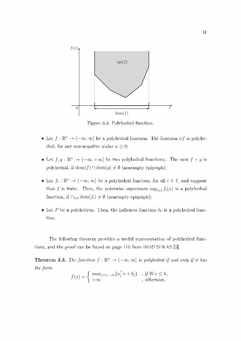
A particular class of extended real-valued functions that arise naturally as the

optimal value function from a linear program is the class of polyhedral functions. We

say that f is a polyhedral function if the epigraph of f is a nonempty polyhedron with

no negative vertical directions, see �gure 3.3. In particular, the function f is closed,

proper and convex. We have, again, the same 4 operations preserving polyhedral

functions. However, some care must be taken: since we must preserve its �nite

description, we don't allow in�nite index sets for supremum, and we also impose

regularity conditions so that the function does not become identically in�nite:

41

f(x)

x0

epi(f)

dom(f)

Figure 3.3: Polyhedral function.

• Let f : Rn → (−∞,∞] be a polyhedral function. The function αf is polyhe-

dral, for any non-negative scalar α ≥ 0;

• Let f, g : Rn → (−∞,+∞] be two polyhedral functions;. The sum f + g is

polyhedral, if dom(f) ∩ dom(g) 6= ∅ (nonempty epigraph);

• Let fi : Rn → (−∞,∞] be a polyhedral function, for all i ∈ I, and suppose

that I is �nite. Then, the pointwise supremum supi∈I fi(x) is a polyhedral

function, if ∩i∈I dom(fi) 6= ∅ (nonempty epigraph);

• Let P be a polyhedron. Then, the indicator function δP is a polyhedral func-

tion.

The following theorem provides a useful representation of polyhedral func-

tions, and the proof can be found on page 110 from BERTSEKAS [5].

Theorem 3.3. The function f : Rn → (−∞,∞] is polyhedral if and only if it has

the form

f(x) =

{maxj=1,...,m{a>j x+ bj} , if Wx ≤ h,+∞ , otherwise,

42

where aj are vectors in Rn, bj are scalars, m is a positive integer, W is a matrix,

and h is a vector such that dom(f) = {x ∈ Rn | Wx ≤ h}.

An example of polyhedral function is the linear function f(x) = c>x. We shall

see in Corollary 3.12 that the optimal value function of an optimization problem with

polyhedral objective function and linear constraints is also polyhedral. In particular,

the optimal value of a linear programming (LP) problem

f(b) = min c>xs.t. Ax ≤ b,

x ∈ Rn,

is also polyhedral. Those are important results for understanding properties of the

cost-to-go functions in the dynamic programming problem. In the general case, the

in�mum operation requires additional regularity conditions to preserve convexity

and closedness. We present those conditions in section 3.3,.

One last idea we will explore is the union of polyhedra which establishes a

connection between convex programming techniques and non-convex problems such

as mixed-integer linear programming problems (MILP). An optimal value function

f of a MILP is de�ned by

f(b) = minx,z c>x+ q>zs.t. Ax+Gz ≤ b,

(x, z) ∈ Rn × Zl,(3.1)

where the vectors and matrices have appropriate dimensions. Using Benders decom-

position BENDERS [4], we can represent f by the minimum of polyhedral functions

fz, f(b) = minz∈Zl fz(b), where each fz(b) is the optimal value function of a LP plus

a linear function:fz(b) = q>z + minx c>x

s.t. Ax ≤ b−Gz,x ∈ Rn.

43

From a geometric perspective, the epigraph of f is described by the union of the

epigraphs of all fz:

epi(f) = {(b, w) ∈ Rm+1 | f(b) ≤ w}= {(b, w) ∈ Rm+1 | fz(b) ≤ w, for some z ∈ Zl}=⋃

z∈Zl

epi(fz).

For simplicity, we restrict the analysis of optimal value functions of a MILP to prob-

lems in which the integer variable can only assume a �nite number of di�erent values.

In particular, we will focus on 0-1 MILP problems where the variable z from (3.1)

belongs to {0, 1}l, instead of Zl. Indeed, these MILP value functions belong to the

class of piecewise polyhedral function, which are the extended real-valued functions

f : Rn → (∞,∞] whose epigraph is a �nite union of polyhedra. Piecewise polyhe-

dral functions are also preserved by the same 4 operations of polyhedral functions:

positive scaling, sums of functions with intersecting domains, �nite maximum and

construction of indicator function. This last one is:

• Let P be a union of polyhedra. Then, the indicator function δP is a piecewise

polyhedral function.

We note that not every piecewise polyhedral function is an optimal value function

from a 0-1 MILP problem. The reason for that is related to Theorem 5.2 (page 98)

of chapter 5.

3.2 Existence of primal solutions

In this section we focus on regularity conditions for the existence of optimal

solutions. In convex optimization, even if the objective function is bounded below

44

or the corresponding in�mum is �nite, there is no guarantee that the minimum

will be achieved by a feasible solution. We present some su�cient conditions for

the existence of optimal solutions which are closely related to the idea of recessions

directions.

From this section onwards, we assume that the optimization problems have

�nite optimal value. In applications, this is a reasonable hypothesis since the capac-

ity to improve a system, reduce cost, or increase pro�t is usually limited. We seize

this occasion to present analogous results for MILPs, building upon the polyhedral

case.

We introduce the notion of lineality space of a set X and a function f for the

statement of the next result. The lineality space of a set X is recc(X)∩(− recc(X)),

and the lineality space of a function f is given by recc(f) ∩ (− recc(f)).

Theorem 3.4 (Existence of primal solution of convex problems). Let X be a closed

convex set, and let f : Rn → (−∞,∞] be a closed convex function with X∩dom(f) 6=∅. Assume that the optimal value of the problem

minx f(x)s.t. x ∈ X

is �nite, and the recession cones and lineality space of both X and f satisfy the

condition

recc(X) ∩ recc(f) = lineal(X) ∩ lineal(f).

Then the problem has at least one optimal solution.

Proof. Let p∗ be the optimal value. Note that p∗ 6= +∞, since X ∩ dom(f) in

nonempty. Let {γk} be a monotone scalar sequence with γk ↓ p∗ and denote

Vk = {x ∈ Rn | f(x) ≤ γk}.

45

The set X∩Vk is nonempty, by the in�mum property. We claim that the intersection

X∗ =∞⋂

k=1

(X ∩ Vk)

is nonempty. Indeed, let xk be the optimal solution of the following problem:

min ‖u‖s.t. u ∈ X ∩ Vk.

Since ‖ · ‖ has compact level sets and is strictly convex, the optimal solution xk

exists and is unique. Then, there are two possibilities for the sequence {xk}: it isbounded, or unbounded.

If {xk} is bounded, there is a subsequence that converges to x ∈ Rn. Since

{X∩Vk} is a sequence of decreasing nonempty closed sets, we have that x belongs to

X ∩ Vk, for all k. So, X∗ is nonempty. If {xk} is unbounded, there is a subsequence{xkj} such that

limj→∞

xkj‖xkj‖

= d ∈ recc(X) ∩ recc(f).

Let yk be the vector de�ned by xk − ‖xk‖d, and note that yk belongs to X ∩ Vk,for all k, since −d ∈ recc(X) ∩ recc(f), by hypothesis. We note that {‖ykj‖/‖xkj‖}converges to 0:

limj→∞

‖ykj‖‖xkj‖

= limj→∞

∥∥∥∥xkj‖xkj‖

− d∥∥∥∥ = 0.

In particular, for su�ciently large j, the norm ‖ykj‖ is smaller than ‖xkj‖, which is

a contradiction with the de�nition of xk.

The polyhedral case requires less regularity conditions to obtain the same

result. In an intuitive manner, the di�erence between both cases here is that the

boundary from a polyhedron di�ers from a straight line just �nite number of times,

while the boundary from a general convex set can be a smooth curve, and so the

optimal solution may diverge to in�nity. For instance, let f be the function

f(x) =

{1/x, if x > 0,

+∞, if x ≤ 0.

46

Then, the in�mum of f over R is equal to 0, however there is no x∗ ∈ R such that

f(x∗) = 0. Indeed, the recession cone of f is equal to R+, but the lineality space of

f is equal to {0}. So, f does not satisfy to the statement of Theorem 3.4.

Theorem 3.5 (Existence of primal solution of polyhedral problems). Let c be a

vector in Rn, A be a matrix in Rm×n and b be a vector in Rm. Assume that the

optimal value of the problemminx c>xs.t. Ax ≤ b,

x ∈ Rn

is �nite. Then the problem has at least one optimal solution.

The 0-1 mixed integer linear case is analogous to the polyhedral case, since

we can use the Benders decomposition to analyze the minimum of a �nite number

of polyhedral problems. This is the main idea for

Corollary 3.6 (Existence of primal solutions of mixed integer 0�1 programs). For

a standard 0-1 MILP,minx,z c>x+ q>z

s.t. Ax+Gz ≤ b,x ∈ Rn, z ∈ {0, 1}l,

if the optimal value is �nite, then there is at least one optimal solution.

Proof. For each binary solution z ∈ {0, 1}l, the corresponding LP is infeasible or

has �nite optimal value:minx c>x+ q>zs.t. Ax ≤ b−Gz,

x ∈ Rn.

Thus, each feasible LP has an optimal solution (Theorem 3.5). Since the original

problem is feasible, there is at least one LP that has �nite optimal value, and since

the number of possibilities for z is �nite, the in�mum for the mixed 0-1 program

corresponds to the lowest LP optimal value. Therefore, the optimal solution for the

47

0-1 MILP problem is the pair (x∗, z∗), where z∗ is the binary solution associated

with lowest LP optimal value and x∗ is the corresponding LP optimal solution.

A very important idea in mixed integer linear programming is to approx-

imate the convex hull of the feasible set. Under mild regularity conditions (see

Theorem 3.8, page 49), the convex hull of a MILP feasible set is a polyhedron and,

as we shall see below, the in�mum of a linear function over a set X equals the

in�mum of the same linear function over the convex hull of X. From theoretical

perspective, we rely on this equality to prove some results for MILPs based on results

from LPs, see Corollary 3.9 (page 50).

Algorithms for solving LPs are much faster than those for solving MILPs, but

an analytical expression of conv(X) is rarely available. In practice, many algorithms

for MILPs create outer approximations of conv(X) using cutting planes, and use that

to get lower bounds for the optimal value.

Lemma 3.7. Let c be a vector in Rn, and let X be a subset of Rn, not necessarily

convex. Then

infx∈conv(X)

c>x = infx∈X

c>x,

and if the in�mum is attained by an element of conv(X) it is also attained by some

element of X.

Proof. Let us denote by w the in�mum in the left-hand side and by w the in�mum

in the right-hand side. Note that w is less than or equal to w, since the convex hull

of X, conv(X), contains the original set X.

Let x ∈ conv(X). Then, x can be described by a convex combination of a

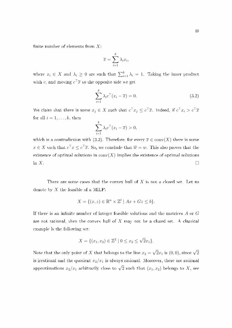
48

�nite number of elements from X:

x =k∑

i=1

λixi,

where xi ∈ X and λi ≥ 0 are such that∑k

i=1 λi = 1. Taking the inner product

with c, and moving c>x to the opposite side we get

k∑

i=1

λic>(xi − x) = 0. (3.2)

We claim that there is some xj ∈ X such that c>xj ≤ c>x. Indeed, if c>xi > c>x

for all i = 1, . . . , k, thenk∑

i=1

λic>(xi − x) > 0,

which is a contradiction with (3.2). Therefore, for every x ∈ conv(X) there is some

x ∈ X such that c>x ≤ c>x. So, we conclude that w = w. This also proves that the

existence of optimal solutions in conv(X) implies the existence of optimal solutions

in X.

There are some cases that the convex hull of X is not a closed set. Let us

denote by X the feasible of a MILP:

X = {(x, z) ∈ Rn × Zl | Ax+Gz ≤ b}.

If there is an in�nite number of integer feasible solutions and the matrices A or G

are not rational, then the convex hull of X may not be a closed set. A classical

example is the following set:

X = {(x1, x2) ∈ Z2 | 0 ≤ x2 ≤√

2x1}.

Note that the only point of X that belongs to the line x2 =√

2x1 is (0, 0), since√

2

is irrational and the quotient x2/x1 is always rational. Moreover, there are rational

approximations x2/x1 arbitrarily close to√

2 such that (x1, x2) belongs to X, see

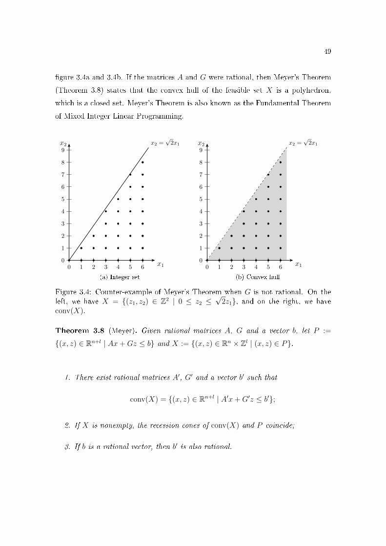
49

�gure 3.4a and 3.4b. If the matrices A and G were rational, then Meyer's Theorem

(Theorem 3.8) states that the convex hull of the feasible set X is a polyhedron,

which is a closed set. Meyer's Theorem is also known as the Fundamental Theorem

of Mixed Integer Linear Programming.

x1

x2

0 1 2 3 4 5 60

1

2

3

4

5

6

7

8

9x2 =

√2x1

(a) Integer set

x1

x2

0 1 2 3 4 5 60

1

2

3

4

5

6

7

8

9x2 =

√2x1

(b) Convex hull

Figure 3.4: Counter-example of Meyer's Theorem when G is not rational. On theleft, we have X = {(z1, z2) ∈ Z2 | 0 ≤ z2 ≤

√2z1}, and on the right, we have

conv(X).

Theorem 3.8 (Meyer). Given rational matrices A, G and a vector b, let P :=

{(x, z) ∈ Rn+l | Ax+Gz ≤ b} and X := {(x, z) ∈ Rn × Zl | (x, z) ∈ P}.

1. There exist rational matrices A′, G′ and a vector b′ such that

conv(X) = {(x, z) ∈ Rn+l | A′x+G′z ≤ b′};

2. If X is nonempty, the recession cones of conv(X) and P coincide;

3. If b is a rational vector, then b′ is also rational.

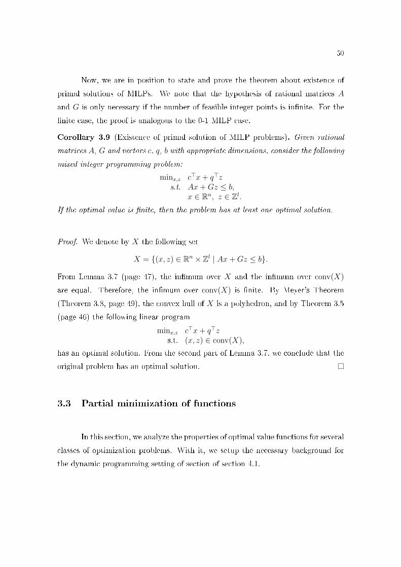
50

Now, we are in position to state and prove the theorem about existence of

primal solutions of MILPs. We note that the hypothesis of rational matrices A

and G is only necessary if the number of feasible integer points is in�nite. For the

�nite case, the proof is analogous to the 0-1 MILP case.

Corollary 3.9 (Existence of primal solution of MILP problems). Given rational

matrices A, G and vectors c, q, b with appropriate dimensions, consider the following

mixed integer programming problem:

minx,z c>x+ q>zs.t. Ax+Gz ≤ b,

x ∈ Rn, z ∈ Zl.If the optimal value is �nite, then the problem has at least one optimal solution.

Proof. We denote by X the following set

X = {(x, z) ∈ Rn × Zl | Ax+Gz ≤ b}.

From Lemma 3.7 (page 47), the in�mum over X and the in�mum over conv(X)

are equal. Therefore, the in�mum over conv(X) is �nite. By Meyer's Theorem

(Theorem 3.8, page 49), the convex hull of X is a polyhedron, and by Theorem 3.5

(page 46) the following linear program

minx,z c>x+ q>zs.t. (x, z) ∈ conv(X),

has an optimal solution. From the second part of Lemma 3.7, we conclude that the

original problem has an optimal solution.

3.3 Partial minimization of functions

In this section, we analyze the properties of optimal value functions for several

classes of optimization problems. With it, we setup the necessary background for

the dynamic programming setting of section of section 4.1.

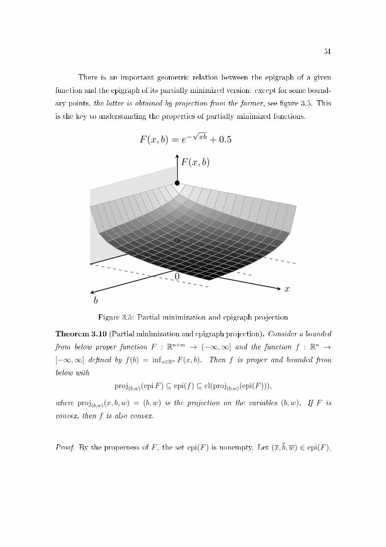
51

There is an important geometric relation between the epigraph of a given

function and the epigraph of its partially minimized version: except for some bound-

ary points, the latter is obtained by projection from the former, see �gure 3.5. This

is the key to understanding the properties of partially minimized functions.

bx

F (x, b)

infx≥0 F (x, b)

0.5

1.5

0

F (x, b) = e−√xb + 0.5

Figure 3.5: Partial minimization and epigraph projection

Theorem 3.10 (Partial minimization and epigraph projection). Consider a bounded

from below proper function F : Rn+m → (−∞,∞] and the function f : Rn →[−∞,∞] de�ned by f(b) = infx∈Rn F (x, b). Then f is proper and bounded from

below with

proj(b,w)(epiF ) ⊆ epi(f) ⊆ cl(proj(b,w)(epi(F ))),

where proj(b,w)(x, b, w) = (b, w) is the projection on the variables (b, w). If F is

convex, then f is also convex.

Proof. By the properness of F , the set epi(F ) is nonempty. Let (x, b, w) ∈ epi(F ),

52

and note that

f(b) = infx∈Rn

F (x, b) ≤ F (x, b) ≤ w.

Thus (b, w) belongs to epi(f). In particular, epi(f) is nonempty and f is a proper

function, since F is bounded from below. Note that for any (b, w) ∈ epi(f) and

every k, there is x ∈ Rn such that

infx∈Rn

F (x, b) ≤ F (x, b) ≤ infx∈Rn

F (x, b) +1

k≤ w +

1

k.

Then, we have (x, b, w + 1/k) ∈ epi(F ), which implies that (b, w + 1/k) belongs to

proj(b,w)(epi(F )) and (b, w) belongs to cl(proj(b,w)(epi(F )).

If F is convex, let (b, w) and (b, w) be two points in epi(f). Then, there exist

sequences {xk} and {xk} such that

F (xk, b)→ f(b) ≤ w, F (xk, b)→ f(b) ≤ w.

Using the de�nition of f and the convexity of F , we have for all α ∈ [0, 1] and k

f(αb+ (1− α)b) ≤ F (αxk + (1− α)xk, αb+ (1− α)b)

≤ αF (xk, b) + (1− α)F (xk, b).

By taking the limit as k →∞, we obtain

f(αb+ (1− α)b) ≤ αf(b) + (1− α)f(b) ≤ αw + (1− α)w.

It follows that the point α(b, w) + (1 − α)(b, w) belongs to epi(f). Thus epi(f) is

convex, implying that f is convex.

We now provide a criteria for the closedness of partial minimization of a

closed convex function F . If we guarantee that the projection of epi(F ) is closed,

then according to Theorem 3.10, the partial minimized function f is also closed. We

resort to Theorem 2.6 about closedness of closed convex under linear transformation

to prove that proj(b,w)(epi(F )) is closed.

53

The following theorem is a version �with parameters� of Theorem 3.4 (page 44)

on the existence of primal optimal solutions. Analogously, we still have an hypoth-

esis of equality of lineality spaces and recession cones.

Theorem 3.11 (Optimal value of convex functions). Let F : Rn+m → (−∞,∞] be

a bounded below closed proper convex function, and let f be the function de�ned by

f(b) = infx∈Rn

F (x, b), for b ∈ Rm.

Assume that for some b ∈ Rm and γ ∈ R the set

Lb,γ := {x ∈ Rn | F (x, b) ≤ γ}

is nonempty and its recession cone is equal to its lineality space. Then f is closed

(proper, convex and bounded below). Furthermore, for each b ∈ dom(f), the set of

minima in the de�nition of f(b) is nonempty.

Proof. From Theorem 3.10, the function f is proper convex and bounded below,

and the epigraph of f also satis�es the following relation:

proj(b,w)(epi(F )) ⊆ epi(f) ⊆ cl(proj(b,w)(epi(F )).

Thus, we only need to prove that the projection of epi(F ) in the (b, w) variables is

closed. Let us denote by A the projection on the variable (b, w). By Theorem 2.6,

if the following condition is satis�ed:

ker(A) ∩ recc(epi(F )) ⊆ lineal(epi(F )),

then the set A epi(F ) is closed and its recession cone is equal to A recc(epi(F )). Note

that A can be represented in the following matrix form:

A =

[0 I 00 0 1

].

54

Therefore the kernel of A is equal to {(dx, 0, 0) ∈ Rn+m+1 | dx ∈ Rn}, so the

intersection ker(A)∩ recc(epi(F )) is given by the recession directions of epi(F ) with

the form (dx, 0, 0). From the de�nition of the recession cone:

recc(F ) = {(dx, db) ∈ Rn+m | (dx, db, 0) ∈ recc(epi(F ))}.

Since the b-variable is �xed, the recession cone and lineality space of Fb := F (b, ·)are given by

recc(Fb) = {dx ∈ Rn | (dx, 0, 0) ∈ recc(epi(F ))}= ker(A) ∩ recc(epi(F )),

lineal(Fb) = {dx ∈ Rn | (dx, 0, 0) ∈ lineal(epi(F ))}= ker(A) ∩ lineal(epi(F )).

From theorem 3.2 (page 40), the recession cone and the lineality space of Lb,γ equals

recc(Fb) and lineal(Fb), respectively, and from the hypothesis on Lb,γ, recc(Fb) is

equal to lineal(Fb). Then, we have

ker(A) ∩ recc(epi(F )) = ker(A) ∩ lineal(epi(F )) ⊆ lineal(epi(F )).

From Theorem 2.6 (page 21), we conclude that A epi(F ) is closed with recession

cone equal to A recc(epi(F )).

To prove the last claim, note that for all b ∈ dom(f) the problem

minx Fb(x)s.t. x ∈ Rn,

has an optimal solution, since the level sets Lb,γ have all the same recession cone,

which implies that the recession cone of Fb is equal to its lineality space (Theo-

rem 3.4, page 44).

In the polyhedral case the result is trivial, since projection of a polyhedron

is always a polyhedron. Note that the boundness assumption on F is important to

ensure the existence of a x-optimal solution.

55

Corollary 3.12 (Optimal value of polyhedral functions). Let F : Rn+m → (−∞,∞]

be a bounded below polyhedral function, and let f be the function de�ned by

f(b) = infx∈Rn

F (x, b), b ∈ Rn.

Then f is polyhedral and bounded below. Furthermore, for each b ∈ dom(f), the set

of minima in the de�nition of f(b) is nonempty.

Proof. This Corollary follows from Theorem 3.10 (page 51) and the fact that pro-

jection of polyhedron is also polyhedron, see Corollary 2.9 (page 26). Moreover, the

existence of optimal solution is guaranteed by Theorem 3.5.

The closedness of a 0-1 MILP optimal value function f can be proved us-

ing the closedness of partial minimization of polyhedral functions. Actually, the

epigraph of f is a �nite union of polyhedrons.

Corollary 3.13 (Optimal value of mixed integer 0�1 programs). Let A, G be ma-

trices and c, q, b be vectors, with appropriate dimensions. Assume that the optimal

value of the following 0-1 mixed integer linear program

f(b) = minx,z c>x+ q>zs.t. Ax+Gz ≤ b,

x ∈ Rn, z ∈ {0, 1}l

is bounded below, for all b ∈ dom(f). Suppose also that dom(f) is nonempty. Then

f piecewise polyhedral. Furthermore, for each b ∈ dom(f), the set of minima in the

de�nition of f(b) is nonempty.

Proof. Let zi ∈ {0, 1}l. The function f is the minimum of a �nite number of

polyhedral functions fi:

fi(b) = minx c>x+ q>zis.t. Ax ≤ b−Gzi,

x ∈ Rn.

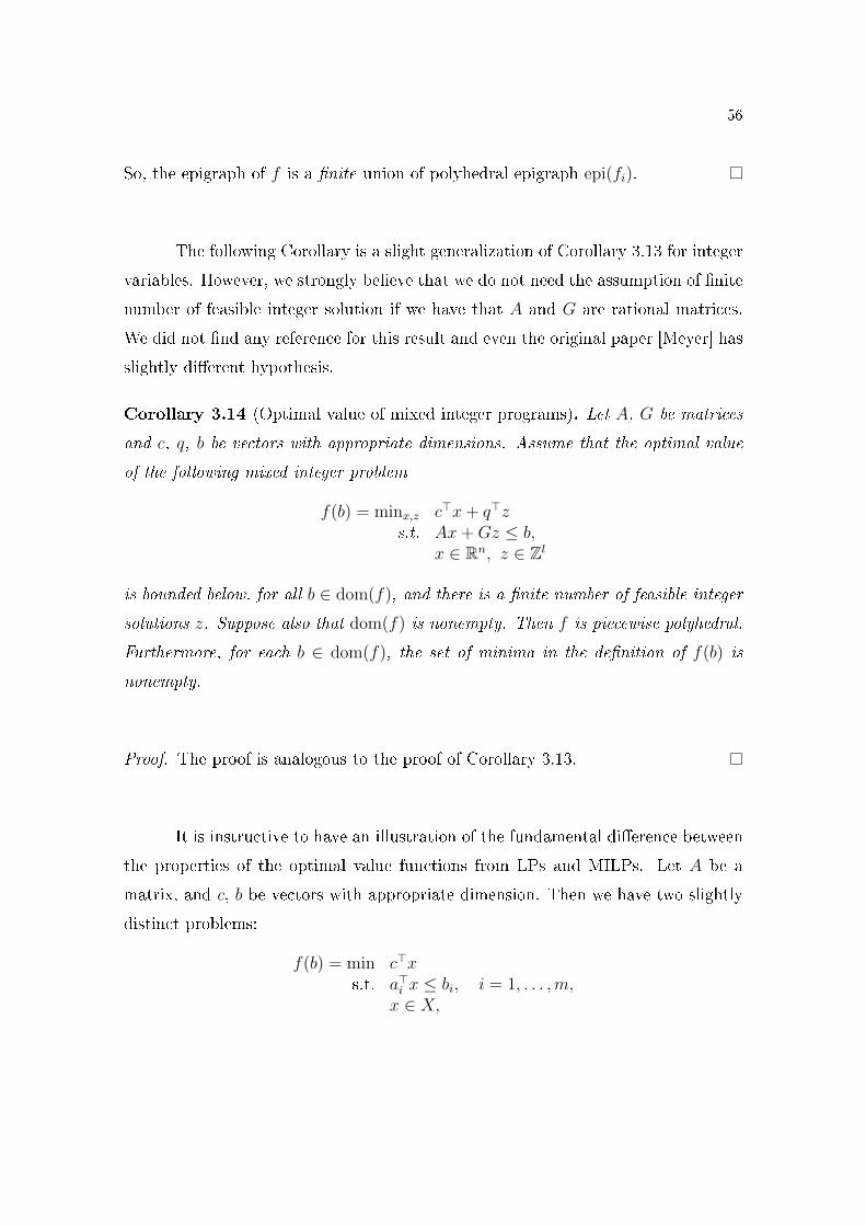
56

So, the epigraph of f is a �nite union of polyhedral epigraph epi(fi).

The following Corollary is a slight generalization of Corollary 3.13 for integer

variables. However, we strongly believe that we do not need the assumption of �nite

number of feasible integer solution if we have that A and G are rational matrices.

We did not �nd any reference for this result and even the original paper [Meyer] has

slightly di�erent hypothesis.

Corollary 3.14 (Optimal value of mixed integer programs). Let A, G be matrices

and c, q, b be vectors with appropriate dimensions. Assume that the optimal value

of the following mixed integer problem

f(b) = minx,z c>x+ q>zs.t. Ax+Gz ≤ b,

x ∈ Rn, z ∈ Zl

is bounded below, for all b ∈ dom(f), and there is a �nite number of feasible integer

solutions z. Suppose also that dom(f) is nonempty. Then f is piecewise polyhedral.

Furthermore, for each b ∈ dom(f), the set of minima in the de�nition of f(b) is

nonempty.

Proof. The proof is analogous to the proof of Corollary 3.13.

It is instructive to have an illustration of the fundamental di�erence between

the properties of the optimal value functions from LPs and MILPs. Let A be a

matrix, and c, b be vectors with appropriate dimension. Then we have two slightly

distinct problems:

f(b) = min c>xs.t. a>i x ≤ bi, i = 1, . . . ,m,

x ∈ X,

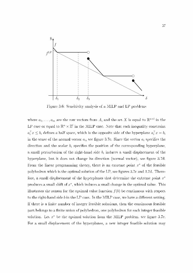
57

δ

$

fLP

f

δ1 δ2 δ3

Figure 3.6: Sensitivity analysis of a MILP and LP problems

where a1, . . . , am are the row vectors from A, and the set X is equal to Rn+l in the

LP case or equal to Rn×Zl in the MILP case. Note that each inequality constraint

a>i x ≤ bi de�nes a half space, which is the opposite side of the hyperplane a>i x = bi

in the sense of the normal vector ai, see �gure 3.7c. Since the vector ai speci�es the

direction and the scalar bi speci�es the position of the corresponding hyperplane,

a small perturbation of the right-hand side bi induces a small displacement of the

hyperplane, but it does not change its direction (normal vector), see �gure 3.7d.

From the linear programming theory, there is an extreme point x∗ of the feasible

polyhedron which is the optimal solution of the LP, see �gures 3.7c and 3.7d. There-

fore, a small displacement of the hyperplanes that determine the extreme point x∗

produces a small shift of x∗, which induces a small change in the optimal value. This

illustrates the reason for the optimal value function f(b) be continuous with respect

to the right-hand side b in the LP case. In the MILP case, we have a di�erent setting.

If there is a �nite number of integer feasible solutions, then the continuous feasible

part belongs to a �nite union of polyhedron, one polyhedron for each integer feasible

solution. Let x∗ be the optimal solution from the MILP problem, see �gure 3.7e.

For a small displacement of the hyperplanes, a new integer feasible solution may

58

or may not be created. If there is no additional integer solution, then the analysis

is analogous to the LP case. If a new integer solution is created, it could produce

a sudden drop in the optimal value if the cost component in the integer direction

is su�ciently smaller than the cost component in the continuous direction, see �g-

ure 3.7f. This illustrates why in the MILP case the optimal value function f(b) is

piecewise continuous with respect to the right-hand side b, with sudden drops at the

discontinuity points.

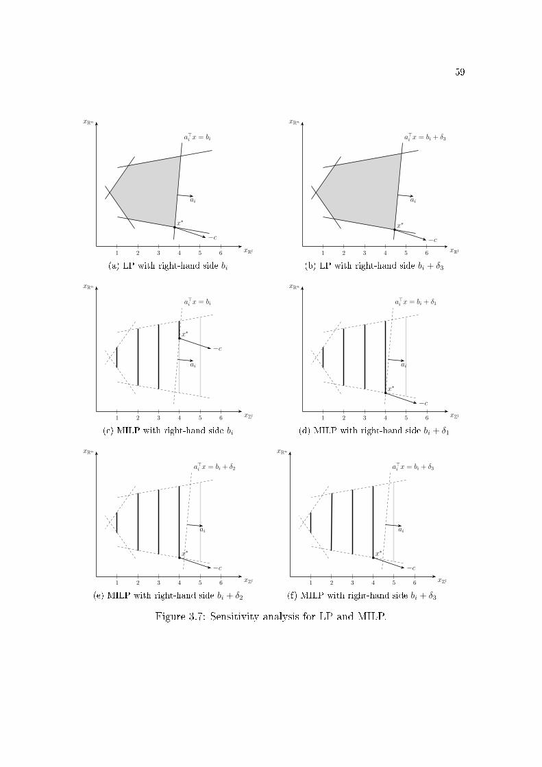
59

xRl

xRn

a>i x = bi

ai

−c

x∗

1 2 3 4 5 6

(a) LP with right-hand side bi

xRl

xRn

a>i x = bi + δ3

ai

−c

x∗

1 2 3 4 5 6

(b) LP with right-hand side bi + δ3

xZl

xRn

a>i x = bi

ai

−c

x∗

1 2 3 4 5 6

(c) MILP with right-hand side bi

xZl

xRn

a>i x = bi + δ1

ai

−c

x∗

1 2 3 4 5 6

(d) MILP with right-hand side bi + δ1

xZl

xRn

a>i x = bi + δ2

ai

−c

x∗

1 2 3 4 5 6

(e) MILP with right-hand side bi + δ2

xZl

xRn

a>i x = bi + δ3

ai

−c

x∗

1 2 3 4 5 6

(f) MILP with right-hand side bi + δ3

Figure 3.7: Sensitivity analysis for LP and MILP.

60

3.4 Conjugacy, Duality and Lagrangian Relaxation

This section is about convex regularization of general functions and its re-

lationship with Lagrangian Duality. We introduce a geometrical point of view to

explain why support hyperplanes are the suitable objects to obtain convex hulls, the

Conjugacy operation as a natural transformation to convexify a function, and an

interpretation of Weak and Strong Duality in terms of the convex regularization of

the primal optimal value function. In this last part, we also show the relationship

between the biconjugate operation and the Lagrangian Relaxation of optimization

problems.

Let D be a closed convex set. We note that D can be described as the

intersection of all closed half spaces H that contains it, where the half space H is

speci�ed by a hyperplane tangent to D, called support hyperplane. Thus, the family

of all support hyperplanes to D is su�cient to describe the points of D. We have

two possibilities to parameterize support hyperplanes:

1. We can provide the boundary points x from D and then obtain the support

hyperplane to D on x; or

2. We may specify a normal vector ~v and then obtain the support hyperplane

with that given orthogonal vector to ~v.

This second approach is the key to generate the convex regularization of a non-

convex function.

Let f be a bounded below function, and assume that f is non-convex, i.e.,

the epigraph of f is a non-convex set. Let y ∈ Rn be a vector, and let ry,x0 be the

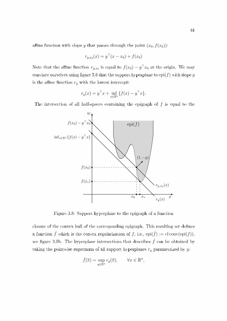
61

a�ne function with slope y that passes through the point (x0, f(x0)):

ry,x0(x) = y>(x− x0) + f(x0)

Note that the a�ne function ry,x0 is equal to f(x0) − y>x0 at the origin. We may

convince ourselves using �gure 3.8 that the support hyperplane to epi(f) with slope y

is the a�ne function ry with the lowest intercept:

ry(x) = y>x+ infx∈Rn{f(x)− y>x}.

The intersection of all half-spaces containing the epigraph of f is equal to the

x

w

x∗x0

f(x0)− y>x0

infx∈Rn{f(x)− y>x}

epi(f)

f(x0)

f(x∗)ry,x0(x)

ry(x)

(1,−y)

Figure 3.8: Support hyperplane to the epigraph of a function

closure of the convex hull of the corresponding epigraph. This resulting set de�nes

a function f which is the convex regularization of f , i.e., epi(f) := cl conv(epi(f)),

see �gure 3.9b. The hyperplane intersections that describes f can be obtained by

taking the pointwise supremum of all support hyperplanes ry parametrized by y:

f(x) = supy∈Rn

ry(x), ∀x ∈ Rn,

62

see �gure 3.9a.

A related notion to the convex regularization is the conjugate function. It is

de�ned, for all y ∈ Rn, by

f ∗(y) = supx∈Rn

{y>x− f(x)}. (3.3)

Note that −f ∗(y) is the intercept of the support hyperplane with slope y. Then,

the convex regularization f can be written as

f(x) = supy∈Rn

{y>x− f ∗(y)} = f ∗∗(x),

in other words, the biconjugate of f is equal to the convex regularization f .

The function f ∗ is always a closed convex function, since its epigraph is the

intersection of closed half spaces

Hx = {(y, w) ∈ Rn+1 | x>y − f(x) ≤ w}

parametrized by x ∈ Rn. However, f ∗ can be proper or improper. Below, Theo-

rem 3.15 states some other properties of the conjugate and biconjugate function. If

f is proper and bounded below, then f is also proper and bounded below. When f

is not proper, the functions f ∗∗ and f may not coincide. For unbounded below func-

tions, f may be improper, even if f is proper. For instance, the function f(x) = −|x|is proper, but the convex regularization is not: f ≡ −∞.

Theorem 3.15 (Conjugacy Theorem). Let f : Rn → R be a function, let f ∗ be its

conjugate, and consider the biconjugate f ∗∗. Then:

1. For all x ∈ Rn,

f(x) ≥ f ∗∗(x).

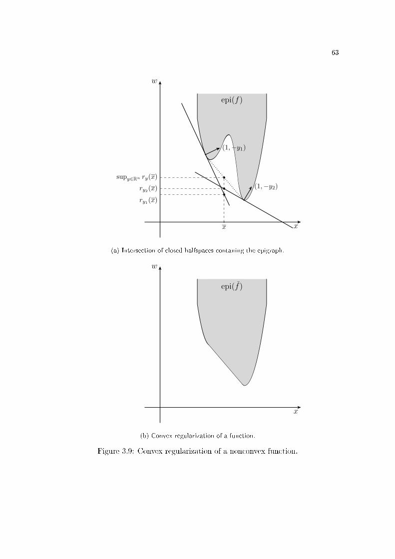
63

x

w

(1,−y1)

(1,−y2)

epi(f)

x

ry1(x)

ry2(x)

supy∈Rn ry(x)

(a) Intersection of closed halfspaces contaning the epigraph.

x

w

epi(f)

(b) Convex regularization of a function.

Figure 3.9: Convex regularization of a nonconvex function.

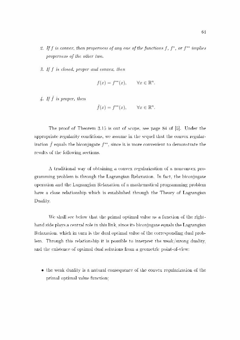
64

2. If f is convex, then properness of any one of the functions f , f ∗, or f ∗∗ implies

properness of the other two.

3. If f is closed, proper and convex, then

f(x) = f ∗∗(x), ∀x ∈ Rn.

4. If f is proper, then

f(x) = f ∗∗(x), ∀x ∈ Rn.

The proof of Theorem 3.15 is out of scope, see page 84 of [5]. Under the

appropriate regularity conditions, we assume in the sequel that the convex regular-

ization f equals the biconjugate f ∗∗, since it is more convenient to demonstrate the

results of the following sections.

A traditional way of obtaining a convex regularization of a nonconvex pro-

gramming problem is through the Lagrangian Relaxation. In fact, the biconjugate

operation and the Lagrangian Relaxation of a mathematical programming problem

have a close relationship which is established through the Theory of Lagrangian

Duality.

We shall see below that the primal optimal value as a function of the right-

hand side plays a central role in this link, since its biconjugate equals the Lagrangian

Relaxation, which in turn is the dual optimal value of the corresponding dual prob-

lem. Through this relationship it is possible to interpret the weak/strong duality,

and the existence of optimal dual solutions from a geometric point-of-view:

• the weak duality is a natural consequence of the convex regularization of the

primal optimal value function;

65

• strong duality occurs when such regularization does not creates a gap with the

primal optimal value function; and

• the optimal dual solution is a derivative of the convex regularization of the

primal optimal value function.

These ideas are important to understand the Benders cut of SDDP and the La-

grangian cuts of SDDiP in a uni�ed way.

Let f : Rn → R, h : Rn → Rm and g : Rn → Rl be real-valued functions, and

let D be a subset of Rn. Consider the following optimization problem:

p(b, c) = minx f(x)s.t. h(x) = b,

g(x) ≤ c,x ∈ D,

(3.4)

where p(b, c) is the primal optimal value as a function of the right-hand sides (RHS)

b ∈ Rm and c ∈ Rl. The Lagrangian function L(x, λ, µ) is de�ned by

L(x, λ, µ) = f(x) + λ>(h(x)− b) + µ>(g(x)− c),

the dual function is de�ned by

φ(λ, µ) =

{infx∈D L(x, λ, µ) if λ ∈ Rm and µ ∈ Rl

+,

−∞ otherwise,

and the dual problem is given by

max φ(λ, µ)s.t. λ ∈ Rm,

µ ∈ Rl.

The optimal value function of the dual problem, denoted by w(b, c), is a function

of the right-hand side parameters b and c. The dual problem is also called the

Lagrangian Relaxation, when the primal one is a MILP. In this context, we refer to

66

w(b, c) as the Lagrangian Relaxation function. The weak duality is the property of

w(b, c) being less than or equal to p(b, c), and the strong duality is when both are

equal. The weak duality holds for all RHS pair (b, c) ∈ Rm+l, but strong duality

usually requires additional regularity conditions (Slater condition, for instance).

We shall prove below the connection between the Lagrangian Relaxation and

the biconjugate of the primal optimal value function p(b, c). For this purpose, we

have to represent the dual function φ(λ, µ) in the following form:

φ(λ, µ) = infx,b,c {f(x) + λ>(b− b) + µ>(c− c)}s.t. h(x) = b

g(x) ≤ cx ∈ D.

(3.5)

Indeed, if µ has a negative component, then φ(λ, µ) is equal to −∞, and so is the

right-hand side of the equation (3.5), since we can increase arbitrarily the corre-

sponding component of c. If all components of µ are non-negative, then increasing

c also increases the objective function f(x) + λ>(b − b) + µ>(c − c). So, the op-

timal solution for c is g(x). Since b is equal to h(x), the right-hand side of (3.5)

equals infx∈D L(x, λ, µ). Therefore, dual function φ(λ, µ) can be represented in the

form (3.5).

By changing the minimization order of (3.5), we can restate the dual function

φ(λ, µ) in terms of the conjugate of p(b, c):

φ(λ, µ) = infb,c

{infx∈D,h(x)=b,g(x)≤c.

{f(x)

}+ λ>(b− b) + µ>(c− c)

}

= infb,c{p(b, c) + λ>b+ µ>c} − λ>b− µ>c

= −p∗(−λ,−µ)− λ>b− µ>c.

The dual optimal solution w(b, c) is the supremum of φ(λ, µ) on (λ, µ), which is the

67

biconjugate of p(b, c):

supλ,µ

φ(λ, µ) = supλ,µ{−p∗(−λ,−µ) + (−λ,−µ)>(b, c)}

= supλ,µ{(λ, µ)>(b, c)− p∗(λ, µ)} = p∗∗(b, c),

where the second equality is obtained by changing (−λ,−µ) for (λ, µ), respectively.

Therefore, Weak Duality occurs because the biconjugate p∗∗(b, c) of the primal op-

timal value function p(b, c) is always a lower bound, for every pair (b, c), and Strong

Duality occurs when there is no gap between the convex regularization p∗∗(b, c) and

the primal optimal function p(b, c). We note that the dual optimal solutions (λ, µ)

are the maximizers in the de�nition of the biconjugate p∗∗(b, c):

(λ, µ) ∈ arg maxλ,µ

φ(λ, µ) ⇐⇒ (−λ,−µ) ∈ arg maxλ,µ{(λ, µ)>(b, c)− p∗(λ, µ)}.

(3.6)

This is an important remark for computing �derivatives� in section 3.5.

The following results characterize the biconjugate of the primal optimal value

function for convex, polyhedral and MILP problems. We recall that when the primal

optimal value function equals the corresponding biconjugate, then we have strong

duality.

Corollary 3.16 (Biconjugate of convex optimal value function). Let F : Rn+m →(−∞,∞] be a bounded below closed proper convex function, and let f be the function

de�ned by partial minimization

f(b) = infx∈Rn

F (x, b), b ∈ Rn.

Assume that for some b ∈ Rn and γ ∈ R the set

Lb,γ = {x ∈ Rm | F (x, b) ≤ γ}

is nonempty and its recession cone is equal to its lineality space. Then the biconjugate

function f ∗∗ is equal to f .

68

Proof. From Theorem 3.11, we have that f is a closed proper convex function, and

from Theorem 3.15 item (c) we have that the biconjugate of a closed proper convex

function is equal to the original function.

Corollary 3.17 (Biconjugate of polyhedral optimal value function). Let F : Rn+m →(−∞,∞] be a bounded below polyhedral function, and let f be the function de�ned

by partial minimization

f(b) = infx∈Rn

F (b, x), b ∈ Rn.

Then the biconjugate function f ∗∗ is equal to f .

Proof. From Corollary 3.12 we have that f is a polyhedral function, and from The-

orem 3.15 item (c) we conclude that f ∗∗ is equal to f .

The following characterization of the biconjugate of a MILP problem is an

important an important result for the Blessing of Binary from the SDDiP, see sec-

tion 6.2.

Corollary 3.18 (Optimal value of mixed integer programs). Let A, G be rational

matrices, and c, q, b be vectors with appropriate dimensions, and X ⊂ Rn × Zl

be a set such that conv(X) is a polyhedron. Assume that the optimal value of the

following mixed integer program

f(b) = minx,z c>x+ q>zs.t. Ax+Gz ≤ b,

(x, z) ∈ X,

is bounded below, for all b ∈ dom(f). Suppose also that dom(f) is nonempty. Then

the biconjugate of f is equal to

f ∗∗(b) = minx,z c>x+ q>zs.t. Ax+Gz ≤ b,

(x, z) ∈ conv(X).

69

Proof. Denote by f(b) the optimal value function from the problem with con-

straint conv(X). Let φ(µ) and φ(µ) be the dual functions from the corresponding

problems with constraint X and conv(X), respectively:

φ(µ) = inf(x,z)∈X

{c>x+ q>z + µ>(Ax+Gz − b)},

φ(µ) = inf(x,z)∈conv(X)

{c>x+ q>z + µ>(Ax+Gz − b)},

for all µ ≥ 0. By Lemma 3.7, we have that φ = φ, and since the biconjugate of

an optimal value function is equal to the corresponding dual optimal value we have

that

f ∗∗(b) = supµ≥0

φ(µ) = supµ≥0

φ(µ) = f∗∗

(b).

Since f is polyhedral, we conclude that

f∗∗

= f.

3.5 Subgradient, chain rule and optimality condition

In this section, we present a more general notion of derivative, the subgradi-

ent, that is crucial for algorithms that solve non-di�erentiable convex programming

problems. We also show how to compute subgradients of optimal value functions, the

chain rule for some convex preserving compositions and some optimality conditions.

Let f : Rn → (−∞,∞] be a proper convex function. We say that a vector

g ∈ Rn is a subgradient of f at a point x ∈ dom(f) if

f(y) ≥ f(x) + g>(y − x), ∀y ∈ Rn.

The set of all subgradients of f at x is called the subdi�erential of f at x and is

denoted by ∂f(x). By convention, ∂f(x) is considered empty for all x /∈ dom(f).

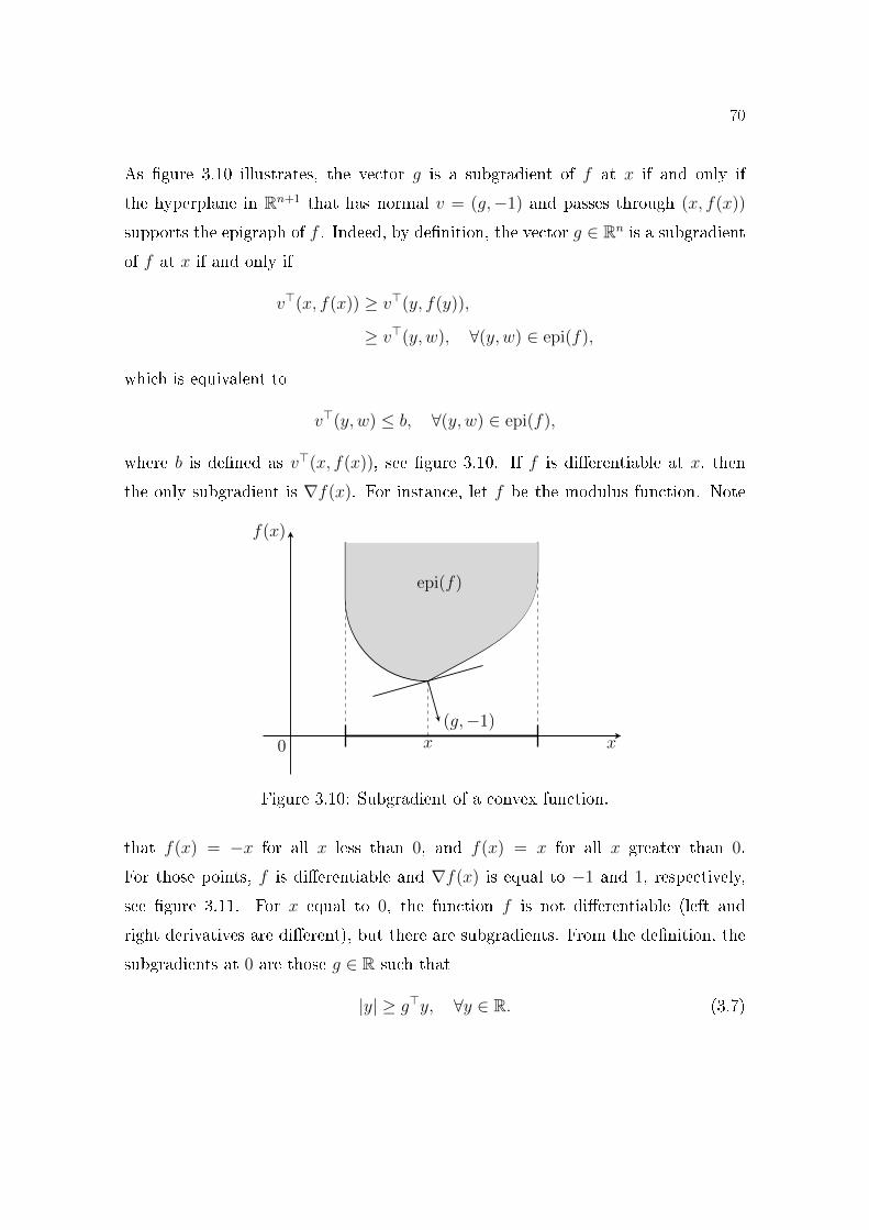
70

As �gure 3.10 illustrates, the vector g is a subgradient of f at x if and only if

the hyperplane in Rn+1 that has normal v = (g,−1) and passes through (x, f(x))

supports the epigraph of f . Indeed, by de�nition, the vector g ∈ Rn is a subgradient

of f at x if and only if

v>(x, f(x)) ≥ v>(y, f(y)),

≥ v>(y, w), ∀(y, w) ∈ epi(f),

which is equivalent to

v>(y, w) ≤ b, ∀(y, w) ∈ epi(f),

where b is de�ned as v>(x, f(x)), see �gure 3.10. If f is di�erentiable at x, then

the only subgradient is ∇f(x). For instance, let f be the modulus function. Note

f(x)

x0

epi(f)

x(g,−1)

Figure 3.10: Subgradient of a convex function.

that f(x) = −x for all x less than 0, and f(x) = x for all x greater than 0.

For those points, f is di�erentiable and ∇f(x) is equal to −1 and 1, respectively,

see �gure 3.11. For x equal to 0, the function f is not di�erentiable (left and

right derivatives are di�erent), but there are subgradients. From the de�nition, the

subgradients at 0 are those g ∈ R such that

|y| ≥ g>y, ∀y ∈ R. (3.7)

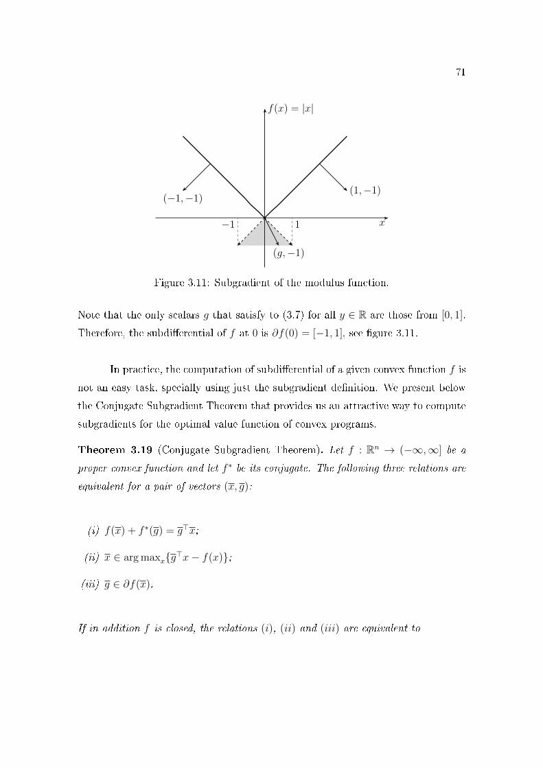
71

(1,−1)(−1,−1)

1−1

(g,−1)

f(x) = |x|

x

Figure 3.11: Subgradient of the modulus function.

Note that the only scalars g that satisfy to (3.7) for all y ∈ R are those from [0, 1].

Therefore, the subdi�erential of f at 0 is ∂f(0) = [−1, 1], see �gure 3.11.

In practice, the computation of subdi�erential of a given convex function f is

not an easy task, specially using just the subgradient de�nition. We present below

the Conjugate Subgradient Theorem that provides us an attractive way to compute

subgradients for the optimal value function of convex programs.

Theorem 3.19 (Conjugate Subgradient Theorem). Let f : Rn → (−∞,∞] be a

proper convex function and let f ∗ be its conjugate. The following three relations are

equivalent for a pair of vectors (x, g):

(i) f(x) + f ∗(g) = g>x;

(ii) x ∈ arg maxx{g>x− f(x)};

(iii) g ∈ ∂f(x).

If in addition f is closed, the relations (i), (ii) and (iii) are equivalent to

72

(iv) g ∈ arg maxg{g>x− f ∗(g)};

(v) x ∈ ∂f ∗(g).

Proof. (i)⇒ (ii): If a pair (x, g) satis�es equation (i), then x attains the supremum

in the de�nition f ∗(g) = supx{g>x− f(x)}.(ii)⇒ (iii): If x is the maximizer from the conjugate de�nition, then the following

inequality holds:

g>x− f(x) ≥ g>x− f(x), ∀x ∈ Rn, (3.8)

which is equivalent to g be a subgradient of f at x.

(iii)⇒ (i): If g is a subgradient of f at x, we have

g>x− f(x) ≥ supx∈Rn

{g>x− f(x)} = f ∗(g),

so equation (i) holds.

By the Conjugacy Theorem (Theorem 3.15-3), if f is closed then the bicon-

jugate f ∗∗ is equal to f . Let us denote by h the conjugate function f ∗. Thus, h∗ is

equal to f , and the relation (i) is equivalent to

h∗(x) + h(g) = x>g.

From relations (ii) and (iii), we conclude that (i) is equivalent to g ∈ arg maxg{x>g−h(g)} and x ∈ ∂h(g). Replacing the notation h by the de�nition f ∗, we conclude

that (i) is equivalent to (iv) and (v).

The following Corollary provides an interesting formula to computing sub-

gradients for optimal value functions of convex programs. We recall that g is an

optimal solution of maxg{g>x − f ∗(g)} if and only if −g is an optimal solution of

the corresponding dual optimal problem, see equation (3.6) from page 67.

73

Corollary 3.20 (Subdi�erential of convex function). Let f : Rn → (−∞,∞] be a

proper closed convex function. Then,

g ∈ ∂f(x) ⇐⇒ g ∈ arg maxg{g>x− f ∗(g)}. (3.9)

Proof. This is the equivalence between items (iii) and (iv) from Theorem 3.19.

We can extend the previous Corollary for Lagrangian Relaxation functions,

that is, for the optimal value function of the Lagrangian dual of a MILP. This will

be useful for solving multistage MILP problems.

Corollary 3.21 (Subdi�erential of convex regularization). Let f : Rn → (−∞,∞]

be a bounded below proper function. Then,

g ∈ ∂f ∗∗(x) ⇐⇒ g ∈ arg maxg{g>x− f ∗(g)}. (3.10)

Proof. From Theorem 3.19 - items (iii) and (iv), we have that

g ∈ ∂f ∗∗(x) ⇐⇒ g ∈ arg maxg∈Rn{g>x− (f ∗∗)∗(g)}.

Since f ∗ is convex, the properness of f ∗∗ implies the properness of f ∗, by Theo-

rem 3.15-(2). By Theorem 3.15-(3), f ∗∗∗ is equal to f ∗, so we conclude the result.

Until now, we have seen the relationship between subgradients of optimal

value functions and dual optimal solutions. However, there are optimization prob-

lems with equal primal and dual optimal values, but no dual optimal solution. For

an example, takemin xs.t. x2 ≤ 0.

Then x∗ = 0 is the only feasible/optimal solution, and we have

q(µ) = infx∈R{x+ µx2} = − 1

4µ, ∀µ > 0,

74

and q(µ) = −∞ for µ ≤ 0, so that q∗ = f ∗ = 0. However, there is no µ∗ ≥ 0 such

that q(µ∗) = q∗ = 0. This is a typical constrained optimization situation where

there are no dual optimal solutions.

The following Theorem presents some su�cient conditions for the existence of

dual optimal solutions, however its proof requires Farkas Lemma and the Nonlinear

Farkas Lemma, which is out of the scope of this document. For a proof, see pages 169

and 173 of Bertsekas.

Theorem 3.22 (Existence of dual optimal solution). Consider the following problem

minx f(x)s.t. h(x) = 0

g(x) ≤ 0,x ∈ X,

where X ⊂ Rn is a convex set, h : X → Rm is an a�ne function, g : X → Rl

and f : X → R are convex functions. Assume that f ∗ is �nite and that one of the

following three conditions holds:

1. There exists x ∈ X such that h(x) = 0 and g(x) < 0, and there exists x ∈ ri(X)

such that h(x) = 0;

2. The function g is a�ne, and there exists x ∈ ri(X) such that h(x) = 0 and

g(x) ≤ 0;

3. The function f and g are a�ne, and X is a polyhedron.

Then the primal and dual optimal values are equal, and the set of optimal solutions

of the dual problem is nonempty.

The interior condition (1) in the preceding proposition is known in the non-

linear programming literature as the Slater condition.

75

The following lemma establishes a relationship between primal and dual op-

timal solutions that is useful for the proof of the chain rule for subdi�erentials. Note

that equation (3.11) remind the de�nition of a Lagrangian Multiplier µ∗ associated

to stationary point x∗. Actually, it is an extension of the Lagrangian Multiplier def-

inition for non-di�erentiable convex programs. In this context, we say that (x∗, µ∗)

is a primal-dual optimal solution pair if x∗ is the optimal solution of a given primal

problem and µ∗ is the optimal solution of the corresponding dual problem.

Lemma 3.23 (Dual solution and Lagrangian Multiplier). Consider the optimization

problemminx f(x)s.t. g(x) ≤ 0,

x ∈ X,where X ⊂ Rn is a convex set, g : X → Rm and f : X → R are convex functions.

Strong duality holds and (x∗, µ∗) is primal-dual optimal solution pair if and only if

x∗ is feasible, µ∗ ≥ 0, and

x∗ ∈ arg minx∈X

L(x, µ∗), µ∗>g(x∗) = 0. (3.11)

Proof. Let us denote by f ∗ and q∗ the primal and dual optimal values, respectively.

If f ∗ = q∗, and x∗ and µ∗ are primal and dual optimal solutions, respectively, then

we have the following relations:

f ∗ = q∗ = supµ∈Rm

φ(µ) = φ(µ∗)

= infx∈X

L(x, µ∗) ≤ L(x∗, µ∗)

= f(x∗) +m∑

i=1

µ∗i gi(x∗) ≤ f(x∗) = f ∗,

where the last inequality follows from the feasibility of x∗, g(x∗) ≤ 0, and the non-

negativity of µ∗, i.e., µ∗ ≥ 0. Therefore, L(x∗, µ∗) = infx∈X L(x, µ∗) and µ∗i gi(x∗) =

0, for all i = 1, . . . ,m.

76

Conversely, suppose that x∗ is feasible, µ∗ ≥ 0, and equation (3.11) is satis-

�ed. Then, we have

q∗ ≥ q(µ∗) = f(x∗) +m∑

i=1

µ∗i gi(x∗) = f(x∗) ≥ f ∗ ≥ q∗.

Therefore, the primal and dual optimal values are equal, f ∗ = q∗, and (x∗, µ∗) is a

primal and dual optimal solution pair.

The concept of subgradient is de�ned for convex functions, and so the results

for the chain rule are restricted to operations that preserve convexity. For a long

list of convexity-preserving rules, see section 3.2 of Boyd. Here, we focus on two

convexity-preserving operations which are important for stochastic programming:

pre-composition with linear mappings, and sums of convex functions.

Theorem 3.24 (Pre-composition with linear mapping). Let f : Rm → (−∞,∞] be

a convex function, let A be an m× n matrix, and assume that the function F given

by

F (x) = f(Ax)

is proper, that is, assume that f is proper and ImA ∩ dom(f) 6= ∅. Then

∂F (x) ⊇ A>∂f(x), ∀x ∈ Rn.

Furthermore, if either f is polyhedral or the range of A contains a point in the

relative interior of dom(f), i.e., ImA ∩ ri(dom(f)) 6= ∅, we have

∂F (x) = A>f(Ax), ∀x ∈ Rn.

Proof. Note that dom(F ) = A−1(dom(f)). If x /∈ dom(F ), then both ∂F (x) = ∅and A>∂f(Ax) = ∅. Let x ∈ dom(F ). If d ∈ A>∂f(Ax), there exists g ∈ ∂f(Ax)

77

such that d = A>g. We have for all x ∈ Rn,

F (x)− F (x)− d>(x− x) = f(Ax)− f(Ax)− (A>g)>(x− x)

= f(Ax)− f(Ax)− g>(Ax− Ax)

≥ 0,

where the last inequality follows from g being a subgradient of f . Therefore,

A>∂f(Ax) ⊂ ∂F (x).

To prove the reverse inclusion under the given assumption, we let d ∈ ∂F (x)

and we show that d ∈ A>∂f(Ax) by viewing x as the solution of an optimization

problem induced by the subgradient de�nition. For all x ∈ Rn

F (x) ≥ F (x) + d>(x− x),

or equivalently

f(Ax)− d>x ≥ f(Ax)− d>x.

Therefore, the pair (x,Ax) is an optimal solution of the following optimization

problemminx,y f(y)− d>x

s.t. Ax = y,(x, y) ∈ Rn × dom(f).

(3.12)

If f is a polyhedral function, (3.12) can be reformulated as a linear programming

problem. If the intersection ImA∩ri(dom(f)) is nonempty, then there is a pair (x, y)

that belongs to Rn× ri(dom(f)) such that Ax = y. In either case, we conclude from

Theorem 3.22 (item 2, page 74) that there is no duality gap, and that there is a

dual optimal solution λ ∈ Rm associated to the equality constraint Ax = y. By

Theorem 3.23, the vector (x,Ax) is the optimal solution of the Lagrangian problem:

min(x,y)∈Rn×dom(f)

{f(y)− d>x+ λ>

(Ax− y)}.

Since the minimization over x is unconstrained, we must have d = A>λ. Thus, Ax

is an optimal solution of

miny∈dom(f)

{f(y)− λ>y},

78

or equivalently

f(y) ≥ f(Ax) + λ>(y − Ax), ∀y ∈ Rm.

Hence λ ∈ ∂f(Ax), so d = A>λ ∈ A>∂f(Ax). Therefore, ∂F (x) = A>∂f(Ax).

The conditions of Corollary 3.25 can be further extended to consider the

sum of a mixture of polyhedral and convex functions. However, the purpose of this

document is to emphasize the additional requirements for proving a given result

in the convex case in comparison to the polyhedral case, not to be an extensive

reference on the subject. For a more general condition, see page 194 from Bertsekas.

Corollary 3.25 (Sum of convex functions). Let fi : Rn → (−∞,∞], i = 1, . . . ,m,

be convex functions, and assume that the function F = f1 + · · ·+ fm is proper, that

is,⋂mi=1 dom(fi) 6= ∅. Then

∂F (x) ⊇ ∂f1(x) + · · ·+ ∂fm(x), ∀x ∈ Rn.

Furthermore, if all functions fi are polyhedral or⋂mi=1 ri(dom(fi)) 6= ∅, we have

equality.

Proof. Let y = (y1, . . . , ym) ∈ Rn·m and f de�ned by f(y) = f1(y1) + · · · + fm(ym).

Then, one can easily check from the de�nition that

∂f(y) = ∂f1(y1)× · · · × ∂fm(ym).

Let A be the linear map that creates m copies of a vector x ∈ Rn:

A =

I...I

, Ax = (x, . . . , x)>.

Note that F (x) = f(Ax). If each fi is polyhedral, f is also polyhedral. If the

intersection ∩mi=1 ri(dom(fi)) is nonempty, ImA ∩ ri(dom(f)) is nonempty. Indeed,

79

let x ∈ ∩mi=1 ri(dom(fi)) and let y = (x, . . . , x). Hence, y belongs to ImA and

ri(dom(f)) = ri(

dom(f1)× · · · × dom(fm))

= ri(dom(f1))× · · · × ri(dom(fm)),

so y also belongs to ri(dom(f)). Therefore, ImA∩ ri(dom(f)) is nonempty. In both

cases, by the conditions of Theorem 3.24, we get

F (x) = A>∂f(x)

=[I · · · I

] (∂f1(x)× · · · × ∂fm(x)

)

= ∂f1(x) + · · ·+ ∂fm(x).

We now present an optimality condition for non-smooth convex programming

problems. This is a natural extension of the di�erentiable case, where we have a

stationary point x∗ ∈ X if and only if −∇f(x∗) belongs to the normal cone of X

at x∗, i.e., if and only if any direction that locally decrease the objective function f

points out of the feasible region X, see page 31 and 73 of Solodov 1. The normal

cone of X at x∗ is given by the directions d that have an angle wider than 90◦ with

all feasible directions from X at x∗:

NX(x∗) = {d ∈ Rn | (x− x∗)>d ≤ 0, ∀x ∈ X}.

We can easily verify from the subgradient de�nition that the subdi�erential of an

indicator function δX(x) is the normal cone NX(x). The following Corollary proves

that a negative subgradient −g ∈ −∂f(x∗) belongs to the normal cone NX(x∗) if

and only if the point x∗ ∈ X is an optimal solution for the problem of minimizing f

over X.

Corollary 3.26 (Optimality condition). Let f : Rn → (−∞,∞] be a proper convex

function, let X be a nonempty convex subset of Rn. Consider the optimization

problemmin f(x)s.t. x ∈ X,

80

and assume that one of the following two conditions holds:

1. f and X are polyhedral, and dom(f) ∩X 6= ∅; or

2. ri(dom(f)) ∩ ri(X) 6= ∅.

Then, a vector x∗ minimizes f over X if and only if

−∂f(x∗) ∩NX(x∗) 6= ∅,

where NX(x∗) is the normal cone at x∗ ∈ X.

Proof. Let F = f + δX , where δX is the indicator function of X. If f is a polyhedral

function and X is a polyhedral set, then F is a polyhedral function. If ri(dom(f))∩ri(X) 6= ∅, we have that

ri(dom(f)) ∩ ri(dom(δX)) = ri(dom(f)) ∩ ri(X) 6= ∅.

In both cases, we are in the conditions of Corollary 3.25. Thus,

∂(f + δX)(x) = ∂f(x) + ∂δX(x).

Note that if g ∈ ∂δX(x), then x ∈ X and also

0 ≥ g>(x− x), ∀x ∈ X,

since δX(x) is equal to 0 if x ∈ X, and equal to∞ otherwise. Hence, ∂X(x) = NX(x).

Additionally, a vector x∗ minimizes f over X if and only if 0 is a subgradient of

∂(f + δX):

f(x) + δX(x) ≥ f(x∗) + δX(x∗) + 0>(x− x∗), ∀x ∈ Rn.

We conclude that x∗ minimizes f over X if and only if the vector 0 belongs to

∂f(x∗) +NX(x∗).

81

4 DECISION UNDER UNCERTAINTY

The purpose of this chapter is to review some concepts of stochastic opti-

mization: dynamic programming, scenario tree and the SDDP algorithm, to guide

the presentation of the SDDiP algorithm in Chapter 6.

4.1 Stochastic dynamic programming

Consider a planning problem in which T ∈ Z+ decisions must be taken se-

quentially along time. Denote by xt ∈ Rnt the vector that represents the decision at

time t, also called stage t. Suppose that the associated constraints are linear,

Ax1 = b1, x1 ≥ 0,

as well as the in�uence of the decision of the previous stage in the decision of the

current stage:

Btxt−1 + Atxt = bt, xt ≥ 0.

Suppose also that the total decision cost is a linear function:

c>1 x1 + · · ·+ c>T xT .

If all the parameters of this model are known, the planning problem is deterministic

and is described by a simple linear program (LP):

minx1,x2,...,xT

c>1 x1 + c>2 x2 + · · · + c>T xT

s.t. A1x1 = b1,B2x1 + A2x2 = b2,

. . ....

BTxT−1 + ATxT = bT ,x1 ≥ 0, x2 ≥ 0, · · · xT ≥ 0.

(4.1)

82

A relevant class of stochastic optimization problems with the deterministic

structure (4.1) is obtained by considering the right-hand sides bt ∈ Rmt as a stochas-

tic process. In this case, each decision xt should be adapted to the random process

realization:

decision(x1) observation(b2) decision(x2)

. . . observation(bT ) decision(xT ).

More formally, each decision xt is a function of all the past observations up to time

t, so we denote xt = xt(b[t]), where b[t] = (b1, b2, . . . , bt). Note that we assume b1 to

be known, so the �rst decision is deterministic.

Since they depend on the random process {bt}Tt=1, each function xt(b[t]) is

referred to as a decision rule or policy.

As the total cost is also a random variable, it is necessary to take a statistic

of it, for example the expected value, to obtain a criterion for choosing a decision

rules. So, we set our stochastic optimization problem as:

minx1,x2(·),...,xT (·)

E[c>1 x1 + c>2 x2(b[2]) + · · ·+ c>T xT (b[T ])

]

s.t. Btxt−1(b[t−1]) + Atxt(b[t]) = bt, t = 1, . . . , T,

xt(b[t]) ≥ 0, t = 1, . . . , T,

(4.2)

where we omit the term B1x0 at the �rst stage. However, this formulation is not

suitable for large-scale problems since it requires evaluating each possible realization

of the process {bt}Tt=1, which implied a very high computational complexity to obtain

the optimal policies. This motivates the introduction of the dynamic programming

formulation, which is suitable for computing �good� feasible policies.

We now proceed with the derivation of the dynamic programming formulation

following the ideas of SHAPIRO [25]. One delicate argument of this derivation is

the interchangeability between the expectation and minimum operators. So, we

83

�rst consider the case of a discrete random variable b, where we denote by pi the

probability of the outcome b = bi. In this way, the interchangeability principle

is given by the following identity between optimal values of di�erent optimization

problems:

minx1,...,xN

N∑

i=1

pi · c>xi

s.t. Axi = bi, i = 1, . . . , N,xi ≥ 0, i = 1, . . . , N,

=N∑

i=1

pi ·

minxi

c>xi

s.t. Axi = bi,xi ≥ 0,

(4.3)

Identity (4.3) occurs because the objective function is separable and there is no

constraint coupling the decisions x1, . . . , xN . The interchangeability principle also

holds in a more general case, replacing the weighted average by the expected value:

minx(·)

E[c>x]

s.t. Ax(b) = b,x(b) ≥ 0,

= E[

minAx=b,x≥0

c>x]. (4.4)

We note that in the left-hand side of equation (4.4) the decision variable x is a

random vector (depending on b) and in the right-hand side the decision variable x

is a vector of Rn, but we now have independent minimization problems for each re-

alization of b. Intuitively, the interchangeability principle states that it is equivalent

to obtain the optimal random variable directly or to construct the optimal random

variable from every possible optimal outcome.

Thus, consider the stochastic programming problem (4.2). Using the Law of

Total Expectation, we can represent (4.2) in the following form:

minx1,x2(·),...,xT (·)

E|b[1]

[E|b[2]

[· · ·E|b[T−1]

[c>1 x1 + c>2 x2(b[2]) + · · ·+ c>T xT (b[T ])

]]]

s.t. Btxt−1(b[t−1]) + Atxt(b[t]) = bt, t = 1, . . . , T,

xt(b[t]) ≥ 0, t = 1, . . . , T,

(4.5)

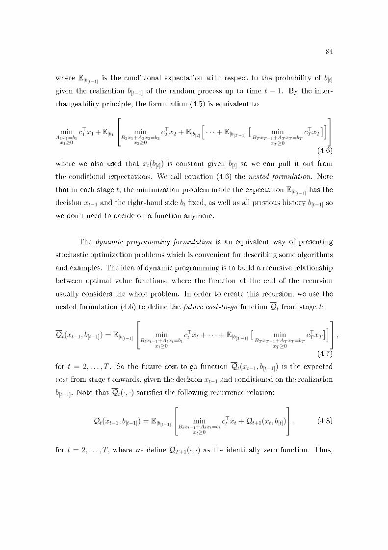
84

where E|b[t−1]is the conditional expectation with respect to the probability of b[t]

given the realization b[t−1] of the random process up to time t − 1. By the inter-

changeability principle, the formulation (4.5) is equivalent to

minA1x1=b1x1≥0

c>1 x1 +E|b1

minB2x1+A2x2=b2

x2≥0

c>2 x2 + E|b[2][· · ·+ E|b[T−1]

[min

BT xT−1+AT xT =bTxT≥0

c>T xT]]

(4.6)

where we also used that xt(b[t]) is constant given b[t] so we can pull it out from

the conditional expectations. We call equation (4.6) the nested formulation. Note

that in each stage t, the minimization problem inside the expectation E|b[t−1]has the

decision xt−1 and the right-hand side bt �xed, as well as all previous history b[t−1] so

we don't need to decide on a function anymore.

The dynamic programming formulation is an equivalent way of presenting

stochastic optimization problems which is convenient for describing some algorithms

and examples. The idea of dynamic programming is to build a recursive relationship

between optimal value functions, where the function at the end of the recursion

usually considers the whole problem. In order to create this recursion, we use the

nested formulation (4.6) to de�ne the future cost-to-go function Qt from stage t:

Qt(xt−1, b[t−1]) = E|b[t−1]

minBtxt−1+Atxt=bt

xt≥0

c>t xt + · · ·+ E|b[T−1]

[min

BT xT−1+AT xT =bTxT≥0

c>T xT]] ,

(4.7)

for t = 2, . . . , T . So the future cost-to-go function Qt(xt−1, b[t−1]) is the expected

cost from stage t onwards, given the decision xt−1 and conditioned on the realization

b[t−1]. Note that Qt(·, ·) satis�es the following recurrence relation:

Qt(xt−1, b[t−1]) = E|b[t−1]

minBtxt−1+Atxt=bt

xt≥0

c>t xt +Qt+1(xt, b[t])

, (4.8)

for t = 2, . . . , T, where we de�ne QT+1(·, ·) as the identically zero function. Thus,

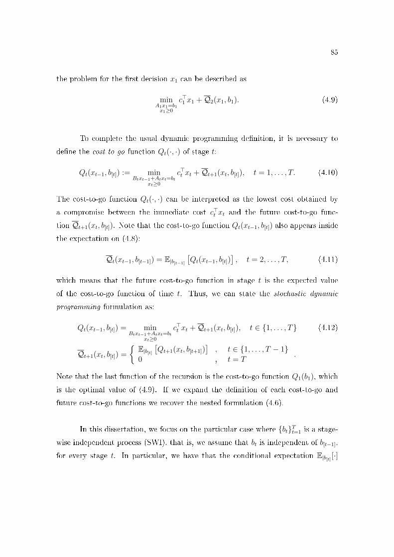
85

the problem for the �rst decision x1 can be described as

minA1x1=b1x1≥0

c>1 x1 +Q2(x1, b1). (4.9)

To complete the usual dynamic programming de�nition, it is necessary to

de�ne the cost-to-go function Qt(·, ·) of stage t:

Qt(xt−1, b[t]) := minBtxt−1+Atxt=bt

xt≥0

c>t xt +Qt+1(xt, b[t]), t = 1, . . . , T. (4.10)

The cost-to-go function Qt(·, ·) can be interpreted as the lowest cost obtained by

a compromise between the immediate cost c>t xt and the future cost-to-go func-

tion Qt+1(xt, b[t]). Note that the cost-to-go function Qt(xt−1, b[t]) also appears inside

the expectation on (4.8):

Qt(xt−1, b[t−1]) = E|b[t−1]

[Qt(xt−1, b[t])

], t = 2, . . . , T, (4.11)

which means that the future cost-to-go function in stage t is the expected value

of the cost-to-go function of time t. Thus, we can state the stochastic dynamic

programming formulation as:

Qt(xt−1, b[t]) = minBtxt−1+Atxt=bt

xt≥0

c>t xt +Qt+1(xt, b[t]), t ∈ {1, . . . , T} (4.12)

Qt+1(xt, b[t]) =

{E|b[t]

[Qt+1(xt, b[t+1])

], t ∈ {1, . . . , T − 1}

0 , t = T.

Note that the last function of the recursion is the cost-to-go function Q1(b1), which

is the optimal value of (4.9). If we expand the de�nition of each cost-to-go and

future cost-to-go functions we recover the nested formulation (4.6).

In this dissertation, we focus on the particular case where {bt}Tt=1 is a stage-

wise independent process (SWI), that is, we assume that bt is independent of b[t−1],

for every stage t. In particular, we have that the conditional expectation E|b[t] [·]

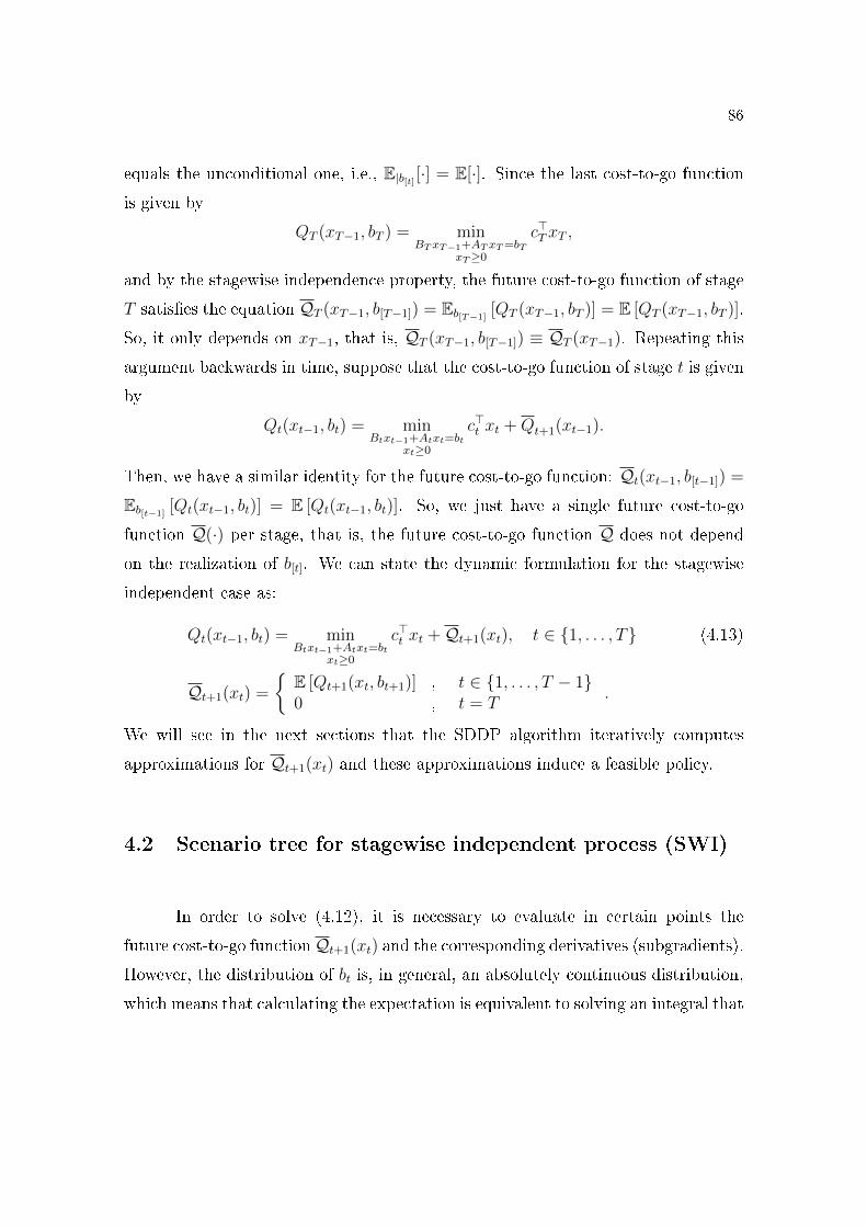
86

equals the unconditional one, i.e., E|b[t] [·] = E[·]. Since the last cost-to-go function

is given by

QT (xT−1, bT ) = minBT xT−1+AT xT =bT

xT≥0

c>T xT ,

and by the stagewise independence property, the future cost-to-go function of stage

T satis�es the equation QT (xT−1, b[T−1]) = Eb[T−1][QT (xT−1, bT )] = E [QT (xT−1, bT )].

So, it only depends on xT−1, that is, QT (xT−1, b[T−1]) ≡ QT (xT−1). Repeating this

argument backwards in time, suppose that the cost-to-go function of stage t is given

by

Qt(xt−1, bt) = minBtxt−1+Atxt=bt

xt≥0

c>t xt +Qt+1(xt−1).

Then, we have a similar identity for the future cost-to-go function: Qt(xt−1, b[t−1]) =

Eb[t−1][Qt(xt−1, bt)] = E [Qt(xt−1, bt)]. So, we just have a single future cost-to-go

function Q(·) per stage, that is, the future cost-to-go function Q does not depend

on the realization of b[t]. We can state the dynamic formulation for the stagewise

independent case as:

Qt(xt−1, bt) = minBtxt−1+Atxt=bt

xt≥0

c>t xt +Qt+1(xt), t ∈ {1, . . . , T} (4.13)

Qt+1(xt) =

{E [Qt+1(xt, bt+1)] , t ∈ {1, . . . , T − 1}0 , t = T

.

We will see in the next sections that the SDDP algorithm iteratively computes

approximations for Qt+1(xt) and these approximations induce a feasible policy.

4.2 Scenario tree for stagewise independent process (SWI)

In order to solve (4.12), it is necessary to evaluate in certain points the

future cost-to-go functionQt+1(xt) and the corresponding derivatives (subgradients).

However, the distribution of bt is, in general, an absolutely continuous distribution,

which means that calculating the expectation is equivalent to solving an integral that

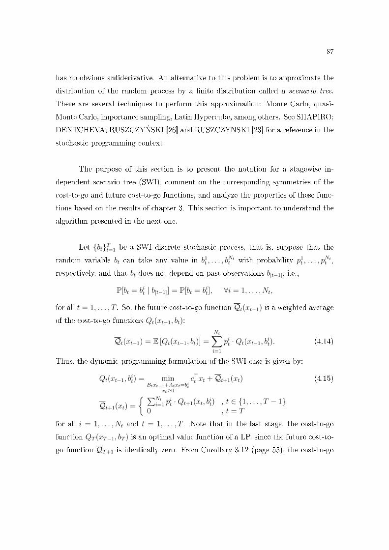
87

has no obvious antiderivative. An alternative to this problem is to approximate the

distribution of the random process by a �nite distribution called a scenario tree.

There are several techniques to perform this approximation: Monte Carlo, quasi-

Monte Carlo, importance sampling, Latin Hypercube, among others. See SHAPIRO;

DENTCHEVA; RUSZCZY�SKI [26] and RUSZCZYNSKI [23] for a reference in the

stochastic programming context.

The purpose of this section is to present the notation for a stagewise in-

dependent scenario tree (SWI), comment on the corresponding symmetries of the

cost-to-go and future cost-to-go functions, and analyze the properties of these func-

tions based on the results of chapter 3. This section is important to understand the

algorithm presented in the next one.

Let {bt}Tt=1 be a SWI discrete stochastic process, that is, suppose that the

random variable bt can take any value in b1t , . . . , b

Ntt with probability p1

t , . . . , pNtt ,

respectively, and that bt does not depend on past observations b[t−1], i.e.,

P[bt = bit | b[t−1]] = P[bt = bit], ∀i = 1, . . . , Nt,

for all t = 1, . . . , T . So, the future cost-to-go function Qt(xt−1) is a weighted average

of the cost-to-go functions Qt(xt−1, bt):

Qt(xt−1) = E [Qt(xt−1, bt)] =Nt∑

i=1

pit ·Qt(xt−1, bit). (4.14)

Thus, the dynamic programming formulation of the SWI case is given by:

Qt(xt−1, bit) = min

Btxt−1+Atxt=bitxt≥0

c>t xt +Qt+1(xt) (4.15)

Qt+1(xt) =

{ ∑Nt

i=1 pit ·Qt+1(xt, b

it) , t ∈ {1, . . . , T − 1}

0 , t = T

for all i = 1, . . . , Nt and t = 1, . . . , T . Note that in the last stage, the cost-to-go

function QT (xT−1, bT ) is an optimal value function of a LP, since the future cost-to-

go function QT+1 is identically zero. From Corollary 3.12 (page 55), the cost-to-go

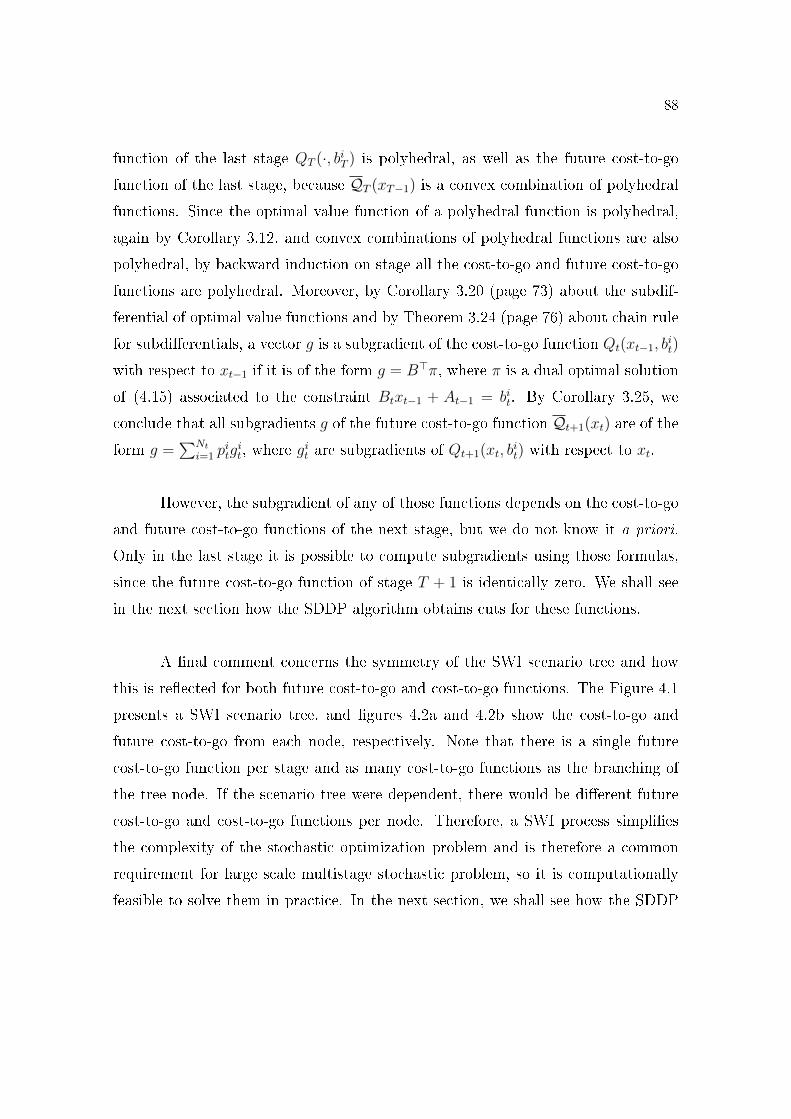
88

function of the last stage QT (·, biT ) is polyhedral, as well as the future cost-to-go

function of the last stage, because QT (xT−1) is a convex combination of polyhedral

functions. Since the optimal value function of a polyhedral function is polyhedral,

again by Corollary 3.12, and convex combinations of polyhedral functions are also

polyhedral, by backward induction on stage all the cost-to-go and future cost-to-go

functions are polyhedral. Moreover, by Corollary 3.20 (page 73) about the subdif-

ferential of optimal value functions and by Theorem 3.24 (page 76) about chain rule

for subdi�erentials, a vector g is a subgradient of the cost-to-go function Qt(xt−1, bit)

with respect to xt−1 if it is of the form g = B>π, where π is a dual optimal solution

of (4.15) associated to the constraint Btxt−1 + At−1 = bit. By Corollary 3.25, we

conclude that all subgradients g of the future cost-to-go function Qt+1(xt) are of the

form g =∑Nt

i=1 pitgit, where g

it are subgradients of Qt+1(xt, b

it) with respect to xt.

However, the subgradient of any of those functions depends on the cost-to-go

and future cost-to-go functions of the next stage, but we do not know it a priori.

Only in the last stage it is possible to compute subgradients using those formulas,

since the future cost-to-go function of stage T + 1 is identically zero. We shall see

in the next section how the SDDP algorithm obtains cuts for these functions.

A �nal comment concerns the symmetry of the SWI scenario tree and how

this is re�ected for both future cost-to-go and cost-to-go functions. The Figure 4.1

presents a SWI scenario tree, and �gures 4.2a and 4.2b show the cost-to-go and

future cost-to-go from each node, respectively. Note that there is a single future

cost-to-go function per stage and as many cost-to-go functions as the branching of

the tree node. If the scenario tree were dependent, there would be di�erent future

cost-to-go and cost-to-go functions per node. Therefore, a SWI process simpli�es

the complexity of the stochastic optimization problem and is therefore a common

requirement for large scale multistage stochastic problem, so it is computationally

feasible to solve them in practice. In the next section, we shall see how the SDDP

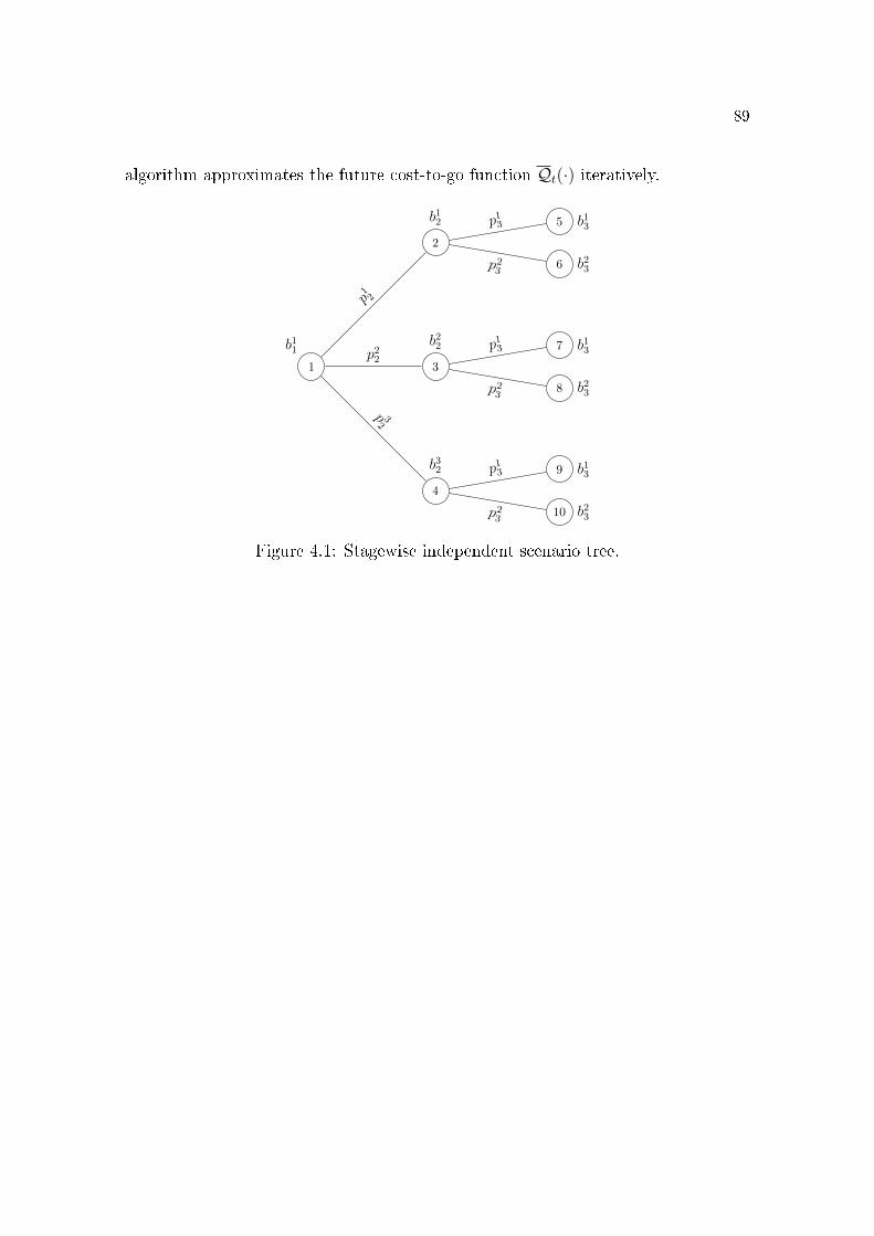
89

algorithm approximates the future cost-to-go function Qt(·) iteratively.

1

b11

4

b32

10 b23p23

9 b13p13

p 32

3

b22

8 b23p23

7 b13p13p22

2

b12

6 b23p23

5 b13p13

p12

Figure 4.1: Stagewise independent scenario tree.

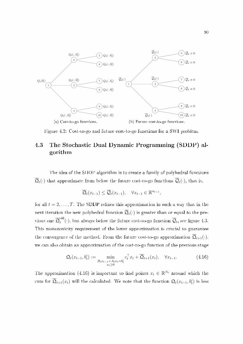
90

1

Q1(b11)

4

Q2(·, b32) 10 Q3(·, b23)

9 Q3(·, b13)

3

Q2(·, b22)

8 Q3(·, b23)

7 Q3(·, b13)

2

Q2(·, b12)

6 Q3(·, b23)

5 Q3(·, b13)

(a) Cost-to-go functions.

1

Q2(·)

4

Q3(·) 10 Q4 ≡ 0

9 Q4 ≡ 0

3

Q3(·)

8 Q4 ≡ 0

7 Q4 ≡ 0

2

Q3(·)

6 Q4 ≡ 0

5 Q4 ≡ 0

(b) Future cost-to-go functions.

Figure 4.2: Cost-to-go and future cost-to-go functions for a SWI problem.

4.3 The Stochastic Dual Dynamic Programming (SDDP) al-gorithm

The idea of the SDDP algorithm is to create a family of polyhedral functions

Qt(·) that approximate from below the future cost-to-go functions Qt(·), that is,

Qt(xt−1) ≤ Qt(xt−1), ∀xt−1 ∈ Rnt−1 ,

for all t = 2, . . . , T . The SDDP re�nes this approximation in such a way that in the

next iteration the new polyhedral function Qt(·) is greater than or equal to the pre-

vious one Qold

t (·), but always below the future cost-to-go function Qt, see �gure 4.3.This monotonicity requirement of the lower approximation is crucial to guarantee

the convergence of the method. From the future cost-to-go approximation Qt+1(·),we can also obtain an approximation of the cost-to-go function of the previous stage

Qt(xt−1, bit) := min

Btxt−1+Atxt=bitxt≥0

c>t xt + Qt+1(xt), ∀xt−1. (4.16)

The approximation (4.16) is important to �nd points xt ∈ RNt around which the

cuts for Qt+1(xt) will the calculated. We note that the function Qt(xt−1, bit) is less

91

xt−10

epi(Qt)

dom(Qt)

epi(Qt)

dom(Qt)

Figure 4.3: Future cost-to-go function approximation.

than or equal to Qt(xt−1, bit), since the corresponding optimization problems have

the same constraints, but the objective function from the former is smaller than or

equal to the latter.

We assume that the future cost-to-go functions Qt(·) are bounded below,

i.e., there is L ∈ R such that Qt(xt−1) ≥ L, for all xt−1 ∈ RNt−1 and every stage

t = 2, . . . , T . Thus, the SDDP algorithm starts with the approximation Qt(·) whois equal to the constant L.

To re�ne the approximation of the future cost-to-go function Qt(·) around a

point x∗t−1, one simply computes subgradients git for Qt(·, bit) at x∗t−1, and note that

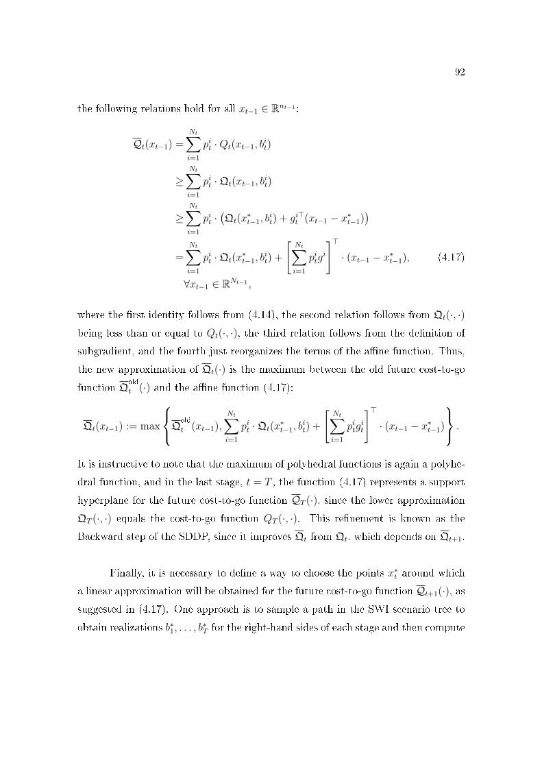
92

the following relations hold for all xt−1 ∈ Rnt−1 :

Qt(xt−1) =Nt∑

i=1

pit ·Qt(xt−1, bit)

≥Nt∑

i=1

pit ·Qt(xt−1, bit)

≥Nt∑

i=1

pit ·(Qt(x

∗t−1, b

it) + gi>t (xt−1 − x∗t−1)

)

=Nt∑

i=1

pit ·Qt(x∗t−1, b

it) +

[Nt∑

i=1

pitgi

]>· (xt−1 − x∗t−1), (4.17)

∀xt−1 ∈ RNt−1 ,

where the �rst identity follows from (4.14), the second relation follows from Qt(·, ·)being less than or equal to Qt(·, ·), the third relation follows from the de�nition of

subgradient, and the fourth just reorganizes the terms of the a�ne function. Thus,

the new approximation of Qt(·) is the maximum between the old future cost-to-go

function Qold

t (·) and the a�ne function (4.17):

Qt(xt−1) := max

Q

old

t (xt−1),Nt∑

i=1

pit ·Qt(x∗t−1, b

it) +

[Nt∑

i=1

pitgit

]>· (xt−1 − x∗t−1)

.

It is instructive to note that the maximum of polyhedral functions is again a polyhe-

dral function, and in the last stage, t = T , the function (4.17) represents a support

hyperplane for the future cost-to-go function QT (·), since the lower approximation

QT (·, ·) equals the cost-to-go function QT (·, ·). This re�nement is known as the

Backward step of the SDDP, since it improves Qt from Qt, which depends on Qt+1.

Finally, it is necessary to de�ne a way to choose the points x∗t around which

a linear approximation will be obtained for the future cost-to-go function Qt+1(·), assuggested in (4.17). One approach is to sample a path in the SWI scenario tree to

obtain realizations b∗1, . . . , b∗T for the right-hand sides of each stage and then compute

93

the optimal solution x∗t ∈ Rnt of (4.16) in each stage t:

x∗t ∈ arg minBtx∗t−1+Atxt=b∗t

xt≥0

c>t xt + Qt+1(xt, bit),

where the previous stage solution x∗t−1 is used in xt−1. This is known as the Forward

step of SDDP, since we choose decisions xt going forward on the tree. The need to

sample paths from the scenario tree instead of going through all the possibilities lies

in the fact that the number of paths increases exponentially with the size T of the

planning horizon.

In short, the SDDP algorithm has two steps and a stopping criterion:

i) Forward step: �nd feasible solutions x∗t for t = 1, . . . , Nt.

ii) Backward step: compute lower linear approximations of the fu-

ture cost-to-go functions centered on the feasible solutions x∗t−1 ob-

tained in the forward step, in decreasing stage order. After re�ning

all approximations of the cost-to-go and future cost-to-go functions,

we estimate a lower bound z := Q1(b1) for the �rst stage.

iii) Stopping criterion: If either a maximum number of iterations is

reached, or the optimal value z makes small relative progress, stop.

Otherwise, do another Forward/Backward step.

The proof of convergence of the SDDP uses that the cost-to-go and future

cost-to-go functions are polyhedral functions, see PHILPOTT; GUAN [21].

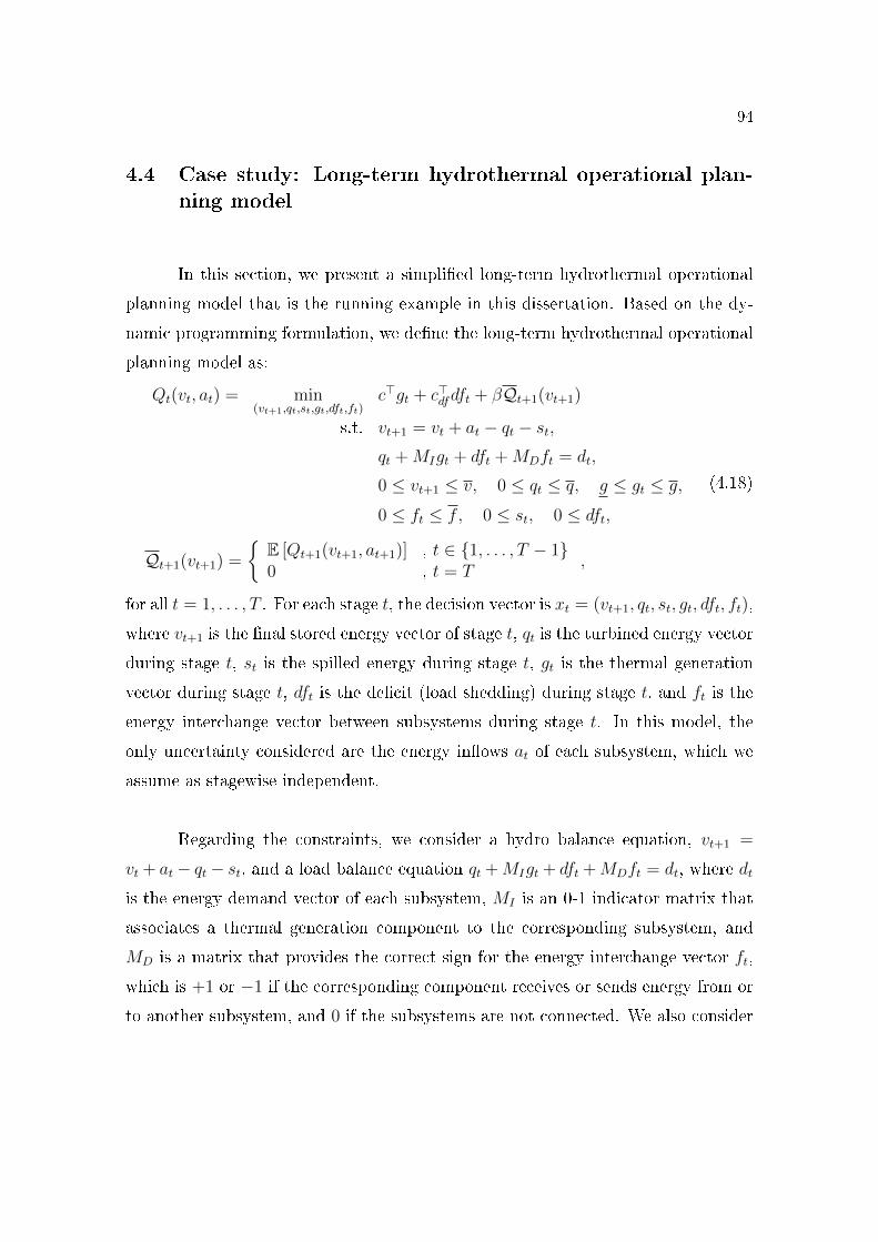
94

4.4 Case study: Long-term hydrothermal operational plan-ning model

In this section, we present a simpli�ed long-term hydrothermal operational

planning model that is the running example in this dissertation. Based on the dy-

namic programming formulation, we de�ne the long-term hydrothermal operational

planning model as:

Qt(vt, at) = min(vt+1,qt,st,gt,dft,ft)

c>gt + c>dfdft + βQt+1(vt+1)

s.t. vt+1 = vt + at − qt − st,qt +MIgt + dft +MDft = dt,

0 ≤ vt+1 ≤ v, 0 ≤ qt ≤ q, g ≤ gt ≤ g,

0 ≤ ft ≤ f, 0 ≤ st, 0 ≤ dft,

Qt+1(vt+1) =

{E [Qt+1(vt+1, at+1)] , t ∈ {1, . . . , T − 1}0 , t = T

,

(4.18)

for all t = 1, . . . , T . For each stage t, the decision vector is xt = (vt+1, qt, st, gt, dft, ft),

where vt+1 is the �nal stored energy vector of stage t, qt is the turbined energy vector

during stage t, st is the spilled energy during stage t, gt is the thermal generation

vector during stage t, dft is the de�cit (load shedding) during stage t, and ft is the

energy interchange vector between subsystems during stage t. In this model, the

only uncertainty considered are the energy in�ows at of each subsystem, which we

assume as stagewise independent.

Regarding the constraints, we consider a hydro balance equation, vt+1 =

vt + at − qt − st, and a load balance equation qt +MIgt + dft +MDft = dt, where dt

is the energy demand vector of each subsystem, MI is an 0-1 indicator matrix that

associates a thermal generation component to the corresponding subsystem, and

MD is a matrix that provides the correct sign for the energy interchange vector ft,

which is +1 or −1 if the corresponding component receives or sends energy from or

to another subsystem, and 0 if the subsystems are not connected. We also consider

95

upper and lower limits for each variable.

In the objective function, we minimize the sum of thermal generation costs,

c>gt, de�cit costs, c>dfdft, and the future cost-to-go function, Qt(vt+1), corrected by

a discount factor β. We note that the hydro generation has no immediate cost in

this model.

In order to emphasize the di�erences among other formulations, we will rep-

resent in section 6.3 the bound constraints by the set Xt and the decision vector by

xt:

xt := (vt+1, qt, st, gt, dft, ft) ∈ Xt,

Thus, planning model (4.18) is compactly represented as

Qt(vt, at) = minxt∈Xt

c>gt + c>dfdft + βQt+1(vt+1)

s.t. (∗)P,(4.19)

where (∗)P indicates the load and energy balance equations from (4.18). Note that

we also omit the de�nition of the future cost-to-go Qt+1(vt+1).

96

5 DISJUNCTIVE CONSTRAINTS

The technique of Disjunctive Constraints provides a method for describing �if-

then� rules in terms of union of polyhedra. There are several important operational

planning rules that �ts into this category of constraint. For instance, the minimum

out�ow of a given reservoir de�ned by the National Water Agency (ANA) considers

di�erent values of minimum out�ow depending on the stored level situation. It is

also possible to represent the risk aversion of low stored volumes by imposing a

minimum thermal dispatch if the stored volume is outside a security region, e.g.,

the one de�ned by the Risk Aversion Curve (CAR) or the Risk Aversion Surface

(SAR). Those examples are described in more detail in section 5.2.

In section 5.1, we present a formula that represents a �nite union of polyhedra

using 0-1 mixed integer linear constraints. This formula works for a large class of

problems, and when it does not work we also guarantee that the corresponding

union of polyhedra could not be represented by any collection of linear constraints

involving real and binary variables.

5.1 Modeling non-convex constraints with binary variables

Disjunctive programming is optimization over union of polyhedra. While

polyhedra are convex, their union do not need to be. In this case, it is impossi-

ble to represent such sets using only continuous variables and convex constraints.

Let {Pi}i∈I be a �nite family of polyhedra, where Pi = {x ∈ Rn ∈| Aix ≤ bi}, andlet P be the corresponding union ∪i∈IPi. The aim of this section is to obtain an

algebraic formula that represents P using continuous and binary variables. Let Q

97

be the following peculiar set:

Q =

{x ∈ Rn

∣∣∣∣x =

∑i∈I xi, Aixi ≤ zibi,

∑i∈I zi = 1,

xi ∈ Rn, zi ∈ {0, 1}, i ∈ I. .

}(5.1)

The set Q plays a central role in understanding how to represent union of polyhedra.

We shall prove that, under some regularity conditions, the set Q equals P , and when

they are di�erent there is no way to represent P using binary variables and linear

constraints.

Lets understand the algebraic representation (5.1). Since each zi is a binary

variable and they sum to one, there is only one j ∈ I such that zj equals 1, and then

the other zi's are equal to zero. Note that the recession cone of Pi has the following

form:

recc(Pi) = {d ∈ Rn | Aid ≤ 0},

for all i ∈ I. Then, each vector x ∈ Q is the sum of a vector xj ∈ Pj and of

recession directions di, for i 6= j. This is half the proof of Lemma 5.1 below. To

prove the general formula (5.2), we introduce the �algebraic recession cone�, de�ned

for a polyhedral set P = {x ∈ Rn | Ax ≤ b} as reccA(P ) = {d ∈ Rn | Ad ≤ 0}.Thus, if P is nonempty, the algebraic recession cone of P equals the the recession

cone of P , but if P is empty the notion of the algebraic recession cone is still well

de�ned.

Lemma 5.1. The set Q de�ned in (5.1) has the following expression:

Q =⋃

i∈IPi +

∑

k∈IreccA(Pk). (5.2)

Proof. Let P be the set on the right-hand side of equation (5.2),

P =⋃

i∈IPi +

∑

k∈IreccA(Pk).

98

We have seen above that Q is a subset of P . We prove the opposite inclusion. Let

x be a vector of P . Then,

x = xj +∑

k∈Idk = (xj + dj) +

∑

k∈Ik 6=j

dk,

for some xj ∈ Pj and dk ∈ recc(Pk), where k ∈ I. Note that xj + dj belongs to Pj.

So, let xi and zi be the following variables:

xi =

{xj + dj i = j,

di i 6= j,e zi =

{1 i = j,

0 i 6= j,

Therefore, x =∑

i∈I xi, 1 =∑

i∈I zi, Axi ≤ zibi, and zi ∈ {0, 1}, for all i ∈ I. We

conclude that x belongs to Q.

An important remark which follows from Lemma 5.1 is that if all polyhedra

have the same recession cone, i.e., recc(Pi) = R, for all i ∈ I, then the algebraic

formula (5.1) represents P , that is, Q = P . However, a question that arises is: �if Q

is di�erent from P , is there another way to represent P using binary variables and

linear constraints?� The following theorem shows that if (5.1) does not su�ce, no

0-1 linear representation of P exists. This is a result from JEROSLOW [18] whose

statement was slightly modi�ed and the corresponding proof simpli�ed.

Theorem 5.2 (Jeroslow). Suppose that P is described by a system of linear equa-

tions with mixed integer variables, i.e., there are matrices A, B, C and a vector b

such that

P =

{x ∈ Rn

∣∣∣∣Ax+By + Cz ≤ b,y ∈ Rm, z ∈ {0, 1}l

}. (5.3)

Then, there is a representation of P by a �nite union of nonempty polyhedra,

P =⋃i∈I Pi, where all polyhedra have the same recession cone. Moreover, any

representation of P by a union of nonempty polyhedra⋃i′∈I′ Pi′ lead to a set Q that

equals P , when using the algebraic formula (5.1).

99

Proof. Let zi be a binary vector of {0, 1}l, and let Pi be the polyhedron de�ned by

setting z equal to zi in inequality (5.3):

Pi := {x ∈ Rn | Ax+By ≤ b− Czi, y ∈ Rm}.

Let I be the set of indexes i such that Pi is nonempty. From Corollary 2.9 (page 26),

the recession cone of these Pi's is given by:

R = {dx ∈ Rn | Adx +Bdy ≤ 0, dy ∈ Rm}. (5.4)

Since this expression is invariant by i, we have proved the �rst part of the theorem.

Let's prove the second part. Suppose that P could be represented by any

�nite union of nonempty polyhedra P =⋃i′∈I′ Pi′ . From Lemma 5.1 (page 97),

Q =⋃

i′∈I′Pi′ +

∑

i′∈I′recc(Pi′) = P +

∑

i′∈I′recc(Pi′).

We claim that∑

i′∈I′ recc(Pi′) equals the polyhedral cone R from (5.4). If so, the

set Q would be equal to P +R, which in turn is equal to P , since each polyhedron

Pi has recession cone equal to R.

Let's prove that∑

i′∈I′ recc(Pi′) = R. Indeed, if P is bounded, the polyhedra

Pi and Pi′ must be bounded, for all i, i′, so the corresponding recession cones are

equal to {0}. In this case, the identity∑

i′∈I′ recc(Pi′) = R is trivially satis�ed. If P

is an unbounded set, there is a polyhedron Pj′ that is unbounded, for some j′ ∈ I ′,and every polyhedron Pi is unbounded, since they have the same recession cone R.

Let d be a nonzero direction of recession of R. If d does not belong to any Pi′ ,

then starting from any point x ∈ Pi′ we have that x+ td does not belong to Pi′ for

some large enough scalar t > 0. However, the vector x belongs to some polyhedron

Pi, and x + td also belongs to Pi, for every positive scalar t, since d is a direction

of recession of R. This is a contradiction with the hypothesis that both unions of

polyhedra are equal to the same set P . Therefore, R is a subset of∑

i′∈I′ recc(Pi′).

100

For the converse inclusion, let d be a nonzero direction of recc(Pj′), and suppose

that d does not belong to R. Let x be a vector of Pj′ . For a large enough scalar

t > 0, x + td does not belong to any of these Pi's, but it belongs to Pj′ . This is

again a contradiction with the hypothesis of generating the same set P . Therefore,

all recession cones recc(Pi′)'s are subsets of R. Since R is a convex cone, the sum

of directions of R also belongs to it, so we conclude that∑

i′∈I′ recc(Pi′) is a subset

of R.

The hypothesis of nonempty union of polyhedra⋃i′I′ Pi′ in the proof of The-

orem 5.2 is necessary, since the formula (5.1) considers each algebraic recession cone

recc(Pi′) even if the polyhedron Pi′ is empty, as shown in Lemma 5.1. Thus, given

a representation of P as union of nonempty polyhedra, we can always aggregate

empty polyhedra Pj′ 's with arbitrary algebraic recession cones that makes the set Q

larger than P .

The algebraic formula (5.2) is an important modeling tool, since it provides

an explicit description of union of polyhedra using linear constrains and binary vari-

ables, and when it fails we have the guarantee that it is impossible to describe that

particular case using any other formula. We also note that the formula (5.2) is an

extension of the �Big-M� modeling approach which is a mixed integer linear formula

for union of bounded polyhedra. If P is bounded, the corresponding polyhedra are

bounded, and the recession cones are all equal to {0}. Therefore, the algebraic for-mula (5.2) is always able to represent a bounded union P . In �gure 5.1a, we show an

example of a union of polyhedra that cannot be represented using binary variables,

and next to it �gure 5.1b depicts the corresponding set Q generated by (5.1).

An useful information for solving mixed integer problems is the knowledge

of the convex hull of the corresponding feasible set. We have seen in Lemma 3.7

(page 47) that the in�mum of a linear function over a set P is equal to the in�mum of

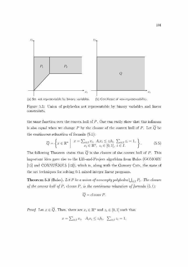
101

x1

x2

P1 P2

(a) Set not representable by binary variables.

x1

x2

Q

(b) Certi�cate of non-representability.

Figure 5.1: Union of polyhedra not representable by binary variables and linearconstraints.

the same function over the convex hull of P . One can easily show that this in�mum

is also equal when we change P by the closure of the convex hull of P . Let Q be

the continuous relaxation of formula (5.1):

Q =

{x ∈ Rn

∣∣∣∣x =

∑i∈I xi, Aixi ≤ zibi,

∑i∈I zi = 1,

xi ∈ Rn, zi ∈ [0, 1], i ∈ I.

}. (5.5)

The following Theorem states that Q is the closure of the convex hull of P . This

important idea gave rise to the Lift-and-Project algorithm from Balas (GOMORY

[15] and CORNUÉJOLS [13]), which is, along with the Gomory Cuts, the state of

the art techniques for solving 0-1 mixed integer linear programs.

Theorem 5.3 (Balas). Let P be a union of nonempty polyhedra⋃i∈I Pi. The closure

of the convex hull of P , cl convP , is the continuous relaxation of formula (5.1):

Q = cl convP.

Proof. Let x ∈ Q. Then, there are xi ∈ Rn and zi ∈ [0, 1] such that

x =∑

i∈I xi, Aixi ≤ zibi,∑

i∈I zi = 1,

102

for all i ∈ I. Let I0 and I+ the set of indexes i such that zi is equal to zero and

greater than zero, respectively. Note that xi belongs to recc(Pi), for all i ∈ I0, and

xi = xi/zi belongs to Pi, for all i ∈ I+. So, the vector x has the following form:

x =∑

i∈I+zixizi

+∑

i∈I0xi

=∑

i∈I+zixi

︸ ︷︷ ︸∈ conv(

⋃i∈I P )

+∑

i∈I0xi

︸ ︷︷ ︸∈∑i∈I recc(Pi)

.

From Theorem 2.13 (page 33), cl convP also has the following expression:

cl conv

(⋃

i∈IPi

)= conv

(⋃

i∈IPi

)+∑

i∈Irecc(Pi).

Therefore, x belongs to cl conv(P ).

On the other hand, let x ∈ cl conv(P ). Again from Theorem 2.13,

x =∑

i∈Iλiyi +

∑

i∈Idi,

where yi ∈ Pi, di ∈ recc(Pi) and λi ∈ [0, 1] such that∑

i∈I λi = 1, for all i ∈ I. LetI

0and I

+be the set of indexes i such that λi = 0 and λi > 0, respectively. Then,

x =∑

i∈I+λi

(yi +

1

λidi

)+∑

i∈I0di.

Let xi be equal to yi+(1/λi)di, and note that xi belongs to Pi, since yi belongs to Pi

and di belongs to recc(Pi), for all i ∈ I+. Let xi and zi be the following vectors:

xi =

{λixi, se i ∈ I+,

di se i ∈ I0,zi = λi.

Therefore,

x =∑

i∈I xi, Aixi ≤ zibi,∑

i∈I zi = 1,

and so x belongs to Q.

103

5.2 Some applications of Disjunctive Constraints

Throughout this section we present some applications of Disjunctive Con-

straints using the notation of section 4.4. Other Brazilian's research in Disjunctive

Constraints can be found in CAMPELLO [9], CAMPELLO; FILHO [10] and CAMPELLO;

FILHO [11].

In subsections 5.2.1 and 5.2.2, we introduce some operational risk aversion

proposals that aim to increase thermal generation if the stored energy is outside a

given security region. These are the Binary Risk Aversion Curve (CAR-B) and the

Binary Risk Aversion Surface (SAR-B) methodologies.

In subsection 5.2.3, we address the topic of de�cit generation. Modeling soft

constraints with penalty methods may introduce side e�ects such as the preventive

de�cit, i.e., occurrence of load curtailment when there is still a reasonable stored

energy available. We propose a non-convex constraint which restricts the possibility

of load curtailment to a speci�c situation of energy stored level.

In subsection 5.2.4, we propose a non-convex constraint for modeling the

minimum energy out�ow constraint. The minimum out�ow depends on the amount

of stored energy, and for lower storage levels the required minimum out�ow becomes

smaller. This is a nontrivial example of application of the formula 5.1, since, without

it, obtaining an expression that represents such constraint would be considerably

di�cult.

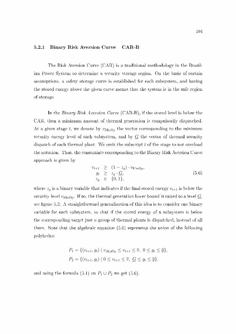
104

5.2.1 Binary Risk Aversion Curve � CAR-B

The Risk Aversion Curve (CAR) is a traditional methodology in the Brazil-

ian Power System to determine a security storage region. On the basis of certain

assumptions, a safety storage curve is established for each subsystem, and having

the stored energy above the given curve means that the system is in the safe region

of storage.

In the Binary Risk Aversion Curve (CAR-B), if the stored level is below the

CAR, then a minimum amount of thermal generation is compulsorily dispatched.

At a given stage t, we denote by vMinOp the vector corresponding to the minimum

security energy level of each subsystem, and by G the vector of thermal security

dispatch of each thermal plant. We omit the subscript t of the stage to not overload

the notation. Thus, the constraints corresponding to the Binary Risk Aversion Curve

approach is given by

vt+1 ≥ (1− zg) · vMinOp,gt ≥ zg ·G,zg ∈ {0, 1},

(5.6)

where zg is a binary variable that indicates if the �nal stored energy vt+1 is below the

security level vMinOp. If so, the thermal generation lower bound is raised to a level G,

see �gure 5.2. A straightforward generalization of this idea is to consider one binary

variable for each subsystem, so that if the stored energy of a subsystem is below

the corresponding target just a group of thermal plants is dispatched, instead of all

them. Note that the algebraic equation (5.6) represents the union of the following

polyhedra:

P1 = {(vt+1, gt) | vMinOp ≤ vt+1 ≤ v, 0 ≤ gt ≤ g},P2 = {(vt+1, gt) | 0 ≤ vt+1 ≤ v, G ≤ gt ≤ g}.

and using the formula (5.1) on P1 ∪ P2 we get (5.6).

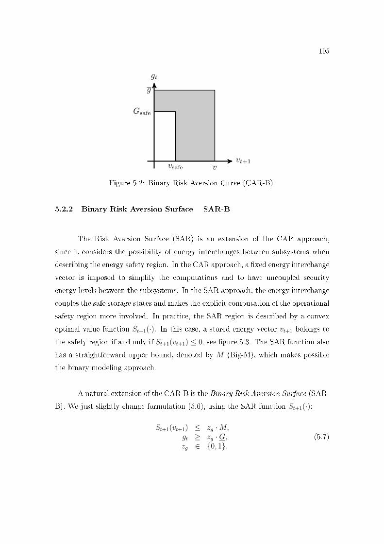
105

vt+1

gt

Gsafe

vsafe v

g

Figure 5.2: Binary Risk Aversion Curve (CAR-B).

5.2.2 Binary Risk Aversion Surface � SAR-B

The Risk Aversion Surface (SAR) is an extension of the CAR approach,

since it considers the possibility of energy interchanges between subsystems when

describing the energy safety region. In the CAR approach, a �xed energy interchange

vector is imposed to simplify the computations and to have uncoupled security

energy levels between the subsystems. In the SAR approach, the energy interchange

couples the safe storage states and makes the explicit computation of the operational

safety region more involved. In practice, the SAR region is described by a convex

optimal value function St+1(·). In this case, a stored energy vector vt+1 belongs to

the safety region if and only if St+1(vt+1) ≤ 0, see �gure 5.3. The SAR function also

has a straightforward upper bound, denoted by M (Big-M), which makes possible

the binary modeling approach.

A natural extension of the CAR-B is the Binary Risk Aversion Surface (SAR-

B). We just slightly change formulation (5.6), using the SAR function St+1(·):

St+1(vt+1) ≤ zg ·M,gt ≥ zg ·G,zg ∈ {0, 1}.

(5.7)

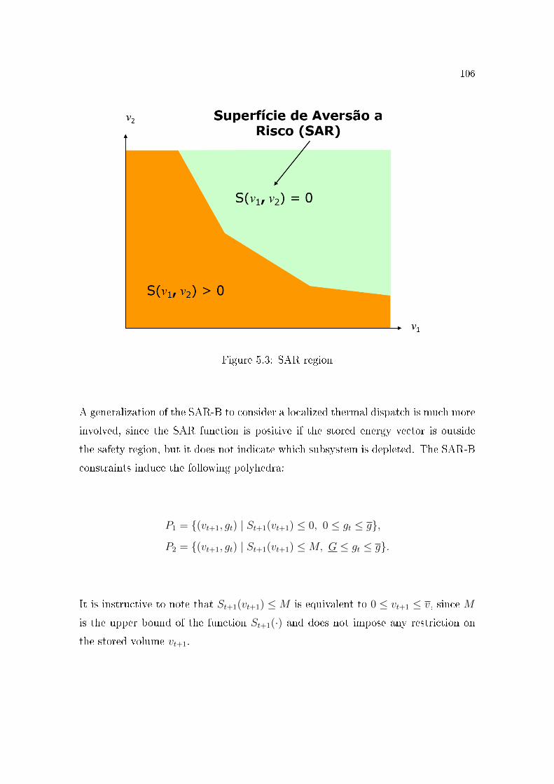
106

Figure 5.3: SAR region

A generalization of the SAR-B to consider a localized thermal dispatch is much more

involved, since the SAR function is positive if the stored energy vector is outside

the safety region, but it does not indicate which subsystem is depleted. The SAR-B

constraints induce the following polyhedra:

P1 = {(vt+1, gt) | St+1(vt+1) ≤ 0, 0 ≤ gt ≤ g},P2 = {(vt+1, gt) | St+1(vt+1) ≤M, G ≤ gt ≤ g}.

It is instructive to note that St+1(vt+1) ≤M is equivalent to 0 ≤ vt+1 ≤ v, since M

is the upper bound of the function St+1(·) and does not impose any restriction on

the stored volume vt+1.

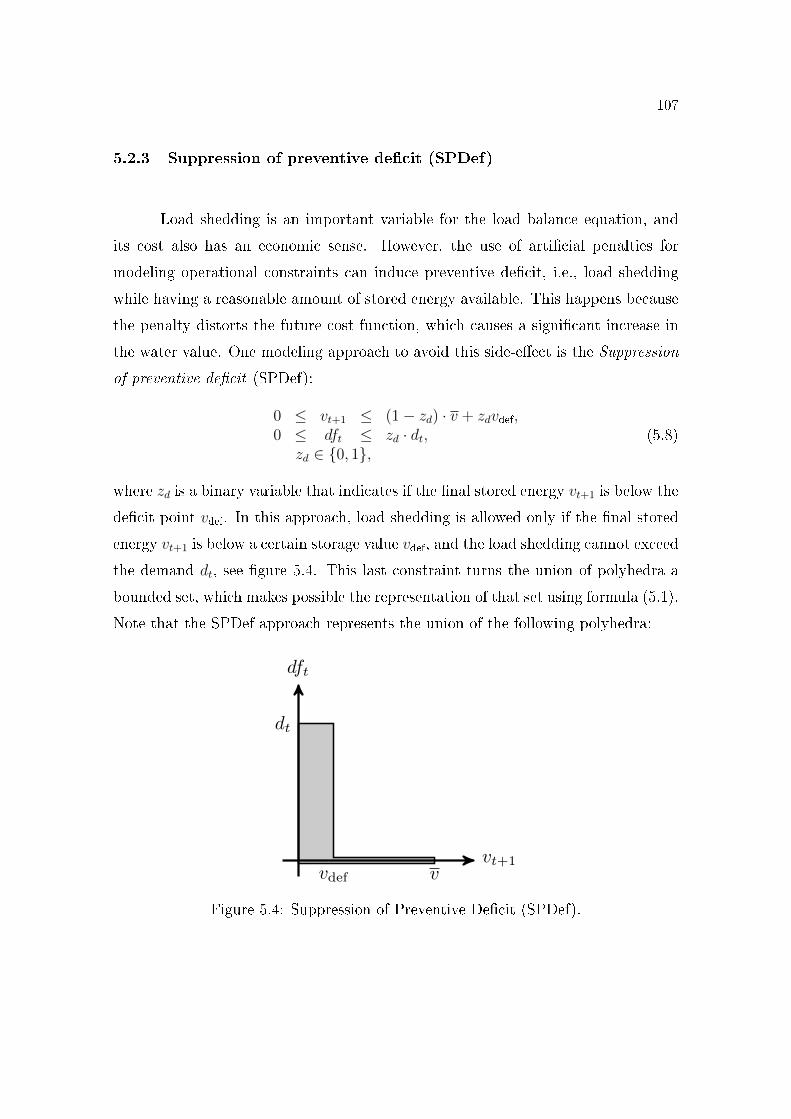
107

5.2.3 Suppression of preventive de�cit (SPDef)

Load shedding is an important variable for the load balance equation, and

its cost also has an economic sense. However, the use of arti�cial penalties for

modeling operational constraints can induce preventive de�cit, i.e., load shedding

while having a reasonable amount of stored energy available. This happens because

the penalty distorts the future cost function, which causes a signi�cant increase in

the water value. One modeling approach to avoid this side-e�ect is the Suppression

of preventive de�cit (SPDef):

0 ≤ vt+1 ≤ (1− zd) · v + zdvdef,0 ≤ dft ≤ zd · dt,

zd ∈ {0, 1},(5.8)

where zd is a binary variable that indicates if the �nal stored energy vt+1 is below the

de�cit point vdef. In this approach, load shedding is allowed only if the �nal stored

energy vt+1 is below a certain storage value vdef, and the load shedding cannot exceed

the demand dt, see �gure 5.4. This last constraint turns the union of polyhedra a

bounded set, which makes possible the representation of that set using formula (5.1).

Note that the SPDef approach represents the union of the following polyhedra:

vt+1

dft

dt

vvdef

Figure 5.4: Suppression of Preventive De�cit (SPDef).

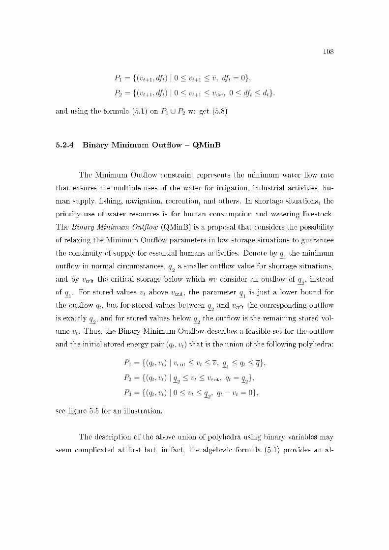
108

P1 = {(vt+1, dft) | 0 ≤ vt+1 ≤ v, dft = 0},P2 = {(vt+1, dft) | 0 ≤ vt+1 ≤ vdef, 0 ≤ dft ≤ dt}.

and using the formula (5.1) on P1 ∪ P2 we get (5.8)

5.2.4 Binary Minimum Out�ow � QMinB

The Minimum Out�ow constraint represents the minimum water �ow rate

that ensures the multiple uses of the water for irrigation, industrial activities, hu-

man supply, �shing, navigation, recreation, and others. In shortage situations, the

priority use of water resources is for human consumption and watering livestock.

The Binary Minimum Out�ow (QMinB) is a proposal that considers the possibility

of relaxing the Minimum Out�ow parameters in low storage situations to guarantee

the continuity of supply for essential humans activities. Denote by q1the minimum

out�ow in normal circumstances, q2a smaller out�ow value for shortage situations,

and by vcrit the critical storage below which we consider an out�ow of q2, instead

of q1. For stored values vt above vcrit, the parameter q

1is just a lower bound for

the out�ow qt, but for stored values between q2and vcrit the corresponding out�ow

is exactly q2, and for stored values below q

2the out�ow is the remaining stored vol-

ume vt. Thus, the Binary Minimum Out�ow describes a feasible set for the out�ow

and the initial stored energy pair (qt, vt) that is the union of the following polyhedra:

P1 = {(qt, vt) | vcrit ≤ vt ≤ v, q1≤ qt ≤ q},

P2 = {(qt, vt) | q2≤ vt ≤ vcrit, qt = q

2},

P3 = {(qt, vt) | 0 ≤ vt ≤ q2, qt − vt = 0},

see �gure 5.5 for an illustration.

The description of the above union of polyhedra using binary variables may

seem complicated at �rst but, in fact, the algebraic formula (5.1) provides an al-

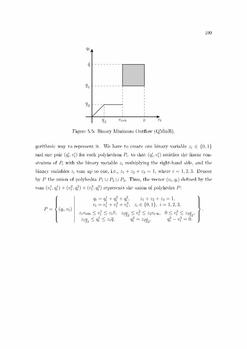
109

q2

vcrit v vt

q2

q1

qt

q

Figure 5.5: Binary Minimum Out�ow (QMinB).

gorithmic way to represent it. We have to create one binary variable zi ∈ {0, 1}and one pair (qit, v

it) for each polyhedron Pi, so that (qit, v

it) satis�es the linear con-

straints of Pi with the binary variable zi multiplying the right-hand side, and the

binary variables zi sum up to one, i.e., z1 + z2 + z3 = 1, where i = 1, 2, 3. Denote

by P the union of polyhedra P1 ∪ P2 ∪ P3. Thus, the vector (vt, qt) de�ned by the

sum (v1t , q

1t ) + (v2

t , q2t ) + (v3

t , q3t ) represents the union of polyhedra P :

P =

(qt, vt)

∣∣∣∣∣∣∣∣∣

qt = q1t + q2

t + q3t , z1 + z2 + z3 = 1,

vt = v1t + v2

t + v3t , zi ∈ {0, 1}, i = 1, 2, 3,

z1vcrit ≤ v1t ≤ z1v, z2q2

≤ v2t ≤ z2vcrit, 0 ≤ v3

t ≤ z3q2,

z1q1≤ q1

t ≤ z1q, q2t = z2q2

, q3t − v3

t = 0.

.

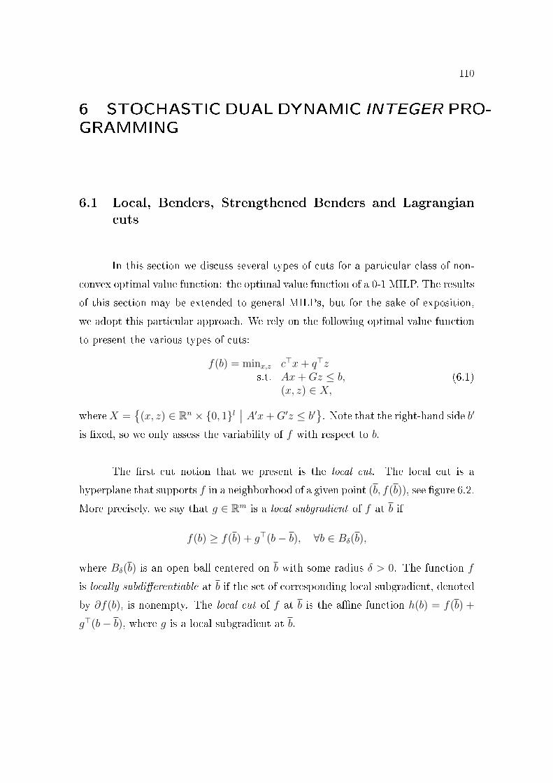
110

6 STOCHASTIC DUAL DYNAMIC INTEGER PRO-

GRAMMING

6.1 Local, Benders, Strengthened Benders and Lagrangiancuts

In this section we discuss several types of cuts for a particular class of non-

convex optimal value function: the optimal value function of a 0-1 MILP. The results

of this section may be extended to general MILPs, but for the sake of exposition,

we adopt this particular approach. We rely on the following optimal value function

to present the various types of cuts:

f(b) = minx,z c>x+ q>zs.t. Ax+Gz ≤ b,

(x, z) ∈ X,(6.1)

whereX ={

(x, z) ∈ Rn × {0, 1}l∣∣ A′x+G′z ≤ b′

}. Note that the right-hand side b′

is �xed, so we only assess the variability of f with respect to b.

The �rst cut notion that we present is the local cut. The local cut is a

hyperplane that supports f in a neighborhood of a given point (b, f(b)), see �gure 6.2.

More precisely, we say that g ∈ Rm is a local subgradient of f at b if

f(b) ≥ f(b) + g>(b− b), ∀b ∈ Bδ(b),

where Bδ(b) is an open ball centered on b with some radius δ > 0. The function f

is locally subdi�erentiable at b if the set of corresponding local subgradient, denoted

by ∂f(b), is nonempty. The local cut of f at b is the a�ne function h(b) = f(b) +

g>(b− b), where g is a local subgradient at b.

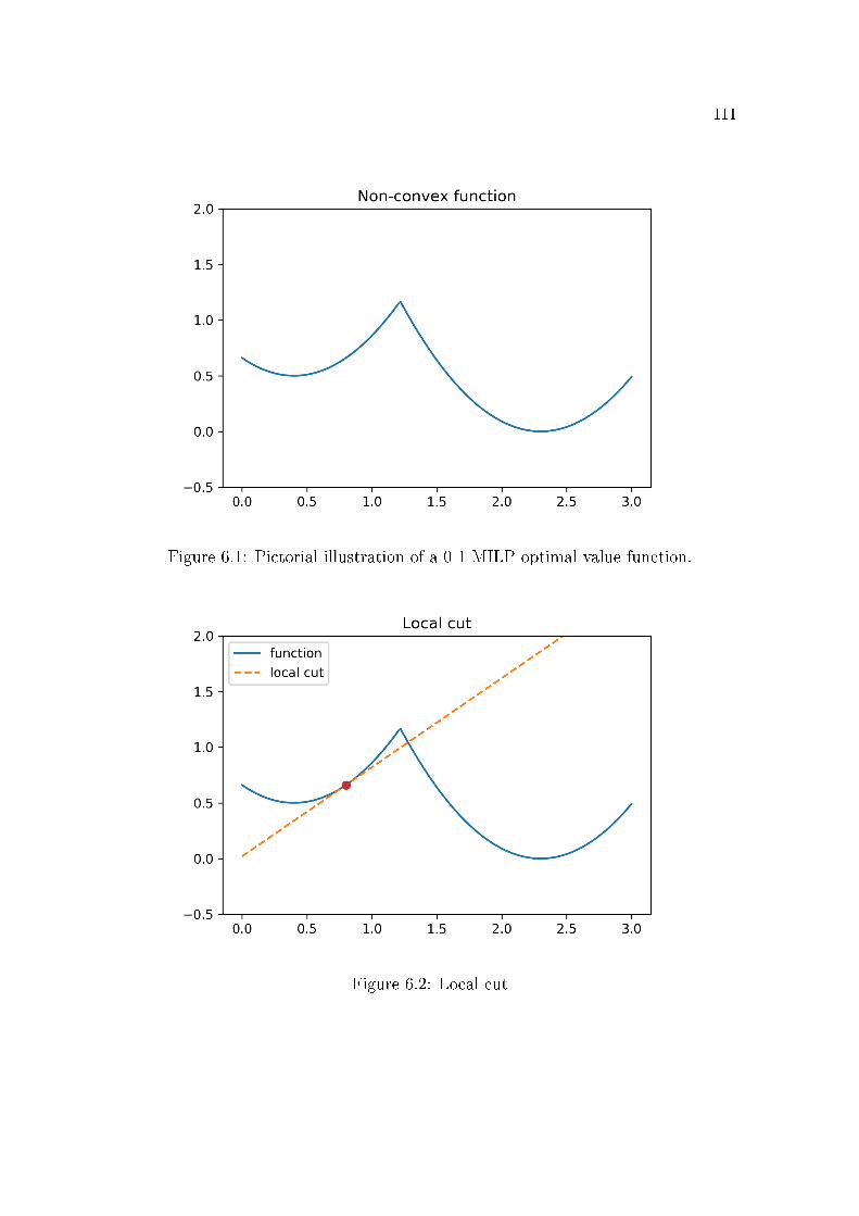
111

Figure 6.1: Pictorial illustration of a 0-1 MILP optimal value function.

Figure 6.2: Local cut

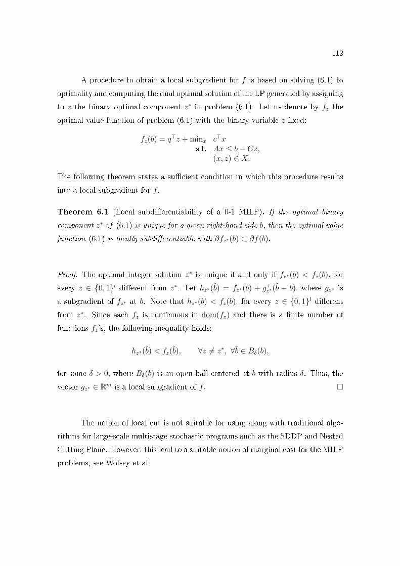
112

A procedure to obtain a local subgradient for f is based on solving (6.1) to

optimality and computing the dual optimal solution of the LP generated by assigning

to z the binary optimal component z∗ in problem (6.1). Let us denote by fz the

optimal value function of problem (6.1) with the binary variable z �xed:

fz(b) = q>z + minx c>xs.t. Ax ≤ b−Gz,

(x, z) ∈ X.

The following theorem states a su�cient condition in which this procedure results

into a local subgradient for f .

Theorem 6.1 (Local subdi�erentiability of a 0-1 MILP). If the optimal binary

component z∗ of (6.1) is unique for a given right-hand side b, then the optimal value

function (6.1) is locally subdi�erentiable with ∂fz∗(b) ⊂ ∂f(b).

Proof. The optimal integer solution z∗ is unique if and only if fz∗(b) < fz(b), for

every z ∈ {0, 1}l di�erent from z∗. Let hz∗(b) = fz∗(b) + g>z∗(b − b), where gz∗ is

a subgradient of fz∗ at b. Note that hz∗(b) < fz(b), for every z ∈ {0, 1}l di�erentfrom z∗. Since each fz is continuous in dom(fz) and there is a �nite number of

functions fz's, the following inequality holds:

hz∗(b) < fz(b), ∀z 6= z∗, ∀b ∈ Bδ(b),

for some δ > 0, where Bδ(b) is an open ball centered at b with radius δ. Thus, the

vector gz∗ ∈ Rm is a local subgradient of f .

The notion of local cut is not suitable for using along with traditional algo-

rithms for large-scale multistage stochastic programs such as the SDDP and Nested

Cutting Plane. However, this lead to a suitable notion of marginal cost for the MILP

problems, see Wolsey et al.

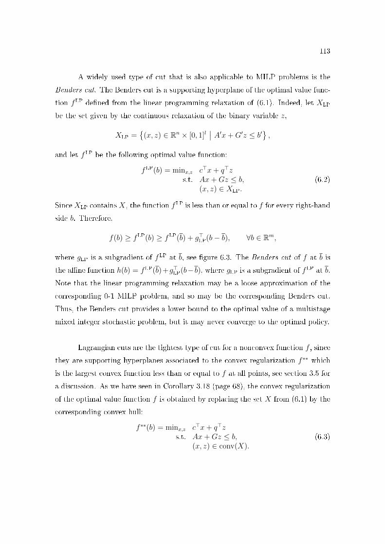
113

A widely used type of cut that is also applicable to MILP problems is the

Benders cut. The Benders cut is a supporting hyperplane of the optimal value func-

tion fLP de�ned from the linear programming relaxation of (6.1). Indeed, let XLP

be the set given by the continuous relaxation of the binary variable z,

XLP ={

(x, z) ∈ Rn × [0, 1]l∣∣ A′x+G′z ≤ b′

},

and let fLP be the following optimal value function:

fLP(b) = minx,z c>x+ q>zs.t. Ax+Gz ≤ b,

(x, z) ∈ XLP.(6.2)

SinceXLP containsX, the function fLP is less than or equal to f for every right-hand

side b. Therefore,

f(b) ≥ fLP(b) ≥ fLP(b) + g>LP(b− b), ∀b ∈ Rm,

where gLP is a subgradient of fLP at b, see �gure 6.3. The Benders cut of f at b is

the a�ne function h(b) = fLP(b)+g>LP(b−b), where gLP is a subgradient of fLP at b.

Note that the linear programming relaxation may be a loose approximation of the

corresponding 0-1 MILP problem, and so may be the corresponding Benders cut.

Thus, the Benders cut provides a lower bound to the optimal value of a multistage

mixed integer stochastic problem, but it may never converge to the optimal policy.

Lagrangian cuts are the tightest type of cut for a nonconvex function f , since

they are supporting hyperplanes associated to the convex regularization f ∗∗ which

is the largest convex function less than or equal to f at all points, see section 3.5 for

a discussion. As we have seen in Corollary 3.18 (page 68), the convex regularization

of the optimal value function f is obtained by replacing the set X from (6.1) by the

corresponding convex hull:

f ∗∗(b) = minx,z c>x+ q>zs.t. Ax+Gz ≤ b,

(x, z) ∈ conv(X).(6.3)

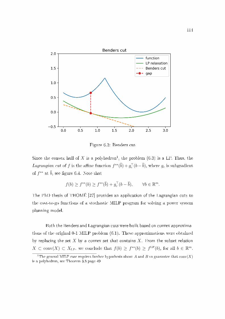
114

Figure 6.3: Benders cut

Since the convex hull of X is a polyhedron1, the problem (6.3) is a LP. Thus, the

Lagrangian cut of f is the a�ne function f ∗∗(b) + g>c (b− b), where gc is subgradientof f ∗∗ at b, see �gure 6.4. Note that

f(b) ≥ f ∗∗(b) ≥ f ∗∗(b) + g>c (b− b), ∀b ∈ Rm.

The PhD thesis of THOMÉ [27] provides an application of the Lagrangian cuts to

the cost-to-go functions of a stochastic MILP program for solving a power system

planning model.

Both the Benders and Lagrangian cuts were built based on convex approxima-

tions of the original 0-1 MILP problem (6.1). These approximations were obtained

by replacing the set X by a convex set that contains X. From the subset relation

X ⊂ conv(X) ⊂ XLP, we conclude that f(b) ≥ f ∗∗(b) ≥ fLP(b), for all b ∈ Rm.

1The general MILP case requires further hypothesis about A and B to guarantee that conv(X)is a polyhedron, see Theorem 3.8 page 49

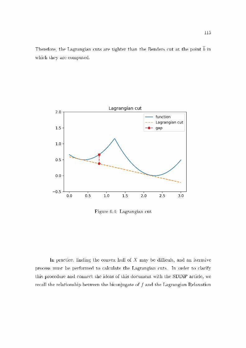
115

Therefore, the Lagrangian cuts are tighter than the Benders cut at the point b in

which they are computed.

Figure 6.4: Lagrangian cut

In practice, �nding the convex hull of X may be di�cult, and an iterative

process must be performed to calculate the Lagrangian cuts. In order to clarify

this procedure and connect the ideas of this document with the SDDiP article, we

recall the relationship between the biconjugate of f and the Lagrangian Relaxation

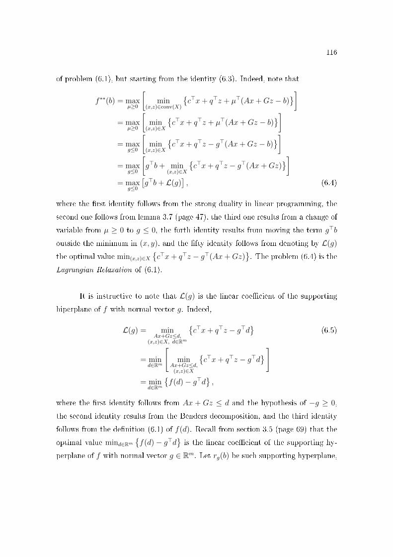
116

of problem (6.1), but starting from the identity (6.3). Indeed, note that

f ∗∗(b) = maxµ≥0

[min

(x,z)∈conv(X)

{c>x+ q>z + µ>(Ax+Gz − b)

}]

= maxµ≥0

[min

(x,z)∈X

{c>x+ q>z + µ>(Ax+Gz − b)

}]

= maxg≤0

[min

(x,z)∈X

{c>x+ q>z − g>(Ax+Gz − b)

}]

= maxg≤0

[g>b+ min

(x,z)∈X

{c>x+ q>z − g>(Ax+Gz)

}]

= maxg≤0

[g>b+ L(g)

], (6.4)

where the �rst identity follows from the strong duality in linear programming, the

second one follows from lemma 3.7 (page 47), the third one results from a change of

variable from µ ≥ 0 to g ≤ 0, the forth identity results from moving the term g>b

outside the minimum in (x, y), and the �fty identity follows from denoting by L(g)

the optimal value min(x,z)∈X{c>x+ q>z − g>(Ax+Gz)

}. The problem (6.4) is the

Lagrangian Relaxation of (6.1).

It is instructive to note that L(g) is the linear coe�cient of the supporting

hiperplane of f with normal vector g. Indeed,

L(g) = minAx+Gz≤d,

(x,z)∈X, d∈Rm

{c>x+ q>z − g>d

}(6.5)

= mind∈Rm

[min

Ax+Gz≤d,(x,z)∈X

{c>x+ q>z − g>d

}]

= mind∈Rm

{f(d)− g>d

},

where the �rst identity follows from Ax + Gz ≤ d and the hypothesis of −g ≥ 0,

the second identity results from the Benders decomposition, and the third identity

follows from the de�nition (6.1) of f(d). Recall from section 3.5 (page 69) that the

optimal value mind∈Rm

{f(d)− g>d

}is the linear coe�cient of the supporting hy-

perplane of f with normal vector g ∈ Rm. Let rg(b) be such supporting hyperplane,

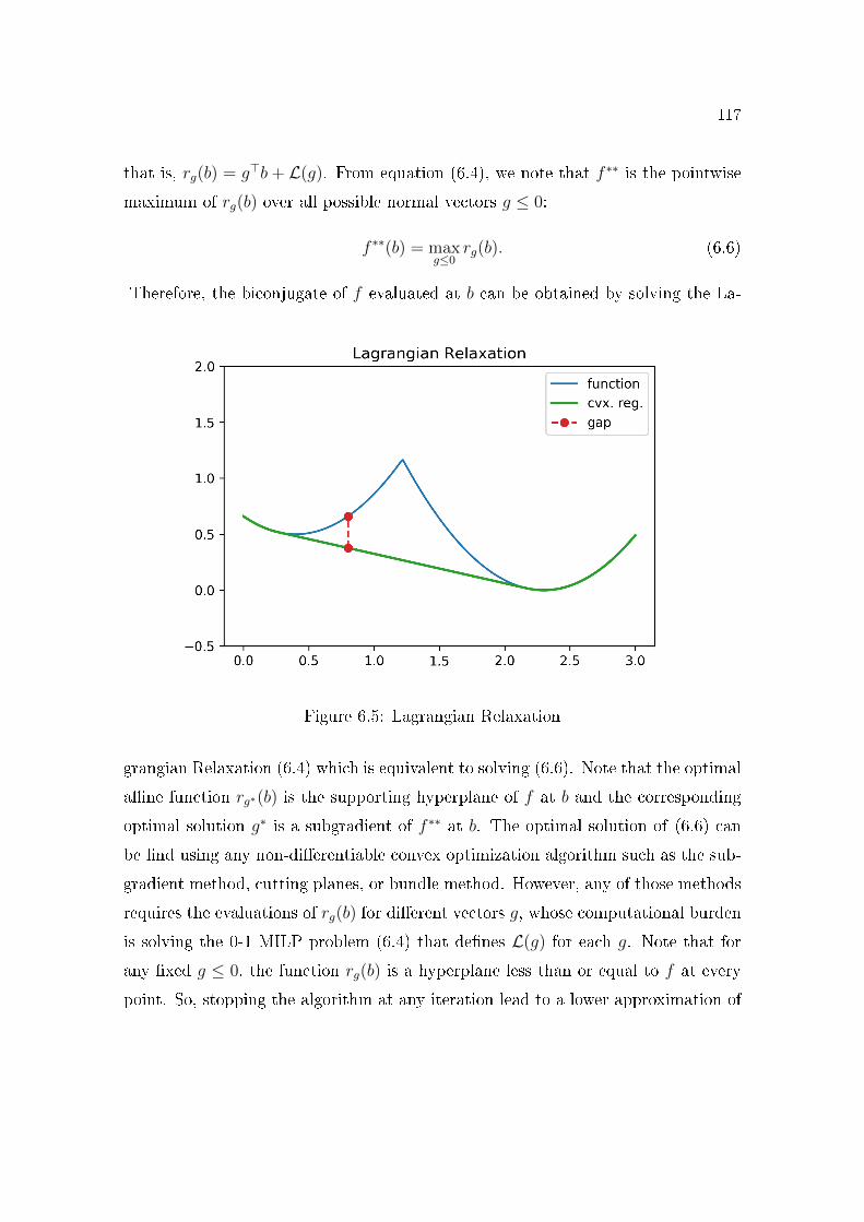
117

that is, rg(b) = g>b + L(g). From equation (6.4), we note that f ∗∗ is the pointwise

maximum of rg(b) over all possible normal vectors g ≤ 0:

f ∗∗(b) = maxg≤0

rg(b). (6.6)

Therefore, the biconjugate of f evaluated at b can be obtained by solving the La-

Figure 6.5: Lagrangian Relaxation

grangian Relaxation (6.4) which is equivalent to solving (6.6). Note that the optimal

a�ne function rg∗(b) is the supporting hyperplane of f at b and the corresponding

optimal solution g∗ is a subgradient of f ∗∗ at b. The optimal solution of (6.6) can

be �nd using any non-di�erentiable convex optimization algorithm such as the sub-

gradient method, cutting planes, or bundle method. However, any of those methods

requires the evaluations of rg(b) for di�erent vectors g, whose computational burden

is solving the 0-1 MILP problem (6.4) that de�nes L(g) for each g. Note that for

any �xed g ≤ 0, the function rg(b) is a hyperplane less than or equal to f at every

point. So, stopping the algorithm at any iteration lead to a lower approximation of

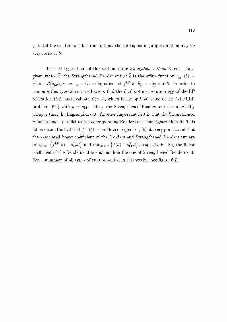
118

f , but if the solution g is far from optimal the corresponding approximation may be

very loose at b.

The last type of cut of this section is the Strengthened Benders cut. For a

given vector b, the Strengthened Bender cut at b is the a�ne function rgLP(b) =

g>LPb + L(gLP), where gLP is a subgradient of fLP at b, see �gure 6.6. In order to

compute this type of cut, we have to �nd the dual optimal solution gLP of the LP

relaxation (6.2) and evaluate L(gLP), which is the optimal value of the 0-1 MILP

problem (6.5) with g = gLP. Thus, the Strengthened Benders cut is numerically

cheaper than the Lagrangian cut. Another important fact is that the Strengthened

Benders cut is parallel to the corresponding Benders cut, but tighter than it. This

follows from the fact that fLP(b) is less than or equal to f(b) at every point b and that

the associated linear coe�cient of the Benders and Strengthened Benders cut are

mind∈Rm

{fLP(d)− g>LPd

}and mind∈Rm

{f(d)− g>LPd

}, respectively. So, the linear

coe�cient of the Benders cut is smaller than the one of Strengthened Benders cut.

For a summary of all types of cuts presented in this section, see �gure 6.7.

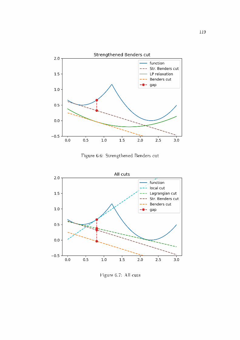
119

Figure 6.6: Strengthened Benders cut

Figure 6.7: All cuts

120

6.2 SDDiP and the Blessing of Binary

In this section, we present the main result of the SDDiP article, the �Blessing

of Binary�, which states that the Lagrangian cuts are �tight� (no convexi�cation gap)

at some special points for a particular class of 0-1 MILP optimal value functions.

Then, we describe how to approximate a general 0-1 MILP problem by a problem

of the Blessing of Binary class, and how to bound the corresponding approximation

error. Those ideas are also suggestions of the SDDiP article.

The class of optimal value functions used in the Blessing of Binary theorem

has the following form:

φ(λ) = minx,y,z

c>x+ c>y + q>z

s.t. y = λ,

(x, y, z) ∈ X,(6.7)

where x is a continuous vector of Rn, y is a continuous vector on the unit cube [0, 1]p,

and z is a binary vector of {0, 1}l such that the feasible set X is given by

X = {(x, y, z) ∈ Rn × [0, 1]p × {0, 1}l | Ax+ F y + Gz ≤ b}.

We denote by φ instead of f the optimal value function and by λ instead of b

the corresponding right-hand side in (6.7) to emphasize the di�erences between

both classes of functions. It is instructive to note two main restrictive aspects in

problem (6.7): the constraint of the right-hand side λ is a trivial equality constraint,

i.e., y = λ, and the variable y is restricted to the unit cube [0, 1]p, which means that

the problem (6.7) is infeasible if λ do not belong to [0, 1]p.

As we have seen in section 6.1, the Lagrangian cut is a supporting hyperplane

to the biconjugate φ∗∗, which has the following expression:

φ∗∗(λ) = minx,y,z

c>x+ c>y + q>z

s.t. y = λ,

(x, y, z) ∈ conv(X),

121

according to Corollary 3.18 (page 68). Surprisingly, the Blessing of Binary states

that there is no gap between the convex regularization φ∗∗ and the original function

φ at the binary points λ ∈ {0, 1}p.

Theorem 6.2 (Blessing of Binary). The convex regularization φ∗∗ equals the original

function φ at the binary points:

φ∗∗(λ) = φ(λ), ∀λ ∈ {0, 1}l. (6.8)

Proof. Let λ ∈ {0, 1}p. If conv(X) ∩ (y = λ) is empty, then both φ∗∗(λ) and φ(λ)

are equal to +∞. Assume that conv(X) ∩ (y = λ) is nonempty, and let (x, y, z) be

a vector on this set. Then, y = λ and

(x, y, λ) =k∑

i=1

αi(xi, yi, zi), (6.9)

where (xi, yi, zi) ∈ X and αi ∈ [0, 1] such that∑k

i=1 αi = 1. Without loss of

generality, suppose that all αi's are positives. Since, λ is an extreme point of the

unit cube [0, 1]p and each yi belongs to [0, 1]p, we have that yi = b, for all i = 1, . . . , k.

Moreover, there is (xi, yi, λ) ∈ X such that

c>xi + c>yi + q>λ ≤ c>x+ c>y + q>λ,

otherwise we have a contradiction with equation (6.9). Thus, we conclude (6.8).

Motivated by Theorem 6.2, the SDDiP algorithm requires two additional

steps before computing the Lagrangian cuts for cost-to-go functions of a stochastic

MILP program: the binarization of the state variables, and the dimensional lifting

of the feature space. After these two steps, we get a cost-to-go function that �ts

the hypothesis of Theorem 6.2, so we guarantee that the Lagrangian cuts are tight

at the binary coordinates. We can increase the overall quality of the resulting cost-

to-go approximation by increasing the number of points in the binarization step. In

122

this section, the cost-to-go function of a stochastic MILP program is represented

by the optimal value function f , see (6.1). An additional hypothesis required for

the SDDiP algorithm is the boundedness of dom(f), i.e., dom(f) ⊂ [−U,U ]m, for

some U > 0.

The binarization step is the process of approximating the block [−U,U ]m by

a uniform grid R, where we have a simple formula involving binary variables to

represent the grid elements. We illustrate this idea with a �nite interval [0, U ]. Let

ε > 0 be such that ε = U/2k, for some k ∈ Z+. The uniform grid of [0, U ] with

precision ε is the following set

R := {0, ε, 2ε, 3ε, . . . , (2k − 1)ε}.

Note that [0, U ] contains R, since all elements of R are non-negative and the largest

one is (2k− 1)ε = (1− 2−k)U , which is less than U . Denote by [k] the set of positive

integers from 1 to k, i.e., [k] = {1, . . . , k}. We can use the following algebraic formula

and k binary variables to generate the elements of R:

bR =k∑

j=1

ε2j−1γj,

where γj ∈ {0, 1}, for all j ∈ [k]. If the scalar γj can have any value in the interval

[0, 1], we can represent any number of [0, (1− 2−k)U ].

We shall extend those ideas to a uniform grid on a symmetric block [−U,U ]m.

The uniform grid with precision ε = U/2k on [−U,U ]m is the Cartesian Product Rm,

where

R := {−(2k − 1)ε, . . . ,−2ε,−ε, 0, ε, 2ε, . . . , (2k − 1)ε}.

Following the same analogy, we represent the elements of Rm using the expression

below:

bR,i =k∑

j=1

ε2j−1(γi,j − γi,j+k), i ∈ [m], (6.10)

123

where γi,j ∈ {0, 1} for all i ∈ [m] and j ∈ [2k]. If each γi,j assumes any value along

the interval [0, 1], the formula (6.10) generates the set [−(1− 2−k)U, (1− 2−k)U ]m.

In order to clarify the exposition of the binarization step, it is convenient to

represent equation (6.10) using a vectorial notation. Let y be a vector of the unit

cube [0, 1]p such that p = 2mk and y satis�es to

y2k(i−1)+j = γi,j,

where i ∈ [m] and j ∈ [2k]. Let F ∈ Rm×p be a matrix whose entries Fi,r are de�ned

by

Fi,r =

ε2j−1 , if r = 2k(i− 1) + j, for some j ∈ [k],

−ε2j−1 , if r = 2k(i− 1) + j + k, for some j ∈ [k],

0 , otherwise.

Note that equation (6.10) is equivalent to the following equality constraint

bR = Fy,

where y ∈ {0, 1}p. Using this notation, we have that F ({0, 1}p) = Rm and F ([0, 1]p) =

[−(1 − 2−k)U, (1 − 2−k)U ]m. Without loss of generality, we assume that F ([0, 1]p)

contains dom(f). Thus, the optimal value function f can be represented as

f(b) = minx,y,z c>x+ q>zs.t. Fy = b,

Ax− Fy +Gz ≤ 0,(x, z) ∈ X, y ∈ [0, 1]p,

(6.11)

see �gure 6.8 for an illustration. We call this representation the binarization step.

The second step in direction of the Blessing of Binary is the lifting of the

feature space of f . We de�ne the lifting of f by the optimal value function φ

obtained from (6.11) with Fy = b replaced by y = λ:

φ(λ) = minx,y,z c>x+ q>zs.t. y = λ

Ax− Fy +Gz ≤ 0,(x, z) ∈ X, y ∈ [0, 1]p.

(6.12)

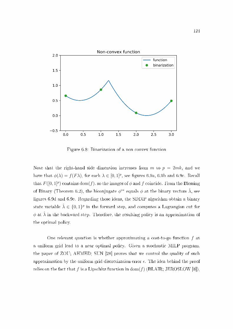
124

Figure 6.8: Binarization of a non-convex function

Note that the right-hand side dimension increases from m to p = 2mk, and we

have that φ(λ) = f(Fλ), for each λ ∈ [0, 1]p, see �gures 6.9a, 6.9b and 6.9c. Recall

that F ([0, 1]p) contains dom(f), so the images of φ and f coincide. From the Blessing

of Binary (Theorem 6.2), the biconjugate φ∗∗ equals φ at the binary vectors λ, see

�gures 6.9d and 6.9e. Regarding those ideas, the SDDiP algorithm obtain a binary

state variable λ ∈ {0, 1}p in the forward step, and computes a Lagrangian cut for

φ at λ in the backward step. Therefore, the resulting policy is an approximation of

the optimal policy.

One relevant question is whether approximating a cost-to-go function f at

a uniform grid lead to a near optimal policy. Given a stochastic MILP program,

the paper of ZOU; AHMED; SUN [28] proves that we control the quality of such

approximation by the uniform grid discretization error ε. The idea behind the proof

relies on the fact that f is a Lipschitz function in dom(f) (BLAIR; JEROSLOW [8]),

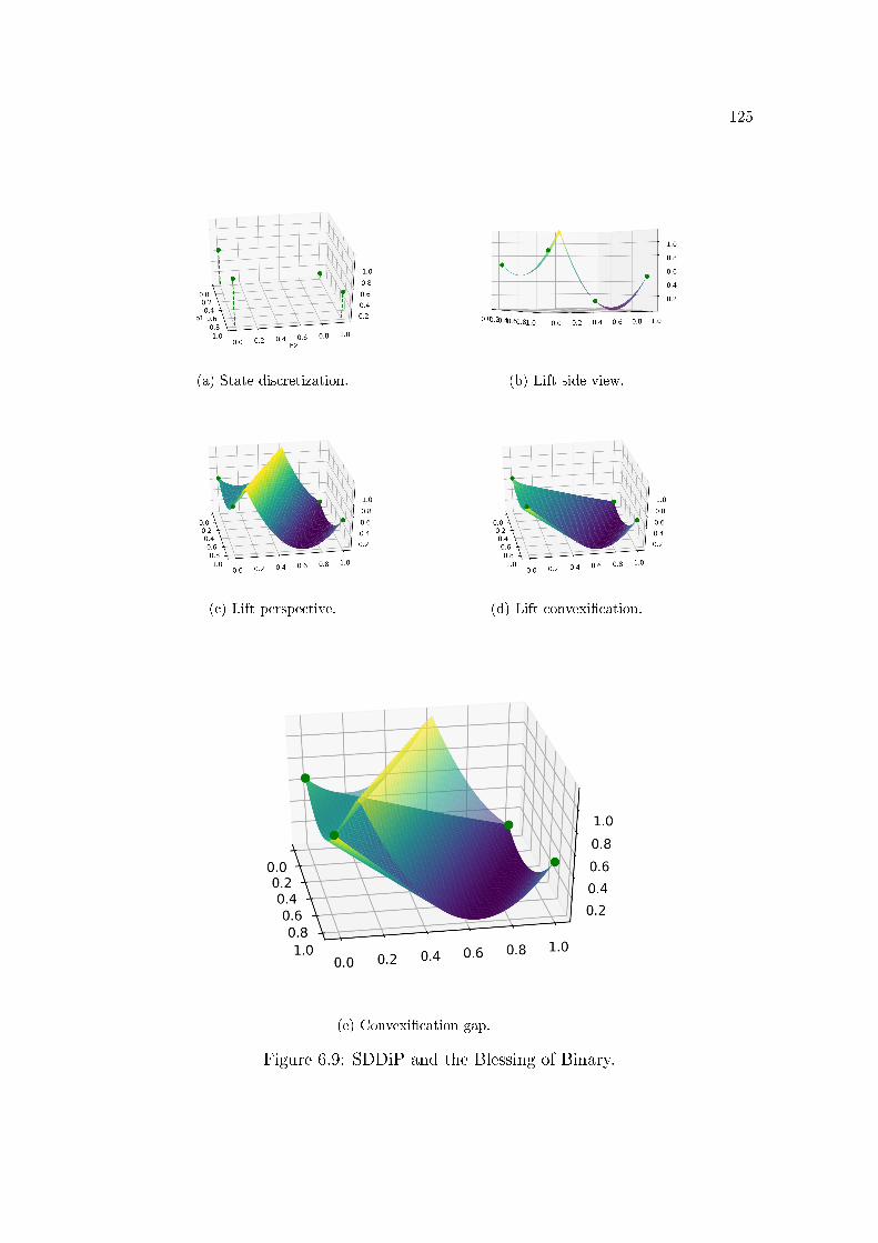
125

(a) State discretization. (b) Lift side view.

(c) Lift perspective. (d) Lift convexi�cation.

(e) Convexi�cation gap.

Figure 6.9: SDDiP and the Blessing of Binary.

126

and for each b ∈ dom(f), there is λR ∈ {0, 1}p such that ‖b− FλR‖ < ε. Therefore,

‖f(b)− φ∗∗(λR)‖ = ‖f(b)− f(bR)‖ ≤ L‖b− bR‖ ≤ Lε.

Thus, the Lagrangian cuts for φ at the binary vectors λR ∈ {0, 1}p approximate f

with arbitrary precision.

6.3 Case study: hydrothermal operational planning with Dis-junctive Constraints

In this section, we present the results for the Disjunctive Constraints approach

given by CAR-B and the De�cit Suppression Constraint (SPDef), so we compare it

with the base case and the traditional penalization approach. These three modeling

options are combined with two types of risk measures: the expected value and the

mean-CVaR, which will be abbreviated by CVaR only.

Let us recall the base model. The objective function is to minimize the

thermal and de�cit costs c>g gt+c>dfdft plus the future cost-to-go function βQt+1(vt+1):

Qt(vt, at) = minxt∈Xt

c>g gt + c>dfdft + βQt+1(vt+1)

s.t. (∗)P,(6.13)

where xt is the decision vector with all operational variables, Xt are the upper

and lower bound limits of each variable, and (∗)P represents the other operational

constraints.

The CAR is a pre-established stored volume curve, denoted by vMinOP (we

omit the subscript t to not overload the notation). One possible use in the optimiza-

tion model (6.13) considers an unit cost θt that penalizes the �nal stored volumes

127

vt+1 which lie below the CAR volume vMinOP:

Qt(vt, at) = minxt∈Xt

c>g gt + c>dfdft + βQt+1(vt+1) + θ>t (vMinOP − vt+1)+

s.t. (∗)P.(6.14)

We call formulation (6.14) the Penalty (Pen) approach. For this example, we con-

sider a constant vector vMinOP equal to 20% of the maximum storage capacity v, and

a penalty value θt between the most expensive thermal cost and the cost of the �rst

de�cit level.

The CAR-B approach follows the same idea of CAR but uses binary variables,

zg ∈ {0, 1}Nsys , to induce thermal generation if the �nal stored volume vt+1 is below

the reference vector vMinOP. We also consider the Suppression of Preventive De�cit

(SPDef) constraint in this formulation that we call the Disjunctive Constraint (Disj.)

approach:

Qt(vt, at) = minxt∈Xt

c>g gt + c>dfdft + βQt+1(vt+1)

s.t. (∗)P,

(1− zg) · vMinOp ≤ vt+1 ≤ (1− zd) · v,MIgt ≥ zg ·G, 0 ≤ dft ≤ zd · dt,zg, zd ∈ {0, 1}Nsys .

(6.15)

We note that the security thermal dispatch is regional, that is, if the �nal stored

volume vi,t+1 of a subsystem i is below the reference value vi,MinOp, then only the

thermal plants from the subsystem i are dispatched. This is the reason for the indi-

cator matrixMI in the constraintMIgt ≥ zgG. For this case study, the vector G has

coordinates that equals the maximum thermal generation capacity of each subsys-

tem, i.e., G = MIg. The SPDef constraint is also regional, since it is only possible

to have a load shedding in a subsystem i, dfi,t > 0, if the corresponding �nal stored

volume vi,t+1 is zero.

These three modeling proposals were combined with two coherent risk mea-

sures: the expected value and CVaR. Recall that a coherent risk measure ρt (SHAPIRO;

128

DENTCHEVA; RUSZCZY�SKI [26]) is a function that associates random costs Z

to real numbers and satis�es some axioms equivalent to the convexity de�nition. The

risk measure appears in the de�nition of the future cost-to-go function Qt+1(vt+1):

Qt+1(vt+1) =

{ρt [Qt+1(vt+1, at+1)] , t ∈ {1, . . . , T − 1},0 , t = T ,

(6.16)

where we call the function ρt[Z] = E[Z] the risk neutral case and ρt[Z] = (1 −λ)E[Z] + λCVaRα[Z] the CVaR case. The parameters used in the CVaR case are

λ = 0.10 and α = 0.05.

For the stochastic in�ow at, we adopted a stagewise independent model with

periodic empirical distribution on each month. The reason for this simpli�cation

is the di�culty in considering an autoregressive model along with the SDDiP algo-

rithm, since the SDDiP requires upper and lower bound limits for the state variables.

As the scenarios of an autoregressive model can assume very high values (and also

very low values), we decided to simplify the in�ow model.

In all cases, we consider four interconnected subsystems, Nsys = 4, based on

the con�guration of the Brazilian Interconnected Power System of January 2015,

with a planning horizon of 5 years (T = 60 monthly stages) that ends in December

2019. Table 6.1 shows the maximum storable energy v, the CAR reference stor-

age vMinOp, and the maximum thermal generation capacity MIg of each subsystem.

To better understand the e�ects of di�erent policies (base case, Pen., Disj. . . . ), we

increased the demand from each stage by a factor of 5%.

All the numerical experiments were performed on a computer with Intel(R)

Core(TM) i7-4790, 8Gb RAM, operational system Ubuntu Xenial (16.04), and Julia

language version 0.6 [6]. We used the packages SDDP.jl [14] and SDDiP.jl [19], and

the resulting optimization problems, both linear and mixed integer linear programs

were solved by Gurobi [16], version 7.0.2.

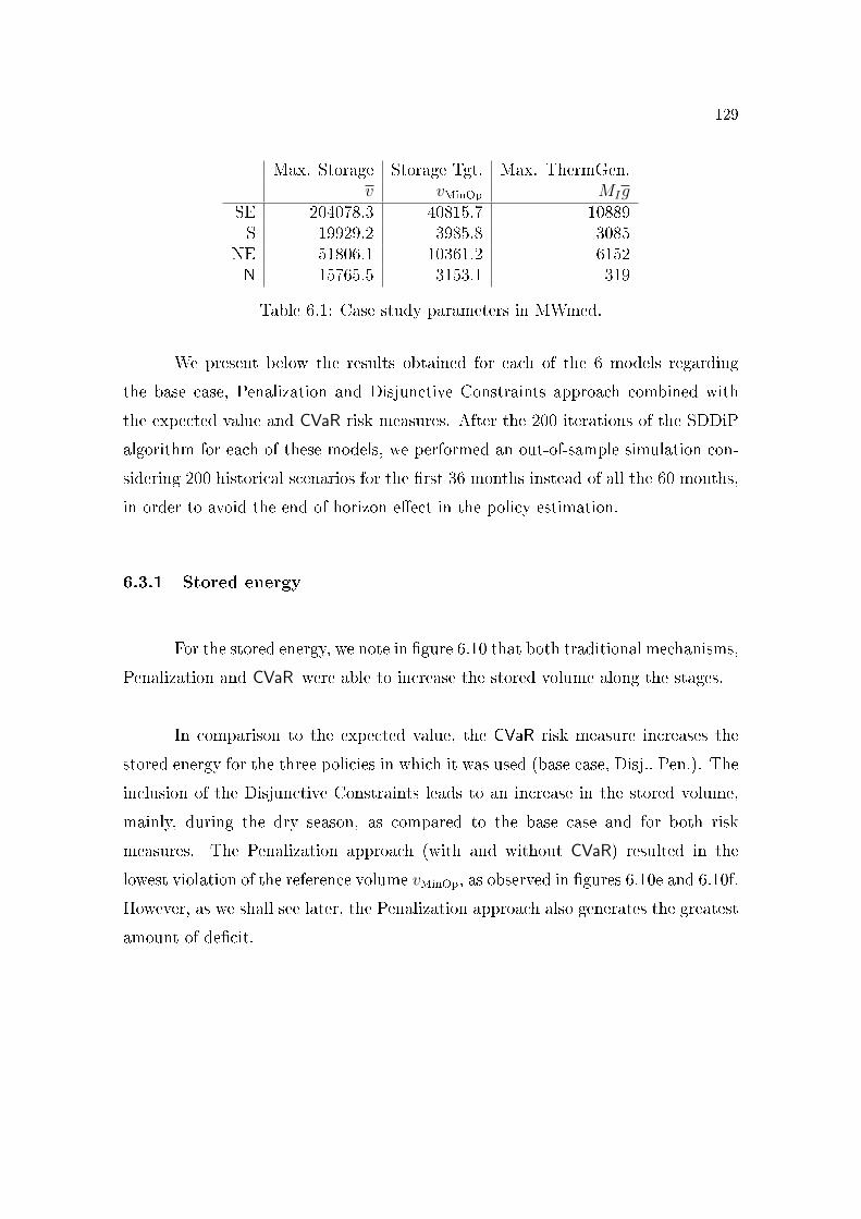
129

Max. Storage Storage Tgt. Max. ThermGen.v vMinOp MIg

SE 204078.3 40815.7 10889S 19929.2 3985.8 3085

NE 51806.1 10361.2 6152N 15765.5 3153.1 319

Table 6.1: Case study parameters in MWmed.

We present below the results obtained for each of the 6 models regarding

the base case, Penalization and Disjunctive Constraints approach combined with

the expected value and CVaR risk measures. After the 200 iterations of the SDDiP

algorithm for each of these models, we performed an out-of-sample simulation con-

sidering 200 historical scenarios for the �rst 36 months instead of all the 60 months,

in order to avoid the end of horizon e�ect in the policy estimation.

6.3.1 Stored energy

For the stored energy, we note in �gure 6.10 that both traditional mechanisms,

Penalization and CVaR were able to increase the stored volume along the stages.

In comparison to the expected value, the CVaR risk measure increases the

stored energy for the three policies in which it was used (base case, Disj., Pen.). The

inclusion of the Disjunctive Constraints leads to an increase in the stored volume,

mainly, during the dry season, as compared to the base case and for both risk

measures. The Penalization approach (with and without CVaR) resulted in the

lowest violation of the reference volume vMinOp, as observed in �gures 6.10e and 6.10f.

However, as we shall see later, the Penalization approach also generates the greatest

amount of de�cit.

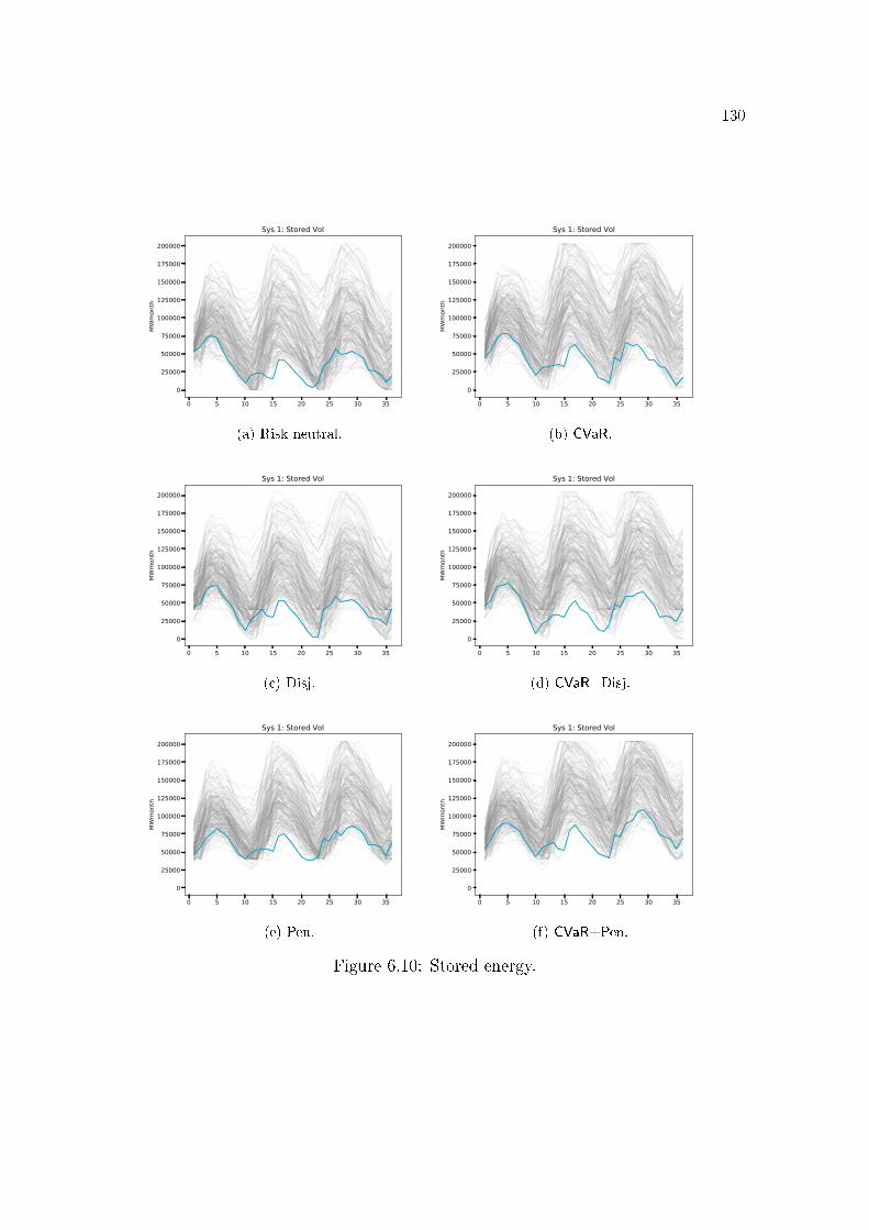
130

0 5 10 15 20 25 30 35

0

25000

50000

75000

100000

125000

150000

175000

200000

MW

mon

th

Sys 1: Stored Vol

(a) Risk neutral.

0 5 10 15 20 25 30 35

0

25000

50000

75000

100000

125000

150000

175000

200000

MW

mon

th

Sys 1: Stored Vol

(b) CVaR.

0 5 10 15 20 25 30 35

0

25000

50000

75000

100000

125000

150000

175000

200000

MW

mon

th

Sys 1: Stored Vol

(c) Disj.

0 5 10 15 20 25 30 35

0

25000

50000

75000

100000

125000

150000

175000

200000

MW

mon

th

Sys 1: Stored Vol

(d) CVaR+Disj.

0 5 10 15 20 25 30 35

0

25000

50000

75000

100000

125000

150000

175000

200000

MW

mon

th

Sys 1: Stored Vol

(e) Pen.

0 5 10 15 20 25 30 35

0

25000

50000

75000

100000

125000

150000

175000

200000

MW

mon

th

Sys 1: Stored Vol

(f) CVaR+Pen.

Figure 6.10: Stored energy.

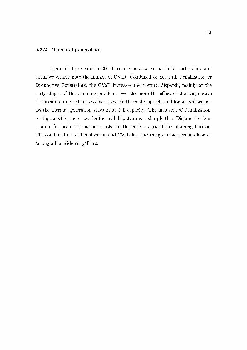
131

6.3.2 Thermal generation

Figure 6.11 presents the 200 thermal generation scenarios for each policy, and

again we clearly note the impact of CVaR. Combined or not with Penalization or

Disjunctive Constraints, the CVaR increases the thermal dispatch, mainly at the

early stages of the planning problem. We also note the e�ect of the Disjunctive

Constraints proposal: it also increases the thermal dispatch, and for several scenar-

ios the thermal generation stays in its full capacity. The inclusion of Penalization,

see �gure 6.11e, increases the thermal dispatch more sharply than Disjunctive Con-

straints for both risk measures, also in the early stages of the planning horizon.

The combined use of Penalization and CVaR leads to the greatest thermal dispatch

among all considered policies.

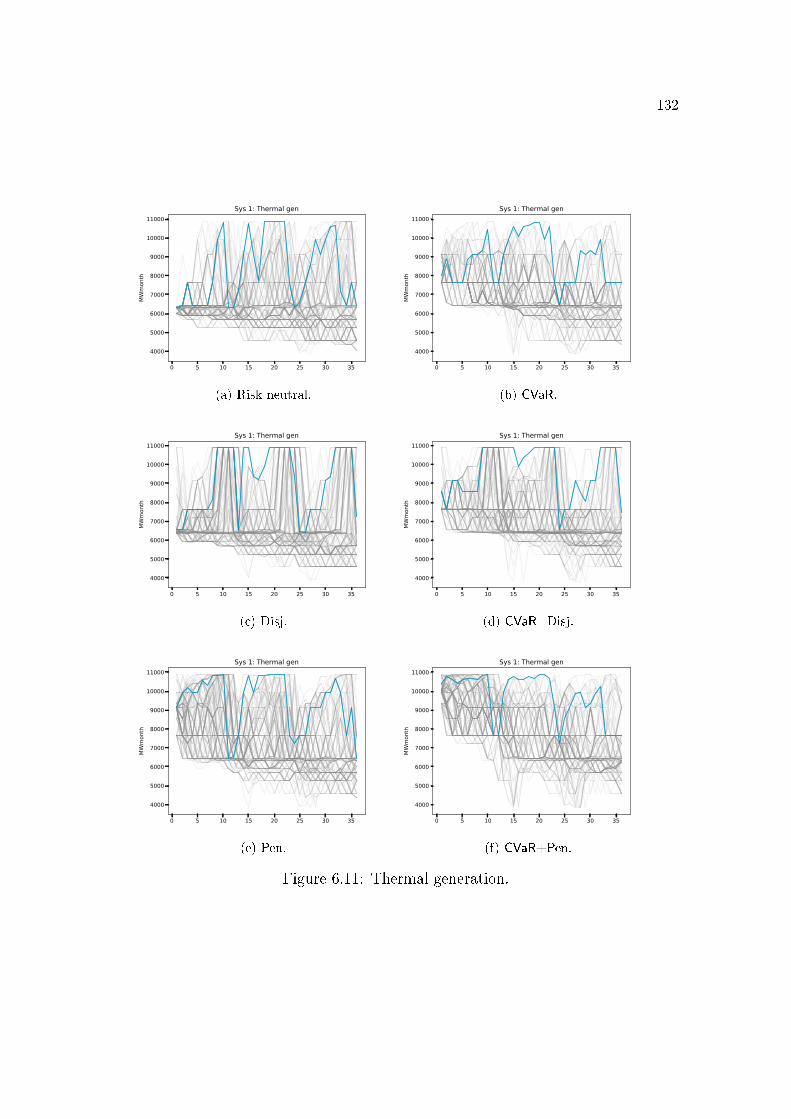
132

0 5 10 15 20 25 30 35

4000

5000

6000

7000

8000

9000

10000

11000

MW

mon

th

Sys 1: Thermal gen

(a) Risk neutral.

0 5 10 15 20 25 30 35

4000

5000

6000

7000

8000

9000

10000

11000

MW

mon

th

Sys 1: Thermal gen

(b) CVaR.

0 5 10 15 20 25 30 35

4000

5000

6000

7000

8000

9000

10000

11000

MW

mon

th

Sys 1: Thermal gen

(c) Disj.

0 5 10 15 20 25 30 35

4000

5000

6000

7000

8000

9000

10000

11000

MW

mon

th

Sys 1: Thermal gen

(d) CVaR+Disj.

0 5 10 15 20 25 30 35

4000

5000

6000

7000

8000

9000

10000

11000

MW

mon

th

Sys 1: Thermal gen

(e) Pen.

0 5 10 15 20 25 30 35

4000

5000

6000

7000

8000

9000

10000

11000

MW

mon

th

Sys 1: Thermal gen

(f) CVaR+Pen.

Figure 6.11: Thermal generation.

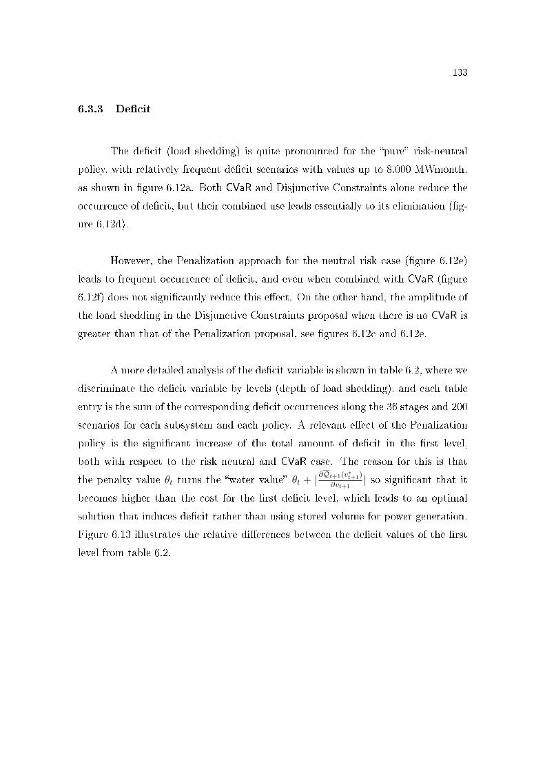
133

6.3.3 De�cit

The de�cit (load shedding) is quite pronounced for the �pure� risk-neutral

policy, with relatively frequent de�cit scenarios with values up to 8.000 MWmonth,

as shown in �gure 6.12a. Both CVaR and Disjunctive Constraints alone reduce the

occurrence of de�cit, but their combined use leads essentially to its elimination (�g-

ure 6.12d).

However, the Penalization approach for the neutral risk case (�gure 6.12e)

leads to frequent occurrence of de�cit, and even when combined with CVaR (�gure

6.12f) does not signi�cantly reduce this e�ect. On the other hand, the amplitude of

the load shedding in the Disjunctive Constraints proposal when there is no CVaR is

greater than that of the Penalization proposal, see �gures 6.12c and 6.12e.

A more detailed analysis of the de�cit variable is shown in table 6.2, where we

discriminate the de�cit variable by levels (depth of load shedding), and each table

entry is the sum of the corresponding de�cit occurrences along the 36 stages and 200

scenarios for each subsystem and each policy. A relevant e�ect of the Penalization

policy is the signi�cant increase of the total amount of de�cit in the �rst level,

both with respect to the risk neutral and CVaR case. The reason for this is that

the penalty value θt turns the �water value� θt + |∂Qt+1(v∗t+1)

∂vt+1| so signi�cant that it

becomes higher than the cost for the �rst de�cit level, which leads to an optimal

solution that induces de�cit rather than using stored volume for power generation.

Figure 6.13 illustrates the relative di�erences between the de�cit values of the �rst

level from table 6.2.

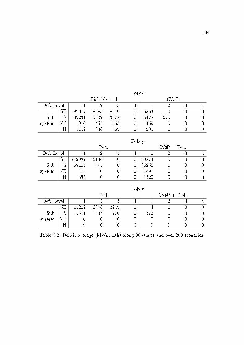
134

PolicyRisk Neutral CVaR

Def. Level 1 2 3 4 1 2 3 4SE 89067 18383 8640 0 6853 0 0 0

Sub S 32231 5509 3878 0 6478 1276 0 0system NE 910 455 463 0 459 0 0 0

N 1152 336 569 0 285 0 0 0

PolicyPen. CVaR + Pen.

Def. Level 1 2 3 4 1 2 3 4SE 219987 2136 0 0 98874 0 0 0

Sub S 69104 591 0 0 36252 0 0 0system NE 413 0 0 0 1899 0 0 0

N 885 0 0 0 1320 0 0 0

PolicyDisj. CVaR + Disj.

Def. Level 1 2 3 4 1 2 3 4SE 13202 6096 3249 0 4 0 0 0

Sub S 5691 1837 270 0 372 0 0 0system NE 0 0 0 0 0 0 0 0

N 0 0 0 0 0 0 0 0

Table 6.2: De�cit average (MWmonth) along 36 stages and over 200 scenarios.

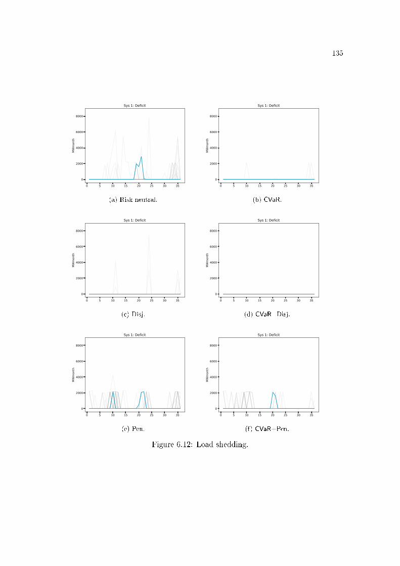
135

0 5 10 15 20 25 30 35

0

2000

4000

6000

8000

MW

mon

th

Sys 1: Deficit

(a) Risk neutral.

0 5 10 15 20 25 30 35

0

2000

4000

6000

8000

MW

mon

th

Sys 1: Deficit

(b) CVaR.

0 5 10 15 20 25 30 35

0

2000

4000

6000

8000

MW

mon

th

Sys 1: Deficit

(c) Disj.

0 5 10 15 20 25 30 35

0

2000

4000

6000

8000

MW

mon

th

Sys 1: Deficit

(d) CVaR+Disj.

0 5 10 15 20 25 30 35

0

2000

4000

6000

8000

MW

mon

th

Sys 1: Deficit

(e) Pen.

0 5 10 15 20 25 30 35

0

2000

4000

6000

8000

MW

mon

th

Sys 1: Deficit

(f) CVaR+Pen.

Figure 6.12: Load shedding.

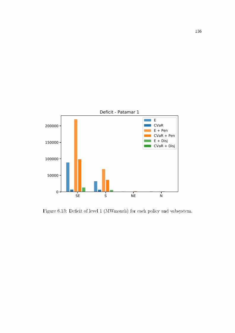
136

SE S NE N0

50000

100000

150000

200000

Deficit - Patamar 1ECVaRE + PenCVaR + PenE + DisjCVaR + Disj

Figure 6.13: De�cit of level 1 (MWmonth) for each policy and subsystem.

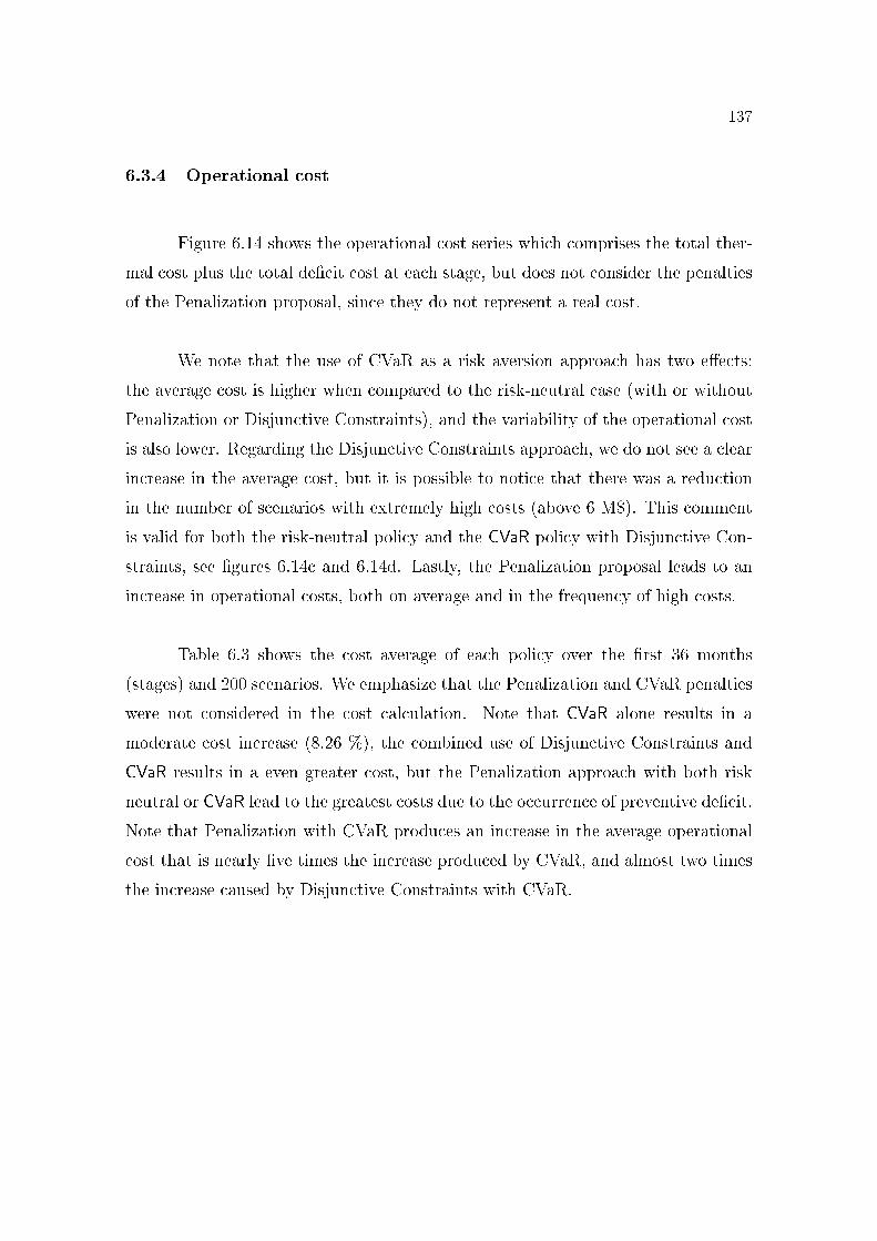
137

6.3.4 Operational cost

Figure 6.14 shows the operational cost series which comprises the total ther-

mal cost plus the total de�cit cost at each stage, but does not consider the penalties

of the Penalization proposal, since they do not represent a real cost.

We note that the use of CVaR as a risk aversion approach has two e�ects:

the average cost is higher when compared to the risk-neutral case (with or without

Penalization or Disjunctive Constraints), and the variability of the operational cost

is also lower. Regarding the Disjunctive Constraints approach, we do not see a clear

increase in the average cost, but it is possible to notice that there was a reduction

in the number of scenarios with extremely high costs (above 6 M$). This comment

is valid for both the risk-neutral policy and the CVaR policy with Disjunctive Con-

straints, see �gures 6.14c and 6.14d. Lastly, the Penalization proposal leads to an

increase in operational costs, both on average and in the frequency of high costs.

Table 6.3 shows the cost average of each policy over the �rst 36 months

(stages) and 200 scenarios. We emphasize that the Penalization and CVaR penalties

were not considered in the cost calculation. Note that CVaR alone results in a

moderate cost increase (8.26 %), the combined use of Disjunctive Constraints and

CVaR results in a even greater cost, but the Penalization approach with both risk

neutral or CVaR lead to the greatest costs due to the occurrence of preventive de�cit.

Note that Penalization with CVaR produces an increase in the average operational

cost that is nearly �ve times the increase produced by CVaR, and almost two times

the increase caused by Disjunctive Constraints with CVaR.

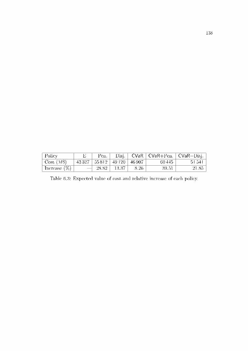
138

Policy E Pen. Disj. CVaR CVaR+Pen. CVaR+Disj.Cost (M$) 43 327 55 812 49 120 46 907 60 445 51 541Increase (%) � 28.82 13.37 8.26 39.51 21.85

Table 6.3: Expected value of cost and relative increase of each policy.

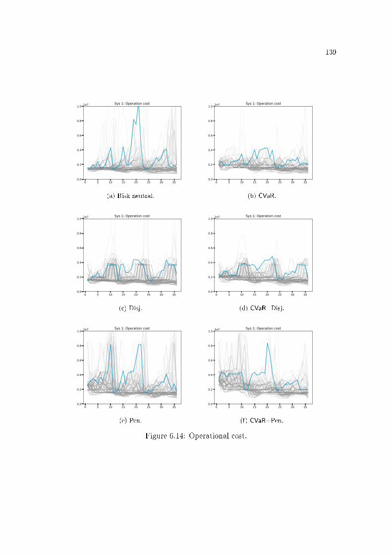
139

0 5 10 15 20 25 30 350.0

0.2

0.4

0.6

0.8

1.0 1e7 Sys 1: Operation cost

(a) Risk neutral.

0 5 10 15 20 25 30 350.0

0.2

0.4

0.6

0.8

1.0 1e7 Sys 1: Operation cost

(b) CVaR.

0 5 10 15 20 25 30 350.0

0.2

0.4

0.6

0.8

1.0 1e7 Sys 1: Operation cost

(c) Disj.

0 5 10 15 20 25 30 350.0

0.2

0.4

0.6

0.8

1.0 1e7 Sys 1: Operation cost

(d) CVaR+Disj.

0 5 10 15 20 25 30 350.0

0.2

0.4

0.6

0.8

1.0 1e7 Sys 1: Operation cost

(e) Pen.

0 5 10 15 20 25 30 350.0

0.2

0.4

0.6

0.8

1.0 1e7 Sys 1: Operation cost

(f) CVaR+Pen.

Figure 6.14: Operational cost.

140

6.3.5 Discretization error

One of the important issues associated with the use of SDDiP is the need to

discretize the state variables. In fact, the greater the precision of discretization, the

closer we expect to be to the non-convex continuous model. However, this leads to

an increase in computational time because it increases the size of the problem and

the number of binary variables.

Figure 6.15 compares the policies for the CVaR and Disjunctive Constraints

approach obtained by the SDDiP algorithm considering an accuracy of ε = 10

MWmonth (�gures on the left) and ε = 1000 MWmonth (�gures on the right) for the

state variable: the stored energy vt. Taking a discretization step 100 times greater

corresponds to reducing the number of binary variables required in each subsystem

by 7 ∼ log2(100). We present the graphics of stored energy, hydro generation and

thermal generation simulated for the same 200 scenarios.

As shown in Figures 6.15a and 6.15b, there is no signi�cant change in stored

energy resulting from a larger discretization step. Also for �gures 6.15c and 6.15d

the hydro generation has a very similar overall behavior � although the result for

the highlighted series is clearly di�erent. However, we note a signi�cant change

regarding thermal generation: in the case of a discretization step of 10 MWmonth

there are di�erent �levels� of thermal generation which concentrate a large proportion

of scenarios, while for the discretization error of 1000 MWmonth those levels are

completely absent.

In order to understand why this happens, let us consider the typical behavior

of these variables in the continuous case. Since the total thermal and de�cit costs as

a function of the �nal storage vt+1 is piecewise linear, there is a strong tendency for

the corresponding optimal solution v∗t+1 to be in a `kink' of this function. In other

141

words, the optimal solution usually dispatches all the thermal plants at their full

capacity up to a certain unit cost, and the hydro generation regulates the di�erence

between the corresponding thermal generation and total demand.

With the discretization of the stored volume, this mechanism is no longer

free, and, unless for the spillage, the hydro generation is also �discretized� and able

only to take values from 10 to 10 MWmonth or from 1000 em 1000 MWmonth.

This reverses the �order� of constraints: �rst we determine the hydro generation

and only then we obtain the thermal generation that meets the demand. Due to the

variability of the in�ow scenarios and depending on the discretization error, we do

not obtain a thermal generation that follows on the same �levels� over some stages,

as is more usual.

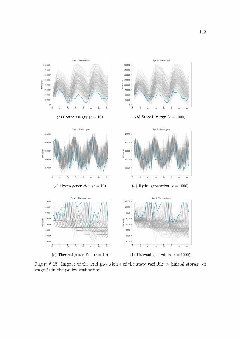
142

0 5 10 15 20 25 30 35

0

25000

50000

75000

100000

125000

150000

175000

200000

MW

mon

th

Sys 1: Stored Vol

(a) Stored energy (ε = 10)

0 5 10 15 20 25 30 35

0

25000

50000

75000

100000

125000

150000

175000

200000

MW

mon

th

Sys 1: Stored Vol

(b) Stored energy (ε = 1000)

0 5 10 15 20 25 30 35

25000

30000

35000

40000

45000

MW

mon

th

Sys 1: Hydro gen

(c) Hydro generation (ε = 10)

0 5 10 15 20 25 30 35

25000

30000

35000

40000

45000

MW

mon

th

Sys 1: Hydro gen

(d) Hydro generation (ε = 1000)

0 5 10 15 20 25 30 35

4000

5000

6000

7000

8000

9000

10000

11000

MW

mon

th

Sys 1: Thermal gen

(e) Thermal generation (ε = 10)

0 5 10 15 20 25 30 35

4000

5000

6000

7000

8000

9000

10000

11000

MW

mon

th

Sys 1: Thermal gen

(f) Thermal generation (ε = 1000)

Figure 6.15: Impact of the grid precision ε of the state variable vt (initial storage ofstage t) in the policy estimation.

143

7 BLESSING OF EXTREME POINTS

In this chapter we revisit two results presented in this dissertation: Balas's

theorem (Theorem 5.3 page 101) and the Blessing of Binary (Theorem 6.2 page 6.2).

In particular, both theorems state that the convex hull operation does not add points

to some special a�ne spaces. We prove that those a�ne spaces are closely related

to particular extreme points, and we call that the �Blessing of extreme points�. We

provide some examples to illustrate this result.

7.1 Balas's theorem revisited

In this section, we investigate more closely Balas's theorem (Theorem 5.3

page 101), and how it can be interpreted geometrically. Let Pi be the polyhedron

given by {x ∈ Rn | Aix ≤ bi}. Formula (5.1), given by

Q =

{x ∈ Rn

∣∣∣∣x =

∑pj=1 yj, Aiyi ≤ zibi, yi ∈ Rn,∑p

j=1 zj = 1, zi ∈ {0, 1}, i = 1, . . . , p.

},

represents the union of polyhedra⋃pi=1(Pi + R), where R =

∑pi=1 reccA(Pi). Recall

that reccA(Pi) := {d ∈ Rn | Aid ≤ 0} are the algebraic recession cones of the

polyhedra Pi. From Theorem 5.3 (page 101), if we consider zi as a continuous

variable in [0, 1], the resulting set Q becomes the convex closure of Q, that is,

Q = cl convQ. We view the set Q as the projection on the x variable of the

following set:

Qlift =

{(x, z) ∈ Rn × {0, 1}p

∣∣∣∣x =

∑pj=1 yj, Aiyi ≤ zibi, yi ∈ Rn,∑pj=1 zj = 1, i = 1, . . . , p.

}. (7.1)

144

Note that Qlift is the Cartesian product of each polyhedron Pi = Pi + R with an

extreme point of the (p− 1)-simplex:

Qlift =

p⋃

i=1

(Pi × {ei}

), (7.2)

where ei ∈ Rp is a canonical basis element. Let Qlift be the set (7.1) with z in the

continuous interval [0, 1]p:

Qlift =

{(x, z) ∈ Rn × [0, 1]p

∣∣∣∣x =

∑pj=1 yj, Aiyi ≤ zibi, yi ∈ Rn,∑pj=1 zj = 1, i = 1, . . . , p.

}. (7.3)

The following theorem proves that Qlift is the convex closure of Qlift.

Theorem 7.1 (Lifted Balas). The convex closure of Qlift equals Qlift, that is,

Qlift = cl conv(Qlift).

Proof. Let (x, z) be a vector of Qlift. For each i, there are yi ∈ Rn such that

x =∑p

i=1 yi, Aiyi ≤ zibi,∑p

i=1 zi = 1,

where zi ∈ [0, 1], for all i = 1, . . . , p. Let I0 and I+ be the set of indexes i such that

zi is equal to zero and greater than zero, respectively. Note that di = yi belongs to

recc(Pi), for all i ∈ I0, and xi = yi/zi belongs to Pi, for all i ∈ I+. So, the vector x

has the following form:

x =∑

i∈I+ziyizi

+∑

i∈I0di =

∑

i∈I+zixi +

∑

i∈I0di,

and z can also be represented as

z =

p∑

i=1

ziei =

p∑

i∈I+ziei +

p∑

i∈I00ei.

So, the pair (x, z) can be represented by the following sum:

(x, z) =∑

i∈I+zi (xi, ei)

︸ ︷︷ ︸conv(

⋃pi=1 Pi×{ei})

+∑

i∈I0(di, 0) .

︸ ︷︷ ︸∑pi=1 recc(Pi)×{0}

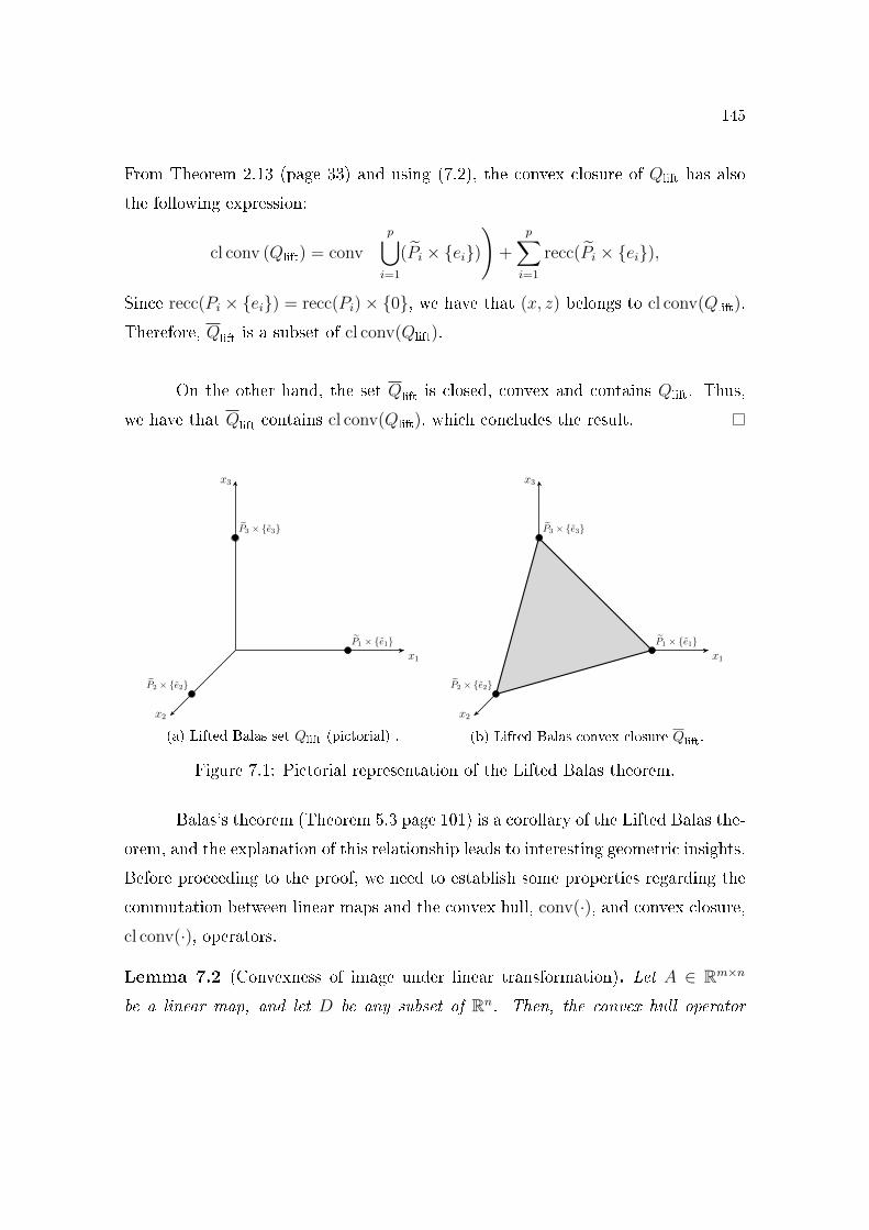
145

From Theorem 2.13 (page 33) and using (7.2), the convex closure of Qlift has also

the following expression:

cl conv (Qlift) = conv

(p⋃

i=1

(Pi × {ei}))

+

p∑

i=1

recc(Pi × {ei}),

Since recc(Pi × {ei}) = recc(Pi)× {0}, we have that (x, z) belongs to cl conv(Qlift).

Therefore, Qlift is a subset of cl conv(Qlift).

On the other hand, the set Qlift is closed, convex and contains Qlift. Thus,

we have that Qlift contains cl conv(Qlift), which concludes the result.

x1

x3

x2

P1 × {e1}

P3 × {e3}

P2 × {e2}

(a) Lifted Balas set Qlift (pictorial) .

x1

x3

x2

P1 × {e1}

P3 × {e3}

P2 × {e2}

(b) Lifted Balas convex closure Qlift.

Figure 7.1: Pictorial representation of the Lifted Balas theorem.

Balas's theorem (Theorem 5.3 page 101) is a corollary of the Lifted Balas the-

orem, and the explanation of this relationship leads to interesting geometric insights.

Before proceeding to the proof, we need to establish some properties regarding the

commutation between linear maps and the convex hull, conv(·), and convex closure,

cl conv(·), operators.

Lemma 7.2 (Convexness of image under linear transformation). Let A ∈ Rm×n

be a linear map, and let D be any subset of Rn. Then, the convex hull operator

146

commutes with A:

A conv(D) = conv(AD).

In particular, if D is convex then A is also convex.

Proof. This is a straightforward argument of commuting convex combinations and

linear maps. Let y ∈ A conv(D). There exist xi ∈ D and λi ∈ [0, 1] for all i =

1, . . . , k such that∑k

i=1 λi = 1, and

y = A

(k∑

i=1

λixi

)=

k∑

i=1

λiAxi ∈ conv(AD).

Let y ∈ conv(AD). There exist xi ∈ D and λi ∈ [0, 1] for all i = 1, . . . , k such that∑k

i=1 λi = 1, and

y =k∑

i=1

λiAxi = A

(k∑

i=1

λixi

)∈ A conv(D).

If D is convex, then conv(D) = D. So, conv(AD) = AD which is equivalent to AD

being convex.

The following theorem is the core argument for proving the Balas theorem

from the Lifted Balas result. It states that any linear map commutes with the

convex closure operator for any �nite union of polyhedra. This result can also be

extended to general closed convex sets with some regularity conditions, but its proof

is unnecessary for this section.

Lemma 7.3 (Commutation of the convex closure operator with a linear map). Let

A be a linear map, and let Pi be polyhedra, for i = 1, . . . , p. Then,

A

[cl conv

(p⋃

i=1

Pi

)]= cl conv

[p⋃

i=1

APi

].

147

Proof. This lemma results from the following relations:

A

[cl conv

(p⋃

i=1

Pi

)]= A conv

(p⋃

i=1

Pi

)+

p∑

i=1

A recc(Pi).

= conv

[A

(p⋃

i=1

Pi

)]+

p∑

i=1

recc(APi)

= conv

(p⋃

i=1

APi

)+

p∑

i=1

recc(APi)

=

[cl conv

(p⋃

i=1

APi

)],

where the �rst equality follows from Theorem 2.13 (page 33), the second equality

follows from Lemma 7.2 just proved and Theorem 2.8 (page 25), the third equality

is noting that A (⋃pi=1 Pi) =

⋃pi=1APi, and the fourth equality follows again from

Theorem 2.13 (page 33).

In the particular case where A is a projection, Lemma 7.3 yields

Theorem 7.4 (Balas revisited). The convex closure of Q equals Q, that is,

Q = cl convQ.

Proof. Recall that Q and Q are the projection in x variable of Qlift and Qlift, respec-

tively. This proof results from the following equations:

Q = projxQlift

= projx

[cl conv

(p⋃

i=1

(Pi × {ei}))]

= cl conv

(p⋃

i=1

Pi

)= cl convQ,

148

where the �rst equality follows from the de�nition of Q and Qlift, the second equality

is the Lifted Balas theorem, the third equality follows from Lemma 7.3 taking A =

projx(·), and the fourth equality follows from the geometric description of Q.

We note that if any �magic� formula provides the description of the convex

closure in a higher dimensional space, we can project it to have the convex closure

in the original space.

A remarkable feature of the Lifted Balas set Qlift is that when the variable z

equals a simplex vertex ei the resulting set becomes Pi × ei:

Qlift ∩ (Rn × {ei}) = Pi × {ei},

see formula 7.1. Even more surprisingly, the convex closure Qlift has also the same

property, that is,

Qlift ∩ (Rn × {ei}) = Pi × {ei},

as we can see in formula 7.3. Actually, this is a general property of sets of the

form⋃pi=1(Pi × {ri}). We call those sets the lift of

⋃pi=1 Pi along {r1, r2, . . . , rp}. If

r1, . . . , rp are extreme points from a convex set, Theorem 7.5 below proves that the

convex hull does not add points to the a�ne space Rn × {ri}, that is,

conv

(p⋃

i=1

(Pi × {ri}))∩ (Rn × {ei}) = Pi × {ei}. (7.4)

This is the discrete version of the Blessing of extreme points. Actually, equation

(7.4) also holds for the convex closure of⋃pi=1(Pi × {ri}), since the closure of inter-

section is the intersection of closures, because the intersection between the relative

interiors of Pi × {ri} and Rn × {ei} is nonempty, see BERTSEKAS [5] page 32 or

ROCKAFELLAR [22] page 47. We provide a pictorial illustration of an extremal

lift in �gure 7.3.

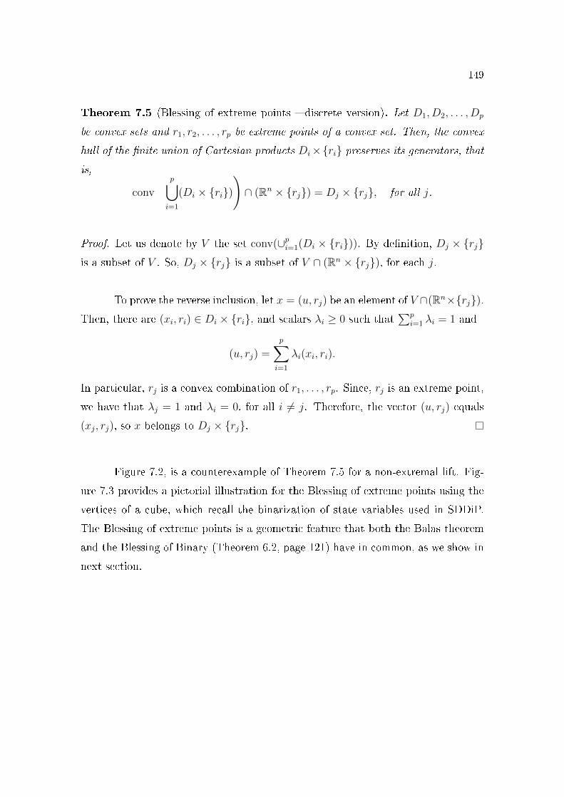
149

Theorem 7.5 (Blessing of extreme points � discrete version). Let D1, D2, . . . , Dp

be convex sets and r1, r2, . . . , rp be extreme points of a convex set. Then, the convex

hull of the �nite union of Cartesian products Di×{ri} preserves its generators, thatis,

conv

(p⋃

i=1

(Di × {ri}))∩ (Rn × {rj}) = Dj × {rj}, for all j.

Proof. Let us denote by V the set conv(∪pi=1(Di × {ri})). By de�nition, Dj × {rj}is a subset of V . So, Dj × {rj} is a subset of V ∩ (Rn × {rj}), for each j.

To prove the reverse inclusion, let x = (u, rj) be an element of V ∩(Rn×{rj}).Then, there are (xi, ri) ∈ Di × {ri}, and scalars λi ≥ 0 such that

∑pi=1 λi = 1 and

(u, rj) =

p∑

i=1

λi(xi, ri).

In particular, rj is a convex combination of r1, . . . , rp. Since, rj is an extreme point,

we have that λj = 1 and λi = 0, for all i 6= j. Therefore, the vector (u, rj) equals

(xj, rj), so x belongs to Dj × {rj}.

Figure 7.2, is a counterexample of Theorem 7.5 for a non-extremal lift. Fig-

ure 7.3 provides a pictorial illustration for the Blessing of extreme points using the

vertices of a cube, which recall the binarization of state variables used in SDDiP.

The Blessing of extreme points is a geometric feature that both the Balas theorem

and the Blessing of Binary (Theorem 6.2, page 121) have in common, as we show in

next section.

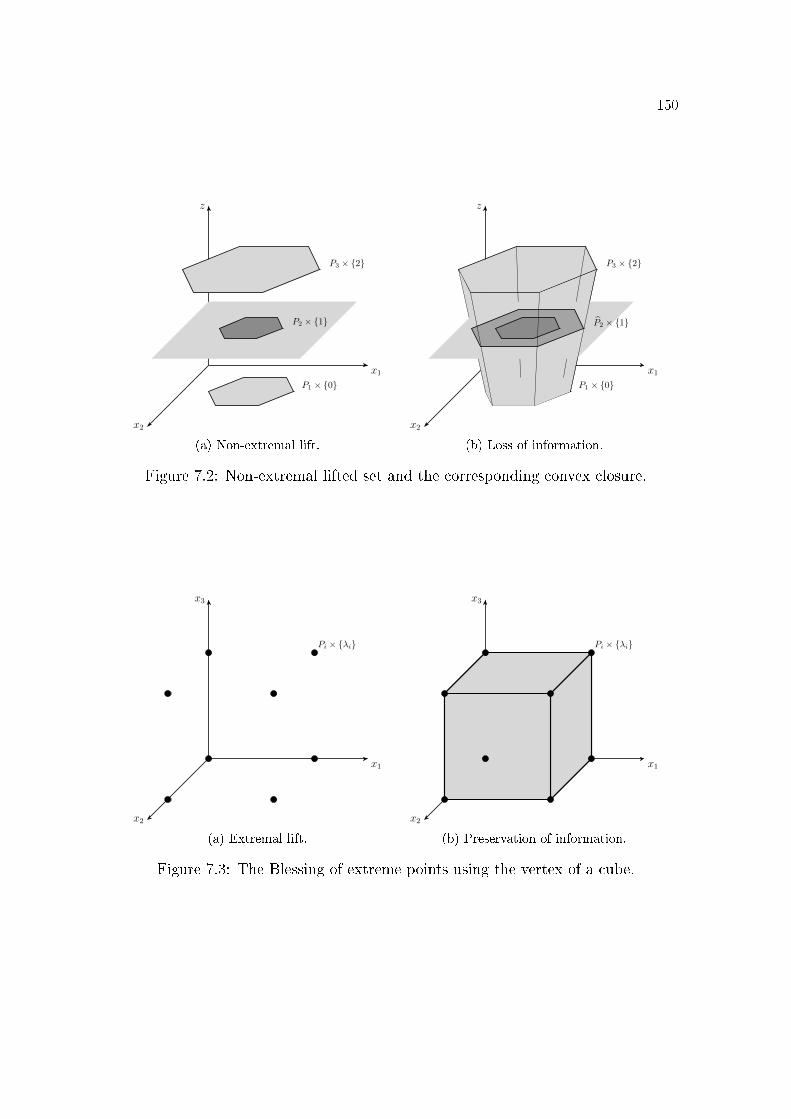
150

x1

z

x2

P1 × {0}

P2 × {1}

P3 × {2}

(a) Non-extremal lift.

x1

z

x2

P1 × {0}

P2 × {1}

P3 × {2}

(b) Loss of information.

Figure 7.2: Non-extremal lifted set and the corresponding convex closure.

x1

x3

x2

Pi × {λi}

(a) Extremal lift.

x1

x3

x2

Pi × {λi}

(b) Preservation of information.

Figure 7.3: The Blessing of extreme points using the vertex of a cube.

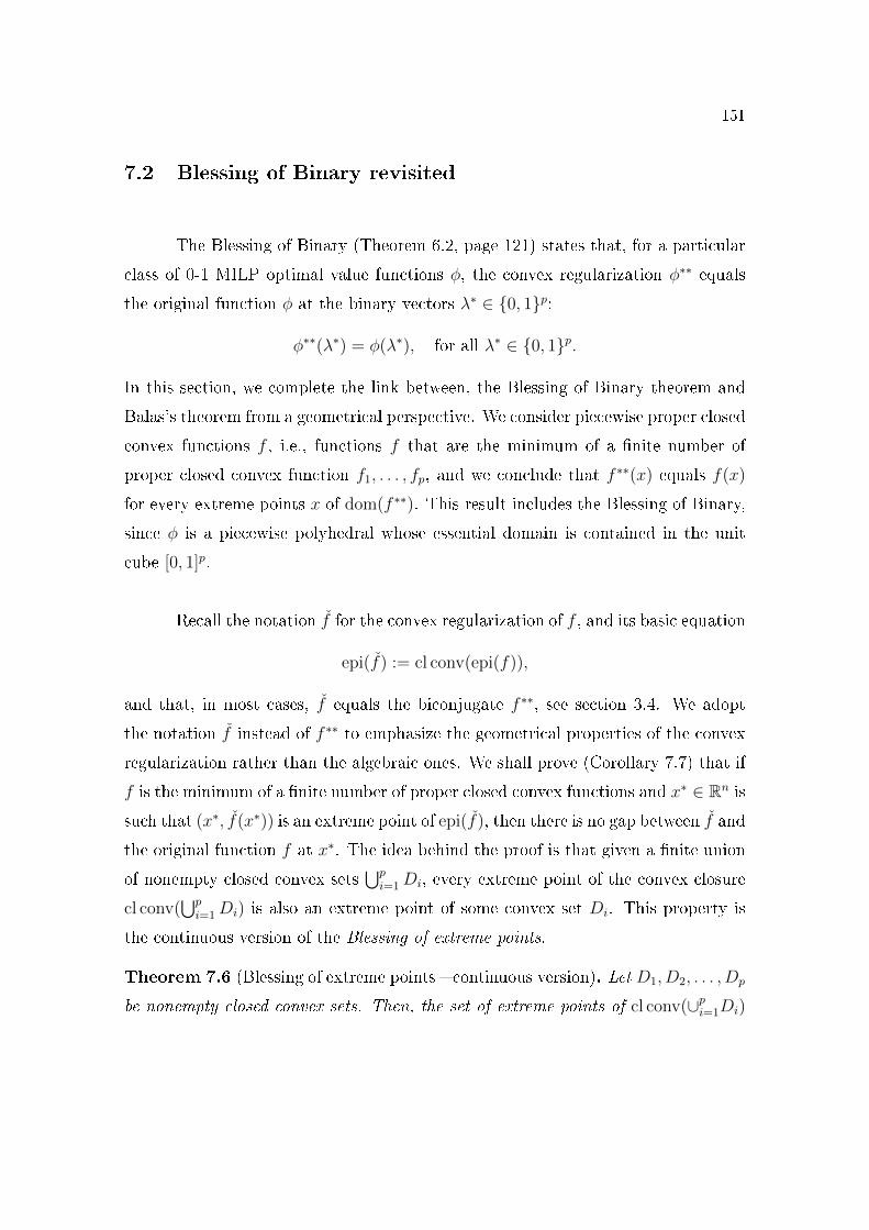
151

7.2 Blessing of Binary revisited

The Blessing of Binary (Theorem 6.2, page 121) states that, for a particular

class of 0-1 MILP optimal value functions φ, the convex regularization φ∗∗ equals

the original function φ at the binary vectors λ∗ ∈ {0, 1}p:

φ∗∗(λ∗) = φ(λ∗), for all λ∗ ∈ {0, 1}p.

In this section, we complete the link between, the Blessing of Binary theorem and

Balas's theorem from a geometrical perspective. We consider piecewise proper closed

convex functions f , i.e., functions f that are the minimum of a �nite number of

proper closed convex function f1, . . . , fp, and we conclude that f ∗∗(x) equals f(x)

for every extreme points x of dom(f ∗∗). This result includes the Blessing of Binary,

since φ is a piecewise polyhedral whose essential domain is contained in the unit

cube [0, 1]p.

Recall the notation f for the convex regularization of f , and its basic equation

epi(f) := cl conv(epi(f)),

and that, in most cases, f equals the biconjugate f ∗∗, see section 3.4. We adopt

the notation f instead of f ∗∗ to emphasize the geometrical properties of the convex

regularization rather than the algebraic ones. We shall prove (Corollary 7.7) that if

f is the minimum of a �nite number of proper closed convex functions and x∗ ∈ Rn is

such that (x∗, f(x∗)) is an extreme point of epi(f), then there is no gap between f and

the original function f at x∗. The idea behind the proof is that given a �nite union

of nonempty closed convex sets⋃pi=1Di, every extreme point of the convex closure

cl conv(⋃pi=1 Di) is also an extreme point of some convex set Di. This property is

the continuous version of the Blessing of extreme points.

Theorem 7.6 (Blessing of extreme points � continuous version). Let D1, D2, . . . , Dp

be nonempty closed convex sets. Then, the set of extreme points of cl conv(∪pi=1Di)

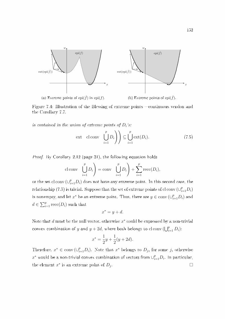
152

x

w

epi(f)

ext(epi(f))

(a) Extreme points of epi(f) in epi(f).

x

w

epi(f)

ext(epi(f))

(b) Extreme points of epi(f).

Figure 7.4: Illustration of the Blessing of extreme points � continuous version andthe Corollary 7.7.

is contained in the union of extreme points of Di's:

ext

(cl conv

(p⋃

i=1

Di

))⊆

p⋃

i=1

ext(Di). (7.5)

Proof. By Corollary 2.12 (page 31), the following equation holds

cl conv

(p⋃

i=1

Di

)= conv

(p⋃

i=1

Di

)+

p∑

i=1

recc(Di),

or the set cl conv (∪pi=1Di) does not have any extreme point. In this second case, the

relationship (7.5) is trivial. Suppose that the set of extreme points of cl conv (∪pi=1Di)

is nonempty, and let x∗ be an extreme point. Thus, there are y ∈ conv (∪pi=1Di) and

d ∈∑pi=1 recc(Di) such that

x∗ = y + d.

Note that d must be the null vector, otherwise x∗ could be expressed by a non-trivial

convex combination of y and y + 2d, where both belongs to cl conv (⋃pi=1Di):

x∗ =1

2y +

1

2(y + 2d).

Therefore, x∗ ∈ conv (∪pi=1Di). Note that x∗ belongs to Dj, for some j, otherwise

x∗ would be a non-trivial convex combination of vectors from ∪pi=1Di. In particular,

the element x∗ is an extreme point of Dj.

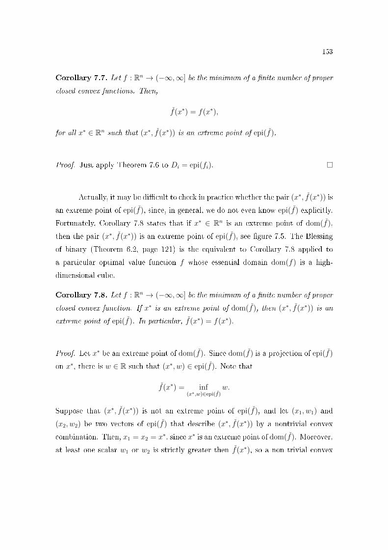
153

Corollary 7.7. Let f : Rn → (−∞,∞] be the minimum of a �nite number of proper

closed convex functions. Then,

f(x∗) = f(x∗),

for all x∗ ∈ Rn such that (x∗, f(x∗)) is an extreme point of epi(f).

Proof. Just apply Theorem 7.6 to Di = epi(fi).

Actually, it may be di�cult to check in practice whether the pair (x∗, f(x∗)) is

an extreme point of epi(f), since, in general, we do not even know epi(f) explicitly.

Fortunately, Corollary 7.8 states that if x∗ ∈ Rn is an extreme point of dom(f),

then the pair (x∗, f(x∗)) is an extreme point of epi(f), see �gure 7.5. The Blessing

of binary (Theorem 6.2, page 121) is the equivalent to Corollary 7.8 applied to

a particular optimal value function f whose essential domain dom(f) is a high-

dimensional cube.

Corollary 7.8. Let f : Rn → (−∞,∞] be the minimum of a �nite number of proper

closed convex function. If x∗ is an extreme point of dom(f), then (x∗, f(x∗)) is an

extreme point of epi(f). In particular, f(x∗) = f(x∗).

Proof. Let x∗ be an extreme point of dom(f). Since dom(f) is a projection of epi(f)

on x∗, there is w ∈ R such that (x∗, w) ∈ epi(f). Note that

f(x∗) = inf(x∗,w)∈epi(f)

w.

Suppose that (x∗, f(x∗)) is not an extreme point of epi(f), and let (x1, w1) and

(x2, w2) be two vectors of epi(f) that describe (x∗, f(x∗)) by a nontrivial convex

combination. Then, x1 = x2 = x∗, since x∗ is an extreme point of dom(f). Moreover,

at least one scalar w1 or w2 is strictly greater then f(x∗), so a non trivial convex

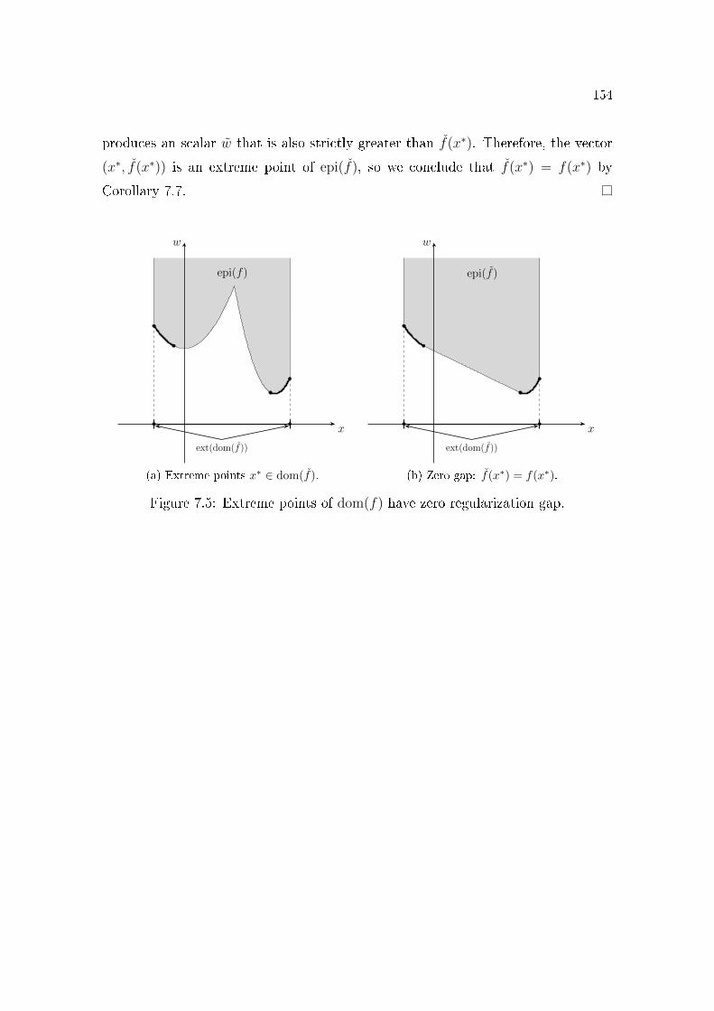
154

produces an scalar w that is also strictly greater than f(x∗). Therefore, the vector

(x∗, f(x∗)) is an extreme point of epi(f), so we conclude that f(x∗) = f(x∗) by

Corollary 7.7.

x

w

ext(dom(f))

epi(f)

(a) Extreme points x∗ ∈ dom(f).

x

w

ext(dom(f))

epi(f)

(b) Zero gap: f(x∗) = f(x∗).

Figure 7.5: Extreme points of dom(f) have zero regularization gap.

155

8 CONCLUSION

This dissertation deals with stochastic optimization considering mixed inte-

ger linear constraints, which constitutes an appropriate framework to model real

life applications. We provided two important results regarding the modeling of

non-convex constraints with binary variables: a geometric interpretation of the Dis-

junctive Constraints formula (eq. (5.1), page 97), and a simpler statement and

proof of the original Jeroslow's theorem about representability of union of polyhedra

(JEROSLOW [18]). The name for the Jeroslow's theorem could be �Fundamental

Theorem of Disjunctive Programming�, since it asserts that the Disjunctive Con-

straint formula (5.1) represents the corresponding union of polyhedra if and only if

that union is representable by a set of linear constraints involving continuous and

binary variables. The Disjunctive Constraints formula (5.1) can be used in several

real life applications, such as modeling operative constraints related to the power

system planning operation. One instructive example is the hydropower plant min-

imum out�ow constraint, which is a non-convex feasible set that would be hard to

model without this theory.

Using the Disjunctive Constraints theory, we proposed a binary model for

the risk aversion of low stored volumes, which we call the �disjunctive constraint

approach�, in such a way that if the stored volume falls below a reference value in a

given subsystem then all the thermals plants from that subsystem are dispatched to

their maximum capacity. We compared this approach with the standard ones such

as the CVaR risk measure and the penalty model induced by CAR (Risk Aversion

Curve). We observed that the penalty approach produces a signi�cant amount of

preventive de�cit when the stored volume reaches the storage reference curve. The

CVaR approach has interesting results in term of increasing the stored volume along

156

the stages, and that happens because the CVaR risk measure penalizes high oper-

ational costs, and low stored volumes are indirectly related with high operational

costs. The disjunctive constraint approach resulted in a better performance than the

CAR penalty approach, since the disjunctive constraints do not induce preventive

de�cit and also dispatches thermal generation in low storage situations. Among all

cases, the best one was the combination between the disjunctive constraints and the

CVaR risk measure, since that combination provided high stored volumes and the

least amount of de�cit. Thus, the combination of CVaR and the disjunctive con-

straints seems a robust methodology for considering precisely both the operational

rules and the risk averseness of low stored volumes. Thanks to the SDDiP algorithm

of ZOU; AHMED; SUN [28], we were able to compare the standard approaches with

the disjunctive approach, which consists in a multistage stochastic mixed integer

linear program.

The SDDiP algorithm is supported by an important theorem called �Blessing

of Binary� (BOB) (ZOU; AHMED; SUN [28]), which states that if f belongs to

a class of MILP value functions, then the convex regularization f equals the non-

convex function f at the binary coordinates of the unit cube, where that unit cube

contains the domain of f . In chapter 7, we proved the �Blessing of Extreme Points�

(BEP), a result that extends and gives a geometrical interpretation for BOB based

on the extreme points of the convex closure of union of closed convex sets D =

cl conv(⋃pi=1Di). The BEP theorem states that every extreme point of D is also an

extreme point of some set Dk:

ext(D) ⊂p⋃

i=1

ext(Di).

Using BEP, we have shown that if f is a piecewise convex function, then there is no

gap between the convex regularization f and the original function f at the extreme

points of the domain of f . This expands the BOB's theorem to a larger class of

functions.

157

As a �nal remark, we emphasize the importance of the interpretation of

functions in terms of sets, and operations on functions in terms of operations on

sets. Due to this geometric view, we were able to describe in which points the

Lagrangian Relaxation of pointwise minima of convex functions have zero duality

gap. We have shown that such a nonconvex function can be represented by a union

of convex sets, ∪pi=1Di, the corresponding Lagrangian Relaxation can be equivalently

described by the convex closure of this union, cl conv (⋃pi=1 Di), and the points which

are preserved under the convex closure operation are the extreme points of D. We

called this property the Blessing of Extreme Points (BEP) property. It is worth

mentioning that the BEP proof was based on the following formula for the convex

closure of union of closed convex sets:

cl conv

(p⋃

i=1

Di

)= conv

(p⋃

i=1

Di

)+

p∑

i=1

recc(Di). (8.1)

At �rst, we have found a proof of (8.1) on a paper of CERIA; SOARES [12]. How-

ever, there was a mistake in that paper (page 601), since the authors claim that

equation (8.1) holds for any closed convex sets based on the assumption that pro-

jection of closed convex sets is always a closed. In chapter 2, we have shown a

counter-example for both claims, and we dedicated a whole chapter for the proof of

equation (8.1) under mild regularity conditions for the closed convex sets Di's.

158

REFERENCES

[1] BALAS, E. Disjunctive Programming. In: Annals of Discrete Mathematics.

[S.l.]: Elsevier, 1979. p.3�51.

[2] BALAS, E. Disjunctive programming: properties of the convex hull of feasible

points. Discrete Applied Mathematics, [S.l.], v.89, n.1-3, p.3�44, dec 1998.

[3] BALAS, E.; CERIA, S.; CORNUÉJOLS, G. A lift-and-project cutting plane

algorithm for mixed 0�1 programs. Mathematical Programming, [S.l.], v.58,

n.1-3, p.295�324, jan 1993.

[4] BENDERS, J. F. Partitioning procedures for solving mixed-variables program-

ming problems. Numerische mathematik, [S.l.], v.4, n.1, p.238�252, 1962.

[5] BERTSEKAS, D. P. Convex Optimization Theory. 1st.ed. [S.l.]: Athena

Scienti�c, 2009.

[6] BEZANSON, J. et al. Julia: a fresh approach to numerical computing. SIAM

Review, [S.l.], v.59, n.1, p.65�98, 2017.

[7] BIRGE, J. R.; LOUVEAUX, F. Introduction to Stochastic Programming

(Springer Series in Operations Research and Financial Engineering).

[S.l.]: Springer, 2011.

[8] BLAIR, C.; JEROSLOW, R. The value function of a mixed integer program: i.

Discrete Mathematics, [S.l.], v.19, n.2, p.121�138, 1977.

[9] CAMPELLO, R. E. Cortes Disjuntivos para o problema do particiona-

mento. 1980. Tese (Doutorado em Ciência da Computação) � Federal University

of Rio de Janeiro/COPPE.

159

[10] CAMPELLO, R. E.; FILHO, N. M. Aspectos Teóricos e Computacionais dos

Cortes Disjuntivos B(4) e B(5). In: Anais do XII Simpósio Brasileiro de

Pesquisa Operacional - SOBRAPO. [S.l.: s.n.], 1980.

[11] CAMPELLO, R. E.; FILHO, N. M. Algoritmo Dual de Cortes para o Problema

de Programaçao Quadrática Não-Convexo. In: XVI Simpósio Brasileiro de

Pesquisa Operacional - SOBRAPO. [S.l.: s.n.], 1981.

[12] CERIA, S.; SOARES, J. Convex programming for disjunctive convex optimiza-

tion. Mathematical Programming, [S.l.], v.86, n.3, p.595�614, dec 1999.

[13] CORNUÉJOLS, G. Valid inequalities for mixed integer linear programs.Math-

ematical Programming, [S.l.], v.112, n.1, p.3�44, 2008.

[14] DOWSON, O.; KAPELEVICH, L. SDDP.jl: a Julia package for Stochastic

Dual Dynamic Programming. Optimization Online, [S.l.], 2017.

[15] GOMORY, R. E. An algorithm for integer solutions to linear programs.Recent

advances in mathematical programming, [S.l.], v.64, p.260�302, 1963.

[16] GUROBI OPTIMIZATION, I.Gurobi Optimizer Reference Manual. 2016.

[17] JEROSLOW, R. Cutting-Plane Theory: disjunctive methods. In: Studies in

Integer Programming. [S.l.]: Elsevier, 1977. p.293�330.

[18] JEROSLOW, R. G. Representability in mixed integer programmiing, I: charac-

terization results. Discrete Applied Mathematics, [S.l.], v.17, n.3, p.223�243,

jun 1987.

[19] KAPELEVICH, L. SDDiP.jl: SDDP extension for integer local or state vari-

ables. 2018.

[20] PEREIRA, M. V.; PINTO, L. M. Multi-stage stochastic optimization applied

to energy planning.Mathematical programming, [S.l.], v.52, n.1-3, p.359�375,

1991.

160

[21] PHILPOTT, A. B.; GUAN, Z. On the convergence of stochastic dual dynamic

programming and related methods. Operations Research Letters, [S.l.], v.36,

n.4, p.450�455, 2008.

[22] ROCKAFELLAR, R. T. Convex Analysis (Princeton Landmarks in

Mathematics and Physics). [S.l.]: Princeton University Press, 1996.

[23] RUSZCZYNSKI, A. Stochastic Programming Handbook In Operations

Research and Management Science - Vol. 10. [S.l.]: Elsevier, 2003.

[24] SHAPIRO, A. Analysis of stochastic dual dynamic programming method. Eu-

ropean Journal of Operational Research, [S.l.], v.209, n.1, p.63�72, 2011.

[25] SHAPIRO, A. Tutorial on risk neutral, distributionally robust and risk

averse multistage stochastic programming. Optimization Online.

[26] SHAPIRO, A.; DENTCHEVA, D.; RUSZCZY�SKI, A. Lectures on stochas-

tic programming: modeling and theory. [S.l.]: SIAM, 2009.

[27] THOMÉ, F. S.Representação de não-convexidades no planejamento da

operação hidrotérmica utilizando PDDE. 2013. Tese (Doutorado em Ciência

da Computação) � Federal University of Rio de Janeiro/COPPE.

[28] ZOU, J.; AHMED, S.; SUN, A. Stochastic Dual Dynamic Integer Pro-

gramming. preprint Optimization Online.