Embed Size (px)
Citation preview

tt503A - Gallep
tt503A – Dispositivos Fotônicos
!
l Aula 1 - Introdução

tt503A - Gallep
Sistemas ópticos: histórico- Sinais de fumaça: <1500 - Dispositivos de semáforo: 1500-1800 - Códigos mecânicos (Chappe): 1792

tt503A - Gallep
n 1976 - Primeiro sistema comercial de transmissão com fibras ópticas entra em funcionamento para distribuição de TV a cabo, Inglaterra;
n 1977 - Primeiro sistema de fibras ópticas aplicado à telefonia - utilizava codificação de pulsos à 1,544 Mb/s, EUA.
n 1870 - Luz é guiada em um jato de água; n 1910 - Análise teórica sobre propagação da luz em cilindros dielétricos; n 1930 - Experiências com fibra de vidro; n 1951 - Fibra em endoscopia; n 1960 - Avanço das fontes ópticas - o laser semicondutor.n 1966 - Sistema de longa distância com fibras de 20 dB/km de atenuação; n 1970 – Fibra comercial com 20 dB/km; n Início da década de 1970 - Fibras monomodo de índice gradual; n 1973 a 1977 - Tempo de vida dos lasers pula de poucas horas para 106
horas; n 1976 - Atenuação da fibra: 0,46 dB/km @ 1200 nm.

tt503A - Gallep
geração I
•A partir de 1976: sistemas que utilizam fibras multimodo de índice degrau ou gradual com atenuação entre 3 e 6 dB/km, para comprimentos de onda de transmissão de 850 nm. •Enlaces projetados para taxas de 2 a 2000 Mbit/s, utilizando LED e lasers de GaAs e detectores de silício. •Distâncias máximas entre repetidores de 5 a 10 km. •Geração preferida para redes locais de computadores •Mesmo nos enlaces de curta distância, estes sistemas apresentam uma relação custo-benefício mais vantajosa em relação aos sistemas que utilizam fios de cobre. •As fibras de plástico trabalham nesta geração
tt503A - Gallep
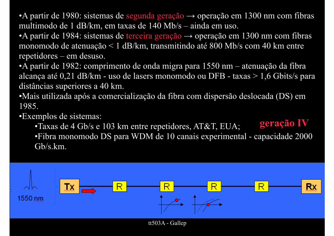
•A partir de 1980: sistemas de segunda geração → operação em 1300 nm com fibras multimodo de 1 dB/km, em taxas de 140 Mb/s – ainda em uso. •A partir de 1984: sistemas de terceira geração → operação em 1300 nm com fibras monomodo de atenuação < 1 dB/km, transmitindo até 800 Mb/s com 40 km entre repetidores – em desuso. •A partir de 1982: comprimento de onda migra para 1550 nm – atenuação da fibra alcança até 0,21 dB/km - uso de lasers monomodo ou DFB - taxas > 1,6 Gbits/s para distâncias superiores a 40 km. •Mais utilizada após a comercialização da fibra com dispersão deslocada (DS) em 1985. •Exemplos de sistemas:
•Taxas de 4 Gb/s e 103 km entre repetidores, AT&T, EUA; •Fibra monomodo DS para WDM de 10 canais experimental - capacidade 2000 Gb/s.km.
geração IV

tt503A - Gallep
g V - Sistemas Coerentes
•Melhoria da sensitividade. •Maior distância entre repetidores. •Modulação analógica e digital em fase e freqüência. •Multiplexação em freqüência.

tt503A - Gallep
g VI ...•Amplificadores ópticos a fibra→ substituem os repetidores, ampliando a distância entre terminais ponto a ponto → compensam as perdas de distribuição de sinal em redes ópticas. •Empregam fibras padrão, de dispersão deslocada ou de dispersão plana. •Com a baixa dispersão, processamento do sinal reduzido à amplificação no domínio óptico. •Os amplificadores ópticos a fibra dopada com Érbio (1550 nm) comerciais introduzidos em 1991. •Amplificadores dopados com Praseodímeo (1300 nm) foram apareceram comercialmente em 1994.

tt503A - Gallep
•Amplificadores ópticos - eliminam a complexidade e o custo dos repetidores; •Ampla banda de transmissão bidirecional; •1996 - 6 canais de vídeo conferência – Noruega. •1998 - 4 a 20 canais para transmissão entre 1 e 10 Gb/s - EUA, Japão e Europa. Taxas de Tb/s em 25 canais - EUA (experimental). •1998 - 100 canais de 10 Gbit/s em 400 km - Lucent. •1998 - 50 canais de 20 Gbit/s, 600 km, amplificadores centrados em 1550 e 1580 nm – NTT, Japão.
G VII -WDM

tt503A - Gallep
G VIII
Sólitons são utilizados para a transmissão óptica da informação. Sóliton: pulso estreito de luz que possui campos eletromagnéticos de amplitudes altíssimas, que provocam efeitos não lineares na fibra. Estes efeitos não lineares podem compensar a dispersão da fibra. Atenuação compensada por amplificadores ópticos. A introdução comercial dos sistemas por sólitons tende a ocorrer em sistemas de grande distância.

tt503A - Gallep "10
9
17 OFC Tutorial | March 2009 All Rights Reserved © Alcatel-Lucent 2009
33 Constellations and ModulationConstellations and Modulation
18 OFC Tutorial | March 2009 All Rights Reserved © Alcatel-Lucent 2009
Examples of Constellations: 1-D1 bit/symbol 2 bits/symbol 3 bits/symbol 4 bits/symbol
In-p
hase 16 symbols
2-ASK or BPSK 4-ASK 8-ASK 16-ASK
10
19 OFC Tutorial | March 2009 All Rights Reserved © Alcatel-Lucent 2009
Examples of Constellations: 2-D1 bit/symbol 2 bits/symbol 3 bits/symbol 4 bits/symbol
In-p
hase
Qua
drat
ure
+
QPSK 8-PSK
2-ASK/4-PSK
16-QAM
4-ASK/4-PSK
2-ASK/8-PSK
20 OFC Tutorial | March 2009 All Rights Reserved © Alcatel-Lucent 2009
BER vs SNR per Bit for Various Modulation Formats (No Coding)
0 2 4 6 8 10 12 14 16 1810
10
10
10
10
10
10
10
10
-8
-7
-6
-5
-4
-3
-2
-1
0
SNR per bit (dB)
BER
16-QAM, 4-ASK64-QAM
BPSK, QPSK, 2-ASK, 4-QAM8PSK
16-QAM
64-QAM
BPSK, 2-ASK
8PSK
1 bit/symbol
2 bits/symbol
3 bits/symbol
6 bits/symbol
QPSK, 4-QAM, 4-ASK
4 bits/symbol
No matter how good the SNR per bit is,there is always a finite probability of error
Some BER curves:
10
19 OFC Tutorial | March 2009 All Rights Reserved © Alcatel-Lucent 2009
Examples of Constellations: 2-D1 bit/symbol 2 bits/symbol 3 bits/symbol 4 bits/symbol
In-p
hase
Qua
drat
ure
+
QPSK 8-PSK
2-ASK/4-PSK
16-QAM
4-ASK/4-PSK
2-ASK/8-PSK
20 OFC Tutorial | March 2009 All Rights Reserved © Alcatel-Lucent 2009
BER vs SNR per Bit for Various Modulation Formats (No Coding)
0 2 4 6 8 10 12 14 16 1810
10
10
10
10
10
10
10
10
-8
-7
-6
-5
-4
-3
-2
-1
0
SNR per bit (dB)
BER
16-QAM, 4-ASK64-QAM
BPSK, QPSK, 2-ASK, 4-QAM8PSK
16-QAM
64-QAM
BPSK, 2-ASK
8PSK
1 bit/symbol
2 bits/symbol
3 bits/symbol
6 bits/symbol
QPSK, 4-QAM, 4-ASK
4 bits/symbol
No matter how good the SNR per bit is,there is always a finite probability of error
Some BER curves:

tt503A - Gallep "11
28
55 OFC Tutorial | March 2009 All Rights Reserved © Alcatel-Lucent 2009
Estimate of Year to Reach Fiber Capacity Limits
One estimates the fiber capacityto reach its limits near 2025!
1
10
100
1000
10000
100000
1000000
1990 2000 2010 2020 2030
Year
Gb/
s
W DMResearchW DMCommercial
Increase in number of
WDM channels
Increase in SE = 1 “dB” / year
WDM Research
WDM
Commercial
2021Capacity limit of C+L bands(140 Tbits/s)
2025Capacity limit in 1300-1620 nm
band(560 Tbits/s)
80 !m2Effective area
100 GbaudSymbol rate
2.6x10⁻²⁰ m2/WNonlinear index
0.2 dB/kmFiber loss
SSMFFiber type
1000 kmOptical path length
Optical PathParameters
Based on current fiber capacity estimates and historical data
Data from Bob Tkach
56 OFC Tutorial | March 2009 All Rights Reserved © Alcatel-Lucent 2009
Physical Phenomena Impacting Capacity NOT Discussed Here
• Minimum loss coefficient that monomode fibers can have due to fundamental material and waveguide properties (ultimate low-loss optical fibers)
Fundamental limit in fiber loss:
Fundamental limit in nonlinear coefficients:
• Monomode fibers with minimum nonlinear refractive index• Monomode fibers with maximum effective area
Other physical effects:• Raman scattering• Brillouin scattering

tt503A - Gallep

tt503A - Gallep

tt503A - Gallep

tt503A - Gallep
tt503A - Gallep

tt503A - Gallep

tt503A - Gallep

tt503A - Gallep

tt503A - Gallep

tt503A - Gallep
tt503A - Gallep

tt503A - Gallep

tt503A - Gallep

tt503A - Gallep

tt503A - Gallep
Exercícios