Embed Size (px)
Citation preview
I Escola de Radioastronomia Atibaia São Paulo
3 a 6 de agosto de 2006
Tutorial de Cosmologia
Carlos Alexandre Wuensche e Ivan Soares Ferreira
1 IntroduçãoPara manipular os dados do WMAP, serão necessárias duas ferramentas disponíveis na Internet (HEALPix e CMBFast) e o software IDL (Interactive Data Language), uma vez que boa parte do tratamento de dados nos mapas é feito com essa linguagem.
O pacote HEALPix (Hierarquical Equal Area Longitude Pixelization) pode ser encontrado no endereço http://healpix.jpl.nasa.gov/. O programa CMBFast pode ser baixado de http://www.cmbfast.org. O CMBFast pode ser compilado em Windows e a parte em IDL do HEALPix tambem funciona em Windows, mas a ferramenta HEALPix de produção de mapas roda somente em ambientes baseados em Unix.
O CMBFast é um programa que gera espectros de potência da baseado num código hidrodinâmico e foi escrito por Uros Seljak e Matias Zaldarriaga. O HEALPix foi concebido por Krzysztof M. Górski, Eric Hivon, Benjamin D. Wandelt, Frode K. Hansen, Anthony J. Banday and Matthias Bartelmann. Entre outras coisas, o HEALPix contém programas para simula de mapas completos de temperatura e polarização da Radiação Cósmica Fundo (RCF), rotinas para ler, escrever e criar imagens de mapas FITS, programas para procurar “neighborsofneighbors” e extremos de um campo aleatório, e várias outras facilidades para manipular dados da RCF.
Existem outros sites que podem ser utilizados em conjunto com ambos e que contem pacotes de análise de dados de domínio público:
• http://lambda.gsfc.nasa.gov Todos os mapas, programas, artigos e figuras referentes ao WMAP podem ser baixados desse site.
• http://camb.info Code for Anisotropies in the Microwave Background. Ele é baseado no CMBFast, escrito em C e Fortran 90 e gera espectros
1

• http://idlastro.gsfc.nasa.gov Biblioteca de rotinas astronômicas para usuários de IDL. Extremamente interessante e com atualizações frequentes.
• http://cosmologist.info/cosmomc/ Site com rotinas para simulações Monte Carlo de mapas de temperatura e polarização da RCF.
• http://cosmologist.info/polar/ Parte do site anterior, contém diversas rotinas e artigos referentes à polarização da RCF.
2 Um tutorial para produção de espectros de potência sintéticos Jatila van der Veen e Carlos Alexandre Wuensche
The purpose of making these models is to see the effects of changing the various cosmological parameters on the shape, location of peaks, and height of peaks, in the power spectrum of the CMB. The goal is to make a collection of models, varying one or two parameters at a time, using CMBFAST to create and view the Power Spectrum of the CMB for each model universe created and compare the models to see the effects of varying each cosmological parameter on the power spectrum.
As you read the introductory information, you will come to questions flagged with a Þ that will help you understand the real questions of how to extract information about the cosmological parameters from the power spectrum of the CMB.
To give you an idea of what we are looking for, here is an example in which we use the current "best estimates" for H0, and the total matter density parameter Omega_M and Omega_Lambda, but we vary the ratio of baryons and cold dark matter.
2
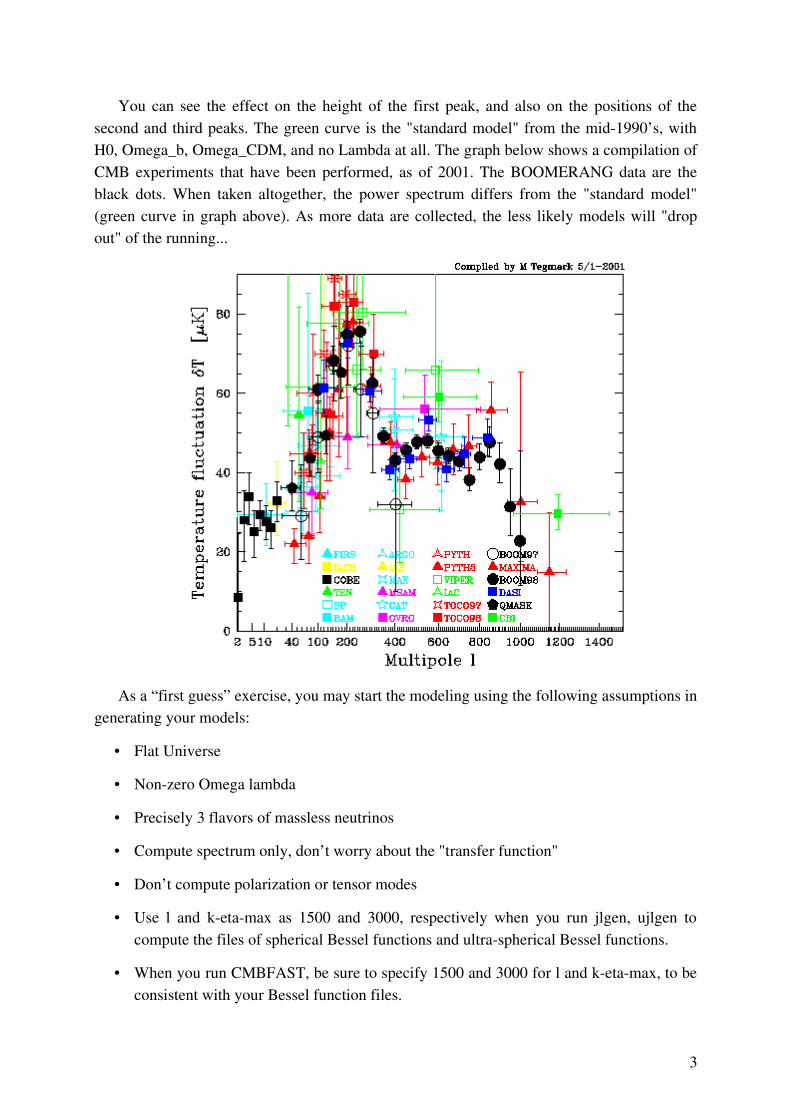
You can see the effect on the height of the first peak, and also on the positions of the second and third peaks. The green curve is the "standard model" from the mid1990’s, with H0, Omega_b, Omega_CDM, and no Lambda at all. The graph below shows a compilation of CMB experiments that have been performed, as of 2001. The BOOMERANG data are the black dots. When taken altogether, the power spectrum differs from the "standard model" (green curve in graph above). As more data are collected, the less likely models will "drop out" of the running...
As a “first guess” exercise, you may start the modeling using the following assumptions in generating your models:
• Flat Universe
• Nonzero Omega lambda
• Precisely 3 flavors of massless neutrinos
• Compute spectrum only, don’t worry about the "transfer function"
• Don’t compute polarization or tensor modes
• Use l and ketamax as 1500 and 3000, respectively when you run jlgen, ujlgen to compute the files of spherical Bessel functions and ultraspherical Bessel functions.
• When you run CMBFAST, be sure to specify 1500 and 3000 for l and ketamax, to be consistent with your Bessel function files.
3
After you get used to the programs, you can play with the values and intervals. For their meaning, refer to page 7 and after.
2.1 Creating your power spectra with CMBFASTFor this project you are going to create a set of your own CMB power spectra using CMBFAST, representing different model universes. In order to run the CMBFAST code, you need to have files of Spherical Bessel functions, and for open models, Ultraspherical Bessel functions. These files are generated using the codes jlgen and ulgen, with the above assumptions for l and ketamax. For this exercise, we assume you have already installed CMBFast (please check the Simple Documentation on CMBFast in the Appendix
1. Download the program itself, CMBFAST from the original site http://www.cmbfast.org This program runs under Linux,.
2. To install and run the program, open a Linux terminal and go to the directory where you downloaded cmbfast.tar.gz.
3. tar zxvf cmbfast.tar.gz.
4. ./configure
5. make.
6. If you want to check different possibilities during the instalalation, type ./configure –help.
7. VERY IMPORTANT: When you run CMBFAST, it is necessary to have the spherical Bessel functions precomputed. To create them, type ./jlgen and input the maximum values the program asks for (1500, 3000). The output file can be named as you wish but, for the sake of memory, it is easier to call it something like jl.dat or jbes.dat.
8. The same thing should be done to create the ultraspherical Bessel functions. You must type ./ujlgen and input the maximum values the program asks for (1500, 3000). The output files can be called, for instance, ujl.dat or ubes.dat.
2.2 Investigating the effects of baryon density on the CMB power spectrumKeep H0=70 km/s/Mpc, Omega_M+Omega_b=0.3, Omega_Lambda=0.7 but vary their proportions. (for example: .05 + .25; .03 + .27) Do 5 runs of CMBFAST with 5 different combinations of Omega_b and Omega_CDM, keeping all the other parameters constant, and set the reionization = 0. Import your data (it will be created as a text file) into gnuplot or grace. CMBFAST will generate an ASCII file of 4 columns; the first column is the "lnumber" and the second column contains the normalized power spectrum values. The third and fourth are the Emode polarization and cross correlated temperature and Emode,
4

respectively. You should graph them all on one graph, using different colors. Be sure to label your graph, and label which color refers to which parameter. When you have all the 5 curves on one graph, import it into Gimp and save it as a .JPG file.
How does changing the ratio of baryons to cold dark matter affect the CMB power spectrum?
2.3 Investigating the effects of changing on the CMB power spectrumThe old "standard model" had H0=50 km/s/Mpc. In the mid1990’s careful measurements of Cepheid variables in the Virgo Cluster of galaxies by Wendy Freedman and colleagues, using data taken with the Hubble Telescope instruments, measured a distance to the Virgo Cluster that was consistent with a value of H0 between 65 and 78 km/sec/Mpc. This created quite an uproar in the cosmological community, because in a Lambda=0 universe, such a value for implies a universe that is only about 9 billion years old younger than the ages of the globular clusters. Since people BELIEVE in the theories of stellar evolution, all sorts of folks tried to prove her wrong. She published and republished with increasing care her very precise measurements and impeccable statistics and kept coming up with an embarrassingly fast value of H0. As long as we accept a nonzero value for Lambda, then all is well. H0 is as fast as Dr. Freedman calculates, and the age of the universe is consistent with its oldest structures!
For the next set of graphs, keep Omega_b=0.05, Omega_CDM=0.25, and Oemga_Lambda=0.7, but vary H0. Start with 50, up to 70, in increments of 5 km/sec/Mpc. Follow the same procedures as before to make your graphs and save all 6 plots on one graph. Again, set the reionization = 0.
How does changing the value of H0, while keeping everything else constant, affect the CMB power spectrum?
2.4 Investigating the effects of reionization of the neutral hydrogen in the early Universe on the CMB power spectrumWe can see by mapping the distribution of neutral hydrogen in the early universe, by looking back through the Lyman alpha forest at redshifts ~5, which represent a lookback time of around 90% of the age of the universe, that there was not as much neutral hydrogen as would be expected. Something reionized the neutral hydrogen (that was formed at "recombination"). Because photons are actually traveling disturbances in the electric fields in space, they interact with charged particles (protons and electrons, which is what hydrogen becomes when it is ionized) more readily than they do with neutral gas. So early reionization of the universe should have an effect on the CMB photons on their way to us.
5

1. Check below, in the “Simple Documentation”, number 5, about how to include the effects of reionization.
2. Keep Omega_b=0.05, Omega_CDM=0.25, and Oemga_Lambda=0.7; keep everything else the same as before. Start with a reference graph of 0 ionization, so you have a baseline for comparison.
3. Since the last scattering surface is specified at z = 1000, and we know that by red shifts of around 5 the universe was almost completely reionized. Select 5 different combinations of red shift and percent reionization, and plot them all on the same graph.
4. Compare your graph with no reionization to the 5 graphs with varying amounts of reionization.
How do the amplitude and locations of the peaks in the CMB power spectrum change as you vary the time and amount of reionization in the universe?
What could have caused early reionization of the neutral hydrogen that formed at the recombination time (t ~ 300,000 years)? (You may need to do some searching in your text or on line to find this one!
2.5 Recreate the “BestFit” WMAP power spectrumNow, based on what you have learned in this tutorial running these models, find the set of parameters released by WMAP (the table with the bestfit cosmological model can be found in the Lambda website listed above or in the WMAP reference paper by Bennett et al., The Astrophysical Journal Suppl. Series, 148, 1, 2003). and run CMBFAST with these parameters. Compare the spectrum with the above graphs you created.
2.6 The WMAP dataNow that you have the power spectra, we will use them to generate CMB maps, both with and without polarized components using the HEALPix package.
3 Using the HEALPix packageCarlos Alexandre Wuensche
3.1 – Introduction
6

The HEALPix (Hierarchical EqualArea Longitude Pixelization) is a software suite to generate, display and analyze CMB maps. The full package can be retrieved at http://healpix.jpl.nasa.gov. It comprises a suite of Fortran 90, C++ and IDL routines available under the same installation. The full documentation can be found with the package.
The installation is straightforward under Linux or Solaris (the ones I have tried), but I was never able to make the Fortran section to work under Windows… Maybe if one achieves it, please email me ([email protected]) to tell me the tricks.
These activities will be used in order to start the students in the use of these tools and may be deepened as one gets more and more acquainted with the full package. The main FORTRAN 90 routines are:
Synfast – generates a synthetic CMB map from a temperature (or temperature and polarization) power spectrum. Output: a CMB synthetic fits file.
Anafast – extracts the Cl and the alm from a given sky map. Output: a Cl (and, optionally, alm) fits file.
Smoothing – smooths a CMB sky map to a given resolution, usually compatible with the window function of an instrument. Output: an smoothed CMB
Hotspot – extracts hot and cold spots from a CMB sky map, giving a list of positions and temperatures of the spots. Output: a map of hot and cold spots in fits format and a list of positions and temperatures as an ascii file
3.2 – Getting started
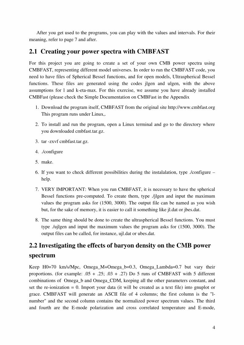
We will use CMB power spectra (generated with the CMBFAST package, in FITS format) as an input to generate a CMB sky map. This is a powerful tool for Monte Carlo simulations of CMB maps to calibrate the results of any given experiment. To get an output map, written in FITS format, just type synfast and answer the questions the program prompts you. The following is a sample of the program interface.
[alex@kohoutek Curso_radioastronomia2006]$ synfast
SYNFAST 2.0.0
*** Synthesis of a Temperature (and Polarisation) map from its power spectrum ***
Single precision outputs
7
Interactive mode. Answer the following questions.
If no answer is entered, the default value will be taken
Do you want to simulate
1) Temperature only
2) Temperature + polarisation
3) Temperature + 1st derivatives
4) Temperature + 1st & 2nd derivatives
5) T+P + 1st derivatives
6) T+P + 1st & 2nd derivates
allowed range: 1 6
default value: 1
1
Parser: simul_type = 1
Enter the resolution parameter (Nside) for the simulated skymap:
(Npix = 12*Nside**2, where Nside HAS to be a power of 2, eg: 32, 512, ...)
default value: 32
128
Parser: nsmax = 128
Enter the maximum l range (l_max) for the simulation.
We recommend: (0 <= l <= l_max <= 383)
default value: 256
128
Parser: nlmax = 128
Enter input Power Spectrum filename
If '' (empty single quotes) is typed, no file is read
(then an alm_file should be entered later on)
default value: /work/Healpix_2.01/test/cl.fits
8
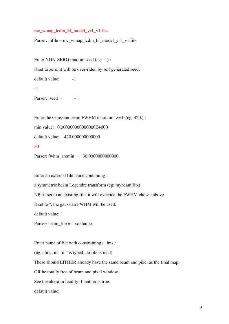
mc_wmap_lcdm_bf_model_yr1_v1.fits
Parser: infile = mc_wmap_lcdm_bf_model_yr1_v1.fits
Enter NONZERO random seed (eg: 1) :
if set to zero, it will be overriden by self generated seed.
default value: 1
1
Parser: iseed = 1
Enter the Gaussian beam FWHM in arcmin >= 0 (eg: 420.) :
min value: 0.000000000000000E+000
default value: 420.000000000000
30
Parser: fwhm_arcmin = 30.0000000000000
Enter an external file name containing
a symmetric beam Legendre transform (eg: mybeam.fits)
NB: if set to an existing file, it will override the FWHM chosen above
if set to '', the gaussian FWHM will be used.
default value: ''
Parser: beam_file = '' <default>
Enter name of file with constraining a_lms :
(eg, alms.fits; if '' is typed, no file is read)
These should EITHER already have the same beam and pixel as the final map,
OR be totally free of beam and pixel window.
See the alteralm facility if neither is true.
default value: ''
9

Parser: almsfile = '' <default>
Enter name of file with precomputed p_lms :
(eg, plm.fits; if '' is typed, no file is read)
default value: ''
Parser: plmfile = '' <default>
Enter Output map file name (eg, test.fits) :
(or !test.fits to overwrite an existing file)
(If '', no map is created)
default value: !test.fits
mapa.fits
Parser: outfile = mapa.fits
Enter file name in which to write a_lm used to synthesize the map :
(eg alm.fits or !alms.fits to overwrite an existing file):
(If '', the alms are not written to a file)
default value: ''
alm_mapa.fits
Parser: outfile_alms = alm_mapa.fits
This run can be reproduced in noninteractive mode, with the command
synfast single paramfile
where paramfile contains
simul_type = 1
nsmax = 128
nlmax = 128
infile = mc_wmap_lcdm_bf_model_yr1_v1.fits
10
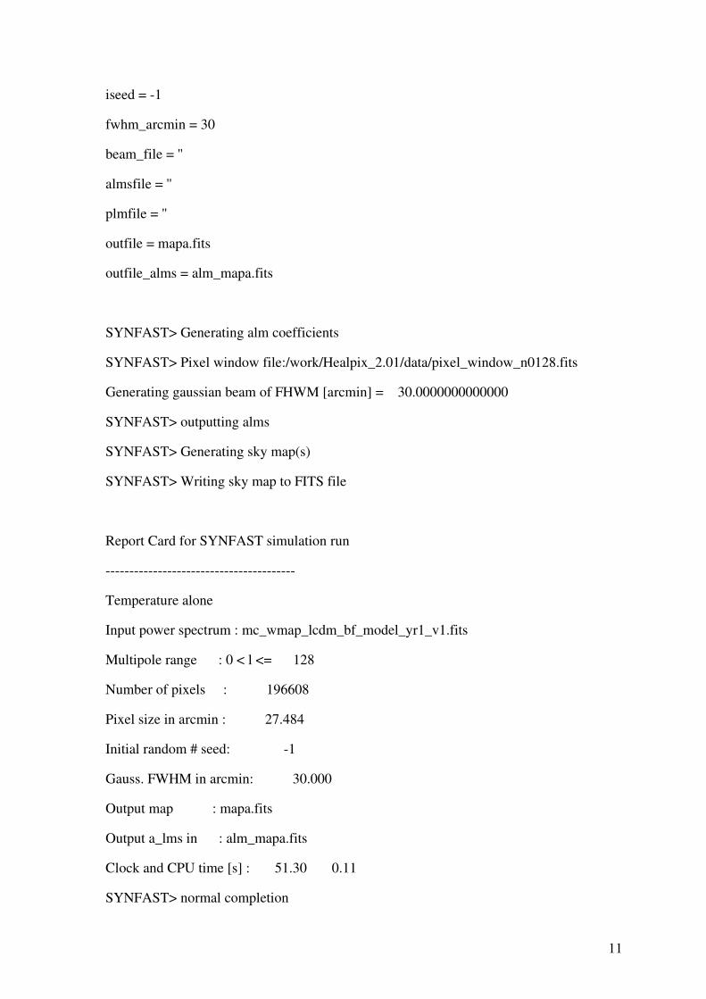
iseed = 1
fwhm_arcmin = 30
beam_file = ''
almsfile = ''
plmfile = ''
outfile = mapa.fits
outfile_alms = alm_mapa.fits
SYNFAST> Generating alm coefficients
SYNFAST> Pixel window file:/work/Healpix_2.01/data/pixel_window_n0128.fits
Generating gaussian beam of FHWM [arcmin] = 30.0000000000000
SYNFAST> outputting alms
SYNFAST> Generating sky map(s)
SYNFAST> Writing sky map to FITS file
Report Card for SYNFAST simulation run
Temperature alone
Input power spectrum : mc_wmap_lcdm_bf_model_yr1_v1.fits
Multipole range : 0 < l <= 128
Number of pixels : 196608
Pixel size in arcmin : 27.484
Initial random # seed: 1
Gauss. FWHM in arcmin: 30.000
Output map : mapa.fits
Output a_lms in : alm_mapa.fits
Clock and CPU time [s] : 51.30 0.11
SYNFAST> normal completion
11

Agora veremos o resultado da extração de um espectro de potência a partir do mapa criado com o programa synfast. Para isso, usamos o programa anafast, com a parte interativa abaixo:
[alex@kohoutek Curso_radioastronomia2006]$ anafast
ANAFAST 2.0.1
*** Analysis and power spectrum calculation for a Temperature/Polarisation map ***
Single precision outputs
Interactive mode. Answer the following questions.
If no answer is entered, the default value will be taken
Do you want to analyse
1) a Temperature only map
2) Temperature + polarisation maps
allowed range: 1 2
default value: 1
1
12

Parser: simul_type = 1
Enter input file name (Map FITS file):
default value: /work/Healpix_2.01/test/map.fits
mapa.fits
Parser: infile = mapa.fits
The map has Nside = 128
Enter the maximum l range (l_max) for the simulation.
We recommend: (0 <= l <= l_max <= 128)
default value: 256
128
Parser: nlmax = 128
Enter FITS file containing pixel mask and/or weight you want to use:
the map(s) will be multiplied by this mask(s) before analysis
(If '', all valid pixels are used with their current value)
default value: ''
Parser: maskfile = '' <default>
Enter the symmetric cut around the equator in DEGREES :
(One ignores data within |b| < b_cut) 0 <= b_cut =
min value: 0.000000000000000E+000
default value: 0.000000000000000E+000
Parser: theta_cut_deg = 0.000000000000000E+000 <default>
One keeps 100.0 % of the original map
To improve the temperature map analysis (specially on a cut sky)
13
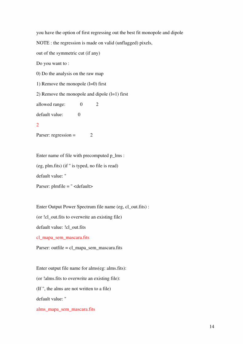
you have the option of first regressing out the best fit monopole and dipole
NOTE : the regression is made on valid (unflagged) pixels,
out of the symmetric cut (if any)
Do you want to :
0) Do the analysis on the raw map
1) Remove the monopole (l=0) first
2) Remove the monopole and dipole (l=1) first
allowed range: 0 2
default value: 0
2
Parser: regression = 2
Enter name of file with precomputed p_lms :
(eg, plm.fits) (if '' is typed, no file is read)
default value: ''
Parser: plmfile = '' <default>
Enter Output Power Spectrum file name (eg, cl_out.fits) :
(or !cl_out.fits to overwrite an existing file)
default value: !cl_out.fits
cl_mapa_sem_mascara.fits
Parser: outfile = cl_mapa_sem_mascara.fits
Enter output file name for alms(eg: alms.fits):
(or !alms.fits to overwrite an existing file):
(If '', the alms are not written to a file)
default value: ''
alms_mapa_sem_mascara.fits
14
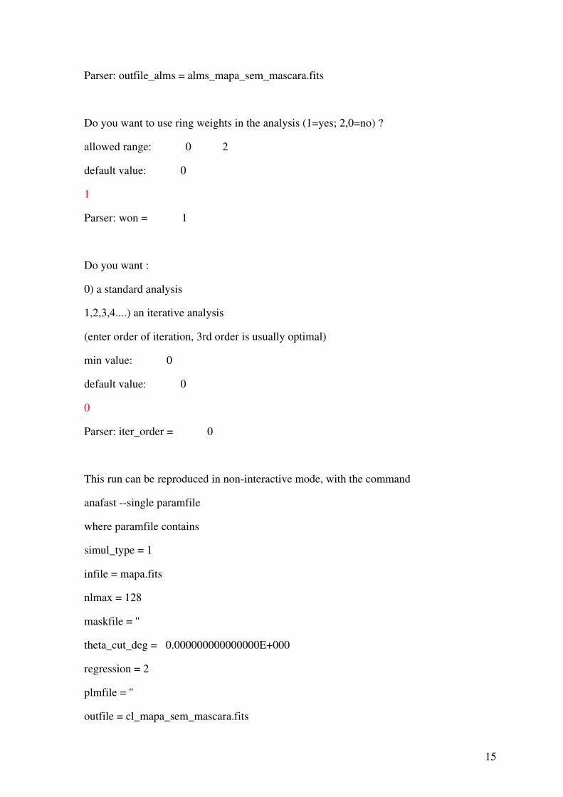
Parser: outfile_alms = alms_mapa_sem_mascara.fits
Do you want to use ring weights in the analysis (1=yes; 2,0=no) ?
allowed range: 0 2
default value: 0
1
Parser: won = 1
Do you want :
0) a standard analysis
1,2,3,4....) an iterative analysis
(enter order of iteration, 3rd order is usually optimal)
min value: 0
default value: 0
0
Parser: iter_order = 0
This run can be reproduced in noninteractive mode, with the command
anafast single paramfile
where paramfile contains
simul_type = 1
infile = mapa.fits
nlmax = 128
maskfile = ''
theta_cut_deg = 0.000000000000000E+000
regression = 2
plmfile = ''
outfile = cl_mapa_sem_mascara.fits
15

outfile_alms = alms_mapa_sem_mascara.fits
won = 1
iter_order = 0
ANAFAST> Inputting map
ANAFAST> Remove monopole (and dipole) from Temperature map
Excluding 0 pixels when computing monopole and/or dipole
Monopole = 1.59 unknown
Dipole = 14.0 unknown
(long.,lat.) = ( 135. , 25.3 ) Deg
ANAFAST> Inputting Quadrature ring weights
ANAFAST> Analyse map
ANAFAST> Compute power spectrum
ANAFAST> outputting Power Spectrum
ANAFAST> outputting alms
Report Card for ANAFAST analysis run
Temperature alone
Input map : mapa.fits
Multipole range : 0 <= l <= 128
Number of pixels : 196608
Pixel size in arcmin : 27.484
Symmetric cut in deg : 0.0000
Output power spectrum: cl_mapa_sem_mascara.fits
Output alm : alms_mapa_sem_mascara.fits
Ring weight file: /work/Healpix_2.01/data/weight_ring_n00128.fits
Clock and CPU time [s] : 102.86 0.20
16
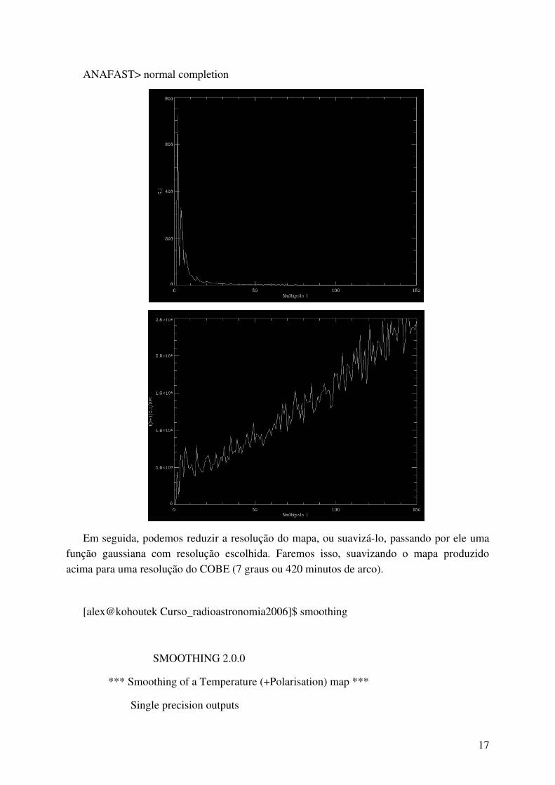
ANAFAST> normal completion
Em seguida, podemos reduzir a resolução do mapa, ou suavizálo, passando por ele uma função gaussiana com resolução escolhida. Faremos isso, suavizando o mapa produzido acima para uma resolução do COBE (7 graus ou 420 minutos de arco).
[alex@kohoutek Curso_radioastronomia2006]$ smoothing
SMOOTHING 2.0.0
*** Smoothing of a Temperature (+Polarisation) map ***
Single precision outputs
17

Interactive mode. Answer the following questions.
If no answer is entered, the default value will be taken
Do you want to analyse
1) a Temperature only map
2) Temperature + polarisation maps
allowed range: 1 2
default value: 1
1
Parser: simul_type = 1
Enter input file name (Map FITS file):
default value: /work/Healpix_2.01/test/map.fits
mapa.fits
Parser: infile = mapa.fits
The map has Nside = 128
Enter the maximum l range (l_max) for the simulation.
We recommend: (0 <= l <= l_max <= 128)
default value: 256
128
Parser: nlmax = 128
To improve the temperature map analysis (specially on a cut sky)
you have the option of first regressing out the best fit monopole and dipole
NOTE : the regression is made on valid (unflagged) pixels,
out of the symmetric cut (if any)
Do you want to :
18

0) Do the analysis on the raw map
1) Remove the monopole (l=0) first
2) Remove the monopole and dipole (l=1) first
allowed range: 0 2
default value: 0
2
Parser: regression = 2
Enter the symmetric cut around the equator in DEGREES :
(One ignores data within |b| < b_cut) 0 <= b_cut =
min value: 0.000000000000000E+000
default value: 0.000000000000000E+000
Parser: theta_cut_deg = 0.000000000000000E+000 <default>
One keeps 100.0 % of the original map
Do you want :
0) a standard analysis
1,2,3,4....) an iterative analysis
(enter order of iteration, 3rd order is usually optimal)
min value: 0
default value: 0
0
Parser: iter_order = 0
Enter name of file with precomputed p_lms :
(eg, plm.fits) (if '' is typed, no file is read)
default value: ''
Parser: plmfile = '' <default>
19

Enter the Gaussian beam FWHM in arcmin >= 0 (eg: 420.) :
min value: 0.000000000000000E+000
default value: 420.000000000000
420
Parser: fwhm_arcmin = 420.000000000000
Enter an external file name containing
a symmetric beam Legendre transform (eg: mybeam.fits)
NB: if set to an existing file, it will override the FWHM chosen above
if set to '', the gaussian FWHM will be used.
default value: ''
Parser: beam_file = '' <default>
Enter Output map file name (eg, test_smooth.fits) :
(or !test_smooth.fits to overwrite an existing file)
default value: !test_smooth.fits
mapa_smooth.fits
Parser: outfile = mapa_smooth.fits
Do you want to use ring weights in the analysis (1=yes,0,2=no) ?
allowed range: 0 2
default value: 0
1
Parser: won = 1
This run can be reproduced in noninteractive mode
if a parameter file with the following content is provided:
20
simul_type = 1
infile = mapa.fits
nlmax = 128
regression = 2
theta_cut_deg = 0.000000000000000E+000
iter_order = 0
plmfile = ''
fwhm_arcmin = 420
beam_file = ''
outfile = mapa_smooth.fits
won = 1
SMOOTHING> Inputting original map
SMOOTHING> Remove monopole (and dipole) from Temperature map
Excluding 0 pixels when computing monopole and/or dipole
Monopole = 1.59 unknown
Dipole = 14.0 unknown
(long.,lat.) = ( 135. , 25.3 ) Deg
SMOOTHING> Inputting Quadrature ring weights
SMOOTHING> Analyse map
SMOOTHING> Alter alm
Generating gaussian beam of FHWM [arcmin] = 420.000000000000
SMOOTHING> Generating sky map(s)
SMOOTHING> Writing smoothed map to FITS file
Report Card for SMOOTHING run
Temperature alone
Input map : mapa.fits
21
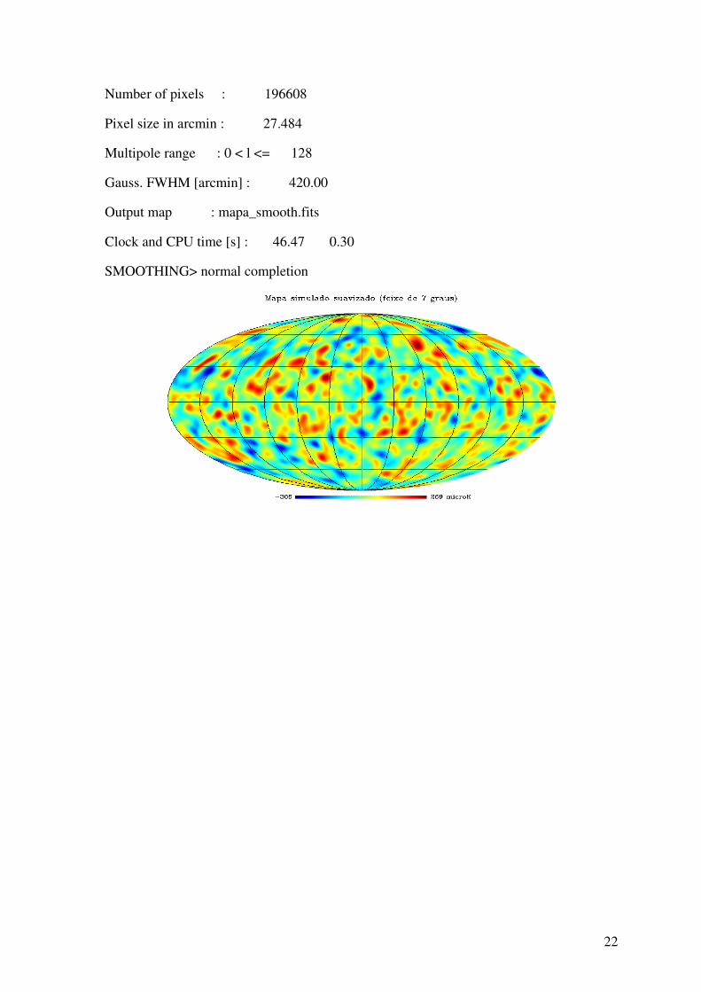
Number of pixels : 196608
Pixel size in arcmin : 27.484
Multipole range : 0 < l <= 128
Gauss. FWHM [arcmin] : 420.00
Output map : mapa_smooth.fits
Clock and CPU time [s] : 46.47 0.30
SMOOTHING> normal completion
22


![[Tutorial] RGH Corona V4 - Tutorial Completo _ Xblog 360](https://img.document.onl/doc/110x75/55cf9ca2550346d033aa7fcc/tutorial-rgh-corona-v4-tutorial-completo-xblog-360.jpg)