Value-at-risk modeling and forecasting with range-based ... · Value-at-risk modeling and forecasting with range-based volatility models: empirical evidence Leandro dos Santos Maciel

DOI: 10.1590/1808-057x201704140ISSN 1808-057X

361

Value-at-risk modeling and forecasting with range-based volatility models: empirical evidence

Leandro dos Santos MacielUniversidade Federal do Rio de Janeiro, Faculdade de Administração e Ciências Contábeis, Departamento de Ciências Contábeis, Rio de Janeiro, RJ, Brazil

Rosangela BalliniUniversidade Estadual de Campinas, Instituto de Economia, Campinas, SP, Brazil

Received on 08.10.2016 – Desk acceptance on 08.18.2016 – 2nd version approved on 03.23.2017

ABSTRACTThis article considers range-based volatility modeling for identifying and forecasting conditional volatility models based on returns. It suggests the inclusion of range measuring, defined as the difference between the maximum and minimum price of an asset within a time interval, as an exogenous variable in generalized autoregressive conditional heteroscedasticity (GARCH) models. The motivation is evaluating whether range provides additional information to the volatility process (intraday variability) and improves forecasting, when compared to GARCH-type approaches and the conditional autoregressive range (CARR) model. The empirical analysis uses data from the main stock market indexes for the U.S. and Brazilian economies, i.e. S&P 500 and IBOVESPA, respectively, within the period from January 2004 to December 2014. Performance is compared in terms of accuracy, by means of value-at-risk (VaR) modeling and forecasting. The out-of-sample results indicate that range-based volatility models provide more accurate VaR forecasts than GARCH models.

Keywords: volatility, forecasting models, financial markets, price range, value at risk (VaR).

R. Cont. Fin. – USP, São Paulo, v. 28, n. 75, p. 361-376, set./dez. 2017



1. INTRODUCTION

Volatility modeling and forecasting play a significant role in derivatives pricing, risk management, portfolio selection, and trading strategies (Leite, Figueiredo Pinto, & Klotzle, 2016). It is also noteworthy for policy makers and regulators, since the volatility dynamics is closely related to stability in financial markets and the economy as a whole. Time series models, such as the generalized autoregressive conditional heteroscedasticity (GARCH) model, stochastic volatility modeling, the implied volatility of option contracts and direct measures, like the realized volatility, are the most common choices to estimate volatility in finance (Val, Figueiredo Pinto, & Klotzle, 2014; Poon & Granger, 2003).

When compared to other methods, the GARCH-type approaches are the most widely used for modeling time-varying conditional volatility, due to their simple form, easy estimation, and flexible adaptation concerning the volatility dynamics. As return-based methods, the GARCH models are designed using data on closing prices, i.e. daily returns. Thus, they may neglect significant intraday price movement information. Also, as the GARCH models rely on the moving averages with gradually decaying weights, they are slow to adapt to changing volatility levels (Andersen, Bollerslev, Diebold, & Labys, 2003; Sharma & Vipul, 2016). To overcome this issue, intraday volatility models emerge as alternative tools. Another simple procedure for modeling intraday variation is adopting price range.

Range is defined as the difference between the highest and lowest market prices over a fixed sampling interval, e.g. day-to-day or week-to-week variability. The literature has claimed that range-based volatility estimators are more effective than historical volatility estimators (e.g. Garman & Klass, 1980; Parkinson, 1980; Rogers & Satchell, 1991; Yang & Zhang, 2000). This approach is easy to implement; it only requires readily available high, low, opening, and closing prices. Andersen and Bollerslev (1998) report the explanatory usefulness of range to discuss the realized volatility. Gallant, Hsu, and Tauchen (1999) and Alizadeh, Brandt, and Diebold (2001), in a stochastic volatility framework, include range in the equilibrium asset price models. Brandt and Jones (2002) stated that a range-based exponential generalized autoregressive conditional heteroskedastic (EGARCH) model provides better results for out-of-sample volatility forecasting than a return-based model. Using S&P 500 data, Christoffersen (2002) stated that range-based volatility showed more persistence than

squared return based on estimated autocorrelations, thus its time series may be used to devise a volatility model within the traditional autoregressive framework.

Dealing with range-based models has not drawn attention in estimating and forecasting volatility, due to their poor performance in empirical studies. Chou (2005) indicates that range-based models cannot capture volatility dynamics and by properly modeling the dynamics, range retains its superiority in forecasting volatility. Thus, the author proposed a range-based volatility method named as conditional autoregressive range (CARR) model. Similarly to the GARCH-type approaches, the CARR model consists in a dynamic approach for the high/low asset price range within fixed time intervals. The empirical results using S&P 500 data showed that the CARR model does provide better volatility estimates than a standard GARCH model.

Li and Hong (2011) also suggest a range-based autoregressive volatility model inspired on the GARCH and EGARCH approaches. The results concerning S&P 500 data demonstrate that a range-based approach successfully captures volatility dynamics and show a better performance than GARCH-type models. On the other hand, Anderson, Chen and Wang (2015) suggest a time range-based volatility model to capture the volatility dynamics of real estate securitization contracts, using a smooth transition copula function to identify nonlinear co-movements between major real estate investment trust (REIT) markets in the presence of structural changes. Further, Chou, Liu and Wu (2007) applied the CARR model to a multivariate context using the dynamic conditional correlation (DCC) model. The authors found that a range-based DCC model is better at forecasting covariance than other return-based volatility methods.

Over the last decade, there has been considerable growth in the use of range-based volatility models in finance (Chou, Chou, & Liu, 2010; Chou, Chou, & Liu, 2015). However, most of the literature evaluates the models in terms of forecasting accuracy, instead of financial applications using volatility forecasts. Moreover, the literature still lacks empirical works addressing range-based volatility models in emergent economies.

This article aims to assess range-based volatility models in the U.S. and Brazilian stock markets. The contribution of this work is twofold. First, theoretically, it suggests a GARCH-type approach designed to incorporate range-based volatility as an exogenous variable in GARCH and threshold autoregressive conditional heteroscedasticity

Leandro dos Santos Maciel & Rosangela Ballini

R. Cont. Fin. – USP, São Paulo, v. 28, n. 75, p. 361-376, set./dez. 2017 363

(TARCH) models. The main goal is to evaluate gains in forecasting by including range as additional information in GARCH-type approaches. Notice that in the CARR model, Chou (2005) addressed range-based modeling using a conditional variance approach, differently from GARCH-type models, which deal with modeling of financial asset returns. Herein, we resort to a GARCH-type approach, i.e. based on returns, but also including range as a source of additional information on volatility. Second, empirically, we evaluate the performance of range-based volatility models in the U.S. and Brazilian stock markets. It is worth noticing that this article contributes to the literature by empirically addressing an emergent market; there is a lack of studies in this context, so our results may provide valuable information for stock market players.

Our empirical analysis use data from the main stock market indexes for the U.S. and Brazilian economies, i.e. S&P 500 and IBOVESPA, respectively, within the period from January 2004 to December 2014. Experimental data employs statistical analysis and also economic criteria in terms of risk analysis. One-step-ahead forecasts are assessed using accuracy measures and statistical tests.

The range-based models are assessed by means of value-at-risk (VaR) forecasting. VaR is the most widely used measure in empirical analysis and its accurate computation is also crucial for other quantile-based risk estimation measures, such as expected shortfall (Wang & Watada, 2011; Hartz, Mittinik, & Paolella, 2006). VaR forecasts produced through traditional approaches, such as historical simulation, exponentially weighted moving average (EWMA), GARCH, and TARCH methods, are compared to the traditional CARR model and to the GARCH and TARCH models that include range-based volatility as an exogenous variable.

This article consists of four parts, in addition to this introduction. Section 2 describes GARCH-type models and range-based volatility approaches, including those suggested in this article. Section 3 briefly reports the methodology, concerning data, performance measurements, basic concepts of VaR, as well as its traditional estimation approaches and validation measures. Section 4 consists of empirical findings and their discussions. Finally, our conclusion suggests issues for further research.

2. VOLATILITY MODELS

This section provides a brief overview of the traditional GARCH and TARCH models, as well as these models using range-based volatility as an exogenous variable. And the CARR method is also described.

2.1 GARCH and TARCH Models

One of the simplest forms for modeling daily returns

may be written as follows:

where rt = ln(Pt) – ln (Pt-1) is the log price return at t, Pt is the asset price at t, ϵt ~ i.i.d.(0,1) is a zero-mean white noise, often assumed to be normal, and σt is time-varying

volatility. Different specifications for σt define different volatility models.

1



The GARCH model was introduced by Bollerslev (1986), as an extension of the autoregressive conditional heteroskedasticity (ARCH) model proposed by Engle (1982), and it allowed including past conditional variance in the current conditional variance equation. It is one of

the most widely used and well-known volatility models due to its flexibility and accuracy to modeling stylized facts of financial asset returns, such as leptokurtosis and volatility clustering.

A GARCH (p, q) model may be described as follows:

where ω > 0 is a constant, αi ≥ 0 is a coefficient to measure the short-term impact of ϵt on conditional variance, and βi ≥ 0 is a coefficient to measure the long-term impact on conditional variance.

The TARCH model is an asymmetric approach based on the assumption that unexpected changes in returns

have different effects on conditional variance, i.e. variance responds differently to positive and negative shocks, accounting for the asymmetry effect. A TARCH (p,q) model is defined according to Glosten, Jagannathan and Runkle (1993):

where It-1 = 1, if rt-1 < 0 (negative shocks), It-1 = 0, if rt-1 ≥ 0 (positive shocks), and the coefficient γi denotes an asymmetric effect, also known as leverage effect. A leverage effect is observed if γi is positive, otherwise γi equals to zero indicates a symmetric response by change in volatility returns.

2.2 Range-Based Volatility Models

Regarding an asset, the range of log prices, Rt, is defined as the difference between the highest daily price Ht and the lowest daily price Lt in a logarithm type, in the trading day t. This may be calculated according to Chou et al. (2015):

It is worth noticing that different range estimators may be considered as those suggested by Parkinson (1980) or Garman and Klass (1980), which also includes opening and closing prices to estimate range. However, herein range-based volatility, just as in (6) is chosen due to its ability to describe volatility dynamics, as claimed by Christoffersen (2002), and also because this is the same measure used in the CARR model. Thus, it is more suitable for comparison purposes.

This article takes two classes of the range-based volatility models. The first concerns including the realized range as an exogenous variable in the variance equation of traditional GARCH and TARCH models. The main goal is evaluating whether range-based volatility provides better information to the GARCH-type models, in order to achieve better forecasts and persistence reduction. Therefore, the GARCH model of equations (2) and (3) may be rewritten as follows:

2

3

4

5

6



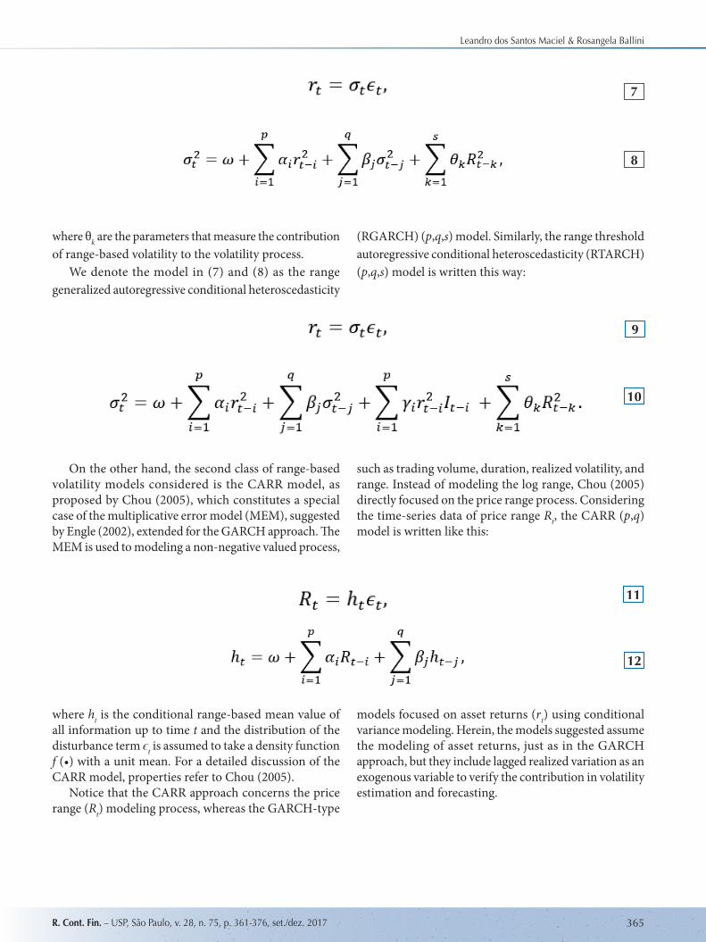
where θk are the parameters that measure the contribution of range-based volatility to the volatility process.

We denote the model in (7) and (8) as the range generalized autoregressive conditional heteroscedasticity

(RGARCH) (p,q,s) model. Similarly, the range threshold autoregressive conditional heteroscedasticity (RTARCH) (p,q,s) model is written this way:

On the other hand, the second class of range-based volatility models considered is the CARR model, as proposed by Chou (2005), which constitutes a special case of the multiplicative error model (MEM), suggested by Engle (2002), extended for the GARCH approach. The MEM is used to modeling a non-negative valued process,

such as trading volume, duration, realized volatility, and range. Instead of modeling the log range, Chou (2005) directly focused on the price range process. Considering the time-series data of price range Rt, the CARR (p,q) model is written like this:

where ht is the conditional range-based mean value of all information up to time t and the distribution of the disturbance term ϵt is assumed to take a density function f (•) with a unit mean. For a detailed discussion of the CARR model, properties refer to Chou (2005).

Notice that the CARR approach concerns the price range (Rt) modeling process, whereas the GARCH-type

models focused on asset returns (rt) using conditional variance modeling. Herein, the models suggested assume the modeling of asset returns, just as in the GARCH approach, but they include lagged realized variation as an exogenous variable to verify the contribution in volatility estimation and forecasting.

7

8

9

10

11

12



3. METHODOLOGY

This section reviews the sources of data and the performance measurements adopted in this article. The basic concepts of VaR modeling and forecasting are also detailed, as well as its validation analysis.

3.1 Data

We consider the highest, lowest, and closing daily prices from the main stock market indexes of U.S. and Brazilian economies, i.e. S&P 500 and IBOVESPA, respectively, within the period from January 2004 to December 2014. Also, as the realizations of volatility are unobservable, a proxy for volatility is required to devise the loss functions for analyzing the performance of models. Squared return is a widely used proxy, but as this is calculated through closing prices, intraday variability is neglected. Patton (2011) suggests using the realized volatility as an unbiased estimator. It is also more efficient than squared return if the log price follows a Brownian motion (Tian & Hamori, 2015). Realized volatility is the sum of squared high-frequency returns within a day. It conveniently avoids data analysis complications, while covering more information during daily transactions. Therefore, ‘true volatility’ is considered through the realized volatility measure. To compute daily realized volatility, data also comprise 1-minute quotations from January 2004 to December 2014, according to the S&P 500 and IBOVESPA indexes. Notice that intraday data was used only to compute daily realized volatility, as a proxy for volatility. The models considered daily price data, provided by Bloomberg. The sample is divided into

two parts: data from January 2004 to December 2010 was taken as the estimation sample (in-sample), while the remaining 4-year data was used as the out-of-sample period for volatility and VaR forecasting. Out-of-sample forecasts are computed having re-estimated volatility models parameters as a basis, according to a fixed data window.

The experimental results are analyzed on the basis of statistical criteria and also considering economic criteria in terms of risk analysis. The subsections below describe the evaluation models.

3.2 Forecast Evaluation

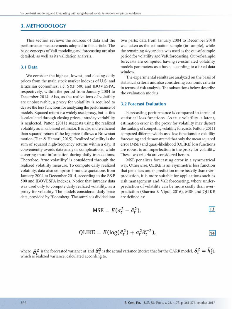
Forecasting performance is compared in terms of statistical loss functions. As true volatility is latent, estimation error in the proxy for volatility may distort the ranking of competing volatility forecasts. Patton (2011) compared different widely used loss functions for volatility forecasting and demonstrated that only the mean squared error (MSE) and quasi-likelihood (QLIKE) loss functions are robust to an imperfection in the proxy for volatility. These two criteria are considered herein.

MSE penalizes forecasting error in a symmetrical way. Otherwise, QLIKE is an asymmetric loss function that penalizes under-prediction more heavily than over-prediction, it is more suitable for applications such as risk management and VaR forecasting, where under-prediction of volatility can be more costly than over-prediction (Sharma & Vipul, 2016). MSE and QLIKE are defined as:

where is the forecasted variance at and is the actual variance (notice that for the CARR model, ), which is realized variance, calculated according to:

13

14



where rt,Δ= ln(Pt) - ln(Pt-Δ) is the discrete sample of the Δ-period return (in this article Δ is equal to 1-minute quotations).

For both MSE and QLIKE, the smaller the values, the more accurate the model is. Despite the good performance of forecasting measures that are widely used in practice, they do not reveal whether the forecast of a model is statistically better than another one. Therefore, it is a must to use additional tests to help comparing two or more competing models in terms of forecasting accuracy.

Moreover, this article employs the Diebold-Mariano (DM) statistic test to evaluate the null hypothesis of equal predictive accuracy between competitive forecasting methods (Diebold & Mariano, 1995). We assume that the losses for forecasting models i and j are given by Li

t and Lj

t, where 𝐿𝑡 = 𝜎𝑡2− 𝜎�𝑡2 . The DM test verifies the null hypothesis E(Li

t) = E(Ljt). The statistic test is based

on the loss differential dt = Lit - Lj

t. The null hypothesis of equal predictive accuracy is:

The DM test is:

where , and T is the total number of forecasts. The variance of , is estimated by the heteroskedasticity and autocorrelation consistent (HAC) estimator, as proposed by Newey and West (1987). According to Diebold and Mariano (1995), under the null hypothesis of equal predictive accuracy, the statistic test follows normal distribution with zero mean value and unitary variance.

3.3 VaR Estimation and Validation

In order to evaluate the usefulness of the volatility

forecasting methods suggested by applying perspective, we examine the performance of forecasting by means of economic criteria in terms of risk analysis. VaR has been adopted by practitioners and regulators as the standard mechanism to measure market risk of financial assets. It determines the potential market value loss of a financial asset over a time horizon h, at a significance or coverage level αVaR. Alternatively, it reflects the asset market value loss over the time horizon h, which is not expected to be exceeded with probability 1 - αVaR, so:

Hence, VaR is the αVaR-th quantile of conditional distribution of returns, defined as: , where CDF(•) refers to the return cumulative distribution

function and CDF-1(•) denotes its inverse. Herein, we consider h = 1, as it bears the greatest practical interest with daily frequency.

15

16

17

18



Therefore, the parametric VaR at t + 1 is given by:

where is the forecasted volatility at and is the critical value from the normal

distribution table at the αVaR confidence level.In a VaR forecasting context, volatility modeling

plays a crucial role, thus it is worth emphasizing the volatility models adopted. In this research, VaR forecasts, as in (19), are obtained using traditional return-based volatility models, like GARCH and TARCH; just as the same approaches that take volatility range as an exogenous variable (RGARCH and RTARCH models), the range-based volatility CARR model is also considered in comparisons. Non-parametric VaR forecasts are also performed by the historical simulation approach, since it is widely used in the literature on VaR modeling. Historical simulation is a non-parametric approach to VaR estimation, where the main issue is constructing the

cumulative distribution function (CDF) for asset returns over time. Unlike parametric VaR models, historical simulation does not assume a particular distribution of the asset returns. In addition to its simple estimation, historical simulation assumes that asset returns consists in independent and identically-distributed random variables, but this is not the case: based on empirical evidence, it is known that asset returns are clearly not independent, as it exhibits certain patterns, such as volatility clustering. Further, this method also applies equal weight to returns over the whole period.

The performance of VaR forecasting models is evaluated using two loss functions: the violation ratio (VR) and the average square magnitude function. The VR is the percentage of actual loss higher than the estimated maximum loss in the VaR framework. The VR is computed as follows:

where δt = 1 if rt < VaRt and δt = 0 if rt ≥ VaRt, if where VaRt is the one-step-ahead forecasted VaR for day t, and T is the number of observations in the sample. Notice that, in some cases, a lower VR does not indicate better performance. If VaR is estimated at a confidence level (1 – αVaR)%, a general αVaR% of violations is expected. A VR much lower (much greater) than αVaR% indicates that VaR is overestimated (underestimated), and this reveals

lower model accuracy, resulting in practical implications, such as changes on investment positions due to VaR alert-based strategies.

The average square magnitude function (ASMF) (Dunis, Laws, & Sermpinis, 2010) considers the amount of possible default measuring the average squared cost of exceptions. It is computed using:

where ϑ is the number of exceptions in the respective model, ξt = (rt – VaRt)

2 when rt < VaRt and ξt = 0, when rt ≥VaRt. The average squared magnitude function enables us to distinguish between models with similar or identical hit rates. For both VR and ASMF measures, the lower values, the higher accuracy. Since VaR estimates potential loss, its accuracy is relevant in investment decisions.

Since VaR encompasses some restrictive assumptions, statistical tests are required to verify the validity of VaR estimates. VaR forecasting models are also assessed by

using unconditional and conditional coverage tests. The unconditional coverage test (LRuc), proposed by Kupiec (1995), examines whether the unconditional coverage rate is statistically consistent with the confidence level prescribed for the VaR model. The null hypothesis is defined as the failure probability of each trial equals the specified probability of this model (αVaR). A failure occurred when the predicted VaR cannot cover the realized loss. The statistic likelihood ratio test is given by:

19

20

21



where , the failure rate, is the maximum likelihood estimate of αVaR, f = denotes a Bernoulli random variable representing the total number of VaR violations for T observations. The null hypothesis of the failure rate αVaR is tested against the alternative hypothesis that the failure rate is different from αVaR, i.e. the test verifies if the observed VR of a model is statistically consistent with the pre-specified VaR confidence level.

Although the LRuc test can reject a model that either overestimates or underestimates the actual VaR, it cannot determine whether the exceptions are randomly distributed.

In a risk management framework, it is of paramount importance that VaR exceptions be uncorrelated over time (Su & Hung, 2011). Thus, the conditional coverage test (LRcc), as proposed by Christoffersen (1998), is addressed. It tests unconditional coverage and serial independence. The statistical test is LRcc = LRuc + LRind; LRind represents the likelihood statistics that checks whether exceptions are independent. Considering the null hypothesis that the failure process is independent and the expected proportion of exceptions equals αVaR, the likelihood ratio is calculated as:

where fij is the number of observations with value i followed by value j (i, j = 0, 1), πij = Pr{δt = j | δt-1 = i}, π01 = f01/(f00 + f01), π11 = f11/(f10 + f11).

4. EMPIRICAL RESULTS

This section presents the empirical results of the range-based volatility models in comparison to return-based volatility models, using data from the main stock market indexes for the U.S. and Brazilian economies, i.e. S&P 500 and IBOVESPA, respectively, within the period from January 2004 to December 2014.

Table 1 displays the statistics of S&P 500 and IBOVESPA returns and range-based volatility. The returns for both S&P 500 and IBOVESPA indexes have a mean value around zero, similar standard deviation, high positive kurtosis, and negative skewness, indicating heavy tails, as usual in financial time series of returns. Regarding the volatility range series, daily ranges for S&P 500 and IBOVESPA have

mean values about 1% and 2%, respectively, and similar standard deviation to the return series (Table 1). However, volatility ranges have a higher kurtosis than the return series and positive skewness, as expected for variance measurement. It is worth observing the different values for autocorrelation functions (ACFs) and of the Ljung-Box Q statistics for returns and range series, which indicate a much higher persistence level for range than return series. This fact confirms the use of the CARR model in range volatility forecasting. Figure 1 shows daily returns and range volatility series of the S&P 500 and IBOVESPA indexes for the period under study. The series reveals volatility clusters.

^^ ^

22

23



Table 1. Descriptive statistics of the S&P 500 and IBOVESPA returns and range-based volatility within the period from January 2004 to December 2014.

Statistics S&P 500 returns S&P 500 range-based volatility IBOVESPA returns IBOVESPA range-based volatility Mean 0.0002 0.0130 0.0003 0.0224

Standard deviation 0.0125 0.0108 0.0181 0.0136Kurtosis 11.5540 20.1899 5.2376 19.2702

Skewness -0.3271 3.6427 -0.0490 3.2491Minimum -0.0947 0.0000 -0.1210 0.0032Maximum 0.1096 0.1090 0.1368 0.1681

ACF(1) -0.1093 0.6987 -0.0112 0.5717ACF(15) -0.0494 0.5316 0.0110 0.4006Q(15) 79.2194 15727.91 26.4686 9507.68

Note: Q(15) statistics represent the Ljung-Box Q statistics for autocorrelation in the returns and range volatility series.Source: Prepared by the authors.

Figure 1. Time series of returns and volatility ranges for S&P 500 and IBOVESPA indexes within the period from January 2004 to December 2014.Source: Prepared by the authors.

Dec 05 Dec 07 Dec 09 Dec 11 Dec 13−0.2

−0.1

0

0.1

0.2

(a) S&P 500 returns

Dec 05 Dec 07 Dec 09 Dec 11 Dec 13−0.2

−0.1

0

0.1

0.2

(b) IBOVESPA returns

Dec 05 Dec 07 Dec 09 Dec 11 Dec 130

0.05

0.1

0.15

(c) S&P 500 volatility range

Dec 05 Dec 07 Dec 09 Dec 11 Dec 130

0.05

0.1

0.15

0.2

(d) IBOVESPA volatility range

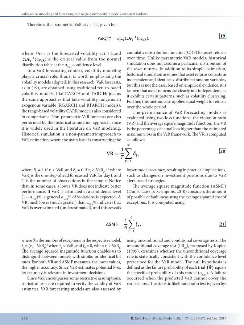
The number of lags, p and q, for GARCH, TARCH, and CARR models, and p, q and s, for RGARCH and RTARCH models, is determined according to the Schwarz criterion. For both indexes, all models were estimated considering p = q = s = 1, which result in parsimonious structures with high accuracy and a few number of parameters. Table 2 displays the estimates of return- and range-based volatility models for the S&P 500 index. The estimation sample considers data from January 2004 to December 2010. All models are affected by the news, as the values of ω in each case are significant, except for RTARCH. In asymmetric models, TARCH and RTARCH, the effect of past squared returns, measured by the parameter α, is negatively related to volatility,

whereas in the symmetric models this parameter has a positive sign. The β value in the range-based CARR model is lower than in the other approaches, indicating a shorter memory in its volatility process. The parameter γ indicates the presence of a leverage effect on the volatility process in the S&P 500 index, i.e. volatility responds differently to negative and positive shocks (returns). The significance of the parameter θ in RGARCH and RTARCH models indicates that range-based volatility provides information to modeling volatility in the S&P 500 index. Finally, the Akaike information criterion and the Bayesian information criterion confirm that the simplicity of models (few number of parameters) is adequate.



Table 2. Return- and range-based volatility model estimates for the S&P 500 index within the period from January 2004 to December 2010.

Parameter GARCH (1,1) TARCH (1,1) RGARCH (1,1,1) RTARCH (1,1,1) CARR (1,1)

ω 1.20E-06(0.0000)

9.66E-07(0.0000)

-2.69E-06(0.0074)

-5.57E-07(0.3711)

3.92E-06(0.0153)

α 0.075(0.0000)

-0.031(0.0000)

0.055(0.0000)

-0.038(0.0000)

0.182(0.0000)

β 0.915(0.0000)

0.953(0.0000)

0.891(0.0000)

0.928(0.0000)

0.802(0.0000)

γ -0.135

(0.0000)-

0.155(0.0000)

-

θ - -0.001

(0.0002)0.003

(0.0052)-

L 5634.65 5677.66 5638.47 5676.15 5077.79AIC -6.392 -6.440 -6.399 -6.440 -5.761BIC -6.383 -6.427 -6.386 -6.425 -5.750

Note: The values in parentheses represent p values, L is the log-likelihood function value, and the AIC and BIC denote the Akaike and Schwarz information criteria, respectively.Source: Prepared by the authors.

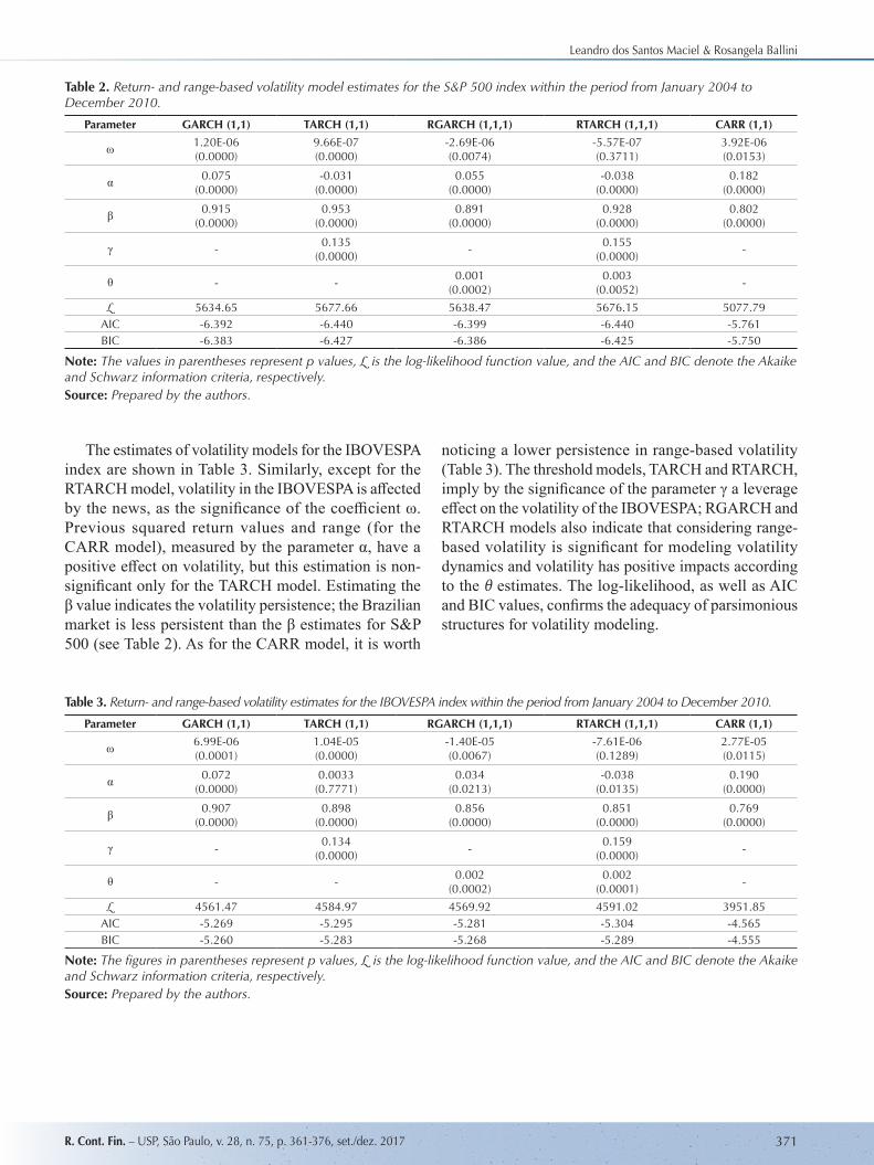
The estimates of volatility models for the IBOVESPA index are shown in Table 3. Similarly, except for the RTARCH model, volatility in the IBOVESPA is affected by the news, as the significance of the coefficient ω. Previous squared return values and range (for the CARR model), measured by the parameter α, have a positive effect on volatility, but this estimation is non-significant only for the TARCH model. Estimating the β value indicates the volatility persistence; the Brazilian market is less persistent than the β estimates for S&P 500 (see Table 2). As for the CARR model, it is worth

noticing a lower persistence in range-based volatility (Table 3). The threshold models, TARCH and RTARCH, imply by the significance of the parameter γ a leverage effect on the volatility of the IBOVESPA; RGARCH and RTARCH models also indicate that considering range-based volatility is significant for modeling volatility dynamics and volatility has positive impacts according to the θ estimates. The log-likelihood, as well as AIC and BIC values, confirms the adequacy of parsimonious structures for volatility modeling.

Table 3. Return- and range-based volatility estimates for the IBOVESPA index within the period from January 2004 to December 2010.

Parameter GARCH (1,1) TARCH (1,1) RGARCH (1,1,1) RTARCH (1,1,1) CARR (1,1)

ω 6.99E-06(0.0001)

1.04E-05(0.0000)

-1.40E-05(0.0067)

-7.61E-06(0.1289)

2.77E-05(0.0115)

α 0.072(0.0000)

0.0033(0.7771)

0.034(0.0213)

-0.038(0.0135)

0.190(0.0000)

β 0.907(0.0000)

0.898(0.0000)

0.856(0.0000)

0.851(0.0000)

0.769(0.0000)

γ -0.134

(0.0000)-

0.159(0.0000)

-

θ - -0.002

(0.0002)0.002

(0.0001)-

L 4561.47 4584.97 4569.92 4591.02 3951.85AIC -5.269 -5.295 -5.281 -5.304 -4.565BIC -5.260 -5.283 -5.268 -5.289 -4.555

Note: The figures in parentheses represent p values, L is the log-likelihood function value, and the AIC and BIC denote the Akaike and Schwarz information criteria, respectively.Source: Prepared by the authors.



Table 4. Performance of volatility forecasting models for the S&P 500 and IBOVESPA indexes based on the MSE and QLIKE criteria within the period from January 2011 to December 2014.

ModelsS&P 500 IBOVESPA

MSE QLIKE MSE QLIKEGARCH 8.7337E-05 -2.2002 2.0099E-04 -1.8630TARCH 8.8467E-05 -2.1405 1.8305E-04 -1.9095

RGARCH 8.1272E-05 -2.6004 1.2468E-04 -2.1896RTARCH 7.9599E-05 -2.8640 1.0051E-04 -2.2177

CARR 7.7771E-06 -2.8763 6.3166E-05 -2.4938

Source: Prepared by the authors.

As mentioned in section 3.2, the forecasting performance of volatility models is evaluated through the MSE and QLIKE loss functions. To evaluate this, realized volatility, computed by (15) and 1-minute quotations of the S&P 500 and IBOVESPA, is taken as a proxy. Our analysis concerns the out-of-sample volatility forecasting, i.e. we use data from January 2011 to December 2014. In the out-of-sample analysis, the volatility model parameters were re-estimated for forecasting by means of a fixed data window. To each prediction, the last observation has been removed, in order to keep the same data window size.

Table 4 displays the forecasting evaluation of the S&P 500 and IBOVESPA indexes for the MSE and QLIKE loss functions. The lower the values, the better the model. As for the S&P 500 index, range-based models – such as the RGARCH, RTARCH, and CARR – showed lower loss function values than the traditional GARCH and

TARCH methods. This was expected, as the standard GARCH models have a limited information set that only includes daily returns. Threshold approaches performed worst (higher loss function values). The results also indicate that the CARR model outperforms the remaining methodologies concerning both MSE and QLIKE values. Similar results are found for the IBOVESPA index. However, the leverage-based methods, TARCH and RTARCH, result in the best performance against GARCH and RGARCH, respectively. Again, including range-based volatility in RGARCH and RTARCH models provides relevant information to volatility process as these models achieved better forecasting performance than the benchmarks (GARCH and TARCH). Further, direct range-based modeling, i.e. the CARR model, emerges as the most accurate approach, with lower MSE and QLIKE values, regarding the alternative methods in focus.

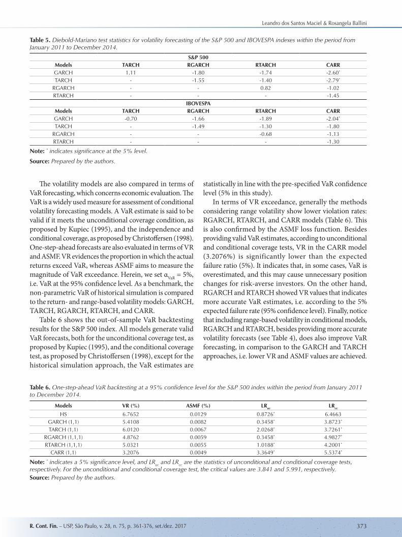
Next, we provide the results of the DM test to verify whether a model is statistically better than another one. Table 5 shows the statistics of the DM test for a pair of competing forecasting models. All statistical values significant at the 5% level are marked with asterisks. For the S&P 500 index, the CARR model provides a better accuracy performance in statistical terms than the GARCH and TARCH models. The CARR model

also outperforms the GARCH model with regard to the IBOVESPA index volatility forecasting according to the DM test. In all the remaining cases, volatility forecasting may be considered as equally accurate in statistical terms. A better performance of the CARR model may be due to the fact that this approach resorts to range-based volatility modeling instead of return-based volatility modeling in GARCH-family models.



The volatility models are also compared in terms of VaR forecasting, which concerns economic evaluation. The VaR is a widely used measure for assessment of conditional volatility forecasting models. A VaR estimate is said to be valid if it meets the unconditional coverage condition, as proposed by Kupiec (1995), and the independence and conditional coverage, as proposed by Christoffersen (1998). One-step-ahead forecasts are also evaluated in terms of VR and ASMF. VR evidences the proportion in which the actual returns exceed VaR, whereas ASMF aims to measure the magnitude of VaR exceedance. Herein, we set αVaR = 5%, i.e. VaR at the 95% confidence level. As a benchmark, the non-parametric VaR of historical simulation is compared to the return- and range-based volatility models: GARCH, TARCH, RGARCH, RTARCH, and CARR.

Table 6 shows the out-of-sample VaR backtesting results for the S&P 500 index. All models generate valid VaR forecasts, both for the unconditional coverage test, as proposed by Kupiec (1995), and the conditional coverage test, as proposed by Christoffersen (1998), except for the historical simulation approach, the VaR estimates are

statistically in line with the pre-specified VaR confidence level (5% in this study).

In terms of VR exceedance, generally the methods considering range volatility show lower violation rates: RGARCH, RTARCH, and CARR models (Table 6). This is also confirmed by the ASMF loss function. Besides providing valid VaR estimates, according to unconditional and conditional coverage tests, VR in the CARR model (3.2076%) is significantly lower than the expected failure ratio (5%). It indicates that, in some cases, VaR is overestimated, and this may cause unnecessary position changes for risk-averse investors. On the other hand, RGARCH and RTARCH showed VR values that indicates more accurate VaR estimates, i.e. according to the 5% expected failure rate (95% confidence level). Finally, notice that including range-based volatility in conditional models, RGARCH and RTARCH, besides providing more accurate volatility forecasts (see Table 4), does also improve VaR forecasting, in comparison to the GARCH and TARCH approaches, i.e. lower VR and ASMF values are achieved.

Table 5. Diebold-Mariano test statistics for volatility forecasting of the S&P 500 and IBOVESPA indexes within the period from January 2011 to December 2014.

S&P 500Models TARCH RGARCH RTARCH CARRGARCH 1.11 -1.80 -1.74 -2.60*

TARCH - -1.55 -1.40 -2.79*

RGARCH - - 0.82 -1.02RTARCH - - - -1.45

IBOVESPAModels TARCH RGARCH RTARCH CARRGARCH -0.70 -1.66 -1.89 -2.04*

TARCH - -1.49 -1.30 -1.80RGARCH - - -0.68 -1.13RTARCH - - - -1.30

Note: * indicates significance at the 5% level.

Source: Prepared by the authors.

Table 6. One-step-ahead VaR backtesting at a 95% confidence level for the S&P 500 index within the period from January 2011 to December 2014.

Models VR (%) ASMF (%) LRuc LRcc

HS 6.7652 0.0129 0.8726* 6.4663GARCH (1,1) 5.4108 0.0082 0.3458* 3.8723*

TARCH (1,1) 6.0120 0.0067 2.0268* 3.7261*

RGARCH (1,1,1) 4.8762 0.0059 0.3458* 4.9827*

RTARCH (1,1,1) 5.0321 0.0055 1.0188* 4.2001*

CARR (1,1) 3.2076 0.0049 3.3649* 5.5374*

Note: * indicates a 5% significance level, and LRuc and LRcc are the statistics of unconditional and conditional coverage tests, respectively. For the unconditional and conditional coverage test, the critical values are 3.841 and 5.991, respectively.Source: Prepared by the authors.



Table 7. One-step-ahead VaR backtesting at the 95% confidence level for the IBOVESPA index within the period from January 2011 to December 2014.

Models VR (%) ASMF (%) LRuc LRcc

HS 6.2359 0.0166 0.9182* 5.4663*

GARCH (1,1) 4.4442 0.0141 0.6789* 3.8721*

TARCH (1,1) 4.1303 0.0154 2.3961* 3.4469*

RGARCH (1,1,1) 3.9434 0.0124 0.9522* 4.7262*

RTARCH (1,1,1) 3.5319 0.0119 3.4413* 5.2039*

CARR (1,1) 3.4813 0.0112 3.7341* 5.7770*

Note: * indicates a 5% significance level, and LRuc and LRcc are the statistics of unconditional and conditional coverage tests, respectively. For the unconditional and conditional coverage test, the critical values are 3,841 and 5,991, respectively.Source: Prepared by the authors.

Table 7 displays the VaR backtesting results for the IBOVESPA index. Valid VaR forecasts are achieved for all models regarding the conditional and unconditional coverage tests, as the LRuc and LRcc are significant at a 5% significance level. Historical simulation has the worst performance in contrast to parametric VaR models in terms of VR and the respective average squared magnitude function values. By including range-based volatility in the GARCH and TARCH models, VaR forecasting is improved, revealing that range provides the volatility process with relevant information, i.e. the VR measure is

decreased by about 12.82% using RGARCH and RTARCH instead of the GARCH and TARCH models (Table 7). This improvement is more relevant in terms of VR for the IBOVESPA index than for the S&P 500 index resorting to the RGARCH and RTARCH models (see Table 6). Also, in the context of the Brazilian stock market, asymmetric volatility models, TARCH and RTARCH, showed to be better than symmetric volatility approaches to indicate the significance of leverage effects on volatility modeling. Again, the CARR model provides a lower VR, which indicates that in some cases VaR is overestimated.

Overall, VaR forecasts generated by range-based volatility models are reliable for both the S&P 500 and IBOVESPA indexes. Furthermore, in the context of the U.S. and Brazilian stock markets, including this exogenous variable in traditional conditional variance models improves

volatility forecasting and also provides more accurate VaR estimates, a key issue in many risk management situations. Therefore, the benefits of addressing range-based volatility are more significant in the Brazilian stock market.

5. CONCLUSION

Volatility is a key variable in asset allocation, derivative pricing, investment decisions, and risk analysis. Thus, volatility modeling, as an important issue in financial markets, has drawn the attention of finance academics and stock market practitioners over the last decades. Since asset price volatility cannot be observed, there is a need to estimate it. In the literature on conditional volatility modeling and forecasting, the GARCH-type models are widely used and well-known due to their accuracy to deal with financial return stylized facts modeling, such as volatility clustering and autocorrelation. However, they are return-based models calculated by means of closing price data. Thus, they fail to capture intraday asset price variability, neglecting significant information.

Price range, or volatility range, defined as the difference between the highest and lowest market prices over a fixed sampling interval, has been known for a long

time and has recently regained critical interest as a proxy for volatility. Many studies showed that we can use the price range scale to improve volatility estimation and forecasting, which is more effective than using squared daily returns. Thus, this article evaluates the performance of range-based volatility models in a risk management application: VaR forecasting. This article suggests the inclusion of volatility range as an exogenous variable in traditional GARCH and TARCH models, in order to evaluate whether range provides additional information on volatility and better volatility forecasting than return-based GARCH-type approaches and CARR model. Our empirical analysis uses data from the main stock market indexes for the U.S. and Brazilian economies, i.e. S&P 500 and IBOVESPA, respectively, thus a developed and an emergent market are addressed; the models are compared in terms of loss functions and statistical



tests for volatility assessment, also considering VaR backtesting approaches.

Our out-of-sample results indicate that range-based volatility models do provide additional information to traditional GARCH and TARCH models. In addition, more accurate VaR forecasts are achieved by the models that include the range as an exogenous variable in the

variance equation for both stock indices evaluated. Future research should include the evaluation of different volatility range measures as the realized range, as well as the comparison of the long-term forecasting models, addressing different volatility patterns, such as in crisis scenarios, and their application to asset trading strategies.

REFERENCES

Alizadeh, S., Brandt, M., & Diebold, F. X. (2001). Range-based estimation of stochastic volatility models or exchange rate dynamics are more interesting than you think. Journal of Finance, 57, 1047-1092.

Andersen, T. G., & Bollerslev, T. (1998). Answering the skeptics: yes, standard volatility models do provide accurate forecasts. International Economic Review, 39, 885-905.

Andersen, T. G., Bollerslev, T., Diebold, F. X., & Labys, P. (2003). Modeling and forecasting realized volatility. Econometrica, 71(2), 579-625.

Anderson, R. I., Chen, Y.-C., Wang, L.-M. (2015). A range-based volatility approach to measuring volatility contagion in securitized real state markets. Economic Modelling, 45, 223-235.

Bollerslev, T. (1986). Generalized autoregressive conditional heteroskedasticity. Journal of Econometrics, 31, 307-327.

Brandt, M., & Jones, C. (2002). Volatility forecasting with range-based EGARCH models (manuscript). Philadelphia, PA: University of Pennsylvania.

Chou, R. Y. (2005). Forecasting financial volatilities with extreme values: the conditional autoregressive range (CARR) model. Journal of Money, Credit and Banking, 37(3), 561-582.

Chou, R. Y., Chou, H., & Liu, N. (2010). Range volatility models and their applications in finance. In C.-F. Lee, & J. Lee (Ed.), Handbook of quantitative finance and risk management (pp. 1273-1281). New York: Springer.

Chou, R. Y., Chou, H., & Liu, N. (2015). Range volatility: a review of models and empirical studies. In C.-F. Lee, & J. Lee (Ed.), Handbook of financial econometrics and statistics (pp. 2029-2050). New York: Springer.

Chou, R. Y., Liu, N., & Wu, C. (2007). Forecasting time-varying covariance with a range-based dynamic conditional correlation model (working paper). Taipé, Taiwan: Academia Sinica.

Christoffersen, P. F. (1998). Evaluating interval forecasts. International Economic Review, 39, 841-862.

Christoffersen, P. F. (2002). Elements of financial risk management. San Diego, CA: Academic.

Diebold, F. X., & Mariano, R. S. (1995). Comparing predictive accuracy. Journal of Business & Economic Statistics, 13(3), 253-263.

Dunis, C., Laws, J., & Sermpinis, G. (2010). Modeling commodity value-at-risk with high order neural networks. Applied Financial Economics, 20(7), 585-600.

Engle, R. F. (1982). Autoregressive conditional heteroskedasticity with estimates of the variance of UK inflation. Econometrica, 50, 987-1008.

Engle, R. F. (2002). New frontiers for ARCH models. Journal of Applied Econometrics, 17, 425-446.

Gallant, R., Hsu, C., & Tauchen, G. (1999). Calculating volatility diffusions and extracting integrated volatility. Review of Economics and Statistics, 81, 617-631.

Garman, M. B., & Klass, M. J. (1980). On the estimation of price volatility from historical data. Journal of Business, 53, 67-78.

Glosten, L. R., Jagannathan, R., & Runkle, D. E. (1993). On the relation between the expected value and the volatility of the nominal excess return on stocks. Journal of Finance, 48(5), 1779-1801.

Hartz, C., Mittinik, S., & Paolella, M. S. (2006). Accurate value-at-risk forecasting based on the normal-GARCH model. Computational Statistics & Data Analysis, 51(4), 2295-2312.

Kupiec, P. (1995). Techniques for verifying the accuracy of risk management models. Journal of Derivatives, 3, 73-84.

Leite, A. L., Figueiredo Pinto, A. C., & Klotzle, M. C. (2016). Efeitos da volatilidade idiossincrática na precificação de ativos. Revista Contabilidade & Finanças, 27(70), 98-112.

Li, H., & Hong, Y. (2011). Financial volatility forecasting with range-based autoregressive model. Financial Research Letters, 8(2), 69-76.

Newey, W. K., & West, K. D. (1987). A simple, positive semi-definite heteroskedasticity and autocorrelation consistent covariance matrix. Econometrica, 55(3), 703-708.

Parkinson, M. (1980). The extreme value method for estimating the variance of the rate of return. Journal of Business, 53, 61-65.

Patton, A. J. (2011). Volatility forecast comparison using imperfect volatility proxies. Journal of Econometrics, 160, 246-256.

Poon, S., & Granger, C. W. J. (2003). Forecasting volatility in financial markets: a review. Journal of Economic Literature, 41, 478-539.



Correspondence address:

Leandro dos Santos MacielUniversidade Federal do Rio de Janeiro, Faculdade de Administração e Ciências Contábeis, Departamento de Ciências ContábeisAvenida Pasteur, 250, sala 242 – CEP: 22290-240Urca – Rio de Janeiro – RJ – BrazilEmail: [email protected]

Rogers, L. C. G., & Satchell, S. E. (1991). Estimating variances from high, low, opening, and closing prices. Annals of Applied Probability, 1, 504-512.

Sharma, P., & Vipul (2016). Forecasting stock market volatility using realized GARCH model: international evidence. The Quarterly Review of Economics and Finance, 59, 222-230.

Su, J., & Hung, J. (2011). Empirical analysis of jump dynamics, heavy tails and skewness on value-at-risk estimation. Economic Modeling, 28(3), 1117-1130.

Tian, S., & Hamori, S. (2015). Modeling interest rate volatility: a realized GARCH approach. Journal of Banking & Finance, 61, 158-171.

Val, F. F., Figueiredo Pinto, A. C., & Klotzle, M. C. (2014). Volatility and return forecasting with high-frequency and GARCH models: evidence for the Brazilian market. Revista Contabilidade & Finanças, 25(65), 189-201.

Wang, S., & Watada, J. (2011). Two-stage fuzzy stochastic programming with value-at-risk criteria. Applied Soft Computing, 11(1), 1044-1056.

Yang, D., & Zhang, Q. (2000). Drift-independent volatility estimation based on high, low, open, and close prices. Journal of Business, 73, 477-491.

Documents

Value-at-risk modeling and forecasting with range-based ... · Value-at-risk modeling and forecasting with range-based volatility models: empirical evidence Leandro dos Santos Maciel