XXXIII ENCONTRO NACIONAL DE ECONOMIA Natal, RN - 06-09/12/2005

ÁREA 9 – ECONOMIA REGIONAL E URBANA

INDUSTRIAL CORES AND PERIPHERIES IN BRAZIL

RICARDO MACHADO RUIZ rmruiz@cedeplar.ufmg.br

EDSON PAULO DOMINGUES epdomin@cedeplar.ufmg.br

SUELI MORO smoro@cedeplar.ufmg.br

Universidade Federal de Minas Gerais (UFMG)

Centro de Desenvolvimento e Planejamento Regional (CEDEPLAR)

Belo Horizonte, Brazil - 2005 Resumo: O objetivo desse artigo é identificar os centros e periferias industriais brasileiras. Esse estudo tem como referência duas bases de dados: a primeira descreve 35600 firmas industriais, e a segunda tem informações sobre a estrutura econômica, social e urbana de 5507 cidades (2000). As conclusões são: (1) 84% do valor da transformação industrial (VTI) está concentrado em algum tipo de cluster industrial; (2) 75% do VTI encontra-se em 15 aglomerações industriais espaciais, que seriam clusters industriais com periferias industrializadas; (3) existem outros 23 clusters industriais (aglomerações locais e enclaves industriais) que respondem por 9% do VTI; (4) e os 16% restantes estão geograficamente dispersos. A principal conclusão desse trabalho é: o Brazil é um caso complexo, pois, se por um lado não é um conjunto desconexo ou isolado de “ilhas industriais”, por outro lado ainda está muito aquém de uma forte integração regional.

Palavras chaves: Brasil, Indústria, Economia Regional, Aglomerações Industriais, Desenvolvimento Regional.

Abstract: The aim of this paper is to identify the Brazilian industrial cores and peripheries. The study is based on two sets of data: the first describes 35600 industrial firms, and the second has information on the economic, social and urban structure of 5507 cities (2000). The conclusions are: (1) 84% of the industrial value-added (IVA) is concentrated in some type of industrial cluster; (2) 75% is in 15 spatial industrial agglomerations, which are industrial clusters with industrialized peripheries; (3) the are other 23 industrial cluster (local industrial agglomerations and industrial enclaves) with 9% of IVA; (4) the remaining 16% is geographically dispersed. Our main conclusion is: the Brazilian economic space is a mixed case. It is not a set of disconnected or isolated industrial islands, but it is still behind a full regional economic integration.

Key words: Brazil, Industry, Regional Economics, Industrial Agglomerations, Regional Development.

JEL / JEL Classification: R11, R12, R23, R30, R58

2

INTRODUCTION The aim of this article is to evaluate the pattern of localization of industrial firms in Brazil.

Two major characteristics of the Brazilian economic space are its heterogeneity and fragmentation. The regional economies have generalized disparities in their subsystems of transportation, urban infrastructure, per capita income, labor skills, as well as innovative capability. For the research proposed herein, these are characteristics which affect the locational preferences of the organizations and their international competitiveness.1

The article has four sections. Section 1 discusses some of the theoretical and empirical aspects related to industrial localization and Brazil’s particularities, in view of its territorial dimension and the fact that Brazil is a developing country that has gone through several constraints to grow. Section 2 seeks to identify the relevant industrial clusters by means of a typology based on the analysis of spatial correlations. Section 3 describes the econometric modeling, the database and presents the models estimated for the industrial localization. Section 4 comments on the implications of the study for regional and industrial development policies.

1. INDUSTRIAL LOCALIZATION

Various indicators can capture the heterogeneity of industrial localization in Brazil. In this

paper, we use an industrial database per municipality , which allows several sectoral and regional analyses. In one of these crosscuts, the industrial production base for each municipality was segmented into four sectors: capital goods and durable consumer goods industry (BCD), non-durable consumer goods (BCND), intermediate goods (BI), and the extraction industry (BE).2

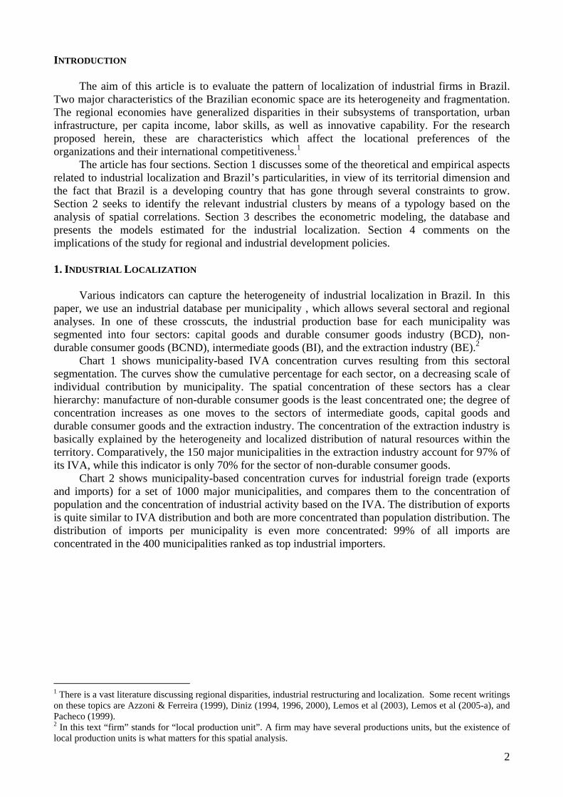
Chart 1 shows municipality-based IVA concentration curves resulting from this sectoral segmentation. The curves show the cumulative percentage for each sector, on a decreasing scale of individual contribution by municipality. The spatial concentration of these sectors has a clear hierarchy: manufacture of non-durable consumer goods is the least concentrated one; the degree of concentration increases as one moves to the sectors of intermediate goods, capital goods and durable consumer goods and the extraction industry. The concentration of the extraction industry is basically explained by the heterogeneity and localized distribution of natural resources within the territory. Comparatively, the 150 major municipalities in the extraction industry account for 97% of its IVA, while this indicator is only 70% for the sector of non-durable consumer goods.

Chart 2 shows municipality-based concentration curves for industrial foreign trade (exports and imports) for a set of 1000 major municipalities, and compares them to the concentration of population and the concentration of industrial activity based on the IVA. The distribution of exports is quite similar to IVA distribution and both are more concentrated than population distribution. The distribution of imports per municipality is even more concentrated: 99% of all imports are concentrated in the 400 municipalities ranked as top industrial importers.

1 There is a vast literature discussing regional disparities, industrial restructuring and localization. Some recent writings on these topics are Azzoni & Ferreira (1999), Diniz (1994, 1996, 2000), Lemos et al (2003), Lemos et al (2005-a), and Pacheco (1999). 2 In this text “firm” stands for “local production unit”. A firm may have several productions units, but the existence of local production units is what matters for this spatial analysis.

3

Chart 1: Concentration per Municipality (IVA, 2000)

Intermediate Goods

Capital and Durable Goods

Non-Durable Consumption Goods

Mining0

50

100

150

200

250

300

350

400

25% 40% 55% 70% 85% 100%

acumulated %

Citi

es

Source: Spatial Industrial Database

Chart 2: Concentration per Municipality of International Trade and Local Indicators

Population

Exports

Imports

IndustrialActivity

Income

0

100

200

300

400

500

600

700

800

900

1000

25% 38% 50% 63% 75% 88% 100%

acumulated %

Citi

es

Source: Spatial Industrial Database

4

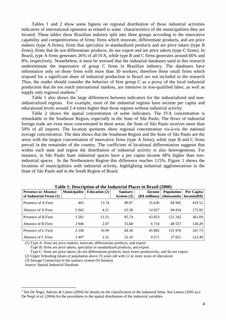
Tables 1 and 2 show some figures on regional distribution of those industrial activities indicative of international openness as related to some characteristics of the municipalities they are located. These tables show Brazilian industry split into three groups according to the innovative capability and competitiveness of firms: firms which innovate, differentiate products, and are price makers (type A firms), firms that specialize in standardized products and are price takers (type B firms), firms that do not differentiate products, do not export and are price takers (type C firms). In Brazil, type A firms generates 26% of all IVA, while type B and C firms generates around 66% and 8%, respectively. Nonetheless, it must be stressed that the industrial databases used in this research underestimate the importance of group C firms in Brazilian industry. The databases have information only on those firms with more than 30 workers; therefore those small firms which respond for a significant share of industrial production in Brazil are not included in the research Thus, the reader should consider the behavior of firm group C as a proxy of the local industrial production that do not reach international markets, are intensive in non-qualified labor, as well as supply only regional markets.3

Table 1 also shows the large differences between indicators for the industrialized and non-industrialized regions. For example, most of the industrial regions have income per capita and educational levels around 2-4 times higher than those regions without industrial activity.

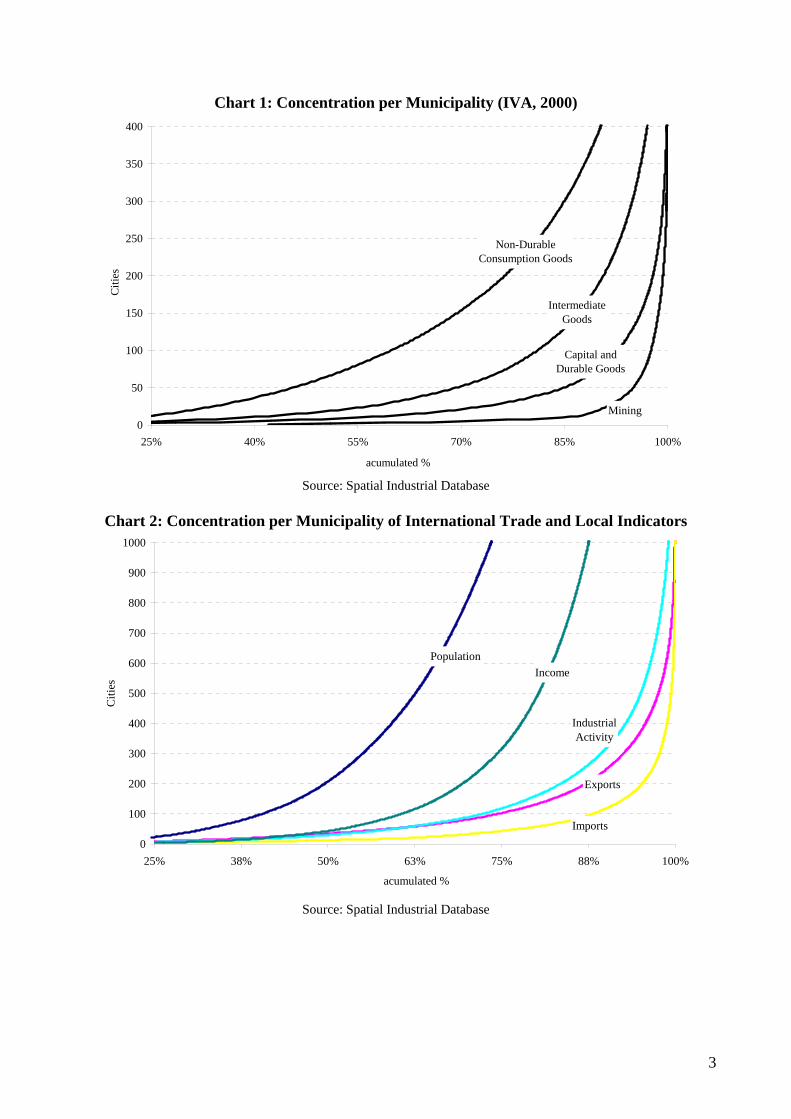
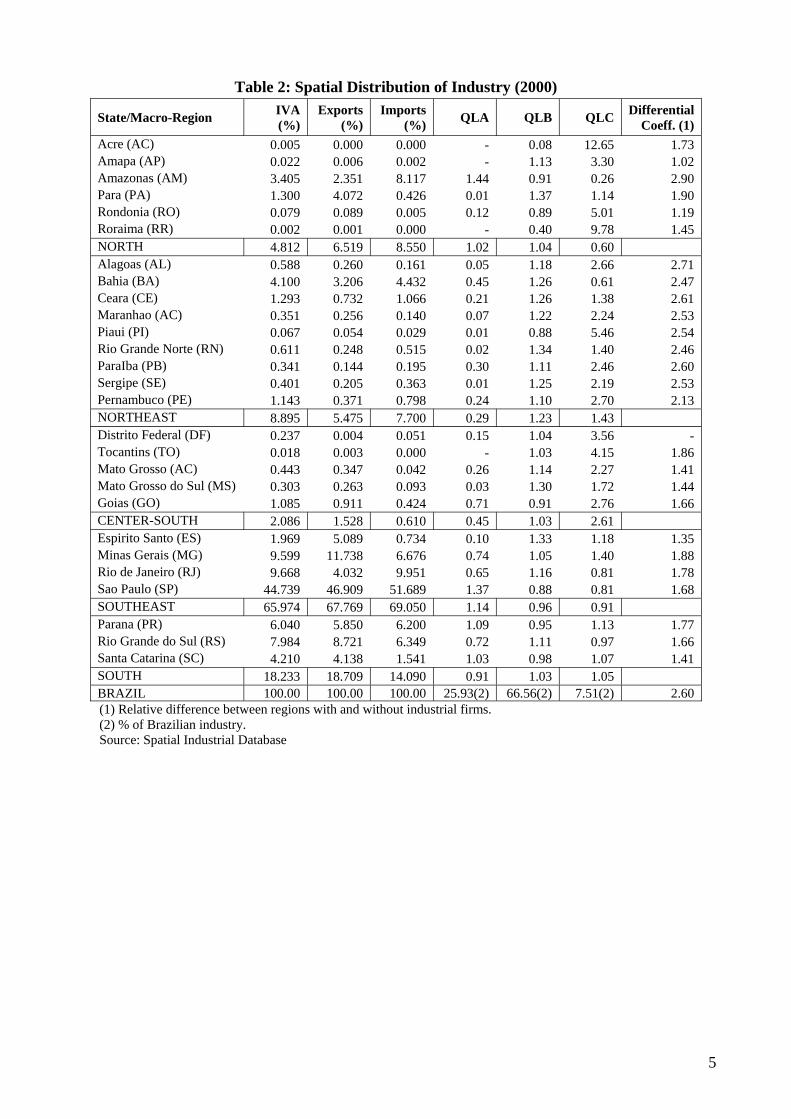
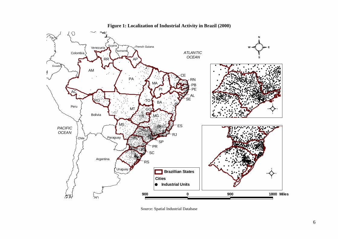
Table 2 shows the spatial concentration of some indicators. The IVA concentration is remarkable in the Southeast Region, especially in the State of São Paulo. The flows of industrial foreign trade are even more concentrated in these areas: the State of São Paulo receives more than 50% of all imports. The location quotients show regional concentration vis-à-vis the national average concentration. The data shows that the Southeast Region and the State of São Paulo are the areas with the largest concentration of innovative firms (type A firms), while type B and C firms prevail in the remainder of the country. The coefficient of locational differentiation suggests that within each state and region the distribution of industrial activity is also heterogeneous. For instance, in São Paulo State industrial spaces have a per capita income 68% higher than non-industrial spaces. In the Northeastern Region this difference reaches 115%. Figure 1 shows the locations of municipalities with industrial activity, highlighting industrial agglomerations in the State of São Paulo and in the South Region of Brazil.

Table 1: Description of the Industrial Places in Brazil (2000) Presence or Absence of Industrial Firms (1)

Municipality Education (2) Sanitary System (3)

Income(R$ millions)

Population (thousands)

Per Capita Income(R$)

Presence of A Firm 465 13.74 90.87 35 636 84 945 419.52

Absence of A Firm 5 042 4.21 63.38 14 927 84 854 175.92

Presence of B Firm 1 561 11.51 85.74 43 853 121 242 361.69

Absence of B Firm 3 946 2.87 55.68 6 710 48 557 138.20

Presence of C Firm 2 100 10.99 84.30 45 892 131 978 347.73

Absence of C Firm 3 407 2.31 52.16 4 671 37 821 123.49(1) Type A: firms are price makers, innovate, differentiate products, and export.

Type B: firms are price takers, specialize in standardized products, and export. Type C: firms are price takers, do not differentiate products, have lower productivity, and do not export.

(2) Upper Schooling (share of population above 25 years old with 12 or more years of education) (3) Sewage Connection to the sanitary system (% houses). Source: Spatial Industrial Database

3 See De Negri, Salerno & Castro (2004) for details on the classification of the industrial firms. See Lemos (2005-a) e De Negri et al. (2004) for the procedures to the spatial distribution of the industrial variables.

5

Table 2: Spatial Distribution of Industry (2000)

State/Macro-Region IVA (%)

Exports(%)

Imports(%) QLA QLB QLC Differential

Coeff. (1)

Acre (AC) 0.005 0.000 0.000 - 0.08 12.65 1.73 Amapa (AP) 0.022 0.006 0.002 - 1.13 3.30 1.02 Amazonas (AM) 3.405 2.351 8.117 1.44 0.91 0.26 2.90 Para (PA) 1.300 4.072 0.426 0.01 1.37 1.14 1.90 Rondonia (RO) 0.079 0.089 0.005 0.12 0.89 5.01 1.19 Roraima (RR) 0.002 0.001 0.000 - 0.40 9.78 1.45 NORTH 4.812 6.519 8.550 1.02 1.04 0.60 Alagoas (AL) 0.588 0.260 0.161 0.05 1.18 2.66 2.71 Bahia (BA) 4.100 3.206 4.432 0.45 1.26 0.61 2.47 Ceara (CE) 1.293 0.732 1.066 0.21 1.26 1.38 2.61 Maranhao (AC) 0.351 0.256 0.140 0.07 1.22 2.24 2.53 Piaui (PI) 0.067 0.054 0.029 0.01 0.88 5.46 2.54 Rio Grande Norte (RN) 0.611 0.248 0.515 0.02 1.34 1.40 2.46 ParaIba (PB) 0.341 0.144 0.195 0.30 1.11 2.46 2.60 Sergipe (SE) 0.401 0.205 0.363 0.01 1.25 2.19 2.53 Pernambuco (PE) 1.143 0.371 0.798 0.24 1.10 2.70 2.13 NORTHEAST 8.895 5.475 7.700 0.29 1.23 1.43 Distrito Federal (DF) 0.237 0.004 0.051 0.15 1.04 3.56 - Tocantins (TO) 0.018 0.003 0.000 - 1.03 4.15 1.86 Mato Grosso (AC) 0.443 0.347 0.042 0.26 1.14 2.27 1.41 Mato Grosso do Sul (MS) 0.303 0.263 0.093 0.03 1.30 1.72 1.44 Goias (GO) 1.085 0.911 0.424 0.71 0.91 2.76 1.66 CENTER-SOUTH 2.086 1.528 0.610 0.45 1.03 2.61 Espirito Santo (ES) 1.969 5.089 0.734 0.10 1.33 1.18 1.35 Minas Gerais (MG) 9.599 11.738 6.676 0.74 1.05 1.40 1.88 Rio de Janeiro (RJ) 9.668 4.032 9.951 0.65 1.16 0.81 1.78 Sao Paulo (SP) 44.739 46.909 51.689 1.37 0.88 0.81 1.68 SOUTHEAST 65.974 67.769 69.050 1.14 0.96 0.91 Parana (PR) 6.040 5.850 6.200 1.09 0.95 1.13 1.77 Rio Grande do Sul (RS) 7.984 8.721 6.349 0.72 1.11 0.97 1.66 Santa Catarina (SC) 4.210 4.138 1.541 1.03 0.98 1.07 1.41 SOUTH 18.233 18.709 14.090 0.91 1.03 1.05 BRAZIL 100.00 100.00 100.00 25.93(2) 66.56(2) 7.51(2) 2.60 (1) Relative difference between regions with and without industrial firms. (2) % of Brazilian industry. Source: Spatial Industrial Database

6

Figure 1: Localization of Industrial Activity in Brazil (2000)

#

#

#

#

#

#

#

#

#

#

#

#

#

#

#

#

#

#

##

##

#

#

#

#

#

##

#

##

#

#

#

#

###

#

##

#

#

## #

#

#

#

#

#

#

#

# #

#

#

#

#

#

#

#

# ##

#

#

#

#

#

###

#

#

#

#

#

#

#

#

#

##

#

#

#

#

#

#

#

# ##

#

#

#

#

#

#

#

# #

#

#

##

#

#

# #

#

##

#

#

#

##

#

#

#

#

#

#

#

#

##

####

#

#

#

#

#

#

##

##

#

#

#

#

#

#

#

#

#

##

##

#

#

#

#

#

#

#

#

#

#

#

#

#

#

#

#

#

#

##

#

#

#

## #

#

#

#

#

#

#

#

#

#

#

#

#

#

#

#

#

# #

##

##

#

#

#

##

##

#

# #

#

#

#

#

#

#

###

# #

#

#

##

#

#

#

#

#

##

##

#

#

# ##

#

##

#

#

#

#

#

#

#

#

#

#

#

#

#

#

#

#

#

##

#

#

#

#

#

#

#

#

#

#

#

#

#

#

##

#

##

#

#

##

#

#

##

#

#

#

##

#

##

#

##

#

#

#

#

##

##

#

#

#

##

#

#

#

#

#

###

#

##

##

#

#

###

#

#

###

#

#

#

###

#

#

#

##

#

#

#

#

#

#

##

#

#

#

#

##

#

#

#

#

#

#

##

#

#

#

##

#

#

#

#

#

#

#

#

#

#

#

#

#

##

#####

##

#

##

#

#

#

#

#

##

#

##

#

##

#

#

#

#

#

#

#

#

#

# ##

#

#

#

#

#

#

#

#

#

#

#

#

#

#

#

#

#

#

#

#

#

#

#

#

#

#

##

#

##

##

#

#

#

#

##

#

##

##

#

#

#

#

#

#

#

#

#

#

#

#

#

#

#

#

#

##

#

#

#

#

#

#

#

#

##

##

#

#

#

#

##

#

#

#

#

#

##

#

#

#

#

##

#

#

#

#

#

#

##

#

#

#

#

##

#

#

#

###

#

#

##

#

##

##

#

##

#

#

##

#

##

#

#

##

#

#

#

#

#

#

#

#

#

#

##

#

##

#

#

##

##

#

#

#

##

#

#

##

#

#

##

##

#

#

#

#

#

#

#

#

#

##

#

#

#

#

##

#

#

###

#

#

#

#

#

#

##

#

#

#

#

#

#

##

#

#

#

#

#

#

#

#

#

#

###

#

##

#

##

#

#

#

#

#

#

#

#

#

#

#

#

#

#

#

#

#

#

#

#

#

##

#

#

#

#

##

#

#

#

#

#

##

##

#

#

#

#

#

#

#

#

#

#

#

#

#

#

#

#

#

#

#

#

#

#

###

#

##

#

#

#

####

#

#

#

#

#

#

#

#

#

#

#

#

#

#

#

#

#

#

##

#

#

#

#

#

#

#

# #

#

#

#

#

#

#

#

#

#

#

#

#

#

#

#

#

#

#

#

###

##

#

#

##

#

#

#

##

##

#

#

#

#

#

#

#

#

#

#

#

#

#

##

#

#

#

#

#

##

#

#

##

#

#

#

#

#

#

#

#

#

#

#

#

#

#

#

#

#

#

#

#

#

##

#

#

#

#

#

#

#

#

#

#

#

#

#

#

#

#

#

##

#

#

#

#

#

#

#

#

#

#

##

##

#

#

#

#

#

#

#

#

#

##

###

#

#

##

#

#

#

#

#

#

#

#

#

#

#

#

#

#

#

#

#

#

#

####

#

#

#

#

#

#

#

#

#

#

#

#

#

#

#

##

#

#

#

#

#

#

#

##

##

#

#

#

#

#

#

#

#

#

#

#

#

#

#

#

#

#

#

#

#

#

#

#

#

#

#

#

#

#

#

#

##

#

#

#

#

#

#

#

#

#

#

#

##

##

#

###

#

#

#

#

#

#

#

##

#

#

#

#

#

#

#

#

#

#

#

#

#

#

#

#

##

#

#

#

#

#

#

#

#

#

#

#

##

#

##

#

##

#

#

#

#

#

#

#

#

#

#

#

#

#

#

#

#

###

#

#

##

#

#

#

#

#

#

##

##

#

#

#

#

#

#

#

#

#

#

#

#

#

#

#

#

#

#

#

#

###

#

#

##

#

#

#

#

#

#

#

#

#

##

#

#

#

#

##

#

#

#

###

#

#

#

#

#

#

#

#

#

#

#

#

#

#

#

#

#

#

#

#

#

#

#

##

##

##

##

##

#

#

##

#

#

#

#

#

#

#

#

#

#

#

#

#

#

#

#

#

#

#

#

##

#

#

#

##

#

#

#

####

#

#

#

#

#

#

#

#

#

#

#

#

##

#

##

#

#

#

#

#

#

#

##

#

#

#

#

#

#

#

#

#

#

##

# #

#

#

#

#

# #

#

#

#

#

#

#

#

#

#

#

#

##

#

#

#

#

#

#

#

##

#

#

#

#

#

#

#

#

#

#

#

#

#

#

#

#

#

#

#

#

#

#

#

##

##

#

#

#

#

#

#

#

#

#

##

##

#

#

#

##

#

#

#

#

#

##

##

#

#

#

#

#

#

#

##

#

#

#

#

#

#

#

#

#

#

#

#

#

#

##

#

#

#

#

##

#

##

##

#

#

##

#

#

#

#

#

#

#

#

#

#

#

#

#

#

#

#

#

#

#

#

#

##

#

#

##

#

#

###

#

#

##

#

#

#

#

#

##

##

#

##

#

## ###

###

### ##

##

#

#

##

###

#

#

########

#####

#####

###

###

##

#

#

# ### #

##

##

#

#

#

#

#

##

#

#

##

#

###

####

#

#

##

#

#

#

#

#

#

#

#

##

##

#

#

#

#

#

#

#

#

##

#

#

###

#

#

#

#

#

##

##

#

#

##

######

#

##

#

##

#

#

##

#

#

#

###

#

####

#

##

#

#

#

##

#

#

#

#

#

#

#

#

#

#

#

#

#

#

#

#

#

#

#

# #

###

#

#

#

#

#

#

#

#

##

###

#

#

#

###

# #

#

#

#

#

##

#

#

#

#

#

#

#

#

#

#

#

#

#

#

#

##

##

##

#

##

#

#

#

#####

##

##

##

## #####

## ##

##

#

###

#

##

#

#

###

##

# ##

#

###

##

#

#

#

#

#

##

# #

###

#

####

#

#

# # ###

###

###

##

#

#

#

##

# # # ##

## ##

##

###### ## #

##

#### #

#

# #### #

#

#

#

##

#

#

#

#

#

#

#

#

#

#

###

##

#

#

##

#

#

#

#

#

##

#

####

#

###

# #

##

##

### #

###

##

###

#

#

#

#

#

#

#

#

#

#

#

###

#

#

##

#

##

####

##

#

#

#

#

#

#

###

#

#

#

#

#

##

#

#

#

#

#

#

#

####

##

#

#

##

#

#

#

###

#

#

#

###

#

#

##

#

##

#

####

##

##

#

#

#

#

#

##

##

##

#

#

#

#

#

#

#

#

#

#

#

#

#

#

#

#

#

#

#

#

#

#

#

#

#

#

##

#

####

#

##

####

###

#

#

#

#

###

#

#

#

#

#

#

#

###

#

#

#

#

#

##

##

#

##

#

#

#

#

#

#

#

#

#

#

#

#

#

#

#

#

#

#

#

#

#

##

#

#

###

##

#

#

##

#

#

#

#

# #

#

#

#

#

#

#

##

#

#

#

#

#

##

#

#

#

#

#

#

#

#

#

#

#

#

#

##

#

##

#

#

#

##

#

#

#

#

#

#

#

#

#

#

#

#

##

#

#

#

#

##

##

# ##

#

##

##

#

#

#

###

#

####

##

#

##

#

# #

#

#

#

##

# #

### # #

#

#

#

#

#

#

#

#

#

#

#

#

##

##

#

#

##

#

#

#

#

#

#

#

#

#

#

#

#

##

#

##

#

#

#

#

#

#

##

#

##

#

#

#

#

#

#

#

#

#

#

###

##

#

#

#

#

#

#

###

#

#

##

#

###

##

## #

##

#

#

#

##

#

#

#

#

#

##

#

#

#

##

##

#

#

##

###

#

##

###

##

##

# #

##

#

##

##

##

# ##

#

# #

####

###

##

##

####

######

##

#

#

## ##

# ## ###

# #

###

## ###### ##

#### ### ## # ### # ## ####

# ## #### # ## ## #### #

###

# ## ## ## # # ## #

## # #### ##

#

#

# #

##

#

#

#

#

#

#

#

##

#

#

#

#

#

#

####

# ##

#

##

##

# #

### #

#

# ####

##

#

# ####

###

## # #

####

#

# ## # ## #

###

#

#

#

#

###

##

##

#

#

##

#

###

####

#

##

##

#

#

# ## ###

##

#

#

#

#

#

##

##

#

# ####

######

AM

AC

PA

RO

MT

TO

MAPI

BA

MG

MS

APRR

#

CE#

RN# PB# PE

# AL# SE

# ES

# RJ#

SP#

PR#

SC#

RS

GOBolivia

Argentina

Paraguay

Uruguay

Peru

Colombia

VenezuelaGuyana

Chile

Ecuador

Suriname#

French Guiana

ATLANTIC OCEAN

PACIFICOCEAN

#

#

#

#

#

#

##

#

##

##

#

#

###

#

#

##

##

##

#

#

#

#

#

##

#

#

#

#

#

##

#####

##

#

##

#

#

#

#

#

# ##

#

#

#

#

#

#

##

###

##

#

###

#

#

#

#

##

#

#

###

#

##

##

#

##

##

##

#

##

#

#

#

#

##

#

#

##

#

#

##

##

#

#

#

##

#

#

#

#

#

#

##

#

#

#

#

#

#

#

#

#

##

#

#

#

#

#

#

#

#

#

#

#

#

#

#

#

#

#

#

#

#

##

#

#

#

#

#

#

#

#

#

#

#

##

#

#

#

#

#

#

#

# #

##

##

#

#

#

#

###

##

#

#

###

#

#

#

#

#

#

#

#

#

#

##

#

#

#

#

#

#

#

#

#

#

#

###

#

#

#

#

#

#

#

#

#

#

#

#

#

#

#

#

#

##

###

#

#

#

##

###

#

#

#

#

#

#

#

#

#

#

#

#

#

#

#

#

#

#

#

#

#

#

#

#

#

#

#

#

#

#

#

#

#

#

#

##

###

#

#

#

#

#

#

#

#

#

#

#

#

#

#

#

##

#

##

#

##

#

#

#

#

#

#

#

#

##

#

#

#

#

#

#

#

#

#

#

#

#

##

#

#

##

#

#

#

#

#

#

#

#

#

#

#

#

#

#

##

##

##

# #

#

#

#

#

#

#

##

#

#

#

####

#

#

#

#

#

#

#

##

#

##

#

#

#

#

#

#

#

#

#

#

#

#

##

#

#

#

#

#

#

##

#

#

#

#

#

#

#

#

#

#

#

#

#

#

#

#

##

##

#

#

#

#

#

#

#

#

#

##

##

#

#

#

##

#

#

#

#

#

##

##

#

#

#

#

#

#

#

##

#

#

#

#

#

#

#

#

#

#

#

#

##

#

#

##

#

#

##

#

#

#

#

#

#

#

#

#

#

#

#

#

#

#

#

###

#

#

##

#

#

##

##

#

##

#

#####

##

#

#####

###

#

##

###

#

#

########

#####

#####

###

##

#

##

#

#

# ### #

##

##

#

#

#

#

#

#

#

#

##

##

####

##

#

#

##

#

#

#

#

#

#

##

#

#

#

#

#

#

##

#

#

####

#

#

#

#

##

##

#

#

##

####

##

#

##

#

###

#

##

#

#

#

####

####

#

#

##

#

#

#

#

#

#

#

#

#

#

#

#

#

#

#

##

###

##

#

#

#

#

#

#

##

###

#

#

#

###

# #

#

#

#

#

##

#

#

#

#

#

#

#

#

#

#

##

##

##

#

##

#

#

#

####

# ##

##

##

## #####

## ##

###

###

#

##

#

#

###

##

# #

#

###

##

#

#

####

#

#

#

#

##

# ## ##

## #

##

###

#### ## #

##

#### #

# #### #

##

#

#

###

##

####

##

#

####

#

#

S

N

EW

#

#

#

#

#

#

#

#

#

#

#

#

#

#

#

##

##

#

###

#

##

#

##

#

#

#

#

###

#

##

#

# #

##

#

#

#

#

#

#

#

#

##

####

#

#

#

#

#

#

##

##

#

#

#

#

##

#

#

#

##

##

##

#

##

#

##

#

##

##

#

## #

#

#

#

#

#

#

#

#

#

#

#

#

##

###

#

#

##

#

#

##

#

# #

##

###

#

#

#

#

##

##

#

#

#

##

#

#

#

#

#

###

#

##

##

##

# ###

#

#

#

##

#

##

#

#

#

#

##

#

#

#

#

#

#

##

#

#

#

##

#

#

#

#

#

#

#

#

#

#

#

##

#

#

#

#

#

##

#

##

#

##

#

#

#

#

##

#

#

#

#

#

#

#

#

#

#

#

#

#

#

#

#

#

#

#

#

#

#

#

#

#

##

#

##

##

#

#

##

#

#

#

#

#

#

#

#

#

#

#

##

#

#

#

#

##

#

#

#

#

#

####

#

#

###

#

#

##

##

##

##

#

##

##

#

##

#

#

#

#

#

#

#

#

#

#

##

#

##

#

##

##

#

#

#

#

#

#

##

#

#

###

#

#

#

#

#

#

#

#

#

#

##

#

#

#

#

##

#

#

#

###

#

##

#

##

#

#

#

#

#

#

#

#

#

###

#

#

#

##

##

#

#

#

#

#

#

#

###

#

#

#

####

#

#

#

#

#

#

#

#

#

#

#

#

#

#

#

#

#

##

#

#

#

#

#

#

##

##

#

#

#

#

##

#

#

#

#

#

#

#

#

#

#

#

#

#

#

#

#

#

#

#

##

#

#

#

#

#

#

#

#

#

#

#

#####

#

#

#

#

##

#

#

#

#

##

##

#

#

#

##

#

#

##

#

#

#

##

##

#

###

#

#

#

#

#

#

#

#

#

#

#

##

#

#

#

#

#

#

#

#

#

##

#

#

#

#

##

#

#

#

#

#

#

###

#

#

#

#

#

#

#

#

#

#

#

##

#

#

#

#

##

#

#

#

###

#

#

#

#

#

#

#

#

##

#

##

###

#

#

#

##

#

#

#

##

#

#

#

#

#

#

#

#

##

##

###

#

##

##

#

#

##

#

#########

S

N

EW

S

N

EW

Cities# Industrial Units

Brazillian States

900 0 900 1800 Miles

Source: Spatial Industrial Database

7

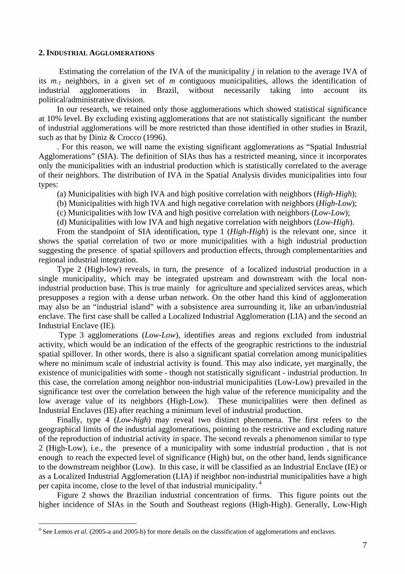
2. INDUSTRIAL AGGLOMERATIONS

Estimating the correlation of the IVA of the municipality j in relation to the average IVA of

its m-1 neighbors, in a given set of m contiguous municipalities, allows the identification of industrial agglomerations in Brazil, without necessarily taking into account its political/administrative division.

In our research, we retained only those agglomerations which showed statistical significance at 10% level. By excluding existing agglomerations that are not statistically significant the number of industrial agglomerations will be more restricted than those identified in other studies in Brazil, such as that by Diniz & Crocco (1996).

. For this reason, we will name the existing significant agglomerations as “Spatial Industrial Agglomerations” (SIA). The definition of SIAs thus has a restricted meaning, since it incorporates only the municipalities with an industrial production which is statistically correlated to the average of their neighbors. The distribution of IVA in the Spatial Analysis divides municipalities into four types:

(a) Municipalities with high IVA and high positive correlation with neighbors (High-High); (b) Municipalities with high IVA and high negative correlation with neighbors (High-Low); (c) Municipalities with low IVA and high positive correlation with neighbors (Low-Low); (d) Municipalities with low IVA and high negative correlation with neighbors (Low-High). From the standpoint of SIA identification, type 1 (High-High) is the relevant one, since it

shows the spatial correlation of two or more municipalities with a high industrial production suggesting the presence of spatial spillovers and production effects, through complementarities and regional industrial integration.

Type 2 (High-low) reveals, in turn, the presence of a localized industrial production in a single municipality, which may be integrated upstream and downstream with the local non-industrial production base. This is true mainly for agriculture and specialized services areas, which presupposes a region with a dense urban network. On the other hand this kind of agglomeration may also be an “industrial island” with a subsistence area surrounding it, like an urban/industrial enclave. The first case shall be called a Localized Industrial Agglomeration (LIA) and the second an Industrial Enclave (IE).

Type 3 agglomerations (Low-Low), identifies areas and regions excluded from industrial activity, which would be an indication of the effects of the geographic restrictions to the industrial spatial spillover. In other words, there is also a significant spatial correlation among municipalities where no minimum scale of industrial activity is found. This may also indicate, yet marginally, the existence of municipalities with some - though not statistically significant - industrial production. In this case, the correlation among neighbor non-industrial municipalities (Low-Low) prevailed in the significance test over the correlation between the high value of the reference municipality and the low average value of its neighbors (High-Low). These municipalities were then defined as Industrial Enclaves (IE) after reaching a minimum level of industrial production.

Finally, type 4 (Low-high) may reveal two distinct phenomena. The first refers to the geographical limits of the industrial agglomerations, pointing to the restrictive and excluding nature of the reproduction of industrial activity in space. The second reveals a phenomenon similar to type 2 (High-Low), i.e., the presence of a municipality with some industrial production , that is not enough to reach the expected level of significance (High) but, on the other hand, lends significance to the downstream neighbor (Low). In this case, it will be classified as an Industrial Enclave (IE) or as a Localized Industrial Agglomeration (LIA) if neighbor non-industrial municipalities have a high per capita income, close to the level of that industrial municipality. 4

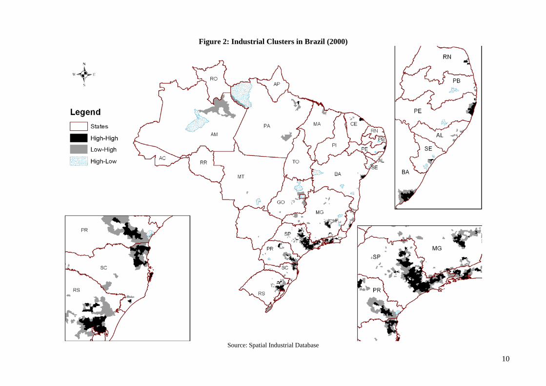
Figure 2 shows the Brazilian industrial concentration of firms. This figure points out the higher incidence of SIAs in the South and Southeast regions (High-High). Generally, Low-High

4 See Lemos et al. (2005-a and 2005-b) for more details on the classification of agglomerations and enclaves.

8

arrangements applies to areas surrounding High-High agglomerations, but also to some isolate points. A High-Low arrangement denotes industrial enclaves or localized industrial agglomerations.

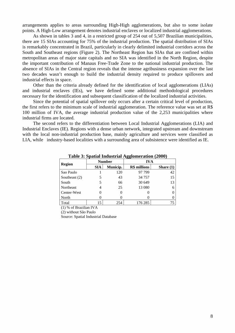
As shown in tables 3 and 4, in a restricted group of 254 out of 5,507 Brazilian municipalities, there are 15 SIAs accounting for 75% of the industrial production. The spatial distribution of SIAs is remarkably concentrated in Brazil, particularly in clearly delimited industrial corridors across the South and Southeast regions (Figure 2). The Northeast Region has SIAs that are confined within metropolitan areas of major state capitals and no SIA was identified in the North Region, despite the important contribution of Manaus Free-Trade Zone to the national industrial production. The absence of SIAs in the Central region reveals that the intense agribusiness expansion over the last two decades wasn’t enough to build the industrial density required to produce spillovers and industrial effects in space.

Other than the criteria already defined for the identification of local agglomerations (LIAs) and industrial enclaves (IEs), we have defined some additional methodological procedures necessary for the identification and subsequent classification of the localized industrial activities.

Since the potential of spatial spillover only occurs after a certain critical level of production, the first refers to the minimum scale of industrial agglomeration. The reference value was set at R$ 100 million of IVA, the average industrial production value of the 2,253 municipalities where industrial firms are located.

The second refers to the differentiation between Local Industrial Agglomerations (LIA) and Industrial Enclaves (IE). Regions with a dense urban network, integrated upstream and downstream with the local non-industrial production base, mainly agriculture and services were classified as LIA, while industry-based localities with a surrounding area of subsistence were identified as IE.

Table 3: Spatial Industrial Agglomeration (2000) Number IVA Region

SIA Municip. R$ millions Share (1) Sao Paulo 1 120 97 799 42 Southeast (2) 5 43 34 757 15 South 5 66 30 649 13 Northeast 4 25 13 080 6 Center-West 0 0 0 0 North 0 0 0 0 Total 15 254 176 285 75 (1) % of Brazilian IVA (2) without São Paulo Source: Spatial Industrial Database

9

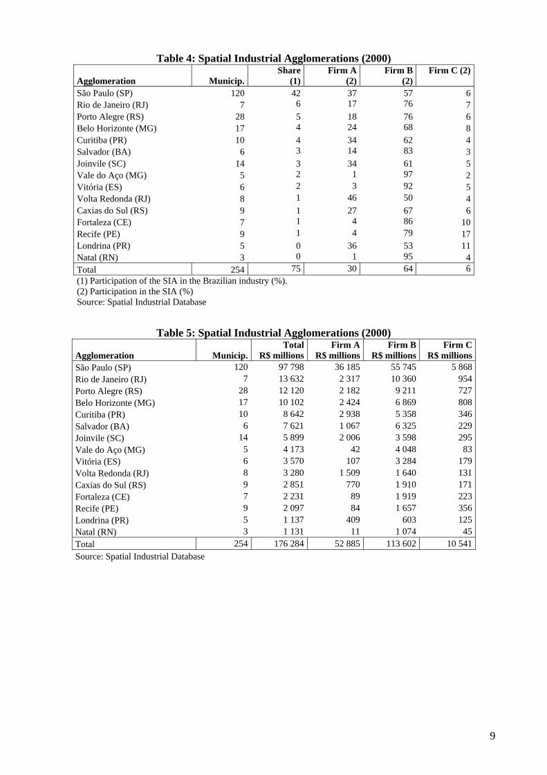
Table 4: Spatial Industrial Agglomerations (2000)

Agglomeration Municip.Share

(1)Firm A

(2)Firm B

(2) Firm C (2)

São Paulo (SP) 120 42 37 57 6Rio de Janeiro (RJ) 7 6 17 76 7Porto Alegre (RS) 28 5 18 76 6Belo Horizonte (MG) 17 4 24 68 8Curitiba (PR) 10 4 34 62 4Salvador (BA) 6 3 14 83 3Joinvile (SC) 14 3 34 61 5Vale do Aço (MG) 5 2 1 97 2Vitória (ES) 6 2 3 92 5Volta Redonda (RJ) 8 1 46 50 4Caxias do Sul (RS) 9 1 27 67 6Fortaleza (CE) 7 1 4 86 10Recife (PE) 9 1 4 79 17Londrina (PR) 5 0 36 53 11Natal (RN) 3 0 1 95 4Total 254 75 30 64 6(1) Participation of the SIA in the Brazilian industry (%). (2) Participation in the SIA (%) Source: Spatial Industrial Database

Table 5: Spatial Industrial Agglomerations (2000)

Agglomeration Municip.Total

R$ millionsFirm A

R$ millionsFirm B

R$ millions Firm C

R$ millionsSão Paulo (SP) 120 97 798 36 185 55 745 5 868Rio de Janeiro (RJ) 7 13 632 2 317 10 360 954Porto Alegre (RS) 28 12 120 2 182 9 211 727Belo Horizonte (MG) 17 10 102 2 424 6 869 808Curitiba (PR) 10 8 642 2 938 5 358 346Salvador (BA) 6 7 621 1 067 6 325 229Joinvile (SC) 14 5 899 2 006 3 598 295Vale do Aço (MG) 5 4 173 42 4 048 83Vitória (ES) 6 3 570 107 3 284 179Volta Redonda (RJ) 8 3 280 1 509 1 640 131Caxias do Sul (RS) 9 2 851 770 1 910 171Fortaleza (CE) 7 2 231 89 1 919 223Recife (PE) 9 2 097 84 1 657 356Londrina (PR) 5 1 137 409 603 125Natal (RN) 3 1 131 11 1 074 45Total 254 176 284 52 885 113 602 10 541Source: Spatial Industrial Database

10

Figure 2: Industrial Clusters in Brazil (2000)

Source: Spatial Industrial Database

11

Figure 3: Spatial Industrial Agglomeration in South and Southeast of Brazil (2000)

Source: Spatial Industrial Database

12

Two criteria were used to differentiate between LIA and IE municipalities: the average per

capita income level of their neighbors and the ratio (the standard deviation divided by the average value) by which per capita income varies between the reference municipality and its neighbors’ average. Industrial localities whose neighbors have an average per capita income higher than the national average and a variance below 0.5 were classified as LIAs, while those having neighbors with an average per capita income below the national average and a variance of 0.5 or over were classified as IEs. An additional criterion differentiated a Concentrated Income Enclave (IE-CI) from a Low Income Enclave (IE-LI). The first identified a high per capita income industrial municipality surrounded by neighbors with a low per capita income while in the second both the industrial municipality and its neighbors have a low per capita income.

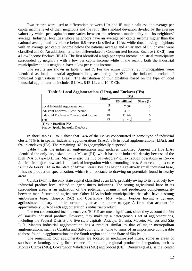
The results are shown in table 6 and 7. For the entire country, 23 municipalities were identified as local industrial agglomerations, accounting for 9% of the industrial product of industrial organizations in Brazil. The distribution of municipalities based on the type of local industrial agglomeration includes 5 LIAs, 8 IE-LIs and 10 IE-CIs.

Table 6: Local Agglomerations (LIAs), and Enclaves (IEs)

IVA

Munic.R$ millions Share (1)

Local Industrial Agglomerations 5 7 064 3 Industrial Enclaves – Low Income 8 3 070 1 Industrial Enclaves – Concentrated Income 10 11 242 5 Total 23 21 377 9 (1) % in Brazilian IVA Source: Spatial Industrial Database

In short, tables 3 to 7 show that 84% of the IVAis concentrated in some type of industrial

cluster75% is in spatial industrial agglomerations (SIAs), 3% in local agglomerations (LIAs), and 6% in enclaves (IEs). The remaining 16% is geographically dispersed.

Table 7 lists the industrial agglomerations and enclaves identified. Among the five LIAs identified the only large-sized one is Macaé (RJ), which has built industrial density because of the high IVA of type B firms. Macaé is also the hub of Petrobrás’ oil extraction operations in Rio de Janeiro. Its major drawback is the lack of integration with surrounding areas. A more complex case is Juiz de Fora's LIA in the State of Minas Gerais. Besides having a relatively small industrial base, it has no production specialization, which is an obstacle to drawing on potentials found in nearby areas.

Cuiabá (MT) is the only state capital classified as an LIA, probably owing to its relatively low industrial product level related to agribusiness industries. The strong agricultural base in its surrounding areas is an indication of the potential dynamism and production complementarity between manufacture and agriculture. Other LIAs include municipalities that also have a strong agribusiness base: Chapecó (SC) and Uberlândia (MG) which, besides having a dynamic agribusiness industry in their surrounding areas, are home to type A firms that account for approximately 50% of each agglomeration’s industrial product.

The ten concentrated income enclaves (EI-CI) are most significant, since they account for 5% of Brazil’s industrial product. However, they make up a heterogeneous set of agglomerations, including the Federal District and five state capitals: Aracaju, Goiânia, Maceió, Manaus and São Luís. Manaus industrial agglomeration has a product similar to that of major metropolitan agglomerations, such as Curitiba and Salvador, and is home to firms of an importance comparable to those found in agglomerations in the South region and in the State of São Paulo.

The remaining four agglomerations are located in medium-sized cities, some in areas of subsistence farming, having little chance of promoting regional production integration, such as Montes Claros (MG), Governador Valadares (MG) and Sobral (CE). Barreiras (BA), is the center

13

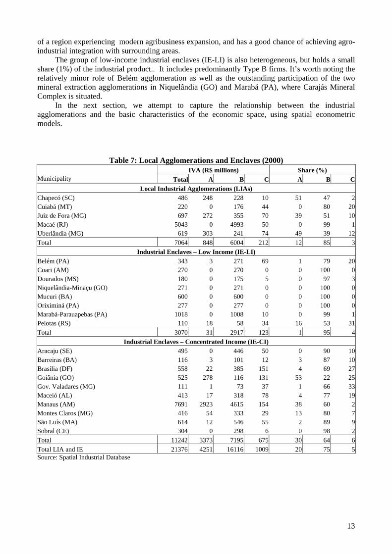
of a region experiencing modern agribusiness expansion, and has a good chance of achieving agro-industrial integration with surrounding areas.

The group of low-income industrial enclaves (IE-LI) is also heterogeneous, but holds a small share (1%) of the industrial product.. It includes predominantly Type B firms. It’s worth noting the relatively minor role of Belém agglomeration as well as the outstanding participation of the two mineral extraction agglomerations in Niquelândia (GO) and Marabá (PA), where Carajás Mineral Complex is situated.

In the next section, we attempt to capture the relationship between the industrial agglomerations and the basic characteristics of the economic space, using spatial econometric models.

Table 7: Local Agglomerations and Enclaves (2000) IVA (R$ millions) Share (%)

Municipality Total A B C A B CLocal Industrial Agglomerations (LIAs)

Chapecó (SC) 486 248 228 10 51 47 2Cuiabá (MT) 220 0 176 44 0 80 20Juiz de Fora (MG) 697 272 355 70 39 51 10Macaé (RJ) 5043 0 4993 50 0 99 1Uberlândia (MG) 619 303 241 74 49 39 12Total 7064 848 6004 212 12 85 3

Industrial Enclaves – Low Income (IE-LI) Belém (PA) 343 3 271 69 1 79 20Coari (AM) 270 0 270 0 0 100 0Dourados (MS) 180 0 175 5 0 97 3Niquelândia-Minaçu (GO) 271 0 271 0 0 100 0Mucuri (BA) 600 0 600 0 0 100 0Oriximiná (PA) 277 0 277 0 0 100 0Marabá-Parauapebas (PA) 1018 0 1008 10 0 99 1Pelotas (RS) 110 18 58 34 16 53 31Total 3070 31 2917 123 1 95 4

Industrial Enclaves – Concentrated Income (IE-CI) Aracaju (SE) 495 0 446 50 0 90 10Barreiras (BA) 116 3 101 12 3 87 10Brasília (DF) 558 22 385 151 4 69 27Goiânia (GO) 525 278 116 131 53 22 25Gov. Valadares (MG) 111 1 73 37 1 66 33Maceió (AL) 413 17 318 78 4 77 19Manaus (AM) 7691 2923 4615 154 38 60 2Montes Claros (MG) 416 54 333 29 13 80 7São Luís (MA) 614 12 546 55 2 89 9Sobral (CE) 304 0 298 6 0 98 2Total 11242 3373 7195 675 30 64 6Total LIA and IE 21376 4251 16116 1009 20 75 5Source: Spatial Industrial Database

14

3. SPATIAL STRUCTURES OF REGIONAL INDUSTRIAL AGGLOMERATIONS 3.1. SPATIAL ECONOMETRIC MODELS

The variables in table 8 were constructed using the aggregation of data on local industrial

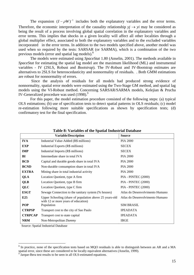
units by municipality. A statistical model of imputation was developed in order to classify firms in two different data-bases: PIA (Industrial Research by Sampling) and PINTEC (Technological Innovation - Industrial Research), both IBGE data bases. The classification of the local units as defined by PINTEC followed our classification (firms A, B and C). The location quotients (QLA, QLB and QLC) for each of these categories were calculated based on the IVA for each type. A municipality’s sector-based industrial structure is captured by variables that indicate sector shares in the total IVA of that municipality. Therefore, BI denotes the participation of the intermediate goods industry, BCD is the indicator for capital goods and durable consumer goods, BCND for non-durable consumer goods and EXTRA for the extraction industry.5

The socio-economic variables listed in table 8 are defined for each of the 5,507 Brazilian municipalities, based on information available from different sources. These selected variables capture some aspects of Brazil’s economic space structure, such as upper schooling levels (E25), aiming to measure educational qualifications across municipalities labor force; population (POP), as a measure of the scale of the local economy and/or market; the percentage of the local population provided with sewage connection to the sanitary system (ESGT), as a measure of urban infrastructure availability; and finally the classification of the municipality compared to certain metropolitan areas (NRM)6. Transportation cost variables were constructed by applying a linear programming procedure to calculate the lowest cost incurred to travel from the center of a given municipality to the city of São Paulo (CTRPSP) and to the nearest state capital (CTRPCAP).7

The spatial econometric models allow the distinction between two types of spatial correlation, resulting in multiplier effects, both global and local... Global effects are captured using SAR (spatial autoregressive) models, and local effects using SMA (spatial moving average) models. The two SAR models most commonly used in spatial econometrics are the spatial autoregressive error and the spatial lag models. Global spatial dependence in error terms is taken into account using spatial autoregressive error terms, as follows:

Y = Xβ + ε (1) ε = λWε + u (2) Y = Xβ + (I-λW)-1 u (3) Where ε is the autocorrelated error term and u é is an i.i.d. error term. The spatial error

model is suitable when the variables that are not included in the model but are present in the error terms are spatially autocorrelated. The spatial lag model is specified as follows:

εβρ ++= XWyY (4) Where W is the spatial weights matrix; X is the matrix of independent variables; β is the

vector of coefficients of independent variables; ρ is the autoregressive spatial coefficient and ε is the error term. Adding Wy as an explanatory variable to model 4 means that the values of variable y in the locality i are related to the values of this variable in neighboring localities. This model’s estimation method must take into account the endogenous nature of variable Wy (Anselin, 1999). Its reduced form gives a more precise interpretation of model 4:

ερβρ 11 )()( −− −+−= WIXWIY (5)

5 The sum of these four variables for a given municipality is equal to 1, so that only three of them should be used in the regressions (the one excluded is reflected in the constant). 6 The modeling effort covered 5179 non-metropolitan and 328 metropolitan municipalities, distributed among 19 metropolitan areas: Belém, Teresina, Fortaleza, Maceió, Natal, Recife, Salvador, São Luís, Goiânia, Brasília, Vitória, Belo Horizonte, Rio de Janeiro, São Paulo, Campinas, Santos, Curitiba, Florianópolis and Porto Alegre. 7 Transportation costs are estimated as a function of the distance and cost of the paving type of federal and state highways (see Castro et al., 1999).

15

The expansion 1)( −− WI ρ includes both the explanatory variables and the error terms. Therefore, the economic interpretation of the causality relationship yj → yi may be considered as being the result of a process involving global spatial correlation in the explanatory variables and error terms. This implies that shocks in a given locality will affect all other localities through a global multiplier effect, associated to both the explanatory variables and to the excluded variables incorporated in the error terms. In addition to the two models specified above, another model was used when so required by the tests: SARSAR (or SARMA), which is a combination of the two previous models (error and spatial lag models).8

The models were estimated using SpaceStat 1.80 (Anselin, 2001). The methods available in SpaceStat for estimating the spatial lag model are the maximum likelihood (ML) and instrumental variables - IV (2SLS, Robust and Bootstrap). The IV-Robust and IV-Bootstrap estimates are alternatives to 2SLS for heteroscedasticity and nonnormality of residuals. . Both GMM estimations are robust for nonnormality of errors.

Since the analysis of residuals for all models had produced strong evidence of nonnormality, spatial error models were estimated using the Two-Stage GM method, and spatial lag models using the VI-Robust method. Concerning SARSAR/SARMA models, Kelejian & Prucha IV-Generalized procedure was used (1998).9

For this paper, the model estimation procedure consisted of the following steps: (a) typical OLS estimations; (b) use of specification tests to detect spatial patterns in OLS residuals; (c) model re-estimation following more suitable specifications as shown by specification tests; (d) confirmatory test for the final specification.

Table 8: Variables of the Spatial Industrial Database Variable/Description Source

IVA Industrial Value-Added (R$ millions) PIA 2000 EXP Industrial Exports (R$ millions) SECEX IMP Industrial Imports (R$ millions) SECEX BI Intermediate share in total IVA PIA 2000 BCD Capital and durable goods share in total IVA PIA 2000 BCND Non-durable consumption share in total IVA PIA 2000 EXTRA Mining share in total industrial activity PIA 2000 QLA Location Quotient, type A firm PIA - PINTEC (2000) QLB Location Quotient, type B firm PIA - PINTEC (2000) QLC Location Quotient, type C firm PIA - PINTEC (2000) ESGT Sewage Connection to the sanitary system (% houses) Atlas do Desenvolvimento Humano E25 Upper Schooling (share of population above 25 years-old

with 12 or more years of education) Atlas do Desenvolvimento Humano

POP Population SIM BRASIL CTRPSP Transport cost to the city of Sao Paulo IPEADATA CTRPCAP Transport cost to state capital IPEADATA NRM Non-Metropolitan Dummy IBGE Source: Spatial Industrial Database

8 In practice, none of the specification tests based on MQO residuals is able to distinguish between an AR and a MA spatial error, since these are considered to be locally equivalent alternatives (Anselin, 1999). 9 Jarque-Bera test results to be seen in all OLS-estimated equations.

16

3.2. DETERMINANTS OF INDUSTRIAL SPATIAL STRUCTURES

The estimated model (table 9) identifies the explanatory variables that are relevant to major industrial agglomerations. These agglomerations were measured according to the IVA of each municipality. Significant variables in explaining such agglomerations were: QLA, QLC, POP, BI, BCD, BCND and CTSPM. The spatial lag model was found to be the most adequate in the specification tests.

The positive and significant value of the coefficient of the lagged dependent variable (W_IVA) points to a global spatial autocorrelation involving both the explanatory variables and the error terms10. This implies that changes (shocks) associated to both the included variables as well as the excluded onesl will produce spillover effects from the municipality’s features to its neighbors. These effects are most noticeable in the closest neighbors, becoming increasingly less perceptible as one moves away from their source.

The resident population of the municipality (POP) and its surrounding area were the most significant variable in explaining the local industrial agglomeration level. This is a proxy variable for the urban scale that is usually found in literature. It confirms the significance of diversification or Jacobian external economies, stemming from the urban scale, in attracting and agglomerating industrial activities (Pred, 1966; Jacobs, 1969; Glaeser et al, 1992). Upper schooling (E25) and infrastructure (ESGT) variables were not significant, and the same is true for the dummy variable representing non-metropolitan municipalities.

The sectoral variables BI, BCD and BDND capture the influence of the municipality’s sectoral structure on industrial concentration. Results indicate that the municipalities with larger number of firms producing capital and durable goods have a larger IVA. In contrast, municipalities with prevalence of manufacturers of non-durable consumer goods have a smaller IVA. This relationship was somehow expected: major IVA agglomerations embrace competitive firms that are capable of differentiating technologically involving directly or indirectly manufacturers of capital and durable goods (A type firms); these are “polarizing” firms. The opposite is usually true for non-durable consumer goods industries: those firms are not very competitive and use established technologies. Such firms will not give rise to industrial agglomerations and, as a matter of fact, they tend to be located outside these agglomerations.

The cost of transportation to state capitals was not significant in explaining municipal IVA. This apparently low ability to polarize industrial activity does not mean that such regional centers have no influence on the organization of their economic spaces; it does mean that being close to a state capital is not enough to play a determinant role in this process when compared to other factors.

The cost of transportation to Brazil’s largest economic center (CTRPSP), São Paulo, proved to have a strong influence on the scale of industrial activity. The closer one gets to São Paulo city, the smaller the transportation costs the higher the income generated by the industrial sector. As regards the organization of the industrial space, this relationship indicates that the area surrounding the São Paulo metropolitan area tends to be most preferred by industrial firms; a classic result of traditional gravitational models applied to regional economics (Isard, 1956; Fujita et al, 1999)11.

10 The spatial weight matrix used in this study is a contiguity matrix for the 5,507 municipalities, built using ArcView 3.2, pursuant to Queen criteria. A matrix was built for the distances between the seats of the various municipalities, but it was not possible to use it with the models because of the computer’s storage capacity and the file’s size (1.2GB). 11 This concentration of industrial activity around the city of de São Paulo can be called the Prime Industrial Agglomeration, once it represents the original and still major industrial agglomeration in Brazil.

17

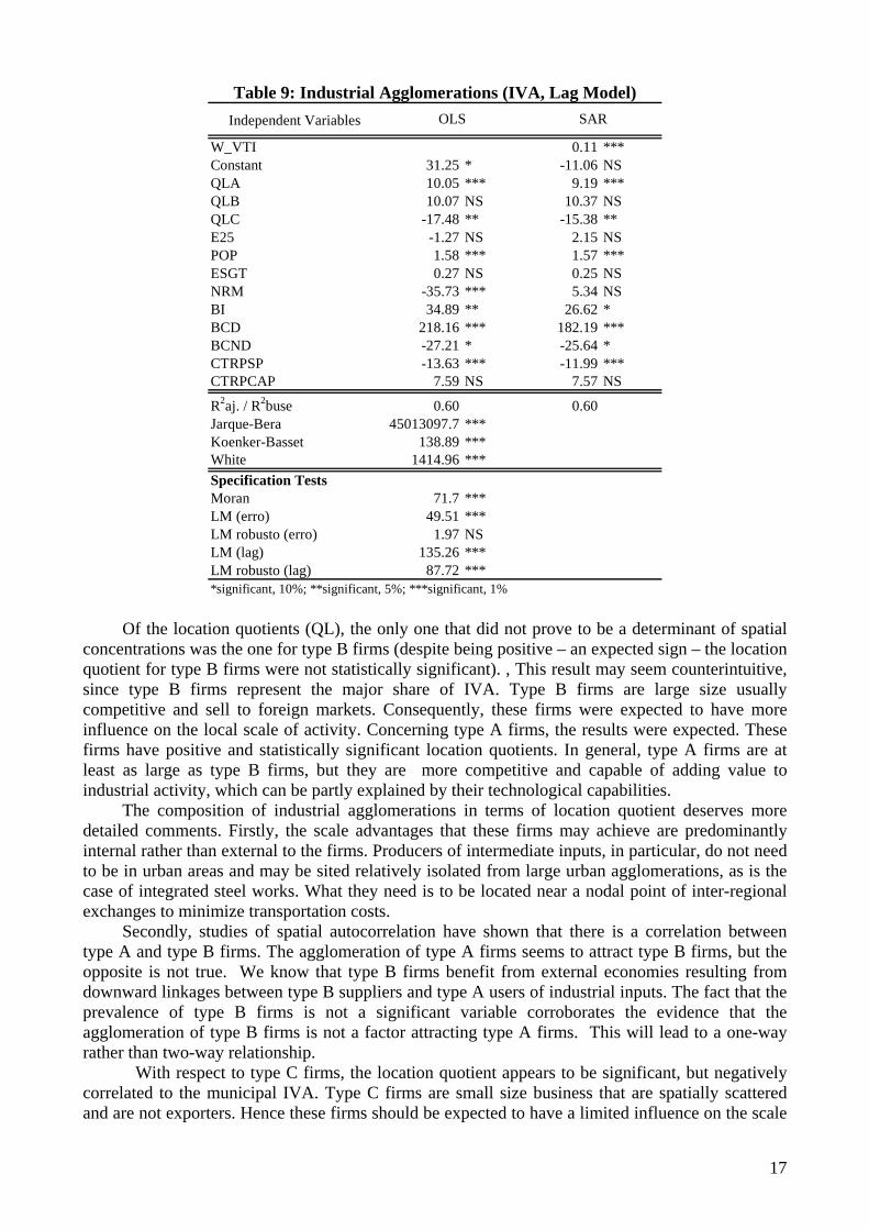
Table 9: Industrial Agglomerations (IVA, Lag Model) Independent Variables

W_VTI 0.11 ***Constant 31.25 * -11.06 NSQLA 10.05 *** 9.19 ***QLB 10.07 NS 10.37 NSQLC -17.48 ** -15.38 **E25 -1.27 NS 2.15 NSPOP 1.58 *** 1.57 ***ESGT 0.27 NS 0.25 NSNRM -35.73 *** 5.34 NSBI 34.89 ** 26.62 *BCD 218.16 *** 182.19 ***BCND -27.21 * -25.64 *CTRPSP -13.63 *** -11.99 ***CTRPCAP 7.59 NS 7.57 NS

R2aj. / R2buse 0.60 0.60Jarque-Bera 45013097.7 ***Koenker-Basset 138.89 ***White 1414.96 ***Specification TestsMoran 71.7 ***LM (erro) 49.51 ***LM robusto (erro) 1.97 NSLM (lag) 135.26 ***LM robusto (lag) 87.72 ****significant, 10%; **significant, 5%; ***significant, 1%

OLS SAR

Of the location quotients (QL), the only one that did not prove to be a determinant of spatial concentrations was the one for type B firms (despite being positive – an expected sign – the location quotient for type B firms were not statistically significant). , This result may seem counterintuitive, since type B firms represent the major share of IVA. Type B firms are large size usually competitive and sell to foreign markets. Consequently, these firms were expected to have more influence on the local scale of activity. Concerning type A firms, the results were expected. These firms have positive and statistically significant location quotients. In general, type A firms are at least as large as type B firms, but they are more competitive and capable of adding value to industrial activity, which can be partly explained by their technological capabilities.

The composition of industrial agglomerations in terms of location quotient deserves more detailed comments. Firstly, the scale advantages that these firms may achieve are predominantly internal rather than external to the firms. Producers of intermediate inputs, in particular, do not need to be in urban areas and may be sited relatively isolated from large urban agglomerations, as is the case of integrated steel works. What they need is to be located near a nodal point of inter-regional exchanges to minimize transportation costs.

Secondly, studies of spatial autocorrelation have shown that there is a correlation between type A and type B firms. The agglomeration of type A firms seems to attract type B firms, but the opposite is not true. We know that type B firms benefit from external economies resulting from downward linkages between type B suppliers and type A users of industrial inputs. The fact that the prevalence of type B firms is not a significant variable corroborates the evidence that the agglomeration of type B firms is not a factor attracting type A firms. This will lead to a one-way rather than two-way relationship.

With respect to type C firms, the location quotient appears to be significant, but negatively correlated to the municipal IVA. Type C firms are small size business that are spatially scattered and are not exporters. Hence these firms should be expected to have a limited influence on the scale

18

of municipal IVA. In fact, this is what has been observed: higher municipal IVA figures are associated to a smaller concentration of type C firm (negative QLC coefficient).

Such “exclusion” of type C firm from large industrial agglomerations may be related to the difficulties experienced by type C firms in sharing economic spaces with leading industrial firms (type A and, secondarily, type B). The high costs associated with urban agglomerations can only be supported by those firms that do add more value to their products (through product and/or process innovation) and this is not, by definition, the case of type C firms. However, in order to remain active, such firms tend to be located in smaller, more scattered industrial centers where costs are lower than in urban areas. To have access to major markets, these firms (or their customers) must bear the costs of transportation. Exceptionally, type C firms are found present in major agglomerations, occupying interstices of the metropolitan space and offering products of low unit price and high transportation cost, including some standardized food products.12

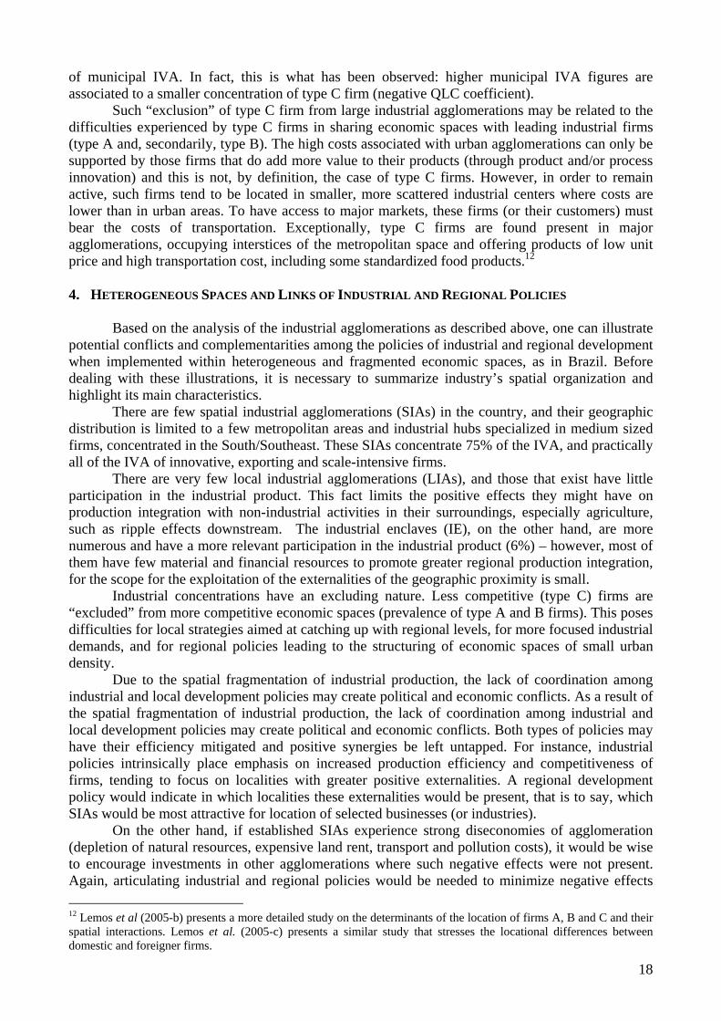
4. HETEROGENEOUS SPACES AND LINKS OF INDUSTRIAL AND REGIONAL POLICIES

Based on the analysis of the industrial agglomerations as described above, one can illustrate potential conflicts and complementarities among the policies of industrial and regional development when implemented within heterogeneous and fragmented economic spaces, as in Brazil. Before dealing with these illustrations, it is necessary to summarize industry’s spatial organization and highlight its main characteristics.

There are few spatial industrial agglomerations (SIAs) in the country, and their geographic distribution is limited to a few metropolitan areas and industrial hubs specialized in medium sized firms, concentrated in the South/Southeast. These SIAs concentrate 75% of the IVA, and practically all of the IVA of innovative, exporting and scale-intensive firms.

There are very few local industrial agglomerations (LIAs), and those that exist have little participation in the industrial product. This fact limits the positive effects they might have on production integration with non-industrial activities in their surroundings, especially agriculture, such as ripple effects downstream. The industrial enclaves (IE), on the other hand, are more numerous and have a more relevant participation in the industrial product (6%) – however, most of them have few material and financial resources to promote greater regional production integration, for the scope for the exploitation of the externalities of the geographic proximity is small.

Industrial concentrations have an excluding nature. Less competitive (type C) firms are “excluded” from more competitive economic spaces (prevalence of type A and B firms). This poses difficulties for local strategies aimed at catching up with regional levels, for more focused industrial demands, and for regional policies leading to the structuring of economic spaces of small urban density.

Due to the spatial fragmentation of industrial production, the lack of coordination among industrial and local development policies may create political and economic conflicts. As a result of the spatial fragmentation of industrial production, the lack of coordination among industrial and local development policies may create political and economic conflicts. Both types of policies may have their efficiency mitigated and positive synergies be left untapped. For instance, industrial policies intrinsically place emphasis on increased production efficiency and competitiveness of firms, tending to focus on localities with greater positive externalities. A regional development policy would indicate in which localities these externalities would be present, that is to say, which SIAs would be most attractive for location of selected businesses (or industries).

On the other hand, if established SIAs experience strong diseconomies of agglomeration (depletion of natural resources, expensive land rent, transport and pollution costs), it would be wise to encourage investments in other agglomerations where such negative effects were not present. Again, articulating industrial and regional policies would be needed to minimize negative effects 12 Lemos et al (2005-b) presents a more detailed study on the determinants of the location of firms A, B and C and their spatial interactions. Lemos et al. (2005-c) presents a similar study that stresses the locational differences between domestic and foreigner firms.

19

typical of an industrial mega-agglomeration. Which regions would be earmarked as potential investment recipients? These could include some of the industrial enclaves or even one of the local industrial agglomerations identified above.

A regional policy, in turn, must be aimed at a less unequal development within the country and prioritize regions deprived of the advantages of growing spatial returns, namely, peripheral regions. In order to develop such regions, regional development policies must create production and reproduction conditions locally in line with the objectives of the industrial policies.

In this respect, but in an opposite manner, the regional policy must select, from among the firms or industries given priority by the industrial policy, those that best suit regional particularities. As many have noticed, the location of firms (or even a group of firms) in some regions may spark strong negative reactions, including population displacement and environmental degradation, while failing to produce the spillover and ripple effects that are essential to sustainable regional development.

To what extent would it be possible to conciliate the objectives, instruments and social players involved in the public policies? The results of this study point to three lines of action which would correspond to the intersection points of industrial policy and regional policy for the Brazilian case. The first would be a policy of industrial promotion and metropolitan production integration of the lesser developed SIAs. The second line of action would be a policy of regional development of the potential SIAS, seeking to construct a regional complementarity based on the successful “industrial districts”. And finally, the third line of action would be the policy for local development of the areas surrounding the localized industrial agglomerations which are isolated within the country, the so-called Industrial Enclaves. The objectives would be to reduce the local territorial segmentation with the offering of an urban physical infrastructure, such as sanitation, transportation and housing.

These three lines of action would have to be implemented on the basis of the two main federal public policies for the production sector, namely the Industrial, Technological and Foreign Trade Policies and the National Policy for Regional Development. The competencies of the firm and the region would need to be integrated.

20

REFERENCES: Anselin, L. (1999). The Moran Scatterplot as an Esda Tool to Assess Local Instability in Spatial

Association, in Spatial Analytical Perspectives on Gis, ed. by M. Fischer, H. J. Scholten, and D. Unwin. London: Taylor Francis, 111-125.

Azzoni, C.R. & Ferreira, D.A. (1999). “Competitividade Regional e Reconcentração Industrial: o futuro das desigualdades regionais no Brasil”. NEMESIS, FEA/USP, São Paulo, Brazil (www.nemesis.org.br, discussion paper).

Castro, N., Carris L. e Rodrigues B. (1999). Custos de Transporte e a Estrutura Espacial do Comércio Interestadual Brasileiro, Pesquisa e Planejamento Econômico, v.29 (3), IPEA/DIPES, Rio de Janeiro, dezembro 1999.

De Negri, J.A., Salerno, M.S., Castro, A.B. (2004). Estratégias competitivas e padrões tecnológicos das firmas na indústria brasileira, Brasília: IPEA, mimeo, 2004.

Diniz, C.C. & Crocco, M.A. (1996). “A Reestruturação Econômica e Impacto Regional: o novo mapa da indústria brasileira”. Revista Nova Economia, Belo Horizonte, v.6, n.1, p. 77-104, Julho.

Diniz, C.C. (1994). “Polygonized Development in Brazil: Neither Decentralization nor Continued Polarization”. International Journal of Urban and Regional Research 18: 293-314.

Diniz, C.C. (2000). A nova geografia econômica do Brasil: condicionantes e implicações (2000). In: Veloso, J.R.V. (org.), Brasil Século XXI. Rio de Janeiro: José Olímpio.

Fujita, M., Krugman, P., & Venables, A.J. (1999). Spatial Economy – Cities, Regions and International Trade. Cambridge, Massachusetts, London, England: The MIT Press. 1999

Glaeser, E.L., Kallal, H.D., Scheinkman, J.A. & Shleifer, A.(1992). “Growth in Cities”. Journal of Political Economy, vol. 100 (6), p. 1126-1152, 1992.

Haddad, E. & Azzoni, C.R. (1999). “Trade Liberalization and Location: Geographical Shifts in the Brazilian Economic Structure”. FEA-USP Discussion Paper. São Paulo, Brazil.

Isard, W. (1956). Location and Space-economy. New York, London: The Technological Press of The MIT and John Wiley & Sons, Inc.

Jacobs, J. (1969). The economy of cities. Random House, New York. Lemos, M.B., Diniz, C.C., Guerra, L.P., Moro, S. (2003). “A nova configuração regional

brasileira e sua geografia econômica”, in Estudos Econômicos, vol. 33 (4), p. 665-700. Lemos, M.B.; Moro, S.; Domingues, E.P. & Ruiz, R.M. (2005-a). “A Organização Territorial da

Indústria no Brasil”. Relatório de Pesquisa: Inovações, Padrões Tecnológicos e Desempenho das Firmas Industriais Brasileiras. Brasília: IPEA.

Lemos, M.B.; Domingues, E.P, Moro, S.;. & Ruiz, R.M. (2005-b). “Espaços Preferenciais e Aglomerações Industriais”. Relatório de Pesquisa: Inovações, Padrões Tecnológicos e Desempenho das Firmas Industriais Brasileiras. Brasília: IPEA.

Lemos, M.B.; Ruiz, R.M; Domingues, E.P. & Moro, S.;. (2005-c). “Empresas Estrangeiras em Espaços Periféricos: o caso Brasileiro”. Relatório de Pesquisa: Inovações, Padrões Tecnológicos e Desempenho das Firmas Industriais Brasileiras. Brasília: IPEA.

Pacheco, C.A. (1999). “Novos Padrões de Localização Industrial? Tendências Recentes e Indicadores da Produção e do Investimento Industrial”. IPEA - Textos para Discussão n.633. Brasília, Brasília: IPEA.

Pred, A. (1966). The Spatial Dynamics of U.S. Urban-Industrial Growth. Cambridge: MIT Press.