GENERIC PHYSICS
A CONCEPTUAL INTERFACE FOR RIGID BODY PHYSICS ENGINES
Carlos Miguel Pimenta Gomes
Dissertação para Obtenção de Grau de Mestre em
Engenharia Informática e de Computadores
Júri Presidente: Prof. Dr. Pedro Diniz
Orientador: Prof. Dr. Mário Rui Gomes
Vogal: Prof. Dr. Pedro Faria Lopes
Setembro 2007


Resumo Desde a revolução científica ocorrida no século XVII até aos nossos dias, a Física tem
revolucionado o mundo com novas invenções e descobertas desde o space shuttle até à energia
nuclear e aos computadores. Hoje em dia com as crescentes capacidades de processamento
dos computadores, os jogadores de vídeo jogos tornaram-se cada vez mais exigentes em termos
de realismo, o que levou à última novidade no mundo dos mundos virtuais – Física.
No princípio os efeitos de física eram totalmente codificados pelo programador mas hoje
existem bibliotecas especializadas chamadas de Motores Físicos. Estas bibliotecas focam-se na
implementação dos efeitos físicos estando normalmente em ligação forte com o processamento
gráfico. Assim o programador fica apenas responsável por integrar a solução na sua aplicação.
Esta técnica produz resultados bastante bons ao nível da performance mas é limitada em termos
de expansibilidade das aplicações. Isto acontece porque estas são desenvolvidas usando os
detalhes de implementação do motor físico escolhido. Assim, mudar de motor físico,
especialmente um melhor, torna-se difícil. Normalmente implica desenvolver uma aplicação de
raiz.
Uma solução seria existir uma camada intermédia que fizesse a transição entre o motor de
física e a aplicação de uma forma genérica e independente da implementação. Assim sendo este
trabalho tenta responder à pergunta “Será possível definir uma abstracção de física genérica,
poderosa o suficiente para permitir o desenvolvimento de aplicações de mundos virtuais,
independentes da solução usada?”
Para desenvolver a nossa solução analisámos a física clássica e a maioria dos motores
físicos existentes no mercado. Focando em física de corpos rígidos e detecção de colisões, esta
análise permitiu a extracção de conceitos, das suas relações e das funções essenciais de uma
simulação física. Com estes dados criámos o modelo conceptual da nossa solução.
Finalmente este modelo foi transformado numa sistema de interfaces. Como caso de estudo
implementámos essa interface com dois motores – Ogre3D para os gráficos e ODE para a física.
No fim usámos esta implementação para criar um pequeno editor de mundos virtuais.
Este editor foi usado para demonstrar que o nosso modelo conceptual resultou numa
interface genérica de programação de física e que permite a criação de mundos virtuais. Apesar
de ter sido apenas demonstrada no contexto de física de corpos rígidos, teoricamente a nossa
técnica pode ser aplicada a todos os domínios da física.
Palavras Chave: Física, Abstracção de Física, Desenvolvimento Independente da
Implementação


Abstract Starting in the XVII century with the scientific revolution, Physics revolutionized the world with
great inventions and discoveries, from the space shuttle to nuclear energy, and even computers.
Nowadays, with the ever increasing capabilities of computers, gamers became more and more
demanding in terms of realism, which led to the latest addition to their virtual worlds – Physics.
Starting by being hardcoded on the application, physics processing evolved into software
libraries called Physics Engines. They focus on implementing the physics effects often in close
connection with the graphics processing. This way the developer is responsible for embedding it
on its own application. This approach works well but limits the scalability of the applications. This
happens because they were specifically developed using the implementation details of the
chosen physics engine. Change to a different physics engine, specially a better one, becomes
very difficult. It often means redeveloping the application from scratch.
A possible solution would be to have an intermediate layer capable of making the bridge
between our applications and the physics engines in a generic way. As such in this work we try to
give an answer to the question: “Is it possible to define a generic physics abstraction, powerful
enough to allow the developing of virtual worlds applications, independent of the solution
underneath?”
To develop our solution we analyzed classical physics and the majority of physics engines
currently on market. Focusing on Rigid Body Physics and Collision Detection this analysis
allowed the extraction of concepts, their relationship and essential simulation functions to
ultimately develop the conceptual model of our solution.
Finally this model was implemented using an object oriented programming into an interface
system. For our case study we implemented the interface with two engines- Ogre3D for the
graphics and ODE for the physics. Finally we used our implementation to develop a simple Virtual
World Editor.
We used our Editor to demonstrate that our conceptual model resulted in a generic physics
programming interface that allows the creation of physically enabled simulations. Although only
demonstrated on the rigid body domain theoretically this approach can be applied to all physics
domains.
Keywords: Physics, Physics Abstraction Layer, Implementation Independent Development


Acknowledgements
I would like to thank my parents for all their support throughout my academic life and mainly
for having educated me and provided me with the means to fully develop my abilities that
ultimately made this work possible.
I would like to thank all the people at GAIPS and my working partners for all the support, ideas
and discussions we’ve had throughout the last year while developing this work as they provided
me with brand new points of view on how to make thinks correctly.
More personally I would like to give a great Thanks to:
Gaips Researcher Guilherme Raimundo, for all the help on theoretical and practical problems
where its assistance proved invaluable.
Gaips Researcher Marco Vala, my accompanying teacher for all the guidance and great ideas
he gave me to develop my work.
My cousin Daniel Pinto, for reading my thesis, appointing mistakes and “making questions”.
He provided me with a point of view of someone out of the Computer Science domain.
Finally I would like to thank my supervisor Professor Mário Rui Gomes for this challenging
work and all the guidelines he gave me.

Contents
1 Introduction ................................................................................................................................ 1 1.1. Motivation ........................................................................................................................ 1
1.2. Problem ........................................................................................................................... 2
1.3. Hypothesis ....................................................................................................................... 3
1.4. Outline ............................................................................................................................. 3
2 Physics Engines: State of The Art ........................................................................................... 5 2.1. A Brief Evolution of Physics Engines ............................................................................... 5
2.2. The Physics Engine and its Features .............................................................................. 7
2.2.1. The Physics Engine ................................................................................................. 7
2.2.2. Features of a State of the Art Physics Engine ......................................................... 8
2.2.3. Existing Physics Engines ....................................................................................... 14
2.2.4. Physics Engines Analysis ...................................................................................... 27
2.3. Summary ....................................................................................................................... 29
3 A Generic Physics System ..................................................................................................... 31 3.1. Simulation ...................................................................................................................... 32
3.2. Concepts ........................................................................................................................ 34
3.2.1. Physical Concepts ................................................................................................. 34
3.2.2. System Concepts ................................................................................................... 39
3.3. Conceptual Model .......................................................................................................... 41
3.4. Interface Architecture ..................................................................................................... 43
3.5. Summary ....................................................................................................................... 45
4 Case Study ............................................................................................................................... 47 4.1. Interface Concretization ................................................................................................. 47
4.1.1. Technology ............................................................................................................ 47
4.1.2. Implementation Decisions...................................................................................... 48
4.1.3. Event Handling System ......................................................................................... 49
4.2. Programming with Concepts ......................................................................................... 51
4.3. World Editor ................................................................................................................... 56
4.3.1. Using our Editor ..................................................................................................... 57
4.4. Summary ....................................................................................................................... 62
5 Conclusion ............................................................................................................................... 63

5.1. Future Work ................................................................................................................... 64
Bibliography ................................................................................................................................. 65
A. Conceptual Model ............................................................................................................... 67
B. Ogre3D/Ode Implementation Details ................................................................................ 68

List of Tables
Table 1: Commercial Physics Engines .......................................................................................... 27
Table 2: Open Source Physics Engines ........................................................................................ 28


List of Figures
Figure 1: Schematic of the architecture of a physics engine ........................................................... 7
Figure 2: Summary Chart for Havok .............................................................................................. 16
Figure 3: Summary Chart for Ageia ............................................................................................... 17
Figure 4: Summary Chart for Euphoria ......................................................................................... 18
Figure 5: Summary Chart for Pseudo ............................................................................................ 19
Figure 6: Summary Chart for Physics and Math Library ............................................................... 20
Figure 7:Summary Chart for TrueAxis ........................................................................................... 21
Figure 8: Summary Chart for UniGine ........................................................................................... 22
Figure 9: Summary Chart for RenderWare ................................................................................... 23
Figure 10: Summary Chart for ODE .............................................................................................. 24
Figure 11:Summary Chart for Newton ........................................................................................... 25
Figure 12:Summary Chart for nV Physics ..................................................................................... 26
Figure 13: Summary Chart for Bullet ............................................................................................. 27
Figure 14 : Typical Virtual World Simulation Cycle ....................................................................... 32
Figure 15 : Physics Update Stages ............................................................................................... 32
Figure 16 : Simulation Cycle in our System .................................................................................. 33
Figure 17: Conceptual Model: Simulation Control ......................................................................... 42
Figure 18 : Conceptual Model: Entity ............................................................................................ 42
Figure 19: Final Interface Architecture .......................................................................................... 44
Figure 22: Example combination between Physics Managers and Entity Physics Components. 49
Figure 24: Example of Interaction with the Event System ............................................................. 50
Figure 25: Application Screenshot. We created the World, Managers and defined the application
cycle. .............................................................................................................................................. 52
Figure 26: Example Application where we added an Entity with a graphics component using a
Crate Mesh. ................................................................................................................................... 53
Figure 27: Physics Enabled Object: The Crate object is moving due to the gravitational force. .. 54
Figure 28: Final Application Example: Only graphically enabled object. They don’t move yet. .... 55
Figure 29: Final Application Example. Example interaction between a Ball and a Crate Entity. .. 55
Figure 30 : Main view of the World Editor ..................................................................................... 57
Figure 31 : World Viewer ............................................................................................................... 57
Figure 32 : World Viewer Examples. From left to right – Simulation Control, Entity, Interaction .. 58
Figure 33: Entity Creation: Two Entities were created and named Ball and Box .......................... 59
Figure 34 : Adding a visual representation to an Entity. ................................................................ 60
Figure 35: World configuration after adding the graphical configurations for the box and ball ..... 60

Figure 36: Configuring Physics behavior on an Entity................................................................... 61
Figure 37 : Final Simulation of the example of interaction between a Ball and a Crate Entity. .... 61
Figure 38 : Conceptual Model ....................................................................................................... 67
Figure 39: Ogre3D/Ode Implementation Schematic ..................................................................... 68

1
Chapter 1
Introduction
“It should be possible to explain the laws of physics to a barmaid.”
Albert Einstein
(1879-1955)
1.1. Motivation
Since ancient times, people have been trying to understand the behavior of matter: the falling
to the ground of unsupported objects, the different properties of materials, and so on. They also
sought to uncover the mysteries of the universe, of the sun, of the moon and all the planets
whose behavior was beyond their comprehension.
In the XVII century, after centuries of medieval obscurity, this curiosity triumphed finally, with
the scientific revolution: physics stepped up to become one of the greatest fields of science,
matched only by the ancient a priori science of mathematics. Physicists like Newton, Maxwell and
Einstein advanced greatly in this field, laying the bricks of our current great technological
achievements.
Known physical effects that occur in nature can be described (at least approximately) in a
mathematical form – this is especially true for the most studied ones, those which directly humans
can sense like gravity, collisions and movement. This property allows us to simulate them in
computer programs. However, these calculations are complex and require a high processing
power.
The processing power requirements lead to the appearance of two approaches to physics
simulation [1]: High Precision Physics and Real Time Physics. In the first one the physical effects
are calculated with great precision. Such approach has historically been applied by scientists with
access to supercomputers in various fields of investigation, although recently the movie industry
has started using it to create special effects (ILM [2]) as well as computer animated movies (e.g.
Pixar’s [3]). On the other hand, in Real Time Physics a rapid response of the system must be
guaranteed in order to maintain a “real-time” sensation for the user. To achieve this, simplified
models of reality that “appear” to be real are used. This is applied for example in video games
where a minimum frame rate must be kept to prevent the simulation from becoming “choppy”.
Real Time Physics is the focus of this work, especially on the video games domain.
If you ask a gamer what is the most important part of a video game they will probably answer
you with the quality of the graphics, the sound effects or even the artificial intelligence (A.I.) of the

2
enemies. That’s because until recently almost everyone forgot one important component that
helps simulation to achieve a true sensation of realism – Physics.
Imagine a video game where you have nearly or completely realistic models, sounds and a
human-like A.I. At first glance it seems as if it is a movie. Imagine however that whatever you do
in this virtual world you always see the same hand-made animation over and over again and no
matter what you try, all the objects in the environment remain forever static. After a while your
initial sensation of a movie-like virtual world is gone, and so is the whole experience.
As such it is imperative that if we want to create even more realistic worlds inside our video
games we need to simulate the real world physical effects to the greatest extent possible for the
player to truly immerse himself into the virtual world. With this purpose in mind, a specialized
software component has been created: the physics engine.
1.2. Problem
There are several physics engines on the market and most of them are designed to be
embedded in the application code. The common practice is to mix graphical and physical code all
together for performance and historical reasons. Until recently most of the physics calculations
(e.g.: collision detection).were done mainly by the graphics component of the application. In
earlier times, developers had to solve physics problems but these were just not important enough
to justify being taken care of separately and were calculated on the graphics engine. The
similarity in some calculations between graphics and physics also contributed. This common
approach works very well and delivers the most performance tuned application possible but with
associated costs in terms of scalability.
For instance, let’s consider long term applications that aren’t supposed to end in a “final boxed
product”, like many research programs. When development is finished, they use the latest
technology of their day but as time passes, the same technology that once was cutting edge
becomes obsolete. As components are usually hard coded and share a great dependency
between them, the cost of changing them is so high, that developers often choose to rebuild the
application from scratch, rather than updating its technology. To worsen the problem, physics
engines implementations are quite different from each other.
If physics engines shared a common base this situation could be solved. This way the
problem we are trying to solve can be resumed in the following question: “Is it possible to define a
generic physics abstraction, powerful enough to allow the developing of virtual worlds
applications, independent of the solution underneath?”

3
1.3. Hypothesis
To answer the question our hypothesis consists in studying the main physical concepts that
form the basis of every physics engine and how they relate and interact with each other. We think
that if we are able to clearly define the concepts relationship model we can produce a
programming interface that translates that model into the computation world. This way the
resulting interface system, being created based on a generic model, shall be possible to connect
to every physics engine. Furthermore our interface system shall be totally independent of the
other application components, especially from graphics.
As a result choosing/changing a physics engine in applications developed with our interface
system becomes easier as no application code must be changed. Developers just need to
connect the chosen physics engine to our interface system. The same is true when upgrading our
interface with new features as previous applications remain functional although not using the new
functionality.
1.4. Outline
The developed work is described on the following chapters.
In Chapter 2 (Physics Engines: State of The Art and Current Trends) an extensive study on
the physics engines is carried. We study their internal architecture and their features. In the end
all important solutions currently on the market (open source and commercial ones) are described
and compared.
In Chapter 3 (A Generic Physics System) the scope of this work is clearly defined and we
theoretically present our solution. We start by explaining how a physics simulation works and the
way we can separate physics from the other application’s components, namely the graphics.
Following this, we define the main concepts that we found through classical physics study and the
previous physics engines analysis. Finally we present the conceptual model of our solution
consisting on the previous concepts and the way they relate/interact with each other.
To allow applications development with our model we need to build a programming interface.
In Chapter 4 (Implementation) we describe how the interface system was developed based on
the conceptual model.
To be usable, the programming interface must be implemented. In Chapter 5 (Case Study) we
present a case study where we implement our interface using a physics engine and a graphics
engine. To demonstrate that our interface allows application development, we used it to develop
a small world editor containing physics simulation
Finally, in Chapter 6 (Conclusion and Future Work) we resume our work and present our
conclusions based on our case study. We finish by suggesting ways to improve this work.

4

5
Chapter 2
Physics Engines: State of The Art
This chapter will try to answer the following questions: What are the main features of the main
physics engines used today? Which physical concepts do they deal with? Which is the best
engine nowadays?
Starting with a brief description of the history of physics engines, we proceed by studying their
inner structure and the features that a state of the art solution must have. We continue by
depicting the principal applied techniques to simulate the mentioned features.
Finally we present and compare the majority of the currently available physics engines
solutions on the market.
2.1. A Brief Evolution of Physics Engines
In the beginning, even when video games were very simple, the physical effects were already
present, as you can see in the classic Tetris where the pieces “fall” from the top. This “fall” is
nothing less than a primitive simulation of gravity.
The years passed and more complex games made their appearance. If we take the example
of Doom we see the introduction of several physical effects like gravity (when the character jumps
or when he carries too much weight and slows the movement speed), friction (when stepping on
different ground like sand) and even effects like velocity, acceleration and primitive collision
detection (like hitting a wall).
These effects (gravity, friction, velocity, acceleration and collision detection) are called
Newtonian Physical Effects [4] and make the basics of a physics simulation.
Until recently all the effects were hard coded into the applications and could not be reused on
other games.
In 1998, a small company named Havok [5] was created with the goal of creating a reusable
physics library that could be integrated in every game that licenses it. This was the birth of the
Physics Engine as we know it today.
"A physics engine is a computer program (software component) that using variables such as
mass, velocity, friction and wind resistance can simulate and predict effects under different
conditions that would approximate what happens in either real life or a fantasy world." [6]
With the appearance of the physics engine the gaming industry was relieved of the burden of
creating their own physical effects and could rely on third party companies to focus their efforts in
researching and developing their physic engines.

6
Today physics engines not only simulate Newtonian Physics but also support many new “high-
tech” effects like cloth or fluids simulation.
Nowadays we are witnessing the advent of the next generation of physical effects with the
introduction of dedicated external processors, also called PPU – Physics Processing Units.
The entrepreneur company Ageia gave the first step towards this goal by developing the
PhysX, a built from scratch chip fully optimized for physics calculations. This chip features:
• High processing parallelization – to be able to process as many “physical events”
as possible per clock.
• High bandwidth between the processing unit and the memory as the quantity of
information that must be stored and retrieved is enormous (object physical properties like
mass, velocity and acceleration and graphical properties like spatial and shape
information).
• Hardware optimization for Physics calculation – to maximize the performance of
the calculations (in terms of precision and velocity).
With the addition of a separate physics processor we have what Ageia calls The Gaming
Triangle [7]:
• CPU: Think and Orchestrate
• GPU: Render and Display
• PPU: Move and Interact
These three components share information between them. The CPU is the responsible for the
game logic, artificial intelligence and for coordinating the PPU and GPU (sending the orders for
them to process). The GPU is responsible for rendering all the graphical objects. The PPU is
responsible for determining the objects positions based on their physical properties and physical
forces exerted on them.
Between the PPU and the GPU there must be a constant interchange of information and
namely spatial information. This information in Ageia’s concept is passed having the CPU as an
intermediate.
Alternative solutions have been proposed and implemented by leading company Havok that
uses the video card processors to calculate physics. This strategy permits the user to reutilize an
old video card to calculate physics instead of having to buy another card just for physics.

7
2.2. The Physics Engine and its Features
2.2.1. The Physics Engine
A physics engine uses the physical attributes of objects in a scene to compute new positions,
orientations and other transformations for objects at each simulation step. The basic input to the
engine is the set of objects subject to physical interactions, and the attributes defined for each
object. These attributes will include geometry, density, elasticity, friction coefficients, constraints,
and external forces and torques.
Figure 1: Schematic of the architecture of a physics engine
A constraint restricts the motion of an object. A typical constraint would be the joint connecting
the upper arm to the lower arm on a human character. The motion of an object is defined by
external forces and by internal forces. A good way to imagine internal forces is to imagine two
skaters on ice holding hands. External forces are generated using their ices skates. Internal
forces can be felt directly as the force they have to exert through their hands to remain together.

8
We cannot model the behavior of each skater by knowing only the external forces; it is
necessary to solve the internal forces. The physics engine uses a module, the Constraint Solver,
to discover these internal forces so that dynamics of a whole object can be calculated as if it was
moving in isolation without a constraint.
The equations of motion for rigid bodies can be derived from Newton’s laws, and are second
order differential equations. These are solved using a general Ordinary Differential Equation
(ODE) solver, which integrates the equations of motion using a succession of small time steps.
When a new position for an object is computed, it may turn out that it has collided with another
object. Because the physics engine uses a discrete time step, the object may have penetrated
the second object, and so it has to back up, and use a series of smaller time steps to find the
instant of the collision. It then uses a Collision Solver to work out the impulsive forces due to the
collision, and adds these forces to any external and constraint forces. It then continues the
simulation, and after a certain number of simulation time steps it updates the attributes of each
modeled object. In particular, it will update the position and orientation of each object. Figure 1
presents us with a typical physics engine architecture [8].
2.2.2. Features of a State of the Art Physics Engine
2.2.2.1. Collision Detection
The goal of collision detection is to report when a geometric contact has occurred or will occur
between two or more physically enabled objects on the virtual world. Collision between objects
can be detected using bounding spheres or boxes [9]. Collision with the world can be detected
using ray-casting.
Certain types of games, such as space and vehicle games produce satisfying results using
these simplified collision models but in some simple situations, such as stacks of boxes, instability
occurs due to accumulation of computation errors. The example of stack of boxes is often used to
compare physics engines in terms of stability.
A simple and fast solution of detecting collisions between objects is through the use of
spheres and ellipsoids. The method consists in mapping a sphere or an ellipsoid to every object
on the scene and test if they intersect. This can be done easily by using the sphere/ellipsoid
equations and calculating intersection points [10]. In the case of using other geometric forms, like
the usual bounding box (parallelepiped), one should test if the objects intersect each other using
the size of the boxes. In terms of complexity the spheres approximation is faster because the
calculations are based on the radius of the sphere while with the box further calculations are
needed. In the case of the ellipsoids calculations are based on the axis length.

9
In [11], Lin and Gottschalk provide a comprehensive review of collision detection techniques
used in areas such as computer-aided-design (CAD), robotics and automation, manufacturing
and computer graphics.
Most modern collision detection schemes attempt to deal with convex, polygonal shapes with
high poly counts and seek to return very accurate collision detail. With these kinds of target
constraints, there are two common approaches taken: feature-oriented (typified by the Lin-Canny
algorithm) and Simplex-oriented (typified by the GJK algorithm) collision detection schemes.
• Feature-oriented collision detection tries to determine the closest “features”
(vertices, edges, or faces) between two polygonal shapes. These features are
compared, and disjointedness or collision is determined based on the distance
between them. The Lin-Canny [12] algorithm, which is the progenitor of feature-based
techniques, does just this, and caches collision feature information to exploit temporal
coherence and probabilistically reduce the computation required in a collision
detection pass. Lin-Canny has spawned many variations and improvements, such as
V-Clip [13] which overcome the algorithm’s Achilles’ heel: its inability to elegantly
handle interpenetrating shapes.
• Simplex-oriented collision detection, as typified by the GJK algorithm [14],
iteratively determines the distance between two objects. A “simplex” is just a fancy
term for a point, line, triangle, tetrahedron… in other words, an n-triangle. The GJK
algorithm iteratively creates simplexes of the shapes’ differences to determine their
distance from each other, and whether they collide. GJK is capable of handling
interpenetrating shapes, and it has also spawned many derivative algorithms which
improve on its efficiency and robustness.
Comparing these two approaches is quite difficult as it depends in various factors like the
shape of the objects to test, the quality of the implementation and in which language it was
implemented. Mirtich in [13] presents a test case where he compares these algorithms. To
counter the difficulties presented above he uses comparison factors such as floating point
operations per call that are less variable. The results give a clear advantage to V-Clip over the
classical Lin-Canny and the simplex approach GTK. V-Clip is faster and guarantees good results.
As an extra, V-Clip doesn’t need to be “tuned” by the user thus diminishing its use complexity.
2.2.2.2. Rigid Body Physics
In physics, a rigid body is an idealization of a solid body of finite size in which deformation is
neglected. In other words, the distance between any two given points of a rigid body remains
constant in time regardless of external forces exerted on it.
A rigid body is characterized by [15]:
• Mass

10
• Position of the Center of Mass
• Orientation
• Linear Velocity
• Angular Velocity: The main difference between a particle and a rigid body is that
the latter may be rotated (having angular velocity). Other difference is that rigid bodies
have volume that affects the way collisions occur.
The equations of motion for rigid body dynamics are second-order differential equations that
are solvable using a number of generic ODE solvers. The most common methods are the Euler
method, a variety of Runge-Kutta methods, Midpoint method, and implicit methods, with or
without adaptive step size control [16]. The choice of method is often a matter of experiment, as
the simpler methods can become unstable due to modeling inaccuracy, and the more accurate
methods can require much more computation.
The simpler of these methods is the Euler Method that consists of a simple stepped
integration of the Newton equations of motion. Logically this technique is also the most inaccurate
in small time steps. The solution to this problem usually consists of using an error correction
factor. By using it, we reduce the probability of highly inaccurate results.
2.2.2.3. Character and Vehicle Physics
Until the advent of video games physics, character motion was performed exclusively through
a series of animations created in some form of 3D modeling program like Maya and 3DstudioMax
(possibly using motion capture) and finally imported into the video game.
With the power of physics the recent approach to characters/vehicles physics consists in
building a skeleton/structure of the character/vehicle and affect it of physical effects. This
skeleton/structure is connected to the 3D model, controlling all of its movement. The analogy with
our own body’s skeleton is correct being our muscles the force applied to the bones by the
physics engine.
One of the most used algorithms for simulating the motion of characters is Featherstone’s
Articulated Body Method (ABM). Featherstone’s ABM is an efficient, linear-time method that
evaluates the equations of motion of arbitrary articulated bodies. The equations provide the
acceleration of the articulated body given its current state and any external forces and joint
torques acting on it. [16]
The primary concept that makes character and vehicle physics possible is joints and
constrained rigid body physics [17].
Joints consist in two or more rigid bodies connected at a point making their movement
dependent of each other.
11
In its unconstrained mode, a rigid body has 6 independent degrees of freedom (DOF): three
translational DOFs and three rotational DOFs. When constrained, some of those DOFs are lost
and thus “constrain” the movement of the rigid body.
Two objects connected at a point with a full rotational joint should have 12 DOF, but 3
translational DOF are lost because of the joint, leaving 9 DOFs: 3 translational (the two bodies
must move together) and 6 rotational (there are no rotational constraints).
The loss of degrees of freedom results in internal forces (and torques) at the joint. Common
constraint types are [18]:
• Point to Point: In this type of constrain two objects are connected in one point,
giving them full movement as long as they stay connected (the connection point remains
connected).
• Point to Nail: This constrain limits the movement of the objects to only two DOFs.
It resembles a common “door joint”. The connection between the objects is a line and
must remain like that.
• Point to Path: In this constrain, the connection translates in a one dimensional
path. It can be imagined like a car shock absorber. The connected objects may only
move on that path and rotate according to the axis defined by it.
Two methods commonly used to compute internal forces are the Penalty Force method [19]
and the Lagrange Multiplier method [20]. Basically both algorithms solve a linear equation system
to discover the internal forces at the joint. Based on those forces the physics engine calculates
the future movement of the rigid bodies (that may remain static if the constrain imposes). The
main difference between them resides in the problem of objects inter-penetration. Using the
penalty force method, a simple method, it doesn’t completely avoid inter-penetration while using
the more precise Lagrange Multiplier method completely solves this problem. The last one is
rather complex and computationally heavy.
The most renowned use of joints in video games is to create Rag dolls. Rag doll, as the name
implies, is the ability to let the characters be influenced by the surrounding environment while
apparently limp themselves, like rag dolls. This technique is sometimes called “Lifelike death
animations” in various video games when talking about this feature.
It is however important to emphasize that rag doll behavior does not imply controlling the user
controlled characters with physics, it merely concerns simulating physical effects on lifeless
characters or lifeless limbs. These simulations can however be mixed with existing animations.
There is however research treating the subject of shifting the character control from the
animations system to the physics system and thus simulating ‘muscles’. This research area is
called dynamic animation [21] or physics-based character animation control [22]. Half Life 2 is the
video game that first featured advanced facial animation based on the simulation of more than
forty muscles [23].

12
2.2.2.4. Soft Body Physics
Soft body dynamics focuses on accurate simulation of flexible objects allowing for easier
creation of secondary motion effects of muscle, hair, cloth, etc. Soft bodies differ from rigid bodies
in that the latter don’t suffer deformation.
Three major considerations must be taken into account when attempting to model accurate
soft body action/reaction:
• Detecting collisions between deforming objects.
• Computing impact forces when bodies collide.
• Determining deformation forces or contact deformation of the bodies to initialize a
deformation technique.
Calculating deformation forces and the deformation itself is very computational intensive. A
good technique is the precomputation of the dynamically deformable objects. This technique is
described in [24] and results in a higher frame rate of the simulation as a whole. This allows an
increase on detail while maintaining good gameplay levels.
In [25], Baraff presents an improved algorithm to correctly simulate cloth objects using large
steps. The problem of large steps in cloth simulation is that it usually results in instability of the
physical system (with the appearance of visual artifacts like out of the place vertexes). The
common algorithms to simulate cloth use explicit calculations such as Euler’s method or Runge-
Kutta methods [16]. Baraff approach goes the other way, using implicit calculation and using
triangular mesh for cloth surfaces (instead of rectangular ones). In his paper Baraff demonstrates
that implicit methods for cloth overcome the performance limits inherent in explicit simulation
methods. Mathematically explicit methods calculate the state of a system at a later time from the
state of the system at the current time, while an implicit method finds it by solving an equation
involving both the current state of the system and the later one.
An interesting approach to soft bodies is through the notion of pressure inside an inflatable
object. In [26] Matyka and Ollila present an innovative way of accurately simulating inflated
objects applying the thermodynamics laws and the Clausius-Clapeyron state equation for
pressure calculation (the pressure can be static or dynamic). Knowing the pressure, the
deformation of the object is accurately calculated resulting in a very precise simulation of a soft
body.
A rather difficult and tedious task when working with clothes and characters is to make them fit
together. Igarashi and Hughes created a system where the user can “dress” the character using
an interactive interface. There are two techniques available to the user: wrapping and surface
dragging [27].
The first technique, wrapping, is for putting the clothes on the body from scratch. The user
paints freeform marks on the clothes and corresponding marks on the body, and in a few seconds
the system places the clothes on the body in such a way that the corresponding marks match.
13
The second technique, surface dragging, is for adjusting the configuration of clothes already
on the body. While a typical cloth-dragging operation moves a set of vertices in a single direction
in 3D space, in this system the dragging operation moves the cloth along the body surface. The
user can also place pushpins to hold some clothing parts fixed during dragging.
2.2.2.5. Fluid Physics
Typical fluid flows vary from rising smoke, fire, clouds and mist to the flow of rivers and oceans
[28]. In the attempt to increase the realism of virtual worlds developers created many adhoc
models that attempt to fake fluid-like effects, such as particles rendered as textured sprites.
However, animating them in a convincing manner is not easy.
A better alternative is to use the physics of fluid flows which have been developed since the
time of Euler, Navier and Stokes (from the 1750’s to the 1850’s). These developments have led to
the so-called Navier-Stokes Equations [29], a precise mathematical model for most fluid flows
occurring in Nature. These equations, however, only admit analytical solutions in very simple
cases. No progress was therefore made until the 1950’s when researchers started to use
computers and develop numerical algorithms to solve the equations. In general, these algorithms
strive for accuracy and are fairly complex and time consuming.
In video games on the other hand what matters most is that the simulations both look
convincing and run fast. In addition, it is important that the solvers aren’t too complex so that they
can be implemented on standard PCs. Furthermore, the highly complex algorithms if applied
directly on video games have a high probability of developing an incorrect state and thus ruining
the simulation. The main reason for this problem is the constant sum of precision errors in the
calculations. After some simulation steps (can be many or few) the small errors turn into a big
error that produces unreal physical behavior. To avoid this, small error corrections are made, that
guarantees the simulation’s stability but turn useless for scientific computation.
In [30] the fluids solver presented on Alias Maya [31] software is briefly described. Their
approach consists of an initial state and three stages that enter an infinite cycle along the
simulation. The initial state represents the “containing space” where the fluid will spread. This
representation divides the virtual space in quads (if in 3D it will become cubes) each one with
some density of fluid.
The three stages of the fluids solver are:
• Add Forces: Here we detect the points where density is increased or decreased.
An example can be the generation of smoke coming from a venting shaft.
• Diffuse: In this stage, fluids are dispersed across the space according to the
fluids equations. The majority of the instability of fluids solvers comes from this stage. To
prevent that, Alias researchers constrained the diffusion to certain limits.

14
• Move: The final stage rules the path of the fluids. If one wants, for example, the
smoke to make a spiral curve, then that is achieved in this stage.
2.2.2.6. Destroyable Objects and Debris
Without a doubt, the great majority of video games feature violence (sometimes exaggerated)
with powerful weapons, crashes and explosions.
Nowadays these explosions consist mainly of a two dimensional movie of a pre-made
explosion and little else (usually games feature several different explosions to reduce the
repetitiveness).After the explosion usually the affected object is replaced by another (showing the
damage) but all the remaining environment remains in the same state. For example a rocket
impact on a thin wall usually leaves only a black patch when the expected result would be its
complete destruction.
Current state of the art physics engines support fully destroyable environments making the
whole experience far more realistic. Until recently this was not possible due to the high complexity
of calculating physics for the resulting objects (and its interactions).
The usual technique nowadays to simulate complete destruction consists in changing the
destroyed object by smaller objects that together have the same shape as the original. Then
when the explosion happens these new objects react to the forces by themselves. The final result
is a destroyed object that always breaks in the same places. Some games try to avoid this
repetitiveness in small objects by replacing them with different parts. The result is less realistic as
the parts put together don’t reproduce the original object.
With the goal of enriching the visual appearance of explosions, current physics engines auto-
generate particles that simulate the debris caused by a real explosion [32]. These particles have
nothing to do to the original object geometry. They are just temporary random objects to create
further chaos and give the sensation of a powerful explosion.
2.2.3. Existing Physics Engines
Some of the features presented above rely on algorithms developed many years ago. The
great advance on gaming physics is due to the high computational power that we have today.
This power allows us to execute those algorithms in real-time.
Because of their complexity, some of the presented features have not been fully implemented
in one solution. Instead there are several solutions that implement many features and some that
focused in one specific feature.
In the following section several solutions available on the market are presented and evaluated
according to those features. In the end there is a summary chart that resumes each engine’s
features, for a better side-by-side comparison.

15
This list is not exhaustive as there are other implemented solutions that have been either
abandoned or became obsolete and thus have been removed.
2.2.3.1. Havok
Web Site: http://www.havok.com/
Description: Havok is a state of the art physics engine and also the most popular among
game developers. Havok provides game’s developers not only with the physics engine but also
with specialized character behavior and animation tools.
Constantly in evolution, this engine is now on the edge of technology by supporting multi-core
CPU and incorporating hardware-accelerated physics using the current capabilities of graphics
cards.
It currently supports every gaming platform on the market including all next generation
consoles system (XBOX360, PS3 and Wii) and has been used in over 150 games including some
of the greatest games like Half Life 2 and Oblivion. Recently Havok has been used to create
special effects in movies such as Poseidon, The Matrix and Troy.
License: Commercial
Pros:
• This is a state of the art engine that implements a great part of the features
described in the previous chapter.
• Specialized tools to handle character behavior and animation, fully integrated
with the physics engine.
• Excellent set of tools to help game’s developers. Havok can be used from within
popular modeling programs such as 3DStudioMax and Maya or using their own provided
editors.
• Support for multi-core processors CPU.
• It’s the only physics engine to support hardware acceleration through graphics
cards.
• Havok’s technology supports every gaming platform (including all next-gen
consoles like PS3, Wii and Xbox 360).
• Havok has partnered with the majority of the giants of computer hardware and
software (like AMD, Intel, Nvidia, AMD, Sony) to guarantee that its product has the best
performance in every system and that it corresponds to clients expectations.
Cons:
• Lack of state of the art Character and Vehicle Physics features
• Lack of support for Ageia’s PPU.
• Expensive solution

16
Figure 2: Summary Chart for Havok
2.2.3.2. Ageia
Web Site: www.ageia.com
Description: Ageia is the most recently player on the physics engine market but brought with
it an entire revolution to the scene.
Ageia’s engine is an evolution of the previously known Novodex engine side by side with
Havok occupies the frontline in physics processing. While Havok supports hardware accelerated
physics on GPUs, Ageia created their own Physics Card – PhysX. Although designed for their
hardware card, Ageia also works on normal CPUs.
Right now only two games support Ageia’s engine but the company already signed
partnerships with some studios to power their games (including Epic Games greatest title –
Unreal Tournament 2007).
License: Free but Closed Source
Pros:
• This is a state of the art engine that implements every feature described in the
previous chapter.
• Support for Hardware Accelerated Physics in its proprietary PPU – PhysX.
• Excellent set of tools to help game’s developers. Ageia can be used from within
popular modeling programs such as 3DStudioMax and Maya or using their own provided
editors.
• Good client-support
• Supports the major next-gen gaming platform (PS3, XBOX360 and PC)
• Free license for non-commercial use.
Cons:
Colision Detection
Rigid Body
Character & Vehicle
Soft Body
Fluids
Destroyable objects
Havok

17
• Yet to be proven technology – currently there are only small demos and two
games that support the PhysX card.
• Extra cost to the user due to the need to buy an extra board that only works with
PhysX-powered games, as the competitors aren’t supporting the PPU.
• Proprietary technology developed without partnership with the games developer.
• Lack of state of the art Character and Vehicle Physics features
Figure 3: Summary Chart for Ageia
2.2.3.3. Euphoria
Web Site: http://www.naturalmotion.com/
Description: Euphoria from NaturalMotion is a newcomer in the market of real-time physics
engine, but the company has a large experience in the movies special effects production division.
Euphoria is a distinct product from all the others as it is dedicated to character animation and
interaction. In contrary to all the other solutions Euphoria is more than just a module to be added
to the game engine, it becomes the core of the application.
The great innovation of the Euphoria Engine is the use of Artificial Intelligence to control the
development of the animations. As an example if a character is falling he will try to land on the
position it hurts him less. And depending on the “reasoning” made by the AI module the animation
develops accordingly.
This engine will be used for the first time in the Indiana Jones game set to launch in Q1 2008
and there’s no public information on performance benchmarks or even technical specifications of
the Euphoria system. This way, there’s no way of comparing it to the other engines presented in
this analysis.
License: Commercial
Colision Detection
Rigid Body
Character & Vehicle
Soft Body
Fluids
Destroyable objects
Ageia
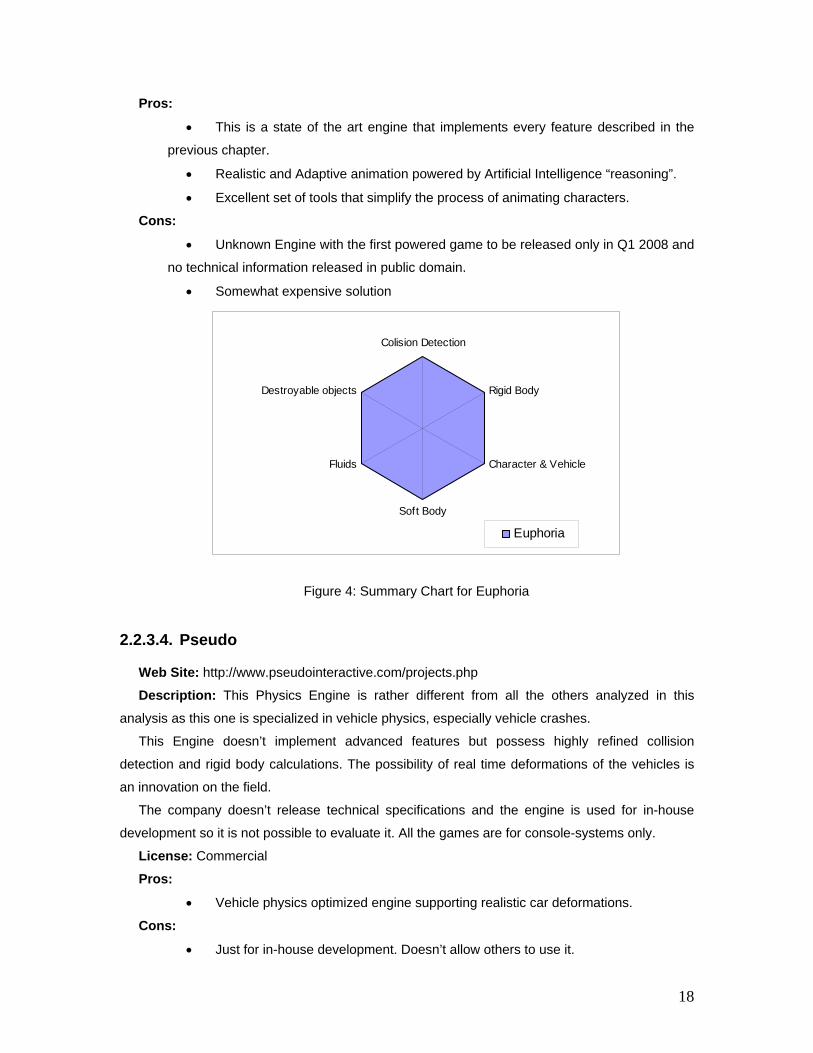
18
Pros:
• This is a state of the art engine that implements every feature described in the
previous chapter.
• Realistic and Adaptive animation powered by Artificial Intelligence “reasoning”.
• Excellent set of tools that simplify the process of animating characters.
Cons:
• Unknown Engine with the first powered game to be released only in Q1 2008 and
no technical information released in public domain.
• Somewhat expensive solution
Figure 4: Summary Chart for Euphoria
2.2.3.4. Pseudo
Web Site: http://www.pseudointeractive.com/projects.php
Description: This Physics Engine is rather different from all the others analyzed in this
analysis as this one is specialized in vehicle physics, especially vehicle crashes.
This Engine doesn’t implement advanced features but possess highly refined collision
detection and rigid body calculations. The possibility of real time deformations of the vehicles is
an innovation on the field.
The company doesn’t release technical specifications and the engine is used for in-house
development so it is not possible to evaluate it. All the games are for console-systems only.
License: Commercial
Pros:
• Vehicle physics optimized engine supporting realistic car deformations.
Cons:
• Just for in-house development. Doesn’t allow others to use it.
Colision Detection
Rigid Body
Character & Vehicle
Soft Body
Fluids
Destroyable objects
Euphoria

19
Figure 5: Summary Chart for Pseudo
2.2.3.5. Physics and Maths Library
Web Site: http://game-physics-engine.info
Description: This is a rather unknown physics engine that supports many aspects of a state
of the art engine although in a rather primitive way.
This engine hasn’t been used in any relevant video game and there aren’t any references to it
in the common gaming sites.
The documentation provided with the engine is scarce and in German. A Forum is also
provided but it contains almost no articles which indicate a very small community of users.
License: Commercial
Pros:
• This engine implements many features described in the previous chapter
although without great detail.
• Includes many templates of physics optimized models like cars, helicopters,
aircrafts and ships.
Cons:
• Lack of implemented games to show the capabilities of the engine
• Scarce documentation and community support (and the existing one is in
German)
• Inexistence of editing tools
Colision Detection
Rigid Body
Character & Vehicle
Soft Body
Fluids
Destroyable objects
Pseudo
20
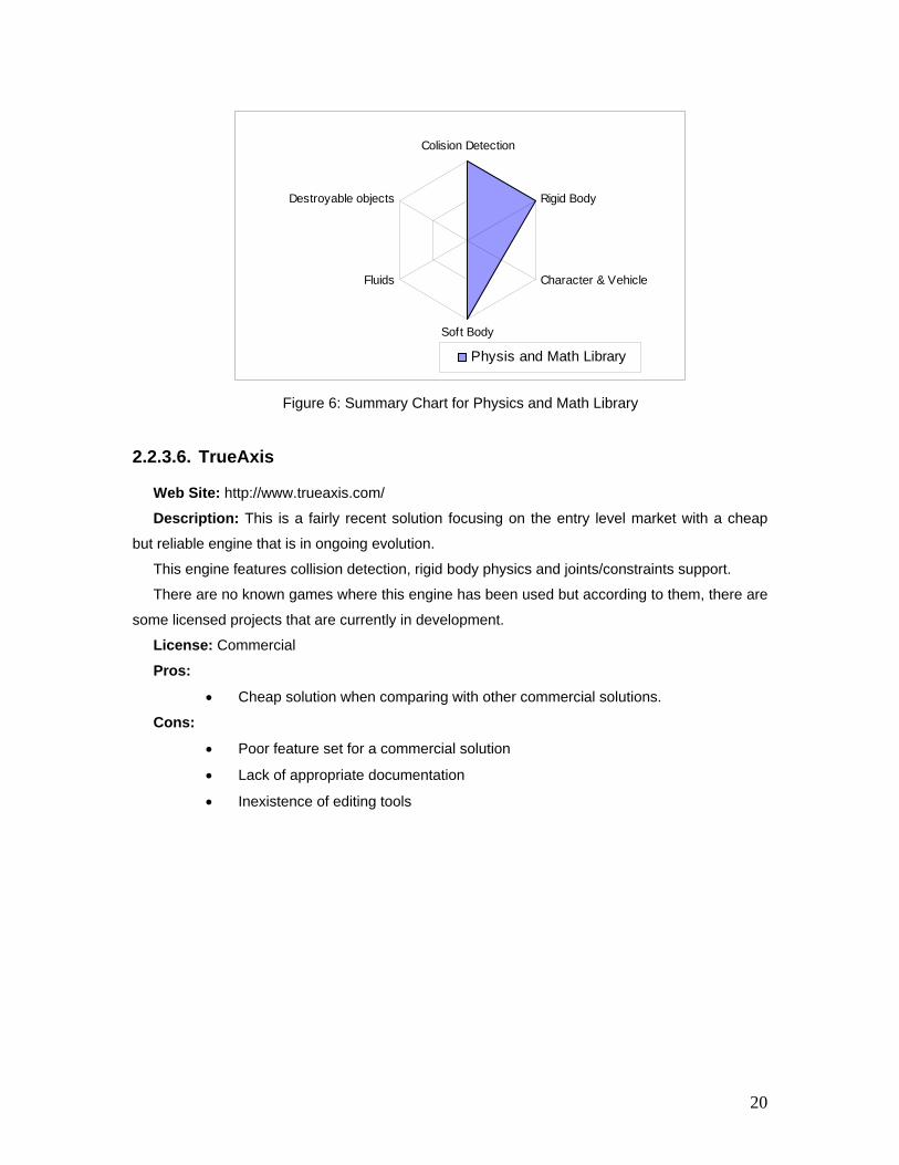
Figure 6: Summary Chart for Physics and Math Library
2.2.3.6. TrueAxis
Web Site: http://www.trueaxis.com/
Description: This is a fairly recent solution focusing on the entry level market with a cheap
but reliable engine that is in ongoing evolution.
This engine features collision detection, rigid body physics and joints/constraints support.
There are no known games where this engine has been used but according to them, there are
some licensed projects that are currently in development.
License: Commercial
Pros:
• Cheap solution when comparing with other commercial solutions.
Cons:
• Poor feature set for a commercial solution
• Lack of appropriate documentation
• Inexistence of editing tools
Colision Detection
Rigid Body
Character & Vehicle
Soft Body
Fluids
Destroyable objects
Physis and Math Library

21
Figure 7:Summary Chart for TrueAxis
2.2.3.7. Unigine
Web Site: http://unigine.com/
Description: UniGine is a powerful game engine composed of a graphics engine, physics
engine sound system and game logic and user interface design.
Speaking of the physics part, it offers all the features of a state of the art engine but according
to user’s opinion on different forums around the Internet, the overall performance of the engine is
quite disappointing.
There are no currently released games made with this engine, but there’s one in the
production phase – Afterfall (33).
License: Commercial
Pros:
• Complete solution to program a video game from scratch without having to pay
more fees for extra software.
• Excellent set of tools
• Good client support and documentation
Cons:
• There are no commercial relevant games made with this software.
• According to some users the performance of this system is not very good.
Colision Detection
Rigid Body
Character & Vehicle
Soft Body
Fluids
Destroyable objects
TrueAxis
22
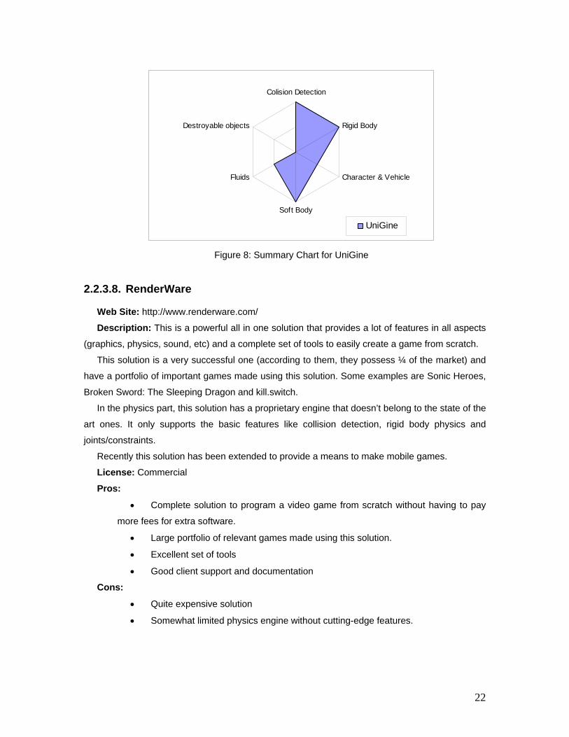
Figure 8: Summary Chart for UniGine
2.2.3.8. RenderWare
Web Site: http://www.renderware.com/
Description: This is a powerful all in one solution that provides a lot of features in all aspects
(graphics, physics, sound, etc) and a complete set of tools to easily create a game from scratch.
This solution is a very successful one (according to them, they possess ¼ of the market) and
have a portfolio of important games made using this solution. Some examples are Sonic Heroes,
Broken Sword: The Sleeping Dragon and kill.switch.
In the physics part, this solution has a proprietary engine that doesn’t belong to the state of the
art ones. It only supports the basic features like collision detection, rigid body physics and
joints/constraints.
Recently this solution has been extended to provide a means to make mobile games.
License: Commercial
Pros:
• Complete solution to program a video game from scratch without having to pay
more fees for extra software.
• Large portfolio of relevant games made using this solution.
• Excellent set of tools
• Good client support and documentation
Cons:
• Quite expensive solution
• Somewhat limited physics engine without cutting-edge features.
Colision Detection
Rigid Body
Character & Vehicle
Soft Body
Fluids
Destroyable objects
UniGine

23
Figure 9: Summary Chart for RenderWare
2.2.3.9. Open Dynamics Engine
Web Site: http://www.ode.org
Description: ODE is an open source physics engine that features rigid body physics, collision
detection and joints/constrains support.
This engine is the most popular open source and free physics engine, which makes it the best
documented and tested. Its development was stopped for some time but in the last two years it
has been revived and many improvements have been made.
It is the primary choice for small developers and that’s the main reason for the existence of a
large internet community.
It has been used in BloodRayne 2 [33] a very successful commercial game.
ODE is distributed under the GNU license, allowing everyone to use it freely in any
application.
License: Open Source/Free
Pros:
• Proven performance of the physics algorithms in dozens of projects – including a
special developed algorithm to prevent interpenetration between colliding objects.
• Most popular open source engine with good documentation and strong
community support.
• Easy integration with major graphics engines through the use of wrappers.
• Cross-platform support
• It’s free for any kind of use.
Cons:
• Quite difficult to configure and tune for realistic behavior.
Colision Detection
Rigid Body
Character & Vehicle
Soft Body
Fluids
Destroyable objects
RenderWare

24
• Lack of support for advanced physical effects (like soft bodies or water physics)
• Lack of pre-made templates for characters and vehicle physics. Effects like
ragdoll must be created by the games developer from scratch (using the joints and
constrains)
• Lack of visual editors.
Figure 10: Summary Chart for ODE
2.2.3.10. Newton Dynamics
Web Site: http://www.newtondynamics.com/
Description: This engine features rigid body physics, collision detection and joints/constrains
support. It is being constantly tuned for physics accuracy and increased performance.
This solution has a primitive built-in support for ragdolls and vehicle physics simulation making
it easier to set up.
It has a large community that provides plenty of support in addition to the extensive
documentation present on the site.
License: Free but Closed Source
Pros:
• Easy to use design of the framework. Developers tried to minimize the amount of
theoretical physics knowledge needed by the end-user to rapidly begin using the engine.
• Support for ragdolls and vehicle physics through ready to use functions.
• Extensive documentation and supporting community.
• Easy integration with major graphics engines through the use of wrappers.
• Cross-platform support.
• It’s free for any kind of use.
Colision Detection
Rigid Body
Character & Vehicle
Soft Body
Fluids
Destroyable objects
ODE

25
Cons:
• Lack of support for advanced physical effects (like soft bodies or water physics)
• Lack of visual editors
Figure 11:Summary Chart for Newton
2.2.3.11. nV Physics
Web Site: http://www.thephysicsengine.com
Description: This newcomer in the physics engine comes from the Middle East from a
company named Khayal Interactive Entertainment that specializes itself on developing custom
made games or parts of them using the outsourcing model.
The nV engine is part of that strategy and is in development for more or less one year and as
such it only features the basic collisions detections, rigid body physics and some
joints/constraints.
The documentation is basically a listing of the current API, because it is changing every day
as development goes on.
License: Free but Closed Source
Pros:
• May become a large player on the physics engines market in one year or two.
Cons:
• Poorly featured engine (as it is in development)
• Poor documentation
• No client support
Colision Detection
Rigid Body
Character & Vehicle
Soft Body
Fluids
Destroyable objects
Newton

26
Figure 12:Summary Chart for nV Physics
2.2.3.12. Bullet
Web Site: http://www.continuousphysics.com/Bullet/
Description: This open source physics engine features collision detection, rigid body and
joints/constraints and is in constant evolution. As a proof of that is the fact that recently a test
version has been released supporting some hardware physics calculation on the GPU.
In a near future this physics engine will be integrated with Blender (a 3D modeling tool [34]) to
provide easy to use physical effects to the developers.
License: Open Source
Pros:
• Fast developing open source engine – it is the most advanced engine on the
open source world.
• Great documentation and community support
Cons:
• Lack of support for advanced physical effects.
• Lack of developing tools.
Colision Detection
Rigid Body
Character & Vehicle
Soft Body
Fluids
Destroyable objects
nV Physics

27
Figure 13: Summary Chart for Bullet
2.2.4. Physics Engines Analysis
To be fair while comparing the solutions we separate those between the commercial ones that
are financed and developed with a commercial intuit (either now or for a future commercialization)
and the ones fully open source that are developed by good will developers.
Table 1 summarizes the commercial solutions described in this paper. CS/Free stands for
Closed Source but free for non commercial use and C stands for Commercial.
Table 1: Commercial Physics Engines
From this chart and from the pros and cons of every engine we conclude that Havok and
Ageia are currently the best Physics Engine solution available on the market. Euphoria
Colision Detection
Rigid Body
Character & Vehicle
Soft Body
Fluids
Destroyable objects
Bullet
28
theoretically is at the same level of the other two but there is no way to prove that as no
nowadays game uses it and there are no benchmarks available.
Both engines support hardware acceleration but each one according to their personal view as
discussed earlier (either using the GPU capabilities or introducing the PPU).
It is also interesting to note in the field of “all-in-one” solutions Unigine appears to be
technically superior to RenderWare although this one has a vast portfolio of successful games
using it.
Pseudo is a very good Physics Engine if the developers are only interested in vehicle realism
as it is highly optimized for that field.
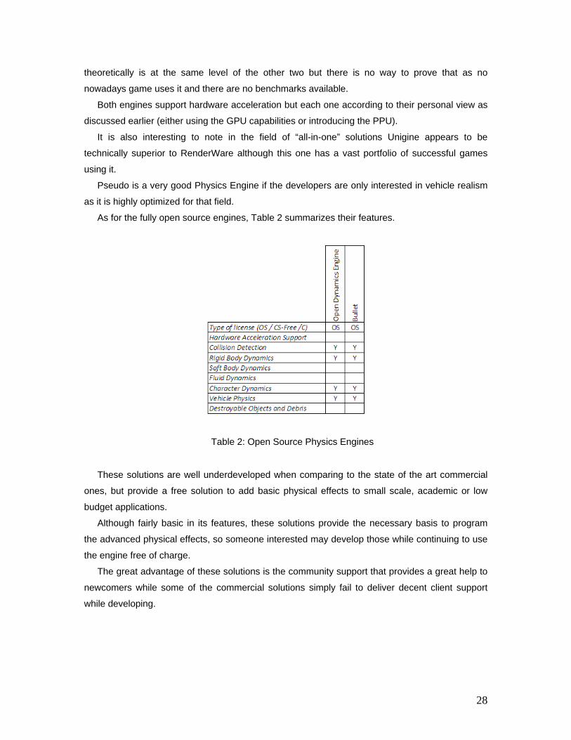
As for the fully open source engines, Table 2 summarizes their features.
Table 2: Open Source Physics Engines
These solutions are well underdeveloped when comparing to the state of the art commercial
ones, but provide a free solution to add basic physical effects to small scale, academic or low
budget applications.
Although fairly basic in its features, these solutions provide the necessary basis to program
the advanced physical effects, so someone interested may develop those while continuing to use
the engine free of charge.
The great advantage of these solutions is the community support that provides a great help to
newcomers while some of the commercial solutions simply fail to deliver decent client support
while developing.

29
2.3. Summary
In this chapter we presented the physics engine and a slight overview of their evolution. We
described the most important features of a state of the art engine as well. They are: collision
detection, rigid body dynamics, character/vehicle dynamics, soft body dynamics, fluids dynamics
and destroyable objects and debris.
We also analyzed and compared the most important solutions available on the market and
used in basically every video game and virtual world simulation. This analysis revealed the great
gap in quality between the commercial solutions and the open-source ones. The main reason for
this difference can be explained by two factors. First, the knowledge needed to implement highly
complex physics is enormous and requires many specialized personnel and tools. Secondly, the
high competitivity of the market requires a great secrecy and protection of the physics algorithms
thus diminishing the possibility of being implemented on open-source distributions.
From the analysis Havok and Ageia share the podium as the most advanced solution
available on the market today. They both implement all the advanced features presented in this
analysis and are fast evolving solutions that are leading the market to hardware accelerated
physics.
Focusing on the open source engines, Bullet and ODE are equivalent. ODE may turn out to be
the best choice in some cases due to the stronger community support and the many already
made plug-ins and connectors to other software.

30
31
Chapter 3
A Generic Physics System
In this chapter we present our solution for the scalability problem. We start by studying the
typical physical simulation cycle and analyzing how physics and graphics can be separated. We
then proceed to explain the main physical concepts that we defined from studying classical
physics and the current physics engine (in the analysis presented on the last chapter). Finally we
present a conceptual model of our solution where we expose the concepts and their relations.
Before starting this chapter we must explain the scope of this work. From our previous
analysis we identified six major physical concept dimensions:
• Collision Detection
• Rigid Body Physics
• Character & Vehicle Physics
• Soft Body Physics
• Fluids
• Destroyable Objects
Looking at the studied engines we state that the great majority only implements the first three
dimensions and the open source solutions only support those same dimensions. Being this work
developed in an academic context it was decided to give priority to open source solutions. That
way and due to time constrains, this work focuses on developing an abstraction of physical
concepts related solely to Collision Detection and Rigid Body Physics.

32
3.1. Simulation
In a virtual world application the typical simulation cycle is made of four simple stages pictured
on Figure 14.
Figure 14 : Typical Virtual World Simulation Cycle
The cycle starts by processing user input such as moving the camera, applying forces,
selecting objects and creating/destroying objects. Following this, Physics are updated so the
collision detection is processed, forces are applied to objects and new positional/rotational
information is calculated for every entity. After Physics, Graphics is processed. In this stage pre-
rendered animations are updated and all graphical information like shaders and shadows are
calculated. Finally the entire World is rendered to screen via the active camera. This is a typical
simulation cycle for a virtual world simulation.
Figure 15 : Physics Update Stages

33
Due to the nature of physics engine, implementations often mix the Physics Update/Graphics
Update stages in one big Application Update stage. This is because physics processing is done a
par with graphics processing.
Analyzing the Physics Update stage we can see that it consists in several sub-stages pictured
on Figure 15. During an update, collisions are detected and motion is altered according to
different parameters like friction and mass. Forces are also applied to the entities and motion is
calculated using classical physics formulas [4]. Finally, the joint contribution of collisions and
added forces result on new positional information for every entity. The order of events may be
different from the one on Figure 15 but the final result of the physics update stage is new
positional/rotational information for every entity on the world.
In light of this knowledge we can separate graphics from physics by making sure that each
update remains independent from each other and passing the positional data through our
abstraction. This way the simulation cycle of our system, displayed on Figure 16, adds a new
stage that does the data transition between physics and graphics.
Figure 16 : Simulation Cycle in our System
To assure the correct separation of physics from graphics our abstraction is designed in a way
that no graphical information is used in physics calculations. All information needed from physics
processing to update graphics is passed through our abstraction as well.

34
3.2. Concepts
Since this work is focused on rigid body physics, it is imperative that we start our concept
collection with Newtonian Physics [4]. These concepts are universal and therefore are common to
every physics engine that supports this feature.
Besides physical concepts there are other concepts that we must include in our abstraction
which we called system concepts. They are related to the way physics engines are structured and
were discovered when we studied their internal architecture mainly from the open source ones.
Following, we present a description of every concept used in our solution.
3.2.1. Physical Concepts
Working with classical physics (Newtonian Physics) the domain we’re working with is Motion.
Motion is a change in position of a body relative to another body or with respect to a frame of
reference or coordinate system. Motion occurs along a definite path, the nature of which
determines the character of the motion. [35]
To define the motion of an object we must also define the following Newtonian concepts.
3.2.1.1. Force
The main concept behind classical physics is Force.
In physics, (Force is) a quantity that changes the motion, size, or shape of a body. Force is a
vector quantity, having both magnitude and direction. The magnitude of a force is measured in
units such as the pound, dyne , and Newton , depending upon the system of measurement being
used. [36]
Force is the way bodies interact with each other and motion is generated. In our scope, with
rigid body physics, we limit our forces to change of the body’s motion state. The change in size
and shape is the domain of soft body physics.
There are two types of forces:
• Internal Forces – these forces occur inside a body and are irrelevant to its
motion. In rigid body physics we discard these forces.
• External Forces – these forces are exerted from the outside of the body and do
affect its motion. These forces may result from a collision, from attraction (like gravity) or
be user defined forces.
In a certain instant, a body is subject to several forces. For calculation purposes we use the
Net Force Vector. This is a pre-calculation where we calculate the resulting force to be applied to
the object. We add all forces contributions to get one simple, final force vector.

3.2.1
As
a cha
rotatio
mapp
a rota
Kn
calcul
Ca
Le
rectam
Th
body
Ma
W
Us
later o
Us
from t
1.2. Positio
s seen previo
ange in posit
onal effects.
ped in the Car
ation matrix.
nowing the fo
late the next s
alling upon Ne
ex II: Mutation
m qua vis illa
he rate of cha
and is in the
athematically
here:
sing our know
on this section
sing the equa
this one its ne
on/Orientat
usly motion im
tion that occu
The position
rtesian coord
rce to be app
state of motio
ewton’s secon
nem motus pr
imprimitur.
ange of mome
same directio
this law trans
Net force
Mas
Acceler
Veloc
Displace
Tim
wn net force v
n) we can cal
ations of motio
ew position an
tion
mplies a chan
urs. A chang
n of the obje
inate system.
plied to a bod
on. The proce
nd law of mot
roportionalem
entum of a bo
on. [37]
slates into the
vector
ss
ration
city
ement
e
vector and the
lculate the res
on and the a
nd orientation
nge in the pos
ge on the bo
ect consists
. The Orienta
dy, and its cu
ess to do this
tion – the law
m esse vi mot
ody is proport
e well known
e body’s mass
sulting accele
cceleration w
n.
sition of the o
ody orientatio
in a three d
ation is usually
urrent position
is using acce
w of acceleratio
trici impressa
tional to the r
formula:
s (the concep
eration.
we can compu
object. In real
on happens a
dimensional
y represented
n/orientation i
lerations and
on:
e, et fieri sec
resultant force
pt of mass wi
ute the body’s
3
lity it is not jus
as well due t
vector usual
d in physics b
sn’t enough t
velocities.
cundum lineam
e acting on th
ll be describe
s velocity, an
35
st
to
ly
by
to
m
he
ed
nd

36
The Equation of motion for a linear movement is calculated using the following formula:
Where:
New Position
Current Position
Linear Velocity
Time Interval
Linear Acceleration
In the case of the angular movement, the previous formula adapts as follows:
Where:
New Orientation
Current Orientation
Angular Velocity
Time Interval
Angular Acceleration
This is clearly a second level differential equation system.
As it was explained in the previous chapter, physics engines calculate these values using a
number of generic Ordinary Differential Equations (ODE) solvers. The most common methods are
the Euler method, a variety of Runge-Kutta methods, Midpoint method, and implicit methods [16].
3.2.1.3. Torque
Forces may be applied anywhere in the body. If applied in the center of mass, the generated
movement will always be of a linear type. There will be no rotation. If we apply a force anywhere
else on the object, depending on the objects geometry, we have a resulting rotational movement.
The responsible force is named Torque. It is a special kind of force that only changes the
37
rotational movement of an object. For instance, if you apply a torque to a stopped object, it will
start spinning around the given axis.
3.2.1.4. Inertia
Newtonian Inertia is a property that measures the way an object resists the change to its state
of motion. This concept was discovered by Isaac Newton and was formalized in its first law of
motion:
Lex I: Corpus omne perseverare in statu suo quiescendi vel movendi uniformiter in directum,
nisi quatenus a viribus impressis cogitur statum illum mutare.
An object at rest will remain at rest unless acted upon by an external and unbalanced force.
An object in motion will remain in motion unless acted upon by an external and unbalanced force.
[38]
The direct consequences of this law are:
• An object that is not moving will not move until an external force acts upon it.
• An object that is in motion will not change its velocity (accelerate/decelerate) until
an external force acts upon it.
Inertia varies with every object. Some present a higher resistance than others. The factor that
alters inertia is the next concept we will describe - Mass.
3.2.1.5. Mass
The concept Mass can be explained as the quantity of matter that a certain object possesses.
The quantity of Mass in a rigid body is always constant because breaking objects are not
considered.
One should not misunderstand Mass with weight as the common sense sometimes misleads
us. Weight is nothing more than the action of gravity in an object (of course affected by its mass).
It varies with gravity but mass is always constant whether in Earth or in the Moon.
In physics, associated with mass, there is the concept of Center of Mass. That’s an imaginary
point where we consider all the mass of the object concentrated and where we apply every
external force that the body suffers. If we have a constant distribution of mass, the center of mass
corresponds to the geometric center in space. In reality this is not what happens since bodies
have variable distributions of mass. In cases like this the center of mass can be calculated, for
example, having the densities of the materials in consideration.
In real life, engineers try to manipulate the center of mass to achieve certain effects. An
example is the racing cars. Engineers make the car the lightest possible and then attach
38
additional weight to the bottom to increase stability in curves, lowering the center of mass. The
same goes with boats.
Mass influences the Inertia factor of a body. High mass means that an object will offer a great
resistance to a change of its movement (high Inertia). A low mass means the opposite; it will offer
little resistance and thus react faster to an external force.
This effect can be also explained using Newton’s second law of motion – the law of
acceleration:
The rate of change of momentum of a body is proportional to the resultant force acting on the
body and is in the same direction.
As one can see, the greater the mass of the object, the greater the force must be to generate
some specific acceleration.
Until now we only described Mass as a factor influencing linear movement (translation). Mass
also influences rotational movement based on its distribution throughout the object. In classical
physics this is called Moment of Inertia or Angular Mass. It measures the rotational Inertia of an
object (resistance to change of its rotational motion state). Mathematically in our 3D world, this
translates into a 3x3 Matrix that contains the moment of inertia for each axis (x, y and z).In
Physics this matrix is called the Inertia Tensor.
Consider two discs with different radius. Disc A has a larger radius than disc B. Considering
equal Mass in both discs and similar distribution, Disc A will present a higher “rotation Inertia”
because its mass is distributed further from the rotating axis. This means Disc A has a higher
moment of Inertia that Disc B.
3.2.1.6. Friction
Friction is a force that goes against any movement by a body when in contact with other body.
It is the force responsible for the common slowing down that we experience every day.
This force has a maximum that is determined by the body surfaces type and the force
between them (Normal Force). There are two types of friction:
• Static friction – it is present when the bodies in contact aren’t moving. To start
moving the applied force must be higher than this static friction. If it is lower the objects
will not move.
• Kinetic Friction – it is present when the bodies are already in motion and rubbing
together. This friction is usually lower than the static friction. This gives truth to the

39
common sense observation that it is harder to start moving something than to keep it
moving (like pulling something).
The classical approximation to friction and that is used in physics engines is the Coulomb
Friction. The equation is as follows:
Where:
Force exerted by
friction
Coefficient of friction
Normal Force
The coefficient of friction is a scalar that defines the “amount” of friction that two specific
surfaces generate when in contact. The coefficient of friction is an empirical measurement. It has
to be measured experimentally, and cannot be found through calculations. Typical values range
from almost zero (low friction) to great friction with values near 2. An example of low friction is
rubber on ice with 0.15 and a high friction example can be a tire on concrete with 1.7.
The coulomb friction model isn’t a perfect one. A good case where it fails corresponds to
adhesive surfaces. Independently of the normal force, the friction in this case is always the same
and dependent on the adherence. The coulomb friction cannot correctly model these cases as it
uses the Normal force in its calculations.
3.2.2. System Concepts
All the above defined concepts are present in every physics engine but come directly from
Classical Physics. The following concepts share some connection to Physics but have a more
Engineering Nature. Some of them came directly from the analysis of the physics engines while
others result from our previous knowledge on physics simulation. They encapsulate all the
components needed to the correct functioning of the simulation.
3.2.2.1. Entity
The entity is the basic building block of our abstraction. Every object of the virtual world is a
specialized entity. It contains the physical properties, constrains, geometries and information
about the object. Apart from the physics component it also contains all the information relative to
graphics, sound, artificial intelligence and input/output.
It manipulates its information and allows the world to access it to further calculations.

40
3.2.2.2. World
The most generic concept in a physics engine is the World. This is analogous to our “Nature”
in which it contains just about everything that exists and knows how they interact. The World is
responsible for managing every component of the simulation (graphics, sound, artificial
intelligence and input/output) and for the simulation cycle. As such to take knowledge of all
existing entities, they must be registered so that the World may control it accordingly.
There may be many Worlds defined in a simulation but if the user wants two entities to belong
to two different Worlds, they must be registered independently. We should note that entities from
one world don’t interact with the others in a different World.
3.2.2.3. Stepper
The Stepper is a special part of the World that is solely responsible for processing the physics
simulation. Given some time value, the Stepper looks at the Entities registered in the World and
calculates their new positions/orientations. These calculations are based on the net forces that
every entity report. These forces may be the result of a global force (gravity), collision reaction
force or user-made force. Collision Detection is also managed by the Stepper.
The time value passed on to the Stepper may be a constant time increment or a variable one.
The difference between them resides on simulation synchronization. If we have a computer
running the simulation at 30 frames per second, and in each frame the simulation time increases
by a factor of 0.1 then after 10 seconds our simulation is at time 3. If we have another computer
running the simulation at the same time but at 15 frames per second, then 10 seconds later we
have the simulation at time 1.5. To synchronize them we use variable time steps where the first
computer would use a time step of 0.1, the other one would use a time step of 0.2. These
calculations can be done automatically, by measuring at each cycle the time consumed to
calculate it.
3.2.2.4. Collision Geometry
Collision detection requires heavy computational resources when many objects are present.
To simplify and accelerate the collision detection mechanism we use simple geometric forms that
surround each object. When processing collisions, these geometries replace the real object and
because of their simpler design are faster to calculate. The performance increase comes at the
cost of realism and collision accuracy. It is frequent to see two objects penetrating each other
before detecting the collision. In the majority of the applications the great performance gain
compensates for the lack of accuracy.
41
The most used collision geometries are:
• Sphere
• Box
• Cylinder
We can also use the graphical geometry information to make a custom collision geometry that
fits the object.
3.2.2.5. Collision Space
Imagine we have one thousand entities in our world. When checking for collisions, and
depending on the collision detection method, we may have to check every entity against all of the
other. This gives a number of one million collision checks every simulation step that turns
troublesome for our computers in heavy simulations.
A good way of accelerating the simulation is to do processing culling. Using techniques like
space partition we can “foresee” which objects may collide and just process those ones. These
techniques are automatically done by the physics engine with little interference from the
developer.
To further increase performance, developers may use Collisions Spaces.
A collision space is a group of collision geometries that belong to a logical group that we know
will never collide with each other. This way the physics engine never checks for collisions
between those geometries and furthermore can optimize the collision detection between this
space by assuming it to just a great geometry made of the fusion of all its components.
A perfect example is an automobile. Imagine you are doing a racing simulation. Let’s assume
that internal collisions between the automobile components can be ignored. This way we group
all geometries of the car in a collision space and this way in the point of view of the Stepper, the
car is nothing more than one great geometry. If the Stepper detects a collision with the space
then it will do a second check to clearly discover which geometry effectively collided. The great
achievement is that in the majority of checks there are no collisions so we never do the second
check that is heavier to compute.
3.3. Conceptual Model
With our concepts clearly defined we proceeded to define the relationship among them. The
way they are connected and how they interact and influence the simulation.
Our conceptual model is divided in two parts. The first one is responsible for managing the
simulation cycle and the simulation general settings. The second part defines the physics
component of our Entity. Note that the graphics part is not present in our conceptual model as it
was not the focus of our work.

42
Figure 17: Conceptual Model: Simulation Control
The diagram presented on Figure 17 illustrates the simulation controller of our abstraction.
The main concept is the World that controls the entire simulation cycle and contains all entities
existing on the virtual world. Under the control of the World are also the physics and graphics
managers. They are responsible for setting up the environment to correctly process both physics
and graphics, accordingly. General settings are defined through the managers.
As for our Entity the diagram in Figure 18 illustrates how it is structured. The Entity is
composed of two main blocks, one responsible for physics calculation and the other for graphics
calculation. Once again the graphics block has not been included in our conceptual model
because it is not our focus. The Physics block is rather complex and defines all the properties our
entity must have to be able to calculate physics behavior.
Figure 18 : Conceptual Model: Entity
The most basic information needed, consists on positional and rotational information. This
information is updated in every simulation cycle in result of the other components. In order to
allow interaction we apply forces of which torque is a special case. We also have the inertia

43
concept, extremely necessary to calculate motion on which mass is included. Finally to make
collision detection possible we have multiple Collision Geometries, with friction being a major
parameter that influences the way objects react to collision.
With this conceptual model we provide the answer to our problem. We have developed a
model based on the very foundations of classical physics. We used the same concepts that Isaac
Newton discovered on the XVIII century and added the engineering concepts needed to perform
a simulation on the computer. This way we have a generic model where every physics engine
that supports rigid body physics can theoretically be mapped.
In Appendix A we present the diagram of our complete conceptual model.
3.4. Interface Architecture
Our conceptual model gives us the theoretical solution to our problem. To make it usable we
need to transform the conceptual model into a programming interface. This chapter describes
how we mapped the concepts and their relations into an object oriented interface system.
From our conceptual model, the first step to translate it into a programming interface was to
directly map the concepts into interfaces. Figure 19: Final Interface Architecture illustrates this in
a UML [39] diagram.
As can be seen, the majority of the interfaces correspond directly to the conceptual model. In
spite of that, there are concepts that have not been converted into interfaces and others that
appeared for the first time.
So in summary the major changes were:
Some concepts were merged into another interface:
• The Torque concept was included into the IForce Interface. We decided to merge
them as Torque is a special type of Force and the methods used to control it don’t
justify an Interface on its own.
• The Mass Interface was included into the IInertia Interface. For simulation purposes
the concept of Mass and Inertia is very close. Often they are treated as one. For this
reason we decided to merge these concepts into one interface.
• The Friction concept was included into the ICollisionGeometry Interface. When a
collision happens, the physics engines deal directly with the collision geometry.
Having the friction properties directly accessible on the ICollisionGeometry interface
provides an easier access to information and reduces information overhead.
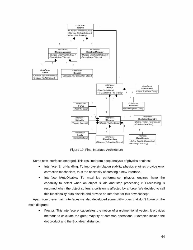
44
Figure 19: Final Interface Architecture
Some new interfaces emerged. This resulted from deep analysis of physics engines:
• Interface IErrorHandling. To improve simulation stability physics engines provide error
correction mechanism, thus the necessity of creating a new interface.
• Interface IAutoDisable. To maximize performance, physics engines have the
capability to detect when an object is idle and stop processing it. Processing is
resumed when the object suffers a collision is affected by a force. We decided to call
this functionality auto disable and provide an Interface for this new concept.
Apart from these main Interfaces we also developed some utility ones that don’t figure on the
main diagram:
• IVector. This interface encapsulates the notion of a n-dimentional vector. It provides
methods to calculate the great majority of common operations. Examples include the
dot product and the Euclidean distance.

45
• IQuaternion. This interface encapsulates the notion of a quaternion [40] and provides
methods to common operations like transitions from quaternion to a rotation matrix
and vice versa.
• IMatrix. This interface encapsulates the notion of a two dimensional NxN matrix and
provides methods to common operations like setting the identity matrix or inverting the
matrix.
Once the interface architecture was concluded we proceeded on to the interface’s methods
definition. We did it by using the knowledge acquired with our related work and by analyzing
several physics engines API1. We chose the methods carefully to make sure they were generic
and essential to a rigid body physics simulation.
3.5. Summary
In this chapter we presented and described our solution to our problem. We started by
studying the simulation cycle and the way information flow along that cycle. We stated that
currently physics and graphics processing were done as one cycle stage instead of two separate
ones. In our solution we decided that the physics processing calculates positional data without
access to any graphical information. This positional data is then passed on to the graphics for
render by our abstraction. This way we guarantee that physics and graphics processing remain
independent and the information flows only through our abstraction.
Following this, we studied classical physics and jointly with the information gathered from the
related work we identified the key concepts needed to setup and run a physics simulation. With
these concepts we developed our conceptual model. Being developed based on generic physical
concepts our solution is theoretically common to physics engines featuring rigid body physics.
This fact makes them adaptable to work with our model and therefore upgrading applications
become easier as all we need to do is to connect a new physics engine to our model.
Applications developed with our solution remain functional because they use generic concepts.
In this chapter we also described how we developed an interface architecture from our
conceptual work. We started by mapping each concept into an interface and after further analysis
we decided that some should be merged and others created. The new interfaces came from
analyzing some physics engine’s APIs. Some auxiliary interfaces were also developed to
encapsulate concepts like vectors, quaternion [40] or matrixes.
1 API stands for Application Program Interface. It is a set of routines provided in libraries that gives access to lower-level functions in a organized way.

46

47
Chapter 4
Case Study
In this chapter we will explain how we implemented our interface using two engines and how it
allowed us to develop a small world editor featuring physical behavior.
The interface implementation required different technologies to be put together. This became
the greatest difficulty in this phase. We also present a small example, with source code, where
we are able to see how simple our interface has turned the development of physical applications.
Our small editor was built exclusively using the previous implementation of our interface for
handling the physics processing.
4.1. Interface Concretization
4.1.1. Technology
Concretizing our interface system required a myriad of technologies. Some were mandatory
because they were part of this work initial description while others were chosen according to their
features and suitability for an academic work.
From the start of this work we have decided that our interface system was to be implemented
using the .Net Framework. The main reason behind this decision has to do with the research
group where we developed this work. In the group there are many applications developed with
the .Net Framework and this way we make it possible to integrate physics effects into already
existing applications.
To make our interface system usable, we need to implement it using real engines. For
graphics processing the engine used was Ogre3D [41]. Once again the main reason for this
choice was the fact that at our group, existing applications use Ogre3D to process graphics.
Furthermore there is another reason that makes this choice even better. Ogre3D is a free open
source engine. This way we can alter the source code as necessary and learn from it.
For the physics processing we decided to use Open Dynamics Engine usually called ODE
[42]. This choice was primary based on the results of our related work and the limitation imposed
by the research group of using open source solutions. We decided to use ODE over Bullet due to
the better documentation and the fact that we had an already implemented solution where ODE
was integrated with Ogre3D. This integration was done by Tuan Kuranes and is free to use and
modify [43]. This existing integration provided a looking window to start studying the way Ogre3D
and ODE works.

48
Concretizing our interface system required three programming languages to be used and
learnt. ODE interface is written in C and Ogre3D in C++. The already existing integration gave us
a C++ interface to ODE so we can assume that both engines are written in C++.
Focusing on .Net Framework our interface system needed to be compatible with the CLR
(Common Language Runtime) [44], the virtual machine of Microsoft .Net Framework. This
brought about a problem because C++ is not directly supported on CLR as it has no automatic
memory management. To solve this problem we used a new version of C++ called Managed C++
[45] to create a wrapper between the engines C++ code and the CLR.
Basically our interface was implemented using Managed C++ and connected with the engines
native code when needed. The main disadvantage of having to use the wrapper is that further
overhead of objects is created as we need to have managed objects and native objects running
at the same time.
Compatibility with CLR means that every .Net Language may be used to develop using our
interface. However we chose to develop using C#, once again because it is the de facto
programming language at our research group.
Finally one last note on the integration between Ogre3D and ODE that we used. Besides
providing a C++ interface for ODE, it also provided a conversion between Ogre3D and ODE data
types. For instance, in Ogre3D rotations are represented as quaternions [40] while in ODE they
are represented as rotation matrixes.
During development the integration was slightly changed by us in order to implement missing
features or correct bugs.
4.1.2. Implementation Decisions
Implementing our interfaces consisted in developing the Managed C++ classes that provided
the functionality of the interfaces methods. This was a process that ranged from directly calling an
ODE function to more complex operations that required the saving of state information and calling
several ODE functions. Besides that there some decisions we made while developing.
First of all we decided that we wanted a generic World and Entity class. The main advantage
of this decision is that we may attach and detach managers to our World as we please. In our
specific case of physics, in the limit, we can do something weird as to use a different engine for
each step. All in runtime and by user command. But due to the intimate relation existing between
the managers and the Entities components we must be careful when doing this. We must
guarantee that the Entities components match the Manager type. If this doesn’t happen the Entity
isn’t processed has the manager doesn’t recognize a compatible physics component.
Figure 20, explains two correct combinations of Managers/Entity Components and one
incorrect. Each arrow means that the Manager/Component is registered and active (thus the use

49
of a double arrow) on the World/Entity. The example supposes we use Ode and Havok Physics
Engine.
Figure 20: Example combination between Physics Managers and Entity Physics Components.
Besides changing managers in runtime we can turn them on or off by simply attaching and
detaching them from the World. As the application state is stored in the World and in the Entity
classes we can do any manager change without compromising the simulation.
The second important decision deals with performance. To increase it we collapsed several
Interfaces into the same class. This is especially true for the Physics class that besides IPhysics
implements the IAutoDisable, IErrorCorrection, IForce and the IVelocity interfaces. For the
developer all remains equal because he works with the interfaces. From our point of view we get
a performance gain by eliminating a great deal of overhead due to the creation of unnecessary
class instances.
The schema on Appendix B provides a full overview of the implemented classes.
4.1.3. Event Handling System
Our event notifying system provides the developer with an easy to use way of knowing exactly
what is going on the simulation. This way the developer gets all the information he needs without
having to directly question each object repeatedly. Based on the event information the developer
can react accordingly or simply inform the application user.

50
Our event system consists in the implementation of the observer design pattern. Figure 21
pictures the way the developer interacts with our event system. It is also how the Observer
Pattern works.
Figure 21: Example of Interaction with the Event System
Some interesting object provides events to the developer. In our example we are using an
Entity providing three events. When someone feels the need to know when that event occurs,
they register themselves to the event on the Entity. As simulation runs if the event happens, the
Entity notifies every registered user that it happened and sends in additional useful information.
With this information the user may react by simply consuming the data or changing the
application status (or simply the Entity from where the event occurred).
In our implementation only Entities and the World possess events. This way global events like
“detect all collisions” are detected on the World and local events like “detect this Entity’s
collisions” are detected on the Entity.
Currently we have implemented some events. The most important event is collision detection.
When an object collides with other object the user is informed of the colliding entities and contact
information like friction and bounciness.
Another useful event is to warn when an entity becomes inactive or becomes active. This has
to do with the AutoDisable function described earlier. Finally we have another set of events to
indicate when the entity is moving or rotating.
Our event system is designed to be expanded with easiness. We used a feature of the C#
language called generics [46]. Generics enable the definition of algorithms and pattern
implementations once, rather than separately for each type. This way we implemented generic
event listeners so that to add a new event the developer just need to do three steps.

51
First of all define the callback function to be called when the event happens. Secondly,
instantiate a new event listener using the new callback. Finally find in the code where the event
may happen and trigger the notify action of the event listener when it happens.
4.2. Programming with Concepts
Having our interface system implementation using Ogre3D and ODE we must test its
capability to develop applications. Developing with our interface is really easy and fast. Following
is a small example where we setup the simulation and create some entities.
The first step towards our goal is to define a World. In the example below we decided to add a
Graphics and Physics Manager. We could add just one of them or even none and add them later.
We also define the default collision space and the default stepper to use. In this case we chose a
OdeSimpleSpace and a OdeQuickStepper, both being ODE-specific implementations for the
generic concepts.
//Creation of a World ION.Environment.World wrl = new World(); //Creation of the Managers GraphicsManager gfx = new OgreGraphicsManager(); PhysicsManager phx=new OdePhysicsManager(); //Registering the Managers on the World wrl.graphics = gfx; wrl.physics = phx; //Creation of the Collision Space Space spc=new OdeSimpleSpace(); wrl.physics.baseSpace = spc; //Determining which stepper to use
wrl.physics.activeStepper = OdeQuickStepper.getInstance();
Now we have a World and two registered managers. All objects were created using default
values. For instance the Physics Manager class automatically defined gravity as 9.8. Running this
source code will result at nothing as we have not called the simulation cycle. The simulation cycle
can be defined in its simple form, using the World or in its complex form using directly the
managers:
Using the simplified form:
while (wrl.render())
wrl.update();

52
It is as simple as it gets. We update everything and render the objects. The application’s
stopping condition was defined to come from the render function.
The complex way that gives full control over the simulation is:
while (wrl.graphics.render()) { wrl.physics.step(); wrl.synchronize(); wrl.graphics.update();
}
Here we see the different phases of the simulation cycle divided. First we calculate positional
data on the physics, then we synchronize physics with graphics using the world and finally we
update the graphics component.
Right now we have an application that displays our world without anything more as can be
seen on Figure 22.
Figure 22: Application Screenshot. We created the World, Managers and defined the application
cycle.
Right now we only created the World and the Managers for the physics and graphics
components. To make things interesting we must add objects to the World and see them interact.
To create an Entity is quite easy. In the following example we create an Entity and add a visual
representation to it (no physics effects).

53
//Creation of the Entity Entity ent = new Entity(); //Creation of the graphics component ent.graphics = new Graphics(); //Creation of a Graphical Mesh (Graphical Geometry) //and inclusion on the Graphics Component Mesh mesh1 = new Mesh("ball.mesh"); ent.graphics.meshes.Add(mesh1); //Entity Registration on the World
wrl.entities.Add(ent);
As a side note on our Ogre3D/ODE implementation we created some graphical helper objects
that weren’t described on the previous chapter as graphics isn’t our focus. Besides that we should
only note that if we create an Entity and don’t register it in the World, it doesn’t exist in practice.
The final result of this simple code is pictured on Figure 23.
Figure 23: Example Application where we added an Entity with a graphics component using a
Crate Mesh.
As of now we only have a static object that doesn’t move. To add Motion we will use our
Physics component.
The necessary code to add physics effects to our Entity is as follows and really shows concept
programming [47]:

54
//Creation of an Physics Component ent.physics = new OdePhysics(); //Setting the Inertia Settings //In this case a Mass value of 1 is used and the Mass Distribution is of type Box ent.physics.inertia = new OdeBoxInertia(1,mesh1.boundingBox); //Setting a Collision Geometry //In this case we use a Box Geometry and attach it to the main collision space defined in the beginning of the simulation - spc CollisionGeometry geom = new OdeBoxCollisionGeometry (mesh1.boundingBox,spc); //Adding the Collision Geometry to the Entity ent.physics.collisionGeometries.Add(geom);
As we see it is really easy to add physical behavior to our Entities. To sample test this we will
position the crate a little bit up so that it will fall down on the floor under the gravity force. For that
we change the following property:
ent.position = new Vector3D(0, 20, 0);
Now the resulting animation develops as pictured on Figure 24.
Figure 24: Physics Enabled Object: The Crate object is moving due to the gravitational force.
This is the simpler example we can program using our Interface System. Note that the
collision with the floor occurs because the Physics Manager creates an infinite plane simulating
the floor as default.
To finalize this section we present a more interesting simple example. Now we will have the
same crate stationary on the floor and will add a Ball Entity that is positioned in an upper position
and slightly to the right. The setup is pictured on Figure 25.
Adding physics components to the two entities we get the sequence pictured on Figure 26.

55
Figure 25: Final Application Example: Only graphically enabled object. They don’t move yet.
Figure 26: Final Application Example. Example interaction between a Ball and a Crate Entity.
As you can see we reduced the complexity of creating physically enabled objects because
using our interface the programmer only deals with physical concepts and abstracts him from the
implementation details. For example defining a box mass distribution may be an extremely

56
complex thing on the ODE physics library, but for us it is simple using the OdeBoxInertia class.
This class is implementing the IInertia interface.
Since we mainly wanted to show how easy it is to program using our interface, we must not
forget that it has many settings and parameters to control the simulation. The following code
shows some options that can be controlled using our interface. This is just a small selection of the
most well known physics parameters.
//Set the friction value for collisions using the //geom Geometry Collision geom.friction = 2F; //Change the entity position and orientation ent.position = new Vector3D(0, 10, 0); ent.orientation = new Quaternion(1, 0, 1, 0); //Active the AutoDisable feature ent.physics.autoDisable.automatic = true; //Set the Entity to auto disable when the linear velocity drops //below the given value. ent.physics.autoDisable.linearVelocityThreshold = 2F; //Turn the entity into an immovable object, this is, it never // moves but affects other objects in a realistic way. ent.physics.immovable = true; //Set the Entity's Linear Velocity ent.physics.velocity.linearVelocity = new Vector3D(1, 0, 0); //Add of a Force in absolute coordinates ent.physics.forces.addAbsoluteForce(new Vector3D(0, 1, 0)); //Add of a Torque Force in absolute coordinates ent.physics.forces.addTorque(new Vector3D(0, 1, 0));
4.3. World Editor
To demonstrate that our implemented interface is suited to be used to develop virtual world
applications we decided to develop a small world editor. This editor was developed using solely
our interface for the physics effects. Once again for the graphics processing we used a small
implementation that provided basic graphics support. To develop the interface system of our
editor we used Windows Forms to be able to develop a Windows-like interface.

57
4.3.1. Using our Editor
The overall user interface of our Editor is presented in Figure 27.
Figure 27 : Main view of the World Editor
It has two main parts:
• World Viewer – This is where the simulation is visualized in real time. It is totally
interactive using the mouse and we can select objects and navigate on the world
using the mouse buttons and the mouse wheel. It is pictured on Figure 28.
Figure 28 : World Viewer

58
• World Controller – this is the menu of the editor. Here we can control in real time our
simulation, create destroy entities and interact with them. We can see some controls
on Figure 29.
Figure 29 : World Viewer Examples. From left to right – Simulation Control, Entity, Interaction
Tabs are divided as:
• Simulation: In this tab we can control the simulation cycle and manage global graphics
and physics settings like gravity and the stepper type.
• Entity: In this tab we control every aspect of the creation/destruction of an Entity. It
has the following sub-tabs:
o Entity: In this tab we can create/destroy an Entity. We can also add or remove
the graphics or physics component. Entity settings for both components are
managed here.

59
o Collision Geometries: In this tab we can add or remove collision geometries
from our Entity. We can also change its location within the entity to produce a
complex collision set.
o Event in this tab we can choose which event of this Entity to be monitored.
• Interaction: In this tab we provide the controls to interact with our Entities using for
example forces or velocities.
• Defaults: In this tab we define the default values that configure our new created
Entities.
• Helpers: In this tab we give access to some extra content on our editor like navigation
speed configuration, skyboxes and camera change.
• Events: in this tab we can choose which global events to monitor. Additionally we can
see information in runtime about triggered events through a textbox.
To briefly demonstrate its use we will repeat the second example of the last section.
Remembering our example we had a stationary crate standing on the floor and a ball positioned
in an upper position, slightly displaced to the right of the box.
The first step consists in creating the Entities. To create an Entity we use the tab Entity and
select Create Entity. We do this twice to create two entities and give them the appropriate names
of Box and Ball. On the display we should see what is pictured on Figure 30.
Figure 30: Entity Creation: Two Entities were created and named Ball and Box
Note that both Graphics component and Physics component are False. This indicates that we
have two entities without a visual representation and physical behavior.
The next step consists in configuring both Entities. In Figure 31 we present the process of
adding a visual representation to our ball Entity. The process is analogous to the box Entity.

60
The first step to add visual representation is to add the Graphics component. We do this by
clicking Add graphics with our Entity selected (orange arrow). An empty Graphics component is
created. To add a Mesh we select the wanted one, in this case its “ball” and click Add (blue
arrow). To place the ball higher on the sky we alter the Y coordinate of its position (red arrow).
This procedure is pictured on Figure 31. Doing the same for the box Entity we have the final
setup of our simulation for graphics which is pictured on Figure 32.
Figure 31 : Adding a visual representation to an Entity.
Figure 32: World configuration after adding the graphical configurations for the box and ball

61
Figure 33: Configuring Physics behavior on an Entity
With the graphical part configured, we pass on to add physical behavior to our entities. Figure
33 shows the process of adding physics behavior to an Entity and adding a simple sphere
collision geometry to our ball. We start by adding a physics component using the default settings
defined in the tab default (orange arrow). The final step consists in adding a collision geometry so
that the entities collide with each other. To do this we choose a sphere collision geometry and
click Add (blue arrow). In the defaults tab we selected an option to adapt the collision geometry
automatically to the graphics mesh so that we don’t need to manually adjust it. In Figure 33 we
increased the radius of the collision geometry to make it visible.
Figure 34 : Final Simulation of the example of interaction between a Ball and a Crate Entity.
62
Finally with everything setup we start our simulation and watch the ball fall into the crate,
colliding and rolling to the right, as can be seen in Figure 34.
And briefly this is our editor, developed entirely using our Interface system and Windows
Forms for the windows user interface.
4.4. Summary
In this chapter we have presented a case study where we showed how we can implement our
interface system to allow it to be use to develop applications.
We started by implementing our interface system using two engines, Ogre3D for the graphics
and ODE for the physics. We showed the technology issues that we had to solve and presented
some features of this implementation such as the event handling system.
Following this, we presented a simple example that shows how we program using our
interface. We saw that programming with our interface becomes easier and more intuitive.
Finally to put our interface and our implementation to the test we implemented a small world
editor where we can interact and control a physics simulation. This editor was developed using
solely our interface.

63
Chapter 5
Conclusion
The main objective of this work was to give an answer to the question: “Is it possible to define
a generic physics abstraction, powerful enough to allow the developing of virtual worlds
applications, independent of the solution underneath?”
Our idea consisted in developing a model based on main physics concepts both from classical
physics and an analysis of the functioning system of the physics engines. To develop applications
using our solution we would build an interface system based on our conceptual model.
We started by analyzing the majority of current physics engines currently on the market. From
this analysis we got a general view of the best solutions in the physics engines area. In
conjunction with some study of classical physics we learned how a physics simulation works and
extracted the main physical concepts needed to perform it. We focused our work solely on rigid
body physics and collision detection due to time constrains.
From our conceptual model we developed an interface system using an object programming
language. Finally as a case study to use as testing ground we implemented the interface with two
engines (Ogre3D for graphics and ODE for physics) and used that implementation to develop a
small world editor featuring physical behavior.
We believe that the objectives set out for this project have been achieved with relative
success. We conceived a physics interface system based on the generic physical concepts and
showed how they could be implemented using two greatly popular engines. On top of that, we
showed that the interface alone can be used to develop complex applications fully featuring
physical behavior. We also showed an application where physical settings can all be changed in
runtime using exclusively our interface.
However it does not provide universal answers. The possibility of creating such a generic
abstraction was demonstrated solely in the domain of rigid body physics and collision detection.
Besides that, and due to time constraints, the interface system of other physics engine, needed to
show in practice the possibility of change of different engines, was not tested. Theoretically these
two conditions are satisfied by our interface. In the first case we should use the same approach of
discovering the main concepts behind the physics domain in focus and then add their relationship
to the conceptual model and finally to the interface. As for the second issue, our editor relies
solely on our interface so if we implement it on other physics engine, changing it is completely
transparent to the application. Having implemented the interface with ODE and being able to run
a flexible rigid body simulation in runtime using our editor, gives us a very good indication that our
model has captured the main concepts and can be mapped on other engines.

64
Besides answering our main question, our interface also has a great advantage –
programming simplicity. In our case study we showed how simple and intuitive it has become to
program a physically-enabled application. Basically we permitted the use of the concept
programming paradigm [48] where the rule is: “Your code should reflect the concepts in your
application” [47]. It simplifies application development because the programmer can articulate his
thought in terms of concepts without caring about implementation details. Possibly a physics
scientist with some programming skills should use our interface with little effort.
As a global conclusion it can be said that the greatest importance of this project lies not in
what it has accomplished per se, but what it has started. It was the first step in what can be a
project with great potential of expansion and many, many upgrading lines. This was our purpose
from day one, and we always had in mind that this was to be the “first stone” in a great structure.
In fact, we’d like to leave some suggestions for future works, written on the next section of this
chapter.
5.1. Future Work
As said earlier this work has a great potential for improvements. First of all we suggest that the
interface be implemented with a state of the art physics engine like Havok [49]. Besides showing
that the interface supports that engine we would have a connection with a state of the art engine
that brings the next recommendation. We suggest that the conceptual model be extended with
more features, in the limit all available in a state of the art engine. That’s where the connection
with Havok would be very positive, as testing ground.
Leaving the physics domain we would suggest that the graphics component be further
developed. As stated earlier, our work provides a minimal functionality in graphics without a
structured architecture. It would be great that the same approach we used in this work were
applied on the graphics domain. Finally we would recommend the upgrade of our editor with all
the new features and an easier to use interface.
65
Bibliography
1. Types of Physics Engines. Wikipedia. [Online] [Cited: 9 24, 2007.] http://en.wikipedia.org/wiki/Physics_engine.
2. Industrial Light and Magic. [Online] [Cited: 09 24, 2007.] http://www.ilm.com/.
3. Pixar Animation Studios. [Online] [Cited: 09 24, 2007.] http://www.pixar.com/.
4. Crowell, B. Newtonian Physics. s.l. : Light and Matte, 1998.
5. Havok. [Online] [Cited: 09 24, 2007.] http::/www.havok.com.
6. Definition of Physics Engine. Wikipedia. [Online] [Cited: 09 24, 2007.] http://en.wikipedia.org/wiki/Physics_engine.
7. Ageia Advanced Gaming Physics. Ageia. [Online] [Cited: 09 24, 2007.] http://www.ageia.com/pdf/wp_advanced_gaming_physics.pdf.
8. Low, C. Games and Physics: Design Issues. 2000.
9. Bade, A. et al. Oriented Convex Polyhedra for Collision Detection in 3D Computer Animation. 2006, ACM Press.
10. Rouwé, J. Collision Detection with Swept Spheres and Ellipsoids. 2003.
11. Lin, M. and Gottschalk. S. Collision Detection between Geometric Models: A Survey. 1998, Proceedings of IMA Conference on Mathematics of Surfaces.
12. Lin, M. and Canny, J. A fast algorithm for incremental distance calculation. 1991, Vols. pages 1008-1014, IEEE Conference on Robotics and Automation.
13. Mirtich, B. V-Clip: fast and robust polyhedral collision detection. 1998, ACM Trans. Graph. 17, 3.
14. Van Den Bergen, G. A Fast and Robust GJK Implementation for Collision Detection of Convex Objects. 1999.
15. Baraff, D. An Introduction to Physically Based Modeling: Rigid Body Simulation I - Unconstrained Rigid Body Dynamics. 1997, Carnegie Mellon University.
16. Press, W., Teukolsky, S., Vetterling, William T., Flannery,Brian P. Numerical Recipes. s.l. : Cambridge University Press, Second Edition, 1992.
17. Baraff, D. An Introduction to Physically Based Modeling:Rigid Body Simulation II—Nonpenetration Constraints. 1997, Carnegie Mellon University.
18. Barzel, R., Barr, D., Alan H. A Modelling System Based on Dynamic Constraints, Computer Graphics. 1988, Vol. Vol. 22 No.4.
19. Baraff, D. Non-penetrating rigid body simulation, in State of the Art Reports. 1993, Eurographics '93, Barcelona, Spain,.
20. —. Linear Time Dynamics using Lagrange Multipliers, Computer. 1996, Graphics Proceedings, SIGGRAPH 96.
21. Bruderlin, A., Calvert, T. Goaldirected dynamic animation of human walking. ACM Press, 1989, Proceedings of the 16th annual conference on Computer graphics and interactive techniquespages 233–242.
22. Faloutsos, P., Van de Panne, M. and Terzopoulos, D. Composable controllers for physics-based character animation. ACM Press, 2001, Proceedings of the 28th annual conference on Computer graphics and interactive techniques, pages 251–260.

66
23. Overview. Half Life 2. [Online] [Cited: 09 24, 2007.] http://half-life2.com/overview.html.
24. James, D. and Fatahalian, K. Precomputing Interactive Dynamic Deformable Scenes. 2003, Carnegie Mellon University.
25. Baraff, D. and Witkin, A. Large Steps in Cloth Simulation. 1998, Computer Graphics Proceedings, Annual Conference Series: 43-54.
26. Matyka, M. and Ollila, M. A pressure model for soft body simulation. 2003, Sigrad, Umea.
27. Igarashi, T., Hughes, D. Clothing Manipulation. 2006, ACM SIGGRAPH 2006 Courses.
28. Bridson, R., Fedwik, C. and R.,Muller-Fischer, M. Fluids Simulation. 2006, Vol. ACM Press, SIGGRAPH 2006 course notes.
29. Waymire, E. Probability & incompressible Navier-Stokes equations: An overview of some recent developments. 2004, Oregon State University.
30. Stam, J. Real-Time Fluid Dynamics for Games. 2003, Alias Wavefront.
31. Alias Maya. [Online] [Cited: 09 24, 2007.] http://www.autodesk.com/maya.
32. More about PhysX. Ageia. [Online] http://www.ageia.com/presskit/downloads/more_about_physx.pdf.
33. Afterfall. [Online] [Cited: 10 30, 2007.] http://www.afterfall.pl/.
34. BloodRayne 2. [Online] [Cited: 09 24, 2007.] http://www.bloodrayne2.com/.
35. Blender Internet:. [Online] [Cited: 09 24, 2007.] http://www.blender.org/.
36. Motion Definition. Encyclopedia, Britannica Concise. [Online] [Cited: 09 24, 2007.] http://www.britannica.com/ebc/article-9372696.
37. The Columbia Encyclopedia. 2007. Sixth Edition.
38. Newton's second law: law of acceleration. Newton's Laws of Motion. [Online] [Cited: 09 24, 2007.] http://newtons-laws-of-motion.com/second.html.
39. Newton's first law: law of inertia. Newton's Laws of Motion. [Online] [Cited: 09 24, 2007.] http://newtons-laws-of-motion.com/first.html.
40. Ojo A., Estevez E. Object-Oriented Analysis and Design with UML. 2005, e-Macao Report
41. Erik D., Martin K., Martin L. Quaternions, Interpolation and Animation. 1998, University of Copenhagen.
42. Ogre3D. [Online] [Cited: 09 24, 2007.] http://www.ogre3d.org/.
43. Open Dynamics Engine. [Online] [Cited: 09 24, 2007.] http://www.ode.org/.
44. OgreOde. Tuan Kuranes Web Site. [Online] [Cited: 09 24, 2007.] http://tuan.kuranes.free.fr/Ogre.html#OgreOde.
45. Erik Meijer, John Gough. Technical Overview of the Common Language Runtime. 2001, Elsevier.
46. Eckel, Bruce. Thinking in C++. s.l. : Prentice Hall, 2000.
47. Michaelis, Mark. Essential C# 2.0. s.l. : Addison-Wesley, 2006.
48. Concept Programming. Sourceforge. [Online] [Cited: 09 24, 2007.] http://mozart-dev.sourceforge.net/cp.html.
49. Savinov, A. An Approach to Programming Based on Concepts. 2007, Technical Report RT0005, Institute of Mathematics and Computer Science.
50. Havok. [Online] [Cited: 09 24, 2007.] http://www.havok.com/.

67
Appendix A:
A. Conceptual Model
Figure 35 : Conceptual Model

68
Appendix B:
B. Ogre3D/Ode Implementation Details
Figure 36: Ogre3D/Ode Implementation Schematic
Recommended