THE ROLE OF MACROECONOMICS IN THE PORTUGUESE
STOCK MARKET
Paulo José Ribeiro Gonçalves
Project submitted as partial requirement for the conferral of
Master in Finance
Supervisor:
Prof. José Dias Curto, Prof. Associado, ISCTE Business School, Departamento de Métodos
Quantitativos
April 2012

The role of macroeconomics in the Portuguese Stock Market
I
Resumo
Este estudo investiga a relação entre variáveis macroeconómicas e o retorno das ações (PSI 20 e
suas empresas), usando dados mensais que variam de Janeiro de 1999 a Novembro de 2011. As
variáveis macroeconómicas utilizadas neste estudo são o índice de preços no consumidor (como
uma proxy para a inflação), índice de produção industrial, taxa de câmbio (EUR/USD), taxas de
juro (taxa de juro a 10 anos e EURIBOR de três meses) e agregado monetário (M2). O modelo de
estimação dos mínimos quadrados ordinários (OLS) foi utilizado para estabelecer a relação entre
variáveis macroeconómicas e retornos do mercado de ações. Os resultados empíricos revelam que
existem alguns casos em que se verifica uma relação estatisticamente significativa entre retornos
das acções e nossas variáveis macroeconómicas. Conclui-se ainda que as variáveis
macroeconómicas afectam os retornos do PSI 20 e as suas empresas da mesma forma. Os
resultados por nós obtidos podem ainda fornecer algumas indicações a gerentes de empresas,
investidores e corretores.
Palavras-chave: Fatores de risco · Variáveis macroeconómicas · Modelo OLS · PSI 20.
JEL Sistema de Classificação: E44 · C32

The role of macroeconomics in the Portuguese Stock Market
II
Abstract
This study investigates the relation between macroeconomic variables and stock market returns
(PSI 20 index and its companies) using monthly data that ranging from January 1999 to
November 2011. Macroeconomic variables used in this study are consumer price index (as a
proxy for inflation), industrial production index, foreign exchange rate (EUR/USD), interest rates
(ten-year interest rate and EURIBOR three-month) and money supply (M2). The ordinary least
square estimation (OLS) model was used in establishing the relation between macroeconomic
variables and stock market returns. Empirical findings reveal that there are a few cases where a
significant relation between stock market returns and our macroeconomic variables occur. Thus,
is clear that the way macroeconomic affects the returns of the PSI 20 index and its companies are
the same. The results may provide some insight to corporate managers, investors and brokers.
Keywords: Risk Factors · Macroeconomic Variables · OLS model · PSI 20 Index.
JEL Classification System: E44 · C32

The role of macroeconomics in the Portuguese Stock Market
III
Table of Contents
Resumo ............................................................................................................................................. I
Abstract ........................................................................................................................................... II
Table of Contents ........................................................................................................................... III
1. Introduction .................................................................................................................................. 1
2. Literature Review ......................................................................................................................... 4
3. Methodology .............................................................................................................................. 10
4. Empirical Study .......................................................................................................................... 12
4.1. Data ...................................................................................................................................... 12
4.1.1. PSI 20 Companies and PSI 20 INDEX ......................................................................... 13
4.1.2. Consumer Price Index (CPI) ......................................................................................... 14
4.1.3. Industrial Production Index (IPI) .................................................................................. 14
4.1.4. Interest Rate (LTR and STR) ........................................................................................ 14
4.1.5. Foreign Exchange Rate (FER) ...................................................................................... 15
4.1.6. Money Supply (M2) ...................................................................................................... 15
4.1.7. Gross Domestic Product (GDP) .................................................................................... 16
4.2. Estimation Results ............................................................................................................... 17
4.2.1. Descriptive Statistics ..................................................................................................... 17
4.2.2. Stationarity Test ............................................................................................................ 20
4.2.3. Multicollinearity ........................................................................................................... 22
4.2.4. Normality of the error term ........................................................................................... 24
4.2.5. Autocorrelation of the error term .................................................................................. 25
4.2.7. Dealing with OLS assumptions problems ..................................................................... 28
4.2.8. Multiple linear regression model results ....................................................................... 30
5. Conclusion .................................................................................................................................. 34
References ...................................................................................................................................... 35

The role of macroeconomics in the Portuguese Stock Market
IV
List of Tables
Table 1: Research Overview: Variables and respective signal ........................................................ 7
Table 2 :Researches Overview ......................................................................................................... 8
Table 3: Count of Observed Signals ................................................................................................ 9
Table 4: Acronyms and Time Period ............................................................................................. 13
Table 5: Acronyms and Expected Signals for the Dependent Variables ....................................... 17
Table 6: Summary statistics for the dependent variables returns ................................................... 18
Table 7: Summary statistics for the compounding rates of change of independent variables ....... 19
Table 8: Normality tests for dependent variables ........................................................................... 19
Table 9: Normality tests for independent variables ....................................................................... 19
Table 10 ADF and KPSS Results for the Dependent Variables .................................................... 20
Table 11: ADF and KPSS Results for the Independent Variables ................................................. 21
Table 12 Collinearity Statistic – VIF ............................................................................................. 23
Table 13: Normality of the error term (Jarque-Bera test) .............................................................. 24
Table 14: Autocorrelation of the error terms ................................................................................. 26
Table 15: Homoscedasticity of error terms .................................................................................... 27
Table 16: Cochrane-Orcutt Procedure statistics ............................................................................. 28
Table 17: Solving Heteroscedasticity Problem (White) ................................................................. 29
Table 18: Solving Autocorrelation and Heteroscedasticity Problem (HAC) ................................. 29
Table 19: Estimated Coefficients ................................................................................................... 30
Table 20: Regression Model's F test and Adjusted R2 ................................................................... 31
Table 21: Analysis of the coefficients ............................................................................................ 32

The role of macroeconomics in the Portuguese Stock Market
1
1. Introduction
Numerous empirical studies have investigated the predictability of stock returns using
macroeconomic variables.
Financial theory suggests that macro-economic variables should systematically affect stock
market returns where individual asset prices are influenced by the wide variety of unanticipated
events and that some events have a more pervasive effect on asset prices than do others.
In a more superficial approach, macroeconomic variables such as interest rates, exchange rates
and inflation have been used as key variables in many financial models. An example, when
computing the NPV of a project which if positive will add value to the company and increase its
stock price, interest rates and inflation, apart from the growth rate, they are the most influential
variables in computing the NPV which is such a central tool to estimate a company‟s true value.
The way projects and investments are financed and selected is based also, on the analysis of these
macroeconomic variables. Therefore, short-run and long-run management, financial, accounting
and portfolio decisions can be made upon the analysis of the relation these variables have with
equity value.
Coherent with the investors‟ ability to diversify, modern financial theory has focused on
methodical or systematic influences as the presumable source of investment risk (i.e. Chen et al.,
1986).
This is not surprising, as macroeconomic variables likely exert important influences on firms‟
expected cash flows, as well as the rate at which these cash flows are discounted. More formally,
insofar as macroeconomic variables affect future investment opportunities and consumption, they
are key state variables in asset-pricing models (Sharpe, 1964; Merton, 1973; Breeden, 1979;
Campbell and Cochrane, 2000) and can represent priced factors in Arbitrage Pricing Theory
(Ross, 1976) but also risk factors in Modern Portfolio Theory (Harry Markowitz, 1959).
The need to understand risk and incorporate it in investors decisions in order to provide
investment performance measurement incite, led to the formulation of the denominated Post-
Modern Portfolio Theory (Sumnicht, 2008; Swisher and Kasten, 2005) which is mainly an

The role of macroeconomics in the Portuguese Stock Market
2
upgrade to the Modern Portfolio Theory by usage of a new risk factor brought up by Sortino and
Meer (1991) known as Downside risk which seems to provide a more reliable tool for choosing
the "best" portfolio.
The point is, risk must be measured in order to make flawless investment decisions and for that
many risk factors have been considered and used in order to model it, but is known that even the
most used risk measures like standard deviation and beta are incomplete measures by itself which
is shown by Sortino and Meer (1991) and Swisher and Kasten (2005). Also, Coaker (2006)
findings reflect the fact that the investment environment is constantly shifting in a random
fashion. Investor utility and the securities markets are affected by much more than return and risk
(standard deviation).
Therefore, the main problem or flaw is the inability to accurately capture risk, that‟s why the
updates to the past financial theories were made by changing or integrating more risk factors in
the mix to achieve a bullet proof model.
Up to now, studies have provided the basis for the belief that a long-term equilibrium exists
between stock prices and macroeconomic variables. Therefore, macroeconomic variables must be
seen also as a risk component and posteriorly integrated in the most used financial models but to
do so, is necessary to understand their real impact, if any, in the stock returns performance and in
a wide variety of macroeconomic variables, which ones must be used as extra-market risk factors.
Moreover, in order to understand the relation between macroeconomic variables and stock returns
and also, identify the most fitting macroeconomic factors, many researchers have been studying
the relation between macroeconomic factors and stock returns in a global scale.
Different countries and different macroeconomic factors have been linked and tested with the
purpose of achieving that main goal. An overview of all the analyzed researches brought up the
idea that the significance of each macroeconomic factor and his sign varies with the country
(Rapach et al., 2004), industry (Günsel and Çukur, 2007) and lags (in a short- or long-term
analysis) used to infer the relation between stock returns and state variables in terms of changes
in the level of prices or in its volatility.

The role of macroeconomics in the Portuguese Stock Market
3
Now the fundamental question must be made, which of these variables should be used as market
risk factors?
This can only be answered by analyzing their relation with the stock returns which we are going
to study and establish in this thesis.
Moreover, identifying macro variables that influence aggregate equity returns has two direct
benefits. First, it may indicate hedging opportunities for investors. Second, if investors as a group
are averse to fluctuations in these variables, they may constitute priced factors.
Nevertheless, and to the best of our knowledge, few studies were made linking macroeconomic
variables and the PSI 20 and even fewer of the released researches worldwide have tried to
understand if the relation between macroeconomic variables and a country stock index is the
same as the relation between macroeconomic variables and the stand-alone index companies.
In conclusion, our purpose is to study the relation between macroeconomic shocks and stock
returns of the PSI 20 and its components. Also, conclude if the relation changes from company to
company, which is expected to happen due to the specific industry features and infer if the
average signal obtain for the relation between the macroeconomic variables with the twenty PSI
20 companies is the same for the PSI 20 Index.
The remainder of this thesis is as follows: Section 2 consists in a detailed literature review.
Section 3 presents the econometric methodology applied to the variables in study. Section 4 deals
with the data (i.e. selection of the macroeconomic variables, sources and expected outcome) and
empirical results. Section 5 contains a summary of our findings and concluding remarks.
The role of macroeconomics in the Portuguese Stock Market
4
2. Literature Review
In the literature review we found that several macroeconomic factors have been considered as
explanatory factors of stock markets returns, namely the inflation rate, industrial production,
interest rate, exchange rate and money supply. Among many others, these state variables were the
most used by the reviewed researches and therefore, they will be the focus of our literature
review and research and their power to explain the stock returns variations comparatively to our
findings.
In most studies consumer price index was used has a proxy for the inflation impact in the stock
returns. Chen et al. (1986), Flannery and Protopapadakis (2001), Rapach et al. (2004), Menike
(2006) and Singh et al. (2010) findings characterize the relation between inflation and stock
returns as having a significant negative impact in the stock returns. Contradictorily, Fama and
Gibbons (1982), Panetta (2001) and Maysami et al. (2004), also Hachicha and Chaabane (2007)
found a significant positive relation between inflation and stock returns. According to Maysami
et al. (2004: 68) “A possible explanation for the positive relation might be the government‟s
active role in preventing prices escalation as the economy continued to improve after the 1997
crisis”. Evidence of inexistence of any significant relation between equity returns and inflation
was found by Floros (2004), Shanken and Weinstein (2006), also by Pilinkus (2009).
Theoretically speaking, inflation has a direct effect over the consumer prices which affect the
purchasing power of the population and therefore, the companies‟ revenue. Causality should then
exist as the stock prices reflect the capital owned by the company and the performance of their
business which suffer great impact from changes in the consumer behavior.
Thus, in accordance to these studies, we conclude that consumer price index as a proxy for the
inflation variable may have a negative impact on stock returns.
For the macroeconomic factor, industrial production, the results found by Fama (1981), Chen et
al. (1986), Panetta (2001), Maysami et al. (2004), Shanken and Weinstein (2006), Mansor et al.
(2009) as well as Savasa and Samiloglub (2010) pointed to significant positive relation between
stock returns and industrial production. Chen et al. (1986) argued that the positive relation
reflects the value of insuring against real systematic production risks.

The role of macroeconomics in the Portuguese Stock Market
5
Although, negative relation (Günsel and Çukur, 2007; Büyükşalvarcı, 2010) as well as no
significant relation (Flannery and Protopapadakis, 2001; Rapach et al., 2004) between industrial
production and stock returns were found. But in an overall, a significant positive relation between
these variables is the expected result.
When studying the interest rates impact on stock market returns, researchers used mainly two
proxies while trying to understand and catalog which may better explain the performance of stock
returns. This two were term spread (i.e. the difference between the long-term government bond
yield and the 3-month Treasury bill rate) and risk premium (i.e. the difference between the Baa
and under bond portfolio returns and the return on a portfolio of long-term government bonds),
both used by Chen et al. (1986), Panetta (2001), Shanken and Weinstein (2006) and Günsel and
Çukur (2007).
Rapach et al. (2004), Menike (2006) and Büyükşalvarcı (2010) findings says that interest rates
have a significant negative effect in the stock returns while Günsel and Çukur (2007) found out a
significant positive relation. For Chen et al. (1986) and Panetta (2001) the sign varies between
the variables term spread and risk premium. Chen et al. (1986) identified a significant negative
relation between term structure and stock returns, and a significantly positive relation between
risk premium and stock returns. While Panetta (2001) stated, in his analysis of the Italian stock
returns that, term spread has a significant positive relation with the Italian index stock returns
versus a significant negative relation between risk premium and stock returns.
Maysami et al. (2004: 68) found in their research that short- and long-term interest rates have
respectively significant positive and negative relations with the Singapore‟s stock market returns.
They justified their findings by saying: “The reason is probably that long-term interest rate serve
as a better proxy for the nominal risk-free component used in the discount rate in the stock
valuation models and may also serve as a surrogate for expected inflation in the discount rate.”
Rapach et al. (2004: 23) yet account the “…interest rates are generally more consistent and
reliable predictors of stock returns than a number of other macroeconomic variables, and that this
is true for a large number of industrialized countries”. Nevertheless, in accordance to these
studies we conclude that short- and long-term interest rates are expected to have a negative
The role of macroeconomics in the Portuguese Stock Market
6
correlation with the stock returns while risk premium and term structure are expected to have a
positive relation with stock returns.
In studies carried out by Menike (2006), Singh et al. (2010), Büyükşalvarcı (2010) and Savasa
and Samiloglub (2010), they all corroborate the existence of a significant negative relation
between stock returns and exchange rate. However, Nantwi and Kuwornu (2011) and Pilinkus
(2009) found no relation between equity returns and exchange rate. Günsel and Çukur (2007: 147)
explained this inexistence of causality between these two variables by stating that a “…company
may use some tools such as derivatives to eliminate exchange rate risk. Therefore, it is not very
surprising not to find any relation between effective exchange rate and industry returns.” Other
researchers like Mansor et al. (2009) and Panetta (2001) found a positive relation between
exchange rate and stock returns. Maysami et al. (2004: 69) “…explained that with the high
import and export content in the Singapore‟s economy, a stronger domestic currency lowers the
cost of imported inputs and allows local producers to be more competitive internationally.”
Based on the literature review we anticipate a positive sign for the relation between exchange rate
and stock returns in an import dominant economy as ours. Also, with a high level of significance,
as concluded by Menike (2006: 64) as being “…the most influential macroeconomic variable”.
Empirically, in researches taken by Hamburger and Kochin (1972), Kraft and Kraft (1977),
Flannery and Protopapadakis (2001), Maysami et al. (2004), Günsel and Çukur (2007), Hachicha
and Chaabane (2007), Pilinkus (2009), Büyükşalvarcı (2010), also Savasa and Samiloglub (2010),
a strong positive linkage between money supply and stock returns was found. In Maysami et al.
(2004: 68) research this finding is explain by the fact that “…money demand is stimulated
through increases in real activity, which in turn drive stock returns”. Hachicha and Chaabane
(2007) in their research said that they were not surprised with this result “…since a decrease in
money supply can lead to lower inflation and lower returns.”
Although, Cooper (1974), Nozar and Taylor (1988), Panetta (2001) and Menike (2006) found no
relation between money supply and stock returns or Singh (2010) which found a negative relation
between those two variables, a significant positive relation between them is the expected result
for our research.

The role of macroeconomics in the Portuguese Stock Market
7
An overview of all the analyzed researches brought up the idea that the significance of each
macroeconomic factor and his sign varies with the country (Rapach et al., 2004), industry
(Günsel and Çukur, 2007) and lags (in a short- or long-term analysis) used to infer the relation
between stock returns and state variables in terms of changes in the level of prices or in its
volatility. As a summary of the literature review, Table 1, Table 2 and Table 3 are presented next;
Table 1: Research Overview: Variables and respective signal
Only six variables which our research is focus on, were analyzed (i.e. Inflation, Industrial Production,
Interest rate, Exchange rate, GDP and Money Supply). Other variables were used in some of these
researches but were omitted in order to reduce the table length and filter the relevant information to our
research. Twenty researches were analyzed and summarized by authors, countries, macroeconomic
variables and their findings. In the column "Observed Signal" a significant positive relation between the
macroeconomic variable and the stock returns is represented with a "+", a significant negative relation
between the macroeconomic variable and the stock returns is represented with a "-" and the existence of
any significance between the variable and the stock returns is represented with a "0". The space in blank
means that macroeconomic variable wasn‟t used by the author(s). Also, to simplify the table; Inflation
(CPI), Industrial Production Index (IPI), Long-Term Interest Rate (LTR), Short-Term Interest Rate (STR),
Risk Premium (RP), Term Structure (TS), Foreign Exchange Rate (FER) and Money Supply (M2).
Authors Macroeconomic Variables
CPI IPI LTR STR RT TS FER M2
Nantwi and Kuwornu (2011) +
0
0
Büyükşalvarcı (2010) 0
Savasa and Samiloglub (2010)
+ 0
+
Singh et al. (2010)
Pilinkus (2009) 0
0 +
Mansor et al. (2009) 0 +
+
Günsel and Çukur (2007) 0
+ + 0 +
Hachicha and Chaabane (2007) +
+ +
Samitas and Kenourgios (2007) + +
Shanken and Weinstein (2006) 0 +
0 0
Menike (2006)
0
Floros (2004) 0
Rapach et al. (2004) 0
Maysami et al. (2004) + + +
+ +
Panetta (2001) + +
+ + 0
Flannery and Protopapadakis (2001) 0
+
Bilson et al. (2000)
+
Kaminsky et al. (1996)
+
Demirguc-Kunt et al. (1998)
+
Chen et al. (1986) + +

The role of macroeconomics in the Portuguese Stock Market
8
Table 2 :Researches Overview
This table synthesizes for each research the countries analyzed and de macroeconomic variables used in the
same study. With this table we pretend to show the variety of countries and macroeconomic variables used in
order to model the relation between both. Research Country Analyzed Macroeconomic Variables
Chen et al. (1986) US
Consumer Price Index (Inflation), Treasury-bill rate,
Long-term government bonds, Industrial production,
Low-grade bonds, Equally weighted equities, Value-
weighted equities, Consumption and Oil price
Kaminsky et al. (1996)
Argentina, Bolivia, Brazil, Chile,
Colombia, Denmark, Finland,
Indonesia, Israel, Malaysia, Mexico,
Norway, Peru, Philippines, Spain,
Sweden, Thailand, Turkey, Uruguay
and Venezuela
M2 multiplier, Domestic credit/GDP, Real interest
rate, Lending-deposit rate ratio, Excess m1 balances,
M2/reserves, Bank deposits, Exports, Terms of trade,
Real exchange rate, Imports, Reserves, Real interest-
rate differential and Deficit/GDP
Panetta (2001) Italy
Industrial production, Inflation, Interest rates (Term
structure and Risk premium), Exchange rates, Oil
prices, Money growth (M2) and Consumption
Floros (2004) Greece Consumer price index and General price index
Rapach et al. (2004)
Belgium, Canada, Denmark, France,
Germany, Italy, Japan, Netherlands,
Norway, Sweden, UK and US
Relative money market rate, Relative 3-month
Treasury bill rate, Relative long-term government
bond yield, Term spread, Inflation rate, Industrial
production growth, Narrow money growth, Broad
money growth and Change in the unemployment rate
Menike (2006) Sri Lankan Exchange rate, inflation rate, money supply and
interest rate
Hachicha and Chaabane (2007) France, Spain,
Portugal, Tunisia, and Egypt
U.S. 3-month Treasury-bill yield, MSCI world index,
Industrial productivity, Nominal exchange rate,
Money supply (M1) and Nominal interest rate
Samitas and Kenourgios (2007)
Czech Republic, France, Germany,
Hungary, Italy, Poland, Slovakia, UK
and US
Industrial production and Domestic interest rate
Mansor et al. (2009) Australia, Hong Kong, Japan, Korea,
Malaysia and Thailand
Inflation rates, Industrial production index and
Foreign exchange rates
Singh et al. (2010) Taiwan Employment rate, Exchange rate, GDP, Inflation and
Money supply
Savasa and Samiloglub (2010) Turkey
Broad money supply (M0), Industrial production
index, Real effective exchange rate index, Long-term
domestic interest rates and US Federal funds rates
Owusu-Nantwi and Kuwornu
(2011)
Ghana Consumer price index, Crude oil price and Exchange
rate and 91 day Treasury bill rate

The role of macroeconomics in the Portuguese Stock Market
9
Table 3: Count of Observed Signals
This table indicates how many times these specific macroeconomic variables (i.e. Inflation, Industrial
Production, Interest rate, Exchange rate and Money Supply) were used in a total of twenty one analyzed
researches and which sign has the biggest frequency, thus the signal that is more expected to be found in
our research. The highlighted numbers (i.e. the ones in bold) represent the expected signal for the relation
between the macroeconomic variable and the stock returns.
Observed Signal
Grand Total Macroeconomic Variables 0 +
Inflation 6 7 3 16
Industrial Production 2 3 8 13
Long-Term Interest rate 1 2 1 4
Short-Term Interest rate 1 5 1 7
Risk Premium (Interest rate) 1 1 2 4
Term Structure (Interest rate) 1 1 2 4
Foreign Exchange rate 3 4 6 13
Money Supply 2 0 7 9
Grand Total 17 23 30 70
The role of macroeconomics in the Portuguese Stock Market
10
3. Methodology
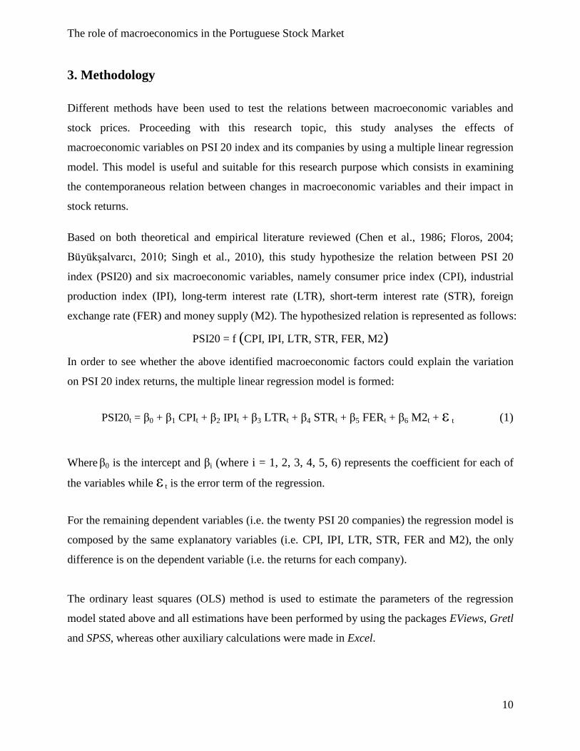
Different methods have been used to test the relations between macroeconomic variables and
stock prices. Proceeding with this research topic, this study analyses the effects of
macroeconomic variables on PSI 20 index and its companies by using a multiple linear regression
model. This model is useful and suitable for this research purpose which consists in examining
the contemporaneous relation between changes in macroeconomic variables and their impact in
stock returns.
Based on both theoretical and empirical literature reviewed (Chen et al., 1986; Floros, 2004;
Büyükşalvarcı, 2010; Singh et al., 2010), this study hypothesize the relation between PSI 20
index (PSI20) and six macroeconomic variables, namely consumer price index (CPI), industrial
production index (IPI), long-term interest rate (LTR), short-term interest rate (STR), foreign
exchange rate (FER) and money supply (M2). The hypothesized relation is represented as follows:
PSI20 = f (CPI, IPI, LTR, STR, FER, M2)
In order to see whether the above identified macroeconomic factors could explain the variation
on PSI 20 index returns, the multiple linear regression model is formed:
PSI20t = β0 + β1 CPIt + β2 IPIt + β3 LTRt + β4 STRt + β5 FERt + β6 M2t + ε t (1)
Where β0 is the intercept and βi (where i = 1, 2, 3, 4, 5, 6) represents the coefficient for each of
the variables while ε t is the error term of the regression.
For the remaining dependent variables (i.e. the twenty PSI 20 companies) the regression model is
composed by the same explanatory variables (i.e. CPI, IPI, LTR, STR, FER and M2), the only
difference is on the dependent variable (i.e. the returns for each company).
The ordinary least squares (OLS) method is used to estimate the parameters of the regression
model stated above and all estimations have been performed by using the packages EViews, Gretl
and SPSS, whereas other auxiliary calculations were made in Excel.

The role of macroeconomics in the Portuguese Stock Market
11
Methodology scheme:
1. Descriptive Statistics: Observations, Mean, Median, Maximum, Minimum, Std. Dev.,
Skewness, Kurtosis, Jarque-Bera test statistic and p-Value;
2. Stationarity variables in order to test whether a time series variable is stationary or not.
The tests applied are ADF (Augmented Dickey-Fuller) and KPSS (Kwiatkowski-Phillips-
Schmidt-Shin) tests;
3. Estimation of the multiple linear regression model;
4. Model assumptions tests:
- Multicollinearity (i.e., Tolerance and Variance Inflation Factor procedure);
- Normality of the error term (i.e., Jarque-Bera test);
- Autocorrelation of the error term (i.e., Durbin-Watsons test and Breusch-
Godfrey test);
- Homoscedasticity of the error term (i.e., White test).
5. Dealing with:
- Multicollinearity (i.e., Change the initial model composition and test again for
Multicollinearity);
- Non-Normality of the error term (This is not a problem for inference as we
have big samples, n > 30);
- Autocorrelation of the error term(i.e., Cochrane-Orcutt procedure);
- Heteroscedasticity of the error term (i.e., White HC standard errors);
- Autocorrelation and Heteroscedasticity of the error term (i.e., Newey-West
test HAC standard errors).

The role of macroeconomics in the Portuguese Stock Market
12
4. Empirical Study
4.1. Data
This section describes the state variables that are used in the empirical analysis. Six
macroeconomic variables were chosen in order to establish the relation between the stock returns
of the twenty companies which compose the PSI 20 Index and the index itself, with
macroeconomic variables. The choice was made based in the most used macroeconomic factors
by the authors of the analyzed researches. Therefore, six macroeconomic variables were selected,
namely: Inflation, Industrial Production, Long and Short-term Interest Rates, Foreign Exchange
Rate and Money Supply.
The Macroeconomic data were extracted from Banco de Portugal statistics while the PSI 20
INDEX and its companies price values were extracted from Yahoo!Finance and crosschecked
with the EURONEXT DataStream. We are using monthly data and the number of observations
varies depending on the financial instrument (Table 4 shows the time period for each financial
instrument and the number of corresponding observations). Note that the sample acquired for the
dependent variables are monthly adjusted closing price (i.e., adjusted for dividends and splits).
Moreover, the logarithm was applied to the initial data in order to work with stationary series.
Based in the empirical results, for the variables which remain non-stationary after applying the
logarithm, they were converted to a monthly continuous rate by taking the first differences of the
logarithmic series (Maysami et al., 2004):
DL(Vj) = ln(Vj) t − ln(Vj) t−1 (2)
Where DL(Vj) is the first differences of the logarithmic (continuous growth rate) of variable j
month t. (Vj) t and (Vj) t−1 are the level of variable i for month t and t − 1 respectively.
The role of macroeconomics in the Portuguese Stock Market
13
Dependent Variables
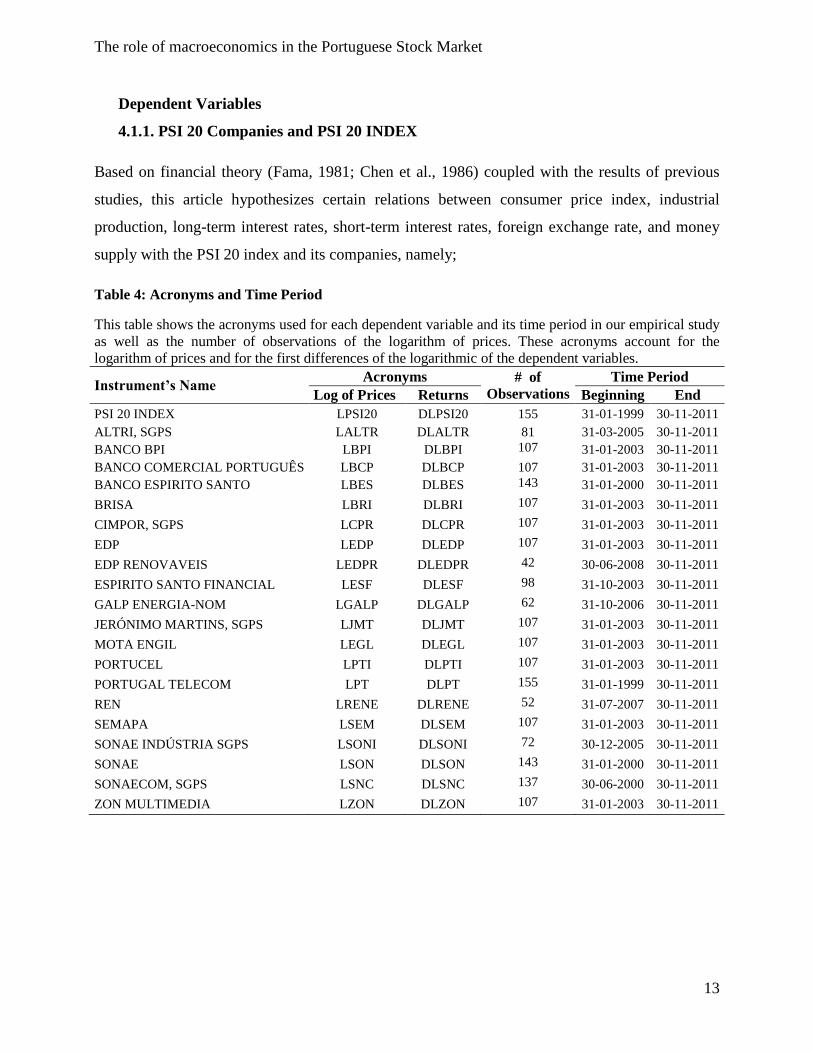
4.1.1. PSI 20 Companies and PSI 20 INDEX
Based on financial theory (Fama, 1981; Chen et al., 1986) coupled with the results of previous
studies, this article hypothesizes certain relations between consumer price index, industrial
production, long-term interest rates, short-term interest rates, foreign exchange rate, and money
supply with the PSI 20 index and its companies, namely;
Table 4: Acronyms and Time Period
This table shows the acronyms used for each dependent variable and its time period in our empirical study
as well as the number of observations of the logarithm of prices. These acronyms account for the
logarithm of prices and for the first differences of the logarithmic of the dependent variables.
Instrument’s Name Acronyms # of
Observations
Time Period
Log of Prices Returns Beginning End
PSI 20 INDEX LPSI20 DLPSI20 155 31-01-1999 30-11-2011
ALTRI, SGPS LALTR DLALTR 81 31-03-2005 30-11-2011
BANCO BPI LBPI DLBPI 107 31-01-2003 30-11-2011
BANCO COMERCIAL PORTUGUÊS LBCP DLBCP 107 31-01-2003 30-11-2011
BANCO ESPIRITO SANTO LBES DLBES 143 31-01-2000 30-11-2011
BRISA LBRI DLBRI 107 31-01-2003 30-11-2011
CIMPOR, SGPS LCPR DLCPR 107 31-01-2003 30-11-2011
EDP LEDP DLEDP 107 31-01-2003 30-11-2011
EDP RENOVAVEIS LEDPR DLEDPR 42 30-06-2008 30-11-2011
ESPIRITO SANTO FINANCIAL LESF DLESF 98 31-10-2003 30-11-2011
GALP ENERGIA-NOM LGALP DLGALP 62 31-10-2006 30-11-2011
JERÓNIMO MARTINS, SGPS LJMT DLJMT 107 31-01-2003 30-11-2011
MOTA ENGIL LEGL DLEGL 107 31-01-2003 30-11-2011
PORTUCEL LPTI DLPTI 107 31-01-2003 30-11-2011
PORTUGAL TELECOM LPT DLPT 155 31-01-1999 30-11-2011
REN LRENE DLRENE 52 31-07-2007 30-11-2011
SEMAPA LSEM DLSEM 107 31-01-2003 30-11-2011
SONAE INDÚSTRIA SGPS LSONI DLSONI 72 30-12-2005 30-11-2011
SONAE LSON DLSON 143 31-01-2000 30-11-2011
SONAECOM, SGPS LSNC DLSNC 137 30-06-2000 30-11-2011
ZON MULTIMEDIA LZON DLZON 107 31-01-2003 30-11-2011

The role of macroeconomics in the Portuguese Stock Market
14
Explanatory Variables and Hypotheses
4.1.2. Consumer Price Index (CPI)
Consumer Price Index is used as a proxy of inflation rate. CPI is chosen as it is a broad base
measure to calculate average change in retail prices for a fixed market basket of goods and
services. The CPI data is compiled from a sample of prices for food, shelter, clothing, fuel,
transportation and medical services that people purchase on daily basis. Inflation is ultimately
translated into nominal interest rate and an increase in nominal interest rates increase discount
rate which results in reduction of present value of cash flows so theoretically, an increase in
inflation has a negatively impact in equity prices. Empirical studies by Chen et al. (1986), Bilson
et al. (2000), Rapach et al. (2004), Menike (2006) and Singh et al. (2010) concluded that inflation
has negative effects on the stock market.
4.1.3. Industrial Production Index (IPI)
Industrial Production Index is used as proxy to measure the growth rate in real sector. Industrial
production consists of the total output of a nation‟s plants, utilities, and mines. From a
fundamental point of view, it is an important economic indicator that reflects the strength of the
economy, and by extrapolation, the strength of a specific currency. Therefore, industrial
production presents a measure of overall economic activity in the economy and affects stock
prices through its influence on expected future cash flows. Chen et al. (1986), Panetta (2001),
Maysami et al. (2004), Shanken and Weinstein (2006) and Savasa and Samiloglub (2010) found a
positive sign. Thus, it is expected that an increase in industrial production index is positively
related to stock returns.
4.1.4. Interest Rate (LTR and STR)
A ten-year interest rate and a three-month time deposit rate (i.e. Rate of return on fixed-rate
Treasury bonds - 10 years and EURIBOR – 3 months) are used as a proxy for long-term and
short-term interest rates, respectively. The intuition regarding the relation between interest rates
and stock prices is well established, suggesting that investors anticipate that increased investment

The role of macroeconomics in the Portuguese Stock Market
15
and spending will boost the companies listed on the stock exchange when the interest rate drops.
Thus, a change in nominal interest rates should move asset prices in the opposite direction as
corroborated by Maysami et al. (2004), Rapach et al. (2004), Menike (2006), Hachicha and
Chaabane (2007) and Büyükşalvarcı (2010) while finding a negative sign for the relation between
interest rates and stock returns. In addiction an interest rate is typically not subjected to revision
and are available immediately, that said, interest rates are likely to be relevant in real time
investment decisions (Rapach, 2004: 23).
4.1.5. Foreign Exchange Rate (FER)
The proxy which has been used to capture the effect of unexpected changes in exchange rates on
stock returns is the rate of change in the US dollar/EUR exchange rate which is an important
factor to determine the international competitiveness. Portugal is mainly an import country. For
an import dominated country currency depreciation will have an unfavorable impact on a
domestic stock market. As the European Union currency depreciates against the U.S. dollar,
products imported become more expensive. However, some imports are essential for production
or cannot be made in Portugal and have an inelastic demand and inevitably we and up spending
more on these when the exchange rate falls in value, which in turn causes lower cash flows,
profits and the stock price of the domestic companies. Demirguc-Kunt et al. (1998), Panetta
(2001), Maysami et al. (2004) and Mansor et al. (2009) found a positive sign. Thus, a positive
relation is expected between foreign exchange rate and stock returns.
4.1.6. Money Supply (M2)
Broad Money (M2) is used as a proxy of money supply. The money supply is basically defined as
the quantity of money (money stock) held by money holders (general corporations, individuals
and local governments). M2 is a category of the money supply that includes all coins, currency
and demand deposits (that is, checking accounts and NOW accounts) and all time deposits,
savings deposits and non-institutional money-market funds. Therefore, an increase in money
supply leads to increase in liquidity that ultimately results in upward movement of nominal
equity prices. Flannery and Protopapadakis (2001), Bilson et al. (2000), Maysami et al. (2004),

The role of macroeconomics in the Portuguese Stock Market
16
Hachicha and Chaabane (2007) and Pilinkus (2009) found a positive sign. Thus, a positive
relation is expected between money supply and stock returns.
4.1.7. Gross Domestic Product (GDP)
GDP is the total value of final goods and services produced within a country's borders in a year.
It is one of the measures of national income and output. It may be used as one indicator of the
standard of living in a country. If a country or a region of the world has a high economic growth
prospects, investors will find them attractive places to invest therefore, GDP growth is expected
to have a positive impact on the stock returns. Even so, we will not use this variable in our model
based in;
1. The methodology used by us to choose the macroeconomic variables was the realization
of the most commonly ones used by all the studies that were analyzed and GDP was
rarely used;
2. GDP data is only possible to arrange in a quarterly basis, while the others
macroeconomic variables are in a monthly basis and thus make better use of data of
returns by not using GDP as an explanatory variable in our model;
3. GDP as an explanatory variable is automatically linked to others macroeconomic
variables which reduces its explanatory power, i.e. interest rate and exchange rate where:
Higher exports (an injection into the circular flow) and falling imports leads to
rising GDP levels;
A lower exchange rate accompanied by lower interest rates will stimulate
consumer spending and general economic recovery (i.e. GDP levels will increase).
Therefore, GDP will not be integrated in our model as an explanatory variable.
In conclusion, the expect signals for each macroeconomic variable in our multiple linear
regression model based on the findings of the reviewed literature and the theoretical relation that
each macroeconomic variable has with stock returns are as follows:
The role of macroeconomics in the Portuguese Stock Market
17
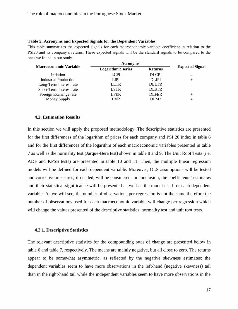
4.2. Estimation Results
In this section we will apply the proposed methodology. The descriptive statistics are presented
for the first differences of the logarithm of prices for each company and PSI 20 index in table 6
and for the first differences of the logarithm of each macroeconomic variables presented in table
7 as well as the normality test (Jarque-Bera test) shown in table 8 and 9. The Unit Root Tests (i.e.
ADF and KPSS tests) are presented in table 10 and 11. Then, the multiple linear regression
models will be defined for each dependent variable. Moreover, OLS assumptions will be tested
and corrective measures, if needed, will be considered. In conclusion, the coefficients‟ estimates
and their statistical significance will be presented as well as the model used for each dependent
variable. As we will see, the number of observations per regression is not the same therefore the
number of observations used for each macroeconomic variable will change per regression which
will change the values presented of the descriptive statistics, normality test and unit root tests.
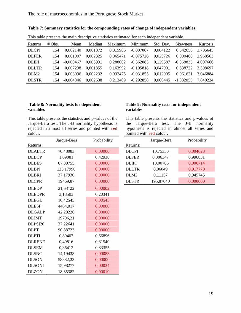
4.2.1. Descriptive Statistics
The relevant descriptive statistics for the compounding rates of change are presented below in
table 6 and table 7, respectively. The means are mainly negative, but all close to zero. The returns
appear to be somewhat asymmetric, as reflected by the negative skewness estimates: the
dependent variables seem to have more observations in the left-hand (negative skewness) tail
than in the right-hand tail while the independent variables seem to have more observations in the
Table 5: Acronyms and Expected Signals for the Dependent Variables
This table summarizes the expected signals for each macroeconomic variable coefficient in relation to the
PSI20 and its company‟s returns. These expected signals will be the standard signals to be compared to the
ones we found in our study.
Macroeconomic Variable Acronyms
Expected Signal Logarithmic series Returns
Inflation LCPI DLCPI Industrial Production LIPI DLIPI +
Long-Term Interest rate LLTR DLLTR
Short-Term Interest rate LSTR DLSTR Foreign Exchange rate LFER DLFER +
Money Supply LM2 DLM2 +

The role of macroeconomics in the Portuguese Stock Market
18
right-hand (positive skewness) tail than in the left-hand. The kurtosis varies in most cases from 2
to 8, being always different from the standard Gaussian distribution which is 3: DLSON, DLESF,
DLJMT and DLCPR are the ones which kurtosis standout in comparison to the other variables
for theirs high values. Moreover, the Jarque-Bera (J-B) test was included in the descriptive
statistics being the normality hypothesis rejected in almost every case as shown below in table 8
and table 9 for the dependent and independent variables, respectively.
Table 6: Summary statistics for the dependent variables returns
This table presents the main descriptive statistics estimated for each dependent variable.
Returns # Obs. Mean Median Maximum Minimum Std. Dev. Skewness Kurtosis
DLALTR 80 0,02658 0,00000 0,63488 -0,63653 0,16152 0,09759 7,59414
DLBCP 106 -0,023009 -0,00249 0,21963 -0,32992 0,10908 -0,28929 2,78076
DLBES 142 -0,019067 -0,00444 0,23852 -0,35889 0,09434 -1,18186 5,42348
DLBPI 106 -0,009742 0,00000 0,25974 -0,47810 0,10013 -1,00341 7,93105
DLBRI 106 -0,002805 0,00554 0,13947 -0,26189 0,06823 -1,03960 5,02359
DLCPR 106 -0,00686 0,00982 0,23730 -1,59857 0,17386 -7,33258 67,75497
DLEDP 106 0,007993 0,01274 0,11683 -0,20133 0,05553 -0,81484 4,49725
DLEDPR 41 -0,013075 -0,01379 0,18848 -0,32226 0,10160 -0,30411 4,22249
DLEGL 106 0,000181 0,00948 0,26826 -0,28838 0,09643 -0,56467 4,04167
DLESF 97 -0,010429 0,00000 0,13103 -0,77171 0,10084 -4,65220 34,90497
DLGALP 61 0,011968 0,02595 0,28566 -0,48245 0,12004 -1,13012 6,39050
DLJMT 106 0,041291 0,02703 1,66991 -0,40368 0,17774 7,17990 68,23480
DLPSI20 154 -0,004812 -0,00182 0,16752 -0,23348 0,05620 -0,65585 5,02014
DLPT 154 0,002699 0,00608 0,23009 -0,42549 0,09108 -0,98651 6,20491
DLPTI 106 0,00719 0,00448 0,19612 -0,14689 0,06657 0,19631 3,16705
DLRENE 52 -0,008241 -0,00707 0,12516 -0,11544 0,05263 -0,20659 2,86706
DLSEM 106 0,007655 0,00496 0,16227 -0,16661 0,06783 0,04614 2,72810
DLSNC 137 -0,01529 -0,00766 0,46304 -0,36115 0,12612 -0,04109 4,57476
DLSON 142 -0,031492 0,00000 0,27088 -3,24168 0,29442 -9,21726 101,04140
DLSONI 71 -0,031992 -0,03213 0,43235 -0,37863 0,12515 -0,01274 5,32422
DLZON 106 -0,007031 -0,00461 0,27774 -0,28117 0,08791 -0,16680 5,01104
The role of macroeconomics in the Portuguese Stock Market
19
Table 8: Normality tests for dependent
variables
Table 9: Normality tests for independent
variables
This table presents the statistics and p-values of the
Jarque-Bera test. The J-B normality hypothesis is
rejected in almost all series and pointed with red
colour.
This table presents the statistics and p-values of
the Jarque-Bera test. The J-B normality
hypothesis is rejected in almost all series and
pointed with red colour.
Jarque-Bera Probability
Jarque-Bera Probability
Returns: Returns:
DLALTR 70,48083 0,00000
DLCPI 10,75330 0,004623
DLBCP 1,69081 0,42938
DLFER 0,006347 0,996831
DLBES 67,80755 0,00000
DLIPI 10,00706 0,006714
DLBPI 125,17990 0,00000
DLLTR 8,06049 0,017770
DLBRI 37,17930 0,00000
DLM2 0,11157 0,945745
DLCPR 19469,87 0,00000
DLSTR 195,87040 0,000000
DLEDP 21,63122 0,00002
DLEDPR 3,18503 0,20341
DLEGL 10,42545 0,00545
DLESF 4464,017 0,00000
DLGALP 42,20226 0,00000
DLJMT 19706,21 0,00000
DLPSI20 37,22641 0,00000
DLPT 90,88723 0,00000
DLPTI 0,80407 0,66896
DLRENE 0,40816 0,81540
DLSEM 0,36412 0,83355
DLSNC 14,19438 0,00083
DLSON 58882,33 0,00000
DLSONI 15,98277 0,00034
DLZON 18,35382 0,00010
Table 7: Summary statistics for the compounding rates of change of independent variables
This table presents the main descriptive statistics estimated for each independent variable.
Returns # Obs. Mean Median Maximum Minimum Std. Dev. Skewness Kurtosis
DLCPI 154 0,002140 0,001872 0,015986 -0,007067 0,004122 0,542656 3,705645
DLFER 154 0,001007 0,002325 0.065471 -0.075726 0,025726 0,000468 2,968563
DLIPI 154 -0,000467 0,005931 0,288002 -0,362083 0,129587 -0,368833 4,007666
DLLTR 154 0,007238 0,001855 0,163992 -0,105818 0,047001 0,538722 3,308697
DLM2 154 0,003096 0,002232 0,032475 -0,031855 0,012005 0,061621 3,046884
DLSTR 154 -0,004846 0,002638 0,213489 -0,292858 0,066445 -1,332055 7,840224
The role of macroeconomics in the Portuguese Stock Market
20
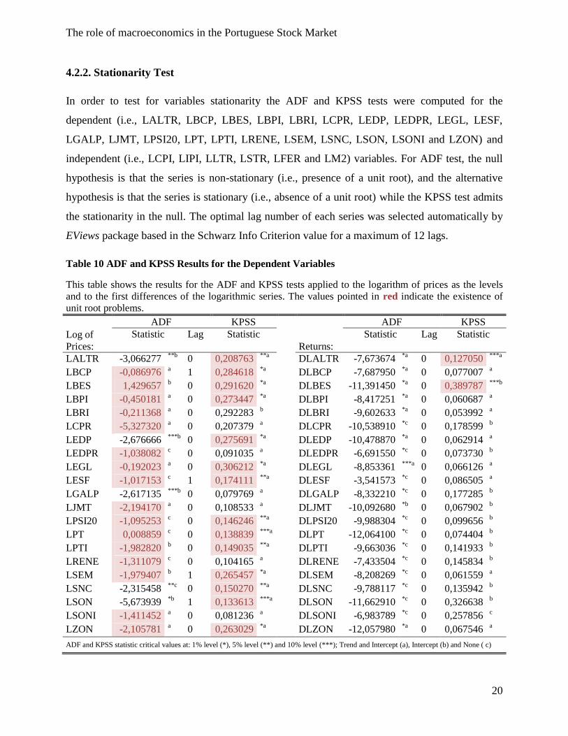
4.2.2. Stationarity Test
In order to test for variables stationarity the ADF and KPSS tests were computed for the
dependent (i.e., LALTR, LBCP, LBES, LBPI, LBRI, LCPR, LEDP, LEDPR, LEGL, LESF,
LGALP, LJMT, LPSI20, LPT, LPTI, LRENE, LSEM, LSNC, LSON, LSONI and LZON) and
independent (i.e., LCPI, LIPI, LLTR, LSTR, LFER and LM2) variables. For ADF test, the null
hypothesis is that the series is non-stationary (i.e., presence of a unit root), and the alternative
hypothesis is that the series is stationary (i.e., absence of a unit root) while the KPSS test admits
the stationarity in the null. The optimal lag number of each series was selected automatically by
EViews package based in the Schwarz Info Criterion value for a maximum of 12 lags.
Table 10 ADF and KPSS Results for the Dependent Variables
This table shows the results for the ADF and KPSS tests applied to the logarithm of prices as the levels
and to the first differences of the logarithmic series. The values pointed in red indicate the existence of
unit root problems.
ADF KPSS
ADF KPSS
Log of
Prices:
Statistic Lag Statistic
Returns:
Statistic Lag Statistic
LALTR -3,066277 **b
0 0,208763 **a
DLALTR -7,673674 *a
0 0,127050 ***a
LBCP -0,086976 a 1 0,284618
*a
DLBCP -7,687950 *a
0 0,077007 a
LBES 1,429657 b 0 0,291620
*a
DLBES -11,391450 *a
0 0,389787 ***b
LBPI -0,450181 a 0 0,273447
*a
DLBPI -8,417251 *a
0 0,060687 a
LBRI -0,211368 a 0 0,292283
b
DLBRI -9,602633 *a
0 0,053992 a
LCPR -5,327320 a 0 0,207379
a
DLCPR -10,538910 *c
0 0,178599 b
LEDP -2,676666 ***b
0 0,275691 *a
DLEDP -10,478870 *a
0 0,062914 a
LEDPR -1,038082 c 0 0,091035
a
DLEDPR -6,691550 *c
0 0,073730 b
LEGL -0,192023 a 0 0,306212
*a
DLEGL -8,853361 ***a
0 0,066126 a
LESF -1,017153 c 1 0,174111
**a
DLESF -3,541573 *c
0 0,086505 a
LGALP -2,617135 ***b
0 0,079769 a
DLGALP -8,332210 *c
0 0,177285 b
LJMT -2,194170 a 0 0,108533
a
DLJMT -10,092680 *b
0 0,067902 b
LPSI20 -1,095253 c 0 0,146246
**a
DLPSI20 -9,988304 *c
0 0,099656 b
LPT 0,008859 c 0 0,138839
***a
DLPT -12,064100 *c
0 0,074404 b
LPTI -1,982820 b 0 0,149035
**a
DLPTI -9,663036 *c
0 0,141933 b
LRENE -1,311079 c 0 0,104165
a
DLRENE -7,433504 *c
0 0,145834 b
LSEM -1,979407 b 1 0,265457
*a
DLSEM -8,208269 *c
0 0,061559 a
LSNC -2,315458 **c
0 0,150270 **a
DLSNC -9,788117 *c
0 0,135942 b
LSON -5,673939 *b
1 0,133613 ***a
DLSON -11,662910 *c
0 0,326638 b
LSONI -1,411452 a 0 0,081236
a
DLSONI -6,983789 *c
0 0,257856 c
LZON -2,105781 a 0 0,263029
*a
DLZON -12,057980 *a
0 0,067546 a
ADF and KPSS statistic critical values at: 1% level (*), 5% level (**) and 10% level (***); Trend and Intercept (a), Intercept (b) and None ( c)

The role of macroeconomics in the Portuguese Stock Market
21
The results of the unit root tests for the independent variables are presented in table 10. In an
overall, the ADF unit root hypothesis is not rejected for the logarithm of prices (except for
LALTR, LEDP, LGALP, LSNC and LSON) and the KPSS stationarity hypothesis is rejected in
the majority of the series of logarithm of prices (except for LBRI, LCPR, LEDPR, LGALP,
LJMT, LRENE and LSONI). On the other hand, for the first differences of the logs the ADF null
hypothesis of a unit root is strongly reject and the KPSS null of stationarity in not reject for
almost every series. Thus, we conclude that our dependent variables are stationary in first
differences.
Table 11: ADF and KPSS Results for the Independent Variables
This table shows the results for the ADF and KPSS tests applied to the logarithm of the independent
variables as the level and to the first differences of the logarithmic. The values pointed in red indicate the
existence of unit root problems.
ADF KPSS
ADF KPSS
Log of Prices:
Statistic Lag Statistic
Returns:
Statistic Lag Statistic
LCPI -3,244657 ***a
12 0,321517 *a
DLCPI -0,544204 c 11 0,243856
b
LFER -2,644824 a 1 0,144168
***a
DLFER -9,074023 *c
0 0,149232 b
LIPI -1,003294 c 13 0,258067
*a
DLIPI -3,299799 *c
12 0,047912 b
LLTR -1,772345 ***
0 0,267530 *a
DLLTR -10,275690 *c
0 0,190096 **a
LM2 -1,970160 b 0 0,104326
a
DLM2 -13,363330 *b
0 0,264741 b
LSTR 0,185822 c 1 0,115864
a
DLSTR -5,130903 *c
0 0,072278 b
ADF and KPSS statistic critical values at: 1% level (*), 5% level (**) and 10% level (***); Trend and Intercept (a), Intercept (b) and None ( c)
The results of the unit root tests for the independent variables are presented in table 11. In an
overall, the ADF unit root hypothesis is not rejected for the logarithm of prices (except for LCPI
and LLTR) and the KPSS stationarity hypothesis is rejected for the series of logarithm of prices
(except for LM2 and LSTR). On the other hand, for the compounding rates of change (i.e., first
Differences) the ADF null hypothesis of a unit root is rejected (except for DLCPI) and the KPSS
null of stationarity in not reject for almost every series (except for DLLTR). Thus, we conclude
that ours independent variables are stationary in first differences in exception for the CPI
compounding rates of change which were considered as non-stationary by the ADF test and for
the LTR compounding rates of change by the KPSS test. In order to have comparable series in
each multiple linear regression model, we decided to work with the first differences of the

The role of macroeconomics in the Portuguese Stock Market
22
logarithmic series which constitute the compounding rates of change of the original variables
which have financial/economic interpretation.
In conclusion, the multiple linear regression models used in our study and based in the previous
results will follows the structure of equation (1) but composed by first differences of the
logarithmic series. A change in the models may occur depending in which or all OLS model
assumptions aren‟t met.
4.2.3. Multicollinearity
When the independent variables are strongly correlated among themselves – condition known as
multicollinearity – the analysis of the adjusted regression model can lead to some confusion and
non-sense. Thus, this condition is one of the first assumptions to validate during the linear
regression.
“In practical context, the correlation between explanatory variables will be non-zero, although
this will generally be relatively benign in the sense that a small degree of association between
explanatory variables will almost always occur but will not cause too much loss of precision”
(Chris Brooks 2008: 170).
There are several signs that suggest the existence of multicollinearity among the variables. For
instance, the R-square being too big or the partial coefficients being too low is a sign of a
possible existence of strong correlation between independent variables; the t-tests for each of the
individual slopes are non-significant (sig > 0.05), but the overall F-test for testing all of the slopes
are simultaneously 0 which makes it significant (sig < 0.05); and the correlations among pairs of
predictor variables are large.
To check if multicollinearity exists in each model we used the Variance Inflation Factor (VIF) to
conclude whether multicollinearity between explanatory variables exists.
The VIF is a measure of how much the variance of the estimated regression coefficient βj is
“inflated” by the existence of correlation among the explanatory variables in the model. For the
purpose of testing the existence of Multicollinearity, VIF values were computed for each multiple
linear regression model. Note that the values of Tolerance and VIF are related as shown in the

The role of macroeconomics in the Portuguese Stock Market
23
equation (3) therefore we will only present the VIF values. If the values of VIF are bigger than 10
we are facing a problem of multicollinearity.
(3)
Where Rj2 is the R
2-value obtained by regressing the j
th variable on the remaining explanatory
variables.
Table 12 Collinearity Statistic – VIF
In this table is presented the VIF values. VIF values will change between regressions because of the difference in
the number of observations used in each one. Therefore, in order to condense the data the VIF values for each
independent variable was grouped by number of observations used in each regression. Thus, group 1 (i.e.,
DLBCP, DLBPI, DLBRI, DLCPR, DLEDP, DLEGL, DLJMT, DLPTI, DLSEM and DLZON), group 2 (i.e.,
DLBES and DLSON) and group 3 (i.e., DLPSI20 and DLPT) were created.
Returns: DLCPI DLFER DLIPI DLLTR DLM2 DLSTR
DLALTR 1,34681 1,05692 1,16299 1,12624 1,02527 1,22333
DLEDPR 1,46391 1,02897 1,30960 1,28630 1,07191 1,33179
DLESF 1,30935 1,06867 1,12871 1,13735 1,03825 1,19895
DLGALP 1,41790 1,09440 1,23197 1,21592 1,04065 1,28185
DLRENE 1,50049 1,07317 1,29368 1,25132 1,04460 1,32110
DLSNC 1,18136 1,03905 1,07644 1,12304 1,03507 1,19652
DLSONI 1,40153 1,08961 1,20258 1,18113 1,03035 1,23292
GROUP 1 1,28955 1,09690 1,10561 1,15735 1,02872 1,20222
GROUP 2 1,19269 1,06001 1,06878 1,10894 1,04064 1,20860
GROUP 3 1,16318 1,05542 1,06798 1,10328 1,04738 1,18742
GROUP 1 = [DLBCP, DLBPI, DLBRI, DLCPR, DLEDP, DLEGL, DLJMT, DLPTI, DLSEM, DLZON]; GROUP 2 =
[BES, SON]; GROUP 3 = [DLPSI20, DLPT]
Due the fact that all the regressions incorporate the same independent variables, VIF values will
change between regressions with different number of observations. Therefore, in order to reduce
the number of outputs of the VIF values for each independent variable was grouped by number of
observations used in each regression. Thus, group 1 (i.e., DLBCP, DLBPI, DLBRI, DLCPR,
DLEDP, DLEGL, DLJMT, DLPTI, DLSEM and DLZON), group 2 (i.e., DLBES and DLSON)
and group 3 (i.e., DLPSI20 and DLPT) were created as you can see in the table above. The
results for the VIF statistic show that the values were never bigger than 10, therefore the
multicollinearity problem doesn‟t exist between independent variables.

The role of macroeconomics in the Portuguese Stock Market
24
4.2.4. Normality of the error term
Recall that the normality assumption [u t ∼ N (0, σ2)] is required in order to conduct single or
joint hypothesis tests about the model parameters. One of the most commonly applied tests for
normality is the Jarque-Bera test. A normal distribution is not skewed and is defined to have a
coefficient of kurtosis of 3, in other words, symmetric and said to be mesokurtic. The J-B null
hypothesis of normally distributed errors is rejected when p-value is < 0, 05.
Table 13: Normality of the error term (Jarque-Bera test)
This table presents the results for the Jarque-Bera test on the residuals which were estimated by regressing
the compounding rates of change of the PSI 20 index and its companies on macroeconomic variables. We
also add the skewness and kurtosis to compare with the J-B results. The p-values pointed in red show
when the J-B normality of the error terms hypothesis is rejected.
Skewness Kurtosis Jarque-Bera Probability
Residual:
DLALTR 0,064286 7,180106 58,29938 0,000000
DLBCP -0,357874 3,055563 2,276274 0,320415
DLBES -0,932702 5,317088 52,35440 0,000000
DLBPI -1,358123 10,41132 275,1832 0,000000
DLBRI -1,009708 4,577480 29,00199 0,000001
DLCPR -6,883698 62,78780 16.624,87 0,000000
DLEDP -0,746162 4,150207 15,67919 0,000394
DLEDPR 0,461382 3,221172 1,538204 0,463429
DLEGL -0,132857 3,623175 2,027031 0,362941
DLESF -4,765403 3,597170 4.760,959 0,000000
DLGALP -0,915468 4,945602 18,14164 0,000115
DLJMT 7,294615 68,61072 19.952,79 0,000000
DLPSI20 -0,504530 4,809951 27,55398 0,000001
DLPT -0,684485 5,300928 45,99693 0,000000
DLPTI 0,329778 3,393802 2,606246 0,271682
DLRENE -0,478668 2,557089 2,410772 0,299576
DLSEM 0,100263 2,877955 0,243385 0,885421
DLSNC -0,200140 4,617682 15,85273 0,000361
DLSON -8,942568 97,037820 54.214,36 0,000000
DLSONI -0,028299 5,275565 15,32831 0,000469
DLZON 0,044765 4,116213 5,538263 0,062716
In this case, the residuals are mainly negatively skewed and are leptokurtic. Hence the null
hypothesis for residuals normality is rejected very strongly (the p-value for the J-B test is zero to

The role of macroeconomics in the Portuguese Stock Market
25
six decimal places), implying that the inferences we make about the coefficient estimates could
be wrong, although the sample is probably just about large enough that we don‟t need to be
concerned as we would if we were working with a small sample. The non-normality in this case
appears to have been caused by a small number of very large negative and positive residuals
representing high monthly shocks.
4.2.5. Autocorrelation of the error term
No autocorrelation is also one of the assumptions under the Gauss-Markov theorem and relates to
the error terms. In more detail, no autocorrelation assumes that the error terms of each
independent variable are uncorrelated. Therefore, if the errors are not uncorrelated with one
another, it would be stated that they are „autocorrelated‟ or that they are „serially correlated‟. A
test of this assumption is therefore required. Therefore, we will compute two tests, the Durbin-
Watson and the Breusch-Godfrey.
Durbin-Watson (DW) is a test for first order autocorrelation (i.e., it tests only for a relation
between an error and its immediately previous value):
u t = ρu t−1 + v t (4)
Where vt ∼ N (0, σ
). Thus, under the null hypothesis, the errors at time t and t − 1 are
independent of one another (H0: ρ = 0) and if this null were rejected (H1: ρ ≠ 0), it would be
concluded that there was evidence of a relation between consecutive errors.
In order to see the levels of significance of the D-W stat we should take into account the
following logic: If the value of the statistic is around 2, we conclude that there isn‟t
autocorrelation. If it is between dl and du or 4-dl and 4-du, we cannot conclude anything about
the nature of the errors‟ autocorrelation and finally if they are over the previous limits we are
assuming that there is autocorrelation (if near 4 – negatively autocorrelated, if near 1 – positively
autocorrelated). In our case and taking into account a dL and dU critical values, the Durbin-
Watson statistic for our models falls mainly on region III were the null hypothesis isn‟t rejected.
The fact that some error terms autocorrelation were given as inconclusive (i.e., DLALTR, DLBPI,
DLEDPR, DLGALP, DLRENE and DLZON multiple linear regression model error terms) show
the limitations of this test and we cannot conclude anything about autocorrelation in these

The role of macroeconomics in the Portuguese Stock Market
26
regressions. Autocorrelation of the error terms were found for DLBCP, DLESF, DLPSI20 and
DLSEM regressions‟ error term, as shown in the table 14.
We are now going for another autocorrelation test, namely, Breush-Godfrey (BG) which is a
more general test for autocorrelation up to the rth order. In its null is assumed no autocorrelation
of r order (i.e., H0: ρ1 = ρ2 = … = ρr = 0). Three error terms were considered autocorrelated by
the BG test, namely, DLBCP, DLBPI and DLGALP while DLESF, DLPSI20 and DLSEM error
terms which were considered autocorrelated by DW statistic is now no autocorrelated with a p-
value close to 0,05 of significance (i.e., 0,0649 and 0,1052 respectively).
Table 14: Autocorrelation of the error terms
This table presents the Durbin-Watson (DW) test and Breusch-Godfrey (BG) test results for the error term of each multiple
linear regression model. For the DW test we consider k = 6 and n = # of Observations, at 5 % of significance points of dL and
dU. For the BG test we considered 12 as the number of lags due the fact that we are using monthly data. The values pointed in
red indicate the existence autocorrelation in the error terms.
Residuals: # of Observations dL dU Durbin-Watson statistics Prob. Chi-Square(12)
DLALTR 80 1,4800 1,8008 1,59661371 b
0,12219839
DLBCP 106 1,5660 1,8044 1,32235313 a
0,03081476
DLBES 142 1,6388 1,8146 1,99412002 c
0,66466723
DLBPI 106 1,5660 1,8044 1,61247547 b
0,01533321
DLBRI 106 1,5660 1,8044 1,85279348 c
0,23135629
DLCPR 106 1,5660 1,8044 1,97669259 c
1,00000000
DLEDP 106 1,5660 1,8044 2,04810728 c
0,21968387
DLEDPR 41 1,1891 1,8493 2,73129253 b
0,14729238
DLEGL 106 1,5660 1,8044 1,86969944 c
0,43631562
DLESF 97 1,5407 1,8025 1,10743759 a
0,51394485
DLGALP 61 1,3787 1,8073 2,35099493 b
0,03440522
DLJMT 106 1,5660 1,8044 1,99083484 c
0,95447501
DLPSI20 154 1,6565 1,8181 1,57315356 a
0,42868496
DLPT 154 1,6565 1,8181 1,97029519 c
0,45058577
DLPTI 106 1,5660 1,8044 2,01247528 c
0,63460379
DLRENE 52 1,3090 1,8183 2,36980681 b
0,13439316
DLSEM 106 1,5660 1,8044 1,55817660 a
0,12512190
DLSNC 137 1,6306 1,8131 1,79126458 b
0,54883329
DLSON 142 1,6388 1,8146 2,03048888 c
0,99217548
DLSONI 71 1,4379 1,8021 1,88001882 c
0,50449033
DLZON 106 1,5660 1,8044 2,33487385 b
0,44215844
Regions for DW test: Positive autocorrelation (a); Inconclusive (b), No autocorrelation (c)
In conclusion, based on the results the existence of autocorrelation in DLBCP, DLBPI and
DLGALP error terms is confirmed. Later on we will deal with this problem accordingly by
applying the Cochrane-Orcutt procedure.
The role of macroeconomics in the Portuguese Stock Market
27
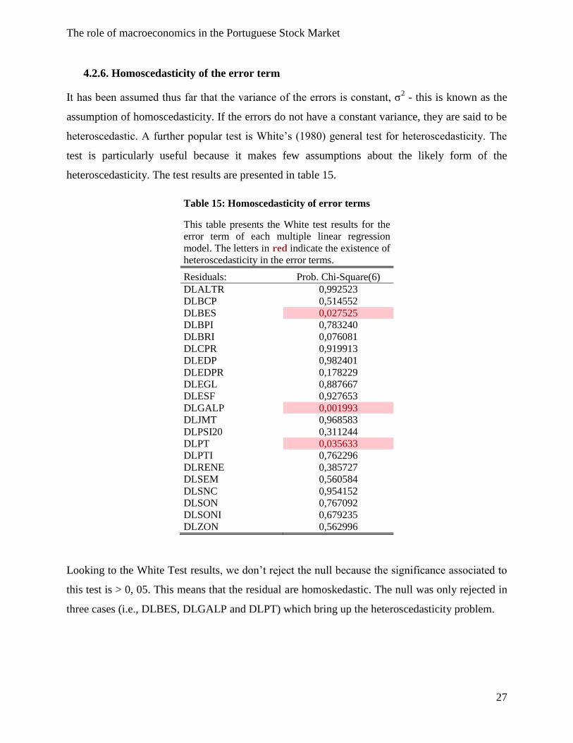
4.2.6. Homoscedasticity of the error term
It has been assumed thus far that the variance of the errors is constant, σ2 - this is known as the
assumption of homoscedasticity. If the errors do not have a constant variance, they are said to be
heteroscedastic. A further popular test is White‟s (1980) general test for heteroscedasticity. The
test is particularly useful because it makes few assumptions about the likely form of the
heteroscedasticity. The test results are presented in table 15.
Table 15: Homoscedasticity of error terms
This table presents the White test results for the
error term of each multiple linear regression
model. The letters in red indicate the existence of
heteroscedasticity in the error terms.
Residuals: Prob. Chi-Square(6)
DLALTR 0,992523
DLBCP 0,514552
DLBES 0,027525
DLBPI 0,783240
DLBRI 0,076081
DLCPR 0,919913
DLEDP 0,982401
DLEDPR 0,178229
DLEGL 0,887667
DLESF 0,927653
DLGALP 0,001993
DLJMT 0,968583
DLPSI20 0,311244
DLPT 0,035633
DLPTI 0,762296
DLRENE 0,385727
DLSEM 0,560584
DLSNC 0,954152
DLSON 0,767092
DLSONI 0,679235
DLZON 0,562996
Looking to the White Test results, we don‟t reject the null because the significance associated to
this test is > 0, 05. This means that the residual are homoskedastic. The null was only rejected in
three cases (i.e., DLBES, DLGALP and DLPT) which bring up the heteroscedasticity problem.

The role of macroeconomics in the Portuguese Stock Market
28
4.2.7. Dealing with OLS assumptions problems
As already stated, in order to make inferences based on the estimated coefficients generated by
the OLS regression model, four assumptions must hold, no perfect collinearity among the
explanatory variables, normality, no autocorrelation and homoscedasticity of the error terms. For
some regressions these assumptions are not verified, namely:
1. Autocorrelation of the error terms: DLBCP and DLBPI;
2. Heteroscedasticity of the error terms: DLBES and DLPT;
3. Autocorrelation and Heteroscedasticity of the error terms: DLGALP.
Therefore, we now present the methods used to deal with these problems.
1. Dealing with autocorrelation of the error terms:
In order to solve this problem, we used the Cochrane-Orcutt procedure in Gretl package and we
were able to remove the existence of autocorrelation in the multiple linear regression models
which DLBCP and DLBPI are dependent variables. As we can see in table below, DW statistic is
now in region III. Therefore, and based on the residuals, there is no first order autocorrelation in
the error terms of each regression model.
Table 16: Cochrane-Orcutt Procedure statistics
This table presents the outcome from using the Cochrane-Orcutt procedure to eliminate the
autocorrelation of the error term in the regressions where DLBCP and DLBPI are the dependent
variables. To analyze the Durbin-Watson statistics we considered k = 6 and n = # of observations.
Iterations ρ # of Observations dL dU DW
DLBCP 4 0,34051 105 1,56340 1,8042 2,049463 c
DLBPI 4 0,23136 105 1,56340 1,8042 1,981755 c
Regions for DW test: Positive autocorrelation (a); Inconclusive (b), No autocorrelation (c)
2. Dealing with heteroscedasticity of the error terms:
“Using heteroscedasticity-consistent standard error estimates. Most standard econometrics
software packages have an option (usually called something like „robust‟) that allows the user to
employ standard error estimates that have been modified to account for the heteroscedasticity
following White (1980). The effect of using the correction is that, if the variance of the errors is
positively related to the square of an explanatory variable, the standard errors for the slope

The role of macroeconomics in the Portuguese Stock Market
29
coefficients are increased relative to the usual OLS standard errors, which would make
hypothesis testing more „conservative‟, so that more evidence would be required against the null
hypothesis before it would be rejected.” (Chris Brooks, 2008:138). After estimating the
regression with heteroscedasticity-robust standard errors the probabilities of the t-statistics were
lower as expected by dealing with the heteroscedasticity of the error terms in the multiple linear
regression models with DLPT and DLBES as dependent variables. Moreover, we show the
change in the standard error estimates by considering the heteroscedasticity-robustness in our
models as presented in table 17.
Table 17: Solving Heteroscedasticity Problem (White)
This table shows the standard error estimates that have been modified to account for the
heteroscedasticity following White (1980), comparing them to its previous estimation. These
estimations relate to the multiple linear regression models which dependent variables are DLBES
and DLPT.
DLBES DLPT
Before After Before After
Independent variables:
DLCPI 1,9669 2,1826 0,8006 1,8508
DLFER 0,3050 0,2461 0,0000 0,3781
DLIPI 0,0612 0,0436 0,5938 0,0651
DLLTR 0,1736 0,1741 0,6674 0,1679
DLM2 0,6421 0,6660 0,3286 0,5312
DLSTR 0,1266 0,1902 0,4472 0,1058
C 0,0090 0,0082 0,8746 0,0095
3. Dealing with autocorrelation and heteroscedasticity of the error terms
As observed above, we are facing heteroscedasticity and autocorrelation problems in the model
where DLGALP is the dependent variable. To try to solve this, we will use the Newey-West
procedure which will work on the standard errors solving the problems in hand for this model.
The change in the coefficients standard errors is as follows:
Table 18: Solving Autocorrelation and Heteroscedasticity Problem (HAC)
This table shows the standard error estimates that have been modified to account for the autocorrelation and
heteroscedasticity problem based on the HAC (Newey-West) and compare them to its previous estimation.
DLCPI DLFER DLIPI DLLTR DLM2 DLSTR C
BEFORE 3,784960 0,588879 0,153387 0,300364 1,207953 0,196693 0,018509
AFTER 2,833774 0,689280 0,166339 0,318915 0,940921 0,155039 0,020259

The role of macroeconomics in the Portuguese Stock Market
30
4.2.8. Multiple linear regression model results
In order to establish the statistical relationship between stock returns and macroeconomic
variables have been defined, tested and estimated, twenty one multiple linear regression models
whose main estimation results are presented next:
Table 19: Estimated Coefficients
This table shows the estimated values for the coefficients and their significance (sig) for each independent
variable in each multiple linear regression model. The values were organized by dependent variables and
the coefficients which are not significant are pointed in red.
DLCPI DLFER DLIPI DLLTR DLM2 DLSTR
Coef. Sig Coef. Sig Coef. Sig Coef. Sig Coef. Sig Coef. Sig
Returns:
DLALTR 1,417 0,754 1,018 0,160 -0,024 0,882 -0,336 0,350 -1,666 0,250 0,109 0,661
DLBCP 0,775 0,761 0,643 0,124 -0,036 0,587 -0,403 0,045 0,884 0,227 0,010 0,958
DLBES 0,042 0,985 0,849 0,001 0,006 0,889 -0,376 0,033 -0,558 0,404 0,254 0,184
DLBPI -0,537 0,826 1,058 0,009 0,018 0,788 -0,172 0,374 -0,055 0,939 -0,019 0,908
DLBRI 1,576 0,331 0,403 0,119 0,083 0,126 -0,384 0,004 -0,455 0,375 -0,012 0,901
DLCPR -4,535 0,302 0,590 0,398 0,094 0,517 -0,199 0,578 1,799 0,197 0,013 0,961
DLEDP 0,612 0,654 0,512 0,020 0,024 0,591 -0,145 0,193 -0,209 0,628 -0,007 0,932
DLEDPR 6,356 0,087 0,834 0,093 -0,206 0,155 0,133 0,601 0,135 0,916 -0,464 0,007
DLEGL 1,591 0,489 0,998 0,007 -0,065 0,392 -0,338 0,074 -0,452 0,535 -0,101 0,460
DLESF -0,977 0,714 0,636 0,137 -0,005 0,961 0,003 0,991 -0,188 0,822 0,011 0,943
DLGALP 3,313 0,248 0,591 0,395 -0,179 0,286 0,038 0,905 0,688 0,468 -0,154 0,326
DLJMT -0,907 0,840 1,076 0,134 0,130 0,382 0,199 0,587 -1,253 0,379 0,128 0,631
DLPSI20 0,206 0,861 0,467 0,011 -0,018 0,610 -0,029 0,781 -0,196 0,608 -0,005 0,945
DLPT 0,459 0,804 1,262 0,001 -0,030 0,648 0,068 0,684 -0,580 0,276 -0,087 0,414
DLPTI 1,976 0,234 0,430 0,105 -0,061 0,264 -0,112 0,406 -0,267 0,610 0,000 0,999
DLRENE 1,799 0,293 0,375 0,126 -0,178 0,009 0,077 0,540 0,130 0,826 -0,191 0,023
DLSEM 0,951 0,580 0,091 0,738 -0,044 0,442 -0,192 0,173 -0,308 0,571 0,042 0,677
DLSNC 1,144 0,680 0,992 0,023 0,038 0,650 0,324 0,180 -1,869 0,036 -0,216 0,224
DLSON -1,519 0,815 -0,62 0,540 0,028 0,888 0,361 0,528 -2,002 0,344 -0,411 0,324
DLSONI 2,268 0,532 0,697 0,237 -0,148 0,296 -0,226 0,449 -1,546 0,193 -0,061 0,752
DLZON -0,359 0,867 0,922 0,008 0,003 0,967 -0,256 0,144 -0,498 0,463 0,018 0,887
We can conclude, after analyzing table 19, that most of the estimated coefficients don‟t have
a statistically significant impact in the variation of stock returns. Even thus, we can still
conclude about the impact that these macroeconomic variables (i.e., CPI, FER, IPI, LTR, M2
and STR) have in the variation of stock returns.

The role of macroeconomics in the Portuguese Stock Market
31
Table 20: Regression Model's F test and Adjusted R2
This table shows the values of the F-statistic, its probability and
adjusted R-squared for each regression model. The values were
organized by dependent variables and the regressions which don‟t
have significant explanatory properties are pointed in red.
F-statistic Prob(F-statistic) Adjusted R2
Returns:
DLPSI20 1,37328 0,22908 0,01443
DLALTR 0,80986 0,56563 -0,01465
DLBCP 1,76835 0,11348 0,16196
DLBES 3,00316 0,00871 0,07855
DLBPI 1,63654 0,14512 0,11102
DLBRI 2,99320 0,00993 0,10225
DLCPR 0,71080 0,64167 -0,01680
DLEDP 1,67485 0,13505 0,03713
DLEDPR 2,09720 0,07933 0,14132
DLEGL 2,75908 0,01600 0,09134
DLESF 0,39862 0,87813 -0,03905
DLGALP 0,60426 0,72570 -0,04121
DLJMT 0,66162 0,68073 -0,01972
DLPT 3,84307 0,00137 0,10031
DLPTI 1,22334 0,30081 0,01260
DLRENE 2,24003 0,05633 0,12731
DLSEM 0,59679 0,73224 -0,02358
DLSNC 1,91012 0,08384 0,03860
DLSON 0,52664 0,78731 -0,02056
DLSONI 0,96102 0,45873 -0,00335
DLZON 2,02695 0,06904 0,05543
F test is an overall significance test of the regression model and as presented in the table above
only four models which have as dependent variables DLBES, DLBRI, DLEGL and DLPT, were
able to capture some of the variations in the stock returns, in other words, the models demonstrate
to have some significance. Also, the adjusted R2 appear to be predominantly low, even taking
negative values which shows lack of power from our regressors (jointly) to explain the variations
in stock returns.

The role of macroeconomics in the Portuguese Stock Market
32
Table 21: Analysis of the coefficients
This table indicates how many times a specific macroeconomic variable (i.e. Inflation, Foreign Exchange
rate, Industrial Production, Interest rates and Money Supply) had a positive or negative effect in the PSI
20 index and its companies. In a total of twenty one analyzed regressions we pointed out the signs with
biggest absolute frequency, in other words, the expected sign for our macroeconomic variables. The
highlighted numbers (i.e. the ones in bold) represent the expected signal for the relation between the
macroeconomic variable and the stock returns estimated by our regression models. The numbers followed
by “*” indicate the sign obtained for the PSI20 relationship with macroeconomic variables. Therefore, if
the number in bold is followed by an “*” it means that the majority of the companies and the PSI20 have
the same relation with the macroeconomic variables. If “*” appears close to a number which isn‟t in bold,
means that the nature of the relation that macroeconomic variable has with the PSI20 is not equal to the
most observed signal between its companies.
DLCPI
DLFER
DLIPI
DLLTR
DLM2
DLSTR
Number of:
Positive signs 15 * 20
* 9
8
5
8
Negative signs 6
1
12
* 13
* 16
* 13
*
Significant coeficientes 0 7
1
3
1
2
Including PSI20 (*)
As an overall, the expected signals for our explanatory variables are as presented above in table
21 which is so interesting due the fact that it shows, by the numbers in bold, which is the most
common outcome for the relation between the macroeconomic variables that we have chosen
with the variation of stock returns.
Therefore, the compounded rate of change of the inflation and foreign exchange rate are expected
to have a positive impact in the variation of sock returns while the remaining dependent variables
are expected to have a negative relation with them. Also, it‟s possible to denote that the most
frequent signal for each independent variable match the signals obtained for the relation with the
returns of the PSI 20 index (see the “*” and the numbers pointed in bold which are an exact
match, see table 21). If there is a match between them, it means that macroeconomic variables
affect the PSI20 and the majority of its companies in the same way.
Also, by comparing our results with the ones obtained by the analysed papers we found some
discrepancies in the impact of DLCPI, DLIPI and DLM2 on the stock returns. The relation
between consumer price index and stock returns variations seems to be positive which weren‟t
expected (we were expecting a negative relationship between them). Industrial production index
and money supply, which were expected to have a positive relation with stock returns, appear to

The role of macroeconomics in the Portuguese Stock Market
33
have a negative one. This is unexpected, principally for the M2 which were never found to have a
negative relation with stock returns in the analysed researches. Fabio Panetta (2001: 27) explains this
fact by saying that “…during a recession, an unexpected rise in economic activity would likely cause
an increase of stock prices, while during an expansion it could be interpreted negatively, generating
inflationary fears and a fall in share prices.” On the other hand, both interest rates and foreign
exchange rate match our expectations. Interest rates (LTR and STR) appear to have a negative
correlation while foreign exchange rate denote a positive relation with the variation of stock returns.
In conclusion, significant relation between the variation of stock returns and the compound rate of
change of macroeconomic variables were hardly found. Even so, DLFER seems to be the most
significant macroeconomic variable (i.e., comparing to the other variables, it was the one that was
more times statistically significant), followed by DLLTR, DLSTR, DLIPI and DLM2 (i.e., DLCPI
was never significant). Also, only three of the selected macroeconomic variables were consistent to
our initial expectations, namely; DLFER, DLLTR and DLSTR.
Also, the instability of the relation between stock returns and macroeconomic factors can lead to
severe bias to the regression model results (spurious relations) even if it‟s apparent that all economic
variables are endogenous in some ultimate sense.
The role of macroeconomics in the Portuguese Stock Market
34
5. Conclusion
Many studies have been conducted to explore the variation of financial markets to
macroeconomic variables theoretically and empirically. Some of these studies have focused on
the relation between stock market prices and fundamental economic indicators. The outcome of
these studies varies greatly regarding the effect of changes of macroeconomic variables in stock
prices. The conclusions raised by the analysed papers were that changes in macroeconomic variables
lead the changes in stock markets and that stock prices can be predicted by means of publicly
available information such as time series data on financial and macroeconomic variables. With this
paper we tried to extend the empirical results by exploring a set of economic state variables as
systematic influences on stock market returns. As a drawback, we rarely found any significant
empirical proof of the endogenous relation between stock returns and macroeconomic variables.
Nevertheless, elations about the nature of their relation could be done and it points to a positive
correlation of the compounded rate of change of consumer price index (DLCPI) and foreign exchange
rate (DLFER) while industrial production (DLIPI), interest rates (DLLTR and DLSTR) and money
supply (DLM2) appear to have a negative impact on the variations of stock returns. Also, it‟s possible
to conclude that the state variables affect the market stock exchange index and its companies the same
way for the great majority of them.
This difference in results between studies only shows the difficulty in modelling stock returns using
macroeconomic variables and the necessity to strengthen the efforts to shorten the length in the
existing gap between the theoretical and empirical significance of systematic state variables risk. It is
apparent that all economic variables are endogenous in some ultimate sense. But still, there is
much to be done in order to model equity variations as function of macro variables compounding
rates of change. We encourage researchers to dig deeper in this matter and test multivariate
approaches in order to extend the conclusions of this study to other sectors and to other markets
which is a goal worth pursuing.

The role of macroeconomics in the Portuguese Stock Market
35
References
Owusu-Nantwi, Victor and John K. M. Kuwornu 19 September, 2011, “Analyzing the effect of
macroeconomic variables on stock market returns: Evidence from Ghana”. Journal of Economics
and International Finance Vol. 3(11), pp. 605-615, 7 October, 2011.
Andrés Solimano, June 2010. “IMF Research on Macro-Financial Linkages: Context, Relevance,
and Diversity of Approaches”.
Ahmet Büyükşalvarcı, “The Effects of Macroeconomics Variables on Stock Returns: Evidence
from Turkey”. European Journal of Social Sciences - Volume 14, Number 3 (2010).
Antonello D‟Agostino, Luca Gambetti and Domenico Giannone, “Macroeconomic Forecasting
And Structural Change”. Working Paper Series Nº 1167 / April 2010.
Bilal Savasa, Famil Samiloglub, “The Impact Of Macroeconomic Variables On Stock Returns In
Turkey: An ARDL Bounds Testing Approach”. University of Aksaray (Afyon Kocatepe
Üniversitesi, İ.İ.B.F. Dergisi (C.X II,S I, 2010).
Tarika Singh, Seema Mehta and M. S. Varsha 12 November, 2010. “Macroeconomic factors and
stock returns: Evidence from Taiwan”. Journal of Economics and International Finance Vol.
2(4), pp.217-227, April 2011.
Donatas Pilinkus, “Stock Market and Macroeconomic Variables: Evidences from Lithuania”.
Economics & Management: 2009. 14. ISSN 1822-6515.
Deepinder Kaur, May, 2009. “Correlation and Causality between Stock Market and Macro
Economic Variables in India: An Empirical Study”. School Of Management And Social Sciences,
Thapar University.
Wan Mansor Wan Mahmood, Nazihah Mohd Dinniah, “Stock Returns and Macroeconomics
Variables: Evidence from the Six Asian-Pacific Countries”. International Research Journal of
Finance and Economics. ISSN 1450-2887 Issue 30 (2009).

The role of macroeconomics in the Portuguese Stock Market
36
“Introductory Econometrics for Finance, SECOND EDITION” by Chris Brooks. The ICMA
Centre, University of Reading.
“Practical Applications of Post-Modern Portfolio Theory”, Vern Sumnicht, MBA, CFP 2008.
Ahmed Hachicha and Abdelkader Chaabane (2007). “Macroeconomic volatility and stock returns:
Evidence from Mediterranean markets”. International Review of Business Research Papers Vol.
3 No. 3 August 2007 Pp. 125-143.
Aristeidis G. Samitas and Dimitris F. Kenourgios (2007) “Macroeconomic factors‟ influence on
„New‟ European countries‟ stock returns: the case of four transition economies”. Int. J. Financial
Services Management, Vol. 2, Nos. 1/2, pp. 34-49.
Jorge Carrera and Luis N. Lanteri (2007). Banco Central de la República Argentina, working
paper 2007/17: “Macroeconomic Shocks and Financial Vulnerability”.
Nil Günsel, Sadõk Çukur, “The Effects of Macroeconomic Factors on the London Stock Returns:
A Sectoral Approach”. International Research Journal of Finance and Economics. ISSN 1450-
2887, Issue 10 (2007).
William J. Coaker II (2006), “The Volatility of Correlation: Important Implications for the Asset
Allocation Decision”, Journal of Financial Planning.
Jay Shanken and Mark I. Weinstein, “Economic forces and the stock market revisited”. Journal
of Empirical Finance 13 (2006) 129–144.
L.M.C.S. Menike, 2006. “The Effect of Macroeconomic Variables on Stock Prices in Emerging
Sri Lankan Stock Market”. Sabaragamuwa University Journal, vol 6, no. 1, pp 50-67.
Menachem Brenner, Paolo Pasquariello, and Marti Subrahmanyam, December 12, 2006.
“Financial Markets and the Macro Economy”.
Post-Modern Portfolio Theory, by Pete Swisher, and Gregory W. Kasten, FPA Journal,
September of 2005.
Floros, Christos. “Stock Returns and Inflation in Greece”. University of Portsmouth, UK. Applied
Econometrics and International Development. AEEADE. Vol. 4-2 (2004).

The role of macroeconomics in the Portuguese Stock Market
37
David E. Rapach, Mark E. Wohar, Jesper Rangvid May 7, 2004, “Macro Variables and
International Stock Return Predictability”. International Journal of Forecasting.
Ramin Cooper Maysami, and Lee , Chuin Howe and Mohamad Atkin Hamzah, (2004) “Relation
between macroeconomic variables and stock market indices cointegration evidence from stock
exchange of Singapore‟s all-S sector indices”. Jurnal Pengurusan, 24. pp. 47-77. ISSN 0127-
2713.
John Boyd, Jian Hu and Ravi Jagannathan (2002). “The Stock Market‟s Reaction to
Unemployment News: “Why Bad News Is Usually Good For Stocks””.
Fabio Panetta February 2001. “The stability of the relation between the stock market and
macroeconomic forces”. Banca d'Italia, Research Department, number 393.
Mark J. Flannery, Aris A. Protopapadakis, January 22, 2001. “Macroeconomic Factors Do
Influence Aggregate Stock Returns”. Review of Financial Studies.
Chris Bilson, Tim Brailsford and Vince Hooper (2000). “Selecting Macroeconomic Variables as
Explanatory Factors of Emerging Stock Market Returns” Department of Commerce, Australian
National University Canberra 0200 AUSTRALIA.
John Y. Campbell and John H. Cochrane, “Explaining the Poor Performance of Consumption-
based Asset Pricing Models”. The Journal of Finance. Volume 55, Issue 6, pages 2863–2878,
December 2000.
Demirguc-Kunt, Asli & Detragiache, Enrica, 1998. "Financial liberalization and financial
fragility," Policy Research Working Paper Series 1917, The World Bank.
Frank A. Sortino and Robert van der Meer, “Downside risk”. The Journal of Portfolio
Management, summer 1991, Vol. 17, No. 4: pp. 27-31.
Graciela L. Kaminsky and Carmen M. Reinhart (1996). “The Twin Crises: The Causes of
Banking and Balance-Of-Payments Problems”. The American Economic Review, Vol. 89, No. 3
(Jun., 1999), 473-500.

The role of macroeconomics in the Portuguese Stock Market
38
Nozar, H. & Taylor, P. 1988. “Stock prices, money supply and interest rates: the question of
causality”. Applied Economics 20(12): 1603-1611.
Chen, N., Roll, R., Ross, S., 1986. “Economic forces and the stock market”. Journal of Business
59:383-403.
Cox, John; Ingersoll, Jonathan; and Ross, Stephen A. 1985. “An intertemporal general
equilibrium model of asset prices”. Econometrica 53:363-84.
Pearce, Douglas K. and V. Vance Roley. "Stock Prices and Economic News." Journal of
Business, Vol. 58, No. 1, (January 1985), pp. 49-67.
Robert Geske, Richard Roll, Mar. 1983, “The Fiscal and Monetary linkage between Stock
Returns and Inflation”. The Journal of Finance, Volume 38, Isuue 1, 1-33.
Fama, E. F. & Gibbons, M. R. 1982. “Inflation, real returns and capital investment”. Journal of
Monetary Economics 9: 297-323.
Eugene F. Fama, "Stock Returns, Real Activity, Inflation, and Money". American Economic
Review, Vol. 71, No. 4 (Sep., 1981), pp. 545-565.
Roll, R., and Ross, S. 1980. “An empirical investigation of the arbitrage pricing theory”. Journal
of Finance 35:1073-1103.
Breeden, Douglas T. 1979. "An intertemporal asset pricing model with stochastic consumption
and investment opportunities." Journal of Financial Economics 7(3):265-296.
Kraft, J. & Kraft, A. 1977. “Determinants of common stock prices: a time series analysis”.
Journal of Finance 32(2): 417-425.
Ross, Stephen A. 1976. “The arbitrage theory of capital asset pricing”. Journal of Economic
Theory 13:341-60.
Cooper, R. 1974. “Efficient capital markets and the quantity theory of money”. Journal of
Finance 29(3): 887-908.

The role of macroeconomics in the Portuguese Stock Market
39
Merton, Robert C. 1973. “An intertemporal capital asset pricing model”. Econometrica 41:867-
87.
Hamburger, M. J. & Kochin, L. A. 1972. “Money and stock prices: the channels of influence”.
Journal of Finance 27(2): 231-249.
William F. Sharpe, “Capital Asset Prices: A Theory of Market Equilibrium under Conditions of
Risk”. The Journal of Finance, Vol. 19, No. 3. (Sep., 1964), pp. 425-442.
Harry M. Markowitz, “Portfolio Selection”. New Haven, CT: Yale University Press, 1959.
Recommended