Working Paper 443

Disentangling the effect of private and public

cash flows on firm value

Cristina Mabel Scherrer Marcelo Fernandes

CEQEF - Nº30

Working Paper Series 06 de março de 2017

WORKING PAPER 443 – CEQEF Nº 30 • MARÇO DE 2017 • 1

Os artigos dos Textos para Discussão da Escola de Economia de São Paulo da Fundação Getulio

Vargas são de inteira responsabilidade dos autores e não refletem necessariamente a opinião da

FGV-EESP. É permitida a reprodução total ou parcial dos artigos, desde que creditada a fonte.

Escola de Economia de São Paulo da Fundação Getulio Vargas FGV-EESP www.eesp.fgv.br

Disentangling the effect of private and public cashflows on firm value

Cristina Mabel Scherrer∗1 and Marcelo Fernandes2

1Aarhus University and CREATES2Sao Paulo School of Economics, FGV and Queen Mary University of

London

This version: February 7, 2017

Abstract

This paper presents a simple model for dual-class stock shares, in which com-mon shareholders receive both public and private cash flows (i.e. dividends andany private benefit of holding voting rights) and preferred shareholders only receivepublic cash flows (i.e. dividends). The dual-class premium is driven not only bythe firm’s ability to generate cash flows, but also by voting rights. We isolate thesetwo effects in order to identify the role of voting rights on equity-holders’ wealth.In particular, we employ a cointegrated VAR model to retrieve the impact of thevoting rights value on cash flow rights. We find a negative relation between thevalue of the voting right and the preferred shareholders’ wealth for Brazilian cross-listed firms. In addition, we examine the connection between the voting right valueand market and firm specific risks.

JEL classification numbers: G32, G34, G38, G15

Keywords: Private benefits, voting right, dual-class shares

∗Department of Economics and Business Economics, Aarhus University, Fuglesansgs Alle 4, 8210 Aarhus V, Denmark.E-mail: cscherrer@econ.au.dk.

1

1 Introduction

In many countries firms have the possibility to issue different types of shares with distinct

voting and dividends rights. Pajuste (2005) and Villalonga and Amit (2006) document

that the fraction of dual-class stocks is over 30% for some European countries and about

12% in the U.S. Shares with different voting rights entail an asymmetry in cash flow and

voting rights. To compensate their restricted voting rights, preferred shareholders receive

dividends before common stockholders. The differences in cash flow and voting rights are

the starting point of a growing literature which discusses minority shareholder protection

and financial markets’ development. Two main questions derive from this debate. First,

how much are investors willing to pay to obtain control? The answer should depend on

the amount of private benefits the controlling shareholder may extract from the firm.

Second, what are the effects of multi-class issuances on the value of the firm?

There are a number of approaches to estimate the premium for voting rights in the

literature. Barclay and Holderness (1989) and Dyck and Zingales (2004) compute the

difference in the price paid by the controlling block and the prevailing market price.

Alternatively, Zingales (1994), Zingales (1995) and Cox and Roden (2002) examine the

price difference of shares with different voting rights. More recently, Kalay et al. (2014)

combine a synthetic non-voting share with the put-call option parity to identify the voting

premium. In general, the empirical evidence indicates, on average, a positive value for

the right to vote. However, its magnitude varies across countries (Dyck and Zingales

(2004)) and over time (Kalay et al. (2014)).

The goal of this paper is to measure the impact of the voting right value in the intrinsic

value of the firm. We are not particularly interested in estimating the voting premium

per se, but in examining how changes in the value of the voting rights may affect the

wealth of shareholders. In particular, we ask how changes in the control premium affect

the cash flows available to all investors. We propose a simple model in which the prices

of common and preferred shares are driven by the fundamental value of the firm. As in

Dyck and Zingales (2004), a dual-class premium arises due to differences in public and

private cash flows. By public cash flows, we define dividend payments to which both

2

shareholder classes have a right. Only the common shareholders may have access to a

share of private benefits through their voting rights.

We disentangle the effects of public and private cash flows on the fundamental value

of the firm to show that increases in the value of voting rights should negatively affect the

wealth of equity holders.1 To test this implication empirically, we identify the voting right

and dividend innovations using a structural cointegrated vector autoregressive (VAR)

model in order to isolate the impact of a shock in the firm’s ability to generate public

and private cash flows. Our assessment focuses on stock data for cross-listed Brazilian

firms, mainly because preferred shares are widespread in Brazil for historical reasons (see

Fernandes and Novaes (2014)).

We find that an increase in the value of the vote negatively affects the amount of pub-

lic cash flows for Brazilian cross-listed firms. A small voting premium presumably signals

little expropriation of minority shareholders and/or a lower value of private benefits.

This is in line with Gompers et al. (2003) and Klapper and Love (2004), who associate

better corporate governance practices with firm value and operating performance, re-

spectively. These results are also in line with the insights of the literature on agency and

entrenchment problems about the desirability of the one-share-one-vote rule (Adams and

Ferreira (2008)). Deviations from one-share-one-vote may induce shareholders to act in

self-interest, which gives rise to a negative impact on the firm value (Burkart and Lee

(2008)).

Our framework also allows us to shed light on what drives the voting right value.

Dyck and Zingales (2004) document that some country-specific factors affect the voting

premium, whereas Gompers et al. (2003) and Klapper and Love (2004) show that equity

holders’ rights may vary across firms within the same country. We ask whether the

voting right value is indeed firm-specific or whether it reacts to broad market conditions

as proxied by the Fama-French factors. We find that, although the Fama-French factors

help explain the behavior of share prices, the voting right value is mainly driven by

firm-specific risk premia.

1 This is consistent with the empirical evidence in the corporate governance literature, e.g. see theexcellent review by Adams and Ferreira (2008).

3

The remainder of the paper proceeds as follows: Section 2 introduces a simple common-

preferred price model. Section 3 briefly describes the estimation procedure. Section 4

documents the empirical analysis for Brazilian cross-listed firms and Section 5 discusses

the importance of firm-specific factors in relation to the voting right value. Section 6

offers some concluding remarks.

2 How do voting rights affect firms’ cash flows?

We propose a simple model in which stock transaction prices reflect not only the unob-

servable fundamental price of the firm, but also the value of voting rights, if any. We then

derive the implications of the model with regard to how changes in the value of corporate

rights may affect cash flow rights.

Consider a firm with two classes of shares. Common shares have cash flow and voting

rights, whereas preferred shares only have cash flow rights. Both share prices depend

on the fundamental value of the firm, given by the present value of the expected public

cash flows. Public cash flows compasses any news that investors perceive as changes in

expected inflows or outflows of cash for the company. It could be closing a new deal or

contract as well as changes in economic outlook, for instance. The price of common shares

also reveals the present value of any expected private cash flow that the voting rights

could generate. Private cash flows reflect any enforcement that complicates or facilitates

private benefits extraction. It could reflect tougher corporate governance legislation from

the company board or national legislation, for instance.

We define the fundamental price, mt, as the present value of the expected stream of

dividend payments to preferred shareholders:

mt = Et

[∞∑i=0

Dp,t+i/(1 + r)i

], (1)

where Et denotes the conditional expectation given that the information set at time t,

Dp,t+i is the dividend payment to the preferred shareholders at time t + i, and r is the

appropriate discount rate.

4

We define the common-preferred premium, dt, as the difference in cash flows rights

between common and preferred shareholders:

dt = Et

[∞∑i=0

Dc,t+i/(1 + r)i

]+ Et

[∞∑i=0

vt+i/(1 + r)i

]︸ ︷︷ ︸

common share holders’ cash flows

− Et

[∞∑i=0

Dp,t+i/(1 + r)i

]︸ ︷︷ ︸

preferred share holders’ cash flows

, (2)

where Dc,t+i denotes dividend payments to common shareholders, vt+i is the voting right

at time t + i and Et [∑∞

i=0 vt+i/(1 + r)i] accounts for the expected present value of the

private cash flows that voting rights may generate. One could argue that the voting

component is only present in large block sales of the stock. However, Zingales (1995)

and Doidge (2004) point out that as long as there is competition on the interest for

control, the expected present value of private benefits should be included in the com-

mon preferred price premium. Therefore, we assume that any common shareholder en-

joys private cash flows. Note that the dividend payments Dc,t+i and Dp,t+i are public

cash flows and Dc,t+i ≤ Dp,t+i holds because preferred shareholders receive at least as

much dividends than common shareholders. It is important to note that the common-

preferred premium, dt, depends on two components: the difference in dividend pay-

ments (Et [∑∞

i=0Dc,t+i/(1 + r)i] − Et [∑∞

i=0Dp,t+i/(1 + r)i]) and the voting right value

(Et [∑∞

i=0 vt+i/(1 + r)i]).

Our first goal is to provide a framework that allows us to disentangle the effect of the

voting right value from the fundamental price of the firm. Because our identification and

estimation strategies rely on a time-series framework, it is natural to model fundamental

prices as random walks as they yield unpredictable returns. For identification purposes

(see details in Section 3), we must also consider the exchange rate. We define the funda-

mental exchange rate (et), the firm’s fundamental share price (time-series counterpart of

(1)) and the common-preferred premium (time-series counterpart of (2)) as latent prices

5

expressed in logarithm terms:2

et = et−1 + ηe

t (3)

mt = mt−1 + ηm

t + πηv

t (4)

dt = dt−1 + ηv

t + κηm

t , (5)

where ηet , η

mt and ηv

t are the innovation terms associated with the fundamental exchange

rate, fundamental share price and the voting right, respectively. The innovations ηet , η

mt

and ηvt are assumed to be contemporaneously uncorrelated. From (4), the innovation term

related to the voting right is allowed to have a direct effect on the firm’s fundamental

price. The primary question is whether changes in the value of voting rights (that signal

changes in private cash flows) affect the cash flows available to all equity holders. To

answer this question one needs to make inference on the value of π.

The common-preferred premium in (5) accommodates shocks from two sources: ηmt

and ηvt . The impact of ηm

t is through the parameter κ, capturing the difference in the

public cash flows (first and third term in (2)). Because ηmt and ηv

t are assumed to be

uncorrelated, ηvt captures everything that relates to private cash flows which are not

contained in ηmt (second term in (2)).

As equations (3) to (5) refer to latent variables, estimation and identification of κ and

π require a relation between latent and observed variables. To this end, we make use of

common and preferred shares. The prices of common, pct , and preferred shares, ppt , can

be defined as a function of the latent price,

ppt = mt + bpηTt (6)

pct = mt + dt + bcηTt , (7)

where ηTt is a transitory noise that contaminates transaction prices and due to trading

frictions represents any deviation from the intrinsic value of the firm. In other words,

bpηTt and bcη

Tt can be seen as short-run deviations from the long-run equilibrium.

2This resulting time-series model is an extended version of Scherrer (2014).

6

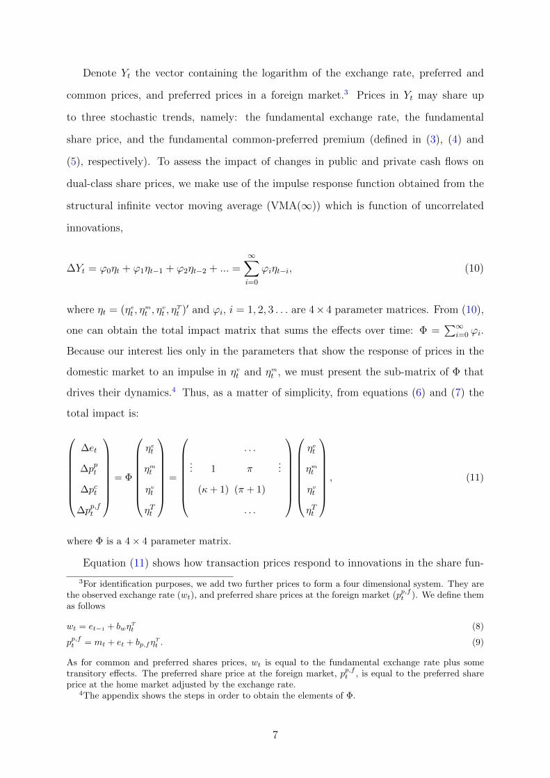
Denote Yt the vector containing the logarithm of the exchange rate, preferred and

common prices, and preferred prices in a foreign market.3 Prices in Yt may share up

to three stochastic trends, namely: the fundamental exchange rate, the fundamental

share price, and the fundamental common-preferred premium (defined in (3), (4) and

(5), respectively). To assess the impact of changes in public and private cash flows on

dual-class share prices, we make use of the impulse response function obtained from the

structural infinite vector moving average (VMA(∞)) which is function of uncorrelated

innovations,

∆Yt = ϕ0ηt + ϕ1ηt−1 + ϕ2ηt−2 + ... =∞∑i=0

ϕiηt−i, (10)

where ηt = (ηet , η

mt , η

vt , η

Tt )′ and ϕi, i = 1, 2, 3 . . . are 4× 4 parameter matrices. From (10),

one can obtain the total impact matrix that sums the effects over time: Φ =∑∞

i=0 ϕi.

Because our interest lies only in the parameters that show the response of prices in the

domestic market to an impulse in ηvt and ηm

t , we must present the sub-matrix of Φ that

drives their dynamics.4 Thus, as a matter of simplicity, from equations (6) and (7) the

total impact is:

∆et

∆ppt

∆pct

∆pp,ft

= Φ

ηet

ηmt

ηvt

ηTt

=

. . .

... 1 π...

(κ+ 1) (π + 1)

. . .

ηet

ηmt

ηvt

ηTt

, (11)

where Φ is a 4× 4 parameter matrix.

Equation (11) shows how transaction prices respond to innovations in the share fun-

3For identification purposes, we add two further prices to form a four dimensional system. They arethe observed exchange rate (wt), and preferred share prices at the foreign market (pp,ft ). We define themas follows

wt = et−1 + bwηT

t (8)

pp,ft = mt + et + bp,fηT

t . (9)

As for common and preferred shares prices, wt is equal to the fundamental exchange rate plus sometransitory effects. The preferred share price at the foreign market, pp,ft , is equal to the preferred shareprice at the home market adjusted by the exchange rate.

4The appendix shows the steps in order to obtain the elements of Φ.

7

damental price and in the voting rights. The parameter π summarizes the impact of ηvt

on preferred share prices. In the same way, π + 1 is the total effect on common shares.

Hence, the parameter π is the effect on the firm fundamental price from an innovation in

the voting right value. Finally, the term 1 +κ gives the total response on common shares

after shocks on the fundamental share price.

The question is what to expect from the parameters π and κ? The parameter π gives

the total response of prices to shocks in the voting right value. The voting right value

is often seen as a function of the private benefits that investors may get from holding

these rights. It can also reflect a possible premium over the preferred share, in mergers

and acquisitions (see Zingales (1994), Zingales (1995) and Dyck and Zingales (2004) for

explanations of private benefits and merger premium). As such, an increase in the value

of voting rights may signal that common shareholders can extract more private benefits

(increase in private cash flows) leading to a negative effect on public cash flows, i.e.

the increase in private benefits comes at the expense of all equity holders because the

share price declines. This economic intuition leads to the first hypothesis that a positive

innovation in private cash flows (an increase in the voting right value) generates a negative

effect on public cash flows (i.e., π < 0).

As for the parameter κ, the intuition on its sign is not so obvious. An increase in

the firm’s expected cash flows could lead to various possibilities of how the dividend

payments are shared between common and preferred shareholders. If no assumptions

are made regarding changes in payout policy and management decision on the split of

dividends between the two share classes, one may argue that, other things being equal,

an increase in the cash flows -results in a relative increase in dividends of both share

classes. Therefore, positive (negative) shocks on the expected future cash flows would then

lead to a proportional increase (decrease) in dividends for both share classes, increasing

(decreasing) the absolute difference between these dividend payments (given that Dc,t+i ≤

Dp,t+i), and hence decreasing (increasing) the common-preferred premium. Therefore,

positive news for the firm’s cash flows may deliver a higher dividend payment for both

share classes and a possible reduction in the common-preferred premium (i.e., κ < 0).

8

We can use the innovations associated with voting rights in (4) and (5) to infer which

variables drive the voting right value: domestic, market or firm specific factors? We

make use of the Fama-French factors to answer this question. It is well known that the

Fama-French factors are able to explain a large portion of the variability of stock returns.

Therefore, if the Fama-French factors are also able to significantly explain the variation

in the voting right value, then it is possible to conclude that market factors drive the

value of voting rights. If this is not the case, then the voting rights value relate to firm

specific factors. The idea is that Fama-French factors help explain the behavior of share

price returns more than they help elucidate the behavior of the voting right. If this is the

case, firm-specific factors play a larger role on the value of the voting rights than market

factors.

3 Estimation procedure

We follow Gonzalo and Granger (1995) and Gonzalo and Ng (2001) for the estimation

of the cointegrated VAR models. We assume that the price system in (10) admits a

cointegrated VAR(p) representation:

∆Yt = ξ1∆Yt−1 + ξ2∆Yt−2 + ...+ ξp∆Yt−p + ζ + ξ0Yt−1 + εt, (12)

where Yt is the vector of observed log prices, ξ0 = αβ′, α is the error correction term, β

is the cointegrating vector and εt is a zero mean white noise process with a non-diagonal

covariance matrix Ω. We estimate the parameters in (12) and then, through dynamic

simulation, back out the infinite VMA(∞) coefficients in (13):

∆Yt = εt + ψ1εt−1 + ψ2εt−2 + ... = Ψ(L)εt, (13)

where L is the usual lag operator and ψi, i = 1, 2, 3, . . . are 4 × 4 parameter matrices,

which are a function of the parameters in (12). The VMA representation in (13) has price

changes as a function of reduced-form (possible correlated) innovations, εt. Innovations

9

in each of the market prices can only affect their respective market prices at time t

(ψ0 = I4 in (13)). The target of this investigation is to achieve a VMA expression driven

by uncorrelated innovations. Equation (14) is the structural counterpart of (13), where

ηt is a 4× 1 vector which contains uncorrelated innovations:

∆Yt = ϕ0ηt + ϕ1ηt−1 + ϕ2ηt−2 + ... =∞∑i=0

ϕiηt−i. (14)

The sum of the effects at all lags, Φ = ϕ0 + ϕ1 + ϕ2 + ..., is the measure we are most

interested in because it delivers the impact on transaction prices as a result of uncorrelated

innovations. 5 These uncorrelated innovations correspond to shocks in the fundamental

share price and in the voting right value, depicted in (11).

We identify Φ as in Gonzalo and Ng (2001) and first define εt as the reduced-form

permanent and transitory innovations: εt = Gεt, with G = [α′⊥, α′Ω−1]′. The covariance

matrix of εt is given by Ξ = GΩG′, where Ω = E(εtε′t) from (12). Because Ξ is likely a

non-diagonal matrix, we implement a further step to find uncorrelated innovations. As

in Scherrer (2014), we define a non-symmetric matrix Ξ = ΞΘ−1, where Θ is a diagonal

matrix constructed with the diagonal elements of Ξ. We then decompose Ξ using the

spectral decomposition (Ξ = SS), recovering ηt = SGεt. The same relation applies to

recover Φ, such that Φ = Ψ(L)G−1S = Ψ(L)ϕ0, with ϕ0 = G−1S. Note that ηt and εt

have the same dimension. Hence, the number of uncorrelated innovations must be equal

to the number of markets. As (12) is a cointegrated system, the number of stochastic

trends is equal to the number of variables in the system minus the number of cointegrated

relations. Because there are at least two stochastic innovations (ηmt and ηvt ), it would not

be possible to identify the system in a cointegrated framework with only two variables.

This is the reason we add the stock price in a foreign market (and then the exchange

rate) in Section 2 and in the empirical analysis in Section 4.

5For a formal definition of uncorrelated permanent and transitory innovations, see Gonzalo andGranger (1995) and Gonzalo and Ng (2001).

10

4 Effects of voting rights on firm value

Investors observe distinct cash flows from common and preferred shares. Dual class

shares are therefore priced differently and the value of the premium between them may

be associated to private cash flows. We assess empirically the impact of changes in the

voting right value on firm value. How do investors who hold a common share perceive

changes to expected future benefits? How do they impact the way they estimate expected

cash flows? What is the relation between private and public cash flows? Do changes in

private benefits affect the cash flows generated by the firms?

In order to answer these questions, one needs both preferred and common shares that

are traded frequently. For that, we use a data set of Brazilian firms. The Brazilian

stock exchange is particularly interesting for this study, given that dual class shares are

exceptionally popular in the country and as so, they have been subject to more studies

in this area.6 Brazilian firms can have up to 50% of the total number of shares issued as

preferred shares.7 This characteristic makes it possible for the stock exchange market to

have significant trading activity in both classes of shares.8

The foreign market is represented by American Depositary Receipts (ADRs). 9 Many

Brazilian firms also trade in the U.S. through ADRs. We start with all Brazilian firms

which currently trade in the U.S. These make up for 25 firms. Out of these, we select

the ones that have common and preferred shares traded on the Brazilian stock exchange.

These are Ambev (beverage), Bradesco (finance), Santander (finance), Braskem (petro-

chemical), Electrobras (energy), Copel (energy), CBD (food distribution), Cemig (en-

ergy), Gerdau (steel), Itau Unibanco (finance), Oi (telecommunication), Petrobras (oil),

6For more information on some particularities of the Brazilian data, Nenova (2001) provides aninteresting study, where she analyzes private benefits for Brazilian firms in the 1990s and find a time-varying behavior.

7Law number 10.303 of 31 October, 2001 states a limit of 50 preferred shares. Before that,Law 6.404 of 15 December, 1976 stated a ratio of 2/3 of preferred shares. Preferred sharesare defined as having none or less voting power than common shares and have some prefer-ence on dividend payments. See http : //www.cvm.gov.br/port/atos/leis/lei10303.asp and http ://www.planalto.gov.br/ccivil03/leis/l6404consol.htm.

8Fernandes and Novaes (2014) also see the advantages of Brazilian data in their extensive study whichshows that government activism reduces the value of minority shareholders voting rights in Brazilianpublic firms.

9For identification purposes Section 2 includes preferred shares at a foreign market and exchange rate.

11

Telefonica (telecommunication), Tim (telecommunication) and Vale (mining). We use

daily prices for preferred and common shares traded in Brazilian currency and ADRs on

preferred shares traded on the NYSE in U.S. dollars as well as the exchange rate. The

sample spans from January 2007 to December 2014.

First we test for cointegration. Table 1 reports the results of the trace and the

maximum eigenvalue tests. The four variable system shows one cointegrating vector for

the majority of the companies. This delivers three common factors. These three common

factors are seen as the stochastic trends presented in Section 2, namely, the fundamental

exchange rate, the fundamental share price and the common-preferred premium. We

then estimate (12) to obtain matrix Φ in (11) (see discussion in Section 3).10 From Φ,

we can infer the model parameters in (4) and (5): π and κ.

Table 2 presents the results of the inference on the model parameters.11 From (11), π

gives the price response to changes in the value of voting rights. This parameter shows the

percentage impact on the fundamental price of the firm (which affects both common and

preferred shares) as a result of a shock in the voting value. For instance, in the first row,

for a 1% innovation on the voting right, there is a -0.96% effect on the fundamental firm

price. All π significant estimates are negative except to Vale.12 The result indicates that

a positive/negative change in the price of the vote decreases/increases the public cash

flows. This result shows that an increase in private cash flows (the ones only common

shareholders receive), seen through a higher voting value, decreases the public cash flows.

This happens because of the negative effect on the fundamental value of the firm. A

low value of voting rights is a signal of low expropriation and private benefits. Such a

situation may arise from better corporate governance and stronger shareholders rights

10We estimate the parameters in (12) using full information maximum likelihood framework of Jo-hansen (1991) where the lag length, p, is determined using the BIC criterium and LM test, such thatthe residuals are white noise processes.

11The parameter π is over identified, given that it can be inferred from more than one position (secondand third row in the third column) in (11), but they deliver inferences that are statistically equal.

12Vale has a positive significant parameter. Note that Vale’s preferred shares are defined as ‘class A’,so that preferred shareholders have the right to vote in General Assembly Deliberations, just as commonshareholders. The only difference is that preferred shareholders do not have a say in the composition ofthe board of directors. Therefore, the voting difference between the two classes is less significant than inthe other firms. This implies that shocks on the voting rights do not have a negative impact on publiccash flows.

12

as in Gompers et al. (2003), who find that companies with stronger shareholder rights

present higher firm value and higher profits. In the same way Klapper and Love (2004)

find that stronger corporate governance is associated with better operating performance

(return on assets).

In 2000 BM&FBovespa launched the ”Novo Mercado” (New Market), which is char-

acterized by the highest level of corporate governance. It is defined by BM&FBovespa

as high standards for transparency and governance. Firms traded on the Novo Mercado

adopt practices of corporate governance superior to the ones required by Brazilian law.

It is interesting to note that companies that are part of the Novo Mercado can only issue

shares with voting rights, not allowing for asymmetry in cash flows and voting rights.

There are two previous findings in the literature which provide insights about our

results. Doidge (2004) finds that foreign firms cross-listing in the U.S. have a voting

premium of 43% lower than firms that do not cross-list. This means that the effect for

firms that do not cross-list could be even higher than the one we unveil here with a higher

negative effect on the firm value after an increase in the voting right value. On the other

hand, Dyck and Zingales (2004) find Brazil is the country (among 39 countries) with the

highest value for corporate control. They relate their results of a higher premium to lower

investor protection and higher willingness to extract private benefits. The lower investor

protection would explain the significantly negative π estimates.

The estimates for κ are significant and negative for all firms. This implies that a

positive shock on the fundamental share price reduces the common-preferred premium in

line with the discussion in Section 2.

In summary, there is evidence that an increase in the value of voting rights generates

a negative effect on firms’ cash flows. We claim that this is because common shareholders

can extract more private benefits and, hence, generate a decrease in public cash flows. A

second finding relates good (bad) news for firms’ cash flows with a decrease (increase) in

the common-preferred premium.

13

5 Voting right and firm specific risk

The fundamental share price, i.e. the expected future dividend payments, is a financial

asset and as such the Fama-French factors should be able to explain a portion of its

variation. The common-preferred premium, and, more specifically, the component related

to the voting right value does not present such a clear intuition. The Fama-French factors,

however, can still be used in this context. Understanding how much of the voting right

value can be explained by these factors sheds light on whether the voting right is specific

to the firm or it has some common component. The main goal of this Section is to

compare how much the Fama-French factors can explain share price returns and the

value of voting rights. We perform this analysis using U.S. factors, as all firms in this

study have ADRs negotiated at NYSE. As a robustness check, we also present the results

of Brazilian factors in the appendix.

The Fama-French factors are the excess return on the market portfolio (MktRF),

small market capitalization minus big (SMB) and high book-to-market ratio minus low

(HML)13. We recover daily estimates of εmt , ηmt , εvt and ηvt for each firm from the estimates

in Section 4 and regress them on the three Fama-French factors.

εmt = β0 + β1MktRFt + β2SMBt + β3HMLt + ut, (15)

ηmt = β0 + β1MktRFt + β2SMBt + β3HMLt + ut, (16)

εvt = β0 + β1MktRFt + β2SMBt + β3HMLt + ut, (17)

ηvt = β0 + β1MktRFt + β2SMBt + β3HMLt + ut. (18)

Note that εmt and εvt are measures still “contaminated” by impacts of other sources than

ηmt and ηv

t , respectively.14 As such, we expect the regressions (15) and (17) to present a

better fit than (16) and (18), as the regressors of the former ones combine information

from both ηmt and ηvt . We also expect the Fama-French factors to explain a larger portion

13The source for the Fama-French factors ishttp : //mba.tuck.dartmouth.edu/pages/faculty/ken.french/datalibrary.html.

14From the identification strategy in Section 2 we have that εmt = ηmt + πηv

t and εvt = ηvt + κηm

t .Furthermore, recall from Section 3 that εt = Gεt and ηt = SGεt.

14

of ηmt than of ηvt , considering the discussion in Section 2. Tables 3 and 4 report the results

of the estimation of (15) - (18). We report the parameter estimates and R-squared for

all companies.

By analysing the R-squared measures, indeed we find that the Fama-French factors

are able to explain the variation in (15) better than in (16). The same applies for (17)

compared to (18). These results corroborate our economic intuition, because there is

more information in εmt and εvt than in their structural counterparts ηmt and ηv

t . We also

find that the R-squared measure drops more from (17) to (18) than from (15) to (16).

This follows mainly because ηmt loads heavily on the market factor, MktRF, inflating the

correlation between MktRF and εvt , as ηmt is contained in εvt . The same is not true for ηvt

that is contained in εmt , but does not contribute as much to the R-squared measure when

comparing (15) and (16).

Comparing the R-squared from the (16) and (18) regression, we find that the Fama-

French factors are able to explain a much larger proportion of ηmt than ηvt . The three

Fama-French factors successfully explain the component associated with the price inno-

vations, however when the innovations related to the voting rights are considered as the

dependent variable as in (18), the picture is completely different. This hints that firm

specific factors play a larger role on determining the value of the vote. We find that the

Fama-French factors only explain, on average, 5% of the variability of ηvt , suggesting that

most of the variability in ηvt is due to firm specific factors.

The result hints two things: First, there is a firm specific component in the voting

right value. This might be because firms have the option to pursue more advanced

corporate practices than the ones required by law as well as some legal rules of investors’

protection may not be binding. Gompers et al. (2003) show that equity holders rights

vary across firms and Klapper and Love (2004) find that companies in the same country

provide different level of protection to investors.15 Second, the voting right value could

well relate to domestic risk factors, that are not included in the Fama-French regression.

LaPorta et al. (1998), for instance, study 49 countries and conclude that the legal rules

15They find that there is a wide variation in firm-level governance with firms which present both goodand bad governance in countries with weak and strong legal systems.

15

to protect investors can vary significantly among countries, and LaPorta et al. (2000)

discuss the differences among countries in their laws related to investor protection and

corporate governance. Tables A.1 and A.2 in the appendix provide results of this same

exercise using domestic risk factors as regressors instead. There is a significant increase

in the R-squared for the price returns, as expected. However, the increase in R-squared

for the voting right returns is not so evident. This result reinforces that the value of

voting rights are driven by firm-specific factors rather than market or domestic market

factors.

It is also relevant to investigate the sign and significance of the estimated parameters

associated with the Fama-French factors. As expected, we find that β1 is always positive

and highly significant for the regressions (15) and (16). When considering estimates of β1

for the regressions (17) and (18), we find them to be mostly negative and significant. This

result indicates that the small share of the voting right value, which the factor MktRF can

explain, happens through a negative relation between the return on holding the voting

right and the return on the market portfolio. This is also in line with the discussion in

Section 2 of a negative value for κ. Hence, a negative value for β1 in (18) captures the

negative effect on the common-preferred premium from shocks on the fundamental price

of the stock (reflecting the positive relation with MktRF).

As a further analysis, Table 5 reports the correlation of the innovations in voting rights

across firms. We find a significant low correlation between the voting rights innovations

across firms. This is in line with common market factors being of reduced importance to

explain variation on the value of voting rights. This result reinforces the conclusion that

firm specific factors play a substantial role in driving the voting right value.

In general, the results in this Section indicate that indeed Fama-French factors help

explain the behavior of the share price returns. By contrast, when voting rights are used

as a dependent variable, we find very different results. Insights that there are firm specific

factors explaining the behavior of the voting right value are suggested.

16

6 Conclusions

This paper presents a simple model for dual-class shares that allows public and private

cash flows affect the fundamental share price. Our aim is to disentangle the effect from

these two sources, so that we can determine how the private benefits of holding the voting

rights affect the fundamental share price and, thus, the equity-holders’ wealth.

We propose a simple time-series model for prices of common and preferred shares

which allows us to identify the innovations associated with the fundamental share price

and voting rights. We find that an increase in the value of the vote (seen as private

cash flows which only common shareholders receive) negatively affects the firm value for

Brazilian cross-listed firms and, therefore, decreases the public cash flows. This is in line

with the literature on agency and entrenchment problems about the desirability of the

one-share-one-vote rule (Adams and Ferreira (2008)).

Our results also shed light on the discussion regarding what drives the value of voting

rights. We use the Fama-French regressions to measure the role of market and firm

specific factors. We find that Fama-French factors explain, on average, only 5% of the

variations on the voting rights innovations. This indicates that there are some firm

specific components (or at a much lower intensity, domestic factors) that explain most of

the variations of the voting rights value.

This paper contributes to the literature on empirical finance and corporate governance.

We show how changes in the value of the vote affect the equity holders’ wealth and,

hence, the results provide insights that one-share-one-vote might be desirable in the open

discussion of how to improve corporate governance.

17

Table 1: Max Eigenvalue and Trace Test

Gerdau Vale Petro Bradesco Ambev Santander Braskem Eletrobras

Ho Ha Max Eigenvalue Test

0 1 231.2 606.8 479.3 286.3 178.3 47.5 284.7 314.51 2 16.7 12.2 8.0 8.8 13.8 17.5 25.7 5.22 3 2.6 2.7 2.1 3.2 3.7 3.5 4.4 2.13 4 0.0 0.2 0.1 0.9 0.9 0.7 1.0 0.1

Conclusion 1cv 1 cv 1 cv 1 cv 1 cv 1 cv 1 cv - 99 1 cv

Ho Ha Trace Test

0 4 214.5 594.6 471.3 277.5 164.5 29.9 259.1 309.31 4 14.1 9.5 5.8 5.6 10.1 14.0 21.3 3.12 4 2.6 2.6 2.1 2.3 2.8 2.8 3.3 2.03 4 0.0 0.2 0.1 0.9 0.9 0.7 1.0 0.1

Conclusion 1 cv 1 cv 1 cv 1 cv 1 cv 1 cv 1 cv - 99 1 cv

Copel CBD Cemig Itau Oi Telefonica Tim

Ho Ha Max Eigenvalue Test

0 1 45.8 470.0 210.9 316.9 22.2 274.9 170.21 2 9.0 20.3 9.5 16.3 9.5 41.1 28.02 3 1.7 5.3 1.2 7.3 2.3 1.9 1.03 4 0.1 0.3 0.1 1.1 0.2 0.0 0.3

Conclusion 1 cv 1 cv 1 cv 1 cv - - 1 cv

Ho Ha Trace Test

0 4 36.8 449.6 201.5 300.6 12.7 233.8 142.21 4 7.3 15.0 8.2 9.1 7.1 39.2 27.02 4 1.6 5.0 1.1 6.2 2.1 1.9 0.73 4 0.1 0.3 0.1 1.1 0.2 0.0 0.3

Conclusion 1 cv 1 cv 1 cv 1 cv - - -

We present results considering two cointegration rank tests: maximum eigenvalue and trace test. For each firm the firstfour rows refer to the maximum eigenvalue test, and the last four rows refer to the trace test. The columns bring theresults for the different firms in our sample. The null hypotheses (of both maximum eigenvalue and trace tests) are zero,one, two and three cointegrating vectors, respectively. The critical values at 5% significance level for the null hypothesisof 1 cointegrating vector is 24.28 (max eigenvalue) and 17.80 (trace). The last row in both tests brings the conclusion. ‘1cv’ means that we are able to conclude with 95% confidence that there is only 1 cointegrating vector and, hence, threecommon stochastic trends in a four variable system. ‘1 cv -99’ means that we cannot reject the null of 1 cointegratingvector at 1% significance level. ‘-’ stands for no conclusion.

18

Table 2: Model Parameters

π κGerdau −0.96 ∗ ∗

(0.14)−0.08(0.06)

Bradesco −0.38 ∗ ∗(0.15)

−0.07 ∗ ∗(0.02)

Ambev −0.11 ∗ ∗(0.11)

−0.02 ∗ ∗(0.03)

Braskem −0.34 ∗ ∗(0.07)

−0.13 ∗ ∗(0.04)

CBD −0.37 ∗ ∗(0.2)

−0.65 ∗ ∗(0.1)

Cemig −0.32 ∗ ∗(0.1)

−0.06 ∗ ∗(0.03)

Itau −0.7 ∗ ∗(0.13)

−0.12 ∗ ∗(0.03)

Telefonica −0.41 ∗ ∗(0.07)

−0.17 ∗ ∗(0.04)

Copel −0.17∗(0.09)

−0.48(0.23)

Eletrobras −0.15∗(0.1)

−0.06 ∗ ∗(0.03)

Oi −0.15(0.17)

−0.07∗(0.07)

Tim −0.15(0.08)

−0.10(0.05)

Vale 0.76 ∗ ∗(0.2)

−0.02(0.01)

Petrobras 0.46(0.2)

−0.01(0.01)

Santander 0.79(0.28)

0.07(0.03)

We report estimates of π and κ. ∗∗ and ∗ denote that the parameterestimates are statistically significant at 5% and 10% levels, respectively.We obtain confidence intervals and standard errors (inside brackets) usingparametric bootstrap algorithm (See Lutkepohl (2007), page 709).

19

Table 3: Fama-French Factors

Gerdau Bradesco Itau Ambev Braskem Petrobras Vale Santanderεmt = β0 + β1MktRFt + β2SMBt + β3HMLt + ut

MktRF 1.21(13.804)

1.04(14.499)

1.00(15.115)

0.62(15.442)

1.04(11.546)

1.00(15.51)

1.09(15.979)

0.67(9.119)

SMB −0.16(−1.26)

−0.30(−2.487)

−0.13(−1.091)

−0.29(−4.024)

−0.15(−1.072)

−0.27(−2.146)

−0.27(−2.5)

−0.01(−0.105)

HML −0.04(−0.283)

0.11(1.024)

0.17(1.578)

−0.24(−3.146)

−0.15(−1.193)

−0.07(−0.488)

−0.09(−0.652)

0.06(0.379)

R2 0.42 0.49 0.43 0.32 0.30 0.29 0.44 0.11

ηmt = β0 + β1MktRFt + β2SMBt + β3HMLt + utMktRF 1.02

(11.161)0.92

(13.079)0.81

(12.47)0.58

(15.098)0.79

(8.803)0.82

(12.56)0.95

(13.47)0.43

(4.457)

SMB −0.15(−1.096)

−0.23(−1.912)

−0.02(−0.137)

−0.28(−3.836)

−0.09(−0.691)

−0.20(−1.45)

−0.26(−2.198)

0.06(0.382)

HML 0.01(0.064)

0.14(1.379)

0.18(1.801)

−0.23(−2.927)

−0.13(−1.066)

−0.03(−0.219)

−0.05(−0.404)

−0.12(−0.587)

R2 0.29 0.40 0.33 0.28 0.18 0.19 0.32 0.03

εvt = β0 + β1MktRFt + β2SMBt + β3HMLt + utMktRF −0.05

(−3.701)−0.10(−7.284)

−0.21(−6.241)

−0.09(−2.786)

−0.42(−10.533)

0.06(5.694)

0.06(5.395)

0.28(11.996)

SMB −0.03(−0.908)

0.08(2.427)

0.11(2.36)

0.11(3.245)

0.10(1.103)

−0.02(−0.774)

0.02(0.468)

−0.08(−1.845)

HML 0.01(0.554)

−0.01(−0.332)

−0.06(−1.21)

0.03(0.82)

0.06(0.776)

0.03(1.425)

−0.01(−0.338)

0.10(1.956)

R2 0.01 0.05 0.16 0.03 0.10 0.03 0.03 0.16

ηvt = β0 + β1MktRFt + β2SMBt + β3HMLt + utMktRF −0.02

(−1.79)−0.06(−5.01)

−0.15(−4.338)

−0.08(−2.638)

−0.34(−9.11)

0.05(4.515)

0.04(3.439)

0.24(8.303)

SMB −0.04(−0.971)

0.07(2.232)

0.11(2.253)

0.11(3.105)

0.09(1.067)

−0.02(−0.662)

0.02(0.641)

−0.09(−1.745)

HML 0.02(0.648)

−0.01(−0.221)

−0.05(−1.021)

0.03(0.741)

0.05(0.657)

0.03(1.354)

−0.01(−0.299)

0.12(1.835)

R2 0.00 0.02 0.09 0.03 0.07 0.02 0.01 0.08

We report parameter estimates considering four variants of the Fama-French regressions. We regress εmt , ηmt , εvt and ηvt on theFama-French factors (MktRF, SMB and HML) by OLS. We report t-statistics based on robust standard errors in parentheses.R2 stands for the R-squared measure.

20

Table 4: Fama-French Factors (cont.)

CBD Cemig Oi Telefonica Eletrobras Copel Timεmt = β0 + β1MktRFt + β2SMBt + β3HMLt + ut

MktRF 0.69(12.763)

0.63(11.511)

0.98(11.321)

0.39(9.099)

0.69(11.914)

0.25(10.568)

0.95(9.892)

SMB −0.08(−0.787)

−0.21(−2.275)

−0.21(−1.092)

−0.17(−1.62)

−0.18(−1.615)

−0.10(−1.844)

−0.08(−0.597)

HML −0.12(−1.33)

−0.13(−1.394)

−0.02(−0.084)

−0.17(−2.65)

−0.02(−0.168)

−0.10(−1.716)

−0.40(−2.727)

R2 0.26 0.17 0.13 0.11 0.13 0.05 0.32

ηmt = β0 + β1MktRFt + β2SMBt + β3HMLt + utMktRF 0.57

(12.467)0.55

(10.702)0.65

(7.733)0.36

(8.967)0.60

(10.894)0.33(9.85)

0.93(10.324)

SMB −0.09(−0.886)

−0.18(−2.085)

−0.23(−1.163)

−0.16(−1.679)

−0.15(−1.271)

−0.17(−2.324)

−0.09(−0.646)

HML −0.10(−1.197)

−0.12(−1.193)

−0.02(−0.096)

−0.16(−2.479)

−0.03(−0.192)

−0.10(−1.414)

−0.36(−2.531)

R2 0.17 0.13 0.06 0.09 0.10 0.08 0.30

εvt = β0 + β1MktRFt + β2SMBt + β3HMLt + utMktRF −0.64

(−12.26)−0.07(−4.141)

−0.46(−4.005)

−0.12(−4.162)

0.04(1.818)

0.73(11.351)

−0.09(−0.852)

SMB −0.07(−0.469)

0.04(1.096)

0.38(1.958)

0.04(0.603)

0.08(1.423)

−0.36(−3.49)

−0.14(−1.175)

HML 0.09(1.046)

0.02(0.718)

−0.17(−1.481)

0.05(1.244)

−0.11(−1.89)

0.05(0.4)

0.33(2.076)

R2 0.10 0.01 0.09 0.02 0.00 0.20 0.01

ηvt = β0 + β1MktRFt + β2SMBt + β3HMLt + utMktRF −0.29

(−8.872)−0.07(−3.978)

−0.20(−1.565)

−0.09(−3.137)

0.04(1.885)

0.85(12.27)

0.06(0.645)

SMB −0.17(−0.99)

0.04(1.038)

0.43(2.072)

0.02(0.318)

0.08(1.355)

−0.45(−3.634)

−0.18(−1.403)

HML 0.03(0.608)

0.02(0.661)

−0.18(−1.526)

0.03(0.784)

−0.11(−1.841)

0.01(0.052)

0.29(1.801)

R2 0.02 0.01 0.03 0.01 0.00 0.24 0.02

We report parameter estimates considering four variants of the Fama-French regressions. We regress εmt , ηmt , εvtand ηvt on the Fama-French factors (MktRF, SMB and HML) by OLS. We report t-statistics based on robuststandard errors in parentheses. R2 stands for the R-squared measure.

21

Table 5: Voting Rights Return Correlation

Gerdau Vale Petro Bradesco Braskem Eletrobras Copel CDB Cemig Itau Oi TelefonicaGerdau 1

Vale -0.03 1Petro -0.04 0.18 1

Bradesco 0.04 0.06 -0.03 1Braskem -0.02 -0.06 -0.07 0.03 1

Eletrobras 0.02 0.00 -0.02 0.03 0.00 1Copel -0.02 0.01 0.05 -0.05 -0.22 0.06 1CDB -0.01 -0.04 0.01 0.02 0.05 -0.04 -0.14 1

Cemig -0.03 0.02 0.00 -0.03 0.04 0.02 -0.13 0.03 1Itau 0.06 -0.03 -0.07 0.21 0.12 -0.01 -0.24 0.05 0.05 1

Oi -0.02 0.02 -0.02 0.03 0.00 -0.02 -0.03 0.05 0.05 0.05 1Telefonica 0.00 -0.01 -0.01 0.01 0.04 0.03 -0.07 0.04 0.05 0.07 0.08 1

We report the empirical correlation matrix computed using the estimates of the firm specific innovations associated withthe voting rights ηvt .

22

A Appendix

A.1 Model derivation

To obtain the structural VMA model with observed price changes as function of perma-

nent uncorrelated innovations, we must compute the first difference of (6) and (7) and

then substitute the uncorrelated innovations from (4) and (5) accordingly.

ppt − ppt−1 = mt −mt−1 + bp

(ηT

t − ηT

t−1

),

pct − pct−1 = mt −mt−1 + dt − dt−1 + bc(ηT

t − ηT

t−1

),

∆ppt = ∆mt + bp (ηT

t − LηT

t ) ,

∆pct = ∆mt + ∆dt + bc (ηT

t − LηT

t ) , (A.19)

where L is the usual lag operator. Setting L = 1, we have that

∆ppt = ηmt + πηvt ,

∆pct = ηmt + πηvt + ηvt + κηmt = (π + 1)ηvt + (κ+ 1)ηmt . (A.20)

A.2 Brazilian risk factors

We repeat the Fama-French regressions using Brazilian risk factors as regressors16 instead

of the U.S. Fama-French factors. As a robustness check, Tables A.1 and A.2 present

the results. Using domestic risk factors significantly improves the explanatory power

of returns in comparison to the results obtained with the U.S. risk factors. Domestic

components indeed help explain the behavior of the firm price. However, the same is not

true for the voting rights value that we do not observe a substantial improvement for

every firm. This reinforces the insight that the value of the voting right is indeed firm

specific and not market related.

16Risk factors are from http : //www.fea.usp.br/nefin/.

23

Table A.1: Brazilian Risk Factors

Gerdau Bradesco Itau Ambev Braskem Petrobras Vale Santanderεmt = β0 + β1MktRF + β2SMB + β3HML+ ut

MktRF 1.23(24.274)

1.14(39.322)

1.16(35.319)

0.54(15.276)

0.92(14.795)

1.34(27.995)

1.15(30.126)

0.69(9.145)

SMB −0.10(−1.495)

−0.03(−0.612)

0.07(1.233)

−0.13(−2.761)

−0.02(−0.218)

0.20(2.799)

0.02(0.553)

0.05(0.602)

HML 0.25(4.013)

−0.02(−0.521)

−0.04(−0.779)

−0.18(−2.835)

0.52(5.8)

0.27(3.291)

0.10(1.563)

0.03(0.312)

R2 0.62 0.74 0.69 0.38 0.38 0.68 0.67 0.15

ηmt = β0 + β1MktRF + β2SMB + β3HML+ utMktRF 1.10

(19.616)1.07

(33.256)1.03

(21.978)0.51

(14.752)0.71

(11.052)1.22

(21.252)1.04

(24.812)0.52

(6.134)

SMB −0.29(−4.681)

−0.14(−2.841)

−0.02(−0.281)

−0.15(−3.189)

−0.12(−1.182)

0.07(0.749)

−0.12(−2.228)

0.00(0.011)

HML 0.28(4.12)

0.02(0.351)

0.01(0.123)

−0.18(−2.763)

0.56(6.03)

0.34(3.638)

0.21(3.045)

0.00(−0.022)

R2 0.53 0.70 0.61 0.36 0.27 0.58 0.57 0.05

εvt = β0 + β1MktRF + β2SMB + β3HML+ utMktRF −0.04

(−3.287)−0.09(−6.928)

−0.20(−7.707)

−0.03(−1.022)

−0.27(−6.615)

0.04(3.257)

0.06(5.712)

0.20(7.388)

SMB 0.03(1.675)

0.02(0.97)

0.04(1.6)

0.05(1.865)

0.20(3.894)

−0.03(−1.642)

−0.01(−0.398)

−0.04(−1.336)

HML −0.07(−3.075)

0.01(0.424)

0.01(0.325)

0.00(−0.169)

−0.22(−3.358)

0.01(0.348)

−0.07(−3.188)

0.06(2.069)

R2 0.03 0.06 0.19 0.01 0.10 0.02 0.05 0.14

ηvt = β0 + β1MktRF + β2SMB + β3HML+ utMktRF −0.01

(−0.684)−0.05(−3.866)

−0.13(−4.469)

−0.02(−0.844)

−0.19(−4.844)

0.02(1.568)

0.04(3.403)

0.14(5.252)

SMB 0.02(0.955)

0.02(0.916)

0.05(1.91)

0.04(1.613)

0.21(4.002)

−0.03(−1.657)

0.00(−0.166)

−0.04(−1.061)

HML −0.06(−2.631)

0.01(0.407)

0.01(0.241)

−0.01(−0.259)

−0.18(−2.707)

0.00(0.084)

−0.07(−3.471)

0.07(1.699)

R2 0.01 0.02 0.09 0.01 0.07 0.01 0.02 0.05

We report parameter estimates considering four variants of the Fama-French regressions (15)- (18) which use domestic risk factors.We regress εmt , ηmt , εvt and ηvt on the Brazilian risk factors associated with the Fama-French factors (MktRF, SMB and HML)by OLS. We report t-statistics based on robust standard errors in parentheses. R2 stands for the R-squared measure.

24

Table A.2: Brazilian Risk Factors (cont.)

CBD Cemig Oi Telefonica Eletrobras Copel Timεmt = β0 + β1MktRFt + β2SMBt + β3HMLt + ut

MktRF 0.67(18.88)

0.59(12.159)

0.67(8.501)

0.35(7.296)

0.69(13.634)

0.19(8.728)

0.72(13.396)

SMB −0.10(−1.306)

−0.26(−3.327)

−0.80(−5.509)

−0.16(−2.65)

−0.31(−3.796)

0.09(2.042)

−0.52(−4.242)

HML −0.07(−0.975)

0.38(5.44)

0.95(5.454)

0.22(4.08)

0.65(7.016)

0.01(0.128)

0.22(1.763)

R2 0.37 0.31 0.22 0.20 0.29 0.04 0.44

ηmt = β0 + β1MktRFt + β2SMBt + β3HMLt + utMktRF 0.55

(15.936)0.51

(10.961)0.39

(4.833)0.34

(7.426)0.61

(11.917)0.22

(7.672)0.71

(13.36)

SMB −0.19(−2.565)

−0.30(−3.83)

−0.89(−6.411)

−0.13(−2.004)

−0.40(−4.661)

−0.02(−0.441)

−0.53(−4.609)

HML −0.01(−0.209)

0.39(5.221)

1.08(6.379)

0.22(3.944)

0.74(7.826)

0.12(1.779)

0.25(2.054)

R2 0.26 0.27 0.18 0.19 0.27 0.07 0.43

εvt = β0 + β1MktRFt + β2SMBt + β3HMLt + utMktRF −0.64

(−17.468)−0.04(−2.381)

−0.49(−6.481)

−0.06(−2.626)

0.09(3.911)

0.70(10.409)

0.05(1.014)

SMB 0.06(0.849)

0.13(4.302)

0.18(1.517)

0.15(4.146)

0.08(2.072)

−0.01(−0.077)

0.12(0.954)

HML 0.12(1.415)

−0.10(−2.101)

−0.04(−0.383)

−0.07(−1.652)

0.11(1.775)

0.36(4.604)

0.16(1.133)

R2 0.14 0.04 0.14 0.04 0.01 0.27 0.00

ηvt = β0 + β1MktRFt + β2SMBt + β3HMLt + utMktRF −0.30

(−12.954)−0.04(−2.314)

−0.29(−3.837)

−0.03(−1.332)

0.09(3.842)

0.73(9.432)

0.19(3.747)

SMB 0.03(0.725)

0.10(3.233)

0.23(2.146)

0.12(3.136)

0.03(0.827)

−0.13(−1.803)

0.13(1.007)

HML 0.11(1.217)

−0.07(−1.542)

−0.09(−0.74)

−0.03(−0.795)

0.16(2.716)

0.49(5.671)

0.17(1.23)

R2 0.02 0.03 0.06 0.02 0.02 0.30 0.02

We report parameter estimates considering four variants of the Fama-French regressions (15)- (18) which usedomestic risk factors. We regress εmt , ηmt , εvt and ηvt on the Brazilian risk factors associated with the Fama-French factors (MktRF, SMB and HML) by OLS. We report t-statistics based on robust standard errors inparentheses. R2 stands for the R-squared measure.

25

7 Acknowledgments

Acknowledgments: We thank Gustavo Fruet Dias and Heitor Almeida for useful com-

ments. Cristina acknowledges support from the Center for Research in Econometric

Analysis of Time Series (CREATES), which is funded by the Danish National Research

Foundation (DNRF78), and from FAPESP Grant 2013/22930-0. Marcelo thanks the fi-

nancial support from FAPESP (2013/22930-0) and CNPq (302272/2014-3). The usual

disclaimers applies.

26

References

Adams, R. and D. Ferreira (2008). One share, one vote: The empirical evidence. Review

of Finance 12, 51–91.

Barclay, M. and C. Holderness (1989). Private benefits from control of public corpora-

tions. Journal of Financial Economics 25, 371–395.

Burkart, M. and S. Lee (2008). One share - one vote: The theory. Review of Finance 12,

1–49.

Cox, S. and D. Roden (2002). The source of value of voting rights and related dividend

promises. Journal of Corporate Finance 8, 337–351.

Doidge, C. (2004). U.s. cross listing and the private benefit of control: Evidence from

dual-class firms. Journal of Financial Economics 72, 519–553.

Dyck, A. and L. Zingales (2004). Private benefits of control: An international comparison.

Journal of Finance 59, 537–600.

Fernandes, M. and W. Novaes (2014). The government as a large shareholder: impact on

the voting premium. Technical report, Sao Paulo School of Economics, FGV, School

of Economics and Finance, Queen Mary University of London and Department of

Economics, PUC-Rio.

Gompers, P., J. Ishii, and A. Metrick (2003). Corporate governance and equity prices.

Quarterly Journal of Economics 118, 107–156.

Gonzalo, J. and C. Granger (1995). Estimation of common long memory components in

cointegrated systems. Journal of Business & Statistics 13, 27–35.

Gonzalo, J. and S. Ng (2001). A systematic framework for analazing the dynamic effects

of permanent and transitory shocks. Journal of Economics Dynamics & Control 25,

1527–1546.

27

Johansen, S. (1991). Estimation and hypothesis testing of cointegration vectors in gaus-

sian vector autoregressive models. Econometrica 59, 1551–1580.

Kalay, A., O. U. Karakas, and S. Pant (2014). The market value of corporate votes:

Theory and evidence from option prices. Journal of Finance 99, 1235–1271.

Klapper, L. and I. Love (2004). Corporate governance, investor protection, and perfor-

mance in emerging markets. Journal of Corporate Finance 10, 703–728.

LaPorta, R., F. L. de Silanes, A. Shleifer, and R. Vishny (2000). Investor protection and

corporate governance. Journal of Financial Economics 58, 3–27.

LaPorta, R., F. L. de Silanes, A. Shleifer, and R. W. Vishny (1998). Law and finance.

Journal of Political Economy 106, 1113–1155.

Lutkepohl, H. (2007). New Introduction to Multiple Time Series Analysis. Springer.

Nenova, T. (2001). Control values and changes in corporate law in brazil. Technical

report, The World Bank.

Pajuste, A. (2005). Determinants and consequences of the unification of dual-class shares.

Technical report, European Central Bank.

Scherrer, C. (2014). Cross listing: price discovery dynamics and exchange rate effects.

CREATES Research Paper 2014-53.

Villalonga, B. and R. Amit (2006). Benefits and costs of control-enhancing mechanisms in

u.s. family firms. Technical report, Harvard Business School and The Wharton School.

Zingales, L. (1994). The value of the voting right: A study of the milan stock exchange

experience. Review of Financial Studies 7, 125–148.

Zingales, L. (1995). What determines the value of corporate votes? Quarterly Journal

of Economics Nov, 1047–1073.

28