Do fiscal communication and clarity of fiscal announcements affect public debt uncertainty? Evidence from Brazil

Tatiana AcarUniversidade Federal FluminenseEmail: tatiana.acar@gmail.com

Gabriel Caldas MontesUniversidade Federal Fluminense e pesquisador do CNPQEmail: gabrielmontesuff@yahoo.com.br

Rodolfo Tomás da Fonseca Nicolay Universidade Católica de PetrópolisUniversidade Cândido Mendes (UCAM) Email: r-nicolay@hotmail.com

ResumoEste artigo analisa os efeitos da comunicação fiscal e da clareza dos anúncios sobre a política fiscal brasileira em relaçao à incerteza sobre a dívida pública. Utilizando diferentes técnicas econométricas (MQO, GMM, ARDL e Regressão Quantílica), os resultados indicam que para reduzir as incertezas sobre o comportamento futuro da dívida pública, não basta apenas aumentar o volume de comunicados em relação à política fiscal. O fornecimento de mais informações deve vir acompanhado de um aumento na clareza dos anúncios divulgados. Assim, nossos resultados revelam que à medida que aumenta-se a clareza dos anúncios fiscais, mais eficaz é o efeito de melhorias na comunicação dos gestores de política econômica na redução da incerteza sobre dívida pública; e este efeito é ainda mais forte quando a incerteza sobre dívida pública é maior.

Palavras-chave: comunicação fiscal; clareza; desacordo; expectativas; dívida pública; incerteza

AbstractThis paper analyzes the effects of fiscal communication and clarity of announcements about fiscal policy on public debt uncertainty. Using different econometric techniques (OLS, GMM, ARDL and Quantile Regressions), the results indicate that, in order to reduce uncertainties about the future behavior of public debt, it is not enough to simply increase the volume of communication about fiscal policy. The provision of more information through communication must be accompanied by improvements in the clarity of the announcements released. Thus, our findings reveal that as clarity of fiscal announcements increases, the stronger is the effect of improvements in communication from fiscal authority in reducing public debt uncertainty; and this effect is even stronger when public debt uncertainty is higher.

Keywords: fiscal communication; clarity; disagreement; expectations; public debt; uncertainty

Área ANPEC: 4 - Macroeconomia, Economia Monetária e Finanças 

1

JEL classification: E62, H30, H63, D84

1. Introduction

This study is the first to analyze the effects of fiscal communication and clarity of announcements about fiscal policy on public debt uncertainty. Since there is evidence that public debt uncertainty (measured by the disagreement in expectations about public debt) affects inflation expectation in Brazil (e.g., Montes and Curi, 2017), it is important to understand, especially in an emerging economy adopting Inflation Targeting, what creates uncertainties in the expectation formation process for the public debt, and what kind of measure policymakers could take to mitigate such uncertainty.

Due to the fact that expectations play a key role in decision making process, studies addressing the process of expectations formation try to identify the determinants and consequences of disagreement in expectations, how to measure the disagreement, and how to link the disagreement in expectations with macroeconomic uncertainties (e.g., Bomberger, 1996; Boero et al., 2008; Mankiw et al., 2003; Patton and Timmermann, 2010; Söderlind, 2011; Dovern et al., 2012; Pfajfar and Santoro, 2013; Andrade et al., 2014; Oliveira and Curi, 2016; Montes et al., 2016; Rico et al., 2016; Montes and Curi, 2017; Acedański, 2017). Although there exist several studies assessing the disagreements in expectations about different economic and financial variables (such as output, inflation, exchange rate and interest rate), a field practically unexplored in the literature on disagreement in expectations is the one related to the disagreement in expectations about fiscal variables.

There are few countries – such as Brazil – that provide a database of expectations formed for different macroeconomic variables, including among them, expectations about fiscal variables. Making use of this Brazilian database of expectations provided by the Central Bank of Brazil (CBB), Montes and Curi (2017) analyzed whether the disagreement in expectations about public debt affects the inflation risk premium in Brazil. They find that when uncertainties related to the future behavior of public debt increase, the inflation risk premium also increases.

Our study complements the study of Montes and Curi (2017), and it is closely related to the work of de Mendonça and Nicolay (2017) since we highlight the role of fiscal transparency and, in particular, fiscal authority communication and clarity of announcements about fiscal policy on the process of expectations formation. However, our study differs from the study presented by de Mendonça and Nicolay (2017) and brings new insights once the main variable under analysis is public debt uncertainty, which we measure by the disagreement in expectations about public debt.

In order to reduce information asymmetries surrounding the fiscal environment, and thus to mitigate uncertainties about fiscal outcomes, fiscal transparency emerges as a useful tool. Fiscal transparency is important to enhance government’s accountability and to increase the society’s confidence in the fiscal management, forcing governments to take better fiscal decisions (de Mendonça and Nicolay, 2017).

Aiming to increase fiscal transparency, governments begin to provide more information to society through communications in different types of media. It is important to highlight that clarity of announcements about fiscal policy is an essential aspect in the process of fiscal policy communication. A bad quality of information leads to wrong interpretation by users, causing uncertainties about future government financial sustainability, which induce financial market experts to adopt inappropriate decisions. Hence, based on the argument that sound private expectations on public debt sustainability is a precondition for the success of fiscal policies and that the readability of communications is potentially an important tool to drive

2

expectations, we analyze the impact of communications and its quality on market expectations about public debt.

Based on the empirical evidence that the disagreement in expectations about public debt is an aspect that influences the process of expectation formation about inflation (Montes and Curi, 2017) and once the readability of communications is potentially an important tool to drive expectations, we investigate whether communication from fiscal authority and clarity of announcements about fiscal policy (i.e., the quality of information) affect the disagreement in expectations about public debt, and thus the uncertainties about future public debt.

The econometric approach makes use of Ordinary Least Squares, Generalized Method of Moments, Autoregressive Distributed Lags and Quantile Regressions. The findings indicate that, in order to reduce uncertainties about the future behavior of public debt, it is not enough to simply increase the volume of communication about fiscal policy. The provision of more information through communication must be accompanied by improvements in the clarity of the announcements released.

2. Communication and disagreement nexus

The first empirical studies about policymaker’s communication were based on the analysis of the effects of central bank communication on financial and economic variables, as well as on expectations about these variables. These studies and the following studies have showed that communication contributes to the effectiveness of monetary policy once it creates genuine news or by reducing noise, for instance, once it lowers market uncertainty (Blinder et al., 2008).

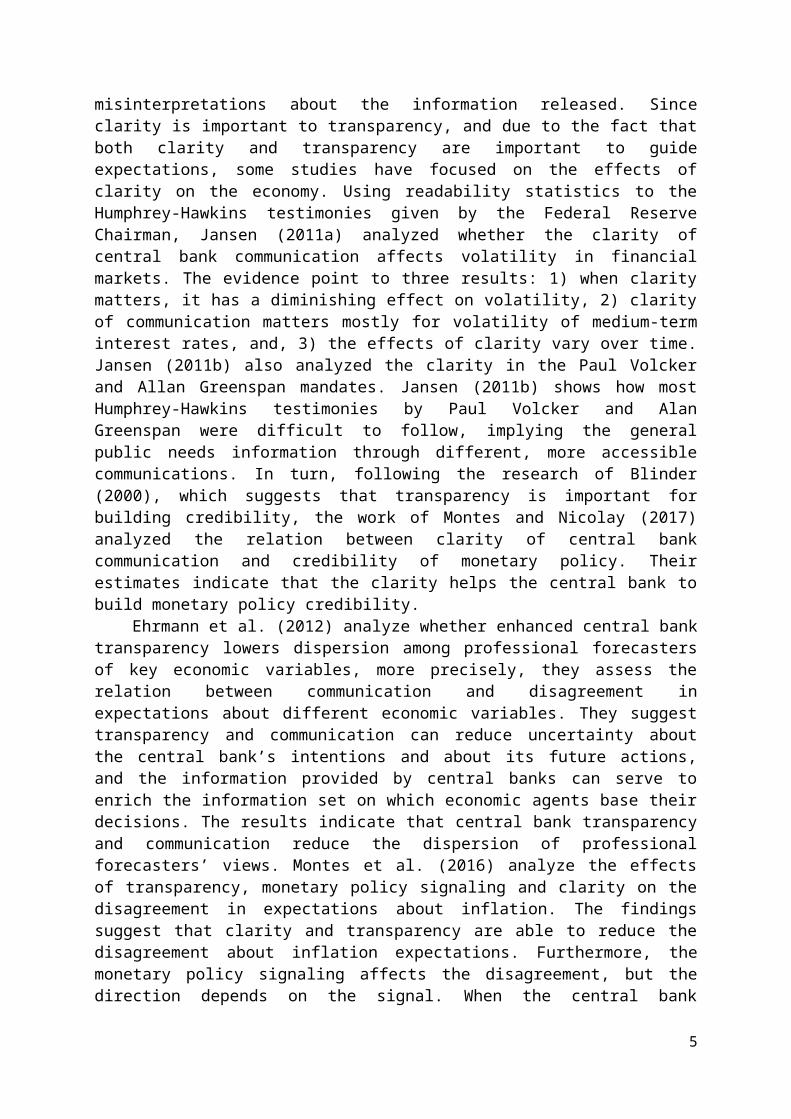
In the recent years, the central bank communication literature turned its attention to the overall clarity of the announcements. Jansen (2011a) argues that the clarity is an essential condition to transparency. If the policy authority lacks clarity in its communications, it may lead to misinterpretations about the information released. Since clarity is important to transparency, and due to the fact that both clarity and transparency are important to guide expectations, some studies have focused on the effects of clarity on the economy. Using readability statistics to the Humphrey-Hawkins testimonies given by the Federal Reserve Chairman, Jansen (2011a) analyzed whether the clarity of central bank communication affects volatility in financial markets. The evidence point to three results: 1) when clarity matters, it has a diminishing effect on volatility, 2) clarity of communication matters mostly for volatility of medium-term interest rates, and, 3) the effects of clarity vary over time. Jansen (2011b) also analyzed the clarity in the Paul Volcker and Allan Greenspan mandates. Jansen (2011b) shows how most Humphrey-Hawkins testimonies by Paul Volcker and Alan Greenspan were difficult to follow, implying the general public needs information through different, more accessible communications. In turn, following the research of Blinder (2000), which suggests that transparency is important for building credibility, the work of Montes and Nicolay (2017) analyzed the relation between clarity of central bank communication and credibility of monetary policy. Their estimates indicate that the clarity helps the central bank to build monetary policy credibility.

Ehrmann et al. (2012) analyze whether enhanced central bank transparency lowers dispersion among professional forecasters of key economic variables, more precisely, they assess the relation between communication and disagreement in expectations about different economic variables. They suggest transparency and communication can reduce uncertainty about the central bank’s intentions and about its future actions, and the information provided by central banks can serve to enrich the information set on which economic agents base their decisions. The results indicate that central bank transparency and communication reduce the dispersion of professional forecasters’ views. Montes et al. (2016) analyze the effects of

3

transparency, monetary policy signaling and clarity on the disagreement in expectations about inflation. The findings suggest that clarity and transparency are able to reduce the disagreement about inflation expectations. Furthermore, the monetary policy signaling affects the disagreement, but the direction depends on the signal. When the central bank indicates an increase (decrease) in the interest rate, it reduces (increase) the disagreement.

Most of the studies about communication concerns the monetary authority. To our knowledge, only de Mendonça and Nicolay (2017) analyze the fiscal authority communication.1 The study shows that the communication released from the fiscal authority and its clarity are important to reduce expectations about the public debt.

In order to provide empirical evidence for the hypothesis that fiscal authority communication and clarity of announcements about fiscal policy affect the disagreement in expectations about public debt, we present the following measures of fiscal authority communication, clarity and disagreement in expectations about public debt for the period 2002M11 – 2017M08. The period of analysis is restricted due to data availability on expectations.

2.1 Measuring Fiscal Authority Communication

To analyze the effect of the fiscal authority communication over the disagreement in expectations about public debt, we use the index proposed by de Mendonça and Nicolay (2017). To build the index we consider the number of releases through “official notes”, which recently become “news”, available from the website of the Ministry of Finance (www.fazenda.gov.br). The index (F_COM) counts only communications concerning fiscal policy actions. We discard any other release, as, for example, calls for contests. The index uses a discrete and positive scale, measuring the volume of releases inside the month. Each announcement receives the value +1. Hence, the index is the number of releases about fiscal policy in the month. Figure 1 shows the behavior of the fiscal authority communication index. The graph reveals that the fiscal communication index increased during the period, suggesting that the level of transparency in relation to fiscal policy is increasing due to the high volume of announcements from the fiscal authority to the public.

Figure 1 - Fiscal Communication Index (F_COM) - 2002M11 – 2017M08.

0

5

10

15

20

25

02 03 04 05 06 07 08 09 10 11 12 13 14 15 16 17

F_COM F_COM TREND (HP filter)

1 At this point, we note that our study – as well as the study presented by Mendonça and Nicolay (2017) – addresses fiscal authority communication, not central bank communication on fiscal policy – as Allard et al. (2013) have done.

4

2.2 Measuring the clarity of the fiscal authority communication

The literature about the clarity of the communication concentrates its analysis on readability measures. This is because most of the communications are made in written releases. Hence, readability is a key piece in this framework. Clarity relates to the lucidity and readability of the text (Jansen, 2011a and 2011b; Bulíř et al., 2013; Montes et al ., 2016; Jansen and Moessner, 2016; de Mendonça and Nicolay, 2017; Montes and Nicolay, 2017). If someone has to process a text with long words or sentences, it will be harder to grasp the message (Jansen, 2011b). In this sense, following the literature, the Flesch Ease Score (Flesch, 1948) is a good proxy to represent the clarity of announcements about fiscal policy.

The Flesch (1948)2 statistics considers textual aspects, as the number of words per sentence and the number of syllables per word. The index indicates the easiness to read the text. The formula of the index is:

(1) FI = 206.835 − 1.015 × (#word/#sentences) − 84.6 × (#syllables/#words)

The value of the FI indicates the clarity straightforward. If the FI increases, it represents higher clarity in the communication. We apply the index in all releases in each month. Hence, we measure the clarity of announcements about fiscal policy for every month in the period under analysis.

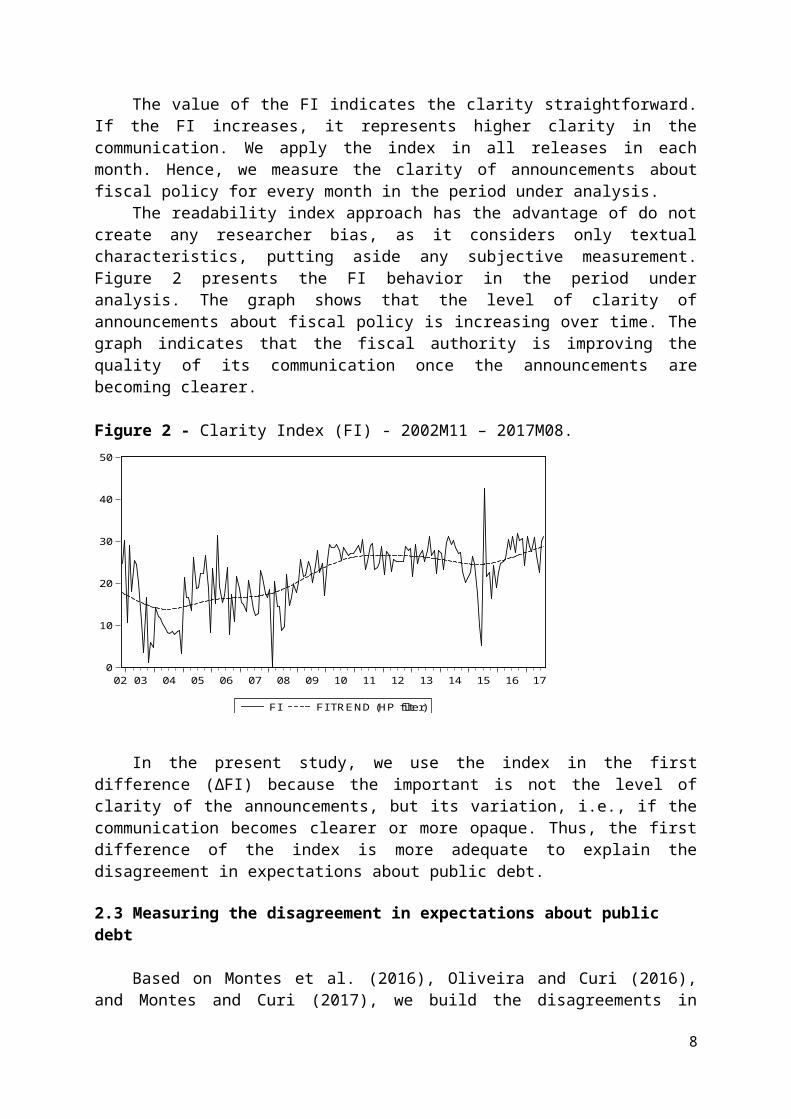
The readability index approach has the advantage of do not create any researcher bias, as it considers only textual characteristics, putting aside any subjective measurement. Figure 2 presents the FI behavior in the period under analysis. The graph shows that the level of clarity of announcements about fiscal policy is increasing over time. The graph indicates that the fiscal authority is improving the quality of its communication once the announcements are becoming clearer.

Figure 2 - Clarity Index (FI) - 2002M11 – 2017M08.Argv

gergaer

0

10

20

30

40

50

02 03 04 05 06 07 08 09 10 11 12 13 14 15 16 17

FI FI TREND (HP filter)

In the present study, we use the index in the first difference (∆FI) because the important is not the level of clarity of the announcements, but its variation, i.e., if the communication

2 To obtain more information about the regression that originates the Flesch formula, see Flesch (1948).

5

becomes clearer or more opaque. Thus, the first difference of the index is more adequate to explain the disagreement in expectations about public debt.

2.3 Measuring the disagreement in expectations about public debt

Based on Montes et al. (2016), Oliveira and Curi (2016), and Montes and Curi (2017), we build the disagreements in expectations about public debt as a proportion of GDP (Dis_debt) using the survey of expectations provided by the CBB.3 In order to understand its construction, it is worth presenting the following notation: is the instant of time the projection is made4, i identifies the agent who releases the forecast ( , where I is the set of agents surveyed5), X is the variable to be forecasted (the net public debt to GDP (debt)). Thus, Ei,tXa+j represents the projection that the i-th agent release at time t about the value that the net public debt to GDP (debt) will take in the end of year a+j6. In turn, Et

minXa+j= min(Ei,tXa+j, ) denotes the minimum value of the distribution, while, Et

maxXa+j= max(Ei,tXa+j, ) denotes its maximum value. The measure of disagreement that we use throughout this paper is Dis_Xt

a+j, which is computed by the range of the distribution defined as7:

(2) Dis_Xta+j = Et

max(X)a+j−¿ Etmin(X)a+j

Forecasts such as Ei,tXa+j are known as fixed event ones because the forecasting horizon varies with the passage of time. Indeed, the prospective period of forecasts made at t for the value that the variable X will take in the end of the year a + j decrease as t progress within a, the year in which expectations are made.8 This pattern of decreasing forecasting horizons as t advances through the year brings about a seasonal behavior in disagreement measures based on fixed event forecasts because expectations dispersion tends to decrease as the forecasting horizon shrinks9.

It is to avoid this seasonal behavior inherent to disagreement measures based on fixed event forecasts that several studies (e.g., Mankiw et al., 2003; Patton and Timmermann, 2010;

3 The CBB releases the maximum, minimum, median, mean, coefficient of variation and standard deviation statistics of the distribution of the daily forecast for the net public debt and for the budget balance in fixed event for the end of the current year and four years ahead.4This instant is characterized by a specific date, namely, a day d, a month m and a year a.5The number of agents in I is I. 6j=0: current year; j=1: next year immediately after the current year; j=2: two years after the current year; j=3: three years after the current year; j=4: four years after the current year. 7 Like Oliveira and Curi (2016), we use this measure of disagreement throughout the paper, as other measures require the knowledge of the entire distribution of expectations. Such information is not provided by the CBB. We are aware of the fact that papers on disagreement often use other measures, such as the inter-quartile range and Kulback-Liebler divergence measure. These two options, though, cannot be calculated without the entire distribution of individual forecasts. The standard deviation – SD(ND) – and the coefficient of variation – CV(ND) – are also frequently used as measures of disagreement. Nevertheless, although these alternative measures are released, the interpolation of the SD(ND) and CV(ND) to transform in fixed horizon is not appropriate for the analysis (see, for instance, Oliveira and Curi (2016)). Thus, it is not possible to re-estimate the equations with such measures.8 An example could help to clarify this issue. Suppose that an agent, in March 2005, computes his expectation about the value of the budget balance in the end of 2005. In this case we can say that the time horizon of the forecast is 10 months because the first 2 months of 2005 have already passed and budget balance figures for January and February are known. By the same line of reasoning, when this agent computes his budget balance expectation in September 2005 about the value of the budget balance at the closing of 2005, the time horizon of his forecast decreases to only 4 months.9Indeed, the disagreement measure observed in March 2005 for the value that the budget balance will take in the end of 2005 tends to be greater than the disagreement measure observed in September 2005 for the value that the same variable will take at the closing of 2005. The divergence measure tends to increase again in March 2006, since the current year becomes 2006 and the time horizon of the forecast becomes 9 months.

6

Dovern et al., 2012; Oliveira and Curi, 2016; Montes and Curi, 2017) recur to fixed horizon forecasts, in which the forecasting horizon does not vary with the passage of time. As proposed in Dovern et al. (2012), the conversion of fixed event forecasts into fixed horizon forecasts is accomplished by applying the formula below:

(3)

Where m represents the month in which the projection is made (or the month containing period t) and EtX12(j+1) denotes the average of agents’ expectations about the value that the variable X will take at the end of the next 12(j+1) months. The same formula is used to interpolate minimum and maximum projections in order to calculate the disagreement in expectation (as well the average expectations). At the end of the process, we derive a term structure of disagreement in expectations, which is comprised by the “vertices” Dis_debtt

12, Dis_debtt

24, Dis_debtt36 and Dis_debtt

48. As the CBB discloses forecasts for the current and the next four years, the formula above can be applied by taking j = 0,1,2,3,4. Therefore, we can always interpolate forecasts for the fixed time horizons of 12, 24, 36 and 48 months.

The procedure described above is performed daily, allowing us to study the term structures of disagreement for each business day. Time series comprised of daily observations are converted to the monthly frequency by monthly averages. The conversion of fixed event forecasts into fixed horizon and the monthly frequency were applied to compute the disagreements in expectations about net public debt to GDP (Dis_debtt

m).After computing the four maturities of the disagreement in expectations about debt

(Dis_debttm), the final step is to extract the first principal component of these series with four

maturities (12, 24, 36, 48 months); these components are good proxies for their common trend. The application of this technique has a long tradition in the study of conventional yield curves (Litterman and Scheinkmann, 1991), which justifies its application to the term structures that we study here. As the monthly averages, it also allows filtering out erratic shifts on a given disagreement measure that do not reflect upon the others. Such movements can be regarded as outliers, thus, they should be ignored from the economic viewpoint. Thus, we obtain the series of the general level of disagreement in expectation about debt (Dis_debtt

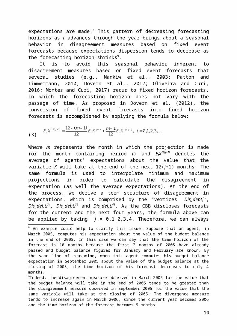
L), which we also use in our estimates. Figure 3 shows the graphs of the term structure of disagreements in expectations about public debt, and also the series of the general level of disagreement in expectation about debt.

Figure 3 - Disagreement in expectations about public debt – 2002M11 – 2017M08.

7

0

5

10

15

20

25

30

35

02 03 04 05 06 07 08 09 10 11 12 13 14 15 16 17

Dis_debt_12 Dis_debt_24Dis_debt_36 Dis_debt_48

-4

-2

0

2

4

6

8

02 03 04 05 06 07 08 09 10 11 12 13 14 15 16 17

Dis_debt_L

3. Empirical analysis

Aiming at observing the effects of fiscal authority communication and clarity of announcements about fiscal policy on the disagreements in expectations about public debt (Dis_debt), we estimate a model for different maturities of the disagreement in expectations about public debt, which captures such effects. The choice of control variables – and thus the basic structure of the model – follows the studies that seek to estimate the determinants of the disagreement in expectations (e.g., Mankiw et al., 2003; Oliveira and Curi, 2016; Montes et al., 2016). In this sense, the control variables are: net public debt as a percentage of GDP (debt)10, volatility of net public debt as a percentage of GDP (v_debt) and, the output gap (gap)11. Following Capistrán and Timmermann (2009) and Ehrmann et al. (2012), which use GARCH models to calculate volatility series used in estimates for the disagreements in expectations, the series of v_debt is constructed using the debt series in a GARCH (1, 1) model (a variation of the ARCH model).12

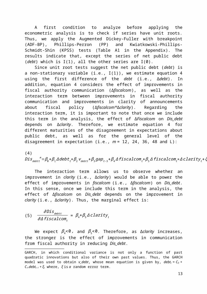
A first condition to analyze before applying the econometric analysis is to check if series have unit roots. Thus, we apply the Augmented Dickey-Fuller with breakpoint (ADF-BP), Phillips-Perron (PP) and Kwiatkowski-Phillips-Schmidt-Shin (KPSS) tests (Table A1 in the Appendix). The results indicate that, except the series of net public debt (debt) which is I(1), all the other series are I(0).

Since unit root tests suggest the net public debt (debt) is a non-stationary variable (i.e., I(1)), we estimate equation 4 using the first difference of the debt (i.e., ∆debt). In addition, equation 4 considers the effect of improvements in fiscal authority communication (∆fiscalcom), as well as the interaction term between improvements in fiscal authority communication and improvements in clarity of announcements about fiscal policy (∆fiscalcom*∆clarity). Regarding the interaction term, it is important to note that once we

10 The variable “debt” is the series “Net public debt (% GDP) - Total - Consolidated public sector - %” (series number 4513).11 The output gap (Gap) is the difference between the seasonally adjusted real GDP series and its long-term trend (generated by the Hodrick-Prescott filter).12 The ARCH model is a model of volatility proposed by Engle (1982). The models of this class serve to capture oscillations in time series. The central idea is that when volatility increases in the behavior of a given series, uncertainty about the future behavior of the series also increases. Bollerslev (1986) developed a generalization of the ARCH model, called GARCH, in which conditional variance is not only a function of past quadratic innovations but also of their own past values. Thus, the GARCH model was used to obtain v_debt, whose mean equation is given by, debtt = C0 + C1.debtt -1 + ξt where, ξ is a random error term.

8

include this term in the analysis, the effect of ∆Fiscalcom on Dis_debt depends on ∆clarity. Therefore, we estimate equation 4 for different maturities of the disagreement in expectations about public debt, as well as for the general level of the disagreement in expectation (i.e., m = 12, 24, 36, 48 and L):

(4) Disdebtt

m=β0+ β1 ∆ debt t+β2 vdebtt+ β3 gapt−3+β4 ∆ fiscalcomt +β5 ∆ fiscalcomt∗∆ clarityt+ζ t

The interaction term allows us to observe whether an improvement in clarity (i.e., ∆clarity) would be able to power the effect of improvements in fiscalcom (i.e., ∆fiscalcom) on Dis_debt. In this sense, once we include this term in the analysis, the effect of ∆fiscalcom on Dis_debt depends on the improvement in clarity (i.e., ∆clarity). Thus, the marginal effect is:

(5)∂ Disdebtt

∂ ∆ fiscalcom t = β4+β5 ∆ clarity t

We expect β4<0 , and β5<0. Therefore, as ∆clarity increases, the stronger is the effect of improvements in communication from fiscal authority in reducing Dis_debt.

The econometric analysis makes use of ordinary least squares (OLS) and the generalized method of moments (GMM) with one-step and two-steps estimations.While OLS estimates are susceptible to problems of simultaneity and endogeneity of the regressors, which is typical in macroeconomic time series, GMM provides consistent estimations (Hansen, 1982). The GMM estimates adopted a standard procedure based on Johnston (1984), i.e., the chosen instruments were dated to the period t-1 or earlier. Overidentification has an important role in the selection of instrumental variables to improve the efficiency of the estimators (Cragg, 1983). In this sense, we perform a standard J-test with the objective of testing this property for the validity of the overidentifying restrictions, i.e., the J-statistic indicates whether the orthogonality condition is satisfied. Due to the problems of serial correlation and heteroskedasticity detected (see table A2 in the Appendix), both OLS and GMM estimates use the Newey-West (HAC) matrix. The two-step GMM estimations (GMM2S) use Windmeijer (2005) correction to address small-sample downward biases on standard errors. Besides, regarding all GMM estimations, we present the Durbin–Wu–Hausman (D-W-H) test of the endogeneity of regressors (Durbin, 1954; Wu, 1973; Hausman, 1978).

4. results

Table 1 shows the estimates through OLS, GMM and GMM2S. One can observe that all GMM estimations are valid (the J statistic obtained for each equation indicates the orthogonality condition is satisfied, and the D-W-H test validates the exogeneity condition of the instruments). With respect to the influence of improvements in fiscal authority communication (∆fiscalcom), the results show that none of the estimated coefficients presented statistical significance. On the other hand, all estimated coefficients for the interaction term (∆fiscalcom* ∆clarity) are negative and statistically significant. Therefore, the findings indicate that improvements in the fiscal authority communication accompanied by improvements in the clarity of the fiscal announcements are able to reduce the disagreement in expectations about public debt. The results show that, in order to reduce uncertainties about the future behavior of public debt, it is not enough to simply increase the volume of communication, the provision of more information through communication must

9

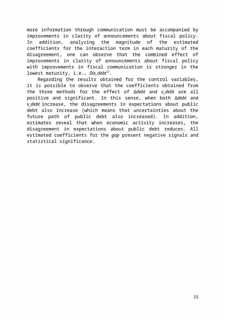
be accompanied by improvements in clarity of announcements about fiscal policy. In addition, analyzing the magnitude of the estimated coefficients for the interaction term in each maturity of the disagreement, one can observe that the combined effect of improvements in clarity of announcements about fiscal policy with improvements in fiscal communication is stronger in the lowest maturity, i.e., Dis_debt12.

Regarding the results obtained for the control variables, it is possible to observe that the coefficients obtained from the three methods for the effect of ∆debt and v_debt are all positive and significant. In this sense, when both ∆debt and v_debt increase, the disagreements in expectations about public debt also increase (which means that uncertainties about the future path of public debt also increased). In addition, estimates reveal that when economic activity increases, the disagreement in expectations about public debt reduces. All estimated coefficients for the gap present negative signals and statistical significance.

10

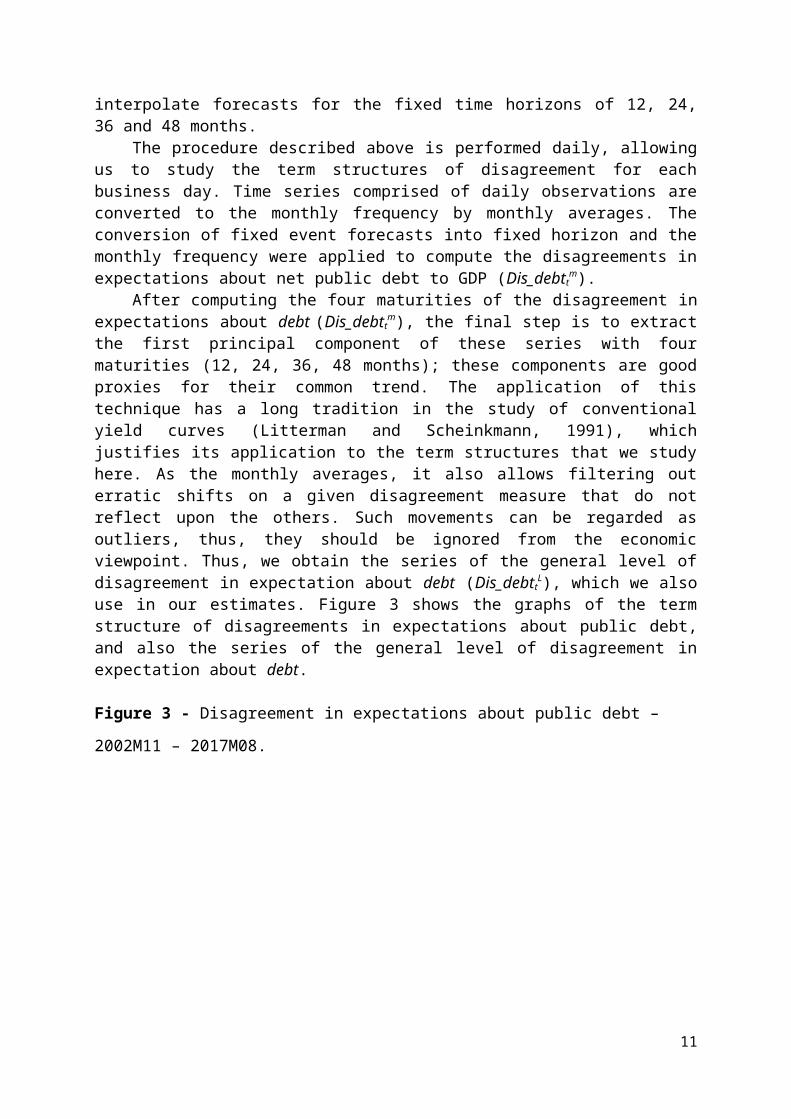
Table 1 - OLS GMM and GMM2S Estimates (Dependent Variables: Dis_debt12,Dis_debt24,Dis_debt36, Dis_debt48 and Dis_debtL)MethodExplanatory variables dis_debt_12 dis_debt_24 dis_debt_36 dis_debt_48 dis_debt_L dis_debt_12 dis_debt_24 dis_debt_36 dis_debt_48 dis_debt_L dis_debt_12 dis_debt_24 dis_debt_36 dis_debt_48 dis_debt_L

C 5.929*** 8.019*** 9.205*** 9.610*** -0.819** 4.308*** 5.803*** 6.871*** 7.100*** -1.607*** 4.191*** 6.379*** 7.685*** 7.594*** -1.666***(0.587) (0.779) (0.889) (1.061) (0.332) (0.329) (0.622) (0.824) 0.584 (0.219) (0.458) (0.720) (0.726) 0.854 (0.324)

∆debt 0.958* 1.588** 1.606** 1.914** 0.632** 1.806*** 2.914*** 2.788** 2.538*** 1.254*** 1.886** 3.748*** 4.301*** 3.150*** 1.006***(0.500) (0.733) (0.791) (0.811) (0.291) (0.634) (0.980) (1.262) 0.869 (0.311) (0.761) (0.881) (0.960) 1.131 (0.370)

v_debt 2.793** 3.615** 4.041* 4.542* 1.575* 6.158*** 8.699*** 10.005*** 11.360*** 3.622*** 6.388*** 8.069*** 8.482*** 10.327*** 3.611***(1.150) (1.814) (2.219) (2.659) (0.805) (0.630) (1.390) (1.846) 1.253 (0.504) (0.953) (1.700) (1.788) 2.28 (0.743)

gap(-3) -50.664*** -52.029** -33.419 -45.712 -19.747** -48.768*** -47.399** -29.605 -36.129* -21.132*** -43.571* -63.772** -20.809 -55.779* -18.934**(15.796) (22.999) (25.689) (28.762) (9.172) (14.894) (21.247) (25.868) 20.509 (6.827) (22.955) (27.803) (36.473) 31.567 (9.456)

∆fiscalcom 0.033 0.027 0.049 0.032 0.015 0.106 0.124 -0.012 -0.079 -0.005 0.084 -0.018 -0.067 -0.119 -0.001(0.041) (0.056) (0.067) (0.072) (0.023) (0.079) (0.097) (0.124) 0.086 (0.027) (0.126) (0.129) (0.121) 0.126 (0.039)

∆fiscalcom* ∆clarity -0.019*** -0.017** -0.008 -0.008 -0.006** -0.041** -0.047** -0.036* -0.028* -0.010* -0.043* -0.031* -0.037* -0.028* -0.018*(0.006) (0.008) (0.007) (0.006) (0.002) (0.016) (0.021) (0.020) 0.014 (0.006) (0.026) (0.018) (0.021) 0.017 (0.009)

Adjusted R2 0.40 0.34 0.29 0.33 0.37 0.39 0.38 0.40 0.52 0.47 0.38 0.36 0.34 0.49 0.46F-statistic 23.93 19.12 15.15 17.81 21.01Prob (F-statistic) 0.00 0.00 0.00 0.00 0.00J-STAT 16.28 13.53 10.61 10.46 15.37 16.27 16.39 16.72 13.97 16.37Prob (J-STAT) 0.64 0.85 0.83 0.98 0.88 0.75 0.98 0.95 0.96 0.96N° Inst/Obs 0.151 0.157 0.133 0.170 0.176 0.163 0.221 0.211 0.188 0.211Durbin–Wu–Hausman 4.64 4.17 1.96 6.08 3.29 5.87 4.52 4.64 1.73 1.81Prob (Durbin–Wu–Hausman) 0.46 0.52 0.85 0.30 0.65 0.32 0.48 0.46 0.88 0.87

OLS GMM GMM2S

Note: Marginal Significance Levels: *** denotes 0.01, ** denotes 0.05 and *10%. Standard errors are in parentheses. Prob (F-statistic) reports the respective p-value of the F-test. Prob (J-statistic) reports the respective p-valued of the J-test. D-W-H test is the Durbin-Wu-Hausman test (difference in J-stats) and null hypothesis is that the regressors are exogenous. Prob (D-W-H) reports the respective p-value of the D-W-H-test.

11

5. Robustness analysis

5.1 ARDL estimates

In order to provide robust results and to test for the existence of a relationship between variables in levels, the analysis is extended and the relations are estimated using the autoregressive distributed-lag (ARDL) modelling approach proposed by Pesaran and Shin (1999) and Pesaran et al. (2001). This method is useful once it is consistent with small samples and it can be applied to a mix of variables I(0) and I(1) in the analysis. According to Pesaran et al. (2001, p. 315), the asymptotic theory developed by them “provides a simple univariate framework for testing the existence of a single level relationship between yt and xt when it is not known with certainty whether the regressors are purely I(0), purely I(1) or mutually cointegrated”. Hence, we estimate the following error correction model – given by equation (6) – for each maturity of the disagreement in expectation about public debt and for the general level (where m = 12, 24, 36, 48 and L), i.e., Dis_debtt

12,Dis_debtt24,Dis_debtt

36, Dis_debtt48 and

Dis_debttL.

(6 )∆ Disdebttm=α 0+∑

i=1

p

φi ∆ Disdebtt−im+∑

i=0

p

γ i∆ debtt−i❑+∑

i=0

p

θ i ∆ vdebtt −i+∑i =0

p

τ i ∆ gapt −i+∑i=0

p

ωi ∆(∆ fiscalcom)t−i+∑i=0

p

μ i∆ (∆ fiscalcom∗∆ clarity)t−i+δ1 debt t+δ 2 vdebtt+δ3 gap t+δ 4 ∆ fiscalcomt+δ5 ∆ fiscalcomt∗∆ clarity t+ξ t0

Where p is the optimal lag length.In order to determine the lag orders for the variables of each equation, we select the model

that optimizes the Adjusted R-squared. In turn, we check the existence of relationships in levels through an F-test for each equation. When a level relationship exists, the F-test indicates which variable should be normalized. The null hypothesis for the non-existence of the relationship in level among variables in both equations is H0: δ1 =δ2 =δ3 =δ4 =δ5 = 0 against the alternative hypothesis H1: δ1 ≠δ2 ≠ δ3 ≠ δ4 ≠ δ5 ≠ 0. Pesaran et al. (2001) provide critical values for the cases where all regressors are I(0) for the lower bound and the cases where all regressors are I(1) for the upper bound. If the reported F-test statistic exceeds their respective upper critical values, then the null hypothesis can be rejected (Bounds test). If the F-test statistic lies between the lower and upper bounds there is a need to determine the order of integration of the variables before proceeding to the analysis. When the relationship in level is confirmed, the next step is to present the coefficients.

Table 2 presents the results of the estimations for equation (6) for each maturity of the disagreement in expectation about public debt, and the general level. One can observe that the reported F-test statistic obtained for each equation exceeds the respective upper critical values (I(1) Bounds), rejecting the null hypothesis for each equation. Moreover, we make the test proposed by Brown et al. (1975) (CUSUM test), in order to check the constancy of the ARDL regressions. The results indicate that all models confirm the stability of causal relationships – see figure A1 in the Appendix.

In relation to the results reported in table 2, the estimates indicate that, in general, the signals of the coefficients are in accordance with the theory. All the coefficients obtained for the effect of v_debt are positive and significant. However, none of the estimated coefficients for the debt and the gap presented statistical significance. In turn, the findings obtained for the effects of improvements in communication from fiscal authority and improvements in communication clarity of announcements about fiscal policy corroborate the results previously reported in table

12

1. All the coefficients for the interaction term (∆fiscalcom*∆clarity) are negative and statistically significant. This result reinforces the idea that improvements in communication from fiscal authority, which are accompanied by improvements in clarity of fiscal announcements, are able to reduce the disagreement in expectations about public debt.

Table 2 - ARDL Estimates – Bounds Tests and Levels EquationsDis_debt_12 ARDL(5, 5, 4, 4, 3, 6) Dis_debt_24 ARDL(6, 5, 4, 1, 6, 6)

Bounds Test Critical Bounds Bounds Test Critical BoundsTest Statistic Value Significance I(1) Bounds Test Statistic Value Significance I(1) BoundsF-Statistic 5.320 10% 3.35 F-Statistic 3.702 10% 3.35K 5 K 5Long run coefficients Long run coefficientsVariables Coefficients Std. Error t-statistic Variables Coefficients Std. Error t-statisticdebt 0.009 0.057 0.168 debt 0.053 0.086 0.622v_debt 4.210*** 1.094 3.848 v_debt 4.279** 1.772 2.416gap -46.214 28.726 -1.609 gap -23.219 37.617 -0.617∆fiscalcom -0.431 0.290 -1.488 ∆fiscalcom -0.808 0.887 -0.911∆fiscalcom* ∆clarity -0.054** 0.025 -2.236 ∆fiscalcom* ∆clarity -0.100** 0.043 -2.354

Dis_debt_36 ARDL(2, 6, 6, 6, 1, 6) Dis_debt_48 ARDL(5, 2, 2, 3, 6, 5)

Bounds Test Critical Bounds Bounds Test Critical BoundsTest Statistic Value Significance I(1) Bounds Test Statistic Value Significance I(1) BoundsF-Statistic 3.471 10% 3.35 F-Statistic 6.390 10% 3.35K 5 K 5Long run coefficients Long run coefficientsVariables Coefficients Std. Error t-statistic Variables Coefficients Std. Error t-statisticdebt 0.132 0.105 1.259 debt 0.195 0.125 1.574v_debt 3.815* 2.189 1.743 v_debt 6.821*** 2.347 2.907gap -7.179 57.355 -0.125 gap -1.961 63.912 -0.031∆fiscalcom 0.295 0.287 1.028 ∆fiscalcom -3.448** 1.651 -2.089∆fiscalcom* ∆clarity -0.104** 0.051 -2.061 ∆fiscalcom* ∆clarity -0.152** 0.063 -2.405

Dis_debt_L ARDL(5, 5, 6, 6, 6, 3)Bounds Test Critical BoundsTest Statistic Value Significance I(1) BoundsF-Statistic 6.092 10% 3.35K 5Long run coefficientsVariables Coefficients Std. Error t-statisticdebt 0.046 0.030 1.553v_debt 1.799*** 0.632 2.849gap -12.486 16.742 -0.746∆fiscalcom -0.319 0.313 -1.019∆fiscalcom* ∆clarity -0.034*** 0.012 -2.940

Notes: Marginal Significance Levels: *** denotes 0.01, ** denotes 0.05 and * denotes 0.1. All equations are estimated with unrestricted constant and no trend.

5.2 Quantile regression

13

Furthermore, we perform quantile regression estimations to observe the effect that improvements in communication from fiscal authority and improvements in clarity of fiscal announcements have on different levels of disagreement in expectations about public debt in different maturities. Introduced by Koenker and Basset (1978), quantile regression divides the distribution in a way that a given proportion of observations is located below the quantile. The quantile regression method estimates the relationship between the dependent variable and explanatory variables at any chosen point in the conditional distribution of the dependent variable. We thus obtain multiple sets of coefficient estimates with each set describing the relationship between the dependent variable and explanatory variables at a certain quantile of the dependent variable. In this sense, it is possible to observe the estimated coefficient to different levels of the disagreement in expectations about public debt distribution.

Therefore, using the quantile regression method, we estimate equation (4) for each maturity of the disagreement in expectation about public debt and for the general level, i.e., Dis_debtt

12, Dis_debtt

24, Dis_debtt36, Dis_debtt

48 and Dis_debttL. Figure 4 summarizes the findings for all

quantile regression estimations, and table 3 shows the results of the estimates.Regarding the estimates for the effect of improvements in communication from fiscal

authority (∆fiscalcom), most of the coefficients do not present statistical significance, which reinforce the findings previously reported. In turn, the estimated coefficients for the interaction term (∆fiscalcom*∆clarity) reveal interesting results, especially to disagreements in expectations about public debt to shorter maturities. Despite the absence of statistical significance for the effect of the interaction term on both Dis_debtt

36andDis_debtt48 in all quantiles, regarding the

effect of the interaction term on Dis_debtt12, the estimates indicate negative and statistically

significant coefficients for the 0.40, 0.50, 0.60, 0.70, 0.80 and 0.90 per cent quantiles. Besides, the effect is stronger in the case where the disagreement is higher, i.e., the estimated coefficient for ∆fiscalcom*∆clarity in the 0.90 per cent quantile is -0.022. In addition, the findings indicate, with statistical significance, that improvements in communication from fiscal authority which are accompanied by improvements in clarity of fiscal announcements are important to reduce Dis_debtt

24 for the 0.80 and 0.90 per cent quantiles.In relation to the control variables, the results obtained for the effect of ∆(debt) show that

all positive coefficients that are statistically significant indicate that the disagreements in expectations about public debt are more affected by ∆(debt) when the disagreement becomes higher (i.e., for higher quantiles).13 In particular, the effect is stronger for higher quantiles of Dis_debtt

48. Therefore, when public debt increases, the disagreements in expectations about public debt in all maturities are affected, but the impact is even higher in those with longer maturities when uncertainties are already high. Besides, all estimated coefficients for v_debt are positive and most shows statistical significance. One can observe through figure 4 that to the extent the disagreement in expectations about public debt increases (higher quantiles), the effect of the volatility of public debt on the disagreements becomes stronger. In addition, the magnitudes of the coefficients are greater for disagreements with longer maturities. The findings for the effect of the gap indicate negative and significant effects for lower quantiles of the disagreement in expectations. Besides, coefficients have greater magnitudes for disagreements with lower maturities.

Figure 4 - Quantile regressions

13 In the graphs, ∆(debt) is represented by d(debt).

14

-1

0

1

2

3

0.0 0.1 0.2 0.3 0.4 0.5 0.6 0.7 0.8 0.9 1.0

Quantile

d(debt)

-4

0

4

8

12

16

20

24

0.0 0.1 0.2 0.3 0.4 0.5 0.6 0.7 0.8 0.9 1.0

Quantile

v_debt

-100

-75

-50

-25

0

25

50

0.0 0.1 0.2 0.3 0.4 0.5 0.6 0.7 0.8 0.9 1.0

Quantile

gap(-3)

-.2

-.1

.0

.1

.2

.3

0.0 0.1 0.2 0.3 0.4 0.5 0.6 0.7 0.8 0.9 1.0

Quantile

d(fis calcom)

-.06

-.04

-.02

.00

.02

.04

0.0 0.1 0.2 0.3 0.4 0.5 0.6 0.7 0.8 0.9 1.0

Quantile

d(fiscalcom)*d(c larity)

Quantile Process Estimates - Dis_debt_24

-2

-1

0

1

2

3

0.0 0.1 0.2 0.3 0.4 0.5 0.6 0.7 0.8 0.9 1.0

Quantile

d(debt)

0

4

8

12

16

0.0 0.1 0.2 0.3 0.4 0.5 0.6 0.7 0.8 0.9 1.0

Quantile

v _debt

-100

-80

-60

-40

-20

0

20

0.0 0.1 0.2 0.3 0.4 0.5 0.6 0.7 0.8 0.9 1.0

Quantile

gap(-3)

-.2

-.1

.0

.1

.2

.3

0.0 0.1 0.2 0.3 0.4 0.5 0.6 0.7 0.8 0.9 1.0

Quantile

d(fis calcom)

-.04

-.03

-.02

-.01

.00

.01

.02

0.0 0.1 0.2 0.3 0.4 0.5 0.6 0.7 0.8 0.9 1.0

Quantile

d(fiscalcom)*d(c lar ity)

Quantile Process Estimates - Dis_debt_12

-0.50

-0.25

0.00

0.25

0.50

0.75

1.00

0.0 0.1 0.2 0.3 0.4 0.5 0.6 0.7 0.8 0.9 1.0

Quantile

d(debt)

-2

0

2

4

6

8

10

0.0 0.1 0.2 0.3 0.4 0.5 0.6 0.7 0.8 0.9 1.0

Quantile

v _debt

-30

-20

-10

0

10

20

0.0 0.1 0.2 0.3 0.4 0.5 0.6 0.7 0.8 0.9 1.0

Quantile

gap( -3 )

-.05

.00

.05

.10

.15

0.0 0.1 0.2 0.3 0.4 0.5 0.6 0.7 0.8 0.9 1.0

Quantile

d( fis c a lc om)

-.016

-.012

-.008

-.004

.000

.004

.008

0.0 0.1 0.2 0.3 0.4 0.5 0.6 0.7 0.8 0.9 1.0

Quantile

d(fisc alcomun)*d(c larity )

Quantile Process Estimates - Dis_debt_L

-2

-1

0

1

2

3

4

0.0 0.1 0.2 0.3 0.4 0.5 0.6 0.7 0.8 0.9 1.0

Quantile

d(debt)

-4

0

4

8

12

16

20

24

0.0 0.1 0.2 0.3 0.4 0.5 0.6 0.7 0.8 0.9 1.0

Quantile

v_debt

-60

-40

-20

0

20

40

60

0.0 0.1 0.2 0.3 0.4 0.5 0.6 0.7 0.8 0.9 1.0

Quantile

gap(-3)

-.2

-.1

.0

.1

.2

.3

.4

0.0 0.1 0.2 0.3 0.4 0.5 0.6 0.7 0.8 0.9 1.0

Quantile

d(fisc alcom)

-.03

-.02

-.01

.00

.01

.02

.03

0.0 0.1 0.2 0.3 0.4 0.5 0.6 0.7 0.8 0.9 1.0

Quantile

d(fiscalcomun)*d(c larity)

Quantile Process Estimates - Dis_debt_36

-2

-1

0

1

2

3

0.0 0.1 0.2 0.3 0.4 0.5 0.6 0.7 0.8 0.9 1.0

Quantile

d(debt)

-5

0

5

10

15

20

25

0.0 0.1 0.2 0.3 0.4 0.5 0.6 0.7 0.8 0.9 1.0

Quantile

v _debt

-80

-60

-40

-20

0

20

40

0.0 0.1 0.2 0.3 0.4 0.5 0.6 0.7 0.8 0.9 1.0

Quantile

gap(-3)

-.2

-.1

.0

.1

.2

.3

0.0 0.1 0.2 0.3 0.4 0.5 0.6 0.7 0.8 0.9 1.0

Quantile

d(fis calcom)

-.03

-.02

-.01

.00

.01

.02

.03

.04

0.0 0.1 0.2 0.3 0.4 0.5 0.6 0.7 0.8 0.9 1.0

Quantile

d(fiscalcom)*d(c lar ity)

Quantile Process Estimates - Dis_debt_48

Figure prepared by the authors

15

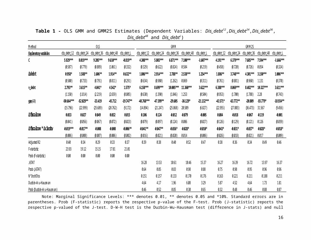
Table 3 - Quantile Regression Estimates

Expalanatory Variables Quantile Coefficient Std. Error Coefficient Std. Error Coefficient Std. Error Coefficient Std. Error Coefficient Std. Error∆debt 0.1 -0.377 0.410 0.416 0.643 0.767 0.474 -0.053 0.432 0.077 0.180

0.2 0.092 0.529 0.851 0.596 0.639 0.556 0.155 0.480 0.083 0.2080.3 0.430 0.607 0.751 0.664 0.457 0.648 0.081 0.547 0.135 0.2380.4 0.478 0.676 0.535 0.727 0.017 0.782 0.286 0.709 0.124 0.2860.5 1.524 0.667 1.050 0.798 0.428 0.955 -0.045 0.574 0.298 0.3050.6 1.352 0.605 1.118 0.913 0.970 1.073 0.432 0.598 0.304 0.2860.7 0.820 0.376 0.921 0.382 1.025 0.614 1.383 0.441 0.291 0.1380.8 0.826 0.212 1.170 0.326 1.275 0.331 1.255 0.453 0.565 0.1150.9 0.554 0.445 1.181 0.746 0.876 0.553 1.468 0.543 0.421 0.219

v_debt 0.1 1.439 0.268 1.461 0.290 1.368 0.199 1.129 0.203 0.562 0.0800.2 1.681 0.486 1.716 0.481 1.261 0.258 1.275 0.302 0.541 0.1020.3 1.902 0.563 1.568 0.424 1.125 0.308 1.619 0.895 0.798 0.3860.4 2.360 1.036 2.112 0.925 1.366 0.505 2.720 2.308 1.102 0.6380.5 4.065 1.609 3.217 1.985 4.158 2.455 5.498 2.692 2.250 1.2830.6 4.089 1.646 5.906 4.560 6.192 4.649 7.539 3.646 2.852 1.3440.7 7.195 1.876 9.658 2.054 10.881 2.125 12.213 1.549 4.307 0.5540.8 6.917 1.845 11.291 2.157 14.010 3.775 12.514 1.491 5.468 1.1550.9 7.616 3.859 14.803 4.265 17.332 2.985 16.809 3.165 5.900 1.107

gap(-3) 0.1 -21.337 11.708 -19.462 14.225 -10.356 9.248 -18.836 8.157 -10.920 3.6160.2 -27.367 12.425 -31.536 9.896 -14.297 9.510 -17.086 8.588 -9.640 3.9040.3 -39.276 11.812 -33.940 10.850 -10.593 9.629 -17.024 9.225 -11.196 3.8890.4 -35.725 13.006 -29.778 11.930 -8.346 9.811 -3.812 13.538 -8.776 4.5610.5 -28.764 14.146 -32.527 14.396 -3.058 16.878 -19.106 16.273 -7.064 5.6560.6 -36.945 14.496 -36.829 19.321 -5.006 22.141 -19.304 20.636 -4.771 5.3140.7 -34.192 18.995 -43.198 28.112 1.712 24.888 -14.453 22.244 -4.233 7.5120.8 -36.890 24.829 -16.376 30.253 12.391 22.200 -18.638 22.611 -0.982 7.6980.9 -37.150 25.608 -13.016 29.559 19.128 18.495 -11.049 20.858 -9.033 10.408

∆fiscalcom 0.1 -0.024 0.039 0.014 0.054 0.019 0.053 -0.013 0.040 0.009 0.0160.2 -0.010 0.041 0.018 0.049 0.057 0.052 -0.012 0.044 0.018 0.0170.3 0.009 0.046 0.017 0.055 0.031 0.053 0.023 0.049 0.009 0.0180.4 0.033 0.052 -0.006 0.055 0.024 0.057 -0.022 0.048 -0.001 0.0200.5 0.010 0.052 -0.001 0.060 0.022 0.063 0.035 0.062 -0.003 0.0200.6 0.030 0.053 -0.001 0.064 0.041 0.069 0.048 0.061 -0.001 0.0190.7 0.050 0.052 0.009 0.063 0.101 0.074 0.061 0.065 0.007 0.0210.8 0.088 0.058 0.093 0.087 0.149 0.081 0.020 0.080 0.039 0.0310.9 0.040 0.105 0.100 0.085 0.194 0.079 0.026 0.089 0.061 0.031

∆fiscalcom* ∆clarity 0.1 -0.006 0.010 -0.008 0.014 -0.002 0.014 0.001 0.007 -0.003 0.0040.2 -0.011 0.013 -0.013 0.014 -0.010 0.008 -0.002 0.007 -0.006 0.0030.3 -0.014 0.011 -0.016 0.013 -0.009 0.008 -0.001 0.007 -0.006 0.0030.4 -0.021 0.009 -0.013 0.012 -0.003 0.009 0.004 0.005 -0.005 0.0030.5 -0.016 0.008 -0.009 0.016 -0.001 0.009 -0.004 0.010 -0.003 0.0030.6 -0.015 0.007 -0.016 0.010 0.002 0.007 -0.005 0.009 -0.002 0.0020.7 -0.010 0.005 -0.008 0.006 -0.003 0.007 -0.003 0.007 -0.001 0.0020.8 -0.020 0.006 -0.011 0.005 0.000 0.007 0.002 0.010 -0.004 0.0020.9 -0.022 0.007 -0.011 0.005 -0.002 0.007 0.006 0.012 -0.004 0.002

Dis_debt_12 Dis_debt_24 Dis_debt_36 Dis_debt_48 Dis_debt_L

Note: Coefficients in bold and underlined denote statistical significance at the 10% level at least. Intercepts are omitted for convenience.

16

6. Conclusion

The present work aimed to provide empirical evidence on the effects of both improvements in the fiscal authority communication and improvements in the clarity of fiscal announcements over public debt uncertainty measured by the disagreement in expectations about public debt. The empirical approach used OLS, GMM, ARDL and Quantile Regression. The results indicate improvements in the fiscal authority communication are important to reduce the disagreement in expectations but only if accompanied by improvements in the clarity of the announcements released.

Disagreement in expectations is related to the general level of uncertainty in the economy. Moreover, disagreement in expectations about public debt reflects the uncertainty about the fiscal results. In this sense, fiscal authority communication and clarity represent important tools to reduce the uncertainty, since both are able to reduce asymmetric information. Furthermore, fiscal authority communication is important to reduce uncertainties, but only if the fiscal authority communicates in a manner that market agents are able to understand.

References

Acedański, J. (2017). Heterogeneous expectations and the distribution of wealth. Journal of Macroeconomics 53: 162–175.

Andrade, P., Crump, R.K., Eusepi, S., Moench, E. (2014). Fundamental disagreement. Federal Reserve Bank of New York Staff Reports 655.

Allard, J., Catenaro, M., Vidal, J.P., Wolswijk, G. (2013). Central bank communication on fiscal policy. European Journal of Political Economy 30 (C): 1-14.

Blinder, A.S. (2000). Central-Bank credibility: why do we care? How do we built it? The American Economic Review, 90 (5): 1421-1431.

Blinder, A.S., Ehrmann, M., Fratzscher, M., De Hann, J., Jansen, D.J. (2008). Central bank communication and monetary policy: A survey of theory and evidence. Journal of Economic Literature 46: 910-945.

Boero, G., Smith, J., Wallis, K.F. (208). Uncertainty and disagreement in economic prediction: the Bank of England Survey of External Forecasters. The Economic Journal 118 (530): 1107-1127.

Bollerslev, T. (1986). Generalized autoregressive conditional heteroskedasticity. Journal of Econometrics 31 (3): 307-327.

Bomberger, W.A. (1996). Disagreement as a measure of uncertainty. Journal of Money, Credit and Banking 28 (3): 381-392.

Brown, R.L., Durbin, J., Evans, J.M. (1975). Techniques for testing the constancy of regression relationships over time. Journal of the Royal Statistical Society Series B (Methodological) 37 (2): 149-192.

Bulíř, A., Čihák, M., Jansen, D. (2013). What drives clarity of central bank communication about inflation? Open Economies Review 24: 125-145.

Capistrán, C., Timmermann, A. (2009). Disagreement and biases in inflation expectations. Journal of Money, Credit and Banking 41: 365–396.

Cragg, J.G. (1983). More efficient estimation in the presence of heteroscedasticity of unknown form. Econometrica 51: 751-763.

de Mendonça, H.F., Nicolay, R.T.F. (2017). Is communication clarity from fiscal authority useful? Evidence from an emerging economy. Journal of Policy Modeling 39 (1): 35–51.

17

Dovern, J., Fritsche, U., Slacalek, J. (2012). Disagreement among forecasters in G7 countries. The Review of Economics and Statistics 94: 1081-1096.

Durbin, J. (1954). Errors in variables. Review of the International Statistical Institute 22: 23–32.Ehrmann, M., Eijffinger, S., Fratzscher, M. (2012), The role of central bank transparency for

guiding private sector forecasts. The Scandinavian Journal of Economics 114 (3): 1018-1052.

Engle, R.F. (1982). Autorregressive conditional heteroskedasticity with estimates of the variance of United Kingdom inflation. Econometrica 50 (4): 987-1007.

Flesch, R. (1948). A new readability yardstick. Journal of Applied Psychology 32: 221-233.Hansen, L.P. (1982). Large sample properties of generalized method of moments estimators.

Econometrica, 50: 1029–1054.Hausman, J. (1978). Specification tests in econometrics. Econometrica, 46 (6): 1251–1271.Jansen, D. (2011a). Does the clarity of central bank communication affect volatility in financial

markets? Evidence from Humphrey-Hawkins testimonies. Contemporary Economic Policy 29: 494-509.

Jansen, D. (2011b) Mumbling with great incoherence: Was it really so difficult to understand Allan Greenspan? Economic Letters 113: 70-72.

Jansen, D., Moessner, R. (2016). Communicating dissent on monetary policy: Evidence from central bank minutes. DNB Working Paper 512.

Johnston, J. (1984) Econometric Methods, 3rd ed., Singapore: McGraw-Hill Book Co.Koenker, R., Bassett, G.W. (1978). Regression quantiles. Econometrica 46 (1): 33–50.Litterman, R., Scheinkmann, J. (1991). Common factors affecting bond returns. Journal of Fixed

Income 1 (1): 54-61. Mankiw, N.G., Reis, R., Wolfers, J. (2003). Disagreement about inflation expectations. NBER

Working Paper No. 9796.Montes, G.C., Nicolay, R.T.F. (2017). Does clarity of central bank communication affect

credibility? Evidences considering governor specific effects. Applied Economics 49 (32): 3163-3180.

Montes, G.C., Oliveira, L.V., Curi, A., Nicolay, R.T.F. (2016). Effects of transparency, monetary policy signaling and clarity of central bank communication on disagreement about inflation expectations. Applied Economics 48 (7): 590-607.

Montes, G.C., Curi, A. (2017). Disagreement in expectations about public debt, monetary policy credibility and inflation risk premium. Journal of Economics and Business 93: 46-61.

Oliveira, L.V., Curi, A. (2016). Disagreement in expectations and the credibility of monetary authorities in the Brazilian inflation targeting regime. EconomiA 17 (1): 56-76.

Patton, A.J., Timmermann, A. (2010). Why do forecasters disagree? Lessons from the term structure of cross-sectional dispersion. Journal of Monetary Economics 57: 803–820.

Pesaran, M.H., Shin, Y. (1999). An autoregressive distributed lag modeling approach to cointegration analysis. In: S. Strom, (ed) Econometrics and Economic Theory in the 20th Century: The Ragnar Frisch centennial Symposium, Cambridge University Press, Cambridge.

Pesaran, M.H., Shin, Y., Smith, R.J. (2001). Bounds testing approaches to the analysis of level relationship. Journal of Applied Econometrics 16 (3): 289-326.

Pfajfar, D., Santoro, E. (2013). News on inflation and the epidemiology of inflation expectations. Journal of Money Credit and Banking 45 (6): 1045–1067 .

Rico, G., Callegari, G., Cimadomo, J. (2016). Signals from the government: Policy disagreement and the transmission of fiscal shocks. Journal of Monetary Economics 82: 107-118.

18

Söderlind, P. (2011). Inflation risk premia and survey evidence on macroeconomic uncertainty. International Journal of Central Banking 7 (2): 113-133.

Windmeijer, F. (2005). A finite sample correction for the variance of linear efficient two-step GMM estimators. Journal of Econometrics 126 (1): 25-51.

Wu, D.M. (1973). Alternative tests of independence between stochastic regressors and disturbances. Econometrica 41 (4): 733–750.

Appendix

Table A1 - Unit Root Tests

Lag I/T Test 10% Band I/T Test 10% Band I/T LM-Test 1%

Dis_debt_12 0 I -4.216 -4.193 4 I -2.777 -2.575 10 I/T 0.187 0.216Dis_debt_24 0 I -4.358 -4.193 6 I -2.506 -2.575 10 I 0.404 0.739∆ Dis_debt_24 0 I -15.626 -4.193 5 N -14.603 -1.616 5 I 0.132 0.739Dis_debt_36 0 I -5.697 -4.193 4 I -2.725 -2.575 10 I/T 0.238 0.216Dis_debt_36 0 I -16.016 -4.193 1 N -14.709 -1.616 1 I 0.151 0.739∆ Dis_debt_48 4 I -6.345 -4.193 8 I -3.218 -2.575 10 I/T 0.206 0.216Dis_debt_L 9 I -5.295 -4.193 7 I/T -3.171 -3.142 10 I/T 0.223 0.216∆ Dis_debt_L 0 I -15.923 -4.193 6 N -14.777 -1.616 7 I 0.202 0.739debt 0 I -3.344 -4.193 3 I/T 1.972 -3.142 10 I/T 0.306 0.216∆ debt 0 I -12.512 -4.193 2 I/T -11.574 -3.142 3 I/T 0.226 0.216v_debt 0 I -5.583 -4.193 4 I -4.775 -2.576 9 I 0.168 0.739gap 3 I -4.533 -4.193 3 N -6.496 -1.616 9 I 0.064 0.739∆fiscalcom 3 I -11.407 -4.193 56 N -41.112 -1.616 47 I 0.160 0.739∆clarity 2 I -12.648 -4.193 28 N -41.026 -1.616 19 I 0.100 0.739

SeriesADF Breakpoint Test Philips-Perron KPSS

Note: Note: ADF Breakpoint test - the final choice of lag was made based on Schwarz information criterion. PP and KPSS tests - Band is the bandwidth truncation chosen for the Bartlett kernel. “I” denotes intercept; “I/T” denotes intercept and trend and; “N” denotes none.∆ is the first difference operator.

Table A2 - LM-Test to Detect Serial Correlation and ARCH-Test to Detect Heteroskedasticity.

dis_debt_12 dis_debt_24 dis_debt_36 dis_debt_48 dis_debt_L

LM(1) test 92.6 103.2 106.1 109.1 103.5Prob. LM(1) test 0.000 0.000 0.000 0.000 0.000ARCH (1) test 56.511 61.382 70.451 69.824 72.706Prob. ARCH (1) test 0.000 0.000 0.000 0.000 0.000

19

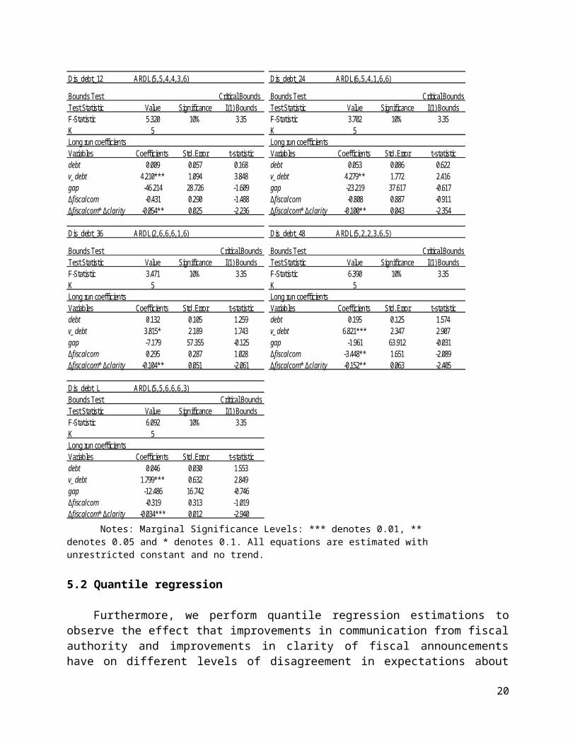
Figure A1 - CUSUM tests – ARDL

ARDL - Dis_debt_12 ARDL - Dis_debt_24

ARDL - Dis_debt_36 ARDL - Dis_debt_48

ARDL - Dis_debt_L

-40

-30

-20

-10

0

10

20

30

40

06 07 08 09 10 11 12 13 14 15 16 17

CUSUM 5% Significance

-40

-30

-20

-10

0

10

20

30

40

06 07 08 09 10 11 12 13 14 15 16 17

CUSUM 5% Significance

-40

-30

-20

-10

0

10

20

30

40

06 07 08 09 10 11 12 13 14 15 16 17

CUSUM 5% Significance

-40

-30

-20

-10

0

10

20

30

40

05 06 07 08 09 10 11 12 13 14 15 16 17

CUSUM 5% Significance

-40

-30

-20

-10

0

10

20

30

40

06 07 08 09 10 11 12 13 14 15 16 17

CUSUM 5% Significance

20