UNIVERSIDADE DE SÃO PAULOINSTITUTO DE FÍSICA

Avaliação de sistemas de controleautomático de exposição em tomografia

computadorizada

Thamiris Rosado Reina

Orientador: Prof. Dr. Paulo Roberto Costa

Dissertação de mestrado apresentada ao Instituto

de Física para a obtenção do título de Mestre em

Ciências.

Banca Examinadora:

Prof. Dr. Paulo Roberto Costa orientador (IFUSP)

Prof. Dr. Alessio Mangiarotti (IFUSP)

Profa. Dra. Isabel Ana Castellano (The Royal Marsden NHS Trust)

São Paulo

2014

UNIVERSITY OF SÃO PAULOINSTITUTE OF PHYSICS

Evaluation of automatic exposure controlsystems in computed tomography

Thamiris Rosado Reina

Advisor: Prof. Dr. Paulo Roberto Costa

Dissertation submitted to the Institute of Physics of

the University of São Paulo for the Master of

Science degree.

Examination Committee:

Prof. Dr. Paulo Roberto Costa advisor (IFUSP)

Prof. Dr. Alessio Mangiarotti (IFUSP)

Prof. Dr. Isabel Ana Castellano (The Royal Marsden NHS Trust)

São Paulo

2014

III

To my parents, Gismeire and Claudio,

who always saw the best there was in

me. To my husband Lucas who held me

up for all this time and never let me fall.

IV

The important thing is

Albert Einstein

V

ACKNOWLEDGMENTS

This work could never exist if my parents Gismeire and Claudio did not support mypassion for Physics and believe I could make it right.

I want to thank my husband Lucas who encourages me every day, supports me everymoment and loves me even when I do not deserve.

I want to thank my beautiful family to help me to be where and who I am: my sister andbrother, my aunts and uncles.

I want to thank my advisor Paulo for accepting a stranger as his student and give methis chance and to have opened the most important door to my career, the first one.

I want to thank my lovely boss, professor and friend Denise that introduced me to realhe most and,

especially to put up with me in smelly tests in the hospitals.

I want to thank my boss, professor and friend Camila who always comes with then

I want to thank my boss, professor and friend Tânia who believed that a raw data likeme could became a great CT image in the Quality Assurance group.

I want to thank my professor and friends Beth and Emico who made me feel welcomeand at home every day, every lunch.

I want to thank my friends and colleagues Micaela, Renato, Juliana, Eric and Ivan tohelp me with this work, to support me in my desperate times (many times) and makeme laugh especially on Fridays (Mica time).

I want to thank the whole group of the Radiation Dosimetry and Medical Physics forthe support in my work and the good coffee times. Especially Nancy and Francisco forhelping me with the dosimeters set up and reading.

I want to thank my eternal dearest friends Stella, Angélica and Luzia for being on myside and understand my absence and, especially, never give up on me.

VI

CONTENTS

LIST OF FIGURES ..................................................................................................... X

LIST OF TABLES .................................................................................................... XX

ACRONYMS .......................................................................................................... XXII

ABSTRACT ........................................................................................................... XXIII

RESUMO............................................................................................................... XXIV

1 INTRODUCTION .................................................................................................... 25

2 THEORY ................................................................................................................ 28

2.1 COMPUTED TOMOGRAPHY EVOLUTION ....................................................... 28

2.1.1 The first generation ........................................................................................ 28

2.1.2 The second generation .................................................................................. 28

2.1.3 The third generation ....................................................................................... 29

2.1.4 The fourth generation .................................................................................... 30

2.1.5 The fifth generation ........................................................................................ 30

2.1.6 The sixth generation ...................................................................................... 31

2.1.7 The seventh generation ................................................................................. 32

2.2 COMPUTED TOMOGRAPHY SCANNERS ........................................................ 33

2.2.1 X-ray tube ........................................................................................................ 33

2.2.2 Detectors ......................................................................................................... 34

2.2.3 Filters ............................................................................................................... 35

2.2.4 Gantry .............................................................................................................. 36

2.2.5 Generator ........................................................................................................ 37

2.2.6 Image reconstruction ..................................................................................... 37

2.2.7 Hounsfield Unit ............................................................................................... 40

VII

2.3 AUTOMATIC EXPOSURE CONTROL ................................................................ 41

2.3.1 Automatic exposure control in general radiology ....................................... 41

2.3.2 Automatic exposure control modalities in computed tomography ........... 42

2.3.2.1 Automatic exposure control systems based on image quality ....................... 43

2.3.2.2 Automatic exposure control systems based on tube current or current-timeproduct ...................................................................................................................... 44

2.3.2.3 Automatic exposure control systems based on reference image .................. 44

2.3.3 Automatic exposure control systems functioning in CT scanners............ 44

2.3.3.1 Longitudinal tube current modulation............................................................. 45

2.3.3.2 Angular tube current modulation ................................................................... 45

2.4 COMPUTED TOMOGRAPHY DOSIMETRY ....................................................... 46

3 METHODS AND MATERIALS ............................................................................... 48

3.1 CLINICAL ROUTINE DATABASE ....................................................................... 48

3.2 COMPUTED TOMOGRAPHY SCANNERS ........................................................ 48

3.2.1 General Electric CT scanner .......................................................................... 48

3.2.2 Philips CT scanner ......................................................................................... 49

3.2.3 Toshiba CT scanner ....................................................................................... 50

3.3 EVALUATION OF THE AUTOMATIC EXPOSURE CONTROL SYSTEMS ........ 51

3.3.1 ImPACT Phantom ........................................................................................... 51

3.3.2 CTDI Phantoms ............................................................................................... 53

3.3.3 Extraction of X-ray tube current data from DICOM header ......................... 56

3.3.3.1 Scanning protocol .......................................................................................... 56

3.3.3.2 Software analysis .......................................................................................... 57

3.3.3.3 Developed spreadsheet ................................................................................. 58

3.3.4 Evaluation of the z-axis dose distribution .................................................... 59

VIII

3.3.4.1 Ionization chamber ........................................................................................ 60

3.3.4.2 Thermoluminescent dosimeters .................................................................... 60

3.4 EVALUATION OF THE IMAGE NOISE ............................................................... 67

3.5 SUMMARY OF THE AUTOMATIC EXPOSURE CONTROL SYSTEMCHARACTERISTICS ................................................................................................ 68

4 RESULTS ............................................................................................................... 70

4.1 EVALUATION OF THE TUBE CURRENT MODULATION AND IMAGE NOISEALONG Z-AXIS ......................................................................................................... 70

4.1.1 General Electric CT Scanners ....................................................................... 71

4.1.1.1 PET/CT Discovery 690 HD ............................................................................ 71

4.1.1.2 LightSpeed Ultra ............................................................................................ 84

4.1.1.3 Discovery 750 HD.......................................................................................... 91

4.1.2 Toshiba CT Scanner ....................................................................................... 93

4.1.3 Philips CT Scanners ....................................................................................... 95

4.1.3.1 Brilliance 16 Model ........................................................................................ 96

4.1.3.2 Brilliance 40 Model ...................................................................................... 110

4.1.3.3 Brilliance 64 Model ...................................................................................... 112

4.1.3.4 Brilliance iCT Model ..................................................................................... 113

4.2 EVALUATION OF THE CT DOSE DISTRIBUTION IN Z-AXIS ......................... 115

4.2.1 GE LightSpeed Ultra..................................................................................... 115

4.2.2 GE Discovery 750 HD ................................................................................... 119

4.2.3 Philips Brilliance 16...................................................................................... 120

4.2.4 Summary of the dose distribution measurements .................................... 124

5 DISCUSSION ....................................................................................................... 126

5.1 GENERAL ELECTRIC AUTOMATIC EXPOSURE CONTROL SYSTEM ...... 126

5.1.1 Current range ................................................................................................ 126

IX

5.1.2 Noise index ................................................................................................... 128

5.1.3 Automatic exposure control mode ............................................................. 128

5.1.4 Scan projection radiograph scout ........................................................... 129

5.1.5 Scan field of view ......................................................................................... 131

5.1.6 Evaluation of z-axis dose profile of GE CT scanners ................................ 131

TIC EXPOSURE CONTROL SYSTEM .......................... 134

IC EXPOSURE CONTROL SYSTEM ............................... 135

5.3.1 AEC Mode ..................................................................................................... 135

5.3.1.1 Z-DOM AEC mode ...................................................................................... 135

5.3.1.2 D-DOM AEC mode ...................................................................................... 136

5.3.2 Collimation .................................................................................................... 140

5.3.3 Patient couch orientation ............................................................................ 140

5.3.4 Current-time product per slice .................................................................... 141

5.3.5 Scan projection radiograph surview ........................................................ 141

5.3.6 AEC response over time .............................................................................. 142

6 GENERAL DISCUSSION AND FUTURE ISSUES .............................................. 145

REFERENCES ........................................................................................................ 147

X

LIST OF FIGURES

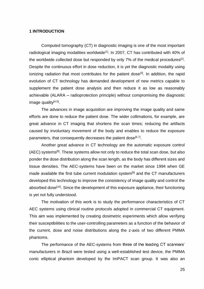
Figure 1 The first generation has a pencil beam translation over the patient to reach an attenuationprofile, which makes the imaging reconstruction system capable to distinguish different types of tissuesand structures. (source: Hypermedia MS[16])......................................................................................... 29

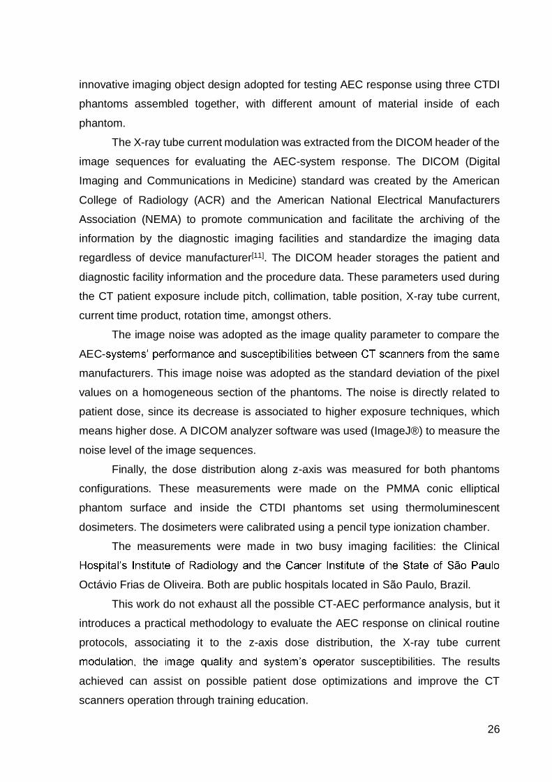
Figure 2 The second generation has a small fan beam which allows a bigger number of detectorssimultaneously. The scan geometry is pretty similar to the first one, but the scan time is quite reduced.The set of detector was parallel as it can be seen in the illustration. (source: Hypermedia MS [16])...... 29

Figure 3 The third generation has the X-ray tube and detectors system rotating without translatinganymore. The fan beam is larger and the detectors are disposed as an arc (30° or 40°). (source:Hypermedia MS[16]) ................................................................................................................................ 30

Figure 4 The fourth generation has a stationary ring of detectors where only the X-ray tube rotates.(source: Hypermedia MS[16]) ................................................................................................................. 31

Figure 5 The Electron-Beam CT (EBCT) does not have X-ray tube, instead an electron beam isaccelerated and deflected to an arc of tungsten target that generated X-ray radiation and a stationaryarc of detectors at the opposite side of the target arc at the gantry. (source: Hypermedia MS[16])....... 31

Figure 6 After the development of the slip-rings technology, the X-ray tube and detectors system couldrotate continuously, allowing the helical or spiral CT scan. As the patient couch translates while the tubeis rotating 360°, the irradiation has a spiral form. (source: Hypermedia MS[16]).................................... 32

Figure 7 The bowtie filter hardens the X-ray beam and its filtration is higher in the borders of the conebeam to compensate the thinner borders of the patient body. .............................................................. 36

Figure 8 Scheme of the gantry axis. Where the patient couch translates in z-axis and the X-ray tubeand detectors system rotated in x-y plane. (source: ImPACT 2001[20]) ................................................ 37

Figure 9 Three cases of imaging formation. Case 1 has the simplest case with a homogeneous imagingobject and monoenergetic radiation. Case 2 has a simple inhomogeneous imaging object andmonoenergetic radiation. Case 3 is closer to reality and it has an inhomogeneous imaging object andpolyenergetic radiation. These three cases illustrate the difficulty of tomographic imaging with X-rayradiation that is naturally polyenergetic (source: Kallender, 2011[12]) ................................................... 39

Figure 10 Examples of filtered back projections. These projections show that the image gets clearerwhen more projections are done and less filtration will be required. (source: Platten, 2003[26]) ........... 40

Figure 11 (a) Example of a bucky with five photocells indicated by the circles and (b) three photocellsindicated by the circles and the square. ................................................................................................ 42

Figure 12 Example of longitudinal tube current modulation regarding AP SPR view. (source: Report05016, MHRA[31]) ................................................................................................................................... 45

Figure 13 (a) Angular tube current modulation and (b) angular combined to longitudinal tube currentmodulation. (source: Report 05016, MHRA[31]) ..................................................................................... 46

Figure 14 The ImPACT Phantom designed to evaluate the AEC-systems functioning. It ishomogeneous, manufactured from acrylic, 300 mm long and it is elliptical-cone shaped with the majoreffective diameter of 350 mm and the minor 50 mm. (source: Report 05016[31]).................................. 52

Figure 15 Piccarrying case with Catphan® as counterweight. ................................................................................... 53

XI

Figure 16 (a) ImPACT Phantom simulates the difference of AP and lateral view thickness and (b) theX-ray tube current has a sinusoidal variation. ....................................................................................... 53

Figure 17 Scheme of the CTDI Phantom with the minor diameter part that simulates pediatric head atthe top, in the middle the intermediate part that simulates adult head and at bottom the major diameterthat simulates adult abdomen and thorax when full filled. .................................................................... 54

Figure 18 Phantom scheme with th

the CTDI phantom without the adult and pediatric head (160 mm and 100 mm diameters). ............... 55

Figure 19 TAP phantom positioned over the patient couch. In the left, the picture of the three phantomsplaced together with the full filled phantom on the left, the phantom without the minor diameter in themiddle and the phantom without the intermediate diameter on the right side. In the right, the front pictureof this set. .............................................................................................................................................. 55

Figure 20 The expected behavior for the X-ray tube current modulation is three tube current valueswith the highest value at the full filled phantom (1) and the lowest value at the one without theintermediate diameter phantom (3). The figure presents this X-ray tube current behavior for a thorax,abdomen and pelvis scanning. .............................................................................................................. 56

Figure 21on allows the user to create an

text document file with the DICOM tags and load it to the Scan Header plugin instead of typing each one

no restriction

................................................................ 58

Figure 22 The data extracted from the DICOM header is presented in an additional box and the usercan select the whole data, copy and paste to a text document file to be processed by another software. ............................................................................................................................................................... 58

Figure 23 (a) SPR of the ImPACT Phantom, and (b) superposition of the SPR of the ImPACT Phantomand X-ray tube current data. The graphics were plotted with the scan projection radiograph of theImPACT Phantom as background for better comprehension of the X-ray tube current behavior. ....... 59

Figure 24 (a) SPR of the TAP phantom and (b) the graphics were plotted with the scan projectionradiograph of the TAP phantom as background for better comprehension of the X-ray tube currentbehavior. ................................................................................................................................................ 59

Figure 25 Thermoplastic tapes with the LiF thermoluminescent dosimeters. Each tape hasapproximately 30 cm length and contains 25 to 28 TLD units. ............................................................. 61

Figure 26 Acrylic sticks with LiF thermoluminescent dosimeters. Each stick has 45 cm length insidethe TAP phantom and contains slots for positioning 25 TLD units. The external diameter of the stickswere designed to fit the holes present in the TAP phantom which are used for insert the pencil typeionization chambers. ............................................................................................................................. 61

Figure 27 Dosimeters tapes placed at the AP and lateral view of the ImPACT Phantom. ................ 62

Figure 28 Acrylic sticks at the center of the TAP phantom. (a) TAP phantom with a stick of dosimetersand (b) inside view from the stick in the phantom. ................................................................................ 62

Figure 29 Thermoplastic tape with dosimeters at the center of the TAP phantom. ........................... 63

XII

Figure 30 ....... 63

Figure 31 (a) Heating and lifting mechanism of the TL/OSL reader Risø and (b) the mechanism withthe sample carousel. (source: DTU Nutech[54]) ..................................................................................... 64

Figure 32 Dosimeter data from the Risø TL/OSL reader in counts per temperature in Celsius degree.The marks in 150 °C and 300 °C delimitate the integration area. ......................................................... 64

Figure 33 (a) the picture of the ionization chamber at the center of the full filled CTDI phantom at thegantry central axis and (b) the dosimeters tape placed inside the same full filled CTDI Phantom. ...... 65

Figure 34 Example of a calibration curve for a set of measurement. The calibration function (y) wasattained by the linear

respectively, 2.47x10-5 mGy/counts and -1.39x10-1 mGy. .................................................................... 66

Figure 35 The ImageJ® user can select a region of interest (ROI), in yellow, using four different shape

Manage

The user can set the measurement for mean CT-value, minimum and maximum, standard deviation,ROI area etc. ......................................................................................................................................... 68

Figure 36 Example of the tube current modulation of the angular AEC mode due to the AP and lateralthickness difference of the body. (Report 05016, MHRA [31]) ................................................................. 70

Figure 37 Ilustration of the expected tube current modulation result for the TAP phantom. Thentom without the 100 mm

............................................. 71

Figure 38 Tube current modulation along z-axis for two different current ranges: the blue linerepresenting the widest tube current modulation (study number 1 - #1) and the red line representing aclinical current range, narrower (study number 2 - #2). ........................................................................ 74

Figure 39 Difference on noise for two current ranges. The blue line represents the noise level for thestudy number 1 (#1) and it is about 5 HU lower than the noise level for the study number 2 (#2 redline) at the thicker part of the phantom, but the X-ray tube current at this point is 10 times higher for thestudy 1. In the thinner part of the phantom, the study number 1 reaches 400 mA higher than the tubecurrent values of the study number 2 but no more than 5 HU difference on noise. The highest noisevalues at the end of the graphic is due to the end of the phantom being imaged with a portion of air. 75

Figure 40 Tube current modulation for different noise index values. The blue line represents the clinicalnoise index of the study number 1 (#1), an intermediate value. The green line represents a higher noiseindex value (study number 3 - #3), meaning that a high image quality is not required, so the AEC-systemturns down the tube current level. The red line represents a lower noise index value (study number 5 -#5), meaning that a high image quality is required, then the AEC-system raises the tube current level. ............................................................................................................................................................... 76

Figure 41 Difference on noise for different noise index values. The blue line represents the noise levelfor the noise index of 11.37 (study number 1 - #1); the green line represents the noise level for the noiseindex of 25 (study number 3 - #3); the red line represents the noise level for the noise index of 5 (studynumber 4 - #4). The higher values at the thinner part of the phantom is due to the last section of thephantom being imaged with a portion of air and the CT numbers vary from about 110 HU until -1,000HU (air CT number). .............................................................................................................................. 76

Figure 42 Tube current modulation for the longitudinal and the longitudinal combined to angular AECmode, Auto mA and Auto + Smart mA, respectively. The blue line represents the Auto mA AEC mode

XIII

(study number 1 - #1) and the red line represents the Auto + Smart mA AEC mode (study number 5 -#5). ........................................................................................................................................................ 77

Figure 43 Difference on noise for the two AEC modes, Auto mA and Auto + Smart mA. The blue linerepresents the Auto mA AEC mode (study number 1 - #1) and the red line represents the Auto + SmartmA AEC mode (study number 5 - #5). .................................................................................................. 77

Figure 44 (a) The figure shows the scout of the entire ImPACT Phantom and (b) the half scout. .... 79

Figure 45 Tube current modulation for a scout made from half of the phantom (from the middle untilthe thinner part of the phantom) and a scan from the entire phantom. The red line represents the AutomA AEC mode on this scan condition (study number 6 - #6) and the green line represents the Auto +Smart AEC mode on this scan condition (study number 7 - #7). .......................................................... 79

Figure 46 Difference on noise for a scan with full scout and the scans with half scout. The blue linerepresents the scan with full scout using Auto mA (study number 1 - #1) and the red and green lines thescans with half scout using, respectively, Auto mA and Auto + Smart mA (studies number 6 and 7 - #6and #7). ................................................................................................................................................. 80

Figure 47 Scout images from AP view for (a) the ImPACT Phantom at the gantry central axis, (b) theImPACT Phantom above the gantry central axis and (c) the ImPACT Phantom below the gantry centralaxis. When the phantom is above the gantry central axis, the imaging system projects a magnified imageas it seems larger for the detectors and when the phantom is below the gantry central axis the imagingsystem projects a shrunken image as it seems smaller for the image detectors. ................................. 81

Figure 48 Scout images from lateral view for (a) the ImPACT Phantom at the gantry central axis, (b)the ImPACT Phantom above the gantry central axis and (c) the ImPACT Phantom below the gantrycentral axis. When the phantom is above or below the gantry central axis the lateral view appearsdisplaced from the center of the image display. For this reason some manufacturers recommend to takethe lateral view SPR first, and if the patient appears at the display center, the AP view SPR can beproceeded. ............................................................................................................................................. 81

Figure 49 Tube current modulation for different couch positioning at the gantry y-axis. The blue linerepresents the ImPACT Phantom at the gantry central axis (study number 1 - #1), the green linerepresents the ImPACT Phantom 74 mm above the gantry central axis (study number 8 - #8) and thered line represents the ImPACT Phantom 76 mm below the gantry central axis (study number 9 - #9). ............................................................................................................................................................... 82

Figure 50 Tube current modulation for scans made from double scout, single AP scout and singlelateral scout. In addition, the difference on tube current modulation for a single lateral scout using bothAEC modes, Auto mA and Auto + Smart mA. The blue line represents the double scout using Auto mA(study number 1 - #1), the purple line represents the single AP scout using Auto mA (study number 10- #10), the red line represents the single lateral scout using Auto mA (study number 11 - #11) and thegreen line represents the single lateral scout using Auto + Smart mA. ................................................ 83

Figure 51 Difference on noise level for the double and single scout and lateral view scout using bothAEC modes. The blue line represents the noise level for the scan made from the double scout usingAuto mA AEC mode (study number 1 - #1), the purple line represents the noise level for the scan madefrom the sinle AP scout (study number 10 - #10), the red line represents the scan made from the singlelateral scout using Auto mA AEC mode (study number 11 - #11) and the green line represents the scanmade from the single lateral scout using Auto + Smart mA AEC mode (study number 12 - #12). Thehigher noise values at the end of the thinner part of the phantom is the portion of the phantom beingimaged with air and the CT number varies from about 110 until -1,000 (air CT number). .................... 83

Figure 52 Tube current modulation for two different scan fields of view (S-FOV). The blue linerepresents the S-FOV for large body scan (study number 1 - #1) and the red line represents the S-FOVfor head scan (study number 2 - #2). .................................................................................................... 86

XIV

Figure 53 Tube current modulation for scans made from scout with two different exposure technique:80 kV with 20 mAs (Scout 1) and 120 kV with 20 mAs (Scout 2). The blue line represents the scan madefrom the scout 1 (study number 1 - #1) and the green line represents the scan made from the scout 2(study number 3 - #3). ........................................................................................................................... 87

Figure 54 Tube current modulation for two different noise index (NI) values: 11.37 and 20. In addition,pitch variation for the NI of 20 was made from 0.75 to 1.5. The blue line represents the scan with clinicalnoise index of 11.37 with pitch value of 0.75 (study number 4 - #4), the yellow line represents the scanwith noise index of 20 and pitch of 1.5 (study number 5 - #5) and the red line represents the scan withnoise index of 20 with pitch value of 0.75 (study number 6 - #6). ......................................................... 89

Figure 55 Tube current modulation for higher values of noise index and same pitch value of 0.75. Thepink line represents the noise index of 25 (study number 7 - #7), the light blue line represents the noiseindex of 30 (study number 8 - #8) and the green line represents the noise index of 50 (study number 9- #9). ...................................................................................................................................................... 89

Figure 56 Noise level for the scan with clinical noise index of 11.37. The tube current modulation isplotted in secondary y-axis. The dark blue line represents the tube current modulation and the light blueline represents the noise level in primary y-axis. The noise level varies in a step pattern accordingly tothe amount of material inside the TAP phantom. .................................................................................. 90

Figure 57 Noise level for the scan with higher noise index of 25. The tube current modulation is plottedin secondary y-axis. The pink line represents the tube current modulation and the red line representsthe noise level in primary y-axis. When there is a significant difference on tube current modulation thenoise level fluctuate about a baseline. The higher noise values at the phantom edges are due to theborder being imaged with a portion of air and the CT number around this sections has bigger variation. ............................................................................................................................................................... 90

Figure 58 Tube current modulation for three current ranges with only the bottom value varying. Theblue line represents the current range used in clinical routine, the narrowest current range used in thisstudy; the orange line represents a wider current range, with the lowest bottom value available and thegreen line represents an intermediate current range. ........................................................................... 92

Figure 59 Difference on noise level for three current ranges with only the bottom value varying. Theblue line represents the noise level of the clinical routine current range; the orange line represents thewider current range noise level, with the lowest bottom value available; and the green line representsthe noise level for the intermediate current range. ................................................................................ 92

Figure 60 Tube current modulation for two different scan fields of view (S-FOV). The blue linerepresents the large body S-FOV and the red line represents the small body S-FOV. ........................ 93

Figure 61 Difference on noise level for two scan fields of view (S-FOV). The blue line represents thenoise level of the large body S-FOV and the red line represents represents the noise level of the smallbody S-FOV. .......................................................................................................................................... 93

Figure 62 Tube current modulation for two SureExposure options. The blue line represents the LowDose SureExposure option, that allows to lower the patient dose; the red line represents the StandardSureExposure option, that tries to balance the patient dose and image quality. .................................. 95

Figure 63 Difference on noise level for two SureExposure options. The blue line represents the noiselevel of the Low Dose SureExposure option, that allows to lower the patient dose; the red line representsthe noise level of the Standard SureExposure option, that tries to balance the patient dose and imagequality. ................................................................................................................................................... 95

Figure 64 Tube current modulation for the longitudinal AEC mode, Z-DOM, and the longitudinal AECmode with the DoseRight AEC option ON. The blue line represents the Z-DOM (study number 1 - #1)and the red line represents the Z-DOM with DoseRight ACS option ON (study number 2 - #2). ......... 99

XV

Figure 65 Difference on noise level for the longitudinal AEC mode, Z-DOM, with the DoseRight ACSoption ON and OFF. The blue line represents the noise level of Z-DOM AEC mode (study number 1 -#1) and the red line represents the noise level of Z-DOM with DoseRight ACS option ON (study number2 - #2). ................................................................................................................................................... 99

Figure 66 Tube current modulation for the longitudinal AEC mode, Z-DOM, and the longitudinal AECmode with the DoseRight AEC option ON using the TAP phantom. The blue line represents the Z-DOMAEC mode (study number 1 - #1) and the red line represents the Z-DOM with DoseRight ACS optionON (study number 2 - #2). ................................................................................................................... 100

Figure 67 Tube current modulation for the angular AEC mode, D-DOM, and the angular AEC modewith the DoseRight AEC option ON. The green line represents the D-DOM AEC mode (study number 3- #3) and the purple line represents the D-DOM with DoseRight AEC option ON (study number 4 - #4). ............................................................................................................................................................. 100

Figure 68 Difference on noise level between the angular AEC mode, D-DOM, and the angular AECmode with DoseRight AEC option ON. The green line represents the D-DOM AEC mode (study number4 - #4) and the purple line represents the D-DOM with DoseRight ACS option ON. .......................... 101

Figure 69 Tube current modulation for the angular AEC mode, D-DOM, and the angular AEC modewith the DoseRight AEC option ON using the TAP phantom. The green line represents the D-DOM AECmode (study number 3 - #3) and the purple line represents the D-DOM with DoseRight AEC option ON(study number 4 - #4). ......................................................................................................................... 101

Figure 70 Tube current modulation for the longitudinal and the angular AEC modes, Z-DOM and D-DOM respectively. The blue line represents the Z-DOM AEC mode (study number 1 - #1) and the greenline represents the D-DOM AEC mode (study number 3 - #3). .......................................................... 102

Figure 71 Difference on noise for the longitudinal and angular AEC modes, Z-DOM and D-DOMrespectively. The blue line represents the noise level for the Z-DOM AEC mode (study number 1 - #1)and the green line represents the noise level for the D-DOM AEC mode (study number 3 - #3). ...... 102

Figure 72 Tube current modulation for the longitudinal and the angular AEC modes, Z-DOM and D-DOM respectively, using the TAP phantom. The blue line represents the Z-DOM AEC mode (studynumber 1 - #1) and the green line represents the D-DOM AEC mode (study number 3 - #3). .......... 103

Figure 73 Tube current modulation for two different collimations, 16 x 1.5 mm (COL 1) and 16 x 0.75mm (COL 2), both with D-DOM AEC mode. The green line represents the collimation of 16 x 1.5 mmwith pitch of 0.938 (study number 3 - #3) and the orange line represents the collimation of 16 x 0.75 mmwith pitch of 0.942 (study number 5 - #5). ........................................................................................... 104

Figure 74 Tube current modulation for two different collimations, 16 x 1.5 mm (COL 1) and 16 x 0.75mm (COL 2), both with D-DOM AEC mode using the TAP phantom. The green line represents thecollimation of 16 x 1.5 mm with pitch of 0.938 (study number 3 - #3) and the orange line represents thecollimation of 16 x 0.75 mm with pitch of 0.942 (study number 5 - #5). .............................................. 104

Figure 75 Tube current modulation for two selected mAs/slice, 250 mAs/slice and 400 mAs/slice, withZ-DOM AEC mode. The blue line represents the Z-DOM AEC mode with 250 mAs/slice (study number1 - #1) and the orange line the Z-DOM AEC mode with 400 mAs/slice (study number 6 - #6). ......... 105

Figure 76 Tube current modulation for scans made from double, single AP and single lateral surviewwith the angular AEC mode D-DOM. The blue line represents the scan made from the double surview(study number 7 - #7), the green line represents the scan made from the single AP surview (studynumber 8 - #8) and the red line represents the scan made from the single lateral surview(study number9 - #9). ................................................................................................................................................. 105

XVI

Figure 77 Tube current modulation for scans made from single AP and single lateral surview withlongitudinal AEC mode, Z-DOM, with DoseRight ACS option ON and OFF. The blue line represents thescan made from single AP surview using only Z-DOM AEC mode (study number 11 - #11); the orangeline represents the scan made from single AP surview using Z-DOM with DoseRight ACS (study number12 - #12); the red line represents the scan made from single lateral surview using only Z-DOM AECmode; the red line represents the scan made from the single lateral surview using only Z-DOM AECmode (study number 13 - #13); the green line represents the scan made from single lateral surviewusing Z-DOM with DoseRight ACS option (study number 14 - #14). .................................................. 106

Figure 78 Tube current modulation using angular AEC mode, D-DOM, for two different patientorientation, i.e. the scan made while the patient couch is getting out of the gantry or while the patientcouch is getting inside of the gantry. Both scans were made from single AP surview. The blue linerepresents the scan made with the patient couch getting out the gantry (study number #9 - #9) and thered line represents the scan made with the patient couch getting in the gantry (study number 10 - #10). ............................................................................................................................................................. 107

Figure 79 Tube current modulation for the longitudinal AEC mode, Z-DOM, with the DoseRight ACSoption ON and OFF response over time. The dark red line represents the scan made in 2013 withDoseRight ACS option OFF (study number 15 - #15); the light red line represents the scan made in2014 with DoseRight ACS option OFF (study number 1 - #1); the dark blue line represents the scanmade in 2013 with DoseRight ACS option ON (study number 16 - #16); the light blue line represents thescan made in 2014 with DoseRight ACS option ON (study number 2 - #2). All the scans were made inboth years in the month of May. .......................................................................................................... 108

Figure 80 Difference on noise for the longitudinal AEC mode, Z-DOM, response over time. The lightred line represents the noise measured from the scan of 2013 (study number 15 - #15) and the dark redline represents the noise measured from the scan made in 2014 (study number 1 - #1)................... 108

Figure 81 Difference on noise for the longitudinal AEC mode, Z-DOM, with DoseRight ACS optionresponse over time. The light blue line represents the noise measured from the scan made in 2013(study number 16 - #16) and the dark blue line represents the noise measured from the scan made in2014 (study number 2 - #2). ................................................................................................................ 109

Figure 82 Tube current modulation response over time for the angular AEC mode, D-DOM, withDoseRight ACS option ON. The green line represents scan made in 2013 (study number 17 - #17) andthe orange line the scan made in 2014 (study number 4 - #4). Both scans were made in the month ofMay. ..................................................................................................................................................... 109

Figure 83 Difference on noise for the AEC response over time for the angular AEC mode, D-DOM,with DoseRight ACS option ON. The green line represents the noise measured from the scan made in2013 (study number 17 - #17) and the orange line represents the noise measured from the scan madein 2014 (study number 4 - #4). Both scans were made in the month of May. .................................... 110

Figure 84 Tube current modulation for the angular AEC mode, D-DOM with the DoseRight ACS optionON and OFF. The blue line represents the D-DOM AEC mode and the red line represents the D-DOMwith DoseRight ACS option. ................................................................................................................ 111

Figure 85 Difference on noise for the angular AEC mode, D-DOM, with the DoseRight ACS option ONand OFF. The blue line represents the noise level for D-DOM and the red line represents the noise levelfor D-DOM with DoseRight ACS option. ............................................................................................. 111

Figure 86 Tube current modulation for scans made from the single AP surview and single lateralsurview using longitudinal AEC mode, Z-DOM. The blue line represents the scan made from the singleAP surview and the red line represents the single lateral surview. ..................................................... 113

Figure 87 Difference on noise for scans made from the single AP surview and single lateral surviewusing longitudinal AEC mode, Z-DOM. The blue line represents the noise measured from the scan made

XVII

from the single AP surview and the red line represents the noise measured from the single lateralsurview. ............................................................................................................................................... 113

Figure 88 Tube current modulation for the longitudinal AEC mode, Z-DOM, with the DoseRight ACSoption ON and OFF and a fixed current-time product per slice (mAs/slice). The blue line represents theDoseRight ACS option ON, the red line represents the DoseRight ACS option OFF and the green linerepresents the fixed mAs/slice that resulted in fixed tube current of 497 mA. ................................... 114

Figure 89 Difference on noise for the longitudinal AEC mode, Z-DOM, with the DoseRight ACS optionON and OFF and a fixed current-time product per slice (mAs/slice). The blue line represents theDoseRight ACS option ON, the red line represents the DoseRight ACS option OFF and the green linerepresents the fixed mAs/slice. ........................................................................................................... 115

Figure 90 Dose measurement inside the TAP phantom, in central position, using noise index of 25.The blue line, in primary y-axis, represents the dose distribution along z-axis and the dots representsthe dosimeters position. The dashed red line represents the tube current modulation plotted in right axis. ............................................................................................................................................................. 116

Figure 91 Dose measurement inside the TAP phantom, in the center, using noise index of 30. Theblue line, in primary y-axis, represents the dose distribution along z-axis and the dots represents thedosimeters position. The dashed red line represents the tube current modulation plotted in right axis. ............................................................................................................................................................. 117

Figure 92 Dose measurement inside the TAP phantom, in the center, using noise index of 50. Theblue line, in primary y-axis, represents the dose distribution along z-axis and the dots represents thedosimeters position. The dashed red line represents the tube current modulation plotted in right axis. ............................................................................................................................................................. 117

Figure 93 Dose measurement inside the TAP phantom, in the center, using fixed tube current of 235mA. The blue line, in primary y-axis, represents the dose distribution along z-axis and the dotsrepresents the dosimeters position. The dashed red line represents the tube current plotted in right axis. ............................................................................................................................................................. 118

Figure 94 Dose measurement on the surface of the ImPACT Phantom at the AP and lateral positionsusing the longitudinal AEC mode, Auto mA. The blue line represents the dose distribution along z-axison the AP surface and the red line represents the dose distribution along z-axis on the lateral surface.The dashed green line represents the tube current modulation plotted in right axis. ......................... 118

Figure 95 Dose measurement on the surface of the ImPACT Phantom at the AP and lateral positionsusing a large body scan field of view and the longitudinal combined to angular AEC mode, Auto + SmartmA. The blue line represents the dose distribution along z-axis on the AP surface and the red linerepresents the dose distribution along z-axis on the lateral surface. The dashed green line representsthe tube current modulation plotted in right axis. ................................................................................ 119

Figure 96 Dose measurement on the surface of the ImPACT Phantom at the AP and lateral positionsusing a small body scan field of view and the longitudinal combined to angular AEC mode, Auto + SmartmA. The blue line represents the dose distribution along z-axis on the AP surface and the red linerepresents the dose distribution along z-axis on the lateral surface. The dashed green line representsthe tube current modulation plotted in right axis. ................................................................................ 120

Figure 97 Dose measurement on the surface of the ImPACT Phantom at the AP and lateral positionsusing the longitudinal AEC mode Z-DOM. The blue line represents the dose distribution along z-axis onthe AP surface and the red line represents the dose distribution along z-axis on the lateral surface. Thedashed green line represents the tube current modulation plotted in right axis. ................................ 121

Figure 98 Dose measurement on the surface of the ImPACT Phantom at the AP and lateral positionsusing the longitudinal AEC mode, Z-DOM, with the DoseRight ACS option ON. The blue line represents

XVIII

the dose distribution along z-axis on the AP surface and the red line represents the dose distributionalong z-axis on the lateral surface. The dashed green line represents the tube current modulation plottedin right axis. ......................................................................................................................................... 122

Figure 99 Dose measurement on the surface of the ImPACT Phantom at the AP and lateral positionsusing the angular AEC mode, D-DOM. The blue line represents the dose distribution along z-axis on theAP surface and the red line represents the dose distribution along z-axis on the lateral surface. Thedashed green line represents the tube current modulation plotted in right axis. ................................ 122

Figure 100 Dose measurement on the surface of the ImPACT Phantom at the AP and lateral positionsusing the angular AEC mode, D-DOM, with the DoseRight ACS option ON. The blue line represents thedose distribution along z-axis on the AP surface and the red line represents the dose distribution alongz-axis on the lateral surface. The dashed green line represents the tube current modulation plotted inright axis. ............................................................................................................................................. 123

Figure 101 Dose measurement on the surface of the ImPACT Phantom at the AP and lateral positionsusing fixed mAs/slice resulting in a fixed tube current of 250. The blue line represents the dosedistribution along z-axis on the AP surface and the red line represents the dose distribution along z-axison the lateral surface. The dashed green line represents the tube current modulation plotted in rightaxis. ..................................................................................................................................................... 123

Figure 102 Dose measurement inside the TAP phantom, in the center, using the longitudinal AECmode, Z-DOM. The blue line, in primary y-axis, represents the dose distribution along z-axis and thedots represents the dosimeters position. The dashed red line represents the tube current plotted in rightaxis. ..................................................................................................................................................... 124

Figure 103 Dose measurements inside the TAP phantom, in central position, varying the noise indexfor the tube current modulation and a fixed tube current of 235 mA. The red line represents the noiseindex of 25, the green line represents the noise index of 30, the purple line represents the noise indexof 50 and the blue line represents the fixed tube current. The dots represents the TLDs positions. .. 132

Figure 104 Difference on dose for the scan fields of view (S-FOV). The dark and light blue linesrepresent, respcectively, the dose distribution along z-axis on AP and lateral surface of the ImPACTPhantom for the large body S-FOV. The dark and light red lines represent, respcectively, the dosedistribution along z-axis on AP and lateral surface of the ImPACT Phantom for the small body S-FOV.The dose in the thicker part of the phantom for the small body S-FOV is about 20% higher than for thelarge body S-FOV, although the tube current modulation is about 22% lower. This may happen becauseof the X-ray tube rotation that highly interferes at the dose measurement on the phantom surface. . 134

Figure 105 Difference on dose distribution along z-axis measured on the ImPACT Phantom surfacefor the longitudinal AEC mode, Z-DOM, with the DoseRight ACS option ON and OFF. The light and bluelines represent, respectively, the dose distribution on the AP and lateral surface of the phantom for theDoseRight ACS option OFF. The dark and light red lines represent, respectively, the dose distributionon the AP and lateral surface of the phantom for the DoseRight ACS option ON. The choice of using theDoseRight ACS option results in higher dose levels. .......................................................................... 136

Figure 106 Difference on dose measured on the ImPACT Phantom surface for the angular andlongitudinal AEC modes, D-DOM and Z-DOM respectively. The light and dark green lines represent,respectively, the dose distribution on the AP and lateral surface of the phantom using D-DOM AECmode. The light and dark blue lines represent, respectively, the dose distribution on the AP and lateralsurface of the phantom using Z-DOM AEC mode. The D-DOM AEC has and inverse behavior of thedose distribution compared to Z-DOM AEC mode. This dose measurement follows the tube currentmodulation response. .......................................................................................................................... 137

Figure 107 Difference on dose measured on the ImPACT Phantom surface for the angular AEC mode,D-DOM, with DoseRight ACS option OFF and the longitufinal AEC mode, Z-DOM, with DoseRight ACSoption ON. The light and dark green lines represent, respectively, the dose distribution on the AP andlateral surface of the phantom using D-DOM AEC mode. The light and dark purple lines represent,

XIX

respectively, the dose distribution on the AP and lateral surface of the phantom using Z-DOM AEC modewith DoseRight ACS. The D-DOM AEC mode has the same dose level of the Z-DOM with DoseRightACS option. However, the dose distribution of Z-DOM with DoseRight ACS follows the phantom shape,i.e. the lower dose level is at the thinner part of the phantom. ............................................................ 138

Figure 108 Difference on dose measured on the ImPACT Phantom surface for the angular AEC mode,D-DOM, and a fixed current-time product per slice (mAs/slice). The light and dark green lines represent,respectively, the dose distribution on the AP and lateral surface of the phantom using D-DOM AECmode. The dark and light red lines represent, respectively, the dose distribution on the AP and lateralsurface of the phantom using fixed mAs/slice. The dose distribution of the D-DOM AEC mode is similarto the fixed mAs/slice, i.e. that this AEC mode is practically the same of not to use the AEC-system. ............................................................................................................................................................. 139

Figure 109 Difference on noise for scans made using the angular AEC mode, D-DOM, and a fixedcurrent time product per slice. Although the dose distribution is about 15% lower for the D-DOM AECmode, the noise level is increased about 20% compared to the fixed mAs/slice noise level. ............ 139

Figure 110 Difference on dose measured on the ImPACT Phantom surface for the angular AEC mode,D-DOM, with DoseRight ACS option ON and OFF. The light and dark green lines represent, respectively,the dose distribution on the AP and lateral surface of the phantom with the DoseRight ACS option OFF.The light and dark orange lines represent, respectively, the dose distribution on the AP and lateralsurface of the phantom with the DoseRight ACS option ON. Both measurements presented anunexpected behavior, i.e. raising dose at the thinner part of the phantom. The DoseRight option ONimparts higher dose, raising the dose more than 20 mGy at the thinner part of the phantom. ........... 140

Figure 111 Surview taken from the AP view of the ImPACT Phantom. The width measured, 380.1 mm,is 50 mm larger than the Philips patient of reference of 330 mm. The average signal measured, 682.43HU, represents the CT number of the image; taking this value and the Hounsfield scale into account,the AEC-system calculates the tube current modulation based on density. ....................................... 142

Figure 112 Surview taken from the lateral view of the ImPACT Phantom. The width measured,260.3 mm, is 70 mm narrower than the Philips patient of reference of 330 mm. The average signalmeasured, 1509.14 HU, represents the CT number of the image; taking this value and the Hounsfieldscale into account, the AEC-system calculates the tube current modulation based on density. ........ 142

XX

LIST OF TABLES

Table 1 -system accordingly to the MHRA Report 05016[31]. .............................................................................. 43

Table 2 -system................................................ 49

Table 3 Parameters available for the Philip -system. ......................................... 50

Table 4 -system. ....................................... 51

Table 5 General scanning protocol parameters selected for the evaluation of the AEC-systems. .... 57

Table 6 Scanning protocol parameters selected for the calibration in axial scan. ............................. 65

Table 7 Results of the fitting procedure for each calibration measurement on GE LightSpeed Ultraand Discovery 750 HD and Philips Brilliance 16. .................................................................................. 67

Table 8 Summary of the automatic exposure control systems evaluated in this work and the studiesmade from their characteristics. ............................................................................................................ 69

Table 9 Description of the studies conducted to evaluate the AEC performance, studies 1 to 5, andthe AEC-system susceptibility to the user, studies 6 to 12. .................................................................. 72

Table 10 Scanning protocol parameters fixed for the PET/CT Discovery 690 HD AEC-systemevaluation. ............................................................................................................................................. 73

Table 11 Parameters settled for the double scout used as a localizer for the phantom scans. ........ 73

Table 12 Parameters altered for testing the AEC-system efficiency. The study number 1, in light gray,is the protocol used as the benchmark. In dark gray are the changes made at each study. The IndicatedCTDIvol represents the value of this quantity displayed in the equipment console. .............................. 73

Table 13 Parameters altered for testing the AEC-system vulnerability. In dark gray are the changesmade at each study referred to the study number 1. ............................................................................ 78

Table 14 -systemresponse. ............................................................................................................................................... 84

Table 15 Scanning protocol parameters settled for the -system. .................................................................................................................................................. 85

Table 16 ............................................................................................................................................................... 85

Table 17 Scanning protocol parameters selected for study the AEC response on different scan fieldsof view and the technique used at the scout. ........................................................................................ 85

Table 18 Study done to evaluate the influence of the scan field of view on the measured CTDIvol. Inthis study, the scanning protocol was fixed and the scan field of view varied to evaluate its influence onCTDIvol measurement. ........................................................................................................................... 86

Table 19 Scanning protocol parameters selected for the evaluation of the AEC-system response onthe TAP phantom. ................................................................................................................................. 88

Table 20 Noise Index values and current range used for testing the AEC-system response. .......... 88

Table 21 Scanning protocol parameters selected for testing the AEC-system response of the GEDiscovery 750 HD. ................................................................................................................................ 91

Table 22 Current range values used to study the AEC-system response. ........................................ 91

Table 23 Scanning protocol parameters available on the SureExposure options studied in this work. ............................................................................................................................................................... 94

Table 24 Scanning protocol parameters used for the evaluation of the Toshiba Aquilion CXL AEC-system. .................................................................................................................................................. 94

Table 25 Parameters varied to evaluate the automatic exposure control system response of PhilipsBrilliance 16. .......................................................................................................................................... 96

XXI

Table 26 Description of studies conducted to evaluate the Philips Brilliance 16 AEC-system responseon clinical performance and its susceptibilities. .................................................................................... 96

Table 27AEC-system on clinical performance and susceptibility. ....................................................................... 98

Table 28 Scanning protocol parameters selected to evaluate of the Philips Brilliance 40 AEC-system. ............................................................................................................................................................. 110

Table 29 Scanning protocol parameters selected to evaluate the Philips Brilliance 64 AEC-sytem. ............................................................................................................................................................. 112

Table 30 Scanning protocol parameters selected to evaluate the Philips Brill -sytem. ............................................................................................................................................................. 114

Table 31 Scanning protocol parameters used for the dose distribution along z-axis measurement. ............................................................................................................................................................. 116

Table 32 Scanning protocol parameters used for the dose distribution in z-axis measurements of theAEC modes and constant current-time product per slice for the Philips Brilliance 16. ....................... 120

Table 33 Parameters varied for the AEC-system response on dose distribution along z-axis. ....... 121

Table 34 Summary of the dose measurements enclosing all the CT manufacturers and CT modelsevaluated. ............................................................................................................................................ 125

Table 35 Evaluation of dose distribution along z-axis inside the TAP phantom by the standard deviationand the minimum and maximum dose values around the average of all dose values. ...................... 132

XXII

ACRONYMS

AAPM American Association of Physicists in MedicineACR American College of RadiologyACS Automatic Current SelectionAEC Automatic Exposure ControlALARA As Low As Reasonably AchievableAP Anterior PosteriorCAE Controle Automático de ExposiçãoCBCT Cone Beam Computed TomographyCR Computed RadiologyCT Computed TomographyCTDI Computed Tomography Dose IndexCTN Computed Tomography NumberD-FOV Display Field of ViewDICOM Digital Imaging and Communications in MedicineDLP Dose Length ProductDOM Dose ModulationDR Digital RadiologyEBCT Electron Beam Computed TomographyFBP Filtered Back ProjectionFOV Field of ViewGE General ElectricHU Hounsfield UnitImPACT Imaging Performance Assessment of CT scannersMHRA Medicine and Healthcare products Regulatory AgencyMSCT Multi Slice Computed TomographyNEMA National Electrical Manufacturers AssociationNI Noise IndexOSL Optically Stimulation LuminescencePA Posterior AnteriorPACS Picture Archiving and Communication SystemPET/CT Positron Emission Tomography/Computed TomographyPMMA Poly(methyl methacrylate) AcrylicPMT PhotomultiplierRIS Radiology Information SystemROI Region of InterestS-FOV Scan Field of ViewSPR Scan Projection RadiographTAP Three Adjacent PhantomsTC Tomografia ComputadorizadaTLD Thermoluminescent dosimeter

XXIII

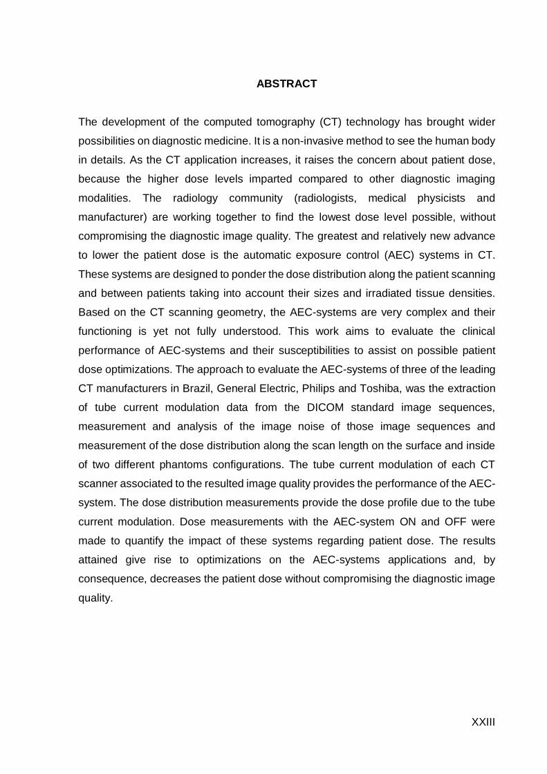
ABSTRACT

The development of the computed tomography (CT) technology has brought wider

possibilities on diagnostic medicine. It is a non-invasive method to see the human body

in details. As the CT application increases, it raises the concern about patient dose,

because the higher dose levels imparted compared to other diagnostic imaging

modalities. The radiology community (radiologists, medical physicists and

manufacturer) are working together to find the lowest dose level possible, without

compromising the diagnostic image quality. The greatest and relatively new advance

to lower the patient dose is the automatic exposure control (AEC) systems in CT.

These systems are designed to ponder the dose distribution along the patient scanning

and between patients taking into account their sizes and irradiated tissue densities.

Based on the CT scanning geometry, the AEC-systems are very complex and their

functioning is yet not fully understood. This work aims to evaluate the clinical

performance of AEC-systems and their susceptibilities to assist on possible patient

dose optimizations. The approach to evaluate the AEC-systems of three of the leading

CT manufacturers in Brazil, General Electric, Philips and Toshiba, was the extraction

of tube current modulation data from the DICOM standard image sequences,

measurement and analysis of the image noise of those image sequences and

measurement of the dose distribution along the scan length on the surface and inside

of two different phantoms configurations. The tube current modulation of each CT

scanner associated to the resulted image quality provides the performance of the AEC-

system. The dose distribution measurements provide the dose profile due to the tube

current modulation. Dose measurements with the AEC-system ON and OFF were

made to quantify the impact of these systems regarding patient dose. The results

attained give rise to optimizations on the AEC-systems applications and, by

consequence, decreases the patient dose without compromising the diagnostic image

quality.

XXIV

RESUMO

O desenvolvimento da tecnologia de tomografia computadorizada (TC) trouxe maiores

possibilidades em medicina diagnóstica. É um método não invasivo de se explorar o

corpo humano detalhadamente. Com o aumento das aplicações em TC, aumenta a

preocupação com as altas taxas de dose administradas quando comparada com

outras modalidades de diagnóstico por imagem. A comunidade científica e os

fabricantes uniram esforços para alcançar níveis menores de dose possíveis, sem

comprometer a qualidade da imagem diagnóstica. O maior e relativamente novo

avanço nessa busca para diminuir os níveis de dose é o controle automático de

exposição (CAE) em TC. Esses sistemas foram projetados para ponderar a

distribuição de dose ao longo do comprimento de varredura e entre pacientes, levando

em consideração o tamanho e as diferentes densidades de tecidos irradiados.

Baseando-se na geometria de aquisição em TC, os sistemas CAE são altamente

complexos. Sendo assim, sua forma de funcionamento ainda não é inteiramente

conhecida. O presente trabalho tem como objetivo avaliar o desempenho clínico dos

sistemas CAE, suas susceptibilidades ao usuário e, com isso, ajudar na otimização

de dose em pacientes. A abordagem utilizada para avaliar os sistemas CAE de três

dos maiores fabricantes de TC no Brasil, General Electric, Philips e Toshiba, foi pela

extração dos valores de corrente anódica do cabeçalho da sequência de imagens no

padrão DICOM, medição e análise do ruído das imagens dessas sequências e a

medição da distribuição da dose ao longo do comprimento de varredura nas

superfícies e dentro de dois simuladores de paciente de formatos diferentes. A

variação da corrente anódica de cada equipamento de TC associada à qualidade da

imagem resultante fornece o desempenho do sistema CAE. As medições de

distribuição de dose fornecem o perfil de dose resultante da modulação de corrente.

Medições com e sem o sistema CAE acionado foram feitas para quantificar a

importância em termos de dose desses sistemas. Os resultados obtidos permitem

otimizações no uso dos sistemas CAE e, consequentemente, a redução da dose no

paciente sem comprometer a qualidade diagnóstica da imagem.

25

1 INTRODUCTION

Computed tomography (CT) in diagnostic imaging is one of the most important

radiological imaging modalities worldwide[1]. In 2007, CT has contributed with 40% of

the worldwide collected dose but responded by only 7% of the medical procedures[2].

Despite the continuous effort in dose reduction, it is yet the diagnostic modality using

ionizing radiation that most contributes for the patient dose[3]. In addition, the rapid

evolution of CT technology has demanded development of new metrics capable to

supplement the patient dose analysis and then reduce it as low as reasonably

achievable (ALARA radioprotection principle) without compromising the diagnostic

image quality[4,5].

The advances in image acquisition are improving the image quality and same

efforts are done to reduce the patient dose. The wider collimations, for example, are

great advance in CT imaging that shortens the scan times; reducing the artifacts

caused by involuntary movement of the body and enables to reduce the exposure

parameters, that consequently decreases the patient dose[6,7].

Another great advance in CT technology are the automatic exposure control

(AEC) systems[8]. These systems allow not only to reduce the total scan dose, but also

ponder the dose distribution along the scan length, as the body has different sizes and

tissue densities. The AEC-systems have been on the market since 1994 when GE

made available the first tube current modulation system[9] and the CT manufacturers

developed this technology to improve the consistency of image quality and control the

absorbed dose[10]. Since the development of this exposure appliance, their functioning

is yet not fully understood.

The motivation of this work is to study the performance characteristics of CT

AEC systems using clinical routine protocols adopted in commercial CT equipment.

This aim was implemented by creating dosimetric experiments which allow verifying

their susceptibilities to the user-controlling parameters as a function of the behavior of

the current, dose and noise distributions along the z-axis of two different PMMA

phantoms.

The performance of the AEC-systems from

manufacturers in Brazil were tested using a well-established test device, the PMMA

conic elliptical phantom developed by the ImPACT scan group. It was also an

26

innovative imaging object design adopted for testing AEC response using three CTDI

phantoms assembled together, with different amount of material inside of each

phantom.

The X-ray tube current modulation was extracted from the DICOM header of the

image sequences for evaluating the AEC-system response. The DICOM (Digital

Imaging and Communications in Medicine) standard was created by the American

College of Radiology (ACR) and the American National Electrical Manufacturers

Association (NEMA) to promote communication and facilitate the archiving of the

information by the diagnostic imaging facilities and standardize the imaging data

regardless of device manufacturer[11]. The DICOM header storages the patient and

diagnostic facility information and the procedure data. These parameters used during

the CT patient exposure include pitch, collimation, table position, X-ray tube current,

current time product, rotation time, amongst others.

The image noise was adopted as the image quality parameter to compare the

AEC-

manufacturers. This image noise was adopted as the standard deviation of the pixel

values on a homogeneous section of the phantoms. The noise is directly related to

patient dose, since its decrease is associated to higher exposure techniques, which

means higher dose. A DICOM analyzer software was used (ImageJ®) to measure the

noise level of the image sequences.

Finally, the dose distribution along z-axis was measured for both phantoms

configurations. These measurements were made on the PMMA conic elliptical

phantom surface and inside the CTDI phantoms set using thermoluminescent

dosimeters. The dosimeters were calibrated using a pencil type ionization chamber.

The measurements were made in two busy imaging facilities: the Clinical

Octávio Frias de Oliveira. Both are public hospitals located in São Paulo, Brazil.

This work do not exhaust all the possible CT-AEC performance analysis, but it

introduces a practical methodology to evaluate the AEC response on clinical routine

protocols, associating it to the z-axis dose distribution, the X-ray tube current

ator susceptibilities. The results

achieved can assist on possible patient dose optimizations and improve the CT

scanners operation through training education.

27

The present work is divided in six chapters:

chapter 1 introduces the aim of this work;

chapter 2 presents the fundamentals on which this research was based;

chapter 3 presents all the instrumentation used in the data collection and

analysis, the CT scanners and AEC parameters evaluated and the conduct for

each essay;

chapter 4 presents the results achieved separated in different CT manufacturers

and their models, illustrating with charts and tables the data collection and its

analysis;

chapter 5 presents the results discussion separated by each manufacturer,

each parameter evaluated;

finally, chapter 6 presents a general discussion and future issues for the

automatic exposure control evaluation.

28

2 THEORY

Since Godfrey Newbold Hounsfield scanned the first tomographic acquisitions

using isotope sources[12] in 1969, only in phantoms by that time, the computed

tomography (CT) technology has improved relatively fast. In four decades, it went from

only head to whole body scanning; scan times flew from 35 minutes to fractions of

second; and the imaging reconstruction is not only much faster but it also has much

more diagnostic quality with matrices that were 80 x 80 pixels are now 512 x 512

pixels[13].

This evolution of the CT scanners is separated in generations[14]. The definitions

of these generations are not yet a consensus amongst all authors, in which some

separate it in four or five generations and other authors in up to seven generations,

considering each improvement of the CT technology a new generation by itself. The

CT historical generation definition, presented by Bushberg[15] was adopted in the

present work.

2.1 COMPUTED TOMOGRAPHY EVOLUTION

2.1.1 The first generationThe first generation of CT scanners was based on rotation and translation

movement of the X-ray tube and detector system (Figure 1). The X-ray beam was

extremely collimated; the so-called pencil-beam. The scanning had to be made with

the X-ray tube and detector system translating over the patient to reach an attenuation

profile, then rotate one degree and repeat the last steps up to complete 180 degrees.

2.1.2 The second generationThe second generation was based on the same acquisition geometry, but

instead of the highly collimated parallel X-ray beam it has a small fan beam, which

enable the number of detectors increase from one or two to even thirty detectors, which

reduces substantially the scanning time (Figure 2). The scan process was made in 180

degrees as in first generation and the detector set was parallel to the X-ray tube.

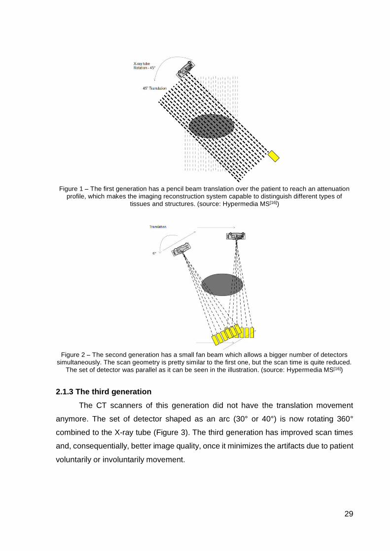
29

Figure 1 The first generation has a pencil beam translation over the patient to reach an attenuationprofile, which makes the imaging reconstruction system capable to distinguish different types of

tissues and structures. (source: Hypermedia MS[16])

Figure 2 The second generation has a small fan beam which allows a bigger number of detectorssimultaneously. The scan geometry is pretty similar to the first one, but the scan time is quite reduced.

The set of detector was parallel as it can be seen in the illustration. (source: Hypermedia MS[16])

2.1.3 The third generationThe CT scanners of this generation did not have the translation movement

anymore. The set of detector shaped as an arc (30° or 40°) is now rotating 360°

combined to the X-ray tube (Figure 3). The third generation has improved scan times

and, consequentially, better image quality, once it minimizes the artifacts due to patient

voluntarily or involuntarily movement.

30

Figure 3 The third generation has the X-ray tube and detectors system rotating without translatinganymore. The fan beam is larger and the detectors are disposed as an arc (30° or 40°). (source:

Hypermedia MS[16])

2.1.4 The fourth generationThis generation has a stationary ring of detectors encircling the patient in the

gantry. The X-ray tube rotates 360° and there are two different configuration of the

tube position depending on the manufacturer. One of them has the X-ray tube inside

the detectors ring and the fan beam incises on a small portion of detectors all over the

circle (Figure 4). The other eliminates the insecurity of the X-ray tube being so close

to the patient once it rotates outside the ring while the detector inclines. The cost of

having so many detectors was the major disadvantage of this generation.

2.1.5 The fifth generationThis generation was developed mostly for cardiac application. The so-called

Electron Beam CT (EBCT) is a stationary type of CT scanner, it means no mechanical

movement (Figure 5). Instead of a conventional X-ray tube, an electron beam is

deflected by magnetic field to strike tungsten arcs circling the patient producing X-

radiation. The photons cross the patient and reach the detectors on the opposite side

to the tungsten arcs. Since it has no mechanical restriction of movement, it can scan

the patient in 50 milliseconds resulting in high sample rates of heart beating. The

greatest disadvantage of this kind of CT scan is the need of larger rooms and the

limitation on image quality once the collimation is not practically possible resulting in

more scattered radiation.

31

Figure 4 The fourth generation has a stationary ring of detectors where only the X-ray tube rotates.(source: Hypermedia MS[16])

Figure 5 The Electron-Beam CT (EBCT) does not have X-ray tube, instead an electron beam isaccelerated and deflected to an arc of tungsten target that generated X-ray radiation and a stationary

arc of detectors at the opposite side of the target arc at the gantry. (source: Hypermedia MS[16])

2.1.6 The sixth generationThe development of the slip ring technology made possible the introduction of

the spiral or helical CT (Figure 6). Slip rings are electro-mechanic conductor dispositive

which er the rotation surface.

These devices made possible the system X-ray tube and detectors to rotate 360°

continuously, without the need of reverse the rotation due to the high voltage cables

as in first till the beginning of third generation.

Helical CT scan has combined the system X-ray tube-detectors movement with

the table translation creating a spiral exposure. This technology introduced many

different considerations in data acquisition. As the scanning is now helical, the raw

data has to be interpolated to reconstruct a planar section.

32

Figure 6 After the development of the slip-rings technology, the X-ray tube and detectors systemcould rotate continuously, allowing the helical or spiral CT scan. As the patient couch translates while

the tube is rotating 360°, the irradiation has a spiral form. (source: Hypermedia MS[16])

2.1.7 The seventh generationThe X-ray tube generates high heat in the X-radiation production, for this reason

radiological equipment need an adequate cooler system, especially CT scans because

the high energy X-ray beam and longer time exposure compared to conventional X-

ray exams. Furthermore, the detectors line limits the fan beam width, resulting in a

collimation that does not utilize a great portion of the X-ray produced.

The development of the multi-slice CT (MSCT) improved this concept[17], once

there are rows of detectors in z axis direction making possible to wider the fan beam,

the so-called cone beam CT (CBCT). At the opposite of single slice CT, the MSCT

does not lose spatial resolution or increase the noise with wider collimation, once

instead of a longer detector it has several solid state detectors combined

computationally. Another consequence is that the slice width is no longer limited to the

collimation aperture but to the detector size.

The detectors dimension is referenced to the isocenter of the gantry and by

software it combines the detectors row. For example a CT scan with 64 channels and

0.5 mm detectors can have the following combinations: 64 x 0.5 mm, 32 x 1.0 mm, 16

x 1.5 mm etc. One more parameter appears in this generation, the so-

the ratio of the table feed d to total collimation ,

resulting in a dimensionless quantity:

33

where N is the number of detectors and T is the detector width. For example, an 8-

slice CT scan (N = 8), with a nominal slice width of T = 1.25 mm and a table feed of

d = 5 mm per rotation has a pitch of p = 0.5. It means that the fan beam will irradiate

the same slice twice.

The MSCT is well established in the market and it has improved with the

development of the technology. Nowadays, there are many improvements like the

flying focal spot, that allows a 128 channels CT Scan to work as a 256 channels; the

dual energy that allows to distinguish different attenuation coefficient; the automatic

exposure control that allows the system to compensate the differences on body size

and density. The CT scanners can perform both axial and helical acquisitions. Biopsy

that requires no table movement (axial scan), for example, can be performed in CT

scanners with much more imaging precision. A dose reduction can be expected

combined to better image quality for the future.

2.2 COMPUTED TOMOGRAPHY SCANNERS

The CT scanners are composed, basically, by an X-ray tube and detectors

system that rotates around the patient couch which translates in the gantry central axis,

a high voltage generator, a computer system and a control panel.

2.2.1 X-ray tubeThe X-ray tube has a cathode and anode inside a vacuum glass enclosure that

provides an insulating medium between its electrodes. This glass is electric insulating

but does not fully avoid voltage arc formation. This issue can be deceased by metallic

covers where ceramic material insulates the cathode and the anode; these kinds of X-

ray tubes have larger anodes. X-ray tubes for diagnostic medicine are designed in two

types: stationary anode tube for low power applications and rotating anodes for high

performance applications[18].

New generations of CT scanners have rotating anodes due to the high

temperature achieved by the X-ray exposure with higher techniques to reach

diagnostic image quality. The helical procedures can work with exposure techniques

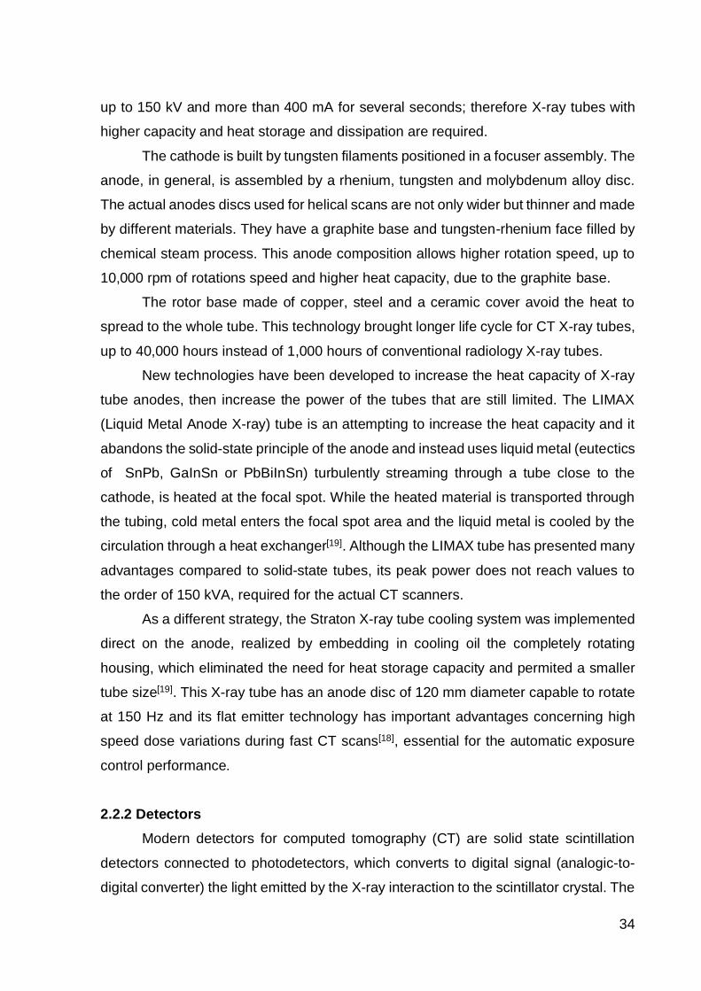
34

up to 150 kV and more than 400 mA for several seconds; therefore X-ray tubes with

higher capacity and heat storage and dissipation are required.

The cathode is built by tungsten filaments positioned in a focuser assembly. The

anode, in general, is assembled by a rhenium, tungsten and molybdenum alloy disc.

The actual anodes discs used for helical scans are not only wider but thinner and made

by different materials. They have a graphite base and tungsten-rhenium face filled by

chemical steam process. This anode composition allows higher rotation speed, up to

10,000 rpm of rotations speed and higher heat capacity, due to the graphite base.

The rotor base made of copper, steel and a ceramic cover avoid the heat to

spread to the whole tube. This technology brought longer life cycle for CT X-ray tubes,

up to 40,000 hours instead of 1,000 hours of conventional radiology X-ray tubes.

New technologies have been developed to increase the heat capacity of X-ray

tube anodes, then increase the power of the tubes that are still limited. The LIMAX

(Liquid Metal Anode X-ray) tube is an attempting to increase the heat capacity and it

abandons the solid-state principle of the anode and instead uses liquid metal (eutectics

of SnPb, GaInSn or PbBiInSn) turbulently streaming through a tube close to the

cathode, is heated at the focal spot. While the heated material is transported through

the tubing, cold metal enters the focal spot area and the liquid metal is cooled by the

circulation through a heat exchanger[19]. Although the LIMAX tube has presented many

advantages compared to solid-state tubes, its peak power does not reach values to

the order of 150 kVA, required for the actual CT scanners.

As a different strategy, the Straton X-ray tube cooling system was implemented

direct on the anode, realized by embedding in cooling oil the completely rotating

housing, which eliminated the need for heat storage capacity and permited a smaller

tube size[19]. This X-ray tube has an anode disc of 120 mm diameter capable to rotate

at 150 Hz and its flat emitter technology has important advantages concerning high

speed dose variations during fast CT scans[18], essential for the automatic exposure

control performance.

2.2.2 DetectorsModern detectors for computed tomography (CT) are solid state scintillation

detectors connected to photodetectors, which converts to digital signal (analogic-to-

digital converter) the light emitted by the X-ray interaction to the scintillator crystal. The

35

scintillation detectors material varies from detectors and they can be made of cadmium

telluride, sintered ceramic gadolinium oxysulfide and cesium iodide[12]. Theses

detectors must have very fast temporal response and the electronic noise must be

lower than half of the maximum quantum noise expected[12].

The scintillators have absorption efficiency between 65% and 85% due to their

high effective atomic number. However, the geometric efficiency is decreased by the

tiny spaces between the single detectors to reduce the crosstalk effect (photons from

adjacent areas).

The detectors size varies from manufacturers; some of them have hybrid

detector systems and they are combined to compose different detector sizes. Smaller

detectors together with short decay times improve the spatial resolution.

2.2.3 FiltersThe X-ray generated by the tube has continuous emitted spectra. It means that

the energy of the photons used in computed tomography range from 0 keV to 150 keV,

since the maximum tube voltage value of CT systems is 150 kV. This characteristic of

the X-ray spectrum is so-called polyenergetic or polychromatic, and it is a

consequence of the process of continuous loss of kinetic energy of the electrons inside

the anode (Bremsstrahlung). For radiological imaging, the X-ray beam must be as

closer as possible to a monochromatic beam, especially in CT imaging due to the

complex image reconstruction process. Filters are employed to absorb the lower

energies of the X-ray spectra. This process is called beam hardening and it results into

a more penetrating beam.

The filters used in CT X-ray equipment have a bow-tie shape due to the fan

beam profile. This filter is positioned in front of the X-ray tube exit window and before

the patient body. The beam is more intensely filtered by the border of the bow-tie filter

than by its central part in order to compensate the ellipsoidal shape of the human body

profile. The result is homogeneous photon fluency at the detectors, besides the

hardened beam (Figure 7).

36

Figure 7 The bowtie filter hardens the X-ray beam and its filtration is higher in the borders of thecone beam to compensate the thinner borders of the patient body.

2.2.4 GantryThe gantry is the main hardware structure of the CT scanner. Inside the gantry

are accommodated the X-ray emitting system (X-ray tube, collimator and filters), the

detector rolls and the electric system that supplies energy for the X-ray generation, for

the detection system, the cooling system, the rotation and table translation systems.

In modern CT scanners, the gantry are designed in order to minimize its size.

For exampl

249 cm long, including the patient couch and the gantry aperture of 70 cm.

The patient alignment in the gantry follows the schemes shown in Figure 8,

where x-y plane is called the axial plane, the x-z plane is called the coronal plane and

the y-x plane the sagittal plane. The patient couch translates along z-axis and the X-

ray tube rotates along x-y plane.

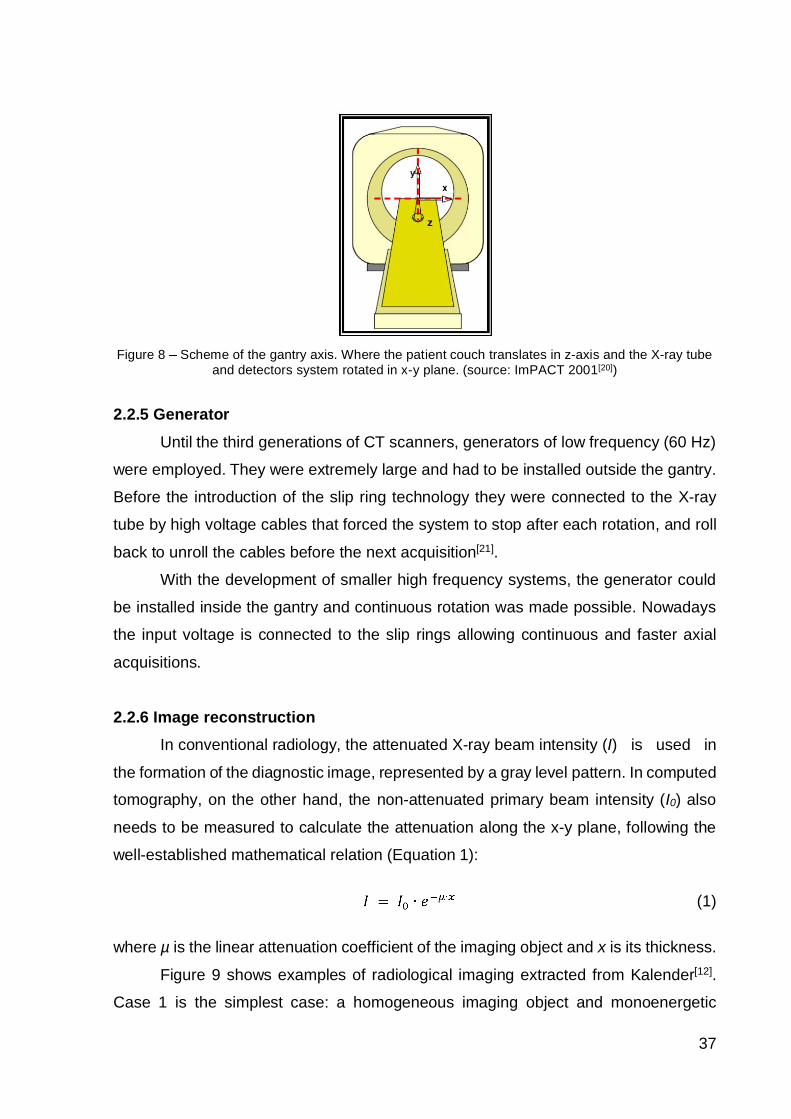
37

Figure 8 Scheme of the gantry axis. Where the patient couch translates in z-axis and the X-ray tubeand detectors system rotated in x-y plane. (source: ImPACT 2001[20])

2.2.5 GeneratorUntil the third generations of CT scanners, generators of low frequency (60 Hz)

were employed. They were extremely large and had to be installed outside the gantry.

Before the introduction of the slip ring technology they were connected to the X-ray

tube by high voltage cables that forced the system to stop after each rotation, and roll

back to unroll the cables before the next acquisition[21].

With the development of smaller high frequency systems, the generator could

be installed inside the gantry and continuous rotation was made possible. Nowadays

the input voltage is connected to the slip rings allowing continuous and faster axial

acquisitions.

2.2.6 Image reconstructionIn conventional radiology, the attenuated X-ray beam intensity (I) is used in

the formation of the diagnostic image, represented by a gray level pattern. In computed

tomography, on the other hand, the non-attenuated primary beam intensity (I0) also

needs to be measured to calculate the attenuation along the x-y plane, following the

well-established mathematical relation (Equation 1):

(1)

where µ is the linear attenuation coefficient of the imaging object and x is its thickness.

Figure 9 shows examples of radiological imaging extracted from Kalender[12].

Case 1 is the simplest case: a homogeneous imaging object and monoenergetic

38

radiation. In this case, the linear attenuation coefficient can be directly calculated by

the equation 1, and once the thickness x is known and the intensities I and I0 can be

measured. The attenuation distribution along the path though remains unknown.

Case 2 represents a simple inhomogeneous object reached by monoenergetic

radiation. In this case the total distribution along the radiation path depends on the

µi. Summation along the total path, using

small increments di must be implemented as the integral of all linear attenuation

coefficient along the path. Computed tomography consists in the exact measurement

of these linear integrals. In 1917, Radon showed that a two-dimensional distribution of

an object image can be determined by an infinite number of linear integrals[12,22]. A

finite number of measurements of the attenuation coefficient µ(x,y) distribution is

enough to compute an image with good approximation. A single projection (radiograph

measurement) does not allow to calculate µi in case 2 or any µ(x,y) distribution.

Case 3 represents a real and more complex case: an inhomogeneous imaging

object and polyenergetic radiation. It turns the radiation intensity quantity highly

dependent on the radiation energy I0(E) and, consequently, so is the attenuation

coefficient µ(E). In this case, the integral on energy along the radiation path must be

carried out first.

To apply the Radon theory and have a tomographic image in diagnostic quality,

multiple projections must be taken in multiple views, at least over 180°, as narrowly

spaced data points as possible. In early CT scanners, the X-ray beam was well

collimated pencil shaped and multiple projections had to be done. Nowadays the cone

beam cover a wider area at each projections and 360º scans are made, ending in much

better data sampling. The multislice CT scanners can measure up to 1500 projection

points and they vary between 600 and 1200 points per projection. The detectors

geometry (as an arc) also improves this data collection.

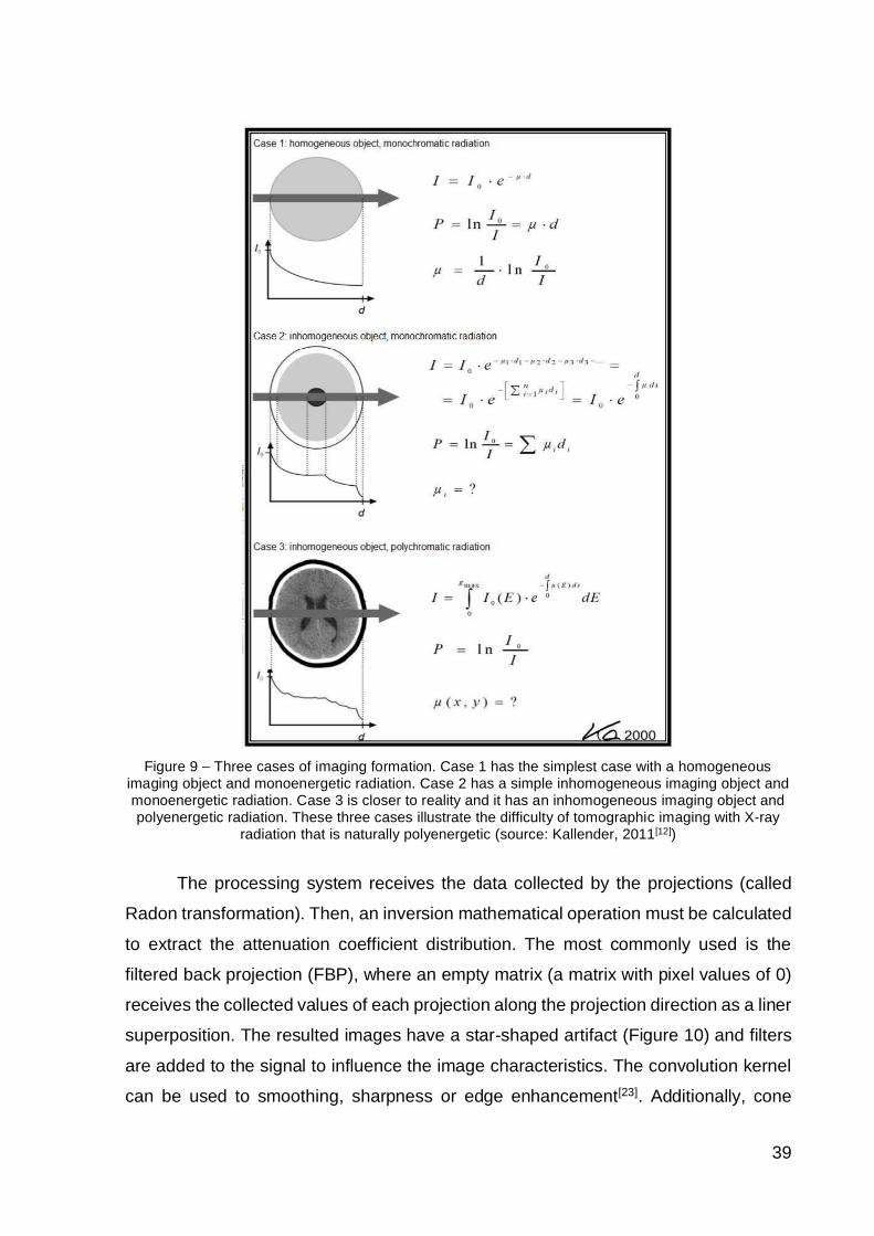
39

Figure 9 Three cases of imaging formation. Case 1 has the simplest case with a homogeneousimaging object and monoenergetic radiation. Case 2 has a simple inhomogeneous imaging object andmonoenergetic radiation. Case 3 is closer to reality and it has an inhomogeneous imaging object andpolyenergetic radiation. These three cases illustrate the difficulty of tomographic imaging with X-ray

radiation that is naturally polyenergetic (source: Kallender, 2011[12])

The processing system receives the data collected by the projections (called

Radon transformation). Then, an inversion mathematical operation must be calculated

to extract the attenuation coefficient distribution. The most commonly used is the

filtered back projection (FBP), where an empty matrix (a matrix with pixel values of 0)

receives the collected values of each projection along the projection direction as a liner

superposition. The resulted images have a star-shaped artifact (Figure 10) and filters

are added to the signal to influence the image characteristics. The convolution kernel

can be used to smoothing, sharpness or edge enhancement[23]. Additionally, cone

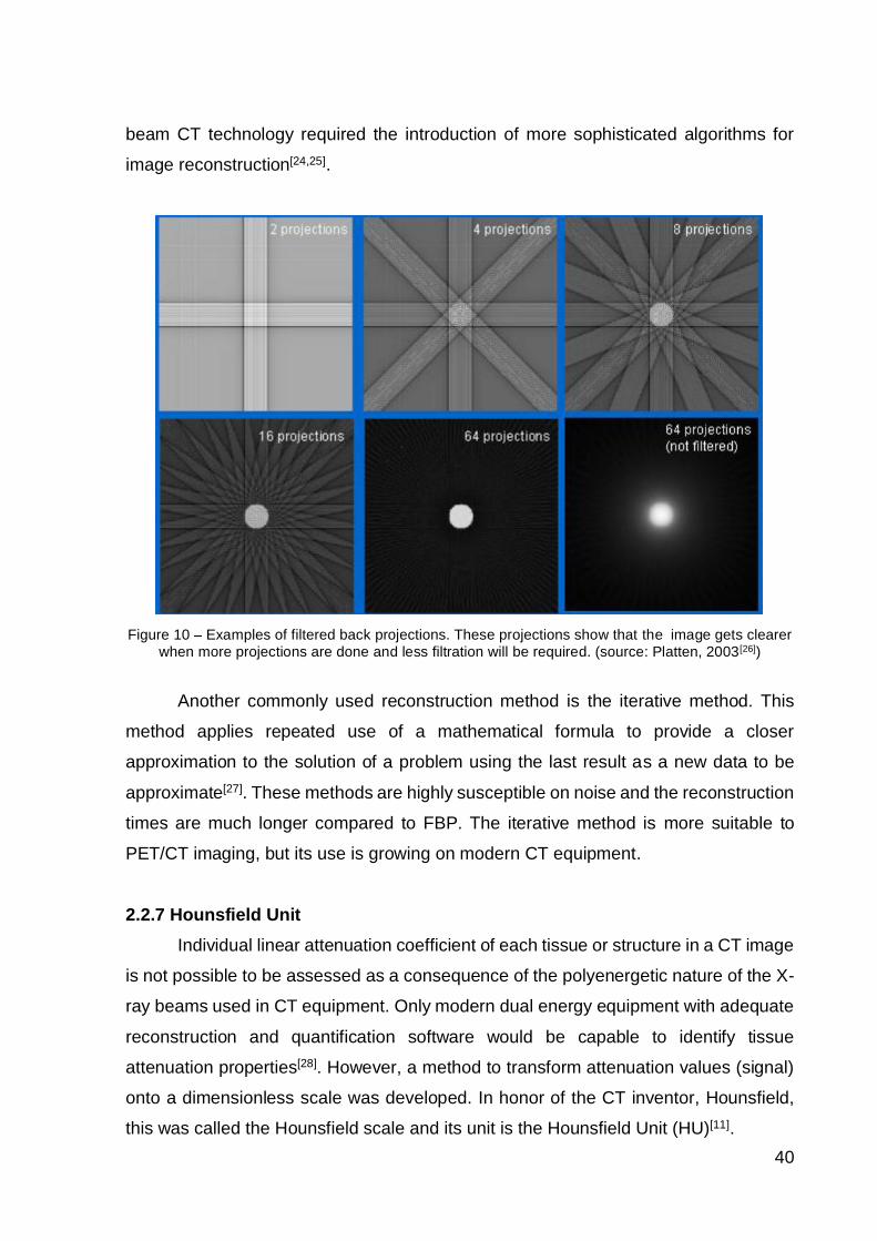
40

beam CT technology required the introduction of more sophisticated algorithms for

image reconstruction[24,25].

Figure 10 Examples of filtered back projections. These projections show that the image gets clearerwhen more projections are done and less filtration will be required. (source: Platten, 2003[26])

Another commonly used reconstruction method is the iterative method. This

method applies repeated use of a mathematical formula to provide a closer

approximation to the solution of a problem using the last result as a new data to be

approximate[27]. These methods are highly susceptible on noise and the reconstruction

times are much longer compared to FBP. The iterative method is more suitable to

PET/CT imaging, but its use is growing on modern CT equipment.

2.2.7 Hounsfield UnitIndividual linear attenuation coefficient of each tissue or structure in a CT image

is not possible to be assessed as a consequence of the polyenergetic nature of the X-

ray beams used in CT equipment. Only modern dual energy equipment with adequate

reconstruction and quantification software would be capable to identify tissue

attenuation properties[28]. However, a method to transform attenuation values (signal)

onto a dimensionless scale was developed. In honor of the CT inventor, Hounsfield,

this was called the Hounsfield scale and its unit is the Hounsfield Unit (HU)[11].

41

The Hounsfield scale is defined by the attenuation of water. The so-

nu 2 presents the CT number (CTN)

in HU:

(2)

where µ is the linear attenuation coefficient of an irradiated imaging object and µwater is

the linear attenuation coefficient of the water. These attenuation coefficients are

considered to have been estimated at the effective energy of the X-ray spectrum.

2.3 AUTOMATIC EXPOSURE CONTROL

The continuous effort to follow the ALARA principle regarding patient dose and

still provide a diagnostic image quality is the main motivation for the development of

automatic exposure control systems (AEC). These AEC-systems are set to find ideal

X-ray exposure parameters for a patient exam to reach the best signal to noise ratio

into the imaging receptor, regardless tissue density, or body thickness. Depending on

the radiology modality, i.e., X-ray tube and detectors set, these AEC-systems respond

differently and that is discussed in the following sections[29].

2.3.1 Automatic exposure control in general radiologyThe automatic exposure control (AEC) system in conventional radiology is

generally preprogramed by the manufacturer in order to the X-ray exposure match the

image receptor system response. This previous calibration is done using ionization

chambers and phantoms. In the past, these receptor systems were called photo-timer

and they worked with photo-multiplying devices instead of ionization chamber,

scintillators or solid state-detectors that are in use nowadays. These AEC-systems

turns off the X-ray exposure as the image receptors has received the proper amount

of radiation, i.e. enough number of photons for diagnostic image quality[30].The image

receptor is located before the imaging system (film, CR, DR etc.) and they have, in

general, three to five photocells placed in the middle of the bucky (Figure 11). They

can be combined or used separately.

The AEC-system can also be programmed to pre-expose the patient with a

preprogramed technique and based on the attenuation it selects a technique. In digital

mammography the equipment selects automatically voltage and current-time product,

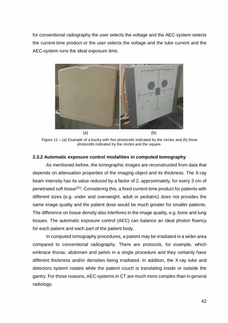
42

for conventional radiography the user selects the voltage and the AEC-system selects

the current-time product or the user selects the voltage and the tube current and the

AEC-system runs the ideal exposure time.

(a) (b)Figure 11 (a) Example of a bucky with five photocells indicated by the circles and (b) three

photocells indicated by the circles and the square.

2.3.2 Automatic exposure control modalities in computed tomographyAs mentioned before, the tomographic images are reconstructed from data that

depends on attenuation properties of the imaging object and its thickness. The X-ray

beam intensity has its value reduced by a factor of 2, approximately, for every 3 cm of

penetrated soft tissue[31]. Considering this, a fixed current-time product for patients with

different sizes (e.g. under and overweight, adult or pediatric) does not provides the

same image quality and the patient dose would be much greater for smaller patients.

The difference on tissue density also interferes in the image quality, e.g. bone and lung

tissues. The automatic exposure control (AEC) can balance an ideal photon fluency

for each patient and each part of the patient body.

In computed tomography procedures, a patient may be irradiated in a wider area

compared to conventional radiography. There are protocols, for example, which

embrace thorax, abdomen and pelvis in a single procedure and they certainly have

different thickness and/or densities being irradiated. In addition, the X-ray tube and

detectors system rotates while the patient couch is translating inside or outside the

gantry. For those reasons, AEC-systems in CT are much more complex than in general

radiology.

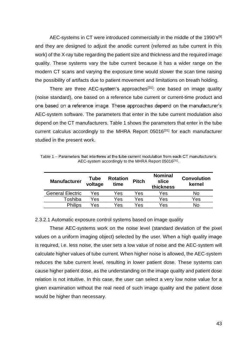
43

AEC-systems in CT were introduced commercially in the middle of the 1990 [9]

and they are designed to adjust the anodic current (referred as tube current in this

work) of the X-ray tube regarding the patient size and thickness and the required image

quality. These systems vary the tube current because it has a wider range on the

modern CT scans and varying the exposure time would slower the scan time raising

the possibility of artifacts due to patient movement and limitations on breath holding.

There are three AEC- approaches[31]: one based on image quality

(noise standard), one based on a reference tube current or current-time product and

AEC-system software. The parameters that enter in the tube current modulation also

depend on the CT manufacturers. Table 1 shows the parameters that enter in the tube

current calculus accordingly to the MHRA Report 05016[31] for each manufacturer

studied in the present work.

Table 1AEC-system accordingly to the MHRA Report 05016[31].

Manufacturer Tubevoltage

Rotationtime Pitch

Nominalslice

thicknessConvolution

kernel

General Electric Yes Yes Yes Yes NoToshiba Yes Yes Yes Yes Yes

Philips Yes Yes Yes Yes No

2.3.2.1 Automatic exposure control systems based on image quality

These AEC-systems work on the noise level (standard deviation of the pixel

values on a uniform imaging object) selected by the user. When a high quality image

is required, i.e. less noise, the user sets a low value of noise and the AEC-system will

calculate higher values of tube current. When higher noise is allowed, the AEC-system

reduces the tube current level, resulting in lower patient dose. These systems can

cause higher patient dose, as the understanding on the image quality and patient dose

relation is not intuitive. In this case, the user can select a very low noise value for a

given examination without the real need of such image quality and the patient dose

would be higher than necessary.

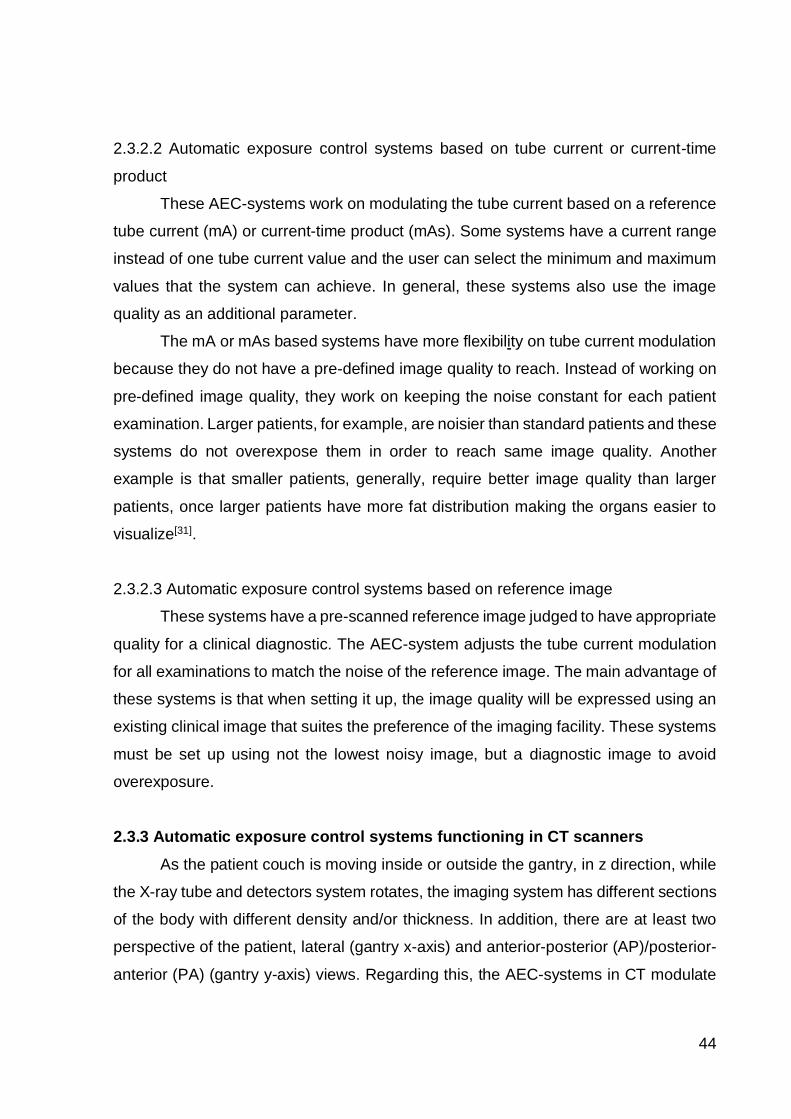
44

2.3.2.2 Automatic exposure control systems based on tube current or current-time

product

These AEC-systems work on modulating the tube current based on a reference

tube current (mA) or current-time product (mAs). Some systems have a current range

instead of one tube current value and the user can select the minimum and maximum

values that the system can achieve. In general, these systems also use the image

quality as an additional parameter.

The mA or mAs based systems have more flexibility on tube current modulation

because they do not have a pre-defined image quality to reach. Instead of working on

pre-defined image quality, they work on keeping the noise constant for each patient

examination. Larger patients, for example, are noisier than standard patients and these

systems do not overexpose them in order to reach same image quality. Another

example is that smaller patients, generally, require better image quality than larger

patients, once larger patients have more fat distribution making the organs easier to

visualize[31].

2.3.2.3 Automatic exposure control systems based on reference image

These systems have a pre-scanned reference image judged to have appropriate

quality for a clinical diagnostic. The AEC-system adjusts the tube current modulation

for all examinations to match the noise of the reference image. The main advantage of

these systems is that when setting it up, the image quality will be expressed using an

existing clinical image that suites the preference of the imaging facility. These systems

must be set up using not the lowest noisy image, but a diagnostic image to avoid

overexposure.

2.3.3 Automatic exposure control systems functioning in CT scannersAs the patient couch is moving inside or outside the gantry, in z direction, while

the X-ray tube and detectors system rotates, the imaging system has different sections

of the body with different density and/or thickness. In addition, there are at least two

perspective of the patient, lateral (gantry x-axis) and anterior-posterior (AP)/posterior-

anterior (PA) (gantry y-axis) views. Regarding this, the AEC-systems in CT modulate

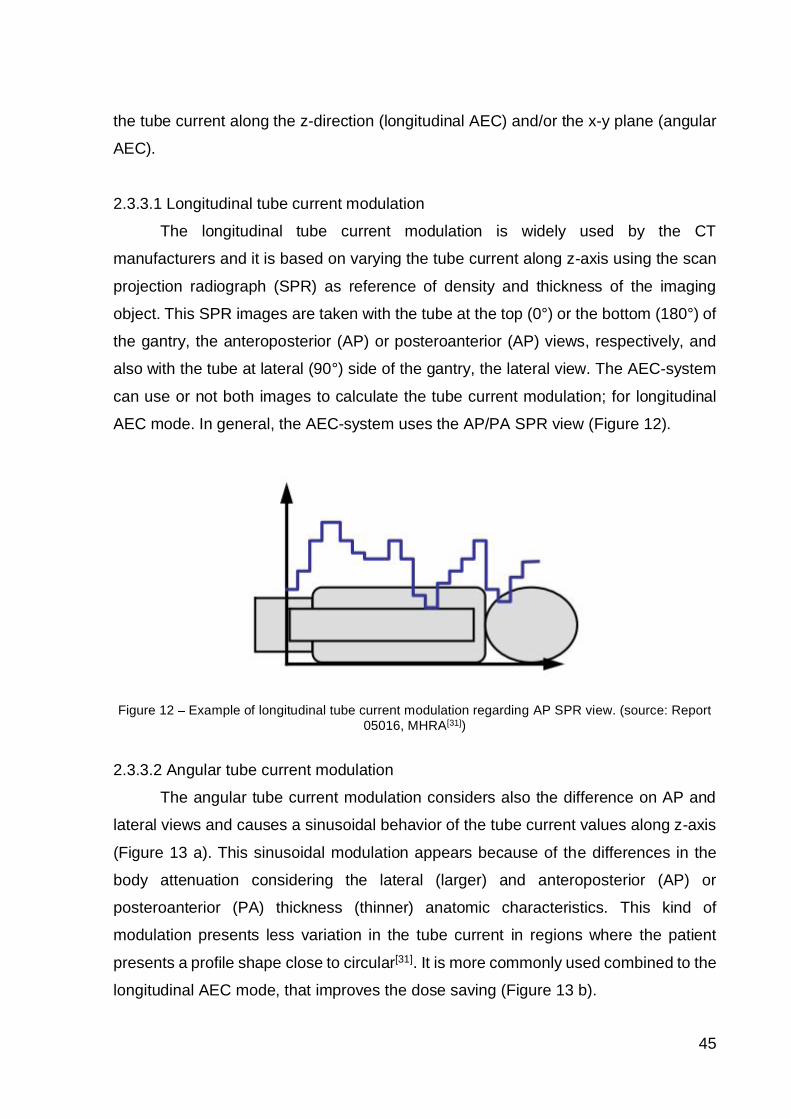
45

the tube current along the z-direction (longitudinal AEC) and/or the x-y plane (angular

AEC).

2.3.3.1 Longitudinal tube current modulation

The longitudinal tube current modulation is widely used by the CT

manufacturers and it is based on varying the tube current along z-axis using the scan

projection radiograph (SPR) as reference of density and thickness of the imaging

object. This SPR images are taken with the tube at the top (0°) or the bottom (180°) of

the gantry, the anteroposterior (AP) or posteroanterior (AP) views, respectively, and

also with the tube at lateral (90°) side of the gantry, the lateral view. The AEC-system

can use or not both images to calculate the tube current modulation; for longitudinal

AEC mode. In general, the AEC-system uses the AP/PA SPR view (Figure 12).

Figure 12 Example of longitudinal tube current modulation regarding AP SPR view. (source: Report05016, MHRA[31])

2.3.3.2 Angular tube current modulation

The angular tube current modulation considers also the difference on AP and

lateral views and causes a sinusoidal behavior of the tube current values along z-axis

(Figure 13 a). This sinusoidal modulation appears because of the differences in the

body attenuation considering the lateral (larger) and anteroposterior (AP) or

posteroanterior (PA) thickness (thinner) anatomic characteristics. This kind of

modulation presents less variation in the tube current in regions where the patient

presents a profile shape close to circular[31]. It is more commonly used combined to the

longitudinal AEC mode, that improves the dose saving (Figure 13 b).

46

(a) (b)Figure 13 (a) Angular tube current modulation and (b) angular combined to longitudinal tube current

modulation. (source: Report 05016, MHRA[31])

2.4 COMPUTED TOMOGRAPHY DOSIMETRY

The computed tomography (CT) dosimetry has the primary dose measurement

concept based on the computed tomography dose index (CTDI)[32]. This quantity

represents the average absorbed dose from a series of contiguous irradiations along

z-axis[33,34]. The measurement geometry is an axial scan protocol, with a water or

PMMA cylindrical phantom in the gantry central axis, using a pencil type ionization

chamber inside the phantom, and its calculation follows the Equation 3:

, (3)

where N is the number of detectors rows, T is the detectors width, NT is the collimation

width and D(z) is the dose profile along z axis.

Currently, the measured and calculated quantity is the CTDI100 which is the

integration of the dose profile along 100 mm which is the length of the most common

commercial pencil type ionization chamber and the limits of the integral would be ± 50

mm. The CTDI100 is calculated, considering that the ionization chamber reading is not

directly the integral of dose along z-axis, using the Equation 4:

, (4)

where the RIC represents the ionization chamber reading, the fcalib a calibration factor

of the reading in kerma units (mGy in this case) and 100 mm is the length of the integral

along z-axis.

Another quantity to consider is the weighted CTDI (CTDIw). This quantity

considers the variation of the CTDI100 across the field of measurement, the field of view

47

(FOV). For body CTDI100 measurement, for example, the CTDI100 measured at the

center of the phantom (CTDI100c) is about half value of the CTDI100 measured at the

peripheries of the phantom (CTDI100p). And the average of these CTDI100 is weighted

by Equation 5:

. (5)

For the helical CT scans the pitch value must be considered, once it defines the

gaps or overlaps that the scan will have. The quantity that appraises this characteristic

of a scan protocol is the volume CTDI (CTDIvol), given by Equation 6:

. (6)

The CT scanner presents the CTDIvol for the user as an indicative of patient

dose[35]. When axial scans are made, the CTDIvol is equal in value to CTDIw as the

acquisition had pitch value of 1. Another quantity displayed by the CT scanner is the

dose-length product (DLP). This quantity considers the whole scan length and it is

given by Equation 7:

. (7)

These CT dosimetric quantities are well established. However the advance on

CT technology has brought the need of different metrics of measurements[36]. The cone

beam CT and a high advanced detection set made possible to use wider collimation to

image a wider area at once and shorten the scan time, which improved especially the

cardiac CT imaging[37,38]. The new metrics of CT dosimetry has been developed and

the American Association of Physicists in Medicine (AAPM) published the Report

111[39,40] with a guide for this new measurement paradigm for wider collimation and

helical scans[41]. Other new recommendations were introduced by the Institute of

Physics and Engineering in Medicine (IPEM)[42] in United Kingdom.

48

3 METHODS AND MATERIALS

3.1 CLINICAL ROUTINE DATABASE

A data collection encompassing CT procedures using AEC protocols over the

total CT examinations accomplished in 2012 in two busy imaging diagnostic facilities

was done in order to quantify the AEC-system usage in these institutions. This data

collection was done by a searching routine on PACS/RIS (Picture Archiving and

Communication System/Radiology Information S

Institute of Radiology and the Cancer Institute of the State of São Paulo Octávio Frias

de Oliveira. This searching routine provided the total number of patients, their gender,

age, number of examinations, clinical imaging protocol, and the CT scanner used for

conducting the procedure.

This information was important to identify the frequency of use of AEC-systems

in the CT scanners from these imaging facilities. It was observed that equipment mainly

dedicated to head and pediatric protocols utilize, in most of the cases, constant tube

current. In these cases, an evaluation on those equipment as proposed in the present

work is meaningless.

3.2 COMPUTED TOMOGRAPHY SCANNERS

Computed tomography equipment of three leading manufacturers in Brazil were

evaluated in the present work: General Electric (GE), Philips and Toshiba.

3.2.1 General Electric CT scannerThree models of General Electric (GE) CT scanners were tested: Discovery 750

HD, PET/CT Discovery 690, both with 64 channels and a LightSpeed Ultra with

8 channels. The first two CT scanners have the longitudinal (Auto mA) and longitudinal

combined to angular (Auto + Smart mA) AEC modes. The last one has only longitudinal

AEC mode. The GE CT scanners AEC-system modulates the tube current based on

the scan projection radiograph (SPR) and they work

on the image noise required by the user. The parameters that can be selected for the

tube current modulation operation are listed in Table 2.

49

Table 2 Parameters available for the GE CT scanners AEC-system.

AEC parameters for GE CT scannersLongitudinal tube

current modulation Auto mA

Angular tubecurrent modulation

Auto + Smart mA (only combinedto longitudinal mode)

Image qualityreference

The noise level of the imagesequence will be the similar of theselected Noise Index with the

[31]

Current rangeMinimum and maximumachievable for the X-ray tubecurrent

Dose stepsThis parameter is inverselyassociated to the Noise Indexvalue

3.2.2 Philips CT scannerFour models of Philips CT scanners where tested: two Brilliance 16 with 16

channels, one Brilliance 40 with 40 channels, one Brilliance 64 with 64 channels and

one Brilliance iCT with 128 channels and flying focal spot technology (i.e. it can

produce up to 256 images as if it had 256 channels).

-systems, named DoseRight, also relies for the

tube current modulation on the SPR name . Philips

designed first the angular AEC mode, DoseRight DOM (Dose Modulation) or just D-

DOM, and the DoseRight ACS (automatic current selection) option to work together.

The longitudinal AEC mode, Z-DOM, was designed later and both AEC modes do not

work together. Philips AEC-systems work using a reference image[31]. The operational

parameters of Phi -system are listed in Table 3.

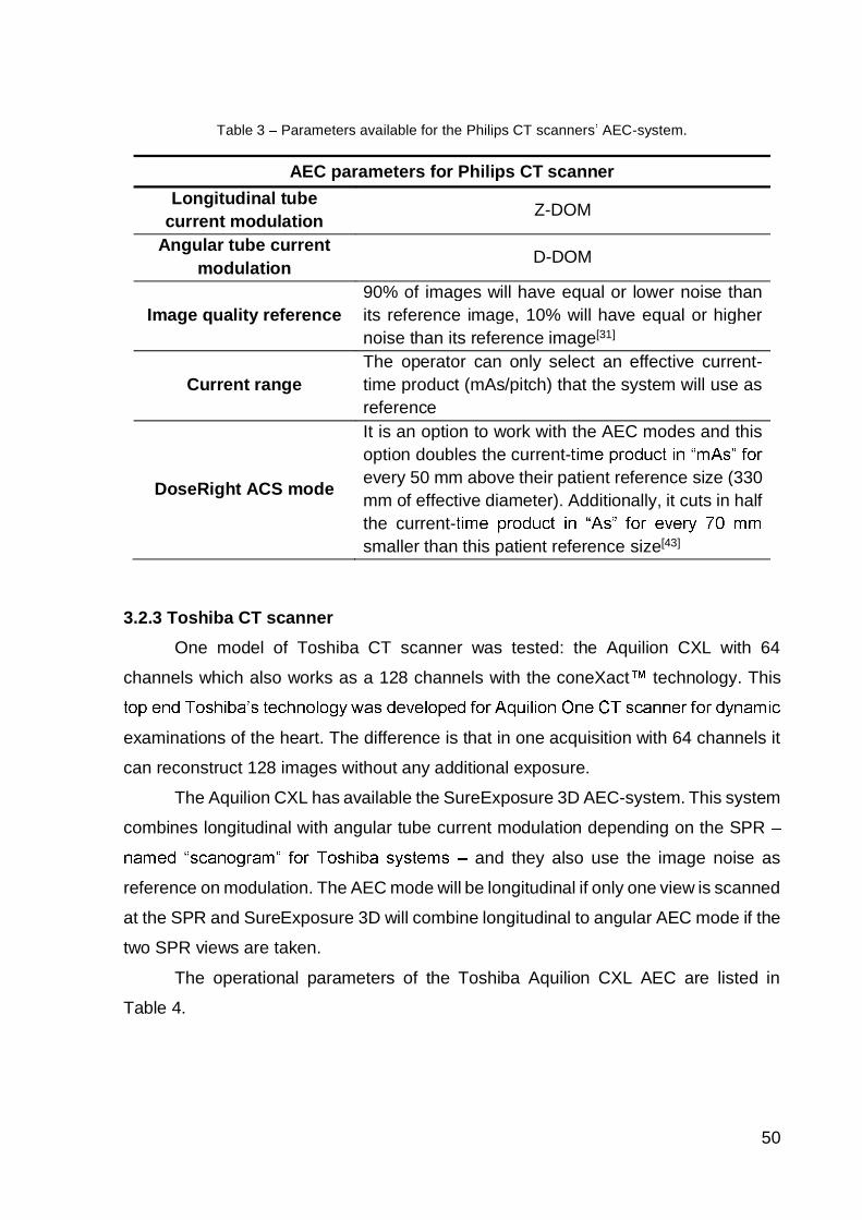
50

Table 3 Parameters available for the Philips CT scanners AEC-system.

AEC parameters for Philips CT scannerLongitudinal tube

current modulation Z-DOM

Angular tube currentmodulation D-DOM

Image quality reference90% of images will have equal or lower noise thanits reference image, 10% will have equal or highernoise than its reference image[31]

Current rangeThe operator can only select an effective current-time product (mAs/pitch) that the system will use asreference

DoseRight ACS mode

It is an option to work with the AEC modes and thisoption doubles the current-every 50 mm above their patient reference size (330mm of effective diameter). Additionally, it cuts in halfthe current-smaller than this patient reference size[43]

3.2.3 Toshiba CT scannerOne model of Toshiba CT scanner was tested: the Aquilion CXL with 64

channels which also works as a 128 channels with the coneXact technology. This

examinations of the heart. The difference is that in one acquisition with 64 channels it

can reconstruct 128 images without any additional exposure.

The Aquilion CXL has available the SureExposure 3D AEC-system. This system

combines longitudinal with angular tube current modulation depending on the SPR

and they also use the image noise as

reference on modulation. The AEC mode will be longitudinal if only one view is scanned

at the SPR and SureExposure 3D will combine longitudinal to angular AEC mode if the

two SPR views are taken.

The operational parameters of the Toshiba Aquilion CXL AEC are listed in

Table 4.

51

Table 4 Parameters available for the Toshiba CT scanners AEC-system.

AEC parameters for Toshiba CT scannerLongitudinal tube

current modulation SureExposure

Angular tubecurrent modulation

SureExposure 3D Itappears as an X-Y checkbutton available only whenthe double SPR is made

Image qualityreference

Standard Deviation, LowDose, High Quality orStandard

Current range

The operator can select theminimum and maximum tubecurrent values achievable bytube current modulation

Reconstruction slicethickness

The tube current modulationvaries when the nominal slicethickness for the firstreconstruction is changed,other parameters alsochanges automatically.

3.3 EVALUATION OF THE AUTOMATIC EXPOSURE CONTROL SYSTEMS

The evaluation of CT scanners AEC-systems performance was done by

acquiring image sequences on two PMMA phantoms (TAP and ImPACT phantoms),

which are described in this chapter. These phantoms were specially designed in order

to induce the variation of the tube current along the z-axis of the CT systems and,

consequently, the X-ray photon fluency in the same direction.

The evaluation of the CT scanners AEC-systems was done using two

methodologies. First, the tube current data were extracted from the DICOM header of

each image sequence. Considering the fact that the tube current data is not

available or easily measurable, the information extracted from the DICOM header is

the most accurate X-ray tube current data accessible. The second step was the

evaluation of the dose distributions in z-axis inside and in the surface of the TAP and

the ImPACT phantoms, respectively.

3.3.1 ImPACT PhantomThe Medicine and Healthcare products Regulatory Agency (MHRA) from United

Kingdom proposed a phantom designed for testing AEC- 05016:

52

[31]. This technical document was

developed by ImPACT CT scanner evaluation group[44]. A homemade version of the

hereafter called ImPACT Phantom was manufactured by the team of the Radiation

Dosimetry and Medical Physics Laboratory of the Physics Institute from University of

São Paulo. This PMMA elliptical cone shaped phantom, 300 mm long is a

homogeneous body with different thickness along the z-axis (Figure 14) which assess

aspects of AEC performance, such as the difference on the X-ray attenuation in AP or

lateral incidence of the beam (Figure 16)[31], and the influence of the effective diameter

of the body.

The phantom is fixed in the Catphan® Phantom (The Phantom Laboratory,

USA) wooden carrying case, which is used as a balance weighted structure. Using this

configuration, it is possible to scan the ImPACT Phantom off the patient couch, i.e. in

the air (Figure 14 and Figure 15).

Figure 14 The ImPACT Phantom designed to evaluate the AEC-systems functioning. It ishomogeneous, manufactured from acrylic, 300 mm long and it is elliptical-cone shaped with the major

effective diameter of 350 mm and the minor 50 mm. (source: Report 05016 [31])

53

Figure 15 Picture of the homemade ImPACT Phantom affixed at the Catphan®carrying case with Catphan® as counterweight.

(a) (b)Figure 16 (a) ImPACT Phantom simulates the difference of AP and lateral view thickness and (b) the

X-ray tube current has a sinusoidal variation.

3.3.2 CTDI Phantoms-system modulates the X-ray

tube current based on the differences at the thickness and the density of the imaging

object. In this case, density means the amount of material of an imaging object with a

given diameter intercepting the X-ray beam.

However, by the design of the ImPACT Phantom, this device can assess only

the response of the AEC-system in terms of the thickness of the imaging object. Hence,

a way to appraise the opposite of that is to have a phantom with uniform diameter and

a variable amount of material inside it along the z-axis. A phantom designed with these

54

characteristics would be able to simulate a variation on density of an imaging object

with constant diameter. This variation must cause different attenuation by the object

on the scan projection radiograph, and consequently different tube current values on

the CT scanning.

Standard PMMA Computed Tomography Dose Index (CTDI) phantoms were

designed by the team of the Radiation Dosimetry and Medical Physics Laboratory of

the Physics Institute from University of São Paulo as a 150 mm thick cylinder PMMA

phantom, composed by two different diameters cylindrical shells and one solid cylinder

nested inside each other (Figure 17). The major cylindrical shell has 320 mm external

diameter, the intermediate cylindrical shell has 160 mm external diameter and the

minor cylinder is a solid block with 100 mm diameter. They are designed to represent

the approximate attenuation conditions for an adult body, adult head/pediatric body

and a pediatric head in CT examinations, respectively[45]. These phantoms are

routinely used during the application of Quality Assurance program by the Radiation

Dosimetry and Medical Physics Laboratory on the CT equipment of the imaging

facilities where all experiments of the present work were done.

Figure 17 Scheme of the CTDI Phantom with the minor diameter part that simulates pediatric headat the top, in the middle the intermediate part that simulates adult head and at bottom the major

diameter that simulates adult abdomen and thorax when full filled.

A set of three adjacent PMMA CTDI phantoms configuration, hereafter called

TAP (as an acronym of Three Adjacent Phantoms) phantom, was designed for the

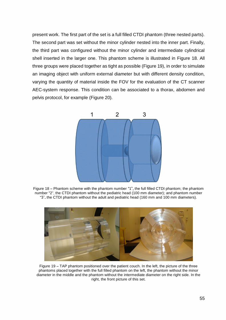
55

present work. The first part of the set is a full filled CTDI phantom (three nested parts).

The second part was set without the minor cylinder nested into the inner part. Finally,

the third part was configured without the minor cylinder and intermediate cylindrical

shell inserted in the larger one. This phantom scheme is illustrated in Figure 18. All

three groups were placed together as tight as possible (Figure 19), in order to simulate

an imaging object with uniform external diameter but with different density condition,

varying the quantity of material inside the FOV for the evaluation of the CT scanner

AEC-system response. This condition can be associated to a thorax, abdomen and

pelvis protocol, for example (Figure 20).

Figure 18 Phantom scheme with the phantom number 1 the full filled CTDI phantom; the phantomnumber 2 the CTDI phantom without the pediatric head (100 mm diameter); and phantom number

the CTDI phantom without the adult and pediatric head (160 mm and 100 mm diameters).

Figure 19 TAP phantom positioned over the patient couch. In the left, the picture of the threephantoms placed together with the full filled phantom on the left, the phantom without the minor

diameter in the middle and the phantom without the intermediate diameter on the right side. In theright, the front picture of this set.

56

Figure 20 The figure presents the tube current modulation behavior for a thorax, abdomen and pelvisscanning. In analogy, the same behavior is expected tube current modulation for the TAP phantom,three tube current values with the highest value at the full filled phantom and the lowest

value at the one without the intermediate diameter phantom .

3.3.3 Extraction of X-ray tube current data from DICOM headerThe X-ray tube current data was extracted from the DICOM header of the image

sequence resulted from each scanning of the ImPACT and the TAP phantoms.

Whenever possible, the scanning protocols on each study had the same operational

parameters to enable comparison. Some parameters had to be different because of

CT scanner limitations or, deliberately, in order to study the susceptibility of the AEC-

system.

The data extractor used was ImageJ®[46] Scan Header[47]. The

data analysis was made using spreadsheets developed in Microsoft® Excel.

3.3.3.1 Scanning protocol

The protocol selected for each This

protocol was chosen considering that abdomen protocols commonly use AEC instead

of constant X-ray tube current. In addition, the parameters listed in Table 5 where kept

the same whenever possible.

57

Table 5 General scanning protocol parameters selected for the evaluation of the AEC-systems.

3.3.3.2 Software analysis

The ImageJ® software was applied to extract the DICOM header information of

X-ray tube current and slice location from the image database resulting from the CT

scans. The ImageJ® is a free software developed by the Medical Imaging Group of the

Department of Physics of the Alma Mater Studiorum, University of Bologna[47] that can

be used to explore DICOM standard images. This software also enables the user to

kinds of analysis of these images patterns.

The plugin used for extracting the DICOM header information was

®

information from an image sequence based on the DICOM tag typed by the user

(Figure 21

Manufacturers Association (NEMA)[11]. The tags for slice location and X-ray tube

current are, respectively: 0020,1041 and 0018,115. The resulted information (Figure

22) was transcribed to a text document file.

Parameter ValueVoltage (kV) 120

Rotation time (s) 1Display FOV (mm) 500

Pitch range of 0.75 and 1.5Nominal slice thickness (mm) 3 or 5

Increment (mm) 3 or 5

58

Figure 21 Lused totext document file with the DICOM tags and load it to the Scan Header plugin instead of typing each

file withthe DICOM tags from the typed num the DICOM tags typed. At last, in

the bottom,

Figure 22 The data extracted from the DICOM header is presented in an additional box and the usercan select the whole data, copy and paste to a text document file to be processed by another

software.

3.3.3.3 Developed spreadsheet

The DICOM header data and the noise level information acquired with ImageJ®

were saved in text document files and organized in spreadsheets on Microsoft® Excel

59

tables. This software allows to separate the information included on the text document

files in columns as it is imported.

The studies made at each CT scanner were separated in tabs and graphics of

X-ray tube current values per table position or noise per table position were plotted

with the image of the phantom scan projection radiograph as background for better

comprehension (Figure 23 and Figure 24).

(a) (b)Figure 23 (a) SPR of the ImPACT Phantom, and (b) superposition of the SPR of the ImPACT

Phantom and X-ray tube current data. The graphics were plotted with the scan projection radiographof the ImPACT Phantom as background for better comprehension of the X-ray tube current behavior.

(a) (b)Figure 24 (a) SPR of the TAP phantom and (b) the graphics were plotted with the scan projectionradiograph of the TAP phantom as background for better comprehension of the X-ray tube current

behavior.

3.3.4 Evaluation of the z-axis dose distributionThermoluminescent dosimeters (TLDs) were used for the evaluation of z-axis

dose distributions associated to the variation of X-ray tube current modulation and

noise levels in the phantoms adopted in the present work. These TLDs were prepared

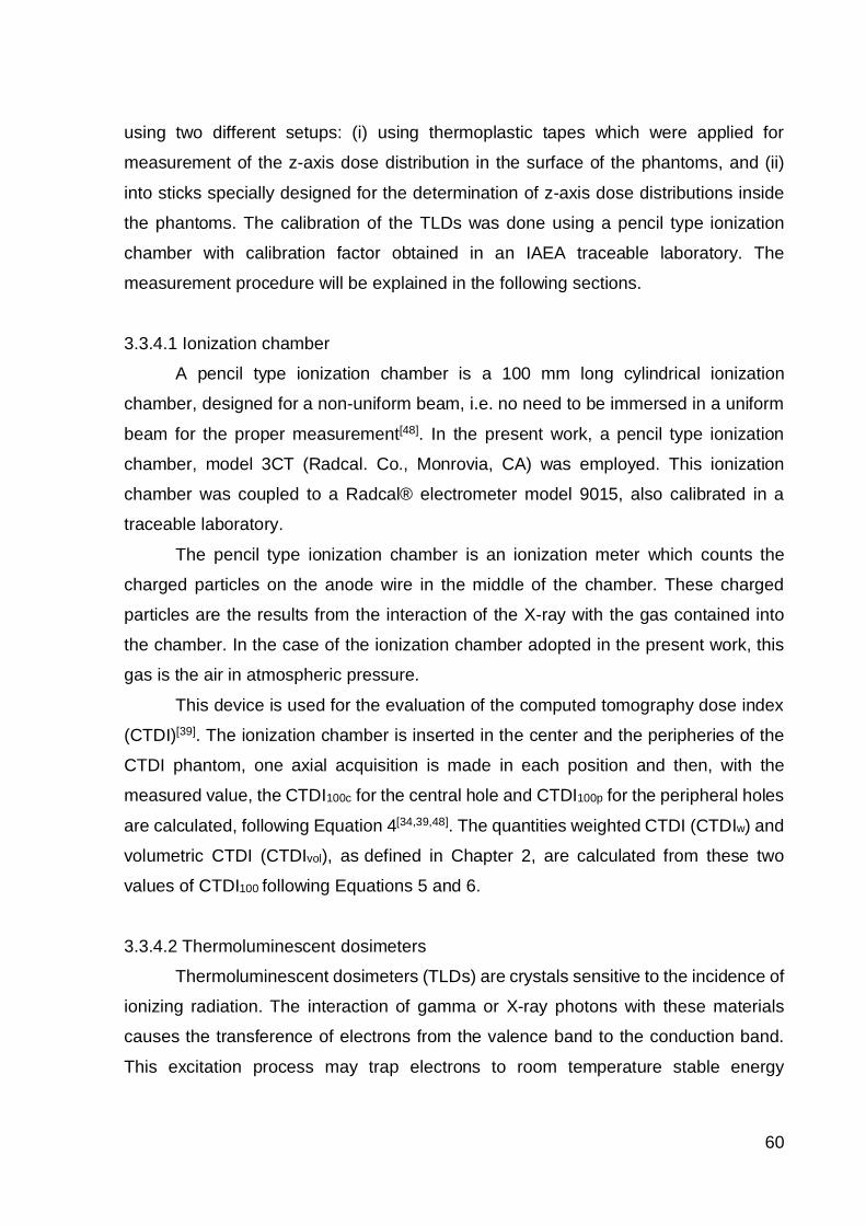
60

using two different setups: (i) using thermoplastic tapes which were applied for

measurement of the z-axis dose distribution in the surface of the phantoms, and (ii)

into sticks specially designed for the determination of z-axis dose distributions inside

the phantoms. The calibration of the TLDs was done using a pencil type ionization

chamber with calibration factor obtained in an IAEA traceable laboratory. The

measurement procedure will be explained in the following sections.

3.3.4.1 Ionization chamber

A pencil type ionization chamber is a 100 mm long cylindrical ionization

chamber, designed for a non-uniform beam, i.e. no need to be immersed in a uniform

beam for the proper measurement[48]. In the present work, a pencil type ionization

chamber, model 3CT (Radcal. Co., Monrovia, CA) was employed. This ionization

chamber was coupled to a Radcal® electrometer model 9015, also calibrated in a

traceable laboratory.

The pencil type ionization chamber is an ionization meter which counts the

charged particles on the anode wire in the middle of the chamber. These charged

particles are the results from the interaction of the X-ray with the gas contained into

the chamber. In the case of the ionization chamber adopted in the present work, this

gas is the air in atmospheric pressure.

This device is used for the evaluation of the computed tomography dose index

(CTDI)[39]. The ionization chamber is inserted in the center and the peripheries of the

CTDI phantom, one axial acquisition is made in each position and then, with the

measured value, the CTDI100c for the central hole and CTDI100p for the peripheral holes

are calculated, following Equation 4[34,39,48]. The quantities weighted CTDI (CTDIw) and

volumetric CTDI (CTDIvol), as defined in Chapter 2, are calculated from these two

values of CTDI100 following Equations 5 and 6.

3.3.4.2 Thermoluminescent dosimeters

Thermoluminescent dosimeters (TLDs) are crystals sensitive to the incidence of

ionizing radiation. The interaction of gamma or X-ray photons with these materials

causes the transference of electrons from the valence band to the conduction band.

This excitation process may trap electrons to room temperature stable energy

61

states[49]. These electrons can be removed by these traps by thermal excitation with

consequent emission of light photons[50].

Lithium-fluoride (LiF) crystals 3 mm x 3 mm size organized in thermoplastic

tapes (Figure 25) and sticks (Figure 26) were positioned along the phantoms z-axis

and used for determination of dose profiles associated to the CT studies evaluated in

the present work. The TLDs were tested previously and its sensitivity presents a

variation better than 6%.

Figure 25 Thermoplastic tapes with the LiF thermoluminescent dosimeters. Each tape hasapproximately 30 cm length and contains 25 to 28 TLD units.

Figure 26 Acrylic sticks with LiF thermoluminescent dosimeters. Each stick has 45 cm length insidethe TAP phantom and contains slots for positioning 25 TLD units. The external diameter of the stickswere designed to fit the holes present in the TAP phantom which are used for insert the pencil type

ionization chambers.

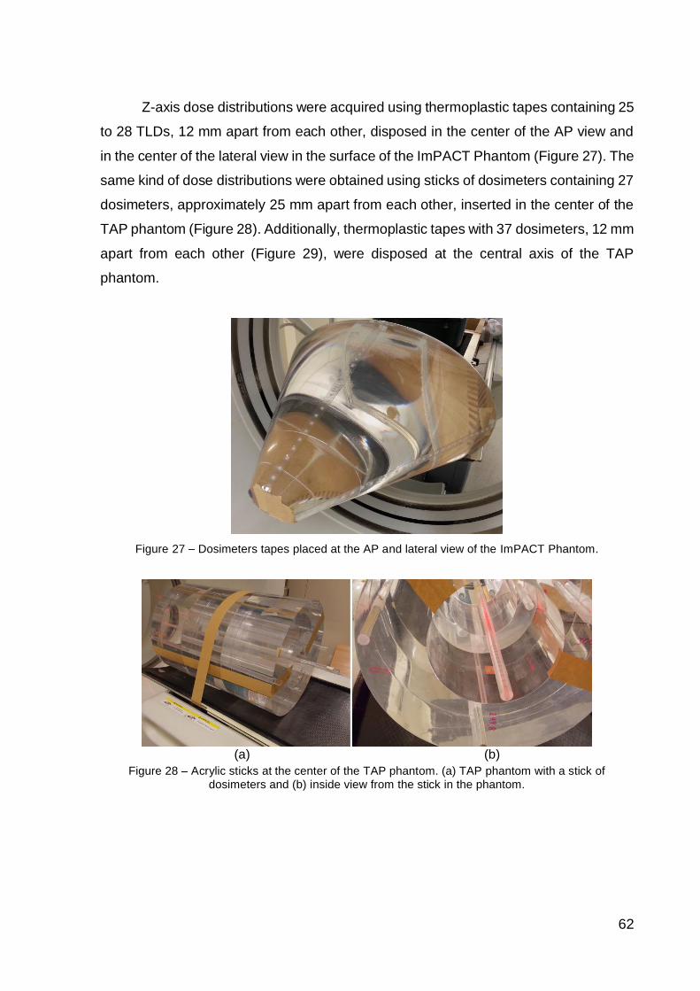
62

Z-axis dose distributions were acquired using thermoplastic tapes containing 25

to 28 TLDs, 12 mm apart from each other, disposed in the center of the AP view and

in the center of the lateral view in the surface of the ImPACT Phantom (Figure 27). The

same kind of dose distributions were obtained using sticks of dosimeters containing 27

dosimeters, approximately 25 mm apart from each other, inserted in the center of the

TAP phantom (Figure 28). Additionally, thermoplastic tapes with 37 dosimeters, 12 mm

apart from each other (Figure 29), were disposed at the central axis of the TAP

phantom.

Figure 27 Dosimeters tapes placed at the AP and lateral view of the ImPACT Phantom.

(a) (b)Figure 28 Acrylic sticks at the center of the TAP phantom. (a) TAP phantom with a stick of

dosimeters and (b) inside view from the stick in the phantom.

63

Figure 29 Thermoplastic tape with dosimeters at the center of the TAP phantom.

A TL/OSL reader, model DA-20 (DTU Nutech Risø, Denmark) was used to read

the information of the thermoluminescent dosimeters. This equipment has a sample

carousel with stainless steel cups with capacity for 48 dosimeters at a time (Figure 30).

The dosimeters were set to be heated at a rate of 10 Celsius degrees per second until

reach 350° C.

Figure 30 Carousel with its 48 stainless steel cups with 47 dosimeters.

The TLDs are heated by a mechanism that lifts the dosimeter cup until the

detection position and then starts heating by a high resistance alloy (Figure 31). The

light emitted from the TLDs is capture by photomultiplier tube (PMT) with a blue filter

to protect the PMT from scattered stimulation light and separate the stimulation and

detection spectral window[51]. The collected light is converted in a digital signal which

as a plot of counts per temperature (Figure 32). These

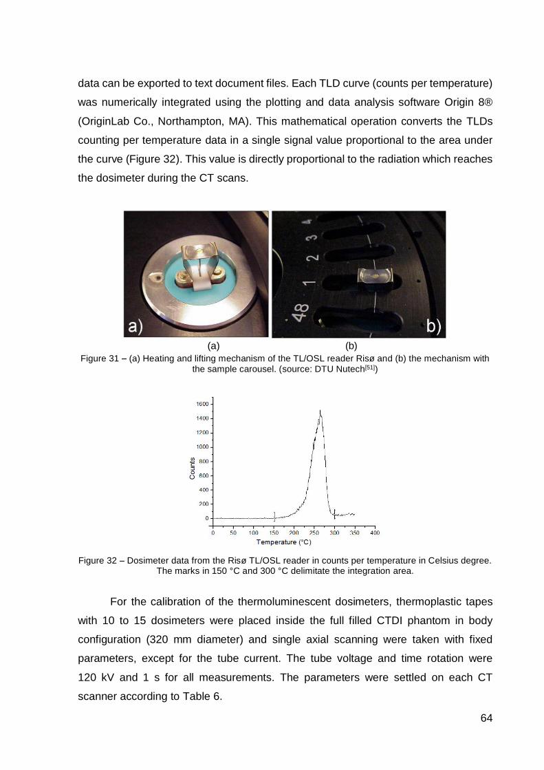
64

data can be exported to text document files. Each TLD curve (counts per temperature)

was numerically integrated using the plotting and data analysis software Origin 8®

(OriginLab Co., Northampton, MA). This mathematical operation converts the TLDs

counting per temperature data in a single signal value proportional to the area under

the curve (Figure 32). This value is directly proportional to the radiation which reaches

the dosimeter during the CT scans.

(a) (b)Figure 31 (a) Heating and lifting mechanism of the TL/OSL reader Risø and (b) the mechanism with

the sample carousel. (source: DTU Nutech[51])

Figure 32 Dosimeter data from the Risø TL/OSL reader in counts per temperature in Celsius degree.The marks in 150 °C and 300 °C delimitate the integration area.

For the calibration of the thermoluminescent dosimeters, thermoplastic tapes

with 10 to 15 dosimeters were placed inside the full filled CTDI phantom in body

configuration (320 mm diameter) and single axial scanning were taken with fixed

parameters, except for the tube current. The tube voltage and time rotation were

120 kV and 1 s for all measurements. The parameters were settled on each CT

scanner according to Table 6.

65

The same single axial scans were used to irradiate the pencil type ionization

chamber (Figure 33 a) instead of the dosimeters tape (Figure 33 b). The CT

measurements reproducibility was tested and it was better than 1%. The ionization

chamber reading was converted in kerma units (Gray) by multiplying the reading value

to the calibration factor provided by a traceable laboratory

is employed in the AEC response results instead of kerma because, in this case, they

are numerically equal[48].Table 6 Scanning protocol parameters selected for the calibration in axial scan.

CT scanner Collimation(mm)

Scan field ofview Tube current

GE LightSpeed Ultra 5 Large50 mA, 100 mA,

150 mA, 200 mA,250 mA, 300 mA

GE Discovery 750 HD 20 Large 100 mA, 300 mA

Philips Brilliance 16 24 500 mm 75 mA, 150 mA,250 mA, 400 mA

(a) (b)Figure 33 (a) the picture of the ionization chamber at the center of the full filled CTDI phantom at the

gantry central axis and (b) the dosimeters tape placed inside the same full filled CTDI Phantom.

The TLDs signals attained from each calibration set generated dose profiles.

Each dose profiles were discretely integrated using the integration tool of the Origin

8® (OriginLab Co., Northampton, MA) software. The integration limits were settled

according to the sensitive length of the ionization chamber (100 mm). The results of

these integrations, divided by the total length of measurement, can be related to the

calibrated dose reading of the ionization chamber[34]. Figure 34 shows the calibration

for Philips Brilliance 16 as an example. Equation 8 shows the calculations done to

relate the dosimeters dose profiles D(z) with measured dose values from the ionization

chamber.

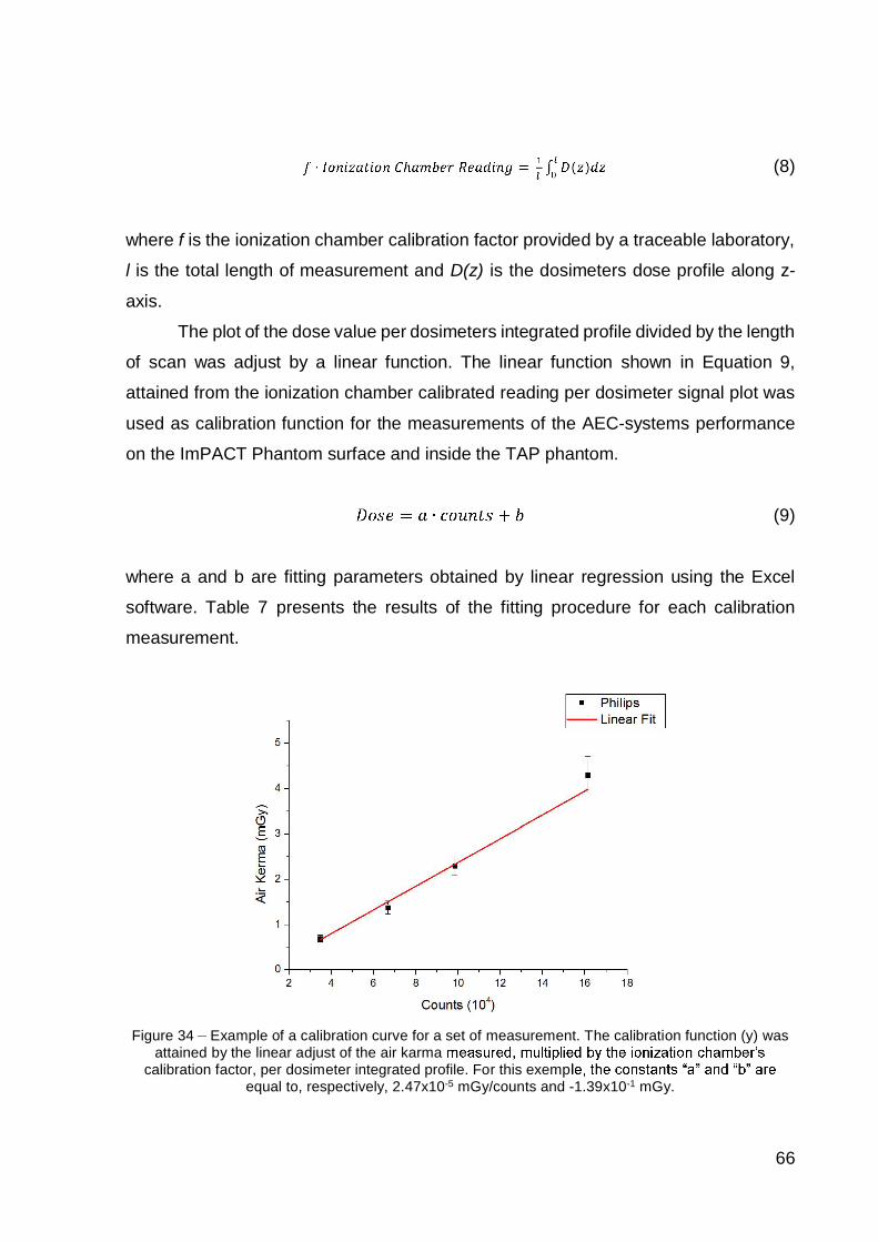
66

(8)

where f is the ionization chamber calibration factor provided by a traceable laboratory,

l is the total length of measurement and D(z) is the dosimeters dose profile along z-

axis.

The plot of the dose value per dosimeters integrated profile divided by the length

of scan was adjust by a linear function. The linear function shown in Equation 9,

attained from the ionization chamber calibrated reading per dosimeter signal plot was

used as calibration function for the measurements of the AEC-systems performance

on the ImPACT Phantom surface and inside the TAP phantom.

(9)

where a and b are fitting parameters obtained by linear regression using the Excel

software. Table 7 presents the results of the fitting procedure for each calibration

measurement.

Figure 34 Example of a calibration curve for a set of measurement. The calibration function (y) wasattained by the linear adjust of the air karma

calibration factor, per dosimeter integrated profile. For this exempequal to, respectively, 2.47x10-5 mGy/counts and -1.39x10-1 mGy.

67

Table 7 Results of the fitting procedure for each calibration measurement on GE LightSpeed Ultraand Discovery 750 HD and Philips Brilliance 16.

CT scanner a(mGy.count-1)

b(mGy) R²

GE LightSpeed Ultra 2.65 x 10-5 -4.49 x 10-1 0.994

GE Discovery 750 HD 2.34 x 10-5 -2.45 x 10-1 1.000

Philips Brilliance 16 2.47 x 10-5 -1.39 x 10-1 0.997

3.4 EVALUATION OF THE IMAGE NOISE

Image quality is an important issue on evaluating resources for saving patient

dose, such as the AEC approaches used in CT procedures. As both phantoms

employed are homogeneous, image noise was the parameter chosen for evaluation of

the balance between patient dose and image quality. The image noise has direct

relation to patient dose, once the image noise is increased by lowering the X-ray

photon fluency, and consequently the dose, and vice versa.

ous image is

associated to the noise in the signal used to produce the image. The noise is mostly a

signal fluctuation of the photon information reaching the detector caused by the

interaction of the X-ray beam to the adjacent area. The noise is decreased as the more

X-ray photons per irradiation area are absorbed by the detector, but it also means the

increase of the patient dose[12].

The pixel noise is designated as the standard deviation ( ) of N pixel CTN

values of a region of interest (ROI) selected at a homogeneous radiological image as

10:

(10)

where CTNi is each pixel value in HU of a ROI and CTN is the mean CT number value

of this ROI.

This evaluation was done using the ImageJ® software to quantify the noise

level. For that, an elliptical region of interest (ROI) was selected at the middle of the

of the software for the measurement of this ROI for each image of the

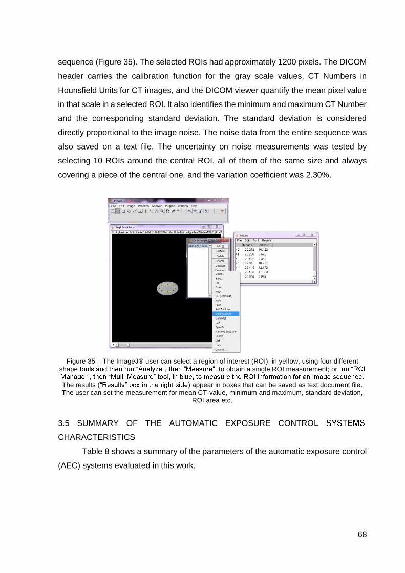
68

sequence (Figure 35). The selected ROIs had approximately 1200 pixels. The DICOM

header carries the calibration function for the gray scale values, CT Numbers in

Hounsfield Units for CT images, and the DICOM viewer quantify the mean pixel value

in that scale in a selected ROI. It also identifies the minimum and maximum CT Number

and the corresponding standard deviation. The standard deviation is considered

directly proportional to the image noise. The noise data from the entire sequence was

also saved on a text file. The uncertainty on noise measurements was tested by

selecting 10 ROIs around the central ROI, all of them of the same size and always

covering a piece of the central one, and the variation coefficient was 2.30%.

Figure 35 The ImageJ® user can select a region of interest (ROI), in yellow, using four differentshape , , to obtain a single ROI measurement; or

,The results ( ) appear in boxes that can be saved as text document file.The user can set the measurement for mean CT-value, minimum and maximum, standard deviation,

ROI area etc.

3.5 SUMMARY OF THE AUTOMATIC EXPOSURE CONTRO

CHARACTERISTICS

Table 8 shows a summary of the parameters of the automatic exposure control

(AEC) systems evaluated in this work.

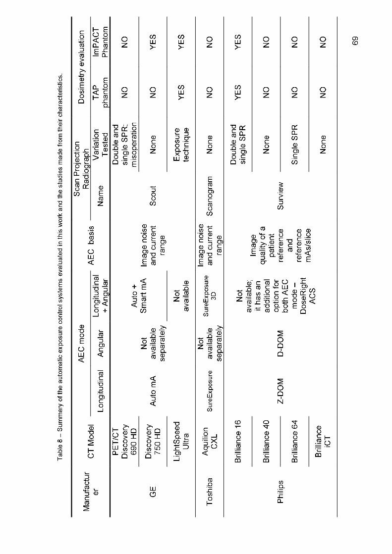
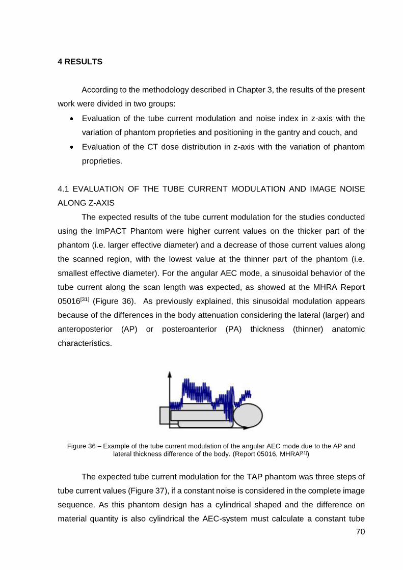
70

4 RESULTS

According to the methodology described in Chapter 3, the results of the present

work were divided in two groups:

Evaluation of the tube current modulation and noise index in z-axis with the

variation of phantom proprieties and positioning in the gantry and couch, and

Evaluation of the CT dose distribution in z-axis with the variation of phantom

proprieties.

4.1 EVALUATION OF THE TUBE CURRENT MODULATION AND IMAGE NOISE

ALONG Z-AXIS

The expected results of the tube current modulation for the studies conducted

using the ImPACT Phantom were higher current values on the thicker part of the

phantom (i.e. larger effective diameter) and a decrease of those current values along

the scanned region, with the lowest value at the thinner part of the phantom (i.e.

smallest effective diameter). For the angular AEC mode, a sinusoidal behavior of the

tube current along the scan length was expected, as showed at the MHRA Report

05016[31] (Figure 36). As previously explained, this sinusoidal modulation appears

because of the differences in the body attenuation considering the lateral (larger) and

anteroposterior (AP) or posteroanterior (PA) thickness (thinner) anatomic

characteristics.

Figure 36 Example of the tube current modulation of the angular AEC mode due to the AP andlateral thickness difference of the body. (Report 05016, MHRA[31])

The expected tube current modulation for the TAP phantom was three steps of

tube current values (Figure 37), if a constant noise is considered in the complete image

sequence. As this phantom design has a cylindrical shaped and the difference on

material quantity is also cylindrical the AEC-system must calculate a constant tube

71

current along each phantom section; the full filled phantom with the highest value, the

phantom without the minor cylinder with an intermediate tube current value and the

phantom without the minor and intermediate cylinders with the lowest value of tube

current.

Figure 37 Ilustration of the expected tube current modulation result for the TAP phantom. The would would be the phantom without the 100

the phantom without the 160 mm cylider.

In the following sections the results from each CT scanner study is showed

separated according to the equipment manufacturers.

4.1.1 General Electric CT Scanners

4.1.1.1 PET/CT Discovery 690 HD

The studies conducted to evaluate the PET/CT Discovery 690 HD on clinical

performance and its susceptibilities are described in Table 9. The scanning protocol

selected to evaluate the clinical performance of this CT scanner was abdomen no

contrast and the operational parameters set for all studies are listed in Table10. Table

11 shows the parameters selected for the double scan projection radiograph scout

for GE.

72

Table 9 Description of the studies conducted to evaluate the AEC performance, studies 1 to 5, andthe AEC-system susceptibility to the user, studies 6 to 12.

Studynumber

AECmode

Phantomemployed Subject of Study

1 Auto mA

ImPACTPhantom

Clinical noise index value using the widestcurrent range available

2 Auto mA Clinical noise index value using clinicalcurrent range and longitudinal AEC mode

3 Auto mA AEC response on higher noise indexvalue using longitudinal AEC mode

4 Auto mA AEC response on lower noise index valueusing longitudinal AEC mode

5Auto +Smart

mA

AEC response on longitudinal combinedto angular AEC mode

6 Auto mA

AEC-misoperation on scout and verify if thesystem has online feedback usinglongitudinal AEC mode

7Auto +Smart

mA

AEC-systemmisoperation on scout and verify if thesystem has online feedback usinglongitudinal combined to angular AECmode

8 Auto mAAEC-couch above the gantry central axis usinglongitudinal AEC mode

9 Auto mAAEC-couch below the gantry central axis usinglongitudinal AEC mode

10 Auto mA AEC-scout using longitudinal AEC mode

11 Auto mA AEC- elateral scout using longitudinal AEC mode

12Auto +Smart

mA

AEC-lateral scout using longitudinal combinedto angular AEC mode

The variations adopted for testing the AEC-system performance are listed in

Table 12. The study number 1, highlighted in light gray, was used for comparison with

all the others as it had an intermediate noise index (NI), the widest current range

available at this GE CT scanner model and the longitudinal AEC mode, Auto mA. For

each modification the equipment showed a different CTDIvol and DLP, also listed in

73

Table 12 and the parameters altered are highlighted in dark gray for better

comprehension.

Table 10 Scanning protocol parameters fixed for the PET/CT Discovery 690 HD AEC-systemevaluation.

Parameter ValueVoltage (kV) 120

Rotation time (s) 1.0Collimation 40

Pitch 0.984Slice Width (mm) 5Increment (mm) 5

S-FOV Large BodyD-FOV 450

Table 11 Parameters settled for the double scout used as a localizer for the phantom scans.

Parameter ValueVoltage (kV) 120

Exposure time (s) 10Current (mA) 10

Start Position (mm) -190End Position (mm) +190

Table 12 Parameters altered for testing the AEC-system efficiency. The study number 1, in lightgray, is the protocol used as the benchmark. In dark gray are the changes made at each study. The

Indicated CTDIvol represents the value of this quantity displayed in the equipment console.

StudyNumber AEC mode Current range

Min. (mA) / Max. mANoiseIndex

IndicatedCTDIvol(mGy)

IndicatedDLP

(mGy*cm)

1 Auto mA 10 700 11.37 19.54 715.1

2 Auto mA 100 300 11.37 14.5 530.5

3 Auto mA 10 700 25.00 5.34 195.4

4 Auto mA 10 700 5.00 32.02 1171.7

5 Auto +Smart mA 10 700 11.37 15.92 582.5

The tube current modulation and the noise level extracted and measured from

the DICOM image sequence are represented, in the Figure 38 to Figure 45, by dots

with simple interpolation lines to facilitate the quantitative analysis. Figure 38 shows

the comparison of the X-ray tube current modulation for the studies number 1 (blue

74

line), and study number 2 (red line). Study number 1 has a wider current range and its

Noise Index (NI) is the same established in the clinical routine. The current range

selected, 10 mA to 700 mA, were the highest and the lowest current values available

for that CT scanner. Study number 2 has the current range in use in the clinical

protocol.

The noise level measured for both current ranges is shown in Figure 39. At the

thinner part of the phantom, the noise level of study number 1 (blue line) is about 5 HU

higher than the noise level of the study number 2 (red line), although Figure 38 shows

a tube current 10 times higher on the thinner part of the phantom for the study number

2. At the thicker part of the phantom, the noise level is about 5 HU lower for the study

number 1 compared to study number 2 with the tube current difference at this part is

400 mA higher for the study number 1. The higher noise values at the end of Figure

39 (table position +150 mm) are due to the system scanning the phantom end and the

air, therefore the mean CT number varies between -1,000 HU (air CT number) and the

CT number of the acrylic (about 100 HU) raising the standard deviation.

Figure 38 Tube current modulation along z-axis for two different current ranges: the blue linerepresenting the widest tube current modulation (study number 1 - #1) and the red line representing a

clinical current range, narrower (study number 2 - #2).

0

100

200

300

400

500

600

700

800

Table Position (mm)

#1 - 10 mA to 700 mA #2 - 100 mA to 300 mA

75

Figure 39 Difference on noise for two current ranges. The blue line represents the noise level for thestudy number 1 (#1) and it is about 5 HU lower than the noise level for the study number 2 (#2 redline) at the thicker part of the phantom, but the X-ray tube current at this point is 10 times higher forthe study 1. In the thinner part of the phantom, the study number 1 reaches 400 mA higher than thetube current values of the study number 2 but no more than 5 HU difference on noise. The highest

noise values at the end of the graphic is due to the end of the phantom being imaged with a portion ofair.

Figure 40 shows the variation of the X-ray tube current with the different

selections of the NI parameter. The study number 3 allows a higher noise level (green

line) and study number 4 restricts the noise level (red line). Both studies are compared

to study number 1 which has the clinical NI (blue line). Figure 41 shows the noise

measured for these studies.

Figure 42 shows the results for the comparison between longitudinal (Auto mA)

according to study 1, and the longitudinal combined to angular AEC mode (Auto +

Smart mA), according to study number 5. The blue line represents the Auto mA AEC

mode and the red line the Auto + Smart mA. Figure 43 shows the noise measured for

both studies. The peak of noise values at the end of the graphics in Figure 41 and 43

are due to imaged air.

0

5

10

15

20

-150 -100 -50 0 50 100

Table Position (mm)

Noise #1 - 10 mA to 700 mA Noise #2 100 mA to 300 mA

76

Figure 40 Tube current modulation for different noise index values. The blue line represents theclinical noise index of the study number 1 (#1), an intermediate value. The green line represents a

higher noise index value (study number 3 - #3), meaning that a high image quality is not required, sothe AEC-system turns down the tube current level. The red line represents a lower noise index value(study number 5 - #5), meaning that a high image quality is required, then the AEC-system raises the

tube current level.

Figure 41 Difference on noise for different noise index values. The blue line represents the noiselevel for the noise index of 11.37 (study number 1 - #1); the green line represents the noise level for

the noise index of 25 (study number 3 - #3); the red line represents the noise level for the noise indexof 5 (study number 4 - #4). The higher values at the thinner part of the phantom is due to the lastsection of the phantom being imaged with a portion of air and the CT numbers vary from about

110 HU until -1,000 HU (air CT number).

0

100

200

300

400

500

600

700

800

Table Position (mm)

#1 - NI = 11.37 #3 - NI = 25 #4 - NI = 5

0,0

5,0

10,0

15,0

20,0

25,0

30,0

Table Position (mm)

#1 Noise - NI = 11.37 #3 Noise - NI = 25 #4 Noise - NI = 5

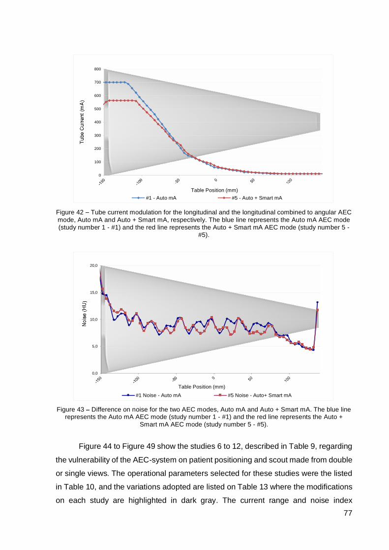
77

Figure 42 Tube current modulation for the longitudinal and the longitudinal combined to angular AECmode, Auto mA and Auto + Smart mA, respectively. The blue line represents the Auto mA AEC mode(study number 1 - #1) and the red line represents the Auto + Smart mA AEC mode (study number 5 -

#5).

Figure 43 Difference on noise for the two AEC modes, Auto mA and Auto + Smart mA. The blue linerepresents the Auto mA AEC mode (study number 1 - #1) and the red line represents the Auto +

Smart mA AEC mode (study number 5 - #5).

Figure 44 to Figure 49 show the studies 6 to 12, described in Table 9, regarding

the vulnerability of the AEC-system on patient positioning and scout made from double

or single views. The operational parameters selected for these studies were the listed

in Table 10, and the variations adopted are listed on Table 13 where the modifications

on each study are highlighted in dark gray. The current range and noise index

0

100

200

300

400

500

600

700

800

Table Position (mm)#1 - Auto mA #5 - Auto + Smart mA

0,0

5,0

10,0

15,0

20,0

Table Position (mm)#1 Noise - Auto mA #5 Noise - Auto+ Smart mA

78

employed are the same of study number 1, 10 mA to 700 mA and 11.37, respectively.

The study number 1 was also used for comparison of the studies 6 to 12 and its

parameters are repeated in Table 13.

Table 13 Parameters altered for testing the AEC-system vulnerability. In dark gray are the changesmade at each study referred to the study number 1.

Studynumber AEC mode scout

Tableheight*

(mm)Patient

orientation

1 Auto mA double 124 Head First

6 Auto mA double -half patient 124 Head First

7 Auto +Smart mA

double -half patient 124 Head First

8 Auto mA double 50 Head First9 Auto mA double 200 Head First

10 Auto mA AP view 124 Feet First11 Auto mA lateral view 124 Feet First

12 Auto +Smart mA lateral view 124 Feet First

The studies number 6 and 7 intend to verify if the AEC-system has a feedback

from the detectors during the exposure. For this investigation, the scout was performed

from the middle up to the thinner part of the ImPACT Phantom (Figure 44) and then

the complete length was scanned, i.e. the tomographic acquisition was made from the

entire phantom. Thus the AEC-system would calculate from the scout a low level of

tube current, but increase those values during the scanning of the thicker part of the

phantom, as soon as it gets less information at the detectors than expected.

Figure 45 shows the results for the half scout for both AEC modes, Auto mA

(red line) and Auto + Smart mA (green line). Figure 46 shows the noise measured for

both scanning made from the half scout, Auto mA (red line) and Auto + Smart mA

(green line) compared to an acquisition made from a full scout (blue line). The peak of

noise values at the end of the graphic are also due to imaged air.

* The table height is the value showed at the gantry display and its referential is the top of the gantry.

79

(a) (b)Figure 44 (a) The figure shows the scout of the entire ImPACT Phantom and (b) the half scout.

Figure 45 Tube current modulation for a scout made from half of the phantom (from the middle untilthe thinner part of the phantom) and a scan from the entire phantom. The red line represents the AutomA AEC mode on this scan condition (study number 6 - #6) and the green line represents the Auto +

Smart AEC mode on this scan condition (study number 7 - #7).

0

5

10

15

20

25

Table Position (mm)

#6 - Half Scout Auto mA #7 - Half Scout Auto mA + Smart mA

80

Figure 46 Difference on noise for a scan with full scout and the scans with half scout. The blue linerepresents the scan with full scout using Auto mA (study number 1 - #1) and the red and green lines

the scans with half scout using, respectively, Auto mA and Auto + Smart mA (studies number 6 and 7 -#6 and #7).

The studies number 8 and 9 intend to verify how much the patient couch out of

the gantry central axis can interfere in the tube current modulation, because of

magnification. The ImPACT Phantom was then moved up (i.e. closer to the X-ray tube

study number 8) and down (closer to the detectors study number 9) at the gantry

central axis resulting in magnification (Figure 47 b) or shrinkage (Figure 47 c) of the

phantom size at the AP view scout and the phantom displacement from the display

center at lateral view scout (Figure 48). Figure 49 shows the results for these

evaluations. The ImPACT Phantom at the gantry central axis (blue line) is compared

to the patient couch moved 74 mm up (red line) and moved 56 mm down (green line)

from the gantry central axis.

0

10

20

30

40

50

60

70

Table Position (mm)#1 Noise - Full Scout Auto mA #6 Noise - Half Scout Auto mA#7 - Noise Half Scout Auto mA + Smart mA

81

(a) (b) (c)Figure 47 Scout images from AP view for (a) the ImPACT Phantom at the gantry central axis, (b) the

ImPACT Phantom above the gantry central axis and (c) the ImPACT Phantom below the gantrycentral axis. When the phantom is above the gantry central axis, the imaging system projects amagnified image as it seems larger for the detectors and when the phantom is below the gantry

central axis the imaging system projects a shrunken image as it seems smaller for the imagedetectors.

(a) (b) (c)Figure 48 Scout images from lateral view for (a) the ImPACT Phantom at the gantry central axis, (b)the ImPACT Phantom above the gantry central axis and (c) the ImPACT Phantom below the gantrycentral axis. When the phantom is above or below the gantry central axis the lateral view appears

displaced from the center of the image display. For this reason some manufacturers recommend totake the lateral view SPR first, and if the patient appears at the display center, the AP view SPR can

be proceeded.

82

Figure 49 Tube current modulation for different couch positioning at the gantry y-axis. The blue linerepresents the ImPACT Phantom at the gantry central axis (study number 1 - #1), the green line

represents the ImPACT Phantom 74 mm above the gantry central axis (study number 8 - #8) and thered line represents the ImPACT Phantom 76 mm below the gantry central axis (study number 9 - #9).

The studies 10 to 12 intend to verify how important the double scout is for the

tube current modulation and what is the difference between the single scout of the AP

(tube at 0°) and lateral views (tube at 90°). Figure 50 shows the comparison of tube

current modulation for the scans made from double scout (blue line), single scout of

the AP view (purple line), single scout of the lateral view (red line) and single scout of

the lateral view with Auto + Smart mA AEC mode (green line). Figure 51 shows the

image noise measured for each sequence: double scout (blue line), single scout AP

view (purple line), single scout lateral view (red line) and single scout lateral view with

Auto + Smart mA (green line).

0

100

200

300

400

500

600

700

800

Table Position (mm)#1- Isocenter #8 - above #9 - below

83

Figure 50 Tube current modulation for scans made from double scout, single AP scout and singlelateral scout. In addition, the difference on tube current modulation for a single lateral scout using bothAEC modes, Auto mA and Auto + Smart mA. The blue line represents the double scout using Auto mA

(study number 1 - #1), the purple line represents the single AP scout using Auto mA (study number10 - #10), the red line represents the single lateral scout using Auto mA (study number 11 - #11) and

the green line represents the single lateral scout using Auto + Smart mA.

Figure 51 Difference on noise level for the double and single scout and lateral view scout using bothAEC modes. The blue line represents the noise level for the scan made from the double scout using

Auto mA AEC mode (study number 1 - #1), the purple line represents the noise level for the scanmade from the sinle AP scout (study number 10 - #10), the red line represents the scan made from thesingle lateral scout using Auto mA AEC mode (study number 11 - #11) and the green line represents

the scan made from the single lateral scout using Auto + Smart mA AEC mode (studynumber 12 - #12).

0

100

200

300

400

500

600

700

800

-150 -100 -50 0 50 100

Table Position (mm)#1 - Double Scout - Auto mA #11 - Lateral Scout - Auto mA#10 - AP Scout - Auto mA #12 - Lateral Scout - Auto + Smart mA

0,0

5,0

10,0

15,0

20,0

25,0

-150 -100 -50 0 50 100

Table Position (mm)#1 - Noise Double Scout - Auto mA #11 - Noise Lateral Scout - Auto mA#10 - AP Scout - Auto mA #12 - Noise Lat. Scout - Auto + Smart mA

84

4.1.1.2 LightSpeed Ultra

The studies conducted to evaluate the LightSpeed Ultra with 8 channels on

clinical performance are described in Table 14. This CT scanner model works only with

the longitudinal AEC mode.

Table 14 -systemresponse.

StudyNumber

Phantomemployed

AECmode Subject of study

1ImPACTPhantom

AutomA

AEC response on clinicalparameters

2 AEC response on different scan fieldof view

3 AEC response on scan made fromdifferent scout exposure technique

4TAP

phantom

AEC response on constant shape(diameter) and different quantity ofmateral using clinical paramters

5

AEC response on constant shape(diameter) and different quantity ofmateral using higher noise indexand higher pitch value

6TAP

phantom

AEC response on constant shape(diameter) and different quantity ofmateral using higher noise indexand lower pitch value

789

The protocol used for the LightSpeed -system evaluation was also

the abdomen no contrast. In this CT scanner the TAP phantom was also tested. The

parameters selected for the phantoms scanning are listed in Table 15. This CT scanner

model has lower X-ray tube current value, 400 mA instead of 700 mA as in the PET/CT

Discovery 690 HD. The highest tube current value was not chosen for not wearing the

equipment. Table 16 lists the parameters settled for the scout.

-system does not have the Auto +

Smart mA AEC mode enable. The operational parameters selected for testing this CT

scanner AEC-system is listed in Table 17. The changes made to evaluate the AEC

susceptibilities are highlighted in dark gray.

85

Table 15 Scanning protocol parameters settled for the evaluation of the LightSpeed Ultra AEC-system.

Parameter ValueVoltage (kV) 120

Rotation time (s) 1.0Slice width (mm) 2.5Increment (mm) 2.5

Scout 0°

Table 16 Operational parameters selected for testing the influence of the scouttechnique.

Scout Voltage (kV) Exposuretime (s) Current (mA)

1 80 1.0 202 120 1.0 20

Table 17 Scanning protocol parameters selected for study the AEC response on different scan fieldsof view and the technique used at the scout.

StudyNumber Scout Collimation

(mm) Pitch S-FOVCurrent range

(mA) Min. Max.

NoiseIndex

IndicatedCTDIvol(mGy)

IndicatedDLP

(mGy*cm)

1 1 20 1.35 Large 10 350 11.5 14.05 481.372 1 20 1.35 Small 10 350 11.5 26.93 922.433 2 20 1.35 Large 10 350 11.5 11.54 401.08

The studies number 1 and 2 compare the AEC- response when the

only change is the scan field of view (S-FOV) mode. This comparison aims to verify if

the tube current modulation changes for different S-FOVs, once the indicated CTDIvol

changed and the measured CTDIvol remains the same. A group of measurements for

testing if the CTDIvol changes for different S-FOV were done on the PET/CT Discovery

690 HD maintaining the CTDI Phantom and the operational parameters and switching

the S-FOV. The results of this study are listed on Table 18. The fixed operational

parameters were: tube voltage of 120 kV, tube current of 200 mA, rotation time of 1 s

and collimation of 20 mm. Figure 52 shows the tube current modulation for two different

S-FOVs, the Large Body (blue line) and Small Body (red line).

86

Table 18 Evaluation of the influence of the scan field of view on the measured CTDIvol in the GEPET/CT Discovery 690 HD. In this study, the scanning protocol was fixed and the scan field of view

varied to evaluate its influence on CTDIvol measurement.

Phantom S-FOVDisplay

FOV(mm)

IndicatedCTDIvol(mGy)

CTDIvolmeasured

(mGy)

Uncertainty(mGy)

Head LargeBody 250 17.51 33.9 0.3

Head SmallBody 250 15.53 33.5 0.1

Head SmallHead 250 35.51 33.5 0.1

Head PediatricBody 250 35.51 33.9 0.2

Head PediatricHead 250 35.51 33.5 0.2

Figure 52 Tube current modulation for two different scan fields of view (S-FOV). The blue linerepresents the S-FOV for large body scan (study number 1 - #1) and the red line represents the S-

FOV for head scan (study number 2 - #2).

The same scanning protocols were settled and the acquisitions were made after

the scout 1 then after the scout 2, listed in Table 16 for evaluating the influence of the

scout technique. This study intends to verify if the AEC-system interprets that a

material is less attenuating when the tube voltage selected for the scout is higher and

its result is showed in Figure 53 with the blue line representing the scout 1 and the

green line the scout 2.

0

50

100

150

200

250

300

350

400

-165 -115 -65 -15 35 85 135

Table Position (mm)

#1 - S-FOV Large Body #2 - S-FOV Head

87

Figure 53 Tube current modulation for scans made from scout with two different exposure technique:80 kV with 20 mAs (Scout 1) and 120 kV with 20 mAs (Scout 2). The blue line represents the scanmade from the scout 1 (study number 1 - #1) and the green line represents the scan made from the

scout 2 (study number 3 - #3).

For the TAP phantom, the LightSpeed -system has shown to be less

sensitive. In order to achieve variation of the tube current, higher values of noise index

(NI) had to be settled for the AEC-system to calculate different tube current values for

the phantom sections. The fixed parameters for the scanning protocols are listed in

Table 19. The NI values and the current range used are listed in Table 20. The current

range top value had to be changed because the X-ray tube capacity was exceeded.

The AEC-system only modulated the tube current for noise index values above 20. A

different pitch value of 1.5 was also settled for the NI of 20 for testing the influence of

the pitch on tube current modulation in this case.

Figure 54 shows the results for the lower NI values: NI of 11.37 (study number

4 - blue line), NI of 20 with pitch value of 1.5 (study number 5 yellow line) and NI of

20 (study number 6 red line). Figure 55 shows the results for the higher NI values;

NI of 25 (study number 7 pink line), NI of 30 (study number 8 light blue line) and NI

of 50 (study number 9 green line) at the same pitch of 0.75. It can be noticed that the

tube current modulation has some peaks in the sections between the phantoms. It

happens because, even though they are adjusted as tight as possible, the AEC-system

still can detect small gaps.

Figure 56 and Figure 57 show two results of noise level. The first, presented in

Figure 56, is the scan with a NI value of 11.37 that resulted in practically constant tube

0

50

100

150

200

250

300

350

400

-165 -115 -65 -15 35 85 135

Table Position (mm)

#1 - Scout 1 #3 -Scout 2

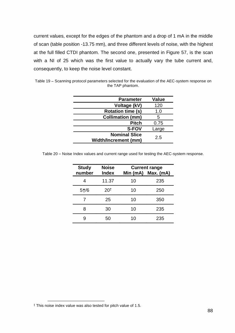
88

current values, except for the edges of the phantom and a drop of 1 mA in the middle

of scan (table position -13.75 mm), and three different levels of noise, with the highest

at the full filled CTDI phantom. The second one, presented in Figure 57, is the scan

with a NI of 25 which was the first value to actually vary the tube current and,

consequently, to keep the noise level constant.

Table 19 Scanning protocol parameters selected for the evaluation of the AEC-system response onthe TAP phantom.

Parameter ValueVoltage (kV) 120

Rotation time (s) 1.0Collimation (mm) 5

Pitch 0.75S-FOV Large

Nominal SliceWidth/Increment (mm) 2.5

Table 20 Noise Index values and current range used for testing the AEC-system response.

Studynumber

NoiseIndex

Current rangeMin (mA) Max. (mA)

4 11.37 10 235

5 /6 20 10 250

7 25 10 350

8 30 10 235

9 50 10 235

This noise index value was also tested for pitch value of 1.5.

89

Figure 54 Tube current modulation for two different noise index (NI) values: 11.37 and 20. Inaddition, pitch variation for the NI of 20 was made from 0.75 to 1.5. The blue line represents the scan

with clinical noise index of 11.37 with pitch value of 0.75 (study number 4 - #4), the yellow linerepresents the scan with noise index of 20 and pitch of 1.5 (study number 5 - #5) and the red line

represents the scan with noise index of 20 with pitch value of 0.75 (study number 6 - #6).

Figure 55 Tube current modulation for higher values of noise index and same pitch value of 0.75.The pink line represents the noise index of 25 (study number 7 - #7), the light blue line represents the

noise index of 30 (study number 8 - #8) and the green line represents the noise index of 50 (studynumber 9 - #9).

0

50

100

150

200

250

-235 -185 -135 -85 -35 15 65 115 165 215

Table Position (mm)

#4 - NI = 11.37 #5 - NI = 20 - Pitch 1.5 #6 - NI = 20

0

50

100

150

200

250

-235 -185 -135 -85 -35 15 65 115 165 215

Table Position (mm)

#7 - NI = 25 #8 - NI = 30 #9 - NI = 50

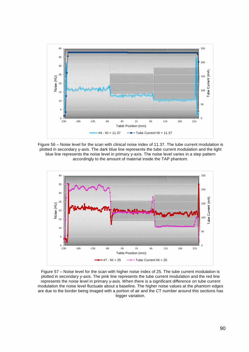
90

Figure 56 Noise level for the scan with clinical noise index of 11.37. The tube current modulation isplotted in secondary y-axis. The dark blue line represents the tube current modulation and the light

blue line represents the noise level in primary y-axis. The noise level varies in a step patternaccordingly to the amount of material inside the TAP phantom.

Figure 57 Noise level for the scan with higher noise index of 25. The tube current modulation isplotted in secondary y-axis. The pink line represents the tube current modulation and the red linerepresents the noise level in primary y-axis. When there is a significant difference on tube current

modulation the noise level fluctuate about a baseline. The higher noise values at the phantom edgesare due to the border being imaged with a portion of air and the CT number around this sections has

bigger variation.

0

50

100

150

200

250

0

5

10

15

20

25

30

35

40

-235 -185 -135 -85 -35 15 65 115 165 215

Table Position (mm)

#4 - NI = 11.37 Tube Current NI = 11.37

0

50

100

150

200

250

0

5

10

15

20

25

30

35

40

-235 -185 -135 -85 -35 15 65 115 165 215

Table Position (mm)

#7 - NI = 25 Tube Current NI = 25

91

4.1.1.3 Discovery 750 HD

The Discovery 750 HD GE also tested for different current

ranges and two different scan fields of view (S-FOV). The clinical current range settled

at the equipment routine was compared to wider current ranges using the

Auto + Smart mA AEC mode. To analyze how the S-FOV interferes at the tube current

modulation , the widest current range was maintained

and two different S-FOVs were compared, both using the Auto mA AEC mode. Table

21 shows the operational parameters selected for testing the AEC-system of this

model. Table 22 shows the current ranges evaluated while the current range in usage

in the clinical routine is highlighted in dark gray.

Table 21 Scanning protocol parameters selected for testing the AEC-system response of the GEDiscovery 750 HD.

Parameter ValueVoltage (kV) 120

Rotation time (s) 1.0Collimation (mm) 20

Pitch 0.969Slice Width (mm) 2.5Increment (mm) 2.5

Noise Index 11.50S-FOV Large Body

Table 22 Current range values used to study the AEC-system response.

Current rangeMin (mA) Max. (mA)

10 65050 650

150 650

Figure 58 shows the result for the tube current range variation and Figure 59

shows the resulting noise measured in the image sequence of these studies. The blue

line represents the clinical current range, the orange line the widest current range and

the green line an intermediate current range value. Again, there is almost no difference

on noise level (fluctuations about 2 HU), but the current values that results 15 times

greater in the thinner part of the ImPACT Phantom (Figure 58).

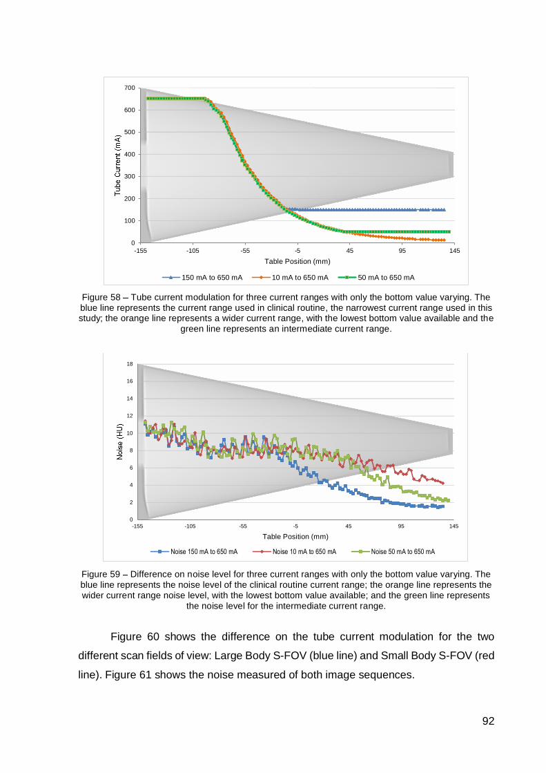
92

Figure 58 Tube current modulation for three current ranges with only the bottom value varying. Theblue line represents the current range used in clinical routine, the narrowest current range used in thisstudy; the orange line represents a wider current range, with the lowest bottom value available and the

green line represents an intermediate current range.

Figure 59 Difference on noise level for three current ranges with only the bottom value varying. Theblue line represents the noise level of the clinical routine current range; the orange line represents thewider current range noise level, with the lowest bottom value available; and the green line represents

the noise level for the intermediate current range.

Figure 60 shows the difference on the tube current modulation for the two

different scan fields of view: Large Body S-FOV (blue line) and Small Body S-FOV (red

line). Figure 61 shows the noise measured of both image sequences.

0

100

200

300

400

500

600

700

-155 -105 -55 -5 45 95 145

Table Position (mm)

150 mA to 650 mA 10 mA to 650 mA 50 mA to 650 mA

0

2

4

6

8

10

12

14

16

18

-155 -105 -55 -5 45 95 145

Table Position (mm)

Noise 150 mA to 650 mA Noise 10 mA to 650 mA Noise 50 mA to 650 mA

93

Figure 60 Tube current modulation for two different scan fields of view (S-FOV). The blue linerepresents the large body S-FOV and the red line represents the small body S-FOV.

Figure 61 Difference on noise level for two scan fields of view (S-FOV). The blue line represents thenoise level of the large body S-FOV and the red line represents represents the noise level of the small

body S-FOV.

4.1.2 Toshiba CT Scanner-system has basically the same options as ,

such as current range, noise level and angular AEC mode ON or OFF. The Toshiba

Aquilion CXL has been working at the Radiology Institute of the Clinical Hospital since

October of 2013 and not many AEC options have been previously tested. It has three

pre-programmed AEC parameters: Standard, Low Dose and High Quality. For

0

100

200

300

400

500

600

700

-140 -90 -40 10 60 110

Table Position (mm)

Large body Small body

0

2

4

6

8

10

12

-140 -90 -40 10 60 110

Table Position (mm)

Noise Large Body Noise Small Body

94

evaluating the Aquilion CXL AEC-system, SureExposure, the Standard and Low Dose

mode were tested in the present work. The parameters of the Standard and Low Dose

AEC options are listed in Table 23. The scanning protocol parameters are listed in

Table 24.

Table 23 Scanning protocol parameters available on the SureExposure options studied in this work.

AEC option Current Range (mA)Min. Max.

StandardDeviation

Standard 80 430 7.5Low Dose 40 400 11

Table 24 Scanning protocol parameters used for the evaluation of the Toshiba Aquilion CXL AEC-system.

Parameter ValueVoltage (kV) 120

Rotation time (s) 0.5Collimation (mm) 64 x 0.5

Pitch 0.828S-FOV (mm) 500

Nominal slicewidth/Increment (mm) 3.0

The tube current modulation for the Low Dose and Standard AEC options are

showed in Figure 62; Figure 63 shows the noise measured from the image sequences.

The blue line represents the Low Dose option and the red line the Standard option.

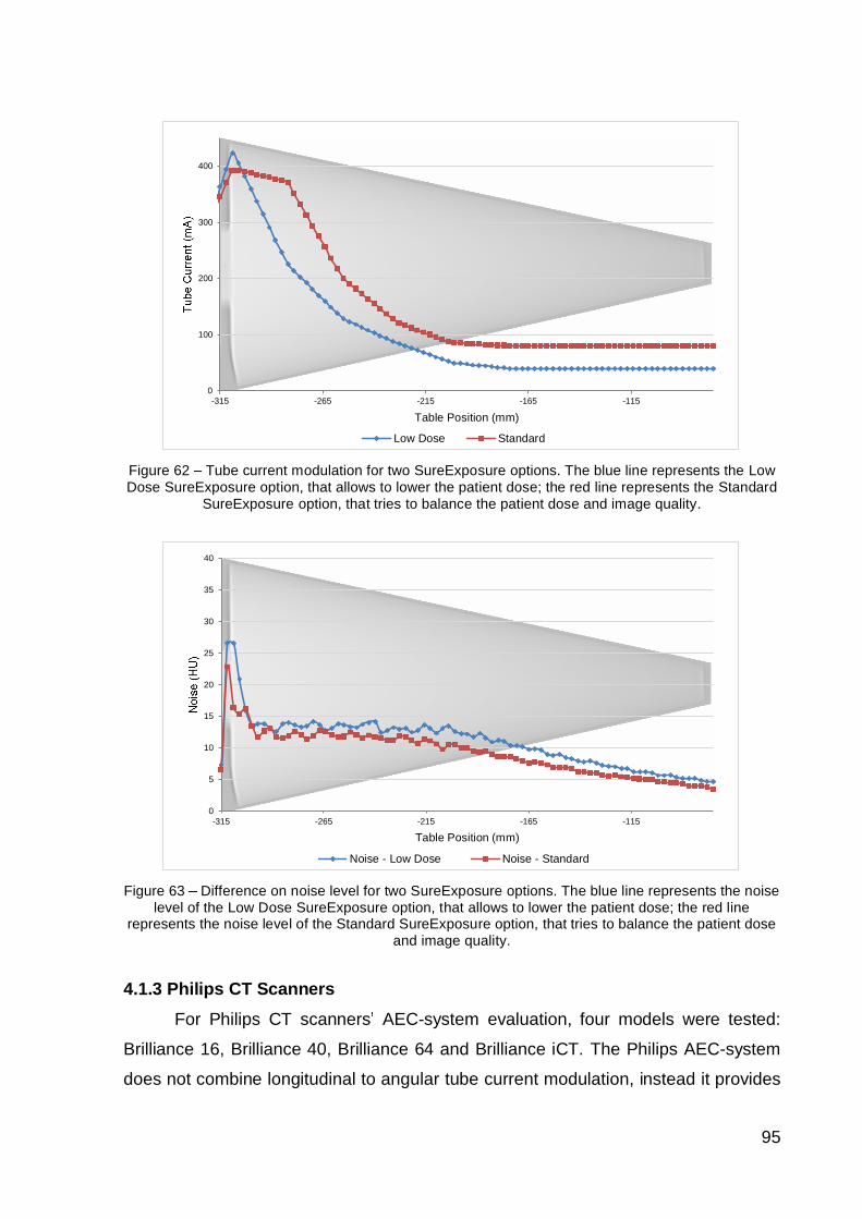
95

Figure 62 Tube current modulation for two SureExposure options. The blue line represents the LowDose SureExposure option, that allows to lower the patient dose; the red line represents the Standard

SureExposure option, that tries to balance the patient dose and image quality.

Figure 63 Difference on noise level for two SureExposure options. The blue line represents the noiselevel of the Low Dose SureExposure option, that allows to lower the patient dose; the red line

represents the noise level of the Standard SureExposure option, that tries to balance the patient doseand image quality.

4.1.3 Philips CT ScannersFor Philips CT scanners AEC-system evaluation, four models were tested:

Brilliance 16, Brilliance 40, Brilliance 64 and Brilliance iCT. The Philips AEC-system

does not combine longitudinal to angular tube current modulation, instead it provides

0

100

200

300

400

-315 -265 -215 -165 -115

Table Position (mm)

Low Dose Standard

0

5

10

15

20

25

30

35

40

-315 -265 -215 -165 -115

Table Position (mm)

Noise - Low Dose Noise - Standard

96

another option to complement the AEC operational mode, the DoseRight ACS. The

following sections introduce tested.

4.1.3.1 Brilliance 16 Model

The evaluation of the AEC-system of Philips Brilliance 16 CT scanner was

through the parameters listed in Table 25.

Table 25 Parameters varied to evaluate the automatic exposure control system response of PhilipsBrilliance 16.

Variation on ParametersAEC modeCollimation

Nominal slice thicknessPatient orientation

Current-time product per sliceScan projection radiograph

surview

The investigations done in this Philips CT scanner model are explained in Table

26. The scanning protocols used for each investigation are listed in Table 27; the

modifications adopted at each study are highlighted in dark gray. The tube voltage was

fixed at 120 kV. The rotation time was fixed at 1 s for the study 1 to 14 and 0.8 s for

the study 15 to 17. The studies 1 to 5 were also made for the TAP phantom, the other

studies were made only for the ImPACT Phantom.

The AEC-system response for the Z-DOM mode with the DoseRight ACS option

ON and OFF, studies number 1 and 2, are shown in Figure 64. Figure 65 shows the

noise measured for both acquisitions. The blue line represents the response of the Z-

DOM with the DoseRight ACS option OFF and the red line represents the Z-DOM with

the DoseRight ACS option ON.

Figure 66 also shows the difference on Z-DOM and Z-DOM with DoseRight ACS

but for the TAP phantom. The blue line represents the Z-DOM mode and the red line Z-

DOM with DoseRight ACS option ON.

Figure 67 shows the response of the D-DOM AEC mode with the DoseRight

ACS option ON and OFF, studies number 3 and 4. Figure 68 shows the noise

measured for both cases. The green line represents the D-DOM with DoseRight ACS

option OFF and the purple line the D-DOM with the DoseRight ACS option ON.

97

Table 26 Description of studies conducted to evaluate the Philips Brilliance 16 AEC-systemresponse on clinical performance and its susceptibilities.

Study Phantomemployed

AECmode

DoseRight ACS Subject of study

1

ImPACTPhantomand TAPphantom

Z-DOM OFF Longitudinal AEC mode response forboth phantoms

2 Z-DOM ON Longitudinal AEC mode with DoseRightACS response for both phantoms

3 D-DOM OFF Angular AEC mode response for bothphantoms

4 D-DOM ON Angular AEC mode with DoseRight ACSoption response for both phantoms

5 D-DOM OFF AEC response on collimation and pitchfor both phantoms

6

ImPACTPhantom

Z-DOM OFF AEC response on mAs/slice

7 D-DOM OFF The difference in AEC response fordouble, single AP and single lateralsurview with angular AEC mode

8 D-DOM OFF

9 D-DOM OFF

10 D-DOM OFF Patient orientation

11 Z-DOM OFFAEC response for single AP and singlelateral surview with longitudinal AECmode with and without the DoseRightACS option

12 Z-DOM ON

13 Z-DOM OFF

14 Z-DOM ON

15 Z-DOM OFF Longitudinal AEC mode response overtime

16 Z-DOM ON Longitudinal AEC mode with DoseRightACS response over time

17 D-DOM ON Angular AEC mode with DoseRight ACSoption response over time

98

Table 27 Scanning protocol parameters selected on each study to evaluate the Philips Brilliance-system on clinical performance and susceptibility.

Study Collimation(mm) Pitch

Nominal slicethickness/Increment

(mm)

AEC mode DoseRightACS Surview Patient

orientation mAs/slice

1 16 x 1.5 0.938 2 Z-DOM OFF double out 250

2 16 x 1.5 0.938 2 Z-DOM ON double out 250

3 16 x 1.5 0.938 2 D-DOM OFF double out 250

4 16 x 1.5 0.938 2 D-DOM ON double out 250

5 16 x 0.75 0.942 2 D-DOM not able double out 250

6 16 x 1.5 0.938 2 Z-DOM OFF double out 400

7 16 x 1.5 0.938 3 D-DOM OFF double out 250

8 16 x 1.5 0.938 3 D-DOM OFF AP out 250

9 16 x 1.5 0.938 3 D-DOM OFF lateral out 250

10 16 x 1.5 0.938 3 D-DOM OFF lateral in 250

11 16 x 1.5 0.938 3 Z-DOM OFF AP out 250

12 16 x 1.5 0.938 3 Z-DOM ON AP out 250

13 16 x 1.5 0.938 3 Z-DOM OFF lateral out 250

14 16 x 1.5 0.938 3 Z-DOM ON lateral out 250

15 16 x 1.5 0.938 2/1 Z-DOM OFF double out 250

16 16 x 1.5 0.938 2/1 Z-DOM ON double out 250

17 16 x 1.5 0.938 2/1 D-DOM ON double out 250

The equipment changes the pitch automatically when this collimation is selected.

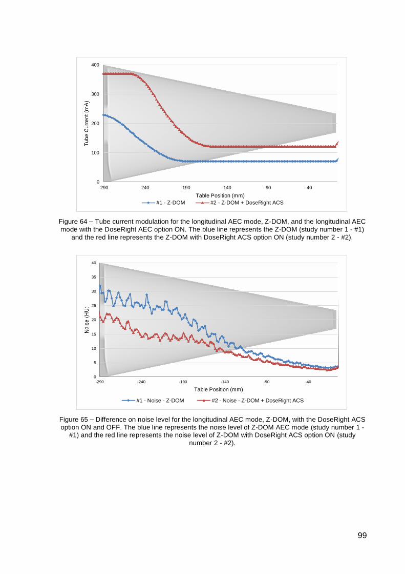
99

Figure 64 Tube current modulation for the longitudinal AEC mode, Z-DOM, and the longitudinal AECmode with the DoseRight AEC option ON. The blue line represents the Z-DOM (study number 1 - #1)

and the red line represents the Z-DOM with DoseRight ACS option ON (study number 2 - #2).

Figure 65 Difference on noise level for the longitudinal AEC mode, Z-DOM, with the DoseRight ACSoption ON and OFF. The blue line represents the noise level of Z-DOM AEC mode (study number 1 -

#1) and the red line represents the noise level of Z-DOM with DoseRight ACS option ON (studynumber 2 - #2).

0

100

200

300

400

-290 -240 -190 -140 -90 -40

Table Position (mm)#1 - Z-DOM #2 - Z-DOM + DoseRight ACS

0

5

10

15

20

25

30

35

40

-290 -240 -190 -140 -90 -40

Table Position (mm)

#1 - Noise - Z-DOM #2 - Noise - Z-DOM + DoseRight ACS

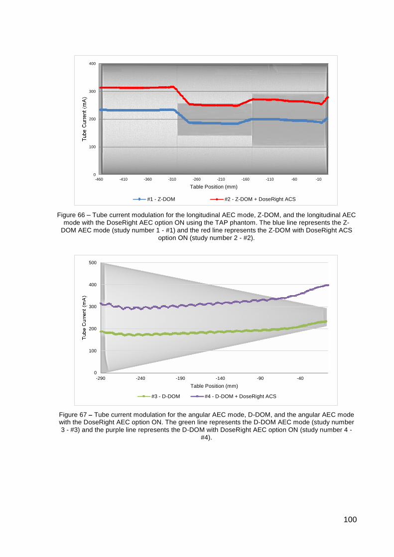
100

Figure 66 Tube current modulation for the longitudinal AEC mode, Z-DOM, and the longitudinal AECmode with the DoseRight AEC option ON using the TAP phantom. The blue line represents the Z-

DOM AEC mode (study number 1 - #1) and the red line represents the Z-DOM with DoseRight ACSoption ON (study number 2 - #2).

Figure 67 Tube current modulation for the angular AEC mode, D-DOM, and the angular AEC modewith the DoseRight AEC option ON. The green line represents the D-DOM AEC mode (study number3 - #3) and the purple line represents the D-DOM with DoseRight AEC option ON (study number 4 -

#4).

0

100

200

300

400

-460 -410 -360 -310 -260 -210 -160 -110 -60 -10

Table Position (mm)

#1 - Z-DOM #2 - Z-DOM + DoseRight ACS

0

100

200

300

400

500

-290 -240 -190 -140 -90 -40

Table Position (mm)

#3 - D-DOM #4 - D-DOM + DoseRight ACS

101

Figure 68 Difference on noise level between the angular AEC mode, D-DOM, and the angular AECmode with DoseRight AEC option ON. The green line represents the D-DOM AEC mode (study

number 4 - #4) and the purple line represents the D-DOM with DoseRight ACS option ON.

Figure 69 shows the difference on D-DOM with the DoseRight ACS option OFF

and ON for the TAP phantom; the green line represents the D-DOM and the purple line

the D-DOM with DoseRight ACS option ON.

Figure 69 Tube current modulation for the angular AEC mode, D-DOM, and the angular AEC modewith the DoseRight AEC option ON using the TAP phantom. The green line represents the D-DOMAEC mode (study number 3 - #3) and the purple line represents the D-DOM with DoseRight AEC

option ON (study number 4 - #4).

0

5

10

15

20

25

30

35

40

-290 -240 -190 -140 -90 -40

Table Position (mm)#3 - Noise - D-DOM #4 - Noise - D-DOM + DoseRight ACS

0

100

200

300

400

-460 -410 -360 -310 -260 -210 -160 -110 -60 -10

Table Position (mm)

#3 - D-DOM #4 - D-DOM + DoseRight ACS

102

Figure 70 shows the comparison of Z-DOM (blue line) and D-DOM (green line)

AEC modes both with the DoseRight ACS option OFF, studies number 1 and 3. Figure

71 shows the noise measured for both cases.

Figure 70 Tube current modulation for the longitudinal and the angular AEC modes, Z-DOM and D-DOM respectively. The blue line represents the Z-DOM AEC mode (study number 1 - #1) and the

green line represents the D-DOM AEC mode (study number 3 - #3).

Figure 71 Difference on noise for the longitudinal and angular AEC modes, Z-DOM and D-DOMrespectively. The blue line represents the noise level for the Z-DOM AEC mode (study number 1 - #1)

and the green line represents the noise level for the D-DOM AEC mode (study number 3 - #3).

0

50

100

150

200

250

-290 -240 -190 -140 -90 -40

Table Position (mm)

#1 - Z-DOM #3 - D-DOM

0

5

10

15

20

25

30

35

40

-290 -240 -190 -140 -90 -40

Table Position (mm)

#1 - Noise Z-DOM #3 - Noise D-DOM

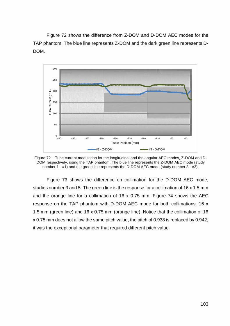
103

Figure 72 shows the difference from Z-DOM and D-DOM AEC modes for the

TAP phantom. The blue line represents Z-DOM and the dark green line represents D-

DOM.

Figure 72 Tube current modulation for the longitudinal and the angular AEC modes, Z-DOM and D-DOM respectively, using the TAP phantom. The blue line represents the Z-DOM AEC mode (study

number 1 - #1) and the green line represents the D-DOM AEC mode (study number 3 - #3).

Figure 73 shows the difference on collimation for the D-DOM AEC mode,

studies number 3 and 5. The green line is the response for a collimation of 16 x 1.5 mm

and the orange line for a collimation of 16 x 0.75 mm. Figure 74 shows the AEC

response on the TAP phantom with D-DOM AEC mode for both collimations: 16 x

1.5 mm (green line) and 16 x 0.75 mm (orange line). Notice that the collimation of 16

x 0.75 mm does not allow the same pitch value, the pitch of 0.938 is replaced by 0.942;

it was the exceptional parameter that required different pitch value.

0

50

100

150

200

250

300

-460 -410 -360 -310 -260 -210 -160 -110 -60 -10

Table Position (mm)

#1 - Z-DOM #3 - D-DOM

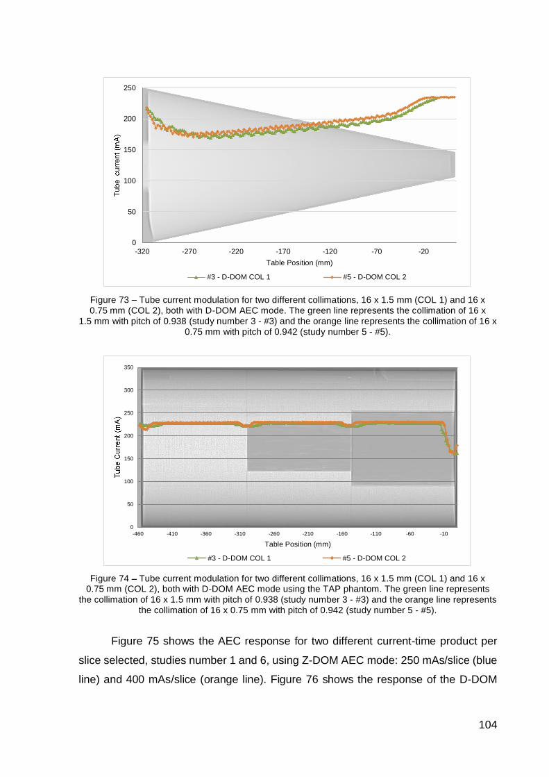
104

Figure 73 Tube current modulation for two different collimations, 16 x 1.5 mm (COL 1) and 16 x0.75 mm (COL 2), both with D-DOM AEC mode. The green line represents the collimation of 16 x

1.5 mm with pitch of 0.938 (study number 3 - #3) and the orange line represents the collimation of 16 x0.75 mm with pitch of 0.942 (study number 5 - #5).

Figure 74 Tube current modulation for two different collimations, 16 x 1.5 mm (COL 1) and 16 x0.75 mm (COL 2), both with D-DOM AEC mode using the TAP phantom. The green line represents

the collimation of 16 x 1.5 mm with pitch of 0.938 (study number 3 - #3) and the orange line representsthe collimation of 16 x 0.75 mm with pitch of 0.942 (study number 5 - #5).

Figure 75 shows the AEC response for two different current-time product per

slice selected, studies number 1 and 6, using Z-DOM AEC mode: 250 mAs/slice (blue

line) and 400 mAs/slice (orange line). Figure 76 shows the response of the D-DOM

0

50

100

150

200

250

-320 -270 -220 -170 -120 -70 -20Table Position (mm)

#3 - D-DOM COL 1 #5 - D-DOM COL 2

0

50

100

150

200

250

300

350

-460 -410 -360 -310 -260 -210 -160 -110 -60 -10

Table Position (mm)

#3 - D-DOM COL 1 #5 - D-DOM COL 2

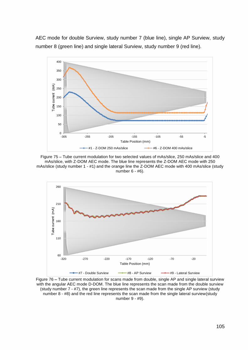
105

AEC mode for double Surview, study number 7 (blue line), single AP Surview, study

number 8 (green line) and single lateral Surview, study number 9 (red line).

Figure 75 Tube current modulation for two selected values of mAs/slice, 250 mAs/slice and 400mAs/slice, with Z-DOM AEC mode. The blue line represents the Z-DOM AEC mode with 250

mAs/slice (study number 1 - #1) and the orange line the Z-DOM AEC mode with 400 mAs/slice (studynumber 6 - #6).

Figure 76 Tube current modulation for scans made from double, single AP and single lateral surviewwith the angular AEC mode D-DOM. The blue line represents the scan made from the double surview

(study number 7 - #7), the green line represents the scan made from the single AP surview (studynumber 8 - #8) and the red line represents the scan made from the single lateral surview(study

number 9 - #9).

0

50

100

150

200

250

300

350

400

-305 -255 -205 -155 -105 -55 -5

Table Position (mm)

#1 - Z-DOM 250 mAs/slice #6 - Z-DOM 400 mAs/slice

60

110

160

210

260

-320 -270 -220 -170 -120 -70 -20

Table Position (mm)

#7 - Double Surview #8 - AP Surview #9 - Lateral Surview

106

Figure 77 shows the comparison of the single AP and lateral Surview for the Z-

DOM AEC mode. The blue line represents Z-DOM with AP Surview, study number 12;

the red line represents Z-DOM with lateral Surview, study 14; the orange line

represents Z-DOM with DoseRight ACS option ON for AP Surview; and the green line

represents the Z-DOM with DoseRight ACS option ON for lateral Surview.

Figure 77 Tube current modulation for scans made from single AP and single lateral surview withlongitudinal AEC mode, Z-DOM, with DoseRight ACS option ON and OFF. The blue line representsthe scan made from single AP surview using only Z-DOM AEC mode (study number 11 - #11); theorange line represents the scan made from single AP surview using Z-DOM with DoseRight ACS

(study number 12 - #12); the red line represents the scan made from single lateral surview using onlyZ-DOM AEC mode; the red line represents the scan made from the single lateral surview using only Z-DOM AEC mode (study number 13 - #13); the green line represents the scan made from single lateral

surview using Z-DOM with DoseRight ACS option (study number 14 - #14).

Figure 78 shows the AEC response for patient orientation using D-DOM AEC

mode. The blue line represents the patient couch getting out of the gantry aperture

during the scanning, study number 10, and the red line the patient couch getting in the

gantry aperture during the scanning, study number 11.

The Figure 79 to Figure 83 show the evaluation of Z-DOM and D-DOM AEC

modes over time. The studies 15 to 17 were done one year before the studies 1 to 14

and they were compared to the studies number 1, 2 and 4. As the protocols scanning

were done with different rotation time, the comparison were done by extracting the

current-

0018,1152) in order to allow comparisons. Figure 79 shows the Z-DOM difference over

time. The dark red line represents the Z-DOM mode in 2013 (study number 14), the

0

100

200

300

400

500

-320 -270 -220 -170 -120 -70 -20

Table Position (mm)#11 - AP Surview - Z-DOM #13 - Lateral Surview -Z-DOM#12 - AP Surview - Z-DOM ACS #14 - Lateral Surview - Z-DOM ACS

107

light red line the Z-DOM in 2014 (study number 1). The dark blue line represents the

Z-DOM with DoseRight ACS option in 2013 (study number 15) and the light blue line

the Z-DOM with DoseRight ACS in 2014 (study number 2). Figure 80 and Figure 81

show the noise measured on these image sequences for the Z-DOM with DoseRight

ACS option OFF and ON, respectively.

Figure 82 shows the difference on D-DOM with DoseRight ACS option ON

response over time. The green line represents the D-DOM with DoseRight ACS option

ON in 2013 (study number 17) and the orange line in 2014 (study number 4). Figure

83 shows the noise measured for both image sequences.

Figure 78 Tube current modulation using angular AEC mode, D-DOM, for two different patientorientation, i.e. the scan made while the patient couch is getting out of the gantry or while the patient

couch is getting inside of the gantry. Both scans were made from single AP surview. The blue linerepresents the scan made with the patient couch getting out the gantry (study number #9 - #9) and the

red line represents the scan made with the patient couch getting in the gantry (study number 10 -#10).

0

50

100

150

200

250

-300 -250 -200 -150 -100 -50 0

Table Position (mm)#9 - D-DOM OUT #10 - D-DOM IN

108

Figure 79 Tube current modulation for the longitudinal AEC mode, Z-DOM, with the DoseRight ACSoption ON and OFF response over time. The dark red line represents the scan made in 2013 with

DoseRight ACS option OFF (study number 15 - #15); the light red line represents the scan made in2014 with DoseRight ACS option OFF (study number 1 - #1); the dark blue line represents the scanmade in 2013 with DoseRight ACS option ON (study number 16 - #16); the light blue line represents

the scan made in 2014 with DoseRight ACS option ON (study number 2 - #2). All the scans weremade in both years in the month of May.

Figure 80 Difference on noise for the longitudinal AEC mode, Z-DOM, response over time. The lightred line represents the noise measured from the scan of 2013 (study number 15 - #15) and the dark

red line represents the noise measured from the scan made in 2014 (study number 1 - #1).

0

50

100

150

200

250

300

350

400

450

-150 -100 -50 0 50 100 150

Table Position (mm)#15 - Z-DOM 2013 #1 - Z-DOM 2014#16 - Z-DOM + ACS 2013 #2 - Z-DOM + ACS 2014

0

5

10

15

20

25

30

35

40

-150 -100 -50 0 50 100 150

Table Position (mm)

#15 - Noise Z-DOM 2013 #1 - Noise Z-DOM 2014

109

Figure 81 Difference on noise for the longitudinal AEC mode, Z-DOM, with DoseRight ACS optionresponse over time. The light blue line represents the noise measured from the scan made in 2013

(study number 16 - #16) and the dark blue line represents the noise measured from the scan made in2014 (study number 2 - #2).

Figure 82 Tube current modulation response over time for the angular AEC mode, D-DOM, withDoseRight ACS option ON. The green line represents scan made in 2013 (study number 17 - #17)

and the orange line the scan made in 2014 (study number 4 - #4). Both scans were made in the monthof May.

0

10

20

30

40

50

-150 -100 -50 0 50 100 150

Table Position (mm)#16 -Noise Z-DOM + ACS 2013 #2 -Noise Z-DOM + ACS 2014

0

100

200

300

400

500

-150 -100 -50 0 50 100 150

Table Position (mm)

#17 - D-DOM + ACS - 2013 #4 - D-DOM + ACS - 2014

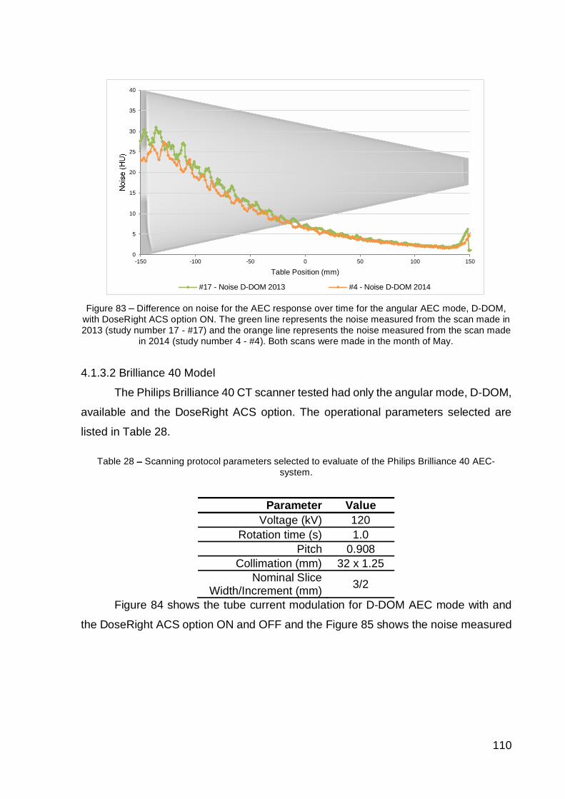
110

Figure 83 Difference on noise for the AEC response over time for the angular AEC mode, D-DOM,with DoseRight ACS option ON. The green line represents the noise measured from the scan made in2013 (study number 17 - #17) and the orange line represents the noise measured from the scan made

in 2014 (study number 4 - #4). Both scans were made in the month of May.

4.1.3.2 Brilliance 40 Model

The Philips Brilliance 40 CT scanner tested had only the angular mode, D-DOM,

available and the DoseRight ACS option. The operational parameters selected are

listed in Table 28.

Table 28 Scanning protocol parameters selected to evaluate of the Philips Brilliance 40 AEC-system.

Parameter ValueVoltage (kV) 120

Rotation time (s) 1.0Pitch 0.908

Collimation (mm) 32 x 1.25Nominal Slice

Width/Increment (mm) 3/2

Figure 84 shows the tube current modulation for D-DOM AEC mode with and

the DoseRight ACS option ON and OFF and the Figure 85 shows the noise measured

0

5

10

15

20

25

30

35

40

-150 -100 -50 0 50 100 150

Table Position (mm)

#17 - Noise D-DOM 2013 #4 - Noise D-DOM 2014

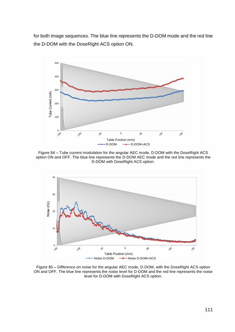
111

for both image sequences. The blue line represents the D-DOM mode and the red line

the D-DOM with the DoseRight ACS option ON.

Figure 84 Tube current modulation for the angular AEC mode, D-DOM with the DoseRight ACSoption ON and OFF. The blue line represents the D-DOM AEC mode and the red line represents the

D-DOM with DoseRight ACS option.

Figure 85 Difference on noise for the angular AEC mode, D-DOM, with the DoseRight ACS optionON and OFF. The blue line represents the noise level for D-DOM and the red line represents the noise

level for D-DOM with DoseRight ACS option.

0

100

200

300

400

500

Table Position (mm)D-DOM D-DOM+ACS

0

10

20

30

40

Table Position (mm)Noise D-DOM Noise D-DOM+ACS

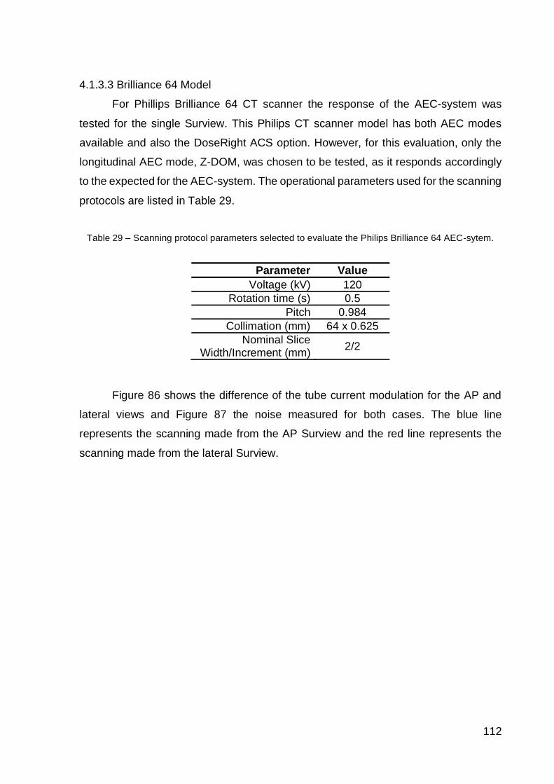
112

4.1.3.3 Brilliance 64 Model

For Phillips Brilliance 64 CT scanner the response of the AEC-system was

tested for the single Surview. This Philips CT scanner model has both AEC modes

available and also the DoseRight ACS option. However, for this evaluation, only the

longitudinal AEC mode, Z-DOM, was chosen to be tested, as it responds accordingly

to the expected for the AEC-system. The operational parameters used for the scanning

protocols are listed in Table 29.

Table 29 Scanning protocol parameters selected to evaluate the Philips Brilliance 64 AEC-sytem.

Parameter ValueVoltage (kV) 120

Rotation time (s) 0.5Pitch 0.984

Collimation (mm) 64 x 0.625Nominal Slice

Width/Increment (mm) 2/2

Figure 86 shows the difference of the tube current modulation for the AP and

lateral views and Figure 87 the noise measured for both cases. The blue line

represents the scanning made from the AP Surview and the red line represents the

scanning made from the lateral Surview.

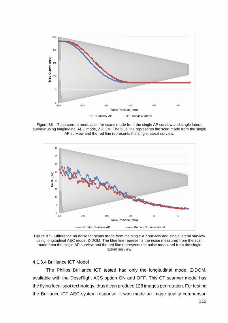
113

Figure 86 Tube current modulation for scans made from the single AP surview and single lateralsurview using longitudinal AEC mode, Z-DOM. The blue line represents the scan made from the single

AP surview and the red line represents the single lateral surview.

Figure 87 Difference on noise for scans made from the single AP surview and single lateral surviewusing longitudinal AEC mode, Z-DOM. The blue line represents the noise measured from the scanmade from the single AP surview and the red line represents the noise measured from the single

lateral surview.

4.1.3.4 Brilliance iCT Model

The Philips Brilliance iCT tested had only the longitudinal mode, Z-DOM,

available with the DoseRight ACS option ON and OFF. This CT scanner model has

the flying focal spot technology, thus it can produce 128 images per rotation. For testing

the Brilliance iCT AEC-system response, it was made an image quality comparison

0

100

200

300

400

500

-295 -245 -195 -145 -95 -45

Table Position (mm)

Surview AP Surview lateral

0

5

10

15

20

25

30

35

40

-295 -245 -195 -145 -95 -45

Table Position (mm)

Ruído - Surview AP Ruído - Surview lateral

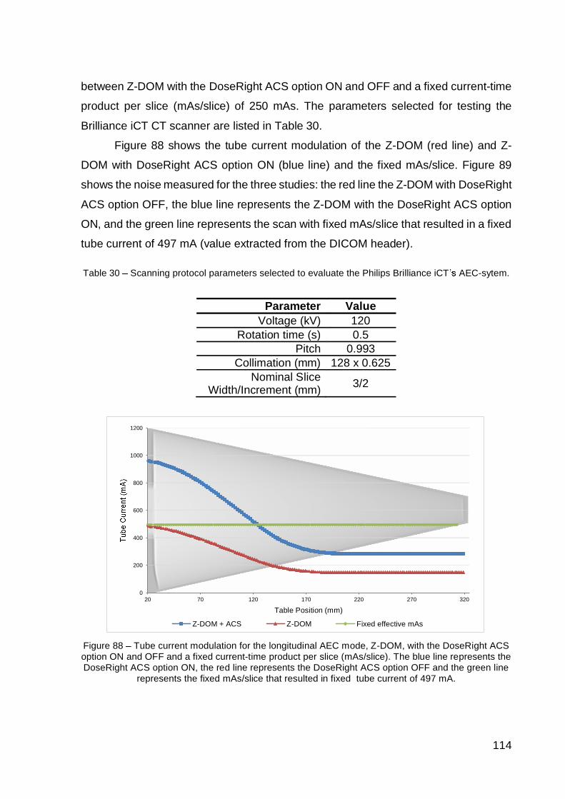
114

between Z-DOM with the DoseRight ACS option ON and OFF and a fixed current-time

product per slice (mAs/slice) of 250 mAs. The parameters selected for testing the

Brilliance iCT CT scanner are listed in Table 30.

Figure 88 shows the tube current modulation of the Z-DOM (red line) and Z-

DOM with DoseRight ACS option ON (blue line) and the fixed mAs/slice. Figure 89

shows the noise measured for the three studies: the red line the Z-DOM with DoseRight

ACS option OFF, the blue line represents the Z-DOM with the DoseRight ACS option

ON, and the green line represents the scan with fixed mAs/slice that resulted in a fixed

tube current of 497 mA (value extracted from the DICOM header).

Table 30 Scanning protocol parameters selected to evaluate the Philips Brilliance iCT AEC-sytem.

Parameter ValueVoltage (kV) 120

Rotation time (s) 0.5Pitch 0.993

Collimation (mm) 128 x 0.625Nominal Slice

Width/Increment (mm) 3/2

Figure 88 Tube current modulation for the longitudinal AEC mode, Z-DOM, with the DoseRight ACSoption ON and OFF and a fixed current-time product per slice (mAs/slice). The blue line represents theDoseRight ACS option ON, the red line represents the DoseRight ACS option OFF and the green line

represents the fixed mAs/slice that resulted in fixed tube current of 497 mA.

0

200

400

600

800

1000

1200

20 70 120 170 220 270 320

Table Position (mm)

Z-DOM + ACS Z-DOM Fixed effective mAs

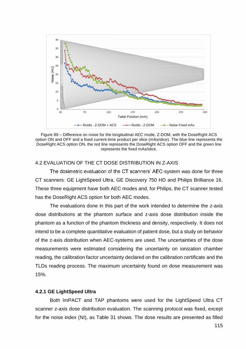
115

Figure 89 Difference on noise for the longitudinal AEC mode, Z-DOM, with the DoseRight ACSoption ON and OFF and a fixed current-time product per slice (mAs/slice). The blue line represents theDoseRight ACS option ON, the red line represents the DoseRight ACS option OFF and the green line

represents the fixed mAs/slice.

4.2 EVALUATION OF THE CT DOSE DISTRIBUTION IN Z-AXIS

-system was done for three

CT scanners: GE LightSpeed Ultra, GE Discovery 750 HD and Philips Brilliance 16.

These three equipment have both AEC modes and, for Philips, the CT scanner tested

has the DoseRight ACS option for both AEC modes.

The evaluations done in this part of the work intended to determine the z-axis

dose distributions at the phantom surface and z-axis dose distribution inside the

phantom as a function of the phantom thickness and density, respectively. It does not

intend to be a complete quantitative evaluation of patient dose, but a study on behavior

of the z-axis distribution when AEC-systems are used. The uncertainties of the dose

measurements were estimated considering the uncertainty on ionization chamber

reading, the calibration factor uncertainty declared on the calibration certificate and the

TLDs reading process. The maximum uncertainty found on dose measurement was

15%.

4.2.1 GE LightSpeed UltraBoth ImPACT and TAP phantoms were used for the LightSpeed Ultra CT

scanner z-axis dose distribution evaluation. The scanning protocol was fixed, except

for the noise index (NI), as Table 31 shows. The dose results are presented as filled

0

5

10

15

20

25

30

35

40

20 70 120 170 220 270 320

Table Position (mm)

Ruído - Z-DOM + ACS Ruído - Z-DOM Noise Fixed mAs

116

line with dots, representing the dosimeter position, and the tube current modulation in

dashed line in secondary y-axis. The scales in Figure 90 to Figure 93 have all been left

equal to facilitate the comparison.

For the TAP phantom, the dose distribution for three NI values was evaluated

and they are listed in Table 31, the three highest values. Figure 90, Figure 91 and

Figure 92 show the results corresponding to NI values of 25, 30 and 50, respectively;

Figure 93 shows the z-axis dose distribution using a fixed tube current value of 235 mA.

Table 31 Scanning protocol parameters used for the dose distribution along z-axis measurement.

Parameter ValueVoltage (kV) 120

Rotation time (s) 1.0Collimation (mm) 5

Pitch 0.75S-FOV Large

Current range 10 - 235Nominal Slice

Width/Increment (mm) 2.5

Noise Index values 11.37/25/30/50

Figure 90 Dose measurement inside the TAP phantom, in central position, using noise index of 25.The blue line, in primary y-axis, represents the dose distribution along z-axis and the dots representsthe dosimeters position. The dashed red line represents the tube current modulation plotted in right

axis.

0

50

100

150

200

250

0

10

20

30

40

50

60

70

-220 -170 -120 -70 -20 30 80 130 180 230

Table Position (mm)

Dose - NI 25 Tube Current - NI 25

117

Figure 91 Dose measurement inside the TAP phantom, in the center, using noise index of 30. Theblue line, in primary y-axis, represents the dose distribution along z-axis and the dots represents thedosimeters position. The dashed red line represents the tube current modulation plotted in right axis.

Figure 92 Dose measurement inside the TAP phantom, in the center, using noise index of 50. Theblue line, in primary y-axis, represents the dose distribution along z-axis and the dots represents thedosimeters position. The dashed red line represents the tube current modulation plotted in right axis.

0

50

100

150

200

250

0

10

20

30

40

50

60

70

-220 -170 -120 -70 -20 30 80 130 180 230

Table Position (mm)

Dose - NI 30 Tube Current NI 30

0

50

100

150

200

250

0

10

20

30

40

50

60

70

-220 -170 -120 -70 -20 30 80 130 180 230

Table Position (mm)

Dose - NI 50 Tube Current - NI 50

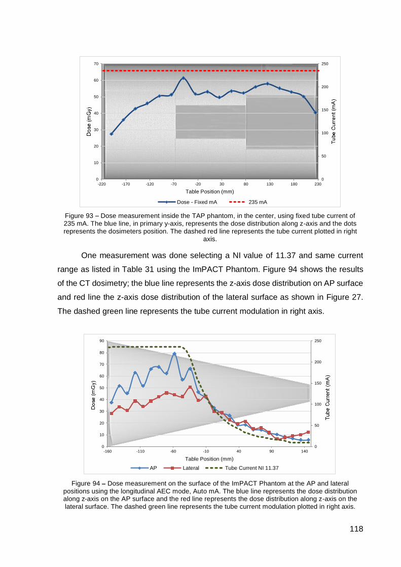
118

Figure 93 Dose measurement inside the TAP phantom, in the center, using fixed tube current of235 mA. The blue line, in primary y-axis, represents the dose distribution along z-axis and the dotsrepresents the dosimeters position. The dashed red line represents the tube current plotted in right

axis.

One measurement was done selecting a NI value of 11.37 and same current

range as listed in Table 31 using the ImPACT Phantom. Figure 94 shows the results

of the CT dosimetry; the blue line represents the z-axis dose distribution on AP surface

and red line the z-axis dose distribution of the lateral surface as shown in Figure 27.

The dashed green line represents the tube current modulation in right axis.

Figure 94 Dose measurement on the surface of the ImPACT Phantom at the AP and lateralpositions using the longitudinal AEC mode, Auto mA. The blue line represents the dose distributionalong z-axis on the AP surface and the red line represents the dose distribution along z-axis on thelateral surface. The dashed green line represents the tube current modulation plotted in right axis.

0

50

100

150

200

250

0

10

20

30

40

50

60

70

-220 -170 -120 -70 -20 30 80 130 180 230

Table Position (mm)

Dose - Fixed mA 235 mA

0

50

100

150

200

250

0

10

20

30

40

50

60

70

80

90

-160 -110 -60 -10 40 90 140

Table Position (mm)

AP Lateral Tube Current NI 11.37

119

4.2.2 GE Discovery 750 HDFor the Discovery 750 HD only the ImPACT Phantom was tested. The

dosimetric measurements were done for two different scan fields of view (S-FOV):

Large Body S-FOV and Small Body S-FOV, compared in Figure 60. The scanning

protocol was the same as listed in Table 21 and current range of 10 mA to 650 mA

was used. The clinical current range is highlighted in Table 22. Figure 95 shows the

dose distribution -FOV and Figure 96

S-FOV, with the tube current modulation represented by a dashed line in right axis.

Figure 95 Dose measurement on the surface of the ImPACT Phantom at the AP and lateralpositions using a large body scan field of view and the longitudinal combined to angular AEC mode,Auto + Smart mA. The blue line represents the dose distribution along z-axis on the AP surface and

the red line represents the dose distribution along z-axis on the lateral surface. The dashed green linerepresents the tube current modulation plotted in right axis.

0

100

200

300

400

500

600

700

0

10

20

30

40

50

60

70

80

90

-155 -105 -55 -5 45 95 145

Table Position (mm)

AP Lateral Large Body

120

Figure 96 Dose measurement on the surface of the ImPACT Phantom at the AP and lateralpositions using a small body scan field of view and the longitudinal combined to angular AEC mode,Auto + Smart mA. The blue line represents the dose distribution along z-axis on the AP surface and

the red line represents the dose distribution along z-axis on the lateral surface. The dashed green linerepresents the tube current modulation plotted in right axis.

4.2.3 Philips Brilliance 16For Brilliance 16 CT scanner both phantoms were used for measurement of the

dose distribution along the z-axis measurement. The scanning protocol parameters

employed are listed in Table 32. For the TAP phantom one measurement was made

with these parameters and for the ImPACT Phantom five measurements were made

and the changes are listed in Table 33. The double Surview was made for the ImPACT

Phantom and single Surview for the TAP phantom, once it has no difference on AP

and lateral views.

Table 32 Scanning protocol parameters used for the dose distribution in z-axis measurements of theAEC modes and constant current-time product per slice for the Philips Brilliance 16.

Parameter ValueVoltage (kV) 120

Collimation (mm) 16 x 1.5Pitch 0.938

Rotation time (s) 1AEC mode Z-DOM

DoseRight ACS OFFEffective mAs 250

0

100

200

300

400

500

600

700

0

10

20

30

40

50

60

70

80

90

100

-155 -105 -55 -5 45 95 145

Table Position (mm)

AP Lateral Small Body

121

Table 33 Parameters varied for the AEC-system response on dose distribution along z-axis.

AECmode

DoseRightACS

Z-DOM OFFZ-DOM OND-DOM OFFD-DOM ON

Fixed mAs/slice

Figure 97 to Figure 101 show the dose distributions and the tube current

modulation. The dosimeters from the AP view are represented by the blue line, the

lateral view by the red line and the tube current modulation is represented for the

dashed green line the values have to be read off the right axis.

Figure 97 shows the dose distribution result for the Z-DOM AEC mode and

Figure 98 for the Z-DOM with DoseRight ACS option ON; Figure 99 shows the result

for D-DOM AEC mode and Figure 100 for the D-DOM with DoseRight ACS. Figure 101

shows the dose distribution result for a fixed current-time product per slice.

Figure 97 Dose measurement on the surface of the ImPACT Phantom at the AP and lateralpositions using the longitudinal AEC mode Z-DOM. The blue line represents the dose distribution

along z-axis on the AP surface and the red line represents the dose distribution along z-axis on thelateral surface. The dashed green line represents the tube current modulation plotted in right axis.

0

50

100

150

200

250

300

350

400

450

0

4

8

12

16

20

-305 -255 -205 -155 -105 -55 -5

Table Position

AP Lateral Z-DOM

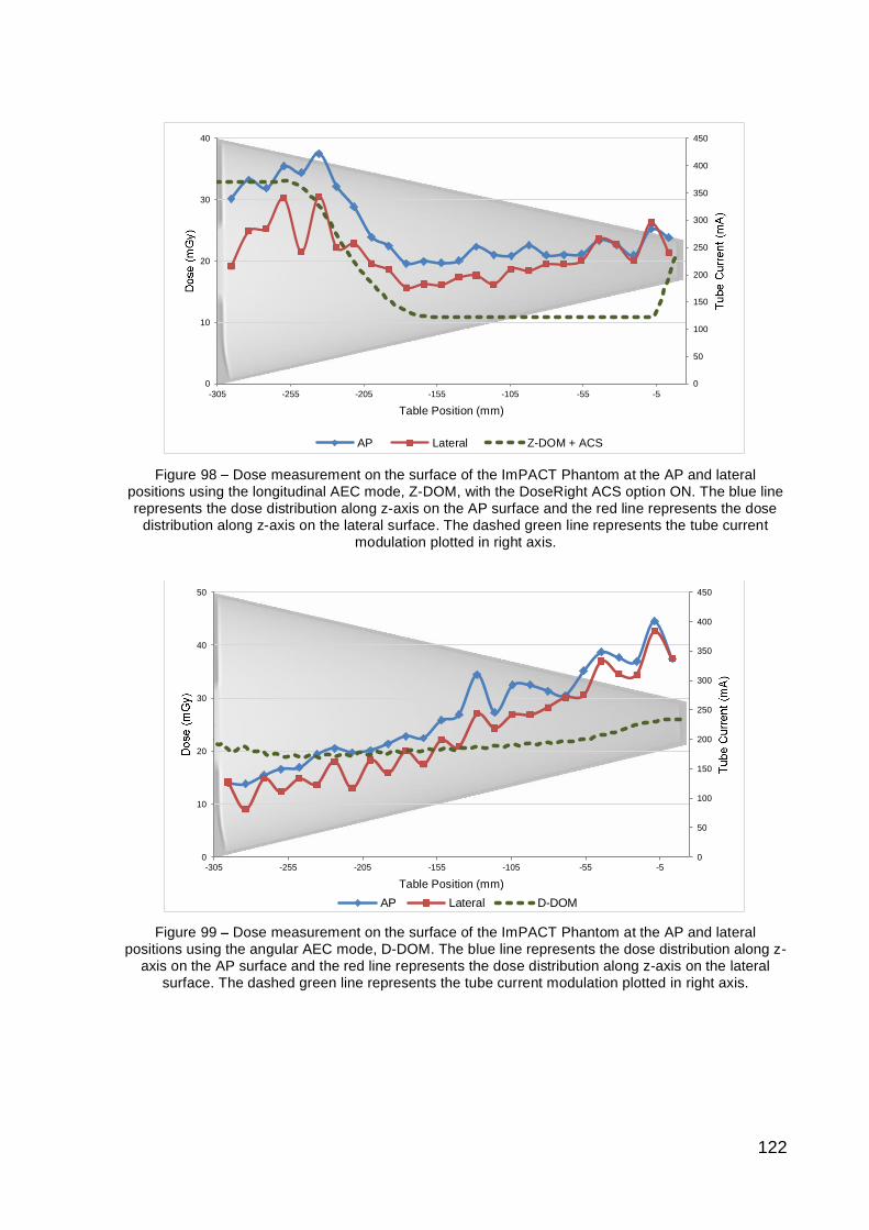
122

Figure 98 Dose measurement on the surface of the ImPACT Phantom at the AP and lateralpositions using the longitudinal AEC mode, Z-DOM, with the DoseRight ACS option ON. The blue linerepresents the dose distribution along z-axis on the AP surface and the red line represents the dose

distribution along z-axis on the lateral surface. The dashed green line represents the tube currentmodulation plotted in right axis.

Figure 99 Dose measurement on the surface of the ImPACT Phantom at the AP and lateralpositions using the angular AEC mode, D-DOM. The blue line represents the dose distribution along z-

axis on the AP surface and the red line represents the dose distribution along z-axis on the lateralsurface. The dashed green line represents the tube current modulation plotted in right axis.

0

50

100

150

200

250

300

350

400

450

0

10

20

30

40

-305 -255 -205 -155 -105 -55 -5

Table Position (mm)

AP Lateral Z-DOM + ACS

0

50

100

150

200

250

300

350

400

450

0

10

20

30

40

50

-305 -255 -205 -155 -105 -55 -5

Table Position (mm)AP Lateral D-DOM

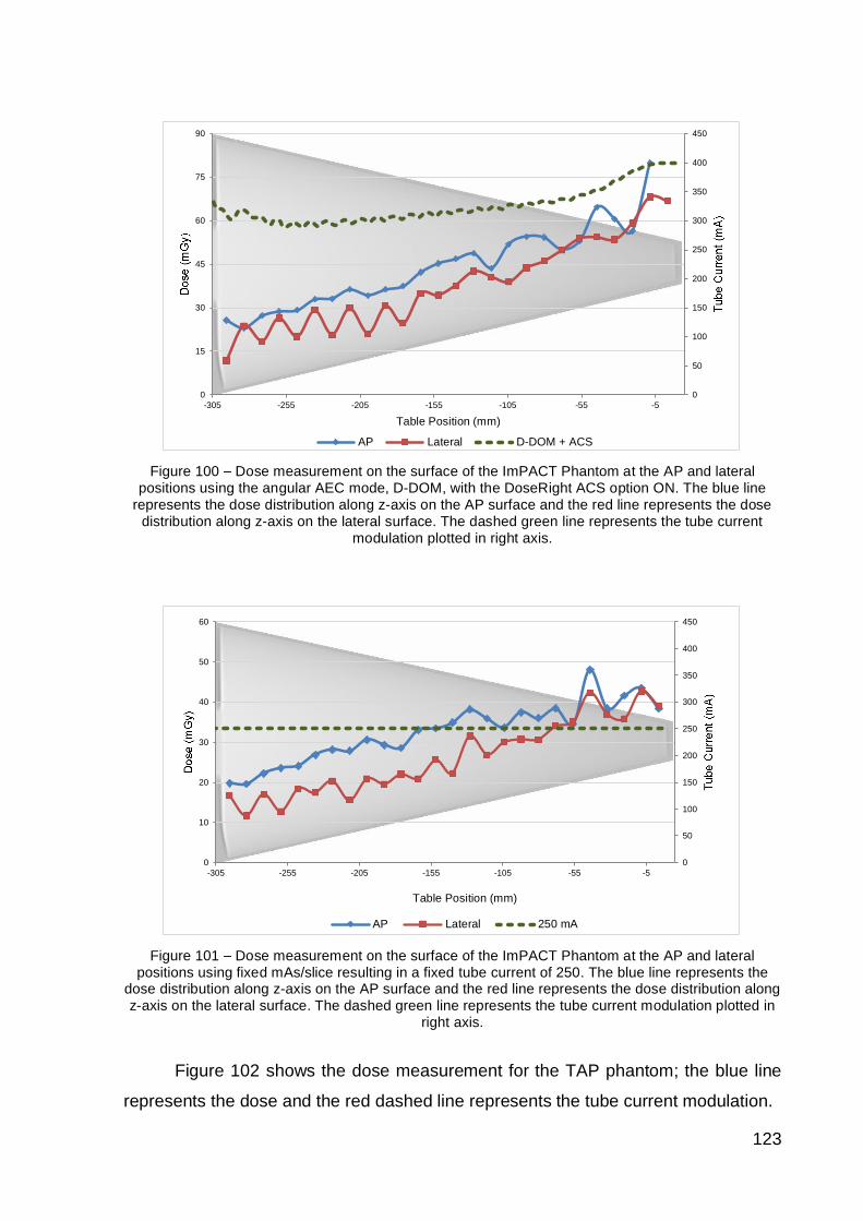
123

Figure 100 Dose measurement on the surface of the ImPACT Phantom at the AP and lateralpositions using the angular AEC mode, D-DOM, with the DoseRight ACS option ON. The blue line

represents the dose distribution along z-axis on the AP surface and the red line represents the dosedistribution along z-axis on the lateral surface. The dashed green line represents the tube current

modulation plotted in right axis.

Figure 101 Dose measurement on the surface of the ImPACT Phantom at the AP and lateralpositions using fixed mAs/slice resulting in a fixed tube current of 250. The blue line represents the

dose distribution along z-axis on the AP surface and the red line represents the dose distribution alongz-axis on the lateral surface. The dashed green line represents the tube current modulation plotted in

right axis.

Figure 102 shows the dose measurement for the TAP phantom; the blue line

represents the dose and the red dashed line represents the tube current modulation.

0

50

100

150

200

250

300

350

400

450

0

15

30

45

60

75

90

-305 -255 -205 -155 -105 -55 -5

Table Position (mm)

AP Lateral D-DOM + ACS

0

50

100

150

200

250

300

350

400

450

0

10

20

30

40

50

60

-305 -255 -205 -155 -105 -55 -5

Table Position (mm)

AP Lateral 250 mA

124

Figure 102 Dose measurement inside the TAP phantom, in the center, using the longitudinal AECmode, Z-DOM. The blue line, in primary y-axis, represents the dose distribution along z-axis and thedots represents the dosimeters position. The dashed red line represents the tube current plotted inright axis. The highest values at the begenning and the end of the graphic represents dosimeters

outside the TAP phantom.

4.2.4 Summary of the dose distribution measurementsTable 34 shows a summary of the dose distribution for each CT manufacturer

and the maximum and minimum tube current of each measured scanning.

0

50

100

150

200

250

0

5

10

15

20

25

30

35

40

-12 38 88 138 188 238 288 338 388 438

Table Position (mm)

Dosimetry Z-DOM

126

5 DISCUSSION

The present work investigated the performance of automatic exposure control

(AEC) systems used in modern CT equipment and its correlation with z-axis dose

distribution. Two different approaches were taken for the AEC-systems response

evaluation: a validated method with difference on thickness of the imaging object, and

a new setup using a phantom configuration on which the thickness remains the same

and the amount of material inside the object varies along z-axis. Each CT scanner

evaluated provided different interpretations of these systems response to different

photon fluency in the detectors. These results will be discussed in detail in the following

sections.

5.1 GENERAL AUTOMATIC EXPOSURE CONTROL SYSTEM

The automatic exposure control (AEC) system of GE CT scanners responded

as expected considering the theory of operation and the goals of these systems in

terms of saving patient doses. The variation of the X-ray tube current values in the z-

axis followed the variation of the ImPACT Phantom effective diameter in the same axis.

For the TAP phantom -system has

shown lower sensitivity.

The obtained results for -system have demonstrated high

susceptibility to operator choices, once any parameter modified causes great variation

on the X-ray tube current modulation for the same patient size and scanning protocol

parameters.

The three GE CT scanners studied in the present work showed a similar

behavior on tube current modulation. The decrease of the Noise Index (NI) value raises

the X-ray tube current and its increase drops off the X-ray tube current values. For NI

values equal or lower than the Reference Noise Index (only prescribed while in protocol

management[52]) the AEC-system uses the minimum and maximum range of values for

the tube current modulation.

5.1.1 Current rangeBased on the analysis of the current range variation data, it can be considered

the key factor for reducing the patient dose without compromising the image quality.

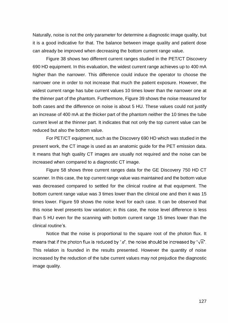
127

Naturally, noise is not the only parameter for determine a diagnostic image quality, but

it is a good indicative for that. The balance between image quality and patient dose

can already be improved when decreasing the bottom current range value.

Figure 38 shows two different current ranges studied in the PET/CT Discovery

690 HD equipment. In this evaluation, the widest current range achieves up to 400 mA

higher than the narrower. This difference could induce the operator to choose the

narrower one in order to not increase that much the patient exposure. However, the

widest current range has tube current values 10 times lower than the narrower one at

the thinner part of the phantom. Furthermore, Figure 39 shows the noise measured for

both cases and the difference on noise is about 5 HU. These values could not justify

an increase of 400 mA at the thicker part of the phantom neither the 10 times the tube

current level at the thinner part. It indicates that not only the top current value can be

reduced but also the bottom value.

For PET/CT equipment, such as the Discovery 690 HD which was studied in the

present work, the CT image is used as an anatomic guide for the PET emission data.

It means that high quality CT images are usually not required and the noise can be

increased when compared to a diagnostic CT image.

Figure 58 shows three current ranges data for the GE Discovery 750 HD CT

scanner. In this case, the top current range value was maintained and the bottom value

was decreased compared to settled for the clinical routine at that equipment. The

bottom current range value was 3 times lower than the clinical one and then it was 15

times lower. Figure 59 shows the noise level for each case. It can be observed that

this noise level presents low variation; in this case, the noise level difference is less

than 5 HU even for the scanning with bottom current range 15 times lower than the

clinical routine .

Notice that the noise is proportional to the square root of the photon flux. It

This relation is founded in the results presented. However the quantity of noise

increased by the reduction of the tube current values may not prejudice the diagnostic

image quality.

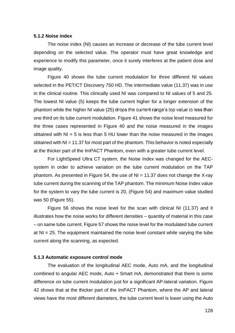
128

5.1.2 Noise indexThe noise index (NI) causes an increase or decrease of the tube current level

depending on the selected value. The operator must have great knowledge and

experience to modify this parameter, once it surely interferes at the patient dose and

image quality.

Figure 40 shows the tube current modulation for three different NI values

selected in the PET/CT Discovery 750 HD. The intermediate value (11.37) was in use

in the clinical routine. This clinically used NI was compared to NI values of 5 and 25.

The lowest NI value (5) keeps the tube current higher for a longer extension of the

phantom while the higher NI value (25)

one third on its tube current modulation. Figure 41 shows the noise level measured for

the three cases represented in Figure 40 and the noise measured in the images

obtained with NI = 5 is less than 5 HU lower than the noise measured in the images

obtained with NI = 11.37 for most part of the phantom. This behavior is noted especially

at the thicker part of the ImPACT Phantom, even with a greater tube current level.

For LightSpeed Ultra CT system, the Noise Index was changed for the AEC-

system in order to achieve variation on the tube current modulation on the TAP

phantom. As presented in Figure 54, the use of NI = 11.37 does not change the X-ray

tube current during the scanning of the TAP phantom. The minimum Noise Index value

for the system to vary the tube current is 20, (Figure 54) and maximum value studied

was 50 (Figure 55).

Figure 56 shows the noise level for the scan with clinical NI (11.37) and it

illustrates how the noise works for different densities quantity of material in this case

on same tube current. Figure 57 shows the noise level for the modulated tube current

at NI = 25. The equipment maintained the noise level constant while varying the tube

current along the scanning, as expected.

5.1.3 Automatic exposure control modeThe evaluation of the longitudinal AEC mode, Auto mA, and the longitudinal

combined to angular AEC mode, Auto + Smart mA, demonstrated that there is some

difference on tube current modulation just for a significant AP-lateral variation. Figure

42 shows that at the thicker part of the ImPACT Phantom, where the AP and lateral

views have the most different diameters, the tube current level is lower using the Auto

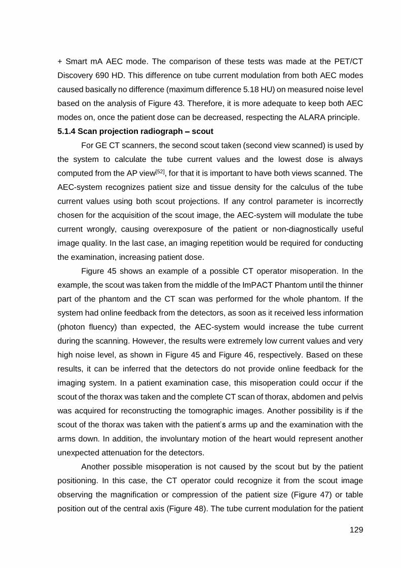
129

+ Smart mA AEC mode. The comparison of these tests was made at the PET/CT

Discovery 690 HD. This difference on tube current modulation from both AEC modes

caused basically no difference (maximum difference 5.18 HU) on measured noise level

based on the analysis of Figure 43. Therefore, it is more adequate to keep both AEC

modes on, once the patient dose can be decreased, respecting the ALARA principle.

5.1.4 Scan projection radiograph scoutFor GE CT scanners, the second scout taken (second view scanned) is used by

the system to calculate the tube current values and the lowest dose is always

computed from the AP view[52], for that it is important to have both views scanned. The

AEC-system recognizes patient size and tissue density for the calculus of the tube

current values using both scout projections. If any control parameter is incorrectly

chosen for the acquisition of the scout image, the AEC-system will modulate the tube

current wrongly, causing overexposure of the patient or non-diagnostically useful

image quality. In the last case, an imaging repetition would be required for conducting

the examination, increasing patient dose.

Figure 45 shows an example of a possible CT operator misoperation. In the

example, the scout was taken from the middle of the ImPACT Phantom until the thinner

part of the phantom and the CT scan was performed for the whole phantom. If the

system had online feedback from the detectors, as soon as it received less information

(photon fluency) than expected, the AEC-system would increase the tube current

during the scanning. However, the results were extremely low current values and very

high noise level, as shown in Figure 45 and Figure 46, respectively. Based on these

results, it can be inferred that the detectors do not provide online feedback for the

imaging system. In a patient examination case, this misoperation could occur if the

scout of the thorax was taken and the complete CT scan of thorax, abdomen and pelvis

was acquired for reconstructing the tomographic images. Another possibility is if the

scout of the thorax was taken with the patient arms up and the examination with the

arms down. In addition, the involuntary motion of the heart would represent another

unexpected attenuation for the detectors.

Another possible misoperation is not caused by the scout but by the patient

positioning. In this case, the CT operator could recognize it from the scout image

observing the magnification or compression of the patient size (Figure 47) or table

position out of the central axis (Figure 48). The tube current modulation for the patient

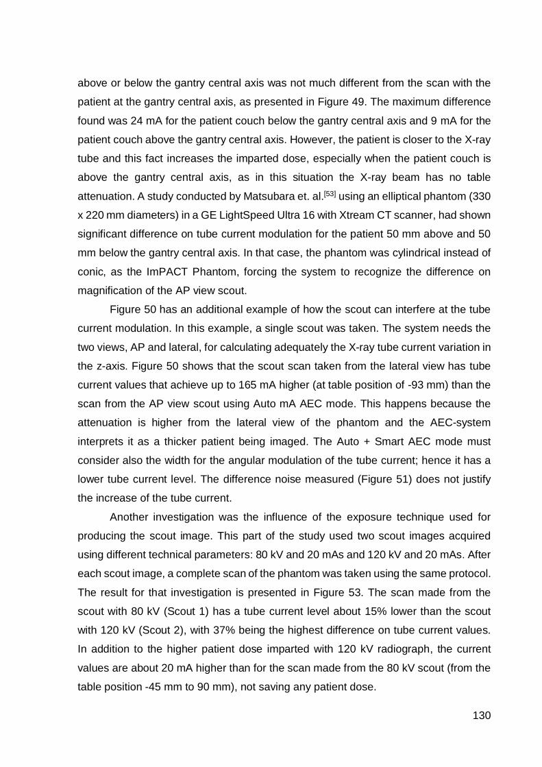
130

above or below the gantry central axis was not much different from the scan with the

patient at the gantry central axis, as presented in Figure 49. The maximum difference

found was 24 mA for the patient couch below the gantry central axis and 9 mA for the

patient couch above the gantry central axis. However, the patient is closer to the X-ray

tube and this fact increases the imparted dose, especially when the patient couch is

above the gantry central axis, as in this situation the X-ray beam has no table

attenuation. A study conducted by Matsubara et. al.[53] using an elliptical phantom (330

x 220 mm diameters) in a GE LightSpeed Ultra 16 with Xtream CT scanner, had shown

significant difference on tube current modulation for the patient 50 mm above and 50

mm below the gantry central axis. In that case, the phantom was cylindrical instead of

conic, as the ImPACT Phantom, forcing the system to recognize the difference on

magnification of the AP view scout.

Figure 50 has an additional example of how the scout can interfere at the tube

current modulation. In this example, a single scout was taken. The system needs the

two views, AP and lateral, for calculating adequately the X-ray tube current variation in

the z-axis. Figure 50 shows that the scout scan taken from the lateral view has tube

current values that achieve up to 165 mA higher (at table position of -93 mm) than the

scan from the AP view scout using Auto mA AEC mode. This happens because the

attenuation is higher from the lateral view of the phantom and the AEC-system

interprets it as a thicker patient being imaged. The Auto + Smart AEC mode must

consider also the width for the angular modulation of the tube current; hence it has a

lower tube current level. The difference noise measured (Figure 51) does not justify

the increase of the tube current.

Another investigation was the influence of the exposure technique used for

producing the scout image. This part of the study used two scout images acquired

using different technical parameters: 80 kV and 20 mAs and 120 kV and 20 mAs. After

each scout image, a complete scan of the phantom was taken using the same protocol.

The result for that investigation is presented in Figure 53. The scan made from the

scout with 80 kV (Scout 1) has a tube current level about 15% lower than the scout

with 120 kV (Scout 2), with 37% being the highest difference on tube current values.

In addition to the higher patient dose imparted with 120 kV radiograph, the current

values are about 20 mA higher than for the scan made from the 80 kV scout (from the

table position -45 mm to 90 mm), not saving any patient dose.

131

5.1.5 Scan field of viewThe field of measurement, scan field of view (S-FOV) for GE, is nominally equal

to the diameter of the primary X-ray beam in axial plane at gantry central axis[54]. In the

CT scanner user interface, the indicated CTDIvol changes for a fixed protocol and

different S-FOVs. The study showed in Table 18, which was conducted in the PET/CT

Discovery 690 HD using the 160 mm (adult head simulator) and the 320 mm (adult

body simulator) CTDI Phantom, demonstrated no variation on calculated CTDIvol for a

fixed protocol and different S-FOVs.

The AEC-system, on the other hand, uses the complete protocol information to

determine the tube current modulation. Figure 52 and Figure 60 show the resulted tube

current modulation for this study for LightSpeed Ultra and GE Discovery 750 HD,

respectively. In Figure 52 the tube current is about 7% lower for head S-FOV compared

to large body S-FOV and about 17% lower for the small body S-FOV compared to large

body S-FOV. Nevertheless the noise measured varied about 5 HU and 2 HU, according

to Figure 53 and Figure 61, respectively. An inconvenient of choosing a smaller S-FOV

is that the equipment can restrict the display field of view (D-FOV) and, by

consequence, the CT image loses the edges of the imaging object.

5.1.6 Evaluation of z-axis dose profile of GE CT scannersFigure 90 to Figure 92 show the impact of noise index (NI) on patient dose in

LightSpeed Ultra CT scanner. Figure 103 shows the central z-axis dose distribution

obtained using the TAP phantom for three different NI values, and also for a fixed X-

ray tube current (Figure 93).

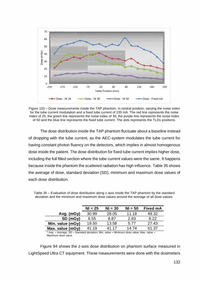
132

Figure 103 Dose measurements inside the TAP phantom, in central position, varying the noise indexfor the tube current modulation and a fixed tube current of 235 mA. The red line represents the noiseindex of 25, the green line represents the noise index of 30, the purple line represents the noise index

of 50 and the blue line represents the fixed tube current. The dots represents the TLDs positions.

The dose distribution inside the TAP phantom fluctuate about a baseline instead

of dropping with the tube current, as the AEC-system modulates the tube current for

having constant photon fluency on the detectors, which implies in almost homogenous

dose inside the patient. The dose distribution for fixed tube current implies higher dose,

including the full filled section where the tube current values were the same. It happens

because inside the phantom the scattered radiation has high influence. Table 35 shows

the average of dose, standard deviation (SD), minimum and maximum dose values of

each dose distribution.

Table 35 Evaluation of dose distribution along z-axis inside the TAP phantom by the standarddeviation and the minimum and maximum dose values around the average of all dose values.

NI = 25 NI = 30 NI = 50 Fixed mAAvg. (mGy) 30.99 28.05 11.18 49.32

SD (mGy) 6.55 8.87 2.83 8.22Min. value (mGy) 19.50 13.58 5.77 27.43Max. value (mGy) 41.19 41.17 14.74 61.37* Avg. Average; SD Standard deviation; Min. value Minimum dose value; Max. valueMaximum dose value.

Figure 94 shows the z-axis dose distribution on phantom surface measured in

LightSpeed Ultra CT equipment. These measurements were done with the dosimeters

0

10

20

30

40

50

60

70

-220 -170 -120 -70 -20 30 80 130 180 230Table Position (mm)

Dose - NI 25 Dose - NI 30 Dose - NI 50 Dose - Fixed mA

133

on the AP and lateral sides of the ImPACT Phantom and they are influenced by two

system constraints: the modulation of the tube current and the X-ray tube rotation. It

results on higher doses at thicker part of the phantom, because of the proximity of the

X-ray tube and the higher tube current values, and a sinusoidal behavior along the

scan length by the attenuation of the imaging object depending on the tube position.

The scan showed at Figure 94 was taken using the Auto mA AEC mode and an

intermediate noise index value (11.37) in the GE LightSpeed Ultra CT scanner. As this

equipment does not have Auto + Smart mA AEC mode, these two AEC operation

modes could not be compared. Figure 95 shows the dose for the Auto + Smart mA

AEC mode in the Discovery 750 HD but with a different current range.

Figure 95 and Figure 96 show the dose for two different S-FOV scans. For this

analysis, Figure 60 must be considered and it shows that Small Body S-FOV has a

difference about 20% on the tube current modulation with lower tube current values.

However, Figure 104 shows that the dose for the Large Body S-FOV scan is lower at

the thicker part until the middle of the phantom. It can happen because there is no

significant difference on tube current values (22% being the highest different value),

so the X-ray tube must have irradiated directly the dosimeters on Small Body S-FOV

scan and, for the Large Body S-FOV scan, the radiation must have been attenuated

for the dosimeters positioned at the opposite side of the phantom.

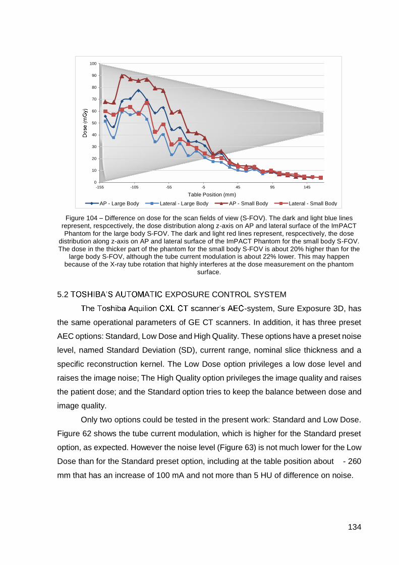
134

Figure 104 Difference on dose for the scan fields of view (S-FOV). The dark and light blue linesrepresent, respcectively, the dose distribution along z-axis on AP and lateral surface of the ImPACTPhantom for the large body S-FOV. The dark and light red lines represent, respcectively, the dose

distribution along z-axis on AP and lateral surface of the ImPACT Phantom for the small body S-FOV.The dose in the thicker part of the phantom for the small body S-FOV is about 20% higher than for the

large body S-FOV, although the tube current modulation is about 22% lower. This may happenbecause of the X-ray tube rotation that highly interferes at the dose measurement on the phantom

surface.

5.2 EXPOSURE CONTROL SYSTEM

-system, Sure Exposure 3D, has

the same operational parameters of GE CT scanners. In addition, it has three preset

AEC options: Standard, Low Dose and High Quality. These options have a preset noise

level, named Standard Deviation (SD), current range, nominal slice thickness and a

specific reconstruction kernel. The Low Dose option privileges a low dose level and

raises the image noise; The High Quality option privileges the image quality and raises

the patient dose; and the Standard option tries to keep the balance between dose and

image quality.

Only two options could be tested in the present work: Standard and Low Dose.

Figure 62 shows the tube current modulation, which is higher for the Standard preset

option, as expected. However the noise level (Figure 63) is not much lower for the Low

Dose than for the Standard preset option, including at the table position about - 260

mm that has an increase of 100 mA and not more than 5 HU of difference on noise.

0

10

20

30

40

50

60

70

80

90

100

-155 -105 -55 -5 45 95 145

Table Position (mm)

AP - Large Body Lateral - Large Body AP - Small Body Lateral - Small Body

135

5.3 XPOSURE CONTROL SYSTEM

AEC-system does not have current range nor noise level

options. The Philips AEC-system works with a reference 330 mm patient size§ and

uses the scan projection radiograph, named surview, to compare the absorption

coefficient of the patient to be scanned with the reference one, and then calculates an

optimal mAs/slice that will keep the noise constant for the whole scan length[43,55]. The

first surview scanned is the one used for this comparison, no matter if two views were

scanned**.

5.3.1 AEC ModeFirst issue to be discussed is the difference of Z-DOM and D-DOM AEC modes.

Z-DOM is extremely sensitive to patient thickness while D-DOM keeps the tube current

almost constant except for the sinusoidal behavior, which is a consequence of the

different attenuation on both views (AP and lateral) of the imaging object during the

rotation. Moreover, for D-DOM the higher tube current values appear at the thinner

part of the phantom. Wood[56] and Sookpeng[57] published studies about AEC-systems

in Philips CT scanners and they have shown similar behavior for D-DOM. These

authors conclude that this AEC mode should not be selected.

5.3.1.1 Z-DOM AEC mode

The longitudinal tube current modulation, Z-DOM, varies the tube current based

on the current-time product per slice indicated after the surview. This AEC mode must

not increase the current-time product beyond the mAs/slice settled in the protocol

parameters and also not decrease more than 70% of that value [55]. The Z-DOM AEC

mode is only available when the DoseRight ACS option is ON before the surview is

made and it can work with the DoseRight ACS option ON and OFF after the surview.

The Philips Clinical Guide about Z-DOM defines that the use of this option in

association with the DoseRight ACS option results in a maximum dose saving[55].

However Figure 64 and Figure 66 show that the DoseRight ACS option ON causes a

great increase on tube current, with an image noise consequently lower (Figure 65).

§Philips does not specify this patient size.**Personal communication from Philips CT application specialist, 4 May 2014.

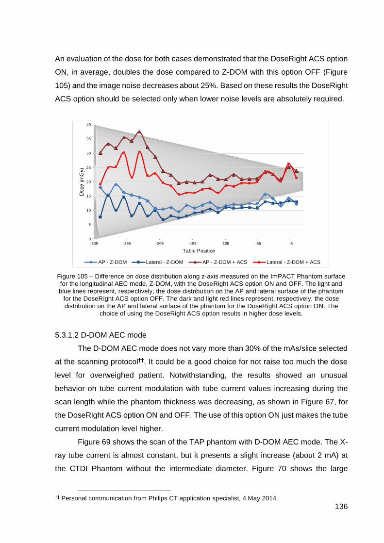
136

An evaluation of the dose for both cases demonstrated that the DoseRight ACS option

ON, in average, doubles the dose compared to Z-DOM with this option OFF (Figure

105) and the image noise decreases about 25%. Based on these results the DoseRight

ACS option should be selected only when lower noise levels are absolutely required.

Figure 105 Difference on dose distribution along z-axis measured on the ImPACT Phantom surfacefor the longitudinal AEC mode, Z-DOM, with the DoseRight ACS option ON and OFF. The light andblue lines represent, respectively, the dose distribution on the AP and lateral surface of the phantom

for the DoseRight ACS option OFF. The dark and light red lines represent, respectively, the dosedistribution on the AP and lateral surface of the phantom for the DoseRight ACS option ON. The

choice of using the DoseRight ACS option results in higher dose levels.

5.3.1.2 D-DOM AEC mode

The D-DOM AEC mode does not vary more than 30% of the mAs/slice selected

at the scanning protocol . It could be a good choice for not raise too much the dose

level for overweighed patient. Notwithstanding, the results showed an unusual

behavior on tube current modulation with tube current values increasing during the

scan length while the phantom thickness was decreasing, as shown in Figure 67, for

the DoseRight ACS option ON and OFF. The use of this option ON just makes the tube

current modulation level higher.

Figure 69 shows the scan of the TAP phantom with D-DOM AEC mode. The X-

ray tube current is almost constant, but it presents a slight increase (about 2 mA) at

the CTDI Phantom without the intermediate diameter. Figure 70 shows the large

Personal communication from Philips CT application specialist, 4 May 2014.

0

5

10

15

20

25

30

35

40

-305 -255 -205 -155 -105 -55 -5

Table Position

AP - Z-DOM Lateral - Z-DOM AP - Z-DOM + ACS Lateral - Z-DOM + ACS

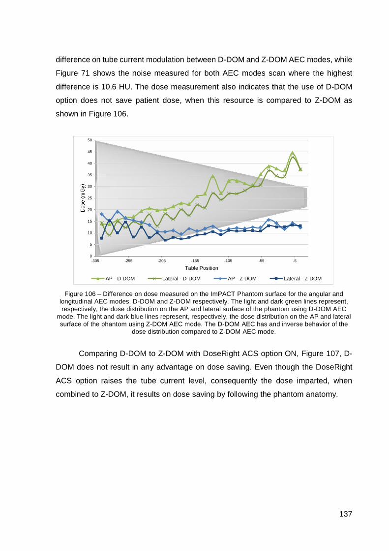
137

difference on tube current modulation between D-DOM and Z-DOM AEC modes, while

Figure 71 shows the noise measured for both AEC modes scan where the highest

difference is 10.6 HU. The dose measurement also indicates that the use of D-DOM

option does not save patient dose, when this resource is compared to Z-DOM as

shown in Figure 106.

Figure 106 Difference on dose measured on the ImPACT Phantom surface for the angular andlongitudinal AEC modes, D-DOM and Z-DOM respectively. The light and dark green lines represent,respectively, the dose distribution on the AP and lateral surface of the phantom using D-DOM AEC

mode. The light and dark blue lines represent, respectively, the dose distribution on the AP and lateralsurface of the phantom using Z-DOM AEC mode. The D-DOM AEC has and inverse behavior of the

dose distribution compared to Z-DOM AEC mode.

Comparing D-DOM to Z-DOM with DoseRight ACS option ON, Figure 107, D-

DOM does not result in any advantage on dose saving. Even though the DoseRight

ACS option raises the tube current level, consequently the dose imparted, when

combined to Z-DOM, it results on dose saving by following the phantom anatomy.

0

5

10

15

20

25

30

35

40

45

50

-305 -255 -205 -155 -105 -55 -5

Table Position

AP - D-DOM Lateral - D-DOM AP - Z-DOM Lateral - Z-DOM

138

Figure 107 Difference on dose measured on the ImPACT Phantom surface for the angularAEC mode, D-DOM, with DoseRight ACS option OFF and the longitufinal AEC mode, Z-

DOM, with DoseRight ACS option ON. The light and dark green lines represent, respectively, the dosedistribution on the AP and lateral surface of the phantom using D-DOM AEC mode. The light and darkpurple lines represent, respectively, the dose distribution on the AP and lateral surface of the phantomusing Z-DOM AEC mode with DoseRight ACS. The D-DOM AEC mode has the same dose level of the

Z-DOM with DoseRight ACS option. However, the dose distribution of Z-DOM with DoseRight ACSfollows the expected behavior, i.e. the lower dose level is at the thinner part of the phantom.

Figure 108 shows D-DOM compared to a fixed mAs/slice scan. D-DOM

decreases the dose of about 15% while it raises the noise of about 20% as Figure 109

shows. Figure 110 shows D-DOM with DoseRight ACS option ON and OFF. The tube

current modulation for both situations are similar and have an unexpected distribution

along z-axis. The DoseRight ACS option, again, results in higher dose level; especially

for the measurement on the AP phantom surface, where the dose becomes more than

20 mGy higher at the thinner part of the phantom.

0

5

10

15

20

25

30

35

40

45

50

-305 -255 -205 -155 -105 -55 -5

Table PositionAP - D-DOM AP - Z-DOM + DoseRight ACSLateral - D-DOM Lateral - Z-DOM + DoseRight ACS

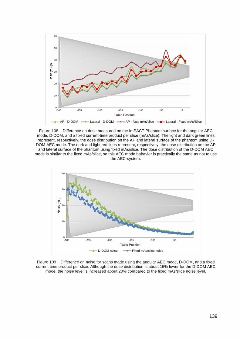
139

Figure 108 Difference on dose measured on the ImPACT Phantom surface for the angular AECmode, D-DOM, and a fixed current-time product per slice (mAs/slice). The light and dark green linesrepresent, respectively, the dose distribution on the AP and lateral surface of the phantom using D-

DOM AEC mode. The dark and light red lines represent, respectively, the dose distribution on the APand lateral surface of the phantom using fixed mAs/slice. The dose distribution of the D-DOM AEC

mode is similar to the fixed mAs/slice, so this AEC mode bahavior is practically the same as not to usethe AEC-system.

Figure 109 Difference on noise for scans made using the angular AEC mode, D-DOM, and a fixedcurrent time product per slice. Although the dose distribution is about 15% lower for the D-DOM AEC

mode, the noise level is increased about 20% compared to the fixed mAs/slice noise level.

0

10

20

30

40

50

60

-305 -255 -205 -155 -105 -55 -5

Table Position

AP - D-DOM Lateral - D-DOM AP - fixes mAs/slice Lateral - Fixed mAs/Slice

0

10

20

30

40

-305 -255 -205 -155 -105 -55

Table Position

D-DOM noise Fixed mAs/slice noise

140

Figure 110 Difference on dose measured on the ImPACT Phantom surface for the angular AECmode, D-DOM, with DoseRight ACS option ON and OFF. The light and dark green lines represent,respectively, the dose distribution on the AP and lateral surface of the phantom with the DoseRight

ACS option OFF. The light and dark orange lines represent, respectively, the dose distribution on theAP and lateral surface of the phantom with the DoseRight ACS option ON. Both measurements

presented an unexpected behavior, i.e. raising dose at the thinner part of the phantom. The DoseRightoption ON imparts higher dose, raising the dose more than 20 mGy at the thinner part of the

phantom.

5.3.2 CollimationFigure 73 shows the tube current modulation for two different collimations using

D-DOM AEC mode. The smaller collimation selected does not allow DoseRight ACS

option to be selected; consequently it does enable Z-DOM AEC mode. The difference

on tube current modulation for both collimations is not significant: the tube current

values for the smaller collimation (16 x 0.75 mm) are about only 2% higher than for

larger collimation (16 x 1.5 mm). It probably happens because the geometry efficiency

is lost when small collimations are employed.

5.3.3 Patient couch orientationFigure 78 shows the difference on tube current modulation for patient couch

orientation using the angular AEC mode, D-DOM. The scan made with the ImPACT

Phantom getting in the gantry aperture presents higher current values along the

phantom scan and it is highly decreased at the end of the thicker part of the phantom

(70 mA lower than the opposite scan direction). It must happen because the AEC-

system calculates the tube current modulation for an increasing thickness, so the

system raises the tube current values to not increase the noise. Scans with Z-DOM

AEC mode must be made to complement this study.

0

10

20

30

40

50

60

70

80

90

-305 -255 -205 -155 -105 -55 -5

Table PositionAP - D-DOM Lateral - D-DOM AP - D-DOM + ACS Lateral - D-DOM + ACS

141

5.3.4 Current-time product per sliceThe AEC-system for Philips CT scanner selects a current-time product per slice

(mAs/slice) after the surview, based on the attenuation coefficient of the patient

reference. This mAs/slice value can be pre-

selected while in protocol management or the user can type a value. This current-time

product per slice is the reference for the AEC-system to calculate the tube current

modulation. It can result in much higher doses if the selected value is too high. Figure

75 shows this difference on tube current modulation for two current-time product

values. The increase of the tube current modulation for the 400 mAs/slice is similar to

the observed for Z-DOM with DoseRight ACS for 250 mAs/slice (Figura 64).

5.3.5 Scan projection radiograph surviewThe scan projection radiograph, surview for Philips, is the patient reference

image -system to calculate the tube current modulation for

the examination. For Philips systems, this image will be compared to a reference image

of a 330 mm patient for an ideal image quality, pre-programmed at the equipment. For

the DoseRight ACS option, the patient surview will be compared to the 330 mm patient

reference image. This option then doubles the current-

50 mm above their patient reference size or it cuts in half the current-time product in

reference size. The DoseRight ACS

uses 98% of the maximum body diameter scanned at the surview to calculate the

increase or decrease of the current-time product[43].

Figure 77 shows the tube current modulation of scans with AP and lateral

surview for D-DOM AEC mode. It indicates no sensitivity of D-DOM on different single

surview views. Figure 76 shows that the single lateral or AP surview does not interfere

much on the tube current modulation for Z-DOM AEC mode. However, for Z-DOM with

the DoseRight ACS option ON the tube current modulation is highly affected.

Considering the DoseRight ACS operating mode, AP view is larger than lateral view

considering width but the lateral view is much thicker. Figure 111 and Figure 112 show

the width and the thickness measurement, with the distance tool and region of interest

(ROI) selected to calculate the mean CT number value. The width is longer for the

AP view (Figure 111) and the mean CT number is higher for the lateral view, which

The width and the CT number were measured using the JiveX® DICOM viewer.

142

means more attenuation. The higher tube current level for the scan made from lateral

surview denotes that Philips AEC-system is very sensitive to tissue density (higher CT

number) or, in this case, quantity of material.

Figure 111 Surview taken from the AP view of the ImPACT Phantom. The width measured,380.1 mm, is 50 mm larger than the Philips patient of reference of 330 mm. The average signal

measured, 682.43 HU, represents the CT number of the image; taking this value and the Hounsfieldscale into account, the AEC-system calculates the tube current modulation based on density.

Figure 112 Surview taken from the lateral view of the ImPACT Phantom. The width measured,260.3 mm, is 70 mm narrower than the Philips patient of reference of 330 mm. The average signal

measured, 1509.14 HU, represents the CT number of the image; taking this value and the Hounsfieldscale into account, the AEC-system calculates the tube current modulation based on density.

5.3.6 AEC response over timeThe reproducibility of a CT scanner can be evaluated over time with the

application of quality assurance programs, including dose evaluation. This evaluation

consists in measure and calculate the CTDI100, CTDIw and CTDIvol and to interpret their

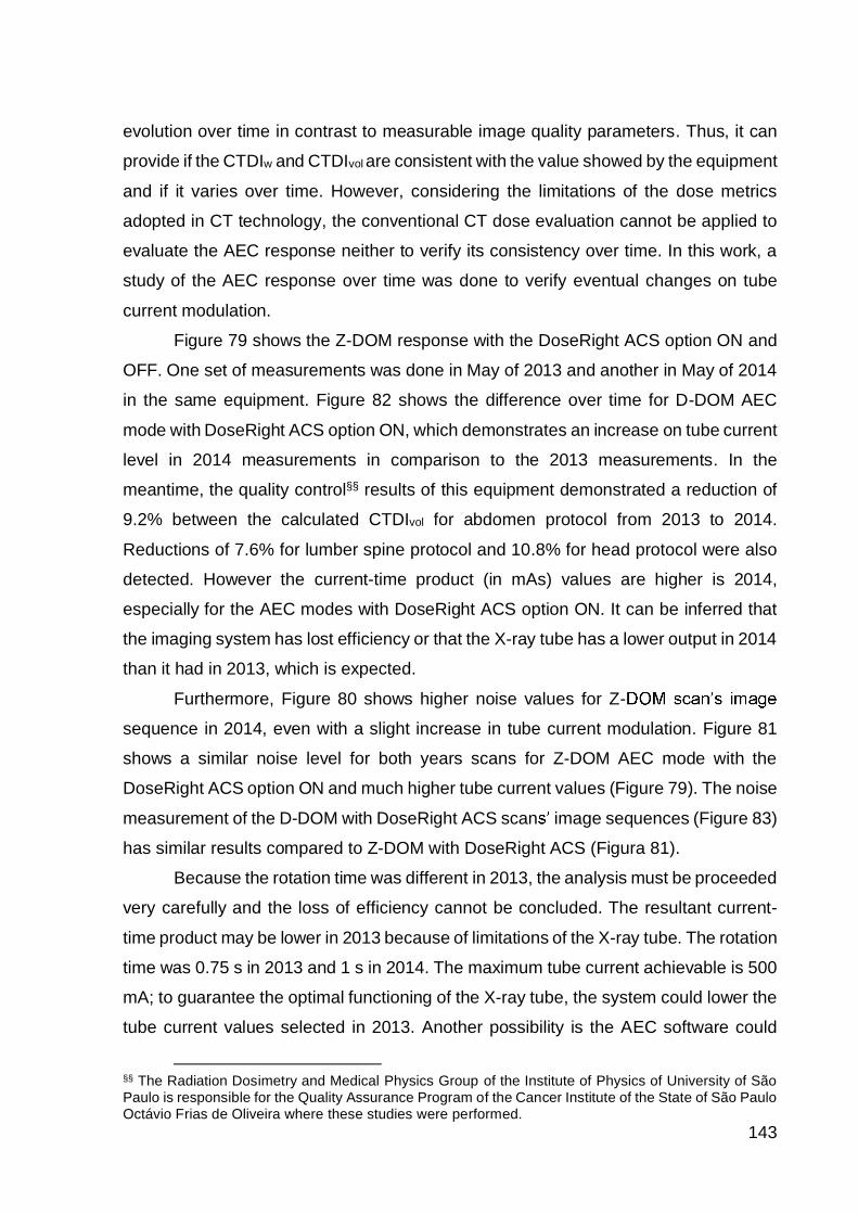
143

evolution over time in contrast to measurable image quality parameters. Thus, it can

provide if the CTDIw and CTDIvol are consistent with the value showed by the equipment

and if it varies over time. However, considering the limitations of the dose metrics

adopted in CT technology, the conventional CT dose evaluation cannot be applied to

evaluate the AEC response neither to verify its consistency over time. In this work, a

study of the AEC response over time was done to verify eventual changes on tube

current modulation.

Figure 79 shows the Z-DOM response with the DoseRight ACS option ON and

OFF. One set of measurements was done in May of 2013 and another in May of 2014

in the same equipment. Figure 82 shows the difference over time for D-DOM AEC

mode with DoseRight ACS option ON, which demonstrates an increase on tube current

level in 2014 measurements in comparison to the 2013 measurements. In the

meantime, the quality control§§ results of this equipment demonstrated a reduction of

9.2% between the calculated CTDIvol for abdomen protocol from 2013 to 2014.

Reductions of 7.6% for lumber spine protocol and 10.8% for head protocol were also

detected. However the current-time product (in mAs) values are higher is 2014,

especially for the AEC modes with DoseRight ACS option ON. It can be inferred that

the imaging system has lost efficiency or that the X-ray tube has a lower output in 2014

than it had in 2013, which is expected.

Furthermore, Figure 80 shows higher noise values for Z-

sequence in 2014, even with a slight increase in tube current modulation. Figure 81

shows a similar noise level for both years scans for Z-DOM AEC mode with the

DoseRight ACS option ON and much higher tube current values (Figure 79). The noise

measurement of the D-DOM with DoseRight ACS scan image sequences (Figure 83)

has similar results compared to Z-DOM with DoseRight ACS (Figura 81).

Because the rotation time was different in 2013, the analysis must be proceeded

very carefully and the loss of efficiency cannot be concluded. The resultant current-

time product may be lower in 2013 because of limitations of the X-ray tube. The rotation

time was 0.75 s in 2013 and 1 s in 2014. The maximum tube current achievable is 500

mA; to guarantee the optimal functioning of the X-ray tube, the system could lower the

tube current values selected in 2013. Another possibility is the AEC software could

§§ The Radiation Dosimetry and Medical Physics Group of the Institute of Physics of University of SãoPaulo is responsible for the Quality Assurance Program of the Cancer Institute of the State of São PauloOctávio Frias de Oliveira where these studies were performed.

144

have been upgraded and the calculus for the tube current modulation has been

changed in 2014. The software version listed in the DICOM header (tag 0018,1020) is

the same for both cases.

145

6 GENERAL DISCUSSION AND FUTURE ISSUES

During the conduction of the present work, it was observed that the comparison

of equipment -

system is not a simple task. GE and Toshiba have similar AEC parameters available

for the user to choose, and the AEC responses on tube current modulation and noise

level are very similar. Philips, on the other hand, works with the current-time product

per slice (mAs/slice), separate AEC modes (longitudinal and angular) and has an

option to compose the tube current modulation calculus.

Despite of any difference on operational parameters, every AEC-system must

vary the tube current based on the scan projection radiograph (SPR) attenuation

information, show an option of tube current or current-time product and show the AEC

modes options.

The distinctions between Philips and GE are exactly on these parameters:

Philips is more sensitive to thickness than GE:

o an example is the TAP phantom scans, in which -system

varied the tube current with clinical operational parameters, while

AEC-system only varied the tube current if very high image noise was

allowed (higher noise index values);

Philips uses a reference of mAs/slice while GE uses X-ray tube current range;

o The current range option provides a better control of the tube current

modulation, but it makes the equipment susceptible to higher tube

current values on tube current modulation than the reference mAs/slice;

GE combines the longitudinal to angular AEC modes while in Philips they work

only separately;

o In addition, the Philip response.

In the present work, the automatic exposure control (AEC) systems from three

of the leading manufacturers in Brazil were tested to evaluate their functioning and

susceptibilities. The evaluation was made through the tube current modulation curve,

the image noise and the dose imparted from computed tomography (CT) scanning,

using tube current modulation compared to fixed tube current, with a methodology

different from the one used in conventional CT dosimetry.

146

The results confirmed that the variation of the tube current during the exposure

can reduce the patient dose without compromise the image quality. In addition, the

most important issue, the results reached in this work give the opportunity to optimize

the patient dose in the facilities where the studies were developed. The possible

optimizations, for example, can be on setting a wider range of tube current modulation

sing angular AEC mode

Another possible application AEC-

analysis on tube current modulation over time can support an evaluation of the imaging

system, X-ray tube and detectors, over time. The measured CTDIvol is insufficient to

analyze the modern CT scanners, so the AEC-system response evaluation over time

can indicate a loss of efficiency of the X-ray tube or detectors, by the need of higher

tube current level for the same protocol configuration and exposure geometry.

The new phantom configuration proposed in this work, the TAP phantom,

suggests that the dose inside the patient is about constant when the adequate tube

current modulation is reached, consequently the photon fluency in the detectors must

follow this behavior. It has also shown to be a good support in the AEC-systems

evaluation for the ImPACT Phantom as it appraises deeply the attenuation sensitivity

of these systems.

For future investigation, a comparison among patient examinations,

anthropomorphic phantom and both phantom configurations employed in this work can

be done to complement the present results. Patient doses could also be estimated

from the dose measurements made when comparing the AEC response for both

phantom and patient, and also by using Monte Carlo approaches. This kind of

investigation can also support improvements in research area of dose profile equations

determination using tube current modulation[58], which is a very innovative way to

determine dose saving methods and calculate the geometric efficiency in CT systems.

147

REFERENCES

1 INTERNATIONAL COMMISSION ON RADIOLOGICAL PROTECTION, ICRP. Managing PatientDose in Computed Tomography. Ann. ICRP 30 (4), 2000. (ICRP publication 87)

2 JÓNÍNA GUÐJÓNSDÓTTIR, BORGNY WEEN, DAG RUNE OLSEN. Optimal Use of AEC in CT: ALiterature Review. Radiologic Technology, v. 81, n. 4, p. 309-317, 2010.

3 Tamm, E. P.; Rong X. J.; Cody D. D.; Ernst, R. D.; Fitzgerald, N. E.; Kundra V. CT Radiation DoseReduction How to Implement Change without Sacrificing Diagnostic Quality. RadioGraphics, v. 31, p.1823-1832, 2011. Available at: <http://www.ncbi.nlm.nih.gov/pubmed/21969662>. Access: Jun 2014.

4 Bankler, A. A.; Kressel, H. Y. Through the looking Glass revisited: The Need for More Meaning andLess Drama in the Reporting of Dose and Dose Reduction in CT. Radiology, v. 265, n. 1, p. 4-8, 2012.

5 Smith-Bindman, R; Miglioretti, D. L. CTDIvol, DLP, and effective dose are excellent measures for usein CT quality improvement. Radiology, v. 261, n. 3, p. 999, 2011.

6 INTERNATIONAL COMISSION ON RADIOLOGICAL PROTECTION, ICRP. Managing Patient Dosein Multi-Detector Computed Tomography (MDCT). Ann. ICRP 37 (1), 2007. (ICRP publication 102)

7 Gomà C.; Ruiz; A., Jornet, N.; Latorre A.; Pallerol, R. M; Carrasco, P.; Eudaldo, T.; Ribas, M. Radiationdose assessment in a 320-detector-row CT scanner used in cardiac imaging. Medical Physics, v. 38,n. 3, p. 1473-1480, 2011.

8 Hsieh, J. Computed tomography: principles, design, artifacts, and recent advances. 2nd ed.SPIE, Washington, 2009.

9 Dose Management Tools:Overview of Available Options. RadioGraphics, v. 26, p. 503-512, 2006.

10 Brisse HJ, Madec L, Gaboriaud G, Lemoine T, Savignoni A, Neuenschwander S, AubertB, Rosenwald JC. Automatic exposure control in multichannel CT with tube current modulation toachieve a constant level of image noise: experimental assessment on pediatric phantoms. MedicalPhysics, v. 34, n. 7, p. 18-33. July 2007.

11 NATIONAL ELECTRICAL MANUFACTURERS ASSOCIATION, NEMA. DICOM STANDARD.Available at: <http://medical.nema.org/standard.html>. Last time accessed: June 2014.

12 Kallender, W. A. Computed Tomography. Fundamentals, system technology, image quality,applications. 3rd ed., Publicis Publishing, Erlagen, 2011.

13 Webb S. From the watching of shadows: the origins of radiological tomography. IOPPublishing, New York, 1990.

14 Goldman, L. W. Principles of CT and CT Technology. Journal of Nuclear Medicine Technology,v. 35, p. 115-128, 2007.

15 J. T. Bushberg, J. A. Seibert, E. M. Leidholdt Jr., J. M. Boone, The Essential Physics of MedicalImaging. Lippincott Williams & Wilkins, 2nd ed., Philadelphia, 2002.

16 MINISTÉRIO DA SAÚDE. Ambiente digital didático para técnico em radiologia. Available at:http://rle.dainf.ct.utfpr.edu.br/hipermidia/. Last access: June 2014.

17 Ulzheimer, S.; Flohr, T. Multislice CT Chapter 1: Current Technology and FutureDevelopments. 3rd ed., Springer, 2009.

148

18 Peter Schardt,a) Josef Deuringer, Jo¨rg Freudenberger, Erich Hell,b) Wolfgang Knüpfer, DetlefMattern, and Markus SchildNew x-ray tube performance in computed tomography by introducing therotating envelope tube technology. Medical Physics, v. 31, n. 9, p. 2699-2706, 2004.

19 Buzug, T. M. Computed Tomography. From Photon Statistics to Modern Cone-Beam CT.Springer, Berlin, 2008.

20 ImPACT. CT Scanner Acceptance Testing. Information Leaflet no.1, version 1.02: London, 2001.

21 Kalender, W. A.; Seissler, W.; Klotz, E.; Vock, P. Spiral volumetric CT with single-breath-holdtechnique continuous transport, and continuous scanner rotation. Radiology, v. 176, n. 1, p. 181-183,1990.

22 Deans, S. R. The Radon Transform and Some of Its Applications. Dover Publications, New York,2007.

23 ZENG, G. L. NOISE-WEIGHTED SPATIAL DOMAIN FBP ALGORITHM. MEDICAL PHYSICS, V.41, N. 5, P. 051906-1-10, 2014.

24 Feldkamp, L. A.; Davis, L. C.; KRESS J. W. PRACTICAL CONE-BEAM ALGORITHM. JOURNALOF OPTICAL SOCIETY OF AMERICA V. 1, N. 6, PP. 612-619 (1984)

25 Costa, P. R.; Araújo, E. C. A. Application of the FDK algorithm for multi-slice tomographic imagereconstruction Revista Brasileira de Engenharia Biomédica, v.26, n. 2, p. 105-120, 2010.

26 Platten, David. Multi-slice helical CT physics and technology, ImPACT, London UK, 2003. [onlinedocument]. Available at: http://www.impactscan.org/slides/eanm2002/sld001.htm. Accessed in: June2014.

27 Dendy, P.P.; Heaton, B. Physics for Diagnostic Radiology. 3rd ed, Boca Raton, London, 2011.

28 Marin, D.; Boll, D. T.; Mileto, A; Nelson, R. C. State of the art: dual-energy CT of the abdomen.Radiology, v. 271, n. 2, p. 327-342, 2014.

29 Aichinger, H. Dierker, J; Joite-Barfuß, S.; Säbel, M. Radiation exposure and image quality in X-ray diagnostic radiology. 2 ed., Springer, 2012.

30 Fosbinder, R. A.; Orth, D. Essentials of Radiologic Science. Wolters Kluwer Health and LippincottWilliams & Wilkins. Pennsylvania, 2012.

31 MEDICINE AND HEALTH CARE PRODUCTS REGULATORY AGENCY, MHRA. CT scannerautomatic exposure control systems. London: MHRA, 2005. (MHRA Report 05016)

32 Shope T. B; Gagne, R. M.; Johnson G. C. A method for describing the doses delivered bytransmission x-ray computed tomography. Medical Physics, v. 8, n. 4, p. 488-495, 1981.

33 Kalender, W. A. Dose in x-ray computed tomography. Physics Medicine Biology, v. 53, n. 3, p.129-150, 2014.

34 AMERICAN ASSOCIATION OF PHYSICISTS IN MEDICINE, AAPM. The measurement, reporting,and management of radiation dose in CT. AAPM concil, 2007. (AAPM Report 96)

35 McCollough, C. H.; Leng, S; Yu, L.; Cody, D. D.; Boone, J. M.; McNitt-Gray, M. F. CT Dose Indexand Patient Dose: They Are Not the Same Thing. Radiology, v. 259, n. 2, p. 311-316, 2011

36 Boone, J. M. The trouble with CTDI100. Medicl Physics, v. 34, n. 4, 1364-1371, 2007.

37 Dixon R. L.; Boone, J. M. Cone beam CT dosimetry: A unified and self-consistent approach includingall scan modalities With or without phantom motion. Medical Physics, v. 37, n. 6, p. 2703-2718, 2010.

149

38 Kitagawa, K.; Lardo, A. C; Lima, J. A. C.; George, R. T. Prospective ECG-gated 320 row detectorcomputed tomography: Implications for CT angiography and perfusion imaging. The InternationalJournal of Cardiovascular Imaging, v. 25, p. 201-208, 2009.

39 AMERICAN ASSOCIATION OF PHYSICISTS IN MEDICINE, AAPM. ComprehensiveMethodology for the Evaluation of Radiation Dose in X-Ray Computed Tomography. AAPMcouncil: 2010. (AAPM Report 111)

40 Descamps, C; Gonzalez, M.; Garrigo, E.; Germanier, A.; Venencia, D. Measurements of the dosedelivered during CT exams using AAPM task group Report no. 111. Jornal of Applied Clinical MedicalPhysics, v. 13, p. 293 302, 2012.

41 AXENTE, M.; HRISTOV, D. Imaging dose in variable pitch body perfusion CT scans: An analysisusing TG111 formalism. Medical Physics, v. 41, n. 6, 061912-1-7, 2014)

42 Platten, D. J.; Castellano, I. A.; Chapple, C-L ; Edyvean, S.; Jansen, J. T. M.; Johnson, B.; Lewis, M.A. Radiation dosimetry for wide-beam CT scanners: recommendations of a working party of the Instituteof Physics and Engineering in Medicine. British Institute of Radiology, v. 86, n. 1027, 2013.

43 PHILIPS MEDICAL SYSTEMS Clinical Guide: Automatic DoseRigh ACS [online document], 2008.Available at: <http://clinical.netforum.healthcare.philips.com>. Accessed in: 29 May 2014.

44 IMPACT SCAN. Available at: <http://www.impactscan.org/>. Accessed in: 18 Jun 2014.

45 KALENDER, W.A. Computed Tomography Fundamentals, System Technology, ImageQuality, Applications. 3rd Ed.; Publicis Publishing, Erlangen, Germany, 2011.

46 IMAGEJ® SOFTWARE. Available at: <http://imagej.nih.gov/ij/download.html>. Accessed in: 14 June2014.

47 SCAN HEADER SOFTWARE. Available at: <http://www.medphys.it/down_scan_header.htm>.Accessed in: 29 May 2014.

48 INTERNATIONAL ATOMIC ENERGY AGENCY, IAEA. Dosimetry in Diagnostic Radiology: Aninternational Code of Practice. Viena. 2007. (Technical Report Series nº 457).

49 Grupen, C; Shwartz, B. Particle Detectors. 2nd ed, Cambridge University Press, New York, 2008.

50 OKUNO, E.; YOSHIMURA, E. M. Física das Radiações. 1ª Edição. São Pulo: Oficina de Textos,2010. ISBN 9788579750052.

51 -20. DTU-Nutech, Denmark, 2014.

52 General Electric Company Auto mA/Smart mA Theory [Brochure] available athttp://www.gehealthcare.com/usen/education/tip_app/docs/AutomA-SmartmA%20Theory.pdf, 2008.(accessed: 29 May 2014)

53 Matsubara, k.; Koshida, k.; Ichikawa, K.; Suzuki, M.; Takata, T.; Yamamoto, T.; Matsui, O.Misoperation of CT Automatic Tube Current Modulation Systems with Inappropriate Patient Centering:Phantom Studies. American Journal of Radiology; v. 192: p. 862-865, Apr. 2009.

54 AMERICAN ASSOCIATION OF PHYSICISTS IN MEDICINE. CT Lexicon versio 1.3. [onlinedocument] Available at: http://www.aapm.org/pubs/CTProtocols/. Accessed in: 14 Jun. 2014.

55 Philips Medical Systems Clinical Guide: Z Axis Dose Modulation (Z DOM) [online document],2008. Available at http://clinical.netforum.healthcare.philips.com/us_en/Operate/Application-Tips/CT/Z-Axis-Dose-Modulation-(Z-DOM). Accessed in: 29 May 2014.

56 Wood, T. Optimisation of the Philips automatic exposure control system. IN: THE 14º MEETINGOF THE CT USER GROUP, CTUG, Edinburgh, 2012.

150

57 Sookpeng S., Martin C. J., Gentle D. J. and Lopez-Gonzalez, M. R. Relationships between patientsize, dose and image noise under automatic tube current modulation systems. Journal ofRadiological Protection, v. 34 p. 103-123, Dec 2013.

58 Dixon, R. L.; Boone, J. M. Dose equations for tube current modulation in CT scanning and theinterpretation of the associated CTDIvol. Medical Physics, v. 40, n. 11, p. 111920-1-14, 2013.