AVALIAÇÃO DO COMPROMETIMENTO PULMONAR EM …repositorio.unicamp.br/bitstream/REPOSIP/309671/1/Villalba_Wander... · V711a Avaliação do comprometimento pulmonar em pacientes com

WANDER DE OLIVEIRA VILLALBA

AVALIAÇÃO DO COMPROMETIMENTO PULMONAR

EM PACIENTES COM ESCLERODERMIA POR MEIO

DO TESTE DA CAMINHADA DE SEIS MINUTOS

CAMPINAS

2006

i

ii

WANDER DE OLIVEIRA VILLALBA

AVALIAÇÃO DO COMPROMETIMENTO PULMONAR

EM PACIENTES COM ESCLERODERMIA POR MEIO

DO TESTE DA CAMINHADA DE SEIS MINUTOS

Tese de Doutorado apresentada à Pós-Graduação da

Faculdade de Ciências Médicas da Universidade Estadual

de Campinas para obtenção do título de Doutor em Clínica

Médica, área de concentração em Clínica Médica.

ORIENTADORA: PROFA. DRA. ILMA APARECIDA PASCHOAL

CAMPINAS

2006

iii

FICHA CATALOGRÁFICA ELABORADA PELA BIBLIOTECA DA FACULDADE DE CIÊNCIAS MÉDICAS DA UNICAMP

Bibliotecário: Sandra Lúcia Pereira – CRB-8ª / 6044

Villalba, Wander de Oliveira V711a Avaliação do comprometimento pulmonar em pacientes com

esclerodermia por meio do teste da caminhada de seis minutos / Wander de Oliveira Villalba. Campinas, SP : [s.n.], 2006.

Orientador : Ilma Aparecida Paschoal

Tese ( Doutorado ) Universidade Estadual de Campinas. Faculdade de Ciências Médicas.

1. Taxa de Sobrevida. 2. Exercícios fisicos. 3. Pulmão - . 4.

Variabilidade. 5. Taxa de Sobrevida. 6. Reumatologia. I. Paschoal, Ilma Aparecida. II. Universidade Estadual de Campinas. Faculdade de Ciências Médicas. III. Título.

Título em inglês : Six minute walk test evaluation of pulmonary involvement in scleroderma patients Keywords: • Survival rate • Exercise • Lung • Variability • Rheumathology Área de concentração : Clínica Médica Titulação: Doutorado em Clínica Médica Banca examinadora: Profa. Dra. Ilma Aparecida Paschoal Prof Dr Rafael Stelmach Profa. Dra. Maria Ignês Zanetti Feltrim Profa. Dra. Lílian Tereza Lavras Costallat Prof Dr Eduardo Mello de Capitani Data da defesa: 14-12-2006

iv

v

vi

DEDICATÓRIA

A Juliana, Victor, Ana

e aos meus Pais.

vii

viii

AGRADECIMENTOS

A Dra Mônica Corso Pereira pela confiança e pelo companherismo durante toda

a realização deste doutorado.

A Profa. Dra. Ilma Aparecida Paschoal, pessoa imprescindível no meu

aprendizado; sua competência, seu incansável estímulo e sua inteligência foram

determinantes para conclusão desta tese.

Aos meus pais pelas suas orações e seu apoio incondicional para nos dar o

melhor e nos impulsionar para as lutas.

A Juliana, minha grande companheira e admiradora com quem freqüentemente

o meu cansaço e preocupação foi compartilhado, pelo seu amor, carinho e compreensão na

conquista de mais uma vitória.

Aos meus filhos, Victor e Ana, pela paciência e compreensão, pelas quais com

certeza, serão recompensados em dobro.

A todos os companheiros e amigos do Serviço de Fisioterapia e Terapia

Ocupacional do HC/UNICAMP pelo apoio e compreensão para realização desta tarefa.

Aos pacientes que nos aceitaram sem nos ter escolhido e que foram nossos

principais colaboradores.

A Deus que, incomparável e inconfundível na sua infinita bondade,

compreendeu os meus anseios e me deu a necessária coragem para atingir meus objetivos.

A Prof. Dr. Percival D Sampaio Barros pela disponibilidade e colaboração que

demonstrou em todos os momentos de que necessitei durante a realização deste trabalho.

ix

x

“Se um dia tudo lhe parecer perdido, lembre-se

de que você nasceu no nada, e que tudo que

conseguiu foi através de esforço e os esforços

nunca se perdem, somente dignificam as pessoas”

(Charles Chaplin)

xi

xii

SUMÁRIO

PÁG.

RESUMO................................................................................................................. xix

ABSTRACT............................................................................................................. xxiii

1- INTRODUÇÃO................................................................................................... 27

2- OBJETIVOS....................................................................................................... 35

3- CASUÍSTICA, MATERIAL E MÉTODOS..................................................... 39

4- RESULTADOS................................................................................................... 43

5- DISCUSSÃO....................................................................................................... 51

6- CONCLUSÕES................................................................................................... 61

7- REFERÊNCIAS BIBLIOGRÁFICAS.............................................................. 65

8- ANEXOS.............................................................................................................. 71

xiii

xiv

LISTA DE ABREVIATURAS

CVF Capacidade Vital Forçada

DPR Doença Pulmonar Restritiva

ES Esclerose Sistêmica

FAV Opacidade tipo faveolamento

FI Fibrose Idiopática

FPI Fibrose Pulmonar Idiopática

HAP Hipertensão Arterial Pulmonar

NYHA New York Heart Academy

PASP Pressão Arterial Sistólica Pulmonar

RET Opacidade tipo reticulado

SpO2 Saturação de pulso de Oxigênio

TC Tomografia computadorizada

TCAR Tomografia computadorizada de alta resolução

TC6 Teste de caminhada de 6 minutos

VF Opacidade em vidro fosco

VEF1 Volume expiratório forçado no 1º segundo

VO2 consumo de oxigênio

∆Sat Delta de saturação – diferença da saturação entre o início e o final do TC6

xv

xvi

LISTA DE TABELAS

PÁG.

Tabela 1- Características tomográficas dos pacientes estudados.................... 45

Tabela 2- Resultados do TC6 (N=110)........................................................... 46

Tabela 3- Análise univariada: variáveis associadas á distância percorrida e

∆Sat.................................................................................................

47

Tabela 4- Análise por regressão logística multivariada: previsão da chance

de percorrer distância < 400 m........................................................

48

Tabela 5- Análise por regressão logística multivariada: previsão da chance

de ∆SatO2 > 4%...............................................................................

49

xvii

xviii

RESUMO

xix

xx

INTRODUÇÃO - O envolvimento pulmonar é a principal causa de morte relacionada a

Esclerose Sistêmica ( ES ). Um teste simples para avaliar a capacidade de exercício é o

teste da caminhada de 6 minutos (TC6), e a distância percorrida é usada como desfecho

primário em experimentos clínicos. A variação da saturação da hemoglobina (Δ Sat)

durante o TC6 é preditiva de mortalidade nos pacientes com Hipertensão Arterial Pulmonar

(HAP). O objetivo deste trabalho foi avaliar a distância percorrida e a queda na saturação

(Δ Sat), no TC6 em pacientes com ES e estabelecer associações entre os resultados do TC6

com outras variáveis clínicas.

MÉTODOS – Foram avaliados 110 pacientes com ES. A variação da saturação foi

determinada pela diferença entre a saturação de repouso e a saturação ao final dos seis

minutos. Foram consideradas como dessaturação variações iguais ou maiores que 4 pontos

percentuais. Os dados clínicos e demográficos foram coletados. Todos os pacientes foram

submetidos a radiograma de tórax, tomografia computadorizada de alta resolução, teste de

função pulmonar, ecocardiograma e pesquisa de marcadores imunológicos no sangue

(Scl70 e FAN).

RESULTADOS – As variáveis que se associaram com uma distância da caminhada < 400m

(p < 0,05) foram a idade, índice de dispnéia, fibrose no radiograma, pressão arterial

pulmonar sistólica > 30 mm Hg e a dessaturação; as variáveis associadas com o Δ Sat

(p < 0,05) foram a idade, anti ScL 70 positivo, índice de dispnéia, fibrose no radiograma de

tórax, CVF < 80%, Pressão sistólica da artéria pulmonar > 30 mm Hg e o escore de

opacidade reticular e vidro fosco na tomografia computadorizada. Na análise de regressão

logística multivariada, três variáveis foram significativas quando testadas com a distância

percorrida: idade, raça e dispnéia; e quatro variáveis foram significativas quando testadas

com Δ Sat: idade, índice de dispnéia, anti Scl 70 positivo e CVF < 80%.

CONCLUSÃO – A dessaturação durante o TC6 fornece informação adicional a respeito da

doença pulmonar em pacientes com ES.

Resumo

xxi

Resumo

xxii

ABSTRACT

xxiii

xxiv

Six minute walk test evaluation of pulmonary involvement in scleroderma patients

Pulmonary involvement is the leading cause of systemic sclerosis (SSc) related deaths. A

simple test to evaluate exercise capacity is the 6-minute walk test (6MWT), and the walk

distance is increasingly used as a primary outcome in clinical trials. Hemoglobin

desaturation during a 6MWT is predictive of mortality in patients with primary pulmonary

hipertension.

Objectives: To evaluate the walk distance and oxygen desaturation (Δsat) during the

6MWT in patients with SSc and to establish correlations between the 6MWT results and

other clinical variables.

Methods: This study analysed 110 SSc patients who underwent 6MWT. Δsat was defined

as a decrease of 4 or more points in saturation between the resting point and the end of the

test. Clinical and demographic data was collected. All the patients underwent radiological

evaluations (X-rays and HRCT), had pulmonary function tests and echocardiograms

performed, and the presence of autoantibodies determined.

Results: The variables associated with a walk distance < 400 m (p<0.05) were age, dyspnea

index, fibrosis on X-ray, PASP ≥ 30 mm Hg, desaturation; the variables associated with

Δsat (p<0.05) were age, positive anti-Scl 70, dyspnea index, fibrosis on X-ray, FVC < 80%,

PASP ≥ 30 mm Hg, ground-glass or reticular opacities on HRCT. In the multivariate

logistic regression analysis, 3 variables were significant when tested with walk distance:

age, race and dyspnea index; and 4 variables were significant when tested with Δsat: age,

dyspnea index, positive anti-Scl-70 and FVC< 80%. (91)

Conclusions: Desaturation during a 6MWT provides additional information regarding

severity of disease in scleroderma patients with pulmonary manifestations.

Abstract xxv

Abstract xxvi

1- INTRODUÇÃO

27

28

Relatada por Hipócrates como causa de mumificação em vida, foi apenas no

século XVIII que a esclerodermia passou a ser mais bem caracterizada como entidade

clínica, a partir da descrição de Carlos Curzio, em Nápoles (1753). O termo esclerodermia,

derivado das raizes gregas skleros = duro e dermis = pele, passou a ser utilizado a partir de

1832. Durante o século XIX, a ocorrência da doença visceral foi considerada como

associação fortuita, apesar da observação de que os pacientes esclerodérmicos morriam

mais cedo que a população geral. Após a descrição de fibrose envolvendo rins, pulmões e

trato gastrintestinal na necropsia de cinco pacientes esclerodérmicos (1924), o

envolvimento visceral passou a ser encarado como importante manifestação clínica da

doença. A partir do reconhecimento de que a esclerodermia era a manifestação cutânea de

uma doença generalizada, foi proposta a denominação “esclerose sistêmica

progressiva”(1945). Em 1988, junto com a proposição da atual classificação, foi sugerida a

supressão do termo progressiva, pelo fato de a doença nem sempre apresentar caráter

progressivo e pela carga emocional que representava para os afetados; surgiu, assim, a

denominação “esclerose sistêmica”. (Marques Neto JF e Sampaio-Barros PD, 2001)

A etiologia e a patogenia da Esclerose Sistêmica (ES) ainda não são

compreendidas completamente

A ES, forma generalizada da esclerodermia, é uma doença inflamatória crônica

do tecido conjuntivo caracterizada por fibrose acometendo pele e vísceras. Encontram-se na

ES três características de processos patofisiológicos distintos: autoimunidade celular e

humoral, doença vascular, e fibrose. Doença vascular, funcional e estrutural, é

freqüentemente a manifestação mais precoce da ES e pode estar associada a outras

manifestações. As anormalidades imunes podem também ocorrer precocemente no curso da

ES. A fibrose, caracterizada pelo acúmulo excessivo do colágeno e de componentes da

matriz extracelular, é geralmente uma característica tardia. Fatores genéticos podem ter um

papel na patogenia da doença afetando a suscetibilidade do hospedeiro ou modificando a

apresentação e os danos clínicos dos órgãos.

É uma doença rara, de prevalência que varia entre 30 e 290 casos por milhão de

habitantes. Apresenta predomínio do sexo feminino que pode aumentar para 15:1, quando

considerada a faixa etária correspondente ao período fértil da mulher (15 a 50 anos), e

Introdução

29

diminuir a 2:1 em pacientes com início da doença acima de 50 anos de idade. A sobrevida é

diminuída significativamente nos pacientes com idade mais avançada. São fatores de pior

prognósticos: o envolvimento difuso da pele, o sexo masculino, a raça negra e a existência

de doença visceral. A ES é considerada um desafio terapêutico dentro do espectro das

doenças difusas do tecido conjuntivo. Nestas duas últimas décadas, consideráveis esforços

tem sido empreendidos no sentido de uma melhor elucidação de sua complexa

fisiopatologia, a fim de obter um melhor controle da doença.

O envolvimento da pele na ES deve ser aferido periodicamente por meio dos

escores cutâneos, que permitem avaliar a extensão do acometimento cutâneo.

(Mayes MD, 2003).

Um grau variado de envolvimento dos pulmões, coração e/ou rins costuma

ocorrer em um número significativo de pacientes esclerodérmicos. Estudos mostram que os

acometimentos viscerais nos pacientes esclerodérmicos costumam aparecer nos primeiros

cinco anos da doença, sendo 70% nos rins, 60-70% no coração e 50-60% nos pulmões.

Portanto é imprescindível o diagnóstico precoce do envolvimento visceral, a fim de se

tentar melhorar o prognóstico destes pacientes. O acometimento pulmonar da ES é bastante

diversificado, podendo aparecer como fibrose intersticial, micronódulos, fibrose pleural,

pneumonias aspirativas e hipertensão pulmonar. A fibrose intersticial é a forma mais

comum de envolvimento pulmonar e sua prevalência varia de 25% a 90% – variabilidade

esta que depende do perfil étnico da população estudada, assim como dos métodos

utilizados para a sua detecção. Os auto-anticorpos apresentados pelo paciente se associam à

presença de fibrose intersticial, sendo ela mais comum nos portadores de anticorpo

anti Scl-70 (ou anti DNA topoisomerase-1) e mais rara nos portadores de anticorpos

anticentrômero. Sua prevalência é também ligeiramente maior na forma difusa da doença

quando comparada com a forma limitada. Estudos mostram a presença de fibrose

intersticial em 40% dos pacientes com forma difusa contra 23% na forma limitada, quando

se utiliza a espirometria com defeito restritivo como elemento marcador de seu

aparecimento. (Simeon CP e cols, 1997; Leroy EC e cols, 1988; Bolster MB e cols, 1993).

Introdução

30

O envolvimento pulmonar pela ES tende a surgir, em geral, dentro dos três

primeiros anos do início da doença e a sua presença aumenta a morbimortalidade nestes

pacientes. Por esta razão, postula-se que portadores de esclerodermia devam ser

acompanhados anualmente com tomografia de alta resolução e/ou espirometria nos

primeiros anos de doença.

A fibrose pulmonar e a hipertensão arterial pulmonar (HAP) são as causas mais

freqüentes de mortes relacionados a doença.. A doença pulmonar restritiva (DPR) na ES é

encontrada em 50-90% dos pacientes e clinicamente se manifesta com quadro de dispnéia

progressiva aos esforços, tosse, mais comumente e dor tipo pleural. Ao exame físico podem

existir estertores crepitantes nas bases pulmonares e também nos casos mais graves, sinais

de “cor pulmonale”. (Bolster MB e cols, 1999; Morelli S e cols, 1997; Williamson DJ e

cols, 1996).

Os pacientes com ES e envolvimento pulmonar podem apresentar uma redução

significativa na capacidade do exercício e na captação do oxigênio. O aparecimento de

dispnéia e/ou a diminuição da capacidade de difusão devem levar à suspeita imediata destas

complicações. A Hipertensão Aretrial Pulmonar (HAP) pode aparecer em 5-40% dos

pacientes esclerodérmicos, isolada ou associada a doença pulmonar restritiva (DPR). A

ecodopplercardiografia é importante para o diagnóstico e o seguimento da HAP. Os casos

não tratados de hipertensão pulmonar em esclerodermia têm mau prognóstico, daí a

necessidade de se manter sob vigilância estes pacientes. Na última década surgiram

avanços para o tratamento da hipertensão arterial pulmonar, incluindo os medicamentos

epoprostenol IV, bosentana e sildenafil VO, treprostinil SC e iloprost inalatório. À medida

que novas terapias vão sendo desenvolvidas, torna-se necessária a realização de estudos

clínicos das mais informativos quanto a técnicas de diagnóstico precoce de complicações.

(Barbosa LSG e cols, 1981; Farber HW e cols, 2004 )

Um teste simples para avaliar a capacidade de exercício é o teste da caminhada

de 6 minutos (TC6). ( Guyatt GH e cols, 1985).

O teste de caminhada de 6 minutos surgiu na década de 70 com o objetivo

inicial de avaliar funcionalmente os portadores de doença pulmonar obstrutiva crônica.

Introdução

31

Devido ao seu baixo custo e facilidade de execução, passou a ser posteriormente aplicado

em outras situações clínicas como em portadores de cardiomiopatia dilatada. Na

Insuficiência Cardíaca , o teste foi aplicado na década de 80 para avaliação funcional destes

pacientes. A distância percorrida no TC6 se correlaciona de forma linear com o consumo de

oxigênia (VO2) aferido diretamente pelo teste cardiopulmonar de exercício, em particular

nos pacientes mais graves, tais como os pacientes em classe funcional IV da NYHA e os

pacientes candidatos a transplante cardíaco, podendo, nestes casos, substituir o VO2 como

marcador prognóstico e indicador do transplante. (Lipkin DP e cols, 1986;

Cahalin L e cols; 1996).

Em relação ao prognóstico, a distância percorrida no teste de 6 minutos provou

eficácia na avaliação da morbi-mortalidade, principalmente nos pacientes que percorreram

distância inferior a 300 metros. Além disso, a distância percorrida no teste de 6 minutos

superou a medida direta do VO2 pela ergometria como marcador prognóstico à curto prazo

(< 6 meses), ocorrendo o inverso quando avaliado a longo prazo. (Bittner V e cols, 1993;

Zugek C e cols, 2000).

A equivalência da distância percorrida no teste de 6 minutos e o VO2 aferido

pela ergoespirometria levou alguns autores como Guyatt GH e cols (1985) a concluírem

que nos portadores de insuficiência cardíaca o VO2 máximo é alcançado antes que pelo

menos 85% da freqüência cardíaca máxima preconizada para a idade sejam atingidos,

,justificando desta forma que o TC6, considerado por muitos especialistas um teste

"submáximo", substitua de forma equivalente a ergoespirometria na avaliação funcional e

no acompanhamento dos pacientes com disfunção ventricular esquerda. Este aspecto tem

motivado novas pesquisas e, certamente, trará, num futuro próximo, uma nova abordagem

na avaliação dos cardiopatas à luz de novos conceitos sobre a fisiologia do exercício.

A dessaturação da hemoglobina, medida pelo oxímetro de pulso durante o TC6

é preditiva de mortalidade nos pacientes com hipertensão arterial pulmonar idioipática e o

TC6 está sendo usado cada vez mais como desfecho primário em experimentos clínicos das

novas drogas indicadas no tratamento da hipertensão pulmonar. Paccioco G e cols (2000),

em seu estudo analisaram a dessaturação de oxigênio e a distância percorrida durante o TC6

para avaliar se há associação com o mortalidade em pacientes com sintomatologia

Introdução

32

moderada de hipertensão arterial pulmonar ( HAP ) idiopática. Os 34 pacientes com HAP

idiopática submeteram-se a um teste da caminhada de seis-minutos (TC6), no período

pré tratamento e a uma avaliação hemodinâmica invasiva, para selecionar a melhor opção

terapêutica. A distância média percorrida foi de 275+/-155 m e a redução na saturação de

oxigênio foi de 8.4+/-4.5 pontos percentuais). Uma distância ≤ 300 m aumentam o risco de

mortalidade em 2,4 vezes, e uma queda na saturação ≥ 10% aumentou o risco da

mortalidade em 2,9 vezes. Somente a distância, o ΔSat, e a resistência vascular pulmonar

(RVP) estiveram relacionados a mortalidade. A dessaturação de oxigênio e a distância

percorrida durante o TC6, podem ser úteis para selecionar pacientes com HAP para quem o

transplante é adequado. Ouros autores também utilizaram o TC6 para avaliações o risco de

mortalidade. (Badesch DB e cols, 2000; Oudiz RJ e cols, 2004; Rubin LJ, 2002).

Poucos estudos foram realizados com TC6 que incluiam a dessaturação, pois a

avaliação da distância é o melhor desfecho, segundo a maioria dos autores, para diagnóstico

de comprometimento pulmonar.

O objetivo deste estudo foi de avaliar a dessaturação e a distância percorrida

durante o TC6 nos pacientes com ES e estabelecer correlações entre os resultados do TC6 e

outros exames clínicos. Nossa hipótese principal é que a dessaturação no TC6 seria pelo

menos tão informativa da presença de envolvimento do pulmão quanto a diminuição na

distância caminhada.

Introdução

33

Introdução

34

2- OBJETIVOS

35

36

1- Avaliar a distância percorrida e a dessaturação ao final dos seis minutos no

TC6 em pacientes com ES.

2- Estabelecer associações entre os dois desfechos do TC6 e dados

demográficos e clínicos destes pacientes.

3- Comparar a sensibilidade dos dois desfechos, distância caminhada e

dessaturação, na detecção do comprometimento pulmonar na esclerodermia.

Objetivos

37

Objetivos

38

3- CASUÍSTICA, MATERIAL E MÉTODOS

39

40

Foram considerados candidatos ao estudo todos os portadores de ES

acompanhados no ambulatório de esclerodermia do Hospital de Clínicas da Unicamp.

Dentre estes doentes, foram selecionados 114 pacientes sem limitações motoras que

impedissem a realização do TC6, com sinal de pulso adequado para realização da oximetria

e que tivessem SpO2 em ar ambiente maior ou igual a 90%. Quatro pacientes destes 114

foram excluídos por apresentarem sinal de pulso inadequado ao final do TC6. A aprovação

para o uso de dados dos pacientes foi obtida no Comitê de Ética em Pesquisa da

Universidade.

Todos os testes (TC6) dos pacientes foram realizados pelo mesmo pesquisador

(WOV) seguindo as normas já estabelecidas (American Thoracic Society, 2002). A pressão

sanguínea e a frequência cardíaca foram medidas e a saturação do oxigênio (SpO2) foi

determinada com um oxímetro do pulso (Nonin Medical; Plymouth, MN). A saturação foi

medida em repouso e imediatamente ao final do período de 6 minutos. Todos os pacientes

foram observados com cuidado durante o teste para evitar exceder seus limites de exercício.

Para análise dos dados, a dessaturação (Δsat) foi definida como uma diminuição da

SpO2 ≥ 4% do valor de base em repouso (Δsat = saturação em repouso - saturação após os

6 minutos). A queda de 4% foi validada em um estudo de hipoxemia durante o exercício

máximo em atletas (Préfaut C e cols, 2000). A distância caminhada foi considerada

anormal quando menor que 400 m. Todos os 110 pacientes se submeteram ao radiograma

de tórax. Os testes de função pulmonar foram executados em um espirômetro ® Am 4000

PC - Anamed® spirometer. A gravidade da dispnéia foi avaliada em todos os pacientes e

foi classificada de acordo com escala de capacidade funcional da New York Heart

Academy (NYHA) (American Heart Association, 1994). Os exames de tomografia de alta

resolução (TCAR) do tórax foram obtidos no aparelho Somaton AR, Siemens Inc e

avaliados semiquantitativamente para a atenuação em vidro fosco (VF), opacidade reticular

(OR) e Faveolamento (F). A pontuação dos achados tomográficos foi baseada na proposta

modificada de Wechsler e cols, (1996) . Para analisar cada varredura da TCAR, os pulmões

foram divididos em seis regiões. Para cada anormalidade, e em cada uma das seis regiões,

um grau de acometimento foi escolhido (entre 0 e 3). A contagem total variou 0 a 18. Os

ecocardiogramas com Doppler foram executados para estimar a pressão sistólica da artéria

pulmonar (PSAP).

Casuística, Material e Métodos

41

Duas variáveis dicotômicas principais foram escolhidas, Δsat ≥4% e distância

caminhada < 400 m, e estas variáveis categóricas foram usadas como dependentes. Os

dados categóricos foram comparados usando testes do qui-quadrado ou o teste exato do

Fisher; os dados contínuos foram comparados usando o teste de Mann-Whitney. As

análises foram executadas em Epi Info, versão 6.04d e SPSS, versão 6.0. Análises de

regressão logística foram usadas para determinar quais informações demográficas,

fisiológicas, sorológicas e radiográficas poderiam predizer a dessaturação ≥ 4 pontos

percentuais ou uma distância caminhada menor que 400 metros. Testes apropriados foram

usados para determinar a interação das variáveis consideradas independentes.

Casuística, Material e Métodos

42

4- RESULTADOS

43

44

Dos 110 pacientes de ES analisados no estudo, 96 (87.3%) eram mulheres.

Quanto a raça, havia 76 (69.1%) caucasóides e 34 (30.9%) não caucasóides. Para

finalidades estatísticas, os pacientes foram subdivididos em um grupo > 36 anos (82

pacientes, 74.5%) e em um grupo < 36 anos (28 pacientes, 25.5%), porque 25% dos

pacientes pertenceram ao primeiro quartil. Quanto ao tipo clínico de ES, 78 (70.9%)

pacientes apresentaram ES limitada e 32 (29.1%) ES difusa. A análise laboratorial revelou

que o anticorpo antinuclear (ANA) era positivo em 86.2% dos casos, enquanto que o

anticorpo anticentrômero estava presente em 10.9%. Anti-SCL 70 foi positivo em 28

pacientes (25.5%), 16 deles (20%) com a forma limitada de ES e 12 (37%) com a forma

difusa de ES.

De acordo com a classificação funcional da NYHA (American Heart

Association, 1994), 91 (82.7%) pacientes estavam na classe I e 19 (de 17.3%) na classe II.

A capacidade vital forçada (CVF) < 80% do previsto estava presente em 45 pacientes

(42.4%). Os valores médios e suas variações expressas como % do valor previsto da CVF,

da VEF1 e do VEF1/CVF foram de 88.5% (35-124), 81.5% (41-137) e 80 (70-99),

respectivamente. Trinta e três pacientes (30%) mostraram opacidade reticular heterogênea

no radiograma de tórax, sugestiva de fibrose pulmonar. As contagens para cada um dos

padrões analisados na TCAR podem ser apreciadas na tabela 1.

Tabela 1- Características tomográficas dos pacientes estudados

Escore ≥ 6 32,4% TC RET

Escore <6 67,6%

Escore ≥ 6 23% TC VF

Escore <6 77%

Escore ≥ 6 11,8% TC FAV

Escore <6 88,2%

TC Ret: opacidade reticular; TC VF: opacidade em vidro fosco; TC FAV: Faveolamento

Resultados

45

Um escore de seis pontos ou mais foi observado na opacidade em vidro fosco

em 23% dos pacientes, na opacidade reticular, em 32.4% e no faveolamento, em 11.8% dos

pacientes. Os resultados do ecocardiograma com Doppler revelaram que a PSAP

era > 30 mmHg em 32 (29.1%) pacientes. As duas variáveis usadas na análise estatística

como dependentes, o Δsat ≥ 4% e a distância da caminhada < 400 m, estavam presentes em

31 (29.5%) e em 32 (28.2%) pacientes, respectivamente. Os resultados do TC6 são

mostrados na tabela 2.

Tabela 2- Resultados do TC6 (N=110)

Distância percorrida (m) * 450 (150/660)

Pacientes com distância caminhada < 400m 31 (28%)

Pacientes com Δsat ≥4% 31 (28%)

Média de Δsat entre pacientes com Δsat ≥ 4% 6.87%

Média de Δsat entre pacientes com Δsat < 4% 0.57%

*Valores da média,máximos e mínimos

∆Sat: Saturação de O2 em repouso –Saturação de O2 ao final dos 6 minutos

Resultados

46

Os resultados da análise estatística referentes ao TC6 são indicados na tabela 3.

Tabela 3- TC6 – Análise univariada: variáveis associadas com distância percorrida e ∆Sat

Variáveis Distância percorrida (p) ∆Sat (p)

Sexo 0.34 1.00

Raça 0.72 0.34

Idade 0.008 0.02

Duração da doença 0.84 0.95

Variante clinica 0.82 0.65

Anticorpo Anti-Nuclear 0.11 0.21

Anti-Scl-70 0.20 < 0.001

Dispnéia 0.003 < 0.001

Raio-X (Fibrose) 0.05 < 0.001

CVF < 80% do valor previsto 0.15 < 0.001

TC – Vidro Fosco 0.88 0.02

TC – Opacidades Reticulares 0.49 < 0.001

TC - Faveolamento 0.30 0.31

Pressão Sistólica na Artéria Pulmonar 0.036 0.01

∆Sat < 0.001

Distância percorrida < 0.001

Estatisticamente significante quando p ≤ 0.05 ( valores significativos destacados em negrito)

TC: tomografia computadorizada; ∆Sat: saturação de hemoglobina com O2 em repouso - saturação de

hemoglobina com O2 ao final dos seis minutos

Resultados

47

Esta tabela mostra que as variáveis que apresentaram associação estatística com

a distância da caminhada < 400 m foram idade, índice do dispnéia, fibrose no raio X de

tórax, PSAP > 30 mmhg e Δsat ≥ 4%. As variáveis que apresentaram associação

estatística com Δsat foram a idade, a presença do anti SCL70, o índice de dispnéia, fibrose

no raio X de tórax, CVF < 80% do valor predito, PSAP > 30 mmhg, presença de opacidade

em VF e opacidade reticular na TCAR; as opacidades em faveolamento não apresentaram

nenhuma associação com Δsat.

Na análise da regressão logística multivariada, três variáveis (idade, raça e

dispnéia) apresentaram significado estatístico quando testadas com a distância caminhada, e

quatro variáveis (idade, índice de dispnéia, Scl-70 positivo e CVF < 80% do valor previsto)

apresentaram significado estatístico quando testados com Δsat (tabela 4 e 5).

Tabela 4- Análise por regressão logística multi-variada: previsão da chance de percorrer

distância < 400 m

Idade (anos) Dispnéia Raça Probabilidade

C 3.2 % I

NC 8.7 %

C 17.3 %

< 36

II

NC 37.4 %

C 20.6 % I

NC 42.6 %

C 61.9 %

> 36

II

NC 82.3 %

C: caucasóide; NC: não caucasóide

Resultados

48

Tabela 5- Análise por regressão logística multi-variada: previsão da chance de

∆SatO2 ≥ 4%

Dispnéia Idade

(anos)

Anti-Scl-70 CVF Probabilidade

> 80 1.2 % Negativo

< 80 6.0 %

> 80 6.1 %

< 36

Positivo

< 80 25.4 %

> 80 8.8 % Negativo

< 80 33.7 %

> 80 33.8 %

I

> 36

Positivo

< 80 72.9 %

> 80 20.5 % Negativo

< 80 57.7 %

>80 57.8 %

< 36

Positivo

< 80 87.9 %

> 80 67.1 % Negativo

< 80 91.5 %

> 80 91.5 %

II

> 36

Positivo

< 80 98.3 %

Resultados

49

Resultados

50

5- DISCUSSÃO

51

52

O teste da caminhada dos seis minutos é simples e barato, requer poucos

profissionais para a sua realização e pode ser aplicado em ambulatórios.

Uma similaridade inesperada foi demonstrada entre a captação de oxigênio no

teste cardiopulmonar de exercício e o TC6 por Trooster T e cols (2002) que analisaram as

respostas fisiológicas do TC6 em pacientes com doença pulmonar obstrutiva crônica. O

consumo de oxigênio elevado durante o TC6 é atribuído a uma quantidade maior de massa

muscular em atividade quando comparado com o teste incremental em bicicleta (Miles DS

e cols, 1980). A produção de gás carbônico e o volume-minuto foram significativamente

mais baixos no TC6. Estes achados indicam que o TC6 provoca alta, embora submáxima,

demanda metabólica e cardiovascular, mas uma sobrecarga ventilatória menor.

Troosters T e cols, (2002) discutem em seu estudo que a velocidade durante a

marcha pode ser controlada pelo paciente para conseguir uma taxa de trabalho e um

consumo de oxigênio sustentado durante o TC6. Se esta hipótese é verdadeira, as

informações fisiológicas obtidas pelo teste são altamente relevantes, já que elas devem

refletir a resposta integrada de sistemas orgânicos envolvidos na captação, transporte e

utilização de oxigênio, que permite um grau elevado de exercício sustentável que envolve o

corpo todo.

As respostas fisiológicas ao caminhar rápido em pacientes com distúrbios de

trocas gasosas são ainda pouco claras. Vinte porcento dos pacientes no estudo de Troosters

T e cols (2002) mostraram maior queda da PaO2 durante a caminhada do que durante o

teste incremental em bicicleta e esta observação corrobora o uso do TC6 como um meio

valioso de se avaliar a dessaturação da oxihemoglobina induzida pelo exercício.

Em pacientes com hipertensão pulmonar o TC6 foi reconhecido como elemento

forte e independente na previsão de mortalidade (Badesch DB e cols, 2000; Oudiz RJ e

cols, 2004; Rubin LJ e cols, 2002). No entanto, em todos estes estudos o desfecho avaliado

do TC6 é a distância caminhada e nenhuma referência é feita à dessaturação.

Na fibrose pulmonar idiopática, Eaton T e cols (2005) demonstraram que a

distância caminhada no TC6 é um valor altamente reprodutível e tem pouca chance de

melhorar com testes repetidos.

Discussão 53

Valores normais da distância caminhada em seis minutos não estão disponíveis.

Empiricamente, Redelmeir DA e cols (1997), sugerem que 700m deve ser a distância

normal esperada no TC6, mas eles não especificam se este valor se aplica a todas as idades.

Troosters T e cols. (1999) avaliaram 51 indivíduos saudáveis entre 50 e 85 anos com o

TC6, sem nenhuma história prévia de doença crônica que pudesse interferir na sua

capacidade de exercício. Na média, estes indivíduos caminharam 631 ± 93m. Correlações

significativas com a altura e com a idade foram encontradas. O TC6 não se associou com a

pontuação num questionário de atividades da vida diária nem ao hábito tabágico dos

participantes, já que as espirometrias eram todas normais. Na regressão logística

multivariada, idade, altura, peso e sexo foram mantidas como variáveis significativamente

associadas e este modelo foi capaz de explicar 66% da variabilidade nas distâncias

caminhadas no TC6.

É bastante comum que pacientes com fibrose pulmonar idiopática e/ou

hipertensão pulmonar tenham saturação de hemoglobina pelo oxigênio normal em repouso.

No entanto, durante exercícios submáximos, alguns deles podem apresentar dessaturação

(Denton CP e cols, 1997). As características demográficas, clínicas, funcionais e

radiológicas que estão significantemente associadas a este fenômeno não estão ainda bem

estabelecidas.

Uma característica fundamental da fisiopatogenia da fibrose pulmonar

idiopática é o prejuízo das trocas gasosas que aparece ou se acentua com a atividade física.

A queda da PaO2 e o alargamento do gradiente alvéolo-arterial de oxigênio nestes

pacientes estão associados a várias anormalidades, tais como disparidades na relação

ventilação-perfusão, limitação da difusão do oxigênio, baixo PO2 venoso misto e

hipertensão pulmonar. A PaO2 ao final de exercício máximo e ao final de exercício

submáximo constante constituem importantes elementos na avaliação da gravidade da

doença na fibrose pulmonar idiopática e estas observações tornam plausível a hipótese de

que a queda da saturação durante o TC6 pode ser uma medida significativa da gravidade da

doença em pacientes com infiltrações intersticiais pulmonares difusas(Augusti AG e cols,

1988; Eaton T e cols, 2005; Lama VN e cols, 2003; Miki K e cols, 2003).

Discussão 54

Lama VN e cols, (2003) demonstraram que pacientes com pneumonia

intersticial usual que dessaturavam durante o TC6 quatro ou mais pontos percentuais

tinham um risco mais de quatro vezes maior de morrer durante o seguimento do que

aqueles que não apresentavam queda na saturação.

Em um outro estudo de 41 pacientes com fibrose pulmonar idiopática a

hipoxemia induzida pelo exercício, avaliada pelo relação ΔPaO2/ΔVO2 durante o teste

cardiopulmonar de exercício, estava altamente correlacionada com a sobrevida

(Miki K e cols, 2003). No entanto, o teste cardiopulmonar de exercício tem sido pouco

utilizado para investigar pacientes com fibrose pulmonar idiopática, provavelmente pelo

seu alto custo e pequena disponibilidade.

No estudo de Eaton T e cols (2005) o valor da dessaturação na oximetria de

pulso foi considerado não reprodutível, em razão de uma variabilidade muito grande em

medidas pareadas. Mas os autores não utilizaram esta variável como uma variável

categórica; ao invés desta estratégia, os valores absolutos da dessaturação foram

computados em dois TC6. Nós acreditamos que a informação importante aqui é fato de que

ocorre dessaturação significativa em alguns pacientes, situação nunca observada em

indivíduos normais durante exercícios submáximos. Certamente é esperado que o valor

absoluto da dessaturação varie, por se tratar de diferentes situações de homeostasia em

diferentes momentos, em indivíduos com anormalidades das trocas gasosas.

Nós hipotetizamos que a dessaturação durante o TC6 forneceria a informação

adicional a respeito da gravidade da doença nos pacientes com o Esclerodermia com

manifestações pulmonares (fibrose intersticial e/ou hipertensão pulmonar).

Em nosso estudo escolhemos 400 m como o limite de distância mínima de

normalidade no TC6 para compensar diferenças de idade, altura, peso, sexo e de força

muscular. Mesmo assim, a idade apresentou uma associação significativa com a distância

menor que 400m no TC6, embora a idade média dos pacientes no estudo fosse 45.5 anos.

Uma outra associação importante com a distância caminhada neste estudo foi a classe

funcional da NYHA dos pacientes. Nós escolhemos usar a classificação de incapacidade da

NYHA, modificada para os pacientes com hipertensão arterial pulmonar, pela coexistência

Discussão 55

de doença parenquimatosa e vascular nos pacientes com esclerodermia. Os pacientes da

classe II, aqueles que estão confortáveis no repouso mas mostram fadiga, palpitação e

dispnéia durante a atividade física moderada, tiveram uma probabilidade muito maior de

caminhar distâncias menores de 400m no TC6. Neste estudo não houve nenhum paciente na

classe III ou IV. Nossos resultados concordam com aqueles obtidos por Miyamoto S e cols,

(2000), que demonstraram nos pacientes com hipertensão arterial pulmonar idiopática boa

correlação entre a distância caminhada e a classe funcional (NYHA).

Nós encontramos uma associação entre a evidência da fibrose no radiograma de

tórax e a distância caminhada < que 400m (p=0.05). Outro achado deste nosso estudo é

que não havia nenhuma relação entre a distância da caminhada < 400m e as características

investigadas na TCAR. É sabido que a TCAR é mais sensível para detectar alterações

precoces de doenças pulmonares intersticiais (Epler GR e cols, 1978). A maioria de nossos

achados de TCAR contabilizou escores mais baixos (< 6 ), o que significa que as alterações

encontradas nestes pacientes eram menos graves. A visualização de fibrose no radiograma

de tórax ocorre provavelmente em doença pulmonar mais grave e este fato deve explicar a

falta da associação da distância caminhada com os achados das varreduras da TCAR,

provavelmente em consequência da menor sensibilidade do radiograma de tórax para lesões

leves. De acordo com Desai SR e cols (2004) a doença intersticial no pulmão de pacientes

com ES é menos extensa, menos grosseira e caracterizada por uma proporção maior de

opacidade em vidro-fosco do que nos pacientes com fibrose pulmonar idiopática (FPI); as

características do CT na doença pulmonar em pacientes com ES assemelham-se aquelas dos

pacientes com pneumonia intersticial idiopática não específica.

Os relatos da prevalência de HAP em pacientes com esclerodermia apresentam

grande variação de valores (5 a 50%), dependendo da metodologia usada e do valor limite

de PSAP considerado para o diagnóstico (Badesch DB e cols, 2000; Barbosa LSG e cols,

1981; Battle RW e cols, 1996; Denton CP e cols, 1997; Morelli S e cols, 2000; Simeon CP

e cols, 1997; MacGregor AJ e cols, 2001; Mukerjee D e cols, 2003; Williamson DJ e cols,

1996; McLaughlin VV e cols, 2005). A HAP está freqüentemente associada com o fibrose

pulmonar nos pacientes com ES difusa, mas pode apresentar-se como uma doença isolada

em ES limitada. A cateterização dos pacientes com ES limitada mostra freqüentemente uma

Discussão 56

arteriopatia pulmonar ( Battle RW e cols, 1996 ). Embora apenas 10 a 15% dos pacientes

com manifestações típicas de ES apresentem HAP até 80% deles podem ter sintomas de

arteriopatia em exames antomopatológicos. O ecocardiograma com doppler é um exame

confiável e fornece medidas reprodutíveis para avaliar a pressão sistólica da artéria

pulmonar (Azevedo AB e cols, 2005; Denton CP e cols, 1997; MacGregor AJ e cols, 2001;

Mukerjee D e cols, 2003; Sitbon O e cols, 2002). Um estudo recente avalia o

ecocardiograma com doppler como teste de seleção para o cateterização do coração direito

em 137 pacientes com ES e ele mostrou uma correlação boa entre PSAP > 45 mmHg no

ecocardiograma e a presença HAP na cateterização do coração (Mukerjee D e cols, 2004).

Trinta por cento dos 110 pacientes com escleroderma descritos aqui tiveram uma pressão

sistólica arterial pulmonar de 30 mmHg ou mais no exame de ecocardiograma (33% dos

pacientes com a forma limitada da doença e 22% dos pacientes com o variante difusa) e

mostraram uma distância significativamente menor da caminhada no TC6. Estes resultados

estão em concordância com os achados dos estudos que avaliaram TC6 nos pacientes com

hipertensão arterial pulmonar de outras etiologias (Rubin LJ e cols, 2002;

Myamoto S e cols, 2000). O valor mínimo de 30 mmHg para afirmar a presença de HAP

(Battle RW e cols, 1996) é baixo e se mostrou suficientemente capaz em nosso estudo para

discriminar entre os pacientes que andaram mais de 400m e aqueles que não conseguiram

andar mais que esse valor.

É muito comum pacientes com fibrose pulmonar e/ou HAP apresentarem em

repouso uma SpO2 normal. Entretanto, durante o exercício submáximo alguns deles

dessaturam (Hallstrand TS e cols, 2005). As características demográficas, funcionais e

radiográficas que estão associadas significativamente com esta queda de saturação de

oxigênio não estão bem estabelecidas, especialmente nos pacientes com escleroderma.

Uma característica da patofisiologia da fibrose pulmonar idiopática é o

comprometimento das trocas gasosas que piora com exercício (Augusti AG e cols, 1988;

King TE e cols, 2001; King TE e cols, 2001). Esta dessaturação durante o exercício

máximo e submáximo é importante para medir a gravidade do acometimento pulmonar na

FPI e estas observações permitem que nós levantemos a hipótese de que a saturação

diminuida durante o andar em ritmo individual pode aferir o nível de comprometimento

Discussão 57

pulmonar nos pacientes com esclerodermia. Lama VN e cols, (2003) demonstraram que

pacientes com pneumonia intersticial que dessaturam durante um TC6 apresentaram um

risco maior de morrer em relação aqueles que não dessaturaram. Em um outro estudo de

41 pacientes com FPI, a hipoxemia induzida pelo exercício foi testada por meio do

ΔPaO2/ΔVO2 e correlacionou-se fortemente com a sobrevida (Miki K e cols, 2003).

Entretanto, o teste cardiopulmonar de exercício é pouco usado para avaliar pacientes com

FPI, provavelmente por causa do custo e a disponibilidade limitada desta modalidade

diagnóstica(Miki K e cols, 2003; Mapel DW e cols, 1996).

No estudo por Eaton T e cols (2005) o valor absoluto da dessaturação da

hemoglobina avaliada pelo oxímetro de pulso foi irreprodutível, com variação inaceitável

da medida. Entretanto os autores não usaram esta variável como categórica e computaram

valores absolutos da dessaturação em dois TC6s. Nós acreditamos que a informação

importante aqui é a ocorrência da dessaturação per si, fato que não é observado em

indivíduos normais (Trooster T e cols, 1999).

Em nosso estudo o Δsat ≥4% associou-se significativamente com a idade, a

classe II da classificação de incapacidade, o radiograma de tórax com sinais do fibrose

intersticial e uma PSAP ≥ 30 mmHg. Estas associações também foram encontradas com a

distância da caminhada (p<0.05). Entretanto associações significativas com algumas

variáveis foram observadas com o Δsat exclusivamente. Este é o caso da presença do

anticorpo Scl 70, encontrado geralmente em pacientes com esclerodermia com FPI difusa.

Redução da CVF na espirometria (< 80% do valor previsto), apareceu também como uma

associação significativa com Δsat (p<0.001).

A associação significativa da dessaturação durante o TC6 com o escore ≥ 6 na

opacidade em VF (p<0.05) e na opacidade reticular (p<0.001) talvez se deva à capacidade

da dessaturação no TC6 em detectar estas anormalidades precoces durante a história natural

da doença do pulmão no escleroderma.

Na regressão logística multivariada a chance de um paciente com ES de andar

menos de 400m no TC6 era 82.3%, se todas as seguintes circunstâncias estivessem

presentes: 36 ou mais anos de idade, raça negra e classe II de incapacidade (tabela 5). Uma

Discussão 58

probabilidade de Δsat ≥4% de 98.3% foi prevista se todas as seguintes circunstâncias

estivessem presentes: idade > 36, FVC< 80, Scl-70 positivo e classe II de incapacidade

funcional (tabela 6).

Curiosamente, a raça apareceu como uma associação importante com a

distância caminhada na análise multivariada, fato este não observado na análise univariada.

A etnicidade influencia a suscetibilidade ao escleroderma e a outras doenças autoimmunes.

Mulheres negras americanas são diagnosticadas quase duas vezes mais com esclerodermia

do que as mulheres caucasianas. Além disso, as americanas negras tem maior probabilidade

de apresentar uma doença clínica mais grave, um início de doença mais precoce e uma taxa

menor de sobrevivência (Mayes MD e cols, 2004).

O comprometimento funcional mais comum nos pacientes com doença de

pulmonar é a troca gasosa ineficiente. Em estágios menos avançados de muitas doenças de

pulmão a SpO2 é normal em repouso, mas quando há um aumento da demanda provocada

pelo exercício, a dessaturação de oxigênio pode aparecer. Portanto, como pôde ser

apreciado neste estudo, além da distância caminhada, a dessaturação de oxigênio pode ser

uma outra variável valiosa a ser avaliada no resultado do TC6.

Discussão 59

Discussão 60

6- CONCLUSÕES

61

62

1- O TC6 mostrou-se aplicável a uma população de pacientes com

esclerodermia, desde que bem selecionados, para garantir a detecção de um bom sinal de

pulso na oximetria, e adequadamente supervisionados durante o teste, para evitar

ultrapassar a capacidade de exercício de cada um dos doentes.

2- As variáveis que apresentaram associação estatística com a distância

caminhada < 400 m foram idade, índice de dispnéia, fibrose no raio X de tórax,

PSAP ≥ 30 mmhg e no Δsat > 4%. As variáveis que apresentaram associação estatística

com Δsat foram a idade, a presença do anti SCL70, índice de dispnéia, fibrose no raio X de

tórax, CVF < 80% do valor previsto, PSAP ≥ 30 mm Hg, presença de opacidade em VF e

opacidade reticular (escore maior que 6) na TCAR; as opacidades em faveolamento não

apresentaram nenhuma associação com Δsat. Na análise da regressão logística

multivariada, três variáveis (idade, da raça e índice de dispnéia) apresentaram significância

estatística quando testadas com a distância caminhada, e quatro variáveis (idade, índice do

dispnéia, presença de Scl-70 e CVF < 80% do valor previsto) foram significativas quando

testadas com Δsat

3- A ocorrência de dessaturação é pelo menos tão informativa quanto a redução

da distância caminhada no TC6 e os resultados obtidos sugerem que ela pode fornecer

informação adicional a respeito do comprometimento pulmonar em pacientes portadores de

Esclerose Sistêmica.

Conclusões

63

Conclusões

64

7- REFERÊNCIAS BIBLIOGRÁFICAS

65

66

Agusti AG, Roca J, Rodriguez-Roisin R, et al. Different patterns of gas exchange response

to exercise in asbestosis and idiopathic pulmonary fibrosis. Eur Respir J 1988; 1:510-516.

American Heart Association. 1994 Revisions to classification of functional capacity and

objective assessment of patients with diseases of the heart. http://www.americanheart.org .

2005

American Thoracic Society. ATS statement: guidelines for the 6-minute walk test. Am J

Respir Crit Care Med 2002; 166:111-117.

Azevedo AB, Sampaio-Barros PD, Torres RM, Moreira C. Prevalence of pulmonary

hipertension in systemic sclerosis. Clin Exp Rheumatol 2005; 23:447-454.

Badesch DB, Tapson VF, McGoon MD, et al. Continuous intravenous epoprostenol for

pulmonary hypertension due to the scleroderma spectrum of disease. Ann Intern Med 2000;

132:425-434.

Barbosa LSG, Leite N, Lederman R, et al. Hipertensão pulmonar maligna na esclerose

sistêmica progressiva. Rev Bras Reumatol 1981; 21:93-96.

Battle RW, Davitt MA, Cooper SM, Buckley LM, Leib ES, Beglin PA et al. Prevalence of

Pulmonary Hypertension in Limited and Diffuse Scleroderma. Chest 1996; 110:1515-1519.

Bittner V, Weiner D, Yusuf S et al. Prediction of mortality and morbidity with a six minute

walk test in patients with left ventricular dysfunction. J Am Med Ass 1993; 270: 1702-1707

Bolster MB, Silver RM. Lung disease in systemic sclerosis (scleroderma). Baillieres Clin

Rheumatol 1993;7:79-97

Bolster MB, Silver RM. Lung disease in systemic sclerosis (scleroderma). Semin Respir

Crit Care Med 1999;20:109-120

Cahalin L, Mathier M et al. The six minute walk test predicts peak oxygen uptake and

survival in patients with advanced heart failure. Chest 1996; 110: 325-332.

Denton CP, Cailes JB, Philips GD, Wells AU, Black C, Du Bois RM. Comparison of

Doppler echocardiography and right heart catheterization in systemic sclerosis. Br J

Rheumatol 1997; 36:239-243.

Referências Bibliográficas

67

Desai SR, Veeraraghavan S, Hansell DM, et al. CT Features of Lung Disease in Patients

With Systemic Sclerosis: Comparison With Idiopathic Pulmonary Fibrosis and Nonspecific

Interstitial Pneumonia. Radiology 2004; 232:560-567.

Eaton T, Young P, Milne D, et al. Six-Minute Walk, Maximal Exercise Tests -

Reproducibility in Fibrotic Interstitial Pneumonia. Am J Respir Crit Care Med 2005;

171:1150-1157.

Epler GR, McLoud TC, Gaensler EA et al. Normal chest roentgenograms in chronic diffuse

infiltrative lung disease. N Engl J Med 1978; 298:934-939

Farber HW, Loscalzo J. Pulmonary arterial hypertension. N Engl J Med. 2004;

14;351(16):1655-65.

Guyatt GH, Sullivan MJ, Thompson et al. The 6-minute walk: a new measure of exercise

capacity in patients with chronic heart failure. Can Med Assoc J, 1985; 132: 919-923.

Hallstrand TS, Boitano LJ, Johnson WC, Spada CA, Hayes JG, Raghu G. The Timed Walk

Test as a measure of severity and survival in idiopathic pulmonary fibrosis. Eur Respir J

2005; 25:96-103.

King TE, Schwarz MI, Brown K et al. Idiopathic pulmonary fibrosis: relationship between

histopathologic features and mortality. Am J Respir Crit Care Med 2001; 164:1025-1032.

King TE, Tooze JA, Schwarz MI et al. Predicting survival in idiopathic pulmonary fibrosis:

scoring system and survival model. Respir Crit Care Med 2001; 164:1171-1181

Lama VN, Flaherty KR, Toews GB, et al. Prognostic Value of Desaturation during a 6-

minute Walk Test in Idiopathic Interstitial Pneumonia. Am J Respir Crit Care Med 2003;

168:1084-1090.

LeRoy EC, Black C, Fleischmajer R et al. Scleroderma (systemic sclerosis): classification,

subsets and pathogenesis. J Rheumatol 1988; 15:202-205.

Lipkin DP, Scriven J, Poole-Wilson P. Six minute walking test for assessing exercise

capacity in chronic heart failure. British Med Journal 1986; 292: 653-655


68

MacGregor AJ, Canavan R, Knight C, et al. Pulmonary hypertension in systemic sclerosis:

risk factors for progression and consequences for survival. Rheumatology 2001; 40:453-

459.

McLaughlin VV, Sitbon O, Badesch DB, Barst RJ, Black C, Galiè N et al. Survival with

first-line bosentan in patients with primary pulmonary hypertension. Eur Respir J 2005;

25:244-249.

Mapel DW, Samet JM, Coutlas DB. Corticosteroids and the treatment of idiopathic

pulmonary fibrosis: past, present, and future. Chest 1996; 110:1058-1067.

Marques-Neto JF e Sampaio-Barros PD. Esclerose Sistêmica. In: Moreira C e Carvalho

MAP, Reumatologia – diagnóstico e tratamento. Rio de Janeiro: Editora Médica e

Científica Ltda; 2001. p.465-80.

Mayes MD. Scleroderma epidemiology. Rhem Dis Clin N Am 2003; 29: 239-254

Miki K, Maekura R, Hiraga T, et al. Impairments and prognostic factors for survival in

patients with idiopathic pulmonary fibrosis. Respir Med 2003; 97:482-490.

Miles DS, Critz JB, Knowlton RG, et al. Cardiovasclar, metabolic, and ventilatory

responses of women to equivalent cycle ergometer and treadmill exercise. Med Sci Sports

Exerc 1980; 12:14-19.

Miyamoto S, Nagaya N, Satoh T, Kyotani S, Sakamaki F, Fujita M et al. Clinical

Correlates and Prognostic Significance of Six-minute Walk Test in Patients With Primary

Pulmonary Hypertension. Am J Respir Crit Care Med 2000; 161:487-492.

Morelli S, Ferrante L, Sgreccia A et al. Pulmonary hypertension is associated with impaired

exercise performance in patients with systemic sclerosis. Scand J Rheumatol 2000; 29:

236-242

Mukerjee D, St George D, Coleiro B, et al. Prevalence and outcome in systemic sclerosis

associated pulmonary arterial hypertension: application of a registry approach. Ann Rheum

Dis 2003; 62:1088-1093.

Oudiz RJ, Schilz RJ, Barst RJ, et al. Treprostinil, a prostacycline analogue, in pulmonary

hypertension associated with connective tissue disease. Chest 2004; 126:420-427.


69

Paciocco G, Martinez FJ, Bossone E, Pielsticker E, Gillespie B, Rubenfire M. Oxygen

desaturation on the six-minute walk test and mortality in untreated primary pulmonary

hypertension. Eur Respir J 2001; 17:647-652.

Préfaut C, Durand F, Mucci P et al. Exercise-induced arterial hypoxemia in athletes: a

review. Sports Med 2000; 30:47-61.

Redelmeier DA, Bayoumi AM, Goldstein R, Guyatt G. Interpreting small differences in

functional status: the six minute walk test in chronic lung disease patients. Am J Respir Crit

Care Med 1997; 155:1278-1282.

Rubin LJ, Badesch DB, Barst RJ et al. Bosentan therapy for pulmonary arterial

hypertension. N Engl J Med 2002; 346:896-903.

Simeon CP, Armadans L, Fonollosa V, et al. Survival prognostic factors and markers of

morbidity in Spanish patients with systemic sclerosis. Ann Rheum Dis 1997;56:723-728.

Sitbon O, Nunes H, Parent F, Garcia G, Herve P, et al. Long-term intravenous epoprostenol

infusion in primary pulmonary hypertension: prognostic factors and survival. J Am Coll

Cardiol 40[4], 780-788. 2002.

Troosters T, Gosselink R, Decramer M. Six minute walking distance in healthy elderly

subjects. Eur Respir 1999; 14:270-274.

Troosters T, Vilaro J, Rabinovich R, Casas A, Barberá JA, Rodrigues-Roisin R et al.

Physiological responses to the 6-min walk test in patients with chronic obstructive

pulmonary disease. Eur Respir 2002; 20:564-569.

Wechsler RJ, Steiner RM, Spirn PW et al. The relationship of thoracic lymphadenopathy to

pulmonary interstitial disease in diffuse and limited systemic sclerosis: CT findings. AJR

1996; 167:101-104.

Williamson DJ, Hayward C, Rogers P, et al. Acute hemodynamic responses to inhaled

nitric oxide in patients with limited scleroderma and isolated pulmonary hypertension.

Circulation 1996;94:477-482.

Zugek C, Keuger C et al. Is the six minutes walk test a reliable substitute for peak oxygen

uptake in patients with dilated cardiomiopathy?. Eur Heart Journal 2000; 21:540-549.


70

8- ANEXOS

71

72

Six-Minute Walk Test for the Evaluationof Pulmonary Disease Severity inScleroderma Patients*

Wander O. Villalba, RT, MSc; Percival D. Sampaio-Barros, MD, PhD;Monica C. Pereira, MD, PhD; Elza M. F. P. Cerqueira, MD, MSc;Cid A. Leme, Jr, MD, MSc; Joao F. Marques-Neto, MD, PhD; andIlma A. Paschoal, MD, PhD

Background: Pulmonary involvement is the leading cause of systemic sclerosis (SSc)-relateddeaths. A simple test to evaluate exercise capacity is the 6-min walk test (6MWT), and the walkdistance is used as a primary outcome in clinical trials. Hemoglobin desaturation during a 6MWTis predictive of mortality in patients with primary pulmonary hypertension. Our objectives wereto evaluate the walk distance and resting oxygen saturation � oxygen saturation after the 6-minperiod (�Sat) during the 6MWT in patients with SSc, and to establish correlations between the6MWT results and other clinical variables.Methods: We analyzed 110 SSc patients. �Sat was defined as a fall of end-of-test saturation > 4%.Clinical and demographic data were collected. All the patients were submitted to chestradiographs and high-resolution CT (HRCT) and underwent pulmonary function testing andechocardiography, and the presence of autoantibodies was determined.Results: The variables associated with a walk distance < 400 m (p < 0.05) were age, dyspneaindex, fibrosis on radiography, pulmonary arterial systolic pressure (PASP) > 30 mm Hg, anddesaturation. The variables associated with �Sat (p < 0.05) were age, positive anti-Scl-70autoantibody, dyspnea index, fibrosis on radiography, FVC < 80% of predicted, PASP > 30 mmHg, and ground-glass or reticular opacities on HRCT. In the multivariate logistic regressionanalysis, three variables were significant when tested with walk distance: age, race, and dyspneaindex; four variables were significant when tested with �Sat: age, dyspnea index, positiveanti-Scl-70 autoantibody, and FVC < 80% of predicted.Conclusions: Desaturation during a 6MWT provides additional information regarding severity ofdisease in scleroderma patients with pulmonary manifestations.

(CHEST 2007; 131:217–222)

Key words: exercise test; exertion; hypoxemia; pulmonary fibrosis

Abbreviations: �Sat � resting oxygen saturation � oxygen saturation after the 6-min period; 6MWD � 6-min walkdistance; 6MWT � 6-min walk test; HRCT � high-resolution CT; IPF � idiopathic pulmonary fibrosis; NYHA � NewYork Heart Association; PAH � pulmonary arterial hypertension; PASP � pulmonary artery systolic pressure;Spo2 � oxygen saturation by pulse oximetry; SSc � systemic sclerosis

T he etiology and pathogenesis of systemic sclero-sis (SSc) remain incompletely understood. SSc is

unique in displaying features of three distinct patho-physiologic processes: cellular and humoral autoim-munity, vascular injury, and tissue fibrosis. Vascularinjury, both functional and structural, is frequentlythe earliest manifestation of SSc and may antedateother manifestations by years. Immune abnormali-ties, especially serum autoantibodies, may also occur

early in the course of SSc. Fibrosis, characterized byexcessive accumulation of collagen and extracellularmatrix components, is usually a late feature. Geneticfactors may play a role in the pathogenesis of thedisease by affecting host susceptibility or by modify-ing clinical presentation and organ damage.1

Survival is significantly diminished in sclerodermapatients compared with age-matched populations.Poor prognostic factors include diffuse skin involve-

CHEST Original ResearchSCLERODERMA PULMONARY DISEASE

www.chestjournal.org CHEST / 131 / 1 / JANUARY, 2007 217

ment, male sex, black race, and visceral organ in-volvement.2–4 Pulmonary fibrosis and pulmonaryarterial hypertension (PAH) are the leading causes ofdisease-related deaths. SSc patients with lung in-volvement show a significant reduction in exercisecapacity and in oxygen uptake.5

A simple test to evaluate exercise capacity is the6-min walk test (6MWT).6 Hemoglobin desaturation,as measured by pulse oximetry during a 6MWT, ispredictive of mortality in patients with primary pul-monary hypertension7; and the 6-min walk distance(6MWD) has been increasingly used as a primaryoutcome in clinical trials of new drugs indicated inthe treatment of pulmonary hypertension in SSc.8–10

The objectives of this study were to evaluate thewalking distance and oxygen desaturation during the6MWT in patients with SSc, and to establish corre-lations between the 6MWT results and other clinicalfindings. As our main hypothesis, we propose thatdesaturation at the end of the walk test would be atleast as informative of severity of lung involvement asthe decrease in walk distance.

Materials and Methods

Patient Selection

Our hospital (Teaching Hospital of the State University ofCampinas) is a reference center for scleroderma patients, and� 250 patients are presently being followed up at the institution.A previous selection excluded from the study patients with severeorgan involvement, articular disabilities, presence of ischemiccutaneous ulcers, or inadequate pulse signal on pulse oximetry(Raynaud phenomenon). If the resting oxygen saturation by pulseoximetry (Spo2) was � 90% in room air, patients were notconsidered eligible for the 6MWT.

One hundred fourteen patients were selected but 4 wereexcluded due to the fact that end-of-test saturation was notreadable because of an inadequate pulse signal. This prospectivestudy analyzed 110 patients with SSc diagnosed according to the

American College of Rheumatology classification criteria11 andwho attended the Scleroderma Outpatient Clinic between Janu-ary 2003 and December 2004. The patients were classified asdiffuse and limited clinical variants.12 Approval for the use ofpatient data was obtained from the Research Ethics Committeeof the university.

Study Design

All patients were tested under standardized conditions13 by thesame technician (W.O.V.). Baseline BP and heart rate weremeasured, and Spo2 was determined using finger probe pulseoximeter (Nonin Medical; Plymouth, MN). The pulse signal wascarefully observed during at least 20 s, and the most frequentvalue on display, measured with a good pulse signal, was chosen.Saturation was measured at rest and immediately after the end ofthe 6-min period, and the patients were carefully observed duringthe test to avoid dangerously exceeding their exercise limits.According to the American Thoracic Society guidelines,13 Spo2should not be used for constant monitoring during the exerciseand the technician must not walk with the patient to observeSpo2. This procedure could interfere with the results of both themeasurement of the oximeter, because of motion artifact and thefinal distance achieved by the patient. Pulse oximeters that betterprotect against motion artifacts and models that can be attachedto the patients and are capable of sending data by telemetry couldhave been used, but these machines are not available at ourinstitution.

For the purpose of data analysis, desaturation (resting oxygensaturation � oxygen saturation after the 6-min period [�Sat]) wasdefined as a decrease in Spo2 from baseline � 4%. The 4% fallwas validated in a study14 of exercise-induced hypoxemia duringmaximal exercise tests in athletes. The walk distance was consid-ered abnormal when � 400 m.

All 110 patients underwent plain chest radiography. Pulmonaryfunction tests were performed using a spirometer (model AM4000 PC; Anamed; Sao Paulo City, Sao Paulo, Brazil). Theseverity of dyspnea was evaluated in all patients, and they wereclassified according the New York Heart Association (NYHA)classification of functional capacity.15

Chest high-resolution CT (HRCT) examinations were per-formed (Somaton AR; Siemens; Erlangen, Germany) and scoredfor ground-glass attenuation, reticular opacities, and honeycomb-ing. The scoring system was based on the proposal of Wechsler etal,16 with modifications. To analyze each CT scan, the lungs weredivided into six regions. For each abnormality, and in each one ofthe six regions, a score grade was chosen (between 0 and 3). Thetotal score varied from 0 to 18. Doppler echocardiography wasperformed to estimate pulmonary artery systolic pressure(PASP).

Statistical Analysis

Two main dichotomic variables were chosen, �Sat � 4% andwalk distance � 400 m, and these categorical variables were usedas dependent variables. Categorical data were compared using �2

tests or Fisher Exact Test when necessary, and continuous datawere compared using Mann-Whitney test. The analyses wereperformed using statistical software (Epi Info, Version 6.04d;Centers for Disease Control and Prevention; Atlanta, GA; andSPSS version 6.0; SPSS; Chicago, IL).

Multiple logistic regression analysis was used to determinewhether baseline demographic, physiologic, serologic, and radio-graphic information could predict desaturation or a walk distance� 400 m. Appropriate tests determined the significance ofinteraction terms.

*From the Department of Physiotherapy (Mr. Wander), Rheu-matology Unit (Drs. Sampaio-Barros and Marques-Neto), Pul-monary Diseases Unit (Drs. Pereira and Paschoal), Departmentof Radiology (Dr. Cerqueira), and Cardiology Unit (Dr. Leme),School of Medical Sciences, State University of Campinas,Campinas, Sao Paulo, Brazil.This work was performed at the Department of Internal Medi-cine, School of Medical Sciences, State University of Campinas,Campinas, Sao Paulo, Brazil.The authors have no financial or other potential conflicts ofinterest to disclose.Manuscript received March 14, 2006; revision accepted July 21,2006.Reproduction of this article is prohibited without written permissionfrom the American College of Chest Physicians (www.chestjournal.org/misc/reprints.shtml).Correspondence to: Wander O. Villalba, RT, MSc, Department ofPhysiotherapy, School of Medical Sciences, State University ofCampinas, UNICAMP, Cidade Universitaria Zeferino Vuz, POBox 6142, Campinas, Sao Paulo, Brazil; e-mail: [email protected]: 10.1378/chest.06-0630

218 Original Research

Results

Among the 110 SSc patients analyzed in thepresent study, 96 patients (87.3%) were female.Regarding race, there were 76 whites (69.1%) and 34African Brazilians (30.9%). For statistical purposes,patients were subclassified into groups � 36 yearsold (82 patients, 74.5%) and � 36 years old (28patients, 25.5%) because 25% of the patients in thestudy belonged to the first quartile. On the topic ofthe SSc clinical variant, 78 patients (70.9%) pre-sented limited SSc and 32 patients (29.1%) pre-sented diffuse SSc. Laboratory analysis revealed thatantinuclear antibody was positive in 86.2% of thecases, while anticentromere antibody was present in10.9%. Anti-Scl-70 autoantibody was positive in 28patients (25.5%): 16 patients (20%) with limited SSc,and 12 patients (37%) with diffuse SSc.

According to the NYHA classification,15 91 pa-tients (82.7%) were classified as grade I, and 19patients (17.3%) were classified as grade II. Analtered FVC (� 80% of predicted) was present in 45patients (42.4%). The medians and range of FVCand FEV1 (expressed percentage of predicted value)and FEV1/FVC were 88.5% (35 to 124%), 81.5% (41to 137%), and 80% (70 to 99%), respectively.

Thirty-three patients (30%) had chest radiographsshowing reticular and heterogeneous opacities sug-gestive of pulmonary fibrosis. The scores for each ofthe analyzed patterns on HRCT can be seen in Table1. A score � 6 points was observed for ground-glassopacities in 23% of the patients, for reticular opaci-ties in 32.4% of the patients, and for honeycombingin 11.8% of the patients. Doppler echocardiographyresults revealed that PASP was � 30 mm Hg in 32patients (29.1%).

The two variables used in the statistical analysis asdependent, �Sat � 4% and walk distance � 400 m,were present in 31 patients (29.5%) and in 32patients (28.2%), respectively. These and furtherinformation regarding the 6MWT results are shownin Table 2.

Statistical data concerning walk distance in 6MWTare stated in Table 3. This table shows that thevariables that presented statistical association with awalk distance � 400 m were age, dyspnea index,fibrosis on chest radiography, PASP � 30 mm Hg,and �Sat � 4%. The variables that presented statis-tical association with �Sat (Table 3) were age,positive anti-Scl-70 autoantibody, dyspnea index, fi-brosis on chest radiograph, FVC � 80% of thepredicted value, PASP � 30 mm Hg, and presenceof ground-glass or reticular opacities on HRCT.

In the multivariate logistic regression analysis,three variables (age, race, and dyspnea index) pre-sented statistical significance when tested with thewalk distance, and four variables (age, dyspnea index,positive anti-Scl-70 autoantibody, and FVC � 80%of the predicted value) presented statistical signifi-cance when tested with �Sat (Tables 4, 5).

Multiple logistic regression analysis revealed thatthe probability of walking � 400 m in the 6MWT fora scleroderma patient in our study was 82.3% if allthe following conditions were present: age � 36years, Afrrican-Brazilian origin, and NYHA class IIclassification of disability (Table 4). However, aprobability of 98.3% for �Sat � 4% was predicted if

Table 1—Tomographic Characteristics of the SubjectsStudied

CT Findings %

Reticular opacitiesScore � 6 32.4Score � 6 67.6

Ground-glass opacitiesScore � 6 23Score � 6 77

HoneycombingScore � 6 11.8Score � 6 88.2

Table 2—6MWT Results (n � 110)

Variables Data

Median walk distance (range), m 450 (150–660)Patients with walk distance � 400 m, No. (%) 31 (28)Patients with �Sat � 4%, No. (%) 31 (28)Mean �Sat among patients with �Sat � 4%, % 6.87Mean �Sat among patients with �Sat � 4%, % 0.57

Table 3—6MWT, Univariate Analysis: VariablesAssociated With Walk Distance and With � Sat

VariablesWalk Distance,

p Value�Sat,

p Value

Sex 0.34 1.00Race 0.72 0.34Age 0.008* 0.02*Disease duration 0.84 0.95Clinical variant 0.82 0.65Antinuclear antibody 0.11 0.21Anti-Scl-70 0.20 � 0.001*Dyspnea 0.003* � 0.001*Chest radiography (fibrosis) 0.05* � 0.001*FVC � 80% of predicted 0.15 � 0.001*CT ground-glass opacity 0.88 0.02*CT reticular opacity 0.49 � 0.001*CT honeycombing 0.30 0.31PASP 0.036* 0.01*�Sat � 0.001*Walk distance � 0.001*

*Significance at p � 0.05.


all the following conditions were present: age � 36years, FVC � 80% of predicted, positive anti-Scl-70autoantibody, and NYHA class II classification ofdisability (Table 5).

Discussion

The 6MWT is a simple and inexpensive test thatrequires a minimum number of health-care staff andcan be performed in an office setting. In patientswith pulmonary hypertension, the 6MWT has beenrecognized as a strong and independent predictor ofmortality.17–19 Nevertheless, in most of these trialsthe parameter analyzed in 6MWT is the walk dis-tance.

In fibrotic idiopathic interstitial pneumonia, Eatonet al20 found that the distance walked during the6MWT is highly reproducible and unlikely to im-prove with repeated testing. Normal values of walkdistance are not available. Troosters et al21 evaluated51 healthy subjects aged 50 to 85 years and no

history of chronic disease with the 6MWT. Onaverage, subjects walked 631 � 93 m (mean � SD).Oxygen saturation remained unaltered throughoutthe tests.

In this study, we chose 400 m as the cut-off limitof the 6MWD to compensate for differences in age,height, weight, sex, and muscle strength. Neverthe-less, age retained a significant association with6MWD of � 400 m, although the median age of thepatients in the study was 45.5 years.

Another important association with walk distancein this study was the NYHA functional class.15 ClassII patients had much greater probability of a 6MWDof � 400 m. Our results agree with the findings ofMiyamoto et al,17 who demonstrated in patients withprimary pulmonary hypertension that the distancewalked during the 6MWT significantly decreased inproportion to the severity of the NYHA functionalclass.

We found an association between the evidence offibrosis on radiography and the walk distance(p � 0.05). Nevertheless, there was no relationshipbetween walk distance and the findings on chestHRCT. It is well known that the HRCT is moresensitive and specific to detect mild alterations ininterstitial pulmonary diseases.22 The majority of ourCT findings (Table 1) were scored in the lowestscore levels (score � 6). According to Desai et al,23

interstitial lung disease in patients with SSc is lessextensive, less coarse, and characterized by a greaterproportion of ground-glass opacities than in patientswith interstitial pulmonary fibrosis (IPF).

The reported rates of PAH in scleroderma patientshave been wide ranging (5 to 50%), depending onthe methodology used and the cut-off value of PASPconsidered for diagnosis.24–27 Doppler echocardiog-raphy is a helpful means of assessing PASP.24–27

The cutoff value of � 30 mm Hg to define thepresence of PAH28 is somewhat low, but in our studyit was significantly associated with 6MWD � 400 mand �Sat � 4%. According to MacGregor et al,26 asingle echocardiography PASP reading � 30 mm Hgin scleroderma is associated with 20% mortality in 20months. The results of 6MWD in our study agreewith the findings in studies10,17 that evaluated6MWD in patients with PAH of other etiologies.

It is quite common among patients with IPFand/or PAH to present with normal Spo2 at rest.However, during submaximal exercise some of themwill show desaturation.29

End-exercise Pao2 during maximal exercise30,31

and submaximal steady-state exercise31 are impor-tant measures of disease severity in IPF, and theseobservations allow us to raise the hypothesis thatdecrease in saturation during self-paced walking is ameaningful measure of disease status in patients with

Table 4—Multivariate Logistic Regression Analysis:Risk Prediction of Walk Distance < 400 m

Age, yr Dyspnea Race Probability, %

� 36 Class I White 3.2African Brazilian 8.7

Class II White 17.3African Brazilian 37.4

� 36 Class I White 20.6African Brazilian 42.6

Class II White 61.9African Brazilian 82.3

Table 5—Multivariate Logistic Regression Analysis:Risk Prediction of � Sat > 4%

DyspneaAge,

yr Anti-Scl-70FVC.

% PredictedProbability,

%

Class I � 36 Negative � 80 1.2� 80 6.0

Positive � 80 6.1� 80 25.4

� 36 Negative � 80 8.8� 80 33.7

Positive � 80 33.8� 80 72.9

Class II � 36 Negative � 80 20.5� 80 57.7

Positive � 80 57.8� 80 87.9

� 36 Negative � 80 67.1� 80 91.5

Positive � 80 91.5� 80 98.3


scleroderma lung disease. Lama et al32 demonstratedthat patients with usual interstitial pneumonia whodesaturate during a 6MWT (�Sat � 4%) had a morethan fourfold-higher hazard of dying during follow-up.

In another study of 41 patients with IPF, exercise-induced hypoxemia evaluated by �Pao2/�oxygenuptake on cardiopulmonary exercise testing wasstrongly correlated with survival.33 However, cardio-pulmonary exercise testing is infrequently used toevaluate patients with IPF,34 probably because of theexpense and limited availability of this diagnosticmodality.

In the study by Eaton et al,20 the value of hemo-globin desaturation on pulse oximetry was found tobe nonreproducible, with unacceptable measure-ment variation. However, they did not use thisvariable as a categorical one; instead, they computedthe values of saturation in two 6MWTs. We believethat the important information here is the occur-rence of desaturation per se, a fact that is notobserved in normal subjects.21

In our study, �Sat � 4% was significantly associ-ated with age, NYHA class II of the classification ofdisability, a radiograph with signs of interstitial fibro-sis, and PASP � 30 mm Hg. These associations werealso found with walk distance (p � 0.05). However,significant associations were observed with somevariables and �Sat exclusively. This was the case withthe presence of a positive anti-Scl-70 autoantibody,generally found positive in scleroderma patients withpulmonary fibrosis.35 Reduction in FVC in spirome-try, another characteristic feature of pulmonary fi-brosis, also had a significant association with �Sat(p � 0.001).

On HRCT, a score � 6 for ground-glass opacities(p � 0.05) and reticular opacities (p � 0.001) wasassociated with �Sat, maybe reflecting the ability ofdesaturation on the 6MWT to detect these earlyinterstitial abnormalities. The variable 6MWD� 400 m in the multiple logistic regression analysismodel was significantly associated with age, race, anddyspnea, while �Sat � 4% was associated with age,dyspnea, and two other variables related to pulmo-nary involvement: FVC � 80% of predicted and apositive Scl-70 antibody. But the statistical modelapplied to the data cannot indicate which of these

dependent variables was stronger in predicting pul-monary disease. Nevertheless, it seems that �Sat� 4% may supply more information on this topic(Table 6).

Curiously, race appeared as an important associa-tion with walk distance on the multivariate analysisbut not in the univariate analysis. It has becomeincreasingly apparent that ethnicity influences sus-ceptibility to scleroderma and other autoimmunediseases. Scleroderma is diagnosed almost twice asoften in African-American women than in whitewomen, and African-American women have moresevere clinical disease, earlier age of onset, andworse survival rates.36

The most common functional impairment in pa-tients with lung disease is impaired gas exchange. Inearly stages, Spo2 is normal at rest, but when thedemand increases, as occurs during exercise, oxygendesaturation may appear. As it could be appreciatedin this study, besides the walking distance, oxygendesaturation may be another valuable outcome vari-able in 6MWT.

References1 Varga J, Korn JH. Pathogenesis of systemic sclerosis: empha-

sis on human data. In: Clements PJ, Furst DE, eds. Systemicsclerosis. 2nd ed. Philadelphia, PA: Lippincott, Williams andWilkins, 2004; 63–88

2 Ferri C, Valentini G, Cozzi F, et al. Systemic sclerosis:demographic, clinical, and serologic features and survival in1012 Italian patients. Medicine (Baltimore) 2002; 81:139–153

3 Geirsson AJ, Wollheim FA, Akesson A. Disease severity of100 patients with systemic sclerosis over a period of 14 years.Ann Rheum Dis 2002; 60:1117–1122

4 Scussel-Lonzeti L, Joyal F, Raynauld JP, et al. Predictingmortality in systemic sclerosis: analysis of a cohort of 309French-Canadian patients with emphasis of features at diag-nosis as predictive factors. Medicine (Baltimore) 2002; 81:154–167

5 Morelli S, Ferrante L, Sgreccia A, et al. Pulmonary hyper-tension is associated with impaired exercise performance inpatients with systemic sclerosis. Scand J Rheumatol 2000;29:236–242

6 Guyatt GH, Sullivan MJ, Thompson PJ, et al. The 6-min walk:a new measure of exercise capacity in patients with chronicheart failure. Can Med Assoc J 1985; 132:919–923

7 Paciocco G, Martinez FJ, Bossone E, et al. Oxygen desatu-ration on the six-minute walk test and mortality in untreatedprimary pulmonary hypertension. Eur Respir J 2001; 17:647–652

Table 6—Comparison of Relative Strength of the Dependent Variables 6MWD < 400 m and � Sat > 4% in theMultiple Logistic Regression Model

Variables Variables Significantly Associated �2Degrees ofFreedom p Value

6MWD � 400 m Age, race, dyspnea 23.494 3 0.000032�Sat � 4% Age, dyspnea, anti-Scl-70, FVC � 80% predicted 51.978 4 0.000001


8 Badesch DB, Tapson VF, McGoon MD, et al. Continuousintravenous epoprostenol for pulmonary hypertension due tothe scleroderma spectrum of disease. Ann Intern Med 2000;132:425–434

9 Oudiz RJ, Schilz RJ, Barst RJ, et al. Treprostinil, a prostacy-cline analogue, in pulmonary hypertension associated withconnective tissue disease. Chest 2004; 126:420–427

10 Rubin LJ, Badesch DB, Barst RJ, et al. Bosentan therapy forpulmonary arterial hypertension. N Engl J Med 2002; 346:896–903

11 Masi AT, Rodnan GP, Medsger TA, et al. Subcommittee forscleroderma criteria of the American Rheumatism Associa-tion Diagnostic and Therapeutic Criteria Committee: prelim-inary criteria for the classification of systemic sclerosis (sclero-derma). Arthritis Rheum 1980; 23:581–590

12 LeRoy EC, Black C, Fleischmajer R, et al. Scleroderma(systemic sclerosis): classification, subsets and pathogenesis.J Rheumatol 1988; 15:202–205

13 American Thoracic Society. ATS statement: guidelines for the6-minute walk test. Am J Respir Crit Care Med 2002;166:111–117

14 Prefaut C, Durand F, Mucci P, et al. Exercise-inducedarterial hypoxemia in athletes: a review. Sports Med 2000;30:47–61

15 American Heart Association. 1994 revisions to classification offunctional capacity and objective assessment of patients withdiseases of the heart. Available at: http://www.american-heart.orghttp://www.americanheart.org. Accessed December11, 2006

16 Wechsler RJ, Steiner RM, Spirn PW, et al. The relationshipof thoracic lymphadenopathy to pulmonary interstitial diseasein diffuse and limited systemic sclerosis: CT findings. AJRAm J Roentgenol 1996; 167:101–104

17 Miyamoto S, Nagaya N, Satoh T, et al. Clinical correlates andprognostic significance of six-minute walk test in patients withprimary pulmonary hypertension. Am J Respir Crit Care Med2000; 161:487–492

18 Sitbon O, Nunes H, Parent F, et al. Long-term intravenousepoprostenol infusion in primary pulmonary hypertension:prognostic factors and survival. J Am Coll Cardiol 2002;40:780–788

19 McLaughlin VV, Sitbon O, Badesch DB, et al. Survival withfirst-line bosentan in patients with primary pulmonary hyper-tension. Eur Respir J 2005; 25:244–249

20 Eaton T, Young P, Milne D, et al. Six-minute walk, maximalexercise tests: reproducibility in fibrotic interstitial pneumo-nia. Am J Respir Crit Care Med 2005; 171:1150–1157

21 Troosters T, Gosselink R, Decramer M. Six-minute walkingdistance in healthy elderly subjects. Eur Respir J 1999;14:270–274

22 Epler GR, McLoud TC, Gaensler EA, et al. Normal chestroentgenograms in chronic diffuse infiltrative lung disease.N Engl J Med 1978; 298:934–939

23 Desai SR, Veeraraghavan S, Hansell DM, et al. CT features oflung disease in patients with systemic sclerosis: comparisonwith idiopathic pulmonary fibrosis and nonspecific interstitialpneumonia. Radiology 2004; 232:560–567

24 Azevedo AB, Sampaio-Barros PD, Torres RM, et al. Preva-lence of pulmonary hypertension in systemic sclerosis. ClinExp Rheumatol 2005; 23:447–454

25 Denton CP, Cailes JB, Philips GD, et al. Comparison ofDoppler echocardiography and right heart catheterization insystemic sclerosis. Br J Rheumatol 1997; 36:239–243

26 MacGregor AJ, Canavan R, Knight C, et al. Pulmonaryhypertension in systemic sclerosis: risk factors for progressionand consequences for survival. Rheumatology 2001; 40:453–459

27 Mukerjee D, St George D, Coleiro B, et al. Prevalence andoutcome in systemic sclerosis associated pulmonary arterialhypertension: application of a registry approach. Ann RheumDis 2003; 62:1088–1093

28 Battle RW, Davitt MA, Cooper SM, et al. Prevalence ofpulmonary hypertension in limited and diffuse scleroderma.Chest 1996; 110:1515–1519

29 Hallstrand TS, Boitano LJ, Johnson WC, et al. The timedwalk test as a measure of severity and survival in idiopathicpulmonary fibrosis. Eur Respir J 2005; 25:96–103

30 King TE, Schwarz MI, Brown K, et al. Idiopathic pulmonaryfibrosis: relationship between histopathologic features andmortality. Am J Respir Crit Care Med 2001; 164:1025–1032

31 King TE, Tooze JA, Schwarz MI, et al. Predicting survival inidiopathic pulmonary fibrosis: scoring system and survivalmodel. Respir Crit Care Med 2001; 164:1171–1181

32 Lama VN, Flaherty KR, Toews GB, et al. Prognostic value ofdesaturation during a 6-minute walk test in idiopathic inter-stitial pneumonia. Am J Respir Crit Care Med 2003; 168:1084–1090

33 Miki K, Maekura R, Hiraga T, et al. Impairments andprognostic factors for survival in patients with idiopathicpulmonary fibrosis. Respir Med 2003; 97:482–490

34 Mapel DW, Samet JM, Coutlas DB. Corticosteroids and thetreatment of idiopathic pulmonary fibrosis: past, present, andfuture. Chest 1996; 110:1058–1067

35 Steen VD. Autoantibodies in systemic sclerosis. Semin Arthri-tis Rheum 2005; 35:35–42

36 Mayes MD, Reveille JD. Epidemiology, demographics, andgenetics. In: Systemic sclerosis. 2nd ed. Philadelphia, PA:Lippincott, Williams and Wilkins, 2004; 1–16


Análise Univariada SEXO | Freq Percent Cum. ------+----------------------- F | 96 87.3% 87.3% M | 14 12.7% 100.0% ------+----------------------- Total | 110 100.0% RACA | Freq Percent Cum. ------+----------------------- A | 1 0.9% 0.9% C | 76 69.1% 70.0% NC | 33 30.0% 100.0% ------+----------------------- Total | 110 100.0% RACAGR | Freq Percent Cum. -------+----------------------- C | 76 69.1% 69.1% NC | 34 30.9% 100.0% -------+----------------------- Total | 110 100.0% IDADE | Freq Percent Cum. ------+----------------------- 18 | 1 0.9% 0.9% 22 | 4 3.6% 4.5% 23 | 1 0.9% 5.5% 24 | 2 1.8% 7.3% 25 | 2 1.8% 9.1% 26 | 2 1.8% 10.9% 27 | 1 0.9% 11.8% 28 | 1 0.9% 12.7% 29 | 2 1.8% 14.5% 30 | 2 1.8% 16.4% 32 | 4 3.6% 20.0% 33 | 4 3.6% 23.6% 34 | 1 0.9% 24.5% 35 | 1 0.9% 25.5% 36 | 1 0.9% 26.4% 37 | 1 0.9% 27.3% 38 | 8 7.3% 34.5% 39 | 1 0.9% 35.5% 40 | 2 1.8% 37.3% 41 | 5 4.5% 41.8% 42 | 3 2.7% 44.5% 43 | 1 0.9% 45.5% 44 | 3 2.7% 48.2% 45 | 2 1.8% 50.0% 46 | 4 3.6% 53.6% 47 | 4 3.6% 57.3% 48 | 4 3.6% 60.9% 49 | 3 2.7% 63.6%

50 | 2 1.8% 65.5% 51 | 2 1.8% 67.3% 52 | 1 0.9% 68.2% 54 | 1 0.9% 69.1% 56 | 1 0.9% 70.0% 57 | 6 5.5% 75.5% 58 | 3 2.7% 78.2% 59 | 1 0.9% 79.1% 60 | 3 2.7% 81.8% 61 | 3 2.7% 84.5% 63 | 5 4.5% 89.1% 64 | 2 1.8% 90.9% 66 | 5 4.5% 95.5% 67 | 2 1.8% 97.3% 68 | 1 0.9% 98.2% 70 | 1 0.9% 99.1% 73 | 1 0.9% 100.0% ------+----------------------- Total | 110 100.0% Mean Std Dev Median 45.491 13.691 45.500 TD | Freq Percent Cum. ------+----------------------- 1 | 2 1.8% 1.8% 2 | 10 9.1% 10.9% 3 | 7 6.4% 17.3% 4 | 9 8.2% 25.5% 5 | 6 5.5% 30.9% 6 | 6 5.5% 36.4% 7 | 7 6.4% 42.7% 8 | 4 3.6% 46.4% 9 | 4 3.6% 50.0% 10 | 7 6.4% 56.4% 11 | 9 8.2% 64.5% 12 | 8 7.3% 71.8% 13 | 3 2.7% 74.5% 14 | 1 0.9% 75.5% 15 | 2 1.8% 77.3% 16 | 3 2.7% 80.0% 17 | 4 3.6% 83.6% 18 | 3 2.7% 86.4% 19 | 2 1.8% 88.2% 21 | 1 0.9% 89.1% 22 | 5 4.5% 93.6% 23 | 1 0.9% 94.5% 24 | 1 0.9% 95.5% 26 | 1 0.9% 96.4% 29 | 1 0.9% 97.3% 33 | 1 0.9% 98.2% 40 | 1 0.9% 99.1% 43 | 1 0.9% 100.0% ------+----------------------- Total | 110 100.0% Mean Std Dev Median 10.609 7.951 9.500

Anexo 2 79

FC | Freq Percent Cum. ------+----------------------- D | 32 29.1% 29.1% L | 78 70.9% 100.0% ------+----------------------- Total | 110 100.0% FAN | Freq Percent Cum. -------+----------------------- N | 15 13.6% 13.6% P-CENT | 12 10.9% 24.5% P-HO | 15 13.6% 38.2% P-NU | 16 14.5% 52.7% P-PO | 52 47.3% 100.0% -------+----------------------- Total | 110 100.0% FANGR | Freq Percent Cum. -----------+----------------------- N | 15 13.6% 13.6% P-CENT | 12 10.9% 24.5% P-HO/NU/PO | 83 75.5% 100.0% -----------+----------------------- Total | 110 100.0% SCL70 | Freq Percent Cum. ------+----------------------- N | 82 74.5% 74.5% P | 28 25.5% 100.0% ------+----------------------- Total | 110 100.0% DISP | Freq Percent Cum. ------+----------------------- I | 91 82.7% 82.7% II | 19 17.3% 100.0% ------+----------------------- Total | 110 100.0% RXFIP | Freq Percent Cum. ------+----------------------- N | 77 70.0% 70.0% S | 33 30.0% 100.0% ------+----------------------- Total | 110 100.0% CVF | Freq Percent Cum. ------+----------------------- 35 | 1 0.9% 0.9% 43 | 1 0.9% 1.9% 46 | 1 0.9% 2.8% 48 | 1 0.9% 3.8% 50 | 2 1.9% 5.7% 52 | 3 2.8% 8.5% 54 | 1 0.9% 9.4% 55 | 1 0.9% 10.4% 56 | 2 1.9% 12.3% 57 | 1 0.9% 13.2%

58 | 1 0.9% 14.2% 61 | 2 1.9% 16.0% 63 | 3 2.8% 18.9% 64 | 5 4.7% 23.6% 66 | 2 1.9% 25.5% 67 | 2 1.9% 27.4% 68 | 2 1.9% 29.2% 69 | 1 0.9% 30.2% 72 | 1 0.9% 31.1% 73 | 1 0.9% 32.1% 74 | 2 1.9% 34.0% 76 | 3 2.8% 36.8% 78 | 3 2.8% 39.6% 79 | 3 2.8% 42.5% 80 | 4 3.8% 46.2% 81 | 1 0.9% 47.2% 82 | 1 0.9% 48.1% 83 | 1 0.9% 49.1% 84 | 1 0.9% 50.0% 85 | 2 1.9% 51.9% 86 | 5 4.7% 56.6% 87 | 1 0.9% 57.5% 88 | 1 0.9% 58.5% 89 | 1 0.9% 59.4% 91 | 1 0.9% 60.4% 92 | 4 3.8% 64.2% 93 | 2 1.9% 66.0% 94 | 3 2.8% 68.9% 95 | 5 4.7% 73.6% 96 | 2 1.9% 75.5% 97 | 4 3.8% 79.2% 98 | 2 1.9% 81.1% 99 | 1 0.9% 82.1% 100 | 1 0.9% 83.0% 101 | 1 0.9% 84.0% 102 | 1 0.9% 84.9% 103 | 3 2.8% 87.7% 104 | 1 0.9% 88.7% 105 | 1 0.9% 89.6% 106 | 1 0.9% 90.6% 107 | 1 0.9% 91.5% 108 | 1 0.9% 92.5% 109 | 1 0.9% 93.4% 111 | 1 0.9% 94.3% 114 | 1 0.9% 95.3% 115 | 1 0.9% 96.2% 117 | 1 0.9% 97.2% 120 | 1 0.9% 98.1% 121 | 1 0.9% 99.1% 124 | 1 0.9% 100.0% ------+----------------------- Total | 106 100.0% Mean Std Dev Median 82.283 19.480 84.500 CVFGR | Freq Percent Cum. -------------+----------------------- < 60 | 15 14.2% 14.2% >= 60 A < 80 | 30 28.3% 42.5% >= 80 | 61 57.5% 100.0% -------------+----------------------- Total | 106 100.0%

Anexo 2 80

FEV | Freq Percent Cum. ------+----------------------- 41 | 1 0.9% 0.9% 42 | 1 0.9% 1.9% 51 | 1 0.9% 2.8% 52 | 1 0.9% 3.8% 54 | 1 0.9% 4.7% 59 | 1 0.9% 5.7% 61 | 3 2.8% 8.5% 62 | 2 1.9% 10.4% 63 | 1 0.9% 11.3% 64 | 1 0.9% 12.3% 65 | 2 1.9% 14.2% 67 | 1 0.9% 15.1% 68 | 2 1.9% 17.0% 69 | 3 2.8% 19.8% 70 | 3 2.8% 22.6% 71 | 1 0.9% 23.6% 72 | 1 0.9% 24.5% 73 | 1 0.9% 25.5% 74 | 1 0.9% 26.4% 75 | 6 5.7% 32.1% 77 | 1 0.9% 33.0% 78 | 3 2.8% 35.8% 79 | 3 2.8% 38.7% 80 | 3 2.8% 41.5% 81 | 3 2.8% 44.3% 82 | 2 1.9% 46.2% 83 | 4 3.8% 50.0% 84 | 1 0.9% 50.9% 85 | 2 1.9% 52.8% 86 | 2 1.9% 54.7% 88 | 2 1.9% 56.6% 89 | 2 1.9% 58.5% 90 | 1 0.9% 59.4% 92 | 3 2.8% 62.3% 93 | 1 0.9% 63.2% 94 | 4 3.8% 67.0% 95 | 1 0.9% 67.9% 96 | 1 0.9% 68.9% 97 | 3 2.8% 71.7% 98 | 2 1.9% 73.6% 100 | 2 1.9% 75.5% 101 | 4 3.8% 79.2% 102 | 3 2.8% 82.1% 104 | 3 2.8% 84.9% 105 | 3 2.8% 87.7% 106 | 1 0.9% 88.7% 110 | 1 0.9% 89.6% 112 | 2 1.9% 91.5% 113 | 2 1.9% 93.4% 114 | 4 3.8% 97.2% 115 | 1 0.9% 98.1% 117 | 1 0.9% 99.1% 131 | 1 0.9% 100.0% ------+----------------------- Total | 106 100.0% Mean Std Dev Median 85.519 17.975 83.500

TCVF | Freq Percent Cum. ------+----------------------- - ND | 5 4.5% 4.5% -DESC | 1 0.9% 5.5% -SARC | 1 0.9% 6.4% N | 42 38.2% 44.5% S | 3 2.7% 47.3% S-01 | 4 3.6% 50.9% S-02 | 10 9.1% 60.0% S-03 | 2 1.8% 61.8% S-04 | 12 10.9% 72.7% S-05 | 7 6.4% 79.1% S-06 | 11 10.0% 89.1% S-07 | 1 0.9% 90.0% S-08 | 2 1.8% 91.8% S-10 | 2 1.8% 93.6% S-11 | 2 1.8% 95.5% S-13 | 1 0.9% 96.4% S-14 | 2 1.8% 98.2% S-16 | 2 1.8% 100.0% ------+----------------------- Total | 110 100.0% TCVFGR | Freq Percent Cum. -------+----------------------- N | 42 42.0% 42.0% S < 6 | 35 35.0% 77.0% S >= 6 | 23 23.0% 100.0% -------+----------------------- Total | 100 100.0% TCRET | Freq Percent Cum. ------+----------------------- - ND | 5 4.5% 4.5% -DESC | 1 0.9% 5.5% -SARC | 1 0.9% 6.4% N | 41 37.3% 43.6% S | 1 0.9% 44.5% S-01 | 3 2.7% 47.3% S-02 | 8 7.3% 54.5% S-03 | 4 3.6% 58.2% S-04 | 9 8.2% 66.4% S-05 | 4 3.6% 70.0% S-06 | 22 20.0% 90.0% S-07 | 1 0.9% 90.9% S-08 | 3 2.7% 93.6% S-09 | 2 1.8% 95.5% S-10 | 1 0.9% 96.4% S-13 | 2 1.8% 98.2% S-17 | 1 0.9% 99.1% S-18 | 1 0.9% 100.0% ------+----------------------- Total | 110 100.0% TCRETGR | Freq Percent Cum. --------+----------------------- N | 41 40.2% 40.2% S < 6 | 28 27.5% 67.6% S >= 6 | 33 32.4% 100.0% --------+----------------------- Total | 102 100.0%

Anexo 2 81

TCFAV | Freq Percent Cum. ------+----------------------- - ND | 5 4.5% 4.5% -DESC | 1 0.9% 5.5% -SARC | 1 0.9% 6.4% N | 71 64.5% 70.9% S | 1 0.9% 71.8% S-01 | 2 1.8% 73.6% S-02 | 6 5.5% 79.1% S-03 | 5 4.5% 83.6% S-04 | 5 4.5% 88.2% S-05 | 1 0.9% 89.1% S-06 | 9 8.2% 97.3% S-08 | 1 0.9% 98.2% S-10 | 2 1.8% 100.0% ------+----------------------- Total | 110 100.0% TCFAVGR | Freq Percent Cum. --------+----------------------- N | 71 69.6% 69.6% S < 6 | 19 18.6% 88.2% S >= 6 | 12 11.8% 100.0% --------+----------------------- Total | 102 100.0% TCTOT | Freq Percent Cum. ------+----------------------- 0 | 38 38.0% 38.0% 2 | 2 2.0% 40.0% 3 | 2 2.0% 42.0% 4 | 7 7.0% 49.0% 5 | 3 3.0% 52.0% 6 | 4 4.0% 56.0% 8 | 3 3.0% 59.0% 9 | 3 3.0% 62.0% 10 | 2 2.0% 64.0% 11 | 2 2.0% 66.0% 12 | 6 6.0% 72.0% 13 | 2 2.0% 74.0% 14 | 2 2.0% 76.0% 15 | 1 1.0% 77.0% 16 | 7 7.0% 84.0% 17 | 2 2.0% 86.0% 18 | 4 4.0% 90.0% 21 | 2 2.0% 92.0% 22 | 2 2.0% 94.0% 24 | 2 2.0% 96.0% 26 | 1 1.0% 97.0% 27 | 1 1.0% 98.0% 32 | 1 1.0% 99.0% 44 | 1 1.0% 100.0% ------+----------------------- Total | 100 100.0% Mean Std Dev Median 7.920 8.884 5.000 TCTOTGR | Freq Percent Cum. --------+----------------------- < 6 | 52 52.0% 52.0% >= 6 | 48 48.0% 100.0% --------+----------------------- Total | 100 100.0%

TCAM | Freq Percent Cum. ------+----------------------- 150 | 3 2.7% 2.7% 180 | 1 0.9% 3.6% 240 | 2 1.8% 5.5% 260 | 1 0.9% 6.4% 300 | 7 6.4% 12.7% 330 | 2 1.8% 14.5% 340 | 1 0.9% 15.5% 360 | 10 9.1% 24.5% 390 | 4 3.6% 28.2% 400 | 1 0.9% 29.1% 410 | 3 2.7% 31.8% 420 | 9 8.2% 40.0% 440 | 2 1.8% 41.8% 450 | 16 14.5% 56.4% 470 | 1 0.9% 57.3% 480 | 12 10.9% 68.2% 510 | 8 7.3% 75.5% 520 | 1 0.9% 76.4% 540 | 12 10.9% 87.3% 550 | 1 0.9% 88.2% 570 | 3 2.7% 90.9% 600 | 5 4.5% 95.5% 620 | 1 0.9% 96.4% 630 | 1 0.9% 97.3% 660 | 3 2.7% 100.0% ------+----------------------- Total | 110 100.0% Mean Std Dev Median 444.727 108.151 450.000 TCAMGR | Freq Percent Cum. -------+----------------------- < 400 | 31 28.2% 28.2% >= 400 | 79 71.8% 100.0% -------+----------------------- Total | 110 100.0% OXIIN | Freq Percent Cum. ------+----------------------- 92 | 2 1.9% 1.9% 93 | 1 1.0% 2.9% 94 | 8 7.6% 10.5% 95 | 7 6.7% 17.1% 96 | 20 19.0% 36.2% 97 | 35 33.3% 69.5% 98 | 26 24.8% 94.3% 99 | 5 4.8% 99.0% 100 | 1 1.0% 100.0% ------+----------------------- Total | 105 100.0% Mean Std Dev Median 96.686 1.489 97.000

Anexo 2 82

ECOPAP | Freq Percent Cum. OXIFIM | Freq Percent Cum. -------+----------------------- -------+----------------------- NL | 77 70.0% 70.0% 76 | 1 1.0% 1.0% S-12 | 1 0.9% 70.9% 77 | 1 1.0% 1.9% S-30 | 1 0.9% 71.8% 78 | 2 1.9% 3.8% S-33 | 1 0.9% 72.7% 84 | 1 1.0% 4.8% S-34 | 2 1.8% 74.5% 85 | 1 1.0% 5.7% S-35 | 2 1.8% 76.4% 87 | 1 1.0% 6.7% S-37 | 1 0.9% 77.3% 88 | 3 2.9% 9.5% S-38 | 3 2.7% 80.0% 89 | 1 1.0% 10.5% S-39 | 1 0.9% 80.9% 90 | 4 3.8% 14.3% S-40 | 6 5.5% 86.4% 91 | 7 6.7% 21.0% S-42 | 3 2.7% 89.1% 92 | 4 3.8% 24.8% S-43 | 1 0.9% 90.0% 93 | 3 2.9% 27.6% S-45 | 4 3.6% 93.6% 94 | 13 12.4% 40.0% S-49 | 1 0.9% 94.5% 95 | 5 4.8% 44.8% S-50 | 2 1.8% 96.4% 96 | 15 14.3% 59.0% S-54 | 1 0.9% 97.3% 97 | 24 22.9% 81.9% S-55 | 2 1.8% 99.1% 98 | 16 15.2% 97.1% S-75 | 1 0.9% 100.0% 99 | 3 2.9% 100.0% -------+----------------------- -------+----------------------- Total | 110 100.0% Total | 105 100.0% ECOPAPGR | Freq Percent Cum. Mean Std Dev Median -------------+----------------------- 94.210 4.642 96.000 < 30 | 78 70.9% 70.9% >= 30 E < 45 | 21 19.1% 90.0% >= 45 | 11 10.0% 100.0% -------------+----------------------- Total | 110 100.0% DELTA | Freq Percent Cum. ------+----------------------- ECT | Freq Percent Cum. 0 | 50 47.6% 47.6% ------+----------------------- 1 | 4 3.8% 51.4% 2 | 4 3.7% 3.7% 2 | 15 14.3% 65.7% 3 | 8 7.3% 11.0% 3 | 5 4.8% 70.5% 4 | 5 4.6% 15.6% 4 | 10 9.5% 80.0% 5 | 11 10.1% 25.7% 5 | 4 3.8% 83.8% 6 | 3 2.8% 28.4% 6 | 9 8.6% 92.4% 7 | 15 13.8% 42.2% 7 | 1 1.0% 93.3% 8 | 4 3.7% 45.9% 8 | 1 1.0% 94.3% 9 | 8 7.3% 53.2% 9 | 2 1.9% 96.2% 10 | 3 2.8% 56.0% 15 | 1 1.0% 97.1% 11 | 6 5.5% 61.5% 16 | 2 1.9% 99.0% 12 | 6 5.5% 67.0% 17 | 1 1.0% 100.0% 13 | 2 1.8% 68.8% ------+----------------------- 14 | 3 2.8% 71.6% Total | 105 100.0% 15 | 6 5.5% 77.1% 16 | 1 0.9% 78.0% Mean Std Dev Median 17 | 1 0.9% 78.9% 2.476 3.603 1.000 20 | 5 4.6% 83.5% 21 | 2 1.8% 85.3% 22 | 3 2.8% 88.1% 23 | 3 2.8% 90.8% DELTAGR | Freq Percent Cum. 24 | 3 2.8% 93.6% --------+----------------------- 25 | 2 1.8% 95.4% >= 4 | 31 29.5% 29.5% 27 | 1 0.9% 96.3% < 4 | 74 70.5% 100.0% 29 | 2 1.8% 98.2% --------+----------------------- 31 | 2 1.8% 100.0% Total | 105 100.0% ------+----------------------- Total | 109 100.0% Mean Std Dev Median 11.367 7.484 9.000

Anexo 2 83

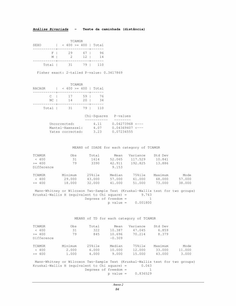
Análise Bivariada - Teste da caminhada (distância) TCAMGR SEXO | < 400 >= 400 | Total -----------+---------------+------ F | 29 67 | 96 M | 2 12 | 14 -----------+---------------+------ Total | 31 79 | 110 Fisher exact: 2-tailed P-value: 0.3417869 TCAMGR RACAGR | < 400 >= 400 | Total -----------+---------------+------ C | 17 59 | 76 NC | 14 20 | 34 -----------+---------------+------ Total | 31 79 | 110 Chi-Squares P-values ----------- -------- Uncorrected: 4.11 0.04273968 <--- Mantel-Haenszel: 4.07 0.04369407 <--- Yates corrected: 3.23 0.07234555 MEANS of IDADE for each category of TCAMGR TCAMGR Obs Total Mean Variance Std Dev < 400 31 1614 52.065 117.529 10.841 >= 400 79 3390 42.911 192.825 13.886 Difference 9.153 TCAMGR Minimum 25%ile Median 75%ile Maximum Mode < 400 29.000 43.000 57.000 61.000 68.000 57.000 >= 400 18.000 32.000 41.000 51.000 73.000 38.000 Mann-Whitney or Wilcoxon Two-Sample Test (Kruskal-Wallis test for two groups) Kruskal-Wallis H (equivalent to Chi square) = 9.743 Degrees of freedom = 1 p value = 0.001800 MEANS of TD for each category of TCAMGR TCAMGR Obs Total Mean Variance Std Dev < 400 31 322 10.387 47.045 6.859 >= 400 79 845 10.696 70.214 8.379 Difference -0.309 TCAMGR Minimum 25%ile Median 75%ile Maximum Mode < 400 2.000 6.000 10.000 12.000 33.000 11.000 >= 400 1.000 4.000 9.000 15.000 43.000 3.000 Mann-Whitney or Wilcoxon Two-Sample Test (Kruskal-Wallis test for two groups) Kruskal-Wallis H (equivalent to Chi square) = 0.043 Degrees of freedom = 1 p value = 0.836529

Anexo 2 84

TCAMGR FC | < 400 >= 400 | Total -----------+---------------+------ D | 10 22 | 32 L | 21 57 | 78 -----------+---------------+------ Total | 31 79 | 110 Chi-Squares P-values ----------- -------- Uncorrected: 0.21 0.64684792 Mantel-Haenszel: 0.21 0.64834809 Yates corrected: 0.05 0.82211102 TCAMGR FAN | < 400 >= 400 | Total -----------+---------------+------ N | 1 14 | 15 P-CENT | 3 9 | 12 P-HO | 7 8 | 15 P-NU | 3 13 | 16 P-PO | 17 35 | 52 -----------+---------------+------ Total | 31 79 | 110 TCAMGR FANGR | < 400 >= 400 | Total -----------+---------------+------ N | 1 14 | 15 P-CENT | 3 9 | 12 P-HO/NU/PO | 27 56 | 83 -----------+---------------+------ Total | 31 79 | 110 Fisher exact: 2-tailed P-value: 0,113 TCAMGR SCL70 | < 400 >= 400 | Total -----------+---------------+------ N | 20 62 | 82 P | 11 17 | 28 -----------+---------------+------ Total | 31 79 | 110 Chi-Squares P-values ----------- -------- Uncorrected: 2.29 0.13036534 Mantel-Haenszel: 2.27 0.13212589 Yates corrected: 1.61 0.20429905

Anexo 2 85

TCAMGR DISP | < 400 >= 400 | Total -----------+---------------+------ I | 20 71 | 91 II | 11 8 | 19 -----------+---------------+------ Total | 31 79 | 110 Chi-Squares P-values ----------- -------- Uncorrected: 10.02 0.00154996 <--- Mantel-Haenszel: 9.93 0.00162856 <--- Yates corrected: 8.32 0.00391620 <--- TCAMGR RXFIP | < 400 >= 400 | Total -----------+---------------+------ N | 17 60 | 77 S | 14 19 | 33 -----------+---------------+------ Total | 31 79 | 110 Chi-Squares P-values ----------- -------- Uncorrected: 4.72 0.02973123 <--- Mantel-Haenszel: 4.68 0.03048355 <--- Yates corrected: 3.77 0.05208711 MEANS of CVF for each category of TCAMGR TCAMGR Obs Total Mean Variance Std Dev < 400 29 2302 79.379 570.387 23.883 >= 400 77 6420 83.377 309.712 17.599 Difference -3.997 TCAMGR Minimum 25%ile Median 75%ile Maximum Mode < 400 35.000 63.000 78.000 97.000 121.000 95.000 >= 400 46.000 68.000 86.000 96.000 124.000 64.000 Mann-Whitney or Wilcoxon Two-Sample Test (Kruskal-Wallis test for two groups) Kruskal-Wallis H (equivalent to Chi square) = 0.659 Degrees of freedom = 1 p value = 0.416958 TCAMGR CVFGR | < 400 >= 400 | Total -------------+---------------+------ < 60 | 7 8 | 15 >= 60 A < 80 | 9 21 | 30 >= 80 | 13 48 | 61 -------------+---------------+------ Total | 29 77 | 106 Chi square = 4.04 Degrees of freedom = 2 p value = 0.13255473

Anexo 2 86

MEANS of FEV for each category of TCAMGR TCAMGR Obs Total Mean Variance Std Dev < 400 29 2339 80.655 484.020 22.000 >= 400 77 6726 87.351 255.625 15.988 Difference -6.695 TCAMGR Minimum 25%ile Median 75%ile Maximum Mode < 400 41.000 65.000 79.000 98.000 114.000 114.000 >= 400 51.000 75.000 85.000 101.000 131.000 75.000 Mann-Whitney or Wilcoxon Two-Sample Test (Kruskal-Wallis test for two groups) Kruskal-Wallis H (equivalent to Chi square) = 2.195 Degrees of freedom = 1 p value = 0.138431 TCAMGR TCVFGR | < 400 >= 400 | Total -----------+---------------+------ N | 8 34 | 42 S < 6 | 12 23 | 35 S >= 6 | 7 16 | 23 -----------+---------------+------ Total | 27 73 | 100 Chi square = 2.43 Degrees of freedom = 2 p value = 0.29702856 TCAMGR TCRETGR | < 400 >= 400 | Total -----------+---------------+------ N | 7 34 | 41 S < 6 | 10 18 | 28 S >= 6 | 11 22 | 33 -----------+---------------+------ Total | 28 74 | 102 Chi square = 3.75 Degrees of freedom = 2 p value = 0.15331087 TCAMGR TCFAVGR | < 400 >= 400 | Total -----------+---------------+------ N | 21 50 | 71 S < 6 | 2 17 | 19 S >= 6 | 5 7 | 12 -----------+---------------+------ Total | 28 74 | 102 Chi square = 4.11 Degrees of freedom = 2 p value = 0.12798704

Anexo 2 87

TCAMGR TCTOTGR | < 400 >= 400 | Total -----------+---------------+------ < 6 | 13 39 | 52 >= 6 | 14 34 | 48 -----------+---------------+------ Total | 27 73 | 100 Chi-Squares P-values ----------- -------- Uncorrected: 0.22 0.63915076 Mantel-Haenszel: 0.22 0.64083175 Yates corrected: 0.06 0.80764883 TCAMGR DELTAGR | < 400 >= 400 | Total -----------+---------------+------ >= 4 | 19 12 | 31 < 4 | 9 65 | 74 -----------+---------------+------ Total | 28 77 | 105 Chi-Squares P-values ----------- -------- Uncorrected: 26.96 0.00000021 <--- Mantel-Haenszel: 26.71 0.00000024 <--- Yates corrected: 24.51 0.00000074 <--- TCAMGR ECOPAPGR | < 400 >= 400 | Total -------------+---------------+------ < 30 | 17 61 | 78 >= 30 E < 45 | 8 13 | 21 >= 45 | 6 5 | 11 -------------+---------------+------ Total | 31 79 | 110 Chi square = 6.37 Degrees of freedom = 2 p value = 0.04139420 <--- MEANS of ECT for each category of TCAMGR TCAMGR Obs Total Mean Variance Std Dev < 400 30 360 12.000 48.138 6.938 >= 400 79 879 11.127 59.445 7.710 Difference 0.873 TCAMGR Minimum 25%ile Median 75%ile Maximum Mode < 400 2.000 7.000 11.000 17.000 27.000 7.000 >= 400 2.000 5.000 9.000 15.000 31.000 7.000 Mann-Whitney or Wilcoxon Two-Sample Test (Kruskal-Wallis test for two groups) Kruskal-Wallis H (equivalent to Chi square) = 0.837 Degrees of freedom = 1 p value = 0.360221

Anexo 2 88

Análise Bivariada - Teste da caminhada (delta) DELTAGR SEXO | >= 4 < 4 | Total -----------+---------------+------ F | 27 65 | 92 M | 4 9 | 13 -----------+---------------+------ Total | 31 74 | 105 Fisher exact: 2-tailed P-value: 1.0000000 DELTAGR RACAGR | >= 4 < 4 | Total -----------+---------------+------ C | 19 54 | 73 NC | 12 20 | 32 -----------+---------------+------ Total | 31 74 | 105 Chi-Squares P-values ----------- -------- Uncorrected: 1.41 0.23550192 Mantel-Haenszel: 1.39 0.23774485 Yates corrected: 0.91 0.34012765 MEANS of IDADE for each category of DELTAGR DELTAGR Obs Total Mean Variance Std Dev >= 4 31 1568 50.581 133.518 11.555 < 4 74 3209 43.365 200.481 14.159 Difference 7.216 DELTAGR Minimum 25%ile Median 75%ile Maximum Mode >= 4 25.000 43.000 51.000 60.000 68.000 57.000 < 4 18.000 33.000 41.500 52.000 73.000 38.000 Mann-Whitney or Wilcoxon Two-Sample Test (Kruskal-Wallis test for two groups) Kruskal-Wallis H (equivalent to Chi square) = 5.898 Degrees of freedom = 1 p value = 0.015161 MEANS of TD for each category of DELTAGR DELTAGR Obs Total Mean Variance Std Dev >= 4 31 277 8.935 26.996 5.196 < 4 74 864 11.676 78.250 8.846 Difference -2.740 DELTAGR Minimum 25%ile Median 75%ile Maximum Mode >= 4 1.000 4.000 10.000 12.000 22.000 11.000 < 4 1.000 5.000 10.000 17.000 43.000 3.000 Mann-Whitney or Wilcoxon Two-Sample Test (Kruskal-Wallis test for two groups) Kruskal-Wallis H (equivalent to Chi square) = 1.220 Degrees of freedom = 1 p value = 0.269271

Anexo 2 89

DELTAGR FC | >= 4 < 4 | Total -----------+---------------+------ D | 10 19 | 29 L | 21 55 | 76 -----------+---------------+------ Total | 31 74 | 105 Chi-Squares P-values ----------- -------- Uncorrected: 0.47 0.49137231 Mantel-Haenszel: 0.47 0.49344290 Yates corrected: 0.20 0.65351962 DELTAGR FAN | >= 4 < 4 | Total -----------+---------------+------ N | 2 13 | 15 P-CENT | 2 9 | 11 P-HO | 6 9 | 15 P-NU | 3 13 | 16 P-PO | 18 30 | 48 -----------+---------------+------ Total | 31 74 | 105 DELTAGR FANGR | >= 4 < 4 | Total -----------+---------------+------ N | 2 13 | 15 P-CENT | 2 9 | 11 P-HO/NU/PO | 27 52 | 79 -----------+---------------+------ Total | 31 74 | 105 Fisher exact: 2-tailed P-value: 0,212 DELTAGR SCL70 | >= 4 < 4 | Total -----------+---------------+------ N | 14 65 | 79 P | 17 9 | 26 -----------+---------------+------ Total | 31 74 | 105 Chi-Squares P-values ----------- -------- Uncorrected: 21.36 0.00000381 <--- Mantel-Haenszel: 21.15 0.00000424 <--- Yates corrected: 19.13 0.00001222 <--- DELTAGR DISP | >= 4 < 4 | Total -----------+---------------+------ I | 17 72 | 89 II | 14 2 | 16 -----------+---------------+------ Total | 31 74 | 105 Fisher exact: 2-tailed P-value: 0.0000002 <---

Anexo 2 90

DELTAGR RXFIP | >= 4 < 4 | Total -----------+---------------+------ N | 11 63 | 74 S | 20 11 | 31 -----------+---------------+------ Total | 31 74 | 105 Chi-Squares P-values ----------- -------- Uncorrected: 25.89 0.00000036 <--- Mantel-Haenszel: 25.64 0.00000041 <--- Yates corrected: 23.55 0.00000121 <--- MEANS of CVF for each category of DELTAGR DELTAGR Obs Total Mean Variance Std Dev >= 4 30 2097 69.900 390.921 19.772 < 4 72 6315 87.708 295.083 17.178 Difference -17.808 DELTAGR Minimum 25%ile Median 75%ile Maximum Mode >= 4 35.000 56.000 66.500 79.000 120.000 50.000 < 4 52.000 78.500 90.000 98.500 124.000 80.000 Mann-Whitney or Wilcoxon Two-Sample Test (Kruskal-Wallis test for two groups) Kruskal-Wallis H (equivalent to Chi square) = 16.955 Degrees of freedom = 1 p value = 0.000038 DELTAGR CVFGR | >= 4 < 4 | Total -------------+---------------+------ < 60 | 9 5 | 14 >= 60 A < 80 | 14 15 | 29 >= 80 | 7 52 | 59 -------------+---------------+------ Total | 30 72 | 102 Chi square = 21.92 Degrees of freedom = 2 p value = 0.00001736 <--- MEANS of FEV for each category of DELTAGR DELTAGR Obs Total Mean Variance Std Dev >= 4 30 2167 72.233 274.323 16.563 < 4 72 6573 91.292 245.533 15.670 Difference -19.058 DELTAGR Minimum 25%ile Median 75%ile Maximum Mode >= 4 41.000 61.000 69.500 82.000 113.000 61.000 < 4 51.000 80.000 92.500 102.000 131.000 94.000 Mann-Whitney or Wilcoxon Two-Sample Test (Kruskal-Wallis test for two groups) Kruskal-Wallis H (equivalent to Chi square) = 23.723 Degrees of freedom = 1 p value = 0.000001

Anexo 2 91

DELTAGR TCVFGR | >= 4 < 4 | Total -----------+---------------+------ N | 6 35 | 41 S < 6 | 10 23 | 33 S >= 6 | 11 11 | 22 -----------+---------------+------ Total | 27 69 | 96 Chi square = 8.98 Degrees of freedom = 2 p value = 0.01123984 <--- DELTAGR TCRETGR | >= 4 < 4 | Total -----------+---------------+------ N | 6 34 | 40 S < 6 | 5 22 | 27 S >= 6 | 17 14 | 31 -----------+---------------+------ Total | 28 70 | 98 Chi square = 15.43 Degrees of freedom = 2 p value = 0.00044660 <--- DELTAGR TCFAVGR | >= 4 < 4 | Total -----------+---------------+------ N | 15 52 | 67 S < 6 | 8 11 | 19 S >= 6 | 5 7 | 12 -----------+---------------+------ Total | 28 70 | 98 Chi square = 3.97 Degrees of freedom = 2 p value = 0.13746167 DELTAGR TCTOTGR | >= 4 < 4 | Total -----------+---------------+------ < 6 | 7 44 | 51 >= 6 | 20 25 | 45 -----------+---------------+------ Total | 27 69 | 96 Chi-Squares P-values ----------- -------- Uncorrected: 11.16 0.00083592 <--- Mantel-Haenszel: 11.04 0.00088999 <--- Yates corrected: 9.69 0.00185088 <---

Anexo 2 92

DELTAGR ECOPAPGR | >= 4 < 4 | Total -------------+---------------+------ < 30 | 17 59 | 76 >= 30 E < 45 | 7 12 | 19 >= 45 | 7 3 | 10 -------------+---------------+------ Total | 31 74 | 105 Chi square = 10.23 Degrees of freedom = 2 p value = 0.00599710 <--- MEANS of ECT for each category of DELTAGR DELTAGR Obs Total Mean Variance Std Dev >= 4 31 370 11.935 46.462 6.816 < 4 73 790 10.822 56.093 7.490 Difference 1.114 DELTAGR Minimum 25%ile Median 75%ile Maximum Mode >= 4 2.000 7.000 9.000 16.000 27.000 9.000 < 4 2.000 5.000 8.000 14.000 31.000 7.000 Mann-Whitney or Wilcoxon Two-Sample Test (Kruskal-Wallis test for two groups) Kruskal-Wallis H (equivalent to Chi square) = 1.374 Degrees of freedom = 1 p value = 0.241115 SCL70 TCTOTGR | N P | Total -----------+---------------+------ < 6 | 47 5 | 52 >= 6 | 28 20 | 48 -----------+---------------+------ Total | 75 25 | 100 Chi-Squares P-values ----------- -------- Uncorrected: 13.68 0.00021730 <--- Mantel-Haenszel: 13.54 0.00023372 <--- Yates corrected: 12.02 0.00052654 <--- SCL70 ECOPAPGR | N P | Total -------------+---------------+------ < 30 | 62 16 | 78 >= 30 E < 45 | 12 9 | 21 >= 45 | 8 3 | 11 -------------+---------------+------ Total | 82 28 | 110 Chi square = 4.37 Degrees of freedom = 2 p value = 0.11221524

Anexo 2 93

Anexo 2 94

Modelo 1: 10 variáveis independentes, excluindo-se os 5 valores em branco (Stepwise) Total number of cases: 105 (Unweighted) Number of selected cases: 105 Number of unselected cases: 0 Number of selected cases: 105 Number rejected because of missing data: 0 Number of cases included in the analysis: 105 Dependent Variable Encoding: Original Internal Value Value 0 0 1 1 Parameter Value Freq Coding (1) (2) FANA 0 15 ,000 ,000 1 11 1,000 ,000 2 79 ,000 1,000 ECTA 0 28 ,000 1 77 1,000 RACAA 0 75 ,000 1 30 1,000 IDADEA 1 77 1,000 0 28 ,000 SCL70A 0 77 ,000 1 28 1,000 DISPA 0 87 ,000 1 18 1,000 ECOPAPA 0 74 ,000 1 31 1,000 CVFA 0 60 ,000 1 45 1,000 RXFIPA 0 73 ,000 1 32 1,000 SEXOA 1 92 1,000 0 13 ,000

Anexo 2

95

Dependent Variable.. TCAMA Beginning Block Number 0. Initial Log Likelihood Function -2 Log Likelihood 121,78219 * Constant is included in the model. Estimation terminated at iteration number 3 because Log Likelihood decreased by less than ,01 percent. Classification Table for TCAMA Predicted 0 1 Percent Correct 0 | 1 Observed +-------+-------+ 0 0 | 77 | 0 | 100,00% +-------+-------+ 1 1 | 28 | 0 | ,00% +-------+-------+ Overall 73,33% ---------------------- Variables in the Equation ----------------------- Variable B S.E. Wald df Sig R Exp(B) Constant -1,0116 ,2207 21,0125 1 ,0000 Beginning Block Number 1. Method: Forward Stepwise (WALD) --------------- Variables not in the Equation ----------------- Residual Chi Square 21,847 with 11 df Sig = ,0256 Variable Score df Sig R SEXOA(1) ,9657 1 ,3258 ,0000 RACAA(1) 2,1477 1 ,1428 ,0348 IDADEA(1) 7,4424 1 ,0064 ,2114 FANA 3,6272 2 ,1631 ,0000 FANA(1) ,0023 1 ,9617 ,0000 FANA(2) 2,2493 1 ,1337 ,0452 SCL70A(1) 3,1091 1 ,0779 ,0954 DISPA(1) 9,2712 1 ,0023 ,2443 RXFIPA(1) 4,5858 1 ,0322 ,1457 CVFA(1) 3,1818 1 ,0745 ,0985 ECOPAPA(1) 5,2440 1 ,0220 ,1632 ECTA(1) 1,5153 1 ,2183 ,0000

Anexo 2

96

Variable(s) Entered on Step Number 1.. DISPA Estimation terminated at iteration number 3 because Log Likelihood decreased by less than ,01 percent. -2 Log Likelihood 113,439 Goodness of Fit 104,999 Chi-Square df Significance Model Chi-Square 8,344 1 ,0039 Improvement 8,344 1 ,0039 Classification Table for TCAMA Predicted 0 1 Percent Correct 0 | 1 Observed +-------+-------+ 0 0 | 69 | 8 | 89,61% +-------+-------+ 1 1 | 18 | 10 | 35,71% +-------+-------+ Overall 75,24% ---------------------- Variables in the Equation ----------------------- Variable B S.E. Wald df Sig R Exp(B) DISPA(1) 1,5669 ,5432 8,3209 1 ,0039 ,2278 4,7916 Constant -1,3437 ,2647 25,7764 1 ,0000 --------------- Variables not in the Equation ----------------- Residual Chi Square 13,988 with 10 df Sig = ,1736 Variable Score df Sig R SEXOA(1) ,5582 1 ,4550 ,0000 RACAA(1) 3,0719 1 ,0797 ,0938 IDADEA(1) 7,4339 1 ,0064 ,2112 FANA 3,5382 2 ,1705 ,0000 FANA(1) ,0004 1 ,9839 ,0000 FANA(2) 2,2202 1 ,1362 ,0425 SCL70A(1) 1,2064 1 ,2720 ,0000 RXFIPA(1) 1,0246 1 ,3114 ,0000 CVFA(1) ,5545 1 ,4565 ,0000 ECOPAPA(1) 2,1117 1 ,1462 ,0303 ECTA(1) 1,7536 1 ,1854 ,0000

Anexo 2

97

Variable(s) Entered on Step Number 2.. IDADEA Estimation terminated at iteration number 4 because Log Likelihood decreased by less than ,01 percent. -2 Log Likelihood 104,607 Goodness of Fit 115,299 Chi-Square df Significance Model Chi-Square 17,176 2 ,0002 Improvement 8,832 1 ,0030 Classification Table for TCAMA Predicted 0 1 Percent Correct 0 | 1 Observed +-------+-------+ 0 0 | 73 | 4 | 94,81% +-------+-------+ 1 1 | 18 | 10 | 35,71% +-------+-------+ Overall 79,05% ---------------------- Variables in the Equation ------------------------ Variable B S.E. Wald df Sig R Exp(B) IDADEA(1) 1,9683 ,7998 6,0568 1 ,0139 ,1825 7,1583 DISPA(1) 1,6475 ,5839 7,9625 1 ,0048 ,2213 5,1940 Constant -2,9769 ,7829 14,4564 1 ,0001 --------------- Variables not in the Equation ----------------- Residual Chi Square 6,858 with 9 df Sig = ,6519 Variable Score df Sig R SEXOA(1) ,7875 1 ,3749 ,0000 RACAA(1) 2,8755 1 ,0899 ,0848 FANA 2,1280 2 ,3451 ,0000 FANA(1) ,2688 1 ,6042 ,0000 FANA(2) 1,7439 1 ,1866 ,0000 SCL70A(1) ,2444 1 ,6210 ,0000 RXFIPA(1) ,2914 1 ,5893 ,0000 CVFA(1) 1,0343 1 ,3092 ,0000 ECOPAPA(1) ,5271 1 ,4678 ,0000 ECTA(1) 1,7199 1 ,1897 ,0000 No more variables can be deleted or added.

Anexo 2

98

Modelo 2: 6 variáveis independentes, com todos os registros (Stepwise) Total number of cases: 110 (Unweighted) Number of selected cases: 110 Number of unselected cases: 0 Number of selected cases: 110 Number rejected because of missing data: 0 Number of cases included in the analysis: 110 Dependent Variable Encoding: Original Internal Value Value 0 0 1 1 Parameter Value Freq Coding (1) (2) FANA 0 15 ,000 ,000 1 12 1,000 ,000 2 83 ,000 1,000 DISPA 0 91 ,000 1 19 1,000 ECOPAPA 0 78 ,000 1 32 1,000 RXFIPA 0 77 ,000 1 33 1,000 RACAA 0 76 ,000 1 34 1,000 IDADEA 1 82 1,000 0 28 ,000

Anexo 2

99

Dependent Variable.. TCAMA Beginning Block Number 0. Initial Log Likelihood Function -2 Log Likelihood 130,82571 * Constant is included in the model. Estimation terminated at iteration number 3 because parameter estimates changed by less than ,001 Classification Table for TCAMA Predicted 0 1 Percent Correct 0 | 1 Observed +-------+-------+ 0 0 | 79 | 0 | 100,00% +-------+-------+ 1 1 | 31 | 0 | ,00% +-------+-------+ Overall 71,82% ---------------------- Variables in the Equation ----------------------- Variable B S.E. Wald df Sig R Exp(B) Constant -,9355 ,2119 19,4826 1 ,0000 Beginning Block Number 1. Method: Forward Stepwise (WALD) --------------- Variables not in the Equation ----------------- Residual Chi Square 23,297 with 7 df Sig = ,0015 Variable Score df Sig R IDADEA(1) 8,2145 1 ,0042 ,2180 DISPA(1) 10,0183 1 ,0015 ,2476 ECOPAPA(1) 5,4041 1 ,0201 ,1613 RXFIPA(1) 4,7248 1 ,0297 ,1443 RACAA(1) 4,1057 1 ,0427 ,1269 FANA 4,2660 2 ,1185 ,0451 FANA(1) ,0674 1 ,7952 ,0000 FANA(2) 3,1589 1 ,0755 ,0941

Anexo 2

100

Variable(s) Entered on Step Number 1.. DISPA Estimation terminated at iteration number 3 because Log Likelihood decreased by less than ,01 percent. -2 Log Likelihood 121,711 Goodness of Fit 110,000 Chi-Square df Significance Model Chi-Square 9,115 1 ,0025 Improvement 9,115 1 ,0025 Classification Table for TCAMA Predicted 0 1 Percent Correct 0 | 1 Observed +-------+-------+ 0 0 | 71 | 8 | 89,87% +-------+-------+ 1 1 | 20 | 11 | 35,48% +-------+-------+ Overall 74,55% ---------------------- Variables in the Equation ----------------------- Variable B S.E. Wald df Sig R Exp(B) DISPA(1) 1,5854 ,5291 8,9769 1 ,0027 ,2309 4,8812 Constant -1,2669 ,2531 25,0473 1 ,0000 --------------- Variables not in the Equation ----------------- Residual Chi Square 14,640 with 6 df Sig = ,0233 Variable Score df Sig R IDADEA(1) 8,2247 1 ,0041 ,2181 ECOPAPA(1) 2,3332 1 ,1266 ,0505 RXFIPA(1) ,8500 1 ,3565 ,0000 RACAA(1) 5,2233 1 ,0223 ,1570 FANA 4,1546 2 ,1253 ,0344 FANA(1) ,0645 1 ,7996 ,0000 FANA(2) 3,0566 1 ,0804 ,0899

Anexo 2

101

Variable(s) Entered on Step Number 2.. IDADEA Estimation terminated at iteration number 4 because Log Likelihood decreased by less than ,01 percent. -2 Log Likelihood 111,876 Goodness of Fit 120,664 Chi-Square df Significance Model Chi-Square 18,950 2 ,0001 Improvement 9,835 1 ,0017 Classification Table for TCAMA Predicted 0 1 Percent Correct 0 | 1 Observed +-------+-------+ 0 0 | 75 | 4 | 94,94% +-------+-------+ 1 1 | 20 | 11 | 35,48% +-------+-------+ Overall 78,18% ---------------------- Variables in the Equation ------------------------ Variable B S.E. Wald df Sig R Exp(B) IDADEA(1) 2,0500 ,7981 6,5968 1 ,0102 ,1874 7,7677 DISPA(1) 1,6767 ,5719 8,5939 1 ,0034 ,2245 5,3477 Constant -2,9879 ,7833 14,5511 1 ,0001 --------------- Variables not in the Equation ----------------- Residual Chi Square 6,980 with 5 df Sig = ,2221 Variable Score df Sig R ECOPAPA(1) ,6727 1 ,4121 ,0000 RXFIPA(1) ,1993 1 ,6553 ,0000 RACAA(1) 4,6375 1 ,0313 ,1420 FANA 2,7655 2 ,2509 ,0000 FANA(1) ,6484 1 ,4207 ,0000 FANA(2) 2,4922 1 ,1144 ,0613

Anexo 2

102

Variable(s) Entered on Step Number 3.. RACAA Estimation terminated at iteration number 4 because Log Likelihood decreased by less than ,01 percent. -2 Log Likelihood 107,332 Goodness of Fit 120,479 Chi-Square df Significance Model Chi-Square 23,494 3 ,0000 Improvement 4,544 1 ,0330 Classification Table for TCAMA Predicted 0 1 Percent Correct 0 | 1 Observed +-------+-------+ 0 0 | 75 | 4 | 94,94% +-------+-------+ 1 1 | 20 | 11 | 35,48% +-------+-------+ Overall 78,18% ---------------------- Variables in the Equation ------------------------ Variable B S.E. Wald df Sig R Exp(B) IDADEA(1) 2,0505 ,8138 6,3489 1 ,0117 ,1823 7,7719 DISPA(1) 1,8336 ,5936 9,5402 1 ,0020 ,2401 6,2562 RACAA(1) 1,0502 ,4967 4,4712 1 ,0345 ,1374 2,8584 Constant -3,3969 ,8374 16,4549 1 ,0001 --------------- Variables not in the Equation ----------------- Residual Chi Square 2,583 with 4 df Sig = ,6299 Variable Score df Sig R ECOPAPA(1) 1,0912 1 ,2962 ,0000 RXFIPA(1) ,2429 1 ,6221 ,0000 FANA 1,8972 2 ,3873 ,0000 FANA(1) ,2892 1 ,5908 ,0000 FANA(2) 1,5864 1 ,2078 ,0000 No more variables can be deleted or added.

Anexo 2

103

Modelo 3: 5 variáveis independentes, com todos os registros (Enter) Total number of cases: 110 (Unweighted) Number of selected cases: 110 Number of unselected cases: 0 Number of selected cases: 110 Number rejected because of missing data: 0 Number of cases included in the analysis: 110 Dependent Variable Encoding: Original Internal Value Value 0 0 1 1 Parameter Value Freq Coding (1) IDADEA 1 82 1,000 0 28 ,000

Anexo 2

104

Dependent Variable.. TCAMA Beginning Block Number 0. Initial Log Likelihood Function -2 Log Likelihood 130,82571 * Constant is included in the model. Beginning Block Number 1. Method: Enter Variable(s) Entered on Step Number 1.. IDADEA Estimation terminated at iteration number 4 because Log Likelihood decreased by less than ,01 percent. -2 Log Likelihood 120,958 Goodness of Fit 109,996 Chi-Square df Significance Model Chi-Square 9,868 1 ,0017 Improvement 9,868 1 ,0017 Classification Table for TCAMA Predicted 0 1 Percent Correct 0 | 1 Observed +-------+-------+ 0 0 | 79 | 0 | 100,00% +-------+-------+ 1 1 | 31 | 0 | ,00% +-------+-------+ Overall 71,82% ---------------------- Variables in the Equation ------------------------ Variable B S.E. Wald df Sig R Exp(B) IDADEA(1) 1,9618 ,7692 6,5039 1 ,0108 ,1855 7,1121 Constant -2,5648 ,7337 12,2182 1 ,0005

Anexo 2

105

Total number of cases: 110 (Unweighted) Number of selected cases: 110 Number of unselected cases: 0 Number of selected cases: 110 Number rejected because of missing data: 0 Number of cases included in the analysis: 110 Dependent Variable Encoding: Original Internal Value Value 0 0 1 1 Parameter Value Freq Coding (1) DISPA 0 91 ,000 1 19 1,000 IDADEA 1 82 1,000 0 28 ,000

Anexo 2

106

Dependent Variable.. TCAMA Beginning Block Number 0. Initial Log Likelihood Function -2 Log Likelihood 130,82571 * Constant is included in the model. Beginning Block Number 1. Method: Enter Variable(s) Entered on Step Number 1.. IDADEA DISPA Estimation terminated at iteration number 4 because Log Likelihood decreased by less than ,01 percent. -2 Log Likelihood 111,876 Goodness of Fit 120,664 Chi-Square df Significance Model Chi-Square 18,950 2 ,0001 Improvement 18,950 2 ,0001 Classification Table for TCAMA Predicted 0 1 Percent Correct 0 | 1 Observed +-------+-------+ 0 0 | 75 | 4 | 94,94% +-------+-------+ 1 1 | 20 | 11 | 35,48% +-------+-------+ Overall 78,18% ---------------------- Variables in the Equation ------------------------ Variable B S.E. Wald df Sig R Exp(B) IDADEA(1) 2,0500 ,7981 6,5968 1 ,0102 ,1874 7,7677 DISPA(1) 1,6767 ,5719 8,5939 1 ,0034 ,2245 5,3477 Constant -2,9879 ,7833 14,5511 1 ,0001

Anexo 2

107

Total number of cases: 110 (Unweighted) Number of selected cases: 110 Number of unselected cases: 0 Number of selected cases: 110 Number rejected because of missing data: 0 Number of cases included in the analysis: 110 Dependent Variable Encoding: Original Internal Value Value 0 0 1 1 Parameter Value Freq Coding (1) ECOPAPA 0 78 ,000 1 32 1,000 DISPA 0 91 ,000 1 19 1,000 IDADEA 1 82 1,000 0 28 ,000

Anexo 2

108

Dependent Variable.. TCAMA Beginning Block Number 0. Initial Log Likelihood Function -2 Log Likelihood 130,82571 * Constant is included in the model. Beginning Block Number 1. Method: Enter Variable(s) Entered on Step Number 1.. IDADEA DISPA ECOPAPA Estimation terminated at iteration number 4 because Log Likelihood decreased by less than ,01 percent. -2 Log Likelihood 111,218 Goodness of Fit 121,299 Chi-Square df Significance Model Chi-Square 19,608 3 ,0002 Improvement 19,608 3 ,0002 Classification Table for TCAMA Predicted 0 1 Percent Correct 0 | 1 Observed +-------+-------+ 0 0 | 75 | 4 | 94,94% +-------+-------+ 1 1 | 20 | 11 | 35,48% +-------+-------+ Overall 78,18% ----------------------- Variables in the Equation ------------------------ Variable B S.E. Wald df Sig R Exp(B) IDADEA(1) 1,9410 ,8070 5,7857 1 ,0162 ,1701 6,9658 DISPA(1) 1,5422 ,5945 6,7303 1 ,0095 ,1901 4,6748 ECOPAPA(1) ,4129 ,5048 ,6689 1 ,4134 ,0000 1,5112 Constant -3,0053 ,7819 14,7728 1 ,0001

Anexo 2

109

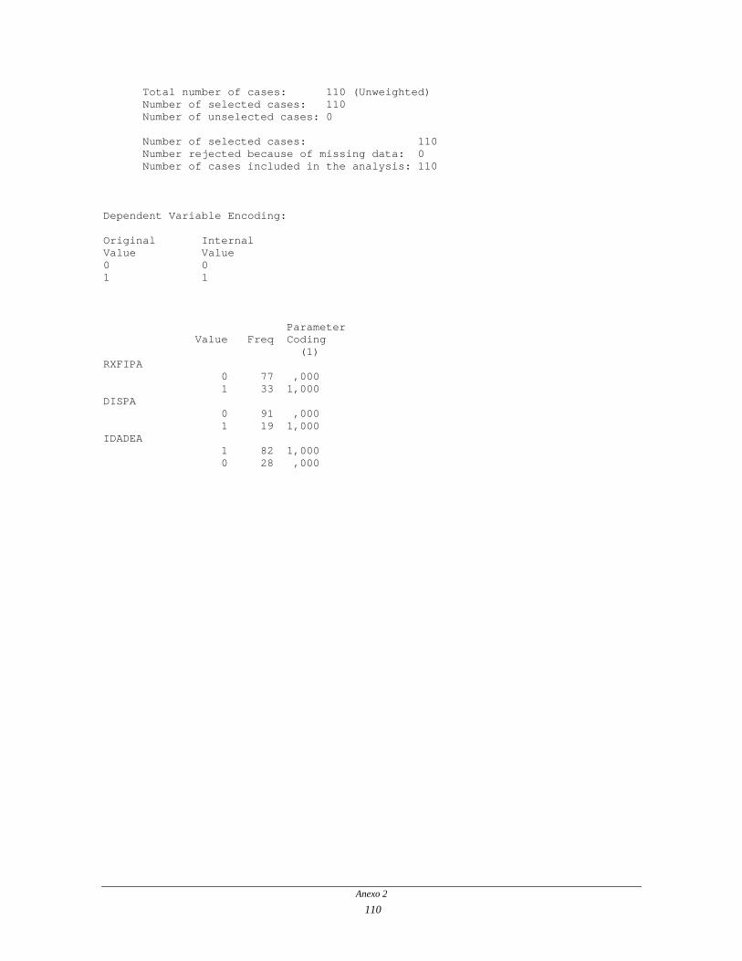
Total number of cases: 110 (Unweighted) Number of selected cases: 110 Number of unselected cases: 0 Number of selected cases: 110 Number rejected because of missing data: 0 Number of cases included in the analysis: 110 Dependent Variable Encoding: Original Internal Value Value 0 0 1 1 Parameter Value Freq Coding (1) RXFIPA 0 77 ,000 1 33 1,000 DISPA 0 91 ,000 1 19 1,000 IDADEA 1 82 1,000 0 28 ,000

Anexo 2

110

Dependent Variable.. TCAMA Beginning Block Number 0. Initial Log Likelihood Function -2 Log Likelihood 130,82571 * Constant is included in the model. Beginning Block Number 1. Method: Enter Variable(s) Entered on Step Number 1.. IDADEA DISPA RXFIPA Estimation terminated at iteration number 4 because Log Likelihood decreased by less than ,01 percent. -2 Log Likelihood 111,680 Goodness of Fit 117,722 Chi-Square df Significance Model Chi-Square 19,146 3 ,0003 Improvement 19,146 3 ,0003 Classification Table for TCAMA Predicted 0 1 Percent Correct 0 | 1 Observed +-------+-------+ 0 0 | 75 | 4 | 94,94% +-------+-------+ 1 1 | 20 | 11 | 35,48% +-------+-------+ Overall 78,18% ---------------------- Variables in the Equation ------------------------ Variable B S.E. Wald df Sig R Exp(B) IDADEA(1) 2,0094 ,8018 6,2805 1 ,0122 ,1809 7,4588 DISPA(1) 1,5510 ,6356 5,9551 1 ,0147 ,1739 4,7161 RXFIPA(1) ,2404 ,5390 ,1989 1 ,6556 ,0000 1,2718 Constant -3,0080 ,7839 14,7256 1 ,0001

Anexo 2

111

Total number of cases: 110 (Unweighted) Number of selected cases: 110 Number of unselected cases: 0 Number of selected cases: 110 Number rejected because of missing data: 0 Number of cases included in the analysis: 110 Dependent Variable Encoding: Original Internal Value Value 0 0 1 1 Parameter Value Freq Coding (1) RACAA 0 76 ,000 1 34 1,000 DISPA 0 91 ,000 1 19 1,000 IDADEA 1 82 1,000 0 28 ,000

Anexo 2

112

Dependent Variable.. TCAMA Beginning Block Number 0. Initial Log Likelihood Function -2 Log Likelihood 130,82571 * Constant is included in the model. Beginning Block Number 1. Method: Enter Variable(s) Entered on Step Number 1.. IDADEA DISPA RACAA Estimation terminated at iteration number 4 because Log Likelihood decreased by less than ,01 percent. -2 Log Likelihood 107,332 Goodness of Fit 120,479 Chi-Square df Significance Model Chi-Square 23,494 3 ,0000 Improvement 23,494 3 ,0000 Classification Table for TCAMA Predicted 0 1 Percent Correct 0 | 1 Observed +-------+-------+ 0 0 | 75 | 4 | 94,94% +-------+-------+ 1 1 | 20 | 11 | 35,48% +-------+-------+ Overall 78,18% ---------------------- Variables in the Equation ------------------------ Variable B S.E. Wald df Sig R Exp(B) IDADEA(1) 2,0505 ,8138 6,3489 1 ,0117 ,1823 7,7719 DISPA(1) 1,8336 ,5936 9,5402 1 ,0020 ,2401 6,2562 RACAA(1) 1,0502 ,4967 4,4712 1 ,0345 ,1374 2,8584 Constant -3,3969 ,8374 16,4549 1 ,0001

Anexo 2

113

Anexo 2

114

Modelo 1: 13 variáveis independentes, excluindo-se os 17 valores em branco (Stepwise) Total number of cases: 93 (Unweighted) Number of selected cases: 93 Number of unselected cases: 0 Number of selected cases: 93 Number rejected because of missing data: 0 Number of cases included in the analysis: 93 Dependent Variable Encoding: Original Internal Value Value 0 0 1 1 Parameter Value Freq Coding (1) (2) FANA 0 15 ,000 ,000 1 9 1,000 ,000 2 69 ,000 1,000 ECTA 0 24 ,000 1 69 1,000 IDADEA 1 67 1,000 0 26 ,000 SCL70A 0 70 ,000 1 23 1,000 DISPA 0 82 ,000 1 11 1,000 RXFIPA 0 66 ,000 1 27 1,000 CVFA 0 55 ,000 1 38 1,000 TCVFB 0 71 ,000 1 22 1,000 ECOPAPA 0 66 ,000 1 27 1,000 TCTOTA 0 49 ,000 1 44 1,000 TCFAVB 0 82 ,000 1 11 1,000 TCRETB 0 63 ,000 1 30 1,000 RACAA 0 67 ,000 1 26 1,000

Anexo 2

115

Dependent Variable.. DELTAA Beginning Block Number 0. Initial Log Likelihood Function -2 Log Likelihood 110,21367 * Constant is included in the model. Estimation terminated at iteration number 3 because parameter estimates changed by less than ,001 Classification Table for DELTAA Predicted 0 1 Percent Correct 0 | 1 Observed +-------+-------+ 0 0 | 67 | 0 | 100,00% +-------+-------+ 1 1 | 26 | 0 | ,00% +-------+-------+ Overall 72,04% ---------------------- Variables in the Equation ----------------------- Variable B S.E. Wald df Sig R Exp(B) Constant -,9466 ,2311 16,7840 1 ,0000 Beginning Block Number 1. Method: Forward Stepwise (WALD) --------------- Variables not in the Equation ----------------- Residual Chi Square 43,323 with 14 df Sig = ,0001 Variable Score df Sig R RACAA(1) 1,9772 1 ,1597 ,0000 IDADEA(1) 7,3583 1 ,0067 ,2205 FANA 2,2679 2 ,3218 ,0000 FANA(1) ,1627 1 ,6867 ,0000 FANA(2) 2,0473 1 ,1525 ,0207 SCL70A(1) 21,0633 1 ,0000 ,4159 DISPA(1) 17,9693 1 ,0000 ,3806 RXFIPA(1) 18,5085 1 ,0000 ,3870 CVFA(1) 15,5011 1 ,0001 ,3500 TCVFB(1) 6,9520 1 ,0084 ,2120 TCRETB(1) 14,1592 1 ,0002 ,3322 TCFAVB(1) ,4377 1 ,5082 ,0000 TCTOTA(1) 9,6109 1 ,0019 ,2628 ECOPAPA(1) 5,1348 1 ,0235 ,1687 ECTA(1) 3,8372 1 ,0501 ,1291

Anexo 2

116

Variable(s) Entered on Step Number 1.. SCL70A Estimation terminated at iteration number 3 because Log Likelihood decreased by less than ,01 percent. -2 Log Likelihood 90,606 Goodness of Fit 92,987 Chi-Square df Significance Model Chi-Square 19,607 1 ,0000 Improvement 19,607 1 ,0000 Classification Table for DELTAA Predicted 0 1 Percent Correct 0 | 1 Observed +-------+-------+ 0 0 | 59 | 8 | 88,06% +-------+-------+ 1 1 | 11 | 15 | 57,69% +-------+-------+ Overall 79,57% ---------------------- Variables in the Equation ------------------------ Variable B S.E. Wald df Sig R Exp(B) SCL70A(1) 2,3080 ,5473 17,7853 1 ,0000 ,3785 10,0542 Constant -1,6794 ,3284 26,1530 1 ,0000 --------------- Variables not in the Equation ----------------- Residual Chi Square 27,186 with 13 df Sig = ,0117 Variable Score df Sig R RACAA(1) 4,1702 1 ,0411 ,1403 IDADEA(1) 4,8299 1 ,0280 ,1602 FANA ,3596 2 ,8354 ,0000 FANA(1) ,3298 1 ,5658 ,0000 FANA(2) ,0254 1 ,8735 ,0000 DISPA(1) 11,4118 1 ,0007 ,2922 RXFIPA(1) 6,3086 1 ,0120 ,1977 CVFA(1) 8,4060 1 ,0037 ,2411 TCVFB(1) 1,7383 1 ,1874 ,0000 TCRETB(1) 6,5896 1 ,0103 ,2041 TCFAVB(1) ,0258 1 ,8725 ,0000 TCTOTA(1) 2,4937 1 ,1143 ,0669 ECOPAPA(1) 2,6362 1 ,1045 ,0760 ECTA(1) 2,8620 1 ,0907 ,0884

Anexo 2

117

Variable(s) Entered on Step Number 2.. DISPA Estimation terminated at iteration number 4 because Log Likelihood decreased by less than ,01 percent. -2 Log Likelihood 79,511 Goodness of Fit 90,257 Chi-Square df Significance Model Chi-Square 30,703 2 ,0000 Improvement 11,096 1 ,0009 Classification Table for DELTAA Predicted 0 1 Percent Correct 0 | 1 Observed +-------+-------+ 0 0 | 57 | 10 | 85,07% +-------+-------+ 1 1 | 8 | 18 | 69,23% +-------+-------+ Overall 80,65% ---------------------- Variables in the Equation ------------------------ Variable B S.E. Wald df Sig R Exp(B) SCL70A(1) 2,2029 ,5940 13,7517 1 ,0002 ,3265 9,0509 DISPA(1) 2,6893 ,8982 8,9639 1 ,0028 ,2514 14,7213 Constant -2,0098 ,3780 28,2682 1 ,0000 --------------- Variables not in the Equation ----------------- Residual Chi Square 16,917 with 12 df Sig = ,1527 Variable Score df Sig R RACAA(1) 7,1657 1 ,0074 ,2165 IDADEA(1) 5,0118 1 ,0252 ,1653 FANA ,6097 2 ,7372 ,0000 FANA(1) ,1677 1 ,6821 ,0000 FANA(2) ,1265 1 ,7221 ,0000 RXFIPA(1) 2,6164 1 ,1058 ,0748 CVFA(1) 4,8168 1 ,0282 ,1599 TCVFB(1) 1,7025 1 ,1920 ,0000 TCRETB(1) 3,2179 1 ,0728 ,1051 TCFAVB(1) ,3699 1 ,5430 ,0000 TCTOTA(1) 1,0090 1 ,3152 ,0000 ECOPAPA(1) ,8399 1 ,3594 ,0000 ECTA(1) 2,7972 1 ,0944 ,0851

Anexo 2

118

Variable(s) Entered on Step Number 3.. RACAA Estimation terminated at iteration number 5 because Log Likelihood decreased by less than ,01 percent. -2 Log Likelihood 72,469 Goodness of Fit 94,525 Chi-Square df Significance Model Chi-Square 37,745 3 ,0000 Improvement 7,042 1 ,0080 Classification Table for DELTAA Predicted 0 1 Percent Correct 0 | 1 Observed +-------+-------+ 0 0 | 65 | 2 | 97,01% +-------+-------+ 1 1 | 14 | 12 | 46,15% +-------+-------+ Overall 82,80% ---------------------- Variables in the Equation ------------------------ Variable B S.E. Wald df Sig R Exp(B) RACAA(1) 1,8212 ,7345 6,1478 1 ,0132 ,1940 6,1791 SCL70A(1) 2,7542 ,7316 14,1708 1 ,0002 ,3323 15,7081 DISPA(1) 3,4013 1,0288 10,9298 1 ,0009 ,2846 30,0039 Constant -2,8644 ,6085 22,1564 1 ,0000 --------------- Variables not in the Equation ----------------- Residual Chi Square 11,428 with 11 df Sig = ,4081 Variable Score df Sig R IDADEA(1) 4,4102 1 ,0357 ,1479 FANA ,9139 2 ,6332 ,0000 FANA(1) ,7922 1 ,3734 ,0000 FANA(2) ,0150 1 ,9026 ,0000 RXFIPA(1) 2,2935 1 ,1299 ,0516 CVFA(1) 2,9181 1 ,0876 ,0913 TCVFB(1) ,7252 1 ,3945 ,0000 TCRETB(1) 1,9413 1 ,1635 ,0000 TCFAVB(1) ,2068 1 ,6493 ,0000 TCTOTA(1) 1,0387 1 ,3081 ,0000 ECOPAPA(1) 1,3839 1 ,2394 ,0000 ECTA(1) 1,2470 1 ,2641 ,0000

Anexo 2

119

Variable(s) Entered on Step Number 4.. IDADEA Estimation terminated at iteration number 5 because Log Likelihood decreased by less than ,01 percent. -2 Log Likelihood 67,377 Goodness of Fit 83,270 Chi-Square df Significance Model Chi-Square 42,837 4 ,0000 Improvement 5,092 1 ,0240 Classification Table for DELTAA Predicted 0 1 Percent Correct 0 | 1 Observed +-------+-------+ 0 0 | 60 | 7 | 89,55% +-------+-------+ 1 1 | 8 | 18 | 69,23% +-------+-------+ Overall 83,87% ---------------------- Variables in the Equation ------------------------ Variable B S.E. Wald df Sig R Exp(B) RACAA(1) 1,7834 ,7571 5,5483 1 ,0185 ,1794 5,9499 IDADEA(1) 1,9440 1,0134 3,6801 1 ,0551 ,1235 6,9869 SCL70A(1) 2,5953 ,7451 12,1308 1 ,0005 ,3032 13,4006 DISPA(1) 3,5153 1,0757 10,6791 1 ,0011 ,2806 33,6271 Constant -4,4211 1,1246 15,4544 1 ,0001 --------------- Variables not in the Equation ----------------- Residual Chi Square 7,176 with 10 df Sig = ,7087 Variable Score df Sig R FANA ,2540 2 ,8807 ,0000 FANA(1) ,2000 1 ,6547 ,0000 FANA(2) ,2101 1 ,6467 ,0000 RXFIPA(1) 2,3845 1 ,1225 ,0591 CVFA(1) 4,3892 1 ,0362 ,1472 TCVFB(1) ,5276 1 ,4676 ,0000 TCRETB(1) ,7558 1 ,3846 ,0000 TCFAVB(1) ,0007 1 ,9783 ,0000 TCTOTA(1) ,7844 1 ,3758 ,0000 ECOPAPA(1) ,4421 1 ,5061 ,0000 ECTA(1) 1,9014 1 ,1679 ,0000

Anexo 2

120

Variable(s) Entered on Step Number 5.. CVFA Estimation terminated at iteration number 5 because Log Likelihood decreased by less than ,01 percent. -2 Log Likelihood 63,112 Goodness of Fit 70,408 Chi-Square df Significance Model Chi-Square 47,101 5 ,0000 Improvement 4,265 1 ,0389 Classification Table for DELTAA Predicted 0 1 Percent Correct 0 | 1 Observed +-------+-------+ 0 0 | 60 | 7 | 89,55% +-------+-------+ 1 1 | 9 | 17 | 65,38% +-------+-------+ Overall 82,80% ---------------------- Variables in the Equation ------------------------ Variable B S.E. Wald df Sig R Exp(B) RACAA(1) 1,5916 ,7898 4,0611 1 ,0439 ,1368 4,9116 IDADEA(1) 2,2864 1,0691 4,5737 1 ,0325 ,1528 9,8392 SCL70A(1) 2,2515 ,7851 8,2249 1 ,0041 ,2377 9,5021 DISPA(1) 3,1852 1,0981 8,4143 1 ,0037 ,2412 24,1729 CVFA(1) 1,3469 ,6593 4,1738 1 ,0411 ,1404 3,8455 Constant -5,1183 1,2532 16,6815 1 ,0000 --------------- Variables not in the Equation ----------------- Residual Chi Square 3,016 with 9 df Sig = ,9637 Variable Score df Sig R FANA ,7362 2 ,6920 ,0000 FANA(1) ,6536 1 ,4188 ,0000 FANA(2) ,5262 1 ,4682 ,0000 RXFIPA(1) ,2041 1 ,6514 ,0000 TCVFB(1) ,1088 1 ,7415 ,0000 TCRETB(1) ,0152 1 ,9017 ,0000 TCFAVB(1) ,4433 1 ,5055 ,0000 TCTOTA(1) ,0359 1 ,8497 ,0000 ECOPAPA(1) ,0844 1 ,7715 ,0000 ECTA(1) ,9845 1 ,3211 ,0000 No more variables can be deleted or added.

Anexo 2

121

Modelo 2: 8 variáveis independentes, excluindo-se os 8 valores em branco (Stepwise) Total number of cases: 102 (Unweighted) Number of selected cases: 102 Number of unselected cases: 0 Number of selected cases: 102 Number rejected because of missing data: 0 Number of cases included in the analysis: 102 Dependent Variable Encoding: Original Internal Value Value 0 0 1 1 Parameter Value Freq Coding (1) (2) FANA 0 15 ,000 ,000 1 10 1,000 ,000 2 77 ,000 1,000 ECOPAPA 0 73 ,000 1 29 1,000 IDADEA 1 75 1,000 0 27 ,000 SCL70A 0 76 ,000 1 26 1,000 DISPA 0 87 ,000 1 15 1,000 CVFA 0 59 ,000 1 43 1,000 RXFIPA 0 72 ,000 1 30 1,000 RACAA 0 72 ,000 1 30 1,000

Anexo 2

122

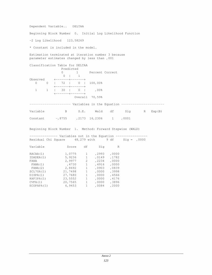
Dependent Variable.. DELTAA Beginning Block Number 0. Initial Log Likelihood Function -2 Log Likelihood 123,58269 * Constant is included in the model. Estimation terminated at iteration number 3 because parameter estimates changed by less than ,001 Classification Table for DELTAA Predicted 0 1 Percent Correct 0 | 1 Observed +-------+-------+ 0 0 | 72 | 0 | 100,00% +-------+-------+ 1 1 | 30 | 0 | ,00% +-------+-------+ Overall 70,59% ---------------------- Variables in the Equation ----------------------- Variable B S.E. Wald df Sig R Exp(B) Constant -,8755 ,2173 16,2306 1 ,0001 Beginning Block Number 1. Method: Forward Stepwise (WALD) --------------- Variables not in the Equation ----------------- Residual Chi Square 48,279 with 9 df Sig = ,0000 Variable Score df Sig R RACAA(1) 1,0775 1 ,2993 ,0000 IDADEA(1) 5,9236 1 ,0149 ,1782 FANA 2,9977 2 ,2234 ,0000 FANA(1) ,4730 1 ,4916 ,0000 FANA(2) 2,8692 1 ,0903 ,0839 SCL70A(1) 21,7498 1 ,0000 ,3998 DISPA(1) 27,7680 1 ,0000 ,4566 RXFIPA(1) 23,5552 1 ,0000 ,4176 CVFA(1) 20,7565 1 ,0000 ,3896 ECOPAPA(1) 6,9453 1 ,0084 ,2000

Anexo 2

123

Variable(s) Entered on Step Number 1.. DISPA Estimation terminated at iteration number 3 because Log Likelihood decreased by less than ,01 percent. -2 Log Likelihood 97,730 Goodness of Fit 101,988 Chi-Square df Significance Model Chi-Square 25,853 1 ,0000 Improvement 25,853 1 ,0000 Classification Table for DELTAA Predicted 0 1 Percent Correct 0 | 1 Observed +-------+-------+ 0 0 | 70 | 2 | 97,22% +-------+-------+ 1 1 | 17 | 13 | 43,33% +-------+-------+ Overall 81,37% ---------------------- Variables in the Equation ----------------------- Variable B S.E. Wald df Sig R Exp(B) DISPA(1) 3,2862 ,8060 16,6225 1 ,0000 ,3440 26,7400 Constant -1,4152 ,2704 27,3969 1 ,0000 --------------- Variables not in the Equation ----------------- Residual Chi Square 28,433 with 8 df Sig = ,0004 Variable Score df Sig R RACAA(1) 3,0455 1 ,0810 ,0920 IDADEA(1) 6,1160 1 ,0134 ,1825 FANA 3,2567 2 ,1963 ,0000 FANA(1) ,2840 1 ,5941 ,0000 FANA(2) 2,9382 1 ,0865 ,0871 SCL70A(1) 16,0319 1 ,0001 ,3370 RXFIPA(1) 12,3860 1 ,0004 ,2899 CVFA(1) 10,4798 1 ,0012 ,2619 ECOPAPA(1) 1,8524 1 ,1735 ,0000

Anexo 2

124

Variable(s) Entered on Step Number 2.. SCL70A Estimation terminated at iteration number 4 because Log Likelihood decreased by less than ,01 percent. -2 Log Likelihood 83,530 Goodness of Fit 97,447 Chi-Square df Significance Model Chi-Square 40,052 2 ,0000 Improvement 14,199 1 ,0002 Classification Table for DELTAA Predicted 0 1 Percent Correct 0 | 1 Observed +-------+-------+ 0 0 | 61 | 11 | 84,72% +-------+-------+ 1 1 | 8 | 22 | 73,33% +-------+-------+ Overall 81,37% ---------------------- Variables in the Equation ------------------------ Variable B S.E. Wald df Sig R Exp(B) SCL70A(1) 2,1386 ,5827 13,4698 1 ,0002 ,3046 8,4876 DISPA(1) 3,2050 ,8602 13,8834 1 ,0002 ,3101 24,6564 Constant -2,0735 ,3762 30,3820 1 ,0000 --------------- Variables not in the Equation ----------------- Residual Chi Square 14,250 with 7 df Sig = ,0469 Variable Score df Sig R RACAA(1) 5,3837 1 ,0203 ,1655 IDADEA(1) 3,9514 1 ,0468 ,1257 FANA ,7151 2 ,6994 ,0000 FANA(1) ,0609 1 ,8051 ,0000 FANA(2) ,2917 1 ,5891 ,0000 RXFIPA(1) 3,3280 1 ,0681 ,1037 CVFA(1) 6,0870 1 ,0136 ,1819 ECOPAPA(1) 1,1719 1 ,2790 ,0000

Anexo 2

125

Variable(s) Entered on Step Number 3.. CVFA Estimation terminated at iteration number 4 because Log Likelihood decreased by less than ,01 percent. -2 Log Likelihood 77,762 Goodness of Fit 94,123 Chi-Square df Significance Model Chi-Square 45,821 3 ,0000 Improvement 5,769 1 ,0163 Classification Table for DELTAA Predicted 0 1 Percent Correct 0 | 1 Observed +-------+-------+ 0 0 | 66 | 6 | 91,67% +-------+-------+ 1 1 | 11 | 19 | 63,33% +-------+-------+ Overall 83,33% ---------------------- Variables in the Equation ------------------------ Variable B S.E. Wald df Sig R Exp(B) SCL70A(1) 1,9136 ,6122 9,7697 1 ,0018 ,2507 6,7774 DISPA(1) 2,8196 ,9027 9,7558 1 ,0018 ,2505 16,7695 CVFA(1) 1,3894 ,5839 5,6617 1 ,0173 ,1721 4,0123 Constant -2,6326 ,4911 28,7380 1 ,0000 --------------- Variables not in the Equation ----------------- Residual Chi Square 9,031 with 6 df Sig = ,1718 Variable Score df Sig R RACAA(1) 4,2016 1 ,0404 ,1335 IDADEA(1) 5,3516 1 ,0207 ,1647 FANA 1,2599 2 ,5326 ,0000 FANA(1) ,6279 1 ,4281 ,0000 FANA(2) ,0593 1 ,8076 ,0000 RXFIPA(1) ,2591 1 ,6107 ,0000 ECOPAPA(1) ,1679 1 ,6820 ,0000

Anexo 2

126

Variable(s) Entered on Step Number 4.. IDADEA Estimation terminated at iteration number 5 because Log Likelihood decreased by less than ,01 percent. -2 Log Likelihood 71,605 Goodness of Fit 86,231 Chi-Square df Significance Model Chi-Square 51,978 4 ,0000 Improvement 6,157 1 ,0131 Classification Table for DELTAA Predicted 0 1 Percent Correct 0 | 1 Observed +-------+-------+ 0 0 | 67 | 5 | 93,06% +-------+-------+ 1 1 | 11 | 19 | 63,33% +-------+-------+ Overall 84,31% ---------------------- Variables in the Equation ------------------------ Variable B S.E. Wald df Sig R Exp(B) IDADEA(1) 2,0659 ,9649 4,5846 1 ,0323 ,1446 7,8928 SCL70A(1) 1,6690 ,6411 6,7768 1 ,0092 ,1966 5,3069 DISPA(1) 3,0554 ,9703 9,9154 1 ,0016 ,2531 21,2305 CVFA(1) 1,6651 ,6227 7,1497 1 ,0075 ,2041 5,2864 Constant -4,4091 1,0640 17,1733 1 ,0000 --------------- Variables not in the Equation ----------------- Residual Chi Square 4,024 with 5 df Sig = ,5460 Variable Score df Sig R RACAA(1) 3,3104 1 ,0688 ,1030 FANA ,2317 2 ,8906 ,0000 FANA(1) ,0992 1 ,7527 ,0000 FANA(2) ,0046 1 ,9462 ,0000 RXFIPA(1) ,0126 1 ,9106 ,0000 ECOPAPA(1) ,1858 1 ,6664 ,0000 No more variables can be deleted or added.

Anexo 2

127

Modelo 3: 6 variáveis independentes, excluindo-se os 5/8 valores em branco (Enter) Total number of cases: 105 (Unweighted) Number of selected cases: 105 Number of unselected cases: 0 Number of selected cases: 105 Number rejected because of missing data: 0 Number of cases included in the analysis: 105 Dependent Variable Encoding: Original Internal Value Value 0 0 1 1 Parameter Value Freq Coding (1) DISPA 0 89 ,000 1 16 1,000

Anexo 2

128

Dependent Variable.. DELTAA Beginning Block Number 0. Initial Log Likelihood Function -2 Log Likelihood 127,42283 * Constant is included in the model. Beginning Block Number 1. Method: Enter Variable(s) Entered on Step Number 1.. DISPA Estimation terminated at iteration number 3 because Log Likelihood decreased by less than ,01 percent. -2 Log Likelihood 98,865 Goodness of Fit 104,981 Chi-Square df Significance Model Chi-Square 28,558 1 ,0000 Improvement 28,558 1 ,0000 Classification Table for DELTAA Predicted 0 1 Percent Correct 0 | 1 Observed +-------+-------+ 0 0 | 72 | 2 | 97,30% +-------+-------+ 1 1 | 17 | 14 | 45,16% +-------+-------+ Overall 81,90% ---------------------- Variables in the Equation ----------------------- Variable B S.E. Wald df Sig R Exp(B) DISPA(1) 3,3880 ,8022 17,8357 1 ,0000 ,3525 29,6057 Constant -1,4434 ,2696 28,6538 1 ,0000

Anexo 2

129

Total number of cases: 105 (Unweighted) Number of selected cases: 105 Number of unselected cases: 0 Number of selected cases: 105 Number rejected because of missing data: 0 Number of cases included in the analysis: 105 Dependent Variable Encoding: Original Internal Value Value 0 0 1 1 Parameter Value Freq Coding (1) RXFIPA 0 74 ,000 1 31 1,000 DISPA 0 89 ,000 1 16 1,000

Anexo 2

130

Dependent Variable.. DELTAA Beginning Block Number 0. Initial Log Likelihood Function -2 Log Likelihood 127,42283 * Constant is included in the model. Beginning Block Number 1. Method: Enter Variable(s) Entered on Step Number 1.. DISPA RXFIPA Estimation terminated at iteration number 4 because Log Likelihood decreased by less than ,01 percent. -2 Log Likelihood 87,571 Goodness of Fit 106,273 Chi-Square df Significance Model Chi-Square 39,852 2 ,0000 Improvement 39,852 2 ,0000 Classification Table for DELTAA Predicted 0 1 Percent Correct 0 | 1 Observed +-------+-------+ 0 0 | 72 | 2 | 97,30% +-------+-------+ 1 1 | 17 | 14 | 45,16% +-------+-------+ Overall 81,90% ---------------------- Variables in the Equation ------------------------ Variable B S.E. Wald df Sig R Exp(B) DISPA(1) 2,8304 ,8487 11,1218 1 ,0009 ,2676 16,9516 RXFIPA(1) 1,8624 ,5545 11,2799 1 ,0008 ,2699 6,4393 Constant -2,0159 ,3622 30,9741 1 ,0000

Anexo 2

131

Total number of cases: 105 (Unweighted) Number of selected cases: 105 Number of unselected cases: 0 Number of selected cases: 105 Number rejected because of missing data: 0 Number of cases included in the analysis: 105 Dependent Variable Encoding: Original Internal Value Value 0 0 1 1 Parameter Value Freq Coding (1) SCL70A 0 79 ,000 1 26 1,000 RXFIPA 0 74 ,000 1 31 1,000 DISPA 0 89 ,000 1 16 1,000

Anexo 2

132

Dependent Variable.. DELTAA Beginning Block Number 0. Initial Log Likelihood Function -2 Log Likelihood 127,42283 * Constant is included in the model. Beginning Block Number 1. Method: Enter Variable(s) Entered on Step Number 1.. DISPA RXFIPA SCL70A Estimation terminated at iteration number 4 because Log Likelihood decreased by less than ,01 percent. -2 Log Likelihood 81,124 Goodness of Fit 101,382 Chi-Square df Significance Model Chi-Square 46,299 3 ,0000 Improvement 46,299 3 ,0000 Classification Table for DELTAA Predicted 0 1 Percent Correct 0 | 1 Observed +-------+-------+ 0 0 | 68 | 6 | 91,89% +-------+-------+ 1 1 | 10 | 21 | 67,74% +-------+-------+ Overall 84,76% ---------------------- Variables in the Equation ------------------------ Variable B S.E. Wald df Sig R Exp(B) DISPA(1) 2,9638 ,8784 11,3843 1 ,0007 ,2714 19,3711 RXFIPA(1) 1,1865 ,6313 3,5326 1 ,0602 ,1097 3,2755 SCL70A(1) 1,6419 ,6462 6,4554 1 ,0111 ,1870 5,1648 Constant -2,3024 ,4064 32,0922 1 ,0000

Anexo 2

133

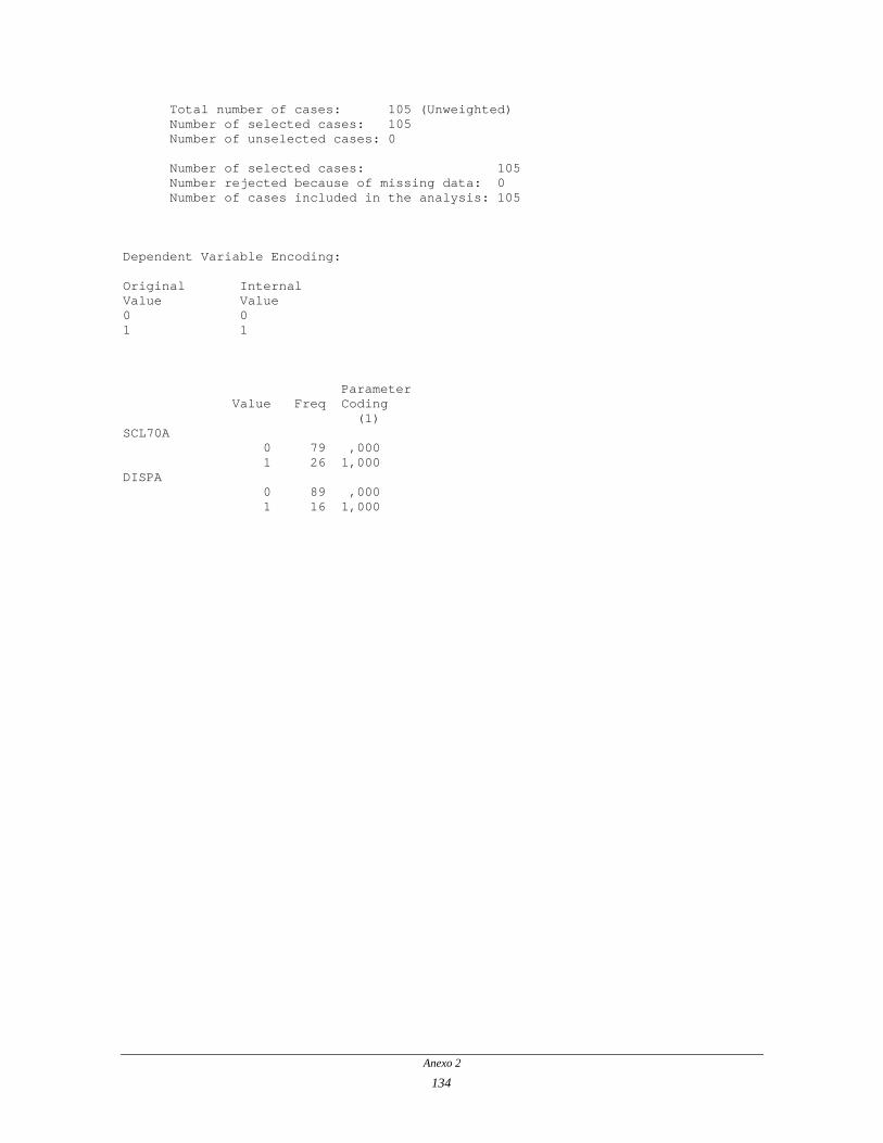
Total number of cases: 105 (Unweighted) Number of selected cases: 105 Number of unselected cases: 0 Number of selected cases: 105 Number rejected because of missing data: 0 Number of cases included in the analysis: 105 Dependent Variable Encoding: Original Internal Value Value 0 0 1 1 Parameter Value Freq Coding (1) SCL70A 0 79 ,000 1 26 1,000 DISPA 0 89 ,000 1 16 1,000

Anexo 2

134

Dependent Variable.. DELTAA Beginning Block Number 0. Initial Log Likelihood Function -2 Log Likelihood 127,42283 * Constant is included in the model. Beginning Block Number 1. Method: Enter Variable(s) Entered on Step Number 1.. DISPA SCL70A Estimation terminated at iteration number 4 because Log Likelihood decreased by less than ,01 percent. -2 Log Likelihood 84,523 Goodness of Fit 100,133 Chi-Square df Significance Model Chi-Square 42,900 2 ,0000 Improvement 42,900 2 ,0000 Classification Table for DELTAA Predicted 0 1 Percent Correct 0 | 1 Observed +-------+-------+ 0 0 | 63 | 11 | 85,14% +-------+-------+ 1 1 | 8 | 23 | 74,19% +-------+-------+ Overall 81,90% ---------------------- Variables in the Equation ------------------------ Variable B S.E. Wald df Sig R Exp(B) DISPA(1) 3,3733 ,8539 15,6073 1 ,0001 ,3268 29,1759 SCL70A(1) 2,1554 ,5843 13,6091 1 ,0002 ,3018 8,6312 Constant -2,0996 ,3753 31,3007 1 ,0000

Anexo 2

135

Total number of cases: 102 (Unweighted) Number of selected cases: 102 Number of unselected cases: 0 Number of selected cases: 102 Number rejected because of missing data: 0 Number of cases included in the analysis: 102 Dependent Variable Encoding: Original Internal Value Value 0 0 1 1 Parameter Value Freq Coding (1) CVFA 0 59 ,000 1 43 1,000 SCL70A 0 76 ,000 1 26 1,000 DISPA 0 87 ,000 1 15 1,000

Anexo 2

136

Dependent Variable.. DELTAA Beginning Block Number 0. Initial Log Likelihood Function -2 Log Likelihood 123,58269 * Constant is included in the model. Beginning Block Number 1. Method: Enter Variable(s) Entered on Step Number 1.. DISPA SCL70A CVFA Estimation terminated at iteration number 4 because Log Likelihood decreased by less than ,01 percent. -2 Log Likelihood 77,762 Goodness of Fit 94,123 Chi-Square df Significance Model Chi-Square 45,821 3 ,0000 Improvement 45,821 3 ,0000 Classification Table for DELTAA Predicted 0 1 Percent Correct 0 | 1 Observed +-------+-------+ 0 0 | 66 | 6 | 91,67% +-------+-------+ 1 1 | 11 | 19 | 63,33% +-------+-------+ Overall 83,33% ---------------------- Variables in the Equation ------------------------ Variable B S.E. Wald df Sig R Exp(B) DISPA(1) 2,8196 ,9027 9,7558 1 ,0018 ,2505 16,7695 SCL70A(1) 1,9136 ,6122 9,7697 1 ,0018 ,2507 6,7774 CVFA(1) 1,3894 ,5839 5,6617 1 ,0173 ,1721 4,0123 Constant -2,6326 ,4911 28,7380 1 ,0000

Anexo 2

137

Total number of cases: 102 (Unweighted) Number of selected cases: 102 Number of unselected cases: 0 Number of selected cases: 102 Number rejected because of missing data: 0 Number of cases included in the analysis: 102 Dependent Variable Encoding: Original Internal Value Value 0 0 1 1 Parameter Value Freq Coding (1) IDADEA 1 75 1,000 0 27 ,000 SCL70A 0 76 ,000 1 26 1,000 CVFA 0 59 ,000 1 43 1,000 DISPA 0 87 ,000 1 15 1,000

Anexo 2

138

Dependent Variable.. DELTAA Beginning Block Number 0. Initial Log Likelihood Function -2 Log Likelihood 123,58269 * Constant is included in the model. Beginning Block Number 1. Method: Enter Variable(s) Entered on Step Number 1.. DISPA SCL70A CVFA IDADEA Estimation terminated at iteration number 5 because Log Likelihood decreased by less than ,01 percent. -2 Log Likelihood 71,605 Goodness of Fit 86,231 Chi-Square df Significance Model Chi-Square 51,978 4 ,0000 Improvement 51,978 4 ,0000 Classification Table for DELTAA Predicted 0 1 Percent Correct 0 | 1 Observed +-------+-------+ 0 0 | 67 | 5 | 93,06% +-------+-------+ 1 1 | 11 | 19 | 63,33% +-------+-------+ Overall 84,31% -- -------------------- Variables in the Equation ------------------------

Variable B S.E. Wald df Sig R Exp(B) DISPA(1) 3,0554 ,9703 9,9154 1 ,0016 ,2531 21,2305 SCL70A(1) 1,6690 ,6411 6,7768 1 ,0092 ,1966 5,3069 CVFA(1) 1,6651 ,6227 7,1497 1 ,0075 ,2041 5,2864 IDADEA(1) 2,0659 ,9649 4,5846 1 ,0323 ,1446 7,8928 Constant -4,4091 1,0640 17,1733 1 ,0000

Anexo 2

139

Total number of cases: 102 (Unweighted) Number of selected cases: 102 Number of unselected cases: 0 Number of selected cases: 102 Number rejected because of missing data: 0 Number of cases included in the analysis: 102 Dependent Variable Encoding: Original Internal Value Value 0 0 1 1 Parameter Value Freq Coding (1) RACAA 0 72 ,000 1 30 1,000 SCL70A 0 76 ,000 1 26 1,000 CVFA 0 59 ,000 1 43 1,000 IDADEA 1 75 1,000 0 27 ,000 DISPA 0 87 ,000 1 15 1,000

Anexo 2

140

Dependent Variable.. DELTAA Beginning Block Number 0. Initial Log Likelihood Function -2 Log Likelihood 123,58269 * Constant is included in the model. Beginning Block Number 1. Method: Enter Variable(s) Entered on Step Number 1.. DISPA SCL70A CVFA IDADEA RACAA Estimation terminated at iteration number 5 because Log Likelihood decreased by less than ,01 percent. -2 Log Likelihood 68,328 Goodness of Fit 76,242 Chi-Square df Significance Model Chi-Square 55,254 5 ,0000 Improvement 55,254 5 ,0000 Classification Table for DELTAA Predicted 0 1 Percent Correct 0 | 1 Observed +-------+-------+ 0 0 | 66 | 6 | 91,67% +-------+-------+ 1 1 | 11 | 19 | 63,33% +-------+-------+ Overall 83,33% ---------------------- Variables in the Equation ------------------------ Variable B S.E. Wald df Sig R Exp(B) DISPA(1) 3,4960 1,0454 11,1830 1 ,0008 ,2726 32,9824 SCL70A(1) 1,9796 ,7120 7,7304 1 ,0054 ,2153 7,2402 CVFA(1) 1,5855 ,6402 6,1339 1 ,0133 ,1829 4,8817 IDADEA(1) 1,9563 ,9752 4,0244 1 ,0448 ,1280 7,0730 RACAA(1) 1,2525 ,7098 3,1141 1 ,0776 ,0949 3,4992 Constant -4,8432 1,1389 18,0838 1 ,0000

Anexo 2

141

Anexo 2

142

Anexo 2

143

+ Disease - +--------+--------+ Odds ratio = 2.60 (0.50 <OR< 17.99*) +| 29 | 67 | 96 +--------+--------+ -| 2 | 12 | 14 +--------+--------+ Fisher exact: 2-tailed P-value: 0.3417869 E 31 79 110 Dependent Variable Encoding: Original Internal Value Value 0 0 1 1 Parameter Value Freq Coding (1) SEXOA 1 96 1,000 0 14 ,000 Dependent Variable.. TCAMA Beginning Block Number 0. Initial Log Likelihood Function -2 Log Likelihood 130,82571 * Constant is included in the model. Beginning Block Number 1. Method: Enter Variable(s) Entered on Step Number 1.. SEXOA Estimation terminated at iteration number 3 because Log Likelihood decreased by less than ,01 percent. -2 Log Likelihood 129,106 Goodness of Fit 109,995 Chi-Square df Significance Model Chi-Square 1,720 1 ,1897 Improvement 1,720 1 ,1897 Classification Table for TCAMA Predicted 0 1 Percent Correct 0 | 1 Observed +-------+-------+ 0 0 | 79 | 0 | 100,00% +-------+-------+ 1 1 | 31 | 0 | ,00% +-------+-------+ Overall 71,82% ---------------------- Variables in the Equation ----------------------- Variable B S.E. Wald df Sig R Exp(B) SEXOA(1) ,9538 ,7953 1,4383 1 ,2304 ,0000 2,5956 Constant -1,7912 ,7636 5,5023 1 ,0190

Anexo 2

144

+ Disease - +--------+--------+ Odds ratio = 2.43 (0.93 <OR< 6.35) +| 14 | 20 | 34 +--------+--------+ Chi-Squares P-values -| 17 | 59 | 76 ----------- -------- +--------+--------+ Yates corrected: 3.23 0.0723455 E 31 79 110 Dependent Variable Encoding: Original Internal Value Value 0 0 1 1 Parameter Value Freq Coding (1) RACAA 0 76 ,000 1 34 1,000 Dependent Variable.. TCAMA Beginning Block Number 0. Initial Log Likelihood Function -2 Log Likelihood 130,82571 * Constant is included in the model. Beginning Block Number 1. Method: Enter Variable(s) Entered on Step Number 1.. RACAA Estimation terminated at iteration number 3 because Log Likelihood decreased by less than ,01 percent. -2 Log Likelihood 126,862 Goodness of Fit 110,000 Chi-Square df Significance Model Chi-Square 3,963 1 ,0465 Improvement 3,963 1 ,0465 Classification Table for TCAMA Predicted 0 1 Percent Correct 0 | 1 Observed +-------+-------+ 0 0 | 79 | 0 | 100,00% +-------+-------+ 1 1 | 31 | 0 | ,00% +-------+-------+ Overall 71,82% ---------------------- Variables in the Equation ----------------------- Variable B S.E. Wald df Sig R Exp(B) RACAA(1) ,8876 ,4441 3,9955 1 ,0456 ,1235 2,4294 Constant -1,2443 ,2753 20,4339 1 ,0000

Anexo 2

145

+ Disease - +--------+--------+ Odds ratio = 7.11 (1.47 <OR< 46.72*) +| 29 | 53 | 82 +--------+--------+ Chi-Squares P-values -| 2 | 26 | 28 ----------- -------- +--------+--------+ Yates corrected: 6.88 0.0087202 E 31 79 110 Dependent Variable Encoding: Original Internal Value Value 0 0 1 1 Parameter Value Freq Coding (1) IDADEA 1 82 1,000 0 28 ,000 Dependent Variable.. TCAMA Beginning Block Number 0. Initial Log Likelihood Function -2 Log Likelihood 130,82571 * Constant is included in the model. Beginning Block Number 1. Method: Enter Variable(s) Entered on Step Number 1.. IDADEA Estimation terminated at iteration number 4 because Log Likelihood decreased by less than ,01 percent. -2 Log Likelihood 120,958 Goodness of Fit 109,996 Chi-Square df Significance Model Chi-Square 9,868 1 ,0017 Improvement 9,868 1 ,0017 Classification Table for TCAMA Predicted 0 1 Percent Correct 0 | 1 Observed +-------+-------+ 0 0 | 79 | 0 | 100,00% +-------+-------+ 1 1 | 31 | 0 | ,00% +-------+-------+ Overall 71,82% ---------------------- Variables in the Equation ------------------------ Variable B S.E. Wald df Sig R Exp(B) IDADEA(1) 1,9618 ,7692 6,5039 1 ,0108 ,1855 7,1121 Constant -2,5648 ,7337 12,2182 1 ,0005

Anexo 2

146

+ Disease - +--------+--------+ Odds ratio = 1.24 (0.43 <OR< 3.71) +| 24 | 58 | 82 +--------+--------+ Chi-Squares P-values -| 7 | 21 | 28 ----------- -------- +--------+--------+ Yates corrected: 0.04 0.8491614 E 31 79 110 Dependent Variable Encoding: Original Internal Value Value 0 0 1 1 Parameter Value Freq Coding (1) TDA 1 82 1,000 0 28 ,000 Dependent Variable.. TCAMA Beginning Block Number 0. Initial Log Likelihood Function -2 Log Likelihood 130,82571 * Constant is included in the model. Beginning Block Number 1. Method: Enter Variable(s) Entered on Step Number 1.. TDA Estimation terminated at iteration number 3 because Log Likelihood decreased by less than ,01 percent. -2 Log Likelihood 130,635 Goodness of Fit 110,000 Chi-Square df Significance Model Chi-Square ,191 1 ,6621 Improvement ,191 1 ,6621 Classification Table for TCAMA Predicted 0 1 Percent Correct 0 | 1 Observed +-------+-------+ 0 0 | 79 | 0 | 100,00% +-------+-------+ 1 1 | 31 | 0 | ,00% +-------+-------+ Overall 71,82% ---------------------- Variables in the Equation ----------------------- Variable B S.E. Wald df Sig R Exp(B) TDA(1) ,2162 ,4994 ,1875 1 ,6650 ,0000 1,2414 Constant -1,0986 ,4364 6,3365 1 ,0118

Anexo 2

147

+ Disease - +--------+--------+ Odds ratio = 1.23 (0.46 <OR< 3.31) +| 10 | 22 | 32 +--------+--------+ Chi-Squares P-values -| 21 | 57 | 78 ----------- -------- +--------+--------+ Yates corrected: 0.05 0.8221110 E 31 79 110 Dependent Variable Encoding: Original Internal Value Value 0 0 1 1 Parameter Value Freq Coding (1) FCA 0 78 ,000 1 32 1,000 Dependent Variable.. TCAMA Beginning Block Number 0. Initial Log Likelihood Function -2 Log Likelihood 130,82571 * Constant is included in the model. Beginning Block Number 1. Method: Enter Variable(s) Entered on Step Number 1.. FCA Estimation terminated at iteration number 3 because Log Likelihood decreased by less than ,01 percent. -2 Log Likelihood 130,618 Goodness of Fit 110,000 Chi-Square df Significance Model Chi-Square ,207 1 ,6488 Improvement ,207 1 ,6488 Classification Table for TCAMA Predicted 0 1 Percent Correct 0 | 1 Observed +-------+-------+ 0 0 | 79 | 0 | 100,00% +-------+-------+ 1 1 | 31 | 0 | ,00% +-------+-------+ Overall 71,82% ---------------------- Variables in the Equation ----------------------- Variable B S.E. Wald df Sig R Exp(B) FCA(1) ,2101 ,4589 ,2095 1 ,6471 ,0000 1,2338 Constant -,9985 ,2553 15,3010 1 ,0001

Anexo 2

148

+ Disease - +--------+--------+ Odds ratio = 4.67 (0.33 <OR< 137.66*) +| 3 | 9 | 12 +--------+--------+ -| 1 | 14 | 15 +--------+--------+ Fisher exact: 2-tailed P-value: 0.2940171 E 4 23 27 + Disease - +--------+--------+ Odds ratio = 6.75 (0.85 <OR< 144.58*) +| 27 | 56 | 83 +--------+--------+ -| 1 | 14 | 15 +--------+--------+ Fisher exact: 2-tailed P-value: 0.0599001 E 28 70 98 Dependent Variable Encoding: Original Internal Value Value 0 0 1 1 Parameter Value Freq Coding (1) (2) FANA 0 15 ,000 ,000 1 12 1,000 ,000 2 83 ,000 1,000 Dependent Variable.. TCAMA Beginning Block Number 0. Initial Log Likelihood Function -2 Log Likelihood 130,82571 * Constant is included in the model. Beginning Block Number 1. Method: Enter Variable(s) Entered on Step Number 1.. FANA Estimation terminated at iteration number 4 because Log Likelihood decreased by less than ,01 percent. -2 Log Likelihood 125,557 Goodness of Fit 109,997 Chi-Square df Significance Model Chi-Square 5,269 2 ,0718 Improvement 5,269 2 ,0718

Anexo 2

149

Classification Table for TCAMA Predicted 0 1 Percent Correct 0 | 1 Observed +-------+-------+ 0 0 | 79 | 0 | 100,00% +-------+-------+ 1 1 | 31 | 0 | ,00% +-------+-------+ Overall 71,82% ---------------------- Variables in the Equation ----------------------- Variable B S.E. Wald df Sig R Exp(B) FANA 3,3906 2 ,1835 ,0000 FANA(1) 1,5402 1,2311 1,5651 1 ,2109 ,0000 4,6654 FANA(2) 1,9093 1,0612 3,2372 1 ,0720 ,0972 6,7482 Constant -2,6388 1,0350 6,5005 1 ,0108

Anexo 2

150

+ Disease - +--------+--------+ Odds ratio = 2.01 (0.73 <OR< 5.48) +| 11 | 17 | 28 +--------+--------+ Chi-Squares P-values -| 20 | 62 | 82 ----------- -------- +--------+--------+ Yates corrected: 1.61 0.2042990 E 31 79 110 Dependent Variable Encoding: Original Internal Value Value 0 0 1 1 Parameter Value Freq Coding (1) SCL70A 0 82 ,000 1 28 1,000 Dependent Variable.. TCAMA Beginning Block Number 0. Initial Log Likelihood Function -2 Log Likelihood 130,82571 * Constant is included in the model. Beginning Block Number 1. Method: Enter Variable(s) Entered on Step Number 1.. SCL70A Estimation terminated at iteration number 3 because Log Likelihood decreased by less than ,01 percent. -2 Log Likelihood 128,629 Goodness of Fit 110,000 Chi-Square df Significance Model Chi-Square 2,197 1 ,1383 Improvement 2,197 1 ,1383 Classification Table for TCAMA Predicted 0 1 Percent Correct 0 | 1 Observed +-------+-------+ 0 0 | 79 | 0 | 100,00% +-------+-------+ 1 1 | 31 | 0 | ,00% +-------+-------+ Overall 71,82% ---------------------- Variables in the Equation ------------------------ Variable B S.E. Wald df Sig R Exp(B) SCL70A(1) ,6961 ,4646 2,2446 1 ,1341 ,0432 2,0059 Constant -1,1314 ,2572 19,3571 1 ,0000

Anexo 2

151

+ Disease - +--------+--------+ Odds ratio = 4.88 (1.55 <OR< 15.66) +| 11 | 8 | 19 +--------+--------+ Chi-Squares P-values -| 20 | 71 | 91 ----------- -------- +--------+--------+ Yates corrected: 8.32 0.0039162 E 31 79 110 Dependent Variable Encoding: Original Internal Value Value 0 0 1 1 Parameter Value Freq Coding (1) DISPA 0 91 ,000 1 19 1,000 Dependent Variable.. TCAMA Beginning Block Number 0. Initial Log Likelihood Function -2 Log Likelihood 130,82571 * Constant is included in the model. Beginning Block Number 1. Method: Enter Variable(s) Entered on Step Number 1.. DISPA Estimation terminated at iteration number 3 because Log Likelihood decreased by less than ,01 percent. -2 Log Likelihood 121,711 Goodness of Fit 110,000 Chi-Square df Significance Model Chi-Square 9,115 1 ,0025 Improvement 9,115 1 ,0025 Classification Table for TCAMA Predicted 0 1 Percent Correct 0 | 1 Observed +-------+-------+ 0 0 | 71 | 8 | 89,87% +-------+-------+ 1 1 | 20 | 11 | 35,48% +-------+-------+ Overall 74,55% ---------------------- Variables in the Equation ----------------------- Variable B S.E. Wald df Sig R Exp(B) DISPA(1) 1,5854 ,5291 8,9769 1 ,0027 ,2309 4,8812 Constant -1,2669 ,2531 25,0473 1 ,0000

Anexo 2

152

+ Disease - +--------+--------+ Odds ratio = 2.60 (0.99 <OR< 6.85) +| 14 | 19 | 33 +--------+--------+ Chi-Squares P-values -| 17 | 60 | 77 ----------- -------- +--------+--------+ Yates corrected: 3.77 0.0520871 E 31 79 110 Dependent Variable Encoding: Original Internal Value Value 0 0 1 1 Parameter Value Freq Coding (1) RXFIPA 0 77 ,000 1 33 1,000 Dependent Variable.. TCAMA Beginning Block Number 0. Initial Log Likelihood Function -2 Log Likelihood 130,82571 * Constant is included in the model. Beginning Block Number 1. Method: Enter Variable(s) Entered on Step Number 1.. RXFIPA Estimation terminated at iteration number 3 because Log Likelihood decreased by less than ,01 percent. -2 Log Likelihood 126,283 Goodness of Fit 110,000 Chi-Square df Significance Model Chi-Square 4,543 1 ,0331 Improvement 4,543 1 ,0331 Classification Table for TCAMA Predicted 0 1 Percent Correct 0 | 1 Observed +-------+-------+ 0 0 | 79 | 0 | 100,00% +-------+-------+ 1 1 | 31 | 0 | ,00% +-------+-------+ Overall 71,82% ---------------------- Variables in the Equation ------------------------ Variable B S.E. Wald df Sig R Exp(B) RXFIPA(1) ,9557 ,4467 4,5775 1 ,0324 ,1404 2,6006 Constant -1,2611 ,2748 21,0682 1 ,0000

Anexo 2

153

+ Disease - +--------+--------+ Odds ratio = 2.04 (0.79 <OR< 5.29) +| 16 | 29 | 45 +--------+--------+ Chi-Squares P-values -| 13 | 48 | 61 ----------- -------- +--------+--------+ Yates corrected: 1.98 0.1598503 E 29 77 106 Dependent Variable Encoding: Original Internal Value Value 0 0 1 1 Parameter Value Freq Coding (1) CVFA 0 61 ,000 1 45 1,000 Dependent Variable.. TCAMA Beginning Block Number 0. Initial Log Likelihood Function -2 Log Likelihood 124,39989 * Constant is included in the model. Beginning Block Number 1. Method: Enter Variable(s) Entered on Step Number 1.. CVFA Estimation terminated at iteration number 3 because Log Likelihood decreased by less than ,01 percent. -2 Log Likelihood 121,776 Goodness of Fit 106,000 Chi-Square df Significance Model Chi-Square 2,624 1 ,1053 Improvement 2,624 1 ,1053 Classification Table for TCAMA Predicted 0 1 Percent Correct 0 | 1 Observed +-------+-------+ 0 0 | 77 | 0 | 100,00% +-------+-------+ 1 1 | 29 | 0 | ,00% +-------+-------+ Overall 72,64% ---------------------- Variables in the Equation ----------------------- Variable B S.E. Wald df Sig R Exp(B) CVFA(1) ,7115 ,4413 2,5998 1 ,1069 ,0694 2,0371 Constant -1,3062 ,3127 17,4543 1 ,0000

Anexo 2

154

+ Disease - +--------+--------+ Odds ratio = 1.25 (0.40 <OR< 3.85) +| 7 | 16 | 23 +--------+--------+ Chi-Squares P-values -| 20 | 57 | 77 ----------- -------- +--------+--------+ Yates corrected: 0.02 0.8766485 E 27 73 100 Dependent Variable Encoding: Original Internal Value Value 0 0 1 1 Parameter Value Freq Coding (1) TCVFB 0 77 ,000 1 23 1,000 Dependent Variable.. TCAMA Beginning Block Number 0. Initial Log Likelihood Function -2 Log Likelihood 116,65177 * Constant is included in the model. Beginning Block Number 1. Method: Enter Variable(s) Entered on Step Number 1.. TCVFB Estimation terminated at iteration number 3 because Log Likelihood decreased by less than ,01 percent. -2 Log Likelihood 116,476 Goodness of Fit 100,000 Chi-Square df Significance Model Chi-Square ,176 1 ,6751 Improvement ,176 1 ,6751 Classification Table for TCAMA Predicted 0 1 Percent Correct 0 | 1 Observed +-------+-------+ 0 0 | 73 | 0 | 100,00% +-------+-------+ 1 1 | 27 | 0 | ,00% +-------+-------+ Overall 73,00% ---------------------- Variables in the Equation ----------------------- Variable B S.E. Wald df Sig R Exp(B) TCVFB(1) ,2206 ,5224 ,1784 1 ,6728 ,0000 1,2469 Constant -1,0473 ,2599 16,2395 1 ,0001

Anexo 2

155

+ Disease - +--------+--------+ Odds ratio = 1.53 (0.56 <OR< 4.16) +| 11 | 22 | 33 +--------+--------+ Chi-Squares P-values -| 17 | 52 | 69 ----------- -------- +--------+--------+ Yates corrected: 0.47 0.4942885 E 28 74 102 Dependent Variable Encoding: Original Internal Value Value 0 0 1 1 Parameter Value Freq Coding (1) TCRETB 0 69 ,000 1 33 1,000 Dependent Variable.. TCAMA Beginning Block Number 0. Initial Log Likelihood Function -2 Log Likelihood 119,88937 * Constant is included in the model. Beginning Block Number 1. Method: Enter Variable(s) Entered on Step Number 1.. TCRETB Estimation terminated at iteration number 3 because Log Likelihood decreased by less than ,01 percent. -2 Log Likelihood 119,058 Goodness of Fit 102,000 Chi-Square df Significance Model Chi-Square ,831 1 ,3619 Improvement ,831 1 ,3619 Classification Table for TCAMA Predicted 0 1 Percent Correct 0 | 1 Observed +-------+-------+ 0 0 | 74 | 0 | 100,00% +-------+-------+ 1 1 | 28 | 0 | ,00% +-------+-------+ Overall 72,55% ---------------------- Variables in the Equation ------------------------ Variable B S.E. Wald df Sig R Exp(B) TCRETB(1) ,4249 ,4631 ,8419 1 ,3588 ,0000 1,5294 Constant -1,1180 ,2794 16,0144 1 ,0001

Anexo 2

156

+ Disease - +--------+--------+ Odds ratio = 2.08 (0.51 <OR< 8.33*) +| 5 | 7 | 12 +--------+--------+ -| 23 | 67 | 90 +--------+--------+ Fisher exact: 2-tailed P-value: 0.3025687 E 28 74 102 Dependent Variable Encoding: Original Internal Value Value 0 0 1 1 Parameter Value Freq Coding (1) TCFAVB 0 90 ,000 1 12 1,000 Dependent Variable.. TCAMA Beginning Block Number 0. Initial Log Likelihood Function -2 Log Likelihood 119,88937 * Constant is included in the model. Beginning Block Number 1. Method: Enter Variable(s) Entered on Step Number 1.. TCFAVB Estimation terminated at iteration number 3 because Log Likelihood decreased by less than ,01 percent. -2 Log Likelihood 118,605 Goodness of Fit 102,000 Chi-Square df Significance Model Chi-Square 1,285 1 ,2571 Improvement 1,285 1 ,2571 Classification Table for TCAMA Predicted 0 1 Percent Correct 0 | 1 Observed +-------+-------+ 0 0 | 74 | 0 | 100,00% +-------+-------+ 1 1 | 28 | 0 | ,00% +-------+-------+ Overall 72,55% ---------------------- Variables in the Equation ------------------------ Variable B S.E. Wald df Sig R Exp(B) TCFAVB(1) ,7327 ,6335 1,3380 1 ,2474 ,0000 2,0807 Constant -1,0692 ,2417 19,5738 1 ,0000

Anexo 2

157

+ Disease - +--------+--------+ Odds ratio = 1.24 (0.47 <OR< 3.28) +| 14 | 34 | 48 +--------+--------+ Chi-Squares P-values -| 13 | 39 | 52 ----------- -------- +--------+--------+ Yates corrected: 0.06 0.8076488 E 27 73 100 Dependent Variable Encoding: Original Internal Value Value 0 0 1 1 Parameter Value Freq Coding (1) TCTOTA 0 52 ,000 1 48 1,000 Dependent Variable.. TCAMA Beginning Block Number 0. Initial Log Likelihood Function -2 Log Likelihood 116,65177 * Constant is included in the model. Beginning Block Number 1. Method: Enter Variable(s) Entered on Step Number 1.. TCTOTA Estimation terminated at iteration number 3 because Log Likelihood decreased by less than ,01 percent. -2 Log Likelihood 116,432 Goodness of Fit 100,000 Chi-Square df Significance Model Chi-Square ,220 1 ,6392 Improvement ,220 1 ,6392 Classification Table for TCAMA Predicted 0 1 Percent Correct 0 | 1 Observed +-------+-------+ 0 0 | 73 | 0 | 100,00% +-------+-------+ 1 1 | 27 | 0 | ,00% +-------+-------+ Overall 73,00% ---------------------- Variables in the Equation ------------------------ Variable B S.E. Wald df Sig R Exp(B) TCTOTA(1) ,2113 ,4510 ,2195 1 ,6394 ,0000 1,2353 Constant -1,0986 ,3203 11,7677 1 ,0006

Anexo 2

158

+ Disease - +--------+--------+ Odds ratio = 2.79 (1.06 <OR< 7.40) +| 14 | 18 | 32 +--------+--------+ Chi-Squares P-values -| 17 | 61 | 78 ----------- -------- +--------+--------+ Yates corrected: 4.37 0.0364968 E 31 79 110 Dependent Variable Encoding: Original Internal Value Value 0 0 1 1 Parameter Value Freq Coding (1) ECOPAPA 0 78 ,000 1 32 1,000 Dependent Variable.. TCAMA Beginning Block Number 0. Initial Log Likelihood Function -2 Log Likelihood 130,82571 * Constant is included in the model. Beginning Block Number 1. Method: Enter Variable(s) Entered on Step Number 1.. ECOPAPA Estimation terminated at iteration number 3 because Log Likelihood decreased by less than ,01 percent. -2 Log Likelihood 125,651 Goodness of Fit 110,000 Chi-Square df Significance Model Chi-Square 5,175 1 ,0229 Improvement 5,175 1 ,0229 Classification Table for TCAMA Predicted 0 1 Percent Correct 0 | 1 Observed +-------+-------+ 0 0 | 79 | 0 | 100,00% +-------+-------+ 1 1 | 31 | 0 | ,00% +-------+-------+ Overall 71,82% ----------------------- Variables in the Equation ------------------------ Variable B S.E. Wald df Sig R Exp(B) ECOPAPA(1) 1,0263 ,4497 5,2095 1 ,0225 ,1566 2,7908 Constant -1,2777 ,2743 21,7026 1 ,0000

Anexo 2

159

+ Disease - +--------+--------+ Odds ratio = 2.05 (0.64 <OR< 6.99*) +| 25 | 56 | 81 +--------+--------+ Chi-Squares P-values -| 5 | 23 | 28 ----------- -------- +--------+--------+ Yates corrected: 1.17 0.2788038 E 30 79 109 Dependent Variable Encoding: Original Internal Value Value 0 0 1 1 Parameter Value Freq Coding (1) ECTA 0 28 ,000 1 81 1,000 Dependent Variable.. TCAMA Beginning Block Number 0. Initial Log Likelihood Function -2 Log Likelihood 128,26923 * Constant is included in the model. Beginning Block Number 1. Method: Enter Variable(s) Entered on Step Number 1.. ECTA Estimation terminated at iteration number 3 because Log Likelihood decreased by less than ,01 percent. -2 Log Likelihood 126,394 Goodness of Fit 108,998 Chi-Square df Significance Model Chi-Square 1,875 1 ,1709 Improvement 1,875 1 ,1709 Classification Table for TCAMA Predicted 0 1 Percent Correct 0 | 1 Observed +-------+-------+ 0 0 | 79 | 0 | 100,00% +-------+-------+ 1 1 | 30 | 0 | ,00% +-------+-------+ Overall 72,48% ---------------------- Variables in the Equation ----------------------- Variable B S.E. Wald df Sig R Exp(B) ECTA(1) ,7195 ,5489 1,7180 1 ,1899 ,0000 2,0534 Constant -1,5260 ,4934 9,5644 1 ,0020

Anexo 2

160

Anexo 2

161

+ Disease - +--------+--------+ Odds ratio = 0.93 (0.23 <OR< 3.98*) +| 27 | 65 | 92 +--------+--------+ -| 4 | 9 | 13 +--------+--------+ Fisher exact: 2-tailed P-value: 1.0000000 E 31 74 105 Dependent Variable Encoding: Original Internal Value Value 0 0 1 1 Parameter Value Freq Coding (1) SEXOA 1 92 1,000 0 13 ,000 Dependent Variable.. DELTAA Beginning Block Number 0. Initial Log Likelihood Function -2 Log Likelihood 127,42283 * Constant is included in the model. Beginning Block Number 1. Method: Enter Variable(s) Entered on Step Number 1.. SEXOA Estimation terminated at iteration number 3 because parameter estimates changed by less than ,001 -2 Log Likelihood 127,412 Goodness of Fit 105,000 Chi-Square df Significance Model Chi-Square ,011 1 ,9165 Improvement ,011 1 ,9165 Classification Table for DELTAA Predicted 0 1 Percent Correct 0 | 1 Observed +-------+-------+ 0 0 | 74 | 0 | 100,00% +-------+-------+ 1 1 | 31 | 0 | ,00% +-------+-------+ Overall 70,48% ---------------------- Variables in the Equation ----------------------- Variable B S.E. Wald df Sig R Exp(B) SEXOA(1) -,0676 ,6431 ,0111 1 ,9163 ,0000 ,9346 Constant -,8109 ,6009 1,8211 1 ,1772

Anexo 2

162

+ Disease - +--------+--------+ Odds ratio = 1.71 (0.64 <OR< 4.53) +| 12 | 20 | 32 +--------+--------+ Chi-Squares P-values -| 19 | 54 | 73 ----------- -------- +--------+--------+ Yates corrected: 0.91 0.3401276 E 31 74 105 Dependent Variable Encoding: Original Internal Value Value 0 0 1 1 Parameter Value Freq Coding (1) RACAA 0 73 ,000 1 32 1,000 Dependent Variable.. DELTAA Beginning Block Number 0. Initial Log Likelihood Function -2 Log Likelihood 127,42283 * Constant is included in the model. Beginning Block Number 1. Method: Enter Variable(s) Entered on Step Number 1.. RACAA Estimation terminated at iteration number 3 because Log Likelihood decreased by less than ,01 percent. -2 Log Likelihood 126,048 Goodness of Fit 105,000 Chi-Square df Significance Model Chi-Square 1,375 1 ,2410 Improvement 1,375 1 ,2410 Classification Table for DELTAA Predicted 0 1 Percent Correct 0 | 1 Observed +-------+-------+ 0 0 | 74 | 0 | 100,00% +-------+-------+ 1 1 | 31 | 0 | ,00% +-------+-------+ Overall 70,48% ---------------------- Variables in the Equation ----------------------- Variable B S.E. Wald df Sig R Exp(B) RACAA(1) ,5337 ,4522 1,3931 1 ,2379 ,0000 1,7053 Constant -1,0445 ,2667 15,3348 1 ,0001

Anexo 2

163

+ Disease - +--------+--------+ Odds ratio = 4.48 (1.14 <OR< 20.57*) +| 28 | 50 | 78 +--------+--------+ Chi-Squares P-values -| 3 | 24 | 27 ----------- -------- +--------+--------+ Yates corrected: 4.79 0.0286120 E 31 74 105 Dependent Variable Encoding: Original Internal Value Value 0 0 1 1 Parameter Value Freq Coding (1) IDADEA 1 78 1,000 0 27 ,000 Dependent Variable.. DELTAA Beginning Block Number 0. Initial Log Likelihood Function -2 Log Likelihood 127,42283 * Constant is included in the model. Beginning Block Number 1. Method: Enter Variable(s) Entered on Step Number 1.. IDADEA Estimation terminated at iteration number 4 because Log Likelihood decreased by less than ,01 percent. -2 Log Likelihood 120,678 Goodness of Fit 105,000 Chi-Square df Significance Model Chi-Square 6,745 1 ,0094 Improvement 6,745 1 ,0094 Classification Table for DELTAA Predicted 0 1 Percent Correct 0 | 1 Observed +-------+-------+ 0 0 | 74 | 0 | 100,00% +-------+-------+ 1 1 | 31 | 0 | ,00% +-------+-------+ Overall 70,48% ---------------------- Variables in the Equation ------------------------ Variable B S.E. Wald df Sig R Exp(B) IDADEA(1) 1,4996 ,6563 5,2212 1 ,0223 ,1590 4,4800 Constant -2,0794 ,6124 11,5309 1 ,0007

Anexo 2

164

+ Disease - +--------+--------+ Odds ratio = 0.86 (0.30 <OR< 2.53) +| 23 | 57 | 80 +--------+--------+ Chi-Squares P-values -| 8 | 17 | 25 ----------- -------- +--------+--------+ Yates corrected: 0.00 0.9523158 E 31 74 105 Dependent Variable Encoding: Original Internal Value Value 0 0 1 1 Parameter Value Freq Coding (1) TDA 1 80 1,000 0 25 ,000 Dependent Variable.. DELTAA Beginning Block Number 0. Initial Log Likelihood Function -2 Log Likelihood 127,42283 * Constant is included in the model. Beginning Block Number 1. Method: Enter Variable(s) Entered on Step Number 1.. TDA Estimation terminated at iteration number 3 because parameter estimates changed by less than ,001 -2 Log Likelihood 127,327 Goodness of Fit 105,000 Chi-Square df Significance Model Chi-Square ,096 1 ,7571 Improvement ,096 1 ,7571 Classification Table for DELTAA Predicted 0 1 Percent Correct 0 | 1 Observed +-------+-------+ 0 0 | 74 | 0 | 100,00% +-------+-------+ 1 1 | 31 | 0 | ,00% +-------+-------+ Overall 70,48% ---------------------- Variables in the Equation ----------------------- Variable B S.E. Wald df Sig R Exp(B) TDA(1) -,1538 ,4948 ,0966 1 ,7560 ,0000 ,8575 Constant -,7538 ,4287 3,0909 1 ,0787

Anexo 2

165

+ Disease - +--------+--------+ Odds ratio = 1.38 (0.50 <OR< 3.78) +| 10 | 19 | 29 +--------+--------+ Chi-Squares P-values -| 21 | 55 | 76 ----------- -------- +--------+--------+ Yates corrected: 0.20 0.6535196 E 31 74 105 Dependent Variable Encoding: Original Internal Value Value 0 0 1 1 Parameter Value Freq Coding (1) FCA 0 76 ,000 1 29 1,000 Dependent Variable.. DELTAA Beginning Block Number 0. Initial Log Likelihood Function -2 Log Likelihood 127,42283 * Constant is included in the model. Beginning Block Number 1. Method: Enter Variable(s) Entered on Step Number 1.. FCA Estimation terminated at iteration number 3 because parameter estimates changed by less than ,001 -2 Log Likelihood 126,958 Goodness of Fit 105,000 Chi-Square df Significance Model Chi-Square ,465 1 ,4952 Improvement ,465 1 ,4952 Classification Table for DELTAA Predicted 0 1 Percent Correct 0 | 1 Observed +-------+-------+ 0 0 | 74 | 0 | 100,00% +-------+-------+ 1 1 | 31 | 0 | ,00% +-------+-------+ Overall 70,48% ---------------------- Variables in the Equation ----------------------- Variable B S.E. Wald df Sig R Exp(B) FCA(1) ,3210 ,4674 ,4716 1 ,4923 ,0000 1,3784 Constant -,9628 ,2565 14,0880 1 ,0002

Anexo 2

166

+ Disease - +--------+--------+ Odds ratio = 1.44 (0.11 <OR< 18.63*) +| 2 | 9 | 11 +--------+--------+ -| 2 | 13 | 15 +--------+--------+ Fisher exact: 2-tailed P-value: 1.0000000 E 4 22 26 + Disease - +--------+--------+ Odds ratio = 3.38 (0.65 <OR< 23.41*) +| 27 | 52 | 79 +--------+--------+ -| 2 | 13 | 15 +--------+--------+ Fisher exact: 2-tailed P-value: 0.1360957 E 29 65 94 Dependent Variable Encoding: Original Internal Value Value 0 0 1 1 Parameter Value Freq Coding (1) (2) FANA 0 15 ,000 ,000 1 11 1,000 ,000 2 79 ,000 1,000 Dependent Variable.. DELTAA Beginning Block Number 0. Initial Log Likelihood Function -2 Log Likelihood 127,42283 * Constant is included in the model. Beginning Block Number 1. Method: Enter Variable(s) Entered on Step Number 1.. FANA Estimation terminated at iteration number 3 because Log Likelihood decreased by less than ,01 percent. -2 Log Likelihood 123,680 Goodness of Fit 104,990 Chi-Square df Significance Model Chi-Square 3,743 2 ,1539 Improvement 3,743 2 ,1539

Anexo 2

167

Classification Table for DELTAA Predicted 0 1 Percent Correct 0 | 1 Observed +-------+-------+ 0 0 | 74 | 0 | 100,00% +-------+-------+ 1 1 | 31 | 0 | ,00% +-------+-------+ Overall 70,48% ---------------------- Variables in the Equation ----------------------- Variable B S.E. Wald df Sig R Exp(B) FANA 3,1627 2 ,2057 ,0000 FANA(1) ,3669 1,0898 ,1134 1 ,7364 ,0000 1,4433 FANA(2) 1,2155 ,7955 2,3347 1 ,1265 ,0513 3,3720 Constant -1,8709 ,7593 6,0712 1 ,0137

Anexo 2

168

+ Disease - +--------+--------+ Odds ratio = 8.77 (2.94 <OR< 26.97) +| 17 | 9 | 26 +--------+--------+ Chi-Squares P-values -| 14 | 65 | 79 ----------- -------- +--------+--------+ Yates corrected: 19.13 0.0000122 E 31 74 105 Dependent Variable Encoding: Original Internal Value Value 0 0 1 1 Parameter Value Freq Coding (1) SCL70A 0 79 ,000 1 26 1,000 Dependent Variable.. DELTAA Beginning Block Number 0. Initial Log Likelihood Function -2 Log Likelihood 127,42283 * Constant is included in the model. Beginning Block Number 1. Method: Enter Variable(s) Entered on Step Number 1.. SCL70A Estimation terminated at iteration number 3 because Log Likelihood decreased by less than ,01 percent. -2 Log Likelihood 107,351 Goodness of Fit 104,995 Chi-Square df Significance Model Chi-Square 20,072 1 ,0000 Improvement 20,072 1 ,0000 Classification Table for DELTAA Predicted 0 1 Percent Correct 0 | 1 Observed +-------+-------+ 0 0 | 65 | 9 | 87,84% +-------+-------+ 1 1 | 14 | 17 | 54,84% +-------+-------+ Overall 78,10% ---------------------- Variables in the Equation ------------------------ Variable B S.E. Wald df Sig R Exp(B) SCL70A(1) 2,1712 ,5067 18,3617 1 ,0000 ,3583 8,7690 Constant -1,5352 ,2946 27,1514 1 ,0000

Anexo 2

169

+ Disease - +--------+--------+ Odds ratio = 29.65 (5.57 <OR< 209.91*) +| 14 | 2 | 16 +--------+--------+ -| 17 | 72 | 89 +--------+--------+ Fisher exact: 2-tailed P-value: 0.0000002 E 31 74 105 Dependent Variable Encoding: Original Internal Value Value 0 0 1 1 Parameter Value Freq Coding (1) DISPA 0 89 ,000 1 16 1,000 Dependent Variable.. DELTAA Beginning Block Number 0. Initial Log Likelihood Function -2 Log Likelihood 127,42283 * Constant is included in the model. Beginning Block Number 1. Method: Enter Variable(s) Entered on Step Number 1.. DISPA Estimation terminated at iteration number 3 because Log Likelihood decreased by less than ,01 percent. -2 Log Likelihood 98,865 Goodness of Fit 104,981 Chi-Square df Significance Model Chi-Square 28,558 1 ,0000 Improvement 28,558 1 ,0000 Classification Table for DELTAA Predicted 0 1 Percent Correct 0 | 1 Observed +-------+-------+ 0 0 | 72 | 2 | 97,30% +-------+-------+ 1 1 | 17 | 14 | 45,16% +-------+-------+ Overall 81,90% ---------------------- Variables in the Equation ----------------------- Variable B S.E. Wald df Sig R Exp(B) DISPA(1) 3,3880 ,8022 17,8357 1 ,0000 ,3525 29,6057 Constant -1,4434 ,2696 28,6538 1 ,0000

Anexo 2

170

+ Disease - +--------+--------+ Odds ratio = 10.41 (3.56 <OR< 31.43) +| 20 | 11 | 31 +--------+--------+ Chi-Squares P-values -| 11 | 63 | 74 ----------- -------- +--------+--------+ Yates corrected: 23.55 0.0000012 E 31 74 105 Dependent Variable Encoding: Original Internal Value Value 0 0 1 1 Parameter Value Freq Coding (1) RXFIPA 0 74 ,000 1 31 1,000 Dependent Variable.. DELTAA Beginning Block Number 0. Initial Log Likelihood Function -2 Log Likelihood 127,42283 * Constant is included in the model. Beginning Block Number 1. Method: Enter Variable(s) Entered on Step Number 1.. RXFIPA Estimation terminated at iteration number 4 because parameter estimates changed by less than ,001 -2 Log Likelihood 102,537 Goodness of Fit 105,000 Chi-Square df Significance Model Chi-Square 24,886 1 ,0000 Improvement 24,886 1 ,0000 Classification Table for DELTAA Predicted 0 1 Percent Correct 0 | 1 Observed +-------+-------+ 0 0 | 63 | 11 | 85,14% +-------+-------+ 1 1 | 11 | 20 | 64,52% +-------+-------+ Overall 79,05% ---------------------- Variables in the Equation ------------------------ Variable B S.E. Wald df Sig R Exp(B) RXFIPA(1) 2,3431 ,4977 22,1647 1 ,0000 ,3978 10,4132 Constant -1,7452 ,3268 28,5241 1 ,0000

Anexo 2

171

+ Disease - +--------+--------+ Odds ratio = 8.54 (2.89 <OR< 26.18) +| 23 | 20 | 43 +--------+--------+ Chi-Squares P-values -| 7 | 52 | 59 ----------- -------- +--------+--------+ Yates corrected: 18.80 0.0000145 E 30 72 102 Dependent Variable Encoding: Original Internal Value Value 0 0 1 1 Parameter Value Freq Coding (1) CVFA 0 59 ,000 1 43 1,000 Dependent Variable.. DELTAA Beginning Block Number 0. Initial Log Likelihood Function -2 Log Likelihood 123,58269 * Constant is included in the model. Beginning Block Number 1. Method: Enter Variable(s) Entered on Step Number 1.. CVFA Estimation terminated at iteration number 4 because Log Likelihood decreased by less than ,01 percent. -2 Log Likelihood 102,379 Goodness of Fit 102,000 Chi-Square df Significance Model Chi-Square 21,204 1 ,0000 Improvement 21,204 1 ,0000 Classification Table for DELTAA Predicted 0 1 Percent Correct 0 | 1 Observed +-------+-------+ 0 0 | 52 | 20 | 72,22% +-------+-------+ 1 1 | 7 | 23 | 76,67% +-------+-------+ Overall 73,53% ---------------------- Variables in the Equation ----------------------- Variable B S.E. Wald df Sig R Exp(B) CVFA(1) 2,1451 ,5055 18,0049 1 ,0000 ,3599 8,5428 Constant -2,0053 ,4026 24,8098 1 ,0000

Anexo 2

172

+ Disease - +--------+--------+ Odds ratio = 3.63 (1.19 <OR< 11.15) +| 11 | 11 | 22 +--------+--------+ Chi-Squares P-values -| 16 | 58 | 74 ----------- -------- +--------+--------+ Yates corrected: 5.43 0.0198497 E 27 69 96 Dependent Variable Encoding: Original Internal Value Value 0 0 1 1 Parameter Value Freq Coding (1) TCVFB 0 74 ,000 1 22 1,000 Dependent Variable.. DELTAA Beginning Block Number 0. Initial Log Likelihood Function -2 Log Likelihood 114,07296 * Constant is included in the model. Beginning Block Number 1. Method: Enter Variable(s) Entered on Step Number 1.. TCVFB Estimation terminated at iteration number 3 because Log Likelihood decreased by less than ,01 percent. -2 Log Likelihood 107,766 Goodness of Fit 96,000 Chi-Square df Significance Model Chi-Square 6,307 1 ,0120 Improvement 6,307 1 ,0120 Classification Table for DELTAA Predicted 0 1 Percent Correct 0 | 1 Observed +-------+-------+ 0 0 | 58 | 11 | 84,06% +-------+-------+ 1 1 | 16 | 11 | 40,74% +-------+-------+ Overall 71,88% ---------------------- Variables in the Equation ----------------------- Variable B S.E. Wald df Sig R Exp(B) TCVFB(1) 1,2878 ,5114 6,3410 1 ,0118 ,1951 3,6250 Constant -1,2878 ,2824 20,7991 1 ,0000

Anexo 2

173

+ Disease - +--------+--------+ Odds ratio = 6.18 (2.15 <OR< 18.17) +| 17 | 14 | 31 +--------+--------+ Chi-Squares P-values -| 11 | 56 | 67 ----------- -------- +--------+--------+ Yates corrected: 13.51 0.0002379 E 28 70 98 Dependent Variable Encoding: Original Internal Value Value 0 0 1 1 Parameter Value Freq Coding (1) TCRETB 0 67 ,000 1 31 1,000 Dependent Variable.. DELTAA Beginning Block Number 0. Initial Log Likelihood Function -2 Log Likelihood 117,26084 * Constant is included in the model. Beginning Block Number 1. Method: Enter Variable(s) Entered on Step Number 1.. TCRETB Estimation terminated at iteration number 3 because Log Likelihood decreased by less than ,01 percent. -2 Log Likelihood 102,520 Goodness of Fit 97,992 Chi-Square df Significance Model Chi-Square 14,741 1 ,0001 Improvement 14,741 1 ,0001 Classification Table for DELTAA Predicted 0 1 Percent Correct 0 | 1 Observed +-------+-------+ 0 0 | 56 | 14 | 80,00% +-------+-------+ 1 1 | 11 | 17 | 60,71% +-------+-------+ Overall 74,49% ---------------------- Variables in the Equation ------------------------ Variable B S.E. Wald df Sig R Exp(B) TCRETB(1) 1,8214 ,4889 13,8809 1 ,0002 ,3183 6,1807 Constant -1,6273 ,3298 24,3490 1 ,0000

Anexo 2

174

+ Disease - +--------+--------+ Odds ratio = 1.96 (0.48 <OR< 7.84*) +| 5 | 7 | 12 +--------+--------+ -| 23 | 63 | 86 +--------+--------+ Fisher exact: 2-tailed P-value: 0.3151818 E 28 70 98 Dependent Variable Encoding: Original Internal Value Value 0 0 1 1 Parameter Value Freq Coding (1) TCFAVB 0 86 ,000 1 12 1,000 Dependent Variable.. DELTAA Beginning Block Number 0. Initial Log Likelihood Function -2 Log Likelihood 117,26084 * Constant is included in the model. Beginning Block Number 1. Method: Enter Variable(s) Entered on Step Number 1.. TCFAVB Estimation terminated at iteration number 3 because Log Likelihood decreased by less than ,01 percent. -2 Log Likelihood 116,181 Goodness of Fit 98,000 Chi-Square df Significance Model Chi-Square 1,080 1 ,2987 Improvement 1,080 1 ,2987 Classification Table for DELTAA Predicted 0 1 Percent Correct 0 | 1 Observed +-------+-------+ 0 0 | 70 | 0 | 100,00% +-------+-------+ 1 1 | 28 | 0 | ,00% +-------+-------+ Overall 71,43% ---------------------- Variables in the Equation ------------------------ Variable B S.E. Wald df Sig R Exp(B) TCFAVB(1) ,6712 ,6342 1,1200 1 ,2899 ,0000 1,9565 Constant -1,0076 ,2436 17,1073 1 ,0000

Anexo 2

175

+ Disease - +--------+--------+ Odds ratio = 5.03 (1.70 <OR< 15.36) +| 20 | 25 | 45 +--------+--------+ Chi-Squares P-values -| 7 | 44 | 51 ----------- -------- +--------+--------+ Yates corrected: 9.69 0.0018509 E 27 69 96 Dependent Variable Encoding: Original Internal Value Value 0 0 1 1 Parameter Value Freq Coding (1) TCTOTA 0 51 ,000 1 45 1,000 Dependent Variable.. DELTAA Beginning Block Number 0. Initial Log Likelihood Function -2 Log Likelihood 114,07296 * Constant is included in the model. Beginning Block Number 1. Method: Enter Variable(s) Entered on Step Number 1.. TCTOTA Estimation terminated at iteration number 4 because parameter estimates changed by less than ,001 -2 Log Likelihood 102,621 Goodness of Fit 96,000 Chi-Square df Significance Model Chi-Square 11,452 1 ,0007 Improvement 11,452 1 ,0007 Classification Table for DELTAA Predicted 0 1 Percent Correct 0 | 1 Observed +-------+-------+ 0 0 | 69 | 0 | 100,00% +-------+-------+ 1 1 | 27 | 0 | ,00% +-------+-------+ Overall 71,88% ---------------------- Variables in the Equation ------------------------ Variable B S.E. Wald df Sig R Exp(B) TCTOTA(1) 1,6151 ,5056 10,2067 1 ,0014 ,2682 5,0286 Constant -1,8383 ,4069 20,4081 1 ,0000

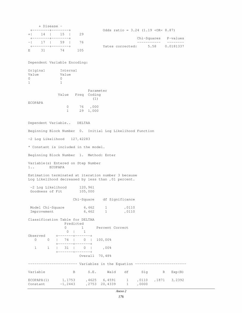
Anexo 2

176

+ Disease - +--------+--------+ Odds ratio = 3.24 (1.19 <OR< 8.87) +| 14 | 15 | 29 +--------+--------+ Chi-Squares P-values -| 17 | 59 | 76 ----------- -------- +--------+--------+ Yates corrected: 5.58 0.0181337 E 31 74 105 Dependent Variable Encoding: Original Internal Value Value 0 0 1 1 Parameter Value Freq Coding (1) ECOPAPA 0 76 ,000 1 29 1,000 Dependent Variable.. DELTAA Beginning Block Number 0. Initial Log Likelihood Function -2 Log Likelihood 127,42283 * Constant is included in the model. Beginning Block Number 1. Method: Enter Variable(s) Entered on Step Number 1.. ECOPAPA Estimation terminated at iteration number 3 because Log Likelihood decreased by less than ,01 percent. -2 Log Likelihood 120,961 Goodness of Fit 105,000 Chi-Square df Significance Model Chi-Square 6,462 1 ,0110 Improvement 6,462 1 ,0110 Classification Table for DELTAA Predicted 0 1 Percent Correct 0 | 1 Observed +-------+-------+ 0 0 | 74 | 0 | 100,00% +-------+-------+ 1 1 | 31 | 0 | ,00% +-------+-------+ Overall 70,48% ----------------------- Variables in the Equation ------------------------ Variable B S.E. Wald df Sig R Exp(B) ECOPAPA(1) 1,1753 ,4625 6,4591 1 ,0110 ,1871 3,2392 Constant -1,2443 ,2753 20,4339 1 ,0000

Anexo 2

177

+ Disease - +--------+--------+ Odds ratio = 2.24 (0.69 <OR< 7.67*) +| 26 | 51 | 77 +--------+--------+ Chi-Squares P-values -| 5 | 22 | 27 ----------- -------- +--------+--------+ Yates corrected: 1.55 0.2127907 E 31 73 104 Dependent Variable Encoding: Original Internal Value Value 0 0 1 1 Parameter Value Freq Coding (1) ECTA 0 27 ,000 1 77 1,000 Dependent Variable.. DELTAA Beginning Block Number 0. Initial Log Likelihood Function -2 Log Likelihood 126,71902 * Constant is included in the model. Beginning Block Number 1. Method: Enter Variable(s) Entered on Step Number 1.. ECTA Estimation terminated at iteration number 3 because Log Likelihood decreased by less than ,01 percent. -2 Log Likelihood 124,354 Goodness of Fit 103,999 Chi-Square df Significance Model Chi-Square 2,365 1 ,1241 Improvement 2,365 1 ,1241

Anexo 2

178

Classification Table for DELTAA Predicted 0 1 Percent Correct 0 | 1 Observed +-------+-------+ 0 0 | 73 | 0 | 100,00% +-------+-------+ 1 1 | 31 | 0 | ,00% +-------+-------+ Overall 70,19% ---------------------- Variables in the Equation ----------------------- Variable B S.E. Wald df Sig R Exp(B) ECTA(1) ,8078 ,5509 2,1500 1 ,1426 ,0344 2,2430 Constant -1,4815 ,4954 8,9428 1 ,0028

Modelo 4: 3 variáveis independentes, com interação e com todos os registros (Enter) Total number of cases: 110 (Unweighted) Number of selected cases: 110 Number of unselected cases: 0 Number of selected cases: 110 Number rejected because of missing data: 0 Number of cases included in the analysis: 110 Dependent Variable Encoding: Original Internal Value Value 0 0 1 1 Parameter Value Freq Coding (1) RACAA 0 76 ,000 1 34 1,000 DISPA 0 91 ,000 1 19 1,000 IDADEA 1 82 1,000 0 28 ,000

Anexo 2

179

Dependent Variable.. TCAMA Beginning Block Number 0. Initial Log Likelihood Function -2 Log Likelihood 130,82571 * Constant is included in the model. Beginning Block Number 1. Method: Enter Variable(s) Entered on Step Number 1.. IDADEA DISPA RACAA Estimation terminated at iteration number 4 because Log Likelihood decreased by less than ,01 percent. -2 Log Likelihood 107,332 Goodness of Fit 120,479 Chi-Square df Significance Model Chi-Square 23,494 3 ,0000 Improvement 23,494 3 ,0000 Classification Table for TCAMA Predicted 0 1 Percent Correct 0 | 1 Observed +-------+-------+ 0 0 | 75 | 4 | 94,94% +-------+-------+ 1 1 | 20 | 11 | 35,48% +-------+-------+ Overall 78,18% -- -------------------- Variables in the Equation ------------------------

Variable B S.E. Wald df Sig R Exp(B) IDADEA(1) 2,0505 ,8138 6,3489 1 ,0117 ,1823 7,7719 DISPA(1) 1,8336 ,5936 9,5402 1 ,0020 ,2401 6,2562 RACAA(1) 1,0502 ,4967 4,4712 1 ,0345 ,1374 2,8584 Constant -3,3969 ,8374 16,4549 1 ,0001

Anexo 2

180

Total number of cases: 110 (Unweighted) Number of selected cases: 110 Number of unselected cases: 0 Number of selected cases: 110 Number rejected because of missing data: 0 Number of cases included in the analysis: 110 Dependent Variable Encoding: Original Internal Value Value 0 0 1 1 Parameter Value Freq Coding (1) RACAA 0 76 ,000 1 34 1,000 DISPA 0 91 ,000 1 19 1,000 IDADEA 1 82 1,000 0 28 ,000 Interactions: INT_1 DISPA(1) by RACAA(1)

Anexo 2

181

Dependent Variable.. TCAMA Beginning Block Number 0. Initial Log Likelihood Function -2 Log Likelihood 130,82571 * Constant is included in the model. Beginning Block Number 1. Method: Enter Variable(s) Entered on Step Number 1.. IDADEA DISPA RACAA DISPA * RACAA Estimation terminated at iteration number 4 because Log Likelihood decreased by less than ,01 percent. -2 Log Likelihood 107,116 Goodness of Fit 120,132 Chi-Square df Significance Model Chi-Square 23,710 4 ,0001 Improvement 23,710 4 ,0001 Classification Table for TCAMA Predicted 0 1 Percent Correct 0 | 1 Observed +-------+-------+ 0 0 | 75 | 4 | 94,94% +-------+-------+ 1 1 | 20 | 11 | 35,48% +-------+-------+ Overall 78,18% ---------------------- Variables in the Equation ------------------------ Variable B S.E. Wald df Sig R Exp(B) IDADEA(1) 2,0932 ,8360 6,2694 1 ,0123 ,1807 8,1110 DISPA(1) 1,6841 ,6758 6,2103 1 ,0127 ,1794 5,3874 RACAA(1) ,9531 ,5400 3,1155 1 ,0776 ,0923 2,5938 INT_1 ,6638 1,4681 ,2044 1 ,6512 ,0000 1,9421 Constant -3,3942 ,8536 15,8100 1 ,0001

Anexo 2

182

Modelo 4: 4 variáveis independ., com interação e excluindo-se valores em branco (Enter) Total number of cases: 102 (Unweighted) Number of selected cases: 102 Number of unselected cases: 0 Number of selected cases: 102 Number rejected because of missing data: 0 Number of cases included in the analysis: 102 Dependent Variable Encoding: Original Internal Value Value 0 0 1 1 Parameter Value Freq Coding (1) CVFA 0 59 ,000 1 43 1,000 DISPA 0 87 ,000 1 15 1,000 SCL70A 0 76 ,000 1 26 1,000

Anexo 2

183

Dependent Variable.. DELTAA Beginning Block Number 0. Initial Log Likelihood Function -2 Log Likelihood 123,58269 * Constant is included in the model. Beginning Block Number 1. Method: Enter Variable(s) Entered on Step Number 1.. SCL70A DISPA CVFA Estimation terminated at iteration number 4 because Log Likelihood decreased by less than ,01 percent. -2 Log Likelihood 77,762 Goodness of Fit 94,123 Chi-Square df Significance Model Chi-Square 45,821 3 ,0000 Improvement 45,821 3 ,0000 Classification Table for DELTAA Predicted 0 1 Percent Correct 0 | 1 Observed +-------+-------+ 0 0 | 66 | 6 | 91,67% +-------+-------+ 1 1 | 11 | 19 | 63,33% +-------+-------+ Overall 83,33% ---------------------- Variables in the Equation ------------------------ Variable B S.E. Wald df Sig R Exp(B) SCL70A(1) 1,9136 ,6122 9,7697 1 ,0018 ,2507 6,7774 DISPA(1) 2,8196 ,9027 9,7558 1 ,0018 ,2505 16,7695 CVFA(1) 1,3894 ,5839 5,6617 1 ,0173 ,1721 4,0123 Constant -2,6326 ,4911 28,7380 1 ,0000

Anexo 2

184

Total number of cases: 102 (Unweighted) Number of selected cases: 102 Number of unselected cases: 0 Number of selected cases: 102 Number rejected because of missing data: 0 Number of cases included in the analysis: 102 Dependent Variable Encoding: Original Internal Value Value 0 0 1 1 Parameter Value Freq Coding (1) CVFA 0 59 ,000 1 43 1,000 DISPA 0 87 ,000 1 15 1,000 SCL70A 0 76 ,000 1 26 1,000 Interactions: INT_1 CVFA(1) by DISPA(1)

Anexo 2

185

Dependent Variable.. DELTAA Beginning Block Number 0. Initial Log Likelihood Function -2 Log Likelihood 123,58269 * Constant is included in the model. Beginning Block Number 1. Method: Enter Variable(s) Entered on Step Number 1.. SCL70A DISPA CVFA CVFA * DISPA Estimation terminated at iteration number 4 because Log Likelihood decreased by less than ,01 percent. -2 Log Likelihood 77,731 Goodness of Fit 93,714 Chi-Square df Significance Model Chi-Square 45,851 4 ,0000 Improvement 45,851 4 ,0000 Classification Table for DELTAA Predicted 0 1 Percent Correct 0 | 1 Observed +-------+-------+ 0 0 | 66 | 6 | 91,67% +-------+-------+ 1 1 | 11 | 19 | 63,33% +-------+-------+ Overall 83,33% ---------------------- Variables in the Equation ------------------------ Variable B S.E. Wald df Sig R Exp(B) SCL70A(1) 1,9061 ,6140 9,6380 1 ,0019 ,2486 6,7270 DISPA(1) 2,6107 1,5012 3,0245 1 ,0820 ,0910 13,6091 CVFA(1) 1,3541 ,6165 4,8248 1 ,0281 ,1512 3,8733 INT_1 ,3267 1,8824 ,0301 1 ,8622 ,0000 1,3864 Constant -2,6107 ,5036 26,8762 1 ,0000

Anexo 2

186

Total number of cases: 102 (Unweighted) Number of selected cases: 102 Number of unselected cases: 0 Number of selected cases: 102 Number rejected because of missing data: 0 Number of cases included in the analysis: 102 Dependent Variable Encoding: Original Internal Value Value 0 0 1 1 Parameter Value Freq Coding (1) CVFA 0 59 ,000 1 43 1,000 DISPA 0 87 ,000 1 15 1,000 SCL70A 0 76 ,000 1 26 1,000 Interactions: INT_1 CVFA(1) by SCL70A(1)

Anexo 2

187

Dependent Variable.. DELTAA Beginning Block Number 0. Initial Log Likelihood Function -2 Log Likelihood 123,58269 * Constant is included in the model. Beginning Block Number 1. Method: Enter Variable(s) Entered on Step Number 1.. SCL70A DISPA CVFA CVFA * SCL70A Estimation terminated at iteration number 4 because Log Likelihood decreased by less than ,01 percent. -2 Log Likelihood 77,549 Goodness of Fit 97,082 Chi-Square df Significance Model Chi-Square 46,034 4 ,0000 Improvement 46,034 4 ,0000 Classification Table for DELTAA Predicted 0 1 Percent Correct 0 | 1 Observed +-------+-------+ 0 0 | 66 | 6 | 91,67% +-------+-------+ 1 1 | 11 | 19 | 63,33% +-------+-------+ Overall 83,33% ---------------------- Variables in the Equation ------------------------ Variable B S.E. Wald df Sig R Exp(B) SCL70A(1) 2,2361 ,9263 5,8283 1 ,0158 ,1760 9,3571 DISPA(1) 2,8444 ,9076 9,8214 1 ,0017 ,2516 17,1920 CVFA(1) 1,5891 ,7336 4,6919 1 ,0303 ,1476 4,8992 INT_1 -,5599 1,2101 ,2140 1 ,6436 ,0000 ,5713 Constant -2,7470 ,5697 23,2460 1 ,0000

Anexo 2

188

Total number of cases: 102 (Unweighted) Number of selected cases: 102 Number of unselected cases: 0 Number of selected cases: 102 Number rejected because of missing data: 0 Number of cases included in the analysis: 102 Dependent Variable Encoding: Original Internal Value Value 0 0 1 1 Parameter Value Freq Coding (1) CVFA 0 59 ,000 1 43 1,000 SCL70A 0 76 ,000 1 26 1,000 DISPA 0 87 ,000 1 15 1,000 IDADEA 1 75 1,000 0 27 ,000

Anexo 2

189

Dependent Variable.. DELTAA Beginning Block Number 0. Initial Log Likelihood Function -2 Log Likelihood 123,58269 * Constant is included in the model. Beginning Block Number 1. Method: Enter Variable(s) Entered on Step Number 1.. IDADEA SCL70A DISPA CVFA Estimation terminated at iteration number 5 because Log Likelihood decreased by less than ,01 percent. -2 Log Likelihood 71,605 Goodness of Fit 86,231 Chi-Square df Significance Model Chi-Square 51,978 4 ,0000 Improvement 51,978 4 ,0000 Classification Table for DELTAA Predicted 0 1 Percent Correct 0 | 1 Observed +-------+-------+ 0 0 | 67 | 5 | 93,06% +-------+-------+ 1 1 | 11 | 19 | 63,33% +-------+-------+ Overall 84,31% -- -------------------- Variables in the Equation ------------------------

Variable B S.E. Wald df Sig R Exp(B) IDADEA(1) 2,0659 ,9649 4,5846 1 ,0323 ,1446 7,8928 SCL70A(1) 1,6690 ,6411 6,7768 1 ,0092 ,1966 5,3069 DISPA(1) 3,0554 ,9703 9,9154 1 ,0016 ,2531 21,2305 CVFA(1) 1,6651 ,6227 7,1497 1 ,0075 ,2041 5,2864 Constant -4,4091 1,0640 17,1733 1 ,0000

Anexo 2

190

Total number of cases: 102 (Unweighted) Number of selected cases: 102 Number of unselected cases: 0 Number of selected cases: 102 Number rejected because of missing data: 0 Number of cases included in the analysis: 102 Dependent Variable Encoding: Original Internal Value Value 0 0 1 1 Parameter Value Freq Coding (1) IDADEA 1 75 1,000 0 27 ,000 DISPA 0 87 ,000 1 15 1,000 CVFA 0 59 ,000 1 43 1,000 SCL70A 0 76 ,000 1 26 1,000 Interactions: INT_1 IDADEA(1) by SCL70A(1)

Anexo 2

191

Dependent Variable.. DELTAA Beginning Block Number 0. Initial Log Likelihood Function -2 Log Likelihood 123,58269 * Constant is included in the model. Beginning Block Number 1. Method: Enter Variable(s) Entered on Step Number 1.. SCL70A DISPA CVFA IDADEA IDADEA * SCL70A Estimation terminated at iteration number 5 because Log Likelihood decreased by less than ,01 percent. -2 Log Likelihood 71,445 Goodness of Fit 85,179 Chi-Square df Significance Model Chi-Square 52,137 5 ,0000 Improvement 52,137 5 ,0000 Classification Table for DELTAA Predicted 0 1 Percent Correct 0 | 1 Observed +-------+-------+ 0 0 | 67 | 5 | 93,06% +-------+-------+ 1 1 | 11 | 19 | 63,33% +-------+-------+ Overall 84,31% ---------------------- Variables in the Equation ------------------------ Variable B S.E. Wald df Sig R Exp(B) SCL70A(1) ,9274 1,9778 ,2198 1 ,6392 ,0000 2,5278 DISPA(1) 3,0644 ,9628 10,1298 1 ,0015 ,2565 21,4206 CVFA(1) 1,6618 ,6254 7,0612 1 ,0079 ,2024 5,2688 IDADEA(1) 1,8671 1,0606 3,0990 1 ,0783 ,0943 6,4693 INT_1 ,8305 2,0942 ,1573 1 ,6917 ,0000 2,2945 Constant -4,2414 1,1153 14,4627 1 ,0001

Anexo 2

192

Total number of cases: 102 (Unweighted) Number of selected cases: 102 Number of unselected cases: 0 Number of selected cases: 102 Number rejected because of missing data: 0 Number of cases included in the analysis: 102 Dependent Variable Encoding: Original Internal Value Value 0 0 1 1 Parameter Value Freq Coding (1) IDADEA 1 75 1,000 0 27 ,000 DISPA 0 87 ,000 1 15 1,000 CVFA 0 59 ,000 1 43 1,000 SCL70A 0 76 ,000 1 26 1,000 Interactions: INT_1 CVFA(1) by IDADEA(1)

Anexo 2

193

Dependent Variable.. DELTAA Beginning Block Number 0. Initial Log Likelihood Function -2 Log Likelihood 123,58269 * Constant is included in the model. Beginning Block Number 1. Method: Enter Variable(s) Entered on Step Number 1.. SCL70A DISPA CVFA IDADEA CVFA * IDADEA Estimation terminated at iteration number 8 because Log Likelihood decreased by less than ,01 percent. -2 Log Likelihood 71,070 Goodness of Fit 81,386 Chi-Square df Significance Model Chi-Square 52,513 5 ,0000 Improvement 52,513 5 ,0000 Classification Table for DELTAA Predicted 0 1 Percent Correct 0 | 1 Observed +-------+-------+ 0 0 | 67 | 5 | 93,06% +-------+-------+ 1 1 | 11 | 19 | 63,33% +-------+-------+ Overall 84,31% ---------------------- Variables in the Equation ------------------------ Variable B S.E. Wald df Sig R Exp(B) SCL70A(1) 1,6706 ,6394 6,8264 1 ,0090 ,1976 5,3151 DISPA(1) 2,9554 ,9611 9,4552 1 ,0021 ,2456 19,2086 CVFA(1) 6,8998 25,2982 ,0744 1 ,7851 ,0000 992,0373 IDADEA(1) 7,1328 25,2842 ,0796 1 ,7779 ,0000 1252,434 INT_1 -5,3304 25,3064 ,0444 1 ,8332 ,0000 ,0048 Constant -9,4206 25,2807 ,1389 1 ,7094

Anexo 2

194

Documents

AVALIAÇÃO DO COMPROMETIMENTO PULMONAR EM …repositorio.unicamp.br/bitstream/REPOSIP/309671/1/Villalba_Wander... · V711a Avaliação do comprometimento pulmonar em pacientes com