Seleção natural

Bio 0208 - 2016

Diogo Meyer

Departamento de Genética e Biologia Evolutiva Universidade de São Paulo

Leitura básica: Ridley 5.6, 5.7, 5.10,5.12

Lembremos o quão complexas e ajustadas são as relações mútuas dos seres vivos uns aos outros e às suas condições físicas de vida. Seria então, improvável, pensar que variações úteis de algum modo a cada ser na grande e complexa batalha da vida, devam às vezes surgir ao longo de milhares de gerações? E se isso ocorre, podemos duvidar (lembrando que mais indivíduos nascem do que podem possivelmente sobreviver) que indivíduos com qualquer vantagem, por mais sutil que seja, sobre os outros, teriam uma melhor chance de sobreviver e procriar? Por outro lado, podemos ter certeza que qualquer variação minimamente prejudicial seria rigidamente rejeitada. Essa preservação das variações favoráveis e a rejeição das prejudiciais eu chamo de Seleção Natural.

Charles Darwin, em A origem das espécies, 1859

Visão contemporânea

→ se há variação na população

→ se essa variação contribui para a sobrevivência e reprodução diferencial

→ se essa variação é herdável

Haverá seleção natural

Genótipo AA Aa aaao nascimento 150 210 140entre adultos 75 105 70sobrevivência 50% 50% 50%

Quando há seleção natural?

Não há seleção: probabilidade de sobrevivência é igual para todos genótipos

Genótipo AA Aa aaao nascimento 150 210 140entre adultos 100 140 70sobrevivência 2/3 2/3 1/2sobrevivência normalizada

1 1 3/4

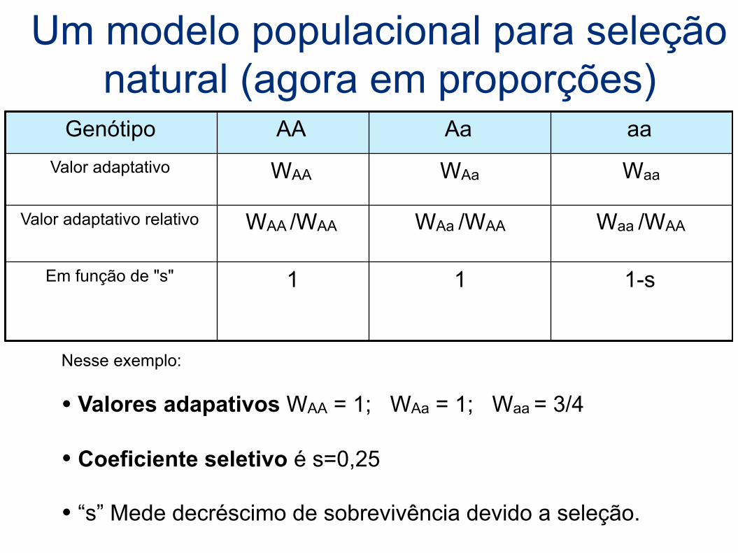
Nesse exemplo:

• Valores adapativos WAA = 1; WAa = 1; Waa = 3/4

• Coeficiente seletivo é s=0,25

• “s” Mede decréscimo de sobrevivência devido a seleção.

Quando há seleção natural?

Genótipo AA Aa aaValor adaptativo WAA WAa Waa

Valor adaptativo relativo WAA /WAA WAa /WAA Waa /WAA

Em função de "s" 1 1 1-s

Um modelo populacional para seleção natural (agora em proporções)

Nesse exemplo:

• Valores adapativos WAA = 1; WAa = 1; Waa = 3/4

• Coeficiente seletivo é s=0,25

• “s” Mede decréscimo de sobrevivência devido a seleção.

O modelo genético de seleção

Parâmetro do modelo evolutivo

No modelo de seleção

Tamanho da população Infinitamente grande

Cruzamento aleatório

Sobrevivência e reprodução dos genótipos

Diferente entre genótipos

mutação e migração Não há

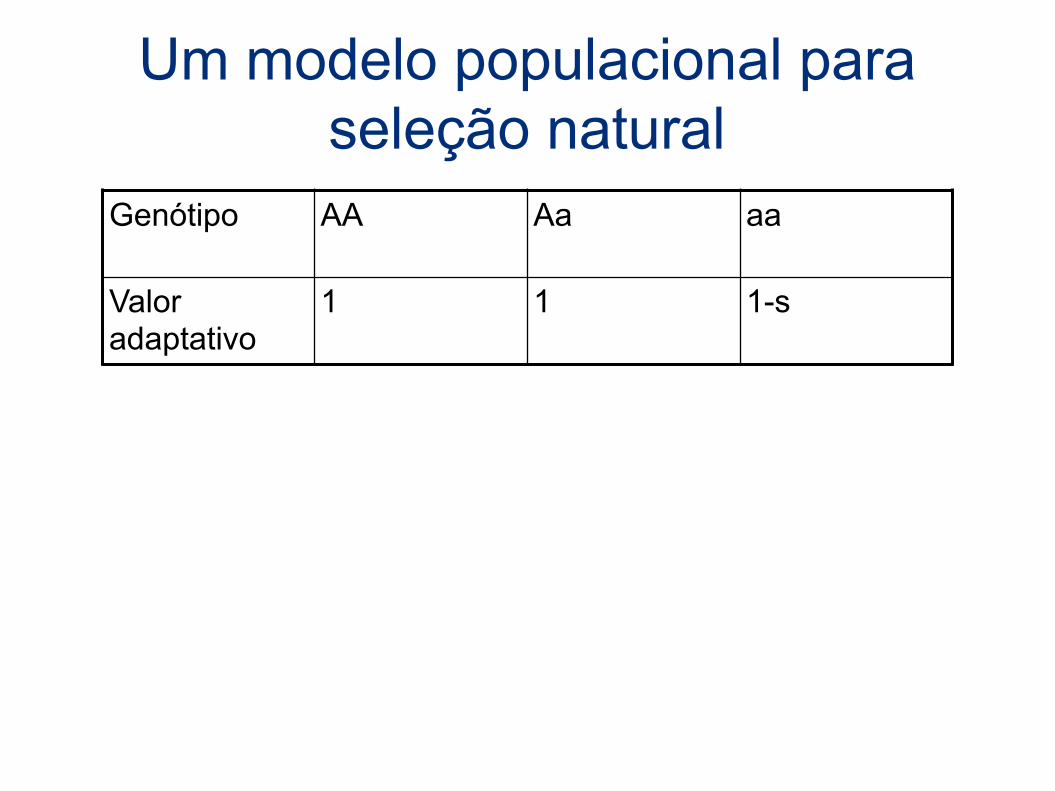
Genótipo AA Aa aa

Valor adaptativo

1 1 1-s

Um modelo populacional para seleção natural

Um modelo populacional para seleção natural

Genótipo AA Aa aa

nascimento p2 2pq q2

Aptidão 1 1 1-s

adultos p2 2pq q2 (1-s)

como calcular:

p -> p’

Exemplo de seleção

ANRV292-ES37-04 ARI 17 October 2006 7:11

Color PolymorphismMelanism in Biston betularia. A classic example of a genetic polymorphism influ-enced by diversifying selection is industrial melanism in the peppered moth, Bistonbetularia (Cook 2003, Grant 2005, Kettlewell 1973, Majerus 1998). Industrial melan-ics were first noticed in England in the mid-nineteenth century and appear to haverapidly spread from a single source. At a particular location, the increase from a lowfrequency to a frequency greater than 90% often took only several decades. Themain selective agent appears to have been differential predation by birds on pollutedand unpolluted resting backgrounds, and extensive gene flow significantly influencedthe spread and distribution of melanics (Cook 2003). The overall case for naturalselection acting on the rise and fall of melanics in peppered moths is indisputable.

Since the introduction of clean air legislation in the 1960s in Great Britain, thefrequency of dominant melanic moths has declined. For example, at Caldy Common,the frequency of melanics declined from greater than 90% in 1960 to below 5% by2002 (Figure 1) (Grant 2005). Also given in Figure 1 is the very similar expecteddecrease of the melanic phenotype, assuming a 15.3% selective disadvantage formelanics [that is, the fitnesses for the dominant melanics and recessive typicals are0.847 and 1.0, respectively (Grant et al. 1996)].

B. betularia is also found in North America, and in some areas the frequency ofmelanics once was quite high (Grant et al. 1996). In the 1960s, clean air legislationalso began to result in better air quality in North America, and the frequency ofmelanics dropped (Grant & Wiseman 2002). Presumably, similar reversals in selec-tion pressures that occurred on both continents were responsible for this remarkableparallel decline. On the basis of crosses between American and British moths, re-searchers concluded that the melanic variants from the two continents are alleles atthe same locus (Grant 2004). When the gene that determines melanism in B. betulariais discovered, then DNA data should be able to determine the cause and relationship

Year

Pro

port

ion

mel

anic

1.0

0.8

0.6

0.4

0.2

0.01959 1969 1979 1989 1999

Expected

Observed

Figure 1The observed decline in thefrequency of melanics from1959 to 2002 at CaldyCommon in England(magenta squares) (Grant2005) and the expecteddecline when there is 15.3%selection against themelanics (dark gray line).

www.annualreviews.org • Genetic Polymorphism 69

Ann

u. R

ev. E

col.

Evol

. Sys

t. 20

06.3

7:67

-93.

Dow

nloa

ded

from

arjo

urna

ls.an

nual

revi

ews.o

rgby

UN

IVER

SITY

OF

CHIC

AG

O L

IBRA

RIES

on

04/3

0/07

. For

per

sona

l use

onl

y.

linha baseada em s=0,153 e dominância da melânica

Redução de forma melânica de biston betularia em regiões sem poluição, na Inglaterra.

CHAPTER 1. SELEÇÃO NATURAL 2

1.2 O modelo básicoIniciaremos nossa análise apresentando um modelo propositalmente simples, quetrata da ação da seleção natural sobre um único lócus bialélico. Para tornar essemodelo mais acessível apresentamos um exemplo hipotético.

AA Aa aaAo nascimento 150 210 140Entre adultos 100 140 70Sobrevivência 2/3 2/3 1/2

Sobrevivência normalizada 1 1 3/4Repare que houve mortalidade em todas as classes genotípicas, mas a inten-

sidade de mortalidade foi diferente entre os genótipos. Uma forma convenientede expressar isso é dividir as frações de sobrevivência pelo valor da sobrevivênciamais elevada (nesse caso, 2/3), resultando nos valores de sobrevivência normal-izada. Em palavras, podemos dizer que indivíduos com os genótipos AA e Aasobrevivem proporcionalmente mais do que os indivíduos aa, esses últimos tendouma sobrevivência 25% menor.

Podemos agora definir alguns termos que serão usados posteriormente.

• A proporção de indivíduos de cada genótipo que sobrevive até a repro-dução é o valor adaptativo associado àquele genótipo (que serão tratadoscomo W

AA

,W

Aa

, Waa.

• Valores adaptativos podem também ser expressos em função da intensi-dade da seleção contra cada genótipo, medido pelo coeficiente de seleção(s). Nesse exemplo temos s = 1/4, que descreve a redução em sobrevivên-cia de aa em relação aos outros genótipos.

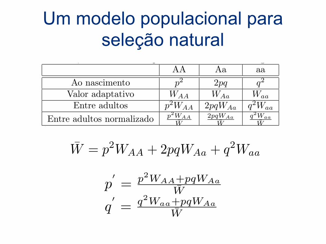
Para tornar o modelo mais geral, podemos expressar as frequências dos genótiposcomo valores esperadosp ara uma população em equilíbrio de Hardy-Weinberg.Desta forma, a tabela anterior poderia ser re-escrita da seguinte forma:

AA Aa aaAo nascimento p

2 2pq q

2

Valor adaptativo W

AA

W

Aa

W

aa

Entre adultos p

2W

AA

2pqWAa

q

2W

aa

Entre adultos normalizado p

2WAA

W̄

2pqWAa

W̄

q

2Waa

W̄

As frequências genotípicas após a seleção precisam ser normalizadas, pois elasagoram não somam 1. Essa normalizadação é feita dividindo cada frequênciaapós a seleção pela soma das frequências totais. Essa soma total é definida comoo valor adaptativo médio:

W̄ = p

2W

AA

+ 2pqWAa

+ q

2W

aa

(1.1)

O valor adaptativo médio pode ser visto de duas formas. Sob um ponto devista, é o fator de normalização para o cálculo das frequências genotípicas apósa seleção. Uma segunda forma de vê-lo é como o quão distante a população está

CHAPTER 1. SELEÇÃO NATURAL 2

1.2 O modelo básicoIniciaremos nossa análise apresentando um modelo propositalmente simples, quetrata da ação da seleção natural sobre um único lócus bialélico. Para tornar essemodelo mais acessível apresentamos um exemplo hipotético.

AA Aa aaAo nascimento 150 210 140Entre adultos 100 140 70Sobrevivência 2/3 2/3 1/2

Sobrevivência normalizada 1 1 3/4Repare que houve mortalidade em todas as classes genotípicas, mas a inten-

sidade de mortalidade foi diferente entre os genótipos. Uma forma convenientede expressar isso é dividir as frações de sobrevivência pelo valor da sobrevivênciamais elevada (nesse caso, 2/3), resultando nos valores de sobrevivência normal-izada. Em palavras, podemos dizer que indivíduos com os genótipos AA e Aasobrevivem proporcionalmente mais do que os indivíduos aa, esses últimos tendouma sobrevivência 25% menor.

Podemos agora definir alguns termos que serão usados posteriormente.

• A proporção de indivíduos de cada genótipo que sobrevive até a repro-dução é o valor adaptativo associado àquele genótipo (que serão tratadoscomo W

AA

,W

Aa

, Waa.

• Valores adaptativos podem também ser expressos em função da intensi-dade da seleção contra cada genótipo, medido pelo coeficiente de seleção(s). Nesse exemplo temos s = 1/4, que descreve a redução em sobrevivên-cia de aa em relação aos outros genótipos.

Para tornar o modelo mais geral, podemos expressar as frequências dos genótiposcomo valores esperadosp ara uma população em equilíbrio de Hardy-Weinberg.Desta forma, a tabela anterior poderia ser re-escrita da seguinte forma:

AA Aa aaAo nascimento p

2 2pq q

2

Valor adaptativo W

AA

W

Aa

W

aa

Entre adultos p

2W

AA

2pqWAa

q

2W

aa

Entre adultos normalizado p

2WAA

W̄

2pqWAa

W̄

q

2Waa

W̄

As frequências genotípicas após a seleção precisam ser normalizadas, pois elasagoram não somam 1. Essa normalizadação é feita dividindo cada frequênciaapós a seleção pela soma das frequências totais. Essa soma total é definida comoo valor adaptativo médio:

W̄ = p

2W

AA

+ 2pqWAa

+ q

2W

aa

(1.1)

O valor adaptativo médio pode ser visto de duas formas. Sob um ponto devista, é o fator de normalização para o cálculo das frequências genotípicas apósa seleção. Uma segunda forma de vê-lo é como o quão distante a população está

CHAPTER 1. SELEÇÃO NATURAL 3

W

AA

W

Aa

W

aa

Interpretação biológica Trajetória para s=0.1 e p inicial 0,05

1 1 1-s Dominante para valor adaptativo maior

●●●●●●●●●●●●●●●●●●●●●●●●●●●●●●●●●●●●●●●●●●●●●●●●●●●●●●●●●●●●●●●●●●●●●●●●●●●●●●●●●●●●●●●●●●●●●●●●●●●●●●●●●●●●●●●●●●●●●●●●●●●●●●●●●●●●●●●●●●●●●●●●●●●●●●●●●●●●●●●●●●●●●●●●●●●●●●●●●●●●●●●●●●

●●●●●●●●●●●●●●●●●●●

●●●●●●●●●●●●●●●●●●●●●●●

●●●●●●●●●●●●●●●●●●●●●●●●●●●●●●

●●●●●●●●●●●●●●●●●●●●●●●●●●●●●●●●●●●●●●●●●●

●●●●●●●●●●●●●●●●●●●●●●●●●●●●●●●●●●●●●●●●●●●●●●●●●●●●●●●●●●●●●●

●●●●●●●●●●●●●●●●●●●●●●●●●●●●●●●●●●●●●●

0 100 200 300 400

0.2

0.4

0.6

0.8

geração

frequ

ênci

a al

élic

a (p

)

1 1-s 1-s Recessivo para valor adaptativo maior

●●●●●●●●●●●●●●●●●●●●●●●●●●●●●●●●●●●●●●●●●●●●●●●●●●●●●●●●●●●●●●●●●●●●●●●●●●●●●●●●●●●●●●●●●●●●●●●●●●●●●●●●●●●●●●●●●●●●●●●●●●●●●●●●●●●●●●●●●●●●●●●●●●●●●●●●●●●●●●●●●●●●●●●●●●●●●●●●●●●●●●●●●●

●●●●●●●●●●●●●●●●●●●

●●●●●●●●●●●●●●●●●●●●●●●

●●●●●●●●●●●●●●●●●●●●●●●●●●●●●●

●●●●●●●●●●●●●●●●●●●●●●●●●●●●●●●●●●●●●●●●●●

●●●●●●●●●●●●●●●●●●●●●●●●●●●●●●●●●●●●●●●●●●●●●●●●●●●●●●●●●●●●●●

●●●●●●●●●●●●●●●●●●●●●●●●●●●●●●●●●●●●●●

0 100 200 300 400

0.2

0.4

0.6

0.8

geração

frequ

ênci

a al

élic

a (p

)

1-s 1 1-s Vantagem de heterozigot

●●●●●●●●●●●●●●●●●●●●●●●●●●●●●●●●●●●●●●●●●●●●●●●●●●●●●●●●●●●●●●●●●●●●●●●●●●●●●●●●●●●●●●●●●●●●●●●●●●●●●●●●●●●●●●●●●●●●●●●●●●●●●●●●●●●●●●●●●●●●●●●●●●●●●●●●●●●●●●●●●●●●●●●●●●●●●●●●●●●●●●●●●●

●●●●●●●●●●●●●●●●●●●

●●●●●●●●●●●●●●●●●●●●●●●

●●●●●●●●●●●●●●●●●●●●●●●●●●●●●●

●●●●●●●●●●●●●●●●●●●●●●●●●●●●●●●●●●●●●●●●●●

●●●●●●●●●●●●●●●●●●●●●●●●●●●●●●●●●●●●●●●●●●●●●●●●●●●●●●●●●●●●●●

●●●●●●●●●●●●●●●●●●●●●●●●●●●●●●●●●●●●●●

0 100 200 300 400

0.2

0.4

0.6

0.8

geração

frequ

ênci

a al

élic

a (p

)

Figure 1.1: Três modelos de seleção natural

da condição "ótima", que é definida pela situação em que todos os indivíduospossuem o valor adaptativo mais elevado.

As frequências genotípicas podem agora ser usadas para calcular as frequên-cias alélicas após a seleção.

p

0= p

2WAA+pqWAa

W̄

q

0= q

2Waa+pqWAa

W̄

Essas fórmulas descrevem a frequência alélica esperada numa geração emfunção dos valores adaptativos (W) e da frequência alélica da geração anterior.A aplicação reiterada dessa expressão permite calcular a trajetória temporal defrequência alélicas. A figura 1.1mostramos três formas de atribuir valores a We o seu impacto sobre as trajetórias de frequências alélicas ao longo do tempo.

Um modelo populacional para seleção natural

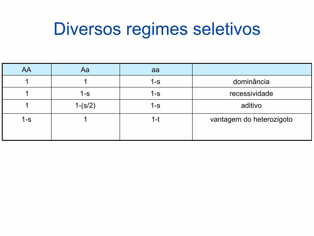
Diversos regimes seletivos

AA Aa aa

1 1 1-s dominância

1 1-s 1-s recessividade

1 1-(s/2) 1-s aditivo

1-s 1 1-t vantagem do heterozigoto

Exemplos de seleção natural

Efeito da seleção num lócus: homogeneidade

Antes da seleção Depois da seleção

Região influenciada por carona genética

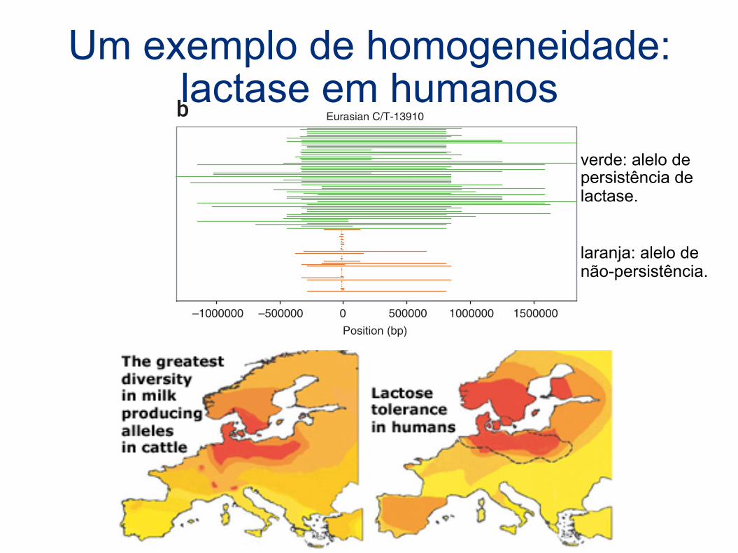
Um exemplo de homogeneidade: lactase em humanos

Um exemplo de homogeneidade: lactase em humanos

in heterozygotes, respectively (Fig. 2b), these associations are notsignificant in the subpopulations or in the meta-analysis (Fig. 3),possibly because of small sample size and loss of power for these SNPs.Additionally, chromosomes with the G-13907 and G-13915 allelesshow EHH spanning B1.4 Mb and B1.1 Mb, respectively (Supple-mentary Fig. 2). Although these results suggest that G-13915 andG-13907 are probable candidate LCT regulatory mutations, largersample sizes from populations containing these alleles are required totest for an association with the lactase persistence trait and to rule outthe possibility that they are simply in LD with a different causal SNP.Identification of transcription factors that bind to the sites of theC-14010, T-13915 and G-13907 variants would also be informativefor clarifying the possible role of these variants in regulatingLCT expression.

Adaptive significance and the origins of pastoralismArcheological evidence suggests that cattle domestication originated insouthern Egypt as early as B9,000 years ago but no later than B7,700years ago and in the Middle East B7,000–8,000 years ago28, consistentwith the age estimate of B8,000–9,000 years (95% c.i. B2,200–19,200years) for the T-13910 allele in Europeans. The more recent ageestimate of the C-14010 allele in African populations, B2,700–6,800years (95% c.i. B1,200–23,000 years), is consistent with archeologicaldata indicating that pastoralism did not spread south of the Sahara and

into northern Kenya until B4,500 years ago and into southern Kenyaand northern Tanzania B3,300 years ago28,29. The ability to digestmilk as adults is likely to be adaptive owing to the increased nutritionalbenefits from milk (carbohydrates as well as fat, protein and calcium)and also because milk is an important source of water in aridregions2,28,30,31. Considering the symptoms of lactose intolerance,which includes water loss from diarrhea, individuals who had thelactase persistence–associated alleles and could tolerate milk could havehad a very strong selective advantage2. This is supported by our highestimates for the selection coefficient (s ¼ 0.035–0.097). Because theselective force, adult milk consumption, is associated with the culturaldevelopment of cattle domestication, the recent and rapid spread ofthe lactase persistence–associated alleles, together with the practice ofpastoralism in East Africa, is an excellent example of ongoing adapta-tion in humans32 and coevolution of genes and culture3.

We observe the oldest age estimates of the C-14010 allele, B6,000–7,000 years (95% c.i. B2,000–16,000 years), in the KenyanNilo-Saharan and Tanzanian Afro-Asiatic populations (Table 1). Wealso observe an old age estimate in the Tanzanian Sandawe, but its lowfrequency suggests it was introduced via recent gene flow (Supple-mentary Discussion). However, we cannot distinguish with certaintywhether this allele first arose in the Cushitic-speaking Afro-Asiaticpopulations, who are thought to have migrated into Kenya andTanzania from Ethiopia B5,000 years ago33 and practice a mixtureof agriculture and pastoralism, or in the Nilotic-speaking Nilo-Saharan populations, who are thought to have migrated into Kenyaand Tanzania from southern Sudan within the past B3,000 years33

and are strict pastoralists28. These results are consistent with bothlinguistic34 and genetic data (F.A.R. and S.A.T., unpublished data)indicating cultural exchange and genetic admixture between thesegroups. The absence of C-14010 in the southern Sudanese Nilo-Saharan–speaking populations suggests that this allele either origi-nated in or was introduced to the Kenyan Nilo-Saharan populationsafter their migration from southern Sudan. Regardless of the popula-tion origins of the C-14010 allele, it spread rapidly throughout theregion along with the cultural practice of pastoralism, consistent witha demic diffusion model of genetic and cultural expansion35.

Implications for identifying disease-associated variantsIt has been hypothesized that genetic variants associated with bothmendelian diseases (such as sickle cell anemia and glucose-6-phos-phate dehydrogenase (G6PD) deficiency) and common complexdiseases (such as hypertension, diabetes, obesity and asthma) maybe at high frequency in modern populations because they wereadaptive in ancient environments16,17,36–38. Thus, identification ofloci that are targets of natural selection could be informative foridentifying disease-risk alleles. The rapid increase in frequency ofgeographically restricted lactase persistence–associated alleles is anexample of local adaptation that would have been missed by studyingother African populations, such as the Yoruba, which do not show asignature of selection at LCT in the HapMap data set16,17. Because ofthe possibility that disease-associated alleles may also be geographi-cally restricted owing to recent, local adaptation, these results suggestthe importance of resequencing analyses in multiple populations, evenfrom within a single geographic region such as Africa.

Our study also indicates how challenging it may be to identifyalleles that are targets of selection. Networks of the 98-kb regionencompassing the LCT and MCM6 genes (Fig. 4) indicate severalhaplotypes that are at high frequency in global populations and thathave ancestral alleles at the lactase persistence–associated SNPs (that is,haplotypes D and E) (Fig. 4). Based on a single-factor ANOVA test,

0Position (bp)

African G/C-14010

Eurasian C/T-13910

–1000000 –500000 500000 1000000 1500000

0Position (bp)

–1000000 –500000 500000 1000000 1500000

a

b

Figure 6 Comparison of tracts of homozygous genotypes flanking the lactasepersistence–associated SNPs. (a) Kenyan and Tanzanian C-14010 lactase-persistent (red) and non-persistent G-14010 (blue) homozygosity tracts.(b) European and Asian T-13910 lactase-persistent (green) and C-13910non-persistent (orange) homozygosity tracts, based on the data from ref. 14.Positions are relative to the start codon of LCT. Note that some tracks aretoo short to be visible as plotted.

3 6 VOLUME 39 [ NUMBER 1 [ JANUARY 2007 NATURE GENETICS

ART I C LES

©20

07 N

atur

e Pu

blis

hing

Gro

up h

ttp://

ww

w.n

atur

e.co

m/n

atur

egen

etic

s

verde: alelo de persistência de lactase.

laranja: alelo de não-persistência.

Seleção natural em populações humanas

!  Comparando Tibetanos e Chineses: Gene EPAS1: Frequência do alelo A em Chineses: 10 % Frequência do alelo A em Tibetanos: 90% Como saber se diferença resulta de seleção?

FST

Akey, J. M. (2002). Genome Research.

Distribuição empírica de FST

Númerode loci

Distribuição empírica

35

Detectando seleção: diferenciação

Diferenciação entre populações

Os mais diferenciados

Seleção natural em populações humanas

!  Comparando Tibetanos e Chineses:

Média genômica EPAS1

Yi et al., 2010

Gene EPAS1: Frequência do alelo A em Chineses: 10 % Frequência do alelo A em Tibetanos: 90% Como saber se diferença resulta de seleção? → ver se deriva explicaria tamanha diferença

Alta diferenciação: gene SLC24A5

non-Europeans for the MATP 374*G and SLC24A5 111*Aalleles (both derived alleles associated with lighter pigmen-tation) were even more striking (MATPEuropean 5 87%;MATPnon-European 5 17%; SLC24A5European 5 100%;SLC24A5non-European 5 46%). The frequency of theSLC24A5 111*A allele outside of Europe is largely ac-counted for by high frequencies in geographically proxi-mate populations in northern Africa, the Middle East, andPakistan (ranging from 62% to 100%).

Signatures of Selection in Pigmentation Genes UsingHapMap Data

To supplement our analyses, we also examined theglobal diversity of our 6 pigmentation genes using datafrom the International HapMap project. Three potentialindicators of directional positive selection (LSBL, Tajima’sD, and lnRH) were calculated in 25-kb overlapping win-dows in European (CEU), East Asian (EAS), and West Af-rican (YRI) populations separately and their significancegauged by an empirical genome-wide distribution.

The first statistic, LSBL (Shriver et al. 2004), decom-poses FST among 3 populations into population-specificcomponents and provides a means to quantify the degreeto which a SNP (or group of SNPs in this case) has changedin allele frequency in one population relative to the other 2.Second, Tajima’s D was used to summarize the allele fre-quency spectrum in each genomic window. Under neutral-ity, Tajima’s D will take on values close to zero.Significantly negative values indicate an excess of rare al-leles that is consistent with recent positive directional selec-tion or a population expansion (Tajima 1989). AlthoughTajima’s D is normally used in cases of full ascertainment(i.e., resequencing), previous studies have established a cor-relation between resequencing and dense genotyping data(Carlson et al. 2005; Voight et al. 2006). Although the Hap-Map data set does suffer from an ascertainment bias toward

common SNPs, this should result in a skew of Tajima Dvalues against negative values that are indicative of direc-tional selection.

Finally, we calculated the related natural log of the ra-tio of heterozygosities (lnRH) between all pairwise popu-lation comparisons (Schlotterer 2002). Strongly negativevalues (i.e., a low ratio) indicate a reduced heterozygosity inone population relative to another and points to population-specific effect (not necessarily the case with significantTajima D values). A simple case of strong and population-specific positive selection is expected to result in stronglynegative Tajima’s D, high LSBL, and negative lnRH val-ues. Although these are relatively simple metrics, whenused together, they may provide nuanced insight in the tim-ing and place of more complex selective events. The full setof results can be found in supplementary table 3 (Supple-mentary Material online).

These data confirm the unusual European-specific pat-terns at MATP and SLC24A5. Both genes display longrange (consecutive windows) and significant indicationsof positive selection for all 3 statistics. In contrast, thereis little evidence of a European-specific pattern in theTYR locus although the nonsynonymous TYR A192CSNP does individually show a strongly significant CEU-LSBL (P , 0.003) in the HapMap data as in our originalfindings. The contrast may be explained by the limitationsof our HapMap sliding window analyses, whereby adjacentSNPs are averaged using a method that does not considerhaplotype structure.

A more complex pattern of evolution is indicated inthe HapMap data for the OCA2 gene. In line with theFST-based survey, it shows consistently strong and signif-icant European LSBL and somewhat more erratic signifi-cance in other measures. However, it also revealsa similar if slightly weaker pattern of significance in theEast Asian population consistent with our original observa-tion of a role in lightly versus darkly pigmented

FIG. 3. Continued

Convergent Evolution of Light Skin Phenotype 717

at FMRP/U

SP/BIBLIOTECA

CENTRA

L on September 29, 2014

http://mbe.oxfordjournals.org/

Dow

nloaded from

Alta diferenciação: evidência de evolução adaptativa da pigmentação (Northon et al., 2007). Nesse caso o alelo comum na Europa e parte da Ásia contribui para a pigmentação cara, e foi favorecido nessas regiões.

Valor adaptativo em zonas de malária

WAA = 0,88 WSS = 0,14 WAS = 1,00

Detectando seleção: distribuição geográfica

Frequência do alelo S da hemoglobina

Regiões com malária

Conceitos chave

- Há diferentes tipos de seleção: - direcional (com diferentes graus de dominância) - vantagem de heterozigoto

- Podemos estabelecer um model determinístico de seleção, que prevê mudança de p

- Usamos várias abordagens para detectar seleção