1

JOB SCHEDULING IN ASSEMBLY LINES AFFECTED BY WORKERS’

LEARNING

Michel Jose Anzanello

Federal University of Rio Grande do Sul (UFRGS)

Av. Osvaldo Aranha, 99, Porto Alegre, RS, Brazil 90035-190

anzanello@producao.ufrgs.br

Flavio Sanson Fogliatto

Federal University of Rio Grande do Sul (UFRGS)

Av. Osvaldo Aranha, 99, Porto Alegre, RS, Brazil 90035-190

ffogliatto@producao.ufrgs.br

ABSTRACT

Customized markets demand a large variety of product models which are typically manufactured

in small lots. Human-based activities are highly affected by the learning process as the production

of a new model takes place. Consequently estimation of lot processing times is difficult,

compromising the efficiency of scheduling techniques. In this paper we propose a new method

that integrates information from learning curve modeling and scheduling heuristics, aiming at

minimizing completion time. The completion time generated by the recommended heuristic,

determined through simulation, deviates 4.9% from the optimal sequence and yields good work

balance among teams of workers. The heuristic is applied in a case study from the shoe

manufacturing industry.

KEYWORDS. Scheduling. Learning curves. Unrelated parallel machines. Operations

Research in Production Management.

36

2

1. Introduction

Mass customized markets demand a large variety of product models typically produced in small

lot sizes. That requires high flexibility of productive resources to enable fast adaptation to the next

model to be produced (DA SILVEIRA et al., 2001). Losses in manual-based operations are inherent to

such context, both in terms of productivity and quality. Job scheduling becomes a challenging task since

lot completion times under learning are often unknown. Such production environments could clearly

benefit from the integration of learning curve (LC) modeling and scheduling techniques.

LCs are non-linear regression models that associate workers’ performance, usually described in

units produced per time interval, to task characteristics. By means of LC modeling the learning profile of

workers may be described in terms of efficiency improvement as an operation is continuously repeated

(UZUMERI AND NEMBHARD, 1998).

Job scheduling is a major issue in the manufacturing and services industries; it aims at allocating

jobs to resources by optimizing an objective (PINEDO, 2008). However, little attention has been given

to the study of workers’ learning impacts on the scheduling framework. The seminal work of Biskup

(1999) presented an analysis on the effect of learning in the position of jobs in a single machine. Latter,

Mosheiov and Sidney (2003) integrated LCs with different parameters for each job to programming

formulations aimed at optimizing objectives such as flow-time and makespan in a single machine, and

flow-time in unrelated parallel machines.

Jobs processing times in Mosheiov and Sidney (2003) were generated under a uniform

distribution. However, statistical distributions may not be appropriate to estimate processing times that

follow a functional pattern as in learning curves. The need for a method to estimate workers’ time to

complete a job becomes evident if better scheduling schemes are desired.

This article addresses the scheduling problem of minimizing the completion time when learning

effects are to be considered. We first use a hyperbolic LC, as proposed by Anzanello and Fogliatto

(2007), to quantitatively evaluate workers’ adaptation to a given set of jobs with variable complexity.

Workers’ learning profiles are then used to estimate processing times of new jobs. In the proposed

approach each worker is considered as an unrelated parallel machine; that is applicable since the speed

of job execution differs independently among workers. Here, machine, worker and team of workers are

treated as synonyms; in addition, lot and job will also have the same meaning. That leads to an

CRm || problem in the standard scheduling representation, where Rm denotes an unrelated parallel

machine environment with m teams of workers, and Cj is the completion time of job j.

In the next step of the proposed method we generate 4 simple heuristics by combining modified

stages of existing heuristics for the unrelated parallel machines problem, and then identify the one with

the best performance. The proposed heuristics are deployed in three stages. In stage 1 an initial job order

is defined testing 2 distinct rules. In stage 2 we decide on jobs to be performed by each of the I teams

such that workload balance among teams is maintained; for that, we test 2 rules. In stage 3 jobs assigned

to each team are sequenced aiming at minimizing completion time, yielding m C||1 problems.

The resulting heuristics are tested simulating jobs with different lot sizes and complexity. The

estimated completion times are then compared with optimal schedules for two teams of workers

obtained by complete enumeration, following two criteria: (i) deviation of the proposed heuristics

objective function values from their optimal value, and (ii) workload unbalance among teams of

workers. The recommended heuristic leads to a 4.9% average deviation from optimality, and

satisfactorily balances workload among teams. That heuristic is then applied to a real shoe

manufacturing application consisting of 3 teams and 90 jobs of distinct size and complexity.

There are two main contributions in this paper. First, we propose and systematize the use of LCs

to precisely estimate the processing time required by different teams of workers to complete a job,

depending on its size and complexity. Second, we combine and test modified stages of scheduling

heuristics from the literature to minimize completion time in unrelated parallel machine environments.

The proposed approach captures workers’ learning effects by means of the processing times, leading to

more realistic scheduling schemes in customized manufacturing applications.

The rest of this paper is organized as follows. In section 2 we provide a brief review of learning

curves models, and the fundamentals of scheduling in unrelated parallel machines. In section 3 we detail

37

3

the method proposed in the paper, which is applied in a case study in section 4. Conclusions close the

paper in section 5.

2. Background

We now review the literature on the paper’s two main subjects: (i) learning curve models, and

(ii) scheduling in unrelated parallel machines.

LCs are mathematical representations of a worker’s performance when repeatedly exposed to a

manual task or operation. As repetitions take place workers require less time to perform a task, either

due to familiarity with the task and tools required to perform it or because shortcuts to task completion

are discovered (WRIGHT, 1936; TEPLITZ, 1991). There are several LC models proposed in the

literature, most notably power models such as Wright’s, and hyperbolic models.

Wright’s model, probably the best known LC function in the literature due to its simplicity and

efficiency in describing empirical data, is given by

bzUt 1 , (1)

where z represents the number of units produced, t denotes the average accumulated time or cost to

produce z units, U1 is the time or cost to produce the first unit, and b is the curve’s slope (1 b 0).

The hyperbolic LC model provides a more precise description of the learning process if

compared to Wright’s model. The 3-parameter hyperbolic model reported in Mazur and Hastie (1978) is

given by

rpx

pxky , (2)

such that 0 rp . In eq. (2) y describes worker’s performance in terms of units produced after x time

units of cumulative practice ( 0y and 0x ), k gives the upper limit of y ( 0k ), p denotes previous

experience in the task given in time units ( 0p ), and r is the operation time demanded to reach k/2,

which is half the maximum performance.

The hyperbolic LC model enables a better understanding of workers’ learning profiles,

potentially optimizing the assignment of jobs to workers (UZUMERI AND NEMBHARD, 1998). In

Anzanello and Fogliatto (2007) jobs are assigned to workers according to the parameters of the

hyperbolic LC, such that teams with higher final performance receive longer jobs and fast learners

receive jobs with smaller lot sizes. However, no additional effort was devoted to the scheduling of jobs

to teams in that study.

Scheduling in parallel machines has received increasing attention in recent years, as reported by

Chen and Sin (1990) and Pinedo (2008). A subclass of this problem is the Unrelated Parallel Machines

problem in which machines are considered as independent and the processing time in each machine

depends only on that machine (PINEDO, 2008). Yu et al. (2002) state that the unrelated parallel machine

problem is one of the hardest in scheduling theory; in fact, most unrelated parallel machine problems are

NP-hard, demanding exponential time for obtaining a solution.

Many heuristics have been proposed to solve the scheduling problem in unrelated parallel

machines. Mokotoff and Jimeno (2002) suggested several heuristics using partial enumeration aimed at

minimizing the makespan (i.e. the completion time of the last job). Chen and Wu (2006) developed a

heuristic to minimize total lateness of secondary operations related to the main job, such as set up

procedures, resource availability and process restrictions. In a similar way, Kim et al. (2009) developed

a heuristic focused on minimization of completion time in scenarios characterized by precedence

restrictions, where a task is to promptly begin after the completion of the previous task. Further

approaches focused on minimization of completion time in unrelated parallel machines are reported by

Suresh and Chaudhuri (1994) and Randhawa and Kuo (1997), while a comprehensive survey on

scheduling methods using tabu search, genetic algorithm and simulated annealing is reported by

Jungwattanakit et al. (2009).

38

4

Research on the impact of the learning process on scheduling problems is still incipient. In

Biskup (1999) workers’ learning is assumed as a function of the job position in the schedule in single

machine applications; the proposed method aimed at minimizing the weighted completion time and

flow-time under a common due date. That method was extended by Mosheiov (2001a, b) to scenarios

comprised of several machines as well as parallel identical machines, using an LC with identical

parameters for all jobs. In a further study, Mosheiov and Sidney (2003) evaluated how distinct learning

patterns affect job sequence using LCs with different parameters for each job. Such LC parameters were

inputted into integer programming formulations to minimize objective functions such as flow-time and

makespan on a single machine; the method was also tested in unrelated parallel machines.

3. Method

The proposed method enables the scheduling of manual-based jobs production environments

characterized by lots of small size. In those cases workers’ learning rate and final performance are the

main variables defining the time to job completion, therefore affecting job scheduling.

There are two steps and several operational stages in the method we propose. In the first step we

identify relevant product models (jobs) and describe those models using classification variables,

following the proposition in Anzanello and Fogliatto (2007). Product models are grouped in

homogeneous families through cluster analysis on those variables. Families are then assigned to

predefined assembly lines, and performance data on teams of workers performing one or more

bottleneck operations is collected. We then use the Hyperbolic LC on each combination of family model

and worker team. The area under the curve defines the processing time of each job.

In the second step we apply new heuristics for job scheduling based on the processing times

obtained from the LC analysis in the first step. The set of worker teams is treated as a set of unrelated

parallel machines; that is valid since processing times of the teams are not related. Next we modify and

integrate stages of scheduling heuristics suggested by Adamopoulous and Pappis (1998), Bank and

Werner (2001), and Pinedo (2008) for minimization of completion time, and generate 4 new choices of

heuristics. These heuristics are also expected to balance the workload among the teams. Finally, we

compare results from the heuristics with the optimal schedule obtained by complete enumeration of

scenarios comprised of two teams of workers.

There are three assumptions in the proposed heuristics: (i) all jobs are available for processing at

time zero, (ii) teams do not process two or more jobs simultaneously, and (iii) preemption and job

splitting are not allowed at any time.

3.1. Step 1 – Estimation of job processing time

Select teams of workers from which learning data will be collected. We recommend choosing

teams comprised of workers familiar with the operations to be analyzed, as well as teams with low

turnover. Teams of workers are denoted by i = 1, ..., I.

The next stage consists of selecting product models for analysis. Products with demand for

customization, reflected in small lot sizes, are the natural choice. We describe product models in terms

of their relevant characteristics, such as physical aspects of the product and complexity of its

manufacturing operations which may be objectively or subjectively assessed. A clustering analysis on

product models is performed using such characteristics as clustering variables; we aim at creating model

families from which learning data will be collected. The clustering procedure allows us to extend LC

data collected from a specific model to others in the same family (JOBSON, 1992; HAIR et al., 1995).

Model families are denoted by f = 1, ..., F.

LC data is collected from teams performing bottleneck manufacturing operations in each model

family; we understand bottleneck operations as manual procedures that demand extra learning time and

workers’ ability. All combinations of i and f must be sampled, and replications are recommended.

Performance data for each combination are to be collected from the beginning of the operation, and

should last until no significant modifications are perceived in the data being collected. Performance data

can be collected by counting the number of units processed in each time interval.

39

5

Data collected from the process are analyzed using the three-parameter hyperbolic model

presented in Eq. (2). The hyperbolic model is selected based on its superior performance in empirical

studies, as reported by Nembhard and Uzumeri (2000) and Anzanello and Fogliatto (2007); however,

other models may also be tested. Parameter estimates for the LC may be obtained through non-linear

regression routines available in most statistical packages. Modelling procedures use the performance

data as the dependent variable (y), and the accumulated operation time as the independent variable (x).

Thus, associated to a given family f there will be a set of parameters kif, pif and rif estimated using

performance data from the i-th team of workers. We then average LC parameters from replications

generating parameters ifk , ifp and ifr . Parameter ifk is later adjusted to represent the final

performance per minute of the operation analyzed. We then construct f sets of graphs consisting of i LCs

per set; those curves represent the performance profile of each team when processing a given product

family.

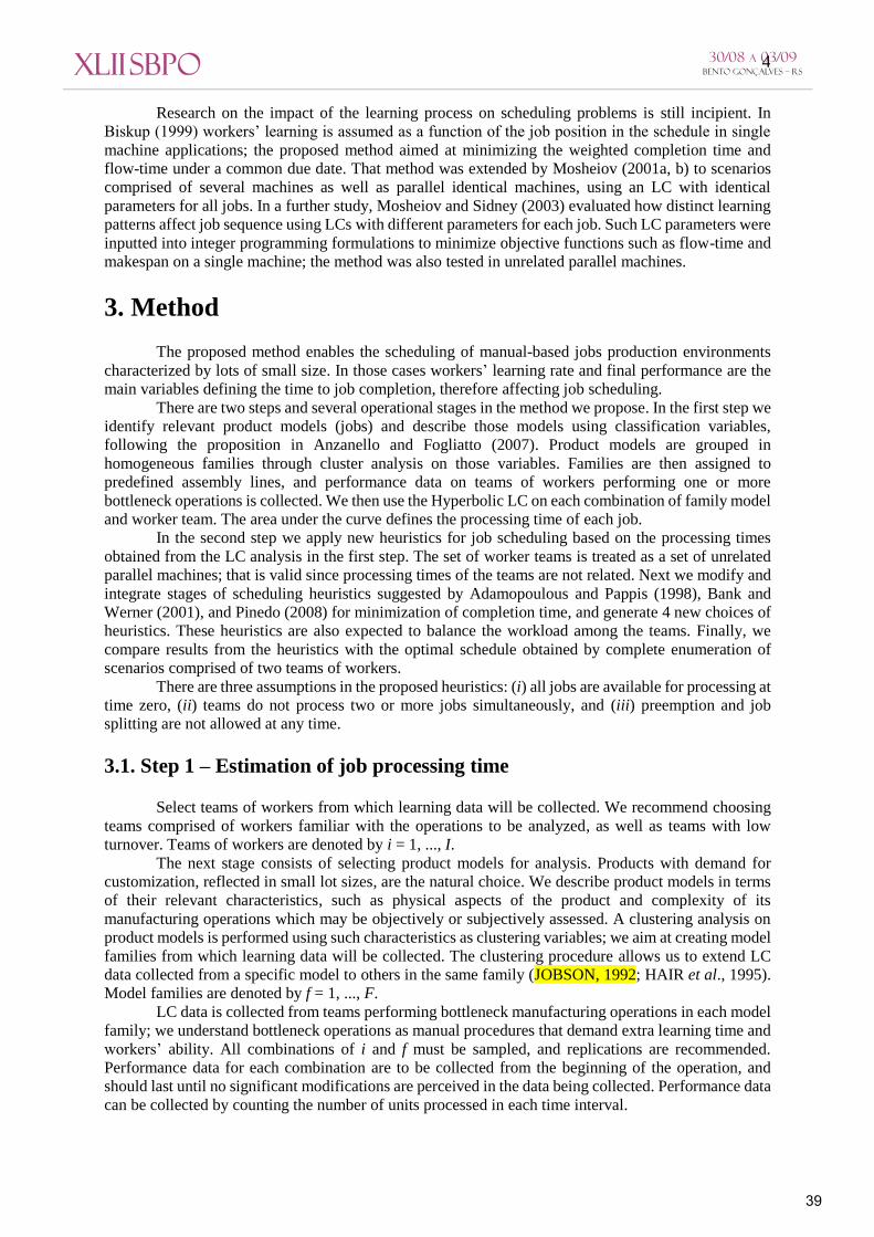
Finally, we use the previously generated graphs to estimate the time required by team i to

perform job j (i.e. the processing times pij). The number of units processed in a given time interval

corresponds to the area under each LC, as illustrated in Figure 1. Hence, the processing time p required

to complete a lot comprised of Q units may be estimated integrating each LC from 0 to p, until an area

equivalent to Q is obtained. We repeat this procedure for each team. It is important to remark that pij

refers to the time to process the entire job comprised of Q units, and not a single unit.

3.2 Step 2 – Scheduling learning dependent jobs

There are three stages in the heuristics proposed here: (i) define an initial order for job

distribution, (ii) assign jobs to teams in a balanced way, and (iii) sequence the subset of jobs assigned to

each team in view of the objective function to be optimized. These stages are explained in detail in the

following sections.

Figure 1: Job processing times

Stage 1 – Define order for job distribution

We initially order the set of N jobs according to two priority rules:

(i) Decreasing Absolute Difference between Jobs’ Processing Times rule – originally suggested

by Adamopoulos and Pappis (1998), this rule searches for the two teams (say A and B) with the smallest

processing times (pij, i = A, B) and calculate their difference, as in Eq. (3). This procedure is repeated for

each job j. Jobs are then listed in decreasing order of Dj and assigned to teams.

|| BjAjj ppD (3)

(ii) Increasing Absolute Difference between Jobs’ Processing Times rule – Similar to rule (i),

but now jobs are listed in increasing order of Dj and assigned to teams.

40

6

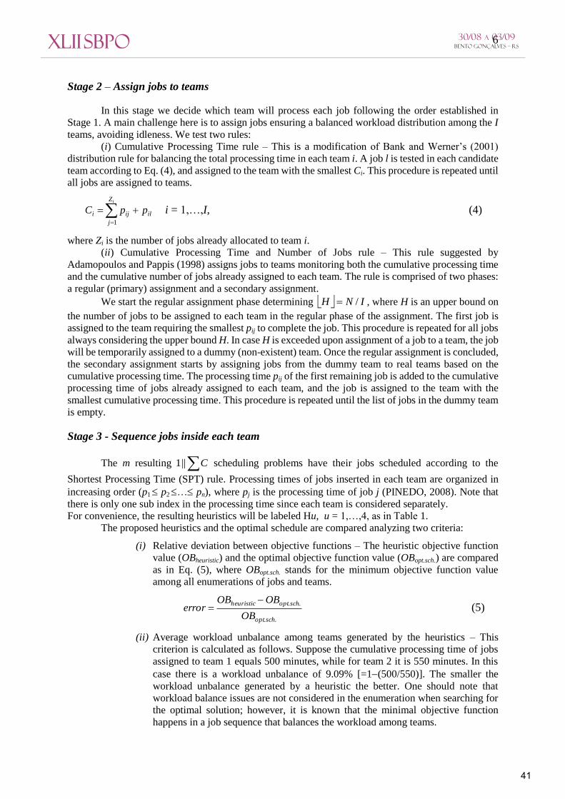
Stage 2 – Assign jobs to teams

In this stage we decide which team will process each job following the order established in

Stage 1. A main challenge here is to assign jobs ensuring a balanced workload distribution among the I

teams, avoiding idleness. We test two rules:

(i) Cumulative Processing Time rule – This is a modification of Bank and Werner’s (2001)

distribution rule for balancing the total processing time in each team i. A job l is tested in each candidate

team according to Eq. (4), and assigned to the team with the smallest Ci. This procedure is repeated until

all jobs are assigned to teams.

il

Z

j

iji ppCi

1

i = 1,…,I, (4)

where Zi is the number of jobs already allocated to team i.

(ii) Cumulative Processing Time and Number of Jobs rule – This rule suggested by

Adamopoulos and Pappis (1998) assigns jobs to teams monitoring both the cumulative processing time

and the cumulative number of jobs already assigned to each team. The rule is comprised of two phases:

a regular (primary) assignment and a secondary assignment.

We start the regular assignment phase determining INH / , where H is an upper bound on

the number of jobs to be assigned to each team in the regular phase of the assignment. The first job is

assigned to the team requiring the smallest pij to complete the job. This procedure is repeated for all jobs

always considering the upper bound H. In case H is exceeded upon assignment of a job to a team, the job

will be temporarily assigned to a dummy (non-existent) team. Once the regular assignment is concluded,

the secondary assignment starts by assigning jobs from the dummy team to real teams based on the

cumulative processing time. The processing time pij of the first remaining job is added to the cumulative

processing time of jobs already assigned to each team, and the job is assigned to the team with the

smallest cumulative processing time. This procedure is repeated until the list of jobs in the dummy team

is empty.

Stage 3 - Sequence jobs inside each team

The m resulting C||1 scheduling problems have their jobs scheduled according to the

Shortest Processing Time (SPT) rule. Processing times of jobs inserted in each team are organized in

increasing order (p1 p2 … pn), where pj is the processing time of job j (PINEDO, 2008). Note that

there is only one sub index in the processing time since each team is considered separately.

For convenience, the resulting heuristics will be labeled Hu, u = 1,…,4, as in Table 1. The proposed heuristics and the optimal schedule are compared analyzing two criteria:

(i) Relative deviation between objective functions – The heuristic objective function

value (OBheuristic) and the optimal objective function value (OBopt.sch.) are compared

as in Eq. (5), where OBopt.sch. stands for the minimum objective function value

among all enumerations of jobs and teams.

..

..

schopt

schoptheuristic

OB

OBOBerror

(5)

(ii) Average workload unbalance among teams generated by the heuristics – This

criterion is calculated as follows. Suppose the cumulative processing time of jobs

assigned to team 1 equals 500 minutes, while for team 2 it is 550 minutes. In this

case there is a workload unbalance of 9.09% [=1(500/550)]. The smaller the

workload unbalance generated by a heuristic the better. One should note that

workload balance issues are not considered in the enumeration when searching for

the optimal solution; however, it is known that the minimal objective function

happens in a job sequence that balances the workload among teams.

41

7

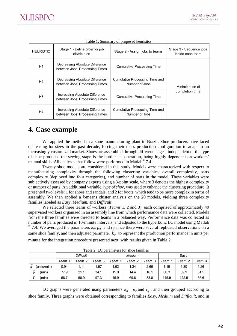
Table 1: Summary of proposed heuristics

4. Case example

We applied the method in a shoe manufacturing plant in Brazil. Shoe producers have faced

decreasing lot sizes in the past decade, forcing their mass production configuration to adapt to an

increasingly customized market. Shoes are assembled through different stages; independent of the type

of shoe produced the sewing stage is the bottleneck operation, being highly dependent on workers’

manual skills. All analyses that follow were performed in Matlab® 7.4.

Twenty shoe models are considered in this study. Models were characterized with respect to

manufacturing complexity through the following clustering variables: overall complexity, parts

complexity (deployed into four categories), and number of parts in the model. These variables were

subjectively assessed by company experts using a 3-point scale, where 3 denotes the highest complexity

or number of parts. An additional variable, type of shoe, was used to enhance the clustering procedure. It

presented two levels: 1 for shoes and sandals, and 2 for boots, which tend to be more complex in terms of

assembly. We then applied a k-means cluster analysis on the 20 models, yielding three complexity

families labeled as Easy, Medium, and Difficult.

We selected three teams of workers (Teams 1, 2 and 3), each comprised of approximately 40

supervised workers organized in an assembly line from which performance data were collected. Models

from the three families were directed to teams in a balanced way. Performance data was collected as

number of pairs produced in 10-minute intervals, and adjusted to the hyperbolic LC model using Matlab

® 7.4. We averaged the parameters kif, pif and rif since there were several replicated observations on a

same shoe family, and then adjusted parameter ifk to represent the production performance in units per

minute for the integration procedure presented next, with results given in Table 2.

Table 2: LC parameters for shoe families

LC graphs were generated using parameters ifk , ifp and ifr , and then grouped according to

shoe family. Three graphs were obtained corresponding to families Easy, Medium and Difficult, and in

HEURISTIC Stage 1 - Define order for job distribution

Stage 2 - Assign jobs to teams Stage 3 - Sequence jobs inside each team

H1 Decreasing Absolute Difference between Jobs' Processing Times

Cumulative Processing Time

H2 Decreasing Absolute Difference between Jobs' Processing Times

Cumulative Processing Time and Number of Jobs

H3 Increasing Absolute Difference between Jobs' Processing Times

Cumulative Processing Time

H4 Increasing Absolute Difference between Jobs' Processing Times

Cumulative Processing Time and Number of Jobs

Minimization of completion time

Team 1 Team 2 Team 3 Team 1 Team 2 Team 3 Team 1 Team 2 Team 3 (units/min) 0.94 1.11 1.57 1.62 1.34 2.66 1.19 1.30 1.26

(min) 77.9 21.1 34.1 15.9 14.4 16.1 80.3 62.9 51.5 (min) 68.7 50.9 97.3 46.9 69.8 38.0 145.9 122.5 66.6

EasyMediumDifficult

kp

r

42

8

each graph there were three average LCs, one for each team analyzed. Areas under the graphs enabled

the estimation of processing times for each team, which were then used in the scheduling heuristics.

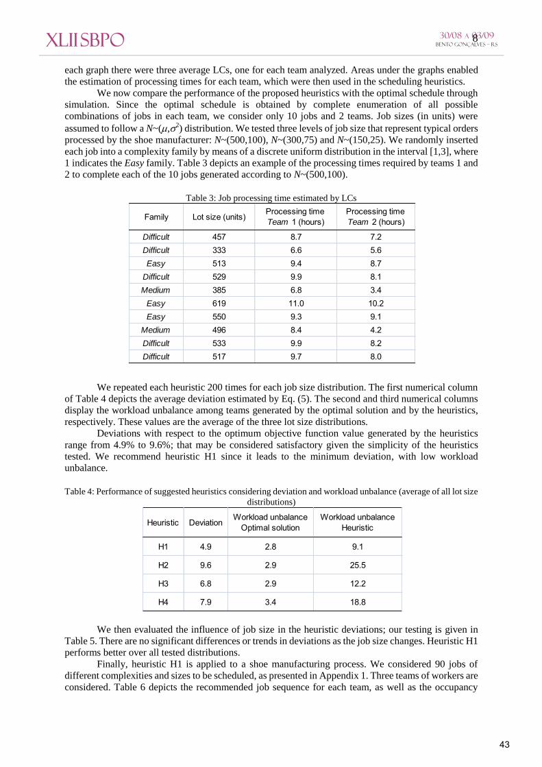
We now compare the performance of the proposed heuristics with the optimal schedule through

simulation. Since the optimal schedule is obtained by complete enumeration of all possible

combinations of jobs in each team, we consider only 10 jobs and 2 teams. Job sizes (in units) were

assumed to follow a N~(,2) distribution. We tested three levels of job size that represent typical orders

processed by the shoe manufacturer: N~(500,100), N~(300,75) and N~(150,25). We randomly inserted

each job into a complexity family by means of a discrete uniform distribution in the interval [1,3], where

1 indicates the Easy family. Table 3 depicts an example of the processing times required by teams 1 and

2 to complete each of the 10 jobs generated according to N~(500,100).

Table 3: Job processing time estimated by LCs

We repeated each heuristic 200 times for each job size distribution. The first numerical column

of Table 4 depicts the average deviation estimated by Eq. (5). The second and third numerical columns

display the workload unbalance among teams generated by the optimal solution and by the heuristics,

respectively. These values are the average of the three lot size distributions.

Deviations with respect to the optimum objective function value generated by the heuristics

range from 4.9% to 9.6%; that may be considered satisfactory given the simplicity of the heuristics

tested. We recommend heuristic H1 since it leads to the minimum deviation, with low workload

unbalance.

Table 4: Performance of suggested heuristics considering deviation and workload unbalance (average of all lot size

distributions)

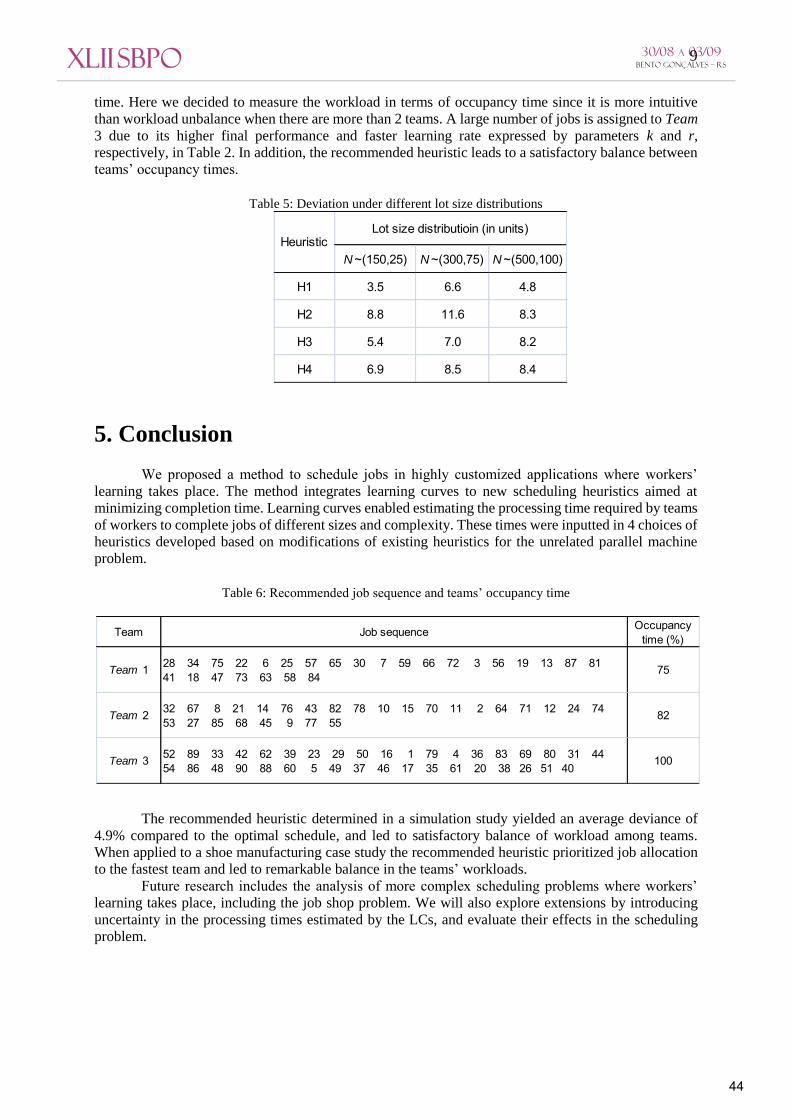
We then evaluated the influence of job size in the heuristic deviations; our testing is given in

Table 5. There are no significant differences or trends in deviations as the job size changes. Heuristic H1

performs better over all tested distributions. Finally, heuristic H1 is applied to a shoe manufacturing process. We considered 90 jobs of

different complexities and sizes to be scheduled, as presented in Appendix 1. Three teams of workers are

considered. Table 6 depicts the recommended job sequence for each team, as well as the occupancy

Difficult 457 8.7 7.2Difficult 333 6.6 5.6Easy 513 9.4 8.7

Difficult 529 9.9 8.1Medium 385 6.8 3.4

Easy 619 11.0 10.2Easy 550 9.3 9.1

Medium 496 8.4 4.2Difficult 533 9.9 8.2Difficult 517 9.7 8.0

Family Lot size (units) Processing time Team 1 (hours)

Processing time Team 2 (hours)

Heuristic Deviation Workload unbalance Optimal solution

Workload unbalance Heuristic

H1 4.9 2.8 9.1

H2 9.6 2.9 25.5

H3 6.8 2.9 12.2

H4 7.9 3.4 18.8

43

9

time. Here we decided to measure the workload in terms of occupancy time since it is more intuitive

than workload unbalance when there are more than 2 teams. A large number of jobs is assigned to Team

3 due to its higher final performance and faster learning rate expressed by parameters k and r,

respectively, in Table 2. In addition, the recommended heuristic leads to a satisfactory balance between

teams’ occupancy times.

Table 5: Deviation under different lot size distributions

5. Conclusion

We proposed a method to schedule jobs in highly customized applications where workers’

learning takes place. The method integrates learning curves to new scheduling heuristics aimed at

minimizing completion time. Learning curves enabled estimating the processing time required by teams

of workers to complete jobs of different sizes and complexity. These times were inputted in 4 choices of

heuristics developed based on modifications of existing heuristics for the unrelated parallel machine

problem.

Table 6: Recommended job sequence and teams’ occupancy time

The recommended heuristic determined in a simulation study yielded an average deviance of

4.9% compared to the optimal schedule, and led to satisfactory balance of workload among teams.

When applied to a shoe manufacturing case study the recommended heuristic prioritized job allocation

to the fastest team and led to remarkable balance in the teams’ workloads.

Future research includes the analysis of more complex scheduling problems where workers’

learning takes place, including the job shop problem. We will also explore extensions by introducing

uncertainty in the processing times estimated by the LCs, and evaluate their effects in the scheduling

problem.

N ~(150,25) N ~(300,75) N ~(500,100)

H1 3.5 6.6 4.8

H2 8.8 11.6 8.3

H3 5.4 7.0 8.2

H4 6.9 8.5 8.4

HeuristicLot size distributioin (in units)

Team Job sequence Occupancy time (%)

Team 1 28 34 75 22 6 25 57 65 30 7 59 66 72 3 56 19 13 87 81 41 18 47 73 63 58 84

75

Team 2 32 67 8 21 14 76 43 82 78 10 15 70 11 2 64 71 12 24 74 53 27 85 68 45 9 77 55

82

Team 3 52 89 33 42 62 39 23 29 50 16 1 79 4 36 83 69 80 31 44 54 86 48 90 88 60 5 49 37 46 17 35 61 20 38 26 51 40

100

44

10

References Adamopoulos, G. and Pappis, C. 1998. Scheduling under a common due-date on parallel unrelated

machines. European Journal of Operational Research, 105: 494-501.

Anzanello, M.J. and Fogliatto, F.S. 2007. Learning curve modeling of work assignment in mass

customized assembly lines. International Journal of Production Research, 45:2919-2938.

Bank, J. and Werner, F. 2001. Heuristic algorithms for unrelated parallel machine scheduling with a

common due date, release dates, and linear earliness and tardiness penalties. Mathematical and

Computer Modelling, 33:363-383.

Biskup, D. 1999. Single-machine scheduling with learning considerations. European Journal of

Operational Research, 115:173-178.

Cehn, T. and Sin, C. 1990. A state-of-the-art review of parallel-machine scheduling research.

European Journal of Operational Research, 47:271-292.

Chen, J. and Wu, T. 2006. Total tardiness minimization on unrelated parallel machine scheduling with

auxiliary equipment constraints. Omega, 34:81-89.

Da Silveira, G.J.C.; Boreinstein, D. and Fogliatto, F.S. 2001. Mass Customization: Literature

Review and Research Direction. International Journal of Production Economics, 72:1-13, 2001.

Hair, J.; Anderson, R.; Tatham, R. and Black, W. 1995. Multivariate Data Analysis with Readings.

Prentice-Hall Inc: New Jersey.

Jobson, J. 1992. Applied Multivariate Data Analysis, Volume II: Categorical and Multivariate

Methods. Springer-Verlag: New York.

Jungwattanakit, J.; Reodecha, M.; Chaovalitwongse, P. and Werner, F. 2009. A comparison of

scheduling algorithms for flexible flow shop problems with unrelated parallel machines, setup times,

and dual criteria. Computers & Operations Research, 36:358-378.

Kim, E.; Sung, C. and Lee, I. 2009. Scheduling of parallel machines to minimize total completion

time subject to s-precedence constraints. Computers & Operations Research, 36:698-710, 2009.

Mazur, J. and Hastie, R. 1978. Learning as Accumulation: a Reexamination of the Learning Curve.

Psychological Bulletin, 85:1256-1274.

Mokotoff, E. and Jimeno, J. 2002. Heuristics based on partial enumeration for the unrelated parallel

processor scheduling problem. Annals of Operations Research, 117: 133-150.

Mosheiov, G. 2001a. Scheduling problems with learning effect. European Journal of Operational

Research, 132:687-693.

Mosheiov, G. 2001b. Parallel machine scheduling with learning effect. Journal of the Operational

Research Society, 52:391-399.

Mosheiov, G. and Sidney, J. 2003. Scheduling with general job-dependent learning curves. European

Journal of Operational Research, 147:665-670.

Nembhard, D. and Uzumeri, M. 2000. An Individual-Based Description of Learning within an

Organization. IEEE Transactions on Engineering Management, 47:370-378.

Pinedo, M. 2008. Scheduling, Theory, Algorithms and Systems. Springer: New York.

Randahwa, S. and Kuo, C. 1997. Evaluating scheduling heuristics for non-identical parallel

processors. International Journal of Production Research, 35: 969-981.

Suresh, V. and Chaudhuri, D. 1994. Minimizing maximum tardiness for unrelated parallel machines.

International Journal of Production Economics, 34:223-229.

Teplitz, C. 1991. The Learning Curve Deskbook: A reference guide to theory, calculations and

applications. Quorum Books: New York.

45

11

Uzumeri, M. and Nembhard, D. 1998. A Population of Learners: A New Way to Measure

Organizational Learning. Journal of Operations Management, 16:515-528.

Wright, T. 1936. Factors affecting the cost of airplanes. Journal of the Aeronautical Sciences,

3:122-128.

Yu, L; Shih, H.; Pfund, M.; Carlyle, W. and Fowler, J. 2002. Scheduling of unrelated parallel

machines: an application to PWB manufacturing. IIE Transactions, 34:921-931.

Appendix 1 – Size and complexity of shoe manufacturing lots

46

12

1 Medium 460 46 Easy 5252 Difficult 345 47 Easy 4503 Difficult 390 48 Difficult 4304 Difficult 640 49 Easy 5905 Fácil 630 50 Medium 4856 Medium 500 51 Easy 3607 Medium 545 52 Medium 7308 Medium 530 53 Easy 5009 Easy 380 54 Difficult 46510 Difficult 505 55 Easy 13011 Difficult 425 56 Difficult 33512 Easy 585 57 Difficult 62013 Easy 610 58 Easy 36014 Medium 440 59 Difficult 51015 Difficult 475 60 Easy 76016 Medium 485 61 Easy 45517 Easy 500 62 Medium 54518 Easy 480 63 Easy 42019 Easy 700 64 Easy 82020 Easy 445 65 Difficult 58021 Difficult 720 66 Difficult 47522 Medium 535 67 Difficult 85523 Medium 530 68 Easy 42024 Easy 580 69 Difficult 56025 Difficult 715 70 Difficult 44526 Easy 400 71 Easy 62027 Easy 460 72 Difficult 44028 Medium 720 73 Easy 44029 Medium 495 74 Easy 52030 Medium 345 75 Medium 56531 Difficult 535 76 Difficult 60532 Medium 715 77 Easy 35033 Medium 615 78 Difficult 54534 Medium 580 79 Medium 46035 Easy 490 80 Difficult 54536 Difficult 600 81 Easy 54037 Easy 580 82 Difficult 55038 Easy 425 83 Medium 36539 Medium 540 84 Easy 27540 Easy 330 85 Easy 44541 Easy 505 86 Difficult 46542 Medium 575 87 Easy 58043 Difficult 585 88 Difficult 30044 Difficult 500 89 Medium 62045 Easy 410 90 Difficult 390

Lot Family Lot size (units) Lot Family Lot size (units)

47