RESUMO

A mineração de dados é definida como o processo automático, ou semi-

automático de extração de conhecimento para identificação de padrões, tendências,

associações e dependências, previamente desconhecidos, de bases de dados, sendo

amplamente utilizada na transformação de dados brutos em conhecimento útil para a

tomada de decisões. Embora as técnicas empregadas em mineração de dados,

tradicionalmente, se baseiam fortemente em métodos estatísticos, em inteligência

artificial e em aprendizagem de máquina, vários dos métodos empregados podem ser

formulados como problemas de otimização. O presente projeto tem por objetivo fazer

uso de métodos de mineração de dados para identificar padrões temporais em atrasos

por congestionamento em aeroportos brasileiros. O transporte aéreo no Brasil foi

recentemente liberalizado e uma de suas consequências foi a concentração dos voos em

alguns hubs. Embora a criação de hubs pareça benéfica às empresas de transporte aéreo

e ofereça algumas vantagens aos viajantes, a concentração excessiva de voos em um

hub pode resultar em alguns impactos econômicos negativos denominados atrasos por

congestionamento, os quais aumentam o tempo total de viagem dos passageiros e o

custo operacional das empresas.

Palavras-chave: mineração de dados; atrasos por congestionamento; formação de

agrupamentos; análise de séries temporais; sistemas de alerta.

1. REALIZAÇÕES NO PERÍODO

Ao longo do primeiro ano do projeto foram realizadas as 5 primeiras etapas,

conforme o cronograma proposto no projeto de pesquisa submetido (Tabela 1). Assim,

foi feita uma atualização da revisão bibliográfica do tema do projeto, a formação e

consistência das bases de dados, a transformação dos dados para geração de variáveis

para o modelo, as análises preliminares com discussão dos resultados obtidos e a

utilização de métodos de mineração de dados para formação de agrupamentos temporais

das séries diárias de atraso.

Tabela 1: Cronograma de atividades do projeto proposto.

ATIVIDADE BIMESTRES

1 2 3 4 5 6 7 8 9 10 11 12

ATUALIZAÇÃO DA REVISÃO BIBLIOGRÁFICA * * * * * *

FORMAÇÃO E CONSISTÊNCIA DAS BASES DE DADOS * *

TRANSFORMAÇÃO DOS DADOS *

ANÁLISES PRELIMINARES E DISCUSSÃO DOS

RESULTADOS *

UTILIZAÇÃO DOS MÉTODOS DE MINERAÇÃO DE

DADOS PARA FORMAÇÃO DE AGRUPAMENTOS

TEMPORAIS

* *

RELATÓRIO PARCIAL *

UTILIZAÇÃO DOS MÉTODOS DE MINERAÇÃO DE

DADOS PARA CRIAÇÃO DE UM MODELO DE

CLASSIFICAÇÃO (UTILIZADOS DA DETECÇÃO

PRECOCE DE ATRASOS POR CONGESTIONAMENTO)

* * * *

TRABALHOS PARA PUBLICAÇÃO * * * * * *

RELATÓRIO FINAL * *

A primeira etapa do projeto foi a atualização da revisão bibliográfica do tema do

projeto. Nesta, foi possível identificar trabalhos relacionados, principalmente, aos

determinantes de atrasos em aeroportos, bem como formas de análise dos dados de

atraso. A identificação dos determinantes de atraso é de fundamental importância para o

projeto pois indica quais são os dados necessários na criação do modelo. Quanto as

formas de análise dos dados de atraso, como é pretendido avançar no estado da arte em

relação aos métodos de mineração de dados, também é de grande importância

identificar o que já foi feito. Assim, foi construído um mapa mental com os

determinantes de atraso (Figura 1) e elencados os trabalhos em mineração de dados

(formação de agrupamentos, análise de associação, classificação e previsão) já

realizados no tema do projeto (Tabela 2).

Figura 1: Determinantes de atraso identificados a partir da revisão de literatura.

Uma vez concluída a revisão de literatura, a próxima etapa foi a formação e

consistência das bases de dados. Desta forma, considerando os determinantes de atraso

identificados na revisão de literatura, foi feita uma busca por dados abertos relacionados

a condições climáticas e de operação dos aeroportos que pudessem ser transformados

para a criação de variáveis que capturassem os efeitos de flutuação de demanda, dos

efeitos de rede (do inglês hubbing effect), do nível de concentração e concorrência e de

efeitos temporais como dia da semana e estação do ano. Assim, foi identificada uma

fonte aberta de dados climáticos (INMET:

http://www.inmet.gov.br/portal/index.php?r=bdmep/bdmep) e uma fonte aberta com

dados de movimentação (pousos e decolagens) dos aeroportos brasileiros (ANAC-VRA:

http://www2.anac.gov.br/vra/basehistorica.asp ). Esses dados foram extraídos e

posteriormente transformados (terceira etapa do projeto) para geração das variáveis de

análise.

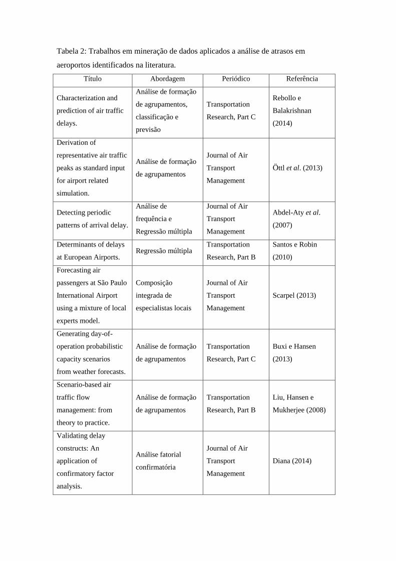
Tabela 2: Trabalhos em mineração de dados aplicados a análise de atrasos em

aeroportos identificados na literatura.

Título Abordagem Periódico Referência

Characterization and

prediction of air traffic

delays.

Análise de formação

de agrupamentos,

classificação e

previsão

Transportation

Research, Part C

Rebollo e

Balakrishnan

(2014)

Derivation of

representative air traffic

peaks as standard input

for airport related

simulation.

Análise de formação

de agrupamentos

Journal of Air

Transport

Management

Öttl et al. (2013)

Detecting periodic

patterns of arrival delay.

Análise de

frequência e

Regressão múltipla

Journal of Air

Transport

Management

Abdel-Aty et al.

(2007)

Determinants of delays

at European Airports. Regressão múltipla

Transportation

Research, Part B

Santos e Robin

(2010)

Forecasting air

passengers at São Paulo

International Airport

using a mixture of local

experts model.

Composição

integrada de

especialistas locais

Journal of Air

Transport

Management

Scarpel (2013)

Generating day-of-

operation probabilistic

capacity scenarios

from weather forecasts.

Análise de formação

de agrupamentos

Transportation

Research, Part C

Buxi e Hansen

(2013)

Scenario-based air

traffic flow

management: from

theory to practice.

Análise de formação

de agrupamentos

Transportation

Research, Part B

Liu, Hansen e

Mukherjee (2008)

Validating delay

constructs: An

application of

confirmatory factor

analysis.

Análise fatorial

confirmatória

Journal of Air

Transport

Management

Diana (2014)

A próxima etapa do projeto foi a realização de análises preliminares e discussão

dos resultados. Nesta etapa, foi identificada a oportunidade de desenvolver um sistema

de alerta para detecção precoce de mudança de tendência na demanda de passageiros do

sistema multi-aeroporto de São Paulo. Desta forma, utilizando as bases de dados

criadas, aplicou-se o método de Holt-Winters multiplicativo para extrair o componente

de tendência do número mensal de passageiros e dos potenciais indicadores de

antecedentes do modelo. Esses componentes de tendência foram, posteriormente,

transformados gerando as variáveis explicativas e explicadas do modelo de previsão.

Para a criação deste modelo foi utilizada uma árvore de regressão e classificação. Desta

forma, foi possível identificar indicadores de antecedentes e gerar um procedimento de

previsão interpretável visando suportar o desenvolvimento de cenários de tendência na

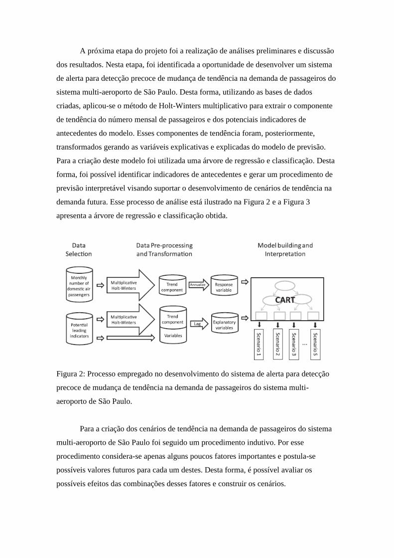
demanda futura. Esse processo de análise está ilustrado na Figura 2 e a Figura 3

apresenta a árvore de regressão e classificação obtida.

Figura 2: Processo empregado no desenvolvimento do sistema de alerta para detecção

precoce de mudança de tendência na demanda de passageiros do sistema multi-

aeroporto de São Paulo.

Para a criação dos cenários de tendência na demanda de passageiros do sistema

multi-aeroporto de São Paulo foi seguido um procedimento indutivo. Por esse

procedimento considera-se apenas alguns poucos fatores importantes e postula-se

possíveis valores futuros para cada um destes. Desta forma, é possível avaliar os

possíveis efeitos das combinações desses fatores e construir os cenários.

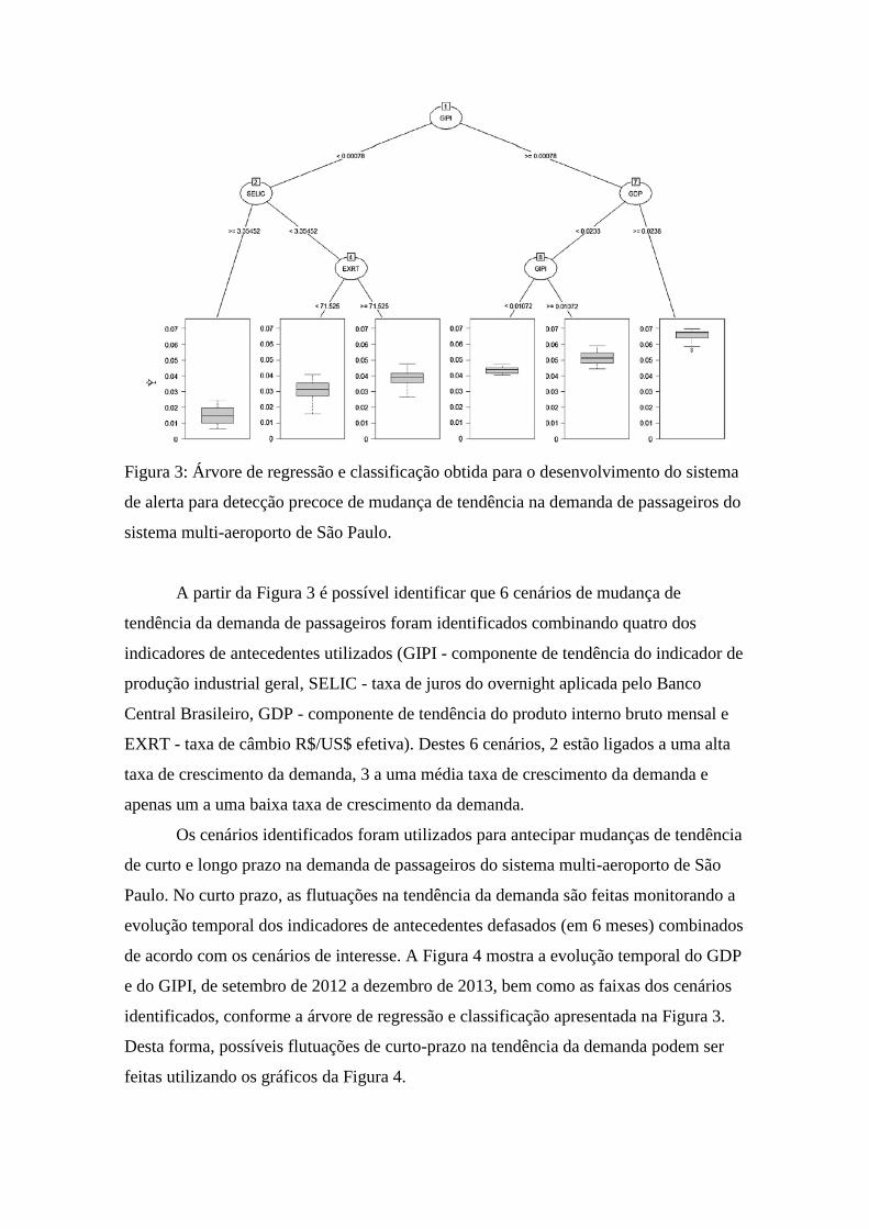
Figura 3: Árvore de regressão e classificação obtida para o desenvolvimento do sistema

de alerta para detecção precoce de mudança de tendência na demanda de passageiros do

sistema multi-aeroporto de São Paulo.

A partir da Figura 3 é possível identificar que 6 cenários de mudança de

tendência da demanda de passageiros foram identificados combinando quatro dos

indicadores de antecedentes utilizados (GIPI - componente de tendência do indicador de

produção industrial geral, SELIC - taxa de juros do overnight aplicada pelo Banco

Central Brasileiro, GDP - componente de tendência do produto interno bruto mensal e

EXRT - taxa de câmbio R$/US$ efetiva). Destes 6 cenários, 2 estão ligados a uma alta

taxa de crescimento da demanda, 3 a uma média taxa de crescimento da demanda e

apenas um a uma baixa taxa de crescimento da demanda.

Os cenários identificados foram utilizados para antecipar mudanças de tendência

de curto e longo prazo na demanda de passageiros do sistema multi-aeroporto de São

Paulo. No curto prazo, as flutuações na tendência da demanda são feitas monitorando a

evolução temporal dos indicadores de antecedentes defasados (em 6 meses) combinados

de acordo com os cenários de interesse. A Figura 4 mostra a evolução temporal do GDP

e do GIPI, de setembro de 2012 a dezembro de 2013, bem como as faixas dos cenários

identificados, conforme a árvore de regressão e classificação apresentada na Figura 3.

Desta forma, possíveis flutuações de curto-prazo na tendência da demanda podem ser

feitas utilizando os gráficos da Figura 4.

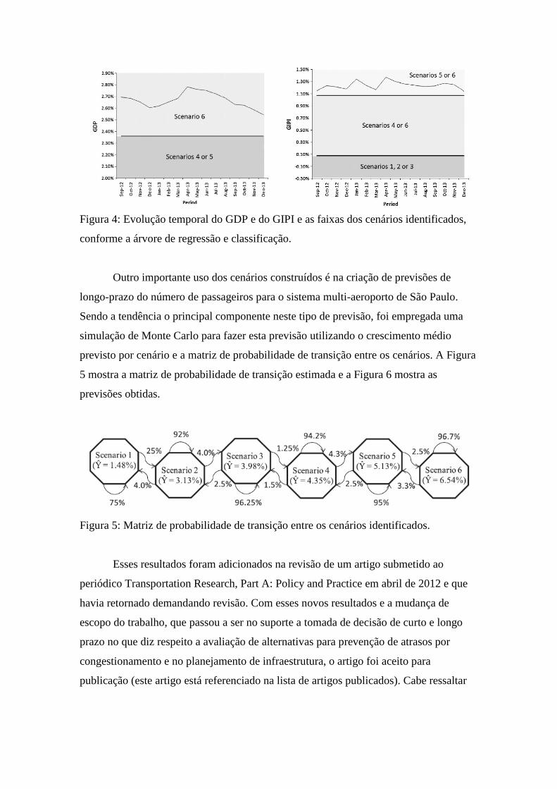
Figura 4: Evolução temporal do GDP e do GIPI e as faixas dos cenários identificados,

conforme a árvore de regressão e classificação.

Outro importante uso dos cenários construídos é na criação de previsões de

longo-prazo do número de passageiros para o sistema multi-aeroporto de São Paulo.

Sendo a tendência o principal componente neste tipo de previsão, foi empregada uma

simulação de Monte Carlo para fazer esta previsão utilizando o crescimento médio

previsto por cenário e a matriz de probabilidade de transição entre os cenários. A Figura

5 mostra a matriz de probabilidade de transição estimada e a Figura 6 mostra as

previsões obtidas.

Figura 5: Matriz de probabilidade de transição entre os cenários identificados.

Esses resultados foram adicionados na revisão de um artigo submetido ao

periódico Transportation Research, Part A: Policy and Practice em abril de 2012 e que

havia retornado demandando revisão. Com esses novos resultados e a mudança de

escopo do trabalho, que passou a ser no suporte a tomada de decisão de curto e longo

prazo no que diz respeito a avaliação de alternativas para prevenção de atrasos por

congestionamento e no planejamento de infraestrutura, o artigo foi aceito para

publicação (este artigo está referenciado na lista de artigos publicados). Cabe ressaltar

que no artigo publicado há o agradecimento a FAPESP já referenciando o número deste

projeto (2013/22416-4).

Figura 6: Previsão de longo prazo do número mensal de passageiros para o sistema

multi-aeroporto de São Paulo.

Posteriormente, foi executada a última etapa prevista para o primeiro ano do

projeto que foi a utilização de métodos de mineração de dados para formação de

agrupamentos temporais das séries diárias de atraso. Em termos de motivação para a

realização do trabalho, sabe-se que depois da liberalização dos transporte aéreo ocorrida

na década de 90, houve a concentração dos voos em alguns hubs resultando em atrasos

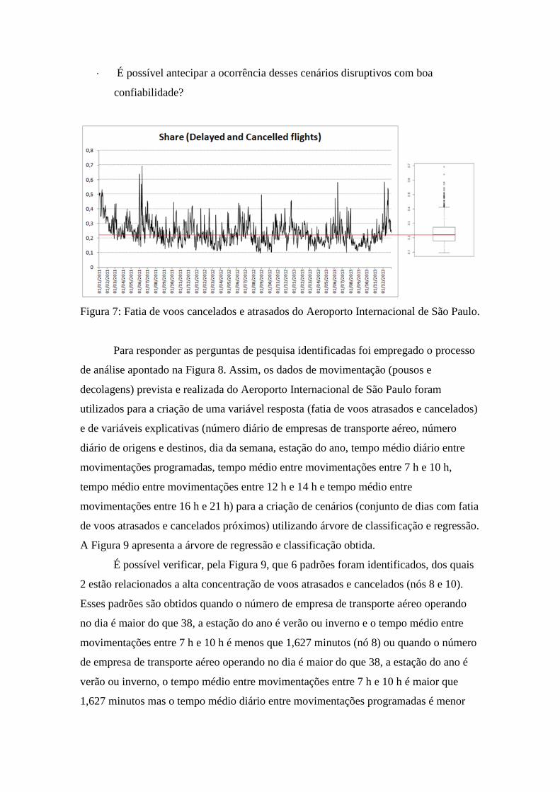
por congestionamento. A Figura 7 mostra a evolução temporal da fatia de voos

atrasados e cancelados no Aeroporto Internacional de São Paulo (principal Hub

brasileiro). É possível verificar, a partir da Figura 7, que cerca de 25% dos dias

considerados apresentam mais de 25% dos voos cancelados ou atrasados e que é

possível identificar dias com mais de 50% dos voos cancelados ou atrasados. Assim, o

vigente projeto se apresenta como uma iniciativa para ajudar a lidar com esse problema.

Como resultado da utilização de métodos de mineração de dados para formação

de agrupamentos temporais das séries diárias de atraso espera-se responder as seguintes

perguntas de pesquisa:

Quais fatores mais contribuem para a ocorrência de atrasos e cancelamentos?

É possível identificar como esses fatores se combinam para resultar em cenários

disruptivos?

É possível antecipar a ocorrência desses cenários disruptivos com boa

confiabilidade?

Figura 7: Fatia de voos cancelados e atrasados do Aeroporto Internacional de São Paulo.

Para responder as perguntas de pesquisa identificadas foi empregado o processo

de análise apontado na Figura 8. Assim, os dados de movimentação (pousos e

decolagens) prevista e realizada do Aeroporto Internacional de São Paulo foram

utilizados para a criação de uma variável resposta (fatia de voos atrasados e cancelados)

e de variáveis explicativas (número diário de empresas de transporte aéreo, número

diário de origens e destinos, dia da semana, estação do ano, tempo médio diário entre

movimentações programadas, tempo médio entre movimentações entre 7 h e 10 h,

tempo médio entre movimentações entre 12 h e 14 h e tempo médio entre

movimentações entre 16 h e 21 h) para a criação de cenários (conjunto de dias com fatia

de voos atrasados e cancelados próximos) utilizando árvore de classificação e regressão.

A Figura 9 apresenta a árvore de regressão e classificação obtida.

É possível verificar, pela Figura 9, que 6 padrões foram identificados, dos quais

2 estão relacionados a alta concentração de voos atrasados e cancelados (nós 8 e 10).

Esses padrões são obtidos quando o número de empresa de transporte aéreo operando

no dia é maior do que 38, a estação do ano é verão ou inverno e o tempo médio entre

movimentações entre 7 h e 10 h é menos que 1,627 minutos (nó 8) ou quando o número

de empresa de transporte aéreo operando no dia é maior do que 38, a estação do ano é

verão ou inverno, o tempo médio entre movimentações entre 7 h e 10 h é maior que

1,627 minutos mas o tempo médio diário entre movimentações programadas é menor

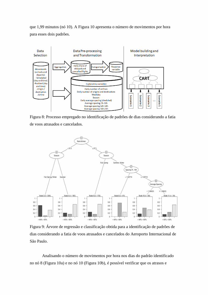
que 1,99 minutos (nó 10). A Figura 10 apresenta o número de movimentos por hora

para esses dois padrões.

Figura 8: Processo empregado no identificação de padrões de dias considerando a fatia

de voos atrasados e cancelados.

Figura 9: Árvore de regressão e classificação obtida para a identificação de padrões de

dias considerando a fatia de voos atrasados e cancelados do Aeroporto Internacional de

São Paulo.

Analisando o número de movimentos por hora nos dias do padrão identificado

no nó 8 (Figura 10a) e no nó 10 (Figura 10b), é possível verificar que os atrasos e

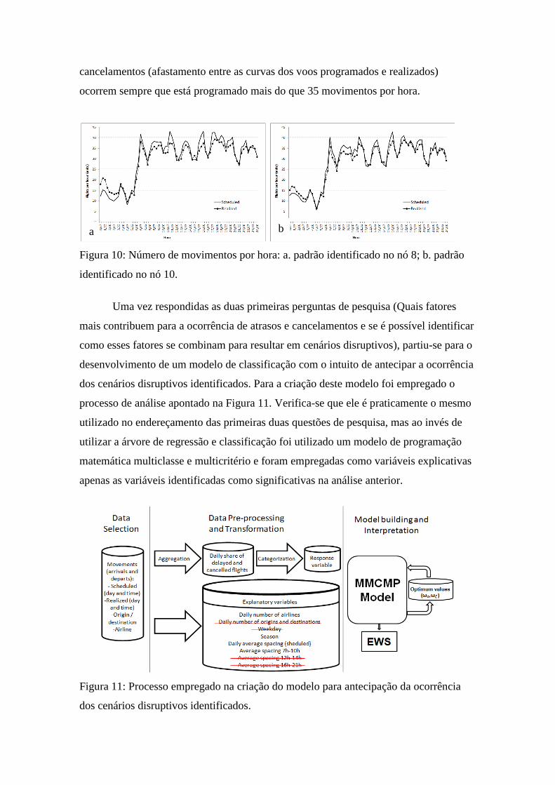
cancelamentos (afastamento entre as curvas dos voos programados e realizados)

ocorrem sempre que está programado mais do que 35 movimentos por hora.

Figura 10: Número de movimentos por hora: a. padrão identificado no nó 8; b. padrão

identificado no nó 10.

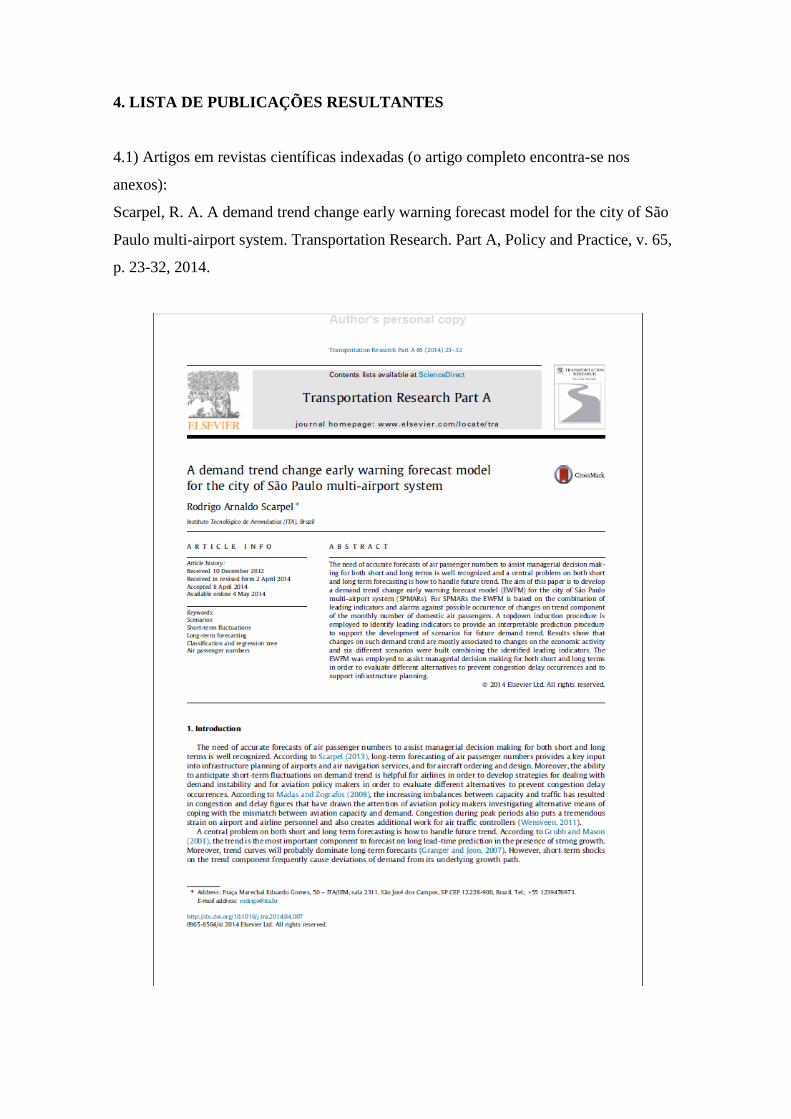
Uma vez respondidas as duas primeiras perguntas de pesquisa (Quais fatores

mais contribuem para a ocorrência de atrasos e cancelamentos e se é possível identificar

como esses fatores se combinam para resultar em cenários disruptivos), partiu-se para o

desenvolvimento de um modelo de classificação com o intuito de antecipar a ocorrência

dos cenários disruptivos identificados. Para a criação deste modelo foi empregado o

processo de análise apontado na Figura 11. Verifica-se que ele é praticamente o mesmo

utilizado no endereçamento das primeiras duas questões de pesquisa, mas ao invés de

utilizar a árvore de regressão e classificação foi utilizado um modelo de programação

matemática multiclasse e multicritério e foram empregadas como variáveis explicativas

apenas as variáveis identificadas como significativas na análise anterior.

Figura 11: Processo empregado na criação do modelo para antecipação da ocorrência

dos cenários disruptivos identificados.

a b

O modelo de programação matemática multiclasse e multicritério utilizado para

a antecipação da ocorrência dos cenários disruptivos foi:

kjorj

n

i

k

j

n

i

ji

jj

ji

k

j

n

i

ji

bbZ

1 1

1

2 1

,

1

,

1 1

,2

Minimize

em que Xnxr são os dados das variáveis explicativas das n observações e r variáveis e as

observações estão divididas em k classes. As variáveis de decisão do modelo são os

limites de classificação (b1,...,bk-1) e os ponderadores das variáveis independentes

(w1,...,wr). O modelo apresenta ainda variáveis de folga e excesso ( e ). Por este

modelo objetiva-se criar uma função linear que possa seja utilizada para classificar

novas observações. Os resultados obtidos foram:

031,1

203,0

..52,0107.16,0.28,0.04,0

179,20

2

1

b

b

WSSeasontSpacingSpacingAvAirlinesNum

Z

w,x i

Desta forma, aplica-se a função linear obtida e caso o valor obtido seja menor

que 0,203 a observação é classificada como um dia com baixa concentração de voos

cancelados ou atrasados. Já, se o valor obtido ficar entre 0,203 e 1,031, a observação é

classificada como um dia com média concentração de voos cancelados ou atrasados.

Porém, se o valor obtido a partir da aplicação da função linear for maior que 1,031, a

observação é classificada como um dia com alta concentração de voos cancelados ou

atrasados. A taxa de acerte desse modelo de classificação para os conjuntos de treino

(60% dos dados) e de validação (40% dos dados) estão na Figura 12.

Figura 12: Taxa de acerto do modelo de classificação para antecipação dos cenários

disruptivos identificados.

11,:.. ,, kjbTS jijij w,xi

11,1, kjbb jjji

nijiji 1,0, ,,

Esses procedimentos, análises e resultados foram apresentados no encontro

anual do INFORMS (Institute for Operations Research and the Management Sciences)

ocorrido entre 9 e 12 de Novembro de 2014, em São Francisco / CA, EUA. O trabalho

foi intitulado "A Data Mining Approach for Early Identification of Potencial Disruptive

Scenarios" (este trabalho está referenciado na lista de trabalhos apresentados em

congressos internacionais). No momento, com as contribuições recebidas na

apresentação do trabalho e alguns novos resultados obtidos, está em elaboração um

artigo que será submetido para uma revista científica indexada (possivelmente o

periódico Transportation Research, Part B:Methodologies).

No que diz respeito às orientações de alunos realizadas, neste primeiro ano foi

concluída a orientação de 1 trabalhos de graduação no tema do projeto (este trabalho

está referenciado na lista de orientações concluídas) e iniciadas 2 novas orientações de

trabalhos de graduação e 1 orientação de mestrado no tema do projeto.

2. APLICAÇÃO DOS RECURSOS DE RESERVA TÉCNICA E BENEFÍCIOS

COMPLEMENTARES

Ao longo do primeiro ano do projeto, os recursos de reserva técnica e benefícios

complementares foram utilizados para participação no INFORMS Annual Meeting

(para divulgação dos resultados do trabalho), para a manutenção de um notebook do

laboratório e para aquisição de material de consumo (um toner). Portanto, ao longo do

primeiro ano, os gastos foram:

1. Manutenção de um notebook (R$72,00): serviço de terceiros necessário para o

desenvolvimento do trabalho.

2. Passagem aérea (R$3.120,00), diárias (R$4.048,00) e inscrição (R$1.683,45)

para participação no INFORMS Annual Meeting: utilização dos benefícios

complementares para divulgação dos resultados do trabalho.

3. Compra de um toner para a impressora laser do laboratório (R$320,36):

insumo necessário para o desenvolvimento do trabalho.

O trabalhos apresentado no INFORMS Annual Meeting foi:

Este trabalho foi apresentado por Rodrigo Arnaldo Scarpel, oralmente no evento

científico INFORMS Annual Meeting ocorrido de 9/11/15 a 12/11/15 em São

Francisco/CA, EUA.

3. PLANO DE ATIVIDADES PARA O PRÓXIMO PERÍODO

Conforme indicado no cronograma de atividades do projeto de pesquisa

submetido (Tabela 1), ao longo do segundo ano do projeto pretende-se utilizar métodos

de mineração de dados para criação de um modelo de classificação (que seria utilizado

na detecção precoce de atrasos por congestionamento), bem como elaborar artigos

científicos para submissão para revistas científicas indexadas.

Quanto às orientações, pretende-se iniciar a orientações de, pelo menos, 1 aluno

de iniciação científica, concluir a orientação dos 2 trabalhos de graduação iniciados em

2015 e continuar a orientação de mestrado iniciada em 2014.

4. LISTA DE PUBLICAÇÕES RESULTANTES

4.1) Artigos em revistas científicas indexadas (o artigo completo encontra-se nos

anexos):

Scarpel, R. A. A demand trend change early warning forecast model for the city of São

Paulo multi-airport system. Transportation Research. Part A, Policy and Practice, v. 65,

p. 23-32, 2014.

4.2) Trabalhos apresentados em conferências internacionais:

Este trabalho foi apresentado por Rodrigo Arnaldo Scarpel, oralmente no evento

científico INFORMS Annual Meeting ocorrido de 9/11/15 a 12/11/15 em São

Francisco/CA, EUA.

5. ORIENTAÇÕES CONCLUÍDAS

5.1) Trabalhos de conclusão de curso (graduação):

Este trabalho de graduação teve por objetivo avaliar o atual contexto de

organização e execução dos procedimentos de pousos e decolagens visando a

otimização operacional e redução dos atrasos por congestionamento no Aeroporto

Internacional de Guarulhos.

REFERÊNCIAS BIBLIOGRÁFICAS

Abdel-Aty, M., Lee, C., Bai, Y. Li, X. e Michalak, M. Detecting periodic patterns of

arrival delay. Journal of Air Transport Management, 13, 355-361, 2007.

Buxi, G. e Hansen, M. Generating Day-of-operation Probabilistic Capacity Scenarios

from Weather Forecasts. Transportation Research Part C, 33, 153-166, 2013.

Diana, T. Validating delay constructs: An application of confirmatory factor analysis. .

Journal of Air Transport Management, 35, 87-91, 2014.

Liu, P. B., Hansen, M. and Mukherjee, A. Scenario-based air traffic flow management:

From theory to practice. Transportation Research Part B, 42, 685-702, 2008.

Öttl, G., Böck, P., Werpup, N. e Schwarze, M. Derivation of Representative Air Traffic

Peaks as a Standard Input for Airport Related Simulation , Journal of Air Transport

Management, 28, 31-39, 2013.

Rebollo, J. J. e Balakrishnan, H. Characterization and prediction of air traffic delays.

Transportation Research Part C, 44, 231-241, 2014.

Santos, G. e Robin, M. Determinants of delays at European airports. Transportation

Research Part B, 44(3), 392-403, 2010.

Scarpel, R.A., Forecasting air passengers at São Paulo International Airport using a

mixture of local experts model. Journal of Air Transport Management, 26, 35–39,

2013.

ANEXOS

Transportation Research Part A 65 (2014) 23–32

Contents lists available at ScienceDirect

Transportation Research Part A

journal homepage: www.elsevier .com/locate / t ra

A demand trend change early warning forecast modelfor the city of São Paulo multi-airport system

http://dx.doi.org/10.1016/j.tra.2014.04.0070965-8564/� 2014 Elsevier Ltd. All rights reserved.

⇑ Address: Praça Marechal Eduardo Gomes, 50 – ITA/IEM, sala 2311, São José dos Campos, SP CEP 12.228-900, Brazil. Tel.: +55 1239476973.E-mail address: rodrigo@ita.br

Rodrigo Arnaldo Scarpel ⇑Instituto Tecnológico de Aeronáutica (ITA), Brazil

a r t i c l e i n f o a b s t r a c t

Article history:Received 10 December 2012Received in revised form 2 April 2014Accepted 8 April 2014

Keywords:ScenariosShort-term fluctuationsLong-term forecastingClassification and regression treeAir passenger numbers

The need of accurate forecasts of air passenger numbers to assist managerial decision mak-ing for both short and long terms is well recognized and a central problem on both shortand long term forecasting is how to handle future trend. The aim of this paper is to developa demand trend change early warning forecast model (EWFM) for the city of São Paulomulti-airport system (SPMARs). For SPMARs the EWFM is based on the combination ofleading indicators and alarms against possible occurrence of changes on trend componentof the monthly number of domestic air passengers. A topdown induction procedure isemployed to identify leading indicators to provide an interpretable prediction procedureto support the development of scenarios for future demand trend. Results show thatchanges on such demand trend are mostly associated to changes on the economic activityand six different scenarios were built combining the identified leading indicators. TheEWFM was employed to assist managerial decision making for both short and long termsin order to evaluate different alternatives to prevent congestion delay occurrences and tosupport infrastructure planning.

� 2014 Elsevier Ltd. All rights reserved.

1. Introduction

The need of accurate forecasts of air passenger numbers to assist managerial decision making for both short and longterms is well recognized. According to Scarpel (2013), long-term forecasting of air passenger numbers provides a key inputinto infrastructure planning of airports and air navigation services, and for aircraft ordering and design. Moreover, the abilityto anticipate short-term fluctuations on demand trend is helpful for airlines in order to develop strategies for dealing withdemand instability and for aviation policy makers in order to evaluate different alternatives to prevent congestion delayoccurrences. According to Madas and Zografos (2008), the increasing imbalances between capacity and traffic has resultedin congestion and delay figures that have drawn the attention of aviation policy makers investigating alternative means ofcoping with the mismatch between aviation capacity and demand. Congestion during peak periods also puts a tremendousstrain on airport and airline personnel and also creates additional work for air traffic controllers (Wensveen, 2011).

A central problem on both short and long term forecasting is how to handle future trend. According to Grubb and Mason(2001), the trend is the most important component to forecast on long lead-time prediction in the presence of strong growth.Moreover, trend curves will probably dominate long-term forecasts (Granger and Jeon, 2007). However, short-term shockson the trend component frequently cause deviations of demand from its underlying growth path.

24 R.A. Scarpel / Transportation Research Part A 65 (2014) 23–32

Different approaches can be employed to deal with such trend component. The first and most usual approach is extrap-olation using time series analysis (Armstrong, 1985). In order to give more control over trend extrapolation Gardner andMcKenzie (1985, 1989) added a damping parameter to the extrapolation model. Grubb and Mason (2001) proposed dampingfuture trend towards the historical average trend instead of with damping to zero. Such modification allowed them to varythe trend used for the predictions and to build different scenarios for future trend. According to Schnaars (1987), the termscenarios is used by many researchers to describe any set of multiple forecasts and the idea of providing multiple forecastsrelies on the recognition that as a forecast is only as accurate as its underlying assumptions, it makes more sense to considera number of plausible assumptions, rather than a single one which may later turn out to be incorrect. Ozyildirim et al. (2010)employed leading indicators for anticipating changes on future trend. According to Jones and Chu Te (1995), the usefulnessof leading indicators is that it enables researchers to determine and predict turning points in the cyclical movements of anactivity of interest.

The aim of this paper is to develop a demand trend change early warning forecast model (EWFM) for the city of São Paulomulti-airport system (SPMARs) to assist managerial decision making for both short and long terms. SPMARs encompassesthe São Paulo International Airport (SBGR), Congonhas Airport (SBSP) and Viracopos Airport (SBVR). An EWFM is based onthe combination of leading indicators and alarms against possible occurrence of changes on a variable of interest. ForSPMARs the variable of interest is the trend component of the monthly number of domestic air passengers. Two of the mostcritical tasks for a EAFM success are the leading indicators identification and the scenarios building. Therefore, in this work atop-down induction procedure is employed to identify leading indicators that could be used for the purpose of anticipatingchanges on the trend component of time series data and to provide an interpretable prediction procedure to support thedevelopment of scenarios for future demand trend. In order to assist managerial decision making the developed EWFM isemployed to anticipate short-term fluctuations on demand trend and to perform long-term forecasting of domestic air pas-senger numbers.

Air transport in Brazil has been recently liberalized and one of the consequences of this process was the concentration offlights in a few hubs (Costa et al., 2010). According to Wensveen (2011), although hubbing seems to benefit airlines andoffers some advantages to travelers, the extent of excessive concentration at a hub can result in some negative economicimpacts, namely, congestion delay which increases passenger’s total travel time and airlines’ operating costs. SPMARs, thatup to date, is the largest multi-airport system in Brazil in terms of total number of air passengers is the place that most suf-fers with such hub concentration and congestion delays caused by excess demand. Thus, a demand trend change EWFM ishelpful for SPMARs not only for long-term forecasting to support infrastructure planning but also to anticipate short-termfluctuations and help minimizing congestion delay occurrences.

The rest of the paper is organized as follows. Section 2 outlines the employed top-down induction procedure. Section 3has two sub-sections, the first focuses on the data selection, pre-processing and transformation steps and the second focuseson model building and on reporting and discussing the obtained results. In Section 4 the EWFM is employed to assist man-agerial decision making for both short and long terms. Conclusions are presented in the final section.

2. Decision trees and CART

Different statistical methods can be employed to extract information from a data set and transform it into an understand-able structure. Such statistical methods most common functions include attribute selection, classification, regression andclustering. In this work two of those functions are performed: attribute selection to identify leading indicators and regressionto provide an interpretable prediction procedure to support the development scenarios for future trend. According toOlafsson et al. (2008), attribute selection involves a process for determining which attributes are relevant in that they predictor explain the data, and conversely which attributes are redundant or provide little information. In regression, the goal is tomap the relationship between a response variable and a set of explanatory variables.

The top-down induction of decision trees is employed in this work due its transparency and hence relative advantage interms of interpretability. Decision tree methods are attractive when the interpretability is an important issue since they aredesigned to detect the important predictor variables and to generate a tree structure to represent the identified recursivepartition. Fig. 1 presents the equivalent partition and tree obtained for a hypothetical example.

According to Banks (2010), such approach has minimal statistical or model assumptions and its most general solution isas follows: Suppose that we have a sample of n observations, a response variable Y1, . . .,Yn and each observation has ar-dimensional vector of covariates x. Most decision tree induction algorithms construct a tree in a top-down manner byselecting attributes one at a time and splitting the data according to the values of those attributes. The most important attri-bute is selected as the top split node, and so forth. In summary, in such method an algorithm is employed to induce a binarytree on the given data, which in turn results in a set of ‘if–then’ rules.

Partitioning acts as a smart bin-smoother that performs automatic variable selection. Formally, it fits the model

Y ¼Xr

j¼1

bjIðx 2 RjÞ þ e ð1Þ

where the regions Rj and the coefficients bj are estimated from data and e is commonly assumed to be a random error. Usu-ally the Rj are disjoint and the bj is the average of the Y values in Rj. A recursive partitioning algorithm has three parts: (1) a

Fig. 1. Two equivalent representations: the relationship between a recursive partition and a regression tree.

R.A. Scarpel / Transportation Research Part A 65 (2014) 23–32 25

way to select a split at each intermediate node; (2) a rule for declaring a node to be terminal; and (3) a rule for estimating thevalue of the response variable (Y) at the terminal node (Banks, 2010).

From the different decision tree induction algorithms available, in this work it is employed the classification and regres-sion tree (CART) proposed by Breiman et al. (1984). Following the three parts of a recursive partitioning algorithm, CARTperforms the first part splitting on the value which most reduces

SSerror ¼Xn

i¼1

ðYi � fcðxiÞÞ2 ð2Þ

where fc is the predicted value from the current tree. On the second part, CART grow an overly complicated tree, and thenprunes it back, using cross-validation to find a tree with good predictive accuracy. Finally, on the third part, CART uses thesample average of the data at the terminal nodes.

3. Empirical study

The EWFM being developed in this paper follows a sequential procedure composed by the steps: (1) data selection; (2)pre-processing and data transformation; and (3) model building and interpretation. Fig. 2 shows the framework employed toidentify leading indicators that are able to anticipate changes on the trend component of SPMARs’ monthly number ofdomestic air passengers and to build an interpretable prediction procedure to support the development of scenarios forfuture trend.

All the analysis were carried out using the R program, version 2.15.2, using the RPART and PARTYKIT packages.

3.1. Data selection, pre-processing and transformation

The starting point is to generate the response variable for the data series of interest. Therefore, it is necessary to make useof a procedure for estimating the trend component of time series data. Since the monthly number of air passengers normallypresents both trend and seasonal components it is applied a modified multiplicative Holt–Winters procedure to estimate

Fig. 2. Employed framework.

26 R.A. Scarpel / Transportation Research Part A 65 (2014) 23–32

such components. The modified multiplicative Holt–Winters procedure is performed using the following recursive updatingequations:

Fig. 3.

1-Step-ahead forecast : ytþ1 ¼ ½Ltð1þ TtÞ�It�sþ1 ð3Þ

Level : Lt ¼ aðyt=It�sÞ þ ð1� aÞ½Lt�1ð1þ Tt�1Þ� ð4Þ

Trend : Tt ¼ c½ðLt=Lt�1Þ � 1� þ ð1� cÞTt�1 ð5Þ

Season : It ¼ dðyt=LtÞ þ ð1� dÞIt�s ð6Þ

Thus, on the employed procedure, the trend is estimated as a multiplicative component, instead of an additive componentand the forecast is obtained multiplying the level by the trend, instead of summing them. The parameters of such model arethe smoothing parameters (a, c and d), considering a multiplicative seasonal component (period s = 1, . . .,12). Their valuesare chosen by minimizing one-step-ahead sum of squared errors. Employing data collected from January, 1994 to August,2012, the obtained values are a = 0.457, c = 0.006 and d = 0.651.

Taking the estimated trend component, Tt, the response variable of the regression model, Yt, is defined as the annualizedvalue for the estimated trend component, obtained by:

Yt ¼ ð1þ TtÞ12h i

� 1 ð7Þ

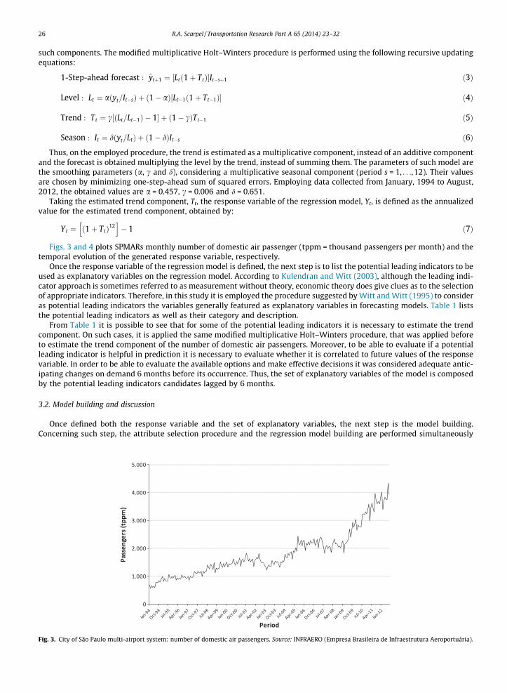
Figs. 3 and 4 plots SPMARs monthly number of domestic air passenger (tppm = thousand passengers per month) and thetemporal evolution of the generated response variable, respectively.

Once the response variable of the regression model is defined, the next step is to list the potential leading indicators to beused as explanatory variables on the regression model. According to Kulendran and Witt (2003), although the leading indi-cator approach is sometimes referred to as measurement without theory, economic theory does give clues as to the selectionof appropriate indicators. Therefore, in this study it is employed the procedure suggested by Witt and Witt (1995) to consideras potential leading indicators the variables generally featured as explanatory variables in forecasting models. Table 1 liststhe potential leading indicators as well as their category and description.

From Table 1 it is possible to see that for some of the potential leading indicators it is necessary to estimate the trendcomponent. On such cases, it is applied the same modified multiplicative Holt–Winters procedure, that was applied beforeto estimate the trend component of the number of domestic air passengers. Moreover, to be able to evaluate if a potentialleading indicator is helpful in prediction it is necessary to evaluate whether it is correlated to future values of the responsevariable. In order to be able to evaluate the available options and make effective decisions it was considered adequate antic-ipating changes on demand 6 months before its occurrence. Thus, the set of explanatory variables of the model is composedby the potential leading indicators candidates lagged by 6 months.

3.2. Model building and discussion

Once defined both the response variable and the set of explanatory variables, the next step is the model building.Concerning such step, the attribute selection procedure and the regression model building are performed simultaneously

City of São Paulo multi-airport system: number of domestic air passengers. Source: INFRAERO (Empresa Brasileira de Infraestrutura Aeroportuária).

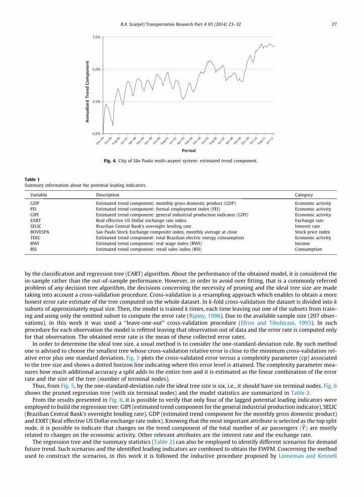
Fig. 4. City of São Paulo multi-airport system: estimated trend component.

Table 1Summary information about the potential leading indicators.

Variable Description Category

GDP Estimated trend component: monthly gross domestic product (GDP) Economic activityFEI Estimated trend component: formal employment index (FEI) Economic activityGIPI Estimated trend component: general industrial production indicator (GIPI) Economic activityEXRT Real effective US Dollar exchange rate index Exchange rateSELIC Brazilian Central Bank’s overnight lending rate Interest rateBOVESPA Sao Paulo Stock Exchange composite index, monthly average at close Stock price indexTEEC Estimated trend component: total Brazilian electric energy consumption Economic activityRWI Estimated trend component: real wage index (RWI) IncomeRSI Estimated trend component: retail sales index (RSI) Consumption

R.A. Scarpel / Transportation Research Part A 65 (2014) 23–32 27

by the classification and regression tree (CART) algorithm. About the performance of the obtained model, it is considered thein-sample rather than the out-of-sample performance. However, in order to avoid over fitting, that is a commonly referredproblem of any decision tree algorithm, the decisions concerning the necessity of pruning and the ideal tree size are madetaking into account a cross-validation procedure. Cross-validation is a resampling approach which enables to obtain a morehonest error rate estimate of the tree computed on the whole dataset. In k-fold cross-validation the dataset is divided into ksubsets of approximately equal size. Then, the model is trained k times, each time leaving out one of the subsets from train-ing and using only the omitted subset to compute the error rate (Ripley, 1996). Due to the available sample size (207 obser-vations), in this work it was used a ‘‘leave-one-out’’ cross-validation procedure (Efron and Tibshirani, 1993). In suchprocedure for each observation the model is refitted leaving that observation out of data and the error rate is computed onlyfor that observation. The obtained error rate is the mean of these collected error rates.

In order to determine the ideal tree size, a usual method is to consider the one-standard-deviation rule. By such methodone is advised to choose the smallest tree whose cross-validation relative error is close to the minimum cross-validation rel-ative error plus one standard deviation. Fig. 5 plots the cross-validated error versus a complexity parameter (cp) associatedto the tree size and shows a dotted horizon line indicating where this error level is attained. The complexity parameter mea-sures how much additional accuracy a split adds to the entire tree and it is estimated as the linear combination of the errorrate and the size of the tree (number of terminal nodes).

Thus, from Fig. 5, by the one-standard-deviation rule the ideal tree size is six, i.e., it should have six terminal nodes. Fig. 6shows the pruned regression tree (with six terminal nodes) and the model statistics are summarized in Table 2.

From the results presented in Fig. 6, it is possible to verify that only four of the lagged potential leading indicators wereemployed to build the regression tree: GIPI (estimated trend component for the general industrial production indicator), SELIC(Brazilian Central Bank’s overnight lending rate), GDP (estimated trend component for the monthly gross domestic product)and EXRT (Real effective US Dollar exchange rate index). Knowing that the most important attribute is selected as the top splitnode, it is possible to indicate that changes on the trend component of the total number of air passengers ðbY Þ are mostlyrelated to changes on the economic activity. Other relevant attributes are the interest rate and the exchange rate.

The regression tree and the summary statistics (Table 2) can also be employed to identify different scenarios for demandfuture trend. Such scenarios and the identified leading indicators are combined to obtain the EWFM. Concerning the methodused to construct the scenarios, in this work it is followed the inductive procedure proposed by Linneman and Kennell

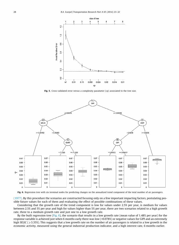
Fig. 5. Cross-validated error versus a complexity parameter (cp) associated to the tree size.

Fig. 6. Regression tree with six terminal nodes for predicting changes on the annualized trend component of the total number of air passengers.

28 R.A. Scarpel / Transportation Research Part A 65 (2014) 23–32

(1977). By this procedure the scenarios are constructed focusing only on a few important impacting factors, postulating pos-sible future values for each of them and evaluating the effect of possible combinations of these values.

Considering that the growth rate of the trend component is low for values under 2.5% per year, is medium for valuesbetween 2.5% and 5% per year and high for values higher than 5% per year, there are two scenarios related to a high growthrate, three to a medium growth rate and just one to a low growth rate.

By the built regression tree (Fig. 6), the scenario that results in a low growth rate (mean value of 1.48% per year) for theresponse variable is achieved just when 6 months early there was low (<0.078%) or negative values for GIPI and an extremelyhigh SELIC (P3.35%). This suggests that a low growth rate on the number of air passengers is related to a low growth in theeconomic activity, measured using the general industrial production indicator, and a high interest rate, 6 months earlier.

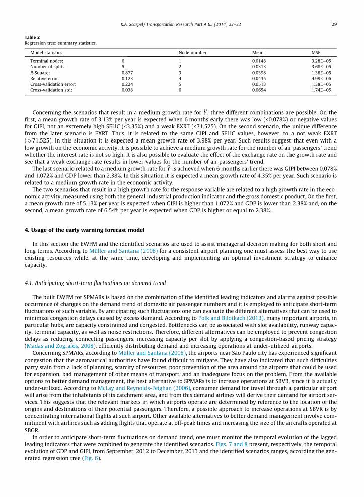
Table 2Regression tree: summary statistics.

Model statistics Node number Mean MSE

Terminal nodes: 6 1 0.0148 3.28E�05Number of splits: 5 2 0.0313 3.68E�05R-Square: 0.877 3 0.0398 1.38E�05Relative error: 0.123 4 0.0435 4.99E�06Cross-validation error: 0.224 5 0.0513 1.38E�05Cross-validation std: 0.038 6 0.0654 1.74E�05

R.A. Scarpel / Transportation Research Part A 65 (2014) 23–32 29

Concerning the scenarios that result in a medium growth rate for bY , three different combinations are possible. On thefirst, a mean growth rate of 3.13% per year is expected when 6 months early there was low (<0.078%) or negative valuesfor GIPI, not an extremely high SELIC (<3.35%) and a weak EXRT (<71.525). On the second scenario, the unique differencefrom the later scenario is EXRT. Thus, it is related to the same GIPI and SELIC values, however, to a not weak EXRT(P71.525). In this situation it is expected a mean growth rate of 3.98% per year. Such results suggest that even with alow growth on the economic activity, it is possible to achieve a medium growth rate for the number of air passengers’ trendwhether the interest rate is not so high. It is also possible to evaluate the effect of the exchange rate on the growth rate andsee that a weak exchange rate results in lower values for the number of air passengers’ trend.

The last scenario related to a medium growth rate for bY is achieved when 6 months earlier there was GIPI between 0.078%and 1.072% and GDP lower than 2.38%. In this situation it is expected a mean growth rate of 4.35% per year. Such scenario isrelated to a medium growth rate in the economic activity.

The two scenarios that result in a high growth rate for the response variable are related to a high growth rate in the eco-nomic activity, measured using both the general industrial production indicator and the gross domestic product. On the first,a mean growth rate of 5.13% per year is expected when GIPI is higher than 1.072% and GDP is lower than 2.38% and, on thesecond, a mean growth rate of 6.54% per year is expected when GDP is higher or equal to 2.38%.

4. Usage of the early warning forecast model

In this section the EWFM and the identified scenarios are used to assist managerial decision making for both short andlong terms. According to Müller and Santana (2008) for a consistent airport planning one must assess the best way to useexisting resources while, at the same time, developing and implementing an optimal investment strategy to enhancecapacity.

4.1. Anticipating short-term fluctuations on demand trend

The built EWFM for SPMARs is based on the combination of the identified leading indicators and alarms against possibleoccurrence of changes on the demand trend of domestic air passenger numbers and it is employed to anticipate short-termfluctuations of such variable. By anticipating such fluctuations one can evaluate the different alternatives that can be used tominimize congestion delays caused by excess demand. According to Polk and Bilotkach (2013), many important airports, inparticular hubs, are capacity constrained and congested. Bottlenecks can be associated with slot availability, runway capac-ity, terminal capacity, as well as noise restrictions. Therefore, different alternatives can be employed to prevent congestiondelays as reducing connecting passengers, increasing capacity per slot by applying a congestion-based pricing strategy(Madas and Zografos, 2008), efficiently distributing demand and increasing operations at under-utilized airports.

Concerning SPMARs, according to Müller and Santana (2008), the airports near São Paulo city has experienced significantcongestion that the aeronautical authorities have found difficult to mitigate. They have also indicated that such difficultiesparty stain from a lack of planning, scarcity of resources, poor prevention of the area around the airports that could be usedfor expansion, bad management of other means of transport, and an inadequate focus on the problem. From the availableoptions to better demand management, the best alternative to SPMARs is to increase operations at SBVR, since it is actuallyunder-utilized. According to McLay and Reynolds-Feighan (2006), consumer demand for travel through a particular airportwill arise from the inhabitants of its catchment area, and from this demand airlines will derive their demand for airport ser-vices. This suggests that the relevant markets in which airports operate are determined by reference to the location of theorigins and destinations of their potential passengers. Therefore, a possible approach to increase operations at SBVR is byconcentrating international flights at such airport. Other available alternatives to better demand management involve com-mitment with airlines such as adding flights that operate at off-peak times and increasing the size of the aircrafts operated atSBGR.

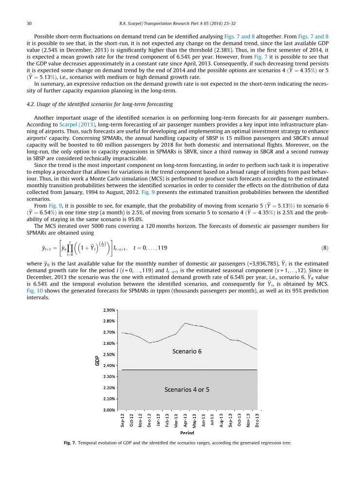
In order to anticipate short-term fluctuations on demand trend, one must monitor the temporal evolution of the laggedleading indicators that were combined to generate the identified scenarios. Figs. 7 and 8 present, respectively, the temporalevolution of GDP and GIPI, from September, 2012 to December, 2013 and the identified scenarios ranges, according the gen-erated regression tree (Fig. 6).

30 R.A. Scarpel / Transportation Research Part A 65 (2014) 23–32

Possible short-term fluctuations on demand trend can be identified analysing Figs. 7 and 8 altogether. From Figs. 7 and 8it is possible to see that, in the short-run, it is not expected any change on the demand trend, since the last available GDPvalue (2.54% in December, 2013) is significantly higher than the threshold (2.38%). Thus, in the first semester of 2014, itis expected a mean growth rate for the trend component of 6.54% per year. However, from Fig. 7 it is possible to see thatthe GDP value decreases approximately in a constant rate since April, 2013. Consequently, if such decreasing trend persistsit is expected some change on demand trend by the end of 2014 and the possible options are scenarios 4 ðbY ¼ 4:35%Þ or 5ðbY ¼ 5:13%Þ, i.e., scenarios with medium or high demand growth rate.

In summary, an expressive reduction on the demand growth rate is not expected in the short-term indicating the neces-sity of further capacity expansion planning in the long-term.

4.2. Usage of the identified scenarios for long-term forecasting

Another important usage of the identified scenarios is on performing long-term forecasts for air passenger numbers.According to Scarpel (2013), long-term forecasting of air passenger numbers provides a key input into infrastructure plan-ning of airports. Thus, such forecasts are useful for developing and implementing an optimal investment strategy to enhanceairports’ capacity. Concerning SPMARs, the annual handling capacity of SBSP is 15 million passengers and SBGR’s annualcapacity will be boosted to 60 million passengers by 2018 for both domestic and international flights. Moreover, on thelong-run, the only option to capacity expansions in SPMARs is SBVR, since a third runway in SBGR and a second runwayin SBSP are considered technically impracticable.

Since the trend is the most important component on long-term forecasting, in order to perform such task it is imperativeto employ a procedure that allows for variations in the trend component based on a broad range of insights from past behav-iour. Thus, in this work a Monte Carlo simulation (MCS) is performed to produce such forecasts according to the estimatedmonthly transition probabilities between the identified scenarios in order to consider the effects on the distribution of datacollected from January, 1994 to August, 2012. Fig. 9 presents the estimated transition probabilities between the identifiedscenarios.

From Fig. 9, it is possible to see, for example, that the probability of moving from scenario 5 ðbY ¼ 5:13%Þ to scenario 6ðbY ¼ 6:54%Þ in one time step (a month) is 2.5%, of moving from scenario 5 to scenario 4 ðbY ¼ 4:35%Þ is 2.5% and the prob-ability of staying in the same scenario is 95.0%.

The MCS iterated over 5000 runs covering a 120 months horizon. The forecasts of domestic air passenger numbers forSPMARs are obtained using

ytþ1 ¼ yo

Yt

i¼0

1þ bY i

� � 112ð Þ

� �" #It�sþ1; t ¼ 0; . . . ;119 ð8Þ

where by0 is the last available value for the monthly number of domestic air passengers (=3,936,785), bY i is the estimateddemand growth rate for the period i (i = 0, . . .,119) and It�s+1 is the estimated seasonal component (s = 1, . . .,12). Since inDecember, 2013 the scenario was the one with estimated demand growth rate of 6.54% per year, i.e., scenario 6, bY 0 valueis 6.54% and the temporal evolution between the identified scenarios, and consequently for bY i, is obtained by MCS.Fig. 10 shows the generated forecasts for SPMARs in tppm (thousands passengers per month), as well as its 95% predictionintervals.

Fig. 7. Temporal evolution of GDP and the identified the scenarios ranges, according the generated regression tree.

Fig. 8. Temporal evolution of GIPI and the identified the scenarios ranges, according the generated regression tree.

Fig. 9. Transition probabilities between the identified scenarios.

Fig. 10. Generated forecasts for the city of São Paulo multi-airport system (in thousands passengers per month).

R.A. Scarpel / Transportation Research Part A 65 (2014) 23–32 31

From the obtained results it is possible to see that the MCS produces forecasts for 2023 of between 67,206 to 92,058 thou-sand domestic passengers. Thus, even if all SBSP and SBGR handling capacities are used to fulfil domestic passengers’demand, by the generated forecasts, in 2023 it is expected that SBVR will need an annual handling capacity of at least 5 mil-lion passengers. However, since approximately 50% of SBGR annual handling capacity is destined to international flights, is2023 it is expected that SBVR will need an annual handling capacity of at least 25 million passengers. Concerning SBVR, itwas recently announced that its annual capacity will be boosted to 22 million passengers by 2018 and to 45 million passen-gers by 2024 by adding a third runway.

32 R.A. Scarpel / Transportation Research Part A 65 (2014) 23–32

5. Conclusions

Due to an excessive concentration of flights, SPMARs has experienced significant congestion that the aeronautical author-ities have found difficult to mitigate. Such difficulties party stain from a lack of planning and an inadequate focus on theproblem. In this paper a demand trend change early warning forecast model (EWFM) was developed to assist managerialdecision making for both short and long terms. The ability to anticipate short-term fluctuations on demand trend is usefulfor aviation policy makers in order to evaluate different alternatives to prevent congestion delay occurrences. Moreover,long-term forecasting of air passenger numbers is a key input for infrastructure planning.

Two of the most critical tasks for a EWFM success are the leading indicators identification and the scenarios building. Inthis paper CART was employed to perform both tasks. Results show that changes on the demand trend component of thedomestic number of air passengers are mostly associated to changes on the economic activity and six different scenarioswere built combining the identified leading indicators. Afterwards, the developed EWFM was used to anticipate short-termfluctuations on demand trend and to generate long-term forecasting of domestic air passenger numbers.

The contributions of the paper to the literature are in both methodology and empirical findings. In terms of methodologycontributions, it is possible to indicate the applied framework, the trend component estimation using the modified Holt–Winters procedure and the usage of CART for the scenarios building inductive procedure. In terms of the empirical findings,the main contributions are the leading indicators identification, the way such indicators combine to generate the scenarios oflow, medium and high growth rate for the demand trend change EWFM and the usage of the built model to assist managerialdecision making for both short and long terms.

Acknowledgement

The author acknowledges the financial support from FAPESP – São Paulo Research Foundation (Grant 2013/22416-4).

References

Armstrong, J.S., 1985. Long-Range Forecasting: From Crystal Ball to Computer, second ed. John Wiley, New York.Banks, D.L., 2010. Statistical data mining. Wiley Interdiscip. Rev.: Comput. Stat. 2 (1), 9–25.Breiman, L., Friedman, J., Olshen, R., Stone, C., 1984. Classification and Regression Trees. Wadsworth International Group, Monterey, CA.Costa, T.F.G., Lohmann, G., Oliveira, A.V.M., 2010. A model to identify airport hubs and their importance to tourism in Brazil. Res. Transp. Econ. 6 (1), 3–11.Efron, B., Tibshirani, R.J., 1993. An Introduction to the Bootstrap. Chapman & Hall, New York.Gardner, E.S.J., McKenzie, E., 1985. Forecasting trend in time series. Manage. Sci. 31, 1237–1246.Gardner, E.S.J., McKenzie, E., 1989. Seasonal exponential smoothing with damped trends. Manage. Sci. 35, 372–376.Granger, C.W.J., Jeon, Y., 2007. Long-term forecasting and evaluation. Int. J. Forecast. 23, 539–551.Grubb, H., Mason, A., 2001. Long lead-time forecasting of UK air passengers by Holt–Winters methods with damped trend. Int. J. Forecast. 17, 71–82.Jones, S.R., Chu Te, G.O., 1995. Leading Indicators of Australian Visitor Arrivals. Occasional Paper No. 19. Bureau of Tourism Research, Canberra.Kulendran, N., Witt, S.F., 2003. Leading indicators tourism forecasts. Tourism Manage. 24, 503–510.Linneman, R.E., Kennell, J.D., 1977. Shirt-sleeve approach to long-range plans. Harvard Business Rev. 55, 141–150.Madas, M.A., Zografos, K.G., 2008. Airport capacity vs. demand: mismatch or mismanagement? Transp. Res. Part A 42, 203–226.McLay, P., Reynolds-Feighan, A., 2006. Competition between airport terminals: the issues facing Dublin Airport. Transp. Res. Part A 40, 181–203.Müller, C., Santana, E.S.M., 2008. Analysis of flight-operating cost and delay: the São Paulo terminal maneuvering area. J. Air Transp. Manage. 14, 293–296.Olafsson, S., Li, X., Wu, S., 2008. Operations research and data mining. Eur. J. Oper. Res. 187 (3), 1429–1448.Ozyildirim, A., Schaitkin, B., Zarnowitz, V., 2010. Business cycles in the Euro area defined with coincident economic indicators and predicted with leading

economic indicators. J. Forecast. 29, 6–28.Polk, A., Bilotkach, V., 2013. The assessment of market power of hub airports. Transp. Policy 29, 29–37.Ripley, B.D., 1996. Pattern Recognition and Neural Networks. Cambridge University Press, Cambridge.Scarpel, R.A., 2013. Forecasting air passengers at São Paulo International Airport using a mixture of local experts model. J. Air Transp. Manage. 26, 35–39.Schnaars, S.P., 1987. How to develop and use scenarios. Long Range Plan. 20 (1), 105–114.Wensveen, J.G., 2011. Air Transportation: A Management Perspective, seventh ed. Ashgate, Aldershot, UK.Witt, S.F., Witt, C.A., 1995. Forecasting tourism demand: a review of empirical research. Int. J. Forecast. 11, 447–475.