Inês Sofia Mendes Carneiroªs Carneiro.pdf · escalas grosseiras para identificação de associações ambientais finas e a falta de inferência estatística (Biffi et al., 2016;

Inês Sofia Mendes Carneiro

Territorial and Social Behaviour of the Pyrenean

desman (Galemys pyrenaicus) assessed from Scat

Deposition

Dissertação apresentada à Universidade de Coimbra para

cumprimento dos requisitos necessários à obtenção do

grau de mestre em Ecologia, realizada sob a orientação

científica do Professor Doutor Paulo Gama Mota

(Departamento de Ciências da Vida, Faculdade de

Ciências e Tecnologia, Universidade de Coimbra) e do

Doutor Lorenzo Quaglietta (Centro de Investigação em

Biodiversidade e Recursos Genéticos)

Julho, 2016

2

Cover image:

Galemys pyrenaicus illustration.

Author: Claude Guerineau

Source: Dessins Desman Des Pyrénées Marie- Claude MC

Guerineau, 2016, at: http://abela11.fr/

3

Agradecimentos

E assim se fecha mais um ciclo.

Nem sempre os dias foram fáceis e por vezes vi o entusiasmo falhar quando

mais precisava dele. Foi nessas alturas que mais agradeci todo o apoio, incentivo e

carinho daqueles que estiveram sempre do meu lado. Sem vocês nada disto teria sido

possível, por isso, queria deixar-vos um especial obrigado.

Em primeiro lugar um especial agradecimento ao Professor Doutor Paulo Gama

por me ter aceitado como sua orientanda. Sei que o meu tema sempre representou um

desafio, mas isso não o fez desistir. Por toda a dedicação, confiança, motivação e

ensinamentos ao longo destes dois anos, o meu mais sincero muito obrigada por ter

estado lá para mim.

Ao Lorenzo, quero agradecer por me teres aceitado como co-orientanda. Por

teres suportado alguns dos meus momentos de desespero e por me teres feito acreditar

em mim. Agradeço também a forma como soubeste alegrar os dias de campo e torná-los

mais leves.

Á Ana Leitão, por ter sido uma ajuda fundamental na fase inicial de escolha do

meu tema. Foi graças a ti que este trabalho se tornou possível. Por teres confiado em

mim e por me teres orientado para este caminho, o meu mais sincero obrigado.

Aos colegas que me acompanharam durante o trabalho de campo: Sofia Tropa

Coelho, Rafael Carvalho e Pedro Lopes um grande obrigado por tudo o que me

ensinaram e por toda a ajuda prestada.

Ao Luís, que apesar de não me conhecer me apoiou numa das fases mais

complicadas deste trabalho. Muito obrigada por todas as horas perdidas em que te fui

incomodar ao laboratório, por todos os e-mails com dúvidas de última hora, por todos

4

os conselhos e dicas. Sem a tua ajuda a estatística teria sido um quebra-cabeças muito

maior. Obrigada!

Aos colegas do laboratório de etologia: Eliana Soukiazes, Pedro Pereira e Felipe

Shibuya, obrigada pela disponibilidade e ajuda quando precisei de esclarecer dúvidas ou

precisei de conselhos.

A todos os professores do Mestrado de Ecologia, um especial agradecimento por

todos os ensinamentos prestados que certamente contribuíram para o meu crescimento

académico e profissional.

Aos meus queridos costeletas: Prima, Di, Nanas, Ju, Ni, Sandro, Selas, Múmia,

Fiúza, João, Diogo e Potty, acho que os agradecimentos vão ser sempre poucos para

retribuir tudo o que já fizeram por mim. Por todo o apoio incondicional,

companheirismo, por todas as conversas e todas as histórias que construímos

juntos…Obrigada até por compreenderem as minhas ausências. A vocês que me

acompanharam ao longo destes 5 anos em Coimbra, sem nunca me falharem, um

grande, grande obrigado! Sem vocês nunca teria sido o mesmo.

Quero apenas deixar um agradecimento especial aos companheiros diários a

quem mais esgotei a paciência: Prima e Sandro por todos os mil desabafos sobre

modelos que vos obriguei a ouvir, por serem os primeiros a quem ligo quando estou em

baixo e por estarem sempre lá. Obrigada, do coração.

Ao Morgan … por teres sido o meu pilar nestes últimos anos. Por nunca

deixares de acreditar em mim e me fazeres perceber as minhas qualidades. Por teres

estado sempre lá para me animar quando mais precisei e por teres sido tão paciente

comigo nos dias que tive que trabalhar até tarde e o stresse se apoderou de mim, ou

mesmo quando estava ausente. Obrigada mesmo pelos momentos em que me obrigaste

a sair da bolha contra a minha vontade e sobretudo por me ouvires. Eu sei que sou o

5

drama em pessoa e que nem sempre sou fácil de suportar! Tu sabes, nunca vou

conseguir agradecer o suficiente.

À Madrinha, Helena Dias, e ao Padrinho, Tiago Pinto, porque não poderia ter

encontrado melhores pessoas para me guiarem na vida académica. À madrinha, por

todos os conselhos, por todas as partilhas, por seres sempre o meu exemplo a seguir.

Sabes que foste sempre a minha inspiração e vais continuar a ser. Venha qualquer

desafio, eu sei que os vais superar, sempre! Ao padrinho, por estares sempre disponível

para me tirares dúvidas, a qualquer hora, por todos os conselhos e por toda a motivação

que sempre me deste. Sabes que me enches de orgulho. Estava destinado dois

oliveirenses cruzarem caminhos em Coimbra!

Não podia passar também sem agradecer às FANS, por compreenderem as

minhas ausências e continuarem a acreditar no meu potencial. Venha o que vier, serão

sempre a família que vai lá estar.

E por último e mais importante … o MAIOR dos agradecimentos aos meus pais

e irmão. São vocês que me dão o incentivo para lutar pelos meus sonhos e claro, sem

vocês nada disto seria possível. Obrigada por acreditarem sempre em mim e apoiarem

as minhas escolhas! Obrigada por estarem sempre disponíveis para mim, por todo o

amor, compreensão, dedicação e confiança depositada. Vocês são o meu porto seguro.

Sei que apesar da “ausência” destes últimos tempos, a minha felicidade é o que mais

importa para vocês e é só disso que preciso. É a vocês que dedico as minhas vitórias.

Obrigada, com todo o meu coração!

6

7

Resumo

Os ecossistemas aquáticos são conhecidos pela sua notável biodiversidade,

contendo cerca de um terço de espécies restritas a este habitat (Charbonnel et al., 2015).

No entanto, encontram-se entre os habitats mais ameaçados do mundo, devido

essencialmente a actividades antropogénicas que afectam gravemente a biodiversidade

aquática (Biffi et al., 2016; Charbonnel et al., 2015). Nestes casos, espécies raras de

carácter endémico e de reduzido tamanho populacional são particularmente importantes

para a biologia de conservação, dada a sua vulnerabilidade (Charbonnel et al., 2015;

Melero, Aymerich, Luque-Larena, & Gosàlbez, 2012).

Dentro das espécies aquáticas raras, Galemys pyrenaicus é um dos mamíferos

Europeus menos conhecido do público em geral e dentro da comunidade científica

(Charbonnel et al., 2015; Melero et al., 2012). O seu estatuto vulnerável, associado à

falta de conhecimentos sobre a ecologia e comportamento da espécie, tem-se revelado

um dos maiores desafios contemporâneos à conservação e gestão da mesma para muitos

cientistas (Melero et al., 2012). Estudos anteriores, focados na selecção de habitat da

toupeira-de-água a uma escala fina, apresentam alguns problemas como a definição de

escalas grosseiras para identificação de associações ambientais finas e a falta de

inferência estatística (Biffi et al., 2016; Charbonnel et al., 2015).

Considerando os problemas descritos, o nosso projecto tenta complementar a

informação existente sobre a selecção de habitat da toupeira-de-água usando descritores

a duas diferentes escalas espaciais (micro-habitat – 0,5 m2 – e transecto - ~200-600m).

Os objectivos principais deste estudo são 1) estudar os padrões que determinam quais as

variáveis ambientais que mais influenciam o comportamento de deposição de

excrementos por parte da toupeira-de-água, a duas escalas diferentes; e 2) perceber a

8

importância ecológica das variáveis de habitat seleccionadas para a deposição de

dejectos como “recursos-chave” para determinar a presença de toupeira-de-água. Para

isso, testámos a influência das variáveis: presença de amieiro, localização nas margens

ou leito, exposição do substrato, velocidade da água e a presença de musgo (variáveis

ambientais e biológicas de escala fina). Também testámos a influência das variáveis:

percentagem de cobertura, “spraintability”, largura do leito, velocidade da água,

percentagem de “pool” e percentagem de “riffle” (variáveis ambientais e biológicas de

larga escala) na abundância de dejectos de toupeira-de-água encontrados por km de

transecto.

Verificámos que a uma escala mais fina a toupeira- de-água depositou os seus

excrementos principalmente em locais não expostos, localizados nas margens do rio,

perto de locais de grande velocidade da água. Ao contrário do que era esperado, a

presença de amieiro não resultou ser determinante na selecção feita pela espécie. A

presença de musgo demonstrou um efeito inconsistente da variável. À escala do

transecto, o uso do habitat local pela toupeira baseado na distribuição dos seus dejectos

parece influenciado pela heterogeneidade de substrato. Estes resultados serão

importantes para perceber quais as características de habitat mais importantes para a

toupeira-de-água, o que poderá permitir inferências sobre a comunicação e organização

social da espécie.

Palavras-chave: ecossistemas aquáticos, espécies em perigo, espécies

endémicas, Galemys pyrenaicus, selecção de habitat, comportamento animal,

comunicação, organização social.

9

Abstract

Freshwater environments are known for its notable biodiversity, holding about

one third of vertebrate species restricted to this ecosystem (Charbonnel et al., 2015).

However, they are amongst the most threatened habitats in the world due to human

activities that cause alterations of the natural river conditions and strongly affect aquatic

biodiversity (Biffi et al., 2016; Charbonnel et al., 2015). In these environments, rare

species with small population sizes and especially endemic species are of particular

interest for conservation biology due to their vulnerability to extinction (Charbonnel et

al., 2015; Melero et al., 2012).

Among rare freshwater species the Pyrenean desman (Galemys pyrenaicus) is

one of the less known European mammals to the general public (Charbonnel et al.,

2015; Melero et al., 2012) and within the scientific community. Its vulnerable status

together with an almost complete lack of knowledge regarding their ecology and

behaviour has made their conservation and management a contemporary challenge for

many scientists (Melero et al., 2012). Previous studies have investigated the habitat

preferences of Pyrenean desman at small- site scale but they present some problems like

the definition of scales too coarse to identify finer habitat associations and the lack of

statistical inference (Biffi et al., 2016; Charbonnel et al., 2015).

Taking into account the described problems, our project tries to complement the

information existent on Pyrenean desman habitat preferences using descriptors at two

different scales (small-site scale – 0,5m2 – and a larger scale - ~200-600m). The main

objectives of this study were 1) to study the patterns that determine which

environmental factors mostly influence the scat deposition behaviour of the Pyrenean

desman at two different scales 2) to understand the ecological importance of the habitat

10

variables selected for scat deposition as key resources for determining the Pyrenean

desmans‟ presence. This was achieved by testing the influence of the variables presence

of alder, bank or bed localization, substrate exposure, water speed and presence of musk

(small-scale environmental and biological variables). We also tested the influence of the

variables: percentage of coverage, spraintability, riverbed width, water speed,

percentage of pool and percentage of riffle (large scale environmental and biological

variables).

We verified that at a small-site scale, Pyrenean desman preferentially selected as

habitat requirements non-exposed sites, preferably at riverbanks near locations of high

river flow. Contrary to what was expected, alder presence was not determinative for

Pyrenean desman selection. Musk revealed inconsistent variable effect, with its

significance varying a lot. At a larger scale, the use of local habitat by the Pyrenean

desman appears to be driven by higher spraintability with transects with abundant

emergent items and greater percentage of substrate heterogeneity preferably selected.

These results will be important also to help understanding which habitat characteristics

are important to the Pyrenean desman, which may draw clues on communication and

social organization of the species.

Keyword: aquatic ecosystems, endangered species, endemic species, Galemys

pyrenaicus, habitat selection, animal behaviour, communication, social organization.

11

Index

1 Introduction ............................................................................................................. 21

1.1 Study species characterization ......................................................................... 24

1.1.1 Taxonomy and Evolution ......................................................................... 24

1.1.2 Species Morphology ................................................................................. 26

1.1.3 Geographic distribution ............................................................................ 27

1.1.4 Ecology ..................................................................................................... 30

1.1.5 Behaviour ................................................................................................. 32

1.1.6 Accompany Fauna and Predators ............................................................. 37

1.1.7 Status and Threats ..................................................................................... 37

1.2 Study framework/importance .......................................................................... 39

1.2.1 Objective ................................................................................................... 40

2 Methodology ........................................................................................................... 43

2.1 Study area ........................................................................................................ 45

2.1.1 Sabor‟s Watersheed .................................................................................. 47

2.1.2 Tua‟s Watersheed ..................................................................................... 49

2.1.3 Paiva‟s Watersheed................................................................................... 50

2.2 Sampling .......................................................................................................... 52

2.3 Scat Survey ...................................................................................................... 55

2.4 Measurements: Marking Site and Habitat characterization ............................. 58

2.4.1 Marking Site Characterization .................................................................. 58

2.4.2 General Habitat Characterization ............................................................. 65

2.5 Scat confirmation ............................................................................................. 67

2.6 Statistical analysis ............................................................................................ 68

2.6.1 Marking Site Characterization .................................................................. 69

2.6.2 General Habitat Characterization ............................................................. 73

3 Results ..................................................................................................................... 75

3.1 Survey results ................................................................................................... 77

3.2 Marking Site Characterization ......................................................................... 78

3.2.1 Presence of scats ....................................................................................... 78

3.2.2 Scats‟ abundance ...................................................................................... 88

3.3 General Habitat Characterization ..................................................................... 98

4 Discussion ............................................................................................................. 101

12

4.1 General discussion ......................................................................................... 103

4.2 Results from Scats‟ Presence ......................................................................... 106

4.3 Results from Scats‟ Abundance ..................................................................... 108

4.4 General habitat characterization .................................................................... 109

4.5 Data limitations .............................................................................................. 110

4.6 Conclusion ..................................................................................................... 111

5 References ............................................................................................................. 113

6 Appendix ............................................................................................................... 123

6.1 Appendix 1 ..................................................................................................... 125

13

List of Figures

Figure 1- Phylogenetic relationships of Talpidae based on mitochondrial cytochrome b

gene sequence data (from: Cabria et al. 2006) ............................................................... 25

Figure 2 - Map representing Galemys pyrenaicus distribution in Portugal based on

studies from 1990 to 1996 (10x10 km UTM) (adapted from Pedroso & Chora 2014). . 29

Figure 3 - Overview of the study area. The three different sub-basins sampled: Sabor,

Tua and Paiva‟s are part of the Douro watershed and are represented in different

colours. ........................................................................................................................... 46

Figure 4 - Overview of the study area with representation of transects sampled

(signalled with a circle) and transects found dry (signalled using a cross). ................... 54

Figure 5 - Pyrenean desman isolated scat. ..................................................................... 57

Figure 6 - Pyrenean desman latrine. .............................................................................. 57

Figure 7 - Scheme representative of the Scat Position evaluation in relation to the river

current. (1) corresponds to the up position; (2) marks the middle position and (3) down

position ........................................................................................................................... 60

Figure 8 - Overview of the study area with green points representing the sites of

confirmed Pyrenean desman‟s presence. ........................................................................ 77

Figure 9 – Data exploration of the response variable: scats‟ presence (named as

“Chosen”) in relation to the variables: Speed, Alder and Exposed, integrated in the

model using 2015 data with “Discrete Sites” as absence points. a) Variation for the

variable speed according to scats‟ presence (1) or absence (0); b) Variation for the

variable exposed in relation to scats‟ presence (1) or absence (0); c) Relative frequency

14

of the presence (1) or absence (0) of Alder for places of scats‟ presence (1) or absence

(0). .................................................................................................................................. 79

Figure 10 – Data exploration of the response variable: scats‟ presence (named as

“Chosen”) in relation to the variables: Bank or Bed, Exposed, Speed, Alder and Musk,

integrated in the model using 2015 data with “Random Sites” as absence points. a)

frequency of the variable bank or bed in relation to scats‟ presence (1) or absence (0); b)

variance for the variable exposed in relation to scats‟ presence (1) or absence (0); c)

variance of the variable speed according to scats‟ presence (1) or absence (0); d) and e)

relative frequencies of the presence (1) or absence (0) of Alder and Musk, respectively,

for places of scats‟ presence (1) or absence (0). ............................................................. 80

Figure 11- Data exploration of the response variable: scats‟ presence (“Chosen”) in

relation to the variables: Exposed, Speed and Musk, integrated in the model using

2014+2015 data with “Discrete Sites” as absence points. a) Variation for the variable

exposed in relation to scats‟ presence (1) or absence (0); b) Variation for the variable

speed according to scats‟ presence (1) or absence (0); c) Relative frequency of the

presence (1) or absence (0) of Alder for places of scats‟ presence (1) or absence (0). .. 84

Figure 12 - Data exploration of the response variable: scats‟ presence (“Chosen”) in


2014+2015 data with “Random Sites” as absence points. a) Variation for the variable

exposed in relation to scats‟ presence (1) or absence (0); b) Variation for the variable

speed according to scats‟ presence (1) or absence (0); c) Relative frequency of the

presence (1) or absence (0) of Alder for places of scats‟ presence (1) or absence (0). .. 85

Figure 13 - Data exploration of the response variable: scats‟ abundance (“Naspraints”)

in relation to the variables: Exposed, Musk and Speed, integrated in the model using

2015 data with “Discrete Sites” as absence points. a) variation of the abundance of scats

in relation to the exposed categories (0- non-exposed; 0.5- partially exposed; 1 –

exposed; b) variation of the abundance of scats in relation to the presence (1) or absence

(0) of musk; c) variation of the abundance of scats in relation to the different categories

of speed (1- null/almost null; 2- weak; 3- medium/strong). ........................................... 89

15


in relation to the variables: Alder, Bank or Bed, Exposed, Musk and Speed, integrated

in the model using 2015 data with “Random Sites” as absence points. a) variation of the

abundance of scats in relation to the alder presence (1) or absence (0); b) variation of the

abundance of scats in relation to the place where it is located (1- bank; 2- riverbed); c)

variation of the abundance of scats in relation to the exposed categories (0- non-

exposed; 0.5- partially exposed; 1 – exposed; d) variation of the abundance of scats in

relation to the presence (1) or absence (0) of musk; e) variation of the abundance of

scats in relation to the different categories of speed (1- null/almost null; 2- weak; 3-

medium/strong). .............................................................................................................. 90


in relation to the variables: Bank or Bed, Exposed, Musk and Speed, integrated in the

model using 2014+2015 data with “Discrete Sites” as absence points. a) Variation of the

abundance of scats according to the place where it is located(1- bank; 2- riverbed); b)

Variation of the abundance of scats in relation to the exposed categories (0- non-

exposed; 0.5- partially exposed; 1 – exposed; c) Variation of the abundance of scats in

relation to the presence (1) or absence (0) of musk; d) Variation of the abundance of


medium/strong). .............................................................................................................. 94


in relation to the variables: Bank or Bed, Exposed, Musk and Speed, integrated in the

model using 2014+2015 data with “Random Sites” as absence points. a) Variation of

the abundance of scats according to the place where it is located(1- bank; 2- riverbed);

b) Variation of the abundance of scats in relation to the exposed categories (0- non-

exposed; 0.5- partially exposed; 1 – exposed; c) Variation of the abundance of scats in

relation to the presence (1) or absence (0) of musk; d) Variation of the abundance of


medium/strong). .............................................................................................................. 95

16

Figure 17 - Data exploration of the response variable: kilometric abundance index

(KAI) in relation to the variables:%coverage, spraintability, speed, mwidth, %pool and

%riffle integrated in the model used to predict the abundance of Pyrenean desman scats

per km of transect. Graphic a) represents the boxplot with the KAI in relation to % of

coverage (0%; 25%; 50%; 75%; 100%); Graphic b) represents the boxplot with the KAI

in relation to spraintability (1: <5%; 2: 5%-19%; 3: 20%-39%; 4: 40%-69%; 5: 70%-

100%); Graphic c) represents boxplot with the KAI in relation to the different categories

of speed (1- null/almost null; 2- weak; 3- medium/strong); Graphic d) represents a

scatterplot with the KAI in relation to the numeric variable mWidth; Graphics e) and f)

represents a scatterplot with the KAI in relation to the percentages attributed to the

variables pool and riffle. ................................................................................................. 99

17

List of Tables

Table 1 - Taxonomic position of the study species: Galemys pyrenaicus. .................... 24

Table 2 - Number of transects visited per river basin and by year ................................ 52

Table 3 – Number of transects visited that were sampled and the number of transects

dry per year ..................................................................................................................... 52

Table 4 - Number of Sites sampled by watershed per year. .......................................... 53

Table 5 – General habitat variables used to describe the riverbank and riverbed of the

transects sampled. ........................................................................................................... 66

Table 6 - Number of scats considered in the study (confirmed and %higher than 70)

divided per year. ............................................................................................................. 78

Table 7 - Best models (ΔAIC < 2) for prediction of the Pyrenean desman scats'

presence using 2015 data with “Discrete Sites” as absence points obtained after the

AIC-based model selection. Best models are in bold and underlined. ........................... 81

Table 8 - Output for the average model of the best models resultant of the predictions

for scats‟ presence using 2015 data with “Discrete Sites” as absence points. Significant

results in bold. ................................................................................................................ 81

Table 9 - Relative importance (RI) of the predictors resultant from model-averaging of

the GLMM for scats' presence using 2015 data with "Discrete Sites" as absence points.

........................................................................................................................................ 81


presence using 2015 data with “Random Sites” as absence points obtained after the


18

Table 11 - Output for the average model of the best models resultant of the GLMM for

scats‟ presence using 2015 data with “Random Sites” as absence points. Significant

results in bold. ................................................................................................................ 83

Table 12 - Relative importance (RI) from model-averaging of the GLMM for scats'

presence using 2015 data with "Random Sites" as absence points. ............................... 83


presence using 2014+2015 data with “Discrete Sites” as absence points obtained after

the AIC-based model selection. Best models are in bold and underlined. ..................... 86


scats‟ presence using 2014+2015 data with “Discrete Sites” as absence points.

Significant results in bold. .............................................................................................. 86


presence using 2014+2015 data with "Discrete Sites" as absence points. ..................... 86


presence using 2014+2015 data with “Random Sites” as absence points obtained after



scats‟ presence using 2014+2015 data with “Random Sites” as absence points.



presence using 2014+2015 data with "Random Sites" as absence points. ..................... 87


abundance using 2015 data with “Discrete Sites” as absence points obtained after the



scats‟ abundance using 2015 data with “Discrete Sites” as absence points. Significant

results in bold. ................................................................................................................ 91


abundance using 2015 data with "Discrete Sites" as absence points. ............................ 91

19


abundance using 2015 data with “Random Sites” as absence points obtained after the



scats‟ abundance using 2015 data with “Random Sites” as absence points. Significant

results in bold. ................................................................................................................ 93


abundance using 2015 data with "Random Sites" as absence points. ............................ 93


abundance using 2014+2015 data with “Discrete Sites” as absence points obtained after


Table 26 - Output for the average model of the best model resultant of the GLMM for

scats‟ abundance using 2014+2015 data with “Discrete Sites” as absence points.



abundance using 2014+2015 data with "Discrete Sites" as absence points. .................. 96


abundance using 2014+2015 data with “Random Sites” as absence points obtained after



scats‟ abundance using 2014+2015 data with “Random Sites” as absence points.



abundance using 2014+2015 data with "Random Sites" as absence points. .................. 97

Table 31 - Best models (ΔAIC < 2) for prediction of the Pyrenean desman KAI

obtained after AIC-based model selection. All the models considered for model

selection are in Apendix 1, Table 38 ............................................................................ 100

20

Table 32 - Output for the average model of the best models resultant of the LM for the

KAI. Almost significant results underlined. ................................................................. 100

Table 33 - Relative importance (RI) from model-averaging of the LM for for the KAI

data. .............................................................................................................................. 100

Table 34 - Transects of repeated visits and number of sampling repetitions divided per

year. .............................................................................................................................. 125

Table 35 - Variables collected for Marking Site Characterization included in 2015 and

2014+2015 analyses which showed high correlation values. (**) means that correlation

is significant at 0.01 (2 tails). ....................................................................................... 126

Table 36 - Variables collected during both years for General Habitat Characterization

which showed high correlation values. (**) means that correlation is significant at 0.01

(2 tails). ......................................................................................................................... 127

Table 37 - Sites of Galemys presence for both years. X signals Galemys‟ presence, 0

indicates presence not detected and the blank space signal data absence (because the site

was not sampled for that year). ..................................................................................... 128

Table 38 - All the models considered in model selection for prediction of the Pyrenean

desman KAI. 1 - %Coverage; 2 – Speed; 3 – Spraintability; 4- mWidth; 5- %Pool; 6-

%Riffle. ........................................................................................................................ 130

21

1 Introduction

22

23

Freshwater environments are known for its notable biodiversity, holding about

one third of vertebrate species restricted to this ecosystem (Charbonnel et al., 2015).

However, they are amongst the most threatened habitats in the world due to human

activities that cause alterations of the natural river conditions and strongly affect

aquatic biodiversity (Biffi et al., 2016; Charbonnel et al., 2015). In these

environments, rare species with small population sizes and especially endemic

species are of particular interest for conservation biology due to their vulnerability

to extinction (Charbonnel et al., 2015; Melero et al., 2012). Extinction rates of

freshwater fauna are extremely high with around 15 000 species worldwide already

extinct (Charbonnel et al., 2015).

Among rare freshwater species the Pyrenean desman (Galemys pyrenaicus) is

one of the less known European mammals to the general public (Charbonnel et al.,

2015; Melero, Aymerich, Santulli, & Gosàlbez, 2014) and within the scientific

community. This is mainly because of difficulties in its studies due to lack of

capture licenses‟ approval and easily scat misidentification when surveys are based

in recording indirect signs without non-genetic confirmation leading to false

presences or absences (Charbonnel et al., 2015; Melero et al., 2014). Its vulnerable

status together with an almost complete lack of knowledge regarding their ecology

and behaviour has made their conservation and management a contemporary

challenge for many scientists (Melero et al., 2012).

Several aspects of the biology and conservation of the species have been

addressed in recent decades including studies on its distribution, e.g.: Bertrand

1993a, Queiroz et al. 1998, Aymerich et al. 2000, Palomo and Gisbert 2002;

morphology, e.g.: Richard 1986, Richard and Michaud 1975 ; diet, e.g.: Bertrand

1993b, Castién & Gonsálbez 1995; general biology, e.g.: Richard 1986;

24

reproduction, e.g.: Castién 1994; and captive behaviour, e.g.: Richard 1986, Queiroz

and Almada 1993 (Melero et al., 2012). Yet, basic knowledge such as distribution

range and habitat preferences are still incomplete for this species (Charbonnel et al.,

2015).

1.1 Study species characterization

1.1.1 Taxonomy and Evolution

The Pyrenean desman (Galemys pyrenaicus) also known as Iberian desman is

classified within the Talpidae family, subfamily Desmaniae and it was first described by

Etienne Geoffroy Saint-Hilaire in 1811 (Marcos, 2004) (Table 1).

Table 1 - Taxonomic position of the study species: Galemys pyrenaicus.

Classification

Kingdom Animalia

Phylum Chordata

Subphylum Vertebrata

Class Mammalia

Order Soricomorpha

Family Talpidae

Genus Galemys

Species Galemys pyrenaicus

Subspecies Galemys pyrenaicus rufulus

In the past, Desmaniae was represented by a higher number of species with a

large geographic distribution but currently besides Pyrenean desman (Galemys

pyrenaicus) the only representative of this sub-family is the Russian desman (Desmana

moschata) (Silva, 2001).

25

The phylogenetic relationship of this species (Figure 1) with the family Talpidae

can be traced to the Eocene however it has always been questioned due to the highly

distinct morphology of desmans from other members of the Talpidae (Cabria, Rubines,

Gómez-Moliner, & Zardoya, 2006). Recent studies based on the desman‟s

mitochondrial genome confirmed its position and also showed the close phylogenetic

relationship between Desmana and Galemys, admitting the morphological evidences

that grouped both genera within Desmaninae subfamily (Cabria et al., 2006).

Figure 1- Phylogenetic relationships of Talpidae based on mitochondrial cytochrome b

gene sequence data (from: Cabria et al. 2006)

26

1.1.2 Species Morphology

Galemys pyrenaicus lives associated with aquatic habitats and exhibits a highly

specialized morphology (Cabria et al., 2006). The hydrodynamic shape of their body

seems appropriate to decrease water resistance and progression effort while moving

(Queiroz, 1996).

It is a small mammal, with a body length between 15-25cm and about 70g of

weight (Marcos, 2004; Queiroz, 1996).

Desman is covered with a dense and glossy dark-brown fur which is silvery-grey

in the abdomen (Marcos, 2004; Queiroz, 1996). This fur is responsible for retaining air

which provides an excellent protection against water and cold (thermal isolation) and

also provides buoyancy (Marcos, 2004; Richard, 1985). The feet, tail and snout are

almost devoid of hairs (Marcos, 2004).

The hind legs of Pyrenean desman are large, wide, and with webbed feet

responsible for water propulsion (Queiroz, A. Bertrand, & Khakhin., 1996; Richard,

1985). Forelegs are short and narrow with sharp and long claws possibly used to ward

off rocks (Richard, 1985). The tail is long and flattened at the tip and it has an important

role in the equilibrium and water propulsion (Queiroz, 1996). At the bare of the tail

desmans presents musk glands (Marcos, 2004).

Pyrenean desman does not have an acute sense of vision since its eyes are very

small. Instead it presents a long, mobile and very developed snout with highly complex

vibrissae and Eimer‟s organs. These structures have an important role for the perception

of objects and preys and rely on tactile and olfactory senses which apparently are used

by desmans to explore its habitat (Marcos, 2004; Queiroz, 1996).

27

It is not easy to distinguish males from females at naked eye due to the lack of

sexual dimorphism (body size or colouration) (González-Esteban, Villate, & Castién,

2003; Vidal, Perez-Serra, & Pla, 2010). However, studies from González-Esteban et al.

2003 revealed the possibility to distinguish them through examination and palpation of

the urinary papilla. Regardless the age or reproductive cycle males show a hard pelvic

arch not present in females.

Age is also a difficult criterion to access based on external biometric parameters

(body mass and length) as desmans‟ population show a high degree of uniformity in

body parameters(González-Esteban, Villate, Castién, Rey, & Gosálbez, 2002). The most

recent criterion developed was also proposed by González-Esteban et al. 2002 and it

estimates age based on dental wear by examining the growth rings on dental sections

and the wear of the upper canine tooth.

1.1.3 Geographic distribution

At present, Galemys pyrenaicus has a restricted geographic distribution limited

to the Pyrenees (Andorra, France and Spain) and to high altitude areas of the North

Iberian Peninsula, more precisely at northern and central Spain and northern Portugal

(ICN, 2005; Marcos, 2004; Queiroz et al., 1996).

Due to its habitat requirements, desman‟s distribution is patchy with some

populations being currently isolated (Nores et al., 1998). It is consider that there is no

connection between the Pyrenean and the North Iberian populations and that the

populations from Cordilheira Central in Spain are also very isolated (ICN, 2005). One

of the greatest threats for the sustainability of animal populations is the fragmentation of

habitats and the reduction of effective population sizes. Isolation can also favour the

28

process of morphological differentiation within the species‟ distribution area and

because of this, there are some authors proposing the existence of two distinct

subspecies of Galemys pyrenaicus: Galemys pyrenaicus rufulus (the variety form from

Iberian Peninsula) and Galemys pyrenaicus pyrenaicus (the typical form from the

Pyrenees) (González-Esteban, Castién, & Gosálbez, 1999). However, there is no clear

differentiation reported between the two possible subspecies (González-Esteban et al.,

1999).

In Portugal, desman occurs in the northern and central mountain ranges with its

southern distribution coinciding with Serra da Estrela and the most suitable areas for its

presence being Bragança, Vila Real, Braga and Viana do Castelo districts (Queiroz et al.

1998; Queiroz et al. 1996).

In terms of river basins, the species seems to occupy all the main watersheds at

North of Douro river ( Minho, Âncora, Lima, Neiva, Cávado, Ave and Leça river

basins) and the main sub-basins of Douro river (Sabor and Tua basins) (Queiroz et al.

1998). However the species seems rare in the innermost watersheds (Teja‟s stream, Côa

River, Mós‟ stream, Aguiar‟s stream and Águeda River) and in the medium and

superior sections of Vouga and Mondego river basins‟ and at the upper sections of the

Zêzere River (Tejo basin) (ICN, 2005; Queiroz et al., 1996).

Galemys pyrenaicus in Portugal (Figure 2) occurs in 4 protected areas of the

north and centre of the country: Peneda-Gerês National Park, Alvão Natural Park,

Montesinho Natural Park and Serra da Estrela Natural Park (Queiroz et al. 1996;

Queiroz et al. 1998).

29

Figure 2 - Map representing Galemys pyrenaicus distribution in Portugal based on studies from

1990 to 1996 (10x10 km UTM) (Pedroso & Chora, 2014).

30

1.1.4 Ecology

1.1.4.1 Habitat

Pyrenean desman is strictly associated and dependent of aquatic habitats (aquatic

and riparian corridor) (ICN, 2005; Marcos, 2004). According to the scientific literature

desmans supposedly occupies habitats where there is cold, permanent flowing and

highly oxygenated and turbulent water (typical characteristics from trout zones)

(Esteban & Iglesias, 2012; Marcos, 2004; Queiroz et al., 1996). Normally, these places

are located between 10 and 1300 m of altitude and they usually present regular flow

(with drought flow higher than 100 l/s), water velocity higher than 0.2ms-1

(Nores et al.,

1998), good alternation between hydro morphological microhabitats (riffle, run and

pool zones) and a riverbed substrate mainly composed by material of high granulometry

such as: cobbles and boulders (Esteban & Iglesias, 2012; Queiroz et al., 1996). Within

these conditions, Pyrenean desman can inhabit stretches ranging from small mountain

rivers, especially the upper sections, to mid reaches, and even canals of water mills

(Marcos, 2004).

These are the main requirements to identify the distribution of the potential area

for the species. At more detailed scale, the minimum requirements for desman‟s

presence seem to be essentially: water quality (which determines food availability) and

the high preservation of banks which is important to shelter maintenance (Esteban &

Iglesias, 2012; Ramalhinho & Tavares, 1989) that is why Galemys pyrenaicus is

frequently referred as a bio-indicator species (Queiroz et al., 1996).

The species appears to prefer unpolluted streams however there are records of its

presence in moderately polluted sites suggesting that desman has a certain tolerance to

pollution (Marcos, 2004).

31

Bank preservation is of extreme importance due to the existence of stonewalls

and riparian vegetation like ash (Fraxinus excelsior) and alder (Alnus glutinosa). Their

exposed roots together with the available rocks create good shelters and allow access to

crevices located under the banks, which desman uses as nests (Marcos, 2004). Pyrenean

desman unlike other species of the family Talpidae does not dig tunnels with numerous

galleries, it digs very simple tunnels or just facilitates access without the need to move

much soil (Esteban & Iglesias, 2012).

The available scientific data does not indicate the presence of the species in

rivers or streams of excessive depth, high sedimentation and/or lack of river bank

shelters along considerable extensions. Other unsuitable habitats include watercourses

of intermittent nature that are physically or ecologically isolated; small coastal streams

flowing directly into the sea; sections of rivers that show a high degree of pollution

(organic or chemical); or lentic habitats, such as dams and natural ponds at high altitude

(Queiroz et al., 1998).

1.1.4.2 Feeding activity

Desman feeds predominantly on aquatic benthonic macroinvertebrates‟ species

ecologically sensible to contamination. This explains its preference for unpolluted, fast-

flowing streams as they usually present high prey abundance and richness (Esteban &

Iglesias, 2012).

Studies on desman‟s diet show a high specialization of it for some groups of

Trichoptera, Plecoptera, Ephemeroptera and Diptera but generally Trichoptera and

Ephemeroptera are found in higher quantities (Esteban & Iglesias, 2012; Marcos, 2004).

This is because® Trichoptera larvae are large and immobile prey and Ephemeroptera

larvae are very abundant, despite its small size (Castién & Gonsálbez, 1995; Esteban &

32

Iglesias, 2012). The prey selection is based on the need to obtain large quantity of

biomass in proportion to the time spent searching for food because desman is a small

species with high energetic needs to obtain homeotermia. In this case, Trichoptera is the

group that contributes the most for Pyrenean desman biomass (Castién & Gonsálbez,

1995; Esteban & Iglesias, 2012).

1.1.4.3 Reproduction

Pyrenean desman‟s reproductive behaviour is largely unknown but it is thought

that the reproductive period occurs between January and July (Marcos, 2004). Male

spermatogenesis probably starts in November and from January to May it is possible to

find sexually active males. Oestrus in females begins in January and its reproductive

period lasts from February to May with first pregnant females appearing in February

and the last in June (Marcos, 2004). The gestation period lasts for about 30 days with

the birth of the young occurring from March to July (ICN, 2005). Usually, the average

litter size is around 3 or 4 (ICN, 2005). Sexual maturity is reached one year after the

birth (ICN, 2005). Pyrenean desman‟s reproductive life lasts just 1 to 2 years, with total

female sterilization being frequent after one or two reproductions, with few individuals

outlasting the 3 years of life (Nores et al., 2002). This also constitutes a limitation factor

for the reproductive ability of the species (Marcos, 2004).

1.1.5 Behaviour

One of the most unknown aspects of the species biology is its behavioural

ecology particularly how individuals use and interact in space and time (Melero et al.,

2012). The social organization and activity patterns of Galemys pyrenaicus has only

been investigated in a few studies conducted by David Stone two decades ago: Stone &

Gorman, 1985; Stone, 1985, 1987a, 1987b and recently by Melero et al., 2012, 2014.

33

However, there is an evident lack of knowledge in what concerns to desman social and

spatiotemporal behaviour which compromises management and conservation plans for

its population.

1.1.5.1 Social organization and Home range occupancy

First studies concerning social behaviour and home range occupancy has shown

that Pyrenean desman confines itself to relatively constant home ranges to which it

shows a strong fidelity. Individuals were first thought to occupy ranges of 200m for

males and 100m for females (Richard & Viallard, 1969) however, some work

developed later by David Stone (Stone & Gorman, 1985; Stone, 1987a, 1987b) revealed

greater ranges for all individuals with males occupying a medium range of 429m and

females a medium range of 301m. The most common pattern of spatial organization

observed was the sedentary lifestyle constituted by pairs of resident adult males and

females living in the same section of the stream but utilizing separated nest sites. In

these cases, female‟s home range was always enclosed within the male‟s range (Stone &

Gorman, 1985; Stone, 1985, 1987a, 1987b) .

In contrast to these, transient desmans were juveniles or solitary adult

individuals which did not always exhibit site fidelity and were regularly seen to change

their ranges. The average home ranges for juveniles were 250m and for adults 572m

(Stone, 1985, 1987b).

The behaviour of males and females at the border areas of their respective

ranges was also noticeably different with males spending most of their time swimming

across the stream, with little associated diving and feeding behaviour while females

were frequently observed feeding. Juveniles displayed a similar pattern to that of the

resident adult females (Stone, 1985, 1987b).

34

According to all of these observations Stone, 1985, 1987b stated that there are

several factors from the behaviour of individual desmans which suggest that their

spatial organization is a form of territoriality proposing that the repetitive patrolling

behaviour of males at border areas provide evidences of territorial demarcation and

defence. However, recent studies also related to social and space-use behaviour

contradict the idea of the species being territorial and avoiding conspecifics, defending

that Pyrenean desman socio-spatial organization is community-based, with non-

exclusive or permanent territories and home range shared between individuals

(Aymerich, Fernández, & Gonsálbez, 2013; Melero et al., 2012).

Resting sites may play an important role in the social organization of the species

playing a role in individual protection and resting behaviour but also in communication

between the species (Melero et al., 2012). Stone, 1985 and Melero et al., 2012 refer

their importance but they also have different ideas on how individuals occupy their

shelters.

Stone, 1985 defends that sedentary and transient individuals always use

separated rest sites and even within the pairs of sedentary individuals it was never

observed their sharing. This emphasizes the theory defended by Stone that Pyrenean

desman is a territorial species which avoids mutual aggressive encounters.

On the other hand, Melero et al., 2012 observed that resting sites are commonly

used by pairs of individuals regardless of their age or sex and that they are shared

simultaneously by conspecific adults of the same or opposite sex. This agrees with the

idea that desman is not a solitary and aggressive species. Melero et al., 2012 also adds

that the continuous use of resting sites by subsequent desmans suggest that these may

constitute a key resource for the species.

35

1.1.5.2 Patterns of activity

Concerning activity patterns, Pyrenean desman is believed to present a biphasic

pattern of activity primarily nocturnal, with individuals being active just after the

22:00h for about 7 hours. A secondary brief period is also evident mostly during the

afternoon lasting between 2 to 4 hours (at least during summer months) (Stone &

Gorman, 1985; Stone, 1985).

Earlier studies on captive desmans performed by Richard 1985b also verified the

biphasic period of activity of the species for most of the year (April to December).

However, during the remaining months he observed that the usual pattern was altered

and desman‟s activity became mostly diurnal. The activity of both sexes decreased

during the months of September, October and November (probably due to the poor

weather as Pyrenean desman is affected by rainfall and temperatures) (Stone, 1987a).

According to Stone, 1987a, paired resident adults were characterized by the

consistent biphasic pattern, as well as the juveniles, exploring their entire range in a 24-

hour period. Solitary desman instead exploit its range in a 48-hour period in which one-

half of their range is visited during an initial 24-hour period.

In terms of daily activity, Melero et al., 2014 conclusions are more or less

consistent with those of Stone, 1987a, 1987b, referring that individuals presented a

bimodal activity pattern in spring with one primary nocturnal activity bout and a short

one during the afternoon. However this pattern changed during autumn to a trimodal

rhythm with individuals including one or two nocturnal resting bouts and reducing their

diurnal activity to a single, shorter bout. This shift in rhythm is supposed to be related

with an individual‟s ability to adapt their behaviour to the duration of the night in

different seasons.

36

The primary nocturnal behaviour referred both by David Stone and Yolanda

Melero may be related to the prey availability, since most invertebrate drift occurs

during the night (Marcos, 2004).

1.1.5.3 Scat deposition and Scent Marking

Pyrenean desmans‟ detection based on indirect traces like scats‟ deposition has

been largely used in studies of the species‟ distribution (Queiroz, 1996). These studies

refer that the majority of scats is deposited on rocks or vegetation (essentially roots)

emergent from the riverbanks (Biffi et al., 2016; Pedroso & Chora, 2014) or riverbed

(Queiroz, 1996; Queiroz et al., 1998). They are also found close to the water level

(usually between 10 and 30 cm of height and distance from water) and the majority of

them are possibly located in sheltered places near indentations and holes‟ entrances, but

sometimes they are also detected in exposed places (Queiroz, 1996; Queiroz et al.,

1998). Galemys pyrenaicus’ scats can be isolated or in latrines (Queiroz, 1996; Queiroz

et al., 1998). In general, latrines are places used to deposit scent-marks, which consists

of faeces, urine and/or secretions of scent glands (Almeida, Barrientos, Merino-Aguirre,

& Angeler, 2012). Border latrines usually have a function in territory maintenance and

acts as information sites for the other members of a population mostly about the use of

resources which is also a reflection of the habitat quality and suitability (Almeida et al.,

2012; Sillero-Zubiri & Macdonald, 1998).

Although it is believed that Pyrenean desmans leave their scats both for

excretion and communication, formal assessments of this topic are missing. The only

studies that refer to scent-marking in Galemys pyrenaicus are the Stone‟s studies on

social organization behaviour of the species: Stone & Gorman, 1985; Stone, 1985,

1987a, 1987b. In his studies he refers that desmans show high familiarity with the

37

boundaries of their range by daily following a routine pattern of movements which

served for the continual renewal of faecal and sub-caudal scent marks at strategic

positions. More recently, Melero et al., 2014 also states evidences of indirect

communication between individuals by means of scent-marks deposition.

1.1.6 Accompany Fauna and Predators

There are some aquatic and semi-aquatic vertebrates that share habitat with

Pyrenean desman. The best known are: brown trout Salmo trutta, viperine snake Natrix

Maura, the white-throated dipper Cinclus cinclus, the Eurasian water shrew Neomys

fodiens, the water vole Arvicola sapidus and the Eurasian otter Lutra lutra (Melero et al.

2014). Most of the species described co-habit friendly with Pyrenean desman but others

are occasional predators of Galemys pyrenaicus (Melero et al., 2014).

Only in the last two decades has it been shown that Pyrenean desman is prey to

several species of fish, birds and other mammals. Some examples include: the pike Esox

lucius, the grey heron Ardea cinera, the little egret Egretta garzetta, the white stork

Ciconia ciconia, the barn owl Tyto alba, the buzzard Buteo buteo, the stoat Mustela

erminia, the weasel Mustela nivalis, the beech marten Martes foina and also the

American mink Mustela vison (Marcos, 2004). Despite all these generalist predators,

the otter Lutra lutra is considered one of the most frequent and major predators

(Fernández-López, Fernández-González, & Fernández-Menéndez, 2014). However

there are no conclusive evidences to date (Queiroz et al., 1996).

1.1.7 Status and Threats

It is hard to obtain precise estimates on Pyrenean desman‟s population size

(Fernandes, Herrero, Aulagnier, & Amori, 2008). However, some studies had been

38

conducted in France, Spain and Portugal using radio-tracking following successful

captures of the individuals in water courses with favourable habitat conditions. The

results show that Pyrenean desman‟s densities are naturally low (around 5 to 10

individuals per kilometre) with estimated lower densities in less favourable habitats

(Fernandes et al., 2008; ICN, 2005). In Portugal, studies developed in Sabor‟s and

Paiva‟s rivers estimated that are less than 10 000 mature individuals divided into small

isolated subpopulations with around 6 resident individuals per kilometre (Chora &

Quaresma, 2001; ICN, 2005; Pedroso & Chora, 2014).

In general, Pyrenean desman‟s populations are considered in regression either in the

context of population dimensions or in what concerns to global and national distribution

area being pointed situations of high population‟s fragmentation and serious

population‟s decline as evidence of the high risk of the species‟ extinction (ICN, 2005).

Besides Quaglietta & Beja, unpublished data, few surveys have been conducted in

Portugal since 90‟s everything points to a progressive regression of the species along

the East (inland), West and South (coastal) boundaries of the species distribution area

(ICN, 2005; Pedroso & Chora, 2014).

Due to the high decreasing population levels and the increasing threats to the

species, in Portugal Pyrenean desman is protected under the law: DL nº 140/99 and DL

nº 49/05 of the Habitats Directive 92/43/CEE, and DL nº 316/89 of the Bern

Convention) and is classified as Vulnerable (VU) by the Portuguese Red Data Book

(Fernandes et al., 2008; Pedroso & Chora, 2014). The fact that Pyrenean desman

confines itself to a specific habitat within a restricted area makes it more vulnerable to

every action and/or activity that causes changes in the aquatic systems and its

denaturalization and consequently in food availability (Marcos, 2004; Pedroso & Chora,

2014). The major threats to the species are essentially: dam‟s construction (which is

39

considered the most significant threat), water organic and chemical pollution,

riverbanks‟ and natural riverine vegetation‟s destruction, restriction of water flow and

gravel/sand extractions (ICN, 2005; Pedroso & Chora, 2014; Queiroz et al., 2005). In

addition to these, there are factors that affect directly the species or populations causing

mortality like: the use of nests, poisons and explosives as fishing methods or the direct

persecution from fishermen (ICN, 2005; Pedroso & Chora, 2014; Queiroz et al., 2005).

Pyrenean desman‟s conservation has been a much discussed topic because of the urgent

need to take actions to counteract the species decrease. The actions proposed include:

appropriate management of water courses, habitat restoration, improvement of

knowledge about the species ecology and behaviour and the use of desman as a flagship

species to promote river conservation amongst the public (Fernandes et al., 2008).

1.2 Study framework/importance

Previous studies have investigated the habitat preferences of Pyrenean desman at

small spatial scale in France, Spain and Portugal. From these studies, some river

characteristics have been reported as preferred by the species, however, these studies are

rather old or consist of “grey literature” (Biffi et al., 2016; Melero et al., 2014). These

preliminary data helped in planning new studies that are arising as the interest in these

species‟ conservation increases but there are still a lack of information on desmans‟

distribution, general biology and ecology with very incomplete knowledge on basic

subjects like species‟ distribution range and habitat preferences (Charbonnel et al.,

2015; Melero et al., 2012, 2014). Other problem within the studies of the species‟

distribution range and habitat preferences is the lack of certainty on the quality of the

presence-absence data based on indirect signs, since DNA analysis was only applied

very recently to faeces confirmation (Charbonnel et al., 2015). Also, the large scales

40

used in most of the studies seem too coarse to identify finer habitat associations because

they did not take into account the particular features of the freshwater environments.

Lack of statistical inference is also noticeable with most of the studies being based on

descriptive observations (Biffi et al., 2016; Charbonnel et al., 2015).

Taking into account the described problems, my thesis project tries to complement

the information existent on Pyrenean desman‟s habitat variables preferably selected for

scat deposition by using two different scales. I believe that this is crucial to clarify the

species ecology behaviour and to improve the design of on-going future research,

management and conservation actions.

1.2.1 Objectives

The main objectives of this study were 1) to determine the ecological variables

that may be related to scat deposition in Pyrenean desman 2) to make a quantitative

assessment of their relative importance, in order to produce predictive models of these

species ecological preferences and space use. This was achieved by testing the influence

of factors such as the presence of alder, bank or bed localization, substrate exposure,

water speed and presence of musk (small-scale environmental and biological variables)

on Pyrenean desman scats‟ presence and on its abundance.

Based on the limited, available literature (Ramalhinho & Tavares 1989; Queiroz

et al. 1998; Melero et al. 2012; Charbonnel et al. 2015; Biffi et al. 2016), we expected

desmans to deposit their scats mainly in non-exposed sites with presence of alder, near

high river flow and probably, with no presence of musk coverage in the substrate.

Concerning the preference for riverbanks or riverbed we could expect both as Queiroz

et al., 1998 results indicate more scat deposition in the riverbed while Biffi et al., 2016;

ICN, 2014a; Pedroso & Chora, 2014 referred the opposite.

41

We also tested the influence of the variables: percentage of coverage,

spraintability (which corresponds to the percentage of substrate available for scat

deposition), riverbed width, water speed, percentage of pool and percentage of riffle

(large scale environmental and biological variables) on the abundance of Pyrenean

desman scats‟ found per km of transect. Based on the available literature (Ramalhinho

& Tavares 1989; Queiroz et al. 1998; Melero et al. 2012; Charbonnel et al. 2015; Biffi

et al. 2016) we expected a high abundance index of Pyrenean desman scats for an

intermediate percentage of coverage, high values of spraintability, narrower riverbed,

high water flow, low percentage of pool and finally a high percentage of riffles.

These results will be important to our understanding of the habitat characteristics

that are important to the Pyrenean desman. This will allow us to formulate and test

hypothesis on communication and social organization of the species.

42

43

2 Methodology

44

45

2.1 Study area

This study was performed in the Sabor‟s and Tua‟s basins, which are considered

the main tributaries of the right bank of Douro‟s river, and secondarily in some rivers

and streams from Paiva‟s basin. Sabor‟s watershed is considered the biggest Douro‟s

sub-basin in national territory and it covers: Bragança, Macedo de Cavaleiros, Vimioso,

Miranda do Douro, Mogadouro, Alfândega da Fé, Carrazeda de Ansiães, Vila Flôr and

Torre de Moncorvo (Queiroz et al., 1998). Tua‟s watershed is the second biggest

Douro‟s sub-basin and it includes the municipalities: Vinhais, Bragança, Macedo de

Cavaleiros, Mirandela, Chaves, Valpaços, Vila Flôr, Carrazeda de Ansiães, Vila Pouca

de Aguiar, Murça and Alijó (Queiroz et al., 1998). As Tua‟s watershed, Paiva‟s

watershed is also classified as the second biggest Douro‟s sub-basin but from the left

bank of the river. It covers: Castelo de Paiva, Cinfães, Arouca, S. Pedro do Sul, Castro

de Aire, Vila Nova de Paiva, Viseu, Moimenta da Beira, Satão and Sernancelhe

(Queiroz et al., 1998). These three areas were all considered as places of Pyrenean

desman‟s presence confirmed during the distribution studies established by Queiroz et

al., 1998

Each of the study areas are characterized below (Figure 3):

46

Figure 3 - Overview of the study area. The three different sub-basins sampled: Sabor, Tua and

Paiva‟s are part of the Douro watershed and are represented in different colours.

47

2.1.1 Sabor’s Watersheed

Sabor River flows from Spain, 2km away from Portuguese border (Serra de

Montesinho) and drains an area of approximately 3868 km2, being that 3453 km

2 (87%

of the total area) are located in Portuguese territory. Its main tributary is Maçãs River

but there are others equally important: Vilariça‟s stream, Azibo River, Fervença River,

Angueira River, Onor‟s river, Vale de Moinhos‟ stream and also S. Pedro‟s stream

(Queiroz et al., 1998). Sabor‟s basin is part of one of the biggest geomorphological units

from the Iberian Peninsula – Hesperian Massif – and it is characterized by the presence

of granite, schist, quartzite and metamorphic rocks (Nunes, 2015) being schist the

dominant. Its altitude gradient ranges between 100m (mouth of the Sabor River) and

1100m (Hills of Bornes and Nogueira) and the annual rainfall gradient ranges from the

500mm to 1000mm. In general, the total annual precipitation increases in direct

association with the altitude and due to these characteristics climate is predominantly

Mediterranean with Continental influence (Nunes, 2015).Mean annual temperature

ranges between 10ºC and 16ºC (Parque Natural de Montesinho, 2016) and considering

the thermicity index, the site has two distinct bioclimatic belts: Meso-mediterranean and

Supra-mediterranean zones (Sabor: Trás-os-Montes, 2012).

Sabor‟s basin reveals an irregular character, concentrating the highest flows

between December and March, due to the values of the precipitation. From July to

September the average values of the flow are quite low and sometimes even null during

the years of marked drought (A. Nunes, 2015).

Land cover is dominated (>80%) by Mediterranean oak forests, mainly cork

oaks (Quercus suber), juniper (Juniperus oxycedrus var. lagunae) and holm (Quercus

rotundifolia) which are the endemic formations of main interests. But the most

48

important vegetation of the Sabor‟s Basin is the riparian flora represented by the

endemic Antirrhinum lopesianum existent in the rocky scarps and by the Petrorrhagia

saxifraga, Festuca duriotagana, and thickets of boxwood Buxus sempervirens (ICN,

2014b). It is also visible the presence of olive groves and other permanent crops, and

arable cropland and pastures (Sabor: Trás-os-Montes, 2012).

Most of the Baixo Sabor is included in the Rede Natura 2000 within the Special

Protection Area (SPA) of the rivers Sabor and Maçãs, classified under the European

Directive 79/409/EEC, and the Sites of Community Importance (SCI) of the rivers

Sabor and Maçãs and of Morais, classified under the and 92/43/EEC (Sabor: Trás-os-

Montes, 2012). The classification as SPA was mostly because of the populations of birds

existent in the area, like: golden eagle (Aquila chrysaetos), Bonelli‟s eagle (Hieraaetus

fasciatus), and Egyptian vulture (Neophron percnopterus). Classification as SCI was

due to the presence of a large number of habitats and species of conservation concern as

the wolf (Canis lupus) (Sabor: Trás-os-Montes, 2012).

In general, the good quality of water, the good conservation status of the

riverbanks and the existence of a preserved ecologic continuum makes this a very

important place to every fauna associated with the aquatic environment, especially to

our study species Galemys pyrenaicus. However, Sabor‟s watershed is characterized by

the presence of Baixo Sabor‟s dam which is considered one of the main threats to the

habitats and aquatic populations of the area because it caused the submersion of an

important stretch of the river and besides this, many are the hydraulic enterprises in

their tributaries.

49

2.1.2 Tua’s Watersheed

Tua River results from the conjoining between Tuela and Rabaçal rivers. These

last two rivers have their source in Spain, with Tuela river flowing from Zamora and

covering all Bragança‟s county and Rabaçal river, flowing from Galiza and entering in

Portugal near Vinhais countil (Beira, 2014; Ferreiro, 2007). The conjoining occurs 4km

North of Mirandela (Beira, 2014; Ferreiro, 2007). Tua‟s watershed has a total dimension

of 3093km2 with Tua River occupying an extension of 56.5km (Queiroz et al., 1998). It

drains in average 12 counties being the biggest in terms of occupied area: Vinhais

(23%), Mirandela (21%) and Valpaços (17%) (Moreira, 2013). Its main tributaries are

Rabaçal, Tuela and Tinhela rivers (Moreira, 2013). The area covered by Tua‟s

watershed have an average height of 509m (Moreira, 2013). The landscape is diverse

and characterized by a variety of lithological and geological structures that are the basis

of the reliefs‟ diversity. The basin is mainly marked by mountain areas but also by

plateaus, especially in Tua‟s base area, and embedded valleys where it is remarkable the

presence of quartzite outcrops (Parque Natural Regional do Vale do Tua, 2013).

The mean annual rainfall ranges from 700mm to 1000mm, irregularly

distributed along the year while mean annual temperature varies between 7ºC and 16ºC

(Mendes, 2005). Thermal and rainfall annual range together with the North-South

orientation of the valley (which confers greater exposure to insolation) determines the

existence of microclimates with typical Sub-Mediterranean vegetation (Caracterização

Física | Rota da Terra Fria, 2016) where domains species like: holm (Quercus

rotundifolia), juniper (Juniperus oxycedrus var. lagunae), and the Portuguese oak

(Quercus faginea) as well as cork oaks (Quercus suber) (S. Nunes, 2003). In the

brushwood it‟s visible mainly: rockrose (Cistus ladanifer), Cistus psilosepalus, Cistus

crispus and rosemary (Rosmarinus officinalis) (S. Nunes, 2003). It is also an area used

50

for agriculture and grazing and in lower areas stands out the irrigated agriculture, olive

groves, almond groves and vineyards (S. Nunes, 2003).

The Natural Regional Park of Tua‟s Valley is designated as protected area under

the law decree nº 142/2008 from July 24th

(Parque Natural Regional do Vale do Tua,

2013) and presents a numerous and diverse fauna. Due to its rare and endangered

character the following species are considered as noteworthy: Lampetra planerii,

Cobitis calderoni, Oenanthe leucura, Aquila fasciata and Rhinolophus euryale; but the

most emblematic are: Bufo bufo, Lutra lutra, Microtus cabrera and our study species

Galemys pyrenaicus.

In general, the rivers included in Tua‟s watershed are considered of good

quality, however there are records of some punctual pollution mainly of industrial

source and also from pig farms and due to the lack of Industrial Water Treatment water

quality is getting compromised. Another major threat to the water quality and obviously

to the aquatic fauna is the construction of hydraulic infrastructures like the Foz Tua‟s

dam.

2.1.3 Paiva’s Watersheed

Paiva‟s river flows from Nave‟s plateau, in Serra de Leomil, Moimenta da Beira

county (Riopaiva, o mais belo rio de Portugal, 2010). It has an extension of 110km and

drains an area of approximately 795,185km2 covering partially the counties: Arouca,

Castelo de Paiva, Castro Daire, Cinfães, Moimenta da Beira, São Pedro do Sul, Sátão,

Sernacelhe, Vila Nova de Paiva and Viseu (Riopaiva, o mais belo rio de Portugal,

2010). Its main tributaries are Covo, Paivô and Ardena rivers but there are others more

secondary but also important, like: Vidoeira, Paivó and Mau rivers and also Tenente

stream (Queiroz et al., 1998). Paiva‟s river basin is characterised by a Temperate

http://www.icnf.pt/portal/naturaclas/patrinatur/lvv/resource/doc/peix/lamp-fluv

http://www.icnf.pt/portal/naturaclas/patrinatur/lvv/resource/doc/peix/cob-calderoni

http://www.icnf.pt/portal/naturaclas/patrinatur/lvv/resource/doc/aves/oen-leu

http://www.icnf.pt/portal/naturaclas/patrinatur/lvv/resource/doc/aves/hie-fas

http://www.icnf.pt/portal/naturaclas/patrinatur/lvv/resource/doc/mam/rhi-eur

http://www.icnf.pt/portal/naturaclas/patrinatur/lvv/resource/doc/aves/bubo

http://www.icnf.pt/portal/naturaclas/patrinatur/lvv/resource/doc/mam/mic-cab

http://www.icnf.pt/portal/naturaclas/patrinatur/lvv/resource/doc/mam/gal-pyr

51

Mediterranean climate with an average annual temperature of 13ºC and an average

annual precipitation higher than 1000 mm (Pinto, 2013). The river and its tributaries

make their route mainly on the

Schist - Greywacke complex, being schist and granitic formations the predominant in

the area (Pinto, 2013). The altitude gradient of Paiva‟s basin ranges between 100 and

800m and it is conditioned by the surrounding relief forms (Pinto, 2013). In the initial

section, the watercourse runs through a plateau where vegetation of Continental

character is predominant (ICN, 2014a). In the medium section, due to the river

orientation, the high slope of the sheds, and the domain of schist substrate, vegetation

presents a Thermo-Mediterranean character with slopes covered by pine and eucalyptus

plantations, scrublands, oaks and cork oaks (ICN, 2014a). At the end section, sheds

have high coverage and good vegetation density, revealing an Atlantic character (ICN,

2014a).

In general, it presents well preserved riparian vegetation with alders (Alnus

glutinosa) forming gallery and bordered by fragmentary oaks (Quercus robur). It also

should be noted the presence of the endemic species Anarrhinum longipedicellatum

(ICN, 2014a). Paiva‟s River is classified as Site of Community Importance (SIC)

included in Rede Natura 2000 territory and it was considered one of the best rivers in

Europe in terms of water quality, assuming big importance to the conservation of

riparian and aquatic fauna like: otter (Lutra lutra), Schreiber's green lizard (Lacerta

schreiberi) and also to our study species Pyrenean desman (Galemys pyrenaicus) (ICN,

2014a). However, threats to the water quality in the area are increasing due to the

implementation of hydraulic enterprises, dams‟ construction and other factors related

with the development of industrial and touristic activities (ICN, 2014a).

52

2.2 Sampling

In 2014, 129 transects were visited, 19 from Paiva‟s basin, 82 from Sabor‟s

basin and 28 from the Tua‟s basin while in 2015: 169 were visited being 71 belonging

to the Sabor‟s basin and 98 from the Tua‟s basin (Table 2; Figure 4)

Table 2 - Number of transects visited per river basin and by year

From the 129 sites visited in 2014, 112 were sampled and 17 were not because

they were dry while in 2015 only 95 of the 169 sites visited were sampled and 74 were

dry (Table 3; Figure 5).

Table 3 – Number of transects visited that were sampled and the number of transects dry per

year

Site Code Count

Year

2014 2015 Total Sites

Sampled/Dry

Sampled 112 95 207

Dry 17 74 91

Total Sites Visited 129 169 298

Year

River Basin 2014 2015 Transects per Basin

Paiva 19 19

Sabor 82 71 153

Tua 28 98 126

Transects per Year 129 169 298

53

From the 112 sites sampled in 2014: 6 belonged to Paiva‟s watershed, 79 to

Sabor‟s watershed and 27 to Tua‟s watershed. In 2015, from the total of 95 sites

sampled, 57 were from the Sabor‟s watershed and 38 from Tua‟s watershed (Table 4).

Table 4 - Number of Sites sampled by watershed per year.

River Watershed

Year

2014 2015 Sites Sampled

per Watershed

Paiva 6 - 6

Sabor 79 57 136

Tua 27 38 65

Sites Sampled per Year 112 95 207

Transects were selected based on the specie‟s distribution studies developed

twenty years ago by Queiroz et al. 1998 which record a Pyrenean desman‟s presence

confirmed of 82% in Tua‟s basin, 74% in Sabor‟s basin and 89% in Paiva‟s basin.

Namely, having access to the data of Queiroz et al. 1998, we re-visited all the

sites sampled twenty years ago by Queiroz and collaborators. To these, we added new

sites, to increase the final sample size and have a more homogeneous and detailed

sampling, particularly of Sabor and Tua watersheds. Site selection criteria were similar

to those used by Queiroz et al., 1998, namely suitable habitat conditions and ease of

access. Additional sites, sampled for other aquatic vertebrate species within the

framework of companion studies (Ferreira, Filipe, Bardos, Magalhães, & Beja, 2016)

and presenting suitable habitats for the Pyrenean desman, were also added.

54

To ensure independence among sampling and to avoid spatial autocorrelation

transects selected were separated between them by a minimum distance of 500m,

especially if they located in the same river.

Figure 4 - Overview of the study area with representation of transects sampled (signalled with a circle) and transects found dry (signalled using a cross).

55

2.3 Scat Survey

Scat survey was carried out between May and September of 2014 and May and

October of 2015. This period is characterized by a typical dry season with little

fluctuating water levels and low rainfall. This is important to minimize variations in the

sign detection probabilities due to removal of faeces by rising water levels or washing

by rain (in other words, to limit false absences), and to facilitate exploration because the

rivers are easier to prospect (Ajo & Cosío, 2009; Charbonnel et al., 2015).

Searches for Pyrenean desman faeces were conducted along river transects of

approximately 600m which approximately matches the mean home range of the species

(Charbonnel et al., 2015). Nores et al., 2012 refer that this is the minimum distance

necessary to guarantee a 95% probability of finding desman evidence. However, some

other studies defend that a distance of 200-250m is sufficient to detect desman‟s

evidence if a previous selection of the favourable habitat is done (Queiroz et al., 1998).

We tried to accomplished the 600 m because we wanted to cover the maximum

range possible used by Pyrenean desman in order to describe the preferable microhabitat

characteristics of the sites where they leave their scats but sometimes, depending on the

transect characteristics it was impossible to fulfil this distance.

In general, each transect was visited once during each year, but there were 29

sites repeated from 2014 to 2015 and even during the same year (see Appendix 1, Table

34). The main reason for the repeated visits was: to re-sample sites were the species was

known to occur twenty years ago but genetic analyses of the current dataset did not

provide substantial results (i.e., there were some failures in the DNA amplification).

River transects were waded by pairs of skilled observers. There were also some data

collected by observers from UTAD (University of Trás-os-Montes e Alto Douro) which

had a previous formation in desman scats‟ identification, were also considered. We tried

56

to limit the number of observers as much as possible during each visit and at least the

most experienced observer was present during all the field survey periods to minimize

the observer bias and to ensure a correct and faster identification of the desman scats.

Each observer was responsible for inspecting a specific riverbank side and also the

substrate along the streambed. They used a flashlight to meticulously examine every

emergent stone, root or trunk of the riverbed and also cavities or potential shelter places

in the banks. These are the favourable places for prospection because they are referred

as the typical places where Pyrenean desman leaves its scats (Silva, 2001). When rivers

were too deep to search by walk, the observers used a float to examine the riverbanks in

order to get information about scats left and/or characterize the type of habitat.

Otherwise this would not be considered because of difficulties in progression. Usually

the river transects were waded upstream to prevent washing the scats.

Pyrenean desman scat‟s identification was based mainly in texture, colour, smell

and size. Usually they present an irregular cylindrical shape and a grainy texture, due to

the remains of chitin from macroinvertebrates exoskeleton (Queiroz et al., 1998). These

traces of chitin are visible at light that is also other reason why it is important to use a

flashlight during the field survey. When scats are fresh they are black with a dry green

or brownish tone and they normally look oily (Queiroz et al., 1998). They also present a

very typical musky smell that almost entirely disappears as the scat gets older and dry

(Queiroz et al., 1998). The size of the scats ranges the 15 to 25mm of length and 3 to 5

mm of width (Queiroz et al., 1998; Silva, 2001). They could appear isolated (Figure 6)

or in groups of two or more scats (Figure 7). Usually, groups with more than three scats

together are called latrines (Queiroz et al., 1998; Silva, 2001), and they are described as

places regularly used by species for marking behavior.

57

All feaces detected and suspected of being left by Pyrenean desman were

collected and stored in plastic tubes with 96% alcool, labelled, and frozen for posterior

laboratory confirmation.

Figure 6 - Pyrenean desman latrine.

Figure 5 - Pyrenean desman isolated scat.

58

2.4 Measurements: Marking Site and Habitat characterization

2.4.1 Marking Site Characterization

The marking site of the “True Sites”: which are the sites with signals of the

Pyrenean desman‟s presence and also “Discrete” and “Random Sites” which are sites

randomly selected that describe places of Pyrenean desman‟s absence, was

characterized by noting in a paper sheet a series of environmental and biological

variables measured at micro-habitat scale (~0,5m2). All the sites characterized along

each transect were geo-referenced.

2.4.1.1 Scat Characterization:

Number of scats observed was determined by counting the number of scats at

the site of detection. When at the same site more than one scat was found, it was only

consider as part of the same count the scats with similar characteristics based on the

opinion of the most experienced observer. We also assigned a probability of belonging

to Pyrenean desman to each collected scat. This percentage was defined by the most

experienced observer based on his previous knowlegde when compared to the

observations of the morphology, length and smell of the scat in the field.

2.4.1.2 Description of the Substrate and Hydrological conditions:

A set of variables was selected according to previous studies on the Pyrenean

desman‟s habitat preferences (Ajo & Cosío, 2009; Charbonnel et al., 2015; Marcos,

2004; Queiroz et al., 1998) that linked species presence to river characteristics (both

water and banks) at a small scale. Physical parameters like substrate and hydrological

conditions were measured and described in ~0,5 m2 area where we found desman signs

for the “True Sites”, and where points were selected as “Random”/ “Discrete Sites”

59

(sites of scat abscence). The variables recorded varied between 2014 to 2015. In 2014

twelve variables were noted: marking site, musk, exposed, otter, cm distance to H2O,

cm height to H2O, cm distance to bank, habitat (riffle, run, pool), speed, cm depth, m

width and bank or bed. In addition to these variables, in 2015 nine other variables were

(making a total of 20 variables): wall, slope of the marking site, scat position, shading,

coverage, alder, cm bank‟s height, bank‟s slope and also spraintability. All the variables

recorded for the description of the site are described below:

Marking Site

Describes the type of substrate found at the sampling site (~0,5m2) using the

categories: pebble (64-128mm), cobble (128-256mm), boulder (256-512mm), rock

(>512mm), outcrop, ground, roots, branch and trunk.

Musk

Binary variable indicating presence or absense of musk covering the substrate at

the sampling site.

Wall

Binary variable indicating if the marked substrate was part of a bank wall or not.

Slope

This variable was measured using an Android application “Angle Meter” which

calculate the approximate angle or slope oh the substrate‟s surface sampled. It was

defined by the following categories:

1- Between 0º and 20º;


60

Cu

rrent D

irection



5- More than 90º;

Otter

Indicates the presence (1) or absence (0) of otter scats within the area defined as

sampled site (0.5m2).

Scat’s position

This variable defines the position of the scat (for “True Sites”), or of the

“Random”/ “Discrete Site” point, in relation to the current. The position is defined in

favour of the current and it is described using the categories: up, middle or down the

current (Figure 8).

(1)

(2)

(3)

Figure 7 - Scheme representative of the Scat Position evaluation in relation to

the river current. (1) corresponds to the up position; (2) marks the middle

position and (3) down position

61

Height to H2O(cm)

This variable is numeric and refers to the height measured from the scat (in case

of the “True Sites”) or from the “Random”/ “Discrete” point to the water surface. This

was measured using a ruler and reported in cm.

Distance to H2O(cm)

This variable is numeric and refers to the distance (horizontal) measured from

the scat (in case of the “True Sites”) or from the point described as “Random”/

“Discrete” to the water surface. The variable was measured using a ruler and it was

described in cm.

Distance to Bank(cm)

Refers to the distance measured from the scat (in case of the “True Sites”) or

from the point described as “Random”/”Discrete” to the closest bankside. It was defined

in cm and measured with the help of a ruler of one meter.

Shading/ Coverage

These variables were estimated individually as a percentage of the area of the

marking site within one meter radius shaded/covered by the riverbank vegetation. They

were classified using the estimated percentages: 0%; 25%; 50%; 75% and >. 0% was

used to describe places with no shade or uncovered while > was used to characterize

sites almost completely shaded or covered by vegetation.

62

Exposed

Refers to the scat (in case of the “True Sites”) or to the point described as

“Random”/”Discrete” and it was classified using 0 when they were hidden or non

exposed; 0.5 when they were partially exposed and 1 when they were totally exposed.

Habitat

Habitat was described considering the riverbed characteristics near the sampled

site. It was defined using one of the three following categories:

Riffle – shallow section with fast flowing current;

Run – area with fast flow, that runs smoother than riffles and is also deper;

Pool – area with greater depths and slower speed;

Depth(cm)

Water depth was estimated near the sampling site using a ruler of one meter. A

category was then attributed following the described criteria:

Low – if the water depth was between 0 and 50cm;

Medium – if water depth was between 50cm and 1m;

High – if the water depth was higher than 1m;

Speed

This varible describes the water velocity near the sampling site and it was

estimated using the categories:

1 – Null/almost null: when there was no perceptible water movement;

2 – Weak: records of low speed flow;

63

3 – Medium/strong;

Alder Presence or Absence

This variable signals the presence (1) or absence(0) of alder (Alnus glutinosa) in

the 0.5m2 area around the scat.

Width(m)

Width was estimated measuring the horizontal distance of the riverbed from the

marking site to the nearest riverbanks using a ruler of one meter. A category was then

attributed following the described criteria:

Narrow – if the riverbed width was less than 2 m;

Medium – if the riverbed width was between 2 and 8 m;

Large - if the riverbed was larger than 8 meters;

Bank or Bed

Indicates the place where the sampled site was located. We used the categories 1

– when the marking site belonged to the bank and 2 – when the marking site was at the

riverbed.

Bank’s Height

This variable indicates an estimated measure of the bank‟s height near the

sampled site in cm.

64

Bank’s Slope

Bank‟s Slope was estimated based on the following categories:

1- 0-20: almost no slope existent (the bank seems part of the riverbed);

2- 20-40: slightly inclined;

3- 40-70: rather inclined;

4- 70-90: vertical;

5- More than 90: excavated;

Spraintability

Refer to the percentage of substrate available for desman‟s scat deposition (i.e.

presence of emergent items and cavities, diversity of substrate types) near the sampled

site. Lower percentages mean that the substrate is very homogeny and so there‟s few

substrate available for scat deposition, while high percentages mean high heterogeneity.

The categories attributed are described below:

1- Less than 5%;

2- 5-19%;

3- 20-39%;

4- 40-69%;

5- 70-100%;

65

2.4.1.3 “Discrete” and “Random Sites” Selection

“Discrete” and “Random Sites” were selected according to the following

methods:

“Discrete Sites” were two points randomly selected within a 10 meters‟ radius

from the site where Pyrenean desman scats were found. We used an Android application

“Random Number” to help to define the distance and the direction (up/down) at which

each “Discrete Site” was from the True marking site. The point randomly selected was

only accepted if no Pyrenean desman presence was detected nearby (i.e., in a ≤ 2m

radius).

“Random Sites” were selected using an Android application “Random

reminder” which randomly produced an alarm during the time we were wading along

the transect. The alarm was adjusted to ring with a frequency that allowed to obtain at

least ~10 random points per transect. These points were also accepted only if no

Pyrenean desman‟s scat presence was detected nearby.

2.4.2 General Habitat Characterization

At the end of the sampling the general habitat characteristics of the transect were

noted. Some variables collected were similar to the ones used for description of the

substrate and hydrological conditions at small scale (area where the scat was found) but

now applied to a larger scale (sampling transect). Variables collected were the same for

both years and they were mainly riverbank and riverbed descriptive variables (Table 5).

66

Table 5 – General habitat variables used to describe the riverbank and riverbed of the transects

sampled.

Category Code Description

Riverbanks

%Rocksbank

Estimated % of rocks found in the riverbanks. It includes all the substrate

with >512mm of surface‟s length. The % was defined by categories: 0, 25,

50, 75, >.

%Stonesbank Estimated % of stones found in the riverbanks. It includes all the substrate

<512 mm of surface‟s length (pebbles, cobbles and boulders). The % was

defined by categories: 0, 25, 50, 75, >.

%Groundbank Estimated % of the riverbanks covered by gravel sediment. The % was


%Sandbank Estimated % of the riverbanks covered by fine sediment. The % was


%Wall Estimated % of wall found in the riverbanks. The % was defined by

categories: 0, 25, 50, 75, >.

Spraintability Estimated % of heterogeneity of substrate available for scat deposition (i.e.

emerging items and cavities and diversity of substrate). 1: <5%; 2: 5-19%;

3: 20-39%; 4: 40-69%; 5: 70-100%.

%Shading Estimated % of the river shaded by the riverbank vegetation. The % was


%Coverage Estimated % of the river covered by the riverbank vegetation. The % was


Riverbed

mWidth Estimated average of the riverbed‟s width in meters.

cmDepth Estimated average of the riverbed‟s depth in meters.

Speed Estimated average of the river‟s water speed. It was defined by: 1 –

null/almost null; 2- weak; 3- medium/strong;

%Riffle Estimated average % of the riverbed with turbulent fast water units with

rapid and shallow flow.

%Run Estimated average % of the riverbed with non-turbulent fast water units of

shallow gradient that flows uniformly.

%Pool Estimated % of the riverbed with slow water units of deep flow.

%Mud Estimated % of the riverbed covered with mud. The % was defined by

categories: 0, 25, 50, 75, >.

%Sand/Gravel Estimated % of the riverbed covered with fine sediment (sand) or gravel.

The % was defined by categories: 0, 25, 50, 75, >.

%Pebble Estimated % of the riverbed covered with pebble (64-128mm). The % was


%Cobble Estimated % of the riverbed covered with cobble (128-256 mm). The %

was defined by categories: 0, 25, 50, 75, >.

%Boulder Estimated % of the riverbed covered with boulder (256-512 mm). The %

was defined by categories: 0, 25, 50, 75, >.

%Outcrop Estimated % of the riverbed covered with substrate with >512mm of

surface‟s length. The % was defined by categories: 0, 25, 50, 75, >.

Other Otter Indicates the presence (1) or absence (0) of otter traces in the riverbank or

riverbed.

Another variable annotated was the number of plausible Pyrenean desman‟s scats

found along the transect. This number was confirmed after by genetic analyses. We

calculated the kilometric abundance index (KAI) dividing the number of Pyrenean

desman‟s scats found by the distance in kilometres covered in each transects.

67

2.5 Scat confirmation

Desman excrements are not easy to differentiate. Some are smaller than usual

and may be confounded with those of shrews, namely: Neomys sp., or Crocidura

russula, which also occur at the same type of habitat (Marcos, 2004). In addition, scats

of other semiaquatic insectivorous vertebrates, including birds, like the white-throat

dipper (Cinclus cinclus), can also be easily confounded with those of the Pyrenean

desman. Thus, a laboratory confirmation is of great importance. Genetic analysis

provides a reliable and non-invasive method to easily distinguish the faeces of the

Pyrenean desman from those of other ecologically related species (Gillet et al., 2014).

In laboratory, genomic DNA from faecal samples was extracted using the Stool

Mini Kit (Quiagen Inc., Hilden, Germany), following the manufacturer‟s instructions

(Charbonnel et al., 2015; Gillet et al., 2014). DNA extractions was conducted in a

separate room with a UV-sterilised platform where no Pyrenean desman tissue samples

were previously treated (Charbonnel et al., 2015; Gillet et al., 2014), to avoid

contaminations. The species identification process was developed by CIBIO (Research

Center in Biodiversity and Genetic Resources) members of the group ConGen at CIBIO

facilities. First, a small cytochrome b fragment of approximately 400bp was amplified

by nested PCR, using specific primers (GPYRF1: 5‟- TTGTAGAATGGAKCTGAGG-

3‟, GPYRF2: 5‟-TTCCTTCACGAAACAGGATC-3‟ and GPYRR1: 5‟-

GTCGGCTGCTAAAAGTCAGAATA-3‟) (Charbonnel et al., 2015). This is suitable

for the amplification of DNA extracted from faeces because this DNA is often degraded

and has low quality (Gillet et al., 2014). Before the nested PCR, single PCRs were

carried out using 0.1 µM of each primer (forward primer GPYRF1 and reverse primer

GPYRR1), 0.34µl of dNTPs, 2.5mM of MgCl2, 1X GoTaq® buffer reaction (Promega

68

Inc., Madison, USA), 1U® GoTaq DNA polymerase (Promega Inc., Madison, USA)

and approximately 20-30ng of DNA in a final volume of 17 µl (Gillet et al., 2014).

Amplifications were performed in a thermal cycler VWR Unocycler using one

activation step at 94 º C for 5 min followed by 40 cycles (denaturation at 94º C for 50 s,

annealing at 52º C for 45 s, extension at 72º C for 45 s) and final extension step at 72º C

for 10 min (Gillet et al., 2014).

For the nested PCR, 0.3 µl of the previous PCR products was used as DNA

template, with addiction of the GPYRF2 as forward primer instead of the GPYRF1

(Gillet et al., 2014). PCR products were then sequenced on an Applied Biosystems®

3730 DNA analyser and verified using CHROMASPRO v 1.5 (Charbonnel et al., 2015;

Gillet et al., 2014). After that, sequences were submitted to the BLAST® functionality

which is available on the NCBI website: http://blast.ncbi.nlm.nih.gov (Charbonnel et

al., 2015; Gillet et al., 2014).

2.6 Statistical analysis

All scats confirmed by the genetic validation were considered for analysis.

However, the process of confirmation is slow and expensive. Thus, in order to have a

more representative sample (N) we also included in the analysis the scats with >70% of

certainty of being Galemys, attributed in field by the most experienced observer in

Pyrenean desman scats‟ identification. These scats were included after checking the

photos taken in field and usually the majority of them were located in sites with

confirmed scats or belong to the same latrine as other confirmed scats.

69

2.6.1 Marking Site Characterization

To understand which microhabitat variables related to substrate and

hydrological conditions of the river were preferentially selected by Pyrenean desman,

two types of models were performed based on presence/absence and the number of

spraints respectively, using as response variables: (1) scats‟ presence (named as

“Chosen”) and (2) abundance (called “Nspraints”). Each model was tested separately

for the two types of absence data: (1) the “Discrete Sites” and (2) the “Random Sites”,

because they presented different spatial relation with the “True Sites”. The two types of

analysis were separately tested for 2015 and for both years together: 2014 + 2015, due

to the reduced number of variables recorded in 2014.

Some of the variables were not considered for all the analyses. Variables like:

otter, cm height to H2O, cm distance to H2O, cm distance to bank, collected in both

years, were not included because they presented a high number of missing values in

comparison to the other variables of interest. Habitat was also excluded because it

showed a strong correlation (see Appendix 1, Table 35) with the explanatory variable

speed and the last was preferably selected because it was more representative and

caused the model to be more efficient (lower AIC). The variables: cm bank‟s height and

bank‟s slope, only collected in 2015, were not considered because when we tested all

the variables applying a Pearson‟s correlation test they presented strong correlation

values see (see Appendix 1, Table 35) between them and both with the variable bank or

bed. Bank or bed was preferably selected because in addition to the correlation

problems cm bank‟s height and bank‟s slope variables also presented high number of

missing values. Shading and coverage, collected in 2015, were also highly correlated

(see Appendix 1, Table 35), as indicated by the Pearson‟s correlation test because of its

closer ecological relationship so, they were tested individually. However, none of the

70

models converged when either shading or coverage were included, so they also were not

considered for the models. Similarly to shading and coverage, none of the models

converged when we added independently the following variables: wall, slope, scat‟s

position, spraintability (all collected only in 2015), depth (cm), width (m) or marking

site (collected during both years), therefore they were not included as part of any model.

2.6.1.1 Presence of scats

Analyses of the 2015data

For the analysis data using “Discrete Sites” as the absence points we accessed

the effect of the explanatory variables: exposed, speed and alder in the dependent

variable: presence of scat deposition, represented by the name “Chosen”, with a

Generalized Linear Mixed Model (GLMM) with binomial distribution (presence

(1)/absence (0)). This type of family is consistent with the data‟s distribution. We used

“Site.Code” as random effect to test the effect of the explanatory variables

independently of the transect to which they belonged and also “Gen.Code” to account

for possible individual variation among scat samples. When using “Random Sites” as

the absence points we accessed the effect of the variables: exposed, speed, alder, musk,

and bank or bed also in the dependent variable: presence of scat deposition (“Chosen”)

by applying a Generalized Linear Mixed Model (GLMM) with binomial distribution

(presence (1)/absence (0)) and only with “Site.Code” as random effect. Although the

explanatory variables musk and bank or bed were not excluded at the beginning of the

analysis, they were not considered in the model using “Discrete Sites” because when

included the model showed lack of convergence. However, when they were added to the

analysis with “Random Sites” the model ran perfectly.

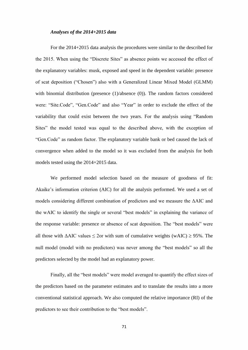
71

Analyses of the 2014+2015 data

For the 2014+2015 data analysis the procedures were similar to the described for

the 2015. When using the “Discrete Sites” as absence points we accessed the effect of

the explanatory variables: musk, exposed and speed in the dependent variable: presence

of scat deposition (“Chosen”) also with a Generalized Linear Mixed Model (GLMM)

with binomial distribution (presence (1)/absence (0)). The random factors considered

were: “Site.Code”, “Gen.Code” and also “Year” in order to exclude the effect of the

variability that could exist between the two years. For the analysis using “Random

Sites” the model tested was equal to the described above, with the exception of

“Gen.Code” as random factor. The explanatory variable bank or bed caused the lack of

convergence when added to the model so it was excluded from the analysis for both

models tested using the 2014+2015 data.

We performed model selection based on the measure of goodness of fit:

Akaike‟s information criterion (AIC) for all the analysis performed. We used a set of

models considering different combination of predictors and we measure the ΔAIC and

the wAIC to identify the single or several “best models” in explaining the variance of

the response variable: presence or absence of scat deposition. The “best models” were

all those with ΔAIC values ≤ 2or with sum of cumulative weights (wAIC) 95%. The

null model (model with no predictors) was never among the “best models” so all the

predictors selected by the model had an explanatory power.

Finally, all the “best models” were model averaged to quantify the effect sizes of

the predictors based on the parameter estimates and to translate the results into a more

conventional statistical approach. We also computed the relative importance (RI) of the

predictors to see their contribution to the “best models”.

72

2.6.1.2 Scats’ abundance

Analyses of the 2015 data

The models performed were similar to the described above for scats‟ presence

analysis; the main differences between them are the response variable used and also the

distribution family applied. For the analysis of the 2015 data using “Discrete Sites” as

the absence points we accessed the effect of the explanatory variables: exposed, speed

and musk in the dependent variable: abundance of scats, represented by the name

“Nspraints”, with a Generalized Linear Mixed Model (GLMM) using a Poisson

distribution. This type of family is consistent with the data‟s distribution. We used

“Site.Code” and “Gen.Code” as random effects. For “Random Sites” data we accessed

the effect of the variables: exposed, speed, alder, musk and bank or bed also in the

dependent variable: abundance of scats (“Nspraints”) by applying a Generalized Linear

Mixed Model (GLMM) with Poisson distribution. Only “Site.Code” was used as

random factor. The explanatory variables bank or bed and alder were not included in the

model using “Discrete Sites” because the model did not converge but when using

“Random Sites” the convergence problem was not found.


For the 2014+2015 data analysis, when using the “Discrete Sites” as absence

points we accessed the effect of the explanatory variables: exposed, speed, bank or bed

and musk in the dependent variable: abundance of scats (“Nspraints”) also using

Generalized Linear Mixed Model (GLMM) with Poisson distribution. The random

factors considered were: “Site.Code”, “Gen.Code” and also “Year”. For the analysis

using “Random Sites” data, we tested the same explanatory variables referred above and

it was also applied a Generalized Linear Mixed Model (GLMM) with Poisson

73

distribution using abundance of scats (“Nspraints”) as response variable. The random

factors used were: “Site.Code” and “Year”.

Both analyses applied for different years were subjected to model selection

based on the Akaike‟s information criterion (AIC) to identify the single or several “best

models” in explaining the scats‟ abundance. The null model was never among the “best

models”. In the end, all the “best models” were model averaged to quantify the effect

sizes and we also computed the relative importance (RI) of the predictors.

2.6.2 General Habitat Characterization

In the analysis of the effect of general habitat variables in the kilometric

abundance index (KAI) the response variable presented high variance and in order to

avoid it we log transformed it. We then applied a LM (Linear Model) with Gaussian

distribution to test the effect of the explanatory variables: %coverage, speed,

%spraintability, mwidth, %pool and %riffle in the response variable KAI, named as

“indexkm” (log transformed). The variables: %rockbank, %stonebank, %groundbank,

%sandbank, %wall and otter were tested but they were not considered in the final model

because they showed p-values near 1 which indicate that they are perfectly non-

significant. Furthermore, when compared the AIC of the model including this variables

and the one without them, the last showed more efficiency (less AIC). The other

variables: %mud, %sand/gravel, %pebble, %cobble, %boulder and %outcrop showed

some high correlation values (see Appendix 1, Table 36) when Pearson‟s correlation

test was applied. However, when including these variables independently (without

correlated variables) they also showed p-values near 1 and increased the AIC of the

model, so they were not included. According to the Pearson‟s correlation test, shading

74

and coverage were also highly correlated (see Appendix 1, Table 36), as well as mwidth

– cmdepth and %riffle – %run (see Appendix 1, Table 36). So, they were tested

independently and the variables considered best for the model were: coverage, mwidth

and %riffle. The model was then subjected to model selection based on the Akaike‟s

information criterion (AIC). The “best models” were also subjected to model averaging

and we also computed the relative importance (RI) of the predictors.

All statistical analyses were performed in R software (R Development Core

Team 2015) using: “lme4” (Bates et al., 2014) and “MuMin” (Barton, 2009) packages,

except for general habitat characterization where: “car” (Fox et al., 2011) and “MuMin”

(Barton, 2009) packages were used.

75

3 Results

76

77

3.1 Survey results

From all the sites sampled, we verified Galemys‟ presence in a total of 48 sites, 23

in 2014 and 30 during 2015 (Figure 9), which indicates that the species‟ presence was

confirmed in 5 sites for both years (see Appendix 1, Table 37).

Figure 8 - Overview of the study area with green points representing the sites of confirmed

Pyrenean desman‟s presence.

A total of 351 Galemys pyrenaicus‟ scats were considered in the study, with 111

of them (52 from 2014 and 59 from 2015) confirmed by the genetic analysis and about

240 (44 from 2014 and 196 from 2015) with percentage higher than 70% (Table 6).

78

Table 6 - Number of scats considered in the study (confirmed and %higher than 70) divided per

year.

N scats Considered

Year % higher than 70 Confirmed Total per Year

2014 44 52 96

2015 196 59 255

Total N 240 111 351

3.2 Marking Site Characterization

3.2.1 Presence of scats


For data using “Discrete Sites” as absence points, AIC-based model selection

found two statistically best models (Table 7) for predicting the Pyrenean desman scats‟

presence (“Chosen”), with the null model not being among the best models

(ΔAIC=304.14). From the variables considered in the best models only alder (Figure 10,

c)) and exposed (Figure 10, b)) showed high importance (RI for predictors=1) in

explaining the presence/absence of scat deposition, whereas the variable speed (Figure

10, a)) had a lower effect (RI=0.65). Effect sizes of the model averaged predictors

(Table 8) indicate that exposed negatively affected (p=0.019) the scats‟ presence and the

latter is associated with the presence of alder (p=0.129) and water speed (p=0.339).

For the data using “Random Sites” as absence points, AIC-based model

selection also found one statistically best model (Table 10). The null model was not part

of the best models (ΔAIC=595.52). Best model showed high importance of the variables

exposed (Figure 11, b)), alder (Figure 11, e)), speed (Figure 11, c)) and bank or bed

(Figure 11, a)) (RI of the first three predictors=1; RI bank or bed=0.99) and lower

79

0.

5

importance of the variable musk (Figure 11, d)) (RI=0.85). Exposed and the category

riverbed (bank or bed 2) showed negative effect (p=<0.001; p=0.004, respectively) on

scats‟ presence while speed (p=<0.001), musk (p=0.113) and presence of alder

(p=0.354) were positively associated with the scats‟ presence (Table 11).

Figure 9 – Data exploration of the response variable: scats’ presence (named as “Chosen”)

in relation to the variables: Speed, Alder and Exposed, integrated in the model using 2015

data with “Discrete Sites” as absence points. a) Variation for the variable speed according to

scats‟ presence (1) or absence (0); b) Variation for the variable exposed in relation to scats‟

presence (1) or absence (0); c) Relative frequency of the presence (1) or absence (0) of Alder for

places of scats‟ presence (1) or absence (0).

80

Figure 10 – Data exploration of the response variable: scats’ presence (named as

“Chosen”) in relation to the variables: Bank or Bed, Exposed, Speed, Alder and

Musk, integrated in the model using 2015 data with “Random Sites” as absence

points. a) frequency of the variable bank or bed in relation to scats‟ presence (1) or

absence (0); b) variance for the variable exposed in relation to scats‟ presence (1) or

absence (0); c) variance of the variable speed according to scats‟ presence (1) or

absence (0); d) and e) relative frequencies of the presence (1) or absence (0) of Alder

and Musk, respectively, for places of scats‟ presence (1) or absence (0).

81

Table 7 - Best models (ΔAIC < 2) for prediction of the Pyrenean desman scats' presence using

2015 data with “Discrete Sites” as absence points obtained after the AIC-based model selection.

Best models are in bold and underlined.

Component models

Variables Df logLik AIC ΔAIC Weight

Alder + Exposed + Speed 6 -71.89 155.79 0.00 0.65

Alder + Exposed 5 -73.53 157.07 1.28 0.35

Exposed + Speed 5 -113.82 237.64 81.86 0.00

Exposed 4 -138.80 285.60 129.82 0.00

Alder + Speed 5 -160.24 330.48 174.69 0.00

Alder 4 -164.29 336.57 180.79 0.00

Speed 4 -198.18 404.36 248.58 0.00

(Null) 3 -226.96 459.93 304.14 0.00

Table 8 - Output for the average model of the best models resultant of the predictions for scats‟

presence using 2015 data with “Discrete Sites” as absence points. Significant results in bold.

Model-averaged coefficients

Estimate Std. Error Adjusted SE z value Pr (> |z|)

(Intercept) 10.3273 6.4812 6.5117 1.586 0.113

Exposed -20.6357 8.7570 8.8001 2.345 0.019

Alder 1 3.2255 2.1146 2.1250 0.956 0.129

Speed 0.6397 0.6672 0.6689 1.518 0.339

Table 9 - Relative importance (RI) of the predictors resultant from model-averaging of the

GLMM for scats' presence using 2015 data with "Discrete Sites" as absence points.

Relative variable importance

Alder Exposed Speed

Importance 1 1 0.65

82


2015 data with “Random Sites” as absence points obtained after the AIC-based model selection.

Best models are in bold and underlined.

Component models:

Variables Df logLik AIC ΔAIC Weight

Alder + Bank or Bed + Musk +Exposed + Speed 7 -94.03 202.06 0.00 0.84

Alder + Bank or Bed +Exposed + Speed 6 -96.77 205.53 3.47 0.15

Alder + Musk +Exposed + Speed 6 -99.84 211.68 9.62 0.01

Alder +Exposed + Speed 5 -102.79 215.57 13.51 0.00

Alder + Bank or Bed + Musk +Exposed 6 -102.40 216.80 14.74 0.00

Bank or Bed + Musk +Exposed + Speed 6 -104.82 221.64 19.58 0.00

Alder + Musk +Exposed 5 -106.93 223.86 21.80 0.00

Bank or Bed +Exposed + Speed 5 -107.46 224.93 22.87 0.00

Alder + Bank or Bed +Exposed 5 -108.37 226.74 24.68 0.00

Musk +Exposed + Speed 5 -111.67 233.34 31.28 0.00

Alder +Exposed 4 -112.97 233.93 31.88 0.00

Exposed + Speed 4 -114.39 236.77 34.72 0.00

Bank or Bed + Musk +Exposed 5 -151.01 312.02 109.96 0.00

Musk +Exposed 4 -156.54 321.08 119.03 0.00

Bank or Bed +Exposed 4 -157.05 322.09 120.04 0.00

Exposed 3 -162.81 331.61 129.56 0.00

Alder + Bank or Bed + Speed 5 -210.05 430.09 228.04 0.00

Alder + Bank or Bed + Musk + Speed 6 -209.88 431.75 229.69 0.00

Alder + Speed 4 -218.58 445.15 243.09 0.00

Alder + Musk + Speed 5 -218.30 446.59 244.53 0.00

Alder + Bank or Bed + Musk 5 -226.31 462.62 260.57 0.00

Alder + Bank or Bed 4 -228.77 465.54 263.48 0.00

Alder + Musk 4 -233.63 475.25 273.19 0.00

Alder 3 -236.18 478.37 276.31 0.00

Bank or Bed + Speed 4 -243.02 494.04 291.99 0.00

Bank or Bed + Musk + Speed 5 -243.02 496.04 293.98 0.00

Speed 3 -259.46 524.93 322.87 0.00

Musk + Speed 4 -259.44 526.88 324.83 0.00

Bank or Bed + Musk 4 -279.90 567.81 365.75 0.00

Bank or Bed 3 -281.73 569.46 367.40 0.00

Musk 3 -239.94 593.88 391.82 0.00

(Null) 2 -295.76 595.52 393.46 0.00

83

Table 11 - Output for the average model of the best models resultant of the GLMM for scats‟

presence using 2015 data with “Random Sites” as absence points. Significant results in bold.



(Intercept) 2.3421 1.4178 1.4222 1.647 0.099

Exposed -10.0780 1.8219 1.8276 5.514 < 0.001

Alder 1 1.0290 1.1070 1.1105 0.927 0.354

Speed 1.5475 0.4411 0.4425 3.497 < 0.001

Musk 1 1.3875 0.8735 0.8750 1.586 0.113

Bank or Bed 2 -1.8824 0.6471 0.6490 2.901 0.004

Table 12 - Relative importance (RI) from model-averaging of the GLMM for scats' presence

using 2015 data with "Random Sites" as absence points.


Exposed Alder Speed Bank or Bed Musk

Importance 1 1 1 0.99 0.85


Using “Discrete Sites” as absence points, AIC-based model selection found two

statistically best models (Table 13) and the null model was not among the best models

(ΔAIC=333.95). The variables exposed (Figure 12, a)) and speed (Figure 12, b); RI for

both predictors=1) showed high importance in explaining the presence/absence of scat

deposition, whereas the variable musk (Figure 12, c); RI=0.27) showed the least

importance. Effect sizes of the model averaged predictors indicated that variables

exposed (p=<0.001) and musk (p=0.910) negatively affected the scats‟ presence and the

latter is associated with faster water speed (p=<0.001) (Table 14).


selection found only one statistically best-model (Table 16). The null model was not

part of the best models (ΔAIC=522.74). The variables included in the best model all

showed high importance in explaining the scats‟ presence/absence: exposed (Figure 13,

a); RI=1), speed (Figure 13, b); RI=1) and musk (Figure 13, c); RI=0.97). Scats‟

84

Figure 11- Data exploration of the response variable: scats’ presence (“Chosen”) in


2014+2015 data with “Discrete Sites” as absence points. a) Variation for the variable exposed

in relation to scats‟ presence (1) or absence (0); b) Variation for the variable speed according to

scats‟ presence (1) or absence (0); c) Relative frequency of the presence (1) or absence (0) of

Alder for places of scats‟ presence (1) or absence (0).

presence was negatively associate with the variable exposed (p=<0.001) whereas speed

(p=<0.001) and musk presented a positive effect (p=0.047) (Table 17).

.

85

Figure 12 - Data exploration of the response variable: scats’ presence (“Chosen”) in


2014+2015 data with “Random Sites” as absence points. a) Variation for the variable

exposed in relation to scats‟ presence (1) or absence (0); b) Variation for the variable speed

according to scats‟ presence (1) or absence (0); c) Relative frequency of the presence (1) or

absence (0) of Alder for places of scats‟ presence (1) or absence (0).

86


2014+2015 data with “Discrete Sites” as absence points obtained after the AIC-based model

selection. Best models are in bold and underlined.

Component models:

Df logLik AIC ΔAIC Weight

Exposed + Speed 6 -173.09 358.18 0.00 0.73

Musk + Exposed + Speed 7 -173.07 360.14 1.95 0.27

Exposed 5 -202.62 415.25 57.06 0.00

Musk + Exposed 6 -202.42 416.83 58.65 0.00

Musk + Speed 6 -303.28 618.56 260.38 0.00

Speed 5 -307.26 624.53 266.34 0.00

Musk 5 -340.16 690.31 332.13 0.00

(Null) 4 -342.07 692.13 333.95 0.00


presence using 2014+2015 data with “Discrete Sites” as absence points. Significant results in

bold.



(Intercept) 2.28278 0.69647 0.69832 3.269 0.001

Exposed -6.22258 0.73464 0.73659 8.448 <0.001

Speed 0.95578 0.24180 0.24244 3.942 <0.001

Musk 1 -0.02349 0.20773 0.20826 0.113 0.910


using 2014+2015 data with "Discrete Sites" as absence points.


Exposed Speed Musk

Importance 1 1 0.27

87


2014+2015 data with “Random Sites” as absence points obtained after the AIC-based model


Component models:



Exposed + Speed 5 -208.42 426.83 7.19 0.03

Musk + Exposed 5 -258.06 526.12 106.48 0.00

Exposed 4 -268.02 544.05 124.41 0.00

Speed 4 -405.28 818.55 398.91 0.00

Musk + Speed 5 -405.15 820.30 400.66 0.00

Musk 4 -466.27 940.54 520.90 0.00

(Null) 3 -468.19 942.37 522.74 0.00


presence using 2014+2015 data with “Random Sites” as absence points. Significant results in

bold.



(Intercept) 1.2802 0.5936 0.5946 2.741 0.055

Exposed -7.1302 0.6555 0.6566 10.859 <0.001

Speed 1.3229 0.2344 0.2348 5.634 <0.001

Musk 1 0.8347 0.4201 0.4207 1.984 0.047


using 2014+2015 data with "Random Sites" as absence points.


Exposed Speed Musk

Importance 1 1 0.97

88

3.2.2 Scats’ abundance


For data using “Discrete Sites” as absence points, AIC-based model selection

found two best models (Table 19) for predicting the Pyrenean desman scats‟ abundance

(“Nspraints”), with the null model not being among the best models (ΔAIC=665.18).

The variables exposed (Figure 14, a)) and speed (Figure 14, c)) were present in both

models so they had the highest importance (RI for predictors=1) while the variable

musk (only present in one of the models) (Figure 14, b)) revealed lower importance

(RI=0.39). Effect sizes of the model averaged predictors (Table 20) indicated a negative

effect of the variable exposed in the scats‟ abundance (p=<0.001) while variables speed

(p=<0.001) and the presence of musk (p=0.615) showed a positive association.


selection also found only one best model (Table 22) and the null model was not part of

the best models (ΔAIC=1636.61). All the variables included in the model showed high

importance: alder (Figure 15, a); RI=1), exposed (Figure 15, c); RI=1), musk (Figure

15, d); RI=1), speed (Figure 15, e); RI=1) and bank or bed (Figure 15, b); RI=0.96).

Exposed and the category riverbed (bank or bed 2) showed negative effect (p=<0.001;

p=0.019, respectively) on scats‟ abundance while water speed (p=<0.001), presence of

musk (p=<0.001), and presence of alder nearby (p=0.178) presented positive association

with the response variable in test (Table 23).

89

Figure 13 - Data exploration of the response variable: scats’ abundance (“Naspraints”) in

relation to the variables: Exposed, Musk and Speed, integrated in the model using 2015

data with “Discrete Sites” as absence points. a) variation of the abundance of scats in relation

to the exposed categories (0- non-exposed; 0.5- partially exposed; 1 – exposed; b) variation of

the abundance of scats in relation to the presence (1) or absence (0) of musk; c) variation of the

abundance of scats in relation to the different categories of speed (1- null/almost null; 2- weak;

3- medium/strong).

90


relation to the variables: Alder, Bank or Bed, Exposed, Musk and Speed, integrated in the

model using 2015 data with “Random Sites” as absence points. a) variation of the abundance

of scats in relation to the alder presence (1) or absence (0); b) variation of the abundance of

scats in relation to the place where it is located (1- bank; 2- riverbed); c) variation of the

abundance of scats in relation to the exposed categories (0- non-exposed; 0.5- partially exposed;

1 – exposed; d) variation of the abundance of scats in relation to the presence (1) or absence (0)

of musk; e) variation of the abundance of scats in relation to the different categories of speed (1-

null/almost null; 2- weak; 3- medium/strong).

91

Table 19 - Best models (ΔAIC < 2) for prediction of the Pyrenean desman scats' abundance

using 2015 data with “Discrete Sites” as absence points obtained after the AIC-based model



abundance using 2015 data with “Discrete Sites” as absence points. Significant results in bold.



(Intercept) -0.3180 0.3386 0.3400 0.935 0.350

Exposed -2.5125 0.1480 0.1486 16.910 <0.001

Speed 0.8569 0.1162 0.1167 7.346 <0.001

Musk 1 0.0606 0.1202 0.1205 0.503 0.615

Table 21 - Relative importance (RI) from model-averaging of the GLMM for scats' abundance

using 2015 data with "Discrete Sites" as absence points.


Exposed Speed Musk

Importance 1 1 0.39

Component models:


Exposed + Speed 5 -637.21 1284.41 0.00 0.61


Musk + Exposed 5 -708.74 1427.47 143.06 0.00

Exposed 4 -711.12 1430.23 145.82 0.00

Musk + Speed 5 -879.96 1769.92 485.51 0.00

Speed 4 -885.88 1779.76 495.35 0.00

Musk 4 -969.30 1946.61 662.20 0.00

(Null) 3 -971.79 1949.59 665.18 0.00

92


using 2015 data with “Random Sites” as absence points obtained after the AIC-based model


Component models:


Alder + Bank or Bed + Musk + Exposed +

Speed 7 -647.23 1308.46 0.00 0.96

Alder + Musk + Exposed + Speed 6 -651.35 1314.70 6.24 0.96

Alder + Bank or Bed + Musk + Exposed 6 -671.53 1355.07 46.61 0.00

Alder + Musk + Exposed 5 -676.57 1363.14 54.68 0.00

Alder + Bank or Bed + Exposed + Speed 6 -675.72 1363.44 54.98 0.00

Alder + Exposed + Speed 5 -685.86 1381.71 73.26 0.00

Alder + Bank or Bed + Exposed 5 -721.77 1453.55 145.09 0.00

Alder + Exposed 4 -731.28 1470.56 162.10 0.00

Bank or Bed + Musk + Exposed + Speed 6 -782.46 1576.93 268.47 0.00


Bank or Bed + Exposed + Speed 5 -810.36 1630.71 322.25 0.00

Exposed + Speed 4 -826.88 1661.76 353.31 0.00

Bank or Bed + Musk + Exposed 5 -857.95 1725.91 417.45 0.00

Musk + Exposed 4 -867.32 1742.65 434.19 0.00

Bank or Bed + Exposed 4 -904.34 1816.68 508.22 0.00

Exposed 3 -920.14 1846.28 537.82 0.00

Alder + Bank or Bed + Musk + Speed 6 -984.14 1980.28 671.82 0.00

Alder + Musk + Speed 5 -1001.97 2013.94 705.48 0.00

Alder + Bank or Bed + Speed 5 -1009.67 2029.35 720.89 0.00

Alder + Speed 4 -1018.63 2045.27 736.81 0.00

Alder + Bank or Bed + Musk 5 -1107.29 2224.57 916.11 0.00

Alder + Bank or Bed 4 -1110.28 2228.56 920.11 0.00

Alder + Musk 4 -1125.47 2258.93 950.47 0.00

Alder 3 -1126.58 2259.17 950.71 0.00


Bank or Bed + Speed 4 -1240.30 2488.60 1180.14 0.00

Musk + Speed 4 -1255.06 2518.12 1209.66 0.00

Speed 3 -1271.45 2548.89 1240.44 0.00

Bank or Bed + Musk 4 -1422.60 2853.19 1544.74 0.00

Bank or Bed 3 -1427.38 2860.76 1552.30 0.00

Musk 3 -1468.82 2943.64 1635.18 0.00

(Null) 2 -1470.53 2945.07 1636.61 0.00

93


abundance using 2015 data with “Random Sites” as absence points. Significant results in bold.



(Intercept) -0.30779 0.39553 0.39676 0.776 0.438

Exposed -2.41119 0.11288 0.11323 21.294 <0.001

Speed 0.58646 0.08604 0.08631 6.795 <0.001

Alder 1 0.27620 0.20428 0.20492 1.348 0.178

Musk 1 1.02273 0.13320 0.13361 7.654 <0.001

Bank or Bed 2 -0.35208 0.14909 0.14944 2.356 0.019


using 2015 data with "Random Sites" as absence points.


Alder Exposed Musk Speed Bank or Bed

Importance 1 1 1 1 0.96


Using “Discrete Sites” as absence points, AIC-based model selection found two

statistically best models (Table 25). The null model was not among the best models

(ΔAIC=1007.77). The variables bank or bed (Figure 16, a)), exposed (Figure 16, b)) and

speed (Figure 16, d)) showed high importance in explaining the scats‟ abundance (RI of

all the predictors=1), unlike the variable musk (Figure 16, c)); RI=0.57). Effect sizes of

the model averaged predictors indicated that riverbed (bank or bed 2) and exposed

negatively affected the scats‟ abundance (p=<0.001 for both) while speed (p=<0.001)

and presence of musk (p= 0.107) are positively associated with it (Table 26).


selection found one statistically best model (Table 28) also for predicting the Pyrenean

desman scats‟ abundance (“Nspraints”) with the null model not being as part of the best

94

models (ΔAIC=1997.12). All the variables included in the best model showed high

importance: exposed (Figure 17, b); RI=1), speed (Figure 17, d); RI=1) bank or bed

(Figure 17, a); RI=1) and musk (Figure 17, c); RI=1). Exposed (p=<0.001) and riverbed

(bank or bed 2; p=<0.001) had a negative effect on scats‟ abundance whereas speed and

presence of musk presented a positive effect (p=<0.001, for both) (Table 29).


relation to the variables: Bank or Bed, Exposed, Musk and Speed, integrated in the model

using 2014+2015 data with “Discrete Sites” as absence points. a) Variation of the abundance

of scats according to the place where it is located(1- bank; 2- riverbed); b) Variation of the


1 – exposed; c) Variation of the abundance of scats in relation to the presence (1) or absence (0)

of musk; d) Variation of the abundance of scats in relation to the different categories of speed

(1- null/almost null; 2- weak; 3- medium/strong).

95


relation to the variables: Bank or Bed, Exposed, Musk and Speed, integrated in the model

using 2014+2015 data with “Random Sites” as absence points. a) Variation of the abundance

of scats according to the place where it is located(1- bank; 2- riverbed); b) Variation of the


1 – exposed; c) Variation of the abundance of scats in relation to the presence (1) or absence (0)

of musk; d) Variation of the abundance of scats in relation to the different categories of speed

(1- null/almost null; 2- weak; 3- medium/strong).

96


using 2014+2015 data with “Discrete Sites” as absence points obtained after the AIC-based

model selection. Best models are in bold and underlined.

Component models:


Bank or Bed + Musk + Exposed + Speed 8 -836.69 1689.37 0.00 0.57


Exposed + Speed 6 -859.89 1731.77 42.40 0.00




Musk + Exposed 6 -949.17 1910.33 220.96 0.00

Exposed 5 -950.48 1910.96 221.58 0.00


Bank or Bed + Speed 6 -1126.59 2265.18 575.80 0.00

Musk + Speed 6 -1222.00 2456.01 766.63 0.00

Speed 5 -1231.13 2472.26 782.88 0.00

Bank or Bed 5 -1264.92 2539.84 850.47 0.00

Bank or Bed + Musk 6 -1264.89 2541.79 852.41 0.00

Musk 5 -1340.03 2690.06 1000.69 0.00

(Null) 4 -1344.57 2697.14 1007.77 0.00

Table 26 - Output for the average model of the best model resultant of the GLMM for scats‟

abundance using 2014+2015 data with “Discrete Sites” as absence points. Significant results in

bold.



(Intercept) -0.4043 0.3335 0.3344 1.209 0.227

Exposed -2.5473 0.1369 0.1372 18.564 <0.001

Speed 0.8882 0.1018 0.1021 8.700 <0.001

Musk 1 0.2355 0.1458 0.1462 1.610 0.107

Bank or Bed 2 -1.7895 0.3140 0.3149 5.683 <0.001


using 2014+2015 data with "Discrete Sites" as absence points.


Exposed Speed Bank or Bed Musk

Importance 1 1 1 0.57

97


using 2014+2015 data with “Random Sites” as absence points obtained after the AIC-based

model selection. Best models are in bold and underlined.

Component models:


Bank or Bed + Musk + Exposed + Speed 7 -1113.22 2240.45 0.00 1


Exposed + Speed 6 -1136.24 2284.48 44.04 0.00




Musk + Exposed 5 -1253.10 2516.20 275.76 0.00

Exposed 4 -1279.74 2567.48 327.03 0.00


Bank or Bed + Speed 5 -1751.12 3512.25 1271.80 0.00

Musk + Speed 5 -1794.71 3599.43 1358.98 0.00

Speed 4 -1817.75 3643.49 1403.05 0.00

Bank or Bed 5 -2026.83 4063.66 1823.21 0.00

Bank or Bed + Musk 4 -2037.53 4083.06 1842.61 0.00

Musk 4 -2110.99 4229.98 1989.54 0.00

(Null) 3 -2115.78 4237.57 1997.12 0.00


abundance using 2014+2015 data with “Random Sites” as absence points. Significant results in

bold.



(Intercept) -0.04718 0.39529 0.39595 0.119 0.905

Musk 1 0.54474 0.10446 0.10464 5.206 <0.001

Exposed -2.44949 0.08465 0.08480 28.887 <0.001

Bank or Bed 2 -0.81753 0.12513 0.12534 6.522 <0.001

Speed 0.63567 0.06534 0.06545 9.712 <0.001


using 2014+2015 data with "Random Sites" as absence points.


Exposed Speed Bank or Bed Musk

Importance 1 1 1 1

98

3.3 General Habitat Characterization

The effect of the explanatory variables in the KAI, used to understand which

variables determine higher scats‟ abundance per km of transect resulted in three best

models after the AIC-based model selection (Table 31), with the null model not being

among the best models (ΔAIC=29.36). The variables: %spraintability (Figure 18, b));

RI=1), %pool (Figure 18, e); RI=0.88), %coverage (Figure 18, a); RI=0.8) and mwidth

(Figure 18, d); RI=0.8) were all present in all of the best models with only

%spraintability showing high importance in explaining scats‟ abundance per km of

transect. The second and third best models included the variables speed (Figure 18, c);

RI=0.41) and %riffle (Figure 18, f); RI=0.38) which showed the lowest importance.

Effect sizes of the model averaged predictors showed that only high

spraintability (spraintability 5) had an almost significant effect in the response variable

(p=0.0618) showing a positive effect (Table 38).

99

Figure 17 - Data exploration of the response variable: kilometric abundance index (KAI)

in relation to the variables:%coverage, spraintability, speed, mwidth, %pool and %riffle

integrated in the model used to predict the abundance of Pyrenean desman scats per km of

transect. Graphic a) represents the boxplot with the KAI in relation to % of coverage (0%;

25%; 50%; 75%; 100%); Graphic b) represents the boxplot with the KAI in relation to

spraintability (1: <5%; 2: 5%-19%; 3: 20%-39%; 4: 40%-69%; 5: 70%-100%); Graphic c)

represents boxplot with the KAI in relation to the different categories of speed (1- null/almost

null; 2- weak; 3- medium/strong); Graphic d) represents a scatterplot with the KAI in relation

to the numeric variable mWidth; Graphics e) and f) represents a scatterplot with the KAI in

relation to the percentages attributed to the variables pool and riffle.

100

Table 31 - Best models (ΔAIC < 2) for prediction of the Pyrenean desman KAI obtained after

AIC-based model selection. All the models considered for model selection are in Apendix 1,

Table 38.

Component models:


%Coverage + Spraintability + mWidth + %Pool 12 -49.77 123.55 0.00 0.26

%Coverage + Speed + Spraintability + mWidth +

%Pool 14 -48.03 124.07 0.52 0.2

%Coverage + Spraintability + mWidth + %Pool +

%Riffle 13 -49.56 125.13 1.58 0.12

Table 32 - Output for the average model of the best models resultant of the LM for the KAI.

Almost significant results underlined.



(Intercept) 0.806316 1.301493 1.325812 0.608 0.5431

mWidth -0.40265 0.042683 0.043627 0.923 0.3560

Spraintability2 -0.050686 0.837625 0.860631 0.059 0.9530

Spraintability3 0.295776 0.768896 0.789900 0.374 0.7081

Spraintability4 1.028074 0.794614 0.815734 1.260 0.2076

Spraintability5 1.555030 0.811526 0.832729 1.867 0.0618

%Pool -0.012259 0.007792 0.007941 1.544 0.1226

Coverage 25% 1.314898 1.022773 1.037928 1.267 0.2052

Coverage 50% 1.474132 1.006924 1.019470 1.446 0.1482

Coverage 75% 1.123617 0.883668 0.897651 1.252 0.2107

Coverage 100% 0.936704 0.833715 0.848990 1.103 0.2699

Speed 2 -0.011603 0.370980 0.381291 0.030 0.9757

Speed 2 0.085889 0.379899 0.389921 0.220 0.8257

%Riffle 0.001562 0.004501 0.004590 0.340 0.7337

Table 33 - Relative importance (RI) from model-averaging of the LM for for the KAI data.


Spraintability %Pool mWidth %Coverage Speed %Riffle

Importance 1 0.88 0.80 0.80 0.41 0.38

101

4 Discussion

102

103

4.1 General discussion

In this study we verified that at a small-site scale, Pyrenean desman selected as

habitat requirements non-exposed sites, preferably at riverbanks near locations of high

river flow. Alder presence showed high importance in explaining the scat deposition

despite the non-significance results we obtained which contradicted the expected.

Presence of musk covering the marking site revealed inconsistent importance and

significance making it difficult to determine if the variable is in fact important for

Pyrenean desman selection.

The negative selection of exposed sites supports the theories that sheltered places

constitute a key resource for Pyrenean desman, not just for individual protection from

predators and for resting behaviour but also for indirect communication of resources

availability between the species (Melero et al., 2012). They also support the lower

probability of scats‟ detection expected for exposed sites due to the fast degradation

caused by the atmospheric agents (i.e. sun, rain, variation in water flow) (Queiroz et al.,

1998).

Permanent fast flowing water is referred as one of the main important habitat

characteristics required for Pyrenean desman‟s presence (Marcos, 2004; Queiroz et al.,

1998). That is consistent with our results for speed, which indicate that Pyrenean scats‟

presence increases with water speed (medium/strong). The preference for high water

speed is likely related to the abundance of aquatic macroinvertebrates (main prey of

Galemys pyrenaicus). Presence of aquatic macroinvertebrates is greater in these fast-

flowing stretches due to a low degree of sedimentation (Biffi et al., 2016; Charbonnel et

al., 2015) which provides high levels of dissolved oxygen and food particles. The

presence of scats near these places possibly signals the availability of food resources.

104

Queiroz et al., 1998 studies on Pyrenean desman‟s habitat selection for scat

deposition reported high number of scats detected in the riverbed rather than in the

bankside. On the other hand, more recent studies: Biffi et al., 2016; Pedroso & Chora,

2014 referred a preferable selection by Pyrenean desman of the substrate in the

riverbanks. Our study contradicted the results obtained by Queiroz et al., 1998 and

supported the recent ones indicating a significantly lower scat deposition in the

riverbed. Differences between our results and the obtained by Queiroz et al., 1998 were

probably associated with the variation on scats‟ detectability between the two studies

due to contrasting weather conditions, habitat structure of the places sampled and

observer‟s bias (which can influence the facility of scat‟s detection) (Charbonnel et al.,

2015).

Lower selection of the substrate in the riverbed for scats‟ deposition could be

explained by the probability of finding less abundant emergent items and variability in

types of substrate in comparison to the riverbanks. The substrate variety in the

riverbanks allows high availability of crevices and cavities which Pyrenean desmans

uses as resting sites instead of digging (Melero et al., 2012). Banks also present high

density of riparian vegetation with some exposed roots creating natural cavities also

considered as good shelters. Since shelters are considered as minimum requirement for

the species presence (ICN, 2005) it seems possible that the low variability of the

emergent substrate in the riverbed decreases the selection in favour of the riverbanks.

Alder presence is referred as very important to Galemys pyrenaicus because apart

from providing shelter it is a deciduous tree very common among the riparian

vegetation which leaves create a heavy layer on the soil retaining the rainwater and

preventing changes in the soil and in the water quality (Ramalhinho & Tavares, 1989).

The aquatic macroinvertebrates are very sensitive to changes in water conditions and

105

since Pyrenean desman depends on them to feed it seems that the existence of a

significant positive relation between the two is possible. Our results indicate a high

importance of the variable in determining the scat deposition, confirming the expected,

despite the non-significant effect we obtained.

As referred above, results for musk presence are inconsistent. Based on the field

observations and on descriptive statistics, we expected a negative effect of the variable

musk on scats‟ presence/abundance which was contradicted by the significantly positive

effects obtained. Musk is mostly found covering exposed substrate where it is frequent

to find scats from Cinclus cinclus (which can be very similar to Pyrenean desmans‟

scats). Since not all the scats were genetically confirmed until the present data, it is

possible that some are false presences.

For the larger scale evaluation of the habitat preferences only spraintability

seemed to have values closer to the significance indicating that high of spraintability

explained the higher abundance of scats‟ found per kilometre of transect. In other

words, transects with high substrate heterogeneity are possibly highly selected by

Pyrenean desman. This is consistent with the habitat selection studies developed by

(Biffi et al., 2016; Charbonnel et al., 2014, 2015; Queiroz et al., 1998).

The analyses considered in this study tried to describe Pyrenean desman habitat

preferences using two types of scale: a small-site scale – describing the differences for

Pyrenean desman occurrence at a small-site characterization (~0.5 m2) and a larger scale

– describing differences at the transect level. This was of great importance to account

given the fact that there is an urgent need to improve the studies on Pyrenean desmans‟

habitat descriptors avoiding finer habitat associations based on grid cells with coarse

106

resolution that cannot account for the spatial structure of the stream network and the

species‟ scale resolution (Biffi et al., 2016) .

4.2 Results from Scats’ Presence

Considering the results for scat deposition in 2015, it is clear that Pyrenean desman

was significantly more present in less exposed substrate. This indicates that exposed

sites are less selected by Galemys pyrenaicus for leaving their marks. However, when

using “Random Sites” two other variables were included in the model: bank or bed and

stream speed which showed an effect on scats‟ presence. Riverbed (bank or bed 2) had a

negative effect on scats‟ presence indicating that Pyrenean desman avoid the riverbed,

selecting the bankside for scat deposition. Scats‟ presence was also associated with

higher stream speed near the substrate. Musk and bank or bed variables were excluded

from the model with “Discrete Sites” due to the lack of convergence obtained when

these variables were included.

Alder showed high importance in determining the presence of scat deposition

although we obtained no significant effect when the variable was included in both

analyses for 2015 data using the two different types of absence points. We were not

expecting the non-significance of this variable but the fact that it was included in the

best model with high importance value indicates that alder explain the presence of scat

deposition.

There were some differences in the variables selected by the models depending on

the type of absence data used: “Discrete Sites” or “Random Sites”. This is probably

related to the variation that each method captures from the sites. “Discrete Sites” were

selected closer to the “True Sites” (where the scat was present), and may present a lower

variability. Also, we cannot exclude that some of the places selected as absence points

107

are actually suitable for scats‟ deposition, but were not chosen just by chance – certainly

Desmans will not deposit scats in all possible available places. Additionally, a possible

spatial autocorrelation could also be explaining these results; however we did not test

this hypothesis. “Random Sites”, on the other hand, were randomly collected along the

river, being less affected by the possibility of similarity with “True Sites”. Also, the

methodology applied for assessing this type of absence points allowed to cover a more

extensive area of the river, making it possible to represent more precisely the river

heterogeneity and to detect more differences in habitat availability.

In order to increase the sample size – even at the cost of using fewer variables - we

assessed the data from both years (2014 and 2015). Here, the variables considered were

identical for the models using “Discrete Sites” or “Random Sites” as absence points:

musk, exposed and speed. Bank or bed was excluded for both models due to lack of

convergence. In this particular case, model non-convergence is probably related to lack

of variance in the explanatory variable with one of the predictors perfectly describing

the criterion in study. Exposed showed similar importance and significance as in the

2015 only analysis. Although variable speed was included in both models referring to

the different year‟s datasets, we found differences for the significance value (non-

significant for 2015 data and positively significant when added the 2014 data). These

differences could be explained by the increase in the sampled number which enhanced

the variability of the predictors within the variable. With respect to “Random Sites” data

and similarly to the results obtained for 2015 it seemed consensual that Pyrenean

desman preferably selected places of high water speed and avoid exposed sites.

108

4.3 Results from Scats’ Abundance

Considering the data from 2015, the results indicate that Pyrenean desman scats‟

appeared particularly associated with less exposed sites and with higher water speed,

and in a similar way for the two types of absent points considered. Musk was not

included in the “Discrete Sites” model, but it was included in “Random Sites” models,

with high desman scats‟ abundance in the substrate covered with musk. This model also

indicates that lower scats‟ abundance was found in riverbed rather than riverbanks.

Alder presence showed again non-significant effect on the scats‟ abundance, however

the high importance value of the variables suggested again, that alder has some

relevance for scat deposition behaviour in desman species.

Due to the lack of convergence, alder and bank or bed variables were also excluded

from the model with “Discrete Sites”. Differences obtained in the variables affecting

scats‟ abundance depending on the type of absence data used are related to the method

applied for the data collection, again. However, there are notable minor differences

between methodologies using abundance as response variable rather than the

dichotomous.

For the years 2014 +2015 there were also no differences between models using

“Discrete Sites” or “Random Sites”. The variables considered in the models of both

methods were: musk, exposed, speed and bank or bed. There was only one difference

between 2014+2015 and 2015 only for the “Discrete Sites” analysis, because „bank or

bed‟ had to be excluded from the later analysis due to lack of convergence. As in the

analysis for the chosen/not chosen, Pyrenean desmans avoid exposed substrates and

preferably select high water speed. Riverbed (bank or bed 2) was also avoided for scat

109

deposition, indicating a preferable selection for riverbanks as referred in more recent

studies (Biffi et al., 2016; Pedroso & Chora, 2014).

In general, we can say that Pyrenean desman scats were found preferably in non-

exposed substrate, near locations of high river flow, in riverbanks and revealed some

preference for substrate covered with musk.

4.4 General habitat characterization

This analysis adjusted to a larger scale was used to check what general habitat

variables have an effect on the abundance of Pyrenean desman scats‟ found per km of

transect prospected between the sites where the presence of Pyrenean desman was

detected. The most important variables considered in the model were: the percentage of

coverage, spraintability, riverbed width and the percentage of pool, but from these

variables only spraintability seemed to have an importance in determining more scats‟

abundance indicating that transects with high substrate heterogeneity are preferred by

Pyrenean desman. These results are in accordance with studies from Biffi et al., 2016

where it is referred that the species seemed to occupy sites with abundant emergent

items and high heterogeneity of river substrates and shelters used as resting sites. Non-

significant results for the other variables are probably justified by the low variety found

between the sites considered. These sites were all confirmed as sites of Pyrenean

desman‟s presence and because of that, all the variables tested presented many

similarities between them.

110

4.5 Data limitations

We outline here some of the limitations of the study. One of the most limiting

problems was the high number of missing values which compromised the consideration

of some variables for the models. This leaves aside the possibility of finding other

important variables affecting the habitat selection. It is important to improve the

methodology applied in field considering the hypothesis of using more efficient and

practical forms.

Also, we needed to considered scats which identification was only based on the

morphology and in the percentage of certainty of being Galemys attributed in field by

the most experienced observer. Despite the reasonable degree of confidence we need to

ensure the genetic confirmation of all the scats considered in order to avoid false

positives that could overestimate the number of presences.

Another limiting factor to refer was the lack of convergence verified for some

models when some variables were included. This lack of convergence means that the

coefficients are not meaningful because the iterative process was unable to find

solutions and it did not allow me to consider the same number of starting variables to all

the models. In order to avoid these problems in future the use of more quantitative

variables should be considered rather than categorical to increase variance between the

variable predictors and avoid undefined results due to zero cell counts when applying

many dummy variables to models with binomial distribution. The number of zeros used

in Poisson distribution should also be controlled.

111

4.6 Conclusion

At a larger scale, the use of local habitat by the Pyrenean desman appears to be

driven by higher spraintability with transects with abundant emergent items and greater

percentage of substrate heterogeneity preferably selected.

At a small-site scale the species seemed to select non-exposed sites, preferably at

riverbanks near locations of high river flow.

Higher heterogeneity of the river substrate allowed the high availability of

crevices and cavities which Pyrenean desmans uses as resting sites instead of digging

(Melero et al., 2012). These resting sites are usually formed by emergent rocks or

exposed roots from the riparian vegetation. They are non-exposed and are mainly

located along the riverbanks (where usually more substrate variety is found). The

possibility to escape from predators as well as the possible important role of resting

sites for the social organization of Pyrenean desman seem to justify this habitat

selection for scat deposition.

The preference for high water speed is likely related to the abundance of aquatic

macroinvertebrates (main prey of Galemys pyrenaicus). Presence of aquatic

macroinvertebrates is greater in this fast-flowing stretches due to lack of sedimentation

(Biffi et al., 2016; Charbonnel et al., 2015) which provides high levels of dissolved

oxygen and food particles.

Our results indicate a general, common behavioural pattern for habitat selection

by Pyrenean desman individuals with resting sites, and food availability signalled as key

resources for the presence of the study species. In the future, the development of home

range occupancy studies and daily activity patterns on the species will increase our

knowledge on the individuals‟ socio-spatial organization and behaviour and will allow

112

identifying other key habitat parameters for the Pyrenean desman species which will

contribute to improve the design of future conservation actions.

For now, it is of great importance to introduce Pyrenean desman to the general

public and highlight the need for more conservation actions focused on the quality of

aquatic ecosystems and the riparian vegetation. Only by understanding how Pyrenean

desman uses the available habitat resources and how the species behaves it will be

possible to define more specific conservation measures that promote habitat quality and

suitability.

113

5 References

114

115

Ajo, R. S., & Cosío, Á. S. (2009). El Desmán Ibérico (Galemys pyrenaicus ) en

Cantabria. Locustella, Anuario de La Naturaleza de Cantabria, 6, 80–88.

Almeida, D., Barrientos, R., Merino-Aguirre, R., & Angeler, D. G. (2012). The role of

prey abundance and flow regulation in the marking behaviour of Eurasian otters in

a Mediterranean catchment. Animal Behaviour, 84(6), 1475–1482.

Aymerich, P., Fernández, Á., & Gonsálbez, J. (2013). Conservar al desmán ibérico : un

reto pendiente. Quercus, 329, 26–34.

Barton, K. (2014). MuMIn: Multi-model inference. R package version 1.10.0. Available

at: http://r-forge.r-project.org/projects/mumin/.

Bates, D., Maechler, M., Bolker, B., & Walker, S. (2014). lme4: Linear mixed-effects

models using Eigen and S4. R package version 1.1-7. Available at: http://lme4.r-

forge.r-project.org/.

Beira, E. (2014). Preservação patrimonial do vale do Tua. Dissertação de Mestrado de

Engenharia Civil. Universidade do Minho.

Biffi, M., Charbonnel, A., Buisson, L., Blanc, F., Némoz, M., & Laffaille, P. (2016).

Spatial differences across the French Pyrenees in the use of local habitat by the

endangered semi-aquatic Pyrenean desman (Galemys pyrenaicus). Aquatic

Conservation: Marine and Freshwater Ecosystems, 26(4), 761–774.

Cabria, M. T., Rubines, J., Gómez-Moliner, B., & Zardoya, R. (2006). On the

phylogenetic position of a rare Iberian endemic mammal, the Pyrenean desman

(Galemys pyrenaicus). Gene, 375, 1–13.

Caracterização Física | Rota da Terra Fria. (2016). Viagem à Natureza: Rota da Terra

116

Fria Transmontana. Retrieved 30 May 2016, from

http://www.rotaterrafria.com/pages/88.

Castién, E., & Gonsálbez, J. (1995). Diet of Galemys pyrenaicus (Geoffroy, 1811) in

the North Of the Iberian Peninsula. Netherlands Journal of Zoology, 45(3), 422–

430.

Charbonnel, A., Buisson, L., Biffi, M., D‟Amico, F., Besnard, A., Aulagnier, S., …

Laffaille, P. (2015). Integrating hydrological features and genetically validated

occurrence data in occupancy modelling of an endemic and endangered semi-

aquatic mammal, Galemys pyrenaicus, in a Pyrenean catchment. Biological

Conservation, 184, 182–192.

Charbonnel, A., D‟Amico, F., Besnard, A., Blanc, F., Buisson, L., Némoz, M., &

Laffaille, P. (2014). Spatial replicates as an alternative to temporal replicates for

occupancy modelling when surveys are based on linear features of the landscape.

Journal of Applied Ecology, 51, 1425–1433.

Chora, S. C., & Quaresma, C. M. (2001). Toupeira-de-água, Galemys pyrenaicus:

Padrões de ocupação espacial e capacidade de transposição da minihídirca de

Fráguas (Rio Paiva, Bacia do Douro). Congr. Nac. Conser. da Nat. (ICN), Lisboa.

Esteban, J. G., & Iglesias, P. A. (2012). Inventario de las poblaciones de Galemys

pyrenaicus en la cuenca del río Ulla y caracterización de su hábitat. Xunta de

Galicia-Consellería Do Medio Rural E Do Mar, Galicia.

Fernandes, M., Herrero, J., Aulagnier, S., & Amori, G. (2008). Galemys pyrenaicus

(Pyrenean Desman). The IUCN Red List of Threatened Species 2008. Downloaded

on 23 December 2014.

http://www.rotaterrafria.com/pages/88

117

Fernández-López, J., Fernández-González, Á., & Fernández-Menéndez, D. (2014).

Confirmación de la depredación de nutria paleártica Lutra lutra (Linnaeus, 1758)

sobre desmán ibérico Galemys pyrenaicus (E. Geoffroy Saint-Hilaire, 1811)

mediante el empleo de técnicas moleculares. Galemys, Spanish Journal of

Mammalogy, 26(1), 1–4.

Ferreira, M., Filipe, A. F., Bardos, D. C., Magalhães, M. F., & Beja, P. (2016).

Modeling stream fish distributions using interval-censored detection times.

Ecology and Evolution, 6(15), 5530–5541.

Ferreiro, N. (2007). Caracterização da Qualidade Ecológica do Rio Tua. Tese de

Mestrado Em Hidrobiolgia. Faculdade de Ciências Da Universidade Do Porto.

Fox, J., Weisberg, S., Adler, D., Bates, D., Baud-Bovy, G., Ellison, S., Firth, D. et al.

(2016). car: Companion to Applied Regression. R package version 2.1-3. Available

at: https://r-forge.r-project.org/projects/car/.

Gillet, F., Cabria, M. T., Némoz, M., Blanc, F., Fournier-Chambrillon, C., Sourp, E., …

Michaux, J. R. (2014). PCR-RFLP identification of the endangered Pyrenean

desman, Galemys pyrenaicus (Soricomorpha, Talpidae), based on faecal DNA.

Mammalia, 184, 182–192.

González-Esteban, J., Castién, E., & Gosálbez, J. (1999). Morphological and colour

variation in the Pyrenean desman Galemys pyrenaicus (Geoffroy, 1811). Zeitschrift

Fur Saugetierkunde, 64(1), 1–11.

González-Esteban, J., Villate, I., & Castién, E. (2003). Sexual identification of Galemys

pyrenaicus. Acta Theriologica, 48(4), 571–573.

González-Esteban, J., Villate, I., Castién, E., Rey, I., & Gosálbez, J. (2002). Age

118

determination of Galemys pyrenaicus. Acta Theriologica, 47, 107–112.

ICN. (2005). Plano Sectorial da Rede Natura 2000 - Fichas de Caracterização e Gestão

das espécies d Mamíferos: Galemys pyrenaicus (Toupeira-de-água). Anexo II da

Directiva de Habitats. Instituto de Conservação Da Natureza, Lisboa.

ICN. (2014a). Plano Sectorial da Rede Natura 2000. Lista Nacional de Sítios - SIC

Continente: Rio Paiva. Instituto de Conservação Da Natureza, Lisboa.

ICN. (2014b). Plano Sectorial da Rede Natura 2000. Lista Nacional de Sítios - SIC

Continente: Rios Sabor e Maçãs. Instituto de Conservação da Natureza, Lisboa.

Marcos, A. F. A. (2004). Effects of River Impoundment on the Presence of the

Pyrenean desman (Galemys pyrenaicus). MSc Environmental Biology. University

of Wales, Swansea.

Melero, Y., Aymerich, P., Luque-Larena, J. J., & Gosàlbez, J. (2012). New insights into

social and space use behaviour of the endangered Pyrenean desman (Galemys

pyrenaicus). European Journal of Wildlife Research, 58(1), 185–193.

Melero, Y., Aymerich, P., Santulli, G., & Gosàlbez, J. (2014). Activity and space

patterns of Pyrenean desman (Galemys pyrenaicus) suggest non-aggressive and

non-territorial behaviour. European Journal of Wildlife Research, 60(4), 707–715.

Mendes, C. A. S. (2005). Clima | Geoparque Terras de Cavaleiros. Retrieved 30 July

2016, from http://www.geoparkterrasdecavaleiros.com/pt-pt/content/clima.

Moreira, G. (2013). Fluvial System Restoration – Case Study : River Tua. Dissertação

de Mestrado Em Engenharia Do Ambiente, Perfil de Engenharia de Sistemas

Ambientais. Faculdadade de Ciências e Tecnologia Da Universidade Nova de

http://www.geoparkterrasdecavaleiros.com/pt-pt/content/clima

119

Lisboa.

Nores, C., Ojeda, F., Ruano, A., Villate, I., Gonzalez, J., Cano, J. M., … Gonza, J.

(1998). Estimating the population density of Galemys pyrenaicus in four Spanish

rivers. Journal of Zoology, 246, 454–457.

Nunes, A. (2015). Recursos Hídricos Na Bacia Do Rio Sabor : Evolução Recente E

Relações Com Mudanças Sócio-Ambientais. Actas Do 6o Congresso Ibérico Sobre

Gestão E Planificação Da Água, 10.

Nunes, S. (2003). Monumentos sob tumulus e meio físico no território entre o Corgo e o

Tua (Trás-os-Montes) : aproximação à questão. Dissertação de Mestrado Em

Arqueologia. Faculdade de Letras Da Universidade Do Porto, 2, 1–299.

Parque Natural de Montesinho (2016). Instituto de Conservação da Natureza e das

Florestas, Lisboa. Retrieved 28 May 2016, from http://www.icnf.pt/portal/ap/p-

nat/pnm/estat-cons.

Parque Natural Regional do Vale do Tua (2013). Adaptado do Regulamento nº 364-

A/2013. Instituto de Conservação da Natureza e das Florestas, Lisboa. Retrieved

30 May 2016, from http://www.icnf.pt/portal/ap/amb-reg-loc/pnrv-tua.

Pedroso, N. M., & Chora, S. (2014). The Iberian desman Galemys pyrenaicus (E.

Geoffroy Saint-Hilaire, 1811) in Portugal: status and conservation. Conservation

and Management of Semi-Aquatic Mammals in Southwestern Europe, 3, 13–18.

Pinto, R. (2013). A paisagem do Sítio de Interesse Comunitário Rio Paiva :

caracterização e avaliação do estado ecológico. Dissertação de Mestrado Em

Ecologia, Ambiente E Território. Faculdade de Ciências Da Universidade Do

Porto.

http://www.icnf.pt/portal/ap/p-nat/pnm/estat-cons

http://www.icnf.pt/portal/ap/p-nat/pnm/estat-cons

http://www.icnf.pt/portal/ap/amb-reg-loc/pnrv-tua

120

Queiroz A. I. & Almada V., (1993). Some observations of Pyrenean desman (Galemys

pyrenaicus Geoffroy) specimens in short captivity. Proceedings of the Meeting on

the Pyrenean Desman, Lisbon, 33-39.

Queiroz, A.I., (1996). Sobre o comportamento das toupeiras-de-água, Galemys

pyrenaicus Geoffroy e Desmana moschata L.. Dissertação de Mestrado em

Etologia. Instituto Superior de Psicologia Aplicada, Lisboa.

Queiroz, A. I., A. Bertrand, & Khakhin., G. (1996). Status and conservation of

Desmaninae in Europe. Council of Europe Nature And Environment Series, 76.

Queiroz A. I., Quaresma C. M., Santos C. P., Barbosa A.J.& Carvalho H.M.,(1998).

Bases para a Conservaçao da Toupeira-de-Água,Galemys pyrenaicus. Estudos de

Biologia e Conservação da Natureza, nº 27. Instituto de Conservação da Natureza,

Lisboa, 27, 1-118.

Queiroz, A. I., Alves, P. C., Barroso, I., Beja, P., Fernandes, M., Freitas, L., …

Sequeira, M. (2005). Galemys pyrenaicus, Toupeira-de-água. Livro Vermelho Dos

Vertebrados de Portugal (Cabral, M.J. et Al., (Eds)). Instituto de Conservação da

Natureza, Lisboa, 435–436.

Ramalhinho, M. G., & Tavares, P. (1989). Distribution and Ecology of Galemys

pyrenaicus (Geoffroy, 1811) (Insectivora, Talpidae) in the “Parque Natural de

Montesinho.” Arquivos Do Museu Bocage, 1(27), 385–392.

Richard, P. B. (1985). The Sensorial World of the Pyrenean Desman, Galemys

pyrenaicus. Acta Zoologia Fenica, 173, 255–258.

Richard B. & Michaud C., (1975). Le carrefour trachéen dans l‟adaptation du Desman

des Pyrénées (Galemys pyrenaicus) à la vie dulçaquicole. Mammalia 39 (3): 467-

121

477

Rio Paiva, o mais belo rio de Portugal (2010). Infopédia, Porto. Retrieved 1 June 2016,

from http://www.riopaiva.org/rio-paiva/ .

Sabor: Trás-os-Montes (2012). Long Term Ecological Researh (Rede LTER - Portugal),

Lisboa. Retrieved 28 May 2016, from http://www.lterportugal.net/sabor.

Sillero-Zubiri, C., & Macdonald, D. W. (1998). Scent-marking and territorial behaviour

of Ethiopian wolves Canis simensis. Journal of Zoology, 245(3), 351–361.

Silva, E. (2001). Estudo da capacidade de transposição de obstáculos do rio Ardena pela

toupeira-de-água (Galemys pyrenaicus). Relatório de Estágio Para Obtenção de

Licenciatura Em Biologia. Faculdade de Ciências Da Universidade Do Porto.

Stone, R. D. (1985). Home Range Movements of the Pyrenean Desman (Galemys

pyrenaicus) (Insectivora: Talpidae). Zeitschrift Fur Angewanate Zoologie, 25–36.

Stone, R. D. (1987a). The activity patterns of the Pyrenean desman (Galemys

pyrenaicus) ( Insectivora : Talpidae ), as determined under natural conditions.

Journal of Zoology, 213, 95–106.

Stone, R. D. (1987b). The social ecology of the Pyrenean desman (Galemys pyrenaicus)

( Insectivora : Talpidae ), as revealed by radiotelemetry. Journal of Zoology, 212,

117–129.

Stone, R. D., & Gorman, M. L. (1985). Social organization of the European mole (Talpa

europaea) and the Pyrenean desman (Galemys pyrenaicus). Mammal Review,

15(1), 35–42.

Vidal, O., Perez-Serra, A., & Pla, C. (2010). A sex determination protocol for the

http://www.riopaiva.org/rio-paiva/

http://www.lterportugal.net/sabor

122

Iberian desman (Galemys pyrenaicus) based on a three primer amplification of

DBX and DBY fragments with non-invasive samples. Conserv. Genet., 11(3),

1185.

123

6 Appendix

124

125

6.1 Appendix 1

Table 34 - Transects of repeated visits and number of sampling repetitions divided per year.

Repetitive Samples Coordinates Year

Sabor Watercourse X Y 2014 2015

Angueira-2 Ribª de Angueira 708399 4604880 1 1

Azibeiro-1 Ribª das Veigas 674845 4609266 1 1

Chacim-2 Rio Azibo 678841 4593791 1 1

Fervença-1 Ribª do Pernacal 689943 4627445 1 1

G-207 Ribª do Medal 683208 4567022 1 2

G-353 Rio Maçãs 703134 4644486 1 1

G-368 Rio de Onor 691367 4632265 1 2

G-378 Rio Igrejas 691193 4634426 1 2

G-380 Ribª Baçal 689491 4645062 1 1

G-391 Rio Sabor 687142 4636318 1 1

G-43 Rio Sabor 687017 4633663 1 1

G-439 - - - 1 1

G-45 Rio Azibo 678097 4596735 2 1

G-46 Ribª do Teixedo 677586 4611628 1 2

G-49 Ribª de Salsas 679319 4605854 1 2

G-50 Ribª de Viveiros 695270 4615460 1 1

G-51 - 687111 4623612 1 1

G-52 Rio Tua 646405 4579707 1 1

G-53 Confluência Rio Maçãs

- Rio Sabor 694323 4591767 1 2

G-55 - 683720 4586077 2

G-59 Rio Sabor 694372 4602335 1 1

G-61 - 689160 4592838 2

G-85 - 663032 4582701 1 1

Tua Watercourse X Y 2014 2015

G-292 Ribª São Mamede 629042 4571044 1 1

G-31 Rio Guadramil 702149 4641898 1 1

G-32 Rio Rabaçal 644499 4609683 1 1

G-426 Rio Rabaçal 653389 4643827 1 1

G-427 Rio Rabaçal 656023 4636348 1 1

G-433 Rio Mente 650628 4645965 1 1

126

Table 35 - Variables collected for Marking Site Characterization included in 2015 and

2014+2015 analyses which showed high correlation values. (**) means that correlation is

significant at 0.01 (2 tails).

Correlation Matrix Marking site Characaterization

2015 Data

Variables TD TR

Shading Coverage 0.814** 0.836**

Habitat Speed -0.733** -0.737**

BankorBed BankSlope -0.856** -0.881**

BankorBed cmHeightBank -0.573** -0.635**

cmHeightBank BankSlope 0.730** 0.768**

2014+2015 Data

Variables TD TR

Habitat Speed -0.704** -0.735**

127

Table 36 - Variables collected during both years for General Habitat Characterization which

showed high correlation values. (**) means that correlation is significant at 0.01 (2 tails).

Correlation Matrix General Habitat Characterization

Variables %Rockbank %Outcrop 0.710**

%Pebble %Cobble 0.607**

%Boulder %Outcrop 0.555**

mWidth cmDepth 0.574**

%Shading %Coverage 0.742**

%Riffle %Run 0.593**

128

Table 37 - Sites of Galemys presence for both years. X signals Galemys‟ presence, 0 indicates

presence not detected and the blank space signal data absence (because the site was not sampled

for that year).

Sites with Galemys’

presence Watercourse

Coordinates Year

X Y 20

14 2015

1 Rio Paiva 606442 4521620 X

14 Rio Touro 610679 4525777 X

Chacim-2 Rio Azibo 677426 4593120 X 0

Fervença-1 Ribª do Pernacal 689408 4627390 X 0

G-292 Ribª São Mamede 629046 4571091 0 X

G-30 Rio de Curros 629393 4604037 X

G-33 Rio de Curros 624572 4594948 X

G-37 Rio Tinhela 633218 4579991 X

G-384 Rio Sabor 681857 4647991 X

G-390 Rio Maçãs 684509 4641888 X

G-395 Rio Baceiro 678286 4644548 X

G-399 Rio Baceiro 676284 4636838 X

G-403 Rio Tuela 669687 4646376 X

G-412 Rio Tuela 671747 4637017 X

G-415 Rio Tuela 665716 4637504 X

G-419 Rio Rabaçal 659811 4645714 X

G-426 Rio Rabaçal 653308 4644000 0 X

G-43 Rio Sabor 687044 4633644 0 X

G-443 Ribª de Veigas 661932 4638275 X

G-449 Ribª da Anta 667860 4646677 X

G-451 Rio Tuela 668455 4644366 X

G-453 Rio Tuela 668340 4642422 X

G-456 Rio Tuela 671486 4643947 X

G-46 Ribª do Teixedo 677546 4611691 X X

G-47 Ribª do Pecal 681275 4616118 X

G-49 Ribª de Salsas 679315 4606090 X X

G-50 Ribª de Viveiros 695025 4615337 X 0

G-75 Rio Torto 634513 4613937 X

G-79 Ribª de São Cibrão 672115 4621752 X X

G-81 Rio de Macedo 662991 4614420 X

Gebelim-1 Ribª Zacarias 673723 4589258 X

Olga-1 Ribª de Vila Franca 679785 4609282 X

PIMATP12 Rio Sabor 681079 4616133 X

Ribª Moinhos Ribª Moinhos 671823 4566421 X X

S10 Ribª Rabo do Burro 669682 4590279 X

S13 Ribª de Limãos 683980 4614905 X

S18 Ribª de Onor 696795 4646965 X

S22 Ribª do Teixedo 677905 4608927 X

129

S4 Rib ª do Medal 675999 4562957 X

Serzeda-1 Ribª de Serzeda 684451 4623194 X

T10 Rio Tinhela 617341 4595659 X

T14 Rio Mousse 643947 4632753 X

T16 Afluente Rio Tinhela 636819 4588240 X

T5 Ribª de Mós 671436 4612771 X

TP26 Rio Azibo 683249 4587294 X

TP57 Rio Sabor 694390 4615831 X

TP76 Ribª Moinhos 672297 4564974 X

TP78 Ribª Zacarias 672086 4588591 X

130

Table 38 - All the models considered in model selection for prediction of the Pyrenean desman

KAI. 1 - %Coverage; 2 – Speed; 3 – Spraintability; 4- mWidth; 5- %Pool; 6- %Riffle.

Component models:

Df logLik AIC ΔAIC Weight 12345 12 -49.77 123.55 0.00 0.26

13456 14 -48.03 124.07 0.52 0.2

123456 13 -49.56 125.13 1.58 0.12

1346 15 -48.03 126.05 2.51 0.07

135 12 -51.47 126.93 3.38 0.05

35 11 -52.82 127.64 4.09 0.03

2345 7 -56.83 127.67 4.12 0.03

345 10 -54.05 128.09 4.55 0.03

235 8 -56.09 128.18 4.63 0.03

1235 9 -55.11 128.22 4.67 0.02

12346 13 -51.12 128.25 4.70 0.02

356 14 -50.42 128.85 5.30 0.02

1356 8 -56.52 129.04 5.49 0.02

3456 12 -52.64 129.27 5.73 0.01

36 9 -55.78 129.55 6.01 0.01

346 7 -57.82 129.63 6.09 0.01

23456 8 -56.95 129.91 6.36 0.01

2356 11 -53.99 129.97 6.42 0.01

12356 10 -54.99 129.98 6.44 0.01

136 14 -51.11 130.22 6.68 0.01

2346 11 -54.27 130.54 6.99 0.01

236 10 -55.32 130.63 7.09 0.01

1236 9 -56.39 130.78 7.23 0.01

1234 13 -52.99 131.98 8.43 0.00

134 13 -54.31 134.63 11.08 0.00

234 11 -57.42 136.84 13.29 0.00

123 9 -59.59 137.17 13.63 0.00

23 12 -56.70 137.40 13.86 0.00

3 8 -60.92 137.85 14.30 0.00

34 6 -63.53 139.06 15.51 0.00

13 7 -62.66 139.32 15.77 0.00

146 10 -59.76 139.52 15.97 0.00

1246 8 -62.59 141.18 17.63 0.00

46 10 -61.00 142.00 18.46 0.00

246 4 -67.30 142.61 19.06 0.00

1456 6 -65.36 142.72 19.18 0.00

16 9 -62.58 143.16 19.62 0.00

131

6 7 -64.92 143.84 20.30 0.00

12456 3 -68.93 143.86 20.31 0.00

26 11 -61.00 143.99 20.44 0.00

126 5 -67.22 144.45 20.90 0.00

456 9 -63.28 144.55 21.00 0.00

2456 5 -67.30 144.59 21.04 0.00

245 7 -65.31 144.62 21.08 0.00

156 6 -66.87 145.75 22.20 0.00

56 8 -64.91 145.82 22.27 0.00

1245 4 -68.91 145.83 22.28 0.00

256 10 -63.01 146.03 22.48 0.00

1256 6 -67.17 146.34 22.79 0.00

145 10 -63.28 146.55 23.00 0.00

45 8 -65.28 146.56 23.02 0.00

5 4 -69.31 146.62 23.07 0.00

125 3 -71.06 148.11 24.57 0.00

25 9 -65.22 148.43 24.88 0.00

15 5 -69.24 148.47 24.93 0.00

124 7 -67.40 148.79 25.25 0.00

24 9 -65.74 149.47 25.93 0.00

4 5 -69.75 149.50 25.96 0.00

12 3 -72.80 151.61 28.06 0.00

14 8 -67.85 151.70 28.15 0.00

2 7 -69.01 152.01 28.47 0.00

(Null) 4 -72.22 152.43 28.89 0.00

1 2 -74.45 152.90 29.36 0.00

Documents

Inês Sofia Mendes Carneiroªs Carneiro.pdf · escalas grosseiras para identificação de associações ambientais finas e a falta de inferência estatística (Biffi et al., 2016;