KINEMATIC CONTROL OF CONSTRAINED ROBOTIC SYSTEMS …gfreitas/documentos/gustavo_sba2011.pdf · mecanismos a partir de suas equações estruturais, ao in-vés de usar explicitamente

KINEMATIC CONTROL OF CONSTRAINED ROBOTIC SYSTEMS

Gustavo M. Freitas∗[email protected]

Antonio C. Leite∗[email protected]

Fernando Lizarralde∗[email protected]

∗Department of Electrical Engineering - COPPEFederal University of Rio de Janeiro

Rio de Janeiro, RJ, Brazil

RESUMO

Controle de Sistemas Robóticos com RestriçõesCinemáticasEste artigo aborda o problema de controle de posturapara sistemas robóticos com restrições cinemáticas. Aideia chave é considerar as restrições cinemáticas dosmecanismos a partir de suas equações estruturais, ao in-vés de usar explicitamente a equação de restrição. Umestudo de caso para robôs paralelos e robôs coopera-tivos é discutido baseado nos conceitos de cinemáticadireta, cinemática diferencial, singularidades e controlecinemático. Resultados de simulação, obtidos a partirde um mecanismo Four-bar-linkage, uma plataforma deGough-Stewart planar e dois robôs cooperativos, ilus-tram a aplicabilidade e a versatilidade da metodologiaproposta.

PALAVRAS-CHAVE: robôs paralelos, robôs redundantes,coordenação de multi-rôbos, singularidades cinemáticas.

ABSTRACT

This paper addresses the posture control problem forrobotic systems subject to kinematic constraints. Thekey idea is to consider the kinematic constraints of themechanisms from their structure equations, instead of

Artigo submetido em 10/03/2011 (Id.: 01293)Revisado em 27/05/2011Aceito sob recomendação do Editor Associado Prof. Carlos Roberto Minussi

explicitly using the constraint equations. A case studyfor parallel robots and cooperating redundant robots isdiscussed based on the following concepts: forward kine-matics, differential kinematics, singularities and kine-matic control. Simulations results, obtained with a four-bar linkage mechanism, a planar Gough-Stewart plat-form and two cooperating robots, illustrate the applica-bility and versatility of the proposed methodology.

KEYWORDS: Parallel robots, redundant robots, multi-robot coordination, kinematic singularities.

1 INTRODUCTION

In advanced robotic systems, accuracy, repeatabilityand load capacity are fundamental skills for carryingout several practical tasks, where the robot end-effectorhas to perform some operation on a constraint surfaceor to manipulate an object of the environment (Sicilianoet al., 2008). The structure of a robot manipulator con-sists of a set of rigid bodies or links connected by meansof revolute or prismatic joints, integrating a kinematicchain. In general, one end of chain is fixed to a base,whereas an end-effector is connected to the other end.From a topological point of view, a kinematic chain canbe classified in (i) open or serial, when there is only onesequence of links and joints connecting the two ends ofthe chain, and (ii) closed or parallel, when a sequenceof links and joints are arranged such that at least oneloop exists. Usually, serial chain robots can present lim-itations in their reachable workspace, kinematic singu-

Revista Controle & Automação/Vol.22 no.6/Novembro e Dezembro 2011 559

larities, reduced accuracy and rigidity, or be sensitive toscaling. These drawbacks could be overcome by the useof parallel robots to increase rigidity, redundant robotsor mobile manipulators (manipulators mounted on amobile robot, e.g., remotely operated vehicles, wheeledrobots) to augment the system workspace and/or avoidsingularities in order to accomplish the task of interest(Murray et al., 1994).

Parallel robots provide a rigid connection between thebase structure and the payload to be handled by theend-effector, with positioning accuracy that is superiorto that obtained by serial chain manipulators (Merlet,1993; Merlet e Gosselin, 2008). The main disadvantagesof using parallel robots are: workspace limitation, morecomplex forward kinematics maps and more involvedsingularity analysis (Wen e O’Brien, 2003; O’Brienet al., 2006; Simas et al., 2009). For instance, in contrastto serial chain manipulators, the singularities in parallelmechanisms may have different characteristics.

In this context, the singularities can be classified intothree basic types (Gosselin e Angeles, 1990; Liu et al.,2003):

(i) configuration space singularities: when the rank ofthe structure equations drops and, thus, the end-effector loses the ability to move instantaneously insome directions;

(ii) end-effector singularities: when the end-effectorloses degrees of freedom (DOF), that is, the mo-tion of the active joints can result in no motion ofthe end-effector;

(iii) actuator singularities: when the actuator of themanipulator or the active joints cannot produceend-effector forces and torques in some directions.

The kinematic and dynamic control problems for paral-lel robots are considered in (Kövecses et al., 2003; Chenget al., 2003; Rosario et al., 2007) and an autonomouscontrol approach to reach the dynamic limits of parallelmechanisms is presented in (Pietsch et al., 2005).

Redundant manipulators have more degrees of freedom1

that those strictly necessary to perform a given task.Redundancy is therefore a relative concept for a robotmanipulator, depending on the particular type of taskto be executed. For example, six DOF are necessary forpositioning and orienting a robot end-effector, thus a6-DOF manipulator is considered non-redundant, how-ever, if only the positioning task is of concern, thesame arm becomes redundant. The extra degrees offreedom provide more dexterity to the robot structure,

and it can be used to avoid kinematic singularitiesand collision with obstacles, as well as to optimize therobot motion with respect to a cost function (e.g., jointtorque energy). Furthermore, considering the pres-ence of mechanical joint limits, redundant manipula-tors can also be used to increase the robot workspace(Siciliano, 1990; Chiaverini et al., 2008). In general,multiple cooperating robot arms and mobile manipu-lators, for instance, belong to the class of redundantrobots (Caccavale e Uchiyama, 2008).

The coordination of multiple robots is an essential activ-ity in several industrial applications, such as, assemblyand manufacturing tasks, where multiple robotic armsare often grasping an object in contact with the envi-ronment. Typical examples include: deburring, contourfollowing, grinding, machining, painting, polishing andobject aligning (Namvar e Aghili, 2005) or even robotdexterous hands (Caurin e Pedro, 2009). In this frame-work, a study of the differential kinematics and manip-ulability indexes for multiple cooperating robot armswith unactuated joints, is presented in (Wen e Wil-finger, 1999; Bicchi e Prattichizzo, 2000). Advancedmotion and force control of cooperative robotics ma-nipulators with passive joint are considered in (Tinoset al., 2006; Pazelli et al., 2011). A screw-based sys-tematic method to derive the relative Jacobian for twocooperating robots is developed in a recently publishedwork (Ribeiro et al., 2008; Simas et al., 2009).

Motivated by several applications to parallel robots andredundant manipulators, this paper provides a controlmethodology for robotic systems under kinematic con-straints based on a novel proposed method (Wen eO’Brien, 2003). The key idea is to consider the kine-matic constraints of these mechanisms from their struc-ture equations, rather than explicitly using the con-straint equations. The major advantage of this method-ology is its applicability and versatility when differentrobotic systems are considered. Simulation results areobtained from the kinematic models of a four-bar link-age mechanism, a planar Gough-Stewart platform andtwo cooperating robots.

Terminology and Notation

In this work, the following notation, definition and as-sumptions will be adopted:

1For some authors, this term has the same meaning as thedegrees of mobility.

560 Revista Controle & Automação/Vol.22 no.6/Novembro e Dezembro 2011

Ea = [ �xa �ya �za ] denotes the orthonormal framea and �xa, �ya, �za denote the unit vectors of the frameaxes.

For a given vector x∈Rn, its elements are denoted

by xi for i=1 · · · n, that is, x=[x1 x2 · · · xn ]T .

ne : number of effective degrees of freedom of themechanism2.

nt : number of degrees of freedom required to per-form a task.

Definition 1 A robotic system can be classified as: (i)non-redundant: ne≤nt; (ii) redundant: ne >nt.

Assumption 1 For an open-chain mechanism consti-tuted by i + 1 links connected by n joints, where thelink 0 is fixed, each joint provides a single degree of mo-bility to the mechanism structure, and n= i.

Assumption 2 For a closed-chain mechanism consti-tuted by i + 1 links, the number of joints n must begreater than i. In particular, the number of closed loopsis equal to n−i.

2 CONSTRAINED ROBOTIC SYSTEMS

This section considers the kinematics of the closed-chainrobotic systems subject to kinematic constraints on ve-locity. The general methodology to derive the forwardkinematics and the differential kinematics equations forconstraint-based robotics systems is to open the loopof the mechanism, propagate the kinematics along thebranches and add the kinematic constraints.

Let p be the position of the end-effector frame EE withrespect to the robot base frame E0, and R ∈ SO(3) theorientation of the end-effector frame EE with respect tothe robot base frame E0

3. In this context, the posture(position and orientation) of the robot end-effector canbe obtained from the forward kinematics map as

{p, R} = k(θ) , (1)

where k(·) : Rn �→ {R3, SO(3)} is a non-linear mapping

and θ ∈ Rn is the vector of joint variables (or generalized

coordinates) expressed in the unconstrained configura-tion space Q. The vector of active joints (or actuated

2The effective degrees of freedom for a mechanism can becalculate by means of the Gruebler’s formula, provided thatthe constraints imposed by the joints are independent (Murrayet al., 1994).

3Special Orthogonal Group SO(3) = {R ∈ R3×3 : RT R =

I, det(R)=1}

joints) is denoted by θa∈Rna , whereas the vector of pas-

sive joints (or unactuated joints) is denoted by θp∈Rnp ,

where n = na +np. Then, we can rearrange the vectorof joint angles, such that, θT =[ θT

a θTp ]. The kinematic

constraints can be locally represented as algebraic con-straints in the configuration space Q by

c(θ) = 0 , (2)

where c(·) :Rn �→Rr. Then, the mechanism has ne =n−r

effective degrees of freedom and the following assump-tion is considered:

Assumption 3 The number of active joints is equal tothe effective degrees of freedom, that is, na =ne.

Note that, the constraint described in (2) is an exampleof holonomic constraint. In general, a constraint is saidto be holonomic if it restricts the motion of the systemto a smooth hypersurface in the configuration space Q(Murray et al., 1994).

Now, considering that the constraint can be written interms of the joints velocity vectors, we have

Jc(θ) θ = 0 , (3)

where Jc = ∂c(θ)∂θ ∈ R

r×n is named the constraint Jaco-bian.

On the other hand, the end-effector velocity v, com-posed by the linear velocity p and the angular velocityω (defined as R = ω × R (Murray et al., 1994)), can berelated with the velocity θ by

v =[

pω

]= Jm(θ) θ , (4)

where Jm∈Rn×n is the manipulator geometric Jacobian

(Siciliano et al., 2008).

Partition the Jacobians Jc and Jm according to the di-mension of active-passive joint variables, θa and θp, wehave Jc = [Jca Jcp ] and Jm = [Jma Jmp ]. Then, with-out loss of generality, the equations (3) and (4) can berewritten as (Wen e O’Brien, 2003; O’Brien et al., 2006):

0 = Jca θa + Jcp θp , (5)

v = Jma θa + Jmp θp , (6)

where Jca ∈ Rnp×na , Jcp ∈ R

np×np , Jma ∈ Rm×na and

Jmp∈Rm×np .

From (5), θp can be calculated in terms of the activejoints as

θp = −J−1cp Jca θa , (7)


where Jcp is invertible if Assumption 3 holds, i.e. thenumber of passive joints is equal to the number of con-straints, np =r.

Substituting (7) into (6), the differential kinematicsequation can be rewritten as

v = (Jma − Jmp J−1cp Jca)︸︷︷︸

J(θa,θp)

θa , (8)

where J ∈R6×n−r. In the case that J be invertible, the

control law is similar to the kinematic control case ofthe serial chain manipulator. For example, for a givendesired position pd(t), a proportional control plus feed-forward could be proposed:

u = θa = Jp(θa)† [K (pd − p) + pd] (9)

where K > 0 is the controller gain matrix and Jp ∈R

3×n−r is the partition of J relating the contributionof the active joint velocity θa to the end-effector lin-ear velocity p. Note that a PI controller could alsobe used, however a PI controller only guarantees zerosteady state error for step-type pd. For the orientationcontrol, a representation of the end-effector orientationR ∈ SO(3) should be considered, e.g. unit quaternion(Murray et al., 1994).

From the analysis of the equation (8), we conclude thata singularity in J occurs when the rank of matrix Jcp

drops. In this case, implies that there is internal motionof the joints, even when the active joints are locked.This type of singularity is named by unstable singularityor actuator singularity (see (Wen e O’Brien, 2003; Kimet al., 2001) for a detailed discussion).

3 PARALLEL MANIPULATORS

In this section, a planar four-bar linkage mechanism isused to illustrate the posture control problem for paral-lel manipulators. In sequence, the presented methodol-ogy is applied to a planar Gough-Stewart platform. Aparallel manipulator is a closed-chain mechanism withend-effector and fixed base, composed by the union oftwo open kinematic chains at least. Parallel manipula-tors can present advantages over open-chain manipula-tors in terms of (i) rigidity of the mechanism, due tothe presence of two or more closed chains, and (ii) actu-ators allocation, since in general only ne actuators arenecessary (Merlet e Gosselin, 2008).

3.1 Kinematic singularities

The singularities of the parallel mechanisms can be clas-sified into (i) serial or end-effector singularity and (ii)

parallel or actuator singularity. When both singularitiesoccur simultaneously, they are named structural singu-larity (Gosselin e Angeles, 1990).

In a serial singular configuration, the joints can havea nonzero velocity while the mechanism is at rest. Inthis case, the end-effector loses degrees of freedom inthe task space. On the other hand, in a parallel sin-gular configuration there exist nonzero velocities of themechanism for which the joint velocities are null, and inthis case the end-effector gains some degrees of freedomin the task space. A parallel singularity is especially im-portant for parallel mechanisms since it corresponds toconfigurations where the robot loses the controlability.Moreover, excessive forces can occur in the vicinity ofsingular poses and consequently to lead the breakdownof robot parts.

Finally, it is worth to mention that in some cases, sin-gular configurations can be useful. For instance, highamplification factors between the actuated joint motionand the end-effector motion can be essential for improv-ing the sensitivity along some measurements directionsfor a parallel robot used as a force sensor, or for accuratepositioning devices with very small workspace (Merlet eGosselin, 2008)

3.2 Planar Four-bar linkage mechanism

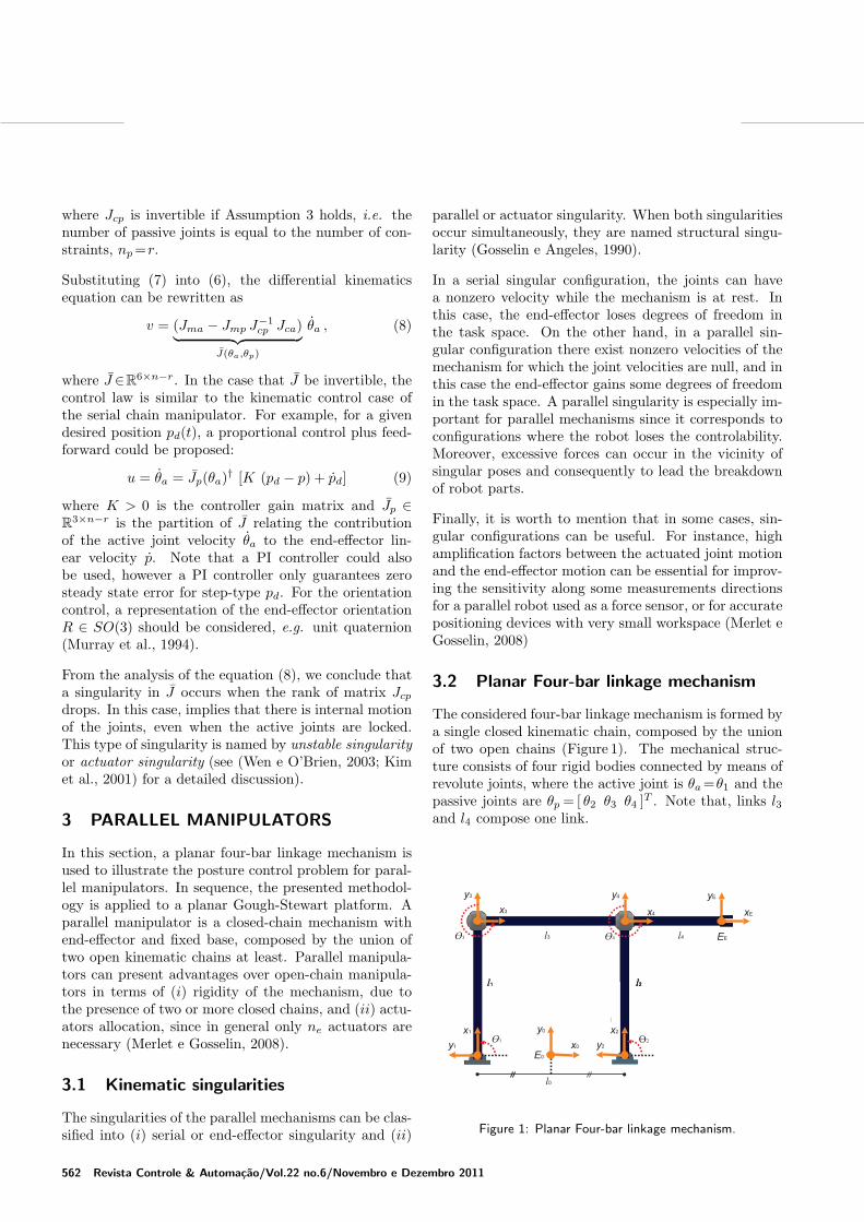
The considered four-bar linkage mechanism is formed bya single closed kinematic chain, composed by the unionof two open chains (Figure 1). The mechanical struc-ture consists of four rigid bodies connected by means ofrevolute joints, where the active joint is θa =θ1 and thepassive joints are θp = [ θ2 θ3 θ4 ]T . Note that, links l3and l4 compose one link.

x1

x3

x2

x0

x4 xE

y0

y1 y2

y3 y4 yE

�2

�4�3

�1

E0

EE

l1l1

l3

l2

l4

l0

l2l2

Figure 1: Planar Four-bar linkage mechanism.


Four-bar linkages are the simplest, least expensive andmost efficient closed-loop kinematic mechanism to per-form a wide variety of complicated motions. Linkage-type mechanisms are primarily used for industrial appli-cations as machine components and tools, automotivesuspensions and bolt cutters.

3.2.1 Forward kinematics

The forward kinematics map of a parallel manipulatoris described by the posture (position and orientation)of the end-effector frame EE with respect to the baseframe E0, derived for each kinematic chain. For parallelmechanisms, the forward kinematics problem is usuallymuch more complex than the inverse kinematics prob-lem, due to the closed loop nature of the mechanism.In order to obtain the forward kinematic an appropri-ate frame Ei for i = 1, · · · , l is attached to i-th link.Thus, the structure equations (or loop equations) of thefour-bar linkage mechanism are given by:

p = p01 + p13 + p3E︸︷︷︸chain 1

= p02 + p24 + p4E︸︷︷︸chain 2

, (10)

φ = θ1 + θ3︸︷︷︸chain 1

= θ2 + θ4︸︷︷︸chain 2

, (11)

where φ ∈ R represents the end-effector orientation (forthe planar case the orientation R is an elementary rota-tion about the z axis, i.e. R = Rz(φ)) and pij ∈R

3 is theposition vector of the origin of frame Ej with respect tothe origin of the frame Ei. The structure equations ofthe mechanism introduce constraints between the jointangles of the manipulator. Considering the planar case,where p∈R

2 and φ∈R, equations (10) and (11) corre-spond to r = 3 constraints. Thus, the four-bar linkagemechanism with n=4 joints has ne = n− r=1 effectivedegrees of freedom. This result can also be obtained byusing the Gruebler’s formula for planar motions (Murrayet al., 1994).

Remark 1 For parallel mechanisms, the number ofpassive joints is always equal to the number of con-straints, that is, np = r. Thus, the vector of jointvariables θ ∈ R

n can be partitioned as (θa, θp), whereθa ∈R

n−r are the active joint variables and θp ∈Rr are

the passive joint variables.

The kinematic constraints of the mechanism allow us tocontrol the end-effector orientation by specifying onlythe angular position of the active joint θa =θ1, and theother joint variables must take on values in order tosatisfy the structure equations. Thus, the passive jointsθp ∈ R

3 can be obtained as a function of active joints

θa ∈R by means of the forward kinematics equation ofthe mechanism, by using the chain 1

p = p01 + p13 + p3E = − l02

�x0 + l1 R01(θ1) �x0 +

(l3 + l4)R01(θ1)R13(θ3) �x0 , (12)

or the chain 2

p = p02 + p24 + p4E =l02

�x0 + l2 R02(θ2) �x0 +

l4 R02(θ2)R24(θ4) �x0 , (13)

where Rij(θi) ∈ SO(3) denotes the orientation of theframe Ej with respect to the frame Ei. Note that, inthis case, Rij is an elementary rotation matrix by anangle θi about the axis z of the frame Ei. After the useof geometric and algebraic identities, the passive jointsθp are obtained by

θ2 = π − arccos(

l20 − l21 + l2d2 l0 ld

)− arccos

(l22 − l23 + l2d

2 l2 ld

),

θ3 = π + arccos(

l21 − l20 + l2d2 l1 ld

)+ arccos

(l23 − l22 + l2d

2 l3 ld

),

θ4 = 2π − arccos(

l22 + l23 − l2d2 l2 l3

),

wherel2d = l20 + l21 − 2lol1 cos(θ1) .

In the case that l3 = l0 and l1 = l2, there always existssolution for θ3 and one has that θ2 = θ1 and θ4 = θ4.

Now, it is possible to obtain the end-effector positionfrom (12) or (13), as well as the end-effector orientationfrom (11), in terms of the active joint θa =θ1.

Remark 2 A more direct technique to solve the in-verse kinematics problem and obtain the passive jointvariables θp is to apply the methods based on Paden-Kahan subproblems, in particular the subproblems 1and 3 (Murray et al., 1994), which are geometricallymeaningful and numerically stable.

3.2.2 Differential kinematics

Analogously, the differential kinematics of a parallel ma-nipulator is computed by considering the various openkinematic chains that compose the mechanism struc-ture. The end-effector velocity v ∈R

3 can be obtainedfrom the time derivative of structure equations, result-ing in a Jacobian matrix for each serial chain

v = S J1

[θ1

θ3

]= S J2

[θ2

θ4

], (14)


where S∈R3×6 is a selection matrix given by:

S =

⎡⎣ 1 0 0 0 0 0

0 1 0 0 0 00 0 0 0 0 1

⎤⎦ , (15)

and the Jacobian matrices J1∈R6×2 and J2∈R

6×2 are4:

J1 =[

�z0 × p1E �z0 × p3E

�z0 �z0

], (16)

J2 =[

�z0 × p2E �z0 × p4E

�z0 �z0

], (17)

with

p1E = l1 R01(θ1) �x0 + p3E , (18)p2E = l2 R02(θ2) �x0 + p4E , (19)p3E = (l3 + l4)R01(θ1)R13(θ3) �x0 , (20)p4E = l4 R02(θ2)R24(θ4) �x0 . (21)

The Jacobian of the mechanism can be rewritten in amore usual form, stacking the Jacobian of each openchain:

[S J1 0

0 S J2

]︸︷︷︸

J

⎡⎢⎢⎣

θ1

θ3

θ2

θ4

⎤⎥⎥⎦

︸︷︷︸θ

=[

II

]︸︷︷︸

A

v , (22)

or equivalentlyJ θ = A v , (23)

where the matrix A ∈ R6×3 has full column rank. Using

this notation, it is possible obtain the constraint Jaco-bian Jc∈R

3×4 and the manipulator Jacobian Jm∈R3×4

by means of:

Jc = A J , Jm = A† J , (24)

where A ∈ R3×6 is the annihilator of A, such that,

A A = 0, and A† ∈ R3×6 is the pseudo-inverse of A,

such that A† A = I. A possible choice is A = [I −I]and A† = [I 0]. From (8), J ∈ R

3×1 can be calculatedby J = Jma − JmpJ

−1cp Jca.

3.2.3 Kinematic control

In this section, the kinematic control approach is used tomodify the posture of the four-bar linkage mechanism inorder to perform a task of interest. Here, we assume thatthe control objective is to drive the current end-effector

4× denotes the vector cross product.

orientation φ to a desired time-varying orientation φd(t),that is,

φ → φd(t) , eφ = φd(t) − φ → 0 , (25)

where eφ∈R is the orientation error.

The control scheme to be designed has to command thevelocity of the active joint θa = θ1 in order to achievethe control objective (25). Then, using a proportionalcontrol law plus feedforward action

u = θa = (J3)−1 ( kφ eφ + φd ) , (26)

where J3 is the third element of J and the orientationerror dynamics is governed by eφ + kφ eφ = 0, providedthat the mechanism motions are away from singular con-figurations. Hence, by a proper choice of kφ as a positiveconstant implies that limt→∞ eφ(t) = 0.

3.3 Planar Gough-Stewart platform

Another usual example of parallel mechanisms is theGough-Stewart platform. Typically, some applicationsof this structure include: aircraft flight simulators, an-tennas and telescopes positioning systems, machine tooland crane technologies, and orthopedic surgery. In thissection, we consider a planar version of the Gough-Stewart platform (Figure 2). The mechanical structureis composed by the union of three open chains andhas nine joints, where three prismatic joints are activeθa = [ d2 d5 d8 ]T , and six revolute joints are passiveθp = [ θ1 θ3 θ4 θ6 θ7 θ9 ]T . We can obtain the effec-tive degrees of freedom for this mechanism by apply-ing the Gruebler’s formula for planar motions (Murrayet al., 1994):

ne = 3(i − n) +n∑

j=1

fi = 3 , (27)

where i is the number of mobile links in the mechanism,n is the number of joints and fi is the number of degreesof freedom for the i-th joint. From (27), we conclude thatthe mechanism has three effective degrees of freedom,which allow us to control the position and orientationof the platform respectively, in order to perform planarpositioning tasks.

3.3.1 Forward kinematics

The solution of the forward kinematics problem for aGough-Stewart platform is a very difficult task due tothe large number and complicated form of the con-straints. From the length of the links, we can solve the


x0

y0

�1

E0

�4

x4

y4y4

x1

y1

x2

y2

x5

y5

xS

yS

x6

y6

x3

y3

x8

y8

x9

y9

y7

x7

�3 �6

�9

�7

ES

d2 d5

d8

Figure 2: Planar Gough-Stewart platform.

structure equations to find the joint angles and then de-termine the platform posture. The forward kinematicsmap of the mechanism can be obtained by calculatingthe position and orientation of the frame Es with re-spect to the base frame E0, specified for each kinematicchain:

ps = p01+p13+p3s︸︷︷︸chain 1

=p04+p46+p6s︸︷︷︸chain 2

=p07+p79+p9s︸︷︷︸chain 3

,

φs = θ1 + θ3︸︷︷︸chain 1

= θ4 + θ6︸︷︷︸chain 2

= θ7 + θ9︸︷︷︸chain 3

, (28)

where φs ∈ R represents the platform orientation (forthe planar case the orientation R is an elementary rota-tion about the z axis, i.e. R = Rz(φ)) p01, p04 and p07

are assumed to be constant and known, with

p03 = d2 R01(θ1) �x0 , (29)p3s = l R01(θ1)R13(θ3) �x0 , (30)p0s = p03 + p3s , (31)p46 = d5 R04(θ4) �x0 , (32)p6s = l R04(θ4)R46(θ6) �x0 , (33)p4s = p46 + p6s , (34)p79 = d8 R07(θ7) �x0 , (35)p9s = l R07(θ7)R79(θ9) �x0 , (36)p7s = p79 + p9s . (37)

Note that, considering a parallel mechanism, the struc-ture equations allow the formulation of a system of equa-tions, containing the kinematic constraint of the mech-anism, that can be used to calculate the angle of thepassive joints θp in terms of the angle of the active jointsθa. The solution for this system of equations can be triv-ial, as in the case of the four-bar linkage mechanism, orbe complex, for the case of the Gough-Stewart platformpresented in this section.

The forward kinematics map of the planar Gough-Stewart platform can be obtained by using the method-ology presented in (Zhang e Gao, 2006), where thesystem with six equations and six unknowns variables(θp∈R

6) is solved by means of the Ritt-Wu’s character-istic set method.

3.3.2 Differential kinematics

The differential kinematics equation is obtained consid-ering the various open chains, which compose the mech-anism structure. The platform velocity can be derivedby differentiating the structure equation, obtaining aJacobian matrix for each chain:

v = SJ1

⎡⎣ θ1

d2

θ3

⎤⎦=SJ2

⎡⎣ θ4

d5

θ6

⎤⎦=SJ3

⎡⎣ θ7

d8

θ9

⎤⎦ , (38)

where vT = [pTs φs], S ∈ R

3×6 is the selection matrixgiven in (15). and the Jacobian matrices J1 ∈ R

6×3,J2∈R

6×3 and J3∈R6×3 are:

J1 =[

�z0 × p0s R01(θ1) �x0 �z0 × p3s

�z0 0 �z0

], (39)

J2 =[

�z0 × p4s R04(θ4) �x0 �z0 × p6s

�z0 0 �z0

], (40)

J3 =[

�z0 × p7s R07(θ7) �x0 �z0 × p9s

�z0 0 �z0

]. (41)

It is important to note that the Jacobians J1, J2 and J3

depends on the angles of the active and passive joints.For the planar Gough-Stewart platform, it is not triv-ial to calculate the position of the passive joints θp interms of the active joints θa by using its forward kine-matics equations. However, in order to obtain the dif-ferential kinematics equations of the system, the posi-tion of the passive joints can be obtained, for instance,by integrating the velocity of the passive joints (7), i.e.θp =

∫J−1

cp Jcaθadτ .


The Jacobian can be rewritten in a more conventionalway, stacking the Jacobians for each open chain.

⎡⎣ S J1 0 0

0 S J2 00 0 S J3

⎤⎦

︸︷︷︸J

⎡⎢⎢⎢⎢⎢⎢⎢⎢⎢⎢⎢⎢⎢⎣

θ1

d2

θ3

θ4

d5

θ6

θ7

d8

θ9

⎤⎥⎥⎥⎥⎥⎥⎥⎥⎥⎥⎥⎥⎥⎦

︸︷︷︸θ

=

⎡⎣ I

II

⎤⎦

︸︷︷︸A

v , (42)

or, equivalentlyJ θ = A v , (43)

where the matrix A ∈ R9×3 has full column rank. By

using this notation, it is possible to obtain the constraintJacobian Jc∈R

6×9 and the manipulator Jacobian Jm∈R

3×9 by means of:

Jc = A J , Jm = A† J , (44)

where a possible choice for A and A† is given by A =[I −I 0] and A† = [I 0 0].

As previously stated, from (8) and by using Jc and Jm,the differential kinematics equation of the mechanismis given by v = J θa, where J ∈ R

3×3 is given by J =Jma − JmpJ

−1cp Jca.

3.3.3 Kinematic control

In accordance with the Section 3.2.3, the kinematic con-trol approach can be used again to modify the pos-ture of the platform, in order to perform a planarpositioning task. Here, we assume that the controlobjective is to follow a desired time-varying posturexsd(t) = [pT

sd(t) φsd(t)]T from the current platform pos-ture xs = [pT

s φs]T , that is,

xs → xsd(t) , es = xsd − xs → 0 , (45)

where es∈R3 is the platform posture error.

Now, the control scheme to be designed has to commandthe velocity of the active joint θa =[ d2 d5 d8 ]T , in orderto achieve the control objective (45). Then, using acontrol law based on a proportional with feedforwardaction

u = θa = J−1 (Ks es + xsd) , (46)where Ks is the controller gain matrix, the posture errordynamics is governed by es+Ks es =0, provided that theplatform motions are away from singular configurations.Hence, by a proper choice of Ks as a positive definitematrix, implies that limt→∞ es(t) = 0.

4 COOPERATING MANIPULATORS

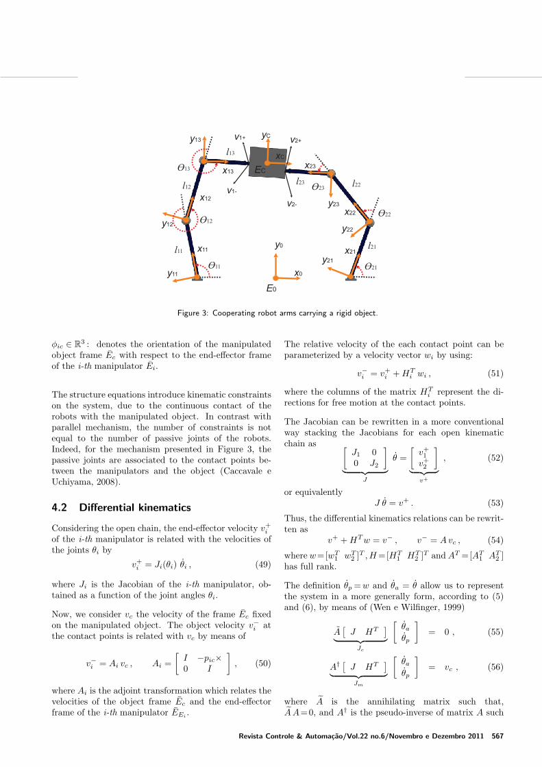
In the robotics area, many tasks are difficult or even im-possible to be performed by using a single robot. Typ-ical examples include: positioning of heavy payloads,complex assembly of multiple parts or manipulation offlexible objects. These tasks become feasible with theemployment of more than one robot operating cooper-atively (Caccavale e Uchiyama, 2008). The mechanismpresented in Figure 3 is constituted by a closed kine-matic chain, where all joints are active, and considers acontinuous contact of the end-effector with the manip-ulated object.

In general, cooperating robots correspond to over-actuated systems or redundant systems, where the ef-fective degrees of freedom are higher than those strictlyrequired to perform a given task (ne >nt). This capac-ity increases the dexterity of the mechanism, and can beused to avoid joint limits, singularities and workspaceobstacles, as well as to minimize the energy consump-tion and joint torques or to optimize a performance in-dex (e.g., manipulability).

4.1 Forward kinematics

The forward kinematics map for a redundant roboticsystem composed by two cooperating robots can be de-scribed by means of the posture of the frame attachedto the manipulated object Ec with respect to the baseframe E0, determined for each manipulator that belongsto the robotic system. The structure equations of theredundant mechanism illustrated in Figure 3 are givenrespectively by

pc = p01 + p1c︸︷︷︸robot 1

= p02 + p2c︸︷︷︸robot 2

, (47)

φc = φ01 + φ1c︸︷︷︸robot 1

= φ02 + φ2c︸︷︷︸robot 2

, (48)

where

p0i∈R3 : is the position vector of the end-effector frame

of the i-th manipulator Ei with respect to the base frameE0.

pic ∈R3 : is the position vector of the manipulated ob-

ject frame Ec with respect to the end-effector frame ofthe i-th manipulator Ei.

φ0i ∈ R3 : denotes the orientation of the end-effector

frame of the i-th manipulator Ei with respect to thebase frame E0.


x0

E0

y21

�11

EC

x21

x22

x23x13

x12

x11y0

y22

y23

y13

y12

y11

yC

xC

�12

�13

�23

�22

�21

l11

l12

l13

l23 l22

l21

v1+ v2+

v1-

v2-

Figure 3: Cooperating robot arms carrying a rigid object.

φic ∈ R3 : denotes the orientation of the manipulated

object frame Ec with respect to the end-effector frameof the i-th manipulator Ei.

The structure equations introduce kinematic constraintson the system, due to the continuous contact of therobots with the manipulated object. In contrast withparallel mechanism, the number of constraints is notequal to the number of passive joints of the robots.Indeed, for the mechanism presented in Figure 3, thepassive joints are associated to the contact points be-tween the manipulators and the object (Caccavale eUchiyama, 2008).

4.2 Differential kinematics

Considering the open chain, the end-effector velocity v+i

of the i-th manipulator is related with the velocities ofthe joints θi by

v+i = Ji(θi) θi , (49)

where Ji is the Jacobian of the i-th manipulator, ob-tained as a function of the joint angles θi.

Now, we consider vc the velocity of the frame Ec fixedon the manipulated object. The object velocity v−

i atthe contact points is related with vc by means of

v−i = Ai vc , Ai =

[I −pic×0 I

], (50)

where Ai is the adjoint transformation which relates thevelocities of the object frame Ec and the end-effectorframe of the i-th manipulator EEi

.

The relative velocity of the each contact point can beparameterized by a velocity vector wi by using:

v−i = v+

i + HTi wi , (51)

where the columns of the matrix HTi represent the di-

rections for free motion at the contact points.

The Jacobian can be rewritten in a more conventionalway stacking the Jacobians for each open kinematicchain as [

J1 00 J2

]︸︷︷︸

J

θ =[

v+1

v+2

]︸︷︷︸

v+

, (52)

or equivalentlyJ θ = v+ . (53)

Thus, the differential kinematics relations can be rewrit-ten as

v+ + HT w = v− , v− = Avc , (54)

where w=[wT1 wT

2 ]T ,H =[HT1 HT

2 ]T and AT =[AT1 AT

2 ]has full rank.

The definition θp = w and θa = θ allow us to representthe system in a more generally form, according to (5)and (6), by means of (Wen e Wilfinger, 1999)

A[

J HT]

︸︷︷︸Jc

[θa

θp

]= 0 , (55)

A† [J HT

]︸︷︷︸

Jm

[θa

θp

]= vc , (56)

where A is the annihilating matrix such that,AA=0, and A† is the pseudo-inverse of matrix A such


that A† A = I. A possible choice for A and A† is givenby A = [A2 −A1] and A† = [A−1

1 0].

Note that, from (8) and by using Jc and Jm, the differ-ential kinematics equation of the object is given by vc =J θa, where J ∈ R

3×6 is given by J = Jma−JmpJ−1cp Jca.

4.3 Selection matrices

The kinematic constraints of the robotic system due tothe contact points are properly represented by means ofa selection matrix H. This matrix acts as a filter thataccepts or rejects components of motion at the contactpoint.

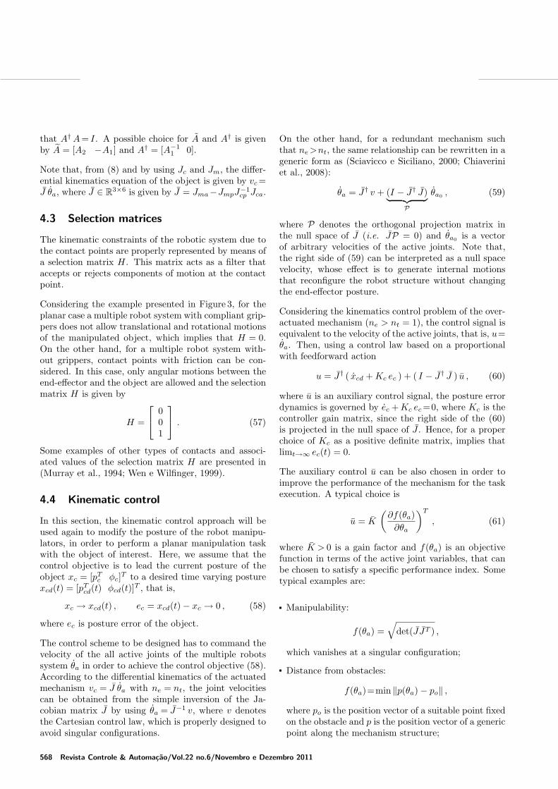
Considering the example presented in Figure 3, for theplanar case a multiple robot system with compliant grip-pers does not allow translational and rotational motionsof the manipulated object, which implies that H = 0.On the other hand, for a multiple robot system with-out grippers, contact points with friction can be con-sidered. In this case, only angular motions between theend-effector and the object are allowed and the selectionmatrix H is given by

H =

⎡⎣ 0

01

⎤⎦ . (57)

Some examples of other types of contacts and associ-ated values of the selection matrix H are presented in(Murray et al., 1994; Wen e Wilfinger, 1999).

4.4 Kinematic control

In this section, the kinematic control approach will beused again to modify the posture of the robot manipu-lators, in order to perform a planar manipulation taskwith the object of interest. Here, we assume that thecontrol objective is to lead the current posture of theobject xc = [pT

c φc]T to a desired time varying posturexcd(t) = [pT

cd(t) φcd(t)]T , that is,

xc → xcd(t) , ec = xcd(t) − xc → 0 , (58)

where ec is posture error of the object.

The control scheme to be designed has to command thevelocity of the all active joints of the multiple robotssystem θa in order to achieve the control objective (58).According to the differential kinematics of the actuatedmechanism vc = J θa with ne = nt, the joint velocitiescan be obtained from the simple inversion of the Ja-cobian matrix J by using θa = J−1 v, where v denotesthe Cartesian control law, which is properly designed toavoid singular configurations.

On the other hand, for a redundant mechanism suchthat ne >nt, the same relationship can be rewritten in ageneric form as (Sciavicco e Siciliano, 2000; Chiaveriniet al., 2008):

θa = J† v + (I − J† J)︸︷︷︸P

θa0 , (59)

where P denotes the orthogonal projection matrix inthe null space of J (i.e. JP = 0) and θa0 is a vectorof arbitrary velocities of the active joints. Note that,the right side of (59) can be interpreted as a null spacevelocity, whose effect is to generate internal motionsthat reconfigure the robot structure without changingthe end-effector posture.

Considering the kinematics control problem of the over-actuated mechanism (ne > nt = 1), the control signal isequivalent to the velocity of the active joints, that is, u=θa. Then, using a control law based on a proportionalwith feedforward action

u = J† ( xcd + Kc ec ) + ( I − J† J ) u , (60)

where u is an auxiliary control signal, the posture errordynamics is governed by ec + Kc ec =0, where Kc is thecontroller gain matrix, since the right side of the (60)is projected in the null space of J . Hence, for a properchoice of Kc as a positive definite matrix, implies thatlimt→∞ ec(t) = 0.

The auxiliary control u can be also chosen in order toimprove the performance of the mechanism for the taskexecution. A typical choice is

u = K

(∂f(θa)

∂θa

)T

, (61)

where K > 0 is a gain factor and f(θa) is an objectivefunction in terms of the active joint variables, that canbe chosen to satisfy a specific performance index. Sometypical examples are:

Manipulability:

f(θa) =√

det(J JT ) ,

which vanishes at a singular configuration;

Distance from obstacles:

f(θa)=min ‖p(θa) − po‖ ,

where po is the position vector of a suitable point fixedon the obstacle and p is the position vector of a genericpoint along the mechanism structure;


Joint limits: θami<θai

<θaMi,

f(θa) = − 12n

n∑i=1

(θai

− θai

θaMi− θami

)2

,

where θaMiand θami

denote the maximum and min-imum joint limits respectively, and θai

is the averagevalue between θaMi

and θami.

4.5 Kinematic singularities

The posture of the manipulator, obtained as a functionof the joint angles θ, is said to be singular if the Jacobianmatrix J has not full rank. From (8) we can observe thatwhen the robot is not in a singular configuration it ispossible to generate velocities and accelerations with theend-effector in certain directions. In order to evaluatethe linear relation (8), the singular value decomposition(SVD) method can be used to obtain the rank of theJacobian J and study quasi-linear mappings (Chiaveriniet al., 2008).

In this context, the SVD of the Jacobian can be repre-sented by

J = U ΣV T =m∑

i=1

σi ui vTi , (62)

where U ∈ Rm×m is the orthogonal matrix of output

singular vectors ui, V ∈Rn×n is the orthogonal matrix

of the input singular vectors vi, and Σ ∈ diag(D, 0) ∈R

m×n is the matrix whose diagonal submatrix D ∈R

m×m contains the singular values σi of the matrix J .Considering that rank(J)=k, we have

σ1 ≥ σ2 ≥ · · · ≥ σr ≥ σk+1 = ... = 0;

R(J) = span{u1 , · · · , uk};

N (J) = span{vk+1 , · · · , vn},

where R(J) denotes the range space of J and N (J)denotes the null space of J . Then, the following analysisin terms of the rank of matrix J can be established:

full rank (k=m): (i) σi �=0 , i=1, · · · , m , (ii) R(J) ∈R

m , (iii) N (J) ∈ Rn−m.

rank deficient (k < m): (i) σi �= 0 , i = 1, · · · , k , (ii)R(J) ∈ R

k ⊂ Rm , (iii) N (J) ∈ R

n−k.

An interpretation of this analysis in terms of velocitiesis presented as follows (Chiaverini et al., 2008):

Feasible velocities: For each configuration of the ma-nipulator, R(J) is the set of the end-effector velocitiesthat can be generated by all possible joint velocities θ,and are called the feasible velocities of the end-effector.The base of R(J) is obtained by the first k outputsingular vectors, which represent the independent lin-ear combinations of the single components of the end-effector velocities. Then, the effect of a singularityis to decrease the dimension of R(J), by eliminatinga linear combination of the components of the end-effector velocities that belong to the feasible velocitiesspace.

Null space velocities: For each configuration of the ma-nipulator, N (J) is the set of joint velocities θ, that donot produce any end-effector velocity, and are calledthe null space velocities. The base of N (J) is obtainedby the last n−k input singular vector, which representthe independent linear combinations of the velocitiesat each joint. The effect of a singularity is to increasethe dimension of N (J), by adding more one indepen-dent linear combination of the joint velocities, whichproduces a zero end-effector velocity.

5 NONHOLONOMIC ROBOTS

Other examples of robotic systems with constraintsare the wheeled mobile robots and multifingered robothands. In general, a constraint is said to be holonomicif it restricts the robot motion to a smooth hypersurfaceof the configuration space. Holonomic constraints canbe represented locally as algebraic constraints on therobot configuration space ci(θ) = 0 for i = 1, · · · , r. Onthe other hand, if the allowable motions of the roboticsystem are restricted by the velocity constraint in theform

A(θ) θ = 0 ,

where A∈Rr×n represents a set of r velocity constraints

that are not integrable, the constraint is said to be non-holonomic.

These constraints arise in robotic systems such aswheeled mobile robots and multifingered robot hands,where angular moment is conserved, as well as rollingcontact is involved. Nonholonomic constraints occurwhen the instantaneous velocities of the robotic systemare restricted to an n − r dimensional subspace, butthe set of reachable configurations is not constrained tosome n − r dimensional hypersurface in the robot con-figuration space (Murray et al., 1994).

Analogously, the challenge is how to consider the prob-lem from the control point of view in order to define the


system velocities which satisfy the constraints. Con-sidering A∈R

n×(n−r) the annihilator of matrix A, theallowable trajectories of the system can be written aspossible solutions of the control system

θ = A(θ)u , (63)

where u ∈ Rn−r is the control signal to be designed in

order to drive the current configuration θ ∈ Rn to a

desired time-varying configuration θd(t)∈Rn.

The main difficulty arises from the fact that this sys-tem has not right pseudoinverse, since A contains morerows than columns, and the linearized system is notcontrollable (Murray et al., 1994). However, there aredifferent approaches to accomplish the control of thissystems, that consists of both physical remove of thenonholonomic constraints and the application of ad-vanced control tools based on nonlinear control the-ory, differential geometry or optimal control (Murrayet al., 1994; Bloch, 2003).

6 SIMULATION RESULTS

In this section, we present simulations results obtainedfrom a four-bar linkage mechanism, a planar Gough-Stewart platform and two cooperating robot arms com-posed by four revolution joints. The adopted struc-tural dimensions are: l0 = 1 m, l1 = 1.2 m, l2 = 1.4 m,l3 = 0.6 m, l4 = 1.4 m, l = 5 m, l11 = l12 = 1.2 m,l21 = l22 = 1 m and l13 = l23 = 0.6 m. For the con-sidered lengths of links, we define the following limits:θ1 ∈ [ 0.72 2.27 ] rad and φ ∈ [ 5.88 7.89 ] rad. The con-trol parameters are: kφ = 50 rad s−1 and Ks = Kc =diag(50mm s−1, 50mm s−1, 1 rad s−1).

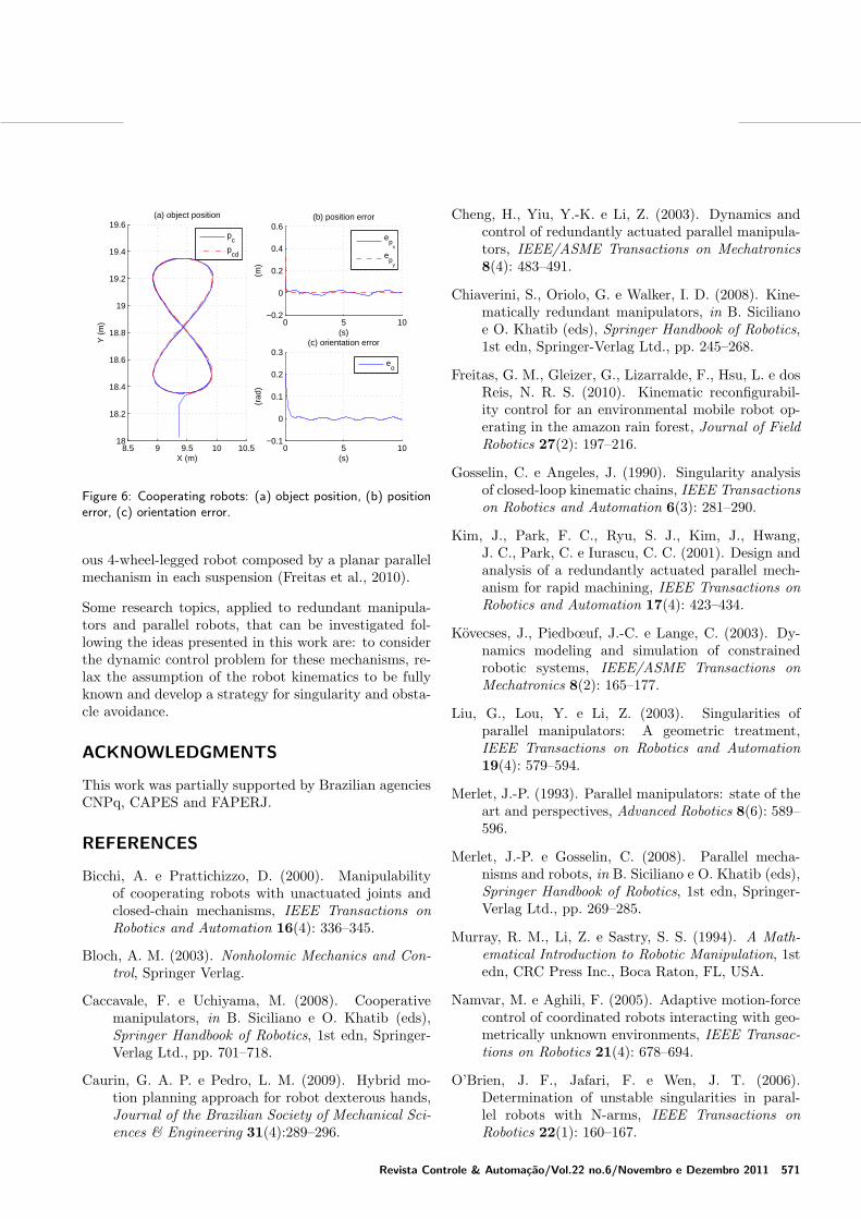
The time evolution for the orientation error of the four-bar linkage mechanism for train of ramps and sinusoidalreferences are shown in Figures 4(b) and 4(d) respec-tively. Figures 5(b) and 5(c) illustrate the time evolu-tion of the position error and orientation error for theGough-Stewart platform. The position and orientationerrors for the object handled by two cooperating robotsare shown in Figures 6(b) and 6(c) respectively. Thetrajectory following for all mechanisms are presented re-spectively in Figures 4(a)-4(c), 5(a) and 6(a), where itcan observe that a good performance is achieved by us-ing the presented methodology.

7 CONCLUSIONS AND PERSPECTIVES

This work presents a control methodology for roboticsystems under kinematics constraints based on a novelscheme in the robotics literature, which regards the con-straints on passive joint velocities. The key idea is to

0 5 106.5

7

7.5(a) end−effector orientation

(s)

(rad

)

φ

d

φ

0 5 10−0.06

−0.04

−0.02

0

0.02(b) orientation error

(s)

(rad

)

0 5 106

6.5

7

7.5(c) end−effector orientation

(s)(r

ad)

0 5 10−0.06

−0.04

−0.02

0

0.02(d) orientation error

(s)

(rad

)

φd

φ

Figure 4: Four-bar linkage mechanism: (a) end-effector orien-tation: train of ramps, (b) orientation error, (c) end-effectororientation: sinusoidal wave form, (d) orientation error.

10 12 14 16 1810

11

12

13

14

15

16

17

18(a) platform position

X (m)

Y (

m)

p

pd

0 5 10−1.5

−1

−0.5

0

0.5

(s)

(m)

(b) position error

ep

x

ep

y

0 5 10−1.5

−1

−0.5

0

0.5(c) orientation error

(s)

(rad

)

Figure 5: Gough-Stewart platform: (a) platform position, (b)position error, (c) orientation error.

consider the kinematic constraints of the mechanismfrom their structure equations, rather than explicitlyinvoking the constraint equation. In order to show theapplicability of the presented methodology, simulationsresults were included for a four-bar linkage mechanism,a planar Gough-Stewart platform and two cooperatingrobots.

It is worth mentioning that the methodology presentedin this section 3 is implemented in the suspension controlsystem of the Environmental Hybrid Robot, recently de-veloped by CENPES/Petrobras, which is an amphibi-


8.5 9 9.5 10 10.518

18.2

18.4

18.6

18.8

19

19.2

19.4

19.6(a) object position

X (m)

Y (

m)

p

c

pcd

0 5 10−0.2

0

0.2

0.4

0.6

(s)

(m)

(b) position error

e

px

ep

y

0 5 10−0.1

0

0.1

0.2

0.3

(s)

(rad

)

(c) orientation error

e

o

Figure 6: Cooperating robots: (a) object position, (b) positionerror, (c) orientation error.

ous 4-wheel-legged robot composed by a planar parallelmechanism in each suspension (Freitas et al., 2010).

Some research topics, applied to redundant manipula-tors and parallel robots, that can be investigated fol-lowing the ideas presented in this work are: to considerthe dynamic control problem for these mechanisms, re-lax the assumption of the robot kinematics to be fullyknown and develop a strategy for singularity and obsta-cle avoidance.

ACKNOWLEDGMENTS

This work was partially supported by Brazilian agenciesCNPq, CAPES and FAPERJ.

REFERENCES

Bicchi, A. e Prattichizzo, D. (2000). Manipulabilityof cooperating robots with unactuated joints andclosed-chain mechanisms, IEEE Transactions onRobotics and Automation 16(4): 336–345.

Bloch, A. M. (2003). Nonholomic Mechanics and Con-trol, Springer Verlag.

Caccavale, F. e Uchiyama, M. (2008). Cooperativemanipulators, in B. Siciliano e O. Khatib (eds),Springer Handbook of Robotics, 1st edn, Springer-Verlag Ltd., pp. 701–718.

Caurin, G. A. P. e Pedro, L. M. (2009). Hybrid mo-tion planning approach for robot dexterous hands,Journal of the Brazilian Society of Mechanical Sci-ences & Engineering 31(4):289–296.

Cheng, H., Yiu, Y.-K. e Li, Z. (2003). Dynamics andcontrol of redundantly actuated parallel manipula-tors, IEEE/ASME Transactions on Mechatronics8(4): 483–491.

Chiaverini, S., Oriolo, G. e Walker, I. D. (2008). Kine-matically redundant manipulators, in B. Sicilianoe O. Khatib (eds), Springer Handbook of Robotics,1st edn, Springer-Verlag Ltd., pp. 245–268.

Freitas, G. M., Gleizer, G., Lizarralde, F., Hsu, L. e dosReis, N. R. S. (2010). Kinematic reconfigurabil-ity control for an environmental mobile robot op-erating in the amazon rain forest, Journal of FieldRobotics 27(2): 197–216.

Gosselin, C. e Angeles, J. (1990). Singularity analysisof closed-loop kinematic chains, IEEE Transactionson Robotics and Automation 6(3): 281–290.

Kim, J., Park, F. C., Ryu, S. J., Kim, J., Hwang,J. C., Park, C. e Iurascu, C. C. (2001). Design andanalysis of a redundantly actuated parallel mech-anism for rapid machining, IEEE Transactions onRobotics and Automation 17(4): 423–434.

Kövecses, J., Piedbœuf, J.-C. e Lange, C. (2003). Dy-namics modeling and simulation of constrainedrobotic systems, IEEE/ASME Transactions onMechatronics 8(2): 165–177.

Liu, G., Lou, Y. e Li, Z. (2003). Singularities ofparallel manipulators: A geometric treatment,IEEE Transactions on Robotics and Automation19(4): 579–594.

Merlet, J.-P. (1993). Parallel manipulators: state of theart and perspectives, Advanced Robotics 8(6): 589–596.

Merlet, J.-P. e Gosselin, C. (2008). Parallel mecha-nisms and robots, in B. Siciliano e O. Khatib (eds),Springer Handbook of Robotics, 1st edn, Springer-Verlag Ltd., pp. 269–285.

Murray, R. M., Li, Z. e Sastry, S. S. (1994). A Math-ematical Introduction to Robotic Manipulation, 1stedn, CRC Press Inc., Boca Raton, FL, USA.

Namvar, M. e Aghili, F. (2005). Adaptive motion-forcecontrol of coordinated robots interacting with geo-metrically unknown environments, IEEE Transac-tions on Robotics 21(4): 678–694.

O’Brien, J. F., Jafari, F. e Wen, J. T. (2006).Determination of unstable singularities in paral-lel robots with N-arms, IEEE Transactions onRobotics 22(1): 160–167.


Pazelli, T., Terra, M. H. e Siqueira, A. A. (2011). Exper-imental investigation on adaptive robust controllerdesigns applied to a free-floating space manipula-tor, Control Engineering Practice 1(1): 1–14.

Pietsch, I. T., Krefft, M., Becker, O. T., Bier, C. C. eHesselbach, J. (2005). How to reach the dynamiclimits of parallel robots ? an autonomous controlapproach, IEEE Transactions on Automation Sci-ence and Engineering 2(4): 369–380.

Ribeiro, L., Guenther, R. e Martins, D. (2008). Screw-based relative jacobian for manipulators cooperat-ing in a task, ABCM Symposium Series in Mecha-tronics 3: 276–285.

Rosario, J. M., Dumur, D. e Machado, J. T. A. (2007).Control of a 6-DOF parallel manipulator througha mechatronic approach, Journal of Vibration andControl 13(9): 1431–1446.

Sciavicco, L. e Siciliano, B. (2000). Modelling andControl of Robot Manipulators, 2nd edn, Springer-Verlag Ltd., New York, NY, USA.

Siciliano, B. (1990). Kinematic control of redundantrobot manipulators: A tutorial, Journal of Intelli-gent and Robotic Systems 3(3): 201–212.

Siciliano, B., Sciavicco, L., Villani, L. e Oriolo, G.(2008). Robotics: Modelling, Planning and Con-trol, 1st edn, Springer-Verlag London Ltd.

Simas, H., Guenther, R., da Cruz, D. F. M. e Mar-tins, D. (2009). A new method to solve robot in-verse kinematics using Assur virtual chains, Robot-ica 27: 1017–1022.

Tinos, R., Terra, M. H. e Ishihara, J. Y. (2006). Motionand force control of cooperative robotic manipu-lators with passive joints, IEEE Transactions onControl System Technology 14(4): 725–734.

Wen, J. T. e O’Brien, J. F. (2003). Singularitiesin three-legged platform-type parallel mechanisms,IEEE Transactions on Robotics and Automation19(4): 720–727.

Wen, J. T.-Y. e Wilfinger, L. S. (1999). Kinematic ma-nipulability of general constrained rigid multibodysystems, IEEE Transactions on Robotics and Au-tomation 15(3): 558–567.

Zhang, G.-F. e Gao, X.-S. (2006). Planar generalizedstewart platforms and their direct kinematics, inH. Hong e D. Wang (eds), Automated Deductionin Geometry, Vol. 3763 of Lecture Notes in Com-puter Science, Springer-Verlag Berlin / Heidelberg,pp. 198–211.


Documents

KINEMATIC CONTROL OF CONSTRAINED ROBOTIC SYSTEMS …gfreitas/documentos/gustavo_sba2011.pdf · mecanismos a partir de suas equações estruturais, ao in-vés de usar explicitamente