Modeling ant foraging: a chemotaxis approach withpheromones and trail formation

Paulo AmorimInstituto de Matemática, Universidade Federal do Rio de Janeiro, Av. Athos da Silveira

Ramos 149, Centro de Tecnologia - Bloco C, Cidade Universitária - Ilha do Fundão, CaixaPostal 68530, 21941-909 Rio de Janeiro, RJ - Brasil

Abstract

We consider a continuous mathematical description of a population of ants andsimulate numerically their foraging behavior using a system of partial differentialequations of chemotaxis type. We show that this system accurately reproducesobserved foraging behavior, especially spontaneous trail formation and efficientremoval of food sources. We show through numerical experiments that trailformation is correlated with efficient food removal. Our results illustrate theemergence of trail formation from simple modeling principles.

Keywords: Ant foraging, Chemotaxis, Pheromones, Mathematical biology,Numerical simulation, Mechanistic models, Animal movement,Reaction-diffusion equations.2010 MSC: 92D-40, 92D-50, 35K-57

1. Introduction

Ant foraging is among the most interesting emergent behaviors in the socialinsects. Perhaps the most striking aspect of ant foraging is how individualsfollowing simple behavioral rules based on local information produce complex,organized and seemingly intelligent strategies at the population level. As such,ant foraging (along with most other activities of an ant colony) is a primeexample of so-called emergent behavior.

It has long been known that one of the main forms of communication amongants is the use of pheromones. These are chemical compounds which individualants secrete and deposit on the substrate and which in effect are used as ameans of communication between ants, transmitting a variety of messages suchas alarm, presence of food, or providing colony-specific olfactory signatures usedto identify nest-mates.

Email address: paulo@im.ufrj.br (Paulo Amorim)URL: http://www.im.ufrj.br/∼paulo/ (Paulo Amorim)

Preprint submitted to Elsevier October 1, 2021

arX

iv:1

409.

3808

v3 [

nlin

.AO

] 2

2 Ju

n 20

15

Among the many documented functions of ant pheromones, we are interestedin their role as a chemical trail indicating the direction to a food source. Manyspecies of ants, especially trail-forming ones, are known to lay a pheromoneas they travel from the food source back to nest. The main attribute of thispheromone is that it is attractive to other ants, who tend to follow the directionof increasing concentration of the chemical. These ants will then reach thefood source and return to the nest while laying pheromone themselves, thusreinforcing the chemical trail in a positive feedback loop. This results in theformation of well defined trails leading from the nest to the food source, allowingfor an efficient transport of the food to the nest. Thus, pheromones play a majorrole in food foraging, where they are widely used (among other strategies) torecruit nest mates to new food sources.

It is clear that the effective simulation and modeling of trail-laying andforaging behavior of ants is a crucial aspect in the understanding of ant ecology.Indeed, for invasive species such as the Fire Ant Solenopsis invicta [46] foragingis, next to reproduction, the most important activity of the colony, and thesole means by which it can ensure its nourishment. A better understandingof foraging dynamics is bound to contribute to a more complete picture ofant ecology. Aside from the scientific value of such knowledge, a thoroughunderstanding of ant behavior is essential in defining appropriate policies inthose cases (as with S. invicta [46] or the Pharaoh’s ant Monomorium pharaonis[20]) where ant species are considered pests.

The entomological research body on ants, their behavior, and their olfactorymeans of communication is vast. Here, we content ourselves with citing someseminal works, as well as some more recent investigations with special relevanceto our analysis. For a general reference on myrmecology (the branch of ento-mology that deals with ants), we refer to the encyclopedic book by Hölldoblerand Wilson [17]. Therein may be found many relevant references up to 1990.The paper [38] contains an overview of the chemical study of pheromones. Con-cerning the trail-laying behavior of ants, and foraging in general, we refer to[5, 8, 10, 11, 12, 36, 37, 42, 43, 47, 49, 48, 50, 55, 56, 57], and the referencestherein, although of course many other papers could be cited.

Concerning the computational simulation of ant trail-laying, we refer to [7,9, 12, 24, 40, 41, 42, 51, 52, 54], although again this list is far from complete.See especially [7] for a recent approach involving directed pheromones, and anexcellent, up-to-date review of available numerical and modeling strategies forant foraging. We encourage the reader to consult that paper for an informativediscussion and overview of the state of the art in ant trail-laying simulations.

Let us just point out that, as observed in [7], ant foraging simulations havein the past been mostly restricted to individual-based, or cellular automaton,models. That approach is certainly fruitful, but is generally limited to relativelysmall populations of ants, as well as somewhat restrictive modeling setups.

From what our bibliographical research could gather, only the work [51]presents a PDE model which (as our own) divides the ant population into twokinds, namely ants leaving the nest and ants returning to the nest (see also[24], where the population is also divided in two different groups). However, the

2

setting in [51] is highly simplified, being one-dimensional, so no trail formationoccurs, and the system proposed in that work is only explored numerically in asimplified ODE version.

Let us also refer to the work [30], where a model for the dispersal of leaf-cutter ants is presented using PDEs. However, in that work trail-laying is nottaken into account.

Thus, to the best of our knowledge, the present work is the first to considerthe modeling and simulation of the whole cycle of food foraging by ants, compris-ing random foraging, discovery and transport of food, recruitment, formation oftrails and fading of trails upon exhaustion of the food sources.1

An outline of the paper follows. In Section 2, we motivate the use of themathematical framework of chemotaxis to model ant foraging. Next, in Sec-tion 3, we present our modeling assumptions derived from an analysis of themyrmecological literature, and deduce our model. In Section 4, we presentand discuss various numerical simulations. In Section 5, we perform a parame-ter space exploration and discuss some consequences and possible experimentalvalidations of the model. In Section 6 we draw some conclusions from our work,discuss some of its limitations, and suggest further lines of inquiry. Finally, theAppendixes deal with the nondimensionalization procedure and the details ofthe numerical scheme.

The main results of this paper were announced in [1].

2. Modeling ant foraging

Many species of ants use recruitment of nest mates through chemical signalsin order to efficiently exploit food sources. The goal is to concentrate the mostindividuals possible in a small region in space and time where the food sourceis located. This minimizes the risk of predation of the ants themselves and theremoval of the food source by other foragers. To this end, eusocial insects haveevolved several strategies, of which trail formation is one of the most well-known[17, Ch.10].

Ants lay trails by depositing pheromones on the substrate, usually by press-ing their sting against the substrate. Pheromones are chemical compounds thatcan diffuse through the substrate or through the air [8] and which the ants detectthrough their antennae. Importantly, ants can discern changes in concentrationof the pheromone by measuring the difference in concentration between eachantenna (see [7] and the references therein), thus allowing them to follow chem-ical gradients. A thorough description of foraging behavior for the fire ant S.saevissima can be found in [55, 56].

Chemotaxis. In this work, we study ant foraging behavior from the mathemat-ical point of view of chemotaxis. The term chemotaxis is used to describe phe-nomena in which the movement of an agent (usually a cell or bacteria) is affected

1As this work went to press, we learned of the paper [6], which proposes a system sharingmany similarities with our own.

3

by the presence of a chemical agent. Typically, individuals follow paths of in-creasing (or decreasing) concentration of the chemical agent, and often producethe agent themselves. This may originate a variety of phenomena, includingfinite time blow-up, segregation of species, and the formation of patterns, whichare of interest to biologists and mathematicians alike.

The original chemotaxis model dates back to Patlak [35] and Keller andSegel [25, 26], and was developed to model the evolution of a density ρ(t, x) ofbacteria and the concentration of a chemical c(t, x), t > 0, x ∈ Rd, according tothe system (presented here in nondimensional form)

∂tρ−∆ρ+∇·(ρχ∇c) = 0,

∂tc−∆c+ τc = ρ,(2.1)

with appropriate (nonnegative) initial data ρ(0, x) and c(0, x). The first equa-tion models a random Brownian diffusion of the bacterial population, with atransport term with velocity vector ∇c and a sensitivity χ. Thus the bacteriadisperse but also have a tendency to follow the direction of steepest gradientof c. In turn, the second equation models the production of the chemical c bythe bacterial population, its diffusion on the substrate and its evaporation withrate τ . For the rich mathematical theory and a survey of results relating tochemotaxis, we refer the reader to the reviews of Hillen and Painter [15] andHorstmann [18, 19].

It is natural (as had already been observed in [7]) to approach ant foragingbehavior from a chemotactic point of view, where the ant population is modeledby a density function rather than by a discrete set of individuals. We will modelthe foraging behavior of ants by deducing a suitable generalization of the chemo-taxis system (2.1) to encompass two types of ant (foraging ants and returningants), as well as the pheromone concentration and food source availability. Notethat chemotactic models have already been applied successfully to multi-speciessituations in other settings, see for instance [34, 45].

Finally, we note that our approach shares some aspects with mechanisticapproaches to animal movement already applied to territory studies of mammalspecies such as wolves by Lewis and collaborators [28, 29, 31]. Indeed, thebasic phenomena of random motion and attractiveness or repulsion to certainchemical or olfactory signals (pheromones in the case of ants, urine marks inthe case of wolves) may be mathematically modeled in a similar way.

3. A continuous chemotaxis-type model of ant foraging

In this section we present our PDE model of ant foraging behavior. Thepopulations of foraging and returning ants are modeled respectively by densityfunctions u(t, x) and w(t, x) depending on x ∈ Ω and t ≥ 0, where Ω is an opensubset of R2, representing the physical domain that the population inhabits,and t is time. Note that in the simulations below, Ω will be a bounded set, butfor modeling purposes, the domain may be all Rd. Even though individual antsare not microscopic, modeling an ant population using a continuous density is

4

reasonable. Indeed, to take the example of the genus Pogonomyrmex, a typi-cal worker measures 1.8mm in body length, while their foraging range usuallyextends to distances of 45–60m [16]. Thus, the ratio of foraging distance toaverage body length may be of the order of 3 × 104. The same assumption isused frequently, for instance, in the continuous modeling of cell dynamics [15].

Moreover, as is customary when modeling physical phenomena using reaction–diffusion equations, such as crowd movements or chemotaxis, the solution maybe seen as the averaged outcome of a great number of individual experimentalruns.

3.1. Presentation of the modelWe propose the following continuous model for ant foraging, which will be

explained in subsequent sections:

∂tu− αu∆u+∇·

(uβu∇v

)= −λ1uc+ λ2wN(x) +M(t)N(x)

∂tw − αw∆w +∇·(w βw∇a

)= λ1uc− λ2wN(x)

∂tv = µP (x)w − δv + αv∆v

∂tc = −γu c.

(3.1)

The variables and quantities used in our model have the following meanings:

Variables

u(t, x) density of foraging antsw(t, x) density of ants returning to the nest with foodv(t, x) concentration of pheromonec(t, x) concentration of food source

Given functions

∇a(x) nest-bound fieldN(x) describes location of the nestM(t) describes foraging ants emerging from the nestP (x) describes decrease in pheromone deposition near the nest.

The constant parameters appearing in system (3.1) are collected in Table 1below, while the quantities appearing in (3.1) are the following given functions:∇a is a given nest-bound vector field, so that a(x) is (the negative of) a potential-like function indicating distance to the nest. N(x), which describes the spatialplacement of the nest, in such a way that

∫ΩN(x) dx gives the total area of the

nest entrance; more exactly, the support of N(x) represents the small regionaround the nest entrance where returning ants turn into foraging ants.

5

The function M(t) is of the form Cχ(0,T ) for some C, T > 0 (here χ denotesa characteristic function) and describes the foraging ants emerging from the nestat rate C until time T ; and P (x), which is a function which decreases to zeroas one approaches the nest, intended to reflect the experimental fact that antsdecrease pheromone deposition as their distance to the nest decreases. We takeP with a paraboloid profile in the simulations below.

Physical parametersIn Table 1, we collect the physical parameters intervening in system (3.1).

Note that we do not provide estimates for the values of these values here, pri-marily since the variations among ant species are huge. Furthermore, manyof them are actually rather difficult to obtain in the literature. Moreover, thenondimensionalisation in Section Appendix A below reduces the number of pa-rameters of which we must know an exact value, so that it is only necessary toknow certain ratios between them.

Table 1: Physical parameters in system (3.1). Here, ` denotes length, t denotes time, food,phero and ants denote some measure of, respectively, food, pheromone, and ant quantity.Parameter Units Physical meaning

αu, αw `2/t Diffusion rate of foraging and returningants

βu`4

t · pheroForaging ants’ pheromone sensitivity

βw `/t Returning ants’ sensitivity to the nest-bound field ∇a(x)

λ1`2

t · foodRate of transformation of foraging intoreturning ants at food site

λ2 t−1 Rate of transformation of returning antsinto foraging ants at nest

µphero

t · antsRate of pheromone deposition

δ t−1 Rate of pheromone evaporationαv `2/t Rate of pheromone diffusion

γ`2

t · antsRate of food removal by foraging ants

The system (3.1) must be supplemented with appropriate boundary condi-tions and initial data.

Boundary conditions and initial dataIn the interest of conservation of the total mass of ants, we impose zero-flux

boundary conditions on system (3.1). That is, we assume that on the boundary

6

∂Ω, it holds (αu∇u− βuu∇v

)· n = 0,(

αw∇w − βww∇a)· n = 0,

∇v · n = 0, c = 0,

(3.2)

where n is the outward unit normal vector to ∂Ω.Note that imposing the boundary conditions (3.6), one can easily check that,

at least for smooth solutions, the system (3.5) preserves the total mass of ants,after they have all emerged from the nest: for each t,∫

Ω

u(t) + w(t) dx = C,

where C is the total quantity, or mass, of ants.The initial data are

u(0, x) = w(0, x) = v(0, x) = 0, c(0, x) = c0(x). (3.3)

At t = 0, no ants and no pheromone are present. Foraging ants will emergefrom the nest according to the function M(t) in (3.1), as described above. Aninitial distribution of food is provided by the function c0.

Analytical resultsMathematically, the system (3.1)–(3.3) is of chemotaxis type and so is ame-

nable to rigorous analysis. In fact, well-posedness results are available for thissystem, which will be the object of a forthcoming paper [2]. Another impor-tant property of the system (3.1)–(3.3) worth mentioning here is that the timeevolution preserves the positivity of solutions, see [2].

As we shall see in Section 5 below, for certain parameter ranges, the for-mation of trails is weak or nonexistent. The well-posedness results in [2] donot take this parameter dependence into account. Thus, it would be interestingto see whether any rigorous estimates of the parameter ranges allowing trailformation could be obtained.

Reference densityAt this point we introduce a reference density uref , which emerges naturally

from the boundary conditions (3.2). It is such that, after all the ants haveemerged from the nest, (u,w, v, c) = (uref , 0, 0, 0) is a steady-state solution tothe system (3.1). Since the total mass of ants C is conserved eventually, wemust have uref = C/|Ω|.

Summary of the modelThe system (3.1) may be interpreted as follows:

• the foraging u-ants emerge from the nest located at x = 0 at rate Muntil time T (or else their initial distribution may be a given function).They disperse randomly according to Fourier’s heat law (or Fick’s law)(αu∆u term). Upon encountering the pheromone v, they follow its gradi-ent (∇·(uβu∇v) term).

7

• When they reach an area with food (indicated by a positive food concen-tration c), foraging ants turn into w-ants (returning ants), by means ofthe coupling source terms ±λ1uc, depleting the food in the process (whichis described by the fourth equation).

• The w-ants now return to the nest with food, by following the (prescribed)nest-bound vector field ∇a(x). This is modeled by the transport term∇·(w βw∇a

). They lay the pheromone v which the u-ants will now follow

to reach the food, according to the chemotactic transport term∇·(uβu∇v)in the first equation.

• When the w-ants reach the nest whose location is modeled by the functionN(x), they leave the food at the nest and re-emerge as u-ants.

• The third equation represents the laying of the pheromones by the w-ants, which evaporates and diffuses. Note the function P (x), describingthe decrease in pheromone deposition as ants approach the nest.

• The last equation represents the depletion of the food when foraging antscome in contact with it.

3.2. Modeling assumptionsWe now describe the modeling assumptions leading to the formulation of

system (3.1),(3.2). We intend to model not one specific species of ant, but ratherto capture in a qualitative way the characteristic properties of ant foraging. Inview of this, we will borrow behavioral aspects from various species of ants.However, in the simulations below we must use concrete values for the variousphysical quantities involved, and for this we shall rely on various sources. Weuse some experimental data on Lasius niger, collected in [7] and available alsoin [5]. Mostly, though, we rely on the descriptions in Wilson’s works [55, 56] onS. saevissima.

Returning to the nest. One of the main assumptions of our model is that antsknow the way back to their nest upon finding a food source. This is reflectedby the introduction of a given nest-bound vector field ∇a(x), derived from apotential-like function a(x) which in the simplest case is just the negative of thedistance to the nest (smoothed at the nest site). Importantly, this assumptionis supported by the literature. Indeed, many species of ants have been provento use visual and olfactory orientation cues to return to the nest [16, 44], aswell as so-called orientation by path integration [32, 53], in which individualscumulatively keep track of changes in direction and thus of the overall directionof the nest. Even the concentration of carbon dioxide (which is greater nearthe nest) is conjectured to serve as a homing guide for returning ants, see [17,p.289].

8

Dynamics near the nest and at the food site. We will assume that the nestis a small but extended region in which ants returning to the nest carryingfood are transformed into foraging ants at a certain rate. We do not take intoaccount any eventual time ants might spend inside the nest. Rather, we supposethat upon reaching the nest entrance, ants instantaneously drop their food andreturn to foraging. Although this might not be realistic, we make the simplifyingassumption that the mass of foraging ants inside the nest is negligible.

We make no attempt to model the mechanics of recruitment which take placein the nest or near its entrance, by which returning ants recruit other ants, oftenby antenna contact or by physically pushing them in the direction of the trail.See [17, p.279] for a description of some species’ intricate dynamics near thenest, and [47] for a model of these dynamics, with an analysis of the measure inwhich they may influence foraging.

At the food site, an inverse transformation takes place: foraging ants aretransformed into returning ants at a fixed rate. Here, we suppose that the antsspend no time feeding at the food site and are able to very quickly grab a portionof food and start their journey back to the nest. Although this is also probablyan oversimplification, the resulting equation for the removal of food by the antsis extremely convenient, not least because it allows one to define the “half-life” ofthe food (that is, the mean time it takes ants having a certain reference densityto remove half the available food), which will serve as the time scale used in thenondimensionalisation procedure below.

Choice of direction when encountering a trail. In line with the experimentalresults in [5], we will suppose that the rate of pheromone deposition decreasesas ants approach the nest. This experimental fact, observed at least in L. nigerants, is especially convenient from the modeling point of view since it acts toprevent over-concentration of pheromone near the nest.

This is related to the more general problem individual ants face when en-countering a trail, of deciding in which direction to follow the trail. Again ourstudy of the literature yields mixed results. For instance, in [55] it is reportedthat ants encountering a trail immediately follow it in the direction away fromthe nest. This is consistent with our assumption that individuals know the gen-eral direction of the nest. However, in the same work instances are reportedwhere an individual ant returning from a food source laying pheromone is fol-lowed closely by another forager, who is obviously attracted to the pheromone,but is traveling in the “wrong” direction. Also, frequent double-backs are re-ported in this and other works, and these may even provide a way to reinforcethe trail when in its early stages [39]. A more recent study [21] shows thatat least for the Pharaoh’s ant M. pharaonis, the geometry of bifurcations ofthe trail serves as an indicator of the polarity of the trail (i.e., of its “right”direction): individuals traveling in the wrong direction correct their path whenencountering a bifurcation by analyzing the angles between trail branches.

The gradual decrease in pheromone deposition when approaching the nestreported in [5] actually provides a plausible and simple mechanism allowingthe “correct” food-bound direction to be chosen more often when an individual

9

encounters a trail. Indeed, as observed in the simulations below, the resultingpheromone profile presents a clear slope leading away from the nest, which isnot orders of magnitude smaller than the slope in pheromone concentrationtransverse to the trail, at least for the relatively short trails we simulate. Thisallows the ants to follow the trail in the direction of the food.

It would be interesting to know if the decrease in pheromone depositionwhen approaching the nest is common to other species, and whether it has anyrelation to the choice of a direction when following a trail. Our numerical resultssuggest it does, although of course results from a model as simplified as oursmust be interpreted with caution, and trail polarity results such as [21] must betaken into account.

Modeling pheromone propagation. The modeling of pheromone propagation isnot straightforward. First, observe that we suppose the ants move in a two-dimensional domain in which they deposit pheromone, which diffuses. But thepheromone will actually diffuse through the half-space of air above the planeof the ants. Therefore, strictly speaking, it should obey a three-dimensionaldiffusion equation on a half-space, with initial data concentrated on its boundary(where the ants deposit the pheromone). It is not clear from the literaturewhether there is any strictly two-dimensional diffusion along the substrate.

Fortunately, the classical work by Bossert and Wilson [8] provides someguidelines. The authors measured and simulated pheromone diffusion using avariety of approaches, taking into account the observations made above, andsuggested that one can model its propagation according to a two-dimensionaldiffusion process acting on the substrate, and provide actual estimates for thediffusion coefficient, which we will use.

Thus, we propose a two-dimensional diffusion equation of the type

∂tv = µw − δv + αv∆v (3.4)

to model pheromone diffusion.In our case, −δv models only the chemical degradation of the pheromone.

According to [17, p.244] and [8], the degradation rate should be quite highto allow for quick abandonment of non-productive trails; still, in [38] a greatvariation in pheromone degradation speed is observed, with trails remainingdetectable from a few hundred seconds to days. See also [22] for specific valuesof pheromone trail decay rates in the case of M. pharaonis. Another advantageof using an equation of type (3.4) is that one remains inside the well-studiedframework of chemotaxis. We will see that, despite these caveats, the choice of(3.4) for pheromone dynamics provides good results in our framework.

10

3.3. Nondimensional systemIn Appendix A, we deduce the following non dimensional version of the

system (3.1),∂tu−∆u+∇·

(uχu∇v

)= −uc+ λwN(x) +M(t)N(x)

∂tw −Dw∆w +∇·(w∇a

)= uc− λwN(x)

∂tv = P (x)w − εv +Dv∆v

∂tc = −u c.

(3.5)

The boundary conditions and initial data (3.2), (3.3) become(∇u− χuu∇v

)· n = 0,(

Dw∇w − w∇a)· n = 0,

∇v · n = 0, c = 0,

(3.6)

where n is the outward unit normal vector to ∂Ω, and

u(0, x) = w(0, x) = v(0, x) = 0, c(0, x) = c0(x). (3.7)

The original system (3.1) is thus reduced to system (3.5), having the dimen-sionless parameters and given functions described in Table 2.

Table 2: Dimensionless parameters in system (3.5)Dimensionless parameter Physical meaning

ε = δ/(γuref) Pheromone degradation rate relative tothe time-scale t

Dv = αv/αu Ratio between diffusion coefficients ofpheromone and foraging ants

Dw = αw/αu Ratio between diffusion coefficients ofreturning ants and foraging ants

χu = (βuµ)/(αuγ) Foraging ants’ pheromone sensitivityλ = λ2/(γuref) Rate of transformation of returning ants

into foraging ants at nest, relative to thetime-scale t

P (x) Describes decreasing pheromone deposi-tion when close to the nest

M(t) Describes foraging ants emerging fromthe nest

N(x) Location of the nesta(x) Potential-like function describing at-

traction to the nest

11

4. Numerical simulation of ant foraging behavior

In this section we present several numerical integrations of the nondimen-sional system (3.5)–(3.7). Details of the numerical procedure may be found inAppendix B.

4.1. Trail formation with two food sourcesWe simulate a setting similar to the one reported in Wilson’s experiments

with the fire ant S. saevissima [55, 56, 57]. The domain is a square arena of4 m2, with the nest at its center, in which two separate food sources are placedat a distance of approximately 100 cm from the nest.

We emphasize that our simulations are not intended to precisely simulate aparticular species, but rather to illustrate the emergence of trail formation fromsimple modeling principles.

The discretization comprises a 160×160 point grid with a total of 25 600 points,and a time-step of 0.002 was used, which corresponds to 0.204 sec. The spaceincrement is dx = dy = 0.225 in the units of (3.5) (see Appendix A), whichcorresponds to dx = dy = 1.25cm.

Estimating parametersWe now turn to the question of estimating actual values for the parameters

and functions appearing in Table 2. We will see it is not straightforward todetermine realistic values for every parameter, partly due to a lack of preciseestimates in the literature.

Let us begin with the values that are well-established in the literature. First,we will take a colony size of 75 000 ants. Colony size is highly variable [17, p.160],varying from less than 10 to a few million. In an area of 4 m2 (a typical value,for instance, for a young fire ant colony [46], or for an experimental setting),this gives a reference density uref = 1.875 ants per cm2.

Diffusion. We will use for the pheromone diffusion coefficient the value αv =

0.01 cm2

s . This is the value used in [7], based on the slightly lower value deter-mined in [8] (which the authors claim is probably underestimated). Surprisingly,we could not find an accurate value for the foraging ants’ diffusion coefficient αu

in the literature. To determine the nondimensional parameter Dv (see Table 2,we assume that foraging ants’ diffusion coefficient αu is ten times larger thanαv. This is supported by values estimated in [30], for leaf-cutter ants of thegenus Atta, who propose αu = 0.39 cm2

s . Since leaf-cutter ants are large, fastants, we lower this value a little to αu = 0.1 cm2

s and will thus use Dv = 0.1.The returning ants have no advantage to divert from their path by random

movement, and so we assume that their diffusion coefficient is the same as thepheromone’s (i.e., small), thus giving Dw = 0.1.

12

Time and space scales. Wemay now estimate t and x. Recall that t = (γuref)−1.

This allows us to relate it to the rate of food removal in the following way.The last equation in the original system (3.1) is ∂tc = −γuc. We focus ourattention on a single point in space and suppose temporarily that u ≡ uref onthat point. In these circumstances, the half-life of the food could be measuredexperimentally, which as far as we know has not been done (assuming, of course,that ants remove the food according to the law appearing in (3.5); this may notbe accurate, see the discussion in the Conclusions section at the end of thispaper). We are left with positing a reasonable value for this half life, which weset at 70 s. A short calculation then gives t = (γuref)

−1 = 70 s/ ln 2 ' 102 s.The spatial scale is then determined as x =

√αut ' 5.5 cm.

Note that the choice of t by this type of reasoning contains assumptions onthe amount of food a single ant can carry. Indeed, for the same reference antdensity uref , a shorter food half-life (and thus different t) must mean that thesame number of ants can carry away more food in the same time.

Pheromone degradation and sensitivity. We take the value associated to phero-mone degradation to be ε = 0.5, for the sake of definiteness. This is obtainedby assuming that the pheromone half-life is 140 s. Note that, as observed in[38], trail pheromones degradation speeds vary widely, with trails remaining de-tectable from a few minutes to days. Here we take a value giving a rather longtime of trail degradation, as suggested in [55].

The pheromone sensitivity χu is probably the most difficult parameter toaccurately estimate. We set a value of χu = 50 for the sake of illustration.As described in the numerical experiments of Section 5, we have simulated thesystem (3.5) for a variety of values of χu and so refer to that section for moredetails.

Food-related parameters. To estimate λ, consider that the speed of transforma-tion of returning ants into foraging ants should be quite high, to prevent cloggingat the nest. Therefore, assuming a density (using the variables of system (3.5))of w = 1 at the nest, and a small “half-life” of returning ants at the nest, we setλ ' 70.

Let us consider the simplified system

∂tu = −uc∂tc = −uc,

(4.1)

which isolates the dynamics of food removal, and assume temporarily that uand c are only time-dependent. Since system (4.1) reduces to the standardlogistic equation, one can easily check that, disregarding spatial dynamics, if atsome time the food concentration is greater than the ant concentration, thenthe system (4.1) will evolve to a steady state with a positive amount of foodand no ants; this corresponds to a situation where ants are not very efficient, orthe food is not desirable. If, in contrast, the ant density is greater that the fooddensity in this scaling, then all the food will be removed (asymptotically) and

13

some ants will still remain. This reflects a greater efficiency in food removal, ora great desirability of the food.

These remarks suggest that taking initial data c0 with numerical valuegreater than the reference ant density uref will model a situation in which foodremoval efficiency (or food desirability) is low, and smaller values of c0 model asituation in which food removal is very rapid (or food desirability is high). So,the choice of c0 reflects ant efficiency and food desirability. For this simulation,we take c0 concentrated on two small regions with maximums of 12 and 6, whichmeans desirable food sources.

Choice of functional terms. We now turn to the choice of the functions P,N,Mand a in (3.6). The function N(x) is a smoothed characteristic function indi-cating the nest entrance; we will suppose that the nest entrance is a circle ofradius 10 cm situated at x = (0, 0) (see the discussion on the dynamics near thenest in a previous section).

P (x) ∈ [0, 1] will be a smooth function of the form Cx2 so that pheromonedeposition is progressively reduced near the nest, which is at the origin. Theconstant C is adjusted in each simulation to allow this reduction to becomenoticeable at a distance of about half the typical trail length from the nest.

To defineM(t) (modeling the emergence of foraging ants from the nest at thestart of the simulation), we make the following assumptions. M(t) = CMχ[0,T ]

for some CM , T , where χ[0,T ] denotes the characteristic function. Then, suppos-ing that ants emerge from the nest at a rate of one ant per cm2s, that the totalpopulation is about 75 000 ants, and converting to the new units, we obtain theappropriate values of CM and T .

The nest-bound potential a(x) is a smoothing of the function −C|x|. Thisway, the vector field ∇a points to the nest with constant norm, except near thenest where it decays to zero. Therefore, C must be the value (in x/t units) ofan individual ant’s speed returning to the nest, which we suppose is 1cm/s =18.35 x/t. Thus we take a(x) = 18.35|x| in (3.5).

We collect in Table 3 the actual values used in this simulation.

4.2. Numerical results of trail formation with two food sourcesIn Figures 1–4, we present the results of one typical simulation. We take a

population of ants approaching the size of a young but established colony of,for instance, the fire ant S. invicta or S. saevissima [17, p.160], [46]. The dataare collected in Table 3.

We present the ants with two different food sources. As discussed in theprevious section, the lower value of food quantity on one of the sources reflectsa lesser quality of the food source or simply a lower density of food. Even so,both food sources are eventually exhausted after about two and a half hours(see Fig. 4), which is consistent with the timescales reported in [55].

One can clearly observe the formation of trails in the foraging and in thereturning ants, as well as the concentration of pheromone on that trail. Also,when the smaller food source is depleted, the evaporation of the pheromoneresults in a quick abandonment of the trail.

14

Figure 1: Foraging ant density (left to right, top to bottom) from t = 14min in incre-ments of 14min, up to the final time of 2.8 hours. Domain is 200 cm× 200 cm.

15

Figure 2: Returning ant density (left to right, top to bottom) from t = 14min inincrements of 14min, up to the final time of 2.8 hours. Domain is 200 cm× 200 cm.

16

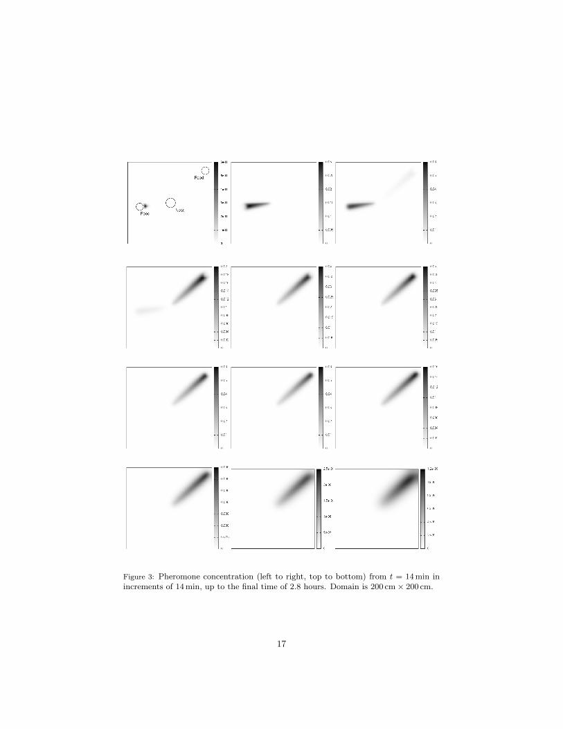
Figure 3: Pheromone concentration (left to right, top to bottom) from t = 14min inincrements of 14min, up to the final time of 2.8 hours. Domain is 200 cm× 200 cm.

17

Table 3: Parameters in system (3.5). See Table 2 for explanation.Parameter Value

Total population 75 000 antsArea of physical domain Ω 4 m2

ε 0.5Dv 0.1Dw 0.1χu 50λ 70c0(x) ∼ 12

t 102 s

x 5.54 cm

Returning ant speed 1 cm/s

Figure 4: Evolution of food quantity. Horizontal axis in hours.

18

5. Food removal efficiency is linked to trail formation

In this section we discuss some consequences and possible experimental val-idations of our model. The main idea is that increased trail formation is cor-related with food removal efficiency, which is in turn related to rather preciseconditions on some of the coefficients of the system (3.5).

In a simplified ecological setting such as the one presented in this work, thequantity which the ants strive to minimize (in an evolutionary sense) would bethe amount of time taken to carry all the food to the nest. So, in this section weinvestigate what is the influence on food removal efficiency of varying parameterson which natural selection can act.

Of particular interest is the question of whether different parameter combi-nations allow or prevent trail formation. To address this question, we focus ouranalysis on the pheromone degradation rate ε and the chemotactic sensitivity ofthe foraging ants, χu. Note that it would be interesting to consider other pairsof parameters; however, these two parameters were chosen precisely because itis less clear, on an intuitive level, what effect their variation might have on theforaging dynamics.

5.1. Parameter space exploration: conditions for trail formationWith this in mind, we now present an exploration of the (ε, χu)−parameter

space, showing how trail formation in foraging ants is affected by the variationof these parameters. Recall that χu is the foraging ants’ chemotactic sensitivityand ε is the pheromone degradation rate.

In Figure 5, we present the density of foraging ants at time t = 1.36 hours,for various simulations using the same parameters as in Table 2, but with asmaller quantity of food. On the horizontal axis, ε varies between the values0.01, 0.1, 0.5, 1, 2.5 and 5, while on the vertical axis χu varies between 20, 40,80, 160, 500 and 1000, from bottom to top.

It is clear from Figure 5 that certain parameter values are more conduciveto trail formation than others. We can see, for instance, that trail formationis suppressed when the pheromone degradation rate ε is large and the ants’sensitivity is low (bottom right of Figure 5). Similarly, trails do not developwell when pheromone degradation is very fast and sensitivity very high (upperleft part of Figure 5).

5.2. Trail formation and food removal efficiencyAs we pointed out, trail formation itself confers no advantage to the ants

if it does not contribute to a more efficient food removal. We now show thattrail forming behavior, as depicted in Figure 5, is correlated with increased foodremoval efficiency. To see this, we compute the evolution of the remaining foodmass for each column and row of Figure 5. Then, we determine for each rowand column what are the parameter values for which food is more efficientlyremoved. The measure we use is the quantity of food remaining at a fixed timeabout 75% of the total simulation time. The results are reported in Table 4.For each column of Figure 5, that minimum is marked with a black star, while

19

for each row the minimum is marked with a white star. These minima are alsoshown in Table 4.

Using this procedure, we can see from Table 4 and Figure 5 that food removalis more efficient precisely when trail formation is more apparent. This stronglysupports the notion that trail formation by foraging ants is a main contributingfactor to a more efficient removal of the food, as is widely assumed.

Another conclusion suggested by the analysis of Table 4 is that greaterchemotactic sensitivity is not always advantageous; rather, increased sensitiv-ity only translates into increased food removal efficiency when the pheromonedegradation rate is sufficiently high. Conversely, a very long lived pheromoneshould be paired with a decreased sensitivity in order to yield efficient foodremoval. In other words, we can postulate a monotone dependence of the sen-sitivity with respect to the pheromone degradation rate.

5.3. Suggestion of experimental workRelation between pheromone degradation rate, chemotactic sensitivity and trailformation. From Table 4 and Figure 5 we can see that, in our simulations,there is a narrow region of the (ε, χu) parameter space leading to an optimalfood removal efficiency (when one of the two parameters is fixed). Moreover,Figure 5 shows that in this region, trail laying is most apparent.

A possible experimental validation of our model would be to consider twoclosely related ant species which use different pheromones, where each phero-mone has a different degradation rate. Our model predicts that, in that case,their sensitivities should lie in the narrow region of the (ε, χu) parameter spacewhere food removal efficiency is greater. Given the appropriate parametersto plug into the equations (3.5), we would be able to predict the chemotacticsensitivity from the knowledge of the degradation rate alone, by constructingTable 4.

To summarize, it may seem natural that chemotactic sensitivity varies withthe pheromone degradation rate. What we have observed in our model is thatnot only is this a monotone dependence, but also that greater food removal effi-ciency occurs in a narrow region of the parameter space, which can, presumably,be known for a particular species of ant. Thus we would expect ε and χu tobe highly correlated in nature, at east for species which do not differ greatly inother respects.

Moreover, our simulations show that food removal efficiency is correlatedwith trail formation, reinforcing the view that trail formation is indeed one ofthe most important adaptations in ants.

Orientation along trails. From our review of the myrmecological literature, oneoutstanding open problem appears to be the question of the choice of directionwhen encountering a trail (this was discussed in detail in Section 3.2). Thepresent work suggest that the ability of ants to measure differences in phero-mone concentration along the length of the trail, and not only across the trail,may play an important role in orienting individuals in the correct direction when

20

Table 4: Food removal efficiency as a function of pheromone evaporation rate and chemotacticsensitivity. A star (?) indicates the minimum value for each column, and a diamond ()indicates the minimum value for each column.

χu \ ε 0.01 0.1 0.5 1 2.5 5

1000 16.58 10.51 3.67 1.35 ? 1.14 ? 3.16 ?

500 11.95 7.99 2.56 ? 1.69 3.34 4.93160 7.08 4.7 3.22 4.26 5.61 6.1480 5.18 4.02 ? 4.59 5.45 6.16 6.4140 4.53 ? 4.5 5.6 6.07 6.42 6.5520 5.02 5.39 6.15 6.38 6.55 6.61

encountering a trail. This lengthwise gradient can be created by a gradual di-minishing of pheromone deposition by returning ants as they approach the nest.Indeed, although other mechanisms to solve this orientation problem have beenfound, and others can be envisaged, our results suggest that gradual diminishingof pheromone deposition can contribute to allow ants to find the correct orien-tation when encountering a pheromone trail, especially in the case of relativelyshort trails (on the order of one to a few meters) as the ones considered here.Thus it could be of interest to carry out more detailed experiments to ascertainwhether lengthwise variation in pheromone concentration along the trail playsany role in individual orientation along the trail.

6. Conclusions and future work

6.1. General conclusionsWe have presented a mathematical model of ant foraging using a system of

PDEs in the mathematical framework of chemotaxis. We have shown numeri-cally that this system can exhibit spontaneous trail formation in the presence offood sources. The fact that trails are formed by the returning ants is built intoour modeling assumptions and as such is not surprising; but we have shown, inaddition, that trail formation occurs also in foraging ants, which is not explicitlystated in the model.

Moreover, we have shown through parameter exploration that trail forma-tion in foraging ants is sensitive to parameter values and, more importantly, iscorrelated with increased food removal efficiency. This allowed us to postulatethat chemotactic sensitivity and pheromone degradation rates should also becorrelated in a way that can be made precise for particular species of ants, andconsequently tested by actual experiments.

Our model allows for the simulation of a whole cycle of food foraging, fromants emerging from a nest onto a foraging ground where food is placed, discov-ering the food and returning to the nest laying pheromones. Recruitment thentakes place, with foraging ants being attracted to the pheromones laid previ-ously by the returning ants. A feedback loop ensues, as more ants reach the

21

Figure 5: Conditions for trail formation in foraging ants. From left to right, ε =0.01, 0.1, 0.5, 1, 2.5, 5. Bottom to top, χu = 20, 40, 80, 160, 500, 1000. ε is the pheromonedegradation rate, χu is the foraging ants’ chemotactic sensitivity (see Table 2). A star? indicates simulations where, for fixed ε, the food removal efficiency is greatest. Awhite star indicates simulations where, for fixed χu, the food removal efficiency isgreatest (see Table 4).

22

food source and return to the nest laying pheromones. Finally, when the foodsource is exhausted, the trail fades away due to the natural evaporation anddiffusion of the pheromone.

6.2. Limitations and future workNaturally, it would be very difficult for the model presented here to provide

a comprehensive description of the extremely complex dynamics taking placeduring the whole foraging cycle of ants. One limitation is that we do not attemptto model in detail what happens near the nest and near the food site. In ourmodel, only chemical signals intervene in the ants’ behavior, whereas it is wellknown that individuals rely on a variety of other sensory and communicationinput to adjust their behavior.

Another clear limitation is the functional form of the last equation of (3.1),governing the removal of food. Intuitively, it would be more reasonable thateach ant reaching the food would consume or carry away a fixed food quantity,rather than a proportion of the available food. As observed in an Section 3.2, thischoice was made primarily to ensure mathematical simplicity and facilitate thenondimensionalisation procedure. The model can, however, be easily adaptedto more realistic food removal models.

Another possible improvement is in the chemotactic transport term for theu-equation in the system (3.5). Indeed, its present form is not entirely realistic,since the (scalar) ant speed, given by |χu∇v| can have large variations, and inparticular can theoretically attain very high values. But the actual movementof ants along trails shows little correlation between ant speed and ant density,see [23, 24]. This is coherent with the informal observation that even on densetrails, ants move along at speeds similar to isolated ants, in contrast to, say,vehicles on a road. Therefore, a different modeling of the transport term couldbe envisaged to account for this lack of the so-called jammed phase in the flux.

Related to this, is the question of the possible unlimited growth of ant densityon trails. In the chemotactic literature, it is usual to introduce a term of theform umax − u in the transport term, which serves as a limiter for the density:when the density reaches the value umax, individuals do not move and so densitywill not increase further. This is called the jammed phase and is usual in themodeling of vehicular or pedestrian traffic. It has been studied, for instance, in[14]. We find that such a mechanism is not realistic in the case of ants, sinceas we pointed out before, no jammed phase is observed [23]. Other modelingstrategies could be deployed to account for a limitation in density. Remark thatthe forthcoming results in [2] actually give a uniform bound for all time on thedensity of ants by some constant C. However, C comes from the mathematicalanalysis and so is not directly related to physical constraints on the ants’ density.

Additionally, it would be more realistic to introduce a transport term inthe foraging ant equation expressing ants’ tendency to stay near the nest, ashas been done in other models of animal movement [28, 29]. This may preventunrealistic situations such as, on the whole R2, with no food present, the densityof foraging ants decreasing to zero everywhere due to the diffusive effect. Weomit such a term for the sake of keeping the model as simple as possible.

23

Finally, as far as we could gather, no experiment has been done to discoverexactly what “diffusion law” is obeyed by ants. In this work we use the usualFickian diffusion since it is the simplest and yields good results in a first ap-proximation. However, it is well known that animal movement may be betterapproximated by other models of diffusion, usually nonlinear models (see forinstance the book [33]). Thus more realistic diffusions could be incorporated inthe model.

Appendix A. Nondimensionalisation

Here, we will describe the nondimensionalisation procedure used to reducethe system (3.1) to the system (3.5). We will use the notation

t = tt∗, x = xx∗, u = uu∗, v = vv∗,

and so on, for the changes of variable involved in nondimensionalisation. Here, t(say) represents the old variable, t∗ the new, nondimensional variable, and t the(dimensional) new scale. Thus, for instance, u∗ is the (new) function definedthrough u u∗(t∗, x∗) = u(tt∗, xx∗).

As is standard procedure, we will formulate the system (3.1) under the newunknowns t∗, x∗, u∗, . . . , and finally remove the ∗ for convenience. Nondimen-sionalisation therefore consists in a judicious choice of t, x, and so on.

Our nondimensionalisation procedure will differ from the usual procedureused often in chemotaxis [15, p.191], in which the time scale is associated withthe decay time (or half-life) of the attracting chemical. That would not beconvenient in our case since this is a highly variable (and usually very short)quantity [8] and presents problems from the modeling point of view (as describedin Section 3.2 above). Thus we set

u = w = uref , (A.1)

so that the density of foraging ants is measured as a proportion to this homoge-nous steady state of a uniformly distributed population.

Since the main objective of foraging is the efficient removal of food sources,it seems natural to consider a time scale tied to the rate of food removal byants. Considering the last equation in (3.1) leads to the choice

t =1

γuref. (A.2)

The physical meaning of t is seen by observing that if the half-life of a foodsource is measured in the units of system (3.1) as, say, t0 (from our modelingassumptions, i.e., the fourth equation in (3.1), t0 does not depend on the initialfood quantity), then assuming constant in space food concentration and foragingant density of uref , the scale will be t = t0/ ln 2 (in the units of t0).

Thus, the last equation of (3.1) becomes simply

∂t∗c∗ = −u∗c∗.

24

Next, choosing

x =

√αu

γuref, v =

µ

γ

yields∂t∗v

∗ = P (x∗)w∗ − εv∗ +Dv∆v∗,

withDv =

αv

αu, ε =

δ

γuref, P (x∗) = P (xx∗).

Proceeding similarly with

Dw =αw

αu, χu =

βuµ

αuγ, λ =

λ2

γuref,

c =γuref

λ1, a =

αu

βw,

N(x∗) = N(xx∗), M(x∗) =t

urefM(xx∗),

gives for the remaining two equations

∂t∗u∗ −∆u∗ +∇·

(u∗χu∇v∗

)= −u∗c∗ + λw∗N(x∗) +M(t∗)N(x∗)

∂t∗w∗ −Dw∆w∗ +∇·

(w∗∇a∗

)= u∗c∗ − λw∗N(x∗)

As is standard practice, we omit the ∗ from all the variables. Collecting theprevious equations we obtain the nondimensional system (3.5).

Appendix B. Details of the numerical scheme

In this appendix we describe the numerical method used to integrate thesystem (3.5)–(3.7). For the spatial discretization, we divide the 2-d computa-tional domain into rectangular cells of sides dx, dy. We use conservative schemesthroughout: the Laplacian terms are discretized using standard centered differ-ences, while the advection terms are discretized using a conservative first-orderupwind scheme (see [13, 27]).

The spatial discretization allows us to reduce the system (3.5)–(3.7) to asystem of ordinary differential equations, which we integrate in time using afourth-order Runge–Kutta method for systems (see [4, p.331]). We also used anexplicit Euler scheme and compared the results of both methods to validate theresults.

The upwind method used is known for its stability in dealing with advec-tion terms. However, being a first order scheme, it introduces some numericalviscosity which tends to smear out results. It would thus be interesting, for fu-ture works, to implement a more accurate method, such as the high resolutionmethods found in [27].

25

AcknowledgementsThe author wishes to thank the referees for insightful suggestions which

contributed greatly to the improvement of the paper. The author was partiallysupported by FAPERJ grant no. APQ1 - 111.400/2014 and CNPq grant no.Universal - 442960/2014-0.

References

[1] Amorim, P., A continuous model of ant foraging with pheromones and trailformation. To appear in Proceedings of XXXV CNMAC (Conference heldin Sep. 2014), SBMAC.

[2] Alonso, R., Amorim, P., Goudon, T. Analysis of a chemotaxis system aris-ing in ant foraging. Submitted.

[3] Bandeira de Melo, E.B., Araújo, A.F.R., Modelling foraging ants in a dy-namic and confined environment. BioSystems 104 (2011) 23–31

[4] R.L. Burden, J.D. Faires, Numerical analysis, ninth edition, Brooks/Cole(2001).

[5] Beckers, R., Deneubourg, J.L., Goss, S., 1992. Trail laying behaviour duringfood recruitment in the ant Lasius niger (L.) - Springer Insectes soc. 39, 1,59–72.

[6] Bertozzi, A.L. et al., Spatiotemporal chemotactic model for ant foraging.Modern Physics Letters B Vol. 28, No. 30 (2014) 1450238

[7] Boissard, E., Degond, P., Motsch, S., 2012. Trail formation based on di-rected pheromone deposition. J. Math. Biol., DOI 10.1007/s00285-012-0529-6.

[8] Bossert, W.H., Wilson, E.O., The Analysis of Olfactory CommunicationAmong Animals. J. Theoret. Biol. (1963) 5, 443–469.

[9] Couzin, I.D., Franks,. N.R., 2002. Self-organized lane formation and opti-mized traffic flow in army ants. Proc. R. Soc. Lond. B (2003) 270 no.1511139–146.

[10] Deneubourg, J.-L., Aron, S., Goss., Pasteels, J.M., 1990. The Self-Organizing Exploratory Pattern of the Argentine Ant. Journal of InsectBehavior, Vol. 3, No. 2, 150–168.

[11] Edelstein-Keshet, L., 1994. Simple models for trail-following behaviour;Trunk trails versus individual foragers. J. Math. Biol., 32, 303–328

[12] Edelstein-Keshet, L., Watmough, J., and Ermentrout, B.G. Trail followingin ants: individual properties determine population behaviour BehavioralEcology and Sociobiology, Vol. 36, No. 2 (1995), pp. 119-133

26

[13] E. Godlewski, P.-A. Raviart, Hyperbolic systems of conservation laws,Mathématiques & Applications (Paris). Ellipses, Paris, 1991

[14] Hillen, T., and Painter, K.J. Global Existence for a Parabolic ChemotaxisModel with Prevention of Overcrowding, Advances in Applied Mathematics26, 280–301 (2001).

[15] Hillen, T., and Painter, K.J. A user’s guide to PDE models for chemotaxis,J. Math. Biol. (2009) 58:183–217.

[16] Hölldobler, B., 1976. Recruitment Behavior, Home Range Orientation andTerritoriality in Harvester Ants, Pogonomyrmex. Behav. Ecol. Sociobiol. 1,3–44.

[17] Hölldobler, B. and Wilson, E.O., 1990. The Ants. The Belknap Press ofHarvard University Press, Cambridge, Mass.

[18] Horstmann, D., From 1970 until now: The Keller–Segel model in chemo-taxis and its consequences I. Jahresberichte der DMV 105 (2003), 103–165.

[19] Horstmann, D. From 1970 until now: The Keller–Segel model in chemotaxisand its consequences II. Jahresberichte der DMV, 106, (2004) pp. 51–69.

[20] Jackson, D., Holcombe, M., Ratnieks, F., 2004. Coupled computationalsimulation and empirical research into the foraging system of Pharaoh’sant (Monomorium pharaonis). Biosystems, Vol. 76, 1–3, 101–112

[21] Jackson, D., Holcombe, M., Ratnieks, F., 2004. Trail geometry gives polar-ity to ant foraging networks Nature, 432 (7019), 907–909

[22] Jeanson R., Ratnieks F.L.W., Deneubourg. J.-L., 2003. Pheromone traildecay rates on different substrates in the Pharaoh’s ant, Monomoriumpharaohs. Physiological Entomology (2003) 28, 192–198

[23] John, A., et. al, 2009. Trafficlike collective movement of ants on trails:absence of jammed phase. Phys. Rev. Lett. 102, 108001.

[24] Johnson, K., Rossi, L.F., 2006. A mathematical and experimental study ofant foraging trail dynamics. Journal of Theoretical Biology, 241, 360–369.

[25] Keller, E., Segel, L., 1970. Initiation of slide mold aggregation viewed asan instability. J. Theor. Biol. 26 (1970), 399–415.

[26] Keller, E., Segel, L., 1971. Model for Chemotaxis. J. theor. Biol. 30, 225–234.

[27] R.J. Levee, Finite volume methods for hyperbolic problems. CambridgeTexts in Applied Mathematics. Cambridge University Press, Cambridge(2002).

27

[28] Lewis, M.A., J.D. Murray. 1993. Modelling territoriality and wolf-deer in-teractions. Nature 366:738–740.

[29] Lewis, M.A., White, K.A.J., and J.D. Murray, 1997. Analysis of a modelfor wolf territories. J. Math. Biol. (1997) 35: 749–774

[30] Motta Jafelice, R., et al., 2011. Fuzzy parameters in a partial differen-tial equation model for population dispersal of leaf-cutting ants. NonlinearAnalysis: Real World Applications 12, 3397–3412.

[31] Moorcroft, P.R, Lewis, M.A., and Robert L Crabtree, R.L. 2006. Mecha-nistic home range models capture spatial patterns and dynamics of coyoteterritories in Yellowstone. Proc. R. Soc. B 2006 273, 1651–1659.

[32] Müller, M., Wehner, R., 1988. Path integration in desert ants, Cataglyphisfortis. Proc. Nat. Acad. Sci. USA, Vol. 85, 5287–5290.

[33] Okubo, A., Levin, S.A. Diffusion and ecological problems: modern perspec-tives. Vol. 14 of Interdisciplinary Applied Mathematics. Berlin: SpringerVerlag.

[34] Painter, K.J., 2009. Continuous Models for Cell Migration in Tissues andApplications to Cell Sorting via Differential Chemotaxis. Bull. Math. Biol.71, 1117–1147

[35] Patlak, C., 1953. Random walk with persistence and external bias. Bull.Math. Biophys. 15, 311–338.

[36] Ramsch, K., et al., 2012. A mathematical model of foraging in a dynamicenvironment by trail-laying Argentine ants. Journal of Theoretical Biology306 (2012) 32–45.

[37] Rauch, E.M, Millonas, M.M. and Chialvo, D.R. Pattern formation andfunctionality in swarm models. Physics Letters A 207 (1995) 185–193.

[38] Regnier, F.E., Law, J.H. Insect pheromones. J. Lipid Res. 9 (1968) 541–551.

[39] Reid, C.R., Lattya, T., Beekam, M. Making a trail: informed Argentineants lead colony to the best food by U-turning coupled with enhancedpheromone laying. (2012) Animal Behaviour, Vol. 84, 6, 1579–1587

[40] Ryan, S.D. A model for collective dynamics in ant raids. (Under review).

[41] Schweitzer, F., Lao, K., Family, F. Active random walkers simulate trunktrail formation by ants. BioSystems 41 (1997) 153–166.

[42] Sumpter, J.T. and Beekman, M. From nonlinearity to optimality: phero-mone trail foraging by ants. Animal Behaviour, 2003, 66, 273–280.

[43] Sumpter, D.J.T. and Pratt, S.C. A modelling framework for understandingsocial insect foraging. (2003) Behav Ecol Sociobiol (2003) 53:131–144

28

[44] Steck, K., Hansson, B., Knaden, M., 2009. Smells like home- Desert ants,Cataglyphis fortis, use olfactory landmarks to pinpoint the nest. Frontiersin Zoology, 6:5.

[45] Tang, X., and Tao, Y., 2008. Analysis of a Chemotaxis Model for Multi-Species Host-Parasitoid Interactions Applied Mathematical Sciences, Vol.2, no. 25, 1239–1252

[46] Tschinkel, W.R., The Fire Ants, Harvard University Press, 2006.

[47] Udiani, O., Pinter-Wollman, N. and Kang, Y. Identifying robustness in theregulation of collective foraging of ant colonies using an interaction-basedmodel with backward bifurcation. (Preprint)

[48] Van Vorhis Key, S.E., Baker, T.C., 1986. Observations on the Trail De-position and Recruitment Behaviors of the Argentine Ant, Iridomyrmexhumilis (Hymenoptera: Formicidae). Annals of the Entomological Societyof America, 79, 2. link

[49] Vittori, K., et.al., 2004. Modeling Ant Behavior Under a Variable Environ-ment. ANTS 2004, LNCS 3172, 190–201.

[50] Vowles, D.M., 1955. The foraging of ants. The British Journal of AnimalBehaviour 3, 1, 1955, 1–13.

[51] Watmough, J., Edelstein-Keshet, L., 1995. A one-dimensional model of trailpropagation by army ants. J. Math. Biology, 33, 459–476

[52] Watmough, J., Edelstein-Keshet, L., 1995. Modelling the Formation of TrailNetworks by Foraging Ants. J. theor. Biol. 176, 357–371

[53] Wehner, R., 2003. Desert ant navigation: how miniature brains solve com-plex tasks. Journal of Comparative Physiology A, 189, 8, 579–588

[54] Weyer, J., 1985. A mathematical model for chemical mass recruitment ofants. J. Math. Biology, 21, 307–315.

[55] Wilson, E.O., 1962. Chemical communication among workers of the fire antSolenopsis saevissima (Fr. Smith) 1. The Organization of Mass-Foraging.Animal Behaviour, 10, 1-2, 134–138.

[56] Wilson, E.O., 1962. Chemical communication among workers of the fire antSolenopsis saevissima (Fr. Smith) 2. An information analysis of the odourtrail. Animal Behaviour, 10, 1-2, 148–158.

[57] Wilson, E.O., 1962. Chemical communication among workers of the fire antSolenopsis saevissima (Fr. Smith) 3. The experimental induction of socialresponses. Animal Behaviour, 10, 1-2, 159–164.

29