F 609 – Tópicos de Ensino de Física I Coordenador: Joaquim Lunazzi

lunazzi@ifi.unicamp.br

Quase-Levitação Induzida Magneticamente

Aluno: André Luiz de Oliveira (IFGW – UNICAMP) andrefismat@gmail.com

Técnico: Jorge Baudin (IFGW – UNICAMP) Co-orientador: George Dourado Loula (IFGW – UNICAMP)

Orientador: Prof. Dr. Flávio César G. Gandra (IFGW - UNICAMP)

2

Índice: 1 - Resumo ------------------------------------------------------------------------- 3 2 - Introdução Teórica. 2.1 - Como é produzido o Campo

�

B -------------------------------------- 4 2.2 - Definição do Campo

�

B ------------------------------------------------ 4 2.3 - Fluxo magnético -------------------------------------------------------- 5

2.4 - Indução eletromagnética --------------------------------------------- 7 2.5 - Correntes de Foucault ----------------------------------------------- 10 2.6 - Material Diamagnético ----------------------------------------------- 12 2.7 - Levitação ou Quase-levitação? ------------------------------------ 14 3 - O projeto 3.1 - Materiais utilizados --------------------------------------------------- 17 3.2 - Montagem --------------------------------------------------------------- 17 3.3 - Equações de força ---------------------------------------------------- 21 4 - Sugestões do coordenador -------------------------------------------------- 23 5 - Comentário do Orientador e Co-orientador ------------------------------ 25 6 - Conclusões ---------------------------------------------------------------------- 26 7 - Referências ---------------------------------------------------------------------- 26

3

Resumo

O projeto inicialmente idealizado por mim, em conjunto com o meu orientador,

Professor Dr. Flávio C. G. Gandra, corresponde ao protótipo confeccionado. Um segundo

projeto, que corresponde a uma outra montagem, mas que segue a mesma temática do

atual, foi sugerido pelo coordenador da disciplina. Por falta de tempo hábil para a

execução de ambos, resolvi optar pela execução do meu projeto, já que ambos são

bastantes similares (ambos abordam o efeito de quase-levitação magnética).

Abaixo, listo as idéias fundamentais de ambos:

1. O projeto tem suas bases fundamentadas na teoria eletromagnética, com ênfase,

principalmente na lei de indução de Faraday. O aparato é composto de dois cilindros ocos

de cobre, que giram em torno do seu eixo longitudinal. De acordo com a lei de indução de

Faraday, ao aproximarmos desses cilindros girantes, um imã permanente, a variação do

fluxo do campo magnético sobre os cilindros, gera nesses uma corrente parasita (corrente

de Foucault1) e, por conseqüência, uma força magnética aparece também no imã e se

opõe ao seu peso, mantendo-o “levitando”..

2. A montagem sugerida pelo coordenador, e que não foi construída por falta de

tempo hábil, consiste na “levitação” decorrente da repulsão entre pólos iguais de

diferentes imãs. Uma discussão mais detalhada da montagem pode ser encontrada com

maiores detalhes podem ser encontrado no item 4 desse relatório.

1 Jean Bernard Léon Foucault (18/09/ 1819 – 11/02/1868) foi físico e astrônomo francês. Foucault era filho de um editor de Paris. Estudo Medicina, que ele abandonou rapidamente para se dedicar à Física. Interessou-se pelos métodos fotográficos de Danguerre. Foucault é particularmente conhecido pela sua experiência demonstrando a rotação da Terra em torno de seu eixo (Pêndulo de Foucault), tendo determinado a velocidade da luz e inventado o giroscópio.

4

Introdução teórica

Como é produzido o campo B�

O campo elétrico eletrostático é gerado por cargas elétricas, o que nos leva a

intuir, que o campo magnético também é gerado por cargas magnéticas. Porém, estas

cargas não existem. O campo magnético deve, então, ser gerado de outras formas:

1 – Partículas eletricamente carregadas em movimento.

2 – Por uma propriedade intrínseca dos materiais.

Para este segundo caso, o magnetismo é conseqüência do momento magnético de spin

eletrônico, presente em materiais que possuem íons com elétrons desemparelhados. Em

alguns destes materiais, a interação entre os momentos individuais gera um momento

macroscópico quando o material é dito orientado. Com estes materiais são

confeccionados imãs permanentes.

Quando a interação é muito fraca ou injexistente, não há ordenamento magnético.[1].

Definição do Campo B�

Para determinarmos um campo elétrico �

E colocamos uma partícula de prova com

carga q em um ponto qualquer do espaço e medimos a força �

EF que este campo faz

sobre ela. Assim, podemos medir o campo elétrico através da relação:

=�

�EFEq

(1.0)

Como não possuímos um monopolo magnético, não podemos definir de forma

análoga o campo �

B . No entanto, observou-se experimentalmente que uma corrente

elétrica forte poderia alterar a orientação de uma bússola, que foi associado ao efeito de

um campo magnético gerado por esta corrente. Posteriormente, uma partícula

movimente-se ao longo desse campo magnético com uma velocidade V�

sofrerá uma

força magnética, �

BF , caso V�

e B�

não sejam paralelos ou antiparalelos entre si. Sabemos

que a direção de �

BF é sempre perpendicular à direção da velocidade, o que sugere que

5

esta seja resultado de um produto vetorial entre a velocidade e o campo magnético. Desta

forma, medimos o campo magnético �

B :

=�

�

�BFBqv

= � ��

BF qv B (1.1)

sBF qvB enθ=�

(1.2)

Onde θ é o ângulo entre a velocidade da partícula de carga q , e o campo

magnético. A direção da força pode ser facilmente encontrada pela regra da mão direita

conforme a figura 1:

Figura 1: Regra da mão direita para determinar a direção da força magnética.

Fluxo Magnético

De acordo com a figura 2 abaixo, o fluxo magnético (Φ ) através da superfície

fechada, S, cujo vetor de área A�

é dado por AnA ˆ=�

é definido por:

dSnBS∫ ⋅=Φ ˆ�

(1.3)

6

Figura 2: Fluxo de B�

através de uma superfície S

Como já sabemos, não existem cargas magnéticas (monopólos magnéticos) e

fazendo uma analogia com a lei de Gauss1 para o caso elétrico, temos que, para essa

superfície S:

0SB dA⋅ =∫� �

� (1.4)

Sendo V o volume contido na superfície S, usando o teorema da divergência

temos:

0=⋅∇∫ dVBS

��

(1.5)

0=⋅∇ B��

(1.6) Com iss,o já temos uma das equações de Maxwell2, que representa uma das

propriedades fundamentais do campo �

B , em que as linhas de força magnética são

sempre fechadas. O fluxo magnético tem como unidade de 1 Wb (Weber)[1].

2 James Clerk Maxwell (13/06/1831 – 05/11/1879) foi Física e Matemático britânico. Conhecido por finalizar a teoria moderna do eletromagnetismo, unindo eletricidade, magnetismo e óptica demonstrando que a luz é uma onda eletromagnética que alguns anos a frente serviu de base para a teoria da relatividade, teve trabalhos importantes em mecânica estatística servindo como uma das bases da mecânica quântica. 3 Johann Carl Friedrich Gauss (30/04/1777 – 23/02/1855) foi Matemático, Astrônomo e Físico alemão, aprendeu a ler e escrever sozinho, aos dez anos demonstrou a fórmula da soma de uma progressão aritmética. Iniciou os estudos de análise matemática ainda jovem ultrapassando seus antecessores, aos dezoito anos inventou o método dos mínimos quadrados, descobriu através de cálculos o planeta Ceres, assentou os fundamentos da teoria matemática do eletromagnetismo e inventou o telégrafo elétrico.

7

=2

1 1Wb

Tm

Indução eletromagnética

Se inserimos uma espira C num campo magnético �

B , conforme mostrado na figura

3 abaixo, teremos que o fluxo através dessa espira será:

SB dAΦ = ∫�

i� (1.7)

Figura 3: espira imersa num campo magnético �

B , com ângulo θ entre B e ��

A .

De acordo com a lei de Faraday1, temos:.

“A corrente elétrica induzida pelo campo magnético em um circuito fechado (espira

C), é proporcional ao número de linhas do fluxo que atravessa a área envolvida do

circuito, por unidade de tempo”.

de fato, a fem induzida na espira é igual à variação no tempo do fluxo magnético através

da espira

1 Michael Faraday (22/09/1791 – 25/08/1867) foi Físico e Químico britânico, considerado um dos cientistas mais influentes de todos os tempos, teve contribuições importantes para a eletricidade e magnetismo e para a química. Foi um grande experimentalista não tinha conhecimentos profundos de matemática avançada, porém suas contribuições são de grande impacto, suas descobertas serviram de base para o trabalho de grandes industriais e engenheiros como Edison, Siemens, Tesla e Westinghouse tornando possível a eletrificação de nossa sociedade atual. Na química descobriu o benzeno, produziu os primeiros cloretos de carbono, e contribuiu para a metalurgia e a metalografia.

8

Φ= = − Bd

Ridt

Є (1.8)

mas = ∫��

i�E dlЄ (1.9)

então B

dEdl

dt= − Φ = − ∫�Є (1.10)

Temos então:

C S

C S

E dl rotE dA

Brot Eda dA

t

=

∂= −∂

∫ ∫

∫ ∫

� � �

i i

�� �

�

(1.11)

e portanto,

Podemos assim dizer que, ∂= −∂

�� B

rot Et

que é outra das equações de Maxwell. onde E,

neste caso, não corresponde ao campo eletrostático.

A variação do fluxo ΦB pode ser pela movimentação da espira ou pela variação do

campo magnético no tempo.

O sinal de menos nas equações que aparece na lei de indução é devido à lei de

Lenz1.

“A corrente induzida em uma espira tem um sentido tal que o campo magnético

produzido pela corrente se opõe à variação do fluxo magnético que induz a corrente”.

1 Heinrich Friedrich Emil Lenz (12/02/1804 – 10/02/1865) foi Físico alemão, estudou Química e Física, fez três expedições em volta do mundo, onde em uma dela estudou as propriedades físicas da água do mar, ganhou fama a formular sua lei em 1833 e a lei de Joule em 1842. Pesquisou condutividade elétrica de vários materiais, o efeito da temperatura sobre a condutividade, descobriu a reversibilidade das máquinas elétricas.

9

Figura 4: sentido das correntes induzidas pela variação de fluxo

Estas correntes induzidas produzem seus próprios campos magnéticos, cuja direção é

normal à superfície[1], [2]. A lei de Lenz está diretamente vinculada ao princípio de

conservação de energia.

Figura 5: Direção das correntes induzidas usando a lei de Lenz

10

Correntes de Foucault

Se um imã é solto em queda livre dentro de um tubo de material condutor, a

corrente elétrica induzida na superfície do tubo, criará sobre o imã uma força magnética

que se opõe ao movimento de queda.

Figura 6: corrente de Foucault induzidas pela queda do imã dentro do tubo, gerando os campos induzidos.

Podemos também pensar em um pêndulo constituído de um materior condutor,

posto a oscilar numa região de campo magnético, conforme figura 7 abaixo:

Figura 7: Pendulos de material condutor entrando em região de campo magnético.

11

A figura 7a mostra um pendulo entrando na região dos pólos de um imã. No disco

metálico aparecerão correntes, cujos sentidos são especificados pela lei de Lenz. As

forças magnéticas proporcionadas por essas correntes (correntes de Foucault) são

equivalentes a uma força de atrito viscoso. Se quisermos reduzir este efeito, basta

fazermos uma série de fendas como figura 7b. Com isso, reduzimos muito o fluxo nas

partes metálicas e obrigamos cada corrente a percorrer um caminho mais longo,

aumentando a resistência e diminuindo a intensidade das correntes induzidas.

Consequêntemente, diminuímos a força magnética proporcionada.

Figura 8: Espira retangular com velocidade v passando sobre um campo �

B entrando no plano do papel.

Vamos estudar um caso simples que servirá de base para as equações que

dominam o projeto. Uma espira retangular com largura h está parcialmente imersa em um

campo magnético uniforme �

B , que entra no plano do papel. Portanto é perpendicular ao

plano da espira. Esta espira é movida com velocidade v para isto é preciso dar uma força �

F constante para esta locomoção parte da espira que esta sobre a ação do campo

diminui e por conseqüência o fluxo também diminui, e de acordo com a lei de Faraday

uma corrente é induzida.

Para determinar esta corrente usamos da equação (1.8) para o calculo deste fluxo.

Φ = =B BA Bhx

Quando diminuímos x o fluxo também diminui e de acordo com a equação (1.9)

temos.

12

Bd d dxBhx Bh Bhv

dt dt dt

Φ= − = = =Є

Φ= = − BdRi

dtЄ

Assim podemos obter a corrente induzida no circuito.

Bhvi

R= −

Observando a figura temos três forças para a parte de espira imersa no campo por

simetria as força � �

1 2F e F se anulam sobrando somente à força �

3F . De acordo com a

equação (1.1).

3F ih B= �� �

Como o ângulo entre o campo e h é 90º

3

2 2

3

F ihB

B h vF

R

=

=

�

�

Podemos também calcular o trabalho para isto usamos a relação P Fv= e

obtemos:[3]

2 2 2B h vP

R=� �

Material Diamagnético

Para o calculo da susceptibilidade diamagnética para um agrupamento de átomos,

é importante que se conheça sobre o movimento eletrônico de cada átomo. Para o nosso

modelo se tornar simples vamos considerar a orbita dos elétrons em torno do átomo como

circular de raio r em um plano de tal forma que tenha ângulos retos com o campo

magnético aplicado.

Antes de aplicarmos o campo magnético o elétron esta em equilíbrio em sua orbita:

0E eF m rω= (1.12)

EF�

é a força elétrica que age sobre o elétron e em e 0ω é a massa e a freqüência angular do elétrons respectivamente.

13

Quando aplicamos o campo uma força adicional é dada ao elétron ev B e r Bω− × = − × , vamos supor que o elétron permaneça na mesma orbita temos:

2

E m eF e rB m rω ω± = (1.13)

Quando combinamos com a equação (1.14) e assumindo que o raio da órbita é

fixo, obtemos:

0 0( )( )m ee B mω ω ω ω ω± = − + (1.14)

0( )ω ω ω− = ∆ É a variação na freqüência angular do elétron. Ou seja, o elétron

acelera ou diminui a velocidade em sua orbita, e este movimento possui um momento que

chamamos de momento magnético orbital e sua variação será sempre no sentido oposto

ao campo aplicado.

2

m

e

eB

mω∆ = ± (1.15)

Quando o campo é aplicado há uma variação de fluxo através da orbita do elétron

considerando-as como espiras temos 2B mr BπΦ = ∆ . Este fluxo passa por n∆ espiras

eletrônicas, n∆ é o número de revoluções que o elétron faz no tempo em que o campo

varia. Este fluxo variável produz um fem de acordo com a lei de Faraday.

2 2m

m

dB dnr n r B

dt dtπ π= ∆ = ∆Є (1.16)

A energia dada ao elétron neste processo é eЄ , que aparece como uma variação

de energia cinética. Dando o mesmo resultado da equação (1.17), o que mostra que a

nossa simplificação não esta errada.

A variação da velocidade angular produz uma variação no momento magnético.

2

2 20

2 2 4m m

e e

e e em r B r H

m mπ µ

π∆ = − = −

� �� (1.17)

Para termos a magnetização devemos somar todos os elétrons de um volume

unitário. Para uma substância contendo N moléculas por unidade de volume.

14

2

20

4m i

ie

NeM H r

m

µ= − ∑� �

(1.18)

Para os materiais Diamagnéticos, mH�

é ligeiramente diferente de H�

, assim temos a

susceptibilidade diamagnética.

2

20

4i

ie

Ner

m

µχ = − ∑ (1.19)

Quando há uma inclinação da orbita de θ com o campo.

2

2 20 cos4

m i iie

Ner

m

µχ θ= − ∑ (1.20)

O diamagnetismo está presente em todos os materiais, entretanto este efeito é

sobrepujado pelo comportamento paramagnético ou ferromagnético que são mais

intensos. [4]

Levitação ou Quase-Levitação?

Quando dois imãs estão próximos, com os pólos iguais voltados para si, eles se

repelem. Earnshaw em 1842 estudando este comportamento chegou a um teorema onde

dizia “É impossível realizar levitação estática de objetos usando qualquer que seja a

combinação de imãs permanentes”. Entretanto este teorema possui algumas exceções

como é o caso dos materiais diamagnéticos.

Suponha que esta força estática ( )F z�

que esta agindo sobre o corpo pode ser

definida em função da posição z sòmente., Para haver equilíbrio entre a força magnética e

a gravidade no ponto de equilíbrio estas forças devem se anular e se este equilíbrio for

estável, a força tem o divergente nulo para o ponto de equilíbrio. Vamos considerar uma

esfera em torno deste ponto e, pelo teorema de Gauss.

15

( )V S

grad FdV F z dA=∫ ∫� � �

�

Então, a integral da força deve ser nula, implicando que F(z) é constante, o que não é

verdade.

Este teorema é aplicado também é para corpos extensos que podem ser flexíveis e

condutores, a exceção é dada aos materiais diamagnéticos. [5]

Para um caso simples vamos mostrar esta exceção. As equações (1.21) e (1.22)

dão o tamanho do campo magnético induzido é o que chamamos de suscetibilidade

magnética χ que pode ser também definida pela magnetização induzida 0

M VBχµ

=� �

onde

B�

é o Campo magnético externo e V é o volume do material e 0µ é a permeabilidade

magnética no vácuo. Para os materiais diamagnéticos 0χ < , onde pela lei de Lenz nos

diz que o campo induzido tem direção contrária ao campo externo aplicado, diferente do

que ocorre para materiais paramagnéticos e ferromagnéticos onde 0χ > .

Tomando somente o eixo z para nosso estudo temos que a energia potencial do

conjunto é.

2

02 2

MB VU Vgz Vgz B

χρ ρµ

= − = −� �

�

(1.21)

Onde g é a aceleração da gravidade, ρ é densidade do material e z é a altura do

corpo. Para que a levitação seja estável temos que ter uma condição de equilíbrio onde a

força tem de ser nula.

2

0

02

VF U Vgdz B

χρµ

= −∇ = − + ∇ =� �� �

(1.22)

2

0

0

2

VB Vgdz

qBB

z

χ ρµ

µ ρχ

∇ =

∂ =∂

��

�� (1.23)

16

O campo precisa ser não homogêneo (em materiais diamagnéticos o campo deve

diminuir de intensidade em razão inversa à distância). Para que este equilíbrio seja

estável a força da equação (1.24) deve ser uma força restauradora 0<⋅∇ F��

.

2 2

0

02

VB

χµ

= ∇ <��

(1.24)

Como já foi discutido não existe monopolos magnéticos 0=⋅∇ B��

. A equação (1.26)

implica que χ deva ser menor que zero, ou seja, a levitação magnética pode ocorrer para

materiais diamagnéticos.

Esta exceção ao teorema de Earnshaw se dá que nos materiais diamagnéticos a

característica é o movimento dos elétrons em torno do núcleo, portanto não há uma

configuração fixa. [5] [6]

Com isto temos a resposta a nossa pergunta, para o nosso caso o

correto é Levitação magnética.

17

Projeto

Materiais utilizados.

Um dos objetivos principais é a utilização de materiais de baixo custo dando

preferências a sucatas e materiais alternativos. Para o projeto utilizamos:

- Imãs de Neodímio com diâmetro 10 mm

- Dois tubos de cobre com 3 cm de diâmetro por 33 cm de comprimento

- 4 rolamentos ABEC 7 com diâmetro interno de 8 mm

- Chapa de acrílico com as dimensões 50X50X1 cm

- Motor de liquidificador comprado em sucateiros

- Tarugo de alumínio de 50 mm de diâmetro por 100 mm de comprimento

- Tarugo de alumínio de 28 mm de diâmetro por 150 mm de comprimento

Montagem

O primeiro passo fundamental é a confecção dos dispositivos para acoplar os tubos

aos rolamentos e os mancais. Eles são as peças fundamentais em nosso sistema girante.

Figura 9: Mancais e Buchas, dispositivos para acoplagem dos tubos de cobre

18

Figura 10: Tubos de cobre rolamentos e rolamentos acoplanos nas buchas.

Após ficarem prontos os mancais e as buchas, acoplamos os tubos, um problema inicial

que tivemos era a transmissão do giro de um tubo ao outro, uma das alternativas era

usinar duas engrenagens o que levaria muito tempo e material. Uma alternativa melhor

empregada foi vestir uma das pontas do tubo com um anel de borracha desta forma por

atrito transmitiríamos o movimento efetivando nosso objetivo.

19

Figura 11: Sistema tubos e Mancais observem o tubo com anel de borracha responsável pela transmissão

do movimento

O giro destes tubos deve ser feito com o trabalho de algum mecanismo, que

poderia ser manual, porém não atingiríamos a velocidade angular necessária. Então

utilizamos de um motor utilizado em liquidificador, este motor foi comprado por um valor

irrisório em sucateiros, este motor possui a seleção de velocidades o que se torna muito

interessante, pois podemos demonstrar a dependência da força induzida com a

velocidade angular do cilindro.

Figura 12: Motor elétrico, utilizado para o trabalho de giro dos cilindros.

20

Para o suporte deste aparato experimental poderíamos utilizar de diversos

materiais, tais como madeira ou chapas de metal. Um material que estava disponível e

daria uma melhor estética ao trabalho foi uma chapa de acrílico com as especificações já

dadas acima.

Figura 13: Esféras de NdFeB com diâmetro de 10 mm usadas para o experimento

Com todos os elementos já prontos foi possível montar todos os componentes

sobre a chapa de acrílico, dando fim as montagens e iniciando a fase de testes.

Figura 13: Dispositivo montado.

21

Equações de Força

Em nosso sistema quando, para simplificar os cálculos vamos considerar apenas

um dos cilindros, vamos considerar uma superfície retangular sobre o cilindro o fluxo

magnético que atravessa essa área é dado pela equação (1.4), assim temos.

cosB BA θΦ = (1.25)

Para derivarmos este fluxo devemos considerar-lo como função do campo, da área

e do ângulo entre o campo e a normal da área, ( , , )B B A θΦ = Φ�

.

Vamos inicialmente definir a diferencial exata deste fluxo diferenciando

parcialmente temos:

| | | |

B B BBd

B A θ∂Φ ∂Φ ∂ΦΦ = + +∂ ∂ ∂

Com isto temos o infinitesimal deste fluxo para o instante 0t t= , quando

começamos a girar este infinitésimo no tempo 0t t dt= + temos a variação do fluxo por

variação de tempo, como definimos na equação (1.10) para a força eletromotriz fem.

ˆcos ( ) cos ˆ ˆBd dBA z dAB d BAsenθ θα θ θαΦ = − + −� � �

ˆcos cos ˆBd dB dA dRi A z B BAsen

dt dt dt dt

θθ θα θΦ= = − = − +�

� �

Є

cos cosˆ ˆ ˆ

dB r h rhB Br hseni z

dt R R R

α θ ω θ ω α θα α= − +

Como o nosso corpo é cilindro a área A r hα= onde r é o raio do cilindro e h é o

comprimento do lado do retângulo que escolhemos como área e esta orientada no sentido

de x− .

Em nosso sistema consideramos o equilíbrio de força, portanto a força que vamos

calcular é a que age no cilindro, entretanto esta força possui a mesma intensidade na

coordenada z equilibrando a força peso do imã.

Usando da equação (1.2) a expressão:

22

F ih B= �� �

Como h e B�

são perpendiculares temos que 90h B hBsen hB× = =� �

.

Aplicando a corrente já calculada em F ihB=�

temos:

2 2 2cosˆ ˆ ˆ

rh B dB r B h senF z B

R dt R

θ ω α θα ω α α = − +

�

Podemos observar que dB B

Edt t

∂= = −∇ ×∂

� �

, que é a forma diferencial da lei de

indução de Faraday, e corresponde a uma das equações de Maxwell. A interpretação

física deste resultado é: Um campo magnético variável com o tempo produz um campo

elétrico sendo este não mais eletrostático.

23

Sugestões do coordenador

O coordenador sugeriu no meio do semestre que fizesse a tentativa de quase-

levitação. Foram tentativas errôneas foram feitas e algumas foram demonstradas por mim

na sala do mesmo. Uma sugestão por email com uma semana e meia antes do termino

do semestre foi posta. Não haveria tempo hábil para a confecção. Porem um pequeno

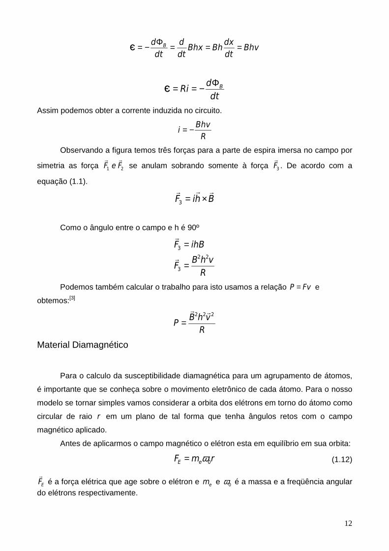
estudo e foi feito sobre o dispositivo como segue abaixo.

Figura 13: brinquedo de quase-levitação comumente chamado de revolution.

Percebe-se claramente que este brinquedo possui um encosto, ele possui em seu

corpo e em sua base imãs permanentes. Neste caso encosto é necessário para este

sistema o Teorema de Earnshaw é aplicado, não podendo haver o fenômeno de levitação.

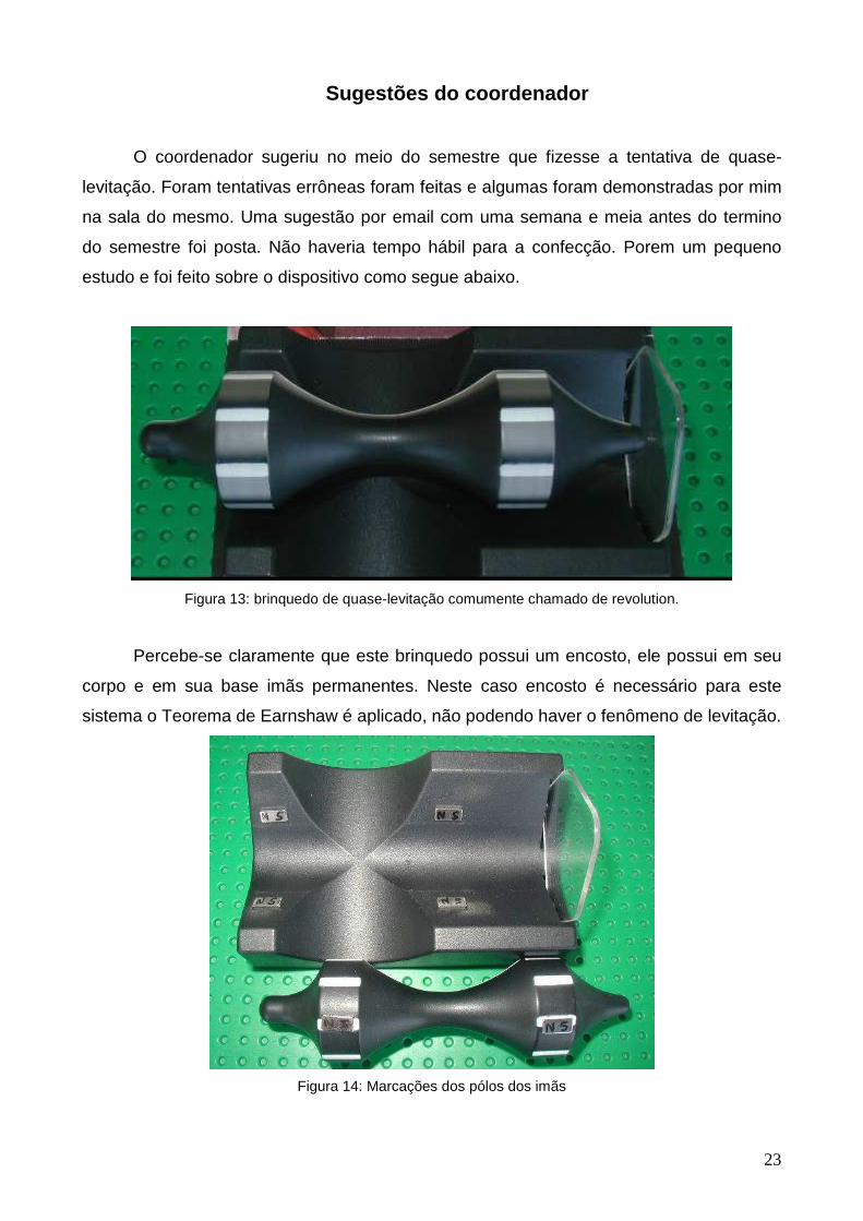
Figura 14: Marcações dos pólos dos imãs

24

Observe que os pólos norte e sul estão voltados para os pólos também norte e sul

do brinquedo. Para ele diferentemente do projeto acima descrito não há o fenômeno de

variação de fluxo, nem de corretes induzidas.

Neste brinquedo o fenômeno aplicado é somente a ação de forças repulsivas, Os

imãs da base devem ter força repulsiva de intensidade tal, que equilibre a força peso do

brinquedo. O aparata transparente que observamos serve justamente para bloquear a

saída do objeto para fora da base.

Estas forças repulsivas não são estáveis não se equilibrando para todos os lados

por este motivo há a necessidade deste aparato.

Esta suposta levitação só é possível pelo giro do brinquedo, o tempo que ele

permanece em quase-levitação o principal fenômeno aplicado é a conservação de

momento angular.

L r p mr v= × = ×� � � � �

Este momento angular pode ser expresso por meio da velocidade angular e o

momento de inércia do brinquedo, os cálculos deste momento de inércia para este

brinquedo seriam muito complicado pelo fato de sua geometria. [7] [8]

L=ω I� �

25

Comentários do Orientador e Co-orientador

O meu orientador realizou os seguintes comentários :

O projeto é interessante e mostra aspectos do magne tismo mais

complicados de se equacionar matemáticamente. O efe ito básico que

se observa são as correntes induzidas em um conduto r que

contrabalançam o peso do imã. O aluno se empenhou b astante em

realizar este projeto, mas que foi parcialmente pre judicado pela demora

na usinagem de peças.

O meu Co-orientador realizou os seguintes comentári os

O projeto do aluno é bastante interessante e motiva uma rica discussão

da teoria eletromagnética, possibilitando um aprend izado aprofundado,

por exemplo, da indução de Faraday, lei de Lenz, co rrentes de Foucalt,

etc. O aluno mostrou-se bastante empolgado com o pr ojeto e

apresentou uma desenvoltura singular. Alguns contra tempos

prejudicaram a finalização do projeto num tempo mai s curto, como por

exemplo, a confecção do protótipo (falta de tempo d e máquina para

usinagem das peças), que não dependia exclusivament e do aluno.

26

Conclusões

O objetivo principal do projeto era aplicar parte da teoria eletromagnética, de forma

mais didática, na tentativa de preencher algumas lacunas com certo êxito alcaçada. As

equações para a força no cilindro girante foram encontradas.

Consegui-se com o embasamento teórico em livros e artigos mostrar as exceções

para o teorema de Earnshaw.

A exemplificação para o sistema sugerida pelo coordenador foi posta em discussão

para futuros alunos desta disciplina.

Referências

[1] – H. Moysés Nussenzveig. 3 Eletromagnetismo, curso de física básica

[2] – David J. Griffiths. Introduction to Electrodynamics

[3] – Halliday Resnick walker. 3 eletromagnetismo, fundamentos da física

[4] – John R. Reitz. Fundamentos da teoria eletromagnética.

[5] – Diamagnetically stabilized magnet levitation. M. D. Simon – L.O.Heflinger – A.K.Geim

aceito em 05/04/2001

[6] – Levitação magnética. Humberto de Andrade Carmona, Universidade Estadual do

Ceará,Campus do Itaperi

[7] - http://www.profisica.cl/comofuncionan/como.php?id=23,

[8] - Halliday resnick Walker. 1 Mecânica, fundamentos da física

Diamagnetically stabilized magnet levitationM. D. Simona)

Department of Physics and Astronomy, University of California, Los Angeles, California 90095

L. O. Heflinger5001 Paseo de Pablo, Torrance, California 90505

A. K. GeimDepartment of Physics and Astronomy, University of Manchester, Manchester, United Kingdomb)

~Received 13 November 2000; accepted 5 April 2001!

Stable levitation of one magnet by another with no energy input is usually prohibited by Earnshaw’stheorem. However, the introduction of diamagnetic material at special locations can stabilize suchlevitation. A magnet can even be stably suspended between~diamagnetic! fingertips. A very simple,surprisingly stable room temperature magnet levitation device is described that works withoutsuperconductors and requires absolutely no energy input. Our theory derives the magnetic fieldconditions necessary for stable levitation in these cases and predicts experimental measurements ofthe forces remarkably well. New levitation configurations are described which can be stabilized withhollow cylinders of diamagnetic material. Measurements are presented of the diamagnetic propertiesof several samples of bismuth and graphite. ©2001 American Association of Physics Teachers.

@DOI: 10.1119/1.1375157#

I. DIAMAGNETIC MATERIALS

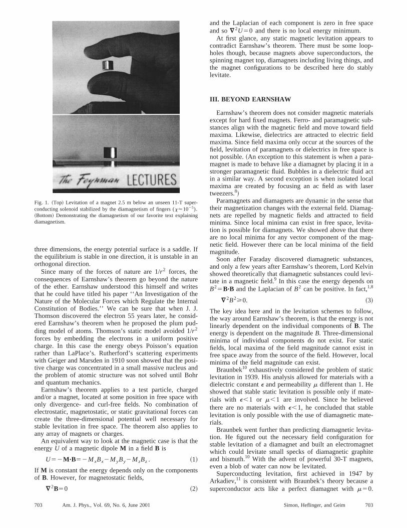
Most substances are weakly diamagnetic and the tinyforces associated with this property make two types of levi-tation possible. Diamagnetic materials, including water, pro-tein, carbon, DNA, plastic, wood, and many other commonmaterials, develop persistent atomic or molecular currentswhich oppose externally applied magnetic fields. Bismuthand graphite are the elements with the strongest diamagne-tism, about 20 times greater than water. Even for these ele-ments, the magnetic susceptibilityx is exceedingly small,x'217031026.

In the presence of powerful magnets the tiny forces in-volved are sufficient to levitate chunks of diamagnetic mate-rials. Living things mostly consist of diamagnetic molecules~such as water and proteins! and components~such asbones!. Contrary to our intuition, these apparently nonmag-netic substances, including living plants and small animals,can be levitated in a magnetic field.1,2

Diamagnetic materials can also stabilize free levitation ofa permanent magnet, which is the main subject of this paper.This approach can be used to make very stable permanentmagnet levitators that work at room temperature without su-perconductors and without energy input. Recently, levitationof a permanent magnet stabilized by the diamagnetism ofhuman fingers (x'21025) was demonstrated at the HighField Magnet Lab in Nijmegen, The Netherlands~Fig. 1!.3,4

While the approximate magnitude of the diamagnetic ef-fect can be derived from simple classical arguments aboutelectron orbits, diamagnetism is impossible within classicalphysics. The Bohr–Leeuwen theorem states that no proper-ties of a classical system in thermal equilibrium can dependin any way on the magnetic field.5,6 In a classical system, atthermal equilibrium the magnetization must always vanish.Diamagnetism is a macroscopic manifestation of quantumphysics that persists at high temperatures,kT@mBohrB.

II. EARNSHAW’S THEOREM

Those who have studied levitation, charged particle traps,or magnetic field design for focusing magnets have probably

run across Earnshaw’s theorem and its consequences. Therecan be no purely electrostatic levitator or particle trap. If amagnetic field is focusing in one direction, it must be defo-cusing in some orthogonal direction. As students, most of usare asked to prove the electrostatic version which goes some-thing like this: Prove that there is no configuration of fixedcharges and/or voltages on fixed surfaces such that a testcharge placed somewhere in free space will be in stable equi-librium. It is easy to extend this proof to include electric andmagnetic dipoles.

It is useful to review what Earnshaw proved and the con-sequences for physics. As can be seen from the title of Earn-shaw’s paper,7 ‘‘On the nature of the molecular forces whichregulate the constitution of the luminiferous ether,’’ he wasworking on one of the frontier physics problems of his time~1842!. Earnshaw wrote before Maxwell’s work, before at-oms were known to be made up of smaller particles, andbefore the discovery of the electron. Scientists were trying tofigure out how the ether stayed uniformly spread out~sometype of repulsion! and how it could isotropically propagatethe light disturbance.

Earnshaw discovered something simple and profound.Particles in the ether could have no stable equilibrium posi-tion if they interacted by any type or combination of 1/r 2

forces. Most of the forces known such as gravity, electrostat-ics, and magnetism are 1/r 2 forces. Without a stable equilib-rium position ~and restoring forces in all directions!, etherparticles could not isotropically propagate wavelike distur-bances. Earnshaw concluded that the ether particles inter-acted by other than 1/r 2 forces. Earnshaw’s paper torpedoedmany of the popular ether theories of his time.

Earnshaw’s theorem depends on a mathematical propertyof the 1/r -type energy potential. The Laplacian of any sum of1/r -type potentials is zero, or¹2Ski /r 50. This means thatat any point where there is force balance (2¹Ski /r 50),the equilibrium is unstable because there can be no localminimum in the potential energy. Instead of a minimum in

702 702Am. J. Phys.69 ~6!, June 2001 http://ojps.aip.org/ajp/ © 2001 American Association of Physics Teachers

three dimensions, the energy potential surface is a saddle. Ifthe equilibrium is stable in one direction, it is unstable in anorthogonal direction.

Since many of the forces of nature are 1/r 2 forces, theconsequences of Earnshaw’s theorem go beyond the natureof the ether. Earnshaw understood this himself and writesthat he could have titled his paper ‘‘An Investigation of theNature of the Molecular Forces which Regulate the InternalConstitution of Bodies.’’ We can be sure that when J. J.Thomson discovered the electron 55 years later, he consid-ered Earnshaw’s theorem when he proposed the plum pud-ding model of atoms. Thomson’s static model avoided 1/r 2

forces by embedding the electrons in a uniform positivecharge. In this case the energy obeys Poisson’s equationrather than LaPlace’s. Rutherford’s scattering experimentswith Geiger and Marsden in 1910 soon showed that the posi-tive charge was concentrated in a small massive nucleus andthe problem of atomic structure was not solved until Bohrand quantum mechanics.

Earnshaw’s theorem applies to a test particle, chargedand/or a magnet, located at some position in free space withonly divergence- and curl-free fields. No combination ofelectrostatic, magnetostatic, or static gravitational forces cancreate the three-dimensional potential well necessary forstable levitation in free space. The theorem also applies toany array of magnets or charges.

An equivalent way to look at the magnetic case is that theenergyU of a magnetic dipoleM in a field B is

U52M "B52MxBx2M yBy2MzBz . ~1!

If M is constant the energy depends only on the componentsof B. However, for magnetostatic fields,

“

2B50 ~2!

and the Laplacian of each component is zero in free spaceand so“2U50 and there is no local energy minimum.

At first glance, any static magnetic levitation appears tocontradict Earnshaw’s theorem. There must be some loop-holes though, because magnets above superconductors, thespinning magnet top, diamagnets including living things, andthe magnet configurations to be described here do stablylevitate.

III. BEYOND EARNSHAW

Earnshaw’s theorem does not consider magnetic materialsexcept for hard fixed magnets. Ferro- and paramagnetic sub-stances align with the magnetic field and move toward fieldmaxima. Likewise, dielectrics are attracted to electric fieldmaxima. Since field maxima only occur at the sources of thefield, levitation of paramagnets or dielectrics in free space isnot possible.~An exception to this statement is when a para-magnet is made to behave like a diamagnet by placing it in astronger paramagnetic fluid. Bubbles in a dielectric fluid actin a similar way. A second exception is when isolated localmaxima are created by focusing an ac field as with lasertweezers.8!

Paramagnets and diamagnets are dynamic in the sense thattheir magnetization changes with the external field. Diamag-nets are repelled by magnetic fields and attracted to fieldminima. Since local minima can exist in free space, levita-tion is possible for diamagnets. We showed above that thereare no local minima for any vector component of the mag-netic field. However there can be local minima of the fieldmagnitude.

Soon after Faraday discovered diamagnetic substances,and only a few years after Earnshaw’s theorem, Lord Kelvinshowed theoretically that diamagnetic substances could levi-tate in a magnetic field.9 In this case the energy depends onB25B"B and the Laplacian ofB2 can be positive. In fact,1,8

“

2B2>0. ~3!

The key idea here and in the levitation schemes to follow,the way around Earnshaw’s theorem, is that the energy is notlinearly dependent on the individual components ofB. Theenergy is dependent on the magnitudeB. Three-dimensionalminima of individual components do not exist. For staticfields, local maxima of the field magnitude cannot exist infree space away from the source of the field. However, localminima of the field magnitude can exist.

Braunbek10 exhaustively considered the problem of staticlevitation in 1939. His analysis allowed for materials with adielectric constante and permeabilitym different than 1. Heshowed that stable static levitation is possible only if mate-rials with e,1 or m,1 are involved. Since he believedthere are no materials withe,1, he concluded that stablelevitation is only possible with the use of diamagnetic mate-rials.

Braunbek went further than predicting diamagnetic levita-tion. He figured out the necessary field configuration forstable levitation of a diamagnet and built an electromagnetwhich could levitate small specks of diamagnetic graphiteand bismuth.10 With the advent of powerful 30-T magnets,even a blob of water can now be levitated.

Superconducting levitation, first achieved in 1947 byArkadiev,11 is consistent with Braunbek’s theory because asuperconductor acts like a perfect diamagnet withm50.

Fig. 1. ~Top! Levitation of a magnet 2.5 m below an unseen 11-T super-conducting solenoid stabilized by the diamagnetism of fingers (x'1025).~Bottom! Demonstrating the diamagnetism of our favorite text explainingdiamagnetism.

703 703Am. J. Phys., Vol. 69, No. 6, June 2001 Simon, Heflinger, and Geim

Flux pinning in Type II superconductors adds some compli-cations and can lead to attractive as well as repulsive forces.

The only levitation that Braunbek missed is spin-stabilizedmagnetic levitation of a spinning magnet top over a magnetbase, which was invented by Roy Harrigan.12 Braunbek ar-gued that if a system is unstable with respect to translation ofthe center of mass, it will be even more unstable if rotationsare also allowed. This sounds reasonable but we now knowthat imparting an initial angular momentum to a magnetictop adds constraints which have the effect of stabilizing asystem which would otherwise be translationallyunstable.13,14 However, this system is no longer truly staticthough once set into motion, tops have been levitated for 50h in high vacuum with no energy input.15

The angular momentum and precession keep the magnettop aligned antiparallel with the local magnetic field direc-tion making the energy dependent only on the magnitudeuBu5@B"B#1/2. Repelling spinning dipoles can be levitatednear local field minima. Similar physics applies to magneticgradient traps for neutral particles with a magnetic momentdue to quantum spin.16 The diamagnetically stabilized float-ing magnets described below stay aligned with the local fielddirection and also depend only on the field magnitude.

IV. MAGNET LEVITATION WITH DIAMAGNETICSTABILIZATION

We know from Earnshaw’s theorem that if we place amagnet in the field of a fixed lifter magnet where the mag-netic force balances gravity and it is stable radially, it will beunstable vertically. Boerdijk~in 1956! used graphite below asuspended magnet to stabilize the levitation.17 Ponizovskiiused pyrolytic graphite in a configuration similar to the ver-tically stabilized levitator described here.18 As seen in TableI, the best solid diamagnetic material is pyrolytic graphitewhich forms in layers and has an anisotropic susceptibility~and thermal conductivity!. It has much higher susceptibilityperpendicular to the sheets than parallel.

It is also possible to levitate a magnet at a location whereit is stable vertically but unstable horizontally. In that case ahollow diamagnetic cylinder can be used to stabilize thehorizontal motion.3,4

The potential energy U of a floating magnet with dipolemomentM in the field of the lifter magnet is

U52M "B1mgz52MB1mgz, ~4!

wheremgzis the gravitational energy. The magnet will alignwith the local field direction because of magnetic torques andtherefore the energy is only dependent on the magnitude ofthe magnetic field, not any field components.

Taking advantage of the irrotational and divergencelessnature of magnetostatic fields in free space and assumingcylindrical symmetry about thez axis, we can expand thefield components as follows:

Bz5B01B8z1 12B9z22 1

4B9~x21y2!1¯ , ~5!

Bx52 12B8x2 1

2B9xz1¯ ,~6!By52 1

2B8y2 12B9yz1¯ ,

where

B85]Bz

]z, B95

]2Bz

]z2 ~7!

and the derivatives are evaluated at the levitation point,x5y5z50. Converting to cylindrical polar coordinates, wehave:

Bz5B01B8z1 12B9z22 1

4B9r 21¯ , ~8!

Br52 12B8r 2 1

2B9rz1¯ . ~9!

Then

B25B0212B0B8z1$B0B91B82%z2

1 14$B8222B0B9%r 21¯ , ~10!

wherer 25x21y2.Expanding the field magnitude of the lifter magnet around

the levitation point using Eqs.~7!–~9! and adding two newtermsCzz

2 and Crr2 which represent the influence of dia-

magnets to be added and evaluated next, the potential energyof the floating magnet is

U52M FB01H B82mg

M J z11

2B9z2

11

4 H B82

2B02B9J r 21¯G1Czz

21Crr2. ~11!

At the levitation point, the expression in the first curlybraces must go to zero. The magnetic field gradient balancesthe force of gravity

B85mg

M. ~12!

The conditions for vertical and horizontal stability are

Kv[Cz212MB9.0 ~vertical stability!, ~13!

Kh[Cr11

4M H B92

B82

2B0J 5Cr1

1

4M H B92

m2g2

2M2B0J

.0 ~horizontal stability!. ~14!

Without the diamagnets, settingCr50 and Cz50, we seethat if B9,0 creating vertical stability, then the magnet isunstable in the horizontal plane. If the curvature is positiveand large enough to create horizontal stability, then the mag-net is unstable vertically.

We first consider the case whereB9.0 and is largeenough to create horizontal stabilityKh.0. The top of Fig. 2shows plots ofKv andKh for the case of a ring magnet lifter.The dashed line shows the effect of theCz term. Where bothcurves are positive, stable levitation is possible ifMB85mg. It is possible to adjust the gradient or the weight ofthe floating magnet to match this condition.

Table I. Values of the dimensionless susceptibilityx in SI units for somediamagnetic materials. The measurement method for the graphites is dis-cussed in a later section.

Material 2x(31026)

Water 8.8Gold 34Bismuth metal 170Graphite rod 160Pyrolytic graphite' 450Pyrolytic graphitei 85

704 704Am. J. Phys., Vol. 69, No. 6, June 2001 Simon, Heflinger, and Geim

We can see that there are two possible locations for stablelevitation, one just below the field inflection point whereB9is zero and one far below the lifter magnet where the fieldsare asymptotically approaching zero. The upper position hasa much stronger gradient than the lower position. The lowerposition requires less diamagnetism to raiseKv to a positivevalue and the stability conditions can be positive over a largerange of gradients and a large spatial range. This is the loca-tion where fingertip stabilized levitation is possible. It is alsothe location where the magnet in the compact levitator ofFig. 4 floats.

The combined conditions for vertically stabilized levita-tion can be written

2Cz

M.B9.

1

2B0S mg

M D 2

. ~15!

Cz is proportional to the diamagnetic susceptibility and getssmaller if the gap between the magnet and diamagnet is in-creased. We can see that the largest gap, or use of weakerdiamagnetic material, requires a largeB field at the levitationposition.

Here it is interesting to note that the inflection point isfixed by the geometry of the lifter magnet, not the strength ofthe magnet. The instability is related to the curvature of thelifter field and force balance depends on the gradient. Thatmakes it feasible to engineer the location of the stable zonesby adjusting the geometry of the lifter magnet and to controlthe gradient by adjusting the strength. With a solenoid, forexample, the stable areas will be determined by the radiusand length of the solenoid and the current can be adjusted toprovide force balance at any location.

The middle plot in Fig. 2 shows that it is also possible toadd a positiveCr to Kh where it turns negative to create aregion where bothKv and Kh are positive, just above theinflection point. The bottom plot shows the lifter field, gra-dient, and curvature on the symmetry axis and the value of2mg/M for a NdFeB floater magnet of the type typicallyused.~The minus sign is used because the abscissa is in the2z direction. The plotted gradient is the negative of thedesired gradient in the1z direction.! Force balance occurswhere the dashed line intersects the gradient curve.

V. EVALUATING THE Cz DIAMAGNETIC TERM

We assume a linear constitutive relation where the mag-netization density is related to the appliedH field by themagnetic susceptibilityx, wherex is negative for a diamag-netic substance.

The magnetic inductionB inside the material is

B5m0~11x!H5m0mH ~16!

wherex, the susceptibility, andm, the relative permeability,are scalars if the material is isotropic and tensors if the ma-terial is anisotropic. A perfect diamagnet such as a Type Isuperconductor hasm50 and will completely cancel thenormal component of an externalB field at its surface bydeveloping surface currents. A weaker diamagnet will par-tially expel an external field. The most diamagnetic elementin the Handbook of Chemistry and Physicsis bismuth withm50.999 83, just less than the unity of free space. Water,typical of the diamagnetism of living things, has am50.999 991. Even so, this small effect can have dramaticresults.

When a magnet approaches a weak diamagnetic sheet ofrelative permeabilitym511x'1, we can solve the problemoutside the sheet by considering an image currentI 8 inducedin the material but reduced by the factor (m21)/(m11)'x/2 ~see Sec. 7.23 of Smythe19!,

I 85Im21

m11'I

x

2. ~17!

If the material were instead a perfect diamagnet such as asuperconductor withx521 andm50, an equal and oppo-site image is created as expected.

To take the finite size of the magnet into account weshould treat the magnet and image as ribbon currents butfirst, for simplicity, we will use a dipole approximationwhich is valid away from the plates and in some other con-ditions to be described. The geometry is shown in Fig. 3.

Fig. 2. ~Top! Stability functionsKv andKh for a ring lifter magnet with o.d.16 cm and i.d. 10 cm. Thex axis is the distance below the lifter magnet. Thedashed line shows the effect of adding diamagnetic plates to stabilize thevertical motion. Levitation is stable where bothKv and Kh are positive.~Middle! The dashed line shows the effect of adding a diamagnetic materialto stabilize the radial motion.~Bottom! Magnetic field~T!, gradient (T/m),and curvature (T/m2) of the lifting ring magnet. The dashed line is equal to2mg/M of a NdFeB floater magnet. Where the dashed line intersects thegradient, there will be force balance. If force balance occurs in a stableregion, levitation is possible.

705 705Am. J. Phys., Vol. 69, No. 6, June 2001 Simon, Heflinger, and Geim

A. Dipole approximation of Cz

We will find the force on the magnet dipole by treating itas a current loop subject to anIÃB force from the magneticfield of the image dipole. The image dipole is inside a dia-magnetic slab a distanceD,

D52d1L, ~18!

from the center of a magnet in free space and has a strengthdetermined by Eq.~17!. The magnet has lengthL and radiusR and is positioned at the origin of a coordinate system atz50. We only need the radial component of the field fromthe induced dipole,Bir at z50.

Using the field expansion equations~7! and ~9! for thecase of the image dipole, we have

Bir 521

2Bi8r 5

m0xM

8p

3r

D4 . ~19!

The lifting force is

Fi5I2pRBir 5M2pR

pR2 Bir 53M2uxum0

4pD4 . ~20!

For equilibrium atz50, the lifting force will be balanced bythe lifting magnet and gravity so that the net force is zero.The net force from two diamagnetic slabs will also be zero ifthe magnet is centered between the two slabs as shown inFig. 4. This is the case we want to consider first.

We now find the restoring force for small displacements inthe z direction from one slab on the bottom,

]Fi

]dz5

]Fi

]D2z52

6M2uxum0

pD5 z. ~21!

For the case of a magnet centered between two slabs of dia-magnetic material, the restoring force is doubled. We canequate this restoring force to theCzz

2 term in the energyexpansion equation~11!. We take the negative gradient ofthe energy term to find the force in thez direction and equatethe terms. For the two-slab case

22Czz5226M2uxum0

pD5 z,

~22!Cz5

6M2uxum0

pD5 .

B. Alternate route to Cz

The same result can be derived directly from the equationfor the potential energy of a magnet with fixed dipoleM inthe induced fieldBi of its image in a para- or diamagneticmaterial,19

Ui52 12 M "Bi . ~23!

We assume that the magnet is in equilibrium with gravityat z50 due to forces from the lifter magnet and possiblyforces from the diamagnetic material and we want to calcu-late any restoring forces from the diamagnetic material. Theenergy of the floater dipoleM in the fieldsBi of the induceddipoles from diamagnetic slabs above and below the magnetis

Ui5uxuM2m0

8p F 1

~2d1L12z!3 11

~2d1L22z!3G . ~24!

We expand the energy around the levitation pointz50,

Ui5Ui01Ui8z1 12 Ui9z

21¯ ~25!

5uxuM2m0

8p F 2

~2d1L !3 148

~2d1L !5 z2G1¯ ~26!

5C16uxuM2m0

pD5 z21¯ ~27!

5C1Czz21¯ . ~28!

This gives the same result as Eq.~22!.

C. Maximum gap D in dipole approximation

Adding diamagnetic plates above and below the floatingmagnet with a separationD gives an effective energy due tothe two diamagnetic plates,

Udia[Czz25

6m0M2uxupD5 z2, ~29!

in the dipole approximation. From the stability conditions@Eqs.~13! and ~14!#, we see that levitation can be stabilizedat the point whereB85mg/M if

12m0M uxupD5 .B9.

~mg!2

2M2B0. ~30!

Fig. 3. Geometry for the image dipole and image ribbon current force cal-culations.

Fig. 4. Diamagnetically stabilized magnet levitation geometry for one com-pact implementation.

706 706Am. J. Phys., Vol. 69, No. 6, June 2001 Simon, Heflinger, and Geim

This puts a limit on the diamagnetic gap spacing

D,H 12m0M uxupB9 J 1/5

,H 24m0B0M3uxup~mg!2 J 1/5

. ~31!

If we are far from the lifter magnet field, we can considerit a dipole momentML at a distanceH from the floater. Theequilibrium condition, Eq.~12!, is

H5H 3MMLm0

2pmg J 1/4

. ~32!

Then, the condition for stability and gap spacing at the levi-tation point is20

D,HH 2uxuM

MLJ 1/5

. ~33!

The most important factor for increasing the gap is using afloater with the strongest possibleM /m. Using the strongestdiamagnetic material is also important. Lastly, a stronger lift-ing dipole further away~largerH! produces some benefit.

D. Surface current approximation

Treating the magnets and images as dipoles is useful forunderstanding the general dependencies, but if the floatermagnet is large compared to the distance to the diamagneticplates, there will be significant errors. These errors can beseen in Eq.~29!, where the energy becomes infinite as thedistanceD52d1L goes to zero. Since the gap spacingd isusually on the order of the floater magnet radius and thick-ness, more accurate calculations of the interaction energy arenecessary.~In the special case when the diameter of a cylin-drical magnet is about the same as the magnet length, thedipole approximation is quite good over the typical distancesused, as can be confirmed in Fig. 6.!

Even treating the lifter magnet as a dipole is not a verygood approximation in most cases. A better approximationfor the field BL from a simple cylindrical lifter magnet oflength l L and radiusRL at a distanceH from the bottom ofthe magnet is

BL5BLr

2 F H1 l L

A~H1 l L!21RL22

H

AH21RL2G , ~34!

where BLr is the remanent or residual flux density of thepermanent magnet material.~The residual flux density is thevalue of B on the demagnetizationB–H curve whereH iszero when a closed circuit of the material has been magne-tized to saturation. It is a material property independent ofthe size or shape of the magnet being considered.! This equa-tion is equivalent to using a surface current or solenoidmodel for the lifter magnet and is a very good approxima-tion. If the lifter is a solenoid,BLr is the infinite solenoidfield m0NI/ l L .

Figure 5 shows the measured field of a lifter ring magnetwe used. The fit of the surface current approximation is bet-ter even 4 cm away, which was approximately the levitationforce balance position. The ring magnet has an additionalequal but opposite surface current at the inner diameter,which can be represented by a second equation of form~34!.

VI. METHOD OF IMAGE CURRENTS FOREVALUATING Cz

The force between two parallel current loops of equal radiia separated by a distancec with currentsI and I 8 can bewritten as~see Sec. 7.19 of Smythe19!

F loops5m0II 8c

A4a21c2 F2K12a21c2

c2 EG , ~35!

whereK andE are the elliptic integrals

K5E0

p/2 1

A12k2 sin2 udu, ~36!

E5E0

p/2A12k2 sin2 u du, ~37!

and

k254a2

4a21c2 . ~38!

We extend this analysis to the case of two ribbon currentsbecause we want to represent a cylindrical permanent magnetand its image as ribbon currents. The geometry is shown inFig. 3. We do a double integral of the loop force equation~35! over the length dimensionL of both ribbon currents.With a suitable change of variables we arrive at the singleintegral

F5m0II 8E21

1

J$12v sgn~v !%dv, ~39!

where

J5A12k2F12 12 k2

12k2 E~k!2K~k!G ,

~40!

k51

A11g2, g5

d

R1

L

2R~11v !,

sgn~v !5sign of v5H 11 if v.0

0 if v50

21 if v,0.

~41!

Fig. 5. Measured field from a ring lifter magnet with fits to a dipole ap-proximation and a surface current approximation. The lifter is a ceramicmaterial withBr of 3200 G. The dimensions are o.d. 2.8 cm, i.d. 0.9 cm, andthickness 0.61 cm.

707 707Am. J. Phys., Vol. 69, No. 6, June 2001 Simon, Heflinger, and Geim

d is the distance from the magnet face to the diamagneticsurface andR andL are the radius and length of the floatingmagnet.

From measurements of the dipole momentM of a magnet,we convert to a current

I 5M

area5

M

pR2 . ~42!

Using Eq.~17!, we have

I 85xM

2pR2 . ~43!

OnceM, x, and the magnet dimensions are known, Eq.~39!can be integrated numerically to find the force. If the force ismeasured, this equation can be used to determine the suscep-tibility x of materials. We used this method to make our ownsusceptibility measurements and this is described below.

In the vertically stabilized levitation configuration shownin Fig. 4, there are diamagnetic plates above and below thefloating magnet and at the equilibrium point, the forces bal-ance to zero. The centering force due to the two plates istwice the gradient of the forceF in Eq. ~39! with respect tod,the separation from the diamagnetic plate, times the verticaldisplacementz of the magnet from the equilibrium position.We can equate this force to the negative gradient of theCzz

2

energy term from Eq.~11!,

22Czz52]F

]dz. ~44!

Therefore, the coefficientCz in Eqs.~11! and ~13! is

Cz52]F

]d~45!

Fig. 6. Force on a magnet above a diamagnetic sheet as a function of distance above the sheet in units of magnet radiusR. Dipole approximation comparedto image current solution for three different magnet length to radius ratios. The force axis is in units ofm0I 2x/2. The ribbon currentI is related to the dipolemomentM of the magnet byM5IpR2. The force gradient axis is in units2m0I 2x/2R.

708 708Am. J. Phys., Vol. 69, No. 6, June 2001 Simon, Heflinger, and Geim

and this force must overcome the instability due to the unfa-vorable field curvatureB9. Figure 6 shows the force andgradient of the force for floating magnets of different aspectratios.

Oscillation frequency. When the vertical stability condi-tions @Eq. ~13!# are met, there is an approximately quadraticvertical potential well with vertical oscillation frequency

n51

2pA1

m H 22]F

]d2MB9J . ~46!

Applying Eq. ~22!, in the dipole approximation, the verticalbounce frequency is

n51

2pA1

m H 12m0M2uxupD5 2MB9J . ~47!

The expression in the curly braces, 2Kv , represents the ver-tical stiffness of the trap. 2Kh represents the horizontal stiff-ness.

The theoretical and measured oscillation frequencies areshown later in Fig. 12. It is seen that the dipole approxima-tion is not a very good fit to the data whereas the imagecurrent prediction is an excellent fit.

VII. THE Cr TERM

We now consider the case just above the inflection pointwhereB9,0. A hollow diamagnetic cylinder with inner di-ameterD as shown in Fig. 7 produces an added energy term~in the dipole approximation!3

Udia[Crr25

45m0uxuM2

16D5 r 2. ~48!

Near the inflection point whereB9 is negligible, the horizon-tal stability condition@Eq. ~14!# becomes

45m0uxuM2

2D5 .MB82

B05

m2g2

MB0, ~49!

D,H 45m0B0M3uxu2~mg!2 J 1/5

. ~50!

This type of levitator can also be implemented on a tabletopusing a large diameter permanent magnet ring as a lifter asdescribed in the middle plot in Fig. 2.

The horizontal bounce frequency in the approximatelyquadratic potential well is

n r51

2pA1

m H 45m0M2uxu8D5 1

MB9

22

MB82

4B0J . ~51!

The expression in the curly braces, 2Kh , represents the hori-zontal stiffness of the trap.

VIII. COUNTERINTUITIVE LEVITATIONCONFIGURATION

There is another remarkable but slightly counterintuitivestable levitation position. It is above a lifter ring magnet withthe floater in an attractive orientation. Even though it is inattractive orientation, it is vertically stable and horizontallyunstable. The gradient from the lifter repels the attractingmagnet but the field doesn’t exert a flipping torque. Thisconfiguration is a reminder that it is not the field directionbut the field gradient that determines whether a magnet willbe attracted or repelled. A bismuth or graphite cylinder canbe used to stabilize the horizontal instability.

Figure 8 shows the stability functions and magnetic fieldsfor this levitation position above the lifter magnet. We haveconfirmed this position experimentally.

IX. EXPERIMENTAL RESULTS

Before we can compare the experimental results to thetheory, we need to know the values of the magnetic dipolemoment of the magnets and the susceptibility of diamagneticmaterials we use. The dipole moment can be determined bymeasuring the 1/r 3 fall of the magnetic field on axis far froma small magnet. For Nd2Fe14B magnet material, it is an ex-cellent approximation to consider the field as created by asolenoidal surface current and use the finite solenoid equa-tion ~34! fit to measurements.

The diamagnetic susceptibility was harder to measure.Values in theHandbook of Chemistry and Physicswereproblematic. Most sources agree on some key values such aswater and bismuth.~There are multiple quantities called sus-ceptibility and one must be careful in comparing values.Physicists use what is sometimes referred to as the volumesusceptibility. Chemists use the volume susceptibility di-vided by the density. There is also a quantity sometimescalled the gram molecular susceptibility which is the volumesusceptibility divided by the density and multiplied by themolecular weight of the material. There are also factors of4p floating around these definitions. In this paper we use thedimensionless volume susceptibility in SI units.!

Fig. 7. Vertical and horizontal stability curves for magnet levitation show-ing the stabilizing effect of a diamagnetic cylinder with an inner diameter of8 mm and the levitation geometry. Magnet levitation is stable where bothcurves are positive and the magnetic lifting force matches the weight of themagnet.

709 709Am. J. Phys., Vol. 69, No. 6, June 2001 Simon, Heflinger, and Geim

The values given in theHandbook of Chemistry and Phys-ics and some other published sources for graphite are inex-plicably low. This could be because graphite rods have manydifferent compositions and impurities. Iron is a major impu-rity in graphite and can overwhelm any diamagnetic effect.We have seen graphite rods that are diamagnetic on one endand paramagnetic on the other. Braunbek noticed that usedgraphite arc rods were more diamagnetic on the side closestto the arc. He speculated that the binder used in the rods wasparamagnetic and was vaporized by the heat of the arc. Wefound that, in practice, purified graphite worked as well asbismuth and our measurements of its susceptibility were con-sistent with this.

Values for a form of graphite manufactured in a specialway from the vapor state, called pyrolytic graphite, are notgiven in theHandbookand the other literature gives a widerange of values. Pyrolytic graphite is the most diamagneticsolid substance known. It has an anisotropic susceptibility.Perpendicular to the planar layers, the diamagnetic suscepti-bility is better than in pure crystal graphite.21 Parallel to theplanar layers, the susceptibility is lower than randomly ori-ented pressed graphite powder.

We developed a technique to measure the diamagneticsusceptibility of the materials we used. Later, we were ableto get a collaborator~Fred Jeffers! with access to a state ofthe art vibrating sample magnetometer to measure somesamples. There was very good agreement between our mea-surements and those made using the magnetometer.

A. Measurements of diamagnetic susceptibility

A simple and useful method for testing whether samplesof graphite are diamagnetic or not~many have impurities that

destroy the diamagnetism! is to hang a small NdFeB magnet,say 6 mm diameter, as the bob of a pendulum with about 1/2m of thread. A diamagnetic graphite piece slowly pushedagainst the magnet will displace the pendulum a few centi-meters before it touches, giving a quick qualitative indicationof the diamagnetism.

The method we used to accurately measure the suscepti-bility was to hang a small NdFeB magnet as a pendulumfrom pairs of long threads so that the magnet could movealong only one direction. The magnet was attached to oneend of a short horizontal drinking straw. At the other end ofthe straw, a small disk of aluminum was glued. A translationstage was first zeroed with respect to the hanging magnetwithout the diamagnetic material present. Then the diamag-netic material to be tested was attached to a micrometertranslation stage and moved close to magnet, displacing thependulum from the vertical. The force was determined by thedisplacement from vertical of the magnet andx was deter-mined from Eqs.~39! and~17!, which is plotted as the forcein Fig. 6.

A sample of bismuth was used as a control and matchedthe value in the standard references.22 Once the value for oursample of bismuth was confirmed, the displacement wasmeasured for a fixed separationd between the magnet andbismuth. All other samples were then easily measured byusing that same separationd, the relative force/translationgiving the susceptibility relative to bismuth.

The difficult part was establishing a close fixed distancebetween the magnet and the diamagnetic material surfacewith high accuracy. This problem was solved by making thegap part of a sensitive LC resonant circuit. Attached to thetranslation stage, a fixed distance from the diamagnetic ma-terial under test, was the L part of the LC oscillator. Whenthe gap between the diamagnet and magnet reached the de-sired fixed value, the flat piece of aluminum on the other sideof the straw from the magnet, came a fixed distance from theL coil, changing its inductance. The separation distancecould be set by turning a micrometer screw to move thetranslation stage until the frequency of the LC circuit reachedthe predetermined value for each sample under test. Thesetup is shown in Fig. 9.

This method was perhaps more accurate for our purposesthan the vibrating sample magnetometer, an expensive in-strument. Our method was independent of the volume of thediamagnetic material. The vibrating sample magnetometer isonly as accurate as the volume of the sample is known.Samples are compared to a reference sample of nickel with aspecific geometry. Our samples were not the same geometryand there was some uncertainty in the volume. Our measure-ments measured the susceptibility of the material in a wayrelevant to the way the material was being used in our ex-periments.

We measured various samples of regular graphite and py-rolytic graphite and bismuth. Our average values for thegraphite materials are shown in Table I and are consistentwith the values from the vibrating sample magnetometer.Our value for graphite is higher than many older values suchas that reported in theHandbook of Chemistry and Physics,but is lower than that stated in a more recent reference.23 Ourvalues for pyrolytic graphite are below the low end of thevalues stated in the literature.18,24The value for the pyrolyticgraphite parallel to the planar layers is from the vibratingsample magnetometer.

Fig. 8. ~Top! Vertical and horizontal stability curves for magnet levitation adistanceH above a ring lifter magnet. The dashed line shows the stabilizingeffect of a diamagnetic cylinder. Magnet levitation is stable where bothcurves are positive and the magnetic lifting force matches the weight of themagnet.~Bottom! B ~T!, B8 ~T/cm!, B9 ~T/cm2!, andmg/M ~T/cm! for a16-cm-o.d., 10-cm-i.d., 3-cm-thick ring lifting magnet and a NdFeB floater.

710 710Am. J. Phys., Vol. 69, No. 6, June 2001 Simon, Heflinger, and Geim

B. Experimental realization of levitation

The fingertip and book stabilized levitation shown in Fig.1 was achieved using a 1-m-diam 11-T superconducting so-lenoid 2.5 m above the levitated magnet where the field was500 G. Using regular graphite and an inexpensive ceramiclifter magnet, it is possible to make a very stable levitatorabout 5 cm tall with a gap D of about 4.4 mm for a 3.175-mm-thick, 6.35-mm-diam NdFeB magnet. Using pyrolyticgraphite, the gap D increases to almost 6 mm for the samemagnet. This simple design~similar to Fig. 4! could findwide application. The stability curves and gradient matchingcondition can be seen in Fig. 10. The magnitude ofCz wasdetermined from the force gradient in Fig. 6 withL/R51 attwo different gapsd using our measured susceptibility ofpyrolytic graphite.

Figure 7 shows an experimental realization of horizontalstabilization at the High Field Magnet Laboratory inNijmegen. We also achieved horizontal stabilization on atabletop using a permanent magnet ring and a graphite cyl-inder.

We were recently able to achieve stable levitation at thecounterintuitive position above the ring lifter magnet~de-scribed above!. The floater is in attractive orientation but isnaturally vertically stable and radially unstable. Radial stabi-lization was provided by a hollow graphite cylinder.

Other configurations for diamagnetically stabilized magnetlevitation are possible and rotational symmetry is not re-quired. For example, at the levitation position described justabove, if an oval magnet or a noncircular array is used for alifter instead of a circular magnet, thex–z plane can bemade stable. Instead of using a hollow cylinder to stabilizethe horizontal motion, flat plates can be used to stabilize they direction motion.

For vertical stabilization with flat plates, if a long bar mag-

net is used horizontally as a lifter, the levitation point can beturned into a line. With a ring magnet, the equilibrium pointcan be changed to a circle. Both of these tricks have beendemonstrated experimentally.

Another quite different configuration is between two ver-tical magnet pole faces as shown in Fig. 11. Between thepole faces, below center and just above the inflection point inthe magnetic field magnitude, the floating magnet is naturallyvertically stable. Diamagnetic plates then stabilize the hori-zontal motion. To our knowledge, this configuration was firstdemonstrated by S. Shtrikman.

Fig. 9. Setup for measuring diamagnetic susceptibility. The diamagneticmaterial is moved close to the magnet, deflecting the magnet pendulum,until the gap between the magnet and diamagnet reaches a preset value.When the aluminum is a fixed distance from the inductor coil, the LC circuitresonates at the desired frequency, corresponding to the preset value of thegap. This is an accurate way to measure the small gap. The force is deter-mined from the displacement of the pendulum. The force is then comparedto the force from a previously calibrated sample of bismuth with the samegap.

Fig. 10. Stability functionsKv andKh for the demonstration levitator. Sta-bility is possible where both functions are positive. The dashed lines showthe effect of two different values of theCz term onKv . The smaller valuecorresponds to a large gap spacingd51.9 mm. The larger value corre-sponds to a gap of only 0.16 mm.~Bottom! The levitation position is where2mg/M intersects the gradient2B8 at approximatelyH54.5 cm below thelifter magnet.B is in T, 2B8 in T/cm, andB9 in T/cm2.

Fig. 11. Graphite plates stabilize levitation of a magnet below the centerlinebetween two pole faces and just above the inflection point in the field mag-nitude. Not shown in the picture but labeled N and S are the 25-cm-diampole faces of an electromagnet spaced about 15 cm apart. The poles can befrom permanent or electromagnets.

711 711Am. J. Phys., Vol. 69, No. 6, June 2001 Simon, Heflinger, and Geim

C. Measurements of forces and oscillation frequencies

One way to probe the restoring forces of the diamagneticlevitator is to measure the oscillation frequency in the poten-tial well. For the vertically stabilized levitator in Fig. 4 wemeasured the vertical oscillation frequency as a function ofthe gap spacingd and compared it to the dipole and imagecurrent forces and prediction equations~46! and ~47!. Thelifting magnet used for this experiment was a 10-cm-long by2.5-cm-diam cylindrical magnet. This magnet was used be-cause its field could be accurately determined from the finitesolenoid equation. The dipole moment was measured to be25 A m2. The floater magnet was a 4.7-mm-diam by 1.6-mm-thick NdFeB magnet with a dipole moment of 0.024 A m2. Itweighed 0.22 g and levitated 8 cm below the bottom of thelifter magnet as expected.

The graphite used was from a graphite rod, not pyrolyticgraphite. We measured this sample of graphite to have asusceptibility of 217031026. The oscillation frequencywas determined by driving an 1800-ohm coil below the levi-tated magnet with a sine wave. The resonant frequency wasdetermined visually and the vibration amplitude kept small.The gap was changed by carefully turning a1

4–20 screw.Figure 12 shows the theoretical predictions and the experi-

mental measurements of the oscillation frequency as a func-tion of gap spacingd. There are no adjustable parameters inthe theory predictions. All quantities were measured in inde-pendent experiments. The agreement between the data andthe image current calculation is remarkably good. There is alimit to how much the total gapD52d1L can be increased.If D is too great, the potential well becomes double humpedand the magnet will end up closer to one plate than the other.The last point withd greater than 1.4 mm was clearly in thedouble well region and was plotted as zero.

X. LEVITATION SOLUTIONS FOR ACYLINDRICALLY SYMMETRIC RING MAGNET

A ring magnet provides many combinations of fields, gra-dients, and curvatures as shown in Fig. 13. Considering thefield topology but not the magnitudes, we show all possible

positions where diamagnets, spin-stabilized magnets, andmagnets stabilized by diamagnetic material can levitate. Thefields and gradients shown may not be sufficient to levitate adiamagnet in the position shown against 1g of gravity, butthe topology is correct if the magnetic field could be in-creased enough.

Each type of levitation has its own requirements for radialand horizontal stability which are shown in Tables II and III.Other requirements such as matching the magnetic field gra-dient tomg/M need be met. The fields must be in the rightdirection so as not to flip the magnet. The directions shownin Table II are all compared to the direction ofB.

The most fruitful place to look for levitation positions isaround the inflection points of the magnetic field. These arethe places where the instability is weakest. The two levita-tion regions in Fig. 13 marked with a question mark have notbeen demonstrated experimentally and are probably not ac-cessible with current magnetic and diamagnetic materials.The lower position with a question mark would work using adiamagnetic cylinder for radial stabilization. However, itmay require more diamagnetism than is available. The levi-tation positions without the question marks have been dem-onstrated experimentally. The position for levitation of a dia-magnet marked with an asterisk has recently beendemonstrated by the authors.

The locations for diamagnetically stabilized magnet levi-tation are interesting for another reason. At these locationsservo control can be used to provide active stabilization very

Fig. 12. Data points on the vertical oscillation frequency vs the gap spacingd with the dipole approximation prediction curve and the image currenttheory curve. The curves are not fit to the data. They are predictions fromthe measured properties of the magnets and diamagnets, with no free param-eters. The last point is beyond the zero frequency limit and is plotted aszero. At zero frequency, the gap is too large to provide stability and thepotential well becomes double humped, with stable points closer to oneplate than the other. This clearly was the case with the last point aroundd.1.4 mm.

Fig. 13. B ~T!, B8 ~T/cm!, and B9 ~T/cm2!, for a 16-cm-o.d., 10-cm-i.d.,3-cm-thick ring lifting magnet showing the fields on axis above and belowthe magnet. All possible levitation positions are shown for spin-stabilizedmagnet levitation, diamagnetically stabilized magnet levitation, and levita-tion of diamagnets.h and v indicate use of diamagnetic material for hori-zontal or vertical stabilization. The two regions with question marks havenot yet been verified experimentally and may be difficult to achieve. Thelevitation of diamagnets marked with an asterisk has recently been demon-strated by the authors.

Table II. Magnetic field requirements for levitation of diamagnets, spin-stabilized magnet levitation, and diamagnetically stabilized levitation ofmagnets. Plus signs~1! and minus signs~2! indicate the sign with respectto the sign ofB.

M aligned withB B8 B9

Levit. of diamagnets 2 2 1 or 2

Spin-stabilized magnet 2 2 1

Diamag. stab. horiz. 1 1 2

Diamag. stab. vert. 1 1 1

712 712Am. J. Phys., Vol. 69, No. 6, June 2001 Simon, Heflinger, and Geim

efficiently, since the instability is weak at those locations.The diamagnetic plates or cylinder act as a very weak servosystem.

ACKNOWLEDGMENTS

We acknowledge fruitful communications with MichaelBerry. We would like to thank Marvin Drandell for his helpfabricating many prototype levitators, Rudy Suchannek forhis translation of Braunbek’s10 papers from German, andFred Jeffers for helping confirm our susceptibility measure-ments. We thank Robert Romer for his support and for keep-ing error out of the manuscript.

a!Electronic mail: msimon@physics.ucla.edub!Formerly High Field Magnet Lab., Nijmegen, The Netherlands.1M. V. Berry and A. K. Geim, ‘‘Of flying frogs and levitrons,’’ Eur. J.Phys.18, 307–313~1997!; http://www-hfml.sci.kun.nl/hfml/levitate.html.

2A. Geim, ‘‘Everyone’s Magnetism,’’ Phys. Today51, 36–39~1998!.3A. K. Geim, M. D. Simon, M. I. Boamfa, and L. O. Heflinger, ‘‘Magnetlevitation at your fingertips,’’ Nature~London! 400, 323–324~1999!.

4M. D. Simon and A. K. Geim, ‘‘Diamagnetic levitation; flying frogs andfloating magnets,’’ J. Appl. Phys.87, 6200–6204~2000!.

5N. W. Ashcroft and N. D. Mermin,Solid State Physics~Harcourt Brace,New York, 1976!, Chap. 31, p. 647.

6R. P. Feynman, R. B. Leighton, and M. Sands,The Feynman Lectures in

Physics~Addison–Wesley, New York, 1963!, Vol. II, Chap. 34, Sec. 6.7S. Earnshaw, ‘‘On the nature of the molecular forces which regulate theconstitution of the luminiferous ether,’’ Trans. Cambridge Philos. Soc.7,97–112~1842!.

8K. T. McDonald, ‘‘Laser tweezers,’’ Am. J. Phys.68, 486–488~2000!.9W. Thomson,Reprint of Papers on Electrostatics and Magnetism~Mac-Millan, London, 1872!, paper XXXIII, pp. 493–499, and paper XXXIV,pp. 514–515.

10W. Braunbek, ‘‘Freischwebende Ko¨rper im elecktrischen und magnetis-chen Feld,’’ Z. Phys.112, 753–763~1939!; ‘‘Freies Schweben diamagne-tischer Korper im Magnetfeld,’’ibid. 112, 764–769~1939!.

11V. Arkadiev, ‘‘A floating magnet,’’ Nature~London! 160, 330 ~1947!.12R. M. Harrigan, U.S. patent 4,382,245~1983!.13M. D. Simon, L. O. Heflinger, and S. L. Ridgway, ‘‘Spin stabilized mag-

netic levitation,’’ Am. J. Phys.65, 286–292~1997!.14M. V. Berry, ‘‘The Levitron™: An adiabatic trap for spins,’’ Proc. R. Soc.

London, Ser. A452, 1207–1220~1996!.15Ed Phillips ~private communication!.16V. V. Vladimirskii, ‘‘Magnetic mirrors, channels and bottles for cold neu-

trons,’’ Sov. Phys. JETP12, 740–746~1961!; W. Paul, ‘‘Electromagnetictraps for charged and neutral particles,’’ Rev. Mod. Phys.62, 531–540~1990!.

17A. H. Boerdijk, ‘‘Technical aspects of levitation,’’ Philips Res. Rep.11,45–56~1956!; ‘‘Levitation by static magnetic fields,’’ Philips Tech. Rev.18, 125–127~1956/57!.

18V. M. Ponizovskii, ‘‘Diamagnetic suspension and its applications~sur-vey!,’’ Prib. Tekh. Eksp.4, 7–14~1981!.

19W. R. Smythe,Static and Dynamic Electricity~Hemisphere Publishing,New York, 1989!, 3rd ed.

20M. V. Berry first suggested the simplification of treating the lifter magnetas a dipole and derived Eq.~33! in a 1997 correspondence with M. D.Simon.

21D. B. Fischback, ‘‘The magnetic susceptibility of pyrolytic carbons,’’Pro-ceedings of the Fifth Conference on Carbon, 1963, Vol. 2, pp. 27–36.

22For example, theHandbook of Chemistry and Physics~The ChemicalRubber Co., Boca Raton, FL, 1992–1993!.

23I. Simon, A. G. Emslie, P. F. Strong, and R. K. McConnell, Jr., ‘‘Sensitivetiltmeter utilizing a diamagnetic suspension,’’ Rev. Sci. Instrum.39,1666–1671~1968!.

24R. D. Waldron, ‘‘Diamagnetic levitation using pyrolytic graphite,’’ Rev.Sci. Instrum.37, 29–35~1966!.

SELF-DELUSION

Theism~and the implicit rejection of reductionism! is a system of knowledge based on igno-rance, and that twin of ignorance, fear. It would certainly be too much to expect a theologian~orindeed a scientist! to admit that his lifetime’s work had been based on a false foundation. It is evenless likely that anyone religious, unless they were exceptionally self-honest and intellectuallysinewy, would admit that the whole history of their church was based on a clever, but understand-able, self-delusion~and in some cases, I suspect, on a straightforward conscious lie!. I considerthat religion is a delusion propagated by a combination of ignorance, art, and fear, fanned intolongevity and ubiquity by the power it gave to those in command.

P. W. Atkins, ‘‘The Limitless Power of Science,’’ inNature’s Imagination—The Frontiers of Scientific Vision, edited byJohn Cornwell~Oxford University Press, New York, 1995!.

Table III. Stability functions for levitation of diamagnets, spin-stabilizedmagnets, and diamagnetically stabilized magnets. The functions must bepositive for stability and assumeB0 in the positivez direction.

Vertical Horizontal

Levit. of diamagnets B0B91B82 B8222B0B9Spin-stabilized magnet B9 B8222B0B9

Diamag. stab. magnet Cz21

2MB9 Cr1

1

4MHB92

B82

2B0J

713 713Am. J. Phys., Vol. 69, No. 6, June 2001 Simon, Heflinger, and Geim

18 Física na Escola, v. 1, n. 1, 2000

É possível um ser vivo levitar? Aocidadão comum, a resposta aessa pergunta está apenas nos

livros de ficção científica. No entanto,a ciência e a tecnologia têm encontradoformas de fazer seres vivos levitarem.

Alguns dispositivos utilizandofeixes de ar podem levar ao fenômeno.Por exemplo, um helicóptero, não queele seja um ser vivo, mas pode conterum. Outros dispositivos utilizam cam-pos magnéticos e materiais supercon-dutores. Já há algum tempo, cientistaspensam no uso do magnetismo paralevitar veículos, seja utilizando ímãspermanentes ou supercondutores.

Um supercondutor resfriadocom nitrogênio líquido, flutuando so-bre um ímã é uma imagem um tantocomum para a comunidade científicahoje em dia, e não surpreenderia umfísico. Supercondutores são materiaisdiamagnéticos perfeitos e a expulsãodo campo magnético de seu interiorcausa sua levitação. Já um pequenosapo, ou mesmo um morango, à tem-peratura ambiente, levitando nocentro de um magneto, é uma ima-gem menos comum.

Apesar de menos comum e sur-preendente, mostra-remos neste artigo queé possível levitar umser vivo. Cientistas,entre eles o autordeste artigo e o russoAndrei Geim, realiza-ram experimentos delevitação de váriosmateriais, no Labora-tório de Altos CamposMagnéticos (HFML)da Universidade Cató-lica de Nijmegen, Ho-

landa, em 19971-3. Nestes experi-mentos levitou-se praticamente tudoque se tinha em mãos, de criaturasvivas como um sapo, gafanhoto, pe-queno peixe, plantas até pequenospedaços de pizza e água. Em 1991,Eric Beaugno e Robert Tournier, uti-lizando o mesmo processo, levitaramágua e algumas substâncias orgâni-cas4. Chamaremos o processo de levi-tação utilizado nesses experimentosde levitação magnética.

A Figura 1 mostra uma seqüên-cia fotográfica de um pequeno sapolevitando no centro de um solenóide.

Para obter levitação magnética énecessário um campo magnético comcaracterísticas especiais e com inten-sidade relativamente alta. O objeto,nesse caso o sapo, é colocado no centrode um magneto do tipo Bitter, comdiâmetro interno de 32 mm, comomostra a Figura 2. Uma correnteelétrica de até 20 kA na bobina domagneto produz campos magnéticosde até 20 Tesla. O conjunto de bobinasdo magneto é projetado de forma queo campo magnético seja máximo ehomogêneo no centro da bobina in-terna (região indicada pela letra A na

Humberto de Andrade CarmonaUniversidade Estadual do Ceará,Campus do ItaperiAv. Paranjana, 1700 - Fortaleza, CEe-mail: carmona@uece.br

○ ○ ○ ○ ○ ○ ○ ○ ○ ○ ○ ○ ○ ○ ○ ○ ○ ○ ○ ○ ○

○ ○ ○ ○ ○ ○ ○ ○ ○ ○ ○ ○ ○ ○ ○ ○ ○ ○ ○ ○ ○

Figura 1. Seqüência fotográfica de um pequeno sapo levitandono centro de um magneto de 20 Tesla.

Neste trabalho descreve-se um experimentomostrando que um ser vivo pode levitar. Longede precisar de ‘poderes extra-sensoriais’, alevitação pode ser alcançada por meio de cam-pos eletromagnéticos. Vejamos como conseguiruma levitação magnética.

Levitação Magnética

19Física na Escola, v. 1, n. 1, 2000

Figura 2). Nas proximidades do topoda bobina interna (região indicada pelaletra B na Figura 2), o campo magné-tico apresenta gradientes nas direçõesaxial e radial. Veremos mais tarde queesses gradientes são importantes paraa observação do fenômeno de levitação.

Apesar de surpreendente, mes-mo para alguns físicos, a levitaçãoestável de materiais comuns em nossodia-a-dia possui uma explicação sim-ples e se baseia em uma propriedadeintrínseca de muitos materiais cha-mada diamagnetismo, que se refere aofato de que esses materiais têm a habi-lidade de expelir um campo magnéticoexterno. O diamagnetismo pode serentendido superficialmente da seguin-te forma: como se sabe, toda matériano universo consiste de átomos, e ca-da átomo possui elétrons em movi-mento em torno de seu núcleo. Aocolocar um átomo em um campomagnético, os elétrons em movi-mento em torno de seunúcleo alteram seusmovimentos de forma ase oporem a essa in-fluência externa, ouseja, esses elétronscriam seu próprio campomagnético de forma quecada átomo funcionacomo um pequeno ímã que aponta nadireção contrária ao campomagnético aplicado. Nesta situação,

diz-se que osátomos estão mag-netizados pelo cam-po magnético exter-no. Como isso acon-tece com todoátomo do material,esse, como um to-do, passa a funcio-nar como um ímã,cujo campo mag-nético aponta na di-reção contrária* aocampo externo.

Quando setenta aproximar ospólos iguais de doisímãs, estes se repe-

lem. No caso do sapo, o pólo positivoda campo externo também repele ospólos positivos de cada átomo mag-netizado do nosso material, uma vezque os campos são contrários. Quan-do essa força de repulsão é maior queo peso do material, esse pode levitar.

Ora, se a explicação parece tãosimples, por que surpreenderia mui-tos físicos? Acontece que o efeito dodiamagnetismo dos materiais, ou seja,o tamanho do campo magnéticoinduzido é, em geral, muito pequeno.O campo induzido em um material dia-magnético, como um sapo, por exem-plo, é cerca de um bilhão de vezes me-nor que o campo magnético de um ímãcomum. Acredita-se, portanto, que sejapreciso um campo magnético externoenorme para produzir um efeito comoa levitação. William Thomson, o LordKelvin, se referindo à levitação demateriais diamagnéticos disse: “Seráprovavelmente impossível observar esse

fenômeno devi-do à impos-sibilidade de seobter um ímãsuficientementeforte e umas u b s t â n c i adiamagnéticas u f i c i e n t e -

mente leve, pois as forças (magnéticas)são excessivamente fracas”5.

Acontece que as forças magné-

ticas não são assim tão fracas. Foipossível observar a levitação de ma-teriais diamagnéticos com camposmagnéticos de cerca de 10 T, relativa-mente comuns em laboratórios hojeem dia, apesar de não existirem naépoca de Kelvin. Para mostrar quecom esse valor de campo magnético épossível observar o fenômeno, preci-samos de uma explicação um poucomais elaborada do que a dada ante-riormente.

A quantidade que mede o tama-nho do campo magnético induzido emum material é a suscetibilidade mag-nética χ, definida de forma que o cam-po magnético induzido = (χ/µ0)V ,onde é o campo magnético externo,V é o volume do material e µ0 é a sus-cetibilidade magnética do vácuo. Paraum material diamagnético, a susceti-bilidade magnética é menor que zero(χ < 0), indicando um campo indu-zido com direção contrária ao campoexterno, enquanto para outros tipos demateriais magnéticos, como ferromag-néticos e paramagnéticos, a susce-tibilidade magnética é maior que zero(χ > 0). Tomando a direção do eixo zcomo o eixo do magneto, a energiapotencial desse material será:

(1)

onde g é a aceleração da gravidade, ρé a densidade do material e z é a alturado corpo. Para que o material flutuede forma estável a uma altura z emalguma posição é necessário que Utenha um ponto de mínimo6. A con-dição de equilíbrio é que a força,

(2)

seja nula. Na direção z, para que a for-ça gravitacional seja compensada pelamagnética, a equação 2 conduz a

(3)

Vê-se, portanto, que para haverequilíbrio não basta um campo mag-nético com alta intensidade (χ para amaioria dos materiais diamagnéticos

Figura 2. Diagrama esquemático de um magneto Bitter. Umacorrente elétrica de até 20 kA atravessa uma bobina elétricade cobre, produzindo campos magnéticos de até 20 T. Umsistema de resfriamento com água em alta pressão é usadopara que o cobre não se aqueça até a fusão.

*Em alguns materiais, como o ferro, os átomos já se comportam naturalmente como ímãs, sendo essa propriedade predominante.Esses materiais (chamados ferromagnéticos e paramagnéticos) ao invés de repelirem o campo externo, na verdade intensificam omesmo, sendo, então, atraídos por um imã.

Apesar de surpreendente, alevitação estável de

materiais comuns possuiuma explicação simples, e

se baseia em umapropriedade intrínseca demuitos materiais chamada

diamagnetismo

Levitação Magnética

20 Física na Escola, v. 1, n. 1, 2000

é pequeno), mas é preciso que este sejatambém não homogêneo (para mate-riais diamagnéticos o campo devediminuir de amplitude com a altura).A partir da equação 3 pode-se estimaro valor da amplitude do camponecessário para levitar um material.Para isso, tome-se como exemplo aágua como material diamagnético:para a água7 χ = -8,8 x 10-6, etomando ρ = 1000 kg/m3, tem-seB∂B/∂z = -1400,9 T2 m-1. A Figura 3mostra o perfil da magnitude do cam-po magnético com a altura z para omagneto esquematizado na Figura 1.

Da Figura 3 tem-se, na posiçãoz = 78 mm onde B = 0.63Bo, que a de-rivada do campo é ∂B/∂z = -8,15B0 m

-1,do que é necessário um campo mag-nético central B0 = 16,5 T para obser-var levitação. Esse valor está de acor-do com o valor necessário para levitaruma pequena quantidade de águamostrada na Figura 4.

Uma questão importante envol-ve a estabilidade do equilíbrio6. Paraque o equilíbrio seja estável a forçadada pela equação (2) deve ser umaforça restauradora, o que pode ser ex-presso matematicamente por

4. Da equação (2) segue que,

(4)

Mas como não existem mono-polos magnéticos ( ) e como nãoexistem correntes na região do centrodo magneto ( ), pode-se mos-trar6 que ∇2B2 ≥ 0. Portanto, a equação(4) implica que uma condição neces-sária para levitação estável é χ ser me-nor que zero. Ou seja, levitação estávelsó pode ocorrer para materiais dia-

magnéticos. Isso significa que se tentarlevitar um pequeno pedaço de ferrousando ímãs, você poderá conseguircom que este seja repelido, mas nãoconseguirá fazê-lo flutuar estavel-mente, qualquer que seja o desenho ouconfiguração dos ímãs que utilizar.

A levitação estável de materiaisdiamagnéticos pode parecer aindamais surpreendente para os físicos,pois aparentemente viola a restriçãoimposta pelo teorema de Earnshaw8

que diz “não é possível atingir levitaçãoestável de um objeto feito de cargas,magnetos e massas com uma configu-ração fixa, com uma combinação qual-quer de forças magnetostáticas, ele-trostáticas e gravitacional’’. A provadesse teorema é dada pela própriaequação (4), a energia potencial deuma amostra magnética (χ > 0), napresença de forças magnetostáticas,não pode apresentar um mínimorequerido para estabilidade.

Como vimos, apenas materiaisdiamagnéticos podem se livrar dasimposições representadas no teoremade Earnshaw. A razão é que o diamag-netismo emerge do movimento doselétrons em torno do núcleo e, por-tanto, o sistema não pode ser conside-rado como “cargas, magnetos e massascom uma configuração fixa”.

Uma vez que se crie a condiçãoadequada de campo magnético, comintensidade e geometria apropriadas,um ser vivo, portanto, pode levitar. Issosignifica que em princípio mesmo umser humano poderia ser suspenso no ar

utilizando essa técnica, o que nãosignifica que podemos fazer tal expe-rimento. O problema é conseguir umcampo magnético alto, em um volu-me grande suficiente, para acomodarum ser humano. Além disso, o valorde campo externo para conseguir B∂B/∂z suficientemente grande para levitarum ser humano aumenta com o vol-ume da região. De acordo comdesenhistas de magnetos do NationalHigh Magnetic Field Laboratory3 emTallahassee, Flórida, com a tecnologiaatual pode-se acomodar objetos de até15 cm.

Apesar de não poder levitar mag-neticamente seres humanos, o fato deas forças magnética e gravitacional secancelarem na escala atômica tornapossível que experimentos que neces-sitam de condições de microgravidade(devemos manter em mente que, comoos objetos são finitos e as condições deB e ∂B/∂z variam espacialmente, emalgumas partes dos objetos as forçasmagnética e gravitacional não se can-celam exatamente) possam ser realiza-dos aqui mesmo na Terra, mesmo comorganismos vivos complexos.

Quanto aos efeitos de altos cam-pos magnéticos em seres vivos, se al-guém lendo esse artigo ficou preo-cupado com efeitos adversos, sapossão provavelmente muito pequenos.Em aplicações médicas, como emressonância magnética nuclear, expe-rimentos com voluntários mostramque não há perigo na exposição acampos magnéticos de até 4 Tesla9.

Figura 4. Levitação de uma porção de águapura. A forma arredondada da gotad’água é devido à ausência de uma forçaresultante.

Figura 3. Amplitude do campo magnéticono eixo do magneto esquematizado naFigura 1. B0 é o valor da amplitude docampo magnético no centro do magneto.

Referências Bibliográficas1. Veja seção “Physics in Action” na Physics

World, v. 10, n. 4, de abril de 1997, p. 28.2. Veja seção “This Week” na New Scientist

154 (2077) de 12 abril de 1997, p. 13.3. Geim, A.K. Physics Today, setembro

(1998).4. Beaugnon, E.; Tournier, R. Nature 349,

470 (1991).5. Thomson, W. (Lord Kelvin), Reprints

of Papers on Electrostatics and Magnetism,MacMillan London, (1872).

6. Berry, M.V.; Geim, A.K. Eur. J. Phys.18, 307 (1997).

7. Kaye, W.G.; Laby, T.H. Tables ofPhysical and Chemical Constants, Longman,London, (1973).

8. Earnshaw, S. Trans. Camb. Phil. Soc.7, 97 (1842); W. T. Sott, Am. J. Phys. 27,418 (1959).

9. Schenck, J.F. Annals NY Acad. Sci 649,285 (1992).

Levitação Magnética