Embed Size (px)
Citation preview
UNIVERSIDADE FEDERAL DO RIO GRANDE DO SUL
FACULDADE DE AGRONOMIA
PROGRAMA DE PÓS-GRADUAÇÃO EM CIÊNCIA DO SOLO
RELAÇÕES CAUSAIS EM SISTEMAS DE PRODUÇÃO AGRÍCOLA E
AGROPECUÁRIA
Tiago Lima Ferreira
(Tese de Doutorado)
i
UNIVERSIDADE FEDERAL DO RIO GRANDE DO SUL
FACULDADE DE AGRONOMIA
PROGRAMA DE PÓS-GRADUAÇÃO EM CIÊNCIA DO SOLO
RELAÇÕES CAUSAIS EM SISTEMAS DE PRODUÇÃO AGRÍCOLA E
AGROPECUÁRIA
Tiago Lima Ferreira
Engenheiro Agrônomo (UEL)
Mestre em Agricultura Tropical e Subtropical (IAC)
Tese a ser apresentada como
um dos requisitos à obtenção do
grau de Doutor em Ciência do Solo
Porto Alegre (RS)
Fevereiro de 2017

ii
Dedico esse trabalho a Deus,
aos meus pais Kátia e César.
Obrigado pela educação, amor e
carinho.
iii
AGRADECIMENTOS
À UFRGS pela infra-estrutura de ensino e pesquisa, disponibilizando
transporte e motorista para as várias viagens a campo para a realização de
amostragens e avaliações.
Aos professores de PPG – Ciência do Solo da UFRGS por terem
colaborado na minha formação.
À CAPES pela concessão da bolsa de doutorado e ao CNPq pelo
financiamento do projeto.
À sociedade brasileira que por meio de arrecadação de impostos
financiam o ensino e a pesquisa no país.
Ao Professor Ibanor Anghinoni pela orientação e amizade. O senhor é um
exemplo de profissional e ser humano que todos nós que tivemos o privilégio de
trabalhar juntos nos espelhamos.
Aos professores Cimélio Bayer, Fabiane Vezzani e Valério de Patta Pillar
pelas valorosas contribuições durante o processo de qualificação.
Ao Glênio Soldera, sócio-propietário da Agropecuária Guajuvira pela
amizade, por acreditar nesse trabalho e por disponibilizar excelentes
acomodações e alimentação durante os trabalhos de campo.
Aos funcionários da Agropecuária Guajuvira: Bernardo, Luciano e dona
Maria.
Aos servidores da UFRGS Adão e Tonho pelas facilitações nos trabalhos
de laboratório.
Ao seu “Zé” pela amizade sincera e facilitações no laboratório de erosão
para a análises de agregados.
Ao colega Luís Fernando da Silva, um “baita” pedólogo, pelo auxílio no
levantamento expedito dos solos encontrados no estudo.
Aos amigos Pedro Höfig e Glauco Marighella da Catena Planejamento
Territorial pela elaboração dos mapas.
A todos os colegas da pós-graduação que tive a oportunidade de conviver
durante esses 3 anos em Porto Alegre.
Ao grupo do laboratório de química e fertilidade do solo: Bernardo,
Fernando Arnuti, João Bonetti, Diego, Amanda, Sérgio, Denardim, Fabrício,
Fernanda, Gabriel e Sara.

iv
Aos colegas do grupo do manejo de solos, especialmente à Tatiana,
Fernando e Dudu.
Aos meus amigos da Agronomia UEL pela amizade e receptividade na
minha volta à Londrina: Josmar, Frog, Neneco, Reis, Daher, Japa.
A galera do grupo “mountain bike na veia” pela parceria nas pedaladas,
minha válvula de escape que trouxe equilíbrio e harmonia no período de escrita
da tese.
Aos meus queridos irmãos: Francisco, Mariana, Gabriele e Cesinha.
Vocês são muito importantes na minha caminhada.
Aos meus amados sobrinhos: Luccas, Guilherme, Mateo e David. Que
Deus abençoe vocês sempre.
À minha querida avó Maria Aparecida pelo carinho e afeto.
E por último, mas de forma especial, à minha noiva Cecília Sacramento
pelo seu carinho, sua dedicação, seu companheirismo e seu amor. Seu olhar de
ternura me fortalece.

v
“Neste mundo não existe verdade universal.
Uma mesma verdade pode apresentar
diferentes fisionomias. Tudo depende
das decifrações feitas através de
nossos prismas intelectuais,
filosóficos, culturais e religiosos”
Dalai Lama
vi
RELAÇÕES CAUSAIS EM SISTEMAS DE PRODUÇÃO AGRÍCOLA E AGROPECUÁRIA1
AUTOR: Tiago Lima Ferreira ORIENTADOR: Ibanor Anghinoni RESUMO
O presente trabalho teve por objetivo compreender sistemas de produção agrícola e agropecuária a campo pela avaliação da diversidade, funcionalidade e dinâmica espaço-temporal de espécies, assim como pelo padrão de variação da qualidade do solo e dos fatores que a determinam. Para isso, foi avaliado na “Agropecuária Guajuvira” localizada no município de São Miguel das Missões – RS quatro sistemas conservacionistas de produção. Foram eles: 1- sistema agrícola tradicional, representando a sucessão soja/trigo e soja/aveia preta amplamente praticada na região; 2- Sistema agrícola irrigado, semelhante ao anterior, mas, com recente inserção de milho no verão; 3- Sistema integrado de produção agropecuária 1, representando a sucessão soja/pastejo de azevém e 4- Sistema integrado de produção agropecuária 2, representando um sistema misto por apresentar alterações na composição de espécies no inverno pela sucessão soja/aveia preta pastejada, soja/aveia preta não pastejada e soja/nabo forrageiro/trigo. O estoque de carbono (EC), estabilidade de agregados do solo (EAS) e índice de manejo de carbono (IMC) foram escolhidos como indicadores da qualidade sistêmica do solo. Seus padrões de variação foram compreendidos pela integração de atributos químicos, físicos e biológicos do solo, assim como por variáveis de paisagem inerentes às unidades amostrais. Os fatores que caracterizaram os sistemas de produção e o uso da análise de caminhos permitiram um maior entendimento de sistemas complexos de produção agrícola e agropecuária a campo.
Palavras-chaves: qualidade do solo, estoque de carbono, agregação do solo, índice de manejo de carbono, análise de caminhos.
___________________ 1Tese de Doutorado em Ciência do Solo. Programa de Pós-Graduação em Ciência do Solo. Faculdade de Agronomia. Universidade Federal do Rio Grande do Sul. Porto Alegre (100 p.). Fevereiro, 2017. Pesquisa realizada com o apoio financeiro da CAPES e CNPq.
vii
CAUSAL RELATIONSHIPS IN AGRICULTURAL AND INTEGRATED CROP-LIVESTOCK SYSTEMS1
AUTHOR: Tiago Lima Ferreira ADVISER: Ibanor Anghinoni
ABSTRACT
The aim of this research was to understand agricultural and integrated crop-livestock production systems by the species diversity, functionality and spatial-temporal dynamics evaluation, as well as of the variation pattern of soil quality and factors that determine then. For this, four no-tillage production systems were evaluated on the "Agropecuária Guajuvira" located in São Miguel das Missões county in southern Brazil. The production systems were: 1- Traditional agricultural system, representing the succession soybean/wheat and soybean/black oat widely practiced in the region; 2- Irrigated agricultural system, similar to the previous one, but, with recent insertion of corn in the summer; 3 - Integrated crop-livestock system 1, representing the succession of soybean /grazed ryegrass and 4 - Integrated crop-livestock system 2, representing a mixed system due changes in species composition during winter by succession of soybean/grazed black oat, soybean/no-grazed black oat and soybean/forage radish/wheat. The carbon stock (CS), soil aggregate stability (SAS) and carbon management index (CMI) were chosen as systemic soil quality indicators. Their variation patterns were understood by the integration of chemical, physical and biological soil attributes, as well as by landscape variables inherent to the sampling units. The factors that characterized the production systems and the path analysis utilization allowed a greater understanding of complex agricultural and integrated crop-livestock production systems in the field. Key-words: soil quality, carbon stock, soil aggregation, carbon management index, path analysis.
___________________ 1Doctoral thesis in Soil Science. Programa de Pós-Graduação em Ciência do Solo. Faculdade de Agronomia. Universidade Federal do Rio Grande do Sul. Porto Alegre (100 p.). February, 2017. Research supported by CAPES and CNPq.

viii
SUMÁRIO
1. INTRODUÇÃO GERAL .................................................................................. 1
2. CAPÍTULO I - REVISÃO BIBLIOGRÁFICA ................................................... 6
2.1. Cenário agrícola atual e os efeitos do sistema especializado ................... 6
2.2. A busca por melhores sistemas de produção ........................................... 8
2.3. Sistemas Integrados de Produção Agropecuária (SIPA) .......................... 9
2.4. O milho irrigado de verão como alternativa de rotação no Rio Grande do Sul .................................................................................................................. 11
2.5. Sistemas de produção com mínima entropia e suas características ...... 11
2.6. Serviços ecossistêmicos ......................................................................... 12
2.7. O solo em seu bioma natural .................................................................. 15
2.8. A qualidade do solo ................................................................................ 15
2.8.1. Qualidade Inerente vs Qualidade Dinâmica do Solo ............................ 17
2.9. Indicadores de Qualidade do Solo .......................................................... 19
2.9.1. Indicadores Biológicos ......................................................................... 20
A) Biomassa microbiana ................................................................................ 21
B) Atividade microbiana em FDA ................................................................... 21
2.10. Indicadores sistêmicos .......................................................................... 22
2.10.1. Estabilidade de agregados ................................................................. 22
2.10.2. Estoque de carbono ........................................................................... 23
2.10.3. Índice de Manejo de Carbono ............................................................ 24
2.11. Procedimentos de amostragem e análise na estatística clássica ......... 24
2.12. Amostragem e abordagem estatística não-clássica .............................. 26
2.13. A busca por padrões ............................................................................. 27
2.14. Análise exploratória de dados ............................................................... 28
A) Análise de agrupamentos .......................................................................... 28
B) Métodos de ordenação .............................................................................. 29
2.15. Análise de caminhos na compreensão de relações causais em ambientes não-experimentais ........................................................................ 30
3. HIPÓTESES E OBJETIVOS GERAIS .......................................................... 32
3.1. HIPÓTESES ........................................................................................... 32
3.2. OBJETIVOS GERAIS ............................................................................. 32
4. CAPÍTULO II – ESTUDO I: AGRICULTURAL PRODUCTION SYSTEMS .. 34
4.1 Introduction .............................................................................................. 34
4.2 Methods ................................................................................................... 35
4.2.1 Localization and systems general descriptions ..................................... 35

ix
4.2.2 System’s fertilization and specific descriptions ..................................... 37
4.2.4 Soil sampling and soil quality indicators ................................................ 40
4.2.4.1 Soil carbon ......................................................................................... 41
4.2.4.2 Soil aggregate stability ....................................................................... 41
4.2.4.3 Carbon management index ................................................................ 41
4.3 Results and discussion ............................................................................ 42
4.3.1 System’s characterization by value assignment criterion ...................... 42
4.3.2 Soil quality indicators ............................................................................ 47
4.3.2.1 Soil organic carbon stock (OCS) ........................................................ 47
4.3.2.2 Soil carbon management index (CMI) ................................................ 49
4.3.2.3 Soil aggregation ................................................................................. 50
4.4 Conclusions ............................................................................................. 51
5. CAPÍTULO III – ESTUDO II: SOIL CARBON STOCKS IN COMMERCIAL PRODUCTION SYSTEMS IN THE SUBTROPIC ENVIRONMENT AS DESCRIBED BY CAUSE-EFFECT RELATIONSHIPS BETWEEN SOIL AND LANDSCAPE VARIABLES .............................................................................. 53
5.1 Introduction .............................................................................................. 53
5.2 Methods ................................................................................................... 54
5.2.1 Soil chemical attributes ......................................................................... 55
5.2.2 Biological attributes ............................................................................... 55
5.2.3 Soybean dry matter ............................................................................... 56
5.2.4 Landscape and soil inherent quality parameters ................................... 56
5.2.5 Variables selection ................................................................................ 58
5.2.6 Data analysis ........................................................................................ 58
5.3 Results ..................................................................................................... 60
5.3.1 Systems models propositions ............................................................... 60
5.3.1.1 Agriculture systems (AS) .................................................................... 60
5.3.1.2 Integrated crop-livestock system (ICLS) ............................................ 64
5.4. Discussions ............................................................................................. 65
5.4.1 Systems models propositions ............................................................... 65
5.4.1.1 Agriculture systems (AS) .................................................................... 65
5.4.1.2 Integrated crop-livestock systems (ICLS) ........................................... 67
5.5 Conclusions ............................................................................................. 69
6. CAPÍTULO IV – ESTUDO III: SOIL AGGREGATE STABILITY IN COMMERCIAL PRODUCTION SYSTEMS IN THE SUBTROPIC ENVIRONMENT AS DESCRIBED BY CAUSE-EFFECT RELATIONSHIPS BETWEEN SOIL AND LANDSCAPE VARIABLES ......................................... 70
6.1 Introduction .............................................................................................. 70
6.2 Methods ................................................................................................... 72
x
6.3 Results ..................................................................................................... 72
6.3.1 Systems models propositions ............................................................... 72
6.3.1.1 Integrated crop-livestock system (ICLS1) ........................................... 74
6.3.1.2 Irrigated agriculture system (IAS) ....................................................... 75
6.4 Discussion ................................................................................................ 77
6.4.1 Models propositions for the systems ..................................................... 77
6.5 Conclusions ............................................................................................. 79
7. CAPÍTULO V – ESTUDO IV: CARBON MANAGEMENT INDEX IN A TRADITIONAL AGRICULTURE SYSTEM AND IN INTEGRATED CROP-LIVESTOCK SYSTEMS IN SUBTROPIC ENVIRONMENT AS DESCRIBED BY SOIL AND LANDSCAPE VARIABLES ............................................................ 80
7.1. Introduction ............................................................................................. 80
7.2 Methods ................................................................................................... 82
7.3 Results ..................................................................................................... 83
7.3.1 Integrated crop-livestock system 1 (ICLS1) .......................................... 83
7.3.2 Integrated crop-livestock system 2 (ICLS2) ........................................... 85
7.3.3 Traditional Agriculture system (TAS) .................................................... 86
7.4 Discussion ................................................................................................ 87
7.5 Conclusions ............................................................................................. 89
8. FINAL CONSIDERATIONS .......................................................................... 90
9. REFERÊNCIAS BIBLIOGRÁFICAS ............................................................ 92
xi
RELAÇÃO DE TABELAS
Table 1. Characteristics and species space-temporal distribution of the integrated crop-livestock systems (ICLS1 and ICLS2), traditional agricultural system (TAS) and irrigated agricultural system (IAS) for nine years. ...................................... 37 Table 2. Value assignment criterion for agricultural production systems characterization ................................................................................................. 39 Table 3. Values assigned for species diversity, species functions, space interactions, amplitude duration and time interval between option for the traditional agricultural system (TAS), irrigated agricultural system (IAS), and integrated crop-livestock systems (ICLS1 and ICLS2). ...................................... 44 Table 4. Criterion descriptions based on aspect azimuths, thermic energy accumulation and C stock accumulation expected to value attribution ............. 58 Table 5. Model fit of seven competing path models that are represented in Fig. 7 for TAS. Fisher’s C statistic, its df and the null probability (P) are indicated. K is the number of parameters needed to fit the model. AICc and ΔAICc are the Akaike values and the difference in AICc relative to Model 1. W gives the model weights. ............................................................................................................. 62 Table 6. Model fit of seven competing path models that are represented in Fig. 8 for IAS. Fisher’s C statistic, its df and the null probability (P) are indicated. K is the number of parameters needed to fit the model. AICc and ΔAICc are the Akaike values and the difference in AICc relative to Model 1. W gives the model weights. ............................................................................................................. 63
Table 7. Model fit of three competing path models that are represented in Fig. 9 for ICLS1. Fisher’s C statistic, its df and the null probability (P) are indicated. K is the number of parameters needed to fit the model. AICc and ΔAICc are the Akaike values and the difference in AICc relative to Model 1. W gives the model weights. ............................................................................................................. 65
Table 8. Model fit of four competing path models that are represented in Fig. 15 for IAS. Fisher’s C statistic, its df and the null probability (P) are indicated. K is the number of parameters needed to fit the model. AICc and ΔAICc are the Akaike values and the difference in AICc relative to Model 1. W gives the model weights. ............................................................................................................. 77
Table 9. Model fit of six competing path models represented in Fig. 17 for ICLS1. Fisher’s C statistic, its degree of freedon (df) and the null probability (P) are indicated. K is the number of parameters needed to fit the model. AICc and ΔAICc are the Akaike values and the difference in AICc relative to Model 1. W gives the model weights. .................................................................................................. 85 Table 10. Model fit of six competing path models that are represented in Fig. 19 for TAS. Fisher’s C statistic, its degree of freedom (df) and the null probability (P) are indicated. K is the number of parameters needed to fit the model. AICc and ΔAICc are the Akaike values and the difference in AICc relative to Model 1. W gives the model weights. ................................................................................... 87
1
LISTA DE FIGURAS
Fig. 1. Qualidade do solo inerente e dinâmica e fatores que influenciam (adaptado de Idowu et al., 2006) ...................................................................... 17 Fig. 2. Characteristics that describes production systems through its dimensions. .......................................................................................................................... 35 subdimensions and practical meaning (adapted from Anghinoni et al., 2013). . 35
Fig. 3. Google earth’s view of the four studied systems: integrated crop-livestock .......................................................................................................................... 36 (ICLS1,2), traditional agricultural (TAS) and irrigated agricultural (IAS). ............ 36
Fig. 4. Soil organic carbon stock (OCS), soil carbon management index (CMI) and soil mean weight diameter (MWD) from the traditional agricultural system (TAS), irrigated agricultural system (IAS) and integrated crop-livestock systems (ICLS1 and ICLS2). ........................................................................................... 48 Fig. 5. Azimuths range on planet Earth as a function of expected thermic energy .......................................................................................................................... 57 Accumulation. *As going down the legend from red color to blue, less soil thermic energy accumulation is expected ...................................................................... 57 Fig. 6. Selected variables for models proposition from different dimensions .... 58
Fig. 7. Causal relationships linking organic carbon stock (OCS) to landscape variable, base stock, basic cation saturation percentage (BCSP), cation exchange capacity (CEC), pHW and particulate organic C stock (POCS) for the traditional agriculture system (TAS). ................................................................. 61
Fig. 8 Causal relationships linking organic carbon stock (OCS) to landscape variable (Altitude and Slope), microbial biomass of carbon (MBC), microbial quotient (qMIC) and soil aggregate stability (SAS) for the irrigated agriculture system (IAS) ..................................................................................................... 63 Fig. 9. Causal relationships linking organic carbon stock (OCS) to landscape variable (Southness), base stock, particulate organic C stock (POCS) and microbial quotient (qMIC) for the integrated crop-livestock agriculture system 1 (ICLS1). ............................................................................................. 64 Fig. 10. Causal relationships linking organic carbon stock (OCS) to landscape variable (Altitude) and particulate organic C stock (POCS) for the integrated crop-livestock system 2 (ICLS2) ................................................................................ 65
Fig. 11. Causal relationships linking soil aggregate stability (ASt) to microbial quotient (qMIC), clay content, base stock (BS), pH in water (pHw), organic carbon stock (OCS) and organic nitrogen stock (ONS) in the traditional agriculture system (TAS). ................................................................................................... 73 Fig. 12 Principal component analysis of soil fertility in the traditional agriculture system (TAS) as represented by pH in water (pHw), base stock (BS), organic carbon stock (OCS), and organic nitrogen stock (ONS). .................................. 73 Fig. 13 Clay content variability in the traditional agriculture system (TAS). ....... 74 Fig. 14. Causal relationships linking soil aggregate stability (ASt) to a sequence of causes starting from microbial quotient (qMIC), passing through the particulate organic carbon stock (POCS) and to the mineral associated organic carbon stock (MOCS) for the integrated crop-livestock system 1 (ICLS1). ............................. 74
Fig. 15. Causal relationships linking soil aggregate stability (ASt) to organic carbon stock (OCS), particulate organic carbon stock (POCS), total organic

2
nitrogen stock (ONS), particulate organic nitrogen stock (PONS), altitude and slope of the irrigated agriculture system (IAS). ................................................. 76 Fig. 16. Principal component analysis of organic carbon soil (OCS), particulate organic carbon soil (POCS), total organic nitrogen stock (ONS), particulate organic nitrogen stock (PONS), and particulate organic nitrogen stock (PONS)in the irrigate agriculture system (IAS). ................................................................. 76 Fig. 17 Causal relationships linking carbon management index (CMI) to soil microbial biomass of carbon (MBC), soil aggregation, organic carbon stock (OCS), clay content and particulate organic carbon (POC) fraction in the integrated crop-livestock system 1 (ICLS1). ...................................................... 84 Fig. 18 Causal relationships linking carbon management index (CMI) to soil base stock (Ca, Mg and K), cation exchangeable capacity (CEC) and soil phosphorus stock in the integrated crop-livestock system 2 (ICLS2). ................................... 86 Fig. 19 Causal relationships linking carbon management index (CMI) to soil base stock (BS), cation exchangeable capacity (CEC), water pH (pHw), southness and clay content in the traditional agriculture system (TAS). ................................... 87
3
1. INTRODUÇÃO GERAL
A diversificação de cultivos na propriedade agrícola confere uma mudança
não apenas no meio biofísico (solo, planta, animal), mas, em sua conjuntura
econômica e social. A busca por sistemas de produção que possam conferir
rentabilidade e estabilidade econômica ao produtor rural, é necessária diante da
baixa diversidade dos sistemas de sucessão ou rotação vigentes.
Aproximadamente 5,45 milhões de hectares no estado do Rio Grande do Sul
foram cultivados apenas com soja na safra 2015/2016, sendo a segunda maior
área dessa cultura entre os estados no Brasil (CONAB, 2016). Por outro lado, o
cultivo de milho no verão seria uma excelente alternativa para a diversificação e
aporte de carbono, se não fosse pelas limitações climáticas de seu cultivo em
sequeiro em algumas regiões, requerendo, portanto, investimentos em irrigação.
Outra alternativa na busca por sistemas de produção mais sustentáveis,
são os sistemas integrados de produção agropecuária (SIPA). Estes sistemas
são caracterizados por serem planejados para explorar sinergismos e
propriedades emergentes, frutos de interações nos compartimentos solo-planta-
animal-atmosfera de áreas que integram atividades de produção agrícola e
pecuária (Moraes et al., 2014). Essa definição pode também se referir a qualquer
tipo de sistema de produção em estado de “complexidade”, ou seja, onde há
interações significativas no meio biofísico.
No que tange às áreas em sistema de plantio direto com rotação de
culturas há mais de 15 anos, uma série de características conferem
complexidade, sinergismos e a emergência de novas propriedades no solo.
4
Conforme Sá (2004), essas áreas se caracterizam por apresentar alto acúmulo
de palha, aumento da ciclagem de nutrientes, fluxo contínuo de carbono (C) e
diminuição na exigência de nutrientes, características intrínsecas da fase de
manutenção do sistema. Nessas condições, a diversidade biológica e funcional
das espécies que compõem o sistema, além da inserção do animal quando se
opta por sistemas integrados de produção agropecuária, causam modificações
nas funções ecossistêmicas do solo. Tais alterações são resultantes de
processos que em uma perspectiva espaço-temporal, passam a atuar de
maneira mais intensa, como por exemplo a ciclagem de nutrientes.
Normalmente, nesses sistemas, a maior intensidade e eficiência na
ciclagem de nutrientes ocorrem por três motivos: 1) Inserção de espécies com
características funcionais sinérgicas aportando carbono (C) e nitrogênio (N) ao
sistema; 2) Contribuição da excreta dos animais aumentando a ciclagem e
diminuindo as perdas de nutrientes; e 3) Estímulo à produção contínua de raízes
pelo pastejo da espécie forrageira, aumentando a rizodeposição de C. Desse
modo, no longo prazo as interações decorrentes desses fatores, promovem
efeitos sinérgicos entre as propriedades do solo. Isso conduz o solo a apresentar
características similares às suas condições antes do início de seu uso pelo
homem. Nesse sentido, ocorrem alterações na estrutura do solo pelo
rearranjamento de partículas a o solo aumenta sua capacidade de exercer suas
funções.
Nesse sentido, os indicadores de sua qualidade (IQS) são importantes
ferramentas para compreender o nível de complexidade do ecossistema solo.
Tais indicadores de qualidade como matéria orgânica do solo (MOS), estoque
de carbono (C) e de nitrogênio (N) e C orgânico particulado (Diekow et al, 2005;
Santos et al, 2011; Conceição et al, 2013; Alburquerque et al, 2015), além de
estado de agregação (Salton et al, 2008; Conceição et al, 2013), C e N da
biomassa microbiana e atividade enzimática (Hungria et al, 2009; Souza et al,
2010; Lopes et al, 2012) entre outros, tem sido, de maneira generalizada,
estudados em experimentos onde há um rigoroso controle experimental. Essa
abordagem permite a compreensão a respeito de mecanismos e processos que
ocorrem no solo e tem, de modo geral, o objetivo de avaliar o impacto do manejo
do solo e da rotação de culturas nas principais funções do solo.
5
Por outro lado, em uma escala de produção comercial, o solo é
caracterizado por ser um ambiente de alta variabilidade, particularmente em
razão da topografia heterogênea no espaço. Dessa maneira, a extrapolação para
diferentes condições de campo de dados obtidos em delineamentos
experimentais, torna-se difícil. Este aspecto sugere que, em levantamentos de
campo, é necessário um maior entendimento dos fatores “não controláveis”, e
que influenciam importantes atributos químicos, físicos e biológicos do solo.
Portanto, a influência de fatores como textura e tipo de solo, e outros gerados a
partir de modelos digitais de elevação (MDE), como declividade, orientação das
vertentes, altitude, curvatura do perfil, índice de umidade topográfica, entre
outros, deve ser entendida (Moore et al., 1993).
O solo, portanto, como um sistema aberto e sensível à quantidade e
qualidade dos materiais orgânicos adicionados, memoriza por meio de
indicadores de qualidade, o histórico das espécies cultivadas em sua superfície.
Nesse sentido, a caracterização de sistemas proposta por Anghinoni et al.
(2013), na medida em que abrange aspectos relacionados à diversidade e sua
dinâmica espaço-temporal, é útil para descrever o sistema solo.
Nesse contexto, o presente estudo teve por objetivo descrever
características de diversidade e dinâmica espaço-temporal de espécies e avaliar
sistemas de produção agrícola e agropecuário em escala de campo,
compreendendo a variação de indicadores de qualidade do solo na paisagem.
Para isso, caracterizamos os sistemas, e os descrevemos por meio de um
conjunto de variáveis de solo e paisagem, propondo modelos de análise de
caminhos.
6
2. CAPÍTULO I - REVISÃO BIBLIOGRÁFICA
2.1. Cenário agrícola atual e os efeitos do sistema especializado
O crescimento da produção agrícola no Brasil até a década de 1950
ocorria, basicamente, pela expansão da área cultivada. Somente a partir da
década de 60, o uso de máquinas, adubos e defensivos químicos, passaram a
ter, também, importância no aumento da produção agrícola. De acordo com os
parâmetros da “Revolução Verde”, incorporou-se um pacote tecnológico à
agricultura tendo, como resultante, a mudança da base técnica, passando a ser
conhecida como modernização da agricultura brasileira (Santos,1986).
Assim que a industrialização da agricultura se firmou, uma série de
questionamentos começou a ser considerada. Assumiu-se, então, que: a) a
eficiência da produção podia ser mais facilmente alcançada pela especialização,
simplificação e concentração; b) a intervenção terapêutica era a forma mais
efetiva de controlar eventos indesejáveis; c) a inovação tecnológica seria sempre
capaz de superar os desafios na produção; d) o controle na gestão era a maneira
mais efetiva de se atingir resultados na produção; e e) a energia barata para
abastecer esse sistema intensivo estaria sempre disponível (Kirschenmann et
al., 2007).
O sistema de produção especializado permitiu um maior abastecimento
de alimentos em nível mundial possibilitando atender uma crescente demanda
nas últimas décadas. Isso foi possível pelo aumento na escala de produção e na
eficiência das operações agrícolas, que por sua vez, foi possível pela utilização
7
de novas tecnologias em maquinários. O desenvolvimento de materiais
genéticos mais produtivos, a utilização de produtos fitossanitários e a correção
e adubação do solo, também muito contribuíram para o aumento da
produtividade agrícola dos sistemas especializados.
Por outro lado, a baixa diversificação de cultivos refletiu negativamente no
âmbito biofísico, ambiental e econômico, com pouca ou nenhuma melhoria no
solo. Perdas de nutrientes por lixiviação e escorrimento superficial contaminando
os corpos d’água, além do aumento dos custos de produção proporcionais aos
aumentos de produtividade, ainda ocorrem na maioria dos sistemas de produção
no Brasil.
Na última década, a adoção da transgenia teve o foco quase que
exclusivamente para solucionar problemas de ervas daninhas e pragas
resistentes, além disso, novas moléculas de produtos fitossanitários têm sido
desenvolvidas para solucionar problemas causados pelo desequilíbrio ecológico,
característicos de sistemas de baixa diversidade. Um exemplo foi o surto
populacional da Helicoverpa armigera, nova praga que ataca várias culturas
como soja, milho, algodão e sorgo e causou prejuízos na ordem dos bilhões de
reais na safra 2012/2013 (Ávila et al., 2013).
Considerando os problemas acima citados, a pesquisa agropecuária vem,
durante décadas, sendo conduzida para “apagar incêndios” causados pelo
manejo inadequado nos sistemas especializados. Em outras palavras, os meios
pelos quais nós encontramos para satisfazer nossas necessidades básicas
humanas durante a última metade do século, agora se tornou a ruína da nossa
existência (Kirschenmann et al., 2007).
Nesse formato, ainda estão ocorrendo várias linhas de pesquisa no
campo da Agronomia. De acordo com Darnhofer et al. (2012), esse formato de
pesquisa emergiu de uma orientação a uma agricultura produtivista, buscando a
otimização das operações agrícolas e empenhando-se em contínuos aumentos
de produtividade. A modernização intensiva do capital tem, então, sido vista
como o modelo desejável de desenvolvimento e a orientação frente ao mercado
de commodities sendo possível pela inovação tecnológica, aumento de escala e
especialização das propriedades agrícolas.
Verifica-se, portanto, que o modelo agrícola pouco diversificado dos
sistemas de produção especializados está sucumbindo e uma mudança faz-se
8
necessária. Não há dúvidas que fatores econômicos predominantemente
influenciam as tomadas de decisão dos produtores rurais, ditado essencialmente
pelas leis de oferta e demanda que regem os preços. Entretanto, a fragilidade de
sistemas de produção com baixa diversidade de espécies, foi percebida antes
mesmo do surgimento do atual modelo de produção agrícola, tendo pouca coisa
sido feita para mudar esse cenário.
Na década de 1920, quando se deu origem a agricultura biodinâmica por
seu idealizador “Rudolf Steiner”, já se percebia a necessidade de uma agricultura
mais ecológica. Conforme Khatounian (2001), naquela época, Steiner focalizava
a propriedade agrícola como um todo e chamando-a de “organismo agrícola” e
relatava que este deveria ser “saudável” do ponto de vista social, econômico e
ecológico. Essas dimensões, 70 anos mais tarde, deram origem ao tripé da
“sustentabilidade” preconizado pela “Agenda 21”: ambiental, econômica e social.
É criado, portanto, um novo desafio no século 21: produzir alimentos de
qualidade, em quantidade que se atenda a demanda, num sistema de produção
diversificado, em alta escala e a preços acessíveis.
2.2. A busca por melhores sistemas de produção
Conforme Khatounian (2001), os efeitos da “Revolução verde” produziram
efeitos muito aquém do esperado do ponto de vista de uma visão mais sistêmica
da propriedade rural. Esse autor comenta que a resposta da comunidade
científica internacional veio com a tentativa de abordagens sistêmicas a partir do
surgimento do “Farming systems approach”, sobre influência da língua inglesa,
e de uma nova concepção teórico-metodológica designada “l’approach
systemique” pela escola francesa.
No Brasil, essas abordagens foram inicialmente utilizadas no começo dos
anos 1980, na EMBRAPA – Semiárido, na EPAGRI e no IAPAR. Nessas três
instituições a abordagem sistêmica foi aplicada ao estudo de pequenas
propriedades, onde o enfoque disciplinar havia se mostrado insuficiente
(Khatounian, 2001).
No século 21, a busca por sistemas de produção mais diversificados tem
recebido cada vez mais ênfase pela pesquisa em vários países. As propriedades
agrícolas na Europa, por exemplo, são reconhecidamente caracterizadas pela
9
sua diversidade, onde muitas são familiares e orientadas à multifuncionalidade
e não, necessariamente, seguem a lógica da produção que está por trás da
pesquisa e extensão, vigente na agricultura (Darnhofer et al., 2012).
Esse tipo de abordagem de pesquisa é conhecido como “Farming System
Research”, pela comunidade científica internacional. Segundo Darnhofer et al.,
(2012), ela salienta que a produção e as atividades relacionadas devem ser
compreendidas como “sistemas”, cujo desempenho depende mais de como suas
diferentes partes interagem, do que como se comportam independentemente
uma das outras. Além disso, se cada componente do sistema, considerado
separadamente, é construído para operar mais eficientemente possível, o
sistema, como um todo, não irá operar da forma mais eficiente possível
(Darnhofer et al., 2012).
Atualmente, grupos de pesquisa que vem trabalhando com enfoque no
sistema solo-planta-animal-atmosfera, buscam imprimir uma visão
interdisciplinar característica da abordagem sistêmica. É o caso da maioria dos
grupos que trabalham com “Sistemas Integrados de Produção Agrícola e
Pecuária” (SIPA).
2.3. Sistemas Integrados de Produção Agropecuária (SIPA)
Os SIPA ou comumente conhecidos como integração lavoura-pecuária
(ILP), podem ser definidos como diversificação, rotação, consorciação e/ou
sucessão das atividades de agricultura e de pecuária dentro da propriedade
rural, de forma harmônica, constituindo um mesmo sistema, de tal maneira que
haja benefícios mútuos para as espécies vegetais e animais. Possibilita, como
uma das principais vantagens, que o solo seja explorado economicamente
durante todo o ano ou, pelo menos, na maior parte dele, favorecendo o aumento
na oferta de grãos, de carne e de leite a um custo mais baixo, devido ao
sinergismo que se cria entre a lavoura e a pastagem (Alvarenga et al., 2005).
A rotação pastagens-culturas de grãos em sistema de plantio direto (SPD)
torna-se, segundo Cassol (2003), uma das estratégias mais promissoras para
desenvolver sistemas de produção menos intensivos no uso de insumos e, por
sua vez, mais sustentáveis no tempo. Desse modo, o efeito sinérgico oriundo da
complementaridade entre as atividades de agricultura e pecuária ilustra a
10
viabilidade do SIPA para produtores rurais (Franzluebbers, 2007). Além disso,
as perspectivas em nível global também são promissoras e tem o
reconhecimento e incentivo da FAO (FAO, 2014).
No Brasil, a adoção dos SIPA tem sido feita tanto por agricultores como
por pecuaristas e tem um enfoque diferente dependendo da região do país. No
Cerrado, por exemplo, o enfoque da integração está na rotação de culturas,
recuperação dos solos e de pastagens degradadas. Já no Sul do Brasil, o
enfoque tem sido também na rotação e diversificação, mas principalmente como
alternativa de renda e utilização da terra nos períodos inter-lavouras de verão.
Em que pese os diferentes enfoques, as benesses dos SIPA têm sido associadas
invariavelmente à redução de custos, aumento da eficiência do uso da terra,
melhoria dos atributos físicos e químicos do solo, redução de pragas e doenças
e aumento de liquidez e de renda (Carvalho et al., 2005).
Além dos fatores já citados, ao considerarmos que em safras com
escassez hídrica, uma pastagem gramínea em área de boa fertilidade do solo é
menos prejudicada que as culturas produtoras de grãos, o equilíbrio econômico
do sistema é beneficiado pela pecuária, tendo em vista que a produção de carne
é menos afetada pelas inconstâncias meteorológicas (Carvalho et al., 2011).
Nesse contexto, o SIPA mostra-se ainda mais promissor, pois,
analisando-se o histórico do desempenho de safras de soja no estado do Rio
Grande do Sul, entre os anos de 1976 a 2016 houve 16 frustrações, o que
significa dizer que a cada nova safra de soja há uma probabilidade de 40 % de
ser frustrada (CONAB, 2016). Além disso, a principal cultura de inverno que
poderia trazer esse equilíbrio econômico, o trigo, registrou 20 frustrações nas 40
safras do mesmo período analisado para a soja (CONAB, 2016). O cultivo de
trigo, portanto, com área quase sempre abaixo de um milhão de hectares, ou
seja, menos de 25 % da área de soja, reflete o baixo interesse dos produtores
rurais. Isso pode ser explicado também pelas instáveis políticas de preços e de
comercialização dessa commodity (Carvalho et al., 2011). Sendo assim, a maior
parte dos 75 % restantes, está em pousio ou sendo cultivada com aveia para
formação de palhada para o SPD, consistindo em alternativa para a produção de
carne ou leite (Carvalho et al., 2011).
11
2.4. O milho irrigado de verão como alternativa de rotação no Rio Grande
do Sul
O milho é a principal cultura comercial de verão que poderia entrar em um
esquema de rotação de culturas aportando alta quantidade de C, dentre tantos
outros benefícios ao sistema de produção. Entretanto, da área total cultivada de
soja e milho este último representou apenas 13 % no estado do Rio Grande do
Sul (CONAB, 2016).
Além do fato de no Estado, não ser possível o cultivo de milho como uma
segunda safra de verão, a perda na competição em área com a soja ocorre pelos
seguintes fatores: maior susceptibilidade às adversidades climáticas, maior
custo dos insumos, volatilidade dos preços do grão, pouca infraestrutura de
armazenamento de grão e baixo incentivo fiscal.
Por outro lado, em algumas regiões no norte do RS a área de produção
de milho irrigado via pivô central tem aumentado. Apesar de não haver um
levantamento consolidado, nas regiões de São Miguel das Missões, Ijuí e
Tupanciretã, isso já é observado. A baixa infraestrutura de armazenamento da
região, tem incentivado produtores a investirem em secadores de grãos e
armazéns graneleiros em suas fazendas. Desse modo, a colheita antecipada e
o armazenamento dos grãos permitem a comercialização em momentos
econômicos mais favoráveis.
O cultivo dessa espécie em sistema irrigado, portanto, apesar de gerar a
necessidade de maior fiscalização na gestão do uso da água, possibilita aportar
quantidades significativas de carbono aos sistemas de produção, como já
observado em sistemas de sequeiro (Albuquerque et al., 2015; Martins & Angers,
2015).
2.5. Sistemas de produção com mínima entropia e suas características
O aumento de complexidade do solo em sistemas de produção em SPD
há mais de 15 anos, indica que nesse ambiente a intensidade de suas funções
ecossistêmicas são diferentes que em áreas de sistema de plantio convencional
(SPC). Isso é confirmado quando se analisa as diferenças entre os valores de
12
referência de atributos químicos do solo para se produzir uma determinada
quantidade de grãos, por exemplo.
Boas produtividades de grãos em áreas de SPD tem sido observada em
faixas de pH e saturação por alumínio consideradas inadequadas quando em
SPC (Anghinoni & Salet, 2000; Nicolodi et al., 2008). Esses trabalhos
demonstram que além dos parâmetros de acidez, há outras relações que
regulam a função ecossistêmica de provisão de alimentos do solo, quando se
passa de SPC para o SPD. Desse modo, sistemas de produção que mimetizam
os processos naturais tendem a melhorar a qualidade do solo, na medida em
que o número de fatores determinantes de sua qualidade aumenta e a
importância de cada fator diminui. Assim, considera-se que o solo nesse
ambiente é mais complexo e apresenta uma menor entropia.
O solo pode ser termodinamicamente considerado um sistema aberto que
tende à um estado estável, caracterizado pela mínima produção de entropia
(Addiscott, 1995). Esse princípio diz respeito ao fluxo de matéria e energia que
passa pelo solo conduzindo-o à auto-organização (Addiscott, 1995). Nesse
sentido, a fotossíntese e a utilização de moléculas de CO2, NH3 e H2O para
formar compostos de estrutura mais complexa como carboidratos e amidos,
constituem em processos de ordenação (Addiscott, 1995).
Assim, o SPD associado a sistemas de rotação de culturas com
diversidade de espécies, favorecem os processos de ordenação na medida em
que acumulam C (Campos et al., 2011; Conceição et al., 2013; Assman et al.,
2014) e aumentam a agregação do solo (Carpenedo & Mielniczuk, 1990; Paladini
& Mielniczuk, 1991). Por outro lado, diferentes áreas em SPD, apresentarão
níveis de complexidade do sistema solo proporcionais ao sistema de culturas e
intensidade de cultivos praticados.
2.6. Serviços ecossistêmicos
O termo “ecossistema” foi introduzido por Tansley (1935), como sendo um
sistema integrado de organismos vivos (parte biótica) e um ambiente inorgânico
não vivo (parte abiótica). É a partir da compreensão dos mecanismos
fundamentais de seu funcionamento e de seu equilíbrio, que as bases racionais
13
da conservação e gestão do patrimônio natural podem ser propostas (Barbault,
2011).
Dentro de um ecossistema há um fluxo contínuo de matéria e energia,
mas, também ocorrem intercâmbios entre as fronteiras que o delimitam (Agren
& Andersson, 2012). Esses autores, a exemplo de Evans (1956), defendem que
pelo fato do ecossistema ser uma unidade básica de estudo, independe da
escala. Na mesma linha de pensamento, Ponge (2015) propõe que o solo
também seja considerado um ecossistema e dentro dele, ocorram outros
ecossistemas, como o ecossistema rizosférico. Entretanto, de modo a evitar o
uso inadequado do termo “ecossistema”, é importante entender que escalas
diferentes implicam em níveis de complexidade e de compreensão diferentes,
pela ciência. Tratando-se de rizosfera, portanto, por ser um ambiente
caracterizado pela alta diversidade biológica, com complexas interações
(Prashnar et al, 2014), muitos processos ainda não foram totalmente elucidados
e, portanto, não há uma delimitação bem definida entre suas fronteiras.
Por outro lado, quando se fala de “Serviços ecossistêmicos” providos pelo
solo, refere-se à sua relação com outros componentes da biosfera, abrangendo
uma escala maior. Assim, seu conceito refere-se ao fluxo de matéria, energia, e
informação oriundos do estoque do “Capital natural” combinado com os serviços
manufaturados e do capital humano para atender o bem-estar humano
(Costanza et al., 1997). Nesse conceito, o “Capital natural” são as reservas
naturais minerais ou vegetais que servem de fonte de matéria e energia para
atender as necessidades humanas.
Nesse contexto, o conceito de “Serviços ecossistêmicos” é bastante
antropocêntrico, na medida em que a visão predominante é que o ecossistema
deva atender as necessidades do homem, ao invés de colocar o homem apenas
como uma espécie que está inserida no ecossistema.
Por outro lado, Sanderson et al (2013), agruparam os Serviços
ecossistêmicos dentro de quatro categorias abrangentes: serviços de provisão
(alimento, forragem, fibras, etc), serviços de suporte (ex: ciclagem de água e
nutrientes), serviços de regulação (ex: purificação da água) e serviços culturais
(ex: experiências harmoniosas). Esse agrupamento já demonstra que há uma
preocupação direta (serviços de provisão e culturais) e indireta (serviços de
14
suporte e regulação) com o bem-estar humano. Essa última já beneficiando
outros seres vivos da biosfera.
Toda ação antrópica pela exploração agrícola dos ecossistemas pode
afetar algumas de suas propriedades. Enquanto sistema complexo, as
propriedades dos ecossistemas são: variabilidade, resiliência, sensibilidade,
persistência, confiabilidade, entre outras. Entretanto, a variabilidade por
representar as mudanças dos estoques e fluxos ao longo do tempo, assim como
a resiliência, por representar a habilidade dos ecossistemas retornarem ao seu
estado natural após um evento de perturbação natural, são as propriedades mais
importantes para uma análise integrada das interconexões entre ecossistemas,
sistema econômico e bem-estar humano (Andrade et al., 2009).
Nesse contexto, pressupõe-se que sistemas agrícolas diversificados,
especialmente os que integram a agricultura e a pecuária, irão conservar os
recursos naturais e acentuar os serviços ecossistêmicos enquanto mantém a
produtividade, quando comparados aos sistemas de monoculturas tradicionais
(Sanderson et al., 2013).
A composição de espécies com diferentes funções em um sistema de
rotação de culturas é uma estratégia importante para melhorar o solo no contexto
de suas funções ecossistêmicas. Martins & Angers (2015), propuseram um
modelo considerando dois importantes serviços ecossistêmicos do solo: o
sequestro de C e a prevenção da erosão. Com esse objetivo, os autores
propuseram com o modelo, que espécies de plantas leguminosas ricas em
lignina e N, favorecem o acúmulo de C, enquanto espécies gramíneas ricas em
pentose, promovem o aumento de macroagregados estáveis em água.
A inserção de pastagens bem manejadas nos esquemas de rotação de
culturas por meio dos SIPA, também é uma estratégia que propicia a
transformação do ecossistema solo. As pastagens cultivadas fornecem serviços
de provisão em forma de alimento, forragem, fibra e combustível (Sanderson et
al, 2013), beneficiando os ecossistemas ao prover o bem-estar humano e
aumentando a qualidade do solo com o acúmulo de carbono (Souza et al., 2009;
Silva et al., 2014; Assmann et al., 2015).
15
2.7. O solo em seu bioma natural
Em biomas, onde não houve ainda a interferência antrópica, o
ecossistema solo está em um equilíbrio dinâmico caracterizado por um alto nível
de organização. Nesse ambiente, o solo apresenta boa estruturação,
estabilidade de seus agregados (STAVI 2010), acúmulo de carbono (An, Mentler
et al. 2010, Jonard et al. 2017), entre outras características que definem uma alta
qualidade do solo. Além disso, na superfície do solo, ou seja, no ecossistema
vegetal, a complexidade é determinada pelas interações entre as diversas
espécies presentes e entre essas espécies e os fatores abióticos
predominantemente vigentes.
Em caso de perturbações, a manutenção dos processos em ecossistemas
é garantida pela redundância funcional das comunidades presentes. Nesse
contexto, a extinção de uma determinada espécie não afeta o ecossistema pelo
efeito compensatório de uma outra espécie de funcionalidade similar e maior
resistência às mudanças em fatores ambientais ou distúrbios (Elmqvist, 2003).
Essa manutenção, no longo prazo, é um tipo de estabilidade definida como
“resiliência” (Pillar et al., 2013).
Nesse sentido, em ecossistemas, a resiliência determina a persistência
de relações dentro de um sistema, sendo uma medida da habilidade desses
sistemas em absorver mudanças e distúrbios e ainda manter as mesmas
relações entre populações e variáveis estáticas, como primeiramente sugerido
por Holling (1973). Fazendo uma analogia ao ecossistema “solo” podemos dizer,
portanto, que uma maior resiliência do solo implica em um maior número de
fatores atuando sinergicamente para manter suas funções ecossistêmicas.
Consequentemente, em razão da resiliência depender do número de fatores e
intensidade de suas relações, quanto maior mais complexo será determinado
sistema e, consequentemente, menor sua entropia.
2.8. A qualidade do solo
O termo “Qualidade do Solo” (QS) tem sido extensamente utilizado nas
últimas décadas, seja em razão do aumento de sua degradação, pela sua
contaminação ambiental ou pela busca de sistemas de produção mais
sustentáveis. Por essas razões, várias definições do termo vêm sendo
16
sugeridas, entretanto, diferentemente do ar e da água, a definição conceitual do
termo QS é complexa e muitas vezes contraditória (Sojka & Upchurch, 1999)
A qualidade no contexto do ar e da água, com raras exceções, implica na
análise de poluentes específicos abaixo de padrões limítrofes de concentração.
(Sojka & Upchurch, 1999). Em outras palavras, salvo exceções, a padronização
de valores de referência de qualidade de ar e água é feita no “estado puro” e de
forma bem menos complexa que no sistema solo.
Apesar da dificuldade de se conceituar QS em razão não apenas da
complexa interação entre suas propriedades, mas, da abrangência de interações
do sistema solo, como por exemplo, com a sociedade e meio ambiente, o
conceito de QS tem sido aprimorado ao longo do tempo.
Do ponto de vista agronômico, a QS pode ser relacionada com a
produtividade de plantas, enquanto do ponto de vista ambiental, pode ser
relacionada com sua capacidade de funcionar como um filtro, requerendo
“capacidade tampão” para receber dejetos ou elementos tóxicos de diferentes
naturezas. Esses dois pontos de vista aparentemente são contraditórios, na
medida em que, para se alcançar altas produtividades no atual modelo de
produção, exige-se a utilização em larga escala de herbicidas e produtos
fitossanitários potencialmente poluidores do meio ambiente. Por essa razão, a
QS deve considerar produção e meio ambiente, trazendo à tona a necessidade
de se diminuir o uso de produtos fitossanitários e ao mesmo tempo buscar novas
alternativas de sistemas de produção.
Nesse sentido, a QS como sendo a “capacidade de o solo exercer suas
funções na natureza” (Doran, 1997), é uma definição curta e objetiva que
considera aspectos de produção e do meio ambiente. Tais funções são:
funcionar como meio para o crescimento das plantas, regular e
compartimentalizar o fluxo de água no ambiente, estocar e promover a ciclagem
de elementos na biosfera, e servir como tampão ambiental na formação,
atenuação e degradação de compostos prejudiciais ao ambiente (Larson &
Pierce, 1994; Karlen et al., 1997).
Para o Serviço de Conservação dos Recursos Naturais (NRCS) do
Departamento de Agricultura dos Estados Unidos (USDA), a QS que atualmente
tem sido referida como “Saúde do Solo”, expressa a capacidade contínua do solo
funcionar como um ecossistema vivo que sustenta as plantas, animais e
17
humanos (USDA-NRCS, 2015). Nesse conceito, a inserção do “fator tempo” pelo
termo “contínua” agrega a ideia de sustentabilidade, palavra essa que no inglês
“sustainability”, significa “the ability to keep in existence”, “keep up”, “maintain”
ou “prolong”, o que por analogia é definido como a capacidade de algo continuar
existindo, de se manter ou de se prolongar no tempo (Cunha et al., 2012).
2.8.1. Qualidade Inerente vs Qualidade Dinâmica do Solo
O solo apresenta condições de exercer suas funções na natureza e
responder ao manejo adotado, mas, são suas características intrínsecas que
determinarão a magnitude da resposta aos diferentes tipos de uso e manejo
adotados.
De acordo com Carter (2002), a composição natural ou inerente do solo é
função do material geológico e fatores estáticos ou variáveis do solo, por
exemplo, material de origem e topografia. O autor conclui que tais características
determinam, em parte, a qualidade do solo.
De modo geral, a qualidade do solo tem sido mais pesquisada no que se
refere a suas características dinâmicas, entretanto, a qualidade inerente do solo
exerce influência direta nessa dinâmica. Idowu et al. (2006) adotam o termo
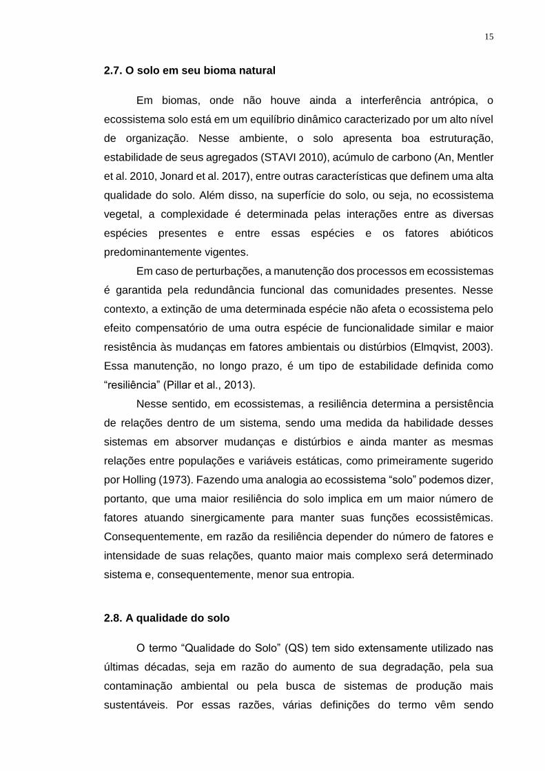
“Saúde do Solo” quando se refere à essa abordagem interativa entre a QS
inerente e a QS dinâmica (Fig. 1), no entanto, de modo geral a literatura trata
dessa interação simplesmente como qualidade do solo.
Fig. 1. Qualidade do solo inerente e dinâmica e fatores que influenciam
(adaptado de Idowu et al., 2006)
18
Segundo Karlen et al. (2003), a qualidade inerente é bastante acessada
em levantamentos e classificação de solos, na medida em que considera fatores
de formação como clima, material de origem, tempo, topografia e vegetação.
Outro fator bastante importante sobre a qualidade inerente do solo frente
à produção de culturas é apontado por Carter (2002). Este autor alerta que isso
envolve fatores extrínsecos que devem ser considerados, que são aqueles que
não fazem parte do sistema solo, mas, que exercem influência sobre a
produtividade das culturas. Esses fatores podem ser climáticos, como:
precipitação, demanda evaporativa e temperatura do ar, ou ainda, parâmetros
hidrológicos e topográficos. Geralmente, qualidade inerente do solo para a
produção de plantas não pode ser avaliada independentemente de fatores
extrínsecos (Carter, 2002).
De qualquer forma, uma abordagem abrangente da qualidade do solo que
envolva além da ciência do solo fatores extrínsecos como os mencionados
acima, sugere estudos interdisciplinares. Conforme Stevenson et al. (2015),
enquanto o estudo dessas características relativamente estáveis do solo tem
sido de domínio da pedologia, o estudo de características dinâmicas que são
sensíveis ao uso do solo, geralmente tem sido objeto de estudo da agronomia,
fertilidade do solo, biologia do solo, qualidade e ecologia do solo.
No entanto, as questões sobre o manejo sustentável do solo só podem
ser respondidas pela integração de dados e técnicas como levantamentos a
campo, técnicas laboratoriais, sistemas de informação geográfica,
sensoriamento remoto e modelos de simulação (Drogers & Bouma, 1997). Desse
modo, o pedologista, que por natureza, é um sintetizador generalista, pode e
deve exercer um papel crucial nessa integração (Drogers & Bouma, 1997).
Nesse contexto, de forma análoga aos conhecidos termos “genótipo” e
“fenótipo”, os termos genoforma e fenoforma podem ser empregados no estudo
do solo no contexto de sistemas e sua integração é essencial para responder as
questões sobre o manejo sustentável do solo. Genoforma diz respeito ao solo
em seu estado natural considerando-o como um estado de referência, portanto,
reconhece que sabemos sobre sua gênese. Por outro lado, a fenoforma seria
uma descrição de como o solo foi alterado. Em particular, a fenoforma reconhece
19
os efeitos do manejo, em longo ou curto prazo, alterando o solo (McBratney et
al., 2014).
Nesse sentido, os levantamentos sistemáticos, sejam em escala regional
ou em áreas comerciais específicas, devem ser feitos de modo a contemplar
tanto o conceito de genoforma como o de fenoforma. De acordo com Bouma et
al. (1998), integrando esses conceitos é possível reconhecer que existe um
levantamento de solos e sua posição na paisagem e que os resultados dos
indicadores de qualidade do solo para diferentes formas de degradação ou
melhoria do solo, são diferentes dependendo do tipo de solo.
2.9. Indicadores de Qualidade do Solo
De acordo com Vezzani & Mielniczuk (2009), desde o início das
discussões dos cientistas sobre qualidade do solo, três linhas têm sido
abordadas. Uma linha procura identificar quais os melhores índices de Qualidade
do solo (IQS), tanto de ordem biológica como física e química. Outra linha
posiciona-se em relação ao que considera a matéria orgânica como o melhor
IQS. E, ainda, uma linha alternativa que deixa de lado a busca de atributos
indicadores e analisa processos no sistema solo-planta, surgindo assim a
abordagem sistêmica da QS.
De acordo com Doran & Parkin (1994), o IQS deve identificar um conjunto
de propriedades básicas do solo, atendendo aos seguintes critérios: elucidar
processos do ecossistema e relacionar aos processos modelos; integrar as
propriedades físicas, químicas e biológicas do solo e os respectivos processos;
ser acessível a muitos usuários e aplicável a condições de campo; ser sensível
a variações de manejo e de clima ao longo do tempo; e, quando possível, ser
componente de banco de dados já existente.
Finalmente, não existe o melhor IQS, pois um indicador pode ser melhor
para um propósito, mas, insuficiente para outro, a depender do enfoque
pretendido. Sendo assim, alguns indicadores são adequados para identificar
melhorias na qualidade do solo com o manejo em longo prazo, como exemplo a
estabilidade de agregados e o estoque de C, e outros mais adequados para
identificar melhorias em curto prazo, por exemplo em áreas de contaminação por
20
elementos tóxicos, como concentração e disponibilidade de elementos químicos,
biomassa microbiana, etc.
2.9.1. Indicadores Biológicos
Existe uma evidência crescente que os atributos microbiológicos do solo
são potencias indicadores antecipados de mudanças em sua qualidade, pois são
mais sensíveis que as características químicas e físicas do solo (Miller & Dick,
1995; Bandick & Dick, 1999; Bending et al., 2004; Peixoto et al., 2010).
Por outro lado, talvez atualmente o estabelecimento consensual de IQS
de ordem biológica seja a mais contraditória. Segundo Schloter et al. (2003), o
indicador microbiológico ou bioquímico ideal para avaliar a qualidade do solo,
deve ser simples de mensurar, funcionar bem em diferentes ambientes e revelar
de forma confiável, quais e onde existem problemas. Entretanto, é pouco
provável que um único indicador ideal possa ser definido em uma simples
medida, por causa da grande quantidade de componentes microbiológicos e
rotas bioquímicas.
De qualquer forma, a escolha de um “Indicador Biológico de Qualidade”
(IBQ) dependerá do objetivo da pesquisa. Assim, algumas linhas de pesquisa
visam desenvolver um IBQ que capture o efeito da diversificação dos cultivos,
utilizando medidas da diversidade funcional da comunidade microbiana (Zak et
al., 1994), embora não haja um consenso ainda, por questionamentos
metodológicos, outros que visam identificar o efeito de manejo e elucidar
processos do ciclo biogeoquímico relacionados ao suprimento de nutrientes às
plantas. Finalmente, dentro de outro escopo, existem também IBQs com
potencial para serem utilizados na recuperação de áreas degradadas ou
contaminadas.
Independentemente do indicador biológico, é preciso cuidado ao se fazer
inferências sobre o “sistema”, por serem altamente sensíveis a diversos fatores.
Em algumas situações inclusive, essas inferências restringem-se apenas à
efeitos de curto prazo, retratando o funcionamento do sistema naquele momento
em que se coletou a amostra. Isso ocorre, porque tanto a população como a
diversidade de espécies, e sua funcionalidade dependerá do substrato
predominante na época da coleta, pois é afetado por temperatura, pela espécie
21
que está presente no campo naquele momento e pela proximidade ou não das
raízes.
A) Biomassa microbiana
A Biomassa Microbiana do Solo (BMS) é o olho da agulha através do qual
toda a matéria orgânica necessita passar (Jenkinson et al., 1977). Esse indicador
é mais sensível, quando comparado aos organismos superiores, e é influenciado
por diferentes fatores ecológicos como a diversidade de plantas, conteúdo de
MOS, umidade do solo e mudanças climáticas (Martinez-Salgado et al., 2010).
A teoria de Odum (1969) diz que a diversificação de plantas, animais e
micróbios em ecossistemas coincide com um aumento na eficiência do uso da
energia. Baseado nessa teoria, Anderson & Domsch (2010), analisaram
aproximadamente 100 parcelas com um histórico de manejo de longo prazo. Os
autores observaram maiores valores da relação Cmicrobiano: Ctotal com a rotação
de culturas em relação à monocultura, indicando menor demanda energética da
comunidade microbiana no sistema mais diversificado, portanto, maior eficiência.
A BMS pode ser associada ao teor de matéria orgânica no solo, à
qualidade e à quantidade de resíduos agrícolas adicionados e às práticas de
manejo adotadas (Venzke Filho et al., 2008). Esses autores verificaram em áreas
de 12 e 22 anos de sistema de plantio direto no estado do Paraná, que tanto o
tempo de adoção do SPD como o aumento da porcentagem de argila
favoreceram o incremento de C e N microbianos.
B) Atividade microbiana em FDA
A atividade microbiana medida pela enzima FDA é bastante promissora
para o uso como indicador de qualidade do solo por sua boa operacionalidade e
rapidez na obtenção dos resultados. O Diacetado de Fluoresceína (FDA) é uma
fluoresceína conjugada a dois radicais acetato (3’6’ – diacetil – fluoresceína),
formando um composto incolor que, ao ser hidrolisado por enzimas - como
proteases, lipases e esterases -, libera como produto da reação a fluoresceína,
que é visível e colorida (Stubberfield & Shaw, 1990; Green et al., 2006). Segundo
Swisher & Carroll (1980), as quantidades de fluoresceína liberadas são
proporcionais à atividade da população microbiana do solo.
22
2.10. Indicadores sistêmicos
No que diz respeito à busca de indicadores que reflitam as propriedades
físicas, químicas e biológicas do solo, no presente estudo consideramos que o
estado de agregação, o estoque de carbono e o Índice de Manejo de Carbono
(IMC), podem ser utilizados como “indicadores sistêmicos do solo”. Esses IQS
são usados tanto para acompanhar a evolução/degradação da QS ao longo do
tempo, como para avaliar o reflexo do manejo e sistema de produção adotado
na QS.
2.10.1. Estabilidade de agregados
Quando duas ou mais partículas primárias de argila se agrupam e a força
que une tais partículas é maior que a força de união entre partículas adjacentes,
fica caracterizada a formação do agregado (Ferreira, 2010). Em solos da região
tropical, a formação e a estabilização dos agregados ocorrem por influência da
matéria orgânica. Em sistemas conservacionistas, ocorre, primeiramente, a
estabilização química da matéria orgânica, iniciando a formação de
microagregados e, com o passar do tempo, a proteção física da matéria orgânica
também passa a influenciar positivamente a estabilidade de agregados.
Conforme Bayer & Mielniczuk (2008), a elevada área superficial específica
e a disposição dos grupos funcionais da MOS, determinam a grande interação
com os óxidos de Fe e Al e caulinita, predominantes em sua fração argila. Isto,
portanto, possibilita a proteção química da matéria orgânica. Com o passar do
tempo, ocorre formação de macroagregados, oriundos da conexão entre
microagregados adjacentes. Essa junção é possível pela cimentação por hifas
de fungos e raízes de plantas (Jastrow & Miller, 1997). Sua formação depende
da matéria orgânica particulada (MOP) recentemente adicionada ao solo (Bayer
et al., 2011) e confere proteção física ao C particulado fino intra-agregado,
podendo representar de 23 a 54 % do C total em Argissolos e Latossolos em
ambiente subtropical (Conceição, et al., 2008).
Nesse sentido, a formação de agregados é bastante afetada pelas
práticas agrícolas ao longo do tempo. Além disso, sua estabilidade decorre da
interação entre as propriedades físicas e químicas sobre a ação dos
23
microrganismos do solo, que por sua vez, são influenciados pela quantidade e
qualidade do C adicionado pelo material vegetal. Por essas razões, a
estabilidade de agregados por refletir toda essa dinâmica e distribuição das
frações de C nas frações de agregados é considerado um indicador sistêmico de
qualidade do solo. A estabilidade de agregados, portanto, é definida como a
resistência de agregados à um determinado processo de dispersão (Strickland
et al., 1988).
2.10.2. Estoque de carbono
O estoque de C até um metro de profundidade, no mundo, varia entre
1462 e 1576 Pg (Lal et al., 1995); entretanto, a maior parte concentra-se em
camadas mais superficiais, onde sofrem mais influência dos restos vegetais da
parte aérea das plantas.
O uso e o manejo do solo podem diminuir ou aumentar os estoques de C
em relação a uma área referência, que normalmente é o bioma predominante na
região de estudo. A diminuição dos estoques de C pode ocorrer tanto após a
derrubada da mata para exploração agrícola, como com o uso contínuo do solo
em sistema de preparo convencional. Entretanto, o sistema de plantio direto, com
rotação de espécies produtoras de alta quantidade de biomassa vegetal pode
aumentar o estoque de C a valores mesmo acima dos encontrados no bioma
original (Sá et al., 2001).
Em sistemas de ILP, o aporte de C ao solo via resíduos vegetais ocorre
de maneira distinta do verificado em sistemas puramente agrícolas (Salton et al.,
2002), pois, o pastejo estimula o crescimento radicular das pastagens e a sua
produção de exsudatos modifica a proporção parte aérea/raízes e a qualidade
do C adicionado ao solo (Bayer et al., 2011).
A exclusão do pastejo por oito anos por Iaque (Bos grunniens) e ovelhas
na China, diminuiu o carbono orgânico do solo. Os resultados obtidos sugerem
que a redução da taxa de lotação, mas não a exclusão, é uma estratégia para a
restauração de áreas degradadas naquela região (Shi et al., 2013).
Como visto, o aumento do estoque de C depende do manejo adotado e
do tempo de adoção. Esses fatores interagindo com características intrínsecas
24
do solo como textura, mineralogia, entre outros, favorecem o acúmulo de C e,
portanto, considera-se esse um indicador sistêmico da qualidade do solo.
2.10.3. Índice de Manejo de Carbono
O Índice de Manejo de Carbono (IMC) é uma ferramenta útil para subsidiar
informações acerca dos melhores sistemas de manejo de solos e culturas, pois
integra numa mesma medida, as variações ocorridas nas diferentes frações da
MOS (Nicoloso et al., 2008).
Esse índice foi primeiramente proposto por Blair et al. (1995), utilizando o
método do fracionamento químico. Esses autores verificaram que o C-lábil tanto
diminui como se recupera mais rapidamente que o C total, considerando a
quantidade do C-lábil em relação ao C-total, como parâmetro para avaliar a
qualidade do solo. O IMC, portanto, é sensível em responder às diferenças do
uso e do manejo do solo quando submetido a pequenas alterações.
Por outro lado, o IMC apresenta algumas dificuldades na metodologia. Por
esse motivo, Diekow et al. (2005) propuseram a utilização do método de
fracionamento físico ao invés do químico, pois o primeiro apresenta vantagens
metodológicas e ao mesmo tempo coerência com o último (Zanatta, 2006, Vieira,
2007). Com essa alteração, a labilidade do C pode ser determinada pela fração
leve (>1,8 g cm-3), utilizando o fracionamento físico densimétrico ou pela fração
particulada (>0,053 mm), utilizando o fracionamento físico granulométrico.
2.11. Procedimentos de amostragem e análise na estatística clássica
Estudos de sistemas de produção a campo requerem a utilização de
procedimentos estatísticos específicos desde seu planejamento até a forma de
análise dos dados. Debatendo sobre o emprego da estatística em estudos de
amostragem de solos a campo, Ferreira et al. (2012), comentaram que a não
adequação aos delineamentos experimentais tradicionais reside na
impossibilidade da casualização das parcelas de uma área com as de outra na
mesma região, pois, elas já são naturalmente distintas e fisicamente separadas.
Entretanto, os autores sugerem que não sendo possível haver casualização no
delineamento experimental, faz-se uma casualização no delineamento amostral
coletando-se unidades amostrais de forma aleatória em uma mesma área.
25
Segundo os autores, fica a dúvida se a casualização realizada dentro de
cada uma dessas áreas, tem o mesmo efeito de casualizações em que as
repetições de diferentes tratamentos são trazidas para um experimento particular
e casualizadas, conforme o plano de delineamentos tradicionais. No entanto,
esse problema pode ser contornado desde que sejam atendidos os pressupostos
básicos de repetição, casualização e controle local, permitindo assim realizar
inferências fidedignas sobre o efeito de tratamentos (Ferreira et al, 2012). De
qualquer maneira, ficam as perguntas: como efetuar esse controle em campo
aberto? ou será que é mesmo necessário esse controle para se testar hipóteses?
Se admitirmos a impossibilidade de um “controle” de variáveis não desejáveis
em abordagens de campo, não seria melhor buscar outra alternativa de análise?
De maneira geral, ao se tratar da pesquisa em campo aberto, dever-se-ia
fazer uma abordagem de “levantamento”, mas, na ciência do solo assim como
em muitas outras áreas, é tratada como um “experimento”. Isso afeta
diretamente o procedimento de amostragens de solo, e os autores orientam que
se busque sítios mais homogêneos dentro de uma mesma área para a coleta.
Assim, é possível uma maior homogeneidade entre as pseudo-repetições e
teoricamente diminuiria o erro, permitindo a comparação entre diferentes
sistemas que, nesse contexto, seriam considerados como “tratamentos”.
Por outro lado, essa estratégia de amostragem que vem sendo tomada e
sugerida por estatísticos clássicos que trabalham na ciência do solo só é feita
por dois motivos: 1- O paradigma predominante apoia-se nas pressuposições da
estatística experimental para levantamentos a campo, que definitivamente não é
um experimento; 2- Existe uma inércia quanto à adoção de ferramentas
estatísticas não-clássicas, pois, a maioria dos livros textos de estatística, mesmo
os mais atuais, não tratam.
Finalmente, os autores relatam que mais importante do que questionar o
uso da amostragem dentro das áreas, e se as supostas pseudorrepetições
realizadas comprometeriam a análise, é questionar se os pressupostos
estatísticos do modelo escolhido foram atendidos o que, em caso de resposta
negativa, comprometeriam a qualidade da inferência (Ferreira et al, 2012).
Novamente é possível verificar que a visão dos autores é com base em
pressupostos da estatística experimental fisheriana, pois, ao se falar em
26
“pseudorepetições”, implica-se que as inferências que se pretende fazer seriam
pelo uso de métodos clássicos da estatística.
2.12. Amostragem e abordagem estatística não-clássica
Como visto, a maioria das abordagens de pesquisa feitas na ciência do
solo e produção de plantas, tem sido realizadas em ambientes experimentais
controlados. Esse modelo de pesquisa possibilita a compreensão de processos
e a elucidação de mecanismos específicos na interação solo e planta.
No entanto, os experimentos têm algumas limitações como o número de
fatores a serem avaliados, ou seja, experimentos fatoriais por exemplo,
normalmente avaliam no máximo a interação de três fatores. Mais do que isso
fica um experimento grande e complicado de se avaliar. Além disso, há uma
limitação de tempo e espaço. De tempo, porque dependendo do sistema a ser
estudado, os fatores que se deseja estudar ainda não se manifestaram e não é
possível obter uma resposta no tempo de uma tese de doutorado. De espaço,
porque a depender da escala que se deseja trabalhar, a implantação de um
experimento torna-se inviável operacionalmente e financeiramente.
Essas características fazem com que seja necessário se trabalhar na
escala de “levantamentos”, onde não se tem o controle dos fatores e uma série
de cuidados deve ser tomada. Nesse sentido, algumas áreas da ciência como a
“Ecologia” têm avançado bastante em abordagens estatísticas robustas para
aplicação em levantamentos. Nela, os levantamentos são realizados em escalas
regionais em ambientes naturalmente heterogêneos e complexos, que são as
florestas. Nesse ambiente, a diversidade está presente de forma muito intensa
no espaço e no tempo, e um correto planejamento amostral associado a uma
abordagem estatística moderna, permite uma melhor compreensão desses
sistemas.
Desse modo, diferentemente do que foi sugerido por Ferreira et al. (2012)
onde, na medida em que se quer comparar sistemas diferentes a campo, os
autores recomendam coletar as unidades amostrais em locais mais homogêneos
entre si, os levantamentos devem ser feitos de forma a contemplar bem a
heterogeneidade da área de estudo valorizando um “n amostral” adequado. Esse
procedimento, ao abranger a área de forma mais representativa, descreve de
27
forma mais fidedigna o que ocorre a campo. De acordo com Wildi et al. (2010),
o objetivo da amostragem é gerar uma descrição numérica do sistema real que
se pretende analisar. Por esse motivo, se considerarmos que há uma
variabilidade inerente à área de estudo, a descrição desse sistema tal como ele
é a campo deve ser feito por uma amostragem sistemática.
Nesse sentido, uma abordagem estatística não-experimental se faz
necessária não apenas no planejamento amostral, mas, também no tratamento
e exploração dos dados. Em sistemas agropecuários mais complexos, a
sugestão é que se busque uma abordagem semelhante à dada nas ciências da
vegetação. Se considerarmos que nos SIPA os efeitos de interações entre os
componentes produzem um efeito tão significativo, senão maior que o de cada
componente individual, naturalmente as inferências baseadas em um conjunto
pequeno de variáveis trariam, em si, imprecisão.
Em ecologia, por exemplo, diferentes efeitos podem ser resultado de um
conjunto de condições devido ao grande número de variáveis que influenciam,
das quais, muitas não estão prontamente disponíveis ao observador (Legendre
& Legendre, 1998). De modo geral, na maioria dos ecossistemas, as condições
ambientais, por exemplo, a altitude e a umidade, modificam na área de estudo
(Wildi, 2010), daí a necessidade de se avaliar a QS inerente para explicar a QS
dinâmica em levantamentos de campo, por exemplo.
2.13. A busca por padrões
Como discutido, a descrição da variabilidade do sistema solo como um
sistema complexo que compõe o ecossistema, deve ser feita por um conjunto de
atributos ou variáveis e serem devidamente interpretadas. Em um ecossistema
florestal, a distribuição de espécies, por exemplo, é tão heterogênea no espaço
e no tempo, que descrever esse fenômeno por uma única variável levaria a
conclusões simplistas de um sistema complexo.
Por esse motivo, todo o esforço em ecologia de planta, assim como em
outras ciências, é no sentido de aprender quais as “regras” que governam o
mundo, ou seja, essas regras causam padrões e esses padrões, na maioria das
vezes, não é revelado pela observação direta do banco de dados original tal

28
como foi coletado a campo, daí a importância do emprego de análises
exploratórias de banco de dados (Wildi, 2010).
Os padrões referem-se a diferentes tipos de regularidades, algumas no
espaço, algumas no tempo e outras relacionadas à similaridade de objetos,
unidimensional ou multidimensional, determinístico ou aleatório (Wildi, 2010).
Este autor comenta que a busca por “padrões” na ecologia de vegetação se
justifica pela não-aleatoriedade da distribuição espaço-temporal das espécies,
ou seja, as espécies são governadas por regras de causas detectáveis e
possíveis de serem descritas por funções matemáticas. Essas causas podem
inclusive estar relacionadas com atributos do solo como umidade, textura,
profundidade efetiva e fertilidade; portanto, podemos considerar que indicadores
de qualidade dinâmica do solo como o estoque de C, a capacidade de troca
catiônica (CTC), etc, também são influenciados por esses atributos e também
exibem um padrão de distribuição não-aleatória.
2.14. Análise exploratória de dados
A) Análise de agrupamentos
Uma das habilidades mais básicas dos seres vivos envolve o
agrupamento de objetos similares para produzir a classificação (Everitt, 2011).
Os seres humanos sempre têm tentado classificar objetos animados ou
inanimados que os circunda (Legendre & Legendre, 1998). Agrupar, é
reconhecer que objetos são suficientemente similares para serem colocados
num mesmo grupo e também identificar distinções ou separações entre grupos
(Legendre & Legendre, 1998), para isso são utilizadas medidas de semelhanças
como as de similaridade para o agrupamento de variáveis e de dissimilaridade
para agrupar unidades amostrais.
Por ser uma análise exploratória, a análise de agrupamentos permite uma
melhor exploração dos dados na medida em que revela padrões que muitas
vezes são de difícil reconhecimento analisando diretamente o banco de dados
original. Além disso, conforme Wildi (2010), a principal vantagem prática da
classificação é a possibilidade de se trabalhar com um pequeno número de
grupos ao invés de um grande número de indivíduos e espécies. Podemos
considerar que essa vantagem apontada pelo autor ao se referir a indivíduos ou
29
espécies, serve para unidades amostrais de solo ou plantas em sistemas
agropecuários, por exemplo.
B) Métodos de ordenação
Assim como o agrupamento, a ordenação também é uma ferramenta de
análise exploratória de dados capaz de revelar padrões em extensos bancos de
dados multivariados. A ordenação é a representação gráfica da similaridade
entre unidades amostrais e/ou entre atributos em um espaço de semelhança
(Wildi, 2010).
Conforme Legendre & Legendre (1998), em ecologia, uma série de
descritores são normalmente observados para cada objeto sobre estudo. Na
maioria das vezes, os ecologistas estão interessados em caracterizar as
principais tendências de variação dos objetos, considerando todos descritores,
não apenas alguns. Essa abordagem ecológica, portanto, deve ser utilizada
também para o entendimento de sistemas integrados de produção agropecuária,
pois, nesses sistemas o nível de complexidade, particularmente do sistema solo
se aproxima mais de sistemas florestais que de sistemas de produção com o
manejo convencional do solo.
Os gráficos de ordenação representam, em seus eixos, uma larga fração
da variabilidade da matriz de dados multidimensionais em um espaço com uma
dimensionalidade relativa reduzida (ou menor) que o banco de dados original
(Legendre & Legendre, 1998). Esses autores comentam que olhar os diagramas
de dispersão dos objetos com respeito a todos possíveis pares de descritores, é
uma abordagem bastante tediosa que geralmente não esclarece muito bem o
problema que se tem em mãos. Nesse sentido, dos extensos bancos de dados
originais, se deriva um gráfico que pode ser plotado ou inspecionado
dinamicamente como uma nuvem de pontos de rotação tri ou quadri-dimensional
(Wildi, 2010).
Dos métodos de ordenação os dois principais são, conforme Wildi (2010):
1- Análise de Componentes Principais (PCA) e 2- Análise de Coordenadas
Principais (PCoA).
30
2.15. Análise de caminhos na compreensão de relações causais em
ambientes não-experimentais
Na década de 1920, o biólogo evolutivo, geneticista e estatístico inglês
Ronald Aylmer Fisher, desenvolveu os métodos de variância com dados
experimentais que permitem conclusões sobre relações de causa e efeito. Esses
métodos constituem a base da estatística clássica e são bastante utilizados.
Dentro da estrutura de um delineamento amostral específico (espacial,
temporal ou experimental), onde a variação é controlada, pode-se dizer que os
dados dão suporte à hipótese de causalidade se uma porção significativa da
variação da variável resposta, é certamente explicada por mudanças que
ocorrem na variável descritiva (Legendre & Legendre, 1998).
Nesse contexto, a robustez de um experimento aleatorizado reside no fato
de que não é necessário fisicamente controlar outra variável causal relevante,
para reduzir (mas, logicamente não excluir) a possibilidade que a associação
observada é devido a alguma causa comum não medida na amostra (Shipley,
2000). Entretanto, a aleatorização não pode garantir que os grupos ou
tratamentos estarão livres de viés por fatores desconhecidos (variáveis
correlacionadas com o tratamento, por exemplo). Isso enfatiza que mesmo
experimentos aleatorizados não propiciam nenhuma garantia automática de
inferência causal, livre de pressuposições subjetivas (Shipley, 2000).
Particularmente em abordagens de levantamentos onde, por natureza,
não há um delineamento experimental com a aleatorização e tampouco a
possibilidade de se controlar variáveis que se correlacionam com o fenômeno
estudado, o problema se agrava. Técnicas estatísticas como a análise de
regressão múltipla, buscam uma melhor compreensão de objetos de estudos
afetados por vários fatores. No entanto, essa análise carrega em si problemas
de colinearidade, levando o pesquisador a retirar variáveis importantes da
análise e perdendo informações.
Finalmente, acreditava-se não ser possível o estabelecimento de relações
causais fora de um experimento e, muito menos, em ambientes mais complexos
como uma floresta ou em SIPA por exemplo. Nesses ambientes, onde as
variações nos fenômenos estudados são de causalidade multidimensional e que
a existência de fatores de variação que se correlacionam é inerente ao meio, a
31
rigidez dos pressupostos estatísticos clássicos dificultam uma melhor
compreensão desses sistemas.
Por outro lado, a possibilidade de realizar inferências de relações de
causa e efeito fora do ambiente experimental não é uma novidade. Da mesma
época de Fisher, um geneticista americano chamado Sewall Green Wright, que
trabalhou ao lado de Fisher, desenvolveu o método de análise de caminhos
(“path analysis”). Apesar de Wright ser reconhecido como um dos biólogos
evolutivos mais influentes do século 20, ele próprio enxergava seu trabalho com
análise de caminhos como uma de suas contribuições científicas mais
importantes (Shipley, 2000).
Esse método, que é baseado em ideias de estabelecer relações causais
sem o uso de experimentos, ficou muitas décadas esquecido. De acordo com
Shipley (2000), isso ocorreu tanto porque o método ia contra a filosofia e a
metodologia subjacentes nas duas principais contundentes escolas estatísticas
na virada do século 20, como por ser metodologicamente incompleto em
comparação com os métodos estatísticos de Fisher, baseados na análise de
variância e experimentos casualizados (Shipley, 2000).
Na década de 1990, Shipley (2000) resgatou a análise de caminhos
sugerindo um teste que verifica a relação de independência entre variáveis, que
compõem um potencial modelo. Esse teste é feito pela elaboração de um
conjunto base (d-separation) e a validação do modelo ocorre quando todas as
relações de independência são aceitas.
A análise de caminhos é uma extensão da regressão linear múltipla que
permite a decomposição e interpretação de relações lineares entre os
descritores. Essa abordagem permite hipotetizar a respeito das relações causais
entre os descritores e examinar as consequências pelos coeficientes de
regressão e correlação calculados entre esses descritores (Shipley, 2000).
Finalmente, a análise de caminhos possibilita o pesquisador a testar a
validade de modelos propostos por ele mesmo, com base em uma matriz de
correlações entre variáveis. A análise dessa matriz muitas vezes pode revelar
correlações indiretas entre variáveis, ou seja, um padrão de correlação entre
duas variáveis pode ser revelado quando se considera uma terceira variável que
é causa comum a elas.
32
3. HIPÓTESES E OBJETIVOS GERAIS
3.1. HIPÓTESES
1- A caracterização de sistemas de produção considerando aspectos
relacionados à diversidade e dinâmica espaço-temporal de espécies, indica o
nível de complexidade do sistema de produção resultando em maior qualidade
do solo.
2- O acesso à fatores inerentes do solo, como sua textura e variáveis de terreno,
assim como às propriedades químicas físicas e biológicas do solo, possibilitam
uma maior compreensão dos padrões de variação da qualidade do solo em
escala de propriedade rural.
3- A integração com bovinos de corte no inverno, ou a adoção de gramíneas de
verão em sistema irrigado, proporcionam maior qualidade do solo que o sistema
de produção tradicional.
4- A análise de caminhos possibilita a proposição de modelos robustos,
revelando conexões diretas e indiretas de fatores que afetam a qualidade do
solo, permitindo uma melhor compreensão de sistemas de produção.
3.2. OBJETIVOS GERAIS
1- Verificar se as características que conferem maior complexidade aos sistemas
de produção resultam em maior qualidade do solo.

33
2- Descrever a qualidade do solo em diferentes sistemas de produção,
compreendendo padrões de variação das propriedades do solo e de variáveis de
paisagem em escala de propriedade rural.
3- Avaliar se sistemas integrados de produção agropecuária e sistemas irrigados
com gramínea de verão, proporcionam uma maior qualidade do solo em relação
ao sistema de cultivo tradicional
4- Utilizar a análise de caminhos para melhor compreender as relações de causa
e efeito que definem de forma direta ou indireta a qualidade do solo em diferentes
sistemas de produção.
34
4. CAPÍTULO II – ESTUDO I: AGRICULTURAL PRODUCTION SYSTEMS
CHARACTERIZATION AND ITS RELATION WITH SOIL QUALITY
4.1 Introduction
The conversion from conventional to no tillage soil management system in
Brazilian subtropical environment during last decades provided lower soil losses
and led to a quality enhancement in soil ecosystem. Furthermore, besides the
majority production systems consist in a summer soybean monoculture, the
grasses species cultivated during winter, favors soil carbon storage.
After more than thirty years of no tillage soil management spreading
throughout Brazil, some studies have demonstrated soil quality (SQ)
enhancement with species diversity increasing and integrated crop-livestock
systems (ICLS) adoption (Carpenedo & Mielniczuk, 1990; Paladini & Mielniczuk,
1991; Bayer et al., 2000; Souza et al., 2009; Silva et al., 2014; Assman et al.,
2015).
In this context, as the soil ecosystem through soil quality indicators
memorizes species rotation in a space-time perspective, Anghinoni et al. (2013),
proposed a production systems characterization through three dimensions (Fig.
2): components diversity (specie’s diversity and functions); space interactions
(distance for components connection); cycle temporality (system’s amplitude
duration and time interval between options).

35
Fig. 2. Characteristics that describes production systems through its dimensions,
subdimensions and practical meaning (adapted from Anghinoni et al., 2013).
Therefore, addressing these dimensions allow us to frame production
systems according to their complexity level. Thus, we intend to comprehend soil
quality from different production systems based on species diversity, functions
and space-temporal composition. For this, we proposed a methodology to
quantitatively characterize the systems, differentiating them and comparing to soil
quality indicators variation on a farm-scale approach.
4.2 Methods
4.2.1 Localization and systems general descriptions
The systems studied is located on “Guajuvira Agropecuária farm” at São
Miguel das Missões county at Rio Grande do Sul state, in southern Brazil (Fig.
3). The geomorphological unit corresponds to the Planalto Medio region (latitude
28°52’23”S, 54°22’58”W, at a medium altitude of 370 meters above sea level).
Climate is classified as Cfa (humid subtropical) according to the Köppen system
of climate classification, with a mean annual rainfall of 1600 mm and an average
temperature of 19 ⁰C. About 90 % of systems area comprises a clayey Oxisol
(Rhodic Haplorthox - Nachtergaele, 2001), deep, well drained, with a clayey
SYSTEM
Space
interaction
Cycle
temporality
Amplitude
duration
Time interval
between
options
Components
diversity
Species Functionallity
Number of
species of a
system
Number of
functions
exercised by
the species
from a system
Period of a
sucession or
rotation
scheme
Time interval
between each
specie during
one complete
cycle
Distance for
components
connection
Dimensions
Subdimensions
Practicalmeaning

36
surface texture of basaltic rock. The original vegetation of this region was a
transaction between natural grassland and Atlantic forest (Hasenack and
Cordeiro, 2006).
Fig. 3. Google earth’s view of the four studied systems: integrated crop-livestock
(ICLS1,2), traditional agricultural (TAS) and irrigated agricultural (IAS).
We evaluated a rainfed traditional agricultural system (TAS) with 75
hectares, an irrigated agricultural system (IAS) with 86 hectares and two rainfed
integrated crop-livestock systems (ICLS1 and ICLS2) with 93 and 166 hectares
respectively (Fig. 3). The ICLS’s were under no-tillage (NT) soil management for
17 years, while the other systems for 21 years. The TAS is the main soybean
production system from Rio Grande do Sul state, and the IAS was similar to TAS
until 2011, when a pivot was installed, and the species and space-time crop
succession configuration changed (Table 1). The ICLS1 was always cultivated
with summer soybean (Glycine max) and main winters with ryegrass (Lollium
multiflorum) under cattle grazing. Otherwise, in the ICLS2 the winter seasons
were cultivated with black oat (Avena strigosa) under cattle grazing every two
winters, and with wheat (Triticum aestivum) or forage radish (Raphanus
sativus)/wheat the others winter seasons (Table 1).
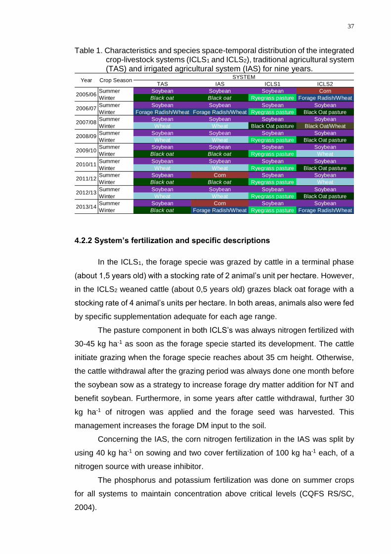
37
Table 1. Characteristics and species space-temporal distribution of the integrated crop-livestock systems (ICLS1 and ICLS2), traditional agricultural system (TAS) and irrigated agricultural system (IAS) for nine years.
4.2.2 System’s fertilization and specific descriptions
In the ICLS1, the forage specie was grazed by cattle in a terminal phase
(about 1,5 years old) with a stocking rate of 2 animal’s unit per hectare. However,
in the ICLS2 weaned cattle (about 0,5 years old) grazes black oat forage with a
stocking rate of 4 animal’s units per hectare. In both areas, animals also were fed
by specific supplementation adequate for each age range.
The pasture component in both ICLS’s was always nitrogen fertilized with
30-45 kg ha-1 as soon as the forage specie started its development. The cattle
initiate grazing when the forage specie reaches about 35 cm height. Otherwise,
the cattle withdrawal after the grazing period was always done one month before
the soybean sow as a strategy to increase forage dry matter addition for NT and
benefit soybean. Furthermore, in some years after cattle withdrawal, further 30
kg ha-1 of nitrogen was applied and the forage seed was harvested. This
management increases the forage DM input to the soil.
Concerning the IAS, the corn nitrogen fertilization in the IAS was split by
using 40 kg ha-1 on sowing and two cover fertilization of 100 kg ha-1 each, of a
nitrogen source with urease inhibitor.
The phosphorus and potassium fertilization was done on summer crops
for all systems to maintain concentration above critical levels (CQFS RS/SC,
2004).
TAS IAS ICLS1 ICLS2
Summer Soybean Soybean Soybean Corn
Winter Black oat Black oat Ryegrass pasture Forage Radish/Wheat
Summer Soybean Soybean Soybean Soybean
Winter Forage Radish/Wheat Forage Radish/Wheat Ryegrass pasture Black Oat pasture
Summer Soybean Soybean Soybean Soybean
Winter Wheat Wheat Black Oat pasture Black Oat/Wheat
Summer Soybean Soybean Soybean Soybean
Winter Wheat Wheat Ryegrass pasture Black Oat pasture
Summer Soybean Soybean Soybean Soybean
Winter Black oat Black oat Ryegrass pasture Wheat
Summer Soybean Soybean Soybean Soybean
Winter Wheat Wheat Ryegrass pasture Black Oat pasture
Summer Soybean Corn Soybean Soybean
Winter Black oat Black oat Ryegrass pasture Wheat
Summer Soybean Soybean Soybean Soybean
Winter Wheat Wheat Ryegrass pasture Black Oat pasture
Summer Soybean Corn Soybean Soybean
Winter Black oat Forage Radish/Wheat Ryegrass pasture Forage Radish/Wheat
Year Crop SeasonSYSTEM
2005/06
2006/07
2012/13
2013/14
2007/08
2008/09
2009/10
2010/11
2011/12
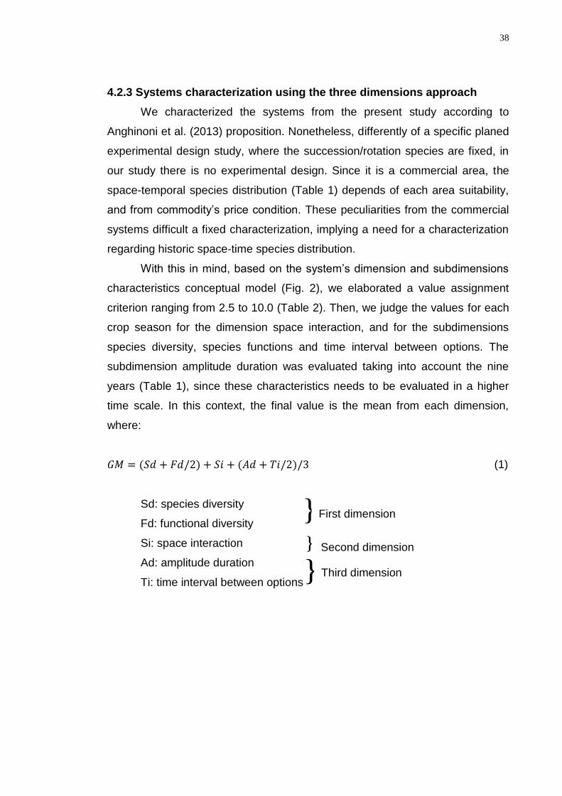
38
Second dimension
}
} }
First dimension
Third dimension
4.2.3 Systems characterization using the three dimensions approach
We characterized the systems from the present study according to
Anghinoni et al. (2013) proposition. Nonetheless, differently of a specific planed
experimental design study, where the succession/rotation species are fixed, in
our study there is no experimental design. Since it is a commercial area, the
space-temporal species distribution (Table 1) depends of each area suitability,
and from commodity’s price condition. These peculiarities from the commercial
systems difficult a fixed characterization, implying a need for a characterization
regarding historic space-time species distribution.
With this in mind, based on the system’s dimension and subdimensions
characteristics conceptual model (Fig. 2), we elaborated a value assignment
criterion ranging from 2.5 to 10.0 (Table 2). Then, we judge the values for each
crop season for the dimension space interaction, and for the subdimensions
species diversity, species functions and time interval between options. The
subdimension amplitude duration was evaluated taking into account the nine
years (Table 1), since these characteristics needs to be evaluated in a higher
time scale. In this context, the final value is the mean from each dimension,
where:
𝐺𝑀 = (𝑆𝑑 + 𝐹𝑑/2) + 𝑆𝑖 + (𝐴𝑑 + 𝑇𝑖/2)/3 (1)
Sd: species diversity
Fd: functional diversity
Si: space interaction
Ad: amplitude duration
Ti: time interval between options

39
Table 2. Value assignment criterion for agricultural production systems characterization
Value Components diversity Space interaction Cycle temporality
Species Functions
Amplitude duration Interval between
options
2.5 One Specie or two from the same family One function Species don’t
share the space One crop season Long
5 Two specie from different families Two functions with
summer soybean
Two species share
the space on
summer or winter
Two crop seasons
one time during
nine crop seasons
Moderately long
7.5 Three species of two families
Two functions with
summer corn or
summer soybean
with two grasses
Two species share
the space on
summer and
winter
Two crop seasons
at least two times
or three crop
seasons once
during nine crop
seasons
Adequate
10 Three species from different families Three functions Three species
share the space
> Three crop
seasons Fast

40
Thus, we considered that a lower value should be assigned for poor
species diversity and functionality systems, with lower space interaction as
cultivated alone, with one crop season amplitude duration and demanding a long
time between options (Table 2). Besides the species diversity, its function needs
to be considered, since it is expected enhancement on SQ with a summer corn
comparing to wheat for example, although, both are grasses. Therefore, it is
expected a higher carbon addition and root effects on soil system from the
summer specie.
To better understand some aspects from the conceptual model proposed
(Anghinoni et al., 2013), we can discuss practical examples. Concerning space
interactions, intercropping production systems as summer Corn/Brachiaria or
ICLS, with cattle grazing as in the present study (Table 1), presents lower space
for species interactions (Table 2), benefiting SQ. Yet, since soybean or corn
harvest period in northern of Rio Grande do Sul state initiate in March, and the
wheat sowing in July, a cover crop as forage radish or black oat in the middle
period will reduce the interval between options, favoring SQ. This latter situation
is observed for example on crop seasons 2006/07 from the TAS and 2006/07 and
2013/2014 from the IAS (Table 1).
4.2.4 Soil sampling and soil quality indicators
We did a systematic soil sampling on a grid of one sampling unit each five
hectares. The soil samples were collected at 0-10 cm layer on may of 2014 after
the summer crop harvest, to determine carbon stocking and soil aggregation
(undisturbed samples).
Soil bulk density was determined with steel rings following the equivalent
mass approach to determine the stocks (Ellert and Bettany, 1995), taking the TAS
as reference for soil mass as long as it represents the main soybean production
system in southern Brazil.
We choose three soil quality indicators that we considered to be systemic,
since it is an effect of species diversity and space-temporal distribution. They are:
carbon stock, soil aggregate stability and carbon management index.
41
4.2.4.1 Soil carbon
Soil samples were air dry and passed through a 2 mm sieve and a sub-
sample was separated to determine the total soil organic carbon (TOC) fraction.
The soil physical fractionation was determined according Cambardella and Elliott
(1992), by dispersing soil with 5 g L-1 of hexametaphosphate. The portion retained
on 53 µm sieve, was considered as the particulate organic carbon fraction (POC).
The mineral associated organic carbon fraction (MOC) was obtained by
difference between TOC and POC fraction. Then, the samples were dried
overnight at 50 ºC, ground and analyzed by dry combustion (CN Flash 2000
Analyser).
4.2.4.2 Soil aggregate stability
The soil aggregation was analyzed by measuring the mean weight
diameter (MWD) after water stable aggregates evaluation. We used the
methodology proposed by Kemper and Chepil (1965) with proposed alterations
by Carpenedo and Mielniczuk (1990) and Silva and Mielniczuk (1997). This
method consists on separate the undisturbed soil samples in breaking points
passing through a 9.52 mm sieve, and sampling laboratory duplicate of 50 grams.
Then we accommodated samples on a PVC tube, filled to the middle with water,
and did a pre-treatment with water for 2 minutes on a rotated shaker before
initiate the wet sieving. The soil weight remained on sieves with a mesh of 4.76,
2.0, 1.0, 0.25 and 0.0053 mm after wet sieving were used to calculate the soil
aggregate stability.
4.2.4.3 Carbon management index
Using the POC obtained by the physical fractionation as the labile C
fraction, and the MOC fraction as the non-labile C fraction, we calculated the
carbon management index (CMI) according to Blair et al., (1995), as described
below:
𝐶𝑀𝐼 = 𝐶𝑃𝐼 𝑥 𝐿𝐼 𝑥 100 (2)
42
where:
𝐶𝑃𝐼 = (𝑆𝑂𝐶 𝑖𝑛 𝑡ℎ𝑒 𝑒𝑣𝑎𝑙𝑢𝑎𝑡𝑒𝑑 𝑠𝑦𝑠𝑡𝑒𝑚 )/(𝑆𝑂𝐶 𝑖𝑛 𝑟𝑒𝑓𝑒𝑟𝑒𝑛𝑐𝑒 𝑎𝑟𝑒𝑎)
𝐿𝐼 = (𝐶 𝑙𝑎𝑏𝑖𝑙𝑖𝑡𝑦 𝑖𝑛 𝑡ℎ𝑒 𝑒𝑣𝑎𝑙𝑢𝑎𝑡𝑒𝑑 𝑠𝑦𝑠𝑡𝑒𝑚)/(𝐶 𝑙𝑎𝑏𝑖𝑙𝑖𝑡𝑦 𝑖𝑛 𝑟𝑒𝑓𝑒𝑟𝑒𝑛𝑐𝑒 𝑎𝑟𝑒𝑎)
𝐶 𝑙𝑎𝑏𝑖𝑙𝑖𝑡𝑦 = (𝑐𝑜𝑛𝑡𝑒𝑛𝑡 𝑜𝑓 𝑙𝑎𝑏𝑖𝑙𝑒 𝐶)/(𝑐𝑜𝑛𝑡𝑒𝑛𝑡 𝑜𝑓 𝑛𝑜𝑛 − 𝑙𝑎𝑏𝑖𝑙𝑒 𝐶)
4.3 Results and discussion
4.3.1 System’s characterization by value assignment criterion
The general mean, which calculation was described on item 5.2.3, were:
4.8, 5.4, 7.1 and 6.9 for the TAS, IAS, ICLS1 and ICLS2 respectively (Table 3).
The 2.5 value for species diversity was assigned for the IAS during
2011/12 crop season (Table 3), because the corn/black oat succession (Table 1)
represents two species from the same family (Table 2). For all crop seasons with
soybean/grass species succession, which the latter was used for cover crop (no
grazed black oat) or grain production (wheat), we assigned the value 5.0 for
species diversity and functionality subdimension (Table 3). These criteria were
adopted as there are two species from different families during the crop season:
soybean with a low nitrogen input for soil system and a grass specie adding C
and improving soil aggregation.
The 7.5 value still for these subdimensions, was assigned to the ICLS2
during crop season 2007/08 (Table 3) since, besides the soybean/black
oat/wheat succession (Table 1), constitutes three species, there are two grasses
during winter (Table 2). Otherwise, the time interval between options is lower,
contributing for further C input to the system and increasing this subdimension
value (Table 3).
The higher value for species diversity and function, was assigned for
systems with three different families exercising different functions (Table 2).
These criteria were observed during 2006/07 crop season from the TAS and IAS
(Table 1) with the soybean/forage radish/wheat succession. Yet, we consider the
summer corn as the most important summer specie, being capable to interrupt
the long-term steady state level that IAS was submitted until crop season 2010/11
(Table 1). With this in mind, we assigned the 10 value for function diversity in crop
season 2013/14, besides the summer corn belongs to the same family than the
winter wheat. Moreover, we also assigned the higher value for species diversity
43
and functions subdimension in all ICLS1 crop seasons and about half the ICLS2.
Here we considered the animal presence contributing to further C input via
excreta and improving nutrient cycling (Carvalho et al., 2010), important functions
to the system. Therefore, the soybean/grass succession with cattle grazing,
consists in three species and functions (Table 2).
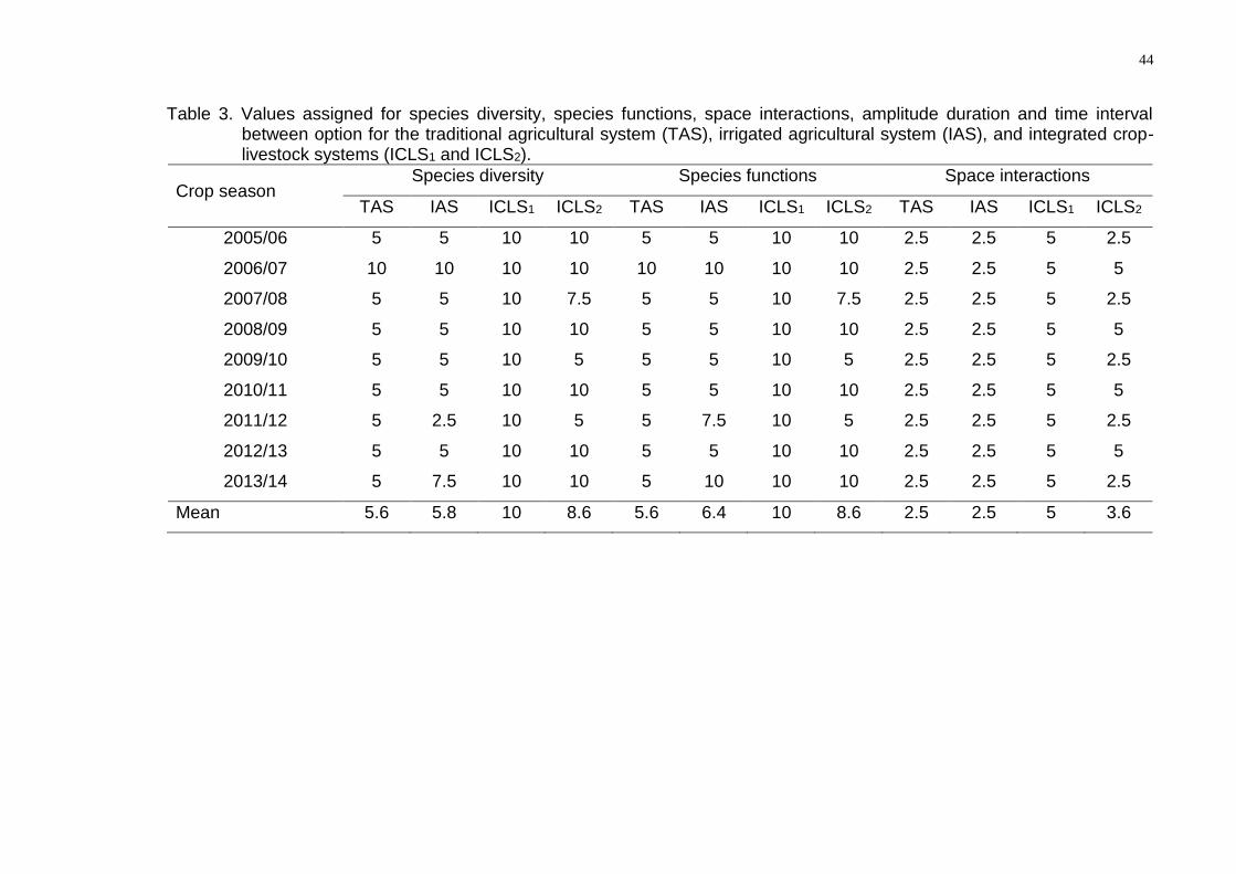
44
Table 3. Values assigned for species diversity, species functions, space interactions, amplitude duration and time interval between option for the traditional agricultural system (TAS), irrigated agricultural system (IAS), and integrated crop-livestock systems (ICLS1 and ICLS2).
Crop season Species diversity Species functions Space interactions
TAS IAS ICLS1 ICLS2 TAS IAS ICLS1 ICLS2 TAS IAS ICLS1 ICLS2
2005/06 5 5 10 10 5 5 10 10 2.5 2.5 5 2.5
2006/07 10 10 10 10 10 10 10 10 2.5 2.5 5 5
2007/08 5 5 10 7.5 5 5 10 7.5 2.5 2.5 5 2.5
2008/09 5 5 10 10 5 5 10 10 2.5 2.5 5 5
2009/10 5 5 10 5 5 5 10 5 2.5 2.5 5 2.5
2010/11 5 5 10 10 5 5 10 10 2.5 2.5 5 5
2011/12 5 2.5 10 5 5 7.5 10 5 2.5 2.5 5 2.5
2012/13 5 5 10 10 5 5 10 10 2.5 2.5 5 5
2013/14 5 7.5 10 10 5 10 10 10 2.5 2.5 5 2.5
Mean 5.6 5.8 10 8.6 5.6 6.4 10 8.6 2.5 2.5 5 3.6
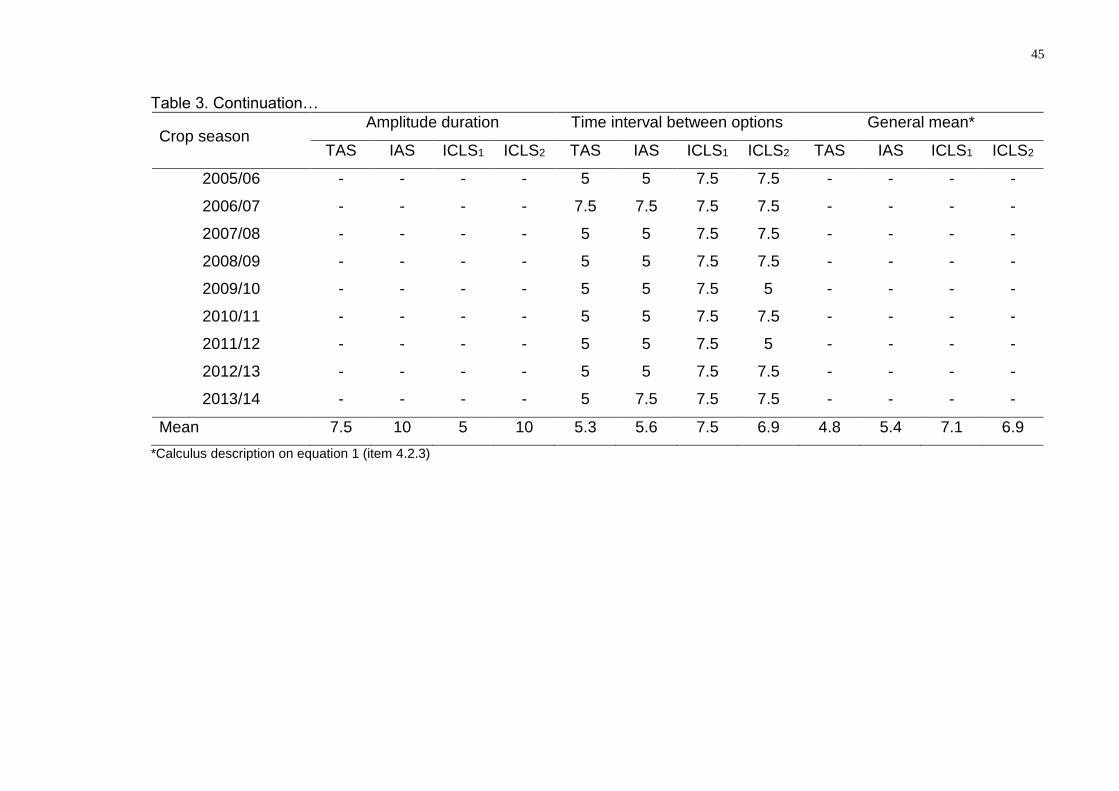
45
Table 3. Continuation…
Crop season Amplitude duration Time interval between options General mean*
TAS IAS ICLS1 ICLS2 TAS IAS ICLS1 ICLS2 TAS IAS ICLS1 ICLS2
2005/06 - - - - 5 5 7.5 7.5 - - - -
2006/07 - - - - 7.5 7.5 7.5 7.5 - - - -
2007/08 - - - - 5 5 7.5 7.5 - - - -
2008/09 - - - - 5 5 7.5 7.5 - - - -
2009/10 - - - - 5 5 7.5 5 - - - -
2010/11 - - - - 5 5 7.5 7.5 - - - -
2011/12 - - - - 5 5 7.5 5 - - - -
2012/13 - - - - 5 5 7.5 7.5 - - - -
2013/14 - - - - 5 7.5 7.5 7.5 - - - -
Mean 7.5 10 5 10 5.3 5.6 7.5 6.9 4.8 5.4 7.1 6.9
*Calculus description on equation 1 (item 4.2.3)
46
For the space interaction dimension, none of the studied systems
presented values above 5 (Table 3). Here, we considered that a value of 7.5
should be assigned in cases where two specie share the space on summer and
winter (Table 2), as with an intercropping during summer and winter forage
grazing system. Yet, a value of 10 we considered for systems with three species
sharing the space (Table 2), as with integrated crop-livestock-forestry systems.
In this context, we assigned the value 5.0 for the ICLS1 and half of the
ICLS2 (Table 3) since, besides the soybean monoculture during summer, there
was a forage specie being grazed by cattle during winters (Table 1), i.e., two
species. Nonetheless, all crop seasons from TAS, IAS and part of the ICLS2, we
assigned 2.5 (Table 3), since there is no space sharing by the species.
With regard to system’s amplitude duration, the attributed values were 7.5,
10, 5 and 10 for the TAS, IAS, ICLS1 and ICLS2 respectively (Table 3). The ICLS1
presented the lower value because a completely rotation cycle lasts just one crop
season. Nevertheless, the assigned value was 5.0, since the soybean/black oat
pasture on 2007/08 crop season (Table 1), interrupted the continuous
soybean/ryegrass succession. Otherwise, the 7.5 value for the TAS (Table 3) was
assigned due to the cycle of three crop seasons from 2005/06 to 2007/08, and
two crop seasons duration from 2009/10 (Table 1). Yet, the highest value was
assigned for the IAS and ICLS2. The former presented a three crop seasons
amplitude duration from 2005/06 to 2007/08, being interrupted by a
soybean/wheat succession on 2008/09, and from 2009/10 to 2011/12 (Table 1).
The ICLS2 presented a three crop seasons amplitude duration from 2005/06 to
2007/08, and from 2011/12 to 2013/14 (Table 1).
The last subdimension analyzed from the cycle temporality dimension,
was the time interval between species (Fig. 2; Table 2), which lower values were
observed in the TAS and IAS. Most crop seasons from these systems presented
one specie on summer and other on winter and we assigned a 5 value. Otherwise
all crop seasons from the ICLS1 and half of the ICLS2 presented two species
during winters, so we assigned a 7.5 value.
We considered that a 10 value should be assigned if two species could be
cultivated both on summer and winter, as the cases of systems with a cover crop
before the summer crop, and a forage specie with cattle grazing during winter.
47
4.3.2 Soil quality indicators
The ICLS1 is the system with higher soil variability as there are two
sampling units identified as Entisols (lowest soil OCS class) and three as Molisol
(highest soil OCS class) (Nachtergaele, 2001). Those sampling units were
disregarded from data analysis, so we can better discuss differences among the
studied systems.
4.3.2.1 Soil organic carbon stock (OCS)
The soil OCS increases from the TAS to the IAS and ICLS’s. For the TAS,
87 % of sampling units presented soil OCS bellow 36 Mg ha-1 (Fig. 4). Otherwise,
the IAS, ICLS1 and ICLS2 presented 55, 25 and 15 % of sampling units in these
lowest classes, i.e., until 30 and between 31 and 35 Mg ha-1 of OCS (Fig. 4).
Comparing the TAS and the IAS, they present the same species space-
time distribution history until crop season 2010/2011 under rainfed system (Table
1), with the same soil type, similar clay content and topography (data not shown).
However, in crop season 2011/12 the pivot was installed in the IAS as described
in item 5.2.1, permitting the adoption of irrigated summer corn. Hence, a slightly
soil OCS enhancement occurs (Fig. 4), since the total organic carbon fraction is
also a result of time under the specific system management.
Otherwise, in the ICLS’s the time under the same management indicates
that these systems are in steady state, and the soil OCS better represent the time
factor. About 37 and 61 % of sampling units from the ICLS1 and ICLS2 storage
more than 40 Mg ha-1 of soil organic carbon (Fig. 4). Therefore, most sampling
units in moderate to high soil OCS classes in the ICLS’s, comparing to the
predominance of lower classes of soil OCS in TAS (Fig. 4), indicate the benefits
of the former systems increasing soil OCS.
This is in agreement with other studies (Carvalho et al., 2010; Salton et al.,
2011; Assmann et al., 2014), but the difference is that in the present study the
TAS are four years more under NT then the ICLS’s (item 5.2.1). Moreover,
moderate grazing permits sufficient herbage harvesting by animals, and
adequate light interception for better plant development, increasing C
accumulation due to its higher total forage production (Carvalho, et al., 2011). In
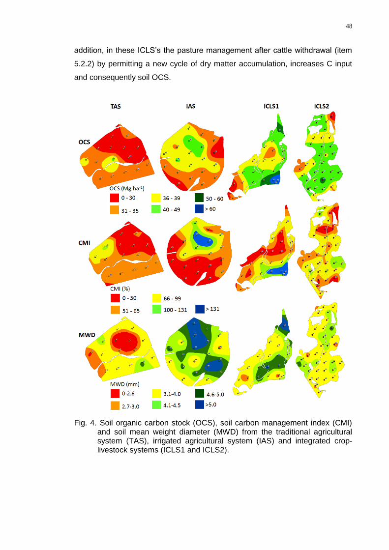
48
addition, in these ICLS’s the pasture management after cattle withdrawal (item
5.2.2) by permitting a new cycle of dry matter accumulation, increases C input
and consequently soil OCS.
Fig. 4. Soil organic carbon stock (OCS), soil carbon management index (CMI) and soil mean weight diameter (MWD) from the traditional agricultural system (TAS), irrigated agricultural system (IAS) and integrated crop-livestock systems (ICLS1 and ICLS2).
49
4.3.2.2 Soil carbon management index (CMI)
The soil CMI presented similar variation pattern than soil OCS, as increase
from the TAS to the IAS and ICLS’s. Nevertheless, in the IAS, there was a slightly
higher number of sampling units in higher range classes, i.e., those with soil CMI
value > 100 %. While in this system 20 % of sampling units are on the two higher
classes, in the TAS about 15 % are in the last but one higher class. These
differences, indicate that soil CMI is more responsible on short-term modification
than soil OCS (Vieira et al., 2007), as with the summer corn introduction in the
IAS
The IAS presented five times more sampling units with CMI values above
65 % than the TAS (Fig. 4). Moreover, none sampling units from the latter system
presented CMI above 100 %, while 20 % were verified in the IAS (Fig. 4). These
differences of classes CMI distribution among these systems, demonstrates the
effect of the high fresh organic matter input by irrigated summer corn cultivation
in the IAS.
Otherwise, in the ICLS1 and ICLS2 31 and 36 % of sampling units
presented moderated values of CMI, i.e., between 66 and 99 %. Besides, 12 and
18 % were with CMI > 100 % in ICLS1 and ICLS2 respectively. This higher CMI
from the ICLS’s, is due to different C fractions input from forage roots C exudates
plus animal’s excreta. Hence, these additional pathways of C input in the ICLS’s,
can lead soil system to a closer quality as in its natural bioma, delivering,
therefore, higher ecosystems service.
Nevertheless, the best practices concerning pasture management needs
to be adopted to reach higher soil quality. In a randomized block design of an
experimental area next to the studied systems, grazing intensity effects has been
compared against a no-grazed area with similar crop and soil management as in
the TAS. Regarding different fractions of soil C and N accumulation, there are no
differences among moderate grazing intensity and no grazed area (Assmann et
al. 2014). However, despite the similarity between the moderated grazing
treatment with ICLS1 and no grazing treatment with our TAS, there is an important
difference concerning pasture management. The period between animal’s
withdrawal and soybean sowing in the experiment is shorter and lower dry matter
is left to soybean. Hence, the pasture management from the studied ICLS’s (item
50
5.2.2), as permit further dry matter addition, benefited C fractions storage
increasing soil quality (Fig. 4).
4.3.2.3 Soil aggregation
According to Silva and Mielniczuk (1998), under a given management, soil
physical conditions tends to a steady state depending of edaphic and climatic
conditions. We understand that systems with different soil aggregation, but within
similar conditions, present different steady state levels.
About 40 and 47 % of sampling units from the TAS presented the soil MWD
lower than 3.1 mm and between 3.1 and 4 mm respectively (Fig. 4). On the other
hand, 70 % of sampling units from the IAS presented soil MWD higher than 4 mm
(Fig. 4).
The TAS cultivating soybean during summers and wheat or black oat on
winters, is the predominant crop management for decades. Nonetheless, the
occurrence of several dry periods during winters affecting mainly wheat
production have been reported (CONAB, 2016). Hence, the TAS does not add
further carbon to the soil suggesting that the system is stable. In contrast, from
the moment that an irrigated summer corn was introduced in the 2011/2012 crop
season on the IAS (Table 1), a disturbance on the steady state is promoted and
after two summer corn seasons the soil MWD increases (Fig. 4), and the soil
system tends to seek for a new steady state.
The importance of irrigated corn on soil aggregation in this short-term
period, is due to a high shoot dry matter input, but mainly due its roots effect on
soil aggregation. The mean productivity of the two corn crops cultivated on
summers of 2011/2012 and 2013/2014 was 12 Mg ha-1, i.e., in this region when
this specie is irrigated the dry matter input potential is high, favoring soil
aggregation. Furthermore, even sampling the soil 60 days after corn harvest,
there was a high content of dead corn roots residues impacting positively the soil
aggregation process.
In rainfed production systems, as the studied TAS and ICLS’s, soybean is
always cultivated during summer seasons (Table 1). Differently from the IAS,
those systems present the same species history for more than 15 years,

51
suggesting that the soil aggregation process is a result of long-term carbon input
mainly from the winter system’s species. Therefore, the main opportunity to
increase organic matter addition in rainfed production systems, is cultivating
grass species during the winter. If on the one hand in the TAS the organic matter
addition was committed mainly due frustrated wheat crops cultivation, in the
ICLS’s the climatic conditions didn’t significantly damaged the ryegrass and black
oat forage production.
The ICLS1 and ICLS2 presented 6 and 9 % of sampling units bellow 3.1
mm, while 50 and 30 % were above 4.0 mm. Various studies reports that grazing
is an important factor to influence soil aggregation (Loss et al., 2011; Salton et
al., 2008; Souza et al., 2010; Tirloni et al., 2012). In the studied ICLS1 and ICLS2,
as the winter forage is managed to input a high dry matter weight to soybean
(item 5.2.2), a mean of 40 Mg ha-1 of organic carbon stock in the 0-10 cm soil
layer is found in both ICLS’s. Otherwise, 30 Mg ha-1 and 35 Mg ha-1 is found in
the TAS and IAS respectively.
4.4 Conclusions
The irrigated corn introduction increase system’s amplitude duration and
species function, as interrupt the traditional summer soybean succession,
providing higher carbon input and increase soil aggregation. Yet, changes
between agricultural and integrated system during winters, also increase the
amplitude duration.
The adoption of integrated crop-livestock systems increases species
diversity, functioning as an additional pathway of carbon input via cattle grazing
and excreta.
The highest values for the space interaction dimension is assigned for the
integrated crop-livestock systems, since during winters cattle grazing share the
same space than the forage specie.
In order to decrease the interval between species benefiting soil quality,
we recommend the adoption of integrated crop-livestock systems, or the forage
radish introduction after soybean harvest and before wheat sowing.
52
The methodology by value assignment as a tool to quantitatively
characterized the systems demonstrate to be efficient. The highest values were
assigned for production systems which presented higher soil organic carbon
stocks and carbon management index. Nevertheless, the roots effect of the
irrigated corn on soil aggregation, suggests that a higher weight should be
assigned to species function subdimension.
53
5. CAPÍTULO III – ESTUDO II: SOIL CARBON STOCKS IN COMMERCIAL
PRODUCTION SYSTEMS IN THE SUBTROPIC ENVIRONMENT AS
DESCRIBED BY CAUSE-EFFECT RELATIONSHIPS BETWEEN SOIL AND
LANDSCAPE VARIABLES
5.1 Introduction
In Brazil, soybean occupy 33,2 millions of hectare and approximately 97 % in
a no-tillage soil management (CONAB, 2016). This system started on the final
seventies of last century, and the soybean is cultivated in succession or rotation
with crops or cover crops with a high biomass production. Experimental data in
general demonstrates this management increase soil carbon stocks (Sá et al.,
2001; Siqueira Neto et al., 2009; Boddey et al., 2010; BAYER, 2011; Campos et
al., 2011; Conceição et al., 2013). More recently integrated crop livestock
systems (ICLS) have been an issue because and even higher carbon
sequestration compared to mostly agriculture systems (AS) is observed (Souza
et al., 2009; Silva et al., 2014; Assmann et al., 2015).
Comprehend complex agroecosystems particularly on open field is a research
goal. During twenties of last century, Wright (1921), proposed the path analysis
method to interpret correlations in complex causal systems, by analyzing
interrelationships in nonexperimental data (Crow, 1990).
Soil science researchers normally have been exploring path analysis by
identifying the direct and indirect effects of independent variables on the studied
54
variable. Bai et al. (2014) found that besides total nitrogen (TN) and soil organic
matter (SOM) exert a weak effect on soil urease activity, through nitrate (NO3-)
this effect was higher. In a similar approach, Gao et al. (2014) found that total
carbon, NO3- and SOM showed direct and indirect positive effects to TN, but
available Phosphorus, total Potassium and total Sulphur indirectly affected TN
through total carbon.
Studying the Chinese terrestrial ecosystems, Liu et al. (2016) explored the
underlying mechanism of nitrogen mineralization (Nmin) and the temperature
sensitivity of Nmin (Q10), i.e., the Nmin increase with a 10 ⁰C in temperature. Path
analyses demonstrated that mean annual temperature and SOM content were
the dominant factors influencing Nmin, and TN was the primary factor affecting
Q10.
On the other hand, ecologists have been exploring path analysis by
analyzing a net of cause-effect relationships followed by a model proposition
(Pillar et al., 2013; Guido et al., 2016). This approach was proposed by Shipley
(2000) and permits one to test the causal claims of the path model, rather than
only measuring the direct influence along each separate path in such a system.
The author introduced the structure equation model, the d-separation and
permutation tests techniques, facilitating the proposition of robust models.
Furthermore, Akaike’s information criterion (AIC) applied to path analytic models
has been recently proposed to select models by evaluating which have more
support (Shipley, 2013).
We understand, that the carbon stock variation should be comprehended
in the light of landscape variation patterns, using a robust statistical cause-effect
relationships approach. We hypothesized that through path analysis it is possible
to verify different factors affecting soil C storage process. For this, we described
different production systems through the comprehension of soil and landscape
factors, which affect the total organic carbon stock increase, and evaluate
different models propositions.
5.2 Methods
The localization and all systems description from this study are presented
on items 4.2.1 and 4.2.2 of chapter 2. Besides the soil sampling on may of

55
2014 as described on item 4.2.4, we did another from the 0-10 cm soil layer on
august from the same year. This sampling was to determine the biological
parameters by collecting soil on plant rows next to roots. At that moment, there
was grazed ryegrass on ICLS1, black oat on TAS and wheat (Tritticum aestivum)
on ICLS2 and IAS. The samples were properly stored on thermic plastic boxes
while in the field, taken to the laboratory and stored for one week on refrigerator
with a temperature of 4 ⁰C before biological analysis initiate.
Stocks calculation, soil carbon fractions and soil aggregate stability
methods, were described in chapter 2 on items 4.2.4, 4.2.4.1 and 4.2.4.2
respectively.
5.2.1 Soil chemical attributes
The exchangeable calcium (Ca) and Magnesium (Mg) was extracted by a
potassium chloride 1 mol L-1 solution, and the exchangeable potassium (K) by
Mehlich-1 (Tedesco et al., 1995). Both the three elements, which forms the base
stock (BS), were determined by atomic absorption spectrometer (PerkinElmer –
AAnalyst 200). The pH and the labile phosphorus (P) extracted by membrane
resin also follows the Tedesco et al. (1995) methodology, where the latter was
determined by spectrophotometer (UV – 1600).
5.2.2 Biological attributes
The soil microbial biomass of carbon (MBC) was extracted by irradiation
on a microwave as described by Ferreira et al. (1999). Then on bottles containing
irradiated and no-irradiated samples was added 50 ml of potassium sulfate 0.5
mol L-1, with a 1:1.25 soil:extractor relation (Vance et al., 1987), shaking for half
an hour and filtering. From the obtained solution the MBC was determined (Silva
et al., 2007a).
The ratio between soil microbial biomass and soil organic carbon, i.e., the
microbial quotient (qMIC) also was determined (Sparling, 1992).
56
5.2.3 Soybean dry matter
We used the same geographic coordinates to collect soybean plants and
evaluate dry matter (DM) weight of shoots. Each plant sample unit comprehend
2 rows of 1 meter length spaced 0.45 meter from each other. The samples were
dried on a forced-air greenhouse maintaining a constant temperature of 65 ⁰C.
5.2.4 Landscape and soil inherent quality parameters
The landscape and associated variables generated were based on a
digital elevation model (DEM) originated from the Topodata radar images, which
is a Shuttle Radar Topography Mission (SRTM) refinement. This interpolation
process permits a spatial resolution of approximately 30 meters (Valeriano and
Rossetti, 2012).
In ArcGIS 10® environment (ESRI, 2010), we generated the Topographic
Wetness Index (TWI) from its specific extension, and from the Spatial Analyst
extension were generated besides the elevation variable, others terrain variables
like slope, profile curvature, flow accumulation and slope aspect (Wilson and
Gallant, 2000). This latter variable, influences the soil energy incidence since is
related to the slope gradient direction, i.e., north-facing, west-facing, south-facing
and east-facing slopes.
Thus, different slope aspects on the landscape causes different C
accumulation due to variations on thermic energy accumulation from the sun
incidence. With this is mind, considering the azimuths from Earth planet (Fig. 5),
we hypothesized as less thermic energy are accumulated higher C stocks is
observed. In other words, C accumulates as follows: South > Southeast/East-
Northeast > West-southwest/West-Northwest > Northwest/Northeast > North
(Fig. 5).
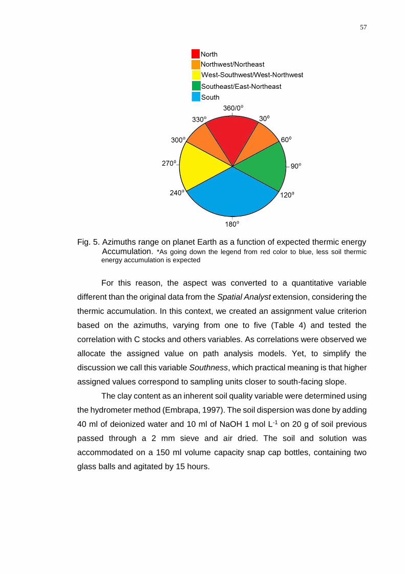
57
Fig. 5. Azimuths range on planet Earth as a function of expected thermic energy Accumulation. *As going down the legend from red color to blue, less soil thermic
energy accumulation is expected
For this reason, the aspect was converted to a quantitative variable
different than the original data from the Spatial Analyst extension, considering the
thermic accumulation. In this context, we created an assignment value criterion
based on the azimuths, varying from one to five (Table 4) and tested the
correlation with C stocks and others variables. As correlations were observed we
allocate the assigned value on path analysis models. Yet, to simplify the
discussion we call this variable Southness, which practical meaning is that higher
assigned values correspond to sampling units closer to south-facing slope.
The clay content as an inherent soil quality variable were determined using
the hydrometer method (Embrapa, 1997). The soil dispersion was done by adding
40 ml of deionized water and 10 ml of NaOH 1 mol L-1 on 20 g of soil previous
passed through a 2 mm sieve and air dried. The soil and solution was
accommodated on a 150 ml volume capacity snap cap bottles, containing two
glass balls and agitated by 15 hours.
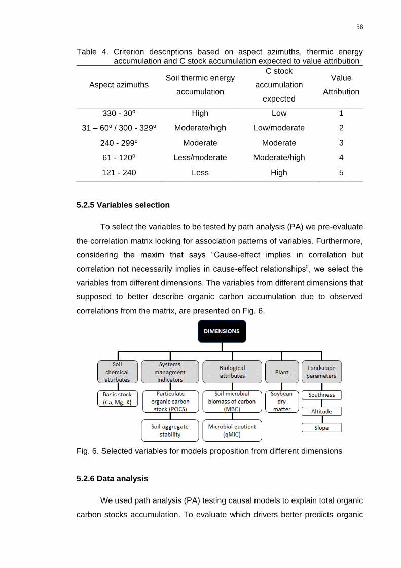
58
Table 4. Criterion descriptions based on aspect azimuths, thermic energy accumulation and C stock accumulation expected to value attribution
Aspect azimuths Soil thermic energy
accumulation
C stock
accumulation
expected
Value
Attribution
330 - 30⁰ High Low 1
31 – 60⁰ / 300 - 329⁰ Moderate/high Low/moderate 2
240 - 299⁰ Moderate Moderate 3
61 - 120⁰ Less/moderate Moderate/high 4
121 - 240 Less High 5
5.2.5 Variables selection
To select the variables to be tested by path analysis (PA) we pre-evaluate
the correlation matrix looking for association patterns of variables. Furthermore,
considering the maxim that says “Cause-effect implies in correlation but
correlation not necessarily implies in cause-effect relationships”, we select the
variables from different dimensions. The variables from different dimensions that
supposed to better describe organic carbon accumulation due to observed
correlations from the matrix, are presented on Fig. 6.
Fig. 6. Selected variables for models proposition from different dimensions
5.2.6 Data analysis
We used path analysis (PA) testing causal models to explain total organic
carbon stocks accumulation. To evaluate which drivers better predicts organic

59
carbon stock (OCS), we proposed causal models linking landscape parameters,
particulate organic carbon stock (POCS), chemical attributes and MBC. For this,
a set of independent relationships between the variables included in the model
was defined adopting the d-separation approach (Shipley, 2000). Permutation
tests was performed to calculate correlations and partial correlations from each
independent relationship (Manly, 2007).
For each causal model, a P-value for a composite probability Fisher’s C
statistic tested by using the ᵡ2 distribution (Shipley, 2000) was calculated. To be
valid, the causal model must present a P-value larger than the acceptable
probability threshold adopted. In the present study we choose for P ≥ 0.1.
A linear regression model were used to determine a non-determination
coefficient (U = 1 – R2) for each response variable representing the portion of
variance not explained (Manly, 2007). Furthermore, a path coefficient (β) and
corresponding probability found by permutation (Manly, 2007) for each causal
link also was calculated. Factors and response variables were centered and
standardized to unit variance, therefore the path coefficients (β) were comparable
across predictors and models.
Among valid models (P ≥ 0.1) we selected those that showed significant
or marginally significant path coefficients for a ρ-value ≤ 0.1, confirming the
validity of each causal links. When more than one model seems to be plausive
we used the Akaike’s information criterion (𝐴𝐼𝐶) for model selection. This
approach evaluate which had more support (Shipley, 2013) and for each
proposed model, we calculated the 𝐴𝐼𝐶 according to the equation: 𝐴𝐼𝐶𝐶 = 𝐶 +
2𝐾 (𝑛 (𝑛 − 𝐾 − 1))⁄ ; where 𝐶 is Fisher’s 𝐶 statistic, 𝐾 is the number of maximum
likelihood parameters that are estimated using the empirical data, and 𝑛 the
sample size (Shipley, 2013). Given competing models, that with the smallest 𝐴𝐼𝐶
value is preferred, and the relative support of the different models is based on the
differences in the 𝐴𝐼𝐶 values relative to the preferred model (i.e. ∆𝐴𝐼𝐶𝐶, see
Shipley, 2013) .
We compare the different models and accepted the ones that presented
∆𝐴𝐼𝐶𝐶 values less than 3, since those models have a substantial support relative
to the best model of the set (see Shipley, 2013). The models with an ∆𝐴𝐼𝐶𝐶
between 3 and 7 is considered to have considerable less support relative to the
best model of the set (Shipley, 2013), but, when convenient we also discuss those
60
models. Each model had a weight (𝑊), which is also taken into account to verify
its support.
Data analysis were done with MULTIV software (available at
http://ecoqua.ecologia.ufrgs.br/main.html), using 25 000 permutations.
5.3 Results
5.3.1 Systems models propositions
For ICLS1, TAS and IAS more than one model were proposed and we used
𝐴𝐼𝐶 for selection, comparison and further discussions. For the ICLS2 we
presented just one valid model since other models besides been validated
presented no-significate path coefficients.
5.3.1.1 Agriculture systems (AS)
All models of the TAS presented one directly cause and one or two
indirectly causes of OCS increase (Fig. 7). From the accepted models, the
variance not explained by the direct causes of OCS remained between 30
(Models 1 and 5) and 53 % (Models 2, 3 and 4).
61
Fig. 7. Causal relationships linking organic carbon stock (OCS) to landscape variable, base stock, basic cation saturation percentage (BCSP), cation exchange capacity (CEC), pHW and particulate organic C stock (POCS) for the traditional agriculture system (TAS).
Among the causal models proposed, Models 1, 2 and 3 presents similar
AICC and W values (Table 5) and we considered then as strong support models.
In Model 1, the base stock is significantly influenced by POCS (β = 0.77; ρ =
0.0004) and also presents a strong relation with OCS (β = 0.84; ρ = 0.0001).
Model 2 suggests that as more soybean DM is produced, more particulate
organic carbon is stocked (β= 0.57; ρ= 0.03), but the OCS increases is directly
related with the POCS (β= 0.68; ρ= 0.005) rather than base stock (Fig. 7; Models
1 and 2). In Model 3, sampling units located on lower altitude positions of the
landscape, caused significate POCS increase (β= -0.45; ρ= 0.09).
In Model 4, we inverted the causal variables of OCS as compared with
Model 1 (Fig. 7), and verified considerably less support (Table 5). Finally, in
Model 5 we connected all the parameters used in Models 1 and 2, but, the model
presented no support.
62
Table 5. Model fit of seven competing path models that are represented in Fig. 7 for TAS. Fisher’s C statistic, its df and the null probability (P) are indicated. K is the number of parameters needed to fit the model. AICc and ΔAICc
are the Akaike values and the difference in AICc relative to Model 1. W gives the model weights.
Model C df P K AICC ΔAICC W
1 0.25 2 0.88 5 16.92 0.00 0.33
2 0.33 2 0.84 5 17,00 0.08 0.32
3 0.53 2 0.77 5 17.20 0.28 0.29
4 3.68 2 0.16 5 20.35 3.43 0.06
5 0.61 6 0.99 7 30.61 13.69 0.00
The IAS, had five valid models with significant path coefficients (Fig. 8).
Among them, Model 1 was the most plausive causal model with AICC= 12.9 and
W= 0.54 (Fig. 8; Table 6). This model suggests that OCS increases was affected
by lower MBC (β= -0.43; ρ= 0.06) and by higher SAS (β= 0.64; ρ= 0.002), and 45
% of OCS variation could not be explained by those variables (Fig. 8). Models 2
and 3, present high support related to Model 1 (ΔAICC and W values; see Table
6), but higher predict capacity (U= 0.27; see Fig. 8). Model 2 indicates a trend for
OCS accumulation on higher altitudes (β= 0.45; ρ= 0.05), whereas Model 3
indicates that this trend is also dependent on lower qMIC (β= -0.62; ρ= 0.005).
Moreover, Model 4 and 5 have no support compared to Model 1. In the
first case, we tried to mix Models 2 and 3 connecting altitude to qMIC and in
Model 5 a position information is added indicating that sampling units positioned
in higher altitudes have lower slope, affecting indirectly OCS.
63
Fig. 8 Causal relationships linking organic carbon stock (OCS) to landscape variable (Altitude and Slope), microbial biomass of carbon (MBC), microbial quotient (qMIC) and soil aggregate stability (SAS) for the irrigated agriculture system (IAS)
Table 6. Model fit of seven competing path models that are represented in Fig. 8 for IAS. Fisher’s C statistic, its df and the null probability (P) are indicated. K is the number of parameters needed to fit the model. AICc and ΔAICc
are the Akaike values and the difference in AICc relative to Model 1. W gives the model weights.
Model C df P K AICC ΔAICC W
1 0.65 2 0.72 5 12.9 0 0.54
2 2.24 2 0.33 5 14.5 1.59 0.24
3 2.52 2 0.28 5 14.7 1.87 0.21
4 7.32 6 0.29 7 25.8 12.9 0.00
5 5.89 12 0.92 9 31.7 18.8 0.00
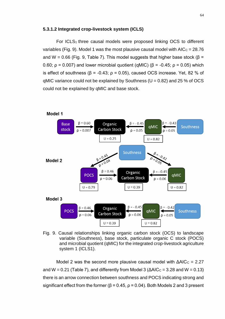
64
5.3.1.2 Integrated crop-livestock system (ICLS)
For ICLS1 three causal models were proposed linking OCS to different
variables (Fig. 9). Model 1 was the most plausive causal model with AICC = 28.76
and W = 0.66 (Fig. 9, Table 7). This model suggests that higher base stock (β =
0.60; ρ = 0.007) and lower microbial quotient (qMIC) (β = -0.45; ρ = 0.05) which
is effect of southness (β = -0.43; ρ = 0.05), caused OCS increase. Yet, 82 % of
qMIC variance could not be explained by Southness (U = 0.82) and 25 % of OCS
could not be explained by qMIC and base stock.
Fig. 9. Causal relationships linking organic carbon stock (OCS) to landscape variable (Southness), base stock, particulate organic C stock (POCS) and microbial quotient (qMIC) for the integrated crop-livestock agriculture system 1 (ICLS1).
Model 2 was the second more plausive causal model with ΔAICC = 2.27
and W = 0.21 (Table 7), and differently from Model 3 (ΔAICC = 3.28 and W = 0.13)
there is an arrow connection between southness and POCS indicating strong and
significant effect from the former (β = 0.45, ρ = 0.04). Both Models 2 and 3 present

65
82 % of qMIC not explained by southness and 39 % of OCS not explained by
POCS and qMIC.
Table 7. Model fit of three competing path models that are represented in Fig. 9 for ICLS1. Fisher’s C statistic, its df and the null probability (P) are indicated. K is the number of parameters needed to fit the model. AICc and ΔAICc
are the Akaike values and the difference in AICc relative to Model 1. W gives the model weights.
Model C df P K AICC ΔAICC W
1 6.14 6 0.41 7 28.76 0 0.66
2 3.03 4 0.55 8 31.03 2.27 0.21
3 9.42 6 0.15 7 32.04 3.28 0.13
For ICLS2 six others models were tested between different variables and
have been validated (P ≥ 0.1), but, with non-significant path coefficients (β). The
model we choose (Fig. 10) presents a highly and significant influence of POCS
on OCS (β = 0.65 and ρ = 0.0001). In the other hand, the OCS increases also
was caused by sample unit altitude on the landscape, presenting a moderate and
marginally significant influence (β = 0.27 and ρ = 0.1). Furthermore, 48 % of OCS
was not explained by its descriptors POCS and Altitude.
Fig. 10. Causal relationships linking organic carbon stock (OCS) to landscape variable (Altitude) and particulate organic C stock (POCS) for the integrated crop-livestock system 2 (ICLS2)
5.4. Discussions
5.4.1 Systems models propositions
5.4.1.1 Agriculture systems (AS)
The OCS increase on the TAS although demonstrated to be dependent of
a set of variables from different dimensions, a connection of all those variables
directly to OCS wasn’t possible (Fig. 7), cause generated non-significate path
coefficients. Since it represents the lower organic C storage and space-temporal
66
species diversity (Table 1), this system is dependent of a few variables with
greater weight on OCS variation. In this context, all the proposed models present
just one variable directly connected and one or two variables indirectly connected
to OCS (Fig. 7).
In this context, although the C addition by total dry matter produced by the
system was not measured, the soybean DM representing all systems as a
summer crop, indicates that for TAS this variable could be important for POCS
formation (Fig. 7). In addition, the 2013/2014 crop season was quietly rainy and
plants produced high biomass. On the other hand, evaluating Model 1, the base
stock presenting strong influence on OCS (β= 0.84; ρ= 0.0001), indicates that
higher chemical fertility can influence carbon storage through latent variables
between then. This could be caused by further total system DM addition, or by
benefiting soil aggregate formation as chemical fertility increases.
For IAS, the main directly factors increasing OCS was SAS and biological
attributes (Fig. 8). The former, indicates that aggregation process is contributing
for organic carbon storage. According to Ontl et al. (2015), in a conversion from
a conventionally tilled corn-soybean rotation to a no-tillage bioenergy cropping
system, while not having measurable short-terms impacts to total OCS, the
particulate organic matter could be preserved through soil aggregation. During
sampling, it was clear the influence of corn roots that remains on soil favoring
aggregate stability and physical organic matter protection on this system.
Furthermore, all area of this system is an Oxisol with most sampling units texture
with more than 70 % of a clay with iron oxides predominance, favoring the
organic-mineral interaction also as an important organic matter stabilization
mechanism.
At the sampling moment, there was a high corn and forage radish biomass
residues on IAS area (Table 1), contributing to a MBC population ranging from
190 to 533 μgC g-1 soil. However, OCS increases was affected by lower MBC and
qMIC (Fig. 8), suggesting that the occurrence of an organic C stabilization by soil
mineral fractions is affecting qMIC as reported by Sparling, 1992. Yet, the roots
effect on soil aggregation protects light fractions of soil organic matter, also
becoming inaccessible to soil microorganisms. The qMIC values varies between
0.85 and 2.68 with a mean of 1.67 in the IAS. This wide range variation of MBC
on IAS, indicate that variables inherent of each sample unit is affecting soil
67
microbial community, and we seek to comprehend them connecting the
landscape parameters on Models 2, 4 and 5.
In Model 2, the ΔAICC= 1.59 and W= 0.24 (Table 6) indicated strong
support relating to the most plausive (Model 1). In this model, no biological
attribute was connected (Fig. 8), and a lower percentage of OCS variability was
not explained (U = 0.27) by altitude and SAS. Higher altitudes directly cause OCS
increases (Model 2), but, also caused lower qMIC on Models 4 and 5. However,
since altitude variation is not high enough to manifest per se effects on
temperature and consequently on carbon fractions, its necessary to investigate
latent variables connected. That’s what we pursuit on Model 5, which although
has no support compared Model 1, presents a significate relation between slope
and altitude. This relationship indicates that sampling units located on higher
altitudes can accumulate more water because of the lower slope, directly
benefiting OCS (Model 2), or through qMIC (Models 4 and 5).
5.4.1.2 Integrated crop-livestock systems (ICLS)
The studied ICLS’s, present higher species diversity and functionality, less
time interval between species options and shorter spatialization, since the forage
and the animal components interact at the same space and time. These
characteristics, as already mentioned, result in higher OCS compared to AS.
Furthermore, a slightly higher microbial quotient on ICLS was also observed and
this is in agreement with Sparling, 1992, which reports qMIC is greater under
pastures, than the equivalent soil under native forest, exotic forest or arable
cropping system.
The area of ICLS1 presents an irregular topography presenting different
aspects and is located on a soil transaction, where the sampling units 6, 20 and
21 (Fig. 4) where identified as Mollisols (Soil Taxonomy, 1999). This soil type
presented the higher OCS of this system (Fig. 4), but, its organic matter quality
is less available for microorganisms, since qMIC = 1.04 %. On the other hand,
the others sampling units of this area which is almost all Oxisols presented qMIC
varying between 1.34 and 4.35 % (data not shown). Sparling (1992), comparing
soils with different OCS also found the same relationship between OCS and
qMIC.
68
Foraging by grazing promotes intensive exudation of organic compounds
by roots (Tisdall and Oades, 1982), which become an energy source for soil
microorganisms. In this context, ICLS1 presented MBC varying between 330 and
976 μgC g-1 soil compared with 164 to 547 μgC g-1 soil on TAS. In Model 1 (Fig.
9), the most plausive one, with a weight of 0.66 (Table 7), as Model 1 from TAS
(Fig.7) present a strong relation between base stock and OCS. As mentioned
before, this could be an effect of latent variables between then benefiting soil
aggregate formation and mainly due to a total system DM production increase.
Moreover, this model presents another directly relation between qMIC and OCS
with a negative and significant path coefficient (β= 0.45; ρ= 0.05). However, the
qMIC is influenced by “Southness” variable, indicating that sampling units that
accumulate less thermic energy during the day, present lower qMIC (Fig. 9).
Similar results were obtained by Nahidan et al (2014) on a rangeland ecosystem
on Iran. These authors observed higher qMIC on south-facing slope, where soil
accumulates more thermic energy on north hemisphere. The same pattern was
reported on a Humic Cambissol with Pinus laricio ecosystem on Italy for MBC by
Sidari et al (2008). These authors found that on soils at south-facing slope,
occurred three times more MBC than the positioned on north-facing slope.
In Model 2 and 3 the POCS was included, but, the former presents an
additional arrow with “Southness” (Fig. 9) with a higher model weight (W= 0.21,
see Table 7). This model indicates that sampling units that accumulate less
thermic energy also has the POCS increased. Furthermore, the significant
contribution of POCS to OCS on this system (β= 0.46; ρ = 0.06) is an effect of C
input through animal excreta, rizodeposition from ryegrass pasture grazed as
also its DM. This latter factor is particularly important since there is a high DM
input from the forage shoot to soil with the adopted management (item 4.2.2).
On ICLS2, which species rotation is a mix between ICLS1 and TAS, the
OCS variation occurs similarly to ICLS1, showing that the higher complexity
compared to TAS tends to distribute the weight of the directly connected
variables. Besides the similar sources of C input from ICLS1, the historic of ICLS2
(Table 1) presents two crop seasons with forage radish which improved nutrient
cycling, and three crop seasons with wheat which input a recalcitrant organic
matter form rich in lignin content.
69
5.5 Conclusions
Path analysis demonstrated to be an appropriate approach to better
comprehend production systems through the light of cause-effect relationships,
and the Akaike’s information criterion enable the proposition of more than one
robust model.
The landscape factors exploration, permits soil carbon storage patterns
understanding on space, and is essential on a farm-scale study.
The base stock is the main direct cause of OCS increasing in the traditional
agriculture system, whereas in the irrigated agriculture system and in the
integrated crop-livestock systems, the directly cause of organic carbon stock
were distributed among base stock, particulate organic carbon stock, soil
aggregate stability, altitude and biological attributes due to higher diversity.
70
6. CAPÍTULO IV – ESTUDO III: SOIL AGGREGATE STABILITY IN
COMMERCIAL PRODUCTION SYSTEMS IN THE SUBTROPIC
ENVIRONMENT AS DESCRIBED BY CAUSE-EFFECT RELATIONSHIPS
BETWEEN SOIL AND LANDSCAPE VARIABLES
6.1 Introduction
The pursuit for a sustainable food and supply commercial production system
is an issue that arouse attention in the last decades. There is a high natural
resources exploration rate nowadays to meet fertilizer demands from crops.
Therefore, the adoption of a production system which produces minimum entropy
and promotes maximum ecosystems services, is required to achieve
sustainability.
In this context, it is necessary to maintain a proper balance between
dissipative and ordering processes in the soil system (Addiscott, 1995), by
adopting managements that increase the latter process. This author suggested
that an audit of small molecules as CO2, NH3 and H2O is a way of assessing
sustainability. However, since soil aggregation is a result from the rearrangement
of particles, flocculation and cementation (Duiker et al., 2003), the assessment of
soil aggregate stability (ASt) also can be used to infer about ordination processes
that build production systems with lower entropy level and hence, more
sustainable. On the other hand, soil ASt is also used as an indicator of soil
structure (Six et al., 2000), whose declination is considered a form of degradation
71
(Chan et al., 2003), i.e., a dissipative process. Therefore, soil ASt encompasses
soil properties interactions and can be used to determine if an agricultural soil is
stable, improving or deteriorating (Portella et al., 2012).
Soil ASt is strongly dependent on land use and management. In subtropic
brazilian environment, no-tillage soil management and the inclusion of grass
species, for a long time have been demonstrating to be efficient strategies to
increase soil aggregate stability (Carpenedo and Mielniczuk, 1990; Paladini and
Mielniczuck, 1991). Otherwise, more recently the integrated crop-livestock
system (ICLS) also has shown higher soil ASt than most of the agriculture
systems or no grazed areas (Salton et al., 2008; Souza et al., 2010). Cases where
soil ASt reaches similar or even higher values to the native forest is also found
(Tirloni et al., 2012).
Nonetheless, most approaches come from experimental data, and a farm-
scale approach comprehending soil ASt variation patterns and associated cause-
effect relationships is becoming more necessary. Thus, a statistical technique as
path analysis, aiming to interpret correlations in complex causal systems, by
analyzing interrelationships in nonexperimental data is required (Crow, 1990).
Recently, a model proposition approach by analyzing a net of cause-effect
relationships using path analysis have been explored by ecologists (Guido et al.,
2016; Pillar et al., 2013). This approach was proposed by Shipley (2000) and
permits one to test the causal claims of the path model, rather than only
measuring the direct influence along each separate path in such a system. This
author introduced the structure equation model, the d-separation and permutation
tests techniques, facilitating the proposition of robust models. Furthermore,
Akaike’s information criterion (AIC) applied to path analytic models has been
recently proposed to select models by evaluating which one has better support
(Shipley, 2013).
We understand, that since soil ASt is an important soil degradation status
indicator which gives robust support to system’s sustainability, should be
comprehended in the light of variation patterns of carbon and associated
variables across landscape. Furthermore, most soils on subtropical ecosystems
will present lower physical degradation, as a reflex of improved production
systems that increases soil ASt. Yet, the factors that promote soil aggregation
can be related to plant species type and soil management (An et al., 2010; Ontl
72
et al., 2015; Portella et al., 2012), soil microbial biomass (Kiem and Kandeler,
1997; Tang et al., 2011), grazed forages (Loss et al., 2011; Salton et al., 2008;
Souza et al., 2010; Tirloni et al., 2012) and different fractions of soil organic matter
(Loss et al., 2011; Ontl et al., 2015). In this context, we expect to comprehend
which factors describes soil aggregate stability variation, evaluating different path
analysis models propositions.
6.2 Methods
The localization, all systems descriptions, detailed soil sampling criteria,
soil carbon fractions and soil aggregate stability methods are presented on
chapter 2. Soil attributes, landscape parameters, soil texture, variables selection
criterion and data analysis description are presented on chapter 3.
6.3 Results
For the ICLS2, the correlation matrix demonstrated a weak relation from
variables with soil aggregate stability. For this reason, it is not possible to build
and to do a model proposition by PA, hence, we disregarded this system and
presented the TAS, IAS and ICLS1 PA models.
6.3.1 Systems models propositions
Before model proposition, several simulations generated non-significate
models and/or models with non-significate path coefficients. From TAS and ICLS1
just one model was proposed (Fig. 11; Fig. 14) while for IAS two models were
proposed and we used the Akaike’s information criterion.
The soil ASt in the traditional agriculture system (TAS) was affected by
inherent factors as clay content, and dynamic factors as soil fertility, soil
management and soil biology attributes (Fig. 11). Before the connection of these
soil fertility and management parameters on PA model, they were synthetized by
using the ordination scores of PCA 1 which explains 84.32 % of variation (Fig.
12). The contribution of each fertility parameters on PCA 1 was 27.6, 26.0, 24.4
and 22.0 % of OCS, BS, ONS and pHw respectively.
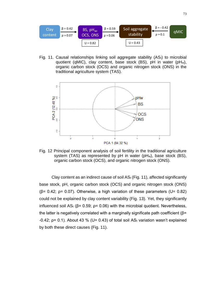
73
Fig. 11. Causal relationships linking soil aggregate stability (ASt) to microbial quotient (qMIC), clay content, base stock (BS), pH in water (pHw), organic carbon stock (OCS) and organic nitrogen stock (ONS) in the traditional agriculture system (TAS).
Fig. 12 Principal component analysis of soil fertility in the traditional agriculture system (TAS) as represented by pH in water (pHw), base stock (BS), organic carbon stock (OCS), and organic nitrogen stock (ONS).
Clay content as an indirect cause of soil ASt (Fig. 11), affected significantly
base stock, pH, organic carbon stock (OCS) and organic nitrogen stock (ONS)
(β= 0.42; ρ= 0.07). Otherwise, a high variation of these parameters (U= 0.82)
could not be explained by clay content variability (Fig. 13). Yet, they significantly
influenced soil ASt (β= 0.59; ρ= 0.06) with the microbial quotient. Nevertheless,
the latter is negatively correlated with a marginally significate path coefficient (β=
-0.42; ρ= 0.1). About 43 % (U= 0.43) of total soil ASt variation wasn’t explained
by both these direct causes (Fig. 11).
β = - 0.42β = 0.42
ρ = 0.1ρ = 0.07
β = 0.59
ρ = 0.06
Soil aggregatestability
BS, pHw, OCS, ONS
U = 0.43
qMICClay
content
U = 0.82
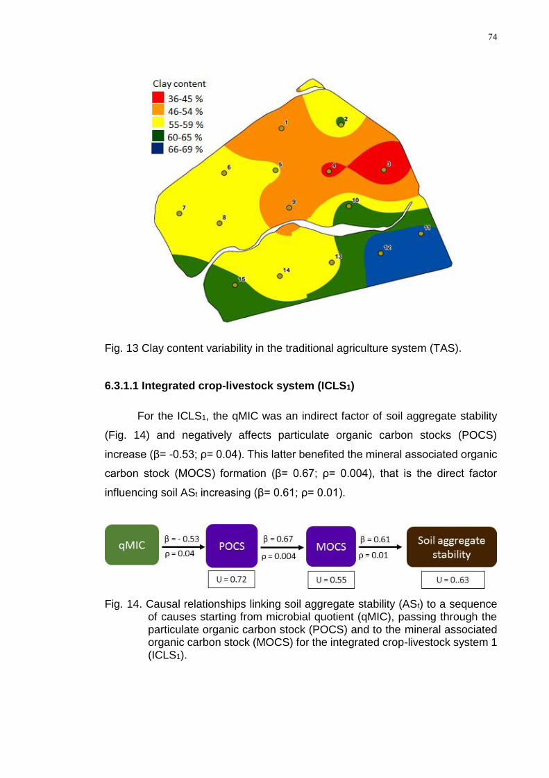
74
Fig. 13 Clay content variability in the traditional agriculture system (TAS).
6.3.1.1 Integrated crop-livestock system (ICLS1)
For the ICLS1, the qMIC was an indirect factor of soil aggregate stability
(Fig. 14) and negatively affects particulate organic carbon stocks (POCS)
increase (β= -0.53; ρ= 0.04). This latter benefited the mineral associated organic
carbon stock (MOCS) formation (β= 0.67; ρ= 0.004), that is the direct factor
influencing soil ASt increasing (β= 0.61; ρ= 0.01).
Fig. 14. Causal relationships linking soil aggregate stability (ASt) to a sequence of causes starting from microbial quotient (qMIC), passing through the particulate organic carbon stock (POCS) and to the mineral associated organic carbon stock (MOCS) for the integrated crop-livestock system 1 (ICLS1).
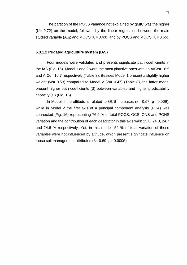
75
The partition of the POCS variance not explained by qMIC was the higher
(U= 0.72) on the model, followed by the linear regression between the main
studied variable (ASt) and MOCS (U= 0.63), and by POCS and MOCS (U= 0.55).
6.3.1.2 Irrigated agriculture system (IAS)
Four models were validated and presents significate path coefficients in
the IAS (Fig. 15). Model 1 and 2 were the most plausive ones with an AICc= 16.5
and AICc= 16.7 respectively (Table 8). Besides Model 1 present a slightly higher
weight (W= 0.53) compared to Model 2 (W= 0.47) (Table 8), the latter model
present higher path coefficients (β) between variables and higher predictability
capacity (U) (Fig. 15).
In Model 1 the altitude is related to OCS increases (β= 0.57, ρ= 0.009),
while in Model 2 the first axis of a principal component analysis (PCA) was
connected (Fig. 16) representing 76.9 % of total POCS, OCS, ONS and PONS
variation and the contribution of each descriptor in this axis was: 25.8, 24.8, 24.7
and 24.6 % respectively. Yet, in this model, 52 % of total variation of these
variables were not influenced by altitude, which present significate influence on
these soil management attributes (β= 0.69, ρ= 0.0005).
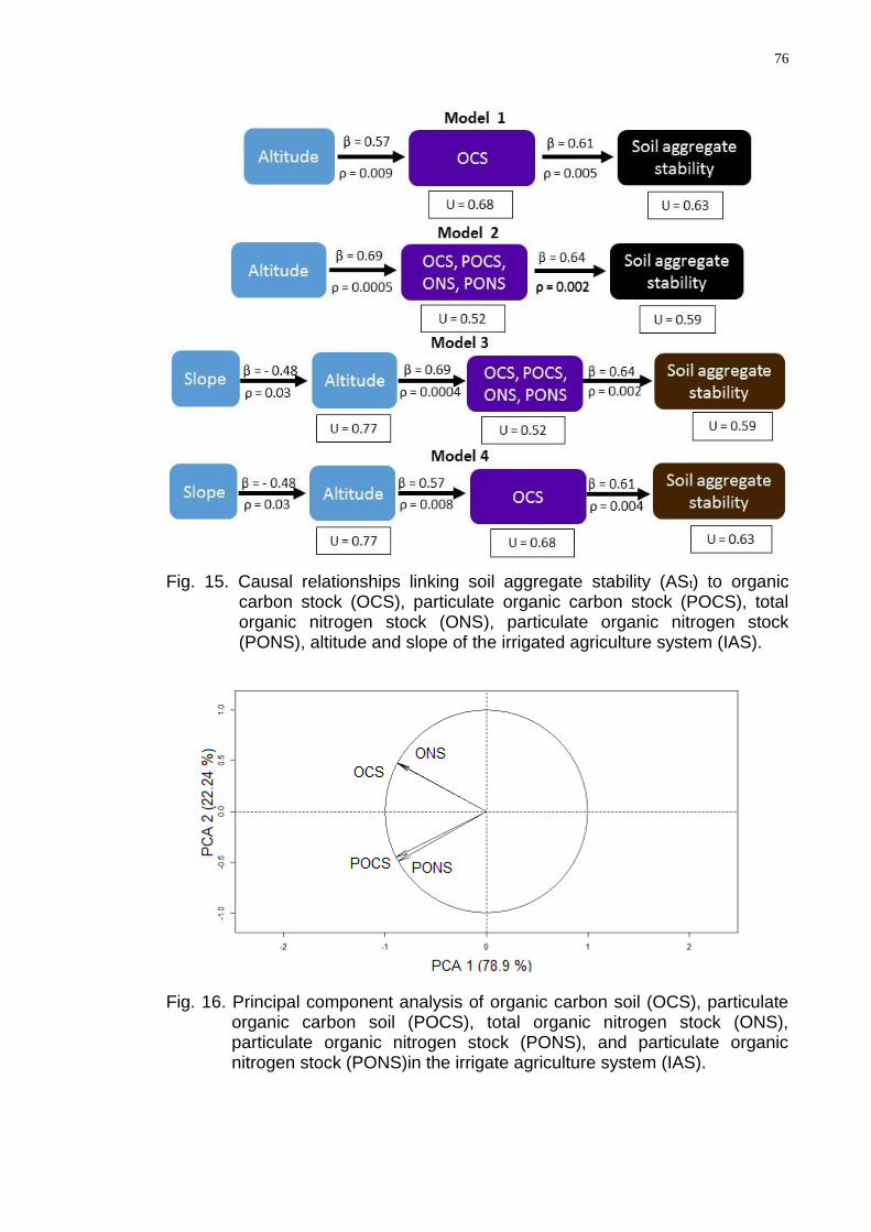
76
Fig. 15. Causal relationships linking soil aggregate stability (ASt) to organic carbon stock (OCS), particulate organic carbon stock (POCS), total organic nitrogen stock (ONS), particulate organic nitrogen stock (PONS), altitude and slope of the irrigated agriculture system (IAS).
Fig. 16. Principal component analysis of organic carbon soil (OCS), particulate organic carbon soil (POCS), total organic nitrogen stock (ONS), particulate organic nitrogen stock (PONS), and particulate organic nitrogen stock (PONS)in the irrigate agriculture system (IAS).
77
Table 8. Model fit of four competing path models that are represented in Fig. 15 for IAS. Fisher’s C statistic, its df and the null probability (P) are indicated. K is the number of parameters needed to fit the model. AICc and ΔAICc
are the Akaike values and the difference in AICc relative to Model 1. W gives the model weights.
Model C df P K AICc ΔAICc W
1 2.18 2 0.33 5 16.5 0.00 0.53
2 2.43 2 0.30 5 16.7 0.3 0.47
3 4.27 6 0.64 7 27.6 11.1 0.00
4 4.28 6 0.64 7 27.6 11.1 0.00
Soil aggregate stability has been significantly influenced by soil
management attributes in all models (Fig. 15). Otherwise, models that connected
all attributes to soil ASt presented slightly higher path coefficient (β= 0.64) and
predictable capacity (U= 0.59).
In Models 3 and 4, besides they have no weight compared the best fit
model (W= 0; see Table 8), the connection of slope to altitude presented negative
effect (β= - 0.48, ρ= 0.03). Yet, 77 % of total altitude variation through the
landscape could not been explained by the slope in this irrigated agriculture
system.
6.4 Discussion
6.4.1 Models propositions for the systems
Comparing the studied systems, the TAS model presented the higher
predictability capacity for soil ASt (U= 0.43), followed by the IAS (U= 0.59 – 0.63)
and the ICLS1 (U= 0.63) (Figs. 12, 14 and 15). Since the IAS and ICLS1 are more
complex systems and presented higher diversity (Table 1), further variables not
considered on the proposed models would be important to explain soil ASt
variation.
All systems presented different fractions of organic carbon as direct cause
of soil ASt (Figs 12, 14 and 15), indicating that feedback between soil organic
carbon cycling and aggregate cycling is occurring (Jastrow and Miller, 1997a). In
the IAS, the summer corn introduction promoted soil aggregation increase, since
the TAS which presents similar species historic until crop season 2010/2011
(Table 1), and the same edaphic conditions, have lower soil ASt. Higher dry
78
matter production of grass species on the IAS was a reflex of nitrogen fertilizer
input (item 4.2.2), hence, all fractions of organic carbon and nitrogen stocks also
increase, benefiting soil ASt (Fig. 15).
According to Six et al (2000), recent inputs of organic matter induce
macroaggregate formation. The higher soil aggregation on the IAS compared to
the TAS (Fig. 4) is because the microaggregates were transformed to
macroaggregates. This process occurs firstly due decomposable organic
materials as microbial and plant derived polysaccharides, and secondly due to
temporary binding agents (Jastrow and Miller, 1997b). The latter mechanism
refers to fine roots, fungal hyphae, bacterial cells, and algae (Jastrow and Miller,
1997b) and were predominant in the IAS. The high density of fine corn roots
physically involving soil microaggregates, promote macroaggregate stabilization,
as suggested by Tisdall and Oades (1979) for ryegrass and by Gale et al. (2000)
for corn.
Yet, all models presented landscape parameters affecting organic carbon
and nitrogen fractions (Fig. 15). These fractions are higher on sampling units
positioned on higher altitudes across landscape, and although Models 3 and 4
have no support comparing the best fit models (Table 8), they indicate that slope
was lower on higher altitudes. Thus, more water accumulation is expected
benefiting its availability for crop production and further dry matter biomass
inputs.
Otherwise, in the TAS the mineral-organic associations by iron and
aluminum oxides as represented by clay content variability (Fig. 13), influenced
part of the organic carbon stocks increases, hence, soil ASt (Fig. 11). In addition,
a higher organic matter input from higher crops and cover crops residues
production, occurs as a response of increased base stock and soil pH due to a
lime application on summer of 2012. Moreover, the only nitrogen input for this
system came from soybean inoculation, therefore, the plants located on clayey
soil produced higher dry matter biomass, stocked more nitrogen in its tissue and
inputs more nitrogen to the soil.
Yet, the lower microbial quotient (qMIC) affected directly or indirectly soil
ASt increases in TAS and ICLS1 respectively (Figs 12 and 14). In both systems,
the mean qMIC found was similar (2.13 % on TAS and 2.15 % on ICLS1). These
values suggest both systems reached its equilibrium (Jenkinson and Ladd, 1981),
79
although, the absolute value of microbial biomass and organic carbon stocks in
the ICLS1 are greater (data not shown).
Therefore, the negative correlation between qMIC and soil ASt in the TAS
(Fig. 11) indicates that sampling units with higher soil ASt, tend to protect soil
organic carbon from microbial biomass assessment. Otherwise, in the ICLS1 the
POCS, negative correlation with qMIC (Fig. 14) indicates that most of this fraction,
besides it is chemically available for microorganism decomposition, it is
inaccessible due to physical protection by soil aggregates.
The proposed model for the ICLS1 (Fig. 14), also shows a carbon storage
process following fractions associated with the soil aggregation. The POCS tends
to benefit organic mineral associations (MOCS), increasing soil ASt.
6.5 Conclusions
Path analysis demonstrated to be an appropriate approach to better
comprehend production systems through the light of cause-effect relationships of
different factors.
All systems presented different fractions of organic carbon as direct cause
of soil aggregate stability, demonstrating the importance of no tillage systems
with species that increases carbon input, to avoid soil degradation.
In the irrigated agricultural systems, the sampling units positioned in higher
altitudes and lower slope, tends to storage more carbon and nitrogen, as a result
of water accumulation, favoring species development and further dry mass input
to the soil on these spots.
The main factor that affected soil aggregation in the traditional agricultural
system, was soil pH and base stock increases, promoting plant development and
dry matter inputs increases in these sampling units, which benefited soil organic
carbon and nitrogen storage.
In the integrated crop-livestock system 1, the lower soil microorganisms
assessment favored the particulate organic carbon fraction storage, which
benefited the organic-mineral carbon associations, hence, increased soil
aggregation.
80
7. CAPÍTULO V – ESTUDO IV: CARBON MANAGEMENT INDEX IN A
TRADITIONAL AGRICULTURE SYSTEM AND IN INTEGRATED CROP-
LIVESTOCK SYSTEMS IN SUBTROPIC ENVIRONMENT AS DESCRIBED BY
SOIL AND LANDSCAPE VARIABLES
7.1. Introduction
Brazilian southern is an important grain producer region and the successions
among soybean/wheat, soybean/fallow or soybean/cover crop, are the main crop
succession practiced during summer/winter respectively. Specifically, in north of
Rio Grande do Sul state, the traditional winter species cultivated are wheat for
grain, or ryegrass and black oat as cover crops for the direct seedling system.
Nonetheless, the occurrence of several dry periods during winters, affecting
mainly wheat production, have been reported during last decades (CONAB,
2016). Hence, the wheat cultivated area from 2015/2016 crop season
corresponded to only 14 % of the soybean cultivated in the following summer,
therefore, about 4,7 millions of hectares was on fallow or with forage cover crops
with high potential for cattle grazing (CONAB, 2016).
Although there is no precise data about the area occupied by integrated crop-
livestock systems (ICLS) in this region, adoption by farmers are slowly increasing.
Cattle production is less susceptible to climate conditions, presenting further
economic incomes (Moraes et al., 2014). Moreover, studies in an experimental
with different grazing intensities in this region, demonstrated that moderated
81
grazing intensity benefits several soil attributes (Carvalho et al., 2010; Costa et
al., 2014; Souza et al., 2009; Souza et al., 2010).
In this context, an interesting approach is to evaluate which level is soil
ecosystem in traditional agricultural and ICLS’s comparing to a never disturbed
ecosystem, i.e., a preserved bioma as natural forest. This latter, inherently
presents several desirable characteristics regarding the provision of ecosystems
services. Carbon sequestration (Lal, 2005), soil aggregation (An et al., 2010) and
improvement on total porosity (Tavares Filho & Tessier, 2010) are some services
provided by natural ecosystems. Thus, considering that soils in natural
ecosystems reached an equilibrium among their properties leading to a long-term
stability (Fedoroff, 1987), this climax status implies in a sustainable condition to
pursuit by production systems to minimize its use impact. Nonetheless, to
differentiate management practices and evaluate the similarities with natural
systems, it is necessary an appropriated soil quality indicator choose.
The soil organic carbon (SOC) and its different fractions are soil parameters
highly influenced by management practices (Haynes, 2005). Mainly the young or
labile SOC fraction is key to interpret changes in quality (Kapkiyai et al., 1999),
being a more sensitive indicator than the SOC and total nitrogen (Biederbeck et
al., 1998). Therefore, under natural ecosystems, a proper balance between
particulate and total soil organic carbon (C) is supporting soil system’s stability.
Thus, the carbon management index (CMI) can be used to verify differences or
similarities among natural and production ecosystems, since considers the C poll
and lability of the system compared to a reference as a natural ecosystem.
The CMI, as a sensible indicator of changes in the total SOC and its labile
fraction, was firstly described by Blair et al (2005). These authors propose the
oxidized by a potassium permanganate solution fraction as the labile carbon (C),
and the non-oxidized fraction as the non-labile C. Otherwise, instead of the
chemical oxidation principles suggested by Blair et al (2005), the physical
fractionation by isolating the particulate organic matter (POM) seems to be more
reliable (Vieira et al., 2007). According these authors, besides the chemical
oxidation attacks some mineral-associated organic material not available to soil
microorganisms, it is possible that some labile compounds inside large fragments
of POM may not be oxidized.
82
Other concern about CMI application is about possible differences between
soil across landscape and soil from the reference area. Hence, it is necessary to
choose more than one reference area, or discard the sampling units
corresponding to a different soil type than the one found in the reference area.
Thus, the comprehension of factors related to soil properties and landscape
variability, are crucial to better directly or indirectly describe the CMI variation on
a farm-scale, for example. For this, an integrated statistical approach condensing
variables, without much information losses, with a cause-effect relationship tool
appropriated to field application, is necessary. In this context, principal
component analysis (PCA) can be used to condensate variables from a specific
dimension, for example, soil chemical attributes, soil biological attributes, etc, and
build a cause-effect relationships model, connecting these variables each other
or to an important response variable.
The path analysis (PA) is an important statistical tool to cause-effect
relationships studies. A new approach has been used by ecologists to propose
robust models by including important variables to describe complex environments
(Pillar et al., 2013; Guido et al., 2016). PA was firstly proposed by Shipley (2000),
by using structure equation model, the d-separation and permutation tests
techniques. Furthermore, when more than one model are validated with
significate path coefficients, Akaike’s information criterion (AIC) can be used to
select models by evaluating which one has better support (Shipley, 2013).
We understand, that the carbon management index variation on farm-
scale approach, should be comprehended in the light of soil properties and
landscape variation patterns. We hypothesized that different soil and landscape
factors can describe directly or indirectly its variation. For this, we used path
analysis techniques and evaluated different models propositions for different long
term agricultural production systems.
7.2 Methods
The localization, all systems descriptions, detailed soil sampling criteria,
soil carbon fractions and soil aggregate stability methods, and carbon
management index calculation methodology, are presented on chapter 2. Soil
83
attributes, landscape parameters, soil texture, variables selection criterion and
data analysis description are presented on chapter 3.
7.3 Results
For the IAS, all model simulation process generated no-valid models or
when they were valid, presented no-significant path coefficients (Appendix 2). For
this reason, we disregarded this system and presented the TAS, ICLS1 and ICLS2
PA models.
7.3.1 Integrated crop-livestock system 1 (ICLS1)
Among validly models (P > 0.1) with significate path coefficients (ρ ≤ 0.1),
we choose six models (Fig. 17) to verify its support and weight (Table 9). The
best fit occurs in Model 1, however, due to similar weights and low ΔAICc value
we consider Model 2 in an equivalent support level (Table 9). The difference
between these models is the indirectly cause of carbon management index, i.e.,
in Model 1 is the soil MBC and in Model 2 is the soil aggregation (Fig. 17). In
Model 1, higher soil MBC significantly decreased the OCS (β = -0.49 and ρ =
0.05), while in Model 2 the OCS increasing is positively influenced by soil
aggregation (β = 0.57 and ρ = 0.02). Nevertheless, the soil OCS as directly cause
of the carbon management index presented higher strength (β = 0.84) and
predictable capacity (U= = 0.29) in Model 2 than in Model 1 (β = 0.64 and U =
0.58).
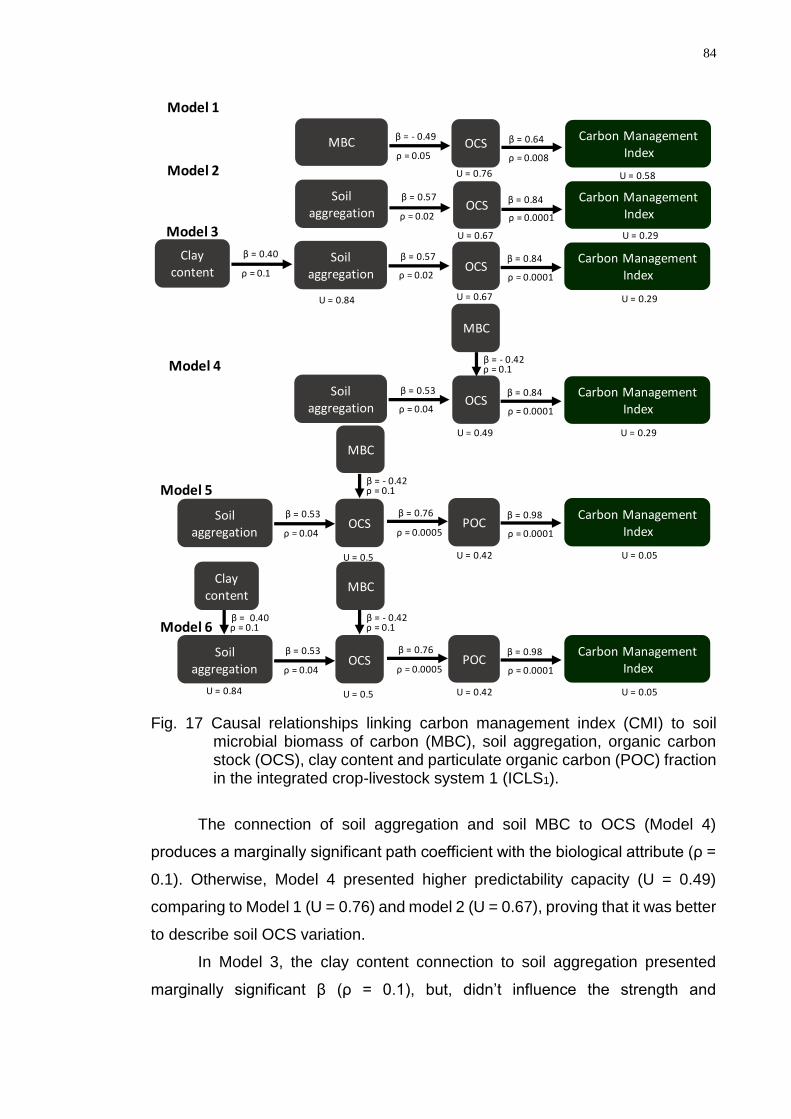
84
Fig. 17 Causal relationships linking carbon management index (CMI) to soil microbial biomass of carbon (MBC), soil aggregation, organic carbon stock (OCS), clay content and particulate organic carbon (POC) fraction in the integrated crop-livestock system 1 (ICLS1).
The connection of soil aggregation and soil MBC to OCS (Model 4)
produces a marginally significant path coefficient with the biological attribute (ρ =
0.1). Otherwise, Model 4 presented higher predictability capacity (U = 0.49)
comparing to Model 1 (U = 0.76) and model 2 (U = 0.67), proving that it was better
to describe soil OCS variation.
In Model 3, the clay content connection to soil aggregation presented
marginally significant β (ρ = 0.1), but, didn’t influence the strength and
β = - 0.49
ρ = 0.05
β = 0.64
ρ = 0.008
Carbon Management Index
U = 0.58
MBC OCS
U = 0.76
Model 1
β = 0.57
ρ = 0.02
β = 0.84
ρ = 0.0001
Carbon Management Index
U = 0.29
Soilaggregation
OCS
U = 0.67
Model 2
β = 0.57
ρ = 0.02
β = 0.84
ρ = 0.0001
Carbon Management Index
U = 0.29
Soilaggregation
OCS
U = 0.67
Model 3
β = 0.40
ρ = 0.1
Clay content
U = 0.84
β = 0.53
ρ = 0.04
β = 0.84
ρ = 0.0001
Carbon Management Index
U = 0.29
Soilaggregation
OCS
U = 0.49
β = - 0.42ρ = 0.1
MBC
Model 4
β = 0.76
ρ = 0.0005
β = 0.98
ρ = 0.0001
Carbon Management Index
U = 0.05
POC
U = 0.42
β = 0.53
ρ = 0.04
Soilaggregation
U = 0.5
OCS
MBC
β = - 0.42ρ = 0.1Model 5
β = 0.76
ρ = 0.0005
β = 0.98
ρ = 0.0001
Carbon Management Index
U = 0.05
POC
U = 0.42
β = 0.53
ρ = 0.04
Soilaggregation
U = 0.5
OCS
MBC
β = - 0.42ρ = 0.1Model 6
Clay content
ρ = 0.1β = 0.40
U = 0.84
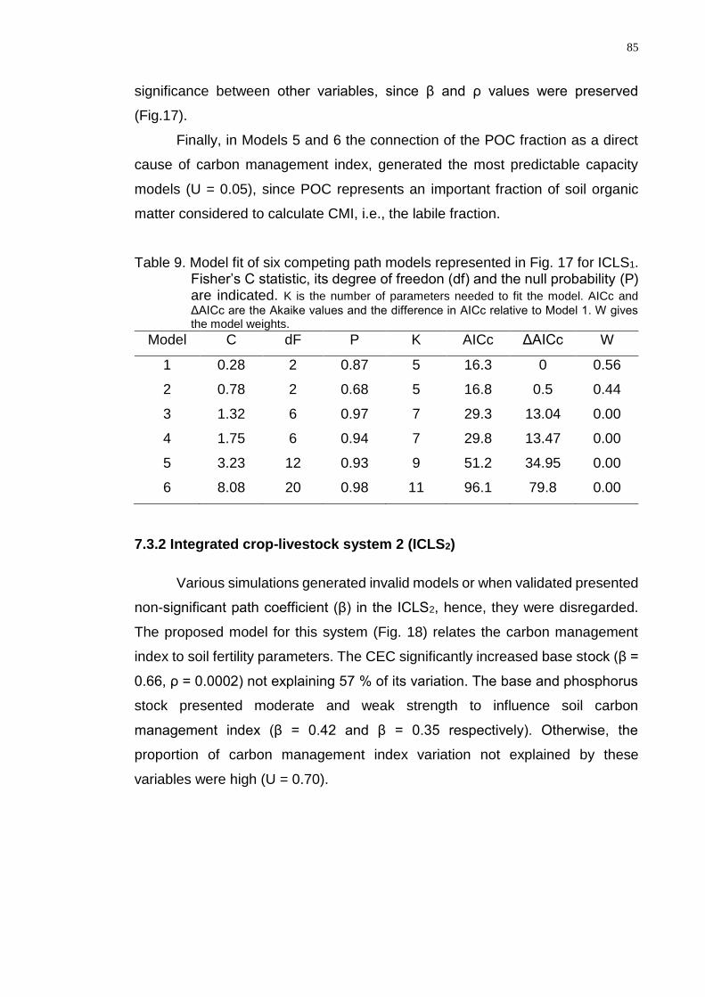
85
significance between other variables, since β and ρ values were preserved
(Fig.17).
Finally, in Models 5 and 6 the connection of the POC fraction as a direct
cause of carbon management index, generated the most predictable capacity
models (U = 0.05), since POC represents an important fraction of soil organic
matter considered to calculate CMI, i.e., the labile fraction.
Table 9. Model fit of six competing path models represented in Fig. 17 for ICLS1. Fisher’s C statistic, its degree of freedon (df) and the null probability (P) are indicated. K is the number of parameters needed to fit the model. AICc and
ΔAICc are the Akaike values and the difference in AICc relative to Model 1. W gives the model weights.
Model C dF P K AICc ΔAICc W
1 0.28 2 0.87 5 16.3 0 0.56
2 0.78 2 0.68 5 16.8 0.5 0.44
3 1.32 6 0.97 7 29.3 13.04 0.00
4 1.75 6 0.94 7 29.8 13.47 0.00
5 3.23 12 0.93 9 51.2 34.95 0.00
6 8.08 20 0.98 11 96.1 79.8 0.00
7.3.2 Integrated crop-livestock system 2 (ICLS2)
Various simulations generated invalid models or when validated presented
non-significant path coefficient (β) in the ICLS2, hence, they were disregarded.
The proposed model for this system (Fig. 18) relates the carbon management
index to soil fertility parameters. The CEC significantly increased base stock (β =
0.66, ρ = 0.0002) not explaining 57 % of its variation. The base and phosphorus
stock presented moderate and weak strength to influence soil carbon
management index (β = 0.42 and β = 0.35 respectively). Otherwise, the
proportion of carbon management index variation not explained by these
variables were high (U = 0.70).
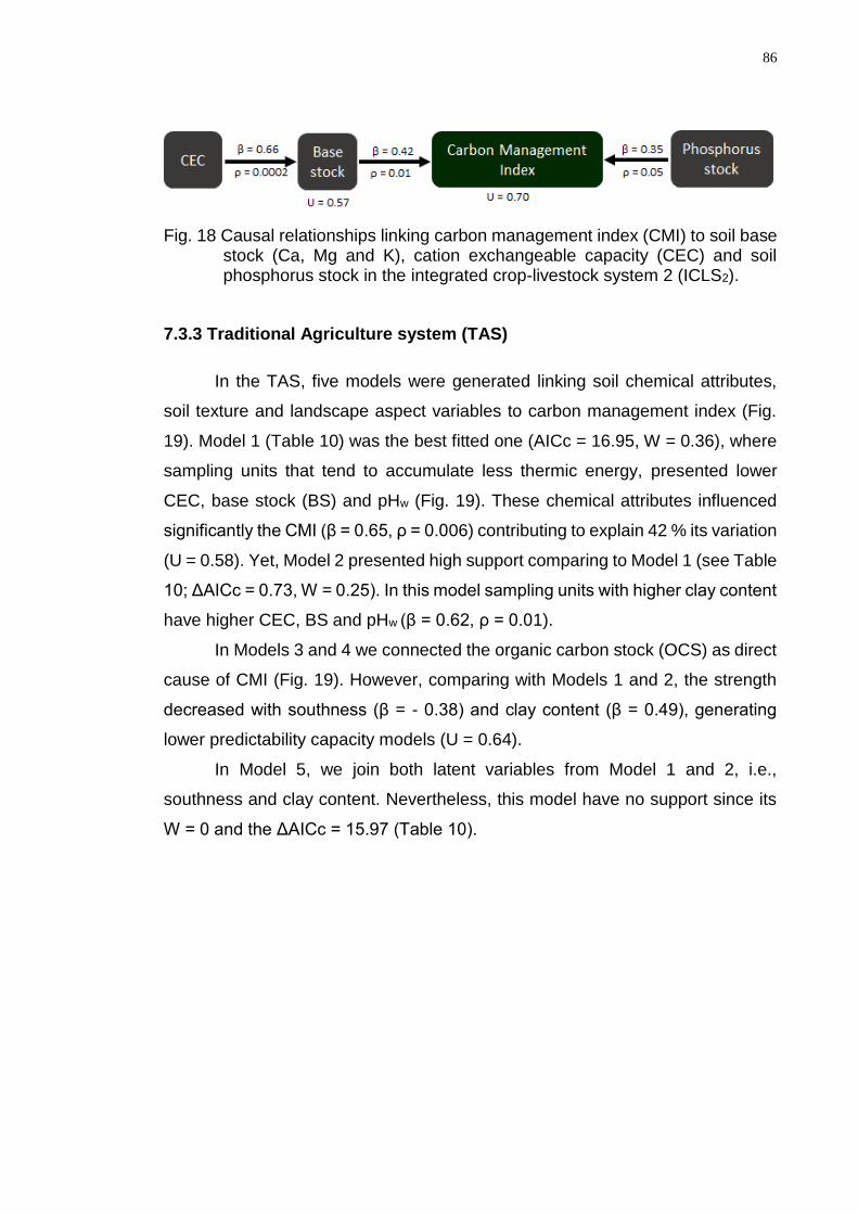
86
Fig. 18 Causal relationships linking carbon management index (CMI) to soil base stock (Ca, Mg and K), cation exchangeable capacity (CEC) and soil phosphorus stock in the integrated crop-livestock system 2 (ICLS2).
7.3.3 Traditional Agriculture system (TAS)
In the TAS, five models were generated linking soil chemical attributes,
soil texture and landscape aspect variables to carbon management index (Fig.
19). Model 1 (Table 10) was the best fitted one (AICc = 16.95, W = 0.36), where
sampling units that tend to accumulate less thermic energy, presented lower
CEC, base stock (BS) and pHw (Fig. 19). These chemical attributes influenced
significantly the CMI (β = 0.65, ρ = 0.006) contributing to explain 42 % its variation
(U = 0.58). Yet, Model 2 presented high support comparing to Model 1 (see Table
10; ΔAICc = 0.73, W = 0.25). In this model sampling units with higher clay content
have higher CEC, BS and pHw (β = 0.62, ρ = 0.01).
In Models 3 and 4 we connected the organic carbon stock (OCS) as direct
cause of CMI (Fig. 19). However, comparing with Models 1 and 2, the strength
decreased with southness (β = - 0.38) and clay content (β = 0.49), generating
lower predictability capacity models (U = 0.64).
In Model 5, we join both latent variables from Model 1 and 2, i.e.,
southness and clay content. Nevertheless, this model have no support since its
W = 0 and the ΔAICc = 15.97 (Table 10).

87
Fig. 19 Causal relationships linking carbon management index (CMI) to soil base stock (BS), cation exchangeable capacity (CEC), water pH (pHw), southness and clay content in the traditional agriculture system (TAS).
Table 10. Model fit of six competing path models that are represented in Fig. 19 for TAS. Fisher’s C statistic, its degree of freedom (df) and the null probability (P) are indicated. K is the number of parameters needed to fit the
model. AICc and ΔAICc are the Akaike values and the difference in AICc relative to Model 1. W gives the model weights.
Model C dF P K AICc ΔAICc W
1 0.28 2 0.87 5 16.95 0 0.36
2 1.01 2 0.60 5 17.68 0.73 0.25
3 1.24 2 0.54 5 17.91 0.96 0.22
4 1.87 2 0.39 5 18.54 1.59 0.16
5 2.92 6 0.82 7 32.92 15.97 0.00
7.4 Discussion
The presented models for the ICLS1 (Fig. 17) indicate that behind carbon
fractions as the main direct cause influencing CMI variation (all models), are
important latent variables related to biological and physical soil attributes.
88
Sampling units with higher soil MBC presenting less OCS (Model 1; Fig. 17),
indicate that soil C accumulation reaches its plateau considering it is a long-term
same soil and crop management system (Table 1). Yet, soil aggregation process
is physical protecting organic carbon favoring its storage (Model 2; Fig. 17). In
this context, for this system soil aggregation is a better indirect descriptor of CMI
(U = 0.29) than soil MBC (U = 0.58).
Still regarding ICLS1, the clay content promoted soil aggregation (Models
3 and 6) through organic - mineral associations. Yet, the lowest not explained
CMI variation were reached with the POC fraction connection (U = 0.05),
indicating that CMI is mainly explained by recent carbon inputs.
The ICLS2 as the most diversity system presented just one validly model
with soil fertility parameters influencing CMI variation (Fig. 18). The CEC
increasing favored Ca, Mg and K storage, which in turn increased CMI. Therefore,
sampling units with higher base and phosphorus stocks, promoted CMI
increasing through higher specie’s biomass development, hence, further dry
matter addition.
In the TAS, landscape aspect, soil chemical attributes and clay content
were the variables connected to CMI (Fig. 19). The low predictability capacity of
Models 3 and 4 (Fig. 19), from the latent variables southness (U = 0.86) and clay
content (0.76) can be explained by further variables that influences OCS
variation, that was not considered in the present models. Pillar et al. (2013),
studying plant community’s stability also found low predictable capacity models
in a grassland ecosystem in southern Brazil, indicating that for field approaches
the predictability is lower, due to the higher complexity environment.
The southness variable representing sampling units with lower thermic
energy accumulation in soil, tends to present lower CEC, BS and pHw. This
observed pattern is due to the negative partial correlation among southness and
clay content (β = -0.56 for model 5) and OCS (β = -0.38 for model 3). Therefore,
as sandy and with lower OCS, these sampling units presented lower buffer
capacity.
89
7.5 Conclusions
The model proposition approach using path analysis, allow to comprehend
soil quality by direct and indirect different soil attributes factors, which affect
carbon management index variation across landscape.
The carbon management index in long-term integrated crop livestock
systems with continued soybean/grazed ryegrass succession, presents
homogenous soil microbial biomass of carbon community, which increase, lead
to an organic carbon decomposition accrual, hence, decrease soil carbon
management index. Otherwise, the higher soil aggregation protects soil carbon
fractions benefiting the carbon management index.
Increasing species diversity by a winter succession between integrated
crop-livestock system and cover crops/wheat associations, tends to increase soil
system complexity, suggesting that variables not considered in the models are
influencing the carbon management index, as presented lower predictability
capacity. Nevertheless, the soil fertility influence the carbon management index
as provide higher dry matter input mainly by winter species.
In the traditional agriculture system, as the less complex system, lower
nutrient cycling is expected, therefore, sampling units with higher soil fertility
increase soil carbon management index, due to higher dry matter inputs.
Furthermore, there is a higher influence from inherent variables increasing the
soil capacity to provide plant development.

90
8. FINAL CONSIDERATIONS
The soil quality enhancement by soil management and agricultural
practices is a farmer knowledge issue for a long time. His perception about the
production system’s characterization by using the three dimensions approach, is
in reality implicitly on his farm’s routine practical meaning. The relationship
between farmers and the environment surround, gives him the practical
experience to know about species diversity and how each species impact soil
system. Moreover, most farmers know how a calendar adjustment concerning the
dynamic space-temporal species distribution can be a simple solution in pursuing
more sustainable production systems.
Since summer soybean is a rentable specie, farmers have the proper
knowledge and infrastructure, the pursuit for higher diversity in large scale
production systems should be concentrated in the winter in a short-term.
Otherwise, the allocation of summer soybean in an intercropping system with a
high carbon input potential species, can be a strategy to keep producing this
rentable specie and increase soil quality.
Intercropping systems during summer or the adoption of integrated crop-
livestock-forestry systems, can lead production systems to further space
interactions. Further multidisciplinary researches needs to be conducted to lead
intercropping systems to a broader adoption by farmers.
The statistical tools nowadays are capable to reveal data and tendencies
that seems to be on the shadows of the complex production systems. In this

91
context are path analysis, structure equation models and other methods to study
cause-effect relationships in natural sciences.
92
9. REFERÊNCIAS BIBLIOGRÁFICAS
ADDISCOTT, T.M. Entropy and Sustainability. European Journal of Soil Science. v. 46, p. 161 – 168, 1995.
AGREN, G. I. ANDERSSON, F. O. Terrestrial Ecosystem Ecology: Principles and Applications. p. 330, 2012.
ALBUQUERQUE, M. A. et al. Carbon and nitrogen in a Ferralsol under zero-tillage rotations based on cover, cash or hay crops. Soil Use and Management. v.31, p. 1-9, 2015.
ALVARENGA, R. C.; NOCE, M. A. Integração Lavoura e Pecuária. Embrapa Milho e Sorgo, doc 47, 16 p., 2005.
AN, S. ET AL. Soil aggregation, aggregate stability, organic carbon and nitrogen in different soil aggregate fractions under forest and shrub vegetation on the Loess Plateau, China. CATENA 81(3), 226-233, 2010.
ANDERSON, T. H.; DOMSCH, K. H. Soil microbial biomass: The eco-physiological approach. Soil Biology and Biochemestry. v.42, p.2039-2043, 2010.
ANDRADE, D. C.; ROMEIRO, A. R. Serviços ecossistêmicos e sua importância para o sistema econômico e bem-estar humano. Texto para Discussão. IE/UNICAMP, Campinas, n. 155, fev. 2009.
ANGHINONI, I.; CARVALHO, P. CP. F.; COSTA, S. E. V. G. A. Abordagem sistêmica do solo em sistemas integrados de produção agrícola e pecuária no subtrópico brasileiro. Tópicos em Ciência do Solo, SBCS, v.8, cap.8, 2013.
ANGHINONI, I.; SALET, R. L. Reaplicação de calcário no sistema plantio direto consolidado. In: KAMINSKI, J. Uso de corretivos da acidez do solo no plantio direto. Boletim técnico, 4, p. 41-59. Pelotas, 2000.

93
ASSMANN, J.M. et al. Soil carbon and nitrogen stocks and fractions in a long-term integrated crop–livestock system under no-tillage in southern Brazil. Agriculture, Ecosystems & Environment 190, 52-59, 2014.
ASSMANN, J.M. et al. Carbon and nitrogen cycling in an integrated soybean-beef cattle production system under different grazing intensities. Pesquisa Agropecuária Brasileira 50, 967-978, 2015.
ÁVILA, C. J.; VIVAN, L. M.; TOMQUELSKI, G. V. Ocorrências, aspectos biológicos, danos e estratégias de manejo de Helicoverpaarmigera (Hubner) (Lepidoptera: Noctuidae) nos sistemas de produção agrícolas. In: Circular técnica 23, p.12, Embrapa, Dourados, 2013.
BANDICK, A.K.; DICK, R.P. Field management effects on soil enzyme activities. Soil Biol. Biochem. v.31, p.1471–1479, 1999.
BARBAULT, R. Ecologia geral: estrutura e funcionamento da biosfera. p. 444, 2011.
BAYER, C. et al. Estabilização do carbono no solo e mitigação das emissões de gases de efeito estufa na agricultura conservacionista. IN: Tópicos em Ciência do Solo, v.7, p.55-118, 2011.
BAYER, C., MIELNICZUK, J. Dinâmica e função da matéria orgânica. In: SANTOS, G. A.; SILVA, L. S.; CANELLAS, L. P.; CAMARGO, F. A. O. Fundamentos da matéria orgânica do solo. 636p, 2008.
BAYER, C.; MIELNICZUK, J.; MARTIN-NETO, L. Efeito de sistemas de preparo e de cultura na dinâmica da matéria orgânica e na mitigação das emissões de CO2. Revista Brasileira de Ciência do Solo, 24, p. 599 – 607, 2000.
BENDING, G.D. et al. Microbial and biochemical soil quality indicators and their potential for differentiating areas under contrasting agricultural management. Soil Biol. Biochem. v.36, p.1785–1792, 2004.
BIEDERBECK, V.O.et al. Soil quality attributes as influenced by annual legumes used as green manure. Soil Biology and Biochemistry 30, p. 1177–1185, 1998.
BLAIR, G. J.; LEFROY, R. D. B.; LISLE, L. Soil Carbon Fractions Based on their Degree of Oxidation, and the Development of a Carbon Management Index for Agricultural Systems. Australian Journal of Agriculture Research, v.46, p. 1459-1466, 1995.
BOUMA, J.; BATJES, N. H.; GROOT, J. J. R. Exploring land quality effects on world food supply. Geoderma, v.86, p.43-59, 1998.
CAMPOS, B.-H.C.D. et al. Carbon stock and its compartments in a subtropical oxisol under long-term tillage and crop rotation systems. Revista Brasileira de Ciência do Solo 35, 805-817, 2011.
CARPENEDO, V.; MIELNICZUK, J. Estado de agregação e qualidade de agregados de Latossolos Roxos, submetidos a diferentes sistemas de manejo. Revista Brasileira de Ciências do Solo. Campinas, v.14, p.99-105, 1990.
94
CARTER, M. R. Soil Quality for Sustainable Land Management: Organic matter and aggregation interactions that maintain soil functions. Agronomy Journal, v. 94, p.38-47, 2002
CARVALHO, P. C. F. et al. Integração Soja-Bovinos de Corte no Sul do Brasil. Boletim técnico, Porto Alegre, 2011.
CARVALHO, P. C. F. et al. Produção animal: mitos, pesquisa e adoção de tecnologia. Canoas-RS, ULBRA, p.7-44, 2005.
CASSOL, L.C. Relação solo-planta-animal num sistema de integração lavoura-pecuária em semeadura direta com calcário na superfície. Tese (Doutorado) – Programa de Pós-Graduação em Ciência do Solo, Faculdade de Agronomia, Universidade Federal do Rio Grande do Sul, Porto Alegre, p. 157, 2003.
CONAB, 2016. Acompanhamento da Safra Brasileira de Grãos. Décimo segundo levantamento, pp. 184. Available in: http://www.conab.gov.br/conteudos.php?a=1252, acessed in 13 – january-2017.
CONCEIÇÃO, P. C.; DIECKOW, J.; BAYER, C. Combined role of no-tillage and cropping systems in soil carbon stocks and stabilization. Soil & Tillage Research. v.129, p. 40-47, 2013.
CONCEIÇÃO, P.C.et al. Fracionamento densimétrico com politungstato de sódio no estudo da proteção física da matéria orgânica em solos. Revista Brasileira de Ciência do Solo v.32, p.541-549, 2008.
COSTA, S.E.V.G.A. et al. Impact of an integrated no-till crop–livestock system on phosphorus distribution, availability and stock. Agriculture, Ecosystems and Environment 190, p. 43-51, 2014.
COSTANZA, R. et al. The value of the world’s ecosystems services and natural capital.Nature, v.387, 1997.
CUNHA, G.R. et al. Depois da Rio+20: Qual o futuro da “agricultura sustentável”? Revista Plantio Direto, p.10-17, 2012.
DARNHOFER, I.; GIBBON, D.; DEDIEU, B. Farming Systems Research: an approach to inquiry. In: Farming Systems Research into the 21st Century: The New Dynamic. Cap. 01, p.03 -32, 2012.
DIEKOW, J. et al. Carbon and nitrogen stocks in physical fractions of a subtropical Acrisol as influenced by long-term no-till cropping systems and N fertilization. Plant and Soil. Dordrecht, v.268, p.319-328, 2005.
DORAN, J.W. & PARKIN, T.B. Defining and assessing soil quality. In: DORAN, J.W.; COLEMAN, D.C.; BEZDICEK, D.F. & STEWART, B.A., eds. Defining soil quality for a sustainable environment. Madison, SSSA, p.1-20, 1994.
DORAN, J.W. Soil quality and sustainability. In: CONGRESSO BRASILEIRO DE CIÊNCIA DO SOLO. Anais. CD-ROM. Sociedade Brasileira de Ciência do Solo. Rio de Janeiro, 1997.
95
DROOGERS, P.; BOUMA, J. Soil survey input in explanatory modeling of sustainable soil management practices. Soil Science Society of America Journal, v.61, p.1704-1710, 1997.
ELLERT, B. H.; BETTANY, J. R. Calculation of organic matter and nutrients stored in soils under contrasting management regimes. Canadian Journal of Soil Science. v. 75, p. 529-538, 1995.
ELMQVIST, T. et al. Response diversity, ecosystem change, and resilience. Frontiers in Ecology and the Environment 1: 488–494, 2003.
EVANS, F. C. Ecosystem as the basic unity in ecology. Science. v. 123, f. 3208, p. 1127-1128, 1956.
EVERITT, B. S. et al. Cluster Analysis. 348 p., 2011.
FEDOROFF N. The production potential of soils. Part 1. Sensitivity of principal soil types to the intense agriculture of north-western Europe. In: Barth E, L’Hermite P, editors. Scientific Basis for Soil Protection in the European Community. London: Elsevier; p. 65-86, 1987.
FERREIRA, D. F.; FILHO, A. C.; DAL’COL LUCIO, A. Procedimentos estatísticos em planejamentos experimentais com restrições na casualização. In: Boletim Informativo Sociedade Brasileira de Ciência do Solo, v.37, n.03, 2012.
FERREIRA, M. M. Caracterização física do solo. In: van LIER, Q. J. Física do Solo. Sociedade Brasileira de Ciência do Solo, 298p., 2010.
FOOD AND AGRICULTURE ORGANIZATION OF THE UNITED NATIONS (FAO), 2014.Disponível em:https://www.fao.org.br/quemSomos.asp. Acessado em: 07 de março de 2014.
FRANZLUEBBERS, A.J. Integrated crop-livestock systems in the Southern USA.Agronomy Journal, v.99, p.362-372, 2007.
GREEN, V.S.; STOTT, D.E.; DIACK, M. Assay for fuorescein diacetate hydrolytic activity: Optimization for soil samples. Soil Biology & Biochemistry, v. 38, p. 693-701, 2006.
HASENACK, H.; CORDEIRO, J.L.P. (org.). Mapeamento da cobertura vegetal do Bioma Pampa. Porto Alegre, UFRGS Centro de Ecologia. 30 p. (Relatório técnico Ministério do Meio Ambiente: Secretaria de Biodiversidade e Florestas no âmbito do mapeamento da cobertura vegetal dos biomas brasileiros). 2006.
HAYNES, R. Labile organic matter fractions as central components of the quality of agricultural soils: an overview. Advance in Agronomy 85, p. 221–268, 2005.
HOLLING, C.S. Resilience and Stability of Ecological Systems, Ann. Rev. Ecol. Syst., 4, 1–23, 1973.
HUNGRIA, M. et al. Soil microbial activity and crop sustainability in a long-term experiment with three soil-tillage and two crop rotation systems. Applied Soil Ecology. v. 42, p. 288-296, 2009.

96
IDOWU, J. et al. Soil health assessment and management: the concepts. A Newsletter for New York Field Crops & Soils, v.16, n.2, 2006.
JASTROW, J. D.; MILLER, R. M. Soil Aggregate Stabilization and Carbon Sequestration: Feedbacks ThroughOrgano-Mineral Associations. In: LAL, R.; KIMBLE, J. M.; FOLLET, R. F.; STEWART, B. A. Soil process and the carbon cycle. 624p, 1997.
JENKINSON, D.S. The soil microbial biomass. New Zealand Soil News 25: 213–218, 1977.
JENKINSON, D. S.; LADD, J. N. Microbial biomass in soil: measurement and turnover. Soil Biochemistry 5, p. 415-17, 1981
JONARD, M. et al. Forest soils in France are sequestering substantial amount of carbon. Science of the total environment, v. 574, p. 616-628, 2017.
KAPKIYAI, J., et al. Soil organic matter and nutrient dynamics in a Kenian nitisol under long-term fertilizer and organic input management. Soil Biology and Biochemistry 31, p. 1773– 1782, 1999.
KARLEN, D. L.; DITZLER, C. A.; ANDREWS, S. S. Soil quality: why and how? Geoderma, v.114, p.145-156, 2003.
KARLEN, D.L. et al Soil quality: A concept, definition, and framework for evaluation (a guest editorial). Soil Science Society of America Journal, 61:4-10, 1997.
KEMPER, W. D.; CHEPIL, W. S. Size distribution of aggregation. In: BLACK, C. A. (Ed). Methods of soil analysis. Madison: American Society of Agronomy, p. 499-510, 1965.
KHATOUNIAN, C. A. A reconstrução ecológica a agricultura. Botucatu, p.348, 2001.
KIRSCHENMANN, F. L. Potential of a New Generation of Biodiversity in Agroecosystems of the Future. Agronomy Journal, v. 99, 2007.
LAL, R. et al. Towards improving the global database on soil carbon. In: LAL, R.; KIMBLE, J.; LEVINE, E.; STEWART, B. A. eds. Soils and global change. Boca Raton, CRC Lewis Publishers, p. 433-436, 1995.
LARSON, W.E.; PIERCE, F.J. The dynamics of soil quality as a measure of sustainable management. In: DORAN, J.W.; COLEMAN, D.C.; BEZDICEK, D.F. & STEWART, B.A., eds. Defining soil quality for a sustainable environment. Madison, SSSA. p.37-51, 1994
LEGENDRE, P.; LEGENDRE, L. Numerical Ecology. 2 ed. Elsevier. New York, 853p. 1998.
LOPES, A. A. C et al. Interpretation of microbial soil indicators as a function of crop yield and organic carbon. Soli Biology & Biochemistry. Soil Science Society of America Journal. v. 77, p. 461-472, 2012.
97
MARTINEZ-SALGADO, M. M. et al. Biological soil quality indicators: a review. Technology and Education Topics in Applied Microbiology and Microbial Biotechnology. 10p. 2010.
MARTINS, M. R.; ANGERS, D. A. Different plant types for different soil ecosystem services. Geoderma, p.266 – 269, 2015.
McBRATNEY, A.; FIELD, D. J.; KOCH, A. The dimensions of soil security. Geoderma. v. 213, p. 203-213, 2014.
MILLER, M.; DICK, R. Thermal stability and activities of soil enzymes as influenced by crop rotations. Soil Biology and Biochemistry, 1995.
MOORE, I. D. et al. Soil attribute prediction using terrain analysis. Soil Science Society American Journal, v. 57, p. 443-452, 1993.
MORAES, A.et al. Integrated crop-livestock systems in the Brazilian subtropics. European Journal of Agronomy 57, 4-9, 2014.
NAHIDAN, S.; NOURBAKHSH, F.; MOSADDEGHI, M.R. Variation of soil microbial biomass C and hydrolytic enzyme activities in a rangeland ecosystem: are slope aspect and position effective? Archives of Agronomy and Soil Science, 2014.
NICOLODI, M. et al. Insuficiência do conceito mineralista para expressar a fertilidade do solo percebida pelas plantas cultivadas no sistema de plantio direto. Revista Brasileira de Ciência do Solo, v.32, p.2735-2744, 2008.
NICOLOSO, R. da S. et al. Balanço do carbono orgânico no solo sob integração lavoura-pecuária no Sul do Brasil. Revista Brasileira de Ciência do Solo, v.32, p.2425-2433, 2008.
ODUM, E.P. The strategy of ecosystem development. Science 164, 262-270, 1969.
PALADINI, F.L.S., MIELNICZUK, J. Distribuição do tamanho dos agregados de um Podzólico Vermelho-Escuro afetado por sistemas de culturas. Revista Brasileira de Ciência do Solo 15, 135-140, 1991.
PEIXOTO, R.S. et al. A decade of land use contributes to changes in the chemistry, biochemistry and bacterial community structures of soils in the Cerrado. Antonie van Leeuwenhoek. v. 98, p. 403–413, 2010.
PILLAR, V. D. et al. Functional redundancy and stability in plant communities. Journal of Vegetation Science 24, 963-974, 2013.
PONGE, J. F. The soil as an ecosystem. Biology and Fertility of Soils 51, 645-648, 2015.
PRASHAR, P.; KAPOOR, N.; SACHDEVA, S. Rhizosphere: its structure, bacterial diversity and significance. Environment, Science and Biotechnologic. v. 13, p. 63-77, 2014.
98
SA, J. C. M. Adubação fosfatada no Sistema de plantio direto. In: YAMADA, T. & ABDALLA, S. R. S. Fósforo na agricultura brasileira. Piracicaba, Potafós, p.201-222, 2004.
SÁ, J. C. M. et al. Organic matter dynamics and carbono sequestration rates for a tillage chronosequence in a Brazilian oxisol. Soil Science Society of American Journal, v.65, p.1486-1499, 2001.
SALTON, J. C. et al. Agregação e estabilidade de agregados do solo em sistemas agropecuários em Mato Grosso do Sul. Revista Brasileira de Ciências do Solo. v. 32, p. 11-21, 2008.
SALTON, J. C. et al. Teor e dinâmica do carbono no solo em sistemas de integração lavoura-pecuária. Pesquisa Agropecuária Brasileira, v.46, n.10, p. 1349-1356, 2011.
SANDERSON, M. A. et al. Diversification and ecosystem services for conservation agriculture: Outcomes from pastures and integrated crop-livestock systems. Renewable Agriculture and Food Systems, v.28, n.2, 2013.
SANTOS, N. Z. et al. Forages, cover crops and related shoot and root additions in no-till rotations to C sequestration in a subtropical Ferralsol. Soil & Tillage Research. v. 111, p. 208-218, 2011.
SANTOS, R. F. Análise crítica da interpretação neoclássica do processo de modernização da agricultura brasileira. In: SANTOS, R.F. dos. Presença de viéses de mudança técnica da agricultura brasileira. São Paulo: USP/IPE, p.39-78, 1986.
SCHLOTER, M.; DILLY, O.; MUNCH, J. C. Indicators for evaluating soil quality. Agriculture Ecosystems and Environment, n.98, p.255-262, 2003.
SHI, X. M. et al. Grazing exclusion decreases soil organic C storage at an alpine grassland of the Qinghai–Tibetan Plateau. Ecological Engineering, v.57, p.183-187, 2013.
SHIPLEY, B. Cause and correlation in biology: a user’s guide to path analysis, structural equations, and causal inference. Cambridge University Press, Cambridge. 2000.
SIDARI, M. et al. Influence of slope aspects on soil chemical and biochemical properties in a Pinus laricio forest ecosystem of Aspromonte (Southern Italy). European Journal of Soil Biology 44, p. 364-372, 2008.
SILVA, E. E.; AZEVEDO, P. H. S.; De-POLLI, H. Determinação do Carbono da biomassa microbiana do solo (BMS-C). Embrapa. Seropédica –RJ. Comunicado Técnico 98, 2007a.
SILVA, F.D.d. et al. Soil carbon indices as affected by 10 years of integrated crop–livestock production with different pasture grazing intensities in Southern Brazil. Agriculture, Ecosystems & Environment 190, 60-69, 2014.
99
SILVA, I. F.; MIELNICZUK, J. Avaliação do estado de agregação do solo afetado pelo uso agrícola. Revista Brasileira de Ciência do Solo. Campinas, v. 21, p. 313-319, 1997.
SOJKA, R. E.; UPCHURCH, D. R. Reservations regarding the soil quality concept. Soil Science society of America Journal. v.63, p.1039-1054, 1999.
SOUZA, E. D. et al. Estoque e Carbono Orgânico e de Nitrogênio no Solo em Sistema de Integração Lavoura-Pecuária em Plantio Direto Submetido a Intensidades de Pastejo. Revista Brasileira de Ciência do Solo, v.33, p.1829-1836, 2009.
SOUZA, E. D. et al. Biomassa Microbiana do Solo em Sistema de Integração Lavoura-Pecuária em Plantio Direto Submetido a Intensidades de Pastejo. Revista Brasileira de Ciência do Solo, v.34, p.79-88, 2010.
SPARLING, G. P. Ratio of microbial biomass carbon to soil organic carbon as a sensitive indicator of changes in soil organic carbon. Australian Journal of Soil Research 30, 195-207, 1992.
STAVI, I. Variability of soil aggregation in a hilly semi-arid rangeland. Journal of Arid Environments 74, 946-953, 2010.
STEVENSON, B. A.; McNEILL, S.; HEWITT, A. E. Characterizing soil quality clusters in relation to land use and soil order in New Zealand: An application of the phenoform concept. Geoderma, p.135 – 142, 2015.
STRICKLAND, T. C. et al. Aggregation ans aggrerate stability in forest and range soils. Soil Science Society of America Journal, v. 52, p. 829-833, 1988.
STUBBERFIELD, L. C. F.; SHAW, P. J. A. A comparison of tetrazolium reduction and FDA hidrolysis with other measures of microbial activity. Journal of Microbiological Methods, v. 12, n. 3-4, p. 151-162, 1990.
SWISHER, R.; CARROLL, C.G. Fluorescein diacetate hydrolysis as an estimator of microbial biomass on coniferous needle surface. Microbial Ecology, v.6, n.3, p.217-226, 1980.
TANSLEY, A. G. The use and abuse of vegetational concepts and terms. Ecology. v. 16, p. 70 – 97, 1935.
TAVARES FILHO, J.; TESSIER, D. Effect of different management systems on porosity of oxisols in Paraná, Brazil. Revista Brasileira de Ciência do Solo 34, p. 899–906, 2010.
TEDESCO, M. J. et al. Análise de solos, plantas e outros materiais. Boletim técnico, 5, 2.ed., 147 p. Porto Alegre: Departamento de Solos da UFRGS, 1995.
USDA-NRCS. National Soil Survey Center. Ames, IA. Disponível em: http://www.nrcs.usda.gov/wps/portal/nrcs/main/soils/health/. Acessado em 01 de setembro de 2015.
100
VENZKE-FILHO, S. P. et al. Biomassa microbiana do solo em sistema de plantio direto na região de Campos Gerais – Tibagi, PR. Revista Brasileira de Ciências do Solo, v.32, p.599-610, 2008.
VEZZANI, F.; MIELNICZUK, J. Uma visão sobre qualidade do solo. Revista Brasileira de Ciência do Solo, v.33, p.743-744, 2009.
VIEIRA, F. C. B. et al. Carbon management index based on physical fractionation of soil organic matter in an Acrisol under long-term no-till cropping systems. Soil and Tillage Research, v.96, p.195-204, 2007.
WILDI, O. Data analysis in vegetation ecology. Switzerland 211 p. 2010.
ZAK, J. C.; WILLIG, M. R.; MOORHEAD, D. L.; WILDMAN, H. G. Functional diversity of microbial communities: A quantitative approach. Soil Biology and Biochemistry, v.26, n.9, p.1101-1108, 1994.
ZANATTA, J. A. Estoques e labilidade do carbono em frações da matéria orgânica de um Argissolo afetados por sistemas de manejo do solo. Dissertação de mestrado, PPG Ciências do Solo, Faculdade de Agronomia, UFRGS, 2006.