Embed Size (px)
Citation preview

UNIVERSIDADE DE SÃO PAULO
FACULDADE DE ECONOMIA, ADMINISTRAÇÃO E CONTABILIDADE
DEPARTAMENTO DE ECONOMIA
PROGRAMA DE PÓS-GRADUAÇÃO EM ECONOMIA
RISCO MORAL DINÂMICO COM APRENDIZADO SOBRE A FUNÇÃO DE
PRODUÇÃO
DYNAMIC MORAL HAZARD WITH LEARNING ABOUT THE
PRODUCTION FUNCTION
Maurício Massao Soares Matsumoto
Orientador: Prof. Dr. Gabriel de Abreu Madeira
Versão Corrigida
SÃO PAULO
2014

Prof. Dr. Marco Antonio Zago
Reitor da Universidade de São Paulo
Prof. Dr. Reinaldo Guerreiro
Diretor da Faculdade de Economia, Administração e Contabilidade
Prof. Dr. Joaquim José Martins Guilhoto
Chefe do Departamento de Economia
Prof. Dr. Marcio Issao Nakane
Coordenador do Programa de Pós-Graduação em Economia

MAURÍCIO MASSAO SOARES MATSUMOTO
RISCO MORAL DINÂMICO COM APRENDIZADO SOBRE A FUNÇÃO DE
PRODUÇÃO
DYNAMIC MORAL HAZARD WITH LEARNING ABOUT THE
PRODUCTION FUNCTION
Dissertação apresentada ao
Departamento de Economia da
Faculdade de Economia, Administração
e Contabilidade da Universidade de São
Paulo como requisito para a obtenção do
título de Mestre em Ciências.
Orientador: Prof. Dr. Gabriel de Abreu Madeira
SÃO PAULO
2014

FICHA CATALOGRÁFICA Elaborada pela Seção de Processamento Técnico do SBD/FEA/USP
Matsumoto, Maurício Massao Soares Dynamic moral hazard with learning about the production function / Maurício Massao Soares Matsumoto. -- São Paulo, 2014. 37 p. Dissertação (Mestrado) – Universidade de São Paulo, 2014. Orientador: Gabriel de Abreu Madeira.
1. Contratos 2. Incentivos 3. Aprendizagem 4. Programação linear
I. Universidade de São Paulo. Faculdade de Economia, Administração e Contabilidade. II. Título. CDD – 346.02

iii
Aos meus pais, Haroldo e Marisa.


iv
AGRADECIMENTOS
Aos meus pais, que sempre fizeram tudo que podiam por mim e pela minha irmã.
Obrigado pelo apoio sempre incondicional, e por me ensinarem o valor dos estudos. À
minha irmã Mônica, que sempre admirei e que me incentivou a voltar para a vida
acadêmica.
À minha turma do mestrado, em que tive o prazer de descobrir colegas inteligentes e
dedicados, com quem aprendi muito, e que também se tornaram grandes amigos. O
percurso foi muito mais divertido e gratificante na companhia de todos vocês. Em
especial aos que se tornaram mais próximos pelos tantos momentos, ideias e cervejas
compartilhados: Bel, Bruna, Dimas, Fabio, Gabriel, João, Julia, Leo, Leopoldo, Luísa,
Natalia, Pedro, Perez. As boas lembranças são muitas: das discussões de listas de
exercício na salinha às idas à praia, das monitorias compartilhadas aos blocos de
carnaval, das corridas na raia aos seminários que organizávamos entre nós, a viagem
para Boston, os churrascos e jantares na casa da Bel. Entre tantas outras.
Também às outras turmas de mestrado e doutorado com quem convivi em meu tempo
na FEA, veteranos e bixos. Em especial: Carnaúba, Laura, Leo Rosa, Rafael Proença e
Renata.
Aos professores do IPE-USP, com quem aprendi muito dentro e fora da sala de aula, às
vezes até no bar. Em especial, agradeço ao meu orientador Gabriel Madeira, pelas
inúmeras conversas (acadêmicas ou não) que me ensinaram muito, por acreditar em
mim e me dar tantas oportunidades. Agradeço também a Bruno Giovanetti, Marcos
Rangel, Marcos Nakaguma, Mauro Rodrigues, Rafael Coutinho e Ricardo Madeira, não
apenas pelas interações acadêmicas, mas também por terem me ajudado nas decisões de
vida e carreira.
Por fim, agradeço à FIPE, CNPq e FAPESP pelo fundamental apoio financeiro.


v
RESUMO
Neste trabalho, propomos uma estratégia numérica para lidar com modelos de risco
moral dinâmico com aprendizado sobre a função de produção. Pela complexidade do
problema, soluções analíticas na literatura têm sido limitadas em seu escopo. A
contribuição é metodológica: através de métodos computacionais, o problema pode ser
estudado sob poucas hipóteses a respeito de formas funcionais. Partindo de um
mecanismo geral, reformulamos o problema como um mecanismo compatível em
incentivos, e então mostramos como este pode ser resolvido por indução retroativa por
meio de uma sequência de programas lineares. Aplicamos o método a alguns casos de
interesse, e confirmamos a conclusão da literatura de que a incerteza sobre a função de
produção aumenta a volatilidade da utilidade do agente para prevenir manipulação de
crenças.

vi
ABSTRACT
In this work we propose a flexible numerical approach to deal with models of dynamic
moral hazard with simultaneous learning about the production function. Because of the
complexity of the problem, analytical solutions have so far been limited in scope. The
contribution is methodological: through computation, the problem can be studied under
few assumptions about functional forms. We depart from a general mechanism,
reformulate it as an incentive compatible mechanism, and show how it can be solved by
backward induction through a sequence of linear programs. We apply our method to a
few cases of interest, and confirm that uncertainty about the production function
increases the volatility of the agent's utility in order to prevent belief manipulation, as
found in the literature.

SUMÁRIO
LISTA DE FIGURAS ....................................................................................................... 1
1. INTRODUCTION ......................................................................................................... 2
2. MODEL AND COMPUTATIONAL FRAMEWORK ................................................. 5
2.1 General mechanism with full history dependence ................................................... 5
2.2 Incentive compatible mechanism ............................................................................. 8
2.3 Continuation problem and backward induction .................................................... 10
2.4 Linear program ...................................................................................................... 15
2.5 Learning ................................................................................................................ 18
2.6 Computation .......................................................................................................... 20
3. IMPLEMENTATION AND VALIDATION .............................................................. 21
3.1 Comparing first and second best outcomes ........................................................... 22
3.2 Impact of uncertainty on incentives ....................................................................... 23
3.3 Removing uncertainty ............................................................................................ 24
4. APPLICATIONS ........................................................................................................ 25
4.1 Belief manipulation ................................................................................................ 25
4.2 Effort matters vs. effort does not matter ............................................................... 28
5. CONCLUSION .......................................................................................................... 32
REFERENCES ............................................................................................................... 34
FIGURES ........................................................................................................................ 36

1
LISTA DE FIGURAS
Figure 1 – Timing of events in period t. ....................................................................................... 36
Figure 2 - Comparison of Pareto frontiers and probability of recommending high effort between
the first and second best ................................................................................................................ 36
Figure 3 - Consumption plans under different (a1, q1) pairs - First best...................................... 37
Figure 4 - Consumption plans under different (a1, q1) pairs - Second best ................................. 37
Figure 5 - Testing the lower bound on the volatility of the agent's utilty. .................................... 38
Figure 6 - Comparing surplus and effort in t=1 without uncertainty. Algorithm in this paper vs.
algorithm in Phelan and Townsend (1991). .................................................................................. 38
Figure 7 - Spaces of feasible second period utility promises (case with learning). ...................... 39
Figure 8 - Spaces of feasible second period utility promises (case with no learning). ................. 39
Figure 9 - Future utility conditional on output, for a1 = aH (case with learning). ....................... 40
Figure 10 - Future utility conditional on output, for a1 = aH (case with no learning). ................ 40
Figure 11 - Utility from current consumption conditional on output, for a1 = aH (case with
learning). ....................................................................................................................................... 41
Figure 12 - Utility from current consumption conditional on output, for a1 = aH (case with no
learning). ....................................................................................................................................... 41
Figure 13 - Comparing the volatility of the agent's expected utility in t=1. ................................. 42
Figure 14 - Impact of learning on surplus, delivered utility and recommended effort. ................ 42
Figure 15 - Space of feasible utility promises for each first period history. ................................. 43
Figure 16 - Looking in detail at contract in two cross sections of the spaces of feasible utility
promises. Panel on the left: (a1, q1)=(aH, qH); panel on the right: (a1, q1)=(aH, qL). ............... 43
Figure 17 - Computed surplus, utility and probability of high effort in t=1. ................................ 44
Figure 18 - Average effort in the second period conditional on high effort being recommended in
t=1. Panel on top: high output in the first period. Panel on the bottom: low output in the first
period. ........................................................................................................................................... 44
Figure 19 – Incentive contraint in t=1 (top) and decomposition of the incentive constraint in t=1
(bottom)......................................................................................................................................... 45
Figure 20 - Future utility promises conditional on q1, when high effort is recommended in the
first period. .................................................................................................................................... 45
Figure 21 – Comparing of the volatility of the agent's expected utility in t=1. ............................ 46
Figure 22 - Impact of learning on surplus, delivered utility and recommended effort. ................ 46

2
1 Introduction
In the standard moral hazard setting, it is assumed that principal and agent knowprecisely how effort affects the distribution of output. However, in many contractual ar-rangements in practice, the production function is not fully known a priori, and so theissue of providing incentives is entangled with a learning process.
A few examples are: a firm hiring a worker whose ability to perform the contractedtask is unknown to both parties; investors contracting a manager for a start-up operating ina market with unknown profitability; a government contracting a firm to provide a publicservice with unknown demand or operating costs.
We propose to study situations in which the production function is stochastic andunknown. In standard moral hazard models , output is uncertain given the level of effortexerted by the agent, but its probability distribution is publicly known. The new ingredienthere is allowing the distribution itself to be unknown, and so principal and agent need tolearn about it as the relationship unfolds. An interesting consequence of this environmentis that the agent can attempt to manipulate the principal’s learning process, in order toachieve private informational rents in subsequent periods.
This learning process is only possible in a dynamic setting, where past histories canbe observed. If the contract is static, the problem is uninteresting because the uncertaintyabout the production function is bundled with the uncertainty of output.
Problems of learning and incentive provisioning are treated separately by most ofthe economic literature. In the dynamic moral hazard literature, it is usually assumedthat the production function is publicly known, e.g. (ROGERSON, 1985; PHELAN;TOWNSEND, 1991). In this case, the problem is greatly simplified by using a recursiveformulation, since past history can be summarized by a single state variable: the agent’scontinuation utility. This has been originally demonstrated in (SPEAR; SRIVASTAVA,1987). When learning is introduced, however, this recursive formulation is no longer pos-sible and the problem becomes fully history dependent.
There have been a few attempts to model learning and moral hazard simultaneously,under no long-term commitment such as in (LAFFONT; TIROLE, 1988; HOLMSTROM,1999). (HOLMSTROM, 1999) shows that if wages are set competitively by the market
3
in every period, the agent is willing to make effort in order to build his reputation (outputis a signal about ability) and increase his future expected wage, even if no contingentcontracts are written (that is, no explicit incentives are given). He analyzes these “implicitcontracts” in a few tractable cases to argue that inefficiencies due to moral hazard maybe alleviated, but not offset, by reputation concerns. This paper inaugurated the “careerconcerns” literature.
(LAFFONT; TIROLE, 1988) studies a hidden action environment with adverse se-lection where the principal learns about the agent’s type as the contract unfolds. The agentavoids making effort because it raises the principal’s expectations on future output, whathas become know as the “ratchet effect”.
In a more recent literature such as (DEMARZO; SANNIKOV, 2011; PRAT; JO-VANOVIC, 2012; HE; WEI; YU, 2013), dynamic moral hazard with learning has beenstudied under full commitment, using a continuous-time principal-agent framework andmaking simplifying hypotheses to maintain tractability. In these papers, the productionfunction is simplified as the sum of an unknown parameter (ability or productivity), aprivately observed effort and an error term. This structure makes the problem tractablebecause productivity and effort become substitutes for production, but interesting casessuch as learning whether effort matters or not for production1 are excluded.
(PRAT; JOVANOVIC, 2012) finds that under a high level of uncertainty about theproduction function, providing incentives is easier through spot contracts (one period con-tracts) like in (HOLMSTROM, 1999), and under low levels of uncertainty full commit-ment contracts can improve ex-ante welfare. They show that under uncertainty about theproduction function, the agent’s utility has to be more volatile to prevent “belief manipula-tion” when implementing the first best level of effort. While (PRAT; JOVANOVIC, 2012)studies the optimal contract that implements high effort, (HE; WEI; YU, 2013) explores asimilar model further to characterize the optimal effort policy.
In a corporate finance setting, (DEMARZO; SANNIKOV, 2011) analyzes the prob-lem of aligning incentives of the CEO of a firm with those of its shareholders, whenproductivity follows random fluctuations. They find that it is possible to implement theoptimal contract by giving the agent a non-tradable share of equity, which offsets the gains
1We study this case in subsection 4.2.

4
from manipulating the principal’s beliefs because he becomes a shareholder himself.Related to this paper, (MANSO, 2011) also studies a dynamic moral hazard environ-
ment with learning. His paper focuses on the tension between exploitation and innovation(that is: whether to learn or not), while here we study the optimal compensation scheduleunder learning.
The literature so far is focused on both extremes of the spectrum of commitment. Onone end there are discrete models with little or no commitment such as the “career con-cerns” literature. On the other end, there are full-commitment models in continuous time.An interesting research agenda would be to study in a uniform and accessible languagethe whole spectrum of commitment, and to investigate what happens to the dynamic moralhazard problem with learning under limited commitment.
Our contribution is to propose an alternative, computational approach to study theproblem under full commitment. Different from the recent literature above mentioned, westudy the problem using a discrete-time principal-agent model, and second we impose littlestructure on preferences and production functions. We build upon the linear programmingframework introduced by (PRESCOTT; TOWNSEND, 1984) to propose a flexible methodfor dealing with dynamic moral hazard with learning about the production function.
This linear programming framework has been extensively used in the moral hazardliterature, in papers such as (PAULSON; TOWNSEND; KARAIVANOV, 2006; KARAIVANOV;TOWNSEND, 2012; DOEPKE; TOWNSEND, 2006; PHELAN; TOWNSEND, 1991;MADEIRA; TOWNSEND, 2008; KILENTHONG; MADEIRA, 2009)2. Computing so-lutions to moral hazard problems has two main advantages: first, it allows the study offeatures of optimal contracts when an analytical solution is not available, such as in (PHE-LAN; TOWNSEND, 1991); second, it permits estimating parameters of the model and dis-tinguishing across competing models using structural techniques when data on contracts isavailable, such as in (PAULSON; TOWNSEND; KARAIVANOV, 2006; KARAIVANOV;TOWNSEND, 2012).
This paper is organized as follows: in Section 2, we justify our methods: departing
2A very good introduction to the linear programming approach to moral hazard problems can be foundin (PRESCOTT, 1999). For a hands-on tutorial on how to implement a static moral hazard linear programusing Matlab, please refer to (KARAIVANOV, 2001)

5
from a general contracting game, we restate it as an incentive compatible mechanism, andshow how it can be solved computationally by backward induction. Then, in Section 3,we show some validation exercises that have been performed, and in Section 4 we discussapplications of the method to cases of interest. Section 5 concludes.
2 Model and computational framework
The general model consists of a dynamic moral hazard environment with full com-mitment, to which we add a Bayesian learning process over the production function. Timeis discrete and finite with T periods, and we assume that the underlying (unknown) pro-duction function is an i.i.d. process.
At the beginning of the contract, principal and agent share a prior about the produc-tion function3. By observing the history of output, both make inferences about the trueproduction function using the Bayes Rule. Since the action undertaken by the agent isprivate information, the agent can manipulate the principal’s learning process in order toextract future informational rents.
This section follows closely (DOEPKE; TOWNSEND, 2006), in order to demon-strate that the general mechanism can be reformulated as a direct mechanism, and thensolved computationally using linear programming techniques.
2.1 General mechanism with full history dependence
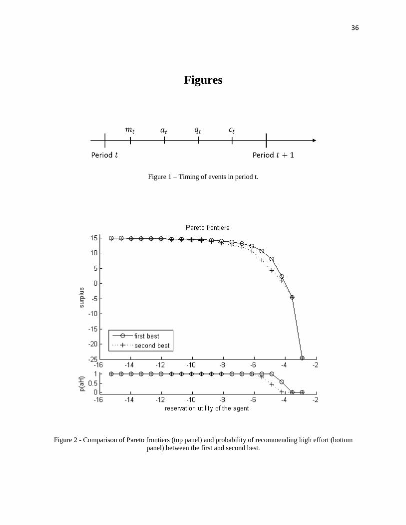
Here we present the model in its most general form. Time is discrete, and the con-tractual relationship lasts T periods4. In any period t, the timing of events is as follows(Figure 1): first, the principal sends the agent a message mt ∈ M , which we can interpretas a recommendation for the agent’s action. Then, the agent executes action at ∈ A, whichis unobserved by the principal. Next, output qt ∈ Q is realized and publicly observed, andfinally the principal pays the agent a compensation ct ∈ C. The agent has no access to
3Although not studied here, an interesting future exercise would be to relax this assumption by intro-ducing asymmetric priors
4We do not study the infinite-time version of the problem because, since a recursive formulation is notpossible, we would not be able to solve it computationally.

6
credit or savings, and so he consumes exactly ct. We impose that A,M ,Q and C be finite,which can be interpreted as an approximation to continuous sets.
We assume full commitment in the contracting game: the principal is able to committo follow the contracting rules established upon signing the contract, and the agent is ableto commit not to quit. It is interesting to note that under full commitment the ex anteoptimal contract can be ex post inefficient. This happens because in future periods, theprincipal is constrained to give incentives for past actions.
Notation - past histories:It will be useful to have clear notations for past histories. Period t history will be
denoted by ht = {mt, at, qt, ct}, and ht = {h0, h1, ..., ht} will be the the history up toperiod t. Information is asymmetric (hidden actions), so that the equivalent histories asobserved by the principal are st = {mt, qt, ct} and st = {s0, s1, ..., st}. Since st and st
are uniquely determined by ht and ht, we will sometimes use the notation st(ht) or st(ht).For completeness, we define s0 = h0 = ∅.
Strategies:The principal chooses outcome functions π(mt|st−1) and π(ct|mt, qt, s
t−1), whichare probability distributions over messages and consumption plans for the agent. Theagent chooses a strategy σ(at|mt, h
t−1).Production function:For now, we model the production function in its most general form, but we will
impose further restrictions in subsection 2.5, where we also describe the Bayesian learningprocess. Since the true underlying production function is unknown, we have a subjectiveprobability distribution f(qt|at, ht−1) of output qt given the action undertaken at. Thedistribution is conditioned on the past history ht−1, because principal and agent learn fromobservation.
Probability of ht:Given {π, σ}, we can define recursively the subjective probability of history ht hap-
pening:
p(ht|π, σ) = p(ht−1|π, σ).π(mt|st−1(ht−1
)).σ(at|mt, h
t−1).f(qt|at, ht−1).π(ct|mt, qt, st−1 (ht−1))

7
And we define p(h0|π, σ) = 1.Preferences:This allows us to calculate U(π, σ) and V (π, σ), the t = 0 expected utility of the
agent and the principal, respectively:
U(π, σ) =T∑t=1
βt−1{∑Ht
p(ht|π, σ).u(ct, at)}
V (π, σ) =T∑t=1
αt−1
{∑Ht
p(ht|π, σ
). (qt − ct)
}Note that the agent’s utility is only required to be time-separable, and is very general
otherwise. We have specialized the principal’s utility function as a risk-neutral expectedsurplus, but the methods proposed here would equally apply to any other time-separableutility function.
In the same fashion, we define probabilities and continuation utilities conditional onrealized histories hk; we will denote those by p(ht|π, σ, hk) and U(π, σ|hk).
Given an outcome function π, an optimal strategy σ maximizes the agent’s utility atevery node hk, that is:
∀σ, k, hk :
(1) U(π, σ|hk) ≤ U(π, σ|hk)
Also, an outcome function π combined with an optimal strategy σ respect the par-ticipation constraint if they provide the agent with his reservation utility U :
(2) U(π, σ) ≥ U
Problem 1. The principal’s problem in the general mechanism is to maximize his utility
V (π, σ), by choice of an outcome function π, subject to the agent’s optimizing behavior
constraints (1) and the participation constraint (2)

8
2.2 Incentive Compatible Mechanism
In this subsection, we restate the problem as an incentive compatible mechanism:that is, a mechanism in which the principal chooses the agent’s actions directly, providedincentive compatibility constraints are respected. We then show, through Proposition 1,that it is possible to restrict ourselves to those mechanisms in order to achieve a solutionto the general problem.
We now restrict the message space M to be equal to A, the action space. The princi-pal chooses outcome functions π(at|st−1) and π(ct|at, qt, st−1), which refer to the recom-mended action at, and the agent is restricted to follow the recommendation (to be “obe-dient”). Since at is now a recommendation for action we will denote ht = {at, at, qt, ct},where at is the true action undertaken by the agent.
Under the outcome function π, the t = 1 subjective probability p(st|π) becomes:
p(st|π) = p(st−1|π).π(at|st−1).f(qt|at, st−1).π(ct|at, qt, st−1)
And so the agent’s utility and the principal’s surplus become:
U (π) =T∑t=1
βt−1
{∑St
p(st|π
).u (ct, at)
}
V (π) =T∑t=1
αt−1
{∑St
(st|π
). (qt − ct)
}Participation constraint:The principal is constrained to provide the agent with his reservation utility U .
(3) U (π) ≥ U
Obedience constraint:In the notation of the previous subsection, the incentive compatible mechanism im-
plies that the agent’s optimal strategy σ is a degenerate distribution with σ (at|st−1, at) =

9
1. That is: the agent executes the recommended action with probability one on the equi-librium path.
It should not be on the agent’s interest to deviate from obedience. We define de-viations as pure strategies δa(at, ht−1) that map histories and recommended actions intoactions actually undertaken by the agent. Under a deviation δa, probabilities are affectedthrough the production function, as follows:
p(ht|π, δa) = p(ht−1|π, δa).π(at|st−1(ht−1)).I(at = δa(at, h
t−1)).
.f(qt|δa(at, ht−1), ht−1).π(ct|at, qt, st−1(ht−1))
The indicator function I is needed because p(ht|π, δa) = 0 if δa(ak, hk−1) 6= ak forsome k ≤ t (or, put more simply, I is the degenerate probability distribution over actionsassociated to the pure strategy δa).
For the agent to be obedient, it must be optimal for him to do so at every node of theequilibrium path, and thus the following must hold:
∀k, sk−1, δa :T∑t=k
βt−k{∑Ht
p(ht|π, δa, sk−1).u(ct, δa(at, ht−1))} ≤(4)
T∑t=k
βt−k{∑St
p(st|π, sk−1).u(ct, at)}
The inequalities (4) might seem less restrictive than their counterparts (1) in the gen-eral mechanism because we only allow deviations to be pure strategies instead of proba-bility distributions as the strategies σ. However, if we allowed for random deviations, wewould simply have linear combinations of the constraints (4), which would not alter theset of feasible outcome functions π.
Problem 2. The principal’s problem in the incentive compatible mechanism is to maximize
his utility V (π), by choice of an outcome function π, subject to the agent’s participation
constraint (3) and the obedience constraints (4).
10
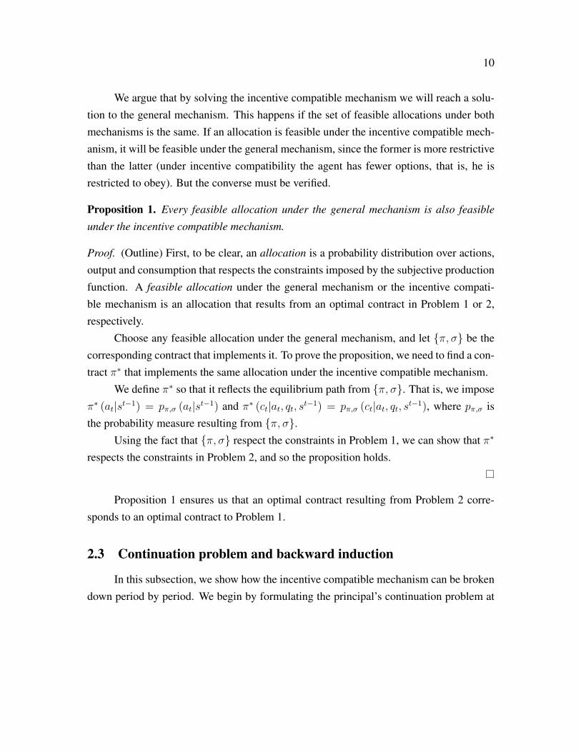
We argue that by solving the incentive compatible mechanism we will reach a solu-tion to the general mechanism. This happens if the set of feasible allocations under bothmechanisms is the same. If an allocation is feasible under the incentive compatible mech-anism, it will be feasible under the general mechanism, since the former is more restrictivethan the latter (under incentive compatibility the agent has fewer options, that is, he isrestricted to obey). But the converse must be verified.
Proposition 1. Every feasible allocation under the general mechanism is also feasible
under the incentive compatible mechanism.
Proof. (Outline) First, to be clear, an allocation is a probability distribution over actions,output and consumption that respects the constraints imposed by the subjective productionfunction. A feasible allocation under the general mechanism or the incentive compati-ble mechanism is an allocation that results from an optimal contract in Problem 1 or 2,respectively.
Choose any feasible allocation under the general mechanism, and let {π, σ} be thecorresponding contract that implements it. To prove the proposition, we need to find a con-tract π∗ that implements the same allocation under the incentive compatible mechanism.
We define π∗ so that it reflects the equilibrium path from {π, σ}. That is, we imposeπ∗ (at|st−1) = pπ,σ (at|st−1) and π∗ (ct|at, qt, st−1) = pπ,σ (ct|at, qt, st−1), where pπ,σ isthe probability measure resulting from {π, σ}.
Using the fact that {π, σ} respect the constraints in Problem 1, we can show that π∗
respects the constraints in Problem 2, and so the proposition holds.
Proposition 1 ensures us that an optimal contract resulting from Problem 2 corre-sponds to an optimal contract to Problem 1.
2.3 Continuation problem and backward induction
In this subsection, we show how the incentive compatible mechanism can be brokendown period by period. We begin by formulating the principal’s continuation problem at
11
any node on the equilibrium path. Then, we show that this formulation allows the solutionof the incentive compatible mechanism by backward induction.
A recursive formulation is not possible in this environment, because there is fullhistory dependence and thus the state space grows with time without bound. But this doesnot mean that the problem cannot be broken down to smaller parts to be solved, which isthe essence of backward induction in game theory.
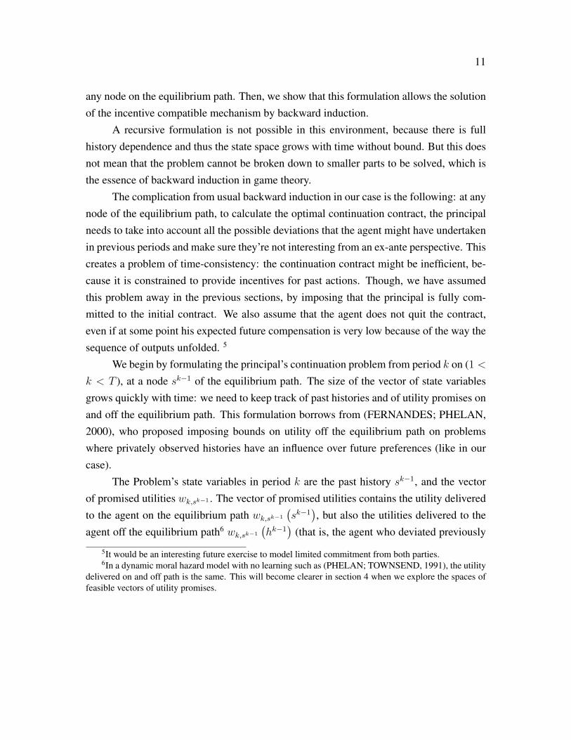
The complication from usual backward induction in our case is the following: at anynode of the equilibrium path, to calculate the optimal continuation contract, the principalneeds to take into account all the possible deviations that the agent might have undertakenin previous periods and make sure they’re not interesting from an ex-ante perspective. Thiscreates a problem of time-consistency: the continuation contract might be inefficient, be-cause it is constrained to provide incentives for past actions. Though, we have assumedthis problem away in the previous sections, by imposing that the principal is fully com-mitted to the initial contract. We also assume that the agent does not quit the contract,even if at some point his expected future compensation is very low because of the way thesequence of outputs unfolded. 5
We begin by formulating the principal’s continuation problem from period k on (1 <k < T ), at a node sk−1 of the equilibrium path. The size of the vector of state variablesgrows quickly with time: we need to keep track of past histories and of utility promises onand off the equilibrium path. This formulation borrows from (FERNANDES; PHELAN,2000), who proposed imposing bounds on utility off the equilibrium path on problemswhere privately observed histories have an influence over future preferences (like in ourcase).
The Problem’s state variables in period k are the past history sk−1, and the vectorof promised utilities wk,sk−1 . The vector of promised utilities contains the utility deliveredto the agent on the equilibrium path wk,sk−1
(sk−1
), but also the utilities delivered to the
agent off the equilibrium path6 wk,sk−1
(hk−1
)(that is, the agent who deviated previously
5It would be an interesting future exercise to model limited commitment from both parties.6In a dynamic moral hazard model with no learning such as (PHELAN; TOWNSEND, 1991), the utility
delivered on and off path is the same. This will become clearer in section 4 when we explore the spaces offeasible vectors of utility promises.

12
and is now at node hk−1 6= sk−1)7. It is necessary to keep track of the agent’s utility offthe equilibrium path to make sure that the ex-ante incentive structure is preserved whenwe solve the problem by backward induction.
Formally, we define the vector wk,sk−1 as a function mapping the space Hk−1(sk−1)
(histories that have sk−1 as its counterpart observable by the principal8) into the real line.That is, wk,sk−1 : Hk−1(sk−1) → R. The space of feasible vectors of utility promises willbe denoted Wk,sk−1 . It is important to note that under different past histories sk−1, thespace Wk,sk−1 is different. This will become evident when we see the results in section 4.
Problem 3. The principal’s continuation problem at node sk−1 of the equilibrium path is:
Vk(sk−1, wk,sk−1
)= max
π
T∑t=k
αt−k
[∑St
p(st|π, sk−1
)(qt − ct)
]subject to constraints (5), (6) and (7), defined below.
Promise-keeping constraint:The outcome function π has to deliver the agent on the equilibrium path the promised
utility 9:
(5)T∑t=k
βt−k
[∑St
p(st|π, sk−1
)u (ct, at)
]= wk,sk−1
(sk−1
)Threat-keeping constraints:The agent who reaches node sk−1 having deviated previously (that is, the agent who
is in node hk−1 which has sk−1 as its counterpart observable by the principal) shouldreceive the promised utility under his maximizing strategy. Note that here we allow theagent who deviated in the past to deviate again. ∀hk−1 ∈ Hk−1(sk−1), hk−1 6= sk−1:
7We will abuse on notation writing sk−1 to denote the history hk−1 in which aj = aj for all j =1, ..., k − 1
8Abusing again on notation, Hk−1(sk−1
)is the inverse of the function sk−1 that maps full histories
hk−1 into their counterpart that is observable by the principal.9If k = 1, then we should define this constraint as an inequality, and it will correspond to the participa-
tion constraint.

13
(6) maxδa
T∑t=k
βt−k
∑Ht(sk−1)
p(ht|π, δa, hk−1
)u(ct, δa
(at, h
t−1)) = wk,sk−1
(hk−1
)
Obedience constraints:At every node on the equilibrium path, the agent should find it at least as attractive
to follow the principal’s recommendation as to deviate. ∀l ∈ {k, ..., T} , sl−1, δa:
(7)T∑t=l
βt−l
[∑Ht
p(ht|π, δa, sl−1
)u(ct, δa
(at, h
t−1))] ≤ T∑t=l
βt−l
[∑St
p(st|π, sl−1
)u (ct, at)
]
Next, we write the continuation problem in a backward induction formulation. First,let us define some useful concepts. Given an outcome function π and an on-path continua-tion node sk, we can define the vector of utility promises at sk, wk+1,sk (π) : Hk
(sk)→ R.
For the agent on the equilibrium path, the future utility at sk will then be:
wk+1,sk (π)(sk)
=T∑
t=k+1
βt−k−1
[∑St
p(st|π, sk
)u (ct, at)
]And for the agent off-path at node hk 6= sk, his future utility will be:
wk+1,sk (π)(hk)
= maxδa
T∑t=k+1
βt−k−1
∑Ht(hk)
p(ht|π, δa, hk
)u(ct, δa
(at, h
t−1))
Proposition 2. For any(sk−1, wk,sk−1
), there is an optimal contract π∗ to the problem
Vk(sk−1, wk,sk−1
)such that, for every continuation node sk, from sk onward π∗ is an
optimal contract to the problem Vk+1
(sk, wk+1,sk (π∗)
).
Proof. (Outline) To prove this proposition, we depart from an optimal outcome function πkthat solves problem Vk
(sk−1, wk
), and an optimal πk+1 that solves Vk+1
(sk, wk+1,sk (π∗)
)

14
for some continuation node sk. We then define an outcome function π∗ that is equal toπk everywhere except in the branch of the contract that starts in sk. In this branch, π∗
is equal to πk+1. This new outcome function π∗, from sk onward, is an optimal contractfor Vk+1
(sk, wk+1,sk (π∗)
)by construction. π∗ is also an optimal contract for problem
Vk(sk−1, wk
), because it respects constraints (5), (6) and (7) and delivers at least the same
surplus as πk (because Vk+1
(sk, wk+1,sk (π∗)
)cannot be lower than the surplus delivered
by πk from sk onward, otherwise πk+1 would not be optimal).By repeating this process for every continuation node sk (there is a finite number of
them), we construct the optimal contract we are looking for.
Proposition 2 allows us to restate the maximized utility of the principal as follows:
Vk(sk−1, wk
)=∑Sk
p(sk|π∗, sk−1
) {(qk − ck) + α.Vk+1
(sk, wk+1,sk (π∗)
)}It is then natural to think of the principal’s optimization problem as choosing over
outcome functions only for period k, π(ak|sk−1
)and π(ck|ak, qk, sk−1); and vectors of
continuation utility promises wk+1,sk . It is possible to apply this procedure if the con-tinuation value functions Vk+1
(sk, wk+1,sk (π∗)
)are known in advance, which is why the
problem needs to be solved backwards.To be clear, we state the continuation problem in its backward induction form:
Problem 4. The principal’s backward induction continuation problem at node sk−1 of the
equilibrium path is:
Vk(sk−1, wk
)= max
π(ak|sk−1),π(ck|ak,qk,sk−1),{wk+1,sk}sk
∑Sk
p(sk|π, sk−1
) {(qk − ck) + α.Vk+1
(sk, wk+1,sk
)}subject to constraints (8), (9) and (10), defined below.
Below we define the constraints mentioned:

15
Promise-keeping constraint:The outcome function π has to deliver the agent the promised utility:
(8)∑Sk
p(sk|π, sk−1
) {u (ck, ak) + β.wk+1,sk
(sk)}
= wk,sk−1
(sk−1
)Threat-keeping constraint:The agent who reaches node sk−1 having deviated previously should receive the
promised utility. ∀hk−1 ∈ Hk−1(sk−1), hk−1 6= sk−1:
(9)maxδa
∑Hk(sk−1)
p(hk|π, δa, hk−1
) {u(ck, δa
(ak, h
k−1))+ β.wk+1,sk(hk)}
= wk(hk−1
)Obedience constraint:The agent should find it at least as attractive to follow the principal’s recommenda-
tion as to deviate in period k. ∀δa : A→ A:
(10)∑Hk(sk−1)
p(hk|π, δa, sk−1
) {u(ck, δa
(ak, h
k−1))+ β.wk+1,sk(hk)}≤ wk,sk−1
(sk−1
)In practice, Wk,sk−1 (the space of feasible vectors of continuation utilities) is not
known in advance - it needs to be calculated previously, when we solve the next-periodproblem Vk+1
(sk, wk+1,sk
).
2.4 Linear program
Finally, in this subsection we formulate the problem using the linear programmingframework first introduced by (PRESCOTT; TOWNSEND, 1984). The advantage of linearprograms is that they are well understood and can be solved easily on a computer using

16
off-the-shelf optimization packages10.Problem 4 is not a linear program, because choice variables π
(ak|sk−1
), π(ck|ak, qk, sk−1)
and wk+1,sk are multiplied in the objective function. So we restate the problem in a slightlydifferent manner: we allow for lotteries over promised utility vectors wk+1,sk and make theprobability distribution π
(wk+1,sk |sk
)the choice variable for the principal instead of the
actual vectors wk+1,sk11. We also discretize the utility spaces Wk,sk−1 in order to have a
finite number of variables. The program is made linear by choosing over joint probabilitydistributions π(at, qt, ct, wt+1,st |st−1, wt) ≡ π (st, wt+1,st|st−1, wt,st−1) instead of the con-ditional probabilities as before, and imposing that π is a probability measure that respectsthe conditional probabilities given by f (qt|at, ht−1).
For a detailed explanation of this linear programming framework, we refer the readerto the excellent introduction in (PRESCOTT, 1999), to its first application to dynamicmoral hazard in (PHELAN; TOWNSEND, 1991) and to the original article (PRESCOTT;TOWNSEND, 1984).
Problem 5. Linear program in period t:
Vt(st−1, wt,st−1
)= max
π
∑st,wt+1,st
π(st, wt+1,st|st−1, wt){
(qt − ct) + βVt+1
(st, wt+1,st
)}subject to constraints (11), (12), (13), (14) and (15) defined below.
Below we define the mentioned constraints:Probability measure constraints12:
(11)
∑st,wt+1,st
π (st, wt+1,st |st−1, wt,st−1) = 1
π (st, wt+1,st|st−1, wt,st−1) ≥ 0 , ∀st, wt+1,st
10In our case, we have used Matlab’s built-in optimization toolbox.11Note that this is in fact more general, since choosing a specific vector wk+1,sk is equivalent to choosing
π(wk+1,sk |sk
)= 1.
12Probability measure constraints are also needed in the formulations of the previous sections, but wemake them explicit here to have the complete linear program as it is computed.
17
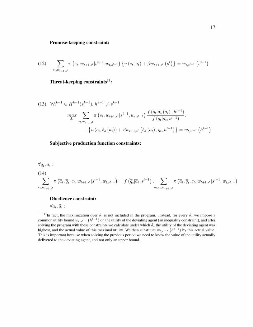
Promise-keeping constraint:
(12)∑
st,wt+1,st
π(st, wt+1,st |st−1, wt,st−1
) {u (ct, at) + βwt+1,st
(st)}
= wt,st−1
(st−1
)Threat-keeping constraints13:
(13) ∀hk−1 ∈ Hk−1(sk−1), hk−1 6= sk−1
maxδa
∑st,wt+1,st
π(st, wt+1,st|st−1, wt,st−1
) f (qt|δa (at) , ht−1)
f (qt|at, st−1).
.{u (ct, δa (at)) + βwt+1,st
(δa (at) , qt, h
t−1)} = wt,st−1
(ht−1
)Subjective production function constraints:
∀qt, at :
∑ct,wt+1,st
π(at, qt, ct, wt+1,st|st−1, wt,st−1
)= f
(qt|at, st−1
).∑
qt,ct,wt+1,st
π(at, qt, ct, wt+1,st |st−1, wt,st−1
)(14)
Obedience constraint:∀at, at :
13In fact, the maximization over δa is not included in the program. Instead, for every δa we impose acommon utility boundwt,st−1
(ht−1
)on the utility of the deviating agent (an inequality constraint), and after
solving the program with these constraints we calculate under which δa the utility of the deviating agent washighest, and the actual value of this maximal utility. We then substitute wt,st−1
(ht−1
)by this actual value.
This is important because when solving the previous period we need to know the value of the utility actuallydelivered to the deviating agent, and not only an upper bound.
18
(15)∑
st,wt+1,st
π(st, wt+1,st |st−1, wt,st−1
) {u (ct, at) + βwt+1,st
(st)}≥
≥∑
st,wt+1,st
π(st, wt+1,st |st−1, wt,st−1
) f (qt|at, st−1)f (qt|at, st−1)
{u (ct, at) + βwt+1,st
(at, qt, s
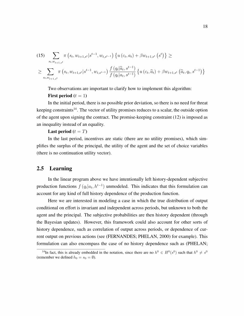
t−1)}Two observations are important to clarify how to implement this algorithm:First period (t = 1)In the initial period, there is no possible prior deviation, so there is no need for threat
keeping constraints14. The vector of utility promises reduces to a scalar, the outside optionof the agent upon signing the contract. The promise-keeping constraint (12) is imposed asan inequality instead of an equality.
Last period (t = T )In the last period, incentives are static (there are no utility promises), which sim-
plifies the surplus of the principal, the utility of the agent and the set of choice variables(there is no continuation utility vector).
2.5 Learning
In the linear program above we have intentionally left history-dependent subjectiveproduction functions f (qt|at, ht−1) unmodeled. This indicates that this formulation canaccount for any kind of full history dependence of the production function.
Here we are interested in modeling a case in which the true distribution of outputconditional on effort is invariant and independent across periods, but unknown to both theagent and the principal. The subjective probabilities are then history dependent (throughthe Bayesian updates). However, this framework could also account for other sorts ofhistory dependence, such as correlation of output across periods, or dependence of cur-rent output on previous actions (see (FERNANDES; PHELAN, 2000) for example). Thisformulation can also encompass the case of no history dependence such as (PHELAN;
14In fact, this is already embedded in the notation, since there are no h0 ∈ H0(s0) such that h0 6= s0
(remember we defined h0 = s0 = ∅).

19
TOWNSEND, 1991), although in a computationally inefficient way when compared totheir algorithm. In section 3 we use this to test our code.
Also, different types of uncertainty can be modeled. A non-exhaustive list can befound below. The kind of uncertainty to be modeled is key to what class of real-worldproblems we are studying. A few questions that could be asked using this framework are:
• Does effort matter and how much? (does f shift or change its dispersion with effortlevel?)
• What is the quality of the project? (what is the mean of f for a given effort level?)
• How risky is the project? (how dispersed is f for a given effort level?)
The specificity of the problem at hand then lies in how to model the conditional distributionof output, f (qt|at, ht−1). In this paper we will make the following modeling choice:
There are n possible states of nature, θ ∈ Θ = {1, . . . , n}, each θ referring toa different (and publicly known) production function fθ (q|a). θ is realized before thecontract is signed, but neither the principal nor the agent can observe it. There is no ex-ante asymmetry of information: upon signing the contract, principal and agent share thesame belief µ (h0) = (µ1, ...µn) ∈ Rn about the state of the world, that is:
µi(h0)≡ p(θ = i)
As output is revealed, principal and agent update their beliefs about the state ofnature using Bayes’ rule:
(16) µi(ht−1
)≡ p
(θ = i|ht−1
)=
Bayes
p (θ = i, ht−1)
p (ht−1)=
p (θ = i, ht−1)∑nj=1 p (θ = i, ht−1)
=
=i.i.d.
p (θ = i) .t−1∏s=1
fi (qs|as)∑nj=1 p (θ = j) .
t−1∏s=1
fj (qs|as)=
µi (h0) .
t−1∏s=1
fi (qs|as)∑nj=1 µj (h0) .
t−1∏s=1
fj (qs|as)

20
At time t ∈ {1, ..., T}, the belief µ (ht−1) allows us then to calculate the subjectiveproduction function:
f(qt|at, ht−1
)=
n∑i=1
µi(ht−1
)fi (qt|at)
It is worth emphasizing that, since the principal does not observe actions, he willupdate his beliefs considering that the agent has followed his recommendations, whereasthe agent will consider the actual levels of effort applied, and so beliefs can diverge fromt = 2 on.
It is interesting to note from equation (16) that the order in which (at, qt) pairs oc-curred does not matter to the update of beliefs. This is a direct consequence of our as-sumption that the underlying production function is i.i.d.. This fact will allow us later toreduce the dimensionality of the computational problem to be solved.
2.6 Computation
The optimal contract is computed by backward induction. We start from the lastperiod (T ), solving one static linear program 5 for each possible history sT−1 and candidatevector of utility promises wT,sT−1 . For a portion of those linear programs, the computerwill find a solution, which allows us to define the spaces of feasible vectors of utilitypromises WT,sT−1 , as well as the associated value functions VT
(sT−1, wT,sT−1
). With
these values stored, we can proceed to calculate the linear programs for period T − 1, andso on.
The computational burden of this algorithm increases exponentially with the numberof periods and the size of grids. The number of periods to be solved impacts on thenumber of possible histories (and thus linear programs) that need to be considered, aswell as the number of deviations that we need to keep track of (since multiple deviationsare a concern). The number of possible deviations increases the dimensionality of thespaces of feasible utility promises Wt,st−1 , which in turn increases the number vectors ofutility promises to be tested in period t (each vector requires solving a linear program),as well as the number of constraints (each threat-keeping constraint refers to a possible
21
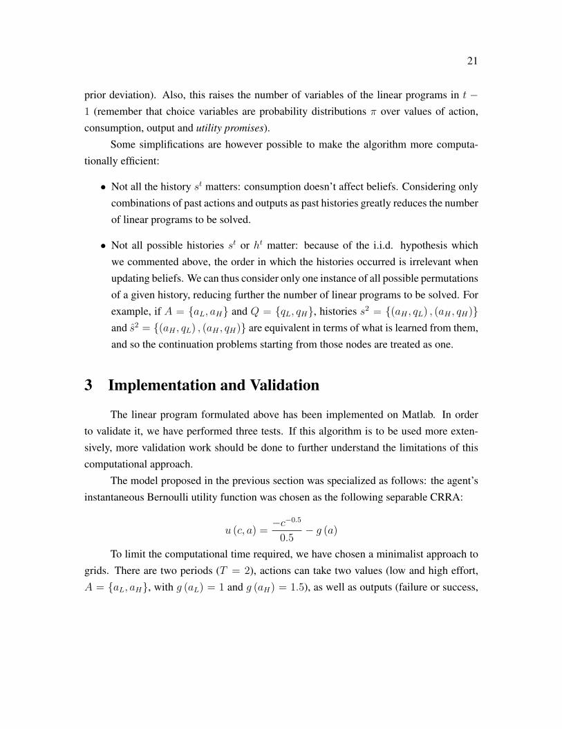
prior deviation). Also, this raises the number of variables of the linear programs in t −1 (remember that choice variables are probability distributions π over values of action,consumption, output and utility promises).
Some simplifications are however possible to make the algorithm more computa-tionally efficient:
• Not all the history st matters: consumption doesn’t affect beliefs. Considering onlycombinations of past actions and outputs as past histories greatly reduces the numberof linear programs to be solved.
• Not all possible histories st or ht matter: because of the i.i.d. hypothesis whichwe commented above, the order in which the histories occurred is irrelevant whenupdating beliefs. We can thus consider only one instance of all possible permutationsof a given history, reducing further the number of linear programs to be solved. Forexample, if A = {aL, aH} and Q = {qL, qH}, histories s2 = {(aH , qL) , (aH , qH)}and s2 = {(aH , qL) , (aH , qH)} are equivalent in terms of what is learned from them,and so the continuation problems starting from those nodes are treated as one.
3 Implementation and Validation
The linear program formulated above has been implemented on Matlab. In orderto validate it, we have performed three tests. If this algorithm is to be used more exten-sively, more validation work should be done to further understand the limitations of thiscomputational approach.
The model proposed in the previous section was specialized as follows: the agent’sinstantaneous Bernoulli utility function was chosen as the following separable CRRA:
u (c, a) =−c−0.5
0.5− g (a)
To limit the computational time required, we have chosen a minimalist approach togrids. There are two periods (T = 2), actions can take two values (low and high effort,A = {aL, aH}, with g (aL) = 1 and g (aH) = 1.5), as well as outputs (failure or success,

22
Q = {qL = 0.5, qH = 15}). The consumption grid C was chosen to have 100 equallyspaced points between 0.1 and 16. We have equalized the discount rates of the principaland the agent to be α = β = 0.95.
Uncertainty about the production function was modeled differently in each case an-alyzed, so both Θ and the associated production functions fθ (q|a) will be specified later.
3.1 Comparing first and second best outcomes
When the agent is risk-averse, moral hazard creates a tension between insurance andthe provision of incentives, even without the learning process we propose here.
In the first best (that is, when the principal can contract effort directly), it is efficientto give the agent a non-contingent compensation. In the second best this is not the case,because under a non-contingent compensation the agent has no incentives to provide effort.The Pareto frontier of the second best should shrink as compared to the first best, becausethe problem is being constrained by incentive compatibility.
In this subsection, we test whether our algorithm reproduces these analytical results.To calculate the first best, it is sufficient to remove the informational constraints from theproblem (that is: obedience and threat-keeping constraints).
Here we imposed Θ = {1, 2}, and the candidate production functions as in Table 1.
f1 (q|a) qL qH
aL 0.8 0.2
aH 0.2 0.8
f2 (q|a) qL qH
aL 0.8 0.2
aH 0.8 0.2
Table 1: Candidate production functions f1and f2
The common prior imposed was µ1 = µ2 = 0.5.In Figure 2, we can see observe two expected features. First, the range of agent’s
reservation utilities for which it is optimal to recommend high effort with probability oneis narrower. This happens because the cost of providing incentives reduces the gains fromhigh effort in the second best. Second, we can see that the Pareto frontier of the second

23
best is everywhere below that of the first best, which is due to the efficiency cost frominformation asymmetry.
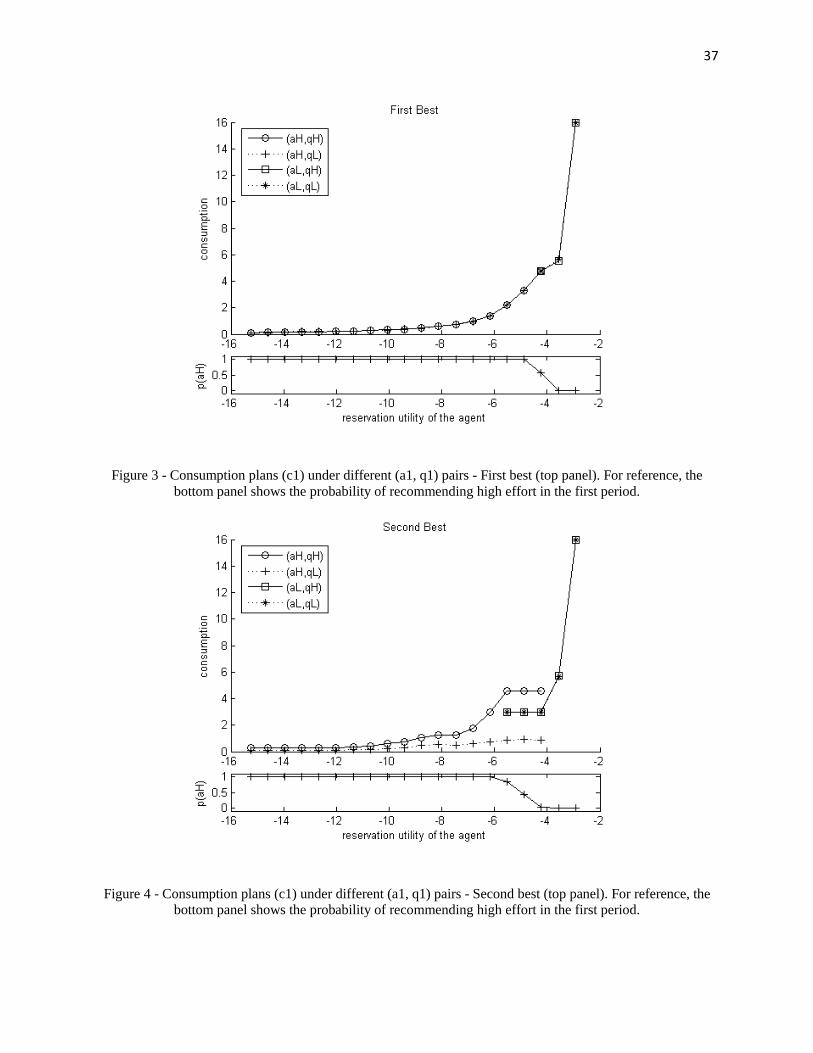
Then, in Figures 3 and 4, we see a few interesting features. First, both on the firstbest and in the second best, it is optimal to offer the agent a fixed compensation whenlow effort is recommended (points on the right of each figure, superposed). Second, whenhigh effort is recommended (points on the left of each figure), in the first best we still havea fixed salary to the agent, while in the second best there is incentive provision throughconsumption: there is a “bonus” on consumption when high output qH occurs.
3.2 Impact of uncertainty on incentives
(PRAT; JOVANOVIC, 2012) study a problem that is similar to ours. In their case,the agent has unknown ability, which is a parameter of the production function. In atwo-period model15, they show that when the prior has more variance (that is, when theuncertainty about the production function is higher), it is necessary to provide more high-powered incentives in order to make the agent exert effort. Intuitively, this happens be-cause when the prior is more uncertain there is more room for the agent to manipulate theprincipal’s beliefs about the production function. This increases the information rents theagent can get in the second period after deviating in the first period. To curb this behavior,the principal needs to make the agent’s compensation fluctuate more with output.
This simple model provides a lower bound on the volatility of the agent’s expectedutility in the first period when the contract implements high effort in both periods. Volatil-ity increases with the variance of the prior over the production function. In this subsection,we calculate analytically this lower bound, and use it to test our algorithm.
We extend slightly the two-period model in (PRAT; JOVANOVIC, 2012) to includethe possibility of nonlinear disutility of effort (the agent’s Bernoulli utility function here is[v (w)− g (a)], with g increasing and possibly convex), and reach the following conditionfor the optimal contract that implements high effort in both periods:
15See appendix C of their paper
24
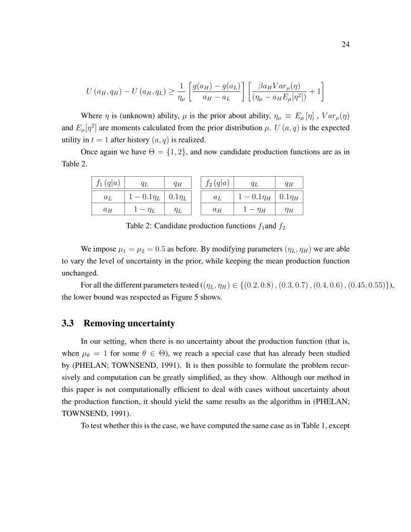
U (aH , qH)− U (aH , qL) ≥ 1
ηµ
[g(aH)− g(aL)
aH − aL
] [βaHV arµ(η)
(ηµ − aHEµ[η2])+ 1
]Where η is (unknown) ability, µ is the prior about ability, ηµ ≡ Eµ [η] , V arµ(η)
and Eµ[η2] are moments calculated from the prior distribution µ. U (a, q) is the expectedutility in t = 1 after history (a, q) is realized.
Once again we have Θ = {1, 2}, and now candidate production functions are as inTable 2.
f1 (q|a) qL qH
aL 1− 0.1ηL 0.1ηL
aH 1− ηL ηL
f2 (q|a) qL qH
aL 1− 0.1ηH 0.1ηH
aH 1− ηH ηH
Table 2: Candidate production functions f1and f2
We impose µ1 = µ2 = 0.5 as before. By modifying parameters (ηL, ηH) we are ableto vary the level of uncertainty in the prior, while keeping the mean production functionunchanged.
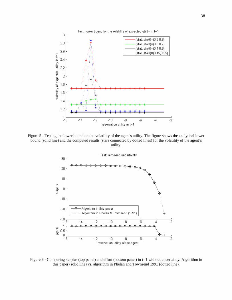
For all the different parameters tested ((ηL, ηH) ∈ {(0.2, 0.8) , (0.3, 0.7) , (0.4, 0.6) , (0.45, 0.55)}),the lower bound was respected as Figure 5 shows.
3.3 Removing uncertainty
In our setting, when there is no uncertainty about the production function (that is,when µθ = 1 for some θ ∈ Θ), we reach a special case that has already been studiedby (PHELAN; TOWNSEND, 1991). It is then possible to formulate the problem recur-sively and computation can be greatly simplified, as they show. Although our method inthis paper is not computationally efficient to deal with cases without uncertainty aboutthe production function, it should yield the same results as the algorithm in (PHELAN;TOWNSEND, 1991).
To test whether this is the case, we have computed the same case as in Table 1, except

25
this time with µ1 = 1 (the production function is f1 (q|a) with certainty). We solved thiscase using the algorithm in (PHELAN; TOWNSEND, 1991) too.
In Figure 6, we can see that both algorithms deliver the same results16.
4 Applications
The algorithm described allows us to compute the optimal contract in a variety ofsituations, and identify its key characteristics. First, in subsection 4.1 we explore a casein which the choice of candidate production functions simplifies the learning process,confirming the conclusion in (PRAT; JOVANOVIC, 2012) that learning harms incentives.Then, we proceed in subsection 4.2 to analyze a case in which both principal and agent donot know for sure whether effort matters or not for production.
4.1 Belief manipulation
In this section we apply our methods to the case in 3.2, choosing (ηL, ηH) = (0.2, 0.8)
and µ1 (s0) = µ2 (s0) = 0.5. We then have the candidate production functions as in Table3.
f1 (q|a) qL qH
aL 0.98 0.02
aH 0.8 0.2
f2 (q|a) qL qH
aL 0.92 0.08
aH 0.2 0.8
Table 3: Candidate production functions f1and f2
In what follows we will say that the belief is more “optimistic” if µ2 is greater, sinceunder f2 the expected output conditional on high effort is greater than under f1.
What is interesting about this case is that no divergence in beliefs is created betweenthe principal and an agent who deviates in case high output happens, as is made clear
16In fact, if we compare contract details such as consumption and utility promises conditional on actionand output, we find that both solutions are very similar. Those comparisons have been omitted for brevity.Small differences can occur because the algorithm in this paper needs to solve larger linear programs, thatsometimes exceed the maximum number of iterations in Matlab and thus do not yield results.

26
in Table 4 with posterior beliefs. On the other hand, when high effort is recommendedand low output occurs, the deviating agent becomes more optimistic than the principal(µ2
(h1)
= 0.49 while µ2 (s1) = 0.2). This simplifies the analysis, as will become clearer.
(aL, qL) (aL, qH) (aH , qL) (aH , qH)
µ2 (s1) 0.49 0.8 0.2 0.8
µ2
(h1)
0.2 0.8 0.49 0.8
Table 4: Posterior conditional on s1 = (aL, qL) for prior µ1 (s0) = µ2 (s0) = 0.5. Thesecond row indicates µ2
(h1)
, the posterior of the agent who deviated in the first period.
We want to understand the role played by learning on incentives, and so in this sub-section we will frequently compare the solution to the case described above to its coun-terpart with no uncertainty about the production function. To pick a comparable case, weneed to have the same ex-ante distribution of probabilities, so we impose the productionfunction f (q|a) in Table 5.
f (q|a) qL qH
aL 0.95 0.05
aH 0.5 0.5
Table 5: “Expected production function”: production function with same ex-ante prob-abilities as the combination of the production functions in Table 3 with prior µ1 (s0) =
µ2 (s0) = 0.5.
The first thing we highlight is the difference between the spaces of feasible utilitypromises in the second period in both cases considered. Without learning, it is not possibleto deliver different utilities to the agents on and off the equilibrium path: since both havethe same beliefs over future productivity, they solve the exact same problem and so there isno margin to punish the agent off-path while holding the on-path agent’s utility constant.Neither is it possible to have different spaces of vectors of utility promises for different

27
first-period histories. The spaces of feasible utility vectors W2,s1 , for all histories s1, areexactly the same, and lie in the diagonal of the Cartesian as can be seen in Figure 8.
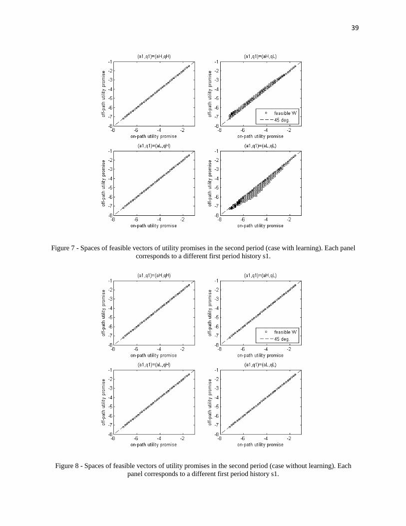
With learning, on the other hand, the space of feasible utility promises is “thick” forlow output shocks, but not for high output shocks, as can be seen in Figure 7. This is aconsequence of the peculiar candidate production functions chosen in this example. In amore general case such as that in the next subsection, the space of feasible utility promisesis “thick” for every first-period history because beliefs on and off-path always diverge, ascan be seen in Figure 15.
The difference between Figures 7 and 8 carries, in fact, the essence of why it ispossible to formulate the problem recursively in the case with no learning about the pro-duction function, while the same does not apply to the case with learning. With learning,future preferences are affected by past histories and so it is necessary to know in whichnode of the equilibrium path we are when we solve the continuation problem.
Then we proceed to examine the impact of learning on incentives. In Figures 9 and10 we can see the optimism of the off-path agent regarding future utilities when a lowoutput shock occurs. When high output occurs there is no distinction between obedientand deviating agents, but when low output occurs the deviating agent expects higher utilityfrom the next period.
The same does not happen with utility from current consumption as we see in Figures11 and 12, since both the deviating and the obedient agent have the same beliefs in t = 1.
This is why in this case, in order to implement high effort in the first period, theprincipal has to increase the volatility of the agent’s utility, as (PRAT; JOVANOVIC, 2012)argues. Figure 13 makes this evident. We will see in section 4.2, that this appears to holdin more general settings.
It is then natural to ask whether this increased volatility comes at a cost on surplus.Figure 14 shows that the surplus loss associated to learning is non-negative and increaseswith the reservation utility of the agent (because it becomes more costly to provide incen-tives through consumption for higher utility values). When the probability of high effortbeing recommended p (a1 = aH) decreases, so does the surplus loss, since incentives arenot needed for low effort. Learning also impacts effort and the participation constraint, butthis will become clearer in the next subsection.

28
4.2 Effort matters vs. effort does not matter
In this subsection, we explore in detail the computed optimal contract for a two-period environment in which the uncertainty about the production function is as in Table1.
This means that if θ = 1, effort matters: under the chosen parameters, aH would berecommended for a wide range of the agent’s reservation utilities if µ1 (s0) = 1. On theother hand, if θ = 2, effort is irrelevant to production: it would be optimal to provide theagent with a fixed salary if µ2 (s0) = 1, encouraging low effort.
We impose µ1 (s0) = µ2 (s0) = 0.5, so that learning can occur between the first andthe second periods.
Given the prior and the production functions, we can easily calculate the posteriorsconditional on each possible on-path first-period history s1, as showed in Table 6. We cansee in particular that, since under low effort aL both production functions f1 and f2 areidentical, there is no learning: the posterior is identical to the prior.
(aL, qL) (aL, qH) (aH , qL) (aH , qH)
µ1 (s1) 0.5 0.5 0.2 0.8
µ1
(h1)
0.2 0.8 0.5 0.5
Table 6: Posterior conditional on s1 for µ1 (s0) = µ2 (s0) = 0.5. The second row indi-cates µ1
(h1)
, the posterior of the agent who deviated in the first period . Each columncorresponds to a different pair of (recommended effort, realized output).
The divergence between beliefs on and off the equilibrium path is what makes thisproblem complex. As described earlier, the first step in solving the problem is to solve thelinear programs in t = 2 and find the spaces of feasible utility promises for each possiblehistory s1. Figure 15 depicts the calculated spaces of feasible utility promises for thiscase. History dependence becomes clear, since we can see that the space associated toeach possible history s1 is different.
We can see that for the same on-path utility promise (x axis in each graph), thereare multiple feasible values of off-path utility (y axis). Those values impact how tight the

29
threat-keeping constraints in period 2 will be. An interesting question is then: what isthe strategy used by the principal to make the off-path agent worse off while keeping theon-path agent’s utility constant? The numerical solution allows us to explore this in detail.Figure 16 illustrates the contracts in two cross sections of the spaces of feasible utilitypromises (for first-period histories s1 = (aH , qH) and s1 = (aH , qL)).
We can see in Figure 16 that the principal uses the difference in perceived probabil-ities (of high and low output) on and off path to punish the off-path agent, by changingthe consumption plans (increasing or decreasing its volatility). Of course, tightening thethreat-keeping constraint comes at a cost on surplus. Interesting to note is the ex-post in-efficiency of such a schedule: once the second period is reached (and the principal knowsthe agent is on the equilibrium path), there is room for a Pareto improvement by renegoti-ating the contract, since the principal can increase his surplus at no utility cost to the agenton the equilibrium path. However, the ability to commit to non-renegotiation can bringex-ante gains to the contractual relationship.
Contract in t = 1
With the solution to all t = 2 programs, it is then possible to compute the contractin t = 1. Through the choices of utility promises of the optimal contract, we can recoverthe whole equilibrium path.
Figure 17 shows us a few general features of the numerical solution. Worth notingare: the concavity of the value function (surplus, or “Pareto frontier”); the participationconstraint does not bind for low levels of reservation utility of the agent; for high valuesof reservation utility it becomes too costly to implement high effort.
Multiple deviationsIn Figure 18, we can see the level of effort in the second period on and off the equi-
librium path when high effort is recommended in the first period (a1 = aH), for differentrealizations of the first-period output q1. It is interesting to note that under learning theagent considers multiple deviations: for high reservation utility values, an agent who de-viates in the first period and receives a good output shock will find it attractive to deviateagain in the second period. This is because he will be more pessimistic about the pro-duction function in the second period than the principal. From Table 6, we see that fors1 = (aH , qH) the principal has posterior µ1 (s1) = 0.8 while the agent who deviated has

30
posterior µ1
(h1)
= 0.5. That is, the principal believes effort is more important than theagent does.
Compared to the case in subsection 4.1, this is a new fact. There, the agent wouldonly consider one-shot deviations, because under any first period history a deviating agentwould be at least as optimistic as the agent on the equilibrium path17. Here, instead, thedeviating agent can be more pessimistic than the agent on-path, and so incentives mightbe less than necessary in the second period and the deviating agent shirks again18.
When confronted with the decision of whether to provide the level of effort recom-mended by the principal or not in t = 1, the agent analyzes his expected utility under eachcourse of action. The role of the incentive constraints in the program is to make sure thatfollowing the recommended level of effort is at least as desirable as deviating.
We can see in Figure 19 (top panel) that the incentive constraint is always tightwhen high effort is recommended. This is expected, since providing incentives for higheffort to a risk-averse agent is costly and so the principal avoids any slack in the incentiveconstraint.
The numerical solution allows us to go farther in this analysis: since we assumedthe agent’s utility is separable, first period incentives can be broken down into three com-ponents: the disutility of effort; the current utility from consumption; and the discountedsecond period utility. In Figure 19 (bottom panel) we can see how those three componentschange under recommended effort, and under deviation.
The difference in the disutility of effort for the obedient and the deviating agent isobvious - different effort levels imply different disutilities. When the principal wants toimplement high effort, this gap in disutilities is what creates the need for incentives.
Incentives in t = 1 are provided in two ways: through current consumption, andthrough future utility promises.
To provide incentives through current consumption, the principal offers higher con-sumption when high output occurs than when low output occurs. Although obedient anddeviating agents receive the same consumption level conditional on output, they differ in
17See appendix C in (PRAT; JOVANOVIC, 2012)18When we graph second period average effort for the case in subsection 4.1 (the equivalent to Figure
18), we see that effort coincides for on path and off path agents. This graph has been omitted for brevity.

31
the probabilities of each output level occurring. Since the obedient agent expects high out-put with higher probability than the deviating agent, giving higher compensation if highoutput occurs creates an incentive for being obedient.
For the future utility component, incentives are more complex: not only do the obe-dient and deviating agents see different probabilities of each output occurring, but theyalso receive different utility levels conditional on output. This is because they will havedivergent beliefs in the second period. Interestingly, there is a region in which the agentwho deviates gets more future utility than the agent who is obedient (for low reservationutility values). This has to be compensated by the principal through more volatility ofcurrent consumption.
If we further decompose the agent’s expected future utility (Figure 20), we can seethat this case is more complex than that in subsection 4.1 (see Figure 9). Now the agentoff-path expects different future utilities than the agent on-path both when high and lowoutput occurs. For low reservation utilities of the agent, there is a region in which thedeviating agent expects lower future utility if high output occurs in the first period than iflow output occurs.
Ultimately, how the principal will make the optimal mix in t = 1 between providingincentives through consumption (front-loading) or through future utility (back-loading) isa quantitative issue of which is less costly.
Comparison to the case with no uncertaintyAs in subsection 4.1, we compare the case with learning to its counterpart without
learning, and check whether the same conclusions hold. Here, the production function thatis ex ante equivalent is given by Table 7.
f (q|a) qL qH
aL 0.8 0.2
aH 0.5 0.5
Table 7: “Expected production function”: production function with same ex-ante prob-abilities as the combination of the production functions in Table 1 with prior µ1 (s0) =
µ2 (s0) = 0.5.

32
When we look at the volatility of the agent’s utility when high effort is recommended(Figure 21), we reach the same conclusion in this case: providing incentives requireshigher volatility under learning.
In Figure 22, we note the loss in surplus from the uncertainty about the productionfunction19. Also, interestingly, we can see the consequences of learning on the partic-ipation constraint, that becomes slack for higher reservation utilities of the agent whencompared to the case with no learning. This is a consequence of the need for strongerincentives to implement high effort under learning: because there is a lower bound on theutility from consumption (C is finite), higher volatility of consumption is only possible ifaverage consumption increases.
Also, it is clear that the region where high effort is recommended is narrower underlearning - it is more costly to implement high effort because of the need for strongerincentives.
5 Conclusion
In this paper we have proposed a computational method to deal with models ofdynamic moral hazard with simultaneous learning about the production function. Thecontribution is methodological: through computation, the problem can be studied underfew assumptions about functional forms. The literature has been dealing with this problemusing continuous-time principal-agent models in which the production function has anunknown additive parameter, thus limited in scope.
We have formulated a general mechanism that can be tackled with our approach, andhave shown how it can be reformulated as an incentive-compatible mechanism that can besolved by backward induction. Finally, we have written the backward induction problemin the linear programming framework of (PRESCOTT; TOWNSEND, 1984), which al-lows computation. The algorithm was simplified to increase computational performance:consumption histories were excluded from the space of state variables, and permutations
19However, there is a dip in surplus loss below zero which we believe can be attributed to the finitenessof the utility grid. This finiteness creates local risk-neutrality for the agent, which could permit increases involatility at no cost on surplus.

33
in past histories (on and off the equilibrium path) were shown to be irrelevant. Those sim-plifications reduce the number of programs that need to be evaluated in each period, aswell as the size of those linear programs.
Our algorithm was validated and applied to a few cases in a simple two-period,two-action, two-output, and two-production function environment. In one application, wehave confirmed the findings of (PRAT; JOVANOVIC, 2012), that uncertainty about theproduction function increases the volatility of the agent’s utility in order to compensatefor gains from belief manipulation by the agent.
The numerical solution is very rich in details, and shows how complex the modelbecomes, as a result of diverging beliefs between the principal and the off-path agent.There is much room for future work in exploring different applications of this algorithm.
An existing gap in the literature, which we have not tackled, is to study in a uniformand accessible language the whole spectrum of commitment in the dynamic moral hazardproblem with learning, and to investigate what happens under limited commitment. Up tonow, on one end of the spectrum there are discrete models with little or no commitmentin the “career concerns” literature. On the other end, there are full-commitment models incontinuous time.
34
ReferencesDEMARZO, P.; SANNIKOV, Y. Learning , Termination , and Payout Policy in DynamicIncentive Contracts. Working Paper, n. 0452686, 2011.
DOEPKE, M.; TOWNSEND, R. M. Dynamic mechanism design with hidden incomeand hidden actions. Journal of Economic Theory, v. 126, n. 1, p. 235–285, jan.2006. ISSN 00220531. Disponıvel em: 〈http://linkinghub.elsevier.com/retrieve/pii/S0022053104001954〉.
FERNANDES, A.; PHELAN, C. A recursive formulation for repeated agency withhistory dependence. Journal of Economic Theory, v. 247, p. 223–247, 2000. Disponıvelem: 〈http://www.sciencedirect.com/science/article/pii/S0022053199926194〉.
HE, Z.; WEI, B.; YU, J. Optimal Long-term Contracting with Learning. 2013.
HOLMSTROM, B. Managerial Incentive Problems: A Dynamic Perspective. Review ofEconomic Studies, v. 66, n. 1, p. 169–182, jan. 1999. ISSN 0034-6527. Disponıvel em:〈http://restud.oxfordjournals.org/lookup/doi/10.1111/1467-937X.00083〉.
KARAIVANOV, A. Computing Moral Hazard Programs With Lotteries Using Matlab.2001.
KARAIVANOV, A.; TOWNSEND, R. M. Dynamic Financial Constraints : DistinguishingMechanism Design from Exogenously Incomplete Regimes. 2012.
KILENTHONG, W. T.; MADEIRA, G. A. Observability and Endogenous Organizations.2009.
LAFFONT, J.-J.; TIROLE, J. The Dynamics of Incentive Contracts. Econometrica, v. 56,n. 5, p. 1153–1175, 1988.
MADEIRA, G. D. A.; TOWNSEND, R. M. Endogenous groups and dynamic selection inmechanism design. Journal of Economic Theory, v. 142, p. 259–293, 2008.
MANSO, G. Motivating Innovation. The Journal of Finance, v. 66, n. 5, p. 1823–1860,out. 2011. ISSN 00221082. Disponıvel em: 〈http://doi.wiley.com/10.1111/j.1540-6261.2011.01688.x〉.
PAULSON, A. L.; TOWNSEND, R. M.; KARAIVANOV, A. Distinguishing LimitedLiability from Moral Hazard in a Model of Entrepreneurship. Journal of PoliticalEconomy, v. 114, n. 1, p. 100–144, 2006.
35
PHELAN, C.; TOWNSEND, R. M. Computing Multi-Period, Information-ConstrainedOptima. The Review of Economic Studies, v. 58, n. 5, p. 853–881, 1991.
PRAT, J.; JOVANOVIC, B. Dynamic contracts when agent’s quality is unknown.n. January, 2012. Disponıvel em: 〈http://federation.ens.fr/ydepot/semin/texte1112/PRA2012DYN.pdf〉.
PRESCOTT, E.; TOWNSEND, R. Pareto Optima and Competitive Equilibria withAdverse Selection and Moral Hazard. Econometrica, v. 52, n. 1, p. 21–46, 1984.Disponıvel em: 〈http://www.jstor.org/stable/10.2307/1911459〉.
PRESCOTT, E. S. A Primer on Moral-Hazard Models. Federal Reserve Bank ofRichmond Economic Quarterly, v. 85, n. 1997, 1999.
ROGERSON, W. P. . Repeated Moral Hazard. Econometrica, v. 53, n. 1, p. 69–76, 1985.
SPEAR, S.; SRIVASTAVA, S. On repeated moral hazard with discounting. TheReview of Economic Studies, v. 54, n. 4, p. 599–617, 1987. Disponıvel em:〈http://restud.oxfordjournals.org/content/54/4/599.short〉.
36
Figures
Figure 1 – Timing of events in period t.
Figure 2 - Comparison of Pareto frontiers (top panel) and probability of recommending high effort (bottom
panel) between the first and second best.
37
Figure 3 - Consumption plans (c1) under different (a1, q1) pairs - First best (top panel). For reference, the
bottom panel shows the probability of recommending high effort in the first period.
Figure 4 - Consumption plans (c1) under different (a1, q1) pairs - Second best (top panel). For reference, the
bottom panel shows the probability of recommending high effort in the first period.
38
Figure 5 - Testing the lower bound on the volatility of the agent's utility. The figure shows the analytical lower
bound (solid line) and the computed results (stars connected by dotted lines) for the volatility of the agent’s
utility.
Figure 6 - Comparing surplus (top panel) and effort (bottom panel) in t=1 without uncertainty. Algorithm in
this paper (solid line) vs. algorithm in Phelan and Townsend 1991 (dotted line).
39
Figure 7 - Spaces of feasible vectors of utility promises in the second period (case with learning). Each panel
corresponds to a different first period history s1.
Figure 8 - Spaces of feasible vectors of utility promises in the second period (case without learning). Each
panel corresponds to a different first period history s1.

40
Figure 9 - Future utility conditional on output for obedient and deviating agents, when a1 = aH (case with
learning).
Figure 10 - Future utility conditional on output for obedient and deviating agents, for a1 = aH (case without
learning).

41
Figure 11 - Utility from current consumption conditional on output for obedient and deviating agents, for a1 =
aH (case with learning).
Figure 12 - Utility from current consumption conditional on output for obedient and deviating agents, for a1 =
aH (case with no learning).

42
Figure 13 - Comparing the volatility of the agent's expected utility conditional on output in t=1, for a1=aH.
Figure 14 - Impact of learning on surplus (top), ex-ante utility (middle) and recommended effort (bottom).
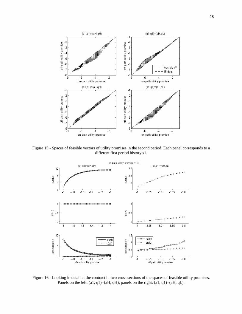
43
Figure 15 - Spaces of feasible vectors of utility promises in the second period. Each panel corresponds to a
different first period history s1.
Figure 16 - Looking in detail at the contract in two cross sections of the spaces of feasible utility promises.
Panels on the left: (a1, q1)=(aH, qH); panels on the right: (a1, q1)=(aH, qL).
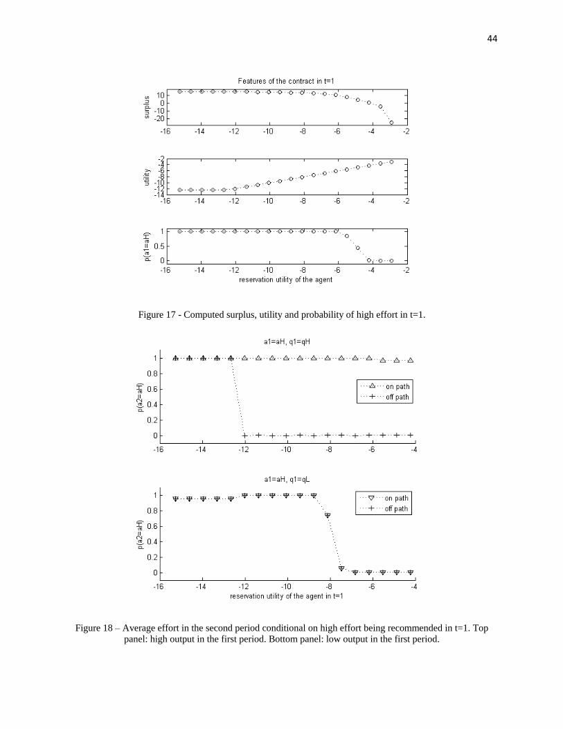
44
Figure 17 - Computed surplus, utility and probability of high effort in t=1.
Figure 18 – Average effort in the second period conditional on high effort being recommended in t=1. Top
panel: high output in the first period. Bottom panel: low output in the first period.

45
Figure 19 – Incentive contraint in t=1 (top) and decomposition of the incentive constraint in t=1 (bottom).
Figure 20 - Future utility promises conditional on q1, when high effort is recommended in the first period.
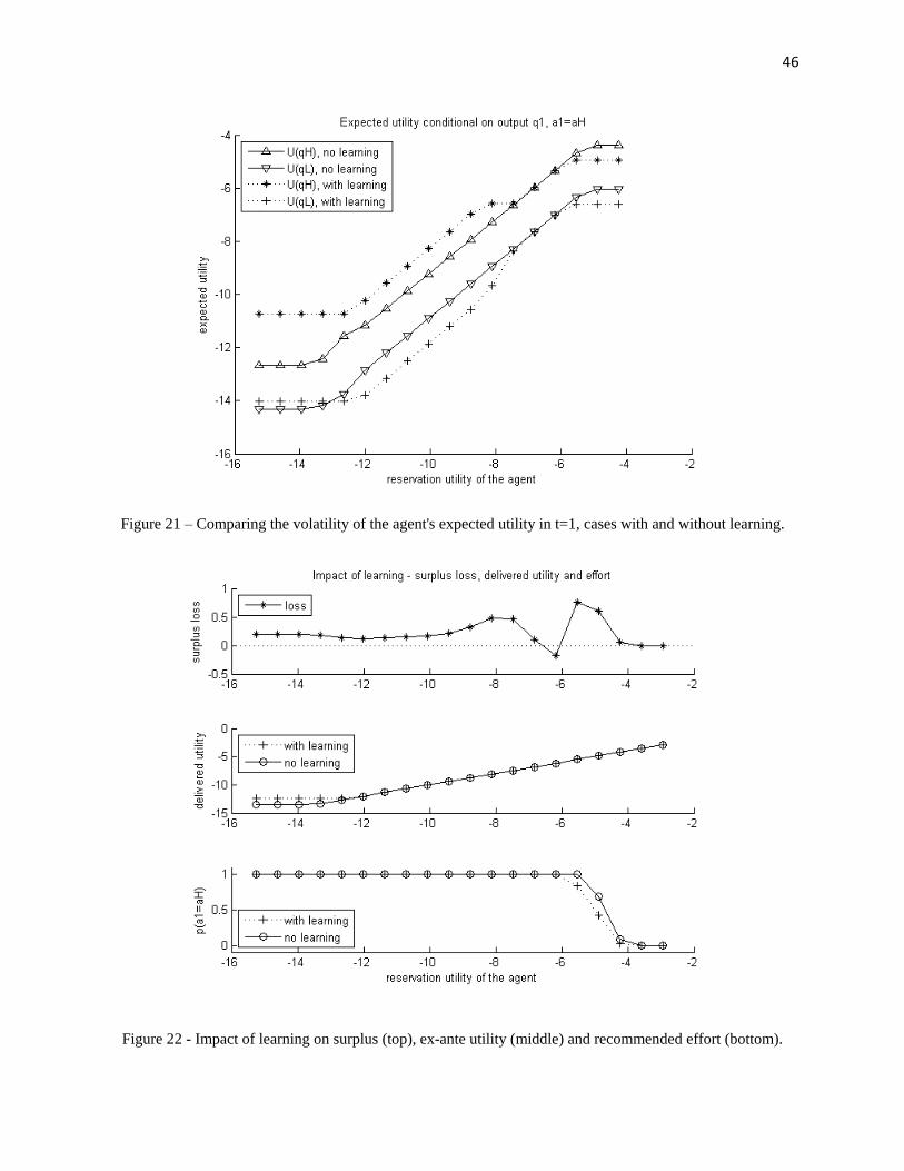
46
Figure 21 – Comparing the volatility of the agent's expected utility in t=1, cases with and without learning.
Figure 22 - Impact of learning on surplus (top), ex-ante utility (middle) and recommended effort (bottom).