Embed Size (px)
Citation preview

DEPARTAMENTO DE
ENGENHARIA MECÂNICA
Simulação Numérica do Processo de
Estampagem de Placas Bipolares Metálicas Dissertação apresentada para a obtenção do grau de Mestre em Engenharia Mecânica na Especialidade de Produção e Projeto
Numerical Simulation of the Stamping Process
of Metallic Bipolar Plates
Autor
Nicolas Marques
Orientador
Diogo Mariano Simões Neto
Júri
Presidente Professor Doutor Luís Filipe Martins Menezes
Professor Catedrático da Universidade de Coimbra
Vogal Professora Doutora Marta Cristina Cardoso de Oliveira Professora Auxiliar da Universidade de Coimbra
Orientador Professor Doutor Diogo Mariano Simões Neto
Professor Convidado da Universidade de Coimbra
Coimbra, Julho, 2016


“I never lose, I either win or learn”
Unknown.


Acknowledgments
Nicolas Marques iii
Acknowledgments
This work as well as my engineering degree would not be possible without the help
and support of my family, my friends and the teachers who supported me through this
educational path.
First and foremost, I want to express my gratitude to my scientific advisor Professor
Diogo Mariano Simões Neto for all the support and guidance during this work. It has been a
privilege to work with a professor with such dedication to his students and insightful
suggestions. Thank you for the knowledge transmitted during this work as well as the sincere
friendship. I am also grateful for the help from Professor Marta Cristina Oliveira Cardoso
and Professor Luís Filipe Martins Menezes on some difficulties encountered in this work.
Secondly, I want to thank especially my good friend Mariana Moura for putting up
with me for all these years of my mechanical engineering degree, always helping me when
needed and for being by my side. Her tips and suggestions for this work have the most
deserved recognition. I greatly appreciate the encouragement and friendship.
I would like to thank my friend António Camilo for proofreading and providing me
with helpful feedback on this work. I want to thank for the continued friendship.
I want to thank my colleagues and friends from all these years, namely Hugo Matos,
André Brás, Diana Almeida, André Travassos, Vânia Sousa, Diogo da Silva and Francisco
Brito. To my friend Adrian de Francisco back in Switzerland for never forgetting me and
always keeping in touch, I want to thank for all the good memories back in the days.
Finally, I want to thank my family for their unconditional love and support, namely
my parents without whom this life would never be possible and for always believing in me
all these years. A huge thanks to my godparents and cousin back in Switzerland for always
encouraging me and for all the support along all these years.
This work was carried out under the project “Improving the manufacturing of metallic
bipolar plates for fuel cells using the rubber forming process” with reference PTDC/EMS-
TEC/0702/2014, co-funded by the Foundation for Science and Technology and the
EU/FEDER, through the program COMPETE2020 with reference POCI-01-0145-FEDER-
016779.

Numerical Simulation of the Stamping Process of Metallic Bipolar Plates
iv 2016

Resumo
Nicolas Marques v
Resumo
Uma placa bipolar é um dos principais componentes de uma célula de combustível,
que é considerada como uma fonte de energia com elevado potencial para transporte e
aplicações portáteis.
O principal objetivo deste trabalho é a otimização do processo de estampagem de
placas bipolares metálicas, usando simulações numéricas do processo de conformação. As
simulações numéricas apresentadas neste estudo foram realizadas com o programa de
elementos finitos DD3IMP.
A geometria do canal de escoamento tem uma grande influência sobre a formabilidade
obtida durante o processo de estampagem. Sendo assim, o objectivo deste trabalho é o de
estudar as diferentes variáveis geométricas, a fim de optimizar as dimensões do canal de
escoamento. Deste modo, é criado um modelo paramétrico em CAD contendo a geometria
das ferramentas de estampagem, que é posteriormente utilizado na simulação numérica com
o método dos elementos finitos. Devido à grande complexidade geométrica de uma placa
bipolar, são criados modelos simplificados, de diferentes zonas representativas. Cada zona
representativa destina-se a estudar uma região diferente da placa bipolar. cobrindo todo o
comportamento de deformação encontrado na placa. Assim, é utilizada uma simples análise
2D para avaliar a secção transversal do canal da placa bipolar, enquanto que é necessária
uma análise 3D para estudar a secção curva do canal de escoamento. Em seguida, é estudado
o material da chapa com uma comparação entre três ligas diferentes, SS 304, Al 5042 e Al
1235. Uma vez que o processo de estampagem influencia os resultados obtidos para a
conformabilidade da chapa, é realizado um estudo entre microestampagem e
hidroconformação.
Os resultados numéricos mostram que o aumento do raio principal, da largura do canal
e a diminuição da profundidade do canal, do raio de curvatura do raio adicionado e da secção
plana do canal, a formabilidade da chapa é melhorada. As áreas críticas das placas metálicas
estampadas correspondem às zonas de curvatura dos canais de escoamento sobre o raio
correspondente. Tanto o aço inoxidável SS 304 como a liga de alumínio Al 1235

Numerical Simulation of the Stamping Process of Metallic Bipolar Plates
vi 2016
demonstram boa formabilidade e o processo microestampagem tem um melhor resultado em
comparação com a hidroconformação.
Palavras-chave: Células de Combustível, Modelo de Elementos Finitos, Placa Bipolar Metálica, Microestampagem e Hidrocomformação, Optimização de Geometria.

Abstract
Nicolas Marques vii
Abstract
A bipolar plate is one of the key components of proton exchange membrane fuel cells,
which are considered as potential power sources for transportation and portable applications.
The main objective of this work is the optimization of the stamping process of metallic
bipolar plates, using the finite element simulation of the forming process. The numerical
simulations presented in this study were carried out with the in-house finite element code
DD3IMP.
The geometry of the flow channel has a large influence on the formability during the
stamping process. Therefore, the aim of the study is to study the different geometrical
variables in order to optimize the flow channel dimensions. Accordingly, a parametric CAD
model containing the stamping tools’ geometry is created, which is posteriorly used in the
simulation with the finite element method. Due to the large complexity of a bipolar plate, a
simplified model with different representative zones is created. Each representative zone
aims to study a different region of the bipolar plate. covering the entire deformation
behaviour found in the plate. Thus, a simple 2D analysis is used to evaluate the straight
channel section of the bipolar plate, while a 3D analysis is required to study the curved
section of the flow channel. Afterwards, the material of the blank is studied with a
comparison between three different alloys, SS 304, Al 5042 and Al 1235. Since the stamping
process influences the results obtained for the formability of the blank, a study between
microstamping and hydroforming is performed.
The numerical results shown that increasing the main radius, the channel width and
the rib width and diminishing the channel depth, the fillet radius and the flat section the
formability of the blank is improved. The critical areas of the stamped metallic plates are on
the curved flow channels on the correspondent fillet radius. Both the stainless steel SS 304
and the aluminium alloy Al 1235 demonstrate good formability and the microstamping
process has an improved result compared with hydroforming in terms of formability.
Keywords PEM Fuel Cell, Finite Element Model, Metallic Bipolar Plate, Flow Channel, Microstamping and Hydroforming, Geometry Optimization.

Numerical Simulation of the Stamping Process of Metallic Bipolar Plates
viii 2016

Table of Contents
Nicolas Marques ix
Table of Contents
List of Figures ....................................................................................................................... xi
List of Tables ....................................................................................................................... xv
Symbols and Acronyms ..................................................................................................... xvii Variables and Symbols .................................................................................................. xvii Acronyms ...................................................................................................................... xvii
1. INTRODUCTION ......................................................................................................... 1 1.1. Fuel Cells ................................................................................................................ 1 1.2. Bipolar Plates .......................................................................................................... 3
1.3. Objectives of the Study and Outline ....................................................................... 4
2. REVIEW ON METALLIC BIPOLAR PLATES .......................................................... 7 2.1. Flow Field Design ................................................................................................... 7 2.2. Materials ............................................................................................................... 11
2.3. Forming Process ................................................................................................... 12 2.3.1. Influence of the main process parameters ..................................................... 14
3. FINITE ELEMENT SIMULATION ........................................................................... 17 3.1. Materials ............................................................................................................... 18 3.2. Boundary Conditions ............................................................................................ 20
3.3. Parametric Model .................................................................................................. 23
3.4. Stamping ............................................................................................................... 27 3.4.1. Influence of the finite element size................................................................ 28 3.4.2. Influence of the boundary conditions ............................................................ 29
3.4.3. Primary optimization ..................................................................................... 30 3.4.4. Influence of tool geometry parameters .......................................................... 37
3.4.5. Comparison between Al 1235 and SS304 ..................................................... 47 3.4.6. Study of the curved channel section .............................................................. 48
3.5. Hydroforming ....................................................................................................... 51 3.6. Results and Discussion ......................................................................................... 55
4. CONCLUSIONS ......................................................................................................... 57
5. REFERENCES ............................................................................................................ 61
APPENDIX A ..................................................................................................................... 65
APPENDIX B ...................................................................................................................... 69

Numerical Simulation of the Stamping Process of Metallic Bipolar Plates
x 2016

List of Figures
Nicolas Marques xi
LIST OF FIGURES
Figure 1.1. Proton exchange membrane fuel cell (PEMFC) assembly (Mahabunphachai et
al., 2010). ................................................................................................................. 2
Figure 1.2. Schematic of a PEM fuel cell (Peng et al., 2014). .............................................. 3
Figure 1.3. Structure of a bipolar plate (a) Top view, (b) Cross Section A-A. ..................... 3
Figure 2.1. Pin-type flow field: (a) Schematic diagram, (b) Results from experimental
hydroforming (Belali-Owsia et al., 2014). .............................................................. 7
Figure 2.2. Series-parallel flow field: (a) Schematic diagram, (b) stamping die set and sheet
(Zhou and Chen, 2015). ........................................................................................... 8
Figure 2.3. Wavelike flow field: (a) Schematic diagram, (b) Previous study (Zhou and
Chen, 2015). ............................................................................................................ 9
Figure 2.4. Serpentine flow field: (a) Schematic diagram, (b) Simulation. .......................... 9
Figure 2.5. Serially linked serpentine flow field (Li and Sabir, 2005). ............................... 10
Figure 2.6. Interdigitated flow field: (a) Schematic diagram, (b) CAD model (Peng et al.,
2014). ..................................................................................................................... 11
Figure 2.7. Representation of a microstamping process (Peng et al., 2014). ...................... 12
Figure 2.8. Representation of a hydroforming process. ...................................................... 12
Figure 2.9. Rubber pad forming: (a) Schematic diagram, (b) Simulation results (Liu et al.,
2010). ..................................................................................................................... 13
Figure 2.10. Representation of tools’ dimensions. .............................................................. 13
Figure 3.1. Stress-strain behaviour for different metals (Smith et al., 2014). Note:
error on the units for the strain. ............................................................................. 18
Figure 3.2. Stress-strain behaviour of the metals studied...................................... 20
Figure 3.3. Representation of a serpentine flow field indicating the selected zones
analysed. ................................................................................................................ 21
Figure 3.4. Representation of the boundary conditions for section 1. ................................. 22
Figure 3.5. Representation of the boundary conditions for section 3. ................................. 22
Figure 3.6. Parametric model for the final geometry of the tools. ...................................... 24
Figure 3.7. Tools’ geometry on CATIA® V5: (a) Straight channel, (b) Curved section. ... 24
Figure 3.8. Orientation of the surfaces representing the tools geometry ............................. 25
Figure 3.9. Mesh representation for the die (a) Before being smoothed, (b) After being
smoothed. .............................................................................................................. 25
Figure 3.10. Die’s geometry and dimension necessary to obtain the shape error. .............. 26

Numerical Simulation of the Stamping Process of Metallic Bipolar Plates
xii 2016
Figure 3.11. Finite element mesh generation in detail: (a) 2D simulation, (b) 3D
simulation. ............................................................................................................. 27
Figure 3.12. Final thickness distribution in function of the number of finite elements along
the blank’s thickness. ............................................................................................ 28
Figure 3.13. Punch force evolution in function of the number of elements along the blank’s
thickness. ............................................................................................................... 29
Figure 3.14. Final thickness distribution for simulations with different boundary conditions
and for a ten channel simplified model. ................................................................ 29
Figure 3.15. Plastic strain distribution for the geometry from Son et al. (2012) for a
thickness of 0.2 mm (Al 5042). ............................................................................. 30
Figure 3.16. Plastic strain for the geometry from Son et al. (2012) for a thickness of 0.1
mm (Al 5042). ....................................................................................................... 31
Figure 3.17. Punch force evolution for a thickness of 0.1 mm and 0.2 mm (Al 5042),
considering the geometry from Son et al. (2012). ................................................. 31
Figure 3.18. Contact forces (a) Before the final contact, (b) During the final contact. ...... 32
Figure 3.19. Plastic strain distribution for the geometry from Son et al. (2012) for a
thickness of 0.1 mm (SS 304). .............................................................................. 32
Figure 3.20. Punch force evolution for two different materials (Al 5042 and SS 304)
considering the geometry from Son et al. (2012). ................................................. 33
Figure 3.21. Plastic strain distribution for an increase in channel and rib width considering
a thickness of 0.1 mm (SS 304). ........................................................................... 33
Figure 3.22. Plastic strain distribution for a geometry without a straight section for a
thickness of 0.1 mm (SS 304). .............................................................................. 34
Figure 3.23. Plastic strain and thickness reduction for the new geometry for a thickness of
0.1 mm (SS 304). .................................................................................................. 35
Figure 3.24. Punch force evolution for the new geometry for a thickness of 0.1 mm (SS
304). ...................................................................................................................... 35
Figure 3.25. Representation of a PEMFC with the new geometry. .................................... 35
Figure 3.26. Plastic strain distribution for the bipolar plate geometry with 79% efficiency
for a thickness of 0.1 mm (SS 304). ...................................................................... 36
Figure 3.27. Die geometry (a) Channel depth of 0.3 mm, (b) Channel depth of 0.65 mm. 37
Figure 3.28. Maximum thickness reduction in function of the channel depth. ................... 38
Figure 3.29. Influence of channel depth on: (a) Final thickness, (b) Punch force evolution.
............................................................................................................................... 38
Figure 3.30. Die geometry: (a) Fillet radius of 0.8 mm, (b) Fillet radius of 1.5 mm. ......... 39
Figure 3.31. Influence of the fillet radius, R: (a) Maximum value of thickness reduction, (b)
Final thickness distribution. .................................................................................. 40
Figure 3.32. Die geometry: (a) Main radius of 0.2 mm, (b) Main radius of 0.55 mm. ....... 41
List of Figures
Nicolas Marques xiii
Figure 3.33. Influence of the main radius, r: (a) Maximum thickness reduction, (b) Overall
thickness distribution. ............................................................................................ 41
Figure 3.34. Equivalent draft angle, α, for the new geometry with an added fillet radius. . 42
Figure 3.35. Plastic strain and thickness: (a) Primary Geometry, (b) Optimized Geometry.
............................................................................................................................... 42
Figure 3.36. Die geometry: (a) Channel and rib width of 3.4 mm, (b) Channel and rib width
of 1.2 mm. ............................................................................................................. 43
Figure 3.37. Influence of the channel and rib width: (a) Thickness reduction, (b) Overall
thickness distribution. ............................................................................................ 44
Figure 3.38. Die geometry: (a) Flat section of 0.2 mm, (b) Flat section of 0.6 mm. .......... 45
Figure 3.39. Influence of the flat section, a: (a) Thickness reduction, (b) Overall thickness
distribution............................................................................................................. 45
Figure 3.40. Plastic Strain distribution: (a) Initial thickness of 0.05 mm, (b) Initial
thickness of 0.25 mm............................................................................................. 46
Figure 3.41. Thickness reduction in function on the blank’s initial thickness. ................... 46
Figure 3.42. Influence of the blank’s initial thickness, t: (a) Overall thickness distribution,
(b) Punch force evolution. ..................................................................................... 47
Figure 3.43. Thickness distribution for stainless steel and aluminium blanks. ................... 48
Figure 3.44. Punch force evolution for stainless steel and aluminium blanks. ................... 48
Figure 3.45. Thickness reduction for 2D and 3D simulations. ............................................ 49
Figure 3.46. Plastic strain distribution: (a) 2D simulation, (b) 3D simulation. ................... 49
Figure 3.47. (a) Progressive mesh, (b) Plastic strain distribution for the curved section with
the straight channel. ............................................................................................... 50
Figure 3.48. Final thickness for the curved section with and without the straight channel. 51
Figure 3.49. Plastic strain distribution for (a) Hydroforming with p = 50 MPa, (b)
Hydroforming with p = 400 MPa. ......................................................................... 52
Figure 3.50. Thickness reduction for hydroforming with pressure from p = 50 MPa to p =
400 MPa. ............................................................................................................... 53
Figure 3.51. Thickness distribution for hydroforming for pressures from 50 MPa to 400
MPa. ...................................................................................................................... 53
Figure 3.52. Die geometry (a) Symmetric optimal geometry for microstamping, (b)
Hydroforming geometry. ....................................................................................... 54
Figure 3.53. Plastic strain for a pressure of 250 MPa for hydroforming: (a) Symmetric
Geometry, (b) New Geometry. .............................................................................. 54
Figure 3.54. Thickness distribution for hydroforming and microstamping. ....................... 55
Figure 3.55. Stress values for rubber pad forming process (Liu et al., 2010). .................... 55
Figure 3.56. Stress values: (a) fully constrained finite element model, (b) free on one
extremity finite element model.............................................................................. 56

Numerical Simulation of the Stamping Process of Metallic Bipolar Plates
xiv 2016
Figure 3.57. Plastic strain: (a) fully constrained finite element model, (b) free on one
extremity finite element model. ............................................................................ 56

List of Tables
Nicolas Marques xv
LIST OF TABLES
Table 2.1. Summary on blank thickness used for metallic bipolar plates. .......................... 14
Table 2.2. Summary on fillet radiuses used for metallic bipolar plates. ............................. 15
Table 2.3. Summary on channel depths used for metallic bipolar plates. ........................... 16
Table 3.1. Voce’s hardening law parameters and elastic properties for Al 5042 with a
blank’s initial thickness of 0.2083 mm. ................................................................ 19
Table 3.2. Swift’s hardening law parameters and elastic properties for Al 1235 (Hadi,
2014) and SS 304 (Liu et al., 2010) with a blank’s initial thickness of 0.1 mm. .. 19
Table 3.3. Tool’s geometrical dimensions for Al 5042 (Son et al., 2012). ......................... 30
Table 3.4. Tool’s geometrical dimensions for an optimized geometry (SS 304). ............... 34
Table 3.5. Tool’s geometrical dimensions for a chemical efficiency of 79% (SS 304). ..... 36
Table 3.6. Tool’s geometrical dimensions for the study on the channel depth (SS 304). ... 37
Table 3.7. Tool’s geometrical dimensions for the study on the afillet radius (SS 304). ..... 39
Table 3.8. Tool’s geometrical dimensions for the study on the main radius (SS 304). ...... 40
Table 3.9. Tool’s geometrical dimensions for the study on the channel and rib width (SS
304). ....................................................................................................................... 43
Table 3.10. Tool’s geometrical dimensions for the study on the flat section (SS 304). ...... 44
Table 3.11. Tool’s geometrical dimensions for the study on blank’s initial thickness (SS
304). ....................................................................................................................... 46
Table 3.12. Tool’s geometrical dimensions for the study of hydroforming (SS 304). ........ 52

Numerical Simulation of the Stamping Process of Metallic Bipolar Plates
xvi 2016

Symbols and Acronyms
Nicolas Marques xvii
SYMBOLS AND ACRONYMS
Variables and Symbols
ℎ – Channel depth
𝐸 – Young’s Modulus
𝑅 – Fillet radius
𝑌, 0 , p , 𝐾 , 𝑛 – Constitutive parameter of Swift’s hardening law
𝑌, 𝑌0, Cy, 𝑌sat – Constitutive parameter of Voce’s hardening law
𝑟 – Main radius
𝑠 – Rib width
𝑡 – Blank thickness
𝑤 – Channel width
𝛼 – Draft angle
𝜈 – Poisson’s ratio
Acronyms
2D – Two Dimensional
3D – Three Dimensional
AFC – Alkaline Fuel Cells
Al – Aluminum
BPP – Bipolar Plate
CAD – Computer Aided Design
DD3IMP – Deep Drawing 3D IMPlicit finite element code
FE – Finite Element
IGES – Initial Graphics Exchange Specification
MCFC – Molten Carbonate Fuel Cells
PAFC – Phosphoric Acid Fuel Cells

Numerical Simulation of the Stamping Process of Metallic Bipolar Plates
xviii 2016
PEM – Polymer Electrolyte Membrane
SOFC – Solid Oxide Fuel Cells
SS – Stainless Steel

INTRODUCTION
1. INTRODUCTION
In the last decades there has been an increasing concern about environmental
consequences on the use of fossil fuel for electricity production and vehicle propulsion. The
dependence on oil became apparent during oil crises, but more importantly is the increase in
global awareness of environmental consequences. Sustainable energy became important
with the increase in population since common sources of energy have poisonous emissions
into the atmosphere (Carrette et al., 2001).
In order to reduce the dependence on fossil fuels and diminish poisonous emissions,
renewable energy from wind, water and sun are already implemented. Nevertheless, these
sources are irregularly available, thus not being suited to cover all electrical needs (Carrette
et al., 2001).
An option for future power generations are fuel cells, which use pure hydrogen and
produce only water, eliminating all local emissions. Fuel cells have higher electrical
efficiencies compared to heat engines and in combination with renewable energy it may be
suited for sustainable energy generation (Carrette et al., 2001).
Fuel cells are dated to as long as 1839 but no practical use was found until the 1950s
(Wang et al., 2011).
1.1. Fuel Cells
Fuel cells are electrochemical devices that convert chemical energy stored in fuels into
electrical energy. The attention on this technology is mainly due to their high efficiency
(60% in electrical energy conversion) and low emissions, which are interesting for
transportation and portable applications (Mahabunphachai et al., 2010). The fuel cells can
be categorised in five main categories: polymer electrolyte membrane (PEM) fuel cells, solid
oxide fuel cells (SOFC), alkaline fuel cells (AFC), phosphoric acid fuel cells (PAFC) and
molten carbonate fuel cells (MCFC). For transportation and portable applications, PEM fuel
cells are promising candidates since they gather the most important characteristics for such
applications (Wang et al., 2011).

Numerical Simulation of the Stamping Process of Metallic Bipolar Plates
2 2016
Figure 1.1. Proton exchange membrane fuel cell (PEMFC) assembly (Mahabunphachai et al., 2010).
Fuel cells are composed by different components assembled in stacks as shown in
Figure 1.1. Each PEMFC stack consists of a membrane electrode assembly and bipolar plates
(Peng et al., 2014). As shown in Figure 1.2, hydrogen gas enters in contact with the anode
where it is adsorbed onto the catalyst surface. Each hydrogen atom then loses an electron
which flows to the cathode as current through an external circuit. The remaining hydrogen
protons flow across de membrane towards the cathode where they enter in contact with air,
which is previously fed to the fuel cell, and the initial electrons to form water, which is then
forced to exit the fuel cell (Holton and Stevenson, 2013). The membranes on PEM fuel cells
are made notably in Nafion® (Wang et al. 2011).
Although fuel cells look promising, the commercialization is still restricted due to the
high cost compared with other sources of energy such as internal combustion engines.
Comparing the prices of these two forms of energy, the fuel cell power is still 4-10 times
more expensive as compared to internal combustion engines. The cost of fuel cells is around
$200-300 per kW while other regular engines cost around $30-50 per kW. Since the bipolar
plates on the fuel cells represent around 35-45% of their cost, it becomes important to have
the price reduced on such plates to improve the commercialization of this technology
(Mahabunphachai et al., 2010).

INTRODUCTION
Figure 1.2. Schematic of a PEM fuel cell (Peng et al., 2014).
1.2. Bipolar Plates
Bipolar plates have an important role on fuel cell stacks. They provide structural
support for the mechanically weak membranes, manage the supply of reactant gases trough
flow channels (see Figure 1.3), improve heat management with a coolant and electrically
connect two cells together in the stack (Peng et al., 2014).
(a) (b)
Figure 1.3. Structure of a bipolar plate (a) Top view, (b) Cross Section A-A.

Numerical Simulation of the Stamping Process of Metallic Bipolar Plates
4 2016
The configuration presented in Figure 1.3 consists of two metallic plates welded
together creating the bipolar plate. This configuration repeats along the stack. The reactants
flow on one side of the plate while the cooling fluid flows on the other side of the same plate
to remove the heat generated by the chemical reaction (Li and Sabir, 2005).
Many materials can be used for manufacturing bipolar plates such as graphite, stainless
steel, aluminium and titanium. However, for portable applications, metallic plates are
preferred due to a much superior manufacturability and higher mechanical strength (Peng et
al., 2014). This topic will be reviewed in depth on section 2.2. The conventional
manufacturing processes used for graphite cannot be applied in metallic bipolar plates.
Forming processes such as microstamping, hydroforming and rubber pad forming are more
adequate to such plates and will be discussed on section 2.3 (Peng et al., 2014).
1.3. Objectives of the Study and Outline
The main objective of this study is to optimize the stamping process used to
manufacture metallic bipolar plates. The finite element method is adopted to perform the
numerical simulations of the forming process, requiring the development of several models.
First, the preliminary results are compared with previous studies of other authors in order to
validate the numerical model. The optimization of the tool’s geometry demands a parametric
model able to easily create the finite element model for each geometry. Then, the influence
of the different geometrical parameters of the channel are analysed, namely the channel
depth, rib and channel width, fillet radius and the blank’s initial thickness. Besides, the
behaviour of different materials is evaluated regarding its utilization in the manufacture of
bipolar plates. Finally, the comparison between stamping and hydroforming is performed to
verify the influence of the forming process on the formability.
This dissertation is organized into four main chapters. For a better understanding and
to improve the readability, this section briefly summarizes the content on each chapter.
Chapter 1 presents the introduction on the subject of the study with a brief
description of different existing fuel cells and the basic chemical functioning.
The importance of the bipolar plates and the requirements for portable
applications are explained, highlighting further improvements required for an
effective commercialization. Thus defining the objectives for this dissertation.

INTRODUCTION
Chapter 2 summarizes the study on metallic bipolar plates achieved on recent
years with a main focus on the flow field design, the materials used and the
most used forming processes. It presents a summary on different channel
dimensions previously used, either for mechanical or chemical optimization.
Chapter 3 presents the numerical study concerning the forming of bipolar plates,
considering different tool geometries, materials for the plate and forming
processes. The finite element model is described along with every step of the
process from tool’s creation, finite element mesh generation to the simulation
itself. The materials used are described with a focus on aluminium and stainless
steel. The boundary conditions adopted are described as well as the number of
finite elements required for accurate simulation results. Each parameter of the
tool’s geometry is studied individually to evaluate their influence and a
comparison between different forming processes is performed. The results
obtained for this study are briefly compared with previous studies to evaluate
the performance of the optimized geometry.
Chapter 4 contains the main conclusions withdrawn from the study presented on
previous chapters.

Numerical Simulation of the Stamping Process of Metallic Bipolar Plates
6 2016

REVIEW ON METALLIC BIPOLAR PLATES
2. REVIEW ON METALLIC BIPOLAR PLATES
This section contains a review about the metallic bipolar plates used in fuel cells,
focusing in the recent progresses in terms of flow field design, materials and different
manufacturing processes.
For the last 20 years, metallic bipolar plates have been developed and experienced, but
improvements have yet to be made for successful commercialization (Peng et al., 2014).
2.1. Flow Field Design
The function of the flow channels in the fuel cells is to provide reactant gases to the
electrolytic membrane and to provide cooling to the fuel cell through a cooling fluid. Several
flow field designs have been studied and improved for traditional graphite bipolar plates but
most of them cannot be applied to stamped metallic plates. For metallic bipolar plates there
are four main types of flow field designs (Peng et al., 2014):
1. Pin-type flow field,
2. Series-parallel flow field,
3. Serpentine flow field,
4. Interdigitated flow field.
(a) (b)
Figure 2.1. Pin-type flow field: (a) Schematic diagram, (b) Results from experimental hydroforming (Belali-Owsia et al., 2014).

Numerical Simulation of the Stamping Process of Metallic Bipolar Plates
8 2016
The pin-type flow field consists of multiple pins along the plate arranged in a regular
pattern. These pins can present a cubic or rounded shape as shown in Figure 2.1. This flow
field is considered to achieve the best results according to the principle of least resistance
regarding the reactant gases flow. However, it leads to an inhomogeneous gas distribution
along the plate and can have an insufficient product water removal. This flow field is best
used for high reactant flows but with lower utilization levels of fuel and oxygen (A.Heinzzel
et al. 2009).
(a) (b)
Figure 2.2. Series-parallel flow field: (a) Schematic diagram, (b) stamping die set and sheet (Zhou and Chen, 2015).
Parallel flow fields (see pattern in Figure 2.2) can be used when there is no
accumulation of water droplets. If droplets are formed, some channels may become blocked
and the remaining gas will flow through the remaining channels creating an uneven gas
distribution (A.Heinzzel et al. 2009).
Regarding the stamping process of the metallic sheets with this kind of geometry,
straight channels can originate excessive springback after stamping, as shown in Figure 2.2
(b). In order to avoid this defect, wavelike flow fields can be applied, which are presented in
see Figure 2.3.

REVIEW ON METALLIC BIPOLAR PLATES
(a) (b)
Figure 2.3. Wavelike flow field: (a) Schematic diagram, (b) Previous study (Zhou and Chen, 2015).
Serpentine flow fields (see pattern in Figure 2.4) are the most used due to the large
length of the path (A.Heinzzel et al. 2009). This flow field presents the best gas distribution
compared with the straight parallel pattern and better performance for current density and
temperature distribution (Peng et al., 2014).
(a) (b)
Figure 2.4. Serpentine flow field: (a) Schematic diagram, (b) Simulation.
The basic serpentine flow field has the disadvantage of creating an excessive pressure
drop from the two ends of the plate due to the extended length of the channel. This excessive
pressure drop can originate a reactant gas short circuiting instead of the desired flow through
the full length of the channel. One way to overcome this problem is to modify the design as
illustrated in Figure 2.5, where the channels are subdivided into different segments. Each

Numerical Simulation of the Stamping Process of Metallic Bipolar Plates
10 2016
segment has its own serpentine configuration with much shorter lengths. This solution results
in an inferior pressure drop (Li and Sabir, 2005).
(a) (b)
Figure 2.5. Serially linked serpentine flow field (Li and Sabir, 2005).
Metallic bipolar plates use cooling flows on the opposite side of the plate, while the
graphite plates use a separate cooling plate. Since the flow channels are produced by
machining on graphite plates, distinct flow field configurations can be obtained for each side
of the plate. However, metallic plates are typically manufactured by stamping processes,
where the configuration of a flow field on one side of the plate determines directly the
configuration on the opposite side. Therefore, it becomes difficult to obtain two continuous
flow fields on both sides of the plate. For example, regarding the serpentine configuration
presented in Figure 2.4 (a), the reactant flow is represented by the channel in white and the
coolant flow is represented by the dark colour. Accordingly, the dark flow field is not
continuous, as highlighted in Figure 2.4 (a). This problem can be solved using interdigitated
flow plates as shown in Figure 2.6. In this case the reactant gas flow field is not continuous
(see Figure 2.6.), hence the fluid is forced to flow through adjacent layers. Adapting this
strategy on stamped metallic plates, the dark channel in Figure 2.6. (a) is continuous which
improves the cooling flow.
The interdigitated flow field has been shown to improve fuel cells efficiency, however,
only at the cost of a high pressure drop (Hu et al., 2009).

REVIEW ON METALLIC BIPOLAR PLATES
(a) (b)
Figure 2.6. Interdigitated flow field: (a) Schematic diagram, (b) CAD model (Peng et al., 2014).
2.2. Materials
The main material used for bipolar plates is graphite (Yoon et al., 2008). It offers good
electrical conductivity, high corrosion resistance and low interfacial contact resistance.
However, the cost of graphite plates is high due to their poor manufacturability and it has
the disadvantage of being brittle and having poor permeability, which forces the use of
thicker plates. In order to decrease the cost of fuel cells, metallic bipolar plates have received
much attention lately, due to a much superior manufacturability, higher mechanical strength,
being non permeable and more durable when submitted to shock and vibration, which is
important when used for portable applications and transport (Peng et al., 2014).
The main handicap on metallic plates is the corrosion, which occurs in the acidic and
humid environment present in a fuel cell. Some solutions for preventing metal degradation
consist on using noble metals, stainless steels, aluminium alloys, titanium and nickel as a
base metal and coating materials to prevent the corrosion on the base metal. Bipolar plates
crafted with noble metals can achieve the performance of graphite plates or even higher but
there is a large cost associated, which limits their commercialization. Cost wise, either the
stainless steel or the aluminium plates are promising along with the correct coatings (Tawfik
et al., 2007).

Numerical Simulation of the Stamping Process of Metallic Bipolar Plates
12 2016
2.3. Forming Process
There are three main forming processes that can be applied in the manufacturing of
metallic bipolar plates, namely:
Microstamping;
Hydroforming;
Rubber pad forming.
The microstamping satisfies the requirements needed for bipolar plates manufacturing
in terms of precision, production rate and cost effectiveness. In this process, expensive dies
with adequate geometry are used to deform a thin sheet of metal as shown in Figure 2.7
(Peng et al., 2014).
Figure 2.7. Representation of a microstamping process (Peng et al., 2014).
The hydroforming process is based on the application of a pressurized fluid which
pushes the metal blank into a cavity with the desired shape. The schematic representation of
this process is shown in Figure 2.8, where the fluid is represented in orange. This forming
process allows to obtain higher drawing ratios, better surface quality and induces less
springback in comparison with microstamping (Peng et al., 2014).
Figure 2.8. Representation of a hydroforming process.

REVIEW ON METALLIC BIPOLAR PLATES
Rubber pad forming is a process that has been growing in the automotive industry (Liu
et al., 2010). It only requires the manufacture of one rigid die since the second one is replaced
by a rubber pad as shown in Figure 2.9. This method, allows to improve the quality obtained
and since only one die needs to be accurately manufactured, the cost and time can be greatly
reduced. Furthermore, the tools assembly is not required to be precise. The adoption of a
rubber pad as tool provides a contact force more distributed along the metal sheet, improving
the formability (Liu et al., 2010).
(a) (b)
Figure 2.9. Rubber pad forming: (a) Schematic diagram, (b) Simulation results (Liu et al., 2010).
The formability is influenced by the adopted sheet metal forming process, but the
channel design should also be taken into consideration. In addition, the channel dimension
design also has an important impact on the fuel cell performance since it influences the water
and reactant transport as well as the reactant utilization efficiency (Peng et al., 2014).
Various parameters have influence on the stamping process such as the channel depth,
h, the width of the channel, w, the width of the rib, s, the draft angle, α, the fillet radius, R of
the tools and the blank thickness, t (Liu et al., 2010). The channel dimension design can be
seen in Figure 2.10.
Figure 2.10. Representation of tools’ dimensions.

Numerical Simulation of the Stamping Process of Metallic Bipolar Plates
14 2016
The thickness of the blank used in the bipolar plates ranges between 0.051 mm and 0.3
mm depending on the blank’s material, as shown in Table 2.2. Blanks with an initial
thickness of 0.1 mm are widely used for stainless steel. In fact, using stainless steel, the
thickness can be reduced to 0.1 mm and still maintain sufficient mechanical strength (Park
et al., 2016). Aluminium bipolar plates with higher initial thickness were also studied by
other authors.
Table 2.1. Summary on blank thickness used for metallic bipolar plates.
Blank Initial Thickness, t (mm) Material References
0.051 SS 304, SS 316 (Mahabunphachai et al., 2010)
0.1 SS 304, SS 316 (Liu and Hua, 2010)
(Park et al., 2016)
(Zhou and Chen, 2015)
(Liu and Hua, 2010)
(Liu et al., 2010)
(Yi et al., 2015)
(Peng et al., 2014)
0.2 SS 316 (Yi et al., 2015)
0.2 Al 1050 (Son et al., 2012)
0.3 Al 1050 (Son et al., 2012)
2.3.1. Influence of the main process parameters
The fillet radius, R, represented in the Figure 2.10, can influence the stamping results,
improving the formability with its increase. Several authors include this parameter in their
analysis for fuel cell efficiency (Peng et al., 2014). A summary on the fillet radius values
used in metallic bipolar plates can be seen in Table 2.2. It ranges between 0.1 mm and 0.5
mm.
REVIEW ON METALLIC BIPOLAR PLATES
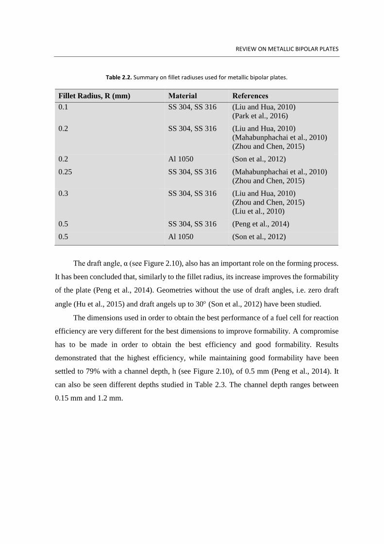
Table 2.2. Summary on fillet radiuses used for metallic bipolar plates.
Fillet Radius, R (mm) Material References
0.1 SS 304, SS 316 (Liu and Hua, 2010)
(Park et al., 2016)
0.2 SS 304, SS 316 (Liu and Hua, 2010)
(Mahabunphachai et al., 2010)
(Zhou and Chen, 2015)
0.2 Al 1050 (Son et al., 2012)
0.25 SS 304, SS 316 (Mahabunphachai et al., 2010)
(Zhou and Chen, 2015)
0.3 SS 304, SS 316 (Liu and Hua, 2010)
(Zhou and Chen, 2015)
(Liu et al., 2010)
0.5 SS 304, SS 316 (Peng et al., 2014)
0.5 Al 1050 (Son et al., 2012)
The draft angle, α (see Figure 2.10), also has an important role on the forming process.
It has been concluded that, similarly to the fillet radius, its increase improves the formability
of the plate (Peng et al., 2014). Geometries without the use of draft angles, i.e. zero draft
angle (Hu et al., 2015) and draft angels up to 30 (Son et al., 2012) have been studied.
The dimensions used in order to obtain the best performance of a fuel cell for reaction
efficiency are very different for the best dimensions to improve formability. A compromise
has to be made in order to obtain the best efficiency and good formability. Results
demonstrated that the highest efficiency, while maintaining good formability have been
settled to 79% with a channel depth, h (see Figure 2.10), of 0.5 mm (Peng et al., 2014). It
can also be seen different depths studied in Table 2.3. The channel depth ranges between
0.15 mm and 1.2 mm.

Numerical Simulation of the Stamping Process of Metallic Bipolar Plates
16 2016
Table 2.3. Summary on channel depths used for metallic bipolar plates.
Channel Depth, h (mm) Material References
0.15 SS 304 (Peng et al., 2014)
0.26 SS 439 (Peng et al., 2014)
0.4 SS 304 (Peng et al., 2014)
0.4 Al 1050 (Son et al., 2012)
0.45 SS 304 (Peng et al., 2014)
0.5 SS 304 (Peng et al., 2014)
(Zhou and Chen, 2015)
(Liu and Hua, 2010)
0.55 SS 304 (Peng et al., 2014)
0.6 SS 304 (Peng et al., 2014)
(Liu et al., 2010)
0.65 SS 304 (Peng et al., 2014)
0.75 SS 304, SS316 (Peng et al., 2014)
(Mahabunphachai et al., 2010)
0.8 SS 304, SS316 (Park et al., 2016)
0.98 SS 304 (Peng et al., 2014)
1.2 SS 304 (Peng et al., 2014)
The rib width, s, and the channel width, w (see Figure 2.10), can influence the
formability and the efficiency of the fuel cell. The values can vary from 0.15 mm to 2.0 mm
(Peng et al., 2014). As previously described in section 1.2, the channel ensures the reactant
flow through the bipolar plates and the rib manages the cooling fluid.

FINITE ELEMENT SIMULATION
3. FINITE ELEMENT SIMULATION
The numerical simulations presented in this study were carried out with the in-house
finite element code DD3IMP1 (Menezes and Teodosiu, 2000), which was specifically
developed for sheet metal forming simulation. Regarding its formulation, an updated
Lagrangian scheme is used to describe the evolution of the deformation. In each increment,
an explicit approach is used to obtain a trial solution for the nodal displacements and then
Newton-Raphson algorithm is used to correct the first trial solution, which finishes when a
satisfactory equilibrium state is achieved. This is repeated until the end of the process. The
Newton-Raphson algorithm is used to solve both the non-linearities associated with the
frictional contact and the elastoplastic behaviour of the deformable body, in a single iterative
loop (Oliveira et al., 2007). In sheet metal forming processes, the boundary conditions are
defined by the contact established between the metallic sheet and the forming tools. The
friction contact is defined by Coulomb’s classical law and the friction coefficient is set as
0.1 for the present work.
The forming tools are considered perfectly rigid in the numerical model, thus only
their exterior surface are described in the numerical model. In this study the tool’s surface is
discretized with quadrilateral elements and is then smoothed with Nagata patches (Neto et
al., 2014).
The discretization of the blank was carried out with isoparametric, 8-node hexahedral
finite elements associated with a selective reduced integration (Menezes and Teodosiu,
2000) (Hughes, 1980).
1 DD3IMP – Contraction of “Deep Drawing 3D IMPlicit finite element code” (Menezes and Teodosiu,
2000).

Numerical Simulation of the Stamping Process of Metallic Bipolar Plates
18 2016
3.1. Materials
The material used for the stamping process of metallic bipolar plates has a large
influence on the manufacturing process as discussed in section 2.2. Three different alloys
for the blank were evaluated. Two sets of aluminium alloys (Al 5042 and Al 1235) and a
stainless steel (SS 304) were chosen. The aluminium Al 5042 is already present in the
DD3IMP materials database, hence its utilization. In the present study, two hardening laws
are used, depending on the material selected. The Voce’s hardening law (see equation (3.1))
is usually used to describe aluminium alloys since it has hardening behaviour with saturation.
On the other hand, the Swift’s hardening law (see equation (3.2)) is more adequate for mild
steels. All the simulations performed in this study consider isotropy in the elastic and plastic
behaviour (von Mises).
Figure 3.1 shows the stress-strain curves for different metals, the choice of aluminium
and stainless steel for stamped metallic plates becomes evident since the elongation before
necking occurs at larger plastic strain values than for other materials.
Figure 3.1. Stress-strain behaviour for different metals (Smith et al., 2014). Note: error on the units for the strain.
p
0 sat 0 y( )[1 exp( C )]Y Y Y Y (3.1)
p
0K( )nY (3.2)

FINITE ELEMENT SIMULATION
The Al 5042 aluminium alloy is described by the Voce hardening law (see equation
(3.1)). The constitutive parameters for this aluminium alloy considering a blank thickness of
0.2083 mm can be seen in Table 3.1 (Neto et al., 2015).
Table 3.1. Voce’s hardening law parameters and elastic properties for Al 5042 with a blank’s initial thickness of 0.2083 mm.
E (GPa) ν Y0 (MPa) Ysat (MPa) Cy
Al 5042 68.9 0.33 267.80 375.08 17.859
The aluminium alloy Al 1235 (Hadi, 2014) and the stainless steel SS 304 (Liu et al.,
2010) are described by Swift’s hardening law (See equation (3.2)) since previous studies
already implemented these materials with Swift’s hardening law despite of Voce’s hardening
law being more appropriate for aluminium.
Liu et al., (2010) described the Swift’s hardening law in function of the blank’s initial
thickness, t, as presented in equation (3.3). The equation has been converted from ksi to
MPa.
The aluminium alloy Al 1235 and the stainless steel SS 304 use hardening laws
described from previous studies, due the time consumption and costs associated with
experimental tensile tests. The constitutive parameters for a blank thickness of 0.1 mm for
aluminium Al 1235 and stainless steel SS 304 can be seen in Table 3.2.
Table 3.2. Swift’s hardening law parameters and elastic properties for Al 1235 (Hadi, 2014) and SS 304 (Liu et al., 2010) with a blank’s initial thickness of 0.1 mm.
E (GPa) ν Y0 (MPa) K (MPa) n
Al 1235 80 0.30 32.93 270.66 0.293
SS 304 162.5 0.30 192.2 850.68 0.206
Swift’s hardening law can describe the aluminium behaviour but some aspects have to
be taken into account when applying it for stainless steel. When stainless steel reaches the
plastic deformation domain, microstructural changes trigger changes of mechanical
22 ( 1.703t 0.578t + 0.249)(1751.959t 677.479t + 319.848)Y [MPa] (3.3)

Numerical Simulation of the Stamping Process of Metallic Bipolar Plates
20 2016
properties. A phase transformation from austenite to martensite can occur which induces
simulation errors when applying Swift’s hardening law. Studies found that while
maintaining low strain rates, the volume fraction of martensite is decreased (Msolli et al.,
2016).
Simulations applying Swift’s hardening law to stainless steel in this study are
acceptable if the simulations represent low strain rates in the stamping process of the metallic
bipolar plates. The stress-strain curve for the three materials in use in this study can be seen
on Figure 3.2.
Figure 3.2. Stress-strain behaviour of the metals studied.
3.2. Boundary Conditions
The proper use of boundary conditions is fundamental to get accurate results in the
numerical simulations. In fact, a body unrestrained with applied load presents infinite
displacements. In this study, the boundary conditions were set to represent as close as
possible the stamping process. Besides, in order to avoid excessive computational costs, only
specific zones of the bipolar plate were analysed. Accordingly, the boundary conditions had
to be adapted in order to represent the correct conditions of the selected representative zones
looking for symmetries, which allow a portion of the structure to be analysed.
0
100
200
300
400
500
600
700
0 0.05 0.1 0.15 0.2
Yiel
d S
tres
s [M
Pa]
Strain
AA1235
SS304
Al 5052

FINITE ELEMENT SIMULATION
Figure 3.3. Representation of a serpentine flow field indicating the selected zones analysed.
Figure 3.3 indicates the different representative zones selected in this study for a
serpentine flow field. Each representative zone aims to study a different region of the bipolar
plate, covering the entire deformation behaviour found in the plate.
1. The first representative zone represents half channel (see Figure 3.4). Adequate
boundary conditions are required to represent the symmetry of the channel.
Thus, the red plane and its parallel plane on the other extremity represent the
constrain in the x direction. In the same way, the blue plane and its parallel
plane on the other extremity represent the constrain in the y direction (plane
strain deformation). These conditions were chosen since channels display
symmetric geometry and load. These boundary conditions represent the most
unfavourable conditions for the forming process, since they constrain the
material flow into the cavity. Besides the study on half channel, ten channels
will be studied to verify the influence of excess material at both extremities.

Numerical Simulation of the Stamping Process of Metallic Bipolar Plates
22 2016
Figure 3.4. Representation of the boundary conditions for section 1.
2. The curved representative zone must also be studied. In this case, the end of
the plate does not represent any symmetry, then the boundary conditions on
such extremities can be set free. Figure 3.5 presents the red plane which
constrains the x direction and the blue plane constrains the y direction.
Figure 3.5. Representation of the boundary conditions for section 3.
This representative zone is favourable to the stamping process, a zone adjacent
to other channels must be studied where material cannot flow as easily since
adjacent channels are also being formed having here symmetry in load and
geometry. This type of restriction is applied to field flows such as a serially
linked serpentines (see Figure 2.5). The same simulation is performed but
introducing boundary condition of symmetry on the four extremities.
3. This section is meant to study the influence of the straight channel on the
curved section, since section 2 does not take this into account. Constraints are
defined similarly to other sections, i.e. boundary conditions of symmetry on
the four extremities.

FINITE ELEMENT SIMULATION
3.3. Parametric Model
To create the tool’s geometry a CAD program was used. Since the tools behave as
rigid bodies, only the outer surface was created using CATIA® V5. In order to guarantee
the symmetry of the final geometry, the dimensions were set on a mid-plane between the
punch and the die (see Figure 3.6) while the tool’s dimensions are obtained with an offset.
The distance between the punch and the die were maintained equal to the blank’s initial
thickness. These dimensions were maintained as variables and exported to Excel in order to
change the geometry for different configurations (see Appendix A).
Seven parameters for this study’s final geometry were exported and varied (see Figure
3.6):
Channel depth, h;
Channel width, w;
Rib width, s;
Blank’s initial thickness, t;
Fillet radius, R;
Main radius, r;
Flat section, a.
Contrary to the classical geometry presented in Figure 2.10, the draft angle is not
represented but it depends on the tool’s radius applied, the larger the radius is, the larger the
draft angle will be. An additional variable is added to the geometry, which is the fillet radius,
R.

Numerical Simulation of the Stamping Process of Metallic Bipolar Plates
24 2016
Figure 3.6. Parametric model for the final geometry of the tools.
From the model represented in Figure 3.6, an extruded surface was created for the
straight channel. In order to represent the curved section of the simplified model (see Figure
3.3) only a revolved surface from the initial sketch was required, instead of the extruded
surface. Both of the tools’ models can be seen in Figure 3.7.
(a) (b)
Figure 3.7. Tools’ geometry on CATIA® V5: (a) Straight channel, (b) Curved section.
With the tool’s surface modelled, the next step consists in exporting the surface in
IGES format for further meshing with the pre-processing program GID®. The first step is to
verify the surface’s normal orientation for simulation purposes. This orientation must be as
indicated in Figure 3.8, i.e. surface normal vectors pointing towards the blank.
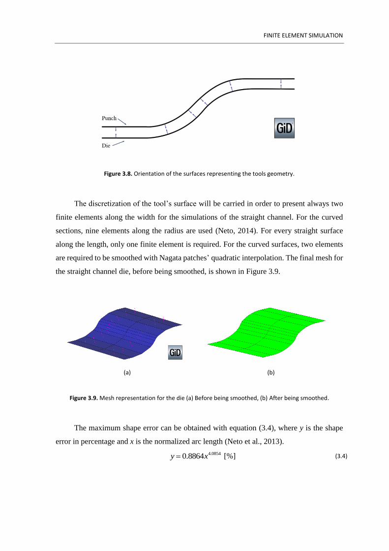
FINITE ELEMENT SIMULATION
Figure 3.8. Orientation of the surfaces representing the tools geometry.
The discretization of the tool’s surface will be carried in order to present always two
finite elements along the width for the simulations of the straight channel. For the curved
sections, nine elements along the radius are used (Neto, 2014). For every straight surface
along the length, only one finite element is required. For the curved surfaces, two elements
are required to be smoothed with Nagata patches’ quadratic interpolation. The final mesh for
the straight channel die, before being smoothed, is shown in Figure 3.9.
(a) (b)
Figure 3.9. Mesh representation for the die (a) Before being smoothed, (b) After being smoothed.
The maximum shape error can be obtained with equation (3.4), where y is the shape
error in percentage and x is the normalized arc length (Neto et al., 2013).
4.08540.8864y x [%] (3.4)

Numerical Simulation of the Stamping Process of Metallic Bipolar Plates
26 2016
The maximum error occurs on the tool’s radius thus both radius used must be verified
(see Figure 3.6). The normalized arc length for both radiuses can be obtained with the
dimensions shown in Figure 3.10 and the equations (3.5) and (3.6).
Figure 3.10. Die’s geometry and dimension necessary to obtain the shape error.
With equation (3.4), the shape error for the fillet radius is 0.024% (see equation (3.7))
and the shape error for the main radius is 0.034% (see equation (3.8)). The shape error as
close to non-influence on the results obtained for this study.
The tools can then be exported to the finite element code DD3IMP for further
simulation. The mesh of the blank is generated on the finite element program using a single
finite element along the width for 2D simulations (plane strain deformation) representing
half a channel. For the length of the blank the number of elements will vary, to be able to
maintain the quadratic elements as square as possible, as shown in Figure 3.11 (a). For
23.602180 0.412180 180
r
lx
r r
(3.5)
25.847180 0.451180 180
r
lx
r r
(3.6)
4.0854 4.08540.8864 0.8864 0.412 0.024%y x (3.7)
4.0854 4.08540.8864 0.8864 0.451 0.034%y x (3.8)

FINITE ELEMENT SIMULATION
simulations which represent the curved sections, the number of elements along the width of
the blank will also vary to maintain cubic elements as shown in Figure 3.11 (b).
(a) (b)
Figure 3.11. Finite element mesh generation in detail: (a) 2D simulation, (b) 3D simulation.
After the process of creating a parametric model and the finite element mesh,
simulations are ready to proceed. The computer used has the following characteristics:
Processor: Intel®Core™ i7-2600K CPU @ 3.40 GHz
Installed memory (RAM): 8.00 GB
System Type: 64-bit Operating System
3.4. Microstamping
A microstamping process as shown in Figure 2.7 is replicated for this study. The
process is divided in two phases: first the die is maintained stationary while the punch moves
towards the blank to form the desired shape. This phase ends when the distance between
both tools is equal to the blank’s initial thickness. The second and final phase is the removal
of both tools in a single instant for the springback effect to occur.
Both plastic strain and thickness reduction are studied as principal parameters to
evaluate the formability of the channel.

Numerical Simulation of the Stamping Process of Metallic Bipolar Plates
28 2016
3.4.1. Influence of the finite element size
The finite element size is important to verify the error committed during the
simulation. Since the objective is to maintain at all times the square form of the finite
element, only the number of elements along the blank’s thickness (and subsequently its size)
were studied. The finite element size along the blank’s length varied to maintain the desired
form and the one element along the width was not altered.
The number of finite elements along the blank’s thickness has been changed between
two and nine, corresponding to an element size between 0.011 and 0.05 mm. In each case
the error was obtained in function of the simulation with the highest number of finite
elements comparing the value obtained for the maximum thickness reduction. The result was
an error inferior to 0.01% which is highly acceptable. Figure 3.12 shows the thickness
reduction of the blank for each simulation. For the minimum thickness all simulations
represent the correct value with a small error. Adopting four finite elements along the
thickness, a good overall results can be obtained as shown in Figure 3.12.
Figure 3.12. Final thickness distribution in function of the number of finite elements along the blank’s thickness.
The number of finite elements has a smaller influence on the punch force than on the
thickness reduction as shown in Figure 3.13. Four or more finite elements reduce or
completely remove the incorrect behaviour in the punch force. Hence, in this study the use
of four elements along the thickness for the finite element simulations. Increasing the
number of finite elements reduces the simulation error but at the cost of an increase in
processing time. Besides, using an even number of finite elements along the thickness allows
to use the mid-plane as a reference for thickness measurements.
0.086
0.088
0.09
0.092
0.094
0.096
0.098
0.1
0 0.2 0.4 0.6 0.8 1 1.2 1.4
Thic
knes
s [m
m]
x [mm]
2 FE 3 FE4 FE 5 FE6 FE 7 FE8 FE 9 FE

FINITE ELEMENT SIMULATION
Figure 3.13. Punch force evolution in function of the number of elements along the blank’s thickness.
3.4.2. Influence of the boundary conditions
Two simulations were performed to verify the influence of the boundary conditions.
The second simplified model in Figure 3.3 with ten channels is used. The first simulation
recreates the conditions described in section 3.2 while the second simulation only applies a
boundary condition for the middle value of x without restrictions on the extremities along
the x direction.
Figure 3.14. Final thickness distribution for simulations with different boundary conditions and a ten channel simplified model.
0
5
10
15
20
25
30
35
40
-0.45-0.4-0.35-0.3-0.25-0.2-0.15-0.1-0.050
Forc
e [N
]
Displacement [mm]
2 FE 3 FE
4 FE 5 FE
6 FE 7 FE
8 FE 9 FE
0.084
0.086
0.088
0.09
0.092
0.094
0.096
0.098
0.1
0.102
0 5 10 15 20 25 30
Thic
knes
s [m
m]
x [mm]
Middle Boundary Condition Boundary Conditions Extremities

Numerical Simulation of the Stamping Process of Metallic Bipolar Plates
30 2016
The simulation with the boundary conditions on the extremities has an increased
thickness reduction compared with the simulation with the boundary condition in the middle.
Besides, the model using free extremities provides a more uniform thickness distribution as
shown in Figure 3.14. For this study, the most disadvantageous model will be used with the
boundary conditions on the extremities since any other model can achieve better results.
Additionally, the final thickness distribution is more uniform, allowing an easier contact
between each flow channel and the membrane with an inferior dimensional error.
3.4.3. Primary optimization
The first simulation presents a tool’s geometry from Son et al. (2012) with the 5042
aluminium alloy for the blank (see section 3.1) considering half a straight channel. The tool’s
geometry follows the scheme shown in Figure 2.10 and the dimensions are indicated in
Table 3.3.
Table 3.3. Tool’s geometrical dimensions for Al 5042 (Son et al., 2012).
w [mm] s [mm] h [mm] R [mm] α [º]
1.2 0.4 0.4 0.4 30
The plastic strain distribution after forming is shown on Figure 3.15 for half a straight
channel. The maximum value of plastic strain is about 0.6 and the thickness reduction is over
28%.
Figure 3.15. Plastic strain distribution for the geometry from Son et al. (2012) for a thickness of 0.2 mm (Al 5042).

FINITE ELEMENT SIMULATION
Since 0.2 mm thickness is half of the channel depth, an attempt to reduce the thickness
to 0.1 mm is made for the next simulation, taking in account the error which can occur since
the aluminium parameters are described for a thickness of 0.2 mm.
The maximum value of plastic strain is around 0.83, as shown in Figure 3.16,
presenting a thickness reduction of over 52%. Therefore, the reduction of the blank thickness
induces an increase in the plastic deformation and occurrence of necking.
Figure 3.16. Plastic strain for the geometry from Son et al. (2012) for a thickness of 0.1 mm (Al 5042).
The evolution of the punch force for both thicknesses is presented in Figure 3.17. As
expected, the force necessary to form the 0.2 mm blank is higher than the 0.1 mm blank. The
sudden force increase at the end is due to a contact between the blank’s extremity and the
tool in the final steps. This contact force is displayed on the top right corner of Figure 3.18
(b). This force peak is common in this process due to the bending effect at the end of forming
stage.
Figure 3.17. Punch force evolution for a thickness of 0.1 mm and 0.2 mm (Al 5042), considering the geometry from Son et al. (2012).
0
10
20
30
40
50
60
70
0 0.1 0.2 0.3 0.4
Forc
e [N
]
Displacement [mm]
Al 5052 0.2 mm
Al 5052 0.1 mm

Numerical Simulation of the Stamping Process of Metallic Bipolar Plates
32 2016
(a) (b)
Figure 3.18. Contact forces (a) Before the final contact, (b) During the final contact.
The results show a low formability for the 5042 aluminium alloy, as expected after the
information obtained from Figure 3.1 regarding the 5XXX aluminium alloys. In order to
improve the formability in the process, the 304 stainless steel will be used for forward
simulations. Since stainless steel blanks with 0.1 mm thickness maintain sufficient
mechanical strength (see section 2.3), this will be the thickness used for this study.
Maintaining the tool’s geometry of previous simulations and with the use of 304
stainless steel, the maximum thickness reduction is over 35% with a maximum plastic strain
of 0.6, as shown in Figure 3.19. These numerical results demonstrate that the adoption of
304 stainless steel allows to improve the thickness reduction for the same initial thickness
and geometry.
Figure 3.19. Plastic strain distribution for the geometry from Son et al. (2012) for a thickness of 0.1 mm (SS 304).

FINITE ELEMENT SIMULATION
The punch force necessary to form the stainless steel is higher than the force required
for the 5042 aluminium, as shown on Figure 3.20. This result is coherent with the stress-
strain curve observed on Figure 3.2.
Figure 3.20. Punch force evolution for two different materials (Al 5042 and SS 304) considering the geometry from Son et al. (2012).
The numerical results demonstrate a critical thickness reduction in the channel, which
jeopardise the fuel cell’s mechanical strength. This is mainly due to the boundary conditions
use in the finite element model. In order to increase the amount of material available to flow
into the cavity, an increase in s and w dimensions (see Figure 2.10) was applied, maintaining
the remaining dimensions unaltered. The obtained plastic strain distribution is presented in
Figure 3.31.
The maximum value of plastic strain decreased to 0.45, while the thickness reduction
is under 25%. The extra material available allows to improve material flow and,
consequently, the formability of the blank.
Figure 3.21. Plastic strain distribution for an increase in channel and rib width considering a thickness of 0.1 mm (SS 304).
0
10
20
30
40
50
60
0 0.1 0.2 0.3 0.4
Forc
e [N
]
Displacement [mm]
SS 304
Al 5052

Numerical Simulation of the Stamping Process of Metallic Bipolar Plates
34 2016
In order to better understand the influence of the extended dimensions s and w, only
the curved section of the 2D model is studied without the straight section of the channel.
According to the results presented in Figure 3.22, the maximum value of plastic strain
increased to 0.68, while the maximum thickness reduction is around 50%. The reduction in
the formability was expected and the numerical results shown the near zero plastic strain on
the highlighted area shown in Figure 3.22.
Figure 3.22. Plastic strain distribution for a geometry without a straight section for a thickness of 0.1 mm (SS 304).
In order to reduce the plastic strain in the critical areas (mainly on the 0.5 mm radius)
of the stamped plate, the geometry of the forming tools was changed by means of the
inclusion of a fillet radius, R, to distribute the plastic strain evenly along the plate (see Figure
3.6). The objective is to increase the plastic strain on the highlighted area shown in Figure
3.22, in order to decrease the plastic strain on the remaining critical areas. The dimensions
of the model represented in Figure 3.6 are shown in Table 3.4.
Table 3.4. Tool’s geometrical dimensions for an optimized geometry (SS 304).
w [mm] s [mm] h [mm] R [mm] r [mm] a [mm] t [mm]
1.3 1.3 0.4 1.3 0.6 0.2 0.1
Figure 3.23 shows both the distribution of the thickness reduction and the plastic strain
distribution. The maximum value of thickness reduction is only 12% and the maximum
plastic strain is approximately 0.21. Thus. the methodology adopted has induced an overall
improvement in formability of 65%.
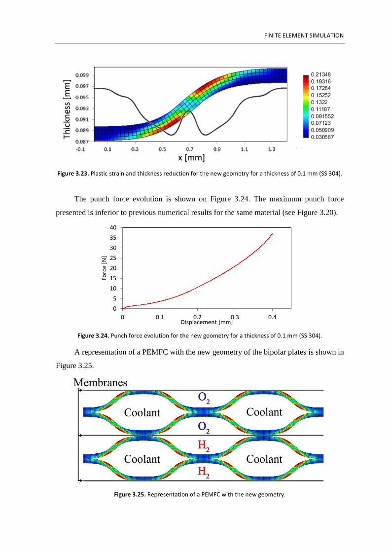
FINITE ELEMENT SIMULATION
Figure 3.23. Plastic strain and thickness reduction for the new geometry for a thickness of 0.1 mm (SS 304).
The punch force evolution is shown on Figure 3.24. The maximum punch force
presented is inferior to previous numerical results for the same material (see Figure 3.20).
Figure 3.24. Punch force evolution for the new geometry for a thickness of 0.1 mm (SS 304).
A representation of a PEMFC with the new geometry of the bipolar plates is shown in
Figure 3.25.
Figure 3.25. Representation of a PEMFC with the new geometry.
0
5
10
15
20
25
30
35
40
0 0.1 0.2 0.3 0.4
Forc
e [N
]
Displacement [mm]

Numerical Simulation of the Stamping Process of Metallic Bipolar Plates
36 2016
The chemical efficiency of the fuel cells is a key factor that should be taken into
account in its manufacturing process. In section 2.3.1, a compromise between fuel cell
efficiency and formability was discussed, the next tool geometry tries to replicate the
geometry imposed for an efficiency of 79%, being the tool’s dimensions shown in Table 3.5.
Although the geometry tested for the best efficiency did not include the fillet radius, R,
involved in the present model, the 1.3 mm radius has been used for the study and a plane
section, a, of 0.20 mm was imposed. The plastic strain distribution presented in Figure 3.26
shows a maximum value of 0.31 and a maximum thickness reduction of 19%. Thus, for the
new geometry of the tools, a greater reaction efficiency could be obtained than 79%
maintaining an adequate mechanical strength.
Table 3.5. Tool’s geometrical dimensions for a chemical efficiency of 79% (SS 304).
w [mm] s [mm] h [mm] R [mm] r [mm] a [mm] t [mm]
1.0 1.6 0.5 1.3 0.5 0.2 0.1
Figure 3.26. Plastic strain distribution for the bipolar plate geometry with 79% efficiency for a thickness of 0.1 mm (SS 304).

FINITE ELEMENT SIMULATION
3.4.4. Influence of tool geometry parameters
A further improvement on the tool’s geometry is required to obtain more favourable
results regarding the formability of the blank. The main geometry parameters are:
Channel depth, h;
Fillet radius, R;
Main radius, r;
Channel and rib width, w and s;
Flat section, a;
Blank’s initial thickness, t.
For a correct study on the influence of each parameter, the model created was
symmetric, maintaining s and w identic and when analysed they are equally changed.
3.4.4.1. Channel depth, h
To evaluate the influence of the channel depth on the formability, the remaining
parameters are unchanged and shown in Table 3.6.
The channel depth starts with a value equal to 0.3 mm and with an increment of 0.05
mm, for each simulation, until the thickness reduction reaches over 30%. In this case, the
range is between 0.3 mm and 0.65 mm and the geometry of the die for these values is shown
in Figure 3.27.
Table 3.6. Tool’s geometrical dimensions for the study on the channel depth (SS 304).
w [mm] s [mm] h [mm] R [mm] r [mm] a [mm] t [mm]
1.2 1.2 0.3 – 0.65 1.3 0.5 0.2 0.1
(a) (b)
Figure 3.27. Die geometry (a) Channel depth of 0.3 mm, (b) Channel depth of 0.65 mm.

Numerical Simulation of the Stamping Process of Metallic Bipolar Plates
38 2016
Figure 3.28 shows the maximum thickness reduction obtained for different channel
depths until the 30% thickness reduction is obtained. The maximum value of thickness
reduction increases quadratically with the channel depth.
Figure 3.28. Maximum thickness reduction in function of the channel depth.
The evolution of the final thickness along the blank in shown in Figure 3.29 (a). The
minimum value of the thickness occurs in the channel radius, presenting a symmetry, namely
for small values of channel depth. The punch force increases as the channel depth increases
as shown in Figure 3.29 (b). Until approximately 0.15 mm of punch displacement, the force
evolution is coincident for all geometries analysed.
(a) (b)
Figure 3.29. Influence of channel depth on: (a) Final thickness, (b) Punch force evolution.
0
5
10
15
20
25
30
35
40
0.3 0.35 0.4 0.45 0.5 0.55 0.6 0.65
Max
imu
m T
hic
knes
s R
edu
ctio
n [
%]
Channel Depth, h [mm]
0.065
0.07
0.075
0.08
0.085
0.09
0.095
0.1
0 0.25 0.5 0.75 1 1.25 1.5
Thic
knes
s [m
m]
x [mm]h=0.3 mm h=0.35 mmh=0.40 mm h=0.45 mmh=0.50 mm h=0.55 mmh=0.60 mm h=0.65 mm
0
10
20
30
40
50
60
-0.7-0.5-0.3-0.1
Pu
nch
Fo
rce
[N]
Punch Displacement [mm]
h=0.30 mm h=0.35 mm
h=0.40 mm h=0.45 mm
h=0.50 mm h=0.55 mm
h=0.60 mm h=0.65 mm

FINITE ELEMENT SIMULATION
3.4.4.2. Fillet radius, R and r.
In order to evaluate the influence of the fillet radius on the formability, the remaining
parameters are set as shown in Table 3.7. The fillet radius starts with 0.8 mm due to the
geometry constraints, using an increment of 0.1 mm for each geometry until the evolution
on the formability stabilises. In this case, the range is between 0.8 mm and 1.5 mm which
corresponds to the geometry of the die shown in Figure 3.30 (a) and (b), respectively.
Table 3.7. Tool’s geometrical dimensions for the study on the a fillet radius (SS 304).
w [mm] s [mm] h [mm] R [mm] r [mm] a [mm] t [mm]
1.2 1.2 0.4 0.8 – 1.5 0.5 0.2 0.1
(a) (b)
Figure 3.30. Die geometry: (a) Fillet radius of 0.8 mm, (b) Fillet radius of 1.5 mm.
Figure 3.31 (a) presents the maximum value of thickness reduction obtained for
different values of fillet radius. The value increases with a quadratic tendency, as shown in
Figure 3.31 (a). The geometry presented in Figure 3.30 (b) shows the similarity with the first
simulations obtained since the fillet radius tends to work as a flat section, providing results
similar to the first simulations without the fillet radius. This observation also explains the
reduction in formability. The impact of the fillet radius on the thickness distribution is
insignificant as highlighted in Figure 3.31 (b), except for the fillet radius of small value.

Numerical Simulation of the Stamping Process of Metallic Bipolar Plates
40 2016
(a) (b)
Figure 3.31. Influence of the fillet radius, R: (a) Maximum value of thickness reduction, (b) Final thickness distribution.
To evaluate the influence of the main radius on the formability, the remaining
parameters are set as shown in Table 3.8.
The main radius starts with 0.55 mm due to the geometry constraints, using an
increment of 0.05 mm for each simulation until 30% thickness reduction is obtained. Thus,
the range is between 0.2 mm and 0.55 mm, which corresponds to the geometry of the die
shown in Figure 3.36 (a) and (b) respectively.
Table 3.8. Tool’s geometrical dimensions for the study on the main radius (SS 304).
w [mm] s [mm] h [mm] R [mm] r [mm] a [mm] t [mm]
1.2 1.2 0.4 1.3 0.2 – 0.55 0.2 0.1
12.6
12.8
13
13.2
13.4
13.6
13.8
0.8 0.9 1 1.1 1.2 1.3 1.4 1.5Max
imu
m T
hic
knes
s R
edu
ctio
n [
%]
Fillet radius, R [mm]
0.086
0.088
0.09
0.092
0.094
0.096
0.098
0.1
0 0.2 0.4 0.6 0.8 1 1.2
Thic
knes
s [m
m]
x [mm]
R=0.8 mm R=0.9 mmR=1.0 mm R=1.1 mmR=1.2 mm R=1.3 mmR=1.4 mm R=1.5 mm

FINITE ELEMENT SIMULATION
(a) (b)
Figure 3.32. Die geometry: (a) Main radius of 0.2 mm, (b) Main radius of 0.55 mm.
Figure 3.33 (a) shows the maximum thickness reduction obtained for different
geometries, specially the modification of the main radius. The predicted thickness value
decreases with a quadratic tendency. The geometry for a main radius of 0.55 mm is smoother
than for a main radius of 0.2 mm, as shown in Figure 3.32. This explains the increase in
formability for higher values of the main radius as long as the main radius increases. The
comparison between Figure 3.31 (b) and Figure 3.33 (b) allows to conclude that the impact
of the main radius is significantly higher than the fillet radius.
(a) (b)
Figure 3.33. Influence of the main radius, r: (a) Maximum thickness reduction, (b) Overall thickness distribution.
The introduction of a new fillet radius onto the geometry removed the previous draft
angle as an input variable. Nonetheless, with a tangent line the equivalent draft angle can
0
5
10
15
20
25
30
35
0.2 0.3 0.4 0.5
Max
imu
m T
hic
knes
s R
edu
ctio
n
[%]
Main radius, r [mm]
0.07
0.075
0.08
0.085
0.09
0.095
0.1
0 0.5 1 1.5
Thic
knes
s [m
m]
x [mm]r=0.55 mm r=0.50 mm
r=0.45 mm r=0.40 mm
r=0.35mm r=0.30mm
r=0.25mm r=0.20mm

Numerical Simulation of the Stamping Process of Metallic Bipolar Plates
42 2016
still be obtained as shown in Figure 3.34. For an geometry with a channel depth of 0.6 mm
and an added radius of 0.8 mm, the draft angle, α (see Figure 2.10), is 48º.
Figure 3.34. Equivalent draft angle, α, for the new geometry with an added fillet radius.
To verify the results of the added radius, simulations of the geometry with only one
fillet radius were recreated with the draft angle equivalent to the angle obtained with the
optimized geometry. For a channel depth of 0.6 mm and a main radius of 0.5 mm the
maximum value of plastic strain obtained was 0.462. On the other hand, the optimized
geometry with equivalent parameters and a fillet radius of 0.8 mm provides a plastic strain
of only 0.395. With a channel depth of 0.5 mm the plastic strain for the geometry with only
one fillet radius was 0.35 and for the optimized geometry the plastic strain was 0.30. This
study for a channel depth of 0.6 mm is shown in Figure 3.35.
(a) (b)
Figure 3.35. Plastic strain and thickness: (a) Primary Geometry, (b) Optimized Geometry.
0.065
0.07
0.075
0.08
0.085
0.09
0.095
0.1
0 0.5 1 1.5
Thic
knes
s [m
m]
x [mm]
Primary Geometry0.065
0.07
0.075
0.08
0.085
0.09
0.095
0.1
0 0.5 1 1.5
Thic
knes
s [m
m]
x [mm]
Optimized Geometry

FINITE ELEMENT SIMULATION
3.4.4.3. Channel and rib width, w and s — Flat section, a
To evaluate the influence of the channel and rib width on the formability, the remaining
parameters are set as shown in Table 3.9.
Table 3.9. Tool’s geometrical dimensions for the study on the channel and rib width (SS 304).
w [mm] s [mm] h [mm] R [mm] r [mm] a [mm] t [mm]
1.2 – 2.4 1.2 – 2.4 0.5 1.3 0.3 0.2 – 1.4 0.1
The channel and rib width start with 1.2 mm and increased with an increment of 0.2
mm until a tendency can be observed. Since the objective is to study the influence of the
plane section, the value of a must also be increased accordingly with the same increment as
the channel and rib dimensions. In this case, the range of the channel and rib width is between
1.2 mm and 3.4 mm and the range for the flat section is between 0.2 mm and 2.4 mm. The
geometry of the die for these values is shown in Figure 3.36.
Figure 3.36. Die geometry: (a) Channel and rib width of 3.4 mm, (b) Channel and rib width of 1.2 mm.
Figure 3.37 (a) shows the maximum value of thickness reduction obtained for different
channel and rib width. It presents a quadratic decreasing tendency and it is expected to tend
to zero for an infinite channel and rib width. The increase in formability was expected due
to the increase in material available to flow into the cavity and form the channel.
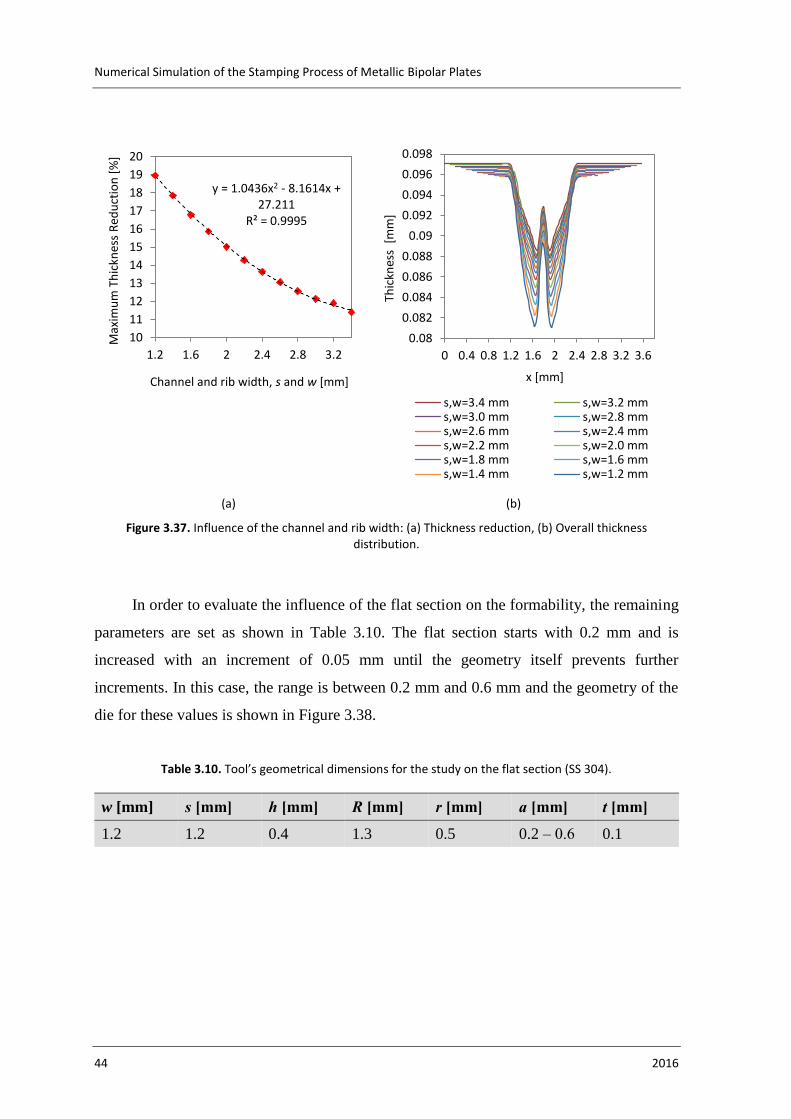
Numerical Simulation of the Stamping Process of Metallic Bipolar Plates
44 2016
(a) (b)
Figure 3.37. Influence of the channel and rib width: (a) Thickness reduction, (b) Overall thickness distribution.
In order to evaluate the influence of the flat section on the formability, the remaining
parameters are set as shown in Table 3.10. The flat section starts with 0.2 mm and is
increased with an increment of 0.05 mm until the geometry itself prevents further
increments. In this case, the range is between 0.2 mm and 0.6 mm and the geometry of the
die for these values is shown in Figure 3.38.
Table 3.10. Tool’s geometrical dimensions for the study on the flat section (SS 304).
w [mm] s [mm] h [mm] R [mm] r [mm] a [mm] t [mm]
1.2 1.2 0.4 1.3 0.5 0.2 – 0.6 0.1
y = 1.0436x2 - 8.1614x +27.211
R² = 0.9995
10
11
12
13
14
15
16
17
18
19
20
1.2 1.6 2 2.4 2.8 3.2
Max
imu
m T
hic
knes
s R
edu
ctio
n [
%]
Channel and rib width, s and w [mm]
0.08
0.082
0.084
0.086
0.088
0.09
0.092
0.094
0.096
0.098
0 0.4 0.8 1.2 1.6 2 2.4 2.8 3.2 3.6
Thic
knes
s [
mm
]x [mm]
s,w=3.4 mm s,w=3.2 mms,w=3.0 mm s,w=2.8 mms,w=2.6 mm s,w=2.4 mms,w=2.2 mm s,w=2.0 mms,w=1.8 mm s,w=1.6 mms,w=1.4 mm s,w=1.2 mm

FINITE ELEMENT SIMULATION
(a) (b)
Figure 3.38. Die geometry: (a) Flat section of 0.2 mm, (b) Flat section of 0.6 mm.
Figure 3.39 (a) shows the maximum value of thickness reduction obtained for different
channel geometries. The geometry presented in Figure 3.38 (b) shows the similarity with the
first simulations obtained since the fillet radius has nearly no influence on the final geometry.
This observation also explains the reduction in formability.
(a) (b)
Figure 3.39. Influence of the flat section, a: (a) Thickness reduction, (b) Overall thickness distribution.
3.4.4.4. Blank’s initial thickness, t.
To evaluate the influence of the blank’s initial thickness on the formability, the
remaining parameters are set as shown in Table 3.11. The thickness studied varies from 0.05
mm to 0.25 mm, since it is the most used thickness range for stainless steel in metallic bipolar
plates. The stainless steel used for the simulations is described for a thickness of 0.1 mm.
Thus, the following study must have into account the error committed for using the same
20
20.5
21
21.5
22
22.5
23
23.5
24
0.2 0.3 0.4 0.5 0.6
Max
imu
m T
hic
knes
s R
edu
ctio
n [
%]
Flat section, a [mm]
0.075
0.08
0.085
0.09
0.095
0.1
0 0.25 0.5 0.75 1 1.25
Thic
knes
s [m
m]
x [mm]a=0.20 mm a=0.25 mma=0.30 mm a=0.35 mma=0.40 mm a=0.45 mma=0.50 mm a=0.55 mma=0.60 mm

Numerical Simulation of the Stamping Process of Metallic Bipolar Plates
46 2016
hardening law. Four different thicknesses are studied starting with the blank’s initial
thickness of 0.05 mm up to 0.25 mm with an increment of 0.05 mm. The results from the
extreme values for the simulations can be seen in Figure 3.40.
Table 3.11. Tool’s geometrical dimensions for the study on blank’s initial thickness (SS 304).
w [mm] s [mm] h [mm] R [mm] r [mm] a [mm] t [mm]
1.2 1.2 0.5 1.3 0.3 0.2 0.05 – 0.25
(a) (b)
Figure 3.40. Plastic Strain distribution: (a) Initial thickness of 0.05 mm, (b) Initial thickness of 0.25 mm.
Figure 3.41 shows the maximum value of thickness reduction obtained in function of
the blank’s initial thickness. For all the values of initial thickness, the predicted thickness
reduction is approximately identical, except for the 0.05 mm blank. Therefore, a blank’s
thickness of 0.05 mm is not adequate for a channel depth of 0.5 mm.
Figure 3.41. Thickness reduction in function on the blank’s initial thickness.
18
18.5
19
19.5
20
20.5
21
21.5
22
0.05 0.07 0.09 0.11 0.13 0.15 0.17 0.19 0.21 0.23 0.25
Max
imu
m T
hic
knes
s R
edu
ctio
n [
%]
Blank's initial thickness [mm]

FINITE ELEMENT SIMULATION
The punch force evolution is shown in Figure 3.42 (b) and, as expected, it increases
with the increase of the blank’s initial thickness. The irregular behaviour in the evolution
results from the number of finite elements, as explained on section 3.4.1.
(a) (b)
Figure 3.42. Influence of the blank’s initial thickness, t: (a) Overall thickness distribution, (b) Punch force evolution.
3.4.5. Comparison between Al 1235 and SS304
All numerical simulations performed previously in this study were focused on the
stainless steel. After the optimization of the geometry, it is necessary to evaluate the
formability for aluminium bipolar plates and compare with the previous results.
Figure 3.43 shows the predicted thickness distribution for the previously used stainless
steel SS 304 compared with the aluminium alloy Al 1235. In fact, the aluminium blanks with
initial thickness of 0.1 mm have an increased formability compared with stainless steel SS
304. It must be taken in account the mechanical strength obtained from thin aluminium
bipolar plates. According to the stress-strain curves presented in Figure 3.2, the punch force
required to form the stainless steel is significantly higher than for the aluminium, as shown
in Figure 3.44.
0
5
10
15
20
25
0 0.5 1 1.5
Thic
knes
s R
edu
ctio
n [
%]
x [mm]
t=0.05 mm t=0.10 mm
t=0.15 mm t=0.20 mm
t=0.25 mm
0
20
40
60
80
100
120
-0.5-0.4-0.3-0.2-0.10P
un
ch F
orc
e [N
]
Punch displacement, z [mm]
t=0.05 mm t=0.10 mm
t=0.15 mm t=0.20 mm
t=0.25 mm

Numerical Simulation of the Stamping Process of Metallic Bipolar Plates
48 2016
Figure 3.43. Final thickness distribution for stainless steel and aluminium blanks.
Figure 3.44. Punch force evolution for stainless steel and aluminium blanks.
3.4.6. Study of the curved channel section
After the study of a single straight channel was completed, the next step consists on
comparing with the representative zone number 2 of the simplified model, shown in Figure
3.38. This square zone of the blank is discretized with 120 finite elements along the x and y
directions and five along the thickness while the representation of the tools is shown in
Figure 3.7 (b). To compare adequately both numerical results, a mirror has been applied on
the 2D simulation (see Figure 3.46 (a)).
0.086
0.088
0.09
0.092
0.094
0.096
0.098
0 0.2 0.4 0.6 0.8 1 1.2 1.4
Thic
knes
s [m
m]
x [mm]
Al1235
SS304
0
5
10
15
20
25
30
35
40
-0.4-0.35-0.3-0.25-0.2-0.15-0.1-0.050
Pu
nch
Fo
rce
[N]
Punch displacement, z [mm]
SS 304
Al 1235

FINITE ELEMENT SIMULATION
Figure 3.45. Thickness reduction for 2D and 3D simulations.
The results for the curved section show an increase in thickness reduction compared
with the straight channel section, as shown in Figure 3.45. This behaviour is explained since
only plane strain deformation occurs in the 2D model and the 3D model presents a
deformation along every orientation with a curved geometry.
(a)
(b)
Figure 3.46. Plastic strain distribution: (a) 2D simulation, (b) 3D simulation.
The comparison of the plastic strain for both the 2D and 3D simulation is shown in
Figure 3.46. The 2D simulation has a maximum plastic strain of 0.22 while the 3D simulation
has a maximum plastic strain of 0.38. The maximum plastic strain for the 3D simulation
occurs in the fillet radius closer to the revolution axis, since the radius of the curvature is
inferior than for the fillet radius represented on the right side of Figure 3.46 (b). Since the
2D model does not represent a curved section of the flow channel, the plastic strain
distribution is symmetric.
The simulation of the curved section using boundary conditions to restrain the four
sides represents the most disadvantageous situation in terms of forming. In order to verify
the influence of the straight channel on the curved section, a comparison between a 3D
0.07
0.075
0.08
0.085
0.09
0.095
0.1
0 0.5 1 1.5 2 2.5
Thic
knes
s [m
m]
x [mm]
3D
2D

Numerical Simulation of the Stamping Process of Metallic Bipolar Plates
50 2016
simulation with only the curved section and a 3D simulation with the curved section with
the straight channel is carried out. The number of finite elements used for the curved section
is 120 for the x and y directions and for the straight channel a progressive mesh was used
(see Figure 3.47 (a)) with 100 elements along the straight channel. This model presents four
finite elements along the thickness.
(a) (b)
Figure 3.47. (a) Progressive mesh, (b) Plastic strain distribution for the curved section with the straight channel.
The comparison between both simulations is shown in Figure 3.48. Although the
results are similar, the curved section with the influence of the straight channel clearly
demonstrates lower deformation, as shown in Figure 3.48. In fact, the minimum thickness is
0.080 mm using the straight channel, while without the straight channel the minimum
thickness is 0.074 mm.
The blank of the 2D simulation contains only 192 nodes, resulting in a simulation of
52 seconds (CPU Time: 357 seconds). When running a 3D simulation, the simulation time
increases drastically. The 3D model presents 72000 nodes with a computational time of 8
hours 43 minutes and 57 seconds (CPU Time: 179580 seconds). Adding the channel, even
with less finite elements along the thickness, increases the number of nodes to 105600
corresponding to a simulation time of 14 hours 12 minutes and 30 seconds (CPU Time:
289111 seconds).

FINITE ELEMENT SIMULATION
Figure 3.48. Final thickness for the curved section with and without the straight channel.
3.5. Hydroforming
In section 2.3 different forming processes were discussed. This study focused on the
microstamping process, but there is a need to evaluate the remaining forming processes to
verify the eventual benefits. This section focuses on the comparison between microstamping
and hydroforming processes.
The hydroforming simulation only requires the die and the application of pressure on
the other side of the blank to create de desired shape. This pressure has to be enough to allow
the blank to accommodate the desired shape but low enough to avoid an increased in
thickness reduction.
The process is divided in two phases: first the die is maintained stationary while a
pressure is applied to the blank to form the desired shape. This phase ends when the selected
pressure is attained. The second phase is the removal of the pressure in a single instant for
the springback effect to occur.
The following simulations use the optimized geometry obtained with microstamping
with the same boundary conditions in order to compare adequately the results. Hence, the
tool geometry used has the dimensions in Table 3.12. The initial thickness of 0.1 mm for
stainless steel is used along with four finite elements along the blank’s thickness.

Numerical Simulation of the Stamping Process of Metallic Bipolar Plates
52 2016
Table 3.12. Tool’s geometrical dimensions for the study of hydroforming (SS 304).
w [mm] s [mm] h [mm] R [mm] r [mm] a [mm] t [mm]
1.2 1.2 0.4 0.8 0.5 0.2 0.1
The first step consists in verifying the pressure required for the geometry used.
Simulations were performed varying the pressure from 50 MPa to 400 MPa with an
increment of 50 MPa. The results for the simulations with a pressure of 50 MPa and 400
MPa are shown in Figure 3.49.
(a) (b)
Figure 3.49. Plastic strain distribution for (a) Hydroforming with p = 50 MPa, (b) Hydroforming with p = 400 MPa.
For the geometry tested, with a pressure above 100 MPa, the simulations have similar
results, when comparing the final desired geometry. Only a slight improvement is obtained
with a pressure of 300 MPa. The simulation with 50 MPa presents inferior results in terms
of final geometry obtained
The thickness reduction obtained for different pressures is shown in Figure 3.50. The
thickness reduction for hydroforming using forming pressures from 100 MPa up to 300 MPa
is under 13.5 %. On the other hand, increasing the pressure above 300 MPa induces an
increase in thickness reduction, while pressures of 50 MPa do not achieve the geometrical
objective.
The thickness reduction obtained with microstamping, for the same geometry, is under
13% which represents better results than the simulations for the hydroforming process.

FINITE ELEMENT SIMULATION
Figure 3.50. Thickness reduction for hydroforming with pressure from p = 50 MPa to p = 400 MPa.
The thickness distribution for hydroforming at different levels of pressure is shown in
Figure 3.51. The increase in pressure induces an increase in the maximum thickness
reduction since its maximum is for a pressure of 400 MPa.
Figure 3.51. Thickness distribution for hydroforming for pressures from 50 MPa to 400 MPa.
Observing the results for the hydroforming process shown in Figure 3.49, with a
symmetric geometry, the highest values of plastic strain are displayed in the first section of
contact between the blank and the die. With this behaviour, the following simulation tries to
increase the plastic strain where the values are lower in order to reduce the plastic strain on
the critical radius. This can be achieved by increasing the radius of the critical point, while
reducing the one on the bottom of the channel. The new geometry compared with the
previous symmetric one is shown in Figure 3.52.
8.5
9.5
10.5
11.5
12.5
13.5
14.5
15.5
0 50 100 150 200 250 300 350 400 450
Max
imu
m T
hic
knes
s R
edu
ctio
n
[%]
pressure, p [MPa]
Hydroforming
Stamping
0.084
0.086
0.088
0.09
0.092
0.094
0.096
0.098
0.1
0 0.2 0.4 0.6 0.8 1 1.2 1.4
Thic
knes
s [m
m]
x [mm]
Hydroforming p=50 MPaHydroforming p=100 MPaHydroforming p=400 MPa

Numerical Simulation of the Stamping Process of Metallic Bipolar Plates
54 2016
(a) (b)
Figure 3.52. Die geometry (a) Symmetric optimal geometry for microstamping, (b) Hydroforming geometry.
The comparison between the symmetric geometry and the new geometry for a pressure
of 250 MPa is shown in Figure 3.53, presenting a plastic strain distribution plotted on the
deformed geometry. The maximum plastic strain for the new geometry occurred in a
different location compared with the symmetric geometry, with a similar value for the
maximum plastic strain obtained.
(a) (b)
Figure 3.53. Plastic strain for a pressure of 250 MPa for hydroforming: (a) Symmetric Geometry, (b) New Geometry.
The thickness distribution along the blank for microstamping and hydroforming with
the different geometries is shown in Figure 3.54. Even though the maximum plastic strain
occurred in a different location, the maximum thickness reduction for both numerical
simulations still occurred on the same fillet radius and with similar results.
The new geometry improves the results in regard of plastic strain and with a decrease
in thickness reduction, but all the results obtained from hydroforming show results inferior
to microstamping.

FINITE ELEMENT SIMULATION
Figure 3.54. Thickness distribution for hydroforming and microstamping.
3.6. Results and Discussion
Liu et al. (2010) studied the deformation on metallic bipolar plates with the rubber pad
forming process. The main study consisted on the formation of a 1.2 mm channel with 0.6
mm of depth. The best results obtained for a concave deformation style were with a
maximum value of stress of 642.5 MPa as shown in Figure 3.55.
Figure 3.55. Stress values for rubber pad forming process (Liu et al., 2010).
For the optimized geometry obtained with this study, it was possible to obtain greater
results. With a fully constrained model, recreating the channels in the worst conditions of
the bipolar plate, it was possible to obtain a maximum value of stress of around 700 MPa for
0.082
0.084
0.086
0.088
0.09
0.092
0.094
0.096
0.098
0 0.2 0.4 0.6 0.8 1 1.2 1.4
Thic
knes
s [m
m]
x [mm]
Microstamping, Symmetric Geometry
Hydroforming p=250 Mpa, New Geometry
Hydroforming p=250 Mpa, Symmetric Geometry

Numerical Simulation of the Stamping Process of Metallic Bipolar Plates
56 2016
a similar geometry with a channel width of 1.2 mm and a channel depth of 0.6 mm. But, if
the boundary conditions used by Liu et al. 2010 were replicated with the added material on
one extremity, the maximum value of stress drops to 556 MPa, as shown in Figure 3.56.
Note that the added material on one extremity will not affect the results since the extremity
is free to move.
(a) (b)
Figure 3.56. Stress values: (a) fully constrained finite element model, (b) free on one extremity finite element model.
The plastic strain for the simulations shown in Figure 3.56 is shown in Figure 3.57,
which demonstrates the influence of the boundary conditions on a finite element model.
(a) (b)
Figure 3.57. Plastic strain: (a) fully constrained finite element model, (b) free on one extremity finite element model.
In sum, for similar conditions as previous studies, the optimized geometry has an
improved formability but the fully constrained model has to be taken into account due to the
accurate representation of the channels from the centre of the metallic bipolar plate.
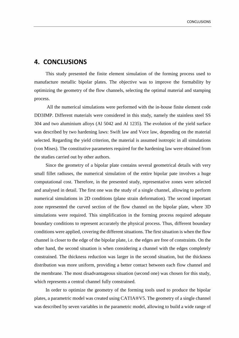
CONCLUSIONS
4. CONCLUSIONS
This study presented the finite element simulation of the forming process used to
manufacture metallic bipolar plates. The objective was to improve the formability by
optimizing the geometry of the flow channels, selecting the optimal material and stamping
process.
All the numerical simulations were performed with the in-house finite element code
DD3IMP. Different materials were considered in this study, namely the stainless steel SS
304 and two aluminium alloys (Al 5042 and Al 1235). The evolution of the yield surface
was described by two hardening laws: Swift law and Voce law, depending on the material
selected. Regarding the yield criterion, the material is assumed isotropic in all simulations
(von Mises). The constitutive parameters required for the hardening law were obtained from
the studies carried out by other authors.
Since the geometry of a bipolar plate contains several geometrical details with very
small fillet radiuses, the numerical simulation of the entire bipolar pate involves a huge
computational cost. Therefore, in the presented study, representative zones were selected
and analysed in detail. The first one was the study of a single channel, allowing to perform
numerical simulations in 2D conditions (plane strain deformation). The second important
zone represented the curved section of the flow channel on the bipolar plate, where 3D
simulations were required. This simplification in the forming process required adequate
boundary conditions to represent accurately the physical process. Thus, different boundary
conditions were applied, covering the different situations. The first situation is when the flow
channel is closer to the edge of the bipolar plate, i.e. the edges are free of constraints. On the
other hand, the second situation is when considering a channel with the edges completely
constrained. The thickness reduction was larger in the second situation, but the thickness
distribution was more uniform, providing a better contact between each flow channel and
the membrane. The most disadvantageous situation (second one) was chosen for this study,
which represents a central channel fully constrained.
In order to optimize the geometry of the forming tools used to produce the bipolar
plates, a parametric model was created using CATIA®V5. The geometry of a single channel
was described by seven variables in the parametric model, allowing to build a wide range of

Numerical Simulation of the Stamping Process of Metallic Bipolar Plates
58 2016
geometries to be used in the finite element simulation. Therefore, the influence of each
geometrical parameter was evaluated in order to increase the formability of the blank. Seven
parameters were tested:
The first parameter to be tested was the channel depth, h. The thickness
reduction increased with the increase of the channel depth. The maximum
value of thickness reduction followed a quadratic crescent tendency as the
channel depth was increased. It was possible to reach a channel depth of 0.65
mm with a maximum thickness reduction of 30%. The increase in channel
depth led to an increase in punch force.
The second parameter was the added fillet radius, R. The thickness reduction
increased with the increase of the fillet radius. Once again, observing the
maximum thickness reduction for each simulation, it was clear that it followed
a quadratic crescent tendency as the fillet radius increased. The best results
were observed for an added fillet radius of 0.8 mm which corresponds to a
maximum thickness reduction of 12.7%. The main fillet radius, r, was also
studied. When the main fillet radius increased, the thickness reduction
decreased with a quadratic tendency. The best results were observed for a main
fillet radius of 0.5 mm (maximum thickness reduction under 15%).
The next parameter studied was a plane section of the cross-section of the
straight channel. To evaluate such section, both the rib, s, and channel width,
s, were increased to maintain the symmetry, as well as the flat section, a. With
the straight section increased, the maximum thickness reduction decreased
with a quadratic tendency.
In order to keep the channel and rib width, the next parameter analysed was the
flat section, a. Increasing this parameter without altering the channel and rib
width, the arc length of the fillet radius changed, reducing the formability of
the blank. Increasing the flat section to 0.6 mm induced a maximum thickness
reduction of 23.7%.
The last parameter was the blank’s initial thickness, t. For stainless steel, an
initial thickness of 0.05 mm led to a maximum thickness reduction of 21.7%,
while for further values of thickness the maximum thickness reduction was
similar for each simulation with values between 18.5% and 19%.

CONCLUSIONS
Considering the 2D simulation of a single channel, the comparison between stainless
steel SS 304 and aluminium alloy Al 1235 was performed. Maintaining the blank’s initial
thickness of 0.1 mm, the aluminium presented higher formability in comparison with
stainless steel, being the improvement of around 2%. For the same geometry, the straight
and curved section of the flow channel presented a maximum plastic strain of 0.22 and 0.39,
respectively. The influence that the straight section of the flow channel has on the curved
section was analysed. The maximum plastic strain decreased from 0.4 to 0.32.
Finally, the influence of the stamping process was evaluated by comparing the
microstamping and the hydroforming processes. Comparing both forming processes with the
same geometry, the microstamping process provides better results in terms of formability.
Applying a pressure between 100 MPa and 300 MPa in the hydroforming process, the
maximum thickness reduction was 13.5%, compared with 12.5% obtained in the
microstamping process. Further values of pressure increase the maximum thickness
reduction, while a pressure of 50 MPa did not achieve the geometrical objective for the
blank, since it presented lack of contact between the blank and the die. Since the optimal
geometry can be different depending on the forming process, an attempt in changing the
geometry was performed, improving the results for hydroforming, but sill presenting inferior
results compared with microstamping.

Numerical Simulation of the Stamping Process of Metallic Bipolar Plates
60 2016

REFERENCES
5. REFERENCES
A.Heinzzel, University of Duisburg-Essen, Duisburg, G., F. Mahlendorf, University of
Duisburg-Essen, Duisburg, G., C. Jansen, University of Duisburg-Essen, Duisburg,
G., 2009. Bipolar Plates. Elsevier 810–816.
Belali-Owsia, M., Bakhshi-Jooybari, M., Hosseinipour, S.J., Gorji, A.H., 2014. A new
process of forming metallic bipolar plates for PEM fuel cell with pin-type pattern.
Carrette, L., Friedrich, K. a, Stimming, U., 2001. Fuel Cells - Fundamentals and
Applications. Fuel Cells 1, 5–39.
Hadi, S., 2014. Micro deep drawing of Aluminium foils AA1235. University of
Wollongong.
Holton, O.T., Stevenson, J.W., 2013. The Role of Platinum in Proton Exchange Membrane
Fuel Cells. Platin. Met. Rev. 57, 259–271.
Hu, P., Peng, L., Zhang, W., Lai, X., 2009. Optimization design of slotted-interdigitated
channel for stamped thin metal bipolar plate in proton exchange membrane fuel cell.
J. Power Sources 187, 407–414.
Hu, Q., Zhang, D., Fu, H., 2015. Effect of flow-field dimensions on the formability of Fe-
Ni-Cr alloy as bipolar plate for PEM (proton exchange membrane) fuel cell. Energy
83, 156–163.
Hughes, T.J.R., 1980. Generalization of selective integration procedures to anisotropic and
nonlinear media. Int. J. Numer. Methods Eng. 15, 1413–1418.
Li, X., Sabir, I., 2005. Review of bipolar plates in PEM fuel cells: Flow-field designs. Int.
J. Hydrogen Energy 30, 359–371.
Liu, Y., Hua, L., 2010. Fabrication of metallic bipolar plate for proton exchange membrane
fuel cells by rubber pad forming. J. Power Sources 195, 3529–3535.
Liu, Y., Hua, L., Lan, J., Wei, X., 2010. Studies of the deformation styles of the rubber-pad
forming process used for manufacturing metallic bipolar plates. J. Power Sources 195,
8177–8184.
Mahabunphachai, S., Necati, Ö., Koc, M., 2010. Effect of manufacturing processes on
formability and surface topography of proton exchange membrane fuel cell metallic
bipolar plates 195, 5269–5277.
Menezes, L.F., Teodosiu, C., 2000. Three-dimensional numerical simulation of the deep-
Numerical Simulation of the Stamping Process of Metallic Bipolar Plates
62 2016
drawing process using solid finite elements. J. Mater. Process. Technol. 97, 100–106.
Msolli, S., Martiny, M., Cardoso, M.C., Moreira, L.P., Mercier, S., Molinari, A., 2016.
Numerical modeling of the deformation of AISI 304L using a tangent additive Mori-
Tanaka homogenization scheme: Application to sheet metal forming. J. Mater.
Process. Technol. 235, 187–205.
Neto, D.M., 2014. Numerical simulation of frictional contact problems using Nagata
patches in surface smoothing 350.
Neto, D.M., Oliveira, M.C., Dick, R.E., Barros, P.D., Alves, J.L., Menezes, L.F., 2015.
Numerical and experimental analysis of wrinkling during the cup drawing of an
AA5042 aluminium alloy. Int. J. Mater. Form.
Neto, D.M., Oliveira, M.C., Menezes, L.F., Alves, J.L., 2014. Applying Nagata patches to
smooth discretized surfaces used in 3D frictional contact problems. Comput. Methods
Appl. Mech. Eng. 271, 296–320.
Neto, D.M., Oliveira, M.C., Menezes, L.F., Alves, J.L., 2013. Improving Nagata patch
interpolation applied for tool surface description in sheet metal forming simulation.
Comput. Des. 45, 639–656.
Oliveira, M., Alves, J., Chaparro, B., Menezes, L., 2007. Study on the influence of work-
hardening modeling in springback prediction. Int. J. Plast. 23, 516–543.
Park, W.T., Jin, C.K., Kang, C.G., 2016. Improving channel depth of stainless steel bipolar
plate in fuel cell using process parameters of stamping. Int. J. Adv. Manuf. Technol.
Peng, L., Yi, P., Lai, X., 2014. Design and manufacturing of stainless steel bipolar plates
for proton exchange membrane fuel cells. Int. J. Hydrogen Energy 39, 21127–21153.
Smith, T.L., Santamaria, A.D., Park, J.W., Yamazaki, K., 2014. Alloy Selection and Die
Design for Stamped Proton Exchange Membrane Fuel Cell (PEMFC) Bipolar Plates.
Procedia CIRP 14, 275–280.
Son, C.-Y., Jeon, Y.-P., Kim, Y.-T., Kang, C.-G., 2012. Evaluation of the formability of a
bipolar plate manufactured from aluminum alloy Al 1050 using the rubber pad
forming process. Proc. Inst. Mech. Eng. Part B J. Eng. Manuf. 226, 909–918.
Tawfik, H., Hung, Y., Mahajan, D., 2007. Metal bipolar plates for PEM fuel cell-A review.
J. Power Sources 163, 755–767.
Wang, Y., Chen, K.S., Mishler, J., Cho, S.C., Adroher, X.C., 2011. A review of polymer
electrolyte membrane fuel cells: Technology, applications, and needs on fundamental

REFERENCES
research. Appl. Energy 88, 981–1007.
Yi, P., Du, X., Kan, Y., Peng, L., Lai, X., 2015. Modeling and experimental study of laser
welding distortion of thin metallic bipolar plates for PEM fuel cells. Int. J. Hydrogen
Energy 40, 4850–4860.
Yoon, W., Huang, X., Fazzino, P., Reifsnider, K.L., Akkaoui, M.A., 2008. Evaluation of
coated metallic bipolar plates for polymer electrolyte membrane fuel cells. J. Power
Sources 179, 265–273.
Zhou, T.-Y., Chen, Y.-S., 2015. Effect of Channel Geometry on Formability of 304
Stainless Steel Bipolar Plates for Fuel Cells—Simulation and Experiments. J. Fuel
Cell Sci. Technol. 12, 051001.

Numerical Simulation of the Stamping Process of Metallic Bipolar Plates
64 2016

APPENDIX A
APPENDIX A
The following page presents a guide to create a parametric model with CATIA®V5
as used for the presented work.

Numerical Simulation of the Stamping Process of Metallic Bipolar Plates
66 2016
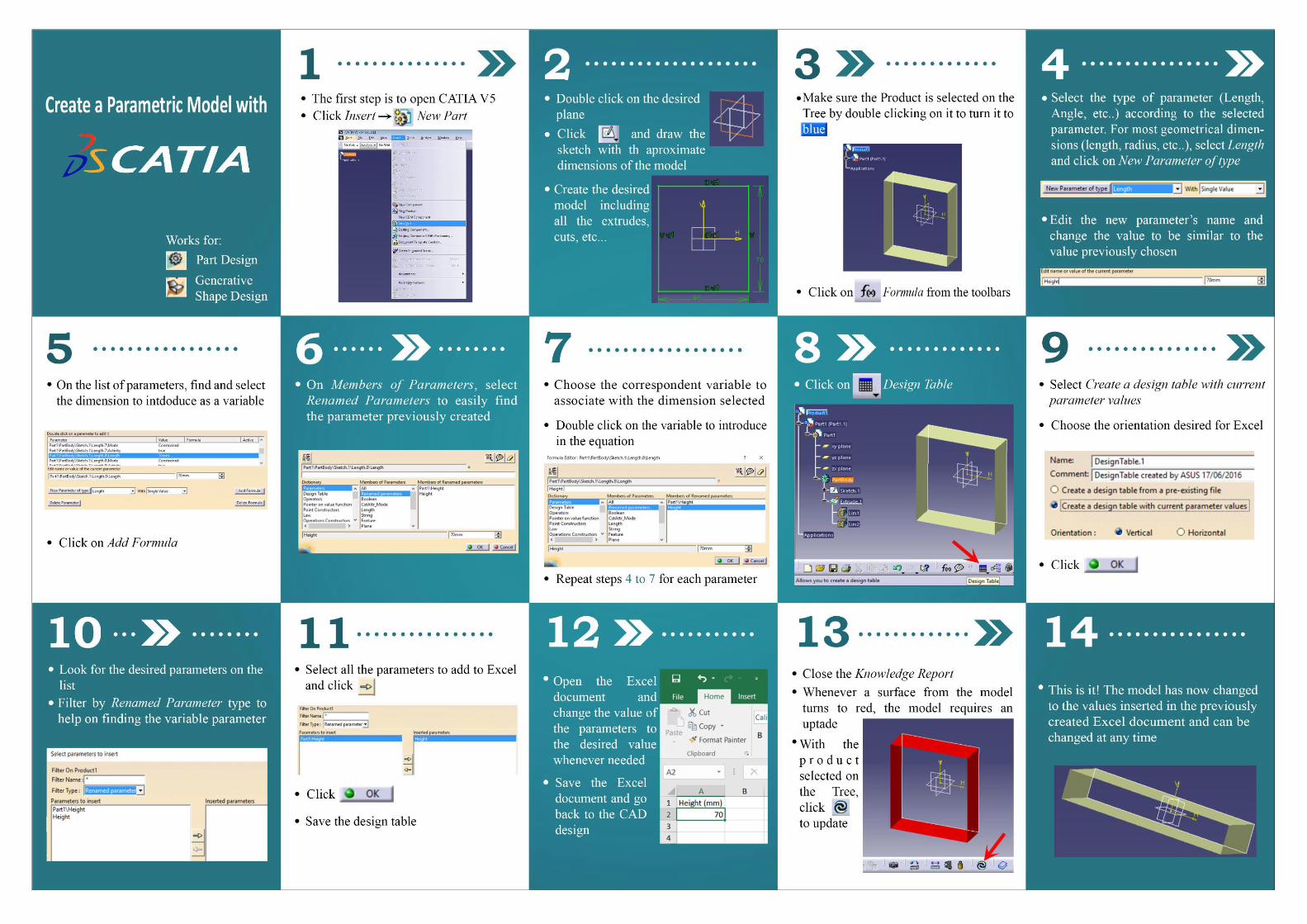

Numerical Simulation of the Stamping Process of Metallic Bipolar Plates
68 2016

APPENDIX B
APPENDIX B
Paper currently in final preparation for submission.

Numerical simulation of the stamping process of stainless steel bipolar
plates and channel geometry optimization
Nicolas Marques, Diogo Neto
ABSTRACT: A bipolar plate is one of the key components of proton exchange membrane fuel cells, which are considered as potential power sources for transportation and portable applications. The main objective of this paper is the optimization of the stamping process of stainless steel SS 304 bipolar plates for PEM fuel cells with the use of numerical models in the simulation of a deep drawing process. The numerical simulations presented in this paper were carried out with the in-house finite element code DD3IMP. The geometry of the flow field has a large influence on the formability during the stamping process. Therefore, the aim of the paper is to study the different geometrical variables in order to optimize the flow channel dimensions. Accordingly, a parametric CAD model containing the stamping tools’ geometry is created, which is posteriorly used in the simulation with a finite element method. The simplified model is used to study the deformation behaviour found in the plate such as a 2D analysis (plane strain deformation) to evaluate the straight channel. The numerical results shown that increasing the main radius, the channel width and the rib width and diminishing the channel depth, the fillet radius and the flat section the formability of the blank is improved
1 INTRODUCTION
In the last decades there has been an increasing
concern about environmental consequences on the
use of fossil fuel for electricity production and
vehicle propulsion. Sustainable energy became
important with the increase in population since
common sources of energy have poisonous
emissions into the atmosphere[1].
In order to reduce the dependence on fossil fuels
and diminish poisonous emissions, renewable
energy from wind, water and sun were already
implemented. Nevertheless, these sources are
irregularly available thus not being suited to cover
all electrical needs[1].
An option for future power generations are fuel
cells, which use pure hydrogen and producing only
water eliminating all local emissions [1].
Fuel cells are electrochemical devices that convert
chemical energy stored in fuels into electrical
energy [2].
The fuel cells can be categorised in five main
categories: polymer electrolyte membrane fuel
cells (PEMFC), solid oxide fuel cells (SOFC),
alkaline fuel cells (AFC), phosphoric acid fuel cells
(PAFC) and molten carbonate fuel cells (MCFC).
For transportation an portable applications, PEM
fuel cells are promising candidates since they
gather the most important characteristics for such
applications [3].
Figure 1.1. Proton exchange membrane fuel cell (PEMFC) assembly [2].
Fuel cells are composed by different components
assembled in stacks as shown in Figure 1.1. Each
stack consists of a membrane electrode assembly
and bipolar plates [4].

(a) (b)
Figure 1.2. Structure of a bipolar plate, (a) Top view, (b) Cross Section A-A.
Bipolar plates have an important role on fuel cell
stacks. They provide structural support for the
mechanically weak membranes, manage the supply
of reactant gases through flow channels (see
Figure 1.2), improve heat management with a
coolant and electrically connect two cells together
in the stack [4].
The configuration presented in Figure 1.2 consists
of two metallic plates welded together creating the
bipolar plate. This configuration repeats along the
stack. The reactants flow on one side of the plate,
while the cooling fluid flows on the other side of
the same plate to remove the heat generated by the
chemical reaction [5].
The main material used for bipolar plates is
graphite [6]. It offers good electrical conductivity,
high corrosion resistance and low interfacial
contact resistance. However, the cost of graphite
plates is high due to their poor manufacturability
and it has the disadvantage of being brittle and
having poor permeability which forces the use of
thicker plates. In order to decrease the cost of fuel
cells, metallic bipolar plates have received much
attention lately due to the much superior
manufacturability, higher mechanical strength,
being non permeable and more durable when
submitted to shock and vibration which is
important when used for portable applications and
transport [4].
The main handicap on metallic plates is the
corrosion which occurs in the acidic and humid
environment present in a fuel cell. Some solutions
for preventing metal degradation consist on using
noble metals, stainless steels, aluminium alloys,
titanium and nickels as base metal and coating
materials to prevent the corrosion on the base
metal. Cost wise, stainless steel is promising along
with the correct coating [7].
2 NUMERICAL MODEL
The main objective of this paper is to optimize the
flow channel geometry with a finite element
model. The results obtained can vary depending on
the finite element code and boundary conditions as
well as the influence of the material used.
2.1 FINITE ELEMENT CODE
The numerical simulations presented in this study
were carried out with the in-house finite element
code DD3IMP1 [8], which was specifically
developed for sheet metal forming simulation.
Regarding its formulation, an updated Lagrangian
scheme is used to describe the evolution of the
deformation. In each increment, an explicit
approach is used to obtain a trial solution for the
nodal displacements and then Newton-Raphson
algorithm is used to correct the first trial solution,
which finishes when a satisfactory equilibrium
state is achieved. This is repeated until the end of
the process. The Newton-Raphson algorithm is
used to solve both the non-linearities associated
with the frictional contact and the elastoplastic
behaviour of the deformable body in a single
iterative loop [9]. In sheet metal forming processes,
the boundary conditions are defined by the contact
established between the metallic sheet and the
forming tools. The friction contact is defined by
Coulomb’s classical law and the friction coefficient
is set as 0.1 for the present paper.
The forming tools are considered perfectly rigid in
the numerical model, thus only their exterior
surface are described in the numerical model. In
this paper the tool’s surface is discretized with
1 DD3IMP – Contraction of “Deep Drawing 3D
IMPlicite finite element code” [8]

quadrilateral elements and is then smoothed with
Nagata patches [10].
The discretization of the blank was carried out with
isoparametric 8-node hexahedral finite elements
associated with a selective reduced integration
[8][11].
2.2 BOUNDARY CONDITIONS
The proper use of boundary conditions is
fundamental to get accurate results in the numerical
simulations. In fact, a body unrestrained with
applied load presents infinite displacements. In this
paper, the boundary conditions were set to
represent as close as possible the stamping process.
Besides, in order to avoid excessive computational
costs, only specific zones of the bipolar plate were
analysed. Accordingly, the boundary conditions
had to be adapted in order to represent the correct
conditions of the selected representative zones
looking for symmetries, which allow a portion of
the structure to be analysed.
Figure 2.1. Representation of a serpentine flow field indicating the selected zones analysed.
Figure 2.1 indicates the different representative
zones selected in this study for a serpentine flow
field. Each representative zone aims to study a
different region of the bipolar plate.
The representative zone number 1 represents half a
channel (see Figure 2.2). Adequate boundary
conditions are required to represent the symmetry
of the channel. Thus, the red plane and its parallel
plane on the other extremity represent the constrain
in the x direction. In the same way, the blue plane
and its parallel plane on the other extremity
constrain in the y direction (plane strain
deformation). These conditions were chosen since
channels display symmetric geometry and load.
These boundary conditions represent the most
unfavourable conditions for the stamping process,
since they constrain the material flow into the
cavity.
Figure 2.2. Representation of the boundary conditions for section 1.
2.3 MATERIAL
The material used for the stamping process of
metallic bipolar plates has a large influence on the
manufacturing process. In the present paper, the
Swift’s hardening law (see equation 2.1)) is applied
to stainless steel considering an isotropic behaviour
(von Mises).
p
0K( )nY (2.1)
The stainless steel SS 304 is used in this paper and
is described with an equation in function of the
blank’s initial thickness [12]. Swift’s hardening
law and elastic properties for SS 304 with a blank’s
initial thickness of 0.1 mm is shown in Table 2.1.
Table 2.1. Swift’s hardening law parameters and elastic properties for stainless steel SS 304 with a blank’s initial thickness of 0.1 mm.
E
(GPa) ν
Y0
(MPa)
K
(MPa) n
SS
304 162.5 0.30 192.2 850.68 0.206
To apply Swift’s hardening law to stainless steels,
some aspects have to be taken into account. When
stainless steel reaches the plastic domain,
microstructural changes trigger changes of
mechanical properties. A phase transformation
from austenite to martensite can occur which
induces simulation errors when applying Swift’s
hardening law. Studies found that while
maintaining low strain rates, the volume fraction of
martensite is decreased [13].
Simulations applying Swift’s hardening law to
stainless steel in this paper are acceptable if the
simulations represent low strain rates in the
stamping process of the metallic bipolar plates.
3 PARAMETRIC MODEL
To study the influence of multiple geometrical
parameters, creating a parametric model simplifies
the process of creating the tools’ geometry for
different studies.

3.1 CHANNEL DIMENSIONS AND FINITE
ELEMENT MESH
Every channel dimension is exported from a CAD
program (CATIA® V5) to an Excel file in order to
change the geometry for different configurations.
Most metallic bipolar plates use a geometry similar
with Figure 3.1 with a draft angle, α, applied and
only one fillet radius.
Figure 3.1. Representation of tool’s dimensions.
This study focuses on the study of an optimized
geometry where a second fillet radius is introduced
and the draft angle, as a variable, disappears. This
geometry is shown in Figure 3.2.
Seven parameters can be changed from the Excel
file: channel depth, h, channel width, w, Rib width,
s, Blank’s initial thickness, t, fillet radius, R, main
radius, r and flat section, a.
The channel dimensions are set on a mid-plane
between the punch and the die to guarantee the
symmetry of the geometry. The tool’s dimensions
are then obtained with an offset from the mid-plan.
Figure 3.2. Parametric model.
For the study on this paper, the main geometrical
parameters will vary between a range of values
described in Table 3.1 with its respective
increment.
Table 3.1. Range of values for the study of geometrical parameters and their respective increments.
Minimum
Value [mm]
Maximum
Value [mm]
Increment
[mm]
w 1.2 2.4 0.05
s 1.2 2.4 0.20
h 0.3 0.65 0.05
R 0.8 1.5 0.10
r 0.2 0.55 0.05
a 0.2 0.6 0.05
The process consists on creating the tool’s surface
geometry with a CAD program and export in an
IGES format for further meshing with the pre-
processing program GID® and smoothed with
Nagata patches’ quadratic interpolation. The final
smoothed tool’s mesh is shown in Figure 3.3.
Figure 3.3. Mesh representation for the die.
The tools can then be exported to the finite element
code DD3IMP for further simulation. The mesh of
the blank is generated using a single finite element
along the width (plane strain deformation) and four
finite elements along the thickness. The number of
finite elements along the blank’s length will be
updated to maintain quadratic elements as square
as possible.
After the process of creating a parametric model
and the finite element mesh, simulations are ready
to proceed.
4 INFLUENCE OF GEOMETRICAL
PARAMETERS
A microstamping process is replicated for this
study. The process is divided in two phases: first
the dies is maintained stationary while the punch
moves towards the blank to form the desired shape.
This phase ends when the distance between both
tools is equal to the blank’s initial thickness. The
second and final phase is the removal of both tools
in a single instant for the springback effect to
occur.

The thickness reduction on the stainless steel blank
is studied as principal parameter to evaluate the
formability of the channel.
4.1 INFLUENCE OF CHANNEL DEPTH, h
To evaluate the influence of the channel depth on
the formability, the remaining parameters are
unchanged and shown in Table 4.1. The channel
depth starts with 0.3 mm and using an increment of
0.05 mm for each geometry until the thickness
reduction reaches over 30%. In this case, the range
is between 0.3 mm and 0.65 mm, which
corresponds to the geometry of the die shown in
Figure 4.1 and Figure 4.2, respectively.
Table 4.1. Tool’s geometrical dimensions for the study on the channel depth (SS 304).
w, s [mm] r [mm] h [mm]
1.2 0.5 0.3 – 0.65
R [mm] a [mm]
1.3 0.2
Figure 4.1. Die geometry for h = 0.3 mm.
Figure 4.2. Die geometry for h = 0.65 mm.
The evolution of the thickness reduction along the
blank is shown in Figure 4.3
Figure 4.3. Influence of channel depth on the final thickness.
A channel depth of 0.65 mm induces a thickness
reduction of over 30% as shown in Figure 4.3.
With a channel depth of 0.3 mm the maximum
thickness reduction is under 10% and with a
channel depth of 0.65 mm the thickness reduction
is over 30%. The maximum value of thickness
reduction increases quadratically with the channel
depth. The punch force is shown in Figure 4.4. and
increases as the channel depth increases Until
approximately 0.15 mm of punch displacement, the
force evolution is coincident for all the geometries
analysed.
Figure 4.4. Influence of channel depth on the punch force.
4.2 INFLUENCE OF THE FILLET RADIUS,
R and r.
In order to evaluate the influence of the fillet radius
on the formability, the remaining parameters are
set as shown in Table 4.2. The fillet radius starts
0.065
0.07
0.075
0.08
0.085
0.09
0.095
0.1
0 0.25 0.5 0.75 1 1.25 1.5
Thic
knes
s [m
m]
x [mm]
h=0.3 mm h=0.40 mmh=0.50 mm h=0.60 mmh=0.65 mm
0
10
20
30
40
50
60
-0.7-0.5-0.3-0.1
Pu
nch
Fo
rce
[N]
Punch Displacement [mm]
h=0.30 mm h=0.40 mmh=0.50 mm h=0.60 mmh=0.65 mm

with 0.8 mm due to the geometry constraints, using
an increment of 0.1 mm for each geometry until the
evolution on the formability stabilises. In this case,
the range is between 0.8 mm and 1.5 mm, which
corresponds to the geometry of the die shown in
Figure 4.5 and Figure 4.6, respectively
Table 4.2. Tool’s geometrical dimensions for the study on the fillet radius (SS 304).
w, s [mm] r [mm] h [mm]
1.2 0.5 0.4
R [mm] a [mm]
0.8 – 1.5 0.2
Figure 4.5. Die geometry for R = 0.8 mm
Figure 4.6. Die geometry for R = 1.5 mm
Figure 4.7. Influence of the fillet radius on thickness reduction.
The thickness distribution along the blank is shown
in Figure 4.7.
The geometry for a fillet radius of 1.5 mm tends to
work as an extended flat section with only one
fillet radius demonstrating inferior results in terms
of formability. With a fillet radius of 0.8 mm the
maximum thickness reduction is 12.7% and with a
fillet radius of 1.5 mm the thickness reduction is
over 13.6%. The value of the maximum thickness
reduction increases with a quadratic tendency.
To evaluate the influence of the main radius on the
formability, the remaining parameters are set as
shown in Table 4.3. The main radius starts with
0.55 mm due to the geometry constraints, using an
increment of 0.05 mm for each simulation until
30% thickness reduction is obtained. Thus, the
range is between 0.2 mm and 0.55 mm, which
corresponds to the geometry of the die shown in
Figure 4.8 and Figure 4.9, respectively.
Table 4.3. Tool’s geometrical dimensions for the study on the main radius (SS 304).
w, s [mm] r [mm] h [mm]
1.2 0.2 – 0.55 0.4
R [mm] a [mm]
1.3 0.2
Figure 4.8. Die geometry for r = 0.2 mm.
Figure 4.9. Die geometry for r = 0.55 mm.
With a main radius of 0.2 mm the maximum
thickness reduction is over 28% and with a main
radius of 0.5 mm the thickness reduction is under
15%. Increasing the main radius decreases the
thickness reduction with a quadratic tendency as
shown in Figure 4.10. The geometry for a main
radius of 0.55 mm is smoother than for a main
radius of 0.2 mm explaining the increase in
formability for higher values of the main radius.
The comparison between Figure 4.7 and Figure
4.10 allows to conclude that the impact of the main
radius is significantly higher than the fillet radius.
0.086
0.088
0.09
0.092
0.094
0.096
0.098
0.1
0 0.2 0.4 0.6 0.8 1 1.2
Thic
knes
s [m
m]
x [mm]R=0.8 mm R=1.0 mmR=1.2 mm R=1.5 mm

Figure 4.10. Influence of the main radius on the thickness reduction.
4.3 INFLUENCE OF THE CHANNEL
WIDTH, RIB WIDTH AND FLAT
SECTION, w, s, a.
To evaluate the influence of the channel and rib
width on the formability, the remaining parameters
are set as shown in Table 4.4.
Table 4.4. Tool’s geometrical dimensions for the study on the channel and rib width (SS 304).
w, s [mm] r [mm] h [mm]
1.2 – 2.4 0.3 0.5
R [mm] a [mm]
1.3 0.2 – 1.4
The channel and rib width start with 1.2 mm and
increased with an increment of 0.2 mm until a
tendency can be observed. Since the objective is to
study the influence of the plane section, the value
of the flat section, a, must also be increased
accordingly with the same increment as the channel
and rib dimensions. In this case, the range if the
channel and rib width is between 1.2 mm and 3.4
mm and the range for the flat section is between
0.2 mm and 2.4 mm. The geometry of the die for
these values is shown in Figure 4.11.
Figure 4.11. Die geometry: (a) Channel and rib width of 3.4 mm, (b) Channel and rib width of 1.2 mm.
The thickness reduction for different channel and
rib width presents a quadratic decreasing tendency
with the increase of these parameters as shown in
Figure 4.12 and it is expected to tend to no
thickness reduction for an infinite channel and rib
width. The increase in formability was expected
due to the increase in material available to flow
into the cavity and form the channel. With a
channel and rib width of 1.2 mm the maximum
thickness reduction is 19% and with a channel and
rib width of 3.4 mm the thickness reduction is
under 12%.
Figure 4.12. Influence of the channel and rib width on the thickness reduction.
In order to evaluate the influence of the flat section
on the formability, the remaining parameters are
set as shown in Table 4.5. The flat section starts
with 0.2 mm and is increased with an increment of
0.05 mm until the geometry itself prevents further
increments. In this case, the range is between 0.2
mm and 0.6 mm and the geometry of the die for
these values is shown in Figure 4.13 and Figure
4.14.
Table 4.5. Tool’s geometrical dimensions for the study of the flat section (SS 304).
w, s [mm] r [mm] h [mm]
1.2 0.5 0.4
R [mm] a [mm]
1.3 0.2 – 0.6
Figure 4.13. Die geometry for a = 0.2 mm.
Figure 4.14. Die geometry for a = 0.6 mm.
5 CONCLUSIONS
The formability of a metallic bipolar plate was
studied in this paper for a microstamping process.
The influence of the geometrical parameters was
tested to consider the dimensions which increase
0.07
0.075
0.08
0.085
0.09
0.095
0.1
0 0.5 1 1.5
Thic
knes
s [m
m]
x [mm]
r=0.55 mm r=0.50 mmr=0.40 mm r=0.30mmr=0.20mm
0.08
0.082
0.084
0.086
0.088
0.09
0.092
0.094
0.096
0.098
0 1 2 3
Thic
knes
s [
mm
]
x [mm]s,w=3.4 mm s,w=2.8 mms,w=2.4 mm s,w=2.0 mms,w=1.6 mm s,w=1.2 mm

the formability of the blank. Six parameters were
tested:
The first parameter to be tested was the
channel depth, h. The thickness reduction
increased with the increase of the channel
depth. The maximum value of thickness
reduction followed a quadratic crescent
tendency as the channel depth was
increased. It was possible to reach a
channel depth of 0.65 mm with a
maximum thickness reduction of 30%.
The increase in channel depth led to an
increase in punch force.
The second parameter was the added fillet
radius, R. The thickness reduction
increased with the increase of the fillet
radius. Once again, observing the
maximum thickness reduction for each
simulation, it was clear that it followed a
quadratic crescent tendency as the fillet
radius increased. The best results were
observed for an added fillet radius of 0.8
mm which corresponds to a maximum
thickness reduction of 12.7%. The main
fillet radius, r, was also studied. When the
main fillet radius increased, the thickness
reduction decreased with a quadratic
tendency. The best results were observed
for a main fillet radius of 0.5 mm
(maximum thickness reduction under
15%).
The next parameter studied was a plane
section of the cross-section of the straight
channel. To evaluate such section, both
the rib, s, and channel width, s, were
increased to maintain the symmetry, as
well as the flat section, a. With the
straight section increased, the maximum
thickness reduction decreased with a
quadratic tendency.
In order to keep the channel and rib width,
the next parameter analysed was the flat
section, a. Increasing this parameter
without altering the channel and rib width,
the arc length of the fillet radius changed,
reducing the formability of the blank.
Increasing the flat section to 0.6 mm
induced a maximum thickness reduction
of 23.7%.
6 REFERENCES
[1] L. Carrette, K. a Friedrich, and U.
Stimming, “Fuel Cells - Fundamentals and
Applications,” Fuel Cells, vol. 1, no. 1, pp.
5–39, 2001.
[2] S. Mahabunphachai, Ö. Necati, and M.
Koc, “Effect of manufacturing processes
on formability and surface topography of
proton exchange membrane fuel cell
metallic bipolar plates,” vol. 195, pp.
5269–5277, 2010.
[3] Y. Wang, K. S. Chen, J. Mishler, S. C.
Cho, and X. C. Adroher, “A review of
polymer electrolyte membrane fuel cells:
Technology, applications, and needs on
fundamental research,” Appl. Energy, vol.
88, no. 4, pp. 981–1007, 2011.
[4] L. Peng, P. Yi, and X. Lai, “Design and
manufacturing of stainless steel bipolar
plates for proton exchange membrane fuel
cells,” Int. J. Hydrogen Energy, vol. 39,
no. 36, pp. 21127–21153, 2014.
[5] X. Li and I. Sabir, “Review of bipolar
plates in PEM fuel cells: Flow-field
designs,” Int. J. Hydrogen Energy, vol. 30,
no. 4, pp. 359–371, 2005.
[6] W. Yoon, X. Huang, P. Fazzino, K. L.
Reifsnider, and M. A. Akkaoui,
“Evaluation of coated metallic bipolar
plates for polymer electrolyte membrane
fuel cells,” J. Power Sources, vol. 179, no.
1, pp. 265–273, Apr. 2008.
[7] H. Tawfik, Y. Hung, and D. Mahajan,
“Metal bipolar plates for PEM fuel cell-A
review,” J. Power Sources, vol. 163, no. 2,
pp. 755–767, 2007.
[8] L. F. Menezes and C. Teodosiu, “Three-
dimensional numerical simulation of the
deep-drawing process using solid finite
elements,” J. Mater. Process. Technol.,
vol. 97, no. 1–3, pp. 100–106, 2000.
[9] M. OLIVEIRA, J. ALVES, B.
CHAPARRO, and L. MENEZES, “Study
on the influence of work-hardening
modeling in springback prediction,” Int. J.
Plast., vol. 23, no. 3, pp. 516–543, Mar.
2007.
[10] D. M. Neto, M. C. Oliveira, L. F. Menezes,
and J. L. Alves, “Applying Nagata patches
to smooth discretized surfaces used in 3D
frictional contact problems,” Comput.
Methods Appl. Mech. Eng., vol. 271, pp.
296–320, 2014.
[11] T. J. R. Hughes, “Generalization of
selective integration procedures to
anisotropic and nonlinear media,” Int. J.
Numer. Methods Eng., vol. 15, no. 9, pp.
1413–1418, Sep. 1980.
[12] Y. Liu and L. Hua, “Fabrication of metallic
bipolar plate for proton exchange
membrane fuel cells by rubber pad
forming,” J. Power Sources, vol. 195, no.
11, pp. 3529–3535, 2010.
[13] S. Msolli, M. Martiny, M. C. Cardoso, L.
P. Moreira, S. Mercier, and A. Molinari,
“Numerical modeling of the deformation of
AISI 304L using a tangent additive Mori-
Tanaka homogenization scheme:
Application to sheet metal forming,” J.

Mater. Process. Technol., vol. 235, pp.
187–205, 2016.