1

Images of Microsoft® Excel dialog boxes © Microsoft. All rights reserved. This content is excluded from ourCreative Commons license. For more information, see http://ocw.mit.edu/help/faq-fair-use/.

2

Tool for Solving a Linear Program:

Excel has the capability to solve linear (and often nonlinear) programming

problems. The SOLVER tool in Excel:

May be used to solve linear and nonlinear optimization problems

Allows integer or binary restrictions to be placed on decision variables

Can be used to solve problems with up to 200 decision variables

3

How to Install SOLVER:

The SOLVER Add-in is a Microsoft Office Excel add-in program that is

available when you install Microsoft Office or Excel. To use the Solver Add-in,

however, you first need to load it in Excel. The process is slightly different for

Mac or PC users.

MAC: 1. Open Excel for Mac 2011 and begin by clicking on the Tools menu. 2. Click Add-Ins, and then in the Add-Ins box, check Solver.xlam and then click OK. 3. After restarting Excel for Mac 2011 (fully Quit Excel 2011), select the Data tab, then select Solver to launch

Microsoft: 1. Click the Microsoft Office Button , and then click Excel Options. 2. Click Add-Ins, and then in the Manage box, select Excel Add-ins and click Go. 3. In the Add-Ins available box, select the Solver Add-in check box, and then click OK. If Solver Add-in is not listed in the Add-Ins available box, click Browse to locate the add-in. If you get prompted that Solver is not currently installed, click Yes to install it. 4. After you load Solver, the Solver command is available in the Analysis group on the Data tab.

4

How to Use SOLVER:

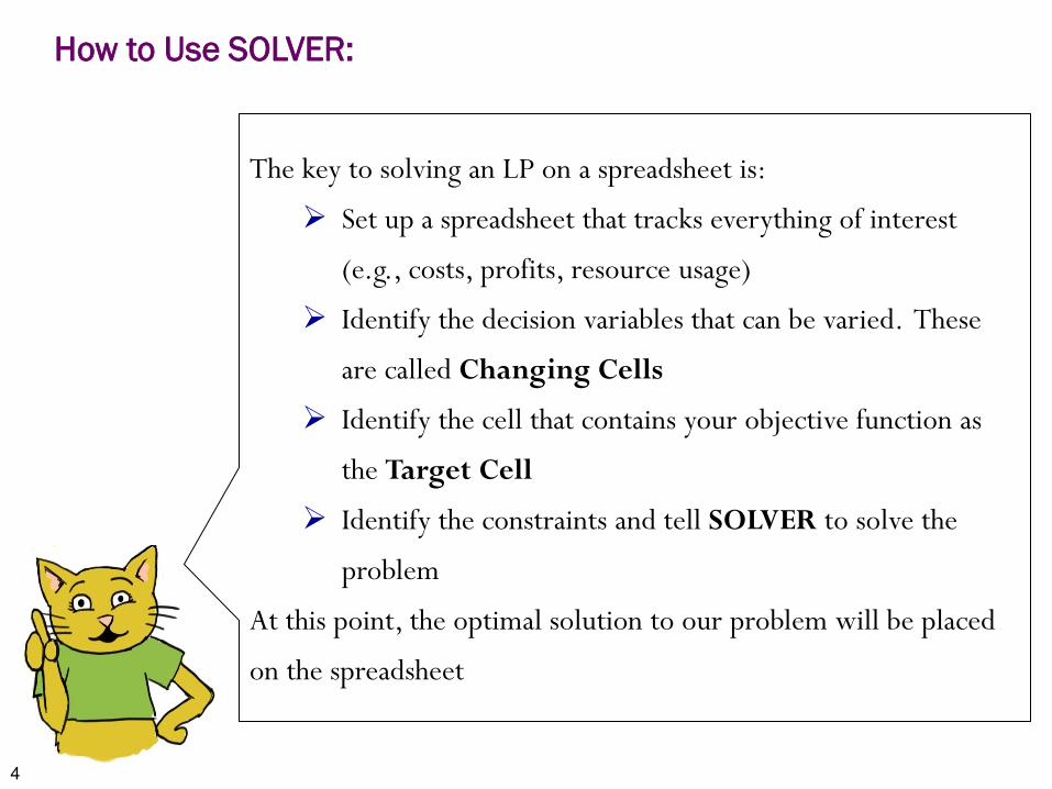
The key to solving an LP on a spreadsheet is:

Set up a spreadsheet that tracks everything of interest

(e.g., costs, profits, resource usage)

Identify the decision variables that can be varied. These

are called Changing Cells

Identify the cell that contains your objective function as

the Target Cell

Identify the constraints and tell SOLVER to solve the

problem

At this point, the optimal solution to our problem will be placed

on the spreadsheet

5

LP Solutions with SOLVER, an Example:

Consider the problem of diet optimization. There are four different types of food: Brownies, Ice Cream, Cola, and Cheese Cake. The nutrition values and cost per unit are as follows: The objective is to find a minimum-cost diet that contains at least 500 calories, at least 6 grams of chocolate, at least 10 grams of sugar, and at least 8 grams of fat.

Brownies Ice Cream Cola Cheese Cake

Calories 400 200 150 500

Chocolate 3 2 0 0

Sugar 2 2 4 4

Fat 2 4 1 5

Cost $0.50 $0.20 $0.30 $0.80

6

LP Solutions with SOLVER, an Example:

STEP 1: Decision Variables

To begin we enter heading for each type of food in B2:E2.

In the range B3:E3, we input trial values for the amount of each food eaten. (Any values will work, but at least one should be positive.)

For example, here we indicate that we are considering eating three brownies, no scoops of chocolate ice cream, one bottle of cola, and seven pieces of pineapple cheesecake.

A B C D E

1 DECISION VARIABLES

2 Brownies Ice Cream Cola Cheese Cake

3 Eaten 3 0 1 7

7

LP Solutions with SOLVER, an Example:

STEP 2: Objective Function

To see if the diet is optimal, we must determine its cost as well as the calories, chocolate, sugar, and fat it provides.

In the range B7:E7,we reference the number of units and in B8:E8 we input the per unit cost for each available food. Then we compute the cost of the diet in cell B10 with the formula

= B7*B8 + C7*C8 +D7*D8+ E7*E8

But it is usually easier to enter the formula

= SUMPRODUCT (B7:E7, B8:E8)

And this is much easier to understand for anyone reading the spreadsheet. The =SUMPRODUCT function requires two ranges as inputs. The first cell in the first range is multiplied by the first cell in the second range, then the second cell in the first range is multiplied by the second cell in the second range, and so on. All of these products are then added. Thus, in cell B10 the =SUMPRODUCT function computes total cost as (3)(50)+(0)(20)+(1)(30)+(7)(80) = 740 cents.

8

LP Solutions with SOLVER, an Example:

STEP 2: Objective Function (cont.)

A B C D E

1 DECISION VARIABLES

2 Brownies Ice Cream Cola Cheese Cake

3 Eaten 3 0 1 7

4

5 OBJECTIVE FUNCTION

6 Brownies Ice Cream Cola Cheese Cake

7 Eaten =B3 =C3 =D3 =E3

8 Cost 50 20 30 80

9

10 Total 740 = SUMPRODUCT ( B7:E7, B8:E8)

9

LP Solutions with SOLVER, an Example:

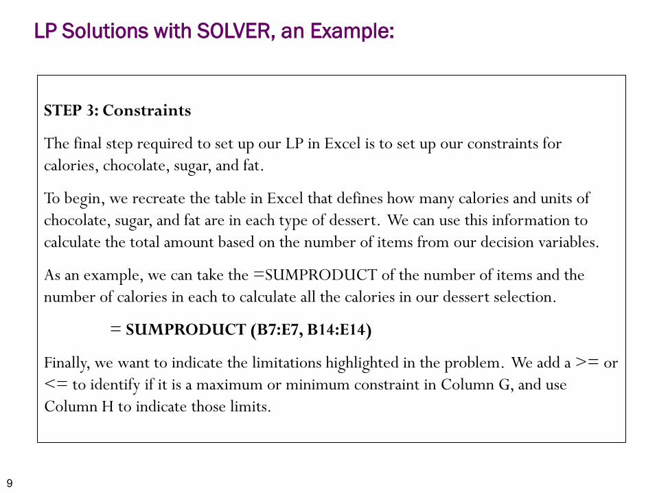
STEP 3: Constraints

The final step required to set up our LP in Excel is to set up our constraints for calories, chocolate, sugar, and fat.

To begin, we recreate the table in Excel that defines how many calories and units of chocolate, sugar, and fat are in each type of dessert. We can use this information to calculate the total amount based on the number of items from our decision variables.

As an example, we can take the =SUMPRODUCT of the number of items and the number of calories in each to calculate all the calories in our dessert selection.

= SUMPRODUCT (B7:E7, B14:E14)

Finally, we want to indicate the limitations highlighted in the problem. We add a >= or <= to identify if it is a maximum or minimum constraint in Column G, and use Column H to indicate those limits.

10

LP Solutions with SOLVER, an Example:

STEP 3: Constraints Formulas (cont.)

A B C D E F G H

12 CONSTRAINTS

13 Brownies Ice Cream Cola Cheese Cake Totals Required

14 Calories 400 200 150 500 =SUMPRODUCT($B$7:$E$7,B14:E14) >= 500

15 Chocolate 3 2 0 0 =SUMPRODUCT($B$7:$E$7,B15:E15) >= 6

16 Sugar 2 2 4 4 =SUMPRODUCT($B$7:$E$7,B16:E16) >= 10

17 Fat 2 4 1 5 =SUMPRODUCT($B$7:$E$7,B17:E17) >= 8

11

LP Solutions with SOLVER, an Example:

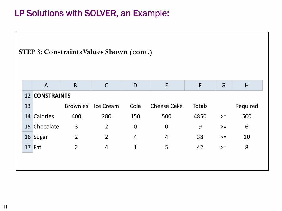
STEP 3: Constraints Values Shown (cont.)

A B C D E F G H

12 CONSTRAINTS

13 Brownies Ice Cream Cola Cheese Cake Totals Required

14 Calories 400 200 150 500 4850 >= 500

15 Chocolate 3 2 0 0 9 >= 6

16 Sugar 2 2 4 4 38 >= 10

17 Fat 2 4 1 5 42 >= 8

12

LP Solutions with SOLVER, an Example:

COMPLETE LP:

A B C D E F G H 1 DECISION VARIABLES 2 Brownies Ice Cream Cola Cheese Cake 3 Eaten 3 0 1 7 4 5 OBJECTIVE FUNCTION 6 Brownies Ice Cream Cola Cheese Cake 7 Eaten 3 0 1 7 8 Cost 50 20 30 80 9

10 Total 740 11 12 CONSTRAINTS 13 Brownies Ice Cream Cola Cheese Cake Totals Required 14 Calories 400 200 150 500 4850 >= 500 15 Chocolate 3 2 0 0 9 >= 6 16 Sugar 2 2 4 4 38 >= 10 17 Fat 2 4 1 5 42 >= 8

13

The SOLVER Parameters Dialog Box

STEP 1:

The SOLVER Parameters Dialog Box is used to describe the optimization problem to Excel. Clicking on Data > Solver, the following will open:

14

The SOLVER Parameters Dialog Box

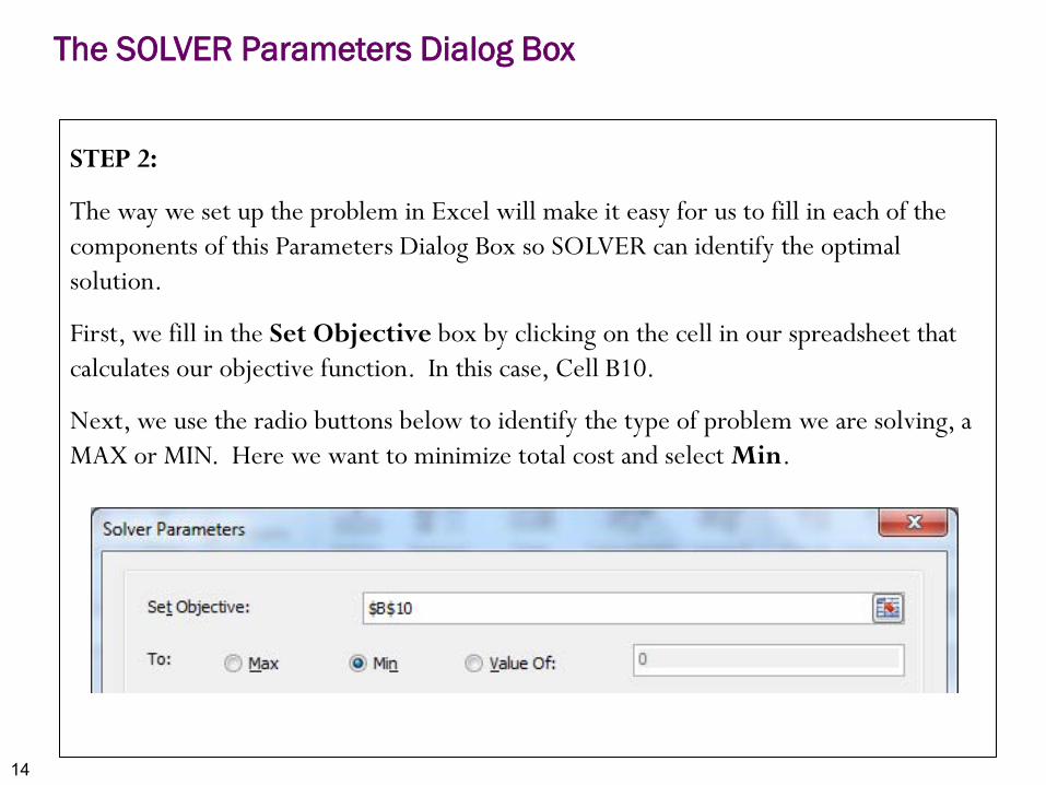
STEP 2:

The way we set up the problem in Excel will make it easy for us to fill in each of the components of this Parameters Dialog Box so SOLVER can identify the optimal solution.

First, we fill in the Set Objective box by clicking on the cell in our spreadsheet that calculates our objective function. In this case, Cell B10.

Next, we use the radio buttons below to identify the type of problem we are solving, a MAX or MIN. Here we want to minimize total cost and select Min.

15

The SOLVER Parameters Dialog Box

STEP 3:

Next, we need to identify the decision variables. SOLVER terms these as variable cells. After clicking into the By Changing Variable Cells box, we can select the decision variable cells in our LP, B3:E3. This tells SOLVER that it can change the number of brownies, scoops of ice cream, sodas, and pieces of cheese cake to reach an optimal solution.

16

The SOLVER Parameters Dialog Box

STEP 4:

We need to add our constraints to SOLVER to ensure our solution does not violate any of them. On the right-hand side of the window, there is a button to Add a constraint. After clicking on this, a box will appear that allows us to add our constraints.

We can use the Cell Reference box to input the totals for each constraint that we calculated. Using Calories as an example, we would click on Cell F14, which computed the total calories from all our desserts.

There are several options for constraint type: <=, >=, =, int (integer), bin (binary), or dif (all different, e.g., assignment, TSP). After adjusting the constraint type to be greater than or equal to (>=) we can click on the cell referencing the minimum quantity permitted, Cell H14. Instead of a reference, we can also enter a specific number. The complete constraint looks as follows:

17

The SOLVER Parameters Dialog Box

STEP 4 (cont.):

The Add button will allow us to include all the other constraints to SOLVER.

When you have constraints structured in the same way (like these are), there is a faster way to add them all to SOLVER. Instead of entering each constraint individually, you can instead add them in one step.

In the Cell Reference box and Constraint box, you can also specify an array of cell references. If both the Cell Reference and Constraint are specified using an array of cell references, the length of the arrays must match and Solver treats this constraint as n individual constraints, where n is the length of each array.

18

The SOLVER Parameters Dialog Box

STEP 4 (cont.):

We have now created four Constraints. SOLVER will ensure that the changing cells are chosen so F14>=H14, F15>=H15, F16>=H16, and F17>=H17. In short, the diet will be chosen to ensure that enough calories, chocolate, sugar, and fat are eaten.

The Change button allows you to modify a constraint already entered and Delete allows you to delete a previously entered constraint. If you need to add more constraints, choose Add.

-OR-

19

The SOLVER Parameters Dialog Box

STEP 5:

After adding all our constraints, here is the SOLVER Parameters Dialog Box:

Note the checked box titled Make Unconstrained Variables Non-Negative. This allows us to capture non-negativity constraints. (Actually, all variables will be constrained to be >= 0).

Additionally, you should change the Select a Solving Method to SIMPLEX LP when you are solving a linear program. The other options allow for solutions for nonlinear programs.

Finally, click Solve for your solution.

20

The SOLVER Parameters Dialog Box

SOLUTION:

After you Solve, the Parameters Dialog Box will close and the decision variables will change to the optimal solution. Because we referenced these cells in all our calculations, the objective function and constraints will also change.

A B C D E F G H 1 DECISION VARIABLES 2 Brownies Ice Cream Cola Cheese Cake 3 Eaten 0 3 1 0 4 5 OBJECTIVE FUNCTION 6 Brownies Ice Cream Cola Cheese Cake 7 Eaten 0 3 1 0 8 Cost 50 20 30 80 9

10 Total 90 11 12 CONSTRAINTS 13 Brownies Ice Cream Cola Cheese Cake Totals Required 14 Calories 400 200 150 500 750 >= 500 15 Chocolate 3 2 0 0 6 >= 6 16 Sugar 2 2 4 4 10 >= 10 17 Fat 2 4 1 5 13 >= 8

21

The SOLVER Parameters Dialog Box

OPTIONS:

The Parameters Dialog Box also has a number of options on how to calculate solutions.

Constraint Precision is the degree of accuracy of the Solver algorithm (for example, how close does the value of the LHS of a constraint have to be before it is considered equal to the RHS).

Max Time allows you to set the number of seconds before Solver will stop.

Iterations, similar to Max Time, allows you to specify the maximum number of iterations (steps of the Solver algorithm) before stopping.

If you want to learn about other options in SOLVER, please reference the SOLVER website:

www.solver.com

22

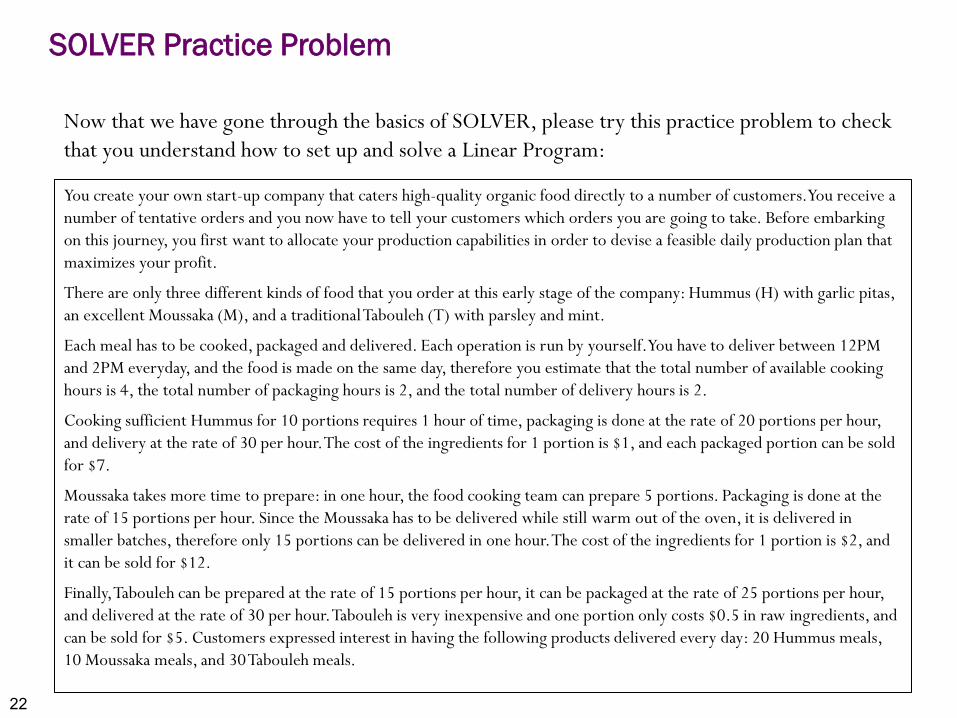
SOLVER Practice Problem

You create your own start-up company that caters high-quality organic food directly to a number of customers. You receive a number of tentative orders and you now have to tell your customers which orders you are going to take. Before embarking on this journey, you first want to allocate your production capabilities in order to devise a feasible daily production plan that maximizes your profit.

There are only three different kinds of food that you order at this early stage of the company: Hummus (H) with garlic pitas, an excellent Moussaka (M), and a traditional Tabouleh (T) with parsley and mint.

Each meal has to be cooked, packaged and delivered. Each operation is run by yourself. You have to deliver between 12PM and 2PM everyday, and the food is made on the same day, therefore you estimate that the total number of available cooking hours is 4, the total number of packaging hours is 2, and the total number of delivery hours is 2.

Cooking sufficient Hummus for 10 portions requires 1 hour of time, packaging is done at the rate of 20 portions per hour, and delivery at the rate of 30 per hour. The cost of the ingredients for 1 portion is $1, and each packaged portion can be sold for $7.

Moussaka takes more time to prepare: in one hour, the food cooking team can prepare 5 portions. Packaging is done at the rate of 15 portions per hour. Since the Moussaka has to be delivered while still warm out of the oven, it is delivered in smaller batches, therefore only 15 portions can be delivered in one hour. The cost of the ingredients for 1 portion is $2, and it can be sold for $12.

Finally, Tabouleh can be prepared at the rate of 15 portions per hour, it can be packaged at the rate of 25 portions per hour, and delivered at the rate of 30 per hour. Tabouleh is very inexpensive and one portion only costs $0.5 in raw ingredients, and can be sold for $5. Customers expressed interest in having the following products delivered every day: 20 Hummus meals, 10 Moussaka meals, and 30 Tabouleh meals.

Now that we have gone through the basics of SOLVER, please try this practice problem to check that you understand how to set up and solve a Linear Program:

23

SOLVER Practice Problem

SOLUTION:

A B C D F G H 1 DECISION VARIABLES 2 Hummus Moussaka Tabouleh 3 Orders 8 6 30 4 5 COST AND/OR PROFIT DATA 6 Hummus Moussaka Tabouleh 7 Orders 8 6 30 8 Profit 6 10 4.5 9 OBJECTIVE FUNCTION

10 Total 243 11 12 CONSTRAINTS 13 Hummus Moussaka Tabouleh Totals Maximum 14 Cooking 0.100 0.200 0.067 4.000 <= 4 15 Packaging 0.050 0.067 0.040 2.000 <= 2 16 Delivery 0.033 0.067 0.033 1.667 <= 2 17 Demand H 8 <= 20 18 Demand M 6 <= 10 19 Demand T 30 <= 30

MIT OpenCourseWarehttp://ocw.mit.edu

15.053 Optimization Methods in Management ScienceSpring 2013

For information about citing these materials or our Terms of Use, visit: http://ocw.mit.edu/terms.