Embed Size (px)
Citation preview

UN
IVER
SID
AD
E D
E SÃ
O P
AULO
Inst
ituto
de
Ciên
cias
Mat
emát
icas
e d
e Co
mpu
taçã
o
Data Warehouses in the era of Big Data: efficient processingof Star Joins in Hadoop
Jaqueline Joice BritoTese de Doutorado do Programa de Pós-Graduação em Ciências deComputação e Matemática Computacional (PPG-CCMC)


SERVIÇO DE PÓS-GRADUAÇÃO DO ICMC-USP
Data de Depósito:
Assinatura: ______________________
Jaqueline Joice Brito
Data Warehouses in the era of Big Data: efficient processingof Star Joins in Hadoop
Doctoral dissertation submitted to the Institute ofMathematics and Computer Sciences – ICMC-USP, inpartial fulfillment of the requirements for the degree ofthe Doctorate Program in Computer Science andComputational Mathematics. FINAL VERSION
Concentration Area: Computer Science andComputational Mathematics
Advisor: Profa. Dra. Cristina Dutra de Aguiar Ciferri
USP – São CarlosFebruary 2018

Ficha catalográfica elaborada pela Biblioteca Prof. Achille Bassi e Seção Técnica de Informática, ICMC/USP,
com os dados inseridos pelo(a) autor(a)
Bibliotecários responsáveis pela estrutura de catalogação da publicação de acordo com a AACR2: Gláucia Maria Saia Cristianini - CRB - 8/4938 Juliana de Souza Moraes - CRB - 8/6176
B862dBrito, Jaqueline Joice Data Warehouses in the era of Big Data:efficient processing of Star Joins in Hadoop /Jaqueline Joice Brito; orientadora Cristina Dutrade Aguiar Ciferri. -- São Carlos, 2018. 161 p.
Tese (Doutorado - Programa de Pós-Graduação emCiências de Computação e Matemática Computacional) -- Instituto de Ciências Matemáticas e de Computação,Universidade de São Paulo, 2018.
1. Star Join. 2. Data Warehouse. 3. Hadoop. 4.Big Data. 5. Cloud Computing. I. Ciferri, CristinaDutra de Aguiar, orient. II. Título.

Jaqueline Joice Brito
Data Warehouses na era do Big Data: processamentoeficiente de Junções Estrela no Hadoop
Tese apresentada ao Instituto de CiênciasMatemáticas e de Computação – ICMC-USP,como parte dos requisitos para obtenção do títulode Doutora em Ciências – Ciências de Computação eMatemática Computacional. VERSÃO REVISADA
Área de Concentração: Ciências de Computação eMatemática Computacional
Orientadora: Profa. Dra. Cristina Dutra deAguiar Ciferri
USP – São CarlosFevereiro de 2018


To the best band in the world, The D!


ACKNOWLEDGEMENTS
I begin thanking my family for the all support and patience. Especial thanks to myhusband Thiago, who always encouraged, assisted and believed in me.
I thank my advisor, Prof. Cristina Dutra de Aguiar Ciferri, for the guidance, support, andcontribution to my development as a researcher.
I thank my internship supervisor, Prof. Yannis Papakonstantinou from the Universityof California San Diego, with whom I had productive discussions, enriching my experience asvisiting researcher in San Diego.
I also thank all the collaborators who have shared their valuable knowledge and con-tributed to my research.
I thank all the friends and coleagues from the ICMC / USP Data Bases and Images Groupthat I made throughout the doctorate, with whom I shared many experiences that helped me growand mature, both scientifically and personally.
I acknowledge financial support from São Paulo Research Foundation (FAPESP), grants2012/13158-9 and 2015/11106-0. I also would like to thank the funding agencies CAPES andCNPQ, and the Microsoft Azure Research Award MS-AZR-0036P for supporting this thesis.
Finally, I thank the ICMC-USP, for the institutional support.


“To find your fame and fortune,
through the valley you must walk.
You will face your inner demons.
Now go my son and rock!”
(Tenacious D)


ABSTRACTBRITO, J. J. Data Warehouses in the era of Big Data: efficient processing of Star Joins inHadoop. 2018. 161 p. Tese (Doutorado em Ciências – Ciências de Computação e MatemáticaComputacional) – Instituto de Ciências Matemáticas e de Computação, Universidade de SãoPaulo, São Carlos – SP, 2018.
The era of Big Data is here: the combination of unprecedented amounts of data collected everyday with the promotion of open source solutions for massively parallel processing has shifted theindustry in the direction of data-driven solutions. From recommendation systems that help youfind your next significant one to the dawn of self-driving cars, Cloud Computing has enabledcompanies of all sizes and areas to achieve their full potential with minimal overhead. Inparticular, the use of these technologies for Data Warehousing applications has decreased costsgreatly and provided remarkable scalability, empowering business-oriented applications such asOnline Analytical Processing (OLAP). One of the most essential primitives in Data Warehousesare the Star Joins, i.e. joins of a central table with satellite dimensions. As the volume of thedatabase scales, Star Joins become unpractical and may seriously limit applications. In this thesis,we proposed specialized solutions to optimize the processing of Star Joins. To achieve this, weused the Hadoop software family on a cluster of 21 nodes. We showed that the primary bottleneckin the computation of Star Joins on Hadoop lies in the excessive disk spill and overhead due tonetwork communication. To mitigate these negative effects, we proposed two solutions based ona combination of the Spark framework with either Bloom filters or the Broadcast technique. Thisreduced the computation time by at least 38%. Furthermore, we showed that the use of full scanmay significantly hinder the performance of queries with low selectivity. Thus, we proposed adistributed Bitmap Join Index that can be processed as a secondary index with loose-bindingand can be used with random access in the Hadoop Distributed File System (HDFS). We alsoimplemented three versions (one in MapReduce and two in Spark) of our processing algorithmthat uses the distributed index, which reduced the total computation time up to 88% for StarJoins with low selectivity from the Star Schema Benchmark (SSB). Because, ideally, the systemshould be able to perform both random access and full scan, our solution was designed to rely ona two-layer architecture that is framework-agnostic and enables the use of a query optimizer toselect which approaches should be used as a function of the query. Due to the ubiquity of joins asprimitive queries, our solutions are likely to fit a broad range of applications. Our contributionsnot only leverage the strengths of massively parallel frameworks but also exploit more efficientaccess methods to provide scalable and robust solutions to Star Joins with a significant drop intotal computation time.
Keywords: Star join, Data Warehouse, Hadoop, Big data, Cloud Computing.


RESUMOBRITO, J. J. Data Warehouses na era do Big Data: processamento eficiente de JunçõesEstrela no Hadoop. 2018. 161 p. Tese (Doutorado em Ciências – Ciências de Computação eMatemática Computacional) – Instituto de Ciências Matemáticas e de Computação, Universidadede São Paulo, São Carlos – SP, 2018.
A era do Big Data chegou: a combinação entre o volume dados coletados diarimente com osurgimento de soluções de código aberto para o processamento massivo de dados mudou parasempre a indústria. De sistemas de recomendação que assistem às pessoas a encontrarem seuspares românticos à criação de carros auto-dirigidos, a Computação em Nuvem permitiu queempresas de todos os tamanhos e áreas alcançassem o seu pleno potencial com custos reduzidos.Em particular, o uso dessas tecnologias em aplicações de Data Warehousing reduziu custos eproporcionou alta escalabilidade para aplicações orientadas a negócios, como em processamentoon-line analítico (Online Analytical Processing- OLAP). Junções Estrelas são das primitivasmais essenciais em Data Warehouses, ou seja, consultas que realizam a junções de tabelasde fato com tabelas de dimensões. Conforme o volume de dados aumenta, Junções Estrelatornam-se custosas e podem limitar o desempenho das aplicações. Nesta tese são propostassoluções especializadas para otimizar o processamento de Junções Estrela. Para isso, utilizamosa família de software Hadoop em um cluster de 21 nós. Nós mostramos que o gargalo primáriona computação de Junções Estrelas no Hadoop reside no excesso de operações escrita do disco(disk spill) e na sobrecarga da rede devido a comunicação excessiva entre os nós. Para reduzirestes efeitos negativos, são propostas duas soluções em Spark baseadas nas técnicas Bloom
filters ou Broadcast, reduzindo o tempo total de computação em pelo menos 38%. Além disso,mostramos que a realização de uma leitura completa das tables (full table scan) pode prejudicarsignificativamente o desempenho de consultas com baixa seletividade. Assim, nós propomosum Índice Bitmap de Junção distribuído que é implementado como um índice secundário quepode ser combinado com acesso aleatório no Hadoop Distributed File System (HDFS). Nósimplementamos três versões (uma em MapReduce e duas em Spark) do nosso algoritmo deprocessamento baseado nesse índice distribuído, os quais reduziram o tempo de computaçãoem até 77% para Junções Estrelas de baixa seletividade do Star Schema Benchmark (SSB).Como idealmente o sistema deve ser capaz de executar tanto acesso aleatório quanto full scan,nós também propusemos uma arquitetura genérica que permite a inserção de um otimizadorde consultas capaz de selecionar quais abordagens devem ser usadas dependendo da consulta.Devido ao fato de consultas de junção serem frequentes, nossas soluções são pertinentes a umaampla gama de aplicações. A contribuições desta tese não só fortalecem o uso de frameworks deprocessamento de código aberto, como também exploram métodos mais eficientes de acesso aosdados para promover uma melhora significativa no desempenho Junções Estrela.
Palavras-chave: Junção Estrela, Data Warehouse, Hadoop, Big Data, Computação em Nuvem.


LIST OF FIGURES
Figure 1 – Traditional data warehousing architecture. Data come from heterogeneoussources. ETL processes extract, clean and transform the data. The trans-formed data is loaded and stored in the central repository: the data warehouse.Reporting and mining tools access the data warehouse, commonly usingstandard SQL language. . . . . . . . . . . . . . . . . . . . . . . . . . . . 36
Figure 2 – Multidimensional cube of the retail chain example. Facts represents sales ofproducts made by suppliers to customers, which are quantified in each cellby the numerical measure quantity. Product, supplier and costumer are thedimensions. . . . . . . . . . . . . . . . . . . . . . . . . . . . . . . . . . . 38
Figure 3 – Star schema of the retail chain example. Dimensions are mapped into satel-lites tables. The fact table points to the dimensions using foreign keys. Thenumerical measure quantity is stored in the fact table. . . . . . . . . . . . . 41
Figure 4 – Star Join over the retail chain example. This query access three dimensions:product, customer and date. The predicates are restricting the data to sales oftoys for customer from the city of Sao Paulo in the year 2017. . . . . . . . . 42
Figure 5 – Bitmap Join Index for the attribute category of the dimension Product. In-stances for the fact and dimension tables are showed in from (a) to (e). TheBitmap Join Index for the attribute category is depicted in (f). . . . . . . . 43
Figure 6 – Row oriented (a) and column oriented (b) storage of the dimension tableProduct from the retail sales example. . . . . . . . . . . . . . . . . . . . . 45
Figure 7 – Representation of the Apache Hadoop Stack with some technologies. . . . . 54
Figure 8 – The HDFS architecture. A client application retrieves metadata from theNameNode, and performs read/write operations directly with the DataNode. 55
Figure 9 – MapReduce applied on the resolution of a word count problem. . . . . . . . 57
Figure 10 – Data Lake: Single huge repository for an enterprise with data from differentsources. The data has different natures, unstructured, semi-structured andstructured, and is usually kept in its native format in the same repository. . . 63
Figure 11 – Example of a Data Warehousing architecture using the Data Lake as stagingarea: Single huge repository for an enterprise with data from different sources.The data has different natures, unstructured, semi-structured and structured,and is usually kept in its native format in the same repository. . . . . . . . . 65
Figure 12 – Hadoop as a Platform for (a) ETL or (b) ELT. . . . . . . . . . . . . . . . . 67
Figure 13 – Hadoop for Data Warehouse Offloading. . . . . . . . . . . . . . . . . . . . 67

Figure 14 – Hadoop for the deployment of a high performnance Data Warehouse. . . . . 68
Figure 15 – Time performance as a function of the amount of (a) shuffled data and the(b) disk spill. We present MapReduce (red dots) and Spark (blue dots)approaches, with the orange line showing the general trend of MapReduceapproaches. We used SSB query Q4.1 with SF 100. Our approaches SP-
Broadcast-Join and SP-Bloom-Cascade-Join require half data spill and aboutone third of the computation time of the best MapReduce algorithm. . . . . 84
Figure 16 – Impact of the Scale Factor SF in the performance of SP-Broadcast-Join andSP-Bloom-Cascade-Join. . . . . . . . . . . . . . . . . . . . . . . . . . . . 86
Figure 17 – Comparing SP-Broadcast-Join and SP-Bloom-Cascade-Join performanceswith (a) 512MB and (b) 1GB of memory per executor. SP-Broadcast-Join
seems reasonably sensitive to low memory cases. . . . . . . . . . . . . . . 87
Figure 18 – Comparing SP-Broadcast-Join and SP-Bloom-Cascade-Join performanceswith 20 executors and variable memory. In special, panel (a) shows thatSP-Broadcast-Join’s performance is impaired with a decreasing memory,being outperformed by SP-Bloom-Cascade-Join eventually. . . . . . . . . . 87
Figure 19 – Comparing SP-Broadcast-Join and SP-Bloom-Cascade-Join performanceswith fixed total memory while increasing the number of executors. Only whenthe total available memory is lower (panel a) SP-Broadcast-Join performanceis impaired. . . . . . . . . . . . . . . . . . . . . . . . . . . . . . . . . . . 88
Figure 20 – Proposed architecture based on an Access Layer and Processing Layer. . . . 93
Figure 21 – A representation of our distributed Star Join Bitmap Index and its distributedversion.(a): Example of instance of a dimension and fact tables. (b): Exampleof instance of the bitmap join index for the attribute value a1 = 10. (c):Physical storage of the distributed bitmap index. (d): Example of applicationto solve an AND operation. . . . . . . . . . . . . . . . . . . . . . . . . . . 95
Figure 22 – Workflow of our solution on a Hadoop-based instance of the architecture anddistributed Bitmap Join Index. . . . . . . . . . . . . . . . . . . . . . . . . 98
Figure 23 – Region of values for the Number of Reducers in which the performance ofthe MapReduce strategies based on full scan were either optimal or very closeto optimal. . . . . . . . . . . . . . . . . . . . . . . . . . . . . . . . . . . . 106
Figure 24 – All of the MapReduce strategies based on full scan showed better performancewith a higher value of Slow Start Ratio. . . . . . . . . . . . . . . . . . . . 107
Figure 25 – The performance of the MR-Bitmap-Join, which combines MapReduce withthe distributed Bitmap Join index, as a function of the Number of Reducers(top) and the Slow Start Ratio (bottom). Note that the range of values in they-axis is smaller than that of all plots in Figures 23 and 24. . . . . . . . . . 107

Figure 26 – The strategies based on random access (green bars) outperformed those thatuse full scan, regardless of the query. The strategy names follow those inTable 2. This experiment was performed with Scale Factor 100 and theselectivity of each of these queries are in Table 5. The improvement providedby the use of the distributed Bitmap Join Index ranged from 59.2% to 88.3%.Red and blue bars refer to full scan approaches. Approaches encoded by bluebars apply optimization. . . . . . . . . . . . . . . . . . . . . . . . . . . . . 109
Figure 27 – Strategies based on random access, both for Spark (a-b) and MapReduce(c-d), outperformed those based on full scan when the query selectivity wassmall. . . . . . . . . . . . . . . . . . . . . . . . . . . . . . . . . . . . . . 110
Figure 28 – When the database is sorted, the performance of the methods based on randomaccess, both for Spark (a-b) and MapReduce (c-d), outperformed those basedon full scan on a broader range of selectivity values. . . . . . . . . . . . . . 111
Figure 29 – A distributed file system with intermediary block sizes benefited the perfor-mance of the methods based on the random access. Methods based on fullscan were not affected significantly. . . . . . . . . . . . . . . . . . . . . . . 112
Figure 30 – The computation times using Spark (a) and MapReduce (b) scale linearly asa function of the database Scale Factor (SF). . . . . . . . . . . . . . . . . . 113
Figure 31 – PlatoDB’s architecture, including details on the segment tree generation andquery processing. . . . . . . . . . . . . . . . . . . . . . . . . . . . . . . . 137
Figure 32 – Grammar of query expressions. . . . . . . . . . . . . . . . . . . . . . . . . 142Figure 33 – Formulas for estimating answer and error for each algebraic operator (single
segment). . . . . . . . . . . . . . . . . . . . . . . . . . . . . . . . . . . . 147Figure 34 – Approximate query answer and associated error for query Q = Sum(Times
(Minus(T,SeriesGen(µ,n)), Minus(T,SeriesGen(µ,n)),1,n). Compressionfunctions and error measures are shown in blue and red, respectively. . . . . 148
Figure 35 – Example of aligned time series segments. The new generated time series T3
is shown in red color. . . . . . . . . . . . . . . . . . . . . . . . . . . . . . 149Figure 36 – Formulas for estimating answer and error for time series operators (multiple
segments). For each output time series segment Sc,i, let Sa,u and Sb,v be theinput segments that overlap with Sc,i. . . . . . . . . . . . . . . . . . . . . . 150
Figure 37 – Formulas for estimating answer and error for the aggregation operator (multi-ple segments). . . . . . . . . . . . . . . . . . . . . . . . . . . . . . . . . . 150
Figure 38 – Segment Tree for Theorem 2. . . . . . . . . . . . . . . . . . . . . . . . . . 154Figure 39 – Query processing performance for correlation query (time shown in ms). . . 157


LIST OF ALGORITHMS
Algorithm 1 – SP-Cascade-Join . . . . . . . . . . . . . . . . . . . . . . . . . . . . . 80Algorithm 2 – SP-Bloom-Cascade-Join . . . . . . . . . . . . . . . . . . . . . . . . . 81Algorithm 3 – SP-Broadcast-Join . . . . . . . . . . . . . . . . . . . . . . . . . . . . 82Algorithm 4 – Creating the Distributed Bitmap Join Index . . . . . . . . . . . . . . . 96Algorithm 5 – Processing the Star-Join Query with the Distributed Bitmap Join index . 99Algorithm 6 – Distributed Bitmap Creation with MapReduce . . . . . . . . . . . . . . 101Algorithm 7 – Bitmap Star-Join Processing in MapReduce . . . . . . . . . . . . . . . 102Algorithm 8 – Bitmap Star-Join Processing in Spark . . . . . . . . . . . . . . . . . . 103Algorithm 9 – PlatoDB Query Processing . . . . . . . . . . . . . . . . . . . . . . . . 153


LIST OF TABLES
Table 1 – Characteristics comparison between Data Warehouses and Data Lakes. . . . 64Table 2 – List of all approaches outlined in this chapter and implemented for our perfor-
mance evaluations in Chapters 6 and 7. The approaches proposed in this thesisare highlighted in bold. The second and third columns distinguish the accessmethod used by each approach (random access vs. full scan). The fourth, fifthand sixth columns identify optimization techniques, if any, as described in thischapter. . . . . . . . . . . . . . . . . . . . . . . . . . . . . . . . . . . . . . 76
Table 3 – Dataset characteristics used in the experiments. We show for each scalingfactor SF the number of tuples in the fact table (# Tuples) and its disk size. . 83
Table 4 – Information about the datasets and bitmap indices used in the experiments.For each value of the Scaling Factor SF, we provide the number of tuples inthe fact table (# Tuples), the size occupied in disk within HBase, the numberof tuples in the fact table per HBase region, the space occupied in disk by eachbitmap array and the number of partitions of each bitmap array. . . . . . . . 104
Table 5 – List of queries used in the experiments. For each query, we show their predicateand approximate selectivity. Queries 4.4, 4.5 and 4.6 were created based onquery 4.3 to provide additional tests of the query selectivity effects on thequery performance. . . . . . . . . . . . . . . . . . . . . . . . . . . . . . . . 105
Table 6 – Query expressions for common statistics. . . . . . . . . . . . . . . . . . . . 141Table 7 – Incremental update of estimated errors for time series operators. . . . . . . . 155Table 8 – Raw data and segment tree sizes. . . . . . . . . . . . . . . . . . . . . . . . . 157


LIST OF ABBREVIATIONS AND ACRONYMS
ACID Atomicity, Consistency, Isolation, Durability
API Application Programming Interface
BASE Basic availability, Soft state and Eventual consistency
BI Business Intelligence
CAP Consistency, Availability, Partition Tolerance
CRM Customer Relationship Management
DaaS Database as a Service
DAG Directed Acyclic Graph
EDW Enterprise Data Warehouse
ERP Enterprise Resource Planning
ETL Extract, Transform, Load
HDFS Hadoop Distributed File System
IaaS Infrastructure as a Service
MOLAP Multidimensional Online Analytical Processing
MPP Massive Parallel Processing
NIST National Institute of Standards and Technology
NoSQL Not only SQL
OLAP Online Analytical Processing
OLTP Online Transaction Processing
PaaS Platform as a Service
PDW Parallel Data Warehousing
RDD Resilient Distributed Dataset
ROLAP Relational Online Analytical Processing
SaaS Software as a Service
SQL Structured Query Language


CONTENTS
1 INTRODUCTION . . . . . . . . . . . . . . . . . . . . . . . . . . . . . . . 291.1 Motivation . . . . . . . . . . . . . . . . . . . . . . . . . . . . . . . . . . . 301.2 Objectives . . . . . . . . . . . . . . . . . . . . . . . . . . . . . . . . . . . . 311.3 Contributions . . . . . . . . . . . . . . . . . . . . . . . . . . . . . . . . . . 311.4 Thesis Organization . . . . . . . . . . . . . . . . . . . . . . . . . . . . . . 32
2 TRADITIONAL DATA WAREHOUSING . . . . . . . . . . . . . . . . . . 352.1 Introduction . . . . . . . . . . . . . . . . . . . . . . . . . . . . . . . . . . 352.2 The Traditional Data Warehousing Architecture . . . . . . . . . . . . . 36
2.2.1 The Data Sources . . . . . . . . . . . . . . . . . . . . . . . . . . . 362.2.2 ETL - Extract, Transform and Load . . . . . . . . . . . . . . . . 372.2.3 The Data Warehouse . . . . . . . . . . . . . . . . . . . . . . . . . 372.2.4 Business Intelligence Applications . . . . . . . . . . . . . . . . . 38
2.3 The Multidimensional Model . . . . . . . . . . . . . . . . . . . . . . . . 382.3.1 Dimensions and Facts . . . . . . . . . . . . . . . . . . . . . . . . . 382.3.2 Aggregation Levels . . . . . . . . . . . . . . . . . . . . . . . . . . 392.3.3 OLAP Queries . . . . . . . . . . . . . . . . . . . . . . . . . . . . . 39
2.4 Relational OLAP Systems . . . . . . . . . . . . . . . . . . . . . . . . . . 402.4.1 The Star Schema . . . . . . . . . . . . . . . . . . . . . . . . . . . 402.4.2 Query processing . . . . . . . . . . . . . . . . . . . . . . . . . . . 40
2.4.2.1 Star Joins . . . . . . . . . . . . . . . . . . . . . . . . . . . . 412.4.2.2 Materialized Views . . . . . . . . . . . . . . . . . . . . . . . 412.4.2.3 The Bitmap Join Index . . . . . . . . . . . . . . . . . . . . . 42
2.5 Parallel Data Warehousing . . . . . . . . . . . . . . . . . . . . . . . . . . 442.5.1 MPP Databases . . . . . . . . . . . . . . . . . . . . . . . . . . . . 442.5.2 Columnar Storage . . . . . . . . . . . . . . . . . . . . . . . . . . . 452.5.3 MPP Engine . . . . . . . . . . . . . . . . . . . . . . . . . . . . . . 46
2.6 Conclusions . . . . . . . . . . . . . . . . . . . . . . . . . . . . . . . . . . . 46
3 BIG DATA TECHNOLOGIES . . . . . . . . . . . . . . . . . . . . . . . . . 493.1 Introduction . . . . . . . . . . . . . . . . . . . . . . . . . . . . . . . . . . 493.2 Big Data . . . . . . . . . . . . . . . . . . . . . . . . . . . . . . . . . . . . 50
3.2.1 Volume, Variety and Velocity . . . . . . . . . . . . . . . . . . . . 50

3.2.2 Analytics and Data Management . . . . . . . . . . . . . . . . . . 513.3 NoSQL Databases . . . . . . . . . . . . . . . . . . . . . . . . . . . . . . . 51
3.3.1 The CAP Theorem . . . . . . . . . . . . . . . . . . . . . . . . . . 523.3.2 NoSQL Main Characteristics . . . . . . . . . . . . . . . . . . . . 523.3.3 Data Storage Paradigms . . . . . . . . . . . . . . . . . . . . . . . 53
3.4 The Apache Hadoop . . . . . . . . . . . . . . . . . . . . . . . . . . . . . 543.4.1 The Hadoop Distributed File System (HDFS) . . . . . . . . . . 553.4.2 File Formats and Storage Engines . . . . . . . . . . . . . . . . . 55
3.4.2.1 The Apache HBase . . . . . . . . . . . . . . . . . . . . . . . 563.4.3 Processing Engines . . . . . . . . . . . . . . . . . . . . . . . . . . 57
3.4.3.1 Hadoop MapReduce . . . . . . . . . . . . . . . . . . . . . . 573.4.3.2 Apache Spark . . . . . . . . . . . . . . . . . . . . . . . . . . 58
3.4.4 SQL on Hadoop . . . . . . . . . . . . . . . . . . . . . . . . . . . . 583.4.4.1 Broadcast . . . . . . . . . . . . . . . . . . . . . . . . . . . . 593.4.4.2 Bloom filters . . . . . . . . . . . . . . . . . . . . . . . . . . 59
3.5 Conclusions . . . . . . . . . . . . . . . . . . . . . . . . . . . . . . . . . . . 60
4 MODERN DATA WAREHOUSES . . . . . . . . . . . . . . . . . . . . . . 614.1 Introduction . . . . . . . . . . . . . . . . . . . . . . . . . . . . . . . . . . 614.2 Evolution of the Data Warehousing Architecture . . . . . . . . . . . . 61
4.2.1 Data Lakes . . . . . . . . . . . . . . . . . . . . . . . . . . . . . . . 624.2.2 The Modern Data Warehousing Architecture . . . . . . . . . . 64
4.3 Use of NoSQL Databases . . . . . . . . . . . . . . . . . . . . . . . . . . 644.4 Data Warehousing with Hadoop . . . . . . . . . . . . . . . . . . . . . . 66
4.4.1 Platform for ETL or ELT . . . . . . . . . . . . . . . . . . . . . . . 664.4.2 Data Warehouse Offloading . . . . . . . . . . . . . . . . . . . . . 664.4.3 High Performance Data Warehouse . . . . . . . . . . . . . . . . 67
4.5 Conclusions . . . . . . . . . . . . . . . . . . . . . . . . . . . . . . . . . . . 68
5 RELATED WORK . . . . . . . . . . . . . . . . . . . . . . . . . . . . . . . 695.1 Introduction . . . . . . . . . . . . . . . . . . . . . . . . . . . . . . . . . . 695.2 Joins in Hadoop . . . . . . . . . . . . . . . . . . . . . . . . . . . . . . . . 705.3 Star Joins in Hadoop . . . . . . . . . . . . . . . . . . . . . . . . . . . . . 715.4 Conclusions . . . . . . . . . . . . . . . . . . . . . . . . . . . . . . . . . . . 75
6 PROCESSING STAR JOINS WITH REDUCED DISK SPILL AND COM-MUNICATION IN HADOOP . . . . . . . . . . . . . . . . . . . . . . . . . 776.1 Introduction . . . . . . . . . . . . . . . . . . . . . . . . . . . . . . . . . . 776.2 Proposed Method . . . . . . . . . . . . . . . . . . . . . . . . . . . . . . . 78
6.2.1 Methodology . . . . . . . . . . . . . . . . . . . . . . . . . . . . . . 78

6.2.2 SP-Cascade-Join . . . . . . . . . . . . . . . . . . . . . . . . . . . . 796.2.3 SP-Bloom-Cascade-Join . . . . . . . . . . . . . . . . . . . . . . . 806.2.4 SP-Broadcast-Join . . . . . . . . . . . . . . . . . . . . . . . . . . . 80
6.3 Performance Analysis . . . . . . . . . . . . . . . . . . . . . . . . . . . . 826.3.1 Experimental Setup . . . . . . . . . . . . . . . . . . . . . . . . . . 826.3.2 Disk spill, network communication and performance . . . . . . 836.3.3 Scaling the dataset . . . . . . . . . . . . . . . . . . . . . . . . . . 856.3.4 Impact of Memory per Executor . . . . . . . . . . . . . . . . . . 85
6.4 Conclusions . . . . . . . . . . . . . . . . . . . . . . . . . . . . . . . . . . . 88
7 EMPLOYING RANDOM ACCESS WITH BITMAP JOIN INDICES FORSTAR JOINS IN HADOOP . . . . . . . . . . . . . . . . . . . . . . . . . . 917.1 Introduction . . . . . . . . . . . . . . . . . . . . . . . . . . . . . . . . . . 917.2 Proposed Method . . . . . . . . . . . . . . . . . . . . . . . . . . . . . . . 92
7.2.1 Combining Processing and Access Layers . . . . . . . . . . . . . 937.2.2 Distributed Bitmap Join Index for random access . . . . . . . . 947.2.3 Using secondary indices with loose binding . . . . . . . . . . . . 977.2.4 Processing Star Joins with the Distributed Bitmap Join Index 97
7.3 Implementations in MapReduce and Spark . . . . . . . . . . . . . . . . 987.3.1 Distributed Bitmap Creation Algorithm with MapReduce . . . 997.3.2 Bitmap Star-join Processing Algorithm in MapReduce . . . . . 1007.3.3 Bitmap Star-join Processing Algorithm in Spark . . . . . . . . . 100
7.4 Performance Evaluation . . . . . . . . . . . . . . . . . . . . . . . . . . . 1047.4.1 Methodology and experimental setup . . . . . . . . . . . . . . . 1047.4.2 Parameter optimization of the MapReduce algorithms . . . . . 1067.4.3 Performance across different approaches . . . . . . . . . . . . . 1087.4.4 Effect of the selectivity . . . . . . . . . . . . . . . . . . . . . . . . 1087.4.5 Influence of the block size . . . . . . . . . . . . . . . . . . . . . . 1117.4.6 Scaling the dataset . . . . . . . . . . . . . . . . . . . . . . . . . . 112
7.5 Conclusions . . . . . . . . . . . . . . . . . . . . . . . . . . . . . . . . . . . 113
8 CONCLUSIONS . . . . . . . . . . . . . . . . . . . . . . . . . . . . . . . . 1158.1 Review of Results . . . . . . . . . . . . . . . . . . . . . . . . . . . . . . . 115
8.1.1 Overview of Data Warehousing in the Era of Big Data . . . . . 1168.1.2 Efficiently Processing Star Joins . . . . . . . . . . . . . . . . . . 1168.1.3 Random Access with Distributed Bitmap Join Indices . . . . . 1168.1.4 Itemized List of Contributions . . . . . . . . . . . . . . . . . . . . 117
8.2 Future Work . . . . . . . . . . . . . . . . . . . . . . . . . . . . . . . . . . 1188.3 Publications . . . . . . . . . . . . . . . . . . . . . . . . . . . . . . . . . . 119

BIBLIOGRAPHY . . . . . . . . . . . . . . . . . . . . . . . . . . . . . . . . . . 121
APPENDIX A EFFICIENT PROCESSING OF APPROXIMATE QUERIESOVER MULTIPLE SENSOR DATA WITH DETERMINISTICERROR GUARANTEES . . . . . . . . . . . . . . . . . . . . 135
A.1 Introduction . . . . . . . . . . . . . . . . . . . . . . . . . . . . . . . . . . 135A.2 System Architecture . . . . . . . . . . . . . . . . . . . . . . . . . . . . . 138A.3 Data and Queries . . . . . . . . . . . . . . . . . . . . . . . . . . . . . . . 141A.4 SEGMENT TREE . . . . . . . . . . . . . . . . . . . . . . . . . . . . . . . 142
A.4.1 Segment Tree Structure . . . . . . . . . . . . . . . . . . . . . . . 143A.4.2 Segment Tree Generation . . . . . . . . . . . . . . . . . . . . . . 144
A.5 Computing Approximate Query Answers and Error Guarantees . . . . 145A.5.1 Single Time Series Segment . . . . . . . . . . . . . . . . . . . . . 146A.5.2 Multiple Segment Time Series . . . . . . . . . . . . . . . . . . . 148
A.6 Proofs . . . . . . . . . . . . . . . . . . . . . . . . . . . . . . . . . . . . . . 149A.6.1 Error measures for the Times operator (Single Segment) . . . 149A.6.2 Proof of the optimality of the error estimation for the formulas
of Figure 33 . . . . . . . . . . . . . . . . . . . . . . . . . . . . . . 150A.7 Navigating the SEGMENT TREE . . . . . . . . . . . . . . . . . . . . . 152A.8 Experimental Evaluation . . . . . . . . . . . . . . . . . . . . . . . . . . . 156
A.8.1 Experimental Results . . . . . . . . . . . . . . . . . . . . . . . . . 156A.9 Related Work . . . . . . . . . . . . . . . . . . . . . . . . . . . . . . . . . . 158A.10 Conclusions . . . . . . . . . . . . . . . . . . . . . . . . . . . . . . . . . . . 160

29
CHAPTER
1INTRODUCTION
Technology has provided organizations with methodologies to perform strategical deci-sions supported by Data Warehouses. Traditionally, data from multiple sources are extracted,parsed, filtered, and then loaded into the Data Warehouse. Thus, the information stored in theData Warehouse is reliable and ready to be used by analysts (CHAUDHURI; DAYAL, 1997).This procedure is known as ETL, which stands for extract, transform and load (SIMITSIS;VASSILIADIS; SELLIS, 2005). Conceptually, data warehouses are organized following themultidimensional model based on facts and dimensions. Facts are abstract representations of thebusiness occurrences, while dimensions represent the entities related to the facts. For instance,in a sale retail chain, a fact can represent a sale event, while the products involved in that saleand their suppliers are represented in dimensions. Commonly, data warehouses are deployed instandard relational databases, where facts and dimensions are mapped into star schemas: eachfact table becomes a central table that refers to its satellite dimension tables through foreign keys.
More recently, the ease of access to large amounts of data from heterogeneous sourceshas been pushing and reshaping these well-established solutions. This new paradigm is fre-quently referred to as Big Data. Besides the unprecedented volume of data collected every day(AGRAWAL; DAS; ABBADI, 2011; HUERTA et al., 2016; DEMIRKAN; DELEN, 2013),shortening the time scale in which decisions are made, is a source of large margins of profits. Tothis end, novel architectures and models, combined with the promotion of open source technolo-gies, are now driving the state of the art on how companies handle information and transformthem into new and attractive products. For instance, NoSQL ("Not only SQL") systems tend torelax the data schema to accommodate a broader range of data formats adequately, organizedin a distributed fashion. This raised the demand for new processing frameworks to efficientlymanipulate this data, with fewer assumptions as possible with respect to their format or tothe cluster characteristics. For instance, the Hadoop framework became very popular in thepast decade for providing the MapReduce model (DEAN; GHEMAWAT, 2004) for processing,and the Hadoop Distributed File System (HDFS) (SHVACHKO et al., 2010) for data storage.

30 Chapter 1. Introduction
Moreover, Spark1 is a framework based on functional programming, which optimizes the dataworkflow, and in-memory computation, minimizing disk access. Concomitantly, a new servicemodel started to become more popular: By offering commodity hardware on-demand, CloudComputing eliminated the need for a large cluster facility for companies to leverage these newestsolutions for data management.
In this thesis, we will study how this paradigm shift affected the state of the art on DataWarehousing and propose solutions for a common primitive in such systems, namely, the StarJoins. Next, we elaborate on the motivations of our work, our objectives, and the organization ofour chapters.
1.1 Motivation
Big Data technologies are relatively new and are constantly evolving pushed by theneed for speed and scalability. Although many studies have investigated the adoption of thesetechnologies to build solutions for Data Warehouses, there is no general agreement and themain results from these investigations are scattered through many papers and documentationweb pages. Thus, the research in this area is not only constantly changing, but there is also agreat number of different points of view that, oftentimes, consider the same problem in differentcontexts. To address this gap, in Chapter 4 we overview how some of the major Big Datatechnologies can be incorporated into Data Warehouses.
In this context of Data Warehouses using Big Data technologies, Star Joins commonlycompose the queries issued in these systems. Star Joins perform joins between the fact table anda subset of its dimension tables. Because in most applications the fact table is humongously large,the use of techniques that optimize how the data is handled is critical to efficiently process StarJoins. A large body of research has investigated the advantages and shortcomings of MapReducestrategies for Star Joins (AFRATI; ULLMAN, 2010; HAN et al., 2011; TAO et al., 2013;ZHANG; WU; LI, 2013; ZHU et al., 2011). However, within MapReduce’s inner structurethey all share a common bottleneck: excessive disk access and cross-communication among thedifferent jobs (JIANG; TUNG; CHEN, 2011). Thus, in Chapter 6 we propose solutions using aframework that is more appropriate for interactive queries such as Star Joins.
Another interesting question is when these strategies to process Star Joins are applied tolow selectivity queries: because in this case the Star Join only requires a small portion of theentire dataset, the use of indices and random access would be more recommended than that ofthe full scan. However, to the best of our knowledge, all proposed solutions in the literatureperform a full scan of the fact table regardless of their selectivity. Indeed, the importance ofindices to the solution of highly selective Star Joins has already been demonstrated for a varietyproblems (GANI et al., 2016; ROUMELIS et al., 2017). For instance, data warehouses in
1 <http://spark.apache.org/>

1.2. Objectives 31
relational databases often use indices to solve a broad range of queries with low selectivity(BRITO et al., 2011; GUPTA et al., 1997). However, Apache Hadoop does not offer nativesupport for random access, thus preventing the use of random access and indices. To fill this gap,in Chapter 7 we tackle this problem exploring methods that enable the use of indices and randomaccess in Hadoop for Star Joins with low selectivity.
1.2 ObjectivesMotivated to develop open-source solutions for Data Warehouses, the primary objective
of this thesis is to propose efficient methods for the processing of Star Joins only using open-source software such as the Hadoop family that can run on commodity clusters deployed on cloudplatforms. Because one of the major characteristics of Data Warehouses is the accumulation ofgreat amounts of data over time, in this thesis we concentrate on the study of solutions that areable to manage massive data (see Section 3.2). Our first overarching hypothesis is that solutionsbased on batch processing frameworks such as Hadoop MapReduce are not appropriate for StarJoins and that using more appropriate frameworks that can handle interactive tasks should renderbetter performance for these queries. Our second hypothesis is that using a distributed indexcombined with a random access methodology should outperform full scan strategies in cases oflow selectivity queries, and would complement the current spectrum of optimized solutions interms of Data Warehouses for general purposes.
1.3 ContributionsIn summary, this thesis makes the following contributions:
• Overview of the current state of the art on modern data warehouses. We described the trendsabout how big data technologies can be incorporated into data warehousing architectures.We highlighted the most common trends, and also discussed of how the Hadoop Apacheframework can be employed as a big data solution for data warehouses.
• Proposal of two efficient algorithms, named SP-Broadcast-Join and SP-Bloom-Cascade-
Join, for the star-join processing with reduced disk spill and network communication. Thesealgorithms benefit from in-memory computation, and from the Bloom filters and broadcastoptimization techniques. Both algorithms were shown competitive fitting candidates tosolve Star Joins in the cloud, reducing the computation time at least by 38% with regardto related work. The results were published in the paper "Jaqueline Joice Brito, Thiago
Mosqueiro, Ricardo Rodrigues Ciferri, and Cristina Dutra de Aguiar Ciferri. Faster cloud
star joins with reduced disk spill and network communication. Proceedings of International
Conference on Computational (ICCS 2016): vol. 80 of Procedia Computer Science, 74–85,
2016", and the implementations were made available on Github (BRITO, 2015).

32 Chapter 1. Introduction
• Proposal of an efficient processing algorithm for low-selectivity Star Joins that rely on atwo-level architecture based on an Access and Processing Layers on top of HDFS able tosupport both random access and full scan.
• Proposal of a distributed Bitmap Join Index that can be used for random access in thecloud. The distributed Bitmap Join Index is partitioned across a distributed system, andfully exploits the parallel resources available on the cluster.
• Proposal of a distributed algorithm to efficiently construct the distributed Bitmap JoinIndex. Our algorithm partitions the index structure across the nodes with a given partitionsize.
• Development of one MapReduce (MR-Bitmap-Join) and two Spark implementations(SP-Bitmap-Join and SP-Bitmap-Broadcast-Join) of the star-join processing algorithm.
• Performance analysis in low-selectivity Star Joins showing that our index-based solutionoutperformed by a factor between 59% and 88% other 11 strategies based on full scan.Experiments were performed with the Access Layer instantiated with HBase, and theProcessing Layer with either Spark or MapReduce. All implementations are provided onGitHub (BRITO; MOSQUEIRO, 2017).
Our methods were validated with star-join queries from the Star Schema Benchmark(SSB), using the Hadoop software family on two clusters of 21 nodes. Our solutions based ona combination of the Spark framework with either Bloom filters or the Broadcast techniquereduced the computation time by at least 38%. Our results showed that the major bottleneckin the computation of Star Joins in Hadoop lies in the excessive disk spill and overhead due tonetwork communication. Moreover, our results also showed that to mitigate these adverse effectsin Hadoop, it is mandatory the use of optimization techniques such as Bloom filters and broadcast.Regarding the processing of Star Joins with low selectivity, our results showed that the use of fullscan significantly hinders their performance. Then, we showed that this problem could be solvedcombining distributed indices with a processing architecture based on open-source softwarethat allows both full scan or random access for reading/writing on the Hadoop Distributed FileSystem (HDFS). Our solutions based on indices and random access reduced the computationtime up to 88% for Star Joins with low selectivity from the SSB.
To the best of our knowledge, there is no other study in the literature that has proposedefficient star-join algorithms based on random access in Hadoop, and also performed a broadperformance evaluation of many related approaches. Therefore, in this thesis, we go a stepforward in the literature for the development of open-source solutions for Data Warehouses.

1.4. Thesis Organization 33
1.4 Thesis OrganizationThe remaining chapters of thesis are organized as follows:
• Chapter 2 describes the basic concepts related to traditional data warehouses, including thetraditional data warehousing architecture, multidimensional model, and use of standardand parallel relational databases.
• Chapter 3 describes the main aspects of big data and related technologies, which includecloud computing, NoSQL databases, and the Apache Hadoop family software.
• Chapter 4 presents an overview of the current state of the art on modern data warehousing.We describe how big data technologies can be incorporated into modern data warehousingarchitectures, and how NoSQL system and open source frameworks can be used in thisarchitecture.
• Chapter 5 details related works from the literature for the star-join processing in Hadoop.
• Chapter 6 presents the results of our proposed methods for the star-join processing in theHadoop that aim to reduce the amount of disk spill and network communication.
• Chapter 7 introduces the results of our proposed methods for the processing of star-joinqueries with low selectivity in the Hadoop using a distributed index with random access.
• Chapter 8 describes the concluding remarks of this thesis, highlighting the main contribu-tions.
• Appendix A presents the results obtained in a project developed during an internship atthe University of California San Diego (UCSD), under the supervision of Prof. Yannis Pa-pakonstantinou. In this project we investigated of the approximate processing of analyticalqueries over sensor data. Therefore, this research represents an additional contribution ofthis thesis.


35
CHAPTER
2TRADITIONAL DATA WAREHOUSING
2.1 Introduction
A data warehousing environment creates solid grounds to the knowledge base of acompany, providing efficiency and flexibility in obtaining strategical and summarized qualityinformation appropriate for decision making (CHAUDHURI; DAYAL; NARASAYYA, 2011).For many years, both academia and industry were primarily focused on developing a soundtechnology for the design, management and use of information systems for decision support(SCHNEIDER; VOSSEN; ZIMÁNYI, 2011). During this time, the term data warehousing hasbecome a synonym of business intelligence (BI).
In a traditional data architecture, the access to information from the diverse data sourcesis done in two steps. First, data from multiple sources are extracted, filtered, and integratedbefore being loaded into the main component of the architecture, the data warehouse. Theseprocesses are known as extract, transform, and load (ETL). Next, analytical queries, known ason-line analytical processing (OLAP), are executed directly in the data warehouse. Therefore,there is no need to access the original data providers (GONZALES et al., 2011; CHAUDHURI;DAYAL; NARASAYYA, 2011).
The data warehouse is conceptually organized by a multidimensional model. For effi-ciency purposes, this abstract model is usually mapped into star-schemas, which corresponds tosets of tables stored in relational database systems. Optimizations techniques based on material-ized views and indices are also applied to obtain higher performance on the query processing. Astechnology advanced over the years, enterprises also expanded their business and the volume databeing generated increased. This new scenario demanded for more scalable platforms that couldprovide higher performance than a centralized database system. Therefore, data warehousesstarted to be deployed in massive parallel processing (MPP) systems.
In this chapter we describe the main concepts related to traditional data warehousing.

36 Chapter 2. Traditional Data Warehousing
In Section 2.2 we present more details of the traditional data warehousing architecture. Themultidimensional model is described in Section 2.3. The use of standard relational systems andMPP architecture is discussed in Sections 2.4 and 2.5, respectively. Conclusion remarks arepresented in Section 2.6.
2.2 The Traditional Data Warehousing ArchitectureThe large amount of data produced by organizations over the years motivated the devel-
opment of tools able to extract useful information that could aid the strategical business decisionsof enterprises. In this scenario, data warehouses and analytical technologies emerged to supportthe decision-making processes.
A traditional data warehousing architecture is depicted in Figure 1. Data from differentsources is extracted and put into a staging area. In this same area, the data is transformed bycleaning, validation and integration processes defined according to the business interests. Thisstaging area is usually implemented in an external database. The transformed data is loadedinto the data warehouse. Then, analytical processing is performed by business intelligenceapplications.
Figure 1 – Traditional data warehousing architecture. Data come from heterogeneous sources. ETLprocesses extract, clean and transform the data. The transformed data is loaded and storedin the central repository: the data warehouse. Reporting and mining tools access the datawarehouse, commonly using standard SQL language.
Source: Elaborated by the author.
2.2.1 The Data Sources
The data sources of a data warehousing architecture are mostly formed by transactionalsystems of the enterprises. Strategical business decisions dictate trends of investments for thecompanies. Therefore, the data warehouses must provide reliable information for the analysts.Consequently, data warehouses are usually maintained separated from the transactional systems.For instance, the enterprise resource planning (ERP) systems are used for fiscal and financial

2.2. The Traditional Data Warehousing Architecture 37
accounting management, whereas customer relationship management (CRM) systems are used toadminister the consumer base. These are just some examples of the data sources that are generallyused in this architecture. Due to the heterogeneity from these numerous data providers, integrationprocesses are mandatory in order to transform the extracted data into reliable information. Theseprocedures are known as ETL.
2.2.2 ETL - Extract, Transform and Load
Before the data is loaded into the data warehouse, an ETL process is employed to ensurethe reliability and consistency of the stored data. ETL stands for a 3-phase process of extraction,transformation and loading (SIMITSIS; VASSILIADIS; SELLIS, 2005). The extraction refersto the process of collecting data from the multiple sources. The collected data is generallytemporarily maintained in a staging area. Because the data come from several sources, theirformat, schema and instances generally present variations. Moreover, it is important to identifyrelevant information. Therefore, an integration is performed in order to accommodate the datainto a conformed schema. Finally, the integrated data is loaded into the data warehouse.
ETL processes are commonly run on a scheduled basis to reflect the changes from theoperational databases. ETL is performed by software tools, and there is a plethora of differentproducts on the market for the efficient design of the data workflow.
2.2.3 The Data Warehouse
A data warehouse is a specially organized database for storing subject-oriented, inte-grated, historical, and non-volatile data. The data warehouse refers to specific subjects definedaccording to the business of interest of the enterprises. For instance, the data warehouse mayrefer to sales and transportation of products. The data is integrated because incompatibilitiesof schema and instances were already solved by the ETL processes. Data warehouses are alsoorganized historically, which means their data always refer to a period of time. For the operationalenvironment, only the current state of the data is relevant. Modifications to the data generatenew entries for the the informational systems (OLAP), producing a history of the performedoperations. This history allows detailed analyzes, providing strategical information used toassist the decision-making processes. This characteristic indicates how fast the volume of a datawarehouse can grow. The data warehouse is considered non-volatile because its data is rarelymodified or removed. The data is usually removed after a long period of time, which occurs whenthere is no more storage space or when this information is no longer relevant for the analyses.Lastly, data warehouses are modeled according to a multidimensional model and organized indifferent levels of aggregation, as described in Section 2.3. This traditional data warehouse isalso referred as the enterprise data warehouse (EDW) (BALA et al., 2009).

38 Chapter 2. Traditional Data Warehousing
2.2.4 Business Intelligence Applications
Business intelligence (BI) applications are sets of software used by companies to analyzedata and generate business insights. These tools have different categories, such as reporting,dashboards, data mining, OLAP, and business monitoring. The majority of these tools access thedata warehouse using standard SQL language.
2.3 The Multidimensional Model
The multidimensional model was designed to reflect the business perspectives by meansof the definition of dimensions and facts. Multiple perspectives can be extracted from a datawarehouse by means of different aggregation levels. This organization in terms of differentperspectives and aggregation levels also guarantees high performance of the OLAP queryprocessing. In this section we discuss these aspects for the design of data warehouses.
2.3.1 Dimensions and Facts
Facts are abstract representation of the occurrences of business transactions. For instance,a fact can represent the occurrence of a sale in a retail chain, which corresponds to a sale of aproduct made by a supplier to a customer. Dimensions represent the entities related to the facts.In the retail chain example, the dimensions are product, customer and supplier. The facts arequantified by numerical measures. In the retail chain example, a numerical measure could be thequantity of product sold.
Figure 2 – Multidimensional cube of the retail chain example. Facts represents sales of products made bysuppliers to customers, which are quantified in each cell by the numerical measure quantity.Product, supplier and costumer are the dimensions.
Source: Elaborated by the author.

2.3. The Multidimensional Model 39
This model has a graphical representation of the data in the format of a multidimen-sional cube. This representation facilitates the understanding of the data warehouse organization.Figure 2 depicts the cube for retail chain example. Product, supplier and customer are thedimensions, and the numerical measure quantity is represented in each cell. Cubes define multi-dimensional views, which include a set of numerical measures and dimensions (CHAUDHURI;DAYAL, 1997).
2.3.2 Aggregation Levels
Very often, the attributes of dimensions can be related to other attributes, composinghierarchies based on different levels of data granularity. For instance, suppose the dimensioncustomer of the retail chain example has attributes to describe geographical location. Thishierarchy could be expressed by (country) � (state) � (city) � (customer). Customer is theattribute with the highest granularity, while country represents the lowest granularity. The �operator defines a partial order, meaning that an aggregation of low granularity can be determinedfrom an aggregation of higher granularity (HARINARAYAN; RAJARAMAN; ULLMAN, 1996).The retail chain data warehousing application is able to aggregate customers according to thislocation hierarchy.
The data warehouse is generally organized in aggregation levels, mostly generated fromthese attribute hierarchies. The lower levels have detailed data up to a higher levels with increasingdegrees of sumarization. (DERAKHSHAN et al., 2008). Other views can also be created fromthe omission of some dimensions. For instance, in the Figure 2 are depicted three different views:(product,customer), (product,supplier) and (supplier, customer). Moreover, ideally, numericalmeasures are additive and can be aggregated by the function sum. This is the case for the quantityof products sold, which means the view (product, supplier) represents the sum of products soldto all customers, classified by product and supplier.
The semantics underlying the multidimensional cube allows not only the visualization ofthe numerical measures in a lower level, but also the identification of the several aggregationsthat can be generated over the dimensions.
2.3.3 OLAP Queries
The data cube is manipulated by the OLAP operations, which navigate through thedifferent aggregation levels. Typical OLAP operations include: drill-down, roll-up, slice and dice,pivot and drill-accross queries (CHAUDHURI; DAYAL, 1997). Drill-down queries analyze thedata in increasingly lower aggregation levels, while roll-up queries request data in progressivelyhigher levels. Slice and dice operations restrict the data to subsets by making cuts in the cube.For instance, range predicates over some dimensions is an example of slice and dice operations.Changes in the perspective of visualization of the cube are made by pivot operations. Finally,

40 Chapter 2. Traditional Data Warehousing
drill-across queries manipulate numerical measures of different cubes related by one or moreshared dimensions.
2.4 Relational OLAP Systems
The multidimensional modeling in terms of dimensions and facts is a conceptual modelof the data. The logical representation of this abstract model depends on the used technology.The most common approach is the use of relational databases, which is known as relationalOLAP (ROLAP). Another approach is the use of specialized multidimensional databases, whichcan store the cube directly. This last method is known as multidimensional OLAP (MOLAP).
ROLAP systems relies on tables for storage and SQL language for accessing the data. Onthe other hand, MOLAP is able to implement the OLAP operations directly on the data structures.ROLAP provides less performance than MOLAP, but ROLAP is more flexible, scalable andbased on a standard technology. In this thesis we focus on ROLAP because it is the most usedapproach for the construction of data warehousing systems. In Section 2.4.1 we present thelogical representation with the star schema, and in Section 2.4.2 we discuss the main aspectsregarding the query processing.
2.4.1 The Star Schema
In data warehouses implemented on relational databases, numerical measures and di-mensions are mapped into star schemas (KIMBALL; ROSS, 2002). A star schema is a set ofrelational tables. More specifically, a central fact table and a set of satellite dimension tables.The fact table stores the numerical measures and foreign keys used to link the facts and thedimensions. Each dimension table, in turn, contain descriptive attributes and a primary key foreach distinct instance. Star schemas are used for OLAP because they offer fast aggregations andsimplified business-reporting logic. In Figure 3 is depicted an example of a star schema for theretail chain example, which has one fact table Sales and the dimensions Product, Date, Customer
and Supplier.
Another schema design called snowflake is generated by the normalization of attributehierarchies from the dimension tables. In this schema, dimension tables are linked to otherdimension tables. The normalization performed by the snowflake schema can provide lower costin the storage because there is a reduction in data redundancy. However, for data warehouses,query performance is the most critical aspect. Thus, the data redundancy generated by the starschema tends to be beneficial to the query performance. This improvement is due to fewer joinsbetween tables performed to answer queries. A possible disadvantage is the cost of maintainingconsistency between redundant data. Furthermore, different fact tables can share one or moredimension tables, which is called fact constellations.

2.4. Relational OLAP Systems 41
Figure 3 – Star schema of the retail chain example. Dimensions are mapped into satellites tables. The facttable points to the dimensions using foreign keys. The numerical measure quantity is stored inthe fact table.
Source: Elaborated by the author.
2.4.2 Query processing
In this section we define the star-join query, which is a very expensive operationscommonly issued over the data warehouse. We also discuss the use of materialized views andindices, which are optimization query processing techniques. The star-join query processing isalso the subject of the investigations performed in this thesis.
2.4.2.1 Star Joins
Star Joins are query patterns that join fact and dimension tables, also making aggregationsand solving the selection conditions defined by predicates. In Figure 4 is showed an exampleof a Star Join involving three dimension tables. Real-life applications usually have a large facttable, rendering a high cost to these operations. The complexity of Star Joins mostly dwells onthe substantial number of cross-table reads and comparisons. Even in non-distributed systems, itinduces massive readouts from a wide range of points in the hard drive.
2.4.2.2 Materialized Views
Each aggregation level of multidimensional cube can be considered as a view. Thesemultiple views can be materialized – i.e., these views can be physically stored as tables inthe database system. The materialization of views is a method widely used to improve thequery performance in data warehouses (AGRAWAL; CHAUDHURI; NARASAYYA, 2000;BAIKOUSI; VASSILIADIS, 2009; KOTIDIS; ROUSSOPOULOS, 2001; HUNG et al., 2007).

42 Chapter 2. Traditional Data Warehousing
Figure 4 – Star Join over the retail chain example. This query access three dimensions: product, customerand date. The predicates are restricting the data to sales of toys for customer from the city ofSao Paulo in the year 2017.
Source: Elaborated by the author.
Instead of the computing joins and aggregations at runtime, these results are pre-stored in thedatabase.
Generally, the large number of dimensions and attribute hierarchies in a data warehousemakes it impractical to materialize all the possible views. This process would generate a highcost of storage and maintenance of all these views. Several strategies and algorithms exist in theliterature for an appropriate choice of which views to materialize (BARALIS; PARABOSCHI;TENIENTE, 1997; AGRAWAL; CHAUDHURI; NARASAYYA, 2000; DERAKHSHAN et al.,2008).
2.4.2.3 The Bitmap Join Index
Indices act as optimized paths towards the data requested by queries. The indexed spaceis organized in a way that retrieving data for a query does not require the analysis of the wholedata. During the search for a given query element, indices reduce the search space, leading tosubsets that contains the query result. As it provides faster data retrieval, indices improve theperformance of database management systems. An index is defined by a data structure, whichcan be stored in the primary (RAM) or secondary (hard drive) memories. Moreover, it is alsodefined by the building and searching algorithms.
Indices have been extensively used, especially for applications that deal with largevolumes of data. A very known approach consists in the usage of bitmap indices (O’NEIL;GRAEFE, 1995; O’NEIL; O’NEIL; WU, 2007; O’NEIL; QUASS, 1997; WU; STOCKINGER;SHOSHANI, 2008). In its simplest form, a bitmap index for an attribute consists of an arrayof bits indicating occurrence of the values. In details, a bitmap index B list all the rows with adetermined predicate value. For each row i satisfying the predicate value, the i-th bit in B is 1,otherwise is 0. Besides requiring low memory space, specially for attributes with low cardinality,bitmap indices are able to solve predicates efficiently by means of bitwise operations as and, or,xor or not. A specific construction called Bitmap Join Index is widely used in data warehouses.

2.4. Relational OLAP Systems 43
productId name category ...1 product #01 toy ...2 product #02 electronic ...3 product #03 cloth ...4 product #04 toy ...
(a) Dimension table Product.
dateId day month year ...20170101 1 1 2017 ...20170102 2 1 2017 ...20170103 3 1 2017 ...20170104 4 1 2017 ...
(b) Dimension table Date.
customerId name city ...1 customer #01 Sao Paulo ...2 customer #02 Campinas ...3 customer #03 Sao Carlos ...4 customer #04 Araraquara ...
(c) Dimension table Customer.
supplierId name city ...1 supplier #01 Ribeirao Preto ...2 supplier #02 Salvador ...3 supplier #03 Sao Carlos ...4 supplier #04 Sao Paulo ...
(d) Dimension table Supplier.
pk f dateId productId ... unitiesSold1 20170101 1 ... 232 20170101 2 ... 333 20170101 3 ... 574 20170102 2 ... 985 20170102 3 ... 566 20170103 4 ... 657 20170103 2 ... 238 20170104 3 ... 87... ... ... ... ...
(e) Fact table Sales.
pk f toy electronic cloth1 1 0 02 0 1 03 0 0 14 0 1 05 0 0 16 1 0 07 0 1 08 0 0 1... ... ... ...
Bittoy Bitelectronic Bitcloth
(f) Bitmap join index for the attribute category.
Figure 5 – Bitmap Join Index for the attribute category of the dimension Product. Instances for the factand dimension tables are showed in from (a) to (e). The Bitmap Join Index for the attributecategory is depicted in (f).
Source: Elaborated by the author.
The Bitmap Join Index uses single bits to represent the ocurrence on the fact table of agiven attribute value in each of the dimension attributes (O’NEIL; GRAEFE, 1995). Thus, joinoperations can be solved by using bitwise logical operators on the index data structure. Becausefact tables in star schemas are usually much larger than the dimension tables, the Bitmap JoinIndex is especially useful in avoiding full scans of fact tables.
In a star schema, a Bitmap Join Index for an attribute α from the dimension table D isa set of bitmap indices for every distinct value of the attribute α . For every value x of α , eachbitmap Bitα=x contains one bit for each tuple in the fact table, indexed by its primary key pk f .Each of these bits represent the occurence (1) or not (0) of the value x in the correspondingtuple of the fact table. Thus, for instance, if the j-th bit of the bitmap Bitα=x is 1 (0), that meansthat the tuple on the fact table with pk f = j is (not) associated with α = x. In the examplefrom Figure 5(f), we show three examples for category = toy, for category = electronic andcategory = cloth. The first tuple of the fact table Sales has category = toy. Thus, star joins canbe solved with this index using bitwise logical operators, avoiding actual joins between the fact

44 Chapter 2. Traditional Data Warehousing
tables and the dimensions. For instance, to find the tuples in the fact table under the conditioncategory = toy OR category = cloth, the bitwise logical operator OR can be applied directly tothe bitmaps Bittoy and Bitcloth. This exemplifies how queries are mapped into logical operationson the bitmap indices.
The bitmap join index has been proven a reliable solution to solve star-join queries evenwhen the number of indexed dimensions is large (LIU; LI; FENG, 2012; BRITO et al., 2011;SIQUEIRA et al., 2012). The primary limitation of this technique is handling attribute with highcardinality, which increases the cost of storage and decreases the overall performance due tosparsity in the bitmaps sequences. These problems can be attenuated by optimization techniques,such as binning (WU; STOCKINGER; SHOSHANI, 2008; STOCKINGER; WU; SHOSHANI,2004; ROTEM; STOCKINGER; WU, 2005), compression (ANTOSHENKOV, 1995; WU;OTOO; SHOSHANI, 2006; GOYAL; ZAVERI; SHARMA, 2006) and coding (O’NEIL; QUASS,1997; WU; BUCHMANN, 1998; CHAN; IOANNIDIS, 1999). Although these techniques couldpotentially aid applications in Big Data too, because our primary goal is to evaluate the resolutionof star joins with random access we will not use any of these optimization strategies.
2.5 Parallel Data Warehousing
Along the years, enterprises started to generated and analyze larger amounts of data. Con-sequently, centralized databases were not able to efficiently handle this workload. It originatedthe demand for scalable solutions brought by the massive parallel parallel processing (MPP)systems. In this section we introduce the MPP databses in Section 2.5.1, and its columnar dataorganization in Section 2.5.2. Lastly, we discuss some details regarding the execution engine ofthese systems in Section 2.5.3.
2.5.1 MPP Databases
The term massive parallel processing (MPP) refers to the coordinated use of multipleprocessors to perform a task in parallel. For efficiency purposes, MPP databases are usually builtas shared-nothing architectures, where each server in the cluster run in parallel and independently.Moreover, each server operates its own memory, disk and processors, sharing only the com-munication network. Ideally, the communication among servers is performed via a high-speedinterconnect. In this architecture, scaling is achieved by the addition of more servers to thecluster, which is known as horizontal scaling.
Regarding the storage layer, two important aspects are data partitioning and assigne-ment (BABU; HERODOTOU et al., 2013). Data partitioning is related to the procedure ofpartitioning the tables according to different strategies. The most known approaches of tablepartitioning are round-robin, hash and range. The round-robin strategy distributes each tupleto a different partition, creating equally sized partitions. The hash strategy assigns tuples to

2.5. Parallel Data Warehousing 45
partitions according to the result of a hash function applied in one or more attributes. Therange strategy assigns partitions by determining the range that the partitioning attribute valuesreside. Assignment is the procedure of distributing the partitions to the nodes of the cluster.Three important factors are related to this procedure: degree of declustering, collocation andreplication.
Degree of declustering specifies the number of nodes that store the partitions of a table.Full declustering means that all nodes of the cluster stores the partitions of a table. Collocation isthe procedure of storing joining partitions in the same node. The collocation of joining tablesimproves the query performance because join operations are processed locally, avoiding datatransmission through the network. However, collocation is not a trivial task when more complexqueries are considered (e.g., star joins). Replication is the storage of partition replicas in differentnodes. Usually, replication is used to promote availability. Even if one or more nodes fail, thedata might be still accessible in a different node.
2.5.2 Columnar Storage
In relational databases, there are mainly two approaches of data storage: row and colum-nar (ABADI; MADDEN; HACHEM, 2008). The row storage organize the tuples of a table assequences of rows. This approach is also kown as row-oriented storage, and it is the standardmethod used in classic relational databases. In the columnar storage, each column of a table iscontiguously stored in disk. Figure 6 depicts the row and columnar storage of the dimensiontable Product from the retail sales example.
In the columnar storage, generally, each attribute is stored in a separate file. Each tuple isassociated with a unique key, which is used to reconstruct the tuples. Compression techniquesare applied because the information entropy of a single column tend to be low. Moreover, somecolumn metadata is usually kept, as maximum and minimum values. These metadata are used toimprove the query processing. For instance, the metadata can be used for predicate pushdown,which applies selection conditions as the data is read, avoiding unnecessary data transmission.The negative aspect of the columnar storage is related to updates. Insertions are usually splitacross separated columns, which are stored in separated files. Optimization of insertions aremade by keeping a buffer and bulk loading them. The partitioning and assignment techniquesare also applicable to columnar databases.
Query patterns searching for specific columns, as in OLAP, benefit from the columnarmodel. This performance improvement is due to the fact that unnecessary attributes are notread. On the other hand, row storage are better suited for update queries, which usually accessmost of the columns. Examples of classic row-oriented MPP databases include Teradata1 and
1 <http://www.teradata.com/>

46 Chapter 2. Traditional Data Warehousing
1 product #01 toy ...
2 product #02 electronic ...
3 product #03 cloth ...
4 product #04 toy ...
(a) Row storage.
1 2 3 4
product #01 product #02 product #03 product #04
toy electronic cloth toy
... ... ... ...
(b) Columnar storage.
Figure 6 – Row oriented (a) and column oriented (b) storage of the dimension table Product from theretail sales example.
Source: Elaborated by the author.
Greemplum2, while Vertica3 and RedShift4 are famous columnar databases.
2.5.3 MPP Engine
To efficiently execute a query, the processing engine breaks a SQL query into multipletasks that are executed across the nodes. Usually, the query processing is orchestrated by a taskcoordinator, which is responsible for invoking the query optimizer, checking the status of thetasks and communicating with the application.
Regarding the parallel query execution, the amount of data communication across thenodes has a strong impact on the performance (BABU; HERODOTOU et al., 2013). Thus,distributed processing algorithms always try to reduce data communication. The most commonstrategy is to increase data locality. The objective is to perform most of the processing locally,avoiding the need to transfer data from/to another node. This locality can be achieved bycollocation of joining partitions in the same node or by replicating small tables. The challengeof increasing locality is to avoid the creation of skewed partitions, which can unbalance theworkload across the nodes.
Additional processing techniques were specifically designed for columnar databases. Forinstance, the processing over compressed columns, which avoids the cost of decompressing thedata before processing it. Another technique is the vectorized processing, which process chunksof data (i.e., columns) applying functions by iterating over an array of values. This techniquereduces the overhead of function calls. Last, the late materialization is another technique thatpostpones the tuple reconstruction, which is expensive because columns are stored in differentlocations in disk.
2 <http://greenplum.org/>3 <https://www.vertica.com/>4 <https://aws.amazon.com/pt/redshift/>
2.6. Conclusions 47
2.6 ConclusionsIn this chapter we presented the basic concepts related to traditional data warehousing.
More specifically, we describe the traditional data warehousing architecture and its main compo-nents: data sources, ETL, data warehouse and BI tools. We also presented the conceptual modelused in data warehouse, which is based on dimensions and facts. Regarding the implementa-tion of data warehousing systems, we discussed the most common approach using relationalsystems, where dimensions and facts of the star schema are mapped into relational tables. Wealso discussed aspects related to the query processing of star joins, and the most applied queryprocessing optimizations: materialized views and the Bitmap Join Index. For large volumes ofdata, we presented the massive parallel processing technology used to deploy distributed datawarehouses, also discussing the data organization and query processing.
In the next chapter, we describe the main technologies related to big data that have beenincorporated by the modern data warehousing architectures in the last years.


49
CHAPTER
3BIG DATA TECHNOLOGIES
3.1 Introduction
The term big data became a buzzword in the last decade (GOOGLE, 2016). However,there is no consensus yet for its definition, and plenty can be found in the literature. Looselyspeaking, many refer to big data as huge amounts of information gathered by companies andresearchers. Examples range in a broad spectrum of applications: the metadata from user’snavigation over the web (RODDEN; HUTCHINSON; FU, 2010); consumption in power gridsand electric supply for smart cities (WANG; SUN, 2015); analytical applications to climatemonitoring (SCHNASE et al., 2017); monitoring of environments and enclosed spaces usingchemical sensors (HUERTA et al., 2016); manipulation of Next Generation Sequencing (NGS)data for pharmaceutical and medical applications (NIEMENMAA et al., 2012; NUAIMI et al.,2015); and many applications to scientific computing (MARX, 2013; SRIRAMA; JAKOVITS;VAINIKKO, 2012; GUARIENTO et al., 2016; RUSSO, ). However, simply collecting a largevolume of data is of no use if one can not extract valuable information from it. This is not asimple task, and it usually involves the analysis of voluminous, unstructured and heterogeneousdata. One of the major accomplishments of this “Big Data Era” is the emergence of familiesof open source software, developed and maintained by people around the world, that enablescompanies and researchers to extract useful information from their data.
Relational databases are not suitable for this scenario, which motivated the developmentof new systems known today as NoSQL ("Not only SQL"). Instead of using relations, in theNoSQL context the data schema is relaxed to properly accommodate a broader range of datamodels. To achieve this, NoSQL systems usually drop the ACID (Atomicity, Consistency, Isola-tion, Durability) properties in favor of increased flexibility and horizontal scalability. However,NoSQL databases are not appropriate for all cases. For some tasks, it is natural to not onlydistribute the data, but also use specific frameworks capable of efficiently handling massive

50 Chapter 3. Big Data Technologies
parallel processing. For instance, Hadoop 1 is a framework that became very popular in the pastdecade. Its processing framework is based on the MapReduce model (DEAN; GHEMAWAT,2004), and it has been successfully applied to solve numerous problems (LEE et al., 2011;GROVER; CAREY, 2012; LI et al., 2014). As MapReduce was designed for batch processing,in several contexts it often results in numerous sequential jobs and excessive hard-drive access,defeating the initial purpose of concurrent computation (BRITO et al., 2016). As a way aroundthese problems, Spark 2 is a framework based on functional programming, which optimizes thedata workflow, and in-memory computation, minimizing disk access. Naturally, both of theseframeworks have Application Programming Interfaces (APIs) to interact with NoSQL databases.
The aforementioned technologies and other big data solutions are generally implementedin cloud computing infrastructures. In this chapter we describe the main innovative technologiesin computer science field that are related to the work presented in this thesis. In Section 3.2is presented the big data definition. NoSQL databases are detailed in Section 3.3. Hadoop andrelated projects are presented in Section 3.4.
3.2 Big DataThe idea of collecting, storing and analyzing large amounts of data is not new. For
instance, companies have been using data warehousing technologies for more than threedecades. However, the term big data is quite recent, beginning to be frequently used in thelast decade (GOOGLE, 2016).
Although big data gives the impression of being only related to large volumes of data,this notion is misleading. The definition of big data is not a consensus, but apparently, the mostaccepted interpretation is expressed in terms of the 3 Vs (MCAFEE et al., 2012): volume, varietyand velocity.
3.2.1 Volume, Variety and Velocity
Volume refers to the massive amounts of data daily gathered by companies. With thedevelopment of affordable storage technologies, companies started to keep all data generatedfrom a variety of systems. Moreover, the Internet also boosted this data collection, increasingthe data heterogeneity and complexity. For instance, all the metadata about user’s navigationover the web is an example. Other examples are data generated by sensor networks, GPSs ofsmartphones, etc.
Variety points out to the heterogeneity of data formats. The data comes from severalsources, which do not use any standard format. For example, data can be text messages, images,audio, json documents, log files, text files, etc. Consequently, relational databases, which were1 <http://hadoop.apache.org/>2 <http://spark.apache.org/>

3.3. NoSQL Databases 51
the standard technology for many years, can not accommodate all these different formatsappropriately.
Velocity indicates the speed in which data is generated, stored and analyzed. Real-timeapplications demand agile data management, and sometimes, dealing with large volumes is noteven a requirement. For some business like the stock market, a decision made instants beforecompetitors translate into substantial margins of profits. Alternative definitions of big data arebased on other Vs (GANDOMI; HAIDER, 2015), but volume, variety and velocity are the mostfrequent.
3.2.2 Analytics and Data Management
Simply collecting big data is of no value if one can not extract value from it. Furthermore,big data may be unstructured or may grow so large at a fast pace that is impossible to manage withstandard databases and analisys tools (VAISMAN; ZIMÁNYI, 2014). Therefore, the emergenceof big data created an appeal for refined analytical techniques and for new technologies used onthe data management.
Analytics refers to techniques used on the extraction of insights from big data. A vastamount of these techniques are based on machine learning methods. For instance, text mining,audio and video analytics, social media analytics, and predictive analytics are examples oftechniques for big data (GANDOMI; HAIDER, 2015).
Regarding the data management, there was a significant growth of technologies able tohandle the Vs of big data. The volume is supported by the distributed and scalable architecturesof the majority of these solutions. The variety demanded for systems that could efficientlyaccommodate unstructured, semi-structured and unstructured formats. Lastly, the velocity re-quired the development of near real-time systems. In this scenario, massive parallel processing(MPP) solutions appeared. NoSQL and in-memory databases, and the Apache Hadoop are someexamples of these big data solutions, which are also discussed in this chapter.
3.3 NoSQL Databases
NoSQL databases refer to a class of systems that do not use the SQL language as standardmethod to manipulate the data. Therefore, NoSQL stands for "Not-only-SQL". Most of thesesystems are designed over scalable, fault-tolerant, distributed architectures for the managementof massive data.
Traditional relational databases are known for supporting the ACID properties, whichare atomicity, consistency, isolation and durability. The atomicity guarantees that transactionsare indivisible. It means that if one part of a transaction fails, the database previous state iskept unchanged. The consistency assures that transactions always maintain a valid state of the

52 Chapter 3. Big Data Technologies
database. Isolation refers to the fact that parallel transactions are independently, and they do notinterfere in each other. Durability is the ability to maintain a valid state after recovering from afailure. NoSQL databases usually do not support the ACID properties, being generally basedon the BASE properties. Before presenting the definition of the BASE properties, we begindiscussing a related topic known as the CAP theorem.
3.3.1 The CAP Theorem
An idea introduced by Brewer (2000), later proven by Gilbert and Lynch (2002), statesthat it is not possible to construct a distributed data store that simultaneously guarantees morethan two out of the three properties of Consistency, Availability and Partition tolerance (CAP).The concept of consistency here is different from the ACID definition. The consistency statesthat all replicas of the data have the same value at any time. The availability guarantees that thesystem continues to operate if at least one node from the cluster is in operation. The partitionfault tolerance guarantees that any loss of messages between nodes does not affect the systemoperation.
As a result from the CAP theorem, NoSQL databases prioritize two from the three CAPproperties, which depend on the requirements of the system. A trend observed in recent years,also motivated by the offer of cloud computing based services, is that NoSQL systems alwaysprovide partition fault tolerance. Thus, some systems choose consistency, while others chooseavailability. These systems are said to follow the BASE properties, which are Basic availability,Soft-state and Eventual consistency. Basically available means that the system remains accessibleeven if part of it unavailable; Soft-state refers to the fact that the system can tolerate someinconsistency for a certain period; and Eventually consistent means that the system will return toa consistent state after some time (GROLINGER et al., 2013).
3.3.2 NoSQL Main Characteristics
NoSQL databases are characterized by the use of simple data storage formats andhorizontal scalability. Due to the demand for large scale data management, horizontal scalabilityhas become essential in big data technologies. Horizontal scalability means that the architecturescales by adding more nodes to the cluster, while vertical scalability means scaling by addingmore power to few machines. Data partitioning is crucial to enable horizotal scalability.
Furthermore, NoSQL systems do not offer all the functionalities that a standard relationaldatabase can provide. For instance, some NoSQL systems do not have the notion of transactions.Moreover, usually NoSQL systems do not support join operations natively. The data access isusually performed by simple APIs such as get, add and remove, also usually by means of keysfrom key-value pairs. Among the most common use cases, we highlight the need for a flexibledata management platform. Because NoSQL systems are not tied to schema definition, they

3.3. NoSQL Databases 53
enable enterprises to create and produce any types of content easily and on demand. For instance,NoSQL databases can be used to manage user-generated content such as images, videos andlogs.
In general, NoSQL databases are classified based on the data storage paradigms that theyprimarily use (KAUR; RANI, 2013; CATTELL, 2010; MONIRUZZAMAN; HOSSAIN, 2013).Some examples of widely used data models are key-value, documents, wide columns and graphs.
3.3.3 Data Storage Paradigms
Key-value stores are the simplest model. Data is organized in key-value pairs indexedby unique keys. Thus, searches are always performed by the keys, not allowing queries overspecific values. Among applications that can benefit of such simple model, we highlight sessionmanagement at high scale. Another example is the retrieval of the latest items viewed on a retailerwebsite. Famous examples of these databases include the Redis 3 and the Riak4.
The document model handle data as collections of formatted entries: the documents.This model is the most flexible regarding the data schema. For instance, it allows different datastructures in each instance of the same entity. Differently from the key-value model, document-based databases are aware of the contents of the documents, allowing searches for specificcontents. MongoDB5 is a famous example of these systems.
Wide column databases organize data as cells grouped into columns. Additionally,columns may compose a column family, which are contiguously stored on hard disk to optimizequeries that deal with columns of the same family. The wide column model is the closest tothe relational model. In this model, the data is commonly indexed by a triple (row, column,timestamp), where row and column are used as index for the cells, and the timestamp is used toidentify different temporal versions of the same data. However, in contrast with the idea of tablesfrom relational models, there is no fixed schema. Databases that use this data model are referredto as wide column-oriented databases. Each column is stored continuously in the hard drive andindependently from each other. The most used wide column-oriented databases are the HBase6
and BigTable (CHANG et al., 2006).
Lastly, graph databases were designed for data inherently described by graphs (e.g.,social networks). The graph model represent the data sets of vertices and nodes. To draw ananalogy with the entity-relationship model, nodes can be viewed as entities and vertices, astheir relationships. Vertices and nodes can be composed of several attributes. In this model,the relations among the elements are in the same level of importance as the data themselves.Naturally, problems like finding the shortest path between two nodes is expected to be much
3 <www.redis.io>4 <www.riak.com>5 <http://www.mongodb.org>6 <http://hbase.apache.org>

54 Chapter 3. Big Data Technologies
faster in this kind of system. Thus, social networks and recommendation engines are commonexamples where the graph model has been successfully applied. The neo4j7 is a known exampleof such NoSQL database.
3.4 The Apache Hadoop
The Apache Hadoop8 is an open-source software platform for scalable, distributed andreliable processing. Originally, the project was mainly composed by the processing frameworkHadoop MapReduce, which was used to process data stored in the Hadoop Distributed FileSystem (HDFS). Nowadays, the Apache Hadoop has evolved to a much more flexible platformthat integrate a great number of storage and processing engines. Moreover, the HDFS becamethe core component of the platform, and the Yarn is the resource manager that allows theintegration of these multiple storage and processing engines. The Hadoop MapReduce is thedefault processing engine yet. We may use ‘Apache Hadoop’ or ‘Hadoop’ interchangeably inthis thesis.
In Figure 7 is depicted a schema of how some technologies can interact with each other,which is also referred as the Hadoop Stack. Besides the distributed file system (i.e., HDFS) andprocessing engines (i.e., MapRedue and Spark), this stack includes the HCatalog, which is astorage management layer for Hadoop to enable tools such as Pig and Hive. Pig is a high levellanguage used for data analyses. Hive is a tool that uses SQL language to query data stored astables. HBase is a wide-column NoSQL database. SparkSQL is a layer over Spark that enablesthe execution of SQL queries. Yarn is a resource manager, allowing multiple engines to run overthe platform. In the next sections we describe the main technologies from the Hadoop Stack thatare used in the investigations presented in this thesis.
3.4.1 The Hadoop Distributed File System (HDFS)
The Hadoop Distributed File System (HDFS) (SHVACHKO et al., 2010) is a highlyscalable, fault-tolerant, and distributed file system especially designed to store large amountsof data with the use of low-cost hardware. The HDFS splits and stores files as sets of blockswith a configurable size (64MB by default). By using large blocks, HDFS reduces the amountof disk seeks and managed metadata when dealing with very large files, which also increasesthe scalability of its master-slave architecture. The NameNode (master node) maintains thefiles’ metadata, such as block locations, while the data itself is stored in the DataNodes (slavenodes). By default, the HDFS maintains three replicas of each data block. Client applications firstinterface with the NameNode to obtain metadata about the locations of blocks of interest, andread/write operations are performed directly with the DataNodes. The architecture of the HDFS
7 <www.neo4j.org>8 <http://hadoop.apache.org/>

3.4. The Apache Hadoop 55
Figure 7 – Representation of the Apache Hadoop Stack with some technologies.
Source: Elaborated by the author.
Figure 8 – The HDFS architecture. A client application retrieves metadata from the NameNode, andperforms read/write operations directly with the DataNode.
Source: Elaborated by the author.
also includes a secondary NameNode that operates as a backup of the main NameNode. In case ofsystem failures in the main NameNode, the secondary NameNode takes its place automatically.
The HDFS architecture is depicted in the Figure 8. In this example, an input file is splitinto 5 blocks, where each block is represented by a distinct geometric shape. Replicates of thesame block are represented by copies of the same geometric shape. Read and write operationsare represented by arrows, linking a client application with the DataNodes.

56 Chapter 3. Big Data Technologies
3.4.2 File Formats and Storage Engines
Any format of data can be stored in the HDFS. However, in order to make a proper useof the platform, the HDFS is used with processing engines that should be able to efficientlymanipulate the data. Thus, the storage format defines how the processing engine interacts interactwith HDFS. The data storage can go from simple file format such as csv files, up to storageengines that provide more complex functionalities over its own file format. The choice of how tostore the data must be based on the organization and processing nature of this data. For instance,structured data is generally stored in a tabular format, and processed trough SQL queries. Thus,in this case the use of a text file format will not provide the best performance for the processingtasks.
Because of the great variety of contents of big data, the most known HDFS-compatibleprocessing engines support numerous file formats trough appropriate APIs. Among the fileformats, we cite binary, text, and sequence files. As storage engines, we highlight the ApacheAvro9 (row-oriented tabular format), the Apache Kudu10 (column-oriented tabular format), theApache Parquet11 (column-oriented tabular format), and the Apache HBase. Next we providemore details of the Apache HBase as we used it in the investigations of this thesis.
3.4.2.1 The Apache HBase
The Apache HBase is an open-source, NoSQL database designed to provide fast readand write operations to applications in Big Data (GEORGE, 2011). Its primary goal is to storeand manage huge tables on clusters based in cloud environments, while leveraging the faulttolerance provided by the Hadoop Distributed File System (HDFS). The HBase data model isthe wide-column family: tables are organized according to uniquely identified rows; within rows,data is grouped into columns families; and every row has the same families. The family of acolumn is what defines how the data is physically stored. Unlike relational databases, the formatof the columns may vary across the rows of the same table. Although HBase organizes data intotables in a similar fashion to relational databases, the data is denormalized and there is no nativejoins.
To provide fast random access, HBase stores its tables in a custom format called HFile.Because the HDFS was designed for batch processing, datasets are usually split into large blocks(the standard block size is 64MB). These blocks are usually read in sequence. HBase uses theHFile format to build a second layer of smaller data blocks over the HDFS, with a standardblock size of 64KB. Indices can be constructed on this second layer (GEORGE, 2011): when arow key is requested, indices redirect the read/write operation to the location of the block wheresuch row is stored. However, HBase reads the entire data block defined by the HFile format, and
9 <https://avro.apache.org/>10 <https://kudu.apache.org/>11 <https://parquet.apache.org/>

3.4. The Apache Hadoop 57
then performs a sequential search to find that particular row key. Therefore, an HFile formatwith large block size adds up to the overhead during the reading operation and sequential search,while smaller block sizes require index data structures that are larger and more complex.
Applications using HBase can make use of a variety of APIs to interact with otherframeworks, such as MapReduce and Spark, and perform joins externally (procedure performedin this thesis). These APIs can execute full scans with filters or random accesses based on rowkeys. One of the goals of HBase is to overcome the drawbacks of HDFS as it provides randomrealtime read/write access to very large tables. Because it lacks many features (trigers, typedcolumns, secondary indexes) of a relational databse, HBase is more like a data store.
3.4.3 Processing Engines
In this thesis we focus our investigations to the Hadoop MapReduce and Apache Sparkframeworks. The MapReduce was our first choice because it is the most known and usedprocessing framework, and it is also the default processing engine of Hadoop. The Sparkframework was chosen because it is based on a very contrasting computation paradigm (i.e.,in-memory computation) when compared to MapReduce. Both Hadoop MapReduce and SpacheSpark are better detailed in the next sections.
3.4.3.1 Hadoop MapReduce
The Hadoop MapReduce is a parallel programming framework that follows the modelintroduced by Google (DEAN; GHEMAWAT, 2004), designed to process large amounts of datain clusters of commodity machines, ensuring high scalability and fault tolerance. This model isbased on the definition of two functions: map and reduce. The map function processes key-valuepairs to generate an intermediate set of data, while the reduce function combines the intermediateresults associated with the same key to generate the aggregated result. Each MapReduce job runsthese two functions in sequence.
In Figure 9 is depicted an example of a word count problem solution using the theMapReduce model. An input file is split and distributed over several nodes. First, the map
function is executed on each of the nodes generating key-value pairs, which represent the words(i.e., keys) and their respective occurrences (i.e., value). Before being sent to the phase, a shuffleis performed to group and distribute the key-value pairs, which are the input of the next phase.The function reduce processes sets of entries grouped by the same key by adding the totaloccurrences of each key, thus generating the output with the respective counts of each word.
In the past decade there was a strong trend towards adopting MapReduce because ofHadoop’s great popularity. For instance, the Hadoop MapReduce framework has been employedto process star-join queries (see Chapter 5). Especially for Star Joins, its processing scheduleoften results in several sequential jobs and excessive disk access, defeating the initial purpose of

58 Chapter 3. Big Data Technologies
Figure 9 – MapReduce applied on the resolution of a word count problem.
Source: Elaborated by the author.
concurrent computation. Thus, it hinders the performance of even the simpler star-join queries.Therefore, other processing engines may represent better solutions (e.g, Spark) to problemswhere the linear programming flow of MapReduce is not adequate. In this thesis, we may useMapReduce to refer to the Hadoop MapReduce.
3.4.3.2 Apache Spark
The Apache Spark12 is a framework based on in-memory computation provided by itsResilient Distributed Dataset (RDD) abstraction (ZAHARIA et al., 2012). RDDs are paralleland fault-tolerant data structures that allow the explicit persistence of intermediate results inmain memory. All data manipulations are always performed through operators over the RDDs.A Spark application is managed by a driver program, responsible for allocating computationresources with the help of a cluster manager (e.g., YARN). All operations on the RDDs arefirst mapped into a Directed Acyclic Graph (DAG) and then reorganized into sets of smallertasks (called stages) based on their mutual dependencies by the DAG scheduler. These tasks areexecuted by processes called executors that run on worker nodes. This abstraction is the reasonwhy Spark has presented remarkable advantages (SHI et al., 2015), specially for iterative tasks,as opposed to batch processing as the original Hadoop MapReduce’s design. In particular, Sparkwas shown to excel in machine learning tasks (ZHU; MARA; MOZO, 2015). Regarding StarJoins, the use of Bloom filters and broadcasting in the Spark framework outperformed solutionsbased on MapReduce (BRITO et al., 2016) (see the results in Chapter 6).
12 <https://spark.apache.org/>

3.4. The Apache Hadoop 59
3.4.4 SQL on Hadoop
Because of the success of the relational model, the great majority of applications ma-nipulate data using the SQL language. Then, the incorporation of the SQL language into theprocessing frameworks was a natural path. The main goal of including SQL support was tofacilitate the development of applications. For instance, writing a star-join query processing isquite complex depending on the number of involved tables. Among the most known initiatives tosupport SQL in Hadoop, we cite the Spark SQL and HiveQL. The Spark SQL13 enables user tomanipulate and query using SQL in Spark. The HiveQL14 is language based on SQL that runsqueries on Hive (detailed in Chapter 5).
With these languages, users are able to easily execute queries over the diverse file formatssupported. Among the most common, join queries are present in the majority of data operationsthe applications. Because Hadoop is a general platform that interacts with multiples storage andprocessing engines, join query optimization is also achieved by techniques such as broadcast andBloom filters, which are also applied in the solutions proposed in this thesis.
3.4.4.1 Broadcast
The broadcast technique consists of transmitting data to all nodes of the cluster. Thistechnique is usually applied on the join query processing by transmitting small tables that arekept into in-memory hash maps. Then, the large tables are read from disk, while the smallertables are already replicated across the nodes. This enables local processing, enhancing the joinperformance as less data is communicated in the network. We use this technique in our solutionsdescribed in Chapters 6 and 7.
3.4.4.2 Bloom filters
Bloom filters are compact data structures built over elements of a data set, and thenused on membership queries (TARKOMA; ROTHENBERG; LAGERSPETZ, 2012). Severalvariations exist, but the most basic implementation consists of a bit array of m positions associatedwith n hash functions. Insertions of elements are made through the evaluation of the hashfunctions, which generates n values indicating positions set to 1. Checking whether an element isin the represented data set is performed evaluating the n hash functions, and, if all correspondingpositions are 1, then the element may belong to the data set. Collisions may happen due to thelimited number of positions in the bit array. If the number of inserted elements is known a priory,the ratio of false positives can be controlled setting the appropriate number of hash functions andarray positions.
For instance, Bloom filters have been used to process star-join query predicates to discardunnecessary tuples from the fact table (ZHANG; WU; LI, 2013; HAN et al., 2011). The main13 <https://spark.apache.org/sql/>14 <https://cwiki.apache.org/confluence/display/Hive/LanguageManual>

60 Chapter 3. Big Data Technologies
idea is to construct Bloom filters for each dimension based on the query predicates. Then, datafrom the fact table can be pruned by checking whether its foreign keys are contained on theseBloom filters. In MapReduce strategies, this construction is performed in an additional job,which generally greatly reduces the amount of data transmitted for following jobs. We use thistechnique in our solutions described in Chapters 6 and 7.
3.5 ConclusionsIn this chapter we presented some of the main technologies for to big data processing.
First, we provided a definition of the term big data, which is generally made in terms of its Vsfeatures: volume, velocity and variety. We also introduced NoSQL databases, which flexibilityand scalability make them ideal to handle some big data workloads. of NoSQL Then, wepresented the Apache Hadoop Framework that is mainly represented by its distributed filesystem, the HDFS. The Hadoop project also boosted the development of other big data solutionssuch as storage and processing engines. Among the processing engines, we presented detailsabout the Hadoop MapReduce and Apache Spark.
In the next chapter we present the state of the art about the modern data warehouse,which incorporated these big data technologies. The overview presented in the next chapter isalso one of the contributions of this thesis.

61
CHAPTER
4MODERN DATA WAREHOUSES
4.1 IntroductionThe remarkable volume of data collected every day combined with the promotion of
open source solutions for massively parallel processing has changed the industry in the directionof data-driven solutions. Some people call this current scenario as the era of Big Data (APPICE;CECI; MALERBA, 2018; LI; LU; MISIC, 2017; HU; MI; CHEN, 2017). In this context,Cloud Computing has enabled companies of all sizes to use these technologies for a varietyof applications, including Data Warehousing. The main advantages brought by the Cloud arereduced costs, flexibility, service on-demand and remarkable scalability. Moreover, NoSQLdatabases provided the flexibility and speed necessary to support a large variety of data formats,which can serve as source of data for parallel frameworks (e.g., Hadoop MapReduce and Spark).Most of these technologies are quite new, which raises the question of how these technologiescan be used to build solutions for voluminous Data Warehouses.
In this chapter we present an overview of the some of the main Big Data technologiescan be incorporated into a Data Warehousing architecture, with focus on the Volume feature ofBig Data. In Section 4.2 is discussed how the Data Warehousing architecture might change inorder to incorporate Big Data. In Section 4.3 we analyse the use of NoSQL databases for theimplementation of Data Warehouses. In Section 4.4 we analyze how the Hadoop framework canbe used for Data Warehousing. Our concluding remarks are presented in Section 4.5.
4.2 Evolution of the Data Warehousing ArchitectureIn the traditional Data Warehousing architecture (see Figure 1), the data is extracted
from different sources, and transformed by cleaning, validation and integration processes definedaccording to the business rules. This transformation usually occurs in the staging area, whichcan be deployed in an external database. Then, the data is conformed in previously defined

62 Chapter 4. Modern Data Warehouses
schemas, allowing the BI tools to use standard SQL language to query the Data Warehouse.Generally, both the Data Warehouses and the heterogeneous sources were tied to relationaltechnology. This architecture was quite static in the sense that the data sources and business ruleswould not change frequently. For large volumes of data, data warehouses were implementedby specifically optimized hardware and software such as Teradata. More recently, these largeData Warehouses are implemented on columnar relational MPP databases such as Vertica andGreenplum (BETHKE, 2015).
Big Data has changed the speed that some decisions must be taken. For decades, onlywell consolidated data was used to generate reliable information for decision making tasks suchas analytics and reporting (CASERTA; CORDO, 2016). However, the intrinsic features of BigData do not fit into prior well-defined rules with schema-on-write, strictly structured data, andthe high latency between data acquisition and analysis. The need to accommodate Big Dataand take fully advantage of its value demanded more scalable and flexible solutions. These newrequirements are strongly related to the Vs features of Big Data (see Section 3.2). Additionally,the traditional architecture was not able to handle different data formats such as semi-structured,unstructured and real-time analyses. Moreover, great part of the data sources have also moved tocloud services, increasing the demand for solutions that can easily interact with such services.
The current trend point to hybrid scenarios where the Data Warehouse coexists with BigData platforms (SETTLES, 2014; KOBIELUS, 2014; CASERTA; CORDO, 2016; SWOYER,2017). Caserta and Cordo (2016) believes that some critical decisions for investors still needa well designed Data Warehouse able to handle large amounts of data managed in relationalstores. (SWOYER, 2017) states that there is still place for the traditional Data Warehouse tosupport traditional BI workloads such as reporting or ad hoc (i.e., OLAP-driven) analysis, butthe Data Warehouse is not the central destination for all data in the enterprise anymore. Also,many people agree that the Data Warehouse should evolve in order to work together with the BigData platforms. Among other features, this evolved data warehouse needs to be able to handlefailures, comport large amounts of data and more agile techniques to support the new businessrequirements change. Lastly, some decisions that have to be made quickly, near real-time, donot fit into the integrated and consolidated Data Warehouse. These decisions are made mostlyon raw data being continuously collected and stored into Big Data platforms that are connectedwith Data Lakes. In the next sections we describe the Data Lakes and how they can be integratedwith the modern Data Warehousing architecture.
4.2.1 Data Lakes
A Data Lake is a centralized, scalable storage location inside an organization aimed todiscover new information and to generate value from the data (MATHIS, 2017; O’LEARY, 2014).Moreover, any type of data of any size can be copied at any data rate using any import method(e.g., batch and streaming) in its native (raw) format. Usually, Data Lakes are components of

4.2. Evolution of the Data Warehousing Architecture 63
Figure 10 – Data Lake: Single huge repository for an enterprise with data from different sources. The datahas different natures, unstructured, semi-structured and structured, and is usually kept in itsnative format in the same repository.
Source: Elaborated by the author.
Big Data platforms, being able to interact with multiple query and processing engines such asApache MapReduce and Apache Spark. Some cloud providers offer Data Lakes as cloud services(RAMAKRISHNAN et al., 2017). HDFS is an option to deploy the Data Lake.
In Figure 10 is depicted a representation of a Data Lake. Data from different sources assensor data from Internet of Things (IoT), enterprise resource planning (ERP), web traffic logs,and others sources, and from different natures, unstructured, semi-structured and structured, arekept in the same repository. In Table 1 is presented a comparison between some characteristicsof Data Warehouses and Data Lakes. The Data Lake must support multiple data formats, andalso facilitate the data acquisition in order to provide agility. Additionally, it must be scalableand low-cost to store large volumes of data. Data Lakes empower the Big Data platforms bymaking it more flexible, allowing new insights from data as new problems appear. Consequently,their analyses become richer and more valuable to the enterprise’s business.
A very contrasting difference is how the data is processed (SPEARE, 2015). The commonapproach to build Data Warehouses is to subject the raw data into ETL processes accordingto the certain prior-defined rules (schema-on-write). Then, the consistent data is loaded intothe data warehouse to be queried by BI and reporting tools. When it comes to Big Data, themain drawback of ETL is the requirement of prior knowledge about the analyses that will beperformed. Thus, an inversion of the ETL phases – named ELT – is more appropriate for DataLakes. ELT stands for extract, load and transform. In ELT, the analysts do not have to decidewhich data to keep because all data is available in the Data Lake. Transformations are onlyapplied as the data is needed. This process is known as schema-on-read. The effort necessary toextract and load the data is reduced because the data is not pre-processed. The Big Data platform

64 Chapter 4. Modern Data Warehouses
Table 1 – Characteristics comparison between Data Warehouses and Data Lakes.
Characteristic Data Warehouses Data Lake
Dataconsolidated, structured and
schema conformed
structured, semi-structuredand unstructured mostly in
raw format
Storage for largevolumes
expensive low cost
Processing schema-on-write schema-on-read
Type of queries OLAP ad hoc
Timeliness High latency related to ETL Real time
Data Acquisition effort high low
Analyses effort low high
Source: Elaborated by the author.
in which the Data Lake is inserted must provide support to tools such as diverse APIs to properlyaccess and process the data.
4.2.2 The Modern Data Warehousing Architecture
Some trends from the industry point to the conception of a Modern Data Warehousingarchitecture that works in synergy with the Big Data platform. However, it is not clear yet ofhow these tools should collaborate with each other. Probably it depends on the specific intereststhat vary among enterprise’s business. Some views have emerged about how Big Data should beincorporated into the Data Warehousing architecture. The first view states that the Data Lake canact as a staging area for the Data Warehouse, off-loading the ETL processing. This approach canreduce the costs and increase the flexibility of usual ETL tools. A representation of this view isdepicted in Figure 11. In another view, the Data Lake is used to store part of the data (archival),having a query layer that can communicate with the Data Warehouse. A third view proposes ahybrid approach where structured data is kept in the Data Warehouse and semi-structured data isstored in another platform, where the Data Warehouse works together with the Data Lake (TIANet al., 2015).

4.3. Use of NoSQL Databases 65
Figure 11 – Example of a Data Warehousing architecture using the Data Lake as staging area: Single hugerepository for an enterprise with data from different sources. The data has different natures,unstructured, semi-structured and structured, and is usually kept in its native format in thesame repository.
Source: Elaborated by the author.
4.3 Use of NoSQL Databases
With several NoSQL systems being released lately (GESSERT et al., 2017), a naturalquestions is whether these systems can be used to implement Data Warehouses. In this sectionwe analyze this question looking at how the main features of these systems would affect theOLAP performance. This analyses assumes the definition of traditional Data Warehouses thathave strictly structured data that previously submitted to a ETL process.
As described in Section 3.3, NoSQL databases were designed to provide the flexibilityand scalability that are not provided by traditional relational systems. NoSQL databases adoptdifferent data models (e.g., key-value and documents) in order to support structured, semi-structured and unstructured data. These systems generally have no native support for joins. Theirmain goal is to provide high throughput for operations that manipulate a single large record at atime.
In the literature, studies have investigated how the star schema should be mapped intowide-column and documents NoSQL databases (BOUSSAHOUA; BOUSSAID; BENTAYEB,2017; CHEVALIER et al., 2015; CHEVALIER et al., 2016). Others have evaluated OLAPquery performance on wide-column oriented databases (CAI et al., 2013; SCABORA et al.,2016). However, because of their design purposes, NoSQL databases can not provide high queryperformance.
Considering the data representation, documents and wide-column oriented NoSQLdatabases are the more appropriate to store structured data among the model described in

66 Chapter 4. Modern Data Warehouses
Section 3.3. However, these two models have some drawbacks. Because these systems do nothave schema definition, the data would be unnecessarily inflated with the use of tags that identifythe fields of every record. Moreover, documents are equivalent to row-storage (see Section 2.5.2).As OLAP queries are characterized by the access of few attributes, columnar storage is moreappropriate for such queries. Although wide-column NoSQL databases usually uses a physicaldata organization similar to relational columnar-storage, they also add a lot of metadata for everycell value (e.g., row-key and column name), resulting in large amounts of data to be processed.Regarding the performance of OLAP queries, NoSQL will not deliver high query performanceas they target applications that require numerous single record access. In other words, they werenot designed for full scan operations, which are necessary for OLAP queries as they filter andaggregate multiple records.
From this analyses, we conclude that the answer to the question if NoSQL databasescan be used to implement Data Warehouses is yes, they can. However, these systems were notdesigned for OLAP, and the performance of these queries will be not as good as if a moreappropriate solution was used.
4.4 Data Warehousing with Hadoop
Among the many Big Data technologies, the Apache Hadoop is one of the most famousas an open-source framework for distributed storage and processing of large amounts of data. Thelarge family of software able to work with Hadoop turn it an interesting tool for the deploymentof Data Warehouses. The industry and academia have been using it for a great variety of tasks. Alarge number of these studies have proposed solutions for Data Warehouses based on Hadoop.In the next sections we discuss different scenarios where Hadoop can be used in the DataWarehousing architecture: (i) platform for ETL; (ii) Data Warehouse offloading; and (iii) highperformance Data Warehouse.
4.4.1 Platform for ETL or ELT
The Apache Hadoop can be used in a modern Data Warehouse both for ETL or ELT pro-cesses (INTEL, 2013; JAMACK, 2014; LIU; THOMSEN; PEDERSEN, 2013; LIU; THOMSEN;PEDERSEN, 2012; BALA; BOUSSAÏD; ALIMAZIGHI, 2014; MISRA; SAHA; MAZUMDAR,2013). Hadoop is a good options because it runs on low cost hardware, resulting in a low costand reliable storage of large quantities of data. It is also able to interact with a great plethora ofBig Data frameworks that support several data formats through rich APIs.
In Figure 12 is depicted a representation of how Hadoop can be used for these processes.As an ETL tool (Figure 12a), Hadoop is used as the staging area for data extracted from themultiple sources. The many storage and processing engines that can run over HDFS are thenused to perform the transformations processes over the raw data. Then, the data is loaded into
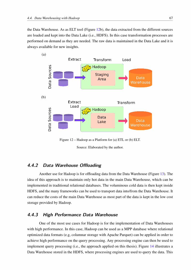
4.4. Data Warehousing with Hadoop 67
the Data Warehouse. As as ELT tool (Figure 12b), the data extracted from the different sourcesare loaded and kept into the Data Lake (i.e., HDFS). In this case transformation processes areperformed on demand as they are needed. The raw data is maintained in the Data Lake and it isalways available for new insights.
(a)
(b)
Figure 12 – Hadoop as a Platform for (a) ETL or (b) ELT.
Source: Elaborated by the author.
4.4.2 Data Warehouse Offloading
Another use for Hadoop is for offloading data from the Data Warehouse (Figure 13). Theidea of this approach is to maintain only hot data in the main Data Warehouse, which can beimplemented in traditional relational databases. The voluminous cold data is then kept insideHDFS, and the many frameworks can be used to transport data into/from the Data Warehouse. Itcan reduce the costs of the main Data Warehouse as most part of the data is kept in the low coststorage provided by Hadoop.
4.4.3 High Performance Data Warehouse
One of the most use cases for Hadoop is for the implementation of Data Warehouseswith high performance. In this case, Hadoop can be used as a MPP database where relationaloptimized data formats (e.g, columnar storage with Apache Parquet) can be applied in order toachieve high performance on the query processing. Any processing engine can then be used toimplement query processing (i.e., the approach applied on this thesis). Figure 14 illustrates aData Warehouse stored in the HDFS, where processing engines are used to query the data. This

68 Chapter 4. Modern Data Warehouses
Figure 13 – Hadoop for Data Warehouse Offloading.
Source: Elaborated by the author.
approach is one of the most investigated in the literature (JIA; PAVLO; ZDONIK, 2012; WANGet al., 2016; KANG; KIM; LEE, 2015).
Figure 14 – Hadoop for the deployment of a high performnance Data Warehouse.
Source: Elaborated by the author.
4.5 ConclusionsIn this chapter we presented an overview of the current state of the use of Big Data
technologies in data warehousing. First, we presented an overview of the evolution of theData Warehousing architecture in order to incorporate Big Data. Next we analyzed the use ofNoSQL databases for the implementation of Data Warehouses, which may not provide the bestperformance due to their design purpose. Then we discussed some use cases for Hadoop in DataWarehousing: (i) as platform for ETL/ELT; (ii) for offloading the Data Warehouse; and (iii) as ahigh performance Data Warehouse.
In the next chapters we present the investigations of this thesis for the efficient processingof star-join queries in Hadoop. In Chapter 6 we propose approaches with reduced disk spilland communication with the use of in-memory computation. In Chapter 7 we propose theemployment of random access in HDFS using distributed indices. The concluding remarks ofthis thesis are presented in Chapter 8.

69
CHAPTER
5RELATED WORK
5.1 IntroductionThe efficient processing of join queries has been a relevant subject of research for many
years (MISHRA; EICH, 1992; DOULKERIDIS; NØRVÅG, 2014). With the release of manyopen-source frameworks as solutions for the massive and distributed data processing such asthe Apache Hadoop, several studies in the literature have investigated how to efficiently processqueries on these frameworks. A considerable portion of these investigations have concentratedtheir effort to optimize relevant queries such as joins. Specifically for star-join queries, many ofthese studies research showed that it is essential to use optimization techniques such as filteringand broadcast.
In this thesis we present our investigations for the efficient processing of star-join queriesin Hadoop. Therefore, in this chapter we present the related work from the literature focusedon the performance improvement of the star-join processing in Hadoop. For the context of thisthesis, when we refer to query processing in Hadoop, we mean queries issued over data storedin the HDFS. We distinguish the related approaches based on the access method used by eachapproach (random access vs. full scan), and we also identify the optimization techniques applied(i.e., filtering and broadcast). In order to facilitate the understanding and legibility of this thesis,we introduce our own names used to refer the approaches that were implemented and comparedin our performance evaluations.
The remainder of this chapter is organized as follows. In Section 5.2 we detail generalapproaches for join queries in Hadoop. In Section 5.3 we present studies specifically related toprocessing of Star Joins. We present our conclusion remarks in Section 5.4.

70 Chapter 5. Related Work
5.2 Joins in Hadoop
In this section we describe general approaches for the efficient processing of joins inHadoop. By general we mean that these approaches can be applied on the star-join processing,but they were not exclusively designed for such queries. We describe approaches that are morerelevant to the subject of the investigations of this thesis. However, a large body of researchhave investigated other types of join queries, which we cite similarity join queries (VERNICA;CAREY; LI, 2010; CHEN et al., 2017; CECH et al., 2017), spatial join queries (ELDAWY;MOKBEL, 2017; LU; GÜTING; FENG, 2016), and data skewed join queries (AFRATI et al.,2015; HASSAN; BAMHA, 2015; MYUNG et al., 2016).
Blanas et al. (2010)
Blanas et al. (2010) investigated the performance of join algorithms for the processingof logs in MapReduce. Join operations are performed as part of filtering, aggregation andmining tasks of data coming from click-streams or event logs. The authors implemented aseries of join algorithms, which we highlight the repartition join and the broadcast join. Therepartition join, also known as reduce-side join, splits and distributes data according to thejoin key. Corresponding pairs of partitions are joined in the reducers. This strategy can beimplemented in a single MapReduce job to process a binary join. The broadcast join, also knownas map-side join, broadcast small tables to all nodes, and maintaining them on the main-memoryof all node as a hash tables. Thus, each node is able to perform the join operation locally inthe mappers. The broadcast join has the limitation of requiring that the small tables fit in themain-memory of the nodes.
Although these strategies were not specifically designed for the star-join processing, bothof them can be used for such task. When applied to the star-join processing, the repartition join
becomes a series of MapReduce jobs, each one corresponding to a repartition join between twotables. In this thesis we refer to this approach as MR-Cascade. The broadcast join can also beefficiently applied to solve Star Joins. In this case, dimension tables are filtered, and loaded intothe main-memory at the setup function of the mappers. Then, the fact table is processed by afull scan operation, and locally joined with dimensions stored in the hash tables. We refer tothis strategy as MR-Broadcast. The drawback of the MR-Cascade is the need of multiple jobs,which incurs in a great amount of disk spill. Additionally, it also has a high communication costbecause unnecessary data from the fact table is transmitted across the cluster. The MR-Broadcast
requires that dimension tables fit into the main-memory of the nodes. Moreover, depending onthe group by and order by clauses of these queries, both approaches may also need additionalMapReduce jobs, causing additional processing delay. Both these algorithms were implementedand compared to our proposed methods. We also implemented an improved version of theMR-Cascade by adding an extra job to filter the fact table with Bloom filters. This algorithm wasnamed MR-Bloom-Cascade.

5.3. Star Joins in Hadoop 71
Thusoo et al. (2009)
Thusoo et al. (2009) proposed a system called Hive, which is a data warehouse solutionfor Hadoop. By data warehouse solution the authors mean a system being able to store structureddata as relational tables, and use a SQL-like language to query the data. Hive support schemadefinition and different data types. The system has a metadata catalog, which stores schemasand and statistics. A declarative language called HiveQL is used to query the data. Hive wasinitially developed by Facebook to process more than 700TB of data. This project is currentlymaintained by Apache. Initially, the join query processing was only performed as sequentialrepartition join jobs (i.e., MR-Cascade). Later they included the support to the broadcast join
(i.e., MR-Broadcast). Thus, this proposal suffers the same limitations discussed on the previoussection.
Lee, Kim and Kim (2012)
Lee, Kim and Kim (2012) proposed a modification in the order that Hadoop assignsdatasets to mappers, with focus on binary joins. The proposed algorithm first processes onetable and builds Bloom filters based on the selected data. These Bloom filters are then globallydistributed and used to filter the second table. The authors also proposed a method to determinethe order that the data must be processed. Performace tests showed that their algorithm outper-fomed the standard join algorithm of Hadoop (i.e., the reduce-side join). The main drawbackof this modification by transforming the map processing into a serial procedure is that it wouldnegatively impact join queries of multiple tables. Additionally, algorithms based on modificationsof the original framework can difficult their portability. We do not consider this approach in ourevaluations because we focus on the original MapReduce framework. Similar approaches alsobased on modifications of Hadoop are not considered because they suffer the same mentionedlimitations (YANG et al., 2007; JIANG; TUNG; CHEN, 2011).
5.3 Star Joins in Hadoop
In this section we describe algorithms specially designed for the efficient star-join pro-cessing in Hadoop. Most of these algorithms were implemented and compared to the algorithmsproposed in this thesis.
Afrati and Ullman (2010)
Afrati and Ullman (2010) proposed an algorithm able to perform joins among multipletables in a single MapReduce job. The proposed algorithm is based on the identification of thereducer to which a mapper must send the data. This mapping procedure is based on a map-
key, which consists of a set of attributes determined by a method proposed to minimize the
72 Chapter 5. Related Work
communication cost. Star Joins are treated as a special case because of its specific characteristics.The minimization cost method defines how much intervals each attribute domain from dimensionsmust be partitioned. These intervals are also called shares. We refer to this approach as MR-
MapKey. The authors compared their proposed algorithm with the MR-Cascade for the executionof join queries between three tables. For different sets of tables with at most one million tuplesand only two attributes, the results showed that the MR-MapKey outperformed the MR-Cascade.However, the authors only tested small datasets and did not assess the star-join processing. Themain drawback of this approach is the need of replicating data in order to process the Star Joinin a single MapReduce job. Moreover, unnecessary data from the fact table is transmitted acrossthe cluster, increasing the communication cost. Lastly, this algorithm performs full scan of thefact table. Besides the map-key method, no other optimizations are applied.
Chen (2010)
Chen (2010) proposed Cheetah, a high performance custom data warehouse built on topof Hadoop and MapReduce. Cheetah has a virtual view of the data warehouse that is organizedas star or snowflake schemas. Based on this view, the author designed a SQL-like language toquery the data. Regarding the star-join processing, Cheetah performs the denormalization ofbig dimension tables, and the use of the broadcast join for small dimensions. The performanceevaluation of this work only analyzed the proposed system, not comparing it with other joinalgorithms. The main drawback of this approach is the denormalization of dimensions, whichmay increase significantly the amount of data to be stored and processed. Moreover, the authordo not provide results showing how much it is worthy to perform the proposed denormalization.This approach is not considered in our evaluations because data denormalization is not a subjectof the proposed investigations of this thesis.
Han et al. (2011)
Han et al. (2011) proposed a MapReduce algorithm named Scatter-Gather-Merge for thestar-join processing in MapReduce. This algorithm always computes Star Joins in three phases.The first phase, called Scather, performs a decomposition of the tuples of the fact and dimensiontables, transforming them into key-value pairs composed of primary keys, foreign keys, andattributes of interest. Each tuple from the fact table generates n key-value pairs, where n is thenumber of dimension tables that participate in the query. The Gather phase processes the join ofthe corresponding key-value pairs created in the Scather phase, i.e., join of fact and dimensionkey-value pairs. The Merge phase combines joined key-value pairs that belong to the same tupleof the fact table, generating the star-join result. This algorithm is then optimized with an extrainitial phase based on Bloom filters used to prune the fact table. The authors tested the proposedalgorithm against the MR-Cascade in the processing of star-join queries from the Star SchemaBenchmark (SSB). The results showed that the proposed algorithm performed better on all tests,

5.3. Star Joins in Hadoop 73
and that the use of Bloom filters improved the performance of the algorithm. Thus, this algorithmapplies filtering with Bloom filters after the full scan of the fact table. The main drawback backof this algorithm is the need of multiple MapReduce jobs, which usually increase the amount ofdisk spill. This algorithm was implemented and compared to the proposed methods of this thesis.We refer to this approach as MR-Bloom-Scatter-Gather.
Zhu et al. (2011)
Zhu et al. (2011) proposed an index called HdBmp, which is a three-level index based onthe Bitmap Join Index for the star-join processing in MapReduce. The first level of the indexis maintained on the master node (NameNode), indicating the name of the second and thirdlevel index files as well as their locations. The second and third levels are maintained on theslave nodes (DataNodes). While the second level refers to the metadata on the third level, i.e.,table, segment, attribute and range of indexed values, the third level corresponds to the bitmapsarrays. The authors proposed a processing algorithm that uses the proposed index to filtersunnecessary data from the fact table. The authors evaluated their algorithms comparing it againstan optimization implemented over what they refer as an improved star-join method. By theirdescription, this improved method is similar to the MR-Bloom-Scatter-Gather without Bloomfilters. The results showed that the HdBmp processing algorithm is scalable and more efficientthan the optimized star-join method. A significant drawback of this proposal is due to the factthat the algorithm uses indices to filter the fact table. In other words, indices are not used topromote random access, which could benefit highly selective star-join queries, as demonstratedin Chapter 7. The use of indices as just filters by this approach adds extra overhead to the querycost. The same effect of pruning the fact table could be achieved with Bloom filters, which has asmaller processing cost. In this thesis we have implemented and compared to our methods a verysimilar approach that we refer as MR-Bitmap-Filter.
Zhang et al. (2013)
Zhang, Wu and Li (2013) proposed an extension of the MR-MapKey by adding an extrainitial MapReduce job to build Bloom filters over the query predicates. These Bloom filters areused to prune the fact table in the second job. Thus, unnecessary data from the fact table is nottransmitted across the cluster, reducing both disk spill and communication cost. The authorsevaluated the performance of this algorithm against the MR-MapKey and MR-Cascade. Theresults showed that their algorithm outperformed the tested algorithms for tables with morethan 5 million records. The main shortcoming of this algorithm is the addition of extra jobs,which may result in some delay due to the high latency to start MapReduce jobs. Anotherdrawback is the full scan of the fact table, which is not appropriate to higly selective queries.We have implemented this algorithm for our performance evaluations, and we refer to it asMR-Bloom-MapKey.

74 Chapter 5. Related Work
Tao et al. (2013)
Tao et al. (2013) proposed an hierarchized version of the MR-MapKey to optimize thecommunication cost. Their proposal is based on reducing the replication of dimension tablesby decomposing the star-join processing into several three-way joins. For instance, consider aStar Join of the fact table F and dimensions D1, D2, D3 and D4. In this example, the hierarchicaldecomposition is done as follows. In the first MapReduce job, the tuples of the fact table aredecomposed into two groups. The first group corresponds the join of F with the dimensions D1
and D2, while the second group joins F with the dimensions D3 and D4. A second MapReducejob performs the join of these two groups. The authors compared their algorithm with the originalversion (i.e., MR-MapKey) and with Hive (i.e., MR-Cascade) using datasets generated with theTPC-H benchmark (PÖSS; FLOYD, 2000). Their results showed that Hive presented the worstperformance, while their algorithms optimized the performance of the original MR-MapKey.However, the authors performed their tests on very small datsets, maximum of 9GB. A drawbackof this approach is the addition of MapReduce jobs to the original algorithm, which may incurin extra disk spill and delay caused by the high latency to start jobs. Another drawback is thefull scan of the fact table, which is not appropriate to higly selective queries. In this thesis weimplemented this algorithm, which we refer as MR-Hierarchized. Our tests for the star-joinprocessing showed a different result, where the MR-MapKey and MR-Cascade outperformed theMR-Hierarchized.
Zhou et al. (2013)
Zhou, Zhu and Wang (2013) investigated the processing of Star Joins in MapReduce.They proposed two algorithms that depend on the data placement strategy. For small dimensions,the fact table is partitioned into foreign key column family and measure column families, whiledimensions are replicated in a distributed cache. For this strategy, they proposed an algorithmcalled Multi-Fragment-Replication Join (MFRJ), which performs local hash lookups to joindimensions with the fact table. This algorithm is very similar to the MR-Broadcast. For largedimensions, each column from the star schema is stored independently on the nodes. It turnspossible the employment of local processing for the join between collocated columns, whichavoids data movement and replication. For this placemnet strategy, the authors proposed analgorithm called MapReduce-Invisible Join (MRIJ). This approach is similar to the MR-Bloom-
Scatter-Gather. Performance tests using the Star Schema Benchmark (SSB) compared theproposed algorithms with Hive with two file formats: RCFile and text. Different configurationswere evaluated (for example, omission of the where clause, large dimension tables and lackof projection of numerical measures). Results showed that the proposed algorithms provided aperformance up to twice as fast as Hive. We did not consider this approach in our evaluationsbecause vertical partitioning of tables was not a subject of the proposed investigations of thisthesis. Moreover, these algorithms are very similar to approaches already implemented (MR-

5.4. Conclusions 75
Broadcast and MR-Bloom-Scatter-Gather).
Lu et al. (2013)
Lu et al. (2013) proposed an efficient and compact indexing scheme called BIDS (BitmapIndex for Database Service) for the analysis of large volumes of data. The BIDS scheme isbased on the bitmap index using compression and coding techniques. BIDS was designed tointeract easily with external systems with a manager responsible for creating the indices whennew data arrives. This manager is able to decide whether or not an index should be built on anattribute, and whether that index should be completely or partially built. Partial indexing is usedto reduce storage costs. Therefore, indices are created only for portions of the most accessed data.This work includes a processing strategy that employs bitmaps indices for filtering attributes,reducing the number of tuples before the join processing. Performance tests evaluated theproposed indexing scheme on Hadoop and HadoopDB. The results showed that the BIDS schemeimproved the query processing performance of both Hadoop and HadoopDB (ABOUZEID et al.,2009). Lu et al. (2013) did not tackle the problem of performing random access on HDFS withthe proposed index. We did not consider this approach in our evaluations because our main goalis the evaluation of the query performance, and not the indexing schema itself.
5.4 Conclusions
In this chapter we summarized the most relevant related work from the literature thatproposed methods for the processing of joins in the Hadoop framework. The vast majority of thedescribed solutions are based in the full scan of the fact table. The small number of proposalsthat employ indices using random access can be explained by the lack of native support ofthe HDFS, which often organize data in rather large blocks. As mentioned in Section 3.4.2.1,although HBase does offer minimal support for random access, the construction of complexbuilt-in indices is not supported. In the past year, new and promising frameworks emerged withmore integrative interface for indices. One strong candidate that offers native support to randomaccess is the Apache Kudu 1, a recent distributed storage engine for relational data. In addition,Pilosa 2 is another recent open source project that offers distributed bitmap indexing with thepromise to accelerate queries of massive datasets. Both of these new frameworks are drivenby the need for speed in high-volume databases, but there still is a gap in terms of specializedtechniques that exploit random access to solve a broad range of problems – including star-joinqueries with low selectivity.
We summarized in Table 2 all related approaches that were also implemented andcompared to the methods proposed in this thesis. In this table the solutions are discriminated
1 <https://kudu.apache.org/>2 <https://www.pilosa.com/>

76 Chapter 5. Related Work
according to their access method (second and third columns) and whether they use optimizationtechniques (fourth and fifth columns). The approaches proposed in this thesis are, namely,SP-Broadcast-Join, SP-Bloom-Cascade-Join, SP-Bitmap-Join, SP-Bitmap-Broadcast-Join, andMR-Bitmap-Join. To the best of our knowledge, no related work addressed the star-join queryprocessing in Spark, or using indices to promote random access on the HDFS. The methodsproposed in this thesis fill this gap in the literature by using in-memory computation provided bySpark combined with optimization techniques to reduce disk spill and network communication,and by proposing the use of indices with the creation of a layer over HDFS that allows the switchbetween random access and full scan.
In the next chapters we propose our methods for the efficient star-join processing inHadoop.
Table 2 – List of all approaches outlined in this chapter and implemented for our performance evaluationsin Chapters 6 and 7. The approaches proposed in this thesis are highlighted in bold. The secondand third columns distinguish the access method used by each approach (random access vs. fullscan). The fourth, fifth and sixth columns identify optimization techniques, if any, as describedin this chapter.
MapReduce AlgorithmsRandomAccess
FullScan
OptimizationFilter Broadcast
MR-Bitmap-Join 3
MR-Cascade 3
MR-MapKey 3
MR-Hierarchized 3
MR-Broadcast 3 3
MR-Bloom-Scatter-Gather 3 3
MR-Bloom-MapKey 3 3
MR-Bloom-Cascade 3 3
MR-Bitmap-Filter 3 3
Spark AlgorithmsRandomAccess
FullScan
OptimizationFilter Broadcast
SP-Bitmap-Join 3
SP-Bitmap-Broadcast-Join 3 3
SP-Broadcast-Join 3 3
SP-Bloom-Cascade-Join 3 3
SP-Cascade-Join 3
Source: Adapted from Brito et al. (2017).
77
CHAPTER
6PROCESSING STAR JOINS WITH REDUCED
DISK SPILL AND COMMUNICATION INHADOOP
6.1 Introduction
The rapid pace at which companies collect data and the creation of the Cloud Computingmodel created a demand for flexible and scalable solutions able to efficiently solve Star Joinsin large datasets. To address these needs, a large body of research is focused on open sourceframeworks such as MapReduce (DEAN; GHEMAWAT, 2008) and Spark (ZAHARIA et al.,2010) to deliver fast batch and interactive processing in the cloud. Because Star Joins aretypical and remarkably expensive operations, specially in data warehousing applications, manyMapReduce strategies Star Joins were proposed in the past and many of them are summarized inChapter 5. However, it is still challenging to avoid excessive disk access and cross-communicationamong the parallel jobs. In particular, unnecessary disk access is often the result of disk spill,i.e., when data is spilled into the disk due to overflowing memory buffer or writing data to diskbetween consecutive jobs. Furthermore, transmitting records that are subsequently discardedin the join operation adds extra cross-communication overhead, blocking the bandwidth of thenetwork. Both of these issues become bottlenecks when when the volume of data increasessignificantly.
In this chapter we propose two methods to the efficiently process Star Joins of datasetsresiding on HDFS: the SP-Broadcast-Join, based on the broadcast technique to promote localprocessing, and the SP-Bloom-Cascade-Join, which uses Bloom filters to prune the fact table.Both of these algorithms reduce disk spill and network communication by applying in-memorycomputation and coordinating data from dimensions and fact tables prior to computing the join.Both algorithms are based on the resilient distributed datasets (RDDs) from Spark.

78 Chapter 6. Processing Star Joins with Reduced Disk Spill and Communication in Hadoop
We compared our strategies to the algorithms discussed in Chapter 5 by using star-joinqueries from the Star Schema Benchmark (SSB). The results showed that both SP-Bloom-
Cascade-Join and SP-Broadcast-Join reduced the computation time at least by 38% in com-parison with six full scan algorithms (see Figure 15) described in Chapter 5. The results alsoshowed that both strategies presented outstanding less disk spill and network communication.We also showed that implementing a simple cascade of joins in Spark (SP-Cascade-Join) isnot enough to outperform the best MapReduce strategies, which endorse the importance ofthe use of optimization techniques such as Bloom filters or broadcast. Lastly, we showed thatSP-Bloom-Cascade-Join and SP-Broadcast-Join scale linearly with the database size, which is anecessary feature to any solution devoted to larger datasets. The obtained results place both oursolutions as efficient and competitive methods to filter and retrieve data from, for instance, datawarehouses in the cloud.
The results presented in this chapter were published in the paper "Jaqueline Joice Brito,
Thiago Mosqueiro, Ricardo Rodrigues Ciferri, and Cristina Dutra de Aguiar Ciferri. Faster
cloud star joins with reduced disk spill and network communication. Proceedings of International
Conference on Computational (ICCS 2016): vol. 80 of Procedia Computer Science, 74–85, 2016".Our Spark algorithms, SP-Broadcast-Joinand SP-Bloom-Cascade-Join, are available at GitHub(BRITO, 2015). The remainder of this chapter is organized as follows. In Section 6.2 we describethe SP-Broadcast-Join and SP-Bloom-Cascade-Join in detail. We show our performance analysesin Section 6.3, and our concluding remarks in Section 6.4.
6.2 Proposed Method
In this section we propose two efficient algorithms for the processing of Star Joins inHadoop. We present details of the applied methodology in Section 6.2.1. Then, in Section 6.2.2,we start proposing the SP-Cascade-Join, which is an algorithm used as baseline in our perfor-mance analyses. Our proposed algorithms, SP-Broadcast-Join and SP-Bloom-Cascade-Join aredetailed in Sections 6.2.4 and 6.2.3, respectively.
6.2.1 Methodology
The algorithms proposed in this chapter are based on three techniques: in-memorycomputation with RDDS, broadcast and Bloom filters. Although Broadcast and Bloom filterswere optimization techniques also used in some of the star-join MapReduce algorithms detailedin Chapter 5, we combined these techniques with the use of RDDs to employ in-memorycomputation.

6.2. Proposed Method 79
In-memory computation with RDDs
Both proposed algorithms are implemented in Spark in order to use in-memory computa-tion though the RDDs. Because RDDs optimize the use of in-memory computation during thestar-join processing, they should reduce the amount of disk spill involved in the join operations.Another goal of using Spark is to avoid the need for performing several sequential jobs, inanalogy with the map-reduce cycles from the MapReduce framework. Between each cycle,MapReduce spills data to disk. Moreover, there is a considerable latency to start a MapReducejob, which imposes an additional overhead.
Broadcast
The broadcast technique applied to star-join queries consists of transmitting the dimen-sion tables to all nodes. Then, the dimensions are loaded into the main memory and each node isable to perform a hash join locally. Thus, there is no need to shuffle the data across the cluster,which reduces the network communication. Moreover, as the star join operation can be solved ina single MapReduce job, it also reduces the amount of disk spill caused by sequential jobs. Thebroadcast is indicated for tables that fit in the available memory, which is its main limitation.
Bloom filters
Bloom filters are compact data structures used to test whether an element belongs to aset. In the processing of Star Joins, Bloom filters are built over each dimension based on thequery predicates. Then, tuples from the fact table can be tested using the Bloom filters anddiscarded before being transmitted over the cluster. Thus, Bloom filters optimize both disk spilland network communication. The amount of disk spill is reduced because less data is spilled todisk across the join processing.
6.2.2 SP-Cascade-Join
Performing a cascade of joins is the most straightforward approach to solve Star Joinswith RDDs. The Spark framework performs binary joins through the join operator using thekey-value abstraction. Fact and dimension tables are represented as RDDs corresponding to listsof key-value pairs containing the attributes of interest. Thus, Star Joins can be computed as asequences of binary joins between these RDDs. For simplicity, we shall refer to this approach asSP-Cascade-Join. We use this algorithm as a baseline method in the performance analyses as itonly applies the in-memory computation through the RDDs as optimization.
Algorithm 1 details the SP-Cascade-Join for solving a star-join query Q. RDDs for eachdimension table table are created in line 2. Then, the filter operator solves the correspondingpredicates of Q in place (line 3). For each RDD, attributes of interest are mapped into key-valuepairs by the mapToPair operator. Next, the RDD for the fact table is created in line 5. The fact

80 Chapter 6. Processing Star Joins with Reduced Disk Spill and Communication in Hadoop
Algorithm 1 – SP-Cascade-Join
input: Q, F and Dinput: Q: star join queryinput: F : fact tableinput: D: set of dimension tablesoutput: result of Q
1: for each d in D do2: RDDd = d3: RDDd .filter( Q ).mapToPair( pkd , ad ) /∗ ad is a set of attributes from d ∗/4: end for
5: RDD = F
6: for each d in D do/∗ f kd′ is the key of the next join and a are attributes from D and F ∗/7: RDD = RDD.join( RDDd ).mapToPair( f kd′ , a )8: end for
9: FinalResult = RDD.reduceByKey( v1 + v2 ).sortByKey( )
return FinalResult
RDD joins with resulting dimension RDDs in lines 6–8. Finally, the operators reduceByKey andsortByKey performs, respectively, aggregation and sorting of the results (see line 9).
6.2.3 SP-Bloom-Cascade-Join
Based on the SP-Cascade-Join, we now add Bloom filters. This optimization avoids thetransmission of unnecessary data from fact RDD through the cascade of join operations. Thesefilters are built for each dimension RDD, containing their primary keys that meet the querypredicates. Therefore, the fact RDD is filtered based on the containment of its foreign keys onthese Bloom filters. We refer to this approach as SP-Bloom-Cascade-Join.
Algorithm 2 exemplifies SP-Bloom-Cascade-Join for solving a star-join query Q. RDDsfor each table are created in lines 2. Then, the filter operator solves predicates of Q in place(line 3). For each RDD, attributes of interest are mapped into key-value pairs by the mapToPair
operator. Dimension RDD keys are also inserted in Bloom filters broadcast to every executor(line 5). The filter operator uses these Bloom filters over the fact RDD, discarding unnecessarykey-value pairs in line 8. This is where SP-Bloom-Cascade-Join should gain in performancecompared to SP-Cascade-Join. Then, the fact RDD joins with resulting dimension RDDs in lines9–11. Finally, reduceByKey and sortByKey performs, respectively, aggregation and sorting of theresults (see line 12).

6.2. Proposed Method 81
Algorithm 2 – SP-Bloom-Cascade-Join
input: Q, F and Dinput: Q: star join queryinput: F : fact tableinput: D: set of dimension tablesoutput: result of Q
1: for each d in D do2: RDDd = d3: RDDd .filter( Q ).mapToPair( pkd , ad ) /∗ ad is a set of attributes from d ∗/4: Bloomd = broadcast( RDDd .collect( ) ) /∗ Bloomd is a Bloom filter for d ∗/5: BFd = broadcast( Bloomd )6: end for
7: RDD = F8: RDD.filter( BFd1 .contains( f kd1) & BFd2 .contains( f kd2) ... & BFdn .contains( f kdn))
9: for each d in D do/∗ f kd′ is the key of the next join and a are attributes from D and F ∗/
10: RDD = RDD.join( RDDd ).mapToPair( f kd′ , a )11: end for
12: FinalResult = RDD.reduceByKey( v1 + v2 ).sortByKey( )
return FinalResult
6.2.4 SP-Broadcast-Join
The SP-Broadcast-Join assumes that all dimension RDDs fit into the executor memory.Note that each node may have much more than one executor running, which may constrainthe application of SP-Broadcast-Join depending on the dataset specifics. Dimension RDDs arebroadcast to all executors, where their data are kept in separate hash maps. Then, all joins areperformed locally in parallel. Since no explicit join operation is needed, SP-Broadcast-Join iscertain to deliver the faster query times. Note that, in general, Bloom filters are much smaller datastructures than hash maps. Thus, memory-wise there probably is a balance between cases whenSP-Broadcast-Join and SP-Bloom-Cascade-Join performs optimally - which will be verified inthe experiments section. This approach is the Spark counterpart of the MR-Broadcast, introducedin Section 5.
Algorithm 3 details this approach applied on a star-join query Q. The algorithm startsby creating RDD for each dimension in line 2. Predicates over dimensions are solved by thef ilter operator in line 3. Hash maps are broadcast variables created for each dimension RDDin line 4, corresponding to lists of key-value pairs. It is important to note that these hash mapscontain not only the dimension primary keys, but all the needed attributes. These hash maps arekept in the executor primary memory. Then, the filter operator access the hash maps to select

82 Chapter 6. Processing Star Joins with Reduced Disk Spill and Communication in Hadoop
Algorithm 3 – SP-Broadcast-Join
input: Q, F and Dinput: Q: star join queryinput: F : fact tableinput: D: set of dimension tablesoutput: result of Q
1: for each d in D do2: RDDd = d3: RDDd .filter( Q ).mapToPair( pkd , ad ) /∗ ad is a set of attributes from d ∗/4: Hd = broadcast( RDDd .collect( ) ) /∗ Hd is a hash map for d ∗/5: end for
6: RDD = F
/∗ The attributes from dimensions are get from the corresponding hash maps ∗/
7: RDD.filter( Hd1 .hasKey( f kd1) & Hd2 .hasKey( f kd2) & ... & Hdn .hasKey( f kdn) ).mapToPair( [Hd1 .getValue( f kd1), H2.getValue( f kd2),...,Hn.getValue( f kdn)], m )
8: FinalResult = RDD.reduceByKey( v1 + v2 ).sortByKey( )
return FinalResult
data that should be joined in line 7. Since all the necessary dimension data are replicated overall executors, the mapToPair operator solves the select clause of Q. As a consequence, there isno need to use the join operator at all, saving a considerable amount of computation. Finally,reduceByKey and sortByKey performs, respectively, aggregation and sorting of the results (seeline 8).
6.3 Performance Analysis
Next, we present the performance analyses of our Spark solutions, SP-Broadcast-Join
and SP-Bloom-Cascade-Join. First, we detail the experimental setup in Section 6.3.1. Then, westart our analyses by comparing the performance of our approaches against other algorithms.Next, we investigate the scalability of our algorithms. Lastly, we assess the impact of the availablememory.
6.3.1 Experimental Setup
We used a cluster of 21 (1 master and 20 slaves) identical, commercial computers runningHadoop 2.6.0 and Apache Spark 1.4.1 over a GNU/Linux installation (CentOS 5.7), each nodewith two 2GHz AMD CPUs and 8GB of memory. To more intensive tests (i.e., Section 6.3.3),we used Microsoft Azure with 21 A4 instances (1 master and 20 slaves), each with four 2.4GHz

6.3. Performance Analysis 83
Intel CPUs and 14GB of memory. In both clusters, we have used YARN as our cluster manager.
We used the Star Schema Benchmark (SSB) (O’NEIL et al., 2009) to generate datasetswith volume controlled by the scale factor SF (see Table 3). Each table is stored in the csvformat in HDFS. The workload was composed of four star-join queries, namely Q3.1, Q3.4,Q4.1 and Q4.3. Queries of class Q3 deals with three dimensions, while class Q4 manipulatesfour dimensions. These queries also have different selectivities: 3.4% for Q3.1, 0.76×10⁻⁴%for Q3.4, 1.6% for Q4.1 and 0.91×10⁻²% for Q4.3.
Unless stated otherwise, each result represents average and standard deviation over5 runs, empirically determined to guarantee a mean confidence interval ±100s. All Sparkimplementations used in the following sections are available at GitHub (BRITO, 2015).
Table 3 – Dataset characteristics used in the experiments. We show for each scaling factor SF the numberof tuples in the fact table (# Tuples) and its disk size.
SF # Tuples Size (GB)50 300 millions 30100 600 millions 60200 1.2 billions 130350 2.1 billions 210500 3 billions 300650 3.9 billions 390
Source: Brito et al. (2016).
6.3.2 Disk spill, network communication and performance
We show in Figure 15 how our approaches compare to six MapReduce strategies (fordetails, see Chapter 5) in terms of disk spill and network communication. We use the notationintroduced in Table 2 to refer to the MapReduce solutions. Notice that all points referring toMapReduce define a trend correlating time performance to network communication and diskspill (orange line in Figure 15). Although Spark is known to outperform MapReduce in a widerange of applications, a direct implementation of sequences of joins (referred to as SP-Cascade-
Join) delivered poor performance and followed the same trends as the MapReduce approaches.SP-Bloom-Cascade-Join and SP-Broadcast-Join, however, are complete outliers (more than3-σ ) and present remarkably higher performances. This highlights the need for additionaloptimizations applied on top/instead of the cascades of joins. In special, notice that both ourstrategies are closely followed by MR-Broadcast and MR-Bloom-MapKey, which processes StarJoins using broadcast and Bloom Filters, respectively. Next, we analyze in more detail each ofthese strategies.
In Figure 15(a) SP-Broadcast-Join and SP-Bloom-Cascade-Join both optimize networkcommunication and computation time of query Q4.1 with SF 100. As mentioned, excessive crosscommunication among different nodes is one of the major bottlenecks in distributed algorithms.

84 Chapter 6. Processing Star Joins with Reduced Disk Spill and Communication in Hadoop
(a) (b)
Figure 15 – Time performance as a function of the amount of (a) shuffled data and the (b) disk spill. Wepresent MapReduce (red dots) and Spark (blue dots) approaches, with the orange line showingthe general trend of MapReduce approaches. We used SSB query Q4.1 with SF 100. Ourapproaches SP-Broadcast-Join and SP-Bloom-Cascade-Join require half data spill and aboutone third of the computation time of the best MapReduce algorithm.
Source: Brito et al. (2016).
When compared to the best MapReduce approaches, SP-Broadcast-Join presents a reductionin data shuffling by a factor of 99% when compared to the MR-Broadcast method, and SP-
Bloom-Cascade-Join, a reduction of almost 48% against MR-Bloom-Scatter-Gather. Althoughthe MR-Bloom-MapKey does deliver ≈ 25% less shuffled data than SP-Bloom-Cascade-Join, itstill delivers a performance nearly 40% slower. Moreover, the results in Figure 15(b) demonstrateone of the main advantages of Spark’s in-memory paradigm: although both best options inMapReduce have low disk spill (1.8GB for MR-Bloom-MapKey and 0.5GB for MR-Broadcast),both SP-Bloom-Cascade-Join and SP-Broadcast-Join show no disk spill at all. In this test, wehave set Spark with 20 executors (on average, 1 per node) and 3GB of memory per executor.If we lower the memory, then we start seeing some disk spill from our approaches and theirperformances drop. We study more on this effect in Section 6.3.4.
It is important to highlight that great portion of the reduction in disk spill is due tothe use of optimization techniques (i.e., Bloom filters and broadcast). Simply implementinga sequence of joins in Spark (i.e., SP-Cascade-Join) still presents considerable higher diskspill and computation time when compared to SP-Broadcast-Join and SP-Bloom-Cascade-Join.Specifically, not only SP-Cascade-Join has non-null disk spill, it is larger than MapReduce bestoptions, although 81% lower than its counterpart, MR-Cascade. SP-Bloom-Cascade-Join andSP-Broadcast-Join shuffles, respectively, 23 and over 104 times less data than SP-Cascade-Join.Therefore, the reduced disk spill and time observed with SP-Broadcast-Join and SP-Bloom-
6.3. Performance Analysis 85
Cascade-Join strategies are not only due to Spark internals to optimize cross-communication anddisk spill. The bottom line is: application of additional techniques (Bloom filters or broadcast) isessential indeed.
It is important to note that this analysis assumed best performance of the MapReduceapproaches. No scenario was observed where either of SP-Broadcast-Join or SP-Bloom-Cascade-
Join trailed the other strategies. More details on MapReduce approaches to star-join processingwill be discussed in the next chapter.
6.3.3 Scaling the dataset
In this section, we investigate the effect of the dataset volume in the performance ofSP-Broadcast-Join and SP-Bloom-Cascade-Join. Methods in general must be somewhat resilientand scale well with the database size. Especially in the context of larger datasets, where solutionssuch as MapReduce and Spark really make sense, having a linear scaling is simply essential.
In Figure 16 we show the effect of the scale factor SF in the computation time consideringthree different queries of SSB. To test both strategies, we have selected queries with considerabledifferent workloads. Especially in low SFs, as shown in Figure 16(b), a constant baseline wasobserved: from SF 50 to 200 the elapsed time simply does not change. However, such datasets arerather small, and do not reflect the applications in which large scale approaches (i.e., MapReduceand Spark) excel. SP-Broadcast-Join and SP-Bloom-Cascade-Join performances grow linearlywith SF in all larger scale factors tested.
6.3.4 Impact of Memory per Executor
As mentioned in Section 6.2.4, broadcast methods usually demand memory to allocatedimension tables. While SP-Broadcast-Join has outperformed any other solution so far, scenarioswith low memory per executor might compromise its performance. Next, we study how theavailable memory to each executor impacts both SP-Broadcast-Join and SP-Bloom-Cascade-Join.We have tested query Q4.1 with SF 200.
Parallelization in Spark is carried by executors. For a fixed executor memory we studiedhow the number of executors change SP-Broadcast-Join and SP-Bloom-Cascade-Join perfor-mance. If enough memory is provided, performance usually follows trends shown in Figure17(a), where we used 1GB per executor. However, as the memory decreases, SP-Broadcast-Join
was severely impacted while SP-Bloom-Cascade-Join seems to be quite resilient. In our cluster,with this particular dataset, 512MB was a turning point: Figure 17(b) shows SP-Broadcast-Join
losing performance gradually. Below 512MB the difference becomes more pronounced. It isimportant to note that the specific value of this turning point (512MB in our tests) likely changesdepending on the cluster, nodes’ configuration and, possibly, dataset.
To explore this effect in detail, we tested the performance using 20 executors while

86 Chapter 6. Processing Star Joins with Reduced Disk Spill and Communication in Hadoop
(a) Query Q3.3. (b) Query Q3.4.
(c) Query Q4.3.
Figure 16 – Impact of the Scale Factor SF in the performance of SP-Broadcast-Join and SP-Bloom-Cascade-Join.
Source: Brito et al. (2016).
decreasing their memory. Results in Figure 18(a) show SP-Broadcast-Join drops in performanceuntil a point where SP-Bloom-Cascade-Join actually outperforms it (again, around 512MB).Furthermore, in Figure 18(a), from 450 to 400MB there is a stunning increase in computationtime: it suddenly becomes more than three times slower. To make sure that this increase intime was not an artifact of a specific executor or node, we analyzed the average time elapsedby all tasks run by all executors. Figure 18(b) clearly shows that the elapsed time becomesapproximately five times larger in this transition, suggesting that tasks are in general requiringmore computation time. For 256MB, there was no enough memory to broadcast all dimensions.Comparatively, however, SP-Bloom-Cascade-Join seems more resilient to the amount of memoryper executor than SP-Broadcast-Join, a feature that could be exploited depending on the resourcesavailable and application.
Finally, in Figure 19 we investigated a slightly more realistic scenario: while fixing the

6.3. Performance Analysis 87
(a) Executor memory of 1GB. (b) Executor memory of 512MB.
Figure 17 – Comparing SP-Broadcast-Join and SP-Bloom-Cascade-Join performances with (a) 512MBand (b) 1GB of memory per executor. SP-Broadcast-Join seems reasonably sensitive to lowmemory cases.
Source: Brito et al. (2016).
(a) (b)
Figure 18 – Comparing SP-Broadcast-Join and SP-Bloom-Cascade-Join performances with 20 executorsand variable memory. In special, panel (a) shows that SP-Broadcast-Join’s performanceis impaired with a decreasing memory, being outperformed by SP-Bloom-Cascade-Joineventually.
Source: Brito et al. (2016).
total memory, the number of executors increase and share memory equally. Thus, althoughthe memory per executor is decreasing, all memory resources are always in use. As expected,with enough memory for each executor performance of both SP-Broadcast-Join and SP-Bloom-
Cascade-Join increase (see Figure 19(b)). Yet, similarly to Figure 17(b), if the number ofexecutors is blindly increased without increasing resources, SP-Broadcast-Join is severelyimpaired while SP-Bloom-Cascade-Join’s performance remarkably remains.
In conclusion, all results in this section indicate a trade off between these two approaches,and defines a clear guideline on how to choose between the two of them depending on the cluster

88 Chapter 6. Processing Star Joins with Reduced Disk Spill and Communication in Hadoop
(a) Total executors memory of 82GB. (b) Total executors memory of 30GB.
Figure 19 – Comparing SP-Broadcast-Join and SP-Bloom-Cascade-Join performances with fixed totalmemory while increasing the number of executors. Only when the total available memory islower (panel a) SP-Broadcast-Join performance is impaired.
Source: Brito et al. (2016).
resources and dataset. Regardless of the number of executors, if their memory is enough to fitdimension RDDs, SP-Broadcast-Join may deliver twice faster query times; however, if memoryis not enough, SP-Bloom-Cascade-Join is the best solution available. It is important to stress thatall results presented in this section would scale up with the SF. Thus, in larger SFs this turningpoint where SP-Broadcast-Join slows down should be larger than 512MB.
6.4 Conclusions
In this chapter we have proposed two approaches to efficiently process Star Joins andinvestigated their efficiency. These new approaches significantly reduce the amount of dataspill and network communication: SP-Broadcast-Join and SP-Bloom-Cascade-Join. We havecompared the performance of our approaches against different MapReduce algorithms. SP-
Broadcast-Join and SP-Bloom-Cascade-Join outperformed all MapReduce approaches by afactor of at least 38% in terms of query execution time. It is important to highlight that simplyimplementing a cascade of joins in Spark, namely, SP-Cascade-Join, was not enough to beatMapReduce options, showcasing the importance of using of Bloom filter or broadcast techniques.We have also shown that both SP-Broadcast-Join and SP-Bloom-Cascade-Join scale linearly withthe database volume, which poses them as competitive solutions for Star Joins in the cloud. WhileSP-Broadcast-Join is usually faster (between 20-50%) when memory resources are abundant,SP-Bloom-Cascade-Join was remarkably resilient in scenarios with scarce memory. In fact, withenough resources available, SP-Broadcast-Join has no disk spill at all. To summarize, all of ourresults point towards a simple guideline: regardless of the number of executors, if their memory isenough to fit dimension RDDs, SP-Broadcast-Join may deliver twice faster query times; however,

6.4. Conclusions 89
if memory is an issue, SP-Bloom-Cascade-Join is the best solution and remarkably robust tolow-memory infrastructures. Therefore, SP-Broadcast-Join and SP-Bloom-Cascade-Join bothwere shown competitive fitting candidates to solve Star Joins in the cloud.
All algorithms investigated in this chapter perform the full scan of the fact table. In thenext chapter we explore the use of indices with focus on low selectivity star-join queries.

91
CHAPTER
7EMPLOYING RANDOM ACCESS WITH
BITMAP JOIN INDICES FOR STAR JOINS INHADOOP
7.1 Introduction
We explored in the last chapter how the combination of open-source frameworks ded-icated to massive and distributed processing, and on-demand hardware provided by cloudcomputing can be used to leverage the application of Star Joins to big data systems. In thiscontext, even queries with low selectivity may require the retrieval of a tremendous amount ofentries. As an example, a company that stores credit card transactions for its clients may needto perform analytics on its dataset, in which performance measures are evaluated per groupof clients. This involves reading nearly the entire database. However, this same company mayperform analyses per individual (say, to make decisions for a loan). In this second scenario, thenumber of tuples required to answer most queries are very small compared to the size of theentire database. This is an example of a query that presents low selectivity. In most relationaldatabases, the use of indices for random access is one of the primary methodologies to improvethe performance of high selective queries (GANI et al., 2016; ROUMELIS et al., 2017), in whichdata of interest is usually sparsely scattered across the hard drive.
However, the common approach for Hadoop solutions is to use batch processing (fullscan of tables) regardless of the query selectivity (PURDILA; PENTIUC, 2016; BLANAS et al.,2010; SCABORA et al., 2016). This is mostly because support for random access in Hadoop isstill in heavy development. Especially for high-selective Star Joins, full scan of the fact tablelead to huge amounts of unnecessary disk access. Moreover, transmitting records discarded inthe joins wastes cross-communication, also blocking further data transmission in the network.Although optimization techniques such as Bloom filters and broadcasting of dimension tables

92 Chapter 7. Employing Random Access with Bitmap Join Indices for Star Joins in Hadoop
rendered competitive solutions for the star-join processing (BRITO et al., 2016), as demonstratedin the previous chapter, there is still a need for improved methods to avoid the full scan of thefact table in certain scenarios.
In this chapter we contribute with a design that allows for the use of full scan and randomaccess and is based on the current state of the Hadoop system. To employ random access in thesolution of high-selective Star Joins, we propose a distributed Bitmap Join Index as a secondaryindex structure with loose-binding that operates on top of an access layer. Our distributed BitmapJoin Index is partitioned across multiple nodes and leverages the parallel computation providedby the processing frameworks from the Hadoop family. We propose a MapReduce algorithmto efficiently construct the distributed index. In more details, our solution of the Star Joins isdivided into two phases: first, the distributed Bitmap Join Index is used to solve the dimensionpredicates; then the requested primary keys are requested from the nodes where they are located.We propose three implementations (one in MapReduce and two in Spark, respectively) of ourprocessing algorithm, namely: MR-Bitmap-Join SP-Bitmap-Join and SP-Bitmap-Broadcast-Join.Because one of our goals is to allow both random access and full scan, we propose a solutionbased on an architecture with two layers on top of HDFS that is able to perform both full scanand random access, depicted in Figure 20. The Access Layer is composed of a storage engineable to perform both full scan and random access. The Processing Layer then connects to theAccess Layer via APIs to retrieve data of interest and process the join operations. We have usedMapReduce and Spark in the Processing Layer, and HBase as the storage engine. To allow theuse of HBase’s APIs, we implemented our distributed index as a secondary index with loosebinding to a primary index defined internally on HBase. To perform performance tests, we storedinstances of the Star Schema Benchmark (SSB) on the Hadoop Distributed File System (HDFS)using the HFile format (HBase tables).
The results presented in this chapter are based on the paper "Jaqueline Joice Brito,
Thiago Mosqueiro, Ricardo Rodrigues Ciferri, and Cristina Dutra de Aguiar Ciferri. Employing
Random Access with a Distributed Bitmap Join Index for Star Joins in the Cloud. In review,
2017". . The remainder of this chapter is organized as follows. In Section 7.2 we present ourmethod to process Star Joins with a distributed version of the Bitmap Join Index. In Section 7.3we detail the implementation of our method in the MapReduce and Spark frameworks. We showour performance analyses in Section 7.4. Finally, we present the concluding remarks for thischapter in Section 7.5.
7.2 Proposed Method
Next, we propose a strategy that enables the use of massive parallel frameworks to solveStar Joins with random access. Our solution operates on top of an architecture composed ofa Processing Layer, and an Access Layer that provides both full scan and random access. For

7.2. Proposed Method 93
Figure 20 – Proposed architecture based on an Access Layer and Processing Layer.
Source: Brito et al. (2017).
low-selectivity queries, while the Processing Layer solves the joins and predicates using thedistributed bitmap index introduced below, the Access Layer can perform both full scan andrandom access to retrieve the data from the HDFS. In the following sections we present ourdistributed Bitmap Join Index, explain pertinent details regarding the implementation and, then,we discuss how to solve Star Joins with this distributed index.
7.2.1 Combining Processing and Access Layers
Ideally, an intelligent system should be able to perform both random access and full scandepending on the query. Relational databases strive on how efficiently they are in selecting theproper methodologies as a function of historical records of query performance. Therefore, wepropose the use of an architecture based on an Access Layer and a Processing Layer (Figure 20).Although we are not interested in how this selection is made, we assume that both layers shoulduse a query optimizer that then decides which strategy will likely render minimal computationtime. Depending on which strategy is chosen, this system will behave in a slightly different wayas described below.
Full scan. The overall strategy is to request from the Access Layer a full scan of the facttable and the dimensions involved in the given query, and then the Processing Layer computesthe join in parallel. We reviewed in chapters 5 and 6 all of the available algorithms that use fullscan. For instance, if the processing framework is Spark, then SP-Broadcast-Join and SP-Bloom-

94 Chapter 7. Employing Random Access with Bitmap Join Indices for Star Joins in Hadoop
Cascade-Join approaches can be employed for optimal computation time, depending on thememory available per node and the size of the dimension tables.
Random Access. To take full advantage of the parallel frameworks, the distributed indexis first loaded and computed by the Processing Layer and, then, a request for the resulting tuplesis sent to the Access Layer. Once the Access Layer receives this request, the tuples are retrievedfrom the appropriate cluster nodes using a random access method. The index loaded by theProcessing Layer is called a secondary index, and the index used by the Access Layer is called aprimary index. The definition of a distributed index structure and how this index is then used arediscussed in the following sections. We do not assume that indices related to a given portion ofthe tables are located on the same node (i.e., no assumption of collocation was used).
It is important to note that this architecture is framework-agnostic – it does not assumesSpark or MapReduce, or even which software instantiates the Access Layer. For a summary of allapproaches considered in this investigation that use either random access or full scan, see table 2.As instances of the Processing Layer, we considered MapReduce and Spark. As an instance ofthe Access Layer, we considered HBase.
7.2.2 Distributed Bitmap Join Index for random access
The distributed Bitmap Join Index is a set of bitmap arrays that is stored on a distributedsystem such as HDFS and was designed to leverage the advantages of parallel processing.Following the same definition from section 2.4.2.3, for every value x of an attribute α , the bitmaparray BitP
α=x contains one bit for each tuple in the fact table that is indexed by the primary keyspk f ∈ P. The set P represents a subset of the primary keys of the fact table, and will be usedto split the index into many nodes. Let us assume that the sequence P1,P2, . . . ,PN represents apartition of the complete set P of all primary keys that compose the fact table. As in the originalBitmap Join Index, each of these bits represent the occurrence (1) or not (0) of the value x in thecorresponding tuple. Thus, the set of pk f that solve a simple predicate such as α = 1 is given bythe list of all bits set to 1 in BitP j
α=1, for j = 1,2, . . .N.
To fully exploit the parallelism that Hadoop systems can provide and to balance theworkload across nodes, partitions are uniformly distributed across the nodes (Figure 21c).Metadata containing information about the location of each partition is stored in the namenode(master). To optimize the loading time of the index files, the bitmap arrays BitP j
α=x are storedin a different file for each attribute and value of that attribute. Without loss of generality, letus assume that the primary keys are the integers 1,2,3, . . . ,Nt , i.e., pk f ∈ Z∩ [1,Nt ], with Nt
being the number of tuples in the database. Within partitions and for each attribute and attributevalue, the bitmap arrays are organized into blocks of size bs that consists of: (i) the primarykey pk f of the first tuple indexed by that block; and (ii) a sequence of bs bits that representthe bitmap values associated with the tuples between the pk f and pk f + bs− 1. Figure 21cshows an example of bitmap partitions with block size bs = 4 tuples. Because the Star Joins

7.2. Proposed Method 95
Figure 21 – A representation of our distributed Star Join Bitmap Index and its distributed version.(a):Example of instance of a dimension and fact tables. (b): Example of instance of the bitmapjoin index for the attribute value a1 = 10. (c): Physical storage of the distributed bitmap index.(d): Example of application to solve an AND operation.
Source: Brito et al. (2017).
often involve predicates that compare different attributes or ranges of attributes, joins mayrequire the use of multiple bitmap arrays associated with the same partition. For instance, thepredicate a1 = 10 AND b1 = 5 from Figure 21b is solved by performing BitP j
a1=10∧BitP jb1=5 for
j = 1,2, . . .N, where ∧ is the bitwise logical AND operator (Figure 21d). Therefore, becauseStar Joins are solved by employing bitwise operations on bitmap arrays BitP j
α=x that share thesame partition, the index structures with the same partition should ideally be stored on the samenode. If not, then the index partition needs to be appropriately transmitted across the cluster,creating additional costs on the query processing.
Because the complexity of the index structures tend to scale with the database, we
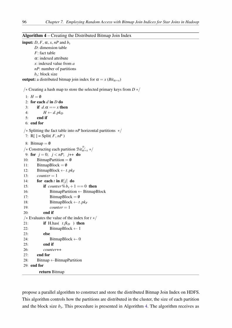
96 Chapter 7. Employing Random Access with Bitmap Join Indices for Star Joins in Hadoop
Algorithm 4 – Creating the Distributed Bitmap Join Indexinput: D, F , α , x, nP and bs
input: D: dimension tableinput: F : fact tableinput: α: indexed attributeinput: x: indexed value from ainput: nP: number of partitionsinput: bs: block sizeoutput: a distributed bitmap join index for α = x (Bitα=x)
/∗ Creating a hash map to store the selected primary keys from D ∗/1: H = /02: for each d in D do3: if d.α == x then4: H ← d.pkD
5: end if6: end for
/∗ Splitting the fact table into nP horizontal partitions ∗/7: R[ ] = Split( F , nP )
8: Bitmap = /0/∗ Constructing each partition BitP j
α=x ∗/9: for j = 0; j < nP; j++ do
10: BitmapPartition = /011: BitmapBlock = /012: BitmapBlock← t.pkF
13: counter = 114: for each t in R[ j] do15: if counter %bs +1 == 0 then16: BitmapPartition← BitmapBlock17: BitmapBlock = /018: BitmapBlock← t.pkF
19: counter = 120: end if/∗ Evaluates the value of the index for t ∗/21: if H.has( t.fkD ) then22: BitmapBlock← 123: else24: BitmapBlock← 025: end if26: counter++27: end for28: Bitmap←BitmapPartition29: end for
return Bitmap
propose a parallel algorithm to construct and store the distributed Bitmap Join Index on HDFS.This algorithm controls how the partitions are distributed in the cluster, the size of each partitionand the block size bs. This procedure is presented in Algorithm 4. The algorithm receives as

7.2. Proposed Method 97
input the fact (F) and dimension (D) tables, the attribute (α) and value (x) being indexed, thenumber of partitions (nP) and block size (bs). The algorithm starts by collecting the primary keysfrom the dimension table and stores the keys that correspond to the indexed value (i.e., α = x)into a hash map (lines 1-6). Then, the fact table is split into nP horizontal partitions (line 7). Eachpartition is processed and generates a corresponding bitmap partition (line 8-29). Within eachpartition, a new bitmap block is created and incorporates the next bs tuples(line 11). The primarykey of the first tuple is stored at the beginning of the blocks (line 12). Finally, the boolean valuesindicating whether the tuple t has the indexed value or not generate bitmap blocks (lines 21-25).
7.2.3 Using secondary indices with loose binding
To allow the use of Hadoop systems without modifications, we propose an implementa-tion where the distributed index, defined as the set of BitP j
α=x, as a secondary index with loosebinding. In general, indices are designed to point to locations on the disk of the tuples beingindexed. Instead, the index BitP j
α=x points to primary keys instead of the location of block on theHDFS. Then, by using HBase’s API, we connect it with the primary index, which points to theactual block location of the indexed tuples. Evidently, single level indexing schemas outperformthose with multiple levels because of the overhead added when accessing the different indexinglevels. Although our solution is suboptimal in terms of indexing schema, it not only allows theuse of Hadoop systems without modification, but also renders better computation time (as shownin the section 7.4).
There are two implementation details regarding how HBase performs random accessthat should be highlighted: how HFile blocks are read and their size. First, athough HBase usesa primary index to locate the HFile block associated with the requested row key, it performssequential search within HFile blocks. This creates an additional overhead that is not present instandard relational systems, that use an offset to access precise hard drive locations. Therefore,HFile blocks should be considered the unit of read of HBase. Second, the block size used byHbase HFile (64KB) is larger than the common size employed by most relational systems. Forinstance, PostgreSQL uses page (unit of read) size of 8KB as default.
7.2.4 Processing Star Joins with the Distributed Bitmap Join Index
The star-join processing pipeline proposed in this investigation is divided in three phases(Figure 22): In the first phase, the distributed Bitmap Join Indices are accessed in each node andevaluated according to the query predicates (green lines in Figure 22). Corresponding bitmappartitions are combined by means of logical bitwise operations, generating a set of primary keys.As discussed in section 7.2.2, because we store corresponding partitions in the same nodes, thisprocedure is executed locally. The second phase consists of sending the set of primary keys to theAccess Layer to execute random access (blue lines in Figure 22). During this phase, the selected
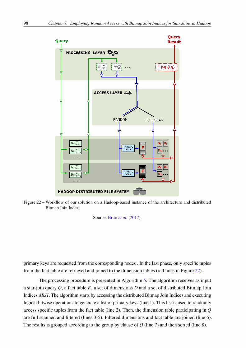
98 Chapter 7. Employing Random Access with Bitmap Join Indices for Star Joins in Hadoop
Figure 22 – Workflow of our solution on a Hadoop-based instance of the architecture and distributedBitmap Join Index.
Source: Brito et al. (2017).
primary keys are requested from the corresponding nodes . In the last phase, only specific tuplesfrom the fact table are retrieved and joined to the dimension tables (red lines in Figure 22).
The processing procedure is presented in Algorithm 5. The algorithm receives as inputa star-join query Q, a fact table F , a set of dimensions D and a set of distributed Bitmap JoinIndices dBJI. The algorithm starts by accessing the distributed Bitmap Join Indices and executinglogical bitwise operations to generate a list of primary keys (line 1). This list is used to randomlyaccess specific tuples from the fact table (line 2). Then, the dimension table participating in Q
are full scanned and filtered (lines 3-5). Filtered dimensions and fact table are joined (line 6).The results is grouped according to the group by clause of Q (line 7) and then sorted (line 8).

7.3. Implementations in MapReduce and Spark 99
Algorithm 5 – Processing the Star-Join Query with the Distributed Bitmap Join indexinput: Q, F , D and Bitinput: Q: star join queryinput: F : fact tableinput: D: set of dimension tablesinput: Bit: set of bitmap join indicesoutput: result of Q
/∗ Execute bitwise logical operations over the bitmap indices Bit according to the predicates of Q ∗/1: KeyList = RunParallelBitwiseLogicalOperations( Q, Bit )
/∗ The list of selected pk f is used for random access to the fact table ∗/2: ResultF = DistributedRandomAccess( F , KeyList )
/∗ Full scan dimension tables applying filters according to the predicates of Q ∗/3: for each d in D do4: Resultd = FilteredFullScan( d, Q )5: end for
/∗ Join of dimensions and fact table ∗/6: Result = Join( ResultF , Resultd )
/∗ Groups and aggregates result ∗/7: Result = GroupBy( Result )
/∗ Sorts the final result ∗/8: FinalResult = OrderBy( Result )
return FinalResult
7.3 Implementations in MapReduce and Spark
In this section we present the implementation details of our proposed methods. InSection 7.3.1 we detail the creation algorithm of distributed Bitmap Join Index in the MapReduceframework. In Sections 7.3.2 and 7.3.3 we present the implementation of the query processingalgorithms in MapReduce and Spark, respectively.
7.3.1 Distributed Bitmap Creation Algorithm with MapReduce
The MapReduce implementation of the bitmap index creation in detailed in Algorithm 6.The algorithm starts by loading the dimension table into the memory of each node at the MapSetup function. The fact table partitions are processed in the Map function, which checks if eachrecord contains (or not) the indexed attribute value. The Map function outputs a set of key-valuepairs corresponding to primary keys and boolean values. The Partitioner function distributes thekey-value pairs evenly across the nP reducers (i.e., nP partitions). The Grouping and SortingComparator function groups and sorts, respectively, the key-value pairs in order to form blocks ofsize bs within each partition. Finally, the Reduce function the key-value pairs grouped according

100 Chapter 7. Employing Random Access with Bitmap Join Indices for Star Joins in Hadoop
to the block size. Moreover, each Reduce task corresponds to a different partition. The Reducefunction process each block of key-value pairs emitting the first fact table primary key pk f askey, and the block bitmap array as value. The bitmap partitions are stored as Sequence Files inthe HDFS.
7.3.2 Bitmap Star-join Processing Algorithm in MapReduce
The MapReduce implementation of the star-join processing is detailed in Algorithm 7.The algorithm consists of two MapReduce jobs: the first processes the bitmap indices and accessthe fact table; the second access dimension tables and performs the join operation. In the first job,the Map function reads the bitmap indices, returning key-value pairs corresponding to primarykeys and bitmap blocks. The Reduce function processes blocks with the same key. It executes thelogical bitwise operations according to the predicates of the query Q (line 1). The, it generatesa list of primary keys (lines 2-8). Lastly, it returns the result of the random access of the facttable (lines 9-12). In the second job, the Map function process the result of the first job (line 2),together with the dimension tables (lines 4-5). The mapping of the dimension records is definedaccording to a parameter p, which computation is detailed by Afrati et al. (AFRATI; ULLMAN,2010). The Partitioner function combines the primary keys and the mapping parameter valuesto define to which Reduce task a record must be sent. The Reduce function performs the joinoperations with the help of hash maps structures (lines 2-8).
7.3.3 Bitmap Star-join Processing Algorithm in Spark
The Spark implementation of the star-join processing is detailed in Algorithm 8. Thealgorithm starts by loading the bitmap arrays in RDDs (lines 1-3). Then, logical bitwise operationsare executed according to the predicates of Q(lines 4-7). The RDD generated in the last step isused to build a partitioned list of primary keys from the fact table (line 8). This list is passed to aBulkGet function that randomly access tuples from the fact table (line 9). Next, the dimensiontables are read and filtered, generating a set of RDDs (lines 9-12). The next step consists in joiningthe resulting RDDs, which depends on the join strategy chosen. The SP-Bitmap-Broadcast-Join
performs a hash join by broadcasting the dimension RDDs to all nodes (lines 14-17), whilethe SP-Bitmap-Join executes a sequence of joins between the dimension and fact RDDs (lines19-22).

7.3. Implementations in MapReduce and Spark 101
Algorithm 6 – Distributed Bitmap Creation with MapReduceinput: F , D, a, value, t, n and minput: F : fact tableinput: D: dimension tableinput: α: indexed attributeinput: x: indexed value of α
input: t: number of tuples of the fact tableinput: nP: number of reducers (equal to number of bitmap)input: bs: number of tuples indexed in each bitmap block partitionsoutput: a join bitmap index representing α = x
Map Setup
H is a hash map to store the filtered dimension table1: Result = ReadDimensionTable(D, α = x)2: H.add( pkD from Result )
Map(k, v)
k is nullv is a record from F
1: if H.has( f kD from v ) then2: Emit ( pk f , 1 )3: else4: Emit ( pk f , 0 )5: end if
Partitioner(k)
k is the value of pkF
1: Returnk ∗nP
t
Grouping/Sorting Comparator(k1, k2)
k1 and k2 are two values of pk f being compared to compose blocks within partitions
1: Returnk1
bs<
k2
bs
Reduce(k, v)
k is the value of pk f stored at the beginning of each blockv is 0 or 1
1: Bitmap← []2: i = 03: for each value in v do4: Bitmap[i] = value5: i+= 16: end for7: Emit ( k, Bitmap )

102 Chapter 7. Employing Random Access with Bitmap Join Indices for Star Joins in Hadoop
Algorithm 7 – Bitmap Star-Join Processing in MapReduceinput: Q, F , D and Bitinput: Q: star join queryinput: F : fact tableinput: D: set of dimension tablesinput: p: set of mapping parameter valuesinput: Bit: set of bitmap join indicesoutput: result of Q
First MapReduce Job
input: Bitoutput: tuples from fact table
Map(k, v)
k is the value of pkF of the first tuple indexedby the bitmap arrayv is a bitmap array
1: Emit (k, v)
Reduce(k, v)
k is the value of pkF of the first tuple indexedby the bitmap arraysv is a set of bitmap arrays with the same pkF
1: Bitmap = BitwiseLogicalOperations( v )2: KeyList← /03: for i ∈ {0, ...,Bitmap.length−1} do4: if Bitmap[i] == 1 then5: pk = k+ i6: KeyList← pk7: end if8: end for9: Result = RandomAcess( KeyList, F )
10: for each tuple in Result do11: Emit ( tuple, null )12: end for
Second MapReduce Job
input: Q, D and Result from Job 1output: tuples from fact table
Map(k, v)
k is nullv is a record from D or result of Job 1
1: if v is from Job 1 then2: Emit ([ f , { f k}], {m})3: else if v is from D then4: for i = 0 toi < pd do5: Emit ([d, pkd , i], {ad})6: end for7: end if
Partitioner(k, v, n)
k is an array of three elementsn is the number of reducers
1: Return r = f (k), where 1≤ r ≤ n
Reduce(k, v)
k is an array of with the table identifier, prima-ry/foreign keys and attributesv is a set of records with the same keyHi is a hash map for the dimension with id = i
1: id = k[0]2: if id is from {d} then3: Hid .add(k[1], v)4: else if each Hi has f ki from k then5: for each value in v do6: Emit (pk f , Hd .get(k. f ki, value))7: end for8: end if

7.3. Implementations in MapReduce and Spark 103
Algorithm 8 – Bitmap Star-Join Processing in Sparkinput: Q, F , D and Bitinput: Q: star join queryinput: F : fact tableinput: D: set of dimension tablesinput: Bit: set of bitmap join indicesoutput: result of Q
1: for each Bitmap in Bit do2: RDDBiti = Bitmap.mapToPair(pkF , bitmap)3: end for
/∗ Logical operations of the bitmap arrays ∗/4: RDDBitmap← /05: for each RDDBiti in RDDBit do6: RDDBitmap = RDDBitmap.join(RDDBiti).mapToPair(pkF , v1 op v2 )7: end for
/∗ Creating an RDD with the list of selected row-ids ∗/8: RDDkeys = paralelize( RDDBitmap.getRowIds() )
9: RDD = BulkGet( F , RDDkeys )
10: for each d in D do11: RDDd = d12: RDDd .filter( Q ).mapToPair( pkd , ad )13: end for
14: if joinStrategy is SP-Bitmap-Broadcast-Join then
15: for each d in D do16: Hd = broadcast( RDDd .collect( ) )17: end for18: RDD.mapToPair( [{Hd .get(ad)}], m )
19:20: else if joinStrategy is SP-Bitmap-Join then
21: RDD = RDDF
22: for each d in D do23: RDD = RDD.join( RDDd ).mapToPair( f kd′ , [ad , m] )24: end for
25: end if

104 Chapter 7. Employing Random Access with Bitmap Join Indices for Star Joins in Hadoop
7.4 Performance EvaluationIn this section we present the results obtained in our experiments. First, in Section 7.4.1
we detail the methodology and experimental setup used to evaluate the performance of ourproposed method. In Section 7.4.2 we present the optimization of two parameters for theMapReduce algorithms for a fair comparison with the Spark approaches. In Section 7.4.3 wecompare the performance of all algorithms in the processing of star-join queries. In the nextsections we continue our experiments considering only our proposed methods and the two bestfull scan approaches of each framework. In Sections 7.4.4 and 7.4.5, we investigate the impactof the query selectivity and data block size, respectively. Finally, we investigate the scalability inSection 7.4.6.
7.4.1 Methodology and experimental setup
Cluster. We set up a cluster in Microsoft Azure with 1 master and 20 slave D3 instances. Eachinstance had four 2.4GHz Intel CPUs, 14GB of memory and 1TB of hard disk. We used HadoopMapReduce 2.6.0 and Spark 1.4.1 as processing engines, YARN 2.6.0 as cluster manager, andHBase 1.1.2.
Datasets. To test the performance of the different star-join algorithms, we used the Star SchemaBenchmark (SSB) (O’NEIL et al., 2009). The size of the dataset was controlled by the ScalingFactor (SF). The queries defined on the SSB have an approximately fixed selectivity regardlessof the SF, which is an important characteristic to study the performance of indices. The Table 4presents detailed information about the datasets used in our tests. Each table was stored into a sin-gle column family and partitioned across 600 HBase regions. We abbreviated the column namesand the family qualifiers to reduce the data volume because HBase replicates this informationfor every value.
Table 4 – Information about the datasets and bitmap indices used in the experiments. For each value ofthe Scaling Factor SF, we provide the number of tuples in the fact table (# Tuples), the sizeoccupied in disk within HBase, the number of tuples in the fact table per HBase region, thespace occupied in disk by each bitmap array and the number of partitions of each bitmap array.
SF# Tuples(billions)
Size (GB)Tuples per
region (×106)Size (MB) of each
bitmap array# of partitions ofeach bitmap array
100 0.6 326 1 71.9 100200 1.2 655 2 143.4 200300 1.8 982 3 214.6 300400 2.4 1310 4 286.2 400
Source: Brito et al. (2017).
Workload. The performance tests were composed of four star-join queries from the SSB, namelyQ2.3, Q3.3, Q3.4 and Q4.3 (Table 5). To test the impact of the query selectivity and block

7.4. Performance Evaluation 105
selectivity on the computation time of that query, we generated the queries Q4.4, Q4.5 and Q4.6by slightly changing the predicate of query Q4.3. Unless stated otherwise, each result representsthe average over 5 runs, and bars represent the standard error. To ensure that each of the replicateswas not influenced by the cache, all nodes’ memories were flushed between each execution.
Table 5 – List of queries used in the experiments. For each query, we show their predicate and approximateselectivity. Queries 4.4, 4.5 and 4.6 were created based on query 4.3 to provide additional testsof the query selectivity effects on the query performance.
Query Predicates Selectivity (%)Q2.3 p_brand = ’MFGR#2221’ and s_region=’EUROPE’ ≈ 0.020
Q3.3(c_city = ’UNITED KI1’ or c_city = ’UNITED KI5’) and (s_city = ’UNITED
KI1’ or s_city = ’UNITED KI5’) and d_year >= 1992 and d_year <= 1997≈ 0.0059
Q3.4(c_city = ’UNITED KI1’ or c_city = ’UNITED KI5’) and (s_city = ’UNITED
KI1’ or s_city = ’UNITED KI5’) and d_yearmonth = ’Dec1997’≈ 0.000083
Q4.3c_region = ’AMERICA’ and s_nation = ’UNITED STATES’ and
(d_year = 1997 or d_year = 1998) and p_category = ’MFGR#14’≈ 0.0077
Q4.4 c_region = ’AMERICA’ and p_category = ’MFGR#14’ and d_year = 1998 ≈ 0.071
Q4.5c_region = ’AMERICA’ and p_category = ’MFGR#14’ and d_year >= 1996
and d_year <= 1998≈ 0.31
Q4.6c_region = ’AMERICA’ and p_category = ’MFGR#14’ and d_year >= 1994
and d_year <= 1998≈ 0.56
Source: Brito et al. (2017).
Distributed Bitmap Join Indices. The distributed Bitmap Join Indices necessary to solve thepredicates in Table 5 were constructed in MapReduce following Algorithm 6. The distributedBitmap Join Indices were constructed offline (i.e., preprocessed). Each bitmap array was split into100 partitions and with the block size corresponding to 3 million tuples (Table 4). The indiceswere stored as sequence files in HDFS and were distributed across the 20 datanodes. The blocksfrom different arrays representing equivalent partitions were stored in the same node. However,there was no collocation between indices and fact table. The MapReduce implementation usedto create the Bitmap Join Index is available on GitHub (BRITO; MOSQUEIRO, 2017).
Tested algorithms. We compared three different versions of our algorithm with several ap-proaches based on full scan. All tested algorithms are summarized in Table 2, and we also use thesame nomenclature listed in this table. From the three versions of our approach, SP-Bitmap-Join
and SP-Bitmap-Broadcast-Join were implemented in Spark and MR-Bitmap-Join was imple-mented in MapReduce. The details about the implementation of our algorithms are presented inAppendices 7.3.3 and 7.3.2. All implementations used in the following sections are available onGitHub (BRITO; MOSQUEIRO, 2017).

106 Chapter 7. Employing Random Access with Bitmap Join Indices for Star Joins in Hadoop
Figure 23 – Region of values for the Number of Reducers in which the performance of the MapReducestrategies based on full scan were either optimal or very close to optimal.
Source: Brito et al. (2017).
7.4.2 Parameter optimization of the MapReduce algorithms
To ensure that the performance of MapReduce strategies can be compared to that ofSpark strategies, we optimized the two parameters that were most influential in our numerical ex-periments: the Number of Reducers and the Slow Start Ratio. We tested queries Q2.3, Q3.3, Q3.4and Q4.3 with SF 100. The Number of Reducers defines how many reducers are concurrentlyinstantiated in each Map-Reduce job. In some strategies, the Number of Reducers should presenta strong impact because it induces an increased amount of replicated data that is transferredduring the join operation. Because some strategies are particularly susceptible to data replication(e.g. the MR-MapKey strategy), it is important to check the existence of an optimal Number ofReducers and use it during performance experiments. The Slow Start Ratio defines the numberof map tasks that must be completed before scheduling reduce tasks for the same job. By default,this ratio is 0.05.
All of the MapReduce strategies based on full scan presented a region of values of theNumber of Reducers in which their performance were either optimal or very close to optimal,regardless of the query (Figure 23). In particular, a higher Number of Reducers benefitedstrategies that do not apply optimizations (e.g. MR-MapKey and MR-Cascade). This is probablybecause the total workload, including data shuffling and processing, can be easily balancedacross all the available reducers. Unexpectedly, full scan approaches based on filtering andbroadcast techniques were optimized with very few reducers (e.g. MR-Bloom-MapKey andMR-Bloom-Scatter-Gather). The only exception was the MR-Bitmap-Filter: its performanceremained stable for a Number of Reducers below 100.
All full scan MapReduce strategies showed a better performance with a higher value

7.4. Performance Evaluation 107
Figure 24 – All of the MapReduce strategies based on full scan showed better performance with a highervalue of Slow Start Ratio.
Source: Brito et al. (2017).
Figure 25 – The performance of the MR-Bitmap-Join, which combines MapReduce with the distributedBitmap Join index, as a function of the Number of Reducers (top) and the Slow Start Ratio(bottom). Note that the range of values in the y-axis is smaller than that of all plots in Figures23 and 24.
Source: Brito et al. (2017).
Slow Start Ratio than the default 0.05 (Figure 24). Thus, in all of the performance tests inthe following sections, we set the Slow Start Ratio to 0.99. For approaches that do not useoptimization techniques, the performance improved between 26.6% and 49.9%. For full scanapproaches with optimization techniques, the performance improved by a factor of between9.4% to 41.4%.

108 Chapter 7. Employing Random Access with Bitmap Join Indices for Star Joins in Hadoop
Finally, the MR-Bitmap-Join strategy (Figure 25), which we propose in this thesis,showed optimal performance with a low Number of Reducers and the same high value forthe Slow Start Ratio. For a Number of Reducers smaller than 100, the performance of ourapproach remained mostly unchanged (similar to the MR-Bitmap-Filter-Join). Regarding theSlow Start Ratio (Figure 25-right), the computation time either remained the same (query Q2.3)or it improved by a factor of 24% or more. Although the MR-Bitmap-Filter employs BitmapJoin Indices to filter the fact tables, its performance was significantly lower than that of theMR-Bitmap-Join and very similar to that of the approaches that use Bloom filters. Therefore, thisshows the strong impact of using an index with random access.
7.4.3 Performance across different approaches
Especially for high selective queries, the use of the distributed Bitmap Join Index pre-sented the best performance regardless of the framework used for their implementation (Fig-ure 26). We have tested queries Q2.3, Q3.3, Q3.4 and Q4.3 with SF 100. Comparing MapReducesolutions based on full scan, the use of filters significantly reduced the computation time(compare blue and red bars in Figure 26). Considering each framework separately, the MR-
Bitmap-Join reduced the total computation time by at least 39.7%; the SP-Bitmap-Join andSP-Bitmap-Broadcast-Join reduced the computation time by at least 77.3%.
For both frameworks, the use of filtering and broadcast techniques by full scan approachesshowed improvement in the performance for almost all queries. For MapReduce strategies, theuse of filters improved the computation time by a factor of between 0.7% and 50.7%. For Sparkstrategies, SP-Bloom-Cascade-Join presented the same performance of SP-Cascade-Join forthe query Q2.3, while the SP-Broadcast-Join improved it by 6.2%. For the rest of the queries,the strategies based on filters showed an improvement in the performance ranging from 7.0% to37.9%. Considering only full scan strategies, the Spark algorithms outperformed the MapReduceapproaches, reducing the computation time by a factor of between 15.8% to 69.5%. Moreover,the MR-Bitmap-Join algorithm outperformed all full-scan strategies based on Spark by a factorof 30.3% to 68.2%.
7.4.4 Effect of the selectivity
Although the strategies based on random access outperformed those based on full scan,this difference in performance inverted as the Block Selectivity, defined as the fraction of accessedblocks, increased above 45%. We tested queries from Q4.3 to Q4.6 (Table 5) with SF 100. Inthe Spark framework, both SP-Bitmap-Broadcast-Join and SP-Bitmap-Join outperformed thebest solutions in Spark that use full scan for all query selectivities under 0.6% (Figure 27a).When the query selectivity was below 0.2%, using the distributed Bitmap Join Index resulted ina performance gain ranging from 62% to 78% with respect to the full-scan strategies. Similarly,the MR-Bitmap-Join also outperformed the best MapReduce strategies based in full scan in the

7.4. Performance Evaluation 109
Figure 26 – The strategies based on random access (green bars) outperformed those that use full scan,regardless of the query. The strategy names follow those in Table 2. This experiment wasperformed with Scale Factor 100 and the selectivity of each of these queries are in Table5. The improvement provided by the use of the distributed Bitmap Join Index ranged from59.2% to 88.3%. Red and blue bars refer to full scan approaches. Approaches encoded byblue bars apply optimization.
Source: Brito et al. (2017).
same region of values for the query selectivity (Figure 27c-d). In analogy to standard relationaldatabases, solutions based on indices tend to outperform other methodologies in a broader rangeof selectivities (in some cases, at least up to 5% (BRITO et al., 2011)). The discrepancy betweenthe range of selectivity in which random access solutions are preferred can be explained by twoindependent factors (both reviewed in section 7.2.3): (i) because the distributed Bitmap Join Indexis a secondary index with loose binding, there is an additional overhead in the communicationwith the primary index; and (ii) because HBase performs sequential searches within the HFileblocks, while standard relational databases use offsets to locate a record within a data block.Indeed, the Block Selectivity in which the strategies based on indices outperformed those based

110 Chapter 7. Employing Random Access with Bitmap Join Indices for Star Joins in Hadoop
(a) (b)
(c) (d)
Figure 27 – Strategies based on random access, both for Spark (a-b) and MapReduce (c-d), outperformedthose based on full scan when the query selectivity was small.
Source: Brito et al. (2017).
on full scan ranged up to almost 50% (Figure 27b). It means that 50% of the total of HFile blockswere accessed. This is why the fraction of blocks retrieved while solving a query (i.e., BlockSelectivity) seems more relevant than the proportion of retrieved tuples (i.e. query selectivity).
Sorting the dataset by some of the query predicates reduced dramatically the BlockSelectivity, consequently decreasing the computation time of the strategies based in randomaccess (Figure 28). Strategies that use indices became more robust to larger values of both queryselectivity and Block Selectivity. By using the same queries (Q4.3 to Q4.6), with SF 100, wesorted the fact table according to the dimension attributes d_year, c_region and p_category.Strategies SP-Bitmap-Broadcast-Join and SP-Bitmap-Join outperformed the best solutions inSpark that use full scan for all selectivities tested (Figure 28a). Indeed, because the query selec-tivity remained the same, this improved performance was due to the reduced Block Selectivity(Figure 28b), which reduced the amount of disk seeks and data read, and the access cost of theprimary index. In Figures 9.b and 9.d, the computation time for the Block Selectivity ≈ 0.2%(query Q4.3) was slightly lower (p < 0.01 using Mann-Whitney or Anova tests) than that of≈ 0.07% (query Q4.4). Although the dataset is sorted by the the predicate of query Q4.4, thisinversion in computation time is explained by the fact that query Q4.3 returns 10 times less tuples.

7.4. Performance Evaluation 111
(a) (b)
(c) (d)
Figure 28 – When the database is sorted, the performance of the methods based on random access, bothfor Spark (a-b) and MapReduce (c-d), outperformed those based on full scan on a broaderrange of selectivity values.
Source: Brito et al. (2017).
On average, SP-Bitmap-Broadcast-Join and SP-Bitmap-Join were faster than SP-Broadcast-Join
and SP-Bloom-Cascade-Join by a factor of 78%. Although with a slightly narrower range, theMR-Bitmap-Join also outperformed the best MapReduce strategies based in full scan in thesame region of values for the Selectivity (Figure 28c-d). The computation time when using thedistributed Bitmap Join Index improved from 44% to 74% compared to the MR-Bloom-MapKey
and MR-Broadcast strategies.
7.4.5 Influence of the block size
We found a trade-off between a large block size (excessive readout) and a small blocksize (increased disk seeks and index complexity) that affects the computation time of Star Joins(Figure 29). We tested Block Size values of 8KB, 64KB and 256KB for queries from Q4.3 toQ4.6 (Table 5) with SF 100. Comparing the panels a-c in Figure 29, random-access strategiesbenefit from small blocks since less data is retrieved from the hard disk. However, because ofthe complexity of the data structure of the primary index increases and because of the elevatedamount of memory required to store a larger number of blocks, a small block size had a stronger

112 Chapter 7. Employing Random Access with Bitmap Join Indices for Star Joins in Hadoop
impact on the SP-Bitmap-Broadcast-Join (panels c-d in Figure 29). The full-scan strategies,however, strived with larger blocks: in all panels of Figure 29, using full scan delivered a fastercomputation time when the block size was 64KB or larger, regardless of the query selectivity. Fora Block Size of 256KB, the effect of query selectivity impacted both SP-Bitmap-Broadcast-Join
and SP-Bitmap-Join more quickly, increasing the computation time up to 71% when comparedto smaller sizes. This drop in performance is likely caused by the more expensive sequentialsearches in larger blocks. For the smallest selectivity (Figure 29a), their performance remainedremarkably stable as a function of the block size, which is probably due to the very small amountof data retrieved and less disk seeks. Thus, as a whole, these approaches presented their bestjoint performance for most queries with a Block Size of 64KB.
(a) (b)
(c) (d)
Figure 29 – A distributed file system with intermediary block sizes benefited the performance of the meth-ods based on the random access. Methods based on full scan were not affected significantly.
7.4.6 Scaling the dataset
The performance of our approaches MR-Bitmap-Join, SP-Bitmap-Join and SP-Bitmap-
Broadcast-Join remained linear with the Scaling Factor SF (Figure 30). In this experiment wecompare the scalability of our approaches against the two best published strategies from eachframework. We have tested query Q4.3 with SFs 100, 200, 300 and 400. The Spark solutionsSP-Bitmap-Join and SP-Bitmap-Broadcast-Join remained remarkably stabled with respect to SF
probably due the differences in the framework and integration of the HBase API. However, thismostly constant dependence will not remain for higher values of SF or higher selectivities.

7.5. Conclusions 113
(a) (b)
Figure 30 – The computation times using Spark (a) and MapReduce (b) scale linearly as a function of thedatabase Scale Factor (SF).
Source: Brito et al. (2017).
7.5 ConclusionsIn this chapter, we proposed a methodology to enable the use of indices and random
access to solve Star Joins when the query selectivity is low. We defined a distributed BitmapJoin Index that does not assume collocation (data and indices may not be in the same node)and can be processed in parallel. Because the computation time required to construct the indexscales with the volume of the dataset, we proposed a MapReduce algorithm to construct theindex leveraging the distributed processing framework already in place in clusters. To usethis index as a secondary index with loose binding with HBase’s internal index, we proposedalgorithms to process the Star Joins: one based on the MapReduce framework, referred to asMR-Bitmap-Join, and two algorithms based on the Spark framework, namely the SP-Bitmap-
Join and the SP-Bitmap-Broadcast-Join approaches. While SP-Bitmap-Join uses the bitmapdirectly, SP-Bitmap-Broadcast-Join is based on the broadcast technique (also explored in chapter6). Comparing their performance to other approaches in their respective framework, thesenew solutions significantly reduced the computation time of queries with low selectivity. Inthe query with the lowest value of selectivity tested, these two new solutions outperformedour solutions SP-Broadcast-Join and SP-Bloom-Cascade-Join from Chapter 6 by at least 77%with respect to execution time. Although the computation time of all of our random-accesssolutions scaled linearly with the volume of the database, we showed that the SP-Bitmap-Join isslightly more robust than SP-Bitmap-Broadcast-Join to selectivity as the HBase block size grows.Therefore, in combination with SP-Broadcast-Join and SP-Bloom-Cascade-Join, SP-Bitmap-Join
and SP-Bitmap-Broadcast-Join contribute to broadening the spectrum of applicability of efficientstrategies to solve Star Joins in the cloud.


115
CHAPTER
8CONCLUSIONS
In this thesis we analyzed how Big Data technologies can be incorporated into DataWarehouses, and proposed efficient algorithms for the efficient processing of Star Joins inHadoop, comparing them with several approaches from the literature. We started by describingtraditional data warehousing architectures based on consolidated data extracted from data sourcesthat are later queried by Business Intelligence (BI) tools. Then, we presented some of the maintechnologies related to Big Data, namely Cloud Computing, NoSQL Systems and the Hadoopsoftware family. As our first contribution, we made an overview of how Big Data technologiescan be incorporated into the modern data warehousing architectures. As other contributions,proposed specialized solutions to optimize the processing of Star Joins by using the Hadoopsoftware family on a cluster of 21 nodes. First, we first proposed solutions based on a combinationof the Spark framework with either Bloom filters or the Broadcast technique in order to reducethe amount of disk spill and network communication. Then, with focus on low selectivity queries,we proposed solutions that combine distributed indices with a processing architecture based onopen-source software that allows both full scan or random access for reading/writing on theHadoop Distributed File System (HDFS). It is important to note that our contributions not onlyleverage the strengths of massively parallel frameworks but also exploit more efficient accessmethods to provide scalable and robust solutions to Star Joins with a significant drop in totalcomputation time.
8.1 Review of Results
In this section we provide an overview about the each of the three main contributionspresented in this thesis. We then follow with our future works and a list of publications.

116 Chapter 8. Conclusions
8.1.1 Overview of Data Warehousing in the Era of Big Data
We analyzed how big data technologies can be incorporated into data warehousing archi-tectures. We first discussed the use of data lakes as the core component of big data platforms, andhow data warehouses are not the only source of information for decision making anymore. Then,we presented how NoSQL systems can be used to implement data warehouses, also discussingsome works from the literature that have proposed their use. Most of these solutions proposeddata denormalization as NoSQL systems do not have native support to joins. We also discussedthe many ways that Hadoop can be applied to enhance the data warehousing architecture. Amongthe presented applications, we highlight the use of Hadoop for the implementation of highperformance data warehouses, which attempts to mimic MPP databases, but also providing moreflexibility and low cost than traditional data warehousing MPP solutions.
From this overview, we focused our investigations on the use of Hadoop to implement ahigh performance data warehouse by proposing efficient methods to solve Star Joins in Hadoop.
8.1.2 Efficiently Processing Star Joins
We showed that the major bottleneck in the computation of Star Joins on Hadoop lies inthe excessive disk spill and overhead due to network communication. To mitigate these negativeeffects, we have proposed two approaches to efficiently process Star Joins: SP-Broadcast-Join
and SP-Bloom-Cascade-Join. Compared to various existing MapReduce algorithms, the SP-
Broadcast-Join and SP-Bloom-Cascade-Join approaches outperformed all other solutions by afactor of at least 38% with respect to their execution time. While SP-Broadcast-Join is oftenfaster than SP-Bloom-Cascade-Join (between 20-50%) when enough memory is available pernode, SP-Bloom-Cascade-Join was remarkably resilient to scenarios with scarce memory. Thisis probably due to the fact that the Bloom Filters used by SP-Bloom-Cascade-Join is a small datastructure and is very unlikely to not fit into the main memory of commodity clusters. Interestingly,SP-Broadcast-Join has no disk spill at all when enough memory is available. Therefore, SP-
Broadcast-Join and SP-Bloom-Cascade-Join both were shown competitive fitting candidates tosolve Star Joins in the cloud. We also showed that simply implementing a sequence of joins inSpark (i.e., SP-Cascade-Join) is not enough to beat the MapReduce best options, showcasing theimportance of using optimization techniques such as Bloom filters or broadcasting.
8.1.3 Random Access with Distributed Bitmap Join Indices
Because we showed that the use of full scan significantly hinder the performance ofqueries with low selectivity, we proposed a distributed Bitmap Join Index that can be processedas a secondary index with loose-binding and can be used with random access in the HadoopDistributed File System (HDFS). Ideally, a general-purpose system should be able to performboth random access and full scan. To achieve this, our solution was designed to rely on a two-

8.1. Review of Results 117
level architecture based on open-source software that uses an Access Layer between processingframeworks and the Hadoop Distributed File System (HDFS) to allow both full scan or randomaccess for reading/writing. The Access Layer is framework-agnostic and enables the use of aquery optimizer to select which approaches should be used as a function of the query. Becausethe computation time required to construct the index scales with the volume of the dataset, weproposed a MapReduce algorithm to construct the index leveraging the distributed processingframework already in place in clusters. To use this index as a secondary index with loose bindingwith HBase’s internal index, we proposed algorithms to process the Star Joins: one based onthe MapReduce framework, referred to as MR-Bitmap-Join, and two algorithms based on theSpark framework, namely the SP-Bitmap-Join and the SP-Bitmap-Broadcast-Join approaches.While SP-Bitmap-Join uses the bitmap directly, SP-Bitmap-Broadcast-Join is also based on thebroadcast technique (explored in chapter 6). Comparing their performance to other approachesin their respective framework, these new solutions significantly reduced the computation timeof queries with low selectivity by a factor up to 88%. Although the computation time of bothsolutions scaled linearly with the database volume, the SP-Bitmap-Join approach is slightly morerobust than SP-Bitmap-Broadcast-Join to the selectivity as the HBase block size grows.
Our approach shows how open-source tools can be used to build a distributed system thatis able to perform both full scan and random access. Although indices are successfully employedin most applications to relational databases, there is a need for approaches and implementationsthat can be attached to widely used Big Data frameworks. The importance of such approachescan be seen by the number of newer initiatives, such as Pilosa1, that propose to address thisissue. Many studies may directly or indirectly benefit from using proper random access indistributed systems (ZHU et al., 2011; LOPES et al., 2014), and our approach shows how thatcan be achieved with very minimal tailoring. There is, of course, much ground to be coveredin terms of constructing, compressing and employing indices to solve complex queries andanalytical processes in the cloud. We believe that our ideas may contribute to foster discussionand collaborative efforts to create novel tools that are also openly available to the community.
8.1.4 Itemized List of Contributions
The main contributions of this thesis are:
• Overview of the current state of the art on modern data warehouses. We described the trendsabout how big data technologies can be incorporated into data warehousing architectures.We highlighted the most common trends, and also discuss of how the Hadoop Apacheframework have been employed as a big data solution for data warehouses.
• Proposal of two efficient algorithms SP-Broadcast-Join and SP-Bloom-Cascade-Join
for the star-join processing with reduced disk spill and network communication. These1 <https://www.pilosa.com/>

118 Chapter 8. Conclusions
methods benefit from in-memory computation, and from the Bloom filters and broadcastoptimization techniques. Both algorithms were shown competitive fitting candidates tosolve Star Joins in the cloud. Implementations were published on Github (BRITO, 2015).
• Definition of a processing architecture based on an Access Layer on HDFS. Because oneof our goals is to allow for both random access and full scan. The Processing Layer wascomposed of either a Hadoop MapReduce or a Spark framework. The Access Layer thenconnects the processing frameworks with an instance of the HBase.
• Proposal of a distributed Bitmap Join Index used to perform random access on HDFSusing the Access Layer. The distributed Bitmap Join Index is partitioned across the cloudand fully exploit the parallel resources available on the cluster. To allow the use of HBase’sAPI, we implemented our distributed index as a secondary index with loose binding to aprimary index defined internally on HBase.
• Proposal of a distributed algorithm that constructs the distributed Bitmap Join Index usingMapreduce.
• Proposal of an efficient processing algorithm for low selectivity Star Joins on data residingin HDFS. The algorithm is divided into two phases: first, the distributed Bitmap Join Indexis used to solve the dimension predicates; then the requested primary keys are retrievedfrom the nodes where they are located. We implemented the proposed algorithm using boththe MapReduce and Spark frameworks, generating one MapReduce algorithm and twoSpark algorithms. These implementations are available on GitHub (BRITO; MOSQUEIRO,2017).
• Proposal of one MapReduce (MR-Bitmap-Join) and two Spark implementations (SP-
Bitmap-Join and SP-Bitmap-Broadcast-Join) of the star-join processing algorithm.
• Performance evaluation of a broad range of Star Joins algorithms on HDFS. To execute theperformance tests, we stored instances of the Star Schema Benchmark (SSB) on the HDFSusing the HFile format (i.e., HBase tables). We compared our novel solution with severalMapReduce and Spark algorithms, since there is no such work available in the literature.By using standard queries defined on the SSB, our approach based on the distributedBitmap Join Index delivers the best computational performance for low selectivity queries,speeding up their performance up to 88% with regard to their competitors.
8.2 Future Work
There are many research topics that can be further extended the investigations describesin this, where we mention:

8.3. Publications 119
• Assess the performance of approaches based on data denormalization: As cited inChapter 4, some works proposed the implementation of data warehouses by means of thedenormalization of the star schema. However, in preliminary experiments that are out ofthe scope of this thesis showed an opposite result. Our insights made us believe that undercertain scale, it is worthy to use a star schema and process star joins instead of using a flattable.
• Assess the performance of the Access Layer with other storage engines: we have usedthe Apache HBase as the storage engine in the performance evaluations of Chapter 7.However, HBase was designed with focus on fast random access, which have impaired fullscan operations. Thus, we believe that our proposed architecture can benefit with the useof a storage engine that has a balanced performance of random and full scan operations.
• Development of solutions native indices for Star Joins: the distributed Bitmap JoinIndex proposed in Chapter 7 is a secondary index using loose-biding, which incurs inprocessing overhead. Thus, the development of a storage engine with native support ofjoin indices can substantially improve the performance of join queries.
• Asses the performance of the star-join processing with optimized storage engines:Storage engines such as Apache Parquet were designed for fast batch processing ofstructured data. Thus, they are optimized for full scan operations, and do not supportrandom access. Thus, it would be interesting to verify if the performance offered byformats such as Parquet can outperform random access based solutions based on HBase orApache Kudu.
8.3 Publications
During the development of this thesis, the following papers were generated:
• Jaqueline Joice Brito, Thiago Mosqueiro, Ricardo Rodrigues Ciferri, and Cristina Dutrade Aguiar Ciferri. Faster cloud star joins with reduced disk spill and network communica-tion. Proceedings of International Conference on Computational (ICCS 2016): vol. 80 ofProcedia Computer Science, 74–85, 2016.
• Lucas C. Scabora, Jaqueline Joice Brito, Ricardo Rodrigues Ciferri, Cristina Dutra deAguiar Ciferri: Physical Data Warehouse Design on NoSQL Databases - OLAP QueryProcessing over HBase. ICEIS (1) 2016: 111-118.
• Jaqueline Joice Brito, Thiago Mosqueiro, Ricardo Rodrigues Ciferri, and Cristina Dutrade Aguiar Ciferri. Employing Random Access with a Distributed Bitmap Join Index forStar Joins in the Cloud. To be submitted, 2017.

120 Chapter 8. Conclusions
• Jaqueline Joice Brito, Korhan Demirkaya, Boursier Etienne, Yannis Katsis, Chunbin Lin,Yannis Papakonstantinou: Efficient Approximate Query Answering over Sensor Data withDeterministic Error Guarantees. CoRR abs/1707.01414 (2017).

121
BIBLIOGRAPHY
ABADI, D. J.; MADDEN, S.; HACHEM, N. Column-stores vs. row-stores: how different are theyreally? In: Proceedings of the ACM SIGMOD International Conference on Managementof Data, SIGMOD 2008, Vancouver, BC, Canada, June 10-12, 2008. [S.l.: s.n.], 2008. p.967–980. Citation on page 45.
ABOUZEID, A.; BAJDA-PAWLIKOWSKI, K.; ABADI, D. J.; RASIN, A.; SILBERSCHATZ,A. Hadoopdb: An architectural hybrid of mapreduce and dbms technologies for analyticalworkloads. In: Proceedings of the 35th International Conference on Very Large Data Bases(VLDB’09). [S.l.: s.n.], 2009. p. 922–933. Citation on page 75.
AFRATI, F. N.; STASINOPOULOS, N.; ULLMAN, J. D.; VASILAKOPOULOS, A. Sharesskew:An algorithm to handle skew for joins in mapreduce. CoRR, abs/1512.03921, 2015. Citation onpage 70.
AFRATI, F. N.; ULLMAN, J. D. Optimizing joins in a map-reduce environment. In: Proceedingsof the 13th International Conference on Extending Database Technology (EDBT 2010).[S.l.: s.n.], 2010. p. 99–110. Citations on pages 30, 71 e 100.
AGARWAL, S.; MOZAFARI, B.; PANDA, A.; MILNER, H.; MADDEN, S.; STOICA, I.Blinkdb: queries with bounded errors and bounded response times on very large data. In:EuroSys. [S.l.: s.n.], 2013. p. 29–42. Citations on pages 136 e 158.
AGRAWAL, D.; DAS, S.; ABBADI, A. E. Big data and cloud computing: Current state andfuture opportunities. In: Proceedings of the 14th International Conference on ExtendingDatabase Technology. [S.l.: s.n.], 2011. (EDBT/ICDT ’11), p. 530–533. ISBN 978-1-4503-0528-0. Citation on page 29.
AGRAWAL, S.; CHAUDHURI, S.; NARASAYYA, V. R. Automated selection of materializedviews and indexes in SQL databases. In: Proceedings of the 26th International Conferenceon Very Large Data Bases (VLDB’00). [S.l.: s.n.], 2000. p. 496–505. Citations on pages 41e 42.
ANTOSHENKOV, G. Byte-aligned bitmap compression. In: CONFERENCE ON DATA COM-PRESSION. Washington, DC, USA: IEEE Computer Society, 1995. p. 476. Snowbird, UT,USA. Proceedings... Citation on page 44.
APPICE, A.; CECI, M.; MALERBA, D. Relational data mining in the era of big data. In:A Comprehensive Guide Through the Italian Database Research Over the Last 25 Years.[S.l.: s.n.], 2018. p. 323–339. Citation on page 61.
BABCOCK, B.; DATAR, M.; MOTWANI, R. Load shedding for aggregation queries over datastreams. In: ICDE. [S.l.: s.n.], 2004. p. 350–361. Citations on pages 136 e 158.
BABU, S.; HERODOTOU, H. et al. Massively parallel databases and mapreduce systems.Foundations and Trends R© in Databases, Now Publishers, Inc., v. 5, n. 1, p. 1–104, 2013.Citations on pages 44 e 46.

122 Bibliography
BAIKOUSI, E.; VASSILIADIS, P. View usability and safety for the answering of top-k queriesvia materialized views. In: Proceedings of the ACM 12th International Workshop on DataWarehousing and OLAP (DOLAP 2009). [S.l.: s.n.], 2009. p. 97–104. Citation on page 41.
BALA, H.; VENKATESH, V.; VENKATRAMAN, S.; BATES, J.; BROWN, S. H. Disasterresponse in health care: A design extension for enterprise data warehouse. Commun. ACM,v. 52, n. 1, p. 136–140, 2009. Citation on page 37.
BALA, M.; BOUSSAÏD, O.; ALIMAZIGHI, Z. P-ETL: parallel-etl based on the mapreduceparadigm. In: 11th IEEE/ACS International Conference on Computer Systems and Appli-cations, AICCSA 2014, Doha, Qatar, November 10-13, 2014. [S.l.: s.n.], 2014. p. 42–49.Citation on page 66.
BARALIS, E.; PARABOSCHI, S.; TENIENTE, E. Materialized views selection in a multidimen-sional database. In: Proceedings of the 23rd International Conference on Very Large DataBases (VLDB’97). [S.l.: s.n.], 1997. p. 156–165. Citation on page 42.
BELLMAN, R. On the approximation of curves by line segments using dynamic programming.Communications of the ACM, v. 4, n. 6, p. 284, 1961. Citation on page 145.
BETHKE, U. Data Warehousing in the age of Big Data. The end of an era? 2015. <https://sonra.io/2015/06/03/data-warehousing-in-the-age-of-big-data-the-end-of-an-era/>. Accessed:2017-11-01. Citation on page 62.
BLANAS, S.; PATEL, J. M.; ERCEGOVAC, V.; RAO, J.; SHEKITA, E. J.; TIAN, Y. A compari-son of join algorithms for log processing in mapreduce. In: Proceedings of the ACM SIGMODInternational Conference on Management of Data. [S.l.: s.n.], 2010. p. 975–986. Citationson pages 70 e 91.
BOUSSAHOUA, M.; BOUSSAID, O.; BENTAYEB, F. Logical schema for data warehouseon column-oriented nosql databases. In: Database and Expert Systems Applications - 28thInternational Conference, DEXA 2017, Lyon, France, August 28-31, 2017, Proceedings,Part II. [S.l.: s.n.], 2017. p. 247–256. Citation on page 65.
BREWER, E. A. Towards robust distributed systems (abstract). In: Proceedings of the 19thAnnual ACM Symposium on Principles of Distributed Computing. [S.l.: s.n.], 2000. p. 7.Citation on page 52.
BRITO, J.; DEMIRKAYA, K.; ETIENNE, B.; KATSIS, Y.; LIN, C.; PAPAKONSTANTINOU,Y. Efficient approximate query answering over sensor data with deterministic error guarantees.CoRR, abs/1707.01414, 2017. Available: <http://arxiv.org/abs/1707.01414>. Citations on pages137, 141, 142, 147, 148, 149, 150, 154, 155 e 157.
BRITO, J. J. Star joins in Spark. 2015. Https://github.com/jaquejbrito/star-join-spark. [Online;accessed 10-February-2018]. Citations on pages 31, 78, 83 e 118.
BRITO, J. J.; MOSQUEIRO, T. Star joins with Bitmap indices. 2017.Https://github.com/jaquejbrito/star-join-bitmap. [Online; accessed 10-February-2018].Citations on pages 32, 105 e 118.
BRITO, J. J.; MOSQUEIRO, T.; CIFERRI, R. R.; CIFERRI, C. D. D. A. Faster cloud star joinswith reduced disk spill and network communication. Procedia Computer Science, Elsevier,v. 80, p. 74–85, 2016. Citations on pages 50, 58, 83, 84, 86, 87, 88 e 91.

Bibliography 123
. Employing random access with a distributed bitmap join index for star joins in the cloud.2017. In review. Citations on pages 76, 93, 95, 98, 104, 105, 106, 107, 109, 110, 111 e 113.
BRITO, J. J.; SIQUEIRA, T. L. L.; TIMES, V. C.; CIFERRI, R. R.; CIFERRI, C. D. de A.Efficient processing of drill-across queries over geographic data warehouses. In: Proceedings ofthe 13th International Conference on Data Warehousing and Knowledge Discovery. [S.l.:s.n.], 2011. p. 152–166. Citations on pages 30, 43 e 109.
CAI, L.; HUANG, S.; CHEN, L.; ZHENG, Y. Performance analysis and testing of hbase basedon its architecture. In: 2013 IEEE/ACIS 12th International Conference on Computer andInformation Science, ICIS 2013, Niigata, Japan, June 16-20, 2013. [S.l.: s.n.], 2013. p. 353–358. Citation on page 65.
CAI, Y.; NG, R. T. Indexing spatio-temporal trajectories with chebyshev polynomials. In:SIGMOD. [S.l.: s.n.], 2004. p. 599–610. Citation on page 143.
CASERTA, J.; CORDO, E. Data Warehousing in the Era of Big Data. 2016. <http://www.dbta.com/BigDataQuarterly/Articles/Data-Warehousing-in-the-Era-of-Big-Data-108590.aspx>. Ac-cessed: 2017-11-01. Citation on page 62.
CATTELL, R. Scalable sql and nosql data stores. SIGMOD Record, v. 39, n. 4, p. 12–27, 2010.Citation on page 52.
CECH, P.; MAROUSEK, J.; LOKOC, J.; SILVA, Y. N.; STARKS, J. Comparing mapreduce-based k-nn similarity joins on hadoop for high-dimensional data. In: Advanced Data Miningand Applications - 13th International Conference, ADMA 2017, Singapore, November 5-6,2017, Proceedings. [S.l.: s.n.], 2017. p. 63–75. Citation on page 70.
CHAN, C. Y.; IOANNIDIS, Y. E. An efficient bitmap encoding scheme for selection queries.In: ACM SIGMOD INTERNATIONAL CONFERENCE ON MANAGEMENT OF DATA.New York, NY, USA: ACM, 1999. p. 215–226. Philadelphia, Pennsylvania. Proceedings...Citation on page 44.
CHAN, K.; FU, A. W. Efficient time series matching by wavelets. In: ICDE. [S.l.: s.n.], 1999. p.126–133. Citations on pages 143, 159 e 160.
CHANG, F.; DEAN, J.; GHEMAWAT, S.; HSIEH, W. C.; WALLACH, D. A.; BURROWS,M.; CHANDRA, T.; FIKES, A.; GRUBER, R. Bigtable: A distributed storage system forstructured data. In: Proceedings of the 7th Symposium on Operating Systems Design andImplementation (OSDI ’06). [S.l.: s.n.], 2006. p. 205–218. Citation on page 53.
CHAUDHURI, S.; DAYAL, U. An overview of data warehousing and olap technology. ACMSIGMOD Record, v. 26, n. 1, p. 65–74, 1997. Citations on pages 29 e 39.
CHAUDHURI, S.; DAYAL, U.; NARASAYYA, V. R. An overview of business intelligencetechnology. Commun. ACM, v. 54, n. 8, p. 88–98, 2011. Citation on page 35.
CHEN, G.; YANG, K.; CHEN, L.; GAO, Y.; ZHENG, B.; CHEN, C. Metric similarity joinsusing mapreduce. IEEE Transactions on Knowledge and Data Engineering, IEEE, v. 29, n. 3,p. 656–669, 2017. Citation on page 70.
CHEN, S. Cheetah: a high performance, custom data warehouse on top of mapreduce. Proceed-ings of the VLDB Endowment, VLDB Endowment, v. 3, n. 1-2, p. 1459–1468, 2010. Citationon page 72.

124 Bibliography
CHEN, Y.; YI, K. Two-level sampling for join size estimation. In: SIGMOD. [S.l.: s.n.], 2017.p. 759–774. Citation on page 160.
CHEVALIER, M.; MALKI, M. E.; KOPLIKU, A.; TESTE, O.; TOURNIER, R. How canwe implement a multidimensional data warehouse using nosql? In: Enterprise InformationSystems - 17th International Conference, ICEIS 2015, Barcelona, Spain, April 27-30, 2015,Revised Selected Papers. [S.l.: s.n.], 2015. p. 108–130. Citation on page 65.
. Document-oriented models for data warehouses - nosql document-oriented for data ware-houses. In: ICEIS 2016 - Proceedings of the 18th International Conference on EnterpriseInformation Systems, Volume 1, Rome, Italy, April 25-28, 2016. [S.l.: s.n.], 2016. p. 142–149.Citation on page 65.
CONDIE, T.; CONWAY, N.; ALVARO, P.; HELLERSTEIN, J. M.; ELMELEEGY, K.; SEARS,R. Mapreduce online. In: NSDI. [S.l.: s.n.], 2010. p. 313–328. Citations on pages 139 e 159.
CONSIDINE, J.; LI, F.; KOLLIOS, G.; BYERS, J. Approximate aggregation techniques forsensor databases. In: ICDE. [S.l.: s.n.], 2004. p. 449–460. Citation on page 159.
CONSIDINE, J.; LI, F.; KOLLIOS, G.; BYERS, J. W. Approximate aggregation techniques forsensor databases. In: ICDE. [S.l.: s.n.], 2004. p. 449–460. Citation on page 159.
DEAN, J.; GHEMAWAT, S. Mapreduce: Simplified data processing on large clusters. In: Pro-ceedings of the 6th Symposium on Operating System Design and Implementation (OSDI2004). [S.l.: s.n.], 2004. p. 137–150. Citations on pages 29, 49 e 57.
. Mapreduce: simplified data processing on large clusters. Communications of the ACM,v. 51, n. 1, p. 107–113, 2008. Citation on page 77.
DEMIRKAN, H.; DELEN, D. Leveraging the capabilities of service-oriented decision supportsystems: Putting analytics and big data in cloud. Decision Support Systems, Elsevier, v. 55,n. 1, p. 412–421, 2013. Citation on page 29.
DERAKHSHAN, R.; STANTIC, B.; KORN, O.; DEHNE, F. K. H. A. Parallel simulated an-nealing for materialized view selection in data warehousing environments. In: Proceedings ofthe 8th International Conference on Algorithms and Architectures for Parallel Processing(ICA3PP 2008). [S.l.: s.n.], 2008. p. 121–132. Citations on pages 39 e 42.
DOULKERIDIS, C.; NØRVÅG, K. A survey of large-scale analytical query processing inmapreduce. The VLDB Journal, Springer, v. 23, n. 3, p. 355–380, 2014. Citation on page 69.
DUDLEY, R. M. Uniform central limit theorems. [S.l.]: Cambridge Univ Press, 1999. Citationon page 155.
ELDAWY, A.; MOKBEL, M. F. Spatial join with hadoop. In: Encyclopedia of GIS. [S.l.: s.n.],2017. p. 2032–2036. Citation on page 70.
FALOUTSOS, C.; RANGANATHAN, M.; MANOLOPOULOS, Y. Fast subsequence matchingin time-series databases. In: SIGMOD. [S.l.: s.n.], 1994. p. 419–429. Citations on pages 143,159 e 160.
GANDOMI, A.; HAIDER, M. Beyond the hype: Big data concepts, methods, and analytics.International Journal of Information Management, Elsevier, v. 35, n. 2, p. 137–144, 2015.Citation on page 51.

Bibliography 125
GANI, A.; SIDDIQA, A.; SHAMSHIRBAND, S.; NASARUDDIN, F. H. A survey on indexingtechniques for big data: taxonomy and performance evaluation. Knowl. Inf. Syst., v. 46, n. 2, p.241–284, 2016. Citations on pages 30 e 91.
GEORGE, L. HBase: the definitive guide: random access to your planet-size data. [S.l.]: "O’Reilly Media, Inc.", 2011. Citation on page 56.
GESSERT, F.; WINGERATH, W.; FRIEDRICH, S.; RITTER, N. Nosql database systems: asurvey and decision guidance. Computer Science - R&D, v. 32, n. 3-4, p. 353–365, 2017.Citation on page 64.
GIBBONS, P. B.; MATIAS, Y.; POOSALA, V. Fast incremental maintenance of approximatehistograms. In: VLDB. [S.l.: s.n.], 1997. p. 466–475. Citation on page 159.
GILBERT, S.; LYNCH, N. A. Brewer’s conjecture and the feasibility of consistent, available,partition-tolerant web services. ACM SIGACT News, v. 33, n. 2, p. 51–59, 2002. Citation onpage 52.
GOLDIN, D. Q.; KANELLAKIS, P. C. On similarity queries for time-series data: Constraintspecification and implementation. In: CP. [S.l.: s.n.], 1995. p. 137–153. Citation on page 141.
GONZALES, M. L.; BAGCHI, K. K.; UDO, G. J.; KIRS, P. Diffusion of business intelligenceand data warehousing: An exploratory investigation of research and practice. In: 44th HICSS.[S.l.: s.n.], 2011. p. 1–9. Citation on page 35.
GOOGLE. Google Trends for Big Data. 2016. Citations on pages 49 e 50.
GOYAL, N.; ZAVERI, S. K.; SHARMA, Y. Improved bitmap indexing strategy for data ware-houses. In: 9. INTERNATIONAL CONFERENCE ON INFORMATION TECHNOLOGY.Washington, DC, USA: IEEE Computer Society, 2006. p. 213–216. Bhubaneswar, Orissa, India.Proceedings... Citation on page 44.
GROLINGER, K.; HIGASHINO, W. A.; TIWARI, A.; CAPRETZ, M. A. Data management incloud environments: Nosql and newsql data stores. Journal of Cloud Computing: Advances,Systems and Applications, v. 2, n. 1, p. 22, Dec 2013. Citation on page 52.
GROVER, R.; CAREY, M. J. Extending map-reduce for efficient predicate-based sampling. In:IEEE 28th International Conference on Data Engineering (ICDE 2012), Washington, DC,USA (Arlington, Virginia), 1-5 April, 2012. [S.l.: s.n.], 2012. p. 486–497. Citation on page50.
GUARIENTO, R. T.; MOSQUEIRO, T. S.; MATIAS, P.; CESARINO, V. B.; ALMEIDA, L. O.;SLAETS, J. F.; MAIA, L. P.; PINTO, R. D. Automated pulse discrimination of two freely-swimming weakly electric fish and analysis of their electrical behavior during dominance contest.Journal of Physiology-Paris, Elsevier, v. 110, n. 3, p. 216–223, 2016. Citation on page 49.
GUPTA, H.; HARINARAYAN, V.; RAJARAMAN, A.; ULLMAN, J. D. Index selection for olap.In: IEEE. Data Engineering, 1997. Proceedings. 13th International Conference on. [S.l.],1997. p. 208–219. Citation on page 30.
HAAS, P. J.; SWAMI, A. N. Sequential sampling procedures for query size estimation. In:SIGMOD. [S.l.: s.n.], 1992. p. 341–350. Citation on page 160.

126 Bibliography
HAN, H.; JUNG, H.; EOM, H.; YEOM, H. Y. Scatter-gather-merge: An efficient star-join queryprocessing algorithm for data-parallel frameworks. Cluster Computing, v. 14, n. 2, p. 183–197,2011. Citations on pages 30, 59 e 72.
HARINARAYAN, V.; RAJARAMAN, A.; ULLMAN, J. D. Implementing data cubes efficiently.ACM SIGMOD Record, v. 25, p. 205–216, 1996. Citation on page 39.
HASSAN, M. A. H.; BAMHA, M. Towards scalability and data skew handling in groupby-joinsusing mapreduce model. In: Proceedings of the International Conference on ComputationalScience, ICCS 2015, Computational Science at the Gates of Nature, Reykjavík, Iceland,1-3 June, 2015, 2014. [S.l.: s.n.], 2015. p. 70–79. Citation on page 70.
HELLERSTEIN, J. M.; HAAS, P. J.; WANG, H. J. Online aggregation. In: SIGMOD Record.[S.l.: s.n.], 1997. v. 26, n. 2, p. 171–182. Citations on pages 139 e 159.
HU, Q.; MI, J.; CHEN, D. Granular computing based machine learning in the era of big data.Inf. Sci., v. 378, p. 242–243, 2017. Citation on page 61.
HUERTA, R.; MOSQUEIRO, T.; FONOLLOSA, J.; RULKOV, N. F.; RODRIGUEZ-LUJAN, I.Online decorrelation of humidity and temperature in chemical sensors for continuous monitor-ing. Chemometrics and Intelligent Laboratory Systems, Elsevier, v. 157, p. 169–176, 2016.Citations on pages 29 e 49.
HUNG, M.-C.; HUANG, M.-L.; YANG, D.-L.; HSUEH, N.-L. Efficient approaches for materi-alized views selection in a data warehouse. Information Sciences, v. 177, n. 6, p. 1333–1348,2007. Citation on page 41.
INTEL. White Paper: Extract, Transform, and Load Big Data with ApacheHadoop*. [S.l.]: Intel, 2013. <https://software.intel.com/sites/default/files/article/402274/etl-big-data-with-hadoop.pdf>. Citation on page 66.
IOANNIDIS, Y. E.; POOSALA, V. Balancing histogram optimality and practicality for queryresult size estimation. In: SIGMOD. [S.l.: s.n.], 1995. p. 233–244. Citations on pages 159e 160.
JAMACK, P. ETL vs. ELT – What’s the Big Difference? 2014. <https://www.ibm.com/developerworks/library/bd-hivetool/index.html>. Accessed: 2017-11-01. Citation on page66.
JERMAINE, C. M.; ARUMUGAM, S.; POL, A.; DOBRA, A. Scalable approximate queryprocessing with the DBO engine. In: SIGMOD. [S.l.: s.n.], 2007. p. 725–736. Citations onpages 136 e 158.
JIA, X.; PAVLO, A.; ZDONIK, S. B. Tastes great, less filling: Low-impact OLAP mapreducequeries on high-performance OLTP systems. TinyToCS, v. 1, 2012. Citation on page 68.
JIANG, D.; TUNG, A. K. H.; CHEN, G. MAP-JOIN-REDUCE: toward scalable and efficientdata analysis on large clusters. IEEE Transactions on Knowledge and Data Engineering,v. 23, n. 9, p. 1299–1311, 2011. Citations on pages 30 e 71.
KANG, W.; KIM, H. G.; LEE, Y. Reducing I/O cost in OLAP query processing with mapreduce.IEICE Transactions, v. 98-D, n. 2, p. 444–447, 2015. Available: <http://search.ieice.org/bin/summary.php?id=e98-d_2_444>. Citation on page 68.

Bibliography 127
KATSIS, Y.; BARU, C.; CHAN, T.; DASGUPTA, S.; FARCAS, C.; GRISWOLD, W.; HUANG,J.; OHNO-MACHADO, L.; PAPAKONSTANTINOU, Y.; RAAB, F. et al. Delphi: Data e-platform for personalized population health. In: IEEE. e-Health Networking, Applications &Services (Healthcom), 2013 IEEE 15th International Conference on. [S.l.], 2013. p. 115–119. Citations on pages 136 e 142.
KAUR, K.; RANI, R. Modeling and querying data in nosql databases. In: Proceedings of the2013 IEEE International Conference on Big Data. [S.l.: s.n.], 2013. p. 1–7. Citation on page52.
KEOGH, E. Fast similarity search in the presence of longitudinal scaling in time series databases.In: ICTAI. [S.l.: s.n.], 1997. p. 578–584. Citations on pages 139, 143, 157, 159 e 160.
KEOGH, E.; CHAKRABARTI, K.; PAZZANI, M.; MEHROTRA, S. Locally adaptive dimen-sionality reduction for indexing large time series databases. SIGMOD Record, v. 30, n. 2, p.151–162, 2001. Citations on pages 139, 143, 159 e 160.
KEOGH, E. J.; CHAKRABARTI, K.; PAZZANI, M. J.; MEHROTRA, S. Dimensionalityreduction for fast similarity search in large time series databases. KAIS, v. 3, n. 3, p. 263–286,2001. Citations on pages 139, 143, 157, 159 e 160.
KEOGH, E. J.; PAZZANI, M. J. An enhanced representation of time series which allows fastand accurate classification, clustering and relevance feedback. In: KDD. [S.l.: s.n.], 1998. p.239–243. Citation on page 145.
. Relevance feedback retrieval of time series data. In: SIGIR. [S.l.: s.n.], 1999. p. 183–190.Citation on page 145.
KIMBALL, R.; ROSS, M. The Data Warehouse Toolkit: The Complete Guide to Dimen-sional Modeling. 2. ed. [S.l.]: Wiley Computer Publishing, 2002. ISBN 0471200247. Citationon page 40.
KOBIELUS, J. No, the data warehouse is not dead. 2014. <https://www.infoworld.com/article/2908085/big-data/no-the-data-warehouse-is-not-dead.html>. Accessed: 2017-11-01. Citationon page 62.
KOTIDIS, Y.; ROUSSOPOULOS, N. A case for dynamic view management. ACM Transac-tions on Database Systems, v. 26, n. 4, p. 388–423, 2001. Citation on page 41.
LAZARIDIS, I.; MEHROTRA, S. Progressive approximate aggregate queries with a multi-resolution tree structure. In: SIGMOD. [S.l.: s.n.], 2001. p. 401–412. Citations on pages 136e 159.
LEE, K.; LEE, Y.; CHOI, H.; CHUNG, Y. D.; MOON, B. Parallel data processing with mapre-duce: a survey. SIGMOD Record, v. 40, n. 4, p. 11–20, 2011. Citation on page 50.
LEE, T.; KIM, K.; KIM, H.-J. Join processing using bloom filter in mapreduce. In: Proceedingsof the 2012 ACM Research in Applied Computation Symposium. [S.l.: s.n.], 2012. (RACS’12), p. 100–105. Citation on page 71.
LI, H.; LU, R.; MISIC, J. V. Guest editorial big security challenges in big data era. IEEEInternet of Things Journal, v. 4, n. 2, p. 521–523, 2017. Citation on page 61.

128 Bibliography
LI, J.; MENG, L.; WANG, F. Z.; ZHANG, W.; CAI, Y. A map-reduce-enabled SOLAP cube forlarge-scale remotely sensed data aggregation. Computers & Geosciences, v. 70, p. 110–119,2014. Citation on page 50.
LIU, S.; LI, G.; FENG, J. Star-join: Spatio-textual similarity join. In: Proceedings of the 21stACM International Conference on Information and Knowledge Management. New York,NY, USA: ACM, 2012. (CIKM ’12), p. 2194–2198. ISBN 978-1-4503-1156-4. Citation on page43.
LIU, X.; THOMSEN, C.; PEDERSEN, T. B. Mapreduce-based dimensional ETL made easy.PVLDB, v. 5, n. 12, p. 1882–1885, 2012. Citation on page 66.
. ETLMR: A highly scalable dimensional ETL framework based on mapreduce. Trans.Large-Scale Data- and Knowledge-Centered Systems, v. 8, p. 1–31, 2013. Citation on page66.
LOPES, C. C.; TIMES, V. C.; MATWIN, S.; CIFERRI, R. R.; CIFERRI, C. D. de A. ProcessingOLAP queries over an encrypted data warehouse stored in the cloud. In: Data Warehousing andKnowledge Discovery - 16th International Conference, DaWaK 2014, Munich, Germany,September 2-4, 2014. Proceedings. [S.l.: s.n.], 2014. p. 195–207. Citation on page 117.
LU, J.; GÜTING, R. H.; FENG, J. Efficient filter and refinement for the hadoop-based spatialjoin. In: 12th International Conference on Mobile Ad-Hoc and Sensor Networks, MSN2016, Hefei, China, December 16-18, 2016. [S.l.: s.n.], 2016. p. 313–319. Citation on page70.
LU, P.; WU, S.; SHOU, L.; TAN, K.-L. An efficient and compact indexing scheme for large-scaledata store. In: Proceedings of the 29th IEEE International Conference on Data Engineering(ICDE 2013). [S.l.: s.n.], 2013. p. 326–337. Citation on page 75.
MADDEN, S.; FRANKLIN, M. J.; HELLERSTEIN, J. M.; HONG, W. Tag: A tiny aggregationservice for ad-hoc sensor networks. SIGOPS, v. 36, n. SI, p. 131–146, 2002. Citation on page159.
MARX, V. Biology: The big challenges of big data. Nature, Nature Research, v. 498, n. 7453, p.255–260, 2013. Citation on page 49.
MATHIS, C. Data lakes. Datenbank-Spektrum, v. 17, n. 3, p. 289–293, Nov 2017. ISSN1610-1995. Citation on page 62.
MCAFEE, A.; BRYNJOLFSSON, E.; DAVENPORT, T. H.; PATIL, D.; BARTON, D. Big data.The management revolution. Harvard Bus Rev, v. 90, n. 10, p. 61–67, 2012. Citation onpage 50.
MISHRA, P.; EICH, M. H. Join processing in relational databases. ACM Computing Surveys(CSUR), ACM, v. 24, n. 1, p. 63–113, 1992. Citation on page 69.
MISRA, S.; SAHA, S. K.; MAZUMDAR, C. Performance comparison of hadoop based toolswith commercial ETL tools - A case study. In: Big Data Analytics - Second International Con-ference, BDA 2013, Mysore, India, December 16-18, 2013, Proceedings. [S.l.: s.n.], 2013. p.176–184. Citation on page 66.

Bibliography 129
MONIRUZZAMAN, A. B. M.; HOSSAIN, S. A. Nosql database: New era of databases forbig data analytics - classification, characteristics and comparison. The Computing ResearchRepository (CoRR), abs/1307.0191, 2013. Citation on page 52.
MYUNG, J.; SHIM, J.; YEON, J.; LEE, S. Handling data skew in join algorithms using mapre-duce. Expert Syst. Appl., v. 51, p. 286–299, 2016. Citation on page 70.
NIEMENMAA, M.; KALLIO, A.; SCHUMACHER, A.; KLEMELÄ, P.; KORPELAINEN, E.;HELJANKO, K. Hadoop-bam: directly manipulating next generation sequencing data in thecloud. Bioinformatics, Oxford University Press, v. 28, n. 6, p. 876–877, 2012. Citation on page49.
NUAIMI, E. A.; NEYADI, H. A.; MOHAMED, N.; AL-JAROODI, J. Applications of big datato smart cities. Journal of Internet Services and Applications, Springer, v. 6, n. 1, p. 25, 2015.Citation on page 49.
O’LEARY, D. E. Embedding ai and crowdsourcing in the big data lake. IEEE IntelligentSystems, IEEE, v. 29, n. 5, p. 70–73, 2014. Citation on page 62.
O’NEIL, E. J.; O’NEIL, P. E.; WU, K. Bitmap index design choices and their performance impli-cations. In: Proceedings of the 11th International Database Engineering and ApplicationsSymposium (IDEAS 2007). [S.l.: s.n.], 2007. p. 72–84. Citation on page 42.
O’NEIL, P. E.; GRAEFE, G. Multi-table joins through bitmapped join indices. ACM SIGMODRecord, v. 24, n. 3, p. 8–11, 1995. Citation on page 42.
O’NEIL, P. E.; O’NEIL, E. J.; CHEN, X.; REVILAK, S. The star schema benchmark and aug-mented fact table indexing. In: Proceedings of the 1th TPC Technology Conference (TPCTC2009). [S.l.: s.n.], 2009. p. 237–252. Citations on pages 82 e 104.
O’NEIL, P. E.; QUASS, D. Improved query performance with variant indexes. In: Proceedingsof the ACM SIGMOD International Conference on Management of Data (SIGMOD 1997).[S.l.: s.n.], 1997. p. 38–49. Citations on pages 42 e 44.
PANSARE, N.; BORKAR, V. R.; JERMAINE, C.; CONDIE, T. Online aggregation for largemapreduce jobs. PVLDB, v. 4, n. 11, p. 1135–1145, 2011. Citations on pages 136, 139, 158e 159.
PAPAPETROU, O.; GAROFALAKIS, M. N.; DELIGIANNAKIS, A. Sketch-based querying ofdistributed sliding-window data streams. PVLDB, v. 5, n. 10, p. 992–1003, 2012. Citation onpage 159.
PIATETSKY-SHAPIRO, G.; CONNELL, C. Accurate estimation of the number of tuplessatisfying a condition. In: SIGMOD. [S.l.: s.n.], 1984. p. 256–276. Citation on page 159.
POOSALA, V.; GANTI, V.; IOANNIDIS, Y. E. Approximate query answering using histograms.IEEE Data Eng. Bull., v. 22, n. 4, p. 5–14, 1999. Citation on page 159.
POOSALA, V.; IOANNIDIS, Y. E.; HAAS, P. J.; SHEKITA, E. J. Improved histograms forselectivity estimation of range predicates. In: SIGMOD. [S.l.: s.n.], 1996. p. 294–305. Citationson pages 159 e 160.
PÖSS, M.; FLOYD, C. New tpc benchmarks for decision support and web commerce. SIGMODRecord, v. 29, n. 4, p. 64–71, 2000. Citation on page 74.
130 Bibliography
POTTI, N.; PATEL, J. M. DAQ: A new paradigm for approximate query processing. PVLDB,v. 8, n. 9, p. 898–909, 2015. Citations on pages 136 e 159.
PURDILA, V.; PENTIUC, S.-G. Single-scan: a fast star-join query processing algorithm. Soft-ware: Practice and Experience, Wiley Online Library, v. 46, n. 3, p. 319–339, 2016. Citationon page 91.
RAMAKRISHNAN, R.; SRIDHARAN, B.; DOUCEUR, J. R.; KASTURI, P.;KRISHNAMACHARI-SAMPATH, B.; KRISHNAMOORTHY, K.; LI, P.; MANU, M.;MICHAYLOV, S.; RAMOS, R.; SHARMAN, N.; XU, Z.; BARAKAT, Y.; DOUGLAS, C.;DRAVES, R.; NAIDU, S. S.; SHASTRY, S.; SIKARIA, A.; SUN, S.; VENKATESAN, R. Azuredata lake store: A hyperscale distributed file service for big data analytics. In: Proceedings ofthe 2017 ACM International Conference on Management of Data, SIGMOD Conference2017, Chicago, IL, USA, May 14-19, 2017. [S.l.: s.n.], 2017. p. 51–63. Citation on page 62.
REISS, F.; GAROFALAKIS, M. N.; HELLERSTEIN, J. M. Compact histograms for hierarchicalidentifiers. In: VLDB. [S.l.: s.n.], 2006. p. 870–881. Citation on page 160.
RODDEN, K.; HUTCHINSON, H.; FU, X. Measuring the user experience on a large scale:user-centered metrics for web applications. In: ACM. Proceedings of the SIGCHI conferenceon human factors in computing systems. [S.l.], 2010. p. 2395–2398. Citation on page 49.
ROTEM, D.; STOCKINGER, K.; WU, K. Optimizing candidate check costs for bitmap in-dices. In: INTERNATIONAL CONFERENCE ON INFORMATION AND KNOWLEDGEMANAGEMENT. New York, NY, USA: ACM, 2005. p. 648–655. Bremen, Germany. Proceed-ings... Citation on page 44.
ROUMELIS, G.; VASSILAKOPOULOS, M.; CORRAL, A.; MANOLOPOULOS, Y. Efficientquery processing on large spatial databases: A performance study. Journal of Systems andSoftware, Elsevier, v. 132, p. 165–185, 2017. Citations on pages 30 e 91.
RUSSO, S. A. Using the Hadoop/MapReduce approach for monitoring the CERN storagesystem and improving the ATLAS computing model. Phd Thesis (PhD Thesis) — Udine U.Citation on page 49.
SCABORA, L. C.; BRITO, J. J.; CIFERRI, R. R.; CIFERRI, C. D. d. A. et al. Physical data ware-house design on nosql databases olap query processing over hbase. In: INSTITUTE FOR SYS-TEMS AND TECHNOLOGIES OF INFORMATION, CONTROL AND COMMUNICATION-INSTICC. International Conference on Enterprise Information Systems, XVIII. [S.l.], 2016.Citations on pages 65 e 91.
SCHNASE, J. L.; DUFFY, D. Q.; TAMKIN, G. S.; NADEAU, D.; THOMPSON, J. H.; GRIEG,C. M.; MCINERNEY, M. A.; WEBSTER, W. P. Merra analytic services: meeting the big datachallenges of climate science through cloud-enabled climate analytics-as-a-service. Computers,Environment and Urban Systems, Elsevier, v. 61, p. 198–211, 2017. Citation on page 49.
SCHNEIDER, M.; VOSSEN, G.; ZIMÁNYI, E. Data Warehousing: from Occasional OLAPto Real-time Business Intelligence (Dagstuhl Seminar 11361). Dagstuhl Reports, v. 1, n. 9, p.1–25, 2011. ISSN 2192-5283. Citation on page 35.
SETTLES, D. Will Hadoop Kill the Enterprise Data Warehouse? 2014. <http://data-informed.com/will-hadoop-kill-enterprise-data-warehouse/>. Accessed: 2017-11-01. Cita-tion on page 62.

Bibliography 131
SHATKAY, H.; ZDONIK, S. B. Approximate queries and representations for large data sequences.In: ICDE. [S.l.: s.n.], 1996. p. 536–545. Citation on page 145.
SHI, J.; QIU, Y.; MINHAS, U. F.; JIAO, L.; WANG, C.; REINWALD, B.; ÖZCAN, F. Clash ofthe titans: Mapreduce vs. spark for large scale data analytics. The Proceedings of the VLDBEndowment, v. 8, n. 13, p. 2110–2121, 2015. Citation on page 58.
SHVACHKO, K.; KUANG, H.; RADIA, S.; CHANSLER, R. The hadoop distributed file system.In: Proceedings of the 26th Symposium on Mass Storage Systems and Technologies (MSST2012). [S.l.: s.n.], 2010. p. 1–10. Citations on pages 29 e 55.
SIMITSIS, A.; VASSILIADIS, P.; SELLIS, T. K. Optimizing ETL processes in data warehouses.In: Proceedings of the 21st International Conference on Data Engineering, ICDE 2005, 5-8April 2005, Tokyo, Japan. [S.l.: s.n.], 2005. p. 564–575. Citations on pages 29 e 37.
SIQUEIRA, T.; CIFERRI, C. d.; TIMES, V.; CIFERRI, R. The sb-index and the hsb-index:efficient indices for spatial data warehouses. GeoInformatica, Springer US, v. 16, n. 1, p.165–205, 2012. ISSN 1384-6175. Available: <http://dx.doi.org/10.1007/s10707-011-0128-5>.Citation on page 43.
SPEARE, G. ETL vs. ELT – What’s the Big Difference? 2015. <https://www.ironsidegroup.com/2015/03/01/etl-vs-elt-whats-the-big-difference/>. Accessed: 2017-11-01. Citation on page63.
SRIRAMA, S. N.; JAKOVITS, P.; VAINIKKO, E. Adapting scientific computing problemsto clouds using mapreduce. Future Generation Computer Systems, Elsevier, v. 28, n. 1, p.184–192, 2012. Citation on page 49.
STOCKINGER, K.; WU, K.; SHOSHANI, A. Evaluation strategies for bitmap indices withbinning. In: 15. INTERNATIONAL CONFERENCE ON DATABASE AND EXPERT SYS-TEMS APPLICATIONS. Berlin/Heidelberg: Spring, 2004. p. 120–129. Zaragoza, Spain. Pro-ceedings... Citation on page 44.
SWOYER, S. It’s the End of the Data Warehouse as We Know It. 2017. <https://tdwi.org/Articles/2017/01/11/End-of-the-Data-Warehouse-as-We-Know-It.aspx?Page=2>. Accessed:2017-11-01. Citation on page 62.
TAO, Y.; ZHOU, M.; SHI, L.; WEI, L.; CAO, Y. Optimizing multi-join in cloud environment. In:Proceedings of the IEEE International Conference on High Performance Computing andCommunications & 2013 IEEE International Conference on Embedded and UbiquitousComputing. [S.l.: s.n.], 2013. p. 956–963. Citations on pages 30 e 74.
TARKOMA, S.; ROTHENBERG, C. E.; LAGERSPETZ, E. Theory and practice of bloom filtersfor distributed systems. IEEE Communications Surveys and Tutorials, v. 14, n. 1, p. 131–155,2012. Citation on page 59.
TERZI, E.; TSAPARAS, P. Efficient algorithms for sequence segmentation. In: SDM. [S.l.: s.n.],2006. p. 316–327. Citation on page 145.
THUSOO, A.; SARMA, J. S.; JAIN, N.; SHAO, Z.; CHAKKA, P.; ANTHONY, S.; LIU, H.;WYCKOFF, P.; MURTHY, R. Hive - a warehousing solution over a map-reduce framework. In:Proceedings of the 35th International Conference on Very Large Data Bases (VLDB’09).[S.l.: s.n.], 2009. p. 1626–1629. Citation on page 71.

132 Bibliography
TIAN, Y.; ZOU, T.; OZCAN, F.; GONCALVES, R.; PIRAHESH, H. Joins for hybrid warehouses:Exploiting massive parallelism in hadoop and enterprise data warehouses. In: Proceedings of the18th International Conference on Extending Database Technology, EDBT 2015, Brussels,Belgium, March 23-27, 2015. [S.l.: s.n.], 2015. p. 373–384. Citation on page 64.
TING, D. Towards optimal cardinality estimation of unions and intersections with sketches. In:SIGKDD. [S.l.: s.n.], 2016. p. 1195–1204. Citation on page 159.
VAISMAN, A. A.; ZIMÁNYI, E. Data Warehouse Systems - Design and Implementation.[S.l.]: Springer, 2014. (Data-Centric Systems and Applications). Citation on page 51.
VERNICA, R.; CAREY, M. J.; LI, C. Efficient parallel set-similarity joins using mapreduce. In:ACM. Proceedings of the 2010 ACM SIGMOD International Conference on Managementof data. [S.l.], 2010. p. 495–506. Citation on page 70.
WANG, D.; SUN, Z. Big data analysis and parallel load forecasting of electric power user side.Proceedings of the CSEE, v. 35, n. 3, p. 527–537, 2015. Citation on page 49.
WANG, H.; SEVCIK, K. C. Histograms based on the minimum description length principle.VLDB J., v. 17, n. 3, p. 419–442, 2008. Citation on page 160.
WANG, Z.; CHU, Y.; TAN, K.; AGRAWAL, D.; El Abbadi, A. Hacube: Extending mapreducefor efficient OLAP cube materialization and view maintenance. In: Database Systems forAdvanced Applications - 21st International Conference, DASFAA 2016, Dallas, TX, USA,April 16-19, 2016, Proceedings, Part II. [S.l.: s.n.], 2016. p. 113–129. Citation on page 68.
WU, K.; OTOO, E. J.; SHOSHANI, A. Optimizing bitmap indices with efficient compression.ACM Transactions on Database Systems, ACM, New York, NY, USA, v. 31, n. 1, p. 1–38,March 2006. ISSN 0362-5915. Citation on page 44.
WU, K.; STOCKINGER, K.; SHOSHANI, A. Breaking the curse of cardinality on bitmapindexes. In: Proceedings of the International Conference on Scientific and StatisticalDatabase Management. [S.l.: s.n.], 2008. p. 348–365. Citations on pages 42 e 44.
WU, M.-C.; BUCHMANN, A. P. Encoded bitmap indexing for data warehouses. In: 14. INTER-NATIONAL CONFERENCE ON DATA ENGINEERING. Washington, DC, USA: IEEEComputer Society, 1998. p. 220–230. ISBN 0-8186-8289-2. Orlando, Florida, USA. Proceed-ings... Citation on page 44.
WU, S.; OOI, B. C.; TAN, K. Continuous sampling for online aggregation over multiple queries.In: SIGMOD. [S.l.: s.n.], 2010. p. 651–662. Citations on pages 136 e 158.
YANG, H.; DASDAN, A.; HSIAO, R.; JR., D. S. P. Map-reduce-merge: simplified relational dataprocessing on large clusters. In: Proceedings of the ACM SIGMOD International Conferenceon Management of Data. [S.l.: s.n.], 2007. p. 1029–1040. Citation on page 71.
ZAHARIA, M.; CHOWDHURY, M.; DAS, T.; DAVE, A.; MA, J.; MCCAULY, M.; FRANKLIN,M. J.; SHENKER, S.; STOICA, I. Resilient distributed datasets: A fault-tolerant abstraction for in-memory cluster computing. In: Proceedings of the 9th USENIX Symposium on NetworkedSystems Design and Implementation. [S.l.: s.n.], 2012. p. 15–28. ISBN 978-931971-92-8.Citation on page 58.

Bibliography 133
ZAHARIA, M.; CHOWDHURY, M.; FRANKLIN, M. J.; SHENKER, S.; STOICA, I. Spark:Cluster computing with working sets. In: Proceedings of the 2Nd USENIX Conference onHot Topics in Cloud Computing (HotCloud’10). [S.l.: s.n.], 2010. p. 10–10. Citation on page77.
ZHANG, C.; WU, L.; LI, J. Efficient processing distributed joins with bloomfilter using mapre-duce. Int J Grid Distrib Comput, v. 6, n. 3, p. 43–58, 2013. Citations on pages 30, 59e 73.
ZHOU, G.; ZHU, Y.; WANG, G. Cache conscious star-join in mapreduce environments. In:Proceedings of the 2nd International Workshop on Cloud Intelligence (Cloud-I ’13). [S.l.:s.n.], 2013. p. 1–7. Citation on page 74.
ZHU, B.; MARA, A.; MOZO, A. CLUS: parallel subspace clustering algorithm on spark.In: New Trends in Databases and Information Systems - ADBIS 2015 Short Papers andWorkshops, BigDap, DCSA, GID, MEBIS, OAIS, SW4CH, WISARD, Poitiers, France,September 8-11, 2015. Proceedings. [S.l.: s.n.], 2015. p. 175–185. Citation on page 58.
ZHU, H.; ZHOU, M.; XIA, F.; ZHOU, A. Efficient star join for column-oriented data storein the mapreduce environment. In: Proceedings of the 8th Conference on Web InformationSystems and Applications (WISA). [S.l.: s.n.], 2011. p. 13–18. Citations on pages 30, 73e 117.


135
APPENDIX
AEFFICIENT PROCESSING OF
APPROXIMATE QUERIES OVER MULTIPLESENSOR DATA WITH DETERMINISTIC
ERROR GUARANTEES
The study presented in this appendix was developed during an internship at the Universityof California San Diego (UCSD), under the supervision of Prof. Yannis Papakonstantinou, incollaboration with Chunbin Lin, Yannis Katsis, Korhan Demirkaya and Etienne Bousier.
A.1 Introduction
The increasing affordability of sensors and storage has recently led to the proliferation ofsensor data in a variety of domains, including transportation, environmental protection, healthcare,fitness, etc. These data are typically of high granularity and as a result have substantial storagerequirements, ranging from a few GB to many TB. For instance, a Formula 1 produces 20GB ofdata during two 90-minute practice sessions 1, while a commercial aircraft may generate 2.5TBof data per day 2.
The magnitude of sensor datasets creates a significant challenge when it comes to queryevaluation. Running analytical queries over the data (such as finding correlations betweensignals), which typically involve aggregates, can be very expensive, as the queries have to accesssignificant amounts of data. This problem becomes worse when queries combine in ad hoc waysmultiple sensor datasets. For instance, consider a data analytics scenario, where a user wantsto combine (a) a location dataset providing the location of users for different points in time (as
1 http://www.zdnet.com/article/formula-1-racing-sensors-data-speed-and-the-internet-of-things/2 http://www.datasciencecentral.com/profiles/blogs/that-s-data-science-airbus-puts-10-000-sensors-in-
every-single

136APPENDIX A. Efficient Processing of Approximate Queries over multiple Sensor Data with
Deterministic Error Guarantees
recorded by their smartphone’s GPS) and (b) an air pollution dataset recording the air quality atdifferent points in time and space (as recorded by air quality sensors) to compute the averagequality of air inhaled by each user over a certain time period3. Answering this query requiresaccessing all location and air pollution measurements in the time period of interest, which can besubstantial for long periods. To solve this problem, researchers have proposed approximate queryprocessing algorithms (JERMAINE et al., 2007; AGARWAL et al., 2013; WU; OOI; TAN, 2010;BABCOCK; DATAR; MOTWANI, 2004; PANSARE et al., 2011, 2011; POTTI; PATEL, 2015;LAZARIDIS; MEHROTRA, 2001) that approximate the query result by looking at a subset ofthe data.
However, existing approaches have the following shortcomings when it comes to thequery processing of multiple sensor data sets:
• Lack of deterministic error guarantees. Most query approximation algorithms provideprobabilistic error guarantees. While this is sufficient for some use cases, it does not coverscenarios where the user needs deterministic guarantees ensuring that the returned answeris within the specified error bounds.
• Lack of support of queries over multiple datasets. Many techniques, such as wavelets,provide error guarantees only for queries over a single dataset. The errors can be arbitrarilylarge for queries ranging over multiple datasets, as they are unaware of how multipledatasets interact with each other.
• Data agnosticism. The majority of existing techniques works for relational data in generaland does not leverage compression opportunities that come from the fact that sensor dataare not random in nature but follow typically smooth continuous phenomena.
To overcome the limitations, we design the PlatoDB system, which leverages the natureof sensor data to compress them and provide efficient processing of analytical queries overmultiple sensor datasets, while providing deterministic error guarantees. In a nutshell, PlatoDBoperates as follows: When initiated, it preprocesses each time series dataset and builds for it abinary tree structure, which provides a hierarchy of summarizations of segments of the originaltime series. A node in the tree structure summarizes a segment of time series through twocomponents: (i) a compression function estimating the data points in the segment, and (ii) errormeasures indicating the distance between the compressed segment and the original one. Thelower level nodes refers to finer-grained segments and smaller errors. During runtime, PlatoDBtakes as input an aggregate query over potentially multiple sensor datasets together with an erroror time budget and utilizes the tree structure for each of the datasets involved in the query toobtain an approximate answer together with a deterministic error guarantee that satisfies the
3 This is a real example encountered during the DELPHI project conducted at UC San Diego, whichstudied how health-related data about individuals, including large amounts of sensor data, can beleveraged to discover the determinants of health conditions (KATSIS et al., 2013).

A.1. Introduction 137
Segment Tree
Generator
Segment Trees
Sensor Data
Query
error
measures
compression
function
Time series T Segment Tree for T
Pre-Processing Offline Online
Error/ Time Budget
Approximate
AnswerError
Guarantee
ETL + Noise
Removal
Query
Processor
Q max ε/ max t
Query Processing
(a) Generating the segment tree of a time series T
S1
S1.1 S1.2
S1.1.1 S1.1.2
Segment S1
Segment S1.1 Segment S1.2
S1.1,1 S1.1.2 S1.2
Segment Tree for T1 Segment Tree for T2
(b) Evaluating a query involving T1 and T2
Figure 31 – PlatoDB’s architecture, including details on the segment tree generation and query processing.
Source: Brito et al. (2017).
time/error budget.
Contributions. In this work, we make the following contributions:
• We define a query language over sensor data, which is powerful enough to express mostcommon statistics over both single and multiple time series, such as variance, correlation,and cross-correlation (Section A.3).
• We propose a novel tree structure (structurally similar to hierarchical histograms) and acorresponding tree generation algorithm that provides a hierarchical summarization ofeach time series independently of the other time series. The summarization is based onthe combination of arbitrary compression functions that can be reused from the literaturetogether with three novel error measures that can be used to provide deterministic errorguarantees, regardless of the employed compression function (Section A.4).
• We design an efficient query processing algorithm operating on the pre-computed treestructures, which can provide deterministic error guarantees for queries ranging overmultiple time series, even though each tree refers to one time series in isolation. Thealgorithm is based on a combination of error estimation formulas that leverage the errormeasures of individual time series segments to compute an error for an entire query(Section A.5) together with a tree navigation algorithm that efficiently traverses the time

138APPENDIX A. Efficient Processing of Approximate Queries over multiple Sensor Data with
Deterministic Error Guarantees
series tree to quickly compute an approximate answer that satisfies the error guarantees(Section A.7).
• We conduct experiments on two real-life datasets to evaluate our algorithms. The resultsshow that our algorithm outperforms the baseline by 1-3 orders of magnitude (Section A.8).
The results presented in this chapter are published in the paper "Jaqueline Brito, KorhanDemirkaya, Boursier Etienne, Yannis Katsis, Chunbin Lin, Yannis Papakonstantinou: EfficientApproximate Query Answering over Sensor Data with Deterministic Error Guarantees. CoRRabs/1707.01414 (2017)".
The remainder of this chapter is organized as follows. We provide an overview of relatedstudies in Section 2. The architecture of PlatoDB is explained in Section 3. The data model andqueries supported by PlatoDB are presented in Section 4. The segment tree is detailed in Section5. The computation of approximate answers and error guarantees are explained in Section 6,while the query processing is presented in Section 7. Results and conclusions are reported inSections 8 and 9, respectively.
A.2 System ArchitectureFigure 31 depicts PlatoDB’s architecture. PlatoDB operates in two steps, performed at
two different points in time. At data import time, PlatoDB pre-processes the incoming time seriesdata, creating a segment tree structure for each time series. At query execution time, it leveragesthese segment trees to provide an approximate query answer together with deterministic errorguarantees. We next describe these two steps in detail.
Off-line Pre-Processing. At data import time, PlatoDB takes as input a set of time series. Thetime series are created from the raw sensor data by the typical Extract-Transform-Load (ETL)scripts potentially combined with de-noising algorithms, which is outside the focus of this work.
For each such time series, PlatoDB’s Segment Tree Generator creates a hierarchy ofsummarizations of the data in the form of a segment tree; a tree, whose nodes summarize the datafor segments of the original time series. Intuitively, the structure of the segment tree correspondsto a way of splitting the time series recursively into smaller segments: The root S1 of the treecorresponds to the entire time series, which can be split into two subsegments (generally ofdifferent length), represented by the root’s children S1.1 and S1.2. The segment corresponding toS1.1 can be in turn split further into two smaller segments, represented by the children S1.1.1 andS1.1.2 of S1.1 and so on. Since each node provides a brief summarization of the correspondingsegment, lower levels of the tree provide a more precise representation of the time series thanupper levels. As we will see later, this hierarchical structure of segments is crucial for the queryprocessor’s ability to adapt to a wide variety of error/time budgets provided by the user. When

A.2. System Architecture 139
the user is willing to accept a large error, the query processor will mostly use the top levels ofthe trees, providing a quick response. On the other hand, if the user demands a lower error, thealgorithm will be able to satisfy the request by visiting lower levels of the segment trees (whichexact nodes will be visited also depends on the query and the interplay of the time series in it).Leveraging the trees, PlatoDB can even provide users with continuously improving approximateanswers and error guarantees, allowing them to stop the computation at any time, similar toworks in online aggregation (HELLERSTEIN; HAAS; WANG, 1997; CONDIE et al., 2010;PANSARE et al., 2011).
Each node of the tree summarizes the corresponding segment through two data items:(a) a compression function, which represents the data points in a segment in a compact way(e.g., through a constant (KEOGH et al., 2001b) or a line (KEOGH, 1997)), and (b) a set oferror measures, which are metrics of the distance between the data point values estimated bythe compression function and the actual values of the data points. As we will see, the queryprocessor uses the compression function and error measures of the segment tree nodes toproduce an approximate answer of the query and the error guarantees, respectively. Interestingly,PlatoDB’s internals are agnostic of the compression function used. As we will discuss inSection A.4, PlatoDB’s query processor works independently of the employed compressionfunctions, allowing the system to be combined with all popular compression techniques. Forinstance, in our example above we utilized the Piecewise Aggregate Approximation (PAA)(KEOGH et al., 2001b), which returns the average of a set of values. However, we could haveused other compression techniques, such as the Adaptive Piecewise Constant Approximation(APCA) (KEOGH et al., 2001a), the Piecewise Linear Representation (PLR) (KEOGH, 1997),or others.
Remark. It is important to note that the segment tree is not necessarily a balanced tree. PlatoDBdecides whether a segment need to be split based on how close the values derived from thecompression function are to the actual values of the segment. PlatoDB splits the segment whenthe difference is large. Intuitively, this means that the segment tree contains more nodes for partsof the domain where the time series is irregular and/or rapidly changing, and fewer nodes for thesmooth parts. PlatoDB treats the problem of finding the splitting positions as an optimization
problem, splitting at positions that can bring the largest error reduction. We will present thesegment tree generator algorithms in Section A.4.
Example 1. Figure 31(a) shows the segment tree for a time series T . The root node S1 of thetree (corresponding to the segment covering the entire time series) summarizes this segmentthrough two items: a set of parameters describing a compression function f1 (in this case thefunction returns the average v of the values of the time series and can therefore be described bythe single value v) and a set of error measures M1 (the details of error measures will be presentedin Section A.4). This entire segment is split into two subsegments S1.1 and S1.2, giving rise to the
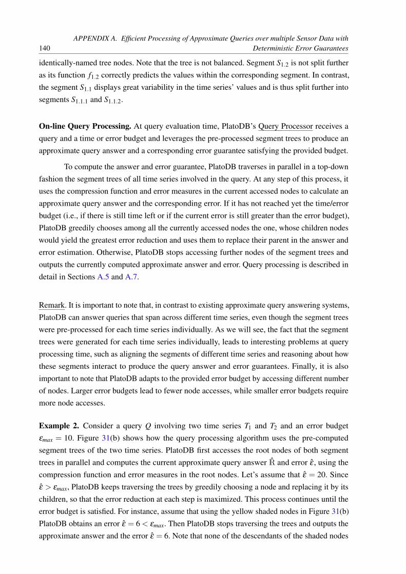
140APPENDIX A. Efficient Processing of Approximate Queries over multiple Sensor Data with
Deterministic Error Guarantees
identically-named tree nodes. Note that the tree is not balanced. Segment S1.2 is not split furtheras its function f1.2 correctly predicts the values within the corresponding segment. In contrast,the segment S1.1 displays great variability in the time series’ values and is thus split further intosegments S1.1.1 and S1.1.2.
On-line Query Processing. At query evaluation time, PlatoDB’s Query Processor receives aquery and a time or error budget and leverages the pre-processed segment trees to produce anapproximate query answer and a corresponding error guarantee satisfying the provided budget.
To compute the answer and error guarantee, PlatoDB traverses in parallel in a top-downfashion the segment trees of all time series involved in the query. At any step of this process, ituses the compression function and error measures in the current accessed nodes to calculate anapproximate query answer and the corresponding error. If it has not reached yet the time/errorbudget (i.e., if there is still time left or if the current error is still greater than the error budget),PlatoDB greedily chooses among all the currently accessed nodes the one, whose children nodeswould yield the greatest error reduction and uses them to replace their parent in the answer anderror estimation. Otherwise, PlatoDB stops accessing further nodes of the segment trees andoutputs the currently computed approximate answer and error. Query processing is described indetail in Sections A.5 and A.7.
Remark. It is important to note that, in contrast to existing approximate query answering systems,PlatoDB can answer queries that span across different time series, even though the segment treeswere pre-processed for each time series individually. As we will see, the fact that the segmenttrees were generated for each time series individually, leads to interesting problems at queryprocessing time, such as aligning the segments of different time series and reasoning about howthese segments interact to produce the query answer and error guarantees. Finally, it is alsoimportant to note that PlatoDB adapts to the provided error budget by accessing different numberof nodes. Larger error budgets lead to fewer node accesses, while smaller error budgets requiremore node accesses.
Example 2. Consider a query Q involving two time series T1 and T2 and an error budgetεmax = 10. Figure 31(b) shows how the query processing algorithm uses the pre-computedsegment trees of the two time series. PlatoDB first accesses the root nodes of both segmenttrees in parallel and computes the current approximate query answer R and error ε , using thecompression function and error measures in the root nodes. Let’s assume that ε = 20. Sinceε > εmax, PlatoDB keeps traversing the trees by greedily choosing a node and replacing it by itschildren, so that the error reduction at each step is maximized. This process continues until theerror budget is satisfied. For instance, assume that using the yellow shaded nodes in Figure 31(b)PlatoDB obtains an error ε = 6 < εmax. Then PlatoDB stops traversing the trees and outputs theapproximate answer and the error ε = 6. Note that none of the descendants of the shaded nodes

A.3. Data and Queries 141
Table 6 – Query expressions for common statistics.
Statistic Symbol Definition Query Expression
Mean E(T )n∑
i=1di
Sum(T,1,n)n
Variance Var(T )n∑
i=1(di−E(T ))2 Sum(Times(T,T ),1,n)− Sum(T,1,n)×Sum(T,1,n)
n
Covariance Cov(T1,T2)
n∑
i=1((d(1)
i −E(T1))(d(2)i −E(T2)))
n−1Sum(Times(T1,T2),1,n)
n−1 − Sum(T1,1,n)×Sum(T2,1,n)n(n−1)
Correlation Corr(T1,T2)
n∑
i=1((d(1)
i −E(T1))(d(2)i −E(T2))√
n∑
i=1(d(1)
i −E(T1))2n∑
i=1(d(2)
i −E(T2))2
Sum(Times(T1,T2))− 1n Sum(T1,1,n)×Sum(T2,1,n)√
Var(T1)Var(T2)
Cross-correlation Coss(T1,T2, `)
n∑
i=1((d(1)
i −E(T1))(d(2)i+`−E(T2))√
n∑
i=1(d(1)
i −E(T1))2n∑
i=1(d(2)
i+`−E(T2))2
Sum(Times(T1,T2))− 1n Sum(T1,1,n)×Sum(T2,1+l,n+l)√
Var(T1)Var(T2)
Source: Brito et al. (2017).
is touched, resulting in big performance savings.
As a result of this architecture, PlatoDB achieves speedups of 1-3 orders of magnitudein query processing of sensor data compared to approaches that use the entire dataset to com-pute exact query answers (more details are included in PlatoDB’s experimental evaluation inSection A.8).
A.3 Data and QueriesBefore describing the PlatoDB system, we first present its data model and query language.
Data Model. For the purpose of this work, a time series T =[(t1,d1), (t2,d2), . . ., (tn,dn)] is asequence of (time, data point) pairs (ti, di), such that the data point di was observed at time ti.We follow existing work (GOLDIN; KANELLAKIS, 1995) to normalize and standardize thetime series so that all time series are in the same domain and have the same resolution. Since alltime series are aligned, for ease of exposition we omit the exact time points and use instead theindex of the data points whenever we need to define a time interval. For instance, we will denotethe above time series simply as T =(d1,d2, ...,dn), and use [i, j] to refer to the time interval [ti, t j].A subsequence of a time series is called a time series segment. For example S = (5.01,5.06) is asegment of the time series T = (5.05, 5.01,5.06, 5.06, 5.08).
Query Language. PlatoDB supports queries whose main building blocks are aggregation queriesover time series. Figure 32 shows the formal definition of the query language and Table 6 listsseveral common statistics that can be expressed in this language.
A query expression Q is an arithmetic expression of the form Arr1⊗Arr2⊗ . . .Arrn,where ⊗ are the standard arithmetic operators (+,−×,÷) and Arri is either an arithmetic literalor an aggregation expression over a time series. An aggregation expression Sum(T, ls, le) over a

142APPENDIX A. Efficient Processing of Approximate Queries over multiple Sensor Data with
Deterministic Error Guarantees
Query Expression (Q)Q → Ar
Arithmetic Expression (Ar)Ar → number
| Agg| Ar⊗Ar where ⊗ ∈ {+,−,×,÷}
Aggregation Expression (Agg)
Agg → Sum(T, `s, `e)`e∑
i=`s
di
Time Series Expression (T )T → base time series
| SeriesGen(υ ,n) (υ ,υ , ...,υ︸ ︷︷ ︸n
)
| Plus(T,T ) (d(1)1 +d(2)
1 , . . . ,d(1)n +d(2)
n )
| Minus(T,T ) (d(1)1 −d(2)
1 , . . . ,d(1)n −d(2)
n )
| Times(T,T ) (d(1)1 ∗d(2)
1 , . . . ,d(1)n ∗d(2)
n )
Figure 32 – Grammar of query expressions.
Source: Brito et al. (2017).
time series T computes the sum of all data points of T in the time interval [ls, le]. Note that thetime series that is aggregated could either be a base time series or a derived time series that wascomputed from a set of base time series through a set of time series operators. PlatoDB allows aseries of time series operators, including Plus(T1,T2), Minus(T1,T2), and Times(T1,T2) (whichreturn a time series that has data points computed by adding, subtracting, and multiplying therespective data points of the original time series, respectively), as well as SeriesGen(v,n), whichtakes as input a value v and a counter n and creates a new time series that contains n data pointswith the value v.
Note that the query language can be used to express many common statistics over timeseries encountered in practice and all the queries we encountered during the DELPHI projectconducted at UC San Diego, which explored how health-related data about individuals, includinglarge amounts of sensor data, can be leveraged to discover the determinants of health conditionsand which served as the motivation for this work (KATSIS et al., 2013). These include the meanand variance of a single time series, as well as the covariance, correlation, and cross-correlationbetween two time series. Table 6 shows how common statistics can be expressed in PlatoDB’squery language.

A.4. SEGMENT TREE 143
A.4 SEGMENT TREE
As explained in Section A.2, at data import time, PlatoDB creates for each time series ahierarchy of summarizations of the series in the form of the segment tree. In this Section we firstexplain the structure of the tree and then describe the segment tree generation algorithm.
A.4.1 Segment Tree Structure
Let T = (d1, . . . ,dn) be a time series. The segment tree of T is a binary tree whosenodes summarize segments of the time series with nodes higher up the tree summarizing largesegments and nodes lower down the tree summarizing progressively smaller segments. Inparticular, the root node summarizes the entire time series T . Moreover, for each node n of thetree summarizing a segment Si = (di, . . . ,d j) of T , its left and right children nodes nl and nr
summarize two subsegments Sl = (di, . . . ,dk) and Sr = (dk+1, . . . ,d j), respectively, which forma partitioning of the original segment Si. As we will see in Section A.7, this hierarchical structureallows PlatoDB to adapt to varying error/time budgets by only accessing the parts of the treerequired to achieve the given error/time budget.
At each node n corresponding to segment Si = (di, . . . ,d j), PlatoDB summarizes thesegment Si by keeping two types of measures: (a) a description of a compression function thatis used to approximately represent the time series values in the segment and (b) a set of errormeasures describing how far the above approximate values are from the real values. As we willsee in Sections A.5 and A.7, PlatoDB uses at query processing time the compression functionand error measures stored in each node to compute an approximate answer of the query anddeterministic error guarantees, respectively. We next describe the compression functions anderror measures stored within each segment tree node in detail.
Segment Compression Function. Let S = (d1, . . . ,dn) be a segment. PlatoDB summarizes itscontents through a compression function f used by the user. PlatoDB supports the use of anyof the compression functions suggested in the literature (KEOGH et al., 2001b; KEOGH et al.,2001a; KEOGH, 1997; FALOUTSOS; RANGANATHAN; MANOLOPOULOS, 1994; CHAN;FU, 1999; CAI; NG, 2004). Examples include but are not limited to the Piecewise AggregateApproximation (PAA) (KEOGH et al., 2001b), the Adaptive Piecewise Constant Approximation(APCA) (KEOGH et al., 2001a), the Piecewise Linear Representation (PLR) (KEOGH, 1997),the Discrete Fourier Transformation (DFT) (FALOUTSOS; RANGANATHAN; MANOLOPOU-LOS, 1994), the Discrete Wavelet Transformation (DWT) (CHAN; FU, 1999), and the Chebyshevpolynomials (CHEB) (CAI; NG, 2004).
To describe the function, PlatoDB stores in the segment node parameters describing thefunction. These parameters depend on the type of the function. For instance, if f is a PiecewiseAggregate Approximation (PAA), estimating all values within a segment by a single value b, then

144APPENDIX A. Efficient Processing of Approximate Queries over multiple Sensor Data with
Deterministic Error Guarantees
the parameter is just a single value b. On the other hand, if f is a Piecewise Linear Approximation(PLR), estimating the values in the segment through a line ax+b, then the function parametersare the coefficients a and b of the polynomial used to describe the line.
In the rest of the document, we will refer directly to the compression function f (insteadof the parameters that are used to describe it). Given a segment (d1, . . . ,dn), we will use f (i) todenote the value for element di of the segment, as derived by f .
Segment Error Measures. In addition to the compression function, PlatoDB also stores a set oferror measures for each time series segment S = (d1, . . . ,dn). PlatoDB stores the following threeerror measures:
• L : The sum of the absolute distances between the original and the compressed time series
(also known as the Manhattan or L1 distance), i.e., L=n∑
i=1|di− f (i)|.
• d∗ : The maximum absolute value of the original time series, i.e., d∗ = max{|di| | 1≤ i≤n}.
• f ∗ : The maximum absolute value of the compressed time series, i.e., f ∗=max{| f (i)| | 1≤i≤ n}.
Example 3. For instance, consider a segment S = (5.12, 5.09,5.07,5.04) summarizedthrough the PAA compression function f = 5.08 (i.e., f (1) = f (2) = f (3) = f (4) =
5.08). Then L = |5.12− 5.08|+ |5.09− 5.08|+ |5.07− 5.08|+ |5.04− 5.08| = 0.1, d∗ =
max{5.12,5.09,5.07,5.04}= 5.12 and f ∗ = max{5.08,5.08,5.08,5.08}= 5.08.
As we will see in Section A.5, the above three error measures are sufficient to computedeterministic error guarantees for any query supported by the system, regardless of the employedcompression function f . This allows administrators to select the compression function bestsuited to each time series, without worrying about computing the error guarantees, which isautomatically handled by PlatoDB.
A.4.2 Segment Tree Generation
We next describe the algorithm generating the segment tree. To build the tree, thealgorithm has to decide how to build the children nodes from a parent node; i.e., how to partitiona segment into two non-overlapping subsegments. Each possible splitting point will lead todifferent children segments and as a result to different errors when PlatoDB uses the childrensegments to answer a query at query processing time. Ideally, the splitting point should bethe one that minimizes the error among all possible splitting points. However, since PlatoDBsupports ad hoc queries and since each query may benefit from a different splitting point, there is

A.4. SEGMENT TREE 145
no way for PlatoDB to choose a splitting point that is optimal for all queries.
Segment Tree Generation Algorithm. Based on this observation, PlatoDB chooses the splittingpoint that minimizes the error for the basic query that simply computes the sum of all data pointsof the original segment. In particular, the segment tree generation algorithm starts from the rootand proceeding in a top-down fashion given a segment S = (d1, . . . ,dn), selects a splitting pointdk that leads into two subsegments Sl = (d1, . . . ,dk) and Sr = (dk+1, . . . ,dn) so that the sum ofthe Manhattan distances of the new subsegments LSl +LSr is minimized.
The algorithm stops further splitting down a segment S, when one of the following twoconditions hold: (i) When the Manhattan distance LS of the segment is smaller than a thresholdτ or (ii) when he size of the segment is below a threshold κ . The choice between conditions(i) and (ii) and the values of the corresponding thresholds τ and κ is specified by the systemadministrator.
Since the algorithm needs time proportional to the size of a segment to compute thesplitting point of a single segment and it repeats this process for every non-leaf tree node, itexhibits a worst-time complexity of O(mn), where n is the size of the original time series (i.e.,the number of its data points) and m number of nodes in the resulting segment tree.
Discussion. Note that by deciding independently how to split each individual segment into twosubsegments, the segment tree generation algorithm is a greedy algorithm, which even thoughmakes optimal local decisions for the basic aggregation query, may not lead to optimal globaldecisions. For instance, there is no guarantee that the k nodes that exist at a particular level of thesegment tree correspond to the k nodes that minimize the error of the basic aggregation query.The literature contains a multitude of algorithms that can provide such a guarantee for a givenk; i.e., algorithms that can, given a time series T and a number k, produce k segments of T thatminimize some error metric. Examples include the optimal algorithm of (BELLMAN, 1961), aswell as approximation algorithms with formal guarantees presented in (TERZI; TSAPARAS,2006). However, all these algorithms have very high worst-time complexity that makes themprohibitive for the large number of data points typically found in sensor datasets and are thereforenot considered in this work. Though several heuristic segmentation algorithms exist, such as theSliding Windows (SHATKAY; ZDONIK, 1996), the Top-down (KEOGH; PAZZANI, 1998) andthe Bottom-Up (KEOGH; PAZZANI, 1999) algorithm, similar do our greedy algorithm, they donot provide any formal guarantees.
Finally, note that the tree generated by the above algorithm will in general be unbalanced.Intuitively, the algorithm will create more nodes and corresponding tree levels to cover segmentsthat contain data points that are more irregular and/or rapidly changing, utilizing fewer nodes forsmooth segments.

146APPENDIX A. Efficient Processing of Approximate Queries over multiple Sensor Data with
Deterministic Error Guarantees
A.5 Computing Approximate Query Answers and ErrorGuarantees
Given pre-computed segment trees for time series T1, . . . ,Tn, PlatoDB answers ad hocqueries over the time series by accessing their segment trees. In particular, to answer a givenquery Q under an error/time budget, PlatoDB navigates the segment trees of the time seriesinvolved in Q, selects segment nodes (or simply segments) that satisfy the budget, and computesan approximate answer for Q together with deterministic error guarantees.
We will next present the query processing algorithm. For ease of exposition, we willstart by describing how PlatoDB computes an approximate query answer and the associatederror guarantees assuming that the segment nodes have been already chosen, and will explain inSection A.7 how PlatoDB traverses the tree to choose the segment nodes.
Approximate query answering problem under given segments. Formally, let T1, . . . ,Tk betime series, such that time series Ti is partitioned into segments S1
i , . . .Sni . Given (a) these
segments and the associated measures as described above and (b) a query Q over the timeseries T1, . . . ,Tk, we will show how PlatoDB computes an approximate query answer R and anestimated error ε , such that the approximate query answer R is guaranteed to be with ±ε of theaccurate query answer R4, i.e., |R− R| ≤ ε .
For ease of exposition, we next first describe the simple case where each time series Ti
contains a single segment perfectly aligned with the single segment of the other series, beforedescribing the general case, where each time series Ti contains multiple segments, which mayalso not be perfectly aligned with the segments of the other time series.
A.5.1 Single Time Series Segment
Let T1, . . . ,Tk be k time series with single aligned segments, i.e., Ti is approximated by asingle segment Si. Also let fi be the compression function and (Li,d∗i , f ∗i ) the error measures ofsegment Si, respectively. To compute the approximate answer and error guarantees of a queryQ over T1, . . . ,Tk using the single segments S1, . . . ,Sk, PlatoDB employs an algebraic approachcomputing in a bottom-up fashion for each algebraic operator op of Q the approximate answerand error guarantees for the subquery corresponding to the subtree rooted at op.
This algebraic approach is based on formulas that for each algebraic query operator, givenan approximate query answer and error for the inputs of the operator, provide the correspondingquery answer and error for the output of the operator. Figure 33 shows the formulas employedby PlatoDB for each algebraic query operator supported by the system. Note that the output
4 Accurate answer means running queries over raw data. But note that, in this work, we can givenestimate errors wihout computing the accurate answers.

A.5. Computing Approximate Query Answers and Error Guarantees 147
signatures differ between operators. This is due to the different types of operators supported byPlatoDB, as explained next. Recall from Section A.3 that PlatoDB’s query language consists ofthree types of operators: (i) time series operators, (ii) aggregation operator, and (iii) arithmeticoperators. While time series operators output a time series, aggregation and arithmetic operatorsoutput a single number. As a result, the formulas used for answer and error estimation, treat thesetwo classes of operators differently: For time series operators, the formulas return, similarly tothe input time series, the compression function and error measures of the output time series. Foraggregation and arithmetic operators on the other hand, which return a single number and not anentire time series, the formulas return simply a single approximate answer and estimated error.Figure 33 shows the resulting formulas. 5
Without going into detail into each of them, we next explain how they can be used tocompute the answer and corresponding error guarantees for an entire query through an example.
Example 4. This example shows how to use the formulas in Figure 33 to compute the ap-proximate answer and associated error for a query computing the variance of a time seriesT consisting of single segment S. For simplicity of the query expression we assume that themean µ of T is known in advance (note that even if µ was not known, the query would stillbe expressible in PlatoDB’s query language, albeit through a longer expression). Let f be thecompression function and (L,d∗, f ∗) the error measures of S. The query can be expressed asQ = Sum(Times (Minus(T,SeriesGen(µ,n)), Minus(T,SeriesGen(µ,n)),1,n). Figure 34 showshow PlatoDB evaluates this query in a bottom-up fashion. It first uses the formula of the Series-Gen operator to compute the compression function ( f = µ) and error measures (L= 0, d∗ = µ ,f ∗ = µ) for the output of the SeriesGen operator. It then computes the compression function( f − µ) and error measures (L, (d∗+ µ), ( f ∗+ µ)) for the output of the Minus operator. Thecomputation continues in a bottom-up fashion, until PlatoDB computes the output of the Sumoperator in the form of an approximate answer R = n( f −µ)2 where n is the number of datapoints in T , and an estimated error ε = (d∗+ f ∗)L.
Importantly, the formulas shown in Figure 33 are guaranteed to produce the best errorestimation out of any formula that uses the three error measures employed by PlatoDB asexplained by the following theorem:
Theorem 1. The estimated errors produced through the use of the formulas shown in Figure33 are the lowest among all possible error estimations produced by using the error measuresdescribed in Section A.4.�
The proof can be found in Appendix A.6.2.
5 Out of the formulas, the most involved are the output measure estimation formulas of the Timesoperator. More details on how they were derived can be found in Appendix A.6.1.

148APPENDIX A. Efficient Processing of Approximate Queries over multiple Sensor Data with
Deterministic Error Guarantees
Time Series Operators
Operator Compr. OutputFunc. Error Measures
f L d∗ f ∗
SeriesGen(υ ,n) υ 0 υ υ
Plus(T1,T2) f1 + f2 L1 +L2 d∗1 +d∗2 f ∗1 + f ∗2Minus(T1,T2) f1− f2 L1 +L2 d∗1 +d∗2 f ∗1 + f ∗2Times(T1,T2) f1× f2 min{ d∗1 ×d∗2 f ∗1 × f ∗2
d∗2L1 + f ∗1L2,f ∗2L1 +d∗1L2}
Aggregation Operator
Operator Approximate EstimatedOutput Error
Sum(T,`s, `e)∑`ei=`s
f (i) L
Arithmetic Operators
Operator Approximate EstimatedOutput Error
Agg + Number ˆAgg+Number ε
Agg − Number ˆAgg−Number ε
Agg × Number ˆAgg×Number ε×numberAgg ÷ Number ˆAgg÷Number ε÷number
Agga +Aggb ˆAgga + ˆAggb εa + εb
Agga−Aggb ˆAgga− ˆAggb εa + εb
Agga×Aggb ˆAgga× ˆAggbˆAggaεb + ˆAggbεa + εaεb
Agga÷Aggb ˆAgga÷ ˆAggbˆAgga+εaˆAggb−εb
− ˆAggaˆAggb
Figure 33 – Formulas for estimating answer and error for each algebraic operator (single segment).
Source: Brito et al. (2017).
A.5.2 Multiple Segment Time Series
Let us now consider the general case, where each time series T contains multiplesegments of varying different sizes. As a result of the varying sizes of the segments, segments ofdifferent time series may not fully align.
Example 5. For instance consider the top two time series T1 = (S1,1,S1,2) and T2 = (S2,1,S2,2)
of Figure 35 (ignore the third time series for now). Segment S1,1 overlaps with both S2,1 and S2,2.Similarly, segment S2,2 overlaps with both S1,1 and S1,2.
One may think that this can be easily solved by creating subsegments that are perfectlyaligned and then using for each of them the answer and error estimation formulas of Section

A.5. Computing Approximate Query Answers and Error Guarantees 149
𝑆𝑢𝑚
𝑇𝑖𝑚𝑒𝑠
𝑀𝑖𝑛𝑢𝑠
𝑇𝑆𝑒𝑟𝑖𝑒𝑠𝐺𝑒𝑛
𝜇
𝑀𝑖𝑛𝑢𝑠
𝑇𝑆𝑒𝑟𝑖𝑒𝑠𝐺𝑒𝑛
𝜇
Figure 34 – Approximate query answer and associated error for query Q = Sum(Times(Minus(T,SeriesGen(µ,n)), Minus(T,SeriesGen(µ,n)),1,n). Compression functionsand error measures are shown in blue and red, respectively.
Source: Brito et al. (2017).
Figure 35 – Example of aligned time series segments. The new generated time series T3 is shown in redcolor.
Source: Brito et al. (2017).
A.5.1.
Example 6. Continuing our example, the two time series T1 and T2 can be split into the threealigned subsegments shown as the output time series T3. Then for each of these output segments,we can compute the error based on the formulas of Section A.5.1.
However, the problem with this approach is that the resulting error will be severelyoverestimated as the error of a single segment of the original time series may be counted multipletimes, as it overlaps with multiple output segments.
Example 7. For instance, for a query over the time series T1 and T2 of Figure 35,the error of S2,2
will be double-counted, as it will be counted towards the error of the two output segments S3,2
and S3,3.
To avoid this pitfall, PlatoDB does not estimate the error for its segment individuallybut instead computes the error holistically for the entire time series. Figures 36 and 37 showthe resulting answer and error estimation formulas for time series operators and the aggregationoperator, respectively. The formulas of the arithmetic operators are omitted as they remain thesame as in the single segment case, as the arithmetic operators take as input single numbersinstead of time series and are thus not affected by multiple segments.

150APPENDIX A. Efficient Processing of Approximate Queries over multiple Sensor Data with
Deterministic Error Guarantees
Time Series Operators
Operator Comp. func. Output Error Measuresf L d∗ f ∗
SeriesGen(υ ,n) υ 0 υ υ
Plus(Ta,Tb){( fc,1, ..., fc,k)| fc,i =fa,u + fb,v i ∈ [1,k]} ∑
pi=1 La,i +∑
qj=1 Lb, j max{dc,i|dc,i = da,u +db,v i ∈ [1,k]}max{ fc,i| fc,i = fa,u + fb,v i ∈ [1,k]}
Minus(Ta,Tb){( fc,1, ..., fc,k)| fc,i =fa,u− fb,v i ∈ [1,k]} ∑
pi=1 La,i +∑
qj=1 Lb, j max{dc,i|dc,i = da,u +db,v i ∈ [1,k]}max{ fc,i| fc,i = fa,u + fb,v i ∈ [1,k]}
Times(Ta,Tb){( fc,1, ..., fc,k)| fc,i =fa,u× fb,v∀i ∈ [1,k]} LTc max{dc,i|dc,i = da,u×db,v i ∈ [1,k]}max{ fc,i| fc,i = fa,u× fb,v i ∈ [1,k]}
Figure 36 – Formulas for estimating answer and error for time series operators (multiple segments). Foreach output time series segment Sc,i, let Sa,u and Sb,v be the input segments that overlap withSc,i.
Source: Brito et al. (2017).
Aggregation Operator
Operator Approximate EstimatedOutput Error
Sum(T,`s, `e) ∑vi=u ∑
|Si|j=1 fi( j) ∑
vi=uLi
Figure 37 – Formulas for estimating answer and error for the aggregation operator (multiple segments).
Source: Brito et al. (2017).
A.6 Proofs
A.6.1 Error measures for the Times operator (Single Segment)
Let f (1) and f (2) be the compression functions of T1 = (d(1)1 , ...,d(1)
n ) and T2 =
(d(2)1 , ...,d(2)
n ) respectively. Let (L1,d∗1 , f ∗1 ) and (L2,d∗2 , f ∗2 ) be the error measures for timeseries T1 and T2. For Times(T1,T2)→ T operator, the compression function f and the errormeasures (L,d∗, f ∗) for the output time series T = (d1, ...,dn) are computed as follows:
• f = f (1)× f (2), i.e., the product of two compression functions.
• L= ∑ni=1 |di− f (i)|= ∑
ni=1 |d
(1)i d(2)
i − f (1)(i) f (2)(i)|. There are two options to transformthis expression.Option 1: L = ∑
ni=1 |d
(1)i d(2)
i − d(1)i f (2)(i) + d(1)
i f (2)(i) − f (1)(i) f (2)(i)| =
∑ni=1 |d
(1)i (d(2)
i − f (2)(i))+ f (2)(i)(d(1)i − f (1)(i))| ≤ f ∗2L1 +d∗1L2.
Option 2: L = ∑ni=1 |d
(1)i d(2)
i − d(2)i f (1)(i) + d(2)
i f (1)(i) − f (1)(i) f (2)(i)| =
∑ni=1 |d
(2)i (d(1)
i − f (1)(i))+ f (1)(i)(d(2)i − f (2)(i))| ≤ d∗2L1 + f ∗1L2.
Thus, we choose the minimal one between these two options. That isL= min{ f ∗2L1 +d∗1L2,d∗2L1 + f ∗1L2}.

A.6. Proofs 151
• d∗ = max{|di| |1≤ i≤ n}= max{|d(1)i d(2)
i | |1≤ i≤ n}≤ d∗1×d∗2 .
• f ∗ = max{| f (i)| |1≤ i≤ n}= max{| f (1)i f (2)i | |1≤ i≤ n}≤ f ∗1 × f ∗2 .
A.6.2 Proof of the optimality of the error estimation for the formulasof Figure 33
Aggregation operator. Depending on whether it is a single segment time series, there are twocases.
Case 1. A time series T (with n data points) contains only one single segment. There are twosubcases depending on whether T is entirely used in the query or not. That is `e− `s = n or not.
Case 1.1. `e− `s = n. In this case, the error ε = ∑`ei=`s|di− f (i) = ∑
ni=1 |di− f (i)|. And
we have L= ∑ni=1 |di− f (i)|. Therefore, we can get ε = L. It means that by using L we are able
to get the accurate error (the optimal error estimation). As desired.
Case 1.2. `e−`s < n. Assume there exists an error estimator A that gives an approximateerror ε , where ε =L−α , where α > 0 is a small value. Let T be time series segment with lengthn such that di = f (i) for i ∈ [1,n− (`e− `s)−1] and di = f (i)+1 for i ∈ [n− (`e− `s),n]. ThusL= ∑
ni=1 |di− f (i)|= `e− `s. For a query with range [1, `e− `s], A gives the approximate error
as `e− `s−α , which is correct as the accurate error is 0. Now we switch the points di with d j
(as well as f (i) with f ( j)) for i ∈ [1, `e− `s], j ∈ [n− (`e− `s),n] to generate a new segment T ′.Note that, T ′ and T have the same L. Now the accurate error is also L= `e− `s. However, A stillgives the approximate error as `e− `s−α , which is incorrect as it produces smaller error thanthe optimal one. Therefore, there does not exist an estimator that produces approximate errorsless than that of our estimator, which means our estimator achieves the lower bound. As desired.
Case 2. A time series T contains multiple segments S1, ...,Sn. Note that, segments S2, ...,Sn−1 areall always entirely used by the query. According to case 1.1, our estimator gives the optimal errorestimation. For the left-most and right-most segments, i.e., S1 and Sn, our estimator achieves thelower bound of error estimation according to case 1.2. As desired.
Plus and Minus operators. Similar to the proof presented above, it is easy to see our estimatorachieves the lower bound. Otherwise, there must exist an incorrect error estimation.
Times operator. We distinguish between two cases.Case 1. Time series T1 with n data points (resp. T2) only contains one segment. Depending onwhether T1 and T2 are entirely used. There are two subcases.
Case 1.1. T1 and T2 are entirely used. The accurate error is ε = ∑ni=1(d
(1)i × d(2)
i −f (1)(1)× f (2)(i)). Let the data point in T1 have the following features d(1)
i = d(1)i+1−1, f (1)(i) =
f (1)(i+ 1)− 1 and f 1(i) = d(1)i − 1 for i ∈ [1,n]. Let T2 have the same data. Thus, L(1) =
∑ni=1 |d
(1)i − f (1)(i)| = n and L(2) = n, d∗1 = d(1)
n = d∗2 = d(2)n and f ∗1 = f (1)(n) = f ∗2 = f (2)(n).

152APPENDIX A. Efficient Processing of Approximate Queries over multiple Sensor Data with
Deterministic Error Guarantees
So the estimated error of our estimator is
ε = min{ f ∗2L1 +d∗1L2,d∗2L1 + f ∗1L2}= n(d(1)n + d(1)
n ) = n(2d(1)n +1)
Assume there exists an error estimator A that produces an approximate error ε ′, whereε ′= ε−α , where α > 0 is a small value. Since the accurate error ε = ∑
ni=1(2 f (1)(i)+1)< ε ′. A
returns the correct estimation. Then we make d(1)i = d(1)
i+1 and f (1)(i) = f (1)(i+1) for i∈ [1,n] inboth two time series. Then the error measures of both time series stay the same. Now, the accurateerror is ε = ∑
ni=1(2d(1)
i +1) = n(2d(1)n +1) = ε . That is our estimator produces the optimal error
(meaning the error is equal to the accurate one). But A still gives the same estimation ε −α ,which is incorrect. So A does not exist, as desired.
Case 1.2. T1 and T2 are not entirely used. The proof is similar to the case 1.2 in the proofof aggregation operator above by making segments that d(1)
i 6= f (1)(i) and d(2)i 6= f (2)(i) only
happen in the query range, which makes ε = ε . So our estimator achieves the lower bound.
Case 2. k segments S(1)1 , ...,S(1)k in time series T1 overlapping one segment S(2) in time series T2
are used in the query with range [a,b]. The proof is similar to that in Case 1.1 and Case 1.2.
Case 3. k1 segments S(1)1 , ...,S(1)k1in time series T1 overlapping k2 segments S(2)1 , ...,S(2)k2
in timeseries T2 are used in the query. The proof is similar to that in Case 2.
Arithmetic Operators For arithmetic operator Ar1⊗ Ar2. There are three cases depending onthe number of approximate answers Agg in the expression.
Case 1. Zero Agg, i.e., both Ar1 and Ar2 are numbers. Ar1⊗Ar2 can be transformed as number1⊗number2 Then the answers are accurate answers. As desired.
Case 2. One Agg, i.e., Ar1⊗Ar2 can be transformed as Agg⊗number. Let ˆAgg and ε be the outputapproximate answer of Agg and the estimated error by PlatoDB. Therefore, we know that ε is thelower bound of |Agg− ˆAgg|. For Agg+number, the error is |Agg+number−( ˆAgg+number)|=|Agg− ˆAgg|. Thus, ε is also the lower bound of Agg+number. Similarly, we can prove the lowerbound property of the errors for {−,×,÷} operators.
Case 3. Two Agg, i.e., Ar1⊗Ar2 can be transformed as Agg1⊗Agg2. Let ˆAgg1 (resp. ˆAgg2)and ε1 (resp. ε2) be the output approximate answer of Agg1 (resp. Agg2) and the estimatederrors provided by PlatoDB, respectively. According to the previous proof, we know that ε1
and ε2 are the lower bound of |Agg1− ˆAgg1| and |Agg2− ˆAgg2| respectively. It is obvious thatε1 + ε2 is the lower bound error of Agg1 +Agg2 and Agg1−Agg2. For Agg1×Agg2, we have|Agg1×Agg2− ˆAgg1× ˆAgg2| ≤ ˆAgg1ε2 + ˆAgg2ε1 + ε1ε2. We can prove it is the lower boundby constructing a case that the accurate error is equals to this one, which means there does notexist a better estimation. Similarly, for Agg1÷Agg2, we can prove
ˆAgg1+ε1ˆAgg2−ε2
− ˆAgg1ˆAgg2
is lower bounderror.

A.7. Navigating the SEGMENT TREE 153
A.7 Navigating the SEGMENT TREESo far we have seen how PlatoDB computes the approximate answer to a query and its
associated error, assuming that the segments that are used for query processing have alreadybeen selected. In this Section, we explain how this selection is performed. In particular, we showhow PlatoDB navigates the segment trees of the time series involved in the query to continuouslycompute better estimations of the query answer under the given error or time budget is satisfied.
Query Processing Algorithm. Let T1, ...,Tm be a set of time series and I1, ...,Im the respectivesegment trees. Let also Q be a query over T1, ...,Tm and εmax/tmax an error/time budget, respec-tively. To answer Q under the given budget, PlatoDB first starts from the roots of I1, ...,Im anduses them to compute the approximate query answer R and corresponding error ε using theformulas presented in Section A.5. If the estimated error is greater than the error budget (i.e.,if ε ≥ εmax) or if the elapsed time is smaller than the allowed time budget, PlatoDB choosesone of the tree nodes used above, replaces it with its children and repeats the above procedureusing the newly selected nodes until the given error/time budget is reached. What is importantis the criterion that is used to choose the node that is replaced at each step by its children. Ingeneral, PlatoDB will have to select between several nodes, as it will be exploring in whichsegment tree and moreover in which part of the selected segment tree it pays off to navigatefurther down. Since PlatoDB aims to reduce the estimated error as much as possible, at each stepit greedily chooses the node whose replacement by its children leads to the biggest reduction inthe estimated error. The resulting procedure is shown as Algorithm 9 6.
Algorithm 9 – PlatoDB Query Processing
input: Segment Trees I1, ...,Im, query Q, error budget εmax or time budget tmaxoutput: Approximate answer R and error ε
1: Access the roots of I1, ...,Im;2: Compute R and ε by using the compression functions and error measures of the
currently accessed nodes (see Section A.5 for details);3: while ε > εmax or elapsed time < tmax do4: Choose a node maximizing the error reduction;5: Update the current answer R and error ε using the compression functions and error
measures of the currently accessed nodes;6: end while
return (R, ε);
Algorithm Optimality. Given its greedy nature, one may wonder whether the query processing6 Note that the algorithm is shown for both error and time budget case. In contrast to the case when a
time budget is provided, in which the algorithm has to always keep a computed estimated answer R toreturn it when the time budget runs out, in the case of the error budget this is not required. Thus, inthe latter case, it suffices to compute R only at the very last step of the algorithm, thus avoiding itsiterative computation during the while loop.

154APPENDIX A. Efficient Processing of Approximate Queries over multiple Sensor Data with
Deterministic Error Guarantees
algorithm is optimal. To answer this question, we have to first define optimality. Since the aim ofthe query processing algorithm is to produce the lowest possible error in the fastest possible time(which can be approximated by the number of nodes that are accessed), we say that an algorithmis optimal if for every possible query, set of segment trees, and error budget εmax it answers thequery under the given budget accessing the lowest number of nodes than any other possiblealgorithm. Since a comparison of any possible algorithm is hard, we also restrict our attentionto deterministic algorithms that access the segment trees in a top-down fashion (i.e, to access anode N all its ancestor nodes should also be accessed). We denote this class of algorithms as A.It turns out that no algorithm in A can be optimal as the following theorem states:
Theorem 2. There is no optimal algorithm in A.
Proof. Consider the following segment trees of two time series T1 and T2. The segment tree ofT1 is shown in Figure 38 and the segment tree of T2 is a tree containing a single node. Nowconsider a query Q over these two time series and an error budget ε = h− 1 where h > 1 isthe height of the T1’s tree. Assume that the query error using the tree roots is εroot = 2h. Alsoassume that whenever the query processing algorithm replaces a node by its children, the errorfor the query is reduced by 1
2h with the exception of the shaded node, which, when replaced byits children, leads to an error reduction of h+1. This means that the query processing algorithmcan only terminate after accessing the children of the shaded node, as the query error in that casewill be at most 2h− (h+1) = h−1. Otherwise, the error estimated by the algorithm will be atleast 2h−2h( 1
2h ) = 2h−1 > h−1, which exceeds the error budget and thus does not allow thealgorithm to terminate. Since the shaded node can be placed at an arbitrary position in the tree,for every given deterministic algorithm, we can place the shaded node in the tree, so that thealgorithm accesses the children of the shaded node only after it has accessed all the other nodesin the tree. However, this is suboptimal, as there is a way to access the children of the shadednode with fewer node accesses (i.e., by following the path from the root to the shaded node).Therefore, no algorithm in A is optimal.
… …
Figure 38 – Segment Tree for Theorem 2.
Source: Brito et al. (2017).
As a result of the above theorem, PlatoDB’s query processing algorithm cannot beoptimal in general. However, we can show that it is optimal for segment trees that exhibit the

A.7. Navigating the SEGMENT TREE 155
following property: For every pair of nodes N and N′ of the segment tree, such that N′ is adescendant of N, the error reduction ε∆(N) achieved by replacing N with its children is greateror equal to the error reduction ε∆(N′) achieved by replacing N′ with its children. Such a tree iscalled fine-error-reduction tree and intuitively it guarantees that any node leads to a greater orequal error reduction than any of its descendants. If all trees satisfy the above property, PlatoDB’squery processing algorithm is optimal:
Theorem 3. In the presence of segment trees that are fine-error-reduction trees, PlatoDB’s queryprocessing algorithm is optimal.
Table 7 – Incremental update of estimated errors for time series operators.
Operator Incremental Error UpdatePlus(Ta,Tb) ε ′ = ε− (La− (La.1 +La.2))
Minus(Ta,Tb) ε ′ = ε− (La− (La.1 +La.2))
Times(Ta,Tb)
ε ′ = ε− (max(pb,1, ..., pb,k)La−max(pb,1, ..., pb,i)La.1 +
max(pb,i, ..., pb,k)La.2), wherepb,i ∈ {d∗b,i, f ∗b,i}
Source: Brito et al. (2017).
Incremental Error Update. Having proven the optimality of the algorithm for fine-error-reduction trees, we will next discuss an optimization that can be employed to speedup thealgorithm. By studying the algorithm, it is easy to observe that as the algorithm moves from a setN = {N1, . . . ,Nn} of nodes to a set N′ = {N1, . . ., Na−1, Na.1, Na.2, Na+1, . . ., Nn} of nodes (byreplacing node Na by its children Na.1 and Na.2), it recomputes the error using all nodes in N′,although only the two nodes Na.1 and Na.2 have changed from the previous node set N.
This observation led to the incremental error update optimization of PlatoDB’squery processing algorithm described next. Instead of recomputing from scratch the errorof N′ using all nodes, PlatoDB incrementally updates the error of N by using only the errormeasures of the newly replaced node Na and the newly inserted nodes Na.1 and Na.2. Let(La,d∗a , f ∗a ), (La.1,d∗a.1, f ∗a.1), and (La.2,d∗a.2, f ∗a.2) be the error measures of nodes Na, Na.1, andNa.2, respectively. Assume that the segments Sb,1, ...,Sb,k overlap with the segment of nodeNa, the segments Sb,1, ...,Sb,i (i≤ k) overlap with the segment of node Na.1, and the segmentsSb,i, ...,Sb,k overlap with the segment of node Na.2. Then the estimated error ε ′ using nodes Na.1
and Na.2 can be incrementally computed from the error ε using node Na through the incrementalerror update formulas shown in Table 77.
7 The SeriesGen operator is omitted, since its input is not a time series and as a result there is no segmenttree associated with its input.

156APPENDIX A. Efficient Processing of Approximate Queries over multiple Sensor Data with
Deterministic Error Guarantees
Probabilistic Extension. While PlatoDB provides deterministic error guarantees, which as wediscussed above are in many cases required, it is interesting to note that it can be easily extendedto provide probabilistic error guarantees if needed. Most importantly this can be done simply bychanging the error measures computed for each segment from (L,d∗, f ∗) to (σε ,ε
∗, f ∗), whereσε is the variance of di− f (i), and ε∗ is the maximal absolute value of di− f (i). Then we canemploy the Central Limit Theorem (CLT) (DUDLEY, 1999) to bound the accurate error ε byPr(ε ≤ ε)≥ 1−α , where α can be adjusted by the users to get different confidence levels. It isinteresting that the rest of the system, including the hierarchical structure of the segment tree andthe tree navigation algorithm employed at query processing time do not need to be modified. Inour future work we plan to further explore this probabilistic extension and compare it to existingapproximate query answering techniques with probabilistic guarantees.
A.8 Experimental Evaluation
To evaluate PlatoDB’s performance and verify our hypothesis that PlatoDB is able toprovide significant savings in the query processing of sensor data, we are conducting experimentson real sensor data. We present here early data points that we have discovered.
Datasets. For our preliminary experiments, we used two real sensor datasets:
1. Intel Lab Data (ILD)8. Smart home data (humidity and temperature) collected at 31-secondintervals from 54 sensors deployed at the Intel Berkeley Research Lab between February28th and April 5th, 2004. The dataset contains about 2.3 million tuples (i.e., 4.6 millionsensor readings in total).
2. EPA Air Quality Data (AIR)9. Air quality data collected at hourly intervals from about1000 sensors from January 1st 2000 to April 1st 2016. The dataset contains about 133million tuples (i.e., 266 million sensor readings in total).
From each dataset we extracted multiple time series, each corresponding to a singleattribute of the dataset; Humidity and Temperature for ILD and Ozone and SO2 for AIR. Wethen used PlatoDB to create the corresponding segment tree for each time series and to answerqueries over them.
Experimental platform. All experiments were performed on a computer with a 4th generationIntel i7-4770 processor (4×32 KB L1 data cache, 4×256 KB L2 cache, 8 MB shared L3 cache,4 physical cores, 3.6 GHz) and 16 GB RAM, running Ubuntu 14.04.1. All the algorithms were
8 <http://db.lcs.mit.edu/labdata/labdata.html>9 <https://www.epa.gov/outdoor-air-quality-data>

A.8. Experimental Evaluation 157
implemented in C++ and compiled with g++ 4.8.4, using -O3 optimization. All data was storedin main memory.
A.8.1 Experimental Results
In our preliminary evaluation, we measured two quantities: First, the size of the segmenttree created by PlatoDB, since this segment tree is stored in main memory, and second, the queryprocessing performance of PlatoDB compared to a system that answers queries using the entiretyof the raw sensor data. In our future work, we will be conducting a more thorough evaluation ofthe system. We next present our preliminary results:
Table 8 – Raw data and segment tree sizes.
Dataset # Tuples Raw Data Segment Tree(0-degree) (1-degree)
ILD 2,313,153 35.29 MB 0.14 MB 0.67 MBAIR 133,075,510 1.98 GB 4.37 MB 8.11 MB
Source: Brito et al. (2017).
Segment tree size. Table 8 shows the size of the raw data and the combined size of thesegment trees built for all the time series extracted from the ILD and AIR datasets.10 Weexperimented with two different compression functions, resulting in different segment tree sizes;a 0-degree polynomial (corresponding to the Piecewise Aggregate Approximation (KEOGHet al., 2001b), where each value within a segment is approximated through the average of thevalues in the segment) and a 1-degree polynomial (corresponding to the Piecewise LinearApproximation (KEOGH, 1997), where each segment is approximated through a line). As shown,the segment trees are significantly smaller than the raw sensor data (about 0.40%−1.90% and0.22%−0.40% smaller for the ILD and AIR datasets, respectively). As a result, the segmenttrees of the time series can be easily kept in main memory, even when the system stores a largenumber of time series.
Query processing performance. We next compared the query processing performance ofPlatoDB against a baseline, which is a custom in-memory algorithm that computes the exactanswer of the queries using the raw data. To compare the systems, we measured the time requiredto process a correlation query between two time series (i.e., correlation(Humidity, Temperature)in ILD and correlation(Ozone and SO2) in AIR)) with a varying error budget (ranging from 5%to 25%). Figure 39 shows the resulting times for each of the two datasets. Each graph depicts theperformance of three systems; Exact, which is the baseline method of answering queries over
10 To make a fair comparison, the raw data size refers only to the combined size of the attributes used inthe time series and does not include other attributes that exist in the original dataset (such as locationcodes etc).

158APPENDIX A. Efficient Processing of Approximate Queries over multiple Sensor Data with
Deterministic Error Guarantees
0 10 20 30 40 50 60 70 80
5 10 15 20 25
Tim
e C
ost(
ms)
Error (%)
ExactApproPlato-0ApproPlato-1
(a) ILD
0 50
100 150 200 250 300 350 400 450
5 10 15 20 25
Tim
e C
ost(
ms)
Error (%)
ExactApproPlato-0ApproPlato-1
(b) AIR.
Figure 39 – Query processing performance for correlation query (time shown in ms).
Source: Brito et al. (2017).
the raw data, and PlatoDB-0, PlatoDB-1, which are instances of PlatoDB using the 0-degree and1-degree polynomial compression functions, as explained above.
By studying Figure 39, we can make the following observations.
• Both instances of PlatoDB outperform Exact by one to three orders of magnitude, depend-ing on the provided error budget.
• In contrast to Exact which always uses the entire raw dataset to compute exact queryanswers, PlatoDB allows the user to select the appropriate tradeoff between time spent inquery processing and resulting error by specifying the desired error budget. The systemadapts to the budget by providing faster responses as the allowed error budget increases;
• Notably, PlatoDB remains significantly faster than Exact even for small error budgets. Inparticular, PlatoDB is over 9× and 37× faster than Exact when the error is 5% in ILD andAIR respectively.
In summary, our preliminary results show that PlatoDB shows significant potentialfor speeding up query processing of ad hoc queries over large amounts of sensor data, as itoutperforms exact query processing algorithms in many cases by several orders of magnitude.Moreover, it can provide such speedups, while providing deterministic error guarantees, incontrast to existing sampling-based approximate query answering approaches that provide onlyprobabilistic guarantees, which may not hold in practice. Despite the difference in guarantees, inour future work we will be conducting a more thorough evaluation of the system comparing italso against sampling-based systems.

A.9. Related Work 159
A.9 Related Work
Approximate query answering has been the focus on an extensive body of work, whichwe will summarize next. However, to the best of our knowledge, this is the first work thatprovides deterministic guarantees for aggregation queries over multiple time series.
Approximate query answering with probabilistic error guarantees. Most of the existingwork on approximate query processing has focused on using sampling to compute approximatequery answers by appropriately evaluating the queries on small samples of the data (JERMAINEet al., 2007; AGARWAL et al., 2013; WU; OOI; TAN, 2010; BABCOCK; DATAR; MOTWANI,2004; PANSARE et al., 2011, 2011). Such approaches typically leverage statistical inequalitiesand the central limit theorem to compute the confidence interval or variance of the computedapproximate answer. As a result, their error guarantees are probabilistic. While probabilisticguarantees are often sufficient, there are not suitable for scenarios where one wants to be certainthat the answer will fall within a certain interval 11.
A special form of sampling-based methods are online aggregation approaches, whichprovide a continuously improving query answer, allowing users to stop the query evaluationwhen they are satisfied with the resulting error (HELLERSTEIN; HAAS; WANG, 1997;CONDIE et al., 2010; PANSARE et al., 2011). With its hierarchical segment tree, PlatoDB cansupport the online aggregation paradigm, while providing deterministic error guarantees.
Approximate query answering with deterministic error guarantees. Approximatelyanswering queries while providing deterministic error guarantees has so far received only verylimited attention (POTTI; PATEL, 2015; LAZARIDIS; MEHROTRA, 2001; POOSALA et
al., 1996). Existing work in the area has focused on simple aggregation queries that involve asingle relational table. In contrast, PlatoDB provides deterministic error guarantees on queriesthat may involve multiple time series (each of which can be though of as a single relationaltable), enabling the evaluation of many common statistics that span tables, such as correlation,cross-correlation and others.
Approximate query answering over sensor data. Moreover, PlatoDB is one of the firstapproximate query answering systems that leverage the fact that sensor data are not random butfollow a usually smooth underlying phenomenon. The majority of existing works on approximatequery answering looked at general relational data. Moreover, the ones that studied approximatequery processing for sensor data, focused on the networking aspect of the problem, studyinghow aggregate queries can be efficiently evaluated in a distributed sensor network (MADDEN et
11 Note that as discussed in Section A.7, PlatoDB can also be extended to provide probabilistic guaranteeswhen deterministic guarantees are not required, simply by modifying the error measures computed foreach segment.

160APPENDIX A. Efficient Processing of Approximate Queries over multiple Sensor Data with
Deterministic Error Guarantees
al., 2002; CONSIDINE et al., 2004a; CONSIDINE et al., 2004b). While these works focused onthe networking aspect of sensor data, our work focuses on the continuous nature of the sensordata, which it leverages to accelerate query processing even in a single machine scenario, wherehistorical sensor data already accumulated on the machine have to be analyzed.
Data summarizations. Last but not least, there has been extensive work on creating summa-rizations of sensor data. Work in this area has come mostly from two different communities;from the database community (IOANNIDIS; POOSALA, 1995; POOSALA et al., 1996; PAPA-PETROU; GAROFALAKIS; DELIGIANNAKIS, 2012; TING, 2016) and the signal processingcommunity (KEOGH et al., 2001b; KEOGH et al., 2001a; KEOGH, 1997; CHAN; FU, 1999;FALOUTSOS; RANGANATHAN; MANOLOPOULOS, 1994, 1994).
The database community has mostly focused on creating summarizations (also referred toas synopses or sketches) that can be used to answer specific queries. These include among othershistograms (IOANNIDIS; POOSALA, 1995; POOSALA et al., 1996; GIBBONS; MATIAS;POOSALA, 1997; POOSALA; GANTI; IOANNIDIS, 1999) (e.g., EquiWidth and EquiDepthhistograms (PIATETSKY-SHAPIRO; CONNELL, 1984), V-Optimal histograms (IOANNIDIS;POOSALA, 1995), Hierarchical Model Fitting (HMF) histograms (WANG; SEVCIK, 2008), andCompact Hierarchical Histograms (CHH) (REISS; GAROFALAKIS; HELLERSTEIN, 2006)),as well as sampling methods (HAAS; SWAMI, 1992; CHEN; YI, 2017), used among other forcardinality estimation (IOANNIDIS; POOSALA, 1995) and selectivity estimation (POOSALAet al., 1996). In contrast to such special-purpose approaches, PlatoDB supports a large class ofqueries over arbitrary sensor data.
The signal processing community on the other hand, produced a variety of methods thatcan be used to compress time series data. These include among others the Piecewise AggregateApproximation (PAA) (KEOGH et al., 2001b), the Adaptive Piecewise Constant Approximation(APCA) (KEOGH et al., 2001a), the Piecewise Linear Representation (PLR) (KEOGH, 1997),the Discrete Wavelet Transform (DWT) (CHAN; FU, 1999), and the Discrete Fourier Transform(DFT) (FALOUTSOS; RANGANATHAN; MANOLOPOULOS, 1994). However, it has notbeen concerned on how such compression techniques can be used to answer general queries.PlatoDB’s modular architecture allows the easy incorporation of such techniques as compressionfunctions, that are then automatically leveraged by the system to enable approximate answeringof a large number of queries with deterministic error guarantees.
A.10 Conclusions
In this chapter we proposed the PlatoDB system that allows users the efficient computa-tion of approximate query answers to queries over sensor data. By utilizing the novel segmenttree data structure, PlatoDB creates at data import time a set of hierarchical summarizations

A.10. Conclusions 161
of each time series, which are used at query processing time to not only enable the efficientprocessing of queries over multiple time series with varying error/time budgets but to alsoprovide error guarantees that are deterministic and are therefore guaranteed to hold, in contrastto the multitude of existing approaches that only provide probabilistic error guarantees. Ourpreliminary results show that the system can in real use cases lead to several order of magnitudeimprovements over systems that access the entire dataset to provide exact query answers. In ourfuture work, we plan to perform a thorough experimental evaluation of the system, in order toboth study the behavior of the system in different datasets and query workloads, as well as tocompare it against systems that provide probabilistic error guarantees.

UN
IVER
SID
AD
E D
E SÃ
O P
AULO
Inst
ituto
de
Ciên
cias
Mat
emát
icas
e d
e Co
mpu
taçã
o


![“Software Based Fingerprint Liveness Detection” …repositorio.unicamp.br/bitstream/REPOSIP/259824/1/...Different fingerprint liveness detection algorithms have been proposed [2]](https://img.document.onl/doc/110x75/5fcf7364f5d5663f1f3f60e7/aoesoftware-based-fingerprint-liveness-detectiona-different-fingerprint-liveness.jpg)