Embed Size (px)
Citation preview

Universidade Nova de Lisboa
Faculdade de Ciências e Tecnologia
Departamento de Informática
Information Technology Service Management:
An Experimental Approach Towards IT Service Prediction
João Carlos Palmela Pinheiro Caldeira
(Licenciado)
Dissertation presented to obtain a Masters degree in Computer Science
Lisboa
(2009)

ii
[ This page has been intentionally left blank ]

iii
This dissertation was prepared under the supervision of
Professor Fernando Brito e Abreu,
Faculdade de Ciências e Tecnologia,
Universidade Nova de Lisboa

iv
[ This page has been intentionally left blank ]

v
Acknowledgements
“If I have seen further it is by standing on the shoulders of giants.”
Isaac Newton (1643 - 1727)
I would like to thank and express my sincere appreciation and recognition to my supervisor
Fernando Brito e Abreu, PhD, for his permanent encouragement and endless support in the
preparation and conclusion of this dissertation. During this work, he was an inexhaustible
source of valuable knowledge and friendship. Highlighting his merits is not only appropriate and just,
but yet an expression of my gratitude for his commitment and professionalism.
Even taking the chance of forgetting someone, I would like to thank to all of those that more
actively, silently or anonymously have contributed to this dissertation. They were:
- All my professors along my earlier studies and later in my academic live. With no
exception they are the truly “giants” behind any of my modest achievements;
- Marko Jäntti, PhD from the Department of Computer Science of University of Kuopio
in Finland for the interest demonstrated in this area of work, for the careful review
and valuable suggestions to improve this dissertation;
- Anita Gupta, PhD from University of Science and Technology in Norway, for reviewing
this document and for suggestions given on the dissertation alignment and topics
explanation;
- José Silva Pinto and Jack Albuquerque for their contributions to improve this
document and endless support in my personal live and professional career. For their
tremendous knowledge and for being an example of honesty in the business
software market. Finally, for always pushing me to go one mile further;
- Emilio Frischknecht, Isalinda Matos and Jorge Gama, my colleges and friends during
the last 10 years, for their constant support, knowledge sharing and all the good
moments we have been through, either at a professional or personal level;

vi
- Carlos Almeida and Fernando Gomes, for being my interminable source of
knowledge, and for their friendship in the last 20 years;
- Mario Bravo, at WeDo Technologies in Portugal, for suggestions about Service Desk
and Incident Management and careful review of this document;
- My colleges at QUASAR, for the valuable contributions and knowledge sharing in the
last 2 years;
- My family members in general, for their active support and for being my foundation
of inspiration, determination and courage at all times;
- My wife, Fátima, for constant support, patience, love and also for giving me the
chance to realize that life can be much superior when it is not planned.
Lisboa, April 2009
João Carlos Palmela Pinheiro Caldeira

vii
Dedications
To Fátima

viii
[ This page has been intentionally left blank ]
ix
Summary
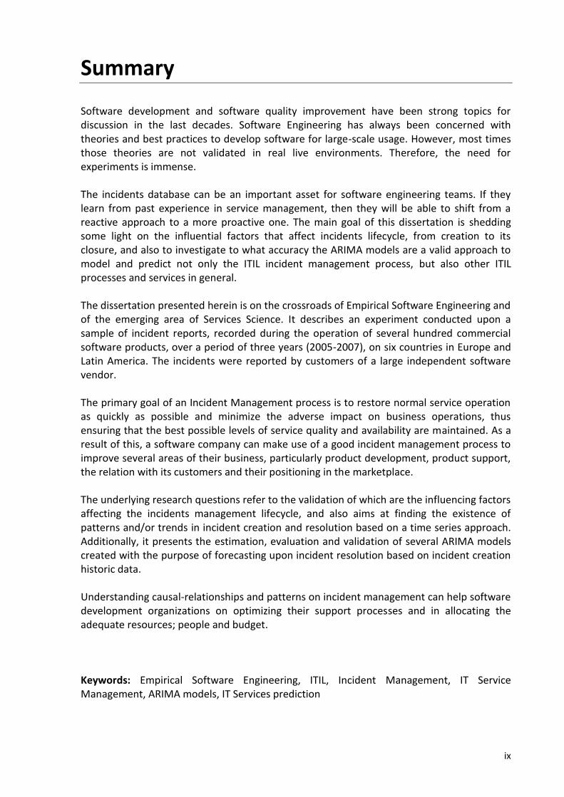
Software development and software quality improvement have been strong topics for discussion in the last decades. Software Engineering has always been concerned with theories and best practices to develop software for large-scale usage. However, most times those theories are not validated in real live environments. Therefore, the need for experiments is immense. The incidents database can be an important asset for software engineering teams. If they learn from past experience in service management, then they will be able to shift from a reactive approach to a more proactive one. The main goal of this dissertation is shedding some light on the influential factors that affect incidents lifecycle, from creation to its closure, and also to investigate to what accuracy the ARIMA models are a valid approach to model and predict not only the ITIL incident management process, but also other ITIL processes and services in general. The dissertation presented herein is on the crossroads of Empirical Software Engineering and of the emerging area of Services Science. It describes an experiment conducted upon a sample of incident reports, recorded during the operation of several hundred commercial software products, over a period of three years (2005-2007), on six countries in Europe and Latin America. The incidents were reported by customers of a large independent software vendor. The primary goal of an Incident Management process is to restore normal service operation as quickly as possible and minimize the adverse impact on business operations, thus ensuring that the best possible levels of service quality and availability are maintained. As a result of this, a software company can make use of a good incident management process to improve several areas of their business, particularly product development, product support, the relation with its customers and their positioning in the marketplace. The underlying research questions refer to the validation of which are the influencing factors affecting the incidents management lifecycle, and also aims at finding the existence of patterns and/or trends in incident creation and resolution based on a time series approach. Additionally, it presents the estimation, evaluation and validation of several ARIMA models created with the purpose of forecasting upon incident resolution based on incident creation historic data. Understanding causal-relationships and patterns on incident management can help software development organizations on optimizing their support processes and in allocating the adequate resources; people and budget. Keywords: Empirical Software Engineering, ITIL, Incident Management, IT Service Management, ARIMA models, IT Services prediction

x
[ This page has been intentionally left blank ]

xi
Sumário
O desenvolvimento de software e a melhoria na qualidade do software têm sido tópicos de grande discussão nos últimos tempos. A Engenharia de Software sempre se preocupou com teorias e melhores prácticas no desenvolvimento de software para uso em larga escala. Contudo, geralmente essas teorias não são validadas em ambientes reais, sendo que a necessidade de experiências é imensa. Uma base de dados de incidentes pode ser essencial para as equipas de engenharia de software. Se for possível aprender com a experiência passada da gestão de serviços, uma abordagem mais proactiva pode tomar o lugar das abordagens tradicionais, tendencialmente reactivas. O contributo pretendido por esta dissertação é identificar factores de influência no ciclo de vida dos incidentes, desde a sua criação até ao seu termino, e ainda, investigar até que nível os modelos ARIMA são uma apróximação válida para modelar e fazer previsões não apenas no processo de gestão de incidentes, mas também em outros processos ITIL e serviços em geral. A dissertação aqui apresentada, insere-se no âmbito da Engenharia de Software Experimental e da área emergente da Ciência dos Serviços. É descrita uma experiência executada com base numa amostra de incidentes reportados durante a exploração de várias centenas de produtos de software comercial, num periodo de três anos (2005-2007), em seis paises da Europa e América Latina. Os incidentes foram reportados pelos clientes de uma empresa de software independente. O objectivo do processo de Gestão de Incidentes é restaurar o funcionamento normal de um serviço no mais curto espaço de tempo possível, minimizando o impacto adverso no negócio, garantindo que os melhores níveis de serviço e de disponibilidade são mantidos. Como resultado disto, as empresas de software podem fazer uso de uma boa gestão de incidentes para melhorar várias áreas do seu negócio, particularmente, o desenvolvimento de software, o suporte aos produtos, a relação com os seus clientes e o seu posicionamento no mercado. As questões de pesquisa subjacentes referem-se à validação de quais são os factores que afectam o ciclo de vida dos incidentes, e ainda à busca de padrões e/ou tendências na criação e resolução de incidentes recorrendo a uma aproximação baseada em séries temporais. Complementarmente, são estimados, analisados e validados vários modelos ARIMA criados com o objectivo de fazerem a previsão da resolução de incidentes com base no histórico de criação dos mesmos. Compreender relações causais e padrões na gestão de incidentes pode ajudar as empresas de software na optimização dos seus processos de suporte e na afectação dos recursos adequados; pessoas e orçamentos. Palavras-chave: Engenharia de Software Experimental, ITIL, Gestão de Incidentes, Gestão de Serviços de Tecnologias de Informação, modelos ARIMA, previsões em serviços de tecnologias de informação.

xii
[ This page has been intentionally left blank ]

xiii
Symbols and notations
ACF – Autocorrelation Function
ACM – Asset and Configuration Management
ANOVA – Analysis of Variance
AR – Auto Regressive
ARIMA – Auto Regressive Integrated Moving Average
CAM – Capacity Management
CM – Change Management
CSV – Comma Separated Values
ERR – The residual component of the series for a particular observation
IM – Incident Management
ITIL – Information Technology Infrastructure Library
ITSM – Information Technology Service Management
H0 – Null hypothesis
H1 – Alternative hypothesis
MA – Moving Average
MAPE – Mean Absolute Percent Error
MaxAPE – Maximum Absolute Percent Error
PACF – Partial Autocorrelation Function
PDCA – Plan, Do, Check, Act
PM – Problem Management
RDM – Release and Deployment Management
SAF – Seasonal Adjustment Factors
SAS – Seasonality Adjusted Series
SLA – Service Level Agreements
SLM – Service Level Management
SM – Service Management
SPSS – Statistical Package for Social Sciences
STC – Smoothed Trend Cycle
SWEBOK – Software Engineering Body of Knowledge

xiv
[ This page has been intentionally left blank ]

xv
Contents
1. Introduction ............................................................................................................. 2
1.1 Motivation ................................................................................................................ 2
1.2 Problem context ....................................................................................................... 3 1.2.1 ITIL (The Information Technology Infrastructure Library) ............................................. 6 1.2.2 Services science ............................................................................................................. 8 1.2.3 Services .......................................................................................................................... 8 1.2.4 Service management ..................................................................................................... 9 1.2.5 Incident management ................................................................................................. 10
1.3 Current research challenges ................................................................................... 11
1.4 Expected contributions ........................................................................................... 12
1.5 Methodological approach ...................................................................................... 13
1.6 Dissertation outline and typographical conventions ............................................. 16
2. Related Work ......................................................................................................... 18
2.1 Research work ........................................................................................................ 18
2.2 A taxonomy ............................................................................................................. 18 2.2.1 ITIL process coverage .................................................................................................. 18 2.2.2 Service concern coverage ............................................................................................ 19 2.2.3 Data collection ............................................................................................................. 20 2.2.4 Methodological approach ........................................................................................... 20 2.2.5 Evolution analysis ........................................................................................................ 21 2.2.6 Contributions to software development lifecycle management ................................ 21
2.3 Studied works ......................................................................................................... 23 2.3.1 Evaluation 1 - [Barash, Bartolini et al., 2007] .............................................................. 23 2.3.2 Evaluation 2 - [Sjøberg, Hannay et al., 2005] .............................................................. 25 2.3.3 Evaluation 3 - [Niessink and Vliet, 2000] ..................................................................... 26 2.3.4 Evaluation 4 - [Jansen and Brinkkemper, 2006] .......................................................... 28 2.3.5 Evaluation 5 - [Mohagheghi and Conradi, 2007]......................................................... 29 2.3.6 Evaluation 6 - [Kenmei, Antoniol et al.] ...................................................................... 31 2.3.7 Evaluation 7 - [Yuen, 1988] ......................................................................................... 32
2.4 Comparative analysis .............................................................................................. 34
3. Influential Factors on Incident Management ........................................................... 38
3.1 Introduction ............................................................................................................ 38
3.2 Research questions ................................................................................................. 38
3.3 Experiment process ................................................................................................ 40
3.4 Sample demographics ............................................................................................ 41 3.4.1 Incident reporting methods ........................................................................................ 43 3.4.2 Incident origin platform .............................................................................................. 44 3.4.3 Incidents by customers businesses area ..................................................................... 45 3.4.4 Incident metrics summary ........................................................................................... 47 3.4.5 Variables and scale types ............................................................................................ 48
3.5 Hypotheses identification and testing .................................................................... 51
3.6 Results discussion ................................................................................................... 58
4. Diachronic Aspects on Incident Management .......................................................... 62

xvi
4.1 Introduction ............................................................................................................ 62
4.2 Research questions ................................................................................................. 63
4.3 Experiment process ................................................................................................ 64
4.4 Sample demographics ............................................................................................ 66 4.4.1 Seasonal patterns ........................................................................................................ 68 4.4.2 Variables and scale types ............................................................................................ 71
4.5 Hypothesis identification and testing ..................................................................... 71 4.5.1 Seasonality analysis ..................................................................................................... 72 4.5.2 Trend analysis .............................................................................................................. 73
4.6 Modeling daily time series with ARIMA ................................................................. 76 4.6.1 Introduction................................................................................................................. 76 4.6.2 Model identification .................................................................................................... 77 4.6.3 Differencing ................................................................................................................. 77 4.6.4 Non-seasonal parameters ........................................................................................... 79 4.6.5 Seasonal parameters ................................................................................................... 79 4.6.6 Model estimation ........................................................................................................ 80 4.6.7 Model validity .............................................................................................................. 84
4.7 Modeling weekly time series with ARIMA ............................................................. 87 4.7.1 Differencing ................................................................................................................. 87 4.7.2 Non-seasonal parameters ........................................................................................... 88 4.7.3 Model estimation ........................................................................................................ 88 4.7.4 Model substantiation .................................................................................................. 89 4.7.5 Model validity .............................................................................................................. 91 4.7.6 What-If scenario .......................................................................................................... 92
4.8 Results discussion ................................................................................................... 95
5. Conclusion and Future Work ................................................................................... 98
5.1 Contributions review .............................................................................................. 98 5.1.1 Benefits for researchers ............................................................................................ 100 5.1.2 Benefits for the industry ........................................................................................... 100
5.2 Threats to the validity ........................................................................................... 102 5.2.1 Internal threats .......................................................................................................... 102 5.2.2 External threats ......................................................................................................... 102
5.3 Evolution and next steps ...................................................................................... 103
Bibliography ................................................................................................................ 105
ITIL and Service Management ...................................................................................... 109
Experimental Approaches ............................................................................................ 117

xvii
Figure Index
Figure 1. Software vendor / Customer interactions ................................................................... 4
Figure 2. Incident lifecycle .......................................................................................................... 5
Figure 3. Incidents lifecycle timing variables .............................................................................. 5
Figure 4. ITIL v3 – Service lifecycle approach (adapted from [Office_of_Government_Commerce, 2007]) ............................................................. 7
Figure 5. Service Logic (adapted from [Office_of_Government_Commerce, 2007]) ................ 9
Figure 6. This dissertation evaluation analysis ......................................................................... 22
Figure 7. This dissertation comparing to Evaluation 1 ............................................................. 24
Figure 8. This dissertation comparing to Evaluation 2 ............................................................. 26
Figure 9. This dissertation comparing to Evaluation 3 ............................................................. 27
Figure 10. This dissertation comparing to Evaluation 4 ........................................................... 29
Figure 11. This dissertation comparing to Evaluation 5 ........................................................... 30
Figure 12. This dissertation comparing to Evaluation 6 ........................................................... 32
Figure 13. This dissertation comparing to Evaluation 7 ........................................................... 33
Figure 14. Experiment workflow – High level steps ................................................................. 40
Figure 15. Experiment process – Detail steps .......................................................................... 41
Figure 16. Entities involved in the study .................................................................................. 43
Figure 17. Incident source histogram ....................................................................................... 44
Figure 18. Incident histogram by platform ............................................................................... 45
Figure 19. Incidents histogram by Business Type ..................................................................... 46
Figure 20. QQ Plots for the schedule variables ........................................................................ 51
Figure 21. Percentage of incident reports per country ............................................................ 57
Figure 22. Experiment Process ................................................................................................. 65
Figure 23. Incident frequencies by category ............................................................................ 66
Figure 24. Incident frequencies per week of the year ............................................................. 68
Figure 25. Incident frequencies per week day ......................................................................... 70
Figure 26. Autocorrelation Function (ACF) ............................................................................... 72
Figure 27. Partial Autocorrelation Function (PACF) ................................................................. 73
Figure 28. Time Series - Incidents Resolved per day ................................................................ 74
Figure 29. STC series - Incidents Resolved per day with systematic seasonal variations removed ................................................................................................................... 74
Figure 30. ERR series for the SAS .............................................................................................. 75

xviii
Figure 31. Q-Q Plot of the ERR Series ....................................................................................... 76
Figure 32. Time Series with Differencing (1) ............................................................................ 78
Figure 33. PACF for the time series after Differencing (1) ....................................................... 78
Figure 34. ACF for the regular time series ................................................................................ 79
Figure 35. PACF for the regular time series .............................................................................. 79
Figure 36. PACF for the time series after seasonal differencing (1) ......................................... 80
Figure 37. ACF for the time series after seasonal differencing (1) ........................................... 80
Figure 38. Plot of ARIMA(2,1,2)(1,1,1) model .......................................................................... 81
Figure 39. Plot of ARIMA(2,1,2)(1,0,1) model .......................................................................... 83
Figure 40. Plot of ARIMA(2,1,2)(1,0,1) model (estimation period from week 1 to 95) ........... 84
Figure 41. Plot of ARIMA(0,1,0)(0,0,0) model – A Random Walk Model ................................. 85
Figure 42. ACF after Differencing(1) ......................................................................................... 87
Figure 43. PACF after Differencing(1) ....................................................................................... 87
Figure 44. Plot of ARIMA(1,1,1) forecast to week 157 with observed values .......................... 89
Figure 45. 4-Plot adapted graph for model validation ............................................................. 90
Figure 46. Forecast values for the weekly Random-Walk model - ARIMA(0,1,0) .................... 91
Figure 47. Predicted support members for the third year (2008) ........................................... 94
Figure 48. Predicted and average support members comparison ........................................... 95
Figure 49. Service Strategy ..................................................................................................... 110
Figure 50. Service Design ........................................................................................................ 111
Figure 51. Service Transition .................................................................................................. 112
Figure 52. Service Operation .................................................................................................. 113
Figure 53. Continual Service Improvement ............................................................................ 114
Figure 54. ITIL process flow .................................................................................................... 115
Figure 55. Random walk autocorrelation correlogram .......................................................... 127
Figure 56. Weak autocorrelation correlogram ....................................................................... 128
Figure 57. Strong autocorrelation correlogram ..................................................................... 129
Figure 58. Sinusoidal model correlogram ............................................................................... 130
Figure 59. Partial autocorrelation correlogram...................................................................... 131
Figure 60. 4-Plot for residuals validation – Invalid ARIMA model .......................................... 136

xix
Table Index
Table 1. Software maintenance categories (in SWEBOK [Abran, Moore et al., 2004]) ............. 3
Table 2. Study type categorization (adapted from [Mohagheghi and Conradi, 2007]) ........... 14
Table 3. ITIL process coverage .................................................................................................. 19
Table 4. Service concern ........................................................................................................... 20
Table 5. Data collection ............................................................................................................ 20
Table 6. Evolution analysis ....................................................................................................... 21
Table 7. Contributions to software development lifecycle management ............................... 22
Table 8. Evaluation 1 ................................................................................................................ 24
Table 9. Evaluation 2 ................................................................................................................ 25
Table 10. Evaluation 3 .............................................................................................................. 27
Table 11. Evaluation 4 .............................................................................................................. 28
Table 12. Evaluation 5 .............................................................................................................. 30
Table 13. Evaluation 6 .............................................................................................................. 31
Table 14. Evaluation 7 .............................................................................................................. 33
Table 15. Summary of related work ......................................................................................... 34
Table 16. Countries with their zones and languages................................................................ 42
Table 17. Incident source ......................................................................................................... 43
Table 18. Incidents by platform ................................................................................................ 44
Table 19. Incident frequencies by Business Type ..................................................................... 45
Table 20. Metrics summary ...................................................................................................... 47
Table 21. Days to resolve incidents (average) .......................................................................... 48
Table 22. Variables used in this experiment, their scale types and description ...................... 49
Table 23. Impact variable details .............................................................................................. 49
Table 24. Priority variable details ............................................................................................. 50
Table 25. Category variable details .......................................................................................... 50
Table 26. Testing Normal distribution adherence with the Kolmogorov-Smirnov test ........... 52
Table 27. Testing the influence of the impact on incident schedules with the Kruskal-Wallis one-way analysis of variance test ............................................................................ 53
Table 28. Testing the influence of the priority on incident schedules with the Kruskal-Wallis one-way analysis of variance test ............................................................................ 54
Table 29. Testing the influence of the originating country on incident schedules with the Kruskal-Wallis one-way analysis of variance test .................................................... 55

xx
Table 30. Testing the influence of the originating zone on incident schedules with the Kruskal-Wallis one-way analysis of variance test .................................................... 55
Table 31. Testing the influence of the category on incident schedules with the Kruskal-Wallis one-way analysis of variance test ............................................................................ 56
Table 32. Results of applying the Chi-Square Test procedure to assess if the distribution of critical priority incidents is the same across countries ............................................ 57
Table 33. Critical priority incidents observed and expected across countries ......................... 58
Table 34. Top 5 Incident Categories ......................................................................................... 67
Table 35. Incident frequencies (Year 2006 and 2007) .............................................................. 68
Table 36. Days of week and incident frequencies .................................................................... 70
Table 37. Variables and Scale types ......................................................................................... 71
Table 38. Average number of days to resolve an incident ....................................................... 80
Table 39. Model Description for ARIMA(2,1,2)(1,1,1) .............................................................. 81
Table 40. Model ARIMA(2,1,2)(1,1,1) statistics ........................................................................ 82
Table 41. Model description for ARIMA(2,1,2)(1,0,1) .............................................................. 83
Table 42. Model ARIMA(2,1,2)(1,0,1) statistics ........................................................................ 83
Table 43. Model ARIMA(2,1,2)(1,0,1) statistics (estimation period from week 1 to 95) ......... 84
Table 44. Model description for ARIMA(0,1,0)(0,0,0) .............................................................. 85
Table 45. Model ARIMA(0,1,0)(0,0,0) statistics ........................................................................ 85
Table 46. Daily model comparison ........................................................................................... 86
Table 47. ARIMA(1,1,1) ............................................................................................................. 88
Table 48. Model ARIMA(1,1,1) statistics .................................................................................. 89
Table 49. ARIMA(0,1,0) ............................................................................................................. 91
Table 50. Model ARIMA(0,1,0) statistics .................................................................................. 91
Table 51. Weekly model comparison ....................................................................................... 92
Table 52. What-if scenario details ............................................................................................ 93
Table 53. What-if scenario statistics ........................................................................................ 93
Table 54. Summary of findings ............................................................................................... 101
Table 55. Hypothesis testing and errors ................................................................................. 123

1
11
Introduction
Contents
1.1 Motivation ....................................................................................................... 2
1.2 Problem context ............................................................................................... 3
1.3 Current research challenges ............................................................................ 11
1.4 Expected contributions ................................................................................... 12
1.5 Methodological approach ............................................................................... 13
1.6 Dissertation outline and typographical conventions ........................................ 16
This chapter introduces the main concepts that are present throughout this dissertation
and the motivation to Incident Management and associated experiments. It also
enumerates the main contributions of this dissertation and presents its outline, with a
brief summary of each of the remaining chapters.

1. Introduction
2
1. Introduction
“If knowledge can create problems, it is not through ignorance that we can solve them.”
Isaac Asimov (1920 - 1992)
1.1 Motivation
Organizations with in-house software development strive in finding the right number of
resources (with the right skills) and adequate budgets. A good way to optimize those figures
is avoiding expenditures on overhead activities, such as excessive customer support. This can
be achieved by identifying incident’s root causes and by using that knowledge to improve
the software evolution process.
Software development and software quality improvement have been strong topics for
discussion in the last decades [Humphrey, 1989; El-Eman, Drouin et al., 1997]. Software
Engineering has always been concerned with theories and best practices to develop software
for large-scale usage. However, most times those theories are not validated in real live
environments [Sjøberg, Hannay et al., 2005]. Several factors were identified that explain this
lack of experimental validation [Jedlitschka and Ciolkowski, 2004].
In real-live operation environments end-users/customers face software faults, lack of
functionalities and sometimes just lack of training. These incidents should be somehow
reported. According to the ITIL good practices [Cannon, 2007; Case, 2007; Iqbal, 2007; Lacy,
2007; Loyd, 2007], in an organization with a Service Management approach, this problem is
addressed by two specific processes: Incident Management [Cannon, 2007], which deals
with the restoration of the service to the end-user within the Service Level Agreements
[Case, 2007; Loyd, 2007] (if they exist), and Problem Management [Cannon, 2007] which
aims at finding the underlying cause of reported incidents.
When an organization implements these ITIL processes, it is assumed that it will address all
types of incidents (software, hardware, documentation, services, etc) raised by the end-
users/customers. This dissertation is concerned only about software-related incidents.
The incidents database can be an important asset for software engineering teams. If they
learn from past experience in service management, then they will be able to shift from a
reactive approach to a more proactive one. The latter approach is referred in the Software

1. Introduction
3
Maintenance chapter of the SWEBOK [Abran, Moore et al., 2004], as reproduced in Table 1,
although seldom brought to practice.
Table 1. Software maintenance categories (in SWEBOK [Abran, Moore et al., 2004])
Correction Enhancement
Proactive Preventive Perfective
Reactive Corrective Adaptive
This dissertation presents a statistical-based analysis of software related incidents resulting
from the operation of several hundred commercial software products, from 2005 to 2007,
on six countries in Europe and Latin America. The incidents were reported by customers of a
large independent software vendor.
The main goal of this work is shedding some light on the influential factors and patterns that
affect incidents lifecycle from creation to its closure, namely the schedule of its phases and
their diachronic aspects. Understanding this lifecycle can help software development
organizations in allocating adequate resources (people and budget), increasing the quality of
services they provide and finally improving their image in the marketplace.
1.2 Problem context
To a clear understanding of this work it is important to frame its contextual areas. This
dissertation is a study based on software incidents reported by customers of a large
software vendor. Those incidents include software bugs, errors and defects found by the
customers on their day-to-day business operations. Technical doubts about the software,
requests for information and other questions in general were also reported by the
customers. The incidents being reported to the Service Desk were recorded and managed in
a Service Management solution which maps and implements the ITIL Incident Management
process [Cannon, 2007]. Figure 1 is a representation of the involved parts which are the
focus of this study. Following the main goal, our task is to analyze quantitative data about
the incidents and the interactions (using schedule variables like time to respond, time to
resolve, etc) between the Service Desk (technical support staff) [Cannon, 2007] and the

1. Introduction
4
customers (as identified in red). A sub-set of the incidents database was exported, a
quantitative analysis took place and the results obtained are presented in the next chapters.
Figure 1. Software vendor / Customer interactions
As relevant as the entities involved, also is the process by which mean the incidents are
being managed. This process comprises a set of activities performed sequentially in order to
achieve a result: the resolution of the incident. In the activities performed by the support
staff, we include the logging, categorization, prioritization, investigation and resolution of
the incidents.
Crucial to this study, is the understanding of the incident status. Incidents status change
during their lifecycle, as represented in represented in Figure 2. The process is a set activities
performed by the support staff and its goal is to guide those to act with good practices to
solve incidents. The incident status is the incident state within each process activity. The
incident status is extremely important to this work because it is the base for all the
computation and measuring of times used in this dissertation. How and why an incident
move from one state to another is guided by the incident management process.
Sales
Dpt.
Service Desk
Software Vendor Customer(s)
Software being sold
Other
Dpts. Software being used
in Production
Incidents being reported
Incidents being managed

1. Introduction
5
Figure 2. Incident lifecycle
Figure 3 represents the incidents lifecycle, since the moment they are created by a customer
or the support staff until their closure. During this period an incident can assume several
states as mentioned in Figure 2. The variables TimeToRespond, TimeToResolve and
TimeToConfirm detailed and studied in chapter III of this work were computed based on this
schema.
Figure 3. Incidents lifecycle timing variables
An incident typically starts when a user reports it either by telephone, email or web. In the
first phase it assumes the state of New. This state is when the incident is categorized, and a
priority and impact is given to it. This state is maintained until the person assigned to work
End-user reports
the incident
The support staff
starts working in the
incident
End-user
confirmation that
the incident is fixed
TimeToRespond TimeToResolve
TimeToConfirm
The support staff
provides a potential
resolution

1. Introduction
6
on the incident really starts to investigate a possible solution for it. Once the technical
analyst assigned begin to search for solutions, the incident state changes to InProgress. This
period is computed by the TimeToRespond variable. The incident will continue InProgress
until a potential solution is found. In certain situations it may be helpful to put the incident
in Pending state, for instance, when a support analyst requests information (log files,
software versions, etc) from the user. In Pending state an incident clock is stopped, and the
variable TimeToResolve is not affected. This variable is only affected when the incident
changes again to InProgress and finally is said to be Resolved, meaning that a potential
solution was found. This state is maintained if the solution needs further investigation and is
not immediately given to the user. The incident state changes to EndUserVerifySolution
when the solution was really provided to the user. In this case the user should check if the
solution was really valid for the incident and should give feedback to the support about it. If
the potential solution solved the incident, the incident is closed and its status updated to
Closed in order to reflect the positive effect of the solution. This time span between a
potential solution is given and a positive feedback from the user is received is the basis for
the variable TimeToConfirm. If the potential solution did not solve the incident then the
support analyst continues to search for another solution and the incident state should be set
back to InProgress and the normal flow to resolve the incident continues.
The Incident Management process is just one of the components of a larger reality faced by
IT organizations, which is usually called IT Service Management (ITSM). To help framing the
research presented in this dissertation in the overall context of ITSM, we briefly describe in
the next section the most widely used terms and concepts. In these processes, ITIL takes an
important part in the behavior of a software organization like the one that is now being
studied. Therefore, we will have a brief overview.
1.2.1 ITIL (The Information Technology Infrastructure Library)
The Information Technology Infrastructure Library (ITIL) was started in late 80´s by the UK
Office of Government Commerce’s (OGC) and is a set of concepts and techniques (good
practices) for managing information technology, infrastructure, development, and
operations.

1. Introduction
7
ITIL was first published in a series of books in 1989, each of which cover an IT management
topic [Office_of_Government_Commerce, 2007]. ITIL gives a detailed description of a
number of important IT practices with comprehensive checklists, tasks and procedures that
can be tailored to any IT organization.
Since then, ITIL has evolved and it is now on its third version. The ITIL Core (version 3)
consists of five publications [Cannon, 2007; Case, 2007; Iqbal, 2007; Lacy, 2007; Loyd, 2007],
whose structure is schematically represented in Figure 4.
Figure 4. ITIL v3 – Service lifecycle approach (adapted from [Office_of_Government_Commerce, 2007])
Each of those publications provides the required guidance for an integrated approach, as
required by the ISO/IEC 20000-1 [ISO/IEC, 2005] standard specification and ISO/IEC 20000-2
[ISO/IEC, 2005] code of practice. ITIL has now a lifecycle approach to all of its processes. This
means that each process can have inputs and outputs from and to another process. An
organization can use the lessons learned (outputs) in Incident Management as best practices
(inputs) for another process, as for instance Release and Deployment Management [Lacy,
2007]. The synergies of this workflow are immense as ITIL v3 highlights the concept of a
“Service” and “Service Management” as a continuous mechanism to improve the processes

1. Introduction
8
and the performance of an IT organization. An overview on the ITIL publications and their
processes can be found on appendix A.
Following this, it is important to briefly explain the concept of a Service, Service
Management and the Incident Management process and put this in a context of what is the
Services Science [Research, 2005].
1.2.2 Services science
Services Science is an interdisciplinary approach to the study, design, and implementation of
services systems – complex systems in which specific arrangements of people and
technologies take actions that provide value for others. In summary is the application of
science, management, and engineering disciplines to tasks that one organization beneficially
performs for and with another.
There is a clear demand [Research, 2005] for the academia, industry, and governments to
focus on becoming more systematic about innovation in the service sector, which is the
largest sector of the economy in most industrialized nations, and is quickly becoming the
largest sector in developing nations as well.
The key to Services Science it is the multidisciplinary approach taken, focusing not merely on
one aspect of a service but rather considering it as a system of interacting parts that include
people, technology, and business. These are very similar aspects that ITIL addresses in its
good practices.
As such, Services Science draws on ideas from a number of existing disciplines – including
Computer Science, Cognitive Science, Economics, Human Resources Management,
Marketing, Operations Research, and others – and aims to integrate them into a coherent
whole.
1.2.3 Services
Services are a means of delivering value to customers by facilitating the outcomes that the
customers want to achieve without the ownership of specific costs and risks. Outcomes are

1. Introduction
9
possible from the performance of tasks and are limited by the presence of certain
constraints. Broadly speaking, services facilitate outcomes by enhancing the performance
and by reducing the grip of constraints. The result is an increase in the possibility of desired
outcomes. While some services enhance the performance of tasks, others have a more
direct impact. They perform the task itself.
Figure 5. Service Logic (adapted from [Office_of_Government_Commerce, 2007])
From the customer’s perspective, value consists of two primary elements: utility or fitness
for purpose and warranty or fitness for use.
Utility is perceived by the customer from the attributes of the service that have a positive
effect on the performance of tasks associated with desired outcomes.
Warranty is derived from the positive effect being available when needed, in sufficient
capacity or magnitude, and dependably in terms of continuity and security.
Utility is what the customer gets, and warranty is how it is delivered. In the context of this
work, Utility is the technical support service provided by the software vendor. Warranty is
the capacity to resolve incidents as needed by the customers. How the technical support
department is structured in terms of technology used, staff allocation and processes with
the aim of providing the service is driven by those two aspects.
1.2.4 Service management

1. Introduction
10
Service management [Office_of_Government_Commerce, 2007] is a set of specialized
organizational capabilities for providing value to customers in the form of services. The
capabilities take the form of functions and processes for managing services over a lifecycle,
with specializations in strategy, design, transition, operation, and continual improvement.
The capabilities represent a service organization’s capacity, competency, and confidence for
action. The act of transforming resources into valuable services is at the core of service
management. Without these capabilities, a service organization is merely a bundle of
resources that by itself has relatively low intrinsic value for customers.
1.2.5 Incident management
In ITIL terminology, an ‘incident’ is defined as:
“An unplanned interruption to an IT service or a reduction in the quality of an IT
service…”[Cannon, 2007].
Incident Management is the process for dealing with all incidents. This can include failures,
queries reported by the users (usually via a telephone call or email to the Service Desk), by
technical staff, or automatically detected and reported by event monitoring tools.
The primary goal of the Incident Management process is: “…to restore normal service
operation as quickly as possible and minimize the adverse impact on business operations,
thus ensuring that the best possible levels of service quality and availability are maintained.”
[Cannon, 2007].
In this context, the software vendor technical support staff wants to minimize the adverse
impact in their customers businesses resulting from software bugs/errors/defects.
The benefits of Incident Management include the ability to:
detect and resolve incidents, which results in lower downtime to the business, which
in turn means higher availability of the service.
align IT activity to real-time business priorities. In fact, Incident Management includes
the capability to identify business priorities and dynamically allocate resources
required.

1. Introduction
11
identify potential improvements to services. This is attained by understanding what
constitutes an incident and also from being in contact with the activities of business
operational staff.
identify additional service or training requirements found in IT or the business.
Incident Management is highly visible to the business, and it is therefore easier to
demonstrate its value than most areas in Service Operation. For this reason, Incident
Management is often one of the first processes to be implemented in Service Management
projects [Office_of_Government_Commerce, 2007]. The added benefit of doing this is that
Incident Management can be used to highlight other areas that need attention – thereby
providing a justification for expenditure on implementing other processes. As a result, a
software company can make use of a good incident management process to improve several
areas of their business, particularly product development, the relation with its customers
and their positioning in the marketplace.
1.3 Current research challenges
The study of an Incident Management process (which includes the study of the people and
the technology involved in the process) or in our case, the study of an incident management
database has always challenges.
The initial (and the major) challenge is to get access to the incident management database.
Companies tend to avoid sharing this sensitive information due to data protection policies.
Reports on incident management are scarce in the literature. The reason for this resides in
the difficulty to have access to an incident management database, due to security policies,
technical limitations or just because companies do not want to expose sensitive data about
their software, their processes and their customers.
In this work, one of the biggest decisions was the choice of which countries to include in the
study. There were incidents reported in more than eighty countries and due to the collection
effort, which involved performing several data capture and transformation procedures, we
could only afford gathering a subset of this population. We decided to select a sample

1. Introduction
12
corresponding to incidents originated in six countries. We consider that with this sample we
can reflect not only the behavior of some European customers but also it represents
different cultural and geographic (Latin America) zones of two of the spoken languages in
two of the European countries chosen.
The data exportation was also a sensitive task due to the lack of normalization and
coherence in some information stored in the incident management database.
The related work about incident management and/or experiments like this focusing on
software defects/errors was scarce, and in fact, we did not find any similar experiment based
on commercial software products. We tried to classify selected studies not only by its type or
work, but also according with their level of ITIL adoption of good practices. Interpreting the
findings without any background data about the software development process turned out
to be a challenging task, and eventually, we could not be as rigorous as we would like.
1.4 Expected contributions
The contributions we want to achieve with this work are directly linked with the research
questions, but in fact, the initial contribution is the study on itself. Together with the
answers to those questions, we also attempt to draw here an experiment design to allow
replication of our study.
We expect to bring some light regarding existing assumptions or myths in the software
business area. Improving the software development process and mainly the software
support process requires attention to at least to topics: understanding the cause-effect
relationships on software incidents and careful investigation of any existing patterns in their
lifecycle. To contribute to this, we first need to understand the incident management
process and we must find answers to the following research objectives (RO):
RO1: Which factors influence incident’s lifecycle?
RO2: Are there patterns in incident’s occurrence?
RO3: Can prediction be a valid approach for managing incidents?
1. Introduction
13
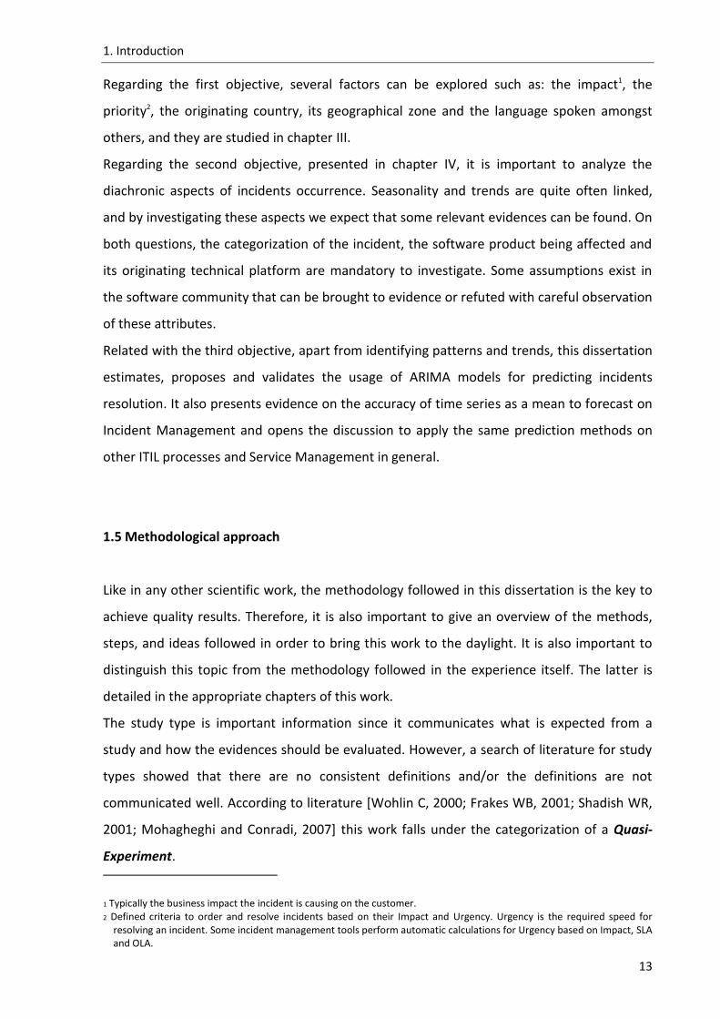
Regarding the first objective, several factors can be explored such as: the impact1, the
priority2, the originating country, its geographical zone and the language spoken amongst
others, and they are studied in chapter III.
Regarding the second objective, presented in chapter IV, it is important to analyze the
diachronic aspects of incidents occurrence. Seasonality and trends are quite often linked,
and by investigating these aspects we expect that some relevant evidences can be found. On
both questions, the categorization of the incident, the software product being affected and
its originating technical platform are mandatory to investigate. Some assumptions exist in
the software community that can be brought to evidence or refuted with careful observation
of these attributes.
Related with the third objective, apart from identifying patterns and trends, this dissertation
estimates, proposes and validates the usage of ARIMA models for predicting incidents
resolution. It also presents evidence on the accuracy of time series as a mean to forecast on
Incident Management and opens the discussion to apply the same prediction methods on
other ITIL processes and Service Management in general.
1.5 Methodological approach
Like in any other scientific work, the methodology followed in this dissertation is the key to
achieve quality results. Therefore, it is also important to give an overview of the methods,
steps, and ideas followed in order to bring this work to the daylight. It is also important to
distinguish this topic from the methodology followed in the experience itself. The latter is
detailed in the appropriate chapters of this work.
The study type is important information since it communicates what is expected from a
study and how the evidences should be evaluated. However, a search of literature for study
types showed that there are no consistent definitions and/or the definitions are not
communicated well. According to literature [Wohlin C, 2000; Frakes WB, 2001; Shadish WR,
2001; Mohagheghi and Conradi, 2007] this work falls under the categorization of a Quasi-
Experiment.
1 Typically the business impact the incident is causing on the customer. 2 Defined criteria to order and resolve incidents based on their Impact and Urgency. Urgency is the required speed for
resolving an incident. Some incident management tools perform automatic calculations for Urgency based on Impact, SLA and OLA.

1. Introduction
14
The main reasons for this categorization are due to lack of randomization in the subjects.
The incidents were not collected randomly; we decided to choose incidents from specific
countries and no treatments were applied to variables, other than the ones that already
exist currently in the database. We have used the scientific method to formulate hypothesis
and tested those against our incidents sample. Detailed study type categorizations can be
found in Table 2 and notions about scientific methods are presented in appendix B.
Table 2. Study type categorization (adapted from [Mohagheghi and Conradi, 2007])
Study Type Definition as given in [Zannier C, 2006] Other definitions
Controlled experiment
Random assignment of treatment to subjects, large sample size (>10), well formulated hypotheses and independent variable selected. Random sampling.
Controlled study [Zelkowitz MV, 1998].
Experimental study where particularly allocation of subjects to treatments are under the control of the investigator[Kitchenham, 2004].
Experiment with control and treatment groups and random assignment of subjects to the groups, and single subject design with observations of a single subject. The randomization applies on the allocation of the objects, subjects and in which order the tests are performed [Wohlin C, 2000].
Experiments explore the effects of things that can be manipulated. In randomized experiments, treatments are assigned to experimental units by chance [Shadish WR, 2001].
Our note: Randomization is used to assure a valid sample that is a representative subset of the study population; either in an experiment or other types of study. However, defining the study population and a sampling approach that assure representativeness is not an easy task, as discussed by [Conradi R, 2005].
Quasi-experiment
One or more points in Controlled Experiment are missing.
In a quasi-experiment, there is a lack of randomization of either subjects or objects [Wohlin C, 2000]
Quasi-experiment where strict experimental control and randomization of treatment conditions are not possible. This is typical in industrial settings [Frakes WB, 2001].
Quasi-experiments lack random assignment. The researcher has to enumerate alternative explanations one by one, decide which are plausible, and then use logic, design, and measurement to assess whether each one is operating in a way that might explain any observed effect [Shadish WR, 2001]
Case study All of the following exist: research questions, propositions (hypotheses), units of analysis, logic linking the data to the propositions and criteria for interpreting the findings [Yin, 2003].
A case study is an empirical inquiry that investigates a contemporary phenomenon within its real-life context, especially when the boundaries between phenomenon and context are not clearly evident. A sister-project case study refers to comparing two almost similar projects in the same company, one with and the other without the treatment [Yin, 2003].
Observational studies are either case studies or field studies. The difference is that multiple projects are monitored in a field study, may be with less depth, while case studies focus on a single project [Zelkowitz MV, 1998].
Case studies fall under observational studies with uncontrolled exposure to treatments, and may involve a control group or not, or being done at one time or historical [Kitchenham, 2004]
Exploratory case study
One or more points in case study are missing.
The propositions are not stated but other components should be present [Yin, 2003]
Experience report
Retrospective, no propositions (generally), does not necessarily answer why and how, often includes lessons learned.
Postmortem Analysis (PMA) for situations such as completion of large projects, learning from success, or recovering from failure [Birk A, 2002]
Meta-analysis
Study incorporates results from several previous similar studies in the analysis.
Historical studies examine completed projects or previously published studies [Zelkowitz MV, 1998]

1. Introduction
15
Study Type Definition as given in [Zannier C, 2006] Other definitions
Example application
Authors describe an application and provide an example to assist the description. An example is not a type of validation or evaluation.
Our note: If an example is used to evaluate a technique already developed or apply a technique in a new setting, it is not classified under example application.
Survey Structured or unstructured questions given to participants.
The primary means of gathering qualitative or quantitative data in surveys are interviews or questionnaires [Wohlin C, 2000]
Structured interviews (qualitative surveys) with an interview guide, to investigate rather open and qualitative research questions with some generalization potential. Quantitative surveys with a questionnaire, containing mostly closed questions. Typical ways to fill in a questionnaire are by paper copy via post or possibly fax, by phone or site interviews, and recently by email or web [Conradi R, 2005]
Discussion Provided some qualitative, textual, opinion- oriented evaluation.
Expert opinion [Kitchenham, 2004].

1. Introduction
16
1.6 Dissertation outline and typographical conventions
This dissertation is organized in a set of chapters which are briefly summarized as follows:
Chapter 2. It presents an overview of the related work, the taxonomy used to categorize it, a
brief comparison to our work and a summary of the gaps this dissertation can fill
within the research area.
Chapter 3. This chapter describes and presents the first results attained with our
experiment, namely the influence factors in the incident’s lifecycle.
Chapter 4. It details the seasonality and trend analysis performed based on a time series
approach. Also discusses whether ARIMA models are a valid technique to
perform forecasts on the incident management process.
Chapter 5. It concludes and summarizes the achievements of this dissertation. As an
evolutionary step it also provides some guidance and opens the discussion for
future work in this area.
To clearly distinguish semantically different elements and provide a visual hint to the reader,
this dissertation uses the following typographical conventions:
Italic script highlights important keywords, variables, scientific terms, formulas,
methods and tools carrying special meaning in the technical or scientific literature;
Bold face denotes topic headers, table headers, research questions, and items in
enumerations.

17
22
Related Work
Contents
2.1 Research work ................................................................................................ 18
2.2 A taxonomy .................................................................................................... 18
2.3 Studied works................................................................................................. 23
2.4 Comparative analysis ...................................................................................... 34
This chapter presents and discusses the related work. It also describes a taxonomy defined
to categorize and compare this work and identify its limitations.

2. Related Work
18
2. Related Work
“There are in fact two things, science and opinion; the former begets knowledge, the latter ignorance.”
Hippocrates (460 BC - 377 BC)
2.1 Research work
To support our research, we have tried to find related work in the area of empirical software
engineering within the ITIL scope. Having searched several digital libraries such as the ones
of ACM, IEEE, Springer or Elsevier, we were able to find only a few papers about incident
management. Even scarcer were those referencing real live experiences about the statistical
analysis of software incidents and how that can help improving the software engineering
process. This section presents a categorized overview of the published works that we found
to be closer related to certain aspects of our work presented hereafter.
2.2 A taxonomy
Taxonomy is the practice and science of classification. Taxonomies, or taxonomic schemes,
are composed of taxonomic units, criterion or categories that are arranged frequently in a
hierarchical structure. Each of those categories must be described in such a way that for a
given subject it will be straightforward to identify if it belongs, or not, to the category.
A taxonomy for classifying related work will allow us to use a more objective set of
comparison criteria, thus facilitating the outline of the current state of the art in this area.
Our proposed taxonomy is composed of six classification criterion which will be described in
the following sections.
2.2.1 ITIL process coverage
The ITIL process coverage criterion highlights the ITIL processes involved on each work.
Those processes are the ones referenced in the ITIL publications (e.g.: Incident Management,
Service Level Management, etc) [Office_of_Government_Commerce, 2007].

2. Related Work
19
Table 3. ITIL process coverage
ITIL Publication ITIL Process
Service Strategy Financial Management, Demand Management, Service Portfolio Management
Service Design
Service Catalog Management, Service Level Management, Capacity Management,
Availability Management, IT service Continuity Management, Information security
Management, Supplier Management
Service Transition Change Management, Asset and Configuration Management, Release and Deployment
Management, Service validation and Testing, Evaluation, Knowledge Management
Service Operation Incident Management, Problem Management, Request Fulfillment, Event
Management, Access Management
Continual Service Improvement Service Reporting, Service Measurement, Service Level Management
According to the above nominal scale we frame this dissertation in the Service Operation
part of ITIL, specifically in the Incident Management (IM) and Problem Management (PM).
This double categorization is due to the fact that incidents are resolved by the Service Desk
using the Incident Management process, and also by second and third line support members
which normally focus more in Problem Management. This study can easily apply to both
processes.
2.2.2 Service concern coverage
The Service concern criterion assesses the three essential aspects of ITIL and services:
technology, people and processes.
The technology aspect refers to all the technical components (typically hardware and
software) involved when dealing with IT services. The people aspect addresses the way
persons are organized and the way they should behave when involved in a certain process.
Finally, the process aspect relates to how activities are linked together in order to deliver
value to a specific business area.
The categories that have been identified for classifying this criterion are the following:

2. Related Work
20
Table 4. Service concern
Absent The topic is not addressed or addressed in a fuzzy way
Partly The topic is addressed insufficiently, not explicit or lacking context
Largely The topic is addressed explicitly and context is provided, although not exhaustively
Fully The topic is addressed exhaustively, sustained with evidence and adequate rationale
According to this ordinal scale, we classify this dissertation with the following grades:
People – Partly, Process – Largely and Technology - Largely.
2.2.3 Data collection
The data collection criteria analyzes the adequacy that the data was treated (or not) in each
article. It measures how detailed and accurate the process of data collection, manipulation,
analysis, and interpretation of the results is performed in a specific work. A detailed
documentation of this process is extremely important for someone trying to replicate an
experiment or study. According to these requisites we propose the following categories:
Table 5. Data collection
Absent No data collection was used or the documentation about the process is absent
Partly Data collection was performed and the process was briefly described
Largely The data collection process is largely documented but not exhaustively
Fully The data collection process is detailed allowing complete experiment replication
According to this ordinal scale, we classify this dissertation with the following grade: Data
Collection – Fully.
2.2.4 Methodological approach
The methodological approach categorizes how deep each work went according to study
types mentioned in chapter I. The type of methodology used in each article is important to

2. Related Work
21
distinguish among the different approaches followed by the authors. This criterion includes
the different study types identified in Table 2 (e.g.: experiment, quasi-experiment, case
study, etc). [Mohagheghi and Conradi, 2007].
According to this nominal scale we classify this dissertation as a Quasi-experiment study
type.
2.2.5 Evolution analysis
In order to really understand the software development and maintenance processes, we
must analyze the incidents and the support process with a chronological perspective. There
are several advantages of performing evolution analysis such as understanding of past,
prediction of the future growth, perform comparisons or document trends, among other
aspects. While performing an evolution analysis, we must consider that incidents have an
associated lifecycle, with a set of phases that range from creation, to resolution and closure.
We also know that software is a very dynamic entity, and software updates, new releases or
product withdrawn are time driven.
Table 6. Evolution analysis
Absent The topic is not addressed or addressed in a fuzzy way
Partly A chronological approach is addressed but insufficiently, not explicit or lacking context
Largely A chronological approach is addressed explicitly and context is provided, although not exhaustively
Fully A chronological approach is addressed exhaustively, sustained with evidence and adequate rationale
According to these criteria, we classify this dissertation with the following grades: Evolution
Analysis – Fully.
2.2.6 Contributions to software development lifecycle management
If we want to highlight the most representative works done in software engineering we must
have a categorization for the contributions given by each of them. For classifying the
different contribution levels we purpose the following criteria:

2. Related Work
22
Table 7. Contributions to software development lifecycle management
Absent No contributions to software development process are identified
Partly Potential contributions are present but are addressed implicitly or in a fuzzy way
Largely Potential contributions are addressed explicit, context is provided, although not exhaustively
Fully Potential contributions are addressed exhaustively and sustained with evidence
According to this ordinal scale, we classify this dissertation with the following grade:
Contributions to Software Development Lifecycle Management – Fully.
Figure 6. This dissertation evaluation analysis

2. Related Work
23
2.3 Studied works
To understand what is the current state of the art we collected several documents and
selected seven of them, the ones that we found to be the most comprehensive. It is
important to point out, that our objective in reviewing these published works was not to
attempt to draw conclusions about the relative merits of the measured aspects but instead
assessing the evaluation methodology using the previous defined taxonomy. Besides that
categorization, we provide, for each work, its main goal (as we perceived it) and a
commented abstract.
2.3.1 Evaluation 1 - [Barash, Bartolini et al., 2007]
Measuring and Improving the Performance of an IT Support Organization in Managing Service
Incidents
Goal - Managing service incidents and improving an IT support organization
Comments - This work has a clear link with ITIL. The main topics addressed are Incident
Management (IM) and Problem Management (PM) and the improvement that an
organization can achieve in their support activities by analyzing incident metrics. With this in
mind, the authors suggest ways on how to improve staff allocation, shift rotation, working
hours and methods for the escalation of incidents.
We could not find, in this work, a clear link between Incident Management or Problem
Management processes with the software development process. We also could not find a
direct relationship to any other ITIL processes beyond the two referred ones. Nevertheless,
we should not forget that if we improve the performance of the IT support organization, we
are indirectly improving the performance of all other areas.
Relation with our work – This work is related with our own since it also addresses the
management of incidents (herein we only address software incidents), and it tries to
improve an IT Support Organization. According to our taxonomy we classify this work as
follow in Table 8.

2. Related Work
24
Table 8. Evaluation 1
ITIL Process
Coverage
Methodological
Approach
Service Concern Data
Collection
Evolution
Analysis
Contributions to
Software Development
Lifecycle Management Technology People Processes
IM , PM Experience
Report
Figure 7. This dissertation comparing to Evaluation 1
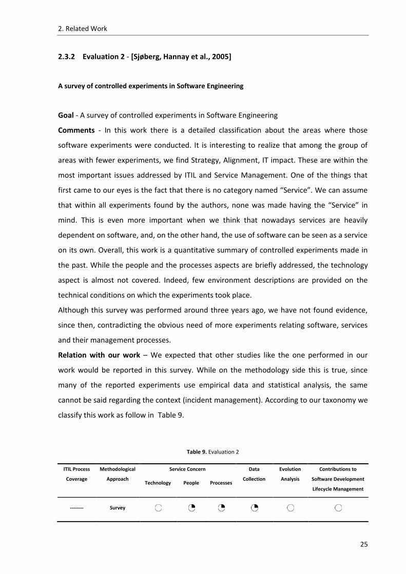
2. Related Work
25
2.3.2 Evaluation 2 - [Sjøberg, Hannay et al., 2005]
A survey of controlled experiments in Software Engineering
Goal - A survey of controlled experiments in Software Engineering
Comments - In this work there is a detailed classification about the areas where those
software experiments were conducted. It is interesting to realize that among the group of
areas with fewer experiments, we find Strategy, Alignment, IT impact. These are within the
most important issues addressed by ITIL and Service Management. One of the things that
first came to our eyes is the fact that there is no category named “Service”. We can assume
that within all experiments found by the authors, none was made having the “Service” in
mind. This is even more important when we think that nowadays services are heavily
dependent on software, and, on the other hand, the use of software can be seen as a service
on its own. Overall, this work is a quantitative summary of controlled experiments made in
the past. While the people and the processes aspects are briefly addressed, the technology
aspect is almost not covered. Indeed, few environment descriptions are provided on the
technical conditions on which the experiments took place.
Although this survey was performed around three years ago, we have not found evidence,
since then, contradicting the obvious need of more experiments relating software, services
and their management processes.
Relation with our work – We expected that other studies like the one performed in our
work would be reported in this survey. While on the methodology side this is true, since
many of the reported experiments use empirical data and statistical analysis, the same
cannot be said regarding the context (incident management). According to our taxonomy we
classify this work as follow in Table 9.
Table 9. Evaluation 2
ITIL Process
Coverage
Methodological
Approach
Service Concern Data
Collection
Evolution
Analysis
Contributions to
Software Development
Lifecycle Management Technology People Processes
-------- Survey

2. Related Work
26
Figure 8. This dissertation comparing to Evaluation 2
2.3.3 Evaluation 3 - [Niessink and Vliet, 2000]
Software maintenance from a service perspective
Goal - Software maintenance and software development from a service perspective
Comments – The authors clearly identify differences between services and products and
how these differences affect the way end-users or customers assess their quality. One of the
more relevant aspects of this work is the focus put on the need for defining Service Level
Agreements (SLA), Service Catalogs and the importance of good Incident and Problem
Management processes in an organization. The three ITIL aspects and the positive impact
they can have in organizations that implement them are highlighted and understood, but not
exhaustively explained. This would be addressed by detailing and giving examples on the

2. Related Work
27
implementation of the above aspects. In brief, the important topics are there, but not
enough detail is provided. This work has clearly a qualitative approach, and therefore no
data collection or statistical analysis is in place.
Relation with our work – The relation lies on the ITIL focus. This is not an empirical study,
but it covers several important aspects of Service Management like Incident Management
(IM), Problem Management (PM) and Service Level Management (SLM). According to our
taxonomy we classify this work as follow in Table 10.
Table 10. Evaluation 3
ITIL Process
Coverage
Methodological
Approach
Service Concern Data
Collection
Evolution
Analysis
Contributions to
Software Development
Lifecycle Management Technology People Processes
IM, PM, SLM Discussion
Figure 9. This dissertation comparing to Evaluation 3

2. Related Work
28
2.3.4 Evaluation 4 - [Jansen and Brinkkemper, 2006]
Evaluating the Release, Delivery, and Deployment Processes of Eight Large Product Software Vendors applying the Customer Configuration Update Model
Goal – Study of the release, delivery and deployment of software
Comments – This is a very interesting paper about the software update process and how it
can help software vendors and end-users/customers in the software deployment process.
The approach taken plays a vital role mainly in the realm of these ITIL processes: Asset and
Configuration Management (ACM), Release and Deployment Management (RDM). This work
is about one of the latest phases in the software development cycle – the deployment phase
– precisely the one when most incidents are usually reported. This is due to the fact that IT
systems and platforms are becoming increasingly more heterogeneous and complex and also
because quality management systems (in general) and SLA verification (in particular) imply
the recording of incidents originated by the operation.
Relation with our work – This work focuses on the technology used to improve the software
deployment process, but does not cover any empirical study or data analysis. It is related to
our work because it touches other key processes in ITIL. According to our taxonomy we
classify this work as follow in Table 11.
Table 11. Evaluation 4
ITIL Process
Coverage
Methodological
Approach
Service Concern Data
Collection
Evolution
Analysis
Contributions to
Software Development
Lifecycle Management Technology People Processes
ACM, RDM Meta Analysis

2. Related Work
29
Figure 10. This dissertation comparing to Evaluation 4
2.3.5 Evaluation 5 - [Mohagheghi and Conradi, 2007]
Quality, productivity and economic benefits of software reuse: a review of industrial studies
Goal – Quality, productivity and economic benefits of software reuse
Comments – This work is about software reuse and its benefits. Based on previous studies,
the authors state that component reuse is related with software with fewer defects. The
latter are identified by means of failures in operation and are the origin of reported
incidents. The end-user perspective is not covered in this paper, and this is vital for a Service
Management approach. Some references are made to software changes, software
deployment and even infrastructure resources required for software execution. These are
somehow disconnected implicit references to ITIL Change Management, Release and

2. Related Work
30
Deployment Management and Capacity Management processes. Although not explicitly, this
work shows how ITIL good practices can cause a tangible and positive impact in the software
development process. This impact, therefore, requires further analysis.
Relation with our work – Shares our objective, of achieving a tangible and positive impact
on the software development process by adopting ITIL-like best practices. According to our
taxonomy we classify this work as follow in Table 12.
Table 12. Evaluation 5
ITIL Process
Coverage
Methodological
Approach
Service Concern Data
Collection
Evolution
Analysis
Contributions to
Software Development
Lifecycle Management Technology People Processes
CM, RDM,
CAM
Case Study
Figure 11. This dissertation comparing to Evaluation 5

2. Related Work
31
2.3.6 Evaluation 6 - [Kenmei, Antoniol et al.]
Trend Analysis and Issue Prediction in Large-Scale Open Source Systems
Goal – Capability of time series to model change requests on open source software
Comments – This work is about using time series to analyze trends and forecast requests on
three open source software applications; Mozilla, Eclipse and JBoss. A change request is a
“wish” and not a fact occurring at the present in a particular customer environment, as the
incidents are. Therefore, a request does not represent any factual information about
software apart any individual and yet very subjective qualitative analysis taken from those
requests. The authors have used the ARIMA models to predict change requests evolution.
Unfortunately, the data collection process, the evolution analysis as well as the contributions
to software development are not detailed enough to justify a higher grade in this criterion.
We are well aware that their work was presented in a condensed format, thus explaining
why the article lacks details in these areas.
Relation with our work – It shares similar goals with our work. It uses a sample of recorded
change requests during a certain period of time and tries to get some evidences about user
change requests, the software development process and software maturity. According to
our taxonomy we classify this work as follow in Table 13.
Table 13. Evaluation 6
ITIL Process
Coverage
Methodological
Approach
Service Concern Data
Collection
Evolution
Analysis
Contributions to
Software Development
Lifecycle Management Technology Processes People
----------- Quasi
Experiment

2. Related Work
32
Figure 12. This dissertation comparing to Evaluation 6
2.3.7 Evaluation 7 - [Yuen, 1988]
On analyzing maintenance process data at the global and detailed levels: A Case Study
Goal – Pattern analysis during the maintenance of a large operating system
Comments – The author has used time series modeling to do spectral analysis on a database
of ‘notices’ (the way he called the incidents; no notion of ITIL or Service Management was
present at that time). Several reports and data analysis are presented such as, plot
inspection, non parametric tests and finally time series models in order to get information
about frequencies, distribution behavior and trends. Although the main quantitative topics
are present, they are insufficiently covered in the article, leaving no space for further
comments.

2. Related Work
33
Relation with our work – It has some common methods with our work: like statistical
analysis, time series modeling and analysis of trends and forecasting, but it lacks ITIL or
Service context and also misses an important part of the scientific method: research
questions and the correspondent hypothesis. According to our taxonomy we classify this
work as follow in Table 14.
Table 14. Evaluation 7
ITIL Process
Coverage
Methodological
Approach
Service Concern Data
Collection
Evolution
Analysis
Contributions to
Software Development
Lifecycle Management Technology Processes People
------------ Quasi
Experiment
Figure 13. This dissertation comparing to Evaluation 7

2. Related Work
34
2.4 Comparative analysis
It is widely accepted that we lack experimentation in Software Engineering in general. This
phenomenon is even more acute on what concerns experimentation related with incidents
and services. Even if the related work is scarce, we should look at it collectively to try to
draw some picture of the current state-of-the-art. For that purpose, a summary of the
categorized related work is presented in Table 15.
Table 15. Summary of related work
Proposal ITIL
Pro
cess
Co
vera
ge
Me
tho
do
logi
cal A
pp
roac
h
Serv
ice
Co
nce
rn
Dat
a C
olle
ctio
n
Evo
luti
on
An
alys
is
Co
ntr
ibu
tio
ns
to S
oft
war
e
De
velo
pm
en
t Li
fecy
cle
Man
agem
en
t
Re
lati
on
wit
h o
ur
wo
rk
Pe
op
le
Pro
cess
es
Tech
no
logy
Barash et al. (2007) IM
PM ER High
Sjoberg et al. (2005) ----- S Medium
Niessink and Vliet (2000)
IM
PM
SLM
D High
Jansen and Brinkkemper (2006) ACM
RDM MA Low
Mohagheghi and Conradi (2007)
CM
RDM
CAM
CS Low
Kenmei et al.(2008) ----- QE High
Yuen, C. H. (1988) ----- QE High
This dissertation IM
PM QE ---------
Legend : Absent Partly Largely Fully
IM – Incident Management, PM – Problem Management, SLM – Service Level Management, ACM –Asset and Configuration Management
RDM – Release and Deployment Management, CM – Change Management, CAM – Capacity Management
ER – Experience Report, S – Survey, D – Discussion, MA – Meta Analysis, CS – Case Study, QE – Quasi Experiment

2. Related Work
35
We tried to contribute to the clarification of comparisons about related work, by presenting
all the studies side-by-side in Table 15.
It is understandably identified by this comparison that the majority of the articles lack
detailed information regarding the people involvement and the process by how each work
was accomplished. This is extremely important when a replication of a certain research is to
be performed, due to the importance of relating the people participating in the activities and
the description of the activities. The technology part is the most leveraged one, as this is
related with the fact that the researchers are totally comfortable with this area. A Quasi-
Experiment approach was presented in two studies, but both of them don´t have the level of
detail needed for experiment replication. Incident and Problem Management processes are
the main ITIL processes studied. Other processes are also mentioned, but those are the ones
with less elaborated information and are sometimes presented in a fuzzy scenario regarding
the application of ITIL good practices. Only three studies present relevant amount of
contributions, but yet not much detailed to the software development lifecycle. The data
collection process is not significant on the majority of the studies and this should be
considered as a topic for further investment by authors researching in this area. The same
conclusion applies to the study of software development process and its diachronic aspects.
As mentioned earlier, software development and support activities are timely driven,
therefore, this must be taken into account by software development organizations. The
majority of the evaluations barely touch this aspect.
As a summary of this comparison, in those works where a quantitative analysis is the main
goal, they lack the correspondent rationale behind the process. In those works where a more
qualitative research was in place, the data collection process and/or a diachronic analysis is
not present or are insufficient. As an overall summary, even considering that this
dissertation is focused on a quantitative approach, we have tried not to neglect qualitative
aspects needed for experiment replication.

2. Related Work
36
[ This page has been intentionally left blank ]

37
33 Influential Factors on Incident Management
Contents
3.1 Introduction ................................................................................................... 38
3.2 Research questions ......................................................................................... 38
3.3 Experiment process ........................................................................................ 40
3.4 Sample demographics ..................................................................................... 41
3.5 Hypotheses identification and testing ............................................................. 51
3.6 Results discussion ........................................................................................... 58
This chapter presents the experiment conducted in order to understand the influential
factors on Incident Management, namely its scheduling variables.

3. Influential Factors on Incident Management
38
3. Influential Factors on Incident Management
"If you want the present to be different from the past, study the past."
Baruch de Spinoza (1632-1677)
3.1 Introduction
This chapter presents a statistical-based analysis of software related incidents resulting from
the operation of several hundred commercial software products, from 2005 to 2007. The
incidents were reported by customers of a large independent software vendor. Although
that vendor operates worldwide, only a limited sample of incidents were collected. This
sample includes incidents from six countries in Europe and Latin America. Further details
regarding the products and their users cannot be provided here due to a non-disclosure
agreement. The main goal of this chapter is shedding some light on the influential factors
that affect incidents lifecycle from creation to its closure, namely the schedule of its phases.
3.2 Research questions
The research questions are one of the first methodological steps an investigator has to take
when undertaking a research, therefore, they must be accurately and clearly defined.
Choosing the research questions is the central element of both quantitative and qualitative
research and in some cases it may precede construction of the conceptual framework of
study. In all cases, it makes the theoretical assumptions in the framework more explicit.
Most of all, it indicates what the researcher wants to know most and first. To help software
engineering improving their methods and processes, it is important to elaborate in the
cause-effects relationships related to the software incidents being reported. In this chapter
we want to have an understanding on the factors that influence the incidents.
To understand incident management we must first be able to find answers for these two
research objectives:
RO1: Which factors influence the lifecycle of incidents?
RO2: Are there patterns in the occurrence of incidents?

3. Influential Factors on Incident Management
39
Regarding RO1, the set of variables that best describe incidents lifecycle at a macroscopic
level are TimeToRespond, TimeToResolve and TimeToConfirm. The answer to RO1 is
important both to clients and service providers. For clients, particularly for large
organizations operating in several countries, it will allow taking decisions in the formulation
and negotiation of Service Level Agreements (SLAs). For service providers it will also help in
finding the adequate level of staffing and operating schedules.
Regarding the possible factors influencing the incidents lifecycle, we can consider the
following variables: Product, Company, Country, Zone, Language, Category, Type, Impact and
Priority. These variables will be fully described in the appropriate section of this chapter.
The following research questions were selected within the scope of this objective:
RQ1: Has the impact of an incident an influence on its lifecycle?
RQ2: Has the priority of an incident an influence on its lifecycle?
RQ3: Has the originating country of an incident an influence on its lifecycle?
RQ4: Has the originating geographical zone of an incident an influence on its
lifecycle?
RQ5: Has the incident category an influence on its lifecycle?
Regarding RO2, the occurrence of incidents can be measured by a simple counting or a
weighted sum (e.g. taking the Impact or Priority as a weight) of incidents matching one of
the possible values of the variable under consideration. For instance, if we were concerned
with the identification of seasonal patterns, we can consider the day within the week
(WeekdayOfCreation) or the week within the year (WeekOfCreation) when the incidents
were reported. Again, the answer to RO2 will bring benefits to client and service provider.
Both will become aware of worst and best-case scenarios and thus take appropriate actions.
We have just considered a possible pattern, which is the distribution of critical incidents, the
ones which give more headaches to all stakeholders. In this case, since the incidents were
recorded using the same incident management system and supposedly using similar
classification criteria, we would expect the proportion of critical incidents to be the same
across countries. In other words, the corresponding research question is simply:
RQ6: Is the distribution of critical incidents the same across countries?

3. Influential Factors on Incident Management
40
3.3 Experiment process
Our empirical process consisted on the four steps represented in Figure 14. We collected the
data on the first days of January 2008 and the data obtained is detailed in the next section. A
detailed version of this process is shown in Figure 15.
Figure 14. Experiment workflow – High level steps
Each of these steps has specific responsibilities, as follows:
Data Collection (Step 1) – This step consists in collecting (exporting) the data from
the incidents database using an incident management system client interface
(Service Desk tool). This tool allowed us to export incidents data into a CSV (Comma
Separated Values). Later, this data was loaded into a spreadsheet (MS Excel).
Data Filtering (Step 2) – In this step we filtered out a very small percentage of cases
that had erroneous data (e.g. invalid dates, missing values).
Data Computation (Step 3) - We computed several variables from existing data,
namely by calculating differences between pairs of dates. These variables are
described in the next section of this chapter in Table 22.
Statistical Analysis (Step 4) - The resulting dataset was then loaded into the SPSS
statistical analysis tool where the testing of a series of hypothesis derived from our
research questions was made.
Step 1Data
Collection
Step 2Data
Filtering
Step 3Data
Computation
Step 4Statistical Analysis

3. Influential Factors on Incident Management
41
Figure 15. Experiment process – Detail steps
3.4 Sample demographics
The subjects of our experiment are around 23 thousand incidents, reported by end-
users/customers, occurred during the operation of around 700 software products3. The
incidents were recorded with a proprietary incident management system during a time span
of three years (2005 to 2007) in around 1500 companies in 6 countries. We also considered
three geographical zones, with two countries in each one. The zones are Latin America (LA),
Southwestern Europe (SE) and Central Europe (CE). Notice that there are 4 languages spoken
in the considered countries: English (EN), French (FR), Portuguese (PT) and Spanish (ES).
Details on this are provided in Table 16.
3 - When a given product is available on different platforms, this number considers those instances as distinct products. Some distinction is also due to different licensing schemes.
Incidents Database
(Step 1)
Data Collection
•Incident Management client tool
Incidents sample
(CSV file)
(Step 2)
Data Filtering
• Load data into Excel
• Purge records (atypical data)
(Step 3)
Data Computation
• Create variables
based on date/time
Incidents sample
(Excel file)
(Step 4)
Statistical Analysis
• Experiment Design
• Research hypothesis
Results report

3. Influential Factors on Incident Management
42
Table 16. Countries with their zones and languages
As part of each incident there are several attributes: the software product, the person who is
reporting the incident, which customer and its type of business, the incident criticality, its
category amongst others. These entities and properties are represented in Figure 16, and it
shows all the information we were able to extract from the incidents. Although this
information could be deeply exploited, we have decided not to do it, due to time constraints,
and also to maintain anonymously end-users, products and organizations.
Country Zone Language # of Incidents # of Customers # of Software Products
England (UK) CE EN 7349 530 460
France (FR) CE FR 8237 554 444
Spain (ES) SE ES 4014 219 359
Argentina (AR) LA ES 535 66 88
Portugal (PT) SE PT 556 37 107
Brazil (BR) LA PT 2221 125 250
Total 22912 1531
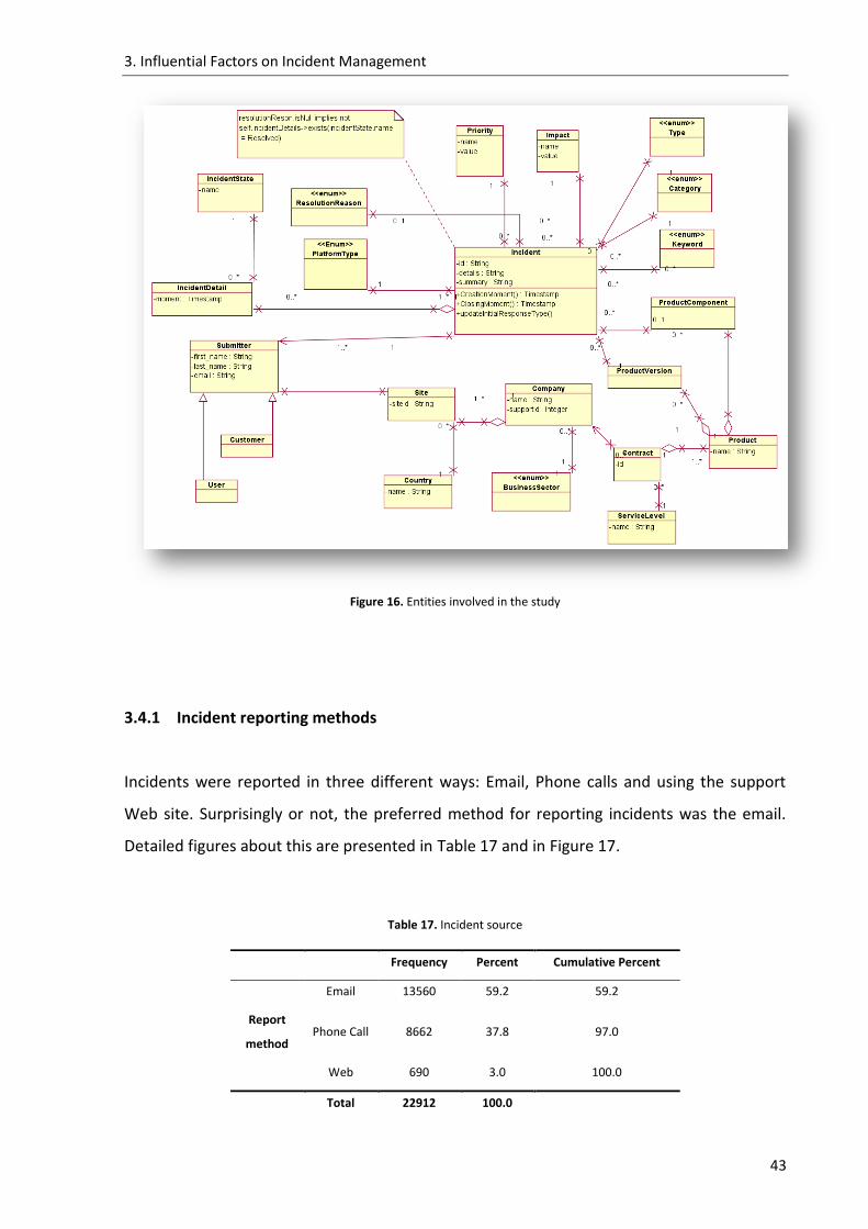
3. Influential Factors on Incident Management
43
Figure 16. Entities involved in the study
3.4.1 Incident reporting methods
Incidents were reported in three different ways: Email, Phone calls and using the support
Web site. Surprisingly or not, the preferred method for reporting incidents was the email.
Detailed figures about this are presented in Table 17 and in Figure 17.
Table 17. Incident source
Frequency Percent Cumulative Percent
Email 13560 59.2 59.2
Report
method Phone Call 8662 37.8 97.0
Web 690 3.0 100.0
Total 22912 100.0

3. Influential Factors on Incident Management
44
Figure 17. Incident source histogram
The email has become a tool with a very broad coverage and is not only a mere method of
creating, transmitting, or storing primarily text-based human communications with digital
communications systems. In addition, it is nowadays used for people to interact directly with
other technical platforms, in this case, the incident management platform.
3.4.2 Incident origin platform
There is a clear segregation on systems/platforms where the software was deployed and
used by the customers: the Mainframe4 and the Distributed Systems5. These two platforms
have different users and they have a very distinct usage. The frequencies of incidents,
represented in Table 18 and Figure 18, vary with the platform and with the quantity of
customers using the software on each of them.
Table 18. Incidents by platform
Frequency Percent Cumulative Percent
Mainframe4 (MF) 4237 18.5 18.5
Product Platform Distributed Systems5 (DS) 16865 73.6 92.1
4 The term usually refers to computers compatible with the IBM System/360 line, first introduced in 1965. (IBM System z10 is the latest incarnation.)
5 All other computer systems (hardware and software) that do not fall under the definition of the term Mainframe
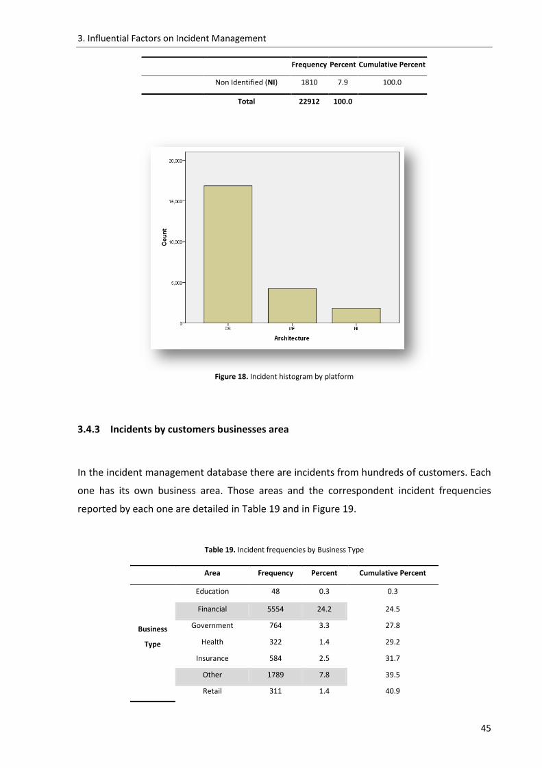
3. Influential Factors on Incident Management
45
Frequency Percent Cumulative Percent
Non Identified (NI) 1810 7.9 100.0
Total 22912 100.0
Figure 18. Incident histogram by platform
3.4.3 Incidents by customers businesses area
In the incident management database there are incidents from hundreds of customers. Each
one has its own business area. Those areas and the correspondent incident frequencies
reported by each one are detailed in Table 19 and in Figure 19.
Table 19. Incident frequencies by Business Type
Area Frequency Percent Cumulative Percent
Business
Type
Education 48 0.3 0.3
Financial 5554 24.2 24.5
Government 764 3.3 27.8
Health 322 1.4 29.2
Insurance 584 2.5 31.7
Other 1789 7.8 39.5
Retail 311 1.4 40.9

3. Influential Factors on Incident Management
46
Area Frequency Percent Cumulative Percent
Services 6118 26.7 67.6
Technology 3340 14.6 82.2
Telecommunications 2041 8.9 91.1
Transportation 800 3.5 94.6
Utility 1241 5.4 100.0
Total 22912 100.0
The top five business areas from where incidents were reported are identified (grey
background) in Table 19. The interesting part in this information is that the area of business
that reported more incidents was the area of Services, exceeding by a few points the
Financial business segment. From these figures, there is evidence that companies in the area
of Services, either IT Services or others, are heavily dependent on software, probably more
than what we could expect when compared with other areas of business.
Figure 19. Incidents histogram by Business Type

3. Influential Factors on Incident Management
47
3.4.4 Incident metrics summary
Table 20. Metrics summary
Country
Geographic Zone
Language # In
cid
en
ts
# In
cid
en
ts D
S
# In
cid
en
ts M
F
# In
cid
en
ts N
on
-Pro
du
cts
# C
ust
om
ers
# o
f d
iffe
ren
t P
rod
uct
s
# D
S P
rod
uct
s
# M
F P
rod
uct
s
# N
on
-Pro
du
cts
# In
cid
en
ts D
S /
# D
S P
rod
uct
s R
atio
# In
cid
en
ts M
F /
# M
F P
rod
uct
s R
atio
# In
cid
en
ts N
P /
# N
on
-Pro
du
cts
Rat
io
# In
cid
en
ts /
# P
rod
uct
Rat
io
Country
Portugal 546 238 282 26 36 104 57 44 3 4.175 6.409 8.666 5.405
Spain 3934 2460 1250 224 214 345 241 101 3 10.207 12.376 74.666 11.502
Brazil 2194 1553 571 70 126 245 175 68 2 8.874 8.397 35 9.028
Argentina 534 328 119 87 66 88 52 33 3 6.307 3.606 29 6.282
England 7138 5719 687 732 511 433 327 102 4 17.489 6.735 183 16.638
France 8007 6140 1230 637 541 434 352 78 4 17.443 15.769 159.25 18.620
Geographic Zone
Latin America 2728 1881 690 157 187 266 186 77 3 10.112 8.961 52.333 10.372
South Europe 4480 2698 1532 250 240 359 251 105 3 10.749 14.590 83.333 12.584
Central Europe 15145 11859 1917 1369 1014 580 451 125 4 26.294 15.336 342.25 26.293
Language
Portuguese 2740 1791 853 96 158 282 194 85 3 9.231 10.035 32 9.820
Spanish 4468 2788 1369 311 273 356 250 103 3 11.152 13.291 103.666 12.550
English 7138 5719 687 732 511 433 327 102 4 17.489 6.735 183 16.638
French 8007 6140 1230 637 541 434 352 78 4 17.443 15.769 159.25 18.620
Table 20 represents the summarization of metrics computed to assess incident ratios across
countries, geographic zones and languages. Non-product incidents refer to incidents
reported by users with no specific software product associated, such as: general questions
about the software organization, about request for information or proposals, and also sales,
contract or technical marketing related issues. The metrics representing ratios show a
standardized method for measuring the interactivity between customers and the software
vendor. Even limited by the reduced sample of incidents, we can observe that these figures

3. Influential Factors on Incident Management
48
vary substantially across countries, geographic zones and languages. With Non-product
ratios we can measure the sales activities before products are acquired. Product related
incident ratios mean the usage of software products in operation, thus giving us a method
for assessing the technical relation between the customer and the vendor. Whilst Portugal
and England have a very different scenario when comparing incidents on the Distributed
Systems(DS) platform, they have very similar figures in the Mainframe(MF) area. France,
Brazil, and Spain have stabilized coefficients, both for DS and MF. If we use the same
rationale for the geographic zone and the language, the main observation is the existence of
different ratios among DS and MF in England/English. A possible reason is that the
Mainframe technical staff in English organizations is skilled enough to resolve incidents
without the software vendor involvement, and the same do not apply for staff in the
Distributed Systems area. Argentina and Portugal have opposite behaviors, both in DS and
MF. Argentina is more active in products of Distributed Systems platform, and Portugal more
active in the Mainframe solutions. This can express the market penetration in each country
of products in both areas.
As a mean for comparing the average time (and their standard deviation statistics) to resolve
incidents among countries, we present those values in Table 21.
Table 21. Days to resolve incidents (average)
DaysToResolve
Minimum Maximum Mean Std. Deviation
Argentina 0.00 182.00 7.9732 17.55165
Brazil 0.00 747.00 15.4862 32.75591
England 0.00 750.00 20.9356 46.43596
Portugal 0.00 669.00 21.8126 53.93901
Spain 0.00 506.00 21.4738 40.39622
France 0.00 664.00 24.0518 46.34707
3.4.5 Variables and scale types
The variables used in this experiment are self-described in Table 22. The choice on the
characterization of the incidents (Category, Impact and Priority) is performed by the person

3. Influential Factors on Incident Management
49
who registers the incident (the end-user/customer or a support staff member). Incidents
have a defined lifecycle as shown in Figure 2 in chapter I. In this chapter we will only
consider closed incidents, since those are the only ones for which we know the values of all
timing variables. Figure 3, presented in chapter I describes how the three timing variables
are calculated, regarding specific milestones on incidents lifecycle.
Table 22. Variables used in this experiment, their scale types and description
Variable name Scale Description
Product Nominal Name of the product causing the incident
Company Nominal Name of the company where the product is installed
Country Nominal Name of the country where the incident was originated
Zone Nominal Zone of the globe where the country lies
Language Nominal Language spoken in the country
Category Nominal Categorizes incident’s root cause according to a predefined list
Impact Ordinal Measures incident’s business criticality
Priority Ordinal Measures incident’s correction prioritization to be considered by the support
Status Nominal Current status of the incident in its life cycle
WeekOfCreation Interval Order of the week (in the year) when the incident occurred. Valid values belong to (1-53)
WeekdayOfCreation Interval Order of the day (in the week) when the incident occurred. Valid values belong to (1-7)
TimeToRespond Absolute Elapsed time from incident creation until a support person has started to work on it
TimeToResolve Absolute Elapsed time from incident creation until a resolution is given to the end-user
TimeToConfirm Absolute Elapsed time since the resolution was given to the end-user until a confirmation is
obtained that the incident is closed
Table 23 and Table 24 provide details about the variables Impact and Priority respectively.
Table 23. Impact variable details
Variable name Valid values Scale Type Description
Impact 1 – Critical
2 – High
3 – Medium
Ordinal Classifies how critical is the incident for the
customer businesses

3. Influential Factors on Incident Management
50
Variable name Valid values Scale Type Description
4 – Low
Table 24. Priority variable details
Variable name Valid values Scale Type Description
Priority 1 – Critical
2 – High
3 – Medium
4 – Low
Ordinal Classifies incident’s correction prioritization to
be considered by the support
Table 25 presents the admissible values for the variable Category.
Table 25. Category variable details
Variable name Scale Type Description
Category Nominal Categorizes incident’s root cause according to a predefined list
Valid values
3rd Party Product Represents an incident reported apparently related with a third party product (e.g.:
Java SDK, .NET Framework, Apache, etc;)
Customer Service Incident is related with the customer care
Customization Incident is related with some configuration of the product
Documentation Incident is related with the product documentation
Function Incident is related with some functionalities in the product
Installation Incident is related with the product installation process
Internationalization Incident is related with the installation in a non English based platform
Compatibility Incident is related with the um compatibility with some other product
License Incident is related with the product license mechanism (e.g.: password, license file,
licensing technology)
Localization Incident has to do with the user interface localization
Performance Incident is related with performance and scalability issues (e.g.: network/database
performance, cluster technologies, failover, etc)
Request for
Information
The incident is related with a request for information from a customer
Security Incident is related with vulnerability in the security
Stability Incident is related with the product or platform stability

3. Influential Factors on Incident Management
51
3.5 Hypotheses identification and testing
This section identifies which are the statistical hypotheses that must be tested in order to
answer the previously stated research questions. We then apply the adequate statistical
tests and interpret their results. Research questions are prefixed by “RQ”.
To assess if we can apply parametric tests in the evaluation of our hypotheses, we need to
test if the outcome variables in our sample match a Normal distribution. In Figure 20 we
reproduce the corresponding QQ plots. The latter plot the quantiles of each variable's
distribution against the quantiles of the Normal distributions. To be Normal, a given variable
should have its points clustered around the straight line, representing the expected Normal
value. As we see, while the two interval variables (WeekdayOfCreation, WeekOfCreation)
seem to be close to the Normal distribution, the same is not true for the three absolute time
variables (TimeToRespond, TimeToResolve, TimeToConfirm).
Figure 20. QQ Plots for the schedule variables
3210-1-2-3
Standardized Observed Value
3
2
1
0
-1
-2
-3
Exp
ecte
d N
orm
al V
alu
e
Normal Q-Q Plot of WeekdayOfCreation
420-2-4
Standardized Observed Value
4
2
0
-2
-4
Exp
ecte
d N
orm
al V
alu
e
Normal Q-Q Plot of WeekOfCreation
3020100
Standardized Observed Value
4
3
2
1
0
-1
-2
Exp
ecte
d N
orm
al V
alu
e
Normal Q-Q Plot of TimeToRespond
20151050-5
Standardized Observed Value
4
2
0
-2
-4
Exp
ecte
d N
orm
al V
alu
e
Normal Q-Q Plot of TimeToResolve
3020100
Standardized Observed Value
4
2
0
-2
-4
Exp
ecte
d N
orm
al V
alu
e
Normal Q-Q Plot of TimeToConfirm
Training Incident is related with user training (e.g.: lack of training)
Uncategorized Incident does not fall under any previous categorization

3. Influential Factors on Incident Management
52
To test the hypothesis of normality we have applied the Kolmogorov-Smirnov one-sample
test, which is based on the maximum difference between the sample cumulative distribution
and the hypothesized cumulative distribution. The underlying hypotheses for this test are
the following:
H0: X ~ N(;) vs. H1: ¬ X ~ N(;)
Table 26. Testing Normal distribution adherence with the Kolmogorov-Smirnov test
WeekOfCreation WeekdayOfCreation TimeToRespond TimeToResolve TimeToConfirm
Kolmogorov-Smirnov Z 15.434 23.006 53.538 47.581 70.117
Asymp. Sig. (2-tailed) .000 .000 .000 .000 .000
Even considering a confidence interval of 99% (which is the same to say that = 0.01 and
the probability of Type I error of 1%) we can conclude, from Table 26, that we must reject
the null hypothesis for all variables, since we get a significance p < , which means that we
have significant Z statistics for all variables being analyzed. In other words, we cannot sustain
that the considered variables of our sample come from a Normal population. As such, we
can only use non-parametric tests in this experiment.
RQ1: Has the impact of an incident an influence on its lifecycle?
In other words, we want to know if incidents with different assigned impacts differ in the
corresponding lifecycle schedules (TimeToRespond, TimeToResolve, TimeToConfirm). Notice
that the Impact is assigned by the person that records the incident in the incident
management system at the time of its creation.
Due to the fact that those schedules are not normally distributed, we can only perform a
nonparametric analysis of variance. We will use the Kruskal-Wallis one-way analysis of
variance, an extension of the Mann-Whitney U test, which is the nonparametric analog of
one-way ANOVA test. The Kruskal-Wallis H test allows assessing whether several
independent samples are drawn from the same population (i.e. if they have similar statistical
distributions). In our case those independent samples are the groups of incidents for each of
the four Impact valid values.

3. Influential Factors on Incident Management
53
Let T be a schedule and i and j two different impact categories. Then, the underlying
hypotheses for this test are the following:
H0: i,j :T i ~ T j vs. H1: ¬ i,j :T i ~ T j
Table 27. Testing the influence of the impact on incident schedules
with the Kruskal-Wallis one-way analysis of variance test
TimeToRespond TimeToResolve TimeToConfirm
Chi-Square 352.381 77.532 18.487
Df 3 3 3
Asymp. Sig. (2-tailed) .000 .000 .000
The Kruskal-Wallis H test statistic is distributed approximately as chi-square. Consulting a
chi-square table with df = 3 ( these 3 degrees of freedom is due to the existence of 4
admissible values for this variable as represented in Table 23) and for a significance of =
0.01 (probability of Type I error of 1%) we obtain a critical value of chi-square of 11.3. Since
this value is less than the computed H values (the first line in Table 27), we reject the null
hypothesis that the samples do not differ on the criterion variable (the Impact). In other
words, given any of the schedule variables, we cannot sustain that the statistical
distributions of the groups of incidents corresponding to each of the Impact categories are
the same. This means that we accept the alternative hypothesis that the impact of an
incident has influence on the three schedule variables. Notice that the smallest H value is
obtained in the TimeToConfirm variable. This means that this is the schedule that differs less
due to the impact. There is not much surprise in this, as this schedule represents the end-
user confirmation that the incident was in fact resolved, and that it can be closed. End-users
tend to ignore this step in the incident management process and they have the same
behavior for all the incidents, independently of their impact.
RQ2: Has the priority of an incident an influence on its lifecycle?
Here we want to know if incidents with different assigned priorities differ in the
corresponding lifecycle schedules (TimeToRespond, TimeToResolve, TimeToConfirm). We will

3. Influential Factors on Incident Management
54
follow the same rationale as for the previous research question, regarding the applicable
statistic and its interpretation.
Table 28. Testing the influence of the priority on incident schedules
with the Kruskal-Wallis one-way analysis of variance test
TimeToRespond TimeToResolve TimeToConfirm
Chi-Square 298.918 80.868 13.210
df 3 3 3
Asymp. Sig. (2-tailed) .000 .000 .004
Again, the critical value of chi-square for (df = 3, = 0.01) is 11.3 (these 3 degrees of
freedom is due to the existence of 4 admissible values for this variable as represented in
Table 24). Since this value is less than the computed H values for each of the schedule
variables (the first line in Table 28), we reject the null hypothesis that the samples do not
differ on the criterion variable (the Priority). In other words, given any of the schedule
variables, we cannot sustain that the statistical distributions of the groups of incidents
corresponding to each of the Priority categories are the same. This means that we accept the
alternative hypothesis that the priority of an incident has influence on the three schedule
variables.
RQ3: Has the originating country of an incident an influence on its lifecycle?
The rational for answering this research question is the same as for the previous one. To
enable the application of the Kruskal-Wallis test, we have automatically recoded the Country
variable from string categories into numerical categories, from 1 to 6. The order is not
important in this scenario.

3. Influential Factors on Incident Management
55
Table 29. Testing the influence of the originating country on incident schedules
with the Kruskal-Wallis one-way analysis of variance test
TimeToRespond TimeToResolve TimeToConfirm
Chi-Square 1666.912 337.181 44.877
df 5 5 5
Asymp. Sig. (2-tailed) .000 .000 .000
Given that the critical value of chi-square for (df = 5, = 0.01) = 15.1 (these 5 degrees of
freedom is due to the existence of 6 countries) and that this value is less than the computed
H values for each of the schedule variables (the first line in Table 29), we reject the null
hypothesis that the samples do not differ on the criterion variable (Country). In other words,
given any of the schedule variables, we cannot sustain that the statistical distributions of the
groups of incidents corresponding to each of the countries are the same. This means that we
accept the alternative hypothesis that the country of an incident has influence on the three
schedule variables.
RQ4: Has the originating geographical zone of an incident an influence on its lifecycle?
The rational for answering this research question is again the same as for the previous one.
To enable the application of the Kruskal-Wallis test, we have automatically recoded the Zone
variable from string categories into numerical categories.
Table 30. Testing the influence of the originating zone on incident schedules
with the Kruskal-Wallis one-way analysis of variance test
TimeToRespond TimeToResolve TimeToConfirm
Chi-Square 1546.415 139.297 17.727
df 2 2 2
Asymp. Sig. (2-tailed) .000 .000 .000
Given that the critical value of chi-square for (df = 2, = 0.01) = 9.21 (these 2 degrees of
freedom is due to the existence of 3 geographic zones), we reject the null hypothesis that
the samples do not differ on the criterion variable (Geographic Zone). In other words, given

3. Influential Factors on Incident Management
56
any of the schedule variables, we cannot sustain that the statistical distributions of the
groups of incidents corresponding to each of the geographical zones are the same. This
means that we accept the alternative hypothesis that the geographical zone where the
incident was reported has influence on the three schedule variables.
RQ5: Has the incident category an influence on its lifecycle?
Again, after performing an automatic recode (for the Category variable), we obtained the
following summary table:
Table 31. Testing the influence of the category on incident schedules
with the Kruskal-Wallis one-way analysis of variance test
TimeToRespond TimeToResolve TimeToConfirm
Chi-Square 837.595 1258.178 612.215
df 15 15 15
Asymp. Sig. (2-tailed) .000 .000 .000
Given that the critical value of chi-square for (df = 15, = 0.01) = 30.6 (these degrees of
freedom is due to the existence of 15 admissible values in this variable as shown in Table 25),
we reject the null hypothesis that the samples do not differ on the criterion variable (the
incident Category). In other words, given any of the schedule variables, we cannot sustain
that the statistical distributions of the groups of incidents corresponding to each category
are the same. This means that we accept the alternative hypothesis that the incident
category has influence on the three schedule variables.
RQ6: Is the distribution of critical priority incidents the same across countries?
Since we know the proportion of the total incident reports originated in each country (see
Figure 21) we can expect that the incidents with critical priority per country follow the same
proportion of values. For this purpose we will use the Chi-Square Test procedure that
tabulates a variable into categories and computes a chi-square statistic. This nonparametric

3. Influential Factors on Incident Management
57
goodness-of-fit test compares the observed and expected frequencies in each country to
test if each one contains the same proportion of values.
Figure 21. Percentage of incident reports per country
To apply this test we have now selected only the critical priority incidents. The result of
applying this test is represented in Table 32. Since the critical value of chi-square for (df = 5,
= 0.01) = 15.1, we reject the null hypothesis that the proportion of critical priority
incidents is the same across countries. This means that we accept the alternative hypothesis
that the proportion of critical priority incidents is different across countries.
Table 32. Results of applying the Chi-Square Test procedure
to assess if the distribution of critical priority incidents is the same across countries
Country
Chi-Square 64.203
df 5
Asymp. Sig. (2-tailed) .000
UKPTFRESBRAR
Country
40,0%
30,0%
20,0%
10,0%
0,0%
Per
cen
t
32,0%
2,46%
35,72%
17,66%
9,72%
2,43%

3. Influential Factors on Incident Management
58
Table 33. Critical priority incidents observed and expected across countries
Observed N Expected N Residual
Argentina (AR) 12.0 17.8 -5.8
Brazil (BR) 39.0 71.2 -32.2
Spain (ES) 154.0 129.3 24.7
France (FR) 198.0 261.5 -63.5
Portugal (PT) 15.0 18.0 -3.0
England (UK) 314.0 234.3 79.7
Total 732.0
3.6 Results discussion
Based on our experiment we cannot sustain that the statistical distributions of the groups of
incidents corresponding to each of the Impact and Priority variables are the same. This
means that the impact and the priority of an incident have influence on the three schedule
variables. This shows evidence on the need to consider the business impact and the priority
in Incident Management process in order to optimize the incident resolution.
Regarding country and geographic zone statistics, given any of the schedule variables, we
observe that the country and the geographic zone of an incident have influence on the three
schedule variables. This behavior was not expected, and, having such a large incident sample
we would expect that incidents should have the same support level regardless they were
being reported from country X or Y, or zone A or B.
A possible reason for this is the fact that customers from different countries and zones are
served by different technical support offices. Although the support staff in these offices has
access to the same incidents database, they have different knowledge about the supported
products. Another admissible explanation is the existence of barriers on the communication
due to language constraints.
Regarding the categories of the incidents we have evidence that the incident category have
influence on the three schedule variables. The performance on responding and resolving the
incidents has an evident dependency from their categorization, meaning that the

3. Influential Factors on Incident Management
59
performance on software support activities is very dependent on the software component
that is potentially causing the incident.
We observe in Table 33 that the proportion of critical incidents is different across countries,
with England and Spain being on the top. This may reflect the importance that the software
has on the organizations on each of those countries. This importance can be somehow
related with the company dimension and/or the country economic strengths. Or, on the
other hand is just a cultural behavior influencing the incident management process; English
and Spanish users think their incidents have higher criticality than they really have.
Nevertheless, according to common policies regarding support contracts, reporting critical
incidents should mean that a customer productive system is not functioning, or on other
words, that the “production is down”. It seems that this happens quite often in England and
Spain.
Regardless of any speculative scenarios or any other assumptions, we would expect that
companies with operations worldwide and mature IT processes should have higher goals of
compliance for their Service Level Agreements than those organizations with just local
operations and with low maturity levels in IT Service Management. These levels of
compliance should have a strong influence on the support given by the software vendor. This
is yet to confirm, as we could not investigate further in this matters due to lack of
information regarding support contracts for particular organizations.

3. Influential Factors on Incident Management
60
[ This page has been intentionally left blank ]

61
44 Diachronic Aspects on Incident Management
Contents
4.1 Introduction ................................................................................................... 62
4.2 Research questions ......................................................................................... 63
4.3 Experiment process ........................................................................................ 64
4.4 Sample demographics ..................................................................................... 66
4.5 Hypothesis identification and testing .............................................................. 71
4.6 Modeling daily time series with ARIMA........................................................... 76
4.7 Modeling weekly time series with ARIMA ....................................................... 87
4.8 Results discussion ........................................................................................... 95
This chapter includes a seasonality and trend analysis on the reported and resolved
incidents. In addition, the ARIMA technique is used to model the Incident Management
process and produce forecasts.

4. Diachronic Aspects on Incident Management
62
4. Diachronic Aspects on Incident Management
“Prediction is very difficult, especially about the future.”
Niels Bohr (1885 - 1962)
4.1 Introduction
Economy changes, technology trends and financial constraints have led most companies to
face tremendous challenges over time. This is also true for the software industry. In this
business area there is an increasing need to react in a short period of time to all the
occurring changes. Software development and software maintenance are two areas of
increasing need for accurate management and near real time reactions. This implies in
understanding the past, manage the present, and predict the future. The main goal is to
change the paradigm and move from a reactive management approach to a proactive
/preventive one.
In such an approach, human, technical, and financial resources should be allocated and de-
allocated in advance according to forecasts. For a technical support department it is
mandatory to know causal-relationships about incidents and what to expect from the
incident management process.
If the support management staff is aware of any seasonality patterns or any trends in the
incidents, individuals or technical resources can be allocated when required and de-allocated
when there is no need from them. We cannot underestimate the strong influence of time in
this requirement. Therefore, a time series approach can be relevant for this to be done
accurately.
While the previous chapter studied cause-effect phenomenon in Incident Management
[Caldeira and Abreu, 2008], the current one intends to study its diachronic aspects by using
time series techniques.
A time series is a collection of consecutive observations generally made at equally spaced
time intervals. From another point of view, these observations are particular realizations of a
stochastic process [Papoulis, 1984], that is, a collection of random variables ordered in time
and defined at a set of time points which may be continuous or discrete.
There are two main goals in time series analysis: (a) identifying the nature of the
phenomenon represented by the sequence of observations, and (b) forecasting (predicting

4. Diachronic Aspects on Incident Management
63
future values of the time series variable). Both of these goals require that the pattern of
observed time series data is identified and more or less formally described. Once the pattern
is established, we can interpret and integrate it with other data (i.e., use it in our theory of
the investigated incidents phenomenon, e.g., seasonal incident creation). Regardless of the
depth of our understanding and the validity of our interpretation (theory) of the
phenomenon, we can extrapolate the identified pattern to predict future events.
Most time series patterns can be described in terms of two basic classes of components:
trend and seasonality. The former represents a general systematic linear or (most often)
nonlinear component that changes over time and does not repeat or at least does not
repeat within the time range captured by our data. The latter may have a formally similar
nature (e.g., exponential growth in incident creation), however, it repeats itself in systematic
intervals over time. Those two general components may coexist in real-life data. For
example, incidents reported by customers can rapidly grow over the years but they still
follow consistent seasonal patterns (e.g., low incident reports in the last weeks of the year).
This chapter it about seasonality and trend analysis related with the reported incidents and
is based on a set of computed variables extracted from the incident management database.
4.2 Research questions
To help software companies improve their support methods and processes, it is important to
elaborate in the incidents, analyze their patterns of occurrence, and if possible, be able to
predict future scenarios.
The goal of this section is to find evidences to answer the previous stated research
objectives, namely RO2 and RO3, by applying the following research questions:
RQ7: Does the incidents density for the analyzed time series exhibit particular
seasonality?
This research question aims at investigating whether the different time series exhibit, for
some particular reasons any periodic patterns (eg: weekly, monthly, yearly).
RQ8: Does the incidents density for the analyzed time series exhibit particular trends?

4. Diachronic Aspects on Incident Management
64
This research question aims at investigating whether the different time series exhibit, for
some particular reasons, different trends (eg: increasing or decreasing).
RQ9: Is forecasting based on ARIMA models a valid approach to predict incident
evolution?
This research question aims at investigating whether ARIMA time series forecasting is better
than a random walk model.
RQ10: What is the accuracy of the ARIMA time series forecasting of incident resolution
based on incident creation?
This research question aims at analyzing the error occurred when performing predictions on
the ARIMA time series.
RQ11: Can we use ARIMA models for What-If analysis (hypothetic scenarios)?
This research question aims at analyzing forecast values by making some assumptions on the
independent variable.
4.3 Experiment process
The data used on the experiment reported on the previous chapter spawned from 2005 to
2007. However, while looking in detail to each year separately, we notice that data from
2005 was considerably sparse. From the beginning of 2006 onwards, the incident report
process happens to have entered in “cruise operation”. This is coincidently confirmed with
the informal knowledge we had regarding the worldwide adoption of the underlying incident
management tool.
Several variables were computed based on the existing data, namely by computing the
frequencies of incidents. The resulting dataset was then loaded into the SPSS statistical
analysis tool, where the statistical analysis took place.
Figure 22 presents a schema of the process:

4. Diachronic Aspects on Incident Management
65
Figure 22. Experiment Process
Each of these steps is performed by a component of the methodology and each has specific
responsibilities as follows:
Data Aggregation (Step 1) – In this step we aggregated the data by day and then by
week, creating distinct daily and weekly time series.
Data Analysis (Step 2.a) – The goal of this step was to identify any seasonality and/or
any trend in the incidents basically by performing a spectral analysis of the variables
and analyzing their autocorrelation.
Data Modeling (Step 2.b) – This step consisted in elaborating the ARIMA model, that
is, find its parameters that allow to maximize its fitness to the observed time series.
Data Evaluation (Step 2.c) - This step consisted in evaluating the ARIMA models with
the identified parameters. Some evaluations were also made with ad-hoc
parameters.
Forecast (Step 3) – Forecasting was done based on the best identified models and
using different estimation periods. The obtained results were compared with the real
data obtained from year 2008 and the forecast values were validated using the 4-Plot
approach.
Step 1 Data
Aggregation
Step 3 Forecast
Step 4 Discussion
and Threats to Validity
Step 2.b Data
Modeling
Step 2.c Data
Evaluation
Step 2.a Data
Analysis

4. Diachronic Aspects on Incident Management
66
Discussion and Threats to Validity (Step 4) – This step includes a general discussion
on the seasonality, trend patterns and on the accuracy of the ARIMA models to
predict on Incident Management process.
4.4 Sample demographics
The subjects of our experiment are days. We have summarized seven variables per day of
the year. Those variables are represented and described in Table 37 in section 4.4.2.
The incident categorization process is critical to understand the types of incidents being
reported and very important to help allocating the right resources in solving the incidents.
The categorization process and the corresponding categories can also present us valuable
information to be used in the software development process. The observed frequencies of
incident categories are represented in Figure 23. Table 25 in the previous chapter details the
admissible categories and explains their purpose.
Figure 23. Incident frequencies by category
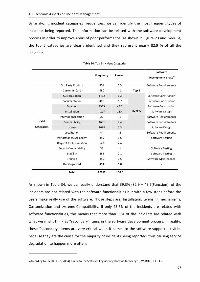
4. Diachronic Aspects on Incident Management
67
By analyzing incident categories frequencies, we can identify the most frequent types of
incidents being reported. This information can be related with the software development
process in order to improve areas of poor performance. As shown in Figure 23 and Table 34,
the top 5 categories are clearly identified and they represent nearly 82,9 % of all the
incidents.
Table 34. Top 5 Incident Categories
Frequency Percent Software
development phase6
Valid
Categories
3rd Party Product 301 1.3 Software Requirements
Customer Care 980 4.3 Top 5 -
Customization 1432 6.2
82,9 %
Software Construction
Documentation 400 1.7 Software Construction
Function 9989 43.6 Software Construction
Installation 4207 18.4 Software Design
Internationalization 22 .1 Software Requirements
Compatibility 1691 7.4 Software Requirements
License 1678 7.3 Software Design
Localization 44 .2 Software Requirements
Performance/Scalability 359 1.6 Software Testing
Request for Information 542 2.4 -
Security Vulnerability 33 .1 Software Testing
Stability 485 2.1 Software Testing
Training 345 1.5 Software Maintenance
Uncategorized 404 1.8 -
Total 22912 100.0
As shown in Table 34, we can easily understand that 39,3% (82,9 – 43,6(Function)) of the
incidents are not related with the software functionalities but with a few steps before the
users make really use of the software. Those steps are: Installation, Licensing mechanisms,
Customization and systems Compatibility. If only 43,6% of the incidents are related with
software functionalities, this means that more than 50% of the incidents are related with
what we might think as “secondary” items in the software development process. In reality,
these “secondary” items are very critical when it comes to the software support activities
because they are the cause for the majority of incidents being reported, thus causing service
degradation to happen more often.
6 According to the [IEEE-CS, 2004]. Guide to the Software Engineering Body of Knowledge (SWEBOK), IEEE-CS.

4. Diachronic Aspects on Incident Management
68
4.4.1 Seasonal patterns
A pattern we were trying to find has to do with the time and season that the incidents are
being reported. The following picture shows the frequencies of incidents summarized per
week of both years (2006 and 2007). Detailed data about incident frequencies is provided in
Table 35.
Figure 24. Incident frequencies per week of the year
Table 35. Incident frequencies (Year 2006 and 2007)
Frequency Percent Cumulative Percent
Weeks 2006+2007
1 353 1.5 1.5 2 542 2.4 3.9 3 413 1.8 5.7 4 440 1.9 7.6 5 446 1.9 9.6 6 436 1.9 11.5 7 400 1.7 13.2 8 393 1.7 14.9 9 433 1.9 16.8
10 429 1.9 18.7 11 487 2.1 20.8 12 448 2.0 22.8 13 410 1.8 24.6 14 392 1.7 26.3 15 321 1.4 27.7 16 411 1.8 29.5 17 418 1.8 31.3 18 324 1.4 32.7

4. Diachronic Aspects on Incident Management
69
Frequency Percent Cumulative Percent
19 341 1.5 34.2 20 340 1.5 35.7 21 357 1.6 37.2 22 380 1.7 38.9 23 307 1.3 40.2 24 386 1.7 41.9 25 418 1.8 43.8 26 394 1.7 45.5 27 410 1.8 47.3 28 379 1.7 48.9 29 380 1.7 50.6 30 354 1.5 52.1 31 339 1.5 53.6 32 289 1.3 54.9 33 287 1.3 56.1 34 323 1.4 57.5 35 326 1.4 58.9 36 378 1.6 60.6 37 424 1.9 62.4 38 418 1.8 64.3 39 460 2.0 66.3 40 538 2.3 68.6 41 428 1.9 70.5 42 626 2.7 73.2 43 622 2.7 75.9 44 537 2.3 78.3 45 521 2.3 80.6 46 567 2.5 83.0 47 801 3.5 86.5 48 790 3.4 90.0 49 678 3.0 92.9 50 670 2.9 95.9 51 590 2.6 98.4 52 292 1.3 99.7 53 66 .3 100.0
Total 22912 100.0
By simple observation, the only pattern we may find is that the amount of incidents being
reported increases from the 32th to the 47th week (roughly from the end of September to the
end of November), and there is a substantial reduction during the last five-six weeks of the
year. The increasing number of incidents after the 32th week is probably the result of
software changes, upgrades and/or tests that companies were doing in order to be prepared
for the last months of the year. Particularly the last month of the year is very intensive for
every business (due to Christmas and New Year) and any testing or any action that can
disturb the normal functioning of their systems is avoided. As such, the number of incidents
reported decreases. This rationale lacks empirical evidence which could be gathered by a
qualitative survey endorsed to interest parties (eg: set of major incident reporters).
Nevertheless, our aim is not to investigate further why the incidents were reported with
such a pattern, instead, we were focused on identifying that a pattern exists, and this is
valuable information for the next sections.

4. Diachronic Aspects on Incident Management
70
Unsurprisingly, the majority of incidents are reported during working days. These
frequencies increase from Monday(2), until it reaches its maximum on Wednesday(4), and
then it has a decreasing behavior until Friday(6). Saturday(7) and Sunday(1) are very quiet
days in terms of incident creation. Figure 25 shows graphically the sum of total incidents per
day within the week for the years in the sample. Notice, based on Table 36 data, that only
1% of the incidents are reported on weekends.
Figure 25. Incident frequencies per week day
Table 36 shows the detailed information about incident frequencies. Further rationale about
this weekly behavior will be presented in the following section.
Table 36. Days of week and incident frequencies
Frequency Percent Cumulative Percent
Days of the
week
Sunday(1) 107 .5 .5
Monday(2) 4216 18.4 18.9
Tuesday(3) 4684 20.4 39.3
Wednesday(4) 4928 21.5 60.8
Thursday(5) 4689 20.5 81.3
Friday(6) 4169 18.2 99.5
Saturday(7) 119 .5 100.0
Total 22912 100.0

4. Diachronic Aspects on Incident Management
71
4.4.2 Variables and scale types
The variables used in this experiment are self-described in Table 37.
Table 37. Variables and Scale types
Variable Scale Description
All_Created Numeric Scale Total of incidents created per day
All_Resolved Numeric Scale Total of incidents resolved per day
All_Created_Week Numeric Scale Total of incidents created per week
All_Resolved_Week Numeric Scale Total of incidents resolved per week
WeekOfCreation Interval Order of the week (in the year) when the incident occurred. Valid values belong to (1-53)
WeekdayOfCreation Interval Order of the day (in the week) when the incident occurred. Valid values belong to (1-7)
DasyToResolve Numeric Scale - Constant Average number of days to resolve an incident
The above variables represent the observations for the studied time series. Their meaning is
relevant for forecast new incidents, pace to close incidents and of the presence and absence
of trends. These variables represent aggregated incidents reported and resolved per day and
week, resulting in 4 time series.
In the modeling sections described later in this chapter we used two variables for the daily
series; one dependent variable (All_Resolved) and one independent variable (All_Created).
Similar to these, we have the weekly series represented by variables All_Created_Week and
All_Resolved_Week. Variables WeekOfCreation and WeekdayOfCreation were used to
identify patterns and variable DaysToResolve is mentioned to present the average days to
resolve incidents.
4.5 Hypothesis identification and testing
The analysis of seasonality and trend components are extremely important when we want to
model time series. The ARIMA parameters (p,d,q) representing the non-seasonal parameters
and (ps,ds,qs) representing the seasonal part of the model, are obtained by carefully

4. Diachronic Aspects on Incident Management
72
observation of those time series patterns. Complete definitions about ARIMA models and its
parameters can be found in the time series section of appendix B.
4.5.1 Seasonality analysis
Seasonal patterns of time series can be verified via correlograms. Either the autocorrelation
function (ACF) or the partial autocorrelation function (PACF) can attest the presence of any
pattern. As seen in [Box and Jenkins, 1970], the PACF is a more accurate mean of analyzing
the seasonality. More information about these functions can be found in appendix B.
Figure 26. Autocorrelation Function (ACF)
As show in Figure 26, there is a moderate correlation between k and k-1 lags (time spans) of
the occurrences of incidents resolved per day. This model represents a sinusoidal behavior
and the stronger correlation factor occurs at every 7 lags. We know that each observation in
our time series represents a day, therefore we can suspect that that there is a weekly
seasonal pattern. To confirm this we should analyze also the PACF. Although with moderate
correlation, but well above the confidence intervals, the PACF show exactly the same pattern
at every 7 lags leaving no doubts about the weekly pattern.

4. Diachronic Aspects on Incident Management
73
Figure 27. Partial Autocorrelation Function (PACF)
As a conclusion and answering RQ7, we can say that our time series has a seasonality period
that repeats every 7 days (weekly). This assumption is the base for the model parameter
identification phase.
4.5.2 Trend analysis
There are no exact way to identify trend components in the time series data; however, as
long as the trend is monotonous (consistently increasing or decreasing) that part of data
analysis is typically not very difficult. This can be graphically viewed by plotting our time
series observations. For analyzing the trend on the performance of the support staff, we use
the daily series, representing resolved incidents per day. This is represented in Figure 28.

4. Diachronic Aspects on Incident Management
74
Figure 28. Time Series - Incidents Resolved per day
The above figure suggests the existence of a trend, with a very smooth increasing pattern. To
confirm this behavior we have done a seasonal decomposition. The seasonal decomposition
procedure decomposes a series into a seasonal component, a combined trend and cycle
component, and an "error" component. The seasonal decomposition procedure creates four
new series:
1. The seasonal adjustment factors (SAF) which indicate the effect of each period on the
level of the series.
2. The seasonally adjusted series (SAS) which is a new series with the values obtained
after removing the seasonal variation of the original series.
3. The smoothed trend-cycle components (STC) show the trend and cyclical behavior
present in the series
4. The residual or "error" values (ERR) representing the values that remain after the
seasonal, trend and cycle components have been removed from the series.
Figure 29. STC series - Incidents Resolved per day with systematic seasonal variations removed

4. Diachronic Aspects on Incident Management
75
Figure 29, plotting the decomposed trend and cycle component, shows that there is a weak
increasing trend. We can also identify a set of peaks, which may identify another pattern of
seasonality. Analysis of the time series show that those peaks reflect the end of year
(November and December) and therefore we can assume there is another seasonality
pattern here, and this is an important observation to RQ7. Regarding trending and
answering RQ8, we may say that the period of data collected is not enough to take
conclusions but it is acceptable to say that it seems there is an increasing trend, although
with some aberrant observations, as mentioned in [Franses, 1998]. To make a clear
statement about trending in this time series requires careful validation and more data to
examine. To validate the de-trended series we should inspect its residuals or error values
(ERR series). Residuals are differences between the predicted de-trended series output from
the model and the measured output from the basic series observations. Thus, residuals
represent the portion of the validation data not explained by the model. Residuals should
not be correlated for the series to be considered valid. Non-correlated residuals mean that
also no correlation exists in the original series and the de-trended one. Observing Figure 30,
we have evidence that the series is valid based on the histogram and residuals QQ-plots. The
histogram shown in Figure 30 and the normal probability plot in Figure 31 sustain that the
distribution of the residuals is normal confirming the basic assumption to validate the de-
trended series.
Figure 30. ERR series for the SAS
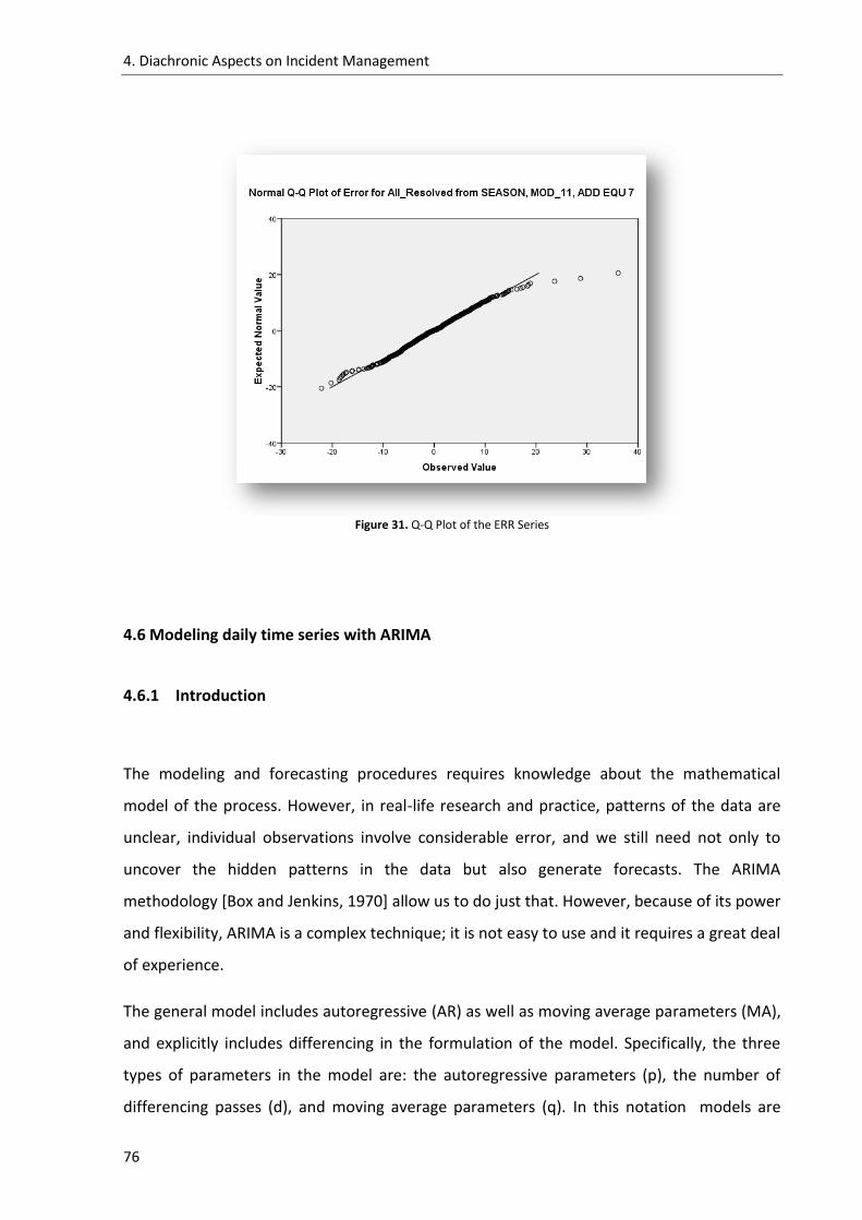
4. Diachronic Aspects on Incident Management
76
Figure 31. Q-Q Plot of the ERR Series
4.6 Modeling daily time series with ARIMA
4.6.1 Introduction
The modeling and forecasting procedures requires knowledge about the mathematical
model of the process. However, in real-life research and practice, patterns of the data are
unclear, individual observations involve considerable error, and we still need not only to
uncover the hidden patterns in the data but also generate forecasts. The ARIMA
methodology [Box and Jenkins, 1970] allow us to do just that. However, because of its power
and flexibility, ARIMA is a complex technique; it is not easy to use and it requires a great deal
of experience.
The general model includes autoregressive (AR) as well as moving average parameters (MA),
and explicitly includes differencing in the formulation of the model. Specifically, the three
types of parameters in the model are: the autoregressive parameters (p), the number of
differencing passes (d), and moving average parameters (q). In this notation models are

4. Diachronic Aspects on Incident Management
77
summarized as ARIMA (p, d, q); so, for example, a model described as (0, 1, 2) means that it
contains 0 (zero) autoregressive (p) parameters and 2 moving average (q) parameters which
were computed for the series after it was differenced once (d=1).
4.6.2 Model identification
The ARIMA models requires 3 non-seasonal parameters, so called p, d, and q and 3 seasonal
parameters, named ps, ds, qs. This model can be decomposed in the non seasonal AR(p) ,
differencing (d) and MA(q). Similarly it has a seasonal part decomposed in seasonal
autoregressive AR(ps) , seasonal differencing (ds) and seasonal moving average MA(qs).
Stationarity does not have to exist originally in a series. However, a series has to be
stationary for the application of ARIMA(p,d,q)(ps,ds,qs) models to be accurate. From an
intuitive point of view, a time series is said to be stationary if there is no systematic change
in mean (no trend), if there is no systematic change in variance and if strictly periodic
variations have been removed.
4.6.3 Differencing
When a time series is not stationary it is quite common to submit the series to a
transformation, normally Differencing. The number of times a series needs to be differenced
until it is stationary is the value that d assumes in the ARIMA model.
As observed earlier in Figure 28, we conclude that our time series is not stationary, therefore,
to make it stationary we have applied a differencing transformation with lag 1 which is
reflected by Figure 32.

4. Diachronic Aspects on Incident Management
78
Figure 32. Time Series with Differencing (1)
It is also common to have pre-differencing transformations to stabilize the variance of the
time series, usually a log or square root transformation. In our case there was no need to
apply any transformation before. After differencing the series once, it has become
stationary, without any trend and with the seasonality peaks removed. This pattern is also
known as the Gaussian effect or White-noise [Wikipedia, 2009].
The PACF in Figure 33 sustains this, as we can observe that the correlations peak in early
lags, but, cut off suddenly. This is a normal behavior of a stationary time series.
Figure 33. PACF for the time series after Differencing (1)

4. Diachronic Aspects on Incident Management
79
Because we had to difference the series once to make it stationary, we have identified our
d=1 parameter.
4.6.4 Non-seasonal parameters
The AR(p) and The MA(q) parameters can be obtained by analyzing the ACF and PACF.
Because the ACF has a sine-wave shape pattern (Figure 34) and the PACF has a set of
exponential decays (Figure 35) we estimate our regular autoregressive parameter AR(p=2)
and our regular moving average parameter MA(q=2). The notions behind the rationale for
identifying the p and q parameters are amply described in appendix B.
4.6.5 Seasonal parameters
As mentioned earlier, our time series has a seasonality period of 7 days (1 week). After
applying a seasonal differencing once (ds=1), and due to the ACF abrupt decay (Figure 37)
and PACF exponential decay (Figure 36), we estimate our seasonal autoregressive parameter
AR(ps=1) and our seasonal moving average parameter MA(qs=1).
Figure 34. ACF for the regular time series Figure 35. PACF for the regular time series
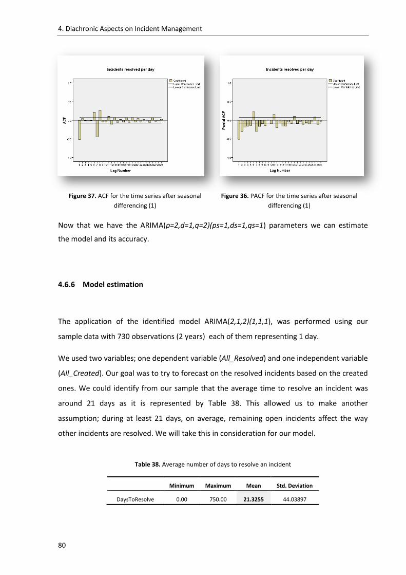
4. Diachronic Aspects on Incident Management
80
Now that we have the ARIMA(p=2,d=1,q=2)(ps=1,ds=1,qs=1) parameters we can estimate
the model and its accuracy.
4.6.6 Model estimation
The application of the identified model ARIMA(2,1,2)(1,1,1), was performed using our
sample data with 730 observations (2 years) each of them representing 1 day.
We used two variables; one dependent variable (All_Resolved) and one independent variable
(All_Created). Our goal was to try to forecast on the resolved incidents based on the created
ones. We could identify from our sample that the average time to resolve an incident was
around 21 days as it is represented by Table 38. This allowed us to make another
assumption; during at least 21 days, on average, remaining open incidents affect the way
other incidents are resolved. We will take this in consideration for our model.
Table 38. Average number of days to resolve an incident
Minimum Maximum Mean Std. Deviation
DaysToResolve 0.00 750.00 21.3255 44.03897
Figure 37. ACF for the time series after seasonal
differencing (1) Figure 36. PACF for the time series after seasonal
differencing (1)
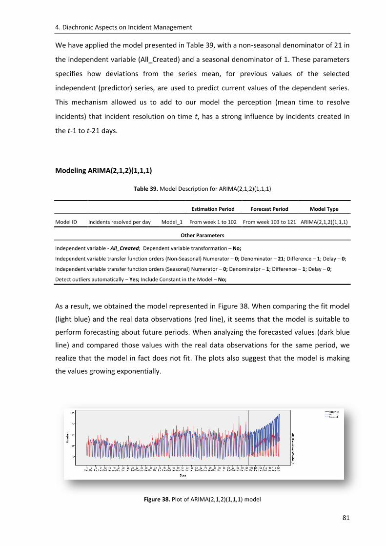
4. Diachronic Aspects on Incident Management
81
We have applied the model presented in Table 39, with a non-seasonal denominator of 21 in
the independent variable (All_Created) and a seasonal denominator of 1. These parameters
specifies how deviations from the series mean, for previous values of the selected
independent (predictor) series, are used to predict current values of the dependent series.
This mechanism allowed us to add to our model the perception (mean time to resolve
incidents) that incident resolution on time t, has a strong influence by incidents created in
the t-1 to t-21 days.
Modeling ARIMA(2,1,2)(1,1,1)
Table 39. Model Description for ARIMA(2,1,2)(1,1,1)
Estimation Period Forecast Period Model Type
Model ID Incidents resolved per day Model_1 From week 1 to 102 From week 103 to 121 ARIMA(2,1,2)(1,1,1)
Other Parameters
Independent variable - All_Created; Dependent variable transformation – No;
Independent variable transfer function orders (Non-Seasonal) Numerator – 0; Denominator – 21; Difference – 1; Delay – 0;
Independent variable transfer function orders (Seasonal) Numerator – 0; Denominator – 1; Difference – 1; Delay – 0;
Detect outliers automatically – Yes; Include Constant in the Model – No;
As a result, we obtained the model represented in Figure 38. When comparing the fit model
(light blue) and the real data observations (red line), it seems that the model is suitable to
perform forecasting about future periods. When analyzing the forecasted values (dark blue
line) and compared those values with the real data observations for the same period, we
realize that the model in fact does not fit. The plots also suggest that the model is making
the values growing exponentially.
Figure 38. Plot of ARIMA(2,1,2)(1,1,1) model

4. Diachronic Aspects on Incident Management
82
To check the accuracy of obtained models we have to inspect its statistics. Table 40 shows
that the model has one predictor/independent variable (All_Created), that 5 outliers have
been removed and that its accuracy is reasonably high by inspecting its stationary R-squared
and ordinary R-squared statistics.
The stationary R-squared statistics is a measure that compares the stationary part of the
model to a simple mean model. This measure is preferable to ordinary R-squared when
there is a trend or seasonal pattern. R-squared statistics estimates the proportion of the
total variation in the series that is explained by the model. This measure is most useful when
the series is stationary.
However, this model has also a very high percentage of errors, represented by the model
average percent error (MAPE) and the model maximum average percent error (MaxAPE).
Due to these statistics, and the observation of the model plots, we have decided to search
for another suitable model other than the ARIMA (2,1,2)(1,1,1).
Table 40. Model ARIMA(2,1,2)(1,1,1) statistics
Model
Number of
Predictors
Model Fit statistics
Stationary
R-squared R-squared MAPE MaxAPE
Number of
Outliers
Incidents resolved per day
Model_1 1 .723 .843 64.329 1273.850 5
Modeling ARIMA(2,1,2)(1,0,1)
Carefully observation of the previous model and based on our experience, we notice that the
model was over-differenced, that seasonal differencing on top of the non-seasonal
differencing was exaggerated. This means that the ds parameter was not adjusted correctly,
thus causing the exponential grow in the forecasted values. We decided to make the ds=0,
the seasonal denominator was removed from the model and we evaluated it again, this time
with ARIMA (2,1,2)(1,0,1).

4. Diachronic Aspects on Incident Management
83
Table 41. Model description for ARIMA(2,1,2)(1,0,1)
Estimation Period Forecast Period Model Type
Model ID Incidents resolved per day Model_2 From week 1 to 102 From week 103 to 121 ARIMA(2,1,2)(1,0,1)
Other Parameters
Independent variable - All_Created; Dependent variable transformation – No;
Independent variable transfer function orders (Non-Seasonal) Numerator – 0; Denominator – 21; Difference – 1; Delay – 0;
Independent variable transfer function orders (Seasonal) Numerator – 0; Denominator – 0; Difference – 0; Delay – 0;
Detect outliers automatically – Yes; Include Constant in the Model – No;
This evaluation showed a better accuracy as represented by the stationary R-squared
statistics (0.908 = 90.8%). The MAPE have reduced but the MaxAPE have increased. Although
still with a huge error margins, this model is far better than the previous one. This can be
confirmed not only by the Stationary R-squared statistics in Table 42, but also graphically by
the plot of the observations; real observed, fit, and forecasted values in Figure 39.
Table 42. Model ARIMA(2,1,2)(1,0,1) statistics
Model
Number of
Predictors
Model Fit statistics
Stationary
R-squared R-squared MAPE MaxAPE
Number of
Outliers
Incidents resolved per day
Model_2 1 .908 .884 50.851 1979.931 4
Figure 39. Plot of ARIMA(2,1,2)(1,0,1) model

4. Diachronic Aspects on Incident Management
84
We have applied again the same model, this time by reducing the estimation period (week 1
to 95) and forecasting from week 96 to week 121. The obtained results are very similar to
the preceding one, but less accurate, as it has a higher error percentage as represented by
the MAPE and MaxAPE in Table 43.
Table 43. Model ARIMA(2,1,2)(1,0,1) statistics (estimation period from week 1 to 95)
Model
Number of
Predictors
Model Fit statistics
Stationary
R-squared R-squared MAPE MaxAPE
Number of
Outliers
Incidents resolved per day
Model_2A 1 .904 .881 56.421 2157.371 4
Figure 40. Plot of ARIMA(2,1,2)(1,0,1) model (estimation period from week 1 to 95)
4.6.7 Model validity
Finally we decided to compare our model with a random walk model. This is a model where
autoregressive (AR) or moving average (MA) parameters are not included. It has the form of
ARIMA(0,d,0)(0,d,0). Since we were differencing our regular series one time, we have used
ARIMA(0,1,0)(0,0,0).

4. Diachronic Aspects on Incident Management
85
Modeling a Random-Walk model ARIMA(0,1,0)(0,0,0)
Table 44. Model description for ARIMA(0,1,0)(0,0,0)
Estimation Period Forecast Period Model Type
Model ID Incidents resolved per day Model_3 From week 1 to 95 From week 96 to 121 ARIMA(0,1,0)(0,0,0)
Other Parameters
Independent variable - All_Created; Dependent variable transformation – No;
Independent variable transfer function orders (Non-Seasonal) Numerator – 0; Denominator – 21; Difference – 1; Delay – 0;
Independent variable transfer function orders (Seasonal) Numerator – 0; Denominator – 0; Difference – 0; Delay – 0;
Detect outliers automatically – Yes; Include Constant in the Model – No;
We can conclude from the below statistics that this model is worse than the other models
except for the first one ARIMA(2,1,2)(1,1,1). Although its stationary R-squared value is high,
it has also a high MAPE and MaxAPE. Comparing the dark blue plot with the red plot in
Figure 41, it shows a clear discrepancy between the model estimation values and real
observations.
Table 45. Model ARIMA(0,1,0)(0,0,0) statistics
Model
Number of
Predictors
Model Fit statistics
Stationary
R-squared R-squared MAPE MaxAPE
Number of
Outliers
Incidents resolved per day
Model_3 1 .846 .809 85.370 2875.744 8
Figure 41. Plot of ARIMA(0,1,0)(0,0,0) model – A Random Walk Model
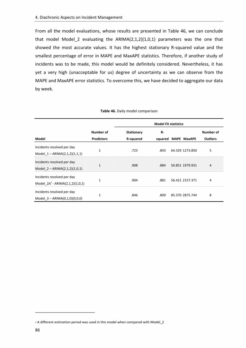
4. Diachronic Aspects on Incident Management
86
From all the model evaluations, whose results are presented in Table 46, we can conclude
that model Model_2 evaluating the ARIMA(2,1,2)(1,0,1) parameters was the one that
showed the most accurate values. It has the highest stationary R-squared value and the
smallest percentage of error in MAPE and MaxAPE statistics. Therefore, if another study of
incidents was to be made, this model would be definitely considered. Nevertheless, it has
yet a very high (unacceptable for us) degree of uncertainty as we can observe from the
MAPE and MaxAPE error statistics. To overcome this, we have decided to aggregate our data
by week.
Table 46. Daily model comparison
Model
Number of
Predictors
Model Fit statistics
Stationary
R-squared
R-
squared MAPE MaxAPE
Number of
Outliers
Incidents resolved per day
Model_1 – ARIMA(2,1,2)(1,1,1) 1 .723 .843 64.329 1273.850 5
Incidents resolved per day
Model_2 – ARIMA(2,1,2)(1,0,1) 1 .908 .884 50.851 1979.931 4
Incidents resolved per day
Model_2A7 - ARIMA(2,1,2)(1,0,1) 1 .904 .881 56.421 2157.371 4
Incidents resolved per day
Model_3 – ARIMA(0,1,0)(0,0,0) 1 .846 .809 85.370 2875.744 8
7 A different estimation period was used in this model when compared with Model_2

4. Diachronic Aspects on Incident Management
87
4.7 Modeling weekly time series with ARIMA
4.7.1 Differencing
Our goal is to check if we can obtain more accurate models simply by using time series
representing the incidents per week and not per day.
Using the same techniques mentioned earlier we have observed that our series was not
stationary. The following figures show the correlograms of our series after differencing with
lag 1. Analyzing the ACF and PACF shows that the series are stationary and therefore suitable
for ARIMA models.
On the previous section, our values represented observations per day and therefore we had
a periodicity of 7 days per week. That model had non-seasonal parameters as well as
seasonal parameters, representing the days and the weeks.
Figure 42. ACF after Differencing(1)
Figure 43. PACF after Differencing(1)

4. Diachronic Aspects on Incident Management
88
In this time series we have only non-seasonal parameters. This is related with the fact that
weeks are not periodic (some years have 365 days and others 366). Due to this constraint,
we have a model in this form; ARIMA(p,d,q). After differencing the series once, we have
identified our d=1parameter.
4.7.2 Non-seasonal parameters
The same techniques used in the previous section apply in this case to identify the AR and
MA parameters. Due to the ACF and PACF quick decay starting at lag 1, and because no
other correlation exists for the remaining lags, we choose to have one autoregressive (AR)
parameter and one moving average (MA) parameter. The weekly time series model is
defined as ARIMA(1,1,1).
4.7.3 Model estimation
Modeling ARIMA(1,1,1)
Table 47. ARIMA(1,1,1)
Estimation Period Forecast Period Model Type
Model ID Incidents resolved per week Model_4 From week 1 to 93 From week 94 to 157 ARIMA(1,1,1)
Other Parameters
Independent variable - All_Created; Dependent variable transformation – No;
Independent variable transfer function orders : Numerator – 0; Denominator – 3; Difference – 1; Delay – 0;
Detect outliers automatically – Yes; Include Constant in the Model – No;
At a first glance, by looking into Table 48, we can notice that this model has a lower
Stationary R-squared statistics when compared with the previous models (daily models). The
major gain with this model is the reduced error rate observed in the MAPE and MaxAPE
statistics. If we take into account that this model is the result of having only one
independent variable, we have to admit that it performs very well.

4. Diachronic Aspects on Incident Management
89
Table 48. Model ARIMA(1,1,1) statistics
Model
Number of
Predictors
Model Fit statistics
Stationary
R-squared R-squared MAPE MaxAPE Statistics
Number of
Outliers
Incidents resolved per week
Model_4 1 .829 .933 6.408 34.760 15.776 2
Figure 44. Plot of ARIMA(1,1,1) forecast to week 157 with observed values
In the end of the experiment we were able to collect more data from year 2008 (week 106 to
157). Even if we have not included this data, neither in the descriptive statistics or used it in
our model estimation period, we used the year 2008 data to validate the evaluated models
and their forecast values. The above plot shows the forecast values (dark blue) when
compared with the real observations period (week 95 to 157) for which we were making the
predictions. We cannot underestimate the strong overlap between the forecast values and
the real values (in red) for the prediction period.
4.7.4 Model substantiation
To validate our model(s) it is imperative that some conditions are verified in the series
residuals. The estimation procedure assumes that the residuals are not auto-correlated and
that they are normally distributed. We have adapted the 4-Plot graph (plus one additional
plot) to help us analyzing the residuals (error series) from our weekly forecast series.

4. Diachronic Aspects on Incident Management
90
Figure 45. 4-Plot adapted graph for model validation
The assumption that the residuals are not correlated is sustained by the two top graphs, the
ACF and PACF. The two graphs in the middle corroborate the premise that the residuals
follow a normal distribution. The scatter plot confirms that the residuals are random
observations, therefore, not auto-correlated. Having all the conditions satisfied, we can
confirm that our model is valid and that the forecast series is trustable in its accuracy.

4. Diachronic Aspects on Incident Management
91
4.7.5 Model validity
To at least compare our previous model with another model we have decided to evaluate
our series against a Random-Walk approach, meaning, to compare it with a model in the
form of ARIMA(0,d,0). Because we have to difference our series once, we used d=1.
Table 49. ARIMA(0,1,0)
Estimation Period Forecast Period Model Type
Model ID Incidents resolved per week Model_5 From week 1 to 95 From week 96 to 157 ARIMA(0,1,0)
Other Parameters
Independent variable - All_Created; Dependent variable transformation – No;
Independent variable transfer function orders : Numerator – 0; Denominator – 3; Difference – 1; Delay – 0;
Detect outliers automatically – Yes; Include Constant in the Model – No;
Table 50. Model ARIMA(0,1,0) statistics
Model
Number of
Predictors
Model Fit statistics
Stationary
R-squared R-squared MAPE MaxAPE
Number of
Outliers
Incidents resolved per week
Model_5 1 .657 .862 8.544 33.915 3
Figure 46. Forecast values for the weekly Random-Walk model - ARIMA(0,1,0)

4. Diachronic Aspects on Incident Management
92
The statistics observed for this model show a worse performance when compared with the
previous one. According with this evidence, we found no interest in validating the residuals
for the current model. Table 51 presents the weekly evaluated models and their comparison.
Table 51. Weekly model comparison
Model
Number of
Predictors
Model Fit statistics
Stationary
R-squared R-squared MAPE MaxAPE
Number of
Outliers
Incidents resolved per week
Model_4 – ARIMA (1,1,1) 1 .829 .933 6.408 34.760 2
Incidents resolved per week
Model_5 – ARIMA (0,1,0) 1 .657 .862 8.544 33.915 3
4.7.6 What-If scenario
The main reason why models and forecasting are so important in academics and corporate
studies across all business areas are because they can help us to make plans for the future.
The future has a tremendous gap of uncertainty and predicting the future requires always
some basic assumptions. Modeling based on certain assumptions is called what-if scenarios
or quite often scenario planning. This is extremely important especially if it includes systems
which recognize that many factors may combine in complex ways to create sometime
surprising futures (due to non-linear feedback loops).
We have taken the previous weekly validated model and have built a case scenario to
forecast on technical resources needed to deal with incident management. Knowing in
advance the incidents to resolve and the technical resources needed should help software
organizations to adapt and adjust quickly to the demand from customers. This, not only
contributes to better service quality, but also to increase effectiveness in allocating financial
resources.
We will use two basic assumptions in this scenario. The first is that (based on our
experience) today, on average, each person in the support department in an organization

4. Diachronic Aspects on Incident Management
93
similar to the one we are studying resolves 30 incidents per week. The second assumption or
trial we are doing is that the incidents creation will grow by 30% on the forecast period
(2008) when compared with the last year. This scenario can be explained by an acquisition or
merger between organizations, or, simply because there were more software products in
operation, which will cause the customers to report more incidents.
We have created another time series called SupportMembers, representing the number of
people needed in each week by dividing the All_Resolved_Week observations from (week 1
to 104, representing year 2006 and 2007) by 30. This is represented in blue in Figure 47.
Table 52. What-if scenario details
Estimation Period Forecast Period Model Type
Model ID SupportMembers Model_5 From week 1 to 104 From week 105 to 157 ARIMA(1,1,1)
Other Parameters
Independent variable - All_Created; Dependent variable transformation – No;
Independent variable transfer function orders : Numerator – 0; Denominator – 3; Difference – 1; Delay – 0;
Detect outliers automatically – Yes; Include Constant in the Model – No;
After evaluating the model, the predicted All_Resolved_Week series was created, and the
correspondent support members was also computed. The value of this resulting series
(predicted SupportMembers) had the number of resources needed for the estimation period
and also for the forecast period (week 105 to 157). This is shown in green in Figure 47.
Table 53. What-if scenario statistics
Model
Number of
Predictors
Model Fit statistics
Stationary
R-squared R-squared MAPE MaxAPE
Number of
Outliers
SupportMembers
Model_5 1 .834 .926 6.987 52.973 2

4. Diachronic Aspects on Incident Management
94
Figure 47. Predicted support members for the third year (2008)
Figure 48 show strong evidence that we cannot rely on simple linear approaches to work on
forecast scenarios. If we had tried an approach where the average number of resources in
the previous year was used to calculate the number of resources needed to support the
growth of 30% in incidents, we would fall into a trap. The average number of resources in
the past two years is represented in green until week 104. If we had increased this average
by 30% (like the 30% increase in incidents) to obtain the average number of resources
needed for the next year, we would have the value represented by the yellow line. This
would cause an estimation of the support staff under the real needs. The required resources
in each week are represented by the blue line, and the average of the predicted resources
for the forecast year is represented by the green line after week 104. The series average is
much above the linear estimation of increasing the staff by 30%.
In fact when increasing the number of incidents 30%, the support members have to increase
on average around 55%, and not the linear 30% that we would expect to be enough. On the
estimation period we had an average of 6.4 staff members (green line to week 104).
Increasing this average of resources by 30% would give 8.32 (6.4*1.3) members on average
in the support (yellow line). In fact the needed number of resources in each week
represented by the blue line has an average of 9.93, meaning a growth in the staff members
of 55% ((9.93/6.4)-1=0.55=55%) for the next year.

4. Diachronic Aspects on Incident Management
95
Figure 48. Predicted and average support members comparison
4.8 Results discussion
Based on the introductory descriptive statistics, that highlights the fact that software
deployment caused a considerable number of the overall incidents, we affirm that marginal
activities to software usage, like, the installation process, initial configuration and license
mechanisms are causing these incidents. To improve the software development, companies
must improve these marginal activities. Making some of these tasks more easy and agile to
the end-user can bring great benefits in the maintenance and in the support processes.
Regarding this chapter research objectives, we realized that the majority of the incidents are
reported during working days and very few are reported over the weekends. We have
identified that our sample has two seasonality patterns: a very strong weekly period and a
weak and yet to confirm yearly decreasing pattern in the last month of the year. When
looking for a trend pattern, we found no strong reasons to ensure that it exists in our
sample.
Answering RQ9, we have strong evidence that ARIMA models can be an accurate method for
predicting the amount of resolved incidents in a specific period, the same is to say, we are
able to predict the expected workload of a support department in order to maintain the
same level of service. With just a single independent variable, representing the incidents
created in previous weeks, we were able to model and predict the behavior of the
dependent variable, the incidents resolved.

4. Diachronic Aspects on Incident Management
96
Although the models used to forecast daily incidents have considerably high goodness of fit,
they have also very large error statistics for MAPE and MaxAPE. These values were large
enough to suggest the daily model rejection. Nevertheless, they performed very well when
the variation in incident creation was not very strong. When incident creation increases or
decreases very rapidly (this happens in November and December) the model did not
perform very well and it was not able to adapt quickly enough to the observed patterns.
On the other hand, the model evaluated with the aggregated weekly data turned to be a
more suitable model. It has a comfortable goodness of fit, but much less error statistics for
the MAPE and MaxAPE. The average number of resolved incidents per week in the time
series is 187.56. The average percentage error in the forecast time series was 6.40 %,
representing a possible calculation error of around 12 incidents per week, which, even in a
conservative scenario is an acceptable error. This result answers to RQ10, and yes, in fact
due to the reduced error percentage in the model, we can be confident on using ARIMA
models to predict on incident resolution based on incident creation.
We have not evaluated any model of the form ARIMA(p,0,0) (i.e., linear model) or
ARIMA(0,0,q) (i.e., Gaussian model) because they would violate the basic assumption that
our series has to be differenced at least once, and this implies having the parameter d in the
model with a value other than 0(zero).
Regarding RQ11, we have seen that resource prediction has to be carefully planned as well,
as we may fall into some erroneous behavior. Nevertheless, ARIMA models can also help in
this task with reliable results. Applying models like the ones we have proposed will certainly
be a powerful method for any organization which aims to achieve more accurate planning,
efficient allocation and proper management of the financial resources related with their
technical support departments.
We are well aware that these models were computed based on only one independent
variable. Even with this constraint, we were able to produce valid results. With no
constraints regarding the access to other data (e.g.: number of people in the support in
general and per product, number of people in the first and second line support, number of
developers for each product, etc..) we are confident that models with much more accuracy
can be constructed.

97
55
Conclusion and Future Work
Contents
5.1 Contributions review ...................................................................................... 98
5.2 Threats to the validity ................................................................................... 102
5.3 Evolution and next steps ............................................................................... 103
This chapter presents this dissertation’s conclusions and resumes its main contributions.

5. Conclusion and Future Work
98
5. Conclusion and Future Work
“The important thing is not to stop questioning.”
Albert Einstein (1879 - 1955)
5.1 Contributions review
In this work we obtained statistically significant evidence that several independent variables
(Impact, Priority, Country, Zone and Category) have an influence on incidents lifecycle, as
characterized by three dependent variables (TimeToRespond, TimeToResolve and
TimeToConfirm).
There is no surprise on the influence of incident’s business criticality (the Impact) and
incident’s correction prioritization recorded by the support (the Priority) on incidents
lifecycle. After all, those incident descriptors were proposed with that same aim.
Not so obvious is the observed fact that either the country or the geographical zone of an
organization reporting an incident has influence on all descriptive variables that characterize
incidents lifecycle. This means that organizations from different countries (or geographical
zones) do not receive the same kind of support, although they are using the same products
and, in principle, paying approximately the same for it.
Several reasons, which we are not able to explore further in this context, may explain this
phenomenon:
exigency on SLAs formalization and compliance verification by clients may somehow
differ from country to country;
cultural differences that cause a distinction on the tolerance to failure by final users
(e.g. not complaining because an incident was not yet solved) or different skills;
language differences that somehow influence the relationship between final users
and the international support that is provided by the software vendor worldwide;
The incident category also has a direct influence on the three schedule variables. However,
we have many kinds of recorded incidents, ranging from those occurring at software

5. Conclusion and Future Work
99
installation, to those related to software functionalities. The incidents can also go from
enhancement requests to “true” bugs. This diversity requires a careful study before any
interpretation of value can be performed. Another apparent surprise was the fact that the
proportion of critical incidents is not the same across countries. In all countries, except the
UK and Spain, the actual number of critical incidents was below the expectation. This may
indicate that end-users in those countries are causing an over-grading in incidents critically
assessment by the support. Sometimes, end-users/customers tend to think that their
incidents have always higher impact, simply because it affects the way they do their work
and not based on the impact the incident has on the business. Again, this issue deserves
further study before sensible conclusions can be drawn.
In a globalized, non–stopping operations and very challenging epoch for all the IT
departments worldwide, the results about the incidents patterns come as a surprise. We
could observe that customers have almost no contact with the technical support during
weekends. During this timeframe, few incidents are being reported and even less are the
incidents being resolved. This can lead us to a question: Is the 24x7 support service a myth?
In fact, most of the companies pay for continuous support and what they make use of, or
what they get, is not really a 24x7 service. Should the support services in a near future be
contracted on a demand basis? If so, with this approach customers can pay for what they
really use. On the other hand, should a mixed approach be in place, using a 24x5 support
service plus an on-demand payment for the extra support during weekends? This is a topic
that can be further investigated in order to identify an efficient method for customers and
software companies. Nevertheless, in a world oriented towards services, a feasible concept
for customers and service providers is to move from an approach where services and
resources are allocated, used and paid in advanced to a method where resources and
services are allocated, used, supported and paid on-demand.
With this idea in mind, we were able to produce suitable ARIMA models to forecast on
values for incidents resolution based on incident creation from previous days and weeks.
Those models prove that with the right level of information we can make very accurate
estimates on services support. With the right information and models, and based on this
dissertation outcomes and lessons learnt, we admit that leveraging the prediction on
services is achievable.

5. Conclusion and Future Work
100
Besides predicting on incidents lifecycle variables we believe that is also possible to predict
on problems, change requests, service requests, service availability or service level
agreements compliance among other things.
On revising and summarizing the evidences provided by this dissertation, we have to
encourage others to pursue this investigation. We have fundaments to think that predictions
related with other ITIL processes is also possible and overall service prediction (including
financial aspects and human resources involved) is a long term and challenging journey, but
yet an achievable goal.
5.1.1 Benefits for researchers
As lessons learnt and testimonials, we can easily point out that we have just started, but we
learnt that there is an immense space to investigate in this area. The potential of topics like
the ITIL processes, Services in general, forecasting and what-if scenarios makes us to suggest
that they are going to be hot topics in the next decades, thus justifying further dedication
and time spent around this matters. Researchers can start their works making some initial
assumptions based our findings: almost half of the incidents are not related with software
functionalities, not all countries have the same level of support, ARIMA models are valid for
prediction and seasonal patterns exist in Incident Management.
Estimate and evaluate models without basic information like, resources and financial figures
related with the processes, limits the quality of the findings and the consequent benefits
obtained.
5.1.2 Benefits for the industry
As a potential benefit for the industry, we see opportunities for product development
dedicated to the analysis, forecasting and reporting on Incident Management and other ITTIL
processes.

5. Conclusion and Future Work
101
Outsourcers, service providers and consultancy firms can also use our study as a support
reference for engaging in short or long-term consultancy projects. Any organizations looking
for improvements in resource allocation and financial expenditures in their Service Support
departments are natural targets for these services. For a quicker reference we provide the
main findings in Table 54.
Table 54. Summary of findings
Research Questions Findings / Results
Chapter III
RO1, RO2
RQ1 and RQ2 The Impact has influence in the incident lifecycle. Using this mechanism to classify
incidents has advantages both for the customer and for the support staff and we confirm
that by using it, a better service is obtained.
RQ 3 and RQ 4 We have proven with our statistics tests that distinct countries and geographic zones
don´t have similar times to respond, resolve and close of the incidents, therefore, we can
conclude that the country and zone from where the incident is open has influence on the
management of the incidents.
RQ5 The category has influence in the incidents scheduling variables, meaning that there is
evidence that the incident lifecycle is influenced by the piece of software (eg: installation,
third-party software, license, etc) that is causing the incident
RQ6 The distribution of critical incidents is not the same across countries, meaning that, in
general, incidents in some countries are more critical than others.
Chapter IV
RO2, RO3
RQ7 There is seasonality in the incident management process. We have identified two
patterns; a weekly period and a yearly period.
RQ8 There is no strong evidence on the existence of trend in the incident management
process, or at least we could not find it within our sampling data. If in fact it really exists,
it was not visible on our radar in this experiment.
RQ9 We observed that ARIMA models can be a sufficiently accurate method for incident
prediction, having an acceptable low error rate.
RQ10 We tested several models and we identified possible and valid ARIMA parameters to use
in forecasting for incident management. We compared our results with the real live data
and they had a match in certain confidence intervals of around 90%, confirming that
these models are trustable. We also conclude that our ARIMA models have better results
than a simple random-walk model, thus justifying further their usage.
RQ11 We have simulated a scenario and have made predictions to obtain the number of
support staff needed if the incidents would grow 30%. This simulation was based on our
best-fit weekly model and the values obtained were compared with a basic and linear
approach which is the one usually followed by the service Desk and Incident Management
managers. The simulation showed us how different the results can be and how easy it is
to enter into wrong calculations when simple linear methods are used to calculate the
staff for a support department.

5. Conclusion and Future Work
102
5.2 Threats to the validity
5.2.1 Internal threats
The main threats to this empirical study are related with data quality and the incident
management process itself.
The main data quality related threats are:
Missing and/or wrong data (product name, version, etc) provided from the end-
users/customers;
Wrong data entered by the support staff (priority, impact, categorization, resolution
codes, etc).
The main Incident Management process threats are:
Lack of skills about the support tool can make some information non reliable (time to
respond to incidents, time to resolve, etc);
Customer non-response to a provided solution can cause incidents to be open when
in fact they could be closed much earlier.
5.2.2 External threats
As an external threat to this empirical study, we can point that there is data missing from the
software development process (resources allocated, activities, development tools,
development methodologies, financial resources, etc.) which could help us not only to better
evaluate and understand some of the results, but also to improve the quality of the ARIMA
models and the results obtained.

5. Conclusion and Future Work
103
5.3 Evolution and next steps
This empirical study was built upon a large sample of real-life data on incidents across a large
period of time, on a long list of commercial products and customers in different countries.
We are conscious that we have only scratched the surface. We plan to continue this work by
replicating this experiment using another incident management database and investigating
more on the inter-dependencies amongst other ITIL processes.
To continue this work, an interesting point to have a deeper look is to validate if the
methods by which the incidents are reported vary within countries. In addition, investigating
if the method by which the incidents are reported affect or not its closure time, or, if the
lifecycle of incidents originated in mainframe systems are the same as the ones originated in
other systems. Testing hypothesis around the influence of the business area on the incidents
lifecycle can also result in interesting findings.
Besides understanding the incident management process, our final aim is proposing some
guidelines to cost-effectively improve software quality, based on incident management
optimization. These guidelines can be focused on the products that appear to have more
reported incidents or simply based on the most frequent incident categories.
To achieve quality results in the ARIMA models there is a clear need to collect more data,
such as information about software development resources and activities performed during
the overall development process.
Finally, to improve the study of the Incident Management process (people, technology and
processes used) practiced at this software vendor, we would like to conduct a study like this
together with a study of the support processes used internally by the software vendor.

5. Conclusion and Future Work
104
[ This page has been intentionally left blank ]

105
Bibliography
This section presents the bibliography.

Bibliography
106
[Abran, A., J. W. Moore, et al., Eds. 2004]. Guide to the Software Engineering Body of Knowledge (SWEBOK), IEEE Computer Society.
[Barash, G., C. Bartolini, et al., 2007]. "Measuring and Improving the Performance of an IT Support Organization in Managing Service Incidents." IEEE Computer.
[Birk A, D. T., Stålhane T, 2002]. "Postmortem: never leave a project without it." IEEE Software 19(3): 43-45.
[Box, G. and M. Jenkins, 1970]. Time Series Forecasting Analysis and Control. San Francisco, Holden Day.
[Caldeira, J. and F. B. Abreu, 2008]. Influence Factors on Incident Management. Proceedings of PROFES'08 Conference. Rome.
[Cannon, D., Wheeldon, D, 2007]. ITIL Service Operation. London, TSO.
[Case, G., Spalding, G., 2007]. ITIL Continual Service Improvement. London, TSO.
[Conradi R, L. J., Slyngstad OPN, Kampenes VB, Bunse C, Morisio M, Torchiano M, Year]. Reflections on conducting an international survey of Software Engineering. Proceedings of the 4th International Symposium on Empirical Software Engineering (ISESE’05).
[El-Eman, K., J.-N. Drouin, et al., Eds. 1997]. SPICE: The Theory and Practice of Software Process Improvement and Capability Determination, IEEE Computer Society Press.
[Fisher, R. A., 1935]. The Design of Experiments. Edinburgh, Oliver & Boyd.
[Frakes WB, S. G., 2001]. "An industrial study of reuse, quality and productivity." J Systems and Software 57 (2001): 99–106.
[Franses, P. H., 1998]. Time series models for business and economic forecasting, Cambridge University Press.
[Goulão, M. and F. B. Abreu, 2007]. Modeling the Experimental Software Engineering Process. QUATIC'2007. Lisbon, Portugal, IEEE Computer Society Press.
[Humphrey, W., 1989]. Managing the Software Process, Addison-Wesley Publishing Company.
[Iqbal, M., Nieves, M., 2007]. ITIL Service Strategy. London, TSO.
[ISO/IEC, 2005]. "ISO 20000-1 - Information technology — Service management — Part 1: Specification."
[ISO/IEC, 2005]. "ISO 20000-2 - Information technology — Service management — Part 2: Code of practice."

Bibliography
107
[Jansen, S. and S. Brinkkemper, Year]. Evaluating the Release, Delivery and Development Processes of Eight Large Product Software Vendors Applying the Customer Configuration Update Model. Proceedings of WISER '06, Shangai, China.
[Jedlitschka, A. and M. Ciolkowski, Year]. Towards Evidence in Software Engineering. Proceedings of the International Symposium on Empirical Software Engineering (ISESE'04), IEEE Computer Society.
[Kendal, M. G. and J. D. Gibbons, 1990]. Rank Correlation Methods. London, Edward Arnold.
[Kenmei, B., G. Antoniol, et al., "Trend Analysis and Issue Prediction in Large-Scale Open Source Systems."
[Kitchenham, B., 2004]. Procedures for performing systematic reviews. Joint technical report, University Technical Report TR/SE-0401 and National ICT Australia Technical Report 0400011T.1.
[Lacy, S., MacFarlane I., 2007]. ITIL Service Transition. London, TSO.
[Loyd, V., Ruud, C., 2007]. ITIL Service Design. London, TSO.
[Maroco, J., 2007]. Análise Estatística com utilização do SPSS, Edições Sílabo.
[McDowall, D., R. McCleary, et al., 1980]. Interrupted Time Series Analysis (Quantitative Applications in the Social Sciences) London, Sage Publications, Inc.
[Mohagheghi, P. and R. Conradi, 2007]. Quality, productivity and economic benefits of software reuse: a review of industrial studies. Empirical Software Engineering, Springer Science + Business Media: 471-516.
[Niessink, F. and H. v. Vliet, 2000]. "Software Maintenance from a Service Perspective." Journal of Software Maintenance: Research and Practice 12(2): 103-120.
[Office_of_Government_Commerce, 2007]. The Official Introduction to the ITIL Service Lifecycle Book. London, TSO (The Stationery Office).
[Pankratz, A., 1983]. Forecasting with Univariate Box - Jenkins Models: Concepts and Cases, John Wiley & Sons, Inc.
[Papoulis, A., 1984]. Probability, Random Variables, and Stochastic Processes, McGraw-Hill.
[Pestana, M. H. and J. N. Gageiro, 2005]. Análise de dados para Ciências Sociais - A complementaridade do SPSS, Edições Sílabo.
[Research, I., 2005]. Services Science: A New Academic Discipline?, IBM.
[Shadish WR, C. T., Campbell DT, 2001]. "Experimental and quasi-experimental designs for generalized causal inference." Houghton Mifflin Company.
[Sjøberg, D. I. K., J. E. Hannay, et al., 2005]. "A survey of controlled experiments in software engineering." IEEE Transactions on Software Engineering 31(9): 733-753.

Bibliography
108
[Vandaele, W., 1983]. Applied Time Series and Box-Jenkins Models.
[Wikipedia. 2009]. "White Noise." from http://en.wikipedia.org/wiki/File:White-noise.png.
[Wohlin C, R. P., Höst M, Ohlsson MC, Regnell B, Wesslén A, 2000]. Experimentation in software engineering, Kluwer.
[Yin, R., 2003]. Case study research, design and methods, Sage.
[Yuen, C. H., 1988]. On analyzing maintenance process data at the global and detailed levels. Proceedings of the International Conference on Software Maintenance. ICSM'88.
[Zannier C, M. G., Maurer F, 2006]. On the success of empirical studies in the International Conference on Software Engineering. Proceedings of the 28th Int’l Conf. on Software Engineering (ICSE’06): 341–350.
[Zelkowitz MV, W. D., 1998]. "Experimental models for validating technology." IEEE Computer: 23–31.

109
AA Appendix A
ITIL and Service Management
This appendix presents the Incident lifecycle used by the Technical Support teams

A. ITIL and Service Management
110
Service Strategy
The Service Strategy volume provides guidance on how to design, develop, and implement
service management not only as an organizational capability but also as a strategic asset. An
overview is provided on the principles underpinning the practice of service management
that are useful for developing service management policies, guidelines and processes across
the ITIL Service Lifecycle. The topics covered in Service Strategy include the development of
markets, internal and external, service assets, Service Catalogue, and implementation of
strategy through the Service Lifecycle. Financial Management, Service Portfolio
Management, Organizational Development, and Strategic Risks are among other major
topics. Organizations can use these concepts and processes to set objectives and
expectations of performance towards serving customers and market spaces, and to identify,
select, and prioritize opportunities. Service Strategy is about ensuring that organizations are
in a position to handle the costs and risks associated with their Service Portfolios, and are set
up not just for operational effectiveness but also for distinctive performance. Decisions
made with respect to Service Strategy have far-reaching consequences including those with
delayed effect. Organizations already adopting ITIL may use this publication to guide a
strategic review of their ITIL-based service management capabilities and to improve the
alignment between those capabilities and their business strategies.
Figure 49. Service Strategy

A. ITIL and Service Management
111
Service Design
The Service Design volume provides guidance for the design and development of services
and service management processes. It covers design principles and methods for converting
strategic objectives into portfolios of services and service assets. The scope of Service Design
is not limited to new services. It includes the changes and improvements necessary to
increase or maintain value to customers over the lifecycle of services, the continuity of
services, achievement of service levels, and conformance to standards and regulations. It
guides organizations on how to develop design capabilities for service management.
Figure 50. Service Design

A. ITIL and Service Management
112
Service Transition
This volume provides guidance for the development and improvement of capabilities for
transitioning new and changed services into operations and also guidance on how the
requirements of Service Strategy encoded in Service Design are effectively realized in Service
Operation while controlling the risks of failure and disruption. The publication combines
practices in Release Management, Program Management, and Risk Management and places
them in the practical context of service management. It provides guidance on managing the
complexity related to changes to services and service management processes, preventing
undesired consequences while allowing for innovation.
Figure 51. Service Transition

A. ITIL and Service Management
113
Service Operation
It embodies practices in the management of service operations. It includes guidelines for
achieving effectiveness and efficiency in the delivery and support of services so as to ensure
value for the customer and the service provider. Strategic objectives are ultimately realized
through service operations, therefore making it a critical capability. It provides ways to
maintain stability in service operations, allowing for changes in design, scale, scope and
service levels. Organizations are provided with detailed process guidelines, methods and
tools for use in two major control perspectives: reactive and proactive. Managers and
practitioners are provided with knowledge allowing them to make better decisions in areas
such as managing the availability of services, controlling demand, optimizing capacity
utilization, scheduling of operations and fixing problems.
Figure 52. Service Operation

A. ITIL and Service Management
114
Continual Service Improvement
This volume provides instrumental guidance in creating and maintaining value for customers
through better design, introduction, and operation of services. It combines principles,
practices, and methods from quality management, Change Management and capability
improvement. Organizations learn to realize incremental and large-scale improvements in
service quality, operational efficiency and business continuity. Guidance is provided for
linking improvement efforts and outcomes with service strategy, design, and transition. A
closed-loop feedback system, based on the Plan, Do, Check, Act (PDCA) model specified in
ISO/IEC 20000, is established and capable of receiving inputs for change from any planning
perspective. Figure 54 shows all the ITIL areas and their basic interactions.
Figure 53. Continual Service Improvement

A. ITIL and Service Management
115
Figure 54. ITIL process flow

A. ITIL and Service Management
116
[ This page has been intentionally left blank ]

117
BB Appendix B
Experimental Approaches
This appendix outlines the main concepts about Quantitative and Qualitative research. It
presents also an overview about the main topics within this dissertation; experimental
designs, scientific methods and statistical analysis.

B. Experimental Approaches
118
Quantitative research
Quantitative research is the systematic scientific investigation of quantitative properties and
phenomena and their relationships. The objective of quantitative research is to develop and
employ mathematical models, theories and/or hypotheses pertaining to natural
phenomena. The process of measurement is central to quantitative research because it
provides the fundamental connection between empirical observation and mathematical
expression of quantitative relationships.
Quantitative research is widely used in both the Natural and Social Sciences, from Physics
and Biology to Sociology and Journalism [Maroco, 2007]. It is also used as a way to research
different aspects of education [Pestana and Gageiro, 2005]. The term quantitative research
is most often used in the Social Sciences in contrast to qualitative research.
Quantitative research is often an iterative process whereby evidence is evaluated, theories
and hypotheses are refined, technical advances are made, and so on. Virtually all research in
Physics is quantitative whereas research in other scientific disciplines, such as Psychology
and Anthropology, may involve a combination of quantitative and other analytic approaches
and methods.
Qualitative research is often used to gain a general sense of phenomena and to form
theories that can be tested using further quantitative research.
Quantitative methods
Quantitative methods are research techniques that are used to gather quantitative data -
information dealing with numbers and anything that is measurable. Statistics, tables and
graphs, are often used to present the results of these methods. They are therefore to be
distinguished from qualitative methods.
Quantitative methods might be used with a global qualitative frame or to understand the
meaning of the numbers produced by quantitative methods. Using quantitative methods, it
is possible to give precise and testable expression to qualitative ideas. This combination of
quantitative and qualitative data gathering is often referred to as mixed-methods research

B. Experimental Approaches
119
Qualitative research
Qualitative researchers aim to acquire an in-depth understanding of human behavior and
the reasons that govern human behavior. Qualitative research relies on reasons behind
various aspects of behavior. Simply put, it investigates the why and how of decision making,
not just what, where, and when. Qualitative researchers typically rely on four methods for
gathering information: (1) participation in the setting, (2) direct observation, (3) in depth
interviews, and (4) analysis of documents and materials.
One way of differentiating qualitative research from quantitative research is that largely
qualitative research is exploratory, while quantitative research hopes to be conclusive.
Scientific method
Quantitative research using statistical methods typically begins with the collection of data
based on a theory or hypothesis, followed by the application of descriptive or inferential
statistical methods. Causal relationships are studied by manipulating factors thought to
influence the phenomena of interest while controlling other variables relevant to the
experimental outcomes. The scientific method is a fundamental technique used by scientists
to raise hypothesis and produce theories. A theory is a conceptual framework that explains
existing facts or predicts new facts. It has the assumption that the world is a cosmos not a
chaos. It assumes that the Scientific Knowledge is predictive and that cause and effect
relationships exist. Knowledge in an area is expressed as a set of theories and theories are
raised upon non refuted hypothesis. The scientific method progresses through a series of
steps:
Observe facts
Formulate hypotheses
Design an experiment
Test the hypotheses
o Execute de experiment
o Collect data
o Analyze data
Interpret the results

B. Experimental Approaches
120
Raise a theory
Express a law
Formulation can be performed through: induction (generalization of observed facts),
abduction (suggestion that something could be). The hypotheses are used to make
predictions and predictions are compared with newly observed facts. Experiments can only
prove that a hypothesis is false and experiments replication is required for wide acceptance
of theories like in pharmaceutical industry, surgery techniques and of course in the software
world.
Experimental designs
The experimental design is the design of all information-gathering exercises defining the
setup of an experiment where variation is present, whether under the full control of the
experimenter or not. Often the experimenter is interested in the effect of some process or
intervention (the "treatment") on some objects (the subjects or experimental units), which
may be people, but in our case are incidents.
Experimental research designs are used for the controlled testing of causal processes.
Usually, one or more independent variables are manipulated to determine their effect on a
dependent variable. The first mathematical methodology for designing experiments was
described in [Fisher, 1935].
To begin the scientific “researching” process we will study a design which deals with what is
involved in performing a “real” experiment. This process involves developing an
experimental design. To begin, it is important to know what basic concepts are included and
a definition/description of each concept [Goulão and Abreu, 2007].
The basic concepts involved are:
1) Hypothesis
2) Independent Variable
3) Dependent Variable (s)

B. Experimental Approaches
121
4) Constant(s)
5) Control (if any)
6) Repeated Trials
7) Experimental Design Diagram
1. Hypothesis: A hypothesis is an educated guess about the relationship between the
variables that can be tested. (e.g. Incidents reported from Latin America countries have less
time to resolve when compared with other geography zones.)
2. Independent Variable (IV): An IV is the variable that is purposefully changed by the
experimenter. (e.g. incident’s priority, incident creation date/time, incident’s impact,
incident reporting country, incident’s close date/time.) Variables characterize themselves by
its name, type of scale and statistic distribution.
3. Dependent Variable (DV): A DV is the variable that responds to the change in the IV. (e.g.
time to respond to incidents, time to resolve incidents, time to close the incident.)
4. Constants (C): Constants are all factors that remain the same during the experiment and
have a fixed value. (e.g. incidents created on the same day, incidents closed on the same
day.)
5. Control: The control is the standard for comparing experimental effects.
6. Repeated Trials: Repeated trials are the number of experimental repetitions, objects, or
organisms tested at each level of the independent variable. (e.g. around 23000 incidents
were studied.)
7. Experimental Design Diagram (EDD): An EDD is a diagram that summarizes the
independent variable, dependent variables, constants, control, number of repeated trials,
experimental title, and hypothesis.
8. Levels of the Independent Variable: Some experiments require the identification of levels
(e.g.: levels of the Impact and Priority variables) of the independent variable.

B. Experimental Approaches
122
Hypotheses formulation and testing
A hypothesis is a formulation of a hypothetical cause-effect relationship between
independent (cause) and dependent (effect) variables. That formulation is stated by splitting
the hypothesis under test into two parts, known as H0 and H1.
In statistics, a null hypothesis (H0) is a concept which arises in the context of statistical
hypothesis testing. The null hypothesis describes in a formal way some aspect of the
statistical behavior of a set of data and this description is treated as valid unless the actual
behavior of the data contradicts this assumption. Statistical hypothesis testing is used to
make a decision about whether the data does contradict the null hypothesis: this is also
called significance testing. A null hypothesis is never proven by such methods, as the
absence of evidence against the null hypothesis does not establish the truth of the null
hypothesis.
In other words, we may either reject, or not reject the null hypothesis but we cannot accept
the null hypothesis. Failing to reject H0 says that there is no strong reason to change any
decisions or procedures predicated on its truth, but it also allows for the possibility of
obtaining further data and then re-examining the same hypothesis.
The alternative hypothesis (H1) and the null hypothesis (H0) are the two rival hypotheses
whose likelihoods are compared by a statistical hypothesis test. Usually the alternative
hypothesis is the possibility that an observed effect is genuine and the null hypothesis is the
rival possibility that it has resulted from chance.
The frequent approach is to calculate the probability that the observed effect will occur if
the null hypothesis is true. If this value (called the "p-value") is small then the result is called
statistically significant and the null hypothesis is rejected in favor of the alternative
hypothesis. If not, then the null hypothesis is not rejected. Incorrectly rejecting the null
hypothesis is a Type I error; incorrectly failing to reject it is a Type II error.
Statistical errors
The terms Type I error (also, α error, or false positive) and type II error (β error, or a false
negative) are used to describe possible errors made in a statistical decision process, namely:

B. Experimental Approaches
123
Type I (α): reject the null-hypothesis when the null-hypothesis is true, and
Type II (β): fail to reject the null-hypothesis when the null-hypothesis is false
Type I error rate (α) represents the maximum accepted error in rejecting the null hypothesis.
This value must be kept low.
Type II error rate (β) represents the error in accepting the null hypothesis. This must be kept
low as well (the conventions are much more rigid with respect to α than with respect to β)
since it is more critical to state that an effect exists (H0 rejected) when in fact this can’t be
sustained, than not being able to recognize that a causal effect exists (H0 accepted).
Table 55. Hypothesis testing and errors
State of the World
H0 H1
Decision
H0 Correct H0 Acceptance(1- α) Type II Error (β)
H1 Type I Error (α) Correct H0 Rejection (1-β)
In statistical hypothesis testing, the p-value is the probability of obtaining a result at least as
extreme as the one that was actually observed, assuming that the null hypothesis is true.
The fact that p-values are based on this assumption is crucial to their correct interpretation.
The significance level of a test is a traditional statistical hypothesis testing concept. In simple
cases, it is defined as the probabilities of making a decision to reject the null hypothesis
when the null hypothesis is actually true (a decision known as a Type I error, or "false
positive determination"). The decision is often made using the p-value: if the p-value is less
than the significance level, then the null hypothesis is rejected. The smaller the p-value, the
more significant the result is said to be.
B. Experimental Approaches
124
Descriptive statistics
Descriptive Statistics are used to describe the basic features of the data gathered from an
experimental study in various ways. A descriptive Statistics is distinguished from inductive
statistics. They provide simple summaries about the sample and the measures. Together
with simple graphics analysis, they form the basis of virtually every quantitative analysis of
data. It is necessary to be familiar with primary methods of describing data in order to
understand phenomena and make intelligent decisions. Various techniques that are
commonly used are classified as:
The development of instruments and methods for measurement
Graphical displays of the data in which graphs summarize the data or facilitate
comparisons.
Tabular description in which tables of numbers summarize the data.
Summary statistics (single numbers) which summarize the data.
In general, statistical data can be briefly described as a list of subjects or units and the data
associated with each of them. Although most research uses many data types for each unit,
this introduction treats only the simplest case.
Statistical inference
Inferential statistics or statistical induction comprises the use of statistics to make inferences
concerning some unknown aspect of a population. It is distinguished from descriptive
statistics.
Statistical inference is inference about a population from a random sample drawn from it or,
more generally, about a random process from its observed behavior during a finite period of
time. It includes:
point estimation
interval estimation
hypothesis testing (or statistical significance testing)
prediction

B. Experimental Approaches
125
Time series In statistics, signal processing, and many other fields, a time series is a sequence of data
points, measured typically at successive times, spaced at (often uniform) time intervals. Time
series analysis comprises methods that attempt to understand such time series, often either
to understand the underlying context of the data points (where did they come from? what
generated them?), or to make forecasts (predictions). Time series forecasting is the use of a
model to forecast future events based on known past events: to forecast future data points
before they are measured. Most time series patterns can be described in terms of two basic
classes of components: trend and seasonality.
Analysis of trends There are no proven "automatic" techniques to identify trend components in the time series
data; however, as long as the trend is monotonous (consistently increasing or decreasing)
that part of data analysis is typically not very difficult. If the time series data contain
considerable error, then the first step in the process of trend identification is called
smoothing.
Smoothing always involves some form of local averaging of data such that the nonsystematic
components of individual observations cancel each other out. The most common technique
is moving average smoothing which replaces each element of the series by either the simple
or weighted average of n surrounding elements, where n is the width of the smoothing
"window" [Box and Jenkins, 1970].
Many monotonous time series data can be adequately approximated by a linear function; if
there is a clear monotonous nonlinear component, the data first need to be transformed to
remove the nonlinearity. Usually a logarithmic, exponential, or (less often) polynomial
function can be used.
Analysis of seasonality Seasonality is another general component of the time series pattern. It is formally defined as
correlational dependency of order k between each i'th element of the series and the (i-k)'th
element [Kendal and Gibbons, 1990] and measured by autocorrelation (i.e., a correlation

B. Experimental Approaches
126
between the two terms); k is usually called the lag. If the measurement error is not too large,
seasonality can be visually identified in the series as a pattern that repeats every k elements.
Seasonal patterns of time series can be examined via correlograms. The correlogram
(autocorrelogram) displays graphically and numerically the autocorrelation function (ACF),
that is, serial correlation coefficients (and their standard errors) for consecutive lags in a
specified range of lags (e.g., 1 through 30). The autocorrelation plot can help answer to this
questions amongst others:
Are the data random?
Is an observation related to an adjacent observation?
Is the observed time series white noise?
Is the observed time series sinusoidal?
What is an appropriate model for the observed time series?
While examining correlograms one should keep in mind that autocorrelations for
consecutive lags are formally dependent. If the first element is closely related to the second,
and the second to the third, then the first element must also be somewhat related to the
third one, and so on. This implies that the pattern of serial dependencies can change
considerably after removing the first order auto correlation (i.e., after differencing the series
with a lag of 1).
Autocorrelations
Autocorrelation plots [Box and Jenkins, 1970] are a commonly-used tool for checking
randomness in a data set. In addition, autocorrelation plots are used in the model
identification stage for autoregressive, moving average time series models [Box and Jenkins,
1970] and in such a case that we do not check for randomness, then the validity of many of
our statistical conclusions becomes suspect. The autocorrelation plot is an excellent way of
checking for such randomness. Examples of the autocorrelation plot for can vary as the
following examples:
Random (= White Noise)
Weak autocorrelation

B. Experimental Approaches
127
Strong autocorrelation and autoregressive model
Sinusoidal model
Random walk (White noise)
Figure 55. Random walk autocorrelation correlogram
Observing the above figure we can make the following conclusions from this plot; there are
no significant autocorrelations and the data are random.
With the exception of lag 0, that is always 1 by definition, almost all of the autocorrelations
fall within the 95% confidence limits (horizontal lines in the above figure). In addition, there
is no apparent pattern (such as the first five being positive and the second five being
negative). This is the absence of a pattern and this implies that there is no associative ability
to infer from a current value Yi as to what the next value Yi+1 will be. Such non-association is
the essence of randomness, which means that adjacent observations do not "co-relate", so
we call this the "no autocorrelation" case.

B. Experimental Approaches
128
Weak autocorrelation
Figure 56. Weak autocorrelation correlogram
We can make the following conclusions from this plot: the data come from an underlying
autoregressive model with moderate positive autocorrelation.
The plot starts with a moderately high autocorrelation at lag 1 (approximately 0.75) that
gradually decreases. The decreasing autocorrelation is generally linear, but with significant
noise. Such a pattern is the autocorrelation plot signature of "moderate autocorrelation",
which in turn provides moderate predictability if modeled properly.

B. Experimental Approaches
129
Strong autocorrelation and autoregressive model
Figure 57. Strong autocorrelation correlogram
We can make the following conclusions from the above plot: the data come from an
underlying autoregressive model with strong positive autocorrelation.
The plot starts with a high autocorrelation at lag 1 that slowly declines. It continues
decreasing until it becomes negative and starts showing an increasing negative
autocorrelation. The decreasing autocorrelation is generally linear with little noise. Such a
pattern is the autocorrelation plot signature of "strong autocorrelation", which in turn
provides high predictability if modeled properly.

B. Experimental Approaches
130
Sinusoidal model
Figure 58. Sinusoidal model correlogram
If such a correlogram is produced from our data, we can conclude that the data come from
an underlying sinusoidal model. The reason for this is that the plot exhibits an alternating
sequence of positive and negative spikes. These spikes are not decaying to zero. Such a
pattern is the autocorrelation plot signature of a sinusoidal model.
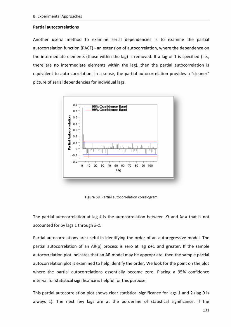
B. Experimental Approaches
131
Partial autocorrelations
Another useful method to examine serial dependencies is to examine the partial
autocorrelation function (PACF) - an extension of autocorrelation, where the dependence on
the intermediate elements (those within the lag) is removed. If a lag of 1 is specified (i.e.,
there are no intermediate elements within the lag), then the partial autocorrelation is
equivalent to auto correlation. In a sense, the partial autocorrelation provides a "cleaner"
picture of serial dependencies for individual lags.
Figure 59. Partial autocorrelation correlogram
The partial autocorrelation at lag k is the autocorrelation between Xt and Xt-k that is not
accounted for by lags 1 through k-1.
Partial autocorrelations are useful in identifying the order of an autoregressive model. The
partial autocorrelation of an AR(p) process is zero at lag p+1 and greater. If the sample
autocorrelation plot indicates that an AR model may be appropriate, then the sample partial
autocorrelation plot is examined to help identify the order. We look for the point on the plot
where the partial autocorrelations essentially become zero. Placing a 95% confidence
interval for statistical significance is helpful for this purpose.
This partial autocorrelation plot shows clear statistical significance for lags 1 and 2 (lag 0 is
always 1). The next few lags are at the borderline of statistical significance. If the

B. Experimental Approaches
132
autocorrelation plot indicates that an AR model is appropriate, we could start our evaluation
with an AR(2) model.
The partial autocorrelation plot can help provide answers to the following questions:
Is an AR model appropriate for the data?
If an AR model is appropriate, what order should we use?
Removing serial dependency
Serial dependency for a particular lag of k can be removed by differencing the series, that is
converting each i'th element of the series into its difference from the (i-k)''th element. There
are two major reasons for such transformations.
First, one can identify the hidden nature of seasonal dependencies in the series.
Autocorrelations for consecutive lags are interdependent, therefore, removing some of the
autocorrelations will change other auto correlations, that is, it may eliminate them or it may
make some other seasonality’s more apparent.
The other reason for removing seasonal dependencies is to make the series stationary which
is necessary for ARIMA and other techniques. In a time series analysis, a stationary series has
a constant mean, variance, and autocorrelation through time meaning that seasonal
dependencies have been removed via Differencing. In this transformation the series will be
transformed as: X=X-X(lag) and the resulting series will be of length N-lag where N is the
length of the original series.
ARIMA (Auto Regressive Integrated Moving Average)
The modeling and forecasting procedures requires knowledge about the mathematical
model of the process. However, in real-life research and practice, patterns of the data are
unclear, individual observations involve considerable error, and we still need not only to
uncover the hidden patterns in the data but also generate forecasts. The ARIMA

B. Experimental Approaches
133
methodology [Box and Jenkins, 1970] allows us to do just that. However, because of its
power and flexibility, ARIMA is a complex technique; it is not easy to use and it requires a
great deal of experience.
The general model includes autoregressive as well as moving average parameters, and
explicitly includes differencing in the formulation of the model. Specifically, the three types
of parameters in the model are: the autoregressive parameters (p), the number of
differencing passes (d), and moving average parameters (q). In the notation introduced by
Box and Jenkins, models are summarized as ARIMA (p, d, q); so, for example, a model
described as (0, 1, 2) means that it contains 0 (zero) autoregressive (p) parameters and 2
moving average (q) parameters which were computed for the series after it was differenced
once (d=1).
Parameter identification
As mentioned earlier, the input series for ARIMA needs to be stationary, that is, it should
have a constant mean, variance, and autocorrelation through time. Therefore, usually the
series first needs to be differenced until it is stationary (this also often requires log
transforming the data to stabilize the variance). The number of times the series needs to be
differenced to achieve stationarity is reflected in the d parameter. In order to determine the
necessary level of differencing, we should examine the plot of the data and the
autocorrelogram. Significant changes in level (strong upward or downward changes) usually
require first order non seasonal (lag=1) differencing; strong changes of slope usually require
second order non seasonal differencing. Seasonal patterns require respective seasonal
differencing. If the estimated autocorrelation coefficients decline slowly at longer lags, first
order differencing is usually needed. However, one should keep in mind that some time
series may require little or no differencing, and that over differenced series produce less
stable coefficient estimates, meaning less accuracy in the time series obtained
In addition we also need to decide how many autoregressive (AR)(p) and moving average
(MA)(q) parameters are necessary to yield an effective but still parsimonious model of the
process (parsimonious means that it has the fewest parameters and greatest number of

B. Experimental Approaches
134
degrees of freedom among all models that fit the data). In practice, the numbers of the p or
q parameters very rarely need to be greater than 2.
The major tools used in the identification phase are plots of the series, correlograms of auto
correlation (ACF), and partial autocorrelation (PACF). The decision is not straightforward and
in less typical cases requires not only experience but also a good deal of experimentation
with alternative models (as well as the technical parameters of ARIMA) [Pankratz, 1983].
However, a majority of empirical time series patterns can be sufficiently approximated using
one of the 5 basic models that can be identified based on the shape of the autocorrelogram
(ACF) and partial auto correlogram (PACF).
The following brief summary is based on practical recommendations of [Vandaele, 1983] and
additional practical advices from [McDowall, McCleary et al., 1980]. Since the number of
parameters (to be estimated) of each kind is almost never greater than 2, it is often practical
to try alternative models on the same data.
One autoregressive (p) parameter: ACF - exponential decay; PACF - spike at lag 1, no
correlation for other lags.
Two autoregressive (p) parameters: ACF - a sine-wave shape pattern or a set of
exponential decays; PACF - spikes at lags 1 and 2, no correlation for other lags.
One moving average (q) parameter: ACF - spike at lag 1, no correlation for other lags;
PACF - damps out exponentially.
Two moving average (q) parameters: ACF - spikes at lags 1 and 2, no correlation for
other lags; PACF - a sine-wave shape pattern or a set of exponential decays.
One autoregressive (p) and one moving average (q) parameter: ACF - exponential
decay starting at lag 1; PACF - exponential decay starting at lag 1.
Parameter estimation and forecasting
The estimates of the parameters are used in the last stage (Forecasting) to calculate new
values of the series (beyond those included in the input data set) and confidence intervals
for those predicted values. The estimation process is performed on transformed

B. Experimental Approaches
135
(differenced) data; before the forecasts are generated, the series needs to be integrated
(integration is the inverse of differencing) so that the forecasts are expressed in values
compatible with the input data. This automatic integration feature is represented by the
letter I in the name of the methodology (ARIMA = Auto-Regressive Integrated Moving
Average).
Seasonal models
Multiplicative seasonal ARIMA is a generalization and extension of the method introduced in
the previous paragraphs to series in which a pattern repeats seasonally over time. In
addition to the non-seasonal parameters, seasonal parameters for a specified lag
(established in the identification phase) need to be estimated. Analogous to the simple
ARIMA parameters, these are: seasonal autoregressive (ps), seasonal differencing (ds), and
seasonal moving average parameters (qs). For example, the model (0,1,2)(0,1,1) describes a
model that includes no autoregressive parameters, 2 regular moving average parameters
and 1 seasonal moving average parameter, and these parameters were computed for the
series after it was differenced once with lag 1, and once seasonally differenced. The seasonal
lag used for the seasonal parameters is usually determined during the identification phase
and must be explicitly specified.
The general recommendations concerning the selection of parameters to be estimated
(based on ACF and PACF) also apply to seasonal models. The main difference is that in
seasonal series, ACF and PACF will show sizable coefficients at multiples of the seasonal lag
(in addition to their overall patterns reflecting the non seasonal components of the series).
Model Evaluation
A good model should not only provide sufficiently accurate forecasts, it should also be
parsimonious and produce statistically independent residuals that contain only noise and no
systematic components (e.g., the correlogram of residuals should not reveal any serial
dependencies). A good test of the model is (a) to plot the residuals and inspect them for any

B. Experimental Approaches
136
systematic trends, and (b) to examine the autocorrelogram of residuals (there should be no
serial dependency between residuals). For the ARIMA model to be considered the residuals
should be systematically distributed across the series (e.g., they could be negative in the first
part of the series and approach zero in the second part). If they contain some serial
dependency, probably the ARIMA model is inadequate. The residuals estimation procedure
assumes that any resulting residual are not autocorrelated and that they are normally
distributed.
Figure 60. 4-Plot for residuals validation – Invalid ARIMA model
A good way to validate the residuals is to use the 4-Plot as it consists of the following:
1. Run sequence plot to test fixed location and variation.
Vertically: Yi
Horizontally: i
2. Lag Plot to test randomness.
Vertically: Yi
Horizontally: Yi-1
3. Histogram to test (normal) distribution.
Vertically: Counts

B. Experimental Approaches
137
Horizontally: Y
4. Normal probability plot to test normal distribution.
Vertically: Ordered Yi
Horizontally: Theoretical values from a normal N(0,1) distribution for ordered Yi
We evaluate and validate our models based on these techniques and assumptions. Figure 60
reveals the following:
1. the fixed location assumption is justified as shown by the run sequence plot in the
upper left corner.
2. the fixed variation assumption is justified as shown by the run sequence plot in the
upper left corner.
3. the randomness assumption is violated as shown by the non-random (oscillatory) lag
plot in the upper right corner.
4. the assumption of a common, normal distribution is violated as shown by the
histogram in the lower left corner and the normal probability plot in the lower right
corner. The distribution is non-normal and is a U-shaped distribution.
5. there are several outliers apparent in the lag plot in the upper right corner.

138
[ This page has been intentionally left blank ]