RESUMO
A mineração de dados é definida como o processo automático, ou semi-
automático de extração de conhecimento para identificação de padrões, tendências,
associações e dependências, previamente desconhecidos, de bases de dados, sendo
amplamente utilizada na transformação de dados brutos em conhecimento útil para a
tomada de decisões. Embora as técnicas empregadas em mineração de dados,
tradicionalmente, se baseiam fortemente em métodos estatísticos, em inteligência
artificial e em aprendizagem de máquina, vários dos métodos empregados podem ser
formulados como problemas de otimização. O presente projeto tem por objetivo fazer
uso de métodos de mineração de dados para identificar padrões temporais em atrasos
por congestionamento em aeroportos brasileiros. O transporte aéreo no Brasil foi
recentemente liberalizado e uma de suas consequências foi a concentração dos voos em
alguns hubs. Embora a criação de hubs pareça benéfica às empresas de transporte aéreo
e ofereça algumas vantagens aos viajantes, a concentração excessiva de voos em um
hub pode resultar em alguns impactos econômicos negativos denominados atrasos por
congestionamento, os quais aumentam o tempo total de viagem dos passageiros e o
custo operacional das empresas.
Palavras-chave: mineração de dados; atrasos por congestionamento; formação de
agrupamentos; análise de séries temporais; sistemas de alerta.

1. REALIZAÇÕES NO PERÍODO
Ao longo do segundo ano do projeto foram realizadas as etapas 6 e 7, conforme
o cronograma proposto no projeto de pesquisa submetido (Tabela 1). Assim, métodos de
mineração de dados foram utilizados na criação de um modelo de classificação para
detectar precocemente atrasos por congestionamento em aeroportos e foram elaborados
trabalhos para publicação.
Tabela 1: Cronograma de atividades do projeto proposto.
ATIVIDADE BIMESTRES
1 2 3 4 5 6 7 8 9 10 11 12
ATUALIZAÇÃO DA REVISÃO BIBLIOGRÁFICA * * * * * *
FORMAÇÃO E CONSISTÊNCIA DAS BASES DE DADOS * *
TRANSFORMAÇÃO DOS DADOS *
ANÁLISES PRELIMINARES E DISCUSSÃO DOS
RESULTADOS *
UTILIZAÇÃO DOS MÉTODOS DE MINERAÇÃO DE
DADOS PARA FORMAÇÃO DE AGRUPAMENTOS
TEMPORAIS
* *
RELATÓRIO PARCIAL *
UTILIZAÇÃO DOS MÉTODOS DE MINERAÇÃO DE
DADOS PARA CRIAÇÃO DE UM MODELO DE
CLASSIFICAÇÃO (UTILIZADOS DA DETECÇÃO
PRECOCE DE ATRASOS POR CONGESTIONAMENTO)
* * * *
TRABALHOS PARA PUBLICAÇÃO * * * * * *
RELATÓRIO FINAL * *
1.1 Criação de um modelo de classificação para detecção precoce de atrasos por
congestionamento.
A criação do modelo de classificação para detecção precoce de atrasos por
congestionamento seguiu um procedimento sequencial composto pelos passos: (1)
seleção e transformação dos dados e (2) criação do modelo e interpretação dos
resultados. Todas as análises foram executadas utilizando o software R, versão 3.1.1.
(pacotes RPART, PARTYKIT e STATS). Optou-se pela criação deste modelo para o
Aeroporto Internacional de São Paulo (GRU) pois é o maior aeroporto do Brasil. Outros
aeroportos como o Aeroporto de Congonhas e o Aeroporto de Brasília também foram
analisados no projeto pelos alunos Bruno Gomes Lima da Rocha e João Marcos de
Miranda em seus trabalhos de conclusão de curso (esses trabalhos estão indicados, neste
relatório, na seção ORIENTAÇÕES CONCLUÍDAS). Posteriormente, o modelo de
classificação criado foi utilizado em um sistema de alerta para antecipar a ocorrência de
dias com alta concentração de voos atrasados.
1.1.1 Seleção e transformação dos dados

As análises foram executadas utilizando dados fornecidos dela Agência Nacional
de Aviação Civil (ANAC). Para a construção do modelo utilizou-se os dados de janeiro
de 2010 a maio de 2014 e de agosto de 2014 a novembro de 2014. Os dados de junho de
2014 a julho de 2014 não foram fornecidos pela ANAC devido a mudanças no seu
sistema de autorização durante a Copa do Mundo no Brasil. Posteriormente, os dados de
dezembro de 2014 a dezembro de 2015 foram utilizados para validar o modelo criado.
A base de dados da ANAC possui todos os dados de voos domésticos e
internacional realizados e cancelados e inclui: aeroporto de origem, aeroporto de
destino, empresa aérea, data e horário programado de saída e de chegada, data e horário
realizado de saída e de chegada e a informação se o voo foi realizado ou cancelado
(incluindo uma justificativa se o voo foi cancelado ou atrasou mais de 30 minutos). Para
analisar os movimentos (pousos e decolagens) realizados no Aeroproto Internacional de
São Paulo, os dados relativos e este aeroporto foram selecionados. Para lidar com os
voos não programados, o horário de realização deste movimento foi também
considerado como o horário programado. Assim, os voos não programados foram
considerados sem atraso.
Os dados selecionados foram então transformados para gerar a variável resposta
e um conjunto de variáveis independentes (ou explicativas) para o modelo. A variável
resposta para este estudo é a fatia diária de movimentos atrasados do aeroporto.
Seguindo padrões internacionais, um voo foi considerado atrasado se este decolou ou
posou mais de 15 minutos depois do horário programado. A Figura 1 mostra a evolução
temporal da fatia diária de movimentos atrasados do Aeroporto Internacional de São
Paulo (GRU).
Figura 1 Fatia diária de movimentos atrasados no GRU.
Um sistema de alerta para antecipar dias com alta concentração de voos
atrasados é baseado na combinação de indicadores e alarmes. Em relação aos
indicadores, os determinantes de atraso identificados na literatura foram considerados

como potenciais variáveis independentes do modelo. A Tabela 1 lista as variáveis
independentes candidatas e suas definições.
Tabela 1 Variáveis independentes candidatas e suas definições.
Variável Definição
HHI Índice Herfindal-Hirschman de concentração
Av.Spacing Média diária do tempo entre movimentos consecutivos (em minutos)
Spacing.6t11 Tempo médio entre movimentação consecutivas das 6:00 às 11:00 (em
minutos)
Spacing.18t23 Tempo médio entre movimentação consecutivas das 18:00 às 23:00 (em
minutos)
Std.Spacing Desvio padrão diário do tempo médio entre movimentação consecutivas (em
minutos)
Av.ConMov Número médio diário de movimentações consecutivas do mesmo tipo (pousos
ou decolagens)
D.NewTerminal Variável dummy com valor 1 se o periodo for março de 2014 ou posterior e 0
caso contrário
Season Estação do ano em que o voo está rpogramado: Verão (dezembro-fevereiro),
Outono (março-maio), Inverno (junho-agosto), Primavera (setembro-
novembro)
Day of week Dia da semana em que o voo está rpogramado (domingo, segunda, terça,
quarta, quinta, sexta e sábado)
No que diz respeito as variáveis consideradas, o índice Herfindal-Hirschman de
concentração (HHI) mede a concentração de mercado em um aeroporto e é baseado na
fatia diária de voo das diferentes companhias aéreas que operam neste aeroporto
(Santos e Robin, 2010). A variável Av.Spacing é a média diária do tempo entre
movimentos consecutivos e de acordo com Abdel-Aty et al.(2007), a chance de voos
atrasarem decresce quando o valor desta variável aumenta. O Av.Spacing se relaciona à
demanda de um aeroporto, uma vez que pode ser estimada dividindo-se o número total
de movimentos programados no dia pelo número de minutos que um aeroporto está em
operação no dia. Entretanto, neste trabalho, o espaçamento entre movimentos
consecutivos foi utilizando não apenas para estimar o Av.Spacing como também para
estimar seu desvio padrão (Std.Spacing), visando considerar a variabilidade deste valor.
O tempo médio entre movimentação consecutivas das 6:00 às 11:00 (pico da manhã) e
das 18:00 às 23:00 (pico noturno) também foram considerados como candidatos a
variável independente do modelo.
A variável Av.ConMov é número médio diário de movimentações consecutivas
do mesmo tipo (pousos ou decolagens) e foi criada para se levar em consideração o mix
de pousos e decolagens consecutivos. A variável dummy (D.NewTerminal) foi criada
para estimar o efeito do novo terminal de passageiros inaugurado no Aeroporto
Internacional de São Paulo em março de 2014. Em relação as variáveis estação do ano
(Season) e dia da semana (Day of week), de acordo com os resultados obtidos por

Abdel-Aty et al. (2007), há padrões de atrasos sazonais e semanais que precisam ser
considerados.
Outros fatores dominantes de atrasos em aeroportos existentes na literatura,
como condições climáticas e capacidade da pista, não foram considerados como
candidatas a variáveis independentes do modelo (e possíveis indicadores do sistema de
alerta) pois seus valores não podem ser antecipados com pelo menos uma semana de
antecedência.
1.1.2 Construção do modelo e interpretação
Com os candidatos a indicadores do sistema de alerta identificados, a próxima
tarefa foi a criação do procedimento de previsão. Neste trabalho, optou-se por empregar
uma composição de especialistas (MEM) considerando: (1) Árvore de regressão e
classificação - CART; (2) Regressão linear múltipla; (3) Modelo de séries temporais. Os
diferentes especialistas empregados se baseiam em diferentes hipóteses em relação aos
dados disponíveis e foram empregados anteriormente na criação de sistemas de alerta de
padrões de demanda em transporte aéreo (Scarpel, 2014), na identificação de
determinantes de atraso em aeroportos (Santos and Robin, 2010; Abdel-Aty et al., 2007)
ou na previsão de atrasos (Rebollo and Balakrishnan, 2014).
1.1.2.1 Árvore de regressão e classificação (CART)
O CART é um especialista apropriado quando interpretabilidade do modelo é
uma questão relevante. Assim, este modelo foi escolhido para gerar um procedimento
de previsão que permita entender como os determinantes de atraso se combinam para
gerar um dia com alta concentração de voos atrasados e para antecipar a ocorrência de
tais dias. No CART, a seleção das variáveis independentes e a tarefa de regressão são
realizados simultaneamente.
Para evitar sobreajuste, as decisões relacionadas a necessidade de poda da árvore
e a determinação do tamanho ideal da árvore foram feitas utilizando um procedimento
de validação cruzada 10-fold. Desta forma, os dados foram particionados em 10
subamostras e o modelo foi treinado 10 vezes, cada vez deixando uma das subamostras
de fora do conjunto de treinamento, e utilizando apenas esta subamostra para estimar o
erro de previsão. Posteriormente o erro de previsão total foi computado como a média
dos erros de previsão estimados.
Um método usual para determinar o tamanho ideal da árvore é considerar a regra
"um desvio padrão". Por esta regra, o tamanho ideal da árvore será aquele em que o erro
estimado no pelo procedimento de validação cruzada estiver próximo ao mínimo erro
estimado na validação cruzada somado a um desvio padrão (Scarpel, 2014). A Figura 2
mostra o erro estimado pelo procedimento de validação cruzada versus um parâmetro de
complexidade (cp) associado ao tamanho da árvore (com uma linha pontilhada
indicando o valor do nível de erro da regra "um desvio padrão"). O parâmetro de
complexidade (cp) mede quanto de acurácia ema partição da árvore fornece e é
estimada como uma combinação linear da soma dos erros ao quadrado e do tamanho da
árvore (número de nós terminais).

Pela Figura 2, aplicando a regra "um desvio padrão", verifica-se que o tamanho
ideal da árvore é 6, ou seja, esta deve ter 6 nós terminais. A Figura 3 mostra a árvore
podada (com 6 nós terminais) e as estatísticas do modelo são disponibilizadas na Tabela
2.
Figura 2 Erro estimado no procedimento de validação cruzada versus o parâmetro de
complexidade (cp).
Figure 3 Árvore de regressão com 6 nós terminais para prever a fatia de voos atrasados
em um dia.
Para avaliar a distribuição diária dos movimentos, os dias alocados a cada um
dos nós terminais foram processados para estimar o número de movimentos horários em
janelas móveis de 20 minutos. A Figura 4 mostra as distribuições diárias obtidas dos
movimentos programados e realizados e a Tabela 3 mostra o número médio diário e o
número médio das 7:00 às 22:00 dos movimentos por hora programados e realizados
para os dias alocados em cada um dos nós terminais.

Tabela 2 Estatísticas do modelo CART.
Model Statistics Node number Mean MSE
Terminal nodes: 6 4 0.161 0.004
Number of splits: 5 5 0.200 0.006
R-Square: 0.307 6 0.300 0.011
Relative error: 0.693 8 0.246 0.006
Cross-validation error: 0.745 10 0.274 0.009
Cross-validation std: 0.031 11 0.384 0.009
Figura 4 Distribuição diária dos movimentos programados e realizados: (a) nó terminal
4; (b) nó terminal 5; (c) nó terminal 6; (d) nó terminal 8; (e) nó terminal 10; (f) nó
terminal 11.
A partir dos resultados apresentados na Figura 4, é possível observar que as
variáveis independentes utilizados na construção da árvore de regressão foram HHI,
Av.Spacing, Std.Spacing e Av.ConMov. Sabendo que a variáveis independente mais
relevante é selecionada na primeira partição (topo da árvore), é possível indicar que a
0
5
10
15
20
25
30
35
40
45
50
0,6
7
1,3
3 2
2,6
7
3,3
3 4
4,6
7
5,3
3 6
6,6
7
7,3
3 8
8,6
7
9,3
3
10
10
,67
11
,33
12
12
,67
13
,33
14
14
,67
15
,33
16
16
,67
17
,33
18
18
,67
19
,33
20
20
,67
21
,33
22
22
,67
23
,33
24
Movim
ents/h
Hour
Scheduled
Actual
Upper 95%
Lower 95%
a
0
5
10
15
20
25
30
35
40
45
50
0,6
7
1,3
3 2
2,6
7
3,3
3 4
4,6
7
5,3
3 6
6,6
7
7,3
3 8
8,6
7
9,3
3
10
10
,67
11
,33
12
12
,67
13
,33
14
14
,67
15
,33
16
16
,67
17
,33
18
18
,67
19
,33
20
20
,67
21
,33
22
22
,67
23
,33
24
Movim
ents/h
Hour
Scheduled
Actual
Upper 95%
Lower 95%
b
0
5
10
15
20
25
30
35
40
45
50
0,6
7
1,3
3 2
2,6
7
3,3
3 4
4,6
7
5,3
3 6
6,6
7
7,3
3 8
8,6
7
9,3
3
10
10
,67
11
,33
12
12
,67
13
,33
14
14
,67
15
,33
16
16
,67
17
,33
18
18
,67
19
,33
20
20
,67
21
,33
22
22
,67
23
,33
24
Movim
ents/h
Hour
Scheduled
Actual
Upper 95%
Lower 95%
c
0
5
10
15
20
25
30
35
40
45
50
0,6
7
1,3
3 2
2,6
7
3,3
3 4
4,6
7
5,3
3 6
6,6
7
7,3
3 8
8,6
7
9,3
3
10
10
,67
11
,33
12
12
,67
13
,33
14
14
,67
15
,33
16
16
,67
17
,33
18
18
,67
19
,33
20
20
,67
21
,33
22
22
,67
23
,33
24
Movim
ents/h
Hour
Scheduled
Actual
Upper 95%
Lower 95%
d
0
5
10
15
20
25
30
35
40
45
50
0,6
7
1,3
3 2
2,6
7
3,3
3 4
4,6
7
5,3
3 6
6,6
7
7,3
3 8
8,6
7
9,3
3
10
10
,67
11
,33
12
12
,67
13
,33
14
14
,67
15
,33
16
16
,67
17
,33
18
18
,67
19
,33
20
20
,67
21
,33
22
22
,67
23
,33
24
Movim
ents/h
Hour
Scheduled
Actual
Upper 95%
Lower 95%
e
0
5
10
15
20
25
30
35
40
45
50
0,6
7
1,3
3 2
2,6
7
3,3
3 4
4,6
7
5,3
3 6
6,6
7
7,3
3 8
8,6
7
9,3
3
10
10
,67
11
,33
12
12
,67
13
,33
14
14
,67
15
,33
16
16
,67
17
,33
18
18
,67
19
,33
20
20
,67
21
,33
22
22
,67
23
,33
24
Movim
ents/h
Hour
Scheduled
Actual
Upper 95%
Lower 95%
f

fatia de voos atrasados em um dia qualquer está muito relacionada a concentração de
mercado no aeroporto. As outras variáveis independentes utilizadas na criação da árvore
de regressão estão relacionadas a demanda (Av.Spacing and Std.Spacing) e ao mix de
pousos e decolagens (Av.ConMov).
Tabela 3 Número médio diário e o número médio das 7:00 às 22:00 dos movimentos
por hora programados e realizados para os dias alocados em cada um dos nós terminais.
Movimentos médios / h Nó 4 Nó 5 Nó 6 Nó 8 Nó 10 Nó 11
Programados Diário 29,80 31,39 33,34 30,44 32,83 32,98
Das 7:00 às 22:00 36,14 37,55 39,26 36,52 38,17 38,19
Realizados Diário 28,84 29,60 32,39 27,74 29,13 29,03
Das 7:00 às 22:00 34,96 35,37 37,35 33,44 34,56 34,12
Muitos autores indicam que a concentração de mercado em um aeroporto é um
importante determinante de atraso. De acordo com Mayer e Sinai (2003), aeroportos
com maior concentração de mercado atrasam menos os voos porque os
sequenciamentos dos voos são realizados para gerar menos atrasos em aeroportos em
que a maior parte dos voos são operados por uma única empresa. Santos e Robin (2010)
também identificaram em seu estudo que voos originados ou com destino a aeroportos
com menor concentração de mercado atrasam mais. Entretanto, de acordo com esses
autores, os atrasos são menores em aeroportos com alta concentração de mercado
porque as companhias aéreas internalizam o congestionamento dos aeroportos. Para
reduzir atrasos em dias de baixa concentração de mercado, como há maior diversidade
de companhias aéreas operando e a demanda excede a capacidade disponível, uma
alternativa é a coordenação dos slots. O Aeroporto Internacional de São Paulo é um
aeroporto com programação dos voos facilitada (Nível 2). Nos aeroportos nível 2,
cooperação e alterações na programação voluntárias são necessárias para evitar
congestionamento. A principal meta com a coordenação dos slots é regular o acesso à
infraestrutura existente e assim adaptar a demanda por serviços aéreos à capacidade
disponível no aeroporto.
A partir da Figura 4 e Tabelas 2 e 3 é possível verificar que o nó terminal com o
maior valor para a variável resposta é o nó 11 (Ŷ=38,4%). Este nó terminal é obtido
quando a concentração de mercado é baixa (HHI < 18.46%), a média diária do número
de voos programados por hora é maior que 32,98 (Av.Spacing < 1.825) e o número
médio de voos consecutivos do mesmo tipo (pousos e decolagens) é menor que 2,07. A
análise da distribuição diária dos movimentos programados e realizados (Figura 4)
mostra que há uma considerável distância entre essas distribuições nos dias alocados ao
nó terminal 11 (Figura 4.f).
Quanto ao nó terminal 10, a única diferença entre os dias atribuídos a este nó e
os dias atribuídos ao nó terminal 11 é o número médio de voos consecutivos do mesmo
tipo (Av.ConMov). Como o valor médio para a variável resposta (Ŷ) é 11,0% inferior
ao do nó 11, é possível indicar que a melhoria no sequenciamento dos voos pelo
aumento do número de movimentos consecutivo do mesmo tipo (pousos ou decolagens)
também pode ser considerada como uma alternativa para se reduzir os atrasos.

O nó terminal com o menor valor médio para a variável resposta é o nó 4
(Ŷ=16,1%). A partir da Tabela 3 é possível verificar que é o nó com a menor demanda
por voos e pela Figura 4.a é possível observar que ao longo do dia há uma pequena
distância entre a distribuição dos movimentos programados e realizados. O nó terminal
4 é obtido quando a concentração de mercado no aeroporto é alta (HHI ≥ 20.9%) e o
desvio padrão do tempo entre movimentos programados consecutivos (Std.Spacing) é
maior que 2,59 minutos. Maiores valores de Std.Spacing são esperados em períodos de
baixa demanda pois o número de movimentos programados é alto apenas nos horários
de pico. Este resultados está de acordo com a literatura uma vez que espera-se menores
atrasos quando a concentração de mercado é maior e a demanda não é alta. Assim, os
dias que foram alocados ao nó terminal 4 podem ser considerados como dias comuns
com baixa movimentação e com a maio parte dos voos realizados pelas 3 maiores
companhias aéreas brasileiras (Azul, Gol e TAM).
O maior nó terminal, em termos de números de dias alocados, é o nó 5 (899
observações). Este nó é obtido quando a concentração de mercado no aeroporto (HHI)
está entre 18,46% e 20,9% e o Std.Spacing é maior que 2,59 minutos. O seu valor
médio para a variável resposta (Ŷ) é 20,0% e a partir da Figura 4.b é possível verificar
que, ao longo do dia, há uma pequena distância entre a distribuição dos voos
programados e realizados.
O nó terminal 6 é o segundo maior em termos de valor médio da variável
resposta (Ŷ). Tal nó é obtido quando o valor de HHI é maior que 18,46% e o valor de
Std.Spacing é menor que 2,59 minutos. A partir da Tabela 3 verifica-se que este nó
terminal concentra os dias com mais alta demanda (média diária de movimentos
programados por hora maior que 33,34) e pela Figura 4.c verifica-se que há uma
movimentação realizada maior que a programada até as 3:00 da manhã, possivelmente
devido a voos atrasados no dia anterior.
O último nó terminal é o número 8. Este nó é obtido quando o valor de HHI é
menos que 18,46% e a demanda é baixa (média diária de movimentos programados por
hora de 30,44 e Av.Spacing ≥ 1,825).
1.1.2.2 Regressão Linear Múltipla (MLR)
A MLR é possivelmente o especialista mais utilizado devido à sua simplicidade
e disponibilidade. De acordo com Kutner et al. (2004), a MLR é uma abordagem
estatística que visa modelar uma variável resposta (Y) utilizando uma função linear
ponderada de um conjunto de variável independentes (X1, X2, ...,Xl) e um termo de erro
ε. Assume-se que o termo de erro seja não correlacionado e seja distribuído conforme
uma gaussiana com média zero e variância (σ2) constante. Os coeficientes da regressão
são comumente estimados utilizando o método dos mínimos quadrados (OLS).
Como mencionado anteriormente, a MLR foi utilizada anteriormente para
identificar os determinantes de atraso em aeroportos (Santos and Robin, 2010; Abdel-
Aty et al., 2007) e em previsão de previsão de atrasos (Rebollo and Balakrishnan,
2014). Este especialista foi criado seguindo os passos sugeridos por Kutner et al.
(2004). Desta forma foi empregado um procedimento de seleção de variáveis para obter

uma sugestão de modelo de regressão. Os resíduos obtidos a partir da aplicação do
modelo estimado foram utilizados para a validação do modelo (etapa final). Neste
trabalho, as variáveis independentes foram selecionadas usando um procedimento
stepwise e o modelo sugerido foi
ii9i8i7i6
i5i4i3i2i10i
WinterConMov.AvFridayMonday
SundayTerminalNew.DSpacing.AvSummerHHIY
Os resultados obtidos são apresentados na Tabela 4 e a Figura 5 mostra os gráficos
obtidos na análise dos resíduos. Pela Tabela 4 é possível verificar que as variáveis
independentes HHI, Av.Spacing e Av.ConMov ficaram com sinal negativo, indicando
que uma menor fatia de voos atrasados é esperada nos dias com maior concentração de
mercado no aeroporto, quando a demanda é menor e quando são sequenciados mais
voos do mesmo tipo. Tais resultados estão de acordo com os resultados obtidos pelo
CART e reforçam as sugestões feitas para reduzir a fatia de voos atrasados no
aeroporto. O coeficiente de D.NewTerminal também ficou negativo sugerindo que a
fatia de voos atrasados reduziu após a inauguração do novo terminal de passageiros em
março de 2014. Em relação as variáveis que ficaram com sinal positivo, os resultados
obtidos sugerem que maiores fatias de voos atrasados são esperadas no verão e inverno
e no domingo, segunda-feira e sexta-feira.
Tabela 4 Coeficientes da regressão linear estimados, desvio padrão, valor-P e
estatísticas de sumarização da MLR.
Coeficiente da
Regressão Valor estimado
Desvio padrão
estimado Valor-P
0 0,869 0,049 0,000
1 -2,073 0,115 0,000
2 0,055 0,005 0,000
3 -0,109 0,016 0,000
4 -0,032 0,007 0,000
5 0,035 0,006 0,000
6 0,025 0,006 0,000
7 0,021 0,005 0,000
8 -0,033 0,017 0,060
9 0,009 0,005 0,044
R 0,271
R2 ajustado 0,267
Erro padrão 0,076
Os gráficos da análise de resíduos (Figura 5) são utilizados para validar o
modelos de regressão obtido, ou seja, se este está aderente às hipóteses de um modelo
de regressão. Como os gráficos de resíduos obtidos (Residuals vs Fitted and Scale-
Location) não mostram um padrão nos pontos e o gráfico de probabilidade normal
(Normal Q-Q) dos resíduos mostra uma razoável concordância entre os quantis teórico e
amostral, é possível afirmar que o modelo de regressão linear obtido pode ser
considerados apropriado.

Figura 5 Gráficos de análise dos resíduos: Resíduos vs Ajustado (Residuals vs Fitted);
Normal Q-Q; Scale-Location.
1.1.2.3 Modelo de séries temporais
Os modelos de séries temporais são utilizados como especialistas quando o
interesse é criar uma previsão baseada somente no comportamento passado da variável
de interesse. Neste trabalho o método de Box-Jenkins (1970) foi empregado na criação
de um modelo para prever o comportamento futura da fatia de movimentos atrasados
em um dia. O modelo desenvolvido usando este método é chamado de auto-regressivo
integrado com médias móveis, ARIMA(p,d,q), em que p é a ordem do componente
auto-regressivo (AR), o d é o grau de diferenciação da série temporal e q é a ordem do
componente de médias móveis (MA). Os modelo ARIMA(p,d,q) são amplamente
utilizados nos campos da estatística e econometria e são criados seguindo os passos: (1)
Identificação do modelo, (2) Estimação dos parâmetros e (3) Verificação de
diagnóstico.
De acordo com Enders (2004), no passo da identificação o pesquisador
visualmente examina o gráfico de função de autocorrelação serial (ACF) e da função de
autocorrelação parcial (PACF). A comparação do ACF e do PACF com os diferentes
processos ARIMA teóricos pode sugerir alguns modelos plausíveis. No passo de
estimação dos parâmetros, cada um dos modelos tentativos é ajustado e os diferentes
coeficientes estimados são examinados. Assim os modelos ajustados são comparados
utilizando o princípio da parcimônia. Box e Jenkins argumentam que modelos
parcimonioso produzem melhores previsões que modelos super parametrizados. Assim
um modelo considerado parcimonioso ajusta bem os dados sem incorporar coeficientes
desnecessários (Enders, 2004). Neste trabalho o critério de informação Akaike (AIC) foi
usado para comparar os modelos tentativos seguindo este princípio.
O terceiro passo do método de Box-Jenkins envolve a verificação de
diagnóstico. De acordo com Enders (2004), é particularmente importante que os
resíduos de um modelo estimado sejam serialmente não correlacionados. Assim,

qualquer modelo tentativo que não gere resíduos não aleatórios deve ser eliminado.
Neste trabalho, a verificação do diagnóstico foi realizada utilizando o p-valor da
estatística Ljung-Box. A estatística Ljung-Box (Ljung e Box, 1978) examina se os
resíduos são independentemente distribuídos e é comumente utilizada para verificar a
adequação de modelos de séries temporais ajustados.
O melhor modelo encontrado seguindo o método de Box-Jenkins foi o
ARIMA(1,0,0)(2,1,0)7. Assim, é um modelo ARIMA sazonal que pode ser expresso por
t15-t318-t2114-t37-t21-t17-tt εYθθYθθYθYθYθYY
em que Yt é a fatia diária de movimentos atrasados no dia t, j (j=1,...,3) são os
parâmetros do modelo (estimados usando o método dos mínimos quadrados) e εt é o
termo de erro aleatório. Os valores estimados para os parâmetros 1, 2 and 3 foram
0,493 (erro padrão = 0,02), -0,632 (erro padrão = 0,02) e -0.316 (erro padrão = 0,02),
respectivamente. O p-valor obtido no teste dos resíduos Ljung–Box foi 0,9128. Deste
forma, pode ser indicado que os resíduos do modelo obtido são aleatórios e que o
modelo se ajusta muito bem aos dados.
Em relação aos uso do modelo ARIMA sazonal obtido como um especialista
para a mistura de especialistas (MEM), o objetivo é criar dois MEMs, um para antecipar
dias congestionados com 1 dia de antecedência e outro com uma semana (7 dias) de
antecedência. Assim, o modelo obtido foi utilizado para gerar previsões um dia adiante
(Ŷt+1) e sete dias adiante (Ŷt+7).
1.1.3 Função de composição e performance de previsão da composição de especialistas
(MEM)
Para concluir a criação do MEM, o passo final é a construção da função de
composição. A função de composição é responsável por promover um esquema de
aprendizagem cooperativo combinando os especialistas para obter um modelo mais
flexível e poderoso. Neste trabalho, como função de composição dos especialistas foi
utilizada a função softmax expressa por
SARIMAMLRCARTl
j
l
j,,c,
xwexp
xwexp
gk
1c 1
ji,jc,
1
ji,jc,
ci,
em que xi,j é o valor da observação i da variável independente j e wc,j são os parâmetros
de composição. Em relação às variáveis empregadas na função softmax, neste trabalho
foram empregadas somente as variáveis significativas da regressão linear múltipla e os
valores dos parâmetros de composição foram estimados minimizando-se a função erro
expressa por
n
1i
2
SARIMAi,iSARIMAi,
2
MLRi,iMLRi,
2
CARTi,iCARTi, YY2
1expgYY
2
1expgYY
2
1expglog
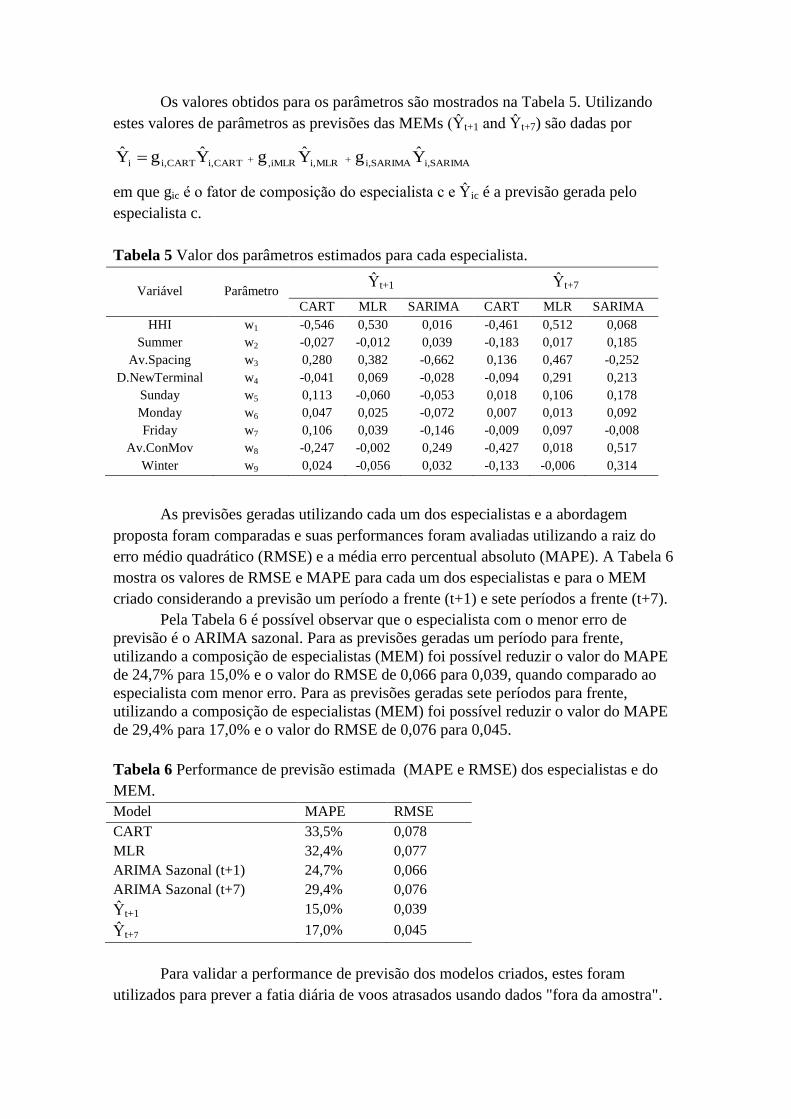
Os valores obtidos para os parâmetros são mostrados na Tabela 5. Utilizando
estes valores de parâmetros as previsões das MEMs (Ŷt+1 and Ŷt+7) são dadas por
SARIMAi,SARIMAi,MLRi,iMLR,CARTi,CARTi,i YgYgYgY
em que gic é o fator de composição do especialista c e Ŷic é a previsão gerada pelo
especialista c.
Tabela 5 Valor dos parâmetros estimados para cada especialista.
Variável Parâmetro Ŷt+1 Ŷt+7
CART MLR SARIMA CART MLR SARIMA
HHI w1 -0,546 0,530 0,016 -0,461 0,512 0,068
Summer w2 -0,027 -0,012 0,039 -0,183 0,017 0,185
Av.Spacing w3 0,280 0,382 -0,662 0,136 0,467 -0,252
D.NewTerminal w4 -0,041 0,069 -0,028 -0,094 0,291 0,213
Sunday w5 0,113 -0,060 -0,053 0,018 0,106 0,178
Monday w6 0,047 0,025 -0,072 0,007 0,013 0,092
Friday w7 0,106 0,039 -0,146 -0,009 0,097 -0,008
Av.ConMov w8 -0,247 -0,002 0,249 -0,427 0,018 0,517
Winter w9 0,024 -0,056 0,032 -0,133 -0,006 0,314
As previsões geradas utilizando cada um dos especialistas e a abordagem
proposta foram comparadas e suas performances foram avaliadas utilizando a raiz do
erro médio quadrático (RMSE) e a média erro percentual absoluto (MAPE). A Tabela 6
mostra os valores de RMSE e MAPE para cada um dos especialistas e para o MEM
criado considerando a previsão um período a frente (t+1) e sete períodos a frente (t+7).
Pela Tabela 6 é possível observar que o especialista com o menor erro de
previsão é o ARIMA sazonal. Para as previsões geradas um período para frente,
utilizando a composição de especialistas (MEM) foi possível reduzir o valor do MAPE
de 24,7% para 15,0% e o valor do RMSE de 0,066 para 0,039, quando comparado ao
especialista com menor erro. Para as previsões geradas sete períodos para frente,
utilizando a composição de especialistas (MEM) foi possível reduzir o valor do MAPE
de 29,4% para 17,0% e o valor do RMSE de 0,076 para 0,045.
Tabela 6 Performance de previsão estimada (MAPE e RMSE) dos especialistas e do
MEM.
Model MAPE RMSE
CART 33,5% 0,078
MLR 32,4% 0,077
ARIMA Sazonal (t+1) 24,7% 0,066
ARIMA Sazonal (t+7) 29,4% 0,076
Ŷt+1 15,0% 0,039
Ŷt+7 17,0% 0,045
Para validar a performance de previsão dos modelos criados, estes foram
utilizados para prever a fatia diária de voos atrasados usando dados "fora da amostra".
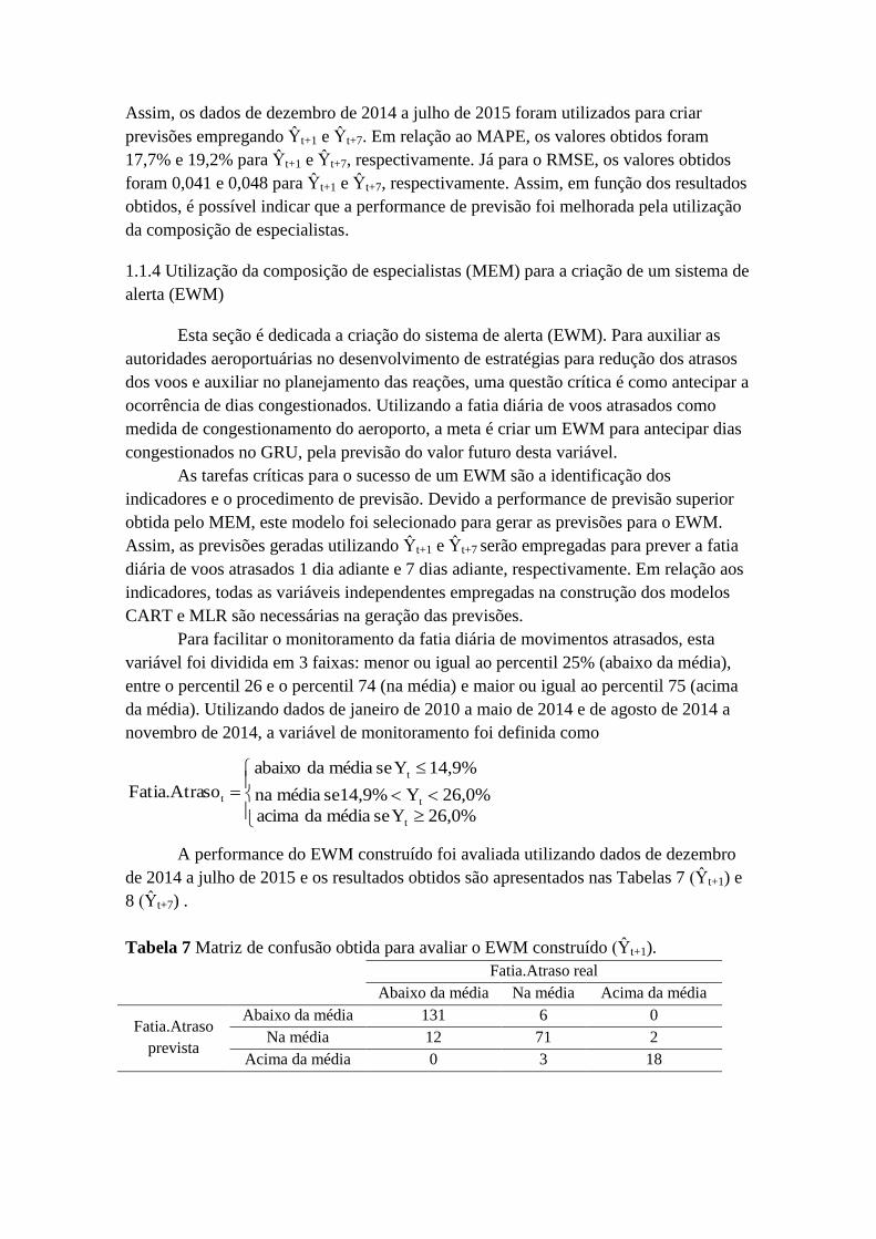
Assim, os dados de dezembro de 2014 a julho de 2015 foram utilizados para criar
previsões empregando Ŷt+1 e Ŷt+7. Em relação ao MAPE, os valores obtidos foram
17,7% e 19,2% para Ŷt+1 e Ŷt+7, respectivamente. Já para o RMSE, os valores obtidos
foram 0,041 e 0,048 para Ŷt+1 e Ŷt+7, respectivamente. Assim, em função dos resultados
obtidos, é possível indicar que a performance de previsão foi melhorada pela utilização
da composição de especialistas.
1.1.4 Utilização da composição de especialistas (MEM) para a criação de um sistema de
alerta (EWM)
Esta seção é dedicada a criação do sistema de alerta (EWM). Para auxiliar as
autoridades aeroportuárias no desenvolvimento de estratégias para redução dos atrasos
dos voos e auxiliar no planejamento das reações, uma questão crítica é como antecipar a
ocorrência de dias congestionados. Utilizando a fatia diária de voos atrasados como
medida de congestionamento do aeroporto, a meta é criar um EWM para antecipar dias
congestionados no GRU, pela previsão do valor futuro desta variável.
As tarefas críticas para o sucesso de um EWM são a identificação dos
indicadores e o procedimento de previsão. Devido a performance de previsão superior
obtida pelo MEM, este modelo foi selecionado para gerar as previsões para o EWM.
Assim, as previsões geradas utilizando Ŷt+1 e Ŷt+7 serão empregadas para prever a fatia
diária de voos atrasados 1 dia adiante e 7 dias adiante, respectivamente. Em relação aos
indicadores, todas as variáveis independentes empregadas na construção dos modelos
CART e MLR são necessárias na geração das previsões.
Para facilitar o monitoramento da fatia diária de movimentos atrasados, esta
variável foi dividida em 3 faixas: menor ou igual ao percentil 25% (abaixo da média),
entre o percentil 26 e o percentil 74 (na média) e maior ou igual ao percentil 75 (acima
da média). Utilizando dados de janeiro de 2010 a maio de 2014 e de agosto de 2014 a
novembro de 2014, a variável de monitoramento foi definida como
26,0%Ysemédiada acima
26,0%Y14,9%semédiana
14,9%Ysemédiada abaixo
soFatia.Atra
t
t
t
t
A performance do EWM construído foi avaliada utilizando dados de dezembro
de 2014 a julho de 2015 e os resultados obtidos são apresentados nas Tabelas 7 (Ŷt+1) e
8 (Ŷt+7) .
Tabela 7 Matriz de confusão obtida para avaliar o EWM construído (Ŷt+1).
Fatia.Atraso real
Abaixo da média Na média Acima da média
Fatia.Atraso
prevista
Abaixo da média 131 6 0
Na média 12 71 2
Acima da média 0 3 18

Tabela 8 Matriz de confusão obtida para avaliar o EWM construído (Ŷt+7).
Fatia.Atraso real
Abaixo da média Na média Acima da média
Fatia.Atraso
prevista
Abaixo da média 120 7 0
Na média 23 67 3
Acima da média 0 6 17
Pelas Tabelas 7 e 8 é possível verificar que Ŷt+1 antecipou corretamente 220 dos
243 dias e que Ŷt+7 antecipou corretamente 204 dos 243 dias. Assim, a acurácia do
EWM criado foi de 90,5% na antecipação do valor de Fatia.Atraso 1 dia adiante e de
83,9% na antecipação 7 dias adiante. Desta forma, é possível indicar que o EWM
desenvolvido possui uma boa capacidade de antecipação dos congestionamentos do
Aeroporto Internacional de São Paulo.
2. APLICAÇÃO DOS RECURSOS DE RESERVA TÉCNICA E BENEFÍCIOS
COMPLEMENTARES
Ao longo do segundo ano do projeto não foi utilizado nenhum recurso de custeio, de
reserva técnica ou de benefícios complementares.
3. LISTA DE TRABALHOS PREPARADOS OU SUBMETIDOS
3.1) Artigos em revistas científicas indexadas (os artigos completos submetidos
encontram-se nos anexos):
Inicialmente foi formulado e submetido ao periódico Transportation Research -
Part C: Emerging Technologies um artigo em que o método CART foi utilizado na
detecção de padrões e antecipação de atrasos e cancelamentos no Aeroporto
Internacional de São Paulo. O artigo se intitula A data analytics approach for
identification and anticipation of daily delay and cancellation patterns e se encontra no
Anexo A deste relatório.
Em função do pedido de revisão recebido, fiz a opção por mudar o foco do
artigo e concentrar os esforços na detecção precoce de atrasos no Aeroporto
Internacional de São Paulo (não mais atrasos e cancelamentos) e no artigo revisado
constam todas as alternativas de modelagem consideradas (CART, MLR, ARIMA e
MEM). O artigo revisado se intitula A data analytics approach for anticipating
congested days at the São Paulo International Airport e se encontra no Anexo B deste
relatório.

5. ORIENTAÇÕES CONCLUÍDAS
5.1) Trabalhos de conclusão de curso (graduação):
RESUMO DO TRABALHO DE GRADUAÇÃO:
O atraso em aeroportos é um importante tema no transporte aéreo e comumente é
analisado sob diferentes perspectivas como na previsão de atrasos e na estimativa dos
custos relativos aos atrasos. Contudo, a avaliação dos determinantes de atraso ainda é
pouco explorada. O objetivo desse trabalho é testar um conjunto de variáveis (índices de
concentração de mercado, movimentação total de aeronaves, condições climáticas e
fluxo de passageiros) que podem explicar os atrasos, representado pelos indicadores
tempo total de atraso e fatia de voos atrasados). Para a implementação desse estudo, foi
escolhido o Aeroporto de São Paulo/Congonhas, um dos aeroportos mais importantes
do Brasil em termos de movimentação de passageiros. Para analisar o relacionamento
entre as variáveis, o estudo apresenta duas diferentes metodologias: análise de regressão
(para análises univariadas) e árvores de inferência condicional (para análises
multivariadas). Em geral, os modelos univariados tiveram um mau desempenho em
vários testes estatísticos (teste de correlação, R² ajustado e análise de resíduos), porém

conclusões acerca das variáveis podem ser tomadas. Por outro lado, a análise
multivariada selecionou apenas três dos determinantes como as melhores variáveis
explicativas para os indicadores de atraso. Finalmente, a comparação entre as variáveis
e uma breve investigação sobre cada uma delas provê informações suficientes para
futuros trabalhos nesse tópico.
RESUMO DO TRABALHO DE GRADUAÇÃO:
Este trabalho tem como objetivo principal utilizar métodos de formação de
agrupamentos em análise de dados para a identificação de perfis de atrasos em voos no
Aeroporto Internacional de Brasília. Para isso, foram avaliadas todas as movimentações,
tanto previstas como efetivamente realizadas, de voos no aeroporto durante o período
que vai de janeiro de 2010 a maio de 2014. Todos os voos com diferença superior a 15
minutos entre o momento real e o previsto de sua movimentação na pista do aeroporto
foram considerados como atrasados. Foram criados, através de técnicas hierárquicas de
agrupamentos, grupos de dias com perfis semelhantes de movimentações previstas, de
movimentações realizadas e de índices horários de atrasos, de modo a identificar
possíveis padrões temporais que caracterizassem a formação desses agrupamentos.
Enquanto tais padrões parecem emergir nos primeiros grupos citados, não há evidência

clara que haja quaisquer padrões na divisão dos dias de acordo com seus perfis de
atraso.
REFERÊNCIAS BIBLIOGRÁFICAS
Abdel-Aty, M., Lee, C., Bai, Y. Li, X. e Michalak, M., Detecting periodic patterns of
arrival delay. Journal of Air Transport Management, 13, 355-361, 2007.
Box, G.E.P. e Jenkins, G., Time Series Analysis: Forecasting and Control. Holden-
Day, San Francisco, 1970.
Enders, W., Applied Econometric Time Series, 2nd
edition. New York: John Wiley &
Sons, 2004.
Kutner, M.H., Nachtsheim, C.J. e Neter, J., Applied Linear Regression Models, 4th
edition. Boston: McGraw-Hill Irwin, 2004.
Ljung, G., Box G. E. P., On a Measure of Lack of Fit in Time Series Models.
Biometrika, 66, 67–72, 1976.
Mayer, C., Sinai, T., Network effects, congestion externalities, and air traffic delays: Or
why not all delays and created evil. The American Economic Review, 93(4), 1194 -
1215, 2003.
Rebollo, J. J. e Balakrishnan, H., Characterization and prediction of air traffic delays.
Transportation Research Part C, 44, 231-241, 2014.
Santos, G. e Robin, M., Determinants of delays at European airports. Transportation
Research Part B, 44(3), 392-403, 2010.
Scarpel, R. A., A demand trend change early warning forecast model for the city of São
Paulo multi-airport system. Transportation Research Part A: Policy and Practice,
65, 23-32, 2014.

ANEXO A
Artigo "A data analytics approach for identification and
anticipation of daily delay and cancellation patterns"
submetido ao periódico Transportation Research - Part C:
Emerging Technologies.

Elsevier Editorial System(tm) for Transportation Research Part C Manuscript Draft Manuscript Number: Title: A data analytics approach for identification and anticipation of daily delay and cancellation patterns Article Type: Research Paper Keywords: early warning model; determinants of delay; classification and regression tree, response planning Corresponding Author: Dr. Rodrigo A Scarpel, Ph.D. Corresponding Author's Institution: Instituto Tecnológico de Aeronáutica First Author: Rodrigo A Scarpel, Ph.D. Order of Authors: Rodrigo A Scarpel, Ph.D. Abstract: Worldwide, most of the airports are not able to operate as planned due to delay problems. In order to help airport authorities develop effective strategies to reduce flight delays one must understand how determinants of delay combine to result in a day with high concentration of delayed and cancelled flights. Furthermore, another critical issue is how to anticipate such days occurrence in order to support response planning. The goal of this work is to deal with such issues by employing a data analytics method. For the São Paulo International Airport, by using a classification and regression tree, it was identified three combinations of determinants of delay that resulted in days with high share of delayed and cancelled flights. Such combinations hold 23.9% of the days and the determinants of delay identified as relevant were airport market concentration and demand. Afterwards, the built model was used to generate a classification procedure for a early warning model. The classification procedure was validated using out-of-sample data and the obtained results proved to be satisfactory. Suggested Reviewers: Amedeo Odoni Hamsa Balakrishnan Martin Michalak Tony Diana

1 2 3 4 5 6 7 8 9 10 11 12 13 14 15 16 17 18 19 20 21 22 23 24 25 26 27 28 29 30 31 32 33 34 35 36 37 38 39 40 41 42 43 44 45 46 47 48 49 50 51 52 53 54 55 56 57 58 59 60 61 62 63 64 65
1. Introduction
Worldwide, most of the airports are not able to operate as planned due to delay
problems. According to Santos and Robin (2010), in 2005 over 20 per cent of all intra-
European flights departed more than 15 min later than their scheduled departure time
and in July 2007, 30 per cent of domestic flights in the US arrived more than 15 min
late. According to Pyrgiotis et al. (2013), the net cost of congestion, which includes
both the direct costs of the delays to the airlines and their passengers and the indirect
costs that these delays cause to the airline industry and to other sectors of the economy,
in a tightly inter-connected and over-scheduled network of airports and aircrafts is
enormous. Such high delay costs motivate the analysis and prediction of air traffic
delays in order to development better delay management mechanisms (Ferguson et al.,
2013).
In Brazil, air transport has been recently liberalized and one of the consequences
of this process was the concentration of flights in a few hubs (Costa et al., 2010).
According to Wensveen (2011), the extent of excessive concentration of flights at a hub
can result in some negative economic impacts, namely, congestion delay which
increases passenger’s total travel time and airlines’ operating costs. Moreover,
congestion during peak periods also puts a tremendous strain on airport and airline
personnel and also creates additional work for air traffic controllers (Wensveen, 2011).
The São Paulo International Airport, that up to date, is the largest Brazilian hub is the
place that most suffers with such hub concentration and congestion delays.
There is a well-developed literature about the determinants of delay at airports.
According to Diana (2014), delay represents the outcome of a trade-off between
demand for arrivals and departures and available airport capacity and according to
Madas and Zografos (2008), the increasing imbalances between capacity and traffic has
resulted in congestion and delay figures. Therefore, when an airport does not have
enough capacity to satisfy demand, flights get delayed and sometimes cancelled.
According to Santos and Robin (2010), the significant variables in explaining delays at
European airports are market concentration, slot coordination, hub airports and hub
airlines. Abdel-Aty et al. (2007) evaluated on-time arrival performance and identified
patterns of flight delay. Based on the detected patterns, variables affecting delay were
identified and the relationship between such variables and flight delay was investigated.
Such authors concluded that air flight delay is mainly increased by adverse weather at
airports, lack of runway capacity, the increase in the number of aircrafts, poor air traffic
control and limited buffer time between flights.
In order to help airport authorities develop effective strategies to reduce flight
delays one must understand how such determinants of delay combine to result in a day
with high concentration of delayed and cancelled flights. Furthermore, another critical
issue is how to anticipate such days occurrence in order to support response planning. In
order to deal with such issues, it is necessary to employ an approach that analyses data
systematically to detect important relationships and interactions among a set of
determinants of delay and accurately generate a classification procedure to anticipate
*ManuscriptClick here to view linked References

1 2 3 4 5 6 7 8 9 10 11 12 13 14 15 16 17 18 19 20 21 22 23 24 25 26 27 28 29 30 31 32 33 34 35 36 37 38 39 40 41 42 43 44 45 46 47 48 49 50 51 52 53 54 55 56 57 58 59 60 61 62 63 64 65
days with high concentration of delayed and cancelled flights. Therefore, the goal of
this work is to address such issues by employing a data analytics method to identify
how the determinants of delay combine to result in a day with high concentration of
delayed and cancelled flight and to build an early warning model (EWM) to anticipate
the occurrence of such days for the São Paulo International Airport (GRU).
An EWM is based on the combination of indicators and alarms against possible
occurrence of changes on a variable of interest (Scarpel, 2014). For the São Paulo
International Airport the variable of interest is share of delayed and cancelled flights in
a day. Two critical tasks for the EWM success are the indicators identification and the
classification procedure. Therefore, this paper intends to contribute to the existing
literature by providing an integrated framework to perform both the identification of
indicators derived by combining determinants of delay and to build a classification
procedure to anticipate days with high concentration of delayed and cancelled flights.
The rest of the paper is organized as follows. Section 2 outlines the employed
data analytics method. Section 3 has two sub-sections, the first focuses on the data
selection and transformation steps and the second focuses on model building and on
reporting and discussing the obtained results. Section 4 is dedicated to the EWM
building and validation. Conclusions are presented in the final section.
2. Background
Data analytics methods are widely employed to develop insights from data by
extracting or detecting patterns from databases. Such methods most common functions
include attribute selection, classification, regression and clustering. In air transportation,
only a few works employed data analytics methods. Abdel-Aty et al. (2007) applied a
frequency analysis method to detect periodic patterns of flight arrival delay and used
statistical methods to identify the factors associated with delay. Liu, Hansen and
Mukherjee (2008) employed statistical clustering to classify arrival capacity data into
patterns of arrival capacity profiles. Öttl et al. (2013) employed cluster analysis to
determine representative airport peak hour traffic situations. Buxi and Hansen (2013)
developed three clustering based methodologies for converting day-of-operation
weather forecasts into day-of-operation probabilistic capacity scenarios for assisting air
traffic managers. Scarpel (2014) created an early warning model using classification and
regression trees in order to build a demand trend change forecast model. Rebollo and
Balakrishnan (2014) employed clustering, classification and regression approaches to
identify delay states and predict air traffic delays.
In this work, the goal is to identify indicators derived from the combination of
determinants of delay and create a classification procedure derived from a prediction
model. Thus, a classification and regression tree is employed to perform both the
attribute selection and the regression tasks. According to Olafsson et al. (2008),
attribute selection involves a process for determining which attributes are relevant to
predict or explain the available data, and conversely which attributes are redundant or
provide little information. In regression, the goal is to map the relationship between a
response variable and a set of explanatory variables.
1 2 3 4 5 6 7 8 9 10 11 12 13 14 15 16 17 18 19 20 21 22 23 24 25 26 27 28 29 30 31 32 33 34 35 36 37 38 39 40 41 42 43 44 45 46 47 48 49 50 51 52 53 54 55 56 57 58 59 60 61 62 63 64 65
Classification and regression trees are attractive when the interpretability is an
important issue since they are designed to detect the important predictor variables and to
generate a tree structure to represent the identified recursive partition (Scarpel, 2014).
According to Banks (2010), such approach has minimal model assumptions and its most
general solution is as follows: Suppose that we have a sample of n observations, a
response variable Y1,…,Yn and each observation has a r-dimensional vector of
covariates x. The classification and regression tree employs a recursive partitioning
algorithm in a top-down manner by selecting attributes one at a time and splitting the
data according to the values of those attributes. Such algorithm has three parts: (1) a
way to select a split at each intermediate node; (2) a rule for declaring a node to be
terminal; and (3) a rule for estimating the value of the response variable (Y) at the
terminal node.
From the different classification tree induction algorithms available, in this work
it is employed the classification and regression tree (CART) proposed by Breiman et al.
(1984). Following the three parts of a recursive partitioning algorithm, CART performs
the first part splitting on the value which most reduces the forecasting sum of squared
error (SSE). On the second part, CART grow an overly complicated tree, and then
prunes it back, using cross-validation to find a tree with good predictive accuracy.
Cross-validation is a resampling approach which enables to obtain a more honest error
rate estimate of the tree computed on the whole dataset. In k-fold cross-validation the
dataset is divided into k subsets of approximately equal size. Then, the model is trained
k times, each time leaving out one of the subsets from training and using only the
omitted subset to compute the error rate (Ripley, 1996). Finally, on the third part, CART
uses the sample average of the data at the terminal nodes as its forecasting value.
3. Model
The study being reported in this paper follows a sequential procedure composed
by the steps: (1) data selection and transformation; and (2) model building and
interpretation. All the analysis were carried out using the R program, version 3.1.1,
using the RPART and PARTYKIT packages.
3.1 Data selection and transformation
The analysis were performed using data from the Brazilian National Civil
Aviation Agency (ANAC) and the Brazilian National Meteorological Institute
(INMET). For building the CART, it was used data for the period beginning January
2010 and ending May 2014 and the period beginning August 2014 and ending
November 2014. Data from June 2014 to July 2014 were not provided by ANAC due to
changes on their authorization system during the World Cup. Afterwards, data from
December 2014 to July 2015 were used to validate the classification procedure derived
from the built CART.
The ANAC database provides data for all performed and cancelled domestic and
international flights including the airports of origin and destination, the flight carrier
code, the scheduled and actual departure and arrival times and the information whether
1 2 3 4 5 6 7 8 9 10 11 12 13 14 15 16 17 18 19 20 21 22 23 24 25 26 27 28 29 30 31 32 33 34 35 36 37 38 39 40 41 42 43 44 45 46 47 48 49 50 51 52 53 54 55 56 57 58 59 60 61 62 63 64 65
the flight was performed or cancelled. On order to analyse the movements performed in
São Paulo International Airport, the flights originated from or destined to such airport
were selected. From INMET climate database, it was selected the precipitation value
based on the daily rainfall at Guarulhos/SP.
Such selected data were transformed to generate both the response and the set of
independent variables for the model. In order to deal with non-scheduled flights, the
scheduled time of such flights was considered as the actual flight time. Thus, the non-
scheduled flights were computed as performed with no delay. The response variable is
the daily share of delayed and cancelled movements (arrivals and departures).
Following international standards and definitions, in this work a movement was
considered delayed if the flight arrived or departed more than 15 minutes of its
scheduled movement time. About the set of independent variables it was considered as a
potential variable for the model all the determinants of delay at airports indicated in the
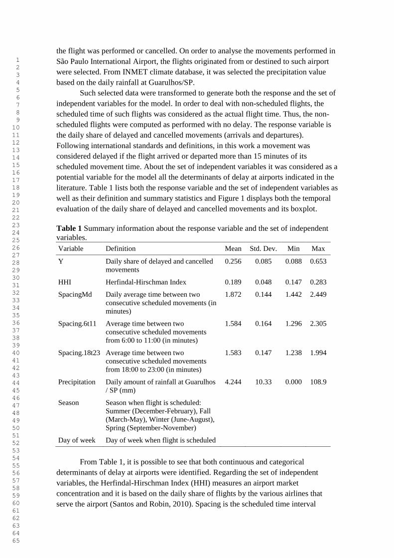
literature. Table 1 lists both the response variable and the set of independent variables as
well as their definition and summary statistics and Figure 1 displays both the temporal
evaluation of the daily share of delayed and cancelled movements and its boxplot.
Table 1 Summary information about the response variable and the set of independent
variables.
Variable Definition Mean Std. Dev. Min Max
Y Daily share of delayed and cancelled
movements
0.256 0.085 0.088 0.653
HHI Herfindal-Hirschman Index 0.189 0.048 0.147 0.283
SpacingMd Daily average time between two
consecutive scheduled movements (in
minutes)
1.872 0.144 1.442 2.449
Spacing.6t11 Average time between two
consecutive scheduled movements
from 6:00 to 11:00 (in minutes)
1.584 0.164 1.296 2.305
Spacing.18t23 Average time between two
consecutive scheduled movements
from 18:00 to 23:00 (in minutes)
1.583 0.147 1.238 1.994
Precipitation Daily amount of rainfall at Guarulhos
/ SP (mm)
4.244 10.33 0.000 108.9
Season Season when flight is scheduled:
Summer (December-February), Fall
(March-May), Winter (June-August),
Spring (September-November)
Day of week Day of week when flight is scheduled
From Table 1, it is possible to see that both continuous and categorical
determinants of delay at airports were identified. Regarding the set of independent
variables, the Herfindal-Hirschman Index (HHI) measures an airport market
concentration and it is based on the daily share of flights by the various airlines that
serve the airport (Santos and Robin, 2010). Spacing is the scheduled time interval

1 2 3 4 5 6 7 8 9 10 11 12 13 14 15 16 17 18 19 20 21 22 23 24 25 26 27 28 29 30 31 32 33 34 35 36 37 38 39 40 41 42 43 44 45 46 47 48 49 50 51 52 53 54 55 56 57 58 59 60 61 62 63 64 65
between two consecutive movements and according to Abdel-Aty et al.(2007), the
probability of the flights being delayed decreases as such value increases. About the
season and day of week, spring and summer may be seen as periods with higher demand
and consequently congestion (Santos and Robin, 2010) and according to the results
obtained by Abdel-Aty et al. (2007), there are seasonal and weekly delay patterns.
Weather condition is also pointed out as a dominant factor of air flight delays. Since São
Paulo International Airport capacity is normally reduced due to rainstorms, it was
chosen to make use of precipitation data to take into account such factor. Concerning
the model's response variable and from Figure 1.b, it is possible to see that the daily
share of delayed and cancelled movements distribution is skewed and has some outliers.
b
Figure 1 Daily share of delayed and cancelled movements: (a) temporal evaluation; (b)
boxplot.
In this work it was chosen to use a classification and regression tree (CART) for
the model building not only because it handles both categorical and numerical data
altogether, but also because it is not sensitive to outliers and skewed distributions.
Moreover, since the goal is to understand how the determinants of delay combine to
result in a day with high concentration of delayed and cancelled flights and to anticipate
such days occurrences, it is necessary to employ a method that provides an interpretable
prediction procedure. Thus, CART is appropriate since decision tree methods are
attractive when the interpretability is an important issue.
3.2 Model building and interpretation
Once defined both the response variable and the set of independnet variables, the
next step is the model building. About such step, as mentioned before, the attribute
selection procedure and the regression tasks were performed simultaneously by using
the classification and regression tree (CART) algorithm. In order to avoid over fitting,
the decisions concerning the necessity of pruning and the ideal tree size were made
taking into account a 10-fold cross-validation procedure. Therefore, the model was
trained 10 times, each time leaving out one of the subsets from training and using only
1 2 3 4 5 6 7 8 9 10 11 12 13 14 15 16 17 18 19 20 21 22 23 24 25 26 27 28 29 30 31 32 33 34 35 36 37 38 39 40 41 42 43 44 45 46 47 48 49 50 51 52 53 54 55 56 57 58 59 60 61 62 63 64 65
the omitted subset to compute the error rate. The obtained error rate is the mean of these
collected error rates.
A usual method to determine the ideal tree size is to consider the one-standard-
deviation rule. By such rule one is advised to choose the smallest tree whose cross-
validation relative error is close to the minimum cross-validation relative error plus one
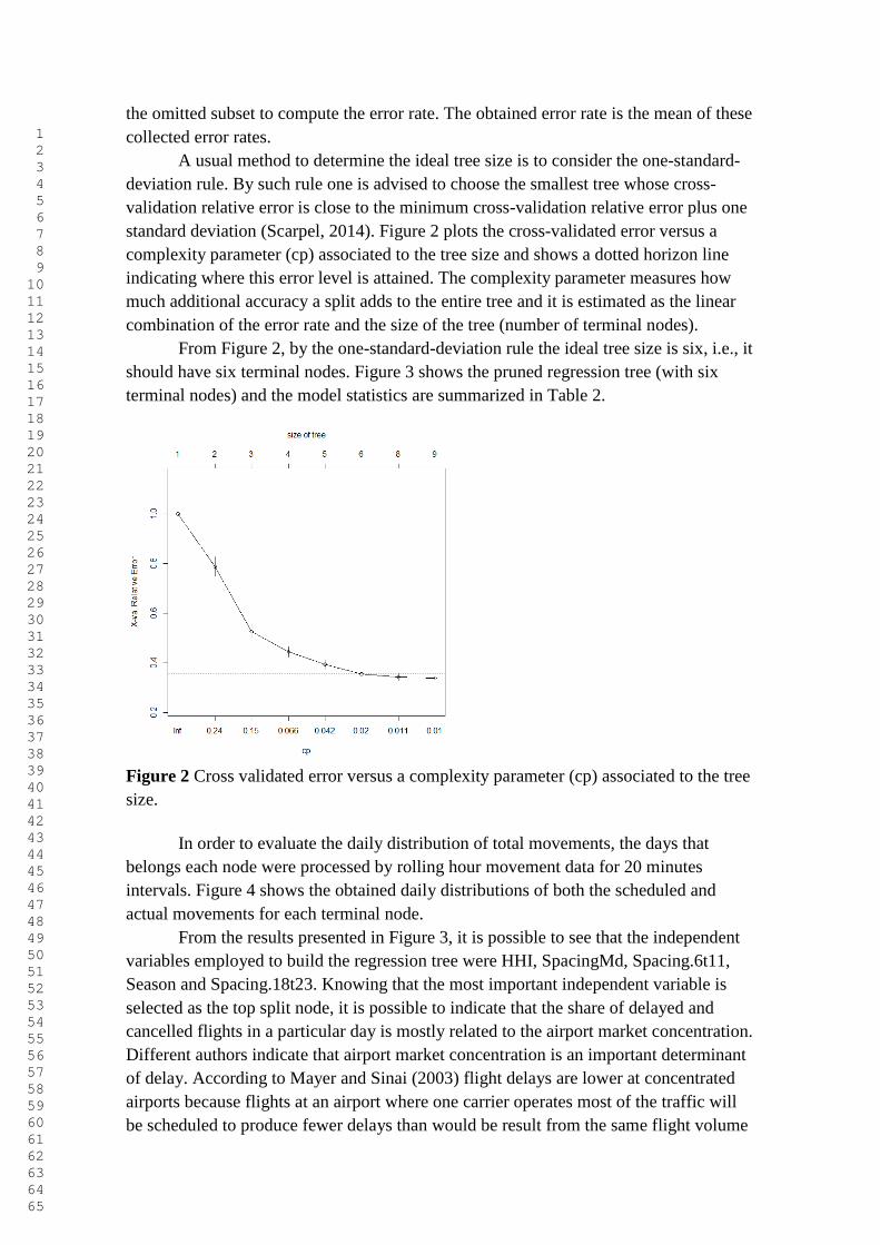
standard deviation (Scarpel, 2014). Figure 2 plots the cross-validated error versus a
complexity parameter (cp) associated to the tree size and shows a dotted horizon line
indicating where this error level is attained. The complexity parameter measures how
much additional accuracy a split adds to the entire tree and it is estimated as the linear
combination of the error rate and the size of the tree (number of terminal nodes).
From Figure 2, by the one-standard-deviation rule the ideal tree size is six, i.e., it
should have six terminal nodes. Figure 3 shows the pruned regression tree (with six
terminal nodes) and the model statistics are summarized in Table 2.
Figure 2 Cross validated error versus a complexity parameter (cp) associated to the tree
size.
In order to evaluate the daily distribution of total movements, the days that
belongs each node were processed by rolling hour movement data for 20 minutes
intervals. Figure 4 shows the obtained daily distributions of both the scheduled and
actual movements for each terminal node.
From the results presented in Figure 3, it is possible to see that the independent
variables employed to build the regression tree were HHI, SpacingMd, Spacing.6t11,
Season and Spacing.18t23. Knowing that the most important independent variable is
selected as the top split node, it is possible to indicate that the share of delayed and
cancelled flights in a particular day is mostly related to the airport market concentration.
Different authors indicate that airport market concentration is an important determinant
of delay. According to Mayer and Sinai (2003) flight delays are lower at concentrated
airports because flights at an airport where one carrier operates most of the traffic will
be scheduled to produce fewer delays than would be result from the same flight volume

1 2 3 4 5 6 7 8 9 10 11 12 13 14 15 16 17 18 19 20 21 22 23 24 25 26 27 28 29 30 31 32 33 34 35 36 37 38 39 40 41 42 43 44 45 46 47 48 49 50 51 52 53 54 55 56 57 58 59 60 61 62 63 64 65
at a less concentrated airport. Santos and Robin (2010) also found on their study that
flights originating from and arriving at airports with low concentration have higher
delays. However, according to such authors delays are lower at highly concentrated
airport because airlines internalise airport congestion. The other relevant independent
variables identified are related to demand. Concerning spacing, since it is based on the
time difference between scheduled flights, it is reduced when more movements are
scheduled. About season, it accounts for seasonal demand patterns.
Figure 3 Regression tree with six terminal nodes for forecasting the share of delayed
and cancelled flights in a day.
Table 2 Regression tree: summary statistics.
Model Statistics Node number Mean MSE
Terminal nodes: 6 3 0.2139 0.0019
Number of splits: 5 5 0.2106 0.0017
R-Square: 0.653 6 0.3800 0.0047
Relative error: 0.347 9 0.2496 0.0011
Cross-validation error: 0.355 10 0.3483 0.0025
Cross-validation std: 0.015 11 0.3891 0.0056
Considering that the concentration of delayed and cancelled flights, in a
particular day, is high for values higher than 30%, from the results presented in Figure 3
and Table 2, it is possible to verify that there are three terminal nodes with high
concentration (nodes 6, 10 and 11) and three terminal nodes with low concentration
(nodes 3, 5 and 9). In this work, the effort is in identifying alternatives to reduce delays
on days with high concentration of delayed and cancelled flights.

1 2 3 4 5 6 7 8 9 10 11 12 13 14 15 16 17 18 19 20 21 22 23 24 25 26 27 28 29 30 31 32 33 34 35 36 37 38 39 40 41 42 43 44 45 46 47 48 49 50 51 52 53 54 55 56 57 58 59 60 61 62 63 64 65
Figure 4 Daily distributions of both the scheduled and actual movements: (a) node 3;
(b) node 5; (c) node 6; (d) node 9; (e) node 10; (f) node 11.
From Figure 3, it is possible to see that node 3 is the biggest terminal node since
almost 65.5% of the days were assigned to it. Such node is achieved when the market is
more concentrated (HHI ≥ 17.56%) and the number of movements performed in the day
is not high (SpacingMd ≥ 1.62). Since São Paulo International Airport operates 24 hours
a day, when the daily average spacing between two consecutive scheduled movements
is higher than or equal to 1.62 minutes, it means that the total number of scheduled
movements in the day is lower than 889. The response variable average value (Ŷ) for
node 3 is 21.39% (7.04% of cancelled movements and 14.35% of delayed movements)
and from Figure 4.a, it is possible to verify that throughout the day there is a slight
distance between the daily distributions of the scheduled and actual movements. Such
results are in accordance with the literature since it is expected lower delays when the
airport market is more concentrated and demand is not high. Therefore, the days that
were assigned to terminal node 3 can be classified as regular low movements days with
most of the flights performed by the 3 biggest Brazilian airlines (Azul, Gol and TAM).
0
5
10
15
20
25
30
35
40
45
50
0.6
71
.33 2
2.6
73
.33 4
4.6
75
.33 6
6.6
77
.33 8
8.6
79
.33
10
10
.67
11
.33
12
12
.67
13
.33
14
14
.67
15
.33
16
16
.67
17
.33
18
18
.67
19
.33
20
20
.67
21
.33
22
22
.67
23
.33
24
Moviments/h
Hour
Scheduled
Actual
a
0
5
10
15
20
25
30
35
40
45
50
0.6
71
.33 2
2.6
73
.33 4
4.6
75
.33 6
6.6
77
.33 8
8.6
79
.33
10
10
.67
11
.33
12
12
.67
13
.33
14
14
.67
15
.33
16
16
.67
17
.33
18
18
.67
19
.33
20
20
.67
21
.33
22
22
.67
23
.33
24
Moviments/h
Hour
Scheduled
Actual
b
0
5
10
15
20
25
30
35
40
45
50
0.6
71
.33 2
2.6
73
.33 4
4.6
75
.33 6
6.6
77
.33 8
8.6
79
.33
10
10
.67
11
.33
12
12
.67
13
.33
14
14
.67
15
.33
16
16
.67
17
.33
18
18
.67
19
.33
20
20
.67
21
.33
22
22
.67
23
.33
24
Moviments/h
Hour
Scheduled
Actual
c
0
5
10
15
20
25
30
35
40
45
50
0.6
71
.33 2
2.6
73
.33 4
4.6
75
.33 6
6.6
77
.33 8
8.6
79
.33
10
10
.67
11
.33
12
12
.67
13
.33
14
14
.67
15
.33
16
16
.67
17
.33
18
18
.67
19
.33
20
20
.67
21
.33
22
22
.67
23
.33
24
Moviments/h
Hour
Scheduled
Actual
d
0
5
10
15
20
25
30
35
40
45
50
0.6
71
.33 2
2.6
73
.33 4
4.6
75
.33 6
6.6
77
.33 8
8.6
79
.33
10
10
.67
11
.33
12
12
.67
13
.33
14
14
.67
15
.33
16
16
.67
17
.33
18
18
.67
19
.33
20
20
.67
21
.33
22
22
.67
23
.33
24
Moviments/h
Hour
Scheduled
Actual
e
0
5
10
15
20
25
30
35
40
45
50
0.6
71
.33 2
2.6
73
.33 4
4.6
75
.33 6
6.6
77
.33 8
8.6
79
.33
10
10
.67
11
.33
12
12
.67
13
.33
14
14
.67
15
.33
16
16
.67
17
.33
18
18
.67
19
.33
20
20
.67
21
.33
22
22
.67
23
.33
24
Moviments/h
Hour
Scheduled
Actual
f

1 2 3 4 5 6 7 8 9 10 11 12 13 14 15 16 17 18 19 20 21 22 23 24 25 26 27 28 29 30 31 32 33 34 35 36 37 38 39 40 41 42 43 44 45 46 47 48 49 50 51 52 53 54 55 56 57 58 59 60 61 62 63 64 65
In contrast, node 5 is the smallest terminal node with only 17 days assigned to it. This
result is consistent since it is not expected to find days with high demand (SpacingMd <
1.62) on Fall or Winter (Figure 3). Its average value for the response variable (Ŷ) is
21.06%. The last terminal node with low concentration of delayed and cancelled flights
is terminal node 9. Such node is achieved when airport market is less concentrated (HHI
< 17,56%) and demand is lower in both peak periods of the day (from 6:00 to 11:00 and
from 18:00 to 23:00). There are 158 days assigned to node 9 and its Ŷ is 24.96%.
Concerning the daily distributions of the scheduled and actual movements for terminal
nodes 5 and 9 (Figures 4.b and 4.d), as seen in Figure 4.a, it is possible to verify that
there is just a slight distance between such distributions.
About the three terminal nodes with high concentration of delayed and cancelled
flights, from the results presented in Figure 3 and Table 2, it is possible to observe that
they hold 23.9% of the days. Node 6 has 133 days assigned to it and its Ŷ is 38.0%,
node 10 has 95 days assigned to it and its Ŷ is 34.8% and node 11 has 167 days
assigned to it and its Ŷ is 38.9%. Two of such terminal nodes (nodes 9 and 10) are
achieved when HHI value is lower than 17,56% and the third node (node 6) is achieved
when HHI value is higher than or equal to 17,56%. Concerning node 6, it is possible to
notice that the high concentration of delayed and cancelled movements is due to a high
demand since such node is achieved when the season is spring or summer and the daily
average spacing between two consecutive scheduled movements is lower than 1.62
minutes, i.e., the number of scheduled movements is higher than 889. According to
Santos and Robin (2010), Spring and Summer may be seen as periods with higher
demand and consequent congestion. From Figure 4.c, it is possible to see that there is
higher actual than scheduled movements until 3:00 a.m., probably due to delayed flights
from the day before, and a higher distance between the daily distributions of the
scheduled and actual movements, specially from 7:00 to 9:00 and from 17:30 to 22:00.
Moreover, it is possible to see that distance between the distributions increases when the
scheduled movements is higher than 37 movements per hour. According to McKinsey
(2010), the São Paulo International Airport (GRU) runway capacity is 49 movements
per hours. Therefore, in order to reduce delays in such days it is necessary to deal with
key operational bottlenecks that do not allow the usage of the available capacity. Such
bottlenecks include airside and passenger terminal capacity issues.
The other two terminal nodes with high concentration of delayed and cancelled
flights are nodes 10 and 11. As mentioned before, both nodes are achieved when airport
market is less concentrated (HHI < 17,56%). The difference between such nodes is that
node 11 is achieved when the average spacing between two consecutive scheduled
movements from 6:00 to 11:00 is lower than 1.62 minutes (that is equivalent to more
than 37 movements per hour), while node 10 is achieved when the average spacing
between two consecutive scheduled movements from 18:00 to 23:00 is lower than 1.59
minutes (that is equivalent to more than 38 movements per hour). Therefore, in both
cases the high concentration of delayed and cancelled movements is due to the
combination of a low market concentration and high demand in peak periods. The
analysis of the daily distribution of the scheduled and actual movements shows that
there is a considerable distance between such distributions throughout the day for both

1 2 3 4 5 6 7 8 9 10 11 12 13 14 15 16 17 18 19 20 21 22 23 24 25 26 27 28 29 30 31 32 33 34 35 36 37 38 39 40 41 42 43 44 45 46 47 48 49 50 51 52 53 54 55 56 57 58 59 60 61 62 63 64 65
terminal node 10 and 11 (Figures 4.e and 4.f, respectively). However, for node 11 it is
possible to see a higher distance between scheduled and actual movements distribution
from 7:00 to 9:00. In order to evaluate the effect of market concentration in the total
movements per hour Table 3 shows both the scheduled and actual daily average number
of movements per hour and the average movements per hour from 7:00 to 22:00 for
each terminal node. From Table 3, it is possible to see that the three terminal nodes
where HHI is lower than 17,56% (nodes 9, 10 and 11) have actual daily average number
of movements per hour lower than 29, while the other nodes have such value higher
than 29. Moreover, comparing nodes 3, 10 and 11, in terms of actual average
movements per hour from 7:00 to 22:00, it is possible to verify that node 3 has lower
demand (36.55 movements per hour) than nodes 10 and 11 (37.47 and 38.18 movements
per hour, respectively) but performs more movements per hour. In order to reduce
delays in days with low market concentration, since there is more diversity in terms of
airlines serving the airport and demand for facilities exceeds availability, slots
coordination can be considered as an alternative. São Paulo International Airport is a
schedule facilitated airport (Level 2). Therefore, cooperation and voluntary schedule
changes are necessary to avoid congestion. The main goal of slots coordination is to
regulate access to infrastructure and, therefore, adapt the demand for air services with
the available airport capacity.
Table 3 Scheduled and actual daily average number of movements per hour and the
average movements per hour from 7:00 to 22:00 for each terminal node.
Average movements / h
Node
3
Node
5
Node
6
Node
9
Node
10
Node
11
Scheduled Daily 30.89 35.23 32.56 30.21 31.48 31.90
From 7:00 to 22:00 36.55 42.35 38.63 36.33 37.47 38.18
Actual Daily 29.58 33.76 29.94 28.99 28.55 28.63
From 7:00 to 22:00 35.24 40.57 35.43 34.63 33.84 34.23
4. EWM building and validation
This section is dedicated to the early warning model (EWM) building and
validation. The EWM is employed to anticipate the occurrence of days with high
concentration of delayed and cancelled flight for the São Paulo International Airport
(GRU). As mentioned before, an EWM is based on the combination of indicators and
alarms against possible occurrence of changes on a variable of interest and two critical
tasks for the EWM success are the indicators identification and the classification
procedure. The indicators identification was addressed using CART. Thus, the next step
is to define the classification procedure that is going to work as an alarm. In this work, it
was chosen to perform a binary classification where the days are discriminated into two
groups and the classification rule is given by
otherwise,0
11or106,Nodeif,1HD
t
t (1)
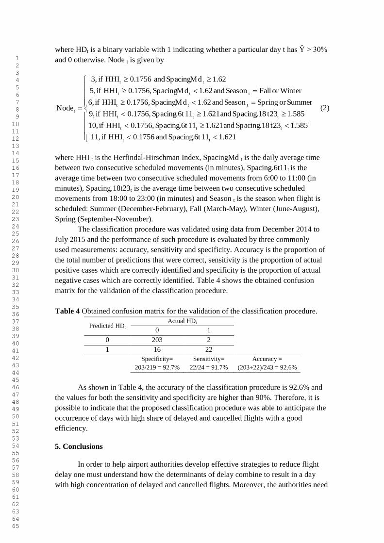
1 2 3 4 5 6 7 8 9 10 11 12 13 14 15 16 17 18 19 20 21 22 23 24 25 26 27 28 29 30 31 32 33 34 35 36 37 38 39 40 41 42 43 44 45 46 47 48 49 50 51 52 53 54 55 56 57 58 59 60 61 62 63 64 65
where HDt is a binary variable with 1 indicating whether a particular day t has Ŷ > 30%
and 0 otherwise. Node t is given by
1.62111Spacing.6t and 0.1756HHIif11,
585.1t23Spacing.18and1.62111Spacing.6t 0.1756,HHIif10,
585.1t23Spacing.18and1.62111Spacing.6t 0.1756,HHIif9,
SummerorSpringSeasonand1.62SpacingMd 0.1756,HHIif6,
WinterorFallSeasonand1.62SpacingMd 0.1756,HHIif5,
1.62SpacingMdand0.1756HHIif 3,
Node
tt
ttt
ttt
ttt
ttt
tt
t (2)
where HHI t is the Herfindal-Hirschman Index, SpacingMd t is the daily average time
between two consecutive scheduled movements (in minutes), Spacing.6t11t is the
average time between two consecutive scheduled movements from 6:00 to 11:00 (in
minutes), Spacing.18t23t is the average time between two consecutive scheduled
movements from 18:00 to 23:00 (in minutes) and Season t is the season when flight is
scheduled: Summer (December-February), Fall (March-May), Winter (June-August),
Spring (September-November).
The classification procedure was validated using data from December 2014 to
July 2015 and the performance of such procedure is evaluated by three commonly
used measurements: accuracy, sensitivity and specificity. Accuracy is the proportion of
the total number of predictions that were correct, sensitivity is the proportion of actual
positive cases which are correctly identified and specificity is the proportion of actual
negative cases which are correctly identified. Table 4 shows the obtained confusion
matrix for the validation of the classification procedure.
Table 4 Obtained confusion matrix for the validation of the classification procedure.
Predicted HDt Actual HDt
0 1
0 203 2
1 16 22
Specificity=
203/219 = 92.7%
Sensitivity=
22/24 = 91.7%
Accuracy =
(203+22)/243 = 92.6%
As shown in Table 4, the accuracy of the classification procedure is 92.6% and
the values for both the sensitivity and specificity are higher than 90%. Therefore, it is
possible to indicate that the proposed classification procedure was able to anticipate the
occurrence of days with high share of delayed and cancelled flights with a good
efficiency.
5. Conclusions
In order to help airport authorities develop effective strategies to reduce flight
delay one must understand how the determinants of delay combine to result in a day
with high concentration of delayed and cancelled flights. Moreover, the authorities need

1 2 3 4 5 6 7 8 9 10 11 12 13 14 15 16 17 18 19 20 21 22 23 24 25 26 27 28 29 30 31 32 33 34 35 36 37 38 39 40 41 42 43 44 45 46 47 48 49 50 51 52 53 54 55 56 57 58 59 60 61 62 63 64 65
to be able to anticipate such days occurrence in order to support response planning. In
this work, such tasks were addressed by using a classification and regression tree
(CART). CART was chosen due its capacity in providing an interpretable prediction
procedure, in handling both categorical and numerical data altogether and because it is
not sensitive to outliers and skewed distributions.
For the São Paulo International Airport, by using CART, it was identified three
combinations of determinants of delay that resulted in days with high share of delayed
and cancelled flights. Such combinations hold 23.9% of the days and the determinants
of delay identified as relevant were airport market concentration and demand.
Therefore, it was possible to verify how airport market concentration and demand
combine to result in a day with high share of delayed and cancelled flights and identify
alternatives to deal with the occurrence of such combinations.
Afterwards, the built model was used to generate a classification procedure for a
early warning model in order to anticipate the occurrence of days with high share of
delayed and cancelled flights. The classification procedure was validated using out-of-
sample data and the obtained results proved to be satisfactory.
For future work, it is intended to use both the generated combinations of
determinants of delay and the classification procedure to predict air traffic delay of
individual flights.
Acknowledgements
The author acknowledges the financial support from FAPESP - Fundação de
Amparo a Pesquisa do Estado de São Paulo (grant 2013/22416-4).
References
Abdel-Aty, M., Lee, C., Bai, Y. Li, X. e Michalak, M. Detecting periodic patterns of
arrival delay. Journal of Air Transport Management, 13, 355-361, 2007.
Banks, D. L. (2010). Statistical Data Mining. Wiley Interdisciplinary Reviews:
Computational Statistics, 2(1), 9-25.
Breiman, L., Friedman, J., Olshen, R. and Stone, C. Classification and Regression
Trees. Wadsworth International Group, Monterey, CA, 1984.
Buxi, G. e Hansen, M. Generating Day-of-operation Probabilistic Capacity Scenarios
from Weather Forecasts. Transportation Research Part C: Emerging
Technologies, 33, 153-166, 2013.
Costa, T. F. G., Lohmann, G. and Oliveira, A. V. M. A model to identify airport hubs
and their importance to tourism in Brazil. Research in Transportation Economics,
6(1), 3-11, 2010.
Diana, T. Validating delay constructs: An application of confirmatory factor analysis. .
Journal of Air Transport Management, 35, 87-91, 2014.
Ferguson, J., Kara, A. Q., Hoffman, K. and Sherry, L. Estimating domestic US airline
cost of delay based on the European model. Transportation Research Part C:
Emerging Technologies, 33, 196-202, 2013.

1 2 3 4 5 6 7 8 9 10 11 12 13 14 15 16 17 18 19 20 21 22 23 24 25 26 27 28 29 30 31 32 33 34 35 36 37 38 39 40 41 42 43 44 45 46 47 48 49 50 51 52 53 54 55 56 57 58 59 60 61 62 63 64 65
Liu, P. B., Hansen, M. and Mukherjee, A. Scenario-based air traffic flow management:
From theory to practice. Transportation Research Part B: Methodological, 42,
685-702, 2008.
Madas, M. A. and Zografos, K, G. Airport capacity vs. demand: mismatch or
mismanagement? Transportation Research Part A: Policy and Practice, 42, 203-
226, 2008.
Mayer, C and Sinai, T. Network effects, congestion externalities, and air traffic delays:
Or why not all delays and created evil. The American Economic Review, 93(4),
1194 - 1215, 2003.
McKinsey. Estudo do setor de transporte aéreo do Brasil. McKinsey & Company.
Available at < https://web.bndes.gov.br/bib/jspui/handle/1408/1464 >, accessed in
July 20, 2015.
Olafsson, S., Li, X. and Wu, S. Operations research and data mining. European
Journal of Operational Research, 187(3), 1429-1448, 2008.
Öttl, G., Böck, P., Werpup, N. and Schwarze, M. Derivation of Representative Air
Traffic Peaks as a Standard Input for Airport Related Simulation , Journal of Air
Transport Management, 28, 31-39, 2013.
Pyrgiotis, N., Malone, K. M. and Odoni, A. Modelling delay propagation within an
airport network. Transportation Research Part C: Emerging Technologies, 27,
60-75, 2013.
Rebollo, J. J. e Balakrishnan, H. Characterization and prediction of air traffic delays.
Transportation Research Part C: Emerging Technologies, 44, 231-241, 2014.
Ripley, B. D. Pattern recognition and neural networks. Cambridge University Press,
Cambridge, 1996.
Santos, G. e Robin, M. Determinants of delays at European airports. Transportation
Research Part B: Methodological, 44(3), 392-403, 2010.
Scarpel, R. A. A demand trend change early warning forecast model for the city of São
Paulo multi-airport system. Transportation Research Part A: Policy and Practice,
65, 23-32, 2014.
Wensveen, J. G. Air transportation: A management perspective, 7th
edition. Ashgate,
Aldershot, UK, 2011.

ANEXO B
Artigo "A data analytics approach for anticipating congested
days at the São Paulo International Airport" submetido ao
periódico Transportation Research - Part C: Emerging
Technologies.

Elsevier Editorial System(tm) for
Transportation Research Part C
Manuscript Draft
Manuscript Number: TRC-D-15-00557R1
Title: A data analytics approach for anticipating congested days at the
São Paulo International Airport
Article Type: Research Paper
Keywords: early warning model; mixture-of-experts model; response
planning; classification and regression tree; multiple linear regression;
time series analysis
Corresponding Author: Dr. Rodrigo A Scarpel, Ph.D.
Corresponding Author's Institution: Instituto Tecnológico de Aeronáutica
First Author: Rodrigo A Scarpel, Ph.D.
Order of Authors: Rodrigo A Scarpel, Ph.D.
Abstract: Worldwide, most of the airports are not able to operate as
planned due to delay problems. Since a high proportion of flights are
affected by delays in congested days, for developing effective strategies
to reduce flight delays and support response planning, a critical issue
is how to anticipate the occurrence of congested days. The goal of this
work is to employ a data analytics approach to build an early warning
model to anticipate the occurrence of such days at the São Paulo
International Airport. Therefore, a Mixture-of-experts model (MEM) was
used to combine modelling approaches that rely on different assumptions
regarding the data available to process. Such approach allows to generate
a more flexible and powerful model that makes good promises of
improvement in the prediction accuracy. The built MEM is composed by a
Classification and Regression Tree, a multiple linear regression and a
seasonal ARIMA and it was used to generate predictions for one period
ahead and for seven periods ahead. The accuracy of the early warning
model was considered satisfactory for anticipating congested days.

1 2 3 4 5 6 7 8 9 10 11 12 13 14 15 16 17 18 19 20 21 22 23 24 25 26 27 28 29 30 31 32 33 34 35 36 37 38 39 40 41 42 43 44 45 46 47 48 49 50 51 52 53 54 55 56 57 58 59 60 61 62 63 64 65
1. Introduction
Worldwide, most of the airports are not able to operate as planned due to delay
problems. According to Santos and Robin (2010), in 2005 over 20 per cent of all intra-
European flights departed more than 15 min later than their scheduled departure time
and in July 2007, 30 per cent of domestic flights in the US arrived more than 15 min
late. According to Pyrgiotis et al. (2013), the net cost of congestion, which includes
both the direct costs of delays to the airlines and their passengers and the indirect costs
that these delays cause to the airline industry and to other sectors of the economy, in a
tightly inter-connected and over-scheduled network of airports and aircrafts is
enormous. Such high delay costs motivate the analysis and prediction of air traffic
delays in order to development better delay management mechanisms (Ferguson et al.,
2013).
In Brazil, air transport has been recently liberalized and one of the consequences
of this process was the concentration of flights in a few hubs (Costa et al., 2010).
According to Wensveen (2011), the extent of excessive concentration of flights at a hub
can result in some negative economic impacts, namely, congestion delay which
increases passenger’s total travel time and airlines’ operating costs. Moreover,
congestion during peak periods also puts a tremendous strain on airport and airline
personnel and also creates additional work for air traffic controllers (Wensveen, 2011).
The São Paulo International Airport, that up to date, is the largest Brazilian hub is the
place that most suffers with such hub concentration and congestion delays.
There is a well-developed literature about the determinants of delay at airports.
According to Diana (2014), delay represents the outcome of a trade-off between
demand for arrivals and departures and available airport capacity and according to
Madas and Zografos (2008), the increasing imbalances between capacity and traffic has
resulted in congestion and delay figures. Therefore, when an airport does not have
enough capacity to satisfy demand, flights get delayed and sometimes cancelled.
According to Santos and Robin (2010), the significant variables in explaining delays at
European airports are market concentration, slot coordination, hub airports and hub
airlines. Abdel-Aty et al. (2007) evaluated on-time arrival performance and identified
patterns of flight delay. Based on the detected patterns, variables affecting delay were
identified and the relationship between such variables and flight delay was investigated.
Such authors concluded that air flight delays mainly increased due to adverse weather at
airports, lack of runway capacity, the increase in the number of aircrafts, poor air traffic
control and limited buffer time between flights.
Since a high proportion of flights are affected by delays in congested days, for
developing effective strategies to reduce flight delays and support response planning, a
critical issue is how to anticipate the occurrence of congested days. In this work, the
daily share of delayed flights is used as a measure of congestion at airports. In order to
predict the occurrence of such days, it is necessary to employ an approach to analyze
data systematically, detect relationships and interactions among a set of determinants of
delay and generate a prediction procedure. Therefore, the goal of this work is to employ
*ManuscriptClick here to view linked References

1 2 3 4 5 6 7 8 9 10 11 12 13 14 15 16 17 18 19 20 21 22 23 24 25 26 27 28 29 30 31 32 33 34 35 36 37 38 39 40 41 42 43 44 45 46 47 48 49 50 51 52 53 54 55 56 57 58 59 60 61 62 63 64 65
a data analytics approach to build an early warning model (EWM) to anticipate the
occurrence of such days at the São Paulo International Airport (GRU). An EWM is
based on the combination of indicators and alarms against the occurrence of changes on
a variable of interest (Scarpel, 2014). For GRU, the variable of interest for anticipating
congested days is the daily percentage of total movements (arrivals and departures) with
delay exceeding fifteen minutes.
Two critical tasks for the EWM success are the indicators identification and the
prediction procedure. Concerning delays at airports, different approaches were used to
deal with such issues as multiple regression analysis (Santos and Robin, 2010; Rebollo
and Balakrishnan, 2014) and time series analysis (Abdel-Aty et al., 2007). The different
approaches rely on quite different assumptions regarding the data available to process.
According to Ferrari and Milioni (2011), choosing the best approach in a modelling
exercise is always an arduous task because of the various uncertainties associated with
the modelling process. Therefore, this paper intends to contribute to the existing
literature by providing a data analytics framework that allows to combine different
possible modelling approaches to build an EWM and to improve the obtained prediction
performance.
The rest of the paper is organized as follows. Section 2 outlines the employed
data analytics method. Section 3 has two sub-sections, the first focuses on the data
selection and transformation steps and the second focuses on model building and on
reporting and discussing the obtained results. Section 4 is dedicated to the EWM
building and validation. Conclusions are presented in the final section.
2. Background
Data analytics methods are widely used to develop insights by extracting or
detecting patterns from data. Such methods most common functions include attribute
selection, classification, regression and clustering. In air transportation, only a few
works employed data analytics methods. Abdel-Aty et al. (2007) applied a frequency
analysis method to detect periodic patterns of flight arrival delays and used statistical
methods to identify the factors associated with such delays. Liu et al. (2008) employed
statistical clustering to classify arrival capacity data into patterns of arrival capacity
profiles. Öttl et al. (2013) employed cluster analysis to determine representative airport
peak hour traffic situations. Buxi and Hansen (2013) developed three clustering based
methodologies for converting day-of-operation weather forecasts into day-of-operation
probabilistic capacity scenarios for assisting air traffic managers. Scarpel (2014) created
an early warning model using classification and regression trees in order to build a
demand trend change forecast model. Rebollo and Balakrishnan (2014) employed
clustering, classification and regression approaches to identify delay states and predict
air traffic delays.
In this work, a data analytics approach called Mixture-of-Experts model (MEM)
is used to perform the regression function. Such modelling approach allows to combine
the predictions produced using different modelling approaches. It is appropriate whether
one is interested on enhancing the performance of the generated predictions. In this

1 2 3 4 5 6 7 8 9 10 11 12 13 14 15 16 17 18 19 20 21 22 23 24 25 26 27 28 29 30 31 32 33 34 35 36 37 38 39 40 41 42 43 44 45 46 47 48 49 50 51 52 53 54 55 56 57 58 59 60 61 62 63 64 65
work, for the EWM building, the Mixture-of Experts model combines a Classification
and Regression Tree (CART), that was used by Scarpel (2014) to create an early
warning model for predicting changes in demand trend and approaches commonly used
in identifying the causes behind delay and for delay prediction such as multiple
regression analysis (Santos and Robin, 2010; Rebollo and Balakrishnan, 2014) and time
series analysis (Abdel-Aty et al., 2007).
2.1 Classification and Regression Trees (CART)
Classification and Regression trees are a very powerful, yet conceptually simple,
method of nonparametric regression (Kutner et al., 2004). In this work, CART was
employed to perform both the attribute selection and regression tasks. According to
Olafsson et al. (2008), attribute selection involves a process for determining which
attributes are relevant to predict or explain the available data, and conversely which
attributes are redundant or provide little information. In regression, the goal is to map
the relationship between a response variable and a set of explanatory variables.
CART are attractive when the interpretability is an important issue since they are
designed to detect the important predictor variables and to generate a tree structure to
represent the identified recursive partition (Scarpel, 2014). According to Kutner et al.
(2004), in CART the range of the response variable is partitioned into segments and
within each segment the estimated regression fit is given by the mean of the responses
in the segment. According to Banks (2010), CART has minimal model assumptions and
its most general solution is as follows: Suppose that we have a sample of n
observations, a response variable Y1,…,Yn and each observation has a r-dimensional
vector of covariates x. The classification and regression tree employs a recursive
partitioning algorithm in a top-down manner by selecting attributes one at a time and
splitting the data according to the values of those attributes. Such algorithm has three
parts: (1) a way to select a split at each intermediate node; (2) a rule for declaring a node
to be terminal; and (3) a rule for estimating the value of the response variable (Y) at the
terminal node.
From the different tree induction algorithms available, in this work it was
employed the one proposed by Breiman et al. (1984). Following the three parts of a
recursive partitioning algorithm, CART performs the first part splitting on the value
which most reduces the forecasting sum of squared error (SSE). On the second part,
CART grow an overly complicated tree, and then prunes it back, using cross-validation
to find a tree with good predictive accuracy. Cross-validation is a resampling approach
which enables to obtain a more honest error rate estimate of the tree computed on the
whole dataset. In k-fold cross-validation the dataset is divided into k subsets of
approximately equal size. Then, the model is trained k times, each time leaving out one
of the subsets from training and using only the omitted subset to compute the error rate
(Ripley, 1996). Finally, on the third part, CART uses the sample average of the data at
the terminal nodes as its forecasting value.
2.2 Mixture-of-experts model (MEM)

1 2 3 4 5 6 7 8 9 10 11 12 13 14 15 16 17 18 19 20 21 22 23 24 25 26 27 28 29 30 31 32 33 34 35 36 37 38 39 40 41 42 43 44 45 46 47 48 49 50 51 52 53 54 55 56 57 58 59 60 61 62 63 64 65
MEM was introduced by Jacobs et al. (1991) and its objective is to explain the
behaviour of some phenomena, under the assumption that there are separate processes
involved in the generation of the data under analysis. Such model is comprised of a set
of models, which perform the role of experts, and a set of mixing weights determined by
the gating function (Ferrari and Milioni, 2011). The experts are responsible for
modelling the generation of outputs and the gating function is responsible for combining
the models.
According to Ferrari and Milioni (2011), MEM’s proposal serves as an
alternative method for solving complex problems, by allowing a combination of many
different simple models to build a more flexible and powerful one. This flexibility
makes good promises of improvement in the accuracy of a model, compared to a unique
simple model. The general architecture of the MEM for a single output is written as
k
1c
ci,ci,i YgY (1)
where i identifies a particular observation, k is the number experts, gic is the weight
factor for the expert c, Ŷic is the prediction generated using expert c and Ŷi is the
prediction produced by the MEM.
Concerning the gating function, it is possible to be interpreted as a probability
classifier where a certain input is assigned to one or more experts, depending on
whether the learning scheme adopted is competitive or cooperative. In the cooperative
scheme, each expert estimates an output and a weighted sum of the experts’ outputs is
computed (Ferrari and Milioni, 2011). For cooperative learning, a commonly used
gating functions is the softmax written as
k1,...,c,
xwexp
xwexp
gk
1c 1
ji,jc,
1
ji,jc,
ci,
l
j
l
j (2)
where xi,j is the value of the observation i for the independent variable j and wc,j are the
mixing parameters. Note that the gi,c are positive and sum to one for each observation.
Concerning the estimation of the mixing parameters, such values are estimated by
minimizing the error function expressed as
2
ci,i
n
1i
k
1c
ci,MEM YY2
1expglogE
According to Jacobs et al. (1991), by minimizing such error function, the
weights of each expert are updated based on their own error in the prediction of the
target. Moreover, the weight-updating factor for each expert is proportional to the ratio
of its error value to the total error. Such features in the error function that cause the
localisation of each expert in their corresponding subspace.

1 2 3 4 5 6 7 8 9 10 11 12 13 14 15 16 17 18 19 20 21 22 23 24 25 26 27 28 29 30 31 32 33 34 35 36 37 38 39 40 41 42 43 44 45 46 47 48 49 50 51 52 53 54 55 56 57 58 59 60 61 62 63 64 65
3. Model
The study being reported in this paper follows a sequential procedure composed
by the steps: (1) data selection and transformation; and (2) model building and
interpretation. All the analyses were carried out employing the R program, version
3.1.1, using the RPART, PARTYKIT and STATS packages.
3.1 Data selection and transformation
The analyses were performed using data provided by the Brazilian National
Civil Aviation Agency (ANAC). For the model building, it was used data from January
2010 to May 2014 and from August 2014 to November 2014. Data from June 2014 to
July 2014 were not provided by ANAC due to changes on their authorization system
during the World Cup. Afterwards, data from December 2014 to July 2015 were used to
validate the built model.
The ANAC database provides data for all performed and cancelled domestic and
international flights including the airports of origin and destination, the flight carrier
code, the scheduled and actual departure and arrival gate time and the information
whether the flight was performed or cancelled. In order to analyse the movements
performed in São Paulo International Airport, the flights originated from or destined to
such airport were selected. For dealing with non-scheduled flights, the scheduled time
of such flights was considered as the actual flight time. Thus, the non-scheduled flights
were computed as performed with no delay. Such selected data were transformed to
generate both the response variable and the set of independent variables for the
considered modelling alternatives.
The response variable is the daily share of delayed movements (arrivals and
departures). Following international standards and definitions, in this work a movement
was considered delayed if the flight arrived or departed more than 15 minutes of its
scheduled movement time. Figure 1 displays the temporal evaluation of the daily share
of delayed movements.
As indicated earlier, an EWM to anticipate days with high concentration of
delayed movements (arrivals and departures) at GRU is based on the combination of
indicators and alarms. Concerning the indicators, the determinants of delay at airports
indicated in the literature were considered as potential independent variables for both
the multiple linear regression and CART models. Table 1 lists the considered set of
independent variables as well as their definition and Figure 2 shows the temporal
evaluation of the considered continuous independent variables.

1 2 3 4 5 6 7 8 9 10 11 12 13 14 15 16 17 18 19 20 21 22 23 24 25 26 27 28 29 30 31 32 33 34 35 36 37 38 39 40 41 42 43 44 45 46 47 48 49 50 51 52 53 54 55 56 57 58 59 60 61 62 63 64 65
Figure 1 Daily share of delayed movements.
Table 1 Summary information about the set of independent variables.
Variable Definition
HHI Herfindal-Hirschman Index
Av.Spacing Daily average time between two consecutive scheduled movements (in
minutes)
Spacing.6t11 Average time between two consecutive scheduled movements from 6:00 to
11:00 (in minutes)
Spacing.18t23 Average time between two consecutive scheduled movements from 18:00 to
23:00 (in minutes)
Std.Spacing Daily standard deviation of the time between two consecutive scheduled
movements (in minutes)
Av.ConMov Daily average number of consecutive movements of the same type (arrivals or
departures), according to the scheduled movement time
D.NewTerminal Dummy variable taking value 1 if the period is March 2014 or later and value
0 otherwise
Season Season when flight is scheduled: Summer (December-February), Fall (March-
May), Winter (June-August), Spring (September-November)
Day of week Day of week when flight is scheduled (Sunday, Monday, Tuesday,
Wednesday, Thursday, Friday and Saturday)

1 2 3 4 5 6 7 8 9 10 11 12 13 14 15 16 17 18 19 20 21 22 23 24 25 26 27 28 29 30 31 32 33 34 35 36 37 38 39 40 41 42 43 44 45 46 47 48 49 50 51 52 53 54 55 56 57 58 59 60 61 62 63 64 65
Figure 2 Temporal evolution of the continuous independent variables: (a) HHI; (b)
Daily average spacing (Av.Spacing); (c) Daily average number of consecutive
movements of the same type (Av.ConMov); (d) Daily standard deviation of the spacing
(Std.Spacing).
0,12
0,14
0,16
0,18
0,20
0,22
0,24
0,26
0,28
0,30
0,32
01/0
1/20
10
01/0
3/20
10
01/0
5/20
10
01/0
7/20
10
01/0
9/20
10
01/1
1/20
10
01/0
1/20
11
01/0
3/20
11
01/0
5/20
11
01/0
7/20
11
01/0
9/20
11
01/1
1/20
11
01/0
1/20
12
01/0
3/20
12
01/0
5/20
12
01/0
7/20
12
01/0
9/20
12
01/1
1/20
12
01/0
1/20
13
01/0
3/20
13
01/0
5/20
13
01/0
7/20
13
01/0
9/20
13
01/1
1/20
13
01/0
1/20
14
01/0
3/20
14
01/0
5/20
14
01/0
7/20
14
01/0
9/20
14
01/1
1/20
14
Her
fin
dal
-Hir
sch
man
In
dex
Perioda
1,40
1,60
1,80
2,00
2,20
2,40
2,60
01/0
1/20
10
01/0
3/20
10
01/0
5/20
10
01/0
7/20
10
01/0
9/20
10
01/1
1/20
10
01/0
1/20
11
01/0
3/20
11
01/0
5/20
11
01/0
7/20
11
01/0
9/20
11
01/1
1/20
11
01/0
1/20
12
01/0
3/20
12
01/0
5/20
12
01/0
7/20
12
01/0
9/20
12
01/1
1/20
12
01/0
1/20
13
01/0
3/20
13
01/0
5/20
13
01/0
7/20
13
01/0
9/20
13
01/1
1/20
13
01/0
1/20
14
01/0
3/20
14
01/0
5/20
14
01/0
7/20
14
01/0
9/20
14
01/1
1/20
14
Av.
Spac
ing
Periodb
1,80
1,90
2,00
2,10
2,20
2,30
2,40
2,50
2,60
2,70
2,80
01/0
1/20
10
01/0
3/20
10
01/0
5/20
10
01/0
7/20
10
01/0
9/20
10
01/1
1/20
10
01/0
1/20
11
01/0
3/20
11
01/0
5/20
11
01/0
7/20
11
01/0
9/20
11
01/1
1/20
11
01/0
1/20
12
01/0
3/20
12
01/0
5/20
12
01/0
7/20
12
01/0
9/20
12
01/1
1/20
12
01/0
1/20
13
01/0
3/20
13
01/0
5/20
13
01/0
7/20
13
01/0
9/20
13
01/1
1/20
13
01/0
1/20
14
01/0
3/20
14
01/0
5/20
14
01/0
7/20
14
01/0
9/20
14
01/1
1/20
14
Av.
Co
nM
ov
Periodc
2,00
2,50
3,00
3,50
4,00
4,50
5,00
5,50
01/0
1/20
10
01/0
3/20
10
01/0
5/20
10
01/0
7/20
10
01/0
9/20
10
01/1
1/20
10
01/0
1/20
11
01/0
3/20
11
01/0
5/20
11
01/0
7/20
11
01/0
9/20
11
01/1
1/20
11
01/0
1/20
12
01/0
3/20
12
01/0
5/20
12
01/0
7/20
12
01/0
9/20
12
01/1
1/20
12
01/0
1/20
13
01/0
3/20
13
01/0
5/20
13
01/0
7/20
13
01/0
9/20
13
01/1
1/20
13
01/0
1/20
14
01/0
3/20
14
01/0
5/20
14
01/0
7/20
14
01/0
9/20
14
01/1
1/20
14
Std
.Sp
acin
g
Periodd

1 2 3 4 5 6 7 8 9 10 11 12 13 14 15 16 17 18 19 20 21 22 23 24 25 26 27 28 29 30 31 32 33 34 35 36 37 38 39 40 41 42 43 44 45 46 47 48 49 50 51 52 53 54 55 56 57 58 59 60 61 62 63 64 65
Regarding the considered variables, the Herfindal-Hirschman Index (HHI)
measures an airport market concentration and it is based on the daily share of flights by
the various airlines that serve the airport (Santos and Robin, 2010). The variable
Av.Spacing is the daily average time interval between two consecutive scheduled
movements and according to Abdel-Aty et al.(2007), the probability of the flights being
delayed decreases as such value increases. Such variable is related to the airport's
demand since it can be also estimated dividing the daily scheduled demand count by the
number of minutes that the airport operates in a day. However, in this work the spacing
between the scheduled movements was used not only to estimate the daily average
spacing but also to estimate its standard deviation (in order to consider its variability).
The daily average spacing from 6:00 to 11:00 (morning peak) and from 18:00 to 23:00
(evening peak) were also used as independent variables. The variable Av.ConMov is the
daily average number of consecutive movements of the same type and it was created to
take into account the mix of departures and arrivals. A dummy variable taking value 1 if
the period is March 2014 or later and value 0 otherwise was used as independent
variable to estimate the effect of the new Passengers Terminal inaugurated in March
2014. About the season and day of week according to the results obtained by Abdel-Aty
et al. (2007), there are seasonal and weekly delay patterns. Other dominant factors of air
flight delays such as weather conditions and runway capacity were not considered as
possible indicators for the EWM because it is not possible to anticipate the value of
such factors at least 7 days in advance.
3.2 Model building and interpretation
Once the possible indicators for the EWM are identified, the next critical task is
the creation of a prediction procedure. In this work, it was chosen to employ a MEM
composed by the experts: (1) CART; (2) Multiple linear regression; (3) Time series
model. Such different approaches rely on quite different assumptions regarding the data
available to process and were used before to create an early warning model for
predicting changes in air transport demand trend (Scarpel, 2014), to identify causes
behind delays (Santos and Robin, 2010; Abdel-Aty et al., 2007) and in delay prediction
(Rebollo and Balakrishnan, 2014).
3.2.1 Classification and Regression tree (CART)
CART is an appropriate expert when interpretability of the obtained model is an
important issue. Thus, such model was chosen in order to generate a prediction
procedure that allows understanding how the determinants of delay combine to result in
a day with high concentration of delayed flights and to anticipate such days occurrences.
In CART the attribute selection procedure and the regression tasks are performed
simultaneously. In order to avoid over fitting, the decisions concerning the necessity of
pruning and the ideal tree size were made taking into account a 10-fold cross-validation
procedure. Therefore, the model was trained 10 times, each time leaving out one of the
subsets from training and using only the omitted subset to compute the error rate. The
obtained error rate is the mean of the collected error rates.

1 2 3 4 5 6 7 8 9 10 11 12 13 14 15 16 17 18 19 20 21 22 23 24 25 26 27 28 29 30 31 32 33 34 35 36 37 38 39 40 41 42 43 44 45 46 47 48 49 50 51 52 53 54 55 56 57 58 59 60 61 62 63 64 65
A usual method to determine the ideal tree size is to consider the one-standard-
deviation rule. By such rule one is advised to choose the smallest tree whose cross-
validation relative error (computed from the omitted subset in the cross-validation
procedure) is close to the minimum cross-validation relative error plus one standard
deviation (Scarpel, 2014). Figure 3 plots the cross-validated error versus a complexity
parameter (cp) associated to the tree size and shows a dotted horizon line indicating
where this error level is attained. The complexity parameter measures how much
additional accuracy a split adds to the entire tree and it is estimated as the linear
combination of the sum of squared errors and the size of the tree (number of terminal
nodes).
From Figure 3, by the one-standard-deviation rule the ideal tree size is six, i.e., it
should have six terminal nodes. Figure 4 shows the pruned regression tree (with six
terminal nodes) and the model statistics are summarized in Table 2.
Figure 2 Cross validated error versus a complexity parameter (cp).
Figure 4 Regression tree with six terminal nodes for forecasting the share of delayed
movements in a day.
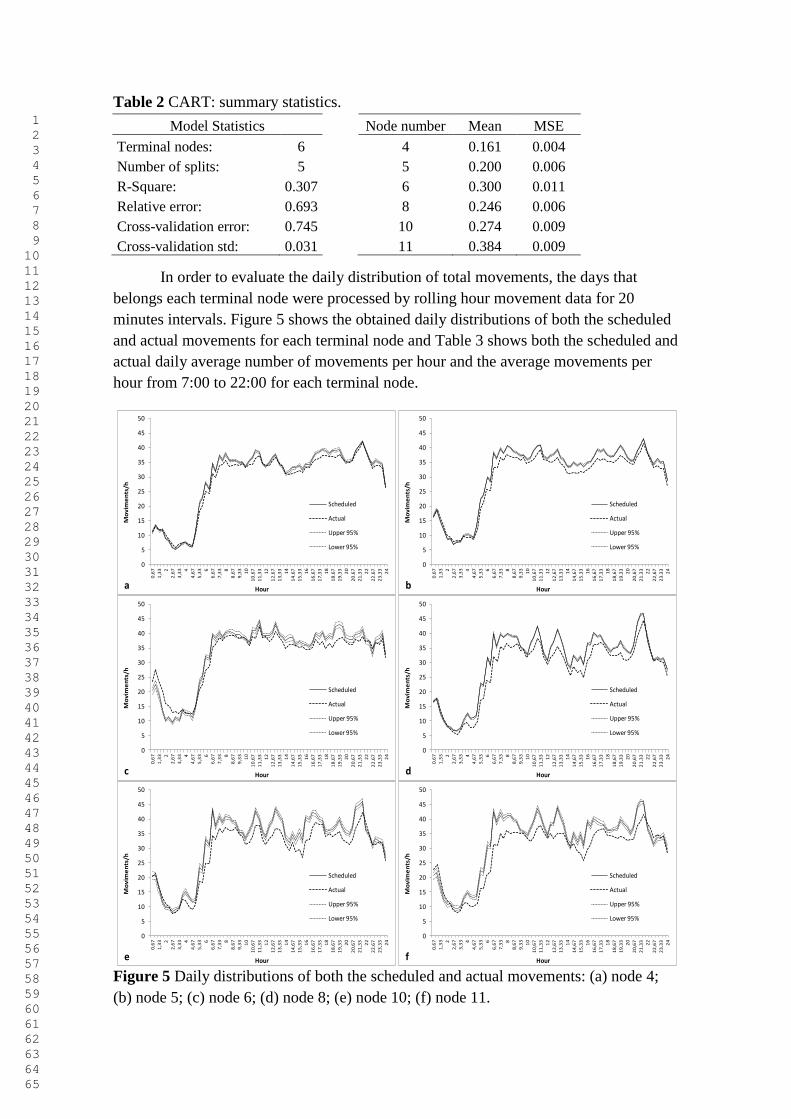
1 2 3 4 5 6 7 8 9 10 11 12 13 14 15 16 17 18 19 20 21 22 23 24 25 26 27 28 29 30 31 32 33 34 35 36 37 38 39 40 41 42 43 44 45 46 47 48 49 50 51 52 53 54 55 56 57 58 59 60 61 62 63 64 65
Table 2 CART: summary statistics.
Model Statistics Node number Mean MSE
Terminal nodes: 6 4 0.161 0.004
Number of splits: 5 5 0.200 0.006
R-Square: 0.307 6 0.300 0.011
Relative error: 0.693 8 0.246 0.006
Cross-validation error: 0.745 10 0.274 0.009
Cross-validation std: 0.031 11 0.384 0.009
In order to evaluate the daily distribution of total movements, the days that
belongs each terminal node were processed by rolling hour movement data for 20
minutes intervals. Figure 5 shows the obtained daily distributions of both the scheduled
and actual movements for each terminal node and Table 3 shows both the scheduled and
actual daily average number of movements per hour and the average movements per
hour from 7:00 to 22:00 for each terminal node.
Figure 5 Daily distributions of both the scheduled and actual movements: (a) node 4;
(b) node 5; (c) node 6; (d) node 8; (e) node 10; (f) node 11.
0
5
10
15
20
25
30
35
40
45
50
0,6
7
1,3
3 2
2,6
7
3,3
3 4
4,6
7
5,3
3 6
6,6
7
7,3
3 8
8,6
7
9,3
3
10
10
,67
11
,33
12
12
,67
13
,33
14
14
,67
15
,33
16
16
,67
17
,33
18
18
,67
19
,33
20
20
,67
21
,33
22
22
,67
23
,33
24
Mo
vim
en
ts/h
Hour
Scheduled
Actual
Upper 95%
Lower 95%
a
0
5
10
15
20
25
30
35
40
45
50
0,6
7
1,3
3 2
2,6
7
3,3
3 4
4,6
7
5,3
3 6
6,6
7
7,3
3 8
8,6
7
9,3
3
10
10
,67
11
,33
12
12
,67
13
,33
14
14
,67
15
,33
16
16
,67
17
,33
18
18
,67
19
,33
20
20
,67
21
,33
22
22
,67
23
,33
24
Mo
vim
en
ts/h
Hour
Scheduled
Actual
Upper 95%
Lower 95%
b
0
5
10
15
20
25
30
35
40
45
50
0,6
7
1,3
3 2
2,6
7
3,3
3 4
4,6
7
5,3
3 6
6,6
7
7,3
3 8
8,6
7
9,3
3
10
10
,67
11
,33
12
12
,67
13
,33
14
14
,67
15
,33
16
16
,67
17
,33
18
18
,67
19
,33
20
20
,67
21
,33
22
22
,67
23
,33
24
Mo
vim
en
ts/h
Hour
Scheduled
Actual
Upper 95%
Lower 95%
c
0
5
10
15
20
25
30
35
40
45
50
0,6
7
1,3
3 2
2,6
7
3,3
3 4
4,6
7
5,3
3 6
6,6
7
7,3
3 8
8,6
7
9,3
3
10
10
,67
11
,33
12
12
,67
13
,33
14
14
,67
15
,33
16
16
,67
17
,33
18
18
,67
19
,33
20
20
,67
21
,33
22
22
,67
23
,33
24
Mo
vim
en
ts/h
Hour
Scheduled
Actual
Upper 95%
Lower 95%
d
0
5
10
15
20
25
30
35
40
45
50
0,6
7
1,3
3 2
2,6
7
3,3
3 4
4,6
7
5,3
3 6
6,6
7
7,3
3 8
8,6
7
9,3
3
10
10
,67
11
,33
12
12
,67
13
,33
14
14
,67
15
,33
16
16
,67
17
,33
18
18
,67
19
,33
20
20
,67
21
,33
22
22
,67
23
,33
24
Mo
vim
en
ts/h
Hour
Scheduled
Actual
Upper 95%
Lower 95%
e
0
5
10
15
20
25
30
35
40
45
50
0,6
7
1,3
3 2
2,6
7
3,3
3 4
4,6
7
5,3
3 6
6,6
7
7,3
3 8
8,6
7
9,3
3
10
10
,67
11
,33
12
12
,67
13
,33
14
14
,67
15
,33
16
16
,67
17
,33
18
18
,67
19
,33
20
20
,67
21
,33
22
22
,67
23
,33
24
Mo
vim
en
ts/h
Hour
Scheduled
Actual
Upper 95%
Lower 95%
f
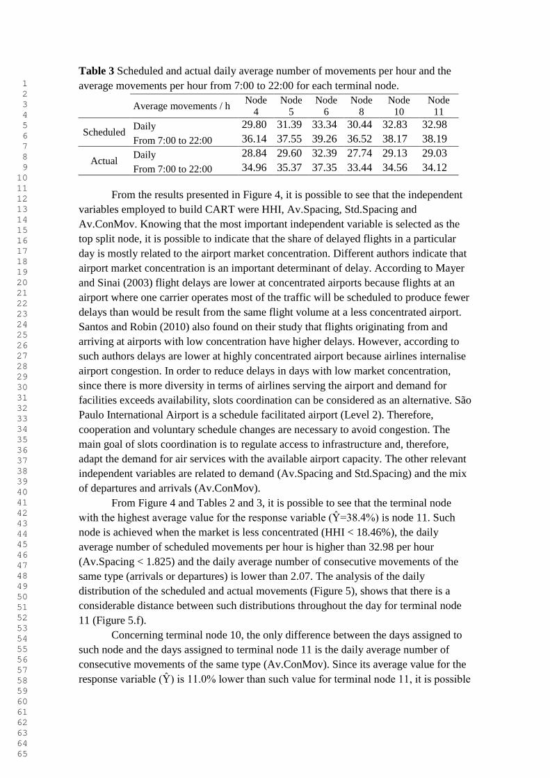
1 2 3 4 5 6 7 8 9 10 11 12 13 14 15 16 17 18 19 20 21 22 23 24 25 26 27 28 29 30 31 32 33 34 35 36 37 38 39 40 41 42 43 44 45 46 47 48 49 50 51 52 53 54 55 56 57 58 59 60 61 62 63 64 65
Table 3 Scheduled and actual daily average number of movements per hour and the
average movements per hour from 7:00 to 22:00 for each terminal node.
Average movements / h
Node
4
Node
5
Node
6
Node
8
Node
10
Node
11
Scheduled Daily 29.80 31.39 33.34 30.44 32.83 32.98
From 7:00 to 22:00 36.14 37.55 39.26 36.52 38.17 38.19
Actual Daily 28.84 29.60 32.39 27.74 29.13 29.03
From 7:00 to 22:00 34.96 35.37 37.35 33.44 34.56 34.12
From the results presented in Figure 4, it is possible to see that the independent
variables employed to build CART were HHI, Av.Spacing, Std.Spacing and
Av.ConMov. Knowing that the most important independent variable is selected as the
top split node, it is possible to indicate that the share of delayed flights in a particular
day is mostly related to the airport market concentration. Different authors indicate that
airport market concentration is an important determinant of delay. According to Mayer
and Sinai (2003) flight delays are lower at concentrated airports because flights at an
airport where one carrier operates most of the traffic will be scheduled to produce fewer
delays than would be result from the same flight volume at a less concentrated airport.
Santos and Robin (2010) also found on their study that flights originating from and
arriving at airports with low concentration have higher delays. However, according to
such authors delays are lower at highly concentrated airport because airlines internalise
airport congestion. In order to reduce delays in days with low market concentration,
since there is more diversity in terms of airlines serving the airport and demand for
facilities exceeds availability, slots coordination can be considered as an alternative. São
Paulo International Airport is a schedule facilitated airport (Level 2). Therefore,
cooperation and voluntary schedule changes are necessary to avoid congestion. The
main goal of slots coordination is to regulate access to infrastructure and, therefore,
adapt the demand for air services with the available airport capacity. The other relevant
independent variables are related to demand (Av.Spacing and Std.Spacing) and the mix
of departures and arrivals (Av.ConMov).
From Figure 4 and Tables 2 and 3, it is possible to see that the terminal node
with the highest average value for the response variable (Ŷ=38.4%) is node 11. Such
node is achieved when the market is less concentrated (HHI < 18.46%), the daily
average number of scheduled movements per hour is higher than 32.98 per hour
(Av.Spacing < 1.825) and the daily average number of consecutive movements of the
same type (arrivals or departures) is lower than 2.07. The analysis of the daily
distribution of the scheduled and actual movements (Figure 5), shows that there is a
considerable distance between such distributions throughout the day for terminal node
11 (Figure 5.f).
Concerning terminal node 10, the only difference between the days assigned to
such node and the days assigned to terminal node 11 is the daily average number of
consecutive movements of the same type (Av.ConMov). Since its average value for the
response variable (Ŷ) is 11.0% lower than such value for terminal node 11, it is possible

1 2 3 4 5 6 7 8 9 10 11 12 13 14 15 16 17 18 19 20 21 22 23 24 25 26 27 28 29 30 31 32 33 34 35 36 37 38 39 40 41 42 43 44 45 46 47 48 49 50 51 52 53 54 55 56 57 58 59 60 61 62 63 64 65
to indicate that an improvement in the scheduling, increasing the number of consecutive
movements of the same type, can be a considered as an alternative to reduce delays.
The terminal node with the lowest average value for the response variable
(Ŷ=16.1%) is node 4. From Table 3, it is possible to see that it is the node with the
lowest demand and Figure 5.a, it is possible to verify that throughout the day there is a
slight distance between the daily distributions of the scheduled and actual movements.
Such terminal node is achieved when the market is more concentrated (HHI ≥ 20.9%)
and the daily standard deviation of the time between two consecutive scheduled
movements (Std.Spacing) is higher than 2.59 minutes. Higher values for Std.Spacing
are expected in periods with lower demand since the number of scheduled movements is
high just during the peak periods. Such results are in accordance with the literature since
it is expected lower delays when the airport market is more concentrated and demand is
not high. Therefore, the days that were assigned to terminal node 4 can be labeled as
regular low movements days with most of the flights performed by the 3 biggest
Brazilian airlines (Azul, Gol and TAM).
The biggest terminal node (899 observations) is the node number 5. It is
achieved when the market concentration (HHI) is between 18,46% and 20,9% and
Std.Spacing is higher than 2.59 minutes. Its average value for the response variable (Ŷ)
is 20.0% and from Figure 5.b, it is possible to verify that throughout the day there is a
slight distance between the daily distributions of the scheduled and actual movements.
Terminal node number 6 has the second highest Ŷ value. Such node is achieved
when HHI is higher than 18.46% and Std.Spacing is lower than 2.59 minutes. From
Table 3, it is possible to see that it is the terminal node with the highest demand (daily
average value of 33.34 scheduled movements per hour) and from Figure 5.c, it is
possible to see that there is higher actual than scheduled movements until 3:00 a.m.,
probably due to delayed flights from the day before.
The last terminal nodes is the number 8. Such node is achieved when HHI is
lower than 18,46% demand is low (daily average value of 30.44 scheduled movements
per hour and Av.Spacing ≥ 1.825).
3.2.2 Multiple Linear Regression (MLR)
MLR is probably the most used expert due to its simplicity and availability.
According to Kutner et al. (2004), MLR is a statistical approach that attempts to model
a response variable (Y) as a linear weighted function of a set of independent variables
(X1, X2, ...,Xl) and an error term ε. The random error term is assumed to be uncorrelated
and to have a normal distribution with mean zero and constant variance σ2. The
regression coefficients are estimated using the ordinary least squares(OLS) method.
As mentioned before MLR was used before for identifying causes behind delays
(Santos and Robin, 2010; Abdel-Aty et al., 2007) and in delay prediction (Rebollo and
Balakrishnan, 2014). Such expert was created following the phases suggested by Kutner
et al. (2004). Thus, it was used a variable selection procedure to build a tentative
regression model. The residuals obtained applying such model were used in a diagnostic
check step and the model was validated in the final step. In this work, the independent

1 2 3 4 5 6 7 8 9 10 11 12 13 14 15 16 17 18 19 20 21 22 23 24 25 26 27 28 29 30 31 32 33 34 35 36 37 38 39 40 41 42 43 44 45 46 47 48 49 50 51 52 53 54 55 56 57 58 59 60 61 62 63 64 65
variables were selected using the stepwise regression method and the suggested
tentative model was
ii9i8i7i6
i5i4i3i2i10i
WinterConMov.AvFridayMonday
SundayTerminalNew.DSpacing.AvSummerHHIY
The obtained results are reported in Table 4 and Figure 6 shows the diagnostic check
plots.
From Table 4, it is possible to verify that independent variables HHI,
Av.Spacing and Av.ConMov have negative coefficients indicating that a lower share of
delayed movements is expected in airports with higher market concentration, when
demand is lower and when it is scheduled more consecutive movements of the same
type. Such results are in accordance with the results obtained using CART and reinforce
the pointed out suggestions to reduce flight delays. The coefficient of D.NewTerminal is
also negative suggesting that the share of delayed movements decreased after the
inauguration of the new Passengers Terminal in March 2014. Concerning the variables
with positive coefficients, the obtained results suggest that a higher share of delayed
movements is expected in both the Summer and Winter and on Sundays, Mondays and
Fridays.
Table 4 Estimated regression coefficients, standard deviations, P-values and summary
statistics for the MLR.
Regression
Coefficient
Estimated Regression
Coefficient
Estimated Standard
Deviation P-value
0 0.869 0,049 0,000
1 -2.073 0,115 0,000
2 0.055 0,005 0,000
3 -0.109 0,016 0,000
4 -0.032 0,007 0,000
5 0.035 0,006 0,000
6 0.025 0,006 0,000
7 0.021 0,005 0,000
8 -0.033 0,017 0,060
9 0.009 0,005 0,044
R 0.271
R2 adjusted 0.267
Standard error 0.076
The diagnostic check plots (Figure 6) are used to investigate the quality of the
fitted model. Since the obtained residual plots (Residuals vs Fitted and Scale-Location)
show no pattern in the points and the normal probability plot (Normal Q-Q) of the
residuals shows a reasonable agreement between theoretical and sample quantiles, it is
possible to indicate that the obtained linear model can be considered appropriate.

1 2 3 4 5 6 7 8 9 10 11 12 13 14 15 16 17 18 19 20 21 22 23 24 25 26 27 28 29 30 31 32 33 34 35 36 37 38 39 40 41 42 43 44 45 46 47 48 49 50 51 52 53 54 55 56 57 58 59 60 61 62 63 64 65
Figure 6 Diagnostic check plots: Residuals vs Fitted; Normal Q-Q; Scale-Location.
3.2.3 Time series model
Time series models are used as experts when one it interested in basing the
prediction solely on the past behaviour of that variable. In this work, the Box-Jenkins
(1970) methodology was used for creating a time series model to predict the future daily
share of delayed movements. The models created using such methodology are called
autoregressive integrated moving-average, ARIMA(p,d,q), where p is the autoregressive
(AR) order, d is the degree of differencing, and q is the moving-average (MA) order.
ARIMA(p,d,q) models are widely used in the fields of statistics and econometrics and
are created following the stages: (1) Model identification, (2) Parameters estimation and
(3) Diagnosis checking.
According to Enders (2004), in the identification stage, the researcher visually
examines the time plot of the series, the autocorrelation function (ACF) and the partial
correlation function (PACF). A comparison of the ACF and PACF to those of various
theoretical ARIMA process may suggest several plausible models. In the parameters
estimation stage, each of the tentative models is fit and the various estimated
coefficients are examined. Then the fitted models are compared using the principle of
parsimony. Box and Jenkins argue that parsimonious models produce better forecasts
than over parameterized models. Thus, a parsimonious model fits the data well without
incorporating any needless coefficients (Enders, 2004). In this work, the Akaike
information criterion (AIC) was used to compare the tentative models following the
principle of parsimony.
The third stage of the Box-Jenkins methodology involves diagnosis checking.
According to Enders (2004), it is particularly important that residuals from an estimated
model be serially uncorrelated. Hence, any of the tentative models yielding non-random
residuals should be eliminated from consideration. In this work, the diagnosis checking
was performed using the p value for the Ljung-Box statistics. The Ljung–Box statistic
(Ljung and Box, 1978) examines whether the residuals are independently distributed
and is commonly used to check the adequacy of time series fitted models.

1 2 3 4 5 6 7 8 9 10 11 12 13 14 15 16 17 18 19 20 21 22 23 24 25 26 27 28 29 30 31 32 33 34 35 36 37 38 39 40 41 42 43 44 45 46 47 48 49 50 51 52 53 54 55 56 57 58 59 60 61 62 63 64 65
The best model found following the Box-Jenkins methodology was the
ARIMA(1,0,0)(2,1,0)7. Thus, it is a seasonal ARIMA model and can be expresses as
t15-t318-t2114-t37-t21-t17-tt εYθθYθθYθYθYθYY
where Yt is the observed daily share of delayed movements in day t, j (j=1,...,3) are the
model parameters (estimated using the OLS method) and εt is a random disturbance
term. The estimated values for 1, 2 and 3 were 0.493 (standard error = 0.02), -0.632
(standard error = 0.02) and -0.316 (standard error = 0.02), respectively. The obtained p
value for the Ljung–Box test for residuals was 0.9128. Therefore it can be stated that the
residuals from the obtained model are random and that the model does fit data quite
well.
Concerning the usage of the obtained seasonal ARIMA(SARIMA) model as an
expert for the MEM, since the goal is to build two EWMs, one for anticipating
congested days one day in advance and the other to anticipate such days one week
(seven days) in advance. Thus, the obtained model was used to generate both one period
ahead prediction (Ŷt+1) and seven periods ahead prediction (Ŷt+7).
3.2.4 Gating function and MEM prediction performance
In order to conclude MEM creation, the final step is the gating function building.
The gating function is responsible to promote a cooperative learning scheme that
combines the individual experts to build a more flexible and powerful model. Thus, in
order to combine the experts it was used the softmax function expressed as
SARIMAMLRCARTl
j
l
j,,c,
xwexp
xwexp
gk
1c 1
ji,jc,
1
ji,jc,
ci,
where xi,j is the value of the observation i for the independent variable j and wc,j are the
mixing parameters. Concerning the variables for the softmax functions, it was used only
the significant variables of the MLR model and the mixing parameters values were
estimated minimizing the error function expressed as
n
1i
2
SARIMAi,iSARIMAi,
2
MLRi,iMLRi,
2
CARTi,iCARTi, YY2
1expgYY
2
1expgYY
2
1expglog
The estimated parameters value are reported in Table 5. Using such parameters
values, MEM's predictions (Ŷt+1 and Ŷt+7) are given by
SARIMAi,SARIMAi,MLRi,iMLR,CARTi,CARTi,i YgYgYgY
where gic is the weight factor for the expert c and Ŷic is the prediction generated using
expert c. The predictions generated using each individual expert and the proposed
approach were compared and their performances were assessed using both the root
mean squared error (RMSE) and the mean absolute percentage error (MAPE). RMSE is
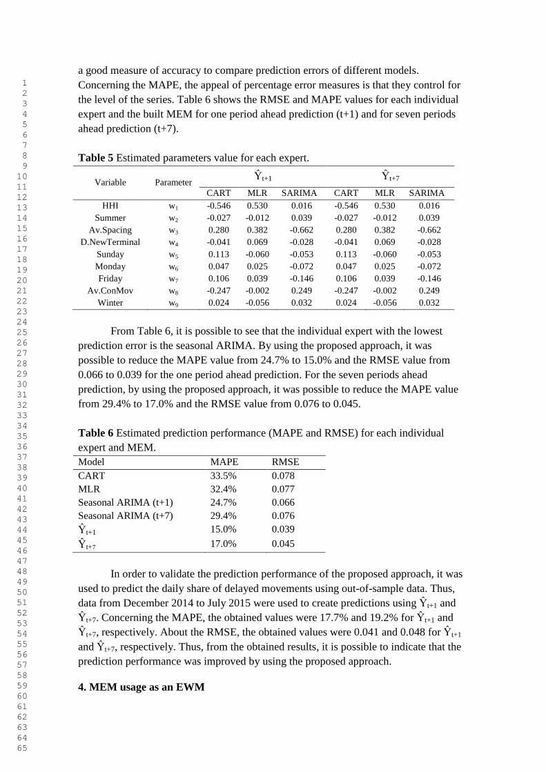
1 2 3 4 5 6 7 8 9 10 11 12 13 14 15 16 17 18 19 20 21 22 23 24 25 26 27 28 29 30 31 32 33 34 35 36 37 38 39 40 41 42 43 44 45 46 47 48 49 50 51 52 53 54 55 56 57 58 59 60 61 62 63 64 65
a good measure of accuracy to compare prediction errors of different models.
Concerning the MAPE, the appeal of percentage error measures is that they control for
the level of the series. Table 6 shows the RMSE and MAPE values for each individual
expert and the built MEM for one period ahead prediction (t+1) and for seven periods
ahead prediction (t+7).
Table 5 Estimated parameters value for each expert.
Variable Parameter Ŷt+1 Ŷt+7
CART MLR SARIMA CART MLR SARIMA
HHI w1 -0.546 0.530 0.016 -0.546 0.530 0.016
Summer w2 -0.027 -0.012 0.039 -0.027 -0.012 0.039
Av.Spacing w3 0.280 0.382 -0.662 0.280 0.382 -0.662
D.NewTerminal w4 -0.041 0.069 -0.028 -0.041 0.069 -0.028
Sunday w5 0.113 -0.060 -0.053 0.113 -0.060 -0.053
Monday w6 0.047 0.025 -0.072 0.047 0.025 -0.072
Friday w7 0.106 0.039 -0.146 0.106 0.039 -0.146
Av.ConMov w8 -0.247 -0.002 0.249 -0.247 -0.002 0.249
Winter w9 0.024 -0.056 0.032 0.024 -0.056 0.032
From Table 6, it is possible to see that the individual expert with the lowest
prediction error is the seasonal ARIMA. By using the proposed approach, it was
possible to reduce the MAPE value from 24.7% to 15.0% and the RMSE value from
0.066 to 0.039 for the one period ahead prediction. For the seven periods ahead
prediction, by using the proposed approach, it was possible to reduce the MAPE value
from 29.4% to 17.0% and the RMSE value from 0.076 to 0.045.
Table 6 Estimated prediction performance (MAPE and RMSE) for each individual
expert and MEM.
Model MAPE RMSE
CART 33.5% 0.078
MLR 32.4% 0.077
Seasonal ARIMA (t+1) 24.7% 0.066
Seasonal ARIMA (t+7) 29.4% 0.076
Ŷt+1 15.0% 0.039
Ŷt+7 17.0% 0.045
In order to validate the prediction performance of the proposed approach, it was
used to predict the daily share of delayed movements using out-of-sample data. Thus,
data from December 2014 to July 2015 were used to create predictions using Ŷt+1 and
Ŷt+7. Concerning the MAPE, the obtained values were 17.7% and 19.2% for Ŷt+1 and
Ŷt+7, respectively. About the RMSE, the obtained values were 0.041 and 0.048 for Ŷt+1
and Ŷt+7, respectively. Thus, from the obtained results, it is possible to indicate that the
prediction performance was improved by using the proposed approach.
4. MEM usage as an EWM

1 2 3 4 5 6 7 8 9 10 11 12 13 14 15 16 17 18 19 20 21 22 23 24 25 26 27 28 29 30 31 32 33 34 35 36 37 38 39 40 41 42 43 44 45 46 47 48 49 50 51 52 53 54 55 56 57 58 59 60 61 62 63 64 65
This section is dedicated to the EWM building. As argued before, in order to
help airport authorities develop effective strategies to reduce flight delays and support
response planning, a critical issue is how to anticipate the occurrence of congested days.
Using the daily share of delayed flights as a measure of congestion at airports, the goal
is to build an EWM to anticipate congested days at GRU by predicting such variable
value.
The critical tasks for the EWM success are the indicators identification and the
prediction procedure. Due to the superior prediction performance obtained using MEM,
such modelling approach was selected to generate the predictions for the EWM. Thus,
the predictions generated using Ŷt+1 and Ŷt+7 are employed to predict the daily share of
delayed flights one day in advance and seven days in advance, respectively. About the
indicators, all independent variables employed by the built CART and MLR models are
necessary to generate the predictions.
In order to facilitate the monitoring of the daily share of delayed movements,
such variable was divided into three ranges: less than or equal to the 25th percentile
(below average), between the 26th and 74th percentiles (average) and higher than or
equal to the 75th percentile (above average). Using data from January 2010 to May
2014 and from August 2014 to November 2014, the monitoring variable was defined as
26.0%Yifaverage,above
26.0%Y14.9%ifaverage,
14.9%Yifaverage,below
DelayShare.
t
t
t
t
The performance of the built EWM was evaluated using data from December
2014 to July 2015 and the obtained results are reported in Tables 7 (Ŷt+1) and 8 (Ŷt+7) .
Table 7 Obtained confusion matrix for evaluating the built EWM (Ŷt+1).
Actual Share.Delay
Below Average Average Above Average
Predicted
Share.Delay
Below Average 131 6 0
Average 12 71 2
Above Average 0 3 18
Table 8 Obtained confusion matrix for evaluating the built EWM (Ŷt+7).
Actual Share.Delay
Below Average Average Above Average
Predicted
Share.Delay
Below Average 120 7 0
Average 23 67 3
Above Average 0 6 17
From Tables 7 and 8, it is possible to verify that Ŷt+1 correctly anticipated 220
out of 243 days and that Ŷt+7 correctly anticipated 204 out of 243 days. Thus, the
accuracy of the built EWM was 90.5% in anticipating the Share.Delay value one day
ahead and 83.9% in anticipating the Share.Delay value seven days ahead.

1 2 3 4 5 6 7 8 9 10 11 12 13 14 15 16 17 18 19 20 21 22 23 24 25 26 27 28 29 30 31 32 33 34 35 36 37 38 39 40 41 42 43 44 45 46 47 48 49 50 51 52 53 54 55 56 57 58 59 60 61 62 63 64 65
5. Conclusions
In this work an early warning model was built for anticipating congested days at
the São Paulo International Airport. Therefore, a data analytics approach called
Mixture-of-experts model (MEM) was used to combine modelling approaches that rely
on different assumptions regarding the data available to process. Such approach allows
to generate a more flexible and powerful model that makes good promises of
improvement in the prediction accuracy.
The built MEM is composed by a CART, a MLR and a seasonal ARIMA.
CART was chosen as an expert due its capacity in providing an interpretable prediction
procedure. By applying CART, it was possible to understand how the determinants of
delay combine to result in a day with high concentration of delayed flights and to point
out alternatives to reduce delay. MLR was chosen as an expert because it was already
used in similar situations to identify causes behind delays and in delay prediction. The
results achieved applying MLR were consistent to the literature and reinforced the
alternatives to reduce delay identified using CART. The seasonal ARIMA was the
individual expert with the lowest prediction error. Afterwards, a gating function was
created to promote a cooperative learning scheme between the individual experts and to
compose the mixture model.
The MEM was used to generate predictions for one period ahead and for seven
periods ahead and the obtained results proved to be satisfactory. Thus, MEM was
selected to generate the predictions for the early warning model (EWM). The accuracy
of the built EWM was also considered satisfactory for anticipating congested days one
day in advance and seven days in advance.
For future work, since MEM proved to be very flexible, it is intended to make
use of other modelling approaches such as Support Vector Regression and Random
Forests to compose the mixture model. Moreover, it is intended to extend such
modelling approach to predict delay of individual flights.
Acknowledgements
The author acknowledges the financial support from FAPESP - Fundação de
Amparo a Pesquisa do Estado de São Paulo (grant 2013/22416-4).
References
Abdel-Aty, M., Lee, C., Bai, Y. Li, X., Michalak, M., 2007. Detecting periodic patterns
of arrival delay. Journal of Air Transport Management, 13, 355-361.
Banks, D. L., 2010. Statistical Data Mining. Wiley Interdisciplinary Reviews:
Computational Statistics, 2(1), 9-25.
Box, G.E.P., Jenkins, G., 1970. Time Series Analysis: Forecasting and Control.
Holden-Day, San Francisco.
Breiman, L., Friedman, J., Olshen, R., Stone, C., 1984. Classification and Regression
Trees. Wadsworth International Group, Monterey, CA.

1 2 3 4 5 6 7 8 9 10 11 12 13 14 15 16 17 18 19 20 21 22 23 24 25 26 27 28 29 30 31 32 33 34 35 36 37 38 39 40 41 42 43 44 45 46 47 48 49 50 51 52 53 54 55 56 57 58 59 60 61 62 63 64 65
Buxi, G., Hansen, M., 2013. Generating Day-of-operation Probabilistic Capacity
Scenarios from Weather Forecasts. Transportation Research Part C: Emerging
Technologies, 33, 153-166.
Costa, T. F. G., Lohmann, G., Oliveira, A. V. M., 2010. A model to identify airport
hubs and their importance to tourism in Brazil. Research in Transportation
Economics, 6(1), 3-11.
Diana, T., 2014. Validating delay constructs: An application of confirmatory factor
analysis. Journal of Air Transport Management, 35, 87-91.
Enders, W., 2004. Applied Econometric Time Series, 2nd
edition. New York: John
Wiley & Sons.
Ferguson, J., Kara, A. Q., Hoffman, K., Sherry, L., 2013. Estimating domestic US
airline cost of delay based on the European model. Transportation Research Part
C: Emerging Technologies, 33, 196-202.
Ferrari, D. B., Milioni, A. Z., 2011. Choices and pitfalls concerning mixture-of-experts
modelling. Pesquisa Operacional, 31(1), 95-111.
Jacobs R.A., Jordan M.I., Nowlan S.J., Hinton G.E., 1991. Adaptive mixtures of local
experts. Neural Computation, 3(1), 79–87.
Kutner, M.H., Nachtsheim, C.J., Neter, J., 2004. Applied Linear Regression Models,
4th
edition. Boston: McGraw-Hill Irwin.
Liu, P. B., Hansen, M., Mukherjee, A., 2008. Scenario-based air traffic flow
management: From theory to practice. Transportation Research Part B:
Methodological, 42, 685-702.
Ljung, G., Box G. E. P., 1976. On a Measure of Lack of Fit in Time Series Models.
Biometrika, 66, 67–72.
Madas, M. A., Zografos, K, G., 2008. Airport capacity vs. demand: mismatch or
mismanagement? Transportation Research Part A: Policy and Practice, 42, 203-
226.
Mayer, C., Sinai, T., 2003. Network effects, congestion externalities, and air traffic
delays: Or why not all delays and created evil. The American Economic Review,
93(4), 1194 - 1215.
Olafsson, S., Li, X., Wu, S., 2008. Operations research and data mining. European
Journal of Operational Research, 187(3), 1429-1448.
Öttl, G., Böck, P., Werpup, N., Schwarze, M., 2013. Derivation of Representative Air
Traffic Peaks as a Standard Input for Airport Related Simulation , Journal of Air
Transport Management, 28, 31-39.
Pyrgiotis, N., Malone, K. M., Odoni, A., 2013. Modelling delay propagation within an
airport network. Transportation Research Part C: Emerging Technologies, 27,
60-75.
Rebollo, J. J., Balakrishnan, H., 2014. Characterization and prediction of air traffic
delays. Transportation Research Part C: Emerging Technologies, 44, 231-241.
Ripley, B. D., 1996. Pattern recognition and neural networks. Cambridge University
Press, Cambridge.
Santos, G., Robin, M., 2010. Determinants of delays at European airports.
Transportation Research Part B: Methodological, 44(3), 392-403.

1 2 3 4 5 6 7 8 9 10 11 12 13 14 15 16 17 18 19 20 21 22 23 24 25 26 27 28 29 30 31 32 33 34 35 36 37 38 39 40 41 42 43 44 45 46 47 48 49 50 51 52 53 54 55 56 57 58 59 60 61 62 63 64 65
Scarpel, R. A., 2014. A demand trend change early warning forecast model for the city
of São Paulo multi-airport system. Transportation Research Part A: Policy and
Practice, 65, 23-32.
Wensveen, J. G., 2011. Air transportation: A management perspective, 7th
edition.
Ashgate, Aldershot, UK.
Recommended


![dummy informe completo - ucacsa.com.mx · FRIJOL Toneladas Edo. Chihuahua 2013 [1] Hectáreas Financiadas por Ucacsa 2013 [2] Hectåreas Financiadas por Ucacsa 2013 [2) Hectáreas](https://img.document.onl/doc/110x75/5eab54d6e55cb478f735f31c/dummy-informe-completo-frijol-toneladas-edo-chihuahua-2013-1-hectreas-financiadas.jpg)