UNIVERSIDADE FEDERAL DO PARANÁ
TIAGO CELSO BALDISSERA
O AMBIENTE LUMINOSO: DO IMPACTO NO CRESCIMENTO E DESENVOLVIMENTO EM NÍVEL DE PLANTA FORRAGEIRA A DOSSÉIS EM
SISTEMAS INTEGRADOS DE PRODUÇÃO AGROPECUÁRIA
CURITIBA
2014
UNIVERSIDADE FEDERAL DO PARANÁ
TIAGO CELSO BALDISSERA
O AMBIENTE LUMINOSO: DO IMPACTO NO CRESCIMENTO E
DESENVOLVIMENTO EM NÍVEL DE PLANTA FORRAGEIRA A DOSSÉIS EM SISTEMAS INTEGRADOS DE PRODUÇÃO AGROPECUÁRIA
Tese apresentada ao Curso de Pós-Graduação em Agronomia, Área de concentração em Produção Vegetal, Setor de Ciências Agrárias, Universidade Federal do Paraná, como requisito parcial para obtenção do título de Doutor em Ciências.
Orientador: Prof. Dr. Paulo C. de Faccio Carvalho Co-orientador: Prof. Dr. Aníbal de Moraes Co-orientadora: Dra. Laíse da Silveira Pontes Co-orientador: Prof. Dr. Sebastião B.C. Lustosa Co-orientador: Dr. Gaetan Loüarn Co-orientadora: Dra. Ela Frak
CURITIBA 2014

AGRADECIMENTOS
Primeiramente e acima de tudo a Deus, pela vida.
Aos meus pais, Selso L. Baldissera e Maria L. S. Baldissera, pelos maiores
ensinamentos que recebi em minha vida, pela compreensão e suporte durante todos os passos
de minha caminhada até este momento.
Aos meus irmãos Felipe e Gabriel, pelas “brigas”, mas acima de tudo pelo
companheirismo das horas que realmente precisei.
Aos meus avôs e avós, especialmente a vó Leobina. Toda minha família que sempre
me apoiou. E à Ana Carolina Sekula pelo seu suporte e compreensão.
Ao professor Paulo César de Faccio Carvalho, pela confiança para o desenvolvimento
do trabalho, pela orientação, apoio, ensinamentos, por todas as oportunidades oferecidas e
pela amizade.
A Dra Laíse da Silveira Pontes, por todas as horas despendidas para me ajudar na
execução do trabalho, por todos os ensinamentos transmitidos.
Aos professores Aníbal de Moraes e Sebastião Brasil Campos Lustosa pelo apoio em
todos os momentos, pelas conversas e boas discussões que sempre me orientaram. Acima de
tudo pela grande amizade.
Ao Dr. Vanderley Porfírio-da-Silva pelos ensinamentos sobre os sistemas integrados
arborizados e pelas conversas e ajuda para o desenvolvimento dos trabalhos.
À minha querida amiga Dra Raquel Santiago Barro pela ajuda sem igual nos trabalhos,
pelas suas sugestões nos trabalhos e pelo grande companheirismo em todos os momentos.
Ao Dr. Gaëtan Louarn e a Dra. Ela Frak pelo aceite para me orientar durante o período
na França, além dos muitos ensinamentos e amizade.
Aos meus amigos e companheiros de trabalho, André Giostri, Danielle Machado, João
Daniel, Edemar Camargo, Keli Guera, João Copla, Miquéias Michetti, Renato Almeida,
Sandoval Carpinelli, Juliano Valenga, Camila Burdak, Adriano Gomes que muito me
ajudaram no desenvolvimento dos experimentos. E também ao grupo de pesquisa em sistemas
integrados e ao grupo de pesquisa em ecologia do pastejo.
A todos os professores com que tive contato e aos funcionários da pós-graduação em
produção vegetal, em especial a secretária do programa de pós-graduação Lucimara Antunes.

A todos os funcionários do IAPAR – Estação Experimental Fazenda Modelo, em
especial aos técnicos Giliardi Stafin e Pedro Paulo Pomkerner. Ainda um agradecimento
especial para o André Luiz de Francisco pelo suporte e amizade.
A todos os funcionários do INRA – Lusignan, em especial ao Laboratório de
Ecofisiologia de Pastagens, que me receberam muito bem durante o meu período na França.
Ao Instituto Agronômico do Paraná (IAPAR), por disponibilizar área, estrutura e
recursos para o desenvolvimento de experimentos.
À Universidade Estadual do Centro-Oeste, pela infra-estrutura disponibilizada para o
desenvolvimento do experimento.
Ao Institut Nationale de la Recherche Agronomique (INRA), pela disponibilidade de
estrutura e recursos para o desenvolvimento de experimentos
Ao CNPQ pelo apoio financeiro (Repensa). A CAPES pela disponibilização das bolsas
no Brasil e da bolsa sanduíche para a França, pelo programa Capes / Cofecub (projeto 684/10)
.
RESUMO
Os sistemas de produção devem atender a demandas quantitativas e qualitativas na produção
de alimentos. Contudo, devem também contemplar exigências de sustentabilidade. Nos
arranjos produtivos existem diversas formas e estratégias de cultivo, dentre elas a integração
de cultivos numa mesma área e ao mesmo tempo. Entretanto, as diferentes espécies competem
pelos recursos do ambiente, dentre eles a luz, que é considerada um dos principais fatores que
interferem na arquitetura das plantas e na dinâmica do dossel vegetal. Deste modo, o objetivo
central deste trabalho foi de estudar os processos de crescimento e desenvolvimento de
espécies forrageiras em ambientes com alterações das condições de luz. Os primeiros dois
capítulos da tese avaliam o efeito das árvores, em integração lavoura-pecuária, sobre o
crescimento e desenvolvimento de: Axonopus catharinensis, Brachiaria brizantha cv.
Marandu, Megathyrsus maximus cv. Aruana, Hemarthria altissima cv. Flórida, Cynodon spp.
hibrido Tifton 85 e Paspalum notatum cv. Pensacola. O terceiro capítulo aborda o efeito da
luz azul no crescimento e desenvolvimento de genótipos de alfafa (Medicago sativa). O
quarto capítulo avalia os efeitos da competição por luz em estandes puros e mistos de alfafa
com festuca, verificando quais processos mais interferem na expansão da área foliar da alfafa.
Foi possível concluir que os mecanismos de resposta ao efeito de árvores em interação com
nitrogênio são espécie-dependentes e apresentam consequências para o manejo do pasto em
sistemas integrados com árvores. O efeito da luz azul foi mais significativo nas alterações das
características morfológicas quando o genótipo de alfafa tinha hábito de crescimento ereto,
que apresenta características de mecanismo de escape a sombra. As diferenças na área foliar
total de plantas de alfafa é dependente principalmente da ramificação lateral dos ramos
principais e do número de ramos, mais do que do tamanho específico de cada folha.
Palavras chave: integração lavoura-pecuária; manejo de pastagens; dossel forrageiro;
competição; interceptação luminosa
ABSTRACT
Production systems should meet the quantity and quality demands on food production.
However, should include the maintenance of production sustainability requirements. There
are several ways and strategies for production systems, some types of them is the consortium
of species in the same area and in the same temporal scale. However, different species
compete for environmental resources, including light, which is considered one of the main
factors that affect plant architecture and dynamics of plant canopy, and may have
consequences for production and also for the management strategies. Thus, the aim of this
study was to evaluate the growth and development of forage species in different light
environmental conditions. The first two chapters of this thesis evaluates the effect of trees and
nitrogen in an integrated crop-livestock system, on the growth and development of tropical C4
grasses: Axonopus catharinensis, Brachiaria brizantha cv. Marandu, Megathyrsus maximus
cv. Aruana, Hemarthria altíssima cv. Flórida, Cynodon spp. hibrido Tifton 85 e Paspalum
notatun cv. Pensacola. The third chapter discusses the effect of blue light on the growth and
development of contrasting genotypes of alfalfa (Medicago sativa). The fourth chapter
evaluates the effects of competition for light in pure and mixed stands of alfalfa with grass,
and which processes more interfere in the expansion of alfalfa leaf area. It was possible to
conclude that there is species dependence for the responses of growth and development due to
the effect of shading by trees and nitrogen, with consequences for the management of these
species in a integrated system with trees. The blue light effect resulted in more significant
changes of the morphological characteristics on the genotype of erect growth habit, showing
the trend that this genotype has characteristics to escape shade. The effect of light competition
in pure stand of alfalfa is greater than in consortium with grass, differences in leaf area of
alfalfa is dependent mainly on lateral branching and number of shoots, harder than the leaf
size.
Key words: integrated crop-livestock system; pasture management; forage canopy; competition; light interception
LISTA DE FIGURAS
CAPITULO 1
Figure 1 – Mean (circle), maximum (triangle) and minimal (square) average monthly air
temperatures from September 2011 to May 2013. Open symbols and short dash lines for full
sun and closed symbols solid lines for integrated crop-livestock system..…...………………46
Figure 2 – Monthly mean soil volumetric water content in the top 200 mm (measured every
15 days)………………………………………………...……….………………………...…..47
Figure 3 – Relationship between sward height (cm) and light interception (%) for six C4
forage species at the integrated crop-livestock system (closed symbols and solid lines) and full
sun (open symbols and short dash lines). Ac – Axonopus catharinesnis, Bb – Brachiaria
brizantha, Mm – Megathyrsus maximus, Ha – Hemarthria altissima, Cc – Cynodon spp., Pn –
Paspalum notatum. ANCOVA results are presented in each panel: two lines in the case of no
interaction and difference between intercepts between the categorical independent variable
(i.e. sward height), and a single line in the case of no significant effect of the continuous
variable. (*P<0.05; **P<0.01; ***P<0.001; ns, not significant)……………………...……...48
CAPITULO 2
Figure 1 – Daily Mean air temperatures during 2011 and 2012 for the experimental
period………………………………………………………………………………….……...75
Figure 2 – Means for the morphogenical and structural parameters for each species and also
within each system (i.e. data shown the species x system interaction). Means with the same
capital letters compares systems, means with small letters compares species within each
system and means with capital letters with * compares species according to the Tukey test (P
>0.05). Bars indicate the standard error of the mean. Species code: Axonopus catharinensis
(Ac); Bb – B. brizantha; Mm – Megathyrsus maximus Ha – Hemarthria altissima; and Cc –
Cynodon spp. Variables code: phyllochron (Phyl.); leaf elongation rate (LER); duration of
leaf elongation (DLE), leaf lifespan (LLS; leaf senescence rate (LSR); stem elongation rate

(SER); number of green leaves (NGL); leaf length (LL); tiller density
(TD).……………………………………..………………………………………………….……...76
Fig. 3 - Means for the morphogenical and structural characteristics for the interaction species
x nitrogen. Means with the same capital letters compares systems, means with small letters
compares species within each system according to the Tukey test (P >0.05). Bars indicate the
standard error of the mean. Species code: Axonopus catharinensis (Ac); Bb – B. brizantha;
Mm – Megathyrsus maximus Ha – Hemarthria altissima; and Cc – Cynodon spp. Variables
code: leaf elongation rate (LER); leaf lifespan (LLS); leaf senescence rate (LSR); number of
green leaves (NGL); leaf length (LL); tiller density
(TD)…………………………………...……………………………………………..……......77
Fig. 4 – Means for the morphogenical and structural parameters for each species and also
within each system (i.e. data shown the species x system interaction). Means with the same
capital letters compares systems, means with small letters compares species within each
system and means with capital letters with * compares species according to the Tukey test (P
>0.05). Bars indicate the standard error of the mean. Species code: Axonopus catharinensis
(Ac); Bb – B. brizantha; Mm – Megathyrsus maximus Ha – Hemarthria altissima; and Cc –
Cynodon spp. Variables code: specific leaf weight (SLW); leaf senescence rate
(LSR)…………………………...……………………………………………………….…….78
Fig. 5 – A) Means for the growth and senescence fluxes for each species and also within each
system (i.e. data shown the species x system interaction).. B) Means for growth and
senescence fluxes for the interaction species x nitrogen. Means for the morphogenical and
structural parameters for each species and also within each system (i.e. data shown the species
x system interaction). Means with the same capital letters compares systems, means with
small letters compares species within each system and means with capital letters with *
compares species according to the Tukey test (P >0.05). Bars indicate the standard error of the
mean. Species code: Axonopus catharinensis (Ac); Bb – B. brizantha; Mm – Megathyrsus
maximus Ha – Hemarthria altissima; and Cc – Cynodon spp………………..……………...79
Supplementary data Fig S1 – Means for morphogenical and structural characteristics and the
interaction species x year condition. Means with the same capital letters compares light
condition, means with small letters compares species within each light condition according to
the Tukey test (P >0.05). Species code: Axonopus catharinensis (Ac); Bb – B. brizantha; Mm
– Megathyrsus maximus Ha – Hemarthria altissima; and Cc – Cynodon spp. Variables code:
phyllochron (Phyl.); duration of leaf elongation (DLE); leaf lifespan (LLS); leaf senescence
rate (LSR); stem elongation rate (SER); number of green leaves (NGL); leaf length (LL);
senescence flux (SF)……….…..……………………………………………………………..80
CAPITULO 3
Figure 1 – Probability of internode and petiole appearance in respect to each node position in
the main axis of contrasted genotypes of Medicago sativa. (B- less bluelight; B+ neutral blue
light). (B4 prostrate; D3 erect)……………………………...………………………...……..101
Figure 2 – Internod lengths in respect to each node position in the main axis. of contrasted
genotypes of Medicago sativa. (B- less bluelight; B+ neutral blue light). (B4 prostrate; D3
erect) (*P< 0.05; **P < 0.01; ***P<0.001; ns, not significant)…………………………….102
Figure 3 - Petiole lengths in respect to each node position in the main axis of contrasted
genotypes of Medicago sativa. (B- less bluelight; B+ neutral blue light). (B4 prostrate; D3
erect) (*P< 0.05; **P < 0.01; ***P<0.001; ns, not significant).…………………………….103
CAPITULO 4
Figure 1. Number of visible primary leaves as a function of thermal time expressed in
cumulative degree-days from shoot emergence during the growth and regrowth phases of Exp.
1. The regression was estimated for all data on the plot (y = 0.0301 x + 1.09, n = 433, r2=
0.94). MA, primary axis; T1, type 1 axis; T2, type 2 axis......................................................108
Figure 2. Numbers of primary and total number of secondary leaves as a function of thermal-
time expressed in cumulative degree-days from shoot emergence during the growth phases of
Exp. 1. The regressions were estimated for all data on the plot (y = 0.0003x2 – 0.0275x, n=
207, r2= 0.91 for secondary leaves; same fit as Fig. 1 for primary leaves). The arrow indicates
the early bloom stage. MA, primary axis………………………………………………........108
Figure 3. (A)Thermal time of primary leaf appearance and axillary budburst according to
node position on the primary axis (MA) shoot and (B) branching probability with respect to
nodal position from the apex at four developmental stages for shoots during the growth phase
of Exp. 1. The regressions were estimated for all data on the plot (y = 0.029x -0.5682, n= 8,
r2= 0,96 for branch budburst; same fit as Fig. 1 for primary leaves)………………….……109
Figure 4. Number of secondary leaves as a function of branch position and thermal time as
predicted by the potential shoot development model (eqns 3–6)………………………..…..109
Figure 5. Relationships between plant leaf area and leaf number (left), and plant leaf area and
maximum leaf size (right) in the four situations studied during Exp 2: (A, B) Pure stands
growth, (C, D) Mixed stands growth, (E, F) Mixed stands regrowth, (G, H) Pure stands
growth. High (HD) and low density (LD) are as indicated in the key in (A). ANCOVA results
are presented in each panel: two lines in the case of an interaction between the categorical
independent variable (i.e. density) and the continuous variable, no line in the case of a non-
significant effect of the continuous variable, and a single line in the case of a significant effect
of the continuous variable without any interaction. In an absence of interaction, D indicates
the level of significance of the categorical independent variable (* p <0.05, ** p<0.01, ***
p<0/001 and ns = not significant). r2 indicates the coefficient of determination of the
regression in the case of a significant effect of the continuous variable………………..…...110
Figure 6. Relationships between plant leaf area and the shoot number (left), and plant leaf area
and the number of leaves per shoot (right) in the four situations studied during Exp. 2: (A, B)
Pure stands growth, (C, D) Mixed stands growth, (E, F) Mixed stands regrowth, (G, H) Pure
stands growth.. High (HD) and low density (LD) are as indicated in the key in (A). ANCOVA
results are presented in each panel: two lines in the case of an interaction between the
categorical independent variable (i.e. density) and the continuous variable, no line in the case
of a non-significant effect of the continuous variable, and a single line in the case of a
significant effect of the continuous variable without any interaction. In an absence of
interaction, D indicates the level of significance of the categorical independent variable (*
p<0.05, ** p<0.01, *** p<0.001 and ns = not significant). r2 indicates the coefficient of
determination of the regression in the case of a significant effect of the continuous
variable…………………………………………………………………………………...….111
Figure 7. Number of secondary leaves per shoot as a function of primary axis development in
the four situations studied during Exp. 2: a) Pure stands growth, b) Pure stands regrowth, c)
Mixed stands growth, d) Mixed stands regrowth. High (HD) and low density (LD) are as
indicated in the key in (A). The plain line represents the relationship predicted by the potential
shoot development model (eqns 3–6). ANCOVA results are presented in each panel: two
dashed lines are plotted in the case of an interaction between the categorical independent
variable (i.e. density) and the continuous variable. P-values indicate the level of significance
of the interactions (* p<0.05, ** p<0.01, *** p<0.001 and ns = not significant)………...…112
Figure 8. Number of secondary leaves at each node position on high (HD) and low density
(LD) plants in the four situations studied during Exp. 2: a) Pure stands growth, b) Pure stands
regrowth, c) Mixed stands growth, d) Mixed stands regrowth. Shoots were selected at a given
stage of development in each situation (shoots with 12-14 primary leaves). The dotted line
represents the number of secondary leaves predicted by the potential shoot development
model (eqns 3–6). P-values indicate the results of the t test for a comparison between LD and
HD at each node position (* p < 0.05, ** p< 0.01, *** p<0.001 and ns = not significant)....113
Figure 9. Comparison between primary shoot size distributions at high (HD) and low density
(LD) in the four situations studied during Exp. 2: a) Pure stands growth, b) Pure stands
regrowth, c) Mixed stands growth, d) Mixed stands regrowth. P-values indicate the level of
significance of the KS-test (* p<0.05, ** p<0.01, *** p<0.001 and ns = not significant)….114
Fig. S1. Diagrams of a) the arrangement of the main axis, secondary and tertiary axes on a
seedling plant (initial growth cycle) and b) the types of main axes emerging either from the
taproot (T2) or from the axil of a leaf just below the cutting height (T1) of a mature plant
during a regrowth cycle. Redrawn from Moreau et al. (2007) and Gosse et al.(1988)…..…119
Fig. S2. Number of leaves on branches as a function of thermal-time accumulation expressed
in cumulative degree-days from shoot emergence during the growth phases of Exp. 1. Open
and closed symbols indicate 2012 and 2009 data, respectively. Date of branch appearance
(DA) and phyllochron (RLa-1) estimated from linear regressions are indicated in each
panel........................................................................................................................................120

Fig. S3. Dynamics of canopy light interception efficiency measured in the different pure and
mixture stands studied…………………………………………………………………….....121

LISTA DE TABELAS
CAPITULO 1
Table 1 – Proportion of variance explained (VE) and statistical significance of F ratios from
analysis of covariance for sward height and for each C4 forage species. Ac – Axonopus
catharinesnis, Bb – Brachiaria brizantha, Mm – Megathyrsus maximus, Ha – Hemarthria
altissima, Cc – Cynodon spp., Pn – Paspalum notatum…………………………………...…43
Table 2 – Sward height means (cm) and standard error (se) at cutting date within each year,
season, nitrogen level and system for the six C4 forage species. See Table 1 for species
codes………………………………………………………………………………………..…44
Table 3 - Sward height means (cm) and standard error (se) for M. maximus (Mm) and P.
notatum (Pn). Data show Year x Season interaction..…………………………………....…..44
Table 4 – Means and standard error (se) of Leaf Length (LL – cm), Sheath Length (SL – cm),
Tiller Density (TD) and leaf:stem ratio for six C4 forage species within each system and
nitrogen treatment. See Table 1 for species codes.……..………….……………………........45
CAPITULO 2
Table 1 - Percentage of variance explained (VE) and statistical significance from the ANOVA
for phyllochron (Phyl.), leaf elongation rate (LER), duration of leaf elongation (DLE), leaf
lifespan (LLS), leaf senescence rate (LSR), stem elongation rate (SER), number of green
leaves (NGL), specific leaf weight (SLW), leaf length (LL), tiller density (TD), growth flux
(GF) and senescence flux (SF)……………….……………………………………………….74
Table 2 – Means and standard error (se) for morphogenetic characteristics and growth and
senescence fluxes for the years 2011 and 2012……...……………………...………………..75
CAPITULO 3
Table 1 – F-ratios and statistical significance of ANOVAs of plant traits in function of blue
light and contrasted genotypes of Medicago sativa………………………..…………….…...99
Table 2 – Plant traits in function of blue light (B- less bluelight; B+ neutral blue light) and
contrasted genotypes of Medicago sativa (B4 prostrate; D3 erect)…………………………..99
Table 3 – Leaf area of main (cm2) axis in function of blue light (B- less bluelight; B+ neutral
blue light) and contrasted genotypes of Medicago sativa (B4 prostrate; D3
erect)………………………………………….…………………………………….………....99
Table 4 - Stem dry weight of the main axis (g) and specific stem weight (g. cm-1) in function
of blue light (B- less bluelight; B+ neutral blue light) and contrasted genotypes of Medicago
sativa (B4 prostrate; D3 erect)………..………………………………………………...…...100
Table 5 – Leaf:stem in function of blue light (B- less bluelight; B+ neutral blue light) and
contrasted genotypes of Medicago sativa (B4 prostrate; D3 erect)…………...................….100
CAPITULO 4
Table 1. Gini coefficient values for plants in pure stands and mixed stands at high density
(HD) and low density (LD) in Exp. 2…………………………………………………..…...109
Table 2. Average leaflet area in the zone of maximum primary leaf size (node rankings 8 to
10) in the different populations and growth phases of Exp. 2. Means with the same letter are
not significantly different according to the Duncan test (p >0.05)………………………….110
Table S1. Environmental conditions experienced for the different growth periods studied
during the two experiments. Tm, PPFD and VPD refer to daily average temperature (°C),
daily average photon flux density (µmole PAR.m-2) and daily average vapour pressure deficit
(kPa), respectively. Values in parenthesis are for minimum and maximum values over the
period…………………………………………………………………………………...…...118
SUMÁRIO
1. INTRODUÇÃO ........................................................................................................ 17 2. CAPÍTULO 1 – Trees canopy and N supply effect on sward height of C4 tropical grasses............................................................................................................................. 20
Abstract ..................................................................................................................... 22 1. Introduction .......................................................................................................... 22 2. Materials and Methods........................................................................................ 25 3. Results.................................................................................................................... 29 4. Discussion.............................................................................................................. 33 5. References.............................................................................................................. 38
3. CAPÍTULO 2 - Morphogenesis and growth dynamics of tropical forage species according to shade and nitrogen ..................................................................................... 49
Abstract ..................................................................................................................... 51 1. Introduction .......................................................................................................... 51 2. Materials and Methods........................................................................................ 54 3. Results.................................................................................................................... 58 4. Discussion.............................................................................................................. 62 5. References.............................................................................................................. 69
4. CAPÍTULO 3 - Effect of blue light on two alfalfa morphotypes contrasting on their growth habits .................................................................................................................. 81
Abstract ..................................................................................................................... 83 1. Introduction .......................................................................................................... 83 2. Material and Methods.......................................................................................... 85 3 Results..................................................................................................................... 88 4. Discussion.............................................................................................................. 91 5. References.............................................................................................................. 95
5. CAPÍTULO 4 – Plant development controls leaf area expansion in alfafa plants competing for light ....................................................................................................... 104 6. CONSIDERAÇÕES FINAIS................................................................................. 122 7. REFERÊNCIAS.......................................................................................................124 8. ANEXOS...................................................................................................................127
17
1. INTRODUÇÃO
Sistemas intensivos de produção requerem altos níveis de energia na forma de trabalho
e insumos. Contudo, muitos desses sistemas apresentam respostas incompatíveis com as
emergentes demandas por sustentabilidade.
O uso de sistemas integrados de produção agrícola e pecuária1 constituem a melhor
alternativa para atingir a sustentabilidade, segundo a FAO (Food and Agriculture
Organization of the United Nations – 2010). A característica diferencial é que estes sistemas
de produção são planejados para explorar sinergismos e propriedades emergentes frutos de
interações nos compartimentos solo-planta-animal-atmosfera de áreas que integram atividades
de produção agrícola e pecuária (Moraes et al., 2012).
Entre as principais peculiaridades que conferem esse predicado aos sistemas
integrados estão: redução da degradação química, física e biológica do solo; aumento da
atividade microbiológica e taxa de mineralização e reestruturação do solo; aumento da
matéria orgânica do solo; equilíbrio no ciclo de pragas e doenças; redução de uso de
agrotóxicos; maior ciclagem de nitrogênio e outros nutrientes; aumento do índice de conforto
térmico animal; melhor retenção da umidade solo; proteção contra erosão; sequestro de
carbono atmosférico; aumento da biodiversidade e da resiliência dos agroecossistemas
(Pagiola et al, 2007; Bernardino e Garcia, 2009; Balbino, 2011; Moraes et al., 2014).
Sendo assim, o aproveitamento das interações em sistemas de produção integrados é
chave para obtenção de sucesso, tendo como resultado final maior sustentabilidade e
produtividade total por unidade de área (Nair, 2011). Nesse sentido, as interações devem ser
planejadas em diferentes escalas espaço-temporais e abranger a exploração de cultivos
agrícolas e produção animal na mesma área de forma concomitante ou sequencial, entre áreas
distintas ou em sucessão (Moraes et al., 2012).
Porém, é necessário o conhecimento e entendimento dos efeitos das interações entre os
fatores bióticos e abióticos envolvidos e, também, considerar sua dinâmica e as características
peculiares de cada ambiente, analisando-os de forma sistêmica. Quando as plantas estão
crescendo em comunidade, experimentam ambiente luminoso heterogêneo em termos de
quantidade e qualidade de luz. A luz é considerada um dos principais fatores que interferem
1 Nesta Tese adotou-se a terminologia Sistemas Integrados de Produção Agropecuária (Moraes et al., 2012) para designar sistemas que conjugam os componentes pecuária e lavoura, o primeiro sendo obrigatório e o segundo podendo se constituir de diferentes cultivos, árvores inclusive. São concebidos para explorar sinergismos e propriedades emergentes e conhecidos comumente como Integração Lavoura-Pecuária. Diferem dos sistemas Silvipastoris e Agrosilvipastoris.
18
na arquitetura das plantas e dinâmica do dossel vegetal, podendo trazer conseqüências para a
produção e também para o manejo das pastagens.
Por exemplo, no caso de sistemas integrados com a presença do componente arbóreo,
o ambiente luminoso no interior do sub-bosque é continuamente modificado. São relatadas
reduções na produção de biomassa e alterações na qualidade da forragem com a redução da
intensidade luminosa, pois o sombreamento imposto a pastagem é considerado o fator isolado
que mais reduz o desempenho produtivo do componente forrageiro (Lin et al., 1999; Feldhake
et al., 2009). Associado aos efeitos do sombreamento, a ocupação de nichos ecológicos
similares que são disputados pelas diversas espécies envolvidas pode gerar diferentes níveis
de competição entre plantas, caso não sejam adequadamente planejados.
Muitos trabalhos desenvolvidos a partir de 1980 já se concentravam na busca de
informações sobre interceptação e uso da radiação em sistemas silvipastoris (Rao et al., 1998).
Alterações na quantidade de radiação solar incidente em sub-bosques silvipastoris têm sido
estudadas por vários grupos de pesquisa no mundo (Bergez et al., 1997; Knowles, 1999;
Silva-Pando et al., 2002; Burner e Belesky, 2004; Feldhake et al., 2009; Lacorte e Esquivel,
2009; Varella et al., 2010).
Em termos qualitativos, a radiação que atinge o estrato herbáceo do sub-bosque, após
a absorção ou reflexão pela copa e tronco das árvores, também é alterada, pois há absorção
preferencial das porções vermelha e azul do espectro solar pelo dossel arbóreo. Assim, a
radiação incidente no sub-bosque apresenta maior proporção de comprimentos de onda cor-
de-laranja, amarelos, verdes e vermelho distante. Essas alterações qualitativas no espectro da
radiação que atinge o estrato herbáceo são as principais responsáveis pelas respostas
morfofisiológicas das plantas crescendo em sub-bosques, em comparação com o crescimento
em ambiente aberto (Cruz, 1997; Healey et al., 1998; Varella et al., 2010). Sob esse cenário, a
plasticidade e / ou adaptação morfofisiológica das plantas assumem papel fundamental na
persistência das espécies neste ambiente.
Portanto, a escolha das espécies forrageiras que irão compor os sub-bosques em
sistemas integrados com componente arbóreo é fundamental, pois aquelas espécies serão
submetidas a condições de luminosidade reduzida e desfolha freqüente, tendo que manter
produção e valor nutritivo para que sejam viáveis agronômica e economicamente.
A composição genética e a flexibilidade fenotípica irão determinar a capacidade das
espécies em se adaptar ao estresse oriundo do processo de competição. Dentre algumas das
respostas gerais das plantas a alterações da quantidade e da qualidade da luz estão os efeitos
que maximizam a captação da luz, a otimização da estrutura em relação parte aérea:raiz,

19
aumento no comprimento dos colmos, além de alterações na morfologia e anatomia das folhas
(aumento da área da folha, maior área foliar específica). Todas essas alterações podem levar,
por exemplo, a mudanças na composição da comunidade vegetal, ou também diminuição da
persistência das pastagens, com reflexos no manejo e na produtividade.
Está tese está organizada em capítulos que tratam, de diferentes formas, o objetivo
geral de avaliar o efeito das mudanças do ambiente luminoso sobre o crescimento e o
desenvolvimento de espécies forrageiras.
Os objetivos específicos referentes a cada capítulo são:
• Capítulo 1: Verificar como às árvores, em sistema integrado, afetam a estrutura do
dossel forrageiro de gramíneas C4 tropicais;
• Capítulo 2: Avaliar a dinâmica dos processos morfogênicos e de crescimento de
gramíneas C4 tropicais sob árvores em sistema integrado;
• Capítulo 3: Mensurar o efeito da luz azul na morfologia e no crescimento da alfafa;
• Capítulo 4: Determinar quais os processos morfogênicos mais afetados e que
influenciam a área foliar total da alfafa em estandes puros ou em consórcio com
gramínea.
20
2. CAPÍTULO 1
Trees canopy and N supply effect on sward height of tropical C4 grasses1
1 Elaborado de acordo com as normas da Revista Agroforestry Systems.
21
Trees canopy and N supply effect on sward height of tropical C4 grasses
Tiago Celso Baldissera1*, Laíse da Silveira Pontes2, André Faé Giostri1, Raquel
Santiago Barro3, Vanderlei Porfírio-da-Silva4, Aníbal de Moraes1, Paulo César de
Faccio Carvalho3.
1UFPR – Universidade Federal do Paraná, Curitiba-PR, Brazil
2IAPAR – Instituto Agronômico do Paraná, Ponta Grossa-PR, Brazil
3UFRGS – Universidade Federal do Rio Grande do Sul, Porto Alegre-RS, Brazil
4Embrapa – Empresa Brasileira de Pesquisa Agropecuária, Colombo-PR, Brazil
* corresponding author: [email protected]
22
Abstract
A study was conducted over two years to determine the influence of shading provided
by trees (Eucalyptus dunnii) canopy and nitrogen availability (0 and 300 kg N ha-1 year-
1) on pasture sward height at 95% light interception (LI), since this is a valuable strategy
of defoliation frequency to deal with the variability of herbage accumulation throughout
the year, particularly with C4 grass pastures. Six perennial tropical forage species were
compared. Plots were cut at 95% LI, and the residual kept was 50% of the sward height
at 95% of LI. The effect of trees caused increases in stem and leaf size, and decreases in
tiller density and leaf stem ratios. Therefore, species growing in the system with trees
showed taller sward heights, except Paspalum notatum and Megathyrsus maximus that
did not show differences between treatments, particularly in the first year of evaluations.
As sward height at 95% of LI was variable as a function of shading and nitrogen
fertilization, and showing species-dependency, caution is deserved to management
targets based on LI. Results suggest that in integrated crop-livestock systems with trees
the sward height would be higher for species that are influenced by shading or nitrogen.
Key words: management; light; integrated crop-livestock systems; shade avoidance
syndrome
1. Introduction
The global features are in a transition state with regards to land use and natural
resources, turning attention to production systems that meet quantitative and qualitative
standards for food production and energy generation, without excluding the
environment preservation (Malézieux et al. 2009). In this context, the integrated crop-

23
livestock systems (ICLS) appear to be an interesting alternative to enhance productivity
and provide environmental services (O´Mara, 2012; Sanderson et al. 2013).
The renewed interest in ICLS is primarily because they provide opportunities for
the diversification of rotations, perenniality, nutrient recycling, and greater energy use
efficiency (Entz et al. 2005). So, since middle 80’s, these production systems are
receiving increasing attention as a sustainable land-management option worldwide (Nair
et al. 2011). Due to its ecological, economic, and social attributes, ICLS can positively
change the biophysical and socio-economic dynamics of farming systems (Keulen and
Schiere 2004), becoming more efficient systems than monocrops (Nair, 2011).
ICLS are systems that can intentionally integrate trees, forage crops, and
livestock into a structural practice of planned interactions (Clason and Sharrow, 2000).
These integrated systems can promote biodiversity, for example, via organic matter
provided by pastures (Lemaire et al. 2003), and especially on no-till systems (Carvalho
et al. 2011).
An important aspect associated with the incorporation of tree species in pastures
(or vice-versa) is microclimate changes imposed by trees canopy, which can affect plant
growth and, consequently, the sward dynamics. For instance, the light quantity (i.e.
photon flux density) and quality (e.g. changes in red: far-red ratios) is dependent of trees
canopy (Beaudet et al. 2011). On ICLS with trees, the light environment is continuously
changed by the tree component and, in general, reductions on light intensity are related
to changes on dry matter production and nutritive value of forage (Varella et al. 2010).
In sustainable ICLS, the success in the integration of herbaceous and woody
components depends on the use of adapted forage genotypes that show good yield
performance and persistence under shading (Nair, 1993). In general, the lower is the
24
incoming radiation level in systems with trees, the lower is forage production (Feldhake
and Belesky, 2009; Paciullo et al. 2008; Devkota et al. 2009; Soares et al. 2009).
Nowadays, methods and models to estimate plant growth in monospecific
cropping systems are well developed (Robertson et al. 2002; Fourcaud et al. 2008), but
its suitability for multispecies systems is unclear. Sward height and leaf area index
(LAI) are the most commonly variables used as tools for grassland management, due to
their high correlation with forage production and sward structure (Laca and Lemaire,
2000; Hammer et al. 2002). Plant growth is primarily conditioned by leaf area, which
largely determines light interception and transpiration in plants, and the consequent net
photosynthesis assimilations (Monteith, 1977). Therefore, sward height (or LAI) can be
used as a cutting criterion, since it reflects the canopy light interception (LI) (Mesquita
et al. 2010).
Several recent studies in Brazil with C4 grass species showed high correlation
between LI and sward height for grasses growing in full sun (Fagundes et al. 1999;
Carnevalli et al. 2006; Trindade et al. 2007). The maximum leaf accumulation had been
observed at 95% LI, which allows high herbage intake rate and animal production
(Trindade et al. 2007, Zanini et al. 2012). Consequently, sward management targets had
been proposed based on sward heights corresponding to the 95% LI momentum.
However, at shading conditions, plants can show mechanisms to tolerate to, or escape
from, a reduced light condition (Ballaré and Casal, 2000; Valladares and Niinemets,
2008). These mechanisms can promote different responses, as higher sward height due
to the stem elongation (Belesky et al. 2011). Further, changes in tiller dynamics (i.e.
reduction in the number of tillers per plant), in the leaf expansion rate, and in specific
leaf area can also occur (Smith and Whitelam, 1997; Ballaré et al. 1997; Kebrom and
Brutnell, 2007; Stamm e Kumar, 2010).

25
Moreover, since nitrogen (N) interferes directly in the capture and use of light
(Lemaire et al. 2007), the N deficit can magnify the responses of plants to shade,
altering their capacity to tolerate low light (Valladares and Niinemets, 2008). Therefore,
due to these plant responses that modulate plant growth as a function of shade or
nitrogen (Jones et al. 1984; Brisson et al. 2008), the relationship between sward height
and LI can be modified. Hence, these relationships need to be measured accurately
when light is a limited resource, in order to contribute to refining management practices
for ICLS with trees.
Additionally, few studies in ICLS had evaluated forage crops growth by using IL
as a criterion of defoliation in order to support management targets. In most rotational
stocking systems, standard pre-defined resting periods are usually adopted (e.g. Paciullo
et al. 2008), in disagreement with the dynamics of plant physiology and growth. So,
decreased pasture production and persistence, as well as reduction of forage quality, can
occur.
We investigate the hypothesis that changes in sward structure due to the
interactive effect of trees and N supply can change the relation between LI and sward
height, and, consequently, the leaf canopy height at the target 95% LI. Therefore, we
compare the interactive effect of shading from Eucalyptus dunnii trees and two nitrogen
levels, upon the sward height at the 95% of LI, for six C4 tropical forage species.
2. Materials and Methods
2.1 Site characteristics
26
The experimental site was located at the Agronomic Institute of Paraná (IAPAR), Ponta
Grossa-PR (25°07’22’’S, 50°03’01’’W), at 880 m altitude. The climate is Cfb according
to Köppen classification, with no dry season, annual precipitation of 1400 mm, more
frequent during spring-summer and scarce in autumn. The soil is an Oxisoil, and texture
is around 30% of clay. The average values of chemical soil analysis during the
experiment period were: P = 4.23 mg dm-3; C = 22.2 g dm-3; pH = 5.14; Al = 0.025
cmolc dm-3; H + Al = 4.23 cmolc
dm-3; Ca = 2.95 cmolc dm-3; Mg = 2.15 cmolc
dm-3; K =
0.16 cmolc dm-3.
2.2 Establishment of the experiment and treatments
Six perennial C4 grasses mostly used in Brazil were studied (Axonopus
catharinensis (Ac), Brachiaria brizantha cv. Marandu (Mb), Megathirsus maximus cv.
Aruana (Mm), Hemarthria altissima cv. Flórida (Ha), Cynodon spp. hybrid Tifton 85
(Cc) and Paspalum notatum cv. Pensacola (Pn)). Most of them hold characteristics
recommended to face shade conditions (see Soares et al. 2009).
Eucalyptus dunnii were planted in 2007, fitting to an east – west orientation,
following the contour, in a double row arrangement using 3m between plants within
rows and 4 m between rows, spaced 20 m apart (3x4x20 m). The initial population was
267 trees ha-1. In the winter – autumn 2011 a thinning management was done and
reduced the population to 155 trees ha-1.
Forage species were planted in pure stands from January 2010: plots of 4.5 m²
(1,5 x 3 m) in full sun (no tree integration) vs. 100 m² (5 x 20 m) in the shaded area. The
trees shading condition will be referred as the Integrated Crop-Livestock System

27
treatment (ICLS). For all species, a standardization cut was performed at 10 cm above
soil level in the beginning of the experimental period.
Treatments were arranged in a randomized block design, with three replicates.
Two system types, ICLS (i.e. shaded) vs. full sun, and two nitrogen levels (0 and 300 kg
ha-1 year-1) were defined as treatments. Nitrogen was applied as urea in the beginning of
the growing season (early spring). Each year, in early spring, calcareous, P2O5 and K2O
were supplied according to soil analysis to ensure these nutrients did not limit plant
growth. Soil water content (%) was measured using the HFM2010 - HidroFarm® in the
20 cm top soil layer for 2012 and 2013 every ~15 days.
2.3 Plant measurements
The light interception (LI) and sward height were measured weekly using a
ceptometer (AccuPAR LP-80) and a sward stick, respectively. At the ICLS, measures
with ceptometer were assessed at five positions, i.e. 2, 4, 10, 16 and 18 m from one of
the trees rows to compose the mean of the plot. Concerning sward height, 20 measures
per plot were performed. In the full sun, 3 and 10 measurements were performed with
ceptometer and sward stick, respectively. The pastures were mechanically harvested
when its canopy reached 95% of LI (cutting frequency). The stubble height
corresponded to a 50% reduction in the cutting height (cutting intensity). Residues were
removed from the site.
Two functional plant traits, sheath length (SL) and mean leaves length (LL) per
tiller, were measured in summer 2012. Ten and 25 tillers were randomly collected in
each plot of the full sun and ICLS treatments, respectively, then traits measures were
taken in the laboratory.
28
The tillers density was assessed in summer 2012 and 2013. Tiller population was
performed by counting tillers number in a 0,0625 m2 square and using 5 and 1 sample
units per plot for ICLS and full sun, respectively.
The leaf:stem ratio was measured in spring and summer 2012, samples were
taken in a 0,0625 m2 square at soil level when the canopy reached 95% of LI. Samples
were manually separated in leaves and stems, so they were dried at 65 ºC until constant
weight.
2.4 Meteorological measurements and thermal time calculation
Photosynthetic photon flux density (PPFD - µmol cm-2 s-1) in full sun and in the ICLS
was measured using a ceptometer (AccuPAR LP-80) for the summer (beginning of the
year) 2011 and 2013. The measurements were taken in the same positions described in
item 2.2, every 30 min from 8:00 to 18:00 o’clock. From December 2011 to July 2012,
the PPFD was measured using bars containing five cells of amorphous silicon in parallel
of 15 x 15 cm, connected to a datalogger (CR1000; Campbell Scientific® Ltda). The
data were collected every 30 s, and mean values were calculated and stored every 5 min.
Hence, light reduction in the ICLS could be calculated as the difference between sensors
at both systems.
Air temperature (Tm) was collected and stored every 5 min in 3 individual
dataloggers (HOBBO U10 - 001 - Onset®) placed at positions 2, 10 and 18 m from one
of the trees rows in the ICLS, and one datalogger in full sun.
2.5 Statistical analyses
29
Statistical analyses were performed using R software (R Development Core Team,
2014). Analyses of covariance (ANCOVA, glm procedure) were performed using the
Tukey method for multiple mean comparison tests in post-ANOVA/ANCOVA. Data
were transformed when necessary to reach the normality of residues. Transformations
were performed using the procedure Box Cox (package MASS). Species were analyzed
separately, since the response of sward height in function of LI is specie-dependent.
Year, season, nitrogen and system effects on sward height were analyzed at the cutting
date (i.e. 95% of LI). Data analyzed using ANCOVA analysis was performed using LI
as a covariant variable. This type of analyses was used because for ICLS it was the LI
average, in distinction to different distances from the tree row, which was used to set the
moment of cut. The actual LI ranged from 91 to 99.5 %. Only interactions that
explained more than 6.5% of the variance were discussed. Regression analyses were
performed between sward height and LI for the longer growing season (i.e. summer).
This analysis was performed with data obtained in the first year. Regression curves
were fitted for each species in each system, then analyses of covariance (ANCOVA, lm
procedure) were used to compare regression curves.
3. Results
3.1 Environment and trees canopy
The mean daily temperature during the experimental period was 1 ºC warmer in full sun
than ICLS (Figure 1). Year 2 was 0.8 ºC warmer than year 1, except during the summer
period (December-March), which was 0.6 ºC colder than first year. The mean of
maximum temperatures was 1.7 ºC higher in full sun, however, the maximum absolute
30
temperature recorded was 36.1 ºC in ICLS and 34.9 ºC in full sun. The mean of minimal
temperatures was 0.2 colder in ICLS than full sun, but the minimum absolute
temperature recorded was -2.9 ºC in full sun and -1.4 ºC in the ICLS. These lower
minimal temperatures are probably due to frozen, which resulted in differences for the
beginning of regrowth in the spring between systems. For instance, in ICLS, pastures
reached 95% of LI almost one month earlier than full sun (data not showed).
Soil moisture (%) was measured from December 2011 until June 2013, and it
was significantly (P<0.05) lower in the ICLS than full sun (Figure 2). However, in the
driest period (November 2012) ICLS area presented a higher percentage of soil moisture
(16.7 ± 2.69%) than full sun (9.37 ± 1.46%).
The percentage of shade increased along the experimental period, from ~ 40 %
in the spring 2011, the beginning of the experiment, to ~ 59 % in the end of summer
2013, due to trees growth. In the summer of the first year, trees presented a height of
17.58 ± 2.4 m and 21.50 ± 3.24 cm of diameter at the breast height. One year later, trees
reached 22.57 ± 2.6 m of height and 27.38 ± 3.04 cm of diameter.
3.2 Sward height
3.2.1 Sward height at the cutting date
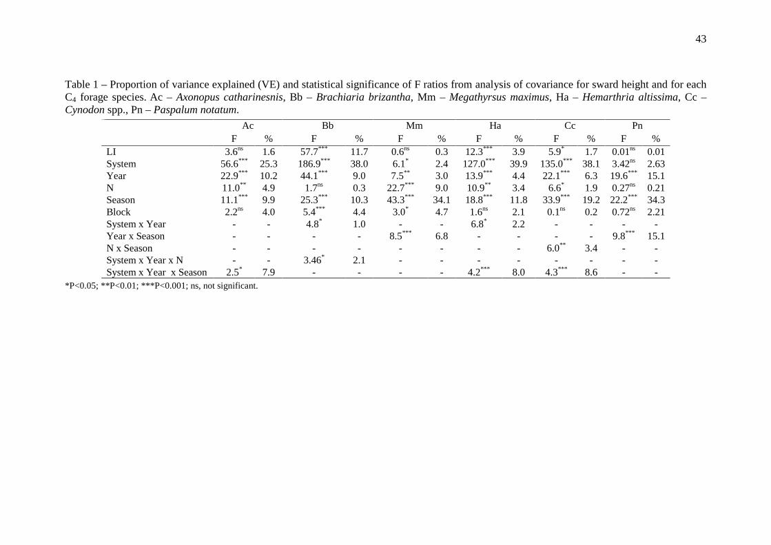
Outputs of the ANCOVA for sward height at the cutting date are shown in Table 1.
ANCOVA reveled that for almost all species, the system and seasonal variations had the
greatest effects on sward surface height (Table 1) in terms of variance explained (VE).
For all species the sward height was higher in the summer and spring and lower in the
autumn (Table 2). The highest differences in sward height between systems were

31
observed for H. altissima (+23 cm on ICLS conditions, Table 2). Only cultivar P.
notatum was not affected by integrated crop-livestock system (ICLS) (P > 0.07).
After these variables, the factor year was an important source of variation,
mainly for B. brizantha (VE = 13%). For this species, the sward height increased 4.6 cm
in the second year. N supply effect was significant for M. maximus, H. altissima and
Cynodon spp., accounting for a maximum of 23% of total variance. Sward height was
higher in N0 than N300 (Table 2), and M. maximus was the species with the highest
increase (+8.4 ± cm) due N fertilizer application.
Some significant interactions were found between the factors analyzed (Table 1).
The most important interactions were between Year x Season, for M. maximus and P.
notatum, and between system x year x season for A. catharinensis, H. altissima and
Cynodon spp.. Means for the interaction Year x Season are showed in Table 3. For M.
maximus, while in the first year the sward height was higher during the summer, in the
second year highest height value was observed during the spring. For P. notatum this
interaction was significant due differences in order of magnitude in all seasons with an
increase in height values from the first to the second year (Table 3). The interaction
system x nitrogen is not showed because presented values than 6.5% in terms of V.E.
3.2.2 Sward height x Light interception
A significant linear regression was observed between sward height and LI for all
species and independent of the system (Figure 3). Since no differences between slopes
(P > 0.15) were observed in ANCOVA for ICLS vs. full sun, the distances between
intercepts could be compared. It means that the higher sward height in ICLS for some
species is independent of LI level (Figure 3). Height values obtained from regressions
32
(Figure 3) were similar to the means found using only the data at the cutting date. The
relative increase of sward height was 37, 36, 32 and 22 % for H. altissima, Cynodon
spp., B. brizantha and A. catharinensis, respectively. The relationship between sward
height and LI of M. maximus and P. notatum was similar (i.e. no differences in slopes
and intercepts) in ICLS and full sun.
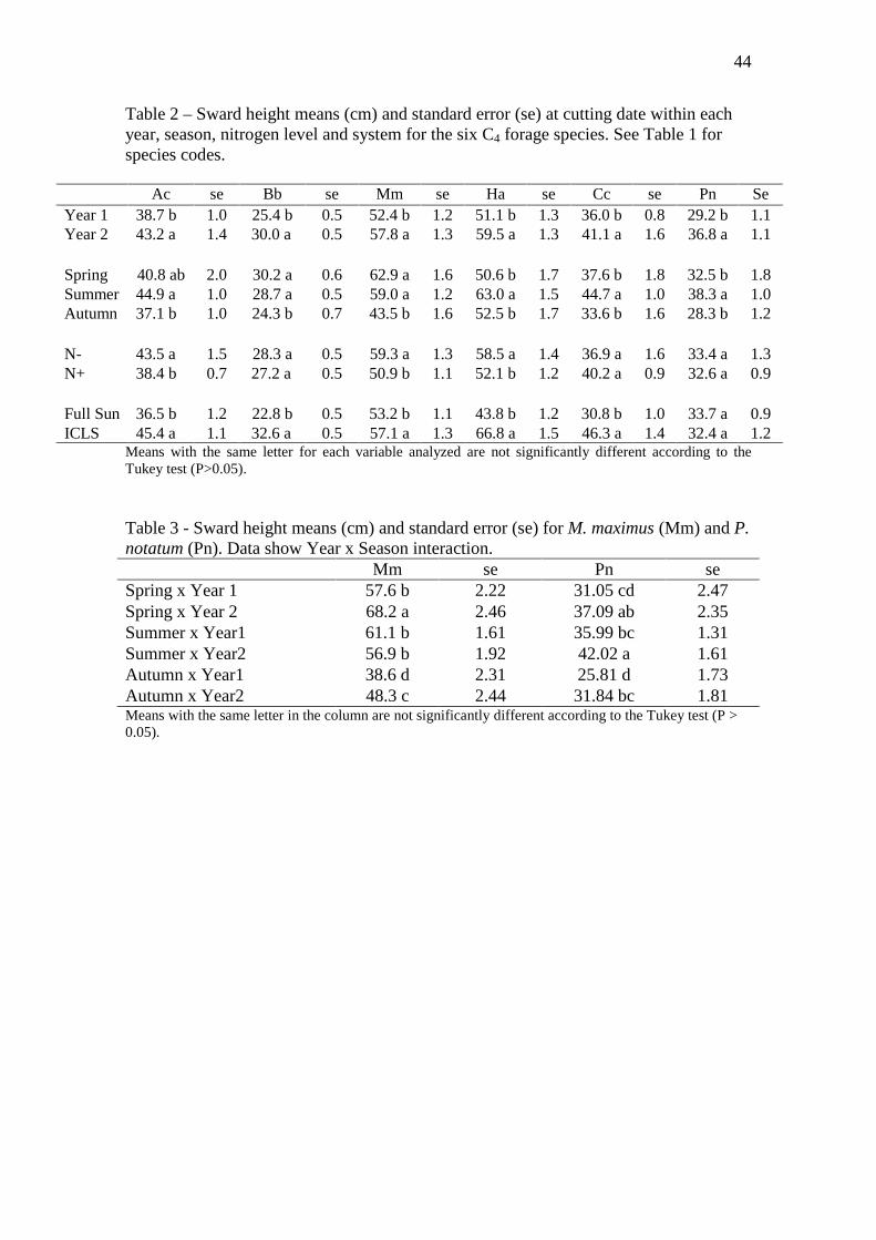
3.3 Plant traits
Leaf length (LL) increased for A. catharinensis, B. brizantha, H. altissima and P.
notatum in ICLS when compared with full sun (Table 4). Nitrogen fertilization had also
a significant effect on leaf length, i.e. it increased on N300 treatment for all species,
except for P. notatum (Table 4).
Sheath length also increased in ICLS, except with M. maximus (Table 4). Further,
plants without N fertilization (i.e. N0) exhibited longer sheaths (Table 4), except P.
notatum.
Nitrogen supply had the strongest effect on tiller density for all species (P <
0.01), except for species H. altissima (P = 0.54). The N input (i.e N300) increased the
number of tillers (Table 4). In relationship to the systems, a reduction on tiller density
was observed in ICLS only for H. altissima (< 34%) and Cynodon spp. (< 47%, Table
4).
Leaf:Stem ratio was mainly affected by season (in terms of V.E.). For all species,
the leaf:stem ratio was higher in spring compared to the summer period (data not
showed). B. brizantha, P. notatum and Cynodon spp. showed higher leaf:stem ratio in
the full sun (Table 4). The opposite was observed for M. maximus and P. notatum, i.e.
33
leaf:stem ratio was higher in ICLS (Table 4). N supply tended to increase leaf:stem ratio,
except for Cynodon spp. (Table 4).
4. Discussion
Our hypothesis that changes in sward structure due to the interactive effect of
trees and N supply can change the relation between LI and sward height was confirmed
by our controlled experiment. Further, important variations on leaf canopy height at
95% LI, mainly across seasons, were observed. Therefore, in order to maintain 95% as
a target LI level, grassland managers should cut or graze each species at different height,
for example, for systems with trees, in conditions of nitrogen limitation and across
seasons (i.e. for swards being vegetative or reproductive).
4.1 Alterations in plant morphology
For the species studied here, changes in plant morphology due the treatments
resulted in changes in sward height at 95% LI (Table 4). For instance, shading increased
the sward height of most species and reduced the tiller density of H. altissima and
Cynodon spp. (Table 2). These are key characteristics of shade avoidance plants, due to
changes in red:far red light. Plants tend to avoid the new tillers production in order to
maintain the allocation of photoassimilates to the existents tillers (Casal, 2000; Wherley
et al. 2005; Evers et al. 2007, Belesky et al. 2011). The effect of light on stems by the
extension of internodes is well demonstrated in the literature for species that presents
shade avoidance strategies (Casal, 2000; Valladares and Niinemets, 2008; Zhu et al.
34
2014). Navas and Garnier (2002) also showed that this effect is independent of other
stresses (i.e. water or nutrient).
The increase on sward height due to an increase in leaf size with shading is
controversy, since other morphological characteristics of leaves can be associated to an
increase in the light capture (Lin et al. 2001), such as leaf angle (Fernández et al. 2004,
Peri et al. 2007a). For instance, P. notatum did not showed differences in sward height
due to the ICLS, despite an increase in leaf length. On the other hand, A. catharinensis,
B. brizantha and H. altissima showed higher sward height and longer leaves (Table 4)
in ICLS. This shade effect on leaf length could be a plant strategy in order to increase
light capture (Dale, 1988).
Leaf length and tiller density increased for all species with N fertilizer
application, except P. notatum, and H. altissima, respectively (Table 4). For leaf length,
this pattern is expected (Lemaire and Chapmman, 1996), since N increases the leaf
expansion rate (Gastal et al. 1992). However, according to Sbrissia and Silva (2001),
sward height is maintained constant despite an increase in leaf size with an increase in
N availability, since heavier leaves alter the leaf angle in the sward structure.
Further, diverse authors (Simon and Lemaire, 1987; Duru and Ducrocq, 2000;
Singer, 2002, Gatti et al. 2013) showed that the bigger importance of N is on leaf
appearance and expansion. Tiller dynamic is much more variable in function of light
and pasture management (Kephart and Buxton, 1993; Sbrissia et al., 2010).
4.2 The differences in sward height per se
There was an increase in the sward height in function of year, mainly for species
cultivated in the ICLS. This effect can be explained by the decrease of light reaching on
35
forage sward (~ 40% in summer of 2012 to ~ 59% in the end of summer 2013). The
magnitude of these differences can be increased throughout the years if the shading
effect increases. Lin et al. (2001) showed, with various C3 and C4 forages species, an
increase in sward height with the increase of shade. In this way it is important the
management of trees in order to reduce the variability on forage growth and
development over time.
Seasonal effects were important in the sward height at 95% LI (Table 1). In
general, there was a decrease from spring and summer to autumn, which could be in
turn explained by stem formation due to plant maturity developmental stage, since
during the fall all species were in vegetative stage (data not shown). A similar pattern in
sward height between seasons was observed by Giacomini et al. (2009) with B.
brizantha and by Medinilla-Salinas et al. (2013) with M. maximus. However, they did
not attribute these differences on sward height to plant maturity.
The relative increase in sward height from full sun to SS was 52, 50, 43, 24 and
7% for H. altissima, Cynodon spp., B. brizantha, A. catharinensis and M. maximus
respectively. Gobbi et al. (2009) showed that reductions on light availability increase
the height of B. brizantha cv. Basilisk. The same pattern was found for Dactylis
glomerata (Peri et al. 2007b), and with a diverse range of C3 and C4 species (Lin et al.
2001). For M. maximus, Medinilla-Salinas et al. (2013) showed that plants growing
without trees were 12.5% taller than in the shaded condition. However, they measured
the plants in a fixed period of regrowth. In a shaded condition, plants can exhibit lower
growth rates (Valladares and Niinemets, 2008), and this can lead to differences in sward
height.
According to Mesquita et al. (2010), N affects only the time and not the height
that swards reaches 95% of LI, due to the acceleration on appearance and tissue
36
expansion of plants with higher amounts of nitrogen (Gastal and Nelson, 1994; Duru
and Ducrocq, 2000; Alexandrino et al. 2005; Paiva et al. 2012). However, a decrease in
sward height at 95% LI for A. catharinensis, M. maximus and H. altissima (Table 2)
with N fertilization was observed, which in turn could be explained by changes in plant
morphology as the increase in sheath length for plants without N nutrition (Table 4).
Since no significant differences were observed in slopes for the regression
analysis for A. catharinensis, B. brizantha, H. altissima and Cynodon spp. between
sward height and light interception (Figura 3), the increase in sward height was
independent of the level of LI. It suggests that an early signal of changes in light quality
is perceived by plants (Ballaré et al. 1987; Aphalo et al. 1999), before the pasture
canopy closure (i.e. 95% of LI). Then, changes in the understory occurred probably due
to changes in light quantity, but also in light quality due to the trees canopy (Varella et
al. 2010; Beaudet et al. 2011). This results can interferes directly in the pasture
management due to the changes in plant morphology related to alterations in light
quality. For example, B. brizantha and Cynodon spp. presented lower values of
leaf:stem ratio in ICLS, which means higher levels of stems in the sward structure.
In full sun canopies, it has been showed that an increase in sward height leads to
a decrease in the leaf:stem ratio (Fonseca et al. 2012), which is directly correlated with
the light competition in the canopy. When LI levels are higher than 95%, there is a
faster increase in stem elongation. In this way, our results can help to target the pre-
grazing sward height in function of shade. However, advances are still necessary about
the post-grazing height. In this work, it was used 50% of the initial height for the cutting
intensity, because follows the pattern of animal behavior. The level of cutting intensity
also has interference on sward structure (Silveira et al. 2010). Belesky et al. (2011)
showed that the long-term of tiller production was compromised for the higher cutting

37
intensity in shaded condition. In this way, studies of leaf lifespan, forage quality and
animal behavior (Fonseca et al. 2013) can help to define better management strategies
for cutting intensities.
To sum up, the response of pasture sward height as a function of shading and
nitrogen fertilization are variable depending on the grass species evaluated. The
management using LI in integrated systems can be used, but the cutting height can be
higher for species that are influenced by shading and by nitrogen.

38
5. References
Alexandrino E, Nascimento Jr D, Regazzi AJ, et al. (2005) Características morfogênicas e estruturais da Brachiaria brizantha cv . Marandu submetida a diferentes doses de nitrogênio e freqüências de cortes. Acta Scientiarum Agronomy 27:17–24.
Aphalo P (1999) Plant-plant signalling, the shade-avoidance response and competition. Journal of Experimental Botany 50:1629–1634. doi: 10.1093/jexbot/50.340.1629
Ballaré CL, Casal JJ (2000) Light signals perceived by crop and weed plants. Field Crops Research 67:149–160.
Ballaré CL, Sánchez RA, Scopel, AL, Casal, JJ, Ghersa, CM. (1987). Early detection of neighbour plants by phytochrome perception of spectral changes in reflected sunlight. Plant, Cell and Environment, 10 : 551-557.
Ballaré CL, Scopel AL, Sanchez RA. (1997) Foraging for light: photosensory ecology and agricultural implications. Plant, Cell and Environment 20:820–825. doi: 10.1046/j.1365-3040.1997.d01-112.x
Beaudet M, Harvey BD, Messier C, et al. (2011) Forest Ecology and Management Managing understory light conditions in boreal mixedwoods through variation in the intensity and spatial pattern of harvest : A modelling approach. Forest Ecology and Management 261:84–94. doi: 10.1016/j.foreco.2010.09.033
Belesky DP, Burner DM, Ruckle JM (2011) Tiller production in cocksfoot (Dactylis glomerata) and tall fescue (Festuca arundinacea) growing along a light gradient. Grass and Forage Science 66:370–380. doi: 10.1111/j.1365-2494.2011.00796.x
Brisson N, Launay M, Mary B, Beaudoin N. (2008). Conceptual basis, formalisations and parameterization of the STICS crop model. Versailles: Quae.
Casal JJ (2000) Phytochromes, cryptochromes, phototropin: photoreceptor interactions in plants. Photochemistry and photobiology 71:1–11.
Carvalho PCF, Moraes A (2011) Integration of Grasslands within Crop Systems in South America. Grasslands Productivity and Ecosystems Services. Eds. Lemaire G, Hodgson J, Chabbi A. p.219-226.
Dale JE (1988) The control of leaf expansion. Ann Rev Physiol Plant Mol Biol 39:267–295.
Devkota NR, Kemp PD, Hodgson J, et al. (2009) Relationship between tree canopy height and the production of pasture species in a silvopastoral system based on alder trees. Agroforestry Systems 76:363–374. doi: 10.1007/s10457-008-9192-8
Duru M, Ducrocq H (2000) Growth and Senescence of the Successive Leaves on a Cocksfoot Tiller . Effect of Nitrogen and Cutting Regime. Annals of Botany 85:645–653. doi: 10.1006/anbo.2000.1117

39
Evers JB, Vos J, Chelle M, et al. (2007) Simulating the effects of localized red:far-red ratio on tillering in spring wheat (Triticum aestivum) using a three-dimensional virtual plant model. The New phytologist 176:325–36. doi: 10.1111/j.1469-8137.2007.02168.x
Fagundes JL, Silva SC, Pedreira CGS, et al. (1999) Índice de área foliar, interceptação luminosa e acúmulo de forragem em pastagens de Cynodon spp. sob diferentes intensidades de pastejo. Scientia Agricola 56:1141–1150.
Feldhake, C M; Beleski DP (2009) Photosynthetically active radiation use efficiency of Dactylis glomerata and Schedonorus phoenix along a hardwood tree-induced light gradient. Agroforestry Systems 75:189–196. doi: 10.1007/s10457-008-9175-9
Fernández ME, Gyenge JE, Schlichter TM (2004) Shade acclimation in the forage grass Festuca Pallescens : biomass allocation and foliage orientation. Agroforestry Systems 60:159–166.
Fonseca L, Carvalho PCF, Mezzalira JC, et al. (2013) Effect of sward surface height and level of herbage depletion on bite features of cattle grazing Sorghum bicolor swards. Journal of animal science 991:4357–4365. doi: 10.2527/jas2012-5602
Fonseca L, Mezzalira JC, Bremm C, et al. (2012) Management targets for maximising the short-term herbage intake rate of cattle grazing in Sorghum bicolor. Livestock Science 145:205–211. doi: 10.1016/j.livsci.2012.02.003
Fourcaud T, Zhang X, Stokes A, et al. (2008) Plant growth modelling and applications: the increasing importance of plant architecture in growth models. Annals of botany 101:1053–63. doi: 10.1093/aob/mcn050
Gastal F, Belanger G, Lemaire G (1992) A Model of the Leaf Extension Rate of Tall Fescue in Response to Nitrogen and Temperature. Annals of Botany. 70: 437-442.
Gastal F, Nelson C (1994) Nitrogen Use within the Growing Leaf Blade of Tal1 Fescue. Plant Physiology 105:191–197.
Gatti ML, Ayala Torales AT, Cipriotti PA, Golluscio RA (2013) Leaf and tiller dynamics in two competing C 3 grass species: influence of neighbours and nitrogen on morphogenetic traits. Grass and Forage Science 68:151–164. doi: 10.1111/j.1365-2494.2012.00881.x
Giacomini AA, Silva SC, Sarmento DOL, et al. (2009) components of the leaf area index of marandu palisadegrass swards subjected to strategies of intermittent stocking. Scientia Agricola 66:721–732.
Gobbi KF, Garcia R, Garcez Neto AF, et al. (2009) Características morfológicas , estruturais e produtividade do capim- braquiária e do amendoim forrageiro submetidos ao sombreamento Morphological and structural characteristics and productivity of Brachiaria grass and forag. Revista Brasileira De Zootecnia 38:1645–1654.
40
Hammer GL, Kropff MJ, Sinclair TR, Porter JR. (2002) Future contributions of crop modelling – from heuristics and supporting decision making to understanding genetic regulation and aiding crop improvement. European Journal of Agronomy 18: 15–31. Jones CA, Ritchie JT, Kiniry JR, Godwin DC, Otter-Nacke SI (1984) The CERES wheat and maize model. In: Proceedings International Symposium on Minimum Datasets for Agrotechnology Transfer. Pantancheru, India: ICRASET.
Kebrom TH, Brutnell TP (2007) The molecular analysis of the shade avoidance syndrome in the grasses has begun. Focus 58:3079–3089. doi: 10.1093/jxb/erm205
Kephart KD, Buxton DR (1993) Forage quality responses of C3 and C4 perennial grasses to shade. Crop Science, Madison, v. 33, p. 831-837. Keulen H, Schiere H (2004) Crop-livestock systems: old wine in new bottles? In: Fischer T et al. (Eds.). New directions for a diverse planet. Proceedings of the IV International Crop Science Congress, Australia, 2004. CD ROM. Laca EA, Lemaire G (2000) Measuring sward structure. In: t’Mannetje L, Jones RM (eds) Field and laboratory methods for grassland and animal production research, pp. 103–122. Wallingford: CAB International. Lemaire G, Chapman D (1996) Tissue flows in grazed plant communities. In: Hodgson J, Illius AW (eds) The ecology and management of grazing systems. Wallingford:
CAB International, pp 3-36.
Lin CH, Mcgraw RL, George MF, Garrett HE (2001) Nutritive quality and morphological development under partial shade of some forage species with agroforestry potential. Agroforestry Systems 53:269–281.
Malézieux, E. Crozat, Y. Duparz, C. Laurans, M. Makowski, D. Valantin-Morison M (2009) Species in cropping systems : concepts , tools and models . A review. Agron Sustain Dev 29:43–62. doi: 10.1051/agro
Medinilla-Salinas L, Vargas-Mendoza MDLC, López-Ortiz S, et al. (2013) Growth, productivity and quality of Megathyrsus maximus under cover from Gliricidia sepium. Agroforestry Systems 87:891–899. doi: 10.1007/s10457-013-9605-1
Mesquita P, Silva SC, Paiva AJ, et al. (2010) Structural characteristics of marandu palisadegrass swards subjected to continuous stocking and contrasting rhythms of growth. Scientia Agricola 67:23–30.
Monteith JL (1977) Climate and the efficiency of crop production in Britain. Philosophical Transactions of the Royal Society B: Biological Sciences 281: 277–294. Nair, PKR (1993) Introduction to agroforestry. Dordrecht: Kluwer Academic Publishers. 499p.

41
Nair PKR (2011) Agroforestry systems and environmental quality: introduction. Journal of Environmental Quality 40:784-790.
Navas M-L, Garnier E (2002) Plasticity of whole plant and leaf traits in Rubia peregrina in response to light, nutrient and water availability. Acta Oecologica 23:375–383. doi: 10.1016/S1146-609X(02)01168-2
O’Mara FP (2012) The role of grasslands in food security and climate change. Annals of botany 110:1263–70. doi: 10.1093/aob/mcs209
Paciullo DSC, Campos NR, Gomide CAM, et al. (2008) Crescimento de capim-braquiária influenciado pelo grau de sombreamento e pela estação do ano. Pesquisa Agropecuária Brasileira 47:917–923.
Paiva AJ, Silva SC, Pereira LET, et al. (2012) Structural characteristics of tiller age categories of continuously stocked marandu palisade grass swards fertilized with nitrogen. Revista Brasileira De Zootecnia 41:24–29.
Peri PL, Lucas RJ, Moot D. (2007) Dry matter production , morphology and nutritive value of Dactylis glomerata growing under different light regimes. Agroforestry Systems 70:63–79. doi: 10.1007/s10457-007-9029-x
Simon JC, Lemaire G (1987) Tillering and leaf area index in grasses in the vegetative phase. Grass and Forage Science 42: 373-380.
Singer JW (2002) Species and Nitrogen Effect on Growth Rate , Tiller Density , and Botanical Composition in Grass Hay Production. Crop Science 42:208–214.
Smith H, Whitelam GC (1997) The shade avoidance syndrome : multiple responses mediated by multiple phytochromes. Plant, Cell and Environment 20:840–844.
Soares AB, Sartor LR, Adami PF, et al. (2009) Influência da luminosidade no comportamento de onze espécies forrageiras perenes de verão. Revista Brasileira de Zootecnia 38:443–451.
Stamm P, Kumar PP (2010) The phytohormone signal network regulating elongation growth during shade avoidance. Access 61:2889–2903. doi: 10.1093/jxb/erq147
Trindade JK, Silva S., Souza Jr S., et al. (2007) Composição morfológica da forragem consumida por bovinos de corte durante o rebaixamento do capim-marandu submetido a estratégias de pastejo rotativo. Pesquisa Agropecuária Brasileira 42:883–890.
Valladares F, Niinemets Ü (2008) Shade Tolerance, a Key Plant Feature of Complex Nature and Consequences. Annual Review of Ecology, Evolution, and Systematics 39:237–257. doi: 10.1146/annurev.ecolsys.39.110707.173506
42
Varella a. C, Moot DJ, Pollock KM, et al. (2010) Do light and alfalfa responses to cloth and slatted shade represent those measured under an agroforestry system? Agroforestry Systems 81:157–173. doi: 10.1007/s10457-010-9319-6
Wherley BG, Gardner DS, Metzger JD (2005) Tall Fescue Photomorphogenesis as Influenced by Changes in the Spectral Composition and Light Intensity. Crop Science 45:562. doi: 10.2135/cropsci2005.0562
Zanini GD, Santos GT, Sbrissia AF (2012) Frequencies and intensities of defoliation in Aruana Guineagrass swards : accumulation and morphological composition of forage. Revista Brasileira Zootecnia 41:905–913.
Zhu J, Vos J, van der Werf W, et al. (2014) Early competition shapes maize whole-plant development in mixed stands. Journal of experimental botany 65:641–53. doi: 10.1093/jxb/ert408
43
Table 1 – Proportion of variance explained (VE) and statistical significance of F ratios from analysis of covariance for sward height and for each C4 forage species. Ac – Axonopus catharinesnis, Bb – Brachiaria brizantha, Mm – Megathyrsus maximus, Ha – Hemarthria altissima, Cc – Cynodon spp., Pn – Paspalum notatum.
*P<0.05; **P<0.01; ***P<0.001; ns, not significant.
Ac Bb Mm Ha Cc Pn F % F % F % F % F % F %
LI 3.6ns 1.6 57.7*** 11.7 0.6ns 0.3 12.3*** 3.9 5.9* 1.7 0.01ns 0.01 System 56.6*** 25.3 186.9*** 38.0 6.1* 2.4 127.0*** 39.9 135.0*** 38.1 3.42ns 2.63 Year 22.9*** 10.2 44.1*** 9.0 7.5** 3.0 13.9*** 4.4 22.1*** 6.3 19.6*** 15.1 N 11.0** 4.9 1.7ns 0.3 22.7*** 9.0 10.9** 3.4 6.6* 1.9 0.27ns 0.21 Season 11.1*** 9.9 25.3*** 10.3 43.3*** 34.1 18.8*** 11.8 33.9*** 19.2 22.2*** 34.3 Block 2.2ns 4.0 5.4*** 4.4 3.0* 4.7 1.6ns 2.1 0.1ns 0.2 0.72ns 2.21 System x Year - - 4.8* 1.0 - - 6.8* 2.2 - - - - Year x Season - - - - 8.5*** 6.8 - - - - 9.8*** 15.1 N x Season - - - - - - - - 6.0** 3.4 - - System x Year x N - - 3.46* 2.1 - - - - - - - - System x Year x Season 2.5* 7.9 - - - - 4.2*** 8.0 4.3*** 8.6 - -
44
Table 2 – Sward height means (cm) and standard error (se) at cutting date within each year, season, nitrogen level and system for the six C4 forage species. See Table 1 for species codes.
Means with the same letter for each variable analyzed are not significantly different according to the Tukey test (P>0.05). Table 3 - Sward height means (cm) and standard error (se) for M. maximus (Mm) and P. notatum (Pn). Data show Year x Season interaction. Mm se Pn se Spring x Year 1 57.6 b 2.22 31.05 cd 2.47 Spring x Year 2 68.2 a 2.46 37.09 ab 2.35 Summer x Year1 61.1 b 1.61 35.99 bc 1.31 Summer x Year2 56.9 b 1.92 42.02 a 1.61 Autumn x Year1 38.6 d 2.31 25.81 d 1.73 Autumn x Year2 48.3 c 2.44 31.84 bc 1.81 Means with the same letter in the column are not significantly different according to the Tukey test (P > 0.05).
Ac se Bb se Mm se Ha se Cc se Pn Se Year 1 38.7 b 1.0 25.4 b 0.5 52.4 b 1.2 51.1 b 1.3 36.0 b 0.8 29.2 b 1.1 Year 2 43.2 a 1.4 30.0 a 0.5 57.8 a 1.3 59.5 a 1.3 41.1 a 1.6 36.8 a 1.1 Spring 40.8 ab 2.0 30.2 a 0.6 62.9 a 1.6 50.6 b 1.7 37.6 b 1.8 32.5 b 1.8 Summer 44.9 a 1.0 28.7 a 0.5 59.0 a 1.2 63.0 a 1.5 44.7 a 1.0 38.3 a 1.0 Autumn 37.1 b 1.0 24.3 b 0.7 43.5 b 1.6 52.5 b 1.7 33.6 b 1.6 28.3 b 1.2 N- 43.5 a 1.5 28.3 a 0.5 59.3 a 1.3 58.5 a 1.4 36.9 a 1.6 33.4 a 1.3 N+ 38.4 b 0.7 27.2 a 0.5 50.9 b 1.1 52.1 b 1.2 40.2 a 0.9 32.6 a 0.9 Full Sun 36.5 b 1.2 22.8 b 0.5 53.2 b 1.1 43.8 b 1.2 30.8 b 1.0 33.7 a 0.9 ICLS 45.4 a 1.1 32.6 a 0.5 57.1 a 1.3 66.8 a 1.5 46.3 a 1.4 32.4 a 1.2
45
Table 4 – Means and standard error (se) of Leaf Length (LL – cm), Sheath Length (SL – cm), Tiller Density (TD) and leaf:stem ratio for six C4 forage species within each system and nitrogen treatment. See Table 1 for species codes. Means with the same letter for each variable analyzed in function of systems and nitrogen effects are not significantly different according to the Tukey test (P > 0.05). ICLS, integrated crop-livestock system.
Ac se Bb Se Mm se Ha se Cc se Pn Se LL Full Sun 22.1 b 2.3 18.0 b 0.6 26.1 a 2.1 14.9 b 0.9 14.9 a 1.2 34.8 b 1.3 LL ICLS 26.2 a 0.9 22.7 a 1.1 27.3 a 1.5 20.0 a 0.7 15.0 a 0.5 42.3 a 1.1 LL N0 22.1 b 0.9 19.4 b 1.2 24.7 b 0.6 18.1 b 0.6 13.4 b 0.4 41.5 a 1.4 LL N300 28.4 a 1.0 24.4 a 1.2 28.9 a 2.1 20.2 a 1.1 16.6 a 0.7 40.5 a 1.5 SL Full Sun 17.8 b 0.7 12.4 b 1.0 25.3 a 1.4 37.6 b 2.1 20.8 b 0.7 11.2 b 0.3 SL ICLS 28.5 a 0.8 16.8 a 0.4 24.4 a 0.7 50.1 a 1.3 31.3 a 0.7 13.1 a 0.1 SL N0 30.7 a 1.2 18.2 a 0.5 25.8 a 0.8 54.5 a 1.8 32.3 a 1.0 12.1 b 0.2 SL N300 21.5 b 0.6 13.9 b 0.6 23.8 b 1.0 41.6 b 1.4 26.8 b 0.6 13.6 a 0.2 TD Full sun 808 a 46 1141 a 46 1351 a 150 952 a 161 3074 a 648 - - TD ICLS 856 a 25 1117 a 56 1435 a 68 707 b 45 1643 b 138 - - TD N0 786 b 37 1022 b 63 1221 b 76 721 a 79 1256 b 159 - - TD N300 911 a 18 1220 a 64 1620 a 72 775 a 56 2508 a 239 - - Leaf:Stem Full Sun 0.90 a 0.12 2.4 a 0.3 0.65 b 0.12 0.34 a 0.05 0.87 a 0.12 1.7 b 0.2 Leaf:Stem ICLS 0.94 a 0.06 1.8 b 0.1 0.91 a 0.06 0.31 a 0.02 0.56 b 0.03 3.7 a 0.5 Leaf:Stem N0 0.74 b 0.04 1.9 a 0.1 0.73 b 0.06 0.26 b 0.02 0.55 a 0.05 4.5 a 0.7 Leaf:Stem N300 1.04 a 0.08 1.9 a 0.2 0.94 a 0.08 0.35 a 0.02 0.67 a 0.05 2.5 b 0.4
46
Figure 1 – Mean (circle), maximum (triangle) and minimal (square) average monthly air temperatures from September 2011 to May 2013. Open symbols and short dash lines for full sun and closed symbols solid lines for integrated crop-livestock system.
Months
Air
tem
pera
ture
(ºC
)
5
10
15
20
25
30
35
AS O N D J F M A M J J A S O N D J F M M2011 2012 2013
47
Figure 2 – Monthly mean soil volumetric water content in the top 200 mm (measured every 15 days).
Soi
l vol
umet
ric w
ater
con
tent
(%
)
5
10
15
20
25
30
35
40
45
Full sunICLS
D J F M A M O N D J M A M J
2011 2012 2013
Months
48
Figure 3 – Relationship between sward height (cm) and light interception (%) for six C4 forage species at the integrated crop-livestock system (closed symbols and solid lines) and full sun (open symbols and short dash lines). Ac – Axonopus catharinesnis, Bb – Brachiaria brizantha, Mm – Megathyrsus maximus, Ha – Hemarthria altissima, Cc – Cynodon spp., Pn – Paspalum notatum. ANCOVA results are presented in each panel: two lines in the case of no interaction and difference between intercepts between the categorical independent variable (i.e. sward height), and a single line in the case of no significant effect of the continuous variable. (*P<0.05; **P<0.01; ***P<0.001; ns, not significant).
Light interception (%)
70 75 80 85 90 95 1000
102030405060708090
70 75 80 85 90 95 100
Sw
ard
heig
ht (
cm)
0
15
30
45
60
75
90
1050
10
20
30
40
50
60
70
80y= 0.81 x - 31.66 r2 0.34***
y= 0.64 x - 23.90 r2 0.43***
y= 0.36 x - 9.83 r2 0.19***
y= 0.22 x - 1.99 r2 0.09***
y= 1.07 x - 46.67 r2 0.32***
y= 1.25 x - 57.84 r2 0.41***
y= 1.30 x - 79.58 r2 0.50***
y= 0.88 x - 37.85 r2 0.48***
y= 0.67 x - 30.15 r2 0.33***
Ac Bb
Mm Ha
Cc Pn
y= 0.33 x - 1.25 r2 0.26**
49
3. CAPÍTULO 2
Morphogenesis and growth dynamics of tropical forage species according to shade and
nitrogen1
1 Elaborado de acordo com as normas da Revista Agroforestry Systems
50
Morphogenesis and growth dynamics of tropical forage species according to shade and
nitrogen
Tiago Celso Baldissera1, Laíse da Silveira Pontes2, Raquel Santiago Barro3, André Faé
Giostri1, Betina Raquel Cunha dos Santos2; Sebastião Brasil Campos Lustosa4; Paulo
César de Faccio Carvalho3.
1UFPR – Universidade Federal do Paraná, Curitiba-PR, Brazil
2IAPAR – Instituto Agronômico do Paraná, Ponta Grossa-PR, Brazil
3UFRGS – Universidade Federal do Rio Grande do Sul, Porto Alegre-RS, Brazil
4UNICENTRO – Universidade Estadual do Centro Oeste, Guarapuava-PR, Brazil
*corresponding author: [email protected]
51
Abstract
Monocultures of six C4 tropical forage species that are widely used in Brazilian
livestock were compared in an experimental field with two systems, i.e. open pasture vs.
under tree canopy (i.e. an integrated crop-livestock system, ICLS), and two levels of N
supply (zero vs. 300 kg of N ha-1 year-1). Our aim was to determine the interactive
shading effect from trees (i.e. Eucalyptus dunnii) canopy, and nitrogen supply on
morphogenetic characteristics and growth parameters of six C4 grass species in order to
assess their potential for use as a component of ICLS. 95% of light interception was
used as a cutting frequency and 50% of initial height as cutting intensity. The shading
effect from trees canopy was specie-dependent. For instance, B. brizantha, M. maximus
and Cynodon spp. had a decrease on leaf growth rates in ICLS with trees, while the
opposite was observed with A. catharinensis. H. altissima maintained the same leaf
growth rates in the two systems, i.e. with and without trees. However, even for species
that showed decreases on values of morphogenetic variables (e.g. phyllochron) and leaf
growth rates, they maintained a satisfactory development and growth in ICLS. The N
supply helps the maintenance of a satisfactory development and growth of forages
species in the ICLS.
Key words: integrated crop-livestock systems; management; light interception;
competition
1. Introduction
Since intensive production systems require high amounts of energy by labor and inputs,
their results become incompatible with the emergent demands that aim to ensure the
52
sustainability of agroecosystems (Carvalho and Moraes, 2011). Integrated crop-
livestock systems (ICLS) appears, therefore, as a good option to increase the overall
land productivity and/or its sustainability by making best use of the environmental
resources and, at the same time, by generating environmental services (O´Mara, 2012;
Sanderson et al. 2013). Further, several reports have demonstrated the value of
including trees in these systems because the integrated timber and livestock production
can generate higher profits, which provide farmers with a means of surviving markets
that fluctuate through time (Zhai et al. 2006).
However, in the ICLS, that can intentionally integrates trees, forage crops, and
livestock into a structural practice of planned interactions (Clason and Sharrow, 2000),
the pasture component is affected by changes in the understory, mainly due changes in
light quantity and quality. The amount of light in an ICLS depends on tree species, tree
density and tree management. Further, the response to shading depends on the forage
species and on soil fertility, especially nitrogen (Paciullo et al. 2011). Therefore, a better
understanding about plant responses to interactive shading and N availability and the
consequent growth dynamics in ICLS is essential to enhance our ability to forecast
management practices and biomass production in order to ensure pasture persistence
and a sustainable production (Hodgson and Silva, 2000).
Morphogenetic processes, like the rate of appearance of new organs, control the
growth and development of plants in a specific environment. These processes determine
sward structural characteristics, as the leaf area index which allows light interception by
the sward, and consequently, the biomass production (Lemaire and Chapman, 1996).
However, management practices, like cutting frequency and intensity and fertilization,
interferes on the plant morphogenesis (Duru and Ducrocq, 2000, Peri et al. 2007b;
Sbrissia et al. 2010). Further, in a system with trees, shade appears like another

53
management effect, as it is possible to manage in a certain way the shade produced by
trees (Combes et al. 2002).
When forage grass plants are growing in association with trees, grass tolerance
depends on the physiological and morphological adaptations for irradiance reduction.
Different hypothesis on the suite of characteristics responsible for species' shade
tolerance have been recognized on the literature as, for example, carbon gain vs. stress
tolerance hypothesis (see Valladares & Niinemets, 2008 for a review). However, most
studies reporting these differing views about shade tolerance were done on woody
species (Seidlova et al. 2009). Further, Valladares & Niinemets (2008) argued that
shade tolerance could depend both on the efficiency of carbon gain in low light and on
the tolerance of stresses interacting with light availability. Therefore, different plant
features can be associated to shading tolerance and N availability, with different
consequences for plant growth dynamic; hence, they need to be identified for a broader
range of forage species.
For instance, shading effect can has a strong influence on morphogenetic
variables by, for example, reductions on leaf appearance, leaf elongation rate and tiller
appearance (Gautier et al. 1999; Granier and Tardieu, 1999; Bos et al. 2000, Casal,
2000), which in turn affect the pasture biomass accumulation. Under moderate shading,
some grass species have the capacity to maintain growth at satisfactory levels (Paciullo
et al. 2008; Soares et al. 2009; Pachas et al. 2013). However, in general, the lower is the
incoming radiation level in systems with trees, the lower is the forage production
(Feldhake and Belesky, 2009; Paciullo et al. 2008; Devkota et al. 2009; Soares et al.
2009). Therefore, detailed studies of tissue dynamic can provide new insights for
changes in sward state variables in response to variation in shading and in N level.

54
The objective of this study was to compare interactive effect of shading,
provided by Eucalyptus dunnii, and two nitrogen levels on the morphogenetics
variables, sward structural characters and growth and senescence fluxes of six C4
tropical forage species.
2. Materials and Methods
2.1 Site characteristics
The experimental site was located at the Agronomic Institute of Paraná (IAPAR), Ponta
Grossa-PR (25°07’22’’S, 50°03’01’’W), at 880 m altitude. The climate is Cfb according
to Köppen classification, with no dry season, annual precipitation of 1,400 mm, more
frequent during spring-summer and scarce in autumn. The soil is an Oxisoil, and texture
is around 30% of clay. The average values of chemical soil analysis during the
experiment period were: P = 4.23 mg dm-3; C = 22.2 g dm-3; pH = 5.14; Al = 0.025
cmolc dm-3; H + Al = 4.23 cmolc
dm-3; Ca = 2.95 cmolc dm-3; Mg = 2.15 cmolc
dm-3; K =
0.16 cmolc dm-3.
2.2 Establishment of the experiment and treatments
Six perennial C4 grasses widely used in Brazilian livestock were studied
(Axonopus catharinensis (Ac), Brachiaria brizantha cv. Marandu (Mb), Megathirsus
maximus cv. Aruana (Mm), Hemarthria altissima cv. Flórida (Ha), Cynodon spp. hybrid
Tifton 85 (Cc) and Paspalum notatum cv. Pensacola (Pn)). Most of them hold
characteristics recommended to face shade conditions (see Soares et al. 2009).

55
Eucalyptus dunnii' trees were planted in 2007, fitting to an east – west
orientation, following the contour, in a double row arrangement using 3m between
plants within rows and 4 m between rows, spaced 20 m apart (3x4x20 m). The initial
population was 267 trees ha-1. In the winter – autumn 2011 a thinning management was
done and reduced the population to 155 trees ha-1.
Forage species were planted in pure stands from January 2010: plots of 4.5 m²
(1,5 x 3 m) in full sun (no trees integration) vs. 100 m² (5 x 20 m) in the shaded area.
The trees shading condition will be referred as the Integrated Crop-Livestock System
treatment (ICLS). Plant measurements were done in December of 2011 and 2012.
Treatments were arranged in a randomized block design, with three replicates.
Two system types, ICLS (i.e. shaded) vs. full sun, and two nitrogen levels (0 and 300 kg
ha-1 year-1) were defined as treatments. Nitrogen was applied as urea in the beginning of
the growing season (in early spring). Each year, in early spring, calcareous, P2O5 and
K2O were supplied according to soil analysis to ensure that these nutrients did not limit
plant regrowth. Soil water content (%) was measured in the top 20 cm soil layer, using
the equipment HFM2010 - HidroFarm during the morphogenesis analysis.
The pastures were mechanically harvested when its canopy reached 95% of LI
(cutting frequency). The stubble height corresponded to a 50% reduction in the cutting
height (cutting intensity). Residues were removed from the site. The light interception
in each plot was monitored every week, using a ceptometer (AccuPAR LP 80).
2.3 Leaf and Plant measurements
Measurements at leaf and plant level were done in 25 and 10 tillers per plot in the full
sun and ICLS, respectively. Only tillers on vegetative stage were marked. For both

56
treatments, marked tillers were located along 2 transects in full sun and 5 in ICLS,
distanced 50 cm between each tiller. The distances of transects in ICLS corresponded to
2,4,10,16 and 18 m from one of the trees rank. Every 2-3 days, during 20 days, the
following measurements were done: the lengths of green and senescing (green parts
only) laminae were measured from the ligule for mature leaves (i.e. those with a visible
ligule) and from the ligule of the last mature leaf for growing leaves; the length of the
pseudostem of vegetative tillers or stem of reproductive tillers (measured from the
ligule of the last mature leaf or the flag leaf to the ground); the appearance of new
leaves.
These measurements were used to calculate the following parameters per plant
part: phyllochron (Phyl – calculated as the inverse of the linear regression between
number of leaves in function of thermal-time); leaf elongation rate (LER – cm tiller-1
ºCd-1); duration of leaf elongation (DLE - ºCd); leaf length (LL – cm); leaf lifespan
(LLS - ºCd); stem elongation rate (SER – cm tiller-1 ºCd-1); leaf blade senescence rate
(LSR – cm tiller-1 ºCd-1); number of green leaves (NGL – leaves tiller-1); final leaf
length (LL – cm).
For each measurement period, destructive samples were collected, at random
and within each plot, to estimate weight per unit length (g DM cm-1) of each plant part.
In the end of each measurement period, the tiller density (TD – tiller m2) per unit
ground area was determined by counting in 1 or 5 samples of 0,0625 m2 per plot in full
sun and ICLS, respectively.
A growth flux (GF – kg ha-1 day-1) was calculated by the following equation:
GF = LER x SWEL x Tm x NEL x TD x 10 Eq. 1
Where: SWEL is the specific weight of expanding leaves (g-1 cm-1); Tm (ºC) is the daily
mean temperature of the experimental period; NEL is the number of expanding leaves
57
per tiller; and the factor 10 is in order to transform in kg ha-1. Senescence flux (SF – kg
ha-1 day-1) was calculated by the following equation:
SF = LSR x SWML x Tm x TD x 10 Eq. 2
Where: SWML is the specific weight of mature leaves (g-1 cm-1); Tm (ºC) is the daily
mean temperature of the experimental period; and the factor 10 is in order to transform
in kg ha-1. The tissue turnover fluxes were calculated per population unit and then per
area (ha), by multiplying the mean tissue fluxes per population unit by the mean density
of these units (i.e. TD).
2.4 Meteorological measurements and thermal time calculation
Photosynthetic photon flux density (PPFD µmol cm-2 s-1) in full sun and in the ICLS
was measured at the same positions described in item 2.3. For the summer 2012, the
PPFD was measured using bars containing five cells of amorphous silicon in parallel of
15 x 15 cm, connected to a datalogger (CR1000; Campbell Scientific® Ltda). The data
were collected every 30 s, and mean values were calculated and stored every 5 min.
Hence, light reduction in the ICLS could be calculated as the difference between sensors
at both systems. For the summer 2013, measurements were taken using a ceptometer
(AccuPAR® LP-80), every 30 min from 8:00 to 18:00 o’clock.
Air temperature (Tm) was collected and stored every 5 min in 3 individuals
dataloggers (Hobbo) located at 2, 10 and 18 m from one of the trees rows in the ICLS,
and one datalogger in full sun. Thermal-time was calculated for integrated and full sun
systems from the daily integration of air temperatures minus the base temperature (Tb):
TT = ∫ −h
bm dtTT0
)](;0max[ Eq. 3
58
where TT is thermal time expressed in cumulative degree days (°Cd, Bonhomme, 2000).
TT is expressed in degree-days, calculated as the sum of the mean daily temperature
minus the base temperature (Tb). During this study, the Tb value used was 10ºC for all
species.
2.5 Statistical analyses
Statistical analyses were performed using R software (R Development Core Team,
2014). Analyses of variance (ANOVA, glm procedure) were performed using the Tukey
method for multiple mean comparison tests in post-ANOVA. Data were transformed
when necessary to reach the normality of residues. Transformations were performed
using the procedure Box Cox (package MASS).
3. Results
3.1 Environmental and tree measurements
The mean daily temperature during the experimental period was 20.2 ºC in ICLS,
created by eucalyptus trees, and 21.0 ºC in full sun treatment in the first year. During
the second year, temperatures increased 2 ºC. Although there was an increase on
temperature from the first to second year, the differences between ICLS and full sun
treatments remained similar (Figure 1).
Soil moisture percentage was also monitored during the experimental period.
Soil moisture was lower in the first year (15±5.42 % and 18±6.48 % in ICLS and full
sun, respectively) when compared to the second year (26±5.46 % and 24±8.60 % in
ICLS and full sun, respectively).

59
Mean trees height ranged from 17.6 ± 2.4 m in summer 2012, with a diameter at
breast height of 21.5 ± 3.24 cm, until 22.6 ± 2.6 m at the end of summer 2013 (27.4 ±
3.04 cm of diameter), which gave tree canopy closures (i.e. % of photosynthetic photon
flux reduction) of ~40 % and ~59 %, respectively.
3.2 Morphogenical and structural characteristics
Outputs of the ANOVA for morphogenical and structural characteristics and growth
fluxes are show in Table 1. ANOVA reveled that species had the greatest effect on all
variables (Table 1), in terms of variance explained (VE). Means per species are showed
in Figure 2. There were significant effects of system, N and year for almost all
variables. Further, interactions of second and third order were also observed (see Table
1). Therefore, interactions between species x system (Figure 2) and species x N levels
(Figure 3) are showed, since they were significant for almost all variables analyzed.
Further, means for the interactions species x year are available in supplementary
material.
The faster species on leaf appearance (i.e. lower Phyllochron) was H. altissima,
and the slowest were M. maximus and B. brizantha (Figure 2). On average, N
fertilization decreased Phyl. (132 ± 4.99 ºCd and 109 ± 3.86 ºCd at N0 and N300,
respectively). Forage species showed a significant higher Phyllochron (Phyl.) in ICLS
(Figure 2). However, H. altissima had a higher Phyl. in full sun, and Cynodon spp. not
showed differences between systems (Figure 2).
Leaf elongation rate (LER) ranged between 0.14 ± 0.007 cm tiller-1 ºCd-1 for B.
brizantha to 0.24 ± 0.01 cm tiller-1 ºCd-1 for H. altissima (Figure 2). Only H. altissima
had a significant higher LER in ICLS (Figure 2). The N fertilization increased LER,
60
except for M. maximus and H. altissima, which not showed significant differences
between N levels (Figure 3). H. altissima displayed the highest duration of leaf
elongation (DLE), while similar values were observed between the others species
(Figure 2). Further, this species and Cynodon spp. were not affected by system (Figure
2). N input decreased the DLE (211 ± 6.87 ºCd and 195 ± 5.87 ºCd at N0 and N300,
respectively). B. brizantha had leaves with longer lifespan than the other species
(Figure 2). Only A. catharinesnis had significant differences on LLS in function of
system (Figure 2). Further, N fertilization decreases the LLS of B. brizantha and
Cynodon spp. (Figure 3).
The stem elongation rate (SER) was higher for A. catharinensis, H. altissima and
Cynodon spp. (Figure 2). ICLS significantly increases the SER for B. brizantha, H.
altissima and Cynodon spp., and decreases the SER for M. maximus (Figure 2). Only A.
catharinensis did not showed differences between systems. The N effect was significant
(Table 1). On average, N fertilization increases the SER (0.020 ± 0.001 cm tiller-1 ºCd-1
and 0.024 ± 0.001 cm tiller-1 ºCd-1 at N0 and N300, respectively).
H. altissima displayed 8.5 ± 0.22 green leaves per tiller (NGL), while M.
maximus displayed a maximum of 3.63 ± 0.08 leaves per tiller (Figure 2). M. maximus
and Cynodon spp. were the species that not exhibited differences for NGL in function of
system. A higher NGL was observed in full sun only for A. catharinensis, the others
species showed higher NGL in ICLS. However, the magnitude of these differences was
small. For instance, A. catharinensis had 4.9 ± 0.28 leaves in full sun and 5.5 ± 0.17
NGL in ICLS, i.e. the difference was only 0.6 leaves. Higher differences were observed
for H. altissima (+1.33 ± 0.41 leaves in full sun, Figure 2). The N fertilization increases
the NGL, mainly for A. catharinensis and H. altissima (Figure 3).
61
The species evaluated increased significantly the leaf length (LL) in ICLS,
except M. maximus and Cynodon spp. (Figure 2). M. maximus has longer leaves
compared to the other species, independently of the system (Figure 2), and also it was
the only species to reduce LL due N fertilization (Figure 3).
Lower tiller density (TD) was observed in ICLS for H. altissima and mainly for
Cynodon spp. (Figure 2). N fertilization significantly increased the number of tillers for
all species (Table 2). This increase ranged between +154 tiller for A. catharinesnis and
+982 tillers for Cynodon spp..
3.3 Explanatory variables
Leaf senescence rate (LSR) and specific leaf weight (SLW) were used for growth and
senescence fluxes’ calculations.
LSR was lower in full sun for H. altissima (Figure 4). The N fertilization
decreased LSR for A. catharinensis, M. maximus and Cynodon spp. (Figure 4). SLW
was significant different only for B. brizantha and M. maximus due to the system, these
species showed a higher SLW in the full sun (Figure 4). The N input decreased SLW for
B. brizantha and increased for M. maximus and Cynodon spp., the other species did not
show significant differences (Figure 4).
3.4 Growth and senescence fluxes
The growth flux (GF) ranged between 46 ± 7.8 kg DM ha-1 day-1 for H. altissima and
105 ± 5.9 kg DM ha-1 for Cynodon spp. (Figure 5). The GF was higher in the full sun,
but A. catharinensis showed the opposite response, with a higher GF in ICLS. No

62
significant differences were observed with H. altissima (Figure 5). N300 treatment
increased GF for all species. Further, the magnitude of these responses was very
different, varying from +11.8 kg ha-1 day-1 for H. altissima and +88.3 kg ha-1 day-1 for
Cynodon spp. that was the species with highest growth flux (GF). The SF was
significantly lower in the ICLS for M. maximus and Cynodon spp (Figure 5). For N
fertilization, differences were observed for A. catharinensis with a lower SF in the
treatment N300 while B. brizantha had a higher SF in the treatment N300 (Figure 5).
3.5 Year effect on variables
Significant differences between years were observed for Phyl., LER, DLE, LSR, SER
and growth and senescence fluxes (Table 1). On average, higher values were observed
in the first year than in the second (Table 2), except for LER, SER and GF.
In general, significant year x species interactions showed significant effects for
some species, while the others remained with similar values between years. For
instance, only B. brizantha had lower NGL in the first year when compared to the
second year, and only H. altissima showed shorter leaves in the second year (see
supplementary material). With Phyl. an opposite response was found. Phyl. was higher
for all species in the first year, except for A. catharinensis (90 ± 16.1 and 131 ± 5.22
ºCd for the first and second year, respectively).
4. Discussion
Phyllochron (Phyl.) was higher in ICLS, except for Cynodon spp. and H. altissima that
not showed differences. Further, this last species had the fast leaf appearance rate (i.e.

63
lower Phyl.), showing values higher than those reported by Oliveira et al. (2000). The
effect of light on Phyl. is divergent on the literature. While some authors indicate that
the competition for light increases the Phyl. (Duru et al. 1993; Gatti et al. 2013), others
results appoints for a reduction (Gautier et al. 1999). A possibility for the increase found
for three species in our study (Figure 2) is a probably lower carbon production and
allocation in ICLS, which in turn affected the Phyl. (Gautier et al. 1999).
Some authors reported that the leaf elongation rate (LER) is directly correlated
with the amount of radiation (i.e. photosynthetic photon flux density - PPFD), and
linked with photoassimilates production (Granier and Tardieu, 1999; Bos et al. 2000).
For instance, Paciullo et al. (2008), observed a higher LER for Brachiaria decumbens
Stapf. growing in a system with 50% of shade. In our study, the effect of shade by trees
on LER was observed only for H. altissima, with an increase on LER in ICLS (Figure
2) when compared to full sun. Further, H. altissima was the only specie with higher leaf
senescence rate in the ICLS (Figure 4). According to Hirosaka (2005), since higher
senescence can provide a faster N remobilization from leaves, this response could be
correlated to a better N condition in shade for the expanding leaves, despite no
significant effects of N inputs for this species (Figure 3) in both light conditions. N has
a markedly effect on LER, mainly by an acceleration on cell division (Gastal and
Nelson, 1994; Duru and Ducrocq, 2000; Alexandrino et al. 2005)
The N input decreases DLE. Further, the duration of leaf elongation was higher
in ICLS, except for H. altissima and Cynodon spp. These results are directly correlated
with the LER increase/decrease by N and shade, since these characteristics are
correlated (Gastal and Nelson, 1999; Duru and Ducrocq, 2000; Vos et al. 2005; Corré,
1983; Tardieu et al. 1999; Cookson and Granier, 2006).

64
Small differences were found in the total number of green leaves in function of
treatments (Figures 2, 3) and year (Figure 6). This characteristic is relatively constant
within a species, but with large variations between species (Lemaire and Chapman,
1996). Only A. catharinensis showed a significant increase on LLS in ICLS (Figure 2).
LLS is the product of phyllochron and the number of mature leaves. As the
number of leaves had a small change in ICLS, the differences observed on LLS could be
related to the lower leaf appearance rate (i.e. higher phyllochron) for this species in
ICLS. This response could be explained by an adaptive process, i.e. plants increase the
leaf lifespan in order to increase the time for doing photosynthesis, since photosynthetic
rates are lower with a light restriction. Also, this response can be just correlated to the
carbon balance and nutrient utilization (e.g. N remobilization) (Chabot and Hicks,
1982). The use of LLS is important as a management tool, because can be used to
define the cutting frequency. Lower LLS means a more frequent cutting regime,
otherwise higher losses in pasture can occur due to senescence (Lemaire and Chapman,
1996). Hence, in relationship to the results observed with LLS, cut frequency can be
similar for all species independently of the system, except for A. catharinensis, which
can be cut lees frequently in ICLS.
Final leaf length (LL) is a function of LER and DLE. Therefore, a higher LL for
H. altissima was probably due a higher LER in ICLS (Figure 2), and the higher LL for
A. catharinensis and B. brizantha can be explained by the higher DLE (Figure 2). An
increase in leaf size due to shade can be a plant strategy in order to increase light
capture (Givnish, 1988).
H. altissima and Cynodon spp. showed lower tiller density (TD) in the ICLS
(Figure 2). TD is an important mechanism to optimize sward leaf area and production
(Matthew et al. 2000). The reduction of light and specially changes in red:far red can
65
avoid the production of new tillers in order to maintain the allocation of
photoassimilates to the existents tillers (Casal, 2000). The effect of N is the opposite of
the light, an increase in N fertilization tends to increase the number of tillers (Cruz and
Boval, 1999).
Stem elongation rate (SER) is an important morphogenical process that has a
large interference on the structure of tropical grass species (Sbrissia and Silva, 2001).
Species showed a higher SER in the ICLS, except M. maximus and A. catharinesnis
(Figure 2). The effect of light on stem elongation is one of the most typical responses of
shade avoidance plants, due to reductions on light quantity and changes in light quality,
plants increase internodes to reach a better light condition (Ballaré et al. 1987; Ballaré et
al. 1997; Casal, 2000).
While shade tended to increase Phyl., N input decreased the Phyl for all species
in a similar way, since no significant interactions between N x system were found for
this variable. The N effect on the increase of leaf appearance is well reported for
tropical species (Garcez Neto et al. 2002; Alexandrino et al. 2004; Pereira et al. 2011).
The N input reduced LLS for all species (Figure 3), similar results were found for two
species of Brachiaria by da Silva et al. (2009), and for Dactylis glomerata by Duru and
Ducrocq (2000).
LER and DLE were lower in the second year, except A. catharinensis (Figure 6).
However, SER was higher in the second year, but not for A. catharinensi species
(Figure 6). These results could be explained by a probable water stress (Granier and
Tardieu, 1999), as the first year was dryer compared to the second year (see section
3.1), or also due to the increase (see section 3.1) in the shade by trees canopy (Lin et al.
2001). Granier and Tardieu (1999) reported that water stress not affect DLE.
66
4.1 Growth and senescence fluxes
The growth flux (GF) was higher in the full sun for B. brizantha, M. maximus and
Cynodon spp.. Only A. altissima showed higher GF in the ICLS and only H. altissima
did not showed significant differences between systems (Figure 5). It was expect a
reduction for all species in the GF in function of reductions in the light quantity by the
trees canopy. However, the responses were species-dependent, i.e. probably due
different species strategies in response to shade (Givnish, 1988; Cruz, 1997).
There was an effect of increase on GF due to N input for all species (Figure 5),
this is an expected response, since N had an impact on LER, DLE and TD as reported
before.
In the second year all species presented a higher GF (Figure 6). Although the
reduction on PPFD reaching the forage canopy due to the trees canopy (see section 3.1),
in the second year, the main daily temperature for the experimental period was higher
compared to the first year (Figure 1), also first year was drier than second year (see
section 3.1). These factors (i.e. water and temperature) could explain the differences
between years for GF, beside the tree growth.
The senescence flux (SF) was significant different for M. maximus and Cynodon
spp., with lower values in the ICLS (Figure 5). A parameter that could explain these
variations in SF is the leaf senescence rate (LSR), however, only H. altissima showed
differences in the LSR.
The N input reduced senescence flux for A. catharinensis and increased for B.
brizantha (Figure 5), the effect of N is expect to reduce the senescence flux, as the plant
necessities a lower remobilization of N from old leaves to produce new leaves
(Hikosaka, 2005).
67
4.2 Relations between morphogenenis and growth fluxes for each species
In general, there was not an exclusive morphogenetic or structural characteristic that
better explain differences in growth flux due to the system or nitrogen, but there is a
specie dependency.
A. catharinensis showed higher GF in the ICLS. Pachas et al. (2013) showed
that the growth rate of A. catharinenis was higher in a silvopastoral system (38% of
PPFD reduction) than full sun. These results could be explained by the higher LER and
higher DLE in the ICLS (Figure 2).
B. brizantha is considered as tolerate to moderate levels of shade (Paciullo et al.
2011). Here, we observed a reduction of 28% on GF in the ICLS. M. maximus and
Cynodon spp. showed also reductions in the GF in ICLS, both of -41%. These results
could be explained by a higher phyllochron in the ICLS (Figure 2) and by a lower
specific leaf weigh (SLW) in this system. Results of Paciullo et al. (2007) shows a
reduction on leaves biomass production with 65% of shade, and no differences with
35% of shade. In the work of Araújo et al. 2011, B. brizantha showed high morphogenic
rates with higher intervals of cutting frequency in a study with coconut trees. For
Cynodon spp. the reduction is also attributed to the drastic reduction on tiller density
(Figure 2), as the other parameters (i.e. Phy. and SLW) did not showed significant
variations from full sun to ICLS.
No differences were found for H. altissima in the GF between treatments. This
species had higher rates for all morphogenical parameters evaluated and longer leaves in
ICLS (Figure 2). However, there was a great reduction in the number of tillers (Figure
2). It is supposed that the higher rates in ICLS compensated the reduction on tillers
density and maintained similar GF. H. altissima had also a negative balance (i.e. SF >

68
GF, see Figure 5) in both systems. Hence, a management with higher cutting frequency
(i.e. lower than 95% of LI) will be probably necessary for this species in order to avoid
losses by senescence.
To sum up, the effect of trees in the growth of tropical forage is specie-
dependent, while B. brizantha, M. maximus and Cynodon spp. had a decrease on growth
rates in ICLS, H. altissima did not changed and A. catharinensis increased leaf growth
rates. However, even the species that showed decreases on leaves growth rates; they
maintained a satisfactory development and growth at the ICLS. Also, the balance of GF
and SF was positive, except for H. altissima that had a negative balance for both
systems (-14.1 and -25.2 kg ha-1 day-1 in full sun and ICLS respectively, Figure 5).
Further, the N supply contributes to the maintenance of a satisfactory development and
growth of forages species in ICLS.
69
5. References
Alexandrino E, Nascimento Jr D, Mosquim PR, et al. (2004) Características Morfogênicas e Estruturais na Rebrotação da Brachiaria brizantha cv . Marandu Submetida a Três Doses de Nitrogênio. Revista Brasileira Zootecnia 33:1372–1379.
Alexandrino E, Nascimento Jr D, Regazzi AJ, et al. (2005) Características morfogênicas e estruturais da Brachiaria brizantha cv . Marandu submetida a diferentes doses de nitrogênio e freqüências de cortes. Acta Scientiarum Agronomy 27:17–24.
Araújo RAS, Cunha FF, Wendling IJ, et al. (2011) morfogênese e crescimento do capim-marandu consorciado com coco-anão sob irrigação e intervalos de desfolha. Bioscience Journal 27:856–864.
Ballaré CL, Sánchez RA, Scopel, AL, Casal, JJ, Ghersa, CM. (1987). Early detection of neighbour plants by phytochrome perception of spectral changes in reflected sunlight. Plant, Cell and Environment, 10 : 551-557.
Ballaré CL, Scopel AL, Sanchez RA. (1997) Foraging for light: photosensory ecology and agricultural implications. Plant, Cell and Environment 20:820–825. doi: 10.1046/j.1365-3040.1997.d01-112.x
Beaudet M, Harvey BD, Messier C, et al. (2011) Forest Ecology and Management Managing understory light conditions in boreal mixedwoods through variation in the intensity and spatial pattern of harvest : A modelling approach. Forest Ecology and Management 261:84–94. doi: 10.1016/j.foreco.2010.09.033
Belesky DP, Burner DM, Ruckle JM (2011) Tiller production in cocksfoot (Dactylis glomerata) and tall fescue (Festuca arundinacea) growing along a light gradient. Grass and Forage Science 66:370–380. doi: 10.1111/j.1365-2494.2011.00796.x
Bonhomme R (2000) Bases and limits to using “degree .day” units. European Journal of Agronomy 13:1–10.
Bos HJ, Tijani-Eniola H, Struik PC (2000) Morphological analysis of leaf growth of maize: responses to temperature and light intensity. NJAS - Wageningen Journal of Life Sciences 48:181–198. doi: 10.1016/S1573-5214(00)80013-5
Chabot BF, Hicks DJ (1982) The ecology of leaf life spans. Ann Rev Ecol Syst 13:229–
259. Carnevalli RA, Silva SC, Bueno AAO, et al. (2006) Herbage production and grazing
losses in Panicum maximum cv . Mombaça under four grazing managements. Tropical Grasslands 40:165 –176.
Carvalho PCF, Moraes A (2011) Integration of Grasslands within Crop Systems in
South America. In: Lemaire G, Hodgson J, Chabbi A (eds) Grassland Productivity and Ecosystem Services. CABI Publishing, Wallingford, pp 219-226.

70
Casal JJ (2000) Phytochromes, cryptochromes, phototropin: photoreceptor interactions in plants. Photochemistry and photobiology 71:1–11.
Cruz P, Boval M (2000) Tiller dynamics of grazed swards. In: Lemaire G, Hodgson J, Moraes A, Carvalho PCF, Nabinger C (eds) Grassland ecophysiology and grazing ecology. CABI Publishing, Wallingford, pp 151-168.
Combes D, Sinoquet H, Varlet-Grancher C (2000) Preliminary measurement and
simulation of the spatial distribution of the Morphogenetically Active Radiation (MAR) within an isolated tree canopy. Annals of Forest Science 57:497–511. doi: 10.1051/forest:2000137
Cookson SJ, Granier C (2006) A dynamic analysis of the shade-induced plasticity in
Arabidopsis thaliana rosette leaf development reveals new components of the shade-adaptative response. Annals of botany 97:443–52. doi: 10.1093/aob/mcj047
Corre´ WJ. 1983. Growth and morphogenesis of sun and shade plants II. the influence of light quality. Acta Botanica Neerlandica 32: 185–202.
Cruz P (1997) Effect of shade on the carbon and nitrogen allocation in a perennial tropical grass , Dichanthium aristatum. Journal of Experimental Botany 48:15–24.
Dodd IC, Munns R, Passioura JB (2002) Does shoot water status limit leaf expansion of nitrogen-deprived barley? Journal of Experimental Botany 53:1765–1770. doi: 10.1093/jxb/erf030
Duru M, Ducrocq H (2000) Growth and Senescence of the Successive Leaves on a Cocksfoot Tiller . Effect of Nitrogen and Cutting Regime. Annals of Botany 85:645–653. doi: 10.1006/anbo.2000.1117
Duru M, Justes E, Langlet A, Tirilly V (1993) Comparaison des dynamiques d’apparition et de mortalité des organes de fétuque élevée, dactyle et luzerne (feuilles, talles et tiges). Agronomie 13:237–252.
Evers JB, Vos J, Chelle M, et al. (2007) Simulating the effects of localized red:far-red ratio on tillering in spring wheat (Triticum aestivum) using a three-dimensional virtual plant model. The New phytologist 176:325–36. doi: 10.1111/j.1469-8137.2007.02168.x
Fagundes JL, Silva SC, Pedreira CGS, et al. (1999) Índice de área foliar, interceptação luminosa e acúmulo de forragem em pastagens de Cynodon spp. sob diferentes intensidades de pastejo. Scientia Agricola 56:1141–1150. doi: 10.1590/S0103-90161999000500016
Garcez Neto AF, Nascimento Jr D, Regazzi AJ, et al. (2002) Respostas Morfogênicas e Estruturais de Panicum maximum cv . Mombaça sob Diferentes Níveis de Adubação Nitrogenada e Alturas de Corte 1 Morphogenetic and Structural Responses of Panicum maximum cv . Mombaça on Different Levels of Nitrogen Fertilization an. Revista Brasileira Zootecnia 31:1890–1900.
71
Gastal F, Nelson C. (1994) Nitrogen Use within the Growing Leaf Blade of Tal1 Fescue. Plant Physiology 105:191–197.
Gatti ML, Ayala Torales AT, Cipriotti PA, Golluscio RA (2013) Leaf and tiller dynamics in two competing C 3 grass species: influence of neighbours and nitrogen on morphogenetic traits. Grass and Forage Science 68:151–164. doi: 10.1111/j.1365-2494.2012.00881.x
Gautier H, Varlet-Grancher C, Hazard L (1999) Tillering Responses to the Light Environment and to Defoliation in Populations of Perennial Ryegrass ( Lolium perenne L .) Selected for Contrasting Leaf Length. Annals of Botany 83:423–429.
Granier C, Tardieu F (1999) Leaf expansion and cell division are affected by reducing absorbed light before but not after the decline in cell. Plant, Cell and Environment 22:1365–1376.
Givnish TJ (1988) Adaptation to Sun and Shade: A whole-plant perspective. Australian Journal of Plant Physiology 15:63–92.
Hikosaka K (2005) Leaf canopy as a dynamic system: ecophysiology and optimality in
leaf turnover. Annals of botany 95:521–33. doi: 10.1093/aob/mci050 Hodgson J, Silva SC (2000) Tiller dynamics of grazed swards. In: Lemaire G, Hodgson
J, Moraes A, Carvalho PCF, Nabinger C (eds) Grassland ecophysiology and grazing ecology. CABI Publishing, Wallingford, pp 1-13.
Lin CH, Mcgraw RL, George MF, Garrett HE (2001) Nutritive quality and
morphological development under partial shade of some forage species with agroforestry potential. Agroforestry Systems 53:269–281.
Lemaire G, Chapman D (1996) Tissue flows in grazed plant communities. In: Hodgson J,Illius AW (eds) The ecology and management of grazing systems. Wallingford: CAB International, pp 3-36. Matthew C, Assuero SG, Black CK, Sackville-Hamilton NR (2000) Tiller dynamics of
grazed swards. In: Lemaire G, Hodgson J, Moraes A, Carvalho PCF, Nabinger C (eds) Grassland ecophysiology and grazing ecology. CABI Publishing, Wallingford, pp 127–150.
Monteith JL. 1977. Climate and the efficiency of crop production in Britain. Philosophical Transactions of the Royal Society B: Biological Sciences
281: 277–294.
O’Mara FP (2012) The role of grasslands in food security and climate change. Annals of botany 110:1263–70. doi: 10.1093/aob/mcs209
Oliveira MAD, Pereira OG, Martinez y Huaman A., et al. (2000) Características Morfogênicas e Estruturais do Capim-Bermuda “ Tifton 85 ” Morphogenetic and Structural Characteristics of “ Tifton 85 ” Bermudagrass ( Cynodon spp .) at Different Ages of Regrowth. Revista Brasileira De Zootecnia 29:1939–1948.
72
Pachas A, Jacobo E, Lacorte S (2013) Graminea y leguminosa para ser usadas en Sistemas Silvopastoriles. 105.
Paciullo DSC, Carvalho CAB, Aroeira LJM, et al. (2007) Morfofisiologia e valor
nutritivo do capim-braquiária sob sombreamento natural e a sol pleno. Pesquisa Agropecuária Brasileira 42:573–579.
Paciullo DSC, Campos NR, Gomide CAM, et al. (2008) Crescimento de capim-
braquiária influenciado pelo grau de sombreamento e pela estação do ano. Pesquisa Agropecuária Brasileira 47:917–923.
Pereira OG, Rovetta R, Ribeiro KG, et al. (2011) Características morfogênicas e estruturais do capim-tifton 85 sob doses de nitrogênio e alturas de corte. Revista Brasileira De Zootecnia 40:1870–1878.
Peri PL, Lucas RJ, Moot D. (2007a) Dry matter production , morphology and nutritive value of Dactylis glomerata growing under different light regimes. Agroforestry Systems 70:63–79. doi: 10.1007/s10457-007-9029-x
Peri PL, Moot DJ, Jarvis P, et al. (2007b) Morphological, Anatomical, and Physiological Changes of Orchardgrass Leaves Grown under Fluctuating Light Regimes. Agronomy Journal 99:1502–1513. doi: 10.2134/agronj2006.0347
Sanderson MA, Archer D, Hendrickson J, et al. (2013) Diversification and ecosystem services for conservation agriculture: Outcomes from pastures and integrated crop–livestock systems. Renewable Agriculture and Food Systems 28:129–144. doi: 10.1017/S1742170512000312
Sbrissia AF, Silva SC (2001) O ecossistema de pastagens e a produção animal. In: REUNIÃO DA SOCIEDADE BRASILEIRA DE ZOOTECNIA, 38, 2001. Piracicaba. Annals... Piracicaba:SBZ, pp 731-754.
Sbrissia AF, Silva SC, Sarmento DOL, et al. (2010) Tillering dynamics in palisadegrass swards continuously stocked by cattle. Plant Ecology 206:349–359. doi: 10.1007/s11258-009-9647-7
Silva CCF, Bonomo P, Pires AJV, et al. (2009) Características morfogênicas e estruturais de duas espécies de braquiária adubadas com diferentes doses de nitrogênio. Revista Brasileira De Zootecnia 38:657–661.
Soares AB, Sartor LR, Adami PF, et al. (2009) Influência da luminosidade no comportamento de onze espécies forrageiras perenes de verão. Revista Brasileira de Zootecnia 38:443–451.
Tardieu, T. Granier, C. Muller B (1999) Modelling leaf expansion in a fluctuating environment : are changes in specific leaf area a consequence of changes in expansion rate? New Phytologist 143:33–43.
Trindade JK, Silva S., Souza Jr S., et al. (2007) Composição morfológica da forragem consumida por bovinos de corte durante o rebaixamento do capim-marandu
73
submetido a estratégias de pastejo rotativo. Pesquisa Agropecuária Brasileira 42:883–890.
Varella a. C, Moot DJ, Pollock KM, et al. (2010) Do light and alfalfa responses to cloth and slatted shade represent those measured under an agroforestry system? Agroforestry Systems 81:157–173. doi: 10.1007/s10457-010-9319-6
Vos J, Van Der Putten PEL, Birch CJ (2005) Effect of nitrogen supply on leaf appearance, leaf growth, leaf nitrogen economy and photosynthetic capacity in maize (Zea mays L.). Field Crops Research 93:64–73. doi: 10.1016/j.fcr.2004.09.013
Walters MB, Reich PB (1999) Low-light carbon balance and shade tolerance in the seedlings of woody plants : do winter deciduous and broad-leaved evergreen species differ? New Phytologist 143:143–154.
Wherley BG, Gardner DS, Metzger JD (2005) Tall Fescue Photomorphogenesis as Influenced by Changes in the Spectral Composition and Light Intensity. Crop Science 45:562. doi: 10.2135/cropsci2005.0562
Zhu J, Vos J, van der Werf W, et al. (2014) Early competition shapes maize whole-plant development in mixed stands. Journal of experimental botany 65:641–53. doi: 10.1093/jxb/ert408

74
Table 1 - Percentage of variance explained (VE) and statistical significance from the ANOVA for phyllochron (Phyl.), leaf elongation rate (LER), duration of leaf elongation (DLE), leaf lifespan (LLS), leaf senescence rate (LSR), stem elongation rate (SER), number of green leaves (NGL), specific leaf weight (SLW), leaf length (LL), tiller density (TD), growth flux (GF) and senescence flux (SF).
*P< 0.05; **P < 0.01; ***P < 0.001; ns, not significant.
Specie System N Year Sp x System
Sp x N Sp x Year
N x Year
Sp x N x Year
Sp x System x
Year Morphogenical characteristics Phyl. 45.16*** 0.85* 3.73*** 1.00** 2.83*** - 2.89*** - - - LER 15.77*** 2.43*** 6.77*** 5.79*** 7.85*** 2.41** - 1.01* - 3.49* DLE 13.03*** 3.55*** 1.18* 2.85*** 2.75* - 5.50*** - - - LLS 16.61*** 2.19** 1.03* 0.33ns 2.14* 3.28** 2.55* - 5.17*** - LSR 31.29*** 1.09** 4.49*** 1.51** 3.61*** 5.15*** 2.92*** 4.25*** 3.14*** - SER 21.98*** 1.26** 1.20** 9.19*** 7.68*** - 6.31*** - - - Structural characteristics NGL 75.49*** 0.03ns 1.50*** 0.02ns 1.23*** 1.21*** 0.75* - 1.46*** - SLW 74.87*** 3.01*** 0.37** 0.02ns 3.70*** 4.66*** - - - - LL 42.73*** 3.32*** 0.41ns 0.21ns 2.20** 4.24*** 1.50* 0.57* 2.34** - TD 42.96*** 4.39*** 10.49*** 0.01ns 7.57*** 3.42*** - - - 1.70**
Growth and senescence fluxes GF 20.77*** 1.88*** 15.84*** 5.18*** 4.69*** 3.98*** - - - 2.52*
SF 13.09*** 0.36ns 0.04ns 1.43* 2.96* 3.36** 2.59* 2.91*** 4.28** -
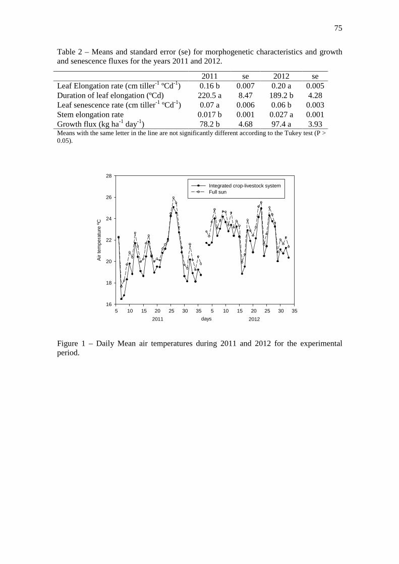
75
Table 2 – Means and standard error (se) for morphogenetic characteristics and growth and senescence fluxes for the years 2011 and 2012.
Means with the same letter in the line are not significantly different according to the Tukey test (P > 0.05).
Figure 1 – Daily Mean air temperatures during 2011 and 2012 for the experimental period.
2011 se 2012 se Leaf Elongation rate (cm tiller-1 ºCd-1) 0.16 b 0.007 0.20 a 0.005 Duration of leaf elongation (ºCd) 220.5 a 8.47 189.2 b 4.28 Leaf senescence rate (cm tiller-1 ºCd-1) 0.07 a 0.006 0.06 b 0.003 Stem elongation rate 0.017 b 0.001 0.027 a 0.001 Growth flux (kg ha-1 day-1) 78.2 b 4.68 97.4 a 3.93
2011
Air
tem
pera
ture
ºC
16
18
20
22
24
26
28
Integrated crop-livestock systemFull sun
2012
5 10 15 20 25 30 355 10 15 20 25 30 35
days

76
Figure 2 – Means for the morphogenical and structural parameters for each species and also within each system (i.e. data shown the species x system interaction). Means with the same capital letters compares systems, means with small letters compares species within each system and means with capital letters with * compares species according to the Tukey test (P >0.05). Bars indicate the standard error of the mean. Species code: Axonopus catharinensis (Ac); Bb – B. brizantha; Mm – Megathyrsus maximus Ha – Hemarthria altissima; and Cc – Cynodon spp. Variables code: phyllochron (Phyl.); leaf elongation rate (LER); duration of leaf elongation (DLE), leaf lifespan (LLS; leaf
SE
R (
cm ti
ller-1
ºC
d-1 )
0.00
0.01
0.02
0.03
0.04
0.05
DLE
(ºC
d)
0
50
100
150
200
250
300
350
400
Phy
l. (º
Cd)
0
20
40
60
80
100
120
140
160
180
200
Full sunICLSSpecies
B A
A
BB
A
AA
B
A
abc
bc aab
ab
bc
d
c c
B*
A*A*
D*C*
Bb
A
B
A
B
A
A
BA
a
b
ab
b
b
a
aA
bb
AB* B*B*
A*
B*
Aa A
B
A
A
BB
A
B
Aa
c
c
a
bbc
a
ab
a
A*
C*
B*
A* A*
LLS
(ºC
d)
0
100
200
300
400
500
600
Bab
A A
A
A
A
A
A
A
Aa a
a
b
b
b
b
b
aB*
A*
C* C*
AB*
LER
(cm
tille
r-1 º
Cd-1
)
0.00
0.05
0.10
0.15
0.20
0.25
0.30
AA
AA
A
A
B
A
A Aab
b
b
c
a
bc
b
a
ab bB*
C*
B*
A*
B*
NG
L
0
2
4
6
8
10
12
BcA
A
A A
A
B
AA
cc
de
a
a
bb
C*
D*
E*
A*
B*
Bd
TD
(til
ler
m2 )
0
500
1000
1500
2000
2500
3000
3500
4000
4500
Ac A
AA A
A
BA
Bc
bb
b a b
b
a
a
A
D*
C*B*
D*
A*
LL (
cm)
0
5
10
15
20
25
30
Bb
A
B
A
AA
B
A
AA
ab
b
c
aa
bc
bc
cd
B*
C*
A*
BC*
D*
Ac Bb Mm Ha Cc Ac Bb Mm Ha Cc
77
senescence rate (LSR); stem elongation rate (SER); number of green leaves (NGL); leaf length (LL); tiller density (TD).
Fig. 3 - Means for the morphogenical and structural characteristics for the interaction species x nitrogen. Means with the same capital letters compares systems, means with small letters compares species within each system according to the Tukey test (P >0.05). Bars indicate the standard error of the mean. Species code: Axonopus catharinensis (Ac); Bb – B. brizantha; Mm – Megathyrsus maximus Ha – Hemarthria altissima; and Cc – Cynodon spp. Variables code: leaf elongation rate (LER); leaf lifespan (LLS); leaf senescence rate (LSR); number of green leaves (NGL); leaf length (LL); tiller density (TD).
LL (
cm)
0
5
10
15
20
25
30
TD
(til
ler
m2 )
0
500
1000
1500
2000
2500
3000
NG
L
0
1
2
3
4
5
6
7
8
9
10
11
12
LLS
(ºC
d)
0
100
200
300
400
500
600
700
LSR
(cm
tille
r-1 º
Cd-1
)
0.00
0.02
0.04
0.06
0.08
0.10
0.12
0.14
0.16
0.18
LER
(cm
tille
r-1 º
Cd-1
)
0.00
0.05
0.10
0.15
0.20
0.25
0.30
N0 N300
A A
A
B
A AA
A
A
Bbc a
a
a
cd bd
b
ab
b
BA
A Ab
c
b d
BA
ce
A Aa bB
A
a
a
BA
cd
BA
b
c B
A
ab
b
BA
cd
B
A
a
a
B
A
B
A A A
AA
B
A
bc
ab
c
c b bc
aa
b
bc
A
B AA
A
B
AA
A
Bb
b cb
a
b
aa
b
b
AA
ba
A
Ac
a
A
B
a
a
A Abc a
A Ad b
Ac Bb Mm Ha CcAc Bb Mm Ha Cc

78
Fig. 4 – Means for the morphogenical and structural parameters for each species and also within each system (i.e. data shown the species x system interaction). Means with the same capital letters compares systems, means with small letters compares species within each system and means with capital letters with * compares species according to the Tukey test (P >0.05). Bars indicate the standard error of the mean. Species code: Axonopus catharinensis (Ac); Bb – B. brizantha; Mm – Megathyrsus maximus Ha – Hemarthria altissima; and Cc – Cynodon spp. Variables code: specific leaf weight (SLW); leaf senescence rate (LSR).
1 2 3 4 5
LSR
(cm
tille
r-1 º
Cd-1
)
0.00
0.02
0.04
0.06
0.08
0.10
0.12
0.14
0.16
0.18
AbcAA
A
A
A
B
A
AA
cdc
d
a
b
ab
a
abcbc
CD* D*
B*
A*
BC*
Full sunICLSSpecies
SLW
(g
cm-1
)
0.000
0.001
0.002
0.003
0.004
0.005
Ac Bb Mm Ha Cc
Ab A
A
B
A
B
A A
AA
a
a
a
c
b
e d
dc
B*
A*
C*
E*
D*
79
Fig. 5 – A) Means for the growth and senescence fluxes for each species and also within each system (i.e. data shown the species x system interaction).. B) Means for growth and senescence fluxes for the interaction species x nitrogen. Means for the morphogenical and structural parameters for each species and also within each system (i.e. data shown the species x system interaction). Means with the same capital letters compares systems, means with small letters compares species within each system and means with capital letters with * compares species according to the Tukey test (P >0.05). Bars indicate the standard error of the mean. Species code: Axonopus catharinensis (Ac); Bb – B. brizantha; Mm – Megathyrsus maximus Ha – Hemarthria altissima; and Cc – Cynodon spp.
SF
(kg
ha-1
day
-1)
0
50
100
150
200
250
SF
(kg
ha-1
day
-1)
0
50
100
150
200
250
GF
(kg
ha-1
day
-1)
0
50
100
150
200
250
N0 N300
B
A
ab
a
B
A
a
a
B
A
ab
a
BA
cb
B
A
b
a
B
Ac Bb Mm Ha Cc
GF
(kg
ha-1
day
-1)
0
50
100
150
200
250
Full sunICLSSpecies
BbA
A
B
A
B
A A
A
Ba
a
a
a
a
c b
a
aA*A*
A*
B*
A*
AbA
A
A
A
B
AA
A
B
b
ab
b
ab
b
ba
a
a
B*B* B*
A* A*
A
B
b
cB
Ab
b A Bb b
A
A
a
a
A
Aa
a
B
Ac Bb Mm Ha Cc
A A
80
Supplementary data Fig S1 – Means for morphogenical and structural characteristics and the interaction species x year condition. Means with the same capital letters compares light condition, means with small letters compares species within each light condition according to the Tukey test (P >0.05). Species code: Axonopus catharinensis (Ac); Bb – B. brizantha; Mm – Megathyrsus maximus Ha – Hemarthria altissima; and Cc – Cynodon spp. Variables code: phyllochron (Phyl.); duration of leaf elongation (DLE); leaf lifespan (LLS); leaf senescence rate (LSR); stem elongation rate (SER); number of green leaves (NGL); leaf length (LL); senescence flux (SF).
SF
(kg
ha-1
day
-1)
0
20
40
60
80
100
LL (
cm)
0
5
10
15
20
25
30
NG
L
0
1
2
3
4
5
6
7
8
9
10
SE
R (
cm. t
iller
-1 º
Cd-1
)
0.00
0.01
0.02
0.03
0.04
0.05
LSR
(cm
till
er-1
ºC
d-1)
0.00
0.02
0.04
0.06
0.08
0.10
0.12
0.14
0.16
0.18
LLS
(ºC
d)
0
100
200
300
400
500
600
700
DLE
(ºC
d)
0
50
100
150
200
250
300
350P
hyll.
(ºC
d)
0
50
100
150
200
250
First YearSecond Year
AbAb Bb
AbBa
Aa
AbAbAb
Ab
Ac Bb Mm Ha Cc
Bb
Aa
Aa
BaAa Aa
Ab
Bc
AbBb
Bb
Aa Aab
Bb AcAb
Aa
BaAab
Bb
AbcAc
BcAc
BbAb
Aa
Aa
AbcAc
Bc
Aa
AaAa
AcAbc Abc
Bc
Aab
Bab
Ac Ac
BdAc
AeAd
Aa Aa
Ab AbAa
Ab
Ac Ac Bbc
AbBb
Aab
Bbc
Aa
Bc
Bb
AbAc
Aa Aa
AabBc
AcAd
Ac Bb Mm Ha Cc
81
4. CAPÍTULO 3
Effect of blue light on two alfalfa morphotypes contrasting on their growth habits1
1 Elaborado de acordo com as normas da Revista Agronomy journal.

82
Effect of blue light on two alfalfa morphotypes contrasting on their growth habits
Tiago Celso Baldissera1,2*, Gaetan Louarn1, Paulo César de Faccio Carvalho3; Ela Frak1
1INRA UR4 URP3F, BP6, F86600 Lusignan, France, 2Universidade Federal do Paraná, Curitiba-PR, Brazil 2Universidade Federal do Rio Grande do Sul, Porto Alegre – RS, Brazil
For correspondence: [email protected]
83
Abstract
Light is considered the major resource driving plant architecture and vegetation
dynamic. Different species and even different genotypes of the same species can exhibit
contrasted strategies to capture and use light. These strategies in the context of light
competition could determine plant's capacity to grow in monoculture or/and in mixtures.
Than, understand morphological responses to blue light could be particularly helpful for
that. The present study aimed to determine the effect of blue less light on the
development and growth of two morphologically contrasted genotypes of Medicago
sativa, that exhibit contrasted growth habits, an erected and other a prostrated
morphotype. During the experimental period, 60 clones of each genotype were grown
under 380 µmol m-2 s-1 of photosynthetic activated radiation (PAR) and 14h
photoperiod. Two light conditions were simulated in growth cabinets: low blue light
level (B-) and neutral light (B+). The differences in the response to blue light of several
morphological parameters (internodes and petiole length, leaf area) between the two
genotypes strongly suggest difference in the strategy for light foraging with genotype
B4 (erect) presenting more trends to escape and genotype D3 (prostated) to tolerate
shade.
Key words: competition; crop mixtures; light quality; pasture canopy; shade-avoidance
1. Introduction
When plants are growing in a canopy, they experience a heterogeneous light
environment in terms of light quantity and also light quality (Varlet-Grancher et al.,
1993a; Ballaré et al., 1997, Holmes and Smith, 1977; Werger et al., 2002). This is
mainly due to interactions of light with plant organs characterized by the capacity to
84
absorb, transmit and reflect solar radiations within the range of 350nm to 800nm
(Smith, 1982).
Both differences in the photon flux density (400-700nm) and changes in light
quality (i.e. Blue, Red and Far red wavebands) induce morphogenetic responses that
affect the capacity of plants to capture light (Tardieu et al., 1999; Lötscher and
Nösberger, 1997; Gautier et al., 2000; Cookson and Granier, 2006). However, light
quality is considered as principal cue driving plant architecture and vegetation dynamic
(Ballaré et al., 1997; Kasperbauer and Hunt, 1992).
Specifically, blue light in the range of 350-500 nm regulates important aspects of
plant development and growth (Varlet-Grancher et al., 1993b). In shade-avoidance
plants, the effects of blue light is well known to trigger a variety of photomorphogenic
responses such changes in stem and leaf length due to the increase in internodes lengths
and leaf elongation rate (Gautier and Varlet-Grancher, 1996; Ballaré and Casal, 2000).
Indeed, blue light can interfere on plant function, due to the influence on gas exchange
through stomatal functioning (Zeiger et al., 1987; Talbott et al., 2002; Barillot et al.,
2010). However, some studies suggest that amplitude and capacity of plants to respond
to blue light depends on the stage of development and species (Casal and Smith, 1988;
Drumm-Herrel and Mohr, 1991; Mitchell and Woodward, 1988).
The enhancement of stem and leaf elongation are due to decrease of blue light
within a plant canopy. The changes in blue light are sensed mainly by two types of
receptors, cryptochromes and the phototropins (Christie and Briggs, 2001; Lin, 2002)
that allow plants to characterize their nearby environment and particularly the intensity
of light competition.
It is well known that light is a major factor of competition between individuals
in growing stands as grasslands, monocultures or in intercropping systems (Wedin and

85
Tilman 1993; Ballaré et al., 1997; Lemaire et al., 2005; Baldissera et al., 2014).
Depending on plant density, genetic heterogeneity (even intra-specific) and the
constraints imposed by the operating mode in these systems (plants density or
diversity/cut/pasture), the lighting conditions of individual plants and light partitioning
between species vary significantly. Consequently, the changes in mass of individuals as
well the proportion of each species and its contribution the overall leaf area index in the
in the stand are related to experienced light conditions (Barilllot et al., 2011). Thus,
different species and even different genotypes of the same species can exhibit contrasted
strategies to capture and use light. These strategies in the context of light competition
could determine plant's capacity to grow in monoculture or/and in mixture and the
morphological responses to blue light could be particularly helpful for that.
The present study aimed to determined the effect of blue less light on the
development and growth of two morphologically contrasted genotypes of Medicago
sativa, that exhibit contrasted growth habits, an erected and a prostrated morphotype
respectively.
2. Material and Methods
The experiments were performed in the laboratory at the INRA Lusignan research
station France. Two morphologically contrasted genotypes of Medicago sativa were
used in this experiment: B4 and D3 an erected and a prostrated morphotype,
respectively. 60 clones of each genotype were prepared in October 2011. During
December 2011 clones were transferred from nursery to greenhouse into 2L individual
plastic pots filled with sand. Clones were maintained in the greenhouse at 15°C during 2
months under additional light sources and were watered 8 times a day. Plants were then
86
transferred into two growth cabinets for three weeks of pre-treatment at 17°C night and
day. During this period clones were grown under 380 µmol m-2 s-1 of photosynthetic
activated radiation (PAR) and 14h photoperiod provided by 6 metallic iodure lamps
(HQI 400W, Osram, France) at 80 % of relative humidity and were automatically
watered 8 times a day with a complete nutrient solution containing 1.9 mol m-3 KNO3,
0.55 mol m-3 Ca(NO3)2, 2.5 mol m-3 NH4NO3, 0.5 mol m-3 CaCl2, 0.1 mol m-3 NaCl, 0.5
mol m-3 MgSO4, 0.4 mol m-3 KH2PO4, 0.3 K2HPO4, 25 10-3 mol m-3 H3BO3, 2 10-3 mol
m-3 MnSO4, 2 10-3 mol m-3 ZnSO4, 0.5 10-3 mol m-3 CuSO4, 0.5 10-3 mol m-3 H2MoO4
and 20 10-3 mol m-3 Fe-HEDTA. Finally, 40 clones of each genotype were selected on
the base of the total number of stems and theirs length. Clones were then cut at 8cm
from the collet (collar) and were randomly distributed under two light treatments in two
others growth cabinets (T°C=17°C, 14h photoperiod, 80% HR, full nutrient solution).
Plants were grown under these conditions until the beginning of flowering (around 2
months) and during this period depending on their developmental stage they received
from 80 to 520 ml per day of full nutrient solution.
2.1 Light treatment
Two light conditions were simulated in the growth cabinets: low blue light level (B-)
and neutral light (B+). The low blue light level (5 µmol m-2 s-1) was thus obtained with
a Lee Filter HT 015 (Lee Filter, Hampshire, England) associated to 9 metallic iodure
lamps (HQI 400W, Osram, France) which supplied high PAR levels. The neutral light
was obtained by using the Lee 216 filter associated to 6 metallic iodure lamps. This
filter provided a neutral shade as it identically lowered the energy from all wavelengths
of the incident light (around 25%). The distance between plants and light sources +
87
filters was adjusted in both growth cabinets in order to provide photon flux with the
same photosynthetic efficiency in B+ (PAR= 407 µmol/m2/s; YPF= 379 µmol/m2/s)
and B- (PAR= 438 µmol/m2/s ; YPF= 383 µmol/m2/s) treatments.
2.2 Morphological measurements
The measurements were done around two months after the beginning of the light
treatments. On each clone a main vigorous growing shoot (main axis) was identified
and it length measured with a ruler. The number of nodes on this shoot as well the
number of associated leaves was reported. For each node rank of this shoot the length of
internodes and petioles were measured with a ruler. Other shoots were cut at 8 cm from
collet, their number reported and total leaf area measured (once leaves separated from
shoots), using a planimeter (LI-3100, LI-Cor, inc, Lincoln, NE, USA).
For the end of regrowth (i.e. after first cut), plant biomass was determined.
Plants were separated in above ground and roots components for total above ground and
roots biomass analysis. Roots were carefully removed from the pot and washed. To
measure dry mass, all samples were dried in the oven for 48h at 60°C.
From the measurements of the main axis it were calculated specific leaf area
(SLA – cm2 g-1), specific stem weight (SSW – g-1 cm-1), leaf:stem ratio of the main axis
(leaves dry weight / stem dry weight). For the biomass measurements from the regrowth
period it was calculated shoot:roots ratio (above ground dry weight / roots dry weight).
2.3 Statistical analyses

88
Statistical analysis were performed using R software (R Development Core Team,
2014). For each node position on the mains axis, T test (t.test procedure) was used to
compare internode and petiole lengths between light treatments for each genotype. The
effects of light treatment, genotype and their interaction on shoot number, total leaf
area, specific leaf area, leaves dry weight of main axis, stem dry weight, of the main
axis, specific stem weight, leaves:stem ratio, total plant dry weight, above ground dry
weight and above ground:roots dry weight ratio were tested by analysis of variance
(ANOVA, aov procedure), and Tukey (HSD.test package AGRICOLAE) method for
multiple mean comparison tests in post-ANOVA. Data were transformed when
necessary to reach the normality of residues, transformations were performed using the
procedure Box Cox (package MASS).
3 Results
3.1 Internodes and petioles lengths
Irrespective of light condition, there were differences in morphological plant
development as described for internode and petiole appearance probability and
evaluated for each genotype and light treatment (Figure 1). All plants presented at least
three nodes, except for genotype D3 growing without blue light. 80% of the plants
showed seven nodes, and the biggest plants reached 14 nodes.
There was a significant (P < 0.04) increase of internode lengths from the 2nd to
the 6th for genotype B4 under blue less (B-) light, whereas no significant (P > 0.29)
changes were observed for D3 genotype (Figure 2). For genotype B4, the length of
petioles was ranged from the maximum of 50 mm and 30 mm in B- and B+ treatments,
89
respectively to around 7mm for both treatments. The genotype D3 exhibited lower
values, ranging for both light treatments from 7mm to 33mm.
For the petiole lengths there was minor effect for genotype B4 compared to the
responses on internode lengths (Figure 3) and significant difference between light
treatments occurred only in the 2nd (P = 0.02) and the 4th node (P = 0.005). As occurred
for internodes length, B- light treatment did not have effect on petioles lengths (P >
0.09) in genotype D3(Figure 3).
3.2 Number of shoots
The total number of shoots was not affected by the blue light treatment, differences
were observed only for genotype (Table 1). The genotype D3 showed a higher average
number of shoots (6.45 shoots) compared to genotype B4 (5.33 shoots) (Table 2).
3.3 Plant leaf area and specific leaf area
The ANOVA outputs showed a significant genotype x blue light treatment interaction
for the leaf area of main axis (Table 1). This interaction was due to the increase in leaf
area for the genotype B4 in the absence of blue light. This genotype exhibited 107 cm2
of leaf area on the main axis under B- conditions whereas only 73 cm2 were measured
under B+ conditions. Genotype D3 did not change main axis leaf area under B-
treatment (49 cm2) and exhibited 64 cm2 on main shoot in the B+ treatment that was
similar to genotype B4 (Table 3). Leaf area of main axis for D3 genotype was slightly
higher in B+ but was not significantly different between light treatments. Consequently,
90
the specific leaf area was affected only by light treatment (Table 1), showing an
increase under B- light conditions (Table 2).
3.4 Dry weight and its partition
The dry weight of leaves and stems were evaluated for the main axis in the first growth
period. The biomass of leaves from the main axis was also higher when exposed to the
treatment with blue light, and genotype B4 showed higher leaves dry weight compared
to genotype D3 (Table 2). For stems, ANOVA results showed an interaction between
light treatment x genotype (Table 1). This interaction was mainly due to the increase of
stem dry weight for plants of genotype B4 growing in B-.
Under B+ treatment the stem weight was similar for both genotypes whereas it
was significantly different under B- treatment (Table 3).The differences in stem weight
can be explained by the specific stem weight (SSW) and stem height (Table 1).
Genotype B4 showed similar SSW (Table 3), but had higher internodes lengths (Figure
2) in the treatment B-, producing longer stems. For genotype D3, there was no
difference in lengths (Figure 2), however the SSW was lower for plants growing
without blue light.
For the regrowth period (i.e. after first cut) it was analyzed the total plant
biomass and its partition between above ground and roots biomass. Total dry weights of
plants were higher with the B+, and there was no difference between genotypes (Table
2).
For above ground and roots biomass the same pattern of total biomass occurred,
where it was affected only by light treatment, with an increase on dry weight for the
plants growing under blue light (B+).

91
4. Discussion
The objective of our study was to analyze the effect of blue less light on the
development and growth of two morphologically contrasted genotypes of Medicago
sativa. The differences in the response to blue light of several morphological parameters
(internodes and petiole length, leaf area) between the two genotypes strongly suggest
difference in the strategy for light foraging with genotype B4 (erect) presenting more
trends to escape and genotype D3 (prostated) to tolerate shade (Givnish, 1988).
4.1 Effects of blue light on Elongation and Leaf area
The effect of light quality (Red:Far Red) on stem elongation is well reported in the
literature, plants trying to escape shade tend to increase stems to reach a better light
condition (Morgan and Smith, 1981; Morgan 1982, Child and Smith, 1987). Our results
demonstrate that the isolated effect of blue light also has an impact on the stem
elongation (Figure 2). In contrast, petiole elongation was slight affected by blue light
treatment on genotype B4 and genotype D3 was not affected at all (Figue 3). The effect
of light quality in petiole elongation is expected to be higher in plants that exhibit a
prostrated pattern of growth, however this was not the case in this work. For white
clover petiole elongation and inclination is affected by blue light (Gautier et al., 1997,
Christophe et al., 2006). Low blue light change petiole inclination and helps to position
leaves in the upper layers of the canopy interfering in light capture. Gautier et al. (2001)
also showed that in the case of white clover, the response of petioles was independent of
the plant position. For the estoloniferous species Potentilla reptans, the response to

92
shade occurred more in a vertical way, due to the increase of petioles lengths, rather
than internodes lengths (Huber and Stuefer, 1997).
The increase in the leaf area of main stem occurred only for genotype B4 in the
absence of blue light (Table 3). Plant leaf area on a stem is dependent of the total
number of leaves and leaf size. According to Gautier et al. (1997), modifications in light
quality can leads to increases of leaf size. However, Baldissera et al. (2014) showed that
in alfalfa competing for light, there was a reduction in final plant leaf area due to plant
density, and this reduction was referred to plant development (i.e. branches appearance,
number of shoots), harder than the size of leaves.
Blue light did not affected total leaf area, but changed specific leaf area, that was
higher for both genotypes (Table 1). In general, plants growing in a reduced light
condition exhibit thinner leaves compared to high light condition, also various authors
showed that the response of SLA is highly correlated with photosynthetic photon flux
density (Tucker et al., 1987; Dale, 1988; Niinemets and Kull, 1998; King, 2003, Petritan
et al., 2009), also the response of SLA can be linked with the species tolerance to shade.
However, some investigations show that more shade-tolerant species tend to show a
higher SLA with the decrease in light availability (Niinemets and Kull, 1997; Barthod
and Epron, 2005; Klooster et al., 2007). But others did not confirm this pattern
(DeLucia et al., 1998; Stancioiu and O’Hara, 2006).
Due to the results found on total leaf area of the main axis (Table 3), it could be
hypothesized that blue light may does not interfere in leaves appearance, but only on
leaf morphology as it has been shown for other forage species (Gautier and Varlet-
Grancher, 1996)
4.2 Effects of blue light on biomass partitioning between leaves and stems
93
The decrease in leaves dry weight (Table 2) corroborates with the results obtained by
Lin et al. (2001), for fifteen forage species including alfalfa, these authors also showed
an increase in total leaf area, decreases on leaves dry weight are directly correlated with
SLA (see section 4.1)
On the other hand, stem weight of the main axes was higher for the genotype B4
for the treatment B- (Table 4), whereas the SSW did not changed, than the increase on
stem weight can be correlated with the increase in internodes lengths (Figure 2),
resulting in longer stems. In the case of genotype D3, the stem weight of main axis
tended to be lower under B- treatment, mainly due to the lower SSW (Table 4), as there
were no changes in internodes lengths (Figure 2). The modulation of carbon allocation
to leaves and stems depends on species and light conditions (Samarakoon et al., 1990)
and often result in distinct leaf:stem ratios between genotypes. Finally in our
experiment, D3 genotype did not changed leaf:stem in response to light treatments
whereas genotype B4 reduced its ratio under B- treatment. This higher leaf:stem ratio
can be positive response, because it trigger a better forage quality (Lin et al., 2001).
This differences in biomass allocation to leaves and stems also agrees with
distinct strategies between genotypes to capture light, that was already commented in
the topic 4.1, and the results showed in our work for the blue light effect are similar
from those reported for changes in red:far-red or in the reduction of photosynthesis
photon fluxes density (Corré 1983; Keiller and Smith, 1989; Fortnum and Kasperbauer
1992, Kasperbauer and Hunt 1992 a,b). While genotype B4 (erect habit of growth)
tended to elevate leaves by increase of stem height, and changing biomass allocation to
stems, genotype D3 (prostrated habit of growth), maintained allocation to leaves and
94
reduced for stems, than we could hypothesize this is correlated with the plagiotropic
pattern of growth of this genotype.
4.3 Effects of blue light on total plant biomass and root-shoot ratio
Total biomass production was reduced by the lack of blue light, also total above ground
and roots biomass followed the same pattern, resulting in no differences for the ratio
above ground:roots dry weight (Table 2). The reduction on biomass can be an effect of
blue light on stomata opening (Smith, 1982; Fankhauser and Chory, 1997; Kinoshita et
al., 2001; Talbott et al., 2002; Barillot et al., 2010). Blue light stimulated stomata
opening, when stomata are closed, it prevents the CO2 passage to the interior of the
cells, resulting in a decrease of photosynthesis. Barillot et al. (2010) showed that under
a decrease level of blue light, there is a instantaneous closure of stomata, and a gradual
reopening after 20 min, but leading to a new steady-state, never reaching the initial
state.
4. 4 summarizing
To sum up, morphological and growth process are affected on alfalfa by blue light,
however contrasting genotypes in their habit of growth showed distinct responses to
light and distinct strategies to capture light. These findings should help in define
management strategies, mainly for consortiums. Baldissera et al. (2014) evaluated the
same erected morphotype, and showed that when growing in a consortium with tall
fescue (Festuca arundineacea), alfalfa tended to overlap the graminea species.
95
5. References
Baldissera TC, Frak E, Carvalho PCDF, Louarn G. 2014. Plant development controls leaf area expansion in alfalfa plants competing for light. Annals of botany 113:145–57. doi: 10.1093/aob/mct251
Ballare CL, Casal JJ. 2000. Light signals perceived by crop and weed plants. Field
Crops Research 67:149–160. Ballaré CL, Scopel AL, Sanchez RA. 1997. Foraging for light: Photosensory ecology
and agricultural implications. Plant, Cell and Environment 20: 820-825. Barillot R, Louarn G, Escobar-Gutiérrez AJ, et al. 2011. How good is the turbid
medium-based approach for accounting for light partitioning in contrasted grass--legume intercropping systems? Annals of botany 108:1013–24. doi: 10.1093/aob/mcr199
Barillot R, Frak E, Combes D, et al. 2010. What determines the complex kinetics of
stomatal conductance under blueless PAR in Festuca arundinacea? Subsequent effects on leaf transpiration. Journal of experimental botany 61:2795–806. doi: 10.1093/jxb/erq115
Barthod S, Epron D. 2005. Variations of construction costs associated to leaf area
renewal in saplings of two co-occurring temperate tree species (Acer platanoides L. and Fraxinus excelsior L.) along a light gradient. Ann. For. Sci. 62: 545–551.
Casal JJ, Smith H. 1988. Persistent effects of changes in phytochrome status on
internode growth in light-grown mustard: occurrence, kinetics and locus of perception. Planta 175:214-220.
Child, R, Smith, H. 1987. Phytochrome action in light-grown mustard:
Kinetics, fluence-rate compensation and ecological significance. Planta 172: 219-229.
Christie JM, Briggs WR. 2001. Blue light sensing in higher plants. The Journal of
biological chemistry 276:11457–60. doi: 10.1074/jbc.R100004200 Christophe A, Moulia B, Varlet-Grancher C. 2006. Quantitative contributions of blue
light and PAR to the photocontrol of plant morphogenesis in Trifolium repens (L.). Journal of experimental botany 57:2379–90. doi: 10.1093/jxb/erj210
Cookson SJ, Granier C. 2006. A dynamic analysis of the shade-induced plasticity in
Arabidopsis thaliana rosette leaf development reveals new components of the shade-adaptative response. Annals of botany 97:443–52. doi: 10.1093/aob/mcj047
Corré WJ. 1983. Growth and morphogenesis of sun and shade plants. II. The influence of light quality. Acta Bot.NeerI. 32:185-202.
96
Dale JE. 1988. The control of leaf expansion. Ann Rev Physiol Plant Mol Biol 39:267–295.
Drumm-Herrel H, Mohr H. 1991. Involvement of phytochrome in light control of stem elongation in cucumber (Cucumis sativus L.) seedlings. Photochemistry and Photobiology 53: 539-544.
Fankhauser C, Chory J. 1997. Light control of plant development. Annu Rev Cell Dev Biol 13:203-29. Fortnum BA, Kasperbauer MJ. 1992. Biomass partitioning and root knot nematode
development in tomato plants under end-of-day red or far-red light. Crop Science 32:408-411.
Gautier H, Varlet-Grancher C. 1996. Regulation of leaf growth of grass by blue light. Physiologia Plantarum 98: 424-430. Gautier, H. Varlet-grancher, C. Baudry N. 1997. Effects of Blue Light on the Vertical
Colonization of Space by White Clover and their Consequences for Dry Matter Distribution. Annals of botany 80:665–671.
Gautier, H.; Varlet-grancher C., Membre JM. 2001. Plasticity of petioles of white clover
(Trifolium repens) to blue light. Physiologia Plantarum 112:293–300. Gautier, H. Mech, R. Prusinkiewicz, P. Varlet-Grancher C. 2000. 3D Architectural
Modelling of Aerial Photomorphogenesis in White Clover (Trifolium repens L.) using L-systems. Annals of Botany 85:359–370. doi: 10.1006/anbo.1999.1069
Givnish TJ. 1988. Adaptation to Sun and Shade: A whole-plant perspective. Australian
Journal of Plant Physiology 15:63–92. Holmes MG, Smith H. 1977. The function of phytochrome in plants growing in the
natural environment. Nature 254: 512-514. Huber H, Stuefer JF. 1997. Shade-induced changes in the branching pattern of a
stoloniferous herb : functional response or allometric effect? Oecologia 110:478–486.
Kasperbauer MJ, Hunt PG. 1992a. Root size and shoot root ratio as influenced by light environment of the shoot. Journal of Plant Nutrition 15: 685-697. Kasperbauer MJ, Hunt PG. 1992b. Cotton seedling morphogenic responses to FR/R
ratio reflected from different colored soils and soil covers. Photochemistry & Photobiology 56:579-584.
Keiller D, Smith H. 1989. Control of carbon partitioning by light quality mediated by
phytochromes. Plant Science. 63: 25-29. King DA. 2003. Allocation of above-ground growth is related to light in temperate
deciduous saplings. Functional Ecology 17:482–488. doi: 10.1046/j.1365-2435.2003.00759.x

97
Kinoshita T, Doi M, Suetsugu N, et al. 2001. Phot1 and phot2 mediate blue light
regulation of stomatal opening. Nature 414:1–4. Janse-Ten Klooster SH, Thomas EJP, Sterck FJ. 2007. Explaining interspecific
differences in sapling growth and shade tolerance in temperate forests. Journal of Ecology 95:1250–1260. doi: 10.1111/j.1365-2745.2007.01299.x
Lemaire G, Avice J-C, Kim T-H, Ourry A. 2005. Developmental changes in shoot N
dynamics of lucerne (Medicago sativa L.) in relation to leaf growth dynamics as a function of plant density and hierarchical position within the canopy. Journal of experimental botany 56:935–43. doi: 10.1093/jxb/eri084
Lin CH, Mcgraw RL, George MF, Garrett HE. 2001. Nutritive quality and
morphological development under partial shade of some forage species with agroforestry potential. Agroforestry Systems 53:269–281.
Lötscher M. Nösberger J. 1997. Branch and root formation in Trifolium repens is
influenced by the light environment of unfolded leaves. Oecologia 111:499–504. Lin CT. 2002. Blue light receptors and signal transduction. Plant Cell 14: 207-225. Mitchell PL, Woodward FI. 1988. Responses of three woodland herbs to reduced
photosynthetically active radiation and low red to far-red ratio in shade. Journal of Ecology 76:807-825.
Morgan DC, Smith H. 1981. Control of developpment in Chenopodium album L. by
shade light. The effects of light quantity (total fluence rate) and light quality (red-far red –ratio). New Phytol. 88: 239-248.
Niinemets U, Kull O. 1998. Stoichiometry of foliar carbon constituents varies along
light gradients in temperate woody canopies: implications for foliage morphological plasticity. Tree physiology 18:467–479.
Petriţan AM, Lüpke B, Petriţan IC. 2009. Influence of light availability on growth, leaf
morphology and plant architecture of beech (Fagus sylvatica L.), maple (Acer pseudoplatanus L.) and ash (Fraxinus excelsior L.) saplings. European Journal of Forest Research 128:61–74. doi: 10.1007/s10342-008-0239-1
Samarakoon SP, Wilson JR, Shelton HM. 1990. Growth, morphology and nutritive
quality of shaded Stenotaphrum secundatum, Axonopus compressus and Pennisetum clandestinum. The Journal of Agricultural Science 114:161. doi: 10.1017/S0021859600072154
Smith H. 1982. Light quality, photoperception, and plant strategy. Annual Review of Plant Physiology 33, 481-518. Stancioiu PT, O’Hara KL. 2006. Morphological plasticity of regeneration subject to
different levels of canopy cover in mixed-species, multiaged forests of the Romanian Carpathians. Trees 20:196–209. doi: 10.1007/s00468-005-0026-2
98
Talbott LD, Zhu J, Han SW, Zeiger E. 2002. Phytochrome and blue light-mediated stomatal opening in the orchid, paphiopedilum. Plant & cell physiology 43:639–46.
Tucker GF, Hinckley TM, Leverenz JW, Jiang S. 1987. Adjustments to foliar
morphology in the acclimation of understory Pacific silver fir following clearcutting. For. Ecol. Manage 21: 249-268.
Varlet-Grancher C, Moulia B, Sinoquet H, Russell G. 1993a. Crop structure and light microclimate: Characterization and applications. Versailles. Varlet-Grancher C, Moulia B, Sinoquet H, Russell G. 1993b. Spectral modification of
light within plant canopies - how to quantify its effects on the architecture of the plant stand. In: Varlet-Grancher C, Moulia B, Sinoquet H, eds. Crop structure and light microclimate. Characterization and applications. Versailles: INRA, 427-451.
Wedin D, Tilman D. 1993. Competition among grasses along a nitrogen gradient:
Initial conditions and mechanisms of competition. Ecological Monographs 63: 199-229.
Werger MJ a., Hirose T, During HJ, et al. 2002. Light partitioning among species and
species replacement in early successional grasslands. Journal of Vegetation Science 13:615–626.
Zeiger E, Gotow K, Mawson B, Taylor S. 1987. The guard cell chloroplast: properties
and functions. In: Biggins J (ed). Proceedings os the 7th International Photosynthesis Congress, V. 4 pp 273-280.
99
Table 1 – F-ratios and statistical significance of ANOVAs of plant traits in function of blue light and contrasted genotypes of Medicago sativa.
*, P < 0.05; **, P < 0.01; ***, P < 0.001; n.s., not significant. Table 2 – Plant traits in function of blue light (B- less bluelight; B+ neutral blue light) and contrasted genotypes of Medicago sativa (B4 prostrate; D3 erect).
B- B+ B4 D3 Shoot number 5.7 (0.24) a 5.9 (0.26) a 5.3 (0.20) b 6.4 (0.26) a Specific leaf area (cm2 g-1)
329.1 (10.9) a 238.3 (11.84) b 284.4 (13.1) a 280.1 (14.6) a
Leaves dry weight of the main axis (g)
231.31 b 312.63 a 315.21 a 22.51 b
Total dry weight (g)
6402.8 (347.5) b 10297.8 (654.3) a 8860.7 (561.5) a 7953.4 (673.5) a
Above ground dry weight (g)
3687.5 (209.7) b 5715.2 (384.9) a 4996.2 (328.1) a 4341.0 (361.1) a
Root dry weight (g)
2691.8 (147.2) b 4421.4 (254.3) a 3801.7 (230.5) a 3360.5 (272.6) a
Ratio Shoot:Root dry weight (g)
1.3 (0.04) a 1.31 (0.03) a 1.3 (0.03) a 1.3 (0.04) a
Means with the same letters for light treatment and for genotype treatment are not significantly different according to the Tukey test (P . 0.05). standard error of the mean in parenthesis. Table 3 – Leaf area of main (cm2) axis in function of blue light (B- less bluelight; B+ neutral blue light) and contrasted genotypes of Medicago sativa (B4 prostrate; D3 erect). B4 D3
B- 107.36 (14.0) Aa 49.08 (7.0) Ab B+ 72.81 (10.1) Ba 64.63 (7.0) Aa
Means with the same capital letters in the column and small letters in the lines are not significantly different according to the Tukey test (P . 0.05). standard error of the mean in parenthesis.
Treatment Genotype Treatment x Genotype Shoot number n.s. 11.47** n.s. Leaf area of main axis n.s. 7.9** 6.86* Specific leaf area 30.77*** n.s. n.s. Leaves dry weight of the main axis
4.89* 4.91* n.s.
Stem dry weight of the main axis
n.s. 9.02** 7.65*
Leaf:stem ratio 10.68** 5.30* 8.12** Specific stem weight 8.70** 15.26*** 5.17* Total dry weight 23.37*** n.s. n.s. Above ground weight 17.99*** n.s. n.s. Roots dry weight 31.17*** n.s. n.s. Above ground:roots ratio n.s n.s n.s
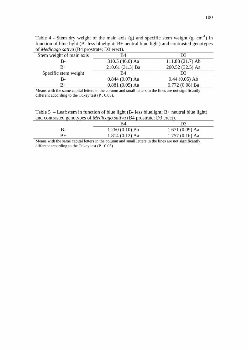
100
Table 4 - Stem dry weight of the main axis (g) and specific stem weight (g. cm-1) in function of blue light (B- less bluelight; B+ neutral blue light) and contrasted genotypes of Medicago sativa (B4 prostrate; D3 erect). Stem weight of main axis B4 D3
B- 310.5 (46.0) Aa 111.88 (21.7) Ab B+ 210.61 (31.3) Ba 200.52 (32.5) Aa
Specific stem weight B4 D3 B- 0.844 (0.07) Aa 0.44 (0.05) Ab B+ 0.881 (0.05) Aa 0.772 (0.08) Ba
Means with the same capital letters in the column and small letters in the lines are not significantly different according to the Tukey test (P . 0.05). Table 5 – Leaf:stem in function of blue light (B- less bluelight; B+ neutral blue light) and contrasted genotypes of Medicago sativa (B4 prostrate; D3 erect). B4 D3
B- 1.260 (0.10) Bb 1.671 (0.09) Aa B+ 1.814 (0.12) Aa 1.757 (0.16) Aa
Means with the same capital letters in the column and small letters in the lines are not significantly different according to the Tukey test (P . 0.05).

101
Figure 1 – Probability of internode and petiole appearance in respect to each node position in the main axis of contrasted genotypes of Medicago sativa. (B- less bluelight; B+ neutral blue light). (B4 prostrate; D3 erect).
0 1 2 3 4 5 6 7 8 9 10 11 12 13 14
Pro
babi
lity
of p
etio
le a
ppea
renc
e
0.0
0.2
0.4
0.6
0.8
1.0B-B+
Rank of node position
0 1 2 3 4 5 6 7 8 9 10 11 12 13 14
B-B+Genotype B4 Genotype D3
Pro
babi
lity
of In
tern
od a
ppea
renc
e
0.0
0.2
0.4
0.6
0.8
1.0 B-B+
Genotype B4
B-B+
Genotype D3
A
B

102
Figure 2 – Internod lengths in respect to each node position in the main axis. of contrasted genotypes of Medicago sativa. (B- less bluelight; B+ neutral blue light). (B4 prostrate; D3 erect) (*P< 0.05; **P < 0.01; ***P<0.001; ns, not significant).
0 1 2 3 4 5 6 7 8 9 10 11 12 13 14
Inte
rnod
leng
ht (
mm
)
0
10
20
30
40
50
60
70
B-B+
Genotype B4
0 1 2 3 4 5 6 7 8 9 10 11 12 13 14
B-B+
Genotype D3
ns
*****
*** **
nsns
ns ns
ns
ns
ns nsns ns ns
ns ns ns
nsns
Rank of node position

103
Figure 3 - Petiole lengths in respect to each node position in the main axis of contrasted genotypes of Medicago sativa. (B- less bluelight; B+ neutral blue light). (B4 prostrate; D3 erect) (*P< 0.05; **P < 0.01; ***P<0.001; ns, not significant).
Rank of node position
0 1 2 3 4 5 6 7 8 9 10 11 12 13 14
Pet
iole
leng
ht (
mm
)
0
10
20
30
40
50
60
70B-B+
0 1 2 3 4 5 6 7 8 9 10 11 12 13 14
B-B+
Genotype B4 Genotype D3
***
ns
nsns
nsns
nsns ns
nsns
ns
ns
ns ns nsns
ns nsns
ns ns ns

104
5. CAPÍTULO 4
Plant development controls leaf area expansion in alfalfa plants competing for light
105
106

107
108
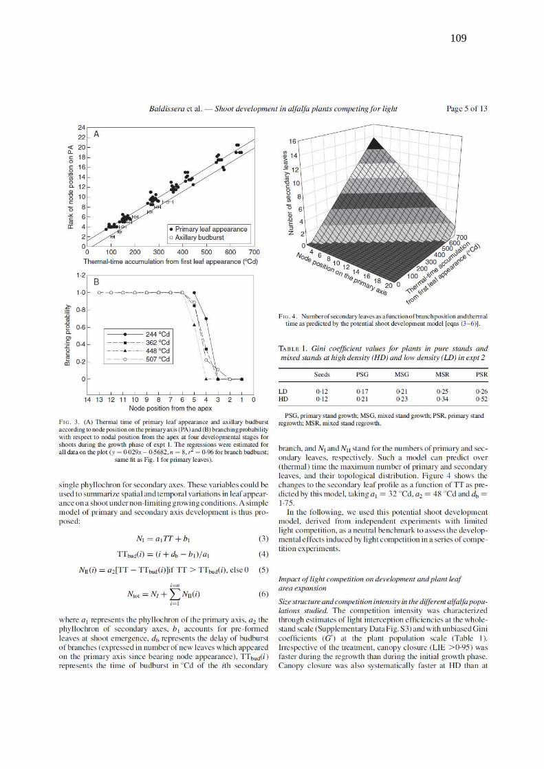
109
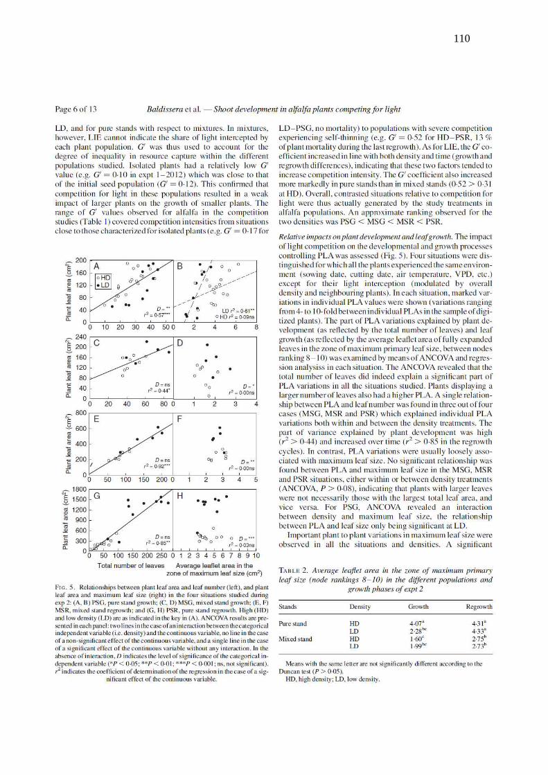
110
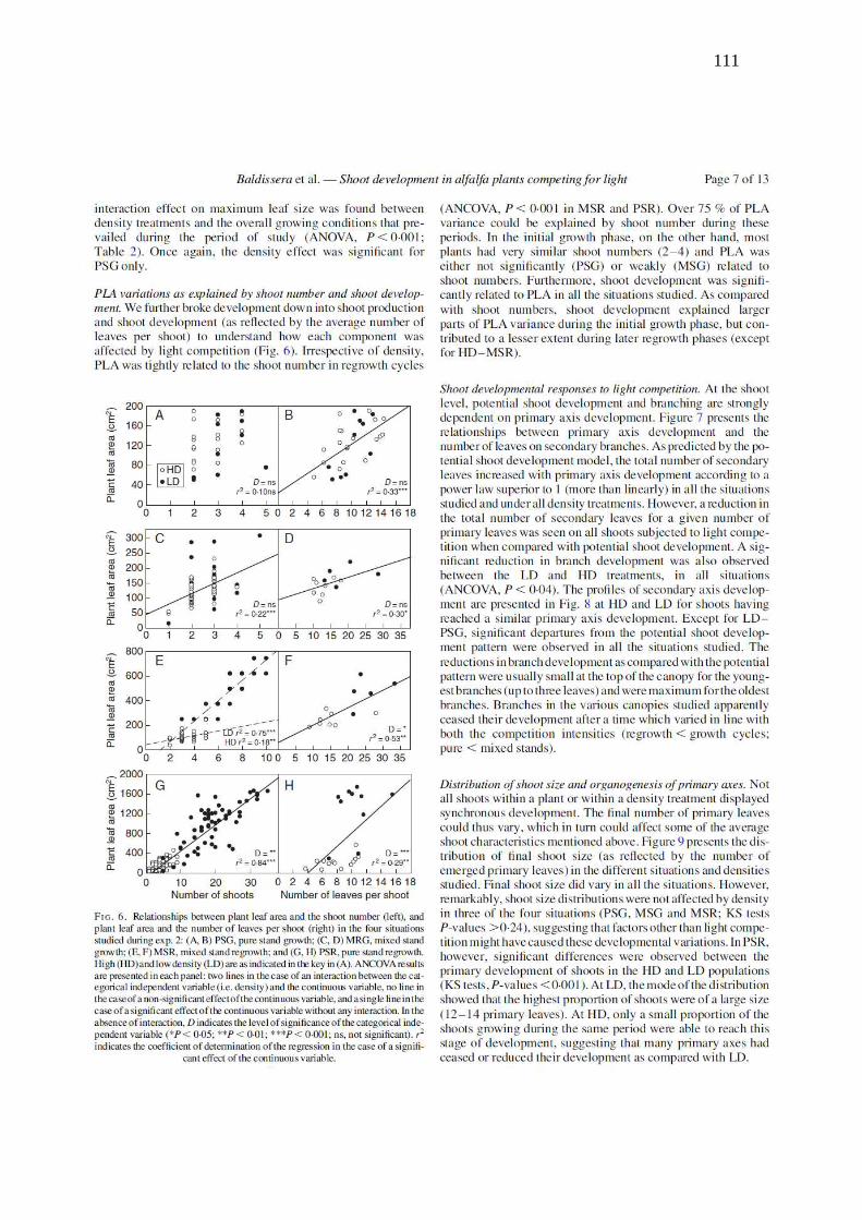
111
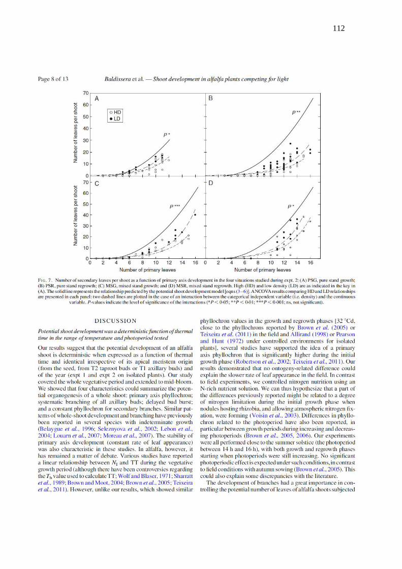
112

113
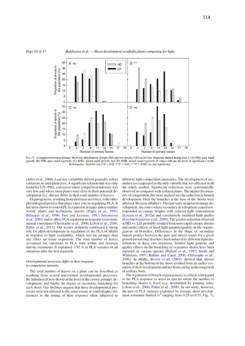
114
115

116

117
118
Table S1. Environmental conditions experienced for the different growth periods
studied during the two experiments. Tm, PPFD and VPD refer to daily average
temperature (°C), daily average photon flux density (µmole PAR.m-2) and daily average
vapour pressure deficit (kPa), respectively. Values in parenthesis are for minimum and
maximum values over the period.
Year Growth period PPFD
Exp 1 2009 1 (Growth) 14.5 (7.2 - 23.6) 1018 1.3 (0.9 - 2)2 (Regrowth) 18.9 (14.3 - 25.1) 1064 1.4 (1.1 - 1.9)
2012 1 (Growth) 16.0 (9.9 - 22.7) 934 1.4 (0.7 - 2)2 (Regrowth) 18.4 (15.4 - 26.5) 981 1.5 (1.1 - 2.1)
Exp 2 2009 1 (Growth) 14.5 (7.2 - 23.6) 1018 1.3 (0.9 - 2)2 (Regrowth) 18.9 (14.3 - 25.1) 1064 1.4 (1.1 - 1.9)
2010 1 (Growth) 15.1 (7.8 - 22.5) 919 1.4 (0.8 - 1.8)2 (Regrowth) 21.0 (13.1 - 26.5) 1136 1.7 (1.1 - 2.2)
Tm VPD

119
Fig. S1. Diagrams of a) the arrangement of the main axis, secondary and tertiary axes on
a seedling plant (initial growth cycle) and b) the types of main axes emerging either
from the taproot (T2) or from the axil of a leaf just below the cutting height (T1) of a
mature plant during a regrowth cycle. Redrawn from Moreau et al. (2007) and Gosse et
al.(1988).

120
Fig. S2. Number of leaves on branches as a function of thermal-time accumulation
expressed in cumulative degree-days from shoot emergence during the growth phases
of Exp. 1. Open and closed symbols indicate 2012 and 2009 data, respectively. Date of
branch appearance (DA) and phyllochron (RLa-1) estimated from linear regressions are
indicated in each panel.
Thermal-time accumulation from first leaf appearence (ºCd)
0 200 400 600 8000 200 400 600 8000
5
10
15
20
0 200 400 600 800
Num
ber
of L
eave
s
0
5
10
15
20
0 200 400 600 800
B1
B2 B4 B8
B3
B6
RLA-1= 42,2 +- 1,09
RLA-1= 47,1 +- 1,54
RLA-1= 50,8 +- 1,91
RLA-1= 49,6 +- 1,84RLA-1= 48,6 +- 1,78 RLA-1= 47,8 +- 2,12
DA=127 +- 8
DA=148 +- 10
DA=176 +- 11
DA=215 +- 10 DA=279 +- 9 DA=315 +- 10
DA=246 +- 9RLA-1= 50,6 +-1,76B5
DA=298 +- 8RLA-1=46,5 +- 1,73 B7
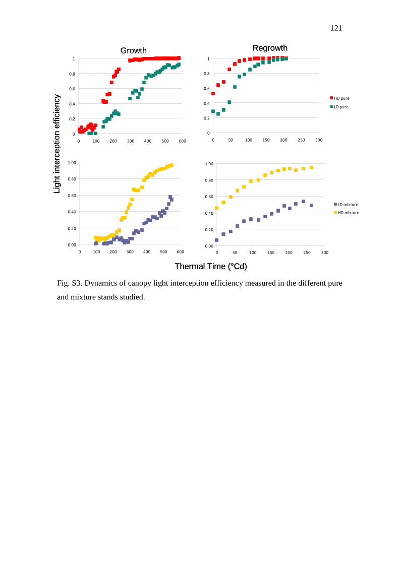
121
Fig. S3. Dynamics of canopy light interception efficiency measured in the different pure
and mixture stands studied.
0
0.2
0.4
0.6
0.8
1
0 100 200 300 400 500 600
HD pure
LD pure
0
0.2
0.4
0.6
0.8
1
0 50 100 150 200 250 300
HD pure
LD pure
0.00
0.20
0.40
0.60
0.80
1.00
0 100 200 300 400 500 600
LD mixture
HD mixture
0.00
0.20
0.40
0.60
0.80
1.00
0 50 100 150 200 250 300
LD mixture
HD mixture
Thermal Time (°Cd)
Ligh
t int
erce
ptio
n ef
ficie
ncy
Growth Regrowth
0
0.2
0.4
0.6
0.8
1
0 100 200 300 400 500 600
HD pure
LD pure
0
0.2
0.4
0.6
0.8
1
0 50 100 150 200 250 300
HD pure
LD pure
0.00
0.20
0.40
0.60
0.80
1.00
0 100 200 300 400 500 600
LD mixture
HD mixture
0.00
0.20
0.40
0.60
0.80
1.00
0 50 100 150 200 250 300
LD mixture
HD mixture
Thermal Time (°Cd)
Ligh
t int
erce
ptio
n ef
ficie
ncy
Growth Regrowth

122
6. CONSIDERAÇÕES FINAIS
Os resultados observados nos diferentes trabalhos desenvolvidos demonstram
que existe grande espécie dependência em função dos efeitos da luz, havendo até
distintas respostas em função de diferentes genótipos de uma mesma espécie, como é o
caso da alfafa. Tal fator dificulta a predição do comportamento das espécies e,
consequentemente, o manejo em função de alterações da luz. Contudo, é possível
apontar alguns mecanismos de alteração das plantas que podem ser utilizados como alvo
da pesquisa e deste modo facilitar a avaliação do comportamento de cada espécie em
relação a luz.
Um dos mecanismos de resposta das plantas comumente observado nos
resultados aqui apresentados, e que já havia sido reportado inúmeras vezes na literatura,
é a elongação do colmo em função das alterações na quantidade e/ou qualidade da luz.
Nos trabalhos realizados com alfafa, os resultados obtidos resultaram em
importantes informações, as quais ajudam na construção de modelos de interceptação da
luz pelo dossel vegetal e, portanto, a predição da produção. Tais resultados também têm
enorme importância para o manejo da alfafa em consórcio com gramíneas. Por
exemplo,...
No caso das espécies tropicais C4 avaliadas sobre o efeito de árvores, A.
catharinensis, B. brizantha, H. altíssima e Cynodon cpp. demonstraram claramente que
as alturas atingidas aos 95% de interceptação luminosa são maiores do que aquelas
obtidas a pleno sol. Para as espécies M. maximus e P. notatum não ocorreram variações
importantes. Demonstrando assim a variabilidade comentada acima para diferentes
espécies, ainda as dificuldades de utilizar o critério de altura como estratégia de manejo
nesses sistemas.
Neste sentido, poderia se sugerir que a pesquisa avance na busca de facilitar o
uso diretamente da medição da interceptação luminosa, como controle da entrada de
animais em pastejo e não do uso da altura.
Outro aspecto importante do manejo a ser abordado é a intensidade de corte. No
trabalho com as espécies arborizadas, foi utilizada uma intensidade de 50% de corte da
altura em que a pastagem atingia 95% de interceptação luminosa, contudo este corte foi
realizado mecanicamente. É necessário deste modo, aliar o comportamento animal nos
estudos de intensidade de manejo de espécies em sistemas integrados com árvores.
123
Ainda, é necessário entender como o efeito da sombra das árvores vai interferir no
comportamento animal. Sugere-se que, principalmente em lugares com altas
intensidades de radiação, os animais iriam pastejar mais nos lugares com maior sombra
ao longo do dia, isso poderia resultar em diferenças na estrutura do dossel da pastagem
ao longo do gradiente de sombra.
Nas metodologias propostas para avaliações das espécies em sistema integrado
com árvores, existe grande importância em separar os diferentes fatores que interferem
no crescimento e no desenvolvimento das plantas. Neste estudo, tentou-se objetivar o
efeito do sombreamento. Contudo, não é possível fazer a completa separação dos efeitos
de água, por exemplo. Inicialmente era pretendida a irrigação das áreas com árvores e a
pleno sol, mas não foi possível realizar em função de custos e logística dos
experimentos.
Por fim, informações a respeito do manejo de espécies forrageiras nos mais
variados tipos de consórcio são de extrema importância, pois auxiliam a técnicos e
produtores na tomada de decisões e também são determinantes para aumentar a adesão
destes tipos de sistemas.
124
7. REFERÊNCIAS
BALBINO, L.C.; CORDEIRO, L.A.M.; PORFÍRIO-DA-SILVA, V.; MORAES, A.;
MARTÍNEZ, G.B.; ALVARENGA, R.C.; KICHEL, A. N.; FONTANELI, R.S.;
SANTOS, H.P.; FRANCHINI, J.C.; GALERANI, P.R. Evolução tecnológica e arranjos
produtivos de sistemas de integração lavoura-pecuária-floresta no Brasil. Pesq.
Agropec. bras., v.46, n.10, p.1-12, 2011.
BALLARE, C.L.; CASAL, J.J. Light signals perceived by crop and weed plants. Field
Crops Research, v.67, p.149–160, 2000.
BALLARÉ, C.L.; SCOPEL, A.L.; SANCHEZ, R.A. Foraging for light: Photosensory
ecology and agricultural implications. Plant, Cell and Environment, v.20, p.820-825,
1997.
BERNARDINO, F.S.; GARCIA, R. Siltemas silvipastoris. Pesquisa Florestal
Brasileira, n.60, p.77-87, 2009.
BURNER, D.M.; BELESKY, D.P. Diurnal effects on nutritive value of alley-cropped
orchardgrass herbage. Crop Science, v.44, p.1776-1780, 2004.
CASAL, J.J. Phytochromes, cryptochromes, phototropin: photoreceptor interactions
in plants. Photochemistry and photobiology, v.71, p.1–11, 2000.
CRUZ, P. Effect of shade on the growth and mineral nutrition of a C4 perennial grass
under field conditions. Plant and Soil, v.188, p.227–237, 1997.
FELDHAKE, C.M.; BELESKY D.P. Photosynthetically active radiation use efficiency
of Dactylis glomerata and Schendonorus phoenix along a hardwood tree-induced light
gradient. Agroforestry Systems, v.75, p.189–196. 2009.
GIVNISH, T.J. Adaptation to Sun and Shade: A whole-plant perspective. Australian
Journal of Plant Physiology, v.15, p.63–92, 1988.
125
HEALEY, K.D.; RICKERT, K.G.; HAMMER, G.L.; BANGE, M.P. Radiation use
efficiency increases when the diffuse component of incident radiation is enhanced under
shade. Australian Journal of Agricultural Research, v.49, p.665–672. 1998.
KNOWLES, R.L. et al. Developing canopy closure model to predict
overstorey/understorey relationships in Pinus radiata silvopastoral systems.
Agroforestry Systems, v.43, p.109-119. 1999.
LACORTE S.M., ESQUIVEL J.L. Sistemas silvopastoriles en la mesopotamia
argentina. Reseña del conocimiento, desarrollo y grado de adopción. In:
CONGRESO NACIONAL DE SISTEMAS SILVOPASTORILES, Posadas
(Misiones, Argentina). Actas. Posadas (Misiones, Argentina), 2009. p. 70-82
LIN, C.H.; MCGRAW, R.L.; GEORGE, M.F.; GARRETT, H.E. Shade effects on
forage crops with potential in temperate agroforestry practices. Agroforestry Systems,
v.44, p.109–119, 1999.
MORAES, A.; CARVALHO, P.C.F.; BARRO, R.S.; LUSTOSA, S.B.C.; PORFÍRIO-
DA-SILVA, V.; REISENDORF-LANG, C.. Perspectivas da pesquisa em sistemas
integrados de produção agrícola e pecuária no Brasil e os novos desafios. In: ANAIS
REUNIÃO ANUAL DA SOCIEDADE BRASILEIRA DE ZOOTECNIA. Brasilia, DF,
2012.
MORAES, A.; CARVALHO, P.C.F.; ANGHINONI, I.; LUSTOSA, S.B.C.; COSTA,
S.E.V.G.A.; KUNRATH, T.R. Integrated crop-livestock systems in the Brazilian
subtropics. European Journal of Agronmy, 2014. In press.
NAIR, P.K.R. Carbon sequestration studies in agroforestry systems: a reality-check
Agroforestry Systems, 2011.
PAGIOLA, S.; RAMÍREZ, E.; GOBBI, J.; HAAN, C.; IBRAHIM, M.; MURGUEITIO,
E.; RUÍZ, J.P. Paying for environmental services of silvopastoral practices in
Nicaragua. Ecological Economics, v. 64, p.374-385, 2007.
126
RAO, M.R.; NAIR, P.K.R.; ONG, C. K. Biophysical interactions in tropical
agroforestry systems. Agroforestry Systems, Dordrecht , v. 38, p. 3–50, 1998.
SILVA-PANDO, F.J.; GONZALEZ-HERNANDEZ, M.P.; ROZADOS-LORENZO,
M.J. Pasture production in a silvopastoral system in relation with microclimate
variables in the Atlantic coast of Spain. Agroforestry Systems, v.56, p.203-
211, 2002.
VARELLA, A.C.; MOOT, D.J.; POLLOCK, K.M. Do light and alfalfa responses
tocloth and slatted shade represent those measured under an agroforestry system?
Agroforestry Systems, v.81, p.157–173, 2010.

127
8. ANEXOS
128
129
130
131
132
133

134
135

136
137
Instructions to Authors Articles for Agronomy Journal (AJ) must be original reports of research not simultaneously submitted to or previously published in any other scientific or technical journal and must make a significant contribution to the advancement of knowledge or toward a better understanding of existing agronomic concepts. The study reported should be applicable to a sizable geographic area or an area of ecological or economic significance and of potential interest to a significant number of scientists. Original research articles are grouped by subject matter into the following categories: Agronomic Application of Genetic Resources; Crop Ecology & Physiology; Crop Economics, Production & Management; Climatology & Water Management; Biometry, Modeling & Statistics; Soil Fertility & Crop Nutrition; Organic Agriculture & Agroecology; Soil Tillage, Conservation & Management; Agronomy, Soils & Environmental Quality; Urban Agriculture; Biofuels; and Pest Interactions in Agronomic Systems. This "Instructions to Authors" is a summary of style and preparation guidelines. For a complete document on style, consult ourPublications Handbook and Style Manual. Membership is not a requirement for publishing in AJ. Consult the ASA–CSSA–SSSA style manual and recent issues of AJ for guidance. For questions not answered in the style manual, consult the Managing Editor. Scope After critical review and approval by the editorial board, AJ publishes articles reporting research findings in soil–plant relationships; crop science; soil science; biometry; crop, soil, pasture, and range management; crop, forage, and pasture production and utilization; turfgrass; agroclimatology; agronomic models; integrated pest management; integrated agricultural systems; and various aspects of entomology, weed science, animal science, plant pathology, and agricultural economics as applied to production agriculture. Notes are published about apparatus, observations, and experimental techniques. Observations usually are limited to studies and reports of unrepeatable phenomena or other unique circumstances. Review and interpretation papers are also published, subject to standard review. Contributions to the Forum section deal with current agronomic issues and questions in brief, thought-provoking form. Such papers are reviewed by the Editor in consultation with the editorial board. Statistical Methods Report enough details of your experimental design so that the results can be judged for validity and so that previous experiments may serve as a basis for the design of future experiments. Means separation procedures are frequently misused. Such misuse may result in incorrect scientific conclusions. Pairwise multiple comparison tests (LSD) should be used only when the treatment structure is not well understood (e.g., studies to compare cultivars). Authors should be aware of the limitations of multiple comparison tests when little information exists on the structure of the treatments (Carmer and Walker, 1985; Chew, 1980; Little, 1978; Nelson and Rawlings, 1983; Petersen, 1977; see also Chew, 1976; Miller, 1981). When treatments have a logical structure, orthogonal contrasts among treatments should be used. Validation of Field Results Experiments that are sensitive to environmental interactions, such as crop performance, usually should be repeated over time or space or both.
Symposia Series Manuscripts resulting from symposia having appropriate subject matter will be considered for publication as a compilation in a single issue of AJ. Sets of manuscripts considered may originate from ASA, CSSA, or SSSA sponsored symposia or from appropriate subject matter symposia sponsored by other organizations. Symposia organizers desiring to publish a compilation of manuscripts in AJ must solicit the Editor with the following prospectus materials: (i) title, location, and date of the symposium; (ii) the organization affiliated with the symposium; (iii) names, addresses, telephone numbers, and email addresses of the solicitors; (iv) a short abstract (~250 words) outlining the overall purpose of the symposium and reasons justifying why the manuscripts should be published as a compilation; and (v) titles and abstracts,

138
written according to the Publications Handbook and Style Manual, for each paper to be considered for publication. Prospectus materials may be submitted to the Editor during any time of the year. Symposia papers are subject to the usual page and production charges for the journal.
Style • Use a comma before the final item in a list of three or more items. For example: “Cores were inside plastic liners, capped, and stored on ice…” • Define all abbreviations at first mention in the abstract or text and again in the tables and figures. Once an abbreviation is used, it should be used throughout the entire article, except at the beginning of a sentence. • The Latin binomial or trinomial and authority must be shown for all plants, insects, pathogens, and animals at first listing. • Both the common and chemical name of pesticides must be given when first mentioned. For example: “Atrazine (2-chloro-4-ethylamino-6-isopropylamino-1,3,5-triazine) was included…” • Identify soils at the series and family level, or at least the Great Group, at first mention. For soils outside the United States, give both the local identification and the U.S. equivalent. Up-to-date U.S. soil descriptions may be checked online (http://soils.usda.gov/technical/classification/osd/index.html). • SI units must be used in all manuscripts. Non-SI units may be added in parentheses. • Spell out numbers one through nine, except when used with units. For decimal quantities <1, place a zero before the decimal point. Use commas for the decimal separator. The comma is not necessary for four-digit numbers (e.g., 73,722, but 7372). • Use the 24-h time system, with four digits for hours and minutes (e.g., 1430 h for 2:30 p.m.). Report dates with the day first, then the month, and the year last. Abbreviate months with more than four letters (e.g., 14 May 2005, 7 June 2007, 10 Aug. 2000, or 26 Sept. 2007).
Manuscript Preparation Submissions Manuscript Central: Complete manuscripts should be submitted as Microsoft Word files at Manuscript Central. New users will be asked to register at this site and will receive a User Name and Password. Format: MS Word files may be submitted. File sizes are restricted to 15 MB. All sections of the manuscript should be double-spaced. Use the page-numbering and line-numbering functions in your original file to allow discussion of particular sections of the manuscript. TeX files are not accepted for review or production of accepted manuscripts. Plagiarism: Authors, be aware that your papers may be screened for plagiarism. Our software product evaluates papers to find significant duplication. If there appears to be major repetition from other sources, we will forward those papers to the AJ Editor for further evaluation and action if warranted, and you may be informed as well. Peer Review: All manuscripts submitted undergo peer review. Agronomy Journal has a double-blind review in that the reviewers do not know the author names and the authors do not know the reviewer names. Therefore, authors should prepare the manuscript with no author information (e.g., no byline, addresses/affiliations, acknowledgments, etc.; these items are entered into the Manuscript Central metadata at submission and are hidden from reviewers. They will be added to a manuscript at acceptance—see Final Accepted Manuscripts). Take care to label tables and figures with reference to the paper’s title, not author names. Reviewers will be able to download any files that you upload to the system, but will not have access to the protected metadata that you enter into text boxes upon submission. Any identification in headers or footers should be similarly anonymous.
As a last consideration, authorship may be unintentionally revealed through such software features as document summaries. If this is a concern, consult your local software experts. When authors submit, they will be asked to enter author and contact information into the system database, and the Editor and Headquarters Staff will have access to this information so that they can contact the authors about the outcome of the review and will use this information for processing accepted files.
See the Editors and Reviewers information page and the Policy for Appeal of Manuscript Review for additional information on review policy. Reviewers: Authors using Manuscript Central will be prompted to provide a list of potential reviewers. These reviewers must not have a conflict of interest involving the authors or paper, and the editorial board has the right to not use any reviewers suggested by authors. Internal Reviews: If internal reviews are required at your research institution, these reviews must be completed prior to submission to the journal. If a manuscript is altered on the basis of an internal review after acceptance, publication will be delayed and the manuscript may be returned to the editorial board for an additional review. Revision of Manuscripts: Authors have four weeks to review and return their manuscript following reviewer and associate editor comments. Manuscripts may be released if revisions are not received, and the paper will have to be submitted as a new manuscript. Supplemental Material: Supplemental material may be included with articles at the discretion of the journal editor and production editor. Authors are encouraged to submit material that contributes to the content and quality of the article. The material must must be submitted along with the original manuscript for peer review. The production editor may limit the quantity of supplemental material posted per issue. Extra images, video, or large tables are examples of appropriate supplemental material. A supplement may consist of one or multiple files; pdf is recommended. If submitting videos please use the format .FLV (Flash Video) with 640 x 480 or 720 x 480 (widescreen) as the resolution. If you do not have this format available to
139
you please contact the Managing Editor. The following are not allowed: executables (.exe) of any kind, java script, TeX, or PowerPoint. Additional figure and/or table charges will be applied for the supplemental material. Manuscripts Format: Manuscripts submitted for review should be MS Word files. File sizes are restricted to 15 MB. All sections of the manuscript should be double-spaced. Use the page-numbering and line-numbering functions in your original file to allow discussion of particular sections of the manuscript. When your paper is accepted you will need to submit a set of final files for production. See Final Accepted Manuscript below for formatting requirements for those files. Title: A short title, not exceeding 12 words, is required. It must accurately describe the manuscript contents. Author-Paper Documentation: The submitting author should have sent each living co-author a draft copy of the manuscript and have obtained the co-author’s assent to co-authorship of it. In a footnote on the title page, include all authors' names and complete mailing addresses. Use an asterisk in the author byline to identify the corresponding author. Professional titles are not listed. Other information, such as grant funding, may be included here or placed in an acknowledgment. From time to time, author names are either added or deleted from a given manuscript between the time of submission and publication. In situations such as this the ethical and responsible manner of handling this type of change is for the lead author to advise the author being added or deleted of the addition or deletion and to notify, in writing, the Editor and Managing Editor of the journal. Abbreviations: Include an "Abbreviations" footnote, which is an alphabetical list of abbreviations used in the article. Elemental abbreviations and variables from equations should not be included. Example: Abbreviations: LAI, leaf area index; PAR, photosynthetically available radiation; RUE, radiation use efficiency. Abstract: An informative, self-explanatory abstract, not exceeding 250 words (150 words for notes), must be included. It should state specifically why and how the study was made, what the results were, and why they are important. Tables: Each table must be on a separate page and numbered consecutively. Do not duplicate matter presented in figures. Use the following symbols for footnotes in the order shown: †, ‡, §, ¶, #, ‡‡, ..., etc. The symbols *, **, and *** are used to show statistical significance at 0.05, 0.01, and 0.001 levels, respectively, and are not used for other footnotes. Figures: Authors are responsible for obtaining all permissions for use of figures from other publishers; supply these releases at the time the accepted manuscript is forwarded for production. Authors are also responsible for obtaining permission from individuals whose images are included in photographs. Please note that ASA-CSSA-SSSA reserves the right to publish and republish any images you submit. Type figure captions in the word-processing file following the references. Authors can publish color photos, figures, and maps. Label all figure parts. Prepare graphs and charts that will read well both on screen and as a PDF file printed from an office-quality printer. The final journal will include a PDF version of each article that closely resembles a printed journal; thus, make the figure type large enough to be legible after reduction to a final width of 8.5 cm (1 column) or 18 cm (2 columns). Authors can test a figure's legibility by reducing it to this size on a copy machine. Use open style or block letters and heavy lines that don't disappear with reduction. Any legend for graph lines or symbols should appear in the figure itself rather than in the captions. References: The author-year system is required; numbered references are not allowed. Single-authored articles should precede multiple-author articles for which the individual is senior author. Two or more articles by the same author(s) are listed chronologically; two or more in the same year are indicated by the letters a, b, c, etc. The reference list can include theses, dissertations, abstract publications, and accessible online material. Material such as personal communications or privileged data should be cited in the text in parentheses. For chapters from books, include author(s), year, chapter title, editor(s), book title, publisher's name and location, and pages. For proceedings references, include author(s), year, article title, editor(s), proceedings' title, location, date, publisher's name and location, and pages. Authors should make sure that all references cited in the text, tables, and figure captions are listed in the reference section and vice versa. Authors should also be sure that spellings of names and dates of the references listed match the citations. Nomenclature: Both the accepted common name and the chemical name of pesticides must be given upon first mention in the manuscript. Use chemical symbols for elements and ions, except at the beginning of a sentence or in a title or heading. The Latin binomial or trinomial and authority must be included with the common name for all plants, insects, pathogens, and animals at first mention. When referring to soils, give at least the subgroup in accord with the U.S. system of soil taxonomy. Ideally, both the series and complete family name should be given. SI Units: The International System of Units (SI) must be used. Corresponding English or metric units may be included in parentheses after the SI value. Official Sources Spelling: Webster's New Collegiate Dictionary. Soil: For soil series names see the "Official Soil Series Descriptions" websitefrom the USDA-NRCS (http://soils.usda.gov/technical/classification/osd/index.html). Amendments to the U.S. system of soil taxonomy (Soil Survey Staff, 1975) have been issued in the National Soil Survey Handbook (NRCS, 1982-1996) and in Keys to Soil Taxonomy (Soil Survey Staff, 1996). Updated versions of these and other resources are available at http://soils.usda.gov/. The Glossary of Soil Science Terms (SSSA, 2001) is available online (https://www.soils.org/publications/soils-glossary). It contains definitions of more than 1800 terms, a procedural guide for tillage terminology, an outline of the U.S. soil classification system, and the designations for soil horizons and layers. Scientific Names of Plants: A Checklist of Names for 3000 vascular plants of Economic Importance (USDA Agric. Handb. 505, see also the USDA Germplasm Resources Information Network database, http://www.ars-grin.gov/npgs/searchgrin.html). Chemical Names of Pesticides: Farm Chemicals Handbook (Meister Publishing, revised yearly). Fungal Nomenclature: Fungi on Plants and Plant Products in the United States (APS Press).
140
Journal Abbreviations: Chemical Abstracts Service Source Index (American Chemical Society, revised yearly). Manuscript Publication Fees Membership in ASA is not a requirement for publication in Agronomy Journal. Page charges are as follows: No charge for pages 1 to 7. Pages 8+ $100/page members, $200/page nonmembers. No charge for tables and figures. Authors may purchase reprints and PDF files. Reprint orders and publication charges are invoiced after the author returns corrected galley proofs. Open Access Option Authors may choose to make their paper open access for an additional fee of $800, above the usual publication fee. Authors may purchase reprints and PDF files. Reprint orders and publication charges are invoiced after the complete issue goes online. Final Accepted Manuscript Sending the Final Manuscript: When your paper is accepted, the following are needed for production: Word File for Editing (MS Word). TeX files are not accepted because they are not compatible with our copyediting and layout system. Use keyboard formatting if possible (i.e., bold, super-/subscripts, simple variables, Greek font, etc.) and use MathType or the Word equation editor for display equations. Submit tables in a word-processing format, not as graphics. *Notice for Word 2007 users: If you have equations, they must be composed using the Microsoft Equation 3.0 editor found under INSERT OBJECT, or with another MathML format such as MathType. Do not use INSERT EQUATION, which creates images (when converted) that cannot be used for typesetting. Regrettably, we will need to return any files created with Word 2007 that contain equations created with INSERT EQUATION to the authors for resetting. Figure Files. Files accepted are pdf, TIF, or EPS. Be sure to check the quality of the file before you send it. A single pdf file with all figures is acceptable. If sending TIF or EPS files, please send one for each figure, joining multi-panel figures into one image. EPS files often do not work if the fonts have not been converted to graphics. Name files with the manuscript number, figure number, and file type extension. Artwork files should adhere to the following resolution settings: 300 dpi for line art; 150 for photos. Color should be RGB rather than CMYK. Do not include figure legends or other extraneous text in a graphic file. Please do not submit graphics as PowerPoint or Excel.
References
ASA, CSSA, and SSSA. 2004. Publications handbook and style manual. www.agronomy.org/publications/style/. ASA, CSSA, and SSSA, Madison, WI. Carmer, S.G., and W.M. Walker. 1985. Pairwise multiple comparisons of treatment means in agronomic research. J. Agron. Educ. 14:19–26. Chew, V. 1976. Comparing treatment means: A compendium. Hort-Science 11:348–357. Chew, V. 1980. Testing differences among means: Correct interpretation and some alternatives. HortScience 15:467–470. Little, T.M. 1978. If Galileo published in HortScience. HortScience 13:504–506. Miller, R.G., Jr. 1981. Simultaneous statistical inference. Springer-Verlag, New York. Nelson, L.A., and J.O. Rawlings. 1983. Ten common misuses of statistics in agronomic research and reporting. J. Agron. Educ. 12:100–105. Petersen, R.G. 1977. Use and misuse of multiple comparison procedures. Agron. J. 69:205–208.
Recommended