repositorio.unb.brrepositorio.unb.br/bitstream/10482/31311/1/2017... · UNIVERSIDADE DE BRASÍLIA FACULDADE DE TECNOLOGIA DEPARTAMENTO DE ENGENHARIA ELÉTRICA BIMODAL HYBRID CONTROL

BIMODAL HYBRID CONTROL OF RIGID-BODY ATTITUDEBASED ON UNIT QUATERNIONS

PAULO PERCIO MOTA MAGRO

TESE DE DOUTORADO EM ENGENHARIA DE SISTEMAS ELETRÔNICOS EDE AUTOMAÇÃO

DEPARTAMENTO DE ENGENHARIA ELÉTRICA

FACULDADE DE TECNOLOGIA

UNIVERSIDADE DE BRASÍLIA

UNIVERSIDADE DE BRASÍLIA

FACULDADE DE TECNOLOGIA

DEPARTAMENTO DE ENGENHARIA ELÉTRICA

BIMODAL HYBRID CONTROL OF RIGID-BODY ATTITUDE BASEDON UNIT QUATERNIONS

CONTROLE HÍBRIDO BIMODAL DE ATITUDE DE CORPOSRÍGIDOS BASEADO EM QUATÉRNIOS UNITÁRIOS

PAULO PERCIO MOTA MAGRO

ORIENTADOR: PROF. JOÃO YOSHIYUKI ISHIHARACOORIENTADOR: PROF. HENRIQUE CEZAR FERREIRA

TESE DE DOUTORADO EM ENGENHARIA DE SISTEMASELETRÔNICOS E DE AUTOMAÇÃO

PUBLICAÇÃO: PPGEA.TD-121/17

BRASÍLIA/DF: SETEMBRO - 2017

To my lovely wife Marciaand my son Philippe

ACKNOWLEDGMENTS

After getting my master’s degree title, eighteen years ago, and after nineteen years of hard work ondesigning and programming instruments in the Process Control and Instrumentation area, I decidedit was time to start a new journey of life. Back to university, I spent the last four years keeping upwith the advances in Control Theory and Mathematics and working on the studies that make up thisthesis. So far, it has been a tough and delightful experience, all at the same time.

Starting with my wife, Marcia Magro, I would like to thank her for all the support given since I firstmet her, in the end of my graduation course.

Also, I would like to express my gratitude to Prof. João Yoshiyuki Ishihara and Prof. HenriqueCezar Ferreira. To Prof. Ishihara for all his worthwhile guidance and his valuable classes thatfulfilled my expectations. To Prof. Henrique for his assistance whenever necessary.

I register my acknowlegments to my fellow students Hugo T. Kussaba, Luis Felipe C. Figueredo (nowpostdoctoral researcher) and Henrique Marra Menegaz (now assistant professor of Faculdade doGama - UnB) for the amiable mood, spirity of cooperation and enthusiasm, features that certainlyinspired me to proceed my research in a focused and determined way.

For those, not mentioned here, who somehow helped me travel this road, my special thanks.

Lastly, I am grateful to the Cordenação de Aperfeiçoamento de Pessoal de Nível Supeior (CAPES)for the doctoral scholarship and to the researchers of Laboratório de Automação e Robótica (LARA)for all the help given.

ABSTRACT

Title: Bimodal hybrid control of rigid-body attitude based on unit quaternionsAuthor: Paulo Percio Mota MagroSupervisor: Prof. João Yoshiyuki IshiharaCo-Supervisor: Prof. Henrique Cezar FerreiraPrograma de Pós-graduação em Engenharia de Sistemas Eletrônicos e de AutomaçãoBrasília, September 12th, 2017

The main objective of this thesis is the development of a hybrid controller capable of solving the rest-to-rest attitude control problem with better performance than the hysteretic hybrid controller of literature interms of settling time or energy consumption. The hybrid nature of the controller, in this case, is an essentialrequirement to achieve global control robust against measurement noise and to prevent undesirable effects suchas unwinding and chattering. The attitude is represented by a unit quaternion since it provides the minimumnumber of parameters that does not present representation singularities.

It is proposed two distinct controllers, both with two binary logic variables for the control of attitude. Thefirst designed controller, named HY, has the main variable determined by an on-off control with hysteresis thatindicates which quaternion representation of the reference attitude should be followed and the other variabledetermined by an on-off control without hysteresis that indicates the chattering prone region. This schemeoffers more opportunities of updating the main variable than the hysteretic hybrid controller, for instance, whenthere is an abrupt variation in the reference attitude. As a consequence, the body is more likely to being pulledtowards the shortest rotation direction. However, this strategy restricts the way the controller is implemented(jumps can not have higher priority than flows).

In the second proposed controller, called bimodal, both variables are determined by an on-off control withhysteresis. The main variable indicates which quaternion representation of the reference attitude should befollowed and the other variable indicates the chattering prone region. This strategy eliminates restrictions onthe way the controller is implemented, but makes the dynamics of these variables more complex, since onevariable influences the behavior of the other. The resulting effect is that the hysteresis width of the on-offcontrol for the main variable adapts according to the state of the other variable being either equal or half of thevalue of the hysteresis width parameter. This controller is a middle term solution in terms of cost between thememoryless discontinuous and the hysteretic hybrid control.

It is presented a formal proof that the two proposed controls lead to global stability without unwinding andare robust against measurement noise. The effectiveness of the controllers is shown through simulations. Theresults indicate that the proposed controllers have advantages when the initial and final angular velocities arelow. In the case of the bimodal controller, even for other initial angular velocities, the energy consumption ofthe system is, on average, lower compared to the hysteretic hybrid controller. Better performances in terms ofenergy consumption occur when the hysteresis band is larger as is the case when cheaper sensors are used or innoisy electromagnetic environments.

As an extension of the results mentioned above, two other contributions were proposed. One of themrefers to the problem of attitude synchronization of a network of rigid bodies (agents). A distributed controlwith globally asymptotically stability property and robustness against noise measurement was proposed for anundirected connected network (cyclic or acyclic) of agents. The other one is related to the kinematic controlof the pose of a rigid body within the unit dual quaternion group. It was proposed an extension of the bimodalattitude controller for the pose. For both cases, formal proofs are presented and simulation results illustrate theadvantages of the proposed controllers.

Keywords: Hybrid system, Attitude control, Robustness, Unit quaternion.

RESUMO

Título: Controle híbrido bimodal de atitude de corpos rígidos baseado em quatérnios unitáriosAutor: Paulo Percio Mota MagroOrientador: Prof. João Yoshiyuki IshiharaCoorientador: Prof. Henrique Cezar FerreiraPrograma de Pós-graduação em Engenharia de Sistemas Eletrônicos e de AutomaçãoBrasília, 12 de setembro de 2017

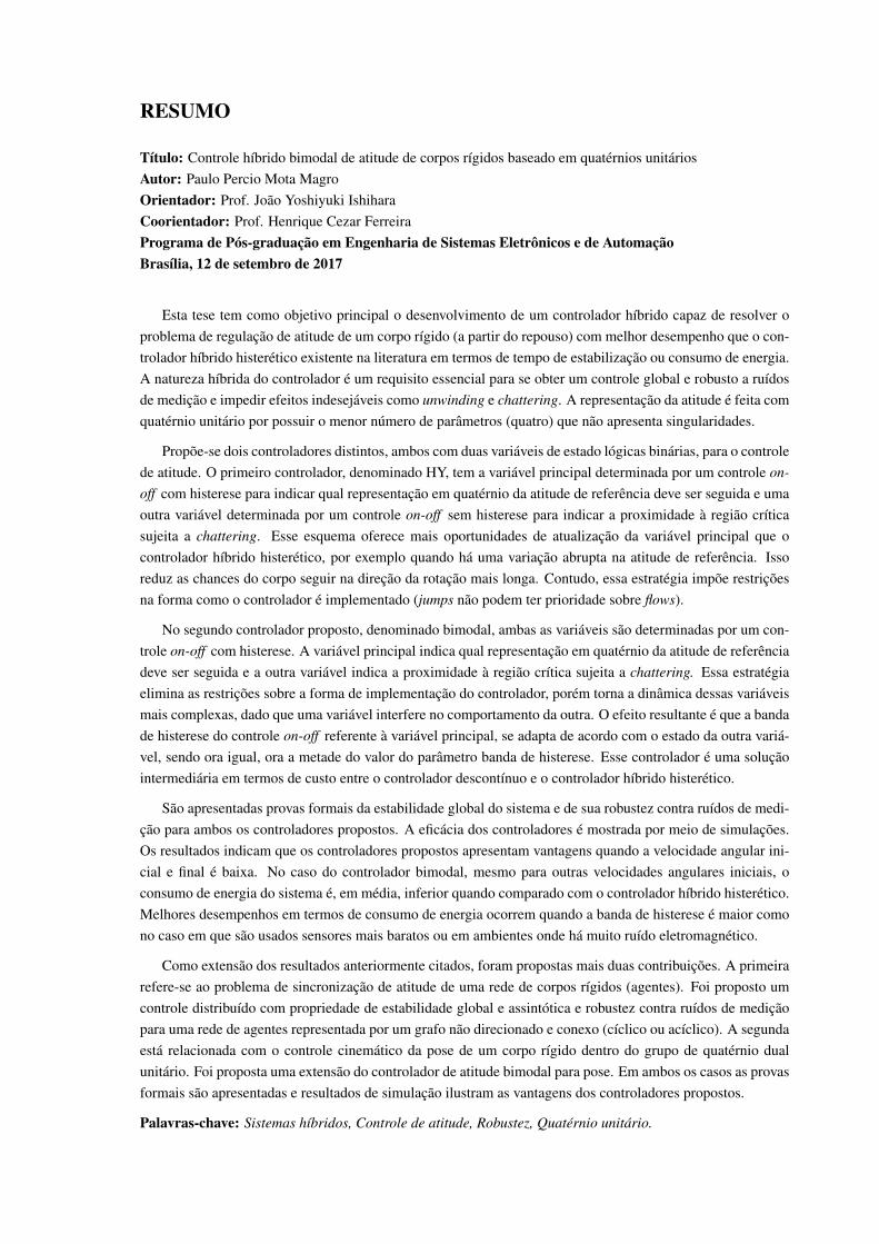
Esta tese tem como objetivo principal o desenvolvimento de um controlador híbrido capaz de resolver oproblema de regulação de atitude de um corpo rígido (a partir do repouso) com melhor desempenho que o con-trolador híbrido histerético existente na literatura em termos de tempo de estabilização ou consumo de energia.A natureza híbrida do controlador é um requisito essencial para se obter um controle global e robusto a ruídosde medição e impedir efeitos indesejáveis como unwinding e chattering. A representação da atitude é feita comquatérnio unitário por possuir o menor número de parâmetros (quatro) que não apresenta singularidades.

Propõe-se dois controladores distintos, ambos com duas variáveis de estado lógicas binárias, para o controlede atitude. O primeiro controlador, denominado HY, tem a variável principal determinada por um controle on-off com histerese para indicar qual representação em quatérnio da atitude de referência deve ser seguida e umaoutra variável determinada por um controle on-off sem histerese para indicar a proximidade à região críticasujeita a chattering. Esse esquema oferece mais oportunidades de atualização da variável principal que ocontrolador híbrido histerético, por exemplo quando há uma variação abrupta na atitude de referência. Issoreduz as chances do corpo seguir na direção da rotação mais longa. Contudo, essa estratégia impõe restriçõesna forma como o controlador é implementado (jumps não podem ter prioridade sobre flows).

No segundo controlador proposto, denominado bimodal, ambas as variáveis são determinadas por um con-trole on-off com histerese. A variável principal indica qual representação em quatérnio da atitude de referênciadeve ser seguida e a outra variável indica a proximidade à região crítica sujeita a chattering. Essa estratégiaelimina as restrições sobre a forma de implementação do controlador, porém torna a dinâmica dessas variáveismais complexas, dado que uma variável interfere no comportamento da outra. O efeito resultante é que a bandade histerese do controle on-off referente à variável principal, se adapta de acordo com o estado da outra variá-vel, sendo ora igual, ora a metade do valor do parâmetro banda de histerese. Esse controlador é uma soluçãointermediária em termos de custo entre o controlador descontínuo e o controlador híbrido histerético.

São apresentadas provas formais da estabilidade global do sistema e de sua robustez contra ruídos de medi-ção para ambos os controladores propostos. A eficácia dos controladores é mostrada por meio de simulações.Os resultados indicam que os controladores propostos apresentam vantagens quando a velocidade angular ini-cial e final é baixa. No caso do controlador bimodal, mesmo para outras velocidades angulares iniciais, oconsumo de energia do sistema é, em média, inferior quando comparado com o controlador híbrido histerético.Melhores desempenhos em termos de consumo de energia ocorrem quando a banda de histerese é maior comono caso em que são usados sensores mais baratos ou em ambientes onde há muito ruído eletromagnético.

Como extensão dos resultados anteriormente citados, foram propostas mais duas contribuições. A primeirarefere-se ao problema de sincronização de atitude de uma rede de corpos rígidos (agentes). Foi proposto umcontrole distribuído com propriedade de estabilidade global e assintótica e robustez contra ruídos de mediçãopara uma rede de agentes representada por um grafo não direcionado e conexo (cíclico ou acíclico). A segundaestá relacionada com o controle cinemático da pose de um corpo rígido dentro do grupo de quatérnio dualunitário. Foi proposta uma extensão do controlador de atitude bimodal para pose. Em ambos os casos as provasformais são apresentadas e resultados de simulação ilustram as vantagens dos controladores propostos.

Palavras-chave: Sistemas híbridos, Controle de atitude, Robustez, Quatérnio unitário.

CONTENTS

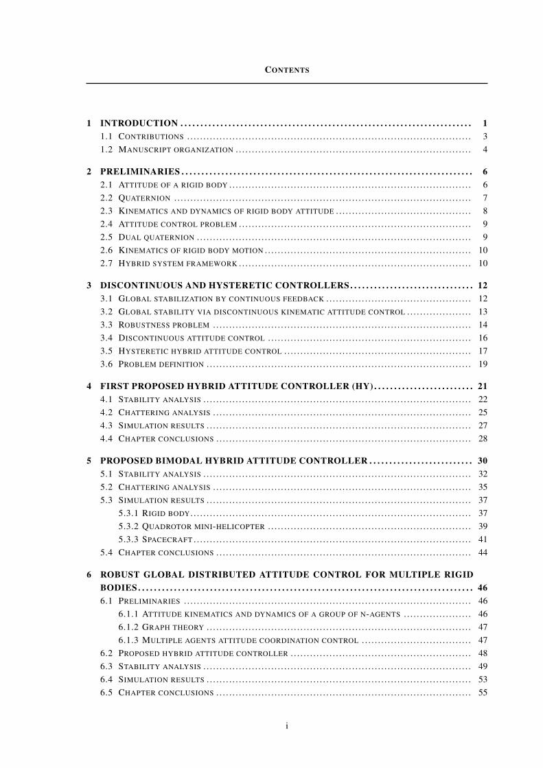
1 INTRODUCTION . . . . . . . . . . . . . . . . . . . . . . . . . . . . . . . . . . . . . . . . . . . . . . . . . . . . . . . . . . . . . . . . . . . . . . . . . 11.1 CONTRIBUTIONS . . . . . . . . . . . . . . . . . . . . . . . . . . . . . . . . . . . . . . . . . . . . . . . . . . . . . . . . . . . . . . . . . . . . . . . . . . . . . . . . . . . . . . . . 31.2 MANUSCRIPT ORGANIZATION . . . . . . . . . . . . . . . . . . . . . . . . . . . . . . . . . . . . . . . . . . . . . . . . . . . . . . . . . . . . . . . . . . . . . . . . . 4

2 PRELIMINARIES . . . . . . . . . . . . . . . . . . . . . . . . . . . . . . . . . . . . . . . . . . . . . . . . . . . . . . . . . . . . . . . . . . . . . . . . . 62.1 ATTITUDE OF A RIGID BODY . . . . . . . . . . . . . . . . . . . . . . . . . . . . . . . . . . . . . . . . . . . . . . . . . . . . . . . . . . . . . . . . . . . . . . . . . . . 62.2 QUATERNION . . . . . . . . . . . . . . . . . . . . . . . . . . . . . . . . . . . . . . . . . . . . . . . . . . . . . . . . . . . . . . . . . . . . . . . . . . . . . . . . . . . . . . . . . . . . 72.3 KINEMATICS AND DYNAMICS OF RIGID BODY ATTITUDE . . . . . . . . . . . . . . . . . . . . . . . . . . . . . . . . . . . . . . . . . . 82.4 ATTITUDE CONTROL PROBLEM . . . . . . . . . . . . . . . . . . . . . . . . . . . . . . . . . . . . . . . . . . . . . . . . . . . . . . . . . . . . . . . . . . . . . . . . 92.5 DUAL QUATERNION . . . . . . . . . . . . . . . . . . . . . . . . . . . . . . . . . . . . . . . . . . . . . . . . . . . . . . . . . . . . . . . . . . . . . . . . . . . . . . . . . . . . . 92.6 KINEMATICS OF RIGID BODY MOTION . . . . . . . . . . . . . . . . . . . . . . . . . . . . . . . . . . . . . . . . . . . . . . . . . . . . . . . . . . . . . . . . 102.7 HYBRID SYSTEM FRAMEWORK . . . . . . . . . . . . . . . . . . . . . . . . . . . . . . . . . . . . . . . . . . . . . . . . . . . . . . . . . . . . . . . . . . . . . . . . 10

3 DISCONTINUOUS AND HYSTERETIC CONTROLLERS. . . . . . . . . . . . . . . . . . . . . . . . . . . . . . . 123.1 GLOBAL STABILIZATION BY CONTINUOUS FEEDBACK . . . . . . . . . . . . . . . . . . . . . . . . . . . . . . . . . . . . . . . . . . . . . 123.2 GLOBAL STABILITY VIA DISCONTINUOUS KINEMATIC ATTITUDE CONTROL . . . . . . . . . . . . . . . . . . . . 133.3 ROBUSTNESS PROBLEM . . . . . . . . . . . . . . . . . . . . . . . . . . . . . . . . . . . . . . . . . . . . . . . . . . . . . . . . . . . . . . . . . . . . . . . . . . . . . . . . 143.4 DISCONTINUOUS ATTITUDE CONTROL . . . . . . . . . . . . . . . . . . . . . . . . . . . . . . . . . . . . . . . . . . . . . . . . . . . . . . . . . . . . . . . 163.5 HYSTERETIC HYBRID ATTITUDE CONTROL . . . . . . . . . . . . . . . . . . . . . . . . . . . . . . . . . . . . . . . . . . . . . . . . . . . . . . . . . . 173.6 PROBLEM DEFINITION . . . . . . . . . . . . . . . . . . . . . . . . . . . . . . . . . . . . . . . . . . . . . . . . . . . . . . . . . . . . . . . . . . . . . . . . . . . . . . . . . . 19

4 FIRST PROPOSED HYBRID ATTITUDE CONTROLLER (HY) . . . . . . . . . . . . . . . . . . . . . . . . . 214.1 STABILITY ANALYSIS . . . . . . . . . . . . . . . . . . . . . . . . . . . . . . . . . . . . . . . . . . . . . . . . . . . . . . . . . . . . . . . . . . . . . . . . . . . . . . . . . . . 224.2 CHATTERING ANALYSIS . . . . . . . . . . . . . . . . . . . . . . . . . . . . . . . . . . . . . . . . . . . . . . . . . . . . . . . . . . . . . . . . . . . . . . . . . . . . . . . . 254.3 SIMULATION RESULTS . . . . . . . . . . . . . . . . . . . . . . . . . . . . . . . . . . . . . . . . . . . . . . . . . . . . . . . . . . . . . . . . . . . . . . . . . . . . . . . . . . 274.4 CHAPTER CONCLUSIONS . . . . . . . . . . . . . . . . . . . . . . . . . . . . . . . . . . . . . . . . . . . . . . . . . . . . . . . . . . . . . . . . . . . . . . . . . . . . . . . 28

5 PROPOSED BIMODAL HYBRID ATTITUDE CONTROLLER . . . . . . . . . . . . . . . . . . . . . . . . . . 305.1 STABILITY ANALYSIS . . . . . . . . . . . . . . . . . . . . . . . . . . . . . . . . . . . . . . . . . . . . . . . . . . . . . . . . . . . . . . . . . . . . . . . . . . . . . . . . . . . 325.2 CHATTERING ANALYSIS . . . . . . . . . . . . . . . . . . . . . . . . . . . . . . . . . . . . . . . . . . . . . . . . . . . . . . . . . . . . . . . . . . . . . . . . . . . . . . . . 355.3 SIMULATION RESULTS . . . . . . . . . . . . . . . . . . . . . . . . . . . . . . . . . . . . . . . . . . . . . . . . . . . . . . . . . . . . . . . . . . . . . . . . . . . . . . . . . . 37

5.3.1 RIGID BODY . . . . . . . . . . . . . . . . . . . . . . . . . . . . . . . . . . . . . . . . . . . . . . . . . . . . . . . . . . . . . . . . . . . . . . . . . . . . . . . . . . . . . . . 375.3.2 QUADROTOR MINI-HELICOPTER . . . . . . . . . . . . . . . . . . . . . . . . . . . . . . . . . . . . . . . . . . . . . . . . . . . . . . . . . . . . . . . 395.3.3 SPACECRAFT . . . . . . . . . . . . . . . . . . . . . . . . . . . . . . . . . . . . . . . . . . . . . . . . . . . . . . . . . . . . . . . . . . . . . . . . . . . . . . . . . . . . . . 41

5.4 CHAPTER CONCLUSIONS . . . . . . . . . . . . . . . . . . . . . . . . . . . . . . . . . . . . . . . . . . . . . . . . . . . . . . . . . . . . . . . . . . . . . . . . . . . . . . . 44

6 ROBUST GLOBAL DISTRIBUTED ATTITUDE CONTROL FOR MULTIPLE RIGIDBODIES . . . . . . . . . . . . . . . . . . . . . . . . . . . . . . . . . . . . . . . . . . . . . . . . . . . . . . . . . . . . . . . . . . . . . . . . . . . . . . . . . . . . 466.1 PRELIMINARIES . . . . . . . . . . . . . . . . . . . . . . . . . . . . . . . . . . . . . . . . . . . . . . . . . . . . . . . . . . . . . . . . . . . . . . . . . . . . . . . . . . . . . . . . . 46

6.1.1 ATTITUDE KINEMATICS AND DYNAMICS OF A GROUP OF N-AGENTS . . . . . . . . . . . . . . . . . . . . . 466.1.2 GRAPH THEORY . . . . . . . . . . . . . . . . . . . . . . . . . . . . . . . . . . . . . . . . . . . . . . . . . . . . . . . . . . . . . . . . . . . . . . . . . . . . . . . . . . 476.1.3 MULTIPLE AGENTS ATTITUDE COORDINATION CONTROL . . . . . . . . . . . . . . . . . . . . . . . . . . . . . . . . . . 47

6.2 PROPOSED HYBRID ATTITUDE CONTROLLER . . . . . . . . . . . . . . . . . . . . . . . . . . . . . . . . . . . . . . . . . . . . . . . . . . . . . . . . 486.3 STABILITY ANALYSIS . . . . . . . . . . . . . . . . . . . . . . . . . . . . . . . . . . . . . . . . . . . . . . . . . . . . . . . . . . . . . . . . . . . . . . . . . . . . . . . . . . . 496.4 SIMULATION RESULTS . . . . . . . . . . . . . . . . . . . . . . . . . . . . . . . . . . . . . . . . . . . . . . . . . . . . . . . . . . . . . . . . . . . . . . . . . . . . . . . . . . 536.5 CHAPTER CONCLUSIONS . . . . . . . . . . . . . . . . . . . . . . . . . . . . . . . . . . . . . . . . . . . . . . . . . . . . . . . . . . . . . . . . . . . . . . . . . . . . . . . 55

i

CONTENTS ii

7 DUAL QUATERNION-BASED BIMODAL GLOBAL CONTROL FOR ROBUST RIGID-BODY POSE KINEMATIC STABILIZATION . . . . . . . . . . . . . . . . . . . . . . . . . . . . . . . . . . . . . . . . . . . . 597.1 HYSTERETIC HYBRID CONTROLLER . . . . . . . . . . . . . . . . . . . . . . . . . . . . . . . . . . . . . . . . . . . . . . . . . . . . . . . . . . . . . . . . . . 597.2 PROPOSED BIMODAL HYBRID CONTROLLER . . . . . . . . . . . . . . . . . . . . . . . . . . . . . . . . . . . . . . . . . . . . . . . . . . . . . . . . . 597.3 STABILITY ANALYSIS . . . . . . . . . . . . . . . . . . . . . . . . . . . . . . . . . . . . . . . . . . . . . . . . . . . . . . . . . . . . . . . . . . . . . . . . . . . . . . . . . . . 60

7.3.1 CHATTERING ANALYSIS . . . . . . . . . . . . . . . . . . . . . . . . . . . . . . . . . . . . . . . . . . . . . . . . . . . . . . . . . . . . . . . . . . . . . . . . 627.4 SIMULATION RESULTS . . . . . . . . . . . . . . . . . . . . . . . . . . . . . . . . . . . . . . . . . . . . . . . . . . . . . . . . . . . . . . . . . . . . . . . . . . . . . . . . . . 637.5 CHAPTER CONCLUSIONS . . . . . . . . . . . . . . . . . . . . . . . . . . . . . . . . . . . . . . . . . . . . . . . . . . . . . . . . . . . . . . . . . . . . . . . . . . . . . . . 63

8 CONCLUSIONS . . . . . . . . . . . . . . . . . . . . . . . . . . . . . . . . . . . . . . . . . . . . . . . . . . . . . . . . . . . . . . . . . . . . . . . . . . . 678.1 FUTURE WORK . . . . . . . . . . . . . . . . . . . . . . . . . . . . . . . . . . . . . . . . . . . . . . . . . . . . . . . . . . . . . . . . . . . . . . . . . . . . . . . . . . . . . . . . . . . 67

BIBLIOGRAPHY . . . . . . . . . . . . . . . . . . . . . . . . . . . . . . . . . . . . . . . . . . . . . . . . . . . . . . . . . . . . . . . . . . . . . . . . . . . . . 69

APPENDICES

A RESUMO ESTENDIDO EM LÍNGUA PORTUGUESA . . . . . . . . . . . . . . . . . . . . . . . . . . . . . . . . . . . 74

B PROOFS OF SOME LEMMAS . . . . . . . . . . . . . . . . . . . . . . . . . . . . . . . . . . . . . . . . . . . . . . . . . . . . . . . . . . . . 79

C PUBLICATIONS . . . . . . . . . . . . . . . . . . . . . . . . . . . . . . . . . . . . . . . . . . . . . . . . . . . . . . . . . . . . . . . . . . . . . . . . . . 88

List of Figures

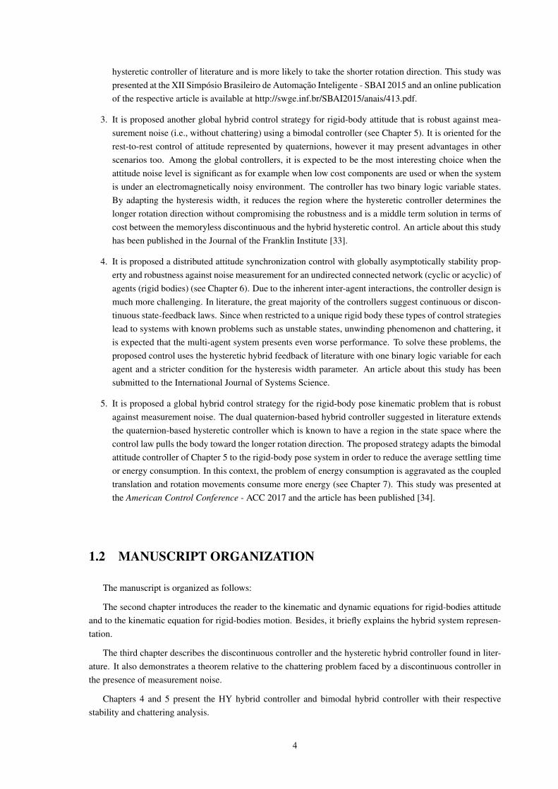
1.1 Examples of areas where the global attitude control can be applied: underwater vehicle andaerospace vehicle. ...................................................................................................... 1

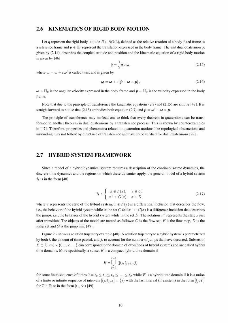
2.1 Body frame, reference frame and fixed-reference frame example. ......................................... 62.2 Example of a solution trajectory to a hybrid system. Solid curves indicate flow and dashed arcs

indicate jumps. .......................................................................................................... 11

3.1 Example of a strategy to stabilize the arm of a clock needle at point A. .................................. 133.2 State space representation of the discontinuous controller. Arrows indicate the direction of

rotation so the attitude is regulated to 1 or −1. ................................................................. 143.3 System behavior for the discontinuous controller when no noise is present in the output y and

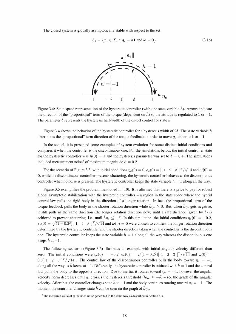
when the output is corrupted by noise. ........................................................................... 173.4 State space representation of the hysteretic controller (with one state variable h). Arrows indi-

cate the direction of the “proportional” term of the torque (dependent on h) so the attitude isregulated to 1 or−1. The parameter δ represents the hysteresis half-width of the on-off controlfor state h. ................................................................................................................ 18

3.5 Comparison of the system behavior when the discontinuous controller and the hysteretic con-troller are applied to highlight the longer rotation direction determined by the hysteretic con-troller. .................................................................................................................... 19

3.6 Comparison of the system behavior when the discontinuous controller and the hysteretic con-troller are applied to highlight the behavior when the initial condition of the system is not atrest. ........................................................................................................................ 19

4.1 Graphical representation of sets C2 and D2...................................................................... 214.2 State space representation of ηe and ‖εe‖ and the proposed regulation with two state variables

(h and m). The parameter δ represents the hysteresis half-width of the on-off control for state h. 224.3 Graphical representation of the jump map for h+ and m+. .................................................. 264.4 Comparison between the discontinuous controller and the proposed HY controller. .................. 284.5 Comparison between the hysteretic controller and the proposed HY controller......................... 29

5.1 Graphical representation of sets C2 and D2...................................................................... 315.2 State space representation and the proposed regulation with two state variables (h and m).

Arrows indicate the direction of the “proportional” term of the torque (dependent on h) so theattitude is regulated to 1 or −1. The hysteresis half-width of the on-off control for state h isδ/2 when m = 1 and δ when m = −1. ........................................................................... 31

5.3 Graphical representation of the jump map for h+ and m+. .................................................. 365.4 Difference between the energy spent when the bimodal and the hysteretic controller is applied

(∆E) as a function of the initial conditions, represented by ηe(0) and Ω................................. 385.5 Comparison between the hysteretic and the proposed bimodal controller for a relatively high

initial angular velocity norm. ........................................................................................ 395.6 Comparison between the discontinuous and the proposed bimodal controller for the quadrotor.... 405.7 Comparison between the hysteretic and the proposed bimodal controller for the quadrotor. ........ 415.8 Comparison between the hysteretic and the proposed bimodal controller for the spacecraft.

Initial condition ηe = −0.4 and ησ near −0.1................................................................... 435.9 Comparison between the hysteretic and the proposed bimodal controller for the spacecraft.

Initial condition ηe = 0.4 and ησ near −0.1. .................................................................... 44

iii

iv

5.10 Difference between the energy spent when the bimodal and the hysteretic controller is applied(∆E) as a function of the initial conditions, represented by ηe(0) and Ω................................. 45

6.1 Agent i state space representation and the proposed regulation. The hysteresis half-width ofthe on-off control for state hi is δi.................................................................................. 49

6.2 Topology of communication. ........................................................................................ 546.3 Evolution of the first component of the attitude of the agents in the first scenario. In the upper

graphic (continuous controller), a specific noise of magnitude lower than 0.2 was applied toagent 4 between 0.6 and 10 s. The lower graphic refers to the hybrid controller. ...................... 56

6.4 Evolution of the attitude qi0 = (ηi0, εi0) of the agents in the second scenario, where εi0 =

(εi0x, εi0y

, εi0z). The graphics on the left refers to the continuous controller and the others on

the right to the hybrid one. ........................................................................................... 576.5 Evolution of the angular velocity ωi = (ωix , ωiy , ωiz ) of the agents in the second scenario.

The graphics on the left refers to the continuous controller and the others on the right to thehybrid one. ............................................................................................................... 58

7.1 State space representation of the hysteretic controller (with one state variable h). Arrows indi-cate the direction of the rotation so the attitude is regulated to 1 or −1. ................................ 60

7.2 State space representation of the bimodal controller (with two state variables, h andm). Arrowsindicate the direction of the rotation so the attitude is regulated to 1 or −1. ........................... 61

7.3 Rotation comparison between the discontinuous and bimodal controllers. ............................. 647.4 Evolution of the translation components of p = pxı + px + pxk for the discontinuous and

bimodal controllers. ................................................................................................... 647.5 Rotation comparison between the hysteretic and bimodal controllers. ................................... 657.6 Evolution of the translation components of p = pxı+px+pxk for the hysteretic and bimodal

controllers. .............................................................................................................. 65

B.1 Geometrical representation of distance d from q = (m, εm). ............................................... 82

LIST OF SYMBOLS AND NOTATIONS

Symbols and notations for scalars, vectors, matrices and quaternions

a, b, c, . . . scalars are represented by lowercase plain letters;a, b, c, . . . vectors are represented by lowercase bold letters;A,B,C, . . . matrices are represented by uppercase plain letters;a, b, c, . . . unit quaternions are represented by lowercase bold letters;A,B,C, . . . quaternions are represented by uppercase bold letters;a, b, c, . . . unit norm vectors are represented by lowercase bold letters with a hat over the letter;‖ · ‖ Euclidean vector norm;〈·, ·〉 inner product;I3 identity matrix of dimension 3;AT transpose of matrix A;

diag(v) diagonal matrix with the diagonal elements being the components of vector ~v;V time derivative of function V ;∇V gradient of Lyapunov function V ; quaternion multiplication operation or dual quaternion multiplication operation;⊗ Kronecker product;× cross-product operation between two three-dimensional vectors;ε dual unit;q−1 inverse of the unit quaternion q;q∗ conjugate of the unit quaternion q;

<(q), =(q) the real and imaginary components of the unit quaternion q;0 null vector or quaternion (0,0);q∗ conjugate of the unit dual quaternion q;

<(q), =(q) real and imaginary components of the unit dual quaternion q.

The only exception refers to Lyapunov function candidates, represented by uppercase plain letter V .

v

vi

Symbols and notation related to sets and groups

R set of real numbers;Rn set of n-tuples of real numbers (x1, x2, . . . , xn) for xi ∈ R, i = 1, . . . , n;H set of quaternions;S3 set of unit quaternions, i.e. the unit 3-sphere;H0 set of pure imaginary quaternions;Sn hypersphere of Rn+1;B closed unit ball in the Euclidean norm of appropriate dimension;H set of dual quaternions;S set of unit dual quaternions;

B(0, r) open ball of radius r in the Euclidean norm of appropriate dimension;A,B,C, . . . sets are represented by uppercase plain letters;A \B set difference operation, i.e., the set of all members of A that are not members of B;

V −1(A) preimage or inverse image of the set A;A closure of set A;

coA closed convex hull of set A;SO(3) group of rigid body rotations, i.e., the 3-dimensional special orthogonal group;SE(3) group of rigid body motions, i.e., the 3-dimensional special Euclidean group;· × · Cartesian product of two sets.X set S3 × R3;Xc set−1, 1.

INTRODUCTION

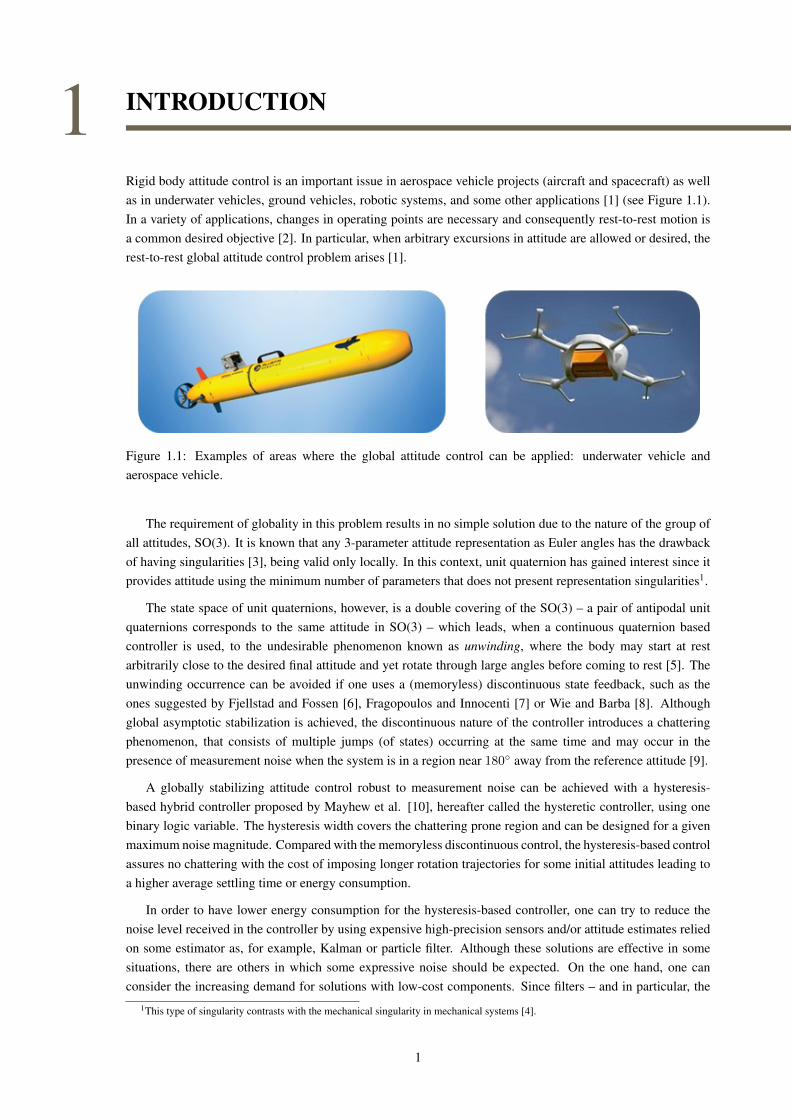
Rigid body attitude control is an important issue in aerospace vehicle projects (aircraft and spacecraft) as wellas in underwater vehicles, ground vehicles, robotic systems, and some other applications [1] (see Figure 1.1).In a variety of applications, changes in operating points are necessary and consequently rest-to-rest motion isa common desired objective [2]. In particular, when arbitrary excursions in attitude are allowed or desired, therest-to-rest global attitude control problem arises [1].

Figure 1.1: Examples of areas where the global attitude control can be applied: underwater vehicle andaerospace vehicle.

The requirement of globality in this problem results in no simple solution due to the nature of the group ofall attitudes, SO(3). It is known that any 3-parameter attitude representation as Euler angles has the drawbackof having singularities [3], being valid only locally. In this context, unit quaternion has gained interest since itprovides attitude using the minimum number of parameters that does not present representation singularities1.

The state space of unit quaternions, however, is a double covering of the SO(3) – a pair of antipodal unitquaternions corresponds to the same attitude in SO(3) – which leads, when a continuous quaternion basedcontroller is used, to the undesirable phenomenon known as unwinding, where the body may start at restarbitrarily close to the desired final attitude and yet rotate through large angles before coming to rest [5]. Theunwinding occurrence can be avoided if one uses a (memoryless) discontinuous state feedback, such as theones suggested by Fjellstad and Fossen [6], Fragopoulos and Innocenti [7] or Wie and Barba [8]. Althoughglobal asymptotic stabilization is achieved, the discontinuous nature of the controller introduces a chatteringphenomenon, that consists of multiple jumps (of states) occurring at the same time and may occur in thepresence of measurement noise when the system is in a region near 180 away from the reference attitude [9].

A globally stabilizing attitude control robust to measurement noise can be achieved with a hysteresis-based hybrid controller proposed by Mayhew et al. [10], hereafter called the hysteretic controller, using onebinary logic variable. The hysteresis width covers the chattering prone region and can be designed for a givenmaximum noise magnitude. Compared with the memoryless discontinuous control, the hysteresis-based controlassures no chattering with the cost of imposing longer rotation trajectories for some initial attitudes leading toa higher average settling time or energy consumption.

In order to have lower energy consumption for the hysteresis-based controller, one can try to reduce thenoise level received in the controller by using expensive high-precision sensors and/or attitude estimates reliedon some estimator as, for example, Kalman or particle filter. Although these solutions are effective in somesituations, there are others in which some expressive noise should be expected. On the one hand, one canconsider the increasing demand for solutions with low-cost components. Since filters – and in particular, the

1This type of singularity contrasts with the mechanical singularity in mechanical systems [4].

1

1

particle filter – are computationally expensive [11], for embedded processors with low memory and processingresources, usually a less effective simplified estimator should be used, resulting in higher attitude estimationnoise. On the other hand, inexpensive sensors result in higher noise levels. For example, in the experiments ofGebre-Egziabher et al. [12], one can notice noise amplitudes around 10 degrees. If further, the system is underelectromagnetic disturbance or its angular velocity is fast, the noise level may be even higher [13].

In this study it was sought a robust globally stabilizing controller which would represent a better solutionin terms of cost when compared with the fixed width hysteresis control. Reduction of costs represented byaverage settling time or energy consumption is important, for instance, in satellites and any other battery-operated systems [14]. It is proposed two hybrid controllers with two binary logic variables (one more thanthe hysteretic controller) for the rest-to-rest control of attitude represented by quaternions. The main variableindicates which quaternion representation of the reference attitude should be followed and the auxiliary oneindicates when the current attitude is far from the chattering prone region. The main idea of the first controlleris to increase the opportunities to update the main variable when compared with the hysteretic controller. Thisis accomplished by the updates induced by the second logic variable. The second controller, called bimodal,was devised from the experience gained with the former. Its main idea is to provide the controller with someadaptive property to the hysteresis width rather than using a fixed width as in the hysteretic controller [10]. Byintroducing a more complex dynamics, the second variable also embodied the hysteresis adaptive function.

As an extension of the results described above, two other contributions were proposed: one on attitudesynchronization control for a network of rigid bodies (agents) and the other one on kinematic control for rigid-body pose within the group of unit norm dual-quaternions.

Regarding the former extension, much research has been developed on attitude coordination control inthe last 10-15 years [15, 16, 17, 18, 19]. Compared with single-agent systems, multi-agent systems havespecial advantages due to its cooperation, such as higher feasibility, accuracy, robustness, scalability, flexibility,robustness, lower cost etc. and have a wide range of applications such as environmental monitoring, search andrescue, space–based interferometers, material handling and so on [20].

As mentioned above, the problem of robust and global attitude stabilization for a single rigid body has beensolved a few years ago [21], but the network scenario arises much more challenges due to the inherent inter-agent interactions. Up to now, the great majority of the studies on attitude synchronization strategy providesat most an almost global asymptotic stable control as in [18, 17] and when it provides global control, it is notrobust to measurement noise.

To the best of the author knowledge, the only study on attitude synchronization of multiple agents thatachieves robust global synchronization is the one of Mayhew et al. in 2012 [21]. It assumes that each agenthas access only to the relative attitude between its neighbors and to its angular velocity relative to the bodyframe. Its goal is to achieve stability of a synchronized state (which is not a specific absolute reference attitude)using a hybrid feedback scheme. The advantage of not requiring inertial attitude measurements has the costof achieving synchronization only for connected and acyclic networks [22]. Actually, there exists a physicalobstacle to the global convergence when the graph contains cycles [22, Theorem 1].

In this study, it is proposed a distributed attitude synchronization control with globally asymptoticallystability property and robustness against noise measurement for an undirected connected network (cyclic oracyclic) of agents. The strategy uses a quaternion representation of the inertial attitude and the hysteretichybrid controller with one binary logic variable, suggested by Mayhew et al. [10], for each agent, to solve theknown problems arisen when continuous or discontinuous state-feedback laws are employed such as presenceof unstable states, unwinding phenomenon and chattering.

Regarding the latter extension, the Lie groups of rigid body motions SE(3) arises naturally in the studyof aerospace and robotic systems. Stemming from the seminal work of Brockett [23] about control theoryon general Lie groups, much of the literature has been devoted to the control of systems defined on SE(3).

2

Although it is usual to design controllers for this system using matrices to represent elements of this Lie group[24, 25], it has been noted by some authors that controllers designed using another type of representation,namely, the unit dual quaternions (Spin(3)×R3), which double covers SE(3), may have advantages regardingcomputational time and storage requirements [26, 27].

It is important to note that since in this case the state space of a dynamical system is a general manifold,some difficulties to design a stabilizing controller to the system can be expected. Actually, the problem ofrobust and global pose stabilization of a rigid body is not simple, but, to a certain extent, analogous to theattitude problem.

Firstly, there is no continuous feedback controller capable of globally asymptotically stabilizing an equilib-rium point on the manifold of the unit dual quaternion group [28].

Secondly, as the Lie group of unit dual quaternions is a double cover for the Lie group of rigid body motionsSE(3) [29, 28], it leads, when a continuous dual quaternion based controller is used, to a phenomenon similarto the “unwinding” in SO(3) [5]: the body may start at rest arbitrarily close to the desired final pose and yettravel to the farther stable point before coming to rest.

Lastly, even using a (memoryless) discontinuous state feedback, it is impossible to achieve robust globalasymptotic stabilization of a disconnected set of points resulted from the double covering of the SE(3) [10, 9].

There are few works on unwinding avoidance in the context of pose stabilization using unit dual quaternions[29, 30, 31, 32]. All of them are based on a discontinuous feedback approach and are prone to chattering forinitial conditions arbitrarily close to the discontinuity.

Inspired on the hysteresis-based hybrid control of Mayhew et al. [10] applied to attitude control stabi-lization, Kussaba et al. [28] extended it to render both coupled kinematics—attitude and translation—stable.However, this pose controller suggested by Kussaba et al. [28] inherits the same cost, aforementioned, of im-posing longer rotation trajectories for some initial attitudes leading to a higher average settling time or energyconsumption. The problem of energy consumption also aggravates in this context, as the coupled translationand rotation movements consume more energy [28].

To reduce this cost, it is proposed a bimodal hybrid control law that combines the bimodal controllerproposed above for the attitude control problem and the control suggested by Kussaba et al. [28] so it representsa compromise in terms of cost between the memoryless discontinuous controller and the hysteretic one.

1.1 CONTRIBUTIONS

The contributions of this manuscript are:

1. It is stated and proved a theorem about the problem faced by a discontinuous attitude controller in thepresence of measurement noise in the unit quaternion space (see Theorem 3.4, page 15). This result is acorrection for a theorem in [10]. In that work, the system is corrupted by noise but the measured variabledoes not belong to the unit quaternion space. Consequently, the system model loses physical sense.

2. It is presented a global hybrid control of rigid-body attitude that is robust against measurement noisethat is oriented for the rest-to-rest control of attitude represented by quaternions (see Chapter 4). Theproposed controller extends a hysteretic hybrid controller of literature by introducing a new binary logicvariable state. The controller is able to detect when the reference changes abruptly and when the currentattitude is far from the reference on the initial instant. This way, it has more opportunities to determinewhich quaternion representation of the reference attitude should be followed compared with the hybrid

3

hysteretic controller of literature and is more likely to take the shorter rotation direction. This study waspresented at the XII Simpósio Brasileiro de Automação Inteligente - SBAI 2015 and an online publicationof the respective article is available at http://swge.inf.br/SBAI2015/anais/413.pdf.

3. It is proposed another global hybrid control strategy for rigid-body attitude that is robust against mea-surement noise (i.e., without chattering) using a bimodal controller (see Chapter 5). It is oriented for therest-to-rest control of attitude represented by quaternions, however it may present advantages in otherscenarios too. Among the global controllers, it is expected to be the most interesting choice when theattitude noise level is significant as for example when low cost components are used or when the systemis under an electromagnetically noisy environment. The controller has two binary logic variable states.By adapting the hysteresis width, it reduces the region where the hysteretic controller determines thelonger rotation direction without compromising the robustness and is a middle term solution in terms ofcost between the memoryless discontinuous and the hybrid hysteretic control. An article about this studyhas been published in the Journal of the Franklin Institute [33].

4. It is proposed a distributed attitude synchronization control with globally asymptotically stability prop-erty and robustness against noise measurement for an undirected connected network (cyclic or acyclic) ofagents (rigid bodies) (see Chapter 6). Due to the inherent inter-agent interactions, the controller design ismuch more challenging. In literature, the great majority of the controllers suggest continuous or discon-tinuous state-feedback laws. Since when restricted to a unique rigid body these types of control strategieslead to systems with known problems such as unstable states, unwinding phenomenon and chattering, itis expected that the multi-agent system presents even worse performance. To solve these problems, theproposed control uses the hysteretic hybrid feedback of literature with one binary logic variable for eachagent and a stricter condition for the hysteresis width parameter. An article about this study has beensubmitted to the International Journal of Systems Science.

5. It is proposed a global hybrid control strategy for the rigid-body pose kinematic problem that is robustagainst measurement noise. The dual quaternion-based hybrid controller suggested in literature extendsthe quaternion-based hysteretic controller which is known to have a region in the state space where thecontrol law pulls the body toward the longer rotation direction. The proposed strategy adapts the bimodalattitude controller of Chapter 5 to the rigid-body pose system in order to reduce the average settling timeor energy consumption. In this context, the problem of energy consumption is aggravated as the coupledtranslation and rotation movements consume more energy (see Chapter 7). This study was presented atthe American Control Conference - ACC 2017 and the article has been published [34].

1.2 MANUSCRIPT ORGANIZATION

The manuscript is organized as follows:

The second chapter introduces the reader to the kinematic and dynamic equations for rigid-bodies attitudeand to the kinematic equation for rigid-bodies motion. Besides, it briefly explains the hybrid system represen-tation.

The third chapter describes the discontinuous controller and the hysteretic hybrid controller found in liter-ature. It also demonstrates a theorem relative to the chattering problem faced by a discontinuous controller inthe presence of measurement noise.

Chapters 4 and 5 present the HY hybrid controller and bimodal hybrid controller with their respectivestability and chattering analysis.

4

Chapter 6 and 7 refer to two distinct subjects that naturally arise from the rigid-body attitude control matter.

Chapter 6 addresses the rigid-body attitude control applied to multi-agent systems in a cooperative control.It describes the proposed controller based on the hybrid hysteretic controller of literature and proves that itrobustly globally asymptotically stabilizes the synchronized state. Chapter 7 focuses on the rigid-body posekinematic stabilization. It shows the proposed bimodal hybrid controller and the proofs of control stability androbustness.

Chapter 8 presents the concluding remarks and suggestions for future work.

Appendix A presents the extended summary in Portuguese language. Appendix B shows the proofs of thelemmas used along the text. Appendix C lists the papers published in or submitted to journals and conferences.

5

PRELIMINARIES

2.1 ATTITUDE OF A RIGID BODY

The expression “attitude of an object” is usually used in Geometry and means the orientation of such objectin space [35, 36]. Rigid body is a completely “undistortable” body. More formally, a rigid body is a collectionof particles such that the distance between any two particles remains fixed, regardless of any motions of thebody or forces exerted on it [37]. In general, the attitude is described by the relationship between two right-handed Cartesian coordinate frames, one frame, called body frame, attached to the rigid body and the otherone, called reference frame, with the same origin as the first, but having its axes parallel to a fixed-referenceor inertial frame [4, 38, 36]. According to Figure 2.1, the fixed-reference frame is Orxryrzr, the body frameis Ouvw and the reference frame is Oxyz, whose axes Ox, Oy and Oz are, by definition, parallel to the axesOrxr, Oryr and Orzr of the fixed-reference frame and whose origin coincides with the one of the body frame.

Figure 2.1: Body frame, reference frame and fixed-reference frame example.

The attitude can be represented in several ways. One of them is the rotation matrix, which can be interpretedas an operator that transforms the coordinates of a point from one frame to another one (passive transformation).For instance, suppose, initially, that the body frame coincides with the reference frame and after a determinedperiod of time (the final moment), the body has rotated an angle θ about axis ω. Figure 2.1 illustrates therotation motion of a body point from point Pa to Pb. Let pa and pb be the vectors that represent the coordinatesof points Pa and Pb relative to a frame. As the body frame is attached to the body, pb = pa, relative to the bodyframe. However, relative to the reference frame,

pb = Rpa. (2.1)

The rotation matrix R transforms vector pa, which represents the position of point Pb relative to the bodyframe, into vector pb that represents the position of the same point Pb, relative to the reference frame.

The rotation matrix forms a group known as the special orthogonal group of order 3, or as the rotation groupon R3,

SO(3) = R ∈ R3×3 : RTR = RRT = I, detR = +1.

6

2

An element of SO(3) can be parametrized byR : R× S2 −→ SO(3), defined as

R(θ, ω) = exp(S(ω)θ),

where θ ∈ R represents an angle, ω ∈ S2 is a rotation axis, Sn = x ∈ Rn+1 : xTx = 1 and

S (x) =

0 −x3 x2

x3 0 −x1

−x2 x1 0

, (2.2)

for x ∈ R3. Equivalently, an element of SO(3) can be parametrized by the Rodrigues formula [37]

R(θ, ω) = I + sin(θ)S(ω) + (1− cos(θ))S(ω)2.

2.2 QUATERNION

The quaternion algebra is a four dimensional associative division algebra over R invented by Hamilton[39], which naturally extends the algebra of complex numbers. It can represent rotations in a similar way asthe complex numbers in the unit circle can represent planar rotations [37, pages 33,34]. The elements 1, ı, , kare the basis of this algebra, satisfying

ı2 = 2 = k2

= ık = −1. (2.3)

The set of quaternions is defined as

H ,η + µ1ı+ µ2+ µ3k : η, µ1, µ2, µ3 ∈ R

.

For ease of notation, the quaternion is denoted asQ ∈ H, where

Q = η + µ, with µ = µ1ı+ µ2+ µ3k

and may be decomposed into a real component and an imaginary component: <(Q) , η and =(Q) , µ suchthatQ = <(Q) + =(Q).

Another commonly used notation isQ = (η,µ),

with a scalar component η ∈ R and a vector component µ = (µ1, µ2, µ3) ∈ R3.

The sum of two quaternions,Qa = (ηa,µa) andQb = (ηb,µb), is defined as

Qa +Qb = (ηa + ηb,µa + µb)

and the multiplication of two quaternions is defined as

Qa Qb = (ηaηb − µTaµb, ηaµb + ηbµa + µa × µb).

The conjugate of a quaternionQ is given byQ∗ = (η,−µ) and the norm of a quaternion, by

‖Q‖ =√Q Q∗ =

√η2 + µTµ =

√η2 + µ2

1 + µ22 + µ2

3.

Pure imaginary quaternions are given by the set

H0 , Q ∈ H : <(Q) = 0

7

which are very convenient to represent vectors of R3. Thus, an Euclidean vector p ∈ R3 can be represented inthe same way as the quaternion p ∈ H0 or as (0,p) ∈ H0, using the other notation with the scalar componentzeroed.

Unit quaternions1 are defined as the quaternions that lie in the subset

S3 , q ∈ H : ‖q‖ = 1 .

The inverse of q , (η, ε) equals its conjugate, q−1 = q∗ = (η,−ε). Thus, qq−1 = q−1q = 1 = (1,0),0 = (0, 0, 0).

The set S3 forms, under multiplication, the Lie group Spin(3), whose identity element is 1 and group inverseis given by the quaternion conjugate q∗.

Given the unit quaternion

q =

(cos

θ

2, ω sin

θ

2

), (2.4)

the mappingR : S3 −→ SO(3) is defined by

R(q) = I + 2ηS(ε) + 2S(ε)2. (2.5)

Note that R(q) = R(−q). As the unit quaternions q and −q represent the same rotation, the unit quaterniongroup double covers the rotation group SO(3).

The transformation from pa to pb, achieved by applying operator R in (2.1), can also be obtained by usingthe unit quaternion q defined in (2.4) and equation [41, page 520]

(0,pb) = q (0,pa) q∗. (2.6)

2.3 KINEMATICS AND DYNAMICS OF RIGID BODY ATTITUDE

Consider a rigid body with inertia matrix J in a rotational motion due to the action of some external torqueτ ∈ R3. Consider also two frames: the reference frame and the body frame attached to the rigid body. Giventhat q represents the rigid-body attitude R ∈ SO(3), defined as the relative rotation of a body frame to areference frame, the quaternion kinematic equation2 is given by

q =1

2q (0,ω), (2.7)

where ω ∈ R3 is the angular velocity expressed in the body frame.

The angular velocity rate is calculated using the dynamic equation (Euler’s equation),

Jω = S (Jω)ω + τ , (2.8)

written in body coordinates [37, page 167], i.e., the torque is expressed in the body frame and the inertia matrixis constant and calculated in the body frame (see Lemma B.1).

1Along the text, the use of unit quaternions follows the Hamilton convention [40], that is, elements of the quaternion are ordered withreal part first, quaternion algebra satisfies ı2 = 2 = k

2= ık = −1 (2.3), operation q (0,v) q∗ performs a passive transformation

of vector v components from local to global frame.2For further details about rigid-body kinematic and dynamic equations refer to [37, 42].

8

2.4 ATTITUDE CONTROL PROBLEM

The attitude control problem may be established as a function of the attitude error. Supposing that qd ∈ S3

represents the desired constant attitude reference (the desired angular velocity is ωd ≡ 0), the attitude error isgiven by qe = (ηe, εe) = q∗d q ∈ S3 and the kinematic equation is described by (Lemma B.2)

qe =1

2qe (0,ω −R(qe)

Tωd) =1

2qe (0,ω). (2.9)

Let X = S3 × R3 and x = (qe,ω) ∈ X . Since each physical attitude R ∈ SO(3) is represented by a pair ofantipodal unit quaternions ±q ∈ S3, the objective of the control becomes to stabilize the set

A = (1,0) , (−1,0) ⊂ X

for the following system

˙x =

[qeω

]= F (x, τ ) , F (x, τ ) ,

[12qe (0,ω)

J−1 (S (Jω)ω + τ )

], (2.10)

by means of an appropriate choice of a feedback torque law τ , which has as information the output of thesystem (2.10) given by

y = (q,ω), (2.11)

that is, q and ω are measured. Note that together with the desired reference, qd, the state x = (qe,ω) isavailable for feedback.

2.5 DUAL QUATERNION

Similarly to how the quaternion algebra was introduced to address rotations in the three-dimensional space,the dual quaternion algebra was introduced by Clifford [43] and Study [44] to describe rigid body movements.This algebra is constituted by the set

H , q + εq′ : q, q′ ∈ H ,

where q and q′ are called the primary part and the dual part of the dual quaternion and ε is called the dual unitwhich is nilpotent—that is, ε 6= 0 and ε2 = 0. Given q = η + µ + ε(η′ + µ′), define <(q) , η + εη′ and=(q) , µ+εµ′, such that q = <(q)+=(q). The dual quaternion conjugate is q∗ , <(q)−=(q) = q∗+εq′∗.

The multiplication of two dual quaternions q1

= q1 + εq′1 and q2

= q2 + εq′2 is given by

q1 q

2= q1 q2 + ε(q1 q′2 + q′1 q2).

The subset of dual quaternions

S = q + εq′ ∈ H : ‖q‖ = 1, q q′∗ + q′ q∗ = 0 (2.12)

forms a Lie group [45] called unit dual quaternions group, whose identity is 1 = 1+ ε0, 0 = 0 + 0ı+ 0+ 0k

and group inverse is the dual quaternion conjugate. The constraint q q′∗ + q′ q∗ = 0 in (2.12) implies that

ηη′ + µTµ′ = 0. (2.13)

An arbitrary rigid body displacement characterized by a rotation q ∈ Spin(3), followed by a translationp = pxı+ py + pzk ∈ H0 expressed in the body frame, is represented by the unit dual quaternion [29, 46]

q = q + ε1

2q p. (2.14)

As the displacement q is equally described by −q, the unit dual quaternions group double covers SE(3).

9

2.6 KINEMATICS OF RIGID BODY MOTION

Let q represent the rigid-body attitude R ∈ SO(3), defined as the relative rotation of a body-fixed frame toa reference frame and p ∈ H0 represent the translation expressed in the body frame. The unit dual quaternion q,given by (2.14), describes the coupled attitude and position and the kinematic equation of a rigid body motionis given by [46]

q =1

2q ω, (2.15)

where ω = ω + εω′ is called twist and is given by

ω = ω + ε [p+ ω × p] , (2.16)

ω ∈ H0 is the angular velocity expressed in the body frame and p ∈ H0 is the velocity expressed in the bodyframe.

Note that due to the principle of transference the kinematic equations (2.7) and (2.15) are similar [47]. It isstraightforward to notice that (2.15) embodies both equation (2.7) and p = ω′ − ω × p.

The principle of transference may mislead one to think that every theorem in quaternions can be trans-formed to another theorem in dual quaternions by a transference process. This is shown by counterexamplesin [47]. Therefore, properties and phenomena related to quaternion motions like topological obstructions andunwinding may not follow by direct use of transference and have to be verified for dual quaternions [28].

2.7 HYBRID SYSTEM FRAMEWORK

Since a model of a hybrid dynamical system requires a description of the continuous-time dynamics, thediscrete-time dynamics and the regions on which these dynamics apply, the general model of a hybrid systemH is in the form [48]

H :

x ∈ F (x), x ∈ C,x+ ∈ G(x), x ∈ D, (2.17)

where x represents the state of the hybrid system, x ∈ F (x) is a differential inclusion that describes the flow,i.e., the behavior of the hybrid system while in the set C and x+ ∈ G(x) is a difference inclusion that describesthe jumps, i.e., the behavior of the hybrid system while in the set D. The notation x+ represents the state x justafter transition. The objects of the model are named as follows: C is the flow set, F is the flow map, D is thejump set and G is the jump map [49].

Figure 2.2 shows a solution trajectory example [48]. A solution trajectory to a hybrid system is parametrizedby both t, the amount of time passed, and j, to account for the number of jumps that have occurred. Subsets ofE ⊂ [0,∞)×0, 1, 2, . . . can correspond to the domain of evolutions of hybrid systems and are called hybridtime domains. More specifically, a subset E is a compact hybrid time domain if

E =

J−1⋃j=0

([tj , tj+1], j)

for some finite sequence of times 0 = t0 ≤ t1 ≤ t2 ≤ . . . ≤ tJ while E is a hybrid time domain if it is a unionof a finite or infinite sequence of intervals [tj , tj+1]× j with the last interval (if existent) in the form [tj , T )

for T ∈ R or in the form [tj ,∞) [49].

10

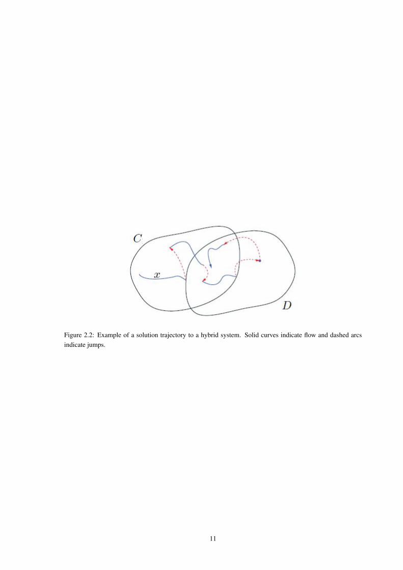
Figure 2.2: Example of a solution trajectory to a hybrid system. Solid curves indicate flow and dashed arcsindicate jumps.

11

DISCONTINUOUS AND HYSTERETICCONTROLLERS

Attitude control of a rigid body is a typical nonlinear control problem and has been studied for decades [50,8, 10], motivated especially by aerospace applications that involve maneuvers or attitude stabilization [1]. It isalso an important problem in underwater vehicles projects, ground vehicles, robotic systems etc [1].

Probably, the first systematic study of spacecraft attitude control began in 1952, which was documented inunpublished form only (and classified as “secret”) [51]. Beforehand, in the second half of 1940’s, many studiesin this area were sponsored by U.S. government agencies. In the open literature, one of the first paper appearedin 1957 (the launch year of Sputnik, the world’s first artificial Earth satellite). It described the problem ofactively controlling one of the axes orientation of an artificial satellite so that it remains pointed downwardtoward the Earth [51].

By 1970, anticipating future spacecraft needs, rapid and large angle reorientation was already subject tostudy [52]. Later on, in 1985, it was published one of the first papers suggesting a discontinuous control feed-back to achieve global attitude control [8]. Finally, only 26 years afterwards, in 2011, Mayhew et al. [10] notedthat for the control of [8], it is possible to find a small measurement noise which is able to induce chattering ofthe state and presented a hybrid feedback control law that solved the global asymptotic stabilization problemand was robust to measurement noise.

3.1 GLOBAL STABILIZATION BY CONTINUOUS FEEDBACK

Bhat and Bernstein [5] proved that the attitude can not be globally stabilized by means of continuousfeedback using Theorem 3.1 below and the fact that SO(3) is a compact manifold, .

LetM be a manifold of dimension m and consider a continuous vector field f onM.

Theorem 3.1 From [4, Theorem 1]

Suppose π : M −→ Q is a vector bundle on Q, where Q is a compact, r-dimensionalmanifold with r ≤ m. Then there exists no equilibrium of f that is globally asymptoticallystable.

An easier way to understand the impossibility of global attitude stabilization using continuous time-invariantfeedback is shown in [1, page 38] using the illustration of Figure 3.1. In this case, the manifold is the circle S1

and the problem refers to the attitude stabilization of the arm of the clock needle using a continuous feedback.To stabilize in configuration A, a continuous force vector field, tangent to the circle, was constructed to rotatethe needle. Since the upper and lower half of the circle point in opposite direction, the vector force field mustvanish somewhere – at point B in this case. Thus, a second unstable equilibrium point is created, an unstableone. Similarly, continuous time-invariant closed-loop vector fields create multiple closed-loop equilibria on therotation group SO(3) and the unit quaternion group S3.

12

3

Figure 3.1: Example of a strategy to stabilize the arm of a clock needle at point A.

3.2 GLOBAL STABILITY VIA DISCONTINUOUS KINEMATIC AT-TITUDE CONTROL

To simplify the problem presentation, only the kinematic attitude control is considered at first. That is, thesystem is described by equation (2.9) and the goal is to design an angular velocity feedback ω to stabilize thesetAk = qe = 1 or qe = −1. The discontinuous feedback is motivated by the following Lyapunov function:

V (qe) = 2 (1− |ηe|) .

Function V is positive definite on S3 with respect toAk, since V (S3\Ak) > 0 and V (Ak) = 0. Consideringthe following control law

ω(qe) = −hεe, (3.1)

where h = sgn (ηe) and

sgn (ηe) ,

−1, ηe < 0,

1, ηe ≥ 0,(3.2)

the time derivative of V is V (qe) = −‖εe‖2, which is negative definite. Note that this control law pulls thebody toward the shortest rotation direction (see Figure 3.2).

The closed-loop had been proved to be globally asymptotically stable1 [7]. However, when the initialcondition of the system is near the discontinuity – i.e., near ηe = 0, a region near 180 away from the referenceattitude –, measurement noise can cause chattering, which consists of multiple jumps (of states) occurring atthe same time and keep the state near the discontinuity indefinitely [10]. Let R = (ηr, εr) ∈ H represent thenoise such that qm = (qe +R) ∈ S3 be the attitude corrupted by noise R at instant t. Note that if ηe is near0, the sign of ηe + ηr and the sign of ηe can be different inducing the controller to change h. This way, thediscontinuous controller is not robust to measurement noise.

1As function V is not a continuously differentiable, LaSalle’s Theorem [53, page 117] can not be applied.

13

JOURNAL OF LATEX CLASS FILES, VOL. 11, NO. 4, DECEMBER 2012 3

[width=8cm]fig/Comhisterese

Fig. 2. State space representation of the hysteretic controller (with one stateh). Arrows indicate the direction of the torque contribution term (dependenton state h) so the attitude is regulated to 1 or −1. The parameter δ representsthe hysteresis half-width of the on-off control for state h.

The state space of the closed-loop system is represented by

x1 = (xp, xc1) ∈ X1 := Xp ×Xc.

The controller objective is to globally asymptotically stabi-lize the set

A1 =x1 ∈ X1 : qe = h1, ω = 0

. (5)

The closed-loop system is given by (2), (3) and the follow-ing dynamics of the controller.

˙h = 0 x1 ∈ C1 :=x1 ∈ X1 : hηe ≥ −δ

,

h+ ∈ sgn (u1) x1 ∈ D1 :=x1 ∈ X1 : hηe ≤ −δ

,

(6)where h+ is the value associated to h just after the statetransition and

sgn (η) =

sgn (η) , |ηe| > 0,

−1, 1 , ηe = 0.

The vector of inputs U1 = (τ , u1) is calculated as follows:τy, qd, h

= −che − ω and u1

y, qd, h

= ηe.

As already mentioned, h determines the orientation of aforce along the axis of rotation. While hηe ≥ 0, it forces themovement to the shorter rotation direction. However, whenhηe < 0, the force still pulls in the same direction (the longerrotation direction) until a safe distance is achieved to preventchattering, i.e., until hηe ≤ −δ.

III. PROPOSED CONTROLLER

As the hysteretic controller, in a specific region of the statespace, determines a force contribution to make the rigid-bodyevolves to the longer rotation direction, we propose to add onemore state to the controller to prevent this behavior and saveenergy.

The proposed controller feedback torque is also given by(4), but it has two states

xc2 =h,m

∈ Xc ×Xc, Xc := −1, 1 .

The state h determines the feedback torque contribution inorder to move qe either to 1 or −1, as well as in the hystereticcontrol. The state m = 1 indicates that |ηe| has reached overthe hysteresis width value but ηe has not crossed zero yet.The state m = −1 indicates the opposite, that ηe has alreadycrossed zero but |ηe| has not reached over the hysteresis widthvalue yet.

The space state of the closed-loop system is represented by

x2 = (x, xc2) ∈ X2 := X ×Xc ×Xc.

The controller objective is to globally asymptotically stabilizethe set

A2 =x2 ∈ X2 : qe = h1,m = 1, ω = 0

. (7)


˙h = 0m = 0

x2 ∈ C2,

h+ ∈ sgn (u2)m+ ∈ u3sgn (u2 − u3δ/2)

x2 ∈ D2,

(8)

C2 :=x2 ∈ X2 :

hηe ≥ −δ

,h = −1 or

m(ηe − δ/2) ≥ −δ) ,h = 1 orm(ηe + δ/2) ≤ δ

,

D2 :=x2 ∈ X2 :

hηe ≤ −δ

or

h = 1,

m(ηe − δ/2) ≤ −δ) orh = −1,m(ηe + δ/2) ≥ δ

.

where m+ and h+ are values associated to m and h, respec-tively, just after state transition. The set D2 can be expressedin a compact form as follows

D2 :=x2 ∈ X2 :

hηe ≤ −δ

ormh(ηe − hδ/2) ≤ −δ

.

The vector of inputs U2 = (τ , u2, u3) is calculated asfollows: τ

y, qd, h,m

= −che − ω, u2

y, qd, h,m

= ηe

and u3

y, qd, h,m

= h.

[width=8cm]fig/figProposto

Fig. 3. State space representation showing the proposed regulation with twostates (h and m). Arrows indicate the direction of the torque contribution term(dependent on state h) so the attitude is regulated to 1 or −1. The parameterδ represents the hysteresis half-width of the on-off control for state h andalso of the on-off control for state m.

Fig. 3 shows the proposed regulation. When state m = −1,the controller behaves as the hysteretic controller. If h = 1,state h changes to −1 when ηe ≤ −δ; if h = −1, state hchanges to 1 when ηe ≥ δ. The controller switches to statem = 1 when the attitude error qe presents ηe ≤ −2δ orηe ≥ 2δ. When state m = 1, the controller behaves as thediscontinuous controller. In other words, if state m = 1, statem will change to m = −1 when ηe goes across zero and enterthe jump set. This fact, anticipate the change of state h. Thisdistinct behavior is what differentiates it from the hystereticcontroller (6) and allows a torque contribution towards theshorter rotation direction.

A. Stability analysis

Consider the closed-loop system of the proposed controller(8) rewritten according to the hybrid systems framework of[11] and given by

H =

˙x2 ∈ F2 (x2) , x2 ∈ C2,

x+2 ∈ G2 (x2) , x2 ∈ D2,

where x2 = (qe, ω, h,m),

F2 (x2) :=

12qe(0, ω)

J−1S (Jω) ω − che − ω

00

,

G2 (x2) :=

qeω

sgn (ηe)hsgn

ηe − hδ/2

.

1

h = −1

1

h = 1

1

1

1

0

1

−1

1

e

Figure 3.2: State space representation of the discontinuous controller. Arrows indicate the direction of rotationso the attitude is regulated to 1 or −1.

3.3 ROBUSTNESS PROBLEM

As mentioned in the previous section, in case of a discontinuous feedback law, when the initial conditionof the system is near the discontinuity, measurement noise can cause chattering and keep the state near thediscontinuity indefinitely [9, 10]. See example of chattering behavior in Figure 3.3 (Section 3.4). Therefore,the stability is not robust to arbitrarily small measurement noise. To simplify notation, qe will be denoted as qin this chapter.

Theorem 3.2 of Sanfelice et al. [9] proves this fact for a generic space. Before it is enunciated, it followssome definitions.

Let O ⊂ Rn be an open set and letMi ⊂ Rn, i ∈ 1, . . . ,m, m > 1, be sets satisfyingm⋃i=1

Mi = O.

LetM , ⋃i,j,i 6=j

Mi ∩Mj , whereMi is the closure of setMi.

Definition 3.1. [9, Definition 2.1] A Carathéodory solution to the system x = f(x), where x ∈ Rn is thestate and f : Rn −→ Rn, on an interval I ⊂ [0,∞) is an absolutely continuous function x : I −→ Rn

that satisfies x(t) = f(x(t)) almost everywhere on I . Given a piecewise constant function e : I −→ Rn, aCarathéodory solution to the system x = f(x + e) on I is an absolutely continuous function x that satisfiesx(t) = f(x(t) + e(t)) for almost every t ∈ I; equivalently, for every t0 ∈ I , x(t) satisfies

x(t) = x(t0) +´ tt0f(x(τ) + e(τ))dτ, ∀t ∈ I.

Theorem 3.2 From [7, Theorem 2.6]

Let ε > 0 and letK satisfyK+B(0, 2ε) ⊂ O. Then, for each x0 ∈ (M+B(0, ε))∩K thereexists a piecewise constant function e : [ 0,∞) → B(0, ε) and a Carathéodory solution xto x = f (x+ e) starting at x0 such that x(t) ∈ (M+ B(0, ε))a for all t ∈ [ 0,∞) suchthat x(τ) ∈ K for all τ ∈ [0, t].

aThe sum of sets follows Minkowski sum definition, i.e., A+B = a + b : a ∈ A, b ∈ B.

Besides, Sanfelice et al. [9] affirmed that this theorem can be extended to systems of the form x =

f (x, κ(x+ e)), with f(·,u) locally Lipschitz uniformly over u’s in the range of κ.

Mayhew et al. [10] also proved this fact (robustness problem) for the discontinuous control law ω(q) =

−sgn(η)ε (3.1). They stated the following theorem.

14

Theorem 3.3 From [8, Theorem 3.2]

Let ω(q) = −sgn(η)ε, M , q ∈ S3 : η = 0. Then for each α > 0 and eachq0 ∈ M∗ , (M+ αB) ∩ S3, there exists a measurable function e : [ 0,∞) → αB and aCarathéodory solution q : [ 0,∞) → S3 to q = 1

2q (0,ω (q + e)) satisfying q(0) = q0

and q(t) ∈M∗ for all t ∈ [ 0,∞) .

This theorem affirms that applying the discontinuous control law, if the initial condition of the system isnear the discontinuity (q0 ∈ M∗), there exist a noise of magnitude not higher than α such that the state willremain near the discontinuity indefinitely. A point that stands out from these two theorems is that the feedbackvariable when corrupted by the measurement noise has no guarantee to belong to the space of the variable. Forinstance, the noise function suggested by Mayhew et al. [10] is e = (−αsgn(η),0). Note that the feedbackdepends on (q + e) /∈ S3, which is not an attitude quaternion representation and is a physical inconsistency.

As a contribution of this manuscript, in the sequel, a new theorem is stated and proved about the existenceof such noise function for the case the sum q + e is restricted to S3.

Theorem 3.4

Let ω(q) = −sgn(η)ε, M , q ∈ S3 : η = 0. Then for each 0 < α <√

2 and eachq0 ∈M∗ , (M+ B(0, α))∩S3, there exists a measurable function e : [ 0,∞) → B(0, α)

and a Carathéodory solution q : [ 0,∞) → S3 to q = 12q (0,ω (q + e)) satisfying

q(0) = q0, (q + e) ∈ S3 and q(t) ∈M∗ for all t ∈ [ 0,∞) .

Proof. The idea of the proof is to find function e such that the direction of ω(q + e) is opposite to thedirection of ω(q). This way, the body always moves toward the longest rotation direction and gets stuck atη = 0.Let q(t) = (η, ε). From Lemma B.5, it is known that the scalar component of q is limited to

|η| < α

√1− α2

4=: m. (3.3)

The range of m depends on α, which is restricted toa 0 < α <√

2. Note that 0 ≤ |η| < m < 1.In order to make the direction of ω(q + e) opposite to the direction of ω(q), let e(t) = (ηr, εr) be definedas

ηr = −η + β (η − sgn(η)m) , (3.4)

where β ∈ (0, 1) so the sign of the sum η + ηr = β (η − sgn(η)m) is opposite to the sign of η (LemmaB.6), i.e.,

sgn(η + ηr) = −sgn(η). (3.5)

The value of εr can be obtained using Lemma B.7, so as to ensure that ‖e(t)‖ is the minimum for thepredefined value of ηr which satisfies (q(t) + e(t)) ∈ S3. Thus,

εr =

√1− (η + ηr)2

1− η2− 1

ε. (3.6)

The proof that ‖e(t)‖ < α follows directly from Lemma B.8.To end the demonstration, following is the proof that the attitude q(t) ∈M∗ for all future time.Let Ω ,

q ∈ S3 : η ≤ α

, VM(q) = η2. Function VM is positive definite on Ω with respect toM, since

VM(q) > 0 for q ∈ Ω \M and VM(q) = 0 for q ∈M.

15

The time derivative of function VM is given by

VM = 〈∇VM(q), q〉 . (3.7)

From the definition of VM,∇VM(q) = (2η,0) and the time derivative of the attitude is given by

q =1

2q (0,ω (q + e)) , (3.8)

q =1

2

(sgn(ηm)εT εm,−ηsgn(ηm)εm − sgn(ηm)ε× εm

), (3.9)

where ηm = η + ηr and εm = ε+ εr. Hence,

VM = ηsgn(η + ηr)εT (ε+ εr) (3.10)

= η (−sgn(η))

√1− (β (η − sgn(η)m))2

1− η2εT ε

(3.11)

= − |η|√

1− β2 (m− |η|)2√

1− η2, (3.12)

where (3.5) was used in (3.11) and εT ε = 1− η2 was used in (3.12).Function VM is negative definite on Ω with respect toM.Since Ω compact, function VM is continuously differentiable and positive definite, and function VM isnegative definite, it is possible to affirm that every solution starting in Ω remains in Ω for all future time.AsM∗ ⊂ Ω, q(t) ∈M∗ for all t ∈ [ 0,∞) .

aThe upper limit can be deduced from (B.19) for η = ±1. The theorem is senseless for α >√

2 because maxq

d(q,M) =√

2

as shown in Lemma B.4.

The following sections refer to the dynamical system (2.10), described in Section 2.4.

3.4 DISCONTINUOUS ATTITUDE CONTROL

In order to achieve global attitude control, some authors, such as Fjellstad and Fossen [6], Fragopoulos andInnocenti [7] and Wie and Barba [8], proposed a discontinuous feedback law like the following

τ 1 (y, qd) = −chεe − ω, (3.13)

where y is defined in (2.11), c > 0 is the gain of the “proportional” term −chεe and h = sgn (ηe). The sgnfunction is defined as in (3.2).

The value of h determines the direction of the “proportional” term so qe is regulated either to 1 = (1,0) or−1 = (−1,0), as shown in Figure 3.2.

The closed-loop (2.10), (2.11) and τ = τ 1, with τ 1 given by (3.13) had been proved to be globallyasymptotically stable [7]. However, when the initial condition of the system is near the discontinuity – i.e.,near ηe = 0, a region near 180 away from the reference attitude –, measurement noise can cause chattering,which consists of multiple jumps (of states) occurring at the same time and keep the state near the discontinuityindefinitely [10]. This way, the discontinuous controller is not robust to measurement noise.

Figure 3.3 illustrates the difference in behavior when the output is corrupted by noise2 for initial conditionsηe(0) = 0, εe(0) = [ 1 2 3 ]T /

√14 and ω(0) = 0. The chattering occurred during the first 6 seconds and

2The measured value of q included noise generated in the same way as described in Section 4.3.

16

can be observed in the graph of hηe. During the chattering behavior, the controller “believes” the sign of ηecontinually changes and, as a consequence, the system has its response lagged.

0 5 10 15 20−1

0

1

with noise

no noise

0 5 10 15 20

−1

1

Time (s)

η ehη e

Figure 3.3: System behavior for the discontinuous controller when no noise is present in the output y and whenthe output is corrupted by noise.

3.5 HYSTERETIC HYBRID ATTITUDE CONTROL

In order to solve the robustness problem of the discontinuous controller, Mayhew et al. [10] proposed ahybrid control with hysteretic feedback by using the same torque feedback (3.13), but having h determined ina different way. The idea of this controller is, instead of changing the dynamics (the value of h) just after thesign of ηe changes, the value of h is kept unchanged until a safe distance from the discontinuity is achieved.According to the definitions at the end of last section (Section 3.4), a safe distance means a distance so thesign of ηe + ηr and ηe can not be different. As this behavior is more complex, a hybrid dynamic controller isconsidered.

The hysteretic controller of [10] has only one state variable h ∈ Xc , −1, 1. The state of the overallsystem is represented by x1 = (x, h) ∈ X1 , X ×Xc and evolves according to (2.10), (2.11), the followingdynamics of the controller3

˙h = 0 x1 ∈ C1 ,x1 ∈ X1 : hηe ≥ −δ

,

h+ ∈ sgn (u1) x1 ∈ D1 ,x1 ∈ X1 : hηe ≤ −δ

,

(3.14)

where h+ is the value associated to h just after the state transition4 and

sgn (u1) ,

1 , u1 > 0,

−1 , u1 < 0,

−1, 1 . u1 = 0.

The vector of inputs is U1 = (τ , u1) and the closed-loop law is achieved by setting

U1 = K1(y, h, qd) , (−chεe − ω, ηe). (3.15)

The parameter δ ∈ (0, 1) represents the hysteresis half-width and provides robustness against chattering causedby output measurement. According to [10, Theorem 5.5], δ must be higher than 2α, where α is the maximumnoise magnitude of the output measurement.

3Along the text, the dynamics representations follow the hybrid systems framework of Goebel et al. [48], summarized in Section 2.7.4Note that for the closed-loop approach u1 = ηe.

17

The closed system is globally asymptotically stable with respect to the set

A1 =x1 ∈ X1 : qe = h1 and ω = 0

. (3.16)

10-1





x1 = (xp, xc1) ∈ X1 := Xp ×Xc.


A1 =x1 ∈ X1 : qe = h1, ω = 0

. (5)


˙h = 0 x1 ∈ C1 :=x1 ∈ X1 : hηe ≥ −δ

,

h+ ∈ sgn (u1) x1 ∈ D1 :=x1 ∈ X1 : hηe ≤ −δ

,


sgn (η) =

sgn (η) , |ηe| > 0,

−1, 1 , ηe = 0.



y, qd, h

= ηe.





xc2 =h,m

∈ Xc ×Xc, Xc := −1, 1 .



x2 = (x, xc2) ∈ X2 := X ×Xc ×Xc.


A2 =x2 ∈ X2 : qe = h1,m = 1, ω = 0

. (7)


˙h = 0m = 0

x2 ∈ C2,

h+ ∈ sgn (u2)m+ ∈ u3sgn (u2 − u3δ/2)

x2 ∈ D2,

(8)

C2 :=x2 ∈ X2 :

hηe ≥ −δ

,h = −1 or

m(ηe − δ/2) ≥ −δ) ,h = 1 orm(ηe + δ/2) ≤ δ

,

D2 :=x2 ∈ X2 :

hηe ≤ −δ

or

h = 1,

m(ηe − δ/2) ≤ −δ) orh = −1,m(ηe + δ/2) ≥ δ

.


D2 :=x2 ∈ X2 :

hηe ≤ −δ


.


y, qd, h,m

= −che − ω, u2

y, qd, h,m

= ηe

and u3

y, qd, h,m

= h.






H =

˙x2 ∈ F2 (x2) , x2 ∈ C2,

x+2 ∈ G2 (x2) , x2 ∈ D2,


F2 (x2) :=

12qe(0, ω)


00

,

G2 (x2) :=

qeω

sgn (ηe)hsgn

ηe − hδ/2

.

1

h = −1

1

h = 1

1

δ

1

0

1

1

1

−δ

1

−1

1

e

Figure 3.4: State space representation of the hysteretic controller (with one state variable h). Arrows indicatethe direction of the “proportional” term of the torque (dependent on h) so the attitude is regulated to 1 or −1.The parameter δ represents the hysteresis half-width of the on-off control for state h.

Figure 3.4 shows the behavior of the hysteretic controller for a hysteresis width of 2δ. The state variable hdetermines the “proportional” term direction of the torque feedback in order to move qe either to 1 or −1.

In the sequel, it is presented some examples of system evolution for some distinct initial conditions andcompares it when the controller is the discontinuous one. For the simulations below, the initial controller statefor the hysteretic controller was h(0) = 1 and the hysteresis parameter was set to δ = 0.4. The simulationsincluded measurement noise5 of maximum magnitude α = 0.2.

For the scenario of Figure 3.3, with initial conditions ηe(0) = 0, εe(0) = [ 1 2 3 ]T /√

14 and ω(0) =

0, while the discontinuous controller presents chattering, the hysteretic controller behaves as the discontinuouscontroller when no noise is present. The hysteretic controller keeps the state variable h = 1 along all the way.

Figure 3.5 exemplifies the problem mentioned in [10]. It is affirmed that there is a price to pay for robustglobal asymptotic stabilization with the hysteretic controller – a region in the state space where the hybridcontrol law pulls the rigid body in the direction of a longer rotation. In fact, the proportional term of thetorque feedback pulls the body in the shorter rotation direction while hηe ≥ 0. But, when hηe gets negative,it still pulls in the same direction (the longer rotation direction now) until a safe distance (given by δ) isachieved to prevent chattering, i.e., until hηe ≤ −δ. In this simulation, the initial conditions ηe(0) = −0.2,εe(0) =

√(1− 0.22)[ 1 2 3 ]T /

√14 and ω(0) = 0 were chosen to contrast the longer rotation direction

determined by the hysteretic controller and the shorter direction taken when the controller is the discontinuousone. The hysteretic controller keeps the state variable h = 1 along all the way whereas the discontinuous onekeeps h at −1.

The following scenario (Figure 3.6) illustrates an example with initial angular velocity different thanzero. The initial conditions were ηe(0) = −0.2, εe(0) =

√(1− 0.22)[ 1 2 3 ]T /

√14 and ω(0) =

0.5[ 1 2 3 ]T /√

14 . The control law of the discontinuous controller pulls the body toward ηe = −1

along all the way as h keeps at −1. Differently, the hysteretic controller is initiated with h = 1 and the controllaw pulls the body to the opposite direction. Due to inertia, it rotates toward ηe = −1, however the angularvelocity norm decreases until ηe crosses the hysteresis threshold (hηe ≤ −δ) – see the graph of the angularvelocity. After that, the controller changes state h to −1 and the body continues rotating toward ηe = −1 . Themoment the controller changes state h can be seen on the graph of hηe.

5The measured value of q included noise generated in the same way as described in Section 4.3.

18

0 5 10 15 20−1

0

1

HystereticDiscontinuous

0 5 10 15 20−1

1

Time (s)

JOU

RN

AL

OF

LAT E

XC

LA

SSFI

LE

S,V

OL

.11,

NO

.4,D

EC

EM

BE

R20

123

[wid

th=8

cm]fi

g/C

omhi

ster

ese

Fig.

2.St

ate

spac

ere

pres

enta

tion

ofth

ehy

ster

etic

cont

rolle

r(w

ithon

est

ate

h).

Arr

ows

indi

cate

the

dire

ctio

nof

the

torq

ueco

ntri

butio

nte

rm(d

epen

dent

onst

ateh

)so

the

attit

ude

isre

gula

ted

to1

or−1

.The

para

met

erδ

repr

esen

tsth

ehy

ster

esis

half

-wid

thof

the

on-o

ffco

ntro

lfo

rst

ateh

.

The

stat

esp

ace

ofth

ecl

osed

-loo

psy

stem

isre

pres

ente

dby

x1=

(xp,x

c1)∈X

1:=

Xp×

Xc.

The

cont

rolle

rob

ject

ive

isto

glob

ally

asym

ptot

ical

lyst

abi-

lize

the

set

A1=

x1∈X

1:qe=

h1,ω

= 0 .

(5)

The

clos

ed-l

oop

syst

emis

give

nby

(2),

(3)

and

the

follo

w-

ing

dyna

mic

sof

the

cont

rolle

r.

˙ h=

0x1∈C

1:=

x1∈X

1:hη e

≥−δ ,

h+∈

sgn(u

1)

x1∈D

1:=

x1∈X

1:hη e

≤−δ ,

(6)

whe

reh+

isth

eva

lue

asso

ciat

edto

hju

staf

ter

the

stat

etr

ansi

tion

and

sgn(η)=

sgn(η),

|ηe|>

0,

−1,1,

η e=

0.

The

vect

orof

inpu

tsU1=

(τ,u

1)

isca

lcul

ated

asfo

llow

s:τ y,q

d,h

=−ch e

−ω

andu1

y,q

d,h

=η e

.A

sal

read

ym

entio

ned,

hde

term

ines

the

orie

ntat

ion

ofa

forc

eal

ong

the

axis

ofro

tatio

n.W

hile

hη e

≥0

,it

forc

esth

em

ovem

ent

toth

esh

orte

rro

tatio

ndi

rect

ion.

How

ever

,w

hen

hη e

<0,

the

forc

est

illpu

llsin

the

sam

edi

rect

ion

(the

long

erro

tatio

ndi

rect

ion)

until

asa

fedi

stan

ceis

achi

eved

topr

even

tch

atte

ring

,i.e

.,un

tilhη e

≤−δ.

III.

PR

OP

OS

ED

CO

NT

RO

LL

ER

As

the

hyst

eret

icco

ntro

ller,

ina

spec

ific

regi

onof

the

stat

esp

ace,

dete

rmin

esa

forc

eco

ntri

butio

nto

mak

eth

eri

gid-

body

evol

ves

toth

elo

nger

rota

tion

dire

ctio

n,w

epr

opos

eto

add

one

mor

est

ate

toth

eco

ntro

ller

topr

even

tth

isbe

havi

oran

dsa

veen

ergy

.T

hepr

opos

edco

ntro

ller

feed

back

torq

ueis

also

give

nby

(4),

but

itha

stw

ost

ates

xc2=

h,m

∈X

c×

Xc,X

c:=

−1,1

.

The

stat

eh

dete

rmin

esth

efe

edba

ckto

rque

cont

ribu

tion

inor

dert

om

oveqe

eith

erto

1or

−1

,as

wel

las

inth

ehy

ster

etic

cont

rol.

The

stat

em

=1

indi

cate

sth

at|η

e|h

asre

ache

dov

erth

ehy

ster

esis

wid

thva

lue

butη e

has

not

cros

sed

zero

yet.

The

stat

em

=−1

indi

cate

sth

eop

posi

te,

that

η eha

sal

read

ycr

osse

dze

robu

t|η e|h

asno

trea

ched

over

the

hyst

eres

isw

idth

valu

eye

t.T

hesp

ace

stat

eof

the

clos

ed-l

oop

syst

emis

repr

esen

ted

by

x2=

(x,x

c2)∈X

2:=

X×

Xc×

Xc.

The

cont

rolle

rob

ject

ive

isto

glob

ally

asym

ptot

ical

lyst

abili

zeth

ese

t

A2=

x2∈X

2:qe=

h1,m

=1,ω= 0 .

(7)

The

clos

ed-l

oop

syst

emis

give

nby

(2),

(3)

and

the

follo

w-

ing

dyna

mic

sof

the

cont

rolle

r.˙ h=

0m

=0

x2∈C

2,

h+∈

sgn(u

2)

m+∈u3sg

n(u

2−u3δ/2)

x2∈D

2,

(8)

C2:=

x2∈X

2: h

η e≥

−δ , h

=−1

or

m(η

e−

δ/2)≥

−δ)

, h=

1orm(η

e+δ/2)≤

δ,

D2:=

x2∈X

2: h

η e≤

−δ or

h=

1,

m(η

e−

δ/2)≤

−δ)

or h

=−1,m

(ηe+δ/2)

≥δ

.

whe

rem

+an

dh+

are

valu

esas

soci

ated

tom

andh

,res

pec-

tivel

y,ju

staf

ter

stat

etr

ansi

tion.

The

setD

2ca

nbe

expr

esse

din

aco

mpa

ctfo

rmas

follo

ws

D2:=

x2∈X

2: h

η e≤

−δ or

mh(η

e−hδ/2)

≤−δ

.

The

vect

orof

inpu

tsU2

=(τ,u

2,u

3)

isca

lcul

ated

asfo

llow

s:τ y,q

d,h

,m =

−ch e

−ω

,u2

y,q

d,h

,m =

η ean

du3

y,q

d,h

,m =

h.

[wid

th=8

cm]fi

g/fig

Prop

osto

Fig.

3.St

ate

spac

ere

pres

enta

tion

show

ing

the

prop

osed

regu

latio

nw

ithtw

ost

ates

(han

dm

).A

rrow

sin

dica

teth

edi

rect

ion

ofth

eto

rque

cont

ribu

tion

term

(dep

ende

nton

stat

eh

)so

the

attit

ude

isre

gula

ted

to1

or−1

.The

para

met

erδ

repr

esen

tsth

ehy

ster

esis

half

-wid

thof

the

on-o

ffco

ntro

lfo

rst

ateh

and

also

ofth

eon

-off

cont

rol

for

stat

em

.

Fig.

3sh

ows

the

prop

osed

regu

latio

n.W

hen

stat

em

=−1,

the

cont

rolle

rbe

have

sas

the

hyst

eret

icco

ntro

ller.

Ifh=

1,st

ateh

chan

ges

to−1

whe

nη e

≤−δ;

ifh

=−1,

stat

eh

chan

ges

to1

whe

nη e

≥δ.

The

cont

rolle

rsw

itche

sto

stat

em

=1

whe

nth

eat

titud

eer

rorqe

pres

ents

η e≤

−2δ

orη e

≥2δ

.W

hen

stat

em

=1,

the

cont

rolle

rbe

have

sas

the

disc

ontin

uous

cont

rolle

r.In

othe

rw

ords

,if

stat

em

=1,

stat

em

will

chan

geto

m=

−1

whe

nη e

goes

acro

ssze

roan

den

ter

the

jum

pse

t.T

his

fact

,ant

icip

ate

the

chan

geof

stat

eh

.Thi

sdi

stin

ctbe

havi

oris

wha

tdi

ffer

entia

tes

itfr

omth

ehy

ster

etic

cont

rolle

r(6

)an

dal

low

sa

torq

ueco

ntri

butio

nto

war

dsth

esh

orte

rro

tatio

ndi

rect

ion.

A.

Stab

ility

anal

ysis

Con

side

rth

ecl

osed

-loo

psy

stem

ofth

epr

opos

edco

ntro

ller

(8)

rew

ritte

nac

cord

ing

toth

ehy

brid

syst

ems

fram

ewor

kof

[11]

and

give

nby

H=

˙ x2∈F2(x

2),

x2∈C

2,

x+ 2∈G

2(x

2),

x2∈D

2,

whe

rex2=

(qe,ω

,h,m

),

F2(x

2):=

1 2qe(0,ω

)J−1 S

(Jω)ω−

ch e

−ω

0 0

,

G2(x

2):=

qe ω

sgn(η

e)

hsg

n η e

−hδ/2

.

JOU

RN

AL

OF

LAT E

XC

LA

SSFI

LE

S,V

OL

.11,

NO

.4,D

EC

EM

BE

R20

123

[wid

th=8

cm]fi

g/C

omhi

ster

ese

Fig.

2.St

ate

spac

ere

pres

enta

tion

ofth

ehy

ster

etic

cont

rolle

r(w

ithon

est

ate

h).

Arr

ows

indi

cate

the

dire

ctio

nof

the

torq

ueco

ntri

butio

nte

rm(d

epen

dent

onst

ateh

)so

the

attit

ude

isre

gula

ted

to1

or−1

.The

para

met

erδ

repr

esen

tsth

ehy

ster

esis

half

-wid

thof

the

on-o

ffco

ntro

lfo

rst

ateh

.

The

stat

esp

ace

ofth

ecl

osed

-loo

psy

stem

isre

pres

ente

dby

x1=

(xp,x

c1)∈X

1:=

Xp×

Xc.

The

cont

rolle

rob

ject

ive

isto

glob

ally

asym

ptot

ical

lyst

abi-

lize

the

set

A1=

x1∈X

1:qe=

h1,ω

= 0 .

(5)

The

clos

ed-l

oop

syst

emis

give

nby

(2),

(3)

and

the

follo

w-

ing

dyna

mic

sof

the

cont

rolle

r.

˙ h=

0x1∈C

1:=

x1∈X

1:hη e

≥−δ ,

h+∈

sgn(u

1)

x1∈D

1:=

x1∈X

1:hη e

≤−δ ,

(6)

whe

reh+

isth

eva

lue

asso

ciat

edto

hju

staf

ter

the

stat

etr

ansi

tion

and

sgn(η)=

sgn(η),

|ηe|>

0,

−1,1,

η e=

0.

The

vect

orof

inpu

tsU1=

(τ,u

1)

isca

lcul

ated

asfo

llow

s:τ y,q

d,h

=−ch e

−ω

andu1

y,q

d,h

=η e

.A

sal

read

ym

entio

ned,

hde

term

ines

the

orie

ntat

ion

ofa

forc

eal

ong

the

axis

ofro

tatio

n.W

hile

hη e

≥0

,it

forc

esth

em

ovem

ent

toth

esh

orte

rro

tatio

ndi

rect

ion.

How

ever

,w

hen

hη e

<0,

the

forc

est

illpu

llsin

the

sam

edi

rect

ion

(the

long

erro

tatio

ndi

rect

ion)

until

asa

fedi

stan

ceis

achi

eved

topr

even

tch

atte

ring

,i.e

.,un

tilhη e

≤−δ.

III.

PR

OP

OS

ED

CO

NT

RO

LL

ER

As

the

hyst

eret

icco

ntro

ller,

ina

spec

ific

regi

onof

the

stat

esp

ace,

dete

rmin

esa

forc

eco

ntri

butio

nto

mak

eth

eri

gid-

body

evol

ves

toth

elo

nger

rota

tion

dire

ctio

n,w

epr

opos

eto

add

one

mor

est

ate

toth

eco

ntro

ller

topr

even

tth

isbe

havi

oran

dsa

veen

ergy

.T

hepr

opos

edco

ntro

ller

feed

back

torq

ueis

also

give

nby

(4),

but

itha

stw

ost

ates

xc2=

h,m

∈X

c×

Xc,X

c:=

−1,1

.

The

stat

eh

dete

rmin

esth

efe

edba

ckto

rque

cont

ribu

tion

inor

dert

om

oveqe

eith

erto

1or

−1

,as

wel

las

inth

ehy

ster

etic

cont

rol.

The

stat

em

=1

indi

cate

sth

at|η

e|h

asre

ache

dov

erth

ehy

ster

esis

wid

thva

lue

butη e

has

not

cros

sed

zero

yet.

The

stat

em

=−1

indi

cate

sth

eop

posi

te,

that

η eha

sal

read

ycr

osse

dze

robu

t|η e|h

asno

trea

ched

over

the

hyst

eres

isw

idth

valu

eye

t.T

hesp

ace

stat

eof

the

clos

ed-l

oop

syst

emis

repr

esen

ted

by

x2=

(x,x

c2)∈X

2:=

X×

Xc×

Xc.

The

cont

rolle

rob

ject

ive

isto

glob

ally

asym

ptot

ical

lyst

abili

zeth

ese

t

A2=

x2∈X

2:qe=

h1,m

=1,ω= 0 .

(7)

The

clos

ed-l

oop

syst

emis

give

nby

(2),

(3)

and

the

follo

w-

ing

dyna

mic

sof

the

cont

rolle

r.˙ h=

0m

=0

x2∈C

2,

h+∈

sgn(u

2)

m+∈u3sg

n(u

2−u3δ/2)

x2∈D

2,

(8)

C2:=

x2∈X

2: h

η e≥

−δ , h

=−1

or

m(η

e−

δ/2)≥

−δ)

, h=

1orm(η

e+δ/2)

≤δ

,

D2:=

x2∈X

2: h

η e≤

−δ or

h=

1,

m(η

e−

δ/2)

≤−δ)

or h

=−1,m

(ηe+δ/2)≥

δ.

whe

rem

+an

dh+

are

valu

esas

soci

ated

tom

andh

,res

pec-

tivel

y,ju

staf

ter

stat

etr

ansi

tion.

The

setD

2ca

nbe

expr

esse

din

aco

mpa

ctfo

rmas

follo

ws

D2:=

x2∈X

2: h

η e≤

−δ or

mh(η

e−hδ/2)≤

−δ

.

The

vect

orof

inpu

tsU2

=(τ,u

2,u

3)

isca

lcul

ated

asfo

llow

s:τ y,q

d,h

,m =

−ch e

−ω

,u2

y,q

d,h

,m =

η ean

du3

y,q

d,h

,m =

h.

[wid

th=8

cm]fi

g/fig

Prop

osto

Fig.

3.St

ate

spac

ere

pres

enta

tion

show

ing

the

prop

osed

regu

latio

nw

ithtw

ost

ates

(han

dm

).A

rrow

sin

dica

teth

edi

rect

ion

ofth

eto

rque

cont

ribu

tion

term

(dep

ende

nton

stat

eh

)so

the

attit

ude

isre

gula

ted

to1

or−1

.The

para

met

erδ

repr

esen

tsth

ehy

ster

esis

half

-wid

thof

the

on-o

ffco

ntro

lfo

rst

ateh

and

also

ofth

eon

-off

cont

rol

for

stat

em

.

Fig.

3sh

ows

the

prop

osed

regu

latio

n.W

hen

stat

em

=−1,

the

cont

rolle

rbe

have

sas

the

hyst

eret

icco

ntro

ller.

Ifh=

1,st

ateh

chan

ges

to−1

whe

nη e

≤−δ;

ifh

=−1,

stat

eh

chan

ges

to1

whe

nη e

≥δ.

The

cont

rolle

rsw

itche

sto

stat

em

=1

whe

nth

eat

titud

eer

rorqe

pres

ents

η e≤

−2δ

orη e

≥2δ

.W

hen

stat

em

=1,

the

cont

rolle

rbe

have

sas

the

disc

ontin

uous

cont

rolle

r.In

othe

rw

ords

,if

stat

em

=1,

stat

em

will

chan

geto

m=

−1

whe

nη e

goes

acro

ssze

roan

den

ter

the

jum

pse

t.T

his

fact

,ant

icip

ate

the

chan

geof

stat

eh

.Thi

sdi

stin

ctbe

havi

oris

wha

tdi

ffer

entia

tes

itfr

omth

ehy

ster

etic

cont

rolle

r(6

)an

dal

low

sa

torq

ueco

ntri

butio

nto

war

dsth

esh

orte

rro

tatio

ndi

rect

ion.

A.

Stab

ility

anal

ysis

Con

side

rth

ecl

osed

-loo

psy

stem

ofth

epr

opos

edco

ntro

ller

(8)

rew

ritte

nac

cord

ing

toth

ehy

brid

syst

ems

fram

ewor

kof

[11]

and

give

nby

H=

˙ x2∈F2(x

2),

x2∈C

2,

x+ 2∈G

2(x

2),

x2∈D

2,

whe

rex2=

(qe,ω

,h,m

),

F2(x

2):=

1 2qe(0,ω

)J−1 S

(Jω)ω−

ch e

−ω

0 0

,

G2(x

2):=

qe ω

sgn(η

e)

hsg

n η e

−hδ/2

.

Figure 3.5: Comparison of the system behavior when the discontinuous controller and the hysteretic controllerare applied to highlight the longer rotation direction determined by the hysteretic controller.

0 5 10 15 20−1

0

1

HystereticDiscontinuous

0 5 10 15 200

0.5

Time (s)

1

hη e

1

ω

Figure 3.6: Comparison of the system behavior when the discontinuous controller and the hysteretic controllerare applied to highlight the behavior when the initial condition of the system is not at rest.

3.6 PROBLEM DEFINITION

The problem of robust and global attitude stabilization for rigid body has been solved. However the choiceof the best rotation direction to stabilize in order to spend less energy is not trivial. Mayhew et al. [10] affirmthat there is a price to pay with the hysteretic controller – a region in the state space where the hybrid controllaw pulls the rigid body in the direction of a longer rotation. The problem that this thesis work solves is

PROBLEM

Find a controller with a better performance between settlingtime and energy consumption than the hysteretic controllersuggested by [10] that keeps the robustness and global con-trol stability.

In order to solve this problem, it is proposed two hybrid solutions by the introduction of one new mode thatis used to indicate if the system attitude is close to a critical region (the chattering prone region):

19

• In Chapter 4, the first proposed hybrid controller (HY controller) is capable of reducing the energy con-sumption of rest-to-rest applications when compared with the hysteretic hybrid controller. Being capableof detecting when the reference changes abruptly or when the current attitude is far from the referenceon the initial instant, it has more opportunities to determine the shorter rotation direction (compared withthe hysteretic controller). But this is not always true when the initial angular velocity direction and theshorter rotation direction are opposite.

• In Chapter 5, a middle term solution in terms of cost between the memoryless discontinuous and thehysteretic hybrid control is proposed by introducing a new mode which also have a hysteresis structure.This new controller, called bimodal controller, reduces the region for the longer direction mentionedabove without compromising the robustness (the controller has the same capability of noise rejectionof the hysteretic controller) and, differently from the HY controller, it does not impose any restrictionson flow and jumps priorities. It is oriented for the rest-to-rest control of attitude, however it spend lessenergy in average for other initial angular velocities.

The two proposed controllers determine the direction to stabilize based only on the attitude information. Cer-tainly, the angular velocity should also be considered. This is still an open problem. The two articles in theliterature that takes the angular velocity into account, to the best of the author’s knowledge, is [54] and [55]. In[54], the authors concluded that hysteretic controller presents advantages. The controller suggested in [55] isan adapted version of the hysteretic controller. Direct comparisons was possible with an adapted version of thebimodal controller in this manuscript (Subsection 5.3.3). The conclusions are favorable to the adapted bimodalcontroller.

20

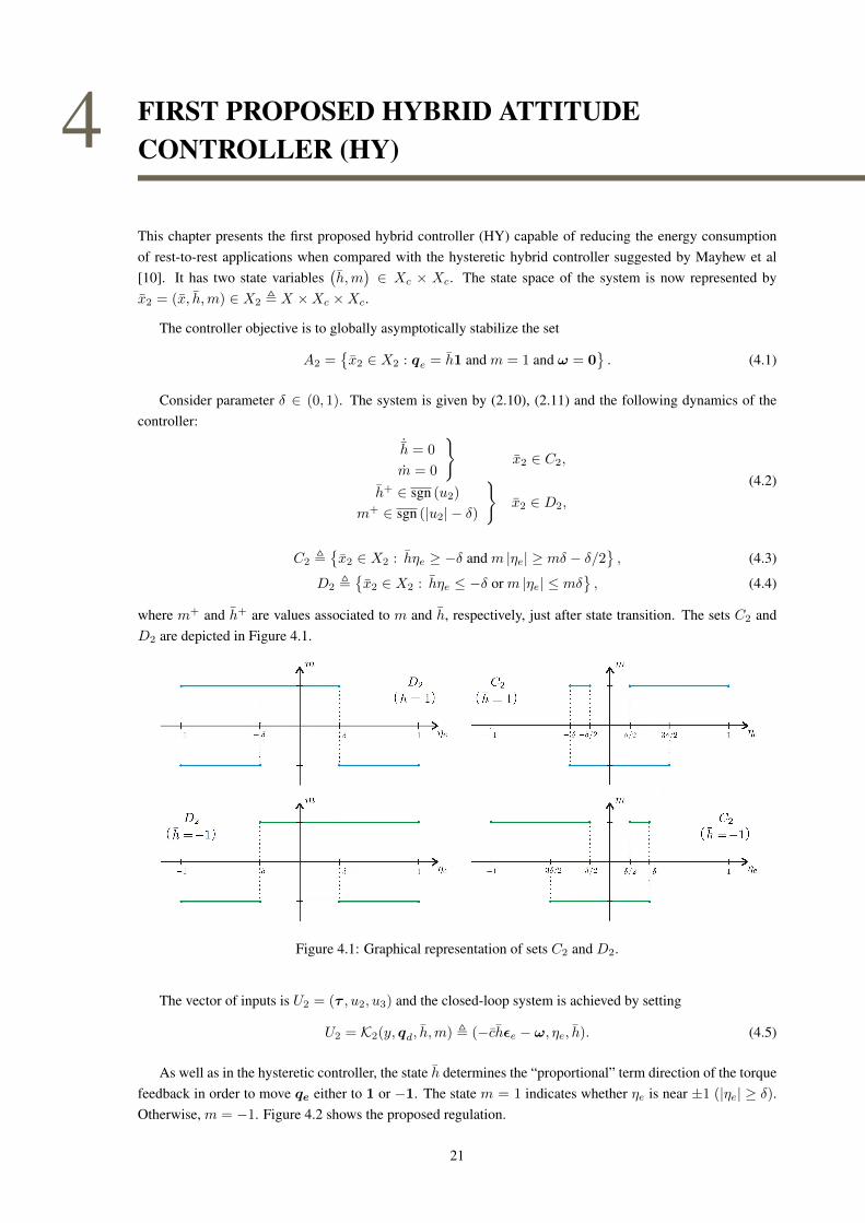
FIRST PROPOSED HYBRID ATTITUDECONTROLLER (HY)

This chapter presents the first proposed hybrid controller (HY) capable of reducing the energy consumptionof rest-to-rest applications when compared with the hysteretic hybrid controller suggested by Mayhew et al[10]. It has two state variables

(h,m

)∈ Xc × Xc. The state space of the system is now represented by

x2 = (x, h,m) ∈ X2 , X ×Xc ×Xc.

The controller objective is to globally asymptotically stabilize the set

A2 =x2 ∈ X2 : qe = h1 and m = 1 and ω = 0

. (4.1)

Consider parameter δ ∈ (0, 1). The system is given by (2.10), (2.11) and the following dynamics of thecontroller:

˙h = 0

m = 0

x2 ∈ C2,

h+ ∈ sgn (u2)

m+ ∈ sgn (|u2| − δ)

x2 ∈ D2,

(4.2)

C2 ,x2 ∈ X2 : hηe ≥ −δ and m |ηe| ≥ mδ − δ/2

, (4.3)

D2 ,x2 ∈ X2 : hηe ≤ −δ or m |ηe| ≤ mδ

, (4.4)

where m+ and h+ are values associated to m and h, respectively, just after state transition. The sets C2 andD2 are depicted in Figure 4.1.

Figure 4.1: Graphical representation of sets C2 and D2.

The vector of inputs is U2 = (τ , u2, u3) and the closed-loop system is achieved by setting

U2 = K2(y, qd, h,m) , (−chεe − ω, ηe, h). (4.5)

As well as in the hysteretic controller, the state h determines the “proportional” term direction of the torquefeedback in order to move qe either to 1 or −1. The state m = 1 indicates whether ηe is near ±1 (|ηe| ≥ δ).Otherwise, m = −1. Figure 4.2 shows the proposed regulation.

21

4





x1 = (xp, xc1) ∈ X1 := Xp ×Xc.


A1 =x1 ∈ X1 : qe = h1, ω = 0

. (5)


˙h = 0 x1 ∈ C1 :=x1 ∈ X1 : hηe ≥ −δ

,

h+ ∈ sgn (u1) x1 ∈ D1 :=x1 ∈ X1 : hηe ≤ −δ

,


sgn (η) =

sgn (η) , |ηe| > 0,

−1, 1 , ηe = 0.



y, qd, h

= ηe.





xc2 =h,m

∈ Xc ×Xc, Xc := −1, 1 .



x2 = (x, xc2) ∈ X2 := X ×Xc ×Xc.


A2 =x2 ∈ X2 : qe = h1,m = 1, ω = 0

. (7)


˙h = 0m = 0

x2 ∈ C2,

h+ ∈ sgn (u2)m+ ∈ u3sgn (u2 − u3δ/2)

x2 ∈ D2,

(8)

C2 :=x2 ∈ X2 :

hηe ≥ −δ

,h = −1 or

m(ηe − δ/2) ≥ −δ) ,h = 1 orm(ηe + δ/2) ≤ δ

,

D2 :=x2 ∈ X2 :

hηe ≤ −δ

or

h = 1,

m(ηe − δ/2) ≤ −δ) orh = −1,m(ηe + δ/2) ≥ δ

.


D2 :=x2 ∈ X2 :

hηe ≤ −δ


.


y, qd, h,m

= −che − ω, u2

y, qd, h,m

= ηe

and u3

y, qd, h,m

= h.






H =

˙x2 ∈ F2 (x2) , x2 ∈ C2,

x+2 ∈ G2 (x2) , x2 ∈ D2,


F2 (x2) :=

12qe(0, ω)


00

,

G2 (x2) :=

qeω

sgn (ηe)hsgn

ηe − hδ/2

.





x1 = (xp, xc1) ∈ X1 := Xp ×Xc.


A1 =x1 ∈ X1 : qe = h1, ω = 0

. (5)


˙h = 0 x1 ∈ C1 :=x1 ∈ X1 : hηe ≥ −δ

,

h+ ∈ sgn (u1) x1 ∈ D1 :=x1 ∈ X1 : hηe ≤ −δ

,


sgn (η) =

sgn (η) , |ηe| > 0,

−1, 1 , ηe = 0.



y, qd, h

= ηe.





xc2 =h,m

∈ Xc ×Xc, Xc := −1, 1 .



x2 = (x, xc2) ∈ X2 := X ×Xc ×Xc.


A2 =x2 ∈ X2 : qe = h1,m = 1, ω = 0

. (7)


˙h = 0m = 0

x2 ∈ C2,

h+ ∈ sgn (u2)m+ ∈ u3sgn (u2 − u3δ/2)

x2 ∈ D2,

(8)

C2 :=x2 ∈ X2 :

hηe ≥ −δ

,h = −1 or

m(ηe − δ/2) ≥ −δ) ,h = 1 orm(ηe + δ/2) ≤ δ

,

D2 :=x2 ∈ X2 :

hηe ≤ −δ

or

h = 1,

m(ηe − δ/2) ≤ −δ) orh = −1,m(ηe + δ/2) ≥ δ

.


D2 :=x2 ∈ X2 :

hηe ≤ −δ


.


y, qd, h,m

= −che − ω, u2

y, qd, h,m

= ηe

and u3

y, qd, h,m

= h.






H =

˙x2 ∈ F2 (x2) , x2 ∈ C2,

x+2 ∈ G2 (x2) , x2 ∈ D2,


F2 (x2) :=

12qe(0, ω)


00

,

G2 (x2) :=

qeω

sgn (ηe)hsgn

ηe − hδ/2

.

1

h = −1

1

h = 1

1

δ

1

1

1

0

1

1

1

0

1

−1

1

−δ

1

−1

1

δ

1

−δ

1

e

1

e

1

m = 1

1

m = 1

1

m = −1

1

m = −1

Figure 4.2: State space representation of ηe and ‖εe‖ and the proposed regulation with two state variables (hand m). The parameter δ represents the hysteresis half-width of the on-off control for state h.

The inclusion of a second discrete state variable (m) to the controller allows the state h to be updated whenm is about to be changed. For this reason, variable m was designed to be changed in two situations: wheneverthe reference attitude changes significantly (and system is near steady state) and on the initial instant in casethe reference is far from the initial attitude (assuming that m(0) = 1). Apart from these two situations, thesystem evolves as if the controller were the hysteretic one, since the feedback law does not depend on m andthe changes on m do not affect h (see Section 4.2).

4.1 STABILITY ANALYSIS

Considering the proposed HY controller (4.2), the system can be written as a function of the vector ofinputs, U2, as follows

H(U2) :

˙x2 = F2 (x2, U2) , x2 ∈ C2,

x+2 ∈ G2 (x2, U2) , x2 ∈ D2,

(4.6)

where x2 = (qe,ω, h,m), U2 = (τ , u2, u3),

F2 (x2, U2) ,

12qe (0,ω)

J−1 (S (Jω)ω + τ )

0

0

,

22

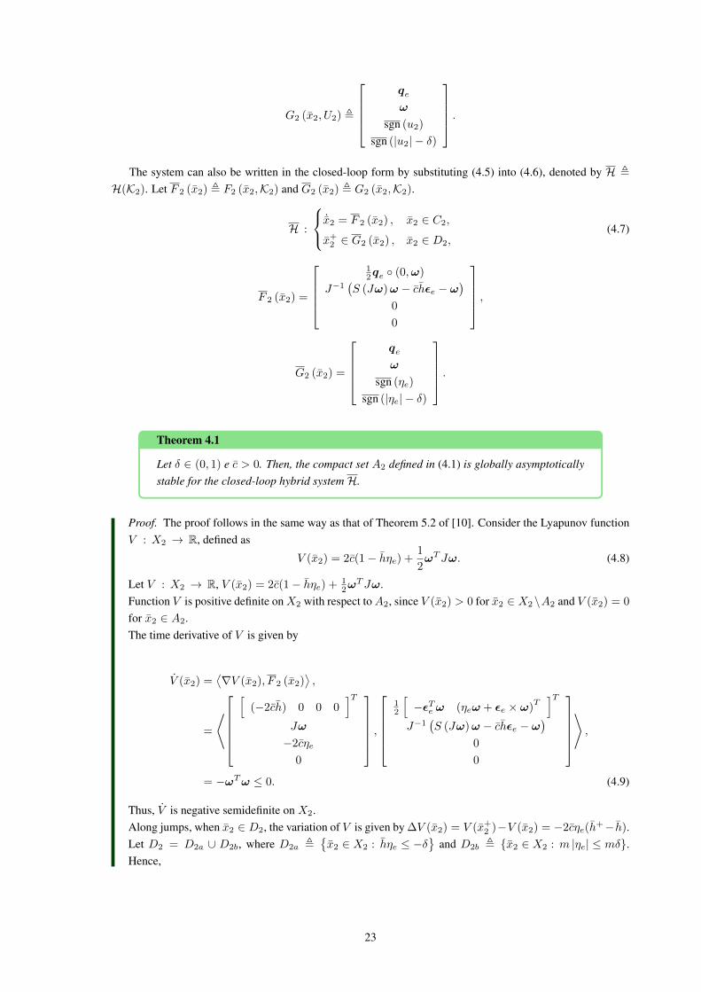
G2 (x2, U2) ,

qeω

sgn (u2)

sgn (|u2| − δ)

.

The system can also be written in the closed-loop form by substituting (4.5) into (4.6), denoted by H ,H(K2). Let F 2 (x2) , F2 (x2,K2) and G2 (x2) , G2 (x2,K2).

H :

˙x2 = F 2 (x2) , x2 ∈ C2,

x+2 ∈ G2 (x2) , x2 ∈ D2,

(4.7)

F 2 (x2) =

12qe (0,ω)

J−1(S (Jω)ω − chεe − ω

)0

0

,

G2 (x2) =

qeω

sgn (ηe)

sgn (|ηe| − δ)

.

Theorem 4.1

Let δ ∈ (0, 1) e c > 0. Then, the compact set A2 defined in (4.1) is globally asymptoticallystable for the closed-loop hybrid systemH.

Proof. The proof follows in the same way as that of Theorem 5.2 of [10]. Consider the Lyapunov functionV : X2 → R, defined as

V (x2) = 2c(1− hηe) +1

2ωTJω. (4.8)

Let V : X2 → R, V (x2) = 2c(1− hηe) + 12ω

TJω.Function V is positive definite onX2 with respect toA2, since V (x2) > 0 for x2 ∈ X2\A2 and V (x2) = 0

for x2 ∈ A2.The time derivative of V is given by

V (x2) =⟨∇V (x2), F 2 (x2)

⟩,

=

⟨[

(−2ch) 0 0 0]T

Jω

−2cηe

0

,

12

[−εTe ω (ηeω + εe × ω)

T]T

J−1(S (Jω)ω − chεe − ω

)0

0

⟩,

= −ωTω ≤ 0. (4.9)

Thus, V is negative semidefinite on X2.Along jumps, when x2 ∈ D2, the variation of V is given by ∆V (x2) = V (x+

2 )−V (x2) = −2cηe(h+− h).

Let D2 = D2a ∪ D2b, where D2a ,x2 ∈ X2 : hηe ≤ −δ

and D2b , x2 ∈ X2 : m |ηe| ≤ mδ.

Hence,

23

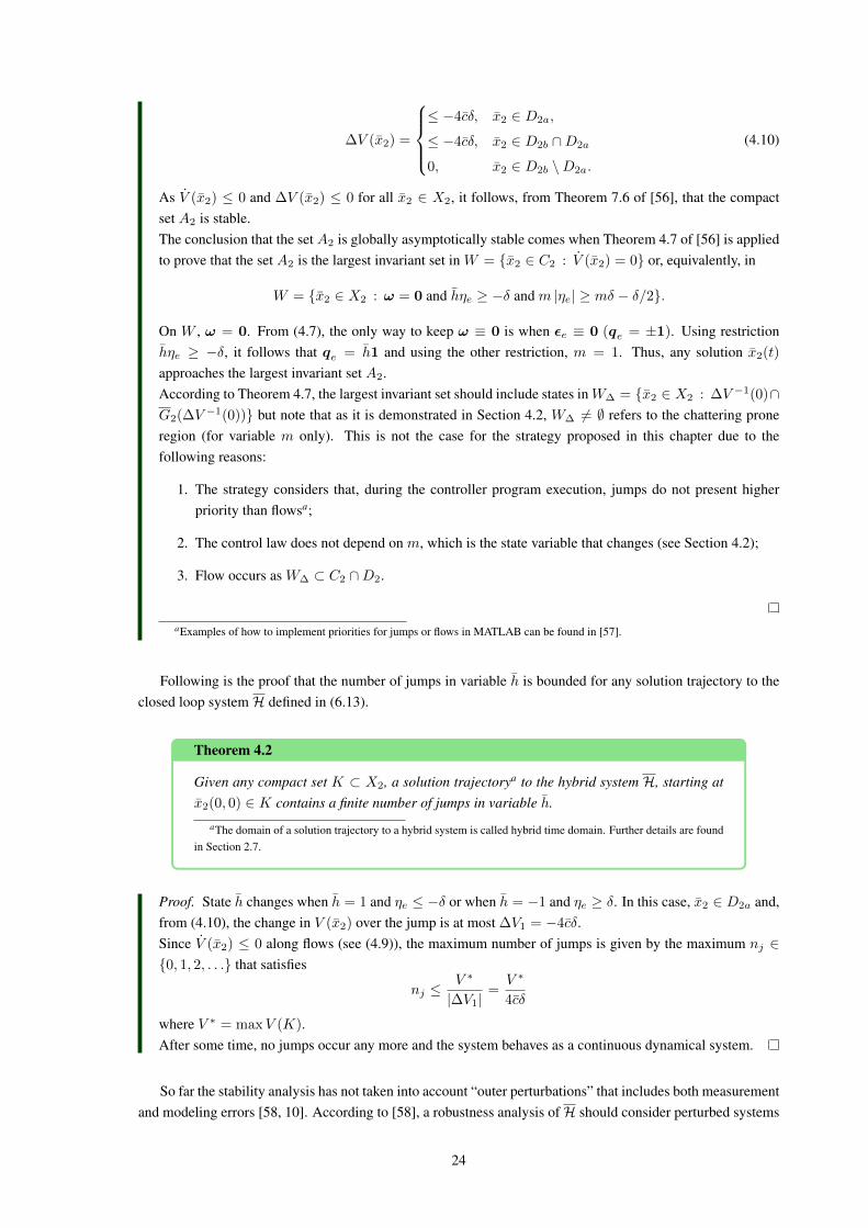
∆V (x2) =

≤ −4cδ, x2 ∈ D2a,

≤ −4cδ, x2 ∈ D2b ∩D2a

0, x2 ∈ D2b \D2a.

(4.10)

As V (x2) ≤ 0 and ∆V (x2) ≤ 0 for all x2 ∈ X2, it follows, from Theorem 7.6 of [56], that the compactset A2 is stable.The conclusion that the set A2 is globally asymptotically stable comes when Theorem 4.7 of [56] is appliedto prove that the set A2 is the largest invariant set in W = x2 ∈ C2 : V (x2) = 0 or, equivalently, in

W = x2 ∈ X2 : ω = 0 and hηe ≥ −δ and m |ηe| ≥ mδ − δ/2.

On W , ω = 0. From (4.7), the only way to keep ω ≡ 0 is when εe ≡ 0 (qe = ±1). Using restrictionhηe ≥ −δ, it follows that qe = h1 and using the other restriction, m = 1. Thus, any solution x2(t)

approaches the largest invariant set A2.According to Theorem 4.7, the largest invariant set should include states inW∆ = x2 ∈ X2 : ∆V −1(0)∩G2(∆V −1(0)) but note that as it is demonstrated in Section 4.2, W∆ 6= ∅ refers to the chattering proneregion (for variable m only). This is not the case for the strategy proposed in this chapter due to thefollowing reasons:

1. The strategy considers that, during the controller program execution, jumps do not present higherpriority than flowsa;

2. The control law does not depend on m, which is the state variable that changes (see Section 4.2);

3. Flow occurs as W∆ ⊂ C2 ∩D2.

aExamples of how to implement priorities for jumps or flows in MATLAB can be found in [57].

Following is the proof that the number of jumps in variable h is bounded for any solution trajectory to theclosed loop systemH defined in (6.13).

Theorem 4.2

Given any compact set K ⊂ X2, a solution trajectorya to the hybrid system H, starting atx2(0, 0) ∈ K contains a finite number of jumps in variable h.

aThe domain of a solution trajectory to a hybrid system is called hybrid time domain. Further details are foundin Section 2.7.

Proof. State h changes when h = 1 and ηe ≤ −δ or when h = −1 and ηe ≥ δ. In this case, x2 ∈ D2a and,from (4.10), the change in V (x2) over the jump is at most ∆V1 = −4cδ.Since V (x2) ≤ 0 along flows (see (4.9)), the maximum number of jumps is given by the maximum nj ∈0, 1, 2, . . . that satisfies

nj ≤V ∗

|∆V1|=V ∗

4cδ

where V ∗ = maxV (K).After some time, no jumps occur any more and the system behaves as a continuous dynamical system.

So far the stability analysis has not taken into account “outer perturbations” that includes both measurementand modeling errors [58, 10]. According to [58], a robustness analysis ofH should consider perturbed systems

24

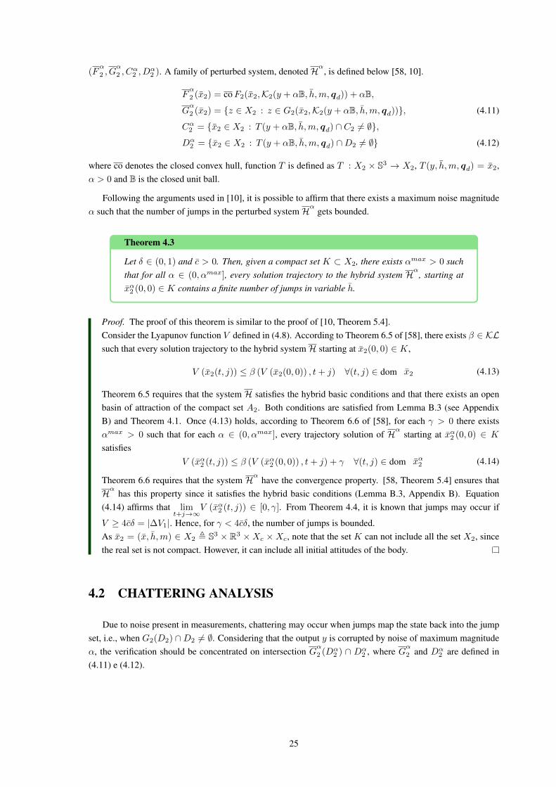
(Fα

2 , Gα

2 , Cα2 , D

α2 ). A family of perturbed system, denotedHα, is defined below [58, 10].

Fα

2 (x2) = coF2(x2,K2(y + αB, h,m, qd)) + αB,

Gα

2 (x2) = z ∈ X2 : z ∈ G2(x2,K2(y + αB, h,m, qd)), (4.11)

Cα2 = x2 ∈ X2 : T (y + αB, h,m, qd) ∩ C2 6= ∅,Dα

2 = x2 ∈ X2 : T (y + αB, h,m, qd) ∩D2 6= ∅ (4.12)

where co denotes the closed convex hull, function T is defined as T : X2 × S3 → X2, T (y, h,m, qd) = x2,α > 0 and B is the closed unit ball.

Following the arguments used in [10], it is possible to affirm that there exists a maximum noise magnitudeα such that the number of jumps in the perturbed systemHα gets bounded.

Theorem 4.3

Let δ ∈ (0, 1) and c > 0. Then, given a compact set K ⊂ X2, there exists αmax > 0 suchthat for all α ∈ (0, αmax], every solution trajectory to the hybrid system Hα, starting atxα2 (0, 0) ∈ K contains a finite number of jumps in variable h.

Proof. The proof of this theorem is similar to the proof of [10, Theorem 5.4].Consider the Lyapunov function V defined in (4.8). According to Theorem 6.5 of [58], there exists β ∈ KLsuch that every solution trajectory to the hybrid systemH starting at x2(0, 0) ∈ K,

V (x2(t, j)) ≤ β (V (x2(0, 0)) , t+ j) ∀(t, j) ∈ dom x2 (4.13)

Theorem 6.5 requires that the system H satisfies the hybrid basic conditions and that there exists an openbasin of attraction of the compact set A2. Both conditions are satisfied from Lemma B.3 (see AppendixB) and Theorem 4.1. Once (4.13) holds, according to Theorem 6.6 of [58], for each γ > 0 there existsαmax > 0 such that for each α ∈ (0, αmax], every trajectory solution of Hα starting at xα2 (0, 0) ∈ K

satisfiesV (xα2 (t, j)) ≤ β (V (xα2 (0, 0)) , t+ j) + γ ∀(t, j) ∈ dom xα2 (4.14)

Theorem 6.6 requires that the system Hα have the convergence property. [58, Theorem 5.4] ensures thatHα has this property since it satisfies the hybrid basic conditions (Lemma B.3, Appendix B). Equation(4.14) affirms that lim

t+j→∞V (xα2 (t, j)) ∈ [0, γ]. From Theorem 4.4, it is known that jumps may occur if

V ≥ 4cδ = |∆V1|. Hence, for γ < 4cδ, the number of jumps is bounded.As x2 = (x, h,m) ∈ X2 , S3 × R3 ×Xc ×Xc, note that the set K can not include all the set X2, sincethe real set is not compact. However, it can include all initial attitudes of the body.

4.2 CHATTERING ANALYSIS

Due to noise present in measurements, chattering may occur when jumps map the state back into the jumpset, i.e., when G2(D2) ∩D2 6= ∅. Considering that the output y is corrupted by noise of maximum magnitudeα, the verification should be concentrated on intersection G

α

2 (Dα2 ) ∩ Dα

2 , where Gα

2 and Dα2 are defined in

(4.11) e (4.12).

25

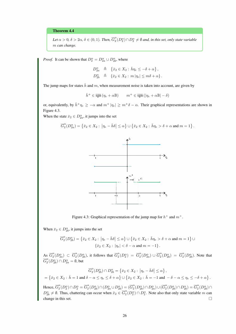
Theorem 4.4

Let α > 0, δ > 2α, δ ∈ (0, 1). Then, Gα

2 (Dα2 )∩Dα

2 6= ∅ and, in this set, only state variablem can change.

Proof. It can be shown that Dα2 = Dα

2a ∪Dα2b, where

Dα2a ,

x2 ∈ X2 : hηe ≤ −δ + α

,

Dα2b , x2 ∈ X2 : m |ηe| ≤ mδ + α .

The jump maps for states h and m, when measurement noise is taken into account, are given by

h+ ∈ sgn (ηe + αB) m+ ∈ sgn (|ηe + αB| − δ)

or, equivalently, by h+ηe ≥ −α and m+ |ηe| ≥ m+δ − α. Their graphical representations are shown inFigure 4.3.When the state x2 ∈ Dα

2a, it jumps into the set

Gα

2 (Dα2a) =

x2 ∈ X2 :

∣∣ηe − hδ∣∣ ≤ α ∪ x2 ∈ X2 : hηe > δ + α and m = 1.

Figure 4.3: Graphical representation of the jump map for h+ and m+.

When x2 ∈ Dα2b, it jumps into the set

Gα

2 (Dα2b) =

x2 ∈ X2 :

∣∣ηe − hδ∣∣ ≤ α ∪ x2 ∈ X2 : hηe > δ + α and m = 1∪

x2 ∈ X2 : |ηe| < δ − α and m = −1 .

As Gα

2 (Dα2a) ⊂ G

α

2 (Dα2b), it follows that G

α

2 (Dα2 ) = G

α

2 (Dα2a) ∪ Gα2 (Dα

2b) = Gα

2 (Dα2b). Note that

Gα

2 (Dα2b) ∩Dα

2a = ∅, but

Gα

2 (Dα2b) ∩Dα

2b =x2 ∈ X2 :

∣∣ηe − hδ∣∣ ≤ α ,=x2 ∈ X2 : h = 1 and δ − α ≤ ηe ≤ δ + α

∪x2 ∈ X2 : h = −1 and − δ − α ≤ ηe ≤ −δ + α

.

Hence, Gα

2 (Dα2 )∩Dα

2 = Gα

2 (Dα2b)∩ (Dα

2a∪Dα2b) = (G

α

2 (Dα2b)∩Dα

2a)∪ (Gα

2 (Dα2b)∩Dα

2b) = Gα

2 (Dα2b)∩

Dα2b 6= ∅. Thus, chattering can occur when x2 ∈ G

α

2 (Dα2 ) ∩Dα

2 . Note also that only state variable m canchange in this set.

26

The HY controller can be considered robust to measurement noise due to the following reasons:

1. The feedback law (3.13) depends on qe, ω and h;

2. qe and ω do not change via jumps and chattering does not occur in variable h (only in m);

3. The proposed strategy considers that, during the controller program execution, jumps do not presenthigher priority than flows;

4. The region of chattering (in variable m) is a subset of C2 ∩D2.

Usually chattering is undesirable and causes unwanted effects as is illustrated for the discontinuous controllerin the next section.

4.3 SIMULATION RESULTS

This section presents simulation results to compare performance of the proposed controller (HY), the dis-continuous controller and the hysteretic controller.

In each simulation, all parameters considered were the same as those used for simulations in [10] to facilitatecomparisons. The inertia matrix used was J = diag(10v), v = [ 1 2 3 ]T /

√14, the control gain c = 1

and parameter δ = 0.4. The initial state of the hysteretic controller was h(0) = 1 and the ones of the proposedcontroller (HY) were h(0) = 1, m(0) = 1. The desired reference was qd = 1 with ωd = 0. The simulationswere performed in MATLAB ambient, using ordinary differential equation solver with variable integration step(ode45) restricted to a maximum step of 1 ms.

The measured value of q (qm) included noise and was calculated as follows: qm = (q + be) / ‖q + be‖2,e = e/ ‖e‖2, where each element e was chosen from a gaussian distribution of zero mean and unitary standarddeviation and b was chosen from a uniform distribution on the interval [0, 0.2].

Figure 4.4 e 4.5 present five graphs each. The first graph, of ηe, shows the attitude evolution either toqe = 1 or qe = −1. The second graph, of hηe, shows not only the evolution to 1 but also the jumps in h. Thethird one presents the variable state m of the HY controller and its jumps. The fourth one shows the evolutionof the angular velocity norm ‖ω‖ and the last one, the energy spent by the applied control feedback strategy√´ t

0τT τdt.

The first scenario (Figure 4.4) illustrates the chattering effect on the discontinuous and the HY controllers.The initial conditions were q(0) = (0, v) and ω(0) = 0. The chattering effect on the discontinuous controllercan be observed in the hηe graph. It induces a lag in response and higher energy consumption. In HY, thiseffect is observed in the m graph, however the system evolution is not affected. Due to the m variable, HYcontroller had a chance to update the discrete variables on the initial moment (h = 1,m = −1). Consequently,it determined a movement toward ηe = 1. Note that depending on the noise on the initial moment, HY couldhave updated h to −1 and determined a movement toward ηe = −1. The system evolution for the hystereticcontroller is not shown as it coincides with the evolution for HY.

The second scenario (Figure 4.5) compares the evolution of the states for the hysteretic and the HY con-trollers when the initial angular velocity direction coincides with the shorter rotation direction. The initialconditions were q(0) = (−0.2,

√1− 0.22v) and ω(0) = 0.3v. This simulation shows that as the initial state

of h for the hysteretic controller is 1, the control law pulls the attitude toward the longer rotation direction(ηe = 1). Thus, the angular velocity decreases, but before the movement is reversed, ηe crosses over the hys-teresis threshold (ηe ≤ −δ). At this moment, h changes to −1 and the control law pulls the attitude toward

27

0 5 10 15 20−1

0

1

DiscontinuousHY

0 5 10 15 20−1

1

0 5 10 15 20−1

1

0 10 20 30 40 50 60 700

0.5

0 10 20 30 40 50 60 700

2

4

Time (s)

1

t 0

τTτdt

1

ω

JOU

RN

AL

OF

LAT E

XC

LA

SSFI

LE

S,V

OL

.11,

NO

.4,D

EC

EM

BE

R20

123

[wid

th=8

cm]fi

g/C

omhi

ster

ese

Fig.

2.St

ate

spac

ere

pres

enta

tion

ofth

ehy

ster

etic

cont

rolle

r(w

ithon

est

ate

h).

Arr

ows

indi

cate

the

dire

ctio

nof

the

torq

ueco

ntri

butio

nte

rm(d

epen

dent

onst

ateh

)so

the

attit

ude

isre

gula

ted

to1

or−1

.The

para

met

erδ

repr

esen

tsth

ehy

ster

esis

half

-wid

thof

the

on-o

ffco

ntro

lfo

rst

ateh

.

The

stat

esp

ace

ofth

ecl

osed

-loo

psy

stem

isre

pres

ente

dby

x1=

(xp,x

c1)∈X

1:=

Xp×

Xc.

The

cont

rolle

rob

ject

ive

isto

glob

ally

asym

ptot

ical

lyst

abi-

lize

the

set

A1=

x1∈X

1:qe=

h1,ω

= 0 .

(5)

The

clos

ed-l

oop

syst

emis

give

nby

(2),

(3)

and

the

follo

w-

ing

dyna

mic

sof

the

cont

rolle

r.

˙ h=

0x1∈C

1:=

x1∈X

1:hη e

≥−δ ,

h+∈

sgn(u

1)

x1∈D

1:=

x1∈X

1:hη e

≤−δ ,

(6)

whe

reh+

isth

eva

lue

asso

ciat

edto

hju

staf

ter

the

stat

etr

ansi

tion

and

sgn(η)=

sgn(η),

|ηe|>

0,

−1,1,

η e=

0.

The

vect

orof

inpu

tsU1=

(τ,u

1)

isca

lcul

ated

asfo

llow

s:τ y,q

d,h

=−ch e

−ω

andu1

y,q

d,h

=η e

.A

sal

read

ym

entio

ned,

hde

term

ines

the

orie

ntat

ion

ofa

forc

eal

ong

the

axis

ofro

tatio

n.W

hile

hη e

≥0

,it

forc

esth

em

ovem

ent

toth

esh

orte

rro

tatio

ndi

rect

ion.

How

ever

,w

hen

hη e

<0,

the

forc

est

illpu

llsin

the

sam

edi

rect

ion

(the

long

erro

tatio

ndi

rect

ion)

until

asa

fedi

stan

ceis

achi

eved

topr

even

tch

atte

ring

,i.e

.,un

tilhη e

≤−δ.

III.

PR

OP

OS

ED

CO

NT

RO

LL

ER

As

the

hyst

eret

icco

ntro

ller,

ina

spec

ific

regi

onof

the

stat

esp

ace,

dete

rmin

esa

forc

eco

ntri

butio

nto

mak

eth

eri

gid-

body

evol

ves

toth

elo

nger

rota

tion

dire

ctio

n,w

epr

opos

eto

add

one

mor

est

ate

toth

eco

ntro

ller

topr

even

tth

isbe

havi

oran

dsa

veen

ergy

.T

hepr

opos

edco

ntro

ller

feed

back

torq

ueis

also

give

nby

(4),

but

itha

stw

ost

ates

xc2=

h,m

∈X

c×

Xc,X

c:=

−1,1

.

The

stat

eh

dete

rmin

esth

efe

edba

ckto

rque

cont

ribu

tion

inor

dert

om

oveqe

eith

erto

1or

−1

,as

wel

las

inth

ehy

ster

etic

cont

rol.

The

stat

em

=1

indi

cate

sth

at|η

e|h

asre

ache

dov

erth

ehy

ster

esis

wid

thva

lue

butη e

has

not

cros

sed

zero

yet.

The

stat

em

=−1

indi

cate

sth

eop

posi

te,

that

η eha

sal

read

ycr

osse

dze

robu

t|η e|h

asno

trea

ched

over

the

hyst

eres

isw

idth

valu

eye

t.T

hesp

ace

stat

eof

the

clos

ed-l

oop

syst

emis

repr

esen

ted

by

x2=

(x,x

c2)∈X

2:=

X×

Xc×

Xc.

The

cont

rolle

rob

ject

ive

isto

glob

ally

asym

ptot

ical

lyst

abili

zeth

ese

t

A2=

x2∈X

2:qe=

h1,m

=1,ω= 0 .

(7)

The

clos

ed-l

oop

syst

emis

give

nby

(2),

(3)

and

the

follo

w-

ing

dyna

mic

sof

the

cont

rolle

r.˙ h=

0m

=0

x2∈C

2,

h+∈

sgn(u

2)

m+∈u3sg

n(u

2−u3δ/2)

x2∈D

2,

(8)

C2:=

x2∈X

2: h

η e≥

−δ , h

=−1

or

m(η

e−

δ/2)

≥−δ)

, h=

1orm(η

e+δ/2)

≤δ

,

D2:=

x2∈X

2: h

η e≤

−δ or

h=

1,

m(η

e−

δ/2)

≤−δ)

or h

=−1,m

(ηe+δ/2)

≥δ

.

whe

rem

+an

dh+

are

valu

esas

soci

ated

tom

andh

,res

pec-

tivel

y,ju

staf

ter

stat

etr

ansi

tion.

The

setD

2ca

nbe

expr

esse

din

aco

mpa

ctfo

rmas

follo

ws

D2:=

x2∈X

2: h

η e≤

−δ or

mh(η

e−hδ/2)

≤−δ

.

The

vect

orof

inpu

tsU2

=(τ,u

2,u

3)

isca

lcul

ated

asfo

llow

s:τ y,q

d,h

,m =

−ch e

−ω

,u2

y,q

d,h

,m =

η ean

du3

y,q

d,h

,m =

h.

[wid

th=8

cm]fi

g/fig

Prop

osto

Fig.

3.St

ate

spac

ere

pres

enta

tion

show

ing

the

prop

osed

regu

latio

nw

ithtw

ost

ates

(han

dm

).A

rrow

sin

dica

teth

edi

rect

ion

ofth

eto

rque

cont

ribu

tion

term

(dep

ende

nton

stat

eh

)so

the

attit

ude

isre

gula

ted

to1

or−1

.The

para

met

erδ

repr

esen

tsth

ehy

ster

esis

half

-wid

thof

the

on-o

ffco

ntro

lfo

rst

ateh

and

also

ofth

eon

-off

cont

rol

for

stat

em

.

Fig.

3sh

ows

the

prop

osed

regu

latio

n.W

hen

stat

em

=−1,

the

cont

rolle

rbe

have

sas

the

hyst

eret

icco

ntro

ller.

Ifh=

1,st

ateh

chan

ges

to−1

whe

nη e

≤−δ;

ifh

=−1,

stat

eh

chan

ges

to1

whe

nη e

≥δ.

The

cont

rolle

rsw

itche

sto

stat

em

=1

whe

nth

eat

titud

eer

rorqe

pres

ents

η e≤

−2δ

orη e

≥2δ

.W

hen

stat

em

=1,

the

cont

rolle

rbe

have

sas

the

disc

ontin

uous

cont

rolle

r.In

othe

rw

ords

,if

stat

em

=1,

stat

em

will

chan

geto

m=

−1

whe

nη e

goes

acro

ssze

roan

den

ter

the

jum

pse

t.T

his

fact

,ant

icip

ate

the

chan

geof

stat

eh

.Thi

sdi

stin

ctbe

havi

oris

wha

tdi

ffer

entia

tes

itfr

omth

ehy

ster

etic

cont

rolle

r(6

)an

dal

low

sa

torq

ueco

ntri

butio

nto

war

dsth

esh

orte

rro

tatio

ndi

rect

ion.

A.

Stab

ility

anal

ysis

Con

side

rth

ecl

osed

-loo

psy

stem

ofth

epr

opos

edco

ntro

ller

(8)

rew

ritte

nac

cord

ing

toth

ehy

brid

syst

ems

fram

ewor

kof

[11]

and

give

nby

H=

˙ x2∈F2(x

2),

x2∈C

2,

x+ 2∈G

2(x

2),

x2∈D

2,

whe

rex2=

(qe,ω

,h,m

),

F2(x

2):=

1 2qe(0,ω

)J−1 S

(Jω)ω−

ch e

−ω

0 0

,

G2(x

2):=

qe ω

sgn(η

e)

hsg

n η e

−hδ/2

.

1

hη e

1

m

Figure 4.4: Comparison between the discontinuous controller and the proposed HY controller.

the shorter rotation direction (ηe = −1). On the other hand, HY controller decides, in the initial moments, tochange h to −1 and the feedback pulls the attitude toward the shorter direction (ηe = −1) . Consequently, thesystem energy consumption is higher when the hysteretic controller is applied. The system evolution for thediscontinuous controller is not shown as it coincides with the evolution for HY.

4.4 CHAPTER CONCLUSIONS

The proposed hybrid control globally asymptotically stabilizes the attitude of a rigid body and is robustagainst noise measurement. It also preserves the good characteristics of the hysteretic controller by avoidingthe undesirable effects of unwinding and chattering due to measurement noise. Given that, during the controllerprogram execution, jumps do not present higher priority than flows, the chattering that occurs in the secondstate variable m does not disturb the evolution of the system.

With one more state variable than the hysteretic controller, the HY controller is able to detect when thereference changes abruptly or when the current attitude is far from the reference on the initial instant. Thisway, it has more opportunities to determine the new state of variable h, is more likely to take the shorterrotation direction and spend less energy.

This study was presented at the XII Simpósio Brasileiro de Automação Inteligente - SBAI 2015 and anonline publication of the respective article is available at http://swge.inf.br/SBAI2015/anais/413.pdf.

28

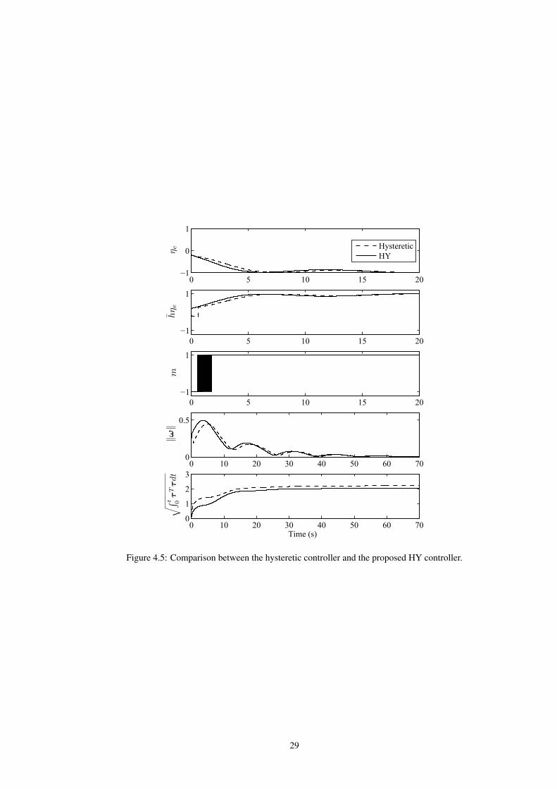
0 5 10 15 20−1

0

1

HystereticHY

0 5 10 15 20−1

1

0 5 10 15 20−1

1

0 10 20 30 40 50 60 700

0.5

0 10 20 30 40 50 60 700

1

2

3

Time (s)

1

m

1

t 0

τTτdt

1

ω

JOU

RN

AL

OF

LAT E

XC

LA

SSFI

LE

S,V

OL

.11,

NO

.4,D

EC

EM

BE

R20

123

[wid

th=8

cm]fi

g/C

omhi

ster

ese

Fig.

2.St

ate

spac

ere

pres

enta

tion

ofth

ehy

ster

etic

cont

rolle

r(w

ithon

est

ate

h).

Arr

ows

indi

cate

the

dire

ctio

nof

the

torq

ueco

ntri

butio

nte

rm(d

epen

dent

onst

ateh

)so

the

attit

ude

isre

gula

ted

to1

or−1

.The

para

met

erδ

repr

esen

tsth

ehy

ster

esis

half

-wid

thof

the

on-o

ffco

ntro

lfo

rst

ateh

.

The

stat

esp

ace

ofth

ecl

osed

-loo

psy

stem

isre

pres

ente

dby

x1=

(xp,x

c1)∈X

1:=

Xp×

Xc.

The

cont

rolle

rob

ject

ive

isto

glob

ally

asym

ptot

ical

lyst

abi-

lize

the

set

A1=

x1∈X

1:qe=

h1,ω

= 0 .

(5)

The

clos

ed-l

oop

syst

emis

give

nby

(2),

(3)

and

the

follo

w-

ing

dyna

mic

sof

the

cont

rolle

r.

˙ h=

0x1∈C

1:=

x1∈X

1:hη e

≥−δ ,

h+∈

sgn(u

1)

x1∈D

1:=

x1∈X

1:hη e

≤−δ ,

(6)

whe

reh+

isth

eva

lue

asso

ciat

edto

hju

staf

ter

the

stat

etr

ansi

tion

and

sgn(η)=

sgn(η),

|ηe|>

0,

−1,1,

η e=

0.

The

vect

orof

inpu

tsU1=

(τ,u

1)

isca

lcul

ated

asfo

llow

s:τ y,q

d,h

=−ch e

−ω

andu1

y,q

d,h

=η e

.A

sal

read

ym

entio

ned,

hde

term

ines

the

orie

ntat

ion

ofa

forc

eal

ong

the

axis

ofro

tatio

n.W

hile

hη e

≥0

,it

forc

esth

em

ovem

ent

toth

esh

orte

rro

tatio

ndi

rect

ion.

How

ever

,w

hen

hη e

<0,

the

forc

est

illpu

llsin

the

sam

edi

rect

ion

(the

long

erro

tatio

ndi

rect

ion)

until

asa

fedi

stan

ceis

achi

eved

topr

even

tch

atte

ring

,i.e

.,un

tilhη e

≤−δ.

III.

PR

OP

OS

ED

CO

NT

RO

LL

ER

As

the

hyst

eret

icco

ntro

ller,

ina

spec

ific

regi

onof

the

stat

esp

ace,

dete

rmin

esa

forc

eco

ntri

butio

nto

mak

eth

eri

gid-

body

evol

ves

toth

elo

nger

rota

tion

dire

ctio

n,w

epr

opos

eto

add

one

mor

est

ate

toth

eco

ntro

ller

topr

even

tth

isbe

havi

oran

dsa

veen

ergy

.T

hepr

opos

edco

ntro

ller

feed

back

torq

ueis

also

give

nby

(4),

but

itha

stw

ost

ates

xc2=

h,m

∈X

c×

Xc,X

c:=

−1,1

.

The

stat

eh

dete

rmin

esth

efe

edba

ckto

rque

cont

ribu

tion

inor

dert

om

oveqe

eith

erto

1or

−1

,as

wel

las

inth

ehy

ster

etic

cont

rol.

The

stat

em

=1

indi

cate

sth

at|η

e|h

asre

ache

dov

erth

ehy

ster

esis

wid

thva

lue

butη e

has

not

cros

sed

zero

yet.

The

stat

em

=−1

indi

cate

sth

eop

posi

te,

that

η eha

sal

read

ycr

osse

dze

robu

t|η e|h

asno

trea

ched

over

the

hyst

eres

isw

idth

valu

eye

t.T

hesp

ace

stat

eof

the

clos

ed-l

oop

syst

emis

repr

esen

ted

by

x2=

(x,x

c2)∈X

2:=

X×

Xc×

Xc.

The

cont

rolle

rob

ject

ive

isto

glob

ally

asym

ptot

ical

lyst

abili

zeth

ese

t

A2=

x2∈X

2:qe=

h1,m

=1,ω= 0 .

(7)

The

clos

ed-l

oop

syst

emis

give

nby

(2),

(3)

and

the

follo

w-

ing

dyna

mic

sof

the

cont

rolle

r.˙ h=

0m

=0

x2∈C

2,

h+∈

sgn(u

2)

m+∈u3sg

n(u

2−u3δ/2)

x2∈D

2,

(8)

C2:=

x2∈X

2: h

η e≥

−δ , h

=−1

or

m(η

e−

δ/2)

≥−δ)

, h=

1orm(η

e+δ/2)≤

δ,

D2:=

x2∈X

2: h

η e≤

−δ or

h=

1,

m(η

e−

δ/2)

≤−δ)

or h

=−1,m

(ηe+δ/2)≥

δ.

whe

rem

+an

dh+

are

valu

esas

soci

ated

tom

andh

,res

pec-

tivel

y,ju

staf

ter

stat

etr

ansi

tion.

The

setD

2ca

nbe

expr

esse

din

aco

mpa

ctfo

rmas

follo

ws

D2:=

x2∈X

2: h

η e≤

−δ or

mh(η

e−hδ/2)≤

−δ

.

The

vect

orof

inpu

tsU2

=(τ,u

2,u

3)

isca

lcul

ated

asfo

llow

s:τ y,q

d,h

,m =

−ch e

−ω

,u2

y,q

d,h

,m =

η ean

du3

y,q

d,h

,m =

h.

[wid

th=8

cm]fi

g/fig

Prop

osto

Fig.

3.St

ate

spac

ere

pres

enta

tion

show

ing

the

prop

osed

regu

latio

nw

ithtw

ost

ates

(han

dm

).A

rrow

sin

dica

teth

edi

rect

ion

ofth

eto

rque

cont

ribu

tion

term

(dep

ende

nton

stat

eh

)so

the

attit

ude

isre

gula

ted

to1

or−1

.The

para

met

erδ

repr

esen

tsth

ehy

ster

esis

half

-wid

thof

the

on-o

ffco

ntro

lfo

rst

ateh

and

also

ofth

eon

-off

cont

rol

for

stat

em

.

Fig.

3sh

ows

the

prop

osed

regu

latio

n.W

hen

stat

em

=−1,

the

cont

rolle

rbe

have

sas

the

hyst

eret

icco

ntro

ller.

Ifh=

1,st

ateh

chan

ges

to−1

whe

nη e

≤−δ;

ifh

=−1,

stat

eh

chan

ges

to1

whe

nη e

≥δ.

The

cont

rolle

rsw

itche

sto

stat

em

=1

whe

nth

eat

titud

eer

rorqe

pres

ents

η e≤

−2δ

orη e

≥2δ

.W

hen

stat

em

=1,

the

cont

rolle

rbe

have

sas

the

disc

ontin

uous

cont

rolle

r.In

othe

rw

ords

,if

stat

em

=1,

stat

em

will

chan

geto

m=

−1

whe

nη e

goes

acro

ssze

roan

den

ter

the

jum

pse

t.T

his

fact

,ant

icip

ate

the

chan

geof

stat

eh

.Thi

sdi

stin

ctbe

havi

oris

wha

tdi

ffer

entia

tes

itfr

omth

ehy

ster

etic

cont

rolle

r(6

)an

dal

low

sa

torq

ueco

ntri

butio

nto

war

dsth

esh

orte

rro

tatio

ndi

rect

ion.

A.

Stab

ility

anal

ysis

Con

side

rth

ecl

osed

-loo

psy

stem

ofth

epr

opos

edco

ntro

ller

(8)

rew

ritte

nac

cord

ing

toth

ehy

brid

syst

ems

fram

ewor

kof

[11]

and

give

nby

H=

˙ x2∈F2(x

2),

x2∈C

2,

x+ 2∈G

2(x

2),

x2∈D

2,

whe

rex2=

(qe,ω

,h,m

),

F2(x

2):=

1 2qe(0,ω

)J−1 S

(Jω)ω−

ch e

−ω

0 0

,

G2(x

2):=

qe ω

sgn(η

e)

hsg

n η e

−hδ/2

.

1

hη e

Figure 4.5: Comparison between the hysteretic controller and the proposed HY controller.

29

PROPOSED BIMODAL HYBRID ATTITUDECONTROLLER

In Chapter 4 it was shown that the introduction of a new mode m allows less expensive solutions. However, itpresents the disadvantage of having restriction in the software implementation and the chattering phenomenonin variable m. In order to avoid chattering (and also the restriction on the software implementation), it isproposed in this chapter that both controller states, h and also m, should have a hysteresis structure, such that,the hysteresis half-width of the on-off control for state m is δ (a lower value would induce chattering) and theone for state h is δa ∈ δ/2, δ, adapted according to the state of m. The shorter width being set when state mindicates that body has moved away from the chattering prone region.

The proposed hybrid controller, called bimodal controller, has two state variables(h,m

)∈ Xc×Xc, Xc ,

−1, 1. As in the hysteretic controller, the state h determines the “proportional” term direction of the torquefeedback in order to move qe either to 1 or−1. The state m is introduced in order to adapt the hysteresis widthδa of the on-off control for state h.

In the bimodal controller, it is considered the same torque feedback suggested by [54], given by

τ 2 = −chεe −Kωω, (5.1)

where Kω = KTω > 0. Adding matrix Kω to (3.13) gives more freedom to tune the control torque. For

practical purposes, this extra torque parameter Kω allows, for instance, the design of a bounded torque and totake into account the constraints of the angular velocity sensors, i.e., the slew rate limits [59] (see example inSection 5.3.2).

Let the state of the system plant + controller be represented by x2 = (x, h,m) ∈ X2 , X ×Xc×Xc. Thecomplete system is given by (2.10), (2.11) and the following dynamics of the controller:

˙h = 0

m = 0

x2 ∈ C2,

h+ ∈ sgn (u2 − u3δ/2)

m+ ∈ u3 sgn (u2 − u3δ/2)

x2 ∈ D2,

(5.2)

C2 ,x2 ∈ X2 :

(hηe ≥ −δ

)and (5.3)(

m = −1 or hηe ≥ −δ/2)

and(m = 1 or hηe ≤ 3δ/2

),

D2 ,x2 ∈ X2 :

(hηe ≤ −δ

)or (5.4)(

m = 1 and hηe ≤ −δ/2)

or(m = −1 and hηe ≥ 3δ/2

),

where m+ and h+ are values associated to m and h, respectively, just after state transition. Note that C2 =

X2 \D2. The sets C2 and D2 are depicted in Figure 5.1.

30

5

Figure 5.1: Graphical representation of sets C2 and D2.

The vector of inputs of the controller is U2 = (τ , u2, u3) and the closed-loop is achieved by setting

U2 = K2(y, h,m, qd) , (−chεe −Kωω, ηe, h). (5.5)

The behavior of the controller can be seen in Figure 5.2.





x1 = (xp, xc1) ∈ X1 := Xp ×Xc.


A1 =x1 ∈ X1 : qe = h1, ω = 0

. (5)


˙h = 0 x1 ∈ C1 :=x1 ∈ X1 : hηe ≥ −δ

,

h+ ∈ sgn (u1) x1 ∈ D1 :=x1 ∈ X1 : hηe ≤ −δ

,


sgn (η) =

sgn (η) , |ηe| > 0,

−1, 1 , ηe = 0.



y, qd, h

= ηe.





xc2 =h,m

∈ Xc ×Xc, Xc := −1, 1 .



x2 = (x, xc2) ∈ X2 := X ×Xc ×Xc.


A2 =x2 ∈ X2 : qe = h1,m = 1, ω = 0

. (7)


˙h = 0m = 0

x2 ∈ C2,

h+ ∈ sgn (u2)m+ ∈ u3sgn (u2 − u3δ/2)

x2 ∈ D2,

(8)

C2 :=x2 ∈ X2 :

hηe ≥ −δ

,h = −1 or

m(ηe − δ/2) ≥ −δ) ,h = 1 orm(ηe + δ/2) ≤ δ

,

D2 :=x2 ∈ X2 :

hηe ≤ −δ

or

h = 1,

m(ηe − δ/2) ≤ −δ) orh = −1,m(ηe + δ/2) ≥ δ

.


D2 :=x2 ∈ X2 :

hηe ≤ −δ


.


y, qd, h,m

= −che − ω, u2

y, qd, h,m

= ηe

and u3

y, qd, h,m

= h.






H =

˙x2 ∈ F2 (x2) , x2 ∈ C2,

x+2 ∈ G2 (x2) , x2 ∈ D2,


F2 (x2) :=

12qe(0, ω)


00

,

G2 (x2) :=

qeω

sgn (ηe)hsgn

ηe − hδ/2

.

1

δ

1

1

1

0

1

−3δ/2

1

−1





x1 = (xp, xc1) ∈ X1 := Xp ×Xc.


A1 =x1 ∈ X1 : qe = h1, ω = 0

. (5)


˙h = 0 x1 ∈ C1 :=x1 ∈ X1 : hηe ≥ −δ

,

h+ ∈ sgn (u1) x1 ∈ D1 :=x1 ∈ X1 : hηe ≤ −δ

,


sgn (η) =

sgn (η) , |ηe| > 0,

−1, 1 , ηe = 0.



y, qd, h

= ηe.





xc2 =h,m

∈ Xc ×Xc, Xc := −1, 1 .



x2 = (x, xc2) ∈ X2 := X ×Xc ×Xc.


A2 =x2 ∈ X2 : qe = h1,m = 1, ω = 0

. (7)


˙h = 0m = 0

x2 ∈ C2,

h+ ∈ sgn (u2)m+ ∈ u3sgn (u2 − u3δ/2)

x2 ∈ D2,

(8)

C2 :=x2 ∈ X2 :

hηe ≥ −δ

,h = −1 or

m(ηe − δ/2) ≥ −δ) ,h = 1 orm(ηe + δ/2) ≤ δ

,

D2 :=x2 ∈ X2 :

hηe ≤ −δ

or

h = 1,

m(ηe − δ/2) ≤ −δ) orh = −1,m(ηe + δ/2) ≥ δ

.


D2 :=x2 ∈ X2 :

hηe ≤ −δ


.


y, qd, h,m

= −che − ω, u2

y, qd, h,m

= ηe

and u3

y, qd, h,m

= h.






H =

˙x2 ∈ F2 (x2) , x2 ∈ C2,

x+2 ∈ G2 (x2) , x2 ∈ D2,


F2 (x2) :=

12qe(0, ω)


00

,

G2 (x2) :=

qeω

sgn (ηe)hsgn

ηe − hδ/2

.

1

h = 1

1

3δ/2

1

δ/2

1

1

1

0

1

−1

1

−δ

1

−δ/2

1

h = −1

1

h = 1 1

h = −1

1

e

1

e

1

m = 1

1

m = −1

Figure 5.2: State space representation and the proposed regulation with two state variables (h and m). Arrowsindicate the direction of the “proportional” term of the torque (dependent on h) so the attitude is regulated to 1

or −1. The hysteresis half-width of the on-off control for state h is δ/2 when m = 1 and δ when m = −1.

The parameter δ ∈ (0, 1) is used to define the basic hysteresis width. The state m has the effect of adaptingthe hysteresis width δa of the on-off control for state h. For m = −1, δa = δ and the controller behaves as thehysteretic controller (h changes when hηe ≤ −δ). For m = 1, δa = δ/2 and h changes when hηe ≤ −δ/2.This distinct behavior is what differentiates the proposed controller from the hysteretic controller by allowingthe change of state h to be anticipated and, consequently, the change of direction of the “proportional” term of

31

the torque contribution towards the shorter rotation direction. The controller switches m from −1 to 1 whenhηe ≥ 3δ/2, that is, when the attitude is far from the chattering prone region and switches m from 1 to −1

when hηe ≤ −δ/2. Note that the controller was designed so that m switches from 1 to −1 together with thechange of h.

It will be shown in the next section that the controller globally asymptotically stabilizes the set

A2 =x2 ∈ X2 : qe = h1, m = 1 and ω = 0

. (5.6)

The following sections will enable us to compare performance of the bimodal controller with the hystereticcontroller. In this comparison, if both controllers use the same value of δ, say, δ = δ, then simulation ex-periments show that the bimodal controller spends less energy on average (see Section 5.3). If the hystereticcontroller uses δ = δ/2 and the bimodal controller uses δ = δ then, from Theorem 5.1 below, the bimodal con-troller avoids chattering for measurement noise of magnitude α < δ/2 while the hysteretic controller avoidschattering only for α < δ/4. That is, the bimodal controller is not just the hysteretic controller with halfhysteresis width, but it is indeed a middle term solution which spends less energy in average while keepingrobustness.


Considering the proposed bimodal controller (5.2), the system can be written as a function of the vector ofinputs, U2, as follows

H(U2) :

˙x2 = F2 (x2, U2) , x2 ∈ C2,

x+2 ∈ G2 (x2, U2) , x2 ∈ D2,

(5.7)

where x2 = (qe,ω, h,m), U2 = (τ , u2, u3),

F2 (x2, U2) ,

12qe (0,ω)

J−1 (S (Jω)ω + τ )

0

0

,

G2 (x2, U2) ,

qeω

sgn (u2 − u3δ/2)

u3 sgn (u2 − u3δ/2)

.By substituting (5.5) in (5.7), it can be written in the closed-loop form, denoted as H , H(K2). Let

F 2 (x2) , F2 (x2,K2) and G2 (x2) , G2 (x2,K2).

H :

˙x2 = F 2 (x2) , x2 ∈ C2,

x+2 ∈ G2 (x2) , x2 ∈ D2,

(5.8)

F 2 (x2) =

12qe (0,ω)

J−1(S (Jω)ω − chεe −Kωω

)0

0

, (5.9)

G2 (x2) =

qeω

sgn(ηe − hδ/2

)h sgn

(ηe − hδ/2

) . (5.10)

32

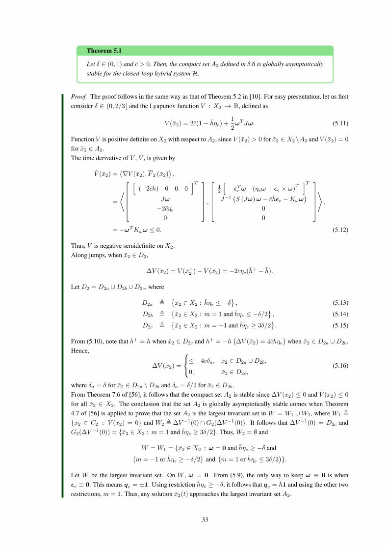
Theorem 5.1

Let δ ∈ (0, 1) and c > 0. Then, the compact set A2 defined in 5.6 is globally asymptoticallystable for the closed-loop hybrid systemH.

Proof. The proof follows in the same way as that of Theorem 5.2 in [10]. For easy presentation, let us firstconsider δ ∈ (0, 2/3 ] and the Lyapunov function V : X2 → R, defined as

V (x2) = 2c(1− hηe) +1

2ωTJω. (5.11)

Function V is positive definite onX2 with respect toA2, since V (x2) > 0 for x2 ∈ X2\A2 and V (x2) = 0

for x2 ∈ A2.The time derivative of V , V , is given by

V (x2) =⟨∇V (x2), F 2 (x2)

⟩,

=

⟨[

(−2ch) 0 0 0]T

Jω

−2cηe

0

,

12

[−εTe ω (ηeω + εe × ω)

T]T

J−1(S (Jω)ω − chεe −Kωω

)0

0

⟩,

= −ωTKωω ≤ 0. (5.12)

Thus, V is negative semidefinite on X2.Along jumps, when x2 ∈ D2,

∆V (x2) = V (x+2 )− V (x2) = −2cηe(h

+ − h).

Let D2 = D2a ∪D2b ∪D2c, where

D2a ,x2 ∈ X2 : hηe ≤ −δ

, (5.13)

D2b ,x2 ∈ X2 : m = 1 and hηe ≤ −δ/2

, (5.14)

D2c ,x2 ∈ X2 : m = −1 and hηe ≥ 3δ/2

. (5.15)

From (5.10), note that h+ = h when x2 ∈ D2c and h+ = −h(∆V (x2) = 4chηe

)when x2 ∈ D2a ∪D2b.

Hence,

∆V (x2) =

≤ −4cδa, x2 ∈ D2a ∪D2b,

0, x2 ∈ D2c,(5.16)

where δa = δ for x2 ∈ D2a \D2b and δa = δ/2 for x2 ∈ D2b.From Theorem 7.6 of [56], it follows that the compact set A2 is stable since ∆V (x2) ≤ 0 and V (x2) ≤ 0

for all x2 ∈ X2. The conclusion that the set A2 is globally asymptotically stable comes when Theorem4.7 of [56] is applied to prove that the set A2 is the largest invariant set in W = W1 ∪W2, where W1 ,

x2 ∈ C2 : V (x2) = 0 and W2 , ∆V −1(0) ∩G2(∆V −1(0)). It follows that ∆V −1(0) = D2c andG2(∆V −1(0)) = x2 ∈ X2 : m = 1 and hηe ≥ 3δ/2. Thus, W2 = ∅ and

W = W1 = x2 ∈ X2 : ω = 0 and hηe ≥ −δ and(m = −1 or hηe ≥ −δ/2

)and

(m = 1 or hηe ≤ 3δ/2

).

Let W be the largest invariant set. On W , ω = 0. From (5.9), the only way to keep ω ≡ 0 is whenεe ≡ 0. This means qe = ±1. Using restriction hηe ≥ −δ, it follows that qe = h1 and using the other tworestrictions, m = 1. Thus, any solution x2(t) approaches the largest invariant set A2.

33

This controller restricts parameter δ to a value lower than or equal to δ∗ = 2/3, δ ∈ (0, δ∗ ]. For thecase δ ∈ (2/3, 1), the system still behaves as proposed until state m changes to −1 (i.e. until the firstjump, in case m(0) = 1). Afterwards, the controller works as the hysteretic controller, since m will notchange any more. The proof of stability for this case follows by similar arguments used to prove the caseδ ∈ (0, 2/3 ].

Following is the proof that the number of jumps is bounded for any solution trajectory to the closed loopsystem H defined in (6.13). In other words, no Zeno solutions (infinite number of jumps in a finite amount oftime [49, Definition 2.5] occur using the bimodal controller.

Theorem 5.2

Given any compact set K ⊂ X2, a solution trajectorya to the hybrid system H, starting atx2(0, 0) ∈ K contains a finite number of jumps.

aThe domain of a solution trajectory to a hybrid system is called hybrid time domain. Further details are foundin Section 2.7.

Proof. There are three types of controller state changes. The first one is when state m = −1 and only stateh changes. It happens when h = 1 and ηe ≤ −δ or when h = −1 and ηe ≥ δ. In this case, x2 ∈ D2a \D2b

and, from (5.16), the change in V (x2) over the jump is at most ∆V1 = −4cδ.The second one is when statem = −1 and only statem changes to 1. It happens when h = 1 and ηe ≥ 3δ/2

or when h = −1 and ηe ≤ −3δ/2. In this case, x2 ∈ D2c and ∆V2 = 0 since V (x2) does not depend onstate m.The last one is when state m = 1 and both states, h and m, change. It happens when h = 1 and ηe ≤ −δ/2or when h = −1 and ηe ≥ δ/2. In this case, x2 ∈ D2b and, from (5.16), the change in V (x2) is at most∆V3 = −2cδ. Note that this third controller state change is only possible if the second one has happenedpreviously.Summing up, V (x2) varies at most ∆V1 = −4cδ each time the controller state change occurs according tothe first type of change and at most ∆V2 + ∆V3 = −2cδ each time a sequence of two jumps occurs (secondtype followed by the third type). Since V (x2) ≤ 0 along flows (see (5.12)), the maximum number of jumpsis given by the maximum nj ∈ 0, 1, 2, . . . that satisfies

nj ≤2V ∗

|∆V2 + ∆V3|+ 1 =

2V ∗

2cδ+ 1 =

V ∗

cδ+ 1

where V ∗ = maxV (K). The unit added on the amount of jumps refers to the case when the initial state ofm is −1 and its final state is 1.After some time, no jumps occur any more and the system behaves as a continuous dynamical system.

So far the stability analysis has not taken into account “outer perturbations” that includes both measurementand modeling errors [58, 10]. According to [58], a robustness analysis ofH should consider perturbed systems(F

α

2 , Gα

2 , Cα2 , D

α2 ). A family of perturbed system, denotedHα, is defined below [58, 10].

Fα

2 (x2) = coF2(x2,K2(y + αB, h,m, qd)) + αB,

Gα

2 (x2) = z ∈ X2 : z ∈ G2(x2,K2(y + αB, h,m, qd)), (5.17)

Cα2 = x2 ∈ X2 : T (y + αB, h,m, qd) ∩ C2 6= ∅,Dα

2 = x2 ∈ X2 : T (y + αB, h,m, qd) ∩D2 6= ∅ (5.18)

where co denotes the closed convex hull, function T is defined as T : X2 × S3 → X2, T (y, h,m, qd) = x2,α > 0 and B is the closed unit ball.

34

Following the arguments used in [10], it is possible to affirm that there exists a maximum noise magnitudeα such that the number of jumps in the perturbed systemHα gets bounded.

Theorem 5.3

Let δ ∈ (0, 1) and c > 0. Then, given a compact set K ⊂ X2, there exists αmax > 0 suchthat for all α ∈ (0, αmax], every solution trajectory to the hybrid system Hα, starting atxα2 (0, 0) ∈ K contains a finite number of jumps.

Proof. The proof of this theorem is analogous to the proof of [10, Theorem 5.4].Consider the Lyapunov function V defined in (5.11). According to Theorem 6.5 of [58], there exists β ∈ KLsuch that every solution trajectory to the hybrid systemH starting at x2(0, 0) ∈ K,

V (x2(t, j)) ≤ β (V (x2(0, 0)) , t+ j) ∀(t, j) ∈ dom x2 (5.19)

Theorem 6.5 requires that the system H satisfies the hybrid basic conditions and that there exists an openbasin of attraction of the compact set A2. Both conditions are satisfied from Lemma B.3 (see AppendixB) and Theorem 5.1. Once (5.19) holds, according to Theorem 6.6 of [58], for each γ > 0 there existsαmax > 0 such that for each α ∈ (0, αmax], every trajectory solution of Hα starting at xα2 (0, 0) ∈ K

satisfiesV (xα2 (t, j)) ≤ β (V (xα2 (0, 0)) , t+ j) + γ ∀(t, j) ∈ dom xα2 (5.20)

Theorem 6.6 requires that the system Hα have the convergence property. [58, Theorem 5.4] ensures thatHα has this property since it satisfies the hybrid basic conditions (Lemma B.3, Appendix B). Equation(5.20) affirms that lim

t+j→∞V (xα2 (t, j)) ∈ [0, γ]. From Theorem 5.2, it is known that jumps may occur if

V ≥ 2cδ = |∆V2 + ∆V3|. Hence, for γ < 2cδ, the number of jumps is bounded.As x2 = (x, h,m) ∈ X2 , S3 × R3 ×Xc ×Xc, note that the set K can not include all the set X2, sincethe real set is not compact. However, it can include all initial attitudes of the body.

5.2 CHATTERING ANALYSIS

Due to noise present in measurements, chattering is possible to occur when jumps map the state back intothe jump set, i.e., when G2(D2)∩D2 6= ∅. When this condition is met, the immediate consecutive jumps mustalso be analyzed to make sure a loop occurs and the following states are mapped to the jump set continuously.Considering that the output y is corrupted by noise of maximum magnitude α, the verification should beconcentrated on intersections G

α

2 (Dα2 ) ∩Dα

2 , Gα

2

(Gα

2 (Dα2 ) ∩Dα

2

)∩Dα

2 , and so on until a loop or an empty

set is achieved, where Gα

2 and Dα2 are defined in (5.17) and (5.18).

Theorem 5.4

Let α ∈ [0, 0.5) be the maximum noise magnitude and δ ∈ (2α, 1). EitherGα

2 (Dα2 )∩Dα

2 =

∅ or Gα

2 (Gα

2 (Dα2 ) ∩Dα

2 ) ∩Dα2 = ∅ for the closed-loop hybrid systemH.

Proof. Firstly consider δ ∈ (0, 2/3 ] and let D2 = D2a ∪D2b ∪D2c, where D2a, D2b and D2c are defined

35

in (5.13), (5.14) and (5.15), respectively. It can be shown that Dα2 = Dα

2a ∪Dα2b ∪Dα

2c, where

Dα2a ,

x2 ∈ X2 : hηe ≤ −δ + α

,

Dα2b ,

x2 ∈ X2 : m = 1 and hηe ≤ −δ/2 + α

,

Dα2c ,

x2 ∈ X2 : m = −1 and hηe ≥ 3δ/2− α

.

The jump maps for states h and m, when measurement noise is taken into account, are given by

h+ ∈ sgn(ηe + αB− hδ/2

)m+ ∈ h sgn

(ηe + αB− hδ/2

)and their graphical representations are shown in Figure 5.3.

Figure 5.3: Graphical representation of the jump map for h+ and m+.

In the sequel, the evolution of state x2 is analyzed after it enters the jump set Dα2 .

When the state x2 ∈ Dα2a, it jumps into the set

Gα

2 (Dα2a) =

x2 ∈ X2 : m = −1 and hηe ≥ δ − α

.

A further jump may occur if Gα

2 (Dα2a) ∩Dα

2 6= ∅, i.e.,(Gα

2 (Dα2a) ∩Dα

2a

)∪(Gα

2 (Dα2a) ∩Dα

2b

)∪(Gα

2 (Dα2a) ∩Dα

2c

)6= ∅.

As Gα

2 (Dα2a) ∩Dα

2a = ∅ and Gα

2 (Dα2a) ∩Dα

2b = ∅,

Gα

2 (Dα2a) ∩Dα

2 = Gα

2 (Dα2a) ∩Dα

2c =x2 ∈ X2 : m = −1 and hηe ≥ 3δ/2− α

. (5.21)

Proceeding with the following jump,

Gα

2

(Gα

2 (Dα2a) ∩Dα

2c

)=x2 ∈ X2 : m = 1 and hηe ≥ 3δ/2− α

.

As Gα

2

(Gα

2 (Dα2a) ∩Dα

2c

)∩Dα

2 = ∅, the state x2 is mapped outside Dα2 .

When the state x2 ∈ Dα2b, it jumps into the set

Gα

2 (Dα2b) =

x2 ∈ X2 : m = −1 and hηe ≥ δ/2− α

.

Note that Gα

2 (Dα2b) ∩Dα

2b = ∅ and Gα

2 (Dα2b) ∩Dα

2a = ∅, but

Gα

2 (Dα2b) ∩Dα

2c =x2 ∈ X2 : m = −1 and hηe ≥ 3δ/2− α

.

36

This is the same set as (5.21). As already analyzed, states in this set are mapped outside Dα2 .

And finally, when the state x2 ∈ Dα2c, it jumps into the set

Gα

2 (Dα2c) =

x2 ∈ X2 : m = 1 and hηe ≥ 3δ/2− α

.

But Gα

2 (Dα2c) ∩Dα

2 = ∅.Hence, no chattering can occur using the bimodal controller strategy. The same conclusion is obtained forthe case δ ∈ (2/3, 1) by following the same arguments and noting that D2c = ∅ and, as a consequence,Dα

2c = ∅.

Note that, from Theorem 5.4, the condition on parameter δ which avoids chattering, given a measurementnoise of maximum magnitude αmax, is δ > 2αmax. This is the same condition for the hysteretic controller[10, Theorem 5.5].


This section presents simulation results to compare performance of the bimodal, the hysteretic and thediscontinuous controller in three distinct scenarios: one using an arbitrary rigid body model and the other twousing realistic models of a quadrotor mini-helicopter and a spacecraft reported in literature.

The simulations were performed in MATLAB ambient, using ordinary differential equation solver withvariable integration step (ode45) restricted to a maximum step of 1 ms.

The measured value qm of the attitude quaternion q included noise and was calculated1 as follows: qm =

(q + be) / ‖q + be‖2, e = e/ ‖e‖2, where each element e ∈ R4 was chosen from a gaussian distributionof zero mean and unitary covariance matrix and b ∈ R was chosen from a uniform distribution on eitherthe interval [0, 0.2] (for Sections 5.3.1 and 5.3.2) or interval [0, 0.1] (for Section 5.3.3). In both cases, b isindependent of e. The initial controller state for the hysteretic controller was h(0) = 1 and for the bimodalcontroller, h(0) = 1 and m(0) = 1. The desired reference was qd = 1 with ωd = 0.

5.3.1 Rigid body

This scenario refers to an arbitrary rigid body whose motion is described by (2.10) with inertia matrix J =

diag(10v), v = [ 1 2 3 ]T /√

14. It is compared the evolution of the system for the hysteretic controller,given by (3.14) and (3.15), and for the proposed bimodal controller, given by (5.2) and (5.5). For tuning ofthe controller parameters, c and Kω , it may be better to start by the derivative gain Kω . According to the timederivative of the Lyapunov function (5.12), the higher the derivative gain, the faster the convergence. Clearly,high derivative gain may not be possible due to measurement noise influence (the control performance canbe degraded) or physical constraints (bounds on control action, slew rate limits etc). In the latter case, referto [59] for a strategy of tuning. Afterwards, the proportional gain c may be chosen so that the system getsunderdamped, if possible. This way the system reaches near the reference faster (and oscillates) and movesaway from the discontinuous region (−δ ≤ ηe ≤ δ). The advantage is that the final value of h may bedetermined faster as well as the quaternion representation of the reference attitude 1 or −1. Here, for easycomparison, the control parameters used, for both controllers, were the same as those used in [10]: c = 1,Kω = I3, I3 is the identity matrix of dimension 3, and the hysteresis parameter δ = 0.4.

Firstly it is presented an overview of the difference of energy spent when the controllers are applied as a

1The formula used equals the one used in [10] to facilitate comparisons.

37

function of the initial state on a contour graph to illustrate the regions where each controller is advantageous.

Let E(t) =√´ t

0τT τdt represent the energy spent by the applied feedback control and Eh(40) and Eb(40)

represent the energy spent when the hysteretic and the bimodal controller is applied, respectively, up to 40s. Figure 5.4 shows a contour graph of the difference between the energy spent when the bimodal and thehysteretic controller is applied (∆E = Eb(40)− Eh(40)) as a function of ηe(0) and Ω that represent the initialconditions q(0) = (ηe(0),

√1− ηe(0)2v) and ω(0) = Ωv. Ω and ηe(0) ranges from −2 to 2 and −1 to 1,

respectively, in steps of 0.05. The simulations were performed up to 40 s, supposed to be enough for the systemto reach near steady state.

∆E ranges from −0.8 to 0.8 units. Negative values mean that less energy is spent when the bimodalcontroller is applied and positive values when the hysteretic controller is applied. Areas of the graph in lightercolors represent negative values whereas the ones in darker colors represent positive values. For reference,the higher values of Eh(40) and Eb(40) were about 5 units, located at (Ω, ηe(0)) around (−2,−1), (−2, 1),(2,−1), (2, 1). Difference in the energy spent (∆E) between -0.06 and 0.06 was considered irrelevant due tothe noise included in the simulation.

−2 −1 0 1 2−1

−0.5

0

0.5

1

−0.8

−0.4

−0.06

0.06

0.4

0.8

η e(0)

Ω

Figure 5.4: Difference between the energy spent when the bimodal and the hysteretic controller is applied (∆E)

as a function of the initial conditions, represented by ηe(0) and Ω.

The proposed bimodal controller aimed to improve performance for the rest-to-rest case (Ω = 0). Figure5.4 confirms the bimodal controller is advantageous even when the initial angular velocity norm (Ω) is nearzero. Regarding the other initial conditions, note that the areas in lighter colors are larger than the ones in darkercolors. So, in a context of arbitrary initial condition, the bimodal controller would be more advantageous onaverage.

The area in black, where the hysteretic controller spends less energy, refers to a region of the state spacewhere the control law pulls the rigid body in the direction of the longer rotation and the initial angular velocityis favorable, i.e., in the same direction. This condition illustrates that the choice of state h is not trivial andshould also depend on the angular velocity. This improvement is left for future research.

Figure 5.5 exemplifies a condition that presents a distinctive initial condition where the body presents arelatively high initial angular velocity to show that the bimodal controller may be viable in such conditions.The initial conditions were q(0) = (0.5,

√1− 0.52v) and ω(0) = −1.5v.

This simulation shows that the movement of both controllers coincided during the first seconds (state h did

38

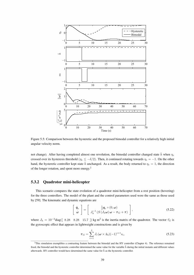
0 5 10 15 20 25 30−1

0

1

HystereticBimodal

0 5 10 15 20 25 30−1

1

0 5 10 15 20 25 30−1

1

0 10 20 30 40 50 60 700

1

2

0 10 20 30 40 50 60 700

5

Time (s)

1

t 0

τTτdt

1

ω

JOU

RN

AL

OF

LAT E

XC

LA

SSFI

LE

S,V

OL

.11,

NO

.4,D

EC

EM

BE

R20

123

[wid

th=8

cm]fi

g/C

omhi

ster

ese

Fig.

2.St

ate

spac

ere

pres

enta

tion

ofth

ehy

ster

etic

cont

rolle

r(w

ithon

est

ate

h).

Arr

ows

indi

cate

the

dire

ctio

nof

the

torq

ueco

ntri

butio

nte

rm(d

epen

dent

onst

ateh

)so

the

attit

ude

isre

gula

ted

to1

or−1

.The

para

met

erδ

repr

esen

tsth

ehy

ster

esis

half

-wid

thof

the

on-o

ffco

ntro

lfo

rst

ateh

.

The

stat

esp

ace

ofth

ecl

osed

-loo

psy

stem

isre

pres

ente

dby

x1=

(xp,x

c1)∈X

1:=

Xp×

Xc.

The

cont

rolle

rob

ject

ive

isto

glob

ally

asym

ptot

ical

lyst

abi-

lize

the

set

A1=

x1∈X

1:qe=

h1,ω

= 0 .

(5)

The

clos

ed-l

oop

syst

emis

give

nby

(2),

(3)

and

the

follo

w-

ing

dyna

mic

sof

the

cont

rolle

r.

˙ h=

0x1∈C

1:=

x1∈X

1:hη e

≥−δ ,

h+∈

sgn(u

1)

x1∈D

1:=

x1∈X

1:hη e

≤−δ ,

(6)

whe

reh+

isth

eva

lue

asso

ciat

edto

hju

staf

ter

the

stat

etr

ansi

tion

and

sgn(η)=

sgn(η),

|ηe|>

0,

−1,1,

η e=

0.

The

vect

orof

inpu

tsU1=

(τ,u

1)

isca

lcul

ated

asfo

llow

s:τ y,q

d,h

=−ch e

−ω

andu1

y,q

d,h

=η e

.A

sal

read

ym

entio

ned,

hde

term

ines

the

orie

ntat

ion

ofa

forc

eal

ong

the

axis

ofro

tatio

n.W

hile

hη e

≥0

,it

forc

esth

em

ovem

ent

toth

esh

orte

rro

tatio

ndi

rect

ion.

How

ever

,w

hen

hη e

<0,

the

forc

est

illpu

llsin

the

sam

edi

rect

ion

(the

long

erro

tatio

ndi

rect

ion)

until

asa

fedi

stan

ceis

achi

eved

topr

even

tch

atte

ring

,i.e

.,un

tilhη e

≤−δ.

III.

PR

OP

OS

ED

CO

NT

RO

LL

ER

As

the

hyst

eret

icco

ntro

ller,

ina

spec

ific

regi

onof

the

stat

esp

ace,

dete

rmin

esa

forc

eco

ntri

butio

nto

mak

eth

eri

gid-

body

evol

ves

toth

elo

nger

rota

tion

dire

ctio

n,w

epr

opos

eto

add

one

mor

est

ate

toth

eco

ntro

ller

topr

even

tth

isbe

havi

oran

dsa

veen

ergy

.T

hepr

opos

edco

ntro

ller

feed

back

torq

ueis

also

give

nby

(4),

but

itha

stw

ost

ates

xc2=

h,m

∈X

c×

Xc,X

c:=

−1,1

.

The

stat

eh

dete

rmin

esth

efe

edba

ckto

rque

cont

ribu

tion

inor

dert

om

oveqe

eith

erto

1or

−1

,as

wel

las

inth

ehy

ster

etic

cont

rol.

The

stat

em

=1

indi

cate

sth

at|η

e|h

asre

ache

dov

erth

ehy

ster

esis

wid

thva

lue

butη e

has

not

cros

sed

zero

yet.

The

stat

em

=−1

indi

cate

sth

eop

posi

te,

that

η eha

sal

read

ycr

osse

dze

robu

t|η e|h

asno

trea

ched

over

the

hyst

eres

isw

idth

valu

eye

t.T

hesp

ace

stat

eof

the

clos

ed-l

oop

syst

emis

repr

esen

ted

by

x2=

(x,x

c2)∈X

2:=

X×

Xc×

Xc.

The

cont

rolle

rob

ject

ive

isto

glob

ally

asym

ptot

ical

lyst

abili

zeth

ese

t

A2=

x2∈X

2:qe=

h1,m

=1,ω= 0 .

(7)

The

clos

ed-l

oop

syst

emis

give

nby

(2),

(3)

and

the

follo

w-

ing

dyna

mic

sof

the

cont

rolle

r.˙ h=

0m

=0

x2∈C

2,

h+∈

sgn(u

2)

m+∈u3sg

n(u

2−u3δ/2)

x2∈D

2,

(8)

C2:=

x2∈X

2: h

η e≥

−δ , h

=−1

or

m(η

e−

δ/2)≥

−δ)

, h=

1orm(η

e+δ/2)

≤δ

,

D2:=

x2∈X

2: h

η e≤

−δ or

h=

1,

m(η

e−

δ/2)≤

−δ)

or h

=−1,m

(ηe+δ/2)

≥δ

.

whe

rem

+an

dh+

are

valu

esas

soci

ated

tom

andh

,res

pec-

tivel

y,ju

staf

ter

stat

etr

ansi

tion.

The

setD

2ca

nbe

expr

esse

din

aco

mpa

ctfo

rmas

follo

ws

D2:=

x2∈X

2: h

η e≤

−δ or

mh(η

e−hδ/2)

≤−δ

.

The

vect

orof

inpu

tsU2

=(τ,u

2,u

3)

isca

lcul

ated

asfo

llow

s:τ y,q

d,h

,m =

−ch e

−ω

,u2

y,q

d,h

,m =

η ean

du3

y,q

d,h

,m =

h.

[wid

th=8

cm]fi

g/fig

Prop

osto

Fig.

3.St

ate

spac

ere

pres

enta

tion

show

ing

the

prop

osed

regu

latio

nw

ithtw

ost

ates

(han

dm

).A

rrow

sin

dica

teth

edi

rect

ion

ofth

eto

rque

cont

ribu

tion

term

(dep

ende

nton

stat

eh

)so

the

attit

ude

isre

gula

ted

to1

or−1

.The

para

met

erδ

repr

esen

tsth

ehy

ster

esis

half

-wid

thof

the

on-o

ffco

ntro

lfo

rst

ateh

and

also

ofth

eon

-off

cont

rol

for

stat

em

.

Fig.

3sh

ows

the

prop

osed

regu

latio

n.W

hen

stat

em

=−1,

the

cont

rolle

rbe

have

sas

the

hyst

eret

icco

ntro

ller.

Ifh=

1,st

ateh

chan

ges

to−1

whe

nη e

≤−δ;

ifh

=−1,

stat

eh

chan

ges

to1

whe

nη e

≥δ.

The

cont

rolle

rsw

itche

sto

stat

em

=1

whe

nth

eat

titud

eer

rorqe

pres

ents

η e≤

−2δ

orη e

≥2δ

.W

hen

stat

em

=1,

the

cont

rolle

rbe

have

sas

the

disc

ontin

uous

cont

rolle

r.In

othe

rw

ords

,if

stat

em

=1,

stat

em

will

chan

geto

m=

−1

whe

nη e

goes

acro

ssze

roan

den

ter

the

jum

pse

t.T

his

fact

,ant

icip

ate

the

chan

geof

stat

eh

.Thi

sdi

stin

ctbe

havi

oris

wha

tdi

ffer

entia

tes

itfr

omth

ehy

ster

etic

cont

rolle

r(6

)an

dal

low

sa

torq

ueco

ntri

butio

nto

war

dsth

esh

orte

rro

tatio

ndi

rect

ion.

A.

Stab

ility

anal

ysis

Con

side

rth

ecl

osed

-loo

psy

stem

ofth

epr

opos

edco

ntro

ller

(8)

rew

ritte

nac

cord

ing

toth

ehy

brid

syst

ems

fram

ewor

kof

[11]

and

give

nby

H=

˙ x2∈F2(x

2),

x2∈C

2,

x+ 2∈G

2(x

2),

x2∈D

2,

whe

rex2=

(qe,ω

,h,m

),

F2(x

2):=

1 2qe(0,ω

)J−1 S

(Jω)ω−

ch e

−ω

0 0

,

G2(x

2):=

qe ω

sgn(η

e)

hsg

n η e

−hδ/2

.

1

m

JOU

RN

AL

OF

LAT E

XC

LA

SSFI

LE

S,V

OL

.11,

NO

.4,D

EC

EM

BE

R20

123

[wid

th=8

cm]fi

g/C

omhi

ster

ese

Fig.

2.St

ate

spac

ere

pres

enta

tion

ofth

ehy

ster

etic

cont

rolle

r(w

ithon

est

ate

h).

Arr

ows

indi

cate

the

dire

ctio

nof

the

torq

ueco

ntri

butio

nte

rm(d

epen

dent

onst

ateh

)so

the

attit

ude

isre

gula

ted

to1

or−1

.The

para

met

erδ

repr

esen

tsth

ehy

ster

esis

half

-wid

thof

the

on-o

ffco

ntro

lfo

rst

ateh

.

The

stat

esp

ace

ofth

ecl

osed

-loo

psy

stem

isre

pres

ente

dby

x1=

(xp,x

c1)∈X

1:=

Xp×

Xc.

The

cont

rolle

rob

ject

ive

isto

glob

ally

asym

ptot

ical

lyst

abi-

lize

the

set

A1=

x1∈X

1:qe=

h1,ω

= 0 .

(5)

The

clos

ed-l

oop

syst

emis

give

nby

(2),

(3)

and

the

follo

w-

ing

dyna

mic

sof

the

cont

rolle

r.

˙ h=

0x1∈C

1:=

x1∈X

1:hη e

≥−δ ,

h+∈

sgn(u

1)

x1∈D

1:=

x1∈X

1:hη e

≤−δ ,

(6)

whe

reh+

isth

eva

lue

asso

ciat

edto

hju

staf

ter

the

stat

etr

ansi

tion

and

sgn(η)=

sgn(η),

|ηe|>

0,

−1,1,

η e=

0.

The

vect

orof

inpu

tsU1=

(τ,u

1)

isca

lcul

ated

asfo

llow

s:τ y,q

d,h

=−ch e

−ω

andu1

y,q

d,h

=η e

.A

sal

read

ym

entio

ned,

hde

term

ines

the

orie

ntat

ion

ofa

forc

eal

ong

the

axis

ofro

tatio

n.W

hile

hη e

≥0

,it

forc

esth

em

ovem

ent

toth

esh

orte

rro

tatio

ndi

rect

ion.

How

ever

,w

hen

hη e

<0,

the

forc

est

illpu

llsin

the

sam

edi

rect

ion

(the

long

erro

tatio

ndi

rect

ion)

until

asa

fedi

stan

ceis

achi

eved

topr

even

tch

atte

ring

,i.e

.,un

tilhη e

≤−δ.

III.

PR

OP

OS

ED

CO

NT

RO

LL

ER

As

the

hyst

eret

icco

ntro

ller,

ina

spec

ific

regi

onof

the

stat

esp

ace,

dete

rmin

esa

forc

eco

ntri

butio

nto

mak

eth

eri

gid-

body

evol

ves

toth

elo

nger

rota

tion

dire

ctio

n,w

epr

opos

eto

add

one

mor

est

ate

toth

eco

ntro

ller

topr

even

tth

isbe

havi

oran

dsa

veen

ergy

.T

hepr

opos

edco

ntro

ller

feed

back

torq

ueis

also

give

nby

(4),

but

itha

stw

ost

ates

xc2=

h,m

∈X

c×

Xc,X

c:=

−1,1

.

The

stat

eh

dete

rmin

esth

efe

edba

ckto

rque

cont

ribu

tion

inor

dert

om

oveqe

eith

erto

1or

−1

,as

wel

las

inth

ehy

ster

etic

cont

rol.

The

stat

em

=1

indi

cate

sth

at|η

e|h

asre

ache

dov

erth

ehy

ster

esis

wid

thva

lue

butη e

has

not

cros

sed

zero

yet.

The

stat

em

=−1

indi

cate

sth

eop

posi

te,

that

η eha

sal

read

ycr

osse

dze

robu

t|η e|h

asno

trea

ched

over

the

hyst

eres

isw

idth

valu

eye

t.T

hesp

ace

stat

eof

the

clos

ed-l

oop

syst

emis

repr

esen

ted

by

x2=

(x,x

c2)∈X

2:=

X×

Xc×

Xc.

The

cont

rolle

rob

ject

ive

isto

glob

ally

asym

ptot

ical

lyst

abili

zeth

ese

t

A2=

x2∈X

2:qe=

h1,m

=1,ω= 0 .

(7)

The

clos

ed-l

oop

syst

emis

give

nby

(2),

(3)

and

the

follo

w-

ing

dyna

mic

sof

the

cont

rolle

r.˙ h=

0m

=0

x2∈C

2,

h+∈

sgn(u

2)

m+∈u3sg

n(u

2−u3δ/2)

x2∈D

2,

(8)

C2:=

x2∈X

2: h

η e≥

−δ , h

=−1

or

m(η

e−

δ/2)≥

−δ)

, h=

1orm(η

e+δ/2)

≤δ

,

D2:=

x2∈X

2: h

η e≤

−δ or

h=

1,

m(η

e−

δ/2)

≤−δ)

or h

=−1,m

(ηe+δ/2)

≥δ

.

whe

rem

+an

dh+

are

valu

esas

soci

ated

tom

andh

,res

pec-

tivel

y,ju

staf

ter

stat

etr

ansi

tion.

The

setD

2ca

nbe

expr

esse

din

aco

mpa

ctfo

rmas

follo

ws

D2:=

x2∈X

2: h

η e≤

−δ or

mh(η

e−hδ/2)

≤−δ

.

The

vect

orof

inpu

tsU2

=(τ,u

2,u

3)

isca

lcul

ated

asfo

llow

s:τ y,q

d,h

,m =

−ch e

−ω

,u2

y,q

d,h

,m =

η ean

du3

y,q

d,h

,m =

h.

[wid

th=8

cm]fi

g/fig

Prop

osto

Fig.

3.St

ate

spac

ere

pres

enta

tion

show

ing

the

prop

osed

regu

latio

nw

ithtw

ost

ates

(han

dm

).A

rrow

sin

dica

teth

edi

rect

ion

ofth

eto

rque

cont

ribu

tion

term

(dep

ende

nton

stat

eh

)so

the

attit

ude

isre

gula

ted

to1

or−1

.The

para

met

erδ

repr

esen

tsth

ehy

ster

esis

half

-wid

thof

the

on-o

ffco

ntro

lfo

rst

ateh

and

also

ofth

eon

-off

cont

rol

for

stat

em

.

Fig.

3sh

ows

the

prop

osed

regu

latio

n.W

hen

stat

em

=−1,

the

cont

rolle

rbe

have

sas

the

hyst

eret

icco

ntro

ller.

Ifh=

1,st

ateh

chan

ges

to−1

whe

nη e

≤−δ;

ifh

=−1,

stat

eh

chan

ges

to1

whe

nη e

≥δ.

The

cont

rolle

rsw

itche

sto

stat

em

=1

whe

nth

eat

titud

eer

rorqe

pres

ents

η e≤

−2δ

orη e

≥2δ

.W

hen

stat

em

=1,

the

cont

rolle

rbe

have

sas

the

disc

ontin

uous

cont

rolle

r.In

othe

rw

ords

,if

stat

em

=1,

stat

em

will

chan

geto

m=

−1

whe

nη e

goes

acro

ssze

roan

den

ter

the

jum

pse

t.T

his

fact

,ant

icip

ate

the

chan

geof

stat

eh

.Thi

sdi

stin

ctbe

havi

oris

wha

tdi

ffer

entia

tes

itfr

omth

ehy

ster

etic

cont

rolle

r(6

)an

dal

low

sa

torq

ueco

ntri

butio

nto

war

dsth

esh

orte

rro

tatio

ndi

rect

ion.

A.

Stab

ility

anal

ysis

Con

side

rth

ecl

osed

-loo

psy

stem

ofth

epr

opos

edco

ntro

ller

(8)

rew

ritte

nac

cord

ing

toth

ehy

brid

syst

ems

fram

ewor

kof

[11]

and

give

nby

H=

˙ x2∈F2(x

2),

x2∈C

2,

x+ 2∈G

2(x

2),

x2∈D

2,

whe

rex2=

(qe,ω

,h,m

),

F2(x

2):=

1 2qe(0,ω

)J−1 S

(Jω)ω−

ch e

−ω

0 0

,

G2(x

2):=

qe ω

sgn(η

e)

hsg

n η e

−hδ/2

.

Figure 5.5: Comparison between the hysteretic and the proposed bimodal controller for a relatively high initialangular velocity norm.

not change). After having completed almost one revolution, the bimodal controller changed state h when ηecrossed over its hysteresis threshold (ηe ≤ −δ/2). Then, it continued rotating towards ηe = −1. On the otherhand, the hysteretic controller kept state h unchanged. As a result, the body returned to ηe = 1, the directionof the longer rotation, and spent more energy.2

5.3.2 Quadrotor mini-helicopter

This scenario compares the state evolution of a quadrotor mini-helicopter from a rest position (hovering)for the three controllers. The model of the plant and the control parameters used were the same as those usedby [59]. The kinematic and dynamic equations are[

qeω

]=

[12qe (0,ω)

J−1h (S (Jhω)ω − τG + τ )

], (5.22)

where Jh = 10−3diag([ 8.28 8.28 15.7 ]) kg m2 is the inertia matrix of the quadrotor. The vector ~τG isthe gyroscopic effect that appears in lightweight constructions and is given by

τG =

4∑i=1

Jr(ω × zb)(−1)i+1si, (5.23)

2This simulation exemplifies a contrasting feature between the bimodal and the HY controller (Chapter 4). The reference remainedfixed, the bimodal and the hysteretic controller determined the same value for the variable h during the initial instants and different valuesafterwards. HY controller would have determined the same value for h as the hysteretic controller.

39

where Jr = 3.4× 10−5 kg m2 is the inertia of the rotor, zb is the unit vector in the direction of the body-framez-axis and si represents the rotational speed of rotor i. The relationship between the rotor speed and the torqueτ is given by [

τ

tz

]=

0 db 0 −dbdb 0 −db 0

k −k k −kb b b b

s2

1

s22

s23

s24

, (5.24)

where d = 0.225 m, b = 29.1 × 10−5 kg m rad−2, k = 1.14 × 10−6 kg m2 rad−2 and tz is a component ofthe total thrust t = [ 0 0 tz ]T expressed in the body frame. The position equations are omitted as they arebeyond the scope of this work.

The plant model is different from (2.10) due to the presence of the gyroscopic effect τG. The contributionof this effect in (5.22) is minimum as the inertia of the rotor is very small. The control law does not needmodifications and the stability analysis is almost the same from that of Section 5.1 since the extra term τG iscanceled during the time derivative V calculation (5.12).

To make a fair comparison, the torque feedback (5.1) was applied to all the controllers. The control pa-rameters used were c = 0.075 and Kω = diag([ c/ρ1 c/ρ2 c/ρ3 ]), ρ1 = ρ2 = 4.2 and ρ3 = 1.74. Ascommented in [59], these parameters were chosen so the stability is not affected by the limits of the angularvelocity sensors. The hysteresis parameter was set to δ = 0.4 for the hysteretic and bimodal controller.

0 1 2 3 4 5−1

0

1

DiscontinuousBimodal

0 1 2 3 4 5−1

1

0 1 2 3 4 5−1

1

0 0.5 1 1.5 2 2.5 3 3.5 4 4.5 50

1

2

0 1 2 3 4 5−0.05

0

0.05

Time (s)

JOU

RN

AL

OF

LAT E

XC

LA

SSFI

LE

S,V

OL

.11,

NO

.4,D

EC

EM

BE

R20

123

[wid

th=8

cm]fi

g/C

omhi

ster

ese

Fig.

2.St

ate

spac

ere

pres

enta

tion

ofth

ehy

ster

etic

cont

rolle

r(w

ithon

est

ate

h).

Arr

ows

indi

cate

the

dire

ctio

nof

the

torq

ueco

ntri

butio

nte

rm(d

epen

dent

onst

ateh

)so

the

attit

ude

isre

gula

ted

to1

or−1

.The

para

met

erδ

repr

esen

tsth

ehy

ster

esis

half

-wid

thof

the

on-o

ffco

ntro

lfo

rst

ateh

.

The

stat

esp

ace

ofth

ecl

osed

-loo

psy

stem

isre

pres

ente

dby

x1=

(xp,x

c1)∈X

1:=

Xp×X

c.

The

cont

rolle

rob

ject

ive

isto

glob

ally

asym

ptot

ical

lyst

abi-

lize

the

set

A1=

x1∈X

1:qe=

h1,ω

= 0 .

(5)

The

clos

ed-l

oop

syst

emis

give

nby

(2),

(3)

and

the

follo

w-

ing

dyna

mic

sof

the

cont

rolle

r.

˙ h=

0x1∈C

1:=

x1∈X

1:hη e

≥−δ ,

h+∈

sgn(u

1)

x1∈D

1:=

x1∈X

1:hη e

≤−δ ,

(6)

whe

reh+

isth

eva

lue

asso

ciat

edto

hju

staf

ter

the

stat

etr

ansi

tion

and

sgn(η)=

sgn(η),

|ηe|>

0,

−1,1,

η e=

0.

The

vect

orof

inpu

tsU1=

(τ,u

1)

isca

lcul

ated

asfo

llow

s:τ y,q

d,h

=−ch e

−ω

andu1

y,q

d,h

=η e

.A

sal

read

ym

entio

ned,

hde

term

ines

the

orie

ntat

ion

ofa

forc

eal

ong

the

axis

ofro

tatio

n.W

hile

hη e

≥0

,it

forc

esth

em

ovem

ent

toth

esh

orte

rro

tatio

ndi

rect

ion.

How

ever

,w

hen

hη e

<0,

the

forc

est

illpu

llsin

the

sam

edi

rect

ion

(the

long

erro

tatio

ndi

rect

ion)

until

asa

fedi

stan

ceis

achi

eved

topr

even

tch

atte

ring

,i.e

.,un

tilhη e

≤−δ.

III.

PR

OP

OS

ED

CO

NT

RO

LL

ER

As

the

hyst

eret

icco

ntro

ller,

ina

spec

ific

regi

onof

the

stat

esp

ace,

dete

rmin

esa

forc

eco

ntri

butio

nto

mak

eth

eri

gid-

body

evol

ves

toth

elo

nger

rota

tion

dire

ctio

n,w

epr

opos

eto

add

one

mor

est

ate

toth

eco

ntro

ller

topr

even

tth

isbe

havi

oran

dsa

veen

ergy

.T

hepr

opos

edco

ntro

ller

feed

back

torq

ueis

also

give

nby

(4),

but

itha

stw

ost

ates

xc2=

h,m

∈X

c×X

c,X

c:=

−1,1

.

The

stat

eh

dete

rmin

esth

efe

edba

ckto

rque

cont

ribu

tion

inor

dert

om

oveqe

eith

erto

1or

−1

,as

wel

las

inth

ehy

ster

etic

cont

rol.

The

stat

em

=1

indi

cate

sth

at|η

e|h

asre

ache

dov

erth

ehy

ster

esis

wid

thva

lue

butη e

has

not

cros

sed

zero

yet.

The

stat

em

=−1

indi

cate

sth

eop

posi

te,

that

η eha

sal

read

ycr

osse

dze

robu

t|η e|h

asno

trea

ched

over

the

hyst

eres

isw

idth

valu

eye

t.T

hesp

ace

stat

eof

the

clos

ed-l

oop

syst

emis

repr

esen

ted

by

x2=

(x,x

c2)∈X

2:=

X×X

c×X

c.

The

cont

rolle

rob

ject

ive

isto

glob

ally

asym

ptot

ical

lyst

abili

zeth

ese

t

A2=

x2∈X

2:qe=

h1,m

=1,ω= 0 .

(7)

The

clos

ed-l

oop

syst

emis

give

nby

(2),

(3)

and

the

follo

w-

ing

dyna

mic

sof

the

cont

rolle

r.˙ h=

0m

=0

x2∈C

2,

h+∈

sgn(u

2)

m+∈u3sg

n(u

2−u3δ/2)

x2∈D

2,

(8)

C2:=

x2∈X

2: h

η e≥

−δ , h

=−1

or

m(η

e−δ/2)

≥−δ)

, h=

1orm(η

e+δ/2)

≤δ

,

D2:=

x2∈X

2: h

η e≤

−δ or

h=

1,

m(η

e−δ/2)

≤−δ)

or h

=−1,m

(ηe+δ/2)

≥δ

.

whe

rem

+an

dh+

are

valu

esas

soci

ated

tom

andh

,res

pec-

tivel

y,ju

staf

ter

stat

etr

ansi

tion.

The

setD

2ca

nbe

expr

esse

din

aco

mpa

ctfo

rmas

follo

ws

D2:=

x2∈X

2: h

η e≤

−δ or

mh(η

e−hδ/2)

≤−δ

.

The

vect

orof

inpu

tsU2

=(τ,u

2,u

3)

isca

lcul

ated

asfo

llow

s:τ y,q

d,h

,m =

−ch e

−ω

,u2

y,q

d,h

,m =

η ean

du3

y,q

d,h

,m =

h.

[wid

th=8

cm]fi

g/fig

Prop

osto

Fig.

3.St

ate

spac

ere

pres

enta

tion

show

ing

the

prop

osed

regu

latio

nw

ithtw

ost

ates

(han

dm

).A

rrow

sin

dica

teth

edi

rect

ion

ofth

eto

rque

cont

ribu

tion

term

(dep

ende

nton

stat

eh

)so

the

attit

ude

isre

gula

ted

to1

or−1

.The

para

met

erδ

repr

esen

tsth

ehy

ster

esis

half

-wid

thof

the

on-o

ffco

ntro

lfo

rst

ateh

and

also

ofth

eon

-off

cont

rol

for

stat

em

.

Fig.

3sh

ows

the

prop

osed

regu

latio

n.W

hen

stat

em

=−1,

the

cont

rolle

rbe

have

sas

the

hyst

eret

icco

ntro

ller.

Ifh=

1,st

ateh

chan

ges

to−1

whe

nη e

≤−δ;

ifh

=−1,

stat

eh

chan

ges

to1

whe

nη e

≥δ.

The

cont

rolle

rsw

itche

sto

stat

em

=1

whe

nth

eat

titud

eer

rorqe

pres

ents

η e≤

−2δ

orη e

≥2δ

.W

hen

stat

em

=1,

the

cont

rolle

rbe

have

sas

the

disc

ontin

uous

cont

rolle

r.In

othe

rw

ords

,if

stat

em

=1,

stat

em

will

chan

geto

m=

−1

whe

nη e

goes

acro

ssze

roan

den

ter

the

jum

pse

t.T

his

fact

,ant

icip

ate

the

chan

geof

stat

eh

.Thi

sdi

stin

ctbe

havi

oris

wha

tdi

ffer

entia

tes

itfr

omth

ehy

ster

etic

cont

rolle

r(6

)an

dal

low

sa

torq

ueco

ntri

butio

nto

war

dsth

esh

orte

rro

tatio

ndi

rect

ion.

A.

Stab

ility

anal

ysis

Con

side

rth

ecl

osed

-loo

psy

stem

ofth

epr

opos

edco

ntro

ller

(8)

rew

ritte

nac

cord

ing

toth

ehy

brid

syst

ems

fram

ewor

kof

[11]

and

give

nby

H=

˙ x2∈F2(x

2),

x2∈C

2,

x+ 2∈G

2(x

2),

x2∈D

2,

whe

rex2=

(qe,ω

,h,m

),

F2(x

2):=

1 2qe(0,ω

)J−1 S

(Jω)ω−ch e

−ω

0 0

,

G2(x

2):=

qe ω

sgn(η

e)

hsg

n η e

−hδ/2

.

JOU

RN

AL

OF

LAT E

XC

LA

SSFI

LE

S,V

OL

.11,

NO

.4,D

EC

EM

BE

R20

123

[wid

th=8

cm]fi

g/C

omhi

ster

ese

Fig.

2.St

ate

spac

ere

pres

enta

tion

ofth

ehy

ster

etic

cont

rolle

r(w

ithon

est

ate

h).

Arr

ows

indi

cate

the

dire

ctio

nof

the

torq

ueco

ntri

butio

nte

rm(d

epen

dent

onst

ateh

)so

the

attit

ude

isre

gula

ted

to1

or−1

.The

para

met

erδ

repr

esen

tsth

ehy

ster

esis

half

-wid

thof

the

on-o

ffco

ntro

lfo

rst

ateh

.

The

stat

esp

ace

ofth

ecl

osed

-loo

psy

stem

isre

pres

ente

dby

x1=

(xp,x

c1)∈X

1:=

Xp×

Xc.

The

cont

rolle

rob

ject

ive

isto

glob

ally

asym

ptot

ical

lyst

abi-

lize

the

set

A1=

x1∈X

1:qe=

h1,ω

= 0 .

(5)

The

clos

ed-l

oop

syst

emis

give

nby

(2),

(3)

and

the

follo

w-

ing

dyna

mic

sof

the

cont

rolle

r.

˙ h=

0x1∈C

1:=

x1∈X

1:hη e

≥−δ ,

h+∈

sgn(u

1)

x1∈D

1:=

x1∈X

1:hη e

≤−δ ,

(6)

whe

reh+

isth

eva

lue

asso

ciat

edto

hju

staf

ter

the

stat

etr

ansi

tion

and

sgn(η)=

sgn(η),

|ηe|>

0,

−1,1,

η e=

0.

The

vect

orof

inpu

tsU1=

(τ,u

1)

isca

lcul

ated

asfo

llow

s:τ y,q

d,h

=−ch e

−ω

andu1

y,q

d,h

=η e

.A

sal

read

ym

entio

ned,

hde

term

ines

the

orie

ntat

ion

ofa

forc

eal

ong

the

axis

ofro

tatio

n.W

hile

hη e

≥0

,it

forc

esth

em

ovem

ent

toth

esh

orte

rro

tatio

ndi

rect

ion.

How

ever

,w

hen

hη e

<0,

the

forc

est

illpu

llsin

the

sam

edi

rect

ion

(the

long

erro

tatio

ndi

rect

ion)

until

asa

fedi

stan

ceis

achi

eved

topr

even

tch

atte

ring

,i.e

.,un

tilhη e

≤−δ.

III.

PR

OP

OS

ED

CO

NT

RO

LL

ER

As

the

hyst

eret

icco

ntro

ller,

ina

spec

ific

regi

onof

the

stat

esp

ace,

dete

rmin

esa

forc

eco

ntri

butio

nto

mak

eth

eri

gid-

body

evol

ves

toth

elo

nger

rota

tion

dire

ctio

n,w

epr

opos

eto

add

one

mor

est

ate

toth

eco

ntro

ller

topr

even

tth

isbe

havi

oran

dsa

veen

ergy

.T

hepr

opos

edco

ntro

ller

feed

back

torq

ueis

also

give

nby

(4),

but

itha

stw

ost

ates

xc2=

h,m

∈X

c×

Xc,X

c:=

−1,1

.

The

stat

eh

dete

rmin

esth

efe

edba

ckto

rque

cont

ribu

tion

inor

dert

om

oveqe

eith

erto

1or

−1

,as

wel

las

inth

ehy

ster

etic

cont

rol.

The

stat

em

=1

indi

cate

sth

at|η

e|h

asre

ache

dov

erth

ehy

ster

esis

wid

thva

lue

butη e

has

not

cros

sed

zero

yet.

The

stat

em

=−1

indi

cate

sth

eop

posi

te,

that

η eha

sal

read

ycr

osse

dze

robu

t|η e|h

asno

trea

ched

over

the

hyst

eres

isw

idth

valu

eye

t.T

hesp

ace

stat

eof

the

clos

ed-l

oop

syst

emis

repr

esen

ted

by

x2=

(x,x

c2)∈X

2:=

X×

Xc×

Xc.

The

cont

rolle

rob

ject

ive

isto

glob

ally

asym

ptot

ical

lyst

abili

zeth

ese

t

A2=

x2∈X

2:qe=

h1,m

=1,ω= 0 .

(7)

The

clos

ed-l

oop

syst

emis

give

nby

(2),

(3)

and

the

follo

w-

ing

dyna

mic

sof

the

cont

rolle

r.˙ h=

0m

=0

x2∈C

2,

h+∈

sgn(u

2)

m+∈u3sg

n(u

2−u3δ/2)

x2∈D

2,

(8)

C2:=

x2∈X

2: h

η e≥

−δ , h

=−1

or

m(η

e−

δ/2)

≥−δ)

, h=

1orm(η

e+δ/2)≤

δ,

D2:=

x2∈X

2: h

η e≤

−δ or

h=

1,

m(η

e−

δ/2)≤

−δ)

or h

=−1,m

(ηe+δ/2)

≥δ

.

whe

rem

+an

dh+

are

valu

esas

soci

ated

tom

andh

,res

pec-

tivel

y,ju

staf

ter

stat

etr

ansi

tion.

The

setD

2ca

nbe

expr

esse

din

aco

mpa

ctfo

rmas

follo

ws

D2:=

x2∈X

2: h

η e≤

−δ or

mh(η

e−hδ/2)≤

−δ

.

The

vect

orof

inpu

tsU2

=(τ,u

2,u

3)

isca

lcul

ated

asfo

llow

s:τ y,q

d,h

,m =

−ch e

−ω

,u2

y,q

d,h

,m =

η ean

du3

y,q

d,h

,m =

h.

[wid

th=8

cm]fi

g/fig

Prop

osto

Fig.

3.St

ate

spac

ere

pres

enta

tion

show

ing

the

prop

osed

regu

latio

nw

ithtw

ost

ates

(han

dm

).A

rrow

sin

dica

teth

edi

rect

ion

ofth

eto

rque

cont

ribu

tion

term

(dep

ende

nton

stat

eh

)so

the

attit

ude

isre

gula

ted

to1

or−1

.The

para

met

erδ

repr

esen

tsth

ehy

ster

esis

half

-wid

thof

the

on-o

ffco

ntro

lfo

rst

ateh

and

also

ofth

eon

-off

cont

rol

for

stat

em

.

Fig.

3sh

ows

the

prop

osed

regu

latio

n.W

hen

stat

em

=−1,

the

cont

rolle

rbe

have

sas

the

hyst

eret

icco

ntro

ller.

Ifh=

1,st

ateh

chan

ges

to−1

whe

nη e

≤−δ;

ifh

=−1,

stat

eh

chan

ges

to1

whe

nη e

≥δ.

The

cont

rolle

rsw

itche

sto

stat

em

=1

whe

nth

eat

titud

eer

rorqe

pres

ents

η e≤

−2δ

orη e

≥2δ

.W

hen

stat

em

=1,

the

cont

rolle

rbe

have

sas

the

disc

ontin

uous

cont

rolle

r.In

othe

rw

ords

,if

stat

em

=1,

stat

em

will

chan

geto

m=

−1

whe

nη e

goes

acro

ssze

roan

den

ter

the

jum

pse

t.T

his

fact

,ant

icip

ate

the

chan

geof

stat

eh

.Thi

sdi

stin

ctbe

havi

oris

wha

tdi

ffer

entia

tes

itfr

omth

ehy

ster

etic

cont

rolle

r(6

)an

dal

low

sa

torq

ueco

ntri

butio

nto

war

dsth

esh

orte

rro

tatio

ndi

rect

ion.

A.

Stab

ility

anal

ysis

Con

side

rth

ecl

osed

-loo

psy

stem

ofth

epr

opos

edco

ntro

ller

(8)

rew

ritte

nac

cord

ing

toth

ehy

brid

syst

ems

fram

ewor

kof

[11]

and

give

nby

H=

˙ x2∈F2(x

2),

x2∈C

2,

x+ 2∈G

2(x

2),

x2∈D

2,

whe

rex2=

(qe,ω

,h,m

),

F2(x

2):=

1 2qe(0,ω

)J−1 S

(Jω)ω−

ch e

−ω

0 0

,

G2(x

2):=

qe ω

sgn(η

e)

hsg

n η e

−hδ/2

.1

m

1

ω(

rad/

s)

1

τ z(N

m)

Figure 5.6: Comparison between the discontinuous and the proposed bimodal controller for the quadrotor.

Figure 5.6 illustrates the chattering behavior when the discontinuous controller is applied and compares itwith the bimodal controller. The hysteretic controller is not shown as it behaves as the bimodal one. The initialconditions were q(0) = (0, [ 0 0 1 ]T ) and ω(0) = 0, i.e., the yaw angle was 180 from the reference.The desired thrust was tz > 4.59 N to compensate the quadrotor weight. The graphs of ηe and the angular

40

velocity norm ‖ω‖ show that the discontinuous system had its response lagged due to the chattering on variableh (caused by measurement noise) for over than 1 s. Recall that, as mentioned in Section 3.4, there exists a noisethat keeps the state near the discontinuity (ηe = 0) indefinitely. On the other hand, the bimodal controller keptstate h unchanged at 1 (as well as state m) and the body moved toward 1. The last graph, of τz , shows only theτz component of the torque τ = (τx, τy, τz) for both controllers as the other components stayed near 0.

0 1 2 3 4 5−1

0

1

HystereticBimodal

0 1 2 3 4 5−1

1

0 1 2 3 4 5−1

1

0 0.5 1 1.5 2 2.5 3 3.5 4 4.5 50

1

2

0 1 2 3 4 5−0.05

0

0.05

Time (s)

JOU

RN

AL

OF

LAT E

XC

LA

SSFI

LE

S,V

OL

.11,

NO

.4,D

EC

EM

BE

R20

123

[wid

th=8

cm]fi

g/C

omhi

ster

ese

Fig.

2.St

ate

spac

ere

pres

enta

tion

ofth

ehy

ster

etic

cont

rolle

r(w

ithon

est

ate

h).

Arr

ows

indi

cate

the

dire

ctio

nof

the

torq

ueco

ntri

butio

nte

rm(d

epen

dent

onst

ateh

)so

the

attit

ude

isre

gula

ted

to1

or−1

.The

para

met

erδ

repr

esen

tsth

ehy

ster

esis

half

-wid

thof

the

on-o

ffco

ntro

lfo

rst

ateh

.

The

stat

esp

ace

ofth

ecl

osed

-loo

psy

stem

isre

pres

ente

dby

x1=

(xp,x

c1)∈X

1:=

Xp×

Xc.

The

cont

rolle

rob

ject

ive

isto

glob

ally

asym

ptot

ical

lyst

abi-

lize

the

set

A1=

x1∈X

1:qe=

h1,ω

= 0 .

(5)

The

clos

ed-l

oop

syst

emis

give

nby

(2),

(3)

and

the

follo

w-

ing

dyna

mic

sof

the

cont

rolle

r.

˙ h=

0x1∈C

1:=

x1∈X

1:hη e

≥−δ ,

h+∈

sgn(u

1)

x1∈D

1:=

x1∈X

1:hη e

≤−δ ,

(6)

whe

reh+

isth

eva

lue

asso

ciat

edto

hju

staf

ter

the

stat

etr

ansi

tion

and

sgn(η)=

sgn(η),

|ηe|>

0,

−1,1,

η e=

0.

The

vect

orof

inpu

tsU1=

(τ,u

1)

isca

lcul

ated

asfo

llow

s:τ y,q

d,h

=−ch e

−ω

andu1

y,q

d,h

=η e

.A

sal

read

ym

entio

ned,

hde

term

ines

the

orie

ntat

ion

ofa

forc

eal

ong

the

axis

ofro

tatio

n.W

hile

hη e

≥0

,it

forc

esth

em

ovem

ent

toth

esh

orte

rro

tatio

ndi

rect

ion.

How

ever

,w

hen

hη e

<0,

the

forc

est

illpu

llsin

the

sam

edi

rect

ion

(the

long

erro

tatio

ndi

rect

ion)

until

asa

fedi

stan

ceis

achi

eved

topr

even

tch

atte

ring

,i.e

.,un

tilhη e

≤−δ.

III.

PR

OP

OS

ED

CO

NT

RO

LL

ER

As

the

hyst

eret

icco

ntro

ller,

ina

spec

ific

regi

onof

the

stat

esp

ace,

dete

rmin

esa

forc

eco

ntri

butio

nto

mak

eth

eri

gid-

body

evol

ves

toth

elo

nger

rota

tion

dire

ctio

n,w

epr

opos

eto

add

one

mor

est

ate

toth

eco

ntro

ller

topr

even

tth

isbe

havi

oran

dsa

veen

ergy

.T

hepr

opos

edco

ntro

ller

feed

back

torq

ueis

also

give

nby

(4),

but

itha

stw

ost

ates

xc2=

h,m

∈X

c×

Xc,X

c:=

−1,1

.

The

stat

eh

dete

rmin

esth

efe

edba

ckto

rque

cont

ribu

tion

inor

dert

om

oveqe

eith

erto

1or

−1

,as

wel

las

inth

ehy

ster

etic

cont

rol.

The

stat

em

=1

indi

cate

sth

at|η

e|h

asre

ache

dov

erth

ehy

ster

esis

wid

thva

lue

butη e

has

not

cros

sed

zero

yet.

The

stat

em

=−1

indi

cate

sth

eop

posi

te,

that

η eha

sal

read

ycr

osse

dze

robu

t|η e|h

asno

trea

ched

over

the

hyst

eres

isw

idth

valu

eye

t.T

hesp

ace

stat

eof

the

clos

ed-l

oop

syst

emis

repr

esen

ted

by

x2=

(x,x

c2)∈X

2:=

X×

Xc×

Xc.

The

cont

rolle

rob

ject

ive

isto

glob

ally

asym

ptot

ical

lyst

abili

zeth

ese

t

A2=

x2∈X

2:qe=

h1,m

=1,ω= 0 .

(7)

The

clos

ed-l

oop

syst

emis

give

nby

(2),

(3)

and

the

follo

w-

ing

dyna

mic

sof

the

cont

rolle

r.˙ h=

0m

=0

x2∈C

2,

h+∈

sgn(u

2)

m+∈u3sg

n(u

2−u3δ/2)

x2∈D

2,

(8)

C2:=

x2∈X

2: h

η e≥

−δ , h

=−1

or

m(η

e−

δ/2)≥

−δ)

, h=

1orm(η

e+δ/2)

≤δ

,

D2:=

x2∈X

2: h

η e≤

−δ or

h=

1,

m(η

e−

δ/2)

≤−δ)

or h

=−1,m

(ηe+δ/2)

≥δ

.

whe

rem

+an

dh+

are

valu

esas

soci

ated

tom

andh

,res

pec-

tivel

y,ju

staf

ter

stat

etr

ansi

tion.

The

setD

2ca

nbe

expr

esse

din

aco

mpa

ctfo

rmas

follo

ws

D2:=

x2∈X

2: h

η e≤

−δ or

mh(η

e−hδ/2)

≤−δ

.

The

vect

orof

inpu

tsU2

=(τ,u

2,u

3)

isca

lcul

ated

asfo

llow

s:τ y,q

d,h

,m =

−ch e

−ω

,u2

y,q

d,h

,m =

η ean

du3

y,q

d,h

,m =

h.

[wid

th=8

cm]fi

g/fig

Prop

osto

Fig.

3.St

ate

spac

ere

pres

enta

tion

show

ing

the

prop

osed

regu

latio

nw

ithtw

ost

ates

(han

dm

).A

rrow

sin

dica

teth

edi

rect

ion

ofth

eto

rque

cont

ribu

tion

term

(dep

ende

nton

stat

eh

)so

the

attit

ude

isre

gula

ted

to1

or−1

.The

para

met

erδ

repr

esen

tsth

ehy

ster

esis

half

-wid

thof

the

on-o

ffco

ntro

lfo

rst

ateh

and

also

ofth

eon

-off

cont

rol

for

stat

em

.

Fig.

3sh

ows

the

prop

osed

regu

latio

n.W

hen

stat

em

=−1,

the

cont

rolle

rbe

have

sas

the

hyst

eret

icco

ntro

ller.

Ifh=

1,st

ateh

chan

ges

to−1

whe

nη e

≤−δ;

ifh

=−1,

stat

eh

chan

ges

to1

whe

nη e

≥δ.

The

cont

rolle

rsw

itche

sto

stat

em

=1

whe

nth

eat

titud

eer

rorqe

pres

ents

η e≤

−2δ

orη e

≥2δ

.W

hen

stat

em

=1,

the

cont

rolle

rbe

have

sas

the

disc

ontin

uous

cont

rolle

r.In

othe

rw

ords

,if

stat

em

=1,

stat

em

will

chan

geto

m=

−1

whe

nη e

goes

acro

ssze

roan

den

ter

the

jum

pse

t.T

his

fact

,ant

icip

ate

the

chan

geof

stat

eh

.Thi

sdi

stin

ctbe

havi

oris

wha

tdi

ffer

entia

tes

itfr

omth

ehy

ster

etic

cont

rolle

r(6

)an

dal

low

sa

torq

ueco

ntri

butio

nto

war

dsth

esh

orte

rro

tatio

ndi

rect

ion.

A.

Stab

ility

anal

ysis

Con

side

rth

ecl

osed

-loo

psy

stem

ofth

epr

opos

edco

ntro

ller

(8)

rew

ritte

nac

cord

ing

toth

ehy

brid

syst

ems

fram

ewor

kof

[11]

and

give

nby

H=

˙ x2∈F2(x

2),

x2∈C

2,

x+ 2∈G

2(x

2),

x2∈D

2,

whe

rex2=

(qe,ω

,h,m

),

F2(x

2):=

1 2qe(0,ω

)J−1 S

(Jω)ω−

ch e

−ω

0 0

,

G2(x

2):=

qe ω

sgn(η

e)

hsg

n η e

−hδ/2

.

JOU

RN

AL

OF

LAT E

XC

LA

SSFI

LE

S,V

OL

.11,

NO

.4,D

EC

EM

BE

R20

123

[wid

th=8

cm]fi

g/C

omhi

ster

ese

Fig.

2.St

ate

spac

ere

pres

enta

tion

ofth

ehy

ster

etic

cont

rolle

r(w

ithon

est

ate

h).

Arr

ows

indi

cate

the

dire

ctio

nof

the

torq

ueco

ntri

butio

nte

rm(d

epen

dent

onst

ateh

)so

the

attit

ude

isre

gula

ted

to1

or−1

.The

para

met

erδ

repr

esen

tsth

ehy

ster

esis

half

-wid

thof

the

on-o

ffco

ntro

lfo

rst

ateh

.

The

stat

esp

ace

ofth

ecl

osed

-loo

psy

stem

isre

pres

ente

dby

x1=

(xp,x

c1)∈X

1:=

Xp×

Xc.

The

cont

rolle

rob

ject

ive

isto

glob

ally

asym

ptot

ical

lyst

abi-

lize

the

set

A1=

x1∈X

1:qe=

h1,ω

= 0 .

(5)

The

clos

ed-l

oop

syst

emis

give

nby

(2),

(3)

and

the

follo

w-

ing

dyna

mic

sof

the

cont

rolle

r.

˙ h=

0x1∈C

1:=

x1∈X

1:hη e

≥−δ ,

h+∈

sgn(u

1)

x1∈D

1:=

x1∈X

1:hη e

≤−δ ,

(6)

whe

reh+

isth

eva

lue

asso

ciat

edto

hju

staf

ter

the

stat

etr

ansi

tion

and

sgn(η)=

sgn(η),

|ηe|>

0,

−1,1,

η e=

0.

The

vect

orof

inpu

tsU1=

(τ,u

1)

isca

lcul

ated

asfo

llow

s:τ y,q

d,h

=−ch e

−ω

andu1

y,q

d,h

=η e

.A

sal

read

ym

entio

ned,

hde

term

ines

the

orie

ntat

ion

ofa

forc

eal

ong

the

axis

ofro

tatio

n.W

hile

hη e

≥0

,it

forc

esth

em

ovem

ent

toth

esh

orte

rro

tatio

ndi

rect

ion.

How

ever

,w

hen

hη e

<0,

the

forc

est

illpu

llsin

the

sam

edi

rect

ion

(the

long

erro

tatio

ndi

rect

ion)

until

asa

fedi

stan

ceis

achi

eved

topr

even

tch

atte

ring

,i.e

.,un

tilhη e

≤−δ.

III.

PR

OP

OS

ED

CO

NT

RO

LL

ER

As

the

hyst

eret

icco

ntro

ller,

ina

spec

ific

regi

onof

the

stat

esp

ace,

dete

rmin

esa

forc

eco

ntri

butio

nto

mak

eth

eri

gid-

body

evol

ves

toth

elo

nger

rota

tion

dire

ctio

n,w

epr

opos

eto

add

one

mor

est

ate

toth

eco

ntro

ller

topr

even

tth

isbe

havi

oran

dsa

veen

ergy

.T

hepr

opos

edco

ntro

ller

feed

back

torq

ueis

also

give

nby

(4),

but

itha

stw

ost

ates

xc2=

h,m

∈X

c×

Xc,X

c:=

−1,1

.

The

stat

eh

dete

rmin

esth

efe

edba

ckto

rque

cont

ribu

tion

inor

dert

om

oveqe

eith

erto

1or

−1

,as

wel

las

inth

ehy

ster

etic

cont

rol.

The

stat

em

=1

indi

cate

sth

at|η

e|h

asre

ache

dov

erth

ehy

ster

esis

wid

thva

lue

butη e

has

not

cros

sed

zero

yet.

The

stat

em

=−1

indi

cate

sth

eop

posi

te,

that

η eha

sal

read

ycr

osse

dze

robu

t|η e|h

asno

trea

ched

over

the

hyst

eres

isw

idth

valu

eye

t.T

hesp

ace

stat

eof

the

clos

ed-l

oop

syst

emis

repr

esen

ted

by

x2=

(x,x

c2)∈X

2:=

X×

Xc×

Xc.

The

cont

rolle

rob

ject

ive

isto

glob

ally

asym

ptot

ical

lyst

abili

zeth

ese

t

A2=

x2∈X

2:qe=

h1,m

=1,ω= 0 .

(7)

The

clos

ed-l

oop

syst

emis

give

nby

(2),

(3)

and

the

follo

w-

ing

dyna

mic

sof

the

cont

rolle

r.˙ h=

0m

=0

x2∈C

2,

h+∈

sgn(u

2)

m+∈u3sg

n(u

2−u3δ/2)

x2∈D

2,

(8)

C2:=

x2∈X

2: h

η e≥

−δ , h

=−1

or

m(η

e−

δ/2)

≥−δ)

, h=

1orm(η

e+δ/2)

≤δ

,

D2:=

x2∈X

2: h

η e≤

−δ or

h=

1,

m(η

e−

δ/2)≤

−δ)

or h

=−1,m

(ηe+δ/2)≥

δ.

whe

rem

+an

dh+

are

valu

esas

soci

ated

tom

andh

,res

pec-

tivel

y,ju

staf

ter

stat

etr

ansi

tion.

The

setD

2ca

nbe

expr

esse

din

aco

mpa

ctfo

rmas

follo

ws

D2:=

x2∈X

2: h

η e≤

−δ or

mh(η

e−hδ/2)≤

−δ

.

The

vect

orof

inpu

tsU2

=(τ,u

2,u

3)

isca

lcul

ated

asfo

llow

s:τ y,q

d,h

,m =

−ch e

−ω

,u2

y,q

d,h

,m =

η ean

du3

y,q

d,h

,m =

h.

[wid

th=8

cm]fi

g/fig

Prop

osto

Fig.

3.St

ate

spac

ere

pres

enta

tion

show

ing

the

prop

osed

regu

latio

nw

ithtw

ost

ates

(han

dm

).A

rrow

sin

dica

teth

edi

rect

ion

ofth

eto

rque

cont

ribu

tion

term

(dep

ende

nton

stat

eh

)so

the

attit

ude

isre

gula

ted

to1

or−1

.The

para

met

erδ

repr

esen

tsth

ehy

ster

esis

half

-wid

thof

the

on-o

ffco

ntro

lfo

rst

ateh

and

also

ofth

eon

-off

cont

rol

for

stat

em

.

Fig.

3sh

ows

the

prop

osed

regu

latio

n.W

hen

stat

em

=−1,

the

cont

rolle

rbe

have

sas

the

hyst

eret

icco

ntro

ller.

Ifh=

1,st

ateh

chan

ges

to−1

whe

nη e

≤−δ;

ifh

=−1,

stat

eh

chan

ges

to1

whe

nη e

≥δ.

The

cont

rolle

rsw

itche

sto

stat

em

=1

whe

nth

eat

titud

eer

rorqe

pres

ents

η e≤

−2δ

orη e

≥2δ

.W

hen

stat

em

=1,

the

cont

rolle

rbe

have

sas

the

disc

ontin

uous

cont

rolle

r.In

othe

rw

ords

,if

stat

em

=1,

stat

em

will

chan

geto

m=

−1

whe

nη e

goes

acro

ssze

roan

den

ter

the

jum

pse

t.T

his

fact

,ant

icip

ate

the

chan

geof

stat

eh

.Thi

sdi

stin

ctbe

havi

oris

wha

tdi

ffer

entia

tes

itfr

omth

ehy

ster

etic

cont

rolle

r(6

)an

dal

low

sa

torq

ueco

ntri

butio

nto

war

dsth

esh

orte

rro

tatio

ndi

rect

ion.

A.

Stab

ility

anal

ysis

Con

side

rth

ecl

osed

-loo

psy

stem

ofth

epr

opos

edco

ntro

ller

(8)

rew

ritte

nac

cord

ing

toth

ehy

brid

syst

ems

fram

ewor

kof

[11]

and

give

nby

H=

˙ x2∈F2(x

2),

x2∈C

2,

x+ 2∈G

2(x

2),

x2∈D

2,

whe

rex2=

(qe,ω

,h,m

),

F2(x

2):=

1 2qe(0,ω

)J−1 S

(Jω)ω−

ch e

−ω

0 0

,

G2(x

2):=

qe ω

sgn(η

e)

hsg

n η e

−hδ/2

.1

m

1

ω(

rad/

s)

1

τ z(N

m)

Figure 5.7: Comparison between the hysteretic and the proposed bimodal controller for the quadrotor.

Figure 5.7 presents the behavior of the bimodal and the hysteretic controllers. The initial conditions wereq(0) = (−0.2,

√1− 0.22[ 0 0 1 ]T ) andω(0) = 0. For the hysteretic controller only, this initial condition

belongs to that region of the state space where the control law pulls the rigid body in the direction of the longerrotation. Consequently, hysteretic and bimodal controllers made the rigid body take a different direction ofrotation from the beginning. Note in the graph of the angular velocity norm ‖ω‖ that the system with thebimodal controller converges faster.

5.3.3 Spacecraft

Here, it is intended to show that for controllers with analogous structure of the hysteretic controller (3.14)and (3.15), the bimodal philosophy can be easily adapted to obtain a new controller with expected advantagessimilar to that of the bimodal controller (5.2) and (6.10). Consider the scenario of a spacecraft attitude controlstudied by [55]. The plant model is given by (2.10) and the torque feedback is given by

τ s = Jωr − S(Jω)ωr − kqTTh ehq − kw(ω − ωr), (5.25)

41

where ωr = ωd − γTTh ehq; ehq = [ (1− hηe) εTe ]T ; kq, kw, γ > 0 and

Th =

[hεTe

ηeI + S(εe)

].

The hysteretic controller for this plant is given by

˙h = 0 x1 ∈ Cs1 ,x1 ∈ X1 : hησ ≥ −δ

,

h+ ∈ sgn (us1) x1 ∈ Ds1 ,x1 ∈ X1 : hησ ≤ −δ

(5.26)

whereησ , kqηe − γεTe J(ω − ωd)/2 (5.27)

and the vector of inputs Us1 = (τ , us1) set to Ks1(y, h, qd) , (τ s, ησ).

Note that (3.14) turns to (5.26) by changing ηe to ησ and the vector of inputs U1 (3.15) turns to Us1 bychanging τ 1 (3.13) to τ s (5.25) and ηe to ησ . The same analogy was applied to obtain the adapted bimodalcontroller for this plant, given by

˙h = 0

m = 0

x2 ∈ Cs2,

h+ ∈ sgn (us2 − us3δ/2)

m+ ∈ us3 sgn (us2 − us3δ/2)

x2 ∈ Ds2,

(5.28)

Cs2 ,x2 ∈ X2 :

(hησ ≥ −δ

)and(

m = −1 or hησ ≥ −δ/2)

and(m = 1 or hησ ≤ 3δ/2

),

Ds2 ,x2 ∈ X2 :

(hησ ≤ −δ

)or(

m = 1 and hησ ≤ −δ/2)

or(m = −1 and hησ ≥ 3δ/2

)and the vector of inputs Us2 = (τ , us2, us3) set to Ks2(y, h,m, qd) , (τ s, ησ, h).

Note also that ησ (5.27) depends on both the attitude and the angular velocity. For the rest-to-rest case,when ω(0) = 0, ησ(0) = ηe(0) and, in the beginning, jump sets Ds1 = D1 (3.14) and Ds2 = D2 (5.4).Hence, if the initial attitude is near ηe(0) = −δ/2 as is the case illustrated in Figure 5.7, the same behavior ofthe controllers is expected, that is, each of them makes the rigid body take a different direction of rotation fromthe beginning, with the hysteretic controller determining a rotation to the longer direction.

Figures 5.8 and 5.9 show the evolution of the system for the hysteretic and the adapted bimodal controllerswhen ησ is near −δ/2 (so the controllers determine a different direction of rotation from the beginning) butω 6= 0. Two symmetric initial attitudes were chosen and the average energy consumption was evaluated. Theparameters used for the simulations for both controllers were the same: the inertia matrix of the spacecraftJ = diag([ 4.35 4.33 3.664 ]) kg m2, kq = 1, kw = 2 and γ = 1. The hysteresis parameter was set toδ = 0.2. The initial conditions for Figure 5.8 were q(0) = (−0.4,

√1− 0.42vs), vs = [ 3 −4 5 ]T /

√50)

and ω(0) = −0.16vs and for Figure 5.9, q(0) = (0.4,√

1− 0.42vs) and ω(0) = 0.275vs. The graph of ηeof Figure 5.8 shows that the adapted bimodal controller made the spacecraft rotate to the shorter direction and,according to the last graph, less energy was spent (Eb(15) = 4.5 and Eh(15) = 6.4). The opposite occurred forFigure 5.9 (Eb(15) = 6.1 and Eh(15) = 5.1). Based on the average of energy spent by the controllers in bothsimulations, it is possible to affirm the adapted bimodal controller spends less energy on average.

Finally it is presented an overview of the difference of energy spent when the controllers are applied as afunction of the initial state on a contour graph to illustrate the regions where each controller is advantageous.

Let E(t) =√´ t

0τT τdt represent the energy spent by the applied feedback control and Eh(20) and Eb(20)

represent the energy spent when the hysteretic and the bimodal controller is applied, respectively, up to 20

42

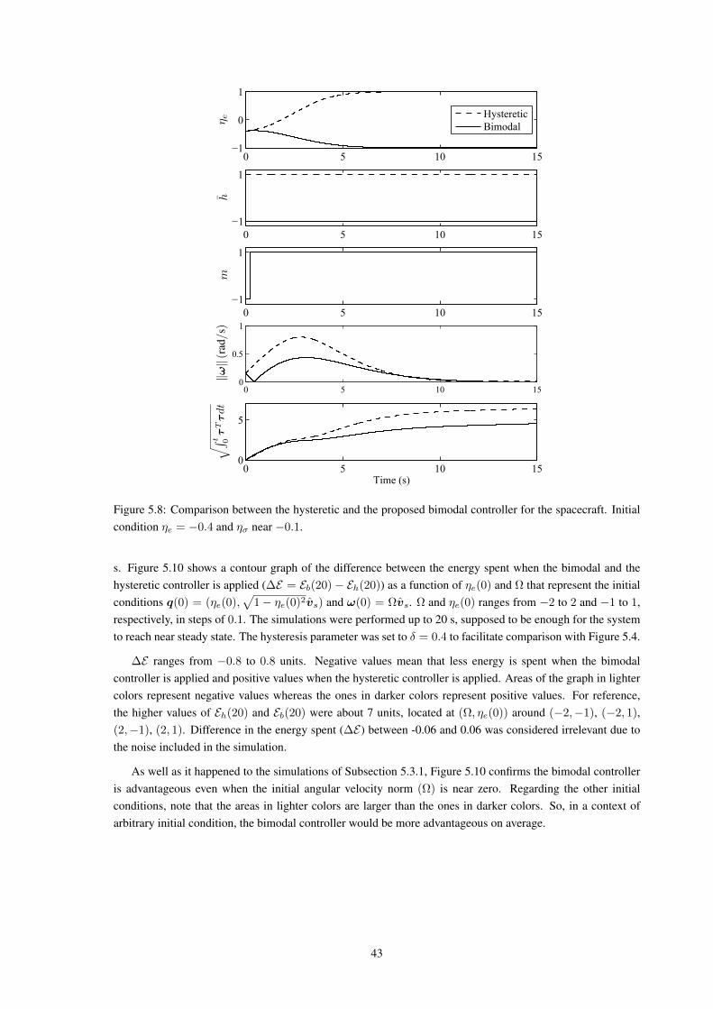
0 5 10 15−1

0

1

HystereticBimodal

0 5 10 15−1

1

0 5 10 15−1

1

0 5 10 150

0.5

1

0 5 10 150

5

Time (s)

JOU

RN

AL

OF

LAT E

XC

LA

SSFI

LE

S,V

OL

.11,

NO

.4,D

EC

EM

BE

R20

123

[wid

th=8

cm]fi

g/C

omhi

ster

ese

Fig.

2.St

ate

spac

ere

pres

enta

tion

ofth

ehy

ster

etic

cont

rolle

r(w

ithon

est

ate

h).

Arr

ows

indi

cate

the

dire

ctio

nof

the

torq

ueco

ntri

butio

nte

rm(d

epen

dent

onst

ateh

)so

the

attit

ude

isre

gula

ted

to1

or−1

.The

para

met

erδ

repr

esen

tsth

ehy

ster

esis

half

-wid

thof

the

on-o

ffco

ntro

lfo

rst

ateh

.

The

stat

esp

ace

ofth

ecl

osed

-loo

psy

stem

isre

pres

ente

dby

x1=

(xp,x

c1)∈X

1:=

Xp×

Xc.

The

cont

rolle

rob

ject

ive

isto

glob

ally

asym

ptot

ical

lyst

abi-

lize

the

set

A1=

x1∈X

1:qe=

h1,ω

= 0 .

(5)

The

clos

ed-l

oop

syst

emis

give

nby

(2),

(3)

and

the

follo

w-

ing

dyna

mic

sof

the

cont

rolle

r.

˙ h=

0x1∈C

1:=

x1∈X

1:hη e

≥−δ ,

h+∈

sgn(u

1)

x1∈D

1:=

x1∈X

1:hη e

≤−δ ,

(6)

whe

reh+

isth

eva

lue

asso

ciat

edto

hju

staf

ter

the

stat

etr

ansi

tion

and

sgn(η)=

sgn(η),

|ηe|>

0,

−1,1,

η e=

0.

The

vect

orof

inpu

tsU1=

(τ,u

1)

isca

lcul

ated

asfo

llow

s:τ y,q

d,h

=−ch e

−ω

andu1

y,q

d,h

=η e

.A

sal

read

ym

entio

ned,

hde

term

ines

the

orie

ntat

ion

ofa

forc

eal

ong

the

axis

ofro

tatio

n.W

hile

hη e

≥0

,it

forc

esth

em

ovem

ent

toth

esh

orte

rro

tatio

ndi

rect

ion.

How

ever

,w

hen

hη e

<0,

the

forc

est

illpu

llsin

the

sam

edi

rect

ion

(the

long

erro

tatio

ndi

rect

ion)

until

asa

fedi

stan

ceis

achi

eved

topr

even

tch

atte

ring

,i.e

.,un

tilhη e

≤−δ.

III.

PR

OP

OS

ED

CO

NT

RO

LL

ER

As

the

hyst

eret

icco

ntro

ller,

ina

spec

ific

regi

onof

the

stat

esp

ace,

dete

rmin

esa

forc

eco

ntri

butio

nto

mak

eth

eri

gid-

body

evol

ves

toth

elo

nger

rota

tion

dire

ctio

n,w

epr

opos

eto

add

one

mor

est

ate

toth

eco

ntro

ller

topr

even

tth

isbe

havi

oran

dsa

veen

ergy

.T

hepr

opos

edco

ntro

ller

feed

back

torq

ueis

also

give

nby

(4),

but

itha

stw

ost

ates

xc2=

h,m

∈X

c×

Xc,X

c:=

−1,1

.

The

stat

eh

dete

rmin

esth

efe

edba

ckto

rque

cont

ribu

tion

inor

dert

om

oveqe

eith

erto

1or

−1

,as

wel

las

inth

ehy

ster

etic

cont

rol.

The

stat

em

=1

indi

cate

sth

at|η

e|h

asre

ache

dov

erth

ehy

ster

esis

wid

thva

lue

butη e

has

not

cros

sed

zero

yet.

The

stat

em

=−1

indi

cate

sth

eop

posi

te,

that

η eha

sal

read

ycr

osse

dze

robu

t|η e|h

asno

trea

ched

over

the

hyst

eres

isw

idth

valu

eye

t.T

hesp

ace

stat

eof

the

clos

ed-l

oop

syst

emis

repr

esen

ted

by

x2=

(x,x

c2)∈X

2:=

X×

Xc×

Xc.

The

cont

rolle

rob

ject

ive

isto

glob

ally

asym

ptot

ical

lyst

abili

zeth

ese

t

A2=

x2∈X

2:qe=

h1,m

=1,ω= 0 .

(7)

The

clos

ed-l

oop

syst

emis

give

nby

(2),

(3)

and

the

follo

w-

ing

dyna

mic

sof

the

cont

rolle

r.˙ h=

0m

=0

x2∈C

2,

h+∈

sgn(u

2)

m+∈u3sg

n(u

2−u3δ/2)

x2∈D

2,

(8)

C2:=

x2∈X

2: h

η e≥

−δ , h

=−1

or

m(η

e−

δ/2)

≥−δ)

, h=

1orm(η

e+δ/2)≤

δ,

D2:=

x2∈X

2: h

η e≤

−δ or

h=

1,

m(η

e−

δ/2)≤

−δ)

or h

=−1,m

(ηe+δ/2)

≥δ

.

whe

rem

+an

dh+

are

valu

esas

soci

ated

tom

andh

,res

pec-

tivel

y,ju

staf

ter

stat

etr

ansi

tion.

The

setD

2ca

nbe

expr

esse

din

aco

mpa

ctfo

rmas

follo

ws

D2:=

x2∈X

2: h

η e≤

−δ or

mh(η

e−hδ/2)≤

−δ

.

The

vect

orof

inpu

tsU2

=(τ,u

2,u

3)

isca

lcul

ated

asfo

llow

s:τ y,q

d,h

,m =

−ch e

−ω

,u2

y,q

d,h

,m =

η ean

du3

y,q

d,h

,m =

h.

[wid

th=8

cm]fi

g/fig

Prop

osto

Fig.

3.St

ate

spac

ere

pres

enta

tion

show

ing

the

prop

osed

regu

latio

nw

ithtw

ost

ates

(han

dm

).A

rrow

sin

dica

teth

edi

rect

ion

ofth

eto

rque

cont

ribu

tion

term

(dep

ende

nton

stat

eh

)so

the

attit

ude

isre

gula

ted

to1

or−1

.The

para

met

erδ

repr

esen

tsth

ehy

ster

esis

half

-wid

thof

the

on-o

ffco

ntro

lfo

rst

ateh

and

also

ofth

eon

-off

cont

rol

for

stat

em

.

Fig.

3sh

ows

the

prop

osed

regu

latio

n.W

hen

stat

em

=−1,

the

cont

rolle

rbe

have

sas

the

hyst

eret

icco

ntro

ller.

Ifh=

1,st

ateh

chan

ges

to−1

whe

nη e

≤−δ;

ifh

=−1,

stat

eh

chan

ges

to1

whe

nη e

≥δ.

The

cont

rolle

rsw

itche

sto

stat

em

=1

whe

nth

eat

titud

eer

rorqe

pres

ents

η e≤

−2δ

orη e

≥2δ

.W

hen

stat

em

=1,

the

cont

rolle

rbe

have

sas

the

disc

ontin

uous

cont

rolle

r.In

othe

rw

ords

,if

stat

em

=1,

stat

em

will

chan

geto

m=

−1

whe

nη e

goes

acro

ssze

roan

den

ter

the

jum

pse

t.T

his

fact

,ant

icip

ate

the

chan

geof

stat

eh

.Thi

sdi

stin

ctbe

havi

oris

wha

tdi

ffer

entia

tes

itfr

omth

ehy

ster

etic

cont

rolle

r(6

)an

dal

low

sa

torq

ueco

ntri

butio

nto

war

dsth

esh

orte

rro

tatio

ndi

rect

ion.

A.

Stab

ility

anal

ysis

Con

side

rth

ecl

osed

-loo

psy

stem

ofth

epr

opos

edco

ntro

ller

(8)

rew

ritte

nac

cord

ing

toth

ehy

brid

syst

ems

fram

ewor

kof

[11]

and

give

nby

H=

˙ x2∈F2(x

2),

x2∈C

2,

x+ 2∈G

2(x

2),

x2∈D

2,

whe

rex2=

(qe,ω

,h,m

),

F2(x

2):=

1 2qe(0,ω

)J−1 S

(Jω)ω−

ch e

−ω

0 0

,

G2(x

2):=

qe ω

sgn(η

e)

hsg

n η e

−hδ/2

.

JOU

RN

AL

OF

LAT E

XC

LA

SSFI

LE

S,V

OL

.11,

NO

.4,D

EC

EM

BE

R20

123

[wid

th=8

cm]fi

g/C

omhi

ster

ese

Fig.

2.St

ate

spac

ere

pres

enta

tion

ofth

ehy

ster

etic

cont

rolle

r(w

ithon

est

ate

h).

Arr

ows

indi

cate

the

dire

ctio

nof

the

torq

ueco

ntri

butio

nte

rm(d

epen

dent

onst

ateh

)so

the

attit

ude

isre

gula

ted

to1

or−1

.The

para

met

erδ

repr

esen

tsth

ehy

ster

esis

half

-wid

thof

the

on-o

ffco

ntro

lfo

rst

ateh

.

The

stat

esp

ace

ofth

ecl

osed

-loo

psy

stem

isre

pres

ente

dby

x1=

(xp,x

c1)∈X

1:=

Xp×

Xc.

The

cont

rolle

rob

ject

ive

isto

glob

ally

asym

ptot

ical

lyst

abi-

lize

the

set

A1=

x1∈X

1:qe=

h1,ω

= 0 .

(5)

The

clos

ed-l

oop

syst

emis

give

nby

(2),

(3)

and

the

follo

w-

ing

dyna

mic

sof

the

cont

rolle

r.

˙ h=

0x1∈C

1:=

x1∈X

1:hη e

≥−δ ,

h+∈

sgn(u

1)

x1∈D

1:=

x1∈X

1:hη e

≤−δ ,

(6)

whe

reh+

isth

eva

lue

asso

ciat

edto

hju

staf

ter

the

stat

etr

ansi

tion

and

sgn(η)=

sgn(η),

|ηe|>

0,

−1,1,

η e=

0.

The

vect

orof

inpu

tsU1=

(τ,u

1)

isca

lcul

ated

asfo

llow

s:τ y,q

d,h

=−ch e

−ω

andu1

y,q

d,h

=η e

.A

sal

read

ym

entio

ned,

hde

term

ines

the

orie

ntat

ion

ofa

forc

eal

ong

the

axis

ofro

tatio

n.W

hile

hη e

≥0

,it

forc

esth

em

ovem

ent

toth

esh

orte

rro

tatio

ndi

rect

ion.

How

ever

,w

hen

hη e

<0,

the

forc

est

illpu

llsin

the

sam

edi

rect

ion

(the

long

erro

tatio

ndi

rect

ion)

until

asa

fedi

stan

ceis

achi

eved

topr

even

tch

atte

ring

,i.e

.,un

tilhη e

≤−δ.

III.

PR

OP

OS

ED

CO

NT

RO

LL

ER

As

the

hyst

eret

icco

ntro

ller,

ina

spec

ific

regi

onof

the

stat

esp

ace,

dete

rmin

esa

forc

eco

ntri

butio

nto

mak

eth

eri

gid-

body

evol

ves

toth

elo

nger

rota

tion

dire

ctio

n,w

epr

opos

eto

add

one

mor

est

ate

toth

eco

ntro

ller

topr

even

tth

isbe

havi

oran

dsa

veen

ergy

.T

hepr

opos

edco

ntro

ller

feed

back

torq

ueis

also

give

nby

(4),

but

itha

stw

ost

ates

xc2=

h,m

∈X

c×

Xc,X

c:=

−1,1

.

The

stat

eh

dete

rmin

esth

efe

edba

ckto

rque

cont

ribu

tion

inor

dert

om

oveqe

eith

erto

1or

−1

,as

wel

las

inth

ehy

ster

etic

cont

rol.

The

stat

em

=1

indi

cate

sth

at|η

e|h

asre

ache

dov

erth

ehy

ster

esis

wid

thva

lue

butη e

has

not

cros

sed

zero

yet.

The

stat

em

=−1

indi

cate

sth

eop

posi

te,

that

η eha

sal

read

ycr

osse

dze

robu

t|η e|h

asno

trea

ched

over

the

hyst

eres

isw

idth

valu

eye

t.T

hesp

ace

stat

eof

the

clos

ed-l

oop

syst

emis

repr

esen

ted

by

x2=

(x,x

c2)∈X

2:=

X×

Xc×

Xc.

The

cont

rolle

rob

ject

ive

isto

glob

ally

asym

ptot

ical

lyst

abili

zeth

ese

t

A2=

x2∈X

2:qe=

h1,m

=1,ω= 0 .

(7)

The

clos

ed-l

oop

syst

emis

give

nby

(2),

(3)

and

the

follo

w-

ing

dyna

mic

sof

the

cont

rolle

r.˙ h=

0m

=0

x2∈C

2,

h+∈

sgn(u

2)

m+∈u3sg

n(u

2−u3δ/2)

x2∈D

2,

(8)

C2:=

x2∈X

2: h

η e≥

−δ , h

=−1

or

m(η

e−

δ/2)

≥−δ)

, h=

1orm(η

e+δ/2)

≤δ

,

D2:=

x2∈X

2: h

η e≤

−δ or

h=

1,

m(η

e−

δ/2)

≤−δ)

or h

=−1,m

(ηe+δ/2)

≥δ

.

whe

rem

+an

dh+

are

valu

esas

soci

ated

tom

andh

,res

pec-

tivel

y,ju

staf

ter

stat

etr

ansi

tion.

The

setD

2ca

nbe

expr

esse

din

aco

mpa

ctfo

rmas

follo

ws

D2:=

x2∈X

2: h

η e≤

−δ or

mh(η

e−hδ/2)≤

−δ

.

The

vect

orof

inpu

tsU2

=(τ,u

2,u

3)

isca

lcul

ated

asfo

llow

s:τ y,q

d,h

,m =

−ch e

−ω

,u2

y,q

d,h

,m =

η ean

du3

y,q

d,h

,m =

h.

[wid

th=8

cm]fi

g/fig

Prop

osto

Fig.

3.St

ate

spac

ere

pres

enta

tion

show

ing

the

prop

osed

regu

latio

nw

ithtw

ost

ates

(han

dm

).A

rrow

sin

dica

teth

edi

rect

ion

ofth

eto

rque

cont

ribu

tion

term

(dep

ende

nton

stat

eh

)so

the

attit

ude

isre

gula

ted

to1

or−1

.The

para

met

erδ

repr

esen

tsth

ehy

ster

esis

half

-wid

thof

the

on-o

ffco

ntro

lfo

rst

ateh

and

also

ofth

eon

-off

cont

rol

for

stat

em

.

Fig.

3sh

ows

the

prop

osed

regu

latio

n.W

hen

stat

em

=−1,

the

cont

rolle

rbe

have

sas

the

hyst

eret

icco

ntro

ller.

Ifh=

1,st

ateh

chan

ges

to−1

whe

nη e

≤−δ;

ifh

=−1,

stat

eh

chan

ges

to1

whe

nη e

≥δ.

The

cont

rolle

rsw

itche

sto

stat

em

=1

whe

nth

eat

titud

eer

rorqe

pres

ents

η e≤

−2δ

orη e

≥2δ

.W

hen

stat

em

=1,

the

cont

rolle

rbe

have

sas

the

disc

ontin

uous

cont

rolle

r.In

othe

rw

ords

,if

stat

em

=1,

stat

em

will

chan

geto

m=

−1

whe

nη e

goes

acro

ssze

roan

den

ter

the

jum

pse

t.T

his

fact

,ant

icip

ate

the

chan

geof

stat

eh

.Thi

sdi

stin

ctbe

havi

oris

wha

tdi

ffer

entia

tes

itfr

omth

ehy

ster

etic

cont

rolle

r(6

)an

dal

low

sa

torq

ueco

ntri

butio

nto

war

dsth

esh

orte

rro

tatio

ndi

rect

ion.

A.

Stab

ility

anal

ysis

Con

side

rth

ecl

osed

-loo

psy

stem

ofth

epr

opos

edco

ntro

ller

(8)

rew

ritte

nac

cord

ing

toth

ehy

brid

syst

ems

fram

ewor

kof

[11]

and

give

nby

H=

˙ x2∈F2(x

2),

x2∈C

2,

x+ 2∈G

2(x

2),

x2∈D

2,

whe

rex2=

(qe,ω

,h,m

),

F2(x

2):=

1 2qe(0,ω

)J−1 S

(Jω)ω−

ch e

−ω

0 0

,

G2(x

2):=

qe ω

sgn(η

e)

hsg

n η e

−hδ/2

.1

m

1

ω(

rad/

s)

1

t 0

τTτdt

Figure 5.8: Comparison between the hysteretic and the proposed bimodal controller for the spacecraft. Initialcondition ηe = −0.4 and ησ near −0.1.

s. Figure 5.10 shows a contour graph of the difference between the energy spent when the bimodal and thehysteretic controller is applied (∆E = Eb(20)− Eh(20)) as a function of ηe(0) and Ω that represent the initialconditions q(0) = (ηe(0),

√1− ηe(0)2vs) and ω(0) = Ωvs. Ω and ηe(0) ranges from −2 to 2 and −1 to 1,

respectively, in steps of 0.1. The simulations were performed up to 20 s, supposed to be enough for the systemto reach near steady state. The hysteresis parameter was set to δ = 0.4 to facilitate comparison with Figure 5.4.

∆E ranges from −0.8 to 0.8 units. Negative values mean that less energy is spent when the bimodalcontroller is applied and positive values when the hysteretic controller is applied. Areas of the graph in lightercolors represent negative values whereas the ones in darker colors represent positive values. For reference,the higher values of Eh(20) and Eb(20) were about 7 units, located at (Ω, ηe(0)) around (−2,−1), (−2, 1),(2,−1), (2, 1). Difference in the energy spent (∆E) between -0.06 and 0.06 was considered irrelevant due tothe noise included in the simulation.

As well as it happened to the simulations of Subsection 5.3.1, Figure 5.10 confirms the bimodal controlleris advantageous even when the initial angular velocity norm (Ω) is near zero. Regarding the other initialconditions, note that the areas in lighter colors are larger than the ones in darker colors. So, in a context ofarbitrary initial condition, the bimodal controller would be more advantageous on average.

43

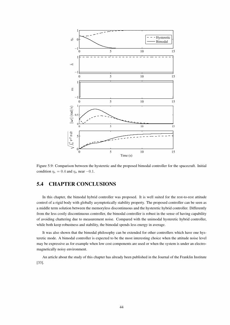
0 5 10 15−1

0

1

HystereticBimodal

0 5 10 15−1

1

0 5 10 15−1

1

0 5 10 150

0.5

1

0 5 10 150

5

Time (s)

JOU

RN

AL

OF

LAT E

XC

LA

SSFI

LE

S,V

OL

.11,

NO

.4,D

EC

EM

BE

R20

123

[wid

th=8

cm]fi

g/C

omhi

ster

ese

Fig.

2.St

ate

spac

ere

pres

enta

tion

ofth

ehy

ster

etic

cont

rolle

r(w

ithon

est

ate

h).

Arr

ows

indi

cate

the

dire

ctio

nof

the

torq

ueco

ntri

butio

nte

rm(d

epen

dent

onst

ateh

)so

the

attit

ude

isre

gula

ted

to1

or−1

.The

para

met

erδ

repr

esen

tsth

ehy

ster

esis

half

-wid

thof

the

on-o

ffco

ntro

lfo

rst

ateh

.

The

stat

esp

ace

ofth

ecl

osed

-loo

psy

stem

isre

pres

ente

dby

x1=

(xp,x

c1)∈X

1:=

Xp×

Xc.

The

cont

rolle

rob

ject

ive

isto

glob

ally

asym

ptot

ical

lyst

abi-

lize

the

set

A1=

x1∈X

1:qe=

h1,ω

= 0 .

(5)

The

clos

ed-l

oop

syst

emis

give

nby

(2),

(3)

and

the

follo

w-

ing

dyna

mic

sof

the

cont

rolle

r.

˙ h=

0x1∈C

1:=

x1∈X

1:hη e

≥−δ ,

h+∈

sgn(u

1)

x1∈D

1:=

x1∈X

1:hη e

≤−δ ,

(6)

whe

reh+

isth

eva

lue

asso

ciat

edto

hju

staf

ter

the

stat

etr

ansi

tion

and

sgn(η)=

sgn(η),

|ηe|>

0,

−1,1,

η e=

0.

The

vect

orof

inpu

tsU1=

(τ,u

1)

isca

lcul

ated

asfo

llow

s:τ y,q

d,h

=−ch e

−ω

andu1

y,q

d,h

=η e

.A

sal

read

ym

entio

ned,

hde

term

ines

the

orie

ntat

ion

ofa

forc

eal

ong

the

axis

ofro

tatio

n.W

hile

hη e

≥0

,it

forc

esth

em

ovem

ent

toth

esh

orte

rro

tatio

ndi

rect

ion.

How

ever

,w

hen

hη e

<0,

the

forc

est

illpu

llsin

the

sam

edi

rect

ion

(the

long

erro

tatio

ndi

rect

ion)

until

asa

fedi

stan

ceis

achi

eved

topr

even

tch

atte

ring

,i.e

.,un

tilhη e

≤−δ.

III.

PR

OP

OS

ED

CO

NT

RO

LL

ER

As

the

hyst

eret

icco

ntro

ller,

ina

spec

ific

regi

onof

the

stat

esp

ace,

dete

rmin

esa

forc

eco

ntri

butio

nto

mak

eth

eri

gid-

body

evol

ves

toth

elo

nger

rota

tion

dire

ctio

n,w

epr

opos

eto

add

one

mor

est

ate

toth

eco

ntro

ller

topr

even

tth

isbe

havi

oran

dsa

veen

ergy

.T

hepr

opos

edco

ntro

ller

feed

back

torq

ueis

also

give

nby

(4),

but

itha

stw

ost

ates

xc2=

h,m

∈X

c×

Xc,X

c:=

−1,1

.

The

stat

eh

dete

rmin

esth

efe

edba

ckto

rque

cont

ribu

tion

inor

dert

om

oveqe

eith

erto

1or

−1

,as

wel

las

inth

ehy

ster

etic

cont

rol.

The

stat

em

=1

indi

cate

sth

at|η

e|h

asre

ache

dov

erth

ehy

ster

esis

wid

thva

lue

butη e

has

not

cros

sed

zero

yet.

The

stat

em

=−1

indi

cate

sth

eop

posi

te,

that

η eha

sal

read

ycr

osse

dze

robu

t|η e|h

asno

trea

ched

over

the

hyst

eres

isw

idth

valu

eye

t.T

hesp

ace

stat

eof

the

clos

ed-l

oop

syst

emis

repr

esen

ted

by

x2=

(x,x

c2)∈X

2:=

X×

Xc×

Xc.

The

cont

rolle

rob

ject

ive

isto

glob

ally

asym

ptot

ical

lyst

abili

zeth

ese

t

A2=

x2∈X

2:qe=

h1,m

=1,ω= 0 .

(7)

The

clos

ed-l

oop

syst

emis

give

nby

(2),

(3)

and

the

follo

w-

ing

dyna

mic

sof

the

cont

rolle

r.˙ h=

0m

=0

x2∈C

2,

h+∈

sgn(u

2)

m+∈u3sg

n(u

2−u3δ/2)

x2∈D

2,

(8)

C2:=

x2∈X

2: h

η e≥

−δ , h

=−1

or

m(η

e−

δ/2)

≥−δ)

, h=

1orm(η

e+δ/2)

≤δ

,

D2:=

x2∈X

2: h

η e≤

−δ or

h=

1,

m(η

e−

δ/2)≤

−δ)

or h

=−1,m

(ηe+δ/2)

≥δ

.

whe

rem

+an

dh+

are

valu

esas

soci

ated

tom

andh

,res

pec-

tivel

y,ju

staf

ter

stat

etr

ansi

tion.

The

setD

2ca

nbe

expr

esse

din

aco

mpa

ctfo

rmas

follo

ws

D2:=

x2∈X

2: h

η e≤

−δ or

mh(η

e−hδ/2)

≤−δ

.

The

vect

orof

inpu

tsU2

=(τ,u

2,u

3)

isca

lcul

ated

asfo

llow

s:τ y,q

d,h

,m =

−ch e

−ω

,u2

y,q

d,h

,m =

η ean

du3

y,q

d,h

,m =

h.

[wid

th=8

cm]fi

g/fig

Prop

osto

Fig.

3.St

ate

spac

ere

pres

enta

tion

show

ing

the

prop

osed

regu

latio

nw

ithtw

ost

ates

(han

dm

).A

rrow

sin

dica

teth

edi

rect

ion

ofth

eto

rque

cont

ribu

tion

term

(dep

ende

nton

stat

eh

)so

the

attit

ude

isre

gula

ted

to1

or−1

.The

para

met

erδ

repr

esen

tsth

ehy

ster

esis

half

-wid

thof

the

on-o

ffco

ntro

lfo

rst

ateh

and

also

ofth

eon

-off

cont

rol

for

stat

em

.

Fig.

3sh

ows

the

prop

osed

regu

latio

n.W

hen

stat

em

=−1,

the

cont

rolle

rbe

have

sas

the

hyst

eret

icco

ntro

ller.

Ifh=

1,st

ateh

chan

ges

to−1

whe

nη e

≤−δ;

ifh

=−1,

stat

eh

chan

ges

to1

whe

nη e

≥δ.

The

cont

rolle

rsw

itche

sto

stat

em

=1

whe

nth

eat

titud

eer

rorqe

pres

ents

η e≤

−2δ

orη e

≥2δ

.W

hen

stat

em

=1,

the

cont

rolle

rbe

have

sas

the

disc

ontin

uous

cont

rolle

r.In

othe

rw

ords

,if

stat

em

=1,

stat

em

will

chan

geto

m=

−1

whe

nη e

goes

acro

ssze

roan

den

ter

the

jum

pse

t.T

his

fact

,ant

icip

ate

the

chan

geof

stat

eh

.Thi

sdi

stin

ctbe

havi

oris

wha

tdi

ffer

entia

tes

itfr

omth

ehy

ster

etic

cont

rolle

r(6

)an

dal

low

sa

torq

ueco

ntri

butio

nto

war

dsth

esh

orte

rro

tatio

ndi

rect

ion.

A.

Stab

ility

anal

ysis

Con

side

rth

ecl

osed

-loo

psy

stem

ofth

epr

opos

edco

ntro

ller

(8)

rew

ritte

nac

cord

ing

toth

ehy

brid

syst

ems

fram

ewor

kof

[11]

and

give

nby

H=

˙ x2∈F2(x

2),

x2∈C

2,

x+ 2∈G

2(x

2),

x2∈D

2,

whe

rex2=

(qe,ω

,h,m

),

F2(x

2):=

1 2qe(0,ω

)J−1 S

(Jω)ω−

ch e

−ω

0 0

,

G2(x

2):=

qe ω

sgn(η

e)

hsg

n η e

−hδ/2

.

JOU

RN

AL

OF

LAT E

XC

LA

SSFI

LE

S,V

OL

.11,

NO

.4,D

EC

EM

BE

R20

123

[wid

th=8

cm]fi

g/C

omhi

ster

ese

Fig.

2.St

ate

spac

ere

pres

enta

tion

ofth

ehy

ster

etic

cont

rolle

r(w

ithon

est

ate

h).

Arr

ows

indi

cate

the

dire

ctio

nof

the

torq

ueco

ntri

butio

nte

rm(d

epen

dent

onst

ateh

)so

the

attit

ude

isre

gula

ted

to1

or−1

.The

para

met

erδ

repr

esen

tsth

ehy

ster

esis

half

-wid

thof

the

on-o

ffco

ntro

lfo

rst

ateh

.

The

stat

esp

ace

ofth

ecl

osed

-loo

psy

stem

isre

pres

ente

dby

x1=

(xp,x

c1)∈X

1:=

Xp×X

c.

The

cont

rolle

rob

ject

ive

isto

glob

ally

asym

ptot

ical

lyst

abi-

lize

the

set

A1=

x1∈X

1:qe=

h1,ω

= 0 .

(5)

The

clos

ed-l

oop

syst

emis

give

nby

(2),

(3)

and

the

follo

w-

ing

dyna

mic

sof

the

cont

rolle

r.

˙ h=

0x1∈C

1:=

x1∈X

1:hη e

≥−δ ,

h+∈

sgn(u

1)

x1∈D

1:=

x1∈X

1:hη e

≤−δ ,

(6)

whe

reh+

isth

eva

lue

asso

ciat

edto

hju

staf

ter

the

stat

etr

ansi

tion

and

sgn(η)=

sgn(η),

|ηe|>

0,

−1,1,

η e=

0.

The

vect

orof

inpu

tsU1=

(τ,u

1)

isca

lcul

ated

asfo

llow

s:τ y,q

d,h

=−ch e

−ω

andu1

y,q

d,h

=η e

.A

sal

read

ym

entio

ned,

hde

term

ines

the

orie

ntat

ion

ofa

forc

eal

ong

the

axis

ofro

tatio

n.W

hile

hη e

≥0

,it

forc

esth

em

ovem

ent

toth

esh

orte

rro

tatio

ndi

rect

ion.

How

ever

,w

hen

hη e

<0,

the

forc

est

illpu

llsin

the

sam

edi

rect

ion

(the

long

erro

tatio

ndi

rect

ion)

until

asa

fedi

stan

ceis

achi

eved

topr

even

tch

atte

ring

,i.e

.,un

tilhη e

≤−δ.

III.

PR

OP

OS

ED

CO

NT

RO

LL

ER

As

the

hyst

eret

icco

ntro

ller,

ina

spec

ific

regi

onof

the

stat

esp

ace,

dete

rmin

esa

forc

eco

ntri

butio

nto

mak

eth

eri

gid-

body

evol

ves

toth

elo

nger

rota

tion

dire

ctio

n,w

epr

opos

eto

add

one

mor

est

ate

toth

eco

ntro

ller

topr

even

tth

isbe

havi

oran

dsa

veen

ergy

.T

hepr

opos

edco

ntro

ller

feed

back

torq

ueis

also

give

nby

(4),

but

itha

stw

ost

ates

xc2=

h,m

∈X

c×X

c,X

c:=

−1,1

.

The

stat

eh

dete

rmin

esth

efe

edba

ckto

rque

cont

ribu

tion

inor

dert

om

oveqe

eith

erto

1or

−1

,as

wel

las

inth

ehy

ster

etic

cont

rol.

The

stat

em

=1

indi

cate

sth

at|η

e|h

asre

ache

dov

erth

ehy

ster

esis

wid

thva

lue

butη e

has

not

cros

sed

zero

yet.

The

stat

em

=−1

indi

cate

sth

eop

posi

te,

that

η eha

sal

read

ycr

osse

dze

robu

t|η e|h

asno

trea

ched

over

the

hyst

eres

isw

idth

valu

eye

t.T

hesp

ace

stat

eof

the

clos

ed-l

oop

syst

emis

repr

esen

ted

by

x2=

(x,x

c2)∈X

2:=

X×X

c×X

c.

The

cont

rolle

rob

ject

ive

isto

glob

ally

asym

ptot

ical

lyst

abili

zeth

ese

t

A2=

x2∈X

2:qe=

h1,m

=1,ω= 0 .

(7)

The

clos

ed-l

oop

syst

emis

give

nby

(2),

(3)

and

the

follo

w-

ing

dyna

mic

sof

the

cont

rolle

r.˙ h=

0m

=0

x2∈C

2,

h+∈

sgn(u

2)

m+∈u3sg

n(u

2−u3δ/2)

x2∈D

2,

(8)

C2:=

x2∈X

2: h

η e≥

−δ , h

=−1

or

m(η

e−δ/2)≥

−δ)

, h=

1orm(η

e+δ/2)≤

δ,

D2:=

x2∈X

2: h

η e≤

−δ or

h=

1,

m(η

e−δ/2)≤

−δ)

or h

=−1,m

(ηe+δ/2)≥

δ.

whe

rem

+an

dh+

are

valu

esas

soci

ated

tom

andh

,res

pec-

tivel

y,ju

staf

ter

stat

etr

ansi

tion.

The

setD

2ca

nbe

expr

esse

din

aco

mpa

ctfo

rmas

follo

ws

D2:=

x2∈X

2: h

η e≤

−δ or

mh(η

e−hδ/2)≤

−δ

.

The

vect

orof

inpu

tsU2

=(τ,u

2,u

3)

isca

lcul

ated

asfo

llow

s:τ y,q

d,h

,m =

−ch e

−ω

,u2

y,q

d,h

,m =

η ean

du3

y,q

d,h

,m =

h.

[wid

th=8

cm]fi

g/fig

Prop

osto

Fig.

3.St

ate

spac

ere

pres

enta

tion

show

ing

the

prop

osed

regu

latio

nw

ithtw

ost

ates

(han

dm

).A

rrow

sin

dica

teth

edi

rect

ion

ofth

eto

rque

cont

ribu

tion

term

(dep

ende

nton

stat

eh

)so

the

attit

ude

isre

gula

ted

to1

or−1

.The

para

met

erδ

repr

esen

tsth

ehy

ster

esis

half

-wid

thof

the

on-o

ffco

ntro

lfo

rst

ateh

and

also

ofth

eon

-off

cont

rol

for

stat

em

.

Fig.

3sh

ows

the

prop

osed

regu

latio

n.W

hen

stat

em

=−1,

the

cont

rolle

rbe

have

sas

the

hyst

eret

icco

ntro

ller.

Ifh=

1,st

ateh

chan

ges

to−1

whe

nη e

≤−δ;

ifh

=−1,

stat

eh

chan

ges

to1

whe

nη e

≥δ.

The

cont

rolle

rsw

itche

sto

stat

em

=1

whe

nth

eat

titud

eer

rorqe

pres

ents

η e≤

−2δ

orη e

≥2δ

.W

hen

stat

em

=1,

the

cont

rolle

rbe

have

sas

the

disc

ontin

uous

cont

rolle

r.In

othe

rw

ords

,if

stat

em

=1,

stat

em

will

chan

geto

m=

−1

whe

nη e

goes

acro

ssze

roan

den

ter

the

jum

pse

t.T

his

fact

,ant

icip

ate

the

chan

geof

stat

eh

.Thi

sdi

stin

ctbe

havi

oris

wha

tdi

ffer

entia

tes

itfr

omth

ehy

ster

etic

cont

rolle

r(6

)an

dal

low

sa

torq

ueco

ntri

butio

nto

war

dsth

esh

orte

rro

tatio

ndi

rect

ion.

A.

Stab

ility

anal

ysis

Con

side

rth

ecl

osed

-loo

psy

stem

ofth

epr

opos

edco

ntro

ller

(8)

rew

ritte

nac

cord

ing

toth

ehy

brid

syst

ems

fram

ewor

kof

[11]

and

give

nby

H=

˙ x2∈F2(x

2),

x2∈C

2,

x+ 2∈G

2(x

2),

x2∈D

2,

whe

rex2=

(qe,ω

,h,m

),

F2(x

2):=

1 2qe(0,ω

)J−1 S

(Jω)ω−ch e

−ω

0 0

,

G2(x

2):=

qe ω

sgn(η

e)

hsg

n η e

−hδ/2

.1

m

1

ω(

rad/

s)

1

t 0

τTτdt

Figure 5.9: Comparison between the hysteretic and the proposed bimodal controller for the spacecraft. Initialcondition ηe = 0.4 and ησ near −0.1.


In this chapter, the bimodal hybrid controller was proposed. It is well suited for the rest-to-rest attitudecontrol of a rigid body with globally asymptotically stability property. The proposed controller can be seen asa middle term solution between the memoryless discontinuous and the hysteretic hybrid controller. Differentlyfrom the less costly discontinuous controller, the bimodal controller is robust in the sense of having capabilityof avoiding chattering due to measurement noise. Compared with the unimodal hysteretic hybrid controller,while both keep robustness and stability, the bimodal spends less energy in average.

It was also shown that the bimodal philosophy can be extended for other controllers which have one hys-teretic mode. A bimodal controller is expected to be the most interesting choice when the attitude noise levelmay be expressive as for example when low cost components are used or when the system is under an electro-magnetically noisy environment.

An article about the study of this chapter has already been published in the Journal of the Franklin Institute[33].

44

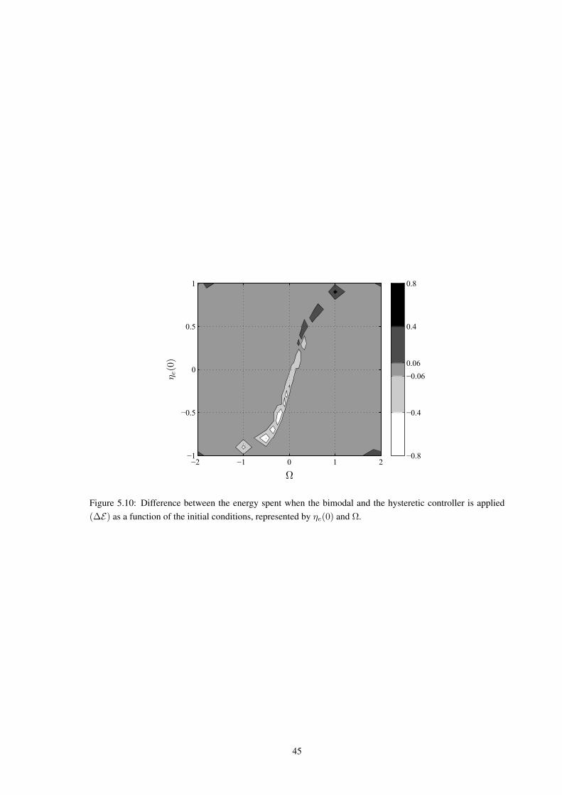
−2 −1 0 1 2−1

−0.5

0

0.5

1

−0.8

−0.4

−0.060.06

0.4

0.8

1

η e(0)

1

Ω

Figure 5.10: Difference between the energy spent when the bimodal and the hysteretic controller is applied(∆E) as a function of the initial conditions, represented by ηe(0) and Ω.

45

ROBUST GLOBAL DISTRIBUTED ATTITUDECONTROL FOR MULTIPLE RIGID BODIES

Rigid-body attitude control applied to multi-agent systems in a cooperative control is an area that has alsobeen studied for decades. In 1978, Labeyrie [60] proposed a stellar interferometer formation from free-flyingtelescopes. Research on multiple mobile robot (and multi-vehicle) systems initiated in the late 1980’s [61]and increased in the 1990’s thanks to the development of inexpensive and reliable wireless communicationssystems [62]. In the late 1990’s and early 2000’s, an area that became highly active was the cooperative controlof multiple aircraft, especially unmanned aerial vehicles (UAVs) [62]. Much research has been developed onattitude coordination control in the last 10-15 years [15, 16, 17, 18, 19] but the great majority of them suggestedcontinuous or discontinuous state-feedback laws that present known problems such as unstable states, unwind-ing phenomenon and chattering. In this chapter, it is proposed a distributed attitude synchronization controlwith globally asymptotically stability property and robustness against noise measurement for an undirectedconnected network (cyclic or acyclic) of rigid bodies (agents). The strategy uses a quaternion representation ofthe attitude and the hysteretic hybrid feedback with one binary logic variable, suggested by [10] (see Section3.5), for each agent.1

6.1 PRELIMINARIES

6.1.1 Attitude kinematics and dynamics of a group of n-agents

For a group of n-agents, in which it is associated an index i = 1, 2, . . . , n for each agent, let qi and ωirepresent, respectively, the attitude and the angular velocity of the agent i relative to each body frame and letq0 represent a fixed reference attitude with angular velocity ω0 = 0 for all the agents.

The attitude error of agent i relative to the common reference attitude is given by

qi0 = (ηi0, εi0) = q∗0 qi. (6.1)

The relative attitude between agent i and j, Rij = RTj Ri = R(qij), is represented by the relative quater-nion

qij = (ηij , εij) = q∗j qi (6.2)

which satisfies the following kinematic equation

qij =1

2qij (0,ωij), (6.3)

where the relative angular velocity ωij is

ωij = ωi −RTijωj . (6.4)

Let X = S3 × R3 and xi = (qi0,ωi) ∈ X . Since each physical attitude R ∈ SO(3) is represented by apair of antipodal unit quaternions ±q ∈ S3, the objective of the control, for each agent, becomes to stabilizethe set

Ai = (1,0) , (−1,0) ⊂ X1The author informs that applying the hysteretic controller suggested by [10], instead of the bimodal controller proposed in Chapter 5,

leads to better results due to restrictions arisen when using the Lyapunov function (6.20).

46

6

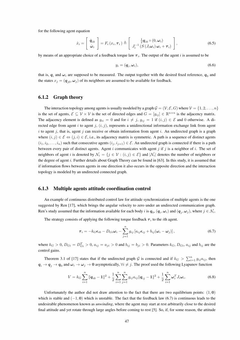
for the following agent equation

xi =

[qi0ωi

]= Fi (xi, τ i ) ,

[12qi0 (0,ωi)

J−1i (S (Jiωi)ωi + τ i)

], (6.5)

by means of an appropriate choice of a feedback torque law τ i. The output of the agent i is assumed to be

yi = (qi,ωi), (6.6)

that is, qi and ωi are supposed to be measured. The output together with the desired fixed reference, q0 andthe states xj = (qj0,ωj) of its neighbors are assumed to be available for feedback.

6.1.2 Graph theory

The interaction topology among agents is usually modeled by a graph G = (V, E , G) where V = 1, 2, . . . , nis the set of agents, E ⊆ V × V is the set of directed edges and G = [gij ] ∈ Rn×n is the adjacency matrix.The adjacency element is defined as gii = 0 and for i 6= j, gij = 1 if (i, j) ∈ E and 0 otherwise. A di-rected edge from agent i to agent j, (i, j), represents a unidirectional information exchange link from agenti to agent j, that is, agent j can receive or obtain information from agent i. An undirected graph is a graphwhere (i, j) ∈ E ⇔ (j, i) ∈ E , i.e., its adjacency matrix is symmetric. A path is a sequence of distinct agents(i1, i2, . . . , in) such that consecutive agents (ij , ij+1) ∈ E . An undirected graph is connected if there is a pathbetween every pair of distinct agents. Agent i communicates with agent j if j is a neighbor of i. The set ofneighbors of agent i is denoted by Ni = j ∈ V : (i, j) ∈ E and |Ni| denotes the number of neighbors orthe degree of agent i. Further details about Graph Theory can be found in [63]. In this study, it is assumed thatif information flows between agents in one direction it also occurs in the opposite direction and the interactiontopology is modeled by an undirected connected graph.

6.1.3 Multiple agents attitude coordination control

An example of continuous distributed control law for attitude synchronization of multiple agents is the onesuggested by Ren [17], which brings the angular velocity to zero under an undirected communication graph.Ren’s study assumed that the information available for each body i is q0, (qi,ωi) and (qj ,ωj), where j ∈ Ni.

The strategy consists of applying the following torque feedback τ i to the ith agent.

τ i = −kGεi0 −DGiωi −n∑j=1

gij [aijεij + bij(ωi − ωj)] , (6.7)

where kG > 0, DGi = DTGi > 0, aij = aji > 0 and bij = bji > 0. Parameters kG, DGi, aij and bij are the

control gains.

Theorem 3.1 of [17] states that if the undirected graph G is connected and if kG >∑ni=1 gijaij , then

qi → qj → q0 and ωi → ωj → 0 asymptotically, ∀i 6= j. The proof used the following Lyapunov function

V = kG

n∑i=1

‖qi0 − 1‖2 +1

2

n∑i=1

n∑j=1

gijaij‖qij − 1‖2 +1

2

n∑i=1

ωTi Jiωi. (6.8)

Unfortunately the author did not draw attention to the fact that there are two equilibrium points: (1,0)

which is stable and (−1,0) which is unstable. The fact that the feedback law (6.7) is continuous leads to theundesirable phenomenon known as unwinding, where the agent may start at rest arbitrarily close to the desiredfinal attitude and yet rotate through large angles before coming to rest [5]. So, if, for some reason, the attitude

47

error of agent i is close to −1, then the unwinding phenomenon may occur. Moreover, if the other agents areclose to the reference, agent i may spend too much time to move away from the unstable equilibrium pointregion since the feedback torque of agent i depends on εi0 and εij which are close to 0. The problem getsworse if measurement noise is taken into account. In this case, the state of agent imay remain near the unstableequilibrium point for an indefinite period of time. This case is exemplified in Section 6.4.

In the next section, it is proposed a modification in the feedback law (6.7) to accommodate the hysteretichybrid controller suggested by [10] in the multiple agents scenario. This way, both equilibrium points, qi0 = 1

and qi0 = −1, for each agent i, become stable and the control becomes global and robust.

6.2 PROPOSED HYBRID ATTITUDE CONTROLLER

This study proposes a global and robust distributed control law for attitude synchronization of multipleagents. The strategy uses the hysteretic hybrid controller suggested by [10] with one state logic variable hi ∈Xc = 1,−1 and vector of inputs Ui = (τ i, ui) for each agent i.

The state of the subsystem plant + controller of agent i is represented by xi = (qi0,ωi, hi) ∈ X ,

S3 × R3 × Xc, i = 1, 2, . . . , n. Each subsystem evolves according to (6.5), (6.6), the following dynamics ofthe controller2

hi = 0 x ∈ Ci ,x ∈ Xn : hiηi0 ≥ −δi

,

h+i ∈ sgn (ui) x ∈ Di ,

x ∈ Xn : hiηi0 ≤ −δi

,

(6.9)

where h+i is the value associated to hi just after state transition,

sgn (ui) =

1 , ui > 0,

−1 , ui < 0,

−1, 1 , ui = 0

and the closed-loop lawUi = K(yi, q0, hi, qj ,ωj) , (τ i, ηi0), j ∈ Ni. (6.10)

The parameter δi ∈ (0, 1) represents the hysteresis half-width and provides robustness against chattering causedby output measurement.

The feedback torque τ i is given by

τ i = −kGihiεi0 −DGiωi −n∑j=1

gij[aijhihjεij + bij(ωi −RTijωj)

], (6.11)

where the control gains kGi > 0, DGi = DTGi > 0, aij = aji > 0 and bij = bji > 0. Note that, differently

from (6.7), RTij multiplies ωj in the torque equation because the coordinates of ωj refers to the agent-j frame.

Figure 6.1 shows the behavior of the subsystem for a hysteresis width of 2δi. The state variable hi deter-mines the torque feedback so the agent attitude qi0 is regulated either to 1 or −1.

Let the state of the whole system be represented by x = (x1, x2, . . . , xn) ∈ Xn. It will be shown in thenext section that the controller globally asymptotically stabilizes the set

A =⋂ni=1 Ai Ai ,

x ∈ Xn : xi = (1,0, 1) or xi = (−1,0,−1)

. (6.12)

2Along the text, the dynamics representations follow the hybrid systems framework of Goebel et al. [48], summarized in Section 2.7.

48

10-1

1

1

1

0

1

−1

1

−δi

1

δi

1

hi = 11

hi = −1

1

i0

1

ηi0

Figure 6.1: Agent i state space representation and the proposed regulation. The hysteresis half-width of theon-off control for state hi is δi.


Considering the proposed controller (6.9) the agent-i subsystem can be written in closed-loop form, denotedbyHi, as

Hi

˙xi = F i (xi) , x ∈ Ci,x+i ∈ Gi (xi) , x ∈ Di,

(6.13)

F i (xi) =

12qi0 (0,ωi)

J−1i (S (Jiωi)ωi + τ i)

0

, (6.14)

Gi (xi) =

qi0ωi

sgn (ηi0)

. (6.15)

Before describing the complete system, by grouping all the agents, its necessary to define the flow and jumpsets as C ,

⋂ni=1 Ci and D ,

⋃ni=1Di, respectively. Note that more than one jump can occur simultaneously

and the jump map is not straightforward. Let the set of agents whose state of hi is about to change be definedas

T (x) , i ∈ V : x ∈ Di (6.16)

and G0 (xi) = [ qTi0 ωTi hi ]T represent a mapping that keeps the state variables of agent i unchanged.Motivated by the mapping suggested in [21], the jump map of x is defined as

Γ(x) =⋃i∈Tγi(x), (6.17)

where γi(x) = [ γTi1 . . . γTin ]T , γij = G0 (xj) , j 6= i and γii = Gi (xi).

The complete system, denoted asH, is given by

H :

˙x = F (x) , x ∈ C,x+ ∈ G (x) , x ∈ D,

(6.18)

where F (x) , [ FT

1 (x1) . . . FT

n (xn) ]T and G (x) , Γ(x).

49

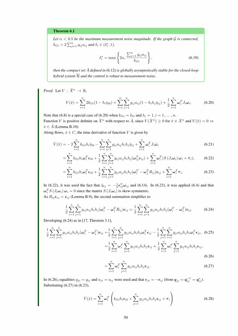
Theorem 6.1

Let α < 0.5 be the maximum measurement noise magnitude. If the graph G is connected,kGi > 2

∑nj=1 gijaij and δi ∈ (δ∗i , 1),

δ∗i = max

2α,

∑nj=1 gijaij

kGi

, (6.19)

then the compact set A defined in (6.12) is globally asymptotically stable for the closed-loophybrid systemH and the control is robust to measurement noise.

Proof. Let V : Xn → R,

V (x) =

n∑i=1

2kGi(1− hiηi0) +

n∑i=1

n∑j=1

gijaij(1− hihjηij) +1

2

n∑i=1

ωTi Jiωi. (6.20)

Note that (6.8) is a special case of (6.20) when kGi = kG and hi = 1, i = 1, . . . , n.Function V is positive definite on Xn with respect to A, since V (Xn) ≥ 0 for x ∈ Xn and V (x) = 0 ⇔x ∈ A (Lemma B.10).Along flows, x ∈ C, the time derivative of function V is given by

V (x) =− 2

n∑i=1

kGihiηi0 −n∑i=1

n∑j=1

gijaijhihj ηij +

n∑i=1

ωTi Jiωi (6.21)

=

n∑i=1

kGihiωTi εi0 +

1

2

n∑i=1

n∑j=1

gijaijhihj(ωTijεij) +

n∑i=1

ωTi (S (Jiωi)ωi + τ i), (6.22)

=

n∑i=1

kGihiωTi εi0 +

1

2

n∑i=1

n∑j=1

gijaijhihj(ωTi − ωTj Rij)εij +

n∑i=1

ωTi τ i. (6.23)

In (6.22), it was used the fact that ηij = − 12εTijωij and (6.14). In (6.23), it was applied (6.4) and that

ωTi S (Jiωi)ωi = 0 since the matrix S (Jiωi) is skew-symmetric.As Rijεij = εij (Lemma B.9), the second summation simplifies to

1

2

n∑i=1

n∑j=1

gijaijhihj(ωTi − ωTj Rij)εij =

1

2

n∑i=1

n∑j=1

gijaijhihj(ωTi − ωTj )εij . (6.24)

Developing (6.24) as in [17, Theorem 3.1],

1

2

n∑i=1

n∑j=1

gijaijhihj(ωTi − ωTj )εij =

1

2

n∑i=1

n∑j=1

gijaijhihjωTi εij −

1

2

n∑j=1

n∑i=1

gjiajihjhiωTi εji, (6.25)

=1

2

n∑i=1

ωTi

n∑j=1

gijaijhihjεij +1

2

n∑i=1

ωTi

n∑j=1

gijaijhihjεij ,

(6.26)

=

n∑i=1

ωTi

n∑j=1

gijaijhihjεij . (6.27)

In (6.26), equalities gji = gij and aji = aij were used and that εji = −εij (from qji = q−1ij = q∗ij).

Substituting (6.27) in (6.23),

V (x) =

n∑i=1

ωTi

kGihiεi0 +

n∑j=1

gijaijhihjεij + τ i

(6.28)

50

and, finally, using the torque definition τ i (6.11) in (6.28),

V (x) =−n∑i=1

ωTi DGiωi −n∑i=1

n∑j=1

gijbijωTi (ωi −RTijωj). (6.29)

Developing the last term of (6.29),

n∑i=1

n∑j=1

gijbijωTi (ωi −RTijωj) =

1

2

n∑i=1

n∑j=1

gijbijωTi (ωi −RTijωj) +

1

2

n∑i=1

n∑j=1

gijbijωTi (ωi −RTijωj),

(6.30)

=1

2

n∑i=1

n∑j=1

gijbijωTi (ωi −RTijωj) +

1

2

n∑i=1

n∑j=1

gjibjiωTj (ωj −RTjiωi),

(6.31)

=1

2

n∑i=1

n∑j=1

gijbij[ωTi (ωi −RTijωj)− ωTj (Rijωi − ωj)

], (6.32)

=1

2

n∑i=1

n∑j=1

gijbij[ωTi (ωi −RTijωj)− ωTj Rij(ωi −RTijωj)

], (6.33)

=1

2

n∑i=1

n∑j=1

gijbij[(ωTi − ωTj Rij)(ωi −RTijωj)

], (6.34)

=1

2

n∑i=1

n∑j=1

gijbij‖ωi −RTijωj‖2. (6.35)

In (6.32), equalities gji = gij , bji = bij and RTji = Rij were used. Now, substituting (6.35) into (6.29),

V (x) =−n∑i=1

ωTi DGiωi −1

2

n∑i=1

n∑j=1

gijbij‖ωi −RTijωj‖2. (6.36)

Note that function V is negative semidefinite on Xn with respect to A, since V (x) ≤ 0 for all x ∈ Xn andV (x) = 0⇔ ωi = 0, i = 1, . . . , n.Along jumps, x ∈ D,

∆V (x) = V (x+)− V (x), (6.37)

where x+ = (x+1 , x

+2 , . . . , x

+n ) ∈ Xn.

From (6.15), q+i0 = qi0, ω+

i = ωi and h+i = −hi. It follows that

∆V (x) = −n∑i=1

2kGi(h+i − hi)ηi0 −

n∑i=1

n∑j=1

gijaij(h+i h

+j − hihj)ηij . (6.38)

In the first summation in (6.38), h+i 6= hi whenever xi ∈ Di, i.e., when i ∈ T (6.16). Regarding the second

summation, h+i h

+j 6= hihj when i ∈ T and j /∈ T and vice-versa. Therefore,

∆V (x) =−∑i∈T

2kGi(h+i − hi)ηi0 −

∑i∈T

∑j /∈T

gijaij(h+i h

+j − hihj)ηij−∑

i/∈T

∑j∈T

gijaij(h+i h

+j − hihj)ηij

=4∑i∈T

kGihiηi0 + 2∑i∈T

∑j /∈T

gijaijhihjηij + 2∑i/∈T

∑j∈T

gijaijhihjηij (6.39)

As aij = aji, gij = gji and ηij = ηji,∑i∈T

∑j /∈T

gijaijhihjηij =∑j /∈T

∑i∈T

gjiajihjhiηji =∑i/∈T

∑j∈T

gijaijhihjηij . (6.40)

51

Hence,

∆V (x) = 4∑i∈T

kGihiηi0 +∑j /∈T

gijaijhihjηij

. (6.41)

Since x ∈ D, according to (6.9) hiηi0 ≤ −δi and given that hihjηij ≤ 1,

∆V (x) ≤ 4∑i∈T

−kGiδi +∑

j∈Ni\T

gijaij

. (6.42)

Suppose that the following restriction is considered,

δi >

∑j∈Ni

gijaij

kGi=

∑nj=1 gijaij

kGi, (6.43)

so that ∆V (x) < 0,∀x ∈ Xn. Thus, from Theorem 7.6 of [56], it follows that the compact set A is stablesince ∆V (x) < 0 and V (x) ≤ 0 for all x ∈ Xn. The conclusion that the set A is globally asymptoticallystable comes when Theorem 4.7 of [56] is applied to prove that the set A is the largest invariant set in

W = x ∈ C : V (x) = 0. (6.44)

In the largest invariant set, V ≡ 0. From (6.36), ωi ≡ 0, i = 1, . . . , n. Using (6.14) and then (6.11), itfollows that τ i ≡ 0 and

kGiεi0 +

n∑j=1

gijaijεij = 0. (6.45)

Left multiplying both members in (6.45) by εTi0 and using the fact that εij = ηj0εi0 − ηi0εj0 − εj0 × εi0,

kGiεTi0εi0 +

n∑j=1

gijaijεTi0(ηj0εi0 − ηi0εj0 − εj0 × εi0) = 0, (6.46)

εTi0

kGi +

n∑j=1

ηj0gijaij

εi0 − εTi0 n∑j=1

ηi0gijaij

εj0 = 0. (6.47)

Since (6.47) is valid for all i, i = 1, . . . , n, the following equation holds.

qsT (P ⊗ I3)qs = 0, (6.48)

where ⊗ is the Kronecker product, qs = [εT10 εT20 . . . εTn0 ]T , P = [pij ] ∈ Rn×n, pii = kGi +∑nj=1 ηj0gijaij and pij = −ηi0gijaij .

Applying Gerschgorin Theorem [64] and supposing that

kGi > 2

n∑j=1

gijaij , (6.49)

matrix P ⊗ I3 gets strictly diagonally dominant and positive definite. Hence, qs = 0 is the only solution to(6.48). As a result, εi0 = 0, i = 1, . . . , n and qi0 = 1 or qi0 = −1 are candidates for the largest invariantset. Finally, using restriction x ∈ C from (6.44), it follows that qi0 = hi1.Summing up, any solution x(t) approaches the largest invariant set A (6.12) as long as hypotheses (6.49) and(6.43) are satisfied. Regarding the robustness of the control, the proof is a direct application of Theorem5.4 and 5.5 of [10] to the system H where it is proved that the number of jumps is bounded and thechattering phenomenon is eliminated if α ∈ [0, 0.5) and δi ∈ (2α, 1). Both restrictions on δi are satisfied ifδi ∈ (δ∗i , 1), where

δ∗i = max

2α,

∑nj=1 gijaij

kGi

.

52

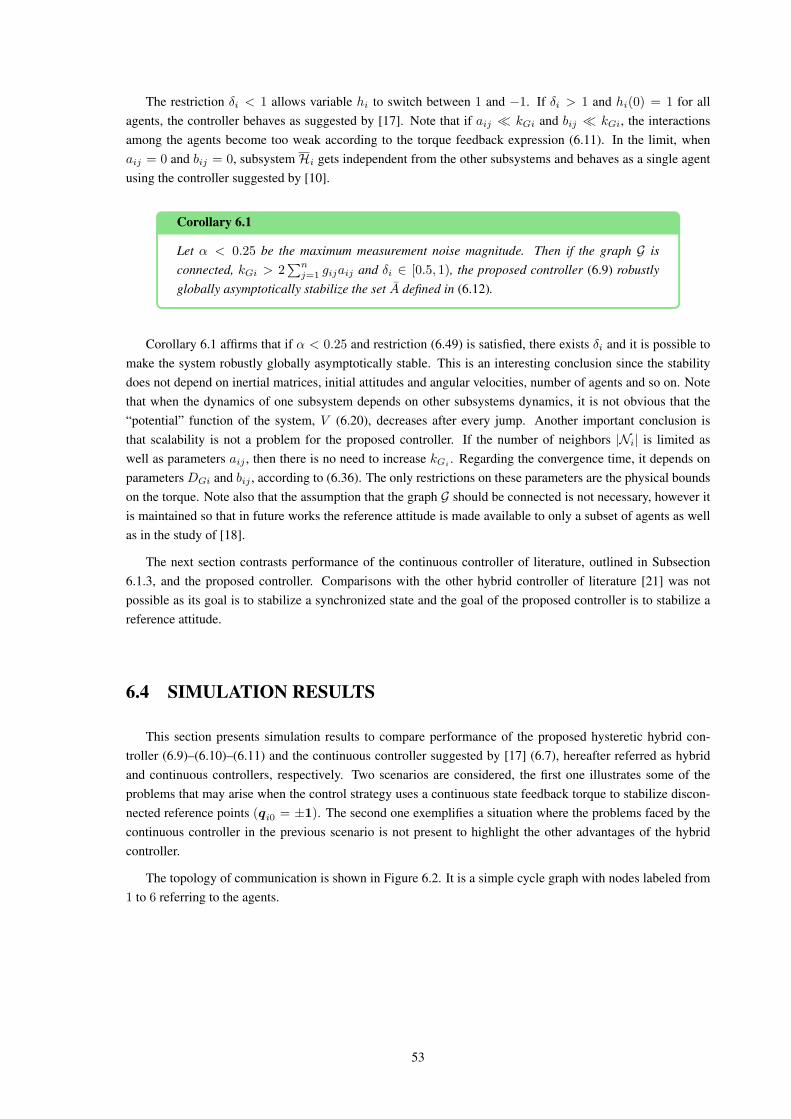
The restriction δi < 1 allows variable hi to switch between 1 and −1. If δi > 1 and hi(0) = 1 for allagents, the controller behaves as suggested by [17]. Note that if aij kGi and bij kGi, the interactionsamong the agents become too weak according to the torque feedback expression (6.11). In the limit, whenaij = 0 and bij = 0, subsystem Hi gets independent from the other subsystems and behaves as a single agentusing the controller suggested by [10].

Corollary 6.1

Let α < 0.25 be the maximum measurement noise magnitude. Then if the graph G isconnected, kGi > 2

∑nj=1 gijaij and δi ∈ [0.5, 1), the proposed controller (6.9) robustly

globally asymptotically stabilize the set A defined in (6.12).

Corollary 6.1 affirms that if α < 0.25 and restriction (6.49) is satisfied, there exists δi and it is possible tomake the system robustly globally asymptotically stable. This is an interesting conclusion since the stabilitydoes not depend on inertial matrices, initial attitudes and angular velocities, number of agents and so on. Notethat when the dynamics of one subsystem depends on other subsystems dynamics, it is not obvious that the“potential” function of the system, V (6.20), decreases after every jump. Another important conclusion isthat scalability is not a problem for the proposed controller. If the number of neighbors |Ni| is limited aswell as parameters aij , then there is no need to increase kGi . Regarding the convergence time, it depends onparameters DGi and bij , according to (6.36). The only restrictions on these parameters are the physical boundson the torque. Note also that the assumption that the graph G should be connected is not necessary, however itis maintained so that in future works the reference attitude is made available to only a subset of agents as wellas in the study of [18].

The next section contrasts performance of the continuous controller of literature, outlined in Subsection6.1.3, and the proposed controller. Comparisons with the other hybrid controller of literature [21] was notpossible as its goal is to stabilize a synchronized state and the goal of the proposed controller is to stabilize areference attitude.


This section presents simulation results to compare performance of the proposed hysteretic hybrid con-troller (6.9)–(6.10)–(6.11) and the continuous controller suggested by [17] (6.7), hereafter referred as hybridand continuous controllers, respectively. Two scenarios are considered, the first one illustrates some of theproblems that may arise when the control strategy uses a continuous state feedback torque to stabilize discon-nected reference points (qi0 = ±1). The second one exemplifies a situation where the problems faced by thecontinuous controller in the previous scenario is not present to highlight the other advantages of the hybridcontroller.

The topology of communication is shown in Figure 6.2. It is a simple cycle graph with nodes labeled from1 to 6 referring to the agents.

53

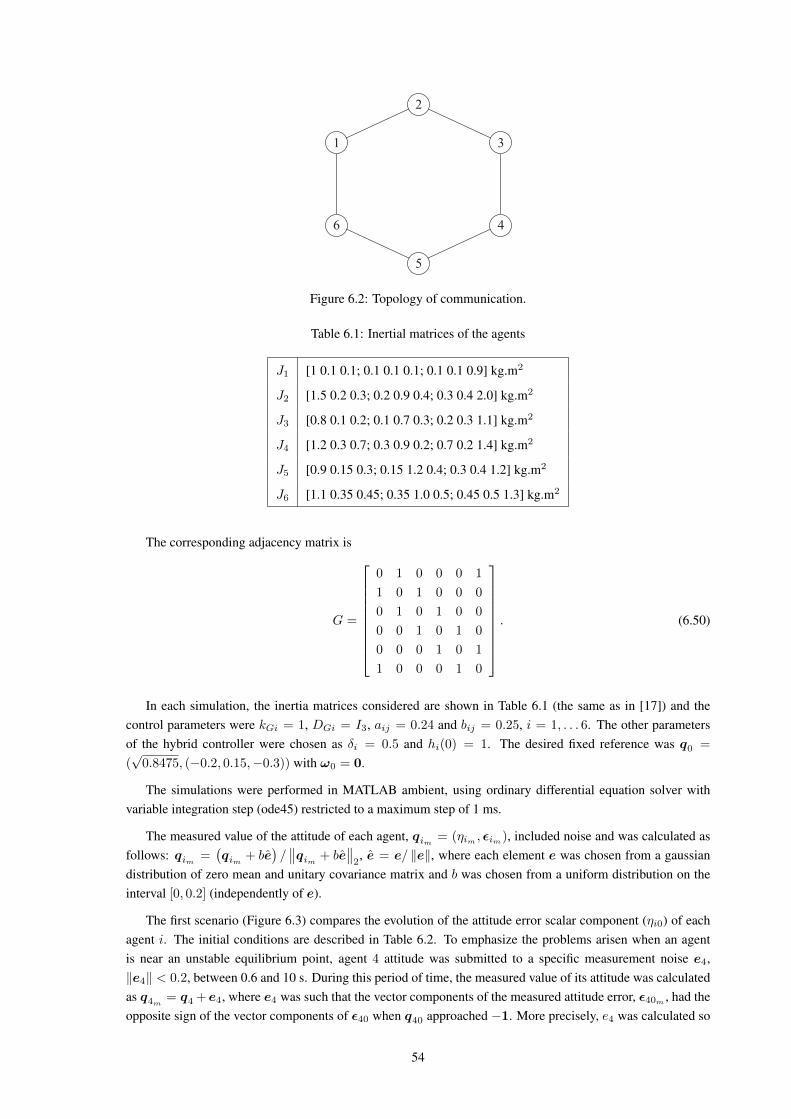
2

3

6

5

4

1

Figure 6.2: Topology of communication.

Table 6.1: Inertial matrices of the agents

J1 [1 0.1 0.1; 0.1 0.1 0.1; 0.1 0.1 0.9] kg.m2

J2 [1.5 0.2 0.3; 0.2 0.9 0.4; 0.3 0.4 2.0] kg.m2

J3 [0.8 0.1 0.2; 0.1 0.7 0.3; 0.2 0.3 1.1] kg.m2

J4 [1.2 0.3 0.7; 0.3 0.9 0.2; 0.7 0.2 1.4] kg.m2

J5 [0.9 0.15 0.3; 0.15 1.2 0.4; 0.3 0.4 1.2] kg.m2

J6 [1.1 0.35 0.45; 0.35 1.0 0.5; 0.45 0.5 1.3] kg.m2

The corresponding adjacency matrix is

G =

0 1 0 0 0 1

1 0 1 0 0 0

0 1 0 1 0 0

0 0 1 0 1 0

0 0 0 1 0 1

1 0 0 0 1 0

. (6.50)

In each simulation, the inertia matrices considered are shown in Table 6.1 (the same as in [17]) and thecontrol parameters were kGi = 1, DGi = I3, aij = 0.24 and bij = 0.25, i = 1, . . . 6. The other parametersof the hybrid controller were chosen as δi = 0.5 and hi(0) = 1. The desired fixed reference was q0 =

(√

0.8475, (−0.2, 0.15,−0.3)) with ω0 = 0.

The simulations were performed in MATLAB ambient, using ordinary differential equation solver withvariable integration step (ode45) restricted to a maximum step of 1 ms.

The measured value of the attitude of each agent, qim = (ηim , εim), included noise and was calculated asfollows: qim =

(qim + be

)/∥∥qim + be

∥∥2, e = e/ ‖e‖, where each element e was chosen from a gaussian

distribution of zero mean and unitary covariance matrix and b was chosen from a uniform distribution on theinterval [0, 0.2] (independently of e).

The first scenario (Figure 6.3) compares the evolution of the attitude error scalar component (ηi0) of eachagent i. The initial conditions are described in Table 6.2. To emphasize the problems arisen when an agentis near an unstable equilibrium point, agent 4 attitude was submitted to a specific measurement noise e4,‖e4‖ < 0.2, between 0.6 and 10 s. During this period of time, the measured value of its attitude was calculatedas q4m

= q4 + e4, where e4 was such that the vector components of the measured attitude error, ε40m, had the

opposite sign of the vector components of ε40 when q40 approached −1. More precisely, e4 was calculated so

54

Table 6.2: Initial condition of the agents for the first scenario

i qi(0) ωi(0)

1 (sin(−π/6), (cos(−π/6), 0, 0)) (0, 0, 0)

2 (sin(π/6), (0, 0, cos(π/6))) (0, 0, 0)

3 (cos(π/6), (0, sin(π/6), 0)) (0, 0,− cos(π/6))

4 (−0.7181, (0.4943,−0.1144, 0.4763)) (0.7, 0.1√

2, 0.7)

5 (sin(π/4), (0, cos(π/4), 0)) (0,− cos(π/4), 0)

6 (cos(π/4), (sin(π/4), 0, 0)) (1, 0, 0)

Table 6.3: Initial condition of the agents for the second scenario

i qi(0) ωi(0)

1 (sin(−π/6), (cos(−π/6), 0, 0)) (0, 0, 0)

2 (cos(π/6), (0, sin(π/6), 0)) (0, 0, 0)

3 (− sin(π/4), (0, 0,− cos(π/4))) (0, 0,− cos(π/6))

4 (cos(π/4), (sin(π/4), 0, 0)) (0.35, 0.05√

2, 0.35)

5 (sin(π/4), (0, cos(π/4), 0)) (0, cos(π/4), 0)

6 (sin(−π/4), (0, 0, cos(−π/4))) (1, 0, 0)

that ε40m= (1 − 0.199/‖ε40‖)ε40. This example demonstrates that the continuous controller is not robust to

arbitrary noise of small magnitude. After reaching an attitude near the unstable point, the resulting torque ofagent 4 pulled its attitude toward the unstable point. Besides, after noise e4 vanishes, it lasted too much time tomove away from the unstable point region and come to rest at the stable point (unwinding phenomenon). On theother hand, the hybrid controller changed h1 and h4 to −1 from the beginning and determined the movementof the respective agents toward the shorter rotation direction.

The second scenario compares the attitude error of all the agents (Figure 6.4) and their respective angularvelocities (Figure 6.5). The initial conditions are described in Table 6.3. The agents reached the reference fasterwhen the hybrid controller was used since the control law pulls agents 1, 3 and 6 toward the shorter rotationdirection. State of variables h1 and h6 was changed to −1 at the beginning. Agent 3 controller, however, kepth3 unchanged at 1 for approximately 0.35 s and started moving toward η30 = −1 due to its initial angularvelocity. As soon as η30m crossed over the hysteresis threshold (η30m < −0.5), h3 was changed to −1 and thecontrol law pulled its attitude error toward −1. The change in h3 is more noticeable in the ω3z

graph.


In this chapter, it was proposed a hybrid distributed attitude synchronization control with globally asymp-totically stability property and robustness against noise measurement for an undirected connected network(cyclic or acyclic) of agents. Application of a hybrid controller solution is much challenging due to the inher-ent inter-agent interactions. The strategy counted on the hysteretic hybrid controller suggested by Mayhew etal. [10] and the robust global stability was obtained at the cost of having one more restriction on the hysteresishalf-width parameter δi.

55

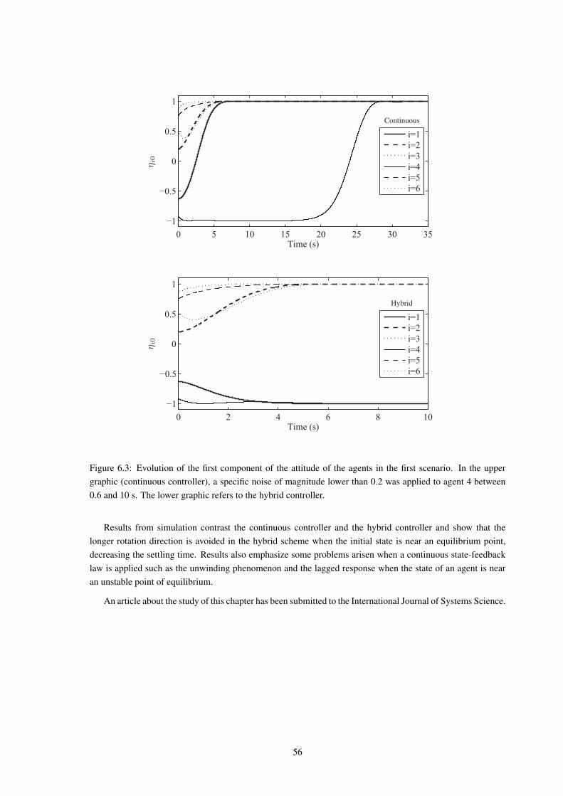
0 5 10 15 20 25 30 35

−1

−0.5

0

0.5

1

Time (s)

i=1

i=2

i=3

i=4

i=5

i=6

0 2 4 6 8 10

−1

−0.5

0

0.5

1

Time (s)

i=1

i=2

i=3

i=4

i=5

i=6

η i0

η i0

Hybrid

Continuous

Figure 6.3: Evolution of the first component of the attitude of the agents in the first scenario. In the uppergraphic (continuous controller), a specific noise of magnitude lower than 0.2 was applied to agent 4 between0.6 and 10 s. The lower graphic refers to the hybrid controller.

Results from simulation contrast the continuous controller and the hybrid controller and show that thelonger rotation direction is avoided in the hybrid scheme when the initial state is near an equilibrium point,decreasing the settling time. Results also emphasize some problems arisen when a continuous state-feedbacklaw is applied such as the unwinding phenomenon and the lagged response when the state of an agent is nearan unstable point of equilibrium.

An article about the study of this chapter has been submitted to the International Journal of Systems Science.

56

0 2 4 6 8 10

−1

−0.5

0

0.5

1

Time (s)

i=1

i=2

i=3

i=4

i=5

i=6

0 2 4 6 8 10−1

−0.5

0

0.5

1

Time (s)

0 2 4 6 8 10−1

−0.5

0

0.5

1

Time (s)

0 2 4 6 8 10−1

−0.5

0

0.5

1

Time (s)

η i0

~ǫ i0x

~ǫ i0y

ǫ i0z

0 2 4 6 8 10

−1

−0.5

0

0.5

1

Time (s)

i=1

i=2

i=3

i=4

i=5

i=6

0 2 4 6 8 10−1

−0.5

0

0.5

1

Time (s)

0 2 4 6 8 10−1

−0.5

0

0.5

1

Time (s)

0 2 4 6 8 10−1

−0.5

0

0.5

1

Time (s)

η i0

~ǫ i0x

~ǫ i0y

ǫ i0z

Continuous Hybrid

Hybrid

Hybrid

Continuous

Continuous

Continuous Hybrid

Figure 6.4: Evolution of the attitude qi0 = (ηi0, εi0) of the agents in the second scenario, where εi0 =

(εi0x, εi0y

, εi0z). The graphics on the left refers to the continuous controller and the others on the right to the

hybrid one.

57

0 2 4 6 8 10

−1

−0.5

0

0.5

1

Time (s)

i=1

i=2

i=3

i=4

i=5

i=6

0 2 4 6 8 10−1

−0.5

0

0.5

1

Time (s)

0 2 4 6 8 10−1

−0.5

0

0.5

1

Time (s)0 2 4 6 8 10

−1

−0.5

0

0.5

1

Time (s)

0 2 4 6 8 10

−1

−0.5

0

0.5

1

Time (s)

i=1

i=2

i=3

i=4

i=5

i=6

0 2 4 6 8 10−1

−0.5

0

0.5

1

Time (s)

ωi x

ωi y

ωi z

ωi x

ωi y

ωi z

HybridContinuous

Continuous

Continuous

Hybrid

Hybrid

Figure 6.5: Evolution of the angular velocity ωi = (ωix , ωiy , ωiz ) of the agents in the second scenario. Thegraphics on the left refers to the continuous controller and the others on the right to the hybrid one.

58

CONCLUSIONS

In this manuscript, two hybrid controllers were proposed in order to improve the solution in terms of cost whencompared with the fixed width hysteresis control of literature. Both of them are well suited for the rest-to-restattitude control of a rigid body with globally asymptotically stability property.

The first proposed controller (HY) offers more opportunities of updating the main logic variable that indi-cates which quaternion representation of the reference attitude should be followed, when compared with thehysteretic hybrid controller, and is more likely to take the shorter rotation direction and spend less energy.However, it presents the disadvantage of having restrictions on flow and jumps priorities. As long as jumps donot have higher priority than flows, robustness against noise measurements is achieved despite the chatteringthat may occur in the auxiliary variable.

The second proposed controller, called bimodal, supersedes the HY controller for not having the mentioneddrawback and can be seen as a middle term solution between the memoryless discontinuous and the hysteretichybrid controller. Differently from the less costly discontinuous controller, the bimodal controller is robust inthe sense of having capability of avoiding chattering due to measurement noise. Compared with the unimodalhysteretic hybrid controller, while both keep robustness and stability, the bimodal spends less energy in av-erage. It was also shown that the bimodal philosophy can be extended for other controllers which have onehysteretic mode. The bimodal controller is expected to be the most interesting choice when the attitude noiselevel may be expressive as for example when low cost components are used or when the system is under anelectromagnetically noisy environment.

Two other studies were added as an extension of the studies described above.

The first study refers to the attitude synchronization control for a network of rigid bodies (agents). It wasproposed a hybrid distributed control with globally asymptotically stability property and robustness againstnoise measurement for an undirected connected network (cyclic or acyclic) of agents. Application of a hybridcontroller solution is much challenging due to the inherent inter-agent interactions. The strategy counted onthe hysteretic hybrid controller of literature and the robust global stability was obtained at the cost of havingone more restriction on the hysteresis half-width parameter δi. Results from simulation show that the longerrotation direction is avoided when the initial state is near an equilibrium point, decreasing the settling time. Itis also emphasized that the great majority of the studies suggest a continuous state-feedback law strategy whichare prone to problems such as the unwinding phenomenon and the lagged response when the state of an agentis near an unstable point of equilibrium.

The second one refers to the kinematic control for rigid-body pose within the group of unit norm dual-quaternions. It is presented a novel control strategy for robust global rigid body kinematic stabilization. Toaddress the topological obstruction to global stability inherent to any rigid body representation—which rendersthe unwinding phenomenon in the case of unit quaternions and unit dual quaternions—it is exploited an hybridcontrol technique based on hysteresis, called bimodal, which ensures solution without chattering, with theintroduction of two binary logic state memory variable that reduces the liability of having the solution trajectorytravel to the farther antipodal equilibrium.

8.1 FUTURE WORK

As an extension to the present work, the author suggests:

67

8

1. A global hybrid control strategy for rigid-body pose problem that is robust against measurement noise,using the kinematic and dynamic equations to describe the pose motion;

2. A distributed pose synchronization control of agents with globally asymptotically stability property androbustness against noise measurement;

3. A global hybrid control strategy for rigid-body attitude problem that is robust against measurement noise,using a control law based on the attitude and the angular velocity;

4. Adapt the multi-agent distributed attitude control of Chapter 6 to the consensus problem (i.e. attitudesynchronization problem only, as in [21]);

5. Extend the rest-to-rest attitude and pose control problem to allow tracking;

6. Extend the multi-agent cooperative pose control problem to allow scenarios where the agents are coupledand subject to holonomic constraints.

68

Bibliography

[1] N. Chaturvedi, A. Sanyal, and N. McClamroch, “Rigid-body attitude control,” IEEE Control Syst., vol. 31,no. 3, pp. 30–51, 2011.

[2] G. Singh, P. Kabamba, and N. McClamroch, “Planar, time-optimal, rest-to-rest slewing maneuvers offlexible spacecraft,” J. Guid. Control Dynam., vol. 12, no. 1, pp. 71–81, 1989.

[3] J. Stuelpnagel, “On the parametrization of the three-dimensional rotation group,” SIAM Rev., vol. 6, no. 4,pp. 422–430, 1964.

[4] M. Spong, S. Hutchinson, and M. Vidyasagar, Robot Modeling and Control. John Wiley & Sons, Inc.,2005.

[5] S. P. Bhat and D. S. Bernstein, “A topological obstruction to continuous global stabilization of rotationalmotion and the unwinding phenomenon,” Syst. Control Lett., vol. 39, no. 1, pp. 63–70, 2000.

[6] O. Fjellstad and T. Fossen, “Quaternion feedback regulation of underwater vehicles,” in Proc. 3rd IEEEConf. Control Appl., vol. 2, Aug. 1994, pp. 857–862.

[7] D. Fragopoulos and M. Innocenti, “Stability considerations in quaternion attitude control using discon-tinuous Lyapunov functions,” Inst. Elect. Eng. Proc., Control Theory Appl., vol. 151, no. 3, pp. 253–258,May 2004.

[8] B. Wie and P. M. Barba, “Quaternion feedback for spacecraft large angle maneuvers,” Journal of Guid-ance, Control, and Dynamics, vol. 8, no. 3, pp. 360–365, 1985.

[9] R. Sanfelice, M. Messina, S. Emre Tuna, and A. Teel, “Robust hybrid controllers for continuous-timesystems with applications to obstacle avoidance and regulation to disconnected set of points,” in Amer.Control Conf., 2006, pp. 3352–3357.

[10] C. Mayhew, R. Sanfelice, and A. Teel, “Quaternion-based hybrid control for robust global attitude track-ing,” IEEE Trans. Autom. Control, vol. 56, no. 11, pp. 2555–2566, Nov. 2011.

[11] J. L. Crassidis, F. L. Markley, and Y. Cheng, “Survey of nonlinear attitude estimation methods,” J. Guid.Control Dynam., vol. 30, no. 1, pp. 12 – 28, 2007.

[12] D. Gebre-Egziabher, G. H. Elkaim, J. D. Powell, and B. W. Parkinson, “A gyro-free quaternion-basedattitude determination system suitable for implementation using low cost sensors,” in Position Locationand Navigation Symposium, IEEE 2000, 2000, pp. 185–192.

[13] A. Cavallo, A. Cirillo, P. Cirillo, G. D. Maria, P. Falco, C. Natale, and S. Pirozzi, “Experimental compar-ison of sensor fusion algorithms for attitude estimation,” IFAC Proceedings Volumes, vol. 47, no. 3, pp.7585 – 7591, 2014, 19th IFAC World Congress.

[14] A. Fu, E. Modiano, and J. Tsitsiklis, “Optimal energy allocation and admission control for communica-tions satellites,” IEEE/ACM Trans. Netw., vol. 11, no. 3, pp. 488–500, Jun. 2003.

[15] R. Kristiansen, A. Loría, A. Chaillet, and P. J. Nicklasson, “Spacecraft relative rotation tracking withoutangular velocity measurements,” Automatica, vol. 45, no. 3, pp. 750 – 756, 2009.

[16] Z. Meng, Z. You, G. Li, and C. Fan, “Cooperative attitude control of multiple rigid bodies with multipletime-varying delays and dynamically changing topologies,” Mathematical Problems in Engineering, pp.853–858, 2010.

69

[17] W. Ren, “Distributed attitude alignment in spacecraft formation flying,” International Journal of AdaptiveControl and Signal Processing, vol. 21, pp. 95–113, 2007.

[18] A. M. Zou, “Distributed attitude synchronization and tracking control for multiple rigid bodies,” IEEETransactions on Control Systems Technology, vol. 22, no. 2, pp. 478–490, 2014.

[19] A. M. Zou and K. D. Kumar, “Distributed attitude coordination control for spacecraft formation flying,”IEEE Transactions on Aerospace and Electronic Systems, vol. 48, no. 2, pp. 1329–1346, APRIL 2012.

[20] L. Ma, H. Min, S. Wang, Y. Liu, and S. Liao, “An overview of research in distributed attitude coordinationcontrol,” IEEE/CAA Journal of Automatica Sinica, vol. 2, no. 2, pp. 121–133, April 2015.

[21] C. G. Mayhew, R. G. Sanfelice, J. Sheng, M. Arcak, and A. R. Teel, “Quaternion-based hybrid feedbackfor robust global attitude synchronization,” IEEE Transactions on Automatic Control, vol. 57, no. 8, pp.2122–2127, Aug 2012.

[22] H. Bai, M. Arcak, and J. T. Wen, “Rigid body attitude coordination without inertial frame information,”Automatica, vol. 44, no. 12, pp. 3170 – 3175, 2008.

[23] R. W. Brockett, “System theory on group manifolds and coset spaces,” SIAM J. Control, vol. 10, no. 2,pp. 265–284, 1972.

[24] F. Bullo and R. M. Murray, “Proportional derivative (PD) control on the Euclidean group,” CaliforniaInstitute of Technology, Technical Report Caltech/CDS 95–010, May 1995.

[25] F. Bullo, R. M. Murray, and A. Sarti, “Control on the sphere and reduced attitude stabilization,” CaliforniaInstitute of Technology, Technical Report Caltech/CDS 95–005, Jan. 1995.

[26] J. Funda, R. H. Taylor, and R. P. Paul, “On homogeneous transforms, quaternions, and computationalefficiency,” vol. 6, no. 3, pp. 382–388, 1990.

[27] J. M. Selig, Geometric Fundamentals of Robotics, 2nd ed., ser. Monographs in Computer Science.Springer, 2007.

[28] H. T. M. Kussaba, L. F. C. Figueredo, J. Y. Ishihara, and B. V. Adorno, “Hybrid kinematic control forrigid body pose stabilization using dual quaternions,” J. Franklin Inst., vol. 354, no. 7, pp. 2769–2787,2017.

[29] D.-P. Han, Q. Wei, and Z.-X. Li, “Kinematic control of free rigid bodies using dual quaternions,” Int. J.Autom. Comput., vol. 5, no. 3, pp. 319–324, 2008.

[30] D. Han, Q. Wei, and Z. Li, “A dual-quaternion method for control of spatial rigid body,” in Proc. 2008IEEE Int. Conf. Networking, Sensing and Control, 2008, pp. 1–6.

[31] D. Han, Q. Wei, Z. Li, and W. Sun, “Control of oriented mechanical systems: A method based on dualquaternion,” in Proc. 17th IFAC World Congr., 2008, pp. 3836–3841.

[32] X. Wang and C. Yu, “Unit dual quaternion-based feedback linearization tracking problem for attitude andposition dynamics,” Syst. Contr. Letts., vol. 62, no. 3, pp. 225–233, 2013.

[33] P. P. M. Magro, J. Y. Ishihara, and H. C. Ferreira, “Robust global bimodal rest-to-rest attitude control ofrigid body using unit quaternion,” J. Franklin Inst., vol. 354, no. 8, pp. 3554–3573, 2017.

[34] P. P. M. Magro, H. T. M. Kussaba, L. F. C. Figueredo, and J. Y. Ishihara, “Dual quaternion-based bimodalglobal control for robust rigid body pose kinematic stabilization,” in 2017 American Control Conference(ACC), May 2017, pp. 1205–1210.

70

[35] J. Wertz, Spacecraft Attitude Determination and Control. Kluwer Academic Publishers, 1978.

[36] Wikipedia, “Orientation (geometry) — Wikipedia, the free encyclopedia,” 2004, [Online; accessed10-November-2016]. [Online]. Available: https://en.wikipedia.org/wiki/Orientation_(geometry)

[37] R. Murray, Z. Li, and S. Sastry, A Mathematical Introduction to Robotic Manipulation. CRC Press,1994.

[38] R. E. S. Cabette, “Estabilidade do movimento rotacional de satélites artificiais,” Ph.D. dissertation, INPE,2006.

[39] W. R. Hamilton, “On quaternions, or on a new system of imaginaries in algebra: Copy of a letter from SirWilliam R. Hamilton to John T. Graves, esq. on quaternions,” Philos. Mag., vol. 25, no. 3, pp. 489–495,1844.

[40] J. Solà, “Quaternion kinematics for the error-state kf,” p. 73, 2016. [Online]. Available:https://hal.archives-ouvertes.fr/hal-01122406v4/document

[41] O. Bottema and B. Roth, Theoretical Kinematics. Dover Publications, Inc., 1990.

[42] M. Shuster, “A survey of attitude representations,” J. Astronaut. Sci., vol. 41, no. 4, pp. 439–517, 1993.

[43] W. K. Clifford, “A preliminary sketch of biquaternions,” in Proc. London Math. Soc., 1871, pp. 381–395.

[44] E. Study, “Von den bewegungen und umlegungen,” Mathematische Annalen, vol. 39, no. 4, pp. 441–565,1891.

[45] X. Wang, D. Han, C. Yu, and Z. Zheng, “The geometric structure of unit dual quaternion with applicationin kinematic control,” J. Math. Anal. Appl., vol. 389, no. 2, pp. 1352–1364, 2012.

[46] Y. Wu, X. Hu, D. Hu, T. Li, and J. Lian, “Strapdown inertial navigation system algorithms based on dualquaternions,” vol. 41, no. 1, pp. 110–132, 2005.

[47] D. P. Chevallier, “On the transference principle in kinematics: its various forms and limitations,” Mech.Mach. Theory, vol. 31, no. 1, pp. 57–76, 1996.

[48] R. Goebel, R. Sanfelice, and A. Teel, “Hybrid dynamical systems,” IEEE Control Syst., vol. 29, no. 2, pp.28–93, Apr. 2009.

[49] ——, Hybrid dynamical systems. Princeton University Press, 2012.

[50] R. E. Mortensen, “Quarternion feedback regulator for spacecraft eigenaxis rotations,” International Jour-nal of Control, vol. 8, no. 3, pp. 297–302, 1968.

[51] R. E. Roberson, “Two decades of spacecraft attitude control,” Journal of Guidance, Control, and Dynam-ics, vol. 2, no. 1, pp. 3–8, 1979.

[52] J. Hrastar, “Attitude control of a spacecraft with a strapdown inertial reference system and onboard com-puter,” NASA, Technical Report Tn D–5959, Sep. 1970.

[53] H. Khalil, Nonlinear Systems. Macmillan Publishing Company, 1992.

[54] C. Mayhew, R. Sanfelice, and A. Teel, “Robust global asymptotic attitude stabilization of a rigid body byquaternion-based hybrid feedback,” in Proc. 48th IEEE Conf. Decision Control., Dec. 2009, pp. 2522–2527.

[55] R. Schlanbusch, A. Loria, and P. J. Nicklasson, “On the stability and stabilization of quaternion equilibriaof rigid bodies,” Automatica, vol. 48, no. 12, pp. 3135 – 3141, 2012.

71

[56] R. Sanfelice, R. Goebel, and A. Teel, “Invariance principles for hybrid systems with connections to de-tectability and asymptotic stability,” IEEE Trans. Autom. Control, vol. 52, no. 12, pp. 2282–2297, Dec.2007.

[57] R. Sanfelice, D. Copp, and P. Nanez, “A toolbox for simulation of hybrid systems in matlab/simulink,” in2013 Hybrid Systems: Computation and Control (HSCC), Apr. 2013, pp. 101–106.

[58] R. Goebel and A. Teel, “Solutions to hybrid inclusions via set and graphical convergence with stabilitytheory applications,” Automatica, vol. 42, no. 4, pp. 573–587, 2006.

[59] J. Guerrero-Castellanos, N. Marchand, A. Hably, S. Lesecq, and J. Delamare, “Bounded attitude controlof rigid bodies: Real-time experimentation to a quadrotor mini-helicopter,” Control Engineering Practice,vol. 19, no. 8, pp. 790 – 797, 2011.

[60] L. Labeyrie, “Stellar interferometry methods,” Ann. Rev. Astron. Astrophys., vol. 16, pp. 77–102, 1978.

[61] L. Parker, “Current state of the art in distributed autonomous mobile robotics,” in Proc. 5th InternationalSymposium on Distributed Autonomous Robotic Systems (DARS), 2000.

[62] R. M. Murray, “Two decades of spacecraft attitude control,” J. Dyn. Sys., Meas., Control, vol. 129, no. 5,pp. 571–583, 2007.

[63] R. Wilson, Introduction to Graph Theory. Pearson, 2012.

[64] C. D. Meyer, Matrix Analysis and Applied Linear Algebra. SIAM, 2001.

[65] J. L. Meriam and L. G. Kraige, Engineering Mechanics: Dynamics. Wiley, 2009.

[66] E. L. Lima, Análise Real Funções de n variáveis - volume 2. IMPA, 2013.

[67] A. Izmailov and M. Solodov, Otimização - volume 1. IMPA, 2009.

72

APPENDICES

73

RESUMO ESTENDIDO EM LÍNGUAPORTUGUESA

O controle de atitude de um corpo rígido é um quesito importante em projetos de veículos aeroespaciais (aero-naves e naves espaciais) assim como em projetos de veículos submarinos, terrestres e em aplicações de sistemasrobóticos, dentre outros [1]. Em uma gama de aplicações, mudanças no ponto de operação são necessárias econsequentemente resolver o problema de regulação a partir do estado inicial em repouso é um objetivo co-mum desejado [2]. Em particular, quando excursões arbitrárias na atitude são desejadas ou permitidas, surge oproblema de se projetar um sistema de controle globalmente estável [1].

O controle global de atitude é um problema desafiante a começar pela escolha apropriada de uma represen-tação para a atitude. É sabido que da gama existente de representações de atitude, nenhuma representação emtrês parâmetros do SO(3) – como é o caso dos frequentemente utilizados ângulos de Euler – é globamente nãosingular e isso é um obstáculo para se conseguir a estabilidade global [3]. Neste contexto, o quatérnio unitáriose torna interessante por representar a atitude com o menor número de parâmetros possível sem singularidades.

O espaço de estados do quatérnio unitário é uma dupla cobertura do SO(3) – um par de quatérnios unitáriosantipodais correspondem à mesma atitude em SO(3) – que leva, quando um controlador contínuo baseado emquatérnio unitário é usado, a um fenômeno indesejado conhecido como unwinding, em que o corpo pode estarem repouso arbitrariamente próximo à atitude final desejada e, ainda assim, rotacionar grandes ângulos antes dechegar ao repouso [5]. Esse efeito pode ser evitado usando-se uma realimentação de estado descontínua (semmemória), tal como as sugeridas por Fjellstad and Fossen [6], Fragopoulos and Innocenti [7] ou Wie and Barba[8]. Apesar da estabilização global assintótica ser alcançada, a natureza descontínua do controlador introduzo fenômeno chattering, que consiste em múltiplos saltos (de estado) ocorrendo ao mesmo tempo, e que podeocorrer na presença de ruído de medição quando o sistema está em uma região próxima de 180 da atitude dereferência [9].

Um controle de atitude com a propriedade de estabilidade assintótica e global e robustez contra ruídos demedição (ou seja, estes ruídos não levam a fenômenos de chattering) foi obtido com o controlador híbridode comportamento histerético sugerido por Mayhew et al. [10]. denominado controlador histerético, usandouma variável lógica binária. O tamanho da banda de histerese que cobre a região propensa a chattering podeser projetado para um determinado nível máximo de ruido, Comparado com o controlador descontínuo (semmemória), o controlador histerético consegue eliminar o chattering ao custo de impor trajetórias de rotaçãomais longas para algumas condições iniciais de atitude levando a um maior tempo médio de estabilização ouconsumo de energia.

Para reduzir o consumo de energia para o controlador histerético, uma alternativa seria reduzir o nível deruido recebido no controlador utilizando-se sensores de alta precisão de preços elevadors e/ou estimadores deatitude baseados na filtragem de Kalman ou de Partículas. Apesar dessas soluções serem efetivas em determi-nadas situações, há outras em que um ruido expressivo já é esperado., De um lado, tem-se a demanda crescentepor soluções baratas com componentes baixo custo. Como filtros – especialmente o Filtro de Partículas, sãocomputacionalmente “caros” [11] – para processadores embedded com pouca memória e recursos computaci-onais, geralmente um estimador simplificado e pouco efetivo é usado, resultando em um ruído de estimação deatitude alto. Por outro lado, sensores de baixo custo resultam em um nível maior de ruído. Por exemplo, noexperimento de Gebre-Egziabher et al. [12], é possível observar ruídos de amplitude em torno de 10 graus. Se,além disso, o sistema estiver imerso em um ambiente com excesso de ruído eletromagnético ou se a velocidadeangular for alta, o nível de ruído é ainda maior [13].

74

A

Neste estudo, procurou-se um controlador com a propriedade de estabilidade global e robusta que repre-sentasse uma melhor solução em termos de custo quando comparado com o controlador de banda de histeresefixa. Redução de custo representada por tempo médio de estabilização ou consumo de energia é importante,por exemplo, em satélites ou sistemas operados por bateria [14]. Propõe-se dois controladores distintos, amboscom duas variáveis de estado lógicas binárias (uma a mais que o controlador histerético) para o controle deatitude representado por quatérnio, O primeiro controlador, denominado HY, tem a variável principal determi-nada por um controle on-off com histerese para indicar qual representação em quatérnio da atitude de referênciadeve ser seguida e uma outra variável auxiliar determinada por um controle on-off sem histerese para indicara proximidade à região crítica sujeita a chattering. Esse esquema oferece mais oportunidades de atualizaçãoda variável principal que o controlador híbrido histerético, por exemplo quando há uma variação abrupta naatitude de referência ou no momento inicial quando a atitude de referência está longe da atitude inicial. Issoreduz as chances do corpo seguir na direção da rotação mais longa. Contudo, essa estratégia impõe restriçõesna forma como o controlador é implementado. Prova-se que o sistema pode apresentar chattering na variávelauxiliar e que esse chattering não afeta a robustez do sistema se “jumps” não tiverem prioridade sobre “flows”.

No segundo controlador proposto, denominado bimodal, ambas as variáveis são determinadas por um con-trole on-off com histerese. A variável principal indica qual representação em quatérnio da atitude de referênciadeve ser seguida e a outra variável indica a proximidade à região crítica sujeita a chattering. Essa estratégiaelimina as restrições sobre a forma de implementação do controlador, porém torna a dinâmica dessas variáveismais complexas, dado que uma variável interfere no comportamento da outra. O efeito resultante é que a bandade histerese do controle on-off referente à variável principal, se adapta de acordo com o estado da outra variá-vel, sendo ora igual, ora a metade do valor do parâmetro banda de histerese. Esse controlador é uma soluçãointermediária entre o controlador descontínuo e o controlador híbrido histerético.

São apresentadas provas formais de que ambos os controladores deixam o sistema com as seguintes propri-edades:

• estabilidade assintótica e global;

• sem unwinding;

• robustez contra ruídos de medição (sem chattering).

A eficácia dos controladores é mostrada por meio de simulações. Em alguns casos foram utilizados modelosrealistas reportados em literatura. Embora os resultados indiquem que o desempenho dos controladores pro-postos apresentam vantagens para a configuração rest-to-rest, os controladores continuam apresentando bomdesempenho mesmo quando a velocidade angular inicial e final não são nulas, desde que relativamente baixas.No caso do controlador bimodal, mesmo para outras velocidades angulares iniciais, o consumo de energia dosistema é, em média, inferior ao consumo do controlador híbrido histerético. Melhores desempenhos ocorremquando a banda de histerese é maior como no caso em que são usados sensores mais baratos ou em ambientesonde há muito ruído eletromagnético.

Como extensão dos resultados descritos acima, duas outras contribuições foram propostas: uma sobrecontrole de sincronização de atitude de uma rede de corpos rígidos (agentes) e outra sobre controle cinemáticode pose de corpo rígido dentro do grupo de quatérnios duais de norma unitária.

Com relação à primeira contribuição, muita pesquisa tem sido desenvolvida em controle de coordenação deatitude nos últimos 10-15 anos [15, 16, 17, 18, 19]. Comparado com o sistema com um só agente, os sistemasmultiagentes têm vantagens interessantes como viabilidade de ser implementado, produção de resultados maisexatos, robustos, menor custo etc., além de ter uma gama de aplicações como monitoramento de ambientes,procura e resgate, interferômetros espaciais, manuseio de materiais dentre outras [20].

Como mencionado acima, o problema de estabilização global e robusta de atitude, para um único corpo

75

rígido, foi resolvido há poucos anos [10], mas a estabilização em um cenário de uma rede de agentes trazmuito mais desafios devido às interações existentes entre os agentes. Até o momento, a maioria dos estudossobre estratégias de sincronização de atitude são capazes de promover uma estabilização quase global comoem [18, 17] e quando é global, não é robusta a ruídos de medição.

O único estudo em sincronização de atitude de múltiplos agentes, que o autor tem conhecimento, e querealiza uma sincronização global e robusta é o de Mayhew et al. (2012) [21]. Assume-se que cada agentetem acesso somente à atitude relativa entre seus vizinhos e à sua velocidade angular em relação ao sistema decoordenadas do corpo. Seu objetivo é alcançar a estabilidade de um estado sincronizado (que não é uma atitudede referência absoluta específica) usando um esquema de realimentação híbrida. A vantagem de não requerersensores para medições de atitude inercial tem o custo de se obter a sincronização apenas para redes conexase acíclicas [22], pois existe um obstáculo físico para a convergência global quando o grafo contém ciclos [22,Theorem 1].

Neste estudo, propõe-se um controle de sincronização de atitude distribuído com a propriedade de esta-bilidade assintótica e global e robustez contra ruídos de medição para uma rede de agentes representada porum grafo não direcionado e conexo (cíclico ou acíclico). A estratégia usa o quatérnio como representação daatitude inercial e uma realimentação híbrida histerética com uma variável lógica binária, sugerida por Mayhewet al. [10], para cada agente, a fim de resolver os conhecidos problemas que surgem quando uma lei de rea-limentação de estados, contínua ou descontínua, é empregada como presença de estados instáveis, fenômeno“unwinding” e “chattering”. O custo de se utilizar esta estratégia é o surgimento de mais uma restrição noparâmetro da banda de histerese δi no controlador de cada agente.

Os resultados das simulações contrastam o controlador contínuo com o controlador híbrido proposto emostram que a direção de rotação mais longa é evitada no caso do esquema híbrido quando o estado inicialestá próximo a um ponto de equilíbrio, reduzindo o tempo de estabilização. Além disso, eles enfatizam algunsdos problemas provenientes da lei de realimentação contínua como o atraso na resposta quando o estado de umagente está muito próximo a um ponto de equilíbrio instável.

Com relação à segunda contribuição, o grupo de Lie do deslocamento de um corpo rígido aparece natural-mente no estudo de sistemas aeroespaciais e robóticos. A partir do trabalho inicial de Brockett [23] sobre teoriade controle em grupos de Lie gerais, grande parte da literatura foi dedicada ao controle de sistemas definidos noSE(3). Embora seja usual projetar controladores para este sistema usando matrizes para representar elementosdeste grupo de Lie [24, 25], alguns autores observaram que os controladores projetados usando-se um outrotipo de representação, a saber, o quatérnio dual unitário para SE(3), podem apresentar vantagens em relação aotempo computacional e aos requisitos de armazenamento [26, 27].

É importante observar que, como neste caso o espaço de estado de um sistema dinâmico é uma variedadegenérica, algumas dificuldades são esperadas para se projetar um controlador capaz de estabilizar o sistema.Na verdade, o problema da estabilização robusta e global de pose de um corpo rígido não é simples, mas é, decerta forma, análogo ao problema de atitude.

Em primeiro lugar, não existe um controlador com realimentação contínua capaz de estabilizar assintotica-mente e globalmente um ponto de equilíbrio na variedade do grupo quatérnio dual unitário [28].

Em segundo lugar, como o grupo de Lie de quatérnio dual unitário é uma cobertura dupla do grupo deLie de deslocamento de corpo rígido SE(3) [29, 28], induz-se, quando um controlador contínuo baseado emquatérnio dual é usado, um fenômeno similar ao de "unwinding" em SO(3) [5]: o corpo rígido pode iniciar dorepouso em uma pose arbitrariamente perto da final desejada e, ainda, ser conduzido para o ponto de equilíbrioestável e mais afastado antes retornar ao repouso.

Por fim, mesmo usando uma realimentação de estado descontínua (sem memória), é impossível obter umaestabilização global e robusta de um conjunto de pontos não conexos, provenientes da cobertura dupla do SE(3)

76

[10, 9].

Há poucos estudos em que se tenta eliminar o problema de “unwinding” no contexto de estabilização depose usando quatérnio dual unitário [29, 30, 31, 32]. Todos sugerem realimentação descontínua e são propensosa “chattering” para condições iniciais arbitrariamente próximas da descontinuidade.

Inspirado no controle híbrido baseado em histerese de Mayhew et al. [10] desenvolvido apenas para es-tabilização do controle de atitude, Kussaba et al. [28] projetou uma extensão desse controlador para obtera estabilidade da atitude e translação de forma acoplada. No entanto, este controlador de pose sugerido porKussaba et al. [28] herda o mesmo custo do controlador histerético de atitude, mencionado anteriormente,de impor trajetórias de rotação mais longas para determinadas atitudes iniciais, fazendo com que o tempo deestabilização ou consumo de energia seja maior. Além disso, o problema do consumo de energia também seagrava neste contexto, pois os movimentos casados de translação e rotação consomem mais energia. [28].

Para reduzir esse custo, propõe-se uma lei de controle bimodal híbrido que combine o controlador bimodalde atitude proposto acima e o controle sugerido por Kussaba et al. [28] de modo que ele represente uma soluçãointermediária em termos de custo entre o controlador descontínuo e o histerético.

Os resultados de simulação comparam a evolução do sistema quando o controlador utilizado é o bimodalcom os controladores descontínuo e o histerético. Uma ideia do consumo de energia pode ser obtida a partir daárea embaixo da curva do gráfico do módulo da velocidade angular quando cada controlador é utilizado.

As contribuições desta tese são:

1. Enuncia-se um teorema sobre um problema que ocorre com o controlador de atitude descontínuo napresença de ruídos de medição no espaço do quatérnio unitário (veja Teorema 3.4, página 15). Esteresultado é uma correção em um teorema de [10] em que o sistema está corrompido por ruído, porém avariável medida não pertence ao espaço do quatérnio unitário. Consequentemente, o modelo do sistemaperde o sentido físico.

2. Apresenta-se um controle de atitude (representada por quatérnios) de um corpo rígido, que é híbrido eglobal, além de ser robusto a ruídos de medição, voltado para casos em que a velocidade angular iniciale final é zero (veja Capítulo 4). O controlador proposto estende um controlador híbrido histerético daliteratura introduzindo uma nova variável de estado lógica e binária. O controlador é capaz de detectarquando a atitude de referência muda abruptamente ou quando a atitude inicial está distante da atitude dereferência. Desta forma, ele tem mais oportunidades de determinar qual representação em quatérnio daatitude de referência deve ser seguida em comparação com o controlador híbrido histerético da literaturae tem mais chances de seguir pela direção de rotação mais curta. Este estudo foi apresentado no XIISimpósio Brasileiro de Automação Inteligente - SBAI 2015 e o respectivo artigo está publicado online,disponível em http://swge.inf.br/SBAI2015/anais/413.pdf.

3. Apresenta-se uma outra estratégia de controle de atitude de corpo rígido, híbrido e global, que é robustoa ruídos de medição (ou seja, não há chattering) por meio do controlador denominado bimodal (vejaCapítulo 5). Ele é apropriado para casos em que a velocidade angular inicial e final são zero e tema atitude represenada por quatérnio, Porém, ele também apresenta vantagens para condições iniciaisgenéricas. Dentre os controladores globais, presume-se que ele seja o mais interessante quando o nívelde ruído na medição da atitude é expressivo como, por exemplo, quando sensores/componentes de baixocusto são usados ou quando o sistema está imerso em ambientes onde há muito ruído eletromagnético. Ocontrolador possui duas variáveis de estado lógicas binárias. Por conseguir adaptar a banda de histerese,ele reduz a região onde o controlador híbrido histerético determina a direção de rotação mais longa,sem comprometer a robustez, sendo uma solução intermediária em termos de custo entre o controladordescontínuo e o híbrido histerético. Um artigo sobre este estudo foi publicado na revista Journal of theFranklin Institute.

77

4. Propõe-se um controle de sincronização de atitude distribuído para uma rede de corpos rígidos (agentes)representada por um grafo não direcionado e conexo (cíclico ou acíclico) que apresente uma estabilidadeglobal e assintótica (veja Capítulo 6). Devido às inerentes interações entre os agentes, o projeto docontrolador é muito mais desafiador. Na literatura, a grande maioria dos controladores sugerem leisde realimentação de estado contínuas ou descontínuas. Como no caso restrito a um único corpo rígidoestes tipos de estratégias de controle levam o sistema a apresentar problemas bem conhecidos comoestados instáveis, fenômeno unwinding e chattering, é esperado que, no caso de sistemas multiagente,haja problemas de desempenho ainda piores. Para resolver estes problemas, o controlador proposto usacomo base o controlador histerético híbrido da literatura com uma variável lógica binária e uma restriçãomais forte para o parâmetro banda de histerese. Um artigo a respeito deste estudo foi submetido à revistalInternational Journal of Systems Science.

5. Propõe-se uma estratégia de controle híbrido global para resolver o problema cinemático de rotação etranslação de um corpo rígido e seja robusto a ruídos de medição (veja Capítulo 7). O controlador híbridobaseado em dual quatérnio sugerido na literatura estende o controlador histerético baseado em quatérnioque, como se sabe, tem um região do espaço de estados onde a lei de controle força o movimento para adireção de rotação mais longa, gastando-se mais energia que o necessário. A estratégia proposta adaptao controlador de atitude bimodal do Capítulo 5 ao sistema de pose de um corpo rígido a fim de reduzir,em média, o tempo de estabilização ou consumo de energia. Neste contexo, o problema de consumode energia é mais grave, pois o movimento de rotação e translação estão acoplados, consumindo maisenergia (veja Capítulo 7). Este estudo foi apresentado no American Control Conference - ACC 2017 e orespectivo artigo foi publicado nos anais do evento.

78

PROOFS OF SOME LEMMAS

In this appendix, the lemmas used along the text are demonstrated.

Lemma B.1 Euler’s equation in body coordinates

Let Jb represent the constant inertia matrix calculated in the body frame, τ b represent theexternal torque expressed in the body frame and ωb represent the current angular velocityof the body frame as seen from the reference frame and expressed in the body frame. Thedynamic equation, known as the Euler’s equation, written in body coordinates, is given by

Jbωb = S(Jbωb

)ωb + τ b. (B.1)

Proof. Consider that variable with a superscript letter b is expressed in the body frame. Absence of thissuperscript letter indicates the variable is expressed in the reference frame. Taking the time derivative ofthe angular momentum [65] expressed in the body frame Lb,

Lb =Jbωb, (B.2)

Lb =Jbωb. (B.3)

As L = RLb, taking its time derivative,

L =RLb, (B.4)

L =RLb +RLb. (B.5)

Using that R = RS(ωb) [37, page 52], (B.2) and (B.3),

L =RS(ωb)(Jbωb) +R(Jbωb). (B.6)

As the torque τ equals the time derivative of the angular momentum and τ = Rτ b ,

τ =R[S(ωb) (Jbωb

)+ Jbωb

], (B.7)

Jbωb =RT τ − S(ωb) (Jbωb

), (B.8)

=S(Jbωb

) (ωb)

+ τ b. (B.9)

79

B

Lemma B.2 Quaternion kinematic equation for the attitude error

Let q represent the current attitude, ω be the current angular velocity, qd represent thedesired attitude and ωd be the desired angular velocity. Given that the attitude error isdefined as qe = q∗d q, the kinematic equation for the attitude error is

qe =1

2qe (0,ωe), (B.10)

where ωe = ω −R(qe)Tωd.

Proof. Take the time derivative of the attitude error,

qe =q∗d q, (B.11)

qe =q∗d q + q∗d q. (B.12)

Substituting the kinematic equation (2.7) into (B.12),

qe =

(1

2qd (0,ωd)

)∗ q + q∗d

(1

2q (0,ω)

), (B.13)

=− 1

2(0,ωd) q∗d q +

1

2q∗d q (0,ω), (B.14)

=1

2qe (0,ω)− 1

2(0,ωd) qe, (B.15)

=1

2qe [(0,ω)− q∗e (0,ωd) qe] , (B.16)

=1

2qe [(0,ω)− (0,R(q∗e)ωd)] , (B.17)

=1

2qe

[(0,ω −R(qe)

Tωd)]. (B.18)

Lemma B.3 Hybrid basic conditions

Let x = (qe,ω) ∈ X , X = S3 × R3, x2 = (x, h,m) ∈ X × 1,−1 × 1,−1 and H,defined either in (4.7) or in (5.8), be a closed-loop autonomous hybrid system. The hybridsystemH satisfies the hybrid basic conditions (Assumption 6.5 of [49])

(A1) C2 and D2 are closed sets;

(A2) F 2 : Rn ⇒ Rn is outer semicontinuous, locally bounded, convex-valued, andF 2(x2) 6= ∅ for all x2 ∈ C2;

(A3) G2 : Rn ⇒ Rn is outer semicontinuous, locally bounded and G2(x2) 6= ∅ for allx2 ∈ D2.

Proof. The hybrid systemH satisfies:

• (A1), D2 is the union of a finite number of closed sets that results in a closed set [66] and C2 is theintersection of closed sets that results in a closed set [66].

• (A2), F 2 is continuous in C2. Consequently, it is outer semicontinuous and locally bounded [49,

80

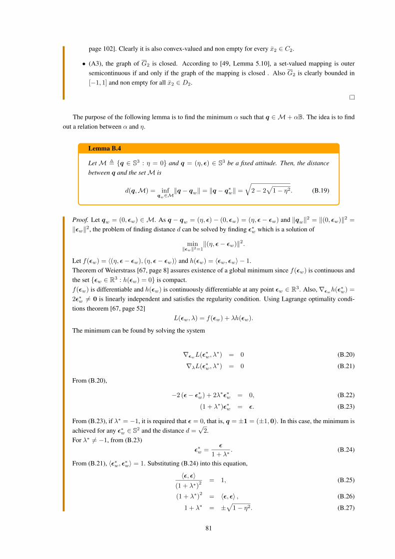
page 102]. Clearly it is also convex-valued and non empty for every x2 ∈ C2.

• (A3), the graph of G2 is closed. According to [49, Lemma 5.10], a set-valued mapping is outersemicontinuous if and only if the graph of the mapping is closed . Also G2 is clearly bounded in[−1, 1] and non empty for all x2 ∈ D2.

The purpose of the following lemma is to find the minimum α such that q ∈ M+ αB. The idea is to findout a relation between α and η.

Lemma B.4

LetM , q ∈ S3 : η = 0 and q = (η, ε) ∈ S3 be a fixed attitude. Then, the distancebetween q and the setM is

d(q,M) = infqw∈M

‖q − qw‖ = ‖q − q∗w‖ =

√2− 2

√1− η2. (B.19)

Proof. Let qw = (0, εw) ∈ M. As q − qw = (η, ε) − (0, εw) = (η, ε − εw) and ‖qw‖2 = ‖(0, εw)‖2 =

‖εw‖2, the problem of finding distance d can be solved by finding ε∗w which is a solution of

min‖εw‖2=1

‖(η, ε− εw)‖2.

Let f(εw) = 〈(η, ε− εw), (η, ε− εw)〉 and h(εw) = 〈εw, εw〉 − 1.Theorem of Weierstrass [67, page 8] assures existence of a global minimum since f(εw) is continuous andthe set εw ∈ R3 : h(εw) = 0 is compact.f(εw) is differentiable and h(εw) is continuously differentiable at any point εw ∈ R3. Also, ∇εwh(ε∗w) =

2ε∗w 6= 0 is linearly independent and satisfies the regularity condition. Using Lagrange optimality condi-tions theorem [67, page 52]

L(εw, λ) = f(εw) + λh(εw).

The minimum can be found by solving the system

∇εwL(ε∗w, λ∗) = 0 (B.20)

∇λL(ε∗w, λ∗) = 0 (B.21)

From (B.20),

−2 (ε− ε∗w) + 2λ∗ε∗w = 0, (B.22)

(1 + λ∗)ε∗w = ε. (B.23)

From (B.23), if λ∗ = −1, it is required that ε = 0, that is, q = ±1 = (±1,0). In this case, the minimum isachieved for any ε∗w ∈ S2 and the distance d =

√2.

For λ∗ 6= −1, from (B.23)ε∗w =

ε

1 + λ∗. (B.24)

From (B.21), 〈ε∗w, ε∗w〉 = 1. Substituting (B.24) into this equation,

〈ε, ε〉(1 + λ∗)

2 = 1, (B.25)

(1 + λ∗)2

= 〈ε, ε〉 , (B.26)

1 + λ∗ = ±√

1− η2. (B.27)

81

Thus, substituting (B.27) into (B.24), ε∗w = ± ε√1−η2

. This results into two possible solutions. Clearly, the

solution that minimizes the problem is achieved when q∗w =

(0, ε√

1−η2

).

The distance d is

d(q,M) = ‖q − q∗w‖ , (B.28)

=

∥∥∥∥∥(η,

(1− 1√

1− η2

)ε

)∥∥∥∥∥ , (B.29)

=

√√√√η2 +

(1− 1√

1− η2

)2

‖ε‖2, (B.30)

=

√√√√η2 +

(1− 2√

1− η2+

1

1− η2

)(1− η2), (B.31)

=

√2− 2

√1− η2. (B.32)

This equation also holds for q = ±1 when λ∗ = −1. Note that the maximum distance is d =√

2.

A geometrical interpretation of distance d is the line segment PQ shown in Figure B.1. Let q = (m, εm).Thus, ‖q − q∗w‖ =

∥∥∥(m,(1− 1√1−m2

)ε)∥∥∥. Since

∥∥∥(1− 1√1−m2

)ε∥∥∥ =

∣∣√1−m2 − 1∣∣ ∥∥∥ ε√

1−m2

∥∥∥ =∣∣1−√1−m2∣∣ is represented by the size of the line segment QR and line segment RP has size |m|, then

‖q − q∗w‖ has the size of segment PQ.

PQ2

= RP2

+ QR2

(B.33)

=

√m2 +

(1−

√1−m2

)2

(B.34)

=

√2− 2

√1−m2 (B.35)

Figure B.1: Geometrical representation of distance d from q = (m, εm).

The lemma that follows looks for the maximum η such that q ∈M+ B(0, α).

82

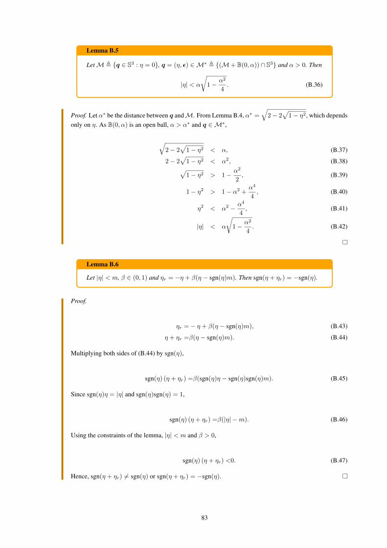
Lemma B.5

LetM , q ∈ S3 : η = 0, q = (η, ε) ∈M∗ , (M+ B(0, α)) ∩ S3 and α > 0. Then

|η| < α

√1− α2

4. (B.36)

Proof. Let α∗ be the distance between q andM. From Lemma B.4, α∗ =√

2− 2√

1− η2, which dependsonly on η. As B(0, α) is an open ball, α > α∗ and q ∈M∗,

√2− 2

√1− η2 < α, (B.37)

2− 2√

1− η2 < α2, (B.38)√1− η2 > 1− α2

2, (B.39)

1− η2 > 1− α2 +α4

4, (B.40)

η2 < α2 − α4

4, (B.41)

|η| < α

√1− α2

4. (B.42)

Lemma B.6

Let |η| < m, β ∈ (0, 1) and ηr = −η + β(η − sgn(η)m). Then sgn(η + ηr) = −sgn(η).

Proof.

ηr =− η + β(η − sgn(η)m), (B.43)

η + ηr =β(η − sgn(η)m). (B.44)

Multiplying both sides of (B.44) by sgn(η),

sgn(η) (η + ηr) =β(sgn(η)η − sgn(η)sgn(η)m). (B.45)

Since sgn(η)η = |η| and sgn(η)sgn(η) = 1,

sgn(η) (η + ηr) =β(|η| −m). (B.46)

Using the constraints of the lemma, |η| < m and β > 0,

sgn(η) (η + ηr) <0. (B.47)

Hence, sgn(η + ηr) 6= sgn(η) or sgn(η + ηr) = −sgn(η).

83

Lemma B.7

Let q = (η, ε) ∈ S3 be a fixed attitude and Qe = (ηe, εe) ∈ H be a measurement noisewith ηe fixed. Given that |η| < 1 and |η + ηe| < 1, the minimum magnitude of noise, ‖Q∗e‖,such that q +Q∗e still represents an attitude, is achieved when

Q∗e =

ηe,√1− (η + ηe)

2

1− η2− 1

ε . (B.48)

Proof. The problem requires to findQ∗e that is a solution of

min‖q+Qe‖2=1

‖Qe‖.

Since ‖Qe‖2 = η2e+‖εe‖2 and ηe is known and fixed, minimizing ‖Qe‖ is equivalent to minimizing ‖εe‖2.

As q +Qe = (η + ηe, ε+ εe), the minimization problem above is equivalent to

min‖ε+εe‖2=1−(η+ηe)2

‖εe‖2.

Let f(εe) = 〈εe, εe〉 and h(εe) = 〈ε+ εe, ε+ εe〉 − 1 + (η + ηe)2.

Theorem of Weierstrass [67, page 8] assures existence of a global minimum since f(εe) is continuous andthe set εe ∈ R3 : h(εe) = 0 is compact.f(εe) is differentiable and h(εe) is continuously differentiable at any point εe ∈ R3. Also, ∇εeh(ε∗e) =

2 (ε+ ε∗e) is linearly independent since ε + εe 6= 0 due to restrictions |η + ηe| < 1 and ‖q + Qe‖ = 1.Hence, the regularity conditions are satisfied.Using Lagrange optimality conditions theorem [67, page 52]

L(εe, λ) = f(εe) + λh(εe).

The minimum can be found solving the system

∇εeL(ε∗e, λ∗) = 0 (B.49)

∇λL(ε∗e, λ∗) = 0 (B.50)

From (B.49)

2ε∗e + 2λ∗ (ε+ ε∗e) = 0, (B.51)

(1 + λ∗) ε∗e = −λ∗ε. (B.52)

For λ∗ = −1, ε = 0. This solution is not possible due to restriction |η| < 1 .For λ∗ 6= −1,

ε∗e = − λ∗ε

1 + λ∗(B.53)

ε+ ε∗e =ε

1 + λ∗(B.54)

From (B.50), 〈ε+ ε∗e, ε+ ε∗e〉 = 1− (η + ηe)2. Substituting (B.54) into this equation,

〈ε, ε〉(1 + λ∗)

2 = 1− (η + ηe)2, (B.55)

1− η2

(1 + λ∗)2 = 1− (η + ηe)

2, (B.56)

1

1 + λ∗= ±

√1− (η + ηe)

2

1− η2. (B.57)

84

Then, substituting (B.57) into (B.54),

ε+ ε∗e = ±√

1− (η + ηe)2

1− η2ε, (B.58)

ε∗e =

±√

1− (η + ηe)2

1− η2− 1

ε. (B.59)

From the two possible solutions, the one which minimizes ‖εe‖2 is

ε∗e =

√1− (η + ηe)2

1− η2− 1

ε. (B.60)

Lemma B.8

Let q = (η, ε) ∈ S3, 0 < α <√

2, β ∈ (0, 1), m = α√

1− α2

4 > |η|. Given Qe =

(ηe, εe), ηe = −η + β (η − sgn(η)m), εe =

(√1−(η+ηe)2

1−η2 − 1

)ε, then the magnitude of

Qe, ‖Qe‖, is lower than α.

Proof. The first part of the proof calculates ‖Qe‖as a function of parameters β, m and η.

‖Qe‖2 = η2e +

∥∥∥∥∥∥√1− (η + ηe)

2

1− η2− 1

ε∥∥∥∥∥∥

2

.

Substituting ‖ε‖2 by (1− η2),

‖Qe‖2 = η2e +

1− (η + ηe)2

1− η2− 2

√1− (η + ηe)

2

1− η2+ 1

(1− η2), (B.61)

= 2− 2η2 − 2ηηe − 2

√1− (η + ηe)

2√

1− η2. (B.62)

Now, substituting ηe by its definition,

‖Qe‖2 = 2

(1− η2 − η (−η + β (η − sgn(η)m))−

√1− (β (η − sgn(η)m))

2√

1− η2

), (B.63)

= 2

(1− βη2 + β |η|m−

√1− β2 (η − sgn(η)m)

2√

1− η2

). (B.64)

Multiplying expression (η − sgn(η)m)2 by sgn(η)2 = 1,

‖Qe‖2 = 2

(1− βη2 + β |η|m−

√1− β2 (sgn(η)η −m)

2√

1− η2

), (B.65)

= 2

(1 + β |η| (m− |η|)−

√1− β2 (m− |η|)2

√1− η2

). (B.66)

The last part of the proof considers that the inequality ‖Qe‖ < α holds and looks for some inconsistencies.Using Lemma B.4, it follows that ‖Qe‖2 < 2− 2

√1−m2 and

2

(1 + β |η| (m− |η|)−

√1− β2 (m− |η|)2

√1− η2

)< 2− 2

√1−m2, (B.67)

85

√1−m2 + β |η| (m− |η|) <

√1 + β2η2 (m− |η|)2 − β2 (m− |η|)2 − η2 (B.68)

As m > |η|, both sides of the inequality are non negative and can be squared,

−m2 + 2β |η| (m− |η|)√

1−m2 < −β2 (m− |η|)2 − η2,

2β |η| (m− |η|)√

1−m2 < −β2 (m− |η|)2+ (m+ |η|) (m− |η|) . (B.69)

Dividing both sides by (m− |η|),

2β |η|√

1−m2 < (1− β2)m+ (1 + β2) |η| . (B.70)

Squaring both sides again, as both of them are non negative,

4β2η2(1−m2

)< (1− β2)2m2 + 2(1− β2)(1 + β2)m |η|+ (1 + β2)2η2, (B.71)

−4β2η2m2 < (1− β2)2m2 + 2(1− β2)(1 + β2)m |η|+ (1− β2)2η2.

Since the left side of the inequality is negative and the right side is positive, the inequality holds. Thus, it isproved that ‖Qe‖ < α.

The following lemmas refer to the multi-agent control chapter (Chapter 6).

Lemma B.9

Let qij = (ηij , εij) = q∗j qi and Rij = RTj Ri = R(qij). Then Rijεij = εij .

Proof. Using (2.5),

Rijεij =(I + 2ηijS(εij) + 2S(εij)

2)εij ,

=εij + 2ηijS(εij)εij + 2S(εij)2εij .

As S(εij)εij = εij × εij = 0,

Rijεij =εij .

Lemma B.10

Let Ji = JTi > 0, kGi > 0, aij > 0, xi = (qi0,ωi, hi) ∈ X , S3 × R3 × 1,−1, i =

1, 2, . . . , n, x = (x1, x2, . . . , xn) ∈ Xn and V : Xn → R,

V (x) =

n∑i=1

2kGi(1− hiηi0) +

n∑i=1

n∑j=1

aij(1− hihjηij) +1

2

n∑i=1

ωTi Jiωi.

Then V (x) = 0⇔ x ∈ A, where

A =

n⋂i=1

Ai, Ai ,x ∈ Xn : xi = (1,0, 1) or xi = (−1,0,−1)

.

86

Proof. As Ji is a positive definite matrix, ωTi Jiωi = 0 ⇐⇒ ωi = 0. Hence,∑ni=1 ω

Ti Jiωi = 0 ⇐⇒

ωi = 0, i = 1, . . . , n.Regarding the first summation, 1 − hiηi0 = 0 ⇐⇒ hiηi0 = 1. Multiplying both sides by hi and sinceh2i = 1, it follows that ηi0 = hi and qi0 = (hi,0) = hi1. Therefore,

∑ni=1 2kGi(1 − hiηi0) = 0 ⇐⇒

qi0 = hi1, i = 1, . . . , n.Finally, the second summation is a consequence of the previous restriction.

hihjηij =hihj(ηj0ηi0 + εTj0εi0),

=hihjηj0ηi0,

=hihjhjhi,

=h2ih

2j = 1.

Hence, the summand 1− hihjηij equals 0.

87

PUBLICATIONS

The following papers have already been published or submitted:

PEER-REVIEWED JOURNALS

P. P. M. Magro, J. Y. Ishihara, and H. C. Ferreira, “Robust global bimodal rest-to-rest attitude control ofrigid body using unit quaternion,” J. Franklin Inst., vol. 354, no. 8, pp. 3554- 3573, 2017.

P. P. M. Magro, and J. Y. Ishihara, “Robust global distributed attitude control for multiple rigid bodiesusing hybrid controller,” Int. J. Syst. Sci., 2017 (submitted for publication).

PEER-REVIEWED CONFERENCES

P. P. M. Magro, H. T. M. Kussaba, L. F. C. Figueredo, and J. Y. Ishihara, “Dual quaternion-based bimodalglobal control for robust rigid body pose kinematic stabilization,” American Control Conference, ACC 2017,May 2017.

H. M. T. Menegaz, J. Y. Ishihara, and P. P. M. Magro, “ Unscented Kalman filter for attitude estimationof satellites,” XII Simpósio Brasileiro de Automação Inteligente, SBAI 2015, Sep. 2015. Link for the article:http://swge.inf.br/SBAI2015/anais/375.pdf.

P. P. M. Magro, J. Y. Ishihara, and H. C. Ferreira, “Controle híbrido robusto e global de atitude de umcorpo rígido usando quatérnions unitários,” XII Simpósio Brasileiro de Automação Inteligente, SBAI 2015,Sep. 2015. Link for the article: http://swge.inf.br/SBAI2015/anais/413.pdf.

88

C

Documents

repositorio.unb.brrepositorio.unb.br/bitstream/10482/31311/1/2017... · UNIVERSIDADE DE BRASÍLIA FACULDADE DE TECNOLOGIA DEPARTAMENTO DE ENGENHARIA ELÉTRICA BIMODAL HYBRID CONTROL